SLM - Uttarakhand Open University

Board of Studies

Unit writing and Editing

Prof. P. D. Pant

Director School of Sciences

Uttarakhand Open University, Haldwani

Prof. P. S. Bisht,

SSJ Campus, Kumaun University, Almora. Dr. Kamal Deolal

Department of Physics

School of Sciences, Uttarakhand Open University

Prof. S.R. Jha,

School of Sciences, I.G.N.O.U., Maidan Garhi,

New Delhi Prof. R. C. Shrivastva,

Professor and Head, Department of Physics, CBSH,

G.B.P.U.A.&T. Pantnagar, India

Department of Physics (School of Sciences)

Dr. Kamal Devlal (Assistant Professor)

Dr. Vishal Sharma (Assistant Professor)

Dr. Gauri Negi (Assistant Professor)

Dr. Meenakshi Rana (Assistant Professor (AC))

Dr. Rajesh Mathpal (Assistant Professor (AC))

Editing

Dr. Meenakshi Rana Department of Physics

Uttarakhand Open University

Writing

1. Dr. Ananna Bardhan

Department of Physics,

Faculty of Applied Sciences (FAS),

Manav Rachna University, Faridabad

2. Dr. Anshuman Sahai


Faculty of Applied Sciences (FAS),

Manav Rachna University, Faridabad

3. Dr. Kamal Devlal Department of Physics


4. Dr. Tara Bhatt


MBPG College, Haldwani, Nainital

5. Dr. Papia Chowdhury

Department of PMSE,

Jaypee Institute of Information Technology, Noida

6. Dr. Meenakshi Rana Department of Physics


7. Dr. S. P. Singh

Department of Physics

GPGC, Lohaghat, champawat, uttarakhand

Course Title and Code : Spectroscopy (MSCPH 507)

ISBN :

Copyright : Uttarakhand Open University

Edition : 2022

Published By : Uttarakhand Open University, Haldwani, Nainital- 263139

Printed By :

MSCPH507

Spectroscopy

DEPARTMENT OF PHYSICS

SCHOOL OF SCIENCES

UTTARAKHAND OPEN UNIVERSITY

Phone No. 05946-261122, 261123

Toll free No. 18001804025

Fax No. 05946-264232, E. mail [email protected]

htpp://uou.ac.in

mailto:[email protected]

MSCPH507

1

Contents Course: Spectroscopy

Course code: MSCPH507

Credit: 3

Unit

number

Block and Unit title Page

number

BLOCK-I

1 Fine spectrum of Hydrogen and Helium 1-32

2 Spectroscopic Terms 33-63

3 Spectra of Alkali Elements 64-97

BLOCK-II

4 Zeeman Effect 98-123

5 Stark Effect 124-149

6 Breadth of Spectra Lines 150-166

7 X Ray Spectra 167-181

BLOCK-III

8 Molecular Energy State and Molecular Spectra 182-201

9 Pure Rotational Spectra 202-229

10 Vibrational Spectra 230-258

11 Pure Rotational Spectra 259-274

BLOCK-IV

12 Electronic spectra 275-293

13 Photoacoustic 294-308

MSCPH507

2

UNIT 1

FINE STRUCTURE OF HYDROGEN AND HELIUM

1.1 Introduction

1.2 Objectives

1.3 Schrödinger’s Time-Independent Wave Equation

1.4 Fine Structure of Hydrogen

1.4.1 Effect due to electron’s spin and orbital motion:

1.4.2 Effect due to relativistic corrections:

1.4.3 Term shift

1.5 Pauli’s Exclusion principle and exchange symmetry

1.6 Hund’s Rule

1.7 Helium Atom and it’s Spectrum

1.7.1 He atom’s spectrum

1.7.2 Quantum Mechanical treatment of He atom

1.6 Summary

1.7 References

1.8 Suggested Readings

1.9 Terminal Descriptive type questions

1.10 Numerical type (Self Assessment Questions)

MSCPH507

3

1.1 Introduction

The conception that matter is composed of small indivisible particles is redundant now.

However, it took lot of time and rigorous efforts to come up with modern day experiments.

In late nineteenth century, most of the scientists were convinced that the matter is made up of

atoms. In 1898, British scientist J.J. Thomson’s suggested plum pudding model which stated

that atoms are like positively charged solid spheres of matter and electron is embedded on it. It

also stated that electrons are negatively charged. Lendard in 1903, observed that the cathode

rays passes mostly undeviated through materials of small thickness. He proposed that the atoms

are composed of positive tiny particles and electrons. However, these models were not

consistent with each other. This was solved by Ernest Rutherford from 1906 to 1911. He

performed a series of experiments in alpha particle scattering.

He bombarded the target (thin gold foil) with alpha particles and carefully studied their

deflection patterns. He observed that most of the alpha particles passed undeviated/ small

deviation through the gold foil. However, some of them showed large deflections and a very

few completely rebounded back. Alpha particles completely reflect because it might have

encountered very heavy mass on its path. However, most of them passed un-deflected. This

was because the heavy mass occupied very less space and atom had lot of empty space in it.

After analysing quantitatively, he also suggested that the heavy mass/particle due to which the

alpha particle showed complete or large deflections was positively charged and almost all the

mass of atom was concentrated in it. He also estimated the size of the particle to be ~ 10-15

m. On the basis of these observations, he suggested a nuclear model. In accordance with this

model, an atom contains positively charged particle – nucleus, placed at the center of the atom.

Almost all the mass of the atom is concentrated at the nucleus of the atom. Outside the nucleus,

electrons with some separation move around it. The space between nucleus and the electrons

in an atom is empty and determines the size of the atom.

The amount of negative and positive charge is equal, thus explaining the charge neutrality of

an atom. He also suggested that electrons are constantly in motion because the electrons at rest

would experience coulombic attraction and fall into nucleus. However, the Rutherford couldn’t

explain much about electron’s motion. It couldn’t explain the absorption and emission spectra

obtained for hydrogen and hydrogen like atoms.

Niel Bohr proposed an atomic model in 1913 which could explain the hydrogen spectral lines.

He suggested that electrons would revolve around the nucleus in circular orbits under the

coulombic attraction between positively changed nucleus and negatively charged electrons. His

model is in accordance with classical laws of mechanics and as per classical laws, the electron

orbit around the nucleus in fixed orbit. These electrons revolve with orbital angular momentum,

�� having a magnitude of 𝑛ℎ

2 , where n is the orbit number 1, 2, ….. and h is the Planck’s

constant. This introduced the concept of quantisation. He also postulated that the electrons

MSCPH507

4

didn’t radiate electromagnetically in the fixed allowed orbits, inspite of being in acceleration

motion. This showed that the electrons moved in stationery orbits without falling into nucleus.

He further stated that the electrons moving in an orbit having energy 𝐸𝑖 when jumps to lower

orbit having energy 𝐸𝑓 emits. Electromagnetic radiation with frequency as =

𝐸𝑓−𝐸𝑖

ℎ 𝑜𝑟 𝐸 = ℎ . Further, electron could also absorb energy quanta of suitable frequency

and hence jump to higher orbit. This explained the observed absorption and emissions spectra

in hydrogen as well as atoms with higher atomic number. The observed line spectra for various

atoms could be now explained with the help of Bohr theory. However, the Bohr’s theory

couldn’t explain the ‘fine structure’ of hydrogen atom. When the line structure was being

observed under high resolution it showed several components of one spectral line with close

energy. Sommerfield in 1916 tried to explain the existence of these components by considering

the Bohr’s circular orbits as elliptical. He evaluated total energy of the electron for a particular

orbit. However, the introduction of elliptical orbit didn’t add any new energy levels and hence

failed to explain ‘Fine Structure’. Therefore, he added relativistic corrections. This could

explain the ‘Fine Structure’ to an extent.

The discrepancies were further removed by considering the Dirac theory which accounted the

spin-orbit coupling effect and quantum – mechanical relativistic corrections. The fine structure

of hydrogen atom shall be discussed later in this unit. To understand the quantum mechanical

approach, the Schrödinger’s treatment to hydrogen atom should be understood.

1.2 Objectives

After studying this unit, the learners should be able to:

Explain and apply Schrödinger’s Time-Independent Wave Equation

Understand and describe the fine Structure of Hydrogen

Apply Pauli’s Exclusion principle and exchange symmetry

State Hund’s Rule

Understand and explain the Helium Atom and it’s Spectrum

1.3 Schrödinger’s Time-Independent Wave Equation

With the development of de-Broglie idea of matter waves, Schröedinger presented his wave

equation in 1926. This equation is known to be the fundamental equations in quantum

mechanics as it represents a differential form of the de-Broglie waves associated with moving

particles, similarly what Newton’s second law of motion was described in classical mechanics

for bulky objects.

A mathematical function ψ was introduced by Schrödinger. It is a complex function of variable

space (the three axes) and time coordinates, associated with a moving particle. The

mathematical representation of wave function ψ can be written as:

MSCPH507

5

�� = ��(𝑥, 𝑦, 𝑧, 𝑡)

where �� is called the wave function of the moving particle, being the characteristic of the

associated de-Broglie wave. It is postulated that �� has the form of a solution of the classical

wave equation.

The differential equation that represents the 3-Dimensional wave motion is:

𝜕2��

𝜕𝑥2+𝜕2��

𝜕𝑦2+𝜕2��

𝜕𝑧2=

1

𝑣2𝜕2��

𝜕𝑡2 …(1)

where v is known as the wave velocity.

Now, the wavelength associated with a particle of mass ‘m’ moving with velocity ‘v’ is given

by:

𝜆 =ℎ

𝑚𝑣

Using Einstein’s postulate E = hνʹ relating the frequency νʹ of the de-Broglie waves with the

total energy E of the particle, we have

∴1

𝑣2=

1

𝜈′2𝜆2=𝑚2𝑣2

𝐸2

Making this replacement in equation (1),

𝜕2��

𝜕𝑥2+𝜕2��

𝜕𝑦2+𝜕2��

𝜕𝑧2=𝑚2𝑣2

𝐸2𝜕2��

𝜕𝑡2

(𝜕2

𝜕𝑥2+

𝜕2

𝜕𝑦2+

𝜕2

𝜕𝑧2) �� =

𝑚2𝑣2

𝐸2𝜕2��

𝜕𝑡2 …(2)

The result of the above equation is of the formula �� = 𝜓𝑒−2𝜋𝑖𝐸𝑡

ℎ⁄ …(3)

Where 𝜓 is the wave function of only space coordinates (here independent of time), i.e.

�� = 𝜓(𝑥, 𝑦, 𝑧)

On differentiating the equation (3) w.r.t time t, we get

𝜕2𝜓

𝜕𝑡2= 𝜓𝑒

−2𝜋𝑖𝐸𝑡ℎ⁄ (−

2𝜋𝑖𝐸

ℎ)2

= −4𝜋2𝐸2

ℎ2𝜓𝑒

−2𝜋𝑖𝐸𝑡ℎ⁄

By substituting for �� and 𝜕2𝜓

𝜕𝑡2 in equation (2), we get

MSCPH507

6

(𝜕2

𝜕𝑥2+

𝜕2

𝜕𝑦2+

𝜕2

𝜕𝑧2) �� = −

4𝜋2𝑚2𝑣2

ℎ2�� …(4)

Considering this case for particle having non-relativistic motion, the particle’s kinetic energy

K=1/2mv2. Thus, if V is the potential energy of the particle, then we can write,

1

2𝑚𝑣2 = 𝐾 = 𝐸 − 𝑉

Or 𝑚2𝑣2 = 2𝑚(𝐸 − 𝑉)

Making this substitution in equation (iv), we get

(𝜕2

𝜕𝑥2+

𝜕2

𝜕𝑦2+

𝜕2

𝜕𝑧2) �� = −

8𝜋2𝑚(𝐸−𝑉)

ℎ2��

Let us use the mathematical symbol called ‘Laplacian operator’

∇2𝜓 +8𝜋2𝑚

ℎ2(𝐸 − 𝑉)𝜓 = 0

Above equation is known as ‘Schrödinger’s time-independent wave equation’ for a particle

with its time-independent ‘eigen function’ ψ as its solution.

Since, you must be aware of the properties of eigen function (i.e. it must be finite everywhere,

single-valued, continuous and should have continuous first derivative everywhere) during your

graduation, let us now concentrate on the quantum mechanical interpretation for one electron

atom (e.g. H-atom) being the simplest bounded system having a positively charged nucleus and

negatively charged electron (-e), moving under Columbian attractive forces.

Consider one-electron of an atom having mass ‘m’ and the nucleus of mass ‘M’ move about at

the centre of mass which is assumed to be fixed. We may consider substituting this actual atom

by an equivalent model of atom in which the nucleus is considered to be infinitely massive and

the electron has reduced mass ‘µ’ given by

𝜇 =𝑀𝑚

(𝑀 +𝑚)

The electron with reduced-mass moves about the infinitely massive (hence, also considered to

be stationary) nucleus with the equivalent electron-nucleus separation as in the actual atom.

We consider an electron of reduced mass ‘µ’ moving under the three-dimensional Columbian

potential defined as a function of (x, y, and z) such as:

𝑉 = 𝑉(𝑥, 𝑦, 𝑧) = −𝑍𝑒2

4𝜋𝜖𝑜√𝑥2 + 𝑦2 + 𝑧2

MSCPH507

7

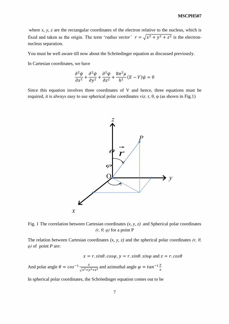
where x, y, z are the rectangular coordinates of the electron relative to the nucleus, which is

fixed and taken as the origin. The term ‘radius vector’ 𝑟 = √𝑥2 + 𝑦2 + 𝑧2 is the electron-

nucleus separation.

You must be well aware till now about the Schröedinger equation as discussed previously.

In Cartesian coordinates, we have

𝜕2𝜓

𝜕𝑥2+𝜕2𝜓

𝜕𝑦2+𝜕2𝜓

𝜕𝑧2+8𝜋2𝜇

ℎ2(𝐸 − 𝑉)𝜓 = 0

Since this equation involves three coordinates of V and hence, three equations must be

required, it is always easy to use spherical polar coordinates viz. r, θ, φ (as shown in Fig.1)

Fig. 1 The correlation between Cartesian coordinates (x, y, z) and Spherical polar coordinates

(r, θ, φ) for a point P

The relation between Cartesian coordinates (x, y, z) and the spherical polar coordinates (r, θ,

φ) of point P are:

𝑥 = 𝑟. 𝑠𝑖𝑛𝜃. 𝑐𝑜𝑠𝜑, 𝑦 = 𝑟. 𝑠𝑖𝑛𝜃. 𝑠𝑖𝑛𝜑 and 𝑧 = 𝑟. 𝑐𝑜𝑠𝜃

And polar angle 𝜃 = 𝑐𝑜𝑠−1𝑧

√𝑥2+𝑦2+𝑧2 and azimuthal angle 𝜑 = 𝑡𝑎𝑛−1

𝑦

𝑥

In spherical polar coordinates, the Schröedinger equation comes out to be

O

x

z

y

P

r

MSCPH507

8

1

𝑟2𝜕

𝜕𝑟(𝑟2

𝜕𝜓

𝜕𝑟) +

1

𝑟2𝑠𝑖𝑛𝜃

𝜕

𝜕𝜃(𝑠𝑖𝑛𝜃

𝜕𝜓

𝜕𝜃) +

1

𝑟2𝑠𝑖𝑛2𝜃

𝜕2𝜓

𝜕𝜙2+8𝜋2𝜇

ℎ2(𝐸 − 𝑉)𝜓 = 0 …(5)

The potential energy V(r) can also be expressed as 𝑉(𝑟) = −𝑍𝑒2

4𝜋𝜖𝑜𝑟 …(6)

Using the method of separation of variable, we first separate the radial component r and angular

terms (θ, φ) assuming that

𝜓(𝑟, 𝜃, 𝜑) = 𝑅(𝑟). 𝑌(𝜃, 𝜑)

where R(r) is the called as radial function depending upon the radius r alone, and Y(θ,φ) is

known as angular function depending upon θ and φ. Thus, equation (1) can be rewritten as

1

𝑟2𝑑

𝑑𝑟(𝑟2

𝜕𝑅

𝜕𝑟)𝑌 +

1

𝑟2𝑠𝑖𝑛𝜃

𝜕


𝜕𝑌

𝜕𝜃)𝑅 +

1

𝑟2𝑠𝑖𝑛2𝜃

𝜕2𝑌

𝜕𝜙2𝑅 +

8𝜋2𝜇

ℎ2(𝐸 − 𝑉(𝑟))𝑅𝑌 = 0

Multiplying the entire equation by 𝑟2

𝑅𝑌 and rearranging, we get

1

𝑅2𝑑

𝑑𝑟(𝑟2

𝑑𝑅

𝑑𝑟) 𝑌 +

8𝜋2𝜇𝑟2

ℎ2(𝐸 − 𝑉(𝑟)) = −

1

𝑌[1

𝑠𝑖𝑛𝜃

𝜕


𝜕𝑌

𝜕𝜃) +

1

𝑠𝑖𝑛2𝜃

𝜕2𝑌

𝜕𝜙2]

The left side of this equation depends on the variable r, while the right side depends upon the

other variables θ and φ. Hence, this equation can be correct only if both sides of it are equal to

the same constant. Let this constant be l(l+1). Thus, we get a radial equation.

1

𝑅2𝑑

𝑑𝑟(𝑟2

𝑑𝑅

𝑑𝑟) 𝑌 +

8𝜋2𝜇𝑟2

ℎ2[𝐸 − 𝑉(𝑟)] = 𝑙(𝑙 + 1) …(7)

And angular equation

−1

𝑌[1

𝑠𝑖𝑛𝜃

𝜕


𝜕𝑌

𝜕𝜃) +

1

𝑠𝑖𝑛2𝜃

𝜕2𝑌

𝜕𝜙2] = 𝑙(𝑙 + 1)

The last equation cab be further separated by substituting

𝜓(𝜃, 𝜑) = 𝛩(𝜃).𝛷(𝜑)

This equation gives

−1

Θ𝑠𝑖𝑛𝜃

𝑑

𝑑𝜃(𝑠𝑖𝑛𝜃

𝑑Θ

𝑑𝜃) + 𝑙(𝑙 + 1)𝑠𝑖𝑛2𝜃 = 𝑚𝑙

2 …(8)

𝑎𝑛𝑑 −1

Φ

𝑑2Φ

𝑑ϕ2= 𝑚𝑙

2 …(9)

Equation (6), (7), and (9) can be written as

𝑑2Φ

𝑑ϕ2+𝑚𝑙

2Φ = 0 …(10)

MSCPH507

9

1

𝑠𝑖𝑛𝜃

𝑑

𝑑𝜃(𝑠𝑖𝑛𝜃

𝑑Θ

𝑑𝜃) + [𝑙(𝑙 + 1) −

𝑚𝑙2

𝑠𝑖𝑛2𝜃] Θ = 0 …(11)

𝑎𝑛𝑑 1

𝑟2𝑑

𝑑𝑟(𝑟2

𝑑𝑅

𝑑𝑟) + [

8𝜋2µ

ℎ2{𝐸 − 𝑉(𝑟)} −

𝑙(𝑙+1)

𝑟2] 𝑅 = 0 …(12)

Thus, we have fragmented the Schröedinger equation of Hydrogen atom into three ordinary

differential equations, each having a single variable r, θ, φ, respectively. After finding the

adequate solutions of these equations, we find the following quantum numbers:

Solution of the equations: The appearance of quantum numbers is explained ahead as:

1. The solution of Φ(φ) equation (10) is Φ𝑚𝑙(𝜑) = 𝐴𝑒𝑖𝑚𝑙𝜙 …(13)

where A is the known as the constant of integration. In order that it is an acceptable

solution, the wave function Φ𝑚𝑙must be a single-valued function of position, that is, it

must have a single value at a given point in space. It is evident that the azimuth angles

φ and φ+2π are actually the same angle. Hence it must by true that

Φ𝑚𝑙(𝜑) = Φ𝑚𝑙(𝜑 + 2𝜋)

or 𝐴𝑒𝑖𝑚𝑙𝜙 = 𝐴𝑒𝑖𝑚𝑙(𝜙+2𝜋)

or 1 = 𝑒𝑖𝑚𝑙(2𝜋)

or 1= cos(ml2π) + i sin(ml2π)

This can only happen when ml is 0 or positive or negative integer, i.e.

𝑚𝑙 = 0,±1,±2, ±3,…

The constant ml is a quantum number of the atom.

2. The solution of Θ(θ) equation (11) is known to be

Θ𝑙.𝑚𝑙(𝜃) = 𝑁𝑙.𝑚𝑙𝑃𝑙|𝑚𝑙|(𝑐𝑜𝑠𝜃) …(14)

where 𝑁𝑙.𝑚𝑙 is a constant and 𝑃𝑙|𝑚𝑙| is ‘Associated Legendre Polynomial’ which has different

forms or different values of l and |ml|, that is

l = |ml|, |ml|+1, |ml|+2, |ml|+3,…

This requirement can be expressed as a condition on ml in the following form:

𝑚𝑙 = 0,±1, ±2,±3,… ,±𝑙

The constant l is another quantum number.

3. For solving equation (12) we must specify V(r). In the present case

MSCPH507

10

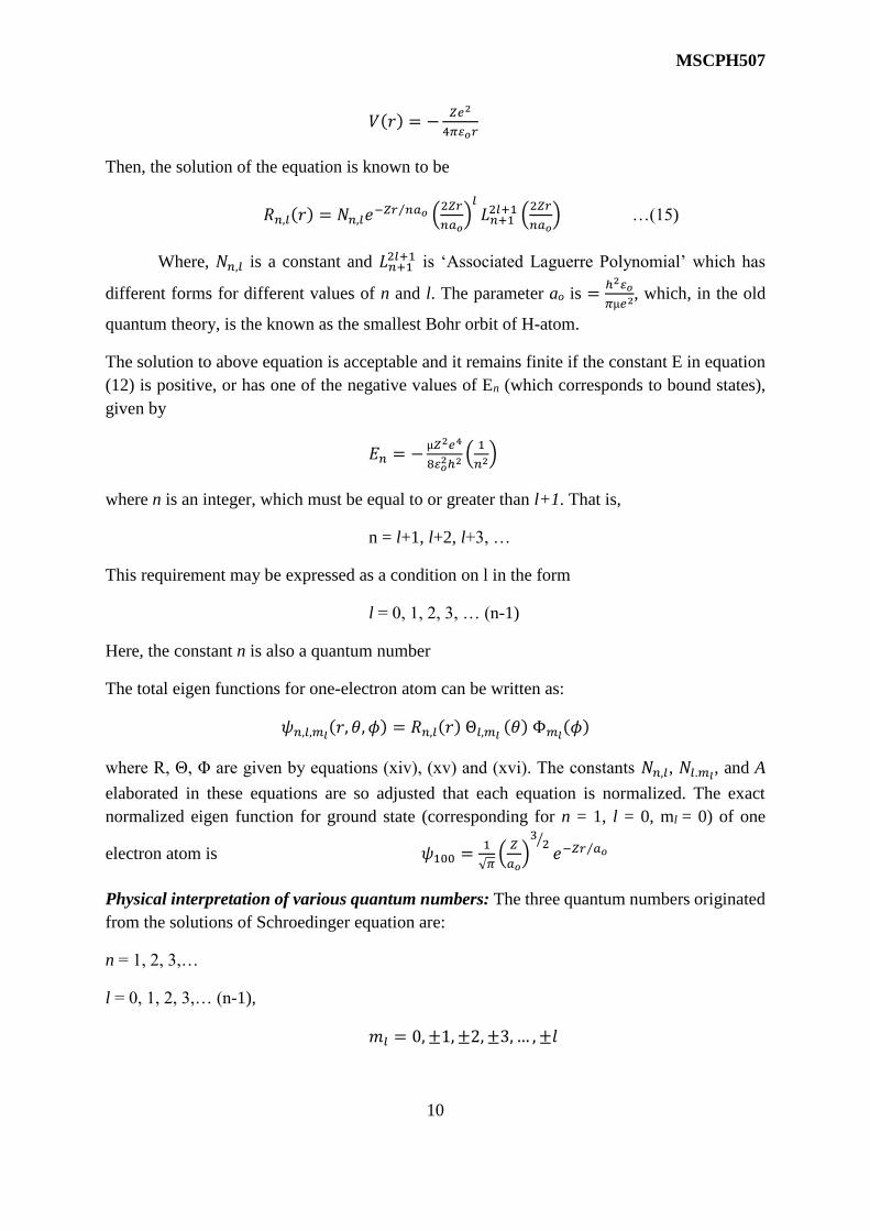
𝑉(𝑟) = −𝑍𝑒2

4𝜋 𝑜𝑟

Then, the solution of the equation is known to be

𝑅𝑛,𝑙(𝑟) = 𝑁𝑛,𝑙𝑒−𝑍𝑟 𝑛𝑎𝑜⁄ (

2𝑍𝑟

𝑛𝑎𝑜)𝑙

𝐿𝑛+12𝑙+1 (

2𝑍𝑟

𝑛𝑎𝑜) …(15)

Where, 𝑁𝑛,𝑙 is a constant and 𝐿𝑛+12𝑙+1 is ‘Associated Laguerre Polynomial’ which has

different forms for different values of n and l. The parameter ao is =ℎ2 𝑜

𝜋µ𝑒2, which, in the old

quantum theory, is the known as the smallest Bohr orbit of H-atom.

The solution to above equation is acceptable and it remains finite if the constant E in equation

(12) is positive, or has one of the negative values of En (which corresponds to bound states),

given by

𝐸𝑛 = −µ𝑍2𝑒4

8 𝑜2ℎ2(1

𝑛2)

where n is an integer, which must be equal to or greater than l+1. That is,

n = l+1, l+2, l+3, …

This requirement may be expressed as a condition on l in the form

l = 0, 1, 2, 3, … (n-1)

Here, the constant n is also a quantum number

The total eigen functions for one-electron atom can be written as:

𝜓𝑛,𝑙,𝑚𝑙(𝑟, 𝜃, 𝜙) = 𝑅𝑛,𝑙(𝑟) Θ𝑙,𝑚𝑙 (𝜃) Φ𝑚𝑙(𝜙)

where R, Θ, Φ are given by equations (xiv), (xv) and (xvi). The constants 𝑁𝑛,𝑙, 𝑁𝑙.𝑚𝑙, and A

elaborated in these equations are so adjusted that each equation is normalized. The exact

normalized eigen function for ground state (corresponding for n = 1, l = 0, ml = 0) of one

electron atom is 𝜓100 =1

√𝜋(𝑍

𝑎𝑜)32⁄

𝑒−𝑍𝑟 𝑎𝑜⁄

Physical interpretation of various quantum numbers: The three quantum numbers originated

from the solutions of Schroedinger equation are:

n = 1, 2, 3,…

l = 0, 1, 2, 3,… (n-1),

𝑚𝑙 = 0,±1,±2,±3,… ,±𝑙

MSCPH507

11

These quantum numbers can be explained as:

Consider the case of one electron atom; we have the total energy of bound states atom obtained

from Schröedinger Equation𝐸𝑛 = −𝜇𝑍2𝑒4

8 𝑜2ℎ2(1

𝑛2). Since, the energy eigen values depends only

on quantum number n, they were in excellent agreement experimental values based on with old

quantum theory of Bohr model. Hence, n is said to be known as “Total” or “Principal Quantum

Number”.

To understand the value of l, we have to consider the radial wave equation based on equation

(12): 1

𝑟2𝑑

𝑑𝑟(𝑟2

𝑑𝑅

𝑑𝑟) + [

8𝜋2µ

ℎ2{𝐸 − 𝑉(𝑟)} −

𝑙(𝑙+1)

𝑟2] 𝑅 = 0

Here, the total energy of atom comprises of two components, viz. kinetic energy K and potential

energy V (for its electrons). Further, kinetic energy is subdivided into radial components due

to motion of electron round the nucleus and orbital component due to the nucleus itself.

Therefore, we have

𝐸 = 𝐾𝑟𝑎𝑑 + 𝐾𝑜𝑟𝑏 + 𝑉(𝑟)

Using this substitution in the radial equation, we have

1

𝑟2𝑑

𝑑𝑟(𝑟2

𝑑𝑅

𝑑𝑟) + [

8𝜋2µ

ℎ2{𝐾𝑟𝑎𝑑 + 𝐾𝑜𝑟𝑏} −

𝑙(𝑙+1)

𝑟2] 𝑅 = 0

Since the radial component is basically originated due to electron motion, hence it is free from

orbital counterpart. And this is only possible when the last two terms are equal to each other

i.e.

𝐾𝑜𝑟𝑏 =ℎ2

8𝜋2µ

𝑙(𝑙+1)

𝑟2

If angular momentum is denoted by 𝐿→, then we know that 𝐿 = 𝜇𝑣𝑟 and therefore,

𝐾𝑜𝑟𝑏 =1

2𝜇𝑣2 =

𝐿2

2µ𝑟2

𝑂𝑟 𝐿2

2µ𝑟2=

ℎ2

8𝜋2µ

𝑙(𝑙+1)

𝑟2

Or L= √(𝑙(𝑙 + 1)ℎ

2𝜋

Since l varies from 0, 1, 2, 3,…(n-1), this proves that the electron can have discrete values of

angular momentum. Finally, the total energy E is also quantized like the orbital angular

momentum and it remains conserved. And this is just demonstrated by quantization of l. Hence,

l is termed as the ‘orbital’ quantum number. The expression for angular momentum was

obtained through the theory of Born-Sommerfield, where k was replaced by √(𝑙(𝑙 + 1). The

method for denoting the state is writing the total angular quantum number along with the

MSCPH507

12

various angular momentum states as letters {like: s (l=0), p(l=1), d(l=2), f(l=3), …}. For

example, a state with n = 2 with l = 0 is shown as 2s state. Similarly, another state with n = 3

and l=1 is written as 3p.

The analysis of ml originates when the atom is placed in an external magnetic field. You can

imagine that when an electron is revolving round the nucleus, it behaves like a small loop of

current having magnetic dipole when placed in an external magnetic field. Its potential energy

depends upon its magnetic moment and its orientation with respect to the field. But here, the

magnitude and direction of the magnetic moment depends upon the magnitude and direction

of angular momentum L of the electron. This also determines the magnetic potential energy.

Since the direction of L is also quantized with respect to external magnetic field. If the field is

along the z-axis, the component of L can be defined as

𝐿𝑧 = 𝑚𝑙ℎ

2𝜋, where 𝑚𝑙 = 0,±1,±2,±3,… ,±𝑙.

Since we can observe that ml describes the quantization of L in magnetic field (known as space

quantization), and finally, the discretization of magnetic energy of the electron. Therefore, ml

is known as magnetic quantum number.

Therefore, n, l, and ml are the three quantum numbers used to specify each of the eigen

functions of single electron atom here n specifies the total energy (the eigen value), l specifies

the angular momentum and ml determines the z-component of the angular momentum of the

electron. For a given value of n, there are different values of l and for every different value of

l we have several values of ml. Hence, several different eigen functions resembles to exactly

the same eigenvalue En. And this property of eigen functions is said to be ‘degenerate’ state.

In accordance with old quantum theory the quantum-mechanical interpretations of

energy states of single electron system matches well with each other. The differences that are

crucial to understand is that in quantum mechanics, the electron should not be considered as

moving around the nucleus in definite orbits. Here it is necessary to consider the relative

probabilities of finding the electron in volume elements at various locations rather than is

specific orbits. For this consideration, we relook the wave-function of single-electron system

i.e.

𝜓𝑛,𝑙,𝑚𝑙(𝑟, 𝜃, 𝜙) = 𝑅𝑛,𝑙(𝑟) Θ𝑙,𝑚𝑙 (𝜃) Φ𝑚𝑙(𝜙)

Where, the symbols have their usual meaning as specified above in equations (9), (10) and (11)

respectively. We must know till now that the electron probability density, given by |𝜓|2 was

mathematically formulated as:

|𝜓|2 = |𝑅|2. |Θ|2. |Φ|2, where |𝜓|2 = 𝜓∗𝜓

We observe that |Φ|2 = Φ∗Φ will result in A2 and since A is a constant; this shows that ψ is

independent of Φ and does not directly determine probability density (|𝜓|2). This also dispels

that the dependent factors were |𝑅|2. |Θ|2. From the relation of radial probability density for

MSCPH507

13

finding the electron between r and r+dr is given by |𝑅|2(4𝜋𝑟2𝑑𝑟). The value of probability

density P(r) is maxima at ao and 4ao. These values of radii ao and 4ao corresponds to n=1 and

n=2 Bohr’s orbit where the electrons is most likely to be found. In Bohr’s orbit at 4ao, the

average distance of electron from the nucleus is given by

�� = ∫ 𝑟∞

0𝑃(𝑟)𝑑𝑟 =

𝑛2𝑎𝑜

𝑍[1 +

1

2{1 −

𝑙(𝑙+1)

𝑛2}]

where, ao is the smallest Bohr orbit. This is same as for the Bohr-Sommerfeld elliptical orbit.

Solved Example No 1:

Question: Find the parity of N atom in ground state.

Solution- It is known that the parity is even if the sum of l values (l) for all the electron

is even; and it carries an odd parity if l is odd.

The electronic configuration of N atom in ground state is given as:

1𝑠2 2𝑠2 2𝑝3

The value of l = 0 for s – electron and l = 1 for p – electron.

Therefore, l = 3

Hence, the parity is odd.

1.4 Fine Structure of Hydrogen

For hydrogen atom, when an electron transmits from one energy level to another, spectral lines

are observed in an emission spectrum. The wavelengths of these lines are in accordance with

Rydberg’s formula. These are collectively known as Line spectra of hydrogen atom. When

these spectral lines split due to spin - orbit coupling effect and quantum mechanical relativistic

corrections, it gives rise to fine structure

1.4.1 Effect due to electron’s spin and orbital motion

The interaction due to internal magnetic field of an atom and electron’s spin magnetic dipole

moment is partly responsible for the fine-structure of one electron atoms (excited state). It is

well understood that the internal magnetic field of an atom arises due to the electron’s orbital

motion. Therefore, this type of interaction is called as spin-orbit interaction.

Let us consider electric field �� , defined as a gradient of potential function V(r), where r

represents the distance between nucleus and electron of an atom.

�� = 𝑔𝑟𝑎𝑑 𝑉(𝑟)

MSCPH507

14

=𝑑�� (𝑟)��

𝑑𝑟 …(16)

where �� is the unit vector in which electric field �� is directed. The magnetic field caused due

to the orbital motion of the associated electron moving with velocity v in electric field �� is:

�� =1

𝑐2(�� × 𝑣 )

=1

𝑐2𝑟

𝑑𝑉(𝑟)

𝑑𝑟(𝑟 × 𝑣 ) {∵ �� =

𝑟

𝑟 𝑓𝑟𝑜𝑚 (1)} …(17)

The orbital motion of an electron causes angular momentum �� , where �� is further defined as

�� = 𝑚𝑟 × 𝑣 , thus equation (17) may be written as

�� =1

𝑚𝑐21

𝑟

𝑑𝑉(𝑟)��

𝑑𝑟 …(18)

The magnetic field �� orients the electron’s spin magnetic moment 𝜇𝑠 and hence the magnetic

potential energy of orientation, Δ𝐸𝑙,𝑠. The expression of Δ𝐸𝑙,𝑠is given as

Δ𝐸𝑙,𝑠 = −𝜇𝑠. �� …(19)

But spin magnetic moment is ∗ 𝜇𝑠 = −𝑔𝑠 (𝑒

2𝑚) 𝑆 , where 𝑔𝑠 = 2 (for electrons) and 𝑆 is spin

angular momentum.

Thus, equation (19) can be written as: Δ𝐸𝑙,𝑠 = −𝑒

𝑚𝑆 . �� …(20)

Substituting the value of �� from equation (18) into (20), we get

Δ𝐸𝑙,𝑠 = −𝑒

𝑚2𝑐21

𝑟

𝑑𝑉(𝑟)

𝑑𝑟𝑆 . �� …(21)

In accordance with ‘Thomson precession’ when nucleus is considered to be in rest, Δ𝐸𝑙,𝑠is

reduced by a factor of 2, i.e.

Δ𝐸𝑙,𝑠 = −𝑒

2𝑚2𝑐21

𝑟

𝑑𝑉(𝑟)

𝑑𝑟𝑆 . �� …(22)

Let us now express the equation (22) in terms of j, l and s quantum numbers.

We know that 𝐽 = �� + 𝑆 …(23)

Taking self dot products of equation (23), we get

𝐽 . 𝐽 = (�� + 𝑆 ). (�� + 𝑆 )

= (�� . �� + �� . 𝑆 + 𝑆 . �� + 𝑆 . 𝑆 )

= (�� . �� + 2 �� . 𝑆 + 𝑆 . 𝑆 ) ( ∵ �� . 𝑆 = 𝑆 . �� )

MSCPH507

15

∴ 𝑆 . �� =1

2[𝐽 . 𝐽 − �� . �� − 𝑆 . 𝑆 ]

=1

2[𝐽2 − 𝐿2 − 𝑆2]

𝑆 . �� =1

2[𝑗(𝑗 + 1) − 𝑙(𝑙 + 1) − 𝑠(𝑠 + 1)]

ℎ2

4𝜋2 …(24)

∴ Δ𝐸𝑙,𝑠 = −𝑒ℎ2

16𝜋2𝑚2𝑐2[𝑗(𝑗 + 1) − 𝑙(𝑙 + 1) − 𝑠(𝑠 + 1)]

1

𝑟

𝑑𝑉(𝑟)

𝑑𝑟 {from eq.22} (25)

As electron is in motion the terms 1

𝑟

𝑑𝑉(𝑟)

𝑑𝑟 is not fixed. Therefore, an average value during

unperturbed motion must be considered. So,

Δ𝐸𝑙,𝑠 = −𝑒ℎ2

16𝜋2𝑚2𝑐2

⏞

1

𝑟

𝑑𝑉(𝑟)

𝑑𝑟

[𝑗(𝑗 + 1) − 𝑙(𝑙 + 1) − 𝑠(𝑠 + 1)]1

𝑟

𝑑𝑉(𝑟)

𝑑𝑟 …(26)

To evaluate the average value of 1

𝑟

𝑑𝑉(𝑟)

𝑑𝑟, the radial probability density of the required state and

potential function V(r) is considered. The potential function V(r) for one-element atoms in

Colombian field is:

𝑉(𝑟) = −1

4𝜋𝜖𝑜

𝑍𝑒

𝑟

𝑑𝑉(𝑟)

𝑑𝑟= −

1

4𝜋𝜖𝑜

𝑍𝑒

𝑟2 …(27)

Substituting the value of 𝑑𝑉(𝑟)

𝑑𝑟 from (27) into (26), we get:

Δ𝐸𝑙,𝑠 = −𝑍𝑒2ℎ2

4𝜋𝜖𝑜(16𝜋2𝑚2𝑐2)[𝑗(𝑗 + 1) − 𝑙(𝑙 + 1) − 𝑠(𝑠 + 1)]

𝑇

𝑟3 ....(28)

Considering radial density function of H-Atom, the average value of 1/r3 can be evaluated as:

𝑇

𝑟3=

𝑍3

𝑎03𝑛3𝑙(𝑙+

1

2)(𝑙+1)

, hen l > 0 …(29)a

where 𝑎0 = (4𝜋𝜖𝑜ℎ

2

4𝜋2𝑚𝑐2) …(29)b

a0 is the radius of the smallest Bohr orbit for hydrogen atom. Substituting the value of 𝑇

𝑟3 from

equation (29)a in (28), we get

Δ𝐸𝑙,𝑠 = −𝑍𝑒2ℎ2

4𝜋𝜖𝑜(16𝜋2𝑚2𝑐2).

𝑍3

𝑎03𝑛3𝑙(𝑙+

1

2)(𝑙+1)

[𝑗(𝑗 + 1) − 𝑙(𝑙 + 1) − 𝑠(𝑠 + 1)] … (30)

The above equation is simplified to the following equation:

Δ𝐸𝑙,𝑠 = 𝑅∞𝛼

2𝑍4ℎ𝑐

2𝑛3𝑙(𝑙+1

2)(𝑙+1)

[𝑗(𝑗 + 1) − 𝑙(𝑙 + 1) − 𝑠(𝑠 + 1)] …(31)

MSCPH507

16

Where, 𝑅∞ =𝑚𝑒4

8𝜖0ℎ3𝑐 (Rydberg constant for infinitely heavy nucleus) and 𝛼 =

𝑒2

2𝜖0ℎ𝑐 (Fine

structure constant).

Due to spin-orbit coupling effect, term shift ∆𝑇𝑙,𝑠 arises

∆𝑇𝑙,𝑠 = −∆𝐸𝑙,𝑠ℎ𝑐

=𝑅∞𝛼

2𝑍4

2𝑛3𝑙(𝑙+1

2)(𝑙+1)

[𝑗(𝑗 + 1) − 𝑙(𝑙 + 1) − 𝑠(𝑠 + 1)] …(32)

For one electron atom like hydrogen s=1/2 and 𝑗 = 𝑙 ± 𝑠 = 𝑙 ± 1 2⁄

Solving the term [𝑗(𝑗 + 1) − 𝑙(𝑙 + 1) − 𝑠(𝑠 + 1)] is l and –(l+1) for j = 𝑙 + 1 2⁄ and j = 𝑙 −

12⁄ , respectively .

The term shift corresponding to j = 𝑙 + 1 2⁄ is

∆𝑇𝑙,𝑠′ = −

𝑅∞𝛼2𝑍4

2𝑛3𝑙(𝑙+1

2)(𝑙+1)

𝑙 …(33)

The term shift corresponding to j = 𝑙 + 1 2⁄ is

∆𝑇𝑙,𝑠′′ =

𝑅∞𝛼2𝑍4

2𝑛3𝑙(𝑙+1

2)(𝑙+1)

(𝑙 + 1) …(34)

Therefore, the coupling effect due to electron’s spin and orbital motion causes splitting of one

energy level into two levels with different j’s for a given l.

The difference in the energy levels is obtained by subtracting (33) from (34).

∆𝑇𝑙,𝑠 = ∆𝑇𝑙,𝑠′ − ∆𝑇𝑙,𝑠

′′

=𝑅∞𝛼

2𝑍4

2𝑛3𝑙 (𝑙 +12)(𝑙 + 1)

(2𝑙 + 1)

=𝑅∞𝛼

2𝑍4

𝑛3𝑙(𝑙+1) …(35)

Putting the values of R∞=1.097×107m-1 and α=1/137 for Hydrogen atom, due to spin-orbit

interaction.

∆𝑇′ = 584𝑍4

𝑛3𝑙(𝑙+1)𝑚−1 = 5.84

𝑍4

𝑛3𝑙(𝑙+1)𝑐𝑚−1 …(36)

From equation no. 36, it is clear that the splitting due to spin-orbit coupling increases with

increasing atomic number (Z) and decreases with higher n and l.

MSCPH507

17

1.4.2 Effect due to relativistic corrections

Apart from spin-orbit interactions, the relativistic effect also contributes in the splitting of

energy levels of hydrogen atom. In order to evaluate the shift due to relativistic corrections,

relativistic Hamiltonian function H for an electron is considered.

It is known that H=K+V where, k=(p2c2 +mo2c4)1/2-moc

2 , is the relativistic kinetic energy, V is

the relativistic potential energy, mo is the rest mass of electron and p its linear momentum.

𝐻 = (𝑝2𝑐2 +𝑚𝑜2𝑐4)

12⁄ −𝑚𝑜𝑐

2 + 𝑉 …(37)

= 𝑚𝑜𝑐2 (1 +

𝑝2

𝑚𝑜2𝑐2)12⁄

−𝑚𝑜𝑐2 + 𝑉

= 𝑚𝑜𝑐2 (1 +

𝑝2

2𝑚𝑜2𝑐2−

𝑝4

8𝑚𝑜4𝑐4+⋯) −𝑚𝑜𝑐

2 + 𝑉

=𝑝2

2𝑚𝑜−

𝑝4

8𝑚𝑜3𝑐2+⋯+ 𝑉 …(38)

Neglecting the higher order terms, it is evident that the change in H due to relativistic correction

is

−𝑝4

8𝑚𝑜3𝑐2

since {𝐻 =𝑝2

2𝑚𝑜+ 𝑉}without relativisticcorrection

Considering −𝑝4

8𝑚𝑜3𝑐2

as perturbation term first order change in energy level can be evaluated.

The operator p is −𝑖ℏ𝜕

𝜕𝑞.

Therefore, −𝑝4

8𝑚𝑜3𝑐2

becomes −1

8𝑚𝑜3𝑐2(−𝑖ℏ

𝜕

𝜕𝑞)4

or −1

8𝑚𝑜3𝑐2ℏ2∇4…(39)

For hydrogen atom, let us consider 𝜓 as unperturbed wave function, then first order shift in

energy due to perturbation term is given as

Δ𝐸𝑟 = −∫𝜓∗ (

ℏ4

8𝑚𝑜3𝑐2)∇4𝜓𝑑𝜏 …(40)

Evaluating the integral in equation no. 25 gives

Δ𝐸𝑟 = −𝑅∞𝛼

2𝑍4ℎ𝑐

𝑛3(1

𝑙+1

2

−3

4𝑛) …(41)

Where α is the fine structure constant and R∞ is the Rydberg’s Constant.

MSCPH507

18

Hence, the term shift due to relativistic correction is

∆𝑇𝑟=−∆𝐸𝑟

ℎ𝑐= −

𝑅∞𝛼2𝑍4ℎ𝑐

𝑛3(1

𝑙+1

2

−3

4𝑛) …(42)

To incorporate the combined effect of spin-orbit coupling and relativistic corrections in a H-

atom spectrum, let us add equations 32 and 42.

1.4.3 Term shift

∆𝑇 = −𝑅∞𝛼

2𝑍4

2𝑛3𝑙(𝑙+1

2)(𝑙+1)

[𝑗(𝑗 + 1) − 𝑙(𝑙 + 1) − 𝑠(𝑠 + 1)] +𝑅∞𝛼

2𝑍4

𝑛3(1

𝑙+1

2

−3

4𝑛)

=𝑅∞𝛼

2𝑍4

𝑛3[1

𝑙+1

2

−𝑗(𝑗+1)−𝑙(𝑙+1)−𝑠(𝑠+1)

2(𝑙+1

2)(𝑙+1)

−3

4𝑛] …(43)

Putting j=l+1/2 and s=1/2, we get

=𝑅∞𝛼

2𝑍4

𝑛3[1

𝑙+1

2

−𝑙

2𝑙(𝑙+1

2)(𝑙+1)

−3

4𝑛] [

1

𝑙+1

2

(1 −1

2𝑙+2) −

3

4𝑛] [

1

𝑙+1

2

(2𝑙+2−1

2(𝑙+1)) −

3

4𝑛]

=𝑅∞𝛼

2𝑍4

𝑛3[1

𝑙+1−

3

4𝑛] …(44)

For j=l-1/2,

=𝑅∞𝛼

2𝑍4

𝑛3[1

𝑙+1

2

−(𝑙−

1

2)(𝑙−

1

2+1)−𝑙(𝑙+1)−

3

4

2𝑙(𝑙+1

2)(𝑙+1)

−3

4𝑛]

=𝑅∞𝛼

2𝑍4

𝑛3[2

2𝑙+1−

(2𝑙−1)

2(𝑙+

1

2)−𝑙2−𝑙−

3

4

2𝑙(𝑙+1

2)(𝑙+1)

−3

4𝑛]

=𝑅∞𝛼

2𝑍4

𝑛3[2

2𝑙+1−

(2𝑙−1)(2𝑙+1)

4−𝑙2−𝑙−

3

4

2𝑙(𝑙+1

2)(𝑙+1)

−3

4𝑛]

=𝑅∞𝛼

2𝑍4

𝑛3[2

2𝑙+1−

(4𝑙2−1)

4−𝑙2−𝑙−

3

4

2𝑙(𝑙+1

2)(𝑙+1)

−3

4𝑛]

=𝑅∞𝛼

2𝑍4

𝑛3[2

2𝑙+1−𝑙2−

1

4−𝑙2−𝑙−

3

4

2𝑙(𝑙+1

2)(𝑙+1)

−3

4𝑛]

=𝑅∞𝛼

2𝑍4

𝑛3[2

2𝑙+1−

−(𝑙+1)

2𝑙(𝑙+1

2)(𝑙+1)

−3

4𝑛]

MSCPH507

19

=𝑅∞𝛼

2𝑍4

𝑛3[2

2𝑙+1+

2

2𝑙(𝑙+1

2)−

3

4𝑛]

=𝑅∞𝛼

2𝑍4

𝑛3(

2

2𝑙+1) [1 +

1

2𝑙−

3

4𝑛]

Δ𝑇 =𝑅∞𝛼

2𝑍4

𝑛3[1

𝑙−

3

4𝑛] …(45)

Equation 44 and 45 cab be replaced by one single equation.

Δ𝑇 =𝑅∞𝛼

2𝑍4

𝑛3[1

𝑗+1

2

−3

4𝑛] …(46)

Equation 46 is identical to equation of energy levels of hydrogen like atom given by

Sommerfeld’s relativistic equation; as

Δ𝑇 =𝑅∞𝛼

2𝑍4

𝑛3[1

𝑘−3

4𝑛]

As seen above, the equation is similar to the equation number 31, where k is equal to 𝑗 +1

2

This equation is known as Dirac Equation.

By substituting the values of 𝑅∞= 1.097 × 107 m-1, α is Rydberg Constant where 𝛼 = 1

137 (fine

structure constant) and Z = 1 for hydrogen atom, we get term shift

Δ𝑇 =584

𝑛3[1

𝑗+1

2

−3

4𝑛] m-1

or Δ𝑇 =5.84

𝑛3[1

𝑗+1

2

−3

4𝑛] cm-1

Using, the term shift values in cm-1, the fine structure of Hα line for n = 3 → n = 2 level is

deduced as shown in Fig. 2

MSCPH507

20

Fig. 2 The fine structure of Hα line for n = 3 → n = 2 level

The selection rules for fine structure of hydrogen atom are

Δl = ± 1

Δj =0, ± 1 but j = 0 ↔ j=0 is not allowed

The above selection rules allow five transitions as shown in the figure. However, only doublets

are observed in general practise instead of these five components. This happens due to thermal

motion of the molecules that results into Doppler broadening. When the Doppler broadening

effect is reduced carefully, all the five components can be observed.


The 𝐻𝑒+ doublet splitting of first excited state (2𝑃12

- 2𝑃32

) is 5.84 𝑐𝑚−1. Evaluate the

corresponding splitting value of H.

Solution- The doublet splitting separation due to spin-orbit interaction is given as:

T = 𝑅 2 𝑍

4

𝑛3 𝑙(+1)

MSCPH507

21

Where, 𝑅 is Rydberg’s constant, is fine structure constant, Z is atomic number and

n, l are constant for a given state.

T𝑍4

For 𝐻𝑒+, Z = 2 and for H, Z = 1

Therefore, 𝑇𝐻𝑒

𝑇𝐻 = (

24

14 ) = 16

𝑇𝐻 = 1

16 𝑇𝐻𝑒+ =

1

16 * 5.84 = 0.365 𝑐𝑚−1

1.5 Pauli’s Exclusion principle and exchange symmetry

To study the spectra of multi-electron atoms, the quantum mechanical properties of identical

particles should be considered. As per the quantum mechanical wave theory, the particles that

can be described by the symmetric total wave functions are called as ‘Bosons’. Therefore,

ψ (1, 2, 3…….. N) = +ψ (1, 2, 3…..N)

From this it is inferred, that all the particles with the integral spins are known as Bosons.

Examples are photons, gravitons, pions, etc.

Opposite to it, the particles that can be completely described by the asymmetric total wave

functions are known as ‘Fermions’. Therefore,

ψ (1, 2, 3…….. N) = -ψ (1, 2, 3…..N)

From this it can be inferred that all the particles with the half integral spins are Fermions.

Examples are electrons, protons, neutrons, etc.

Pauli in Year 1925, formulated basic principle that governs the electronic configuration of the

atoms. Pauli’s Exclusion Principle states that “no two fermions can exist in the same quantum

state”. This can be further extended that the existence of two electrons with same spin

orientation in one atomic orbital is not possible.

Let us consider two identical non – interacting particles 1 and 2 having quantum state, a and b,

then the wave function of the system is

ψ ab (1, 2) = ψa(1).ψb(2)

Let us now consider particle to be in state b and particle 2 in state a, then the wave function

would be

ψ ba (1, 2) = ψb(1).ψa(2)

As these particles are indistinguishable, ψ ab and ψ ba, both have equal likelihood. Therefore,

the system can be described by linear combination of both.

MSCPH507

22

𝜓(1, 2) =1

√2[𝜓𝑎(1) 𝜓𝑏(2) ± 𝜓𝑏(1) 𝜓𝑎(2)]

Where, 1

√2 is the normalisation constant.

For Bosons, where total wave function is symmetric, the above equation becomes

𝜓𝐵𝑜𝑠𝑒(1, 2) =1

√2[𝜓𝑎(1) 𝜓𝑏(2) + 𝜓𝑏(1) 𝜓𝑎(2)]

And for Formions (Anti – symmetric Wave),

𝜓𝐹𝑜𝑟𝑚𝑖(1, 2) =1

√2[𝜓𝑎(1) 𝜓𝑏(2) − 𝜓𝑏(1) 𝜓𝑎(2)]

If the quantum states a ≡ b, then

𝜓𝐵𝑜𝑠𝑒(1, 2) ≠ 0

𝜓𝐹𝑜𝑟𝑚𝑖(1, 2) ≠ 0

Therefore, two Bosons can exist in the same quantum state whereas two Fermions cannot

because because the wave function vanishes identically in case of fermions. This further

indicates that fermions cannot be described by the same set of quantum numbers.


Consider a system comprising two Bose particles with same quantum number a construct

normalised wave function.

Solution- Let the two Bose particles be 1 and 2. The normalised wave function is given

as:-

𝑠 (1, 2) =

1

√2[𝜓𝑎(1) 𝜓𝑏(2) + 𝜓𝑏(1) 𝜓𝑎(2)]

where 1

√2 is normalisation factor. Both the Bose particles are associated with same

quantum number ‘a’. Therefore, a = b.

𝑠 (1, 2) =

1

√2[𝜓𝑎(1) 𝜓𝑎(2) + 𝜓𝑎(1) 𝜓𝑎(2)]

= √2 𝑎 (1) 𝑎 (2)

1.6 Hund’s Rule

These rules are as follows:-

1. The terms with largest multiplicity lie at the lowest.

MSCPH507

23

2. The terms with largest L lie at the lowest for terms with same multiplicity.

3. The levels with lowest value of J lies at the lowest for half – filled or lesser in outermost

sub shell and for more than half – filled sub shell, the level with longest J has lowest in

energy for terms of an atom.

1.7 Helium Atom and it’s Spectrum

1.7.1 He atom’s spectrum

Two identical particles, when treated quantum mechanically act under the influence of

exchange of forces. This force may be attractive or repulsive depending on the orientation of

spin of the particles. If we consider two electrons, parallel spins repel, however the antiparallel

spins attract.

A system having two electrons in an atom such as He atom may exist in singlet or triplet state.

The two electrons two and two have spin quantum numbers as 𝑠1 =1

2 and 𝑠2 =

1

2 respectively.

Thus, the 𝑆 (spin angular momentum) of the considered system isℎ

2 √𝑆(𝑆 + 1). S can have all

the values from (𝑠1 + 𝑠2) to (𝑠1 − 𝑠2) with a difference of one. Therefore, S = 1, 0.

S = 1 corresponds to antiparallel spins and S = 0 to parallel spins:

𝑠1 =1

2 and 𝑠2 =

1

2 gives S = 1

𝑠1 =1

2 and 𝑠2 =

1

2 gives S = 0

The Z component (𝑆𝑍) is given as 𝑆𝑍 = 𝑀𝑠ℎ/2, where 𝑀𝑠 has all the possible values from

+S to –S. That is

𝑀𝑠 = 1, 0, −1 for S = 1

And 𝑀𝑠 = 0 for S = 0

Therefore, there are three possible values of 𝑀𝑠for S = 1, resulting into three possible spin

states known as ‘triplet states’ whereas, for S = 0 the value of 𝑀𝑠 = 0and thus singlet spin

state arises due to parallel configuration and singlet state due to antiparallel configuration.

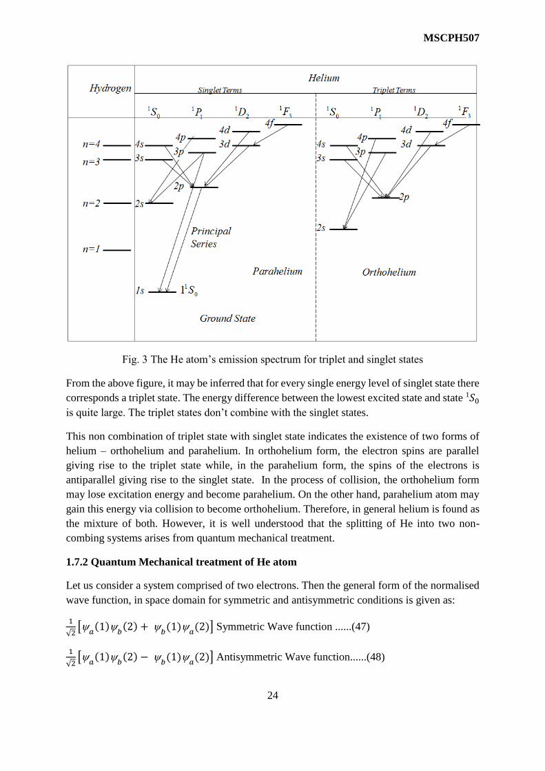
The He atom’s emission spectrum for triplet and singlet states is shown in Fig. 3 below:

MSCPH507

24

Fig. 3 The He atom’s emission spectrum for triplet and singlet states

From the above figure, it may be inferred that for every single energy level of singlet state there

corresponds a triplet state. The energy difference between the lowest excited state and state 1𝑆0

is quite large. The triplet states don’t combine with the singlet states.

This non combination of triplet state with singlet state indicates the existence of two forms of

helium – orthohelium and parahelium. In orthohelium form, the electron spins are parallel

giving rise to the triplet state while, in the parahelium form, the spins of the electrons is

antiparallel giving rise to the singlet state. In the process of collision, the orthohelium form

may lose excitation energy and become parahelium. On the other hand, parahelium atom may

gain this energy via collision to become orthohelium. Therefore, in general helium is found as

the mixture of both. However, it is well understood that the splitting of He into two non-

combing systems arises from quantum mechanical treatment.

1.7.2 Quantum Mechanical treatment of He atom

Let us consider a system comprised of two electrons. Then the general form of the normalised

wave function, in space domain for symmetric and antisymmetric conditions is given as:

1

√2[

𝑎(1)

𝑏(2) +

𝑏(1)

𝑎(2)] Symmetric Wave function ......(47)

1

√2[

𝑎(1)

𝑏(2) −

𝑏(1)

𝑎(2)] Antisymmetric Wave function......(48)

MSCPH507

25

Where a and b represent space quantum numbers.

The spin coordinate can have two orientations – spin up (+1/2) and spin down (-1/2). Thus

there are only two possible wave functions - + and -. Thus, there are only two possible wave

functions corresponding to spin up and spin down states. These lead to four possible ways in

which spin wave function can exist. The normalised form of these spin wave functions are

given below.

1+

2+

1

√2[1+

2− +

1−

2+]

1−

2−

1

√2[1+

2− −

1−

2+]

The first three forms (eqn 49) are for parallel orientation of electrons giving rise to the triplet

states and the last form (eqn 50) is due to antiparallel orientation that results into singlet state.

It is also known that the total wave function may be written in terms of spin wave function and

space wave function as:

𝑡𝑜𝑡= ........(51)

Therefore the total wave function for He atom may be written as:

1

√2[

𝑎(1)

𝑏(2) +

𝑏(1)

𝑎(2)]

1+

2+

1

√2[

𝑎(1)

𝑏(2) +

𝑏(1)

𝑎(2)]

1

√2[1+

2− +

1−

2+]

1

√2[

𝑎(1)

𝑏(2) +

𝑏(1)

𝑎(2)]

1−

2−

These forms represent the parallel orientation (Triplet State)

1

√2[

𝑎(1)

𝑏(2) +

𝑏(1)

𝑎(2)]

1

√2[1+

2− −

1−

2+]

This form represents the antiparallel orientation (Singlet state)

Due to first three forms of symmetric spin wave function (eqn 49), triplet state arises while the

antisymmetric spin wave function (eqn 50) gives rise to singlet state. If we ignore the

interaction due to coulomb field, all these four states are degenerate. However, if the coulomb

interaction is considered, the exchange degeneracy gets removed and splits each state into

singlet and three fold degenerate triplet state (Fig. 4). Therefore, splitting of He atom into

Singlet – Triplet can be explained under coulomb effect.

Symmetric (Triplet State).........(49)

Antisymmetric (Singlet State)........ (50)

MSCPH507

26

Fig. 4 Splitting of He atom into Singlet – Triplet can be explained under coulomb effect

The electrons in the ground state have same quantum numbers, that is a = b = 1s and hence

there exists single wave function in the space domain as 1𝑠(1)

1𝑠(2). This space wave

function is symmetric with respect to the exchange of electrons. In order to satisfy the pauli’s

exclusion principle, the space wave function needs to be combined with antisymmetric spin

wave function [1

√2(1+

2− −

1−

2+). Such a combination results into singlet state. This further

indicates the absence of triplet state for the ground state.

Except for this ground state, there exist triplet states with singlet states for higher energy levels.

The energy due to coulomb interaction (1

4𝑜

𝑒2

𝑟12)between the two electrons is lesser in the triplet

state compared to the singlet state. This is because the average distance (𝑟12) between the

electrons is greater in triplet state compared to singlet state. Henceforth, the singlet states lie in

the upper level compared to triplet states.

It is also observed that the energy level of the ground state is much lower compared to other

higher levels. The electrons of the ground state are strongly bounded by the nucleus compared

to higher energy levels. The perturbation may be adopted to calculate the energy of ground and

higher levels of He atom.

Let us now consider He atom (Z = 2) having charge on nucleus (+Ze) and two electrons say 1

and 2. Then the Hamiltonian operator (H) is given as:

H = −ℎ2

82𝑚(1

2 + 22) −

1

4𝑜

𝑍𝑒2

𝑟1 −

1

4𝑜

𝑍𝑒2

𝑟2+−

1

4𝑜

𝑒2

𝑟12 ...........(52)

Where 𝑟1 and 𝑟2 are the distances between the nucleus and electrons 1 and 2 respectively.

While, 𝑟12 is the distance between the electrons 1 and 2. Due to the coulomb repulsive potential

MSCPH507

27

energy between the two electrons, the term 1

4𝑜

𝑒2

𝑟12 is taken positive while all other forces are

attractive. The motion of the nucleus and few interactions such as spin-spin and spin-orbit

coupling are neglected in the present calculation as they are very weak compared to the

coulomb interaction. The attractive potential energy between the nucleus and the electrons

make the terms 1

4𝑜

𝑍𝑒2

𝑟1 and

1

4𝑜

𝑍𝑒2

𝑟2 make the terms negative. Hence the wave equation

becomes:

H = [−ℎ2

82𝑚(1

2 + 22) −

1

4𝑜

𝑍𝑒2

𝑟1 −

1

4𝑜

𝑍𝑒2

𝑟2+ −

1

4𝑜

𝑒2

𝑟12] ...........(53)

And also, H = 𝐸 ..........(54)

The perturbation method is employed to solve eqn 53 and 1

4𝑜

𝑒2

𝑟12 is considered as the perturbing

term. Here eqn 53 can be written as:

(H˚ + H′) = 𝐸

Where H˚ + H′ = H

Thus the wave equation (for ground state – 1s1s) for unperturbed part can be written as:

H˚˚ = 𝐸˚˚ ........(55)

Where ˚ = ˚1s(1)˚1s(2)

And E˚ = E˚1s(1)E˚1s(2)

The unperturbed wave function is treated as the product of two wave functions of hydrogen

like atoms in the ground state. The eigen value of ˚ is the sum of the individual eigen values

of ˚1s(1) and ˚1s(2) respectively.

We also know that the wave function of the hydrogen like atoms in the ground state is

˚1s = 1

√(Z ao⁄ )

3

2 exp (−𝑍𝑟 ao⁄ ) ........(57)

And the eigen value of the ˚1s is E˚1s = −Z2EH

Here, 𝐸𝐻 = 𝑚𝑒4

802ℎ2= 13.6 eV .........(58)

Substituting the values from eqns 58 and 57 into 56, we get:

˚ = 1

(Z ao⁄ )3 exp (

−𝑍(𝑟1 + 𝑟2)ao⁄ )

E˚ = −2Z2EH

.......(56)

..........(59)

MSCPH507

28

As for He atom Z = 2

E˚ = −8EH

= - 8 × 13.6 eV

= -108.8 eV

However, the experimental results show that this value is -78.98 eV. This simply highlights the

role of coulomb interaction between the two electrons play a key role in determining the energy

state of He atom.

Therefore, the introduction of perturbation term representing coulombic repulsion term is done.

Now, for the evaluation of first order energy perturbation evaluation of first order energy

perturbation, we will consider the following equation:

E′ = ∫˚H′d

𝐸′ =∬1

(Z ao⁄ )

3exp (

−𝑍(𝑟1 + 𝑟2)ao⁄ ) (

1

4𝑜

𝑒2

𝑟12) 1

(Z ao⁄ )3exp (

−𝑍(𝑟1 + 𝑟2)ao⁄ ) d1 d2

= (𝑒2

𝜋2) (𝑍

𝑎𝑜)∫ ∫ ∫ ∫ ∫ ∫

𝑒−2𝑍(𝑟1 + 𝑟2)

𝑎𝑜4𝜋휀𝑜𝑟12

𝑟12𝑑𝑟1𝑠𝑖𝑛𝜃1𝑑𝜃1𝑑𝜑1

2𝜋

0

𝜋

0

∞

0

2𝜋

0

𝜋

0

∞

0

𝑟12𝑑𝑟2𝑠𝑖𝑛𝜃2𝑑𝜃2𝑑𝜑2

Therefore, 𝐸′ =5𝑍𝑒2

32𝜋𝑜ao=5

4𝑍 (

𝑒2

8𝜋𝑜ao) =

5

4𝑍𝐸𝐻 =

5

4× 2 × 13.6 = 34.0𝑒𝑉

The total energy becomes: E = Eo + E′

= -108.8+34.0

= -74.8eV

This value is almost equal to the experimental results with an error limit of ~5%. However, for

higher precision and accuracy, the variation method may be employed. If we consider He like

atoms that are heavier than the He atoms like Li+, Be++, B+++ and many more, the error gets

reduced. This is because the nuclear charge increases and the interaction between the nucleus

and the electron become more important rather than the electron interaction and hence the

perturbation term becomes more accurate.

1.6 Summary

The Schröedinger treatment on hydrogen and like atoms gives rise to principal quantum

number, angular quantum number and azimuthal quantum number which further coined the

concept of discreteness and quantization of energy. These quantum numbers and their

discreteness could explain the line spectra of the hydrogen and hydrogen like atoms. Further,

MSCPH507

29

these discrete energy levels split due to electron’s orbital and spin motion. The relativistic

corrections in addition to spin-orbit coupling effect give rise to term shift. This term shift

determines the fine structure of hydrogen and hydrogen like atoms.

For atoms with more than one electron, the Pauli’s exclusion principle and the exchange

symmetry becomes important. The Pauli’s principle stated that no two fermions can exist in

the same quantum state. Two particle systems like He atom have two identical particles. When

such a system is treated quantum mechanically, they act under the influence of exchange of

forces. This force may be attractive or repulsive depending on the orientation of spin of the

particles. If we consider two electrons, parallel spins repel, however the antiparallel spins

attract. Due to symmetric spin wave function, triplet state arises while the antisymmetric spin

wave function gives rise to singlet state. If we ignore the interaction due to coulomb field, all

these four states are degenerate. However, if the coulomb interaction is considered, the

exchange degeneracy gets removed and splits each state into singlet and three fold degenerate

triplet state. Therefore, splitting of He atom into Singlet - Triplet can be explained under

coulomb effect. For every single energy level of singlet state there corresponds to a triplet state.

The triplet states don’t combine with the singlet states. This non combination of triplet state

with singlet state indicates the existence of two forms of helium – orthohelium and parahelium.

In orthohelium form, the electron spins are parallel giving rise to the triplet state while, in the

parahelium form, the spins of the electrons is antiparallel giving rise to the singlet state. In

general helium is found as the mixture of both.

The transitions taking place between the different energy states gives rise to spectral lines. By

employing appropriate selection and intensity rules, these transitions between different energy

levels are determined. In one electron atoms, all the states exist as doublets except the ground

state. The fine structure is obtained due to the transitions between these doublets. However, the

selection rules must be accounted for actually observable fine structure. A more complex fine

structure is expected for more than one electron systems as these involve terms with higher

multiplicities. However, the determination of these transitions is again governed by selection

rules. Due to the closed shells in the atoms, the optical electrons available for transitions and

hence spectra formation are few. Therefore, as the periodic number increases the complexity

in the determination of fine structure of atoms doesn’t increase. Apart from this, the selection

rules also reduce its complexity. Furthermore, the application of Pauli’s exclusion principle

also reduces its complexity.

1.7 References

1. K. Veera Reddy, Symmetry and Spectroscopy of Molecules, New Age Publishers; Second

edition, 2009, ISBN-10: 8122424511.

2. Ghoshal S.N. , Atomic Physics (Modern Physics), S Chand & Company, 2010, ISBN-10:

9788121910958.

MSCPH507

30

3. Donald L. Pavia, Introduction to Spectroscopy, 2015, Cengage Learning India Private

Limited; 5 edition, 2015, ISBN-10: 8131529169.

4. Mool Chand Gupta, Atomic and Molecular Spectroscopy, New Age International Private

Limited, 2001, ISBN-10: 8122413005

5. Raj Kumar, Atomic and Molecular Physics, Campus Books International, 2013, ISBN-

10: 8180300358


1. Banwell, Fundamentals of Molecular Spectroscopy, McGraw Hill Education; Fourth

edition, 2017, ISBN-10: 9352601734.

2. White H. E., Introduction to Atomic Spectra, MCGRAWHILL, ISBN-10: 9352604776.

3. Colin Banwell, Elaine McCash, Fundamentals for Molecular Spectroscopy, McGraw Hill

Education; 4 edition, 1994, ISBN-10: 0077079760.

4. Benjamin Bederson, Herbert Walther, Advances in Atomic, Molecular, and Optical

Physics: 48, Academic Press; 1 edition, 2002, ISBN-10: 9780120038480.

5. Savely G. Karshenboim, Valery B. Smirnov, Precision Physics of Simple Atomic Systems

(Lecture Notes in Physics), Springer; 2003 edition, ISBN-10: 3540404899.

6. Max Born, R. J. B-. Stoyle, J. M. Radcliffe, , Atomic Physics (Dover Books on Physics),

Dover Publications Inc.; Ed. 8th,1990, ISBN-10: 0486659844

7. Gerhard Herzberg, Atomic Spectra and Atomic Structure, Dover Books on Physics, (2010),

ISBN-10: 0486601153


Q-1. Consider a two- electron system and write its spin function for anti symmetric and

symmetric combinations.

Q-2. Describe the helium atom with the help of energy - level diagram. State the conditions

under which helium electrons transits into higher state.

Q-3. Treat helium atom quantum mechanically and hence explain its spectrum.

Q-4. Discuss the salient features of helium atom spectra. How does it differ from hydrogen

spectra?

Q-5. Discuss the helium spectra for parahelium and orthohelium states.

MSCPH507

31

Q-6. Evaluate the energy for ground state of He atom.

Q-7. Apply Pauli’s exclusion principle to prove that the He atom exists in singlet state only in

ground state.

Q-8. What do you understand by identical particles? Describe the exchange symmetry for

identical particles wave function.

Q-9. Differentiate between symmetric and anti symmetric wave functions.

Q-10. State and discuss Pauli’s exclusion principle for symmetric and anti symmetric wave

functions.

Q-11. State the limitations of Bohr – Sommerfeld model. Discuss the quantum mechanical

treatment on hydrogen atom.

Q-12. Discuss hydrogen atom quantum mechanically and hence explain all the quantum

numbers involved.

Q-13. Obtain the energy levels and associated quantum numbers of a hydrogen by solving the

radial part of the Schroedinger wave equation.

Q-14. Discuss the physical significance of quantum numbers obtained from hydrogen atom’s

Schroedinger equation.

Q-15. Discuss fine structure of hydrogen atom in light of spin – orbit coupling and relativistic

corrections.

Q-16. Draw and explain the energy levels for fine structure of hydrogen atom. Elaborate the

results from Dirac theory.

Q-17. Deduce the expressions for spin – orbit interaction energy and relativistic correction

energy terms hence evaluate the net term shift for hydrogen like atoms.

Q-18. Consider hydrogen like atoms and apply first order perturbation theory to deduce the

fine – structure splitting of n l due to spin – orbit interaction.

Q-19. Using Dirac theory to show transitions from n = 3 to n = 2 states for a hydrogen atom.

Q-20. Comment on the statement that the “the ground state of He atom lies much deeper

compared to the H atom’s ground level, however, the excited states lie closely to each other.”

1.10 Numerical type (Self Assessment questions)

Q-1. The first order excited state (2𝑃12

- 2𝑃32

) doublet splitting values is 0.365 𝑐𝑚−1 for a H

atom. Evaluate the corresponding splitting separation value of He+ .

MSCPH507

32

(Ans- 5.84 𝑐𝑚−1 )

Q-2. Find the parity of O atom in ground state.

(Ans- Even Parity)

Q-3. The first order state (2𝑃12

- 2𝑃32

) doublet splitting value is 0.365 𝑐𝑚−1for a H atom. Evaluate

the corresponding splitting separation for 𝐿𝑖++.

(Ans- 29.6 𝑐𝑚−1 )

Q-4. Prove that the total number of electrons is 2𝑛2 for a closed shell ( n is principal quantum

number)

Q-5. Consider a wave function for two particles-

3 ( 1, 2) = A [

𝑎 (1)

𝑏 (2)

𝑏 (1)

𝑎 (2)]. Evaluate the value of A.

(Ans- 1

√2 )

Q-6. Write the exchange symmetric wave function for ground and excited state (1s 2s) of He

atom.

MSCPH507

33

UNIT 2 SPECTROSCOPIC TERMS

2.1 Introduction

2.2 Objectives

2.3 Spectroscopic Terminology

2.4 L-S Coupling

2.4.1 Lande Interval Rule

2.4.2 Normal and Inverted Multiplets

2.4.3 Determination of Spectral terms

2.4.4 Selection Rules in L-S coupling

2.5 j-j Coupling

2.5.1 Selection Rules in j-j coupling

2.6 Summary

2.7 References




MSCPH507

34

2.1 Introduction

The atomic models given by Rutherford, Bohr and Sommerfeld were incapable of explaining

spectral lines due to fine structure splitting of simplest system (one electron atoms). Although,

the Sommerfeld model could give some theoretical explanation to fine structure of spectral

lines, it was partial success. The Sommerfeld model was incapable of predicting number of

spectral lines correctly and the relative intensities among these spectral lines. Going forward,

the findings of the relatively new experiments like Zeeman effect, Paschen - Back effect, Stark

effect etc., could not get accommodated in the older atomic models. Bohr model suffered from

one more major objection. It was based on two fundamental theories that opposed each other.

The frequencies corresponding to emission spectra was explained and understood on the basis

of quantum theory, however the motion of electrons in the stationary orbits was as per the

classical laws. Therefore, the older models had become insufficient to explain and interpret

new ideas related to atomic structure. This finally resulted in evolution of vector atom model.

The vector atom model inculcated the conception of space quantization and the electron spin.

Before detailing the concepts of ‘quantization of space’, ‘spinning electron’ and various

coupling schemes, we shall first discuss the concept of orbital magnetic dipole moment and

Bohr Magneton.

Let us consider one electron atom with orbital quantum number l that is orbiting around the

nucleus. This orbiting electron serves as a tiny current loop and its movement produces

magnetic field. An electron with electronic charge -e, mass m revolves around the nucleus in

Bohr orbit of radius r with velocity v as illustrated in Fig.1 below. The current produced is

given as:

𝑖 = 𝑒/𝑇 (Magnitude only)

Where T is the electron’s orbital time period

𝑇 = (2𝑟)/𝑣

Therefore, 𝑖 = 𝑒𝑣/2𝑟

Also, we know that the magnetic dipole moment 𝑙 in a

current loop with area a and current i is given as:

𝑙 = 𝑖𝐴

𝑙 =

𝑒𝑣

2𝑟𝑟2

𝑙 =

𝑒𝑣𝑟

2 .............(1)

As electron is negatively charged, the direction of 𝑙 is opposite to that of �� . Also the magnitude

of 𝐿 is given as:

Fig. 1 Movement of electron in Bohr’s

circular orbit

MSCPH507

35

𝐿 = 𝑚𝑣𝑟 ......(2)

Thus from (1) and (2) equations we get

𝑙

𝐿=

𝑒

2𝑚 ......(3)

The ratio 𝑙

𝐿 is constant for an electron and is called as ‘gyromagnetic ratio’.

The eqn 3 may be rewritten in vector form as:

𝑙 = −𝑔𝑙

𝑒

2𝑚�� .......(4)

Negative sign indicates that 𝑙 and �� are oppositely directed.

𝑙 = −𝑔𝑙

𝑒

2𝑚�� , where 𝑔𝑙 = 1 (orbital g factor)

The magnitude values of �� (orbital angular momentum) and 𝑙 (orbital magnetic momentum)

are given as:

�� = ℎ

2 √𝑙(𝑙 + 1)

𝑙 =

𝑒ℎ

4𝑚 √𝑙(𝑙 + 1)

Where, l is orbital quantum number.

The quantity 𝑒ℎ

4𝑚 is called Bohr magneton (

𝐵 ) and has a value of 9.27 × 10−24𝐴𝑚2 for an

electron.

𝑙 = √𝑙(𝑙 + 1)𝐵

The eqn number 4 can be written as

𝑙= −𝑔𝑙 (

2𝜋𝜇𝐵h⁄ ) ��

Solved Example 1:

Question: In terms of Bohr magneton, evaluate the spin dipole moment of an electron.

Solution: The spin magnetic moment is given as:

𝑠 = 𝑔𝑠

𝑒

2𝑚𝑆

The magnitude of 𝑠 is given as;

𝑠 = 𝑔𝑠

𝑒

2𝑚𝑆

MSCPH507

36

For 𝑔𝑠 = 2 and 𝑠 = √𝑠(𝑠 + 1)ℎ

2

𝑠 = √3/2 (ℎ

2) for S = 1/2

Therefore, 𝑠 = 2

𝑒

2𝑚

√3

2

h

2

= √3𝑒ℎ

4𝑚

But the Bohr magneton is 𝐵=

𝑒ℎ

4𝑚

Therefore, 𝑠= √3𝐵

Quantisation of Space

The quantisation of space was based on quantum theory. In the presence of magnetic field �� ,

the electron precesses along the direction of the magnetic field. The orbital angular momentum

�� traces a cone around�� . The angle between �� and �� is as shown in the fig. 2 below.

The z component L is given as:

𝐿𝑍 = 𝐿 𝐶𝑜𝑠𝜃

𝐶𝑜𝑠𝜃 = 𝐿𝑍

𝐿

The magnitude of orbital angular momentum �� and its Z

component is given as:

𝐿 = ℎ

2 √𝑙(𝑙 + 1)

𝐿𝑍 = 𝑚𝑙ℎ

2𝜋

Where, l is orbital quantum number and 𝑚𝑙 is magnetic orbital

quantum number.

𝐶𝑜𝑠𝜃 = 𝐿𝑍

𝐿

𝐶𝑜𝑠𝜃 = 𝑚𝑙

√𝑙(𝑙+1)

𝑚𝑙 = (0,±1, ±2,……… . , ±𝑙) for a given l in 2l+1

possible ways for a given l. These further states that ‘’ can

have 2l+1 discrete values. These discrete orientations give

rise to space quantization.

Fig. 2 Representation of angle

between orbital angular momentum

vector L and external magnetic field B

MSCPH507

37

The space quantization of orbital angular momentum �� corresponding to 𝑙 = 1 is shown in the

fig. 3 below.

𝑚𝑙 = 1, 0, −1

𝐿𝑍 = ℎ

2𝜋, 0, −

ℎ

2𝜋

The orientations given by ‘’ is given as:

𝐶𝑜𝑠𝜃 = 𝑚𝑙

√𝑙(𝑙+1)

𝐶𝑜𝑠𝜃 = 1√2⁄ (𝑓𝑜𝑟 𝑚𝑙 = 1)

𝐶𝑜𝑠𝜃 = 0 (𝑓𝑜𝑟 𝑚𝑙 = 0)

𝐶𝑜𝑠𝜃 = −1√2⁄ (𝑓𝑜𝑟 𝑚𝑙 = 1)

Spinning Electron

The relativistic corrections inculcated by sommerfeld

atomic model could explain fine structure of hydrogen atom to an extent. This explanation

failed in case of atoms other than hydrogen. Further this theory couldn’t explain the

experimental results obtained by Zeeman Effect. In 1925, Goudsmit and Uhlenbeck introduced

the conception of ‘Spinning Electrons’. They suggested that the electrons must be treated as

charged particle that spins about its own axis. Thus the electron itself carries intrinsic spin

angular momentum (𝑆 ) and magnetic spin dipole momentum (𝜇𝑠 ).

The magnitude values of 𝑆 given as:

𝑆 = ℎ

2 √𝑠(𝑠 + 1)

Where, s is spin quantum number and has a value of 𝑠 = 1

2

The z component S is given as:

𝑆𝑍 = 𝑚𝑠ℎ

2𝜋

Where, 𝑚𝑠 is called as the ‘spin magnetic quantum number’ and can have two possible values

𝑚𝑠 = ±1

2 according to 2s + 1 = 2. This states that the electron spin can have only two

possible orientations in up and down directions.

Experimentally, it is been determined that the gyromagnetic ratio of the spinning electron (𝜇𝑠

𝑆)

is two times the gyromagnetic ratio due to the corresponding orbital motion (𝜇𝑙

𝐿).

Fig. 3 Discrete orientations of orbital

angular momentum �� for l=1

MSCPH507

38

Therefore, 𝜇𝑠 = −2𝑒

2𝑚𝑆

Negative sign indicates that 𝑆 and 𝑆 are oppositely directed.

𝜇𝑆 = −𝑔𝑙𝑒

2𝑚𝑆 where 𝑔𝑙 = 2 (spin g factor)

Vector Model of Atom

The spin (𝑆 ) and orbital (�� ) angular momentums are combined to determine the total angular

momentum of the electrons. Since the 𝑆 and �� are vector quantities, the total angular

momentum (𝐽 ) is also a vector quantity.

The Orbital angular momentum (�� )

𝐿 = ℎ

2 √𝑙(𝑙 + 1)

𝐿𝑍 = 𝑚𝑙ℎ

2𝜋 (Z component)

l is the orbital quantum number, 𝑚𝑙 is the orbital magnetic quantum number such that 𝑚𝑙 =

𝑙, 𝑙 − 1,……… . ,0, −𝑙 + 1,−𝑙

The Spin angular momentum (𝑆 )

𝑆 = ℎ

2 √𝑠(𝑠 + 1)

𝑆𝑍 = 𝑚𝑠ℎ

2𝜋 (Z component)

s is the spin quantum number, 𝑚𝑠 is the magnetic spin quantum number such that 𝑚𝑠 = 𝑙, 𝑙 −

±1/2

Therefore the total angular momentum 𝐽 , is given as:

𝐽 = �� + 𝑆

𝐽 = ℎ

2 √𝑗(𝑗 + 1)

𝐽𝑍 = 𝑚𝑗ℎ

2𝜋 (Z component)

j is often called as inner quantum number, 𝑚𝑙 is the magnetic inner quantum number such that

𝑚𝑗 = 𝑗, 𝑗 − 1,……… . ,0, −𝑗 + 1,−𝑗

Also, 𝐽𝑧 = 𝐿𝑧 + 𝑆𝑧

𝑚𝑧 = 𝑚𝑗 +𝑚𝑠

MSCPH507

39

Since 𝑚𝑙 is the integral number and 𝑚𝑠 = ±1/2, therefore 𝑗 = 𝑙 ± 𝑠 is half integral number.

The quantum numbers 𝐽 , �� and 𝑆 are quantised and the relative orientations correspond to

𝑗 = 𝑙 − 𝑠 for J > L

𝑗 = 𝑙 + 𝑠 for J < L

In the vector model, the �� and 𝑆 precess around �� , as shown in fig. 4a; but when placed under

the influence of external magnetic field �� , �� precesses around �� (Fig. 4b).

Solved Example 2:

Question: Corresponding to j = 3

2 , evaluate the number of possible orientations of total angular

momentum J along with z- axis.

Solution- The magnitude of J and its z axis component is given as :

J = √𝑗(𝑗 + 1) ℎ

2

And 𝐽𝑧 = mjℎ

2

Now for j= 3

2

Atom

Atom

Fig. 4a Fig. 4b

Fig. 4 Representation of Vector model of an atom

MSCPH507

40

mj = 3

2 , 1

2 , −1

2 , −3

2

Corresponding to mj and j, the angle between J and z axis is determined.

cos = 𝐽𝑧

𝐽 =

𝑚𝑗

√𝑗(𝑗+1)

√𝑗(𝑗 + 1) = √3

2 (3

2+ 1) =

√15

2

Therefore, cos = 2𝑚𝑗

√15

For mj = 3

2 , 1

2 , −1

2 , −3

2 we have cos as:

cos = 0.775, 0.258, -0.258, -0.775

Therefore, = 39.2 , 75.0 , 105 , 140.8

There are four possible orientations.

2.2 Objectives


Understand and explain the concepts of space quantisation, spinning electron and

hence visualise vector model of an atom.

Define various spectroscopic terminology

Apply L-S coupling and j-j coupling schemes on the atoms and hence determine the

spectroscopic terms

Discuss Lande’s interval rule and Normal and inverted multiplets

Apply selection rules while determining the transitions during L-S and j-j coupling

2.3 Spectroscopic Terminology

There are few spectroscopic terms associated with the atomic spectra. To understand the

coupling criteria and mechanism, the acquaintance with following terms is necessary.

1. State:

It defines the overall motion of the electrons in atoms. Four quantum numbers

associated with each electron defines the state of an atom. Ground state has lowest

energy. States with same energies are denoted as degenerate states.

2. Energy Level:

It is defined as aggregation of states with same energy, provided external electric or

magnetic fields are absent. It is specified by total angular momentum J. The energy

level of ground state is minimal.

MSCPH507

41

3. Sublevel:

In the presence of external magnetic or electric field, the energy levels spit into

sublevels. These sublevels are specified by different magnetic quantum numbers.

4. Spectroscopic Term:

It is defined as aggregation of levels specified by multiplicity and an orbital angular

momentum. For example, ‘3P’ term is weighed mean of ‘3P0’, ‘3P1’ and ‘3P2’.

5. Configuration:

The electronic configuration of an atom is characterized by quantum numbers n and l

associated with the orbitals of the electrons. For example the electronic configuration

of 5B is 1s2 2s2 2p1.

6. Equivalent Orbitals:

It is defined as orbital having same value of n and l. The electrons present in these

orbitals are known as equivalent electrons.

7. Statistical Weight:

It is defined as the number of states present for a particular J. For a certain specific

level, the statistical weight is calculated as 2J+1.

8. Line Transition:

It is defined as transition between two energy two energy levels.

9. Component:

It is defined as transition between two sublevels.

10. Multiplet Transition:

It is defined as aggregation of transitions associated with two terms.

11. Resonance Line:

The transition representing lowest frequency among all the transitions from ground to

higher energy levels is known as resonance line.

Let us now consider an atom with N multielectrons and atomic number Z such that N Z. The

nucleus acquires the charge +Ze. The multielectrons are distributed as completely filled

subshells around the nucleus and some as partially filled. The electrons in the outermost shell

are optically active, only if it is partially filled. Five following prominent energy terms should

be present in the Hamiltonian of the considered atom:

(a) The kinetic energy of the electrons

(b) The electrostatic energy of the electrons

MSCPH507

42

(c) The residual electrostatic energy of the electrons

(d) The spin-spin correlation energy

(e) The spin-orbit interaction energy

In the heavier atoms, the spin-orbit energy term dominates over the other four energy terms

and this type of atoms combine in accordance with j-j coupling. In the lighter atoms, the

residual electrostatic energy of the electrons and the spin-spin correlation energy of electrons

show dominance over the other terms and this type of atom combine in accordance with L-S

coupling. Let us now discuss L-S and j-j couplings individually.

2.4 L-S COUPLING

Apart from the kinetic energy of the electrons and the electrostatic energy of the electrons, the

perturbations due to residual electrostatic interaction, spin-spin correlation and spin-orbit

correlations are involved in the Hamiltonian of an atom. As the spin-orbit correlations are much

weaker compared to residual electrostatic interactions, spin-spin correlations for a lighter atom,

the L-S coupling is followed by these atoms. Let us now discuss these two dominant effects

independently.

(i) Spin-spin Correlation Effect:

As an effect of spin-spin interaction, a resultant spin angular momentum 𝑆 is obtained

due to strong coupling of individual spin angular momentum vectors 𝑠 of individual

optical electrons. The magnitude of 𝑆 isℎ

2 √𝑆(𝑆 + 1) and can have values as

𝑆 = |𝑠1 + 𝑠2 + 𝑠3 + … . . . | min, |𝑠1 + 𝑠2 + 𝑠3 + … . . . | min+1,( 𝑠1 +𝑠2 + 𝑠3 +....... )

The energies associated with different 𝑆 is also different. The state with lowest energy

has highest values of 𝑆 . This further indicates that the spin-spin interaction between the

individual electrons splits the principal energy level with different values of 𝑆 and

multiplicity 2S + 1.

For 1 electron atom:

𝑆 = 𝑠 = 1

2

Thus, 2S+1 = 2 (Doublet level)


𝑠1= 1 2⁄ ; 𝑠2= 1 2⁄

S = |𝑠1 − 𝑠2| , |𝑠1 − 𝑠2| + 1, .....( 𝑠1 + 𝑠2)

= 0, 1

Thus, 2S+1 = 1 and 3 (Singlet and triplet levels)


MSCPH507

43

𝑠1= 1 2⁄ ; 𝑠2= 1 2⁄

; 𝑠3= 1 2⁄

For this evaluation, let us consider S as combination of two electrons and then couple

with third electron (𝑠3= 1 2⁄) individually. We know S = 0, 1

For S = 0 in combination with 𝑠3= 1 2⁄ give 𝑆 = 1/2.

For S = 1 in combination with 𝑠3= 1 2⁄ give 𝑆 =

1

2,3

2.

Therefore, we get S = 1/2, 1/2, 3/2, that is., two sets of doublets and one set of quartets

are obtained for three electron atom.

Let us generalize the possible values of S for N number of electrons:

S = 0, 1, 2, ...... N (when N is even)

S = 1/2, 3/2, 5/2, ......N/2 (when N is odd)

Previously, it has been stated that the state with highest S has lowest energy. To

understand this statement, an atom with two electrons is considered. We have seen that

the spin-spin interaction effect splits the unperturbed energy level into singlet and triplet

levels. As the total eigen function remains antisymmetric with respect to exchange of

electrons, the distance between the two electrons is smaller for singlet state having

antiparallel spins. This distance is larger for triplet state with parallel spins. Therefore,

in the triplet state the electrostatic repulsion energy (positive) is less compared to singlet

state and hence the triplet energy level lies deeper compared to singlet level.

(ii) The residual electrostatic interaction effect:

As an effect of residual electrostatic interaction, a resultant orbital angular momentum

�� is obtained due to strong coupling of individual orbital angular momentum vectors 𝑙

of individual optical electrons. The magnitude of �� isℎ

2 √𝐿(𝐿 + 1) and can have values

as:

�� = |𝑙1 + 𝑙2 + 𝑙3 + … . . . | min, |𝑙1 + 𝑙2 + 𝑙3 + … . . . | min+1,( 𝑙1 +𝑙2 + 𝑙3 +....... )

The energies associated with different �� is also different such that the state associated

with lowest energy has highest values of �� . As discussed in the earlier section, the

energy levels split due to spin-spin interaction. Similarly, the energy levels also split

due to residual electrostatic interaction. However, the separation in the split energy

levels due to residual electrostatic interaction is lesser compared to spin-spin

interaction. Each splitted energy level carries different values of �� .

For �� = 0, 1, 2, 3, 4, ……. the associated levels are designated as S, P, D, F, G, ......

MSCPH507

44

Let us evaluate for:

For 3p3d electrons:

𝑙1 = 1 ; 𝑙2 = 2

S = |𝑙1 − 𝑙2| , |𝑙1 − 𝑙2| + 1, ..... ( 𝑙1 + 𝑙2)

= 1, 2, 3 (For P, D and F states)

For 2p3p4d electrons:

For this evaluation, the two p electrons will be combined first (L) as they are not tightly

bound.

𝑙1 = 1 ; 𝑙2 = 2

Thus L = 0, 1, 2

Now let us combine with d electron (𝑙3 = 3) individually

L = 0 ; 𝑙3 = 2

Thus L = 2 (D state)

L=1 ; 𝑙3 = 2

Thus L = 1, 2, 3 (P, D and F states)

L=2 ; 𝑙3 = 2

Thus L = 0, 1, 2, 3, 4 (S, P, D F and G states)

Therefore, overall we get one S, two P’s, three D’s, two F’s and one G state.

Earlier in this section, it is been mentioned that the state with lowest energy has largest

value of L. The coulomb repulsion between two electrons is minimal at maximum

distance. Thus, the electrostatic repulsion is least when the electrons are present at the

opposite ends of a diameter of an orbit. In this condition, electrons revolve in same

direction around the nucleus and their individual orbital angular moments are in parallel

direction. From exchange symmetry of wave functions, it is very well known that the

antisymmetric eigen function corresponds to parallel direction of two electrons. Thus,

state with higher L, is associated with antisymmetric total wave function carries lower

energy.

(iii) Spin- Orbit interaction effect:

As the spin-orbit interactions is weaker compared spin-spin interaction and residual

electrostatic interaction, the spin angular moments and orbital angular moments couple

individually first to resultant 𝑆 and �� respectively. Thereafter, the resultant spin angular

momentum 𝑆 and the resultant orbital angular moment �� combine with each other to

form resultant total angular moment 𝐽 of the atom.

𝐽 = �� + 𝑆

MSCPH507

45

The magnitude of 𝐽 is ℎ

2 √𝐽(𝐽 + 1) and quantum number 𝐽 has values as:

𝐽 = |�� + 𝑆 |, |�� − 𝑆 | + 1,…… . (�� + 𝑆 )

The number of J values are determined as (2S + 1) when L>S and (2L+1) when S>L. If

S is integral value, J also has integral value and if S is half integral value, J also has half

integral value. This further indicates that the splitting due to spin-orbit interaction is

comparatively less spaced than splitting due to spin-spin interaction and residual

interaction. These levels are characterised by quantum number J which has degeneracy

(2J+1). The collection of these J levels form ‘fine structure multiplet’. Further, the

spacing between these multiplets is defined by Lande Interval Rule.

2.4.1 Lande Interval Rule

The spin-orbit interaction energy for the atoms obeying L-S coupling is given by:

𝐸𝑙,𝑠 = 𝑎(�� + 𝑆 ),

where ‘a’ is known as interaction energy constant.

We know that

𝐽 = �� + 𝑆 ,

Let’s take self-scalar product of above equation

𝐽. 𝐽 = (𝐿 + 𝑆 ).(�� + 𝑆 )

𝐽. 𝐽 = 𝐿. 𝐿 + 𝑆. 𝑆 + 2𝐿. 𝑆

2𝐿. 𝑆 = [|𝐽 |2− |�� |

2− |𝑆 |

2]

𝐿. 𝑆 =1

2[|𝐽 |

2− |�� |

2− |𝑆 |

2]

Thus, 𝐸𝑙,𝑠 = 𝑎

2[|𝐽 |

2− |�� |

2− |𝑆 |

2]

𝐸𝑙,𝑠 = 𝑎

2[𝐽(𝐽+1) – L(L+1) – S(S+1)] h2/42

{ As 𝐽 = √𝐽(𝐽 + 1)ℎ/2 ; �� = √𝐿(𝐿 + 1)ℎ/2 and 𝑆 = √𝑆(𝑆 + 1)ℎ/2 }

Thus, 𝐸𝑙,𝑠 = 𝐴[𝐽(𝐽+1) – L(L+1) – S(S+1)]

where A= ah2/82 (another constant).

MSCPH507

46

As L-S coupling multiplet has same values of L and S for fine structure levels and only differs

in values of j. Therefore, the energy difference for the fine structure levels having J as one level

and J+1 for another level is given as:

𝐸𝐽+1 − 𝐸𝐽 = 𝐴[𝐽(𝐽+1)(J+2) – J(J+1)]

𝐸𝐽+1 − 𝐸𝐽 = 2𝐴[J+1]

This shows that the energy difference is proportional to the term (J+1). Larger the value of J,

greater will be the energy difference and consequently larger spacing.

2.4.2 Normal and Inverted Multiplets

Generally, the lowest lying level in a multiplet carries lowest value of J. These types of

multiplets are known as normal multiplets. However, the multiplets in which the lowest lying

level is designated with highest value of J are known as inverted mutiplets.

The normal multiplets are stable in nature. The orbital angular momentum�� and the magnetic

field �� caused by the motion of electrons in orbit (under the influence of nucleus) in same

direction. In such a situation the spin magnetic moment 𝜇 𝑠 of the electron lies in the same

direction as that of �� . This builds up a stable state as illustrated in fig. 5. As the electron is

negatively charged 𝜇 𝑠 is in opposite direction to 𝑆 . Therefore, �� and 𝑆 are in opposite directions

and hence attain lowest energy as well as the lowest value of 𝐽 . In this condition 𝜇 𝑠 points

opposite to �� , corresponding to inverted multiplet (least stable). Some perturbing influences

give rise to inverted multiplets.

Fig. 5 Orientations of 𝜇 𝑠, �� , 𝑆 and �� in normal and inverted multiplets

MSCPH507

47

Solved Example 3:

Question: The energy levels with increasing energy in a multiplet are separated with 3:5 ratio

for line spectrum of an arbitrary atom. Designate S, L and J quantum numbers to these levels

via using Lande’s interval rule.

Solution: Let us consider a normal mutiplet in accordance with the energies associated

with a level, the lowest energy is designated with J and the consecutive higher levels are

designated with J+1 and J+2 respectively. Then the energy (E) of of the levels with J+1

and J+2 level is 5/3 E. According to Lande interval rule, the energy interval of

consecutive levels for a given multiplet is directly proportional to the J value of the upper

level

𝐸 = 2𝐴 (𝐽 + 1) 5

3= 2𝐴 (𝐽 + 2)

By dividing the above two equations, we get

3

5= 𝐽 + 1

𝐽 + 2

3(J + 2) = 5(J + 1)

3J + 6 = 5J + 5

2J= 1

J= 1

2

The values of J with increasing energy levels are given as – J = 1

2 ; 3

2 ; 5

2 .

We also know,

𝐽 = |�� + 𝑆 |, |�� − 𝑆 | + 1,…… . (�� + 𝑆 )

The maximum and minimum values of J are 5

2 and

1

2 respectively.

|�� − 𝑆 | = 1

2

|�� + 𝑆 | = 5

2

If L> S

L-S = 1

2

L+S = 5

2

MSCPH507

48

Subtraction and addition gives

L = 3

2 and S = 1

But L cannot be half – integral, therefore S < L, then

S – L = 1

2

S + L = 5

2

Subtraction and addition gives,

S = 3

2 and L= 1

2.4.3 Determination of Spectral Terms

Only the optical electrons present in the atoms are useful for the determination of spectral terms

of L-S coupling. This is because the core electrons present in the atom do not contribute in the

determination of angular momentum.

The odd or even spectral terms are determined by the electronic configuration. The odd

electronic configuration results into odd spectral terms and even spectral term is associated

with the even electronic configuration. The even or odd electronic configuration is further

determined by l’s of optical electrons. If the summation of l’s (l) is odd, then the electronic

configuration is odd and if the l is even then the electronic configuration is also even. The

superscript ˚, is written after L symbol for only odd spectral term. Let us understand this

statement with an example. A term ‘3P’ arising from an odd electronic configuration is written

as ‘3P˚’ and ‘3P’ arising from an even electronic configuration 2p 3p is simply written as ‘3P’.

Now we would determine the spectral terms of the atoms under below given three categories:

(a) One optical electron atoms:

Let us compute the spectral term for atoms with one optical electron such as hydrogen like

atom. The ground state electronic configuration of hydrogen like atom is given as 1s

And for this configuration = 1/2 ; 𝑙 = 0

Such that 𝑆 = 𝑠 = 1/2 and the multiplicity 2S+1 = 2

𝐿 = 𝑙 = 0 (S State)

𝐽 = |�� + 𝑆 |, |�� − 𝑆 | + 1,…… . (�� + 𝑆 ) = 1/2

Hence, the spectral term for the ground state hydrogen like atom would be: 𝟐𝑺𝟏𝟐⁄.

Let us now determine the spectral terms for the excited states of hydrogen like atoms:

2s,3s, 4s..........................2𝑺𝟏𝟐⁄

2p, 3p, 4p........................2𝑷˚𝟏𝟐⁄, 2𝑷˚

𝟑𝟐⁄

MSCPH507

49

3d, 4d..............................2𝑫𝟑𝟐⁄, 2𝑫𝟓

𝟐⁄

Now, we would compute the spectral terms for alkali atoms. For this, let us consider Lithium

(Li) as alkali atom, having electronic configuration as 1s22s.

The spectral term would be 2𝑺𝟏𝟐⁄.

(b) Two or More Non-Equivalent optical electron atoms:

We would now compute the spectral term for an atom having two non-equivalent electrons in

its outer shell, having an electronic configuration: 4p4d

For the above configuration

𝑠1= 1 2⁄ ; 𝑠2= 1 2⁄

; 𝑙1 = 1 ; 𝑙2 = 1

Thus, S =0,1 and multiplicity (2S+1) = 1, 3

L = 1, 2, 3 (P, D, F states)

Therefore, we have a total of six terms – three singlet and three triplet terms.

All these terms arise from odd electronic configuration – 4p4d and this configuration has l =

1+2 = 3

The spectral terms associated with above configuration are: 1P˚, 1D˚, 1F˚, 3P˚, 3D˚, 3F˚

Let us now evaluate J

𝐽 = |�� + 𝑆 |, |�� − 𝑆 | + 1,…… . (�� + 𝑆 )

For Singlet terms we have,

𝑆 = 0 ; 𝐿 = 1 𝑔𝑖𝑣𝑒𝑠 𝐽 = 1 1𝑃1˚

𝑆 = 0 ; 𝐿 = 2 𝑔𝑖𝑣𝑒𝑠 𝐽 = 2 1𝐷2˚

𝑆 = 0 ; 𝐿 = 3 𝑔𝑖𝑣𝑒𝑠 𝐽 = 3 1𝐹3˚

For triplet terms, we have

𝑆 = 1 ; 𝐿 = 1 𝑔𝑖𝑣𝑒𝑠 𝐽 = 0, 1, 2 3𝑃0˚ , 3𝑃1

˚, 3𝑃2˚

𝑆 = 1 ; 𝐿 = 2 𝑔𝑖𝑣𝑒𝑠 𝐽 = 1, 2, 3 3𝐷1˚ , 3𝐷2

˚ , 3𝐷3˚

𝑆 = 1 ; 𝐿 = 3 𝑔𝑖𝑣𝑒𝑠 𝐽 = 2, 3, 4 3𝐹2˚ , 3𝐹3

˚, 3𝐹4˚

MSCPH507

50

This indicates that the single level representing the configuration 4p4d splits into 12 levels as

shown in the fig. 6. The spin-spin interaction splits it into singlet (S = 0) and triplet (S = 1)

levels. As shown in the figure, the triplet state lies lower to the singlet state owing to higher

multiplicity. The residual electrostatic interaction further splits the two levels into three levels

namely; P, D and F levels. Here also the F level lies at the lowest owing to highest l value.

Now, due to spin orbit interaction, the triplet state is further split up into three fine-structure

levels characterised by different J values. The spacing between these levels is determined by

Lande Interval Rule, such that the levels with lowest J lie at the lowest for a given normal

multiplet. Furthermore, each J level is 2J+1 fold degenerate. Henceforth, a total of 60

degenerate levels can be obtained for a level representing 4p4d electronic configuration.

Let us now evaluate for three non-equivalent optical electrons. For this, the spins of two

electrons are first combined then the third spin is combined. Similarly, the orbital angular

momentum of two electrons that are more closely bound is combined first and thereafter the

third electron’s orbital angular momentum is combined. The electronic configuration under

consideration is 3d4s5p (l = 3; odd configuration)

Let’s combine the spins first

𝑠1= 1 2⁄ ; 𝑠2= 1 2⁄

; 𝑠3= 1 2⁄

Lets combine 𝑠1= 1 2⁄ and 𝑠2= 1 2⁄

first to get S = 0, 1. Then, 𝑠3= 1 2⁄ is combined with

S to get values as S = 1/2, 1/2, 3/2. Subsequently, the multiplicities 2S + 1 are 2, 2 and

4. These states correspond to two sets of doublets and one set ‘quartet’.

Let us now combine orbital angular moments

Fig. 6 Splitting of 4p4d level under L-S coupling scheme

MSCPH507

51

Consider 3d and 4s first

𝑙1 = 2 ; 𝑙2 = 0

Thus, L = 2

Now combine the l for 5p electron (l3 = 1).

Therefore, L = 1, 2,3 (P, D, F states)

Hence, there exists two sets of three doublets terms and one set of three quartet terms.

The spectral terms are: 2P˚, 2D˚, 2F˚, 2P˚, 2D˚, 2F˚, 4P˚, 4D˚, 4F˚ that is 2P˚(2), 2D˚(2), 2F˚(2), 4P˚, 4D˚, 4F˚

By inculcating the spin orbit interaction, we get now: 2𝑃1/2, 3/2

˚ (2); 2𝐷3/2, 5/2 ˚ (2); 2𝐹5/2, 7/2

˚ (2), 2𝑃1/2, 3/2, 5/2 ˚ , 4𝐷1/2, 3/2, 5/2, 7/2

˚ ,

4𝐹 3/2, 5/2, 7/2, 9/2 ˚

A total of 23 levels are obtained.

(c) Two or more equivalent optical electron atoms:

The quantum numbers n and l are same for two equivalent electrons. To satisfy Pauli’s

exclusion principle, ml and ms (remaining quantum numbers) differ. Due to equivalence,

certain spectral terms are not allowed. Let us understand this with example of two non

equivalent and equivalent p electrons.

Non equivalent - 2p and 3p give rise to 1S, 1P, 1D, 3S, 3P, 3D

Equivalent – 2p2 gives rise to 1S, 1D and 3P spectral terms respectively. Thus, 3D, 3S and 1P

are missing.

To determine the spectral terms for equivalent electrons, following points should be kept

in mind:

1. 1𝑆0 term is always formed for closed sub-shell (S2, p6, d10, .....)

The maximum number of equivalent electrons in a closed sub-shell is 2(2l + 1). These

exist in antiparallel pairs. These electrons have:

ml = 0 ; ms = 0

And hence ML = 0; MS = 0

Correspondingly, L = 0 (S State)

S = 0 and the multiplicity 2S + 1 = 1 (Singlet State)

J = 0

These above values are satisfied only for the term 1𝑆0. This suggests that the total spin

and the angular momentums are zero for completely filled sub shell.

2. The electronic configuration (nl)q and (nl)r-q have same spectral terms. The symbol ‘r’

represents maximum number electrons present in a shell (2(2l + 1)) and ‘q’ being even

MSCPH507

52

integral number. This implies that the electronic configurations like p5 and p1; d8 and

d2 will have same spectral terms.

Let us now consider two equivalent p electrons (p2) and evaluate its spectral term. For

this we would place the atom under very strong magnetic field so that all the internal

couplings are broken and individual 𝑙 and 𝑠 vectors exist. For a p electron l = 1, ml = -1,

0, 1 and ms = 1/2, -1/2. Therefore, ml and ms can possibly combine in following ways:

ml = 1 0 -1 1 0 -1

ms = 1/2 ½ ½ -1/2 -1/2 -1/2

(a) (b) (c) (d) (e) (f)

Thus, there exists six possible ways (a, b, c, d, e, f) of configuration. The above six

combinations are for single p electrons. This can be done by taking these six ways twice

at a time. However, ml and ms cannot be same for two equivalent electrons due to Pauli’s

exclusion principle. Such a type of combination allows fifteen possible ways (6C2=

6!/2!(6- 2)! = 15)

The possible combinations are given as follows:

ab ac ad ae af;

bc bd be bf;

cd ce cf;

de df;

ef;

Under strong field two ml and ms values combine individually to form ML and MS

respectively. Therefore, the following ML and MS are obtained.

𝑚𝑙1 = 1 0 -1

ML = 2 1 0 1

ML = 1 0 -1 0

ML = 0 -1 -2 -1

S P D 𝑚𝑙2

From the table, it is noticed that ML can take values 2, 1 and 0.

(i) For ML = 2; L = 2 (D State) and for Ms = 0

The spectral term as 1D (S = 0)

Apart from ML = 2, ML has values -2, -1, 0, 1 and with MS = 0 gives

The spectral term as 1D

Therefore the 1D term abides with following combinations:

MSCPH507

53

Combinations ad ae af bf cf 1D ML 2 1 0 -1 -2

MS 0 0 0 0 0

(ii) For ML = 1 and MS = 1

The spectral term is 3P (L = 1, S = 1)

For ML = 1, 0, -1; L = 1(P State) and MS = 1

The spectral term is 3P and the combinations are

Combinations ab ac bc bd cd ce de df ef 3P ML 1 0 -1 1 0 -1 1 0 -1

MS 1 1 1 0 0 0 -1 -1 -1

(i) For ML = 0 and MS = 0

Only one combination is justified and the spectral term is 1S (L = 0, S = 0)

Combinations bc

1S ML 0

MS 0

Therefore the spectral terms for two equivalent p electrons are 1D, 3P, 1S. Henceforth, the fine

structure levels are 1D2, 3P0, 1, 2,

1S0.

The above exercise is bit cumbersome. These spectral terms can be evaluated by using Breit’s

Scheme. Under this scheme, a table as shown below is written bearing all possible values of

ML. The ML values are evaluated by combining ml1 and ml2 values of two electrons

respectively. The ml1 and ml2 values are written in row and column respectively. The

summation of ML are noted below ml1 and towards the left of ml2 . As shown in the table below,

there exists three sets of nine ML values in L shaped (dotted) lines. These sets are

2 1 0 -1 -2 (i set)

1 0 -1 (ii set)

0 (iii set)

For the above ML values, the corresponding L = 2, 1 and 0 gives one D, P and S term.

Singlet (S = 0) or triplet (S = 1) are obtained by combing the spins of two electrons. The spin

quantum number ms of the electrons is same for the triplet state and hence to satisfy the Pauli’s

exclusion principle ml should differ. Therefore, ML values placed on the diagonal cannot be

combined (ml1 and ml2 values are same at the diagonal). Thus, for S = 1, the ML values are

1,0,-1 (ii set) and the corresponding term 3P or 3P0, 1, 2 fine - structure multiplet.

MSCPH507

54

Let’s discuss for Singlet state (S = 0) now. The spin quantum number ms differ and hence any

value of ML is allowed. As the ML values corresponding to set ii have been designated for term 3P, the remaining sets i and iii are combined for Singlet state. Thus, the spectral terms obtained

are 1D2 and 1S0.

Therefore, the two equivalent p electrons give the following spectral terms: 1S0, 1D2,

3P0, 1, 2.

The p4 will also have same terms.

Let us repeat the above exercise for two d electrons which has electronic configuration (nd)2.

Write the Breit’s scheme for the ML values.

ml1 = 2 1 0 -1 -2

ML = 4 3 2 1 0 2

ML = 3 2 1 0 -1 1

ML = 2 1 0 -1 -2 0

ML = 1 0 -1 -2 -3 -1

ML = 0 -1 -2 -3 -4 -2

S P D F G ml2

The above table deduces five sets of ML values:

4 3 2 1 0 -1 -2 -3 -4 i set

3 2 1 0 -1 -2 -3 ii set

2 1 0 -1 -2 iii set

1 0 -1 iv set

0 v set

These L values = 0, 1, 2, 3, 4 (set v, iv, iii, ii, i) correspond to S, P, D, F, G respectively.

For the Triplet state (S = 1). As discussed in the above example (p2 configuration) here only

diagonal ML values are not taken into consideration. Therefore, the limited ML values are:

3 2 1 0 -1 -2 -3 ii set

1 0 -1 iv set

For above ML values; L = 3 and 1 which give 3F and 3P terms or 3F2, 3, 4 and 3P0,1,2 fine-structure

multiplets respectively.

For Singlet state (S = 0); the ML values of left out sets, that is i, iii and v are combined and term 1G, 1D and 1S are obtained.

Therefore, the term values of two d electron are: 1S0, 1D2,

1G4, 3P0,1,2,

3F2,3,4.

MSCPH507

55

d8 configuration will also have same spectral terms as stated above.

2.4.4 Selection Rules in L-S Coupling:

The atoms in which L-S coupling is applicable abide by following selection rules:

1. When an electron jumps to make one transition at a time then l value should change by one

unit. That is l = 1.

The above selection rule follows ‘Laporte Rule’. The Laporte rule states that in an electric

– dipole transition, the parity of the electronic configuration must change and hence the l

must change by an odd number for one electron atom. If two electrons are involved in a

transition simultaneously then l will be odd for one electron and even for second electron.

That is l1 = 1; l2 = 0,2.

2. The total quantum number, n can take up any values.

3. For a complete atom, the L, S and J must follow:

L = 0, 1 (L = 0 is not allowed for one electron atom)

S = 0

J = 0, 1 but for J = 0 J = 0

When the coupling between the spin and orbit is weak, L-S coupling holds good. The spacing

between the fine-structure levels for a given multiplet is much less compared to spacings

between different multiplets itself. This happens only in lighter atoms, thus the L-S coupling

holds good. This we saw in case of He (Unit I, Section 1.7) that there was no inter combination

between singlet and triplet state. As the atoms become heavier, the spin-orbit interaction starts

predominating and hence the L-S coupling breaks up. This gives rise to j-j coupling in heavier

atoms.


Question: The separation, between the adjacent components for a normal triplet state is 20cm-

1 and 40cm-1 respectively for an atom following L-S coupling. The separations for higher states

are 22cm-1 and 33cm-1 respectively. Evaluate the terms for the two states and draw energy level

diagrams for the allowed transitions.

Solution: The quantum numbers J, J+1 and J+2 are associated with lowest for normal

triplet state. By applying Lande’s interval rule, we get,

𝐽 + 1

𝐽 + 2=20

40

This gives J=0,

Therefore, J=0, 1, 2 (in increasing energy order)

MSCPH507

56

We know J=|L-S|, |L-S|+1,…., |L+S|. The minimum and maximum value of J is 0 and

2, respectively.

|L-S|=0,

(L+S)=2

If L>S, then L-S=0 and L+S=2

This gives S=1, so that 2S+1=3

L=1 (p state)

This gives the term 𝑃0 ,3 𝑃1 , 𝑃2

33 .

Let us evaluate for higher states,

𝐽 + 1

𝐽 + 2=22

33

This gives J=1,

Therefore, J= 1, 2,3, … (in increasing energy order)

Since J=|L-S|, |L-S|+1,…., |L+S|. The minimum and maximum value of J is 0 and 2,

respectively.

|L-S|=1,

(L+S)=3

This gives S=1, so that 2S+1=3

L=2 (D state)

This gives the term 𝐷1 ,3 𝐷2 , 𝐷3

33

By applying selection rule ΔJ=0, ±1

MSCPH507

57

This gives a total of six transitions as shown in figure above.

2.5 j-j Coupling

In heavier atoms, the magnetic spin-orbit interaction factor present in the Hamiltonian,

dominates over the spin-spin interaction and residual electrostatic interaction. This dominance

results into j-j coupling. This spin-orbit interaction dominance also implies that the interaction

between spin and orbit for a single electron is strongly coupled compared to spin momentum

coupling and orbital momentum coupling in the individual electrons. Therefore, the splitting

of the unperturbed energy level is more affected by spin-orbit interactions compared to spin-

spin interactions and residual electrostatic interactions.

The resultant angular momentum j of magnitude √j(j + 1)h/2 is obtained due to strong

coupling between spin and orbital angular momentums of individual electrons. The quantum

number j takes vales from j = l – 1/2 to j = l + 1/2 (half integral values only). This implies that

the well spaced split energy levels are obtained due to strong spin- orbit interaction. Each of

these energy levels correspond to different j values such that j = l – 1/2 be lowest and j =

l + 1/2 be highest.

Thereafter, this j of individual electrons combine due to residual electrostatic and spin-spin

interaction with each other. The resultant total angular momentum J of an atom vary from J =

|j1 + j2 + j3 + … . . . | min, |j1 + j2 + j3 + … . . . | min+1,( j1 +j2 + j3 +....... ) and magnitude

as J = √J(J + 1)h/2 .

Let us understand the j-j splitting illustratively by considering the level having electronic

configuration as 4p4d (fig. 7),

MSCPH507

58

For the p – electrons: 𝑙1 = 1; 𝑠1 =1

2; 𝑙1 =

1

2,

3

2

For the d – electrons: l1 = 2; s2 =1

2; j1 =

3

2,

5

2

The above values of j1 and j2 may possibly combine in following ways:

(1/2,3/2); (1/2,5/2); (3/2,3/2); (5/2,5/2)

Thus the j-j coupling splits the energy levels into four ways such that (1/2,3/2) is the lowest

and (3/2,5/2) is the highest level. These levels further combine to give:

(1/2,3/2) J = 1, 2

(1/2,5/2) J = 2,3

(3/2,3/2) J = 0,1,2,3

(3/2,5/2) J = 0,1,2,3

It is relatively quite seldom to find pure j-j coupling. As atoms transit from being lighter to

heavier there is a gradual shift from L-S to j-j coupling.

Fig. 7 Splitting of 4p4d level under j-j coupling scheme

MSCPH507

59

2.5.1 Selection Rules in j-j Coupling

The atoms in which j-j coupling is applicable abide by following selection rules:

1. The selection rule follows ‘Laporte Rule’. The Laporte rule states that in an electric -dipole

transition, the parity of the electronic configuration must change and hence the l must

change by an odd number for one electron atom. If two electrons are involved in a transition

simultaneously then l will be odd for one electron and even for second electron. That is

l1 = 1; l2 = 0,2. This rule is same as for L-S coupling.

2. When an electron jumps to make one transition at a time then j value should follow j =

0,1 and for other electrons j = 0

3. For a complete atom, the J must follow:

𝐿 = 0, 1 but for J = 0 J = 0

S = 0 and L = 0, 1 do not hold good for j-j coupling.

Solved Example 5:

Question: Two optically active electrons in two- valance electrons are associated with

following quantum numbers as:

𝑛1 = 6, 𝑙1= 3, 𝑠1= 1

2

𝑛2 = 5, 𝑙2 = 1, 𝑠2 = 1

2

(a) Obeying the L-S coupling scheme, evaluate the possible values of L, S and J.

(b) Obeying the j-j coupling scheme, evaluate the possible values of J.

Solution: (a) Given Data:

𝑙1= 3, 𝑙2 = 1

Therefore, 𝐿 = |𝑙1 − 𝑙2|, |𝑙1 − 𝑙2| + 1, ----------------- |𝑙1 + 𝑙2|

L= 2, 3, 4

𝑠1 = 1

2 ; 𝑠2 =

1

2

Therefore, S = |𝑠1 − 𝑠2|, |𝑠1 − 𝑠2| + 1, ----------------- |𝑠1 + 𝑠2|

S = 0, 1

Therefore, J values are J =|𝐿 − 𝑆|, -----------------------|𝐿 + 𝑆|

For S = 0 and L = 2, 3, 4 the values of J = 2, 3, 4

For S = 1 and L = 2, 3, 4 the values of J = 1, 2, 3; 2, 3, 4 and 3, 4, 5

(b) Given Data:

For 𝑛1 , 𝑙1 = 3, 𝑠1 = 1

2

Therefore, 𝑗1 =|𝑙1 − 𝑠1|, |𝑙1 − 𝑠1| + 1, ----------------- |𝑙1 + 𝑠1|

MSCPH507

60

= 5

2 , 7

2

For 𝑛2 , 𝑙2 = 1, 𝑠2 = 1

2

Therefore, 𝑗2 = 1

2 , 3

2

This gives four combinations of 𝑗1 and 𝑗2 as:

(1

2 ,5

2) ; (

1

2 ,7

2) ; (

3

2 ,5

2) ; (

3

2 ,7

2)

These combinations give J values as follows:

(1

2 ,5

2) Gives J = 2, 3

(1

2 ,7

2) Gives J = 3 ,4

(3

2 ,5

2) Gives J = 1, 2, 3, 4

(3

2 ,7

2) Gives J = 2, 3, 4, 5

There are a total of 12 in number J values.

2.6 Summary

As the Bohr-Sommerfeld model became incapable of explaining the fine structure splitting,

Zeeman effect, Paschen-Back effect, Stark effect etc.,. The, evolution of vector model of an

atom seeded the concept of space quantization and spinning electrons. This further explained

the splitting due to various interaction energies - the kinetic energy of the electrons, the

electrostatic energy of the electrons, residual electrostatic interaction, spin-spin correlation and

spin-orbit correlations that are involved in the Hamiltonian of an atom. This gave rise to

splitting due to various coupling schemes namely L-S and j-j coupling. In the heavier atoms,

the spin-orbit energy term dominates over the other interaction energy terms and this type of

atoms combine in accordance with j-j coupling. In the lighter atoms, the residual electrostatic

energy of the electrons and the spin-spin correlation energy of electrons show dominance over

the other terms and this type of atom combine in accordance with L-S coupling.

As the spin-orbit interactions is weaker in L-S coupling, compared spin-spin interaction and

residual electrostatic interaction, the spin angular moments and orbital angular moments couple

individually first to resultant S and L respectively. Thereafter, the resultant spin angular

momentum S and the resultant orbital angular moment L combine with each other to form

resultant total angular moment J of the atom.

MSCPH507

61

In heavier atoms, the magnetic spin-orbit interaction factor present in the Hamiltonian,

dominates over the spin-spin interaction and residual electrostatic interaction. This dominance

results into j-j coupling. This spin-orbit interaction dominance also implies that the interaction

between spin and orbit for a single electron is strongly coupled compared to spin momentum

coupling and orbital momentum coupling in the individual electrons. Therefore, the splitting

of the unperturbed energy level is more affected by spin-orbit interactions compared to spin-

spin interactions and residual electrostatic interactions.

The spectroscopic terms are further determined as per these coupling schemes and the allowed

transitions follow the selection rules governed by these coupling schemes.

2.7 References

6. K. Veera Reddy, Symmetry and Spectroscopy of Molecules, New Age Publishers; Second

edition, 2009, ISBN-10: 8122424511.

7. Ghoshal S.N. , Atomic Physics (Modern Physics), S Chand & Company, 2010, ISBN-10:

9788121910958.



9. Mool Chand Gupta, Atomic and Molecular Spectroscopy, New Age International Private

Limited, 2001, ISBN-10: 8122413005


10: 8180300358



edition, 2017, ISBN-10: 9352601734.


10. Colin Banwell, Elaine McCash, Fundamentals for Molecular Spectroscopy, McGraw Hill

Education; 4 edition, 1994, ISBN-10: 0077079760.

11. Benjamin Bederson, Herbert Walther, and Advances in Atomic, Molecular, and Optical


12. Savely G. Karshenboim, Valery B. Smirnov, Precision Physics of Simple Atomic Systems

(Lecture Notes in Physics), Springer; 2003 edition, ISBN-10: 3540404899.




ISBN-10: 0486601153

MSCPH507

62


Q-1. Discuss different types of coupling schemes in atoms with the help of illustrative

examples.

Q-2. What do you understand by L-S coupling? Discuss various interaction energy terms

involved in L-S coupling of an atom.

Q-3. Consider two-valance electron atom. Apply L-S and j-j coupling on this atom and prove

that the numbers of terms are same under both the coupling schemes for ps electronic

configuration.

Q-4. Differentiate between L-S and j-j coupling. Give examples to support your answer.

Q-5. Explain the concept of equivalent and non-equivalent electrons with the help of examples.

Q-6. Discuss vector model of an atom.

Q-7. Deduce an expression for magnetic dipole moment for a hydrogen atom. Also evaluate

Bohr magneton.

Q-8. Discuss Lande’s interval rule for L-S coupling.

Q-9. State various selection rules for j-j and L-S coupling schemes. Consider an oxygen atom

and apply the selection rules to find the allow transitions from 1D and 1S terms.

Q-10. What is the condition of the atoms that L-S coupling transits into j-j coupling? Explain

with the help of examples.

2.10 Numerical type (Self Assessment questions)

Q-1. Consider an electronic configuration1𝑠22𝑠22𝑝1. Evaluate the values of l, s and j for the

corresponding L, S and J of an atom.

(Ans- 𝑙 = 𝐿 = 1 ; 𝑠 = 𝑆 = 1

2; 𝑗 = 𝐽 =

1

2,3

2 )

Q-2. Evaluate the term symbol for an aluminium atom that has two 3s electrons and one 8p

electron in the outer most shell.

(Ans- 2𝑃12

)

Q-3. Two 3s electrons are present in the outer shell of magnesium. Evaluate term symbol of its

ground state.

(Ans- 1𝑆0 )

Q-4. Evaluate the spectroscopic notation for the following states;

MSCPH507

63

(a) 𝐿 = 1; 𝑆 = 1 2⁄

(b) 𝐿 = 2; 𝑆 = 7 2⁄

(c) 𝐿 = 3; 𝑆 = 3

(Ans- (a) 2𝑃12,3

2

(b) 2𝑃32,5

2,7

2,9

2,11

2

(c) 7𝐹0,1,2,3,4,5,6)

Q-5. Find the values of L, S and J for the spectroscopic term 4𝐷52

.

(Ans- = 2; 𝑆 =3

2; 𝐽 =

5

2 )

Q-6. Compute the spectral terms for two equivalent d electrons.

(Ans- 1𝑆0; 1𝐷2; 1𝐺4; 3𝑃0,1,2; 3𝐹2,3,4)

Q-7. Consider an odd electron configuration 2𝑝23𝑝 and evaluate its spectroscopic terms.

(Ans- 2𝑆12

0; 2𝑃12,3

2

0 (3); 2𝐷32,5

2

0 (2); 2𝐹52,7

2

0 ; 4𝑆32

0; 4𝑃12,3

2,5

2

0 ; 4𝐷12,3

2,5

2,7

2

0 )

Q-8. Diagrammatically represent the term values of 3𝑝 4𝑑 electronic configuration for L-S

and j-j coupling.

Q-9. Compute the spectral terms arising from neutral nitrogen atom.

(Ans- 2𝑃12,3

2

0 ; 𝐷32,5

2

0 ; and 4𝑆32

0)

Q-10. Evaluate the electronic configuration of N+ and hence evaluate the spectral terms.

(Ans- 1𝑠22𝑠22𝑝2; 1𝑆0; 1𝐷2; 3𝑃0,1,2)

Q-11. Prove that the neutral carbon atom gives spectroscopic terms as 1𝑆0 , 3𝑃0,1,2 and 1𝐷2.

Draw the energy level diagram for it.

Q-12. Consider the data of quantum numbers of two electrons in a two valance electron atom

as:

𝑛1 = 5; 𝑙1 = 0; 𝑠1 =1

2

𝑛2 = 4; 𝑙2 = 1; 𝑠2 =1

2

Find the possible values of the l and j under (a) L-S coupling (b) j-j coupling

Q-13. Evaluate the angle between 𝐽 and z axis largest value of j and mj (Given:𝑙 = 4 𝑎𝑛𝑑 𝑠 =1

2)

(Ans – 25.2˚)

MSCPH507

64

UNIT 3 SPECTRA OF ALKALI EARTH ELEMENTS

3.1 Objectives

3.2 Introduction of Alkali Spectra

3.3 Ritz Combination Principle

3.4 Theory of comprehensive features of the Alkali spectra

3.5 Fine structure in Alkali Spectra: The Spinning Electron

3.6 The Ratio of Intensity (for the Doublets)

3.7 Essential factors of Alkaline Earth Spectra

3.8 Two valence electron Vector Model

3.9 Interaction Energy (Triplet separation) in L – S and j – j couplings

3.10 Comparison of the terms used in L – S and j – j couplings

3.11 Regularities in Complex Spectra

3.12 Summary

3.13References

3.14Suggested Readings

3.15Terminal Descriptive type questions


MSCPH507

65

3.1. Objectives


Understand and explain the features of spectra of alkali or alkali like atoms.

Better comprehend the absorption spectra and simultaneously the ionisation potential

Apply the spin-orbit interaction to understand the doublet separation for an alkali

atom.

Elaborate in depth the splitting of S and P levels in alkali atoms resulting of the four

series.

Appreciate the quantitative intensity relation of the doublet spectra stated by Burger,

Dorgelo and Ornstein.

Understand the broad and fine-structure spectra of Alkaline Earth atoms with vector

model of to valance electron atom.

Apply the selection rules for analytical investigation of spin-orbit interaction showing

the triplet and anomalous triplets splitting.

Calculate the energy of interaction involving L-S and j-j coupling.

3.2. Introduction to Alkali Spectra

As we all know, hydrogen is the simplest atom, studied so far. Next that comes in line with

respect to its spectra is the ‘Alkali Atoms’. These alkali atoms include Li, Na, K, Rb, Cs and

Fr having their individual spectra whose experimental study was done by renowned scientists

Bergmann, Rydberg, Living and Dewar. The study recognized that emission spectrum of the

alkali atoms show spectral lines in form of four series. These include: A principal series of

bright and constant lines, a sharp series of fine lines, a diffuse series of approximately broader

lines and a fundamental (also called Bergmann) series in the infra-red region.

From the Balmer’s formula for hydrogen, Rydberg edged out that alkali series can be expressed

by similar formulae, as given below:

As per Balmer’s formula,

𝜈 = 𝜈∞ −𝑅

𝑛2

Rydberg’s representation,

Principal: 𝜈𝑝𝑚 = 𝜈𝑝

∞ − 𝑅

(𝑚+𝑝)2 , m =2, 3, 4…… ∞

Sharp: 𝜈𝑠𝑚 = 𝜈𝑠

∞ − 𝑅

(𝑚+𝑠)2 , m =2, 3, 4…… ∞

Diffuse: 𝜈𝑑𝑚 = 𝜈𝑑

∞ − 𝑅

(𝑚+𝑑)2 , m = 3, 4, 5…… ∞

MSCPH507

66

Fundamental: 𝜈𝑓𝑚 = 𝜈𝑓

∞ − 𝑅

(𝑚+𝑓)2 , m = 4, 5, 6…… ∞

Where 𝜈∞ of all the equations are the wave numbers of the convergence limits of its specific

series and these terms are called as ‘fixed terms’. The ‘running terms’ that is, p, s, d and f shows

the Rydberg corrections for the specific series.

Rydberg perceived that different series of same atom have following relations among

themselves:

1. The convergence limit is same in diffuse and sharp series (𝜈𝑑∞ = 𝜈𝑠∞ ).

2. The common convergence limit of sharp and diffuse series is equal to the first running

term of the principal series.

𝜈𝑠∞ = 𝜈𝑑

∞ − 𝑅

(2 + 𝑝)2

3. The convergence limit of the principal series is equal to the running term (with m=1)

of the sharp series.

𝜈𝑝∞ = 𝑅

(1 + 𝑠)2

4. The convergence limit of the fundamental series is equal to the first running term (with

m = 3) of the diffuse series.

𝜈𝑓∞ = 𝑅

(3 + 𝑑)2

Therefore, keeping the above relations into consideration, the above Rydberg formulae can be

represented as follows:

Principal: 𝜈𝑝𝑚 = 𝑅

(1+𝑠)2−

𝑅

(𝑚+𝑝)2 , m =2, 3, 4…… ∞

Sharp: 𝜈𝑠𝑚 = 𝑅

(2+𝑝)2−

𝑅

(𝑚+𝑠)2 , m =2, 3, 4…… ∞

Diffuse: 𝜈𝑑𝑚 = 𝑅

(2+𝑝)2−

𝑅

(𝑚+𝑑)2 , m = 3, 4, 5…… ∞

Fundamental: 𝜈𝑓𝑚 = 𝑅

(3+𝑑)2−

𝑅

(𝑚+𝑓)2 , m = 4, 5, 6…… ∞

Rydberg – Schuster Law: The difference in the wave number of the principal series limit and

the sharp (or diffuse) series limit is equal to the wave number of the first line of the principal

series:

MSCPH507

67

𝜈𝑝∞ − 𝜈𝑠 (𝑜𝑟 𝑑)

∞ = 𝑅

(1 + 𝑠)2−

𝑅

(2 + 𝑝)2= 𝜈𝑝2

Runge’s law: The difference in the wave number of the diffuse series limit and the fundamental

series limit is equal to the wave number of the first line of the diffuse series:

𝜈𝑑∞ − 𝜈𝑓

∞ = 𝑅

(2 + 𝑝)2−

𝑅

(3 + 𝑑)2= 𝜈𝑑3

3.3. Ritz Combination Principle

The plausibility of the occurrence of other species was pinpointed by Ritz, as a result of the

change in the ‘fixed term’ present in the formula for the main series. Such new series has been

recognised in many different spectra’s, even in that of hydrogen spectra.

For example, the main principal series and sharp series of the alkali spectra are explained in

the form of abbreviations as follows:

𝜈𝑝𝑚 = 1𝑆 −𝑚𝑃, where m = 2, 3, 4…..∞ ………………1

𝜈𝑠𝑚 = 2𝑃 −𝑚𝑆 , where m = 2, 3, 4…..∞ ………………2

Ritz predicted the series that was achieved by variation in the ‘fixed term’ 1S and 2P to 2S,

3S….. and 3P, 4P,….. . Thus, the principal series is now represented as

2𝑆 − 𝑚𝑃,where m = 3, 4, 5… . .∞3𝑆 − 𝑚𝑃,where m = 4, 5, 6… . .∞

} …………...3

And the combination sharp series are represented as

3𝑃 −𝑚𝑆,where m = 4, 5, 6… . .∞4𝑃 −𝑚𝑆,where m = 5, 6, 7… . .∞

} ……………4

It can be observed that the fixed terms that existed in equation number 3 are included

in the running terms of equation 2. Moreover, the fixed terms occurring in equation 4 are

included in the running terms of equation 1. Thus the final prediction of series is simple sum

or the difference of the terms of the main series. The resulting series are therefore termed as

the ‘combination series’ and the possibility of their occurrence is called as ‘Ritz combination

principle’.

3.4. Theory of comprehensive features of the Alkali spectra

It is understood till now that in case of alkali atoms, one can assume it to be consisting of an

inert atom-as atom as its core composed of the nucleus and completed sub-shells, plus a single

valence electron. In this case, the next incomplete sub-shell is s sub shell coming next after

fully occupied outermost p sub-shell. It is known widely that during the optical excitation

MSCPH507

68

process, only the valence electron is responsible for its optical spectra. The inert gas atoms are

neutral due their symmetrical distribution of charge throughout.

Considering the case of Na atom, it has the outer most configurations of 3s, which leads

to an S-term. For other possible excitation terms, can be: 4s, 5s, 6s, … S-terms; 3p, 4p, 5p, …

P-terms; 3d, 4d, 5d,…D-terms, 4f, 5f, 6f,… F-terms. With the constant energy of the core, the

total optical energy of the optically active electron in that state is consider to be its total energy

(taking the energy due to core as constant and as zero, here for the sake of simplicity). One

can look into the quantum mechanics for considering the energies of H-atom. In H-atom, the

total energy is dependent on shell n only. When we consider the case of alkali atom, the electron

revolves around the ‘central field’ of the nucleus along with the core electrons. Mathematically,

this is given by

𝐸𝑛,𝑙 = −2𝜋2𝜇(𝑍𝑛𝑒)

2𝑒2

(𝑛ℎ)2

where is the reduced mass,

Zne is the effective charge of the nucleus for nth shell.

The value of Zne will be greater than that of e because of Ze charge of the nucleus by the (Z-

1)e charge of the electron in the core, which is not equated or perfectly balanced. This results

in the more negative energy of the alkali atoms as compared to H-atom. With same n.

corresponding to above result, one can conclude that the energy levels of alkali atoms will be

lower in energy values as compared to H-atom. Although, with increasing value of n levels in

alkali atoms, energy will finally approach to those corresponding level of H-atom and try to

stabilize the atom more and more with increasing screening effect.

In contrast to Hydrogen, the energy of an alkali atom not only depends on n but also depends

on l values. Since the probability of finding the electron near the nucleus is largest for l=0 (s-

electron) and decrease for increasing values of l. Thus for a given n, the energy is most negative

for s electrons and further keeps on decreasing for p,d,f,… electrons. This is depicted in the

Figure 1.

MSCPH507

69

Figure 1.The alkali levels of Na atom, where the shift is greatest for s and becomes smaller for

p,d,f,…levels.

The selection rule for such allowed transitions are n = any integer, and l = 1. The observed

transition in the emission spectra corresponds to the following series:

np 3s, n > 2 , known as Principal Series

ns 3p, n > 3 , known as Sharp Series

nd 3p, n > 2 , known as Diffuse Series

nf 3d, n > 3 , known as Fundamental Series

Experimentally, we have huge number of atoms, so we observe all the four series collectively.

Ultimately, the principal series is observed because the entire excited electron returns to the

ground state making this series as most intense.

The important observations noted from Figure 1 are stated as follows. The sharp and

diffuse series have the same limit that corresponds to the jump of electron from infinity to 3p

level. The absorption spectrum of Na is obtained when the light from a source is passed through

the cooled vapours of Na. The absorption spectra of alkali atoms follow the selection rule of

l=1. Usually at room temperature, the atoms in the vapour state are in ground energy state,

the only possible absorption transition occurs as 3snp, for n>2. This results as the principal

MSCPH507

70

series, which is the only series occurring both for absorption and as well as emission. The limit

of this series corresponds to either the complete removal of 3s electron (in case of absorption)

or de-exciting to 3s level from infinity (in case of emission). This gives the ionization potential

of the atom, when converted in eV.

With the above understanding of the methodology of absorption, when the electron transits

from 3s3p, the only transition possible is 3p3s which results in the only resonance yellow

D-line in emission spectra. These are termed as resonance lines. Usually the other transition

may results from other possible paths, say for e.g. the transition from 3s4p and back to

normal state may occur from (i) 4p3s, (ii) 4p4s3p3s, (iii) 4p3d3p3s, thus

emitting other lines in the spectrum as well.

3.5. Fine structure in Alkali Spectra: The Spinning Electron

Splitting of fine structure is obtained by the alkali atoms when the lines of the optical spectra

are emitted from the atoms. The fine structure splitting is smaller for the light weighted atoms

and increases promptly with the increase in the atomic number. Sharp series constitutes lines

in close doublets with separation of similar wave number. In the same way, for the principal

series, each line is also in doublet form but here the wave number separation declines speedily

between the two components and the declination is towards the lines of increase in the wave

number. On the other hand, diffuse as well as the fundamental series express a three component

fine structure and therefore, are also known as ‘Compound doublets’ rather than the triplets.

However, the fundamental series has negligible fine structure in the lines.

Alkali spectral analysis show that the line splitting are etched back to the level splitting

and the S levels are single while other levels like P, D, F are the doublet levels. The spin of the

electron give rise to the splitting of the levels. It is through the nuclear electric field, the electron

moves and that creates the interaction between the spin magnetic moment (of the optically

active electrons) and the internal magnetic field. This type of interaction is known as the Spin

– Orbit interaction. This interaction causes the coupling of the orbital angular momentum 𝑙 of

the optical electron with that of the spin angular momentum 𝑠 to give rise to the resultant 𝑗

about which both the coupled momentums 𝑙 and 𝑠 precess further. 𝑗 is also termed as the total

angular momentum of the alkali atom as the angular momentum of the core is equal to zero.

There are two values which the quantum number j can exhibit as the spin and orbital angular

momenta are parallel or anti-parallel:

𝑗 = 𝑙 ± 𝑠 = 𝑙 ±1

2

The placement of the spin with respect to the orbit results in the splitting of each energy level

in two, one which corresponds to 𝑗 = 𝑙 + 1

2 and the other corresponds to𝑗 = 𝑙 −

1

2. The

exception is the S-level for which l = 0. The complete notation of levels is as given below:

MSCPH507

71

Level l S Multiplicity

(2s+1)

j Full

notation

S 0 ½ 2 1/2 2S1/2

P 1 ½ 2 3/2, 1/2 2P3/2, 2P1/2

D 2 ½ 2 5/2, 3/2 2D5/2, 2D3/2

F 3 ½ 2 7/2, 5/2 2F7/2, 2F5/2

The components in every doublet levels, analogous to the j’s smaller value are more stable and

thus placed deeper. The stable state arrives when the spin magnetic moment of the electron, 𝜇𝑠

channels in the direction of the magnetic field �� generated due to the orbital motion of the

electrons in the nuclear electric field. Moreover, this �� is in the same direction as that of the𝑙 ,

which is the angular momentum. Since the electron is negatively charged, the directions of the

spin moment 𝜇𝑠 and 𝑠 are opposite to each other. As 𝜇𝑠 is in the same direction to that of 𝑙 for

a stable state, the latter becomes opposite to 𝑠 , while the value of j is very low, j = l – s. On

the contrary, the higher value of j corresponds to the unstable or the less stable state, as shown

in Figure 2.

Figure 2. (A) The lower value of j corresponds to less stable state where 𝑙 is opposite to 𝑠 (B)

the higher value of j corresponds to less stable state.

The interaction between the spin magnetic moment of an electron and an atom’s internal

magnetic field arising from the electron’s orbital motion through the nuclear electric field is

called as the Spin – Orbit Interaction. Although, it is a weak interaction, it is the partial reason

behind the fine structure of the excited states of an electron atom. The spin – orbit interactions

that acts on the optically active electron cause the splitting of the energy levels of the alkali

atom, and can be calculated by deriving the expression for the interaction energy.

MSCPH507

72

Let us take the �� as the electric field, in which the electrons are moving with a gradient of a

potential function V(r). Here ‘r’ is the distance between the electron and nucleus.

�� = 𝑔𝑟𝑎𝑑 𝑉(𝑟)

Since, 𝑔𝑟𝑎𝑑 𝑟 = 𝑟

𝑟

�� = 𝑟

𝑟 𝑑𝑉(𝑟)

𝑑𝑟

The magnetic field, that is, �� , which arises from the electron’s orbital motion with velocity 𝑣

in the electric field �� can be written as

�� =1

𝑐 (�� × 𝑣 )

�� =1

𝑐𝑟 𝑑𝑉(𝑟)

𝑑𝑟(𝑟 × 𝑣 )

Since, the angular momentum of the electron is expressed as �� = 𝑚 𝑟 × 𝑣 ,

�� =1

𝑚𝑐 1

𝑟

𝑑𝑉(𝑟)

𝑑𝑟 ��

The internal magnetic field �� of the atom can cause different orientations for the spin magnetic

moment 𝜇𝑠 of the electron and the electron itself. For different orientations, the potential energy

is also different. The magnetic potential energy of the orientation can be expressed as

∆𝐸𝑙𝑠 = −𝜇𝑠 . ��

But,

𝜇𝑠 = −𝑔𝑠𝑒

2𝑚𝑐𝑠 , where 𝑔𝑠 = 2

Therefore, the above expression for the magnetic potential energy can be written in terms of

the spin angular momentum of the electron, 𝑠 , which is given below

∆𝐸𝑙𝑠 = −𝑒

2𝑚𝑐𝑠 . ��

Now, substituting the value of �� , we get


𝑚2𝑐21

𝑟

𝑑𝑉(𝑟)

𝑑𝑟𝑠 . ��

This is the energy in the reference frame in which the electron is at rest. The relativistic

transformation to the normal reference frame in which the nucleus is at rest, the energy is

MSCPH507

73

reduced by the factor of 2. This is called as the ‘Thomas Precession’. Therefore, the spin – orbit

interaction energy can be expressed as


2𝑚2𝑐21

𝑟

𝑑𝑉(𝑟)

𝑑𝑟𝑠 . ��

In the terms of quantum numbers, that is, l, s, and j, the expression can be written as

𝑗 = 𝑙 + 𝑠

If we take a self dot product of the above equation, we have

𝑗 . 𝑗 = (𝑙 + 𝑠 ) . (𝑙 + 𝑠 )

Since, 𝑠 . 𝑙 = 𝑙 . 𝑠

𝑗 . 𝑗 = (𝑙 . 𝑙 ) + (𝑠 . 𝑠 ) + 2𝑠 . 𝑙

Therefore,

𝑠 . 𝑙 =1

2[𝑗 . 𝑗 − 𝑙 . 𝑙 − 𝑠 . 𝑠 ]

=1

2[𝑗(𝑗 + 1) − 𝑙(𝑙 + 1) − 𝑠(𝑠 + 1)]

ℎ2

4𝜋2

Now,

∆𝐸𝑙𝑠 = −𝑒ℎ2

16𝜋2𝑚2𝑐2[𝑗(𝑗 + 1) − 𝑙(𝑙 + 1) − 𝑠(𝑠 + 1)]

1

𝑟

𝑑𝑉(𝑟)

𝑑𝑟

Generally, 1

𝑟

𝑑𝑉(𝑟)

𝑑𝑟 term is not constant during the motion of electron. Therefore, its average

value is taken.

∆𝑬𝒍𝒔 = −𝒆𝒉𝟐

𝟏𝟔𝝅𝟐𝒎𝟐𝒄𝟐[𝒋(𝒋 + 𝟏) − 𝒍(𝒍 + 𝟏) − 𝒔(𝒔 + 𝟏)]

𝟏

𝒓

𝒅𝑽(𝒓)

𝒅𝒓

This is the general expression for the interaction energy, provided that the 1

𝑟

𝑑𝑉(𝑟)

𝑑𝑟 average value

is calculated through the probability density which is attained from the Hartree eigen functions.

The above equation reveals that the interaction energy, that is, ∆𝐸𝑙𝑠 = 0, when 𝑙 = 0 as 𝑗 =

𝑠 =1

2. For the other values of 𝑙, ∆𝐸𝑙𝑠 has two values, one being positive and the other being

negative.

MSCPH507

74

As per the Hartree theory, an orbital electron present in ‘n’ shell of an alkali atom moves in a

potential field,

𝑉(𝑟) = −𝑍𝑛𝑒

𝑟

Here 𝑍𝑛 is a constant which is equal to 𝑍(𝑟) examined at the average value of r for the shell n.

The value of 𝑍(𝑟) is such that 𝑍(𝑟) → 𝑍 as 𝑟 → 0 and 𝑍(𝑟) → 1 as 𝑟 → ∞. The above quantity

𝑍𝑛𝑒 is called the effective nuclear charge for a particular shell n.

𝑑𝑉(𝑟)

𝑑𝑟= −

𝑍𝑛𝑒

𝑟2

Therefore, the final equation can be expressed as follows:

∆𝑬𝒍𝒔 = −𝒁𝒏𝒆

𝟐𝒉𝟐

𝟏𝟔𝝅𝟐𝒎𝟐𝒄𝟐[𝒋(𝒋 + 𝟏) − 𝒍(𝒍 + 𝟏) − 𝒔(𝒔 + 𝟏)]

𝟏

𝒓𝟑

1

𝑟3

is calculated using the radial eigen functions 𝑅𝑛𝑙(r) of an alkali atom. The value of 1

𝑟3

is

finally written as

1

𝑟3

=

𝑍𝑛3

𝑎03𝑛3𝑙 (𝑙 +12)(𝑙 + 1)

, provided 𝑙 > 0

Where 𝑎0 is the radius of the smallest Bohr orbit of hydrogen atom and 𝑎0 =ℎ2

4𝜋2𝑚𝑒2.

Now if we introduce the value of 𝑎0 in the above equation of interaction energy will be:

∆𝑬𝒍𝒔 = −𝒁𝒏𝒆

𝟐𝒉𝟐

𝟏𝟔𝝅𝟐𝒎𝟐𝒄𝟐[𝒋(𝒋 + 𝟏) − 𝒍(𝒍 + 𝟏) − 𝒔(𝒔 + 𝟏)]

𝒁𝒏𝟑

𝒂𝟎𝟑𝒏𝟑𝒍 (𝒍 +𝟏𝟐)(𝒍 + 𝟏)

The above equation can be simplified as

∆𝑬𝒍𝒔 = −𝑹∞𝜶

𝟐𝒉𝒄 𝒁𝒏𝟒

𝟐𝒏𝟑𝒍 (𝒍 +𝟏𝟐)(𝒍 + 𝟏)

[𝒋(𝒋 + 𝟏) − 𝒍(𝒍 + 𝟏) − 𝒔(𝒔 + 𝟏)]

Where 𝑅∞ = 2𝜋2𝑚𝑒4

𝑐ℎ3 is the Rydberg constant for a very boundlessly heavy nucleus and 𝛼 =

2𝜋𝑒2

ℎ𝑐 is the fine structure constant.

The shift of energy level in the wave number due to the spin – orbit interaction is

MSCPH507

75

∆𝑻𝒍𝒔 =−∆𝑬𝒍𝒔𝒉𝒄

= −𝑹∞𝜶

𝟐 𝒁𝒏𝟒

𝟐𝒏𝟑𝒍 (𝒍 +𝟏𝟐)(𝒍 + 𝟏)

[𝒋(𝒋 + 𝟏) − 𝒍(𝒍 + 𝟏) − 𝒔(𝒔 + 𝟏)]

For a single optically active electron of an alkali atom,

𝑠 =1

2 and 𝑗 = 𝑙 ± 𝑠 = 𝑙 ±

1

2

Substituting this,

𝑗(𝑗 + 1) − 𝑙(𝑙 + 1) − 𝑠(𝑠 + 1) = 𝑙, for 𝑗 = 𝑙 +1

2

𝑗(𝑗 + 1) − 𝑙(𝑙 + 1) − 𝑠(𝑠 + 1) = (𝑙 + 1), for 𝑗 = 𝑙 −1

2

Now, the shift in the level, with respect to 𝑗 = 𝑙 +1

2 and 𝑗 = 𝑙 −

1

2 is expressed as

∆𝑇𝑙𝑠′ = −𝑅∞𝛼

2 𝑍𝑛4

2𝑛3 (𝑙 +12)(𝑙 + 1)

∆𝑇𝑙𝑠′′ = −𝑅∞𝛼

2 𝑍𝑛4

2𝑛3𝑙 (𝑙 +12)

Therefore, the spin – orbit interaction causes the splitting of the 𝑙- level into two different levels

of 𝑗, one in upward direction and the other in downward direction. The separation between the

two,

∆𝑇 = ∆𝑇𝑙𝑠′′ − ∆𝑇𝑙𝑠′

∆𝑇 = −𝑅∞𝛼

2 𝑍𝑛4

2𝑛3 (𝑙 +12)[1

𝑙+

1

𝑙 + 1]

∆𝑇 = −𝑅∞𝛼

2 𝑍𝑛4

𝑛3𝑙(𝑙 + 1)

Putting the value of 𝑅∞ = 1.097 × 105 cm-1 and 𝛼 = 1 137⁄ , we get

∆𝑇 = 5.84 𝑍𝑛

4

𝑛3𝑙(𝑙 + 1)cm−1

If 𝛼 is the screening constant, then 𝑍𝑛 = 𝑍 − 𝜎, such that

∆𝑻 = 𝟓. 𝟖𝟒 (𝒁 − 𝝈)𝟒

𝒏𝟑𝒍(𝒍 + 𝟏)𝐜𝐦−𝟏

MSCPH507

76

This equation shows that the splitting of the levels for an alkali atom decreases with increase

in ‘n’ for same level 𝑙. Further it increases with increase in the atomic number and decreases

with increase in 𝑙 (for same ‘n’). Moreover, for the value of 𝑙 = 0, the splitting is equal to zero.

For a given value of ‘n’, the relative splitting of the P2, D2 and F2 levels can be drawn as follows

(in Figure 3):

Figure 3. The relative splitting of the P2, D2 and F2 levels.

The splitting of Alkali levels involved in the emission of the lines of the four series are shown

in Figure 4. The S2 are the single components and written as 2S1/2. The splitting of 2P is given

as 2P3/2 and 2P1/2, where 2P1/2 is deeper and there is decrease in splitting with increase in ‘n’. In

the same way, 2D and 2F levels can be splitted into 2D5/2, 2D3/2,

2F7/2 and 2F5/2, although these

splitting are very small.

MSCPH507

77

Figure 4. The emission of lines of the four series due to the splitting of involved alkali levels.

There are selection rules which are:

∆𝑛 = 𝑎𝑛𝑦 𝑖𝑛𝑡𝑒𝑔𝑒𝑟 (𝑖𝑛𝑐𝑙𝑢𝑑𝑖𝑛𝑔 𝑧𝑒𝑟𝑜)

∆𝑙 = ±1

∆𝑗 = 0,±1

These rules provide an insight to the formation of the single as well as the compound doublet

structure of the spectral lines.

As per example, let us take the resonance doublet of sodium atom, called as D1 and D2 lines.

These lines arise from the 32P → 32S transition, which is corresponding to the given two

transitions:

32P1/2 → 32S1/2 (D1 5896 Å)

32P3/2 → 32S1/2 (D2 5890 Å)

The separation in the wave number between D1 and D2 lines and that between 32P3/2 and 32P1/2

is similar as shown in Figure 5. Other higher wave number lines of the principal series owe

their doublet structure to the doubling of higher aP levels such as 42P, 52P, …….levels. As we

know, increase in ‘n’ decreases the splitting of these levels it causes the decrease in the wave

number separation between the doublet components.

MSCPH507

78

Figure 5. The separation in the wave number between D1 and D2 lines.

Now for the sharp series, the doublets are formed by the transition n2S1/2 → 32P3/2, 32P1/2. Here,

the value of n = 4, 5, 6…. . In this type of series, separation in the wave number between the

doublet components of all the lines is equal and similar to that between 32P3/2 and 32P1/2 levels

where there is termination to all the transitions.

On the other hand, for the diffuse as well as the fundamental series, the lines display a three

component structure and are called compound doublet. In the given Figure 6, transition 32D5/2,

32D3/2 → 32P3/2, 32P1/2 arise for a diffuse series. Here, both the 2D and 2P levels split and allow

three transitions via selection rules.

Figure 6. The splitting of allowed both the 2D and 2P levels.

MSCPH507

79

However, the 2D level splitting is too small to cause ordinary resolution to display only two

components. Ignoring the 2D level splitting, all the lines of the diffuse series have similar

doublet separations since the lines of the sharp series are equal to the separation between 32P3/2

and 32P1/2 levels.

The lines of the diffuse as well as the fundamental series are called doublets, although it has

three components to be called as triplets. This is because they come from the doublet level

transitions. Here the term ‘doublet’ clearly refers to the multiplicity of the energy levels and

not to the number of the components in the spectral lines.

3.6. The Ratio of Intensity (for the Doublets)

There are certain intensity rules that line intensities follow in doublet spectra:

1. The transition where 𝑗 and 𝑙 change in the similar manner give rise to the strongest line

in any doublet.

2. If the same doublet contains more than one such lines, then the line having the highest

value of 𝑗, is the strongest.

Taking Figure 5 into consideration, we can see in the principal – series doublet, line 2P3/2 – 2S1/2 is stronger than line 2P1/2 – 2S1/2, as in the 2P3/2 – 2S1/2 line, the value of 𝑗

and 𝑙 change in same way, that is, by -1. On the other hand, in line 2P1/2 – 2S1/2, the

value of 𝑗 changes by zero while 𝑙 changes by -1.

Similarly, it can be seen in Figure 6, there is a diffuse – series compound doublet with

two strong lines, 2D5/2 – 2P3/2 and 2D3/2 – 2P1/2, where both the value of 𝑗 and 𝑙 change

in same way, that is, by -1. Having the higher value of 𝑗, makes the 2D5/2 – 2P3/2,

stronger. On the other hand, for the faint satellite, 2D3/2 – 2P3/2, the values change

differently, that is, the value of 𝑗 changes by zero while 𝑙 changes by -1.

In the doublet spectra, quantitative intensity relations have been observed. The intensity

ratio in the doublet of the sharp series line in sodium is 2:1. Similar ratio was observed

for the diffuse and the principal series, if the 2D level splitting is unresolved and if self-

absorption is avoided, respectively.

Burger, Dorgelo and Ornstein discovered the quantitative rules for the relative

intensities, according to which these apply not only to the doublets, but to all the

multiplets also. These are as follows:

(A) The sum of the intensities of those lines of a multiplet arising from a common level

is proportional to the quantum weight 2𝑗 + 1 of that level.

(B) The sum of the intensities of those lines of a multiplet ending on a common level is

proportional to the quantum weight of that level.

Taking an example of a principal series doublet (Figure 7), here are the two component

lines beginning from the upper levels 2P3/2 and 2P1/2, and terminating on the common

lower level 2S1/2.

MSCPH507

80

Figure 7. Schematic showing the generation of principle series doublet.

Ratio of the intensities would be same as the ratio of the quantum weights of the doublet

levels. Therefore,

𝐼𝑏𝐼𝑎=2(32) + 1

2 (12) + 1

=4

2= 2: 1

Similarly the ratio can be calculated for the sharp series.

Now taking an example of diffuse – series compound doublet as shown in Figure 8

below. The line ‘b’ arises from the 2D5/2 level while the lines ‘a’ and ‘c’ arise from the

level 2D3/2. Therefore,

MSCPH507

81

Figure 8. Schematic showing the diffuse series compound doublet.

𝐼𝑏𝐼𝑎 + 𝐼𝑐

=2 (52) + 1

2 (32) + 1

=6

4= 3: 2

Further, the line ‘c’ terminates on the level 2P1/2 while ‘a’ and ‘b’ terminates on the 2P3/2

level.

𝐼𝑐𝐼𝑎 + 𝐼𝑏

=2(12) + 1

2 (32) + 1

=2

4= 1: 2

Thus, solving both the above equations, we get

𝑐 =5

9𝑏 , 𝑎 =

1

9𝑏

This means that

𝑎: 𝑏: 𝑐 = 1

9: 1:5

9

Or it can be written as

𝑎: 𝑏: 𝑐 = 1: 9: 5

If ‘a’ and ‘b’ are not resolved, then we shall see two lines with an intensity ratio

MSCPH507

82

(1 + 9): 5 = 2: 1

Similarly, the intensity ratio for the compound doublet of the fundamental series is

calculated and is found to be 1:20:14 that will roughly be equal to 3:2.

This is the splitting between the levels 42P3/2 and 42P1/2.

Now, for the wavelength 4047.2 and 4044.1 Å, we have

𝑑𝜈 =(4047.2 − 4044.1) × 10−8𝑐𝑚

(4047.2 × 10−8𝑐𝑚) × (4044.1 × 10−8𝑐𝑚)

𝑑𝜈 =3.1

4047.2 × 4044.1 × 10−8𝑐𝑚

𝑑𝜈 = 18.9 𝑐𝑚−1

This is the splitting between the levels 52P3/2 and 52P1/2.

3.7. Essential factors of Alkaline Earth Spectra

An alkaline earth atom constitutes two electrons in its valence shell, which are optically active,

outside the subshells or the closed shells. Alkaline earth atoms include Be, Mg, Ca, Sr, Ba and

Ra. Two types of spectral lines arise from the spectrum of such type of atoms, which are –

Singlets and Triplets. As discussed in chapter 10, the lines of all the types can be categorised

into four different series: Principal, sharp, diffuse and fundamental. There are certain relations

among these series, which are as follows:

1. A common convergence limit has been observed between the singlet sharp (1S) as well

as the singlet diffuse (1D) series. Similarly, the triplet sharp and diffuse (3S and 3D)

have different common convergence limit.

2. The common limit of the singlet sharp and diffuse series (1S and 1D) and that of the

principal series (1P) have a difference of wave number and is equal to the wave number

of the first member of the principal series (1P). On the other hand, when we look into

the triplet series, the wave number difference between the common convergence limit

of triplet sharp and diffuse (3S and 3D) series and that of the convergence limit of triplet

principal series (3P), is equal to the wave number of the first member of the (3S) sharp

series. This is called as the Rydberg – Schuster Law.

3. Runge Law states that the difference in the wave number between the convergence limit

of 1S and 1D series and that of the limit of 1F series is equal to the wave number of the

first member of the 1D series. This law holds true for the triplet series also, that is, the

wave number difference between the common limit of the triplet 3S and 3D series and

that of the limit of 3F series is equal to the wave number of the first member of the 3D

series.

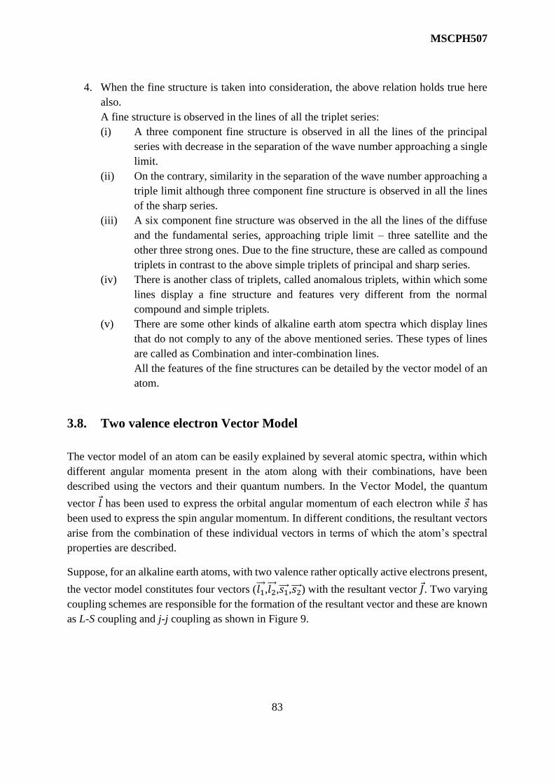
MSCPH507

83

4. When the fine structure is taken into consideration, the above relation holds true here

also.

A fine structure is observed in the lines of all the triplet series:

(i) A three component fine structure is observed in all the lines of the principal

series with decrease in the separation of the wave number approaching a single

limit.

(ii) On the contrary, similarity in the separation of the wave number approaching a

triple limit although three component fine structure is observed in all the lines

of the sharp series.

(iii) A six component fine structure was observed in the all the lines of the diffuse

and the fundamental series, approaching triple limit – three satellite and the

other three strong ones. Due to the fine structure, these are called as compound

triplets in contrast to the above simple triplets of principal and sharp series.

(iv) There is another class of triplets, called anomalous triplets, within which some

lines display a fine structure and features very different from the normal

compound and simple triplets.

(v) There are some other kinds of alkaline earth atom spectra which display lines

that do not comply to any of the above mentioned series. These types of lines

are called as Combination and inter-combination lines.

All the features of the fine structures can be detailed by the vector model of an

atom.

3.8. Two valence electron Vector Model

The vector model of an atom can be easily explained by several atomic spectra, within which

different angular momenta present in the atom along with their combinations, have been

described using the vectors and their quantum numbers. In the Vector Model, the quantum

vector 𝑙 has been used to express the orbital angular momentum of each electron while 𝑠 has

been used to express the spin angular momentum. In different conditions, the resultant vectors

arise from the combination of these individual vectors in terms of which the atom’s spectral

properties are described.

Suppose, for an alkaline earth atoms, with two valence rather optically active electrons present,

the vector model constitutes four vectors (𝑙1 ,𝑙2 ,𝑠1 ,𝑠2 ) with the resultant vector 𝐽 . Two varying

coupling schemes are responsible for the formation of the resultant vector and these are known

as L-S coupling and j-j coupling as shown in Figure 9.

MSCPH507

84

Figure 9: The vector model of L-S coupling.

The L-S coupling is a common type of coupling and exists in most of the lighter atoms. In this

type of coupling the 𝑙1 and 𝑙2 of two electrons, that is the individual orbital angular momentum

vectors are coupled to each other strongly, thus giving rise to a resultant orbital angular

momentum vector �� . Therefore, the corresponding quantum number L can take the values

𝐿 = |𝑙1 − 𝑙2|; |𝑙1 − 𝑙2| + 1,… . . (𝑙1 + 𝑙2)

This can provide numerous terms of the atom. These terms are expressed as S, P, D, ….. as per

the value of L= 0,1,2…. .

In similar manner, 𝑠1 and 𝑠2 of two electrons, that is the individual orbital angular momentum

vectors are coupled to each other strongly, thus giving rise to a resultant orbital angular

momentum vector 𝑆 . Therefore, the corresponding quantum number S can take the values

𝐿 = |𝑠1 − 𝑠2|; |𝑠1 − 𝑠2| + 1, … . . (𝑠1 + 𝑠2)

Since the value of 𝑠1 = 𝑠2 = 1

2, the S = 0, 1.

Thus in value of multiciplicity (2S+1) is 1 and 3, which means that the two electrons give rise

to singlet and triplet terms.

Now, for the formation of the total angular momentum 𝐽 (resultant) of an atom, the spin – orbit

interaction, that is �� and 𝑆 are less strongly coupled to each other. Therefore, both �� and 𝑆

move slowly around 𝐽 . Therefore, the values of quantum number 𝐽 can be

𝐽 = |𝐿 − 𝑆|; |𝐿 − 𝑆| + 1,… . . (𝐿 + 𝑆)

MSCPH507

85

The spin orbit interaction is important for each and every multiplet term, which being a

combination of fine structure levels, each designated with a J value.

Now this vector model can be used to describe the spectrum of the two electron atom, let’s

suppose Ca (Z=20). The configuration, generally called as ground state configuration is

1𝑠22𝑠22𝑝63𝑠23𝑝6 4𝑠2

For the electrons which are optically active,

𝑙1 = 0, 𝑙2 = 0, 𝑠1 =1

2 , 𝑠2 =

1

2

Thus,

L = 0 (S-term)

S = 0, 1 so that (2S+1) = 1, 3

And

J = 0, 1

The terms used are 1S0 and 3S0. Since the electrons (4s2) are equivalent, the term 3S1 is excluded

by Pauli’s principle. Therefore, only singlet S- term 1S0 arises from the normal atom.

The optically active electrons, either one or both present in the outer valence shell rise to the

higher levels or states when the atom is excited. It seems true that excitation of just one of the

optical electrons can give rise to the lines of all the eight series present in a spectrum.

Configuration Terms

4s 5s, 4s 6s,…. 51S0, 61S0, …… and 53S1, 5

3S1, …….

4s 4p, 4s 5p,….. 41𝑃𝑜1, 51𝑃𝑜1, … and 43𝑃𝑜2, 1, 0 ; 5

3𝑃𝑜2, 1, 0 ; ……

4s 3d, 4s 4d,….. 31D2, 41D2,…… and 33D1, 2, 3 ; 4

3D1, 2, 3 ; …….

4s 4f,…. 41𝐹𝑜3,…….. and 43𝐹𝑜2, 3, 4 ; ……..

The energy levels with respect to the terms given in the table above, can be designed as per in

Figure 10. When the spin – orbit interactions are studied, it displays different levels with triplet

splitting of the levels of the same L which converges swiftly with the increasing value of n.

Moreover, it shows that intervals of 3P are broader than that of the respective intervals of 3D.

Similarly, the intervals of 3D are broader than that of the respective intervals of 3F.When the

excited electron jumps back through any path, as per the selection rules, it emits different

spectral series.

∆𝑆 = 0

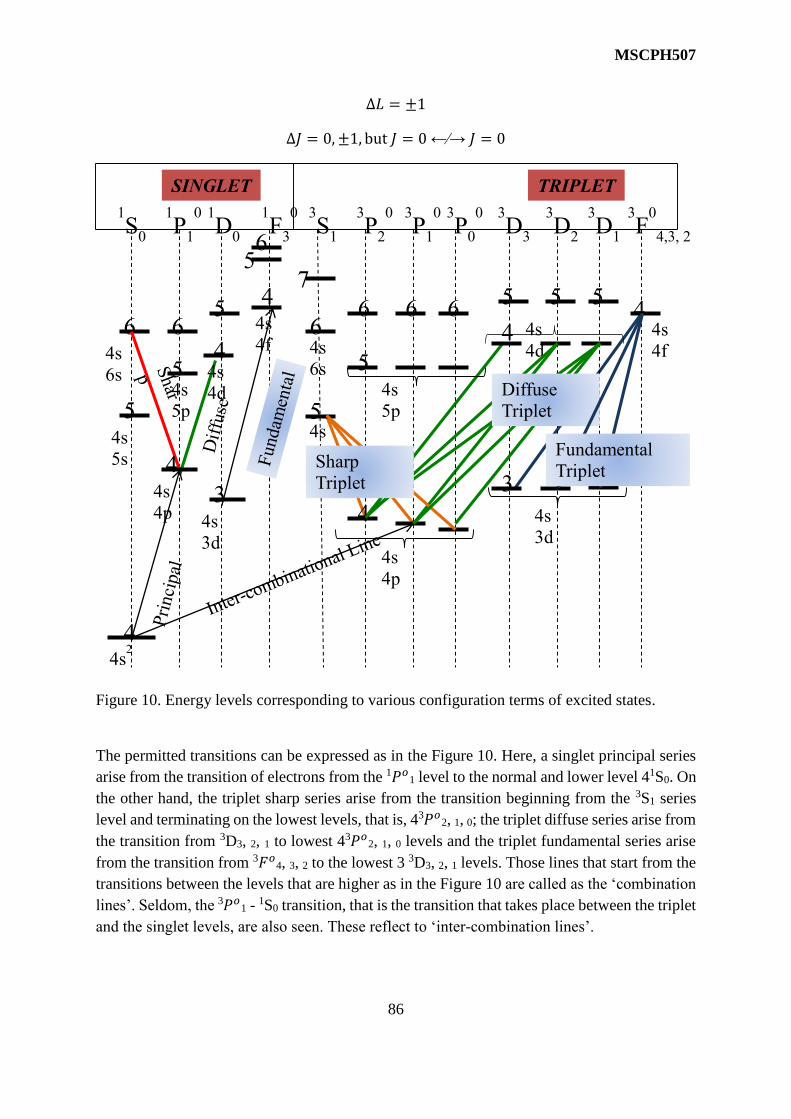
MSCPH507

86

∆𝐿 = ±1

∆𝐽 = 0, ±1, but 𝐽 = 0 ←∕→ 𝐽 = 0

Figure 10. Energy levels corresponding to various configuration terms of excited states.

The permitted transitions can be expressed as in the Figure 10. Here, a singlet principal series

arise from the transition of electrons from the 1𝑃𝑜1 level to the normal and lower level 41S0. On

the other hand, the triplet sharp series arise from the transition beginning from the 3S1 series

level and terminating on the lowest levels, that is, 43𝑃𝑜2, 1, 0; the triplet diffuse series arise from

the transition from 3D3, 2, 1 to lowest 43𝑃𝑜2, 1, 0 levels and the triplet fundamental series arise

from the transition from 3𝐹𝑜4, 3, 2 to the lowest 3 3D3, 2, 1 levels. Those lines that start from the

transitions between the levels that are higher as in the Figure 10 are called as the ‘combination

lines’. Seldom, the 3𝑃𝑜1 - 1S0 transition, that is the transition that takes place between the triplet

and the singlet levels, are also seen. These reflect to ‘inter-combination lines’.

1S

0

1P

1

0

6

5

4s

5s

4s2

5

4

SINGLET

4s

6s

4

4

4s

4p

6

5

4s

5p

5

4s

4d

4

3

4s

3d

6

4s

4f

1D

0

1F

3

0

5

4s

5s

6

4s

6s

3S

1

7

3P

2

0

TRIPLET

6 6 6 5 5 5

5

4

4s

4p

4s

5p

4

3P

1

0 3P

0

0

3D

3

3D

2

3D

1 3F

0

4,3, 2

4s

4d

4

3

4s

3d

Sharp

Triplet

Diffuse

Triplet

4s

4f

Fundamental

Triplet

MSCPH507

87

(a) (b)

Figure 11. (a) Simple and (b) Compound triplet structure formation, respectively.

Figure 11(a) and (b) displays a simple as well as the compound triplet structure (3D → 3P),

respectively. The order of the levels is regular as the lower j valued levels are placed lower.

Moreover, the spacing obeys the Lande’s interval rule. The 3P2 – 3P1 and 3P1 – 3P0 intervals

exists in ratio 2:1, and that of 3D3 – 3D2 and 3D2 – 3D1 intervals exists in 3:2 ratio.

There are following rules which govern the relative intensities of the spectral lines. This rule

says that where ∆𝐿 changes in the similar way as that of ∆𝐽. Out of these, the transition with

the largest value of L and J, give rise to the strongest lines.

The Anomalous Triplets: The alkaline earth elements as well as the alkaline earth ion

spectra’s exhibit few multiplets with structure difference from that of simple or compound

triplets, with respect to the intensities and the relative separations. These multiplets are then

called as anomalous triplets and these are generated as a result of excitation of both of the

optical electrons (Figure 12).

Wavenumber ()

3S

1

Simple Triplet

3P

2

3P

1

3P

0

3D

3

3D

2

3D

1

3P

2

3P

1

3P

0

Compound Triplet

Wavenumber ()

MSCPH507

88

Figure 12. Depiction of the transition resulting in the formation of anomalous triplet.

A multiplet in Ca at 4300Å gives rise to six lines. An examination of this multiplet proposes

its generation from the transition between two 3P terms with same splitting. The lowest 4s 4p 3𝑃𝑜 state constitutes the lower state of the multiplet while the upper state is an anomalous term

which is labelled as 3𝑃′ that is not included in the normal term series of the atom. In this term,

both the optical electrons are excited to 4p subshell. This configuration gives three terms, that

is, 3P, 1D, 1S out of which 3P only combines to all in a strong manner, as per the selection rule.

If we write the symbol in full, we get transitions

4p2 3𝑃′→ 4s 4p 3𝑃𝑜

In this scenario, ∆𝐿 = 0, is possible, providing that ∆𝑙 = ±1 (even ↔ odd) for that one electron

that skips or jumps.

The j – j coupling scheme in the vector model of two electron atom constitutes the spin and

the orbital vectors, 𝑠1 and 𝑙1 of one electron are coupled firmly to each other to give rise to a

resultant 𝑗1 around which the two individual vectors precess swiftly. In the similar way, 𝑠2 and

𝑙2 of the another electron give rise to resultant 𝑗2 . The two resultants 𝑗1 and 𝑗2 , themselves

couple with each other strongly, thus giving rise to 𝐽 , which is the total angular momentum.

3P

o

2

3P

o

1

3P

o

0

4s4p

4p2

3P

1

2

3P

1

1

3P

1

0

Wavenumber ()

Origin of Anomalous Triplet

MSCPH507

89

The individual resultant vectors precess quite slowly around the total angular momentum.

(Figure 13)

Figure 13. Vector model of two electron j-j coupling.

The terms and the 𝐽 values for this type of coupling are similar to those of the L – S coupling.

Moreover, this type of coupling occurs seldom.

3.9. Interaction Energy (Triplet separation) in L – S and j – j couplings

For every different value of J, the atomic terms consists of multiplet components dues to spin-

orbit interaction. This interaction is dependent on the fourth power of atomic number Z which

gets further large in heavier atoms.

From the relation of the shift in fine-structure level from the hypothetical centre, for a

single electron atom, the interaction energy is given by:

−∆𝑇𝑙𝑠 =𝑅∞

2𝑛3𝑙(𝑙+1

2)(𝑙+1)

[𝑗(𝑗 + 1) − 𝑙(𝑙 + 1) − 𝑠(𝑠 + 1)]cm-1

= 𝑎𝑗∗2 − 𝑙∗2 − 𝑠∗2

2

Where 𝑎 =𝑅∞𝛼

2𝑍4

𝑛3𝑙(𝑙+1

2)(𝑙+1)

𝑐𝑚−1; 𝑗∗ = √𝑗(𝑗 + 1), 𝑙∗ = √𝑙(𝑙 + 1), 𝑎𝑛𝑑 𝑠∗ = √𝑠(𝑠 + 1)

MSCPH507

90

For two optical electrons there could be four possibilities of arrangement of angular momenta

𝑙1∗, 𝑙2

∗ , 𝑠1∗, 𝑠2

∗ and these four possibilities can be paired um in six possible interactions the ways

as (𝑎) 𝑙1∗ 𝑤𝑖𝑡ℎ 𝑙2

∗ , (𝑏) 𝑠1∗𝑤𝑖𝑡ℎ 𝑠2

∗(𝑐) 𝑙1∗ 𝑤𝑖𝑡ℎ 𝑠1

∗, (𝑑) 𝑙2∗ 𝑤𝑖𝑡ℎ 𝑠2

∗, (𝑒) 𝑙1∗ 𝑤𝑖𝑡ℎ 𝑠2

∗, (𝑓) 𝑙2∗ 𝑤𝑖𝑡ℎ 𝑠1

∗.

It is seen that in L-S coupling, the interaction mentioned by processes (a), (b) are most probable

over process (c) and (d), while the process I & (f) are least probable. Using the cosine law of

𝑗∗2 = 𝑙∗2 + 𝑠∗2+ 2𝑙∗2𝑠∗2cos (𝑙∗𝑠∗),

Therefore, the general terms will be: −∆𝑇𝑙𝑠 = 𝑎𝑙∗𝑠∗cos (𝑙∗𝑠∗). For the above interactions, the

related energies are:

∆𝑇1 = 𝑎1𝑠1∗ 𝑠2

∗cos (𝑠1 ∗ 𝑠2∗)

∆𝑇2 = 𝑎2𝑙1∗ 𝑙2∗cos (𝑙1

∗ 𝑙2∗)

∆𝑇3 = 𝑎2𝑙1∗𝑠2∗cos (𝑙1

∗ 𝑠2∗)

∆𝑇4 = 𝑎2𝑙2∗ 𝑠1

∗cos (𝑙1 ∗ 𝑠1

∗)

Since, in 𝑠1∗ and 𝑠2

∗ precess around in the fixed angles to form their resultant S*, and therefore

its magnitude remains fixed. Similar observations were taken for 𝑙1∗ and 𝑙2

∗ around L*. Again

using the cosine law in terms to calculate S*2, L*2, we have,

∆𝑇1 =1

2𝑎1(S

∗2 − s1∗2 − s2

∗2)

∆𝑇2 =1

2𝑎2(L

∗2 − l1∗2 − l2

∗2)

Here L* and S* also precess around J* in the similar manner as l* and s* do for a single electron

process around j*. The energy of interaction is due to coupling in between l1* and s1

* and in

between l2* and s2

* is given by the terms ∆𝑇3 and ∆𝑇4, respectively. Since the angle between

the vector changes continuously, we have to involve the average values obtained by the cosine

functions between the vectors. This average value is given by

cos(𝑙1∗ 𝑠1

∗) = 𝑐𝑜𝑠(𝑙1∗ 𝐿∗ )𝑐𝑜𝑠(𝐿∗𝑆∗)𝑐𝑜𝑠(𝑆∗𝑠1

∗)

And

cos(𝑙2∗ 𝑠2

∗) = 𝑐𝑜𝑠(𝑙2∗ 𝐿∗ )𝑐𝑜𝑠(𝐿∗𝑆∗)𝑐𝑜𝑠(𝑆∗𝑠2

∗)

Using the average cosine values from ∆𝑇1, ∆𝑇2, and rearranging the terms from the cosine laws

on the we get:

∆𝑇3 + ∆𝑇4 =1

2(𝑎3𝑐3 + 𝑎4𝑐4)(J

∗2 − L∗2 − S∗2)

Where, 𝑐3 =𝑙1∗2−𝑙2

∗2+𝐿∗2

2𝐿∗2.𝑠1∗2−𝑠2

∗2+ S∗2

2 S∗2 and

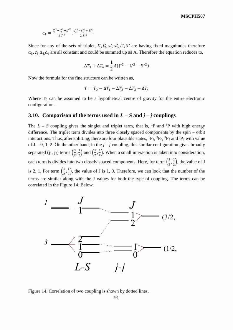
MSCPH507

91

𝑐4 =𝑙2∗2−𝑙1

∗2+𝐿∗2

2𝐿∗2.𝑠2∗2−𝑠1

∗2+ S∗2

2 S∗2

Since for any of the sets of triplet, 𝑙1∗, 𝑙2

∗ , 𝑠1∗, 𝑠1

∗, 𝐿∗, 𝑆∗ are having fixed magnitudes therefore

𝑎3, 𝑐3,𝑎4,𝑐4 are all constant and could be summed up as A. Therefore the equation reduces to,

∆𝑇3 + ∆𝑇4 =1

2𝐴(J∗2 − L∗2 − S∗2)

Now the formula for the fine structure can be written as,

𝑇 = 𝑇0 − ∆𝑇1 − ∆𝑇2 − ∆𝑇3 − ∆𝑇4

Where T0 can be assumed to be a hypothetical centre of gravity for the entire electronic

configuration.

3.10. Comparison of the terms used in L – S and j – j couplings

The L – S coupling gives the singlet and triplet term, that is, 1P and 3P with high energy

difference. The triplet term divides into three closely spaced components by the spin – orbit

interactions. Thus, after splitting, there are four plausible states, 1P1, 3P0,

3P1 and 3P2 with value

of J = 0, 1, 2. On the other hand, in the j – j coupling, this similar configuration gives broadly

separated (j1, j2) terms (3

2,1

2) and (

1

2,1

2). When a small interaction is taken into consideration,

each term is divides into two closely spaced components. Here, for term (3

2,1

2), the value of J

is 2, 1. For term (1

2,1

2), the value of J is 1, 0. Therefore, we can look that the number of the

terms are similar along with the J values for both the type of coupling. The terms can be

correlated in the Figure 14. Below.

Figure 14. Correlation of two coupling is shown by dotted lines.

1

2

2

1

0

1

3

P

1

P

J

L-S

terms

1

0

J

(3/2,

1/2)

(1/2,

1/2)

j-j

terms

MSCPH507

92

The coupling intermediate can exist with the extreme values but the terms can be determined

through their J values as the total angular momentum of the atom is always conserved as the

coupling changes.

3.11. Regularities in Complex Spectra

Atomic spectra of a complex atom constitute different regularities which are as follows:

(i). The Hartley Law of Constant Doublet separation

According to Hartley (1983), the components of the multiplets of a spectral series

constitute constant wave separation. Let us take an example: same wave number

separation is present in all the doublet lines of the sharp series of an alkali atom.

It is an undeniable repercussion of the concept of energy levels. The transitions

that are starting from or terminating on a doublet level gives two sets of lines,

which are separated by the energy interval between two segments of the level.

(ii). The Rydberg – series relationships

According to the Rydberg’s observation, the spectral lines of a complex atom

splits into several series, with many recognized series can be denoted by a formula

comparable to Balmer’s formula of the hydrogen series

𝒗𝒎 = 𝒗∞ −𝑹

(𝒎+ 𝝁)𝟐; 𝜇 < 1 and 𝑚 = 2,3,4,… .∞

Where, 𝑣∞, also called convergence limit and 𝜇 are constant, which vary from one

series to another. This can be interpreted from Schroedinger theory which

explains that an electron which is at far distance from the nucleus travel through

into the potential field and reach the field because of the singly charged nucleus,

as that of hydrogen, due to the shielding effect of the inner electrons. Therefore,

higher excited states of a neutral atom where only one electron is excited, reach

for hydrogen.

(iii). The Alternation law of Multiplicities

According to this law, the spectral terms that generates from the consecutive

elements present in the periodic table, alternates between even and odd

multiplicities. As taking an example, the elements in fourth period, the

multiplicities are:

K – Doublets

Ca – Singlets, Triplets

Sc – Doublets, Quartets

Ti – Singlets, Triplets, Quintets

MSCPH507

93

This law is an effect of the combination of the spin properties of different valence

electrons. Therefore, the even multiplicity arises from the odd number of

electrons while the odd ones arise from the even number of electrons.

1 electron – Doublet

2 electrons – Singlet, Triplet

3 electrons – Doublet, Quartet

4 electrons – Singlet, Triplet, Quintet

(iv). Connection between member of same Chemical Group

The chemically similar atom spectra show noticeable connection. Such atoms

have analogous electron configuration giving rise to analogous sets of excited

energy levels, further results in similar spectra.

(v). The Displacement Law

Kossel and Sommerfeld stated this law in year 1919. According to this law, the

energy level and the spectrum of any neutral atom of Z atomic number closely

simulate the energy level and the spectrum of the singly ionised atom of atomic

number Z+1 coming next in the periodic table. This law is based on the fact that

the electron configuration of two such atoms would be same. Therefore, the

spectrum of the hydrogen atom is similar to that of the He atom while the doublet

series of Li, Na, K, … and so on, which are the alkali metals, are similar to the

doublet series of Be+, Mg+, Ca+,… and so on, the ionised alkaline earth metals.

(vi). Isoelectronic Sequences

The displacement law can also be applicable to the series with adjacent elements,

each one of them ionised to a successively greater degree. Therefore, the series

of atoms, whose electron configurations are similar, are called as an ‘Isoelectronic

Sequence’. As per example, the atoms that form the isoelectronic sequence are as

follows:

K – Z=19

Ca+ – Z=20

Sc++– Z=21

Ti+++– Z=22

These can also be written as:

K I, Ca II, Sc III, Ti IV

The spectrum lines and the energy level generating from each of the atoms show

great resemblance. For example, similar relative intensities for the various

transitions, same type of fine structure splitting, etc.

MSCPH507

94

3.12. Summary

This unit III is in continuation with previously discussed Unit I and II where most of the

basic details and properties related to Hydrogen atom and its spectra were discussed. In this

Unit III, we have summarised the whole unit in two halves. The first comprises of studies

about the spectra of alkali and the second half considers the spectra about the alkaline earth

spectra.

In first part, the fundamental introduction to the formation of four spectral lines were

observed and elaborated. The Rydberg-Schuster Law and Runge’s Law were found to be

established in alkali series. The concept of ‘combinational’ series was established by Ritz

combination principle. With the effect of increase in the shell value n, the alkali levels

approach the corresponding H-levels because of the screening effect and also in comparison

to hydrogen, it was found that the energy not only depends on n value but also on l. thus all

alkali levels with a given n are shifted lower than the corresponding H-levels. The selection

rule for the absorption spectra of Na atoms was revealed. It was noted that the optically

active electron in atom absorbs quantised energy and gets excited to the higher levels. The

concept of spin-orbit interaction leading to j was considered in details. The mathematical

formulation for considering the screening effect gave a good agreement for doublet

separation with experimental results. Quantitative rules for intensity relations were also

discussed.

In the second half section of this unit, the essential features of alkaline earth spectra are

elaborated in details. Vector Model, in which various angular momenta occurring in the

atomic spectra are considered. In this model, the combined form of the resultant vectors,

and subsequently their spectral properties were briefed. LS and jj coupling schemes are

quantitatively and qualitatively discussed in details. Further, one can easily calculate the

interaction energy for the triplet separation in L-S and j-j coup;ing using the mathematical

operations therein.

3.13. References

11. K. Veera Reddy, Symmetry and Spectroscopy of Molecules, New Age Publishers;

Second edition, 2009, ISBN-10: 8122424511.

12. Ghoshal S.N. , Atomic Physics (Modern Physics), S Chand & Company, 2010, ISBN-

10: 9788121910958.



14. Mool Chand Gupta, Atomic and Molecular Spectroscopy, New Age International

Private Limited, 2001, ISBN-10: 8122413005


10: 8180300358

MSCPH507

95

3.14. Suggested Readings


edition, 2017, ISBN-10: 9352601734.


17. Colin Banwell, Elaine McCash, Fundamentals for Molecular Spectroscopy, McGraw

Hill Education; 4 edition, 1994, ISBN-10: 0077079760.

18. Benjamin Bederson, Herbert Walther, Advances in Atomic, Molecular, and Optical


19. Savely G. Karshenboim, Valery B. Smirnov, Precision Physics of Simple Atomic

Systems (Lecture Notes in Physics), Springer; 2003 edition, ISBN-10: 3540404899.




ISBN-10: 0486601153

3.15. Terminal Descriptive type questions

1. How will you explain the common features of spectra of alkali like atoms?

2. Even though H and Na belong to the single valance electron system, distinguish between

the spectra obtained for two atoms.

3. Show the conception of spinning electrons that result for the doubling of levels in the

spectra of alkalis.

4. Using the spin-orbit interaction energy for a single non-penetrating valence electron,

elaborate and discuss the separation of 2P and 2D terms of alkali spectra.

5. Explain the theoretical background along with the essential features of the spectra of

alkaline earth elements.

6. Describe using the vector model of an atom for explaining its spectra with two electrons

outside the closed shell.

7. Discuss the vector model of an atom consisting of the two valance electrons in terms of L-

S and j-j couplings.

3.16. Numerical type (Self Assessment Questions)

1. The mean position of the first pair of lines of the principal series of sodium is 16960 cm-1.

If the convergence limit of the sharp series lines is at 24490 cm-1, calculate the ionisation

potential of sodium.

Ans. The first principal line is obtained from the transition of 3s-3p and the convergence

limit is obtained from 3p-∞. The sum of wave numbers will be (referring to Figure 1)

16960+24490=41450cm-1. This corresponds to 3s-∞, resulting in the ionization of atom

having energy 5.14eV. [Use 1eV=8066cm-1].

2. The longest wavelength lines in the series (𝑛, 𝑙) → (4,0) in potassium have wavelengths

7699.0, 7664.9, 4047.2, 4044.1Å respectively. Construct the relevant part of the energy level

MSCPH507

96

diagram and calculate the splitting between the levels with the same values of n and l but

different j.

Ans. The given wavelengths represent the first two doublets of the principal series of

potassium, and arise from the transitions

4 2P3/2, 1/2 → 4 2S1/2

5 2P3/2, 1/2 → 4 2S1/2

Diagram showing the splitting between the levels

The line splitting in the wave number are the corresponding level splitting with the

same values of n and l but different j. We know that the wave number 𝑣 is the reciprocal

of wavelength 𝜆

𝜈 =1

𝜆

So that

𝑑𝜈 = −1

𝜆2𝑑𝜆

Numerically, it can be written as

𝑑𝜈 =𝑑𝜆

𝜆2 × 𝜆2

2S

1/2

2P

3/2

2P

1/2

6s

5s

4s

5p

4p

6p

Potassium

4044.1 Å 4047.2 Å

7699 Å

7664.9Å

MSCPH507

97

For the wavelengths 7699.0 and 7664.9 Å, we have

𝑑𝜈 =(7699.0 − 7664.9) × 10−8𝑐𝑚

(7699.0 × 10−8𝑐𝑚) × (7664.9 × 10−8𝑐𝑚)

𝑑𝜈 =34.1

7699.0 × 7664.9 × 10−8𝑐𝑚

𝑑𝜈 = 57.8 𝑐𝑚−1

MSCPH507

98

UNIT 4 ZEEMAN EFFECT

STRUCTURE:

4.1. Introduction

4.2. Objectives

4.3. Zeeman effect and its experimental study

4.3.1. Classical interpretation of normal Zeeman effect

4.3.2. Vector atom model and Normal Zeeman effect

4.3.3. Quantum mechanical interpretation of normal Zeeman effect

4.4. Anomalous Zeeman effect

4.4.1. Quantum mechanical treatment of anomalous Zeeman effect

4.5. Paschen-Back effect

4.5.1. Quantum mechanical treatment of Paschen-Back effect

4.6. Spin orbit correction

4.7. Summary

4.8. Glossary

4.9. Terminal Questions

4.10. References

4.11. Answers

MSCPH507

99

4.1 INTRODUCTION

The Zeeman effect is a magneto-optical phenomenon in which spectral lines are affected by an

applied magnetic field and split into several components. This was first observed by Zeeman

in 1896 and hence called Zeeman effect. He found if a source of light giving line spectra be

placed in a magnetic field, the lines were split into a number of component lines, symmetrically

distributed about the original line. Doublets, triplets and even more complex system were

observed.

Primarily, it was observed that a single spectral line splits into three components such that one

line has got a large frequency, other a lower frequency than the frequency of original line and

a third one has a frequency of original line. This was named as normal Zeeman effect. But later

on, more complicated splitting was observed and was called anomalous Zeeman effect.

However, when a huge magnetic field is applied the splitting is called Paschen-Back effect.

The effect of electric field on spectral line was observed by Stark in 1913 and is called Stark

effect.

4.2 OBJECTIVES:

This unit introduces the effect of magnetic field on the spectral lines of atom which is called as

Zeeman effect. Depending on the strength of the magnetic field we have normal, anomalous

Zeeman effect and Paschen-Back effect. In this unit we will study about these effects and their

classical and quantum mechanical explanation. After going through this unit, the students will

be able to know about

1. The normal Zeeman effect, anomalous Zeeman effect and Paschen-Back effect.

2. The experimental study of above effects.

3. The classical and quantum mechanical explanation of above.

4. The spin orbit interaction.

4.3 ZEEMAN EFFECT AND ITS EXPERIMENTAL STUDY

Zeeman effect was discovered by Pieter Zeeman in 1896. He observed that if a source of light

producing line spectrum is placed in a magnetic field, the spectral lines are split up into

MSCPH507

100

components. When the splitting is into two or three lines, then it is called normal Zeeman effect

because it can be explained easily by classical theory. But when the applied magnetic field is

weak, then the splitting of a single line takes place into a number of components. This effect is

called anomalous Zeeman effect. The normal Zeeman effect is observed rarely whereas the

anomalous Zeeman effect is observed in general. The experimental arrangement for studying

normal Zeeman effect is shown in fig. 4.1

In the given arrangement, an electromagnet

MM capable of producing a very strong

magnetic field and having conical pieces

PP, through which holes are drilled

lengthwise, is set up. A source L emitting

spectral lines; say a sodium vapour lamp, is

placed between the pole pieces. The

spectral lines are observed with a high

resolving power instrument with a constant

deviation spectrometer S. The light can be

viewed perpendicular as well as parallel to

the magnetic field.

When light is viewed parallel to the magnetic field through the hole drilled in the pole pieces,

a single line is observed to be split up into two components (doublet). One component has a

higher frequency than the original line and the other lower. The original line is not observed.

Also, the original line is not polarized but the other two components are circularly polarized in

opposite direction. The outer components are known as σ components and the middle one is π

component. The σ components are symmetrically situated about the original line, so the change

in wavelength dλ, known as Zeeman shift, is the same in both cases (fig 4.2).

When light is observed perpendicular to the magnetic field, a triplet i.e., three component lines

are seen. One component line is observed in the same position as the original line and the other

two components, one on either side of this line are separated by equal amounts. These three

components are plane polarized but the vibrations of the central line is parallel to the magnetic

field while those of outer ones perpendicular to the field (fig. 4.2).

Figure 4.1: Experimental arrangement for

studying Zeeman effect

MSCPH507

101

Figure 4.2: Normal Zeeman Effect

4.3.1 CLASSICAL INTERPRETATION OF NORMAL ZEEMAN EFFECT:

It is observed that when magnetic field is applied, a single spectral line splits up into three

components such that one line has got a larger frequency, other a lower frequency than the

original line and the third one has the same frequency as that of the original line. This is called

normal Zeeman effect.

The normal Zeeman effect is explained on the basis of Lorentz classical theory. According to

this theory if a source of light is placed in a magnetic field, the frequency of motion of electron

moving in a circular orbit gets modified.

Let us consider an electron in an atom moving in a circular orbit of radius ‘r’ with a linear

velocity ‘v’ and angular velocity ‘ω’. Let ‘e’ and ‘m’ be the charge and mass of electron

respectively. The centripetal force acting on the electron towards the centre in the absence of

the magnetic field,

F = 𝑚𝑣2

𝑟 = 𝑚𝑟𝜔2 ………………..(1)

Now, let an external magnetic field ‘B’ be applied in a direction perpendicular to the plane of

the orbits of the two circular components. Then, an additional radial force of magnitude Bev

acts on the electron. The direction of this force will be outwards from the center for clockwise

MSCPH507

102

motion but inwards towards the center for anticlockwise motion. The resulting complex motion

of the electron subjected to an additional radial force is called Larmor precession. This

produces change in the angular velocity without any change in the form of the orbit.

Let d𝜔 be the change in angular velocity caused by the magnetic field. For the circular motion

in the clockwise direction, the additional radial force is directed away from the center,

Therefore 𝐹 − 𝐵𝑒𝑣 = 𝑚𝑟 (𝜔 + 𝑑𝜔 )2 ……………….(2)

𝑚𝑟𝜔2 −𝑚𝑟 (𝜔 + 𝑑𝜔 )2 = 𝐵𝑒𝜔𝑟

Or -2mr𝜔𝑑𝜔 = 𝐵𝑒𝜔𝑟 𝑛𝑒𝑔𝑙𝑒𝑐𝑡𝑖𝑛𝑔 (𝑑𝜔)2

Or d𝜔 = −𝐵𝑒

2𝑚 ………………(3)

For the circular motion in the anticlockwise direction, the additional radial force is directed

towards the centre.

Therefore F + Bev = mr (𝜔 + 𝑑𝜔 )2

Or d𝜔 = + 𝐵𝑒

2𝑚 ………………..(4)

The two cases can be combined into the equation

d𝜔 = ±𝐵𝑒

2𝑚 ………………(5)

If ν be the frequency of vibration of the electron,

Then 𝜔 = 2𝜋𝜈

Or d𝜔 = 2𝜋𝑑𝜈

Or dν = 𝑑𝜔

2𝜋

Therefore, change in frequency of the spectral line,

dν = ± 𝐵𝑒

4𝜋𝑚 …………….(6)

If ν and 𝜆 are the frequency and wavelength of the original line,

MSCPH507

103

ν = 𝑐

𝜆

or dν = - 𝑐

𝜆2 dλ

Therefore, the Zeeman shift

dλ = ± 𝐵𝑒𝜆2

4𝜋𝑚𝑐 ………………(7)

Taking a spectral line of known wavelength λ, and applying a magnetic field B, the Zeeman

shift dλ is measured.

From equation (7),

𝑒

𝑚 = (

4𝜋𝑐

𝐵𝜆2) dλ

From above equation, 𝑒

𝑚 can be calculated.

𝑒

𝑚 is found to be 1.757 × 1011 CKg-1 which is in

agreement with the value of 𝑒

𝑚 of the electron obtained from Thomson’s experiment.

4.3.2 VECTOR MODEL AND NORMAL ZEEMAN EFFECT:

We have studied that Lorentz was able to explain normal Zeeman effect quite satisfactorily

using classical theory. Later, Debye was able to interpret the same using vector atom model

where, the concept of electron spin was not taken into account, but only orbital motion was

considered.

Here only the angular momentum possessed by the electron due to its orbital motion is taken

into account. The magnitude of this orbital angular momentum which is quantized is given by

𝑝𝑙 = 𝑙.

ℎ

2𝜋

……………….(1)

The corresponding magnetic moment is given by

µ𝑙 = 𝑙 .

𝑒ℎ

4𝜋𝑚𝑐

= 𝑒

2𝑚𝑐 𝑝𝑙 ………………(2)

MSCPH507

104

The vectors l and µ𝑙 will act along the same line, viz., perpendicular to the orbital plane. In the

presence of external magnetic field B, the vector l will execute Larmor precession round the

field direction as axis whose frequency is given by

𝜔𝑖 = 𝐵

µ𝑙𝑝𝑙

= 𝑒

2𝑚 B ………………(3)

The effect of this Larmor precession is to alter the energy of the system by an amount ΔE,

which is given by

ΔE = 𝜔𝑙 × Projection of mechanical momentum on the field direction

ΔE = 𝑒

2𝑚 B 𝑝𝑙 cos𝜃 =

𝑒𝐵

2𝑚 𝑙ℎ

2𝜋 cos𝜃

ΔE = 𝑒ℎ𝐵

4𝜋𝑚 𝑚𝑙 …………….(4)

Since cos𝜃 = 𝑚𝑙

Now change in energy means that each energy level of the undisturbed state of the atom is,

splitted into a number of levels which is given by (2l + 1) and the magnitude of separation is

proportional to the strength of magnetic field.

Now suppose that E1 and E2 are the energies of the two levels in the presence of magnetic field

and E01 and E02 in the absence of magnetic field with the two values of ml as 𝑚𝑙1 and 𝑚𝑙2 . Then

we have

E1 = E01 + ΔE1 = E01 + 𝑚𝑙1 𝑒ℎ𝐵

4𝜋𝑚 …………………………(5)

E2 = E02 + ΔE2 = E02 + 𝑚𝑙2 𝑒ℎ𝐵

4𝜋𝑚 …………………………(6)

If transitions take place between these two above multiplet states, a multiplet group of lines

will result. The frequency 𝜈 of any of these lines is obtained from equations (5) and (6) by

using Bohr’s frequency condition i.e.

E1 - E2 = E01 - E02 + 𝑒ℎ𝐵

4𝜋𝑚 ( 𝑚𝑙1 - 𝑚𝑙2 )

hν = hν0 + Δml 𝑒ℎ𝐵

4𝜋𝑚

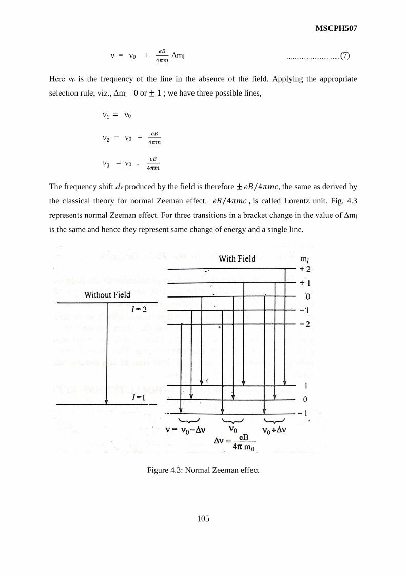
MSCPH507

105

ν = ν0 + 𝑒𝐵

4𝜋𝑚 Δml ……………………….. (7)

Here ν0 is the frequency of the line in the absence of the field. Applying the appropriate

selection rule; viz., Δml = 0 or ± 1 ; we have three possible lines,

𝜈1 = ν0

𝜈2 = ν0 + 𝑒𝐵

4𝜋𝑚

𝜈3 = ν0 - 𝑒𝐵

4𝜋𝑚

The frequency shift dν produced by the field is therefore ±𝑒𝐵 4𝜋𝑚𝑐,⁄ the same as derived by

the classical theory for normal Zeeman effect. 𝑒𝐵 4𝜋𝑚𝑐 ,⁄ is called Lorentz unit. Fig. 4.3

represents normal Zeeman effect. For three transitions in a bracket change in the value of Δml

is the same and hence they represent same change of energy and a single line.

Figure 4.3: Normal Zeeman effect

MSCPH507

106

4.3.3 QUANTUM MECHANICAL EXPLANATION OF NORMAL ZEEMAN

EFFECT

Here the procedure is to calculate the interaction of magnetic field with the angular momentum

of electrons. The magnetic moment of an electron moving in its orbit is given by

µL = -𝑒

2𝑚𝑜 L

This magnetic moment interacts with external magnetic field and gives the perturbing

Hamiltonian as

H’ = - µL.B

= 𝑒

2𝑚𝑜 L . B

To calculate the splitting of spectrum lines, the operator forms of H’ is used in the perturbation

theory. The first order interaction energy is

ΔE = ∫ Ψ* �� Ψ dτ

ΔE = 𝑒

2𝑚𝑜 ∫ Ψ* �� Ψ dτ

Let us assume that B is directed towards z axis; then

B = Bz

ΔE = 𝑒

2𝑚𝑜 Bz ∫ Ψ* �� Ψ dτ

But the average value of z-component of angular momentum is ML h. Hence, change in energy

value is (changing Bz to B)

ΔE = 𝑒ℎ

2𝑚𝑜 Bz ML

Therefore, the energy of the having the orbital quantum number ML1 is

E1 = E(1) + 𝑒ℎ

2𝑚𝑜 BML1

And E2 = E(2) + 𝑒ℎ

2𝑚𝑜 BML2

MSCPH507

107

(E2 – E1) = (E2 – E1) + 𝑒ℎ

2𝑚𝑜𝑐 B ΔML

hν = hν0 + 𝑒ℎ

2𝑚𝑜 B ΔML

ν = ν0 + 𝑒𝐵

4𝜋𝑚𝑜 ΔML

The expression when subjected to selection rule ΔML = 0, ±1 gives rise to Zeeman normal

triplet. ΔML = 0 corresponds to π components and ΔML = ±1 gives σ components

Self-Assessment question (SAQ) 1: Choose the correct option-

1. The number of spectral lines seen in normal Zeeman effect is

a) Greater than 3

b) Equal to 3

c) Less than 3

2. In normal Zeeman effect we take

a) Only orbital motion in account

b) Only spin motion in account

c) Both the above

3. The rule for ΔML=0 gives

a) π component

b) σ component

c) none of above

4. 4 ANOMALOUS ZEEMAN EFFECT

When the applied magnetic field is weak as compared to the internal magnetic field, a single

spectral line is splitted into a more complex - greater number of components. This is called

anomalous Zeeman effect. The Lorentz or Debye theory was able to explain normal Zeeman

effect but it was unable to explain anomalous Zeeman effect. To achieve this the idea of spin

MSCPH507

108

of electron was introduced. By introducing this the total angular momentum of the atom j*

becomes the vector sum of the orbital and spin angular moments, l* and s*, i.e.,

j* = l* + s* ……………. (1)

In this case the coupling between l* and s* is intact, so that there is physical significance in

compounding l* and s* into j* and then considering the precession of j* about B.

The magnetic moment due to orbital motion

𝜇𝑙 = l* 𝑒ℎ

4𝜋𝑚

……………… (2)

This 𝜇𝑙 𝑖𝑠 directed opposite to l* because of negative

charge of electron. Similarly, magnetic moment due to

spin is given by,

𝜇𝑠 = 2s* 𝑒ℎ

4𝜋𝑚

……………… (3)

𝜇𝑠 is directed opposite to s*. This is shown in fig 4.4.

Now since l* and s* precess around j*,

𝜇𝑙 and 𝜇𝑠 will also precess around 𝜇𝑗 ( 𝜇𝑗 is not in

the line of the resultant of 𝜇𝑙 and 𝜇𝑠).

To find out the resultant magnetic moment of the

electron, we resolve 𝜇𝑙𝑠 into two directions, one along j*

and the other perpendicular to it. The perpendicular

component average out to zero due to the continuous change in direction and the parallel

components add together. We can say that the parallel components of 𝜇𝑙 and 𝜇𝑠 contribute

for 𝜇𝑗 while perpendicular components do not. Hence

𝜇𝑗 = Component of 𝜇𝑙 𝑎𝑙𝑜𝑛𝑔 𝑡ℎ𝑒 direction of j* + component of 𝜇𝑠 along the direction of j*

𝜇𝑗 =. 𝑒ℎ

4𝜋𝑚 l* cos ( l* j* ) +

𝑒ℎ

4𝜋𝑚 2s* cos ( s* j* )

= 𝑒ℎ

4𝜋𝑚 [ l* cos ( l* j*) + 2s* cos ( s* j*) ]

Figure 4.4: The precession of

mechanical and magnetic moments

MSCPH507

109

Or

𝜇𝑗 = j*g = [ l* cos ( l* j*) + 2s* cos ( s* j*) ]

………………………….(4)

In terms of Bohr Magneton.

But according to cosine law,

cos ( l*j*) = 𝑗∗2+ 𝑙∗2− 𝑠∗2

2𝑗∗ 𝑙∗

and cos (sl*j*) = 𝑗∗2+ 𝑠∗2− 𝑙∗2

2𝑗∗ 𝑠∗

Putting the values in equation (4), we write

j*g = [𝑗∗2+ 𝑙∗2− 𝑠∗2

2𝑗∗ +

𝑗∗2+ 𝑠∗2− 𝑙∗2

𝑗∗ ]

or g = 1 + 𝑗(𝑗+1)+ 𝑠(𝑠+1)−𝑙(𝑙+1)

2𝑗(𝑗+1) …………….(5)

Writing 𝑗∗2 = j(j+1) and so on.

With this value of g, the total magnetic moment of the electron is

𝜇𝑗 = j*g, in the unit of Bohr magneton.

If now the atom is placed in the weak magnetic field, the total angular momentum vector j*

precesses around the B direction. The result of this precession is the change in the energy of

electron by the amount.

∆𝐸 = 𝜇𝑗B cos(j*B)

= j*gh cos(j*B)

∆𝐸 = mjgB ……………(6)

This equation again shows that change in the energy is proportional to the magnetic field

strength. In the ordinary unit of energy in the above expression,

MSCPH507

110

∆𝐸 = mjg 𝑒ℎ

4𝜋𝑚0 B

Hence ∆𝜈 = mjg 𝑒𝐵

4𝜋𝑚0

∆�� = ∆ mjgO

where O = 𝑒𝐵

4𝜋𝑚0𝑐 = Lorentz unit.

Figure 4.5: Anomalous Zeeman effect

Further, since mj has (2j + 1) values right from -j to +j, so a given level is split up into (2j + 1)

sublevels with the application of magnetic field. When this mj is subjected to the selection rule

∆ mj = 0 or ± 1, we get the transition shown in fig. 4.5, for the sodium D lines. The longer

wavelength components 32S1/2 – 32P3/2 splits into four lines. The magnitude of component

separation is governed by the factor ∆ mjg showing fig. 4.6. Since g is different for different

𝑣𝑎𝑙𝑢𝑒𝑠 of j, we get different components for the same change in the value of ∆ mj. In this case

∆ mj = 0 give rise to 𝜋 components while ∆ mj = ± 1 gives to 𝜎 components.

Thus, it is clear that Lande’s g factor is important in order to explain the anomalous Zeeman

effect.

MSCPH507

111

Figure 4.6: The orientations of total angular moment vector in magnetic field

4.4.1 QUANTUM MECHANICAL TREATMENT OF ANOMALOUS ZEEMAN

EFFECT

When the source emitting spectral lines is subjected to weak magnetic field, the spin and the

orbital angular momentum are separately conserved, and L, S and J are well defined. When we

take the spin of the electron into account, the magnetic moment is given by

µJ = µL + µS,

µJ = - 𝑒

2𝑚𝑜 [L + 2S]

The perturbing Hamiltonian comes out to be

H’ = - µJ B

H’ = 𝑒

2𝑚𝑜 [L + 2S] . B

The change in energy value due to the perturbation is

ΔE’ = ∫ Ψ* ��’ Ψ dτ

= 𝑒

2𝑚𝑜 �� ∫ Ψ* (�� + 2�� )Ψ dτ

MSCPH507

112

= 𝑒

2𝑚𝑜 [(B.��) + 2 (��. ��)]

Further if B is directed along z-axis. B = Bz and

(��. ��) = 𝐽.��

𝐽2 ��. 𝐽 =

𝐽2+��2+��2

2𝐽2��. 𝐽

and (��. ��) = 𝐽 (𝐽+1)+𝑆(𝑆+1)−𝐿(𝐿+1)

2𝐽 (𝐽+1) BMJℏ

MJ is the Z component of total angular magnetic moment which is associated with the electron

of the atom. The above relations follow from the fact that in a weak magnetic field L and S

vectors precess rapidly round their resultant J and, hence, in the average only the component

along J survives and the perpendicular component averages to zero. With the substitution, we

get (Replace Bz by B)

ΔE’ = 𝑒

2𝑚𝑜 B [

𝐽 (𝐽+1)+𝑆(𝑆+1)−𝐿(𝐿+1)

2𝐽 (𝐽+1)] MJℏ

ΔE’ = g µB BMJ

Where g = 1+ 𝐽 (𝐽+1)+𝑆(𝑆+1)−𝐿(𝐿+1)

2𝐽 (𝐽+1),

And µB = 𝑒ℎ

2𝑚𝑜 is Bohr magneton

The energy expression then becomes,

EJ1 = E(1) + ΔEJ1

Or EJ1 = E(1) + µB BMJ1 g1

EJ2 = E(2) + µB BMJ2 g2

And ν = 𝐸(2)− 𝐸(1)

ℎ +

𝑒𝐵

4𝜋𝑚𝑜 Δ(MJ g)

Or �� = 𝜈0 + Δ(MJ g), In Lorentz Unit.

The equation implies that anomalous splitting depends not on Δ(MJ) but on Δ(MJg) informing,

thereby, that it is ‘g’ which is responsible for anomalous splitting.

MSCPH507

113

The expressions are same as derived on classical lines and with the selection rule ΔMJ = 0, ±1,

it explains anomalous Zeeman effect. ΔMJ = 0 gives π components and ΔMJ = ±1 gives σ

components.

Self-Assessment question (SAQ) 2: Choose the correct option-

1. Anomalous Zeeman effect takes into account

a) Spin motion of electron

b) Orbital motion of electron

c) Both (a) and (b)

2. The ration of spin magnetic moment 𝜇𝑠 to the spin angular momentum |𝑠 | is

a) e/2m

b) 2e/2m

c) 0

d) 3e/2m

3. In the Anomalous Zeeman effect, the resonance line D1 and D2 of sodium arise from

transition’s

a) 2P1/2→2S1/2

b) 2P3/2→2S1/2

c) Both (a) and (b)

d) None of the above

4.5 PASCHEN – BACK EFFECT:

We have already studied that in Zeeman effect, the external magnetic field is weak as compared

with the internal magnetic field due to spin and orbital motion of valence electron. Here the

precession of 𝑙∗ and 𝑠∗ around 𝑗∗ is much faster than that of 𝑗∗ around B which makes no change

due to motion of 𝑙∗ and 𝑠∗ into other motions. However, when the external magnetic field is

increased in strength, the coupling between 𝑙∗ and 𝑠∗ breaks down and 𝑗∗loses its significance.

𝑙∗ and 𝑠∗are quantized separately and precess more or less independently around B as shown

MSCPH507

114

in fig 4.7. This is known as Paschen – Back effect. Further, when the motion of 𝑙∗ and

𝑠∗become separately quantized, the perpendicular component of magnetic moment, does not

average out to zero and contributes to the total magnetic moment, i.e., now total magnetic

moment is not equal to mj. Due to this kind of splitting, whatever be the anomalous Zeeman

pattern in the weak magnetic field it is converted into normal pattern in the strong magnetic

field.

The angular velocities of two precessions are

ωl = B𝑒

2m0 and ωS = B

𝑒

2m0 2.

Therefore, the change in interaction energy due to

these two motions is the sum of two changes, i.e.

ΔE = ΔElB + ΔEsB,

Where

ΔElB = B𝑒

2m0 l*

ℎ

2𝜋 cos(l*B),

ΔEsB = B2𝑒

2m0 ℎ

2𝜋 cos(s*B)

Or ΔElB = 𝑒ℎ

4𝛱𝑚𝑜 Bml,

ΔEsB = 𝑒ℎ

4𝛱𝑚𝑜 2Bms

Therefore, ΔE = (ml + 2ms) B 𝑒ℎ

4𝛱𝑚𝑜

The quantity, (ml + 2ms) is known as strong field quantum number. In terms of the frequency

change

Figure 4.7: Precession of l* and s*

vectors in Paschen-Back effect

MSCPH507

115

Δν = Δ(ml ± 2ms) 𝑒𝐵

4𝛱𝑚𝑜

And in terms of wave number

Δ�� = Δ(ml ± 2ms) 𝑒𝐵

4𝛱𝑚𝑜𝑐

= Δ(ml ± 2ms), in Lorentz unit

Now since Δml = 0 or ±1, and Δ ms=0 or ±1.

We get three different frequencies. It means that the result is normal Zeeman triplet as said

before. As a specific example, we consider a principal series doublet,

(2P3/2 ⟶ 2S1/2 and 2P1/2 ⟶ 2S1/2)

In the strong field, P level is split up into six levels, because for a particular value of l(l+1), ml

has (2l + 1) values (here 1, 0, -1) and for each value of ml, ms has two values (+1

2 and -

1

2); and

levels with same value of (ml + 2ms) coincide. So, on the whole, we have five sub levels of P

level and two sub levels of S level. The values of different quantum numbers are given in the

table

Term l s ml ms ml + 2 ms a ml ms

2P3/2

1 +1

2 1 +

1

2 2 𝑎

2

1 +1

2 0 +

1

2 1 0

1 +1

2 -1 +

1

2 0 −

𝑎

2

2P1/2

1 +1

2 1 -

1

2 0 −

𝑎

2

1 +1

2 0 -

1

2 -1 0

1 +1

2 -1 -

1

2 -2 𝑎

2

2S1/2

0 +1

2 0 +

1

2 +1 0

0 +1

2 0 -

1

2 -1 0

MSCPH507

116

The allowed transitions are shown in fig. 4.8, with the coincidence of the transitions having the

same value Δ(ml + 2ms).

Figure 4.8: Paschen-Back effect

The allowed transitions in figure are correct up to the first approximation.

Figure 4.9: Transition from weak to strong magnetic field

MSCPH507

117

4.5.1 QUANTUM MECHANICAL TREATMENT OF PASCHEN-BACK EFFECT

In a strong situation magnetic field L and S are not well defined and do not give a well-defined

resultant J. In such a situation L and S precess independently round the direction of B. The

values of equation 10 and equation 11 then modify as

(��.��) = (Bz Lz) = B ML ℏ

(��.��) = (Bz Sz) = Bz Ms ℏ

The change in energy is

ΔE’ = 𝑒ℎ

2𝑚𝑜 B(ML + 2MS)

The strong field quantum number (ML + 2MS) when subjected to selection rule Δ (ML + 2MS)

= 0, ±1, gives rise to Paschen-Back Effect.

Self-Assessment question (SAQ) 3: Choose the correct option

1. The strength of mag. Field is max. in

a) Normal Zeeman effect

b) Paschen-Back effect

c) Anomalous Zeeman effect

2. The total magnetic quantum number J precess around external magnetic field in

a) Normal Zeeman effect

b) Anomalous Zeeman effect

c) Paschen-Back effect

4.6 SPIN – ORBIT CORRECTION

In practice, the residual spin-orbit coupling changes the relative energies of the components of

different terms. This can be allowed for by adding a small coupling term 𝑎𝑀𝐿𝑀𝑠 in the

expression for the magnetic interaction energy, which now becomes

MSCPH507

118

−∆𝑇 = (𝑀𝐿 + 2𝑀𝑆)𝐿′ + 𝑎𝑀𝐿𝑀𝑆

Where 𝐿′ =𝑒𝐵

4𝜋𝑚0𝑐 is the Lorentz unit.

As a result of this, each of the two σ-components of the normal triplet splits into narrow doublet,

triplet, etc., according to original field-free transition was a doublet, triplet, etc., transition. In

the present field-free transition 2P⟶2S, each σ-component split into a doublet with a separation

just two-thirds that of the field free-doublet.

The Paschen-Back effect has experimentally been observed for very narrow multiplets only,

such as the Li doublet having a field-free separation of 0.34 cm-1. The reason is that the effect

occurs when the magnetic splitting exceeds the fine-structure (field-free) splitting. The

ordinarily available fields, for example, a field of 4.3 tesla can produce a magnetic splitting of

about 2 cm-1, which is larger than the fine-structure splitting of Li doublet, and Paschen-Back

effect can easily be observed. On the other hand, this magnetic splitting is much less than the

fine structure splitting of sodium resonance doublet (17 cm-1). Hence a field of 4.3 tesla cannot

produce Paschen-Back effect in sodium doublet. Instead, an abnormally large field is required.

So far, we have considered the cases when the external field is either very weak (Zeeman effect)

or very strong (Paschen-Back effect), as compared to the internal field in the atom. For

intermediate fields (comparable with internal field) complicated patterns are obtained.

Question: The calcium line of wavelength 𝜆 = 4226.73 Å (P→S) exhibits normal Zeeman

splitting when placed in uniform magnetic field of 4 Webers/m2. Calculate the wavelength of

three components of normal Zeeman pattern and the separation between them.

Sol. We know that

𝜈 = 𝜈0 ±𝑒𝐵

4𝜋𝑚

Δ𝜈 = 𝜈 − 𝜈0 =𝑒𝐵

4𝜋𝑚

Δ𝜈 = 1.7588 × 1011𝑐𝑜𝑢𝑙𝑜𝑚𝑏

𝑘𝑔

1

4𝜋4 ×

𝑊𝑒𝑏𝑒𝑟𝑠

𝑚2

MSCPH507

119

= 0.56 × 1011 𝑐𝑦𝑐𝑙𝑒𝑠/𝑠𝑒𝑐

Since 𝜈 =𝑐

𝜆,

𝑑𝜈 = −𝑐

𝜆2𝑑𝜆

|𝑑𝜆| = −𝜆2

𝑐𝑑𝜈

=(4226.70 × 10−10𝑚)2

3 × 10 8𝑚/𝑠𝑒𝑐× 0.56 × 1011 𝑐𝑦𝑐𝑙𝑒𝑠/𝑠𝑒𝑐

= 3 × 10 −10 𝑚

= 0.33 Å

Thus, the wavelengths of three normal Zeeman components are

4226.40 Å, 4226.73 Å, 4227.06 Å

Question: Determine the normal Zeeman effect of the cadmium red line of 6438 Å when the

atoms are placed in a magnetic field of 0.009 T.

Sol. The change in wavelength is given by

𝑑𝐸 = −𝑐ℎ1

𝜆2𝑑𝜆 or |𝑑𝜆| = −

𝜆2

𝑐ℎ𝑑𝐸

𝑑𝐸 = −𝑒ℏ

2𝑚𝐵 = (5.79 × 10−5

𝑒 𝑉

𝑇) (0.009𝑇)

= 5.21 × 10−7𝑒𝑉

|𝑑𝜆| = −𝜆2

𝑐ℎ𝑑𝐸 =

(6438 Å)(5.21 × 10−7𝑒 𝑉)

12.4 × 103𝑒𝑉

|𝑑𝜆| = 1.74 × 10−3Å

MSCPH507

120

Question: The spin -orbit effect splits the 3P→3S transition into two lines, 5890 Å

corresponding to 2P3/2→2S1/2 and 5896 Å corresponding to 2P1/2→2S1/2. Calculate, by using

these wavelengths, the effective magnetic induction experienced by an outer electron in the

sodium atom as a result of its orbital motion.

Sol. We know that

|𝑑𝜆| =𝜆2

𝑐𝑑𝜈

6 × 10−10 =(5893 × 10−10 𝑚)2

3 × 108 𝑚/𝑠𝑒𝑐∆𝜈

∆𝜈 =6 × 10−10 × 3 × 108𝑚/𝑠𝑒𝑐

(5893 × 10−10 𝑚)2

=18

(5893)2× 1018𝑐𝑝𝑠

but

Δ𝜈 =𝑒𝐵

4𝜋𝑚

B =18

(5893)2× 1018 ×

4 × 3.14

1.7588 × 1011

𝐵 = 18.5 𝑇.

Question: Evaluate the Lande g-factor for the 3P1 level in the 2p3s configuration of the 6C

atom, and use the result to predict the splitting of the level when the atom is in an external

magnetic field of 0.1 T.

Sol: For the 3P1 level, we have

L=1, S=1, J=1 and so

𝑔 = 1 +𝐽(𝐽 + 1) − 𝐿(𝐿 + 1) + 𝑆(𝑆 + 1)

2𝐽(𝐽 + 1)

= 1 +1(1 + 1) − 1(1 + 1) + 1(1 + 1)

2 × 1(1 + 1)= 1 +

1

2=3

2

MSCPH507

121

For J=1, the possible values of Mj are 1, 0, -1 and so the level is split into three components.

The wave-number shift of the component is given by

∆𝑇 = ±𝑔𝑀𝑗𝑒𝐵

4𝜋𝑚𝑐

The Zeeman level corresponding to Mj=0 remains unshifted while those corresponding to

Mj=±1 are shifted by

∆𝑇 = ±𝑔𝑀𝑗𝑒𝐵

4𝜋𝑚𝑐

∆𝑇 = ±3

2

(1.6 × 10−19𝐶)(0.1 𝑁𝐴−1𝑚−1)

4 × 3.14 × (9.1 × 10−31𝐾𝑔)(3.0 × 108 𝑚𝑠−1)

= ±7.0 𝑚−1

= ±0.07 𝑐𝑚−1

4.7. SUMMARY

Classically we have that when charge particle undergoes periodic motion, they emit light and

the frequency of radiation is the characteristic of the element concerned. Now when these

particles are subjected to external magnetic field, then we have studied that they undergo

variation in frequency of emitted radiation. This effect was studied in 1896 by Zeeman. It was

observed by him that a single spectral line splitted into three lines of frequencies greater than,

less than and same as that of the original line. This was called normal Zeeman effect. This kind

of splitting is explained classically as well as quantum mechanically by taking only orbital

motion of the electron into account. When the applied magnetic field is less than internal

magnetic field of the atom then we get multiple splitting of the spectral line which is called

anomalous Zeeman effect. This is explained by taking the spin motion of electron also into

account. When the external applied magnetic field is more than the internal field of the atom

then the splitting obtained is due to Paschen-Back effect. In this case, the orbital and spin

angular momentum are quantize separately and they precess independently around the external

magnetic field.

4.8 Glossary

Precession- to move around

Spectral line- light of particular wavelength emitted by a source

Discreate- separate and distinct

Anomalous- deviation from normal or standard behavior

Unperturbed- undisturbed

MSCPH507

122

4.9. TERMINAL QUESTIONS

1. What are the normal and anomalous Zeeman effects? Use classical idea to explain

normal Zeeman effect.

2. Explain clearly the phenomenon of anomalous Zeeman effect and Paschen-Back effect.

Describe the spectral patterns expected for the yellow lines of sodium according to these

two effects.

3. Describe the effect of weak magnetic field on the spectral lines emitted by an atom

having two valance electrons.

Calculate the Zeeman patterns for the transition sp 3P1→sd 2D1 in LS coupling.

4. Define Lande’s splitting factor and derive expressions for its values for L-S and j-j

coupling in a two-electron system.

5. Outline the theory of Paschen-Back effect and discuss the Paschen-Back pattern for a 2P→ 2S transition.

6. An electron in He+ is in an n=2 orbit. What is its magnetic moment due to its orbital

motion according to Bohr theory?

7. What is the frequency difference in the photons emitted in the normal Zeeman effect

corresponding to transitions from adjacent magnetic sublevels to the same final state in

a magnetic field of 1.2 T?

4.10 REFERENCES

Raj Kumar, Atomic and Molecular Spectra: Laser, Kedar Nath Ram Nath Publication, Meerut,

India, 2011

S.L Gupta, V. Kumar and R.C. Sharma, Elements of Spectroscopy, Pragati Prakashan, 22 ed.

Meerut, India, 2010

J. B. Rajam, Atomic Physics, SChand Publication, New Delhi, India, 2008

4.11 ANSWERS

Self-Assessment question (SAQ)1:

Ans. 1. (b)

Ans. 2. (a)

Ans. 3. (a)


Ans. 1. (c)

Ans. 2. (b)

Ans. 3. (c)


MSCPH507

123

Ans. 1. (b)

Ans. 2. (b)

Terminal question

Ans. 6. 1.85×10-23 T

Ans. 7. 1.08×1010 Hz

MSCPH507

124

CHAPTER 5 STARK EFFECT

Structure

5.1. Aims and Objectives

5.2. Introduction: Stark Effect

5.3. Stark Effect in Hydrogen Atom

5.4. Weak and Strong Field Stark Effect

5.4.1. Weak Field Effect

5.4.2. Strong Field Effect

5.4.2.1. Strong-Field Stark Splitting Of Hydrogen Levels

5.5. Quantum Mechanical Treatment of Stark Effect

5.5.1. The Unperturbed System

5.5.2. Important Results of Perturbation Theory

5.5.3. Effect of Electric Field on The Ground State Of Hydrogen

5.5.4. Effect of Electric Field on The Degenerate Energy Levels

5.5.4.1. The N=2 State Of Hydrogen in External Field

5.6. Hyperfine Structure

5.6.1. Isotope Effect

5.6.2. Nuclear Spin and Hyperfine Splitting

5.6.2.1. Vector Atom Model

5.6.3. Intensity Ratio and Determination Of Nuclear Spin:

5.8. Glossary

5.9. Terminal Questions

5.10. References

5.11. Answers

MSCPH507

125

5.1. Aims and objectives

In the previous unit, we have studied about the effect of magnetic field on the spectral line.

Now, in this unit we will study the effect of electric field on the spectral line which is called

Stark effect. After going through this unit we will come to know:

1. What is Stark effect?

2. Stark effect in hydrogen atom.

3. The qualitative and Quantum mechanical treatment of Stark effect.

4. Hyperfine structure of spectral line.

5.2. INTRODUCTION: STARK EFFECT

In late 1913 Johannes Stark (1874–1957), the professor of experimental physics at the technical

university of Aachen, discovered the effect of electric fields on spectral lines. This phenomenon

is usually referred to as the Stark effect and is analogue of the magnetic field effect on spectral

i.e. Zeeman effect. Stark worked with specially constructed discharge tubes. Stark’s tube

allowed stable electric fields of up to 100,000 Vcm−1.

In numerous experiments, Stark demonstrated the following:

• The spectrum lines in the Balmer series of hydrogen split up into several components

• The number of these components increases with the series number

• Splitting and polarization of Balmer lines is symmetric to the original line

• The splitting seemed to be asymmetric for some other elements

• The distances between the hydrogen spectral-line components (in units of frequency or

wavenumber) are all integer multiples of a smallest line distance

• The splitting interval Δ increases proportionally with the electric field E (i.e., Δ∼E for

not too small or too large E) first order stark effect or linear Stark effect

• For very small electric fields and atoms not subject to a permanent dipole moment, Δ

actually increases by the second power of E (‘quadratic Stark effect’)

In the presence of external electric field, emission lines from atoms or ions (particle carrying

an electric dipole moment) split into several polarised components. When viewed

perpendicular to field, some of components of each line are plane polarised with electric field

vector parallel to the field (π-components) and the other are polarised with electric field vector

perpendicular to the field (σ-components). When viewed parallel to field, only σ-components

appear which are now unpolarised. This phenomenon is called the Stark effect.

The magnitude of the wavelength separation and the relative intensity among the split line

components depend on the field strength. The splitting of the emission lines is ascribed to the

resolution of magnetic sublevels which are degenerate in the absence of an external field. The

variation of relative intensity among the split line components is interpreted as a change of

electric dipole moment between the magnetic sublevels of the transition; this change is caused

by the wavefunction mixing. Stark effect generally increases as the square of the applied field

strength (quadratic Stark effect). For hydrogen like system special condition prevail due to the

level degeneracy and hence linear Stark effect (shift is linear in applied field strength) is

obtained. The relationship for splitting of spectral line in stark effect is not simple and unique

like Zeeman effect. So Stark effect is of no particular value as a help in analysis of spectrum

but plays an important role in the theories of molecule formation from atom, broadening of

spectral lines and dielectric constants.

MSCPH507

126

The amount of splitting and or shifting is called the Stark splitting or Stark shift. In general,

one distinguishes first- and second-order Stark effects. The first-order effect is linear in the

applied electric field, while the second-order effect is quadratic in the field. When the

split/shifted lines appear in absorption, the effect is called the inverse Stark effect.

Figure 5.10

5.3. STARK EFFECT IN HYDROGEN ATOM

J. Stark discovered that the Balmer lines emitted by hydrogen atoms placed in an electric field

of the order of 105 V/cm are split into a number of polarised components.

All hydrogen lines from symmetrical patterns, but the pattern depends markedly on

quantum number n of the term involved. The number of Stark lines, and the total width

of the pattern increases with n. The line 𝐻𝛽 shows a larger number of Stark components

than 𝐻𝛼, the line 𝐻𝛾 showing still more larger numbers.

The wave number shifts are integer multiples of a unit which is proportional to the

strength of the electric field and is same for all hydrogen lines.

Except for circular polarisation in longitudinal observation, the polarisation properties

of Stark lines resemble those of the Zeeman lines. But, in contrast to Zeeman lines, the

π-components shows greater shifts than the σ-components.

The hydrogen lines involving the lower energy states (small n) shows only a

symmetrical splitting proportional to the field strength about their field-free positions.

This is known as the ‘first-order’ or ‘linear’ Stark effect.

For lines involving higher states the Stark components shows unidirectional

displacement proportional to the square of the field strength. This is known as the

‘second-order’ Stark effect.

For hydrogen, at high field strength, a quadratic effect is superimposed on linear effect,

and results essentially in a one-sided shift of the whole splitting pattern (Fig. 5.2)

MSCPH507

127

In order to obtain theoretically the Stark effect splitting of H and H-like ions for low field

strengths, relativity and spin effects have to be considered, and these then give an

unsymmetrical splitting of the individual fine structure components.

Fig. 5.11: Stark Effect in Hydrogen: The until then degenerate excited energy levels are split

up if an exterior electric field is applied.

5.4. WEAK AND STRONG FIELD STARK EFFECT

The electric field is said to be WEAK when the splitting of energy level is smaller than the

fine-structure splitting and STRONG when the splitting of the energy levels is greater than the

fine-structure splitting.

5.4.1. WEAK FIELD EFFECT

A weak field for hydrogen atom is one for which the interaction energy between the electron’s

total angular momentum j and the electric field F is less than the

magnetic interaction energy between orbital angular momentum I

and spin momentum s, that is for which the Stark splitting is

smaller compared with the fine-structure splitting. In such a field,

I and s couple to form j which precesses around F with projection

𝑚𝑗ℎ/2𝜋, where

𝑚𝑗= +j, j-1, j-2, …., -j

Figure 5.12

MSCPH507

128

However, in contrast to Zeeman levels, the Stark levels +𝑚𝑗 and -𝑚𝑗 arising from a given

unperturbed level have the same energy.

The energy levels of hydrogen atom for the two states n=2 and n=3 are shown in Fig 5.4. the

field-free levels and theoretical pattern for 𝐻𝛼 are given at the left, and the weak-field levels

and Stark pattern at the right. The unperturbed levels for each 𝑛(22𝑃3/2 𝑎𝑛𝑑 32𝐷5/2) do not

show Stark splitting because in these states the atom has no electric moment.

The selection rules for the weak-field Stark effect are the same as those for the Zeeman effect,

i.e.

∆𝑚𝑗 = 0 gives π components

∆𝑚𝑗 = ±1 gives σ components

According to these rules, each of the fine-structure components should show symmetrical stark

pattern, as shown at the lower right. However, since the fine-structure components of 𝐻𝛼 have

not been completely resolved, the weak-field stark pattern has never been observed.

Figure 5.13: fine structure and weak field Stark effect for hydrogen Hα line

5.4.2. STRONG FIELD EFFECT

A strong electric field for hydrogen is one for which the interaction energy between the

electron’s total angular momentum j and the field F is greater than the magnetic interaction

MSCPH507

129

energy between electron’s orbital momentum I and spin momentum s, that is, for which the

(Stark) splitting of the energy levels due to the field is greater than the fine-structure splitting.

The strong-Field Stark effect is actually been observed. In such a field the magnetic coupling

between I and s is broken down and I is quantised with respect to and precesses independently

around the field F. The spin is not acted on by F.

Schwarzschild and Epstein in 1916 explained the observed stark effect in Hydrogen atom and

ionised helium by quantising hydrogen like atom in an electric field.

The effect of a homogeneous

electric field F, parallel to the z-axis,

on an electron moving in a Kepler

ellipse is different from that of a

magnetic field. For the Kepler

motion the centre of gravity of the

electron averaged over its orbit does

not coincide with the nucleus and

thus forms an electric dipole. The

torque on the orbital dipole exerted

by the electric field causes a

precession the orbital about the z-

axis. However, the orbital angular

momentum I is not a constant, and

the orbital quantum number 𝑙 is no

longer a “good” quantum number.

The projection of I on the electric

axis is 𝑙𝑧, given by 𝑚𝑙ℎ

2𝜋 where 𝑚𝑙 is the electric quantum number. 𝑙𝑧 is still a constant of

motion and 𝑚𝑙 retain its strict meaning. Calculation carried out in parabolic coordinates given

the energy values as:

𝐸 = 𝐸0 −3𝑎0𝑒

2𝑍𝐹𝑛(𝑛2 − 𝑛1)

Where 𝐸0 is the electric field free energy of the atom, 𝑎0is the Bohr radius, nis the usual total

quantum number, and 𝑛1 and 𝑛2 are two new quantum numbers, subjected to the condition

𝑚𝑙 = 𝑛 − 𝑛2 − 𝑛1 − 1

The allowed values are

𝑛 = 0, 1, 2, ……… ,∞

𝑚𝑙 = 0,±1,±2,………… ,±(𝑛 − 1)

𝑛1 = 0, 1, 2, ……… , (𝑛 − 1)

𝑛2 = 0, 1, 2, ……… , (𝑛 − 1)

𝑛1 limits the electron’s motion to the region between the two paraboloids of revolution 𝜉𝑚𝑖𝑛

and 𝜉𝑚𝑎𝑥; while 𝑛2 limits it to the region between the two paraboloids of revolution 𝜂𝑚𝑖𝑛 and

𝜂𝑚𝑎𝑥. Thus, confined to the region intersected by the two pairs of paraboloids, the electron has

Figure 5.14

MSCPH507

130

three periodic motions, one around the field F given by 𝑚𝑙, and one each along the 𝜂 and 𝜉

coordinates given by 𝑛1 and 𝑛1. Since the last two periods are not necessarily the same, the

orbit is not closed and the electron in time covers every point in the intersected region.

5.4.2.1. STRONG-FIELD STARK SPLITTING OF HYDROGEN LEVELS

The term shift is given by

−Δ𝑇 =Δ𝐸

ℎ𝑐=3𝑎0𝑒

2𝑍ℎ𝑐𝐹𝑛(𝑛2 − 𝑛1)

Pitting the known values of 𝑎0, e, h and c, we get

−Δ𝑇 =3(0.53 × 10−10 𝑚)(1.6 × 10−19 𝐶)

2𝑍(6.63 × 10−34 𝐽𝑠)(3.0 × 108 𝑚𝑠−1)𝐹𝑛(𝑛2 − 𝑛1)

=6.40 × 10−5 𝐶/𝐽

𝑍𝐹𝑛(𝑛2 − 𝑛1)

=6.40 × 10−5 𝑉−1

𝑍𝐹𝑛(𝑛2 − 𝑛1)

If the field F is expressed in V/cm, then this becomes

−∆𝑇 =6.40 × 10−5

𝑍𝐹𝑛(𝑛2 − 𝑛1) 𝑐𝑚

−1

Thus, the Stark levels in a hydrogen like atom are all shifted by integral multiples of a

fundamental amount from the original level.

The quantity 𝑛(𝑛2 − 𝑛1) represent the Stark shift. Allowed values of n, 𝑛1and 𝑛2 shows that

there is exactly 𝑛2 possible states for Stark effect similar to Zeman effect but certain levels fall

together in Stark effect. Further, the Stark-shift for the ground state of Hydrogen is zero.

The selection rules for the strong-field Stark effect are as follows:

∆𝑚𝑙 = 0 gives π components

∆𝑚𝑙 = ±1 gives σ components

the transition ∆𝑚𝑙 = 1 and ∆𝑚𝑙 = −1 gives components circularly polarised in opposite sense.

But a transition ∆𝑚𝑙 = −1 occurs for every transition ∆𝑚𝑙 = 1 and the superposition of the

two gives linearly polarised components in transverse observation and unpolarised components

in longitudinal observation.

n 𝑛2 𝑛1 𝑛2 − 𝑛1 𝑛(𝑛2 − 𝑛1) 𝑚𝑙

(𝑛 − 𝑛2 − 𝑛1−1) 1 0 0 0 0 0

2

1 1 0 0 -1

1 0 1 2 0

0 1 -1 -2 0

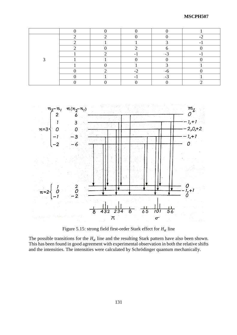
MSCPH507

131

0 0 0 0 1

3

2 2 0 0 -2

2 1 1 3 -1

2 0 2 6 0

1 2 -1 -3 -1

1 1 0 0 0

1 0 1 3 1

0 2 -2 -6 0

0 1 -1 -3 1

0 0 0 0 2

Figure 5.15: strong field first-order Stark effect for 𝐻𝛼 line

The possible transitions for the 𝐻𝛼 line and the resulting Stark pattern have also been shown.

This has been found in good agreement with experimental observation in both the relative shifts

and the intensities. The intensities were calculated by Schrödinger quantum mechanically.

MSCPH507

132

Thus, the comparison of weak-field and strong-field Stark effect:

Electric

Field

Level energy Transition rules

Weak ∆𝑚𝑗 = 0 gives π components

∆𝑚𝑗 = ±1 gives σ components

Strong 𝐸 = 𝐸0 −

3𝑎0𝑒

2𝑍𝐹𝑛(𝑛2 − 𝑛1)

∆𝑚𝑙 = 0 gives π components

∆𝑚𝑙 = ±1 gives σ components

Figure 5.16: Comparison of level shifting for hydrogen in weak—field and strong field (n=2

and n=3 line)

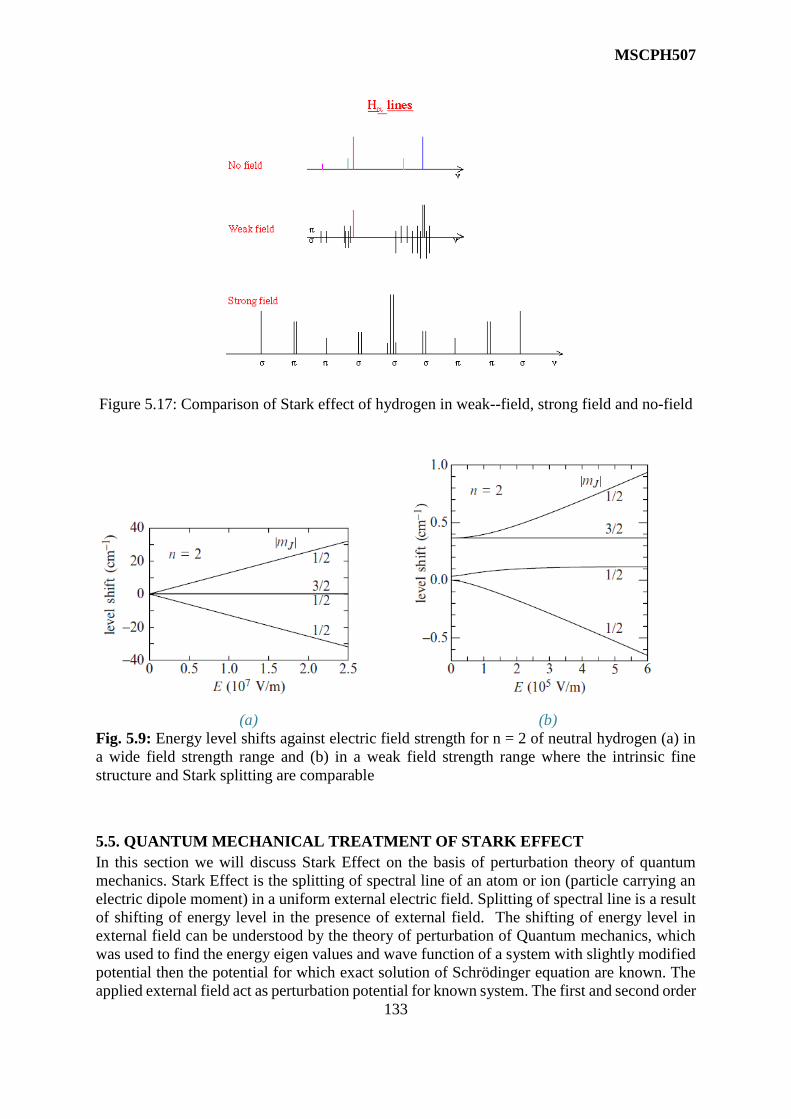
MSCPH507

133

Figure 5.17: Comparison of Stark effect of hydrogen in weak--field, strong field and no-field

(a) (b)

Fig. 5.9: Energy level shifts against electric field strength for n = 2 of neutral hydrogen (a) in

a wide field strength range and (b) in a weak field strength range where the intrinsic fine

structure and Stark splitting are comparable

5.5. QUANTUM MECHANICAL TREATMENT OF STARK EFFECT

In this section we will discuss Stark Effect on the basis of perturbation theory of quantum

mechanics. Stark Effect is the splitting of spectral line of an atom or ion (particle carrying an

electric dipole moment) in a uniform external electric field. Splitting of spectral line is a result

of shifting of energy level in the presence of external field. The shifting of energy level in

external field can be understood by the theory of perturbation of Quantum mechanics, which

was used to find the energy eigen values and wave function of a system with slightly modified

potential then the potential for which exact solution of Schrödinger equation are known. The

applied external field act as perturbation potential for known system. The first and second order

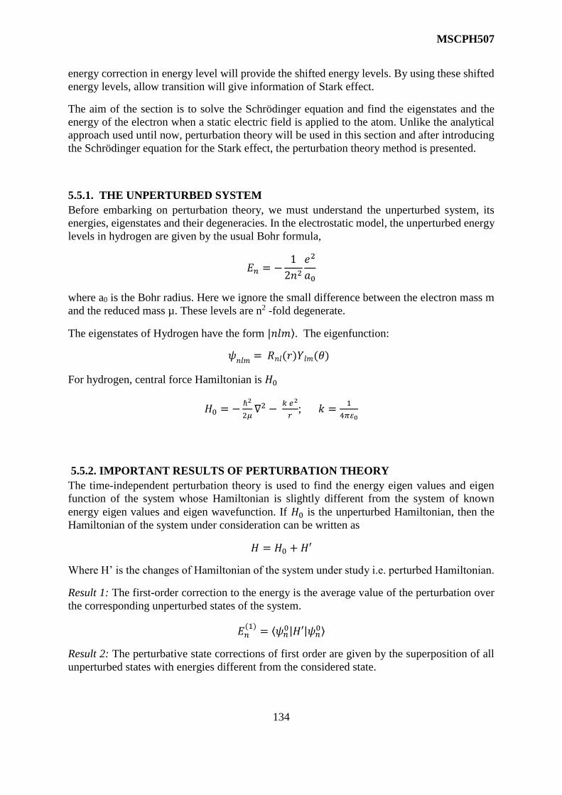
MSCPH507

134

energy correction in energy level will provide the shifted energy levels. By using these shifted

energy levels, allow transition will give information of Stark effect.

The aim of the section is to solve the Schrödinger equation and find the eigenstates and the

energy of the electron when a static electric field is applied to the atom. Unlike the analytical

approach used until now, perturbation theory will be used in this section and after introducing

the Schrödinger equation for the Stark effect, the perturbation theory method is presented.

5.5.1. THE UNPERTURBED SYSTEM

Before embarking on perturbation theory, we must understand the unperturbed system, its

energies, eigenstates and their degeneracies. In the electrostatic model, the unperturbed energy

levels in hydrogen are given by the usual Bohr formula,

𝐸𝑛 = −1

2𝑛2𝑒2

𝑎0

where a0 is the Bohr radius. Here we ignore the small difference between the electron mass m

and the reduced mass µ. These levels are n2 -fold degenerate.

The eigenstates of Hydrogen have the form |𝑛𝑙𝑚⟩. The eigenfunction:

𝜓𝑛𝑙𝑚 = 𝑅𝑛𝑙(𝑟)𝑌𝑙𝑚(𝜃)

For hydrogen, central force Hamiltonian is 𝐻0

𝐻0 = −ℏ2

2𝜇∇2 −

𝑘 𝑒2

𝑟; 𝑘 =

1

4𝜋 0

5.5.2. IMPORTANT RESULTS OF PERTURBATION THEORY

The time-independent perturbation theory is used to find the energy eigen values and eigen

function of the system whose Hamiltonian is slightly different from the system of known

energy eigen values and eigen wavefunction. If 𝐻0 is the unperturbed Hamiltonian, then the

Hamiltonian of the system under consideration can be written as

𝐻 = 𝐻0 + 𝐻′

Where H’ is the changes of Hamiltonian of the system under study i.e. perturbed Hamiltonian.

Result 1: The first-order correction to the energy is the average value of the perturbation over

the corresponding unperturbed states of the system.

𝐸𝑛(1)= ⟨𝜓𝑛

0|𝐻′|𝜓𝑛0⟩

Result 2: The perturbative state corrections of first order are given by the superposition of all

unperturbed states with energies different from the considered state.

MSCPH507

135

𝜓𝑛(1)= ∑

⟨𝑚|𝐻′|𝑛⟩

𝐸𝑛0 − 𝐸𝑚

0 |𝜓𝑚0 ⟩

𝑚≠𝑛

Thus, the energy and wave function corrected to first order are

𝐸𝑛 = 𝐸𝑛0 + ⟨𝜓𝑛

0|𝐻′|𝜓𝑛0⟩

𝜓𝑛 = 𝜓𝑛0 + ∑

⟨𝑚|𝐻′|𝑛⟩


0 |𝜓𝑚0 ⟩

𝑚≠𝑛

Result 3: The perturbative energy corrections of second order are determined by all unperturbed

states with energy different from the considered state.


0|𝐻′|𝜓𝑛(1)⟩

𝐸𝑛(2)= ∑

|⟨𝑚|𝐻′|𝑛⟩|2


0 |𝜓𝑚0 ⟩

𝑚≠𝑛

5.5.3. EFFECT OF ELECTRIC FIELD ON THE GROUND STATE OF HYDROGEN

Consider an atom situated at origin. Let an external electric field E applied along the positive

z-axis. If r is the position vector of the electron, the electric dipole moment µ=-er interacts

with the electric field E giving an additional potential energy to the electron

H’= -µ.E = erE cos𝜃 =eEz ; e-positive

Where 𝜃 is the angle the position vector makes with z-axis. Since this extra energy term is very

small, it can be treated as a perturbation on the Hamiltonian of the system Hº

Hº= -ℏ2

2𝜇∇2 −

𝑘 𝑒2

𝑟; 𝑘 =

1

4𝜋 0

The ground state of the Hydrogen atom (|nlm > = ψ100) is non-degenerate and first order

correction to the energy

𝐸(1) = ⟨𝜓100|𝑒𝐸𝑟𝑐𝑜𝑠𝜃|𝜓100⟩ (5.1)

Where 𝜓100 is the hydrogen ground state wave function:

𝜓100 = 1

(𝜋𝑎03)1/2

𝑒𝑥𝑝 (−𝑟

𝑎0)

The 𝜃 part of the integral in equation (5.1) vanishes as

∫ 𝑐𝑜𝑠𝜃 𝑠𝑖𝑛𝜃 𝑑𝜃 = −∫ 𝑐𝑜𝑠𝜃 𝑑(𝑐𝑜𝑠𝜃) = 0𝜋

0

𝜋

0

MSCPH507

136

Hence, the ground state of hydrogen atom will not show a first-order Stark effect and we have

to calculate the second-order energy shift.

The second-order energy shift presented in the next section, present a method of solving

perturbation on the basis Dalgarno and Lewis method. They found an operator F (scalar

function) such that

𝐸𝜓10 = 𝜓1

(1)

The second order energy correction


0|𝐻′|𝜓𝑛(1)⟩

𝐸1(2)= ⟨𝜓1

0|𝐻′𝐹|𝜓10⟩

and

𝐻′𝜓𝑛0 + 𝐻0𝜓𝑛

(1)= 𝐸𝑛

(1)𝜓𝑛0 + 𝐸𝑛

0𝜓𝑛(1)

𝐻′𝜓10 + 𝐻0𝐹𝜓1

0 = 𝐸1(1)𝜓10 + 𝐹𝐸1

0𝜓10

Since 𝐸1(1)

is zero and 𝐸10𝜓1

0 = 𝐻0𝜓10,

(𝐹𝐻0 − 𝐻0𝐹)𝜓10 = 𝐻′𝜓1

0

[𝐹, 𝐻0]𝜓10 = 𝐻′𝜓1

0

{Since the scalar function F commutes with -ke2/r in 𝐻0, the relation ∇2(𝐹𝜓10) = F∇2(𝜓1

0) +𝜓10∇2𝐹 + 2∇𝜓1

0. ∇𝐹}

ℏ2

2𝜇(𝜓1

0∇2𝐹 + 2∇𝜓10. ∇𝐹) = 𝐻′𝜓1

0

This gives the differential equation that determines the operator F. Substituting the values of

𝜓10 in the above equation

∇2F −2

𝑎0

𝜕𝐹

𝜕𝑟=2𝜇

ℏ2𝑒𝐸𝑟𝑐𝑜𝑠𝜃

The angular part of the right- hand side of the above equation comes from cos𝜃 which is the

Legendre polynomial P1. Therefore, F may be assumed to be of the following form

F=f(r) P1

This value of F when substituted in equation satisfied b f(r) which leads to

𝐹 =𝜇

ℏ2𝑒𝐸 𝑎0 (

𝑟

2+ 𝑎0) 𝑟𝑐𝑜𝑠𝜃

The second order correction is then

𝐸1(2)= ⟨𝜓1

0|𝐻′𝐹|𝜓10⟩

MSCPH507

137

= −𝜇

ℏ2𝑒2𝐸2𝑎0

1

𝜋𝑎03∫ ∫ 𝑐𝑜𝑠2𝜃𝑠𝑖𝑛𝜃𝑑𝜃𝑑𝜑∫ (

𝑟5

2+ 𝑎0𝑟

4) 𝑒𝑥𝑝 (−2𝑟

𝑎0) 𝑑𝑟

∞

0

2𝜋

0

𝜋

0

= −4

3

𝜇

ℏ2𝑒2𝐸2

𝑎02 ∫ (

𝑟5

2+ 𝑎0𝑟

4) 𝑒𝑥𝑝 (−2𝑟

𝑎0) 𝑑𝑟

∞

0

On solving, we get

𝐸1(2)= −

9

4

𝜇

ℏ2𝑒2𝐸2𝑎0

4 = −9

4𝑘𝑎03𝐸2

Since 𝑎0 = ℏ2/𝑘𝜇𝑒2. The ground state energy corrected to second order is found to be

𝐸1 = 𝐸10 −

9

4𝑘𝑎03𝐸2

As the correction is proportional to the square of E, it is often referred to as the quadratic Stark

effect.

The correction term (−9/4𝑘)𝑎03𝐸2 is due to the distortion of the charge distribution of the 1s-

electron by the electric field E and therefore we may say that the atom has been polarized b the

field. The extent of this polarisation is measured by the polarizability α, which is defined as the

ratio of the induced electric dipole moment µ to the external field E

µ= 𝛼 E

The energy of an induced dipole in an applied field is given by –(1/2) 𝛼𝐸2. Equating this energy

change with the energy due to perturbation calculation

−1

2𝛼𝐸2 = −

9

4𝑘𝑎03𝐸2

The polarizability of Hydrogen atom in its ground state is

𝛼 =9

2𝑘𝑎03

5.5.4. EFFECT OF ELECTRIC FIELD ON THE DEGENERATE ENERGY LEVELS

In the case of degenerate energy levels, unperturbed wave function of the system can be taken

as the linear combination of degenerate wave functions. For simplicity let us consider a case in

which 𝐸𝑛0 is two-fold degenerate. Let 𝜓𝑛

0 and 𝜓𝑙0 be eigenfunctions corresponding to eigenstate

𝐸𝑛0 = 𝐸𝑙

0 and a linear combination of tow be

𝜙 = 𝑐𝑛𝜓𝑛0 + 𝑐𝑙𝜓𝑙

0

Where cn and cl are constants.

First-order correction:

𝐻′𝜓𝑛0 + 𝐻0𝜓𝑛

(1)= 𝐸𝑛

(1)𝜓𝑛0 + 𝐸𝑛

0𝜓𝑛(1)

MSCPH507

138

𝐻′|(𝑐𝑛𝜓𝑛0 + 𝑐𝑙𝜓𝑙

0) > +𝐻0|𝜓𝑛(1)>= 𝐸𝑛

(1)|(𝑐𝑛𝜓𝑛

0 + 𝑐𝑙𝜓𝑙0) > +𝐸𝑛

0|𝜓𝑛(1)> (5.2)

Operating eq.(5.2) from left by < 𝜓𝑛0|

𝑐𝑛 < 𝜓𝑛0|𝐻′|𝜓𝑛

0 > +𝑐𝑙 < 𝜓𝑛0|𝐻′|𝜓𝑙

0 > +< 𝜓𝑛0|𝐻0|𝜓𝑛

(1) >= 𝑐𝑛𝐸𝑛(1) + 𝐸𝑛

0 < 𝜓𝑛0|𝜓𝑛

(1) >

Since 𝐻0 is Hermitian,

< 𝜓𝑛0|𝐻0|𝜓𝑛

(1) >= 𝐸𝑛0 < 𝜓𝑛

0|𝜓𝑛(1) >

So

𝑐𝑛 < 𝜓𝑛0|𝐻′|𝜓𝑛

0 > +𝑐𝑙 < 𝜓𝑛0|𝐻′|𝜓𝑙

0 >= 𝑐𝑛𝐸𝑛(1)

(𝐻′𝑛𝑛 − 𝐸𝑛1)𝑐𝑛 + (𝐻′𝑛𝑙)𝑐𝑙 = 0 (5.3)

Operating eq. (5.2) from left by < 𝜓𝑙0|

(𝐻′𝑛𝑙)𝑐𝑛 + (𝐻′𝑙𝑙 − 𝐸𝑛1)𝑐𝑙 = 0 (5.4)

Equation (5.3) and (5.4) together form a set of simultaneous equations for the coefficients

𝑐𝑛and 𝑐𝑙. A nontrivial solution of these equations exists only if the determinant of coefficients

vanishes.

|𝐻′𝑛𝑛 − 𝐸𝑛

(1) 𝐻′𝑛𝑙

𝐻′𝑙𝑛 𝐻′𝑙𝑙 − 𝐸𝑙(1)| = 0 (5.5)

This is called the secular equation and its two solutions are:

𝐸𝑛±(1)=1

2(𝐻′𝑛𝑛 + 𝐻′𝑙𝑙) ±

1

2[(𝐻′𝑛𝑛 − 𝐻′𝑙𝑙)

2 + 4|𝐻′𝑛𝑙|2](

12)

Now the corrected energies are:

𝐸𝑛 = 𝐸𝑛0 + 𝐸𝑛+

(1) and 𝐸𝑙 = 𝐸𝑛

0 + 𝐸𝑛−(1)

Both the energies will be real as the diagonal matrix element H’nn and H’ll pf the Hermitian

operator H’ are real. If H’nn =H’ll and H’nl=0, En+=En- and the degeneracy is not removed in the

first order.

When the two roots of eq. (5.5) are distinct, each can be used to calculate the ratio 𝑐𝑛/𝑐𝑙 either

from eq. (5.3) or from (5.4). the normalization condition 𝑐𝑛2 + 𝑐𝑙

2 = 1 allows us to calculate the

values of 𝑐𝑛 and 𝑐𝑙.

5.5.4.1. THE N=2 STATE OF HYDROGEN IN EXTERNAL FIELD

The first excited state (n=2) of hydrogen atom is four-fold degenerate, with |𝑛𝑙𝑚⟩: |200⟩, ||210⟩, |211⟩, and |21 − 1⟩. Similar to previous discussion, let the applied external field is

along the positive Z-axis which interacts with the electric dipole moment giving the perturbing

Hamiltonian H’=eEz=eErcos𝜃.

MSCPH507

139

For 4-fold degenerate state, the application of perturbation theory requires the evaluation of

sixteen matrix elements of H’. The four diagonal matrix elements out of these sixteen elements

are zero, since they correspond to the same parity (H’ is of odd parity). The off-diagonal matrix

elements between states of different m values are zero since

∫ exp[𝑖(𝑚′ −𝑚)𝜑]𝑑𝜑 = 0 2𝜋

0 if m’≠m

The remaining two matrix elements ⟨200|𝐻′|210⟩ and ⟨210|𝐻′|200⟩ are the only

nonvanishing ones. These can be evaluated using the values of

𝜓200 =1

4√2𝜋

1

𝑎03 (2 −

𝑟

𝑎0) 𝑒𝑥𝑝 (−

𝑟

2𝑎0)

And

𝜓210 =1

4√2𝜋

1

𝑎03/2

𝑟

𝑎0𝑒𝑥𝑝 (−

𝑟

2𝑎0) 𝑐𝑜𝑠𝜃

Therefore

⟨200|𝐻′|210⟩ =𝑒𝐸

32𝜋𝑎04∫ ∫ ∫ (2 −

𝑟

𝑎0) 𝑟2𝑒𝑥𝑝 (−

𝑟

𝑎0) 𝑐𝑜𝑠2𝜃𝑟2𝑠𝑖𝑛𝜃𝑑𝑟𝑑𝜃𝑑𝜑

∞

0

𝜋

0

2𝜋

0

=𝑒𝐸

16𝜋𝑎04∫ 𝑐𝑜𝑠2𝜃𝑟2𝑠𝑖𝑛𝜃𝑑𝜃∫ (2𝑟4 −

𝑟5

𝑎0) 𝑒𝑥𝑝 (−

𝑟

𝑎0) 𝑑𝑟

∞

0

𝜋

0

= −3𝑒𝐸𝑎0

So,

⟨200|𝐻′|210⟩ = −3𝑒𝐸𝑎0

⟨210|𝐻′|200⟩ = −3𝑒𝐸𝑎0

The perturbation matrix is therefore

𝐻′ = [

0 −3𝑒𝐸𝑎0 0−3𝑒𝐸𝑎0 0 00 0 00 0 0

]

The secular determinant is then

[ −𝐸2

(1)−3𝑒𝐸𝑎0 0 0

−3𝑒𝐸𝑎0 −𝐸2(1)

0 0

0 0 −𝐸2(1)

0

0 0 0 −𝐸2(1)]

= 0

The four roots of this determinant are 3𝑒𝐸𝑎0, −3𝑒𝐸𝑎0, 0 and 0. The state |200> and |210> are

affected by the electric field whereas the state |211> and |21-1> are not. The four-fold

MSCPH507

140

degeneracy is thus lifted partially. Corresponding eigenstate can be evaluated using equation

(5.3) and (5.4)

The eigenstate corresponding to the eigenvalues 3𝑒𝐸𝑎0 is then (|200>-|210>)/√2. In a similar

way the eigenstate for eigenvalue −3𝑒𝐸𝑎0 is (|200>+|210>)/√2.

Fig. 5.10. Energies and wave functions of the first excited state of hydrogen atom in an electric

field E.

The hydrogen atom in the first excited state thus possesses a permanent electric dipole moment

of magnitude 3𝑒𝑎0 with three different orientations- one state parallel to the external electric

field, one state antiparallel to the field and two states with zero component along the field. The

states |211> and |21-1> do not possess dipole moments and therefore do not have a first-order

interaction with the field.

Self-Assessment Questions (SAQ) 1:

1. The splitting of spectral line in Stark effect increase with

a) Increase in B

b) Decrease in B

c) Increase in E

d) Decrease in E

2. In the First-order Stark effect, the splitting is proportional to

a) E

b) Square of E

c) Cube of E

d) All of above

3. In strong field Stark-effect, the splitting of energy level is

a) Less than fine structure splitting

Energy

𝐸20

+ 3𝑒𝐸𝑎0

𝐸20

𝐸20

− 3𝑒𝐸𝑎0

Eigenstate

1

2(|200 > −|210 >)

|211 >, |21 − 1 >

1

2(|200 > −|210 >)

MSCPH507

141

b) Greater than fine structure splitting

c) Equal to fine structure splitting

d) None of the above

5.6. HYPERFINE STRUCTURE

In this section, we will go through the hyperfine structure of atoms. Various origins of the

hyperfine structure are discussed. The coupling of nuclear and electronic total angular

momentum is explained.

Many fine-structure components of spectral lines, when examined under high resolution, are

further splitted into components with separations of the order of 2 cm-1, which is very much

smaller than those of the ordinary multiplet structure. This splitting is called the “hyperfine

structure” and is caused by properties of the atomic nucleus. There are two type of nuclear

effects that produce hyperfine structure.

The first is due to the presence of isotopic species in the element under investigation. The

energy levels of isotopes are slightly displaced relative to each other, producing spectral

transitions at slightly displaced relative to each other, producing spectral transition at slightly

different wave numbers. Therefore, different isotopes of same element have slightly different

spectral lines.

The second type of effect arises because the charged nucleus processes as spin angular

momentum and the associated magnetic dipole moment. An interaction between the internal

magnetic field produced by the orbital motion of the electrons in the atom and the spin magnetic

dipole moment of the nucleus causes a hyperfine splitting of the spectral terms. As nuclear

dipole moments are smaller than electronic magnetic dipole moments by 10-3, the hyperfine

splitting is smaller than the spin-orbit splitting by the same factor. Hyperfine structure, with

energy shifts typically orders of magnitudes smaller than those of a fine-structure shift, results

from the interactions of the nucleus (or nuclei, in molecules) with internally generated electric

and magnetic fields.

5.6.1. ISOTOPE EFFECT

Different isotopes of an element have same number and arrangement of extranuclear electrons,

differ from one another in mass. Since the nuclear mass enters into Rydberg constant for an

atom, different isotopes have slightly different values of Rydberg constant. Correspondingly,

the same transitions in different isotopes give rise to slightly different wave numbers.

Let us calculate the shift for 𝐻𝛽 line (4861.33Å) due to presence of deuterium.

The Rydberg constant for hydrogen and deuterium

𝑅𝐻 = 𝑅∞1

1 +𝑚𝑀𝐻

= 1.09677 × 107 𝑚−1

𝑅𝐷 = 𝑅∞1

1 +𝑚𝑀𝐷

= 1.097074 × 107 𝑚−1

MSCPH507

142

The transition formula for this transition from Balmer’s formula

1

𝜆𝐻= 𝑅𝐻 (

1

22−1

42)

1

𝜆𝐷= 𝑅𝐷 (

1

22−1

42)

𝜆𝐷𝜆𝐻=𝑅𝐻𝑅𝐷

𝜆𝐷 − 𝜆𝐻𝜆𝐻

=𝑅𝐻 − 𝑅𝐷𝑅𝐷

Δ𝜆 = 𝜆𝐷 − 𝜆𝐻 = −𝜆𝐻 (𝑅𝐷 − 𝑅𝐻𝑅𝐷

)

= −4861.33 Å (109707.4 − 109677.6

109707)

= −1.32 Å

Observed calculated

𝑯𝜶 1.79 1.787

𝑯𝜷 1.33 1.323

𝑯𝜸 1.19 1.182

𝑯𝜹 1.12 1.117

Many cases of isotope-shift are not as simple as that for hydrogen. In fact, for the rare earth

and heavier atoms, the main contribution to isotope shift is not due to a difference in mass but

due to a change in nuclear radius with mass and the deviation of the nuclear magnetic field

from being purely a coulombic one.

Sm150→Sm152 shift is double that of Sm152→Sm154

Usual increase is not from Sm150→Sm152

5.6.2. NUCLEAR SPIN AND HYPERFINE SPLITTING

In many cases the isotope effect is not sufficient to explain the hyperfine structure. The number

of hyperfine structure components is often considerably greater than the number of isotopes.

In particular, elements which have only one isotope in appreciable amount also show hyperfine

structure splitting. Likewise, the number of components of different lines is frequently quite

different for one and the same element. These hyperfine structures can be quantitatively

explained, when it is assumed that the “atomic nucleus possess an intrinsic angular momentum

with which is associated a magnetic moment”. This angular momentum can have different

magnitudes for different nuclei and of course, for different isotope of the same element. This

is known as Nuclear spin.

MSCPH507

143

Thus, the atomic nucleus possesses an intrinsic spin angular momentum I with which is

associated a magnetic dipole moment 𝝁𝒍. Similar to electron, the magnitude of the nuclear

angular momentum

𝐈 = √𝐼(𝐼 + 1)ℎ

2𝜋

Where I is the “nuclear spin quantum number” which has different values for nuclei of odd

mass numbers. Thus, angular momentum has different magnitude for different nuclei and also

for different isotopes of the same element.

Just as L, S and J have quantised components along an axis in space, the component of I along

z-axis is

I𝑧 = 𝑀𝐼ℎ

2𝜋

Where the nuclear magnetic quantum number 𝑀𝐼 has 2I+1 values given by

𝑀𝐼 = 𝐼, 𝐼 − 1, 𝐼 − 2,……… ,−𝐼

The motion of nuclear protons produces a magnetic moment 𝜇𝑙which is proportional to the

angular momentum, and which we shall write

𝜇𝐼 = 𝑔𝐼 (𝑒

2𝑚𝑝) 𝐈

Where e and 𝑚𝑝 are respectively the charge and mass of proton. The quantity 𝑔𝑙 is called the

‘nuclear g factor’. The magnitude of the nuclear magnetic moment is

𝜇𝐼 = 𝑔𝐼 (𝑒

2𝑚𝑝)√𝐼(𝐼 + 1)

ℎ

2𝜋

= 𝑔𝐼√𝐼(𝐼 + 1)𝑒ℎ

4𝜋𝑚𝑝

The quantity 𝑒ℎ

4𝜋𝑚𝑝 forms a natural unit for the measurement of nuclear magnetic moment and

is called the ‘nuclear magnetron’ 𝜇𝑁. It is 1/1836 times the Bohr magnetron (because the mass

of the proton is 1836 times the mass of electron). Thus

𝜇𝐼 = 𝑔𝐼√𝐼(𝐼 + 1) 𝜇𝑁

The component of 𝜇𝐼 along the z-axis is

𝜇𝐼𝑧 = 𝑔𝐼𝑀𝐼 𝜇𝑁

Where 𝑀𝐼 = 𝐼, 𝐼 − 1, 𝐼 − 2,……… ,−𝐼

Since the maximum values of 𝑀𝐼 is I, the maximum observed component of 𝜇𝐼 is 𝑔𝐼𝐼 𝜇𝑁, and

is commonly called the ‘nuclear magnetic moment’. It is roughly 1000 times smaller than

electron magnetic moment.

MSCPH507

144

5.6.2.1. VECTOR ATOM MODEL

Let us now construct the vector atom model with nuclear spin taken

into account. The total angular momentum of the whole atom is the

sum of three angular momenta: the electron orbital angular

momentum L, the electron spin singular momentum S and the nuclear

spin singular momentum I. that is, the total angular momentum is

F=L+S+I=J+I

As a result of interaction between electron orbit and spin L and S

precess rapidly around their resultant J. Further, the interaction

between the nuclear magnetic moment and the magnetic field

produced by the orbital and spin motions of the atomic electrons

couples I with J (because nuclear magnetic moment is so much

smaller than electronic magnetic moment). Correspondingly the

energy differences are very much smaller.

The quantised values of the total angular momentum F are

√𝐹(𝐹 + 1)ℎ

2𝜋, where hfs quantum number F can take the values:

𝐹 = 𝐽 + 𝐼, 𝐽 + 𝐼 − 1, 𝐽 + 𝐼 − 2,…… ,−( 𝐽 + 𝐼)

Giving 2J+1 values if 𝐼 ≥ 𝐽, or 2I+1 values if 𝐼 ≤ 𝐽. This means that as a result of I.J interaction,

each fine-structure J-level split into 2J+1 (if 𝐼 ≥ 𝐽) or 2I+1 (if 𝐼 ≤ 𝐽) hfs levels, each

characterised by an F value.

Interaction energy:

The I - J interaction energy can be shown to be given by

𝐸𝐼,𝐽′ =1

2𝐴′[𝐹(𝐹 + 1) − 𝐼(𝐼 + 1) − 𝐽(𝐽 + 1)]

Where A’ is a constant. The various hfs (hyperfine fine structure) levels of a given term of a

given atom have the same I and same J, but differ in F. Hence the separation between two hfs

levels can be obtained by substituting first F+1, then F, in the above equation and taking the

difference. This gives

∆𝐸′ =1

2𝐴′[(𝐹 + 1)(𝐹 + 2) − 𝐹(𝐹 + 1)]

= 𝐴′(𝐹 + 1)

Thus, energy interval between consecutive hfs levels F and F+1 is proportional to the larger of

the F values (Lande’s interval rule). The order of hfs levels in some hypermultiplets is normal

(smallest F level deepest) while in other it is inverted (largest F level deepest) (Fig. 5.12).

Figure 5.11

MSCPH507

145

Figure 5.12

The selection rule for F electric dipole transitions is similar to that for j:

∆𝐹 = 0, ±1 𝑏𝑢𝑡 𝐹 = 0 ↮ 𝐹 = 0

Example 1:

For the H atom, with a proton as the nucleus, the

experiments give the values

I = 1/2, gI = +5.58 ⇒ (μN)z = ±2.79μK .

For the ground state 𝑆1/22 is j = 1/2, I = 1/2

⇒ F =0 or F = 1.

This gives the two hyperfine components.

𝐸𝐼,𝐽′ =1

2𝐴′[𝐹(𝐹 + 1) − 𝐼(𝐼 + 1) − 𝐽(𝐽 + 1)]

Ehfs(F = 0) = 𝐸(1,0,1/2) − 3

4𝐴

Ehfs(F = 1) = 𝐸(1,0,1/2) + 1

4𝐴

with the separation ΔE = A = 5.8 ×10−6 eV.

Figure 5.13: Hyperfine structure

of the 1𝑆1/22 state of the H atom.

The hyperfine coupling constant is

A = 0.047cm−1.

MSCPH507

146

Δ.ν = ΔE/hc = 0.047 cm−1 ⇒ Δν =1.42 GHz, Δλ = 21 cm.

Example 2: For Hyperfine Structure of bismuth (I=9/2)

line 4722 Å.

The fine-structure in bismuth shows j-j coupling. The

transition corresponding to this line is

6𝑝27𝑠, ( 1

2,1

2 ,3

2)12→ 6𝑝3, (

1

2,1

2 ,3

2)32

With a nuclear spin I=9/2 and J=1/2, the initial state is

split into two hfs levels with F= 5,4 which are in normal

order. Again, with I=9/2 and J=3/2, the final state is split

into four hfs levels with F= 6, 5, 4, 3 which are in

inverted order.

The selection rule ∆F=0, ±1 (but 𝐹 = 0 ↮ 𝐹 = 0)

allows six transitions. Hence, the Bi line 4722 Å shows

six Hyperfine components.

5.6.3. INTENSITY RATIO AND DETERMINATION OF NUCLEAR SPIN

When hfs components are observed due to the splitting of only one of the terms, a measurement

of the intensity ratio of the observed components leads to the determination of nuclear spin.

This is based on the ‘sum rule’, according to which the sum of the intensities of all the

transitions starting from or ending on the same level is proportional to the statistical weight

2F+1 of that level. This situation arises in the hfs of the resonance lines (D2, 5890 Å) of sodium.

In this case, the ratio of the intensities of the two observed hfs components equal to the ratio of

the weights (2F+1) of the hfs levels of the term 2S1/2. When I is unknown, the F values of the

two hfs levels of the term 2S1/2 (𝐽 =1

2) would be 𝐼 +

1

2 and 𝐼 −

1

2. Hence

𝐼𝑛𝑡𝑒𝑛𝑠𝑖𝑡𝑦 𝑟𝑎𝑡𝑖𝑜 =2 (𝐼 +

12) + 1

2 (𝐼 −12) + 1

=𝐼 + 1

𝐼

The observed intensity ratio is 5:3. Thus,

𝐼 + 1

𝐼=5

3

𝐼 =3

2

Thus, the nuclear spin I is determined.

When the hfs components are observed due to the splitting of both the terms, as in case of Bi

line 4722 Å (Fig. 5.14), then also an analysis of the hyperfine structure can also lead to the

Figure 5.14

MSCPH507

147

determination of nuclear spin. When all the hyperfine components are fully resolved, as in case

of Bi, then constant wave-number difference occur between pairs of components. For example,

we have

𝑐 − 𝑏 = 𝑒 − 𝑑

𝑑 − 𝑏 = 𝑒 − 𝑐

These differences correspond to level difference in the lower and the upper state respectively.

We arrange the wave numbers of the hyperfine components in a square array such that along

each row and along each column they increase (or decrease) regularly, and the difference

between them in two successive rows and successive column is constant. Then, all the

components in any row correspond to the same upper hfs level, while all those in any column

correspond to the same lower hfs level. This will enable us to construct hfs energy levels for

the upper and the lower states. For example, in the above case of Bi, when the wave numbers

of the 6 observed components are filled in the square array, we obtain 2 hfs levels in the upper

state and 4 in the lower state, as shown below:

Flower

Fupper

3 4 5 6

4 a (b-a) b (c-b) c

(q-p

)

(e-c)

5 d (e-d) e (f-e) f

Now, two case may arise:

The upper and lower states have different J values and have also different number of

hfs levels. In this case, number of hfs level is always (2J+1). We may apply the Land’s

interval rule to obtain the F values of the hfs levels from the interval ratio. Thus, all F

values of the state whose J value is already known are determined. From this the nuclear

spin I can be calculated. In the above case, for the lower state F= 3, 4, 5, 6 and J=3/2,

so that

𝐼 =9

2

The upper and the lower states have different J values but have the same number of hfs

levels. In this case this number is always 2I+1; hence I may be evaluated.

Self-Assessment Questions (SAQ) 2:

1. The Hyperfine structure of spectral line arises due to

MSCPH507

148

a) Isotope effect

b) Nuclear spin

c) Both ‘a’ and ‘b’

d) None of above

2. Numbers of Hyperfine components are present in Bi (6722 Å)

a) 5

b) 4

c) 3

d) 6

3. Intensity ratio of hyperfine components of sodium D2 line (5890Å)

a) 5:3

b) 4:5

c) 2:2

d) 3:5

5.7. SUMMARY

The Stark effect is the shift in atomic energy levels caused by an external electric field. The

magnitude of the wavelength separation and the relative intensity among the split line

components depend on the field strength. Stark effect generally increases as the square of the

applied field strength (quadratic Stark effect). For hydrogen like system special condition

prevail due to the level degeneracy and hence linear Stark effect (shift is linear in applied field

strength) is obtained.

Hyperfine structure is the splitting of individual multiplet (J→J transitions) components into a

number of components lying extremely close together under the high resolution. The

magnitude of the splitting is ~2 cm−1. Hyperfine structure is caused by properties of the atomic

nucleus, either due to presence of isotope or due to an interaction between the internal magnetic

field produced by the orbital motion of the electrons in the atom and the spin magnetic dipole

moment of the nucleus.

5.8. GLOSSARY

Polarisation- restrict vibration to one direction

Symmetrical- made up of similar part

Coupling- to join

Quantised- to have only certain values

Intrinsic- belonging

Isotope- elements having same atomic number and different atomic mass

5.9. TERMINAL QUESTIONS

1. Discuss Stark Effect with the overview of classical electrostatic.

2. Discuss the First order and Second order on the basis of Perturbation theory.

3. Why the hydrogen atom in the ground state does not show a first-order Stark effect?

4. Draw the Hyperfine structure of the fine structure component 𝐷2 (5890 Å) of sodium

(I=3/2). Transition 2P3/2→2S1/2.

5. Draw the Hyperfine levels for 2D5/2 of Bismuth (I=9/2). If the separation of 𝐷22

5/2 and

𝐷22

5/2 is 30 cm-1. Calculate the separation of all adjacent Hyperfine levels.

MSCPH507

149

5.10. REFERENCES

1. G. Aruldhas, Quantum Mechanics, PHI learning, New Delhi, India, 2009

2. G. Hertzberg, Atomic Spectra and Atomic Structure, Dover Publication, New York,

USA, 1944

3. R. Kumar, Atomic and Molecular Spectra: Laser, Kedar Nath Ram Nath Publication,

Meerut, India, 2011

4. J. J. Sakurai, Modern Quantum Mechanics, Addison, Wesley Publication House,

USA, 1994

5. Wolfgang Demtröder, Atoms, Molecules and Photons: An Introduction to Atomic-,

Molecular and Quantum-Physics, Springer-Nature, Germany, 2010

5.11. ANSWERS


Ans. 1. (c)

Ans. 2. (a)

Ans. 3. (b)


Ans. 1. (c)

Ans. 2. (d)

Ans. 3. (a)

Terminal question

Ans. 5. 𝐷32

5/2 − 𝐷42

5/2 = 40 cm-1

𝐷42

5/2 − 𝐷52

5/2 = 50 cm-1

𝐷52

5/2 − 𝐷62

5/2 = 60 cm-1

𝐷62

5/2 − 𝐷72

5/2 = 70 cm-1

MSCPH507

150

UNIT 6 BREADTH OF

SPECTRAL LINES

Structure

6.1 Objective

6.2 Introduction

6.3 Spectral Line Breadth

6.4 Causes of Spectral Line Breadth

6.4.1 Natural Breadth

6.4.2 Doppler Effect

6.4.3 External Effects

6.4.1.1 Collision Damping

6.4.1.2 Pressure Broadening

6.4.1.3 Stark Broadening

6.4.1.4 Instrument Broadening

6.5 Voigt Profile

6.6 Summary

6.7 Glossary

6.8 Reference Books

6.9 Suggested Reading

6.10 Terminal Questions

MSCPH507

151

6.1 Objectives

After studying this unit, you will come to know about:

1. Spectral line breadth.

2. Causes of spectral line breadth.

3. Define natural breadth

4. Define Doppler effect

5. Define external effects

6.2 Introduction

In the previous chapters, we have already discussed the two main important transition

phenomena; Absorption and emission. Spectral lines are narrow emission or absorption

features in the spectra of gaseous sources. Spectral lines are intrinsically quantum phenomena

and have no explanation in classical physics. The classical concepts of ideal particles and

waves are blurred in quantum mechanics: classical particles (e.g., electrons) and waves (e.g.,

radio waves) behave as both particles and waves.

An individual atom/molecule making a transition between energy levels emits one photon with

a well-defined energy / frequency. However, profiles of real spectral lines are not infinitely

narrow.

Figure 6.1: Width of the spectral line.

e.g. for an emission line, width of the spectral line Δν could be defined as the full width at

MSCPH507

152

half the maximum intensity of the line (Figure 6.1).

In molecular spectroscopy, the spectral lines depend on two factors:

1. Width of the spectral lines decides the sharpness or broadness of the line

2. Intensity of the spectral lines decides the strength of the signal

6.3 Spectral Line Breadth

If the spectral line is sharp, it will have no width i.e. it can be seen at a specific frequency only.

If the spectral line is broad, it will have a certain width i.e. It is spread over a range of

frequencies. The breadth of a spectral line is defined as the separation in the cm-1 between two

points whose intensities are half that of the maximum intensity. Figure 6.2 represents a) a sharp

spectral line and b) a spectral line having observable width. A spectral line is a dark or bright

line

Figure 6.2: a) A sharp spectral line b) A sharp spectral line having width.

6.4 Causes of Spectral Line Breadth

Generally, the spectral lines observed are broad. The width or broadening depends on the

following factors:

1. Natural Breadth

MSCPH507

153

2. Doppler Effect

3. External Effects: (collision damping, pressure broadening, stark effect etc.)

6.4.1 Natural Breadth

This type of broadening is usually much smaller than other broadening mechanisms. Natural

also known as intrinsic broadening. This type of spectral line broadening is one cause of the

width Δν in a line profile function φ(ν). It arises from the spontaneous decay rate. In quantum

mechanics by using the Heisenberg uncertainty principle, if we consider a bunch of atoms, their

lifetimes are affected by the uncertainty in their energy states from. Such as given below:

(6.1)

Where E is the energy spread of a state and t is the mean time for which atoms remain in that

state. A photon in a certain energy state will therefore have a range of possible frequencies

when it decays to a lower state.

(6.2)

The value of mean life is inversely proportional to the energy breadth of the state. From this

we can say that ground state and metastable states are sharp, while the other states are quite

broad.

The line profile function resulting from Natural Broadening is the Lorentzian Profile. It is

proportional to A10. This shows that the larger values of A result in more broadening or wider

profile function.

(6.3)

If radiation is present, then stimulated emission effects must be added to the spontaneous

emission ones. Overall though, natural line broadening is not the dominant broadening effect

and isn’t often directly observed, except in the line wings. Natural line width isn’t often directly

observed, except in the line wings in low-pressure (nebular) environments. Other broadening

mechanisms usually dominate.

MSCPH507

154

The half intensity breadth of a spectral line due to the transition from an excited state to the

ground state is given by:

(6.4)

For the ordinary excited state, the value of mean time is 10-8 sec. Hence, by using the above

formulae the value of energy breadth is given as: 107 s-1.

For a visible wavelength (6000 Å). This corresponds to a wavelength broadening of

= Å

This shows that the value of wavelength broadening is quite small and it cannot be measured

by ordinary spectroscopic methods.

6.4.2 Doppler Effect

Unlike the other forms of broadening, Doppler broadening does not involve intra- or inter-

atomic interactions. This type of broadening is due to the motions of the atoms with respect to

an observer. Doppler broadening is sometimes called inhomogeneous broadening since each

atom contributed its own frequency to the profile. Hence, removal of a (non-random) sample

of atoms (e.g., by saturating a transition at a particular frequency) will distort the line shape.

MSCPH507

155

Figure 6.3: Doppler broadening.

Two basic mechanisms:

1) Energy levels themselves are not infinitely sharp: emitted photons have a range of

frequencies.

2) Atoms and molecules in the gas are moving relative to the observer: observed photons don't

have the same frequency as the emitted photons because of the Doppler Effect.

DDoppler Effect

It is named after an Austrian physicist Christian Doppler, who proposed it in 1842

in Prague. The Doppler effect also known as Doppler shift. It is defined as the change

in frequency of absorbed or emitted radiation when the source is moving towards or away

from the observer. It is observed in case of gaseous samples as the molecules of the gases

are in a state of continuous random motion. If the source emitting the radiation is moving

away from the observer or the observing instrument with a velocity ‘v’ , then the observer

or instrument detects the radiation of frequency ϑ

𝜗0 = 𝜗 /1+ v/c

where 𝜗0 is frequency of radiation detected by the observer, f is the frequency emitted by

the source, v is the velocity of the radiation and c is velocity of light.

If the source emitting the radiation is moving away from the observer or the observing

instrument, then the observer or instrument detects the radiation of frequency 𝜗0.

MSCPH507

156

𝜗0 = 𝜗 /1- v/c

The difference ∆𝜗 = 𝜗 − 𝜗0 is called Doppler shift or broadening.

When the source of the waves is moving toward the observer, each successive wave crest is

emitted from a position closer to the observer than the previous wave. Therefore, each wave

takes slightly less time to reach the observer than the previous wave. Hence, the time between

the arrivals of successive wave crests at the observer is reduced, causing an increase in the

frequency. While they are travelling, the distance between successive wave fronts is reduced,

so the waves "bunch together”. Conversely, if the source of waves is moving away from the

observer, each wave is emitted from a position farther from the observer than "spread out". The

previous wave, so the arrival time between successive waves is increased, reducing the

frequency. The distance between successive wave fronts is then increased, so the waves.

As the gas molecules are moving in different directions with different speeds, some towards

and some away from the observer, so the spectral lines arise from all the resulting DOPPLER

SHIFTS.

The shape of the Doppler shift resembles that of Maxwell's distribution of speeds as at a

particular temperature the speed of the gas molecules is given by Maxwell's distribution.

Let us assume a Maxwell distribution of velocities: the probability that the velocity of an atom of

an ideal gas lies between 𝜗 and 𝜗 + 𝑑𝜗 is given by

𝑑𝑃 = 4𝜋 (𝜇

2𝜋𝑅𝑇)

3

2𝑒(−𝜇𝑣2

2𝑅𝑇)

32 𝑣2𝑑𝑣 (6.5)

Here R is the universal constant and its value is given as: 8.31 J/(mol-K).

T is the temperature.

𝜇 is defined as atomic weight.

We can write the Doppler shift as given below

∆𝜗 = 𝜗 − 𝜗0 = 𝜗0𝑣

𝑐

bility that the velocity of an atom of the gas lies between is given as .m.k;

MSCPH507

157

𝑣 = 𝑐𝜗− 𝜗0

𝜗0 (6.6)

Here, 𝜗0 is the source of light, 𝜗 is the apparent frequency measured by the observer, 𝑣 is the

velocity relative to the observer. On putting the value of 𝑣 from equation 6.6 to equation 6.5,

we will get the value of relative intensity in the terms of frequency as:

𝐼(𝜗) = 𝑐𝑜𝑛𝑠𝑡𝑎𝑛𝑡 𝑒−𝜇𝑐2(𝜗− 𝜗0)

2

2𝑅𝑇𝜗02

(6.7)

Figure 6.4 gives the plot for the relative intensity expression. If we set the exponential term in the

the equation 6.7 as one half, we will get the situation at which the intensity drops to half of its maximum value.

So by putting the exponential term in the equation 6.7 as ½;

𝑒−𝜇𝑐2(𝜗− 𝜗0)

2

2𝑅𝑇𝜗02

= 1

2 (6.8)

By taking loge both sides.

−𝜇𝑐2(𝜗− 𝜗0)2

2𝑅𝑇𝜗02 = log𝑒 2 (6.9)

By rearranging terms in the equation 6.9.

𝜗 − 𝜗0 =𝜗0

𝑐√2𝑅𝑇

𝜇log𝑒 2 (6.10)

Multiplying equation 6.10 by 2 we will get line breadth as 𝛿𝜗. Thus,

𝛿𝜗 = 2(𝜗 − 𝜗0)√2𝑅𝑇

𝜇log𝑒 2 (6.11)

√log𝑒 2 = √0.693 = 0.832

MSCPH507

158

∴ 𝛿𝜗 = 1.66𝜗0

𝑐√2𝑅𝑇

𝜇 (6.12)

Equation 6.12 represent Doppler broadening and it is directly proportional to the square root

of the temperature and frequency and inversely proportional to the square root of the atomic

weight. Equation 6.12 represent the Doppler broadening in terms of frequency, by using below\

equation we can convert half intensity line breadth in terms of wavelength.

Now, 𝛿𝜗

𝜗=𝛿𝜆

𝜆

𝛿𝜆 = 1.66𝜆0

𝑐√2𝑅𝑇

𝜇 (6.13)

Equation 6.13 clearly represent that line breadth due to Doppler broadening increases with

increasing temperature and decreases with increasing atomic weight.

Figure 6.4

MSCPH507

159

If we consider Doppler-broadened spectral lines at three different temperatures, we observe

line broadens as the temperature is increased. The reason behind is that Doppler Broadening

increases with temperature as molecular speed increases with rise in temperature. So in order

to get maximum sharpness of the spectra, it is essential to work at low temperatures.

Figure 6.5: Shapes of Doppler-broadened spectral lines at three different temperatures.

6.4.3 External Effects

A number of external effects are also in nature that will cause the broadening in the spectral

lines. Some of them are mentioned below:

Collision Damping

Pressure Broadening

Stark Broadening

Instrument broadening

Now in the coming sections we will discuss them.

6.4.1.1 Collision Damping

In a dense gas, atoms/molecules are colliding frequently. This effectively reduces the

lifetime of states further, to a value smaller than the quantum mechanical lifetime. If the

frequency of collisions is νcol, then expect to get a collisional linewidth of about Δν ∼ νcol.

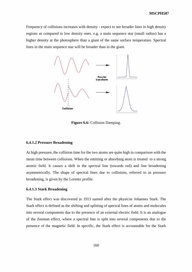
MSCPH507

160

Frequency of collisions increases with density - expect to see broader lines in high density

regions as compared to low density ones. e.g. a main sequence star (small radius) has a

higher density at the photosphere than a giant of the same surface temperature. Spectral

lines in the main sequence star will be broader than in the giant.

Figure 6.6: Collision Damping.

6.4.1.2 Pressure Broadening

At high pressure, the collision time for the two atoms are quite high in comparison with the

mean time between collisions. When the emitting or absorbing atom is treated to a strong

atomic field. It causes a shift in the spectral line (towards red) and line broadening

asymmetrically. The shape of spectral lines due to collisions, referred to as pressure

broadening, is given by the Lorentz profile.

6.4.1.3 Stark Broadening

The Stark effect was discovered in 1913 named after the physicist Johannes Stark. The

Stark effect is defined as the shifting and splitting of spectral lines of atoms and molecules

into several components due to the presence of an external electric field. It is an analogue

of the Zeeman effect, where a spectral line is split into several components due to the

presence of the magnetic field. In specific, the Stark effect is accountable for the Stark

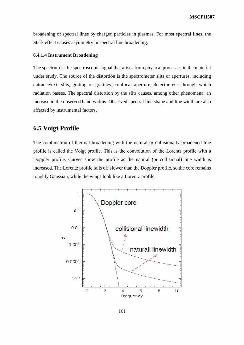
https://www.wordhippo.com/what-is/another-word-for/treated.html

https://www.sciencedirect.com/topics/earth-and-planetary-sciences/line-spectra

MSCPH507

161

broadening of spectral lines by charged particles in plasmas. For most spectral lines, the

Stark effect causes asymmetry in spectral line broadening.

6.4.1.4 Instrument Broadening

The spectrum is the spectroscopic signal that arises from physical processes in the material

under study. The source of the distortion is the spectrometer slits or apertures, including

entrance/exit slits, grating or gratings, confocal aperture, detector etc. through which

radiation passes. The spectral distortion by the slits causes, among other phenomena, an

increase in the observed band widths. Observed spectral line shape and line width are also

affected by instrumental factors.

6.5 Voigt Profile

The combination of thermal broadening with the natural or collisionally broadened line

profile is called the Voigt profile. This is the convolution of the Lorentz profile with a

Doppler profile. Curves show the profile as the natural (or collisional) line width is

increased. The Lorentz profile falls off slower than the Doppler profile, so the core remains

roughly Gaussian, while the wings look like a Lorentz profile.

MSCPH507

162

Figure 6.7: Voigt profile: combination of thermal and natural (or collisional) broadening

The wider Doppler broadening dominates near the center of the line, but since the Doppler

profile decreases exponentially, natural and pressure broadening make a greater

contribution farther from the center of the line. Most stellar spectra lines have a profile

described by a Voigt profile. The use of Voigt profile are fit to observations of absorption

towards quasars to measure temperatures and column densities of the gas along line of

sight.

6.6 Summary

In this unit, you have studied the spectral line broadening and their causes in detail. Strength

of different spectral lines depends upon the abundance of different elements, and on the

excitation/ ionization state (described in part by the Boltzmann formula). Width of spectral

lines depends upon: natural linewidth (small), collisional linewidth (larger at high density)

and thermal linewidth (larger at higher temperature). You have also studied the dependence

of temperature and pressure and different types of broadening. To check your progress,

self-assessment questions (SAQs) are given place to place. Many terminal questions are

given in the unit for practice and to make the concept clear.

6.7 Glossary

Spectrum

The set of colors into which a beam of light can be separated, or a range

of waves.

rotational A rotation is a circular movement of an object around a center of

rotation.

vibrational A molecular vibration is a periodic motion of the atoms of a molecule

relative to each other,

Emission

spectrum

The distribution of electromagnetic radiation released by a substance

whose atoms have been excited by heat or radiation.

absorption

spectrum

The spectrum formed by electromagnetic radiation that has passed

through a medium in which radiation of certain frequencies is absorbed

https://www.collinsdictionary.com/dictionary/english/certain

https://www.collinsdictionary.com/dictionary/english/frequency

MSCPH507

163

Transition

The process or a period of changing from one state or condition to

another

The act of making something wider.

Doppler

Collision

Relating to, or utilizing a shift in frequency in accordance with

the Doppler effect.

the act of colliding; a coming violently into contact

6.8 Reference Books

1. Atomic & Molecular spectra Laser: By Raj Kumar (KNRM Publication-Meerut)

2. Structure and properties of Material: By MA Wahab (Narosa Publishing House –

Delhi)

3. Molecular Spectra and Molecular Structure I: G. Herzberg (Van-Nostrand Rein-hold,

1950)

4. Atomic Physics by J.H.Fewkes & John Yarwood. Vol. II (Oxford Univ. Press,

1991).

5. Physics of Atoms and Molecules, Bransden and Joachein. (Longman Scientific and

Technical)


1. Fundamental of Molecular Spectroscopy. C N Banwell and E M Mc Cash (Tata Mc

Graw Hills)

2. Gupta Kumar Sharma – Elements of Spectroscopy, Pragati Prakashan.

3. Modern Physics, Beiser, Tata McGraw Hill

4. 2. Optical Spectroscopy in Chemistry and Life Sciences, W. Schmidt; Wiley-VCH.

5. Atkins, P.W.; de Paula, J. (2006). "13.3: Linewidths". Physical Chemistry (8th ed.).

Oxford University Press. pp. 436–438. ISBN 0198700725.


Long answer type questions:

MSCPH507

164

1. Show that φ(ν)=∆ ν-2 well away from the center of a line with a Lorentzian broadening

profile.

2. Calculate the line-of-sight thermal velocity dispersion ∆νD of line photons emitted

from a hydrogen cloud at a temperature of 104 K.

3. Calculate the natural broadening line width of the Lyman α line, given that Aul=5x108

s–1. Convert to km/sec via the Doppler formula.

4. Mention the difference between line and Doppler broadening.

Numerical type questions:

1. Estimate the fractional width of a spectral line of 5000 Å wavelength emitted from

a level of a life time of 10-8 sec.

2. Calculate the Doppler half-life intensity breadth of the sodium D-lines at 5893 Å

corresponding to the temperature of 500 K. Value of R= 8.31 J/(mol-K), c= 3x108

m/s, atomic weight of sodium = 22.99 g/mol.

3. Calculate the Doppler half-life intensity breadth of the sodium D-lines at 5893 Å

corresponding to the temperature of 400 K. Value of R= 8.31 J/(mol-K), c= 3x108

m/s, atomic weight of sodium = 22.99 g/mol.

4. Calculate in Å the Doppler half-intensity breadth of mercury green line 5461 Å, if

the light source is at 1000 K. Given R= 8.31 J/(mol-K), c= 3x108 m/s, atomic

weight of mercury = 200.59 g/mol.

Answer 1: 1.33 x10-4 Å; 2: 0.02 Å; 4: 0.0087 Å

Objective Question

Question 1: One of the causes of the breadth of the spectral lines is:

a) Doppler effect

b) Dispersion

c) Reflection

MSCPH507

165

d) Diffraction

Question 2: Doppler broadening most significant at:

a) Low P, high T, small λ

b) High P, high T, high λ

c) Small P, small T, small λ

d) Low P, Low T, Low λ

Question 3: Collision broadening is most significant at:

a) High P, low T, large λ

b) High P, low T, large λ

c) High P, low T, large λ

d) High P, low T, large λ

Question 4: The width or broadening depends on the which?

a) Natural Breadth

b) Doppler Effect

c) External Effects

d) All of the above

Question 5: In a real radiation spectrum the emission and absorption lines tend to overlap

with each other due to

MSCPH507

166

a) Vibrational transition

b) Electronic transitions

c) Presence of spectral lines of various gases

d) Line broadening

Question 6: The Doppler broadening mechanism dominates over other broadening under:

a) Low pressure and high temperature

b) High pressure and low temperature

c) Low temperature in infrared

d) High pressure in infrared

Answer 1: a; 2: a; 3: a; 4: d; 5: d; 6: a;

MSCPH507

167

UNIT 7: X Rays

Structure

7.1 Introduction

7.2 Objective

7.3 X-ray Continuous spectra and Line spectra

7.4 Kossel’s explanation of line spectra

7.5 X ray emission spectra and Moseley law

7.6 X ray absorption spectra

7.7 Fine structure of X ray emission spectra

7.8 X ray spectra and optical spectra

7.9 Summary

7.10 Glossary

7.11 References

7.12 Suggested reading

7.13 Terminal questions

MSCPH507

168

7.1 Introduction

In 1895, Roentgen observed that when a beam of fast moving electrons struck on a

suitable target, some rays are produced that have highly penetrating power. These rays were

named as X-rays. Actually when fast moving electrons are deaccelerated, and according to

classical electromagnetic theory, these deaccelerated electron emit electromagnetic radiations

(Bremsstarhlung) which are known as X-rays.

For the production of X-rays we use a Coolidge tube. This tube has a target of a metal

which have high melting point and high atomic numbers, for example tungsten, platinum,

molybdenum etc. In this tube under lower pressure, electron are emitted from a filament and

struck on a target (anode) due to high voltage difference (1000 to 30000 V) at anode. When we

observe spectra of X-rays, we have two types of spectra, namely continuous spectra and

characteristic (line) spectra. The continuous spectra arises due to deacceleration of electron

when they hit the target. The intensity of continuous spectra depends on the energy of incident

electron and not depends on target material. On the other hand, the line spectra arise when

some electrons emitted from filament, penetrate the target material, hit and eject electron form

inner shells of target atom. These spectra give the information about the target material.

7.2. Objective

After reading this unit we will able to understand

(i) continuous spectra of X-rays

(ii) Characteristic spectra or line spectra of X-rays

(iii) Significance of line spectra

(iv) Emission spectra

(v) Absorption spectra

(vi) Fine structure in X-rays

(vii) Doublets in X-rays spectra

7.3. X-Rays Continuous And Line Spectra

When the X-rays are produced at low potential applied between target and filament, some

electrons penetrate the core of atoms of target material and deaccelerated. The deaccelerated

electrons emit X-rays and give continuous spectra. The intensity of continuous spectra depends

on the energy of incident electron and not depends on target material.

MSCPH507

169

𝜆𝑚𝑖𝑛 =ℎ𝑐

𝑒𝑉 where V is applied potential

𝜆𝑚𝑖𝑛 =12400

𝑉

The continuous spectra do not give the information about target material. Other type of

radiation is line spectra, which consists of distinct spectral line whose frequencies are

characteristic of the material of target. This type of spectra is also called characteristic spectra

as it gives the information about atomic structure of atoms of target materials. The

characteristic X-rays are produced when extremely high energy electrons penetrate well inside

the atoms of target material, and hit the bounds electrons of K, L, M shells and bound electron

is ejected from the shell (says K shell). As an electron ejected from K shell, an another electron

from any higher energy shell say L, M. jump at the vacancy at K shell, and during thus

transmission an x-ray emitted as shown in figure 1. The figure 2 shows the line spectra

corresponding to such transition.

Figure 7.1: X Ray production by high energy electron penetration in an atom.

MSCPH507

170

Figure 7.2: Characteristic X ray line spectra.

7.4 Explanation of Characteristic X-Ray Spectra

The most of element shows series of lines known as K series, L series and M

series. On minute observation, each series contains number of lines named as K,

K....., L, L.... and M, M.... etc. K. series appears when the x ray tube operated at

highest voltage near 70,000 V as K electrons are strongly bound with nucleus and need

maximum energy to eject. On the other hand, L series appear at voltage in the order of

2500 volt as M shell electrons are bound relatively loosely than K and L shell electrons.

Kossel first explained the feature of X-ray line spectra. Since electrons are

arranged in K, L, M ....... shells in normal state and K shell electrons are bound most

strongly with positively charged nucleus. Thus K shell electrons require maximum

energy to eject. Kossel explained that in an high energy electrons penetrates well inside

an target atom, it eject the electron of K shell, and immediately an electron from outer

shell, says L shell jump to K shell, X-ray photon of higher energy is emitted similarly

an electron from N shell may jump to K shell. These lies of K series are designated as

K, K, K, K ..... respectively as shown in figure 7.3.

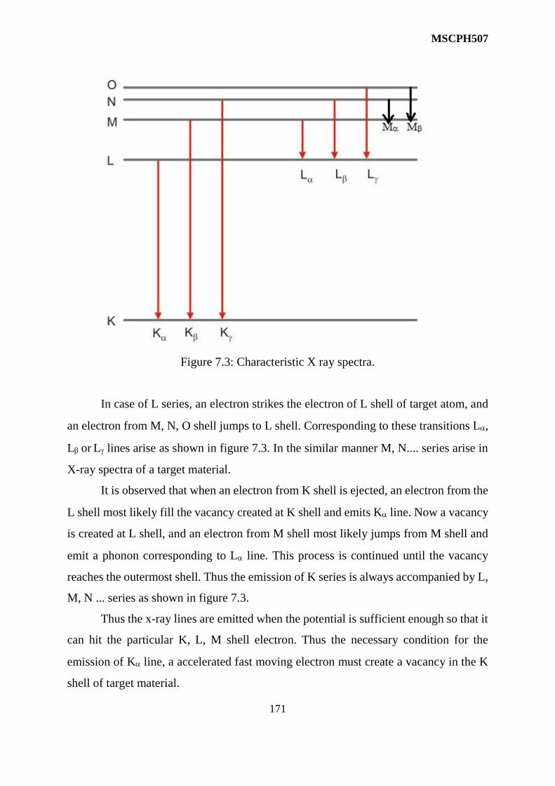
MSCPH507

171

Figure 7.3: Characteristic X ray spectra.

In case of L series, an electron strikes the electron of L shell of target atom, and

an electron from M, N, O shell jumps to L shell. Corresponding to these transitions L,

L or L lines arise as shown in figure 7.3. In the similar manner M, N.... series arise in

X-ray spectra of a target material.

It is observed that when an electron from K shell is ejected, an electron from the

L shell most likely fill the vacancy created at K shell and emits K line. Now a vacancy

is created at L shell, and an electron from M shell most likely jumps from M shell and

emit a phonon corresponding to L line. This process is continued until the vacancy

reaches the outermost shell. Thus the emission of K series is always accompanied by L,

M, N ... series as shown in figure 7.3.

Thus the x-ray lines are emitted when the potential is sufficient enough so that it

can hit the particular K, L, M shell electron. Thus the necessary condition for the

emission of K line, a accelerated fast moving electron must create a vacancy in the K

shell of target material.

MSCPH507

172

7.5 X-Rays Emission Spectra And Moseley Law

In 1913, Moseley studied the X-ray radiation of different elements. On this

experiment he recorded the photographs of different – different elements. He observed

K and K lines and later he observed that K and K lines are itself close doublets.

These doublets are four lines designed as K1, K2, K1, K2.

Moseley found that as atomic number increases, K lines shift towards higher

frequency. On this observation he stated that “The frequency of each corresponding K

lines is approximately proportional to the square of atomic number of target element.

The trend is shown in figure 4, and mathematically given as.

= RA2(Z-)2

σ)(ZAR

ν

Where A and are constants for a given transition. In case of K line.

= 1, 4

3A2

Figure 7.4: Moseley Law

by analogy with hydrogen line atoms the Moseley law can be given as

22 2

1

1

11ZR

MSCPH507

173

Similarly L, L series also composed of a number of lines.

7.6 X-ray Absorption Spectra

When a beam of X-rays passes through a film of a substance, and transmitted

light is analyze through an X-ray spectrograph, an absorption spectra of that substance

has been obtained. The absorption spectra of a substance are quite different from the

emission spectra of some substance absorption lines are not observed corresponding to

emission lines like K, K, K .... In absorption spectra, a continuous region of absorption

bounded by a sharp edge in the position of the limit of the emission of K series is

observed as shown in figure 7.5. These edges are characteristics of absorber substance

and called absorption edge. The frequency of absorption edge is k is called K

absorption limit.

It is clear that an x-ray emission line say K line occurs in the spectra when an

electron jump from L shell to K shell of substance. In absorption spectra this line would

be occurs when an electron jump from K shell to L shell. But it is not possible as L shell

is already full with 8 electrons. Thus K line cannot be observed in the absorption

spectra of X-ray.

Figure 7.5: Absorption spectra of X ray.

MSCPH507

174

Now we will explain the sharp edge occurred in the absorption spectra. In an x-

ray photon has sufficient energy to eject an electron from it inner shells say k shell, such

photon can be absorbed by k shell electron. But the frequency of such photon should be

greater than a certain value say k such that it can provide the energy required to remove

the e- of K shell (Wk)

Thus hk = Wk

The frequencies lower that this k value would not be able to remove an K shell

electron and such photon transmitted by substance. At frequency k, the absorption

process suddenly started and continues for frequencies greater than k as shown in

figure. Thus K absorption edge observed in the x-ray spectra corresponding to k

frequency. Absorption beyond the k indicates that K electron ejected to infinity with

kinetic energy say Ek as Einstein photoelectric equation (Ek = hk – Wk), where Wk is

corresponding to work function.

In case of L series, when we observed the x-ray absorption we will observed

three absorption edges designed a LI, LII, LIII. This occurs because L emission lines form

three groups according to their escalation voltages. It indicates L shell has three energy

levels the L series edges are shown in figure 7.5.

Similarly M absorption spectra shows S and N absorption spectra gives 7 edges.

7.7 Fine Structure of X-Rays Spectra

Kossel’s explained the x ray spectra on the basis of electron’s transmission in K, L, M,

.... shell. But actually this explanation is only a rough approximation. When we observe the x-

ray spectra more precision, we see each line of K series (K, K, K....) is a doublet, and other

series are more complex. These large numbers of lines are called fine structure. It is observed

that absorption edges shows that K level is single L level is 3 fold and M level is 5 fold. The

higher levels are shown by only heavier elements which are more complex.

The x ray levels arise due to removed of an electron from a shell. The x ray rotation of

shell K, L, M are due by removal of electron from these shell respectively. When electron from

15 shell is removed the neutral atom raised to higher energy K state. If one electron remains in

MSCPH507

175

15 subshell, this energy state is represented by I25½ as in the standard notation in spectroscopy

for k level.

For next shell principal quantum number n=2, i.e. L shell, 25 level will again give rise

to a state 225½. This is corresponding to L1 level. In this shell there is another p subshell of 6

electrons. If an electron eject from this subshell, configuration becomes 2p5. This gives rise of

some states as a single electron in p subshell. Hence the states arise as 22P½ and 22P 3/2.

Corresponding to LII and LIII levels as shown in figure. Hence L shell has 3 absorption edges

corresponding to LI, LII and LIII states.

In case of third shell n=3 i.e. M shell, there as 3 subshells as 3s, 3p and 3d. The removal

of an electron from this shell the possible incomplete subshells are 3s, 3p5, 3d9. These give the

rise of the states 325½ , 32P½, 32P3/2, 32P5/2 respectively. These 5 states of M shells are

represented by MI, MII, MIII, MIV, Mv respectively. The levels are displayed in figure 7.6.

MSCPH507

176

Figure 7.6: Fine structure of x-rays spectra

The selection rule for x-ray spectra is given as

n is arbitrary

L = 1

J = 0, 1

Thus it is clear that the x-ray lines K1 and K2 arises due to transmission from K level to LII

and LIII. Similarly 3 groups of lines in L series appears due to transmission to LIII, LII, LI to M

or N levels. Figure 6 displays the K and L series arise due to transmission. Similarly the M

series can be shown due to transmission among different subshells of M and N.

MSCPH507

177

7.8 X-Ray Spectra and Optical Spectra

We can compare x-ray spectra and optical spectra on the basis of following aspects.

(i) In the X ray spectra the tightly bond inner shell electrons say K shell or L shell

electron are involved in transition. On the other hand, in optical spectra, the only

outermost shell electrons are involved in the transition.

(ii) The frequencies of x ray spectra are about thousand times more than optical spectra.

Since X ray spectra is related to complete removal of inner shell electrons hence the

frequency range is quite higher.

(iii) In x ray spectra, the frequencies of x ray lines increase steadily, not periodically for

different elements when their atomic number Z increases. This is because for heavy

elements (more Z), the electrons of inner shells hold more strongly and need more

energy for removal. Thus the X ray spectra of elements of nearby atomic number

are very similar. On the other hand the in optical spectra, no similarity in the

elements of nearby atomic number. This is because the structure of outermost shell

changes for the elements of nearby Z.

(iv) In case of x ray spectra, the emission spectra consist of desecrate lines and

absorption spectra consists of continuous region bounded by sharp edges. On the

other hand, in optical spectra, emission lines are and absorption lines are same or

both are identical.

SAQ 1 : In x ray emission, what happens when an high energy electron beam strikes on

K shell electron?

SAQ 2 : What do you mean by K, K, K .... lines?

SAQ 3 : What is the difference between emission spectra and absorption spectra?

SAQ 4 : Write down Moseley law.

SAQ 5 : What is absorption edge in x ray absorption spectra?

SAQ 6 : What is fine structure?

SAQ 7 : Give the selection rule for x ray spectra.

SAQ 8 : What are the range of frequencies of x ray spectra and optical spectra.

SAQ 9 : What happens when an electron from K shell of an element removed

completely from its shells?

MSCPH507

178

Example 1: Calculate the required voltage that must be applied to an x ray tube to produce x

ray of wave length 0.1A (given e = 4.8 × 10-10esu, C = 3 × 1010 cm/sec, h = 6.62 ×

10-27 erg-5)

Solution: The electron is accelerated in x ray tube. If V is the accelerating voltage, e is change

of electron then the energy E of emitted photons can be given as.

λ

hchνEev

cm100.1esu104.8

cm/5103erg106.62

eλ

hcν

810

10527

= 413.75 esu

= 413.7 × 300 Volt

= 1.24 × 105 Volt

Example 2: How much energy goes into the quantum emitted when an L-electron drops into

empty K shell in copper (Z = 29).

[guen R= 109737cm-1 and 1 cm-1= 1.239 × 10-4 ev]

Solution: from moseley’s law, x-ray wavelength is given by

22

2

2

1

1

11

λ

1ZR

Where h2=2 and n1=1 for transmission from L shell (n = 2) to k shell (n = 2)

corresponding to K line. Thus

21ZR4

3

λ

1

=228109737

4

3

= 6.4525 × 10-7 cm-1

Corresponding energy E = 6.4525 × 10-7 × 1.239 × 10-4

7.9946 × 103 eV

Example 3: Calculate the wave length of K line of higher (given atomic number Z = 47, R =

109737 cm-1)

Solution: According to moseley law

MSCPH507

179

22

2

2

1

1

11

λ

1ZR

Where symbols are usual meaning and 1 and 2 are transition from L shell to K shell

21ZR4

3

λ

1

2461097374

3

= 1.74 × 10-8 cm

cm81074.1

1λ

= 0.57A

Example 4: If K radiation of M0(Z=42) has wavelength 0.75A, calculate the wavelenght of

K radiation of cu (atomic number Z = 29)

Solution: According to moseley law of K line

22

2

2

1

1

11

λ

1ZR

21ZR4

3

λ

1

2

2

2

Cu

2

Mo

mo

cu

28

41

1Z

1Z

λ

λ

1.60A28

410.75

28

41λλ

2

2

2

2

MoCu

7.9 Summary

1. When fast moving electrons are deaccelerated, these deaccelerated electron emit

electromagnetic radiations (Bremsstarhlung) which are known as X-rays.

2. The intensity of continuous x ray spectra depends on the energy of incident electron and not

depends on target material.

𝜆𝑚𝑖𝑛 =ℎ𝑐

𝑒𝑉 where V is applied potential

𝜆𝑚𝑖𝑛 =12400

𝑉

3. Kossel explained that in an high energy electrons penetrates well inside an target atom, it

eject the electron of K shell, and immediately an electron from outer shell, says L shell jump

MSCPH507

180

to K shell, X-ray photon of higher energy is emitted similarly an electron from N shell may

jump to K shell. These lies of K series are designated as K, K , K .

4. Moseley law states that as atomic number increases, K lines shift towards higher frequency.

He stated that “The frequency of each corresponding K lines is approximately proportional to

the square of atomic number of target element”. Mathematically

= RA2(Z-)2

5. Kossel’s explained the x ray spectra on the basis of electron’s transmission in K, L, M, ....

shells. When we observe the x-ray spectra more precision, we see each line of K series (K,

K, K....) is a doublet, and other series are more complex. These large numbers of lines are

called fine structure.

7.10 Glossary

X-rays : Electromagnetic radiation of wavelength of 0.01 to 1A

Line spectra : Dark or bright lines in continuous spectrum in a narrow frequency

range

Emission line : if source emit specific wavelength of radiation

Absorption line : If a substance absorbs a specific wavelength from radiation

Fine structure : Splitting of a the main spectral line of a substance into two or more

spectral lines

Optical spectra : Spectra arises due to outmost electron of atom

Selection rule : Also known as transitions rule give the possibility of transitions

from one quantum state to another

7.11 References

1. Atomic and Molecular spectra. Raj Kumar, Kedarnath Ramnath Publication, Meerut

7.12 Suggested reading:

1. C.N. Benwell and E.M. McCash. Fundamental of molecular spectroscopy

2. Introduction to Atomic spectra. H.E. White.

7.13 Technical Questions

7.13.1 Short Answer type question

1. Give the Kossel’s explanation of x-ray spectra

σ)(ZAR

ν

MSCPH507

181

2. What is x-ray emission spectra?

3. Explain Moseley law.

4. What is absorption edge in x ray spectra?

5. What is fine structure? Discuss the fine structure of x ray.

6. Give comparison between x ray spectra and optical spectra.

7.13.2 Long Answer type questions

1. Explain emission spectra of X rays and deduce Moseley’s law.

2. Explain absorption spectra of X ray and discuss how it is different from emission

spectra?

3. Discuss the fine structure of X rays. Give the diagram from the possible transition in x

ray spectra.

4. Give a comparison between optical and x ray spectra an explain why in optical spectra

of element of nearby atomic number are qualitatively very similar, while the optical

spectra of these elements are different.

MSCPH507

182

UNIT 8

MOLECULAR ENERGY STATES AND

MOLECULAR SPECTRA

Structure

8.1 Objective

8.2 Introduction

8.3 Molecular Spectra

8.3.1 Regions of the Electromagnetic Spectrum

8.3.2 Effect of Electromagnetic Radiation

8.4 Types of Molecular Spectra

8.4.1 Pure Rotational Spectra

8.4.1.1 Salient Feature of Rotational Spectra

8.4.2 Vibrational–Rotational Spectra

8.4.2.1 Salient Feature of Vibrational–Rotational Spectra

8.4.3 Electronic Spectra

8.4.3.1 Salient Feature of Electronic Spectra

8.5 Atomic Spectra

8.6 Types of Molecular Energy States and Associated Spectra

8.7 The Born-Oppenheimer Approximation

8.8 Summary

8.9 Glossary

8.10 Reference Books

8.11Suggested Readings


MSCPH507

183

8.1 Objectives

After studying this unit, you will come to know about:

1. Molecular spectra and its kinds.

2. Pure rotational spectra of diatomic molecules and its salient features.

3. Vibrational rotational spectra of diatomic molecules and its salient features.

4. Electronic spectra of diatomic molecules and its salient features.

5. Types of molecular energy states and associated spectra.

6. The Born-Oppenheimer approximation

8.2 Introduction

The absorption and emission of molecules arise from transitions between allowed energy

states; ground and excited ones. The energy-level scheme of molecules is different from that

of atoms and is relatively complicated; there are two main reasons for this. Firstly, we cannot

classify molecular energy states according to the electronic angular momentum L (as we do in

atoms) which is not conserved in molecules. Secondly, the nuclear motion in molecules cannot

be ignored, as we can do in atoms. In a diatomic molecule, for example, the nuclei vibrate along

the internuclear axis, and in addition the whole system rotates about its center of mass. The

energy of each of these vibrational and rotational motion is quantized, with the result that there

are many more energy levels in a molecule than in an atom.

Molecular spectroscopy is defined as the study of the interaction of electromagnetic waves and

matter. So far we have studied about the interaction of electromagnetic waves with atoms, i.e.

when the emitting substance is in atomic state. However, here the emitting substance is a

molecule, which may contain two (diatomic) or more atoms (polyatomic). Molecular spectra

are band spectra which appear as a continuous band when observed with a low resolving power

instrument. With high resolving power instruments, molecular spectra disclose a three-fold

structure:

1. Each band is composed of a large number of lines which are arranged with great regularity

which are crowded together at the long wavelength side, i.e. at the band head and as they

recede from the band head, the lines become more widely separated and also weaker.

2. There is a regular sequence in which the several bands follow one another, and thus

constitute a group of bands.

3. There is a close and regular arrangement of different groups of bands which form a band

system.

MSCPH507

184

8.3 Molecular Spectra

The spectra emitted by molecules (When the emitting substance is in molecular state) is known

as molecular spectra. It appears as a continuous band, therefore it is also known as band spectra.

A band has a sharp intense edge on one side (band head) which decreased in intensity towards

the other side. The study of molecular spectra is known as molecular spectroscopy.

8.3.1 Regions of the Electromagnetic Spectrum

The entire range of electromagnetic waves is known as the electromagnetic spectrum. This

includes electromagnetic energy ranging from gamma rays to radio waves. In general the

electromagnetic spectrum is mainly divided into six regions. In order of decreasing wavelength

(increasing energy and frequency) different regions are mentioned below:

(i) Radio frequency region (100 to 10 m): Radio waves have the longest wavelength in the

electromagnetic spectrum. To transmit a variety of data, radio waves are used. They are also

used in wireless networking, television and amateur radio.

(ii) Microwave region (or far infra-red region) (1mm to 1m): Microwaves are essentially high

frequency radio waves. They have wavelengths in the range of 1mm to 1m. Microwaves are

used for many applications. They are beneficial for satellite communication, studying the Earth

from space, radar technology etc.

(iii) Infra-red region (780 nm - 1000 µm): Infrared spectrum divided into the three main regions

Near Infrared (NIR): 0.7 – 1.3µm

Shortwave Infrared (SWIR): from 1.3 – 3 µm

Far or Thermal Infrared from 3 - 100 µm

Infrared radiation is mainly used in remote sensing.

(iv) Visible and ultraviolet region (1 nm to 750nm): Ultraviolet (UV) light has wavelengths of

approximately 1 – 380 nm. The main source of ultraviolet energy is the Sun. The UV waves

are invisible for the human, however some insects, can see them.

Visible light wavelengths range from 400 – 750 nm. Human eyes can see only this region of

the electromagnetic spectrum. Each individual wavelength within the spectrum of visible light

wavelengths is represented by a particular color. The visible portion of the electromagnetic

spectrum is mainly used in remote sensing.

(v) X-ray region (0.01 – 10 nm): X-Rays range in wavelength from 0.01 – 10 nm. These rays

are generated from superheated gas from exploding stars and quasars. The main important

properties of the X-rays is that they are able to pass through a variety of materials. The most

common use of X-rays are in the field of medical imaging and for checking cargo and luggage.

MSCPH507

185

(vi) Gamma rays region (< 0.01 nm): Gamma rays are produced by the hottest objects in the

universe, including neutron stars, pulsars, and supernova explosions. These rays are

biologically hazardous.

8.3.2 Effect of Electromagnetic Radiation

There are two processes of interaction of electromagnetic radiation with the matter available.

They are photo physical interaction and photochemical interaction. Both the photo physical

and photochemical processes are used to study the nature and characteristics properties of

molecules in their different energy states. If the chemical identity of a molecule is retained after

the interaction, the process is called a photo physical process, if not, then it is called a

photochemical process. The interaction of specific frequency with a molecule takes place

between the electric field component of radiation and electric dipole moment of the

molecule. Because of interactions, the transition of molecules can occur from ground state to

excited state or vice versa. The energy level at which a molecule exists is referred to as its state.

Two basic processes is observed when light interacts with matter:

• Absorption process

• Emission process

A molecule can move from one level to another level by using a finite amount of energy.

Normally, a molecule exists in their most stable state referred to as the ground state or lower

energy state. The transition from the ground state (E0) to the excited state (E1) requires some

form of energy input. When the radiation interacts with molecules, it absorbs a suitable amount

of energy and jump from its ground energy state to its nearest excited energy state by following

the famous equation as:

where λ is wavelength of incident radiation, υ is frequency of incident radiation, h is Planck's

constant and c is the velocity of light. This process is known as absorption (Figure 8.1). Process

of emission is just the opposite phenomenon of absorption. In this process, molecules that are

in excited state decay to the lower levels by emitting radiation (Figure 8.1).

MSCPH507

186

Figure 8.1: Absorption and emission process.

Electromagnetic radiation may also reorient the molecule along the direction of the field, which

can break some bond. Now in the following sections, we will discuss different types of

molecular spectra.

8.4 Type of Molecular Spectra

The molecular spectra can be divided into three spectral ranges corresponding to the different

type of transition between molecular energy states.

1. Pure rotational spectra

2. Vibration-rotational spectra

3. Electronic spectra

8.4.1 Pure Rotational Spectra

These spectra are observed in absorption in the far infrared or in the microwave region. It

involves transitions between rotational states of the molecules. Rotational spectroscopy is

called pure rotational spectroscopy, to distinguish it from roto-vibrational spectroscopy (the

molecule changes its state of vibration and rotation simultaneously) and vibronic spectroscopy

(the molecule changes its electronic state and vibrational state simultaneously). For a molecule

to exhibit a pure rotational spectrum it must possess a permanent dipole moment (otherwise

the photon has no means of interacting “nothing to grab hold of”). Normally, a molecule must

be polar to be able to interact with a microwave. A polar rotor appears to have an oscillating

electric dipole. However, homonuclear diatomic molecules such as O2, H2, do not have a dipole

moment and, hence, no pure rotational spectrum. For rotational spectroscopy, molecules are

classified according to symmetry into spherical top, linear and symmetric top.

MSCPH507

187

8.4.1.1 Salient Feature of Rotational Spectra

The salient features of the pure rotational spectra are given below:

1. The band which appears in the infra-red region is due to transition involving very small

energy changes, about 0.005ev. With such a small quantum of energy, electronic and

vibrational energy states will not be excited or in other words only transitions that are purely

rotational in character will appear. Therefore bands that appear in the infra-red region arise

due to the changes in the rotational energy of the molecule unaccompanied by changes in

electronic or vibrational energy. Only those molecules which have permanent electric

dipole moment can give rise to pure rotational spectra. Thus homonuclear diatomic

molecules such as H2, O2, N2 etc. do not exhibit pure rotation spectra. While heteronuclear

diatomic molecules such as HF, HCl, HBr etc. exhibit pure rotation spectra.

2. In practice, rotational spectra are observed in absorption. For heteronuclear diatomic

molecules such as HF, HCl, HBr, Co etc. the rotational spectra consist of a simple series of

absorption maxima, which are very nearly equidistant on a wave number scale. A

measurement of the frequencies of these maxima help to determine the moment of inertia

and the internuclear distance.

3. The basic molecular requirement for the emission or absorption of radiation by a transition

between rotational energy states is that the molecule must have a permanent dipole

moment. This is in line with classical electrodynamics according to which a rotating

molecule can lead to the emission of radiation, only if a changing dipole moment is

associated with it. During the rotation of a heteronuclear diatomic molecule, having a

permanent dipole moment, the component of this dipole moment in a fixed direction

changes periodically with the frequency of rotation of the molecule, emitting radiations of

the same frequency. However, homonuclear molecules have no dipole moment and hence

there is no emission of infra-red radiation.

4. Further infra-red radiation can be absorbed by a rotating molecule and thereby increase

rotation, only if a permanent dipole moment is present such a molecule interacts with the

oscillating electric field of the incident radiation to absorb rotational energy and produce

absorption spectra.

8.4.2 Vibration-Rotational Spectra

These spectra are observed in absorption in the near infrared region. Each spectrum consists

of an intense band (known as fundamental) which is followed by a few weak bands (known as

overtones). If the molecule in its equilibrium position has a dipole moment, as is always the

case for the heteroatomic molecules, this dipole moment will in general change if the

internuclear distance changed. Thus, on the basis of classical electrodynamics the molecular

vibration would lead to the emission of light at the oscillation frequency. Conversely, the

oscillator could be set in vibration by absorption of light at this frequency. Therefore, all

heteroatomic molecules in principle are said to be infrared active that is they can absorb or emit

infrared radiation. Contrary, all homoatomic diatomic molecules do not have any dipole

MSCPH507

188

moment and cannot be set in vibration by absorption of infrared light. These molecules are said

to be infrared inactive.

8.4.2.1 Salient features of vibrational-rotational spectra

1. When there are transitions between vibrational states of the same electronic state of

molecule, we get vibrational-rotational molecular spectra. Such a spectra is observed in a

near infra-red region of the electromagnetic spectrum.

2. Vibrational-rotational spectra, like pure rotational spectra, are observed only for molecules

that have permanent dipole moments such as HCl, HCN, HF (heteronuclear diatomic

molecules).

3. The internuclear distance changes when the nuclei of these molecules vibrate relative to

each other. Thus these molecules possess an oscillating dipole moment, which according

to classical electrodynamics emits radiations of frequency that fall in near infra-red region-

conversely, if electromagnetic radiation falls on such a molecule then oscillating dipole

interactions will the incident radiation and can absorb radiation of frequency of near infra-

red region.

4. In practice, vibrational-rotational spectra are observed in absorption.

If the molecule in its equilibrium position has a dipole moment, as is always the case for the

heteroatomic molecules, this dipole moment will in general change if the internuclear distance

changed. Thus, on the basis of classical electrodynamics the molecular vibration would lead to

the emission of light at the oscillation frequency. Conversely, the oscillator could be set in

vibration by absorption of light at this frequency. Therefore, all heteroatomic molecules in

principle are said to be infrared active that is they can absorb or emit infrared radiation.

Contrary, all homoatomic diatomic molecules do not have any dipole moment and cannot be

set in vibration by absorption of infrared light. These molecules are said to be infrared inactive.

Infrared transitions

W. Coblentz coined the first systematic use of infrared technique in 1905. Infrared R

spectroscopy can be divided into three areas based on spectral region: far-IR, mid-IR, and near-

IR. A molecule will be IR active when there is a change in dipole moment of the molecule with

time. Due to change in dipole moments, the bond lengths and bond angles suffer a variation,

which in turn appears as vibrational and bending modes. If one or more bond lengths of the

molecule changes symmetrically, vibrational modes are known as symmetric stretching

vibrational (υ) modes. Let us take an example of a linear CO2 molecule.

There is a small net positive charge on C atom and O has small negative charges. In the

symmetric stretching mode both the C=O bonds change simultaneously (Figure 8.2). If two

bonds are in opposite atomic motions. One bond is elongating while the other is contracting.

The vibration of molecules is known as asymmetric stretching (α) mode. In α stretching

MSCPH507

189

vibration shown in Figure 8.2 a periodic alteration in the dipole moment is observed. If one or

more bond angles of the molecules change while bond lengths remain constant, vibrational

mode is known as bending mode (δ). In the δ vibration, a change in dipole moment is also

observed (Figure 8.2).

In CO2, symmetric stretching mode for both the C=O bonds changes simultaneously and

resultant dipole moment remains zero for the whole system as shown in Figure 8.2. As a result

the symmetric υ mode remains “infrared inactive”. Whereas, due to a periodic alteration in the

dipole moment, α stretching vibration, is “IR active”. In the δ vibration, a change in dipole

moment is also observed and that results in “IR activity”.

Figure 8.2: Different vibrational modes of carbon dioxide molecule showing the dipole moment

and IR activity.

MSCPH507

190

8.4.3 Electronic Spectra

These spectra are observed both in emission and absorption regions. Each spectrum consists of

a large number of bands. Each band has a sharp edge (Band head) on one side which decreases

in intensity towards the other side. Actually, a band is composed of a series of lines which draw

further apart with the increase of distance from the band head. The band is said to be ‘degraded’

towards the side opposite to the bard-head. These spectra are observed for the hetro-nuclear as

well as for the homonuclear diatomic molecules.

8.4.3.1 Salient Features of Electronic spectra

1. Electronic spectra is the most complex molecular spectra which appear in the visible and

ultraviolet regions and involve the change in all the three energies (electronic, vibrational

and rotational) of the molecule.

2. These spectra are obtained in emission and absorption regions.

3. The spectral band exhibits a fine structure which is more complicated. The head formation

tendency is story and the bands are degraded either towards violet or toward the red. All

molecules give electronic spectra.

4. Homo-nuclear molecules (H2, N2, O2 etc.) do not give neither rotational nor vibrational-

rotational spectra because of having no permanent dipole moments but they give electronic

spectra because of the instantaneous dipole moment changes during the redistribution of

change which results in the transition.

Electronic transitions

When an electron in its lowest energy state gains some energy and transfers to its excited

states, is known as molecular electronic transition. This process involves promotion of an

electron from a bonding or nonbonding molecular orbital to an antibonding molecular orbital.

These transitions provide information regarding the structure of a molecule and determine

many more molecular properties. Electronic transitions are measured by Ultraviolet and visible

spectroscopy and fall in the ultraviolet and visible region (190 nm-700 nm) of the

electromagnetic spectrum both in absorption and emission modes. The electronic transition is

mainly possible by absorbing photon energy equivalent to the separation of energy levels

between which the electron transited. Mostly four types of electronic excitation exist in

molecules (Figure 8.3).

1. σ→σ*

2. π→π*

3. n→σ*

4. n→π*

MSCPH507

191

Figure 8.3: Possible transition between bonding (σ, π), anti-bonding (σ*, π*), and nonbonding

(n) orbitals.

Energies associated with different molecular transitions are in the following order.

n→π* < π→π* < n→σ* < σ→π* < σ→σ*

The wavelength corresponding to the σ→σ* transition is located at the far ultraviolet region of

the electromagnetic spectrum. The n→π* and π→π* are located at a near visible part of the

spectrum. The strength of an electronic transition is expressed in terms of “oscillator strength”

(f) and defined as the ratio of the experimental transition probability to that of the ideal case of

a harmonic oscillator.

It is a dimensionless quantity and totally allowed transition corresponds to the oscillator

strength 1, when all the molecules are transferred to the higher energy state.

8.5 Atomic Spectra

When electrons of an atom are excited to higher energy states, the radiations that are absorbed

in this process appear as the absorption spectra of atoms. In a similar way, electronic spectra

of molecules arise when the electrons of a molecule are excited to higher energy states. The

energy involved in this process is generally large and electronic spectra of molecules are

usually found in visible and ultraviolet regions. Therefore electronic spectra arise due to the

changes in the arrangement of molecular electrons. We shall discuss electronics spectra of

diatomic molecules.

The electronic transition is the result of change in electronic energy. A small change in the

electronic energy will be accompanied by a large change in the vibrational energy of the

molecule. These vibrational energy changes give rise to vibrational transitions which form a

group of various bands. Further, a small change in the vibrational energy will be accompanied

by a large change in the rotational energy of the molecule. These rotational energy changes

MSCPH507

192

give rise to rotational transitions forming a series of lines in each band-the so called fine

structure of each band.

8.6 Types Of Molecular Energy States And Associated Spectra

Molecular energy states arise from the rotation of a molecule as a whole and from the vibration

of its constituent nuclei relative to one-another as well as from changes in its electronic

configuration. Rotational states are separated by quite small energy-interval ( 10-3ev) and the

spectra arising from transitions between these states are in the far infra-red or microwave

region. Vibrational states are separated by somewhat larger energy intervals ( 10-1ev) and the

vibrational spectra fall in the near infra-red region. The electronic states have higher energy

separation ( 10ev) and the corresponding spectra fall in the visible and ultraviolet regions.

The two nuclei vibrate about their respective equilibrium positions along the internuclear axis,

and the molecule rotates about the center of mass. Schrodinger's equation for the nuclear

motion in a diatomic molecule is.

[- 12

22

When M1 and M2 are the masses of the nuclei and V(r) is the Potential energy function consisting

of the instantaneous electronic energy and electrostatic energy of the two nuclei. is the

nuclear eigenfunction which E is the eigenvalues for the whole molecule. Besides electronic

bands. We have non-electronic bands also (for which e=0) such bands are of two types:

Vibration-rotational bands and pure rotational bands.

The explanation for three types of band spectra demands that the internal energy of a molecule,

i.e. the energy other than the translational is essentially of three kinds, namely electronic,

vibrational and rotational which are all quantised and thus the molecule possesses only certain

discrete energy states. The transition between two energy states of a molecule, as a result of

either absorption or emission of energy, will give rise to a spectral line in the spectrum of that

molecule. Suppose energy difference of two states is (E – E'') then the wave number

(frequency in cm-1) corresponding to the line, arising due to transition between these two states

will be:

cm-1,

where c is the velocity of light.

The three types of bands, discussed above, are correlated with

MSCPH507

193

1. Change in the rotational energy

2. Simultaneous change of the rotational and vibrational energies, and

3. Simultaneous change in the rotational, vibrational and electronic energies.

Figure 8.4: Diagram representing electronic, rotational and vibrational energy levels.

The diagram shows that:

i. A molecule has a number of discrete electronic levels with separation of the same order

as in atoms. A transition between two electronic levels results in a radiation that falls in a

visible or ultraviolet region.

ii. With each electronic level are associated a number of vibrational energy levels whose

spacing decreases with increasing quantum number, ν. A transition between two vibrational

levels results in a radiation which falls in a near infrared region.

iii. With each vibrational level is associated a set of rotational levels whose spacing

increases with increasing quantum number, J. A transition between two rotational energy

levels results in a radiation that falls in a far infrared or microwave region.

Fig. 8.4, shows transition from: Electronic level A to electronic level B

Vibrational level v'' = 0to vibrational level v' = 0

Rotational level J'' = 1 to rotational level J' = 3

8.7 The Born-Oppenheimer Approximation

The Born-Oppenheimer approximation is the assumption that the electronic motion and the

nuclear motion in molecules can be separated. It leads to a molecular wave function in terms

of electron positions and nuclear positions.

MSCPH507

194

This involves the following assumptions:

1. The electronic wave function depends upon the nuclear positions but not upon their

velocities, i.e., the nuclear motion is so much slower than electron motion that they can be

considered to be fixed.

2. The nuclear motion (e.g., rotation, vibration) sees a smeared out potential from the speedy

electrons.

We know that if a Hamiltonian is separable into two or more terms, then the total Eigen

functions are products of the individual Eigen functions of the separated Hamiltonian terms,

and the total eigenvalues are sums of individual eigenvalues of the separated Hamiltonian

terms.

Consider, for example, a Hamiltonian, which is separable into two terms, one involving

coordinate q1 and the other involving coordinate q2.

With the overall Schrödinger equation being

If we assume that the total wave function can be written in the form

,

where ψ1(q1) and ψ2(q2) are Eigen functions of H1 and H2 with eigenvalues E1 and E2, then

(8.1)

(8.2)

(8.3)

(8.4)

(8.5)

MSCPH507

195

Thus the Eigenfunctions of are products of the Eigenfunctions of H1 and H2, and the

eigenvalues are the sums of eigenvalues of H1 and H2.

The Eigenfunctions and eigenvalues of this Hamiltonian, which will be given by solution of

the time-independent Schrödinger equation

We first invoke the Born-Oppenheimer approximation by recognizing that, in a dynamical

sense, there is a strong separation of time scales between the electronic and nuclear motion,

since the electrons are lighter than the nuclei by three orders of magnitude. This can be

exploited by assuming a quasi-separable ansatz of the form

where ϕN(R) is a nuclear wave function and ϕe(x, R) is an electronic wave function that depends

parametrically on the nuclear positions. If we look again at the Hamiltonian, we would notice

right away that the term VeN would prevent us from applying this separation of variables. The

Born-Oppenheimer (named for its original inventors, Max Born and Robert Oppenheimer) is

based on the fact that nuclei are several thousand times heavier than electrons. The proton,

itself, is approximately 2000 times more massive than an electron. In a dynamical sense, the

electrons can be regarded as particles that follow the nuclear motion adiabatically, meaning

that they are ``dragged'' along with the nuclei without requiring a finite relaxation time. This,

of course, is an approximation, since there could be non-adiabatic effects that do not allow the

electrons to follow in this ``instantaneous'' manner, however, in many systems, the adiabatic

separation between electrons and nuclei is an excellent approximation. Another consequence

of the mass difference between electrons and nuclei is that the nuclear components of the wave

function are spatially more localized than the electronic component of the wave function. In

the classical limit, the nuclear are fully localized about single points representing classical point

particles.

After these considerations, HN(R) can be neglected since TN is smaller than Te by a factor

of M/m. Thus for a fixed nuclear configuration, we have

Such that

MSCPH507

196

This is the “clamped-nuclei'” Schrödinger equation. Quite frequently VNN(R) is neglected in

the above equation, which is justified since in this case is just a parameter so that VNN(R) is

just a constant and shifts the eigenvalues only by some constant amount. Leaving VNN(R) out

of the electronic Schrödinger equation leads to a similar equation,

(8.6)

(8.7)

where we have used a new subscript “e'' on the electronic Hamiltonian and energy to distinguish

from the case where VNN is included.

We now consider again the original Hamiltonian. If we insert a wavefunction of the form ψ(r,

R)=ϕe(r, R)ϕN(R), we obtain

(8.8)

Since Te contains no dependence,

However, we may not immediately assume

(this point is tacitly assumed by most introductory textbooks). By the chain rule,

Using these facts, along with the electronic Schrdöinger equation,

we simplify Equation to

(8.9)

MSCPH507

197

(8.10)

(8.11)

We must now estimate the magnitude of the last term in brackets. A typical contribution has

the form 1/(2M)∇2R ϕe(r, R) , but ∇R ϕe(r, R) is of the same order as ∇r ϕe(r, R) since the derivatives

operate over approximately the same dimensions. The latter is ϕe(r, R)Pe, with Pe the momentum

of an electron. Therefore

Since m/M~1/10000 the term in brackets can be dropped, giving

This is the nuclear Shrödinger equation we anticipated-the nuclei move in a potential set up by

the electrons.

To summarize, the large difference in the relative masses of the electrons and nuclei allows us

to approximately separate the wavefunction as a product of nuclear and electronic terms. The

electronic wavefucntion ϕe(r,R) is solved for a given set of nuclear coordinates,

and the electronic energy obtained contributes a potential term to the motion of the nuclei

described by the nuclear wavefunction ϕN(R).

MSCPH507

198

In the conclusion we can say that Born approximation enables us to solve the complete

molecula wave equation in the the following way:

1. For a given electronic state of a molecule the electronic wave equation is solved for a range

of nuclear coordinates (internuclear separations).

2. The eigenvalues E are the characteristic energies for the whole molecule in the given

electronic state. A different set of wavefunction and energy eigen value is found for each

electronic state of the molecule.

3. The total wavefunction of the system is the obtained by the product of wavefunctions of

the coordinates of the nuclei and electrons.

Self Assessment Question (SAQ) 1: What do you understand by dipole moment?

Self Assessment Question (SAQ) 2: Why dipole moment is important in molecular

spectroscopy?

Self Assessment Question (SAQ) 3: Homonuclear diatomic molecules are microwave

inactive. Why?

Self Assessment Question (SAQ) 4: Heteronuclear diatomic molecule will show rotational

spectrum or not?

Self Assessment Question (SAQ) 5: What is the main condition that a molecule will be

microwave active or not? Give some examples.

Self Assessment Question (SAQ) 6: What is the main condition for a molecule to be IR active?

Self Assessment Question (SAQ) 7: What do you mean by degrees of freedom of a molecule?

What is its value for a linear molecule and a nonlinear molecule?

Self Assessment Question (SAQ) 8: Which of the following molecules will show microwave

spectrum: H2, HCl, CH4, CH3Cl, CH2Cl2, H2O, SF6. Why?

8.8 Summary

In this unit, you have studied the electronic, vibrational and rotational spectra of diatomic

molecules in detail. Transitions between different rotational levels give rise to pure rotational

spectra of diatomic molecules. Transitions between different rotational levels give rise to pure

rotational spectra in the microwave or far infrared region. This study helps in evaluation of

molecular parameters. The transition between vibrational levels results in the vibrational

spectra which are observed in the near infrared region. This gives information about molecular

structure, bond length, interatomic distances etc. In electronic spectra which are obtained in

visible and ultraviolet regions, transition from one electronic level to the other level takes place.

This is accompanied by change in vibrational and rotational energy. This gives rise to

MSCPH507

199

vibrational coarse structure and rotational fine structure. We are able to get information about

the rotational constants and vibrational frequencies of both ground and excited electronic states.

8.9 Glossary

Spectrum

The set of colours into which a beam of light can be separated, or a range of

waves

rotational A rotation is a circular movement of an object around a center of rotation.

vibrational A molecular vibration is a periodic motion of the atoms of a molecule relative

to each other,

Emission

spectrum

The distribution of electromagnetic radiation released by a substance whose

atoms have been excited by heat or radiation.

Absorption

spectrum

The spectrum formed by electromagnetic radiation that has passed through a

medium in which radiation of certain frequencies is absorbed

Transition The process or a period of changing from one state or condition to another.

8.10 References Books

1. Atomic & Molecular spectra Laser: By Raj Kumar (KNRM Publication-Meerut)

2. Structure and properties of Material: By MA Wahab (Narosa Publishing House –Delhi)


1950)

4. Atomic Physics by J.H.Fewkes& John Yarwood. Vol. II (Oxford Univ. Press, 1991).


Technical)

6. Molecular Spectroscopy, C N Banwell.

7. Fundamental of Molecular Spectroscopy. C N Banwell and E M Mc Cash (Tata Mc Graw

Hills)



2. Optical Spectroscopy in Chemistry and Life Sciences, W. Schmidt; Wiley-VCH.

https://www.collinsdictionary.com/dictionary/english/certain

https://www.collinsdictionary.com/dictionary/english/frequency

MSCPH507

200


Short and long answer type question

1. What is the meaning of Molecular spectra?

2. How many ranges in Molecular spectra can be classified?

3. Discuss various types of spectra.

4. Account for: “The molecules have rotational and vibrational states but atom do not”.

5. What are the salient features of rotational spectra?

6. Why do homonuclear diatomic molecules not exhibit pure rotation spectra?

7. Why is a vibrating diatomic molecule considered as an anharmonic oscillator?

8. Which physical quantities can we calculate from vibration rotation spectra?

9. Is electronic spectra exhibited by all molecules? Give proper reason.

Objective type question

1. The different types of energies associated with a molecule are __________

a) Electronic energy

b) Vibrational energy

c) Rotational energy

d) All of the mentioned

2. During the motion, if the centre of gravity of molecule changes, the molecule possess

__________

a) Electronic energy

b) Rotational energy

c) Translational energy

d) Vibrational energy

3. The correct order of different types of energies is __________

a) Eel >> Evib >> Erot >> Etr

b) Eel >> Erot >> Evib >> Etr

c) Eel >> Evib >> Etr >> Erot

d) Etr >> Evib >> Erot >> E el

4. The region of electromagnetic spectrum for nuclear magnetic resonance is __________

a) Microwave

b) Radio frequency

c) Infrared

d) UV-rays

MSCPH507

201

5. Which of the following is an application of molecular spectroscopy?

a) Structural investigation

b) Basis of understanding of colors

c) Study of energetically excited reaction products

d) All of the mentioned

Answer 1- d; 2-c; 3- a; 4-b; 5-d

MSCPH507

202

UNIT 9 PURE ROTATIONAL SPECTRA

Structure

9.1 Introduction

9.2 Objectives

9.3 Salient features of rotational spectra

9.3.1 Conditions for a molecule to show Rotational spectra

9.3.2 Dipole moment

9.3.3 Role of dipole moment in rotational transition

9.3.4 Classification of molecules depending on rotation

9.3.4.1 Linear molecules

9.3.4.2 Symmetric top type molecules

9.3.4.3 Spherical top type molecules

9.3.4.4 Asymmetric top type molecules

9.4 Rotational Spectra of diatomic molecule

9.4.1 Rigid Rotator

9.4.2 Energy levels of Rigid Rotator

9.4.3 Intensities of rotational spectral lines

9.4.4 Effect of Isotope

9.5 Non Rigid Rotator

9.6 Linear Polyatomic Molecules

9.7 Symmetric Top Molecules

9.8 Asymmetric Top Molecules

9.9 Instrumentation for Rotational Spectroscopy

9.10 Applications of Rotational Spectroscopy

9.11 Summary

9.12 Glossary

9.13 References



9.15.1 Short Answer type

9.15.2 Long Answer type

MSCPH507

203

9.1 Introduction

The story starts with the idea of the atom and molecule. An atom has a central nucleus with

positively charged protons and uncharged neutrons in it and negatively charged electrons

revolving around the nucleus. Usually atoms in nature cannot exist independently, rather atoms

combine with other atoms of the same element or atoms of other elements. When atoms

combine, they form a new structure called molecule. So molecular structure is a resultant of

two or more atoms. Examples: Oxygen (O2), Ozone (O3), Water (H2O), Sodium chloride

(NaCl), Nitric acid (HNO3) etc.

By knowing the various chemical and physical properties of molecules, we can get the

knowledge about various properties of that molecule under consideration. To know a person,

one has to interact with that person. Similarly to know a molecule you have to interact with

that molecule. When a molecule interacts with some external field (electric or magnetic), the

response that molecule shows due to that interaction, appears in the form of molecular spectra.

The response may come in the form of absorption or emission of electromagnetic radiation.

Spectroscopy is the output of that interaction in terms of measurement and interpretation of

absorption and emission of radiation when atoms or molecules or ions move from one energy

state to another state. To know the detail about the molecular structure and its properties, one

requires a total knowledge about the quantum mechanics with investigation and theoretical

interpretation of different spectroscopic techniques. Molecular spectroscopy measures various

characteristics of absorbed or emitted radiation during transition between energy states by

frequency ( or ), wavelength (), wavenumber ( 𝑜𝑟��), energy () as their units.

Molecule possesses different energy states. They are main rotational states, vibrational states

and electronic energy states. Molecular rotational energy states arise from the rotation of

molecular counter parts, i.e. atoms about their center of gravity as a whole. Molecular

vibrational energy states arise from the vibrations of its atoms relative to each other due to

periodic displacement of the atoms from their equilibrium position. Similarly the molecular

electronic energy states may arise from changes in their electronic configuration since electrons

associated with each atom are in continuous motion. In current unit we are going to discuss

about the spectroscopy related to molecular rotational energy state transitions. Rotational

energy states are separated by small energy interval (10-3eV). The molecular spectra arise from

the transition between two rotational energy states are observed in the microwave region of the

electromagnetic spectrum with wavelength range from 0.1 mm to 1 cm.

9.2 Objectives

After studying this unit, you should be able to-

understand the meaning of rotation of molecules

understand the rotational spectra of linear and nonlinear rigid and nonrigid rotators,

solve problems using rotational energy transitions

apply the theory of rotation to identify the intensity of spectral lines

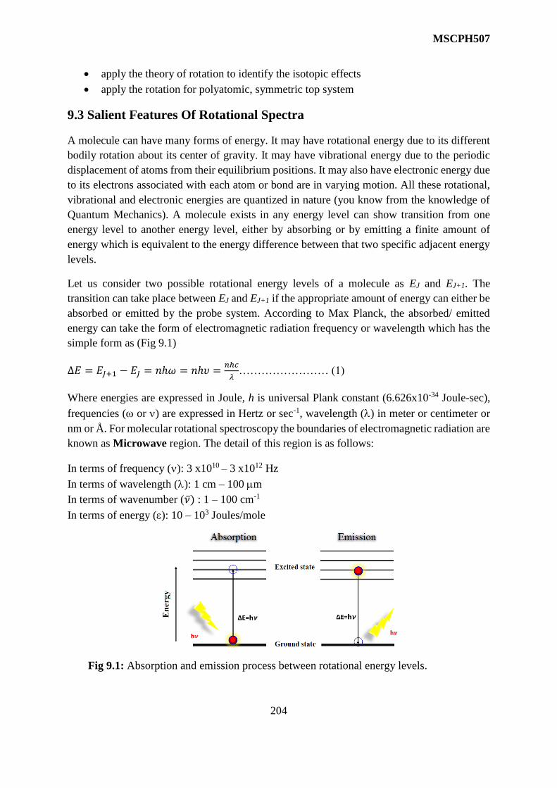
MSCPH507

204

apply the theory of rotation to identify the isotopic effects

apply the rotation for polyatomic, symmetric top system

9.3 Salient Features Of Rotational Spectra

A molecule can have many forms of energy. It may have rotational energy due to its different

bodily rotation about its center of gravity. It may have vibrational energy due to the periodic

displacement of atoms from their equilibrium positions. It may also have electronic energy due

to its electrons associated with each atom or bond are in varying motion. All these rotational,

vibrational and electronic energies are quantized in nature (you know from the knowledge of

Quantum Mechanics). A molecule exists in any energy level can show transition from one

energy level to another energy level, either by absorbing or by emitting a finite amount of

energy which is equivalent to the energy difference between that two specific adjacent energy

levels.

Let us consider two possible rotational energy levels of a molecule as EJ and EJ+1. The

transition can take place between EJ and EJ+1 if the appropriate amount of energy can either be

absorbed or emitted by the probe system. According to Max Planck, the absorbed/ emitted

energy can take the form of electromagnetic radiation frequency or wavelength which has the

simple form as (Fig 9.1)

∆𝐸 = 𝐸𝐽+1 − 𝐸𝐽 = 𝑛ℎ𝜔 = 𝑛ℎ𝜐 =𝑛ℎ𝑐

𝜆…………………… (1)

Where energies are expressed in Joule, h is universal Plank constant (6.626x10-34 Joule-sec),

frequencies ( or ) are expressed in Hertz or sec-1, wavelength () in meter or centimeter or

nm or Å. For molecular rotational spectroscopy the boundaries of electromagnetic radiation are

known as Microwave region. The detail of this region is as follows:

In terms of frequency (): 3 x1010 – 3 x1012 Hz

In terms of wavelength (): 1 cm – 100 m

In terms of wavenumber (��) : 1 – 100 cm-1

In terms of energy (): 10 – 103 Joules/mole

Fig 9.1: Absorption and emission process between rotational energy levels.

MSCPH507

205

9.3.1 Conditions for a molecule to show Rotational spectra

When the interaction of electromagnetic radiation of proper frequency with a molecule (having

rotational/vibrational/electronic energy levels) happens then different energy level transitions

may appear. The rotational energy level transitions will only appear when the incident

frequency is equivalent to the energy difference between two adjacent rotational energy levels

as described in equation 1. The molecules having a permanent dipole moment are said to be

eligible for rotational energy level transitions. So molecule with permanent dipole moment are

said to be ‘microwave active’. Usually heteronuclear molecules are generally microwave

active. Example: HCl, H2O etc. The molecules which do not have a permanent dipole moment,

doesn’t show rotational or microwave spectra and are said to be ‘microwave inactive’. Usually

homonuclear molecules are microwave inactive. Example: H2, CO2, O2 etc.

9.3.2 Dipole moment

A dipole is defined as molecules or atoms with equal and opposite electrical charges separated

by a small distance (Fig 9.2). In a molecule if one atom carries a permanent net positive charge

and other atom carries a permanent net negative charge then the molecule is said to have a

permanent electric dipole moment. Example: HCl. Hydrogen carries the positive charge and

Cl carries the negative charge. H2, CO2 have no charge separation between the atoms and so

they zero dipole moment.

Fig 9.2: Dipole creation

9.3.3 Role of dipole moment in rotational transition

Let us consider the rotation of a simple diatomic molecule AB having a dipole moment due to

its separated negative charge (A-) and positive charge (B+) densities. If we consider the pure

rotation of AB where center of gravity does not move, then with time we can observe the

positive and negative charges change their place periodically (Fig 9.3).

Fig 9.3: Rotating molecule

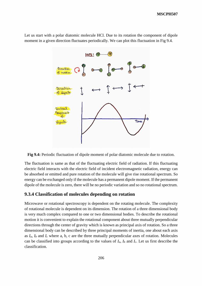
MSCPH507

206

Let us start with a polar diatomic molecule HCl. Due to its rotation the component of dipole

moment in a given direction fluctuates periodically. We can plot this fluctuation in Fig 9.4.

Fig 9.4: Periodic fluctuation of dipole moment of polar diatomic molecule due to rotation.

The fluctuation is same as that of the fluctuating electric field of radiation. If this fluctuating

electric field interacts with the electric field of incident electromagnetic radiation, energy can

be absorbed or emitted and pure rotation of the molecule will give rise rotational spectrum. So

energy can be exchanged only if the molecule has a permanent dipole moment. If the permanent

dipole of the molecule is zero, there will be no periodic variation and so no rotational spectrum.

9.3.4 Classification of molecules depending on rotation

Microwave or rotational spectroscopy is dependent on the rotating molecule. The complexity

of rotational molecule is dependent on its dimension. The rotation of a three dimensional body

is very much complex compared to one or two dimensional bodies. To describe the rotational

motion it is convenient to explain the rotational component about three mutually perpendicular

directions through the center of gravity which is known as principal axis of rotation. So a three

dimensional body can be described by three principal moments of inertia, one about each axis

as Ia, Ib and Ic where a, b, c are the three mutually perpendicular axes of rotation. Molecules

can be classified into groups according to the values of Ia, Ib and Ic. Let us first describe the

classification.

MSCPH507

207

9.3.4.1 Linear molecules

All the atoms in this type of molecules are arranged in a straight line. Example: HCl, CO2,

OCS, C2H2 etc. Here the three axes or rotation are described as (Fig 9.4a):

H-Cl

O-C-O

a) The molecular or bond axis. Let it be a axis.

b) The direction of end over end rotation in the plane of the paper passing through the

center of gravity of the molecule and perpendicular to a axis. Let it be b axis.

c) The direction of end over end rotation at right angles to the plane i.e. axis perpendicular

to both a and b axes and passing through the center of gravity of the molecule. Let it be

c axis.

As the nuclei of the atoms give the main contribution to mass and are situated in a axis, so the

moment of inertia about a axis is tentatively zero (only approximation) and so Ia=0 for linear

molecule. Again, since Ib and Ic are correspond to the end over end rotation and so they are

equal (Ib = Ic).

So for linear molecule: Ia=0 and Ib = Ic.

(Note: Moment of inertia is a measure of an object's resistance to changes in its rotation rate.

It is the rotational analog of mass. A molecule can have three different moments of inertia Ia,

Ib and Ic according to the axis of rotation.)

Fig 9.4a: Moment of inertia of linear HCl molecule.

9.3.4.2 Symmetric top type molecules

In symmetric top type molecules all the three moments of inertia are non-zero. Example:

methyl chloride (CH3Cl) where three hydrogen atoms are bonded tetrahedrally with carbon.

Here C-Cl bond axis can be considered as a axis on which the center of gravity lies. This time

Ia is not negligible since it involves the rotation of three massive hydrogen atoms of this axis.

So Ia ≠ 0. The two mutually perpendicular b and c axes lie in the plane perpendicular to a axis

and these end over end in and out rotation are remain identical. So Ib = Ic. A molecule of this

type spinning about a axis behaves like spinning top and known as symmetric top molecule.

MSCPH507

208

So for symmetric top molecule: Ia ≠ 0 and Ib = Ic.

There are two subdivisions of symmetric top molecule. They are: prolate symmetric top and

oblate symmetric top.

For prolate symmetric top molecule Ia Ib = Ic. Example: CH3Cl, CH3F.

For oblate symmetric top molecule Ia Ib = Ic. Example: BF3, BCl3 (Fig. 9.5).

Fig 9.5. Methyl chloride (CH3Cl) and Boron trifluoride (BF3)

9.3.4.3 Spherical top type molecules

The molecule in which all three moment of inertia are equal is known as spherical top.

Example: CH4, CCl4. Spherical top molecules have no dipole moment and so they are

microwave inactive (Fig. 9.6).

So for spherical top molecule: Ia = Ib = Ic.

Fig 9.6. Methane (CH4) and water (H2O)

9.3.4.4 Asymmetric top type molecules

Molecules in this category have all three moment of inertia different. Example: H2O, CH3OH,

CH2CHCl. Majority of the natural molecules belong to the category of asymmetric top. (Fig.

9.6).

So for asymmetric top molecule: Ia ≠ Ib ≠ Ic.

Till now we have discussed different categories of molecules in terms of their moment of

inertia. If we combine all then overall rotating molecules can be classified into four main groups

as (Table 1):

MSCPH507

209

Serial no Moment of Inertia Type of molecule

1. Ia=0 and Ib = Ic. Linear molecule

2. Ia ≠ 0 and Ib = Ic.

Ia Ib = Ic.

Ia Ib = Ic.

Symmetric top molecules

prolate symmetric top

oblate symmetric top

3. Ia = Ib = Ic. Spherical top molecule

4. Ia ≠ Ib ≠ Ic. Asymmetric top molecule

Table 9.1: Classification of rotating molecules in terms of moment of inertia.

Self Assessment Question (SAQ) 1: What do you mean by dipole moment? Why dipole

moment is important in molecular spectroscopy?

Self Assessment Question (SAQ) 2: Homonuclear diatomic molecules are microwave

inactive. Why? Heteronuclear diatomic molecule will show rotational spectrum or not?

Self Assessment Question (SAQ) 3: What is the main condition that a molecule will be

microwave active or not? Give some examples.

9.4 Rotational Spectra Of Diatomic Molecule

Rotational energy states arise from the rotation of the molecule as a whole. A detailed picture

of a particular molecule (bond length, force constant, bond angles) can be obtained from its

permitted rotational energy level transition or from rotational spectrum. Let us consider the

case of a simple heteronuclear diatomic molecule. The molecule can rotate as a whole about

an axis passing through the center of gravity and perpendicular to the line joining the nuclei

i.e. along internuclear axis. We will now try to investigate what type of spectrum this rotating

system will show on the basis of quantum theory and will also try to compare the computed

rotation spectrum with the experimental one.

9.4.1 Rigid rotator

We will start with the simple possible model of rotating diatomic molecule which is known as

dumbbell model as shown in Fig 9.7. Two atoms of masses m1 and m2 considered to be point

like are joined by a rigid bar (bond length) of distance R. The bar is considered as weightless.

The bond length is represented as

𝑅 = 𝑟1+ 𝑟2 ………………………………….. (2)

MSCPH507

210

Fig 9.7. Rotation of rigid diatomic molecule with two masses m1 and m2 joined by a rigid bar

of length R=r1+r2, about its center of mass or center of gravity C.

The molecule can rotate about its center of mass (C). From the definition of center of mass

𝑚1𝑟1 = 𝑚2𝑟2 ……………………………………. (3)

𝑚1𝑟1 = 𝑚2𝑟2 = 𝑚2(𝑅 − 𝑟1) from equation (2)

𝑟1(𝑚1 +𝑚2) = 𝑚2𝑅

𝑟1 =𝑚2𝑅

(𝑚1+𝑚2) 𝑎𝑛𝑑 𝑟2 =

𝑚1𝑅

(𝑚1+𝑚2) …………………. (4)

The moment of inertia of this molecule about the axis passing through center of mass C and

perpendicular to the line joining the atoms is

𝐼 = 𝑚1𝑟12 +𝑚2𝑟2

2……………………………… (5)

= 𝑚2𝑟2𝑟1 +𝑚1𝑟1𝑟2 using equation (3)

= 𝑟1𝑟2 (𝑚1 +𝑚2)………………………………. (6)

𝐼 =𝑚1 𝑚2

(𝑚1+𝑚2)𝑅2 = 𝜇𝑅2……………. (7) using equation (4)

Where we have used 𝜇 =𝑚1 𝑚2

(𝑚1 +𝑚2)⁄ as reduced mass of the system. Equation 7 defines

the moment of inertia in terms of atomic masses and the bond length. Here instead of

considering the rotation of the dumbbell we have considered the rotation of single mass at a

fixed point R from the axis of rotation. Such system is called as simple rigid rotator.

MSCPH507

211

9.4.2 Energy levels of rigid rotator

To determine the possible energy states of rigid rotator, we have to use the concept of quantum

theory. So we have to solve the Schrödinger equation in terms of amplitude of wave motion ψ

for the system having mass , potential energy V, total energy of the mass point E as:

𝜕2𝜓

𝜕𝑥2+𝜕2𝜓

𝜕𝑦2+𝜕2𝜓

𝜕𝑧2+8𝜋2𝜇

ℎ2(𝐸 − 𝑉)𝜓 = 0…………… (8)

Here we have to consider V=0 since no potential energy is associated with the rotation as long

as the rotator is considered as completely rigid. So the modified Schrödinger equation will be

𝜕2𝜓

𝜕𝑥2+𝜕2𝜓

𝜕𝑦2+𝜕2𝜓

𝜕𝑧2+8𝜋2𝜇

ℎ2𝐸𝜓 = 0………………. (9)

Where x2+y2+z2 =R2 is a constant. The solution of the above equation (consult Arther Beiser,

Modern Physics) in terms of ψ is single valued, finite and continuous occurs only for certain

values of rotational energy levels EJ namely the Eigen values as

𝐸𝐽 =ℎ2𝐽(𝐽+1)

8𝜋2𝜇𝑅2=ℎ2𝐽(𝐽+1)

8𝜋2𝐼………………………. (10)

Where J is the rotational quantum number and can take the integer values 0, 1, 2, 3……Thus

we have a series of discrete energy levels whose energy values increase quadratically with

increasing J. Equation 10 is expressed in Joules. Now to calculate the emitted or absorbed

rotational wavenumber we know that according to quantum theory the absorption of light

quantum takes place as a result of the transition of the rotator from lower (E’’) to higher (E’)

energy state, whereas the emission of a light quantum takes place as a result of a transition of

the rotator from a higher to a lower energy state. The wave number of absorbed or emitted light

quantum is (in units of cm-1) expressed as

�� =𝐸′

ℎ𝑐−𝐸′′

ℎ𝑐……………………….. (11)

Where E/hc=J is known as rotational term or energy in wavenumber (in units of cm-1) and is

expressed as

휀𝐽 =𝐸

ℎ𝑐=ℎ𝐽(𝐽+1)

8𝜋2𝑐𝐼= 𝐵𝐽(𝐽 + 1)…………. (12) where J = 0,1,2,3…….

Where the constant 𝐵 =ℎ

8𝜋2𝑐𝐼 is called as rotational constant. It is also expressed in units of

cm-1.

From equation 12 we can show the allowed energy levels (Fig 9.8a). For J=0 we have J=0

=0 and so we can say that the molecule is not rotating at all. For J=1 the energy is J=2= 2B

which is the lowest value of rotational energy. Similarly for higher values of J we get J as 6B,

12B, 20B etc. It is important to mention here that in principle there no limit to get the values

of J with increasing J values but in practice there comes a point at which the centrifugal force

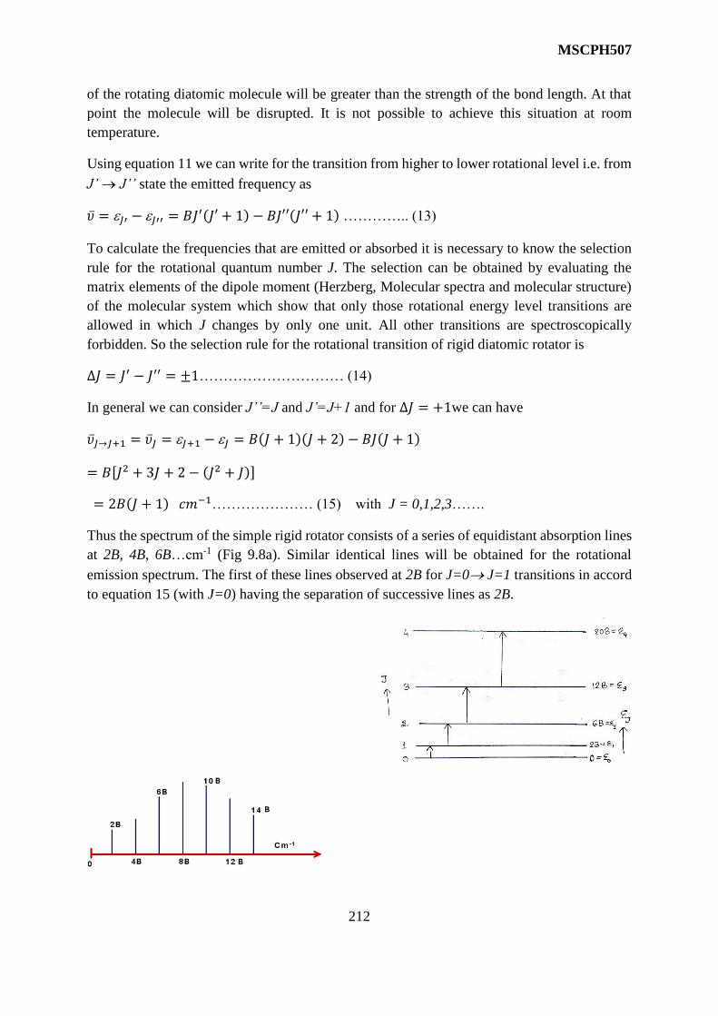
MSCPH507

212

of the rotating diatomic molecule will be greater than the strength of the bond length. At that

point the molecule will be disrupted. It is not possible to achieve this situation at room

temperature.

Using equation 11 we can write for the transition from higher to lower rotational level i.e. from

J’ J’’ state the emitted frequency as

�� = 𝐽′ − 𝐽′′ = 𝐵𝐽′(𝐽′ + 1) − 𝐵𝐽′′(𝐽′′ + 1) ………….. (13)

To calculate the frequencies that are emitted or absorbed it is necessary to know the selection

rule for the rotational quantum number J. The selection can be obtained by evaluating the

matrix elements of the dipole moment (Herzberg, Molecular spectra and molecular structure)

of the molecular system which show that only those rotational energy level transitions are

allowed in which J changes by only one unit. All other transitions are spectroscopically

forbidden. So the selection rule for the rotational transition of rigid diatomic rotator is

Δ𝐽 = 𝐽′ − 𝐽′′ = ±1………………………… (14)

In general we can consider J’’=J and J’=J+1 and for ∆𝐽 = +1we can have

��𝐽→𝐽+1 = ��𝐽 = 𝐽+1 − 𝐽 = 𝐵(𝐽 + 1)(𝐽 + 2) − 𝐵𝐽(𝐽 + 1)

= 𝐵[𝐽2 + 3𝐽 + 2 − (𝐽2 + 𝐽)]

= 2𝐵(𝐽 + 1) 𝑐𝑚−1………………… (15) with J = 0,1,2,3…….

Thus the spectrum of the simple rigid rotator consists of a series of equidistant absorption lines

at 2B, 4B, 6B…cm-1 (Fig 9.8a). Similar identical lines will be obtained for the rotational

emission spectrum. The first of these lines observed at 2B for J=0 J=1 transitions in accord

to equation 15 (with J=0) having the separation of successive lines as 2B.

MSCPH507

213

Fig 9.8a. Allowed rotational energies of a rigid diatomic molecule, their allowed transition

probabilities according to selection rule and the spectrum arise from transition.

According to equation 11 and 15 the rotational frequency can be calculated as

𝜐𝑟𝑜𝑡 = ��𝐽𝑐 = 𝑐2𝐵(𝐽 + 1) ≈ 2𝑐𝐵𝐽…………………. (16)

which is approximately equal to the frequency of the spectral line that has this rotational energy

state (J) as upper state i.e. if the rotational transition is from J-1 J.

Example 1: Experimental rotation spectrum of HCl shows the first rotational line at 21.2 cm-

1. Using this value one can easily determine the moment of inertia and hence the bond length

of HCl (Fig 9.8b).

Fig 9.8b. Experimental Rotational spectrum of HCl with separation between any two lines is

21.2 cm-1.

Here

��0→1 = 2𝐵 = 21.2 cm-1

𝐵 = 10.6 cm-1=1060m-1.Using the relation 𝐼 =

ℎ

8𝜋2𝐵𝑐 we have 𝐼𝐻𝐶𝑙 =

ℎ

8𝜋2𝐵𝑐=

2.63𝑥10−47𝑘𝑔𝑚2

𝜇 =𝑚1𝑚2

𝑚1 +𝑚2=

(1𝑔𝑚𝑜𝑙

) (35𝑔𝑚𝑜𝑙

)

(36𝑔𝑚𝑜𝑙

) (6.023𝑥1023)= 1.61𝑥10−24𝑔𝑚 = 1.61𝑥10−27𝑘𝑔

𝑅2 =ℎ

8𝜋2𝜇𝐵𝑐=

6.626𝑥10−34𝐽. 𝑠𝑒𝑐

8𝜋2(1.61𝑥10−27𝑘𝑔)(1060 m−1) (3x108𝑚

𝑠 )= 1.63𝑥10−20𝑚2

𝑅 = 1.27𝑥10−10𝑚 = 1.27Å

Wave Number in

cm-1

Rota

tional

Abso

rban

ce

MSCPH507

214

9.4.3 Intensities of rotational spectral lines

The pure rotational spectrum of a rigid diatomic molecule consists of a series of equidistant

lines corresponding to the transitions, J=0 J=1, J=1J=2, J=2J=3 and so on. To identify

the relative intensities of the different spectral lines from equation 15 and Fig 9.8a-c, we need

the knowledge of the relative probabilities of transition between rotational energy levels. The

factor that decides the intensity of lines is the number of molecules present in each energy

level. So the line intensities will be directly proportional to the initial number of molecules in

each level. The population of molecules in each level follows the Boltzmann distribution. We

know that the rotational energy at the lowest energy level has been zero since J=0 (from

equation 12), so if we have N0 molecules in this lowest energy state then the number of

molecules in any higher energy state J is given by according to Boltzmann distribution

𝑁𝐽 = 𝑁0𝑒(−𝐸𝐽

𝑘𝑇⁄ )

= 𝑁0𝑒(−𝐵𝑐ℎ𝐽(𝐽+1)

𝑘𝑇⁄ )………(17)

Where c is expressed in cm/sec, and B is in cm-1. We can easily say that NJ is varying with J.

Let us consider a typical case where B = 2 cm-1 and temperature as T= 300K. The relative

population (𝑁1

𝑁0) at J=1 can be obtained as 0.98. So we see that there are almost as many

molecules in the state J=1 at equilibrium as in the J=0 state. Again the population depends on

the degeneracy of each level, which is (2J+1) since each energy level is (2J+1) fold degenerate.

So taking degeneracy into account the total relative population at an energy EJ will be

𝑃𝑜𝑝𝑢𝑙𝑎𝑡𝑖𝑜𝑛(2𝐽 + 1)𝑒(−𝐸𝐽

𝑘𝑇⁄ )

…………….. (18)

Differentiating equation 18 shows that the population is a maximum at the nearest J value to

𝐽 = √𝑘𝑇

2ℎ𝑐𝐵−1

2……………… (19)

That is the rotational energy level to this J value will have the maximum population. So the

transition originating from the level having this J value will have the maximum intensity as

described in Fig 9.8c for HCL molecule at various temperature.

MSCPH507

215

Fig 9.8c. Relative population of HCl including degeneracy with B value as 10.6 cm-1 at two

different temperatures: 300K and 1000K.

9.4.4 Effect of Isotope

When an atom is replaced by one of its isotope, the interatomic bond distance remains the same

as the electronic charge distribution does not change duo to this substitution. The resulting

substance is identical chemically with the original. However a change in the total mass of the

system due to changes in the nuclear mass appears and hence a change in the moment of inertia

and B value of the molecular system appears. It is observed that if the atomic mass increases

due to isotopic substitution the B value decreases as B1/I.

Example 2: Two isotopes of carbon monoxide. They are 12C16O having B value 1.921cm-1 and m’C16O having B’ value 1.836 cm-1. The change in the B value reflects in the rotational energy

levels of the two isotopes as described in Fig 9.9. The spectrum of the heavier species shows a

smaller separation between the lines (2B’) than that of the lighter one (2B). For clarity the

spectrum of heavier one is shown by dashed lines. Here the heavier mass is m’. Observation of

the decreased separation of lines helps us to evaluate the precise atomic weights by using the

relation (prime refers to the heavier atom)

𝐵

𝐵′=

ℎ

8𝜋2𝐼𝑐

8𝜋2𝐼′𝑐

ℎ=𝐼′

𝐼=𝜇′

𝜇= 1.046…………….. (20)

Taking the mass of oxygen as 16 and that of 12C to be 12 we have

𝜇′

𝜇= 1.046 =

16𝑚′

16 + 𝑚′12 + 16

1216

𝑚′ = 13 which is the atomic weight of 13C.

So rotation spectroscopy can give directly an estimate of the abundance of isotopes by

comparison of absorption intensities.

Rotational quantum number J

(2𝐽+1)𝑒(−𝐸𝐽𝑘𝑇

⁄)

MSCPH507

216

Fig 9.9. The effect of isotopic substitution on the energy levels and rotational spectrum of a

diatomic molecule such as carbon monoxide. Dashed lines are for isotope.

Example2: Below is the rotational spectrum of HCl isotopes as 1H35Cl and 1H37Cl. By

identifying the wavenumber of transitions one can easily determine the atomic masses, bond

length, and relative abundance of the isotopes (Fig 9.10).

Fig 9.10. Rotational spectrum of a diatomic molecule hydrogen chloride isotopes.

Problem 1: What is the change in the rotational constant B when hydrogen is replaced by

deuterium in the hydrogen molecule?

Solution: Denoting the isotopically substituted hydrogen by prime

𝐵

𝐵′=

ℎ

8𝜋2𝐼𝑐

8𝜋2𝐼′𝑐

ℎ=𝐼′

𝐼=𝜇′

𝜇

𝜇 =𝑚𝐻

2 𝜇′ =

𝑚𝐷

2= 𝑚𝐻

𝐵

𝐵′=2𝑚𝐻

𝑚𝐻= 2, 𝐵′ =

𝐵

2

Spectral lines in cm-1

Rotational energy

Level transitions with

Selection rule ΔJ=+1

Wave Number in cm-1

Rota

tional

Abso

rban

ce

1H35Cl

1H37Cl

MSCPH507

217

So change in rotational constant: 𝐵 − 𝐵′ =𝐵

2

Problem 2: The first line (J=0J=1) in the rotational spectrum of carbon monoxide (12C16O)

has a frequency of 3.8424 cm-1. Calculate the rotational constant and the C-O bond length in

CO. Given Avogadro number is 6.023x1023 /mol.

Solution: For first line, 2B= 3.8424 cm-1. B= 1.9212 cm-1 = 192.12 m-1.

I=R2 = ℎ

8𝜋2𝐵𝑐, 𝑅2 =

ℎ

8𝜋2𝜇𝐵𝑐

So, 𝜇 =𝑚1𝑚2

𝑚1+𝑚2=

(12𝑔

𝑚𝑜𝑙)(16𝑔

𝑚𝑜𝑙)

(28𝑔

𝑚𝑜𝑙)(6.023𝑥1023)

= 1.1385𝑥10−23𝑔𝑚 = 1.1385𝑥10−26𝑘𝑔

𝑅2 =ℎ

8𝜋2𝜇𝐵𝑐=

6.626𝑥10−34𝐽. 𝑠𝑒𝑐

8𝜋2(1.1385𝑥10−26𝑘𝑔)(192.12 m−1) (3x108𝑚

𝑠 )

𝑅 = 1.131𝑥10−10𝑚 = 1.131Å

Problem 3: What is the average period of rotation of HCl molecule if it is in the J=1 state. The

internuclear distance of HCl is 0.1274nm. Given the mass of hydrogen and chlorine atoms are

1.673x10-27 kg and 58.06x10-27kg.

Solution: We have rotational energy of a classical oscillator =1

2𝐼𝜔2

Rotational energy of quantum oscillator 𝐸𝐽 =ℎ2𝐽(𝐽+1)

8𝜋2𝜇𝑅2=ℎ2𝐽(𝐽+1)

8𝜋2𝐼

Equation both the above equation we get 𝜔2 =ℎ2𝐽(𝐽+1)

4𝜋2𝐼2

Also we can write angular frequency 𝜔 =ℎ√𝐽(𝐽+1

2𝜋𝐼

I=R2 =(1.673x10−27 kg)(58.06x10−27kg)(0.1274x10−9𝑚)

2

59.733𝑥10−27𝑘𝑔=0.0264x10-45 kgm2

=ℎ√𝐽(𝐽 + 1

2𝜋𝐼=(6.626𝑥10−34𝐽. 𝑠𝑒𝑐)√2

2𝜋(0.0264x10−45𝑘𝑔𝑚2)= 56.5116𝑥1011𝑠𝑒𝑐−1 = 56.5116𝑥1011𝐻𝑧

Period of rotation 𝑇 =2𝜋

𝜔=

2𝜋

56.5116𝑥1011𝑠𝑒𝑐−1= 1.112𝑥10−12𝑠𝑒𝑐

Self Assessment Question (SAQ) 4: Which of the following molecules will show microwave

spectrum: H2, HCl, CH4, CH3Cl, CH2Cl2, H2O, SF6. Why?

Self Assessment Question (SAQ) 5: Distinguish between symmetric top (prolate and oblate),

spherical top and asymmetric top molecules. Which are suitable for microwave spectroscopy?

MSCPH507

218

Self Assessment Question (SAQ) 6: The intensity of J=0 J=1 is often not the most intense

rotational line. Why?

Self Assessment Question (SAQ) 7: Outline the effect of isotopic substitution on the rotational

spectra of molecules.

Self Assessment Question (SAQ) 8: Prove that for maximum population 𝐽 = √𝑘𝑇

2ℎ𝑐𝐵−1

2

Self Assessment Question (SAQ) 9: Choose the correct option-

(a) For linear diatomic molecule the relation of moment inertia are

(i) Ib=0 and Ia = Ic (ii) Ic=0 and Ib = Ia (iii) Ia=0 and Ib = Ic (iv) Ia≠0 and Ib = Ic

Self Assessment Question (SAQ) 10: Fill in the blank-

(i) Region of rotational spectrum in terms of wavenumber is ……….

(ii) Relation between centrifugal distortion constant and rotational constant is

……………..

(iii) Prolate type asymmetric rotator can be represented by its moment of inertia

as………..

9.5 Non rigid rotator

In rigid rotator model we have observed that the separation between the adjacent rotational

lines remain fixed as 2B. In reality it is found that the separation between the adjacent lines

decreases steadily with increasing J value. If we check the experimental and computed

rotational spectrum of hydrogen fluoride (HF) as given below in table 9.2, it is observed from

the table that as J increases, B value also decreases for the experimental spectrum. The reason

for this decreases in B may be observed if we calculate the internuclear distances from B value.

It is observed that the bond length increases with J. We can say that our assumption of existence

of rigid rotator is only an approximation. So the bond is not rigid as we assumed rather all

bonds are elastic to a certain extent. It is quite obvious that the molecule cannot be a strict, rigid

rotator when it is also able to carry out vibrations in the direction of the line joining the two

nuclei. Therefore a better model for representing the rotations of the molecule is given by the

“non rigid rotator” that is a rotating system consisting of two mass points which are not

connected by a massless rigid bar rather by a massless spring.

Rotational

transition

Bcal in cm-1 Bexp in cm-1 Bond length req in

Å

J=0 J=1 20.56 20.55 0.929

J=1 J=2 20.56 20.48 0.931

J=2 J=3 20.56 20.43 0.932

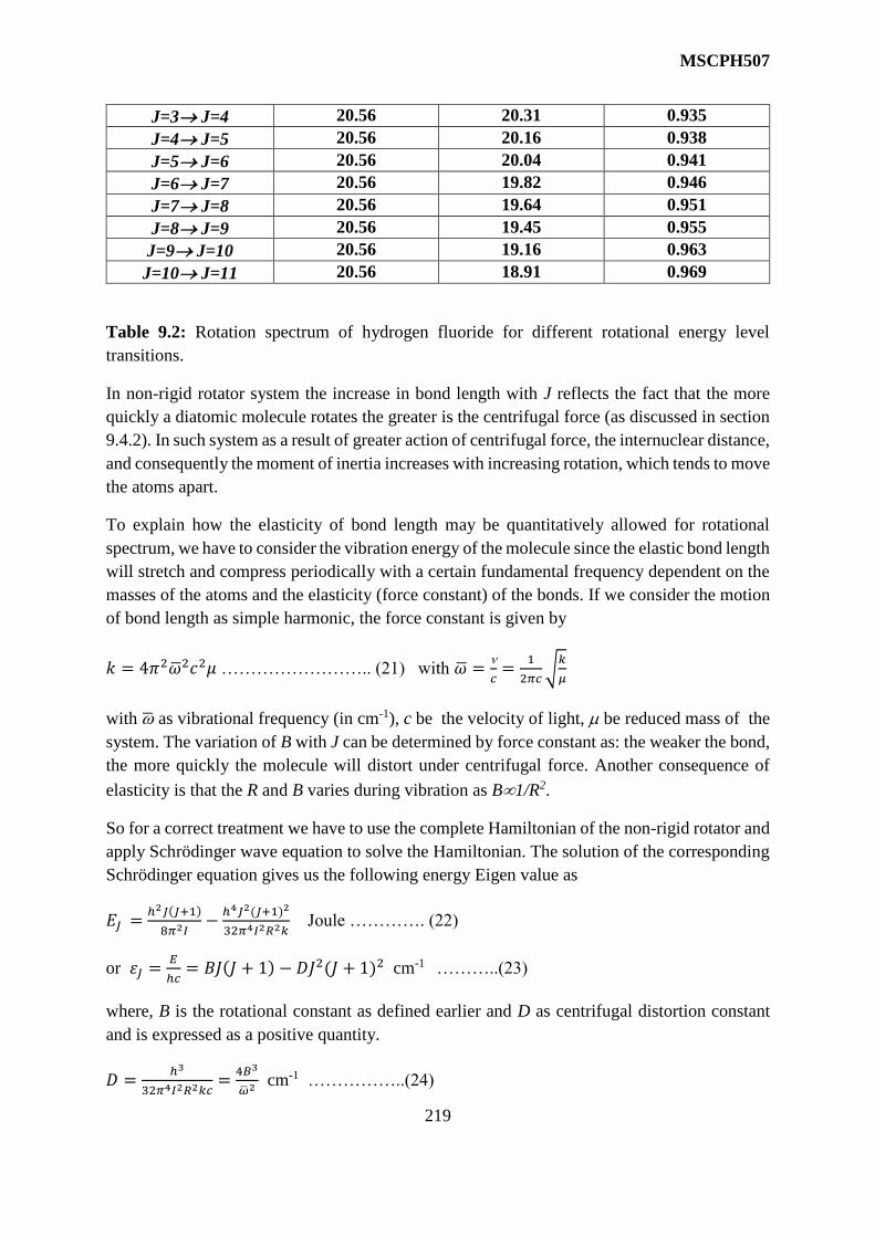
MSCPH507

219

J=3 J=4 20.56 20.31 0.935

J=4 J=5 20.56 20.16 0.938

J=5 J=6 20.56 20.04 0.941

J=6 J=7 20.56 19.82 0.946

J=7 J=8 20.56 19.64 0.951

J=8 J=9 20.56 19.45 0.955

J=9 J=10 20.56 19.16 0.963

J=10 J=11 20.56 18.91 0.969

Table 9.2: Rotation spectrum of hydrogen fluoride for different rotational energy level

transitions.

In non-rigid rotator system the increase in bond length with J reflects the fact that the more

quickly a diatomic molecule rotates the greater is the centrifugal force (as discussed in section

9.4.2). In such system as a result of greater action of centrifugal force, the internuclear distance,

and consequently the moment of inertia increases with increasing rotation, which tends to move

the atoms apart.

To explain how the elasticity of bond length may be quantitatively allowed for rotational

spectrum, we have to consider the vibration energy of the molecule since the elastic bond length

will stretch and compress periodically with a certain fundamental frequency dependent on the

masses of the atoms and the elasticity (force constant) of the bonds. If we consider the motion

of bond length as simple harmonic, the force constant is given by

𝑘 = 4𝜋2��2𝑐2𝜇 …………………….. (21) with �� =

𝑐=

1

2𝜋𝑐√𝑘

𝜇

with as vibrational frequency (in cm-1), c be the velocity of light, be reduced mass of the

system. The variation of B with J can be determined by force constant as: the weaker the bond,

the more quickly the molecule will distort under centrifugal force. Another consequence of

elasticity is that the R and B varies during vibration as B1/R2.

So for a correct treatment we have to use the complete Hamiltonian of the non-rigid rotator and

apply Schrödinger wave equation to solve the Hamiltonian. The solution of the corresponding

Schrödinger equation gives us the following energy Eigen value as

𝐸𝐽 = ℎ2𝐽(𝐽+1)

8𝜋2𝐼−ℎ4𝐽2(𝐽+1)2

32𝜋4𝐼2𝑅2𝑘 Joule …………. (22)

or 휀𝐽 =𝐸

ℎ𝑐= 𝐵𝐽(𝐽 + 1) − 𝐷𝐽2(𝐽 + 1)2 cm-1 ………..(23)

where, B is the rotational constant as defined earlier and D as centrifugal distortion constant

and is expressed as a positive quantity.

𝐷 =ℎ3

32𝜋4𝐼2𝑅2𝑘𝑐=4𝐵3

��2 cm-1 ……………..(24)

MSCPH507

220

The above equation 23 is only applied for the simple harmonic force field. If the force field is

anharmonic the expression will become

휀𝐽 =𝐸

ℎ𝑐= 𝐵𝐽(𝐽 + 1) − 𝐷𝐽2(𝐽 + 1)2 + 𝐻𝐽3(𝐽 + 1)3 +⋯ cm-1 …………… (25)

From equation 24 it is evident that centrifugal distortion effect is greatest for molecules with

smaller moment of inertia and small force constants. In a given molecule, the effect of D is to

decrease the rotational energy (equation 23) which increases rapidly for higher rotational states.

It is only in very rare cases the experimental data consider the introduction of the term H.

The selection rule for the non-rigid rotator is again Δ𝐽 = ±1. So the frequency of transition for

J=1J=J+1 is given by (only considering up to D term)

��𝐽→𝐽+1 = 𝐽+1 − 𝐽

= 𝐵[(𝐽 + 1)(𝐽 + 2) − 𝐽(𝐽 + 1)] − 𝐷[(𝐽 + 1)2(𝐽 + 2)2 − 𝐽2(𝐽 + 1)2]

= 2𝐵(𝐽 + 1) − 4𝐷(𝐽 + 1)3 cm-1 ………………(26) with J=0,1,2,3……

The first term in equation 26 is the same as that of rigid rotator. The additional term gives the

shift of the lines of the spectrum of a rigid molecule which increase with J as (J+1)3. Fig 9.11

gives the schematic representation of the energy levels and the spectrum of non-rigid rotator as

well as rigid rotator. We can see that the rotational spectrum of non-rigid rotator is similar to

that of rigid rotator expect each line is displaced slightly to low frequency. The knowledge of

D allows us to determine the J value of the lines in an observed spectrum. Also the D value

helps us to determine the vibrational frequency of the diatomic molecule.

Fig 9.11. Representation of the energy levels and spectrum of rigid and non-rigid diatomic

rotator.

Rigid Rotator

휀𝐽 = 𝐵𝐽(𝐽 + 1)

Non Rigid Rotator

휀𝐽 = 𝐵𝐽(𝐽 + 1) − 𝐷𝐽2(𝐽 + 1)2

0 2B 4B 6B 8B 10B

cm-1

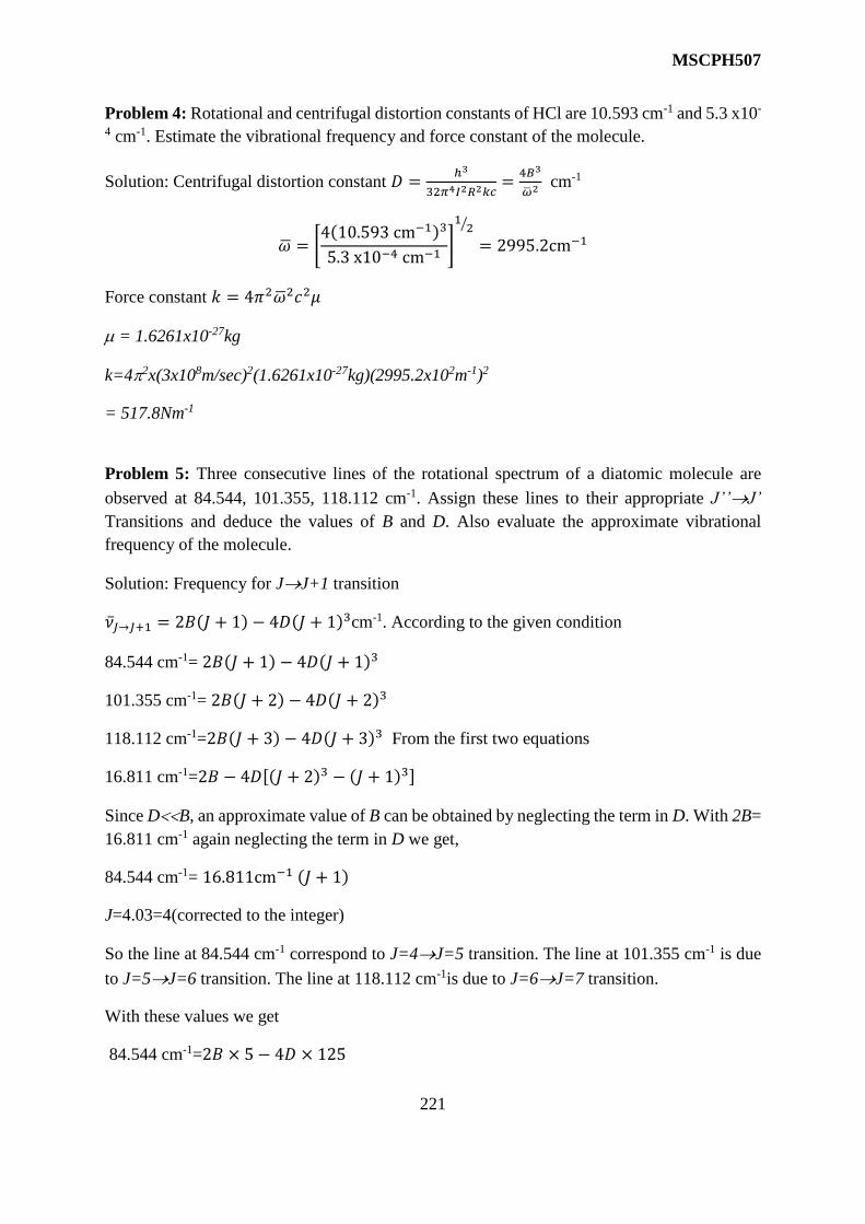
MSCPH507

221

Problem 4: Rotational and centrifugal distortion constants of HCl are 10.593 cm-1 and 5.3 x10-

4 cm-1. Estimate the vibrational frequency and force constant of the molecule.

Solution: Centrifugal distortion constant 𝐷 =ℎ3


��2 cm-1

�� = [4(10.593 cm−1)3

5.3 x10−4 cm−1]

12⁄

= 2995.2cm−1

Force constant 𝑘 = 4𝜋2��2𝑐2𝜇

= 1.6261x10-27kg

k=42x(3x108m/sec)2(1.6261x10-27kg)(2995.2x102m-1)2

= 517.8Nm-1

Problem 5: Three consecutive lines of the rotational spectrum of a diatomic molecule are

observed at 84.544, 101.355, 118.112 cm-1. Assign these lines to their appropriate J’’J’

Transitions and deduce the values of B and D. Also evaluate the approximate vibrational

frequency of the molecule.

Solution: Frequency for JJ+1 transition

��𝐽→𝐽+1 = 2𝐵(𝐽 + 1) − 4𝐷(𝐽 + 1)3cm-1. According to the given condition

84.544 cm-1= 2𝐵(𝐽 + 1) − 4𝐷(𝐽 + 1)3

101.355 cm-1= 2𝐵(𝐽 + 2) − 4𝐷(𝐽 + 2)3

118.112 cm-1=2𝐵(𝐽 + 3) − 4𝐷(𝐽 + 3)3 From the first two equations

16.811 cm-1=2𝐵 − 4𝐷[(𝐽 + 2)3 − (𝐽 + 1)3]

Since DB, an approximate value of B can be obtained by neglecting the term in D. With 2B=

16.811 cm-1 again neglecting the term in D we get,

84.544 cm-1= 16.811cm−1 (𝐽 + 1)

J=4.03=4(corrected to the integer)

So the line at 84.544 cm-1 correspond to J=4J=5 transition. The line at 101.355 cm-1 is due

to J=5J=6 transition. The line at 118.112 cm-1is due to J=6J=7 transition.

With these values we get

84.544 cm-1=2𝐵 × 5 − 4𝐷 × 125

MSCPH507

222

101.355 cm-1=2𝐵 × 6 − 4𝐷 × 216 . Solving these two equations we get

B= 8.473 cm-1 and D=3.7x10-4 cm-1. Again by using the relation 𝐷 =ℎ3


��2

We can calculate �� = 2564.4cm−1.

Self Assessment Question (SAQ) 11: What is centrifugal distortion? Explain the effect of

centrifugal distortion on the moment of inertia and energy of a diatomic molecule. How

centrifugal distortion can help to determine the force constant of a bond?

Self Assessment Question (SAQ) 12: The observed rotational spectrum of HF shows decrease

in the line separation on the high frequency side. Why?

Self Assessment Question (SAQ) 13: Find the frequencies of the J=1J=2 and J=2J=3

rotational absorption lines in NO, who’s molecules have the moment of inertia 1.65x10-46 kg

m2.

Self Assessment Question (SAQ) 14: Calculate the energies of the four lowest non zero

rotational energy levels of the H2 and D2 molecules where D represents deuterium atom H21.

9.6 Linear Polyatomic Molecules

Linear polyatomic molecules can also be treated similar to the diatomic molecules since Ia=0

and Ib = Ic. Similarly the energy levels EJ are given by the same formula identical to that of the

diatomic molecules as

��𝐽→𝐽+1 = 𝐽+1 − 𝐽 = 2𝐵(𝐽 + 1) − 4𝐷(𝐽 + 1)3 cm-1 with J=0,1,2,3……

Spectrum will show the same 2B separation modified by the distortion constant. So the whole

theory of diatomic molecules are equally applicable to all linear molecules. However there are

some points are needed to be understand. They are:

1. The moment of inertia for end over end rotation of the polyatomic linear molecule is

considerably greater than that of the diatomic molecule, The B value will be much

smaller. Usually for diatomic molecules B value are observed to be 10 cm-1 while for

linear triatomic molecule B value is observed as tentatively around 1 cm-1 or less. So

for larger linear molecules it will be smaller more. As a result of this the spectral lines

are observed to be more closely spaced.

2. The molecule should have a permanent dipole moment to be microwave active.

Example: OCS molecule is microwave active, whereas OCO or CO2 is not. Also

isotopic substitution does not lead to microwave activity.

3. A noncyclic polyatomic linear molecule having N atoms contains N-1 individual bond

lengths. So in a triatomic molecule like OCS, there we have two bond length as rCO and

rCS. The molecule has only one moment of inertia for the end over end rotation of OCS.

So only one value can be determined from the microwave spectrum of OCS. If we study

the spectra OCS molecule for different transitions we will observe there is no existence

MSCPH507

223

of centrifugal distortion and so B remains constant at 0.2027 cm-1. And the moment of

inertia comes out to be as Ib=137.95 x10-47 kg m2. From this observation, it is impossible

to deduce the values of the bond lengths rCO and rCS. To overcome this problem if we

study the molecule with different atomic masses, but with the same bond lengths then

we may get the value of different moment of inertia.

Let us consider the rotation of OCS where rO, rC, rS represent the distances of the atoms from

the center of gravity having corresponding masses as mO, mC, mS (Fig-9.12).

Fig 9.12. Linear polyatomic molecule carbon oxysulphide (OCS) showing the distances of each

atom (ro, rc, rs) from center of gravity.

Following the figure moments of OCS will be given by

mOrO+mCrC =mSrS ……………………(27)

The moment of inertia will be

𝐼 = 𝑚𝑂𝑟𝑂2 +𝑚𝐶𝑟𝐶

2 +𝑚𝑆𝑟𝑆2………………. (28)

Again we have rO=rCO+rC rS=rCS-rC ……….(29)

Substituting equation 29 into equation 27 we get

(𝑚𝐶 +𝑚𝑂 +𝑚𝑆)𝑟𝑆 = 𝑚𝑆𝑟𝐶𝑆 −𝑚𝑂𝑟𝐶𝑂…………………. (30)

𝑀𝑟𝑆 = 𝑚𝑆𝑟𝐶𝑆 −𝑚𝑂𝑟𝐶𝑂……………………………. (31)

Where M is the total mass of the molecule. Now substituting equation 29 to equation 28 we get

𝐼 = 𝑚𝑂(𝑟𝐶𝑂 + 𝑟𝐶)2 +𝑚𝐶𝑟𝐶

2 +𝑚𝑆(𝑟𝐶𝑆 − 𝑟𝐶)2

= 𝑀𝑟𝐶2 + 2𝑟𝐶(𝑚𝑂𝑟𝐶𝑂 −𝑚𝑆𝑟𝐶𝑆) + 𝑚𝑂𝑟𝐶𝑂

2 +𝑚𝑆𝑟𝐶𝑆2

Substituting for rC from equation 31 we get

MSCPH507

224

𝐼 = 𝑚𝑂𝑟𝐶𝑂2 +𝑚𝑆𝑟𝐶𝑆

2 −(𝑚𝑂𝑟𝐶𝑂−𝑚𝑆𝑟𝐶𝑆)

2

𝑀…………………. (32)

If we consider the isotope of 16OCS as 18OCS then for mass of isotope of oxygen we may write

mO’ for mO and by applying it in the equation 32 we will get the moment of inertia of the 18OCS

as

𝐼′ = 𝑚′𝑂𝑟𝐶𝑂2 +𝑚𝑆𝑟𝐶𝑆

2 −(𝑚′𝑂𝑟𝐶𝑂−𝑚𝑆𝑟𝐶𝑆)

2

𝑀′……………….. (33)

The analysis of the spectra of the parent 16OCS and isotope 18OCS molecules give I and I’ from

which the two unknown bond lengths rCO and rCS can be evaluated form the spectrum of the

isotope. Point to be noted here that for isotopic substitution we have considered the bond length

remains unaltered.

Self Assessment Question (SAQ) 15: The rotational constant for 12H14CN and 12D14CN are

1.4782 and 1.2077 cm-1. Calculate the moments of inertia of these molecules and the

internuclear distances of C-H and CN bonds.

9.7 Symmetric Top Molecules

Rotational energy levels of this type of molecules are more complicated than a linear molecule

but due to the symmetry, the pure rotational spectra of symmetric top molecules are relatively

simple. The condition for symmetric top molecule: Ia ≠ 0 and Ib = Ic .There are two directions

of rotation in which the molecule might absorb or emit energy. They are one about the main

symmetry axis and another one is perpendicular to this axis. As mentioned earlier, for the

molecule CH3Cl the main axis is C-Cl bond axis. So we need two quantum numbers (K and J)

to describe the degree of rotation one for Ia and the other for Ib or Ic. The condition for the

quantum number K is that it cannot be greater than J. K can be negative, so we can imagine

positive and negative values of K to correspond with clockwise and anticlockwise rotation

about the symmetry axis. In general K can take the values:

K= J, J-1, J-2,……..0,…….,-(J-1), -J …………….(34)

If we take the case of a rigid symmetric top molecule with no centrifugal distortion effect, the

Schrödinger equation may be solved to give the allowed energy levels for rotation as

휀𝐽,𝐾 =𝐸𝐽,𝐾

ℎ𝑐= 𝐵𝐽(𝐽 + 1) + (𝐴 − 𝐵)𝐾2 cm-1 …………(35)

Where 𝐵 =ℎ

8𝜋2𝑐𝐼𝐵 and 𝐴 =

ℎ

8𝜋2𝑐𝐼𝐴

The selection rule for the energy transitions are ∆𝐽 = +1 and ∆𝐾 = 0

If we apply the selection rule in equation 35 the frequency of transition will be

��𝐽,𝐾→𝐽+1,𝐾 = 𝐽+1,𝐾 − 𝐽,𝐾 = 𝐵[(𝐽 + 1)(𝐽 + 2) + (𝐴 − 𝐵)𝐾2 − [𝐵𝐽(𝐽 + 1) + (𝐴 − 𝐵)𝐾2]

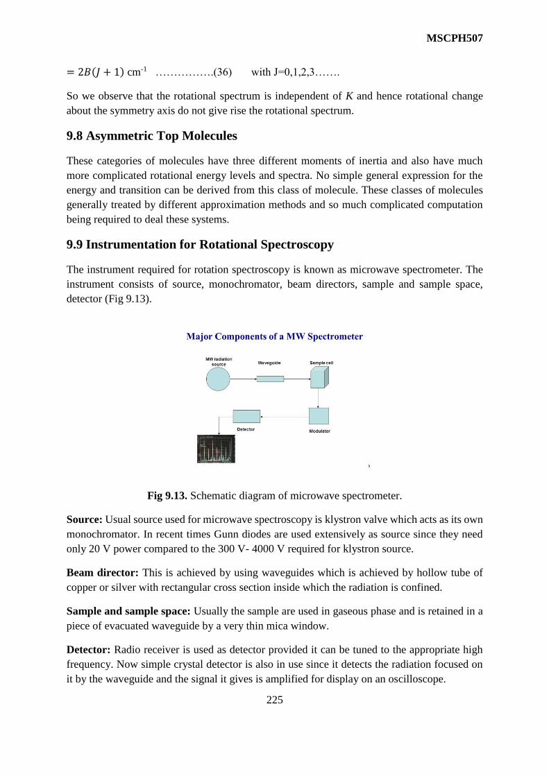
MSCPH507

225

= 2𝐵(𝐽 + 1) cm-1 …………….(36) with J=0,1,2,3…….

So we observe that the rotational spectrum is independent of K and hence rotational change

about the symmetry axis do not give rise the rotational spectrum.

9.8 Asymmetric Top Molecules

These categories of molecules have three different moments of inertia and also have much

more complicated rotational energy levels and spectra. No simple general expression for the

energy and transition can be derived from this class of molecule. These classes of molecules

generally treated by different approximation methods and so much complicated computation

being required to deal these systems.

9.9 Instrumentation for Rotational Spectroscopy

The instrument required for rotation spectroscopy is known as microwave spectrometer. The

instrument consists of source, monochromator, beam directors, sample and sample space,

detector (Fig 9.13).

Fig 9.13. Schematic diagram of microwave spectrometer.

Source: Usual source used for microwave spectroscopy is klystron valve which acts as its own

monochromator. In recent times Gunn diodes are used extensively as source since they need

only 20 V power compared to the 300 V- 4000 V required for klystron source.

Beam director: This is achieved by using waveguides which is achieved by hollow tube of

copper or silver with rectangular cross section inside which the radiation is confined.

Sample and sample space: Usually the sample are used in gaseous phase and is retained in a

piece of evacuated waveguide by a very thin mica window.

Detector: Radio receiver is used as detector provided it can be tuned to the appropriate high

frequency. Now simple crystal detector is also in use since it detects the radiation focused on

it by the waveguide and the signal it gives is amplified for display on an oscilloscope.

MSCPH507

226

9.10 Applications of Rotational Spectroscopy

Molecular structure: A whole molecular structure can be examined by rotational

spectroscopy. Rotational constant can be obtained with a very high accuracy. Moment of inertia

can be determined. The rotational spectroscopy can readily distinguish the presence of isotopes

in a sample and can even detect the presence of different conformational isomers provided they

have a different moment of inertia.

Dipole moment and nature of bond: Precise determination of electric dipole moment is

possible from microwave spectroscopy by measurement of the Stark Effect (not discussed yet).

Dipole moment can also throw light on the nature of the molecular bond present in the sample.

Chemical examination of interstellar space: Microwave spectroscopy has extended the

analysis to the detection of simple stable molecules in space. Some 100 or molecules have been

already been characterized by this process. Some of them are existence of water, ammonia and

formaldehyde. Such observations are done by comparing the relative intensities of various

rotational transitions of samples like ammonia which helps us to estimate the temperature of

the interstellar material.

Microwave oven: Microwave oven is one of the major application areas of rotational

spectroscopy for today’s industry especially in the kitchen. Its mode of operation depends upon

the absorption of the microwave radiation by the food in which it is bathed. Water molecule is

the basic requirement of the microwave oven to operate. Water molecules present in food only

absorb the microwave radiation and are raised to the higher rotational levels. The food

molecules which are mainly biological in nature are too large in size to be able to rotate so they

do not take part in rotational level transitions. With the presence of many rotational excited

states, after absorption the excess rotational energies of the water molecules are re emitted as

heat which is used to cook the food. In conventional oven, food is heated from outside and it

is used till its food center has been raised to sufficiently high temperature which is time

consuming process. For microwave heating, water molecules throughout the whole bulk food

are excited and used to heat and cook the food. This is the reason why cooking time in

microwave oven is lesser than normal oven.

It is essential to ensure that the door of microwave oven should be properly sealed under

working so that no radiation is allowed to leak out.

Self Assessment Question (SAQ) 16: Microwave communication systems operate over long

distances in the atmosphere. The same is true for radar which locates objects such as ships,

aircrafts by microwave pulses they reflect. The region of molecular rotational spectra is

microwave region of em radiation. Can you comment on why atmospheric gases do not absorb

microwaves to any great extent?

MSCPH507

227

Self Assessment Question (SAQ) 17: Microwave oven cannot be used to boil egg or to cook

dry food. Why?

Self Assessment Question (SAQ) 18: A space probe was designed to seek CO in the

atmosphere of Saturn by looking for lines in its rotational spectrum. If the bond length of CO

is112.8 pm, at what wavenumber do the first three rotational transitions appear? What

resolution would be needed to determine the isotopic ratio of 13C to 12C on Saturn by observing

the first three 13CO rotational lines as well? How could the experiment be extended to estimate

the temperature of Saturn’s atmosphere?

9.11 Summary

In this unit, you have studied about rotational spectroscopy. To present the clear understanding

of rotational motion, some basic definitions like dipole moment, moment of inertia, energy,

energy transition have been discussed. You have studied about the requirements of specific

molecules to show rotational spectra. You have discussed about different categories of

molecules like linear, symmetric top, asymmetric top in terms of their moment of inertia. You

have also studied about the theories of rotational spectroscopy in detail for different linear

molecular systems like diatomic rigid rotator, diatomic non-rigid rotator, polyatomic linear

molecules, etc. You have also studied about the isotopic effect on the pure rotational spectra.

In the unit, you have seen the characteristics of rotational spectra for symmetric and asymmetric

top molecules. You have also studied the detailed instrumentation and techniques used to do

rotational spectroscopy. You have been informed about different application areas of the use

of rotational spectroscopy for the industry starting from your kitchen to interstellar space. Many

solved examples are given in the unit to make the concepts clear. To check your progress, self

assessment questions (SAQs) are given place to place.

9.12 Glossary

Spectroscopy – the study of the interaction between matter and electromagnetic radiation

Dipole moment- A dipole moment is the product of the magnitude of the charge and the distance

between the centers of the positive and negative charges.

Moment of inertia- A quantity expressing a body's tendency to resist angular acceleration,

which is the sum of the products of the mass of each particle in the body with the square of its

distance from the axis of rotation.

9.13 References

1. Modern Aspects of Microwave Spectroscopy, G.W. Chanty; Academic Press 1979.

2. Fundamental of Molecular Spectroscopy, C.N. Banwell, E.M. McCash; Tata Mc Graw Hill.

3. Microwave Molecular Spectra (Vol 9) , W. Gordy, R. L. Cook; John Wiley 1970.

MSCPH507

228

4. Molecular Spectra and Molecular Structure (I, II), G. Herzberg; D. Van Nostrand Comp.

Inc, Princceton.

5. Molecular Structure and Sepctroscopy, G. Aruldas, PHI Learning Pvt Ltd, 2011.





(Should be divided into Short Answer type, Long Answer type, Numerical, Objective type)

9.15.1 Short Answer type

1. How microwave oven works?

2. How many revolution per second does a CO molecule make when J=3? The CO bond length

is 0.1131 nm.

3. Show that a substantial number of molecules of a gas are in excited rotational states at

temperature 300K.

4. Mention the difference between rotational and vibrational spectra.

9.15.2 Long Answer type

1. Explain different types of rotator molecules in terms of their moment of inertia

2. Derive the rotational energy value for a diatomic rigid rotator by using the quantum

mechanical model. Identify the transition frequency value for two rotational level

transition.

3. Why the concept of non-rigid rotator is needed? What correction do you need to explain

non-rigid rotator and why?

4. The energy levels of a rigid symmetric top molecule are given by

휀𝐽,𝐾 =𝐸𝐽,𝐾

ℎ𝑐= 𝐵𝐽(𝐽 + 1) + (𝐴 − 𝐵)𝐾2 cm-1 .What are A, B, J, and K. State the selection rules

for

allowed transitions.

5. Write notes on-

(i) Dipole moment (ii) Microwave oven (iii) Isotopic effect on rotational spectroscopy

MSCPH507

229

9.15.2 Numerical type

1. Let the number of molecules in the first excited state are 98% of the number of

molecules in the ground state at 23 ºC. Can one estimate the value of Rotational constant

(B)?

2. Calculate the ratio of the number of molecules (NJ ) in the rotational state J=5 to J=0

in a

Sample of HI at 300K. Use the moment of inertia of the HI molecule 4.31x10-47kg m2.

3. Estimate the frequencies of the J = 1 J = 2 and J = 2 J = 3 rotational absorption

lines in NO, whose molecules have the moment of inertia 1.65 x 10-46 kg.m2.

4. The rotational constant for H12C14N and D12C14N are 1.4782 and 1.2077 cm-1

respectively. Calculate the moments of inertia of each molecule and bond lengths of C-

H, C-D and C N .Given the mass mH=1.008 amu, mD=2.014, mC=12 amu, mN=14.003

amu.

5. Consider a diatomic molecule as non – rigid rotator with rotational constant B=10.5

cm-1 and distortion constant D=5.0x10-4cm-1. Obtain vibrational frequency, and force

constant of the molecule. Consider reduced mass of the molecule as 1.6x10-27Kg.

6. Three consecutive lines in microwave spectra are observed at 82.19 cm-1, 123.15cm-1,

and 164 cm-1. Obtain the value of the rotational constant and assign the J values between

which the transition occurs for rotational line at 164 cm-1.

7. Rotational and distortion constants of HCl molecule are 10.593 cm-1 and 5.3x10-4

respectively. If the force constant is 517.8 Nm-1 and vibrational frequency is 2995.2

x102 m-1. Using these data can we obtain the reduced mass of the molecule? If yes, then

find its value.

8. For ClF molecule, the bond length is 0.1630 nm and the centrifugal distortion is 10-4B,

where B is the rotational constant. Calculate the spacing between first four lines. Use

atomic mass mCl= 35.45 amu and mF= 19 amu.

MSCPH507

230

UNIT 10 VIBRATIONAL SPECTRA

Structure

10.1 Introduction

10.2 Objectives

10.3 Salient features of vibrational spectra

10.4 Vibrations of various molecular structures

10.4.1 Vibration of diatomic molecule

10.4.2 The harmonic oscillator

10.4.2.1 Energy levels of harmonic oscillator

10.4.2.2 Spectrum of harmonic oscillator

10.4.3 The anharmonic oscillator

10.4.3.1 Spectrum of anharmonic oscillator

10.5 Diatomic vibrating rotator

10.5.1 The fine structure of vibrating rotator spectrum

10.6 Vibrations of polyatomic molecule 10.6.1 Fundamental vibrations for H2O

10.6.2 Fundamental vibrations for CO2

10.7 Isotope Effect

10.8 Instrumentation for Vibrational Spectroscoy

10.9 Applications for Vibrational Spectroscoy

10.9.1 Identification of molecular constituents

10.9.1.1 Skeletal vibrations

10.9.1.2 Group vibrations

10.9.2 Identification of molecular structure

10.9.3 Characterization of transition phases of Ceramic material

10.9.4 Characterization of Biological material

10.10 Summery

10.11 Glossary

10.12 References


10.14 Solved Problems

10.15 Self Assignment Questions


10.16.1 Short Answer type Questions

10.16.2 Long Answer type Questions

10.16.3 Numerical and objective type Questions

MSCPH507

231

10.1 Introduction

The atoms in a molecule do not remain in a fixed relative position, but vibrate about some mean

position. A molecule may have many different modes of vibration. When sufficiently excited,

a molecule can vibrate as well as it can rotate. So the vibrations of its atoms with respect to

each other has an energy level spacing as we have already observed the rotational energy levels

of molecules due to rotation of the atoms with respect to center of gravity. Transitions between

these vibrational levels result vibrational spectra which give an insight into the discrete motion

of the atoms in the molecular system. Vibrational frequencies of the molecule also help us to

get valuable information regarding molecular structure, symmetry, bond length, inter and

intramolecular interaction etc.

10.2 Objective

After studying this unit, you should be able to-

define vibrational motion of atoms in molecule

study the effect of vibrational motion on diatomic harmonic oscillator, anharmonic

oscillator

study the effects of vibration and rotation on molecule

apply the laws vibrational spectroscopy for identifying different modes of normal

vibrations in linear and nonlinear molecules

apply the concept of vibrational spectroscopy to different infrared spectra of complex

molecules

learn to apply the knowledge of vibrational spectroscopy for different industrial

applications

10.3 Slient Features Of Vibrational Spectra

For vibrational spectroscopy to be observed it is the vibration between atoms rather than

rotation is important. The vibration gives rise to a change in dipole moment in the molecular

system which results transitions between vibrational energy levels and give rise vibrational

spectra. Vibrational energy states are separated by an energy interval of 104 Joule/mole. The

molecular spectra arise from the transition between two vibrational energy states are observed

in the infrared region of the electromagnetic spectrum with a wavelength range from 100 m

to 1 m. Vibrational spectroscopy also known as infrared spectroscopy also. Let us discuss the

vibrational spectra due to the change in dipole moment with an example. Consider linear carbon

dioxide (CO2) molecule. In CO2, three atoms are arranged linearly with a small net positive

charge on the carbon atom (2+) and small negative charges on the oxygen atoms (-) (Fig

10.1). If we consider the possibility of vibration, it can happen between two CO bonds.

MSCPH507

232

Fig10.1 Charge distribution in CO2.

During the period of vibration between the atoms in CO2 molecule as a whole, alternately

stretching and compression of the CO bonds happens simultaneously with respect to its center

of gravity at C. For the symmetric stretching condition, both the C-O bonds on both sides of a

central carbon atom stretched and compressed in equal amount with respect to C and so the

resultant dipole moment remains zero throughout the whole vibration process (Fig 10.2). Since

there is no change dipole moment is observed during “symmetric stretch”, the particular

vibration due to symmetric stretching mode is ‘infrared inactive’.

Fig10.2 Symmetric stretching vibration of CO2 in terms of stretched and compressed mode

with respect to center.

For antisymmetric stretching mode the amount of stretching or compression of both bonds are

not equal and simultaneous. At the same time one bond stretches while the other is compressed

or vice versa (Fig 10.3). As a result of this asymmetric stretching or compression, the total

change in dipole moment for the whole CO2 molecule shows a periodic alteration. Since a

change in dipole moment exists for asymmetric stretching mode, the vibrations is thus ‘infrared

active’.

Fig10.3 Asymmetric stretching vibration of CO2 in terms of stretched and compressed mode

with respect to normal.

2

Vertical Component

of Dipole

Dipole

Moment

Asymmetric

Stretching

S

Time

MSCPH507

233

Another vibrational mode exists for this linear molecule which is bending mode. For bending

mode also CO2 shows change in dipole moment and so this mode also acts as ‘infrared active’

mode (Fig 10.4). We have to keep one point in mind that in neither of these vibrational motions

does the center of gravity move. So change in dipole moment is the main requirement for the

molecule to show vibrational or infrared spectroscopy. Homonuclear diatomic molecule has no

change in dipole moment and so they are infrared inactive.

For molecular vibrational spectroscopy the boundaries of electromagnetic spectrum is known

as Infrared region. The detail of this region is as follows:

In terms of frequency (): 3 x1012 – 3 x1014 Hz

In terms of wavelength (): 100 m – 1 m

In terms of wavenumber () : 100 – 104 cm-1

In terms of energy (): 103 – 105 Joules/mole

Fig10.4 Bending vibration of CO2 and associated change in dipole moment with respect to

normal.

10.4 Vibration Of Various Molecular Structures

10.4.1 Vibration of diatomic molecule

The simplest step to consider the possible assumption about the form of different vibrations is

diatomic molecule. Let us start with the stable configuration of molecule. Two atoms in a

stable diatomic molecule settle at an equilibrium internuclear distance (req) when the balancing

for attractive and repulsive forces appears between them. The repulsive force appears due to

the repulsion between the positively charged nuclei of both atoms and between their negative

electron clouds. The attractive force appears between the nucleus of one atom and electrons of

MSCPH507

234

the other. So squeezing the atoms more from their equilibrium position will generate repulsive

force to rise rapidly, similarly pulling apart them will be resisted by the generation of attractive

force. The restoring force exerted by the two atoms of the molecule on each other when they

are displaced from their equilibrium position (req) which is proportional to the change of the

internuclear distance (r). The compression and extension of the bond length may follow the

behavior of a spring which obeys Hook’s law as

𝑓 = −𝑘(𝑟 − 𝑟𝑒𝑞)………….. (1)

Where f is restoring force, k is the force constant, r is the distance of two atoms and req is the

mean internuclear distance or equilibrium distance.

Any attempt to disrupt req or bond length requires an input energy as potential energy as

described in equation (2) as

𝑉 =1

2𝑘(𝑟 − 𝑟𝑒𝑞)

2……….. (2)

At the energy minimum, the internuclear distance is referred as the equilibrium distance req or

equilibrium bond length which can be described by a parabolic curve (red line) as Fig 10.5. For

periodic motion each atom moves towards or away from each other so that the placement from

the equilibrium position is the sine function of time. Such a motion of the two atoms can be

reduced to the simple harmonic vibration of the single mass point about the equilibrium

position. Such model is known as harmonic oscillator.

Fig10.5 Variation of Potential energy curve of diatomic molecule.

MSCPH507

235

10.4.2 The harmonic oscillator

According to classical mechanics, a harmonic oscillator is defined as the mass point as mass

(m) on which an acted force (f) is proportional to the distance (x) from the equilibrium position

and is directed toward the equilibrium position. As force = mass x acceleration, so we may say

𝑓 = −𝑘𝑥 = 𝑚𝑑2𝑥

𝑑𝑡2……….. (3)

where k is the force constant. The solution of the differential equation 3 is well-known to us

and can be expressed as

𝑥 = 𝑥0𝑠𝑖𝑛(2𝜋𝜈𝑜𝑠𝑐𝑡 + 𝜑)…….. (4)

where x0 is the amplitude of vibration and is the phase constant dependent on the initial

conditions. The vibrational frequency 𝜔𝑜𝑠𝑐 is given by equations 5a and 5b as

𝜔𝑜𝑠𝑐 =1

2𝜋√𝑘

𝑚 𝑖𝑛 𝐻𝑧……………….. (5a)

��𝑜𝑠𝑐 =1

2𝜋𝑐√𝑘

𝑚 𝑖𝑛 𝑐𝑚−1………………. (5b)

Since force is negative derivative of potential energy V so we may express equation 2 as

𝑉 =1

2𝑘𝑥2 = 2𝜋2𝑚𝜔𝑜𝑠𝑐

2𝑥2………….. (6)

This equation justifies the parabola nature (red line) of the potential energy curve in Fig 10.5.

Again we know that for diatomic molecule the restoring force is applied by the atoms on each

other when they are forcefully displaced from their equilibrium position and the force is

proportional to the change of req. If we assume that this relation hold good for diatomic

molecule then for mass m1 and m2 with their distances from r1 and r2 from the center of gravity

(Fig 9.7 of unit 9), we can express the relations as

𝑚1𝑑2𝑟1𝑑𝑡2

= −𝑘(𝑟 − 𝑟𝑒𝑞)

𝑚2𝑑2𝑟2

𝑑𝑡2= −𝑘(𝑟 − 𝑟𝑒𝑞)

where r is the distance of two atoms and req=R is the mean internuclear distance or equilibrium

distance. We can combine both the above equations as (by using equation 4 of unit 9)

𝑚1 𝑚2

(𝑚1 +𝑚2)

𝑑2(𝑟 − 𝑟𝑒𝑞)

𝑑𝑡2= −𝑘(𝑟 − 𝑟𝑒𝑞) 𝑠𝑖𝑛𝑐𝑒 𝑟𝑒𝑞 𝑖𝑠 𝑐𝑜𝑛𝑠𝑡𝑎𝑛𝑡.

𝜇𝑑2(𝑟 − 𝑟𝑒𝑞)

𝑑𝑡2= −𝑘(𝑟 − 𝑟𝑒𝑞)………… . (7)

MSCPH507

236

Equation 7 is identical with equation 3 of harmonic oscillator except that x is replaced by

(𝑟 − 𝑟𝑒𝑞), the change of internuclear distance from its equilibrium value. So we have reduced

the vibration of two atoms of a molecule to the vibration of a single mass point whose

amplitude equals to the change of internuclear distance of the molecule.

10.4.2.1 Energy levels of harmonic oscillator

If we assume the potential energy (V) of the two nuclei is given by equation 6 then the

Schrödinger equation describing the motion of the representative particle in harmonic oscillator

is given by

𝜕2𝜓

𝜕𝑥2+8𝜋2𝜇

ℎ2(𝐸 −

1

2𝑘𝑥2)𝜓 = 0…………… (8)

Equation 8 gives a single valued, finite and continuous solution which vanish at infinity and

do not exist for all Eigen values of Ev but exist only for a entrain quantized Ev values as

𝐸𝑣 =ℎ

2𝜋√𝑘

𝜇(𝑣 +

1

2) = ℎ𝜔𝑜𝑠𝑐 (𝑣 +

1

2) Joules ………..(9) with v=0,1,2,3…..

Where v is the vibrational quantum number. Converting the energy Eigen value in

spectroscopic unit we get the energies of harmonic vibrator as

휀𝑣 =𝐸𝑣

ℎ𝑐= (𝑣 +

1

2) ��𝑜𝑠𝑐 𝑐𝑚

−1……….(10)

The values of equation 9 and 10 are the only energy values allowed by the quantum theory for

the harmonic oscillator and so for the harmonically vibrating molecule. It should be noted that

in contrast to the rigid rotator the state of lowest energy at v=0 does not have Ev=0 rather it has

the value

𝐸0 =ℎ

2𝜋√𝑘

𝜇(1

2) =

1

2ℎ𝜔𝑜𝑠𝑐 Joules with 𝜔𝑜𝑠𝑐 in Hz or

휀0 =1

2��𝑜𝑠𝑐 𝑐𝑚

−1 With ��𝑜𝑠𝑐 in cm-1……………(11)

So even in lowest vibrational state the vibrational energy is present. This energy 1

2��𝑜𝑠𝑐 is

known as zero point energy. Due to the existence of zero point energy, the diatomic molecule

can never have zero energy value. As a result of that, the atoms can never be completely be at

rest relative to each other. In spite of zero point vibration the state v=0 is known as vibration

less state.

The prediction of zero point energy creates a basic difference between the quantum mechanical

approach and classical approach to deal with molecular vibrations. Quantum mechanics insists

that the molecule must always vibrate to some extent which justifies the existence of zero point

energy. Classical mechanics has no objection to the molecule possessing no vibrational energy.

MSCPH507

237

10.4.2.2 Spectrum of harmonic oscillator

The molecule with unlike or heteronuclear atoms in its equilibrium position always has a dipole

moment. This dipole moment arises due to change in the internuclear distance. Example: HCl.

Vibrational spectra will only be observed in heteronuclear molecules and not in homonuclear

molecules since they don’t have dipole moment or change in dipole moment. Example: N2, O2

etc. It is considered that the change in dipole moment with internuclear distance is linear.

According to classical electrodynamics, the dipole moment changes with a frequency equal to

the frequency of the mechanical vibration. This would lead to the emission of light of

frequency 𝜔𝑜𝑠𝑐 . Similarly the oscillator could be set in vibration by absorption of light of

frequency 𝜔𝑜𝑠𝑐.

According to Quantum mechanics the emission of radiation takes place as a result of a

transition of the oscillator from higher to lower state and absorption takes place for the

transition of the oscillator from lower to higher state. The wavenumber (cm-1) of emitted or

absorbed light between two vibrational states is given by

�� = 𝐸𝑣′

ℎ𝑐−𝐸𝑣′′

ℎ𝑐 ………….. (12)

Where v’ and v’’ are the vibrational quantum numbers of the upper and lower energy states. In

order to determine which particular transition can actually occur we have to evaluate the

expectation value of the density matrix () of the molecule. In your Quantum mechanics and

Atomic and molecular physics courses you have already studied that the probability of

transition from one quantum state | 𝑛 ⟩to another quantum state |𝑚 ⟩ is given by

𝑇𝑛𝑚 = ⟨𝑛|𝜌|𝑚⟩……….. (13)

If 𝑇𝑛𝑚 = ⟨𝑛|𝜌|𝑚⟩ ≅ 0 𝑜𝑟 → 0 then the transition is forbidden. If not then

𝑇𝑛𝑚 = 𝑝 𝑤𝑖𝑡ℎ 0 < 𝑝 < 1

So for harmonic oscillator the transition probability are zero except when p is between 0 and

1. If the two quantum or vibrational states are v’ and v’’ then the allowed transition will follow

the selection rule for the vibrational quantum number as

∆𝑣 = 𝑣′ − 𝑣′′ = ±1 ………………… (14)

Applying the selection rule we can get the value of transition frequency for emission as

��𝑣+1→𝑣 = 𝑣+1 − 𝑣 = (𝑣 + 1 +1

2) ��𝑜𝑠𝑐 − (𝑣 +

1

2) ��𝑜𝑠𝑐 = ��𝑜𝑠𝑐 cm-1………………(15)

Similarly for absorption

��𝑣→𝑣+1 = 𝑣+1 − 𝑣 = ��𝑜𝑠𝑐 cm-1

MSCPH507

238

So the vibrational level transitions are equally spaced transitions between any two neighboring

states which gives rise to same energy change (Fig 10.6).

Fig10.6 Vibrational energy levels and allowed transition between them for harmonic

oscillator model.

(Note: The frequency of the radiated light is equal to the frequency 𝜔𝑜𝑠𝑐(= 𝑐��𝑜𝑠𝑐) of the

oscillator.)

10.4.3 Diatomic molecule as Anharmonic oscillator

In real diatomic molecule the actual potential energy curve is not as simple parabola as it is for

harmonic oscillator (Fig 10.5 (red one)). In an actual molecule when the two atoms are placed

at larger distance from each other, the attractive force becomes zero and correspondingly the

potential energy has a constant value as described in Fig 10.5 (blue line). The minimum of the

curve reaches at equilibrium internuclear distance (req). It its nearby points the potential energy

curve can be represented approximately by a parabola. This is the reason why the model of

harmonic oscillator represents the main characteristics of the vibrational spectrum very well.

If the bond between two atoms are stretched beyond a certain limit, the bond will break and the

molecule will dissociates into two atoms. For small amplitude of stretching and compression

of the bond length the bond may be considered as elastic, but for larger amplitude of stretching

and compression of the bond length, tentatively for more than 10 percent change compared to

the initial bond length, a complicated behavior of the potential energy curve appears. A purely

empirical expression which fits the real potential energy curve of vibrating diatomic molecule

is given by Morse function (Fig 10.7) was derived by P.M. Morse as

𝑉(𝑟) = 𝐷𝑒𝑞[1 − 𝑒𝑥𝑝{𝑎(𝑟𝑒𝑞 − 𝑟)}]2 ……..(16)

Where Deq is the dissociation energy, a is the constant for a given molecule, req is the

equilibrium internuclear distance corresponds to minimum V(r).

��𝑜𝑠𝑐

MSCPH507

239

Fig10.7 The vibrational energy levels for harmonic and anharmonic oscillator and some

transitions.

If we use the potential of equation 16 in the Schrödinger equation 8 and solve the newly formed

Schrödinger equation of anharmonic oscillator we get the allowed vibrational energy eigen

values corresponds to different energy levels as

휀𝑣 =𝐸𝑣

ℎ𝑐= (𝑣 +

1

2) ��𝑒 − (𝑣 +

1

2)2

𝑥𝑒��𝑒 + (𝑣 +1

2)3

𝑦𝑒��𝑒 𝑐𝑚−1 ……….(17) with v=

0,1,2,3…..

Where ��𝑒 =𝜔𝑜𝑠𝑐

𝑐 is considered as the equilibrium oscillation frequency (expressed in wave

number, we will describe about it in later section) of the anharmonic system, xe and ye are the

anharmonicity constants which are very small and positive for bond stretching vibrations. So

retaining only up to first anharmonic terms the equation (17) will become

휀𝑣 =𝐸𝑣

ℎ𝑐= (𝑣 +

1

2) ��𝑒 − (𝑣 +

1

2)2

𝑥𝑒��𝑒 𝑐𝑚−1………….. (18)

as xe is positive the effect of this anharmonicity is to crowd more closely the vibrational levels

with increasing value of v. Some of these levels are shown in Fig 10.7. It should be mentioned

that equation 18 is an approximation only as we can consider more precise expressions of

energy levels also with rapidly diminishing magnitudes. These terms are only important for

higher values of v. We can rewrite the equation 18 as

~𝜔𝑒 ~2��𝑒 ~3��𝑒

MSCPH507

240

휀𝑣 = ��𝑒 {1 − 𝑥𝑒 (𝑣 +1

2)} (𝑣 +

1

2) 𝑐𝑚−1……………. (19)

If we compare equation 18 with equation 10 of harmonic oscillator we get

��𝑜𝑠𝑐 = ��𝑒 {1 − 𝑥𝑒 (𝑣 +1

2)} 𝑐𝑚−1…….. (20)

So we may conclude that anharmonic oscillator behaves like the harmonic oscillator but with

a oscillation frequency which decreases steadily with increasing v.

If we consider a vibrational energy state with v=-1/2, then according to equation 19, =0. It

means the molecule will be at equilibrium point with zero vibrational energy. Then the

oscillation frequency will be

��𝑜𝑠𝑐 = ��𝑒 𝑐𝑚−1………………… (21)

For ground state (v=0), the oscillation frequency and zero point energy for anharmonic

oscillator

will be

��0 = ��𝑒 (1 −1

2𝑥𝑒) 𝑐𝑚

−1 And 휀0 =1

2ω𝑒 (1 −

1

2𝑥𝑒) 𝑐𝑚

−1 …… (22)

So we see that zero point energy of anharmonic oscillator slightly differ from that of harmonic

oscillator.

10.4.3.1 Spectrum of anharmonic oscillator

For anharmonic oscillator the selection rules are considered as

∆𝑣 = 𝑣′ − 𝑣′′ = ±1,±2, ±3,±4…… .. ……. (23)

Thus the selection rules are same as the harmonic oscillator with some additional possibility of

larger jumps between the energy levels like 2, 3….etc. Though the other possibilities of

transitions are allowed but applications of Boltzmann distribution can show that the additional

possibilities have rapidly diminishing probability and so these transitions have less observable

intensity. Usually spacing between two lowest vibrational levels comes out to be of the order

of 103cm-1. At room temperature at around T=300K, if we apply Boltzmann distribution we

can get

𝑁𝑣=1

𝑁𝑣=0= 𝑒𝑥𝑝 {−

6.63𝑥10−34𝑥3𝑥1010𝑥103

1.38𝑥10−23𝑥300} = exp(−4.8) = 0.008…………(24)

So we can see that v=1 state has only about 0.01 per cent of the ground state population under

room temperature. So to a very good approximation we need to consider only transitions

originating from v=0 state. We can ignore all transitions originating at v=1 or more. The

frequencies of first few possible transitions are described as (Fig 10.7):

MSCPH507

241

1. Fundamental absorption with considerable intensity: v = 0 v = 1, ∆𝒗 = ±𝟏

��0⟶1 = ∆휀 = 𝑣=1 − 𝑣=0

= (1 +1

2) ��𝑒 − (1 +

1

2)2

𝑥𝑒��𝑒 − {1

2��𝑒 − (

1

2)2

𝑥𝑒��𝑒}

= ��𝑒(1 − 2𝑥𝑒) cm-1 ……………….. (25)

2. First overtone with small intensity: v = 0 v = 2, ∆𝒗 = ±𝟐

��0⟶2 = ∆휀 = 𝑣=2 − 𝑣=0

= (2 +1

2)𝜔𝑒 − (2 +

1

2)2

𝑥𝑒��𝑒 − {1

2��𝑒 − (

1

2)2

𝑥𝑒��𝑒}

= 2��𝑒(1 − 3𝑥𝑒) cm-1 ………………… (26)

3. Second overtone with negligible intensity: v = 0 v = 3, ∆𝒗 = ±𝟑

��0⟶3 = ∆휀 = 𝑣=3 − 𝑣=0

= (3 +1

2) ��𝑒 − (3 +

1

2)2

𝑥𝑒��𝑒 − {1

2��𝑒 − (

1

2)2

𝑥𝑒��𝑒}

= 3��𝑒(1 − 4𝑥𝑒) cm-1 ……………… (27)

And so on…….

The three transitions are shown in Fig 10.7. As xe 0.01 is very small the three spectral

frequencies fundamental, first overtone , second overtone may be considered as ��𝑒 , 2��𝑒 , 3��𝑒.

By measurement of these frequencies one can easily evaluate xe and ��𝑒.

Till now we have ignored the transition from v=1 to higher states. If the temperature of the

sample is high or if the vibration has a particularly low frequency means v=1 level is not far

from v=0 level, the population of v=1 state may be appreciable. The wave number of the

transition from v=1 to is given by

��1⟶2 = ∆휀 = 𝑣=2 − 𝑣=1

= (2 +1

2) ��𝑒 − (2 +

1

2)2

𝑥𝑒��𝑒 − [(1 +1

2) ��𝑒 − (1 +

1

2)2

𝑥𝑒��𝑒]

= ��𝑒(1 − 4𝑥𝑒) cm-1 ……………(28)

This is very weak absorption frequency and it will be found close to and at slight lower

wavenumbers than the fundamental frequency. Such weak absorptions bands are called as hot

bands since high temperature is the main condition for their appearance. A hot band will

increase in intensity as the temperature of the sample is increased.

10.5 Diatomic Vibrating Rotator

Till now we have considered the rotation and vibration of the molecule quite separately.

However rotation and vibration can take place simultaneously and in fact the observed fine

structure of the rotation bands suggests that rotation and vibration in molecule occurs

MSCPH507

242

simultaneously. So we will consider a model in which simultaneous rotation and vibration takes

place simultaneously. The model is known as vibrating rotator or rotating oscillator.

The energies of rotations and vibrations are very different so we may say that a diatomic

molecule can execute rotations and vibrations quite independently. The approximation which

considers both motion is known as Born –Oppenheimer approximation. The approximation

considers that combined rotational-vibrational energy is simply the sum of separate energies as

𝐸𝑡𝑜𝑡𝑎𝑙 = 𝐸𝑟𝑜𝑡 + 𝐸𝑣𝑖𝑏 Joules………………… (29)

휀𝑡𝑜𝑡𝑎𝑙 = 휀𝑟𝑜𝑡 + 휀𝑣𝑖𝑏 cm-1 ……………….......(30)

휀𝐽,𝑣 = 휀𝐽 + 휀𝑣

Substituting the values of 휀𝐽 and 휀𝑣 from equation 23 of unit 9 and equation 18 of unit10 we

get

휀𝐽,𝑣 = 휀𝐽 + 휀𝑣

= 𝐵𝐽(𝐽 + 1) − 𝐷𝐽2(𝐽 + 1)2+(𝑣 +1

2) ��𝑒 − (𝑣 +

1

2)2

𝑥𝑒��𝑒 cm-1 ……… (31)

Where J= 0,1,2….. and v= 0,1,2…..

The selection rules for the combined notation will be same as that of individual notation as

∆𝑣 = ±1,±2, ±3,±4…… .. and Δ𝐽 = ±1 …………(32)

Now consider the vibrational transition for ∆𝑣 = ±1 means transition from v=0v=1. Also

assume that B and D are same for both the states. Let us consider upper energy state by single

prime and lower energy state by double prime. Then we get

�� = Δ휀𝐽,𝑣 = 휀𝐽′,𝑣=1 − 휀𝐽′′,𝑣=0

= 𝐵[𝐽′(𝐽′ + 1) − 𝐽′′(𝐽′′ + 1)] − 𝐷[𝐽′2(𝐽′ + 1)2 − 𝐽′′

2(𝐽′′ + 1)2]

+(1 +1

2) ��𝑒 − (1 +

1

2)2

𝑥𝑒��𝑒 − {1

2��𝑒 − (

1

2)2

𝑥𝑒��𝑒} 𝑐𝑚−1

= ��𝑒(1 − 2𝑥𝑒) + 𝐵(𝐽′ − 𝐽′′)(𝐽′ + 𝐽′′ + 1) − 𝐷[𝐽′

2(𝐽′ + 1)2 − 𝐽′′2(𝐽′′ + 1)2]𝑐𝑚−1……(33)

Using the selection rule Δ𝐽 = +1 = 𝐽′ − 𝐽′′ = +1 we get R branch frequencies as

��𝑅 = ��0 + 2𝐵(𝐽′′ + 1) − 4𝐷(𝐽′′ + 1)3 𝑐𝑚−1 𝑤𝑖𝑡ℎ 𝐽′′ = 0,1,2,3……… .. ……..(34)

Again using the selection rule Δ𝐽 = −1 = 𝐽′ − 𝐽′′ = −1 we get P branch frequencies as

��𝑃 = ��0 − 2𝐵(𝐽′ + 1) − 4𝐷(𝐽′ + 1)3 𝑐𝑚−1 𝑤𝑖𝑡ℎ 𝐽′ = 0,1,2,3……… .. …………(35)

MSCPH507

243

Where we have used ��0 = ��𝑒(1 − 2𝑥𝑒) which is the frequency of v=0v=1 transition and

known as band center or band origin or Q branch line. So the lines corresponding to Δ𝐽 = +1

are called R Branch lines and lines corresponding to Δ𝐽 = −1 are called P Branch lines. This

notation is the part of the sequence like O, P, Q, R, S corresponds to Δ𝐽 = −2,−1,0, +1,+2

respectively.

Equations 34 and 35 may be combined into a single equation as

��𝑃,𝑅 = ��0 + 2𝐵𝑚 − 4𝐷𝑚3 𝑐𝑚−1 𝑤𝑖𝑡ℎ 𝑚 = ±1,±2,±3……… .. ………….(36)

Where m replaces J’’+1 in equation 34 and J’+1 in equation 35. It takes positive values for R

branch lines and negative values for P branch lines. Usually D is extremely small so we may

ignore D. Then equation 36 will be

��𝑃,𝑅 = ��0 + 2𝐵𝑚 𝑐𝑚−1 𝑤𝑖𝑡ℎ 𝑚 = ±1, ±2,±3 ………(37)

Fig10.8 Some transition for vibrating rotator between the energy levels with vibrational states

v=0 and v=1.

The vibration-rotation spectrum according to equation 37 will have both P and R branch lines

each consisting of equally spaced lines with separation 2B. The P branch lines will appear at

the lower frequency side whereas R branch lines will appear at higher frequency side of band

center. The spectrum is shown in Fig 10.8.

MSCPH507

244

By analysing the spectrum one can calculate the value of band center and B from the spacing

between lines. From B value one can calculate the value of bond length and force constant.

10.5.1 The fine structure of rotating vibrator spectrum-Breakdown of Born-

Oppenheimer approximation

A detailed investigation of the experimental absorption band shows that the spacing between

the rotational lines decreases as the frequency increases. So far we have assumed that vibration

and rotation proceed independently without interaction. So constant rotational spacing 2B

should appear between the lines of P and R branches. It is a fact that a molecule vibrates 103

times during a course of single rotation. So it is a proven fact that bond length also changes

during the rotation. Since bond length changes, so moment of inertia and B value also changes.

For simple oscillator motion due to fixed equilibrium bond length it will not vary with

vibrational energy (Fig 10.5). B is proportional to 1/r2. In real system i.e. in anharmonic

oscillator, an increase in vibrational energy is accompanied by an increase in bond length with

increase in vibrational amplitude and hence the value of B is dependent on the vibrational

quantum number v. So B varies even more with the vibrational energy. So we may say that

since req increases with the vibrational energy, B is smaller in the upper vibrational state than

in the lower. We can express the rotational constant as

𝐵𝑣 = 𝐵𝑒 − 𝛼 (𝑣 +1

2)…………….(38)

Where Bv is the rotational constant in vibrational level, Be is the equilibrium rotational constant

and as the small positive constant for each molecule under consideration. If we restrict our

discussion to the fundamental vibrational change means the change between v=0v=1

vibrational energy levels, considering the respective B values as B0 and B1 with B0> B1 we can

get the transition frequency as

�� = Δ휀𝐽,𝑣 = 휀𝐽′,𝑣=1 − 휀𝐽′′,𝑣=0

= ��𝑒(1 − 2𝑥𝑒) + 𝐵1𝐽′(𝐽′ + 1) − 𝐵0𝐽

′′(𝐽′′ + 1)

= ��0 + 𝐵1𝐽′(𝐽′ + 1) − 𝐵0𝐽

′′(𝐽′′ + 1) cm-1 …………….(39)

Again we have two conditions. Same as previous case for R branch, Δ𝐽 = +1 = 𝐽′ − 𝐽′′ = +1

��𝑅 = ��0 + 𝐵1(𝐽′′ + 1)(𝐽′′ + 2) − 𝐵0𝐽

′′(𝐽′′ + 1)

= ��0 + (𝐽′′ + 1)(𝐵1 + 𝐵0) + (𝐵1 − 𝐵0)(𝐽

′′ + 1)2 𝑐𝑚−1 𝑤𝑖𝑡ℎ 𝐽′′ = 0,1,2,3 ….. (40)

For P branch, Δ𝐽 = −1 = 𝐽′ − 𝐽′′ = −1

MSCPH507

245

��𝑃 = ��0 − (𝐽′ + 1)(𝐵1 + 𝐵0) + (𝐵1 − 𝐵0)(𝐽

′′ + 1)2 𝑐𝑚−1 𝑤𝑖𝑡ℎ 𝐽′ = 0,1,2,3……… …..

(41)

If we combined equations 40 and 41 we get

��𝑃,𝑅 = ��0 + (𝐵1 + 𝐵0)𝑚 + (𝐵1 − 𝐵0)𝑚2 𝑐𝑚−1 𝑤𝑖𝑡ℎ 𝑚 = ±1,±2,±3……… .. …… (42)

Where m is positive value for R branch lines and negative value for P branch lines. If B1=B0

then equation 42 reduces to equation 37. For the case B1< B0 then (𝐵1 − 𝐵0)𝑚2 is always

negative irrespective of the sign of m and its magnitude increase as m increases. As the first

two terms are positive so the presence of this term is to crowd the rotational lines of the R

branch with increasing m values. While for P branch lines the second and third terms are

negative and so the lines become more widely spaced (Fig 10.9).

Fig10.9 P and R branch lines and their spacing between the lines in HCl molecule.

10.6 Vibbbrations of Polyatomic Molecule

A molecule having n atoms has 3n degrees of freedom. The translational movement uses 3 and

rotational movement uses 3 of 3n degrees of freedom. So a nonlinear of atoms of n atoms has

3n-6 fundamental vibrations. For linear molecule since there is no rotation about the bond axis

it will only have 3n-5 fundamental vibrations. Again for both the cases since molecules with n

atoms has (n-1) bonds between the atoms, n-1 number of the vibrations are for bond stretching

motions. The other 2n-5 number of vibrations for non-linear molecule and 2n-4 vibrations for

linear molecule are for bending motions. Let us consider two cases one for linear polyatomic

molecule (CO2) and other for non-linear polyatomic molecule (H2O).

10.6.1 Fundamental vibrations for H2O

H2O is a non-linear triatomic molecule. For this according to previous mentioned rule there

must be 3n-6 = 3 allowed fundamental vibrational motions. The three vibrational motions are

referred as normal modes of vibrations. The three normal modes are: symmetric stretching (1),

asymmetric stretching (3) and symmetric bending (2).

��/cm-1

MSCPH507

246

Fig10.10 Vibrational modes of water: symmetric stretching (1), asymmetric stretching (3),

symmetric bending (2)

In order to be infrared active there must be change in change in dipole moment during the

vibrations. According to fig 10.10 each mode has a change in dipole moment so for H2O

molecule all modes are infrared active.

10.6.2 Fundamental vibrations for CO2

CO2 is a linear molecule and so it has 4 normal vibrations. For this molecule there are two

different sets of symmetry axes. There is an infinite number of two fold axes. There is an

infinite number of two fold axes (C2) passing through the carbon atom at right angle to the

bond direction. There is a fold axis (C) passing through the bond axis itself.

MSCPH507

247

Fig10.11 Vibrational modes of CO2: symmetric stretching (1), asymmetric stretching (3),

symmetric bending (2).

Symmetric stretching mode produces o change in dipole moment so this vibtational mode is

infrared inactive. Rest two modes are infrared active (Fig 10.11).

10.7 Isotope Effect

For isotopic molecules that is molecules that differ only by the mass of one or both of the nuclei

but not by their atomic number, the vibrational frequencies are observed to be different.

Assuming harmonic vibrations the vibrational frequency osc is given by as equation 5 we can

express

𝜔𝑜𝑠𝑐 =1

2𝜋√𝑘

𝜇 𝑖𝑛 𝐻𝑧

The force constant k since it is determined by the electronic motion only, is exactly the same

for different isotope molecules. But the reduced mass will be different for different isotopes.

So if we try with the superscript i which distinguish an isotope molecule from the ordinary

molecule then we have

𝜔𝑜𝑠𝑐𝑖

𝜔𝑜𝑠𝑐= √

𝜇

𝜇𝑖= 𝜌 ……. (43)

The behavior of isotopic molecule has a smaller frequency. This can be easily visualized if we

consider that the larger of mass hanging on a spring, then is the smaller is its vibrational

frequency. If the superscript i refers to the heavier isotope then the constant will be smaller

than 1. The values of for the isotopic pairs 1H35Cl and 1H37Cl are 0.99924 and 0.71720. If we

substitute equation 43 into equation 10 as

휀𝑣 =𝐸𝑣

ℎ𝑐= (𝑣 +

1

2) ��𝑒 ………. (10)

We find for the vibrational levels of two isotope molecules for the case of harmonic oscillators

MSCPH507

248

휀𝑣 = (𝑣 +1

2) ��𝑒 휀𝑣

𝑖 = (𝑣 +1

2) ��𝑒

𝑖 = 𝜌��𝑒 (𝑣 +1

2) ……………. (44)

If anharmonicity is taken into account the calculation become more complicated and to solve

the energy levels we need the applicability of some very good approximation method. After

application of such approximations the energy values will be obtained as

휀𝑣 =𝐸𝑣

ℎ𝑐= (𝑣 +

1

2) ��𝑒 − (𝑣 +

1

2)2

𝑥𝑒��𝑒 + (𝑣 +1

2)3

𝑦𝑒��𝑒 +⋯

휀𝑣𝑖 = (𝑣 +

1

2) ��𝑒

𝑖 = 𝜌��𝑒 (𝑣 +1

2) − 𝜌2𝑥𝑒��𝑒 (𝑣 +

1

2)2

+ 𝜌3𝑦𝑒��𝑒 (𝑣 +1

2)3

+⋯ ……….

(45)

or in other words we may write

��𝑒𝑖 = 𝜌��𝑒, ��𝑒

𝑖𝑥𝑒𝑖 = 𝜌2𝑥𝑒��𝑒, ��𝑒

𝑖𝑦𝑒𝑖 = 𝜌3𝑦𝑒��𝑒…………. (46)

For isotopes the separations of the vibrational energy levels increase with the increasing v

values. The energy level of the higher isotope always lie higher than those of the heavier.

10.8 Instrumentation for Vibratioanl Spectroscoy

Infrared spectroscopy is generally divided into three regions- the near IR region, mid IR region

and far IR region. The essential components of the IR spectrometer are source, fore optics,

monochromator, and beam directors with amplifier, sample, and detector. The block diagram

of double beam IR spectrometer is shown in Fig 10.12.

Fig 10.12. Schematic diagram of double beam IR spectrometer.

In double beam instrument the beam is splitted into two parts one is directed through the sample

and the other is directed through the reference sample. The two beam are then compared either

continuously or alternatively many times in a second. So in double beam instruments, the

fluctuations in the source intensity, detector response and amplifier gain are compensated by

observing the sample to reference signal ratio.

Source: The source is always which maintained at red or white light. The most commonly used

sources are the globar filament and the Nernst glower. The Nernst glower consists of a spindle

MSCPH507

249

of rare earth oxide (thorium, cesium or zirconium) of about 2.5 cm long and 0.25 cm diameter

with a peak around 1.4 m (7100 cm-1). The Nernst requires to be preheated before it will emit,

but once red-heat is reached the temperature is maintained by the current. The globar is a low

resistance rod of silicon carbide with black body peak between 1.8 to 2.0 m (5500-5000cm-

1). It is more useful in longer wavelengths.

Fore optics: The fore optics consists of mirrors aluminized or silvered on their surfaces, and

rotating chopper. Mirrors divide the source radiation into two equivalent beams of which one

passes through the sample and the other passes through an equivalent path and is called the

reference beam. The two beams meet at the rotating chopper. The rotating chopper alternately

allows the sample beams through the spaces or reflects the reference beam with a

predetermined period.

Monochromator: Monochromator splits the polychromatic radiation into its component

wavelengths. It is achieved by using prisms or grating or both. Rock salt prisms usually used

as monochromator for the region 650-4000 cm-1.

Detector: Thermopiles, bolometers and Golay cells are used as detectors. The IR detectors

measure the radiant energy by its heating effect. Two main types of sensing are used for

detection. One sensing the heating effect of the radiation and the other depending on the

photoconductivity. For both cases greater the effect at a given frequency, greater is the

transmittance of the sample at that frequency. The detector does not show any signal when the

energy transmitted by reference and sample cells are equal. If the sample absorbs radiation,

there will be an inequality in two beams and a signal is produced. The signal is then fed to a

gain amplifier which amplifies the low intensity signal to a useable level with minimum

thermal and electrical noise.

Sample: The sample is held between plates of polished mineral salt rather than glass. Pure

liquid samples are studied in thickness of about 0.01mm while solution should be at the order

of 0.1-10 mm thickness. Gas samples are placed at pressure of up to 1 atm and are contained

in long glass cell of 5 to 10 cm closed at their ends with rock salt windows. Recording of IR

spectra of solid samples are more difficult because the solid particles reflect and scatter the

incident radiation and so the transmittance becomes low. For solid samples three common

techniques are used in recording the IR data. They are:

Mull Technique = If the solid cannot be dissolved in a suitable solvent, it is best

examined by grinding it very finely in paraffin oil (nujol) and then forming a suspension

or mull. This mull can then held between salt plates in the same way as pure liquid of

solvent. Here the main constraint condition is that refractive index of the sample liquid

and its solid phase should not be very different otherwise the scattering will be high.

For best result the sample particles must be less than that of the wavelength of radiation

used.

Pellet Technique = In this technique for handling solids, the sample should be grinded

very finely with potassium bromide. Under high pressure this materials will flow

MSCPH507

250

slightly and so the mixture can usually be pressed into a transparent disk. This may then

be placed directly in the IR beam in a suitable holder. The main disadvantage of this

method is that anomalous spectra may result from physical and chemical changes

induced during grinding. A common change of this type is the absorption of water from

atmosphere.

Solid films = Spectra of solids may also be recorded by depositing a thin film of a solid

on the suitable window material. A concerned layer of solution of the substance is

allowed to evaporate slowly on the window material forming a thin uniform film. By

changing the concentration thickness of the film can be adjusted.

Recorder: The amplified signal from the detector is moved to an attenuator which cuts down

the radiation coming out of the reference beam until energy balance is restored. This is achieved

by a motor which droves the attenuator into the reference beam when an absorption band is

encountered and out of the beam when the band is passed over.

10.9 Applications for Vibrational Spectroscopy

Applications of infrared spectroscopy are spread in different areas. Invention Fourier

transformed infrared (FTIR) spectroscopy added more interest in the field of IR spectroscopy.

Different areas of applications are:

10.9.1 Identification of molecular constituents (skeletal vibrations and group

frequencies)

Due to 3n-6 and 3n-5 rules a complex molecule is likely to have infrared spectrum due to its

large number of normal vibrational modes. Identification of any molecular constituent is done

by assigning the experimentally observed vibrations into various stretching and bending

modes. The normal modes of a molecule can be divided into two major classes: skeletal or

finger print vibrations and characteristic group vibrations.

10.9.1.1 Skeletal vibrations

The region in the range 700-1400 cm-1 is very important in IR absorption bands which contains

mainly bending and certain stretching vibrations for most of the organic molecules in the form

of linear or branched chain structure. A molecular or structural moiety can be identified by the

assignments of the observed bands in this region. Some important group of molecules are

-c-o-c-

Such modes or vibrations are known as skeletal vibrations. Presence of functional groups

generally show some marked changes in the pattern of skeletal bands. Skeletal modes of IR

spectroscopy are used to gather information of different planets like Saturn, Uranus, and

MSCPH507

251

Neptune etc. The atmosphere of these planets are mainly composed of hydrogen and helium.

IR spectroscopy were proved to be extremely useful for the determination of different hydrogen

and helium based constituents in these planets. Skeletal modes of IR spectroscopy are also very

useful in comparing the spectra of natural and synthetic compounds.

10.9.1.2 Group vibrations

Group vibrations are frequencies that are associated with certain structural units such as –CH3,

-OH, -NH2, -CN etc. which appear a fairly constant region in the spectrum. Group frequencies

are almost independent of the structure of the molecule as a whole. The approximate

consistency of the position of the group frequencies form the basis of the structural analysis of

an unknown compound. There are some factors which affects the group frequencies. They are

Internal factors involving changes in the atomic mass, vibrational coupling, resonance

effects, hydrogen bonding etc.

External factors such as physical states (gas, liquid, solid, solution, solvent,

concentration) and temperature. The effect of every factor is independent. So the

influence of any factor on the particular group frequency can be identified

individually.

It is observed that vibrations of lighter atoms (–CH3, -OH, -NH2 etc.) in terminal groups are

observed at high frequency side of the IR spectrum. Whereas those of heavier atoms (-C-Cl, -

C-Br, metal-metal etc.) are observed at low frequency side. –CH3 group gives rise a C-H

symmetric stretching absorption in the region between 2850-2890 cm-1, asymmetric stretching

absorption in the region between 2940-2980 cm-1, a symmetric deformation mode at about

1375 cm-1 and asymmetric deformation mode at about 1470 cm-1. Some important group

frequencies are listed in the table 10.1. The idea of group vibrations also covers the motions of

isolated features of a molecule which have frequencies not too far near those of the skeletal

vibrations.

Group Approximate frequency (cm-1)

-OH 3600

-NH2 3400

CH 3300

CH2 3030

-CH3 2970 (asymmetric stretch)

2870 (symmetric stretch)

1460 (asymmetric deformation)

1375 (symmetric deformation)

-CH2- 2930(asymmetric stretch)

2860(symmetric stretch)

1470 (asymmetric deformation)

-SH 2580

-CN 2250

-CC- 2220

>CO 1750-1600

MSCPH507

252

>CC< 1650

>CN< 1600

>CS 1100

>C-F 1050

-COOH 2800-3000 (symmetric OH)

1600-1750 (symmetric C=O)

1220-1300 (symmetric C-O)

-CHO 2700-2870 (symmetric C-H )

1670-1740 (symmetric C=O)

Table 10.1. Characteristic frequencies of some molecular groups

A very important consideration we have note at this point. As we know that IR spectrum only

appears if the vibrations produces by the change in electrical dipole moment of the molecule.

So it is reasonable to suppose that more polar a bond, the more intense will be the infrared

spectrum arising from the vibrations of the bond. For this reason the ionic crystal lattices often

give rise to very strong IR absorptions. The reverse effect is true for Raman spectroscopy.

It should be mentioned that complete interpretation of the IR spectrum of a complex molecule

can be a very complicated tusk. Only practice can give necessary intuition for making correct

assignment of the group frequencies.

10.9.2 Identification of molecular structure

From the observed P, Q, R branches of the IR spectra of polyatomic molecules, estimate of the

rotational constants are possible. Then from B values moment of inertias and interatomic

distances can be determined. IR spectroscopy is also useful is determining the shape of the

molecule. For AB2 type of polyatomic molecules, whether the molecule is linear symmetric

type or linear nonsymmetrical type or bent symmetric or bent asymmetric type can be

determined by their IR spectrum. If the IR spectrum shows some bands with P-R contour then

the molecule is linear. If all the modes of linear molecule are IR active then the molecule is

linear nonsymmetric. If all modes are not IR active then the molecule is linear symmetric. If

no band shows the simple P-R structure, then the molecule is nonlinear. For nonlinear

molecules the number of active fundamental bands decide whether the molecule is symmetric

or nonsymmetric.

10.9.3 Characterization of transition phases of Ceramic material

Particle size and state of aggregation of ceramic type materials have a very strong effect in their

IR spectra. So IR spectroscopy has been considered as a very effective tool in the

characterization of the dihydroxylation behavior of ceramic material. Example-Boehmite

(AlOOH) precursor gel, which is one of the most widely used gels in the operation of high

temperature ceramics, abrasives and composites. At room temperature boehmite gel shows

peaks at 485, 625, 742 cm-1 indicating the Al-O bonding in its octahedral structure. When

temperature increases from 45C-1100C the structural changes appear in it from its octahedral

MSCPH507

253

form to tetrahedral form due to dihydroxylation. IR spectroscopy can be efficiently used to

follow the structural changes taking place during this dihydroxylation process of boehmite

precursor gel.

10.9.4 Characterization of Biological material

For different biological samples are applications of IR spectroscopy are

Most biological samples are aqueous based and surface specific so their complex

characteristics can only be evaluated by IR spectroscopy

Most biological experiments require instruments with extremely high signal to noise

ratio which is only achieved by FTIR spectrometers.

Artificial devices used for temporary and permanent life support. Artificial surfaces are

poorly tolerated by blood and so allotting is often initiated. FTIR is used to study the

events that occur at the blood-biomaterial interface.

For antibiotics and virus synthesis, an FTIR spectrometer is used to quantify the level

of product in the fermentation mixture. The data is then transferred to another computer

that evaluated the analysis and take appropriate control of action for the production

through a preprogrammed logic operation. In this way IR spectroscopy is now

extensively in use for biomedical research in the area of toxicology, mutagenesis and

cellular research.

10.10 Summary

Throughout the present chapter we have considered the consequence of elasticity on bond

length since the atoms in a molecule do not remain in fixed relative positions but vibrate about

some mean position. We have considered first the case of diatomic molecule where we

observed that the infrared or vibrational spectrum arises if molecular motion is in vibration.

After that we have dealt with more practical case of diatomic molecule undergoing vibration

and rotation simultaneously. Then we have extended our discussion to some more complex

system like isotopes. We have observed that IR spectroscopy is extensively used in different

areas of industry

10.11 Glossary

IR Spectroscopy- Infrared Spectroscopy

FTIR- Fourier Transformed Infrared

Elasticity- is the ability of a body to resist a distorting influence and to return to its original size

and shape when that influence or force is removed.

Molecular vibration- A molecular vibration is a periodic motion of the atoms of a molecule

relative to each other, such that the center of mass of the molecule remains unchanged.

MSCPH507

254

Normal modes of vibration- The normal modes of vibration are: asymmetric, symmetric,

wagging, twisting, scissoring, and rocking for polyatomic molecules.

10.12 References

1. The Infrared Spectra of Complex Molecules, L.J. Bellamy;Chapman and Hall, Vol I,II, 1980.

2. Fundamental of Molecular Spectroscopy, C.N. Banwell, E.M. McCash; Tata Mc Graw Hill.

3. Fourier Transformed Infrared Spectroscopy,P. R. Griffiths; J.A.D. de. Hareth; John Wiley

1986.

4. Molecular Spectra and Molecular Structure (I, II), G. Herzberg; D. Van Nostrand Comp.

Inc, Princceton.

5. Molecular Structure and Sepctroscopy, G. Aruldas, PHI Learning Pvt Ltd, 2011.




10.14 Solved Problems

Problem1: The frequency of OH stretching vibration in CH3OH is 3300 cm-1. Estimate the

frequency of OD stretching vibration in CH3OD.

Solution: 𝜔𝑂𝐻

𝜔𝑂𝐷= √

𝜇𝑂𝐷

𝜇𝑂𝐻= √

16×2

18

17

16×1= 1.37

𝜔𝑂𝐷 =3300

1.37= 2401 cm-1

Problem2: The fundamental and the first overtone for CO are 2143.26 cm-1 and 4260.04 cm-

1. Find the equilibrium vibrational frequency and anharmonicity constant for CO.

Solution: ��𝑒 − 2��𝑒𝑥𝑒 = 2143.26………1

2 ��𝑒 − 6��𝑒𝑥𝑒 = 4260.04………2

Multiplying first equation by 3 and subtracting we get

��𝑒 = 2169.74 𝑐𝑚−1

Applying the value of ��𝑒 equation 1 or 2 we get xe= 0.00617.

Problem3: The fundamental and the first overtone transition of 14N16O are given by 1876.06

cm-1 and 3724.20 cm-1 .Evaluate the equilibrium vibrational frequency, the anharmonicity

constant, zero point energy and the force constant of the molecule.

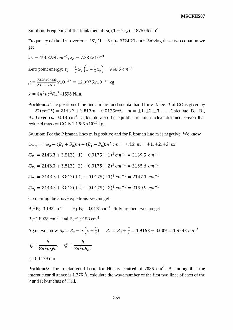
MSCPH507

255

Solution: Frequency of the fundamental: ��𝑒(1 − 2𝑥𝑒)= 1876.06 cm-1

Frequency of the first overtone: 2��𝑒(1 − 3𝑥𝑒)= 3724.20 cm-1. Solving these two equation we

get

��𝑒 = 1903.98 𝑐𝑚−1, 𝑥𝑒 = 7.332𝑥10

−3

Zero point energy: 휀0 =1

2��𝑒 (1 −

1

2𝑥𝑒) = 948.5 𝑐𝑚

−1

𝜇 =23.25𝑥26.56

23.25+26.56𝑥10−27 = 12.3975𝑥10−27 kg

𝑘 = 4𝜋2𝜇𝑐2��𝑒2=1598 N/m.

Problem4: The position of the lines in the fundamental band for v=0v=1 of CO is given by

�� (𝑐𝑚−1) = 2143.3 + 3.813𝑚 − 0.0175𝑚2, 𝑚 = ±1,±2,±3…… Calculate B0, B1,

Be. Given e=0.018 cm-1. Calculate also the equilibrium internuclear distance. Given that

reduced mass of CO is 1.1385 x10-26 kg.

Solution: For the P branch lines m is positive and for R branch line m is negative. We know

��𝑃,𝑅 = 𝜈𝜔 0 + (𝐵1 + 𝐵0)𝑚 + (𝐵1 − 𝐵0)𝑚2 𝑐𝑚−1 𝑤𝑖𝑡ℎ 𝑚 = ±1, ±2,±3 so

��𝑃1 = 2143.3 + 3.813(−1) − 0.0175(−1)2 𝑐𝑚−1 = 2139.5 𝑐𝑚−1

��𝑃2 = 2143.3 + 3.813(−2) − 0.0175(−2)2 𝑐𝑚−1 = 2135.6 𝑐𝑚−1

��𝑅0 = 2143.3 + 3.813(+1) − 0.0175(+1)2 𝑐𝑚−1 = 2147.1 𝑐𝑚−1

��𝑅1 = 2143.3 + 3.813(+2) − 0.0175(+2)2 𝑐𝑚−1 = 2150.9 𝑐𝑚−1

Comparing the above equations we can get

B1+B0=3.183 cm-1 B1-B0=-0.0175 cm-1 . Solving them we can get

B1=1.8978 cm-1 and B0=1.9153 cm-1

Again we know 𝐵𝑣 = 𝐵𝑒 − 𝛼 (𝑣 +1

2), 𝐵𝑒 = 𝐵0 +

𝛼

2= 1.9153 + 0.009 = 1.9243 𝑐𝑚−1

𝐵𝑒 =ℎ

8𝜋2𝜇𝑟𝑒2𝑐, 𝑟𝑒

2 =ℎ

8𝜋2𝜇𝐵𝑒𝑐

re= 0.1129 nm

Problem5: The fundamental band for HCl is centred at 2886 cm-1. Assuming that the

internuclear distance is 1.276 Å, calculate the wave number of the first two lines of each of the

P and R branches of HCl.

MSCPH507

256

Solution: The reduced mass of HCl= (1.008

𝑘𝑔𝑘𝑚𝑜𝑙𝑒⁄ )(35.45

𝑘𝑔𝑘𝑚𝑜𝑙𝑒⁄ )

(36.46𝑘𝑔

𝑘𝑚𝑜𝑙𝑒⁄ )(6.023𝑥1026

𝑚𝑜𝑙𝑒⁄ )= 1.6275𝑥1027𝑘𝑔

The rotational constant 𝐵 =ℎ

8𝜋2𝜇𝑟𝑒2𝑐=

6.626×10−34𝐽−𝑆

8𝜋2(1.6275𝑥1027𝑘𝑔)(1.276×10−10𝑚)2(3×108𝑚

𝑠)

= 10.6129 × 102 = 10.6129𝑐𝑚−1

��𝑃,𝑅 = ��0 + 2𝐵𝑚 𝑐𝑚−1 𝑤𝑖𝑡ℎ 𝑚 = ±1,±2,±3

��𝑃1 = 2886 − 2 × 10.6129 = 2864.77 𝑐𝑚−1

��𝑃2 = 2886 − 4 × 10.6129 = 2843.55 𝑐𝑚−1

��𝑅0 = 2886 + 2 × 10.6129 = 2907.23 𝑐𝑚−1

��𝑅1 = 2886 + 4 × 10.6129 = 2928.45 𝑐𝑚−1

10.15 Self Assesment Questions

Self Assessment Question (SAQ) 1: What is the main condition for a molecule to be IR active?

Self Assessment Question (SAQ) 2: What do you mean by degrees of freedom of a molecule?

What is its value for a linear molecule and a nonlinear molecule?

Self Assessment Question (SAQ) 3: What do you mean by normal modes?

Self Assessment Question (SAQ) 4: What are the selection rules of P,R,Q branch lines?

Self Assessment Question (SAQ) 5: For CO2 molecule which mode is IR active and which

mode is not? Why?

Self Assessment Question (SAQ) 6: What do you mean by zero point energy? What is its

value? What do you mean by vibrational less state?

Self Assessment Question (SAQ) 7: What is the need of anharmonic oscillator to consider?

Self Assessment Question (SAQ) 8: What do you mean by dissociation energy?

Self Assessment Question (SAQ) 9: What do you mean by oscillation frequency? Write down

its value.

Self Assessment Question (SAQ) 10: Why anharmonic constant appears? Express its value.

Self Assessment Question (SAQ) 11: What do you mean by equilibrium oscillation

frequency?

Self Assessment Question (SAQ) 12: What do you mean by fundamental, first overtone,

second overtone vibrations? Mention their values.

MSCPH507

257

Self Assessment Question (SAQ) 13: Why the breakdown of Born-Oppenheimer

approximation appears for vibrating rotator?

Self Assessment Question (SAQ) 14: In higher vibrational states what will happen to

molecular bond length and why?

Self Assessment Question (SAQ) 15: What do you mean by skeletal and group frequencies?

Which one is important to characterize the molecular structure?

Self Assessment Question (SAQ) 16: Why for astronomical studies Infrared spectroscopy

plays a major role?

Self Assessment Question (SAQ) 17: What do you mean by FTIR spectroscopy?


(Should be divided into Short Answer type, Long Answer type, Numerical, Objective type)

10.16.1 Short Answer type question

1. IR spectrum of a symmetric AB2 molecule gives 3 prominent lines. Check whether the

molecule is linear or not?

2. Separation between P and R branch lines are different. Why?

3. What are hot bands? Why are they called so?

4. Homonuclear diatomic molecule does not show vibrational spectrum. Why?

5. The spacing between lines in P and R branch lines of CO2 is 4B instead of 2B. Why?

6. How many normal modes would you expect to be observed in the infrared absorptionspectra

of H2O and CO2 ?

10.16.2 Long Answer type question

1. Explain the effect of anharmonicity on the vibrational spectra of a diatomic molecule.

2. What parameters one can get from a study of the vibration-rotation spectrum of the

heteronuclear diatomic molecule? Explain how are they estimated?

3. What are the effects of isotope on the spectrum of vibrating rotator?

4. Explain different vibrational modes with figures for H2O and CO2 and explain which modes

of them are IR active and why?

5. Outline the theory of rotation-vibration spectrum of a diatomic molecule. How many normal

Modes of vibrations are possible for these molecules: HBr, O2. Why water can’t be used as a

solvent for infrared spectroscopy?

MSCPH507

258

6. How many normal modes of vibrations are possible for the following molecules OCS, SO2,

CH4, CH3I?

7. Assuming that the force constant for C C, C C, and C-C are in the ratio of 3:2:1. The

normal range of C C stretch absorption is 1630 – 1690 cm-1. What range is expected for C-

C, and C C stretch vibration? Why monochromator (grating / prism) are made up of rock

salts like NaCl / KBr?

8. Using a block diagram show essential components of IR spectroscopy.

10.16.3 Numerical and objective questions

1. Calculate the amplitude of vibration in the v=0 level of the molecule CO which has a force

constant of 1870 N/m.

2. Assume that the H2 molecule behaves like a harmonic oscillator with force constant k = 573

Nm-1. Find the vibrational quantum number corresponding to its dissociation energy 4.5 eV.

Given the atomic mass of H atom is 1.68x10-27kg, and h=6.63x10-34J-s.

3. The equilibrium vibrational frequency of the I2 molecule is 215 cm-1. The anharmonicity

constant is 0.003. At temperature 300K what is the intensity of the band for transition

v=1v=2 relative to that of the transition for v=0v=1?

4. The fundamental vibrational frequency of HCl is 2989 cm-1. Find the force constant.

5. The position of the lines in the fundamental band for v=0v=1 of HCl is given by

�� (𝑐𝑚−1) = 2886.0 + 20.577𝑚 − 0.3034𝑚2, 𝑚 = ±1, ±2,±3…… Calculate B0, B1,

Be. Given e=0.3019 cm-1.

6. Calculate the energy in cm-1 of the photon absorbed when HCl moleculegoes from the state

v=0, J’’=1v=1, J’=0 and v=0, J’’=1v=1, J’=2. Assume that v=0 and v=1 states have the

same B values. Given �� = 2990cm-1, xe=0.0174, rHCl=0.124 nm.

Objective type question

1. Identify true or false:

a. A infrared spectrum is possible only for the molecules with a permanent dipole moment.

b. The selection rule for fundamental vibrational transition is Δv=2.

c. For linear molecule the number of vibrational frequencies are 6.

MSCPH507

259

Unit 11 RAMAN SPECTRA

Structure

11.1 Introduction

11.2 Objective

11.3 Raman effect

11.4 Experimental Arrangement of Raman Effect

11.5 Quantum theory of Raman Effect

11.6 Intensity of Raman lines

11.7 Vibrational Raman spectra

11.8 Pure rotational Raman spectra

11.9 Raman shift

11.10 Comparison of Raman and Infrared spectra

11.11 Application of Raman spectra

11.12 Summary

11.13 Glossary

11.14 References

11.15 Suggested reading

11.16 Terminal questions

MSCPH507

260

11.1 Introduction

Rayleigh theoretically study the scattering and shows that in scattering of light, the intensity of

scattered light is inversely proportional to the forth power of wavelength (𝐼 =1

𝜆4). This is

called Rayleigh scattering. We know the colour of sky is blue due to greater scattering of blue

light as it is shorter wavelength. The scattering of lights takes place due to dust particles

suspended in atmosphere. In Rayleigh scattering, only incident wavelengths are present in

scattered light. No other wavelengths are present in scattered light therefore Rayleigh scattering

is also called coherent scattering.

While studying the Rayleigh scattering, Raman found that when a beam of light was

passing through some mediums like benzene or toluene, the scattered light contained some

additional frequencies along with incident frequency (Rayleigh frequency). This effect was

observed by CV Raman in 1928, and called Raman Effect.

11.2. Objective:

After studying this unit we will able to understand:

I. Raman effect and its discovery

II. Quantum theory of Raman effect

III. Pure rotational Raman effect

IV. Infra-red spectra and Raman spectra

V. Applications of Raman spectra

11.3 Raman Effect:

When a monochromatic beam of light passes through a gas, organic liquids like benzene or

toluene, or a transparent solid, a small part of light scattered in all directions. The scattered

light contains some other frequencies along with frequency of incident light (Rayleigh lines).

The spectral lines of additional frequencies are called Raman lines. The frequency of incident

light is called Rayleigh line or exciting line. The Raman lines corresponding to each Rayleigh

line occur symmetrically on both ride of Rayleigh line as shown in figure 7.1. The lines on the

low frequency side of Rayleigh line is called stoke line, while the lines on the higher frequency

side is called anti-stoke lines. The intensity of antistoke lines are much weaker than stoke lines.

It is also observed that the displacement of Raman Stoke lines from the Rayleigh line do not

depend on the Rayleigh frequency.

MSCPH507

261

Rayleigh line (exciting lines)

Stoks lines Anti-stoks lines

(cm-1)

Figure 7.1: Raman Spectra of diatomic gas

If we change the frequency of incident light or used another Rayleigh line, we get other Raman

lines for the same medium. However, the displacements of Raman lines from Rayleigh line are

same. Thus for a particular material the displacement of Raman lines from Rayleigh line

remains same. Thus the Raman displacements are characteristics of a scattering material.

Raman displacement is denoted by ∆ν (in cm-1) unit which is wavenumber and

proportional to energy

ν = λ =E

hc=1

𝜆=ν′

𝑐

Where λ or ν is wave number, E is energy and ν′ is frequency of incident light, h and c

have its usual meanings ∆ν denotes the Raman displacement from Rayleigh line.

Under low resolution we observe one stoke Raman line and one anti-stoke Raman line

each having same displacement ∆v. The Raman displacement ∆v is corresponding to main

vibrational rotational absorption band near infrared band. On the other hand at high resolution,

approximately equidistance lines are found on both side of Rayleigh line. This is pure rotational

Raman spectrum as shown in figure 7.1.

11.4 Experimental Arrangement of Raman Experiment:

The basic arrangement for obtaining the Raman spectra is shown in figure 7.2. In this

Experiment a liquid for which Raman spectra is to be obtained is filled in a tube which is called

Raman tube figure 7.2. Raman tube is a thin walled glass tube about 15 cm long and 2 cm

diameter. One end is closed with a optically plane glass from which scattered light can be

emerged towards spectrometer and other is drawn out into the horn shape covered by black

tape. This black colour horns shape end causes reflection of backward scattered light. The

Raman tube is illuminated by a large spiral shaped lamp L wrapped around the Raman tube T.

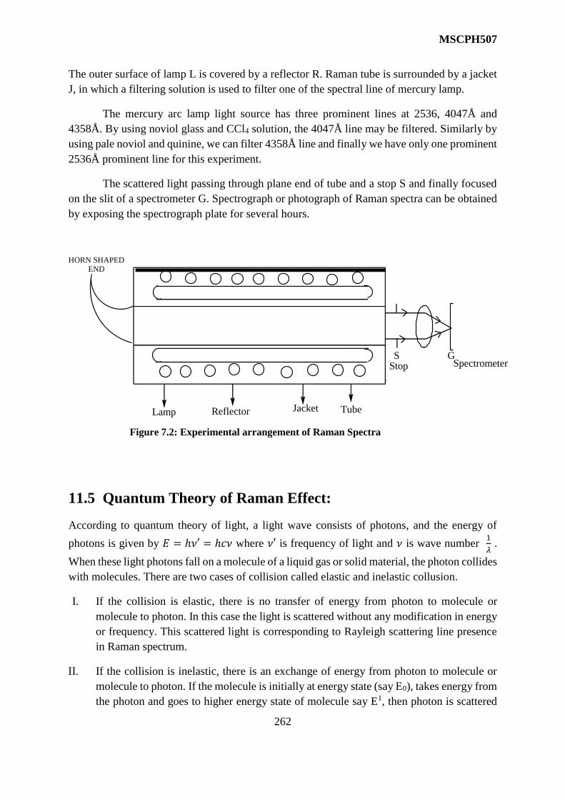
MSCPH507

262

The outer surface of lamp L is covered by a reflector R. Raman tube is surrounded by a jacket

J, in which a filtering solution is used to filter one of the spectral line of mercury lamp.

The mercury arc lamp light source has three prominent lines at 2536, 4047Å and

4358Å. By using noviol glass and CCl4 solution, the 4047Å line may be filtered. Similarly by

using pale noviol and quinine, we can filter 4358Å line and finally we have only one prominent

2536Å prominent line for this experiment.

The scattered light passing through plane end of tube and a stop S and finally focused

on the slit of a spectrometer G. Spectrograph or photograph of Raman spectra can be obtained

by exposing the spectrograph plate for several hours.

SSpectrometer

GStop

HORN SHAPED END

Lamp Reflector Jacket Tube

Figure 7.2: Experimental arrangement of Raman Spectra

11.5 Quantum Theory of Raman Effect:

According to quantum theory of light, a light wave consists of photons, and the energy of

photons is given by 𝐸 = ℎ𝜈′ = ℎ𝑐𝜈 where 𝜈′ is frequency of light and 𝜈 is wave number 1

𝜆 .

When these light photons fall on a molecule of a liquid gas or solid material, the photon collides

with molecules. There are two cases of collision called elastic and inelastic collusion.

I. If the collision is elastic, there is no transfer of energy from photon to molecule or

molecule to photon. In this case the light is scattered without any modification in energy

or frequency. This scattered light is corresponding to Rayleigh scattering line presence

in Raman spectrum.

II. If the collision is inelastic, there is an exchange of energy from photon to molecule or

molecule to photon. If the molecule is initially at energy state (say E0), takes energy from

the photon and goes to higher energy state of molecule say E1, then photon is scattered

MSCPH507

263

with a smaller energy (ℎ𝑐𝜈 − ∆𝐸) where ∆𝐸 = 𝐸′ − 𝐸0 as shown in figure 7.3. In this

case the frequency of Raman line is less than incident frequency. The scattered light has

frequency ℎ𝑐𝜈−∆𝐸

ℎ and in term of wave number shift =

∆E

hc such Raman lines are called

Stoke line.

There is another possibility called inelastic collision. If the molecule is initially at higher energy

state E1 and after collision it shifted to lower energy state E0, now the scattered photon emerges

with increased energy (ℎ𝑐𝜈 + ∆𝐸) after gaining an addition energy ∆E. In this case the

frequency of scattered light is greater than incident light. The frequency of scattered light is ℎ𝑐𝜈+∆𝐸

ℎ and the wave number shift is again

∆E

hc but now this line is in another side to Rayleigh

line. Such Raman lines are called anti-stoke lines. The stoke line and anti-stoke lines are

symmetrically situated on both side of Rayleigh (indent) line.

11.6 Intensity of Raman lines:

At normal temperature, the number of molecule in lower energy state is more than

molecules in higher energy state E1. When radiation falls on molecule there is more transition

from lower to higher energy state. In this process molecules absorb energy from photons.

However, the transition from higher to lower energy state in which photon absorbs energy from

hc hc-

Ehc

+

Ehc

E

Stokes line Anti-stokes line

E'

E0

Figure 7.3: Quantum Theory of Raman Scattering

MSCPH507

264

molecule is very few. Since Stoke lines are corresponding to transition from lower energy state

to higher energy state therefore Stoke lines are more intense than anti-stoke line. In some case

the anti-stoke lines are so faint or weak that they are not observed.

If the temperature increases, more molecules are available at higher energy state E1 and

transition from higher energy state to lower energy state also increase and consequently anti-

stokes lines becomes brighter.

11.8 Pure Rotational Raman Spectra:

Pure rotational Raman spectra arises when the transition from one rotational energy

state to another rotational energy state of a molecule.

In case of diatomic molecule, the energy involved in the different motion of molecules

can be divided into three categories as translational, rotational, and vibrational energies. The

rotational energy of a diatomic molecule is given by

𝐸𝑗 =1

2I ω2 where I is moment of inertia and 𝜔 is angular frequency.

If J is angular momentum then we know 𝐿 = Iω

or 𝐸𝑗 =1

2

L2

I

Angular momentum can be given as 𝐿 = √J(J + 1) ħ where J is rotational quantum number

and have values J = 0, 1, 2, 3………………..

thus 𝐸𝑗 = J(J + 1)ħ2

2I (1)

The selection rule for pure rotational transition is ∆J = 0, + 2

∆J = 0 is corresponding to Rayleigh line. The transition from J→J+2 (absorption) gives stoke

rotational Raman line and J+2→J gives the Anti Stoke Raman rotational Raman lines as shown

in figure 7.4.

From eq. 1 the rotational energy in terms of wave number can be expressed as

1

𝜆= 𝑣 =

𝐸𝑗

𝘩𝑐=ħ2

2IhcJ(J + 1)

or 𝑣 =h

8 π2IcJ(J + 1)

h

8 π2Ic= B is another constant known as rotational constant. Then the wave number for

rotational energy is can be expressed as

𝑣 = 𝐵 J(J + 1) where J=0, 1, 2, 3……….

MSCPH507

265

For rotational Raman lines the selection rule is ∆J = + 2, therefore the wave number of

the rotational Raman lines are given by

𝑣𝑟𝑎𝑚𝑎𝑛 = 𝜈𝑟𝑎𝑦𝑙𝑒𝑖𝑔ℎ𝑡 ± [𝑣𝑗+2 − 𝑣𝑗]

= 𝜈𝑟𝑎𝑦𝑙𝑒𝑖𝑔ℎ𝑡 ± [𝐵 (J + 2)(J + 3) − 𝐵 J(J + 1)]

= 𝜈𝑟𝑎𝑦𝑙𝑒𝑖𝑔ℎ𝑡 ± 𝐵[4 J + 6]

= 𝜈𝑟𝑎𝑦𝑙𝑒𝑖𝑔ℎ𝑡 ± 4𝐵( J + 3/2)

Thus rotation Raman Shift is

∆𝜈 = 𝑣𝑟𝑎𝑚𝑎𝑛 − 𝜈𝑟𝑎𝑦𝑙𝑒𝑖𝑔ℎ𝑡 = 4𝐵( J + 3/2)

∆𝜈 = 6𝐵, 10𝐵, 14𝐵, 18𝐵……………….

Thus in pure rotational Raman spectrums, a series of equidistance lines corresponding to

different Raman shift are situated on both side of Rayleigh line. The separation between two

successive lines is 4B as shown in figure 7.4.

Pure rotational molecular spectra can be shown by molecules that have permanent electric

dipole moment. Thus the homonucleus diatomic molecule such as H2, O2, N2, symmetric linear

molecule O=C=O etc. do not exhibit rotational spectra. But homonucleus molecule exhibits

rotational Raman spectra. Homonucleus molecules like H2, N2, O2, the rotational Raman lines

are alternately weak and strong due to symmetric properties of rotational energy levels. On the

other hand hetronucleus molecule like HF, HCl, HBr, CO etc. exhibit rotational spectra.

MSCPH507

266

J=5

J=0

J=1

J=2

J=3

J=4

Ej= Eo=0

E1=h2

I

E2 = 3E1

E3= 6E1

E4=10E1

E5=15E1

14B 6B10B18B 6B 10B 14B 18B

Stoks lines Anti- Stoks line

Figure 7.4: Pure rotational Raman Spectra

cm-1

11.9 Vibrational Raman Spectrum:

The Vibrational Raman Spectrum arises when the transition takes place from one

vibrational level to another vibrational level of the same electronic state of a molecule.

Quantum mechanically, a molecule can be treated as a harmonic oscillator. If ν' is classical

frequency of harmonic oscillator, then the energy E of such molecule can be given as

E=h ν' (v+1/2)

Where v = 0, 1, 2, 3, 3………are integer number corresponding to different energy

states. ν' is classical frequency given as

ν′ =1

2π√k

m′ where k = force constant and m' = reduced mass

In terms of wave number, the vibrational energy can be given as

G(v) =E

hc=ν′

𝑐(v +

1

2)

MSCPH507

267

Where G(v) is known as vibration term and ν′

𝑐 is known as vibrational constant denoted by ω

thus

G(v) = ω (v +1

2) in cm-1

Corresponding to different vibrational levels v =1,2,3,4.......

G(v) = 1

2ω,

3

2ω,

5

2ω ……

In case of vibrational Raman spectrum, if ν is the wave number of incident light

(Rayleigh line), Raman lines are symmetrically arise on either side of Rayleigh line. The

selection rule (possible transition) for vibrational Raman spectrum is

∆ ν = + 1

Thus the vibrational Raman lines are situated on either side of Rayleigh line as

𝜈𝑟𝑎𝑚𝑎𝑛 = 𝜈 ± [G(v + 1) − G(v)]

If transition takes place from v =1 to v = 0 states then

𝜈𝑟𝑎𝑚𝑎𝑛 = 𝜈 ± [ω3

2 − ω

1

2] = 𝜈 ± ω

Similarly for transition v = 2 to v =1 state

𝜈𝑟𝑎𝑚𝑎𝑛 = 𝜈 ± [ω5

2 − ω

3

2] = 𝜈 ± ω

Thus in general the vibration Raman lines arises as

𝜈𝑟𝑎𝑚𝑎𝑛 = 𝜈 ± ω

Vibrational Raman shift is given as

∆𝜈 = 𝜈𝑟𝑎𝑚𝑎𝑛~𝜈 = ω

This is Raman Shift in terms of wave number corresponding to absorption band of

vibrational energy levels and generally observed near infra-red spectrum.

11.10 Comparison between Raman and infrared spectra:

The infrared absorption spectra arises when a transition between vibration state v = 0

to v = 1 takes place. This transition is similar to vibration stoke Raman line in which some

MSCPH507

268

vibration state involved. Hence, there is an agreement between infrared and Raman spectra but

the mechanism of production of both spectra are quite different.

In infrared spectra, we provide the radiation energy exactly same as energy difference

between two different vibrational states; whereas in Raman spectra we provide a radiation of

higher frequency and there is a change in energy corresponding to two energy states of

molecule.

Further, in infrared band there is a change in molecular electric dipole moment due to

molecular vibrational states. Thus permanent magnetic moment is must for occurrence of

infrared spectra. On the other hand, Raman spectra arise due to polarizability of a molecule and

no need of permanent dipole moment.

11.11 Application of Raman spectroscopy

11.11.1 Molecular structure:

Raman Effect is an important tool for study of structure of a molecule. Vibrational

Raman spectra can be used for determining the force constant of diatomic molecule. As we

know vibrational Raman shift ∆v=ω where ω is vibrational constant given by 𝜔 =ν′

𝑐. Here ν′

is classical frequency of vibration of molecule and given as ν′ =1

2√𝑘

𝑚′ . By this relation the

force constant k can be obtained. On the other hand, by using Rotational Raman Spectra, the

bond length of a molecule can be determined.

11.11.2 Structure of triatomic molecule:

With the help of Raman lines, its intensity and number of lines we can determine

whether a triatomic molecule is symmetric or asymmetric. For structure infrared spectrum is

also used along with the Raman spectrum for more information.

Theoretically we use rule of mutual exclusion. According to this rule a molecule with

centre of symmetry transitions that are allowed in the infrared are for hidden in Raman spectra

and vice versa. However, all transitions forbidden in one must occur in the other is not always

true. Sometime some transitions may be forbidden in both Raman and infrared spectrum.

For example CO2 has two strong bands in infrared absorption spectrum at 668cm-1 and

at 2349cm-1while a strong band at wave number 1389cm-1 in Raman spectra. As none of the

bands appear both in Raman as well as infrared spectrum thus the CO2 molecule has a centre

of symmetry and CO2 has linear structure as O-C-O.

Example1: In a Raman study of a material, the wavelength of a light source used is 5460Ǻ.

The stoke line is observed at 5520Ǻ. Find the wavelength of anti stoke line

Solution: The light source provides the Rayleigh line for the Raman spectra. The location of

Rayleigh line in terms of wave number ν can be given as

MSCPH507

269

𝜈 =1

5460 X 10−8cm= 18318𝑐𝑚−1

The stoke line is given as

𝜈 =1

5520 X 10−8cm= 18116𝑐𝑚−1

The displacement in terms of wave number is

∆ 𝜈 = 𝜈 − 𝜈𝑠𝑡𝑜𝑘𝑒 = 18315 – 18116 = 199cm-1

The stoke line and anti-stoke lines are symmetrically located on either side of Rayleigh

line. Therefore, the location of anti-stoke line is

∆ 𝜈 = 𝜈 + 𝜈𝑎𝑛𝑡𝑖𝑠𝑡𝑜𝑘𝑒

𝜈𝑎𝑛𝑡𝑖𝑠𝑡𝑜𝑘𝑒 = 𝜈 + ∆ 𝜈 = 18315+199=18514cm-1

The corresponding wave length = 1

18514 𝑐𝑚−1 = 5401Ǻ

Example 2: When a celylene is irradiated with the 4358Ǻ light source, a Raman line

corresponding to vibration spectra is observed at 4768Ǻ. Calculate the fundamental frequency

(frequency corresponding to vibrational constant ) for this vibration.

Solution: The wave number corresponding to exciting line(Rayleigh line) is

ν = 1

4358𝑋10−8= 22946𝑐𝑚−1

Raman line is located at

νraman = 1

4768𝑋10−8= 20973𝑐𝑚−1

This is stoke line

In case of vibrational Raman spectra, the Raman displacement is given as

∆ ν = ν raman- ν = ω

Where ω is vibrational constant ν′

𝑐 and ν′ is frequency.

Thus ω = 22946 - 20973 = 1973 cm-1

Hence, vibration frequency ν' = ωc = 1973 X 3 X 1010

ν' = 5.92 x 1013cm-1

MSCPH507

270

Example 3: A substance shows Raman lines at 4567Ǻ when the wavelength of incident light

(Rayleigh line) is 4358Ǻ. Find out the positions of stoke and anti-stoke lines for the same

substance when a light of 4047Ǻ is used.

Solution: The wave number ν corresponding to incident light or Rayleigh line is

ν = 1

4358𝑋10−8𝑐𝑚−1 = 22946𝑐𝑚−1

The Raman line corresponding to 4567Ǻ is

νraman = 1

4567𝑋10−8𝑐𝑚−1 = 21896𝑐𝑚−1

The Raman Shift or wave number displacement is

∆ ν = ν – ν raman= 22946 – 21896

∆V = 1050cm-1

We know that the Raman shift is a characteristic of material and remains same for all

incident light or Rayleigh line.

Now if the light used is of wavelength 4047Ǻ, then in terms of wave number the

Rayleigh line corresponding to incident light.

ν = 1

4047 𝑋 10−8= 24710 𝑐𝑚−1

Since the Raman shift ∆ ν remain same therefore position of Stoke line is

= ν - ∆ ν = 24710 – 1050 = 23660cm-1

Wave length of Stoke line =𝜆𝑠𝑡𝑜𝑘𝑒 = 1

23660 𝐶𝑚−1 = 42265Ǻ

Similarly Anti Stoke line = ν+∆ν

= 24710 + 1050 = 23760 Cm-1

Wave length of anti-stoke line 1

25760𝐶𝑚−1 = 3.882 𝑋 108𝑐𝑚

= 3882Ǻ

Self assessment questions (SAQ)

SAQ1: What are Raman lines?

SAQ2: Why Stoke lines are more intense than anti-stoke line?

SAQ3: Explain the unit of Raman displacement?

MSCPH507

271

SAQ4: Give the Rotational energy in terms of rotational quantum number?

SAQ5: What is rotational constant?

SAQ6: What is classical frequency of molecular vibrations?

SAQ7: Define Vibrational Constant?

SAQ8: How structure of molecule can be studied with the help of Raman spectroscopy?

11.12 Summary

1. Rayleigh scattering, only incident wavelengths are present in scattered light. No other

wavelengths are present in scattered light therefore Rayleigh scattering is also called coherent

scattering. The frequency of incident light is called Rayleigh line or exciting line.

2. When a monochromatic beam of light passes through a gas, organic liquids like benzene or

toluene, or a transparent solid, a small part of light scattered in all directions. In the spectral

lines, if there are some additional frequencies, they are called Raman lines.

3. The Raman lines corresponding to each Rayleigh line occur symmetrically on both ride of

Rayleigh line. The lines on the low frequency side of Rayleigh line is called stoke line, while

the lines on the higher frequency side is called anti-stoke lines.

4. The intensity of antistoke lines is much weaker than stoke lines. Displacement of Raman

Stoke lines from the Rayleigh line do not depend on the Rayleigh frequency.

5. Raman displacement is denoted by ∆ν (in cm-1 unit) which is wavenumber and proportional

to energy

ν = λ =E

hc=1

𝜆

6. Rotational energy in terms of wave number

𝑣 =h

8 π2IcJ(J + 1)

𝑣 = 𝐵 J(J + 1) where J=0, 1, 2, 3………(J is rotational quantum number)

Where h

8 π2Ic= B is rotational constant.

7. Rotation Raman Shift is

∆𝜈 = 𝑣𝑟𝑎𝑚𝑎𝑛 − 𝜈𝑟𝑎𝑦𝑙𝑒𝑖𝑔ℎ𝑡 = 4𝐵( J + 3/2)

∆𝜈 = 6𝐵, 10𝐵, 14𝐵, 18𝐵……………….

8. In terms of wave number, the vibrational energy can be given as

MSCPH507

272

G(v) =E

hc=ν′

𝑐(v +

1

2)

where v = 0, 1, 2, 3, ...are integer number corresponding to different energy states.

G(v) = ω (v +1

2) in cm-1

9. vibrational Raman lines are situated on either side of Rayleigh line as

𝜈𝑟𝑎𝑚𝑎𝑛 = 𝜈 ± [G(v + 1) − G(v)]

10. Vibrational Raman shift ∆𝜈 = 𝜈𝑟𝑎𝑚𝑎𝑛~𝜈 = ω

11.13 Glossary

Rayleigh line: Wave number ν corresponding to incident light

Wave number: inverse of wavelength 1

𝜆 = ν or (

𝐸

𝘩𝑐)

Spectrum: A band of colours

Selection rule: A rule specify the possibility of transition among the different energy levels

Rotational energy state: energy state arises due to rotations in molecule

Vibrational energy state: energy state arises due to vibration of molecule.

Rotational spectra: Spectrum due to transitions among rotational states

Vibrational spectra: Spectrum due to transitions among vibrational energy states of molecule.

Raman Displacement: separation between Rayleigh line and Raman line in terms of wave

number ν.

Stoke line: particular wavelength (or wave number) present in the Raman spectra of a molecule

on the low frequency side of Rayleigh line.

Anti-stoke line: Particular wavelength (or wave number ) present in the Raman spectra on the

higher frequency side of Rayleigh line.

11.14 References

Raj Kumar, Atomic and molecular spectra, KedarNath Raman, Nath Publication, Meerut

CL Arora and PS Hemne, Physics for Degree students, S Chand Publication, Delhi

MSCPH507

273

11.15 Suggested Reading

1. CL Arora, Atomic and Molecular Physics, S Chand and Company Ltd., New Delhi

2. M. Alonso and EJ Finn, Fundamental University Physics, Addison-Wesley Publication

Company.

3. HE., White., Introduction to Atomic Spectra, McGraw Hill Publication, New Delhi.

4. CN Banwell, Fundamental of Molecular Spectroscopy, Tata McGraw Hill Publication, New

Delhi.

5. John R., Introduction to Raman Spectroscopy, FerraoKazuaNakamoto, Academic Press, New

York


11.16.1 Short answer type questions

1. What is Raman Effect?

2. Explain the intensity of Stoke and anti-stoke lines?

3. Give the characteristic of molecular spectra.

4. Explain rotational Raman spectra.

5. Explain Vibrational Raman spectra.

6. What do you mean by Raman shift?

7. Give a comparison between Raman and infrared spectra.

8. With the help of Raman spectra, how the structure of a molecule can be studied.

11.16.2 Long answer type questions

1. Explain the Raman spectra with the help of experimental setup.

2. Explain rotational Raman spectra. Obtain the Rotational Raman shift with the help of

vibrational constant.

3. Give the explanation of pure rotational Raman spectra. Find out the expression for rotational

Raman shift and Rotational constant.

4. Give the applications of Raman spectrum.

5. Discuss the main features of vibrational and rotational Raman spectra of a diatomic molecule.

Give the necessary theory.

6. Discuss Raman spectra of diatomic molecules and point out the similarities and differences in

infrared and Raman spectra.

MSCPH507

274

7. Describe the salient features of Raman spectra of a hetronucleus diatomic molecule and how

this can be explained.

8. Explain how Raman spectra depends on polarisability of a molecule and entirely independent

from the presence of permanent dipole moment.

9. Consider H2 , N2 , HCl and OH molecule. Explain which of these molecule show infrared

spectrum and which will give Raman Spectrum.

10. Distinguish between scattering and Rayleigh scattering.

11.16.3 Numerical type questions

1. A sample is irradiated with a light source of wave length 3458 Å. If the stoke lines are observed

at 4458 Å, find out the wavelength of anti-stoke line. [Ans. 4262 Å]

2. In the vibrational Raman spectra of HF, Raman lines are observed at 2670 Å and 3430 Å. What

is the fundamental vibrational frequency of molecule? [Ans. 1.24×1014

Hz]

3. The exciting line in an experiment with Raman Effect is 5460 Å. If the stoke line has 𝜆=5520

Å, Calculate the wavelength of anti-stoke line. [Ans. 5400

Å]

MSCPH507

275

UNIT 12

ELECTRONIC SPECTRA

Structure

12.1 Introduction to Electronic spectra: Franck Condon Principle

12.2 Salient Features of Molecular Electronic spectra

12.3 Formation of electronic spectra; electronic transition

12.4 Vibrational Structure of Electronic Band-System in Emission

12.5 Electronic Band spectra in Absorption

12.6 Observed Intensity Distribution (Vibrational) in Band system

12.7 Rotational Intensity Distribution


12.9 References

MSCPH507

276

12.1 Franck Condon Principal

when electrons of an atom are excited to higher energy states, the radiations that are absorbed

in this process appear as the absorption spectra of atoms. In a similar way, electronic spectra

of molecules arise when the electrons of a molecule are excited to higher energy states. The

energy involved in this process is generally large and electronic spectra of molecules are

usually found in visible and ultraviolet region. Therefore, electronic spectra arise due to the

changes in the arrangement of molecular electrons. We shall discuss electronics spectra of

diatomic molecules.

The electronic transition is the result of change in electronic energy. A small change in the

electronic energy will be accompanied by a large change in the vibrational energy of the

molecule. These vibrational energy changes give rise to vibrational transitions which form a

group of various bands. Further, a small change in the vibrational energy will be accompanied

by a large change in the rotational energy of the molecule. These rotational energy changes

give rise to rotational transitions forming a series of line in each band-the so called fine

structure of each band.

12.2 Salient Features of Molecular Electronic spectra

Electronic spectra is the most complex molecular spectra which appear in the visible and ultra

violet regions and involve the change in all the three energies (electronic, vibrational and

rotational) of the molecule. These spectra are obtained in emission and absorption regions. The

spectral band exhibit a fine structure which is more complicated. The head formation tendency

is story and the bands are degraded either towards violet or toward the red. All molecules give

electronic spectra.Homo-nuclear molecules (H2,N2,O2 etc.) do not give neither rotational nor

vibrational- rotational spectra because of having no permanent dipole moments but they give

electronic spectra because of the instantaneous dipole moment changes during the

redistribution of change which results in the transition.

12.3 Formation of electronic spectra; electronic transition

Each electronic state of the molecule has a different potential energy curve. For stable

electronic state, the curve, is characterized by a minimum at an equilibrium inter-nuclear

distance 𝛾e a dissociation limit De, a set of discrete vibrational levels and sets of discrete

rotational levels. Fig 5.1 shows the two potential energy curves for a diatomic molecule. The

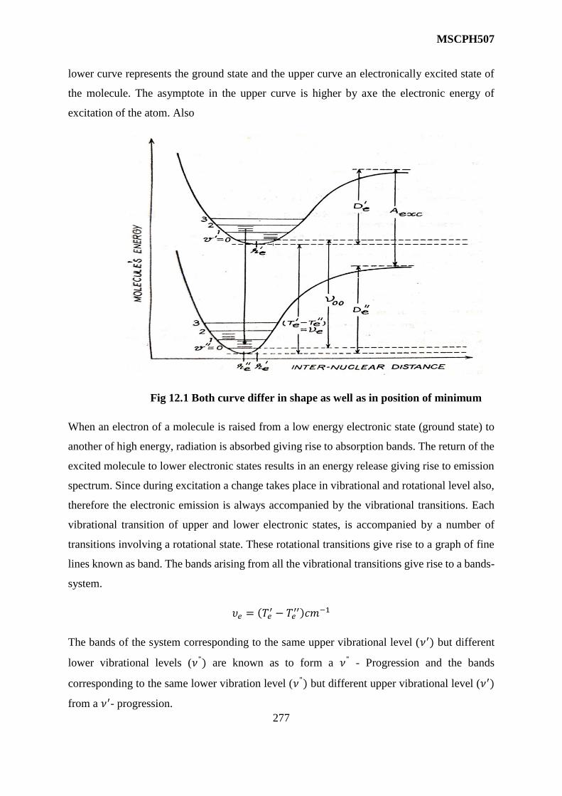
MSCPH507

277

lower curve represents the ground state and the upper curve an electronically excited state of

the molecule. The asymptote in the upper curve is higher by axe the electronic energy of

excitation of the atom. Also

Fig 12.1 Both curve differ in shape as well as in position of minimum

When an electron of a molecule is raised from a low energy electronic state (ground state) to

another of high energy, radiation is absorbed giving rise to absorption bands. The return of the

excited molecule to lower electronic states results in an energy release giving rise to emission

spectrum. Since during excitation a change takes place in vibrational and rotational level also,

therefore the electronic emission is always accompanied by the vibrational transitions. Each

vibrational transition of upper and lower electronic states, is accompanied by a number of

transitions involving a rotational state. These rotational transitions give rise to a graph of fine

lines known as band. The bands arising from all the vibrational transitions give rise to a bands-

system.

𝜐𝑒 = (𝑇𝑒′ − 𝑇𝑒

′′)𝑐𝑚−1

The bands of the system corresponding to the same upper vibrational level (𝜈′) but different

lower vibrational levels (𝜈") are known as to form a 𝜈" - Progression and the bands

corresponding to the same lower vibration level (𝜈") but different upper vibrational level (𝜈′)

from a 𝜈′- progression.

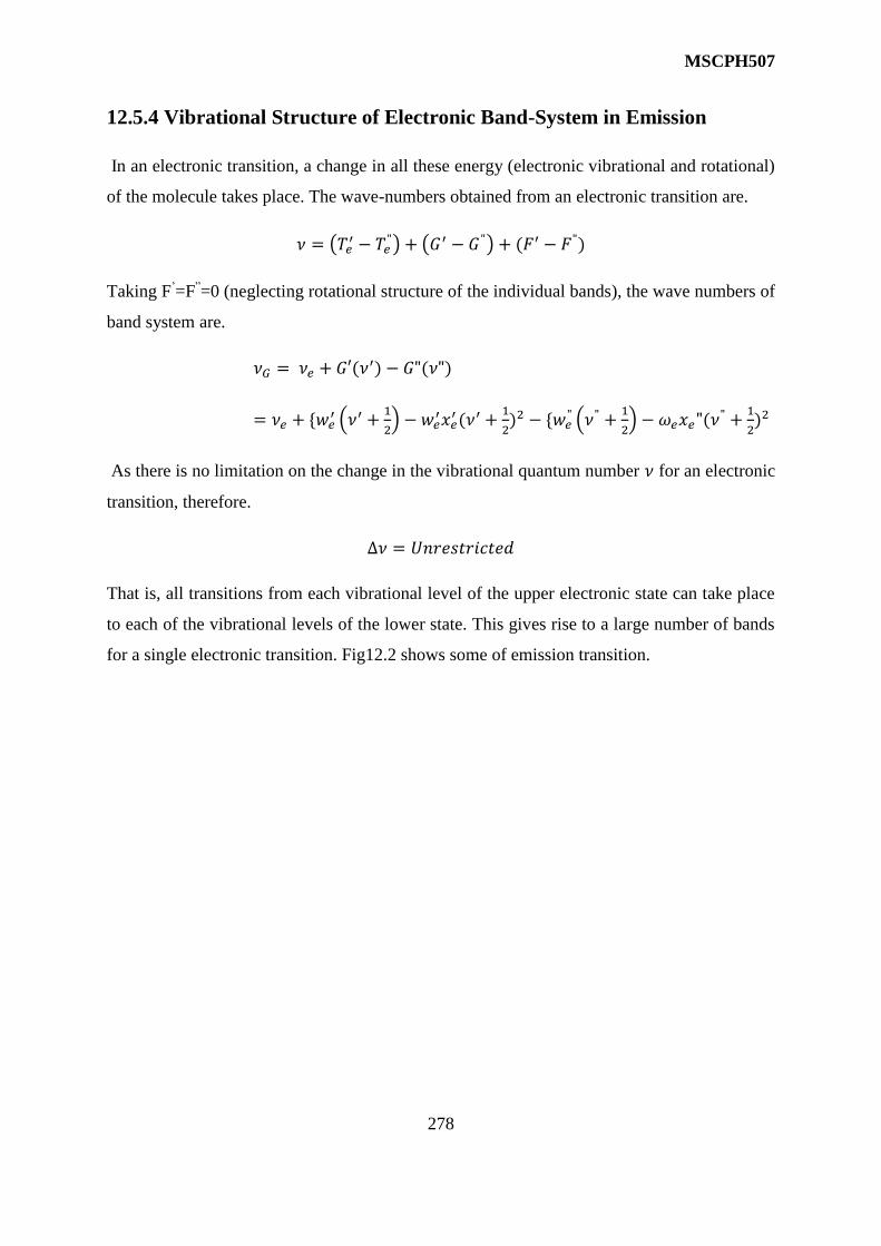
MSCPH507

278

12.5.4 Vibrational Structure of Electronic Band-System in Emission

In an electronic transition, a change in all these energy (electronic vibrational and rotational)

of the molecule takes place. The wave-numbers obtained from an electronic transition are.

𝜈 = (𝑇𝑒′ − 𝑇𝑒

") + (𝐺′ − 𝐺") + (𝐹′ − 𝐹")

Taking F’=F”=0 (neglecting rotational structure of the individual bands), the wave numbers of

band system are.

𝜈𝐺 = 𝜈𝑒 + 𝐺′(𝜈′) − 𝐺"(𝜈")

= 𝜈𝑒 + {𝑤𝑒′ (𝜈′ +

1

2) − 𝑤𝑒

′𝑥𝑒′ (𝜈′ +

1

2)2 − {𝑤𝑒

" (𝜈" +1

2) − 𝜔𝑒𝑥𝑒"(𝜈

" +1

2)2

As there is no limitation on the change in the vibrational quantum number 𝜈 for an electronic

transition, therefore.

Δ𝜈 = 𝑈𝑛𝑟𝑒𝑠𝑡𝑟𝑖𝑐𝑡𝑒𝑑

That is, all transitions from each vibrational level of the upper electronic state can take place

to each of the vibrational levels of the lower state. This gives rise to a large number of bands

for a single electronic transition. Fig12.2 shows some of emission transition.

MSCPH507

279

Fig.12.2

It can be band –system may be divided in to different groups. Each group contains a few close

bands. These are known as sequences (Δ𝜈 = 𝑐𝑜𝑛𝑠𝑡𝑎𝑛𝑡 𝑓𝑜𝑟 𝑒𝑎𝑐ℎ 𝑠𝑒𝑞𝑢𝑒𝑛𝑐𝑒). Bands of

sequences lie along the diagonal or along a line parallel to diagonal of the (Deslandre table).

Bands in the horizontal rows and in the vertical columns are knows as 𝜈"− 𝑎𝑛𝑑 𝜈′ -

progressions respectively.

12.5 Electronic Band spectra in Absorption

An electronic absorption spectrum consists of a series of bands which come more and more

closer toward high wave-number side and ultimately give a continuum. All emission band

systems are not observed in absorption. A large number of 𝜈" −Progressions (related to 𝜈′ =

0,1,2, − − −)of emission bards occur while there is only a single 𝜈′- Progression (related to

𝜈" = 0) of bands occur in the absorption spectrum. Other progressions (related to 𝜈" =

0,1,2, − − −) occur, if at all in very poor intersities Fig 5.3 shows the energy level diagram

and the corresponding transitions. The bands coverage at a point corresponding to the

transition.

MSCPH507

280

Fig.12.3

The wave numbers of the band-origins of a system are

𝜈0 = 𝜈𝑒 + 𝐺1(𝜈1) − 𝐺11(𝜈11)

=𝜈𝑒 + {𝑤𝑒1 (𝜈1 +

1

2) − 𝑤𝑒

1𝑥𝑒1(𝜈1 +

1

2)2} − {𝑤𝑒

11 (𝜈11 +1

2) − 𝑤𝑒

11𝑥𝑒11(𝜈11 +

1

2)2}

For the observed absorption progression of bands 𝜈11 = 0

𝜈0 = 𝜈𝑒 + 𝑤𝑒1 (𝜈1 +

1

2) − 𝑤𝑒

1𝑥𝑒1(𝜈1 +

1

2)2 −

1

2𝑤𝑒11 +

1

4𝜔𝑒" 𝑥𝑒

" .

For the first few bands of this progression, we have 𝜈′ = 0,1,2,3, − − − −−

The wave numbers of these bands and wave number separations are

Wave numbers First difference

𝜐𝑒 +1

2𝜔𝑒′ −

1

4𝜔𝑒′𝑥𝑒′ −

1

2𝜔𝑒′′ +

1

4𝜔𝑒′′𝑥𝑒

′′ 𝜔𝑒′ − 2𝜔𝑒

′𝑥𝑒′

𝜐𝑒 +3

2𝜔𝑒′ −

9


1

2𝜔𝑒′′ +

1


′′ 𝜔𝑒′ − 4𝜔𝑒

′𝑥𝑒′

MSCPH507

281

𝜐𝑒 +5

2𝜔𝑒′ −

25


1

2𝜔𝑒′′ +

1


′′ 𝜔𝑒′ − 6𝜔𝑒

′𝑥𝑒′

𝜐𝑒 +7

2𝜔𝑒′ −

49


1

2𝜔𝑒′′ +

1


′′

With the increase of 𝜈′, first difference (wave-number separation between successive bands)

decreases, that is levels come closer and closer. The second difference (2𝜔𝑒′𝑥𝑒′ ) between the

adjacent bands is the same. Thus the vibrational constant 𝜔𝑒. can be determined if 𝜔𝑒

′𝑥𝑒′ is

knows.

Potential Structure of Electronic Bonds: - The fine structure of individual bands of electronic

spectra due to the rotation of the molecule, that is each line of band corresponds to a change in

all the three energies of the molecule. The wave number of a line (J:J”) is given as

𝜈 = 𝜈𝑒 + (𝐺′ − 𝐺") + (𝐹′ − 𝐹")

=𝜈0 + 𝐹′(𝜈.

′𝐽′) − 𝐹"(𝜈". 𝐽"),

where 𝜈0 = 𝜈𝑒 + (𝐺′ − 𝐺") is the band origin.

Putting the values of rotational terms F’ and F” of the upper and lower electronic states, we

get’

𝜈 = 𝜈0 + 𝐵𝜈′𝐽′(𝐽′ + 1) − 𝐵𝜈

"𝐽(J+ 1),

The selection rule is Δ𝐽 = ±1

R-branch – Transitions corresponding to Δ𝐽 = 𝐽′ − 𝐽" = +1

Provide one set of lines known as R-branch, Putting J’=J”+1, we get

𝜈𝑅 = 𝜈0 + 2𝐵𝜈′(3𝐵𝜈′ − 𝐵𝜈")J”+( 𝐵𝜈

′ − 𝐵𝜈")J”2

R-branch is a series of lines R(0),R(1),R(2),-------------having J”=0,1,2,----------

P-branch – Transitions corresponding to Δ𝐽 = 𝐽′ − 𝐽" = −1

Provide another setoff lines known as P-branch. Putting J’=J”-1, we get

𝜈𝑃 = 𝜈0 − (𝐵𝜈′ − 𝐵𝜈")J”+ ( 𝐵𝜈′ − 𝐵𝜈")J”2

MSCPH507

282

P-branch is a series of lines P(1), P(2), P(3),-------------having J”=1,2,3,----------in Fig 12..4

shows the transitions and the band-structure obtained. P-and P- branch can be incorporated in

a single parabolic equation.

𝜈 = 𝜈0 + (𝐵𝜈′ + 𝐵"𝜈)m+(B'ν-B"ν)𝑚

2

where m = J”+1=1,2,3,------------- for R(0),R(1),R(2),------

m = J”+1=1,2,3,------------- for P(1),P(2),P(3) --------

and m= o for band origin,

Fig.12.4

Fortrat Parabola:- The fig 12.5 shows the plots of above equation when (𝐵𝜈′ − 𝐵𝜈") is

negative (red- degraded band) and when (𝐵𝜈′ − 𝐵𝜈") is positive (violet – degraded band). These

are known as ‘Fortrat Parabola’ The vertex of the Parabola represents the band-head.

Differentiating the able equation and equation d𝜈/dm to zero, we get

𝑑𝜈

𝑑𝑚= (𝐵𝜈

′ + 𝐵"𝜈)+2(Bν'-B"ν)𝑚 = 0

This gives the value of m at which the vertex of the Fortrat Parabola (band-head) lies as

m vertex = - (𝐵𝜈′+𝐵𝜈")

2(𝐵𝜈′−𝐵𝜈")

MSCPH507

283

Fig.12.5

Putting this value, the wave number separation between band-head and band origin is obtained

as

𝜈𝑅𝑒𝑎𝑑 − 𝜈0 = −(𝐵𝜈′ + 𝐵𝜈)

(𝐵𝜈′+𝐵𝜈")

2(𝐵𝜈′−𝐵𝜈") + (Bv′ − Bν" )

(𝐵𝜈′+𝐵𝜈")2

4(𝐵𝜈′−𝐵𝜈)2

= - (𝐵𝜈′+𝐵𝜈")

2

4(𝐵𝜈′−𝐵𝜈)2

Thus 𝜈ℎ𝑒𝑎𝑑 − 𝜈0 is positive for a band degraded to the red and negative for a band degraded to

the violet.

12.6 Observed Intensity Distribution (Vibrational) in Band system

(Franck-Condon Principal) The Intensity distribution among the bands of a band-system of

electronic spectra varies from one molecule to another and from one band-system to another of

the same molecule. The intensity distribution of absorption bands of O2,Co2 and I2 is shown in

12.6.

In the spectrum of O2 (0,0) band is maximum intense and the intensity of successive bands

(𝜈′ − 𝑃𝑟𝑜𝑔𝑟𝑒𝑠𝑠𝑖𝑜𝑛) 𝑤𝑖𝑡ℎ 𝜈" = 0) decreases rapidly. In the spectrum of co2 the intercity of

bands along the progression first increases rapidly to a maximum and then decreases. In the

spectrum of I2, the intensity of bands increases gradually and the maximum reaches at a very

high 𝜈′ − 𝑣𝑎𝑙𝑢𝑒 .thus a long progression is obtained.

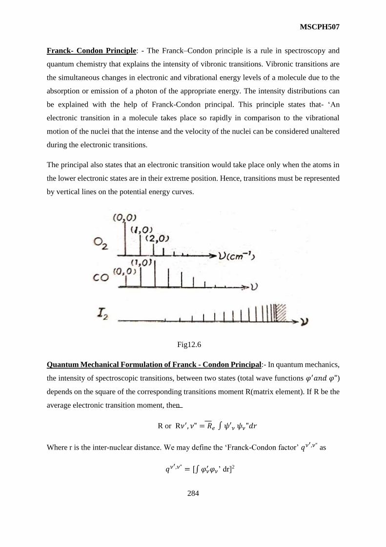
MSCPH507

284

Franck- Condon Principle: - The Franck–Condon principle is a rule in spectroscopy and

quantum chemistry that explains the intensity of vibronic transitions. Vibronic transitions are

the simultaneous changes in electronic and vibrational energy levels of a molecule due to the

absorption or emission of a photon of the appropriate energy. The intensity distributions can

be explained with the help of Franck-Condon principal. This principle states that- ‘An

electronic transition in a molecule takes place so rapidly in comparison to the vibrational

motion of the nuclei that the intense and the velocity of the nuclei can be considered unaltered

during the electronic transitions.

The principal also states that an electronic transition would take place only when the atoms in

the lower electronic states are in their extreme position. Hence, transitions must be represented

by vertical lines on the potential energy curves.

Fig12.6

Quantum Mechanical Formulation of Franck - Condon Principal:- In quantum mechanics,

the intensity of spectroscopic transitions, between two states (total wave functions 𝜑′𝑎𝑛𝑑 𝜑")

depends on the square of the corresponding transitions moment R(matrix element). If R be the

average electronic transition moment, then

R or R𝜈′, 𝜈" = 𝑅𝑒 ∫ 𝜓′𝜈 𝜓𝜈"𝑑𝑟

Where r is the inter-nuclear distance. We may define the ‘Franck-Condon factor’ 𝑞𝜈′,𝜈" as

𝑞𝜈′,𝜈" = [∫𝜑𝜈

′𝜑𝜈’ dr]2

MSCPH507

285

The Franck-Condon factor and also the relative intensities depend upon the relative positions

of the maxima and the nodes of the vibrational wave function 𝜓𝜈 in two states quantum

mechanically we may state the principle as follows:-

A vibrational transition will have a large Franck-Condon factor only if one of the two turning

points of a level of one electronic state lies nearly at the same inter nuclear distance as one of

the two turning points of a level of the other state, except for 𝜈 = 0 level for which the middle

point of the level must be subetituted (in place of turning point)

Intensity Distribution in Absorption Bands: - Franck - Condon principle explains it. Fig 12.7

shows the three typical situations of absorption transitions between two electronic states in a

diatomic molecule. The equilibrium in inter-nuclear distances are equal in both states in fig

12.7(a), slightly greater in upper state in (b), and much greater in upper state in (c) In fig

12.7(a), the transition 𝜈" = 0—𝜈′ = 0 is the most probable one because of connecting the

configurations of high probability and it appears as a vertical line (r remains unchanged).other

transitions are also taking place but week in intensity. Thus (0,0) band has maximum intensity

and for higher bands decreases rapidly. This is the case of o2 molecule.

Fig.12.7

In fig 12.7(b), the most probable transition is 𝜈" = 0—𝜈′ = 2. Other transitions to the 𝜈′ =

0,1,2,3,4, − − − are taking place but weak in intensity. Thus, the intensity first increase from

MSCPH507

286

(0,0) band and after reaching a maximum for (2,0) band intensity decreases. This is the case of

co molecule.

In fig 12.7(b), the most probable transitions is 𝜈" = 0—𝑐𝑜𝑛𝑡𝑖𝑛𝑛𝑢𝑛 of upper electronic state.

Thus molecule is dissociated so that a progression of weak bands terminated to a continuum of

maximum absorption intensity occurs. This is the case of I2 molecule,

Intensity Distribution in Emission Bands:- The distribution of intensity in a band progression

with 𝜈′ = 0 in emission corresponds exactly to that of a progression with 𝜈" = 0 in absorption.

The intensity maximum at a 𝜈" value is obtained whose value depends on the relative portion

of the maxima of the two potential curves. The larger value of 𝜈” is obtained for intensity

maximum for the greater difference 𝑟′𝑒 − 𝑟′′𝑒. The intensity distribution for band progression

in emission (for 𝜈′ > 0) is different from that for 𝜈′ = 0. For 𝑂2+ and Co, the fig 12.7 shows

the Condon parabola. This is a plot of intensities at the bands of a system in a 𝜈′ − 𝜈" array

exactly similar to a Deslandre table and joining the most intense bands. Thus a Condon

parabola may be defined as the locus of most intense bands in a 𝜈′ − 𝜈" array.

Fig.12.8

The potential curves are not symmetrical. This means transitions will be more probable from

(or to) the one side than the other in accordance with Franck-Condon principal. Therefore, for

MSCPH507

287

a red-end degraded system, (r’>r”), the right part of the Condon parabola is stronger while for

violet-end degraded system (r’ < r”), the left part is stronger.

12.7 Rotational Intensity Distribution

The intensity of a line in an electronic band depends upon the rotational levels of the initial

electronic state and upon the transition probability in emission or absorption of that line. For a

transition 1Σ − 1Σ, the value of intensity factor i for the lines of R –and P- branches is given

by

iR(J) = iP(J)= J’+J”+1

If a graph between intensity and J is plotted, then in 1Σ − 1Σ electronic band an intensity

maximum in each of R- and P-branches is found, fig. 12.9. with the increase of temperature,

the maxima shift to higher J values. The R-branch is stronger in absorption while P- branch is

stronger in emission.

Fig.12.9

Solved Problems

Q.1 Rotational analysis of one band system is given by 𝜈 = 24762 + 25𝑚 − 2.1𝑚2 𝑐𝑚−1.

Deduce the position of the band-head, the values of B𝜈′𝑎𝑛𝑑𝐵𝜈" and the degradation of the

band.

MSCPH507

288

Sol:- 𝜈 = 24762 + 25𝑚 − 2.1𝑚2𝑐𝑚−1 ----------------- (i)

The line of P and R branches of a band are represented by a single formula

𝜈 = 𝜈𝑜 + (𝐵𝜈′ − 𝐵𝜈")𝑚 + (𝐵𝜈′ − 𝐵𝜈")𝑚2

where 𝜈0 is the band origin. Comparing it with the eq.(1), we get

𝜈0 = 24762𝑐𝑚−1, 𝐵𝜈′ + 𝐵𝜈" = 25𝑐𝑚−1

and 𝐵𝜈′ − 𝐵𝜈" = −2.1𝑐𝑚−1

solving these equations., we get.

𝐵𝜈′ = 11.45𝑐𝑚−1 𝑎𝑛𝑑 𝐵𝜈" = 13.55𝑐𝑚−1

Now m venterx = - 𝐵𝜈′+𝐵𝜈"

2(𝐵𝜈′−𝐵𝜈")= −

25

2𝑥(−2.1)= 5.9

That is, the head lies at 6 (whole number). Putting m=6 in eq.(1) we get

𝜈ℎ𝑒𝑎𝑑 = 24762 + (25𝑥6) − (2.1 𝑥 62) = 24836.4𝑐𝑚−1

This is clear that the band-head lies towards the high-frequency side of the band-origin so

that

the band is degraded towards the law frequency side or ‘toward the red’.

Q.2:- The 5’-0” transition is Hcl35 occurs at 99022 cm-1. Calculate the position of the band

origin of same transition for Pcl35 on the basis of the assumption that in both the electronic

states the molecule behaves as harmonic oscillator. Given that.

𝜔𝑒′ = 2710cm-1 𝜔𝑒

′′ = 2990cm-1 for Hcl35

m'(Hcl) = .979889 m” (Hcl) = 1.90500

Sol:- 𝜌 = √(0.979889

1.90500) = 0.7172

The origin of an electronic band is given by

𝜈0 = 𝜈𝑒 + 𝜈𝜈

MSCPH507

289

= 𝜈𝑒 + [𝜔𝑒′ (𝜈′ +

1

2) − 𝜔𝑒"(𝜈" +

1

2)]

91022= 𝜈𝑒 + [2710 (5 +1

2) − 2990 (

1

2)]

𝜈𝑒 = 77612 𝑐𝑚−1

This represents the energy difference between potential energy minima of two electronic state

that remain unchanged. Position of new band origin is given by

𝜈0′ = 𝜈𝑒 + 𝜌𝜈𝜈

= 77612+0.7172(𝜈0 − 𝜈𝑒)

= 77612+0.7172(91022-77612)

= 87230cm-1

Q.3:- The zero point energy of the ground state of N2 is 1176 cm-1 and that of its lowest excited

state is 727 cm-2. The energy difference between the minima of the potential energy cueves is

50,206 cm-1. What is the energy of the 𝜈′ = 0—𝜈′′ = 0 transition is cm-1? What is the

corresponding wavelength?

Sol:- The wave numbers of the band origins of a system are given by 𝜈0 = 𝜈𝑒 + (𝐸𝜈′−𝐸𝜈"

ℎ𝑐)

In our case Zero point energy of ground state = 𝐸𝜈"

Zero point energy of excited state =𝐸0′

Therefore, 𝜈0 = 𝜈𝑒 + (𝐸0′−𝐸0"

ℎ𝑐)

𝜈𝑒 = 50206 𝑐𝑚−1

𝐸0′

ℎ𝑐= 727𝑐𝑚−1

𝐸0′

ℎ𝑐= 1176 𝑐𝑚−1

So that frequency of (0-0) bands is

𝜈00 = 50,206 + (727 − 1176)

MSCPH507

290

= 50,206-449

= 49,757 cm-1

Corresponding wave length of (0-0) band is given by

𝜆00 =1

𝜈00=

1

49,757 𝑐𝑚 = 2010 Å

Q.4:- The bands of a system are given by relation 𝜈 = 19221.2 + (1611.3𝑈′ − 40.7𝑈12) −

(1495.7𝑈" − 31.5𝑈"2) where U = 𝜈 +1

2 calculate the position of (0,0) band. Towards which

side is the band degraded? Given that U’= 𝜈+ 1

2

Sol:- we know that band that band origin of the system is represented by

𝜈0 = 𝜈𝑒 + (𝜔𝑒′𝑢′ − 𝜔𝑒′ 𝑥𝑒′ 𝑢

′2) − (𝜔𝑒′′𝑢′′ − 𝜔𝑒′′ 𝑥𝑒′′ 𝑢′′

2)

Comparing it with

𝜈 = 19221.2 + (1611.3𝑢′ − 40.7𝑢′2) − (1495.74" − 31.54"2)

we get 𝜈𝑒 = 19221.2 𝑐𝑚−1, 𝜔𝑒

′ = 1611.3𝑐𝑚−1, 𝜔𝑒′𝑥′ = 40.7

𝜔𝑒′′ = 1495.7cm-1, 𝜔𝑒′′𝑥" = 31.5cm-1

for (0,0) bard 𝜈′ = 0, 𝜈" = 0

Hence u’= 1

2 𝑎𝑛𝑑 𝑢" =

1

2

Substituting equation for 𝜈00. we get.

𝜈00 = νe + (1

2 ωe

′ −1

4 ωe′xe’) - (

1

2 ωe

′′ −1

4 ωe′′xe’’)

= 19221.2+(1

2𝑥1611.3 −

1

4 𝑥40.7) − (

1

2 𝑥 1495.7 −

1

4𝑥31.5)

= 19276.7 cm-1

As this case 𝜔𝑒′ > 𝜔𝑒”

Hence B’>B or B’- B” is positive; so bands are degraded towards the violet.

MSCPH507

291

MCQ Problem

1. Which statement is correct about the vibrational ground state of an H2 molecule?

The molecule is vibrating.

The molecule is in its lowest vibrational level but is not vibrating.

The molecule is static in its ground state.

In its vibrational ground state, the molecule has no vibrational energy.

2. Which value is the correct reduced mass of HF?

1.59 × 10–27 kg

6.30 × 1026 kg

5.72 × 1026 kg

1.75 × 10–27 kg

3. Which statement is incorrect about CO2?

CO2 is linear.

CO2 has two degenerate bending modes of vibration.

The IR spectrum of CO2 shows four absorptions.

CO2 has two stretching modes of vibration.

4.Which of the following transitions between rotational energy levels is not allowed?

J = 1 ← J = 3

J = 1 → J = 0

J = 1 ← J = 2

J = 0 ← J = 1

5. For which of the following molecules could a pure rotational spectrum not be observed in

the gas phase?

MSCPH507

292

Answers : (1) a (2) a (3) c (4) a (5) c

Short and Long Answer Problems

Q.1:- Write a note (short) on Franck-Condon principle?

Q.2 :- Give an account of the salient features observed in the electronic spectrum of a diatomic

molecule. Discuss the conditions under which the band-heads are degraded towards violet red

in the electronic spectrum.

Q.3:- Discuss rotational fine structure of electronic vibrational transitions. What is Fortrat

diagram?

Q,4:- The band-head of the branch is always at J= -1

2, while that of the P-or R-branch may be

any where explain.

Q.5:- Describe Franck-Condon principle in emission and absorption.

Q.6:- How did it become known as .Franck-Condon Principle?

Q.7:- The dissociation energy of H2 molecule is 4.45 ev and that of D2 molecule is 4.54ev. Find

the zero-point energy of H2 molecule.

Q.8:-You are given a Franck –Condon parabola. What information’s could be deduced from it about

the molecule?

HCl

NO

N2

CO

MSCPH507

293

References

1.Atomic & Molecular spectra Laser: By Raj Kumar (KNRM Publication-Meerut)

2.Structure and properties of Material: By MA Wahab (Narosa Publishing House –Delhi)

3.Molecular Spectra and Molecular Structure I: G. Herzberg (Van-Nostrand Rein-hold, 1950)

4· Atomic Physics by J.H.Fewkes& John Yarwood. Vol. II (Oxford Univ. Press, 1991).


Technical)

6. Molecular Spectroscopy, C N Banwell.

7· Fundamental of Molecular Spectroscopy. C N Banwell and E M Mc Cash (Tata Mc Graw

Hills)

MSCPH507

294

UNIT 13

PHOTOACAUSTIC

Structure

13.0 Introduction to photoacoustic effect

13.1 Photothermal Phenomena and Detection Techenques

13.2 Electret Microphone and Piezoelectric Detection

13.3 Photo-thermal Beam Detection (PBD)

13.4 Photo-thermal Radiometry and Other Remote Sensing Techniques

13.5 Photo thermal Displacement Spectroscopy (PDS)

13.6 Photoelectric Detection:

13.7 Interferometric Detection

13.8 Theory of the Photoacoustic effect in condense media

13.9 Advantages of Photoacoustic Spectroscopy

13.10 Applications of Photoacoustic in different fields

MSCPH507

295

13.0 Introduction to photoacoustic effect

Photoacoustic effect was discovered by Alexander G Bell in 1881. Bell accidently stumbled

onto this effect as he was experimenting with this invention of the photo phone. Photoacoustic

effect is essentially the generation of acoustic waves on irradiating certain substances by a

modulated electromagnetic radiation ranging from radio frequency to X-rays. The

photoacoustic effect or optoacoustic effect is the formation of sound waves following light

absorption in a material sample. In order to obtain this effect, the light intensity must vary,

either periodically or as a single flash. There are different mechanisms that produce the

photoacoustic effect. The primary universal mechanism is photo-thermal its mechanism

consists of the following stages:

Conversion of the absorbed pulsed.

Temporal changes of the temperatures at the loci.

Expansion and contraction of temperature changes (diffusion of the thermal pulsations).

In applying the photoacoustic effect there exist various modes of measurement. Thus, when a

sample is irradiated by a modulated electromagnetic waves, absorption of photons (Photon

energy) generates excited internal energy levels. All or part of the absorbed photon energy is

then transformed in to heat (thermal energy) through non-radiative relaxation processes in the

sample. In a gas this heat energy appears as vibrational energy of the gas molecules, while in a

solid or liquid, it appears as vibrational energy of ions or atoms. Photoacoustic (PA) generation

is generally due to photo thermal heating effect apart from other mechanisms. Since the

radiation incident on the sample is intensity modulated, the internal heating of the sample,

which in turn produces acoustic signal of same frequency as that of modulating signal.

A condenser microphone can pick this signal. The sample to be studies is often enclosed in a

PA cell.

(i) For the case of gases and liquids the sample generally fills the entire chamber where

as in the case of solids, the sample fills only a portion of the chamber and the rest

of the chamber is filled with a non-absorbing gas such as air. In addition, the cell

also contains a sensitive microphone, which acts as acoustic transducer. Thus the

periodic heating of the sample due to the absorption of modulated electromagnetic

radiations results in a periodic heat flow from the sample to the gas, which itself

MSCPH507

296

does not absorb the radiation. This periodic heat flow in turn produces pressure

variations in the gas medium at the same frequency at which the incident beam is

modulated. A sensitive microphone placed in the PA cell and converted in to

electrical signals directly monitors these pressure variations.

(ii) In case of sample in the form of thin film, bulk solid samples and liquids, it is

possible to measure the heat production through subsequent pressure or stress

variation in the sample itself by means of a piezoelectric transducer, which is placed

in intimate contact with the sample. Thus the acoustic output signal amplitude

directly gives the measure of absorption of the incident beam of radiation. This

output is often processed through a ‘phase sensitive detection’ technique.

Fig.13.1 Common direct PA generations mechanism

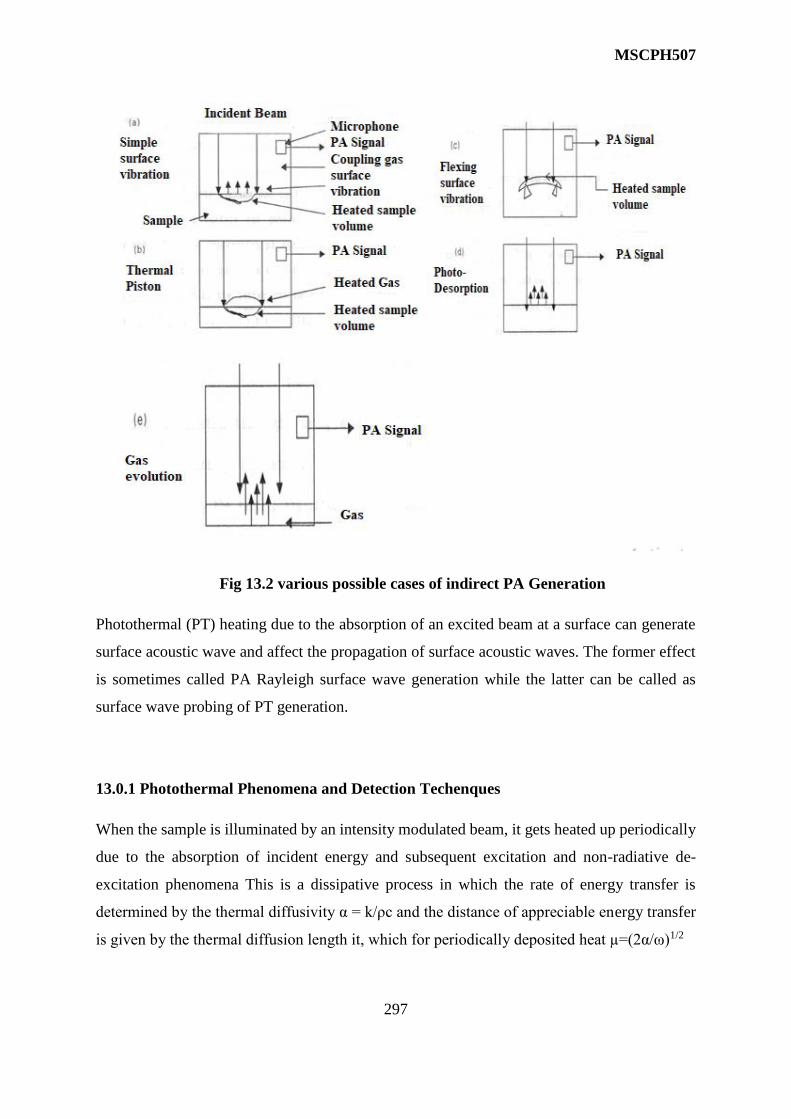
MSCPH507

297

Fig 13.2 various possible cases of indirect PA Generation

Photothermal (PT) heating due to the absorption of an excited beam at a surface can generate

surface acoustic wave and affect the propagation of surface acoustic waves. The former effect

is sometimes called PA Rayleigh surface wave generation while the latter can be called as

surface wave probing of PT generation.

13.0.1 Photothermal Phenomena and Detection Techenques

When the sample is illuminated by an intensity modulated beam, it gets heated up periodically

due to the absorption of incident energy and subsequent excitation and non-radiative de-

excitation phenomena This is a dissipative process in which the rate of energy transfer is

determined by the thermal diffusivity α = k/ρc and the distance of appreciable energy transfer

is given by the thermal diffusion length it, which for periodically deposited heat µ=(2α/ω)1/2

MSCPH507

298

Fig.13.3 Block diagram showing the optical absorption and various possible de-excitation

Channels.

Detection methods can either be applied to the sample directly when it is called direct PT effect

or to the coupling medium adjacent to the sample which is the indirect PT effect. The second

method lies on the assumption that only the sample absorbs the indirect light but not the

coupling medium.

13.0.2 Electret Microphone and Piezoelectric Detection:

The conventional P A microphone detection technique is a non-contact, remote sensing

technique. In this case, a displacement sensitive detector such as a capacitor microphone proves

to be an excellent heat detector. With the availability of sensitive microphone and associated

electronics, it is possible to detect temperature rise in a gas of 10-6 °C or a thermal input of the

order 10-9 cal/cm3 –sec. The response time of the gas-microphone system to the order of 100 µ

sec or longer. In the case of solids or liquids, for measuring heat in the sample by means of a

MSCPH507

299

piezoelectric detector placed in intimate contact with the sample. It can detect temperature

changes of 10-7 °C to 10-6 OC, which for a particular solids or liquids corresponds to thermal

inputs of the order of 10-6 cal/cm3-sec. Since the sample with a displacement sensitive detector

such as microphone would be 10 to 100 times less sensitive than a pressure sensitive device

such as a piezoelectric detector.

(a) (b)

Fig.13.4 Transducer assembly for PZT detection for solids

(a) opaque and (b) transparent.

13.0.3 Photo-thermal Beam Detection (PBD)

This is a non-contact technique originally proposed by Boccara et al and Fournier et al. It is

based on the concept of beam deflection by thermally induced changes in the refractive index.

The absorption of a modulated pumping beam followed by the diffusion of the deposited heat

causes a gradient in the refractive index in a thin layer of gas (or liquid) adjacent to the sample

surface. Assuming that the probe beam passes through the coupling medium parallel to the

sample surface at a distance x from the surface, it will be deflected by an angle ϕ from its

original path Fig. 13.6. For small deflections, ϕ is given by

∅ = (𝐿

𝑛0) [𝜕𝑛 𝜕𝑇⁄ ].𝑇0 [

𝜕𝑇𝑔

𝜕𝑋] .𝑋=𝑋0 ………………(1)

MSCPH507

300

where Tg (x, t) = θ exp. (-σg.x).exp. (jωt) is the temperature distribution in the coupling

medium(gas), no is the refractive index of the gas at ambient temperature (To) and L is the

length of the sample illuminated by the pump beam.

Fig.13.5 PBD experimental configuration

The PBD technique has been employed in the measurement of optical absorption coefficient

of thin films, solids, liquids and gases and more recently to a quite diverse class of problems

ranging from imaging to scanning microscopy.

13.0.4 Photo-thermal Radiometry and Other Remote Sensing Techniques:

Photo thermal radiometry (PTR) is a non-contact technique in which the specimen is irradiated

with amplitude modulated light. This results in pulsating surface temperature and similar

pulsation in the thermal radiation emanating from the irradiated region. The technique was

originally proposed by Kanstad and Nordal. The thermal radiation from the illuminated area is

collected by an appropriate optical system and focused on an infrared detector. The experiment

can also be performed using pulsed laser with boxcar or transient detection.By Stefan-

Boltzmann law, the total radiant energy emitted from a body of emissivity `e' at temperature T

is given by

MSCPH507

301

W = eσT4 ……………… (2)

where σ is the Stefan's constant. For a temperature change δT due to the absorption of energy

E from a radiation of wavelength λ, the change in radiant energy is

δW = 4σeT3 δT …………………(3)

The PTR signal in a broadband detector over the entire thermal radiation spectrum may be

written as

S = 4σeT3 A Sin2θ dT ………………..(4)

where A is the detector area and θ the collecting angle.

Fig.13.6 Experimental arrangement for PTR measurement

13.0.5 Photo thermal Displacement Spectroscopy (PDS)

The basic principle involved in PDS is that whenever a sample gets heated due to photo thermal

effect, the surface expands due to thermal effect thereby getting displaced. The magnitude of

displacement is related quantitatively to the optical absorption coefficient. A schematic

representation of this technique is shown in figure 13.7. For an absorbing layer of thickness, 1,

on a transparent substrate, the photo thermal surface displacement h is given by

ℎ =∝𝑡ℎ 𝛽𝑃

2𝐴𝑓𝑐𝜌 ……………… . . (5)

MSCPH507

302

where αth - thermal expansion coefficient, R - the fraction of the absorbed light, P - incident

power, f – modulating frequency, A - area of optically illuminated region, ρ – the mass density

and c - specific heat capacity.

Fig.13.7 PDS principle

13.0.6 Photoelectric Detection

This is another example of contact type photo thermal detection technique. It is based on the

use of pyroelectric thin films to detect the temperature change in the sample when exposed to

modulated heating. In a pyroelectric material a temperature fluctuation induces an electrical

current proportional to the rate of change of its average heat content

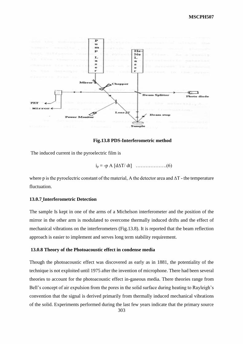
MSCPH507

303

Fig.13.8 PDS-Interferometric method

The induced current in the pyroelectric film is

ip = -p A [d∆T/ dt] ……………….(6)

where p is the pyroelectric constant of the material, A the detector area and ∆T - the temperature

fluctuation.

13.0.7 Interferometric Detection

The sample Is kept in one of the arms of a Michelson interferometer and the position of the

mirror in the other arm is modulated to overcome thermally induced drifts and the effect of

mechanical vibrations on the interferometers (Fig.13.8). It is reported that the beam reflection

approach is easier to implement and serves long term stability requirement.

13.0.8 Theory of the Photoacoustic effect in condense media

Though the photoacoustic effect was discovered as early as in 1881, the potentiality of the

technique is not exploited until 1975 after the invention of microphone. There had been several

theories to account for the photoacoustic effect in-gaseous media. There theories range from

Bell’s concept of air expulsion from the pores in the solid surface during heating to Rayleigh’s

convention that the signal is derived primarily from thermally induced mechanical vibrations

of the solid. Experiments performed during the last few years indicate that the primary source

MSCPH507

304

of photoacoustic signal from a condensed sample, as measured by the gas microphone method,

arises from the periodic heat flow from the sample to the surrounding gas with the subsequent

change in the gas pressure within the cell.

The first attempt to develop an exact theory of photoacoustic effect in solid was carried out by

porker in order to give a quantitative explanation for photo acoustic signal emanating from cell

window while performing photo acoustic effect in condensed media was formulated by

Rosencwaig and Gorsho. This theory now commonly referred to as the RG theory, shows they

in a gas-microphone measurement of a PA signal, the signal depends both on the generation of

an acoustic pressure disturbance at the sample-gas interface and on the transport of this

disturbances through the gas to the microphone. The generation of the surface pressure

disturbances depends in turns on the periodic variations of temperature at the sample-gas

interface.

13.0.9 Advantages of Photoacoustic Spectroscopy

Since the photoacoustic signal is generated only after the absorption of optical signal, the light

that transmitted or elastically, scattered by the sample does not interfere with the photoacoustic

spectroscopic (PS) measurements. This is of greater importance when one works with

essentially transparent media, such as polluted gasp that have few absorbing centers. Since the

method is insensitive to the scattered radiation it Is possible to obtain optical absorption data

on highly scattering materials such as powders, amorphous solids, gels and colloids. Another

advantage is the capability of obtaining absorption spectra of optically opaque samples, since

the method does not depend on the detection of photons.Coupled with this is the capability,

unique to photoacoustic spectroscopy, of performing non-destructive depth profile analysis of

absorption as a function of depth in to a material. The PA effect results from a radiation less

energy conversion process and is therefore complementary to radiative and photo chemical

processes. Thus PAS can be used as a sensitive, though indirect method for studying the

phenomena of fluorescence and photosensitivity in matter.

Table 13.1 Comparison of various techniques optical absorption measurement for weak

optical absorption measurement

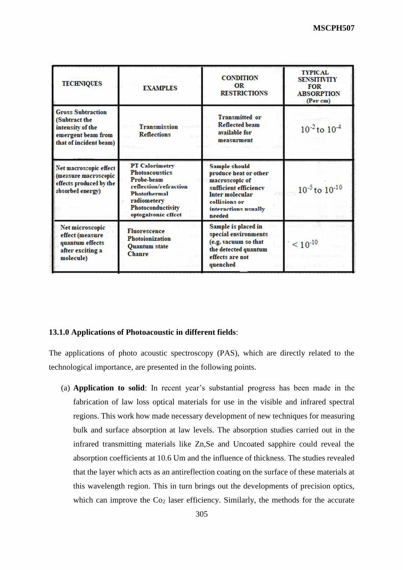
MSCPH507

305

13.1.0 Applications of Photoacoustic in different fields:

The applications of photo acoustic spectroscopy (PAS), which are directly related to the

technological importance, are presented in the following points.

(a) Application to solid: In recent year’s substantial progress has been made in the

fabrication of law loss optical materials for use in the visible and infrared spectral

regions. This work how made necessary development of new techniques for measuring

bulk and surface absorption at law levels. The absorption studies carried out in the

infrared transmitting materials like Zn,Se and Uncoated sapphire could reveal the

absorption coefficients at 10.6 Um and the influence of thickness. The studies revealed

that the layer which acts as an antireflection coating on the surface of these materials at

this wavelength region. This in turn brings out the developments of precision optics,

which can improve the Co2 laser efficiency. Similarly, the methods for the accurate

MSCPH507

306

determination of photoluminescence quantum efficiencies and relaxation processes are

of considerable importance.

(b) Application to weak Absorption in Gases: One of the most significant applications

of photoacoustic effect is the sensitive detection of pollutant gas species present in the

atmosphere. The studies could attain a sensitivity limit of few parts per billion, which

is considered to be a remarkable achievement the photoacoustic spectroscopic

technology.

(c) Application to thin films: The use of Photoacoustic technique for measuring

absorption in thin films, minelayers or even multilayers has been reported. For thin

films of powders or for liquids, the pulsed Photoacoustic technique provides

measurement of an absorption coefficient as low as 10-3 cm-1 for a thickness of 10-8 cm.

the photoacoustic method has been successfully employed to measure the enthalpy of

absorbed materials like pyridine on evaporated Polycrystalline nickel films this provide

the absolute rate deposition of a single monolayer of surface absorption coefficient at

various monolayer and the of deposition of layers on the substrate ‘Consequently’ this

technique finds its application in the field of semiconductor industry in which the

detailed analysis of the changes in Physical properties at each monolayer is often

necessary to develop highly efficiently semiconductor devices since the photoacoustic

signal is a function of the thermal propagation within the sample, it is possible to

determine the thermal properties like thermal diffusivity and thermal conductivity with

great accuracy normally not attainable with other technique.

(d) Microwave and Interference Spectroscopy

Originally studies of (PA) were carried out in the LW -Visible region of the electromagnetic

spectrum. Such studies can be carried out at any wavelength provided, the material under

study has absorption in the wavelength used. Several authors have used PP. detection for

microscopic absorption studies over a wide range of materials. The use of PAS in the near

IR region can be carried out using the same instrumentation as for UV-Visible region. The

absorption bands observed in the near IR region for solid and liquid samples are attributable

to overtones and combinations of the fundamental vibrational modes of particular bands.

Most frequently observed bands are those relating to hydrogenic systems e.g.: -CH, -OH,

and -NH.

(e ) Surface Studies:

MSCPH507

307

PAS can be used in the study of adsorbed and chemisorbed molecular species and

compounds on the surface of metals, semiconductors and even insulators. Such studies can

be done at any wavelength, provided the substrate is non-absorbing at that wavelength. The

PAS experiment gives optical absorption spectra of the adsorbed or chemisorbed

compounds on the surface of the substrate.

(f) Chemical Studies:

PAS is ideally suited to catalytic studies since catalytic substances are by their very nature

difficult to investigate by conventional spectroscopic means. These difficulties arise from

the fact that in heterogeneous catalysis the catalyst is often in the form of a fine powder.

(g)Photoacoustic in Biology and Medicine: A Photoacoustic method of determining the

absorption of a material is widely being used in biological as well as in medical fields many

of the above-mentioned samples occur naturally in insoluble states; many others are

membrane bound or part of bone or tissue structure. These materials are found to function

biologically with in a more or less solid matrix. Photoacoustic spectroscopy through its

capability of providing optical data on intact biological matter, even with materials, which

are optically opaque, holds great promise both as a research tool and as a diagnostic tool in

biology and medicine.

(h)Miscellaneous Applications: Photoacoustic spectroscopy is a tool for the study of

radiation chemistry. Another important area of application of photoacoustic spectroscopy

is in photosynthesis. This technique can be used to measure energy conversion and storage,

for molecular structure and interaction studies as well as oxygen evolution in

photosynthetic systems. The bond gap energies of semiconductors can be obtained by

photoacoustic spectroscopy. Study of the strength characteristics of thin films is another

application of photoacoustic method.

Problems Sets

Q.1 What is photoacoustic effect.

Q.2 Explain about the different mechanisms for producing the photoacoustic effect.

Q.3 Discuss about the direct and indirect PA generation mechanism.

MSCPH507

308

Q.4 Why does PAS require pulses of light instead of a continuous steady source of light to

hit the

Sample.

Q.5 Draw the block diagram showing the optical absorption and various possible de-excitation

channels.

Q.6 write a short note on Electret Microphone and Piezoelectric Detection mechanism.

Q.7 Give brief idea of Experimental arrangement for PTR measurement.

Q.8 Give the Advantages of Photoacoustic Spectroscopy.

Q.9Write the applications of Photoacoustic in different fields.

References:-

1. Atom, Laser And Spectroscopy:S. N. Thakur, D. K. Rai(PHI Learning Pvt. Ltd).

2. Atomic & Molecular spectra Laser: by Raj Kumar (KNRM Publication-Meerut)

3. The Feynman's lectures volumes.

4. Introductory Nuclear Physics: by K S Krane.

5. Atomic and molecular spectra: by Dr D K Jain (Lokpriya publishing house –Meerut)

6. Structure and properties of Material: By MA Wahab (Narosa Publishing House –Delhi)


1950)

8. Atomic Physics by J.H.Fewkes& John Yarwood. Vol. II (Oxford Univ. Press, 1991).


Technical)

10. Fundamental of Molecular Spectroscopy. C N Banwell and E M Mc Cash (Tata Mc

Graw Hills)

https://www.google.co.in/search?tbo=p&tbm=bks&q=inauthor:%22D.+K.+RAI%22

SLM - Uttarakhand Open University

Documents

Transcript of SLM - Uttarakhand Open University