Site-specific PSHA : combined effects of single-station-sigma ...

5

Special section - The geosciences perspective on seismic response assessment and application to risk mitigation

Site-Specific PSHA: Combined Effects of Single-Station-Sigma, Host-to-Target Adjustments and Nonlinear Behavior. A case study at Euroseistest

Claudia Aristizabal1,2, Pierre-Yves Bard1 & Céline Beauval1 1 Univ. Grenoble Alpes, CNRS, IRD, Univ. Gustave Eiffel, ISTerre, 38000 Grenoble, France.2 Suramericana S.A., Medellín, Colombia.

CA, 0000-0003-0562-4050; P-YB., 0000-0002-3018-1047 ; CB, 0000-0002-2614-7268.

Ital. J. Geosci., Vol. 141, No. 1 (2022), pp. 5-34, 16 figs., 7 tabs. https://doi.org/10.3301/IJG.2022.02

Research article

Corresponding author e-mail:[email protected]

Citation: Aristizabal C., Bard P-Y. & Beauval C. (2022) - Site-Specific PSHA: Combined Effects of Single-Station-Sigma, Host-to-Target Adjustments and Nonlinear Behavior. A case study at Euroseistest. Ital J. Geosci, 141 (1), 5-34, https://doi.org/10.3301/IJG.2022.02.

Associate Editor: Claudio ChiarabbaGuest Editor: Giuseppe di Giulio

Submitted: 06 June 2021

Accepted: 01 November 2021

Published online: 03 February 2022

ABSTRACTThis study takes advantage of the available information for an example, well-known, site in Greece (TST site at Euroseistest) to illustrate the epistemic variability in probabilistic seismic hazard assessment (PSHA) estimates. The purpose is not to perform an exhaustive site-specific PSHA at this particular site, but to investigate the sensitivity of the results to the approach used for including site effects, from basic ones to more demanding and realistic ones, in order to better appreciate the “benefits” versus the required costs and efforts of each approach. The TST site, located at the center of the Mygdonian basin in North-Eastern Greece is characterised by soft shallow soils over thick, medium stiffness deposits with a complex underground geometry, resting on very hard bedrock. Three different levels are considered for the incorporation of site response, from level 0 (generic or partially generic) to site-specific ones, with linear (level 1) or non-linear (level 2) site response analysis. The basic methods rely on one or several site proxies (VS30, VSZ and f0), whereas the most complex ones couple site response assessment (instrumental or numerical, implying site-specific characterization or instrumentation) with various reference rock hazard adjustments (single-station sigma, host-to-target adjustments, depth correction). Results are compared in terms of Uniform Hazard Spectra for a 5000 years return period, a typical value for critical facilities. For each level, the epistemic uncertainties are described and their impacts on hazard estimates are quantified. The use of the VS30 proxy in ground-motion prediction equations (GMPEs) leads to a clear underestimation of the hazard for the linear case (i.e., short return periods), especially around the site fundamental period, because of resonance and basin effects. On the other hand, soil nonlinearity largely impacts the hazard estimates, and linear amplification approach leads to an overestimation of the hazard, with unrealistic high levels at very long return periods. Site-specific hazard estimates for thick, Euroseistest-like sites, with complex geometry and rheology, are thus shown to come up against several additional epistemic uncertainties implying a large approach-to-approach variability. This may lead to increased hazard estimates, counterbalancing the decrease due to the use of reduced, single-site aleatory uncertainty in reference rock hazard estimates. For the time being, it thus looks unrealistic to promise a systematic reduction in hazard estimates with site-specific studies, while it might also indicate that uncertainties in generic hazard estimates could presently be underestimated.

KEY-WORDS: Site Effects, Epistemic Uncertainty, PSHA, Single-station-sigma, Host-to-target adjustments, Linear and Nonlinear behavior, Site Response analysis.

INTRODUCTION

Several recent dramatic events drew the attention on the need to carefully reassess the very rare, high-impact, seismic hazard for large urban centers and critical facilities. Presently, the trend all over the world is to more and more rely on probabilistic approaches to estimate seismic hazard, aiming at determining ground-motion exceedance probabilities over future time windows. Past examples have shown that site effects can significantly amplify ground motions (e.g., in Mexico City during the 1985 Michoacán and 2017 Puebla earthquakes, see Sánchez-Sesma,1998; Chávez-García & Bard, 1994; Çelebi et al., 2018; Galvis et al., 2018). Several authors have thus been working on the development of methods to estimate hazard curves

© The Authors, 2022

SUPPLEMENTARY MATERIAL is available at:https://doi.org/10.3301/IJG.2022.02

https://www.italianjournalofgeosciences.it/300/specialissues-1/the-geosciences-perspective-on-seismic-response-assessment-and-application-to-risk-mitigation.html

http://0000-0003-0562-4050

https://orcid.org/0000-0002-3018-1047

https://orcid.org/0000-0002-2614-7268

https://doi.org/10.3301/IJG.2022.02

mailto:[email protected]



6

C. ARISTIZABAL ET AL.

and uniform hazard spectra (UHS) including site effects within a probabilistic framework (Kramer, 1996; Lee et al., 1998, 1999; Lee, 2000; Tsai 2000; Silva et al., 2000; Cramer, 2003; Bazzurro & Cornell, 2004a,b; Stewart et al., 2006; Papaspiliou et al., 2012a,b; Rathje et al., 2015; Barani & Spallarossa 2016; Haji-Soltani & Pezeshk, 2017; Aristizabal et al., 2018b).

Despite the clear evidence of the site effects impact on ground estimates and its variability, most probabilistic seismic hazard studies are still focused on rock sites (McGuire & Toro, 2008). The amplification of the site is often added later by applying amplification factors. This crude way of integrating site effects may lead to hazard estimates that are potentially either under-estimated (e.g., at some frequencies when resonance effects are ignored) or over-estimated (e.g., when nonlinear effects are not properly accounted for). As an example, the site amplification factors accounted for in the present version of Eurocode 8 for different site classes, are the same whatever the considered location in Italy, Greece, or any other active seismic area, therefore somehow ignoring the non-linearity of site response. Similarly, many ground-motion prediction equations (GMPEs) still in use in PSHA codes do not account for nonlinear behaviour. Nonetheless, among the newest (e.g., NGAW2, Bozorgnia et al., 2014; RESORCE, Douglas et al., 2014), several models account for the soil nonlinearity as a function of the acceleration level. Besides non-linearity, other factors may lead to significant variability in site-specific hazard estimates, depending on the geometry of the site (surface and underground topography potentially leading to 2D or 3D effects), the hardness of the local bedrock, and the approach used for the estimation of site amplification (instrumental or numerical).

The purpose of the present study is to illustrate the epistemic variability in site-specific PSHA estimates on one example site, the well-studied Euroseistest site in Greece. All hazard calculations are based on the area source model from SHARE (Woessner et al., 2015). After a quick methodological overview and a presentation of the study area, an overview of the various prerequisites needed for PSHA is given, depending on the approach and the characteristics of reference rock. The results obtained with the different approaches are then presented first for the reference rock and then at the site surface. Their comparison leads to in-depth discussions emphasizing the epistemic uncertainties related to each approach and their impact on hazard estimates. At last, recommendations are provided on how to integrate site effects into PSHA; while most complex approaches intend to better model the physics of site response, they are generally associated with an additional level of epistemic uncertainty.

METHODOLOGICAL OVERVIEW

Following Cramer (2003), Bazzurro & Cornell (2004b), Rathje et al. (2015) and Pecker et al. (2017), the incorporation of site effects in PSHA analyses may be performed either with hybrid methods where the probabilistic rock hazard is combined with a deterministic site response, or with fully probabilistic methods where both the rock hazard and the site response are considered in a probabilistic framework. Besides, the site response may be accounted for either in a crude way (using a gross proxy) or through more elaborated site-specific methods. This fourfold general classification based

on these two criteria may be further refined according to the approach selected for the estimation of site amplification and depending on the adjustments that may be required for the rock hazard. Table 1 proposes a detailed classification for the range of methods that include site effects into PSHA, with increasing level of complexity: level 0 corresponds to basic generic approaches, level 1 corresponds to linear site-specific responses in hybrid methods – for which hybrid and fully probabilistic approaches provide the same results -, and finally level 2 accounts for non-linear site response with hybrid of fully probabilistic approaches.

Furthermore, Level 1 is broken down into 3 alternative methods, depending on the way the amplification function is estimated. Level 2 is broken down into 5 alternative methods, with different levels of complexity; only 2 out these 5 methods are applied in the present study. The horizontal lines in Table 1 correspond to issues that may be common to different approaches and require specific actions. For instance, non-standard reference rock conditions (hard rock, reference site at depth) call for specific hazard adjustments, while site-specific amplification allow to reduce the ground-motion variability to be considered in the GMPE for the rock PSHA estimates.

The aim of the present study is to apply these different approaches to the Euroseistest site, and each of the specific items in these lines and columns will be commented in more detail in the following on the Euroseistest example.

STUDY AREA: LOCATION, RECORDINGS AND UNDERGROUND STRUCTURE

The Euroseistest site is located at the center of the Mygdonian sedimentary basin at about 30km to the North East of Thessaloniki in northern Greece (Fig. 1a). The Mygdonian basin has been extensively investigated within the framework of various European projects (Euroseistest, Euroseismod, Euroseisrisk, Ismod) and recently in an extensive benchmarking exercise on the numerical simulation of ground-motions (Maufroy et al., 2015, 2016, 2017). The basin is densely instrumented with surface accelerometers, as well as a vertical array with 6 sensors over 200 m depth at the central station of the basin TST. Stations are jointly maintained by ITSAK and AUTH. The accelerometric recordings have been gathered and made available in a specific open access database (Pitilakis et al., 2013). The stations considered in the present study are located at the center of the Euroseistest basin, one at the surface, TST0, and the other one at the bottom of the basin, TST196, at 196 m depth (Fig. 1b).

Instrumental Characterization

This instrumental database has given rise to numerous investigations aiming at characterizing the site amplification with respect to the various possible reference rocks. The site amplification estimates may be found in Riepl et al., 1998; Raptakis et al., 1998; Ktenidou et al., 2015a; 2018 and Maufroy et al., 2017. These instrumental estimates depend on the used dataset, and also on the selected reference sensor (surface or downhole). The reference stations considered in the present study are either the PRO station,

7

SITE-SPECIFIC PSHA AT EUROSEISTEST

Tabl

e 1

- Gen

eric

, par

tially

Site

-Spe

cific

and

Site

-Spe

cific

App

roac

hes

for t

he in

tegr

atio

n o

f site

eff

ects

into

Pro

babi

listic

Sei

smic

Haz

ard

Ass

essm

ent.

Leve

l 0G

ener

ic o

r Par

tially

Site

-Spe

cific

Ap

proa

ches

Site

-Spe

cific

App

roac

hes

Leve

l 1Li

near

Site

Res

pons

eAF

(f) G

roun

d-m

otio

n-in

depe

nden

t

Leve

l 2N

onlin

ear S

ite R

espo

nse

AF (S

a, f)

Gro

und-

mot

ion-

depe

nden

t

Leve

l 0a

Leve

l 0b

Leve

l 1a

Leve

l 1b

Leve

l 1c

Leve

l 2a

Leve

l 2b

Leve

l 2c

Leve

l 2d

Leve

l 2e

Site

Effe

cts

Estim

atio

n M

etho

d

Use

of p

roxy

in

GM

PEs.

e.g.

VS3

0, m

easu

red

or

infe

rred

, lin

ear

or n

onlin

ear.

Site

effe

cts

by p

roxy

in

GM

PEs

and

Ampl

ifica

tion

Fact

ors.

(e.g

. SAP

E

(Vs,

z , f

o).

Cade

t et a

l.,

2012

a)O

ther

pro

xies

co

uld

also

be

incl

uded

)

Inst

rum

enta

lIn

stru

men

tal

Num

eric

alM

ostly

num

eric

al, i

nstr

umen

tal o

nly

if hu

ndre

ds o

f rec

ordi

ngs

avai

labl

e at

the

site

, sp

anni

ng a

wid

e en

ough

leve

l ran

ge

Hyb

rid M

etho

dB

ased

on

disa

ggre

gatio

n Cr

amer

200

3U

HS

Roc

k • A

F(f)

Hyb

rid M

etho

d

Full

Prob

abili

stic

In

tegr

atio

n B

ased

M

etho

d

Anal

ytic

al

appr

oxim

atio

n of

the

full

conv

olut

ion

met

hod

Clas

sica

l PSH

A w

ith S

ite-S

peci

fic

GM

PE

Full

Prob

abili

stic

St

ocha

stic

Met

hod

AF(f

) fro

m S

ite-

spec

ific

Res

idua

l(δ

S2Ss

) and

ϕss

fr

om G

MPE

s)(e

.g. K

teni

dou

et

al.,

2015

a, 2

018)

AF(f

) fro

m

Stan

dard

Sp

ectr

al R

atio

s (S

SR),

with

rock

re

fere

nce

stat

ion

outc

ropp

ing

or

dow

nhol

e(e

.g. R

apta

kis

et

al.,

1998

)

AF(f

) fro

m

Num

eric

al

sim

ulat

ions

of

wea

k gr

ound

-m

otio

n1D

, 2D

or 3

D(e

.g. A

ristiz

abal

, 20

18a;

b)

AF(S

a,f)

from

nu

mer

ical

si

mul

atio

ns o

f st

rong

gro

und-

mot

ion

1D, 2

D o

r 3D

(e.g

. Baz

zurr

o &

Co

rnel

l, 20

04a)

Full

PSH

A So

il(C

ram

er 2

003,

B

azzu

rro

&

Corn

ell,

2004

a,b;

R

athj

e et

al.,

20

15)

Clas

sica

l PSH

A R

ock

Haz

ard

Curv

e *A

F(Sa

,f)(e

.g. B

azzu

rro

&

Corn

ell,

2004

a,b;

Ar

istiz

abal

et a

l.,

2018

a;b)

Clas

sica

l PSH

A So

il(e

.g. B

azzu

rro

&

Corn

ell,

2004

a,b;

Papa

spili

ou e

t al.,

20

12a,

b)

Stoc

hast

ic P

SHA

Soil

(e.g

. Aris

tizab

al e

t al

., 20

18a;

b)

Prer

equi

site

:R

ock

haza

rdN

ot N

eces

sary

Stan

dard

-roc

kV S3

0 = 8

00 m

/sN

o /Y

es(V

erify

if in

clud

ed

insi

de δ

S2Ss

re

sidu

als)

Site

-spe

cific

Bed

rock

(e.g

. VS =

260

0 m

/s)

GM

PEs

Hos

t-to

-tar

get

Adju

stm

ent

No

No

Yes

(If n

eces

sary

)

Unc

erta

inty

in G

MPE

s R

ock

Haz

ard

Tota

l Sta

ndar

d D

evia

tion

(σ to

tal)

σ to

tal o

r σss

Sing

le-s

tatio

n St

anda

rd D

evia

tion

(σss

)

Site

Res

pons

e U

ncer

tain

ties

Alea

tory

ϕ -

No

Addi

tiona

l Unc

erta

inty

ϕSS

,S o

r ϕSS

if a

vaila

ble,

No

Addi

tiona

l Unc

erta

inty

Epis

tem

icn/

aVa

rious

SAPE

(f)

Unc

erta

inty

on

δS2S

sD

iffer

ent A

F (In

stru

men

tal o

r Num

eric

al),

Soil

Profi

les,

Deg

rada

tion

Curv

es, P

ropa

gatio

n Co

des,

1D

, 2D

or 3

D M

odel

s.

Calc

ulat

ion

ofSo

il H

azar

d

Clas

sica

l PSH

AAp

proa

ch 1

and

2N

UR

EG 6

728

n/a

n/a

Appr

oach

4N

UR

EG 6

728

Appr

oach

3N

UR

EG 6

728

n/a

SAPE

(f)

δS2S

s

8


outcropping on the valley edge, or the downhole TST196 station at the bottom of the basin (Fig. 1b). We use the amplification estimates by Raptakis et al. (1998) and Ktenidou et al. (2015a, 2018). Besides, for the downhole sensor TST196 station, located on hard rock, an analysis of the “κ” parameter characterizing the high-frequency decay is required. We use the values from Ktenidou et al. (2015b).

Underground structure

To perform a site-specific hazard assessment at Euroseistest, the geological, geophysical and geotechnical data at the site of interest are needed. Previous studies at Euroseistest provide a detailed soil profile, the geometry of the basin, the shear-wave velocity at both the bedrock and the surface, which allow to properly parameterise the soil properties. Given the uncertainties

in such measurements, different velocity models have been proposed for the Euroseistest basin (e.g., Jongmans et al., 1998, Raptakis et al., 2000, Chávez-García 2000). For the present study, they have been condensed in a relatively simple profile consisting of a stack of horizontal layers (Fig. 2a) associated with simplified degradation curves (Fig. 2b) taken from Pitilakis et al. (1999). As shown in the shear-wave velocity profile (Fig. 2a), the Euroseistest basin is described by a soft-soil at the top of the basin (Fig. 2a), with an average shear wave velocity on the first 30 m of Vs30=186 m/s. At the bottom of the basin, a large impedance contrast between sediments and bedrock is identified, since the bedrock has a shear wave velocity of 2600 m/s at 196 m depth.

The different parameters required in the present study to model the soil profile are displayed in Table 2: Vs, shear wave

Fig. 1 - (a) Euroseistest location at Volvi basin in North Eastern Greece. (b) Euroseistest PRO-STE simplified cross-section with the main stations used in this study (TST0 and TST196), as well as the sketch of the current station array (modified from Pitilakis et al., 1999).

(b)

(a)

9


velocity; Vp, compressive wave velocity; ρ, material density; QS, anelastic attenuation factor; ϕ: friction angle; K0: coefficient of lateral earth pressure at-rest. Instrumental and numerical studies performed have shown a fundamental frequency (f0) around 0.6 - 0.7 Hz (Riepl et al., 1998; Raptakis et al., 2000; Maufroy et al., 2015, 2016 and 2017).

PREREQUISITES FOR SITE-SPECIFIC APPROACHES

If the reference rock considered in the site amplification is much harder than standard rock (e.g., if TST196 is considered), as the GMPEs currently used in PSHA are valid only for standard rock (~800 m/s), corrections must be applied to the UHS obtained to adapt it to hard rock conditions. Moreover, when site-specific approaches are considered, the variability (sigma) of the GMPE used to estimate probabilistic rock hazard may be reduced (Al Atik et al., 2010).

Reference-rock issues

At Euroseistest, the reference rock used to estimate site amplification AF(f) is located either at depth (sensor TST196,

Fig. 1b) or on an outcrop (sensors STE or PRO, Fig. 1b). The TST196 location corresponds to a S-wave velocity of 2600 m/s (Tab. 2) which is much higher than the standard rock velocity around 800 m/s considered for rock condition in current GMPEs. If TST196 has been used to estimate the site amplification function, then the uniform hazard spectrum at 2600 m/s is required. The uniform hazard spectrum obtained for 800m/s with a GMPE must be modified using correction factors accounting for (1) a higher shear wave velocity, (2) different regional and local attenuation characterised through the high frequency attenuation factor, κ, (Anderson & Hough, 1984); and (3) the effects of constructive and destructive interferences between upgoing and down-going waves, which are different at surface and depth (Cadet et al., 2012).

Rock to Hard-rock corrections and implementation for TST196

There are actually very few GMPEs derived for hard-rock (e.g., Laurendeau et al., 2018), and the shear wave velocity validity range of most GMPEs does not exceed 1200-1500 m/s, due to lack of data on hard rock sites. In addition, it is generally accepted that

Fig. 2 - Euroseistest case study: (a) 1D shear wave, Vs, and compressive wave, Vp, soil profiles between TST0 and TST196 stations (see Fig. 1b) based on Raptakis et al.,1998; (b) non-linear degradation curves showing the decrease of the shear modulus with shear strain, and (c) the increase of shear damping with shear strain (Pitilakis et al., 1999).

Table 2 - Material properties of the Euroseistest soil profile (based on Raptakis et al., 1998).

Layer Depth (m) Vs (m/s) Vp (m/s) ρ (kg/m3) QS f K0

1 0.0 144 1524 2077 14.4 47 0.26

2 5.5 177 1583 2083 17.7 19 0.67

3 17.6 264 1741 2097 26.4 19 0.68

4 54.2 388 1952 2117 38.8 27 0.54

5 81.2 526 2200 2151 52.6 42 0.33

6 131.1 701 2520 2215 70.1 69 0.07

7 183.0 2600 4500 2446 - - -

*Water Table at 1 m depth. Vs: shear wave velocity. Vp: Compressive wave velocity. ρ: soil density. QS: Anelastic attenuation factor. φ: Friction angle. K0: Coefficient of earth pressure at rest.

(a) (b) (c)

10


harder rocks are associated to smaller attenuation, which may affect significantly the high-frequency contents.

Several approaches have thus been proposed to adjust the ground motion predicted for standard rock to hard rock (e.g., Campbell, 2003; Al Atik et al., 2014; Laurendeau et al., 2018), generally referred to as “host-to-target adjustment” (HTTA) procedures. Their goal is to take into account any possible difference in source, propagation, and rock site conditions between the so-called host area with many strong motion data where GMPE can be developed (e.g., Western North America, or the Mediterranean area, or Japan), and the target site, using physics-based models such as the stochastic model presented in detail in Boore (2003). Detailed descriptions and critical discussions of pros and cons of each HTTA approach can be found in Bard et al. (2020). HTTA procedures most often combine shear wave velocity corrections (VSC) and high frequency attenuation correction or kappa corrections (KC). The target site here is the Euroseistest TST station at 196m depth.

- Shear wave velocity correction (impedance correction)

The TST196 reference station is located on very hard rock at the bottom of the basin, with a shear wave velocity of 2600 m/s. The shear wave correction (VSC) is performed following the approach developed by Boore (2003) based on stochastic modeling of ground motion. A “crustal amplification function” A(f) must be derived, directly linked to the crustal velocity profile Vs(z) between the source depth and the surface. This amplification function ignores resonance phenomena and accounts only for the impedance ratio between the source at depth and the surface. The frequency dependence is established through the quarter wavelength approximation: for a given frequency f, the impedance to be considered is the average one down to a depth corresponding to a quarter wavelength. The velocity correction VSC(f) is the ratio between the crustal amplification function associated to the velocity profile of the actual site (here VS = 2600 m/s) and the crustal amplification function associated to a standard rock site with VS30 = 800 m/s:

Detailed descriptions and critical discussions of pros and cons of each HTTA approach can be 188

found in BARD et alii, 2019. HTTA procedures most often combine shear wave velocity 189

corrections (VSC) and high frequency attenuation correction or kappa corrections (KC). The 190

target site here is the Euroseistest TST station at 196m depth. 191

4.1.1.1 Shear wave velocity correction (impedance correction) 192

The TST196 reference station is located on very hard rock at the bottom of the basin, with a 193

shear wave velocity of 2600 m/s. The shear wave correction (VSC) is performed following 194

the approach developed by BOORE 2003 based on stochastic modeling of ground motion. A 195

"crustal amplification function" A(f) must be derived, directly linked to the crustal velocity 196

profile Vs(z) between the source depth and the surface. This amplification function ignores 197

resonance phenomena and accounts only for the impedance ratio between the source at depth 198

and the surface. The frequency dependence is established through the quarter wavelength 199

approximation: for a given frequency f, the impedance to be considered is the average one 200

down to a depth corresponding to a quarter wavelength. The velocity correction VSC(f) is the 201

ratio between the crustal amplification function associated to the velocity profile of the actual 202

site (here VS = 2600 m/s) and the crustal amplification function associated to a standard rock 203

site with VS30 = 800 m/s: 204

𝑉𝑉𝑉𝑉𝑉𝑉ሺ𝑓𝑓ሻ =𝐴𝐴൫𝑓𝑓ሺ𝑧𝑧ሻ൯𝑉𝑉𝑉𝑉=2600𝑚𝑚/𝑉𝑉𝐴𝐴൫𝑓𝑓ሺ𝑧𝑧ሻ൯𝑉𝑉𝑉𝑉30=800𝑚𝑚/𝑉𝑉

Eq. 1

In practice, since the deep velocity profile is only rarely known, crustal amplification 205

functions are often estimated on the basis of a family of "generic profiles" VS(z, VS30) which 206

have a common velocity at large depth (3600 m/s beyond 8 km depth) and are parameterized 207

according to the shallow velocity VS30 (BOORE & JOYNER, 1967; COTTON et alii, 2006). Figure 208

3a displays the amplification functions determined for the standard rock and the hard-rock 209

Eq. 1

In practice, since the deep velocity profile is only rarely known, crustal amplification functions are often estimated on the basis of a family of “generic profiles” VS(z, VS30) which have a common velocity at large depth (3600 m/s beyond 8 km depth) and are parameterised according to the shallow velocity VS30 (Boore & Joyner, 1967; Cotton et al., 2006). Figure 3a displays the amplification functions determined for the standard rock and the hard-rock sites, while Figure 3b shows the VSC correction obtained applying Eq. 1. This velocity correction factor must be applied directly to the Fourier spectrum corresponding to standard rock UHS. For further information on how to derive the crustal amplification functions the reader should refer to Boore (2003).

- High Frequency Attenuation Factor Correction (κ correction or KC):

Anderson & Hough (1984) proposed that the shape of the Fourier acceleration spectrum at high frequencies could be generally described in Eq. 2.

sites, while Figure 3b shows the VSC correction obtained applying Eq. 1. This velocity 210

correction factor must be applied directly to the Fourier spectrum corresponding to standard 211

rock UHS. For further information on how to derive the crustal amplification functions the 212

reader should refer to BOORE 2003. 213

4.1.1.2 High Frequency Attenuation Factor Correction (κ correction or KC): 214

ANDERSON & HOUGH (1984) proposed that the shape of the Fourier acceleration spectrum at 215

high frequencies could be generally described in Eq. 2. 216

𝐴𝐴ሺ𝑓𝑓ሻ = 𝐴𝐴0𝑒𝑒−𝜋𝜋𝜋𝜋𝜋𝜋 Eq. 2

Where A0 is a constant that depends on source properties, epicentral distance, and other 217

second order factors, f is the frequency and κ is the high-frequency attenuation factor or the 218

spectral decay parameter of the Fourier amplitude spectrum. The value of κ describes the 219

systematic behavior of the spectral decay of S waves, related to the attenuation of such waves 220

when propagating through the crust (regional attenuation) and when propagating upward just 221

under the recording site. It is generally considered as the sum of terms, κ = κ0 + m R, where 222

the linear increase with epicentral (or hypocentral) distance R is related to the regional 223

characteristics of S-wave damping (at large crustal depth), while κ0 is a site-specific term 224

corresponding to the damping profile just under the site. 225

Returning to HTTA, the host region and the target site may have different shear attenuation 226

and therefore different κ values. The distance dependent term is most often accounted for 227

through the spatial decay coefficients and is often thought not to vary much between regions 228

with a similar tectonic background. On the contrary, the site-specific term κ0 is expected to 229

vary strongly, and a high-frequency attenuation factor correction (KC) is often implemented 230

in HTTA procedures. Currently, several methodologies describing how to account for κ0 231

Eq. 2

Where A0 is a constant that depends on source properties, epicentral distance, and other second order factors, f is the frequency and κ is the high-frequency attenuation factor or the spectral decay parameter of the Fourier amplitude spectrum. The value of κ describes the systematic behavior of the spectral decay of S waves, related to the attenuation of such waves when propagating through the crust (regional attenuation) and when propagating upward just under the recording site. It is generally considered as the sum of terms, κ = κ0 + m R, where the linear increase with epicentral (or hypocentral) distance R is related to the regional characteristics of S-wave damping (at large crustal depth), while κ0 is a site-specific term corresponding to the damping profile just under the site.

Fig. 3 - Rock to hard rock corrections for TST site at Euroseistest. (a) Crustal amplification functions for a standard rock site (VS=800 m/s, blue) and for a hard-rock site (VS=2,600 m/s, green). (b) The Shear Wave Velocity Correction (VSC) corresponding to the ratio between these two quarter-wavelength crustal amplification functions.

(b)(a)

11


Returning to HTTA, the host region and the target site may have different shear attenuation and therefore different κ values. The distance dependent term is most often accounted for through the spatial decay coefficients and is often thought not to vary much between regions with a similar tectonic background. On the contrary, the site-specific term κ0 is expected to vary strongly, and a high-frequency attenuation factor correction (KC) is often implemented in HTTA procedures. Currently, several methodologies describing how to account for κ0 effects are available in the literature (Campbell, 2003; Cotton et al., 2006; Douglas et al., 2006; Van Houtte et al., 2011; Bora et al. 2013). The κ0 correction performed here follows the methodology proposed by Al Atik et al. (2014), which is the most recent and quite widely used.

In principle, κ0 should be known for both the host GMPE and the target site. In general, κ0 is known for the target but not for the host. The host site is characterised by many recordings from different (rock and soft soil) sites without any special consideration for their high frequency decay. Therefore, this κ0 correction (KC) may vary from one GMPE to another, as the average host κ0 may vary from one strong-motion data base to another. The κ correction is therefore more complex than the VSC correction, the κ -scaling factors must be determined for each GMPE.

We follow the main steps of Al Atik et al. (2014) technique to generate κ0 correction factors for UHS scaling at Euroseistest:

- Use the GMPE to predict the host response spectrum (RS) for a site with VS30=800 m/s. The response spectrum is determined for a scenario earthquake deduced from disaggregation at the Euroseistest site. Our disaggregation calculations show that the magnitude range contributing the most to the hazard at 5000 years return period is Mw=[5.5-7.5], with the maximum of contributions around Mw 6.5, at distances up to 20 km (PGA and 0.2 second spectral period). Therefore, we generate a host response spectrum for a magnitude 6.5 at 10 km (RS800).

- Calculate a Fourier amplitude spectrum (FAS800) consistent with this response spectrum, RS800, using inverse random vibration theory (IRVT) as implemented in the program Strata (Kottke & Rathje, 2008a, b).

- Multiply the host FAS800 by the Vs correction factors to obtain the Fourier amplitude spectrum of a rock with a Vs=2600 m/s, FAS2600.

- Estimate κh from the FAS2600 based on the slope in the high frequency spectrum by fitting the Anderson & Hough (1984) κ function (see Eq. 2).

- Apply κ scaling by multiplying the host FAS2600 by the following factor: (see Eq. 3).

(4) Estimate κh from the FAS2600 based on the slope in the high frequency spectrum by 257

fitting the ANDERSON & HOUGH (1984) κ function (see Eq. 2) . 258

(5) Apply κ scaling by multiplying the host FAS2600 by the following factor : (see Eq. 3). 259

𝑒𝑒൫−𝜋𝜋 𝑓𝑓 ሺ𝜅𝜅𝑡𝑡−𝜅𝜅ℎሻ൯ Eq. 3

(6) Convert κ-scaled FAS to response spectrum using random vibration theory, to obtain 260

RS2600. 261

(7) Calculate the VS-κ scaling factor for response spectrum by dividing the κ-scaled 262

response spectrum (RS2600) by the response spectrum at VS30=800 m/s (RS800) 263

(8) Apply this scenario-specific correction factor to the UHS obtained at 800 m/s, to get the 264

UHS at 2600 m/s. 265

For the study to be fully complete, uncertainties on the target and host kappa values should be 266

tracked and quantified in order to estimate a median VS-κ scaling factor with associated 267

uncertainties for each GMPE. In the present example, for sake of simplicity, only single 268

values were considered for κh and κt. The target 𝜅𝜅𝑡𝑡 value was estimated as 𝜅𝜅𝑡𝑡=0.024 s from 269

KTENIDOU et alii, 2014; 2015b. The host kappa values have been estimated according to the 270

above procedure (items 1 to 4) for different GMPEs. The results listed in Table 3 exhibit a 271

significant variability in host-kappa values from one GMPE to another. These values are 272

consistent with those found by KOTTKE 2017. 273

4.1.1.3 Combined Vs- κ Correction (VSC-KC): 274

Most often Vs and κ scaling must be both performed. As shown in the previous section, we 275

apply κ correction after the Vs correction in order to avoid a bias on the final target kappa 276

value. The decision of whether to apply first the VS correction and then the κ correction or 277

vice versa is not straightforward. We do not follow AL ATIK et alii, 2014 who propose to start 278

with the κ correction. 279

Eq. 3

- Convert κ-scaled FAS to response spectrum using random vibration theory, to obtain RS2600.

- Calculate the VS-κ scaling factor for response spectrum by dividing the κ-scaled response spectrum (RS2600) by the response spectrum at VS30=800 m/s (RS800)

- Apply this scenario-specific correction factor to the UHS obtained at 800 m/s, to get the UHS at 2600 m/s.

For the study to be fully complete, uncertainties on the target and host kappa values should be tracked and quantified in order to estimate a median VS-κ scaling factor with associated uncertainties for each GMPE. In the present example, for sake of simplicity, only single values were considered for κh and κt. The target κt value was estimated as κt = 0.024 s from Ktenidou et al. (2014), (2015b). The host kappa values have been estimated according to the above procedure (items 1 to 4) for different GMPEs. The results listed in Table 3 exhibit a significant variability in host-kappa values from one GMPE to another. These values are consistent with those found by Kottke 2017.

- Combined Vs- κ Correction (VSC-KC):

Most often Vs and κ scaling must be both performed. As shown in the previous section, we apply κ correction after the Vs correction in order to avoid a bias on the final target kappa value. The decision of whether to apply first the VS correction and then the κ correction or vice versa is not straightforward. We do not follow Al Atik et al. (2014) who propose to start with the κ correction.

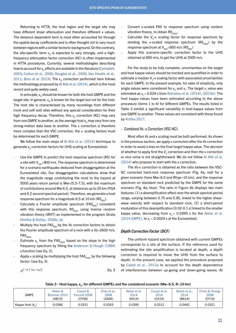
The Vs-κ correction is obtained as the ratio between the VSC-KC corrected hard-rock response spectrum (Fig. 4a; red) for a given scenario (here Mw=6.0 and Rhyp=10 km), and the response spectrum on standard rock predicted by the GMPE for the same scenario (Fig. 4a; blue). The ratio in Figure 4b displays two main features: (1) a deamplification effect over the whole spectral period range, varying between 0.75 and 0.95, linked to the higher shear-wave velocity with respect to standard rock, (2) a short-period modulation of this deamplification [0.02-0.1 s] linked to the smaller kappa value, decreasing from κ h = 0.0395 s for the Akkar et al. (2014 GMPE), to κ t = 0.0024 s at the Euroseistest.

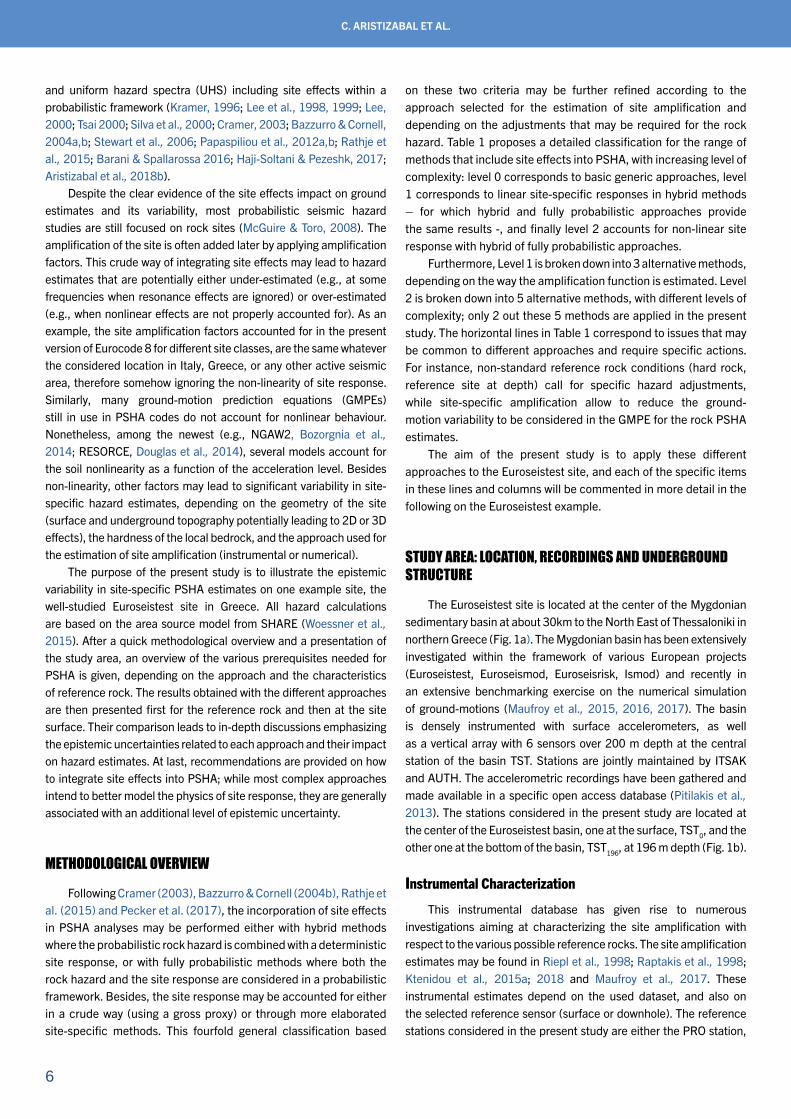
Depth Correction Factor (DCF)

The uniform hazard spectrum obtained with current GMPEs corresponds to a site at the surface. If the reference used for estimating the site amplification is located at depth, a depth correction is required to move the UHS from the surface to depth. In the present case, we applied the procedure proposed by Cadet et al., 2012a to account for the depth dependence of interferences between up-going and down-going waves. At

Table 3 - Host kappa, κh, for different GMPEs and the considered scenario (Mw=6.5, R=10 km)

GMPEAkkar &

Bommer 2010 (AB10)

Cauzzi & Faccioli 2008

(CY08)

Zhao et al., 2006

(ZA06)

Akkar et al. 2014

(AA14)

Cauzzi et al. 2014

(CA14)

Boore et al., 2014

(BA14)

Chiou & Youngs 2008

(CY14)

Kappa Host (kh) 0.0366 0.0331 0.0353 0.0395 0.0312 0.0442 0.0321

12


the surface they systematically interfere constructively (free-surface effect), while at depth they may interfere destructively or constructively depending on the ratio between the depth and the wavelength. This depth correction factor (DCF) is described in the dimensionless frequency space as the product of two frequency-dependent functions, C1 and C2 (Eq. 4).

The Vs-κ correction is obtained as the ratio between the VSC-KC corrected hard-rock 280

response spectrum (Figure 4a; red) for a given scenario (here Mw=6.0 and Rhyp=10 km), and 281

the response spectrum on standard rock predicted by the GMPE for the same scenario (Figure 282

4a; blue). The ratio in Figure 4b displays two main features: (1) a deamplification effect over 283

the whole spectral period range, varying between 0.75 and 0.95, linked to the higher shear-284

wave velocity with respect to standard rock, (2) a short-period modulation of this 285

deamplification [0.02-0.1 s] linked to the smaller kappa value, decreasing from 𝜅𝜅ℎ=0.0395 s 286

for the AKKAR et alii, 2014 GMPE, to 𝜅𝜅𝑡𝑡=0.0024 s at the Euroseistest. 287

4.1.2 Depth Correction Factor (DCF) 288

The uniform hazard spectrum obtained with current GMPEs corresponds to a site at the 289

surface. If the reference used for estimating the site amplification is located at depth, a depth 290

correction is required to move the UHS from the surface to depth. In the present case, we 291

applied the procedure proposed by CADET et alii, 2012a to account for the depth dependence 292

of interferences between up-going and down-going waves. At the surface they systematically 293

interfere constructively (free-surface effect), while at depth they may interfere destructively or 294

constructively depending on the ratio between the depth and the wavelength. This depth 295

correction factor (DCF) is described in the dimensionless frequency space as the product of 296

two frequency-dependent functions, C1 and C2 (Eq. 4). 297

DCF = C1ሺfሻ ∙ C2ሺfሻ Eq. 4

C1 (Eq. 5) is linked to the free surface and attenuation effects, while C2 (Eq. 6) is linked with 298

the destructive interference effects mainly around the fundamental frequency. C2 is therefore 299

peaked at the fundamental destructive frequency fdest and characterized by a peak amplitude 300

Eq. 4

C1 (Eq. 5) is linked to the free surface and attenuation effects, while C2 (Eq. 6) is linked with the destructive interference effects mainly around the fundamental frequency. C2 is therefore peaked at the fundamental destructive frequency fdest and characterised by a peak amplitude A. The proposed functional forms are a smoothed step (arctan) for C1, and Gaussian like for C2 (see Cadet et al., 2012a for more details):

A. The proposed functional forms are a smoothed step (arctan) for C1, and Gaussian like for 301

C2 (see CADET et alii, 2012a for more details): 302

𝐶𝐶1ሺ𝑓𝑓ሻ = 1 + 𝐵𝐵 ∙ arctan ሺ𝑓𝑓/𝑓𝑓𝑑𝑑𝑑𝑑𝑑𝑑𝑑𝑑ሻ𝜋𝜋 2Τ Eq. 5

𝐶𝐶2ሺ𝑓𝑓ሻ = 1 + ሺ𝐴𝐴 − 1ሻ ∙ 𝑒𝑒−ሺ𝑓𝑓/𝑓𝑓𝑑𝑑𝑑𝑑𝑑𝑑𝑑𝑑−1ሻ2

ሺ2𝜎𝜎ሻ2 Eq. 6

Following Cadet et alii, 2012a, we use the generic values for the correction of response 303

spectra, i.e., A=1.8, σ=0.15, and B=0.8, while the frequency dependence is controlled by the 304

actually measured destructive frequency of the soil column (fdest = 𝑉𝑉𝑉𝑉തതത/4H = 0.7 Hz), where H 305

is the depth of the downhole instrument and 𝑉𝑉𝑉𝑉തതത the average velocity over that depth. 306

4.1.3 Purely instrumental correction: use of site-specific residual (δS2S,rock) 307

As explained in BARD et alii, 2019, the availability of numerous recordings at the rock 308

reference sites allows to use a purely instrumental correction, derived from the systematic 309

comparison of reference rock recordings with the GMPE predictions. Also, as described in AL 310

ATIK et alii, 2010, the corresponding residuals 𝛥𝛥𝑑𝑑𝑑𝑑 (Eq. 7) can be decomposed in a between-311

event term 𝛿𝛿𝐵𝐵𝑑𝑑 and a 𝛿𝛿𝑊𝑊𝑑𝑑𝑑𝑑 within-event term, where subscripts e and s stand for event e and 312

station s: 313

𝛥𝛥𝑑𝑑𝑑𝑑 = 𝛿𝛿𝑊𝑊𝑑𝑑𝑑𝑑 + 𝛿𝛿𝐵𝐵𝑑𝑑 Eq. 7

Then, the within-event residual term, 𝛿𝛿𝑊𝑊𝑑𝑑𝑑𝑑 , can be further broken down into a site term, 314

δS2Ss, and a site-and-event corrected residual 𝛿𝛿𝑊𝑊𝑊𝑊𝑑𝑑𝑑𝑑 with zero mean, as follows: 315

𝛿𝛿𝑊𝑊𝑑𝑑𝑑𝑑 = 𝛿𝛿𝑊𝑊2𝑊𝑊𝑑𝑑 + 𝛿𝛿𝑊𝑊𝑊𝑊𝑑𝑑𝑑𝑑 Eq. 8

Eq. 5
















station s: 313





Eq. 6

Following Cadet et al. (2012a), we use the generic values for the correction of response spectra, i.e., A=1.8, σ=0.15, and B=0.8, while the frequency dependence is controlled by the actually measured destructive frequency of the soil column (fdest = Vs/4H = 0.7 Hz), where H is the depth of the downhole instrument and Vs the average velocity over that depth.

Purely instrumental correction: use of site-specific residual (δS2S, rock)

As explained in Bard et al. (2020), the availability of numerous recordings at the rock reference sites allows to use a purely instrumental correction, derived from the systematic comparison of reference rock recordings with the GMPE predictions. Also, as described in Al Atik et al. (2010), the corresponding residuals Δes (Eq. 7) can be decomposed in a between-event term δBe and a δWes within-event term, where subscripts e and s stand for event e and station s:
















station s: 313





Eq. 7

Then, the within-event residual term, δWes, can be further broken down into a site term, δS2Ss, and a site-and-event corrected residual δWSes with zero mean, as follows:
















station s: 313





Eq. 8

Ktenidou et al. (2015a) performed this analysis and calculated δS2Ss

term at TST site using the Akkar et al. (2014) GMPE, for various oscillator periods (Eq. 9 and Eq. 10). They obtained the values listed in Table 4, separately for the surface (TST0) and downhole sites (TST196). For each site, the δS2Ss term has been calculated either applying the GMPE with its site term S based on the value of the VS30 proxy (WIST), or without its site term (WOST) with respect to standard rock reference (VS30 = 800 m/s).

KTENIDOU et alii, 2015a performed this analysis and calculated 𝛿𝛿𝛿𝛿2𝛿𝛿𝑠𝑠 term at TST site using 316

the AKKAR et alii, 2014 GMPE, for various oscillator periods (Eq. 9 and Eq. 10). They 317

obtained the values listed in Table 4, separately for the surface (TST0) and downhole sites 318

(TST196). For each site, the 𝛿𝛿𝛿𝛿2𝛿𝛿𝑠𝑠 term has been calculated either applying the GMPE with its 319

site term S based on the value of the VS30 proxy (WIST), or without its site term (WOST) 320

with respect to standard rock reference (VS30 = 800 m/s). 321

𝑙𝑙𝑙𝑙ሺ𝑌𝑌ሻ = 𝑙𝑙𝑙𝑙[𝑌𝑌𝑅𝑅𝑅𝑅𝑅𝑅ሺ𝑀𝑀𝑤𝑤, 𝑅𝑅, 𝛿𝛿𝑆𝑆𝑅𝑅ሻ] + 𝑙𝑙𝑙𝑙[𝛿𝛿ሺ𝑉𝑉𝑠𝑠30, 𝑃𝑃𝑃𝑃𝑃𝑃𝑅𝑅𝑅𝑅𝑅𝑅ሻ] + 𝜀𝜀𝜀𝜀 Eq. 9

322

𝑙𝑙𝑙𝑙ሺ𝛿𝛿ሻ =

ە۔

ۓ

𝑏𝑏1 𝑙𝑙𝑙𝑙 ൬ 𝑉𝑉𝑆𝑆30𝑉𝑉𝑅𝑅𝑅𝑅𝑅𝑅

൰ + 𝑏𝑏2 𝑙𝑙𝑙𝑙 ൦𝑃𝑃𝑃𝑃𝑃𝑃𝑅𝑅𝑅𝑅𝑅𝑅 + 𝑐𝑐 ቀ 𝑉𝑉𝑆𝑆30

𝑉𝑉𝑅𝑅𝑅𝑅𝑅𝑅ቁ

𝑛𝑛

ሺ𝑃𝑃𝑃𝑃𝑃𝑃𝑅𝑅𝑅𝑅𝑅𝑅 + 𝑐𝑐ሻ ቀ 𝑉𝑉𝑆𝑆30𝑉𝑉𝑅𝑅𝑅𝑅𝑅𝑅

ቁ𝑛𝑛൪

𝑏𝑏1 𝑙𝑙𝑙𝑙 𝑚𝑚𝑚𝑚𝑙𝑙ሺ𝑉𝑉𝑆𝑆30, 𝑉𝑉𝐶𝐶𝐶𝐶𝐶𝐶𝑉𝑉𝑅𝑅𝑅𝑅𝑅𝑅

൨

Nonlinear term

Linear term

Eq. 10

The corresponding "site-specific" 𝛿𝛿𝛿𝛿2𝛿𝛿𝑠𝑠 terms based on residuals are plotted in Figure 6a as a 323

function of oscillator period (red curves). Residuals at the downhole site are negative when 324

calculated with respect to standard rock (WIST, red dashed curve). Moreover, residuals are 325

larger in the WOST case (dashed lines) than in the WIST case (negative for TST196, and 326

positive for TST0). At this stage, site-specific residuals (Figure 6a) and depth corrections 327

(Figure 5) cannot be compared, since the DCF correction should be combined with the VSC-328

KC correction before being compared with the residual approach. 329

Eq. 9

Fig. 4 - Combined Vs-κ correction at Euroseistest site: (a), response spectrum (RS) on standard rock predicted by the GMPE (VS30 800 m/s, blue) and Vs-κ corrected response spectrum (RS) (VS30=2600 m/s, red); (b) Vs-κ scaling factor, which is the ratio between the scaled response spectrum (VS30=2600 m/s) and the response spectrum predicted by the GMPE at VS30 =800 m/s. The GMPE used is Akkar et al., 2014. Calculations performed for a scenario earthquake Mw 6.0 at 10km. The target κ is 0.0024 s.

(b)(a)

13


Nonlinear term

KTENIDOU et alii, 2015a performed this analysis and calculated 𝛿𝛿𝛿𝛿2𝛿𝛿𝑠𝑠 term at TST site using 316

the AKKAR et alii, 2014 GMPE, for various oscillator periods (Eq. 9 and Eq. 10). They 317

obtained the values listed in Table 4, separately for the surface (TST0) and downhole sites 318

(TST196). For each site, the 𝛿𝛿𝛿𝛿2𝛿𝛿𝑠𝑠 term has been calculated either applying the GMPE with its 319

site term S based on the value of the VS30 proxy (WIST), or without its site term (WOST) 320

with respect to standard rock reference (VS30 = 800 m/s). 321

𝑙𝑙𝑙𝑙ሺ𝑌𝑌ሻ = 𝑙𝑙𝑙𝑙[𝑌𝑌𝑅𝑅𝑅𝑅𝑅𝑅ሺ𝑀𝑀𝑤𝑤, 𝑅𝑅, 𝛿𝛿𝑆𝑆𝑅𝑅ሻ] + 𝑙𝑙𝑙𝑙[𝛿𝛿ሺ𝑉𝑉𝑠𝑠30, 𝑃𝑃𝑃𝑃𝑃𝑃𝑅𝑅𝑅𝑅𝑅𝑅ሻ] + 𝜀𝜀𝜀𝜀 Eq. 9

322

𝑙𝑙𝑙𝑙ሺ𝛿𝛿ሻ =

ە۔

ۓ

𝑏𝑏1 𝑙𝑙𝑙𝑙 ൬ 𝑉𝑉𝑆𝑆30𝑉𝑉𝑅𝑅𝑅𝑅𝑅𝑅

൰ + 𝑏𝑏2 𝑙𝑙𝑙𝑙 ൦𝑃𝑃𝑃𝑃𝑃𝑃𝑅𝑅𝑅𝑅𝑅𝑅 + 𝑐𝑐 ቀ 𝑉𝑉𝑆𝑆30

𝑉𝑉𝑅𝑅𝑅𝑅𝑅𝑅ቁ

𝑛𝑛

ሺ𝑃𝑃𝑃𝑃𝑃𝑃𝑅𝑅𝑅𝑅𝑅𝑅 + 𝑐𝑐ሻ ቀ 𝑉𝑉𝑆𝑆30𝑉𝑉𝑅𝑅𝑅𝑅𝑅𝑅

ቁ𝑛𝑛൪

𝑏𝑏1 𝑙𝑙𝑙𝑙 𝑚𝑚𝑚𝑚𝑙𝑙ሺ𝑉𝑉𝑆𝑆30, 𝑉𝑉𝐶𝐶𝐶𝐶𝐶𝐶𝑉𝑉𝑅𝑅𝑅𝑅𝑅𝑅

൨

Nonlinear term

Linear term

Eq. 10

The corresponding "site-specific" 𝛿𝛿𝛿𝛿2𝛿𝛿𝑠𝑠 terms based on residuals are plotted in Figure 6a as a 323

function of oscillator period (red curves). Residuals at the downhole site are negative when 324

calculated with respect to standard rock (WIST, red dashed curve). Moreover, residuals are 325

larger in the WOST case (dashed lines) than in the WIST case (negative for TST196, and 326

positive for TST0). At this stage, site-specific residuals (Figure 6a) and depth corrections 327

(Figure 5) cannot be compared, since the DCF correction should be combined with the VSC-328

KC correction before being compared with the residual approach. 329

Eq. 10

Linear term

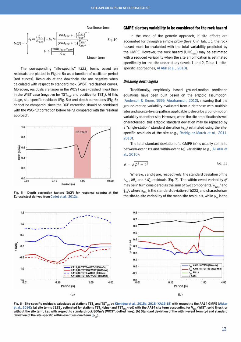
The corresponding “site-specific” δS2Ss terms based on residuals are plotted in Figure 6a as a function of oscillator period (red curves). Residuals at the downhole site are negative when calculated with respect to standard rock (WIST, red dashed curve). Moreover, residuals are larger in the WOST case (dashed lines) than in the WIST case (negative for TST196, and positive for TST0). At this stage, site-specific residuals (Fig. 6a) and depth corrections (Fig. 5) cannot be compared, since the DCF correction should be combined with the VSC-KC correction before being compared with the residual approach.

GMPE aleatory variability to be considered for the rock hazard

In the case of the generic approach, if site effects are accounted for through a simple proxy (level 0 in Tab. 1 ), the rock hazard must be evaluated with the total variability predicted by the GMPE. However, the rock hazard (UHSrock) may be estimated with a reduced variability when the site amplification is estimated specifically for the site under study (levels 1 and 2, Table 1 , site-specific approaches, Al Atik et al., 2010).

Breaking down sigma

Traditionally, empirically based ground-motion prediction equations have been built based on the ergodic assumption, (Anderson & Brune, 1999; Abrahamson, 2012), meaning that the ground-motion variability evaluated from a database with multiple sites and source-to-site paths is applicable to describe ground-motion variability at another site. However, when the site amplification is well characterised, this ergodic standard deviation may be replaced by a “single-station” standard deviation (σSS) estimated using the site-specific residuals at the site (e.g., Rodriguez-Marek et al., 2011, 2013).

The total standard deviation of a GMPE (σ) is usually split into between-event (τ) and within-event (f) variability (e.g., Al Atik et al., 2010):

4.2 GMPE aleatory variability to be considered for the rock hazard 330

In the case of the generic approach, if site effects are accounted for through a simple proxy 331

(level 0 in Table 1 ), the rock hazard must be evaluated with the total variability predicted by 332

the GMPE. However, the rock hazard (UHSrock) may be estimated with a reduced variability 333

when the site amplification is estimated specifically for the site under study (levels 1 and 2, 334

Table 1 , site-specific approaches, AL ATIK et alii, 2010). 335

4.2.1 Breaking down sigma 336

Traditionally, empirically based ground-motion prediction equations have been built based on 337

the ergodic assumption, (ANDERSON & BRUNE, 1999; ABRAHAMSON 2012), meaning that the 338

ground-motion variability evaluated from a database with multiple sites and source-to-site 339

paths is applicable to describe ground-motion variability at another site. However, when the 340

site amplification is well characterized, this ergodic standard deviation may be replaced by a 341

“single-station” standard deviation (σSS) estimated using the site-specific residuals at the site 342

(e.g. RODRIGUEZ-MAREK et alii, 2011; 2013). 343

The total standard deviation of a GMPE (σ) is usually split into between-event (τ) and within-344

event (ϕ) variability (e.g. AL ATIK et alii, 2010): 345

𝜎𝜎 = ඥ𝜙𝜙2 + 𝜏𝜏2 Eq. 11

Where 𝜎𝜎 , τ and 𝜙𝜙 are, respectively, the standard deviation of the 𝛥𝛥𝑒𝑒𝑒𝑒 , 𝛿𝛿𝐵𝐵𝑒𝑒 and 𝛿𝛿𝑊𝑊𝑒𝑒𝑒𝑒 346

residuals (Eq. 7). The within-event variability 𝜙𝜙2 may be in turn considered as the sum of 347

two components, 𝜙𝜙𝑆𝑆2𝑆𝑆𝑒𝑒2 and 𝜙𝜙𝑆𝑆𝑆𝑆

2 , where 𝜙𝜙𝑆𝑆2𝑆𝑆𝑒𝑒 is the standard deviation of δS2Ss and 348

characterizes the site-to-site variability of the mean site residuals, while ϕSS is the standard 349

Eq. 11

Where σ, τ and f are, respectively, the standard deviation of the Δes

, δBe and δWes residuals (Eq. 7). The within-event variability f2 may be in turn considered as the sum of two components, fS2Ss

2 and fSS

2, where fS2Ss is the standard deviation of δS2Ss and characterises the site-to-site variability of the mean site residuals, while fSS is the

Fig. 5 - Depth correction factors (DCF) for response spectra at the Euroseistest derived from Cadet et al., 2012a.

Fig. 6 - Site-specific residuals calculated at stations TST0 and TST196 by Ktenidou et al., 2015a, 2018 (KA15;18) with respect to the AA14 GMPE (Akkar et al., 2014): (a) site terms δS2Ss, estimated for stations TST0 (blue) and TST196 (red) with the AA14 site term accounting for VS30 (WIST, solid lines), or without the site term, i.e., with respect to standard rock 800m/s (WOST, dotted lines). (b) Standard deviation of the within-event term (ϕ) and standard deviation of the site specific within-event residual term (φSS).

(b)(a)

14


standard deviation of the within-event residual term (δWes), i.e., the variability of the site amplification around δS2Ss. The total standard deviation can thus be expressed as:

deviation of the within-event residual term (δWes), i.e., the variability of the site amplification 350

around δS2Ss. The total standard deviation can thus be expressed as: 351

𝜎𝜎 = ට𝜙𝜙𝑆𝑆2𝑆𝑆𝑆𝑆2 + 𝜙𝜙𝑆𝑆𝑆𝑆

2 + 𝜏𝜏2 Eq. 12

When the site term is estimated in a site-specific way (including the associated epistemic 352

uncertainties), the total sigma may be replaced by the smaller, "single-station" sigma, which 353

does not have to account for the site-to-site variability: 354

𝜎𝜎𝑆𝑆𝑆𝑆 = ට𝜙𝜙𝑆𝑆𝑆𝑆2 + 𝜏𝜏2 Eq. 13

In such a case, the site-specific uniform hazard spectrum, 𝑈𝑈𝑈𝑈𝑈𝑈𝑆𝑆𝑠𝑠𝑠𝑠𝑠𝑠−𝑆𝑆𝑠𝑠𝑠𝑠𝑠𝑠𝑠𝑠𝑠𝑠𝑠𝑠𝑠𝑠ሺ𝑇𝑇ሻ, can be derived 355

by adjusting the "reference" UHS obtained with the single-station variability with the site-356

specific amplification factor AFs, as follows: 357

𝑈𝑈𝑈𝑈𝑈𝑈𝑈𝑈𝑆𝑆𝑆𝑆𝑆𝑆−𝑠𝑠𝑠𝑠𝑆𝑆𝑠𝑠𝑆𝑆𝑠𝑠𝑆𝑆𝑠𝑠ሺ𝑇𝑇ሻ = 𝑈𝑈𝑈𝑈𝑈𝑈𝜎𝜎𝑠𝑠𝑠𝑠ሺ𝐺𝐺𝐺𝐺𝐺𝐺𝐺𝐺ሻሺ𝑇𝑇ሻ · 𝐴𝐴𝐴𝐴𝑆𝑆ሺ𝑇𝑇ሻ Eq. 14

4.2.2 Application to Euroseistest: Single-station variability 358

Table 5 lists the value of 𝜙𝜙𝑆𝑆𝑆𝑆 for the two locations TST0 and TST196 , as derived by KTENIDOU 359

et alii, 2018 from weak to moderate motions recorded at these stations (PGA < 1 m/s2). These 360

within-event variabilities are compared to the total standard deviation 𝜙𝜙 in the GMPE AKKAR 361

et alii, 2014, as well as to the average 𝜙𝜙𝑆𝑆𝑆𝑆 value proposed by RODRIGUEZ-MAREK et alii, 2013 362

from an analysis of a large database of ground-motions from different regions (California, 363

Switzerland, Taiwan, Turkey and Japan), which may be used as a default value when no site-364

specific estimate is available. Figure 6b displays these 𝜙𝜙𝑆𝑆𝑆𝑆 values with respect to the 365

oscillator period. These single-station variabilities are much lower than the AA14 total 366

Eq. 12

When the site term is estimated in a site-specific way (including the associated epistemic uncertainties), the total sigma may be replaced by the smaller, “single-station” sigma, which does not have to account for the site-to-site variability:




2 + 𝜏𝜏2 Eq. 12


















Eq. 13

In such a case, the site-specific uniform hazard spectrum, UHSSite-specific(T), can be derived by adjusting the “reference” UHS obtained with the single-station variability with the site-specific amplification factor AFs, as follows:




2 + 𝜏𝜏2 Eq. 12


















Eq. 14

Application to Euroseistest: Single-station variability

Table 5 lists the value of fSS for the two locations TST0 and TST196, as derived by Ktenidou et al. (2018) from weak to moderate motions recorded at these stations (PGA < 1 m/s2). These within-event variabilities are compared to the total standard deviation f in the GMPE Akkar et al. (2014), as well as to the average fSS value proposed by Rodriguez-Marek et al. (2013) from an analysis of a large database of ground-motions from different regions (California, Switzerland, Taiwan, Turkey and Japan), which may be used as a default value

when no site-specific estimate is available. Figure 6b displays these fSS values with respect to the oscillator period. These single-station variabilities are much lower than the AA14 total within-event standard deviation, over the whole period range at TST0 and mainly at short to intermediate periods for TST196. They are also generally smaller than the 0.45 average value proposed by Rodriguez-Marek et al. (2013), except at long periods for TST196. These rather large fSS values at TST196 might be related with the relatively limited dataset over which these statistics could be derived (limited range in magnitude and distance of events). The recordings used correspond only to low-to-moderate magnitude events, with a site response always in the linear domain (see Ktenidou et al., 2018, and Bard et al., 2020, for more details). Nonetheless, several past studies suggest that fSS from strong motion data tends to be smaller than fSS from weak motion data (Abrahamson & Sykora, 1993; Toro et al., 1997). Using these single station sigmas at Euroseistest will lead to a reduction of hazard, with respect to hazard calculated with the total sigma. As the fSS

values might be overestimated at long periods (above 1.0 s), these hazard estimates may be considered as upper bounds.

REFERENCE-ROCK HAZARD ESTIMATES AT EUROSEISTEST

This section presents the UHS estimated at the down-hole reference site TST196 for a 5000 year return period, with a discussion of the respective impacts of the single-station sigma, the rock-to-hard rock correction and the depth correction. All the PSHA computations (for rock and generic sites as well, level 0a) were performed with the OpenQuake engine which is now widely used worldwide probably because of its free availability and of its various characteristics as presented in Pagani et al. (2014).

Table 4 - Site terms (δS2Ss) used in this study. Residuals based on Akkar et al., 2014 GMPE as derived by Ktenidou et al., 2015a, and corresponding to a natural logarithm scale.

Period (s) δS2Ss TST0-WIST δS2Ss TST196-WIST δS2Ss TST0-WOST δS2Ss TST196-WOST

0.00 0.285 -0.442 0.8708 -0.5628

0.01 0.231 -0.393 0.8124 -0.5133

0.02 0.199 -0.359 0.757 -0.4742

0.05 0.510 -0.639 0.8062 -0.6999

0.10 0.412 -0.714 0.7892 -0.7914

0.13 0.262 -0.606 0.8169 -0.7209

0.15 0.146 -0.580 0.8198 -0.7193

0.20 0.088 -0.366 0.9982 -0.5535

0.30 0.081 -0.242 1.2327 -0.4794

0.50 0.006 -0.137 1.3249 -0.4091

0.65 -0.038 -0.250 1.3332 -0.5324

0.75 0.000 -0.166 1.4054 -0.4563

1.00 -0.061 0.057 1.3521 -0.2348

2.00 -0.026 0.110 1.2429 -0.1519

3.00 -0.026 0.110 1.2429 -0.1519

4.00 -0.026 0.110 1.2429 -0.1519

15


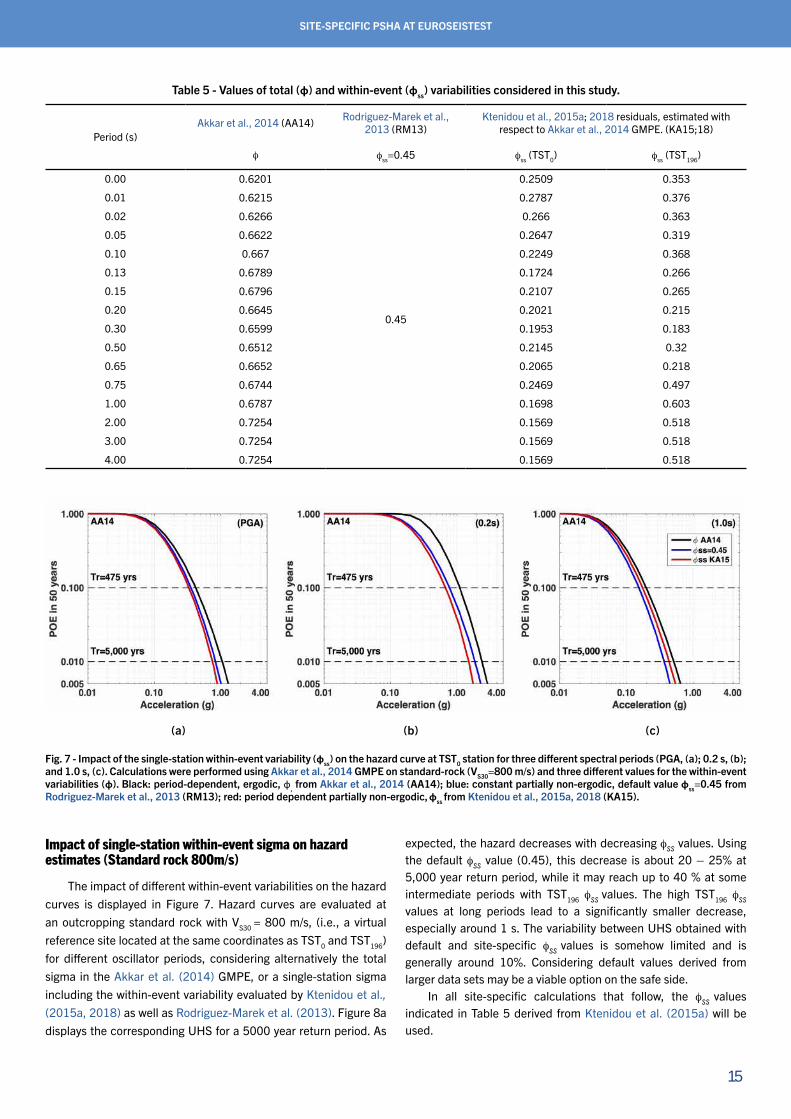
Impact of single-station within-event sigma on hazard estimates (Standard rock 800m/s)

The impact of different within-event variabilities on the hazard curves is displayed in Figure 7. Hazard curves are evaluated at an outcropping standard rock with VS30 = 800 m/s, (i.e., a virtual reference site located at the same coordinates as TST0 and TST196) for different oscillator periods, considering alternatively the total sigma in the Akkar et al. (2014) GMPE, or a single-station sigma including the within-event variability evaluated by Ktenidou et al., (2015a, 2018) as well as Rodriguez-Marek et al. (2013). Figure 8a displays the corresponding UHS for a 5000 year return period. As

expected, the hazard decreases with decreasing fSS values. Using the default fSS value (0.45), this decrease is about 20 – 25% at 5,000 year return period, while it may reach up to 40 % at some intermediate periods with TST196 fSS values. The high TST196 fSS values at long periods lead to a significantly smaller decrease, especially around 1 s. The variability between UHS obtained with default and site-specific fSS values is somehow limited and is generally around 10%. Considering default values derived from larger data sets may be a viable option on the safe side.

In all site-specific calculations that follow, the fSS values indicated in Table 5 derived from Ktenidou et al. (2015a) will be used.

Table 5 - Values of total (φ) and within-event (φss) variabilities considered in this study.

Period (s)Akkar et al., 2014 (AA14) Rodriguez-Marek et al.,

2013 (RM13)Ktenidou et al., 2015a; 2018 residuals, estimated with

respect to Akkar et al., 2014 GMPE. (KA15;18)

f fss=0.45 fss (TST0) fss (TST196)

0.00 0.6201

0.45

0.2509 0.353

0.01 0.6215 0.2787 0.376

0.02 0.6266 0.266 0.363

0.05 0.6622 0.2647 0.319

0.10 0.667 0.2249 0.368

0.13 0.6789 0.1724 0.266

0.15 0.6796 0.2107 0.265

0.20 0.6645 0.2021 0.215

0.30 0.6599 0.1953 0.183

0.50 0.6512 0.2145 0.32

0.65 0.6652 0.2065 0.218

0.75 0.6744 0.2469 0.497

1.00 0.6787 0.1698 0.603

2.00 0.7254 0.1569 0.518

3.00 0.7254 0.1569 0.518

4.00 0.7254 0.1569 0.518

Fig. 7 - Impact of the single-station within-event variability (φss) on the hazard curve at TST0 station for three different spectral periods (PGA, (a); 0.2 s, (b); and 1.0 s, (c). Calculations were performed using Akkar et al., 2014 GMPE on standard-rock (VS30=800 m/s) and three different values for the within-event variabilities (φ). Black: period-dependent, ergodic, φ, from Akkar et al., 2014 (AA14); blue: constant partially non-ergodic, default value φss=0.45 from Rodriguez-Marek et al., 2013 (RM13); red: period dependent partially non-ergodic, φss from Ktenidou et al., 2015a, 2018 (KA15).

(a) (b) (c)

16


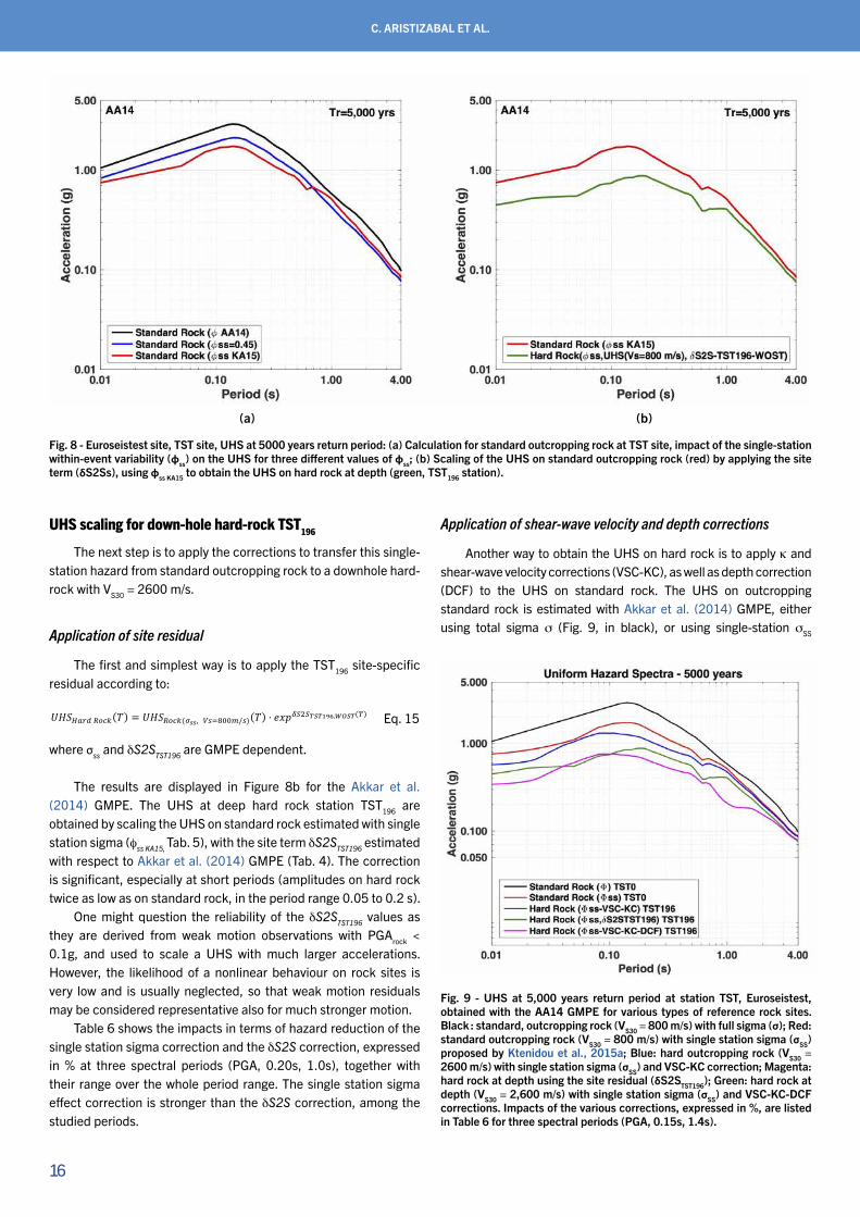
UHS scaling for down-hole hard-rock TST196

The next step is to apply the corrections to transfer this single-station hazard from standard outcropping rock to a downhole hard-rock with VS30 = 2600 m/s.

Application of site residual

The first and simplest way is to apply the TST196 site-specific residual according to:

virtual reference site located at the same coordinates as TST0 and TST196) for different 390

oscillator periods, considering alternatively the total sigma in the AKKAR et alii, 2014 GMPE, 391

or a single-station sigma including the within-event variability evaluated by KTENIDOU et alii, 392

2015a; 2018 as well as RODRIGUEZ-MAREK et alii, 2013. Figure 8a displays the corresponding 393

UHS for a 5000 year return period. As expected, the hazard decreases with decreasing ϕss 394

values. Using the default ϕss value (0.45), this decrease is about 20 – 25% at 5,000 year return 395

period, while it may reach up to 40 % at some intermediate periods with TST196 ϕss values. 396

The high TST196 ϕss values at long periods lead to a significantly smaller decrease, especially 397

around 1 s. The variability between UHS obtained with default and site-specific ϕss values is 398

somehow limited and is generally around 10%. Considering default values derived from 399

larger data sets may be a viable option on the safe side. 400

In all site-specific calculations that follow, the ϕss values indicated in Table 5 derived from 401

KTENIDOU et alii, 2015a will be used. 402

5.2 UHS scaling for down-hole hard-rock TST196 403

The next step is to apply the corrections to transfer this single-station hazard from standard 404

outcropping rock, to a downhole hard-rock with VS30 = 2600 m/s. 405

5.2.1 Application of site residual 406

The first and simplest way is to apply the TST196 site-specific residual according to: 407

𝑈𝑈𝑈𝑈𝑈𝑈𝐻𝐻𝐻𝐻𝐻𝐻𝐻𝐻 𝑅𝑅𝑅𝑅𝑅𝑅𝑅𝑅ሺ𝑇𝑇ሻ = 𝑈𝑈𝑈𝑈𝑈𝑈𝑅𝑅𝑅𝑅𝑅𝑅𝑅𝑅ሺ𝜎𝜎𝑠𝑠𝑠𝑠, 𝑉𝑉𝑉𝑉=800𝑚𝑚/𝑉𝑉ሻሺ𝑇𝑇ሻ · 𝑒𝑒𝑒𝑒𝑒𝑒𝛿𝛿𝛿𝛿2𝛿𝛿𝑇𝑇𝑇𝑇𝑇𝑇196,𝑊𝑊𝑊𝑊𝑇𝑇𝑇𝑇ሺ𝑇𝑇ሻ Eq. 15

where 𝜎𝜎𝑉𝑉𝑉𝑉 and 𝛿𝛿𝑈𝑈2𝑈𝑈𝑇𝑇𝛿𝛿𝑇𝑇196 are GMPE dependent. 408

Eq. 15

where σss and δS2STST196 are GMPE dependent.

The results are displayed in Figure 8b for the Akkar et al. (2014) GMPE. The UHS at deep hard rock station TST196 are obtained by scaling the UHS on standard rock estimated with single station sigma (fss KA15, Tab. 5), with the site term δS2STST196 estimated with respect to Akkar et al. (2014) GMPE (Tab. 4). The correction is significant, especially at short periods (amplitudes on hard rock twice as low as on standard rock, in the period range 0.05 to 0.2 s).

One might question the reliability of the δS2STST196 values as they are derived from weak motion observations with PGArock < 0.1g, and used to scale a UHS with much larger accelerations. However, the likelihood of a nonlinear behaviour on rock sites is very low and is usually neglected, so that weak motion residuals may be considered representative also for much stronger motion.

Table 6 shows the impacts in terms of hazard reduction of the single station sigma correction and the δS2S correction, expressed in % at three spectral periods (PGA, 0.20s, 1.0s), together with their range over the whole period range. The single station sigma effect correction is stronger than the δS2S correction, among the studied periods.

Application of shear-wave velocity and depth corrections

Another way to obtain the UHS on hard rock is to apply κ and shear-wave velocity corrections (VSC-KC), as well as depth correction (DCF) to the UHS on standard rock. The UHS on outcropping standard rock is estimated with Akkar et al. (2014) GMPE, either using total sigma σ (Fig. 9, in black), or using single-station σSS

Fig. 8 - Euroseistest site, TST site, UHS at 5000 years return period: (a) Calculation for standard outcropping rock at TST site, impact of the single-station within-event variability (φss) on the UHS for three different values of φss; (b) Scaling of the UHS on standard outcropping rock (red) by applying the site term (δS2Ss), using φss KA15 to obtain the UHS on hard rock at depth (green, TST196 station).

Fig. 9 - UHS at 5,000 years return period at station TST, Euroseistest, obtained with the AA14 GMPE for various types of reference rock sites. Black : standard, outcropping rock (VS30 = 800 m/s) with full sigma (σ); Red: standard outcropping rock (VS30 = 800 m/s) with single station sigma (σSS) proposed by Ktenidou et al., 2015a; Blue: hard outcropping rock (VS30 = 2600 m/s) with single station sigma (σSS) and VSC-KC correction; Magenta: hard rock at depth using the site residual (δS2STST196); Green: hard rock at depth (VS30 = 2,600 m/s) with single station sigma (σSS) and VSC-KC-DCF corrections. Impacts of the various corrections, expressed in %, are listed in Table 6 for three spectral periods (PGA, 0.15s, 1.4s).

(a) (b)

17


(red). Then, by applying VSC-KC and DCF corrections to the UHS on standard rock, the UHS on deep hard rock may be obtained (magenta). To understand the relative effects of the VSC-KC and DCF corrections, the UHS corrected with VSC-KC only is also displayed (blue), while the corresponding values for three different periods are listed in Table 6.

The depth correction is stronger than the VSC-KC correction among all period ranges. The short period range is associated mainly to κ0 effect (Fig. 4a) which somehow “boosts” the short period and counterbalance the VSC effect, resulting in a very small VSC-KC correction. The intermediate period range (between 0.5 and 1.5 s) is associated to the destructive interference effects at depth (Fig. 5). Combined, these two corrections result in hazard reductions between [8-45]% among all periods, that are approximately equal to the hazard reductions corresponding to the consideration of single station sigma σSS instead of total sigma σ [12-45]% (Fig. 8a).

Comparison between both approaches

The UHS at TST196 station, located on hard rock at depth, is thus obtained either applying VSC-KC and DCF corrections to the UHS on standard rock (magenta curve in Fig. 9) or by applying site residual scaling (green). The UHS obtained through these two different methods are rather close. The site residual correction (δS2STST196) lead to slightly larger values than the VSC-KC-DCF correction over most of the period range. The average difference is about 23% , but it reaches a factor of 2 around 1.0 s as a consequence of the destructive interference (at fdest in the C2 correction). However, these relative differences remain relatively small compared to the overall correction from the outcropping standard rock (black and red curves) to the hard-rock down-hole location (magenta and green curves). At short and intermediate periods, the spectral accelerations obtained on hard rock at depth are much lower than the accelerations on outcropping standard rock (e.g. [0.66 – 0.87] g compared with [1.5-2.5] g at 0.2s). At long periods (larger than 1.0 s), the reduction in acceleration is lower.

As a conclusion, for this particular Euroseistest example, the reduction on rock hazard estimates is mainly due to single-station-sigma corrections (fss) and to depth corrections (DCF), with smaller contributions of the host-to-target corrections (HTT, i.e. VSC-KC), because of the relatively large κ0 value at hard rock

(κt = 0.024 s). Single-station-sigma corrections and depth corrections are comparable in the short to intermediate period range, while at long periods the largest reduction comes for the reduced aleatory variability. The total reductions are very significant (up to a factor of 3 at some periods) and emphasise the importance of a careful assessment of the reference rock in site-specific hazard assessment studies. However, these conclusions might be different for another site (for instance with a hard-bedrock with a smaller κ0 value), and could also be modulated would the epistemic uncertainty be considered in the different steps. One might question also the use of single-station variability UHS rock spectrum when using the Cadet et al. (2012a) depth correction, since the latter is mainly a generic correction tuned on the site-specific fundamental destructive frequency fdest: part of the differences between magenta and green curves in Figure 9 might be related to this variability issue.

ESTIMATION OF SITE-SPECIFIC SURFACE HAZARD

The various approaches to include site effects into PSHA are now applied to the Euroseistest TST site, starting with generic or only partially site-specific approaches (level 0), and going on with site-specific approaches involving first a linear (level 1) and then a non-linear (level 2) site response (Tab. 1). For each approach, details are provided about their practical implementation and the associated issues, and the results are discussed and compared.

Level 0 - Generic or Partially Site-Specific Approaches

The site effects are accounted for in an average and approximate way through one or several site proxies.

Level 0a – use of site proxies in GMPEs

This is the simplest (and most widely used) approach, which consists in assuming that the actual amplification at the site of interest can be reasonably approximated by the site term of the GMPEs used in the hazard estimation. In other words, the specific response of the site under study is assumed to be satisfactorily captured by the average site amplification of all stations in the GMPE

Table 6 - Impacts in terms of hazard reduction of the various corrections, expressed in %, at three spectral periods (PGA, 0.20s, 1.0s), together with their range over the whole period range.

Period (s) 0.01 (PGA) 0.2 1.0 [0.01-4.0]

5.2.1 Application of site residualSingle Station Sigma (SSS) 28% 40% 12% [12-41] %

DCF Site Residuals (δS2S) 29% 26% 18% [9-36] %

SSS & DCF 57% 65% 30% [23-71] %

5.2.2 Application of shear-wave velocity and depth corrections

Single Station Sigma (SSS) 28% 40% 12% [12-41] %

VSC-KC 18% 16% 7% [-3-18] %

DCF Cadet et al., 2012b 21% 18% 45% [8-45] %

SSS & VS-KC & DCF 67% 74% 64% [18-75] %

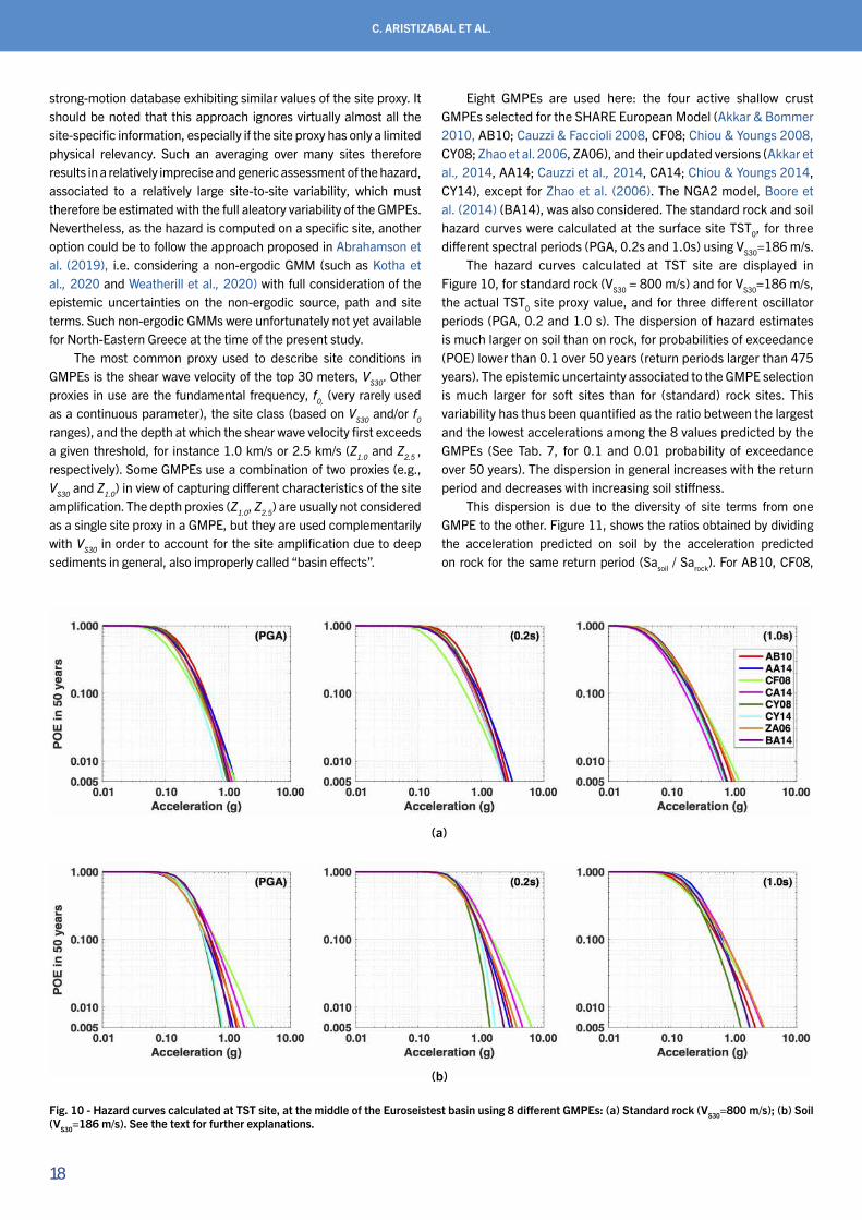
18


strong-motion database exhibiting similar values of the site proxy. It should be noted that this approach ignores virtually almost all the site-specific information, especially if the site proxy has only a limited physical relevancy. Such an averaging over many sites therefore results in a relatively imprecise and generic assessment of the hazard, associated to a relatively large site-to-site variability, which must therefore be estimated with the full aleatory variability of the GMPEs. Nevertheless, as the hazard is computed on a specific site, another option could be to follow the approach proposed in Abrahamson et al. (2019), i.e. considering a non-ergodic GMM (such as Kotha et al., 2020 and Weatherill et al., 2020) with full consideration of the epistemic uncertainties on the non-ergodic source, path and site terms. Such non-ergodic GMMs were unfortunately not yet available for North-Eastern Greece at the time of the present study.

The most common proxy used to describe site conditions in GMPEs is the shear wave velocity of the top 30 meters, VS30. Other proxies in use are the fundamental frequency, f0, (very rarely used as a continuous parameter), the site class (based on VS30 and/or f0 ranges), and the depth at which the shear wave velocity first exceeds a given threshold, for instance 1.0 km/s or 2.5 km/s (Z1.0 and Z2.5 , respectively). Some GMPEs use a combination of two proxies (e.g., VS30 and Z1.0) in view of capturing different characteristics of the site amplification. The depth proxies (Z1.0, Z2.5) are usually not considered as a single site proxy in a GMPE, but they are used complementarily with VS30 in order to account for the site amplification due to deep sediments in general, also improperly called “basin effects”.

Eight GMPEs are used here: the four active shallow crust GMPEs selected for the SHARE European Model (Akkar & Bommer 2010, AB10; Cauzzi & Faccioli 2008, CF08; Chiou & Youngs 2008, CY08; Zhao et al. 2006, ZA06), and their updated versions (Akkar et al., 2014, AA14; Cauzzi et al., 2014, CA14; Chiou & Youngs 2014, CY14), except for Zhao et al. (2006). The NGA2 model, Boore et al. (2014) (BA14), was also considered. The standard rock and soil hazard curves were calculated at the surface site TST0, for three different spectral periods (PGA, 0.2s and 1.0s) using VS30=186 m/s.

The hazard curves calculated at TST site are displayed in Figure 10, for standard rock (VS30 = 800 m/s) and for VS30=186 m/s, the actual TST0 site proxy value, and for three different oscillator periods (PGA, 0.2 and 1.0 s). The dispersion of hazard estimates is much larger on soil than on rock, for probabilities of exceedance (POE) lower than 0.1 over 50 years (return periods larger than 475 years). The epistemic uncertainty associated to the GMPE selection is much larger for soft sites than for (standard) rock sites. This variability has thus been quantified as the ratio between the largest and the lowest accelerations among the 8 values predicted by the GMPEs (See Tab. 7, for 0.1 and 0.01 probability of exceedance over 50 years). The dispersion in general increases with the return period and decreases with increasing soil stiffness.

This dispersion is due to the diversity of site terms from one GMPE to the other. Figure 11, shows the ratios obtained by dividing the acceleration predicted on soil by the acceleration predicted on rock for the same return period (Sasoil / Sarock). For AB10, CF08,

Fig. 10 - Hazard curves calculated at TST site, at the middle of the Euroseistest basin using 8 different GMPEs: (a) Standard rock (VS30=800 m/s); (b) Soil (VS30=186 m/s). See the text for further explanations.

(a)

(b)

19


ZA06 and CA14, these ratios remain mostly constant and above 1.0, whatever the hazard level. These GMPEs predict linear behavior with systematic amplification at all return periods (all acceleration levels) and for the three spectral periods. On the other hand, for AA14, CY08, CY14 and BA14, the ratios decay with increasing return period (increasing level of acceleration) for the three different spectral periods. These models include a nonlinear component in the site term (as shown for instance in Eq. 10 for the AA14 case). The large impact of the GMPE selection on soft soil hazard curves is thus mainly due to the variability of the GMPE site terms: some of them are only data driven, others are partially constrained by 1D numerical simulations.

This simple test demonstrates the high level of epistemic uncertainty linked with the site term in the generic PSHA approach, drawing the attention on the large differences between linear and non-linear models. One immediate conclusion is that hazard studies for soil sites should include a careful analysis of their site terms, to ensure that the whole range of epistemic uncertainties is captured.

However, as the goal of the present study is mainly methodological to illustrate the sensitivity of site-specific PSHA to the selected approach, and not to achieve a complete site-specific PSHA study at Euroseistest, we will limit the rest of the paper to the use of one single GMPE. The comparison in Figure 11 indicates that the AA14 GMPE can be considered a good choice, since it lies in the middle of other models, while also involving a non-linear site amplification model. Another advantage is that its standard deviation σ is separated in between event (τ) and within-event terms (f), which is a requirement for using single-station sigma (σSS) in PSHA calculations. Moreover, this GMPE was in the short list of equations selected for crustal earthquakes in the GEM project (Stewart et al., 2015).

Finally, using the selected AA14 GMPE, the hazard disaggregation at TST rock site is performed for the 5000 year

return period at three different spectral periods (PGA, 0.2s and 1.0s, see Annex A in the Electronic Supplementary Material). The results indicate a major contribution from magnitudes Mw=[6.0-7.0] and short distances (Rhyp=[0-20] km). This information will be used whenever (magnitude, distance) pairs that contribute most to the hazard are required for some site-specific approaches.

Level 0b – A posteriori modification of the site term using a “SAPE”

This approach requires a further methodological step with respect to Level 0a. The simple site amplification term embedded in GMPEs may be considered as a first-order model for the target site response, but some additional site-specificity can be included to improve its description. An independent site correction factor can be applied as a post-processing to the rock uniform hazard spectrum (UHS). In other words, the idea is to estimate the hazard curve on rock and handle the site term through specific Site Amplification Prediction Equations (SAPEs). The SAPE concept was introduced by Cadet et al. (2012a, b) to allow the estimation of site amplification to be fully independent of the GMPE derivation, thus avoiding any possible trade-off with source or path terms. In principle, in the long run, the use of SAPEs could allow to account also for other kinds of site effects, such as surface or subsurface geometry (aggravation factors for topography or basin effects, see Chavez-Garcia & Faccioli 2000; Riga et al., 2016 or Boudghene-Stambouli et al., 2018), or nonlinear effects (Derras et al., 2020), in a more physical - though still simplified - way than what is currently proposed in most recent GMPEs.

Amplification factors were derived by Cadet et al. (2012a, b) from the recordings at a large number of Japanese KiK-net sites,

Fig. 11 - Evolution of the GMPE site term (i.e., ratio of the spectral acceleration on soil with respect to rock spectral acceleration for the same return period) with the reference rock motion for the eight selected GMPEs, for three oscillator periods (PGA, (a); 0.2 s, (b); 1.0 s, (c)).

Table 7 - Ratio between the larger and the lower accelerations, among the 8 values obtained with the 8 different GMPEs, on rock and on soil (bold italic). POE = probability of exceedance over a 50 years life time.

POE Return period(years)

PGA Sa (0.2s) Sa (1.0s)

Rock Soil Rock Soil Rock Soil

0.1 475 1.41 1.55 1.78 1.70 1.43 1.49

0.01 4975 1.46 2.76 1.38 3.42 1.73 2.15

(a) (b) (c)

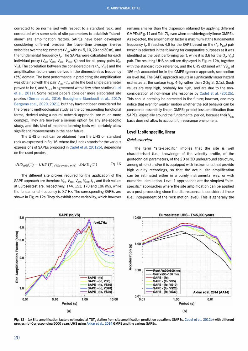
20


corrected to be normalised with respect to a standard rock, and correlated with some sets of site parameters to establish “stand-alone” site amplification factors. SAPEs have been developed considering different proxies: the travel-time average S-wave velocities over the top z meters (VSZ, with z = 5, 10, 20 and 30 m), and the fundamental frequency f0. The SAPEs were calculated for each individual proxy (VS5, VS10, VS20, VS30, f0) and for all proxy pairs (f0 , VSZ). The correlation between the considered pairs (f0 , VS Z ) and the amplification factors were derived in the dimensionless frequency (f/f0) domain. The best performance in predicting site amplification was obtained with the pair VS30 - f0, while the best single parameter proved to be f0 and VS30, in agreement with a few other studies (Luzi et al., 2011). Some recent papers consider more elaborated site proxies (Derras et al., 2016; Boudghene-Stambouli et al., 2017; Bergamo et al., 2020, 2021), but they have not been considered for the present methodological study as the corresponding functional forms, derived using a neural network approach, are much more complex. They are however a serious option for any site-specific study, and this kind of machine learning tools will certainly allow significant improvements in the near future.

The UHS on soil can be obtained from the UHS on standard rock as expressed in Eq. 16, where the j index stands for the various expressions of SAPEs proposed in Cadet et al. (2012b), depending on the used proxies.

and for all proxy pairs (f0, VSZ). The correlation between the considered pairs (f0, VSZ) and the 576

amplification factors were derived in the dimensionless frequency (f/f0) domain. The best 577

performance in predicting site amplification was obtained with the pair VS30 - f0, while the best 578

single parameter proved to be f0 and VS30, in agreement with a few other studies (LUZI et alii, 579

2011). Some recent papers consider more elaborated site proxies (DERRAS et alii, 2016; 580

BOUDGHENE-STAMBOULI et alii, 2017; BERGAMO et alii, 2020, 2021), but they have not been 581

considered for the present methodological study as the corresponding functional forms, 582

derived using a neural network approach, are much more complex. They are however a 583

serious option for any site-specific study, and this kind of machine learning tools will 584

certainly allow significant improvements in the near future. 585

The UHS on soil can be obtained from the UHS on standard rock as expressed in Eq. 16, 586

where the j index stands for the various expressions of SAPEs proposed in CADET et alii, 587

2012b, depending on the used proxies. 588

𝑈𝑈𝑈𝑈𝑈𝑈𝑠𝑠𝑠𝑠𝑠𝑠𝑠𝑠ሺTሻ = 𝑈𝑈𝑈𝑈𝑈𝑈 ሺ𝑇𝑇ሻ ሺVS30=800 𝑚𝑚/𝑠𝑠ሻ ∙ 𝑈𝑈𝑆𝑆𝑆𝑆𝑆𝑆 𝑗𝑗ሺ𝑇𝑇ሻ Eq. 16

The different site proxies required for the application of the SAPE approach are therefore VS5, 589

VS10, VS20, VS30, f0 , and their values at Euroseistest are, respectively, 144, 153, 170 and 186 590

m/s, while the fundamental frequency is 0.7 Hz. The corresponding SAPEs are shown in 591

Figure 12a. They do exhibit some variability, which however remains smaller than the 592

dispersion obtained by applying different GMPEs (Figure 11 and Table 7), even when 593

considering only linear GMPEs. As expected, the amplification factor is maximum at the 594

fundamental frequency f0. It reaches 4.8 for the SAPE based on the (f0, VS30) pair (which is 595

selected in the following for comparative purposes as it was identified as the best performing 596

pair), while it is 3.6 for the (f0, VS5) pair. The resulting UHS on soil are displayed in Figure 597

12b, together with the standard rock reference, and the UHS obtained with VS30 of 186 m/s 598

Eq. 16

The different site proxies required for the application of the SAPE approach are therefore VS5, VS10, VS20, VS30, f0 , and their values at Euroseistest are, respectively, 144, 153, 170 and 186 m/s, while the fundamental frequency is 0.7 Hz. The corresponding SAPEs are shown in Figure 12a. They do exhibit some variability, which however

remains smaller than the dispersion obtained by applying different GMPEs (Fig. 11 and Tab. 7), even when considering only linear GMPEs. As expected, the amplification factor is maximum at the fundamental frequency f0. It reaches 4.8 for the SAPE based on the (f0, VS30) pair (which is selected in the following for comparative purposes as it was identified as the best performing pair), while it is 3.6 for the (f0, VS5) pair. The resulting UHS on soil are displayed in Figure 12b, together with the standard rock reference, and the UHS obtained with VS30 of 186 m/s accounted for in the GMPE (generic approach, see section on level 0a). The SAPE approach results in significantly larger hazard estimates at the surface (e.g. 4-5g rather than 2-3g at 0.1s). Such values are very high, probably too high, and are due to the non-consideration of non-linear site response by Cadet et al. (2012b). This should certainly be corrected in the future; however, one may notice that even for weaker motion whether the soil behavior can be considered essentially linear, GMPEs predict less amplification than SAPEs, especially around the fundamental period, because their VS30 basis does not allow to account for resonance phenomena.

Level 1: site specific, linear

Quick overview

The term “site-specific” implies that the site is well characterised (i.e., knowledge of the velocity profile, of the geotechnical parameters, of the 2D or 3D underground structure, among others) and/or it is equipped with instruments that provide high quality recordings, so that the actual site amplification can be estimated either in a purely instrumental way, or with numerical simulation. Level 1 approaches are the simplest “site-specific” approaches where the site amplification can be applied as a post-processing since the site response is considered linear (i.e., independent of the rock motion level). This is generally the

Fig. 12 - (a) Site amplification factors estimated at TST0 station from site amplification prediction equations (SAPEs, Cadet et al., 2012b) with different proxies; (b) Corresponding 5000 years UHS using Akkar et al., 2014 GMPE and the various SAPEs.

(a) (b)

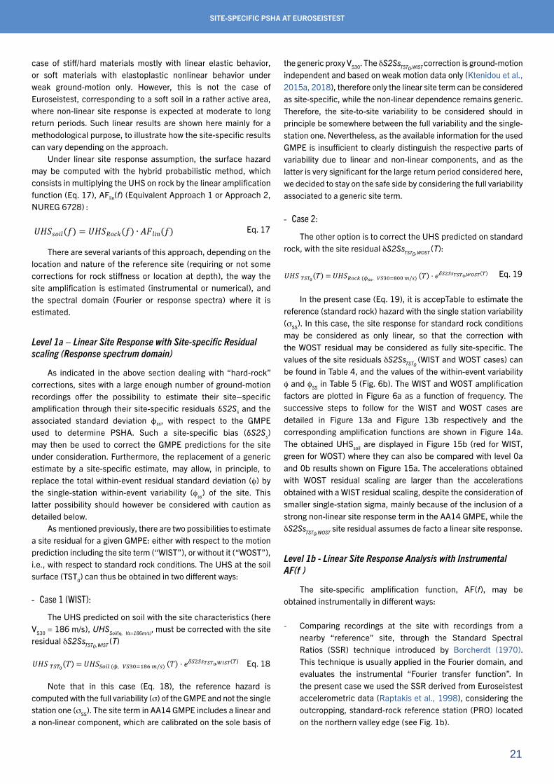
21


case of stiff/hard materials mostly with linear elastic behavior, or soft materials with elastoplastic nonlinear behavior under weak ground-motion only. However, this is not the case of Euroseistest, corresponding to a soft soil in a rather active area, where non-linear site response is expected at moderate to long return periods. Such linear results are shown here mainly for a methodological purpose, to illustrate how the site-specific results can vary depending on the approach.

Under linear site response assumption, the surface hazard may be computed with the hybrid probabilistic method, which consists in multiplying the UHS on rock by the linear amplification function (Eq. 17), AFlin(f) (Equivalent Approach 1 or Approach 2, NUREG 6728) :

Under linear site response assumption, the surface hazard may be computed with the hybrid 622

probabilistic method, which consists in multiplying the UHS on rock by the linear 623

amplification function (Eq. 17), AFlin(f) (Equivalent Approach 1 or Approach 2, NUREG 624

6728) : 625

𝑈𝑈𝑈𝑈𝑈𝑈𝑠𝑠𝑠𝑠𝑠𝑠𝑠𝑠ሺ𝑓𝑓ሻ = 𝑈𝑈𝑈𝑈𝑈𝑈𝑅𝑅𝑠𝑠𝑅𝑅𝑅𝑅ሺ𝑓𝑓ሻ ∙ 𝐴𝐴𝐴𝐴𝑠𝑠𝑠𝑠𝑙𝑙ሺ𝑓𝑓ሻ Eq. 17

There are several variants of this approach, depending on the location and nature of the 626

reference site (requiring or not some corrections for rock stiffness or location at depth), the 627

way the site amplification is estimated (instrumental or numerical), and the spectral domain 628

(Fourier or response spectra) where it is estimated. 629

6.2.2 Level 1a – Linear Site Response with Site-specific Residual scaling (Response 630

spectrum domain) 631

As indicated in Section 4.1.1 dealing with "hard-rock" corrections, sites with a large enough 632

number of ground-motion recordings offer the possibility to estimate their site–specific 633

amplification through their site-specific residuals δS2Ss and the associated standard deviation 634

ϕss, with respect to the GMPE used to determine PSHA. Such a site-specific bias (δS2Ss) may 635

then be used to correct the GMPE predictions for the site under consideration. Furthermore, 636

the replacement of a generic estimate by a site-specific estimate, may allow, in principle, to 637

replace the total within-event residual standard deviation (ϕ) by the single-station within-638

event variability (ϕss) of the site. This latter possibility should however be considered with 639

caution as detailed below. 640

As mentioned previously, there are two possibilities to estimate a site residual for a given 641

GMPE: either with respect to the motion prediction including the site term ("WIST"), or 642

Eq. 17

There are several variants of this approach, depending on the location and nature of the reference site (requiring or not some corrections for rock stiffness or location at depth), the way the site amplification is estimated (instrumental or numerical), and the spectral domain (Fourier or response spectra) where it is estimated.

Level 1a – Linear Site Response with Site-specific Residual scaling (Response spectrum domain)

As indicated in the above section dealing with “hard-rock” corrections, sites with a large enough number of ground-motion recordings offer the possibility to estimate their site–specific amplification through their site-specific residuals δS2Ss and the associated standard deviation φss, with respect to the GMPE used to determine PSHA. Such a site-specific bias (δS2Ss) may then be used to correct the GMPE predictions for the site under consideration. Furthermore, the replacement of a generic estimate by a site-specific estimate, may allow, in principle, to replace the total within-event residual standard deviation (f) by the single-station within-event variability (fss) of the site. This latter possibility should however be considered with caution as detailed below.

As mentioned previously, there are two possibilities to estimate a site residual for a given GMPE: either with respect to the motion prediction including the site term (“WIST”), or without it (“WOST”), i.e., with respect to standard rock conditions. The UHS at the soil surface (TST0) can thus be obtained in two different ways:

- Case 1 (WIST):

The UHS predicted on soil with the site characteristics (here VS30 = 186 m/s), UHSSoil(f, Vs=186m/s), must be corrected with the site residual δS2SsTST0,WIST (T)

without it ("WOST"), i.e., with respect to standard rock conditions. The UHS at the soil643

surface (TST0) can thus be obtained in two different ways:644

Case 1 (WIST) :645

The UHS predicted on soil with the site characteristics (here VS30 = 186 m/s),646

𝑈𝑈𝑈𝑈𝑈𝑈𝑈𝑈𝑆𝑆𝑆𝑆𝑆𝑆ሺ𝜙𝜙, 𝑉𝑉𝑉𝑉=186𝑚𝑚/𝑉𝑉ሻ, must be corrected with the site residual 𝛿𝛿𝑈𝑈2𝑈𝑈𝑉𝑉𝑇𝑇𝑇𝑇𝑇𝑇0,𝑊𝑊𝑊𝑊𝑇𝑇𝑇𝑇ሺ𝑇𝑇ሻ :647

𝑈𝑈𝑈𝑈𝑈𝑈 𝑇𝑇𝑇𝑇𝑇𝑇0ሺ𝑇𝑇ሻ = 𝑈𝑈𝑈𝑈𝑈𝑈𝑇𝑇𝑆𝑆𝑆𝑆𝑆𝑆 ሺ𝑆𝑆, 𝑆𝑆𝑇𝑇30=186 𝑚𝑚/𝑚𝑚ሻ ሺ𝑇𝑇ሻ · 𝑒𝑒𝛿𝛿𝑇𝑇2𝑇𝑇𝑚𝑚𝑇𝑇𝑇𝑇𝑇𝑇0,𝑊𝑊𝑊𝑊𝑇𝑇𝑇𝑇ሺ𝑇𝑇ሻ⬚ Eq. 18

Note that in this case (Eq. 18), the reference hazard is computed with the full variability (σ) of648

the GMPE and not the single station one (σSS). The site term in AA14 GMPE includes a linear649

and a non-linear component, which are calibrated on the sole basis of the generic proxy VS30.650

The 𝛿𝛿𝑈𝑈2𝑈𝑈𝑉𝑉𝑇𝑇𝑇𝑇𝑇𝑇0,𝑊𝑊𝑊𝑊𝑇𝑇𝑇𝑇 correction is ground-motion independent and based on weak motion data651

only (KTENIDOU et alii, 2015a; 2018), therefore only the linear site term can be considered as652

site-specific, while the non-linear dependence remains generic. Therefore, the site-to-site653

variability to be considered should in principle be somewhere between the full variability and654

the single-station one. Nevertheless, as the available information for the used GMPE is655

insufficient to clearly distinguish the respective parts of variability due to linear and non-656

linear components, and as the latter is very significant for the large return period considered657

here, we decided to stay on the safe side by considering the full variability associated to a658

generic site term.659

Case 2:660

The other option is to correct the UHS predicted on standard rock, 𝑈𝑈𝑈𝑈𝑈𝑈𝑅𝑅𝑆𝑆𝑅𝑅𝑅𝑅ሺ𝑆𝑆𝑠𝑠𝑠𝑠, 𝑆𝑆𝑚𝑚=800𝑚𝑚/𝑚𝑚ሻ661

with the site residual 𝛿𝛿𝑈𝑈2𝑈𝑈𝑉𝑉𝑇𝑇𝑇𝑇𝑇𝑇0,𝑊𝑊𝑊𝑊𝑇𝑇𝑇𝑇ሺ𝑇𝑇ሻ :662

Eq. 18

Note that in this case (Eq. 18), the reference hazard is computed with the full variability (σ) of the GMPE and not the single station one (σSS). The site term in AA14 GMPE includes a linear and a non-linear component, which are calibrated on the sole basis of

the generic proxy VS30. The δS2SsTST0,WIST correction is ground-motion independent and based on weak motion data only (Ktenidou et al., 2015a, 2018), therefore only the linear site term can be considered as site-specific, while the non-linear dependence remains generic. Therefore, the site-to-site variability to be considered should in principle be somewhere between the full variability and the single-station one. Nevertheless, as the available information for the used GMPE is insufficient to clearly distinguish the respective parts of variability due to linear and non-linear components, and as the latter is very significant for the large return period considered here, we decided to stay on the safe side by considering the full variability associated to a generic site term.

- Case 2:

The other option is to correct the UHS predicted on standard rock, with the site residual δS2SsTST0,WOST (T):

𝑈𝑈𝑈𝑈𝑈𝑈𝑈𝑇𝑇𝑇𝑇𝑇𝑇0ሺ𝑇𝑇ሻ = 𝑈𝑈𝑈𝑈𝑈𝑈𝑅𝑅𝑅𝑅𝑅𝑅𝑅𝑅𝑈ሺ𝑅𝑅𝑠𝑠𝑠𝑠,𝑈𝑈𝑈𝑉𝑉𝑇𝑇30=800𝑈𝑚𝑚𝑚𝑚𝑚ሻ𝑈ሺ𝑇𝑇ሻ ·𝑈𝑒𝑒𝛿𝛿𝑇𝑇2𝑇𝑇𝑚𝑚𝑇𝑇𝑇𝑇𝑇𝑇0,𝑊𝑊𝑊𝑊𝑇𝑇𝑇𝑇ሺ𝑇𝑇ሻ Eq. 19

In the present case (Eq. 19), it is acceptable to estimate the reference (standard rock) hazard663

with the single station variability (σSS). In this case, the site response for standard rock664

conditions may be considered as only linear, so that the correction with the WOST residual665

may be considered as fully site-specific. The values of the site residuals δS2SsTST0 (WIST and666

WOST cases) can be found in Table 4, and the values of the within-event variability 𝜙𝜙 and667

𝜙𝜙𝑚𝑚𝑚𝑚 in Table 5 (Figure 6b). The WIST and WOST amplification factors are plotted in Figure668

6a as a function of frequency. The successive steps to follow for the WIST and WOST cases669

are detailed in Figure 13a and Figure 13b respectively and the corresponding amplification670

functions are shown in Figure 14a. The obtained UHSsoil are displayed in Figure 15b (red for671

WIST, green for WOST). The accelerations obtained with WOST residual scaling are larger672

than the accelerations obtained with a WIST residual scaling, despite the consideration of673

smaller single-station sigma, mainly because of the inclusion of a strong non-linear site674

response term in the AA14 GMPE, while the 𝛿𝛿𝑈𝑈2𝑈𝑈𝑆𝑆𝑇𝑇𝑇𝑇𝑇𝑇0,𝑊𝑊𝑊𝑊𝑇𝑇𝑇𝑇 site residual assumes de facto a675

linear site response.676

6.2.3 Level 1b - Linear Site Response Analysis with Instrumental AF(f.)677

The site-specific amplification function, AF(f), may be obtained instrumentally in different678

ways:679

• Comparing recordings at the site with recordings from a nearby "reference" site,680

through the Standard Spectral Ratios (SSR) technique introduced by BORCHERDT681

1970. This technique is usually applied in the Fourier domain, and evaluates the682

instrumental "Fourier transfer function". In the present case we used the SSR derived683

from Euroseistest accelerometric data (RAPTAKIS et alii, 1998), considering the684

Eq. 19

In the present case (Eq. 19), it is accepTable to estimate the reference (standard rock) hazard with the single station variability (σSS). In this case, the site response for standard rock conditions may be considered as only linear, so that the correction with the WOST residual may be considered as fully site-specific. The values of the site residuals δS2SsTST0 (WIST and WOST cases) can be found in Table 4, and the values of the within-event variability f and fSS in Table 5 (Fig. 6b). The WIST and WOST amplification factors are plotted in Figure 6a as a function of frequency. The successive steps to follow for the WIST and WOST cases are detailed in Figure 13a and Figure 13b respectively and the corresponding amplification functions are shown in Figure 14a. The obtained UHSsoil are displayed in Figure 15b (red for WIST, green for WOST) where they can also be compared with level 0a and 0b results shown on Figure 15a. The accelerations obtained with WOST residual scaling are larger than the accelerations obtained with a WIST residual scaling, despite the consideration of smaller single-station sigma, mainly because of the inclusion of a strong non-linear site response term in the AA14 GMPE, while the δS2SsTST0,WOST site residual assumes de facto a linear site response.

Level 1b - Linear Site Response Analysis with Instrumental AF(f.)

The site-specific amplification function, AF(f), may be obtained instrumentally in different ways:

- Comparing recordings at the site with recordings from a nearby “reference” site, through the Standard Spectral Ratios (SSR) technique introduced by Borcherdt (1970). This technique is usually applied in the Fourier domain, and evaluates the instrumental “Fourier transfer function”. In the present case we used the SSR derived from Euroseistest accelerometric data (Raptakis et al., 1998), considering the outcropping, standard-rock reference station (PRO) located on the northern valley edge (see Fig. 1b).

22


Fig. 13 - Procedures to obtain the site surface UHS for: (a) Level 1a, Case 1 WIST, the Amplification Function is available in the response spectra domain with respect to standard-rock condition; (b) Level 1a, Case 1 WOST, the Amplification Function is available in the response spectra domain with respect to soil condition; (c) level 1b, the Amplification Function is available in the Fourier domain with respect to standard-rock condition; (d) level 1b, the Amplification Function is available in the response spectrum using site residuals, with respect to hard-rock conditions at depth: the UHS on standard rock needs to be corrected (VS-κ and depth) before applying the site amplification factor; (e) level 1c, the amplification function is computed numerically with respect to the down-hole site. (Modified from Rathje et al., 2005).

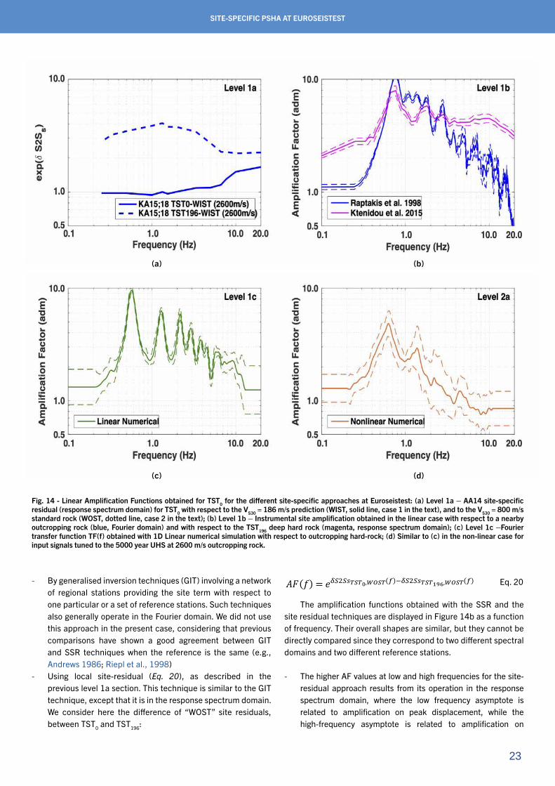
23


- By generalised inversion techniques (GIT) involving a network of regional stations providing the site term with respect to one particular or a set of reference stations. Such techniques also generally operate in the Fourier domain. We did not use this approach in the present case, considering that previous comparisons have shown a good agreement between GIT and SSR techniques when the reference is the same (e.g., Andrews 1986; Riepl et al., 1998)

- Using local site-residual (Eq. 20), as described in the previous level 1a section. This technique is similar to the GIT technique, except that it is in the response spectrum domain. We consider here the difference of “WOST” site residuals, between TST0 and TST196:

outcropping, standard-rock reference station (PRO) located on the northern valley685

edge (see Figure 1b).686

• By generalized inversion techniques (GIT) involving a network of regional stations687

providing the site term with respect to one particular or a set of reference stations.688

Such techniques also generally operate in the Fourier domain. We did not use this689

approach in the present case, considering that previous comparisons have shown a690

good agreement between GIT and SSR techniques when the reference is the same691

(e.g., ANDREWS 1986, RIEPL et alii, 1998)692

• Using local site-residual (Eq. 20), as described in section 6.2.2. This technique is693

similar to the GIT technique, except that it is in the response spectrum domain. We694

consider here the difference of "WOST" site residuals, between TST0 and TST196:695

𝐴𝐴𝐹𝐹ሺ𝑓𝑓ሻ = 𝑒𝑒𝛿𝛿𝛿𝛿2𝛿𝛿𝑠𝑠𝑇𝑇𝑇𝑇𝑇𝑇0,𝑊𝑊𝑊𝑊𝑇𝑇𝑇𝑇ሺ𝑓𝑓ሻ−𝛿𝛿𝛿𝛿2𝛿𝛿𝑠𝑠𝑇𝑇𝑇𝑇𝑇𝑇196,𝑊𝑊𝑊𝑊𝑇𝑇𝑇𝑇ሺ𝑓𝑓ሻ Eq. 20

The amplification functions obtained with the SSR and the site residual techniques are 696

displayed in Figure 14b as a function of frequency. Their overall shapes are similar, but they 697

cannot be directly compared since they correspond to two different spectral domains and two 698

different reference stations.699

• The higher AF values at low and high frequencies for the site-residual approach700

results from its operation in the response spectrum domain, where the low frequency701

asymptote is related to amplification on peak displacement, while the high-frequency702

asymptote is related to amplification on PGA. Both peak values are sensitive to703

amplification in other frequency bands, so that they may be significantly larger than704

1.0. Conversely, in the Fourier domain, the PRO to TST0 Fourier transfer function is705

very close to 1.0 at low frequency: wavelengths are too long to see any difference706

Eq. 20

The amplification functions obtained with the SSR and the site residual techniques are displayed in Figure 14b as a function of frequency. Their overall shapes are similar, but they cannot be directly compared since they correspond to two different spectral domains and two different reference stations.

- The higher AF values at low and high frequencies for the site-residual approach results from its operation in the response spectrum domain, where the low frequency asymptote is related to amplification on peak displacement, while the high-frequency asymptote is related to amplification on

Fig. 14 - Linear Amplification Functions obtained for TST0 for the different site-specific approaches at Euroseistest: (a) Level 1a – AA14 site-specific residual (response spectrum domain) for TST0 with respect to the VS30 = 186 m/s prediction (WIST, solid line, case 1 in the text), and to the VS30 = 800 m/s standard rock (WOST, dotted line, case 2 in the text); (b) Level 1b – Instrumental site amplification obtained in the linear case with respect to a nearby outcropping rock (blue, Fourier domain) and with respect to the TST196 deep hard rock (magenta, response spectrum domain); (c) Level 1c –Fourier transfer function TF(f) obtained with 1D Linear numerical simulation with respect to outcropping hard-rock; (d) Similar to (c) in the non-linear case for input signals tuned to the 5000 year UHS at 2600 m/s outcropping rock.

(a)

(c)

(b)

(d)

24


PGA. Both peak values are sensitive to amplification in other frequency bands, so that they may be significantly larger than 1.0. Conversely, in the Fourier domain, the PRO to TST0 Fourier transfer function is very close to 1.0 at low frequency: wavelengths are too long to see any difference between PRO and TST0 underground conditions). And it is below 1.0 at very high frequency because of the effects of damping in the 200 m thick sedimentary deposits.

- Similarly, the slightly lower amplification of the TST0/ TST196

residual ratio around the 0.7 Hz fundamental frequency, comes from the inherent smoothing of the response spectrum approach, even though the reference rock is harder than for the PRO to TST0 Fourier transfer function.

The site amplification relying on SSR technique is provided as a Fourier transfer function. The rock UHS must thus be first converted into a rock Uniform Hazard Fourier Amplitude spectrum (UHFAS), then the site amplification can be applied in the Fourier domain, and at last it is necessary to come back in the response spectrum domain. These conversions from the response spectrum domain to the Fourier domain, and vice versa, are performed using the Inverse Random Vibration Theory (IRVT) and the forward random vibration theory (RVT) (Campbell 2003; Al Atik et al., 2014). These techniques presented in the above section dealing with VS-κ corrections are applied here for the same scenario event and with typical duration values. The successive steps to follow are detailed in Figure 13a. In the residual approach, as the site amplification is provided in the response spectrum domain, it must be applied directly to the hard-rock UHS. When needed, VS-κ and depth corrections must similarly be applied to the UHS on standard rock to obtain the UHS on hard rock (Fig. 13d).

The resulting UHS at 5,000 years are shown in Figure 15b (SSR based in blue, residual based in magenta). They exhibit much larger differences than the corresponding amplification functions (Fig. 14b), because of large differences in the reference rock UHS. The site residual approach leads to much lower values than the approach based on SSR, over the whole period range. Both reference rock corresponds to single-station PSHA estimates, however one is an outcropping standard rock (in the case of AF(f) based on the SSR technique), the other is a deep hard rock site (in the residual approach). As shown in Figure 9, the latter is much smaller than the former.

Level 1c – Linear Site Response Analysis with Numerical AF(f)

The amplification function can be also estimated numerically. Here we only considered the 1D ground response, but the same approach could be used with 2D or 3D simulation codes, as done by Chavez-Garcia et al. (2000), Makra et al. (2016) or Maufroy et al. (2015, 2016, 2017). The linear 1D response has been computed using the time-domain code NOAH (Nonlinear Anelastic Hysteretic finite difference code, Bonilla, 2000), applied here in the linear domain with the velocity profile indicated in Figure 2, and considering outcropping hard-rock reference conditions (as usually done in numerical modelling techniques). The site amplification is thus provided here in the Fourier domain (as in level 1b, Fig. 13c), which requires again a swap from the response spectrum domain to the Fourier domain. The procedure is illustrated in Figure 13e. The single-station sigma standard-rock UHS response spectrum is first corrected for VS and kappa. The resulting response spectrum is transformed in the Fourier

Fig. 15 - (a) Euroseistest UHS on soil from generic or partially site-specific approaches (level 0a and level 0b); (b) Euroseistest hazard spectra on soil for the hybrid site-specific hazard approaches (levels 1a, 1b, 1c and 2a); the additional symbols (open circles) stand for the Aristizabal et al., 2018b results.

(a) (b)

25


domain using IRVT (Al Atik et al., 2014), multiplied by the Fourier transfer function corresponding to the linear response of the 1D soil column, and then the surface response spectrum is derived from site surface Fourier spectra using forward RVT.

The level 1c 1D numerical transfer function is displayed in Figure 14c. The linear Fourier transfer function cannot be compared simply with the instrumental one in Figure 14b, since the reference is not the same: the instrumental AF is estimated with respect to outcropping rock (PRO station), while the linear numerical AF is estimated with respect to hard rock (TST196). Nevertheless, the well separated resonance peaks in the numerical transfer function show that 2D and 3D effects are indeed ignored in the 1D approach. Such peaks can be identified also in the surface response spectrum displayed in Figure 15b (dark green curve). The UHS obtained is lower than the SSR-based level 1b UHS (blue) and higher than the residual-based level 1b UHS (magenta). The amplitudes are approximately comparable to the approach 1a based on residuals (site residual δS2SsTST0,WOST, light green). Most of the differences between the various approaches come from the reference hazard (within or outcropping conditions, standard or hard-rock).

Level 2: site specific, non-linear

Euroseistest is characterised by soft deposits and the site response is expected to be non-linear at least for long return periods. The amplification function AF(f) thus depends not only on the reference rock motion level Sar(f), but also on the details of the time-history (e.g., its phase content) which partly controls the strain values. A given absolute level at site surface may be reached for different rock reference motion (corresponding to different return periods and / or different earthquake scenarios) and amplification levels corresponding to different non-linear site response. A full probabilistic estimate at soft sites should then couple the analysis of rock hazard and the distribution of conditional site amplification.

Following Bazzuro & Cornell (2004a, b), several approaches have been proposed to account for non-linear site response in probabilistic site-specific hazard calculations. They are labelled as sublevels 2a to 2e in Table 1 , which all involve an analysis of non-linear site response. They are briefly presented in this section. A nonlinear analysis could in principle be performed on an instrumental basis only, however it is not possible at Euroseistest since there are no recordings of strong enough motion. The non-linear site response is thus accounted for only with numerical simulation tools (NOAH and SHAKE codes), which are briefly presented. An overview is then given of the principles of the five “level 2” methods mentioned in Table 1, but only two of them could be applied here and give rise to specific results for Euroseistest.

Non-linear site response at Euroseistest

The nonlinear computations used here are detailed in Aristizabal et al. (2018b), a study dedicated to the comparison of two fully probabilistic site-specific approaches (levels 2b and 2c).

Their basis is thus only shortly summarised; the interested reader should refer to Aristizabal et al. (2018a, b) for more details

We consider only 1D, 1-component site response analysis. Recent benchmarking studies (Stewart et al., 2008; Régnier et al., 2016b, 2018) recommend the use of several non-linear codes to better capture the associated epistemic uncertainty, however we have applied only one fully nonlinear code, the NOAH (Nonlinear Anelastic Hysteretic finite difference code, Bonilla, 2000) time-domain code. Our goal is not to propose a complete site-specific PSHA study at Euroseistest, but to illustrate how much the hazard results depend on the approach selected. Nonetheless, a linear equivalent approach (SHAKE, Schnabel et al., 1972) has also been considered for methods 2b and 2c.

The low-strain parameters of the soil column are described in Figure 2 and Table 2 (same as in level 1c). The non-linear parameters have been defined through the G/Gmax degradation curves and, when needed, the strength profile has been derived from the friction angle f and K0 (coefficient of earth pressure at rest) values, according to the user manual (Bonilla 2000). The computations were performed using the actual soil profile, with a reference motion being specified for hard-rock (VS30 = 2600 m/s), outcropping conditions. The corresponding rock hazard therefore includes only the VSC-KC corrections, without the depth correction (DCF).

Approaches for including non-linear site response in Site-specific PSHA

To perform a site-specific PSHA, there are two main approaches. The hybrid approach (level 2a) combines a probabilistic approach for the reference rock hazard and a deterministic approach for the site amplification, conditioned by the level of rock hazard. The fully probabilistic approach, first introduced by Cramer (2003), implies the convolution of a non-linear, rock-motion dependent, site-amplification function having its own distribution, with the hazard curve on rock. Several methods have been proposed for the practical implementation of this convolution.

- Hybrid approach

This approach is formally the same as the one considered in level 1c, except that the (deterministic) site amplification is tuned to the reference rock hazard level as follows (Eq. 21):

6.3.2 Approaches for including non-linear site response in Site-specific PSHA 800

To perform a site-specific PSHA, there are two main approaches. The hybrid approach (level 801

2a) combines a probabilistic approach for the reference rock hazard and a deterministic 802

approach for the site amplification, conditioned by the level of rock hazard. The fully 803

probabilistic approach, first introduced by CRAMER 2003, implies the convolution of a non-804

linear, rock-motion dependent, site-amplification function having its own distribution, with 805

the hazard curve on rock. Several methods have been proposed for the practical 806

implementation of this convolution. 807

6.3.2.1 Hybrid approach 808

This approach is formally the same as the one considered in level 1c, except that the 809

(deterministic) site amplification is tuned to the reference rock hazard level as follows (Eq. 810

21): 811

𝐻𝐻𝐻𝐻𝑠𝑠𝑠𝑠𝑠𝑠𝑠𝑠 = 𝑈𝑈𝐻𝐻𝐻𝐻𝑅𝑅𝑅𝑅𝑅𝑅_𝑅𝑅𝑠𝑠𝑅𝑅𝑅𝑅ሺ𝑆𝑆𝑆𝑆𝑆𝑆𝑅𝑅𝑆𝑆𝑅𝑅𝑅𝑅, 𝐵𝐵𝑠𝑠𝑆𝑆𝑅𝑅ℎ𝑠𝑠𝑠𝑠𝑅𝑅ሻ ∙ 𝐴𝐴𝐴𝐴ሺ𝐼𝐼𝐼𝐼𝑠𝑠𝐼𝐼𝑆𝑆𝑆𝑆𝐼𝐼𝑅𝑅𝐼𝐼𝐼𝐼𝑆𝑆𝑠𝑠, 𝑁𝑁𝑆𝑆𝐼𝐼𝑅𝑅𝑆𝑆𝑠𝑠𝑅𝑅𝑆𝑆𝑠𝑠ሻሺ𝑓𝑓, 𝐻𝐻𝑆𝑆𝑆𝑆ሻ Eq. 21

The non-linearity of the site response is accounted for, but not its variability associated to the 812

sensitivity to details (phase) ot the input rock time series. The resulting surface spectrum can 813

no longer be considered as a uniform hazard spectrum associated to the return period of the 814

rock reference. The exceedance probabilities may differ from one oscillator period to another 815

because of the non-linear energy transfer process, and the replacement of a convolution by a 816

simple multiplication may change the exceedance probability. The examples investigated in 817

BAZZURRO & CORNELL 2004b indicate that this hybrid method tends to be non-conservative at 818

all frequencies and for all return periods. Nonetheless, this hybrid approach is widely used by 819

the engineering and scientific community (called Approach 1 or Approach 2 in NUREG 820

6728). 821

Eq. 21

The non-linearity of the site response is accounted for, but not its variability associated to the sensitivity to details (phase) ot the input rock time series. The resulting surface spectrum can no longer be considered as a uniform hazard spectrum associated to the return period of the rock reference. The exceedance probabilities may differ from one oscillator period to another because of the non-linear energy transfer process, and the replacement of a convolution by a simple multiplication may change the exceedance probability. The examples investigated in Bazzurro & Cornell (2004b) indicate that this hybrid method tends to be non-conservative at all frequencies

26


and for all return periods. Nonetheless, this hybrid approach is widely used by the engineering and scientific community (called Approach 1 or Approach 2 in NUREG 6728).

The procedure is similar to level 1c, with one difference: the site response is nonlinear, and the NOAH code operates in the time domain. Acceleration time series compatible with the UHS reference rock spectrum must be used. We have selected ten real accelerograms corresponding to the scenario events (Mw=[6.0-7.0] and Rhyp=[0-20] km, see Annex A), and tuned them to the VSC-KC corrected UHS spectrum using the iterative procedure used in Causse et al. (2014): the original Fourier phase spectrum of the real accelerograms is kept unchanged to capture the actual nonstationarity, while the Fourier amplitude spectrum is iteratively adapted to optimally match the target response spectrum.

The average amplification function is obtained in the Fourier domain (Fig. 14d), according to (Eq. 22):

The procedure is similar to level 1c, with one difference: the site response is nonlinear, and 822

the NOAH code operates in the time domain. Acceleration time series compatible with the 823

UHS reference rock spectrum must be used. We have selected ten real accelerograms 824

corresponding to the scenario events ( Mw=[6.0-7.0] and Rhyp=[0-20] km, see Annex A), and 825

tuned them to the VSC-KC corrected UHS spectrum using the iterative procedure used in 826

CAUSSE et alii. 2014: the original Fourier phase spectrum of the real accelerograms is kept 827

unchanged to capture the actual nonstationarity, while the Fourier amplitude spectrum is 828

iteratively adapted to optimally match the target response spectrum. 829

The average amplification function is obtained in the Fourier domain (Figure 14d), according 830

to (Eq. 22): 831

𝑇𝑇𝑇𝑇ሺ𝑓𝑓ሻ = Eq. 22 ۄ𝑇𝑇𝐹𝐹𝐹𝐹𝑠𝑠𝑠𝑠𝑠𝑠𝑠𝑠,𝑠𝑠ሺ𝑓𝑓ሻ/𝑇𝑇𝐹𝐹𝐹𝐹𝑟𝑟𝑟𝑟𝑟𝑟𝑟𝑟,𝑠𝑠ሺ𝑓𝑓ሻۃ

where the symbol < > stands for the geometrical average of the Fourier spectral ratios over 832

the selected time series i. The amplification obtained is significantly reduced with respect to 833

the linear case, especially in the high frequency range. The resulting average transfer function 834

is displayed in Figure 14d and its corresponding surface response spectrum is displayed in 835

Figure 15b. This method predicts the lowest amplitudes among the different method 836

implemented (up to 1.0 s). The UHS obtained is close to the UHS level 1a, relying on a 837

residual scaling with site term (WIST), the method that accounts for non-linear behavior in a 838

generic way. 839

6.3.2.2 Full Probabilistic Integration Based Method 840

CRAMER 2003 and BAZZURO & CORNELL 2004b were the first authors to propose and 841

implement a method to account for site effects in a fully probabilistic framework. This 842

method, corresponding to level 2b, is named here the Full Probabilistic Integration Based 843

Eq. 22

where the symbol < > stands for the geometrical average of the Fourier spectral ratios over the selected time series i. The amplification obtained is significantly reduced with respect to the linear case, especially in the high frequency range. The resulting average transfer function is displayed in Figure 14d and its corresponding surface response spectrum is displayed in Figure 15b. This method predicts the lowest amplitudes among the different method implemented (up to 1.0 s). The UHS obtained is close to the UHS level 1a, relying on a residual scaling with site term (WIST), the method that accounts for non-linear behavior in a generic way.

- Full Probabilistic Integration Based Method

Cramer (2003) and Bazzuro & Cornell (2004b) were the first authors to propose and implement a method to account for site effects in a fully probabilistic framework. This method, corresponding to level 2b, is named here the Full Probabilistic Integration Based Method and is equivalent to Approach 3 in NUREG 6728. The site amplification function is convolved with the hazard on rock, as follows:

Method and is equivalent to Approach 3 in NUREG 6728. The site amplification function is 844

convolved with the hazard on rock, as follows: 845

𝐻𝐻𝐻𝐻𝑆𝑆𝑆𝑆𝑆𝑆𝑆𝑆ሺ𝑍𝑍ሻ = ∫ 𝑃𝑃 [𝑌𝑌 ≥ 𝑧𝑧𝑥𝑥|𝑥𝑥]

∞

0𝑓𝑓𝑥𝑥ሺ𝑥𝑥ሻ𝑑𝑑𝑥𝑥 Eq. 23

where HC means hazard curve, i.e. annual probability of exceedance as a function of soil 846

hazard level Z=Sas(f); x is rock hazard, x=Sar(f); Y is the input dependent site amplification 847

Y= AF(f, Sar) and P(Y) its distribution conditioned by the rock motion level; fx(x) is the 848

probability density function (pdf) of Sar(f). Most codes currently used to calculate PSHA do 849

not include this feature. The OpenQuake engine (http://www.globalquakemodel.org/) would 850

need to be modified to include such a tool. We did not apply this method to Euroseistest. 851

6.3.2.3 Level 2c – Full Convolution Analytical Method (AM) 852

BAZZURRO & CORNELL 2004b proposed to replace the numerical convolution process (Eq. 23) 853

by an analytical one making use of a closed form solution. Several assumptions are required: 854

i) The median amplification function AF (f, Sar) can be described by a piece-wise linear 855

dependence on the rock motion Sar (in a log-log scale at every frequency); 856

ii) Its variability can be described by a lognormal distribution, 857

iii) The rock hazard can be represented locally (around the return period of interest) by a 858

power law dependence on hazard level. 859

Such an approach is very appealing since it offers several advantages: 860

i) The amplification due to site effects is considered as an a posteriori correction to the 861

hazard calculations. 862

ii) The full probabilistic meaning of the hazard curve and UHS is respected. 863

iii) The calculations of the hazard curve on soil are very simple and with low 864

computational demand. 865

Eq. 23

where HC means hazard curve, i.e. annual probability of exceedance as a function of soil hazard level Z=Sas(f); x is rock hazard, x=Sar(f); Y is the input dependent site amplification Y= AF(f, Sar) and P(Y) its distribution conditioned by the rock motion level; fx(x) is the probability density function (pdf) of Sar(f). Most codes currently used to calculate PSHA do not include this feature. The OpenQuake engine (http://www.globalquakemodel.org/) would need to be modified to include such a tool. We did not apply this method to Euroseistest.

- Level 2c – Full Convolution Analytical Method (AM)

Bazzurro & Cornell (2004b) proposed to replace the numerical convolution process (Eq. 23) by an analytical one making use of a closed form solution. Several assumptions are required:

i. The median amplification function AF (f, Sar) can be described by a piece-wise linear dependence on the rock motion Sar (in a log-log scale at every frequency);

ii. Its variability can be described by a lognormal distribution, iii. The rock hazard can be represented locally (around the return

period of interest) by a power law dependence on hazard level.

Such an approach is very appealing since it offers several advantages:

i. The amplification due to site effects is considered as an a posteriori correction to the hazard calculations.

ii. The full probabilistic meaning of the hazard curve and UHS is respected.

iii. The calculations of the hazard curve on soil are very simple and with low computational demand.

The implementation of this method in Bazzurro & Cornell (2004b) indicate that such assumptions are acceptable. Nonetheless, Aristizabal et al. (2018) have shown that for the Euroseistest site, the non-linearity is too strong at intermediate to large return periods. Some terms in the closed form solution get unrealistically large values, using either the nonlinear code NOAH or the equivalent linear SHAKE code (Schnabel 1972). This happens whenever the ground acceleration saturates because of limited strength. Aristizabal et al. (2018) have shown that the method is not adapted to soft deposits at Euroseistest.

- Level 2d – Classical PSHA with Soil Specific Attenuation Equation

Bazurro & Cornell (2004b) proposed to simply tune the GMPE used in the hazard calculation. The GMPE is turned into a site-specific GMPE by replacing its generic site term by a specific one tuned to the site-specific, non-linear numerical simulations, as follows:

The implementation of this method in BAZZURRO & CORNELL 2004b indicate that such 866

assumptions are acceptable. Nonetheless, ARISTIZABAL et alii, 2018 have shown that for the 867

Euroseistest site, the non-linearity is too strong at intermediate to large return periods. Some 868

terms in the closed form solution get unrealistically large values, using either the nonlinear 869

code NOAH or the equivalent linear SHAKE code (SCHNABEL 1972). This happens whenever 870

the ground acceleration saturates because of limited strength. ARISTIZABAL et alii, 2018 have 871

shown that the method is not adapted to soft deposits at Euroseistest. 872

6.3.2.4 Level 2d – Classical PSHA with Soil Specific Attenuation Equation 873

BAZURRO & CORNELL 2004b proposed to simply tune the GMPE used in the hazard 874

calculation. The GMPE is turned into a site-specific GMPE by replacing its generic site term 875

by a specific one tuned to the site-specific, non-linear numerical simulations, as follows: 876

𝑙𝑙𝑙𝑙 𝑆𝑆𝑆𝑆𝑆𝑆𝑆𝑆𝑆𝑆𝑆𝑆ሺ𝑓𝑓ሻ = 𝑙𝑙𝑙𝑙 𝑆𝑆𝑆𝑆𝑅𝑅𝑆𝑆𝑅𝑅𝑅𝑅𝑅𝑅𝑅𝑅𝑅𝑅𝑅𝑅,𝑆𝑆ሺ𝑓𝑓ሻ + 𝑙𝑙𝑙𝑙ሺ𝐴𝐴𝐴𝐴𝑆𝑆𝑆𝑆𝑆𝑆𝑆𝑆−𝑆𝑆𝑆𝑆𝑆𝑆𝑅𝑅𝑆𝑆𝑆𝑆𝑆𝑆𝑅𝑅ሺ𝑓𝑓ሻሻ Eq. 24

This approach is equivalent to approach 4 in NUREG 6728 (MCGUIRE et alii, 2001); it was 877

applied by PAPASTILIOU et alii, 2012b. In the Euroseistest case, the reference rock is much 878

harder than the site conditions accounted for in most GMPEs and the rock GMPE should be 879

first corrected for rock hardness. Although this could be achieved with the VS-κ corrections, it 880

was not applied here as it is not yet implemented in the OpenQuake engine, used for PSHA 881

computations. 882

6.3.2.5 Level 2e – Full Probabilistic Stochastic Method 883

ARISTIZABAL et alii, 2018 proposed to account for site response in PSHA in a fully 884

probabilistic way, combining Monte Carlo sampling and time series simulations. Rather than 885

integrating frequency-magnitude distributions as in classical PSHA, a very long earthquake 886

catalog is generated from the source model with the Monte Carlo method. A stochastic point-887

source approach (BOORE 2003), that provides synthetic time histories on rock for every 888

Eq. 24

This approach is equivalent to approach 4 in NUREG 6728 (McGuire et al., 2001); it was applied by Papastiliou et al. (2012b). In the Euroseistest case, the reference rock is much harder than the site conditions accounted for in most GMPEs and the rock GMPE should be first corrected for rock hardness. Although this could be achieved with the VS-κ corrections, it was not applied here as it is not yet implemented in the OpenQuake engine, used for PSHA computations.

- Level 2e – Full Probabilistic Stochastic Method

Aristizabal et al. (2018) proposed to account for site response in PSHA in a fully probabilistic way, combining Monte Carlo sampling and time series simulations. Rather than integrating frequency-magnitude distributions as in classical PSHA, a very long earthquake catalog is generated from the source model with the Monte Carlo method. A stochastic point-source approach (Boore, 2003), that provides synthetic time histories on rock for every earthquake in the catalog, is combined with a 1D numerical site

http://www.globalquakemodel.org/


27


response code to propagate the time histories from depth to surface. The hazard curve is then established from simple statistics on the synthetic ground-motions at the soil surface. Two site response codes are used, an equivalent-linear (SHAKE91, Schnabel et al., 1993) and a non-linear code (NOAH, Bonilla, 2001) to illustrate the large uncertainty associated to this step.

There is one step in the method that was difficult to tackle, the tuning of the source and path parameters required by the Boore (2003) stochastic point-source approach. The synthetic hazard curve obtained on rock, directly from the exceedance rates of stochastic time histories, should fit the hazard curve on the reference rock obtained applying classical PSHA (application of GMPE Akkar et al. (2014), as well as VS-κ corrections). More details are provided in Aristizabal et al. (2018).

The calculations were performed for three spectral periods: PGA (0s), 0.2 s and 1.0 s. For the 5,000 year return period, the resulting hazard values are 0.4, 0.45 and 0.65 g when using the linear equivalent approach (SHAKE), and 0.2, 0.65 and 0.7 g when using a fully non-linear simulation code (NOAH). These values actually correspond to the mean NL “saturation” levels provided by the extensive 1D NL site response simulations, illustrated in Figure 12 of Aristizabal et al. (2018). These results also show that the saturation is reached for input motion levels with return periods lower than 5000 years for the reference hard rock (see Fig. 9). The saturation thus corresponds to the vertical asymptote of the site-surface hazard curves, and it must be emphasised that such asymptotes are extremely sensitive to the constitutive law adopted for the soft soils: The epistemic uncertainty associated to NL 1D site response is very large.

These hazard values are indeed significantly lower than those obtained with the hybrid level 2a approach (Fig. 14b), although both results were obtained with the same fully NL code (NOAH). We cannot propose yet definitive explanations for this apparent inconsistency. Nevertheless, the response of NL systems is known to be highly dependent both on the frequency content of the excitation and on its phase properties. The stochastic simulations used as input in Aristizabal et al. (2018) are characterised by a random phase, while the real signals considered here are non-stationary and have non-random phase properties. We consider that these phase properties of the input motion might be the origin of the large differences, in agreement with the results by Causse et al. (2014), who find a much lower variability of NL 1D site response for random phase signals compared with real signals. When considering the NL response plots in Figure 12 of Aristizabal et al. (2018), one can notice the upper bound of the saturation levels is slightly higher than the mean values indicated above, i.e., 0.5, 0.6 and 1.0 g for SHAKE, and 0.2, 0.7 and 1.0 g for NOAH, for spectral periods PGA, 0.2 and 1.0 s, respectively. These values are also indicated with specific symbols at the corresponding spectral periods in Figure 15b.

DISCUSSION

The hazard results obtained at Euroseistest are summarised in Figure 16. The uniform hazard spectra obtained for soil following

different methodologies are superimposed in Figure 16a to the uniform hazard spectra obtained for different rock references. These results have been obtained at one unique location, nonetheless their analysis leads to a few key conclusions that may be of interest for any site-specific hazard assessment.

All the analysis is based on a single GMPE (AA14), which was selected as an accepTable choice since it predicts levels that correspond to the average acceleration considering the eight models selected. Besides, the AA14 GMPE is a relatively recent GMPE with a clear separation between-event (τ) and within-event (f) aleatory variability terms, which are fundamental for this study. Moreover, this GMPE was in the short list of equations selected for crustal earthquakes in the GEM project (Stewart et al., 2015). Nevertheless, an interesting exercise could be to replicate this study with other GMPEs to validate the findings, i.e. the important approach-to-approach uncertainty observed whatever the ground motion model.

The variability obtained, with the use of one single GMPE, for the UHS on rock (in grey) comes mainly from the consideration of a full or reduced aleatory variability, and from the characteristics of the reference rock (velocity and attenuation, within or outcropping motion conditions). At 0.1s, the amplitude varies between 0.8 and 1.5g. The variability obtained on soil, including the soft soil response, is significantly enlarged, e.g. the amplitude varies between 1.1 and 4.0 g at 0.1s. This increase of the hazard variability on soil with respect to rock was observed after applying the generic PSHA approach with different GMPEs (level 0a, see the corresponding section). While the variability on rock is mostly related to the reference rock properties (shear-wave velocity, kappa, outcropping or within motion), the variability on soil is also related to the selected method to derive the site-specific hazard (method-to-method variability).

This study provides some hints on the main elements controlling the variability of hazard estimates at the soil surface (Fig. 16b). The most striking one is the type of soil behavior, linear or non-linear. As expected, the linear approaches predict systematically larger hazard values (in magenta) than methods that consider nonlinear behavior (in green), especially at short periods. The difference in the results between linear and nonlinear methods is particularly exacerbated at Euroseistest because of the presence of very soft soils at shallow depth, and of a thick alluvial deposit with a large impedance contrast at large depth. For large input motion, shear strains reach large values over the whole soil column, resulting in significant to large damping, which “kills” the reverberation phenomena and the associated resonances.

At the Euroseistest TST station, the hazard estimates accounting for nonlinearity are thus much lower than hazard estimates relying on linear amplification. Such reduction of hazard might be expected for most sites with thick and soft deposits in highly active seismic areas. The consideration of linear amplification could be appropriate for short return periods in seismic zones with moderate to low activity. Nevertheless, for large return periods (or even for intermediate return periods in highly seismic zones such as at Euroseistest), ignoring nonlinearity leads to an overestimation of the hazard, with unrealistic high

28


levels. Site-specific studies accounting for nonlinear site response is thus highly recommended. In most cases, nonlinearity can be evaluated with numerical simulations only as there are very few sites with a large enough number of strong events recordings. The uncertainty related to the choice of the non-linear code needs to be addressed. The recent benchmarking exercises on nonlinear simulation codes (e.g., Stewart et al., 2008; Régnier et al., 2016b, 2018) have demonstrated that the numerical estimates of nonlinear site response are associated with a significant amount of epistemic uncertainty, which increases with the input motion level. We did not consider this particular kind of epistemic uncertainties in the present study.

The results show that the 1D numerical linear amplification function (red line in magenta zone, Fig. 16b) underestimates the hazard estimates obtained with linear instrumental functions. It strongly suggests that 2D/3D effects are present and significant, as shown in Maufroy et al. (2016, 2017), and that they do impact the instrumental data but cannot be captured with a simple 1D wave propagation model. 2D/3D simulation tools, or at least 2D/3D aggravation factors (Riga et al., 2016; Boudghene-Stambouli et al., 2018; Kristek et al., 2018; Moczo et al., 2018) should be used to derive more realistic estimates of AF(f). They have not been considered here to avoid too many complexities, but their results would probably be similar to those obtained with instrumental estimates of AF(f). Even though such basin effects are certainly affected by soil non-linearity, they might remain significant at least at low frequencies, where damping effects are less important and 1D non-linear simulations considered in level

2 approaches may have an underestimation bias. 2D/3D non-linear simulation codes do exist and are used by several groups and companies, but one must keep in mind that they have never been cross-checked by any benchmarking exercise, and that it is likely that the associated model uncertainty is higher than the one associated to 1D nonlinear codes (see Régnier et al., 2016, 2018). A simple solution on the safe side would be to apply the linear 2D/1D or 3D/1D aggravation factors (Moczo et al., 2018) to the results of 1D nonlinear numerical simulation.

Amongst the generic approaches, the level 0b approaches using site terms based on more than one proxy (here f0 and VS30

proxies,) lead to a significantly larger hazard than if considering only the VS30 proxy in the GMPE (level 0a, see Fig. 12b and Fig. 15a). The SAPE does not account for nonlinear behavior, while the selected GMPE does account for it in a generic way (especially in the short period range). The cumulated effects of low values of both f0 and VS30 proxies lead to larger (linear) amplification in the SAPE case than the sole effect of a low VS30 considered in most GMPEs (including AA14). This explains the differences at long periods, where moreover nonlinear effects are not expected to be significant. It is therefore recommended to develop other multi-proxy SAPEs including non-linear terms, such as for instance in Régnier et al. (2016a) or Derras et al. (2020).

The approaches using site residuals may lead to very different results depending on the way the site residuals are computed, i.e., whether the GMPE site terms are considered or not (WIST or WOST). Such differences reach factors up to 3 (see Fig. 14a) with the AA14 GMPE, and come primarily from the non-linear

Fig. 16 - Summary of uniform hazard spectra (5000 years return period) obtained at Euroseistest (TST location): (a) Distribution of UHS obtained on rock (grey) and on soil (red) with various generic, partially and fully site-specific approaches (levels 0a, 0b, 1a, 1b, 1c and 2a, see Table 7); (b) UHS obtained at the surface on soft soil, distinguishing linear (magenta) and nonlinear (green) approaches, instrumental (blue) and numerical (red) estimates. The strong green area stand for the NL results presented in this study, the light green extension includes the results of Aristizabal et al., 2018b. The UHS obtained with a generic approach (level 0) using AA14 GMPE for VS30=186 m/s is also superimposed (black).

(a) (b)

29


site term in AA14. The δS2Ss residuals are estimated mainly from weak to moderate motion recordings, and thus correspond to linear site response residuals. When they are estimated with respect to rock motion, their application to much stronger motion does not take into account the changes in site response due to non-linear behavior. Conversely, when they are estimated with respect to the “generic site” motion, their application to much stronger motion combines the linear, site-specific part, and the non-linear, generic site term embedded in the GMPE. The impact of non-linearity for the present thick, soft site is so large that the WIST approach considering full sigma leads to much lower hazard than for the WOST approach considering single-station sigma.

Our aim is to understand the impact of some methodological choices on the hazard estimates, we did not perform a complete hazard study for the Euroseistest site. A complete hazard study would require the consideration of several GMPEs, with the associated GMPE-specific HTT adjustments, and the consideration of the epistemic uncertainty associated to each site amplification AF(f), for each site-specific approach. For instance, numerical estimates of AF(f) (or transfer function TF(f)) should include the variability associated to uncertainties in soil characteristics (velocity and damping profiles, non-linear properties), and to simulation codes as well (1D-2D-3D, various implementations of nonlinear behavior, which were shown to imply an uncertainty factor of at least a factor ± 50% during the PRENOLIN Benchmark, Régnier et al., 2016b, 2018). Instrumental estimates of AF(f) or TF(f) derived from any acceptable technique (site-to-reference spectral ratio, site residual, generalised inversion, etc.) should also include the event-to-event variability. Most probabilistic hazard software do not yet include all the corresponding tools, so that it should be performed through dedicated, post-processing codes. Nevertheless, we consider that a proper accounting for these additional epistemic uncertainties would not drastically modify the approach-to-approach variability that is obtained in this study.

LESSONS FOR SITE-SPECIFIC HAZARD STUDIES

Site-specific hazard calculations aim to provide improved hazard estimates at well-characterised sites. The differences between the “generic” site terms included in state-of-the art GMPEs and site-specific site response may have different physical origins, related to the poor characterization of a site with a single proxy (most often the “shallow” parameter VS30). A single proxy cannot simultaneously properly account for 2D or 3D geometrical effects, the impedance contrast with the local deep bedrock, and the non-linear properties of the site material. Moreover, the site-specific estimates of site response and the hazard on rock can be decoupled only if the site-response is linear and without any dependence on source characteristics (e.g., azimuth or depth). At present, there is an overall consensus in the engineering community to neglect source characteristics, but to account as much as possible for soil non-linearity. As only the most recent GMPEs are able to take into account nonlinear behavior, and only in a very generic and approximate way, classical PSHA methods

and software are not presently designed to provide site-specific hazard estimates in a fully satisfactory way.

Several approaches have been proposed over the last two decades to combine rock-hazard with site-specific estimates of site response, with different complexity levels and different sources of epistemic uncertainty. The aim of this work was to illustrate the application of various approaches on one example site, discuss the associated issues, and compare their results, in order to better appreciate the “benefits” versus the required costs and efforts when performing this type of analysis.

There are certainly numerous limitations in this single example of application, which prevent from drawing too general conclusions and recommendations. The example site is characterised by a large amplification over a broad frequency range, due to a combination of several factors (the large velocity contrast at depth, the low velocity at surface, and the graben structure leading to additional “basin effects”). As a consequence, the true site amplification is significantly larger than the generic, average amplification accounted for in GMPEs. The site-specific hazard estimates are larger than the generic level 0a estimates for low acceleration levels / short return periods. On the contrary, the site-specific hazard estimates are lower than the generic estimates at long return periods / large acceleration levels, due to the softness and thickness of the alluvial deposits, associated to a large impedance contrast, that exacerbates the impact of non-linear effects. We derive the following “lessons” for sites similar to the Euroseistest TST site, but we consider that some of these lessons might be valid for other types of soil sites.

From a purely scientific viewpoint, there is no doubt that a site-specific approach is always preferable, whatever it costs, as it is based on a refined knowledge of the site characteristics and the site response. However, site-specific hazard studies are most often targeted on critical industrial facilities. The owners of these facilities have to decide whether they take on the associated additional cost with respect to a “classical” generic (level 0a) study. The arguments most often put forward to rationalise such an additional cost are, on the scientific side, the avoidance of a double-counting of uncertainty and an improvement in the mean estimate of hazard at the site, and sometimes also on the economic side with the possibility of some hazard reduction due to the use of single-station standard deviation (σSS) instead of the ergodic one (σ). The latter argument does not prove to be verified in the present Euroseistest example, although it is one of the best-known sites worldwide. The amount of additional epistemic uncertainties associated with the various site-specific approaches compensate the reduction of aleatory uncertainty, for all cases but level 2 approaches that take into account site non-linearities. In level 2 approaches, the joint consideration of single-site sigma and nonlinear site response, or the consideration of full sigma with the “WIST” site residual approach (Level 1a), lead to a reduced hazard with respect to the level 0 approach. Moreover, the drastic hazard reduction due to nonlinear effects should not be generalised to all possible real situations, since the present example corresponds to a rather highly active seismic area, with thick and soft-soils with high impedance contrast at large depth, implying large strains over a large depth and prominent damping

30


effects. We believe that scientists should not promise a systematic reduction in hazard estimates with site-specific studies.

In parallel to fully site-specific studies, it is thus probably reasonable to develop some intermediate-complexity approaches. A promising approach is the development of “stand-alone” SAPEs, which could be added independently to any “rock” GMPE. The joint use of multiple site proxies and neural network tools (see for instance the recent overview by Bergamo et al., 2020) may allow to provide statistical, still generic, predictions of site response that are closer to the actual one, and may also include non-linear (Derras et al., 2020) or geometrical effects (Boudghene-Stambouli et al., 2018). Another recommended approach is to equip the site under study with sensitive, instrumentation: even in moderately active areas, a few years at most are enough to obtain enough recordings to apply the level 1a approach: the coupling between site-specific residuals (linear domain) and generic, non-linear terms embedded in the GMPEs does bring significant improvement with respect to the fully generic GMPE approach.

Of course, improvements are also needed concerning fully site-specific approaches. From a methodological viewpoint, considering the prominent effects of soil non-linearity and 2D/3D effects in the Euroseistest case, high priority should be given to the development of numerical simulation codes coupling 2D/3D effects and non-linear behavior, and to their careful benchmarking through verification and validation exercise similar to what has been recently achieved on 1D simulation tools (Stewart et al., 2008; Régnier et al., 2016b, 2018). As also mentioned earlier, site-specific hazard studies should also include the consideration of epistemic uncertainties in site response estimates. Some of these uncertainties, especially when considering 2D and 3D effects, are related to the sensitivity of site response to the back-azimuth and incidence angles of incoming waves, as shown in Maufroy et al. (2017) for the Euroseistest case. Methodological developments coupling this sensitivity with a disaggregation of rock hazard could be one way to limit the impact of such epistemic uncertainties on the increase of hazard estimates.

In summary, site-specific hazard estimates for sites with complex geometry and rheology, face difficulties related to large epistemic uncertainties and approach-to-approach variability. These large epistemic uncertainties can lead to an increase of hazard estimates, counterbalancing the decrease due to the use of reduced sigma in GMPEs. Such a result might suggest that uncertainties in generic hazard estimates are likely to be underestimated.

ELECTRONIC SUPPLEMENTARY MATERIAL

This article contains electronic supplementary material which is available to authorised users.

ACKNOWLEDGEMENTSThis work has been supported by a grant from Labex OSUG@2020 (Investissements d’avenir –ANR10 LABX56 - http://www.osug.fr/labex-osug-2020/) and by the European STREST project (Harmonised approach to stress tests for critical infrastructures against natural hazards - http://www.strest-eu.org). Special thanks are due to Fabian Bonilla for facilitating the use of the nonlinear code NOAH (Bonilla, 2000) and additional technical assistance on its usage. Also, we would like to acknowledge Olga J. Ktenidou and Fabrice Cotton for providing the site-specific residuals analysis at

the Euroseistest, as well as to Fabrice Hollender and Nikos Theodoulidis for facilitating valuable geotechnical and site-specific data to build the nonlinear models. All ground-motion records used in this study were downloaded using the PEER Strong-motion Database (Pacific Earthquake Engineering Research Center - http://ngawest2.berkeley.edu/). Hazard calculations on rock and soil (only Level 0) have been performed using the Openquake engine and the post-processing toolkits developed by the GEM Foundation (http://www.globalquakemodel.org/), as well as the SHARE area source model (http://www.share-eu.org/). The software Strata developed by Albert Kottke was used to perform the IRVT and RVT calculation and is publicly available at (https://github.com/arkottke/irvt/).

REFERENCES

Abrahamson N.A. (2012) - Application of Single-Station Sigma Ground-motion Prediction Equations in Practice. 15th World Conference on Earthquake Engineering, (WCEE), September 24-28, 2012, Lisbon, Portugal.

Abrahamson N.A. & Sykora D. (1993) - Variations of ground-motions across individual sites. In Proc. of the DOE Natural Phenomena Hazards Mitigation Conf (pp. 192-198).

Abrahamson N. A., Kuehn N. M., Walling M. & Landwehr N. (2019). Probabilistic seismic hazard analysis in California using nonergodic ground-motion models. Bulletin of the Seismological Society of America, 109(4), 1235-1249.

Akkar S. & Bommer J.J. (2010) - Empirical equations for the prediction of PGA, PGV, and spectral accelerations in Europe, the Mediterranean region, and the Middle East. Seismological Research Letters, 81(2), 195-206, https://doi.org/10.1785/gssrl.81.2.195.

Akkar S., Sandıkkaya M.A., Bommer J. J. et al., (2014) - Empirical Ground-motion Models for Point- and Extended-Source Crustal Earthquake Scenarios in Europe and the Middle East. Bulletin of Earthquake Engineering, 12(1), 359-387.

Atik L.A., Abrahamson N., Bommer J.J., Scherbaum F., Cotton F. & Kuehn N. (2010) - The variability of ground-motion prediction models and its components. Seismological Research Letters, 81(5), 794-801.

Al Atik L., Kottke A., Abrahamson N. & Hollenback J. (2014) - Kappa (κ) scaling of ground-motion prediction equations using an inverse random vibration theory approach. Bulletin of the Seismological Society of America, 104(1), 336-346, https://doi.org/10.1785/0120120200.

Anderson J.G. & Hough S. E. (1984) - A model for the shape of the Fourier amplitude spectrum of acceleration at high frequencies. Bulletin of the Seismological Society of America, 74(5), 1969-1993.

Andrews D. J. (1986) - Objective determination of source parameters and similarity of earthquakes of different size. In: S. Das, J. Boatwright, and C. H. Scholz (Eds), Earthquake Source Mechanics, American Geophysical Union, Washington, D.C., 259-268.

Aristizábal C., Bard P.Y., Beauval C., Lorito S. & Selva J. (2016) - Guidelines and case studies of site monitoring to reduce the uncertainties affecting site-specific earthquake hazard assessment. STREST Deliverable D3.4 - Harmonized approach to stress tests for critical infrastructures against natural hazards (http://www.strest-eu.org/opencms/opencms/results/), 2016. Web. 25 Apr. 2016.

Aristizabal C. (2018a) - Integration of site effects into probabilistic seismic hazard methods (Doctoral dissertation, Université Grenoble Alpes).

Aristizabal C., Bard P.-Y., Beauval C. & Gómez J.C (2018b) - Integration of Site Effects into Probabilistic Seismic Hazard Assessment (PSHA): A Comparison between Two Fully Probabilistic Methods on the Euroseistest Site. Geosciences, 8, 285.

http://www.osug.fr/labex-osug-2020/

http://www.osug.fr/labex-osug-2020/

http://www.strest-eu.org

http://www.strest-eu.org


http://www.share-eu.org/

https://github.com/arkottke/irvt/

https://doi.org/10.1785/gssrl.81.2.195

https://doi.org/10.1785/0120120200

https://doi.org/10.1785/0120120200

http://www.strest-eu.org/opencms/opencms/results/

http://www.strest-eu.org/opencms/opencms/results/

31


Barani S. & Spallarossa D. (2017) - Soil amplification in probabilistic ground motion hazard analysis. Bulletin of Earthquake Engineering, 15(6), 2525-2545.

Bard P.Y., Bora S.S., Hollender F., Laurendeau A. & Traversa P. (2020) - Are the standard VS-Kappa host-to-target adjustments the only way to get consistent hard-rock ground motion prediction? Pure and Applied Geophysics, 177(5), 2049-2068, https://doi.org/10.1007/s00024-019-02173-9.

Bazzurro P. (1998) - Probabilistic seismic damage analysis, Ph.D. Dissertation, Stanford University, Stanford, California.

Bazzurro P. & Cornell C.A. (2004a) - Ground-motion Amplification in Nonlinear Soil Sites with Uncertain Properties. Bulletin of the Seismological Society of America, 94(6), 2090-2109, December 2004.

Bazzurro P. & Cornell C.A. (2004b) - Nonlinear Soil-Site Effects in Probabilistic Seismic-Hazard Analysis Bulletin of the Seismological Society of America, 94(6), 2110-2123, December 2004.

Bergamo P., Hammer C. & Fäh D. (2020) - Towards improvement of site condition indicators. Deliverable 7.4 of Work package WP7 Networking databases of site and station characterization, SERA EU Project (Seismology and Earthquake Engineering Research Infrastructure Alliance for Europe; Horizon 2020, grant agreement #730900). http://www.sera-eu.org/export/sites/sera/home/.galleries/Deliverables/SERA_D7.4_IMPROVEMENT_SITE_INDICATORS-1.pdf.

Bergamo P., Hammer C. & Fäh D. (2021) - On the relation between empirical amplification and proxies measured at Swiss and Japanese stations: Systematic regression analysis and neural network prediction of amplification. Bulletin of the Seismological Society of America, 111(1), 101-120.

Bonilla L.F. (2000) - NOAH: User’s Manual, Institute for Crustal Studies, University of California, Santa Barbara.

Boore D. (2003) - Simulation of ground-motion using the stochastic method. Pure and Applied Geophysics, 160(3-4), 635-676.

Boore D.M. & Joyner W.B. (1997) - Site amplifications for Generic Rock Sites. Bulletin of the Seismological Society of America, 87, 327-341.

Boore D.M., Stewart J.P., Seyhan E. & Atkinson G.M. (2014) - NGA-West2 equations for predicting PGA, PGV, and 5% damped PSA for shallow crustal earthquakes. Earthquake Spectra, 30(3), 1057-1085.

Bozorgnia Y., Abrahamson N.A., Atik L.A., Ancheta T.D., Atkinson G.M., Baker J.W., Baltay A., Boore D.M., Campbell K.W., Chiou B.S.-J., Darragh R., Day S., Donahue J., Graves R.W., Gregor N., Hanks T., Idriss I.M., Kamai R., Kishida T., Kottke A., Mahin S.A., Rezaeian S., Rowshandel B., Seyhan E., Shahi S., Shantz T., Silva W., Spudich P., Stewart J.P., Watson-Lamprey J., Wooddell K. & Youngs R. (2014) - NGA-West2 research project. Earthquake Spectra, 30(3), 973-987.

Boudghene-Stambouli A.B., Zendagui D., Bard P.-Y. & Derras B. (2017) - Deriving amplification factors from simple site parameters using generalized regression neural networks: implications for relevant site proxies. Earth, Planets and Space, 69(1), 99.

Boudghene-Stambouli A., Bard P.-Y., Chaljub E., Moczo P., Kristek J., Stripajova S., Durand C., Zendagui D. & Derras B. (2018) - 2D/1D Aggravation Factors: From A Comprehensive Parameter Study To Simple Estimates With A Neural Network Model. 16ECEE (16th European Conference on Earthquake Engineering), Thessaloniki, Greece, June 18-21, 2018, paper #624, 12 pages.

Cadet H., Bard P.-Y. & Rodriguez-Marek A. (2012a) - Site effect assessment using KiK-net data: Part 1. A simple correction procedure for surface/downhole spectral ratios, Bulletin of Earthquake Engineering, 10(2), 421-448.

Cadet H., Bard P.-Y., Duval A.-M. & Bertrand E. (2012b) - Site effect assessment using KiK-net data: part 2. Site amplification prediction equation based on f0 and Vsz., Bulletin of Earthquake Engineering 10(2), 451-489.

Campbell K.W. (2003) - Prediction of strong ground motion using the hybrid empirical method and its use in the development of ground-motion (attenuation) relations in eastern North America. Bulletin of the Seismological Society of America, 93(3), 1012-1033.

Causse M., Laurendeau A., Perrault M., Douglas J., Bonilla F. & Guéguen P. (2014) - Eurocode 8-compatible synthetic time-series as input to dynamic analysis. Bulletin of Earthquake Engineering, 12(2), 755-768, https://doi.org/10.1007/s10518-013-9544-2.

Cauzzi C., Edwards B., Donat F., Clinton J., Wiemer S., Kästli P., Cua G., Giardini D. (2014) - New predictive equations and site amplification estimates for the next-generation Swiss ShakeMaps. Geophysical Journal International, 200(1), 421-438. https://doi.org/10.1093/gji/ggu404.

Cauzzi C., Faccioli E. & Costa G. (2008) - Broadband (0.05 to 20 s) prediction of displacement response spectra based on worldwide digital records. Journal of Seismology, 12(4), 453-475.

Çelebi M., Sahakian V. J., Melgar D., & Quintanar L. (2018) - The 19 September 2017 M 7.1 Puebla-Morelos earthquake: Spectral ratios confirm Mexico City zoning. Bulletin of the Seismological Society of America, 108(6), 3289-3299.

Chaljub E., Maufroy E., Moczo P., Kristek J., Hollender F., Bard P.-Y., Priolo E., Klin P., de Martin F., Zhang Z., Zhang W. & Chen X. (2015) - 3-D numerical simulations of earthquake ground-motion in sedimentary basins: testing accuracy through stringent models. Geophysical Journal International, 201(1), 90-111.

Chávez-García F.J. & Bard P.-Y. (1994) - Site effects in Mexico City eight years after the September 1985 Michoacan earthquakes. Soil Dynamics and Earthquake Engineering, 13(4), 229-247.

Chávez-García F.J., Raptakis D., Makra, K. & Pitilakis K. (2000) - Site effects at Euroseistest—II. Results from 2D numerical modeling and comparison with observations. Soil Dynamics and Earthquake Engineering. 19(1), 23-39. https://doi.org/10.1016/S0267-7261(99)00026-3.

Chávez-García F.J. & Faccioli E. (2000) - Complex site effects and building codes: Making the leap. Journal of Seismology, 4, 23-40. Kluwer Academic Publishers.

Chiou B. S.-J. & Youngs R.R. (2008) - An NGA model for the average horizontal component of peak ground-motion and response spectra. Earthquake Spectra, 24(1), 173-215.

Chiou B. S.-J. & Youngs R.R. (2014) - Up-date of the Chiou and Youngs NGA model for the average horizontal component of peak ground motion and response spectra. Earthquake Spectra 30, 1117-1153.

Cotton F., Scherbaum F., Bommer J.J. & Bungum H. (2006) - Criteria for selecting and adjusting ground-motion models for specific target regions: Application to central Europe and rock sites. Journal of Seismology, 10(2), 137-156, https://doi.org/10.1007/s10950-005-9006-7.

Cramer C.H. (2003) - Site-specific seismic-hazard analysis that is completely probabilistic. Bulletin of the Seismological Society of America, 93(4), 1841-1846.

Delavaud E., Scherbaum F., Kuehn N. & Allen T. (2012) - Testing the global applicability of ground-motion prediction equations for active shallow crustal regions. Bulletin of the Seismological Society of America, 102(2), 707-721, https://doi.org/10.1785/0120110113.

https://doi.org/10.1007/s00024-019-02173-9

https://doi.org/10.1007/s00024-019-02173-9

http://www.sera-eu.org/export/sites/sera/home/.galleries/Deliverables/SERA_D7.4_IMPROVEMENT_SITE_INDICATORS-1.pdf



https://doi.org/10.1007/s10518-013-9544-2

https://doi.org/10.1093/gji/ggu404

https://doi.org/10.1093/gji/ggu404

https://doi.org/10.1016/S0267-7261(99)00026-3

https://doi.org/10.1016/S0267-7261(99)00026-3

https://doi.org/10.1007/s10950-005-9006-7

https://doi.org/10.1007/s10950-005-9006-7

https://doi.org/10.1785/0120110113

32


Derras B., Bard P.-Y. & Cotton F. (2016) - Site-Condition Proxies, Ground-motion Variability, and Data-Driven GMPEs: Insights from the NGA-West2 and RESORCE Data Sets. Earthquake spectra, 32(4), 2027-2056.

Derras B., Bard P.-Y., Régnier J. & Cadet H. (2020) - Non-linear modulation of site response: Sensitivity to various surface ground-motion intensity measures and site-condition proxies using a neural network approach. Engineering Geology, 269, https://doi.org/10.1016/j.enggeo.2020.105500.

Douglas J., Akkar S., Ameri G., Bard P.-Y., Bindi D., Bommer J.J., Singh Bora S., Cotton F., Derras B., Hermkes M., Kuehn N. M., Luzi L., Massa M., Pacor F., Riggelsen C., Sandıkkaya M.A., Scherbaum F., Stafford P.J. & Traversa P. (2014) - Comparisons among the five ground-motion models developed using RESORCE for the prediction of response spectral accelerations due to earthquakes in Europe and the Middle East. Bulletin of Earthquake Engineering, 12(1), 341-358, https://doi.org/10.1007/s10518-013-9522.

Galvis F., Miranda E., Heresi P., Dávalos H. & Silos J. R. (2017) - Preliminary Statistics of Collapsed Buildings in Mexico City in the September 19, 2017 Puebla-Morelos Earthquake. John A. Blume Earthquake Engineering Center, Stanford University.

Haji-Soltani A. & Pezeshk S. (2017) - A Comparison of Different Approaches to Incorporate Site Effects into PSHA: A Case Study for a Liquefied Natural Gas TankA Comparison of Different Approaches to Incorporate Site Effects into PSHA: A Case Study for an LNG Tank. Bulletin of the Seismological Society of America, 107(6), 2927-2947.

Jongmans D., Pitilakis K., Demanet D., Raptakis D., Riepl J., Horrent C., Tsokas G., Lontzetidis K. & Bard P. Y. (1998) - EURO-SEISTEST: determination of the geological structure of the Volvi basin and validation of the basin response. Bulletin of the Seismological Society of America, 88(2), 473-487, https://doi.org/10.1785/BSSA0880020473.

Konno K. & Ohmachi T. (1998) - Ground-motion characteristics estimated from spectral ratio between horizontal and vertical components of microtremor. Bulletin of the Seismological Society of America, 88(1), 228-241.

Kotha S.R., Weatherill G., Bindi D. & Cotton F. (2020) - A regionally-adapTable ground-motion model for shallow crustal earthquakes in Europe. Bulletin of Earthquake Engineering, 18, 4091-4125.

Kottke A.R. & Rathje E.M. (2008a) - Technical Manual for Strata. PEER Report 2008/10. University of California, Berkeley, California.

Kottke A.R. & Rathje E.M. (2008b) - A Semi-Automated Procedure for Selection and Scaling of Recorded Earthquake Motions for Dynamic Analysis. Earthquake Spectra, Earthquake Engineering Research Institute, 24(4), 911-932.

Kottke A.R. (2017) - VS30–κ0 relationship implied by ground-motion models? In 16th World Conference on Earthquake Engineering (16WCEE).

Kramer S. L. (1996) - Geotechnical Earthquake Engineering. Prentice-Hall, Inc. New Jersey, 348-422.

Kristek J., Moczo P., Bard P.-Y., Hollender F. & Stripajová S. (2018) - Computation of amplification factor of earthquake ground motion for a local sedimentary structure. Bulletin of Earthquake Engineering, 16 (6), 2451-2475, https://doi.org/10.1007/s10518-018-0358-0.

Ktenidou O.J., Cotton F., Abrahamson N.A. & Anderson J.G. (2014) - Taxonomy of κ: A review of definitions and estimation approaches targeted to applications. Seismological Research Letters, 85(1), 135-146.

Ktenidou O.J., Roumelioti Z., Abrahamson N.A., Cotton F., Pitilakis K. & Hollender F. (2015a) - Site effects and ground-motion variability: traditional spectral ratios vs. GMPE residuals. SSA Annual Meeting, Pasadena, 21-23 April.

Ktenidou O.J., Abrahamson N.A., Drouet S. & Cotton F. (2015b) - Understanding the physics of kappa (κ): Insights from a downhole array. Geophysical Journal International, 203(1), 678-691.

Ktenidou O.J., Roumelioti Z., Abrahamson N.A., Cotton F., Pitilakis K. & Hollender F. (2018) - Understanding single-station ground motion variability and uncertainty (sigma): lessons learnt from EUROSEISTEST. Bulletin of Earthquake Engineering, 16(6), 2311-2336.

Laurendeau A., Bard P.-Y., Hollender F., Perron V., Foundotos L., Ktenidou O.J. & Hernandez B. (2018) - Derivation of consistent hard rock (1000< V S< 3000 m/s) GMPEs from surface and down-hole recordings: analysis of KiK-net data. Bulletin of Earthquake Engineering, 16(6), 2253-2284, https://doi.org/10.1007/s10518-017-0142-6.

Lee R.C. (2000) - A methodology to integrate site response into probabilistic seismic hazard analysis, Site Geotechnical Services, Savannah River Site, 3 February 2000.

Lee R.C., Maryak M. E. & Kimball J. (1999) - A methodology to estimate site-specific seismic hazard for critical facilities on soil or soft-rock sites (abstract). Seismological Research Letters, 70, 230.

Lee R.C., Silva W.J. & Cornell C.A. (1998) - Alternatives in evaluating soil- and rock-site seismic hazard (abstract). Seismological Research Letters, 69, 81.

Luzi L., Puglia R., Pacor F., Gallipoli M.R. et al., (2011) - Proposal for a soil classification based on parameters alternative or complementary to Vs30. Bulletin of Earthquake Engineering, 9(6), 1877-1898.

Makra K. & Chávez-García F.J. (2016) - Site effects in 3D basins using 1D and 2D models: an evaluation of the differences based on simulations of the seismic response of Euroseistest. Bulletin of Earthquake Engineering, 14(4), 1177-1194.

Maufroy E., Chaljub E., Hollender F., Kristek J., Moczo P., Klin P., Priolo E., Iwaki A., Iwata T., Etienne V., De Martin F., Theodoulidis N., Manakou M., Guyonnet-Benaize C., Pitilakis K. & Bard P.-Y. (2015) - Earthquake ground motion in the Mygdonian basin, Greece: the E2VP verification and validation of 3D numerical simulation up to 4 Hz. Bulletin of the Seismological Society of America, 105, 1398-1418, https://doi.org/10.1785/0120140228.

Maufroy E., Chaljub E., Hollender F., Bard P.-Y., Kristek J., Moczo P., De Martin F., Theodoulidis N., Manakou M., Guyonnet-Benaize C., Hollard N. & Pitilakis K. (2016) - 3D Numerical simulation and ground motion prediction: Verification, validation and beyond - lessons from the E2VP project. Soil Dynamics and Earthquake Engineering 91, 53-71 (special 6ICEGE issue), http://dx.doi.org/10.1016/j.soildyn.2016.09.047.

Maufroy E., Chaljub E., Theodoulidis N., Roumelioti Z., Hollender F., Bard P.-Y., De Martin F., Guyonnet-Benaize C. & Margerin L. (2017) - Source-related variability of site response in the Mygdonian basin (Greece) from accelerometric recordings and 3-D numerical simulations. Bulletin of the Seismological Society of America, 107(2), 787-808. https://doi.org/10.1785/0120160107.

https://doi.org/10.1016/j.enggeo.2020.105500

https://doi.org/10.1016/j.enggeo.2020.105500

https://doi.org/10.1007/s10518-013-9522

https://doi.org/10.1785/BSSA0880020473

https://doi.org/10.1785/BSSA0880020473

https://doi.org/10.1007/s10518-018-0358-0

https://doi.org/10.1007/s10518-018-0358-0

https://doi.org/10.1007/s10518-017-0142-6

https://doi.org/10.1007/s10518-017-0142-6

https://doi.org/10.1785/0120140228

https://doi.org/10.1785/0120140228

http://dx.doi.org/10.1016/j.soildyn.2016.09.047

http://dx.doi.org/10.1016/j.soildyn.2016.09.047

https://doi.org/10.1785/0120160107

https://doi.org/10.1785/0120160107

33


McGuire R.K., Silva W.J. & Costantino C.J. (2001) - Technical Basis for Revision of Regulatory Guidance on Design Ground-motions: Hazard-and Risk-Consistent Ground-motion Spectra Guidelines. NUREG/CR-6728, U.S. Nuclear Regulatory Commission, Washington, D.C.

McGuire R.K. & Toro G.R. (2008) - Site-specific seismic hazard analysis. 14th WCEE (World Conference on Earthquake Engineering), October 12-17, 2008, Beijing, China.

McGuire R.K., Silva W.J. & Costantino C.J. (2001) - NUREG/CR-6728. Technical Basis for Revision of Regulatory Guidance on De-sign Ground-motions: Hazard-and Risk-Consistent Ground Mo-tion Spectra Guidelines. US: United States Nuclear Regulatory Commission.

Moczo P., Kristek J., Bard P.-Y., Stripajová S., Hollender F., Chovanová Z., Kristeková M. & Sicilia D. (2018) - Key structural parameters affecting earthquake ground motion in 2D and 3D sedimentary structures, Bulletin of Earthquake Engineering, 16(6), 2421-2450, https://doi.org/10.1007/s10518-018-0345-5.

Pagani M., Monelli D., Weatherill G., Danciu L., Crowley H., Silva V., Henshaw P., Butler L., Nastasi M., Panzeri L., Simionato M. & Vigano D. (2014) - OpenQuake engine: an open hazard (and risk) software for the global earthquake model. Seismological Research Letters, 85(3), 692-702.

Papastiliou M., Kontoe S. & Bommer J.J. (2012a) - An exploration of incorporating site response into PSHA - Part I: Issues related to site response analysis methods, Soil Dynamics and Earthquake Engineering, 42, 302-315.

Papastiliou M., Kontoe S. & Bommer J.J. (2012b) - An exploration of incorporating site response in to PSHA – part II: Sensitivity of hazard estimates to site response approaches, Soil Dynamics and Earthquake Engineering, 42, 316-330.

Pecker A., Faccioli E., Gurpinar A., Martin C. & Renault P. (2017) - An overview of the SIGMA research project. Springer, Berlin, https://doi.org/10.1007/978-3-319-58154-5.

Pitilakis K., Roumelioti Z., Raptakis D., Manakou M., Liakakis K., Anastasiadis A. & Pitilakis, D. (2013) - The Euroseistest strong ground-motion database and web portal. Seismological Research Letters, 84(5), 796-804, https://doi.org/10.1785/0220130030.

Pitilakis K., Raptakis D., Lontzetidis K., Tika-Vassilikou T. & Jongmans D. (1999) - Geotechnical and geophysical description of EURO-SEISTEST, using field, laboratory tests and moderate strong motion recordings. Journal of Earthquake Engineering, 3(03), 381-409.

Raptakis D., Chávez-Garcıa F. J., Makra K. & Pitilakis K. (2000) - Site effects at Euroseistest—I. Determination of the valley structure and confrontation of observations with 1D analysis. Soil Dynamics and Earthquake Engineering, 19(1), 23-39, https://doi.org/10.1016/S0267-7261(99)00026-3.

Raptakis D., Theodulidis N. & Pitilakis K. (1998) - Data Analysis of the Euroseistest Strong-motion Array in Volvi (Greece): Standard and Horizontal-to-Vertical Spectral Ratio Techniques. Earthquake Spectra, 14(1), 203-224.

Rathje E.M., Kottke A.R. & Ozbey M.C. (2005) - Using inverse random vibration theory to develop input Fourier amplitude spectra for use in site response. In Proceedings of the 16th International Conference on Soil Mechanics and Geotechnical Engineering: TC4 Earthquake Geotechnical Engineering Satellite Conference (pp. 12-16).

Rathje E.M. & Ozbey M.C. (2006) - Site-specific validation of random vibration theory-based seismic site response analysis. Journal of geotechnical and geoenvironmental engineering, 132(7), 911-922.

Rathje E.M., Pehlivan M., Gilbert M. & Rodriguez-Marek A. (2015) - Incorporating site response into seismic hazard assessment for critical facilities: a probabilistic approach. In “Perspectives on Earthquake Geotechnical Engineering”, 93-11, Springer.

Régnier J., Cadet H. & Bard P.-Y. (2016a) - Empirical Quantification of the Impact of Nonlinear Soil Behavior on Site Response. Bulletin of the Seismological Society of America, 106(4), 1710-1719, https://doi.org/10.1785/0120150199.

Régnier J., Bonilla L.F., Bard P.Y., Bertrand E., Hollender F., Kawase H., Sicilia D., Arduino P., Amorosi A., Asimaki D., Boldini D., Chen L., Chiaradonna A., DeMartin F., Ebrille M., Elgamal A., Falcone G., Foerster E., Foti S., Garini E., Gazetas G., Gélis C., Ghofrani A., Giannakou A., Gingery J.R., Glinsky N., Harmon J., Hashash Y., Iai S., Jeremić B., Kramer S., Kontoe S., Kristek J., Lanzo G., di Lernia A., Lopez-Caballero F., Marot M., McAllister G., Mercerat E.D., Moczo P., Montoya-Noguera S., Musgrove M., Nieto-Ferro A., Pagliaroli A., Pisanò F., Richterova A., Sajana S., Santisi d’Avila M.P., Shi J., Silvestri F., Taiebat M., Tropeano G., Verrucci L. & Watanabe K. (2016) - International benchmark on numerical simulations for 1D, nonlinear site response (PRENOLIN): Verification phase based on canonical cases. Bulletin of the Seismological Society of America, 106(5), 2112-2135, https://doi.org/10.1785/0120150284.

Régnier J., Bonilla L.F., Bard P.Y., Bertrand E., Hollender F., Kawase H., Sicilia D., Arduino P., Amorosi A., Asimaki D., Boldini D., Chen L., Chiaradonna A., DeMartin F., Elgamal A., Falcone G., Foerster E., Foti S., Garini E., Gazetas G., Gélis C., Ghofrani A., Giannakou A., Gingery J., Glinsky N., Harmon J., Hashash Y., Iai S., Kramer S., Kontoe S., Kristek J., Lanzo G., di Lernia A., Lopez-Caballero F., Marot M., McAllister G., Mercerat E.D., Moczo P., Montoya-Noguera S., Musgrove M., Nieto-Ferro A., Pagliaroli A., Passeri F., Richterova A., Sajana S., Santisi d’Avila M.P., Shi J., Silvestri F., Taiebat M., Tropeano G., Vandeputte D. & Verrucci L. (2018). PRENOLIN: International benchmark on 1D nonlinear site-response analysis—Validation phase exercise. Bulletin of the Seismological Society of America, 108(2), 876-900. https://doi.org/10.1785/0120170210.

Riga E., Makra K. & Pitilakis K. (2016) - Aggravation factors for seismic response of sedimentary basins: A code-oriented parametric study. Soil Dyn. Earthq. Eng., 91, 116-132

Riepl J., Bard P.Y., Hatzfeld D., Papaioannou C. & Nechtschein S. (1998) - Detailed evaluation of site-response estimation methods across and along the sedimentary valley of Volvi (EURO-SEISTEST). Bulletin of the Seismological Society of America, 88(2), 488-502.

Rodriguez-Marek A., Cotton F., Abrahamson N.A., Akkar S., Al Atik L., Edwards B., Gonzalo A. Montalva & Dawood, H. M. (2013). A model for single-station standard deviation using data from various tectonic regions. Bulletin of the Seismological Society of America, 103(6), 3149-3163. https://doi.org/10.1785/0120130030.

Rodriguez-Marek A., Montalva G.A., Cotton F. & Bonilla F. (2011) - Analysis of single-station standard deviation using the KiK-net data. Bulletin of the Seismological Society of America, 101(3), 1242-1258, https://doi.org/10.1785/0120100252.

Rodriguez-Marek A., Rathje E.M., Bommer J.J., Scherbaum F. & Stafford P.J. (2014) - Application of single-station sigma and site-response characterization in a probabilistic seismic-hazard analysis for a new nuclear site. Bulletin of the Seismological Society of America, 104(4), 1601-1619. https://doi.org/10.1785/0120130196.

Sánchez-Sesma F., Chávez-Pérez S., Suarez M., Bravo M.A. & Pérez-Rocha L.E. (1988) - The Mexico earthquake of September 19, 1985 - On the seismic response of the Valley of Mexico. Earthquake spectra, 4(3), 569-589.

https://doi.org/10.1007/s10518-018-0345-5

https://doi.org/10.1007/978-3-319-58154-5

https://doi.org/10.1007/978-3-319-58154-5

https://doi.org/10.1785/0220130030

https://doi.org/10.1016/S0267-7261(99)00026-3

https://doi.org/10.1016/S0267-7261(99)00026-3

https://link.springer.com/book/10.1007/978-3-319-10786-8

https://link.springer.com/book/10.1007/978-3-319-10786-8

https://doi.org/10.1785/0120150199

https://doi.org/10.1785/0120150199

https://doi.org/10.1785/0120150284

https://doi.org/10.1785/0120170210

https://doi.org/10.1785/0120170210

https://doi.org/10.1785/0120130030

https://doi.org/10.1785/0120100252

https://doi.org/10.1785/0120130196

34


Schnabel P., Seed H.B. & Lysmer J. (1972) - Modification of seismograph records for effect of local soil conditions, Bull. Seism. Soc. Am. 62, 1649-1664.

Seyhan E. & Stewart J.P. (2014) - Semi-empirical nonlinear site amplification from NGA-West 2 data and simulations. Earthquake Spectra, 30, 1241-1256.

Stewart J.P., Douglas J., Javanbarg M., Bozorgnia Y., Abrahamson N.A., Boore D.M., Campbell K.W., Delavaud E., Erdik M. & Stafford P. J. (2015) - Selection of ground motion prediction equations for the global earthquake model. Earthquake Spectra, 31(1), 19-45.

Stewart J.P., Goulet C., Bazzurro P. & Claasse R. (2006) - Implementation of 1D ground response analysis in probabilistic assessments of ground shaking potential. Presented in GeoCongress 2006, Feb. 26 – March 6p.

Stewart J.P., On-Lei Kwok A., Hashash Y.M.A., Matasovic N., Pyke R., Wang Z., Yang Z. (2008) - Benchmarking of Nonlinear Geotechnical Ground Response Analysis Procedures, Pacific Earthquake Engineering Research Center. University of California, Berkeley. https://peer.berkeley.edu/sites/default/files/web_peer804_onathan_p._stewart_annie_on-lei_kwok.pdf

Toro G.R., Abrahamson N.A. & Schneider J.F. (1997) - Model of strong ground-motions from earthquakes in central and eastern

North America: best estimates and uncertainties. Seismological Research Letters, 68(1), 41-57.

Van Houtte C., Drouet S., & Cotton F. (2011) - Analysis of the origins of κ (kappa) to compute hard rock to rock adjustment factors for GMPEs. Bulletin of the Seismological Society of America, 101(6), 2926-2941.

Weatherill, G., Kotha, S. R., & Cotton, F. (2020) - A regionally-adapTable “scaled backbone” ground motion logic tree for shallow seismicity in Europe: Application to the 2020 European seismic hazard model. Bulletin of Earthquake Engineering, 18(11), 5087-5117.

Woessner J., Laurentiu D., Giardini D., Crowley H., Cotton F., Grünthal G., Valensise G., Arvidsson R., Basili R., Demircioglu M.B., Hiemer S., Meletti C., Musson R.W., Rovida A.N., Sesetyan K., Stucchi M. & The SHARE Consortium (2015) - The 2013 European seismic hazard model: key components and results. Bulletin of Earthquake Engineering, 13(12), 3553-3596, https://doi.org/10.1007/s10518-015-9795-1.

Zhao J.X., Zhang J., Asano A., Ohno Y., Oouchi T., Takahashi T., Ogawa H., Irikura K., Thio H.K.; Somerville P.G., Fukushima Y. & Fukushima Y. (2006) - Attenuation relations of strong ground motion in Japan using site classification based on predominant period. Bulletin of the Seismological Society of America, 96(3), 898-913. https://doi.org/10.1785/0120050122.

https://doi.org/10.1007/s10518-015-9795-1

https://doi.org/10.1785/0120050122

https://doi.org/10.1785/0120050122

Site-specific PSHA : combined effects of single-station-sigma ...

Documents

Transcript of Site-specific PSHA : combined effects of single-station-sigma ...