�����������������

Citation: Montenegro, D.; Dugan, R.

Simplified A-Diakoptics for

Accelerating QSTS Simulations.

Energies 2022, 15, 2051. https://

doi.org/10.3390/en15062051

Academic Editor: Abu-Siada Ahmed

Received: 13 January 2022

Accepted: 7 March 2022

Published: 11 March 2022

Publisher’s Note: MDPI stays neutral

with regard to jurisdictional claims in

published maps and institutional affil-

iations.

Copyright: © 2022 by the authors.

Licensee MDPI, Basel, Switzerland.

This article is an open access article

distributed under the terms and

conditions of the Creative Commons

Attribution (CC BY) license (https://

creativecommons.org/licenses/by/

4.0/).

energies

Article

Simplified A-Diakoptics for Accelerating QSTS SimulationsDavis Montenegro * and Roger Dugan

Distribution Planning and Operations, EPRI, Knoxville, TN 37932, USA; rdugan@epri.com* Correspondence: dmmartinez@epri.com

Abstract: The spread of distributed energy resources (DERs) across the distribution power systemdemands complex planning studies based on quasi-static-time-series (QSTS) simulations, requiring asignificant amount of computing time to complete, leading planners to look for alternatives to QSTS.Diakoptics based on actors (A-Diakoptics) is a technique for accelerating simulations combiningtwo computing techniques from different engineering fields: diakoptics and the actor model. Di-akoptics is a mathematical method for tearing networks, reducing their complexity by using smallersubcircuits that can be solved independently. The actor model is used to coordinate the interactionbetween these subcircuits and their control actions, given the pervasive inconsistency that can befound when dealing with large-scale models. A-Diakoptics is a technique that simplifies the powerflow problem for improving the simulation time performance, leading to faster QSTS simulations.This paper presents a simplified algorithm version of A-Diakoptics for modernizing sequential powersimulation tools to use parallel processing. This simplification eliminates critical points found inprevious versions of A-Diakoptics, improving the performance of the algorithm and facilitating itsimplementation to perform QSTS simulations. The performance of the new version of A-Diakopticsis evaluated by its integration into EPRI’s open-source simulator OpenDSS, which uses standardcomputing architectures and is publicly available.

Keywords: power distribution; power system analysis computing; power system simulation; smartgrids; time series analysis

1. Introduction

Quasi-static-time-series (QSTS) simulation is a valuable tool for assessing the behav-ior of distribution power systems over time [1]. By performing daily, yearly, and othertime-based simulations, power engineers can characterize the impact of time-varyingpower devices such as solar photovoltaic generation (PV), energy storage, loads, gener-ators, voltage regulators, and shunt capacitors, among other control devices within thedistribution system.

The proliferation of distributed energy resources (DERs) has generated the need forstudies such as hosting capacity, interconnection studies, microgrids, etc. These studiesare QSTS based, and depending on the time-step resolution and simulation duration,the computational burden can be considerable, requiring a significant computing time tocomplete; this has led some planners and analysts to disregard QSTS simulations as anoption for planning and other studies.

On the other hand, current computing architectures are branded by the introduction ofmulticore computing, a feature that allows computer applications to be accelerated by dis-tributing tasks on multiple cores to work concurrently. This is conceptually straightforward,but it requires applications to be compatible with the parallel programming paradigm.

In the power system simulations domain, there are several techniques for makingsimulations compatible with parallel processing. Some of these techniques look for reducingthe computational burden by dividing the total simulation time in multiple cores usingtemporal parallelization [2].

Energies 2022, 15, 2051. https://doi.org/10.3390/en15062051 https://www.mdpi.com/journal/energies

Energies 2022, 15, 2051 2 of 13

Other techniques link the computational burden to the circuit complexity, whichis addressed by tearing the interconnected circuit into multiple subcircuits. These newsubcircuits are solved separately using multicore computers to obtain the solution for theinterconnected circuit. This approach is known as spatial parallelization, which addressesmultiple techniques aiming to tear the interconnected model for its processing. Thesetechniques are classified into two large groups, depending on the power flow problemformulation: bordered block diagonal matrix (BBDM) [3] and piecewise methods; thelast one is the one in which diakoptics can be found, which is the base for the modelpresented in this paper called diakoptics based on actors (A-Diakoptics) [4,5]. A moredetailed description and bibliography about the differences between the model-partitioningtechnique groups mentioned above can be found here [4,6].

A-Diakoptics combines two computing techniques from different engineering fields—diakoptics and the actor model. Diakoptics is a mathematical method for tearing net-works [7,8]. Initially proposed by Gabriel Kron and later used and modified by otherauthors, diakoptics is a technique for tearing large physical circuits into several subcircuitsto reduce the modeling complexity and accelerate the solution of the power flow problemusing a computer network. In previous publications, the authors of this paper offered anextensive literature review on diakoptics as well as provided a populated list of referencesfor the reader to review [4–6].

The actor model [9,10] is used to coordinate the interaction between subcircuits. Theactor model is an information model for dealing with inconsistency robustness in parallel,concurrent, and asynchronous systems. This information model permits multiple processesto be executed in parallel sharing information using messages. As a result, informationconsistency can be guaranteed, avoiding common issues when working with parallelprocessing, such as race conditions and memory underutilization, among others.

A-Diakoptics is a technique that seeks to simplify the power flow problem to achievea faster solution at each simulation step. Consequently, the total time reduction whenperforming QSTS will be evident at each simulation step with A-Diakoptics.

This paper presents a simplified algorithm for implementing A-Diakoptics in stan-dard multicore computers. This simplification eliminates critical points found in previousversions of A-Diakoptics, improving the performance of the algorithm and facilitating its im-plementation to perform QSTS simulations. To evaluate the performance of the new versionof A-Diakoptics, this method was integrated into EPRI’s open-source simulator OpenDSS,which can be executed in standard computing architectures and is publicly available.

2. Background2.1. The Power Flow Problem in OpenDSS

While the power flow problem is probably the most common problem solved with theprogram, the OpenDSS is not best characterized as a power flow program. Its heritage isfrom general-purpose power system harmonics analysis tools. Thus, it works differentlythan most existing power flow tools. This heritage also gives it some unique and powerfulcapabilities for modeling complex electrical circuits. The program was originally designedto perform nearly all aspects of distribution planning for distributed generation (DG),which includes harmonics analysis. It is relatively easy to make a harmonics analysisprogram solve a power flow, while it can be quite difficult to make a power flow programperform harmonics analysis.

The OpenDSS program is designed to perform a basic distribution-style power flow inwhich the bulk power system is the dominant source of energy. However, it differs from thetraditional radial circuit solvers in that it solves networked (meshed) distribution systemsas easily as radial systems. It is intended to be used for distribution companies that mayalso have transmission or subtransmission systems. Therefore, it can also be used to solvesmall- to medium-sized networks with a transmission-style power flow.

Energies 2022, 15, 2051 3 of 13

Nearly all variables in the formulation result in a matrix or an array (vector) torepresent a multiphase system. Many of the variables are complex numbers representingthe common phasor notation used in frequency-domain AC power system analysis.

OpenDSS uses a standard nodal admittance formulation that can be found doc-umented in many basic power system analysis texts. The textbook by Arrillaga andWatson [11] is useful for understanding this because it also develops the admittance mod-els for harmonics analysis similarly to how OpenDSS is formulated. A primitive admittancematrix, Yprim, is computed for each circuit element in the model. These small matricesare used to construct the main system admittance matrix, Ysystem, that knits the circuitmodel together. The solution is mainly focused on solving the nonlinear system admittanceequation of the following form:

IPC(E) = YsystemE (1)

where IPC(E) values are the compensation currents from power conversion (PC) elements inthe circuit. The currents injected into the circuit from the PC elements, IPC(E), are functionsof voltage, as indicated, and represent the nonlinear portion of the currents from elementssuch as load, generator, PV system, and storage. There are several ways this set of nonlinearequations could be solved. The most popular way in OpenDSS is a simple fixed-pointmethod that can be written concisely [12].

En+1 =[Ysystem

]−1 IPC(En) n = 0, 1, 2 . . . until converged (2)

From (2), it can be inferred that every time, an expression such as the followingis found:

E =[Ysystem

]−1 I (3)

The solver in OpenDSS is called an actor in OpenDSS since the introduction of theparallel processing suite [2], and this is the base for the A-Diakoptics analysis.

2.2. The Simplified A-Diakoptics Method

The initial form of A-Diakoptics was developed in 2018 as the result of EPRI’s partici-pation in the SunShot National Laboratory Multiyear Partnership Program (SuNLaMP).SuNLaMP is a government initiative that brought together national laboratories (such asSandia National Laboratories and National Renewable Energy Laboratory), the privateresearch sector (EPRI), academia (Georgia Institute of Technology), and private industry(CYME International T&D) to investigate novel technologies for accelerating QSTS sim-ulations in power systems using modern computing architectures [13]. From there, thegeneral expression for describing the interactions between the actors (subcircuits) and thecoordinator is as follows:

ET = ZTT I0(n−1) − ZTCZ−1CCZCT I0(n) (4)

where ET is the total solution of the system (the voltages in all the nodes of the system).I0 is the vector containing the currents injected by the PC elements, and the time instants nand n + 1 are discrete time instants to describe the different times in which the vector ofcurrents is calculated [6]. ZTT is the trees matrix and contains the admittance matrices forall the subcircuits contained in the interconnected system after the partitioning. The formof ZTT is as follows:

ZTT =

[Y1]

−1 0 . . . 0

0. . .

......

. . ....

0 . . . . . . [Yn]−1

(5)

n = 0, 1, 2 . . . # o f sub− circuits

Energies 2022, 15, 2051 4 of 13

The subcircuits contained in ZTT are not interconnected in any way. The connectionsare through external interfaces that define the relationship between them. ZTC, ZCT, andZCC are interfacing matrices for interfacing the separate subsystems using a graph definedby the contours matrix (C), as described in [6]. ZTTI0(n−1) corresponds to the solutionsdelivered when solving the subsystems, and ZTCZCC

−1ZCTI0(n) is the interconnection matrixto find the total solution to the power flow problem.

The form of ZTT proposes that multiple OpenDSS solvers can find independent partialsolutions that when complemented with another set of matrices, can calculate the voltagesacross the interconnected power system. However, in this approach, the interconnectionmatrix is a dense matrix that operates on the injection currents vector provided by the latestsolution of the subsystems.

Nowadays, sparse matrix solvers are very efficient, and therefore, operating with adense matrix is not desirable. The aim of this part of the project is to simplify the expressionthat defines the interconnection matrix to find a sparse equivalent that can be solved usingthe KLUSolve [14] module already employed in OpenDSS.

Assuming that the times in which the subsystems are solved, and the interconnectionmatrix is operated, are the same and fit into the same time window (ideally), A-Diakopticscan be reformulated as

ET = ZTT I0(n) − ZTCZ−1CCZCT I0(n) (6)

Additionally, in OpenDSS, the interconnected feeder is solved using

ET = [YI I ]−1 I0 (7)

where YII is the YBus matrix that describes the interconnected feeder. Equating Equations (6) and (7),the expression is transformed into

[YI I ]−1 I0(n) = ZTT I0(n) − ZTCZ−1

CCZCT I0(n) (8)

This new expression can be taken to the admittance domain since ZTT is built usingthe YBus matrices that describe each one of the subsystems created after tearing theinterconnected feeder. The new equation is reformulated as

[YI I ]−1 I0(n) = [YTT ]

−1 I0(n) − ZTCZ−1CCZCT I0(n) (9)

[YI I ]−1 = [YTT ]

−1 − ZTCZ−1CCZCT (10)

Then, the interconnection matrix can be reformulated as

ZTCZ−1CCZCT = [YXX ]

−1 = [YTT ]−1 − [YI I ]

−1 (11)

This new formulation proposes that the interconnection matrix is equal to an aug-mented representation of the link branches between the subsystems. To support thisconclusion, take the simplification proposed by Happ in [15], where:

ec′ = −ZCT I0(n) (12)

ZCT = CTZTT → ec′ = −CTZTT I0(n) (13)

This expression is similar to the partial solution formulation of the Diakoptics equationbut includes the contours matrix; then, if the partial solution is called ET(0), it is possibleto define

ec′ = −CTET(0) (14)

On the other hand, ZTC, which is the non-conjugate transposed of ZCT, is calculatedas follows:

ZTC = ZTTC (15)

Energies 2022, 15, 2051 5 of 13

Replacing the new equivalences for ZCT and ZTC the equation proposed in (4) isreformulated as follows:

ET = ZTT I0(n) + ZTT Ic (16)

Or, in terms of sparse matrices,

ET = [YTT ]−1 I0(n) + [YTT ]

−1 Ic = [YTT ]−1(

I0(n) + Ic

)(17)

where:Ic = −CZ−1

CCCTET(0) (18)

In this equation, its partial and complementary solutions use information calculatedfrom the interconnection matrix ZCC. ZCC is a small matrix that contains information aboutthe link branches, and the calculation of IC does not represent a significant computationalburden in medium- and large-scale circuits. With this approach, all the matrix calculationsare made using sparse matrix solvers, reducing the computational burden.

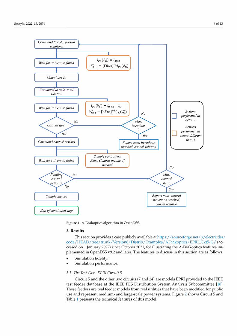
The architecture for implementing this simplified approach considers the optimiza-tion of computational resources for reducing the burden of the operations around thealgorithm. This optimization comprehends memory handling, actor coordination, andmessage structure between actors, and it is described in detail in [16]. Figure 1 describesthe implementation of the simplified A-Diakoptics method in OpenDSS 9.3 and later.

Figure 1 presents how the main loops of the OpenDSS algorithm are decomposedinto the set of distributed solvers implemented as actors. Each actor (including the co-ordinator) is executed in its own CPU and counts with its own memory and hardware.All of the actors are executed in parallel and concurrently in an asynchronous parallelcomputing environment.

Actors remain on standby when not executing any job. A message sent to an actortriggers an event that sets the busy flag for the actor in the global context and leads theactor to perform the job given in the message. Once the actor has finished the job, it updatesits state by marking a ready flag in the global context, making it visible to all of the otheractors. When the YBUS matrices within actors >2 are smaller than the interconnected system,it is expected that the solution time required for solving the subnetworks is substantiallylower than that required for solving the interconnected model, as discussed in [5,13]. Thecalculation of IC is very fast, given the size of the mathematical problem proposed; at thesame time, it solves and avoids moving values between actors by using pointers, adding anegligible overhead to the solution process in parallel.

With the architecture proposed in this implementation of A-Diakoptics, the algorithmbecomes available for all QSTS simulation modes. The previous version of the algorithmwas only available for yearly simulation. The new implementation is available for the snap,direct, yearly, daily, time, and duty cycle simulation modes in OpenDSS [17].

Centralizing the results on a single memory space (Actor 1) makes it possible toinsert monitors and energy meters and request simulation information directly from themodel using a single actor, a feature that was not available in the previous version of theA-Diakoptics suite.

The previous considerations are true only if the matrix ZCC is a fraction of the size of thelargest subnetwork in the system, which is the one representing the largest computationalburden in the parallel solver, as explained in [16].

Energies 2022, 15, 2051 6 of 13Energies 2022, 15, x FOR PEER REVIEW 6 of 13

Figure 1. A-Diakoptics algorithm in OpenDSS.

3. Results This section provides a case publicly available at https://sourceforge.net/p/elec-

tricdss/code/HEAD/tree/trunk/Version8/Distrib/Examples/ADiakoptics/EPRI_Ckt5-G/ since October 2021, for illustrating the A-Diakoptics features implemented in OpenDSS v9.2 and later. The features to discuss in this section are as follows: • Simulation fidelity; • Simulation performance.

3.1. The Test Case: EPRI Circuit 5 Circuit 5 and the other two circuits (7 and 24) are models EPRI provided to the IEEE

test feeder database at the IEEE PES Distribution System Analysis Subcommittee [18]. These feeders are real feeder models from real utilities that have been modified for public use and represent medium- and large-scale power systems. Figure 2 shows Circuit 5 and Table 1 presents the technical features of this model.

Figure 1. A-Diakoptics algorithm in OpenDSS.

3. Results

This section provides a case publicly available at https://sourceforge.net/p/electricdss/code/HEAD/tree/trunk/Version8/Distrib/Examples/ADiakoptics/EPRI_Ckt5-G/ (ac-cessed on 1 January 2022) since October 2021, for illustrating the A-Diakoptics features im-plemented in OpenDSS v9.2 and later. The features to discuss in this section are as follows:

• Simulation fidelity;• Simulation performance.

3.1. The Test Case: EPRI Circuit 5

Circuit 5 and the other two circuits (7 and 24) are models EPRI provided to the IEEEtest feeder database at the IEEE PES Distribution System Analysis Subcommittee [18].These feeders are real feeder models from real utilities that have been modified for publicuse and represent medium- and large-scale power systems. Figure 2 shows Circuit 5 andTable 1 presents the technical features of this model.

Energies 2022, 15, 2051 7 of 13Energies 2022, 15, x FOR PEER REVIEW 7 of 13

Figure 2. EPRI’s Circuit 5.

Table 1. Circuit 5 technical features.

Feature Name Value Number of buses 2998 Number of nodes 3437 Total active power 7.281 MW

Total reactive power 3.584 Mvar

Figure 2 indicates the link branches for the two-zone and four-zone partitioning with blue and orange arrows, respectively. Tables 2 and 3 present the partition statistics for two- and four-zone partitioning, respectively. The partition method for obtaining these statistics was the automated option through MeTIS [19]. For more extensive partitioning (five, six, and seven zones), the manual procedure specifying the link branches was used [17].

The partition statistics reveal a moderate imbalance in the case of two zones that is more pronounced in the case of four zones. The imbalances are expected given the repre-sentation of single-phase low-voltage networks within the model, making it more difficult for the tearing algorithm to balance the node distribution between zones. The calculation methods for the partition statistics and their interpretation details are presented in [17].

Table 2. Partition statistics for Circuit 5 feeder, two zones.

Name Value Circuit reduction (%) 32.24

Maximum imbalance (%) 52.43

Figure 2. EPRI’s Circuit 5.

Table 1. Circuit 5 technical features.

Feature Name Value

Number of buses 2998Number of nodes 3437Total active power 7.281 MW

Total reactive power 3.584 Mvar

Figure 2 indicates the link branches for the two-zone and four-zone partitioning withblue and orange arrows, respectively. Tables 2 and 3 present the partition statistics for two-and four-zone partitioning, respectively. The partition method for obtaining these statisticswas the automated option through MeTIS [19]. For more extensive partitioning (five, six,and seven zones), the manual procedure specifying the link branches was used [17].

Table 2. Partition statistics for Circuit 5 feeder, two zones.

Name Value

Circuit reduction (%) 32.24Maximum imbalance (%) 52.43Average imbalance (%) 26.21

Table 3. Partition statistics for Circuit 5 feeder, four zones.

Name Value

Circuit reduction (%) 45.94Maximum imbalance (%) 88.11Average imbalance (%) 53.75

Energies 2022, 15, 2051 8 of 13

The partition statistics reveal a moderate imbalance in the case of two zones thatis more pronounced in the case of four zones. The imbalances are expected given therepresentation of single-phase low-voltage networks within the model, making it moredifficult for the tearing algorithm to balance the node distribution between zones. Thecalculation methods for the partition statistics and their interpretation details are presentedin [17].

3.2. The Simulation Fidelity and Performance

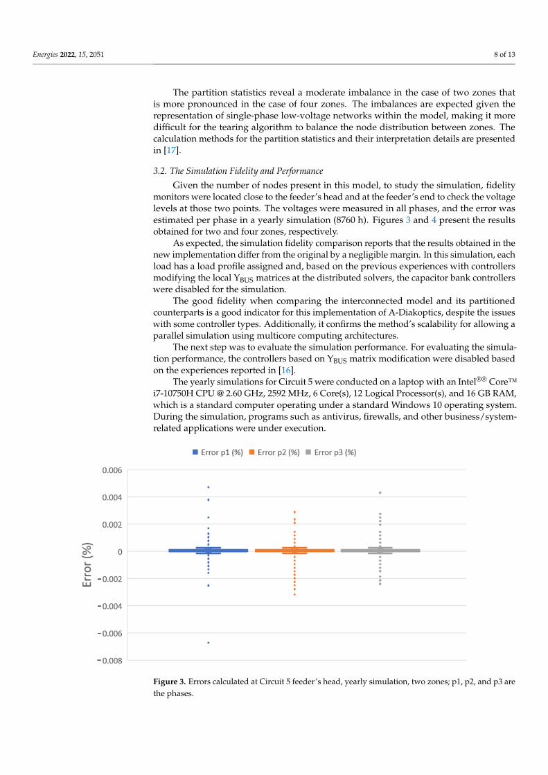
Given the number of nodes present in this model, to study the simulation, fidelitymonitors were located close to the feeder’s head and at the feeder’s end to check the voltagelevels at those two points. The voltages were measured in all phases, and the error wasestimated per phase in a yearly simulation (8760 h). Figures 3 and 4 present the resultsobtained for two and four zones, respectively.

As expected, the simulation fidelity comparison reports that the results obtained in thenew implementation differ from the original by a negligible margin. In this simulation, eachload has a load profile assigned and, based on the previous experiences with controllersmodifying the local YBUS matrices at the distributed solvers, the capacitor bank controllerswere disabled for the simulation.

The good fidelity when comparing the interconnected model and its partitionedcounterparts is a good indicator for this implementation of A-Diakoptics, despite the issueswith some controller types. Additionally, it confirms the method’s scalability for allowing aparallel simulation using multicore computing architectures.

The next step was to evaluate the simulation performance. For evaluating the simula-tion performance, the controllers based on YBUS matrix modification were disabled basedon the experiences reported in [16].

The yearly simulations for Circuit 5 were conducted on a laptop with an Intel®® Core™i7-10750H CPU @ 2.60 GHz, 2592 MHz, 6 Core(s), 12 Logical Processor(s), and 16 GB RAM,which is a standard computer operating under a standard Windows 10 operating system.During the simulation, programs such as antivirus, firewalls, and other business/system-related applications were under execution.

Energies 2022, 15, x FOR PEER REVIEW 8 of 13

Average imbalance (%) 26.21

Table 3. Partition statistics for Circuit 5 feeder, four zones.

Name Value Circuit reduction (%) 45.94

Maximum imbalance (%) 88.11 Average imbalance (%) 53.75

3.2. The Simulation Fidelity and Performance Given the number of nodes present in this model, to study the simulation, fidelity

monitors were located close to the feeder's head and at the feeder’s end to check the volt-age levels at those two points. The voltages were measured in all phases, and the error was estimated per phase in a yearly simulation (8760 h). Figures 3 and 4 present the results obtained for two and four zones, respectively.

As expected, the simulation fidelity comparison reports that the results obtained in the new implementation differ from the original by a negligible margin. In this simulation, each load has a load profile assigned and, based on the previous experiences with control-lers modifying the local YBUS matrices at the distributed solvers, the capacitor bank con-trollers were disabled for the simulation.

The good fidelity when comparing the interconnected model and its partitioned counterparts is a good indicator for this implementation of A-Diakoptics, despite the is-sues with some controller types. Additionally, it confirms the method’s scalability for al-lowing a parallel simulation using multicore computing architectures.

The next step was to evaluate the simulation performance. For evaluating the simu-lation performance, the controllers based on YBUS matrix modification were disabled based on the experiences reported in [16].

Figure 3. Errors calculated at Circuit 5 feeder’s head, yearly simulation, two zones; p1, p2, and p3 are the phases.

Figure 3. Errors calculated at Circuit 5 feeder’s head, yearly simulation, two zones; p1, p2, and p3 arethe phases.

Energies 2022, 15, 2051 9 of 13Energies 2022, 15, x FOR PEER REVIEW 9 of 13

Figure 4. Errors calculated at Circuit 5 feeder’s head, yearly simulation, four zones; p1, p2, and p3 are the phases.

The yearly simulations for Circuit 5 were conducted on a laptop with an Intel®® Core™ i7-10750H CPU @ 2.60 GHz, 2592 MHz, 6 Core(s), 12 Logical Processor(s), and 16 GB RAM, which is a standard computer operating under a standard Windows 10 operat-ing system. During the simulation, programs such as antivirus, firewalls, and other busi-ness/system-related applications were under execution.

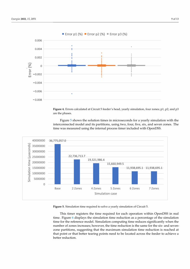
Figure 5 shows the solution times in microseconds for a yearly simulation with the interconnected model and its partitions, using two, four, five, six, and seven zones. The time was measured using the internal process timer included with OpenDSS.

This timer registers the time required for each operation within OpenDSS in real time. Figure 6 displays the simulation time reduction as a percentage of the simulation time for the reference model. Simulation computing time reduces significantly when the number of zones increases; however, the time reduction is the same for the six- and seven-zone partitions, suggesting that the maximum simulation time reduction is reached at that point or that better tearing points need to be located across the feeder to achieve a better reduction.

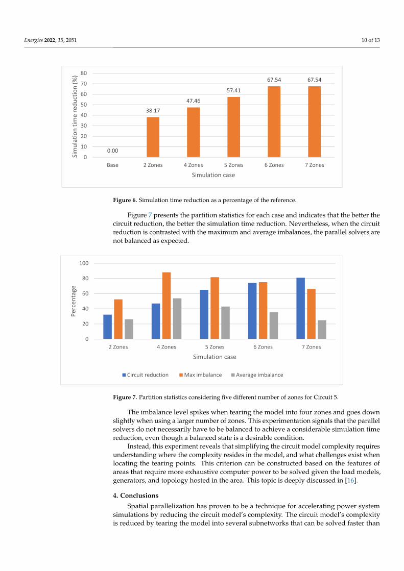
Figure 7 presents the partition statistics for each case and indicates that the better the circuit reduction, the better the simulation time reduction. Nevertheless, when the circuit reduction is contrasted with the maximum and average imbalances, the parallel solvers are not balanced as expected.

The imbalance level spikes when tearing the model into four zones and goes down slightly when using a larger number of zones. This experimentation signals that the par-allel solvers do not necessarily have to be balanced to achieve a considerable simulation time reduction, even though a balanced state is a desirable condition.

Instead, this experiment reveals that simplifying the circuit model complexity re-quires understanding where the complexity resides in the model, and what challenges exist when locating the tearing points. This criterion can be constructed based on the fea-tures of areas that require more exhaustive computer power to be solved given the load models, generators, and topology hosted in the area. This topic is deeply discussed in [16].

Figure 4. Errors calculated at Circuit 5 feeder’s head, yearly simulation, four zones; p1, p2, and p3are the phases.

Figure 5 shows the solution times in microseconds for a yearly simulation with theinterconnected model and its partitions, using two, four, five, six, and seven zones. Thetime was measured using the internal process timer included with OpenDSS.

Energies 2022, 15, x FOR PEER REVIEW 10 of 13

Figure 5. Simulation time required to solve a yearly simulation of Circuit 5.

Figure 6. Simulation time reduction as a percentage of the reference.

Figure 7. Partition statistics considering five different number of zones for Circuit 5.

4. Conclusions Spatial parallelization has proven to be a technique for accelerating power system

simulations by reducing the circuit model’s complexity. The circuit model’s complexity is reduced by tearing the model into several subnetworks that can be solved faster than the

36,775,057.0

22,736,713.719,321,986.4

15,660,949.511,938,695.1 11,938,695.1

0

5000000

10000000

15000000

20000000

25000000

30000000

35000000

40000000

Base 2 Zones 4 Zones 5 Zones 6 Zones 7 Zones

Sim

ulat

ion

time

(µse

cond

s)

Simulation case

0.00

38.1747.46

57.41

67.54 67.54

0

10

20

30

40

50

60

70

80

Base 2 Zones 4 Zones 5 Zones 6 Zones 7 Zones

Sim

ulat

ion

time

redu

ctio

n (%

)

Simulation case

0

20

40

60

80

100

2 Zones 4 Zones 5 Zones 6 Zones 7 Zones

Perc

enta

ge

Simulation case

Circuit reduction Max imbalance Average imbalance

Figure 5. Simulation time required to solve a yearly simulation of Circuit 5.

This timer registers the time required for each operation within OpenDSS in realtime. Figure 6 displays the simulation time reduction as a percentage of the simulationtime for the reference model. Simulation computing time reduces significantly when thenumber of zones increases; however, the time reduction is the same for the six- and seven-zone partitions, suggesting that the maximum simulation time reduction is reached atthat point or that better tearing points need to be located across the feeder to achieve abetter reduction.

Energies 2022, 15, 2051 10 of 13

Energies 2022, 15, x FOR PEER REVIEW 10 of 13

Figure 5. Simulation time required to solve a yearly simulation of Circuit 5.

Figure 6. Simulation time reduction as a percentage of the reference.

Figure 7. Partition statistics considering five different number of zones for Circuit 5.

4. Conclusions Spatial parallelization has proven to be a technique for accelerating power system

simulations by reducing the circuit model’s complexity. The circuit model’s complexity is reduced by tearing the model into several subnetworks that can be solved faster than the

36,775,057.0

22,736,713.719,321,986.4

15,660,949.511,938,695.1 11,938,695.1

0

5000000

10000000

15000000

20000000

25000000

30000000

35000000

40000000

Base 2 Zones 4 Zones 5 Zones 6 Zones 7 Zones

Sim

ulat

ion

time

(µse

cond

s)

Simulation case

0.00

38.1747.46

57.41

67.54 67.54

0

10

20

30

40

50

60

70

80

Base 2 Zones 4 Zones 5 Zones 6 Zones 7 Zones

Sim

ulat

ion

time

redu

ctio

n (%

)

Simulation case

0

20

40

60

80

100

2 Zones 4 Zones 5 Zones 6 Zones 7 Zones

Perc

enta

ge

Simulation case

Circuit reduction Max imbalance Average imbalance

Figure 6. Simulation time reduction as a percentage of the reference.

Figure 7 presents the partition statistics for each case and indicates that the better thecircuit reduction, the better the simulation time reduction. Nevertheless, when the circuitreduction is contrasted with the maximum and average imbalances, the parallel solvers arenot balanced as expected.

Energies 2022, 15, x FOR PEER REVIEW 10 of 13

Figure 5. Simulation time required to solve a yearly simulation of Circuit 5.

Figure 6. Simulation time reduction as a percentage of the reference.

Figure 7. Partition statistics considering five different number of zones for Circuit 5.

4. Conclusions Spatial parallelization has proven to be a technique for accelerating power system

simulations by reducing the circuit model’s complexity. The circuit model’s complexity is reduced by tearing the model into several subnetworks that can be solved faster than the

36,775,057.0

22,736,713.719,321,986.4

15,660,949.511,938,695.1 11,938,695.1

0

5000000

10000000

15000000

20000000

25000000

30000000

35000000

40000000

Base 2 Zones 4 Zones 5 Zones 6 Zones 7 ZonesSi

mul

atio

n tim

e (µ

seco

nds)

Simulation case

0.00

38.1747.46

57.41

67.54 67.54

0

10

20

30

40

50

60

70

80

Base 2 Zones 4 Zones 5 Zones 6 Zones 7 Zones

Sim

ulat

ion

time

redu

ctio

n (%

)

Simulation case

0

20

40

60

80

100

2 Zones 4 Zones 5 Zones 6 Zones 7 Zones

Perc

enta

ge

Simulation case

Circuit reduction Max imbalance Average imbalance

Figure 7. Partition statistics considering five different number of zones for Circuit 5.

The imbalance level spikes when tearing the model into four zones and goes downslightly when using a larger number of zones. This experimentation signals that the parallelsolvers do not necessarily have to be balanced to achieve a considerable simulation timereduction, even though a balanced state is a desirable condition.

Instead, this experiment reveals that simplifying the circuit model complexity requiresunderstanding where the complexity resides in the model, and what challenges exist whenlocating the tearing points. This criterion can be constructed based on the features ofareas that require more exhaustive computer power to be solved given the load models,generators, and topology hosted in the area. This topic is deeply discussed in [16].

4. Conclusions

Spatial parallelization has proven to be a technique for accelerating power systemsimulations by reducing the circuit model’s complexity. The circuit model’s complexityis reduced by tearing the model into several subnetworks that can be solved faster than

Energies 2022, 15, 2051 11 of 13

the original interconnected model. The partial solutions are put together through a tensor-based interconnection approximation, which delivers an accurate solution that matches theoriginal with a low error margin.

One method for performing spatial parallelization is Diakoptics, which, in combinationwith a framework for providing inconsistency robustness within a parallel computing ar-chitecture, is called A-Diakoptics. The previous implementation of this technique in EPRI’sopen-source distribution simulator software OpenDSS provided limited access to thistechnique, given that the implementation aimed to cover the needs of a particular project.

Through the project presented in this document, the previous implementation of A-Diakoptics in OpenDSS was reformulated using a simplified approach, optimizing criticalareas of the algorithm and the mathematical formulation. Many other improvements atthe implementation level were performed in this new version of A-Diakoptics to facilitateaccess to electrical variables through monitors and meters.

This implementation of A-Diakoptics was validated using yearly QSTS simulationsin terms of fidelity and performance using as reference the interconnected model. Thesimulation results revealed the benefits of modernizing sequential power simulation toolsinto parallel processing, which is the standard for computing architectures nowadays.This paper introduced A-Diakoptics as a method for achieving such modernization andOpenDSS, given that it is distributed as an open-source project using the internet, presentsa practical example of how this modernization can be implemented.

A simulation test case was used for illustrating the computational time gains, compar-ing the sequential and parallel performance on a yearly QSTS. The computing time gainswere evaluated for an incremental number of partitions, displaying and discussing thebenefits and limits of the algorithm. This test case is publicly available on the internet forthe reader to evaluate if desired.

The results presented confirm the performance improvement in QSTS simulationsfor medium- and large-scale power system models. They also provide guidance onthe objectives of circuit tearing for reducing the circuit model complexity to accelerateQSTS simulations.

The test cases presented in this document and the A-Diakoptics capabilities are avail-able in OpenDSS version 9.3, which can be downloaded from the internet. In addition to thetest case presented in this paper, five more test cases offering different levels of complexityare available at OpenDSS/Code/[r3354]/trunk/Version8/Distrib/Examples/A-Diakoptics(sourceforge.net) (accessed on 1 January 2022). These cases and their purpose are discussedin [16] and serve as sources of reference for applying A-Diakoptics with OpenDSS in otherapplications.

Additional to the methods presented in this paper, others using different paralleliza-tion techniques and approaches have also been investigated as the result of the SunShotNational Laboratory Multiyear Partnership Program (SuNLaMP). The findings, conclu-sions, and a more extended explanation of these methods can be found in [13]. For futureimplementations and demonstrations on methods for accelerating simulations, we expectto continue to use OpenDSS as the open-source project for serving as a proof of conceptfor this type of research, demonstrating viable techniques and methods for modernizingpower simulation tools.

Author Contributions: D.M. developed the A-Diakoptics technique and performed the implemen-tation within OpenDSS. He also performed the technical analysis for obtaining the results herepresented. R.D. is the original author of the simulation tool OpenDSS, his technical advice wasvital for the project development. All authors have read and agreed to the published version ofthe manuscript.

Funding: This project was funded originally by the SunShot National Laboratory Multiyear Partner-ship Program (SuNLaMP) [13]. The recent improvements on the technique and implementation werefunded by EPRI under the Technology Innovation program for 2021.

Institutional Review Board Statement: Not applicable.

Energies 2022, 15, 2051 12 of 13

Informed Consent Statement: Not applicable.

Data Availability Statement: The results of this study and data sources are available at [16], whichcan be accessed through the EPRI member center at https://www.epri.com/research/programs/0TIZ12/results/3002021419 (accessed on 1 January 2022).

Conflicts of Interest: The authors declare no conflict of interest.

Nomenclature

A-Diakoptics Actor-based diakopticsBBDM Bordered block diagonal matrixDG Distributed generationE Array of complex numbers representing the voltages at each node in the modelIPC(E) Array of complex numbers representing compensation currents from power

conversion devices (shunt connected)PC Power conversion device (shunt connected)PV Photovoltaic cells arrayQSTS Quasi static time seriesYSystem/YBus Admittance matrix of the power system modelYII YSystemZCC Connection’s matrix, built by combining the contours matrix (also called tensors)

with ZTT and the links between the subsystemsZCT/TC Complementary matrices, obtained with partial components of ZCCZTT Trees matrix containing the inverted Y matrices of the isolated subsystems when

tearing the interconnected system

References1. Deboever, J.; Zhang, X.; Reno, M.J.; Broderick, R.J.; Grijalva, S.; Therrien, F. Challenges in Reducing the Computational Time of QSTS

Simulations for Distribution System Analysis; Sandia National Laboratories: Albuquerque, NM, USA, 2017.2. Montenegro, D.; Dugan, R.C.; Reno, M.J. Open Source Tools for High Performance Quasi-Static-Time-Series Simulation Using

Parallel Processing. In Proceedings of the 2017 IEEE 44th Photovoltaic Specialist Conference (PVSC), Washington, DC, USA,25–30 June 2017; pp. 3055–3060. [CrossRef]

3. Shahidehpour, M.; Wang, Y. Communication and Control in Electric Power Systems: Applications of Parallel and Distributed Processing;Wiley: Hoboken, NJ, USA, 2004.

4. Montenegro, D. Actor’s Based Diakoptics for the Simulation, Monitoring and Control of Smart Grids. Université Grenoble Alpes,2015GREAT106, 2015. Available online: https://tel.archives-ouvertes.fr/tel-01260398 (accessed on 1 November 2021).

5. Montenegro, D.; Ramos, G.A.; Bacha, S. Multilevel A-Diakoptics for the Dynamic Power-Flow Simulation of Hybrid PowerDistribution Systems. IEEE Trans. Ind. Inform. 2016, 12, 267–276. [CrossRef]

6. Montenegro, D.; Ramos, G.A.; Bacha, S. A-Diakoptics for the Multicore Sequential-Time Simulation of Microgrids Within LargeDistribution Systems. IEEE Trans. Smart Grid. 2017, 8, 1211–1219. [CrossRef]

7. Kron, G. Detailed Example of Interconnecting Piece-Wise Solutions. J. Frankl. Institute. 1955, 1, 26. [CrossRef]8. Kron, G. Diakoptics: The Piecewise Solution of Large-Scale Systems; (No. v. 2); Macdonald: London, UK, 1963.9. Hewitt, C. Actor Model of Computation: Scalable Robust Information Systems. In Inconsistency Robustness 2011, Stanford

University; Standford University, Ed.; 16–18 August 2011; No. 1; Standford University: Stanford, CA, USA, 2012; Volume 1, p. 32.10. Hewitt, C.; Meijer, E.; Szyperski, C. The Actor Model (Everything You Wanted to Know, but Were Afraid to Ask). Microsoft.

Available online: http://channel9.msdn.com/Shows/Going+Deep/Hewitt-Meijer-and-Szyperski-The-Actor-Model-everything-you-wanted-to-know-but-were-afraid-to-ask (accessed on 15 May 2015).

11. Watson, N.; Arrillaga, J. Institution of Engineering and Technology. Power Systems Electromagnetic Transients Simulation; Institution ofEngineering and Technology: London, UK, 2003.

12. Dugan, R. OpenDSS Circuit Solution Technique; p. 1. Available online: https://sourceforge.net/p/electricdss/code/HEAD/tree/trunk/Version8/Distrib/Doc/OpenDSS%20Solution%20Technique.pdf.1773234 (accessed on 1 January 2022).

13. Rapid QSTS Simulations for High-Resolution Comprehensive Assessment of Distributed PV. SAND2021-2660. 2021. Availableonline: https://www.osti.gov/servlets/purl/1773234 (accessed on 1 November 2021).

14. Davis, T.A.; Natarajan, E.P. Algorithm 907: KLU, a direct sparse solver for circuit simulation problems. ACM Trans. Math. Softw.2010, 37, 36. [CrossRef]

15. Happ, H.H. Piecewise Methods and Applications to Power Systems; Wiley: Hoboken, NJ, USA, 1980.16. Advancing Spatial Parallel Processing for QSTS: Improving the A-Diakoptics Suite in OpenDSS; EPRI: Palo Alto, CA, USA, 2021.

Energies 2022, 15, 2051 13 of 13

17. Montenegro, D.; Dugan, R.C. Diakoptics Based on Actors (A-Diakoptics) Suite for OpenDSS; EPRI, Online; 2021. Available online:https://sourceforge.net/p/electricdss/code/HEAD/tree/trunk/Version8/Distrib/Doc/A-Diakoptics_Suite.pdf (accessed on 1November 2021).

18. Fuller, J.; Kersting, W.; Dugan, R.; Jr, S.C. Distribution Test Feeders. IEEE Power and Energy Society. Available online:http://ewh.ieee.org/soc/pes/dsacom/testfeeders/ (accessed on 23 October 2013).

19. Karypis, G.; Kumar, V. A Fast and High Quality Multilevel Scheme for Partitioning Irregular Graphs. SIAM J. Sci.Comput. 1998,20, 359–392. [CrossRef]