simple binding F + G B Mathematical Modeling

Chemical Kinetics: Simple Binding: F +G⇋B

Gary D. Knott

Civilized Software Inc.

12109 Heritage Park Circle

Silver Spring MD 20906

phone:301-962-3711

email:[email protected]

URL:www.civilized.com

February 13, 2015

0.1 Simple Binding

Consider the reaction F +Gk1⇋

k2B.

The study of this reaction is common in chemistry and biochemistry. For example, F could be ahormone or drug and G the associated receptor sites. The symbol B represents the bound complex.

Let us also allow F (t), G(t), and B(t) to be functions which specify the concentrations of F , G,and B respectively at time t. Then we have the differential equation model:

dB

dt(t) = k1F (t)G(t)− k2B(t), B(0) = B0,

F (t) = F0 − (B(t)−B0),

G(t) = G0 − (B(t)−B0),

where F0, G0, and B0 are the initial concentrations of F , G, and B respectively, and the molarassociation and dissociation rate constants k1 and k2 appear as the proportionality constants forthe terms which occur in dB/dt.

Note that k1 = (dB

dt(0) + k2B0)/(F0G0), so when B0 = 0 and F0 and G0 are known, k1 may be

estimated from the initial velocity dB/dt(0), which can, in turn, be estimated from a few pointswith t near 0.

The solution to our differential equation is:

B(t) = (S(B0 −R)−R(B0 − S)ed·k1·t)/(B0 −R− (B0 − S)ed·k1·t),

1

2

where

S = A+ d/2

R = A− d/2

d = 2(A2 − (F0 +B0)(G0 +B0))1/2

A = (F0 +G0 + 2B0 + k2/k1)/2

An appropriate definition of this function in MLAB involves using auxiliary functions as follows:

fct B(T) = H1((F0+G0+2*B0+K2/K1)/2,T)

fct H1(A,T) = H2(A,SQRT(4*(A^2-(F0+B0)*(G0+B0))),T)

fct H2(A,D,T) = H3(A+D/2,A-D/2,EXP(D*K1*T))

fct H3(S,R,E) = ((B0-R)*S-(B0-S)*R*E)/(B0-R-(B0-S)*E)

It is useful to study this example carefully. Many occasions will arise where functions will need tobe defined with the help of auxillary functions in a similar manner.

If we have time-course data consisting of time-values vs. concentration-values of one or more ofthe species B, F , or G, we can use a curve-fitting program like MLAB that handles ODE models,(or in this case, since we have an algebraic model, a program like MLAB that handles non-linearmodels,) to estimate the values of k1, k2, and even F0 and G0 and B0, (although usually B0 is 0.)It is actually easier and more transparent to use the ODE model than it is to use the algebraicmodel.

Note we must have data at early times before equilibrium is approached; data at late times willallow us to estimate the equilibrium constant k1/k2, but k1 and k2 will not be separably estimablewith only late time data.

Moreover, if we try to estimate all the parameters F0, G0, k1, and k2, we are likely to get a goodpictorial fit, but also estimates that are completely non-unique, where varying any parameter canbe compensated by varying the others, so that our estimates are essentially worthless. If we havepreviously determined k1/k2 by fitting an equilbrium model, this will help in reducing the “degreesof freedom”.

Note however, when k1 and k2 are known, (or k1/k2 in the equilibrium case,) we can use kinetic orequilibrium data measuring any of F , G, or B to “assay” the initial amounts of F or G or both byestimating F0 and/or G0 via curve-fitting, (again assuming B0 is known.) Examples of fitting ourkinetic model to data will be given below.

0.2 Derivation of the Kinetic Model

Suppose we have a volume with #F free F -molecules and #G free G-molecules and also #B B-molecules and S solvent molecules; #F is a function of time, #F (t), and similarly, #G is a functionof time, #G(t), and #B is a function of time, #B(t). But S is assumed to be constant.

3

Let N(t) be the total number of molecules present at time t; N(t) = #F (t) +#G(t) +#B(t) + S.As F +G⇋B, N(t) varies. Note the minimum possible value of N(t) is #F (0)+#G(0)+#B(0)−min(#F (0),#G(0))+S and the maximum possible value of N(t) is #F (0)+#G(0)+2#B(0)+S.

Now for a random “collision” of molecules occurring at or sufficiently near time t, the probability

that this is a collision of an F -molecule and a G-molecule is#F (t)

N(t)·#G(t)

N(t)+

#G(t)

N(t)·#F (t)

N(t),

since we first pick one molecule and then the second to form our collision, and the first is either anF -molecule and the second is a G-molecule, or vice-versa. (This is assuming the number of eachtype of molecule is large enough so that a “sampling with replacement” model is adequate. The

“true” probability is

(

#F

1

)(

#G

1

)

/

(

N

2

)

=2#F#G

N(N − 1).)

We take a time-interval It containing t such that It is short enough that N(t) does not appreciablychange during It.

Now, looking at our stochastic collision process, assume that during the small interval of timeIt containing t, the expected number of “collisions” of molecules per second in our volume isproportional to N(t)2 · Lt, i.e., αN(t)2 · Lt, where Lt is the length, i.e., the duration, of thetime-interval It.

This assumption is acceptable when we also accept that the number of collisions between molecule iand molecule j during the time-interval It follows a Poisson distribution with the density parameterλLt, i.e., P (there are k (i, j)-collisions during It) ≈ e−λLt(λLt)

k/k!. Then the expected mumber ofcollisions between molecule i and molecule j during the time-interval It is approximately λLt. Hereλ is an unknown parameter specifying the expected mumber of collisions between any fixed pair of

molecules during a time-interval of unit length. Now since we have

(

N

2

)

pairs of molecules that

can be the components of a collision, the expected number of collisions during the time-interval It

is approximately

(

N

2

)

λLt ≈ αN2Lt where α = λ/2.

The Poisson distribution arises as follows. Let an interval I of length L be divided into nL subin-

tervals of length1

n. Here the interval I is choosen so that L is an integer multiple of

1

n. Suppose

the probability of at least one event (such as a collision between two particles), in any length-1

nsubinterval of I is pn, and the occurrence of events in each subintegral is independent of the occur-rence of events in any other disjoint subintegral. Then the probability of k “non-empty” disjoint

length-1

nsubintervals is

(

nL

k

)

pkn(1−pn)nL−k, and the expected number of non-empty subintervals

is npn.

Now when1

nis small, we may suppose the probability of more than one event in a length-

1

n

subinterval is negligibly small, so that p2n → 0 as1

n→ 0. Also, considering a length-

1

nsubinterval

as two length-1

2nsubintervals, we see that pn = p2n + p2n − p22n; this is the probability that one or

more events occur in the first length-1

2nsubinterval or in the second length-

1

2nsubinterval, (p22n is

4

subtracted because it is counted twice in p2n+p2n). Thus pn < 2p2n and nLpn < 2nLp2n, and since

p2n → 0 as1

n→ 0, nLpn increases monotonically to some limit λL as

1

n→ 0. (If nLpn increased to

∞ then there would be an infinite number of events expected in the interval I, which we dismissas a possiblity.)

Then as n → ∞,

(

nL

k

)

pkn(1− pn)nL−k → e−λL(λL)k/k! for k ≥ 0. This is because

(

nL

k

)

pkn(1− pn)nL−k =

(nL)k

k!pkn

∑

0≤i≤nL−k

(nL− k)i

i!(−pn)

i

=(nL)k

k!

1

(nL)k(nLpn)

k∑

0≤i≤nL−k

(nL− k)i

i!

1

(nL− k)i(−(nL− k)pn)

i

→1

k!(λL)k

∑

0≤i≤∞

1

i!(−λL)i

=(λL)k

k!e−λL

where (a)m := a(a + 1) · · · (a −m + 1). Thus the probability of k events during a time-interval of

length L is(λL)k

k!e−λL, and the expected number of such events during a time-interval of length L

is

∑

0≤k≤∞

k(λL)k

k!e−λL = λL

∑

1≤k≤∞

λL)k−1

(k − 1)!e−λL

= λL∑

0≤k≤∞

(λL)k

k!e−λL

= λLe−λL∑

0≤k≤∞

(λL)k

k!

= λL.

Now of the approximately αN(t)2 ·Lt collisions during the interval It, the expected number of FG-

collisions is approximately

(

#F (t)

N(t)·#G(t)

N(t)+

#G(t)

N(t)·#F (t)

N(t)

)

· αN(t)2 ·Lt = 2α#F (t)#G(t) ·Lt

FG-collisions.

The proportionality “constant” α depends upon the density of molecules in our volume. If we wereto have N varying as our volume remained constant then α would vary accordingly. If, however,our volume also varies to maintain a constant density, as is generally the case for a solution, ormore generally, for any volume maintained at constant pressure, then α is constant, (although αgenerally depends on temperature.)

Let the fraction β of these FG-collisions be energetic enough to bind to form a B molecule.

5

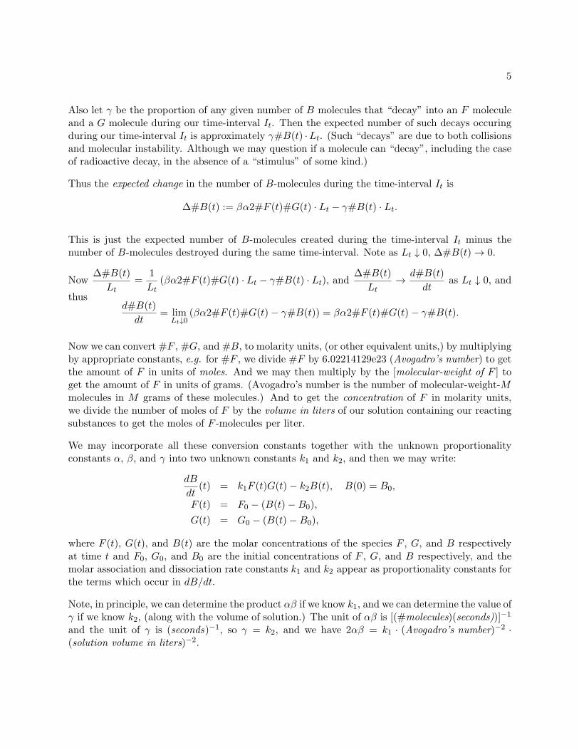
Also let γ be the proportion of any given number of B molecules that “decay” into an F moleculeand a G molecule during our time-interval It. Then the expected number of such decays occuringduring our time-interval It is approximately γ#B(t) ·Lt. (Such “decays” are due to both collisionsand molecular instability. Although we may question if a molecule can “decay”, including the caseof radioactive decay, in the absence of a “stimulus” of some kind.)

Thus the expected change in the number of B-molecules during the time-interval It is

∆#B(t) := βα2#F (t)#G(t) · Lt − γ#B(t) · Lt.

This is just the expected number of B-molecules created during the time-interval It minus thenumber of B-molecules destroyed during the same time-interval. Note as Lt ↓ 0, ∆#B(t) → 0.

Now∆#B(t)

Lt=

1

Lt(βα2#F (t)#G(t) · Lt − γ#B(t) · Lt), and

∆#B(t)

Lt→

d#B(t)

dtas Lt ↓ 0, and

thusd#B(t)

dt= lim

Lt↓0(βα2#F (t)#G(t)− γ#B(t)) = βα2#F (t)#G(t)− γ#B(t).

Now we can convert #F , #G, and #B, to molarity units, (or other equivalent units,) by multiplyingby appropriate constants, e.g. for #F , we divide #F by 6.02214129e23 (Avogadro’s number) to getthe amount of F in units of moles. And we may then multiply by the [molecular-weight of F ] toget the amount of F in units of grams. (Avogadro’s number is the number of molecular-weight-Mmolecules in M grams of these molecules.) And to get the concentration of F in molarity units,we divide the number of moles of F by the volume in liters of our solution containing our reactingsubstances to get the moles of F -molecules per liter.

We may incorporate all these conversion constants together with the unknown proportionalityconstants α, β, and γ into two unknown constants k1 and k2, and then we may write:

dB

dt(t) = k1F (t)G(t)− k2B(t), B(0) = B0,

F (t) = F0 − (B(t)−B0),

G(t) = G0 − (B(t)−B0),

where F (t), G(t), and B(t) are the molar concentrations of the species F , G, and B respectivelyat time t and F0, G0, and B0 are the initial concentrations of F , G, and B respectively, and themolar association and dissociation rate constants k1 and k2 appear as proportionality constants forthe terms which occur in dB/dt.

Note, in principle, we can determine the product αβ if we know k1, and we can determine the value ofγ if we know k2, (along with the volume of solution.) The unit of αβ is [(#molecules)(seconds))]−1

and the unit of γ is (seconds)−1, so γ = k2, and we have 2αβ = k1 · (Avogadro’s number)−2 ·

(solution volume in liters)−2.

6

0.3 Units

In the first-order ordinary differental equation dB/dt(t) = k1F (t)G(t)−k2B(t), we have F (t), G(t)and B(t) given in molarity units, i.e., moles/liter – ormilliliter ormicroliter, etc. And then dB/dt(t)has the unit (moles/liter)/second – or nanosecond or minute or hour, etc. But then F (t)G(t) hasthe unit moles2/liter2 and thus k1 must be a constant with the unit (liter)/(moles·second), or moregenerally, (liter)/(moles·time-unit), and k2 must be a constant with the unit 1/second, or moregenerally, (time-unit)−1, in order for our differential equation to be dimensionally consistent. Notek1 and k2 do not have interconvertable units, thus the values of k1 and k2 are not easily comparableas a measure of either the speed or the equilibrium levels of our reaction. However, the bigger k1

and the smaller k2, the more “irreversible” the reaction F + Gk1⇋

k2B is. If k2 = 0, the reaction is

completely irreversible.

We have the following units in common use.

fraction composition by mass: (mass of solute)/(mass of solute plus solvent).

fraction composition by volume: (volume of solute)/(volume of solution).Note the volume of the solution is in general not exactly equal to the volume of the solvent plusthe volume of the solute, even when both are in the same state of matter, due to various effects.

molarity concentration (moles/liter): (moles of solute)/(liters of solution).We compute the moles of a solute by dividing the mass of the solute in grams by the molecularweight of the solute to obtain a number approximately equal to the number of molecules of solutepresent scaled by the reciprocal of Avogadro’s number; this is the mole amount of the solute.

molality concentration (moles/kg): (moles of solute)/(kg of solvent).The molarity for water solvent at 25-degrees C is approximately the same as the molality.

mole fraction composition: (moles of solute1)/(∑

imoles of solutei).Here the solvent is taken as another solute.

normality (charge concentration): (valence)(#ions)(moles of solute)/(liters of solution).Here we focus on either positive ions or negative ions and, in either case, represent their molarconcentrations with positive values.

pH (− log10 charge concentration) Generally only used when the ion being measured is H+. Sincethe equilibrium constant of the reaction H2O ⇋ H+ + OH− is approximately 10−14, we have[H+][OH−] = 10−14[H2O] where here the square brackets denote concentration amounts, and with[H2O] ≈ 55.5 moles/liter, and [H+] = [OH−], we have [H+] = (10−14)1/2, so the pH-value is 7 for1 liter of water. (??) If pH = 14 in 1 liter of solution, then [H+] = 10−14 which we take to besuffuciently close to 0 for pH = 14 to serve as the upper bound of pH, representing very little H+

ion present.

7

0.4 Derivation of the ODE Solution

We will consider the form of our ODE where B0 = 0 for simplicity. Thus we have

dB

dt(t) = k1F (t)G(t)− k2B(t), B(0) = 0,

F (t) = F0 −B(t),

G(t) = G0 −B(t),

where F0 and G0 are the initial concentrations of F and G respectively, and the molar associationand dissociation rate constants k1 and k2 appear as the proportionality constants for the termswhich occur in dB/dt.

Thus we have the non-linear ODE

B′(t) = k1(F0 −B(t))(G0 −B(t))− k2B(t),

or equivalently,B′ = k1F0G0 − [(F0 +G0)k1 + k2]B + k1B

2.

Let

q0(t) = k1 · F0 ·G0

q1(t) = −[(F0 +G0) · k1 + k2]

q2(t) = k1.

Note q0 6= 0 and q2 6= 0 is assumed, and generally q1 6= 0 as well. (Note our ODE is well-definedwhen k2 = 0. And if k1 = 0, we have a linear ODE.) We write q0(t), q1(t), q2(t) this first timeto indicate that, in general, the coefficents in our quadratic righthand-side can be functions of t,although here they are trivial (constant) functions.

Thus we have B′ = q0 + q1B + q2B2 with B(0) = B0 = 0.

This means B′(0) = q0 + q1B0 + q2B20 = q0.

This is a non-linear first-order ordinary differential equation known as a Riccatti equation. Wecan convert this ODE to a linear second-order ODE and this second-order ODE will have constantcoefficients when, as here, our Riccatti equation has constant coefficents.

Let v = q2B. Then v′ = (q2B)′ = q′2B + q2B′ = (q0 + q1B + q2B

2)q2 + q′2v

q2since

v

q2= B. (Note

here q2 is constant, so q′2 = 0 and v′ = q2B′.)

Thus

v′ = q0q2 + (q1q2 + q′2)B + q22B2

= q0q2 + (q1q2 + q′2)v

q2+ v2

= q0q2 + (q1 +q′2q2)v + v2.

8

Let s = q0q2 and r = q1 +q′2q2

= q1. Then v′ = s+ rv + v2.

Now let u(t) be a function such that −u′

u= v, i.e., v = (− log(u))′.

Then v′ = −(u′

u)′ = −(

u′′

u) + (

u′

u2)u′ = −(

u′′

u) + v2, so v′ − v2 = −(

u′′

u).

And thus −u′′

u= s+ rv = s+ r(−(

u′

u)), so −u′′ = su+ r(−u′), or u′′ = −su+ ru′, or

u′′ − ru′ + su = 0.

And we have B =v

q2=

−u′

q2u, so B0 =

−u′(0)

q2(0)u(0), and B′(0) = q0(0) + q1(0)B0 + q2(0)B

20 , and

with B0 = 0, we have B′(0) =: B′0 = q0. And also −u′(0) = 0, i.e., u′(0) = 0.

And u′′ = ru′− su, so u′′(0) = ru′(0)− su(0), or u′′(0) = −su(0) where s = q0q2. Let u(0) = δ 6= 0.

Then u′′(0) = −q0q2δ and u(0) =q0B′

0

δ sinceq0B′

0

= 1.

So we have u(0) = δ = −u′′(0)/(q0q2) and u′(0) = 0 as the initial conditions needed for oursecond-order linear ODE u′′ − ru′ + s = 0.

———————–

Now, let us consider how, in general, we may solve a second-order linear ODE: y′′ + a1y′ + a0y = f

with the initial values y(0) and y′(0) given.

We may proceed as follows. First note that the general solution is given by y = yc + yp where yc isthe general solution of the homogeneous equation y′′ + a1y

′ + a0y = 0 containing two constants ofintegration to be determined, and yp is a particular solution of the equation y′′ + a1y

′ + a0y = f ,i.e., yp satisfies y′′ + a1y

′ + a0y = f together with the initial conditions yp(0) = α and y′p(0) = βwith α and β chosen in any way we wish; yc is generally called the complementary solution of thedifferential equation y′′ + a1y

′ + a0y = f .

This is because the linear operator [D2 + a1D + a0] applied to yc is 0, and [D2 + a1D + a0]applied to yp is f , so [D2 + a1D + a0] applied to yc + yp is f and also y(0) = yc(0) + yp(0) andy′(0) = y′c(0)+y′p(0), and these two equations can be used to determine the two unknown constantsin yc. Thus y(t) = yc(t) + yp(t) is the solution of our ODE. (This follows from the uniqueness ofsolutions of well-formed initial-condition problems.)

Now [D2 + a1D + a0] = [D − λ1][D − λ2] where λ1 and λ2 are the roots of the quadratic equationx2 + a1x+ a0 = 0. Since (x− λ1)(x− λ2) = 0, we have λ1λ2 = a0 and λ1 + λ2 = −a1.

Our ODE can be written in operator form as [D−λ2][D−λ1]y = f , and the associated homogeneousODE is [D − λ2][D − λ1]y = 0. This latter equation is equivalent to [D − λ2](y

′ − λ1y) = 0. Letw = y′ − λ1y. Then [D − λ2]w = 0, or equivalently, w′ − λ2w = 0. But this first-order linear ODE

9

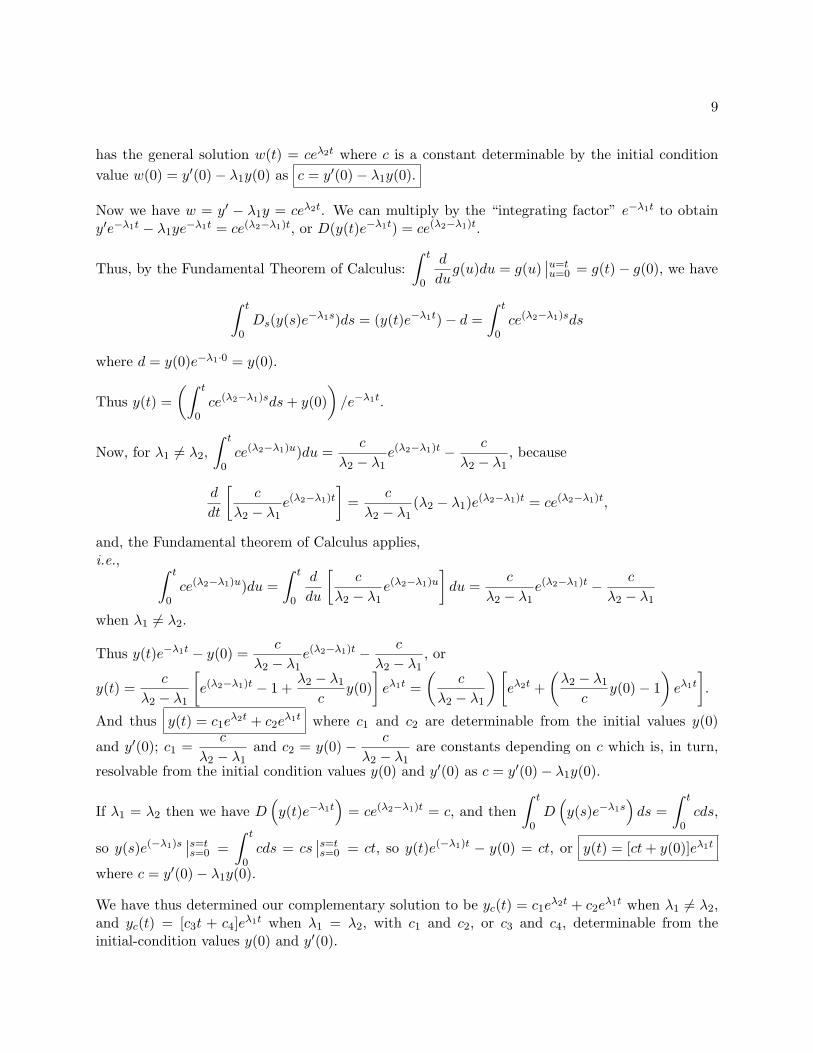
has the general solution w(t) = ceλ2t where c is a constant determinable by the initial condition

value w(0) = y′(0)− λ1y(0) as c = y′(0)− λ1y(0).

Now we have w = y′ − λ1y = ceλ2t. We can multiply by the “integrating factor” e−λ1t to obtainy′e−λ1t − λ1ye

−λ1t = ce(λ2−λ1)t, or D(y(t)e−λ1t) = ce(λ2−λ1)t.

Thus, by the Fundamental Theorem of Calculus:

∫ t

0

d

dug(u)du = g(u)

∣

∣

u=tu=0 = g(t)− g(0), we have

∫ t

0Ds(y(s)e

−λ1s)ds = (y(t)e−λ1t)− d =

∫ t

0ce(λ2−λ1)sds

where d = y(0)e−λ1·0 = y(0).

Thus y(t) =

(∫ t

0ce(λ2−λ1)sds+ y(0)

)

/e−λ1t.

Now, for λ1 6= λ2,

∫ t

0ce(λ2−λ1)u)du =

c

λ2 − λ1e(λ2−λ1)t −

c

λ2 − λ1, because

d

dt

[

c

λ2 − λ1e(λ2−λ1)t

]

=c

λ2 − λ1(λ2 − λ1)e

(λ2−λ1)t = ce(λ2−λ1)t,

and, the Fundamental theorem of Calculus applies,i.e.,

∫ t

0ce(λ2−λ1)u)du =

∫ t

0

d

du

[

c

λ2 − λ1e(λ2−λ1)u

]

du =c

λ2 − λ1e(λ2−λ1)t −

c

λ2 − λ1

when λ1 6= λ2.

Thus y(t)e−λ1t − y(0) =c

λ2 − λ1e(λ2−λ1)t −

c

λ2 − λ1, or

y(t) =c

λ2 − λ1

[

e(λ2−λ1)t − 1 +λ2 − λ1

cy(0)

]

eλ1t =

(

c

λ2 − λ1

)[

eλ2t +

(

λ2 − λ1

cy(0)− 1

)

eλ1t

]

.

And thus y(t) = c1eλ2t + c2e

λ1t where c1 and c2 are determinable from the initial values y(0)

and y′(0); c1 =c

λ2 − λ1and c2 = y(0) −

c

λ2 − λ1are constants depending on c which is, in turn,

resolvable from the initial condition values y(0) and y′(0) as c = y′(0)− λ1y(0).

If λ1 = λ2 then we have D(

y(t)e−λ1t)

= ce(λ2−λ1)t = c, and then

∫ t

0D

(

y(s)e−λ1s)

ds =

∫ t

0cds,

so y(s)e(−λ1)s∣

∣

s=ts=0 =

∫ t

0cds = cs

∣

∣

s=ts=0 = ct, so y(t)e(−λ1)t − y(0) = ct, or y(t) = [ct+ y(0)]eλ1t

where c = y′(0)− λ1y(0).

We have thus determined our complementary solution to be yc(t) = c1eλ2t + c2e

λ1t when λ1 6= λ2,and yc(t) = [c3t + c4]e

λ1t when λ1 = λ2, with c1 and c2, or c3 and c4, determinable from theinitial-condition values y(0) and y′(0).

10

We must find our particular solution yp by “guessing”, although there are systematic ways to makesuccessful guesses when f is one of many simple functions. In particular, when f(t) is a constant

α, we can determine a particular solution of the equation y′′ + a1y′ + a0y = α as yp(t) =

α

a1t when

a0 = 0 and a1 6= 0, and yp(t) =α

a0when a0 6= 0. (And yp(t) =

sα

2t2 when a0 = 0 and a1 = 0.)

———————–

For our particular case: u′′ − ru′ + su = 0, we have r 6= 0 and s 6= 0, and the right-hand-side“forcing function” is equal to 0 so u(t) = uc(t) + up(t), and up(t) = 0, so u(t) = uc(t).

We have the differential operator D2−rD+s which corresponds to the quadratic equation x2−rx+

s = 0 whose roots are λ1 =r − [r2 − 4s]1/2

2and λ2 =

r + [r2 − 4s]1/2

2where s = q0q2 = k21F0G0

and r = q1 = −[(F0 +G0)k1 + k2]. Note λ1λ2 = s and λ1 + λ2 = r.

Note we require r2 − 4s > 0, i.e., (F 20 − 2F0G0 + G2

0)k21 + 2(F0 + G0)k1k2 + k22 > 4k21F0G0 which

always holds when F0 +G0 > 0 and k1 > 0 and k2 > 0, or when k1 > 0 and F0 6= G0. (If F0 = G0

and k2 = 0 then we have λ1 = λ2 = −F0k1 and the corresponding solution u = (ct+u(0))eλ1t holdswith c = 0.)

And when r2 > 4s, we have λ1 6= λ2 and u(t) = c1eλ2t + c2e

λ1t where c1 =c

λ2 − λ1and c2 =

u(0)−c

λ2 − λ1with c = u′(0)−λ1u(0). And we have u′(0) = 0 and u(0) = δq0/B

′0 = −u′′(0)/(q0q2),

so c = −λ1u(0) = −λ1δq0B′

0

.

And

q2B = −u′

u

= −c1λ2e

λ2t + c2λ1eλ1t

c1eλ2t + c2e

λ1t

= −c1λ2e

(λ2−λ1)t + c2λ1

c1e(λ2−λ1)t + c2

And λ2 − λ1 = [r2 − 4s]1/2, c1 =c

λ2 − λ1, c2 =

q0B′

0

δ −c

λ2 − λ1and c = −λ1

q0B′

0

δ.

With B(0) = B0 = 0, we have B′0 = q0, so u(0) = δ and c = −λ1δ and c1 =

−λ1δ

λ2 − λ1, and

11

c2 = δ −−λ1δ

λ2 − λ1=

λ2δ

λ2 − λ1, and then

B = −

[

−λ1λ2δ

λ2 − λ1e(λ2−λ1)t +

λ1λ2δ

λ2 − λ1

]

/

[

−λ1δ

λ2 − λ1e(λ2−λ1)t +

λ2δ

λ2 − λ1

]

= −

[

−λ1λ2

λ2 − λ1e(λ2−λ1)t +

λ1λ2

λ2 − λ1

]

/

[

−λ1

λ2 − λ1e(λ2−λ1)t +

λ2

λ2 − λ1

]

= −

[

−λ1λ2e(λ2−λ1)t + λ1λ2

−λ1e(λ2−λ1)t + λ2

]

.

Thus B(t) =λ1λ2e

(λ2−λ1)t − λ1λ2

−λ1e(λ2−λ1)t + λ2

where λ1 =r − [r2 − 4s]1/2

2and λ2 =

r + [r2 − 4s]1/2

2with

s = q0q2 = k21F0G0 and r = q1 = −[(F0 + G0)k1 + k2] such that λ1 6= λ2. (If λ1 = λ2, we have

F0 = G0 and k2 = 0 and then B(t) = F0 −F0

F0k1t+ 1= G0 −

G0

G0k1t+ 1.)

0.5 Chemical Kinetic Modeling

Suppose we have specific kinetic data, time versus B-concentration, appearing as the rows of atwo-column matrix, BM . Note time vs. G-concentration or time vs. F -concentration can be easilyconverted to time vs. B-concentration. In MLAB, if GM is a 2 column matrix of time vs. G-concentration for example, we merely type

* BM = (GM COL 1)&’(G0-B0-(GM COL 2))

and BM is then the desired time vs. B-concentration matrix of data points.

We may use the curve-fitting facility of MLAB to compute estimates of k1 and k2, and even F0,G0, and/or B0 if necessary.

——————————————————————–

Given the kinetic data: (0, 0), (.2, .072), ... entered below with B0 = 0, F0 = 1 and G0 = 1, we canestimate k1 and k2 as follows.

MLAB Mathematical Modeling System, Revision: June 12, 2013

Executing file: /usr/local/lib/mlab/mlab

Copyright: Civilized Software, Inc. (301)962-3711, email: [email protected]

Web-site: WWW.CIVILIZED.COM

Wed Aug 20 16:00:26 2014

Your current working directory is: /home/knott/

Use FILEDIR to reach any other directory.

12

’* ’ is the command prompt

This copy of MLAB belongs to csi choptank

d col 1 = 0:4:.2

d col 2 = list(0, .072, .127, .168, .200, \

.170, .187, .205, .176, .197, .165, \

.228, .235, .212, .197, .215, .227, \

.221, .216, .204, .210 )

fct B’t(t) = k1*(F0-(B(t) -B0))*(G0-(B(t) -B0)) -k2*B

init B(0) = 0

F0 = 1; G0 = 1; B0 = 0

/* Guess k1 = initial slope. */

k1 = .072/.2; k2 = 2*k1

tv = 0:4.2!127

draw d, pointtype "+" linetype none

draw points(B,tv) linetype dashed

view

13

constraints q = { k1 >0, k2>0, G0 >0, F0 >0, B0 >=0}

fit(k1,k2), b to d with weight ewt(d)

final parameter values

value error dependency parameter

0.4681184643 0.06528559617 0.9795234833 K1

1.371659988 0.201698861 0.9795234833 K2

4 iterations

CONVERGED

best weighted sum of squares = 3.156126e+01

weighted root mean square error = 1.288844e+00

weighted deviation fraction = 4.233717e-02

R squared = 9.098160e-01

draw points(B, tv) color red

view

Now suppose we have the same data, but F0 is unknown. Then we can estimate k1, k2, and F0 asfollows.

k1 = .072/.2; k2 = 2*k1; F0 = .5; G0 = 1

fit(k1,k2,F0), b to d with weight ewt(d), constraints q


14


0.7380400592 9.696694591 0.9999969975 K1

1.176742194 6.870010323 0.999981958 K2

0.6406740748 8.475673511 0.9999984767 F0

10 iterations

CONVERGED




R squared = 9.100870e-01

no active constraints

draw points(B, tv) color yellow linetype alternate

view

Note the extremely-high dependency values (greater than .99.) These are matched by very largeerror values. This means the parameters with such high dependency values are dependent on one-another. Changing one can be compensated by suitably changing the others, i.e., our estimates arenot unique.

Now let us look at estimating k1, k2, F0, and G0 using the same kinetic data.

k1 = .072/.2; k2 = 2*k1; F0 = .5; G0 = .5

15

fit(k1,k2,F0,G0), b to d with weight ewt(d), constraints q



0.9528428531 10.11946107 0.9999944158 K1

1.106581655 4.324644348 0.9999520682 K2

0.7082117644 406.2857598 0.999999999 F0

0.7082117643 406.2207178 0.999999999 G0

6 iterations

CONVERGED




R squared = 9.102791e-01


draw points(B, tv) color pink linetype alternate

view

Again we have very high dependency values. The values we obtain are not only not well-determined;they depend on the initial guesses.

Finally let us assume k1 and k2 are known from prior modeling as k1 = .46812 and k2 = 1.37166,and let us look at estimating F0, and G0 using the same kinetic data as above.

k1 = .46812; k2 = 1.37166; F0 = .5; G0 = .5

16

fit(F0,G0), b to d with weight ewt(d), constraints q



1.577750772 1.090627947 0.9992427369 F0

0.6650012081 0.3499321856 0.9992427369 G0

4 iterations

CONVERGED




R squared = 9.102412e-01


draw points(B, tv) color green

view

And yet again we have high dependency values, thus we can estimate k1 and k2, given F0, G0 andB0, reasonably uniquely, but estimating F0 and G0 given k1 and k2 and B0 is problematic.

The following example shows that G0 can be well-estimated when k1, k2, and F0 are accurate.

k1 = .5; k2 = 1.5; F0 = 1; G0 = 2

17

fit(G0), b to d with weight ewt(d), constraints q



1.015055099 0.01600248526 0 G0

4 iterations

CONVERGED




R squared = 9.096548e-01


draw points(B, tv) color red

view

0.6 Chemical Equilibrium Modeling

The equilibrium constant, K, of the reaction F +Gk1⇋

k2B, is defined as K = k1/k2. At equilibrium

(say at time te where te is suitably large), we have dB/dt(te) = 0, and hence k1F (te)G(te) −k2B(te) = 0. (Of course we may never be at equilibrium, so we understand we are simplifying thecircumstances.)

18

Thus,k2k1

·B(te)

F (te)G(te)= 1, so multiplying by

k1k2

, we have

K = B(te)/(F (te)G(te)) = B(te)/((F0 +B0 −B(te))(G0 +B0 −B(te))).

Thus K(F0+B0−B(te))((G0+B0−B(te)) = B(te) or K−1B(te) = (F0+B0)(G0+B0)−B(te)(G0+

F0 + 2B0) +B(te)2.

So B(te)2 − ((G0 + F0 + 2B0) + K−1)B(te) = (F0 + B0)(G0 + B0) = 0, and, using the quadratic

formula, we have 2B(te) = (G0+F0+2B0+K−1)±[(G0+F0+2B0+K−1)2−4(F0+B0)(G0+B0)]1/2.

Now, to determine the sign + or −, consider the case where B0 > 0, F0 = 0, and G0 = 0;in this case, B will dissasociate until equilibrium is reached. Then we have B(te) ≤ B0 and2B(te) = (2B0 +K−1)± [(2B0 +K−1)2 − 4B2

0 ]1/2. And, if the plus-sign applies, we have 2B(te) =

2B0 +K−1 + [(4B20 = 4B0K

−1 − 4B20 ]

1/2 = 2B0 +K−1 + 2[B0K−1]1/2, so B(te) = B0 +

1

2K−1 +

[B0K−1]1/2 > B0. Therefore, the plus-sign cannot be the correct choice of sign, and we have

2B(te) = (G0 + F0 + 2B0 +K−1)− [(G0 + F0 + 2B0 +K−1)2 − 4(F0 +B0)(G0 +B0)]1/2.

Define Be(F0, G0, B0) = B(te), the amount of B at equilibrium or “saturation”. Then we have thefollowing equation, called the saturation equation.

Be(F0, G0, B0) = [(F0+G0+2B0+1/K)− ((F0+G0+2B0+1/K)2− 4(F0+B0)(G0+B0))1/2]/2.

If we have data points for a so-called saturation curve consisting of pairs of F0 values with associatedBe values for fixed values of G0 and B0, then curve-fitting can be used with the above functionin order to estimate K. Indeed K can be estimated even when we have points (F0, G0, Be) fromthe saturation surface in 3-space, where arbitrary values of F0 and G0 have been paired, and B0 isfixed. (Usually, B0 = 0.)

Define Be = B(te), Fe = F (te), and Ge = G(te). Then from the basic relations: K = Be/(FeGe),Fe +Be = F0 +B0, and Ge +Be = G0 +B0, we may write a number of equivalent relationships.

Michaelis-Menten Equation(1) (Be vs. Fe):

Be = K(G0 +B0)Fe/(1 +KFe)

Michaelis-Menten Equation(2) (Be/(B0 +G0) vs. Fe):

Be/(B0 +G0) = KFe/(1 +KFe)

Lineweaver-Burk Equation (1/Be vs. 1/Fe):

1/Be = (1/(K(G0 +B0)))(1/Fe) + 1/(G0 +B0)

Eadie-Wilkinson-Dixon Equation (Fe/Be vs. Fe):

Fe/Be = Fe/(G0 +B0) + 1/(K(G0 +B0))

19

Scatchard Equation (Be/Fe vs. Be):

Be/Fe = −KBe +K(G0 +B0)

Hill Equation (log [(Be/(G0 +B0))/(1−Be/(G0 +B0)] vs. log Fe):

log((Be/(G0 +B0)/(1−Be/(G0 +B0))) = log Fe + log K

(Also see the “direct linear plot” of Cornish-Bowden in Biochem. J. Vol 137, p. 143, 1974)

Some of these relationships are inspired by analogous relations for enzyme reactions where theyarise in different forms. Most are linear relations in K or 1/K for simple binding, and this accountsfor their popularity—they are easy to use as models with linear regression methods in order toestimate K. For the non-linear Michaelis-Menten forms, constraints are often necessary. In spite oftheir traditional use, however, the errors introduced when transforming data to the appropriate formmay limit the accuracy obtainable when using any of these models; and in general biased estimatesof K will result. See Rodbard, D., “Mathematics of Hormone-Receptor Interaction”, in Receptorsfor Reproductive Hormones, Plenum Pub. Corp., NY, 1973.

The saturation equation above may thus be preferred, although usually there is little difference. Atany rate, the values of K obtained using various models should be checked by computing theoreticalpredicted values for Be vs. F0 and comparing them to the observed values. The major difficultyfor the various linear forms is that both the independent and the dependent-variable data valueshave non-normally-distributed error. As a result, linear Euclidean curve-fitting (with appropriateweights) should be employed with these models. The results should be checked in the saturationequation. That value of K which yields the lowest sum-of-squares in the saturation model shouldbe used.

Here is an example comparing the saturation equation model with the Michaelis-Menten (1) modeland the Scatchard model.

FCT B(F0)=((F0+G0+2*B0+1/K)-SQRT((F0+G0+2*B0+1/K)^2-4*(F0+B0)*(G0+B0)))/2

FCT BE(FE) = (G0+B0)*FE/(1/K+FE)

FCT BS(BE) = -K*BE+K*(G0+B0)

B0 = 0; G0 = 1;

/* M = F0 values, BE values */

M = read(data,100,2)

/* generate M1 = corresponding data (FE,BE) for the Michaelis-Menten model */

M1 = (M COL 1) - (M COL 2) + B0

M1 COL 2 = M COL 2

/* generate M2 = corresponding data (BE/FE,BE) for the Scatchard model */

M2 = (M COL 2)

20

M2 COL 2 = (M1 COL 2)/’(M1 COL 1)

K = 2

FIT(K), B TO M



1.996602727 0.0420400256 0 K

1 iterations

CONVERGED

best weighted sum of squares = 1.446128e-02

weighted root mean square error = 1.925622e-02


R squared = 9.691570e-01

KS = K

FIT(K), BE TO M1



2.0043749954 0.0397621839 0 K

1 iterations

CONVERGED




R squared = 9.622617e-01

KM = K

FIT(K), BS TO M2



2.0008431423 0.0360417006 0 K

1 iterations

CONVERGED




R squared = 9.358569e-01

KC = K

/* draw MM model + data with the above K */

K = KS

TOP TITLE "Saturation Model"

DRAW M, LINETYPE NONE, POINTTYPE STAR

DRAW POINTS(B, 1:5!101)

K = KM

21

DRAW POINTS(B, 1:5!101) LINETYPE DASHED

K = KC

DRAW POINTS(B, 1:5!101) LINETYPE ALTERNATE

VIEW

K = KS

TOP TITLE "Michaelis-Menten Model"

DRAW M1, LINETYPE NONE, POINTTYPE STAR

DRAW POINTS(BE, MINV(M1 col 1):MAXV(M1 col 1)!101)

K = KM

DRAW POINTS(BE, MINV(M1 col 1):MAXV(M1 col 1)!101) LINETYPE DASHED

K = KC

DRAW POINTS(BE, MINV(M1 col 1):MAXV(M1 col 1)!101) LINETYPE ALTERNATE

VIEW

22

/* draw Scatchard model + data with the above K */

K = KS

TOP TITLE "Scatchard Model"

DRAW M2, LINETYPE NONE, POINTTYPE STAR

DRAW POINTS(BS, MINV(M2 col 1):MAXV(M2 col 1)!101)

K = KM

DRAW POINTS(BS, MINV(M2 col 1):MAXV(M2 col 1)!101) LINETYPE DASHED

K = KC

DRAW POINTS(BS, MINV(M2 col 1):MAXV(M2 col 1)!101) LINETYPE ALTERNATE

VIEW

23

Note that for the data studied above, all the models give comparable results. Indeed the estimatedK-values are so close, the curves are almost superimposed.

The second Michaelis-Menten equation is useful when the amount, G0 + B0, is not known. Thenmeasuring a quantity proportional to Be/(G0 + B0) vs. Fe is commonly done, and K can bedetermined in unknown units. Indeed, by introducing another parameter, D, to obtain Be/(B0 +G0) = DKFe/(1+KFe) and computing D and K by fitting this model to data points (Fe, Be/(B0+G0)), where Fe and Be are measured in moles and B0+G0 is measured in grams, then D(B0+G0)has the unit moles, and so (B0+G0)/(D(B0+G0)) = 1/D is the molecular weight of a G molecule.(This device for computing molecular weight assumes that B0 = 0 or that an F molecule is muchlighter than a G molecule.) Fitting the saturation equation to obtain both K and G0 +B0 may bea better approach.

0.7 Cooperative Binding

Often the binding of F and G is complicated by cooperative effects. Namely, k1 and/or k2 appearto be dependent upon the relative amount of B. This can be due to allosteric shape changes in themolecules or sites G which occur during binding. Various other explanations, including multipleclasses of sites, are also possible. If k1/k2 increases as B increases, we have positive cooperativity;if k1/k2 decreases as B increases we have negative cooperativity.

Suppose, then, that k1 and k2 are functions of B. Thus,

dB/dt(t) = k1(B(t)) · F (t) ·G(t)− k2(B(t)) ·B(t),

24

with F (t) = F0 − (B(t)−B0), G(t) = G0 − (B(t)−B0), and B(0) = B0, as before.

Now suppose that all cooperative effects are due to changes in k2, in particular, suppose

k1(B) = k01, and k2(B) = k02(1 + p ·B/(G0 +B0)).

This is the same as saying k2(B)− k2(0) = pB/(G0 +B0). Thus we assume that the change in k2from the “ground state” k2(0) = k02, is proportional to the fraction of occupied sites, B/(G0 +B0),with the proportionality-constant p.

Note then, that dk2/dt(B(t)) = (p/(G0 +B0))dB/dt(t), so dk2/dB(B) = p/(G0 +B0).

There are of course many other functional relationships which could be postulated. For example,we could assume that dk2/dt(B(t)) = A(dB/dt)h, or we could assume k1 and k2 vary together incertain ways. Indeed, changes in k1 will give cooperative effects unobtainable by changes in k2alone. k1 and k2 need not change monotonically; we may have variation which results in intervalsof positive cooperativity and other intervals of negative cooperativity.

Since cooperativity, without qualification as to its cause, is merely a mathematical description, andnot a structural description, the choice of how k1(B) and k2(B) are defined is dependent upon theactual physical situation and the desired uses of the mathematical model. The particular choicehere has the same effect as that made by DeMeyts in his analysis of cooperativity (DeMeyts, P.,Woebroeck, M., “The structural basis of insulin-receptor binding and cooperative interactions”, inMembrane Proteins (ed. P.Nicholls et al.) FEBS 11th Meeting, Vol. 45 Symposium A4, PergamonPress, pp. 319–323, 1977).

Now let te be the time when equilibrium is approached, and let B(te) = Be, F (te) = Fe, andG(te) = Ge. Then, at equilibrium, we have the equilibrium constant K as a function of Be,K(Be) = k1(Be)/k2(Be) = Be/(FeGe). Thus, K(Be) = k01/(k

02(1 + pBe/(G0 + B0))), or, K(Be) =

k0/(1 + pBe/(G0 +B0)), where k0 = K(0).

Note for −1 < p < 0, we have positive cooperativity, for p = 0, we have no cooperativity (K(Be) =K(0)), and for p > 0, we have negative cooperativity.

It is convenient to define p in terms of another parameter, a, called the F , G interaction factor, sothat p = (1 − a)/a, and hence a = 1/(1 + p). Note for 0 < a < 1, we have negative cooperativity,for a = 1, we have no cooperativity, and for a > 1, we have positive cooperativity.

Indeed, if ∆G0 is the energy needed (or released) (i.e., the change in free energy) for bindingthe first F molecule to a G molecule, and if ∆G1 is the energy used (or released) for bindingan F molecule to the last unoccupied G molecule (whereupon B = G0 + B0), then we have theclassical thermodynamic relations: ∆G0 = −RT log K(0), and ∆G1 = −RT log K(G0+B0), whereR is the gas constant (about 1.987 calories/degree/mole) and T is the absolute temperature. Thus,K(G0+B0)/K(0) = exp(−(∆G1−∆G0)/RT ), and, by assumption, K(G0+B0)/K(0) = 1/(1+p) =a, so a has the interpretation: a = K(B0 +G0)/K(0); it is the ratio of the equilibrium constant Kwith all G-sites occupied, to K with no occupied G-sites.

DeMeyts has observed that the relation K(Be) = k0/(1 + ((1− a)/a) ·Be/(G0 +B0)) may be usedin the various equilibrium models given before to obtain the corresponding cooperative models.

25

Thus, we substitute K(Be) for K to obtain models which now involve the parameters F0, G0, B0,a, and k0. Curve-fitting which yields a value for a obviously different from one, should be followedby fitting with a fixed to one. If the latter fit is clearly inferior, cooperative binding phenomenamay be present.

In particular, for a 6= 1, the cooperative Michaelis-Menten(2) relation is:

Be/(B0 +G0) = (−a(1 + k0Fe) + [a2(1 + k0Fe)2 + 4a(1− a)k0Fe]

1/2)/(2(1− a)).

The cooperative Scatchard equation is:

Be/Fe = k0(B0 +G0 −Be)/(1 + (1− a)Be/(a(G0 +B0))).

The cooperative Hill equation is obtainable by substitution from the cooperative Michaelis-Menten(2) equation above, however, it can be plotted in MLAB, without using explicit algebra, as follows,assuming B0, G0, k0, and a are already set, with a 6= 1.

FCT BE(FE) = (B0+G0)*(-A*(1+K0*FE)+ \

SQRT(A*A*(1+K0*FE)^2+4*A*(1-A)*K0*FE))/(2*(1-A))

FUNCTION HILLT(BE) = LOG((BE/(G0+B0))/(1-BE/(G0+B0)))

LFEV = -12:2:.2

M = LFEV &’ (HILLT ON BE ON EXP ON LFEV)

DRAW M

The Hill-plot matrix M has rows which are points of the form:

log((Be/(G0 +B0))/(1−Be/(G0 +B0))) vs. log Fe.

Normally a Hill-plot, as defined above, is a straight line with slope 1, however, this is not the casefor a 6= 1. DeMeyts has shown that, in general, the slope

d(log((Be/(G0 +B0))/(1−Be/(G0 +B0))))/d(log Fe)

decreases when a decreases and increases when a increases, and attains its minimum value whenFe = 1/k0, independently of a.

simple binding F + G B Mathematical Modeling

Documents

Transcript of simple binding F + G B Mathematical Modeling