NBER WORKING PAPER SERIES

“SICK OF LOCAL GOVERNMENT CORRUPTION? VOTE ISLAMIC”

J. Vernon HendersonAri Kuncoro

Working Paper 12110http://www.nber.org/papers/w12110

NATIONAL BUREAU OF ECONOMIC RESEARCH1050 Massachusetts Avenue

Cambridge, MA 02138March 2006

We gratefully acknowledge support of the National Science Foundation (SES 0416840), which made thisproject possible. We thank Ifa Isfandiarni of the University of Indonesia for her diligent and carefulsupervision of the survey and participation in survey design. Ben Olken provided helpful comments on issuesof culture versus politics and Pedro Dal Bó, Ross Levine and Sandy Henderson provided helpful commentson a preliminary draft of the paper. The views expressed herein are those of the author(s) and do notnecessarily reflect the views of the National Bureau of Economic Research.

©2006 by J. Vernon Henderson and Ari Kuncoro. All rights reserved. Short sections of text, not to exceedtwo paragraphs, may be quoted without explicit permission provided that full credit, including © notice, isgiven to the source.

“Sick of Local Government Corruption? Vote Islamic”J. Vernon Henderson and Ari KuncoroNBER Working Paper No. 12110March 2006JEL No. H7, O1, P16, R5

ABSTRACT

Indonesia has a tradition of corruption among local officials who harass and collect bribes from

firms. Corruption flourished in the Suharto, pre-democracy era. This paper asks whether local

democratization that occurred after Suharto reduced corruption and whether specific local politics,

over and above the effects of local culture, affect corruption. We have a firm level data set for 2001

that benchmarks bribing activity and harassment at the time when Indonesia decentralized key

responsibilities to local democratically elected governments. We have a second data set for 2004 on

corruption at the end of the first democratic election cycle. We find that, overall, corruption declines

between these time periods. But specific politics matter. Islamic parties in Indonesia are perceived

as being anti-corruption. Our data show voting patterns reflect this belief and voters’ perceptions

have some degree of accuracy. In the first democratic election, localities that voted in legislatures

dominated by secular parties, including Megawati’s party, experienced significant relative increases

in corruption, while the reverse was the case for those voting in Islamic parties. But in the second

election in 2004, in those localities where corruption had increased under secular party rule, voters

“threw the bums out of office” and voted in Islamic parties.

J. Vernon HendersonDepartment of EconomicsBox BBrown UniversityProvidence, RI 02912and NBERj_henderson@brown.edu

Ari KuncoroDepartment of EconomicsUniversity of IndonesiaJakarta, Indonesiaarik@cbn.net.id

1

Sick of Local Government Corruption? Vote Islamic.1

J. Vernon Henderson Ari Kuncoro Brown University University of Indonesia NBER Brown University

March 2, 2006

Abstract: Indonesia has a tradition of corruption among local officials who harass and collect bribes from firms. Corruption flourished in the Suharto, pre-democracy era. This paper asks whether local democratization that occurred after Suharto reduced corruption and whether specific local politics, over and above the effects of local culture, affect corruption. We have a firm level data set for 2001 that benchmarks bribing activity and harassment at the time when Indonesia decentralized key responsibilities to local democratically elected governments. We have a second data set for 2004 on corruption at the end of the first democratic election cycle. We find that, overall, corruption declines between these time periods. But specific politics matter. Islamic parties in Indonesia are perceived as being anti-corruption. Our data show voting patterns reflect this belief and voters’ perceptions have some degree of accuracy. In the first democratic election, localities that voted in legislatures dominated by secular parties, including Megawati’s party, experienced significant relative increases in corruption, while the reverse was the case for those voting in Islamic parties. But in the second election in 2004, in those localities where corruption had increased under secular party rule, voters “threw the bums out of office” and voted in Islamic parties.

In 1999 Indonesia democratized; and in 2001 with fiscal decentralization, local

democracy took full flight. Democratization was imposed on a regime which in the late 1990’s

was ranked consistently as among the most corrupt in the world (Bardhan, 1997 and Mocan,

2004). A significant portion of corruption occurs at the local level, where local government

officials collect bribes to supplement their salaries: at the time of decentralization in 2001, our

data indicate that bribes paid to local officials averaged 6% of costs for manufacturing firms. This

paper examines two key questions. Did democratization with decentralization reduce (or increase)

corruption at the local level per se? Second, do specific politics in the form of local legislature

composition matter? With democratization, corruption in Indonesia has become a commanding

political issue, manifested in exposés in the press, indictments, and political campaigns (McLeod,

2005). Our key finding will be that districts which voted in greater proportions of Islamic party

representatives to the local assembly experienced much greater reductions in corruption. While

the results are specific to local governments in Indonesia, they hint at broader implications for the

effect of democratization on corruption and the role of Islamic parties in political processes.

We start with the nature of politics in Indonesia and the timing of political events and our

surveys. In 1999 Indonesia held nation-wide elections, where local as well as national assemblies

1 We gratefully acknowledge support of the National Science Foundation (SES 0416840), which made this project possible. We thank Ifa Isfandiarni of the University of Indonesia for her diligent and careful supervision of the survey and participation in survey design. Ben Olken provided helpful comments on issues of culture versus politics and Pedro Dal Bó, Ross Levine and Sandy Henderson provided helpful comments on a preliminary draft of the paper.

2

were elected. The share of representatives of each party in local assemblies is proportional to their

share of the vote in local elections. Local assemblies were elected in 1999 in anticipation of

decentralization in January 2001, which occurred as planned with key governmental functions

such as education and administration of many national regulations being turned over to the local

district (kabupaten) governments, bypassing provincial governments. Kabupaten in Indonesia are

similar to USA counties, but with full responsibilities for local services.

Under current laws, all local parties must be national parties. In 1999 there were 5 (out of

a total of 40) major political parties, 2 of which are secular—GOLKAR, the former ruling party

under Suharto, and Megawati’s PDIP party. These two parties play a key role in our analysis.

Other significant parties have Islamic roots and are viewed as less accepting of corruption than

secular parties. While the dominant Islamic party, PKB, has not made corruption its national

platform issue, our fieldwork suggests that it is viewed as substantially less corrupt at the local

level than secular parties. Another Islamic party (PKS) has emerged as a major party on an anti-

corruption platform focused on corruption associated with the secular parties. The 1999 national

elections led initially to a coalition government between Megawati’s secular party, PDIP, and the

main Islamic party, PKB, with the first President, Abdurachman Wahid, drawn from PKB.

Our first survey took place in fall 2001, benchmarking corruption at the dawn of

decentralization, or full local democratization (Kuncoro, 2003, World Bank, 2003). But 2001 also

was the year when the national coalition between PKB and Megawati’s PDIP party fell apart,

with Megawati taking over as President, after Wahid was impeached. After that, at the local level,

PDIP often aligned with the other major secular party, GOLKAR. Our second survey was carried

out in early 2005 and covers information on corruption in 2004. In late 2004, the Megawati

period ended with the direct election of Susilo Bambang Yudhoyono as President, following the

second round of elections (in a five year election cycle) of representatives to national and local

assemblies. We observe that local government corruption drops substantially between 2001 and

2004. We link that reduction to decentralized democracy, not with Megawati assuming office,

since Megawati’s party during 2001-2004 was associated with corruption, in line with results

from our data. However we note that we don’t know for certain what happened between the fall

of Suharto in 1998 and 2001. A prevailing view is that from 1998-2001, it was “business as

usual” (Kuncoro, 2003, World Bank, 2003), but our results are specific to the 2001-2004 interval.

Why would a regime switch to local democracy matter? While legislative measures can

potentially affect corruption (Olken, 2005), in Indonesia there haven’t been significant new

legislative measures (World Bank 2003, Chapter 3). But there is greater enforcement of existing

laws, in a context where corruption is now a major political issue. In the new, democratic era,

3

under a freer press, newspapers write exposés (Brunetti and Wider, 2003); young and ambitious

local prosecutors make reputations through official investigations and indictments; firms and

local offices of the national chamber of commerce can lobby legislators to protect firms from

harassment and to discipline local officials; and local political parties may gain votes with anti-

corruption stances. As part of this process the national government created several anti-corruption

agencies and commissions. A further element is that with decentralization, elected officials may

try to deter corruption to attract local investment, in the context of inter-jurisdictional competition

for firms (Brueckner and Saavendra, 2001, Henderson and Kuncoro, 2004, Fisman and Gatti ,

2002 and Mocan, 2005). In terms of regime switches, the economics literature discusses the

notion of multiple equilibria under corruption (Cadot 1987, Andvig and Moene, 1991, Tirole

1996, Bardham 1997), based on information asymmetries, intergenerational reputation modeling,

or punishments versus rewards when corrupt officials are few versus many.

Our notion of the effect of the regime switch follows Mookerjee and Png (1995), who

analyze the effects of increasing punishments of corrupt officials. Significant increases in

punishment deter bribe solicitation and amounts, especially in a context like Indonesia where the

firms being solicited may turn officials in. With expanded opportunities for redress, officials may

reduce bribe demands, so firms find it cheaper to pay the bribe than make the effort to seek

redress. In addition, democratization may induce a change in the local corruption environment,

through greater local social sanctions against corruption with more public scrutiny of illicit

activity and firm owners increasingly refusing to pay bribes. While we associate corruption

reductions at the local level with decentralized democracy, there is always a problem of

separating regime switch effects from effects of unobserved changes in other accompanying

conditions. Thus much of our focus will be on the effects of specific local politics—the impacts

on corruption of legislature composition in the competitive political environment.

Why might local assembly composition matter (Pettersson-Lidbom, 2003)? In Indonesia,

opportunities for redress are related to whether local assembly representatives support corruption

reduction. We hypothesize that redress opportunities for firms and the direct and indirect

punishment costs for corrupt officials rise and the level of corruption declines as the proportion of

district representatives from Islamic parties rises. Direct punishment costs include dealing with

complaints, indictments of an official or their boss, loss of job, or hindering of career

advancement. Indirect costs include local social sanctions faced by corruption officials, where the

local corruption environment may be affected by the attitude towards corruption within the local

assembly. Moreover career law enforcement officials may feel freer to pursue corruption cases at

the local level with the political backing offered by Islamic representatives. An objection to the

4

idea that Islamic parties deter corruption is that the cross-country literature argues that Islamic

countries are more corrupt (e.g., Mocan, 2004). That fact is difficult to disentangle from the fact

that they are generally also much less democratic and ruled by secular regimes, with a less

developed “rule of law”; and it says little about within country effects of religious and political

differences across regions.

The real difficulty in evaluating the role of Islamic parties is to disentangle local

assembly composition effects from the effects on bribe solicitation of “local culture”. There are

two distinct, not well correlated aspects to district culture: devoutness of the population and the

corruption environment at the time of democratization. Our fieldwork suggests that today devout

Muslims are distinctly less willing to pay bribes; and, ceteris paribus, some sects of devout

Muslims are more inclined to vote for Islamic parties. But if devoutness affects bribing and vote

choices, that makes the role of Islamic parties more difficult to assess, regardless of whether they

are taking anti-corruption stances as strategic political choices or as an expression of their own

devoutness. One needs to disentangle whether corruption differences across districts occur

because of differences in Islamic parties’ representation in local assemblies or differences in

devoutness of voters. Although this is an obvious problem to worry about in identifying assembly

composition effects, when we turn to discussing our identification strategy, the more difficult

problem will concern the prevailing local corruption environment at the time of decentralization.

Our data suggest this environment was unrelated to measures reflecting local devoutness. But

there is still the identification problem that districts which for idiosyncratic reasons had a history

of more corruption may have a different, unobserved attitude towards bribing that also is

correlated with their voting behavior.

Our surveys are constructed to elicit information about bribing activity involving local

officials. We are not focused on the other major forms of corruption—bribes paid to reduce

corporate income tax liabilities, issuance of FDI or export/import licenses for large firms, and

police extortion. All these involve national officials; and the first two mostly very large firms. We

are focused on day-to-day corruption involving local officials that eats away at almost all firms.

1. Red Tape, Harassment, and Bribes

What is the nature of local corruption? In Indonesia, firms are required to obtain a variety of

locally set licenses and “retributions”. Officials from the local Ministry of Industry monitor firms

to make sure they have the full array of licenses and that all are up-to-date. Officials from the

local Ministry of Labor inspect licenses and equipment in connection with safety regulation.

5

Visiting plants purportedly to inspect and monitor is the basic form of harassment used by

officials to elicit bribe payments. The creation of red tape through licensing has a long history in

Indonesia, with efforts in the mid-1990’s by the central government (encouraged by the World

Bank) to curtail the array of licenses in order to encourage foreign and domestic investment.

However, immediately following the national decentralization legislation in 1999, localities, in

anticipation of decentralization in 2001, felt empowered to create a greater array of licenses and

retributions, with sharper limits on the time licenses are valid before needing renewal.

Firms pay bribes for several reasons. When a license is up for renewal, bribes reduce

waiting time to renewal and harassment when a license has expired. Bribes are paid to get

officials out of the plant who are there in the guise of inspecting licenses and ensuring equipment

safety. Similarly bribes are paid to placate officials, who claim a plant needs a license that in fact

is not required. Since 2001, empowered by a national “pro-labor” ministerial directive which

greatly strengthened the application of pro-labor laws, other bribes (which we record separately)

to local labor officials are paid by firms to resolve disputes over severance and overtime pay in

their favor and to have strikes declared illegal (albeit in an open shop environment). While this is

a separate source of bribe activity, it feeds into the first, since inspection of licenses and

equipment safety allows labor officials to sniff around plants for hints of labor troubles.

One could categorize this bribe activity to reduce the harassment from regulations under

the efficient grease hypothesis (Liu 1985, Becker and Maher 1986, Bardhan 1997, and Cai, Fang,

and Xu 2005), with the caveat, however, that localities are imposing regulations, so local officials

can demand bribes (e.g., Banerjee, 1994, and Kaufman and Wei, 1998). Harassment is costly

because it takes up the entrepreneur and her managers’ time (Kaufman and Wei, 1999, Svennson,

2003, and Henderson and Kuncoro, 2004). In Henderson and Kuncoro (2004) we argue that, on

the eve of decentralization in 2001, bribes were part of compensation packages of local officials.

Corruption was greater in localities that had limited fiscal resources, with bribes being a form of

indirect taxation to supplement the salaries of local officials and bring them up to competitive

market wages.2

2 Both before and after decentralization, localities received most of their revenues as transfers

from the central government, with localities having little de facto independent means of raising revenue. The fiscal situations are detailed in Henderson and Kuncoro (2004). Since decentralization, the fiscal situation is in flux, with new spending responsibilities of local governments, new sources of transfers with formulas undergoing on-going adjustment, and new developing sources of local revenues, in particular a sales tax. Moreover the imposition of local democracy and the development of local anti-corruption campaigns have changed the whole environment, as discussed above.

6

To motivate the empirical analysis we discuss a very simple model. Firms and local

officials who harass them each have their own optimization problem. Firms seek to maximize

profits where

max ,( , ( , , , ))

where 0; 0; , 0; 0.

i j i ij ij i ij j i iX b

X h v l b

p y X h v l b W X b

y y h h h

θΠ = − −

> < > < (1)

In equation (1), firm faces a price, , ji p for its product sold in locality j. Its output y is produced

with inputs chosen by the firm, iX , at prices, jW in district j; but output is reduced by

harassment, ( )h ⋅ , experienced by the firm, which takes up the entrepreneur’s time and may create

discontent in the factory. ( )h ⋅ is specified as a “black-box” process that involves some

underlying game (Henderson and Kuncoro, 2004) . But the outcome, ( )h ⋅ , is declining in bribes,

ib , offered by the firm to make officials leave and is increasing in (costly) visits, ijv , by officials

in district j to firm i. Harassment is increasing in red tape, or licenses and retributions, ijl ,

required by district j of firm i. Finally there is a vector of observed and unobserved items

affecting harassment, ,ijθ such as how adept the entrepreneur is at dealing with local officials,

idiosyncratic greed of local officials, religious convictions of the entrepreneur, socio-political

climate in the district, and redress opportunities available to firms that face bribe demands.

Optimizing with respect to choice of bribes, bribes are censored at zero if ( ) ( ) 1h by h⋅ ⋅ < at

0ib = ; and bribes are given by the implicit function from ( ) ( ) 1 0h by h⋅ ⋅ − = so that

( , , , , ).j i ij ij ijb b p X l v θ= (2)

We expect the level of bribes to be increasing in and v l ; but ensuring that in the model requires

restrictions on the functions such as , 0, , 0.hh bb bl bvy h h h≥ ≤

For local officials, their choice of number of visits is based on the optimization problem

max [ ( )] ( , , , , )ij ij ij i ijvE b c v l d e ε⋅ − , (3)

for ( )b ⋅ given in (2). ijd is vector of items affecting the cost of officials’ visits such as the distance

from the officials’ location in jurisdiction j (the district capital) to firm i; ie is any characteristics

of the firm (over and above ijl ) which legitimately require officials to visit the firm; and ijε are

other aspects that affect the costs of visits, such as censure from local legislators concerning

harassment or the extent to which local officials “are expected” to make up salary deficits from

7

competitive wages through bribes. From the first order condition [ ( )] ( ) 0v vE b c⋅ − ⋅ = , we can

specify a visit equation

( , , , , , )ij ij ij i i ij ijv v l d e X ε θ= . (4)

We estimate equations based on (2) and (4) in the last sections of the paper. In doing so,

one issue is what firm characteristics can be treated as exogenous. It is clear in (2), that from (4),

ijv is endogenous, where potentially either ijd or elements of not in i ie X in (4) can be used as

instruments in estimation of (2). However, what about , or even ij il X , especially given the notion

that officials impose red tape to generate bribes? We follow two approaches in estimation. In the

first, while we treat visits as endogenous, we assume, red tape, ijl , is pre-determined before the

regime switch in 2001 by (a) the industry the firm is in, (b) regulations enacted in districts in late

1999 and 2000, and (c) firm size at the time these regulations were introduced. In this version,

one problem is that our instruments for ijv are weak. Another is that firm licensing and retribution

requirements may not be strictly pre-determined. But we only have weak instruments for these

measures as well, because, in any district, licenses are determined by firm characteristics that also

may affect bribes and visits and we have no cross district measures that adequately explain cross

district variation in licenses in 2004.3

Our second approach is a reduced form one, where we replace ijl and ijv by their

determinants, which are mostly firm characteristics; and focus just on the overall effect of politics

on bribe activity—both the direct effect and any indirect effect through visits and license

requirements. Our primary results involve this reduced form approach. For bribes, the reduced

form is

( , , , , ),j i i ij ijb b p X e d θ= (5)

where ijθ contains observed and unobserved local political-cultural considerations affecting bribe

activity. Finally we also worry about whether firm characteristics, iX , are affected by local

cultural and political conditions; and, while we do not have strong instruments to predict these,

we experiment with certain even more reduced form specifications.

3 In 2001, licenses were more connected to fiscal circumstances and a district’s need for revenues to pay employee compensation through bribes received (Henderson and Kuncoro, 2004).

8

The remaining econometric issue concerns how to identify the role of politics, aspects of

which are observed, separate from the local culture, which is largely unobserved. We state our

identification strategy after we discuss our data and the context in more detail.

2. Data, Specifications, and Econometric Issues.

We utilize two corruption surveys. In the first conducted in late 2001, a team under Ari

Kuncoro chose a random sample of 1808 enterprises in 64 districts on Java and other major

islands of Indonesia. The survey environment was carefully constructed, using qualified locals as

interviewers (dialect and social issues).4 The key questions concerned the fraction of costs

devoted to bribes paid to local officials to “smooth business operations” and the main forms of

red tape, in particular the number of business licenses (locally set and issued) required of each

firm in their particular district. Licenses may be required to start a business, export, make noise,

create congestion, pollute in different dimensions, operate particular kinds of machinery, and so

on. The mean number of licenses per firm (including service and retail firms) was 5.8 and the

standard deviation 5. There were a number of qualitative questions. One concerned the

difficulties firms have with “retributions and levies” required to operate an escalator, water pump,

generator, and the like. Another concerned a then relatively new phenomenon—difficulties with

labor troubles. On firm characteristics, fieldwork strongly indicates that firms are cagey, willing

to reveal bribe information under appropriate interview circumstances, but unwilling at the same

time to then reveal much detailed economic information. In the first survey, firm size was

measured by sales in discrete categories. These data are analyzed in Henderson and Kuncoro

(2004).

For this paper, as noted, the 2001 survey provides a benchmark on the degree of

corruption at the time of decentralization. In early 2005 we conducted a second survey to assess

corruption in 2004. The second survey differed in aspects of sample design and questions. It

covered only manufacturing firms and it covered only and all of Java. 2707 firms were

interviewed. While there are 105 districts in Java, 2 are essentially national parks and 6 have

4 In the Indonesian political context, in more remote areas, the team sometimes recruited a representative from the (non-governmental) local chamber of commerce to accompany surveyors to interviews to help stimulate an Indonesian “conversation among friends”, so firms were more forthcoming in revealing bribe information. Local offices of the chamber of commerce in the Suharto era played a complex role. Apart from a primary function of promoting local business, they also provided an outlet for local political discontent about government policy and practices among business owners. Compared to other parts of Indonesia, on Java where the current work is focused, less use of these representatives was made in 2001, and little use was made in the 2004 survey work.

9

almost no manufacturing. These second 6 are integrated into surrounding areas to define 97

districts that we look at. In terms of overlap with the first survey, overlap occurs for 37 districts

and 178 firms (in 24 of those districts). Finally the second survey is not entirely random. We

over-sampled in districts with low populations of firms with a target of a minimum of 20

responses per district5 and we over-sampled in 3-4 districts with large numbers of original firms,

in order to increase firm sample overlap.

The survey for 2004 asked specifically about the number of “levies and retributions” a

firm faces (mean of 2.6), as well as the number of licenses (mean of 6.4). Besides bribes to local

officials “to smooth business operations” affected by red tape, which we call “red tape” bribes,

we asked a second bribe question about bribes paid to local labor officials in dealing with strikes,

severance terms, minimum wages, and over time pay, which we call “labor bribes”. As we will

see, the first type of bribe declined significantly between 2001 and 2004, while the second

(presumed to be new since 2001) made up some portion of the difference. One could interpret this

in a Shleifer and Vishny (1993) framework as competition between labor and industry ministry

officials leading to a division of bribes associated with industrial activities. But the presumption

is that more bribes will be generated in this circumstance. There are more officials to harass firms

and complementary dimensions on which to harass; labor officials sniffing around for labor

troubles can incidentally also harass firms over licensing and safety.

In the second survey we sought more detailed economic data, getting “exact” firm

employment and recording sales and capital stock information in interval form. In asking bribe

questions, we worked with the surveyors to distinguish between firms who truly paid zero bribes,

versus firms who were uncomfortable providing an answer (only 73 out of 2707 firms). Finally in

2005 we asked the “exact” number of visits made by local officials to the plant in 2004, a variable

we interpret as the key form of harassment.

Specifications and econometric issues

In estimation, we focus on two relationships—bribes which firms decide to pay and visits

which local officials decide to make. For bribes, our measure is bribes as a share of costs—in

principle equation (2) or (5) divided by the cost function for the firm. Experimentation suggested

a very simple form:

1 2 ijbribe/costs ( ) ln(no. licenses+retributions)+ ln(no. of visits)+ ( )+i jC X P Zβ β η= + (6)

The ( )iC X function captures cost effects and any firm-specific bribe related characteristics, such

as whether the owner is a Chinese Indonesian, traditionally subject to more harassment. ( )jP Z

5 The lowest number in our 97 districts is 16.

10

relates to political conditions which might signal resistance to making bribes or unwillingness to

press for them. ijη represents unmeasured components of local tastes, the political process, local

officials, and entrepreneurs. In (6) we lump the count of licenses and retributions together;

separately they give similar results. The visits equation has a similar form as we will see later;

and the issues for estimation of the two are similar.

In general we estimate equation (6) by a Tobit specification, treating zero bribe responses

as a censoring problem. This seemed the simplest and a commonly accepted approach. We will

also report 2SLS results on key specifications; and later in the section on robustness we report

separate discrete-continuous choice results. Estimation does not account for selectivity in location

decisions: the effect of corruption on where firms locate. For example, firms adept at dealing with

local officials may be more willing to choose corrupt areas. We do not have the data to model

selection but we believe it is not an issue. In our data, the 2001 regime switch leaves relative

bribing activity in districts in 2001 and 2004 uncorrelated (see later). That would suggest most

firm locations, characteristics, and license requirements are determined prior to the conditions

driving 2004 harassment-bribe activity in districts. Only 5% of our firms were born after 2001

(and dropping them does not change results).

Political Variables.

The key econometric issue involves political variables. We hypothesize that greater local

assembly shares of representatives from the secular parties, PDIP and GOLKAR, in the Megawati

era positively affect bribing. Results where we replace PDIP-GOLKAR by the share of votes held

by the key “anti-corruption” Islamic parties, PKB and PKS, mirror the ones we get, given the two

are highly negatively correlated (-0.70). We choose the PDIP-GOLKAR share simply because we

have direct instruments for votes for these two parties (see below).

As noted above, the identification issue is that greater representation from PDIP-

GOLKAR may be correlated either with voters’ personal tastes concerning corruption related to

devoutness or with the local corruption environment. The local corruption environment involving

bureaucrats and local firms in 2001 is not related to devoutness measures, but arises from more

idiosyncratic aspects of district history and administration. Our key measure of local devoutness

is the ratio of Islamic to state elementary schools in a district in 1990, reflecting religious

attitudes of voters in 1999. That taste measure has a zero correlation coefficient (-.01) with the

initial corruption environment, measured by average bribe activity in 2001,6 but is strongly

6 We also have another measure of devoutness, the ratio of small prayer-houses to mosques. In devout areas where people want to do regular daily devotions, rather than commute repeatedly to the mosque in the

11

correlated with PDIP-GOLKAR vote shares (-.38).7 As we will see, areas which voted more

heavily for PDIP-GOLKAR in 1999 tended to have initially relatively lower levels of corruption

(-.20). It may be that in high corruption areas people were already prepared to vote Islamic in the

hope of changing the local environment; or it may be in less corrupt areas, people were more

willing to vote for secular parties, not perceiving corruption as such an issue. For the latter, voters

in these areas were then subsequently “surprised” by an increase in corruption relative to other

areas, after 2001. We will present data which suggest that districts that “were cheated on” and

experienced increases in corruption then voted against secular parties in 2004. All this discussion

means that PDIP-GOLKAR vote shares are correlated with unobserved aspects of local culture

that affect bribing and we need instruments that are unrelated to both devoutness and the initial

corruption environment.

Instruments draw upon aspects of Java history and culture (Liddle, 1999 and Vatikiotis,

1998). The first deals with voter views on the role of Islam in politics per se, which affect party

vote, but are separable from devoutness or the initial corruption climate. On Java, there are

abangan and santri Muslims, both of whom may be equally devout (i.e., potentially opposed to

corruption). But abangan are less traditional and orthodox, historically having incorporated in

home practices aspects from Buddhism and Hinduism (two religions that at different times

dominated parts of Java). The distinction in terms of religious practices and identification of who

is santri versus abangan is blurred today with a general increase in religiosity over the last 30

years; and decades ago santri Muslims broke into two groups: traditional (more rural) and reform,

where the latter favored a more individual interpretation of the Quran. For us there are two key

distinctions: (i) abangan Muslims are more averse to the existence of Islamic parties, to

incorporating Islam into politics, and, thus, to voting for Islamic parties; and (ii) they tend to live

in non-coastal areas, more in the hinterland of Central and East Java where Buddhism and

Hinduism once flourished. So the first instrument for vote share is the fraction of population in

2000 in a district living in villages that are on the coast (noting Java is a long, narrow island),

indicating populations that are more willing to vote for Islamic parties, independent of the local

corruption environment or devoutness.8

For other instruments, one of the secular parties, GOLKAR, draws strength from (mostly

former) government employees, who worked for the Suharto regime in 1990 and out of loyalty village center, they build small prayer-houses nearby to reduce their “commuting costs” and, perhaps also, to signal their devotion. The simple correlation coefficient between bribes in 2001 and prayer-houses is .10. 7 Correlation coefficients are calculated with district level data where the sample is 87 if avg. bribe activity in 2001 is not one of the variables and 30 otherwise. 8 The simple correlation coefficients of percent living in coastal villages with PDIP-GOLKAR, avg. bribe ratio in 2001, and the devoutness measure are -.34, .063, and .13 respectively.

12

tend still to vote for GOLKAR. This very small fraction (1.9%) of the population is a strong

instrument for GOLKAR and seems corruption neutral, meaning (i) that it is not correlated with

bribing (is not a significant regressor on its own, does not significantly affect the coefficient on

the PDIP-GOLKAR variable, and has a simple correlation coefficient with initial bribe activity of

-.086) and (ii) specification tests on orthogonality of residuals to instruments pass readily.9

Finally, for instruments, PDIP is partially an outgrowth of an amalgam of parties forced in the

Suharto era, which included the traditional Christian parties. While the numbers are small

(average 4.3%), the fraction of the population that is Christian in 1995 is a strong instrument for

PDIP vote share in 1999. The fraction Christian noticeably raises Sargan values in specification

tests on certain formulations or appears as a significant covariate in some ordinary Tobit

formulations, noticeably affecting the coefficient on PDIP-GOLKAR variable (although not our

base case in Table 5 below).10 In general we rely on just the first two instruments.

As we will detail later in the section on robustness, we experiment directly with adding

controls for district devoutness, including the Islamic school measure. In IV estimation these

measures do not play a significant role, so we don’t focus on them here. But there is one element

of the local political process we haven’t discussed. That is the selection of local leaders.

After democratization in 1999, the local district premiers, or bupati’s, start to be elected

by local assemblies in time staggered elections (over a 5 year horizon across districts). Before that

bupati’s were bureaucrats appointed by the center. Starting in late 2004, bupatis as their staggered

terms end are now elected by direct popular vote. But in the time period we are looking at, they

were elected by local assemblies. We know the sponsoring party in each assembly of the elected

bupati. Some bupati’s are the same bureaucrats who held the job before and some are new to the

position. We think of the position being much like a city manager in the USA appointed by a

local city council, where some are professionals and some political figures. From simple probit

analysis, the chances that a selected bupati was sponsored by PDID or GOLGAR is increasing in

the PDID-GOLKAR vote share in 1999. However there is absolutely no discontinuity in the

selection process—as, for example, when one or both parties top 50% of the vote or attain a

plurality. Indonesian politics is strongly affected by the notion of “consensus”, so sharp

9 In the basic ordinary Tobit result in Table 5, column 5 below, the PDIP-GOLKAR coefficient (standard error) in an ordinary Tobit (with clustered errors) is .0842 (.0369). Adding in the two instruments, changes the PDIP-GOLKAR coefficient to .0827 (.0417) with coefficients (standard errors) on the percent government employee and percent coastal variables of .628 (.418) and -.0316 (.0639) respectively. In the basic IV Tobit result in Table 5, column 4, the PDIP-GOLKAR coefficient (standard error) is .199 (.0897). If we drop the percent government employee as an instrument so the model is just identified the coefficient rises to .231 (.0904). 10 We note its simple correlation coefficient with 2001 avg. bribe is -.36, so it is related to the initial culture of corruption.

13

discontinuities may be less likely. Moreover in corruption estimation below, controlling for

PDIP-GOLKAR vote share, which party sponsored the bupati has no affect on corruption per se.

While we hoped bupati selection would be an important element in corruption which would allow

for a regression discontinuity analysis (van der Klaauw, 1999), this possibility did not bear fruit.

The notion of consensus will be important in thinking about results. PDIP-GOLKAR has

over 50% of the vote in 71% of our districts, although a single party only holds the majority in

11% of districts. In 29% of districts, PDIP-GOLKAR has over 60% of the vote and in 13% under

40%. We will argue that effects are linear in vote share, with no discontinuity such as at 50%.

The climate of corruption just gets increasingly worse continuously as the secular parties’

combined vote shares rise and they increasingly dominate the “consensus”. In the section on

robustness we will discuss non-linear and discontinuous specifications in detail.

Finally we note that, in examining political effects, we do not have recorded vote shares

for all districts. Due to its designation as a national capital region, Jakarta has provincial status

and a provincial assembly and its 5 districts have no local assemblies. Second, in 5 other of our

97 districts, votes were not published; generally there was some controversy about the voting in

those districts. While numbers were released informally at the time to determine legislative

shares, these shares are not in the public record and so far we have been unable to uncover them.

Thus identification of legislature composition effects is based on 87 districts.

3. Results: The Effect of Democratization on Corruption, 2001 versus 2004.

We start by examining changes in corruption between 2001 and 2004, using two over-

time comparisons. One is for 178 firms which overlap in our two time periods: 2001 at the time

of decentralization, and 2004 at the end of the first election cycle and Megawati’s rule. Second

we have 37 districts in which we surveyed in both 2001 and 2004. We pool all manufacturing

firms surveyed in these districts, to compare 2001 and 2004 behaviors. These first exercises show

us correlations in the data. Towards the end of this section we start to deal with identification of

causal effects and then in section 4 we focus on trying to establish a causal link between

corruption and Islamic party shares.

Individual Firm Differences over Time.

Table 1 gives tabulations for the 178 firms which overlap samples. In Table 1 first we

look at bribing activity connected with red tape. In the comparison, in 2001, people reluctant to

answer the bribe question were given a zero while for 2004 they were a given a missing value. So

in the first row we know that a maximum of 128 firms paid bribes in 2004, while in 2001 a

14

minimum of 136 paid bribes. The second line is even more revealing. For those reporting bribes,

bribes as a share of costs fell dramatically from a mean of 8.0 to 4.5. Continuing down the rows,

red tape declined modestly (noting in 2001, given the wording of the question many firms did not

count their license to operate a business per se in the license total). Median time spent with local

public officials also fell. However we have a new category and new type of bribe in 2004—bribes

for labor relations that developed because of the national pro-labor ministerial directive issued in

2001. While relatively fewer firms paid these, for those that do, the bribes were large. Overall, to

be consistent with 2001 if we count missing values as zeros in 2004, the average bribe ratio of 6.1

in 2001 declined modestly to 5.8 in 2004 including labor bribes.11 We tried a crude weighting by

sales size (using mid-points of size categories) to get a weighted average which indicates no

change. It is clear bribing for red tape declined, but there was now a new source of local bribes,

potentially restoring much of the difference.12 To get a better sense of what happened, we turn to

some partial correlations in the data.

Among our 178 firms, 50 who paid red tape bribes in 2001 reported absolutely zero

bribes in 2004, while 30 firms which paid no red tape bribes in 2001 reported bribes in 2004. In

this small sample, for firms reporting bribes in both periods no significant OLS or fixed effect

results on bribe amounts emerge in statistical analysis although the time effect is noticeably

negative. Fixed effect Tobits with just two observations per firm are strongly biased. However a

“conditional” or fixed effects logit identified by firms who switched bribe-no bribe status

suggests some interesting patterns. Results are given in Table 2, where we separate results for just

red tape bribes (columns 1 and 2) and then those for red tape and labor bribes combined (columns

3 and 4). Results are similar. Controlling for firm fixed effects, (changes in) size variables don’t

seem to matter. However export activity may affect bribes and certainly changes in the number of

licenses do.

The key results concern time effects and political parties. There are four districts with no

recorded political votes and that is controlled for with a dummy variable (here interacted with

time, as the vote share is). In columns (1) and (3) a time dummy for 2004 is negative indicating,

ceteris paribus, the likelihood of paying bribes declined between the two time periods. We think

this is a democratization-decentralization effect. Other changes at the time of the regime switch

11 If we exclude missing values in 2004, the average rises to 6.33 in 2004. 12 When we first got back questionnaires and saw the drop in red tape bribes and rise in labor ones, we worried that some firms may have been confused about the two types of bribes, since both red tape and labor bribes may be paid to officials from the local Ministry of Labor (but red tape only to officials from the local Ministry of Industry). We then went back out into the field with our lead surveyors and resurveyed about 70 firms to make sure there was no confusion; there was none.

15

such as Megawati’s ascension to power and the introduction of labor bribe activity should only

work to increase corruption, while local democratization per se increases the forums for people to

protest corrupt behavior and empowers people to say no. In columns 2 and 4, this time effect is

significantly less in districts which voted more for PDIP-GOLKAR, implying legislature

composition is correlated with changing bribe activity. While the regime switch reduced the

probability of paying bribes overall, point estimates suggest the effect could reverse in districts

with heavy PDIP-GOLKAR support. By 65% vote share for PDIP-GOLKAR, the likelihood of

bribe activity starts to increase overall between time periods.

How robust is this PDIP-GOLKAR time effect? Throughout we conduct robustness

checks, although these are done in more detail in later sections when samples are larger. Here we

focus on two key ones. The first is to make sure results aren’t explained by correlated changes in

economic conditions, where perhaps districts that do better economically pay more or less bribes,

with economic changes potentially being correlated with vote shares. Second bribe responses (as

opposed to actual activity) could be correlated with firms’ perceptions of the local government,

where for example if firms are more positive in a district they are less willing to “complain” (i.e.,

report bribes), and perceptions and outcomes may also be related to vote shares. For changes in

economic conditions we look at GDP per capita in a district, assigning 1999 values to 2001 and

2003 values to 2004. For perceptions, we ask respondents on a scale of 1 (best) to 6 (worst) how

they rate the efficiency of local government provision of basic services before and after regional

autonomy. Here we look at the change in individual responses, assigning to 2001 firms’

perceptions before regional autonomy and to 2004 their perceptions after regional autonomy, both

covered in survey for 2004. Results are in columns 1 and 2 of Table 3, for the Table 2, column 4

formulation, where, given this is a fixed effects logit, we are assessing the effect of time changes

in covariates. Increases in income and decreases in inefficiency (lowering the value of the

covariate) are both insignificantly associated with decreases in reported bribes. For each, the

Table 2 time-PDIP-GOLKAR coefficient of .0830 is little changed at .0965 and .0871

respectively. We experimented with other attitudinal questions, changes in district average

attitudinal responses, and other specifications. 13 The results presented are as strong as any, in

terms of effects on the PDIP-GOLKAR variable.

13 For example, results are similar if we enter a time dummy multiplied by the change in the district average efficiency rating in 2001 versus 2004. Then the PDIP-GOLKAR coefficient (standard error) is .0783 (.0294), while the effect on the time dummy of the average attitudinal change is 2.07 (1.37). For income done in this fashion (time dummy interacted with the percent change in GDP p.c.), the PDIP-GOLKAR coefficient is .0951 (.0314), while the income coefficient is -1.65 (1.53).

16

These logit results are suggestive but the sample size is small and magnitudes from fixed

effect logit coefficients are difficult to interpret. While the Table 2, column 3 result suggests that

if the probability of a firm paying a bribe in 2001 was .7, by 2004 that had fallen to .5, we can’t

anchor initial probabilities. The estimation also assumes that size and license effects are constant

over time, which may not be the case. To enrich the analysis and expand the sample size for over-

time comparisons, we pool all manufacturing firms in 2001 and 2004 which were surveyed in the

37 overlapping districts.

District Level Time Differences

We start by exploring correlations of vote shares with other measures for 30 districts in

which we have recorded 1999 vote shares, as well as 2001 and 2004 bribe data. Here we look at

all bribes: red tape bribes in 2001 and red tape and labor bribes in 2004, so any bribe reductions

over time are a minimum, based on assuming labor bribes in 2001 are zero everywhere. For the

30 districts with vote shares recorded, Figure 1a shows that the average (including zeros) bribe

ratio in 2001 declined with the PDIP-GOLKAR vote share (with a simple correlation coefficient

of -.20), but rose in 2004 (.37). Correspondingly (which holds for all figures to follow), in Figure

1b the fraction of firms paying bribes mirrors these same vote-time patterns. If, for these 30

districts, we regress the change in average bribe ratio on PDIP-GOLKAR vote share in 1999, the

coefficient (standard error) is .0966 (.0438), indicating how in net bribes changed between the

time periods in response to vote shares. Adding on either the percent change in district ln (GDP

p.c.) or the change in perceived district level government inefficiency leaves the PDIP-GOLKAR

effect unchanged and significant, and both coefficients of these added variables are insignificant.

The results in Figure 1 support the notion that districts with lower initial corruption were

more willing to vote for PDIP-GOLKAR, but they paid for their votes with increases in

corruption, related to how heavily they voted for PDIP-GOLKAR. Figure 2 shows that the 2004

pattern continues over to all our 87 districts: the average bribe ratio in 2004 rose sharply with

PDIP-GOLKAR vote share in 1999. Figure 3 shows something else that is also critical to our

thinking, that decentralization and Megawati’s assent to Presidency was a regime switch. Figure 3

plots district bribe activity in 2001 versus 2004: rather than there being a 45 degree regression

line, there is modest negative relationship (-0.14 is the simple correlation coefficient).

Finally Figure 4 shows a punishment effect, where initially less corrupt districts that

voted for PDIP-GOLKAR in 1999 and experienced increases in corruption, then voted to “throw

the bums out of office”. In Figure 4a, we look at the 30 districts with overlapping data and plot

the 2004-2001 average bribe ratio change against the 2004-1999 vote change. In the second wave

of elections, districts that experienced high increases in corruption then voted big reductions in

17

PDIP-GOLKAR vote shares. In a footnote to the Figure, we show this correlation is not due to

mean reversion in voting behavior. After accounting for 1999 vote share levels, increases in bribe

activity are associated with declines in vote shares for PDIP-GOLKAR (and adding in the percent

change in GDP p.c. has no effect on the result). Finally, Figure 4b shows for all districts on Java

that those with low 2004 bribe activity saw little or no change in PDIP-GOLKAR vote shares,

while those with high bribe activity saw big secular party vote share reductions. This is a

suggestive sharp correlation in the data.

To explore these correlations further we then estimated these relationships for the pooled

sample of 1677 firms (679 from 2001). Results on a Tobit specification to equation (5) are given

in Table 4. In the pooled sample we measure overall effects of covariates and how those change

between 2001 and 2004. Column 1 reports without political variables. There, firm size effects

change dramatically over time. In 2001 bribes as a fraction of costs decline with firm size, while

in 2004 no such pattern exists, suggesting officials start to harass bigger firms relatively more. In

2001 exporters pay more bribes; by 2004 that effect seems to disappear. Only the marginal

license effect is unchanged over time.

What about the effect of the regime switch? In Table 4, a time dummy for 2004 is

negative suggesting a 5.3 drop in bribes as a percent share of costs. In columns 2-5 we explore the

political aspects. In column 2, we add in the vote/legislature share of PDIP-GOLKAR and that

variable interacted with the 2004 time dummy. The base coefficient of -.14 suggests (under a

non-“marginal” interpretation of Tobit coefficients) that in 2001 a 10% increase in PDIP-

GOLKAR vote share reduced the percent bribe ratio by 1.4. However the .30 coefficient on vote

share interacted with time suggests that the net effect in 2004 is reversed and that a 10% vote

share increase then led in net to a 1.6 percent bribe ratio increase in 2004.

In columns 3-5 of the table, we attempt to correct for issues of simultaneity, to establish a

causal link between bribing and assembly composition. But we note that with the small sample of

districts in Table 4, IV results may be less compelling than later results based on larger samples.

First we estimate a reduced form bribe equation, where we treat licenses as endogenous,

determined by firm characteristics and politics and remove them as a covariate. Second we

instrument as explained earlier for PDIP-GOLKAR vote share. Column 3 contains 2-step IV

Tobit results14 ; column 4 2SLS results, and column 5 ordinary Tobit results for the reduced form

specification. Note the base period PDIP-GOLKAR coefficient is now zero and insignificant,

which is reassuring since there should be no causal effect of initial vote on initial corruption. For

the 2-step Tobit the net effect increases from the .16 effect in column 2 to .19 (and more in the 14 The MLE version in this case did not converge, unlike in the rest of the paper.

18

ordinary Tobit in column 5). This number, .19, corresponds to the number, .20, we get for

reduced form IV Tobit specifications for the later cross-sectional analysis. In general as expected,

2SLS coefficients are lower all-round compared to Tobit ones. Note the instruments are strong

and the Sargan test in column 4 is excellent; but the Wald test in column 3 fails to reject

exogeneity of all covariates, a general issue we will discuss later.

In Table 3 we again explore robustness of results. In columns 3 and 4 of Table 3, to the

Table 4, column 5 formulation, we add respectively the district perceived average level of local

government inefficiency in each time period and the district ln(GDP p.c.), as well as each

interacted with the time dummy. The average efficiency variable interacted with time is

significant suggesting that inefficiency in 2004 is associated with higher bribes. But in both cases

PDIP-GOLKAR effects are little changed, netting at .20 and .21, compared to the column 5,

Table 4 net effect of .22.15

4. The Overall Effects of Politics on Local Corruption

In this section we identify local assembly composition effects from cross-sectional

variation in bribing activity in 2004. Our primary results are for the reduced form specification

based on equation (5), where we substitute in firm characteristics which determine licenses and

visits. We have also a measure of transport costs of visits by local officials which affects the

number of visits: the population weighted average of distance from villages in the firm’s sub-

district to the district capital. In examining results, our focus is on the vote share variable, which

in this reduced form specification captures both direct effects on bribes and indirect effects

through the number of visits and licenses. In the next section we will report results for the

structural equation, where we have a weak instruments problem.

The basic results are in Table 5. Columns 1 and 2 report on the specification for red tape

bribes to which the structural model reported in the next section applies most directly, showing

IV Tobit (MLE) and then ordinary Tobit results. In columns 3-4, we present results on overall

local corruption since that is the prime concern, adding in bribes for labor troubles to those for red

tape. We focus on the effect of politics on total bribes. While we use a Tobit specification, for the

political variable we report 2SLS results and footnote one set of full 2SLS results. 15 Entering these effects as simply one variable, either the change in district attitudes or change in income each interacted with a time dummy produces similar results (no effect on PDIP-GOLKAR effects). We also explored controlling for local culture and devoutness, as detailed in later sections, by adding in a variable, the ratio of Islamic to state elementary schools in 1990. That control has no effect here: the base school ratio coefficient (standard error) is -3.85 (4.37) and the ratio interacted with time has a coefficient of 3.62 (6.08), implying in 2004 its net effect is zero. And its insertion raises the PDIP-GOLKAR net effect to .27.

19

In Table 5 for firm characteristics, there is a common pattern across columns. The red

tape bribe ratio increases with firm employment up to about 120 employees (median 40; mean

168) and increases over all ranges for the total bribe ratio. The bribe ratio increases initially with

capital stock but peaks before the biggest firms, with bigger increases for total than red tape

bribes. Labor bribes tend to affect bigger firms more. Being an exporter or having FDI has a weak

positive effect on bribes. In these reduced form equations, Chinese entrepreneurs who face

discrimination and have fewer opportunities for redress in general pay significantly more bribes,

with the bribe ratio rising by 1.2 for red tape and a whopping 2.6 for overall bribes. In estimation,

the cost of visit variable, distance from the plant’s sub-district to the district capital, has a weak

effect. Industry dummies generally don’t matter. As we will see in the next two sections, the

capital stock, export, FDI and being Chinese bribe effects mostly work indirectly through impacts

on numbers of licenses, rather than directly affecting bribes.

The pattern of legislature composition effects on bribing is consistent across columns. In

columns 1 and 3, the IV coefficients are .15 and .20 for red tape and total bribes respectively and

are 2-2.5 times larger than ordinary Tobit coefficients. We believe IV estimates of political

effects are greater than non-IV ones because of the unobserved traditional, local “environment of

corruption”, which acted to increase bribe levels. Figure 1 suggests that, if 2001 bribes reflect the

tradition of corruption in a locality, this is negatively correlated with PDIP-GOLKAR 1999 vote

share, biasing that coefficient downward.

The .20 coefficient in column 3 on PDIP-GOLKAR corresponds to the .19 point estimate

in the over-time comparisons in Table 3. Based on IV results (and a non-marginal interpretation

to Tobit coefficients), a 10% increase in secular party assembly composition raises the total bribe

ratio by 2.0% (with a mean overall bribe ratio of 3.4). The marginal Tobit effect is about 1.2,

accounting for the probability of paying a bribe; this corresponds to the 2SLS effect of 1.3. These

are large effects and constitute our basic result. Moreover the political effects in Table 5 are

almost double those for the structural model in the next section; Table 5 results are a net

combined effect: the direct effect of politics on bribing and the indirect effect of politics through

changes in harassment and red tape. Political effects are viewed as varying continuously with

vote shares (see Figure 2), but we report on experiments with non-linearity below.

In terms of tests of the specification, while Wald-tests can’t reject exogeneity of

covariates overall, the p-value is not large. And, while t-tests can’t reject equality of ordinary and

IV Tobit coefficients for the political variable alone, t-values are not small-- 1.3 and 1.4

respectively for red tape and all bribe comparisons. These results combined with our beliefs

suggest that doing IV estimation is correct; but we also have two other pieces of evidence. First,

20

for a linear formulation accounting for heteroscedasticity, we performed a basic Hausman (1978)

t-test in an OLS bribe equation on the coefficient of the usual added term: the residuals from the

first stage regression of PDIP-GOLKAR on exogenous variables and instruments. That

coefficient is always negative, consistent with our priors. For the all bribe equation, as formulated

in Table 5, the t-statistic is still only -1.3; but for red tape bribes it is -3.13. Second, if we are less

conservative in our instrumenting and add the percent Christian in the population in 1995 as a

third instrument, in the IV Tobit formulation, the Wald p-value for red tape bribes in now at .05

while for total bribes it is .13. More particularly, with greater precision in estimation, t-tests reject

equality of IV and ordinary Tobit estimates in both cases. Sargan values in 2SLS estimation of

this formulation suggest a less conservative instrumenting approach is valid for the specifications

in Table 5: Sargan p-values in 2SLS either stay the same (all bribes) or actually rise (red tape

bribes).

Robustness

In Table 6, we conduct two types of robustness tests concerning the magnitude of

legislature composition effects. For these we report just the ones for all bribes; results for red tape

bribes are similar. In the first set in Table 6a, we look at robustness of the Table 5 results to

sample weights, specifications, and other considerations. In Table 6b, we look at the effect of

adding in other covariates, representing a variety of district economic, social, and political

conditions. Finally we have a discussion of non-linear specifications to political effects.

Alternative specifications. Our sample of 2004 firms is non-random with over-sampling of firms

in smaller districts and in a few of the districts that overlap with sample districts in 2001. We

have not weighted in estimation and an issue is whether that affects results. We don’t know the

relevant population of firms in 2004, to create exact weights, but we can try one plausible

experiment to determine if weighting is a critical problem. To construct our basic sample, we

drew on the census bureau’s [BPS] list of medium and large size firms (most firms over about 12

employees) in 2003. But in over-sampling in districts with few firms, surveyors sometimes

extended the sample into smaller size firms. In the experiment, we restrict the estimating sample

to all firms over 12 employees (2272 of 2474) and use as weights our sample count relative to the

BPS count in 2003 for each district, in estimating a weighted IV Tobit. Doing so in column 1

raises the PDIP-GOLKAR coefficient to .25.16

16 From the 2000 PODES, we have an inventory of all village activity including a count of all manufacturing enterprises as reported by village heads; these include some very small, “informal” sector firms that are well below the BPS and our horizon and have huge numbers. Nevertheless, based upon this count, we also estimate weighted IV Tobits. For these PODES weights, the coefficient of .199 falls to .153 and remains significant.

21

In column 2, we treat firm characteristics such as size and FDI and export status as also

endogenous, substituting in controls for local economic conditions that should determine firm

characteristics—a measure of market potential, average employee compensation from the annual

survey of manufacturers, indirect taxes (which are mostly local property taxes) over capital stock

as a proxy for the local cost of capital, and the number of own industry enterprises as a source of

local scale externalities. The first variable is from 1994 and the next three from 1997, where we

use historical variables to mitigate issues of correlation with contemporaneous errors terms.

Market potential is the distance discounted sum of GDP of the own and all other districts on

Java.17 The first three variables are entered as a second order expansion. While scale externalities

clearly matter, the variables in the second order expansion generally are weak statistically.

Regardless, in column 3, now the IV vote share coefficient is .21, which is little different from the

.20 in Table 5, suggesting the indirect effects of corruption through firm size are minimal.

In the political process, we lumped PDIP and GOLKAR together, in part because we

believe it is the total that matters. In column 3 we split the vote out and add a third instrument: the

percent of the population that is Christian in 1995. In the split the PDIP coefficient is larger at .26

and much more precisely estimated than the GOLKAR coefficient at .17. But for the same model

run for red tape bribes alone, the PDIP and GOLKAR respective coefficients (standard errors) are

.135 (.0573) and .200 (.116). The only conclusion we draw is that the PDIP effect is more

precisely estimated.

Finally, we turn to the issue that we have estimated a Tobit, imposing a common

functional form on the decision of whether to bribe or not, and if so what ratio of bribes to pay,

treating the problem as a simple censoring one. In column 4 of Table 6a, we show the results for

the bribe equation for the sample where bribes are positive, estimated by 2SLS with a Heckman

selection term based on a reduced form Probit. As in the rest of the table we focus just on the vote

share coefficient, which is .115, consistent with the marginal effect of .12 on expected bribing

activity in the Tobit framework. The selection coefficient is statistically significant. To get

convergence in the bribe equation we had to drop industry, export and FDI dummies (which are

never significant in continuous bribe formulations). In the (reduced form) selection equation we

have the full set of firm characteristics as well as our instruments to control for politics.

17 In the sum, GDP in each district is discounted by .8

ijAd , where ijd is distance in 100’s of miles from the capital of the own district, i, to that of j. The .8 exponent is taken from Au and Henderson (2005). The A is given a value such that .8

ijAd is normalized to be one for the smallest own district. For the own district, following standard empirical practices the distance, iid , is 2/3 radius of the district, where that is the average distance “commuted” by any firm to the center (if all firms were uniformly spread over a circular district).

22

Other covariates. In Table 6b, we look at the effect on results of adding in other covariates.

Except for the last column, we treat the added covariates as endogenous (with instruments

footnoted in the table); but results differ little if they are treated as exogenous, in the sense that

PDIP-GOLKAR coefficients still hover around .20 and the added covariates remain insignificant.

First we look at the effect of “political competition”—how concentrated vote shares are. It could

be that in districts where votes are more spread across parties, there is a greater degree of

“competition” which induces, say, less corruption, because the governing coalition is more

responsive to voters in its attempt to retain office. The degree of vote concentration is measured

by a standard Hirschman-Herfindahl index: the sum of squared vote shares of each of the 40

parties. The higher the index the more votes are concentrated. In column 1 this variable is positive

as expected but insignificant, and only serves to raise the PDIP-GOLKAR coefficient.

In column 2 of the table, we add in average profitability of manufacturing firms from the

Annual Survey of Medium and Large Size Firms in 2001, where profitability could raise bribes

firms are willing to pay, and could be correlated with vote shares. That variable is also

insignificant, with no effect on the PDIP-GOLKAR coefficient. In column 3 we add in the count

of manufacturing firms in the 2001 annual survey just noted. That count could reduce the cost of

traveling to collect bribes or could better reflect long term productivity and local economic

conditions. While that coefficient is positive, the PDIP-GOLKAR coefficient again is unaffected.

Then we add in the perceived district average efficiency in 2004 and ln(GDP p.c.) in 2003,

variables used in Table 3 above. Again there are no significant effects. We also experimented

with adding in the percent change in GDP p.c. from 1999 to 2003 and the change in district

average inefficiency. The change in income has an insignificant negative sign and the change in

inefficiency a positive insignificant one, with respective PDIP-GOLKAR coefficients (standard

error) of .234 (.0953) and .194 (.0768).18

In the last column we attempt to control for local “tastes” concerning corruption based on

the notion that devout Muslims find corruption offensive. We don’t know devoutness of our

owners, but we have districts characteristics that reflect local devoutness. The prime one noted

earlier is the ratio of Islamic elementary schools to government schools, reflecting inculcation of

religious practices as well as parental views. Once we control for tastes we add our third

instrument, percent Christian, since it then readily passes our specification tests on its inclusion.

In the last column the coefficient on the devoutness variable is negative but insignificant; the

PDIP-GOLKAR coefficient is little changed at .196. The PDIP-GOLKAR coefficient also

18 Here when we instrument for the change in income from 1999-2003 we replace GDP p.c. 94 as an instrument with the percent change in GDP p.c. from 1994-1999 (partial F of 149).

23

remains in the neighborhood of .20 when we add in higher order terms of the school variable or

add in another measure of devoutness combined with the school variable.19

Non-linearities and discontinuities. We have relied on a linear specification to assembly

composition effects. We settled on this after trying both regression discontinuity approaches and

modeling non-linearities. In particular we tried a sharp discontinuity approach where in an

ordinary Tobit we entered a cubic in vote shares and a dummy for when the PDIP-GOLKAR

share tops 50%. We also did this for PDIP vote shares alone. In both cases the coefficient on the

dummy variable for having a majority of assembly seats is insignificant and has the wrong sign

(negative). We also looked at the 26 districts where PDIP-GOLKAR (and PDIP alone in 10

districts) vote shares lie between 45 and 55%. Again a dummy variable for being over 50% is

completely insignificant in both cases, with the wrong sign.

Ordinary Tobit results from dividing PDIP-GOLKAR vote shares into a series of dummy

variable categories (<40%, 40% to <50%, 50% to <60%, 60% to <70% and ≥ 70%) suggested a

sharper jump in bribing as we move into the last two categories; although when allowing for a

simple differential in slope coefficient beyond 50%, such an effect is zero. We then experimented

in ordinary and IV Tobit estimation with quadratic and cubic formulations. A cubic doesn’t

produce significant results. A quadratic specification has suggestive ordinary Tobit results

[coefficients (standard errors) of -.241 (.161) PDIPGLKR + .00350** (.00172) PDIPGLKRsq.]

but completely insignificant IV ones [coefficients (standard errors) of -.0617 (.322) PDIPGLKR

+ .00321 (.00343) PDIPGLKRsq., with first stage F’s of 88 and 75]. In general there is not strong

evidence of non-linearity and certainly no form that we are comfortable quantifying.

5. The Anatomy of Bribing in 2004

In the next two sections we turn to structural estimation results, looking first at the bribe

equation and then equations for visits and licenses. We start with the structural version of

equation (6) based on equation (2) for bribes paid by firms in 2004. We examine red tape bribes,

19 The second measure is the ratio of prayer-houses to mosques discussed in footnote 6. With a cubic in the school variable (which has insignificant coefficients), the PDIP-GOLKAR Tobit coefficient (standard error) [and 2SLS coefficient (standard error)] is .203 (.140) [.161 (.0715)]. With a quadratic in the school and the prayer-house variables, the results are .17 (.129) [.129 (.0686)]. Note as we add these district level terms with just 97 districts, at least Tobit errors tend to blow up. For the quadratic in tastes the coefficients (s.e.’s) are -5.18 (9.25) school ratio – 21.3 ( 14.9) school ratio squared -1.35* (.712) pray/mosq. ratio- .00108 (.0221) pray/mosq. ratio squared + 4.96** (1.36) school ratio*pray/mosq. ratio. The ratio of Islamic to state primary schools has a mean .26 and s.d. .15 and the ratio of pray-houses to mosques has a mean 3.9 and s.d. 2.7.

24

since the structural model is designed for those; the structural form results are even less precise

for total bribes. In the structural model we treat visits as endogenous and licenses as pre-

determined. The specification is very simple. Controlling for visits and licenses, bribes as a

fraction of costs are unrelated to most firm characteristics—industry, export activity, FDI

investment, capital stock and the like. As we will see in Section 6, these items definitely create

red tape and visits; but in this structural form, the bribe ratio is only related to overall scale which

takes a quadratic form in employment. The bribe ratio seems unrelated also to firm cost and

demand conditions such as the wage rate in the district and a measure of district market potential

(see later); arguably these could affect bribes and costs in the same proportion leaving the ratio

unchanged. Being Chinese has a positive, but insignificant effect in this table.

Columns 1 and 2 of Table 7 present IV Tobit (MLE) and ordinary Tobit estimates, where

in column 1 we instrument for visits with several variables. There are two travel cost variables

facing officials visiting firms, starting with the distance from the sub-district of a firm to the

district capital, discussed earlier. Second, coastal areas are viewed as more inaccessible, so we

use the fraction of the population in a sub-district living in coastal villages as a second

instrument. Then there are variables which seem to draw more excuses for visits, although not

more bribes conditional on visits. These instruments are whether a firm is in “high tech” activity

(machinery, electronics, transport, and instruments) or is an exporter. These four variables turn

out to be are weak instruments. Their partial-F in first stage regressions for column 1 is 5.2; and

that is the best it gets. That gives us the fundamental dilemma in estimation that led to our focus

on a reduced form specification. We have weak instruments for visits; and trying to additionally

instrument for licenses at the same time (also with weak instruments) produces unstable and non-

credible results. In Table 7, we present results assuming licenses are predetermined, largely in

1999 and 2000, before the regime switch in 2001.

In column 1, a one standard deviation increase in the number of visits (9.9) from the

mean (6.6) increases the red tape bribe ratio by 2.4, where the mean red tape bribe ratio is 1.8 for

the estimating sample. That coefficient in IV estimation is imprecisely estimated, although IV and

ordinary Tobit results are quite similar. Increasing the number of licenses and retributions by one

standard deviation (5.7) from the mean (8.1) raises the bribe ratio by 1.2, again a large effect. The

bribe ratio peaks at a firm employment level of 26 in column 1. In general in the table, the bribe

ratio starts to fall with firm size beyond some size at or below the median (40).

In Table 7, in columns 3-4, we introduce the influence in a district of having voted for

PDIP-GOLKAR. The IV Tobit coefficient is .0802 for the structural form model in this table

compared to .146 for the reduced form red tape bribe equation in Table 5; and the corresponding

25

2SLS coefficient in this table is .0704 compared to .104 in Table 5. Reduced form coefficients are

larger because they capture both direct and indirect effects on bribing. In Table 7, given the

simultaneous attempt to instrument for visits, the PDIP-GOLKAR coefficient in column 3 is

insignificant. We note however that standard errors for MLE Tobit are based on clustering, which

enlarges the standard errors as expected, but doesn’t allow for heteroscedasticity. In contrast the

robust, clusterd standard errors for 2SLS for the same equation are relatively noticeably smaller.

And the 2SLS coefficient is strongly significant, as reported in square brackets in the table. In

general, this is a pattern throughout the work: the PDIP-GOLKAR coefficient under 2SLS tends

to have a higher level of significance than under MLE Tobit.

6. Harassment and Red Tape

In this section we look first at the second part of our corruption model: what determines

the degree of harassment as measured by number of visits in equation (4). We estimate a

“structural” version where licenses and retributions are treated as exogenous. Visits are

determined by firm employment size, licenses and retributions, whether the firm exports, whether

it is in a high tech industry, and cost of visit variables. Other firm characteristics seem to play no

role in determining the number of visits. For the cost of visit variables, besides the population

weighted average of distance from villages in the firm’s sub-district to the district capital used

earlier, we add in the proportion of the population living in coastal areas in the sub-district (as

raising transport costs) and a variable representing the ease of visiting multiple local plants, the

ratio of total manufacturing establishments to land in the sub-district based on the PODES (an

inventory of village characteristics collected every three years). After examining the structural

relationship, we turn to the reduced form version where we add in firm characteristics that

additionally determine licenses and retributions such as a more detailed industry breakdown,

capital stock, and FDI status.

Columns 1 and 2 of Table 8 report results on the structural model, with column 1 being

the IV results when we instrument for party vote shares. IV and ordinary Tobit results are

virtually identical. Visits increase with the number of licenses, being a high tech industry, being

an exporter, and with firm size up to 150 (about mean size and way above median size). The cost

of visit variables have the correct signs throughout the table, but only the variable measuring the

density of local manufacturing establishments is ever significant at even a 10% level. This reveals

our problem with weak instruments in Table 7 above. Finally for the key variable, PDIP-

26

GOLKAR vote shares, while the IV coefficient says that an increase in vote share of 10 points

increases visits by .7 (from a mean of 7.4), the effect is not significant.

In columns 3-4 when we remove the license variable in columns 1 and 2 and add in more

firm characteristics, we see that capital stock size and being Chinese additionally significantly

affect visits, indirectly through license requirements. Again IV and ordinary Tobit results are

virtually the same. In this more reduced form version, the vote share coefficient is a little larger

(.09 versus .07) and is significant at a 10% level in the ordinary Tobit estimates. The Wald test on

exogeneity of covariates is far from rejecting exogeneity.

Finally in Table 9 we turn to licenses and retributions, estimating relationships by OLS

and 2SLS. Requirements increase monotonically with firm employment and capital stock size.

Being Chinese or an exporter, or having FDI increases licenses and retributions firms face. The

Chinese effect is surely a discrimination effect: Chinese are “intimidated” into subscribing to

licenses that other firms typically would not be required to hold. Here again the need for

instrumenting is unclear and PDIP-GOLKAR vote share coefficients while positive are not

significant. From these results it would appear that license requirements depend on firm

characteristics per se; and the effect of politics is at best small. Regardless, given PDIP-GOLKAR

effects are positive in both Tables 8 and 9, we can see why in Table 5 versus 7, the effect of vote

shares on bribes rises when we move to the reduced form and add in indirect effects of politics on

visits and licenses.

7. Conclusions

In Indonesia the introduction of local democracy is associated with decreased local

corruption. However specific politics, separate from local devoutness and the traditional local

corruption environment matter. Corruption falls in areas which vote more heavily for Islamic

parties. As local vote shares and hence local legislature seat shares of secular parties rise, the

relative degree of corruption rises. The baseline results suggest a secular party vote share increase

of 10% raises the bribe ratio by 1.2 (marginal Tobit effect), where the mean ratio is 3.4. But an

interesting aspect is that it appears voters in what became corrupt districts initially did not

associate voting for secular parties with corruption. They were “fooled” in the first election cycle,

but then responded by changing their votes towards Islamic parties in the next cycle.

These results based on local politics may provide optimism for reduction of corruption at

the national level, in the long term. First, a change in local corruption environments surely

impacts corruption at the national level per se. But the potential ability of Islamic parties to garner

27

political support based on anti-corruption stances raises the stakes at the national level. If secular

parties over time do not clean house at the national level, then one or more of the Islamic parties

may have enhanced chances of regaining dominance of the national political scene. Seeing voters

turn to Islamic parties in the face of corrupt incumbent assemblies suggests that the political issue

of corruption is a powerful one and may play out as (if) other Islamic countries democratize.

However, while the current government in Indonesia has a focus on corruption reduction at the

national level, people believe that the immediate prospects for substantial improvement are dim:

corruption still serves to fund national political party activities and national bureaucrats still rely

on corruption proceeds to supplement their salaries to meet market compensatory pay.

28

References Andvig, J.C. and K.O. Moene (1990), “How Corruption May Corrupt,” Journal of Economic Behavior and Organization, 13, 63-76 Banerjee, A. (1994), “A Theory of Misgovernance,” MIT working paper. Bardhan, P. (1997), “Corruption and Development: A Review of Issues,” Journal of Economic Literature, 35, 1320-1346. Beck, P.J. and M.W. Maher (1986), “A Comparison of Bribing and Bidding in Thin Markets,” Economics Letters, 20, 1-5. Besley, T. and A. Case (1995), “Incumbent Behavior: Vote Seeking, Tax-Setting, and Yardstick Competition,” American Economic Review, 85, 25-45. Brueckner, J.K. and L.A. Saavendra (2001), “Do Local Governments Engage in Strategic Competition,” National Tax Journal, 54, 202-229. Brunetti, A. and B. Weder (2003), “A Free Press is Bad News for Corruption,” Journal of Public Economics, 87, 1801-1824. Cadot, O. (1987), “Corruption as a Gamble,” Journal of Public Economics, 33, 223-244. Cai, H, H. Fang, and L.C. Yu (2005), “Eat, Drink, Firms, and Government: An Investigation of Corruption From Entertainment and Travel Costs of Chinese Firms,” NBER Working Paper # 11592. Case, A.C., H.S. Rosen and J.R. Hines (1993), “Budget Spillovers and Fiscal Policy Interdependence,” Journal of Public Economics, 52, 285-307. Fisman, R. and G. Roberta (2002), “Decentralization and Corruption: Evidence Across Countries,” Journal of Public Economics, 83, 325-345 Henderson, J.V. and A. Kuncoro (2004), “Corruption in Indonesia,” NBER Working Paper # 10674. Kaufman, D. and J. Wei (1999), “Does ‘Grease Money’ Speed Up the Wheels of Commerce,” NBER Working Paper No. 7093 Kuncoro, A. (2003), “Bribery at the Local Government Level in Indonesia: A Preliminary Descriptive Analysis,” University of Indonesia mimeo. Lee, L-F., G.S. Maddala and R.P. Trost (1980), “Asymptotic Covariance Matrices of Two-Stage Probit and Two-Stage Tobit Methods for Simultaneous Equations Models with Selectivity,” Econometrica, 48, 491-504. Liddle, R.W. (1999), “The Islamic Turn in Indonesia: A Political Explanation”, in Religion, Globalization, And Political Culture in the Third World, J. Haynes (ed.) N.Y.: St, Martins Press. Lui, F. (1985), “An Equilibrium Queuing Model of Bribery,” Journal of Political Economy, 93, 760-781. Mauro, P. (1995), “Corruption and Growth,” Quarterly Journal of Economics, 110, 681-712. McLeod, R.H. (2005), “Survey of Recent Developments”, Bulletin of Indonesian Economic Studies, 41, 133-57. Mocan, N. (2004), “What Determines Corruption? International Evidence from Micro Data,” NBER

29

Working Paper No. 10460. Mookherjee, D. and J.P.L. Png (1995), “Corruptible Law Enforcers: How Should They be Compensated,” Economic Journal, 105, 145-159. Olsen B (2005), “Monitoring Corruption: Evidence from a Field Experiment in Indonesia,” NBER Working Paper # 11753. Pettersson-Lidbom, P. (2003), “Do Parties Matter for Fiscal Choices? A Regression-Discontinuity Approach,” Working Paper No. 15, Stockholm University. Rasmusen E. and J.M. Ramseyer (1994), “Cheap Bribes and the Corruption Ban: A Co-ordination Game Among Rational Legislators,” Public Choice, 78, 305-327. Rose-Ackerman, S. (1978), Corruption: A study in political economy, New York Academic Press (1994). ______________ “Reducing Bribery in the Public Sector,” in Corruption and democracy, D.V. Trang (ed.), Budapest Institute for Constitutional and Legislative Policy. Sah, R. (1988), “Persistence and Pervasiveness of Corruption: New Perspectives,” Yale Economic Growth Center Discusser Paper 560. Shleifer, A. and R.W. Vishny (1993), “Corruption,” Quarterly Journal of Economics, 108, 599-617. Svensson, J. (2003), “Who Must Pay Bribes and How Much?: Evidence From a Cross-Section of Firms,” Quarterly Journal of Economics, 118, 207-230. Tirole, J. (1996), “A Theory of Collective Reputations,” Review of Economic Studies, 63, 1-22. Van der Klaaw, W (2003), “Estimating the Effect of Financial Aid Offers on College Enrollments: A Regression Discontinuity Approach,” International Economic Review, 43. Vatikiotis, M.R.J. (1998), Indonesian Politics under Suharto (3rd edition), N.Y.: Routledge. World Bank (2003), “Combating Corruption in Indonesia: Enhancing Accountability For Development,” East Asia Poverty Reduction and Economic Management.

30

Table 1. The 2001 and 2004 comparison: 178 firms

2001 2004 No. (out of 178) paying bribe for red tape 136 116

[12 missing] If pay, bribe as % of costs: mean median

8.04 5

4.53 2

No. of licenses 10.94 [lower bound]

10.56

Median time with local officials [Scale: 1 (0-5%), 2 (5-15%),.6 (>75%)]

2 1

% paying labor bribes n.a. 57 [8 missing]

If pay, labor bribe as % of costs mean median

n.a. n.a.

5.2 1.2

(Unweighted) Avg. total bribe as % of costs, overall

6.14 5.79

Crude weighted avg. total bribes as share of total costs

5.6 5.7

Table 2. Bribe or not, 2001 vs. 2004. “Fixed effects” logit; 178 firms in 24 districts.

Red tape bribe, or not

Red tape bribe, or not

Red tape+ labor bribe, or not

Red tape + labor bribe, or not

Small-medium size (500m -1b)

.00924 (.565)

-.143 (.655)

-.204 (.627)

-.320 (.651)

Medium size (1b – 5b)

-.0975 (.714)

(.0413 (.755)

-.212 (.736)

.286 (.844)

Large size (>5b)

-.0549 (.776)

-.137 (.854)

-.225 (.789)

-.501 (.954)

Dummy: export or not

1.13* (.635)

.970 (.667)

1.17 (.726)

1.10** (.378)

Ln (no. of licenses)

.481** (.231)

.592** (.286)

.872** (.292)

1.05** (.378)

Time Dummy, 2004 [D2004]

-.967** (.347)

-4.52** (1.52)

-.831** (.362)

-5.35** (1.72)

D2004* share ’99 PDIP-Golkar vote

.0652** (.0257)

.0830** (.0290)

Control: no recorded ‘99 vote

yes yes

N [no. firms] {bribe ‘01 & no bribe ‘04}

160 [80] {50}

160 [80] {50}

140 [70] {40}

140 [70] {40}

One asterisk indicates a 10% significance level and two a 5% level.

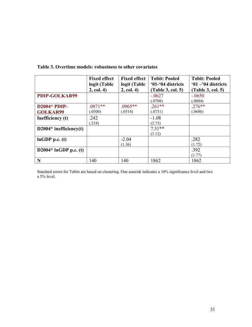
31

Table 3. Overtime models: robustness to other covariates Fixed effect

logit (Table 2, col. 4)

Fixed effect logit (Table 2, col. 4)

Tobit: Pooled ‘01-‘04 districts (Table 3, col. 5)

Tobit: Pooled ‘01 –’04 districts (Table 3, col. 5)

PDIP-GOLKAR99 -.0627 (.0708)

-.0650 (.0684)

D2004* PDIP-GOLKAR99

.0871** (.0300)

.0965** (.0314)

.261** (.0731)

.276** (.0686)

Inefficiency (t) .242 (.218)

-1.08 (2.73)

D2004* inefficiency(t) 7.31** (3.12)

lnGDP p.c. (t) -2.04 (1.36)

.282 (1.72)

D2004* lnGDP p.c. (t) .392 (1.77)

N 140 140 1862 1862 Standard errors for Tobits are based on clustering. One asterisk indicates a 10% significance level and two a 5% level.

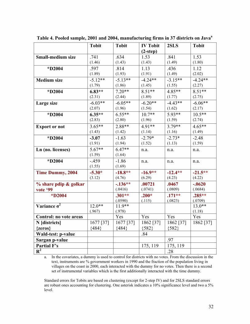
32

Table 4. Pooled sample, 2001 and 2004, manufacturing firms in 37 districts on Javaa

a. In the covariates, a dummy is used to control for districts with no votes. From the discussion in the text, instruments are % government workers in 1990 and the fraction of the population living in villages on the coast in 2000, each interacted with the dummy for no votes. Then there is a second set of instrumental variables which is the first additionally interacted with the time dummy.

Standard errors for Tobits are based on clustering (except for 2-step IV) and for 2SLS standard errors are robust ones accounting for clustering. One asterisk indicates a 10% significance level and two a 5% level.

Tobit Tobit IV Tobit (2-step)

2SLS Tobit

Small-medium size

.741 (1.46)

.634 (1.43)

1.53 (1.43)

.841 (1.49)

1.53 (1.80)

*D2004

.597 (1.89)

.814 (1.93)

1.13 (1.91)

.436 (1.49)

1.12 (2.02)

Medium size

-5.12** (1.79)

-5.13** (1.86)

-4.24** (1.45)

-3.15** (1.55)

-4.24** (2.27)

*D2004

6.83** (2.31)

7.20** (2.44)

8.51** (1.89)

4.85** (1.77)

8.51** (2.75)

Large size

-6.03** (2.07)

-6.05** (1.96)

-6.20** (1.54)

-4.43** (1.62)

-6.06** (2.17)

*D2004

6.35** (2.83)

6.55** (2.80)

10.7** (1.96)

5.93** (1.59)

10.5** (2.74)

Export or not

3.65** (1.43)

2.88** (1.42)

4.91** (1.14)

3.79** (1.16)

4.65** (1.49)

*D2004

-3.07 (1.91)

-1.63 (1.94)

-2.79* (1.52)

-2.73* (1.13)

-2.48 (1.59)

Ln (no. licenses)

5.67** (1.59)

6.47** (1.64)

n.a. n.a. n.a.

*D2004

-.459 (1.55)

-1.86 (1.69)

n.a. n.a. n.a.

Time Dummy, 2004

-5.30* (3.12)

-18.8** (4.76)

-16.9** (6.29)

-12.4** (4.23)

-21.5** (4.22)

% share pdip & golkar vote ‘99

-.136** (.0416)

.00721 (.0741)

.0467 (.0809)

-.0620 (.0684)

*D2004 .301** (.0590)

.200* (.115)

.171** (.0823)

.285** (.0709)

Variance σ2 12.0** (.967)

11.9** (.978)

13.0** (1.18)

Control: no vote areas Yes Yes Yes Yes N [districts] {zeros}

1677 [37] {484}

1677 [37] {484}

1862 [37] {582}

1862 [37] {582}

1862 [37]

Wald-test: p-value .84 Sargan p-value .97 Partial F’s 175, 119 175, 119 R2 .28

33

Table 5. “Reduced form” models of bribes

IV Tobit [MLE]; red tape bribesd

Tobit: Red tape bribes

IV Tobit [MLE]: All bribes

Tobit: all bribes

’99 vote : PDIP-GOLKAR [2SLS]

.146** [.104**] (.0346) [(.0708)]

.0597** (.0205)

.199** [.130**] (.0897) [(.0493)]

.0842** (.0369)

Ln (employ) 2.53** (.633)

2.50** (.622)

2.68** (1.33)

2.71** (1.32)

Ln (employ) sq. -.263** (.0721)

-.255** (.0694)

-.175** (.145)

-.175** (.141)

Dummy: rent capital .535 (.663)

.379 (.622)

.994 (1.29)

.868 (1.26)

Capital size: 500m-1b 1.18** (.429)

1.22** (.402)

2.46** (.872)

2.35** (.837)

Capital size: 1b-5b

3.08** (.829)

3.05** (.814)

4.21** (1.22)

4.06** (1.24)

Capital size: 5b-20b

1.59** (.548)

1.67** (.528)

3.06** (.924)

3.47** (1.00)

Capital size: over 20b

1.27 (.850)

1.29* (.762)

1.02 (1.36)

1.79 (1.40)

Dummy FDI .767 (.783)

.838 (.821)

.831 (1.18)

1.24 (1.26)

Dummy export .540 (.551)

.249 (.503)

.596 (.971)

.108 (.872)

Dummy Chinese 1.17** (.528)

1.34** (.484)

2.61** (1.26)

2.81** (1.04)

Controls: no vote, ind. dummy, visit cost

Yesab Yes Yesc Yes

N [zeros] 2582 [1160] 2582 [1160] 2474 [932] 2474 [932] Variance σ2 [ρ]e 6.34** [-.101]

(.505) [(.0731)] 6.36 (.552)

11.0 [-.116] (.751) [(.108)]

10.9 (.812)

Wald test: p-value .16 .28 Partial F’s: 1st stage 245 245 Sargan p-value: 2SLS [.41] [.84] R2: 2SLS [.16] [.195]

a. There are 8 categories of industries. None of the 7 dummy variables have coefficients that are significant at 10% or better level in column 1.

b. From visit equation in Table 8, the control is avg. distance from villages in sub-district to district capital. The coefficient is always insignificant.

c. Here wood [3.77 (1.93] is significant. d. 2SLS coefficients (standard errors) for column 1 variables are, in order, as follows: .104** (.0346); .808**

(.346); -.100** (.0391); .184 (.307); .518** (.266); 2.02** (.580); .543 (.356); .523 (.511); .607 (.647); .151 (.373); and .539* (.294). These coefficients are about 60% of column 1 coefficients.

e. ρ’s are the correlation of the error terms between the main bribe equation and the equation for vote share.

Standard errors for Tobits are based on clustering; and, for 2SLS, standard errors are robust ones accounting for clustering. One asterisk indicates a 10% significance level and two a 5% level.

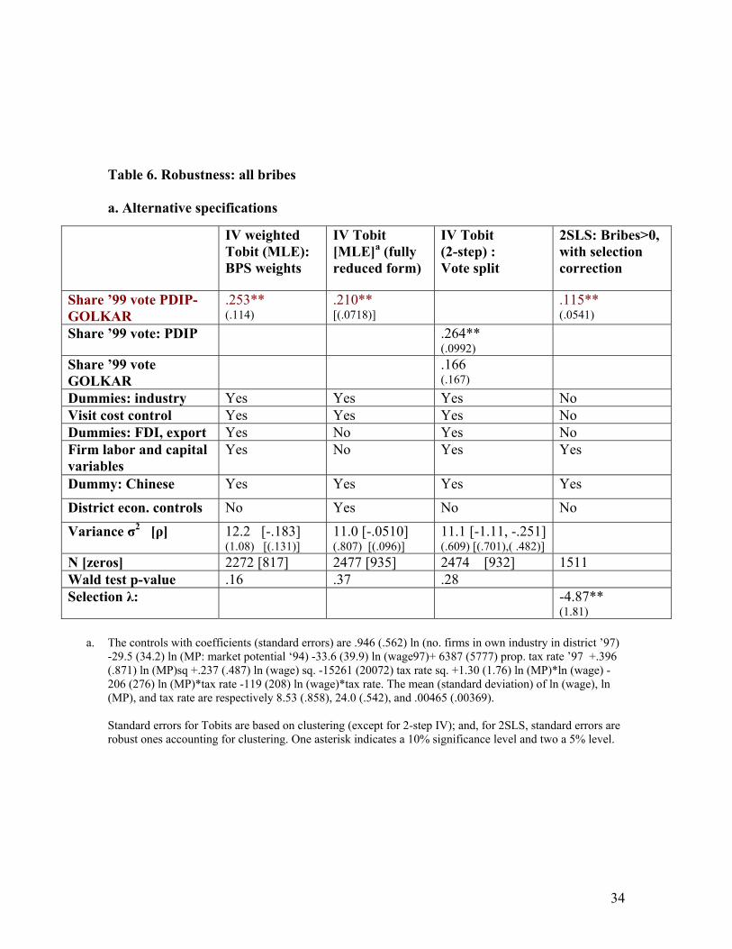
34

Table 6. Robustness: all bribes a. Alternative specifications

a. The controls with coefficients (standard errors) are .946 (.562) ln (no. firms in own industry in district ’97)

-29.5 (34.2) ln (MP: market potential ‘94) -33.6 (39.9) ln (wage97)+ 6387 (5777) prop. tax rate ’97 +.396 (.871) ln (MP)sq +.237 (.487) ln (wage) sq. -15261 (20072) tax rate sq. +1.30 (1.76) ln (MP)*ln (wage) -206 (276) ln (MP)*tax rate -119 (208) ln (wage)*tax rate. The mean (standard deviation) of ln (wage), ln (MP), and tax rate are respectively 8.53 (.858), 24.0 (.542), and .00465 (.00369).

Standard errors for Tobits are based on clustering (except for 2-step IV); and, for 2SLS, standard errors are robust ones accounting for clustering. One asterisk indicates a 10% significance level and two a 5% level.

IV weighted Tobit (MLE): BPS weights

IV Tobit [MLE]a (fully reduced form)

IV Tobit (2-step) : Vote split

2SLS: Bribes>0, with selection correction

Share ’99 vote PDIP-GOLKAR

.253** (.114)

.210** [(.0718)]

.115** (.0541)

Share ’99 vote: PDIP .264** (.0992)

Share ’99 vote GOLKAR

.166 (.167)

Dummies: industry Yes Yes Yes No Visit cost control Yes Yes Yes No Dummies: FDI, export Yes No Yes No Firm labor and capital variables

Yes No Yes Yes

Dummy: Chinese Yes Yes Yes Yes

District econ. controls No Yes No No

Variance σ2 [ρ] 12.2 [-.183] (1.08) [(.131)]

11.0 [-.0510] (.807) [(.096)]

11.1 [-1.11, -.251] (.609) [(.701),( .482)]

N [zeros] 2272 [817] 2477 [935] 2474 [932] 1511 Wald test p-value .16 .37 .28 Selection λ: -4.87**

(1.81)

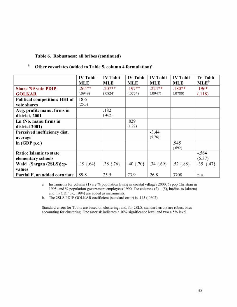
35

Table 6. Robustness: all bribes (continued)

b. Other covariates (added to Table 5, column 4 formulation)a

IV Tobit

MLE IV Tobit MLE

IV Tobit MLE

IV Tobit MLE

IV Tobit MLE

IV Tobit MLEb

Share ’99 vote PDIP-GOLKAR

.265** (.0949)

.207** (.0824)

.197** (.0774)

.224** (.0947)

.180** (.0780)

.196* (.118)

Political competition: HHI of vote shares

18.6 (25.3)

Avg. profit: manu. firms in district, 2001

.182 (.462)

Ln (No. manu firms in district 2001)

.829 (1.22)

Perceived inefficiency dist. average

-3.44 (5.76)

ln (GDP p.c.) .945 (.692)

Ratio: Islamic to state elementary schools

-.564 (5.37)

Wald {Sargan (2SLS)}:p-values

.19 {.64} .38 {.76} .40 {.70} .34 {.69} .52 {.88} .35 {.47}

Partial F, on added covariate 89.8 25.5 73.9 26.8 3708 n.a.

a. Instruments for column (1) are % population living in coastal villages 2000, % pop Christian in 1995, and % population government employees 1990. For columns (2) – (5), ln(dist. to Jakarta) and ln(GDP p.c. 1994) are added as instruments.

b. The 2SLS PDIP-GOLKAR coefficient (standard error) is .145 (.0602).

Standard errors for Tobits are based on clustering; and, for 2SLS, standard errors are robust ones accounting for clustering. One asterisk indicates a 10% significance level and two a 5% level.

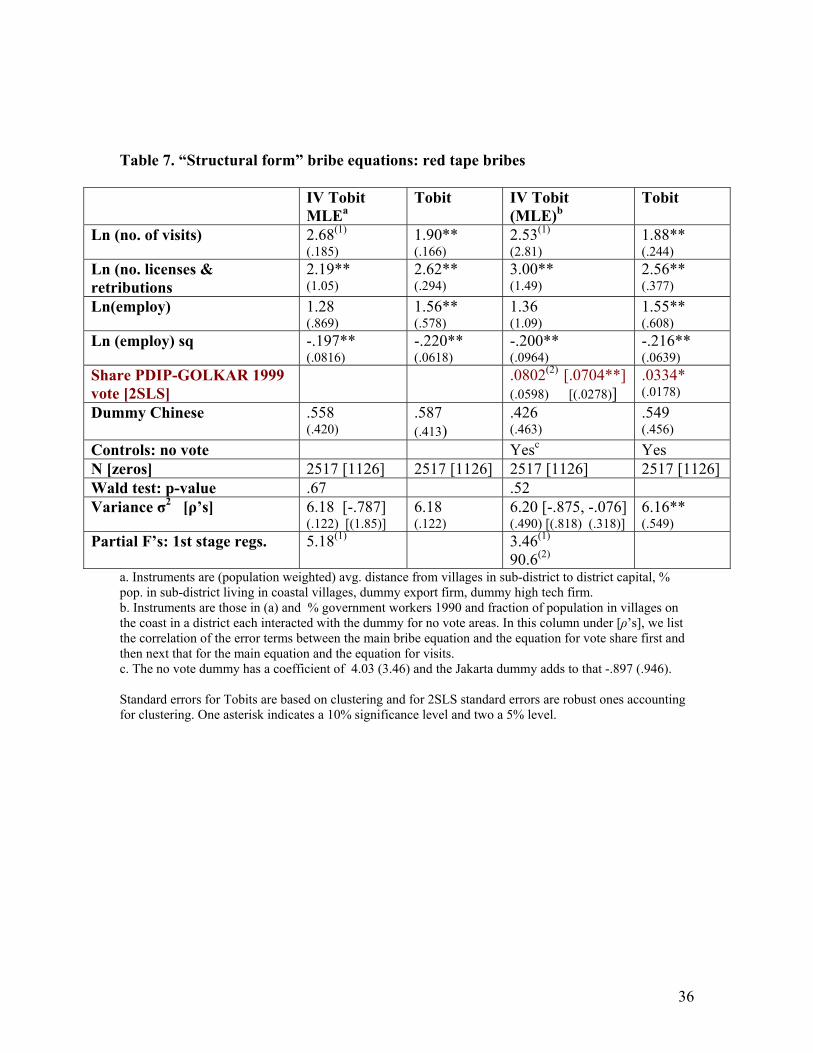
36

Table 7. “Structural form” bribe equations: red tape bribes

IV Tobit MLEa

Tobit IV Tobit (MLE)b

Tobit

Ln (no. of visits) 2.68(1) (.185)

1.90** (.166)

2.53(1) (2.81)

1.88** (.244)

Ln (no. licenses & retributions

2.19** (1.05)

2.62** (.294)

3.00** (1.49)

2.56** (.377)

Ln(employ) 1.28 (.869)

1.56** (.578)

1.36 (1.09)

1.55** (.608)

Ln (employ) sq -.197** (.0816)

-.220** (.0618)

-.200** (.0964)

-.216** (.0639)

Share PDIP-GOLKAR 1999 vote [2SLS]

.0802(2) [.0704**] (.0598) [(.0278)]

.0334* (.0178)

Dummy Chinese .558 (.420)

.587 (.413)

.426 (.463)

.549 (.456)

Controls: no vote Yesc Yes N [zeros] 2517 [1126] 2517 [1126] 2517 [1126] 2517 [1126] Wald test: p-value .67 .52 Variance σ2 [ρ’s] 6.18 [-.787]

(.122) [(1.85)] 6.18 (.122)

6.20 [-.875, -.076] (.490) [(.818) (.318)]

6.16** (.549)

Partial F’s: 1st stage regs. 5.18(1) 3.46(1) 90.6(2)

a. Instruments are (population weighted) avg. distance from villages in sub-district to district capital, % pop. in sub-district living in coastal villages, dummy export firm, dummy high tech firm. b. Instruments are those in (a) and % government workers 1990 and fraction of population in villages on the coast in a district each interacted with the dummy for no vote areas. In this column under [ρ’s], we list the correlation of the error terms between the main bribe equation and the equation for vote share first and then next that for the main equation and the equation for visits. c. The no vote dummy has a coefficient of 4.03 (3.46) and the Jakarta dummy adds to that -.897 (.946). Standard errors for Tobits are based on clustering and for 2SLS standard errors are robust ones accounting for clustering. One asterisk indicates a 10% significance level and two a 5% level.

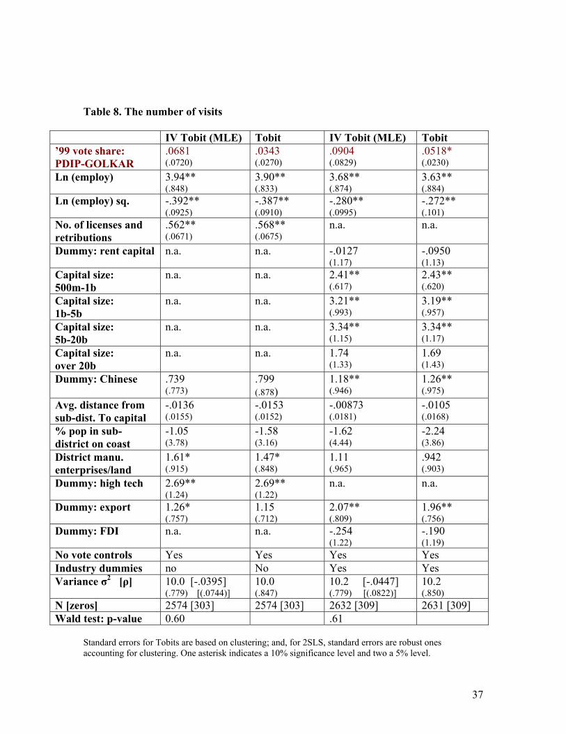
37

Table 8. The number of visits

IV Tobit (MLE) Tobit IV Tobit (MLE) Tobit ’99 vote share: PDIP-GOLKAR

.0681 (.0720)

.0343 (.0270)

.0904 (.0829)

.0518* (.0230)

Ln (employ) 3.94** (.848)

3.90** (.833)

3.68** (.874)

3.63** (.884)

Ln (employ) sq. -.392** (.0925)

-.387** (.0910)

-.280** (.0995)

-.272** (.101)

No. of licenses and retributions

.562** (.0671)

.568** (.0675)

n.a. n.a.

Dummy: rent capital n.a. n.a. -.0127 (1.17)

-.0950 (1.13)

Capital size: 500m-1b

n.a. n.a. 2.41** (.617)

2.43** (.620)

Capital size: 1b-5b

n.a. n.a. 3.21** (.993)

3.19** (.957)

Capital size: 5b-20b

n.a. n.a. 3.34** (1.15)

3.34** (1.17)

Capital size: over 20b

n.a. n.a. 1.74 (1.33)

1.69 (1.43)

Dummy: Chinese .739 (.773)

.799 (.878)

1.18** (.946)

1.26** (.975)

Avg. distance from sub-dist. To capital

-.0136 (.0155)

-.0153 (.0152)

-.00873 (.0181)

-.0105 (.0168)

% pop in sub-district on coast

-1.05 (3.78)

-1.58 (3.16)

-1.62 (4.44)

-2.24 (3.86)

District manu. enterprises/land

1.61* (.915)

1.47* (.848)

1.11 (.965)

.942 (.903)

Dummy: high tech 2.69** (1.24)

2.69** (1.22)

n.a. n.a.

Dummy: export 1.26* (.757)

1.15 (.712)

2.07** (.809)

1.96** (.756)

Dummy: FDI n.a. n.a. -.254 (1.22)

-.190 (1.19)

No vote controls Yes Yes Yes Yes Industry dummies no No Yes Yes Variance σ2 [ρ] 10.0 [-.0395]

(.779) [(.0744)] 10.0 (.847)

10.2 [-.0447] (.779) [(.0822)]

10.2 (.850)

N [zeros] 2574 [303] 2574 [303] 2632 [309] 2631 [309] Wald test: p-value 0.60 .61

Standard errors for Tobits are based on clustering; and, for 2SLS, standard errors are robust ones accounting for clustering. One asterisk indicates a 10% significance level and two a 5% level.

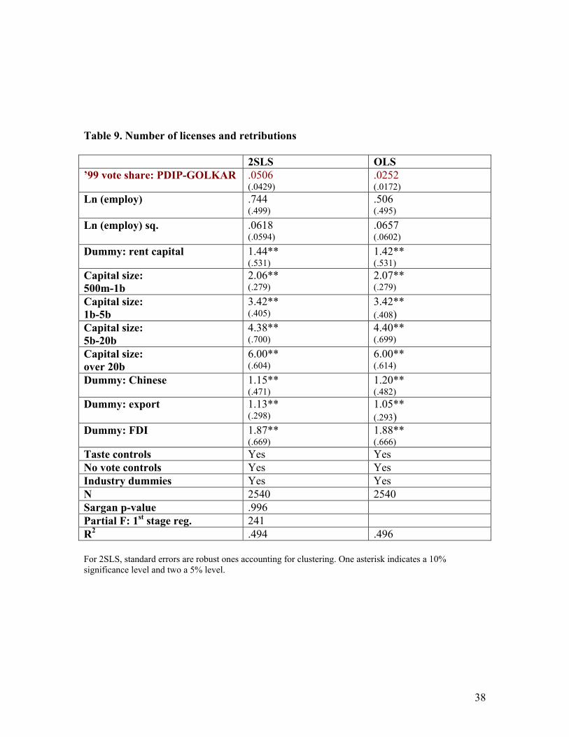
38

Table 9. Number of licenses and retributions 2SLS OLS ’99 vote share: PDIP-GOLKAR .0506

(.0429) .0252 (.0172)

Ln (employ)

.744 (.499)

.506 (.495)

Ln (employ) sq.

.0618 (.0594)

.0657 (.0602)

Dummy: rent capital 1.44** (.531)

1.42** (.531)

Capital size: 500m-1b

2.06** (.279)

2.07** (.279)

Capital size: 1b-5b

3.42** (.405)

3.42** (.408)

Capital size: 5b-20b

4.38** (.700)

4.40** (.699)

Capital size: over 20b

6.00** (.604)

6.00** (.614)

Dummy: Chinese 1.15** (.471)

1.20** (.482)

Dummy: export 1.13** (.298)

1.05** (.293)

Dummy: FDI 1.87** (.669)

1.88** (.666)

Taste controls Yes Yes No vote controls Yes Yes Industry dummies Yes Yes N 2540 2540 Sargan p-value .996 Partial F: 1st stage reg. 241 R2 .494 .496 For 2SLS, standard errors are robust ones accounting for clustering. One asterisk indicates a 10% significance level and two a 5% level.

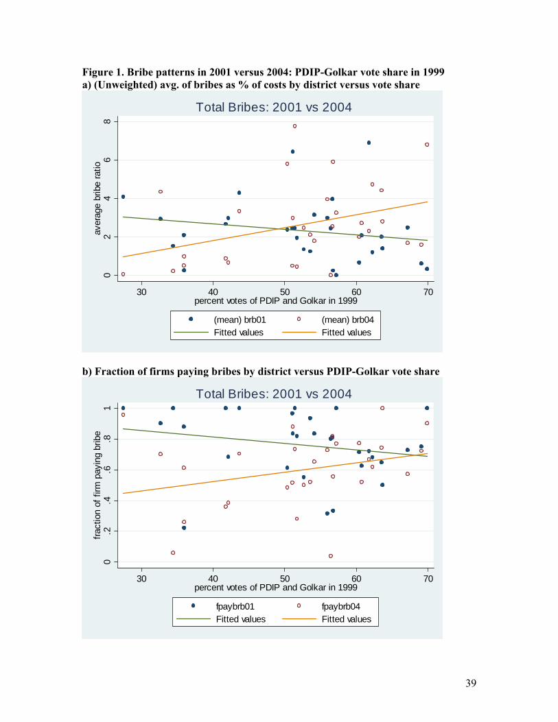
39

Figure 1. Bribe patterns in 2001 versus 2004: PDIP-Golkar vote share in 1999 a) (Unweighted) avg. of bribes as % of costs by district versus vote share

02

46

8av

erag

e br

ibe

ratio

30 40 50 60 70percent votes of PDIP and Golkar in 1999

(mean) brb01 (mean) brb04Fitted values Fitted values

Total Bribes: 2001 vs 2004

b) Fraction of firms paying bribes by district versus PDIP-Golkar vote share

0.2

.4.6

.81

fract

ion

of fi

rm p

ayin

g br

ibe

30 40 50 60 70percent votes of PDIP and Golkar in 1999

fpaybrb01 fpaybrb04Fitted values Fitted values

Total Bribes: 2001 vs 2004

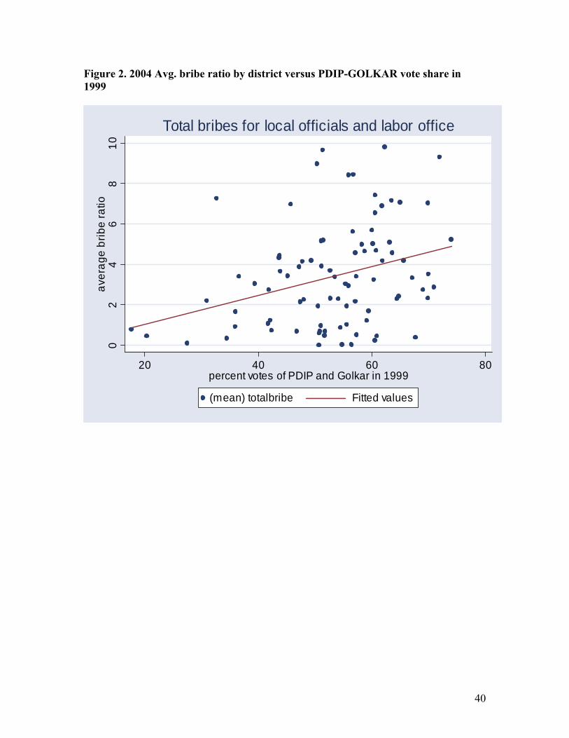
40

Figure 2. 2004 Avg. bribe ratio by district versus PDIP-GOLKAR vote share in 1999

02

46

810

aver

age

brib

e ra

tio

20 40 60 80percent votes of PDIP and Golkar in 1999

(mean) totalbribe Fitted values

Total bribes for local officials and labor office

41

Figure 3. Bribe activity in 2001 versus 2004 by district

02

46

8av

erag

e br

ibe

ratio

200

4

0 2 4 6 8average bribe ratio 2001

average bribes: 2001 vs 2004 Fitted values

Total Bribes: 2001 vs 2004

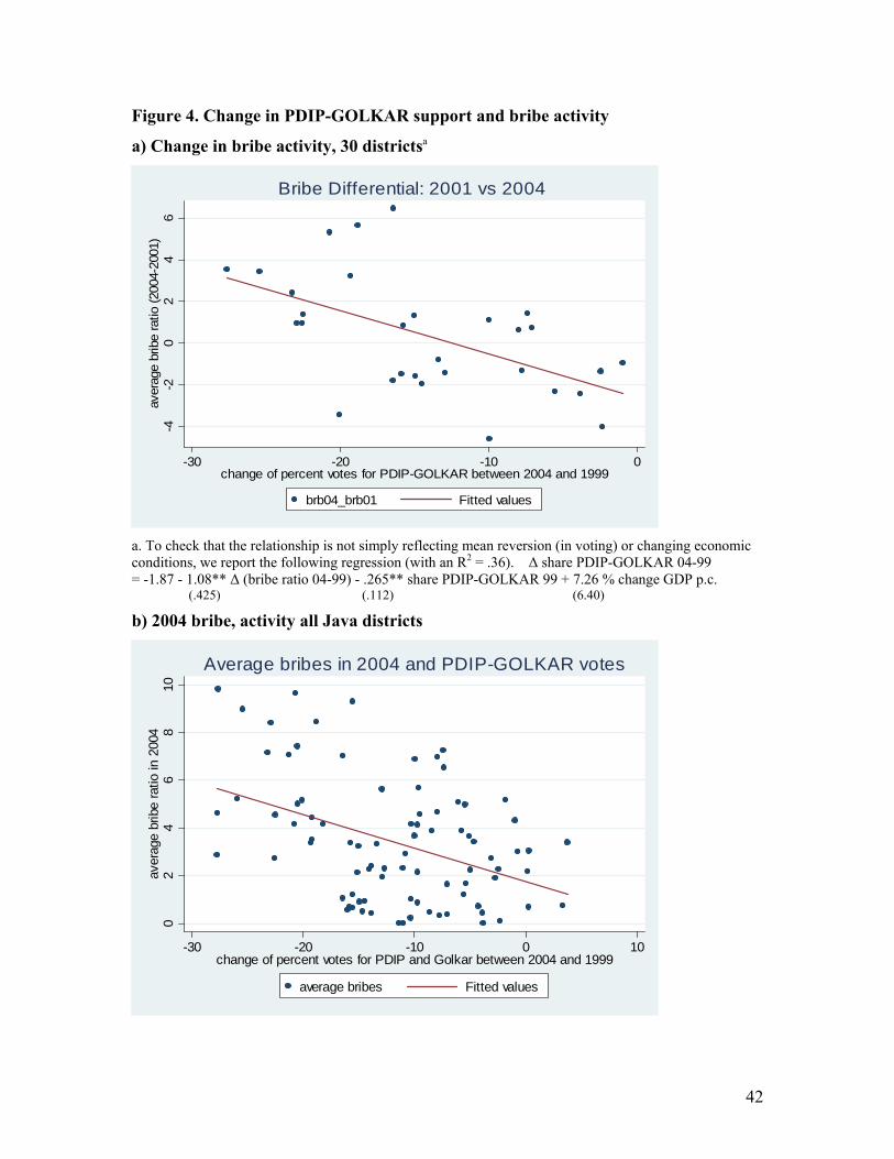
42

Figure 4. Change in PDIP-GOLKAR support and bribe activity

a) Change in bribe activity, 30 districtsa -4

-20

24

6av

erag

e br

ibe

ratio

(200

4-20

01)

-30 -20 -10 0change of percent votes for PDIP-GOLKAR between 2004 and 1999

brb04_brb01 Fitted values

Bribe Differential: 2001 vs 2004

a. To check that the relationship is not simply reflecting mean reversion (in voting) or changing economic conditions, we report the following regression (with an R2 = .36). ∆ share PDIP-GOLKAR 04-99 = -1.87 - 1.08** ∆ (bribe ratio 04-99) - .265** share PDIP-GOLKAR 99 + 7.26 % change GDP p.c. (.425) (.112) (6.40)

b) 2004 bribe, activity all Java districts

02

46

810

aver

age

brib

e ra

tio in

200

4

-30 -20 -10 0 10change of percent votes for PDIP and Golkar between 2004 and 1999

average bribes Fitted values

Average bribes in 2004 and PDIP-GOLKAR votes