Ship Resistance and Propulsion Prof. Dr. P. Krishnankutty ...

Ship Resistance and Propulsion Prof. Dr. P. Krishnankutty

Department of Ocean Engineering Indian Institute of Technology Madras

Lecture - 12

Canal Effects on Resistance Holtrap-Mennen Method for Ship Resistance Prediction

We have been discussing about shallow water resistance in the previous class, and when

we consider the shallow water, we have not considered any restriction the width wise

direction. That means we have not considered the canal effect or river effect, we

considered only the water effect on their resistance. Also we have seen that the resistance

when the vessels move from deep to shallow water, the speed of the vessel reduces in

two counts.

One is the due to the flow around it, which is called the potential effect, because of the

construction of the flow under the bottom the flow velocity increases, and where we have

pressure decrease and ship sinks more resulting in more wetted surface. Increase in

resistance of the ship is termed as a potential effect other aspect is the wave making

increases in the shallow water. There will be increase resistance due to the increase in the

wave size and subsequent increase in resistance due to the higher waves formed by the

vessel when it moves in the shallow water region.

(Refer Slide Time: 01:23)

Now, the things get more complicated when the ship moves into a canal or into a river

where the boundaries and the banks of the river canal is getting closer to the ship. They

will be additional effect coming to which and hence the flow velocity around the ship

and subsequent effect on the resistance of the vessels. So, that is what is what we are

going to look into in this lecture, so the shallow water with lateral restriction that what

you consider here for the canal effect. So, you know ships mainly or vessels which are

designed to operate in the inland water ways.

You know we have the three national inland water ways which are one Brahmaputra and

other one Hubli and third one Kerala. So, this the auto vessels are operating in these

region vessels exclusive designed exclusively for operation in inland water ways. So, the

vessels which you design for the operation inland water ways should be able to operate at

the required speed for which you need to consider the increase in resistance due to the

restrictions imposed by the water depth.

That is the shallow water and also the effects coming from the boundaries of the canal or

river so the aspects also should be considered. So, here Landweber suggested based on

the experimental studies the extension of Schlichtings method what we have discussed in

the shallow water. We said a Schlichtings method which has been used for the prediction

of resistance in shallow water provided. You know the resistance of the vessel in deport

a condition the resistance of the vessel in deport a condition is normally estimated

because of standard procedure. The standard methods for the estimation of resistance

vessel in deport a condition, so an information about the deport resistance of the vessel is

readily available.

So, what do you do is you take that values and now you make corrections which will

apply for the shallow water effect that is what is done interesting where he made many

assumptions, many assumptions are controversial. Still, it gives a practical solution or

engineering solution for the problem still continuity, we used to estimate the shallow

water resistance. So, what Landweber does is, he just borrowed the same method

Schlichtings method and applied for the vessels operating in canals and also for rivers.

So, here he has given that correction for the wave making part of the resistance is still

value that is what its assumption that is its Schlichting used assume that the waves

generated by the ship in deep water.

The same type of waves, same pattern same size of the wave is created when the same

vessel operate at a lower speed in shallow water. So, that means the same wave

resistance applicable at the lower speed in shallow water which a vessel implies that the

wave size increase at the same speed as it does in the deport a condition. So, that is what

is done here, Landweber also assumes that or he has found from the experiment that the

what way restrictions in the transits direction are not go into influence the wave part. So,

the correction which has been applied for the shallow water still holds good for the

vessel which operates in canal.

Also, no correction required for the wave making part whether its operation shallow

water mean meant compare with shallow water and canal. So, the same can be extended

here the speed of the translation of the wave in a channel depends only on the water

depth. So, that is what it says it is unrestricted as in unrestricted shallow water, so the

same water depth whether you use restricted water depth or un restricted shallow water it

is going to be the same wave.

Hence, the methods suggested by Schlichtings can be adopted in this case also when the

vessel operates in canal or rivers the speed correction for potential flow has to be

modified. The ship operates through shallow water and also through canals the flow

around the ship will be different.


So, what do what do you consider here is you consider shallow water effect the ship is

floating at the spot line and you see the bottom is very close to the bottom of the water

bottom of the water waves where to close the bottom of the ship. So, when you consider

shallow water, we have already seen that there is a construction of flow over just

between the bottom and the water wave which leads to the increase of flow velocity.

When the flow velocity increase the pressure drops and when the pressure drops the ship

has to sink more to make up the loss by and see due to the reduce the pressure. When it

sinks more, then they will be the wetted surface increases and due to the increase in

wetted surface area.

Also, due to the increase in flow velocity there will be increase in resistance, but when

you consider now the case with canal, you just consider just rectangular canal channel

and base of water level. Now, you consider a ship the section view cross section ship is

folding is like this, so this is the boundary of the canal. So, in addition to the construction

here due to shallow water you have also there is a restriction of region for the flow of

water when the ship is moving the water is escaping towards half side towards the raise

side.

So, due to this restriction again the flow velocity increases and further drop in pressure

and for the sink age of the vessel. Hence, more increase in resistance of the vessel so that

is a reason physical reason given for to increase in resistance when the ship operates in

canals or rivers, so that is what we have explained here.


So, there will be an additional limitation on the channel walls, so due to the lateral

restriction of the water wave. So, Landwaber he has used another parameter that is the

square root of Ax by Rh that is Ax is a section area of the maximum section of the ship

under water below water and Rh is the hydraulic radius.

So, in their Schlichtings method he used A x by R h was the water depth, now

Landweber when we when we considers the resistance of the ship in a canal the h

component or h. The water depth is replace by another factor called the hydraulic radius,

how do you estimate the hydraulic radius or how do you define the hydraulic radius that

equal to area of the cross check of the channel divide by wetted perimeter. So, here if

you consider the rectangular channel as we consider here with width is b and water depth

is equal h, then you can see that the area of the section is on the water is b h minus A x

that is the total water section area.

That is the section area of the channel and divided a perimeter b plus 2 h that gives a

wetted perimeter of the channel plus p that is a wetted perimeter of the ship. So, that

gives a total wetted perimeter, so this is an expression which he has suggested to

estimate the hydraulic radius which will go as a parameter here. So, we have already

seen we will come to that the whole that velocity difference is estimated, so the same

expression what is if you look if b is very high b means breadth of the channel is very

high.

It is as good as saving the shallow water because the boundaries are far away, so it is as

good as shallow water. So, if you look to this b is very high, so the second term becomes

insignificant because the b is very high here also b is very high. These two term becomes

insignificant, so that means b h by b its leads to h, so which implies that Rh is equal to h.

So, the same formula holds good for the shallow water also not only for canal if b is

large which implies that the boundaries of the channel are far away which is as good as

saying it is a shallow water region. So, when a ship is rectangular channel we have

already said that this is the expression for hydraulic radius


If you look to the figure which we discuss in the previous class and see that here, again

see that this is the pictures used Schlichtings and Landweber added one more curve to

that this is the one Landweber. So, what do you did is you plotted v h by v i v h by v i in

this axis against square root of Ax by Rh, so we do that is spot is plotted, so this you

have this curve. Now, what do you do is you know what is this value A x you know what

is the ship section area under water you know what is the hydraulic radius which we

have what we discuss.

Formally, you can find out Rh, so you know what this value square root of A x by Rh is

and then you find out with along this axis what the value is. Then take the inter section of

that curve this curve, then you find out what is v h by v i, So, v h by v I i we have already

discuss in the previous Schlichtings method v h is the actual speed of the vessel when it

operates the shallow water and v i is the intermediate speed which we have already seen.


I think if you recall the expression which we discussed v I is coming from this

expression, so it is coming from the finite water depth wave theory. So, v i is coming

from this expression which is known and from this curve what do you get is the v h by v

I know v i, we will find out what is the v h that is the speed achievable by the vessel

when it operates through the channel, so we have seen here.


So, what do you get we get this quantity the curve we have seen there is a Landweber

curve v h by v i against square root of A x by R h. I think there is a mistake here there

should be square root only in the top that numerate, so this quantity from the graph you

get this value and from which by knowing v i which is known from the wave theory

expression what I have shown to you now. So, you get v h that is a speed of the ship in

the canal, so here what implies that if you recall what we discussed in the shallow water

effect assume that for the same resistance what is the speed. We have found that there are

speed reduction in two counts, one is by we will show that.


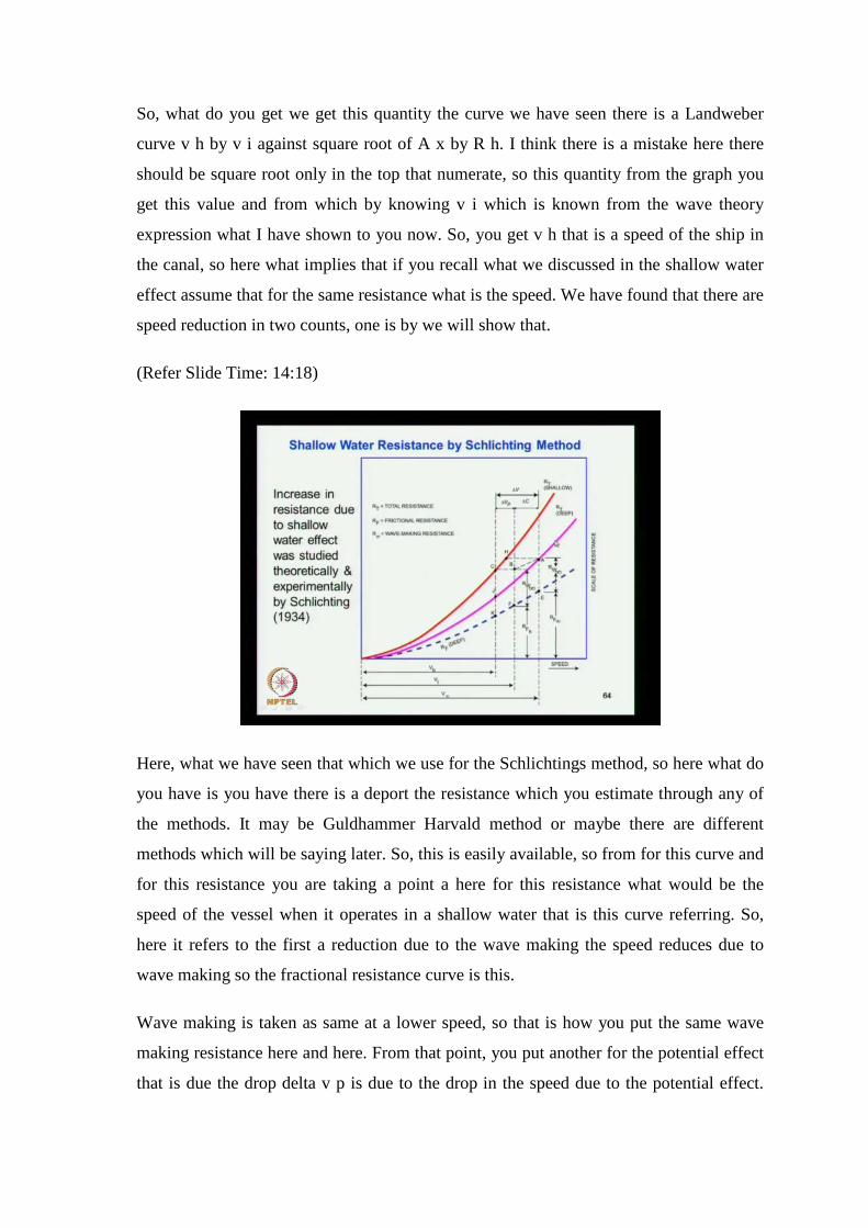
Here, what we have seen that which we use for the Schlichtings method, so here what do

you have is you have there is a deport the resistance which you estimate through any of

the methods. It may be Guldhammer Harvald method or maybe there are different

methods which will be saying later. So, this is easily available, so from for this curve and

for this resistance you are taking a point a here for this resistance what would be the

speed of the vessel when it operates in a shallow water that is this curve referring. So,

here it refers to the first a reduction due to the wave making the speed reduces due to

wave making so the fractional resistance curve is this.

Wave making is taken as same at a lower speed, so that is how you put the same wave

making resistance here and here. From that point, you put another for the potential effect

that is due the drop delta v p is due to the drop in the speed due to the potential effect.

Finally, you get a point c and that point c is a point on the total resistance of the vessel in

shallow water that is the procedure adopted by Schlichtings. So, here also you follow the

same procedure only thing that v i is now come b h is come from the Landweber curve,

so that is the difference where you use the hydraulic radius in place of the water depth.


So, that completes the water depth effect and the boundary effect a wall effect on the

total resistance of the ship. Now, we see there are different methods of prediction of the

resistance of a ship for different that we will see what the limitations applications of a

different methods and most of this methods based on the experimental studies are.

Systematic model tests have been carried out and the resistance let has been obtained and

that has been presented in a very systematic way for the use of designers.

When you design a ship you know that you need to know the recommend what is that

resistance offered by the vessel and then by knowing the propulsion c efficiency and all

that you will be able to predict the power required for the ancient. So, which again go as

input into the design of the ship and so the initial stages of the design and even after even

different stages were designs.

These methods are useful to estimate resistance some powering of the ship and finally,

wants a design has been converged. Then you go for a model tests and using the model

tests you recheck the resistance recheck the power. They are propulsion aspects

including the performing self propulsion does and all that and also the purple efficiency,

then you find out what is the transmission losses de rating and all that and finally, arrive

at the ancient power required for the ship.


So, we see the different methods with various methods which we discuss as here are one

is Holtrop and Mennen method other one is Van Oortmerssen method then Guldhammer

Harvald method Fungs method Mercier and Savitsky method. So, these are the different

method which will be discussing here which is used for the prediction of resistance of

vessels marine class there are small vessels some others exclusively for small vessels.

Some methods more general, some methods are exclusive of bigger shapes and all that,

so you just that when a progress with the lecture.


So, here first we look into the Holtrop and Mennen method so here generally says that

this is limited for the vessels with Froude number less than 0.5, so do not have play to

planning cross and high speed vessels. So, limit the use this method only for vessels with

Froude number less than 0.5 and also he put other parameters of the vessels which have

been considered for the experimental studies by this group. Based on this, the resistance

data has been prepared and presented in more systematic way may be finally using a

regression expression. We see that later words have expression used, so here they are of

with this side these types of vessels we can apply that is tankers and bull carriers.

You can do it, he has put the limit Froude number 0.24 that is the Froude number of

maximum Froude number 0.24. Usually, these vessels come in that range then the

prismatic coefficient various from 0.73 to 0.85. That is the range of the ship, so if your

ship which the ship which you design follow of all in within this range, then only you

apply it if you apply for the vessels which fall outer than the range.

Then, naturally this standard chance of inaccuracy in that prediction then length and

breadth ratio of the ship 5.1 to 7.1 that is the range suggested and b by t breadth to draft

ratio is 2.4 to 3.4. So, this is the range of applicability of this method and for other type

of ship trawlers coasters and tugs small curves. Generally, we can see it is the Froude

number maximizes allows 0.38 and these are the limits for C p that is 0.55 to 0.65 l b by

3.9 to 6.3 b by t 2.1 to 3. So, these are the application limits for these types of vessels,

similarly we have the containers ship and destroy relatively faster ship.

You can say the max of Froude number is 0.45 and this are the ranges of C p l by b b by

t, so then cargo liners relatively low velocity 0.3 is the Froude number maximum limits.

This methods application and this are the range of application of the parameters like C p

from 0.56 to 0.75. So, its big bite range and l b by b y 0.3 to 8 again its range is wide

took then b by t 2.4 to 4, so these are range of application of this method for type of

vessel. Then RO RO ships and car ferries this is a Froude number maximum then you

can see the variations here C p l b by b and b by t. So, when you use when you design

any of this vessels and you see that its falling with in this limits then you can use Holtrop

and Mennen method more reliably.


So, here R d presents is a total resistance is equal to this expression given for that where

is common is R of referring to fractional resistance which come from ITTC. You already

know that c f is equal to 0.075 divided by log R n minus to the whole square that is the

expression for c f value. Then this is a form factor which has been suggested by ITTC

1978 method, so we have to use the form factor. We have already discussed about what

is form factor, it is due to the increase in flow velocity due to the three dimensional

curvature of the ship. The ITTC formula has been derived based on the tests carried out

on flat plates whether three dimensional flow variations has been ignored.

So, when you cancel the ship which is totally different from the flat plate then the flow

around the ship the velocity of the flow increase due to the curvature nature. This flow

velocity results in increased frictional resistance because we know that frictional resist is

proportional to v power 1.825. So, naturally when the velocity increases the friction

resistance was also increase, so that variation is not considered in the ITTC flat plate

formula so this accounts for that form effect.

We have already discussed about the how the estimation of the form factor mainly use by

Prohaskas method, we have just been followed adopted by ITTC and recommended for

yours. Then you have the R, this quantity is appendages of resistance, so often you do the

resistance tests without the appendages without the rudder without Bleigh Keel without

the sharf brackets. So, there are many appendages which are of included in the resistance

estimation performed by model tests. So, if it is not included then you have to give a

allowance for the appendages resistance additional resistance offered by the appendages

so that is what is doing here by this term. Then you have the wave making resistance R w

which is the primary component in resizer resistance.

So, you have the wave making resistance here and all set includes the wave breaking

resistance. So, wave breaking resistance you already know that is due to the rest increase

into resistance due to the breaking of the bow wave. When the bow wave exists a limit or

the straightness of the bow wave go beyond a limit and it breaks and resulting in

increasing resistance due to the breaking of the wave.

Then, R b is an additional pressure resistance of bulbous bow near the water surface

though if there is an increase in resistance effect when the bulbous bow which comes

closer to surface it creates more disturbance and effect. Due to that, then the transom

with the transom is not if it is immersed, then obviously there will be a sudden flow

separation and the transom and the transom immersed there will be a flow separation I

think you know that.


If you concerned ship with a transom, so if you consider transom, so oppose a water line

is here the transom is not immersed. So, if you consider water plain at this land, then you

will get a very smooth shape, if you consider at this position. So, it is more suppose the

transom immerses suppose the water design water line is here, so you will have the same

thing here it will be somewhat or may be like this. So, the ship will have an abrupt

change when the flow is there, there is an abrupt change of the flow at that when the

transom immerses.

Due to that, there will be a increase in resistance because in the flow separates there will

be a formation of dish and a dish leads to increase in resistance. So, when the transom is

immersed there will be a increase in resistance which is accounted by this term R t R so

that is what is prescribed here. Then you know that is a model ship correlation allowance

which we also we discussed the correlation allowance is given when you do the

resistance estimation for prototype ships because the model which is normally made of

wax or fibre glasses.

Other materials having very good very high finish for suffers, but when it comes to a

ship the ship is not going to such a good finish it will have the all the wall joints or it

may have the plates deformations between the frames. These things are not properly

predicted by the represented if the geometric model of the ship when it done the model

tests. So, there will be the increase in to resistance due to the in coefficient of the surface

and also due to the increase in roughness of the skin of the ship, so that increase in

resistance accounted by this allowance. So, this called the model ship correlation, so

these are the different terms which appear in the total resistance represented by Holtrop

and Mannen.


Now, we see how these components are estimated, so R f we know the first component

we know it is coming from ITTC formula. This is coming from that is because c f you

get from ITTC formula into half row s v square you get R f value. So, you do not need

that explanation for that, then we have this form factor one plus k one next term is given

by this expression by Holtrop Mannen.

So, we have to put c 1 3 into 0.93 plus c 12 into b by l R into whole raise to point this of

quantity, then you have 0.95 minus C p, C p is the prismatic coefficient raise to this one.

Then 1 minus C p plus this into l c b raise to so much l c b is a natural centre of point c

and l c b is here is given as percentage of the length about midship. I mean forward of

midship is taken a positive, so there is this gone percentage usually you get about two to

three percent forward of the midship or some ships we get so much. So, there it will be

negative, so l c b is place an importance role in resistance because when you say l c b is

positive that means the centre of forward a midship.

It implies that the hull of the ship is more in the forward side when you say l c b forward

means it is the concentration of volume is towards of forward. So, when the hull become

more in the forward the flow separation though the flow will be or the resistance

component will be higher. So, usually that is you know correction given for the l c b

position so if faster ship you will find that l c b is after midship you will say slow ship.

Then you may find l c b forward of it, so here SS C p say then l R is a length of a run

means you must have studied will a consider the ship.


Suppose, against the water plain it is coming like this half of it and you know that you

call this angle this angle is entry angle, half entry, half angle, half entry and this length

we continues till the when it is a parallel region. This length you call it angle length say l

R, so that is the length here, once you know the water plain of the load water length then

you know the form of it you can measure what is l R from that. So, that is l R b is a

breadth, so all this parameter is known is b is known, so you know what is C p you know

what is l c b all from the design accept c 1 3 or c 1 2. These two parameter c t b know

which is define below, so here l R what you get is if you do not you can use this formula

also for l R l R by l is equal to 1 minus C p into 0.06 into C p l c b by C p minus 1.

We know all this values from the design, so you get what is l R by l l is known from

which you will get l R. So, you get substitute here you get l R, then you need c 1 2 this

quantity here, so c 1 2 is given here that is for t by l greater than 0.05 use this expression

for t by l between 0.02 and 0.05 use this value this expression over here. For t by l less

than 0.02, use this values, so depending on what is the draft to run the ratio of the ship,

so which was appropriate relation here and find out what is c 1 2 substitute it here.


Now, we are left out with c 1 3, let us see that what is there c 1 3 is equal to 1 plus 0.003

into C stern what is C stern is a coefficient indicates the after body form after body form

you have. You can see that the form of the ship is basically defend as normal form, it is

the conventionally used for the test then there is a b form and there is a u form. So, these

are the three form generally classified, so depending on the what type of form of the

section you used for the ship in the after region you choose the value from.

This if it is a V section, you choose minus 10, then C stern is equal to normal no

correction no this is not required and so here this is one C stern. So, what you get is you

get find out what is a c 13 here and then you substitute back to the previous expression.

So, everything is known you can find out what is 1 plus k 1 and then you put the 1 plus k

1 here.

So, R f is not coming from ITTC 1 plus k 1 no way estimated, now you look to the

wetted surface area. How it is defined the wetted surface area of the hull can be

approximated by S, S equal to l, length of the ship 2 times draft plus breadth of the ship

in the square root of mid ship be the coefficient into this expression into coefficient.

Then you have the mid ship area of coefficient here then b by t here, then water plain

area coefficient. Then finally the bulbous of fact A BT there is a transverse sectional area

of the bulb divided by c b the transverse section area of the bulb, means when you

consider this ship as bulbous bow which is considered.


Now, we are left out with c one three a ship that bulbous bow and this is the forward

perpendicular and you know this is the usually the position of the water line load water

line. So, if we take a section here you will see that the section may be its coming in the

forward section it may be slightly it is going to be like this. Then you take the area this is

the half of it this into two because we have considering the full area the whole area that

is A BT area of a bulb it is a transom, so that is A BT.

So, you take a section at the of the bulb at the forward perpendicular take the underwater

area of that section that is given as A BT is a transfer section area of the bulb so which

go as a input here. So, all the parameter are known here, so you can find out what is the

wetted surface area of the ship it is an approximate form which will be used.


In the design appendage, resistance is equal to 0.5 ro V square into surface area of the

appendage you have the Bleigh keel, you have the rudder and other appendages. You

have to know appendage into 1 plus k 2 equivalents into C F, so you find out C F again

from ITTC formula. Then you have this 1 plus k 2 expression which is given in the next

sheet, so ro is the density V is the ship speed. So, once you the appendages, you will you

can find out what is a surface area and all that, so 1 plus k 2 is appendages resistance

factors. So, here one thing we have to note is that C F is also I have mentioned it is

coming from ITTC formula. So, one thing we have to note is the appendage resistance

you know is directly only related to C F and no other components.

Resistance are not considering appendage resistance, we are not having C W here, no

other or other components coming here the reason for that is the suppose you can say

Bleigh keel which is at the bottom of the ship. It is not going to create in a wave, so you

just a making an assumption that it contributes solute of friction essence is acceptable

and may be the popular bracket and popular bossing and all that. So, this also sufficiently

and submerged in water. So, its effects at the face of a, so create a wave is not there and

rudder also moral a same so this appendages generally the contribution is only on the

frictional side not on the wave making side.

That is why this expression is confirming only to the C F parameter, not other

parameters. So, once you know 1 plus k 2, this surface area is coming from the

appendage once you design the rudder. Once you design the Bliegh keel, you know what

a surface of this you can use that value C F is coming from here. You know the Reynolds

number and all that, so you can that C F and only thing left is the unknown is 1 plus k 2,

so we see it is given in a next slide here.


So, you can see the values here 1 plus k 2 rudder behind skeg, you have a skeg and

rudder behind it. So, use this 1 plus k 2 values 1.522 rudder behind stern no skeg, then

mean behind stern means behind the popular stern. Then you have this one this is a

parameter twin screw balance rudder if you are using balance rudder twin screw. So,

popularly to select the factor from here shaft brackets turn by this quantity the skeg

alone. You give this one strut bossing, this one hull bossing, you have then shaft

stabilizer fins if you are using it is a putting out to this subliming fin use this factor if say

dome.

So, not domes are used for naval vessels, you know that if you have a dome previously it

used to be a mid ship region. Now, a day’s, they only preferred at the bulbous bow, the

naval vessel they combined it with the bulb the bow part. So, the dome plus a bulbous

will be sink loaded, so it is now they say generally preferred because that dome its

basically for under water scanning in all that using sound waves. So, you if you put at the

forward and it will be less disturbed, you know the seven should be less so the signals

which you get are clearer.

So, the clarity of the signals is better when you put it the dome at the far end and also the

dome will save the purpose of a bulbous bow. So, that is why, so if you are using that

find out this, then Bleigh keel is this, so depending on what type of appendage you are

using and you choose this 1 plus k 1 k 2 value from here. Then finally you find out the 1

plus k 2 equivalent is represented by this expression that is 1 plus k 2 of one component

plus its wetted surface area.

Then, 1 plus k 2 of the next component and it is a wetted surface, and then divided by

total wetter surface area. That gives the 1 plus k 2 which will go as in the go into this

here and then you find out what is the R appendage and it goes into this portion that is an

x what we get here, now the next component is wave making resistance R w.


So, this R w is expression c 1 into c 2 into c 5 into volume displacement role g in the

exponential of this parameter. Now, you find out what is c 1 on to all this parameter c 1

is done by this expression, so much into c 7 raised 2 of this value T by B draft by breadth

power this and 90 minus i is the half angle entry raise with this, so this are the parameter,

we see how this parameters x. So, c 1 is coming from here, now you have to know what

is c 7, c 7 is given by this expression it is based on B by l less than b by l ratio.

If it is less than 0.11, you use this expression if it is between 0.11 in 0.25, you use this

expression or if it is between greater than 0.25, use this expression. So, depending on the

vessel dimensions L and B you find out where it lies and take the appropriate expression

and then find out what is c seven c two is given by exponential of that is e power minus

1.89 the square root of c three and that is what is given here. We will see what is c 3,

now and k R and c 5 is given by this expression, so here you can see that c 2 is a

parameter which accounts for that reduction. The wave resistance due to the action of

bulbous bow, so you can see that c 2 is coming from c 3 and will be in the next slide, we

will see the c 3, c 3 is coming here.


Here, c 3 depends on the bulbous parameter; c 3 is depending on A BT that is area of the

bulbous bow. I have already explain that, then though out of parameter related to the

bulbous bow, so c 3 determined c 2 and hence c 2 is the parameter which accounts for

the bullbous bow effect. So, c 5 what do we see here, the expresses the influence of

transom you can say that represents a transom immersed area is a transom of the ship.

So, take the transom of the ship and take the underwater area of the transom and there is

a 80, so then b t into c m.

So, this gives c 5, so that is what a t represents, the immersed the part of the transverse

area of the transom at 0 speed. So, that means 0 speed means when the speed is high, the

water surface changes elevation changes. So, do not take that in calm water, you take the

static condition where the underwater area of the transom is.

So, the half next is half angle of entrance, now we have seen this we have seen c 1, we

have seen c 2 and coming from what is say from c 3. It is coming c 5 is coming from

here and row and g, we know, now we see other parameters here half angle of entrance

given by this expression. You know already what effects may half draught during into

half angle of entrance and small of the half angle of entrains find out the ship form will

be and fast. The ships usually have small values for half angle of entrains and bulk

carries and tankers which are more fold.

They will have a larger angle of entrains for the load water line, so e that is a half angle

of entrains is given by this expression even this all known l by B C w p water plain area

coefficient C p L R already explained. Also, given in the expression, this known volume

displacement L cubes, so everything is known so what you do is you can straight find out

what is i e value. Then c 3 as a c which use them c 2 had is area of the bulb and your

having this the ratio of 1.5 A BT t f is a drafted forward and h b is the position of centre

of transverse area above the keel that is the h b, h b is, you find out the centre of the

position.


You find this A, area centre may be somewhere here the word is this, it is h B, so that is

the value, so which should get from the form descent. So, that is h B, so once you get all

this parameter reason find out c 3 and then you substitute it here, you get c 2. So, all

these parameters are obtained now and the one parameter left out you can see m 1 and m

2 and lambda to be obtained. Let us see how it is a lambda is given by this lambda is

equal to given by this expression if L by B is less than 12 or given by this expression if L

by B is greater than 12.


So, this will also go to that expression m 1 and m 2 which written is also given here, m 1

depending again on length root draft ratio displacement raise to third by L and B by L.

Then c 16, here c 16 we are getting from this expression which is depending on C p

value C p less than 0.8. You have to use this expression if C p is more than 0.8, use this

expression, so from which we get c 1 6 substitute c 1 6. Here, other parameters are

known you get m 1, now coming to m 2 c 15 into C p square into this quantity over here.

So, here you have to find out c 15, c 15 again depends on L q by volume displacement.

So, depending on that if it is less than 5, 12 use this greater than this, use this and if it is

between this, use this expression. So, depending on once you find this quantity you

should choose the appropriate relation here, find out c 1 5 substitute c 1 5, here you get

m 2. So, all the quantities are now known here you get R w, so R w will go to this

expression here.


So, you get this term here then the additional resistance due to presence of the bulbous

bow p near the surface is determined that is R B.


We have already seen that this is the additional resistance when bulbous bow comes to

the surface. If it is not coming to the surface, you discard that if it is coming to surface,

then you use this expression here. This is the expression P B raise to minus two f n i A

BT you know that and you see that these are the is R b value, so here P B is measure is a

measure of the emergence of the bow which is given by this. I can say that P B is given

by this expression, now we know what h B, A BT is and all that you know you find out

what is P B then the F n i is the Froude number based on the immersion. So, it depending

on the immersion the water length changes so the Froude number also changes.

So, you take it accordingly here, so that is what is the v into curve g into t f minus h p

minus all this parameter are known, so you find out what is F n i. From this, once you get

P B and FN i you go here you get R b that is a next term appearing in the expression for

the total resistance of put forward by Holtrop and Mannen. So, there is a, then you find

out what additional resistance due to the immersion of transom, so R t R that is equal to

0.5 rho V square a t into c 6.

So, here what do you do is you find out all every you know everything except c 6, c 6 is

taken from this formula that is the c 6 is equal by F T F N T, F N T is equal to less than

5, F N T I think it should be a Froude number. It is given here FNT is given by V by

square root of 2 g a t into B plus B into C w, so everything is now this are transom

submerged area and B breadth is a water plain area coefficient.

So, we can find out what is F N T, so F N T you substitute here, then you get c 6, then

you substitute c 6 here, you get R, T R that is a transom in resistance due to a transom

immersion. Then the model ship correlation allowance is R A is equal to half rho V

square S into C A C A is the correlation allowance coefficient. Usually, it is given as

0.0004, so that is a correlation allowance 0.000430 and 4 that is normal.


So, if you know that C A value, you can use it and all if you have another expression that

also can be used for that. So, with that we have we can estimate what is R B what is R T

R and finally, we go to the expression here a total resistance. We have already seen all

this terms you just subtitle it there, so you get the total resistance, so that is how the

Holtrop and Mannen method has been revolt and presented.

Finally, you put the limitation of the hull parameters C p between this 1.55, 2.85 L by B

is taken 3.9 to 15 B by T for 2.1 to 4 Froude number less than 0.5. The drafted forward

divided by load length of load water length should be greater than 0.04, so if you look all

this aspects, then we will satisfy this parameters. You can use the Holtrop and Mannen

method and the Holtrop and mannen method you know it is based on experiments carried

out on the different types of models in a systematic way and you flow the vessel fall in

this the results are reliable.


So, that is what we have, so that completes the first method as the Holtrop and Mannen

method for the estimation of resistance.

Thank you, we will continue in the next class.

Ship Resistance and Propulsion Prof. Dr. P. Krishnankutty ...

Documents

Transcript of Ship Resistance and Propulsion Prof. Dr. P. Krishnankutty ...