Session 6 - COPYRIGHTED MATERIAL

1

Session 6

Open � le: CMALS1_session6_ver2010.ppsx

c01.indd 1 6/3/2015 2:28:23 PM

COPYRIG

HTED M

ATERIAL

2 Instructor Guide Part 1: Financial Reporting, Planning, Performance, and Control

Session 5 Recap

Note that if sessions are being run on the same day, the recap of the previous session can be skipped.

Remind participants of the material covered in Session 5, which included the discussion of forecasting techniques, from Section B, Topic 3.

Ask participants if they have any questions on the topic or the exercise that included many of the concepts covered in Section B.

c01.indd 2 6/3/2015 2:28:24 PM

Session 6 3

Session 6 Overview

Explain to participants that in this session, they begin studying Section C: Performance Management. Th e session covers Topic 1: Cost and Variance Measures and a current variance exercise.

c01.indd 3 6/3/2015 2:28:24 PM


Section C: Performance Management

Explain that this section covers fi nancial and nonfi nancial performance mea-sures that allow the organization to evaluate its business units and compare its actual results to planned goals. Th is analysis is the essential next step to the bud-geting process and is critical to the continuing implementation of the organiza-tion’s strategy.

Specifi cally, this section covers the three topics of

1. Cost and variance measures—variance analysis2. Responsibility centers and reporting segments—including types of responsibil-

ity centers, transfer pricing techniques, and allocation of common costs3. Performance measures—including both fi nancial and nonfi nancial measures

and the use of the balanced scorecard

c01.indd 4 6/3/2015 2:28:24 PM

Session 6 5

Section C, Topic 1: Cost and Variance Measures

Explain: “Control” is an important part of the management cycle. Actual results must be compared to the original plan: the combination of a profi t plan and standards.

Th e diff erences between actual and plan/standard are called “variances” and they may be favorable (better than plan) or unfavorable (worse than plan).

Discuss: Variances facilitate “management by exception” in that variances call for attention in proportion to their magnitude. In other words, devote management attention to the few things that cause the largest variance from plan.

c01.indd 5 6/3/2015 2:28:25 PM


Explain: A standard cost system, when it’s practical, is both informative and convenient.

It’s informative because it calls attention to things that potentially could result in a fi rm’s results falling short of plan.

It’s convenient because it allows the same item in inventory to be valued at the same unit cost, rather than having to keep track of separate layer or, even, specifi c identity.

And it’s informative and convenient because it provides a “line of demarcation” between marketing and manufacturing. Manufacturing essentially “transfers” its output to marketing at the standard variable manufacturing cost. Manufacturing retains its own variances—both favorable and unfavorable. Marketing earns a con-tribution margin on the diff erence between the selling price and the standard vari-able manufacturing cost.

c01.indd 6 6/3/2015 2:28:25 PM

Session 6 7

Discuss: When a fi rm uses a standard cost system, it will have a product cost sheet, developed during the annual planning process, for each of its products. It will show the resources (material, labor, etc.) needed to produce the product, the cost of each of those resources, and the dollar content of each resource in a unit of the product.

Th e cost sheet will be the basis on which cost variances are calculated and will also be the basis on which marketing contribution margins are calculated.

c01.indd 7 6/3/2015 2:28:25 PM


Discuss: Th is is the income statement for Bounce for the year 2015. It show a comparison of actual results (operating profi t of only $35,760) against the profi t plan operating income of $270,000. Th e profi t plan will be referred to as the “static budget.” Obviously, there is a huge operating profi t shortfall!

We can see the diff erence (variance) for each of the lines of the income state-ment, but there is very little we can confi dently point to as underlying causes. It would certainly appear that the fi xed costs—both manufacturing and SG&A—were under good control.

Note: Since total units sold appears on the income statement, we do know that the total units sold was signifi cantly below plan. Th at would probably explain revenue being below plan. It would also explain variable cost of goods sold being below plan.

But was each of them the amount below plan that they should have been? Th at can’t be explained from the information provided.

c01.indd 8 6/3/2015 2:28:25 PM

Session 6 9

Discuss: Th is is the same budget as before with the addition of one important feature—the fl exible budget. Since actual units sold were 80% of the budgeted units, the static budget for revenue and variable costs was multiplied by 80%.

Now, a lot more information is available. Look at the diff erence between the static budget and the fl exible budget on either the contribution margin line or the operating income line. Th at $192,000 diff erence is the sales volume variance and it is the amount of operating profi t lost due to not selling the number of units that were planned to be sold. It could also be calculated as (30,000 units – 24,000 units) × $32/unit. Th e $32/unit is the diff erence between the planned selling price of $120/unit and the planned variable cost of $88/unit.

Th e diff erence between the actual and the fl exible budget is called the fl exible budget variance; its value is an unfavorable $42,240. Th e fl exible budget consists of failures to control costs and any deviations from planned selling prices. Notice that, in this case, the actual selling price of an average of $125/unit resulted in operating profi t being $120,000 higher than it otherwise would have been [($125/unit-$120/unit) × 24,000 units]. Looking at the results that Marketing produced, the sales volume variance was an unfavorable $192,000 and the selling price variance was a favorable $120,000 for a net unfavorable variance of $72,000. Th is should cause management to consider whether a diff erent actual selling price could have pro-duced a better overall contribution margin.

Nevertheless, the remaining $162,240 unfavorable of the fl exible budget vari-ance suggests the bulk of the failure to achieve budgeted operating income lies with a failure to control costs. Now, management needs to see what can be learned from variance analysis.

c01.indd 9 6/3/2015 2:28:26 PM


Discuss: Th is is what actually happened during 2015. It is the basis for the sub-sequent variance calculations

c01.indd 10 6/3/2015 2:28:26 PM

Session 6 11

Explain: Th e above derives the defi nition of these two variances in great detail.Note: It is critical to understand that in this formulation, a positive result sig-

nals an unfavorable variance while a negative result signals a favorable variance.Note: Th e idea most oft en forgotten is the defi nition of SH.In short, the two variances together perfectly explain the diff erence between

actual dollars spent and the dollars that can be debited into inventory.

c01.indd 11 6/3/2015 2:28:26 PM


Discuss: From the facts, the direct labor variance calculations are straightfor-ward. Be very clear that the standard hours are the hours that should have been used to produce 24,000 units. Th e purpose of variance analysis is to be fair to those whose performance is being measured. Based on what they accomplished (actual output), you need to compare the resources the organization did use to the amount of resources the organization should have used to accomplish that level of actual output.

Exam tip: If the standard labor hours planned are provided in a question, you must train yourself to ignore that piece of information as it is not relevant.

c01.indd 12 6/3/2015 2:28:26 PM

Session 6 13

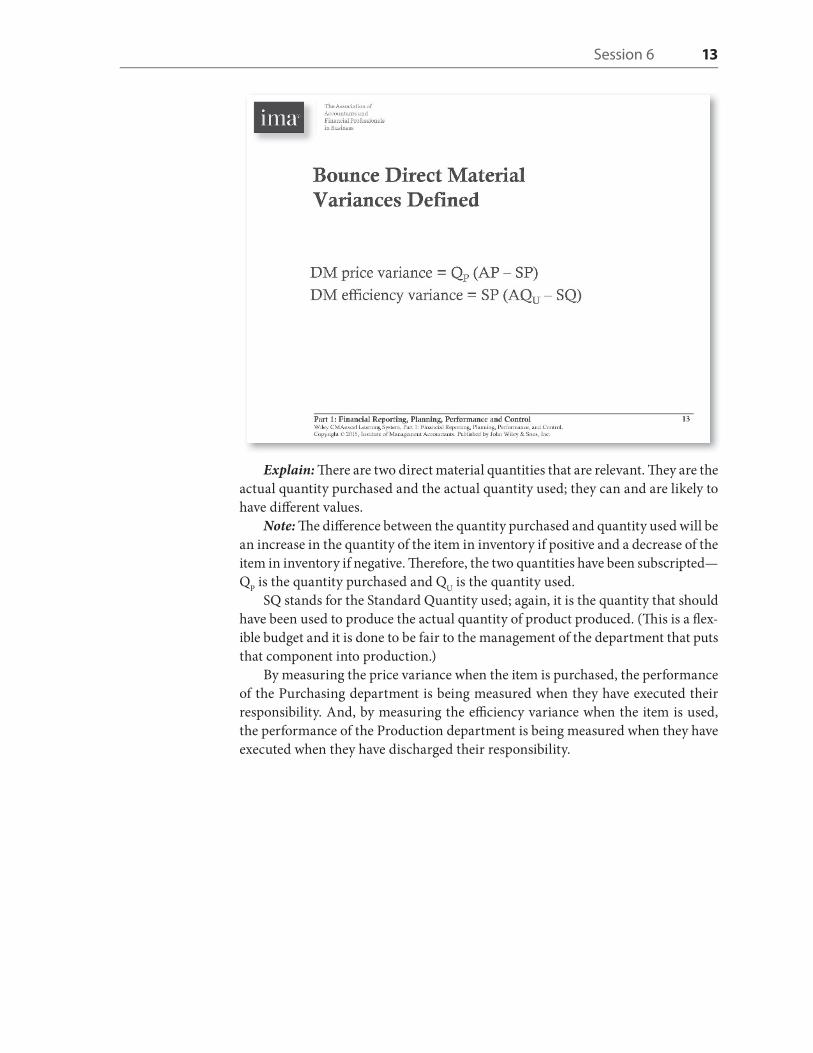
Explain: Th ere are two direct material quantities that are relevant. Th ey are the actual quantity purchased and the actual quantity used; they can and are likely to have diff erent values.

Note: Th e diff erence between the quantity purchased and quantity used will be an increase in the quantity of the item in inventory if positive and a decrease of the item in inventory if negative. Th erefore, the two quantities have been subscripted—QP is the quantity purchased and QU is the quantity used.

SQ stands for the Standard Quantity used; again, it is the quantity that should have been used to produce the actual quantity of product produced. (Th is is a fl ex-ible budget and it is done to be fair to the management of the department that puts that component into production.)

By measuring the price variance when the item is purchased, the performance of the Purchasing department is being measured when they have executed their responsibility. And, by measuring the effi ciency variance when the item is used, the performance of the Production department is being measured when they have executed when they have discharged their responsibility.

c01.indd 13 6/3/2015 2:28:27 PM


Discuss: Both of these variances are very large. Such variance would be likely only in the instance of a commodity with highly volatile prices caused by large fl uc-tuations in supply and/or demand. Th e effi ciency variance seems unlikely under most circumstances.

Note: In calculating variances, students must be careful to ensure that both the price and quantity purchased/used are expressed in the same units of measure. Otherwise, erroneous results will occur.

c01.indd 14 6/3/2015 2:28:27 PM

Session 6 15

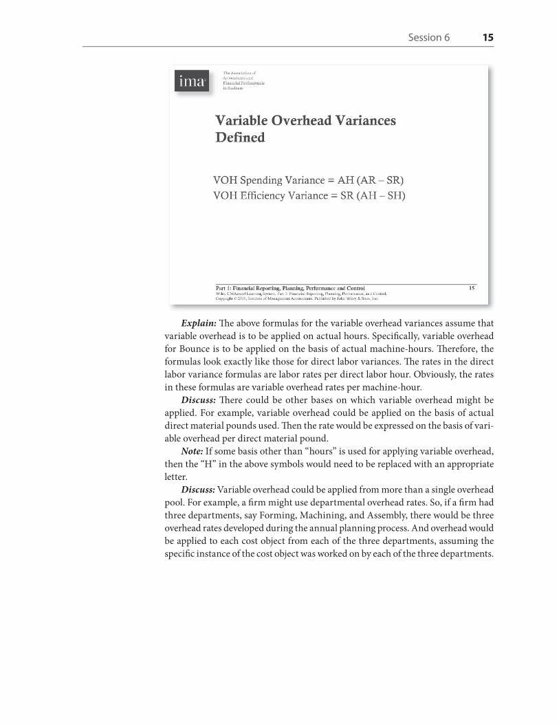
Explain: Th e above formulas for the variable overhead variances assume that variable overhead is to be applied on actual hours. Specifi cally, variable overhead for Bounce is to be applied on the basis of actual machine-hours. Th erefore, the formulas look exactly like those for direct labor variances. Th e rates in the direct labor variance formulas are labor rates per direct labor hour. Obviously, the rates in these formulas are variable overhead rates per machine-hour.

Discuss: Th ere could be other bases on which variable overhead might be applied. For example, variable overhead could be applied on the basis of actual direct material pounds used. Th en the rate would be expressed on the basis of vari-able overhead per direct material pound.

Note: If some basis other than “hours” is used for applying variable overhead, then the “H” in the above symbols would need to be replaced with an appropriate letter.

Discuss: Variable overhead could be applied from more than a single overhead pool. For example, a fi rm might use departmental overhead rates. So, if a fi rm had three departments, say Forming, Machining, and Assembly, there would be three overhead rates developed during the annual planning process. And overhead would be applied to each cost object from each of the three departments, assuming the specifi c instance of the cost object was worked on by each of the three departments.

c01.indd 15 6/3/2015 2:28:27 PM


Note: Remember to call attention to the fact that values that turn out to be nega-tive are favorable variances, given the sign convention.

c01.indd 16 6/3/2015 2:28:28 PM

Session 6 17

Explain: Th ere are many ways to defi ne the production volume variance, all of which should produce the same result.

c01.indd 17 6/3/2015 2:28:28 PM


Explain that we are turning our attention now to the Production Volume Variance. It is important to note that there is no variance as easy as the fi xed over-head variance to calculate. Simply compare the actual fi xed overhead to the budget established during annual planning.

Note: We never did say what the basis for applying fi xed overhead would be. Assume it is also machine-hours. If so, the fi xed overhead rate would be $8.33333 per machine-hour. Th erefore, overhead applied on the basis of machine-hours would be 24,000 units × 1.2 hours per unit × $8.33333 per machine-hour = $240,000.

c01.indd 18 6/3/2015 2:28:28 PM

Session 6 19

Discuss: Th e calculation of the mix variance above shows that the shift from a 60:40 mix to a 50:50 mix cost the fi rm $1,920 in unfavorable sales mix variance. And the loss of 400 units in sales cost an additional $1,680 in unfavorable sales vol-ume variance. A fi rm would only use this form of analysis when units of diff erent products can be meaningfully aggregated.

“Standard” CM is the diff erence between the revenue valued at expected selling price and standard variable manufacturing cost. Th is means that it has not been aff ected by any manufacturing variances. Th us, it is something that Marketing can be expected to control.

Discuss with students that if any product was sold at a price that diff ers from the expected selling price, the dollar amount of that would be measured and it, too, would aff ect the CM.

c01.indd 19 6/3/2015 2:28:28 PM


Th e other way to do it would be to treat the two rubber materials as independent ingredients and calculate material effi ciency variances for each. If one were favor-able and the other unfavorable, then there is some degree of substitution going on.

c01.indd 20 6/3/2015 2:28:29 PM

Session 6 21

Explain that mix and yield variances are the further breakdown of the effi -ciency (or usage) variance. Mix and yield variances are used when a product has two or more ingredients or labor costs that can be substituted for one another. Th ey diff er from the sales mix variance, which measures the mix of various fi nished goods sold by the fi rm.

Review the three calculations:

1. Budgeted Cost per Unit × Actual Total Quantity Used × Actual Mix Ratio2. Budgeted Cost per Unit × Actual Total Quantity Used × Budgeted Mix Ratio3. Budgeted Cost per Unit × Budgeted Total Quantity Used × Budgeted Mix Ratio

Th e mix variance is calculation 1 minus calculation 2. Th e yield variance is calculation 2 minus calculation 3. Each substitutable ingredient or labor cost used would be calculated separately and then summed for each of the three amounts.

Refer participants to the text example using synthetic and natural rubber ingre-dients for more information.

Conclude the discussion of this topic by asking participants if they have any questions on Topic 1: Cost and Variance Measures.

c01.indd 21 6/3/2015 2:28:29 PM


Session 6 Exercise

Refer participants to the Session 6 Exercise in their Participant Guide. Explain that in this exercise, they will compute a complete set of variances.

c01.indd 22 6/3/2015 2:28:29 PM

Session 6 23

Session 6 Exercise: Current Variance

Section C, Topic 1: Cost and Variance MeasuresAunt Molly’s Old Fashioned Cookies bakes cookies for retail stores. The company’s best-selling cookie is chocolate nut supreme, which is marketed as a gourmet cookie and regularly sells for $8.00 per pound. The standard cost per pound of choco-late nut supreme, based on Aunt Molly’s normal monthly production of 400,000 pounds, is shown next.

Cost Item Quantity Standard Unit Cost Total Cost

Direct materials

Cookie mix 10 oz. $0.02 /oz. $0.20

Milk chocolate 5 oz. 0.15 /oz. 0.75

Almonds 1 oz. 0.50 /oz. 0.50

$1.45

Direct labor

Mixing 1 min. $14.40 /hr. $0.24

Baking 2 min. 18.00 /hr. 0.60

$0.84

Variable overhead* 3 min. $32.40 /hr. $1.62

Total standard cost per pound $3.91

*Variable overhead is applied based on total direct labor hours.

Aunt Molly’s management accountant, Karen Blair, prepares monthly budget reports based on these standard costs. Presented next is April’s contribution report that compares budgeted and actual performance.

Contribution Report April Year 1

Budget Actual Variance

Units (in pounds) 400,000 450,000 50,000 F

Revenue $3,200,000 $3,555,000 $355,000 F

Direct material 580,000 865,000 285,000 U

Direct labor 336,000 348,000 12,000 U

Variable overhead 648,000 750,000 102,000 U

Total variable costs 1,564,000 1,963,000 399,000 U

Contribution margin $1,636,000 $1,592,000 $44,000 U

Justine Molly, president of the company, is disappointed with the results. Despite a sizable increase in the number of cookies sold, the product’s expected contribution to the overall profitability of the firm decreased. Molly asked Blair to identify the reasons why the contribution margin decreased. Blair has gathered the next information to help in her analysis of the decrease.

c01.indd 23 6/3/2015 2:28:29 PM


Usage Report April Year 1

Cost Item Quantity Actual Cost

Direct materials

Cookie mix 4,650,000 oz. $ 93,000

Milk chocolate 2,660,000 oz. 532,000

Almonds 480,000 oz. 240,000

Direct labor

Mixing 450,000 min. $ 108,000

Baking 800,000 min. 240,000

Variable overhead 750,000

Total variable costs $1,963,000

Question 1: Prepare an explanation of the $44,000 unfavorable variance between the budgeted and actual contribution margin for the chocolate nut supreme cookie product line during April Year 1 by calculating the next variances. Assume that all materials are used in the month of purchase.

1. Sales price variance2. Material price variance3. Material quantity variance4. Labor efficiency variance5. Variable overhead efficiency variance6. Variable overhead spending variance7. Contribution margin volume variance

c01.indd 24 6/3/2015 2:28:29 PM

Session 6 25

1. Sales price variance =

2. Material price variance =

3. Material quantity variance =

4. Labor efficiency variance =

5. Variable overhead efficiency variance =

c01.indd 25 6/3/2015 2:28:29 PM


6. Variable overhead spending variance =

7. Contribution margin volume variance =

Summary

1. Sales price variance

2. Material price variance

3. Material quantity variance

4. Labor efficiency variance

5. Variable overhead efficiency variance

6. Variable overhead spending variance

7. Contribution margin volume variance

c01.indd 26 6/3/2015 2:28:29 PM

Session 6 27

Question 2a: Explain the problems that might arise in using direct labor hours as the basis for allocating overhead.

Question 2b: How might activity-based costing solve the problems described in Question 2a?

c01.indd 27 6/3/2015 2:28:29 PM


Session 6 Exercise Solution: Current Variance

Question 1: Prepare an explanation of the $44,000 unfavorable variance between the budgeted and actual contribution margin for the chocolate nut supreme cookie product line during April Year 1 by calculating the following variances. Assume that all materials are used in the month of purchase.

1. Sales price variance2. Material price variance3. Material quantity variance4. Labor efficiency variance5. Variable overhead efficiency variance6. Variable overhead spending variance7. Contribution margin volume variance

The $44,000 unfavorable variance between budgeted and actual contribution margin for the chocolate nut supreme cookie product line during April Year 1 is explained by the calculations of the next variances. All materials were used in the month of the purchase.

1. Sales Price Variance = Actual Units × (Actual Price – Budgeted Price)

Actual: Revenue/Units = $3,555,000 = $7.90 /Unit450,000 units

Budgeted: Revenue/Units = $3,200,000

= $8.00/Unit400,000 units

Sales Price Variance = 450,000 Units × ($7.90 – $8.00) = $45,000 U

2. Material Price Variance = Actual Quantity Used × (Standard Price – Actual Price)

Ounces Used

(Standard Price – Actual Price*)

Cookie Mix 4,650,000 × ($0.02 − $0.02) = $ 0

Milk chocolate 2,660,000 × ($0.15 − $0.20) = 133,000 U

Almonds 480,000 × ($0.50 − $0.50) = 0

$133,000 U

* Actual total cost/actual total quantity

c01.indd 28 6/3/2015 2:28:30 PM

Session 6 29

3. Material Quantity Variance = Standard Price × [(Standard Usage per Unit × Actual Units Produced) – Actual Quantity Used]

Standard Price Ounces Used*

Cookie mix 0.02 × [(10 × 450,000 units) – 4,650,000] = $ 3,000 U

Milk chocolate 0.15 × [(5 × 450,000 units) – 2,660,000] = 61,500 U

Almonds 0.50 × [(1 × 450,000 units) – 480,000] = 15,000 U

$79,500 U

* Standard Ounces × Actual Units Produced) – Actual Units Used = Variance

4. Labor Efficiency Variance = Standard Hourly Rate × (Standard Hours – Actual Hours)

Standard Cost Minutes Used*

Mixing ($14.40/hr. 60 minutes) × [(1 min. × 450,000 units) – 450,000 min.] = $ 0

Baking ($18.00/hr. 60 minutes) × [(2 min. × 450,000 units) – 800,000 min.] = 30,000

$30,000 F

* [(Standard Minutes × Actual Units Produced) – Actual Minutes Used] = Variance

5. Variable Overhead Efficiency Variance = Standard Hourly Rate × (Standard Hours – Actual Hours)

$32.40/hr× [(3 min. × 450,000 units) − (450,000 min. + 800,000 min.)]60 min

= $54,000 F

6. Variable Overhead Spending Variance = (Actual Minutes × Standard Overhead Rate) – Actual Variable Overhead

[(450,000 min. + 800,000 min.) ×

(

$32.40/hr.)]− $750,000 = $75,000 U60 min.

7. Contribution Margin Volume Variance = Budgeted Unit Contribution* × (Actual Units – Budgeted Units)

* $1,636,000 Contribution Margin = $4.09400,000 Budgeted Units

$4.09 × (450,000 Units – 400,000 Units) = $204,500 F

c01.indd 29 6/3/2015 2:28:30 PM


Summary

1. Sales price variance $45,000 U

2. Material price variance 133,000 U

3. Material quantity variance 79,500 U

4. Labor effi ciency variance 30,000 F

5. Variable overhead effi ciency variance 54,000 F

6. Variable overhead spending variance 75,000 U

7. Contribution margin volume variance 204,500 F

$44,000 U

Question 2a: Explain the problems that might arise in using direct labor hours as the basis for allocating overhead.

A problem may be that direct labor hours is not an appropriate base for Aunt Molly’s Old Fashioned Cookies because it may not be the activity that drives variable overhead. A good indication of this disconnect is shown in the variance analysis. The labor effi ciency variance is favorable while the variable overhead spending variance is unfavorable. Another problem is that baking requires con-siderably more power than mixing, which could distort product costs.

Activity-based costing (ABC) may solve the problems described in Question 2a and therefore is an alternative that Aunt Molly’s should consider, since direct labor does not seem to have a direct cause-and-eff ect relationship with variable overhead. If the same proportion of these activities is used in all of Aunt Molly’s products, ABC may not be benefi cial; however, if the prod-ucts require a diff erent mix of these activities, ABC would be benefi cial.

Question 2b: How might activity-based costing solve the problems described in Question 2a?

c01.indd 30 6/3/2015 2:28:30 PM

Session 6 31

Session 6 Wrap-Up

Ask participants if they have questions on the material in Session 6.Review the Session 6 content.Remind participants that Session 7 completes Section C with discussions of

Topic 2: Responsibility Centers and Reporting Segments and Topic 3: Performance Measures. Th ey then will review the Practice Questions for Section C.

c01.indd 31 6/3/2015 2:28:30 PM

c01.indd 32 6/3/2015 2:28:30 PM

Session 6 - COPYRIGHTED MATERIAL

Documents

Transcript of Session 6 - COPYRIGHTED MATERIAL