Second-price Auctions with Power-Related

Distributions

Luke Froeb �

Owen Graduate School of Management

Vanderbilt University

Nashville, TN 37203

luke.m.froeb@vanderbilt.edu

Steven Tschantz and Philip Crooke

Department of Mathematics

Vanderbilt University

February 21, 2001

Abstract

We analyze a class of parametric second-price auction models where

asymmetry is modeled by allowing bidders to take di�erent numbers

of draws from the same distribution. We compute the closed-form

distribution of price and construct likelihood and method-of-moments

estimators to recover the underlying value distribution from observed

prices. We derive a Her�ndahl-like formula that predicts merger ef-

fects and �nd that merger e�ects depend on the shares of the merg-

ing bidders, the variance, and the \shape" of the distribution. We

generalize the model by allowing bidders to mix over power-related

distributions. The dominant strategy equilibrium implies that an auc-

tion among bidders who mix over distributions can be expressed as

a mixture of auctions. This implies that an auction among bidders

with potentially correlated values can be expressed as a mixture over

independent power-related auctions.

Keywords: second-price, private-values auctions; merger; antitrust.JEL Classi�cations: D44: Auctions; L41: Horizontal Anticompetitive

Practices. C50: Econometric Modeling;�Corresponding author. We wish to acknowledge useful comments from Bruce Cooil.

Support for this project was provided by the Dean's fund for faculty research.

1 Introduction

A merger, modeled as a bidding coalition, will have a price e�ect in a second-price auction only when the merging parties are the two best bidders. Thefrequency this event, and the magnitude of the resulting price change deter-mine expected price e�ects, which depend critically on the joint distributionof bidder values. Merger evaluation is thus a problem of estimation{howto recover the underlying joint value distribution from available data. Itis then a simple matter to compute merger e�ects or the magnitude of themarginal cost reductions necessary to o�set price e�ects (Tschantz, Crooke,and Froeb [2000]).

This paper is motivated by the problem of recovering bidder value distri-butions from price data in private-values English and second-price auctions.Interest in second-price format is rising with the popularity of Internet auc-tions where use of proxy bidding serves to \Vickrify" an English auction(Lucking-Reiley [2000]), making it resemble the Vickrey [1961] second-price,sealed-bid auction.

Athey and Haile [2000] show that the joint bidder value distribution isnonparametrically identi�ed in independent private values (IPV) second-price auctions with data on either: (i) the highest or lowest values and theidentity of the bidder; or (ii) at least two values and two bidder identities.It is possible that IPV models are also nonparametrically identi�ed withdata on prices (second-highest values) but, even if true, there are reasonsfor using parametric models. The length and quality of some data sets makenonparametric estimation diÆcult, and a parametric approach makes it easyto incorporate other kinds of information into the estimation, like estimatesof the variance or the price-cost margins of bidders.

In this paper, we analyze a class of parametric second-price auctionmodels where asymmetry among bidders is modeled by allowing bidders totake di�erent numbers of \draws" from any base distribution. We derivea closed-form expression for the distribution of price, conditional on theidentity of the winning bidder. One of the implications of bidder asymmetryis a moment restriction on prices and winning probabilities or \shares," i.e.,

bidders drawing from better distributions win more frequently, and at betterprices, than other bidders. This restriction leads to a method-of-momentsestimator constructed by regressing prices on shares.

The methodology is applied to the problem of predicting merger e�ects.Parametric models are likely to be particularly useful for this applicationbecause estimation must be done using available data, and within the time

2

constraints mandated by the merger statutes.1 Power-related auctions giverise to a Her�ndahl-like predictor where merger e�ects depend on the sharesof the merging bidders, the variance, and the "shape" of the distribution,underscoring the importance of structural estimation as an element of mergerpolicy.

Mixing over a base of power-related distributions allows us to generalizethe model in the same way that mixed logit models can approximate moregeneral random utility models (Berry, Levinsohn, and Pakes [1995]; Brown-stone and Train [1999]; McFadden and Train [1999]). The dominant strategyequilibrium of a second-price auction implies that an auction among bidderswho draw from a mixture of power-related distributions is equivalent to amixture of power-related auctions. Estimation and analysis is facilitated bythe closed-form expressions of power-related auctions.

2 A Second-price Auction Model

Following the notation in Tschantz, Crooke, and Froeb [2000], the value ofthe i-th bidder is speci�ed as the sum of two random variables,

Vi = Xi + Y: (2.1)

Xi is the private value of bidder i and Y is a common shock to all bidders'values. The variables (X1; : : : ; Xn; Y ) are mutually independent. We assumethat the common component Y is common knowledge, and simply shiftsobserved bids from auction to auction. In the taxonomy of Athey and Haile[2000], this is a conditionally independent private-values model with withindependent components (CIPV-I).

In Tschantz, Crooke, and Froeb [2000], each Xi is assumed to followa Gumbel distribution with di�erent means, but the same variance. Forthis family of distributions, they derive a closed-form expression for thedistribution of prices. We now generalize their results to the power-relateddistributions considered by Waehrer and Perry [1998].

De�nition 1. The random variables X1 and X2, having cumulative dis-

tribution functions F1 and F2, respectively, are power-related if there is

some positive number s, such that F2(x) = [F1(x)]s = F s

1 (x) for all x.

De�nition 2. A family of power-related distributions generated by

a cumulative distribution function (CDF) F (x) is the set of distributions

fF s(x) : s 2 R+g.1Section 7A Clayton Act, 15 U.S.C. Section 18a.

3

Any distribution in a family of power-related distributions can serve as thebase distribution for the family. For example, the Gumbel distributions usedby Tschantz, Crooke, and Froeb [2000] are from the family of power-relateddistributions:

Fi(x) = ee��(x��i) = F si(x) (2.2)

where F (x) = e�e��x and si = e��i .In a cost auction, where the low bid wins, rather than a value auction

where the high bid wins, two distributions are power-related if F2(x) =1 � (1 � [F1(x)])

s. All of the results and closed-form expressions of thepower-related value auctions extend to power-related cost auctions.

3 Order Statistics for Power-Related Distributions

In this section, the distribution of order statistics for independent draws fromfamilies of power-related distributions are derived. The formulas for orderstatistics drawn from heterogeneous distributions can be found in Section2.8 of David [1981] but unlike David, we compute order statistics condi-

tional on the identity of the winning bidder. By conditioning on the bidders'identities, we are implicitly assuming that researchers have data on auctionparticipants, prices, and the identity of the winner.

3.1 Distribution of the Maximum Value

Families of power-related distributions are useful for modeling second-priceauctions because the family is closed under the maximum function, i:e:,if bidders are making independent draws from distributions in the samepower-related family, then the distribution of the maximum value belongsto the same family. This property facilitates modeling auction equilibria. Inparticular, the maximum function is used to compute winning probabilities(the probability that a bidder will have a value higher than the maximum ofrivals' values) and prices (the maximum of rivals' values), and to computethe e�ects of a merger or bidding coalition (the merged �rm has a valueequal to the maximum of coalition member values).

Let Xi for i = 1; 2; : : : ; n be independent random variables from a familyof power-related distributions. Suppose Xi has the CDF Fi(x) = F si(x) fora positive constant si. We assume that F (x) is di�erentiable and thereforecontinuous. The results below can be extended to discrete distributions butthe analysis is complicated by the possibilities of ties.

4

Lemma 1. If Xmax = maxfX1;X2; : : : ;Xng, then Xmax has CDF F smax(x)where smax =

Pni=1 si.

Proof: Using independence, the CDF of the maximum is

Fmax(x) = Prob(Xmax � x) = Prob(Xi � x; i = 1; 2; : : : ; n)

=

nYi=1

Prob(Xi � x)

=

nYi=1

F si(x)

= (F (x))Pn

i=1 si = F smax(x):

If si is a positive integer, then the F si(x) can be interpreted as the distribu-tion of the maximum of si draws. A strong or high-mean-value bidder is onewhose value is the maximum of a large number of number of draws, and thisincreases the mean of the distribution. For example, taking the maximum ofsi draws from a Gumbel distribution increases the mean by log(si)=�, i.e.,

F si(x) = e�e��(t�(�i+

log si� ))

: (3.1)

Note that the maximum of power-related family of Gumbel variates has thesame variance as the distribution of each variable from which the maximumis computed.

Waehrer and Perry [1998] derive a closed-form expression for the prob-ability that bidder i wins the auction, i:e:, the probability that Xi is themaximum,

pi � Prob(Xi = Xmax) =si

smax:

For power-related Gumbel distributions, winning probabilities have the fa-miliar logit form

pi =e��iPnj=1 e

��j:

In what follows, we will refer to the winning probability as the \share" ofbidder i.

5

3.2 Distribution of the Price

In an open auction, the second-highest value determines the price and, onaverage, di�erent bidders win at di�erent prices. Bidders drawing frommore favorable distributions win more frequently, and at better prices thanthose drawing from less favorable distributions because they are not biddingagainst themselves. In other words, when a high-mean-value bidder wins,the losing bidders are relatively weak by virtue of the fact that the high-mean-value bidder is not among them. Consequently, they are easier tooutbid, on average.

The key to computing the distribution of the second-highest value is thatthe probability that Xi is the maximum value is independent of the valueof the maximum. This independence property permits us to express thedistribution of the second-highest bid as the weighted sum of the distributionof the maximum and the distribution of the maximum of the losing bidders.To prove this, it will suÆce to consider two bidders.

Proposition 1. Suppose X1 and X2 are distributed as F si(x) for i = 1; 2.Then for any x, the probability

Prob(X1 = maxfX1;X2g j maxfX1;X2g � x) =s1

s1 + s2� p1 (3.2)

is a constant that is independent of x. The distribution of X1 given thatX1 is the maximum of X1 and X2 is the same as the distribution of the

maximum, i.e.,

Prob(X1 � x jX1 = maxfX1; X2g) = F s1+s2(x): (3.3)

The distribution of X2 given that X1 is the maximum of X1 and X2 is given

by

Prob(X2 � x jX1 = maxfX1;X2g) =�1

p1

�F s2(x) +

�1� 1

p1

�F s1+s2(x):

(3.4)

Proof: See Appendix.

We introduce some notation for the case of n bidders, drawing randomvalues, X1;X2; : : : ;Xn, as originally speci�ed.

De�nition 3. The symbol, X�i = maxfXj : 1 � j � n; j 6= ig, denotesthe maximium value among the bidders, excluding bidder i.

6

The random variable X�i has CDF F s�i(x), where

s�i =nXj=1

j 6=i

sj:

The distribution of the second-highest value given that Xi = Xmax followsfrom Proposition 1,

FX�ijX�i<Xi(x) =

�1

pi

�F�i(x) + (1� 1

pi)Fmax(x): (3.5)

The symbol X�ijXi > X�i denotes the second-highest value given thatbidder i has the highest value, and thus wins the auction. From the distri-bution of the second-highest value we compute the means and variances ofthe observed bids in terms of the means and variances of the power-relatedvalue distributions. Letting �(s) and �2(s) be the mean and variance of thedistribution with CDF F s(x), we obtain

E(X�i jXi > X�i) =

�1

pi

��(s�i) +

�1� 1

pi

��(smax) (3.6)

Var(X�i jXi > X�i) =

�1

pi

��2(s�i) +

�1� 1

pi

��2(smax)

+1

pi

�1� 1

pi

�(�(smax)� �(s�i))2 : (3.7)

3.3 Joint Distribution of the Three-Highest Values

The same kinds of closed-form expressions can be derived for the joint dis-tribution of the k-highest values. These expressions can be used to computelikelihood functions and moments for losing, as well as winning bids. Inthis section, we compute the joint distribution of the three-highest of the Xi

conditioned on the identities of the highest and second-highest bidders. ItsuÆces to consider just three random variables X1, X2, and X3, taking X1

to be the highest value, X2 to be the second-highest value, and X3 to be thethird-highest value, i.e., the maximum of the other Xi. In the following, lets12 = s1 + s2, s13 = s1 + s3, s23 = s2 + s3, and s123 = s1 + s2 + s3.

Proposition 2. If Xi has CDF F si(x) for i = 1; 2; 3, then

Prob(X1 > X2 > X3) =s1s123

� s2s23

= p1 � p2p2 + p3

(3.8)

7

The joint distribution of X1, X2, and X3, given X1 and X2 are the �rst and

second-highest, respectively, is

Prob(X1 � x1 ^X2 � x2 ^X3 � x3 jX1 > X2 > X3)

=s123s1

� s23s2

��F s1(x1)F

s2(x2)Fs3(x3)� s2

s12� F s12(x2)F

s3(x3)

� s3s23

� F s1(x1)Fs23(x3) +

s2s3s12s123

� F s123(x3)

�

for x3 � x2 � x1. Hence the joint distribution of X2 and X3 given X1 and

X2 are the �rst and second-highest, respectively, is

Prob(X2 � x2 ^X3 � x3 jX1 > X2 > X3)

=s123s1

� s23s2

��F s2(x2)F

s3(x3)� s2s12

� F s12(x2)Fs3(x3)

� s3s23

� F s23(x3) +s2s3

s12s123� F s123(x3)

�:

The distribution of X3 given X1 and X2 are the �rst and second-highest,

respectively, is

Prob(X3 � x jX1 > X2 > X3) =

s123s1

� s23s2

��s1s12

� F s3(x)� s3s23

� F s23(x) +s2s3

s12s123� F s123(x)

�

for x3 � x2.

Proof: See Appendix.

De�nition 4. The symbol, X�ij = maxfXk : 1 � k � n; k 6= i; k 6= jg,denotes the maximum of the bidders' values not including bidders i and j

The random variable X�ij has CDF F s�ij (x), where

s�ij =nX

k=1k 6=i;j

sk:

8

Let sij = si + sj. It follows from Proposition 2 that the expectation of thethird-highest value given Xi > Xj > X�ij is

E(X�ij jX�ij < Xj < Xi) = (3.9)sisij� �(s�ij)� s�ij

s�i� �(s�i) + sjs�ij

sijsmax� �(smax)

sismax

� sjs�j

:

This expression can be used to construct a method-of-moments estimator. Inthe above expression, it is worth noting that the following identities relatingsi, s�i, s�ij and pi, pj hold:

s�isi

=1

pi� 1

sisij

=pi

pi + pjs�ijsij

=1

pi + pj� 1

s�ijs�i

=1� pi � pj1� pi

:

4 Recovering the Value Distribution from Bid Data

In this section, we consider the problem of recovering the bidders' valuedistributions from observed price data. If we adopt the convention that thedistribution of the maximum value, Fmax(x), is the base distribution forthe family, then the individual distribution functions can be expressed asFi(x) = F pi

max(x) where pi = si=smax, and Fmax(x) = [F (x)]smax = F smax(x).The estimation problem is to recover the winning probabilities, pi, and thebase distribution, Fmax(x), from observed bid data.

Without the common unobservable shock, it would be possible to con-struct maximum-likelihood estimators directly from the distributions of Sec-tion 3. With the common shock, the distribution of the price paid by bidderi is a convolution of two distributions, i.e., Bi = (X�ijX�i < Xi) + Y .In our private-values treatment, the variable Y is a nuisance variable thatcomplicates recovery of the power-related distributions of interest.

In what follows, we assume the existence of data on prices and bidderidentities and their distinguishing characteristics across a sample of auctions.

9

We treat each auction as an independent event, but recognize that thisassumption may not be appropriate in the presence of collusion, as in abid-rotation scheme, or with bidder capacity constraints.

4.1 Data on Prices

We develop some two-step method-of-moments estimators to recover thevalue distribution from data on prices. In the �rst step, we estimate thewinning probabilities, and in the second, the distribution of the maximumvalue.

4.1.1 Estimating the Winning Probabilities

In the �rst step, the identity of winning bidders are \predicted" as a functionof observed bidder characteristics using a maximum-likelihood estimator,analogous to a random-utility, discrete-choice model (e:g: Train [1986]). Thelog-likelihood is constructed from the probability of winning across a sampleof T auctions as

L =TXt=1

log(pit): (4.1)

The variable i is taken as a function of t that gives the winning bidderin the t-th auction, i:e:; pit is the probability that the t-th auction is wonby bidder i. The estimated location parameters, p̂it, are the �tted valuesfrom this estimation. For the Gumbel distribution of [2000], Equation 4.1is equivalent to a logit log-likelihood

L =

TXt=1

log(e�itPntk=1 e

�kt)

where �it is the location parameter of i-th bidder's value distribution, de�nedin Equation 3.1. With data on rank-ordered bidder identities, the liklihoodwould include the probabilities of lower-valued bidders, analogous to therank-ordered logit model of Hausman and Ruud [1987].

4.1.2 Recovering Fmax from Prices

Once we have estimated probabilities, a straightforward method-of-momentsapproach is suggested by Equation 3.6. The moment restriction for the pricepaid by bidder i is

10

E(bi) = E(X�ijX�i < Xi) + E(Y ) (4.2)

=

�1

p̂i

��(smax(1� p̂i)) +

�1� 1

p̂i

��(smax) +E(Y )

where s�i = smax(1� p̂i), p̂i is the estimated probability that bidder i winsthe auction, and bi is the observed price, i:e:; the realized value of the ran-dom variable, Bi. A minimum distance estimator can recover the unknownparameters of the base distribution, Fmax(x) = [F (x)]smax from the observedprices. The expected value of the common value component, E(Y ), can alsobe estimated as a function of observable auction characteristics, but un-observed variation in Y may be correlated with the auction participationdecision. If so, this would induce a spurious correlation between the char-acteristics of auction participants and prices.

4.2 Within-auction Estimators

Estimators based solely on prices have diÆculty distinguishing between-auction variation in Y from within-auction variation in Xi . The problemis that an outlying price could mean either that the variance of Xi is largeor that the variance of Y is large. To better distinguish between the twopossibilities requires data on losing bids. In these cases, within-auction esti-mators based on the di�erences between bids permit more precise estimationof Fmax.

4.2.1 Di�erence between the Two-highest Values

In a second-price sealed-bid auction, data on the �rst two values might beobserved. Lower-ranked values are probably less precise for the same rea-son that lower-ranked choices are less precise (Hausman and Ruud [1987]).A method-of-moments estimator can be constructed from the di�erence be-tween the highest and second-highest bids. Note that this is also the surplusor price-cost margin of bidder i which may also be observed.

De�nition 5. The symbol, �i = Xmax � (X�ijX�i < Xi), denotes the

di�erence between the two highest values.

Let Æi be the observed realization of �i. The moment restriction is computedfrom Equation 3.6 as

E(Æi) = 1p̂i(�(smax)� �(smax(1� p̂i))) (4.3)

11

A minimum-distance estimator can be used to recover the parameters ofthe distribution Fmax. This is equivalent to a regression of the Æi on theright-hand-side of Equation 4.3.

In the special case of a Gumbel distribution, the distribution of thedi�erences has a closed form expression that can be used to construct amaximum-likelihood estimator,

F�i(t) = 1��

1

pi + p�ie�t

�: (4.4)

4.2.2 Di�erence Between the Second and Third-highest Values

In government procurement, losing oral bids are sometimes recorded (e:g:Brannman and Froeb [2000]). Depending on the precise bidding mechanism,the di�erence between the second and third-highest bids can be taken asthe di�erence between the second and third-highest values because it is adominant strategy for losing bidders to bid up to their values. In contrast,the di�erence between the two-highest bids is not informative about thevalue distribution because the winner is trying only to outbid the second-highest-value bidder.

We construct a method-of-moments estimator using the di�erence be-tween the second and third-highest bids.

De�nition 6. The symbol, �ij = (X�ijX�i < Xi) � (X�ij jX�i < Xj <Xi), denotes the di�erence between the second and third-highest values in an

auction where the two-highest bidders are i and j respectively.

Let Æij be the observed realization of �ij. The moment restriction iscomputed from Proposition 2 as

E(Æij) =

�pj � 1

pj(pi + pj)

��(smax(1� pi � pj))

��pi + pj(1� pi)� 1

pipj(pi � 1)

��(smax(1� pi))

+

p2i + p2j � pj � 1

pi(pi + pj)

!�(smax):

As above, a method-of-moments estimator of the parameters of the distri-bution Fmax can be constructed from this moment restriction.

12

Again, in the special case of the Gumbel distribution, the di�erencesbetween the second- and third-highest values has a closed-form distributionthat can be used to construct a maximum likelihood estimator,

F�i;j(t) = 1��

pj + p�ijpj + p�ije�t

��pi + pj + p�ij

pi + pj + p�ije�t

�: (4.5)

5 Predictors of Merger E�ects

In this section, we apply the model to the problem of merger prediction.To model merger e�ects, we assume that the value of the merged �rm isthe maximum of its coalition member values. This merger characterizationhas been used by the antitrust enforcement agencies to model the e�ects ofmergers between hospitals, mining equipment companies, defense contrac-tors, and others (Baker [1997]). From Lemma 1, we know that the valuedistribution of the merged �rm is from the same power-related family as itscoalition members. This property means that post-merger expected priceslie on the same price/share moment restriction as the pre-merger expectedprices. Since the share of the merged coalition is the sum of their pre-mergershares, the post-merger expected price can be computed from the momentrestriction. This relationship gives rise a Her�ndahl-like formula.

The expected pro�t to bidder i, since bidder i wins only a fraction pi ofthe auctions is

E(pro�ti) � piE(Xmax �Bi)

= pi

��(smax)�

��1

pi

��(s�i) +

�1� 1

pi

��(smax)

��= �(smax)� �(smax(1� pi)): (5.1)

Hence, a bidder's pro�t is simply a function of pi.

De�nition 7. The expected pro�t to a bidder with winning probability p is

h(p) = �(smax)� �(smax(1� p))

The total expected pro�t to all bidders is

E(pro�t) �nXi=1

E(pro�ti) =nXi=1

h(pi) (5.2)

If bidders i and j with winning probabilities pi and pj merge, then their shareafter the merger is pi + pj. Because the auction is eÆcient, the increase in

13

the expected pro�t to the bidders is equal to the loss in revenue to theauctioneer. This implies that the expected revenue loss of the merger is

�E(pro�t) = h(pi + pj)� h(pi)� h(pj): (5.3)

The curvature in the h function determines the loss of revenue due to amerger.

The merger e�ects are also related to the standard deviation of theXi value components. Suppose F](x) = F ((x � b)=a) is a translated andrescaled version of F (x). Then the family of distributions power-relatedto F](x) results from translating and rescaling the distributions power-related to F (x). De�ning �] and �2] from F], we see that for each s,

�](s) = a�(s) + b, �2] (s) = a2�2(s). Thus taking h] de�ned as in De�-nition 7, we have h](p) = ah(p). One is tempted to argue that a largerstandard deviation in the base distribution leads to bigger merger e�ects,but a larger standard deviation also changes the winning probabilities of themerging bidders. If it makes them smaller, then a larger standard deviationcan reduce the e�ects of a mergers.

6 Families of Power-related Distributions

For the uniform and extreme-value families, both �(s) and �(s) have closed-form expressions.

6.1 Uniform Power-related Distributions

Let

F (x) =

(x�ab�a ; if x 2 [a; b]

0; otherwise

and let F smax(x) be the base distribution for the family. If smax > 1, thenthe base distribution is \pushed" towards the upper bound of the domain.If smax < 1, then the base distribution is pushed towards the lower boundof the domain.

The moments for the family are

�(s) =a+ bs

s+ 1(6.1)

�2(s) =(b� a)2s

(s+ 1)2(s+ 2)(6.2)

14

so that pro�t is given by the function

h(p) =p(b� a)smax

(1 + smax)(1 + (1� p)smax): (6.3)

6.5 7 7.5 8 8.5 9 9.5 10VALUE

DENSITY

1+2, SHARE= 0.8

3, SHARE= 0.2

2, SHARE= 0.3

1, SHARE= 0.5

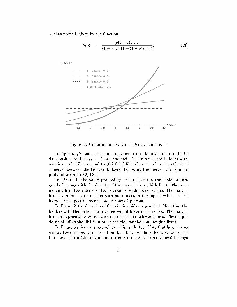
Figure 1: Uniform Family: Value Density Functions

In Figures 1, 2, and 3, the e�ects of a merger on a family of uniform(6; 10)distributions with smax = 5 are graphed. There are three bidders withwinning probabilities equal to (0:2; 0:3; 0:5) and we simulate the e�ects ofa merger between the last two bidders. Following the merger, the winningprobabilities are (0:2; 0:8).

In Figure 1, the value probability densities of the three bidders aregraphed, along with the density of the merged �rm (thick line). The non-merging �rm has a density that is graphed with a dashed line. The merged�rm has a value distribution with more mass in the higher values, whichincreases the post-merger mean by about 7 percent.

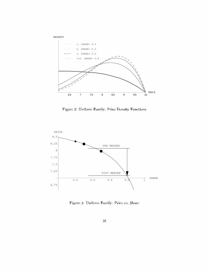
In Figure 2, the densities of the winning bids are graphed. Note that thebidders with the higher-mean values win at lower-mean prices. The merged�rm has a price distribution with more mass in the lower values. The mergerdoes not a�ect the distribution of the bids for the non-merging �rms.

In Figure 3 price vs: share relationship is plotted. Note that larger �rmswin at lower prices as in Equation 3.6. Because the value distribution ofthe merged �rm (the maximum of the two merging �rms' values) belongs

15

6.5 7 7.5 8 8.5 9 9.5 10PRICE

DENSITY

1+2, SHARE= 0.8

3, SHARE= 0.2

2, SHARE= 0.3

1, SHARE= 0.5

Figure 2: Uniform Family: Price Density Functions

0.2 0.4 0.6 0.8 1SHARE

6.75

7.25

7.5

7.75

8

8.25

8.5

PRICE

PRE MERGER

POST MERGER

Figure 3: Uniform Family: Price vs: Share

16

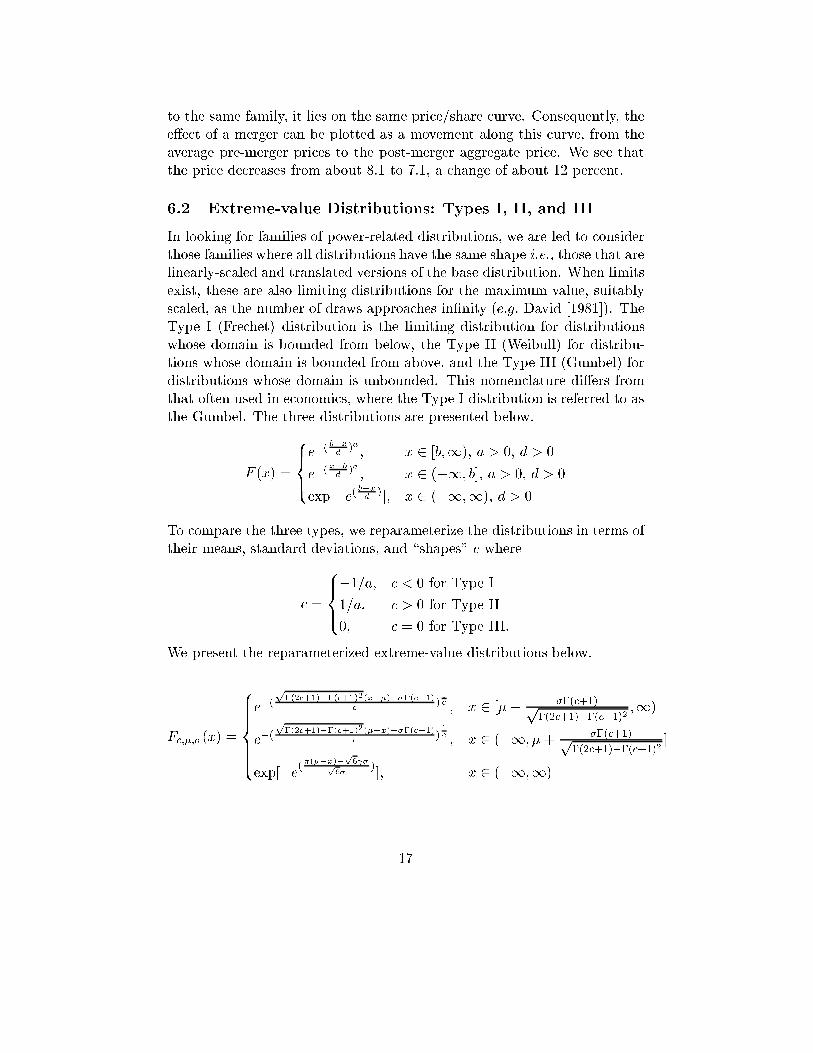
to the same family, it lies on the same price/share curve. Consequently, thee�ect of a merger can be plotted as a movement along this curve, from theaverage pre-merger prices to the post-merger aggregate price. We see thatthe price decreases from about 8:1 to 7:1, a change of about 12 percent.

6.2 Extreme-value Distributions: Types I, II, and III

In looking for families of power-related distributions, we are led to considerthose families where all distributions have the same shape i.e., those that arelinearly-scaled and translated versions of the base distribution. When limitsexist, these are also limiting distributions for the maximum value, suitablyscaled, as the number of draws approaches in�nity (e:g: David [1981]). TheType I (Frechet) distribution is the limiting distribution for distributionswhose domain is bounded from below, the Type II (Weibull) for distribu-tions whose domain is bounded from above, and the Type III (Gumbel) fordistributions whose domain is unbounded. This nomenclature di�ers fromthat often used in economics, where the Type I distribution is referred to asthe Gumbel. The three distributions are presented below.

F (x) =

8><>:e�(

b�xd)a ; x 2 [b;1), a > 0, d > 0

e�(x�bd)a ; x 2 (�1; b], a > 0, d > 0

exp[�e( b�xd )]; x 2 (�1;1), d > 0

To compare the three types, we reparameterize the distributions in terms oftheir means, standard deviations, and \shapes" c where

c =

8><>:�1=a; c < 0 for Type I

1=a; c > 0 for Type II

0; c = 0 for Type III:

We present the reparameterized extreme-value distributions below.

Fc;�;�(x) =

8>>>><>>>>:

e�(p�(2c+1)��(c+1)2(x��)+��(c+1)

c)1c ; x 2 [�� ��(c+1)p

�(2c+1)��(c+1)2 ;1)

e�(p�(2c+1)��(c+1)2(��x)+��(c+1)

c)1c ; x 2 (�1; �+ ��(c+1)p

�(2c+1)��(c+1)2 ]

exp[�e(�(��x)�

p6 �p

6�)]; x 2 (�1;1)

17

This parameterization implies that the likelihood of the so-called \trin-ity" distribution (e:g:; Cooil [1995], Embrechts, Kluppelberg and Mikosch[1999]) is a continuous function of the shape parameter c.

8.5 9 9.5 10 10.5 11 11.5VALUE

DENSITY

Type III

Type II

Type I

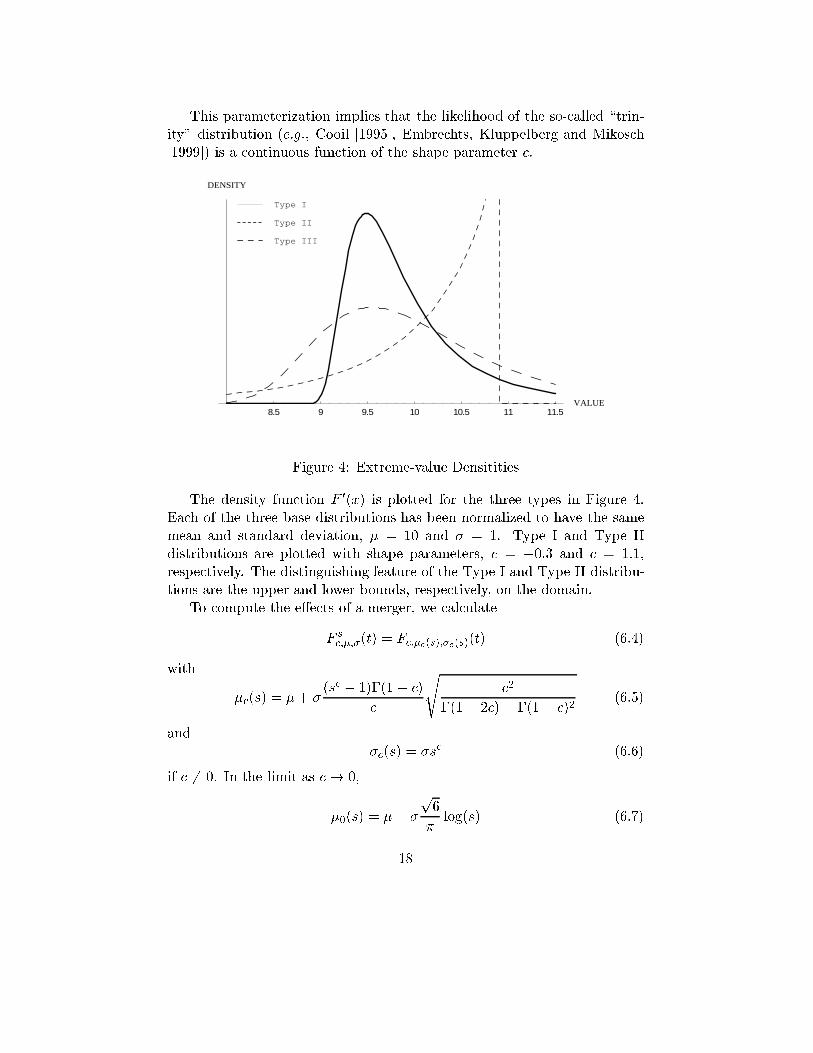
Figure 4: Extreme-value Densitities

The density function F 0(x) is plotted for the three types in Figure 4.Each of the three base distributions has been normalized to have the samemean and standard deviation, � = 10 and � = 1. Type I and Type IIdistributions are plotted with shape parameters, c = �0:3 and c = 1:1,respectively. The distinguishing feature of the Type I and Type II distribu-tions are the upper and lower bounds, respectively, on the domain.

To compute the e�ects of a merger, we calculate

F sc;�;�(t) = Fc;�c(s);�c(s)(t) (6.4)

with

�c(s) = �+ �(sc � 1)�(1 � c)

c

sc2

�(1� 2c)� �(1� c)2(6.5)

and�c(s) = �sc (6.6)

if c 6= 0. In the limit as c! 0,

�0(s) = �+ �

p6

�log(s) (6.7)

18

0.2 0.4 0.6 0.8 1SHARE

5

6

7

8

9

10PRICE

PRE MERGER POST MERGER

Type III

Type II

Type I

Figure 5: Extreme-value Family: Price vs: Share

and �0(s) = �. Then, with smax � 1,

hc(p) = �c(1)� �c(1� p)

= �(1� (1� p)c)�(1� c)

c

sc2

�(1� 2c) � �(1� c)2(6.8)

provided c 6= 0. In the limit as c! 0, we have

h0(p) = ��p6

�log(1� p) (6.9)

which is the formula derived in Tschantz, Crooke and Froeb [2000] for thelogit auction model.

In Figure 5, we plot the e�ects of a merger using the three extreme-value curves considered above and the same three winning probabilities,(0:2; 0:3; 0:5). Again, we consider a merger between the two-largest �rms.The pre and post-merger share/price equilibrium points are denoted withdots for each of the �rms. The merger has its biggest e�ect in the Type Idistribution. The e�ect of the merger is not only to increase the mean ofthe distribution of the merged �rm, but also to increase its variance. Thismeans that when it wins, it is likely to be further away from the second-highest bid, increasing its pro�t. In contrast, the Type II distribution has a

19

very small merger e�ect. Here the e�ect of a merger is to increase the meanand decrease the variance. It is the decrease in variance that gives it a smallmerger e�ect. The Type III distribution, which has a constant variance, hasa merger e�ect that lies in between the other two types.

Note the critical role played by the curvature of the functions in Figure5. For the Type I merger, the price e�ect is only 1:8 percent; for Type II 35:7percent; and for Type III, 4:8 percent. This �nding suggests estimating theshape parameter of the trinity distribution that combines all three extremevalue distributions.

7 Mixtures of Power-related Distributions

The biggest drawback to using power-related distributions is the restrictiveway that joint bidder value distributions are modeled. We would like tobe able to accommodate more general private-value models, including cor-relations across bidder values. This is especially important for the mergerapplication where the most critical question is whether the merging �rmsare \closer" to one another than they are to the other competitors.

Mixtures of power-related distributions can approximate more generalvalue distributions in the same way that mixtures of logit random utilitymodels can approximate more general random utility models (McFaddenand Train [1999]). We de�ne

fi(x) =mXj=1

wijgij(x) (7.1)

to be is the distribution of bidder i's value expressed as a discrete mixtureover mi power-related distributions fgijg with mixing weights fwijg.

A joint IPV model can be approximated as the product of independentdistributions, with each bidder mixing over a set of power-related distribu-tions. Each bidder i takes a draw from one of their mi base distributionsfgijg. Since all base distributions are power-related to one another, the re-sulting auction is among power-related bidders. Let M =

Qni=1mi denote

the number of such auctions.

20

f(x1; x2; : : : ; xn) =

nYi=1

fi(xi)

=

nYi=1

miXj=1

wijgij(xi)

=

m1Xi=1

m2Xj=1

� � �mnXk=1

w1iw2j : : : wnkg1i(x1)g2j(x2) : : : gnk(xn)

=

MXm=1

wmfm(x1; x2; : : : ; xn)

Independence across bidder values implies that wm = w1iw2j : : : wnk orthat the weight given to the joint occurrence of a particular combinationpower-related distributions is proportional to the product of their weightsin Equation 7.1. Correlation among bidder values is induced by choos-ing the mixing weights, fwmg, so that some combinations of power-relateddistributions occur together more frequently than would be implied by in-dependence. For example, two bidders' values are positively correlated ifthey are likely to draw from their high mean-value distributions at the sametime.

The equivalence of a single auction in which bidders mix over distribu-tions to a mixture of auctions facilitates estimation and analysis if the basedistributions are all power-related. The distribution of price is a mixtureof the closed-form price distributions from Section 3, and the e�ect of amerger is a mixture of the merger e�ects from Section 5. The equivalencefollows from the dominant strategy equilibrium of the second-price auction.In a �rst-price sealed-bid auction, bidding functions depend on on the entirejoint value distribution, so the equivalence breaks down (e:g: Bajari [1996]).

21

8 Conclusion

In this paper we have analyzed a parametric class of second-price indepen-dent private-values auction models that have closed-form estimators andmerger predictors. We show how to generalize the class by mixing, andconjecture that these mixed power-related auction models will prove usefulin approximating unknown joint value distributions in the same way thatmixed logit models have proven useful in approximating unknown randomutility models.

A Appendix: Proofs of Propositions

Proposition 1

Suppose X1 and X2 are distributed as F si(x) for i = 1; 2. Then for anyx,

Prob(X1 = maxfX1; X2g j maxfX1;X2g � x) =s1

s1 + s2� p1 (A.1)

is a constant independent of x. The distribution of X1 given that X1 is the

maximum of X1 and X2 is the same as the distribution of the maximum,

i.e.,

Prob(X1 � x jX1 = maxfX1; X2g) = F s1+s2(x) (A.2)

The distribution of X2 given that X1 is the maximum of X1 and X2 is given

by

Prob(X2 � x jX1 = maxfX1;X2g) =�1

p1

�F s2(x) +

�1� 1

p1

�F s1+s2(x)

(A.3)Proof: We �rst de�ne

Æ(s; x;�x) =

(F s(x+�x)�F s(x)F (x+�t)�F (x) � sF s�1(x); F (x+�x)� F (x) 6= 0

0; F (x+�x)� F (x) = 0

We note that lim�x!0 Æ(s; x;�x) = Æ(s; x; 0) = 0 and

F s(x+�x)� F s(x) = [sF s�1(x) + Æ(s; x;�x)][F (x +�x)� F (x)]:

22

We introduce the auxiliary function

g(x) = Prob(X1 = maxfX1;X2g ^maxfX1;X2g < x)

�p1Prob(maxfX1;X2g < x)

where p1 =s1

s1+s2. We shall prove that g(x) � 0. We note that if F (x) > 0

for x 2 (�1;1), then limx!�1 g(x) = 0. If there exists a � such thatF (�) = 0, then limx!� g(x) = 0.

Suppose �x > 0. Then using the de�nition of g(x) and the expressionfor F s(x +�x)� F s(x), we calculate the following string of equalities andinequalities.

jg(x +�x)� g(x)j

= jProb(X2 � X1 ^ x < X1 � x+�x)� p1Prob(x < max(X1; X2) � x+�x)j

= jProb(X2 < x < X1 � x+�x) + Prob(x < X2 � X1 � x+�x)

�p1Prob(X1 < x � X2 � x+�x)� p1Prob(X2 < x < X1 � x+�x)

�p1Prob(x < X1 � X2 � x+�x)� p1Prob(x < X2 � X1 � x+�x)j

= jProb(X2 < x < X1 � x+�x) + Prob(x < X1 � x+�x ^ x < X2 � x+�x)

�Prob(x < X1 � X2 � x+�x)� p1Prob(X2 < x < X1 � x+�x)

�p1Prob(x < X1 � x+�t ^ x < X2 � x+�x)

�p1Prob(X1 < x � X2 � x+�x)j

� jProb(X2 � x < X1 � x+�x)

�p1(Prob(X2 � x < X1 � x+�x) + Prob(X1 � x < X2 � x+�x))j+(1 + p1)Prob(X1 2 [x; x+�x] ^X2 2 [x; x+�x])

= jF s2(x) [F s1(x+�x)� F s1(x)]

�p1 [(F s2(x)(F s1(x+�x)� F s1(x)) + F s1(x)(F s2(x+�x)� F s2(x))] j+(1 + p1)jF s1(x+�x)� F s1(x)j � jF s2(x+�x)� F s2(x)j

23

= jF s2(x)(s1Fs1�1(x) + Æ(s1; x;�x))(F (x +�x)� F (x))

�p1(F s2(x)(s1Fs1�1(x) + Æ(s1; x;�x))(F (x +�x)� F (x))

+F s1(x)(s2Fs2�1(x) + Æ(s2; x;�x))(F (x +�x)� F (x)))j

+(1 + p1)js1F s1�1(x) + Æ(s1; x;�x)j � js2F s2�1(x) + Æ(s2; x;�x)j �jF (x+�x)� F (x)j2

� js1 � p1(s1 + s2)j � jF (x+�x)� F (x)jF s1+s2�1(x)+jÆ(s1; x;�x)j � jF (x+�x)� F (x)jF s2(x)

+p1(jÆ(s1; x;�x)jF s2(x) + jÆ(s2; x;�x)jF s1(x)) � jF (x+�x)� F (x)j+(1 + p1)js1F s1�1(x) + Æ(s1; x;�x)j � js2F s2�1(x) + Æ(s2; x;�x)j �jF (x+�x)� F (x)j2

= jÆ(s1; x;�x)j � F s2(x) � (F (x+�x)� F (x))

+p1(jÆ(s1; x;�x)jF s2(x) + jÆ(s2; x;�x)jF s1(x)) � (F (x+�x)� F (x))

+(1 + p1)js1F s1�1(x) + Æ(s1; x;�x)j � js2F s2�1(x) + Æ(s2; x;�x)j �(F (x+�x)� F (x))2

since s1 � p1(s1 + s2) = 0. This shows that

jg(x+�x)� g(x)j � �(F (x+�x)� F (x))

where � is a function of a single variable such that limz!0�(z) = 0 andin particular, jg(x +�x)� g(x)j � A(F (x +�x)� F (x)) where A is someconstant. A similar type of inequality can be found if �x < 0. This impliesthat for any � > 0 and any x 2 R with F (x) 6= 0, there is a �x > 0 suchthat for � 2 [x��x; x+�x], jg(�)� g(x)j < �jF (�)�F (x)j. We now showthat g(x) must be identically 0 by showing that jg(x)j < � for any positive�.

If F (x) = 0, then g(x) = 0. Suppose g(x) > 0 and let � be an arbitrarypositive number. Choose a number x0, �1 < x0 � x, such that 0 < g(x0) <�=2. Consider a sequence of points x0 < x1 < x2 < : : : < xn = x so that oneach subinterval [xi; xi+1], we have

jg(xi+1)� g(xi)j < �

2(F (xi+1)� F (xi)) :

24

Consider the covering of [x0; x]: f[x2i � �x2i; x2i + �x2i]g. We chose thiscovering so that x2i+1 lies in the overlap between x2i+2 ��x2i+2 and x2i +�x2i. Using the bound jg(xi+1)� g(xi)j < �

2 (F (xi+1)� F (x)), we have

jg(x)j = g(x0) +n�1Xi=0

(g(xi+1) � g(xi))

� jg(x0)j+n�1Xi=0

jg(xi+1)� g(xi)j

<�

2+

n�1Xi=0

�

2(F (xi+1)� F (xi)

� �

2+

�

2(F (x) � F (x0))

� �

2+

�

2= �:

Having shown that

Prob(X1 = maxfX1;X2g ^maxfX1;X2g � t) = p1Prob(maxfX1;X2g � t);

we have

p1 = Prob(X1 = maxfX1; X2g j maxfX1;X2g � x)

=Prob(X1 = maxfX1;X2g ^maxfX1;X2g � x)

Prob(maxfX1;X2g � x):

This proves the �rst part of the propostion.Next consider the conditional probability:

Prob(X1 � x jX1 = maxfX1;X2g)

=Prob(X1 � x ^ X1 = maxfX1; X2g)

Prob(X1 = maxfX1;X2g)

=Prob(X1 = maxfX1; X2g j maxfX1; X2g � x) � Prob(maxfX1;X2g � x)

Prob(X1 = maxfX1;X2g)

=p1Prob(maxfX1;X2) � xg

p1

= F s1+s2(x):

25

The �nal part of the propostion is proved using the following string of iden-tities.

Prob(X2 � x jX1 = maxfX1;X2g)

=Prob(X2 � x ^ X2 � X1)

p1

=Prob(X2 � x < X1) + Prob(X2 � X1 � x)

p1

=Prob(X2 � x)� Prob(X2 � x ^ X1 � x) + Prob(X2 � X1 � x)

p1

=Prob(X2 � x)� Prob(X2 � x ^ X1 � x) + p1Prob(X2 � x ^ X1 � x)

p1

=F s2(x) + (p1 � 1)F s1+s2(x)

p1

=

�1

p1

�F s2(x) +

�1� 1

p1

�F s1+s2(x):

This completes the proof of the proposition.

Proposition 2 If Xi has CDF F si(x) for i = 1; 2; 3, then

Prob(X1 > X2 > X3) =s1s123

� s2s23

= p1 � p2p2 + p3

(A.4)

The joint distribution of X1, X2, and X3, given X1 and X2 are the �rst and

second-highest, respectively, is

Prob(X1 � x1 ^X2 � x2 ^X3 � x3 jX1 > X2 > X3)

=s123s1

� s23s2

��F s1(x1)F

s2(x2)Fs3(x3)� s2

s12� F s12(x2)F

s3(x3)

� s3s23

� F s1(x1)Fs23(x3) +

s2s3s12s123

� F s123(x3)

�

for x3 � x2 � x1. Hence the joint distribution of X2 and X3 given X1 andX2 are the �rst and second-highest, respectively, is

26

Prob(X2 � x2 ^X3 � x3 jX1 > X2 > X3)

=s123s1

� s23s2

��F s2(x2)F

s3(x3)� s2s12

� F s12(x2)Fs3(x3)

� s3s23

� F s23(x3) +s2s3

s12s123� F s123(x3)

�:

The distribution of X3 given X1 and X2 are the �rst and second-highest,

respectively, is

Prob(X3 � x jX1 > X2 > X3) =

s123s1

� s23s2

��s1s12

� F s3(x)� s3s23

� F s23(x) +s2s3

s12s123� F s123(x)

�

for x3 � x2.Proof: Using the previous proposition, we have the following:

Prob(X1 > X2 > X3)

= Prob(X2 > X3)� Prob(X2 > X3 ^X2 � X1)

=s2s23

� s2s123

=s1s2

s123s23

=s1s123

� s2s23

:

This proves the �rst result.Next consider the probability

Prob(X1 � x1 ^ X2 � x2 ^ X3 � x3 ^ X1 > X2 > X3)

= Prob(X1 � x1 ^X2 � minfx1; x2g ^X3 � minfx1; x2; x3g ^X1 > X2 > X3):

27

We restrict ourselves to the case when x3 � x2 � x1. Then

Prob(X1 � x1 ^X2 � x2 ^X3 � x3 ^X1 > X2 > X3)

= Prob(X3 < X2 < X1 � x3) + Prob(X3 < X2 � x3 < X1 � x1)

+Prob(X3 � x3 < X2 < X1 � x2)

+Prob(X3 � x3 < X2 � x2 < X1 � x1)

= Prob(X3 < X2 < X1 � x3) + Prob(X3 < X2 � x3 < X1 � x1)

+Prob(X3 � x3)

�Prob(X2 < X1 � x2)

�Prob(X2 < X1 � x3)� Prob(X2 � x3 < X1 � x2)

�+Prob(X3 � x3 < X2 � x2 < X1 � x1)

=s1s2

s123s23� F s123(x3) +

s2s23

� F s23(x3) [Fs1(x1)� F s1(x3)]

+F s3(x3)

�s1s12

� F s12(x2)

� s1s12

� F s12(x3)� F s2(x3) [Fs1(x2)� F s1(x3)]

�+F s3(x3)(F

s2(x2)� F s2(x3))(Fs1(x1)� F s1(x2))

= F s1(x1)Fs2(x2)F

s3(x3)� s2s12

� F s12(x2)Fs3(x3)

� s3s23

� F s1(x1)Fs23(x3) +

s2s3s12s123

� F s123(x3):

The second formula of the propostion follows from this identity by lettingx1 ! 1. The remaining identities of the proposition follow by lettingx2 !1 and x3 = x. This completes the proof of the proposition.

28

References

[2000] Athey, Susan, and Philip Haile \Identi�cation of Standard AuctionModels," MIT Department of Economics, Working Paper 00-18, (Au-gust, 2000).

[1996] 1996 Bajari, Patrick, \A Structural Econometric Model of the SealedHigh-bid Auction: With Applications to Procurement of HighwayImprovements," working paper, University of Minnesota, (November,1996).

[1997] Baker, Jonathan B., \Unilateral Competitive E�ects Theories inMerger Analysis," Antitrust, 11(2) (Spring, 1997), 21-26.

[1995] Berry, Steve, James Levinson, and Ariel Pakes, \Automobile Pricesin Market Equilibrium," Econometrica, 63 (July 1995), 841{890.

[2000] Brannman, Lance, and Luke Froeb, \Mergers, Cartels, Set-Asides,and Bidding Preferences in Asymmetric Second-Price Auctions," Re-view of Economics and Statistics, 82(2) (2000), pp. 283-290.

[1999] Brownstone, David, and Kenneth Train, \Forecasting New Prod-uct Penetration with Flexible Substitution Patterns," with Journal of

Econometrics, 89(1) (1999), pp. 109-129.

[1995] Cooil, Bruce, \Limiting Multivariate Distributions of IntermediateOrder Statistics," The Annals of Probability, 13(2) (1985), 469-477.

[1981] David, Herbert A, Order Statistics. Second Edition. New York:Wiley, 1981.

[1999] Embrechts, Paul, Claudia Kluppelberg, Thomas Mikosch, Mod-

elling Extremal Events for Insurance and Finance. Second Print-ing. New York: Springer, 1999.

[1987] Hausman, Jerry, and Paul Ruud, \Specifying and Testing Econo-metric Models for Rank-Ordered Data," Journal of Econometrics, 34(1987), 83-104.

[2000] Lucking-Reiley, David, \Auctions on the Internet: What's Be-ing Auctioned, and How?" Journal of Industrial Economics, 48(3)(September 2000), pp. 227-252.

29

[1999] McFadden, Daniel, and Kenneth Train, \Mixed MNL Models forDiscrete Response," Journal of Applied Econometrics, 89(1) (1999),pp. 109-129.

[1986] Train, Kenneth, Qualitative Choice Analysis. Cambridge, Mas-sachusetts: The MIT Press, 1986.

[2000] Tschantz, Steven, Philip Crooke, and Luke Froeb, \Mergers in Sealedvs. Oral Auctions," International Journal of the Economics of Business,7(2) (July, 2000), pp. 201-213.

[1992] U.S. Department of Justice and Federal Trade Commission, Horizon-tal Merger Guidelines, April 2, 1992.

[1961] Vickrey, W, \Counterspeculation, Auctions, and Competitive SealedTenders," Journal of Finance, 16 (1961), 8-37.

[1998] Waehrer, Keith, and Martin K. Perry, \The E�ects of Mergers inOpen Auction Markets," working paper, 1998.

30