arX

iv:g

r-qc

/050

9129

v1

30

Sep

200

5Search for gravitational waves from binary black hole inspirals in LIGO data

B. Abbott,13 R. Abbott,13 R. Adhikari,13 A. Ageev,21, 28 J. Agresti,13 P. Ajith,2 B. Allen,41 J. Allen,14 R. Amin,17

S. B. Anderson,13 W. G. Anderson,30 M. Araya,13 H. Armandula,13 M. Ashley,29 F. Asiri,13, * P. Aufmuth,32 C. Aulbert,1

S. Babak,7 R. Balasubramanian,7 S. Ballmer,14 B. C. Barish,13 C. Barker,15 D. Barker,15 M. Barnes,13,+ B. Barr,36

M. A. Barton,13 K. Bayer,14 R. Beausoleil,27, $ K. Belczynski,24 R. Bennett,36, # S. J. Berukoff,1,† J. Betzwieser,14 B. Bhawal,13

I. A. Bilenko,21 G. Billingsley,13 E. Black,13 K. Blackburn,13 L. Blackburn,14 B. Bland,15 B. Bochner,14,‡ L. Bogue,16

R. Bork,13 S. Bose,43 P. R. Brady,41 V. B. Braginsky,21 J. E. Brau,39 D. A. Brown,13 A. Bullington,27 A. Bunkowski,2,32

A. Buonanno,37 R. Burgess,14 D. Busby,13 W. E. Butler,40 R. L. Byer,27 L. Cadonati,14 G. Cagnoli,36 J. B. Camp,22

J. Cannizzo,22 K. Cannon,41 C. A. Cantley,36 J. Cao,14 L. Cardenas,13 K. Carter,16 M. M. Casey,36 J. Castiglione,35

A. Chandler,13 J. Chapsky,13,+ P. Charlton,13,§ S. Chatterji,13 S. Chelkowski,2, 32 Y. Chen,1 V. Chickarmane,17,¶ D. Chin,38

N. Christensen,8 D. Churches,7 T. Cokelaer,7 C. Colacino,34 R. Coldwell,35 M. Coles,16,‖ D. Cook,15 T. Corbitt,14 D. Coyne,13

J. D. E. Creighton,41 T. D. Creighton,13 D. R. M. Crooks,36 P. Csatorday,14 B. J. Cusack,3 C. Cutler,1 J. Dalrymple,28

E. D’Ambrosio,13 K. Danzmann,32,2 G. Davies,7 E. Daw,17,aD. DeBra,27 T. Delker,35,• V. Dergachev,38 S. Desai,29

R. DeSalvo,13 S. Dhurandhar,12 A. Di Credico,28 M. Diaz,30 H. Ding,13 R. W. P. Drever,4 R. J. Dupuis,13 J. A. Edlund,13,+

P. Ehrens,13 E. J. Elliffe,36 T. Etzel,13 M. Evans,13 T. Evans,16 S. Fairhurst,41 C. Fallnich,32 D. Farnham,13 M. M. Fejer,27

T. Findley,26 M. Fine,13 L. S. Finn,29 K. Y. Franzen,35 A. Freise,2,⋆ R. Frey,39 P. Fritschel,14 V. V. Frolov,16 M. Fyffe,16

K. S. Ganezer,5 J. Garofoli,15 J. A. Giaime,17 A. Gillespie,13,♣ K. Goda,14 L. Goggin,13 G. Gonzalez,17 S. Goßler,32

P. Grandclement,24,♠ A. Grant,36 C. Gray,15 A. M. Gretarsson,10 D. Grimmett,13 H. Grote,2 S. Grunewald,1 M. Guenther,15

E. Gustafson,27, && R. Gustafson,38 W. O. Hamilton,17 M. Hammond,16 C. Hanna,17 J. Hanson,16 C. Hardham,27 J. Harms,20

G. Harry,14 A. Hartunian,13 J. Heefner,13 Y. Hefetz,14 G. Heinzel,2 I. S. Heng,32 M. Hennessy,27 N. Hepler,29 A. Heptonstall,36

M. Heurs,32 M. Hewitson,2 S. Hild,2 N. Hindman,15 P. Hoang,13 J. Hough,36 M. Hrynevych,13, W. Hua,27 M. Ito,39

Y. Itoh,1 A. Ivanov,13 O. Jennrich,36, ** B. Johnson,15 W. W. Johnson,17 W. R. Johnston,30 D. I. Jones,29 G. Jones,7

L. Jones,13 D. Jungwirth,13,++ V. Kalogera,24 E. Katsavounidis,14 K. Kawabe,15 S. Kawamura,23 W. Kells,13 J. Kern,16, $$

A. Khan,16 S. Killbourn,36 C. J. Killow,36 C. Kim,24 C. King,13 P. King,13 S. Klimenko,35 S. Koranda,41 K. Kotter,32

J. Kovalik,16,+ D. Kozak,13 B. Krishnan,1 M. Landry,15 J. Langdale,16 B. Lantz,27 R. Lawrence,14 A. Lazzarini,13 M. Lei,13

I. Leonor,39 K. Libbrecht,13 A. Libson,8 P. Lindquist,13 S. Liu,13 J. Logan,13, ## M. Lormand,16 M. Lubinski,15 H. Luck,32, 2

M. Luna,33 T. T. Lyons,13, ## B. Machenschalk,1 M. MacInnis,14 M. Mageswaran,13 K. Mailand,13 W. Majid,13,+

M. Malec,2, 32 V. Mandic,13 F. Mann,13 A. Marin,14,†† S. Marka,9 E. Maros,13 J. Mason,13,‡‡ K. Mason,14 O. Matherny,15

L. Matone,9 N. Mavalvala,14 R. McCarthy,15 D. E. McClelland,3 M. McHugh,19 J. W. C. McNabb,29 A. Melissinos,40

G. Mendell,15 R. A. Mercer,34 S. Meshkov,13 E. Messaritaki,41 C. Messenger,34 E. Mikhailov,14 S. Mitra,12 V. P. Mitrofanov,21

G. Mitselmakher,35 R. Mittleman,14 O. Miyakawa,13 S. Miyoki,13,§§ S. Mohanty,30 G. Moreno,15 K. Mossavi,2 G. Mueller,35

S. Mukherjee,30 P. Murray,36 E. Myers,42 J. Myers,15 S. Nagano,2 T. Nash,13 R. Nayak,12 G. Newton,36 F. Nocera,13

J. S. Noel,43 P. Nutzman,24 T. Olson,25 B. O’Reilly,16 D. J. Ottaway,14 A. Ottewill,41,¶¶ D. Ouimette,13,++ H. Overmier,16

B. J. Owen,29 Y. Pan,6 M. A. Papa,1 V. Parameshwaraiah,15 C. Parameswariah,16 M. Pedraza,13 S. Penn,11 M. Pitkin,36

M. Plissi,36 R. Prix,1 V. Quetschke,35 F. Raab,15 H. Radkins,15 R. Rahkola,39 M. Rakhmanov,35 S. R. Rao,13 K. Rawlins,14,‖‖

S. Ray-Majumder,41 V. Re,34 D. Redding,13,+ M. W. Regehr,13,+ T. Regimbau,7 S. Reid,36 K. T. Reilly,13 K. Reithmaier,13

D. H. Reitze,35 S. Richman,14,aaR. Riesen,16 K. Riles,38 B. Rivera,15 A. Rizzi,16,•• D. I. Robertson,36 N. A. Robertson,27,36

C. Robinson,7 L. Robison,13 S. Roddy,16 A. Rodriguez,17 J. Rollins,9 J. D. Romano,7 J. Romie,13 H. Rong,35,♣ D. Rose,13

E. Rotthoff,29 S. Rowan,36 A. Rudiger,2 L. Ruet,14 P. Russell,13 K. Ryan,15 I. Salzman,13 V. Sandberg,15 G. H. Sanders,13, ***

V. Sannibale,13 P. Sarin,14 B. Sathyaprakash,7 P. R. Saulson,28 R. Savage,15 A. Sazonov,35 R. Schilling,2 K. Schlaufman,29

V. Schmidt,13,+ + + R. Schnabel,20 R. Schofield,39 B. F. Schutz,1, 7 P. Schwinberg,15 S. M. Scott,3 S. E. Seader,43

A. C. Searle,3 B. Sears,13 S. Seel,13 F. Seifert,20 D. Sellers,16 A. S. Sengupta,12 C. A. Shapiro,29, $$$ P. Shawhan,13

D. H. Shoemaker,14 Q. Z. Shu,35, ## A. Sibley,16 X. Siemens,41 L. Sievers,13,+ D. Sigg,15 A. M. Sintes,1, 33 J. R. Smith,2

M. Smith,14 M. R. Smith,13 P. H. Sneddon,36 R. Spero,13,+ O. Spjeld,16 G. Stapfer,16 D. Steussy,8 K. A. Strain,36

D. Strom,39 A. Stuver,29 T. Summerscales,29 M. C. Sumner,13 M. Sung,17 P. J. Sutton,13 J. Sylvestre,13,†† A. Takamori,13,‡‡

D. B. Tanner,35 H. Tariq,13 M. Tarallo,13 I. Taylor,7 R. Taylor,36 R. Taylor,13 K. A. Thorne,29 K. S. Thorne,6 M. Tibbits,29

S. Tilav,13,§§§ M. Tinto,4,+ K. V. Tokmakov,21 C. Torres,30 C. Torrie,13 G. Traylor,16 W. Tyler,13 D. Ugolini,31 C. Ungarelli,34

M. Vallisneri,6,¶¶¶ M. van Putten,14 S. Vass,13 A. Vecchio,34 J. Veitch,36 C. Vorvick,15 S. P. Vyachanin,21 L. Wallace,13

H. Walther,20 H. Ward,36 R. Ward,13 B. Ware,13,+ K. Watts,16 D. Webber,13 A. Weidner,20, 2 U. Weiland,32 A. Weinstein,13

R. Weiss,14 H. Welling,32 L. Wen,1 S. Wen,17 K. Wette,3 J. T. Whelan,19 S. E. Whitcomb,13 B. F. Whiting,35 S. Wiley,5

C. Wilkinson,15 P. A. Willems,13 P. R. Williams,1,‖‖‖ R. Williams,4 B. Willke,32, 2 A. Wilson,13 B. J. Winjum,29,† W. Winkler,2

S. Wise,35 A. G. Wiseman,41 G. Woan,36 D. Woods,41 R. Wooley,16 J. Worden,15 W. Wu,35 I. Yakushin,16 H. Yamamoto,13

S. Yoshida,26 K. D. Zaleski,29 M. Zanolin,14 I. Zawischa,32,aaaL. Zhang,13 R. Zhu,1 N. Zotov,18 M. Zucker,16 and J. Zweizig13

2

(The LIGO Scientific Collaboration, http://www.ligo.org)1Albert-Einstein-Institut, Max-Planck-Institut fur Gravitationsphysik, D-14476 Golm, Germany

2Albert-Einstein-Institut, Max-Planck-Institut fur Gravitationsphysik, D-30167 Hannover, Germany3Australian National University, Canberra, 0200, Australia

4California Institute of Technology, Pasadena, CA 91125, USA5California State University Dominguez Hills, Carson, CA 90747, USA

6Caltech-CaRT, Pasadena, CA 91125, USA7Cardiff University, Cardiff, CF2 3YB, United Kingdom

8Carleton College, Northfield, MN 55057, USA9Columbia University, New York, NY 10027, USA

10Embry-Riddle Aeronautical University, Prescott, AZ 86301USA11Hobart and William Smith Colleges, Geneva, NY 14456, USA

12Inter-University Centre for Astronomy and Astrophysics, Pune - 411007, India13LIGO - California Institute of Technology, Pasadena, CA 91125, USA

14LIGO - Massachusetts Institute of Technology, Cambridge, MA 02139, USA15LIGO Hanford Observatory, Richland, WA 99352, USA

16LIGO Livingston Observatory, Livingston, LA 70754, USA17Louisiana State University, Baton Rouge, LA 70803, USA

18Louisiana Tech University, Ruston, LA 71272, USA19Loyola University, New Orleans, LA 70118, USA

20Max Planck Institut fur Quantenoptik, D-85748, Garching,Germany21Moscow State University, Moscow, 119992, Russia

22NASA/Goddard Space Flight Center, Greenbelt, MD 20771, USA23National Astronomical Observatory of Japan, Tokyo 181-8588, Japan

24Northwestern University, Evanston, IL 60208, USA25Salish Kootenai College, Pablo, MT 59855, USA

26Southeastern Louisiana University, Hammond, LA 70402, USA27Stanford University, Stanford, CA 94305, USA28Syracuse University, Syracuse, NY 13244, USA

29The Pennsylvania State University, University Park, PA 16802, USA30The University of Texas at Brownsville and Texas Southmost College, Brownsville, TX 78520, USA

31Trinity University, San Antonio, TX 78212, USA32Universitat Hannover, D-30167 Hannover, Germany

33Universitat de les Illes Balears, E-07122 Palma de Mallorca, Spain34University of Birmingham, Birmingham, B15 2TT, United Kingdom

35University of Florida, Gainesville, FL 32611, USA36University of Glasgow, Glasgow, G12 8QQ, United Kingdom

37University of Maryland, College Park, MD 20742 USA38University of Michigan, Ann Arbor, MI 48109, USA

39University of Oregon, Eugene, OR 97403, USA40University of Rochester, Rochester, NY 14627, USA

41University of Wisconsin-Milwaukee, Milwaukee, WI 53201, USA42Vassar College, Poughkeepsie, NY 12604

43Washington State University, Pullman, WA 99164, USA( RCS ; compiled 28 December 2005)

We report on a search for gravitational waves from binary black hole inspirals in the data from the secondscience run of the LIGO interferometers. The search focusedon binary systems with component masses between3 and 20M⊙. Optimally oriented binaries with distances up to 1 Mpc could be detected with efficiency of atleast 90%. We found no events that could be identified as gravitational waves in the 385.6 hours of data that wesearched.

PACS numbers: 95.85.Sz, 04.80.Nn, 07.05.Kf, 97.80.–d

* Currently at Stanford Linear Accelerator Center+ Currently at Jet Propulsion Laboratory$ Permanent Address: HP Laboratories# Currently at Rutherford Appleton Laboratory†Currently at University of California, Los Angeles‡Currently at Hofstra University

§ Currently at Charles Sturt University, Australia¶ Currently at Keck Graduate Institute‖ Currently at National Science FoundationaCurrently at University of Sheffield

•Currently at Ball Aerospace Corporation⋆ Currently at European Gravitational Observatory

3

I. INTRODUCTION

The Laser Interferometric Gravitational Wave Observatory(LIGO) [1] consists of three Fabry-Perot-Michelson interfer-ometers, which are sensitive to the minute changes that wouldbe induced in the relative lengths of their orthogonal arms by apassing gravitational wave. These interferometers are nearingthe end of their commissioning phase and were close to designsensitivity as of March 2005. During the four science runsthat have been completed until now (first (S1) during 2002,second (S2) and third (S3) during 2003 and fourth (S4) dur-ing 2005) all three LIGO interferometers were operated stablyand in coincidence. Although these science runs were per-formed during the commissioning phase they each representthe best broad-band sensitivity to gravitational waves that hadbeen achieved up to that date.

In this paper we report the results of a search for gravi-tational waves from the inspiral phase of stellar mass binaryblack hole (BBH) systems, using the data from the secondscience run of the LIGO interferometers. These BBH sys-tems are expected to emit gravitational waves at frequenciesdetectable by LIGO during the final stages of inspiral (decayof the orbit due to energy radiated as gravitational waves),the merger (rapid infall) and the subsequent ringdown of thequasi-normal modes of the resulting single black hole.

The rate of BBH coalescences in the Universe is highly un-certain. In contrast to searches for gravitational waves fromthe inspiral phase of binary neutron star (BNS) systems [2],it is not possible to set a reliable upper limit on astrophys-ical BBH coalescences. That is because the distribution ofthe sources in space, in the component mass space and in the

♣ Currently at Intel Corp.♠ Currently at University of Tours, France&& Currently at Lightconnect Inc.Currently at W.M. Keck Observatory** Currently at ESA Science and Technology Center++ Currently at Raytheon Corporation$$ Currently at New Mexico Institute of Mining and Technology /MagdalenaRidge Observatory Interferometer## Currently at Mission Research Corporation††Currently at Harvard University‡‡Currently at Lockheed-Martin Corporation§§ Permanent Address: University of Tokyo, Institute for Cosmic Ray Re-search¶¶ Permanent Address: University College Dublin‖‖ Currently at University of Alaska Anchorageaa

Currently at Research Electro-Optics Inc.••Currently at Institute of Advanced Physics, Baton Rouge, LA*** Currently at Thirty Meter Telescope Project at Caltech+ + + Currently at European Commission, DG Research, Brussels, Belgium$$$Currently at University of Chicago## Currently at LightBit Corporation††Permanent Address: IBM Canada Ltd.‡‡Currently at The University of Tokyo§§§ Currently at University of Delaware¶¶¶ Permanent Address: Jet Propulsion Laboratory‖‖‖ Currently at Shanghai Astronomical Observatoryaaa

Currently at Laser Zentrum Hannover

spin angular momentum space is not reliably known. Addi-tionally, the gravitational waveforms for the inspiral phase ofstellar-mass BBH systems which merge in the frequency bandof the LIGO interferometers are not known with precision. Weperform a search that aims at detection of BBH inspirals. Inthe absence of a detection, we use a specific nominal modelfor the BBH population in the Universe and the gravitationalwaveforms given in the literature to calculate an upper limitfor the rate of BBH coalescences.

The rest of the paper is organized as follows. Sec. II pro-vides a short description of the data that was used for thesearch. In Sec. III we discuss the target sources of the searchand we explain the motivation for using a family of phe-nomenological templates to search the data. In Sec. IV wegive a detailed discussion of the templates and the filteringmethods. In Sec. V A we provide information on various dataquality checks that we performed, in Sec. V B we describe indetail the analysis method that we used and in Sec. V C weprovide details on the parameter tuning. In Sec. VI we de-scribe the estimation of the background and in Sec. VII wepresent the results of the search. We finally show the calcula-tion of the rate upper limit on BBH coalescences in Sec. VIIIand we provide a brief summary of the results in Sec. IX.

II. DATA SAMPLE

During the second science run, the three LIGO interferome-ters were operating in science mode (see Sec. V A). The threeinterferometers are based at two observatories. We refer totheobservatory at Livingston, LA, as LLO and the observatory atHanford, WA as LHO. A total of 536 hours of data from theLLO 4 km interferometer (hereafter L1), 1044 hours of datafrom the LHO 4 km (hereafter H1) interferometer, and 822hours of data from the LHO 2 km (hereafter H2) interferom-eter was obtained. The data was subjected to several qualitychecks. In this search, we used only data from times whenthe L1 interferometer was running in coincidence with at leastone of H1 and H2, and we only used continuous data of dura-tion longer than 2048 s (see Sec. V B). After the data qualitycuts, there was a total of 101.7 hours of L1-H1 double coinci-dent data (when both L1 and H1 butnot H2 were operating),33.3 hours of L1-H2 double coincident data (when both L1and H2 butnot H1 were operating) and 250.6 hours of L1-H1-H2 triple coincident data (when all three interferometerswere operating) from the S2 data set, for a total of 385.6 hoursof data.

A fraction (approximately 9%) of this data (chosen to berepresentative of the whole run) was set aside as “playground”data where the various parameters of the analysis could betuned and where vetoes effective in eliminating spurious noiseevents could be identified. The fact that the tuning was per-formed using this subset of data does not exclude the possibil-ity that a detection could be made in this subset. However, toavoid biasing the upper limit, those times were excluded fromthe upper limit calculation.

As with earlier analyses of LIGO data, the output of the an-tisymmetric port of the interferometer was calibrated to obtain

4

a measure of the relative strain∆L/L of the interferometerarms, where∆L = Lx − Ly is the difference in length be-tween thex arm and they arm andL is the average arm length.The calibration was measured by applying known forces to theend mirrors of the interferometers before, after and occasion-ally during the science run. In the frequency band between100 Hz and1500 Hz, the calibration accuracy was within 10%in amplitude and10◦ of phase.

III. TARGET SOURCES

The target sources for the search described in this paperare binary systems that consist of two black holes with com-ponent masses between 3 and 20M⊙, in the last secondsbefore coalescence. Coalescences of binary systems consistof three phases: the inspiral, the merger and the ringdown.We performed the search by matched filtering the data us-ing templates for the inspiral phase of the evolution of thebinaries. The exact duration of the inspiral signal dependsonthe masses of the binary. Given the low-frequency cutoff of100 Hz that needed to be imposed on the data (see Sec. V B)the expected duration of the inspiral signals in the S2 LIGOband as predicted by post-Newtonian calculations varies from0.607 s for a3 − 3 M⊙ binary to 0.013 s for a20 − 20 M⊙

binary.The gravitational wave signal is dominated by the merger

phase which potentially may be computed using numericalsolutions to Einstein’s equations. Searching exclusivelyforthe merger using matched-filter techniques is not appropri-ate until the merger waveforms are known. BBH mergers areusually searched for by using techniques developed for de-tection of unmodeled gravitational wave bursts [3]. However,for reasons that will be explained below, it is possible thatthesearch described in this paper was also sensitive to at leastpart of the merger of the BBH systems of interest. Certainre-summation techniques have been applied to model the latetime evolution of BBH systems which makes it possible toevolve those systems beyond the inspiral and into the mergerphase [4, 5, 6, 7, 8, 9, 10] and the templates that we usedfor matched filtering incorporate the early merger features(inaddition to the inspiral phase) of those waveforms.

The frequencies of the ringdown radiation from BBH sys-tems with component masses between 3 and 20M⊙ rangefrom 295 Hz to 1966 Hz [11, 12, 13] and the gravitationalwave forms are known. Based on the frequencies of these sig-nals, some of the signals are in the S2 LIGO frequency bandof good sensitivity and some are not. At the time of the searchpresented in this paper, the matched-filtering tools necessaryto search for the ringdown phase of BBH were being devel-oped. In future searches we will look for ringdown signalsassociated with inspiral candidates.

Finally, we have verified through simulations that the pres-ence of the merger and the ringdown phases of the gravita-tional wave signal in the data does not degrade our ability todetect the inspiral phase, when we use matched filter tech-niques.

A. Characteristics of BNS and BBH inspirals

We use the standard conventionc = G = 1 in the remainderof this paper.

The standard approach to solving the BBH evolution prob-lem uses the post-Newtonian (PN) expansion [10] of the Ein-stein equations to compute the binding energyE of the binaryand the fluxF of the radiation at infinity, both as series ex-pansions in the invariant velocityv (or the orbital frequency)of the system. This is supplemented with the energy balanceequation (dE/dt = −F ) which in turn gives the evolutionof the orbital phase and hence the gravitational wave phasewhich, to the dominant order, is twice the orbital phase. Thismethod works well when the velocities in the system are muchsmaller compared to the speed of light,v ≪ 1. Moreover, thepost-Newtonian expansion is now complete to orderv7 giv-ing us the dynamics and orbital phasing to a high accuracy[14, 15]. Whether the waveform predicted by the model tosuch high orders in the post-Newtonian expansion is reliablefor use as a matched filter depends on how relativistic the sys-tem is in the LIGO band. For the second science run of LIGO,the interferometers had very good sensitivity between 100 and800 Hz so we calculate how relativistic BNS and BBH sys-tems are at those two frequencies.

The velocity in a binary system of total mass M is relatedto the frequencyf of the gravitational waves by

v = (πMf)1/3. (1)

When a BNS system that consists of two1.4M⊙ compo-nents enters the S2 LIGO band, the velocity in the system isv ≃ 0.16; when it leaves the S2 LIGO band at 800 Hz, it isv ≃ 0.33 and the system is mildly relativistic. Thus, relativis-tic corrections are not too important for the inspiral phaseofBNS.

BBH systems of high mass, however, would be quite rela-tivistic in the S2 LIGO band. For instance, when a10−10M⊙

BBH enters the S2 LIGO band the velocity would bev ≃0.31. At a frequency of 200 Hz (smaller than the frequencyof the innermost stable circular orbit, explained below, whichis 220 Hz according to the test-mass approximation) the ve-locity would bev ≃ 0.40. Such a binary is expected tomerge producing gravitational waves within the LIGO fre-quency band. Therefore LIGO would observe BBH systemsin the most non-linear regime of their evolution and therebywitness highly relativistic phenomena for which the perturba-tive expansion is unreliable.

Numerical relativity is not yet in a position to fully solvethe late time phasing of BBH systems. For this reason, inrecent years, (non-perturbative) analytical resummationtech-niques of the post-Newtonian series have been developed tospeed up its convergence and obtain information on the latestages of the inspiral and the merger [16]. These resummationtechniques have been applied to the post-Newtonian expandedconservative and non-conservative part of the dynamics andare called effective-one-body (EOB) and P-approximants(also referred to as Pade approximants) [4, 5, 6, 7, 8, 9]. Someinsights into the merger problem have been also provided in

5

[17, 18] by combining numerical and perturbative approxima-tion schemes.

The amplitude and the phase of the standard post-Newtonian (TaylorT3, [16]), EOB, and Pade waveforms, eval-uated at different post-Newtonian orders, differ from eachother in the last stages of inspiral, close to the innermost sta-ble circular orbit (ISCO, [16]). The TaylorT3 and Pade wave-forms are derived assuming that the two black holes movealong a quasi-stationary sequence of circular orbits. The EOBwaveforms, extending beyond the ISCO, contain features ofthe merger dynamics. All those model-based waveforms arecharacterized by different ending frequencies. For the quasi-stationary two-body models the ending frequency is deter-mined by the minimum of the energy. For the models thatextend beyond the ISCO, the ending frequency is fixed by thelight-ring [6, 19] of the two-body dynamics.

We could construct matched filters using waveforms fromeach of these families to search for BBH inspirals but yet thetrue gravitational wave signal might be “in between” the mod-els we search for. In order not to miss the true gravitationalwave signal it is desirable to search a space that encompassesall the different families and to also search the space “in be-tween” them.

B. Scope of the search

Recent work by Buonanno, Chen and Vallisneri [19] (here-after BCV) has unified the different approximation schemesinto one family of phenomenological waveforms by introduc-ing two new parameters, one of which is an amplitude cor-rection factor and the other a variable frequency cutoff, inorder to model the different post-Newtonian approximationsand their variations. Additionally, in order to achieve highsignal-matching performance, they introduced unphysicalpa-rameters in the phase evolution of the waveform.

In this work we used a specific implementation of the phe-nomenological templates. As these phenomenological wave-forms are not guaranteed to have a good overlap with thetruegravitational wave signal it is less meaningful to set upperlimits on either the strength of gravitational waves observedduring our search or on the coalescence rate of BBH in theUniverse than it was for the BNS search in the S2 data [2].However, in order to give an interpretation of the result ofour search, we did calculate an upper limit on the coalescencerate of BBH systems, based on two assumptions: (1) that themodel-based waveforms that exist in the literature have goodoverlap with a true gravitational wave signal and (2) that thephenomenological templates used have a good overlap withthe majority of the model-based BBH inspiral waveforms pro-posed in the literature [19].

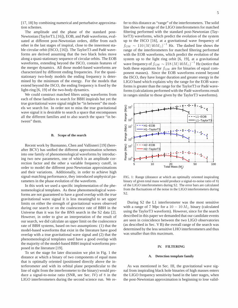
To set the stage for later discussion we plot in Fig. 1 thedistance at which a binary of two components of equal massthat is optimally oriented (positioned directly above the in-terferometer and with its orbital plane perpendicular to theline of sight from the interferometer to the binary) would pro-duce a signal-to-noise ratio (SNR, see Sec. IV) of8 in theLIGO interferometers during the second science run. We re-

fer to this distance as “range” of the interferometers. The solidline shows the range of the LIGO interferometers for matchedfiltering performed with the standard post-Newtonian (Tay-lorT3) waveforms, which predict the evolution of the systemup to the ISCO [16], at a gravitational wave frequency offGW ∼ 110 (M/40M⊙)−1 Hz. The dashed line shows therange of the interferometers for matched filtering performedwith the EOB waveforms, which predict the evolution of thesystem up to the light ring orbit [6, 19], at a gravitationalwave frequency offGW ∼ 218 (M/40M⊙)−1 Hz (notice thatboth these equations forfGW are for binaries of equal com-ponent masses). Since the EOB waveforms extend beyondthe ISCO, they have longer duration and greater energy in theLIGO band which explains why the range for the EOB wave-forms is greater than the range for the TaylorT3 or Pade wave-forms (calculations performed with the Pade waveforms resultin ranges similar to those given by the TaylorT3 waveforms).

10 20 50

100

101

Ran

ge (

Mpc

)

L1−EOBL1−TaylorT3

10 20 50

100

101

Ran

ge (

Mpc

) H1−EOBH1−TaylorT3

5 10 20 50 100

100

101

Total Mass (Mo)

Ran

ge (

Mpc

) H2−EOBH2−TaylorT3

FIG. 1: Range (distance at which an optimally oriented inspiralingbinary of given total mass would produce a signal-to-noise ratio of8)of the LIGO interferometers during S2. The error bars are calculatedfrom the fluctuations of the noise in the LIGO interferometers duringS2.

During S2 the L1 interferometer was the most sensitivewith a range of7 Mpc for a 10 − 10M⊙ binary (calculatedusing the TaylorT3 waveform). However, since for the searchdescribed in this paper we demanded that our candidate eventsare seen in coincidence between the two LIGO observatories(as described in Sec. V B) the overall range of the search wasdetermined by the less sensitive LHO interferometers and thuswas smaller than this maximum.

IV. FILTERING

A. Detection template family

As was mentioned in Sec. III, the gravitational wave sig-nal from inspiraling black hole binaries of high masses entersthe LIGO frequency sensitivity band in the later stages, whenthe post-Newtonian approximation is beginning to lose valid-

6

ity and different versions of the approximation are beginningto substantially differ from each other. In order to detect theseinspiral signals we need to use filters based on phenomeno-logical waveforms (instead of model-based waveforms) thatcover the function space spanned by different versions of thelate-inspiral post-Newtonian approximation.

It must be emphasized at this point that black hole binarieswith small component masses (corresponding to total massup to 10M⊙) enter the S2 LIGO sensitivity band at an earlyenough stage of the inspiral that the signal can be adequatelyapproximated by the stationary phase approximation to thestandard post-Newtonian approximation. For those binariesit is not necessary to use phenomenological templates for thematched filtering; the standard post-Newtonian waveformscan be used as in the search for BNS inspirals. However, us-ing the phenomenological waveforms for those binaries doesnot limit the efficiency of the search [19]. In this search, inor-der to treat all black hole binaries uniformly, we chose to usethe BCV templates with parameters that span the componentmass range from 3 to 20M⊙.

The phenomenological templates introduced in [19] matchvery well most physical waveform models that have been sug-gested in the literature for BBH coalescences. Even thoughthey are not derived by calculations based on a specific phys-ical model they are inspired by the standard post-Newtonianinspiral waveforms. In the frequency domain, they are

h(f) ≡ A(f)eiψ(f), f > 0, (2)

where the amplitudeA(f) is

A(f) ≡ f−7/6(

1 − αf2/3)

θ (fcut − f) (3)

and the phaseψ(f) is

ψ(f) ≡ φ0 + 2πft0 + f−5/3∞∑

n=0

fn/3ψn. (4)

In Eq. (3) θ is the Heaviside step function and in Eq. (4)t0andφ0 are offsets on the time of arrival and on the phase ofthe signal respectively. Also,α, fcut andψn are parametersof the phenomenological waveforms.

Two components can be identified in the amplitude partof the BCV templates. Thef−7/6 term comes from therestricted-Newtonian amplitude in the Stationary Phase Ap-proximation (SPA) [20, 21, 22]. The termαf2/3 × f−7/6 =αf−1/2 is introduced to capture any post-Newtonian ampli-tude corrections and to give high overlaps between the BCVtemplates and the various models that evolve the binary pastthe ISCO frequency. Additionally, in order to obtain highmatches with the various post-Newtonian models that predictdifferent terminating frequencies, a cutoff frequencyfcut isimposed to terminate the waveform.

It has been shown [19] that in order to achieve high matcheswith the various model-derived BBH inspiral waveforms it isin fact sufficient to use only the parametersψ0 andψ3 in thephase expression in Eq. (4), if those two parameters are al-lowed to take unphysical values. Thus, we set all otherψn

coefficients equal to 0 and simplify the phase to

ψ(f) = φ0 + 2πft0 + f−5/3(ψ0 + ψ3f) (5)

≡ φ0 + ψs(f) (6)

where the subscripts stands for “simplified”.For the filtering of the data, a bank of BCV templates was

constructed over the parametersfcut,ψ0 andψ3 (intrinsic tem-plate parameters). For details on how the templates in thebank were chosen see Sec. V B. For each template, the signal-to-noise ratio (defined in Sec. IV B) is maximized over theparameterst0, φ0 andα (extrinsic template parameters).

B. Filtering and signal-to-noise ratio maximization

For a signals, the signal-to-noise ratio (SNR) resultingfrom matched-filtering with a templateh is

ρ(h) =〈s, h〉

√

〈h, h〉, (7)

with the inner product〈s, h〉 being

〈s, h〉 = 2

∫ ∞

−∞

s(f)h∗(f)

Sh(|f |)df = 4ℜ

∫ ∞

0

s(f)h∗(f)

Sh(f)df (8)

andSh(f) being the one-sided noise power spectral density.Various manipulations (given in detail in App. A) give the

expression for the SNR (maximized over the extrinsic parame-tersφ0,α andt0) that was used in this search. That expressionis

ρmaximized = 12

√

|F1|2 + |F2|2 + 2ℑ(F1F ∗2 ) (9)

+ 12

√

|F1|2 + |F2|2 − 2ℑ(F1F ∗2 ).

where

F1 =

∫ fcut

0

4s(f)a1f− 7

6

Sh(f)e−iψs(f)df (10)

F2 =

∫ fcut

0

4s(f)(b1f− 7

6 + b2f− 1

2 )

Sh(f)e−iψs(f)df. (11)

The quantitiesa1, b1 andb2 are dependent on the noise and thecutoff frequencyfcut and are defined in App. A. The originalsuggestion of Buonanno, Chen and Vallisneri was that for theSNR maximization over the parameterα the values of(α ×

f2/3cut ) should be restricted within the range[0, 1], for reasons

that will be explained in Sec. V C 1. However, in order to beable to perform various investigations on the values ofα weleave its value unconstrained in this maximization procedure.More details on this can be found in Sec. V C 1.

7

V. SEARCH FOR EVENTS

A. Data quality and veto study

The matched filtering algorithm is optimal for data witha known calibrated noise spectrum that is Gaussian andstationary over the time scale of the data blocks analyzed(2048 s, described in Section V B), which requires stable,well-characterized interferometer performance. In practice,the performance is influenced by non-stationary optical align-ment, servo control settings, and environmental conditions.We used two strategies to avoid problematic data. The firststrategy was to evaluate data quality over relatively long timeintervals using several different tests. As in the BNS search,time intervals identified as being unsuitable for analysis wereskipped when filtering the data. The second strategy was tolook for signatures in environmental monitoring channels andauxiliary interferometer channels that would indicate an envi-ronmental disturbance or instrumental transient, allowing usto veto any candidate events recorded at that time.

The most promising candidate for a veto channel wasL1:LSC-POBI (hereafter referred to as “POBI”), an auxiliarychannel measuring signals proportional to the length fluctua-tions of the power recycling cavity. This channel was foundto have highly variable noise at70 Hz which coupled into thegravitational wave channel. Transients found in this channelwere used as vetoes for the BNS search in the S2 data [2].Hardware injections of simulated inspiral signals [23] wereused to prove that signals in POBI would not veto true inspi-ral gravitational waves present in the data.

Investigations showed that using the correlations betweenPOBI and the gravitational wave channel to veto candidateevents would be less efficacious than it was in the BNS search.Therefore POBI was not used a an a-priori veto. However, thefact that correlations were proven to exist between the POBIsignals and the BBH inspiral signals made it worthwhile tofollow-up the BBH inspiral events that resulted at the end ofour analysis and check if they were correlated with POBI sig-nals (see Sec. VII B).

As in the BNS search in the S2 data, no instrumental vetoeswere found for H1 and H2. A more extensive discussion ofthe LIGO S2 binary inspiral veto studies can be found in [24].

B. Analysis Pipeline

In order to increase the confidence that a candidate eventcoming out of our analysis is a true gravitational wave and notdue to environmental or instrumental noise we demanded thecandidate event to be present in the L1 interferometer and atleast one of the LHO interferometers. Such an event wouldthen be characterized as a potential inspiral event and be sub-ject to thorough examination.

The analysis pipeline that was used to perform the BNSsearch (and was described in detail in [2]) was the startingstructure for constructing the pipeline used in the BBH inspi-ral search described in this paper. However, due to the dif-ferent nature of the search, the details of some components of

the pipeline needed to be modified. In order to highlight thedifferences of the two pipelines and to explain the reasons forthose, we describe our pipeline below.

First, various data quality cuts were applied on the data andthe segments of good data for each interferometer were inden-tified. The times when each interferometer was in stable op-eration (called science segments) were used to construct threedata sets corresponding to: (1) times when all three interfer-ometers were operating (L1-H1-H2 triple coincident data),(2)times whenonly the L1 and H1 (andnot the H2) interfer-ometers were operating (L1-H1 double coincident data) and(3) times whenonly the L1 and H2 (andnot the H1) interfer-ometers were operating (L1-H2 double coincident data). Theanalysis pipeline produced a list of coincident triggers (timesand template parameters for which the SNR threshold was ex-ceeded and all cuts mentioned below were passed) for each ofthe three data sets.

The science segments were analyzed in blocks of 2048 s us-ing theFINDCHIRP implementation [25] of matched filteringfor inspiral signals in the LIGO Algorithm library [26]. Theoriginal version ofFINDCHIRP had been coded for the BNSsearch and thus had to be modified to allow filtering of thedata with the BCV templates described in Sec. IV.

The data for each 2048 s block was first down-sampledfrom 16384 Hz to 4096 Hz. It was subsequently high-passfiltered at 90 Hz in the time domain and a low frequency cut-off of 100 Hz was imposed in the frequency domain. Theinstrumental response for the block was calculated using theaverage value of the calibration (measured every minute) overthe duration of the block.

The breaking up of each segment for power spectrum es-timation and for matched-filtering was identical to the BNSsearch [2] and is briefly mentioned here so that the terminol-ogy is established for the pipeline description that follows.

Triggers were not searched for within the first and last64 sof a given block, so subsequent blocks were overlapped by128 s to ensure that all of the data in a continuous science seg-ment (except for the first and last 64 s) was searched. Anyscience segments shorter than2048 s were ignored. If a sci-ence segment could not be exactly divided into overlappingblocks (as was usually the case) the remainder of the segmentwas covered by a special2048 s block which overlapped withthe previous block as much as necessary to allow it to reachthe end of the segment. For this final block, a parameter wasset to restrict the inspiral search to the time interval not cov-ered by any previous block, as shown in Fig. 2.

Each block was further split into 15 analysis segments oflength 256 s overlapped at the beginning and at the end by 64s. The average power spectrumSh(f) for the 2048 s of datawas estimated by taking the median of the power spectra ofthe 15 segments. We used the median instead of the mean toavoid biased estimates due to large outliers, produced by non-stationary data. The calibration was applied to the data in eachanalysis segment.

In order to avoid end-effects due to wraparound of the dis-crete Fourier transform when performing the matched filter,the frequency-weighting factor1/Sh(f) was truncated in thetime domain so that its inverse Fourier transform had a max-

8

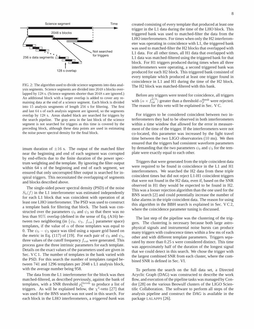
FIG. 2: The algorithm used to divide science segments into data anal-ysis segments. Science segments are divided into2048 s blocks over-lapped by128 s. (Science segments shorter than2048 s are ignored.)An additional block with a larger overlap is added to cover any re-maining data at the end of a science segment. Each block is dividedinto 15 analysis sesgments of length256 s for filtering. The firstand last64 s of each analysis segment are ignored, so the segmentsoverlap by128 s. Areas shaded black are searched for triggers bythe search pipeline. The gray area in the last block of the sciencesegment is not searched for triggers as this time is covered by thepreceding block, although these data points are used in estimatingthe noise power spectral density for the final block.

imum duration of±16 s. The output of the matched filternear the beginning and end of each segment was corruptedby end-effects due to the finite duration of the power spec-trum weighting and the template. By ignoring the filter outputwithin 64 s of the beginning and end of each segment, weensured that only uncorrupted filter output is searched for in-spiral triggers. This necessitated the overlapping of segmentsand blocks described above.

The single-sided power spectral density (PSD) of the noiseSh(f) in the L1 interferometer was estimated independentlyfor each L1 block that was coincident with operation of atleast one LHO interferometer. The PSD was used to constructa template bank for filtering that block. The bank was con-structed over the parametersψ0 andψ3 so that there was noless than95% overlap (defined in the sense of Eq. (A16) be-tween two neighboring (in{ψ0, ψ3, fcut} parameter space)templates, if the value ofα of those templates was equal to0. Theψ0 − ψ3 space was tiled using a square grid based onthe metric in Eq. (117) of [19]. For each pair ofψ0 andψ3,three values of the cutoff frequencyfcut were generated. Thisprocess gave the three intrinsic parameters for each template.Details on the exact values of the parameters used are given inSec. V C 1. The number of templates in the bank varied withthe PSD. For this search the number of templates ranged be-tween 741 and 1296 templates per 2048 s L1 analysis block,with the average number being 958.

The data from the L1 interferometer for the block was thenmatched-filtered, as described previously, against the bank oftemplates, with a SNR thresholdρthresh

L to produce a list oftriggers. As will be explained below, theχ2-veto [27] thatwas used for the BNS search was not used in this search. Foreach block in the LHO interferometers, atriggered bankwas

created consisting of every template that produced at leastonetrigger in the L1 data during the time of the LHO block. Thistriggered bank was used to matched-filter the data from theLHO interferometers. For times when only the H2 interferom-eter was operating in coincidence with L1, the triggered bankwas used to matched-filter the H2 blocks that overlapped withL1 data. For all other times, all H1 data that overlapped withL1 data was matched-filtered using the triggered bank for thatblock. For H1 triggers produced during times when all threeinterferometers were operating, a second triggered bank wasproduced for each H2 block. This triggered bank consisted ofevery template which produced at least one trigger found incoincidence in L1 and H1 during the time of the H2 block.The H2 block was matched-filtered with this bank.

Before any triggers were tested for coincidence, all triggerswith (α× f

2/3cut ) greater than a thresholdαthresh

F were rejected.The reason for this veto will be explained in Sec. V C.

For triggers to be considered coincident between two in-terferometers they had to be observed in both interferometerswithin a time window that allowed for the error in measure-ment of the time of the trigger. If the interferometers were notco-located, this parameter was increased by the light traveltime between the two LIGO observatories (10 ms). We thenensured that the triggers had consistent waveform parametersby demanding that the two parametersψ0 andψ3 for the tem-plate were exactly equal to each other.

Triggers that were generated from the triple coincident datawere required to be found in coincidence in the L1 and H1interferometers. We searched the H2 data from these triplecoincident times but did not reject L1-H1 coincident triggersthat were not found in the H2 data, even if, based on the SNRobserved in H1 they would be expected to be found in H2.This was a looser rejection algorithm than the one used for theBNS search [2] and could potentially increase the number offalse alarms in the triple coincident data. The reason for usingthis algorithm in the BBH search is explained in Sec. V C 2,where the coincidence parameter tuning is discussed.

The last step of the pipeline was the clustering of the trig-gers. The clustering is necessary because both large astro-physical signals and instrumental noise bursts can producemany triggers with coalescence times within a few ms of eachother and with different template parameters. Triggers sepa-rated by more than 0.25 s were considered distinct. This timewas approximately half of the duration of the longest signalthat we could detect in this search. We chose the trigger withthe largest combined SNR from each cluster, where the com-bined SNR is defined in Sec. VI.

To perform the search on the full data set, a DirectedAcyclic Graph (DAG) was constructed to describe the workflow, and execution of the pipeline tasks was managed by Con-dor [28] on the various Beowulf clusters of the LIGO Scien-tific Collaboration. The software to perform all steps of theanalysis pipeline and construct the DAG is available in thepackageLALAPPS [26].

9

C. Parameter Tuning

An important part of the analysis was to decide on the val-ues of the various parameters of the search, such as the SNRthresholds and the coincidence parameters. The parameterswere chosen so as to compromise between increasing the de-tection efficiency and lowering the number of false alarms.

The tuning of all the parameters was done by studying theplayground data only. In order to tune the parameters we per-formed a number of Monte-Carlo simulations, in which weadded simulated BBH inspiral signals in the data and searchedfor them with our pipeline. While we used the phenomenolog-ical detection templates to perform the matched filtering, weused various model-based waveforms for the simulated sig-nals that we added in the data. Specifically, we chose to injecteffective-one-body (EOB, [4, 5, 6, 8]), Pade (PadeT1, [4]) andstandard post-Newtonian waveforms (TaylorT3, [16]), all ofsecond post-Newtonian order. Injecting waveforms from dif-ferent families allowed us to additionally test the efficiency ofthe BCV templates for recovering signals predicted by differ-ent models.

In contrast to neutron stars, there are no observation-basedpredictions about the population of BBH systems in the Uni-verse. For the purpose of tuning the parameters of our pipelinewe decided to draw the signals to be added in the data from apopulation with distances between 10 kpc and 20 Mpc fromthe Earth. The random sky positions and orientations of thebinaries resulted in some signals having much larger effec-tive distances (distance from which the binary would give thesame signal in the data if it were optimally oriented). It wasdetermined that using a uniform-distance or uniform-volumedistribution for the binaries would overpopulate the larger dis-tances (for which the LIGO interferometers were not very sen-sitive during S2) and only give a small number of signals inthe small-distance region, which would be insufficient for theparameter tuning. For that reason we decided to draw the sig-nals from a population that was uniform inlog(distance). Forthe mass distribution, we limited each component mass be-tween 3 and 20M⊙. Populations with uniform distribution oftotal mass were injected for the tuning part of the analysis.

There were two sets of parameters that we could tune inthe pipeline: the single interferometer parameters, whichwereused in the matched filtering to generate inspiral triggers ineach interferometer, and the parameters which were used todetermine if triggers from different interferometers wereco-incident. The single interferometer parameters that needed tobe tuned were the ranges of values forψ0 andψ3 in the tem-plate bank, the number offcut frequencies for each pair of{ψ0, ψ3} in the template bank and the SNR thresholdρthresh.The coincidence parameters were the time coincidence win-dow for triggers from different interferometers,δt, and thecoincidence window for the template parametersψ0 andψ3.Due to the nature of the triggered search pipeline, parametertuning was carried out in two stages. We first tuned the sin-gle interferometer parameters for the primary interferometer(L1). We then used the triggered template banks (generatedfrom the L1 triggers) to explore the single interferometer pa-rameters for the less sensitive LHO interferometers. Finally

the parameters of the coincidence test were tuned.

1. Single interferometer tuning

Based on the playground injection analysis it was de-termined that the range of values forψ0 had to be[10, 550000] Hz5/3 and the range of values forψ3 had to be[−4000, −10] Hz2/3 in order to have high detection efficiencyfor binaries of total mass between 6 and 40M⊙.

Our numerical studies showed that using between 3 and 5cutoff frequencies per{ψ0, ψ3} pair would yield very highdetection efficiency. Consideration of the computational costof the search led us to use 3 cutoff frequencies per pair,thus reducing the number of templates in each bank by 40%compared to a template bank with 5 cutoff frequencies per{ψ0, ψ3} pair.

Our Monte-Carlo simulations showed that, in order to beable to distinguish an inspiral signal from an instrumentalorenvironmental noise event in the data, the minimum require-ment should be that the trigger has SNR of at least7 in eachinterferometer. A threshold of 6 (that was used in the BNSsearch) resulted in a very large number of noise triggers thatneedlessly complicated the data handling and post-pipelineprocessing.

A standard part of the matched-filtering process is theχ2-veto [27]. Theχ2-veto compares the SNR accumulated ineach of a number of frequency bands of equal inspiral tem-plate power to the expected amount in each band. Gravita-tional waves from inspiraling binaries give smallχ2 valueswhile instrumental artifacts give highχ2 values. Thus, thetriggers resulting from instrumental artifacts can be vetoed byrequiring the value ofχ2 for a trigger to be below a threshold.The test is very efficient at distinguishing BNS inspiral sig-nals from loud non-Gaussian noise events in the data and wasused in the BNS inspiral search [2] in the S2 data. However,we found that theχ2-veto was not suitable for the search forgravitational waves from BBH inspirals in the S2 data. Theexpected short duration, low bandwidth and small number ofcycles in the S2 LIGO frequency band for many of the possi-ble BBH inspiral signals made such a test unreliable unless avery high threshold on the values ofχ2 were to be set. A highthreshold, on the other hand, resulted in only a minimal re-duction in the number of noise events picked up. Additionallytheχ2-veto is computationally very costly. We thus decidedto not use it in this search.

As mentioned earlier, the SNR calculated using the BCVtemplates was maximized over the template parameterα. Forevery value ofα, there is a frequencyf0 for which the ampli-tude factor(1 − αf2/3) becomes zero:

f0 = α−3/2. (12)

If the value ofα associated with a trigger is such that the fre-quencyf0 is greater than the cutoff frequencyfcut of the tem-plate (and consequentlyα f2/3

cut ≤ 1), then the high-frequencybehavior of the phenomenological template is as expected foran inspiral gravitational waveform. If the value ofα is such

10

0.4 0.5 0.6 0.7 0.8 0.9 1

0

αF = 0

0.4 0.5 0.6 0.7 0.8 0.9 1

0

αF = 1

0.3 0.4 0.5 0.6 0.7 0.8 0.9 1

0

time (s)

αF = 2

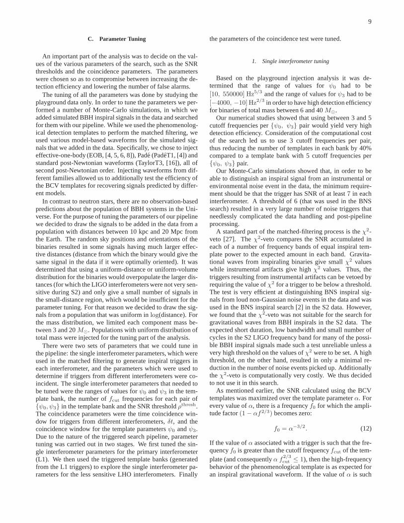
FIG. 3: Time domain plots of BCV waveforms for different valuesof αF . The top plot is forαF = 0, the middle is forαF = 1 and thebottom is forαF = 2. For all three waveformsψ0 = 150000 Hz5/3,ψ3 = −1500 Hz2/3 andfcut = 500 Hz. It can be seen that thebehavior is not that of a typical inspiral waveform forαF = 2.

thatf0 is smaller than the cutoff frequencyfcut (and conse-quentlyα f

2/3cut > 1), the amplitude of the phenomenolog-

ical waveform becomes zero before the cutoff frequency isreached. For such a waveform, the high-frequency behaviordoes not resemble that of a typical inspiral gravitational wave-form. For simplicity we define

αF ≡ αf2/3cut . (13)

The behavior of the BCV waveforms for three different valuesof αF is shown in Fig. 3, where it can be seen that for the caseof αF = 2 the amplitude becomes zero and then increasesagain.

Despite that fact, many of the simulated signals that weadded in the datawerein fact recovered with values ofαF >1, with a higher SNR than the SNR they would have been re-covered with, had we imposed a restriction onα. Additionallysome signals gave SNR smaller than the threshold for all val-ues ofα that gaveαF ≤ 1. Multiple studies showed that thiswas due to the fact that we only had a limited number of cutofffrequencies in our template bank and in many cases the lackof the appropriate ending frequency was compensated for bya value ofα that corresponded to an untypical inspiral gravi-tational waveform.

We performed various investigations which showed that re-jecting triggers withαF > 1 allowed us to still have a veryhigh efficiency in detecting BBH inspiral signals (althoughnot as high as if we did not impose that cut) and the cut pri-marily affected signals that were recovered with SNR close tothe threshold. It was also proven that such a cut reduced thenumber of noise triggers significantly, so that the false-alarmprobability was significantly reduced as well. The result was

that such a cut provided a clearer distinction between the noisetriggers that resulted from our pipeline and the triggers thatcame from simulated signals injected in the data. In order toincrease our confidence in the triggers that came out of thepipeline being BBH inspiral signals, we rejected all triggerswith αF > 1 in this search.

As mentioned in Sec. IV, the initial suggestion of Buo-nanno, Chen and Vallisneri was that the parameterαF be con-strained from below to not take values less than zero. Thissuggestion was based on the fact that for values ofα < 0,the amplitude factor(1 − αf

2/3cut ) can substantially deviate

from the predictions of the post-Newtonian theory at high fre-quencies. Investigations similar to those described for the cutαF ≤ 1 did not justify rejecting the triggers withαF < 0, sowe set no low threshold forαF .

2. Coincidence parameter tuning

After the single interferometer parameters had been se-lected, the coincidence parameters were tuned using the trig-gers from the single interferometers.

The time of arrival of a simulated signal at an interferome-ter could be measured within±10 ms. Since the H1 and H2interferometers are co-located,δt was chosen to be10 ms forH1-H2 coincidence. Since the light-travel time between thetwo LIGO observatories is10 ms,δt was chosen to be20 msfor LHO-LLO coincidence.

Because we performed a triggered search, the data from allthree LIGO interferometers was filtered with the same tem-plates for each 2048 s segment. That led us to set the valuesfor the template coincidence parameters∆ψ0 and∆ψ3 equalto 0. We found that that was sufficient for the simulated BBHinspiral signals to be recovered in coincidence.

The slight misalignment of the L1 interferometer with re-spect to the LHO interferometers led us to choose to not im-pose an amplitude cut in triggers that came from the two dif-ferent observatories. This choice was identical to the choicemade for the BNS search [2].

We considered imposing an amplitude cut on the triggersthat came from triple coincident data and were otherwise co-incident between H1 and H2. A similar cut was imposed onthe equivalent triggers in the BNS search. The cut relied onthe calculation of the “BNS range” for H1 and H2. The BNSrange is defined as the distance at which an optimally orientedneutron star binary, consisting of two components each of 1.4M⊙, would be detected with a SNR of 8 in the data. The valueof the range depends on the PSD. For binary neutron stars thevalue of the range can be calculated for the 1.4-1.4M⊙ binaryand then be rescaled for all masses. That is because the BNSinspiral signals always terminate at frequencies above 733Hz(ISCO frequency for a 3-3M⊙ binary, according to the test-mass approximation) and thus for BNS the larger part of theSNR comes from the high-sensitivity band of LIGO. For blackhole binaries, on the other hand, the ending frequency of theinspiral varies from 110 Hz for a 20-20M⊙ binary up to 733Hz for a 3-3M⊙ binary (according to the test-mass approxi-mation). That means that the range depends not only on the

11

PSD but also on the binary that is used to calculate it. Thatcan make a cut based on the range very unreliable and forcerejection of triggers that should not be rejected. In order tobe sure that we would not miss any BBH inspiral signals, wedecided to not impose the amplitude consistency cut betweenH1 and H2.

VI. BACKGROUND ESTIMATION

We estimated the rate of accidental coincidences (alsoknown as background rate) for this search by introducingan artificial time shift∆t to the triggers coming from theL1 interferometer relative to the LHO interferometers. Thetime-shift triggers were fed into the coincidence steps of thepipeline and, for the triple coincident data, to the step of thefiltering of the H2 data and the H1-H2 coincidence. By choos-ing a shift larger than 20 ms (the time coincidence windowbetween the two observatories), we ensured that a true gravi-tational wave could never produce coincident triggers in thetime-shifted data streams. To avoid correlations, we usedshifts longer than the duration of the longest waveform thatwe could detect (0.607 s given the low-frequency cutoff im-posed, as explained in Sec. III). We chose to not time-shift thedata from the two LHO interferometers relative to one anothersince there could be true correlations producing accidental co-incidence triggers due to environmental disturbances affectingboth of them. The resulting time-shift triggers correspondedonly to accidental coincidences of noise triggers. For a giventime shift, the triggers that emerged from the pipeline wereconsidered as one single trial representation of an output froma search if no signals were present in the data.

A total of 80 time-shifts were performed and analyzed inorder to estimate the background. The time shifts ranged from∆t = −407 s up to∆t = +407 s in increments of10 s. Thetime shifts of±7s were not performed.

A. Distribution of background events

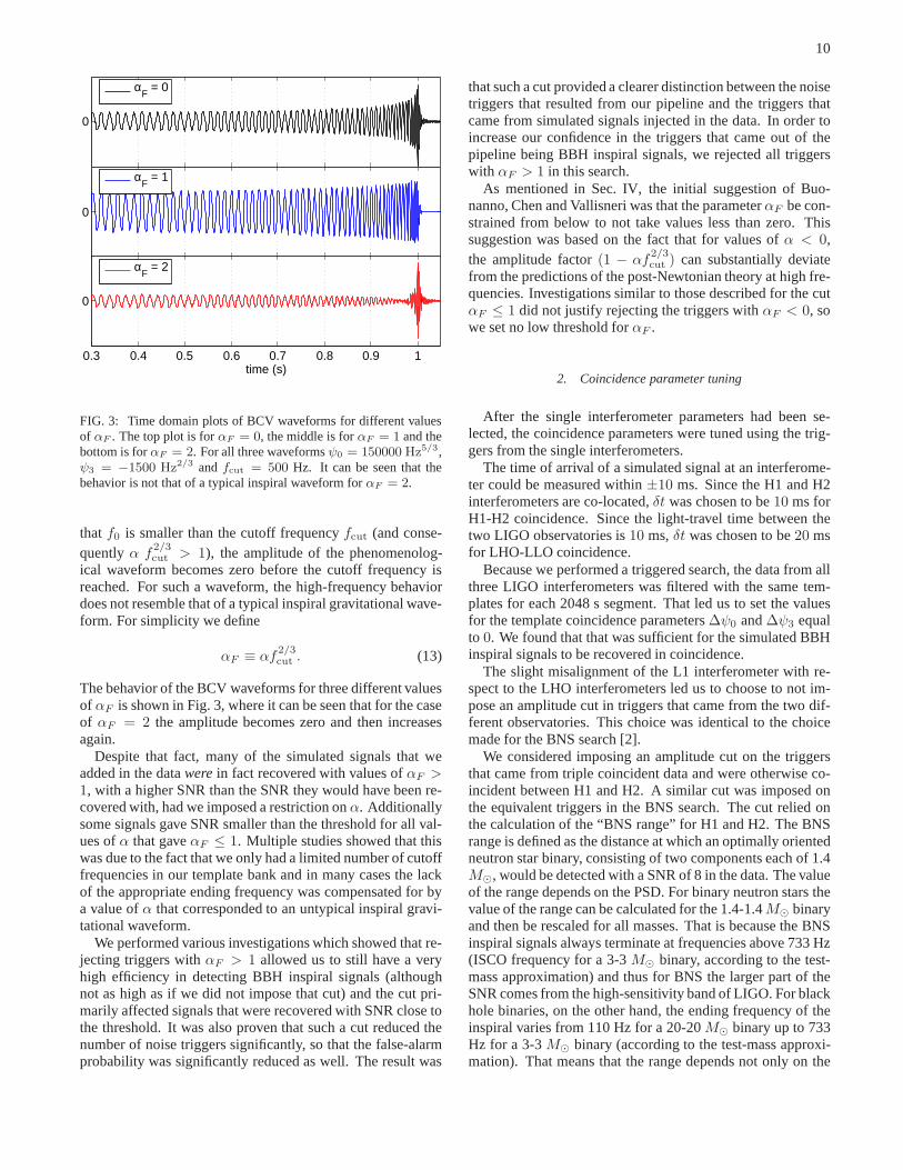
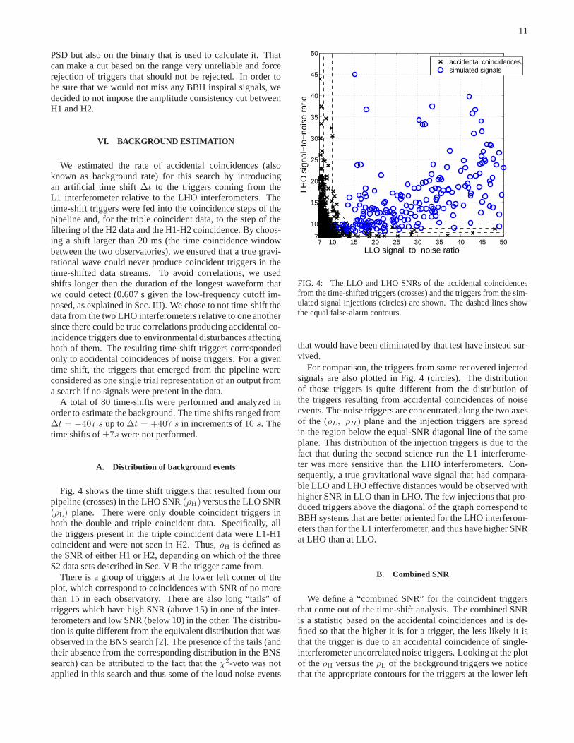
Fig. 4 shows the time shift triggers that resulted from ourpipeline (crosses) in the LHO SNR(ρH) versus the LLO SNR(ρL) plane. There were only double coincident triggers inboth the double and triple coincident data. Specifically, allthe triggers present in the triple coincident data were L1-H1coincident and were not seen in H2. Thus,ρH is defined asthe SNR of either H1 or H2, depending on which of the threeS2 data sets described in Sec. V B the trigger came from.

There is a group of triggers at the lower left corner of theplot, which correspond to coincidences with SNR of no morethan15 in each observatory. There are also long “tails” oftriggers which have high SNR (above 15) in one of the inter-ferometers and low SNR (below 10) in the other. The distribu-tion is quite different from the equivalent distribution that wasobserved in the BNS search [2]. The presence of the tails (andtheir absence from the corresponding distribution in the BNSsearch) can be attributed to the fact that theχ2-veto was notapplied in this search and thus some of the loud noise events

7 10 15 20 25 30 35 40 45 507

10

15

20

25

30

35

40

45

50

LLO signal−to−noise ratio

LHO

sig

nal−

to−

nois

e ra

tio

accidental coincidencessimulated signals

FIG. 4: The LLO and LHO SNRs of the accidental coincidencesfrom the time-shifted triggers (crosses) and the triggers from the sim-ulated signal injections (circles) are shown. The dashed lines showthe equal false-alarm contours.

that would have been eliminated by that test have instead sur-vived.

For comparison, the triggers from some recovered injectedsignals are also plotted in Fig. 4 (circles). The distributionof those triggers is quite different from the distribution ofthe triggers resulting from accidental coincidences of noiseevents. The noise triggers are concentrated along the two axesof the (ρL, ρH ) plane and the injection triggers are spreadin the region below the equal-SNR diagonal line of the sameplane. This distribution of the injection triggers is due tothefact that during the second science run the L1 interferome-ter was more sensitive than the LHO interferometers. Con-sequently, a true gravitational wave signal that had compara-ble LLO and LHO effective distances would be observed withhigher SNR in LLO than in LHO. The few injections that pro-duced triggers above the diagonal of the graph correspond toBBH systems that are better oriented for the LHO interferom-eters than for the L1 interferometer, and thus have higher SNRat LHO than at LLO.

B. Combined SNR

We define a “combined SNR” for the coincident triggersthat come out of the time-shift analysis. The combined SNRis a statistic based on the accidental coincidences and is de-fined so that the higher it is for a trigger, the less likely it isthat the trigger is due to an accidental coincidence of single-interferometer uncorrelated noise triggers. Looking at the plotof theρH versus theρL of the background triggers we noticethat the appropriate contours for the triggers at the lower left

12

corner of the plot are concentric circles with the center at theorigin. However, for the tails along the axes the appropriatecontours are “L” shaped. The combination of those two kindsof contours gives the contours plotted with dashed lines inFig. 4. Based on these contours, we define the combined SNRof a trigger to be

ρC = min{√

ρ2L + ρ2

H, 2ρH − 3, 2ρL − 3}. (14)

After the combined SNR is assigned to each pair of triggers,the triggers are clustered by keeping the one with the high-est combined SNR within 0.25 s, thus keeping the “highestconfidence” trigger for each event.

VII. RESULTS

In this section we present the results of the search in theS2 data with the pipeline described in Sec. V B. The com-bined SNR was assigned to the candidate events according toEq. (14).

A. Comparison of the unshifted triggers to the background

There were 25 distinct candidate events that survived all theanalysis cuts. Of those, 7 were in the L1-H1 double coincidentdata, 10 were in the L1-H2 double coincident data and 8 werein the L1-H1-H2 triple coincident data. Those 8 events ap-peared only in the L1 and H1 data streams and even thoughthey were not seen in H2 they were still kept, according to theprocedure described in Sec. V B.

90 130 170 210 250 290 330−3

−2

−1

0

1

2

log 10

(# o

f eve

nts)

with

ρC2 >

ρ2 , p

er s

2

ρ2

accidental coincidencess2 result

FIG. 5: Expected accidental coincidences per S2 (triangles) withone standard deviation bars. The number of events in the S2 (circles)is overlayed.

In order to determine if there was an excess of candidateevents above the background in the S2 data, we compared the

number of zero-shift events to the expected number of acci-dental coincidences in S2, as predicted by the time-shift anal-ysis described in Sec. VI. Fig. 5 shows the mean cumula-tive number of accidental coincidences (triangles) versusthecombined SNR squared of those accidental coincidences. Thebars indicate one standard deviation. The cumulative numberof candidate events in the zero-shift S2 data is overlayed (cir-cles). It is clear that the candidate events are consistent withthe background.

B. Investigations of the zero-shift candidate events

Even though the zero-shift candidate events are consistentwith the background, we investigated them carefully. We firstlooked at the possibility of those candidate events being cor-related with events in the POBI channel, for the reasons de-scribed in Sec. V A.

It was determined that the loudest candidate event and threeof the remaining candidate events that resulted from our anal-ysis were coincident with noise transients in POBI. That ledus to believe that the source of these candidate events was in-strumental and that they were not due to gravitational waves.The rest of the candidate events were indistinguishable fromthe background events.

C. Results of the Monte-Carlo simulations

As mentioned in Sec. V B, the Monte-Carlo simulations al-low us not only to tune the parameters of the pipeline, but alsoto measure the efficiency of our search method. In this sectionwe look in detail at the results of Monte-Carlo simulations inthe full data set of the second science run.

Due to the lack of observation-based predictions for thepopulation of BBH systems in the Universe, the inspi-ral signals that we injected were uniformly distributed inlog(distance), with distance varying from 10 kpc to 20 Mpcand uniformly distributed in component mass (this mass dis-tribution was proposed by [29]), with each component massvarying between 3 and 20M⊙.

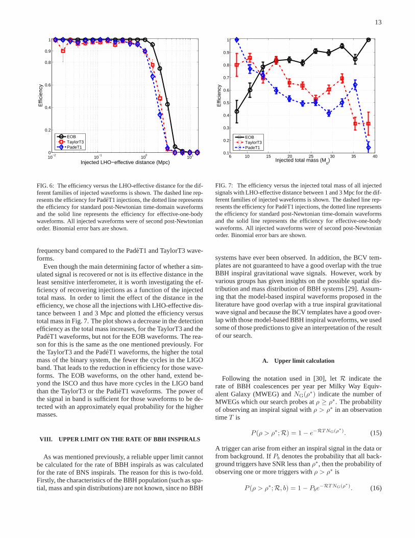
Fig. 6 shows the efficiency of recovering the injected sig-nals (number of found injections of a given effective distancedivided by the total number of injections of that effective dis-tance) versus the injected LHO-effective distance. We choseto plot the efficiency versus the LHO-effective distance ratherthan versus the LLO-effective distance since H1 and H2 wereless sensitive than L1 during S2.

Our analysis method had efficiency of at least90% for re-covering BBH inspiral signals with LHO-effective distanceless than 1 Mpc for the mass range we were exploring. Itshould be noted how the efficiency of our pipeline varied fordifferent injected waveforms. It is clear from Fig. 6 that theefficiency for recovering EOB waveforms was higher than thatfor TaylorT3 or PadeT1 waveforms for all distances. Thisis expected because the EOB waveforms have more power(longer duration and larger number of cycles) in the LIGO

13

10−2

10−1

100

101

0

0.2

0.4

0.6

0.8

0.9

1

Injected LHO−effective distance (Mpc)

Effi

cien

cy

EOBTaylorT3PadeT1

FIG. 6: The efficiency versus the LHO-effective distance forthe dif-ferent families of injected waveforms is shown. The dashed line rep-resents the efficiency for PadeT1 injections, the dotted line representsthe efficiency for standard post-Newtonian time-domain waveformsand the solid line represents the efficiency for effective-one-bodywaveforms. All injected waveforms were of second post-Newtonianorder. Binomial error bars are shown.

frequency band compared to the PadeT1 and TaylorT3 wave-forms.

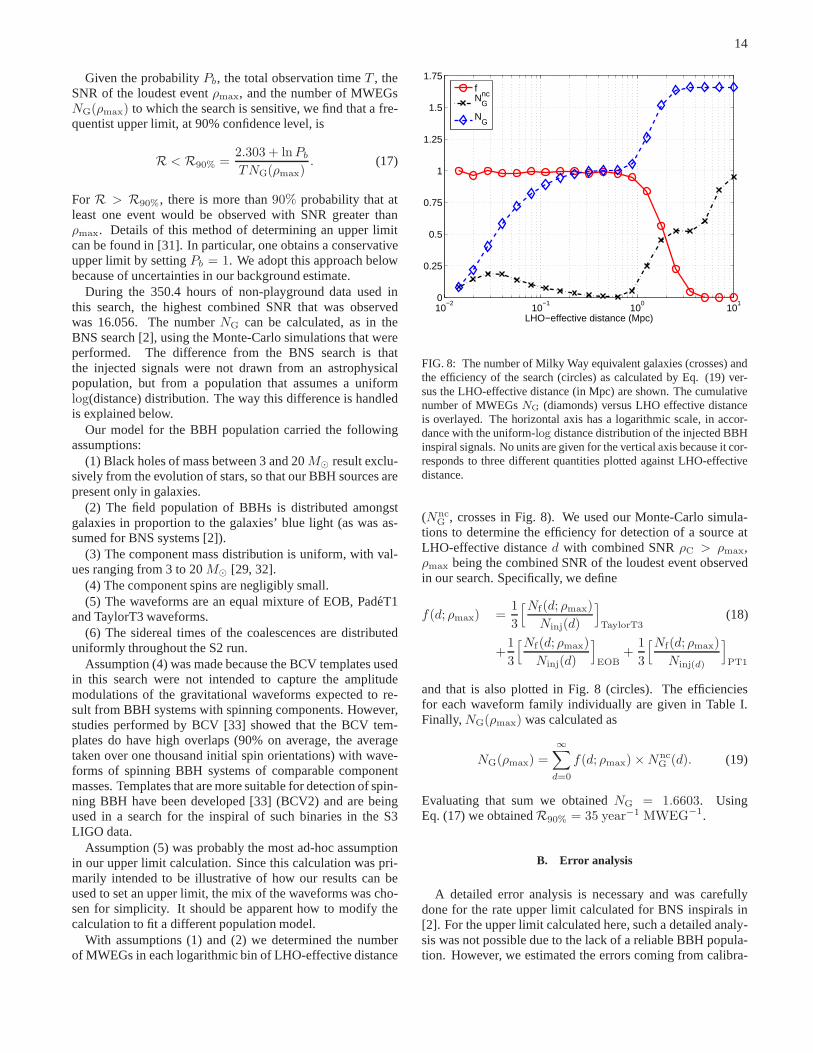
Even though the main determining factor of whether a sim-ulated signal is recovered or not is its effective distance in theleast sensitive interferometer, it is worth investigatingthe ef-ficiency of recovering injections as a function of the injectedtotal mass. In order to limit the effect of the distance in theefficiency, we chose all the injections with LHO-effective dis-tance between 1 and 3 Mpc and plotted the efficiency versustotal mass in Fig. 7. The plot shows a decrease in the detectionefficiency as the total mass increases, for the TaylorT3 and thePadeT1 waveforms, but not for the EOB waveforms. The rea-son for this is the same as the one mentioned previously. Forthe TaylorT3 and the PadeT1 waveforms, the higher the totalmass of the binary system, the fewer the cycles in the LIGOband. That leads to the reduction in efficiency for those wave-forms. The EOB waveforms, on the other hand, extend be-yond the ISCO and thus have more cycles in the LIGO bandthan the TaylorT3 or the PadieT1 waveforms. The power ofthe signal in band is sufficient for those waveforms to be de-tected with an approximately equal probability for the highermasses.

VIII. UPPER LIMIT ON THE RATE OF BBH INSPIRALS

As was mentioned previously, a reliable upper limit cannotbe calculated for the rate of BBH inspirals as was calculatedfor the rate of BNS inspirals. The reason for this is two-fold.Firstly, the characteristics of the BBH population (such asspa-tial, mass and spin distributions) are not known, since no BBH

6 10 15 20 25 30 35 400.1

0.2

0.3

0.4

0.5

0.6

0.7

0.8

0.9

1

Injected total mass (Mo)

Effi

cien

cy

EOBTaylorT3PadeT1

FIG. 7: The efficiency versus the injected total mass of all injectedsignals with LHO-effective distance between 1 and 3 Mpc for the dif-ferent families of injected waveforms is shown. The dashed line rep-resents the efficiency for PadeT1 injections, the dotted line representsthe efficiency for standard post-Newtonian time-domain waveformsand the solid line represents the efficiency for effective-one-bodywaveforms. All injected waveforms were of second post-Newtonianorder. Binomial error bars are shown.

systems have ever been observed. In addition, the BCV tem-plates are not guaranteed to have a good overlap with the trueBBH inspiral gravitational wave signals. However, work byvarious groups has given insights on the possible spatial dis-tribution and mass distribution of BBH systems [29]. Assum-ing that the model-based inspiral waveforms proposed in theliterature have good overlap with a true inspiral gravitationalwave signal and because the BCV templates have a good over-lap with those model-based BBH inspiral waveforms, we usedsome of those predictions to give an interpretation of the resultof our search.

A. Upper limit calculation

Following the notation used in [30], letR indicate therate of BBH coalescences per year per Milky Way Equiv-alent Galaxy (MWEG) andNG(ρ∗) indicate the number ofMWEGs which our search probes atρ ≥ ρ∗. The probabilityof observing an inspiral signal withρ > ρ∗ in an observationtimeT is

P (ρ > ρ∗;R) = 1 − e−RTNG(ρ∗). (15)

A trigger can arise from either an inspiral signal in the dataorfrom background. IfPb denotes the probability that all back-ground triggers have SNR less thanρ∗, then the probability ofobserving one or more triggers withρ > ρ∗ is

P (ρ > ρ∗;R, b) = 1 − Pbe−RTNG(ρ∗). (16)

14

Given the probabilityPb, the total observation timeT , theSNR of the loudest eventρmax, and the number of MWEGsNG(ρmax) to which the search is sensitive, we find that a fre-quentist upper limit, at 90% confidence level, is

R < R90% =2.303 + lnPbTNG(ρmax)

. (17)

For R > R90%, there is more than90% probability that atleast one event would be observed with SNR greater thanρmax. Details of this method of determining an upper limitcan be found in [31]. In particular, one obtains a conservativeupper limit by settingPb = 1. We adopt this approach belowbecause of uncertainties in our background estimate.

During the 350.4 hours of non-playground data used inthis search, the highest combined SNR that was observedwas 16.056. The numberNG can be calculated, as in theBNS search [2], using the Monte-Carlo simulations that wereperformed. The difference from the BNS search is thatthe injected signals were not drawn from an astrophysicalpopulation, but from a population that assumes a uniformlog(distance) distribution. The way this difference is handledis explained below.

Our model for the BBH population carried the followingassumptions:

(1) Black holes of mass between 3 and 20M⊙ result exclu-sively from the evolution of stars, so that our BBH sources arepresent only in galaxies.

(2) The field population of BBHs is distributed amongstgalaxies in proportion to the galaxies’ blue light (as was as-sumed for BNS systems [2]).

(3) The component mass distribution is uniform, with val-ues ranging from 3 to 20M⊙ [29, 32].

(4) The component spins are negligibly small.(5) The waveforms are an equal mixture of EOB, PadeT1

and TaylorT3 waveforms.(6) The sidereal times of the coalescences are distributed

uniformly throughout the S2 run.Assumption (4) was made because the BCV templates used

in this search were not intended to capture the amplitudemodulations of the gravitational waveforms expected to re-sult from BBH systems with spinning components. However,studies performed by BCV [33] showed that the BCV tem-plates do have high overlaps (90% on average, the averagetaken over one thousand initial spin orientations) with wave-forms of spinning BBH systems of comparable componentmasses. Templates that are more suitable for detection of spin-ning BBH have been developed [33] (BCV2) and are beingused in a search for the inspiral of such binaries in the S3LIGO data.

Assumption (5) was probably the most ad-hoc assumptionin our upper limit calculation. Since this calculation was pri-marily intended to be illustrative of how our results can beused to set an upper limit, the mix of the waveforms was cho-sen for simplicity. It should be apparent how to modify thecalculation to fit a different population model.

With assumptions (1) and (2) we determined the numberof MWEGs in each logarithmic bin of LHO-effective distance

10−2

10−1

100

101

0

0.25

0.5

0.75

1

1.25

1.5

1.75

LHO−effective distance (Mpc)

fN

Gnc

NG

FIG. 8: The number of Milky Way equivalent galaxies (crosses) andthe efficiency of the search (circles) as calculated by Eq. (19) ver-sus the LHO-effective distance (in Mpc) are shown. The cumulativenumber of MWEGsNG (diamonds) versus LHO effective distanceis overlayed. The horizontal axis has a logarithmic scale, in accor-dance with the uniform-log distance distribution of the injected BBHinspiral signals. No units are given for the vertical axis because it cor-responds to three different quantities plotted against LHO-effectivedistance.

(NncG , crosses in Fig. 8). We used our Monte-Carlo simula-

tions to determine the efficiency for detection of a source atLHO-effective distanced with combined SNRρC > ρmax,ρmax being the combined SNR of the loudest event observedin our search. Specifically, we define

f(d; ρmax) =1

3

[Nf(d; ρmax)

Ninj(d)

]

TaylorT3(18)

+1

3

[Nf(d; ρmax)

Ninj(d)

]

EOB+

1

3

[Nf(d; ρmax)

Ninj(d)

]

PT1

and that is also plotted in Fig. 8 (circles). The efficienciesfor each waveform family individually are given in Table I.Finally,NG(ρmax) was calculated as

NG(ρmax) =

∞∑

d=0

f(d; ρmax) ×NncG (d). (19)

Evaluating that sum we obtainedNG = 1.6603. UsingEq. (17) we obtainedR90% = 35 year−1 MWEG−1.

B. Error analysis

A detailed error analysis is necessary and was carefullydone for the rate upper limit calculated for BNS inspirals in[2]. For the upper limit calculated here, such a detailed analy-sis was not possible due to the lack of a reliable BBH popula-tion. However, we estimated the errors coming from calibra-

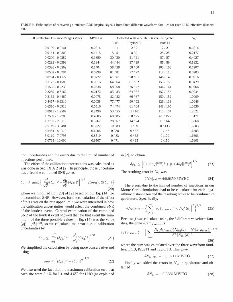
15

TABLE I: Efficiencies of recovering simulated BBH inspiral signals from three different waveform families for each LHO-effective distancebin.

LHO-Effective Distance Range (Mpc) MWEGs Detected withρ > 16.056 versus Injected NG

EOB TaylorT3 PadeT1

0.0100 - 0.0141 0.0814 1 / 1 2 / 2 2 / 2 0.0814

0.0141 - 0.0200 0.1415 5 / 5 8 / 9 25 / 25 0.2177

0.0200 - 0.0282 0.1850 30 / 30 21 / 21 57 / 57 0.4027

0.0282 - 0.0398 0.1844 44 / 44 37 / 39 85 / 86 0.5832

0.0398 - 0.0562 0.1404 58 / 58 58 / 60 100 / 103 0.7207

0.0562 - 0.0794 0.0999 81 / 81 77 / 77 117 / 118 0.8203

0.0794 - 0.1122 0.0722 61 / 61 78 / 81 146 / 146 0.8916

0.1122 - 0.1585 0.0515 64 / 64 81 / 82 155 / 155 0.9429

0.1585 - 0.2239 0.0338 68 / 68 76 / 77 144 / 144 0.9766

0.2239 - 0.3162 0.0172 83 / 83 64 / 67 152 / 155 0.9934

0.3162 - 0.4467 0.0075 82 / 82 66 / 67 150 / 152 1.0009

0.4467 - 0.6310 0.0038 77 / 77 90 / 92 126 / 133 1.0046

0.6310 - 0.8913 0.0516 74 / 74 61 / 64 148 / 165 1.0536

0.8913 - 1.2589 0.2490 53 / 55 81 / 101 115 / 154 1.2622

1.2589 - 1.7783 0.4505 68 / 85 38 / 75 61 / 156 1.5171

1.7783 - 2.5119 0.5267 28 / 67 14 / 74 11 / 147 1.6368

2.5119 - 3.5481 0.5222 10 / 83 1 / 69 0 / 133 1.6603

3.5481 - 5.0119 0.6005 0 / 88 0 / 67 0 /156 1.6603

5.0119 - 7.0795 0.8510 0 / 83 0 / 65 0 /170 1.6603

7.0795 - 10.000 0.9507 0 / 71 0 / 65 0 /150 1.6603

tion uncertainties and the errors due to the limited number ofinjections performed.

The effect of the calibration uncertainties was calculatedaswas done in Sec. IX A 2 of [2]. In principle, those uncertain-ties affect the combined SNRρC as

δρC ≤ max{[ρ2

L

ρ2C

(δρL)2+ρ2H

ρ2C

(δρH)2]1/2

, 2(δρH), 2(δρL)}

(20)where we modified Eq. (23) of [2] based on our Eq. (14) forthe combined SNR. However, for the calculation of the effectof this error on the rate upper limit, we were interested in howthe calibration uncertainties would affect the combined SNRof the loudest event. Careful examination of the combinedSNR of the loudest event showed that for that event the min-imum of the three possible values in Eq. (14) was the value(ρ2

L + ρ2H)1/2, so we calculated the error due to calibration

uncertainties by

δρC ≤[ρ2

L

ρ2C

(δρL)2 +ρ2H

ρ2C

(δρH)2]1/2

. (21)

We simplified the calculation by being more conservative andusing

δρC ≤[

(δρL)2 + (δρH)2]1/2

. (22)

We also used the fact that the maximum calibration errors ateach site were8.5% for L1 and4.5% for LHO (as explained

in [2]) to obtain

δρC ≤[

(0.085 ρmaxL )2 + (0.045ρmax

H )2]1/2

. (23)

The resulting error inNG was

δNG|cal = ±0.0859 MWEG. (24)

The errors due to the limited number of injections in ourMonte-Carlo simulations had to be calculated for each loga-rithmic distance bin and the resulting errors to be combinedinquadrature. Specifically,

δNG|MC ={

∞∑

d=0

[

δf(d; ρmax) ×NncG (d)

]2}1/2

. (25)

Becausef was calculated using the 3 different waveform fam-ilies, the errorδf(d; ρmax) is

δf(d; ρmax) =[

∑

appr

Nf(d; ρmax)(Ninj(d) −Nf(d; ρmax))

32 [Ninj(d)]3

]1/2

(26)where the sum was calculated over the three waveform fami-lies: EOB, PadeT1 and TaylorT3. This gave

δNG|MC = ±0.0211 MWEG. (27)

Finally we added the errors inNG in quadrature and ob-tained

δNG = ±0.0885 MWEG. (28)

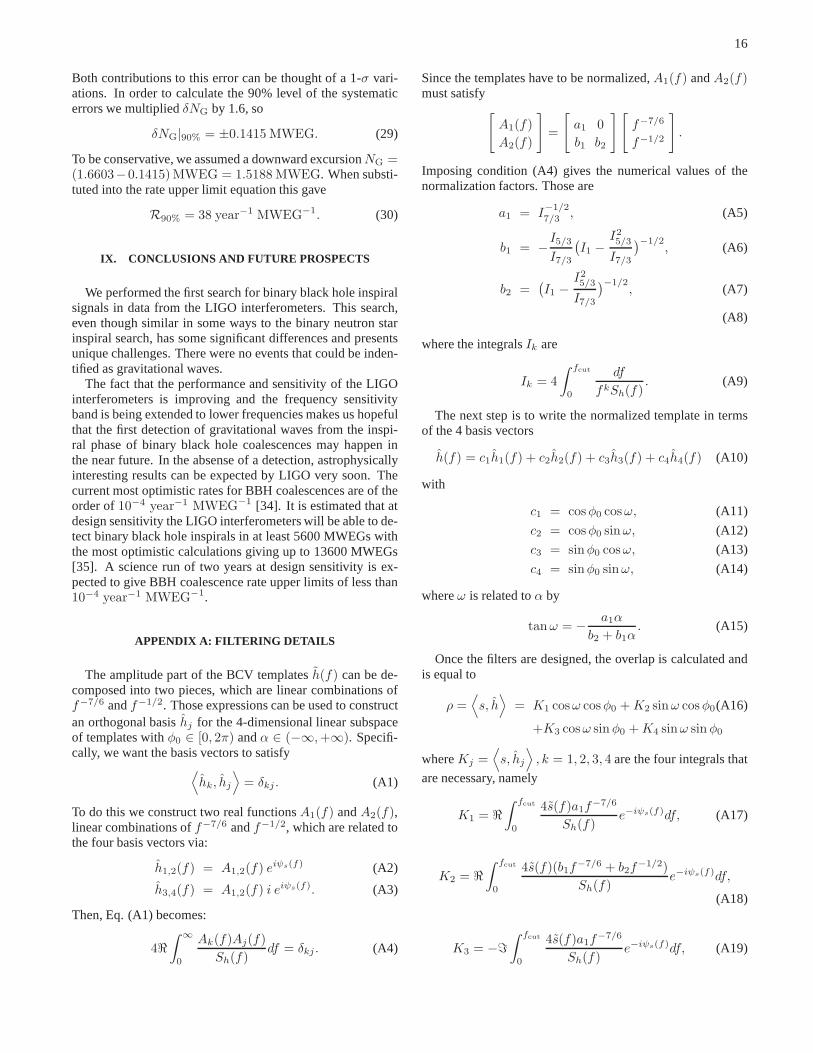
16

Both contributions to this error can be thought of a 1-σ vari-ations. In order to calculate the 90% level of the systematicerrors we multipliedδNG by 1.6, so

δNG|90% = ±0.1415 MWEG. (29)

To be conservative, we assumed a downward excursionNG =(1.6603−0.1415) MWEG = 1.5188 MWEG. When substi-tuted into the rate upper limit equation this gave

R90% = 38 year−1 MWEG−1. (30)

IX. CONCLUSIONS AND FUTURE PROSPECTS

We performed the first search for binary black hole inspiralsignals in data from the LIGO interferometers. This search,even though similar in some ways to the binary neutron starinspiral search, has some significant differences and presentsunique challenges. There were no events that could be inden-tified as gravitational waves.

The fact that the performance and sensitivity of the LIGOinterferometers is improving and the frequency sensitivityband is being extended to lower frequencies makes us hopefulthat the first detection of gravitational waves from the inspi-ral phase of binary black hole coalescences may happen inthe near future. In the absense of a detection, astrophysicallyinteresting results can be expected by LIGO very soon. Thecurrent most optimistic rates for BBH coalescences are of theorder of10−4 year−1 MWEG−1 [34]. It is estimated that atdesign sensitivity the LIGO interferometers will be able tode-tect binary black hole inspirals in at least 5600 MWEGs withthe most optimistic calculations giving up to 13600 MWEGs[35]. A science run of two years at design sensitivity is ex-pected to give BBH coalescence rate upper limits of less than10−4 year−1 MWEG−1.

APPENDIX A: FILTERING DETAILS

The amplitude part of the BCV templatesh(f) can be de-composed into two pieces, which are linear combinations off−7/6 andf−1/2. Those expressions can be used to constructan orthogonal basishj for the 4-dimensional linear subspaceof templates withφ0 ∈ [0, 2π) andα ∈ (−∞,+∞). Specifi-cally, we want the basis vectors to satisfy

⟨

hk, hj

⟩

= δkj . (A1)

To do this we construct two real functionsA1(f) andA2(f),linear combinations off−7/6 andf−1/2, which are related tothe four basis vectors via:

h1,2(f) = A1,2(f) eiψs(f) (A2)

h3,4(f) = A1,2(f) i eiψs(f). (A3)

Then, Eq. (A1) becomes:

4ℜ

∫ ∞

0

Ak(f)Aj(f)

Sh(f)df = δkj . (A4)

Since the templates have to be normalized,A1(f) andA2(f)must satisfy

[

A1(f)

A2(f)

]

=

[

a1 0

b1 b2

][

f−7/6

f−1/2

]

.

Imposing condition (A4) gives the numerical values of thenormalization factors. Those are

a1 = I−1/27/3 , (A5)

b1 = −I5/3

I7/3

(

I1 −I25/3

I7/3

)−1/2, (A6)

b2 =(

I1 −I25/3

I7/3

)−1/2, (A7)

(A8)

where the integralsIk are

Ik = 4

∫ fcut

0

df

fkSh(f). (A9)

The next step is to write the normalized template in termsof the 4 basis vectors

h(f) = c1h1(f) + c2h2(f) + c3h3(f) + c4h4(f) (A10)

with

c1 = cosφ0 cosω, (A11)

c2 = cosφ0 sinω, (A12)

c3 = sinφ0 cosω, (A13)

c4 = sinφ0 sinω, (A14)

whereω is related toα by

tanω = −a1α

b2 + b1α. (A15)

Once the filters are designed, the overlap is calculated andis equal to

ρ =⟨

s, h⟩

= K1 cosω cosφ0 +K2 sinω cosφ0(A16)

+K3 cosω sinφ0 +K4 sinω sinφ0

whereKj =⟨

s, hj

⟩

, k = 1, 2, 3, 4 are the four integrals that

are necessary, namely

K1 = ℜ

∫ fcut

0

4s(f)a1f−7/6

Sh(f)e−iψs(f)df, (A17)

K2 = ℜ

∫ fcut

0

4s(f)(b1f−7/6 + b2f

−1/2)

Sh(f)e−iψs(f)df,

(A18)

K3 = −ℑ

∫ fcut

0

4s(f)a1f−7/6

Sh(f)e−iψs(f)df, (A19)

17

K4 = −ℑ

∫ fcut

0

4s(f)(b1f−7/6 + b2f

−1/2)

Sh(f)e−iψs(f)df.

(A20)Maximizing the SNR overφ0 andω we get

ρmaximized = 12

√

(K1 +K4)2 + (K2 −K3)2 (A21)

+ 12

√

(K1 −K4)2 + (K2 +K3)2.

The values ofφ0 andα that give the maximized SNR are

φmax0 =

1

2arctan

K2 +K3

K1 −K4−

1

2arctan

K2 −K3

K1 +K4, (A22)

αmax = −b2 tanωmax

a1 + b1 tanωmax, (A23)

where

ωmax =1

2arctan

K2 −K3

K1 +K4+

1

2arctan

K2 +K3

K1 −K4. (A24)

An extensive discussion on the values ofα is provided inSec. V C 1.

An equivalent expression for the SNR, which is computa-tionally less costly, can be produced if we define

F1 = K1 − iK3, (A25)

F2 = K2 − iK4.

Eq. A22 can then be written as

ρmaximized = 12

√

|F1|2 + |F2|2 + 2ℑ(F1F ∗2 ) (A26)

+ 12

√

|F1|2 + |F2|2 − 2ℑ(F1F ∗2 ).

ACKNOWLEDGMENTS

The authors gratefully acknowledge the support of theUnited States National Science Foundation for the construc-tion and operation of the LIGO Laboratory and the ParticlePhysics and Astronomy Research Council of the United King-dom, the Max-Planck-Society and the State of Niedersach-sen/Germany for support of the construction and operation ofthe GEO600 detector. The authors also gratefully acknowl-edge the support of the research by these agencies and by theAustralian Research Council, the Natural Sciences and Engi-neering Research Council of Canada, the Council of Scientificand Industrial Research of India, the Department of Scienceand Technology of India, the Spanish Ministerio de Educaciony Ciencia, the John Simon Guggenheim Foundation, the Lev-erhulme Trust, the David and Lucile Packard Foundation, theResearch Corporation, and the Alfred P. Sloan Foundation.

[1] A. Abramovici et al., Science256, 325 (1992).[2] B. Abbott et al. (LIGO Scientific Collaboration), submitted to

Phys. Rev. D (2005), web location:gr-qc/0505041.[3] B. Abbott et al., Class. Quant. Grav.21, S677 (2004).[4] T. Damour, B. R. Iyer, and B. S. Sathyaprakash, Phys. Rev.D

57, 885 (1998).[5] A. Buonanno and T. Damour, Phys. Rev. D59, 084006 (1999).[6] A. Buonanno and T. Damour, Phys. Rev. D62, 064015 (2000).[7] T. Damour, P. Jaranowski, and G. Schafer, Phys. Rev. D62,

084011 (2000).[8] T. Damour, B. R. Iyer, and B. S. Sathyaprakash, Phys. Rev.D

63, 044023 (2001).[9] T. Damour, B. Iyer, P. Jaranowski, and B. S. Sathyaprakash,

Phys. Rev. D67, 064028 (2003).[10] L. Blanchet, T. Damour, G. Esposito-Farese, and B. R. Iyer,

Phys. Rev. Lett.93, 091101 (2004), gr-qc/0406012.[11] F. Echeverria, Phys. Rev. D40, 3194 (1989).[12] E. W. Leaver, Proc. R. Soc. London Ser. A402, 285 (1985).[13] J. D. E. Creighton, Phys. Rev. D60, 022001 (1999).[14] L. Blanchet, G. Faye, B. R. Iyer, and B. Joguet, Phys. Rev. D65,

061501 (2002), gr-qc/0105099.[15] L. Blanchet, Living Rev. Rel.5, 3 (2002), gr-qc/0202016.[16] L. Blanchet, B. R. Iyer, C. M. Will, and A. G. Wiseman, Class.

Quant. Grav.13, 575 (1996).[17] J. G. Baker, M. Campanelli, C. O. Lousto, and R. Takahashi,

Phys. Rev. D65, 124012 (2002), astro-ph/0202469.

[18] J. G. Baker, M. Campanelli, and C. O. Lousto, Phys. Rev. D65,044001 (2002), gr-qc/0104063.

[19] A. Buonanno, Y. Chen, and M. Vallisneri, Phys. Rev. D67,024016 (2003).

[20] S. Droz, D. J. Knapp, E. Poisson, and B. J. Owen, Phys. Rev. D59, 124016 (1999).

[21] K. S. Thorne, inThree hundred years of gravitation, editedby S. W. Hawking and W. Israel (Cambridge University Press,Cambridge, 1987), chap. 9, pp. 330–458.

[22] B. S. Sathyaprakash and S. V. Dhurandhar, Phys. Rev D44,3819 (1991).

[23] S. Fairhurst et al.,Analysis of inspiral hardware injections dur-ing s2(2004), in preparation.

[24] N. Christensen, P. Shawhan, and G. Gonzalez, Class. Quant.Grav.21, S1747 (2004).

[25] B. A. Allen, W. G. Anderson, P. R. Brady, D. A. Brown, andJ. D. E. Creighton (2005), gr-qc/0509116.

[26] LSC Algorithm Library software packagesLAL andLALAPPS,the CVS tag versionsinspiral-bcv-2004-10-28-0and inspiral-bcv-2005-02-03-0 of LAL

and LALAPPS were used in this analysis., URLhttp://www.lsc-group.phys.uwm.edu/lal.

[27] B. Allen, Phys. Rev. D71, 062001 (2005).[28] T. Tannenbaum, D. Wright, K. Miller, and M. Livny, inBe-

owulf Cluster Computing with Linux, edited by T. Sterling (MITPress, 2001).

18

[29] K. Belczynski, V. Kalogera, and T. Bulik, Astrophys. J.572,407 (2002).

[30] B. Abbott et al. (LIGO Scientific Collaboration), Phys.Rev. D69, 122001 (2004).

[31] P. R. Brady, J. D. E. Creighton, and A. G. Wiseman, Class.Quant. Grav.21, S1775 (2004).

[32] T. Bulik, D. Gondek-Rosinska, and K. Belczynski, Mon. Not.Roy. Astron. Soc.352, 1372 (2004).

[33] A. Buonanno, Y. Chen, and M. Vallisneri, Phys. Rev. D67,104025 (2003).

[34] R. O’Shaughnessy, C. Kim, T. Fragkos, V. Kalogera, andK. Belczynski, ApJ, in press (2005), astro-ph/0504479.

[35] P. Nutzman, V. Kalogera, L. S. Finn, C. Hendrickson, andK. Belczynski, Astrophys. J.612, 364 (2004).