
SDP System Data Model View
95
SDP Architecture > Data Models SDP System Data Model View Contributors: K. Kirkham, P. Wortmann TABLE OF CONTENTS 1 Primary Representation 8 2 Element Catalogue 9 2.1 Elements and Their Properties 9 2.1.1 Global Sky Model 9 2.1.2 Science Data Model 9 2.1.2.1 Local Sky Model 10 2.1.2.2 Calibration Solutions (a.k.a. Gain Tables) 10 2.1.2.3 SDP Quality Assessment metrics 11 2.1.2.4 Processing Block Configuration 11 2.1.2.5 Processing logs 12 2.1.2.6 Other Data Product Catalogue Metadata 12 2.1.3 Processing Data Models 12 2.1.4 SDP Data Products 13 2.1.5 Science Event Alerts 14 2.1.6 Science Data Product Catalogue 14 2.1.7 Raw Input Data 15 2.1.8 Telescope Configuration Data 15 2.1.9 Telescope State Information 16 2.1.10 Scheduling Block Configuration 16 2.1.11 SKA Project Model 17 2.2 Relations and Their Properties 17 2.3 Element Interfaces 18 3 Context Diagram 19 4 Variability Guide 19 5 Rationale 19 5.1 Constructability 19 5.2 Primary Functionality 19 6 Related Views 19 7 References 19 8 Execution Control Data Model View Packet 21 8.1 Primary Representation 21 8.1.1 Processing Control Data Model 23 8.1.2 Deployment Data Model 25 Document No: SKA-TEL-SDP-0000013 Unrestricted Revision: 07 Author: K. Kirkham, P. Wortmann, et al. Release Date: 2019-03-15 Page 1 of 95
-
Upload
khangminh22 -
Category
Documents
-
view
1 -
download
0
Transcript of SDP System Data Model View
SDP Architecture > Data Models
SDP System Data Model View
Contributors: K. Kirkham, P. Wortmann
TABLE OF CONTENTS
1 Primary Representation 8
2 Element Catalogue 9
2.1 Elements and Their Properties 9
2.1.1 Global Sky Model 9
2.1.2 Science Data Model 9
2.1.2.1 Local Sky Model 10
2.1.2.2 Calibration Solutions (a.k.a. Gain Tables) 10
2.1.2.3 SDP Quality Assessment metrics 11
2.1.2.4 Processing Block Configuration 11
2.1.2.5 Processing logs 12
2.1.2.6 Other Data Product Catalogue Metadata 12
2.1.3 Processing Data Models 12
2.1.4 SDP Data Products 13
2.1.5 Science Event Alerts 14
2.1.6 Science Data Product Catalogue 14
2.1.7 Raw Input Data 15
2.1.8 Telescope Configuration Data 15
2.1.9 Telescope State Information 16
2.1.10 Scheduling Block Configuration 16
2.1.11 SKA Project Model 17
2.2 Relations and Their Properties 17
2.3 Element Interfaces 18
3 Context Diagram 19
4 Variability Guide 19
5 Rationale 19
5.1 Constructability 19
5.2 Primary Functionality 19
6 Related Views 19
7 References 19
8 Execution Control Data Model View Packet 21
8.1 Primary Representation 21
8.1.1 Processing Control Data Model 23
8.1.2 Deployment Data Model 25
Document No: SKA-TEL-SDP-0000013 Unrestricted
Revision: 07 Author: K. Kirkham, P. Wortmann, et al. Release Date: 2019-03-15 Page 1 of 95
SDP Architecture > Data Models
8.2 Element Catalogue 25
8.2.1 Elements and Their Properties 25
8.2.1.1 Execution Control 26
8.2.1.2 Service 26
8.2.1.3 Service Deployment 26
8.2.1.4 Buffer Storage 27
8.2.1.5 Scheduling Block Instance 28
8.2.1.6 Processing Block 28
8.2.1.7 Workflow, Processing Components, Execution Engine 29
8.2.1.8 Resource Request 30
8.2.1.9 Resource Period 30
8.2.1.10 Resource Assignment 31
8.2.1.11 Workflow Stage 32
8.2.1.12 Deployment 33
8.2.1.13 Data Island 34
8.2.1.14 Storage 35
8.2.2 Relations and Their Properties 35
8.2.3 Element Interfaces 35
8.2.4 Element Behavior 35
8.3 Context Diagram 35
8.4 Variability Guide 36
8.5 Rationale 36
8.6 Related Views 36
8.7 Reference Documents 36
9 Sky Model View Packet 37
9.1 Primary Representation 37
9.2 Element Catalogue 38
9.2.1 Elements and Their Properties 38
9.2.1.1 Source 39
9.2.1.2 Component 39
9.2.2 Relations and Their Properties 40
9.2.3 Element Interfaces 40
9.2.4 Element Behavior 40
9.3 Context Diagram 41
9.4 Variability Guide 41
9.5 Rationale 42
9.6 Related Views 42
9.7 References 42
10 Gridded Data Model View Packet 43
10.1 Primary Representation 43
10.2 Element Catalogue 44
Document No: SKA-TEL-SDP-0000013 Unrestricted
Revision: 07 Author: K. Kirkham, P. Wortmann, et al. Release Date: 2019-03-15 Page 2 of 95
SDP Architecture > Data Models
10.2.1 Element and Their Properties 44
10.2.2 Relations and Their Properties 44
10.2.3 Element Interfaces 44
10.2.4 Element Behavior 45
10.2.5 Indices and Keys 45
10.2.6 Structure and Access Patterns 45
10.3 Context Diagram 45
10.4 Variability Guide 47
10.5 Rationale 47
10.6 Related Views 47
10.7 References 48
11 Image Data Model View Packet 49
11.1 Primary Representation 49
11.2 Element Catalogue 49
11.2.1 Elements and Their Properties 49
11.2.2 Relations and Their Properties 49
11.2.3 Element Interfaces 50
11.2.4 Element Behavior 50
11.2.5 Indices and Keys 50
11.2.6 Structure and Access Patterns 50
11.3 Context Diagram 52
11.4 Variability Guide 52
11.5 Rationale 52
11.6 Related Views 54
11.7 Reference Documents 54
12 Processing Data Model View Packet 55
12.1 Primary Representation 55
12.2 Element Catalogue 56
12.2.1 Elements and Their Properties 56
12.2.1.1 Imaging Data Models 56
12.2.1.1.1 Visibility 56
12.2.1.1.2 Image 56
12.2.1.1.3 Gridded Data 56
12.2.1.2 Non-Imaging Data Models 57
12.2.2 Relations and Their Properties 57
12.2.3 Element Behavior 57
12.3 Context Diagram 59
12.4 Variability Guide 59
12.5 Rationale 59
12.6 Related Views 59
12.7 Reference Documents 59
Document No: SKA-TEL-SDP-0000013 Unrestricted
Revision: 07 Author: K. Kirkham, P. Wortmann, et al. Release Date: 2019-03-15 Page 3 of 95
SDP Architecture > Data Models
12.8 Non-Imaging Data Model View Packet 60
12.8.1 Primary Representation 60
12.8.2 Element Catalogue 61
12.8.2.1 Element and Their Properties 61
12.8.2.1.1 Pulsar Search Data Model 61
12.8.2.1.1.1 Raw input data 61
12.8.2.1.1.2 Science Data Model 63
12.8.2.1.1.3 Pulsar Search SDP Data Products 64
12.8.2.1.1.4 Science Event Alert (TBC) 64
12.8.2.1.2 Single Pulse/Fast Transient Data Model 65
12.8.2.1.2.1 Raw input data 65
12.8.2.1.2.2 Science Data Model 66
12.8.2.1.2.3 Single Pulse/Fast Transient SDP Data Products 67
12.8.2.1.2.4 Science Event Alert 67
12.8.2.1.3 Pulsar Timing Mode Data Model 67
12.8.2.1.3.1 Raw input data 67
12.8.2.1.3.2 Science Data Model 68
12.8.2.1.3.3 Pulsar Timing SDP Data Products 69
12.8.2.1.3.4 Science Event Alert (TBC) 70
12.8.2.1.4 Dynamic Spectrum Mode Data Model 70
12.8.2.1.4.1 Raw input data 70
12.8.2.1.4.2 Science Data Model 71
12.8.2.1.4.3 Dynamic Spectrum SDP Data Products 71
12.8.2.1.5 Flow Through Mode Data Model 72
12.8.2.1.5.1 Raw input data 72
12.8.2.1.5.2 Science Data Model 72
12.8.2.1.5.3 Flow Through Mode SDP Data Products 72
12.8.2.2 Relations and Their Properties 72
12.8.2.3 Element Interfaces 72
12.8.2.4 Element Behavior 72
12.8.2.5 Indices and Keys 72
12.8.2.6 Structure and Access Patterns 73
12.8.3 Context Diagram 73
12.8.4 Variability Guide 73
12.8.5 Rationale 73
12.8.6 Related Views 73
12.8.7 Reference Documents 73
12.9 Visibility Data Model 74
12.9.1 Scope, Terminology 74
12.9.2 Primary representation 75
12.9.2.1 Versioning 77
12.9.2.2 Keywords 77
Document No: SKA-TEL-SDP-0000013 Unrestricted
Revision: 07 Author: K. Kirkham, P. Wortmann, et al. Release Date: 2019-03-15 Page 4 of 95
SDP Architecture > Data Models
12.9.3 Element Catalogue 77
12.9.3.1 Elements and Their Properties 77
12.9.3.1.1 Data 77
12.9.3.1.2 Metadata 78
12.9.3.2 Relations and Their Properties 78
12.9.3.3 Element Interfaces 80
12.9.3.4 Element Behavior 80
12.9.3.5 Indices and Keys 80
12.9.3.6 Structure and Access Patterns 80
12.9.4 Context Diagram 81
12.9.5 Variability Guide 81
12.9.6 Rationale 81
12.9.7 Related Views 81
12.9.8 References 81
13 Science Data Model View Packet 83
13.1 Primary Representation 83
13.2 Element Catalogue 84
13.2.1 Elements and Their Properties 84
13.2.1.1 Processing Block 84
13.2.1.2 Processing Log 84
13.2.1.3 Quality Assessment Metrics 84
13.2.1.4 Telescope State Subset 85
13.2.1.5 Local Sky Model 85
13.2.1.6 Telescope Configuration Data Subset 85
13.2.1.7 Calibration Solution Tables 85
13.2.2 Relations and Their Properties 85
13.2.3 Element Interfaces 85
13.2.4 Element Behavior 85
13.3 Context Diagram 86
13.4 Variability Guide 86
13.5 Rationale 86
13.6 Related Views 86
13.7 References 87
14 SDP Data Product Catalogue View Packet 87
14.1 Primary Representation 87
14.2 Element Catalogue 88
14.2.1 Elements and Their Properties 88
14.2.1.1 Project 88
14.2.1.2 Observation 88
14.2.1.3 Processing Block Information 88
14.2.1.4 Data Product Index 88
Document No: SKA-TEL-SDP-0000013 Unrestricted
Revision: 07 Author: K. Kirkham, P. Wortmann, et al. Release Date: 2019-03-15 Page 5 of 95
SDP Architecture > Data Models
14.2.2 Relations and Their Properties 88
14.2.2.1 Access Rights 88
14.2.3 Element Interfaces 89
14.3 Context Diagram 89
14.4 Variability Guide 89
14.5 Rationale 89
14.6 Related Views 90
14.7 Reference Documents 90
15 Transient Source Catalogue View Packet 91
15.1 Primary Representation 91
15.2 Element Catalogue 91
15.2.1 Elements and Their Properties 91
15.2.2 Relations and Their Properties 91
15.2.3 Element Interfaces 92
15.2.4 Element Behavior 92
15.3 Context Diagram 92
15.4 Variability Guide 92
15.5 Rationale 92
15.6 Related Views 92
15.7 Reference Documents 93
16 Appendix A 93
16.1 Metadata 93
17 Applicable Documents 94
Document No: SKA-TEL-SDP-0000013 Unrestricted
Revision: 07 Author: K. Kirkham, P. Wortmann, et al. Release Date: 2019-03-15 Page 6 of 95

SDP Architecture > Data Models
ABBREVIATIONS CBF Correlator Beamformer
CSP Central Signal Processor
CDTS Channelized Detected Time Series
DECJ Declination (J2000)
DM Dispersion Measure
DSM Dynamic Spectrum Mode
FOV Field Of View
GSM Global Sky Model
ICD Interface Control Document
ID Identification
IVOA International Virtual Observatory Alliance
LSM Local Sky Model
LTS Local Telescope State
MJD Modified Julian Date
OCL Optimised Candidate List
OCLD Optimised Candidate List and Data
PSF Point Spread Function
PSRFITS Pulsar Flexible Image Transport System
PSS Pulsar Search
PST Pulsar Timing
PTD Pulsar Timing Data
RAJ Right Ascension (J2000)
RFI Radio Frequency Interference
SB Scheduling Block
SDP Science Data Processor
SDM Science Data Model
SKAPM SKA Project Model
SPOCLD Single Pulse Optimised Candidate List and Data
SRC SKA Regional Centre
S/N Signal to Noise
TBC To be confirmed
TBD To be determined
TM Telescope Manager
TMC Telescope Monitor & Control
TOA Time of Arrival
Document No: SKA-TEL-SDP-0000013 Unrestricted
Revision: 07 Author: K. Kirkham, P. Wortmann, et al. Release Date: 2019-03-15 Page 7 of 95
SDP Architecture > Data Models
1 Primary Representation
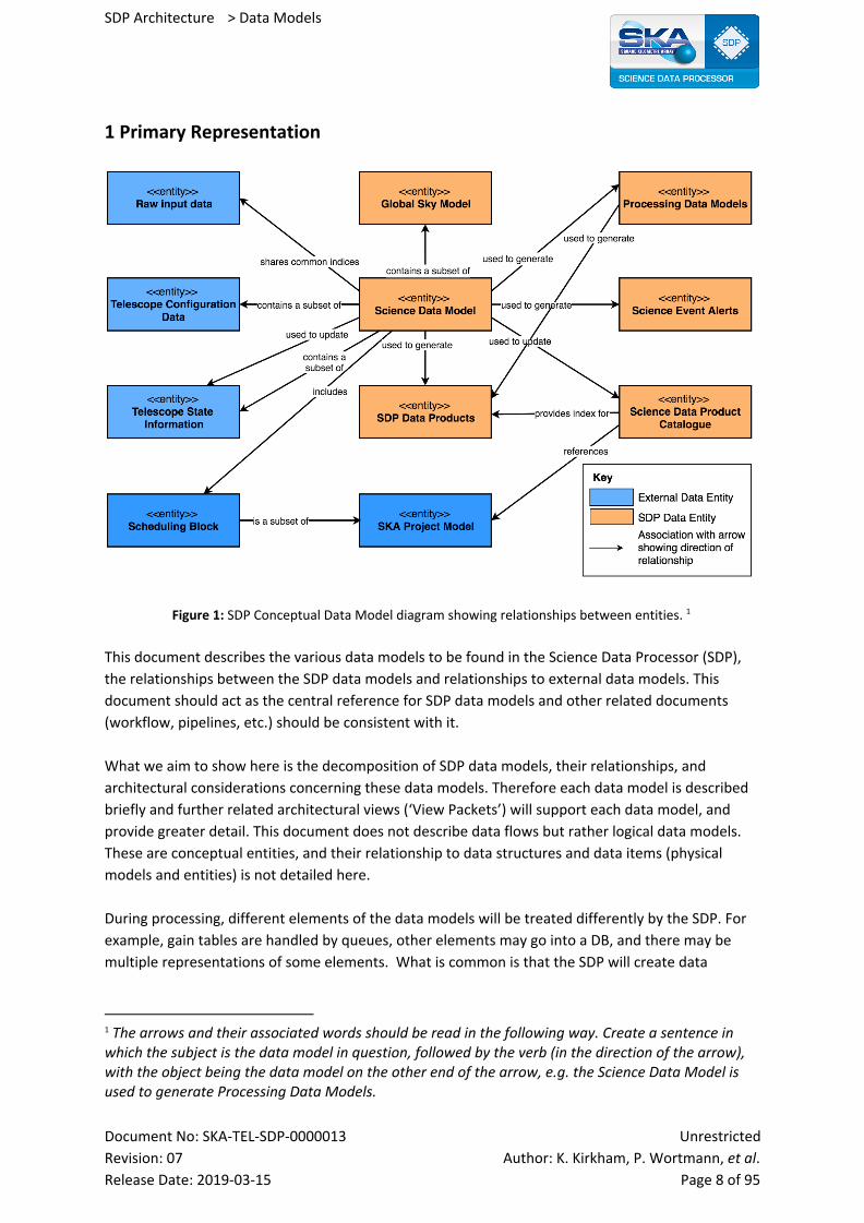
Figure 1: SDP Conceptual Data Model diagram showing relationships between entities. 1
This document describes the various data models to be found in the Science Data Processor (SDP),
the relationships between the SDP data models and relationships to external data models. This
document should act as the central reference for SDP data models and other related documents
(workflow, pipelines, etc.) should be consistent with it.
What we aim to show here is the decomposition of SDP data models, their relationships, and
architectural considerations concerning these data models. Therefore each data model is described
briefly and further related architectural views (‘View Packets’) will support each data model, and
provide greater detail. This document does not describe data flows but rather logical data models.
These are conceptual entities, and their relationship to data structures and data items (physical
models and entities) is not detailed here.
During processing, different elements of the data models will be treated differently by the SDP. For
example, gain tables are handled by queues, other elements may go into a DB, and there may be
multiple representations of some elements. What is common is that the SDP will create data
1 The arrows and their associated words should be read in the following way. Create a sentence in which the subject is the data model in question, followed by the verb (in the direction of the arrow), with the object being the data model on the other end of the arrow, e.g. the Science Data Model is used to generate Processing Data Models.
Document No: SKA-TEL-SDP-0000013 Unrestricted
Revision: 07 Author: K. Kirkham, P. Wortmann, et al. Release Date: 2019-03-15 Page 8 of 95

SDP Architecture > Data Models
products which contain elements of these data models, and these data products will be stored and
delivered to SRCs.
Note that this architectural view excludes data items used to configure and manage SDP internal
components (e.g. configuration database), because they don’t intersect with the data models
described here.
2 Element Catalogue
2.1 Elements and Their Properties Note that these are conceptual data models and therefore certain properties needed for
implementation such as primary keys are not mentioned in this document.
2.1.1 Global Sky Model
This is a catalogue of sky components stored as a searchable database. It accommodates the
following:
● Point sources with full Stokes parameters
● Time variability
● Resolved sources using compact basis set representations
● Complex spectral structures
● Information on planetary and solar radiation sources
● Images (i.e. pixelated images with world coordinate system, and units)
Multiple ways to represent the sky model position are supported and interpreted by an API. Note
that the Global Sky Model is not complete without a module to interpret the data. The Global Sky
Model must be extensible and flexible.
2.1.2 Science Data Model
The Science Data Model consists of the following high level data entities:
● Local Sky Model (LSM)
● Subset of the Telescope Configuration Data (refer to Telescope Configuration Data section)
● Subset of the Telescope State Information (refer to Telescope State section)
● Gain Tables (Calibration Solutions)
● SDP Quality Assessment metrics
● Processing Block
● Processing Logs
● Other Data Product Catalogue metadata
Relationships to other data entities:
● Shares common indices with Raw Input Data
● Is used to generate Science Event Alerts
● Is used to update the Science Data Product Catalogue
● Is used to generate Science Data products
● Includes the Scheduling Block
● Contains a subset of the Telescope State Information
● Updates the Telescope State Information
Document No: SKA-TEL-SDP-0000013 Unrestricted
Revision: 07 Author: K. Kirkham, P. Wortmann, et al. Release Date: 2019-03-15 Page 9 of 95
SDP Architecture > Data Models
● Contains a subset of the GSM
● Contains a subset of Telescope Configuration Data
● Is used to generate Processing Data Model
The SDM does not include the Raw Input Data, Processing Data Models or SDP Data Products, but
does include references to these data entities.
At least one instance of the SDM is associated with each Scheduling Block. The working assumption
is that there is one instance of the SDM associated with each Processing Block.
The Science Data Model and its sub-components must be extensible to accommodate changes
throughout the lifespan of the Observatory.
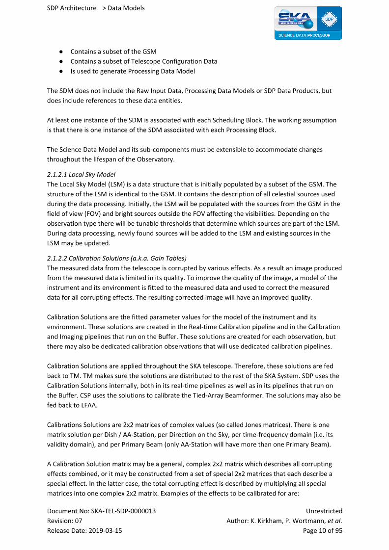
2.1.2.1 Local Sky Model
The Local Sky Model (LSM) is a data structure that is initially populated by a subset of the GSM. The
structure of the LSM is identical to the GSM. It contains the description of all celestial sources used
during the data processing. Initially, the LSM will be populated with the sources from the GSM in the
field of view (FOV) and bright sources outside the FOV affecting the visibilities. Depending on the
observation type there will be tunable thresholds that determine which sources are part of the LSM.
During data processing, newly found sources will be added to the LSM and existing sources in the
LSM may be updated.
2.1.2.2 Calibration Solutions (a.k.a. Gain Tables)
The measured data from the telescope is corrupted by various effects. As a result an image produced
from the measured data is limited in its quality. To improve the quality of the image, a model of the
instrument and its environment is fitted to the measured data and used to correct the measured
data for all corrupting effects. The resulting corrected image will have an improved quality.
Calibration Solutions are the fitted parameter values for the model of the instrument and its
environment. These solutions are created in the Real-time Calibration pipeline and in the Calibration
and Imaging pipelines that run on the Buffer. These solutions are created for each observation, but
there may also be dedicated calibration observations that will use dedicated calibration pipelines.
Calibration Solutions are applied throughout the SKA telescope. Therefore, these solutions are fed
back to TM. TM makes sure the solutions are distributed to the rest of the SKA System. SDP uses the
Calibration Solutions internally, both in its real-time pipelines as well as in its pipelines that run on
the Buffer. CSP uses the solutions to calibrate the Tied-Array Beamformer. The solutions may also be
fed back to LFAA.
Calibrations Solutions are 2x2 matrices of complex values (so called Jones matrices). There is one
matrix solution per Dish / AA-Station, per Direction on the Sky, per time-frequency domain (i.e. its
validity domain), and per Primary Beam (only AA-Station will have more than one Primary Beam).
A Calibration Solution matrix may be a general, complex 2x2 matrix which describes all corrupting
effects combined, or it may be constructed from a set of special 2x2 matrices that each describe a
special effect. In the latter case, the total corrupting effect is described by multiplying all special
matrices into one complex 2x2 matrix. Examples of the effects to be calibrated for are:
Document No: SKA-TEL-SDP-0000013 Unrestricted
Revision: 07 Author: K. Kirkham, P. Wortmann, et al. Release Date: 2019-03-15 Page 10 of 95
SDP Architecture > Data Models
● Weights
● Ionospheric Faraday Rotation
● Antenna Jones Matrices
● Ionospheric TEC/ ΔTEC
● Model Parameters
Each of these effects will have their own time- and frequency scale on which they vary. This list is not
exhaustive because there may be as-yet unknown effects to be calibrated. The Calibration Solution
data model is designed to be as general as possible, in order to capture the output of any calibration
algorithm, including ones that are developed in future. The types of calibration solutions that are
necessary depend on the telescope configuration and frequency band, so they will be different for
the two SKA phase 1 telescopes.
2.1.2.3 SDP Quality Assessment metrics
A set of metrics to determine the quality of Science Data Products.
A metric is given by these parameters:
● Name
● Value
● Date/time
● Origin (observation-id, pipeline component, …)
It should always be possible to produce a new Quality Assessment metric. There is no definitive list
of Quality Assessment metrics at this moment. When the QA metrics are further defined, which will
occur during prototyping and further development, data/time elements will be accurately specified.
2.1.2.4 Processing Block Configuration
A Processing Block is an atomic unit of processing from the viewpoint of scheduling. A Processing
Block is a complete description of all the parameters necessary to run a workflow. The list given
below is an example of the sorts of parameters required, and this is extensible. A given Scheduling
Block Instance may contain multiple Processing Blocks.
The Processing Block Configuration contains the following items (TBC):
● Processing Block ID
● Type (Real-time/batch)
● Processing Block parameters
● Abstract Resource Requirements
○ Real-time processing Compute Capacity
○ Batch processing Compute Capacity
○ Buffer Storage Capacity
○ Long Term Storage Capacity
● Science Pipeline Workflow Script (referenced by name and code revision)
Document No: SKA-TEL-SDP-0000013 Unrestricted
Revision: 07 Author: K. Kirkham, P. Wortmann, et al. Release Date: 2019-03-15 Page 11 of 95

SDP Architecture > Data Models
2.1.2.5 Processing logs
Processing logs are defined by SKA1-SYS_REQ-2336 [AD02] as “a log detailing the processing
configuration” and are essential for interpretation of Science Data Products. Processing logs may
also contain other information necessary for the interpretation of Science Data Products.
2.1.2.6 Other Data Product Catalogue Metadata
Work still needs to be done to identify these elements. It is not believed that accommodating these
elements will require architectural changes to the data model.
2.1.3 Processing Data Models
These were previously called Intermediate Data Models / products. Processing Data Model is a
placeholder for all intermediate data that a workflow may create. As such it must be extensible. The
Processing Data Models contain data items used during the processing of data. Note that All these
image products use the logical data model described in the Image Data Model View Packet.
Data Items Logical data model used Physical data model used (data format, etc.)
Facet
Visibility Set Visibility Data Model
● Block Visibility
● Coalesced Visibility ● Model Visibility ● Partially-corrected Visibility
UV Grid GriddedData Model
Intermediate imaging products 2
● Residual Image Image Data Model
● Sky Components / shapelets Image Data Model
● Dirty Image Image Data Model
● PSF Image ● Model Image
Image Data Model
Imaging Kernels
● W-kernel
● A-kernel
● Anti-aliasing kernel
● Over-sampled kernels
Note that If model and partially-corrected visibilities, and model image need to be stored, will have
impact on platform I/O performance and storage capacity.
Also there is on-going discussion as to whether store or recalculate on-the-fly the image kernels.
2 Note that the intermediate imaging products can be used both in processing and can comprise the final preserved science data products.
Document No: SKA-TEL-SDP-0000013 Unrestricted
Revision: 07 Author: K. Kirkham, P. Wortmann, et al. Release Date: 2019-03-15 Page 12 of 95
SDP Architecture > Data Models
2.1.4 SDP Data Products
This section provides a list and description of the data products which the SDP will deliver. SDP Data
Products are independent of each other and are not derived from a common object type.
Transient Source Catalogue
Time ordered catalogue of candidate transient objects pertaining to each detection alert
from the real-time Fast Imaging.
Science Data Product Catalogue
A database relating to all Science Products which have been processed by the SDP. It
includes associated scientific metadata that can be queried and searched and includes all
information so that the result of a query can lead to the delivery of data. This includes
metadata necessary to support IVOA data models and protocols.
Image Products 1: Image Cubes
1. Imaging data for Continuum, as cleaned restored Taylor term images (n.b. no image
products for Slow Transients detection have been specified – maps are made,
searched and discarded).
2. Residual image (i.e. residuals after applying CLEAN) in Continuum.
3. Clean component image (or a table, which could be smaller).
4. Spectral line cubes:
a. Spectral line cube with continuum emission remaining
b. Spectral line cube after continuum emission subtracted
5. Residual spectral line image (i.e. residuals after CLEAN applied).
6. Representative Point Spread Function for observations (cutout, small in size
compared to the field of view (FOV)).
7. Sensitivity Cubes (as per SDP_REQ-397).
Image Products 2: Gridded Data
1. Calibrated visibilities, gridded at the spatial and frequency resolution required by the
experiment. One grid per facet (so this grid is the FFT of the dirty map of each facet).
2. Accumulated Weights for each uv cell in each grid (without additional weighting
applied).
Calibrated Visibilities
Calibrated visibility data (for example for EoR experiments) and direction dependent
calibration information, with time and frequency averaging performed as requested to
reduce the data volume. Calibrated visibilities refers to visibilities after
direction-independent calibration and subtraction of strong sources with
direction-dependent calibration. These are the visibilities being exported to the Regional
Centres, so Direction-dependent corrections will be limited to model subtraction at this
point.
Sieved Pulsar and Transient Candidates
A data cube which will be folded and de-dispersed at the best Dispersion Measure (DM),
period and period derivative determined from the search; a single ranked list of non-imaging
Document No: SKA-TEL-SDP-0000013 Unrestricted
Revision: 07 Author: K. Kirkham, P. Wortmann, et al. Release Date: 2019-03-15 Page 13 of 95
SDP Architecture > Data Models
transient candidates from each scheduling block; for those transients deemed of sufficient
interest, the associated “filterbank” data will also be archived; a set of diagnostics/heuristics
that will include metadata associated with the scheduling block and observation.
Pulsar Timing Solutions
For each of the observed pulsars the output data from the pulsar timing section will include
the original input data as well as averaged versions of these data products (either averaged
in polarisation, frequency or time) in PSRFITs format; the arrival time of the pulse; the
residuals from the current best fit model for the pulsar; an updated model of the arrival
times.
Dynamic Spectrum Data
1. RFI Cleaned PSRFITS file (for Dynamic spectra mode)
2. Calibrated PSRFITS file (for Dynamic spectra mode)
Transient Buffer Data
Voltage data passed through from the CSP when the transient buffer is triggered. The
Transient Buffer in LOW will come from LFAA rather than CSP.
Science Data Model
Each instance of the Science Data Model (refer to section 2.1.2) is stored as a data product
when the processing finishes.
2.1.5 Science Event Alerts
Alerts produced by SDP following the detection of astronomical events.
Types of alerts:
● Single Pulse (non-imaging transient) Detection
● Pulsar Detection
● Imaging Transient Detection
The alerts themselves are formatted as IVOA alerts and sent to TM. These are recorded in a Science
Alert Catalogue which provides a searchable and retrievable record of past alerts.
This is one part of the data model which will not be extensible.
2.1.6 Science Data Product Catalogue
Catalogue of SDP Data Products. This is in itself a data product which is distributed to regional
centres.
The architecture for this catalogue is of a flat data structure - there are no use cases at the present
time which would require a more complex data structure. Each element within the catalogue will
index all the elements of the collection of data items (see below) that form an SDP Data Product.
The full metadata associated with a data product will itself be one of these data items. Each entry in
the catalogue will however contain a subset of the metadata against which searches can be made.
The one relational link is to the SKA project model (SKAPM) to associate each data item with an entry
in the SKAPM.
Document No: SKA-TEL-SDP-0000013 Unrestricted
Revision: 07 Author: K. Kirkham, P. Wortmann, et al. Release Date: 2019-03-15 Page 14 of 95
SDP Architecture > Data Models
Collection of data items: Physical data files/objects when considered together constitute a single SDP
Data Product. Example: a spectral line image cube where n multiple files each contain a subset of the
channels together with associated metadata file(s).
The SDP will be able to track a quality flag per SDP Data Product. Note that if only partial data
products are to be retained, new workflows will need to be created. In particular the Processing
Block Controller will need to flag the data appropriately and new workflows will be needed to deal
with discarded data.
Independent checks will be carried out on files for data product bitrot. Furthermore, the catalogue
will store checksums of all Data Product files. This is meant as a safeguard to detect data corruption,
both for data stored in Long Term Storage as well as for data exchanged between SDP instances and
SKA Regional Centres.
SDP will track a quality flag per SDP Data Product as catalogue meta data (such as “GOOD”, “BAD” or
“JUNK”). This flag will initially be set by the workflow, depending on its assessment of the Data
Product’s quality. Depending on the flag, delivery might be prevented or delayed (depending on
subscription rules). The quality flag can be updated after the fact using a direct interface to Delivery,
as well as by workflows. For example, when data has been identified as unusable, we might want to
run a workflow that updates the quality flag as well as data lifecycle policies to cause underlying data
to be discarded.
Furthermore, the catalogue will store checksums of all Data Product files. This is meant as a
safeguard to detect data corruption, both for data stored in Long Term Storage as well as for data
exchanged between SDP instances and SKA Regional Centres.
2.1.7 Raw Input Data
Raw input data:
● Visibility Data
● Pulsar & Transient Search Data
○ Pulsar Search Candidates
○ Single Pulse Candidates (fast transients)
● Pulsar Timing Data
○ Pulsar timing mode data (folded pulse profile data)
○ Dynamic Spectra Data
○ Flow Through mode data (raw beam-formed voltage data)
● Transient Buffer Data
2.1.8 Telescope Configuration Data
SDP requires a subset of the Telescope Configuration Data items for processing.
Minimal set of data items which SDP needs to subset:
● Beam Model:
○ Antenna Voltage Beams (Table defining beam parameters)
■ MID: Dish voltage beam
■ LOW: Embedded element pattern (Antenna dipole voltage beam)
Document No: SKA-TEL-SDP-0000013 Unrestricted
Revision: 07 Author: K. Kirkham, P. Wortmann, et al. Release Date: 2019-03-15 Page 15 of 95

SDP Architecture > Data Models
○ Antenna Positions
■ MID: Dish position
■ LOW: Station nominal centre position
● RFI (flagging) mask
● Calibration parameters (Jones matrix per antenna, frequency channel and time step)
● Measure data: Table defining leap seconds and all kinds of corrections for celestial
movements.
The interface to get a subset of the Telescope Configuration Data needs to provide the ability to
subset other items as required in the future.
2.1.9 Telescope State Information
Telescope State Information contains all information about the telescope’s state, environment and
behaviour. SDP requires a subset of this information for processing, and updates Telescope State
Information.
Subset of Telescope State Information needed by SDP:
● Parallactic angle, or (preferred):
○ longitude of telescope
○ latitude of telescope
○ RA of phase centre
○ Declination of phase centre
● *Flags on antennas/stations (missing etc) - if not already applied
● *Antenna/station pointing
○ LOW: station voltage beam (or equivalently station gains and beamformer
delays)
○ MID: actual pointing (in same coordinate system as the commanded)
○
● MID: *Antenna on/off source (noise source)
● Current values of each of the receptor gains
● GPS ionospheric measurements (TEC values) for each station
● Weather
* Telescope State Information data needed in real-time (a.k.a fast telescope state).
SDP updates to Telescope State Information:
● Real-time calibration solutions (Jones Matrices)
● Pointing Solutions
● Antenna/station location and delay calibration solutions
2.1.10 Scheduling Block Configuration
According to [AD02], Scheduling Blocks are the indivisible executable units of a project and contain
all information necessary to execute a single observation. A scheduling block may be stopped and
cancelled but not paused and resumed.
Document No: SKA-TEL-SDP-0000013 Unrestricted
Revision: 07 Author: K. Kirkham, P. Wortmann, et al. Release Date: 2019-03-15 Page 16 of 95
SDP Architecture > Data Models
All Scheduling Block data items are included in the Science Data Model. Scheduling Block data items
are needed for processing or for the Science Data Product Catalogue.
Scheduling Block data items are concerned with configuration of the observation, and contain the
‘recipe’ for the observation.
The architecturally important features of the Scheduling Block are that it should be extensible, and
that one Scheduling Block contains one or more Processing Blocks. The SDP cannot receive a
Processing Block except as part of a Scheduling Block.
The data items in the Telescope Configuration/Telescope State Information may have the same or
similar name as those in the Scheduling Block. The Scheduling Block contains observation
configuration parameters whereas the Telescope Configuration Data or Telescope State Information
contain parameters that describe the state of the telescope, e.g. commanded pointing (in Scheduling
Block) vs. actual pointing (in Telescope State Information).
Refer to [RD8] and descriptions of the Observation Configuration Data Model for further details.
2.1.11 SKA Project Model
List of data items that SDP needs to reference (via Scheduling Block ID):
● All data related to a particular project (e.g. Project ID, PI)
Note: There is an SKA system level architectural question about whether SDP should subset required
data items in the Science Data Product Catalogue or whether it would be done via a database
relation to the SKA Project Model database.
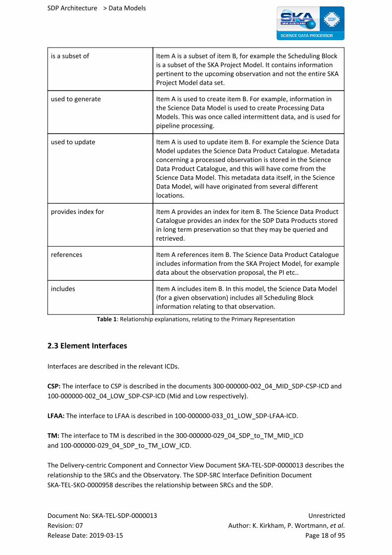
2.2 Relations and Their Properties The primary representation shows all major relationships between entities. The table below lists
these relationships. These are not exceptions to the primary representation diagram, but simply list
the relationships depicted in this diagram. Note that the relationships do not represent data flow or
interfaces between SDP and other elements. It shows the context of logical data model entities.
Relationship Description
shares common indices with This means that Item A shares common indices with item B. In this case, the Science Data Model shares common indices with raw input data. These common indices are provided by TM, and are used by SDP in processing. For example, SDP will only process raw data according to the indices provided by TM.
contains a subset of Item A contains a subset of the data model in item B. For example, the Science Data Model contains a subset of the Telescope State Information, pertaining to the observation. It does not contain the entirety of Telescope State Information for the telescope.
Document No: SKA-TEL-SDP-0000013 Unrestricted
Revision: 07 Author: K. Kirkham, P. Wortmann, et al. Release Date: 2019-03-15 Page 17 of 95
SDP Architecture > Data Models
is a subset of Item A is a subset of item B, for example the Scheduling Block is a subset of the SKA Project Model. It contains information pertinent to the upcoming observation and not the entire SKA Project Model data set.
used to generate Item A is used to create item B. For example, information in the Science Data Model is used to create Processing Data Models. This was once called intermittent data, and is used for pipeline processing.
used to update Item A is used to update item B. For example the Science Data Model updates the Science Data Product Catalogue. Metadata concerning a processed observation is stored in the Science Data Product Catalogue, and this will have come from the Science Data Model. This metadata data itself, in the Science Data Model, will have originated from several different locations.
provides index for Item A provides an index for item B. The Science Data Product Catalogue provides an index for the SDP Data Products stored in long term preservation so that they may be queried and retrieved.
references Item A references item B. The Science Data Product Catalogue includes information from the SKA Project Model, for example data about the observation proposal, the PI etc..
includes Item A includes item B. In this model, the Science Data Model (for a given observation) includes all Scheduling Block information relating to that observation.
Table 1: Relationship explanations, relating to the Primary Representation
2.3 Element Interfaces
Interfaces are described in the relevant ICDs.
CSP: The interface to CSP is described in the documents 300-000000-002_04_MID_SDP-CSP-ICD and
100-000000-002_04_LOW_SDP-CSP-ICD (Mid and Low respectively).
LFAA: The interface to LFAA is described in 100-000000-033_01_LOW_SDP-LFAA-ICD.
TM: The interface to TM is described in the 300-000000-029_04_SDP_to_TM_MID_ICD
and 100-000000-029_04_SDP_to_TM_LOW_ICD.
The Delivery-centric Component and Connector View Document SKA-TEL-SDP-0000013 describes the
relationship to the SRCs and the Observatory. The SDP-SRC Interface Definition Document
SKA-TEL-SKO-0000958 describes the relationship between SRCs and the SDP.
Document No: SKA-TEL-SDP-0000013 Unrestricted
Revision: 07 Author: K. Kirkham, P. Wortmann, et al. Release Date: 2019-03-15 Page 18 of 95
SDP Architecture > Data Models
3 Context Diagram
The SDP Conceptual Data Model diagram shown in Figure 1 is a context diagram and therefore no
additional context diagram is necessary.
4 Variability Guide
There is no variability at this level.
5 Rationale
5.1 Constructability Requirements: SDP_REQ-828 (Constructability)
We needed to introduce a single high-level data entity called the Science Data Model, which
encapsulates all information needed to process a particular grouping of data. The grouping of data
models in the Science Data Model (and its relationships) allows for the ability to pull together
information from a number of sources and provides flexibility in implementation.
We have chosen not to have a unified structure (like ALMA), because of cost and implementation
considerations. However, re-use of the ALMA table physical data model for appropriate elements of
the data model is not precluded.
5.2 Primary Functionality Functionality required by L1 requirements is addressed by the following data models.
The Global Sky Model is a long-lived data entity which evolves over the course of the project. It is an
explicit requirement of the observatory and serves other elements of the telescope.
Processing Data Models are required because the processing is organised as a directed acyclic graph
and therefore intermediate data products must be managed explicitly as parts of the graph.
Science Data Products, Science Event Alerts and Science Data Product Catalogue are required by L1
requirements.
6 Related Views
Not applicable.
7 References
The following documents are referenced in this document. In the event of conflict between the
contents of the referenced documents and this document, this document shall take precedence.
[RD1]
ALMA SDM Tables Short Description. COMP-70.75.00.00-00?-A-DSN. June 12 2015. Draft. The ALMA Export Data Format, ALMA-70.00.00.00-004-A-SPE:
http://docplayer.net/48193909-Alma-export-data-format.html
Document No: SKA-TEL-SDP-0000013 Unrestricted
Revision: 07 Author: K. Kirkham, P. Wortmann, et al. Release Date: 2019-03-15 Page 19 of 95

SDP Architecture > Data Models
[RD2] Data Models for the SDP Pipeline Components, Ger van Diepen et al, 2/12/2016 Rev B. (unclassified).
[RD3] SKA-TEL-SDP-0000139 SDP Memo 033: Sky Model Considerations. DRAFT. Ian Heywood.
[RD4] SKA-TEL-SDP-0000210 SDP Memo 105: SDP Intermediate Data Products. DRAFT.
Anna Scaife.
[RD8] SKA-TEL-TM-0000242 TMC Software Architecture Document, Rev 01, Subhrojyoti Roy Chaudhuri.
[RD9] 601-000000-002 OSO Software Architecture Document, Rev 01, Alan Bridger. TM number T4000-0000-AR-002.
[RD10] SKA-TEL-SKO-0000893, Telescope Model Project Report, Rev 01
Document No: SKA-TEL-SDP-0000013 Unrestricted
Revision: 07 Author: K. Kirkham, P. Wortmann, et al. Release Date: 2019-03-15 Page 20 of 95
SDP Architecture > Data Models
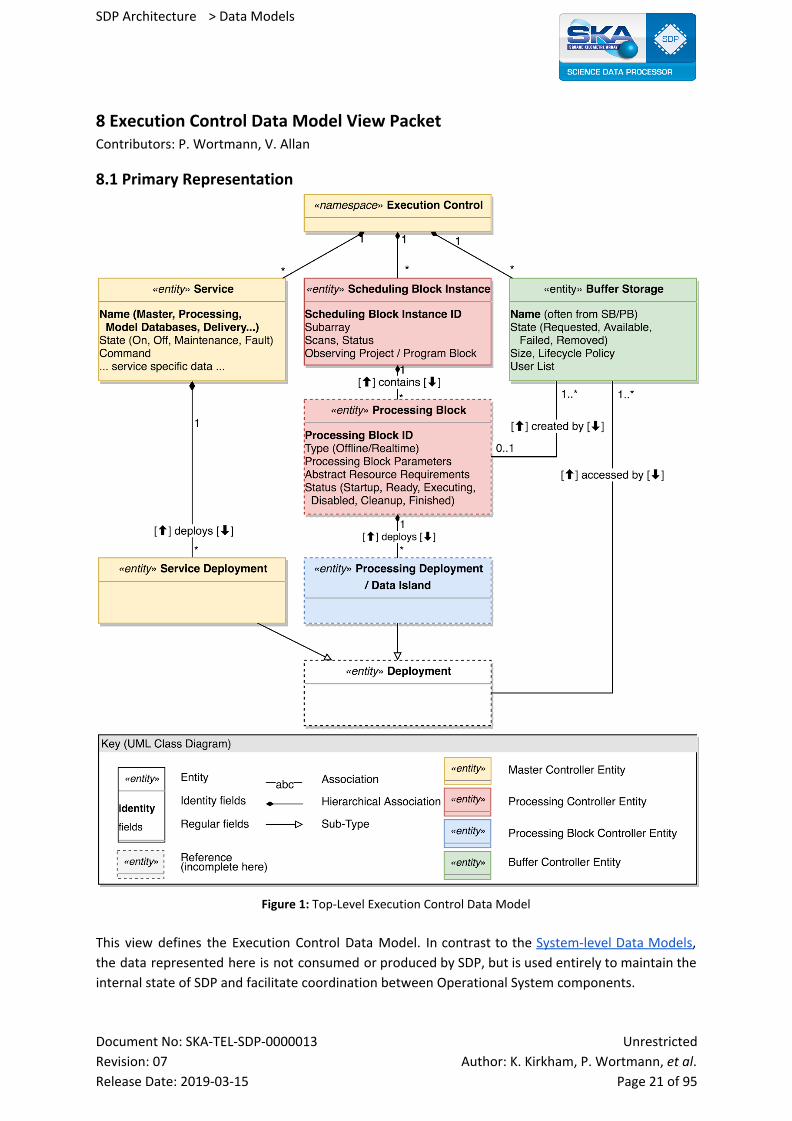
8 Execution Control Data Model View Packet Contributors: P. Wortmann, V. Allan
8.1 Primary Representation
Figure 1: Top-Level Execution Control Data Model
This view defines the Execution Control Data Model. In contrast to the System-level Data Models,
the data represented here is not consumed or produced by SDP, but is used entirely to maintain the
internal state of SDP and facilitate coordination between Operational System components.
Document No: SKA-TEL-SDP-0000013 Unrestricted
Revision: 07 Author: K. Kirkham, P. Wortmann, et al. Release Date: 2019-03-15 Page 21 of 95
SDP Architecture > Data Models
Elements shown here are data entities, signifying data stored in the configuration database and
possibly replicated in other places as needed. Relations are entity associations. Hierarchical
associations determine the structure of the data within the configuration database. This means that
the path connecting every element to the root “Execution Control” element qualified with element
identity information would determine the full path of the entity within the store.
The data shown here is going to be held and maintained by the Execution Control Component (see
Operational System C&C View) using the Configuration Database (see Execution Control C&C View).
Note that while we represent it as a database schema, the SDP configuration is purely transient data.
Therefore database technologies focused on long-term persistence would not be a suitable choice
for implementation, instead we would use configuration services with a focus on reliability and
scalable subscription interfaces (such as Apache ZooKeeper, Consul or etcd). In fact, another
alternative would be to maintain this data model using transaction queues (for example using
Apache Kafka). This document should be seen as a logical data model that could fit a large number of
possible physical implementations.
Reading Guide: The controllable entities within SDP are organised in a strictly hierarchical fashion in
order to provide clear hierarchies of ownership. What this especially means is that all Deployments
will have exactly one “owner”, so it is uniquely identified at which point a given resource can be
released. This ensures that the system does not “leak” resources or Platform configuration changes.
At the upper-most level, the name space is split into three categories. Services are long-lived entities
and are managed at the upper most level by the Master Controller (see Execution Control C&C
View). Examples include the Master and Processing Controller themselves, but also Delivery, Model
Databases and Buffer Services. These services will have very different characteristics and might use
and store different configuration data internally. On the other hand, all of them must implement the
same basic attributes to allow the master controller to track (and command) their state as well as
declare how their deployed components are to be managed by the platform.
Furthermore, the most significant category of control entities deals with the primary function of the
SDP, which is processing observation data. The top-level structure of this tree is managed by the
Processing Controller (see again Execution Control C&C View). In this tree, entities are strongly
associated with a Scheduling Block Instance / Processing Block path. This means that we see all
lower-level processing entities as being associated with exactly one Processing Block at all times. See
next section for more detail on those entities.
Finally, Buffer Storage exists semi-independently of both services and processing. This means that
while services and processing will create and delete storage, the option is left open to control
storage directly where appropriate. This means that SDP can fulfil its role as a data store even if
associated processing or services are not yet fully automated.
Document No: SKA-TEL-SDP-0000013 Unrestricted
Revision: 07 Author: K. Kirkham, P. Wortmann, et al. Release Date: 2019-03-15 Page 22 of 95
SDP Architecture > Data Models
8.1.1 Processing Control Data Model
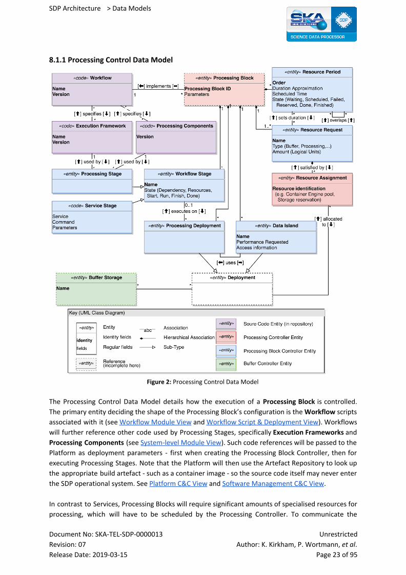
Figure 2: Processing Control Data Model
The Processing Control Data Model details how the execution of a Processing Block is controlled.
The primary entity deciding the shape of the Processing Block’s configuration is the Workflow scripts
associated with it (see Workflow Module View and Workflow Script & Deployment View). Workflows
will further reference other code used by Processing Stages, specifically Execution Frameworks and
Processing Components (see System-level Module View). Such code references will be passed to the
Platform as deployment parameters - first when creating the Processing Block Controller, then for
executing Processing Stages. Note that the Platform will then use the Artefact Repository to look up
the appropriate build artefact - such as a container image - so the source code itself may never enter
the SDP operational system. See Platform C&C View and Software Management C&C View.
In contrast to Services, Processing Blocks will require significant amounts of specialised resources for
processing, which will have to be scheduled by the Processing Controller. To communicate the
Document No: SKA-TEL-SDP-0000013 Unrestricted
Revision: 07 Author: K. Kirkham, P. Wortmann, et al. Release Date: 2019-03-15 Page 23 of 95

SDP Architecture > Data Models
resource requirements, the control script of the Workflow (see Workflow Module View) will create
Resource Periods & Requirements, documenting upper bounds for what resources will be required in
what order and for how long. These resource requests will be used by the the Processing Controller
to formulate a schedule that maps resources available to the SDP in the foreseeable future to
Processing Blocks. Once the resources in question are available, the Processing Controller will
indicate availability to the appropriate Processing Block Controller by adding Resource Assignments
to the Processing Block entity in the configuration.
Assigned resources will be used by the Processing Block for two purposes: Executing workflow stages
and allocating Data Islands for holding storage. The corresponding configuration is created by the
Workflow script when the Processing Block is created, but will be marked as waiting for resources
and/or dependencies. As resources become assigned to the Processing Blocks and other workflow
stages finish, the Processing Block Controller executing the Workflow script will mark Workflow
Stages as ready for execution.
Execution of a Workflow Stage will generally cause deployment of new components. For example,
for a Model Databases Stage a Science Data Model Builder component might get started (see Model
Databases C&C View), or a Processing Stage might deploy Execution Engines on assigned resources
(see Processing C&C View). Note that for the moment we see only Processing Stages and Data
Islands as consuming dynamically assigned resources, which makes non-Processing stages “free” for
the purpose of Processing Block scheduling. This especially means that only Processing Stages would
generally be impacted in case of immediate processing resource shortage.
Another notable case is Buffer stages, which would be used to create data islands involving new or
existing storage subjects with some desired performance guarantees. As this might involve migration
of data, such service stages could take significant time to execute.
Document No: SKA-TEL-SDP-0000013 Unrestricted
Revision: 07 Author: K. Kirkham, P. Wortmann, et al. Release Date: 2019-03-15 Page 24 of 95

SDP Architecture > Data Models
8.1.2 Deployment Data Model
Figure 3: Deployment Data Model
All software deployments requested by the Operational System will be tracked in the configuration
database. A deployment is defined by Operations Management Scripts (see Platform Module View)
that describe the change to made to the cluster configuration. Typically this would involve deploying
one or more containers, including setting up network connectivity, replication, health checks, restart
policy and everything else required by the component in question. The deployed software should be
specified in terms of a code reference / tag such that the Platform can look up a matching build
artefact in the Artefact Repository (see Platform C&C view).
In case of processing deployments, the software is expected to get started on specified resources. It
might also require access to certain Buffer Storage. It is the responsibility of the platform and the
deployment script to instantiate the software runtime environment to specification, i.e. using
specified resources and providing access to the given storage.
After the deployment has been performed, the configuration database should be updated with
information about how to access the running software. This is to both to provide a mechanism for
other software to access provided services as well as document interfaces for direct monitoring and
debugging (e.g. SSH access).
8.2 Element Catalogue
8.2.1 Elements and Their Properties
This subsection goes into more detail about Execution Control data entities. Given that the
configuration database acts as intermediate between basically all components of the SDP
Document No: SKA-TEL-SDP-0000013 Unrestricted
Revision: 07 Author: K. Kirkham, P. Wortmann, et al. Release Date: 2019-03-15 Page 25 of 95
SDP Architecture > Data Models
Operational System, its contents must be carefully considered. Therefore we are going to identify for
each entity:
Responsible: The component(s) responsible for creating and maintaining this data entity of the configuration. This does not mean that the component in question is the only one doing updates to the entity (e.g. the state might get changed by outside intervention). However it is mainly responsible for ensuring that the contained information is valid (e.g. implement the schema).
Lifetime/Count: Decides when the entity in question will be created and when it will be removed from the configuration. All configuration database entities are transient. Connected to this is the question of how many entities of this type we expect to exist in the configuration at any given time.
Consumers/ Update Rate:
Main components that are going to monitor this entity for change, and order of magnitude for often updates would be expected on average.
8.2.1.1 Execution Control
Responsible: Master Controller
Lifetime/Count: SDP Operational System, 1
Consumers/ Update Rate:
Services that take global view of configuration (e.g. Master, TANGO control), updates per service or Scheduling Block (~ minutes).
Root of the Configuration Database name space. Contains all entities stored in the Configuration
Database.
8.2.1.2 Service
Responsible: Master Controller
Lifetime/Count: SDP Operational System, ~10
Consumers/ Update Rate:
Services, especially the service in question. Updates per service state update (~ hours). Some information (e.g. Platform resource availability or failure recovery data) might be updated more often, but have specialised consumers.
Representation of a service within the configuration database. Will be used to track and control the
state of services and collect deployments associated with them. See also the state documentation in
the Operational System C&C view [RD01].
The service in question might use the configuration database to store more internal data - for
example to implement state recovery after failure as explained in the Execution Control C&C View
[RD02] - but that is not specified here.
8.2.1.3 Service Deployment
Responsible: Service / Master Controller
Lifetime/Count: Containing Service, ~100
Consumers/ Update Rate:
Platform, service in question, Master Controller for forced shutdown. Updated as service deployments change (~ minutes).
Deployment associated with a service. Initial service deployments will often be static, e.g. created
automatically by orchestration scripts, which might or might not be under control of the Master
Controller. The service might add further dynamic deployments as needed. A service that is in the
Document No: SKA-TEL-SDP-0000013 Unrestricted
Revision: 07 Author: K. Kirkham, P. Wortmann, et al. Release Date: 2019-03-15 Page 26 of 95

SDP Architecture > Data Models
“Off” state is expected to not have active deployments associated with it, and the master controller
might use the registered deployments to forcefully shut down a service.
In contrast to Processing Deployments, service resources are not dynamically allocated. Instead it is
expected that they use global shared resources, which might have been statically allocated by either
the deployment scripts or the service.
8.2.1.4 Buffer Storage
Responsible: Buffer Controller
Lifetime/Count: Storage present in Buffer, ~100
Consumers/ Update Rate:
Services, Processing, TANGO interface (~ minutes)
Control object associated with storage managed by the Buffer. This offers an interface to the Buffer’s
storage lifecycle database, allowing services and processing to create and update entries, as well as
requesting the storage in question to be made available.
Figure 4: Buffer Storage Entity states
To start an interaction about a Buffer object, a component creates a Buffer Storage entity in state
Query or Create depending on whether it intends to create a new storage object or query
information about an existing one. The entity should add a reference to itself to the “usage list”. Any
further process that wants to query the Buffer storage object in question should add itself to this list
in order to prevent the entity from getting cleaned up prematurely (a “locking” mechanism).
Once the Buffer has received the query and created the Storage entry in the lifecycle database, it
moves the state to Available. This indicates that the buffer object can be requested if enough
capacity is available. In this state (as well as Request & Ready) the lifecycle policy of the storage
object can be updated by setting the appropriate field (possibly have a separate “commanded”
policy field). This means that the lifecycle policy can be changed using this mechanism without
actually requesting the underlying storage object.
On the other hand, if a service or processing wants to access the underlying data, it will have to
Request the Buffer storage in question. This will consume Buffer resources, and might fail for that
reason. It is the responsibility of the requestor to ensure that enough resources are available (so e.g.
Document No: SKA-TEL-SDP-0000013 Unrestricted
Revision: 07 Author: K. Kirkham, P. Wortmann, et al. Release Date: 2019-03-15 Page 27 of 95

SDP Architecture > Data Models
Delivery is responsible for not requesting more Buffer resources than were allocated to it). Note that
available Buffer resources might fluctuate, so this might happen even if resource constraints were
observed at the time of the request.
Once the storage is accessible, it will move into the Ready state. At this point compute deployments
should be able to mount the underlying storage. Note that for high performance access, additional
“Data Island” deployment steps might be required in order to provide specialised storage access
interfaces.
If the Buffer detects a problem with the storage, it will move it to the Failed state. This should
indicate the underlying storage actually being lost - a forced purge should just move the storage
object to the Available state. In either case, the Buffer Storage entity will remain in the configuration
database as long as usage of it is registered. Once the usage list is empty, the Buffer component will
clear up the entity. Depending on the data lifecycle policy, this might cause the buffer object to be
deleted or migrated to Long Term Storage.
8.2.1.5 Scheduling Block Instance
Responsible: Processing Controller
Lifetime/Count: Processing on Scheduling Block, ~100
Consumers/ Update Rate:
Monitoring with global view, especially TANGO interface. Updated as TM adds new scheduling blocks (~minutes).
Observation schedule context for processing created by the Telescope Manager. From the point of
view of SDP, this serves to group together activities associated with processing observations.
Scheduling Block Instances are inserted into the configuration database using a control interface
implementation such as the SDP Subarray TANGO device, see Execution Control C&C [RD02]. From
that point on they become the responsibility of the Processing Controller, which is expected to
implement Processing Blocks associated with them. After all processing on a particular Scheduling
Block / Scheduling Block Instance is finished (including Delivery persisting information) the
Scheduling Block / Scheduling Block Instance will get removed from the configuration.
8.2.1.6 Processing Block
Responsible: Processing Controller
Lifetime/Count: Processing on Scheduling Block, ~1000
Consumers/ Update Rate:
Created as TM adds new scheduling blocks (~minutes), populated by Workflow Script, after that only occasionally addition of Workflow Stages (~minutes)
Representation of processing to be done for an observation for the purpose of Execution Control.
Associated with workflow scripts to execute, which specify the resources to request and workflow
stages to execute. This will result in Processing Deployments and Data Islands to be associated with
the Processing Block.
Along with Scheduling Blocks, associated Processing Blocks will be inserted into the configuration
database using a control interface. Initially this will just be Processing Block parameters such as the
parameterized workflow.
Document No: SKA-TEL-SDP-0000013 Unrestricted
Revision: 07 Author: K. Kirkham, P. Wortmann, et al. Release Date: 2019-03-15 Page 28 of 95

SDP Architecture > Data Models
Figure 5: Processing Block Entity states
Once a Processing Block is registered in the configuration, the Processing Controller is expected to
run the Startup phase of the workflow and populate the remaining Processing Block configuration,
especially concerning requested resources (this execution might look like an early version of the
Processing Block Controller). This moves the Processing Block into the Waiting state. These resource
requests will then be scheduled by the Processing Controller. Once scheduled resources are
available, the Processing Controller will assign them to the Processing Block, which might cause first
Workflow stages to run.
Once enough Resource Assignments are available for the Processing Block Controller to deploy
processing and data islands, the Processing Controller will start the Processing Block Controller,
moving the Processing Block into the Ready state. From there it will progress to the Executing state
once the Processing Block Controller starts assigning resources to workflow stages. Note that this
state means that the Processing Block is currently executing Workflow Stages, so this might not
correspond directly to TM states.
At any point after Startup, the Processing Block might enter either the Aborted or the Cleanup state.
This can either happen because the workflow finished or because TM requested the state change. In
the Aborted state the Processing Block does not release any held resources (especially storage). This
is to prevent inputs and intermediate data products from getting discarded, as they might still get
used for other (e.g. replacement) Processing Blocks or failure diagnosis. However, eventually the
Processing Block will enter the Cleanup phase, which will run the appropriate workflow script part in
order to free the appropriate resources and publish any useable Data Products as appropriate.
8.2.1.7 Workflow, Processing Components, Execution Engine
Responsible: Workflow Repository
Lifetime/Count: Independent, ~1000
Consumers/ Update Rate:
Updated as code gets pushed into code repositories. Only versions deployed to Artefact Repository are valid to reference from configuration.
Workflows and Processing Components/Execution Engines will be maintained independently of each
other in different repositories, see also Science Pipeline Management Use Case View. SDP will not
interact with these code repositories directly, and will instead learn about these entities indirectly:
Continuous Deployment (see Software Management C&C View) would provide the Artefact
Document No: SKA-TEL-SDP-0000013 Unrestricted
Revision: 07 Author: K. Kirkham, P. Wortmann, et al. Release Date: 2019-03-15 Page 29 of 95
SDP Architecture > Data Models
Repository (see Platform C&C View) with current build artefacts as they are created, which
TM/observation planning would then reference for Processing Blocks.
The code references might still use indirections (e.g. generic workflows like “standard ICAL” or
version tags like “latest stable”), which are resolved by the Processing Controller before the
Processing Block gets started up by SDP. This should ensure that a consistent set of versions is
selected for execution. Note that this means that a Processing Block might have to be restarted or
re-issued in order to update the executed code (such as applying bug fixes).
As explained in the Workflow Scripts and Deployment View, the Workflow will define the start-up,
execution and clean-up behaviour of the Workflow with respect to the SDP configuration. This might
especially deploy processing component specific to the workflow in question. These should have
been built as artefacts alongside the workflow, and therefore will be retrieved from the Artefact
Repository.
8.2.1.8 Resource Request
Responsible: Processing Block Controller
Lifetime/Count: Processing Block, ~1000
Consumers/ Update Rate:
Consumed by Monitoring and Processing Controller. Updated as resources get assigned, typically only once in its lifetime (~ minutes).
Documents an amount of resource that the execution of a Processing Block will require. The
duration for which the resources in question will be required is given by association with a number
of Resource Periods.
The amount of resources will be given in “logical” units as appropriate to Platform-level resource
scheduling. This should mostly be seen as a specification of the desired deployment environment, as
the Processing Controller and the Platform should have freedom to satisfy requests by using partial
resources (e.g. a part of a more powerful node, or a node with extra unused capabilities).
8.2.1.9 Resource Period
Responsible: Processing Block Controller
Lifetime: Processing Block, ~1000
Consumers/ Update Rate:
Consumed by Monitoring and Processing Controller. Updated as execution progresses to new periods (~ minutes).
Resource periods define the phases of a Processing Block’s resource requests. Typical Processing
Blocks are expected to have three periods:
1. Acquire and stage inputs (requires storage resources for inputs)
2. Perform processing (requires processing and storage resources for inputs+outputs)
3. Persist and publish Data Products (requires storage resources for outputs)
Furthermore, there might be an extra period associated with the Processing Block in which no
processing or stages takes place, but storage resources are still not freed. This would be used for
handling dependencies between Processing Blocks, such as that of batch processing on Receive. This
would be represented by a “must contain” dependency between Resource Periods of different
Processing Blocks.
Document No: SKA-TEL-SDP-0000013 Unrestricted
Revision: 07 Author: K. Kirkham, P. Wortmann, et al. Release Date: 2019-03-15 Page 30 of 95

SDP Architecture > Data Models
Figure 6: Resource Period Entity states
Resource Period start in the Not Scheduled state. As a result of scheduling, the Resource Period
should move to either the Scheduled or Schedule Failed state. In case scheduling was successful, the
information about when the Period is forecast to happen should be added. If scheduling fails - which
might happen after the period was scheduled previously no such information will be given, causing
an alarm state or even a failure of the Processing Block.
Once the scheduled time has arrived and the Processing Controller has verified the availability of the
scheduled resources, it will generate assignments to hand over ownership of the resources in
question. This will move the period into the Reserved state, which signals to the Processing Block
that Workflow Stages requiring the resources in question can be started.
To end the period, the reserved resources must first be freed. Typically this should be done by the
Processing Block Controller, either because all necessary processing finished or because the
workflow script detected that the period would run out of time and aborted processing. However,
after a certain grace period the Processing Controller is expected to forcefully free any resources still
in use by deployments or data islands in order to prevent system deadlock. In any case, this should
lead to all assignments to be removed and the period getting moved to the Done state, which it will
stay in until the Processing Block itself gets removed.
Note that resource periods associated with a Processing Block can be in different states. This is
important, because we do not want to free resources associated with an earlier period unless we can
progress to a later period. This also serves to document exactly at which point scheduling failed. Also
note that multiple periods of a Processing Block can be in the “Reserved” state at the same time, as
cleaning up an earlier period might overlap with execution of the next.
8.2.1.10 Resource Assignment
Responsible: Processing Controller
Lifetime/Count: Resource Periods, ~100 (typically fewer assignments than requests)
Consumers/ Update Rate:
Consumed by Monitoring and Processing Block Controller. Updated as resources get assigned, typically only once in the lifetime of a Resource Request (~ minutes).
Document No: SKA-TEL-SDP-0000013 Unrestricted
Revision: 07 Author: K. Kirkham, P. Wortmann, et al. Release Date: 2019-03-15 Page 31 of 95
SDP Architecture > Data Models
Resource Assignments will be granted to the Processing Block by the Processing Controller once the
scheduled time for the associated Resource Period(s) has arrived.
The assignment will indicate appropriate logical resources available to the platform such that it can
be used in Deployments. This must not necessarily refer to a concrete piece of hardware, so often
this will just be a reference to a portion of a resource pool managed by the Platform. However, the
Processing Controller will be need to ensure a certain amount of resource locality, so the assignment
should be specific enough to provide the necessary tools for locality optimisation (e.g. “12 x 16-core
nodes from rack A”).
8.2.1.11 Workflow Stage
Responsible: Processing Block Controller
Lifetime/Count: Processing Block, ~1000 inactive, <100 running
Consumers/ Update Rate:
Monitoring, Processing Block Controller, Workflow Stage in question. Updated as stage runs (dependent on stage).
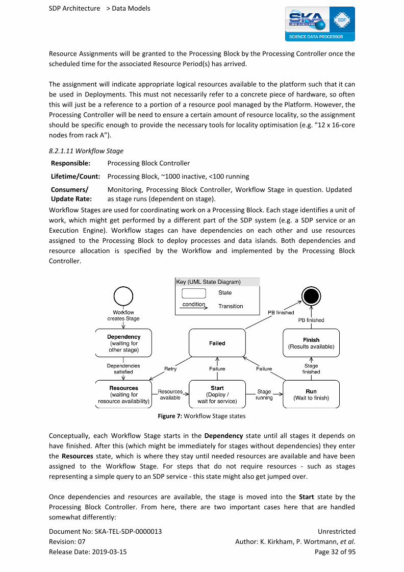
Workflow Stages are used for coordinating work on a Processing Block. Each stage identifies a unit of
work, which might get performed by a different part of the SDP system (e.g. a SDP service or an
Execution Engine). Workflow stages can have dependencies on each other and use resources
assigned to the Processing Block to deploy processes and data islands. Both dependencies and
resource allocation is specified by the Workflow and implemented by the Processing Block
Controller.
Figure 7: Workflow Stage states
Conceptually, each Workflow Stage starts in the Dependency state until all stages it depends on
have finished. After this (which might be immediately for stages without dependencies) they enter
the Resources state, which is where they stay until needed resources are available and have been
assigned to the Workflow Stage. For steps that do not require resources - such as stages
representing a simple query to an SDP service - this state might also get jumped over.
Once dependencies and resources are available, the stage is moved into the Start state by the
Processing Block Controller. From here, there are two important cases here that are handled
somewhat differently:
Document No: SKA-TEL-SDP-0000013 Unrestricted
Revision: 07 Author: K. Kirkham, P. Wortmann, et al. Release Date: 2019-03-15 Page 32 of 95

SDP Architecture > Data Models
1. Service stages are executed by the appropriate SDP service (e.g. Model Databases, Buffer,
Delivery…). This means that at this point the service in question is meant to pick up up all
necessary information from the configuration database and either do the work or deploy
worker components as needed.
2. On the other hand, Execution Engine will be deployed by the Processing Block Controller
itself. This will especially deploy the Execution Engine Interface implementation (see
Workflow Module View [RD05]), which from that point onwards is in charge of the Workflow
Stage.
The component performing the execution (Service / Execution Engine Interface) will perform
necessary initialisation steps and set the state to either Failed or Run depending on success. Failed
workflow stages are expected to deallocate resources (but not necessarily intermediate data
products) in a way that allows the Workflow Stage to be attempted again. If on the other hand the
Workflow Stage finishes successfully, all deployments are going to be freed and the state will be set
to Finished. This signals to the Processing Block Controller that the (intermediate) Data Products of
the stage are available, which might unblock dependent stages or cause the Processing Block to
finish.
8.2.1.12 Deployment
Responsible: Service or Processing Block Controller
Lifetime/Count: Service or Processing Block / Workflow Stage, ~100
Consumers/ Update Rate:
Platform, Controller that is monitoring deployment, ~minutes
Deployments describe reversible and repeatable changes to the platform configuration, such as
starting a container, hanging some hardware configuration - up to booting up an entire
infrastructure of hardware and software. The entirety of deployments contained in the configuration
database should describe the the exact Platform configuration of all parts of the Operational System.
This should be implemented according to best practices of IT Configuration Management or
infrastructure-as-code, which means that the Platform configuration is described by scripts for a
Platform-provided Configuration Management system, with Execution Control’s Configuration
Database providing the dynamic parameters. These scripts are described as “Configuration” in the
Platform Module View. Scripts parameters are going to be stored with the deployment entity.
The key property of deployments is that it should be possible to reliably un-do them without
knowledge about the details of the deployment’s function. This is critical to implement forced
resource deallocation in case services or Processing Blocks need to get aborted due to failures in
services or processing (see Execution Control C&C View).
Document No: SKA-TEL-SDP-0000013 Unrestricted
Revision: 07 Author: K. Kirkham, P. Wortmann, et al. Release Date: 2019-03-15 Page 33 of 95
SDP Architecture > Data Models
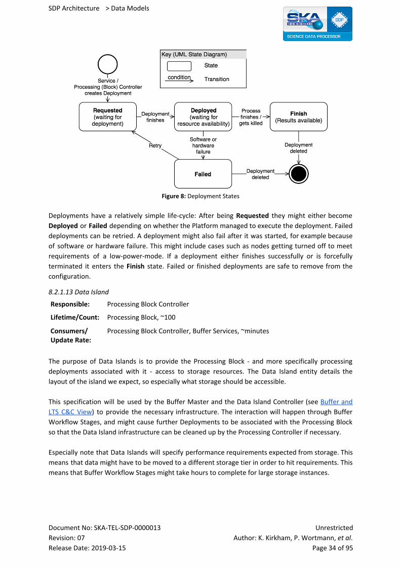
Figure 8: Deployment States
Deployments have a relatively simple life-cycle: After being Requested they might either become
Deployed or Failed depending on whether the Platform managed to execute the deployment. Failed
deployments can be retried. A deployment might also fail after it was started, for example because
of software or hardware failure. This might include cases such as nodes getting turned off to meet
requirements of a low-power-mode. If a deployment either finishes successfully or is forcefully
terminated it enters the Finish state. Failed or finished deployments are safe to remove from the
configuration.
8.2.1.13 Data Island
Responsible: Processing Block Controller
Lifetime/Count: Processing Block, ~100
Consumers/ Update Rate:
Processing Block Controller, Buffer Services, ~minutes
The purpose of Data Islands is to provide the Processing Block - and more specifically processing
deployments associated with it - access to storage resources. The Data Island entity details the
layout of the island we expect, so especially what storage should be accessible.
This specification will be used by the Buffer Master and the Data Island Controller (see Buffer and
LTS C&C View) to provide the necessary infrastructure. The interaction will happen through Buffer
Workflow Stages, and might cause further Deployments to be associated with the Processing Block
so that the Data Island infrastructure can be cleaned up by the Processing Controller if necessary.
Especially note that Data Islands will specify performance requirements expected from storage. This
means that data might have to be moved to a different storage tier in order to hit requirements. This
means that Buffer Workflow Stages might take hours to complete for large storage instances.
Document No: SKA-TEL-SDP-0000013 Unrestricted
Revision: 07 Author: K. Kirkham, P. Wortmann, et al. Release Date: 2019-03-15 Page 34 of 95
SDP Architecture > Data Models
8.2.1.14 Storage
Responsible: Processing Block Controller
Lifetime/Count: Processing Block, ~100
Consumers/ Update Rate:
Processing Block Controller, Buffer Services, ~minutes
Represents a storage instance made available to Processing through a Data Island. This can be used
by other deployments to read or write data stored in the Buffer.
While storage instances can be created in the context of Data Islands, storage instances are tracked
independently by the Buffer in the Storage Lifecycle Database (see Buffer and LTS C&C View). The
“Storage identification” is a reference to their canonical name of the Storage Instance for the
purpose of the Buffer. This means that if the Storage ID matches a storage instance used for another
Data Island, this means that the storage is meant to be shared between the Data Islands. This can
especially happen across Processing Blocks, which can be used to data produced by Receive or Data
Products of past Processing Blocks (which might have to be brought back from Long Term Storage)
The lifecycle policy of the storage (see Buffer Data Lifecycle View) is another attribute that will be
synchronised with (or to) the Storage Lifecycle Database. It decides what happens to the storage in
absence of references from the configuration, so i.e. after the processing block as finished or one of
the Data Islands gets released. Storage holding Data Products and other “precious” data will typically
indicate that the data is to be kept indefinitely (which can obviously be overridden later as
appropriate). Even for transient data such as received visibilities we might indicate a certain
minimum time that it needs to be kept alive before removal.
8.2.2 Relations and Their Properties
Most relations shown on the primary representation are hierarchical in nature and therefore are
expected to map well to a hierarchical namespace of a key-value store.
8.2.3 Element Interfaces
N/A
8.2.4 Element Behavior
Most of the dynamic behaviour of the Execution Control Data Model is about implementing the
various behaviours of Execution Control. In the Execution Control C&C View behaviour sections, a lot
of the interactions shown will either be accompanied by or accomplished through updates to the
SDP configuration managed by Execution Control.
8.3 Context Diagram The Execution Control Data Model stands mostly on its own, but has links to and overlaps with other
data models:
● The System-level Data Model View describes the information that will be exchanged with TM
as well as with processing (e.g. in storage or queues). Processing and Scheduling Block data is
something that will appear on both sides.
● The data model associated with the Buffer Lifecycle View interacts with the Data
Island/Storage management of the configuration.
Document No: SKA-TEL-SDP-0000013 Unrestricted
Revision: 07 Author: K. Kirkham, P. Wortmann, et al. Release Date: 2019-03-15 Page 35 of 95
SDP Architecture > Data Models
8.4 Variability Guide The Execution Control Data Model is meant to be flexible in allowing SDP to add and remove
functionality. A few examples:
● Services can easily be added and removed. Adding extra components is just a matter of
instructing the Master Controller to bring up a new type of deployment.
● Deployment types are not hard-coded, and resources are only managed at a fairly high level.
This means that the Platform is afforded a lot of freedom in how software is actually
deployed. Containers are likely going to be the default choice, but other options are still
possible - such as deploying images to bare metal, binaries on existing machines or Apache
Spark programs to Mesos clusters.
● Resource requirements are associated with coarse-grained Resource Periods, not with
Workflow Stages. This keeps scheduling complexity down and allows the Workflow to adjust
workflow stages to execute at basically any point.
● Workflow stages especially do not have explicit dependencies, instead the semantics of the
“Dependency” state is defined by the workflow in question. This means that we do not have
to enumerate all the different types of dependencies (e.g. via storage/queues/databases…).
8.5 Rationale The most important quality here is modifiability - see variability guide above.
8.6 Related Views The data shown here is kept in the Configuration Database in Execution Control, see Execution
Control C&C View.
8.7 Reference Documents The following documents are referenced in this document. In the event of conflict between the
contents of the referenced documents and this document, this document shall take precedence.
(no referenced documents)
Document No: SKA-TEL-SDP-0000013 Unrestricted
Revision: 07 Author: K. Kirkham, P. Wortmann, et al. Release Date: 2019-03-15 Page 36 of 95
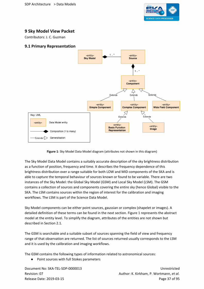
SDP Architecture > Data Models
9 Sky Model View Packet Contributors: J. C. Guzman
9.1 Primary Representation
Figure 1: Sky Model Data Model diagram (attributes not shown in this diagram)
The Sky Model Data Model contains a suitably accurate description of the sky brightness distribution
as a function of position, frequency and time. It describes the frequency dependence of this
brightness distribution over a range suitable for both LOW and MID components of the SKA and is
able to capture the temporal behaviour of sources known or found to be variable. There are two
instances of the Sky Model: the Global Sky Model (GSM) and Local Sky Model (LSM). The GSM
contains a collection of sources and components covering the entire sky (hence Global) visible to the
SKA. The LSM contains sources within the region of interest for the calibration and imaging
workflows. The LSM is part of the Science Data Model.
Sky Model components can be either point sources, gaussian or complex (shapelet or images). A
detailed definition of these terms can be found in the next section. Figure 1 represents the abstract
model at the entity level. To simplify the diagram, attributes of the entities are not shown but
described in Section 2.1.
The GSM is searchable and a suitable subset of sources spanning the field of view and frequency
range of that observation are returned. The list of sources returned usually corresponds to the LSM
and it is used by the calibration and imaging workflows.
The GSM contains the following types of information related to astronomical sources:
● Point sources with full Stokes parameters
Document No: SKA-TEL-SDP-0000013 Unrestricted
Revision: 07 Author: K. Kirkham, P. Wortmann, et al. Release Date: 2019-03-15 Page 37 of 95
SDP Architecture > Data Models
● Time variability
● Resolved sources using compact basis set representations
● Complex spectral structures
● Information on planetary and solar radiation sources
In the case of planetary and solar radiation sources, it is likely that the models will be taken from
existing external ephemeris services. Currently only major solar system objects are needed in the
GSM for the purpose of schedule and execute the SDP processes.
Large sources are split into multiple components: collections of Gaussians, shapelets, images, etc.
For extremely large sources like diffuse galactic emission, the GSM supports full sky image that
includes diffuse emission and it is up to the imager (A-projection, faceting, etc.) to incorporate
primary beam structure. Bright components in the galactic plane like supernova remnants (SNR) can
be added as separate collections of Gaussians, shapelets, (postage-stamp) images, etc. The imaging
workflow predict module, for instance, expects both a sky model image (for degridding) and sky
model components (to either be added to the image before degridding or predict using a direct
Fourier transform).
9.2 Element Catalogue 9.2.1 Elements and Their Properties
The sky model data model has the following structure:
● Source is defined as a 'real' astronomy source. This may consist of a number of separated
regions on the sky. For example a double radio source may have two extended 'lobes' of
emission with little or no emission in the region between them. A source consists of one or
more components.
● Component describes a single object component. This is one of:
○ Simple component described in terms of a Gaussian model appropriate for
unresolved or sources which are expected to be marginally resolved
○ Complex component where the representation is:
■ Image, or multiple sky images at different resolutions
■ Basis Function Representation where the structure is specified in terms of a
specified set of basis vectors. The representation may also have a frequency
dependence. The data model allows any basis set to be supported. For each
basis set corresponding code to interpret the basis is included in the
in-memory data-models module. Common basis sets include
● Shapelets. Generally a shapelet is an orthonormal polynomial
(Hermite) multiplied by a Gaussian. There are rectangular and polar
shapelets. A detailed mathematical representation of shapelets can
be found in [RD9.1].
● A series of delta functions - often referred to as “clean components”
● Spherical harmonics for structure on the sphere
○ Wide field component. This will be supported by the Healpix representation which
is a common standard for wide-field or near all-sky images and allows for a
multi-resolution representation.
Document No: SKA-TEL-SDP-0000013 Unrestricted
Revision: 07 Author: K. Kirkham, P. Wortmann, et al. Release Date: 2019-03-15 Page 38 of 95
SDP Architecture > Data Models
9.2.1.1 Source
Properties of the Source entity:
● Name. Astronomical name of the source (e.g. Fornax A, Cen A)
● Coordinates
○ Coordinate system
○ Epoch
○ Ephemeris data for solar-system objects
● Position expressed in coordinate system
● Extent expressed in coordinate system - used for searching on relevance
● Number of components
● Link or index to each component
● Quality information
9.2.1.2 Component
Component can be either a Simple, Complex (Shapelet or Image) or wide field. A component
contains a common list of attributes (frequency independent) and a list of attributes that are
dependent of type and frequency. Every component contains or is represented at least as a simple
component. Additional types of component can be added as an extension of the simple component
with additional attributes for the frequency dependant part.
The frequency-independent attributes of a component are mainly of the type (Simple, Shapelet,
Image or Wide-field) and its position in the reference coordinate system defined in the parent
source, that is: right ascension (RA) and declination (DEC), and its uncertainty in the measured (or
calculated) position.
The component contains frequency-dependant attributes. These attributes are usually of type
scalars or array (vector) of scalars with corresponding unit. Each of this attributes also has a
uncertainty value. The list of attributes for simple components are taken from [RD9.2] and contains
the following kind of attributes:
● Reference frequency
● Time when the attribute’s values were last updated
● Polarisation information (I, Q, U, V)
● Rotation Measure
● Spectral Indices per polarisation (as polynomial coefficients describing the model spectrum
of the component). There will be special cases of Faraday-complex linearly polarised
components (example, primary components) which will require a full spectrum information
instead of spectral indices.
● FWHM of the major and minor axis of the Gaussian
● Position angle or orientation of the gaussian
In addition to the list above, there is also an “origin” attribute which contains information of
instrument of origin this Model was obtained.
Document No: SKA-TEL-SDP-0000013 Unrestricted
Revision: 07 Author: K. Kirkham, P. Wortmann, et al. Release Date: 2019-03-15 Page 39 of 95

SDP Architecture > Data Models
For Complex component that are described as a shapelet, there are additional frequency-dependant
attributes the describe the shapelet coefficients (See [RD9.1]).
When the component cannot be described as a shapelet, an image of the component is stored in the
data model. This image contains also metadata information and frequency dependant information.
In order to support time variability, for a determined component uniquely identified by position and
frequency, there will be multiple values in time. The time will be the time when the attributes were
calculated (or the image obtained).
A wide field component is represented as a HEALpix data entity. The logical data model for HEALpix
is described in [RD9.7].
9.2.2 Relations and Their Properties
The relations between the entities are either composition (part-of) or generalisation (is an extension)
are depicted in Figure 1. The GSM and LSM are instances of the abstract Sky Model entity described
here.
The GSM is usually queried by the calibration and/or imaging workflows.
9.2.3 Element Interfaces
This document describes mainly the data structure contained in the Sky Model. Despite not being
specific on the implementation, it is important to describe here the intended usage of this data as
part of future implementation of the module or service which supports the Sky Model. Access to the
Global Sky Model will be an API supported by the service implementation.
The interface to the Sky Model should support:
● Interface for managing source entries
● Insert, Read, Update and Delete operations.
The primary consumer of this data will be the calibration and imaging workflows. This module will
query the Global Sky Model “service” in order to obtain the local sky model of the observing field.
This query is usually in the form of cone search around a centre position of the sky and frequency.
The return will be a list (table) describing each source component in the region of interest.
9.2.4 Element Behavior
Insertion of new values for a component in the internal catalogue are added to the database with a
corresponding timestamp. Consumer requesting a cone search by default will return a list of sources
and components with the most up-to-date attribute values (simple or complex). Alternatively the
GSM will support other type of query parameters such as time or frequency.
The service will likely search the internal catalogue first for sources and components in the region. If
no sources are found, the service will search external catalogues.
Document No: SKA-TEL-SDP-0000013 Unrestricted
Revision: 07 Author: K. Kirkham, P. Wortmann, et al. Release Date: 2019-03-15 Page 40 of 95
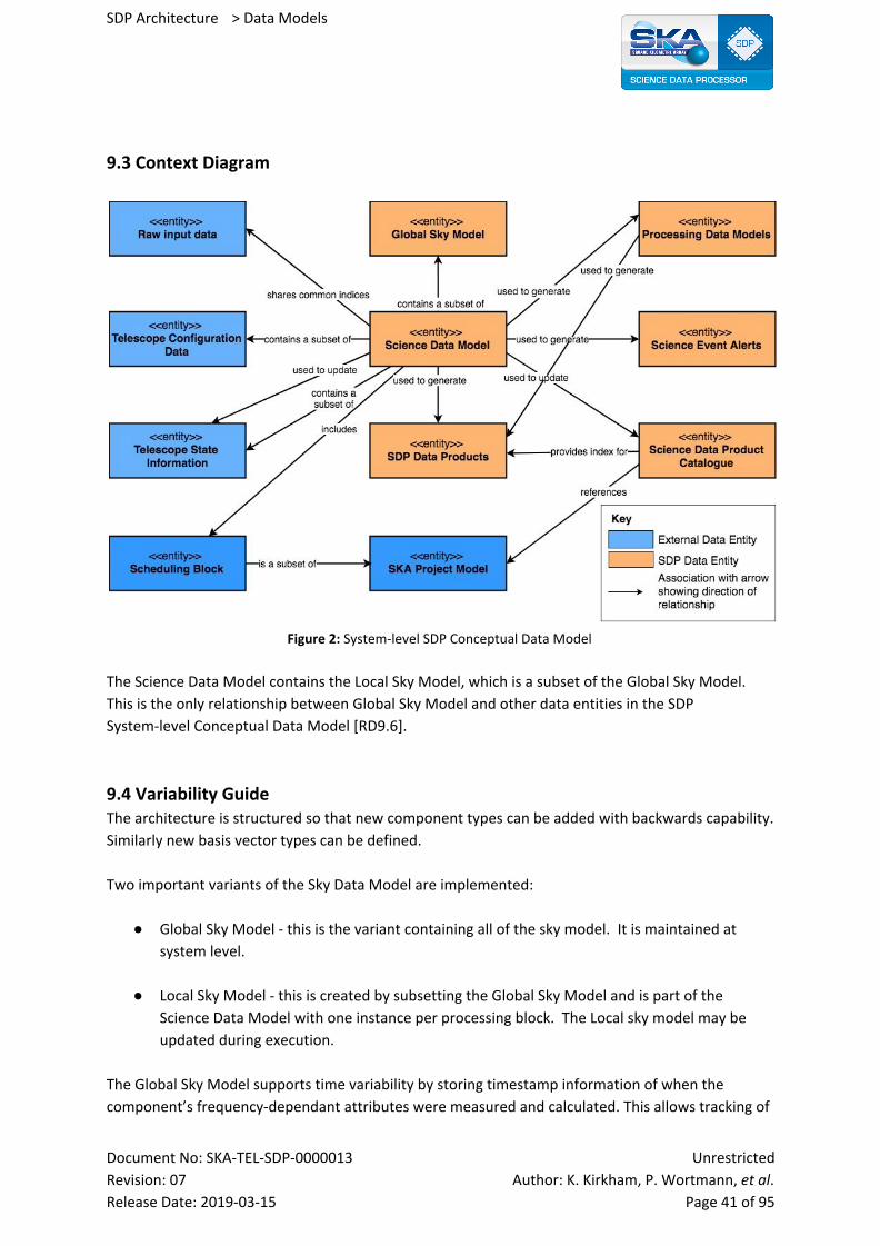
SDP Architecture > Data Models
9.3 Context Diagram
Figure 2: System-level SDP Conceptual Data Model
The Science Data Model contains the Local Sky Model, which is a subset of the Global Sky Model.
This is the only relationship between Global Sky Model and other data entities in the SDP
System-level Conceptual Data Model [RD9.6].
9.4 Variability Guide The architecture is structured so that new component types can be added with backwards capability.
Similarly new basis vector types can be defined.
Two important variants of the Sky Data Model are implemented:
● Global Sky Model - this is the variant containing all of the sky model. It is maintained at
system level.
● Local Sky Model - this is created by subsetting the Global Sky Model and is part of the
Science Data Model with one instance per processing block. The Local sky model may be
updated during execution.
The Global Sky Model supports time variability by storing timestamp information of when the
component’s frequency-dependant attributes were measured and calculated. This allows tracking of
Document No: SKA-TEL-SDP-0000013 Unrestricted
Revision: 07 Author: K. Kirkham, P. Wortmann, et al. Release Date: 2019-03-15 Page 41 of 95
SDP Architecture > Data Models
changes in the component’s attributes. There is an additional attribute, ORIGIN which allows
capturing the origin of this component, whether internal (SKA instrument) or from an external
catalogue or instrument.
9.5 Rationale The need for a Sky Model is nothing new in radio interferometry. Most of the existing calibration and
imaging software packages rely on some form of sky model. LOFAR [RD9.4] and ASKAP [RD9.3]
telescopes have implemented similar services that support a Global Sky Model for their calibration
and imaging needs. Most of the entities and its attributes are found also in external catalogues (see
Section 2 of [RD9.2]).
Most of the entities and attributes described in this document were collated from existing
implementations and adapted for SKA, including the option of extending the types of components.
9.6 Related Views ● Image data model view
● System-level Data Model View
● Science Data Model View
● ICAL Workflow View Packet
● Imaging Workflow View Packet
9.7 References The following documents are referenced in this document. In the event of conflict between the
contents of the referenced documents and this document, this document shall take precedence.
[RD9.1] Yatawatta, “Shapelets and Related Techniques in Radio-Astronomical Imaging,” URSI GA, Istanbul, Turkey, Aug. 2011.
[RD9.2] SKA-TEL-SDP-0000139 SDP Memo 033: Sky Model Considerations
[RD9.3] CSIRO ASKAP Science Data Archive Data Model schema
[RD9.4] The LOFAR Transient Pipeline online documentation https://tkp.readthedocs.io/en/r3.0/devref/database/schema.html#database-schema
[RD9.5] Scheers, L. H. A. (2011). Transient and variable radio sources in the LOFAR sky: an architecture for a detection framework https://dare.uva.nl/search?identifier=68164d5a-7bba-42bf-8638-876678ecb1d4
[RD9.7] https://healpix.jpl.nasa.gov
Document No: SKA-TEL-SDP-0000013 Unrestricted
Revision: 07 Author: K. Kirkham, P. Wortmann, et al. Release Date: 2019-03-15 Page 42 of 95
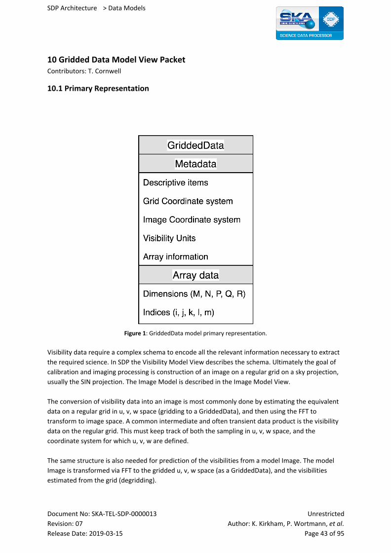
SDP Architecture > Data Models
10 Gridded Data Model View Packet Contributors: T. Cornwell
10.1 Primary Representation
Figure 1: GriddedData model primary representation.
Visibility data require a complex schema to encode all the relevant information necessary to extract
the required science. In SDP the Visibility Model View describes the schema. Ultimately the goal of
calibration and imaging processing is construction of an image on a regular grid on a sky projection,
usually the SIN projection. The Image Model is described in the Image Model View.
The conversion of visibility data into an image is most commonly done by estimating the equivalent
data on a regular grid in u, v, w space (gridding to a GriddedData), and then using the FFT to
transform to image space. A common intermediate and often transient data product is the visibility
data on the regular grid. This must keep track of both the sampling in u, v, w space, and the
coordinate system for which u, v, w are defined.
The same structure is also needed for prediction of the visibilities from a model Image. The model
Image is transformed via FFT to the gridded u, v, w space (as a GriddedData), and the visibilities
estimated from the grid (degridding).
Document No: SKA-TEL-SDP-0000013 Unrestricted
Revision: 07 Author: K. Kirkham, P. Wortmann, et al. Release Date: 2019-03-15 Page 43 of 95
SDP Architecture > Data Models
There are three reasons for elevating the gridded data to a well-defined model:
1. GriddedData is a required science product for some HPSOs (e.g. lensing)
2. Binding the grid and coordinates into one Model allows compact interfaces
3. Many gridding/degridding gridding algorithms make use of a set of common functions
In addition to this most commonly used approach to gridding the data prior to an FFT, there are
other newer approaches that proceed differently. For example, IDG ([RD10.1]) transforms patches of
data to the image plane directly and then performs an inverse transform back to uv space. This in
effect grids the data and the GriddedData model can be used as an intermediate product. Another
relatively new technique, w-stacking ([RD10.2]) can be implemented as a collection of GriddedData
(as done, for example, in the ARL).
10.2 Element Catalogue
10.2.1 Element and Their Properties
The grid data type consists of metadata and array data.
The metadata are
● Grid coordinate system: maps the indices of the array data to the physical coordinates of the
pixels. Typically the axes are u, v, w, frequency. The axes u, v, w are conjugate to the image
coordinate system. The definition comes from the SDM.
● Image coordinate system: Describes the image plane coordinate system associated with the
grid coordinate system i.e. the direction, frame, and projection. The definition comes from
the SDM. Note that image coordinate system can be in l, m, n (i.e. a cube encompassing part
of the celestial sphere). Note that there is no Image data just the coordinate system.
● Visibility units: the units of the visibility data, such as Jy, None. The definition comes from
the SDM.
● Array information: information on the size and layout of the array data. Possible layouts are
described in Section 2.6.
The array data consists of a four-dimensional array of pixels (U, V, W, frequency). The elements in
the array are can be typed e.g. float, complex, visibility as a 4-vector, visibility as a 2x2 matrix.
10.2.2 Relations and Their Properties
n/a
10.2.3 Element Interfaces
GriddedData plays a central role in imaging. The interfaces are not listed here. Instead we list the
functions that must be supported by the GriddedData API:
● Construction from Image Data and Visibility Data.
● Gridding: insertion of visibility values using e.g. convolutional gridding. W, A, and I projection
are supported.
Document No: SKA-TEL-SDP-0000013 Unrestricted
Revision: 07 Author: K. Kirkham, P. Wortmann, et al. Release Date: 2019-03-15 Page 44 of 95
SDP Architecture > Data Models
● De-gridding: extraction of visibility values using e.g. convolutional degridding. W, A, and I
projection are supported.
● Anti-aliasing, including correction in image space.
● Fourier transforms: from Image Model, using a number of algorithms e.g. 2D FFT, W
stacking, 3D FFT. Sub-sectioning and shifts in both Image and UVW are required.
● Inverse Fourier transform: to Image Model, using a number of algorithms e.g. 2D FFT, W
stacking, 3D FFT. Sub-sectioning and shifts in both Image and UVW are required.
● Weighting such as noise inverse-variance weighting, robust weighting, uniform weighting.
● Tapering with UV coordinate, such as Gaussian or Tukey tapering.
● Bad data flagging, for example by deviation from the gridded data in u,v,w neighbourhood
● Addition, subtraction and other dyadics.
● Insertion into and extraction from other GriddedData,
● Persistence (e.g. via the SDP Buffer)
● Conversion to science data product.
10.2.4 Element Behavior
The element is a passive data holder. It is constructed, manipulated by various functions, persisted
and moved as required, and ultimately converted to a Science Data product.
10.2.5 Indices and Keys
The grid array data indices are mapped by the coordinate system to and from the world coordinates
of the pixel in the grid. The spatial axes (u, v, w) are in the projection specified by the image
coordinate system.
10.2.6 Structure and Access Patterns
GriddedData participates in some of the most resource-hungry processing. The primary access
patterns are:
● By pixel (e.g. visibility 4-vector or 2x2-matrix).
● Random access in u,v and possibly w, needed for gridding and degridding. Slowly changing
locality can be used to limit access rates.
● Regular access for FFTs, separately for each channel.
● Strided access for GriddedData being used as an oversampled convolution function.
Parallel access is required so that different parts of the grid may be read or written simultaneously.
10.3 Context Diagram Gridded Data is used in imaging steps Predict and Invert as defined in the Imaging Data Model view.
See figure 2. There are summations implied at the termination of the partition loops so that the
predicted visibility is the sum over all partitions and the image is the (weighted) sum over all
partitions.
Document No: SKA-TEL-SDP-0000013 Unrestricted
Revision: 07 Author: K. Kirkham, P. Wortmann, et al. Release Date: 2019-03-15 Page 45 of 95
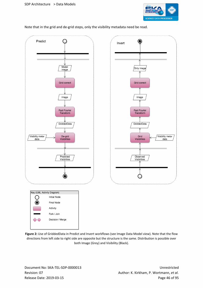
SDP Architecture > Data Models
Note that in the grid and de-grid steps, only the visibility metadata need be read.
Figure 2: Use of GriddedData in Predict and Invert workflows (see Image Data Model view). Note that the flow
directions from left side to right side are opposite but the structure is the same. Distribution is possible over
both Image (Grey) and Visibility (Black).
Document No: SKA-TEL-SDP-0000013 Unrestricted
Revision: 07 Author: K. Kirkham, P. Wortmann, et al. Release Date: 2019-03-15 Page 46 of 95

SDP Architecture > Data Models
Distribution of these workflows is possible using many methods:
● W stacking: W has multiple planes ([RD10.2])Time slices: a collection of GriddedData, one for
each snapshot.
● Facets: a collection of GriddedData, one for each facet
● Image Domain Gridding: IDG ([RD10.1]) decomposes into a collection of multiple DataGrids,
one per subsection of uvw space.
10.4 Variability Guide GriddedData will vary according to algorithm and partitioning. Some examples:
● 2D and w projection imaging: W is a single plane.
● W stacking: W has multiple planes.
● Combined W stacking/W projection is also possible. The range in W is limited to the gap
between slices.
● Time slices: a collection of GriddedData, one for each snapshot. Time is not necessarily a
regular axis so we use a collection rather than encoding Time into a regular axis.
● Facets: a collection of GriddedData, one for each facet. Similarly to Time, we use a collection
rather than encoding facet number into an axis.
● Image Domain Gridding: IDG decomposes into multiple GriddedData.
10.5 Rationale ● GriddedData is a science data product, needed for lensing studies, for example.
● GriddedData may be the result of a complex processing chain including calibration, flagging,
model subtraction.
● FFT’s for the SKA context often dominate the processing costs. The GriddedData model
allows co-addition of grids prior to FFTs instead of co-adding dirty images after FFT’s.
● Convolution functions can use the GriddedData interface by specifying an appropriate offset
and stride into a GriddedData.
● Development of gridding/degridding algorithms is likely to continue for the foreseeable
future. GriddedData is useful in expressing current and new algorithms.
● Detailed tracking of coordinate systems in both Image and Fourier space is essential to
problem partitioning.
● Use of GriddedData factors existing algorithms in a more compact and robust form.
● Storing results in GriddedData format allows avoidance of the zero-padding bloat incurred in
the FFT (though this also could be done by storing critically sampled images and sinc
interpolation before e.g. cleaning.)
10.6 Related Views ● Image Data Model View
● Visibility Data Model View
● Imaging Data Model View
Document No: SKA-TEL-SDP-0000013 Unrestricted
Revision: 07 Author: K. Kirkham, P. Wortmann, et al. Release Date: 2019-03-15 Page 47 of 95

SDP Architecture > Data Models
10.7 References
The following documents are referenced in this document. In the event of conflict between the
contents of the referenced documents and this document, this document shall take precedence.
[RD10.1] Sebastiaan van der Tol, Bram Veenboer, and André R. Offringa, Image Domain Gridding: a fast method for convolutional resampling of visibilities. A&A, Volume 616, August 2018
[RD10.2] T. J. Cornwell, M. A. Voronkov, and B. Humphreys, “Wide field imaging for the Square Kilometre Array,” arXiv.org, vol. astro-ph.IM. SPIE, p. 5861, 25-Jul-2012.
Document No: SKA-TEL-SDP-0000013 Unrestricted
Revision: 07 Author: K. Kirkham, P. Wortmann, et al. Release Date: 2019-03-15 Page 48 of 95
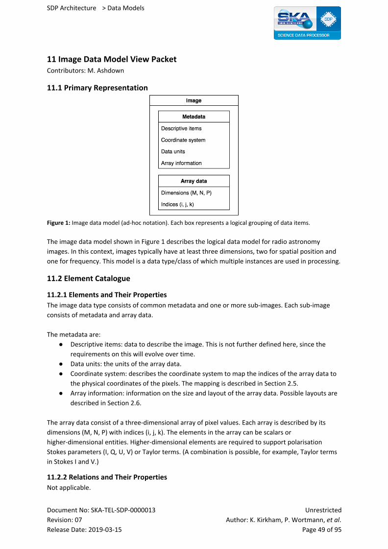
SDP Architecture > Data Models
11 Image Data Model View Packet Contributors: M. Ashdown
11.1 Primary Representation
Figure 1: Image data model (ad-hoc notation). Each box represents a logical grouping of data items.
The image data model shown in Figure 1 describes the logical data model for radio astronomy
images. In this context, images typically have at least three dimensions, two for spatial position and
one for frequency. This model is a data type/class of which multiple instances are used in processing.
11.2 Element Catalogue
11.2.1 Elements and Their Properties
The image data type consists of common metadata and one or more sub-images. Each sub-image
consists of metadata and array data.
The metadata are:
● Descriptive items: data to describe the image. This is not further defined here, since the
requirements on this will evolve over time.
● Data units: the units of the array data.
● Coordinate system: describes the coordinate system to map the indices of the array data to
the physical coordinates of the pixels. The mapping is described in Section 2.5.
● Array information: information on the size and layout of the array data. Possible layouts are
described in Section 2.6.
The array data consist of a three-dimensional array of pixel values. Each array is described by its
dimensions (M, N, P) with indices (i, j, k). The elements in the array can be scalars or
higher-dimensional entities. Higher-dimensional elements are required to support polarisation
Stokes parameters (I, Q, U, V) or Taylor terms. (A combination is possible, for example, Taylor terms
in Stokes I and V.)
11.2.2 Relations and Their Properties
Not applicable.
Document No: SKA-TEL-SDP-0000013 Unrestricted
Revision: 07 Author: K. Kirkham, P. Wortmann, et al. Release Date: 2019-03-15 Page 49 of 95
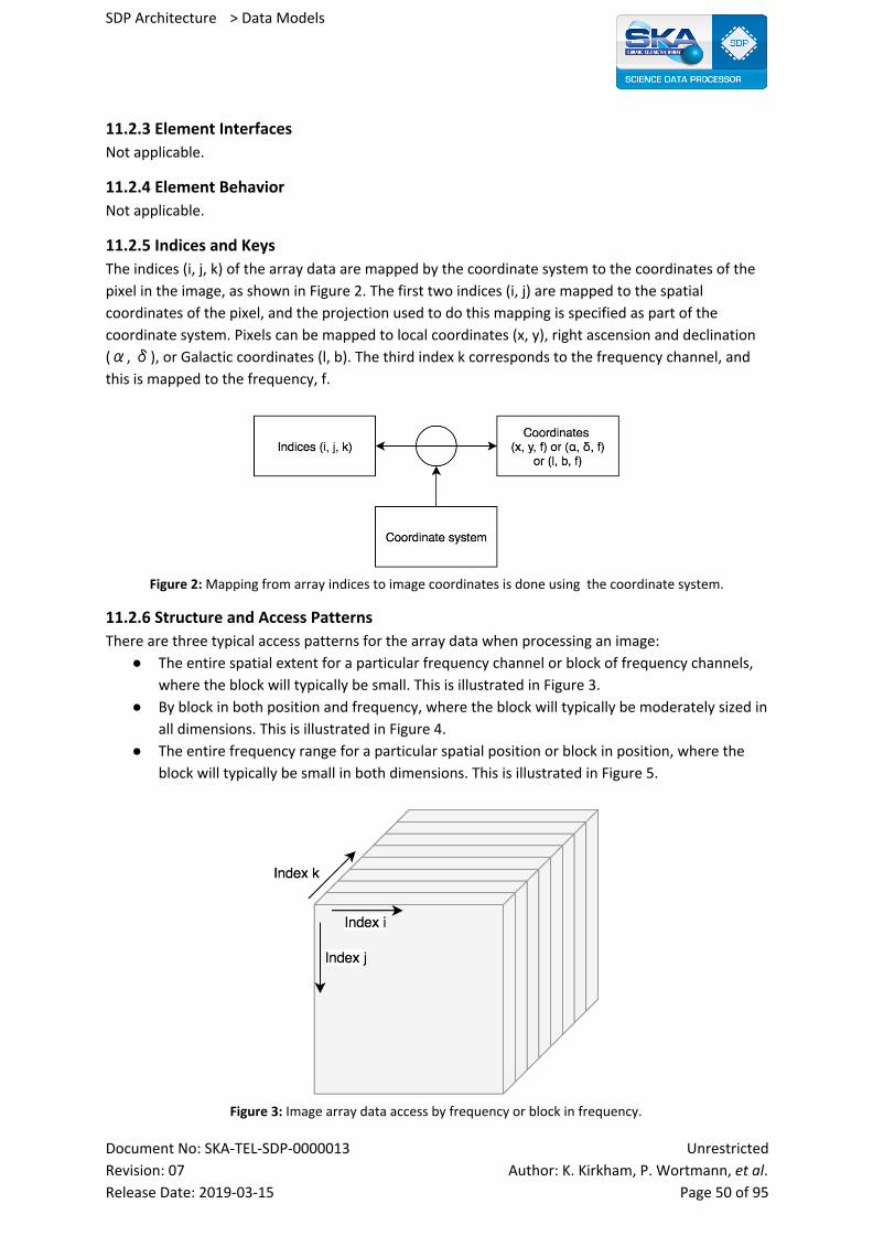
SDP Architecture > Data Models
11.2.3 Element Interfaces
Not applicable.
11.2.4 Element Behavior
Not applicable.
11.2.5 Indices and Keys
The indices (i, j, k) of the array data are mapped by the coordinate system to the coordinates of the
pixel in the image, as shown in Figure 2. The first two indices (i, j) are mapped to the spatial
coordinates of the pixel, and the projection used to do this mapping is specified as part of the
coordinate system. Pixels can be mapped to local coordinates (x, y), right ascension and declination
(α, δ), or Galactic coordinates (l, b). The third index k corresponds to the frequency channel, and
this is mapped to the frequency, f.
Figure 2: Mapping from array indices to image coordinates is done using the coordinate system.
11.2.6 Structure and Access Patterns
There are three typical access patterns for the array data when processing an image:
● The entire spatial extent for a particular frequency channel or block of frequency channels,
where the block will typically be small. This is illustrated in Figure 3.
● By block in both position and frequency, where the block will typically be moderately sized in
all dimensions. This is illustrated in Figure 4.
● The entire frequency range for a particular spatial position or block in position, where the
block will typically be small in both dimensions. This is illustrated in Figure 5.
Figure 3: Image array data access by frequency or block in frequency.
Document No: SKA-TEL-SDP-0000013 Unrestricted
Revision: 07 Author: K. Kirkham, P. Wortmann, et al. Release Date: 2019-03-15 Page 50 of 95
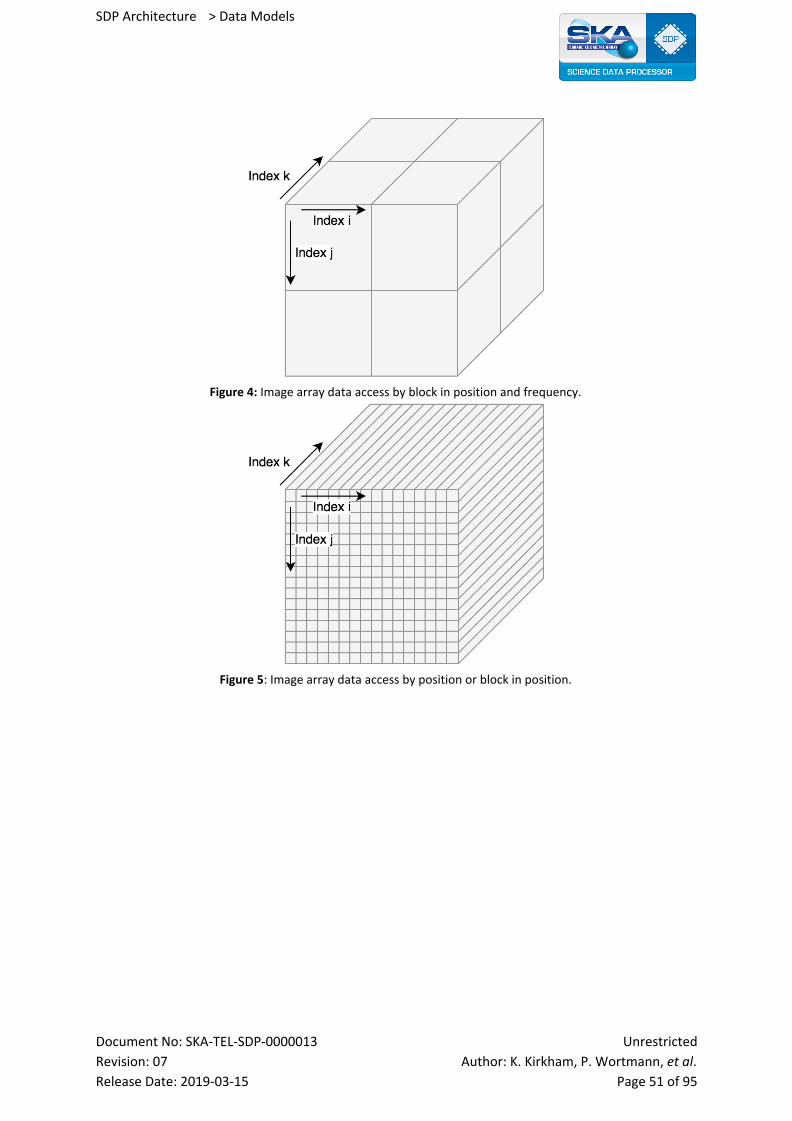
SDP Architecture > Data Models
Figure 4: Image array data access by block in position and frequency.
Figure 5: Image array data access by position or block in position.
Document No: SKA-TEL-SDP-0000013 Unrestricted
Revision: 07 Author: K. Kirkham, P. Wortmann, et al. Release Date: 2019-03-15 Page 51 of 95
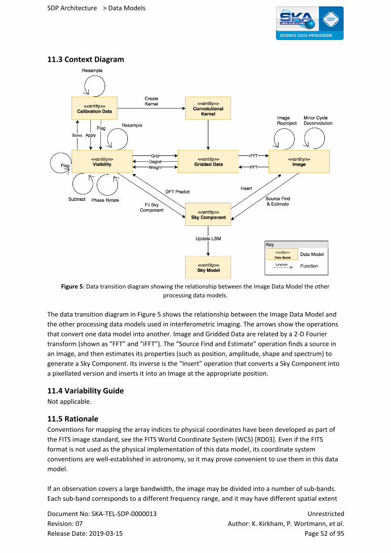
SDP Architecture > Data Models
11.3 Context Diagram
Figure 5: Data transition diagram showing the relationship between the Image Data Model the other
processing data models.
The data transition diagram in Figure 5 shows the relationship between the Image Data Model and
the other processing data models used in interferometric imaging. The arrows show the operations
that convert one data model into another. Image and Gridded Data are related by a 2-D Fourier
transform (shown as “FFT” and “iFFT”). The “Source Find and Estimate” operation finds a source in
an Image, and then estimates its properties (such as position, amplitude, shape and spectrum) to
generate a Sky Component. Its inverse is the “Insert” operation that converts a Sky Component into
a pixellated version and inserts it into an Image at the appropriate position.
11.4 Variability Guide Not applicable.
11.5 Rationale Conventions for mapping the array indices to physical coordinates have been developed as part of
the FITS image standard, see the FITS World Coordinate System (WCS) [RD03]. Even if the FITS
format is not used as the physical implementation of this data model, its coordinate system
conventions are well-established in astronomy, so it may prove convenient to use them in this data
model.
If an observation covers a large bandwidth, the image may be divided into a number of sub-bands.
Each sub-band corresponds to a different frequency range, and it may have different spatial extent
Document No: SKA-TEL-SDP-0000013 Unrestricted
Revision: 07 Author: K. Kirkham, P. Wortmann, et al. Release Date: 2019-03-15 Page 52 of 95
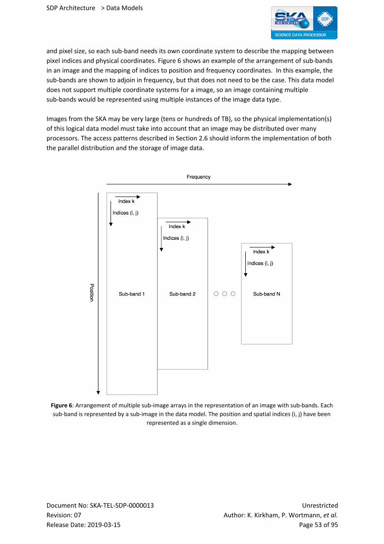
SDP Architecture > Data Models
and pixel size, so each sub-band needs its own coordinate system to describe the mapping between
pixel indices and physical coordinates. Figure 6 shows an example of the arrangement of sub-bands
in an image and the mapping of indices to position and frequency coordinates. In this example, the
sub-bands are shown to adjoin in frequency, but that does not need to be the case. This data model
does not support multiple coordinate systems for a image, so an image containing multiple
sub-bands would be represented using multiple instances of the image data type.
Images from the SKA may be very large (tens or hundreds of TB), so the physical implementation(s)
of this logical data model must take into account that an image may be distributed over many
processors. The access patterns described in Section 2.6 should inform the implementation of both
the parallel distribution and the storage of image data.
Figure 6: Arrangement of multiple sub-image arrays in the representation of an image with sub-bands. Each
sub-band is represented by a sub-image in the data model. The position and spatial indices (i, j) have been
represented as a single dimension.
Document No: SKA-TEL-SDP-0000013 Unrestricted
Revision: 07 Author: K. Kirkham, P. Wortmann, et al. Release Date: 2019-03-15 Page 53 of 95

SDP Architecture > Data Models
11.6 Related Views The Processing Component Module View provides the context for this view as shown in Section 3.
11.7 Reference Documents The following documents are referenced in this document. In the event of conflict between the
contents of the referenced documents and this document, this document shall take precedence.
[RD11.1] FITS World Coordinate System (WCS), https://fits.gsfc.nasa.gov/fits_wcs.html
Document No: SKA-TEL-SDP-0000013 Unrestricted
Revision: 07 Author: K. Kirkham, P. Wortmann, et al. Release Date: 2019-03-15 Page 54 of 95

SDP Architecture > Data Models
12 Processing Data Model View Packet Contributors: J. C. Guzman
12.1 Primary Representation
Figure 1: Primary Representation of the Processing Data Model
The Processing Data Model is a placeholder for all data created, updated or transformed by the
imaging or non-imaging workflows. The Processing Data Model is mainly a generalisation of different
types of data model handled by the workflow pipelines, such as visibilities, gridded data and images
as depicted in Figure 1. As a general logical data model, the Processing Data Model contains
metadata and n-dimensional data, commonly referred as data cubes. Most of this document (and
individual element Views) describes the logical representation of the model.
This data model was previously called intermediate data models as it represents mainly the data
consumed and produced by the scientific workflow pipelines that are not required to be sent to the
Delivery system, hence stored indefinitely or part of the Science Data Products. This data model
currently extends to n-dimensional data such as visibilities, gridded data and images, but could be
extended to other intermediate data products in the future.
Document No: SKA-TEL-SDP-0000013 Unrestricted
Revision: 07 Author: K. Kirkham, P. Wortmann, et al. Release Date: 2019-03-15 Page 55 of 95
SDP Architecture > Data Models
This document follows from the System-level Data Model View to decompose further into individual
data models that are handled by the workflow pipeline. These individual data models are described
briefly in the next section and further detailed on their own View packet.
12.2 Element Catalogue
12.2.1 Elements and Their Properties
12.2.1.1 Imaging Data Models
12.2.1.1.1 Visibility
The Visibility Data Model describes the data structures containing visibilities, weights, flags and
UVW-coordinates. It does not describe the visibility data format as it comes from the correlator. The
latter is described in the CSP - SDP ICD [AD10].
The Visibility Data Model comprises of metadata and a high-dimensional data cube. The metadata
contains all necessary information to perform calibration and imaging tasks. The high-dimensional
cube of data consists of visibility, weights, flags and UVW coordinates. Different types of axes can be
used to access the high-dimensional cube of data: time, frequency, baseline, etc.
A detailed description of the Visibility Data Model can be found following this view.
12.2.1.1.2 Image
The Image Data Model consists of metadata and an array of data. The metadata contains descriptive
information about the radio astronomical image (could include instrument information or telescope
configuration data), world coordinate system, units of the data and description of the array. The
array data consist of a three-dimensional array of pixel values.
There are different types of images depending on the task or algorithms executing within the
imaging workflow pipeline:
● Residual Image
● Sky Components / shapelets
● Dirty Image
● PSF Image
Detailed Image Data Model is described above.
12.2.1.1.3 Gridded Data
Gridded data is a rectangular array of complex values. Probably 8-byte floats are needed to have
sufficient accuracy. The shape of the array is the same as the shape of the image. Probably it’ll even
be larger to accommodate image padding. For Continuum Imaging a few Taylor terms have to be
used in order to solve for the spectral index. For Spectral Line Imaging one image is made per
frequency channel and no Taylor Terms are added.
There are two compositions of Gridded Data:
● Time slices: a collection of GriddedData, one for each snapshot.
Document No: SKA-TEL-SDP-0000013 Unrestricted
Revision: 07 Author: K. Kirkham, P. Wortmann, et al. Release Date: 2019-03-15 Page 56 of 95
SDP Architecture > Data Models
● Facets: a collection of GriddedData, one for each facet
● Convolution Kernels such as: w-kernel, a-kernel, anti-aliasing, over-sampled.
The detailed Gridded Data Model is described above.
12.2.1.2 Non-Imaging Data Models
The Non-Imaging Data Models is a generalisation of data used by different non-imaging workflow
pipelines:
● Pulsar Search
● Single Pulse (Fast transient) Search
● Pulsar Timing Mode
● Dynamic Spectrum Mode
● Flow Through Mode
The detailed Non-Imaging Data Model is described below.
12.2.2 Relations and Their Properties
Processing Data Models are related to the Science Data Products (Calibrated UV grids) and to the
Science Data Model (Local Sky Model). A Local Sky Model is needed by the imaging workflow to
generate a Model Image. A detailed description of the relationship between these data models is in
the Processing Component Module View.
Gridded Data (UV Grids) generated by the imaging pipeline workflow will be stored as Science Data
Products.
Bear in mind that several of the Processing Data Models are also used by the calibration pipeline
workflows. There is a Calibration Data Model describing these in greater detail.
12.2.3 Element Behavior
Processing Data Models are primarily consumed or produced by the imaging and non-imaging
processing components. Transitions between data models are performed by algorithms present in
the processing components module. Details of these transitions are described in the Processing
Component Data Module View.
Document No: SKA-TEL-SDP-0000013 Unrestricted
Revision: 07 Author: K. Kirkham, P. Wortmann, et al. Release Date: 2019-03-15 Page 57 of 95
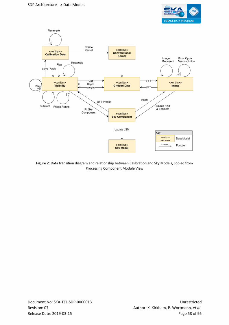
SDP Architecture > Data Models
Figure 2: Data transition diagram and relationship between Calibration and Sky Models, copied from
Processing Component Module View
Document No: SKA-TEL-SDP-0000013 Unrestricted
Revision: 07 Author: K. Kirkham, P. Wortmann, et al. Release Date: 2019-03-15 Page 58 of 95
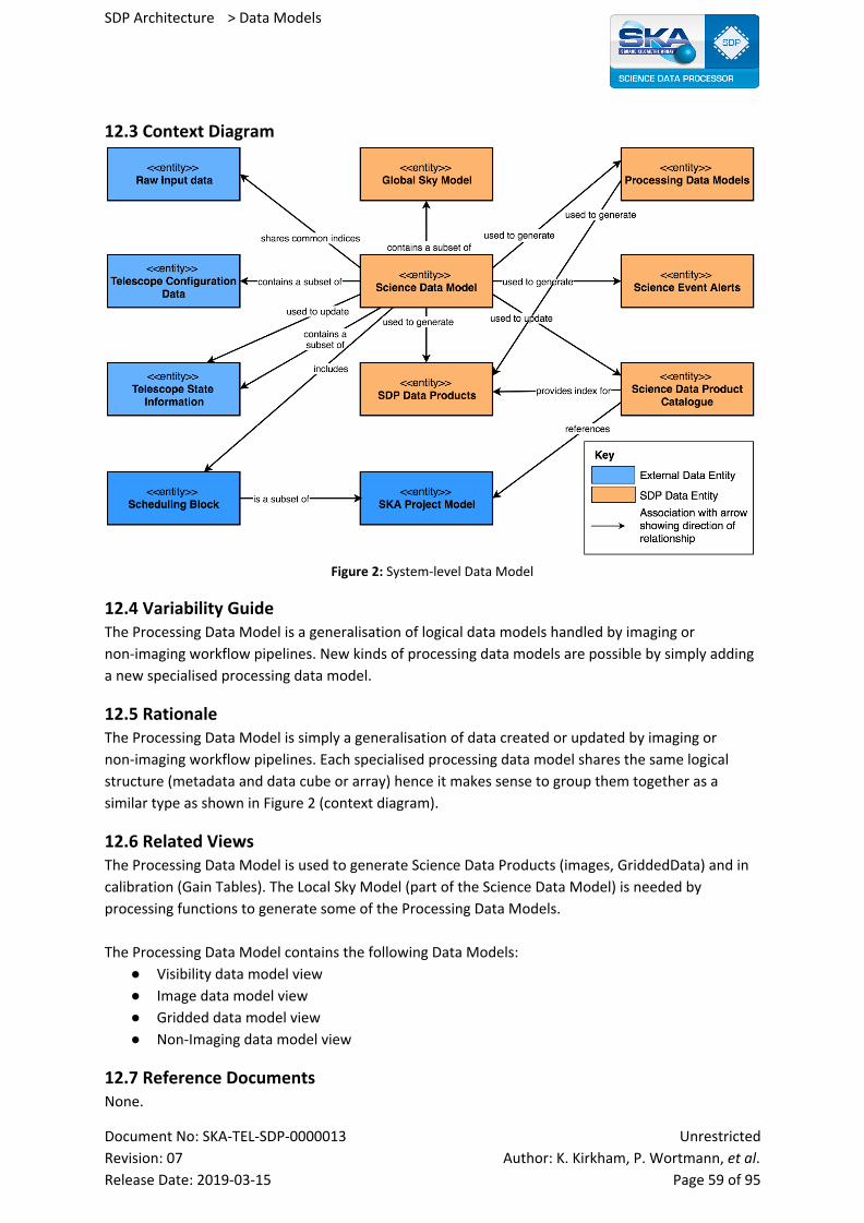
SDP Architecture > Data Models
12.3 Context Diagram
Figure 2: System-level Data Model
12.4 Variability Guide The Processing Data Model is a generalisation of logical data models handled by imaging or
non-imaging workflow pipelines. New kinds of processing data models are possible by simply adding
a new specialised processing data model.
12.5 Rationale The Processing Data Model is simply a generalisation of data created or updated by imaging or
non-imaging workflow pipelines. Each specialised processing data model shares the same logical
structure (metadata and data cube or array) hence it makes sense to group them together as a
similar type as shown in Figure 2 (context diagram).
12.6 Related Views The Processing Data Model is used to generate Science Data Products (images, GriddedData) and in
calibration (Gain Tables). The Local Sky Model (part of the Science Data Model) is needed by
processing functions to generate some of the Processing Data Models.
The Processing Data Model contains the following Data Models:
● Visibility data model view
● Image data model view
● Gridded data model view
● Non-Imaging data model view
12.7 Reference Documents None.
Document No: SKA-TEL-SDP-0000013 Unrestricted
Revision: 07 Author: K. Kirkham, P. Wortmann, et al. Release Date: 2019-03-15 Page 59 of 95
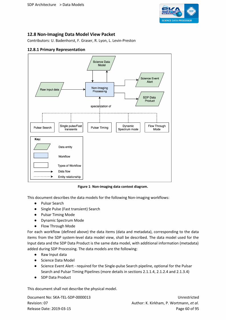
SDP Architecture > Data Models
12.8 Non-Imaging Data Model View Packet Contributors: U. Badenhorst, F. Graser, R. Lyon, L. Levin-Preston
12.8.1 Primary Representation
Figure 1: Non-imaging data context diagram.
This document describes the data models for the following Non-imaging workflows:
● Pulsar Search
● Single Pulse (Fast transient) Search
● Pulsar Timing Mode
● Dynamic Spectrum Mode
● Flow Through Mode
For each workflow (defined above) the data items (data and metadata), corresponding to the data
items from the SDP system-level data model view, shall be described. The data model used for the
Input data and the SDP Data Product is the same data model, with additional information (metadata)
added during SDP Processing. The data models are the following:
● Raw Input data
● Science Data Model
● Science Event Alert - required for the Single-pulse Search pipeline, optional for the Pulsar
Search and Pulsar Timing Pipelines (more details in sections 2.1.1.4, 2.1.2.4 and 2.1.3.4)
● SDP Data Product
This document shall not describe the physical model.
Document No: SKA-TEL-SDP-0000013 Unrestricted
Revision: 07 Author: K. Kirkham, P. Wortmann, et al. Release Date: 2019-03-15 Page 60 of 95
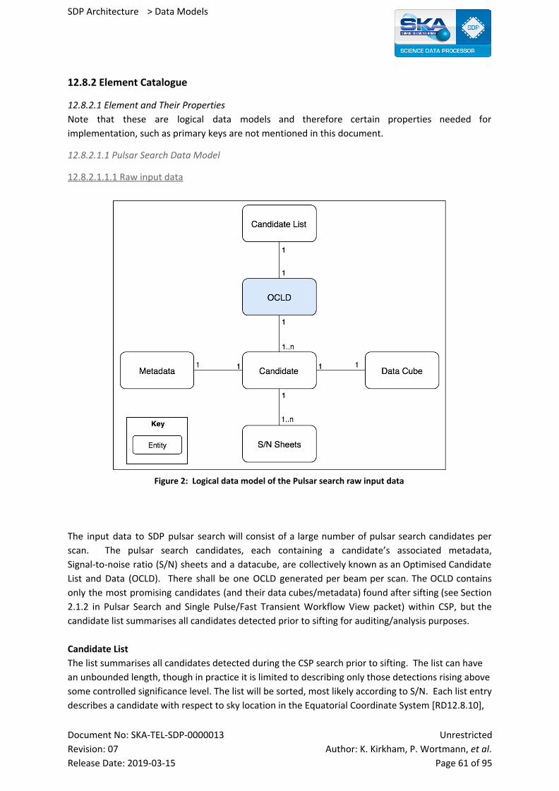
SDP Architecture > Data Models
12.8.2 Element Catalogue
12.8.2.1 Element and Their Properties
Note that these are logical data models and therefore certain properties needed for
implementation, such as primary keys are not mentioned in this document.
12.8.2.1.1 Pulsar Search Data Model
12.8.2.1.1.1 Raw input data
Figure 2: Logical data model of the Pulsar search raw input data
The input data to SDP pulsar search will consist of a large number of pulsar search candidates per
scan. The pulsar search candidates, each containing a candidate’s associated metadata,
Signal-to-noise ratio (S/N) sheets and a datacube, are collectively known as an Optimised Candidate
List and Data (OCLD). There shall be one OCLD generated per beam per scan. The OCLD contains
only the most promising candidates (and their data cubes/metadata) found after sifting (see Section
2.1.2 in Pulsar Search and Single Pulse/Fast Transient Workflow View packet) within CSP, but the
candidate list summarises all candidates detected prior to sifting for auditing/analysis purposes.
Candidate List
The list summarises all candidates detected during the CSP search prior to sifting. The list can have
an unbounded length, though in practice it is limited to describing only those detections rising above
some controlled significance level. The list will be sorted, most likely according to S/N. Each list entry
describes a candidate with respect to sky location in the Equatorial Coordinate System [RD12.8.10],
Document No: SKA-TEL-SDP-0000013 Unrestricted
Revision: 07 Author: K. Kirkham, P. Wortmann, et al. Release Date: 2019-03-15 Page 61 of 95
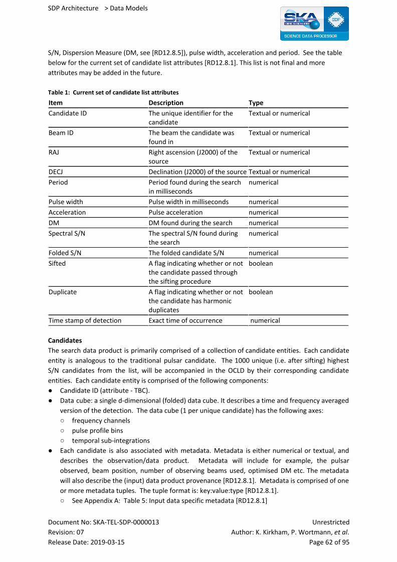
SDP Architecture > Data Models
S/N, Dispersion Measure (DM, see [RD12.8.5]), pulse width, acceleration and period. See the table
below for the current set of candidate list attributes [RD12.8.1]. This list is not final and more
attributes may be added in the future.
Table 1: Current set of candidate list attributes
Item Description Type
Candidate ID The unique identifier for the candidate
Textual or numerical
Beam ID The beam the candidate was found in
Textual or numerical
RAJ Right ascension (J2000) of the source
Textual or numerical
DECJ Declination (J2000) of the source Textual or numerical
Period Period found during the search in milliseconds
numerical
Pulse width Pulse width in milliseconds numerical
Acceleration Pulse acceleration numerical
DM DM found during the search numerical
Spectral S/N The spectral S/N found during the search
numerical
Folded S/N The folded candidate S/N numerical
Sifted A flag indicating whether or not the candidate passed through the sifting procedure
boolean
Duplicate A flag indicating whether or not the candidate has harmonic duplicates
boolean
Time stamp of detection Exact time of occurrence numerical
Candidates
The search data product is primarily comprised of a collection of candidate entities. Each candidate
entity is analogous to the traditional pulsar candidate. The 1000 unique (i.e. after sifting) highest
S/N candidates from the list, will be accompanied in the OCLD by their corresponding candidate
entities. Each candidate entity is comprised of the following components:
● Candidate ID (attribute - TBC).
● Data cube: a single d-dimensional (folded) data cube. It describes a time and frequency averaged
version of the detection. The data cube (1 per unique candidate) has the following axes:
○ frequency channels
○ pulse profile bins
○ temporal sub-integrations
● Each candidate is also associated with metadata. Metadata is either numerical or textual, and
describes the observation/data product. Metadata will include for example, the pulsar
observed, beam position, number of observing beams used, optimised DM etc. The metadata
will also describe the (input) data product provenance [RD12.8.1]. Metadata is comprised of one
or more metadata tuples. The tuple format is: key:value:type [RD12.8.1].
○ See Appendix A: Table 5: Input data specific metadata [RD12.8.1]
Document No: SKA-TEL-SDP-0000013 Unrestricted
Revision: 07 Author: K. Kirkham, P. Wortmann, et al. Release Date: 2019-03-15 Page 62 of 95
SDP Architecture > Data Models
○ See Appendix A: Table 6: Provenance specific metadata [RD12.8.1]
● Each candidate is also expected to have three S/N sheets (2-d matrices) computed by the CSP,
which contain S/N values found during different optimizations of the folded data. The sheet size
is determined from the number of trial periods, period derivatives and DMs. The sheets include:
○ A sheet describing the resulting S/N values for different values of period and period
derivative.
○ A sheet describing the resulting S/N values for different values of period and DM.
○ A sheet describing the resulting S/N for different values of period-derivative and DM.
12.8.2.1.1.2 Science Data Model
The Science Data Model for Pulsar Search includes the following:
● Known Pulsar and Fast Transient Sources: Each new pulsar candidate needs to be compared to a
database of known pulsars, and flagged as ‘new’ or ‘known’ as appropriate. If flagged as ‘known’,
then the details of the known source believed to match the candidate should be attached as
metadata. It is possible for a candidate to match 1 or more known sources. In addition, each new
candidate also needs to be compared to a database of known Fast Transient Sources (such as
Rotating Radio Transients [RRATs,RD12.8.6] and Fast Radio Bursts [FRBs,RD12.8.7]) as for pulsar
sources. The database should at least include information about (but not limited to) type of
source, source name, position in the sky (e.g. Right Ascension and declination), DM, pulse width,
and flux density. For pulsars, the database should include spin period and any potential binary
parameters such as binary period, projected semi-major axis, longitude of periastron, and
eccentricity.
● Classification Model: The classification model (which comes from the TMC Configuration
Repository) is a mathematical model that can apply new classification labels to candidates as
they arrive from the CSP (e.g. labels such as noise, interference, pulsar, single-pulse burst, or
FRB). Such models are typically stored as serialised objects that contain the classifier
configuration parameters, and the learned mathematical function (e.g. [RD8]). In practice the
parameters are often stored as many key value pairs. However the ‘learned’ function can be
stored in a variety of ways depending on the classification algorithm used. For example, a neural
network model can be represented via 1 or more matrices containing connection weights
between artificial neurons. Sometimes classification models are saved in common file formats
such as HDF5 or JSON (e.g. see [RD7]). Irrespective of the format used, for each classification
model it is important to know which data set was used to train it. This information must be
maintained alongside the model. Note that a classification model used to label pulsar
candidates, is unsuitable for use on single-pulse data (see Section 4.1 in Pulsar Search and Single
Pulse/Fast Transient Workflow View packet). Thus those two classification models must be
maintained separately.
● Processing Block Configuration: Configuration of the different processing steps in the processing
workflow.
○ Configuration parameters for generate heuristics, classification, selection & evaluation steps
in the workflow.
Document No: SKA-TEL-SDP-0000013 Unrestricted
Revision: 07 Author: K. Kirkham, P. Wortmann, et al. Release Date: 2019-03-15 Page 63 of 95
SDP Architecture > Data Models
12.8.2.1.1.3 Pulsar Search SDP Data Products
The Pulsar Search SDP Data Product consists of the following:
● Original OCLDs from multiple beams.
● Additional metadata appended to the OCLD (as derived during the processing of the workflow),
will comprise the following:
○ Sifting Metadata: This will include “duplicate scores” and labels with additional information
e.g. known sources.
○ Heuristics metadata: This will consist of (likely less than 100) real numbers (up to 8N heuristic
bytes) for each candidate.
○ Classification metadata: This will describe the predicted class label for each candidate. The
label for each candidate could be a real number, an integer, or even a textual description.
○ Selection metadata (likelihood score). The score could be represented using a 8 byte real
value.
12.8.2.1.1.4 Science Event Alert (TBC)
Alert generation for the pulsar search pipeline is not mandated, and there is no requirement to
deliver it. This is why this section is labelled as TBC. However there are many reasons why it is useful
to generate pulsar search alerts. For example, alerts can help ensure that telescope time is utilised
effectively (related to dynamic scheduling).
To enable alerts to be generated, we do not design out an alert generation capability for the pulsar
search pipeline. Thus if a known source exhibits unusual behaviour, or a candidate possesses a
likelihood score greater than the alert threshold, an alert will be generated. Alerts will be formatted
as IVOA alerts and sent to TM. An alert message will consist of:
● alert text (200 x 2 byte (16-bit) unicode characters)
● alert metadata (200 x 2 byte (16-bit) unicode characters)
● the alert threshold (a single 8 byte real value)
● The candidate data (~1-2.6 Mb).
Document No: SKA-TEL-SDP-0000013 Unrestricted
Revision: 07 Author: K. Kirkham, P. Wortmann, et al. Release Date: 2019-03-15 Page 64 of 95
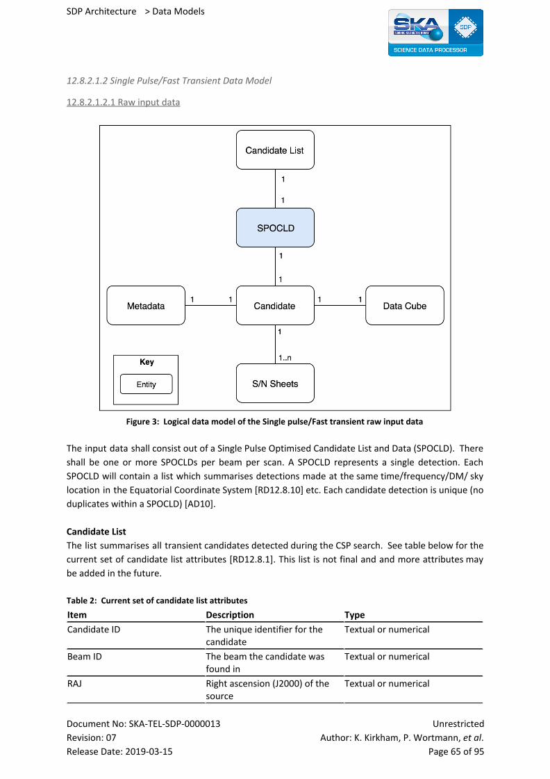
SDP Architecture > Data Models
12.8.2.1.2 Single Pulse/Fast Transient Data Model
12.8.2.1.2.1 Raw input data
Figure 3: Logical data model of the Single pulse/Fast transient raw input data
The input data shall consist out of a Single Pulse Optimised Candidate List and Data (SPOCLD). There
shall be one or more SPOCLDs per beam per scan. A SPOCLD represents a single detection. Each
SPOCLD will contain a list which summarises detections made at the same time/frequency/DM/ sky
location in the Equatorial Coordinate System [RD12.8.10] etc. Each candidate detection is unique (no
duplicates within a SPOCLD) [AD10].
Candidate List
The list summarises all transient candidates detected during the CSP search. See table below for the
current set of candidate list attributes [RD12.8.1]. This list is not final and and more attributes may
be added in the future.
Table 2: Current set of candidate list attributes
Item Description Type
Candidate ID The unique identifier for the candidate
Textual or numerical
Beam ID The beam the candidate was found in
Textual or numerical
RAJ Right ascension (J2000) of the source
Textual or numerical
Document No: SKA-TEL-SDP-0000013 Unrestricted
Revision: 07 Author: K. Kirkham, P. Wortmann, et al. Release Date: 2019-03-15 Page 65 of 95
SDP Architecture > Data Models
DECJ Declination (J2000) of the source Textual or numerical
Time stamp of detection Exact time of occurrence numerical
Pulse width Pulse width in milliseconds numerical
Reference frequency The observing frequency that the timestamp refers to.
numerical
DM DM found during the search numerical
Spectral S/N The spectral S/N found during the search
numerical
Sifted A flag indicating whether or not the candidate passed through the filtering procedure
boolean
Duplicate A flag indicating whether or not the candidate has harmonic duplicates
boolean
Candidates
The search data product is comprised of only one candidate entity comprised of the following
components:
● Candidate ID (attribute - TBC).
● Data cube: a single d-dimensional (filterbank) data cube (polarisation and power versus
frequency and time). The single pulse/fast transient data cube has the following axes:
○ frequency channels
○ polarisations
○ samples
● Each candidate is also associated with metadata. Metadata is either numerical or textual, and
describes the observation/data product. Metadata will include for example nearby pulsars, the
beam position, number of observing beams used, optimised DM etc. The metadata will also
describe the (input) data product provenance [RD12.8.1]. Metadata is comprised of one or more
metadata tuples. The tuple format is: key:value:type [RD12.8.1].
○ See Appendix A: Table 5: Input data specific metadata [RD12.8.1]
○ See Appendix A: Table 6: Provenance specific metadata [RD12.8.1]
● Each candidate is also expected to have 2 (TBD) sheets [AD10]:
○ A 1-dimensional matrix describing a frequency vs S/N plot (S/N per frequency channel)
○ A 1-dimensional Dispersion Measure vs S/N plot
12.8.2.1.2.2 Science Data Model
The Science Data Model for Single Pulse/Fast Transient also includes the following:
● Known Pulsar and Fast Transient Sources: Each new Fast Transient candidate needs to be
compared to a database of known RRAT Sources [RD12.8.6] and FRBs [RD12.8.7], and flagged as
‘new’ or ‘known’ as appropriate. If flagged as ‘known’, then the details of the known source
believed to match the candidate should be attached as metadata. It is possible for a candidate to
match 1 or more known sources. The RRAT and FRB known source database should at a
minimum include information about (but not limited to) the type of source, source name,
position in the sky (e.g. Right Ascension and declination), dispersion measure, pulse width, and
flux density. In addition, since some pulsars exhibit very bright single pulses of radio emission,
each new candidate also needs to be compared to a database of known pulsars. This known
Document No: SKA-TEL-SDP-0000013 Unrestricted
Revision: 07 Author: K. Kirkham, P. Wortmann, et al. Release Date: 2019-03-15 Page 66 of 95
SDP Architecture > Data Models
pulsar database should include spin parameters and any potential binary parameters such as
binary period, projected semi major axis, longitude of periastron, and eccentricity.
● Classification Model: The classification model (which comes from the TMC Configuration
Repository) is a mathematical model that can apply new classification labels to candidates as
they arrive from the CSP (e.g. labels such as noise, interference, pulsar, single-pulse burst, or
FRB). Such models are typically stored as serialised objects that contain the classifier
configuration parameters, and the ‘learned’ mathematical function (e.g. [RD8]). In practice the
parameters are often stored as key value pairs. However the learned function can be stored in a
variety of ways depending on the classification algorithm used. For example, a neural network
model can be represented via 1 or more matrices containing connection weights between
artificial neurons. Sometimes classification models are saved in common file formats such as
HDF5 or JSON (e.g. see [RD7]). Irrespective of how the model is persisted, for each classification
model it is important to know which data set was used to train it. This information must be
maintained alongside the model. Note that a classification model used to label single-pulse
events, is unsuitable for use on pulsar candidate data (see Section 4.1 in Pulsar Search and Single
Pulse/Fast Transient Workflow View packet). Thus those two classification models must be
maintained separately.
● Processing Block Configuration: Configuration of the different processing steps in the Pulsar
Search and Single Pulse/Fast Transient Workflow View packet processing workflow.
○ Configuration parameters for generate heuristics, classification, selection & evaluation steps
in the workflow.
12.8.2.1.2.3 Single Pulse/Fast Transient SDP Data Products
The Single Pulse/Fast Transient SDP Data Product consists of the following:
● Original SPOCLDs from multiple beams.
● Additional metadata appended to the SPOCLD (as derived during the processing of the
workflow), will include the following:
○ Heuristics metadata: This will consist of (likely less that 100) real numbers (up to 8N heuristic
bytes) for each candidate.
○ Classification metadata: This will describe the predicted class label for each candidate. The
label for each candidate could be a real number, an integer, or even a textual description.
○ Selection metadata (likelihood score). The score could be represented using a 8 byte real
value.
12.8.2.1.2.4 Science Event Alert
If a candidate’s likelihood score is greater than a TM defined alert threshold, then an alert will be
generated. Alerts will be formatted as IVOA alerts and sent to TM. An alert message will consist of:
● alert text (200 x 2 byte (16-bit) unicode characters)
● alert metadata (200 x 2 byte (16-bit) unicode characters)
● the alert threshold (a single 8 byte real value)
● The candidate data. (~1-2.6 Mb)
12.8.2.1.3 Pulsar Timing Mode Data Model
12.8.2.1.3.1 Raw input data
SDP receives coherently de-dispersed, detected pulsar data cubes in PSRFITS format
[RD12.8.8,RD12.8.9] along with associated metadata.
Document No: SKA-TEL-SDP-0000013 Unrestricted
Revision: 07 Author: K. Kirkham, P. Wortmann, et al. Release Date: 2019-03-15 Page 67 of 95
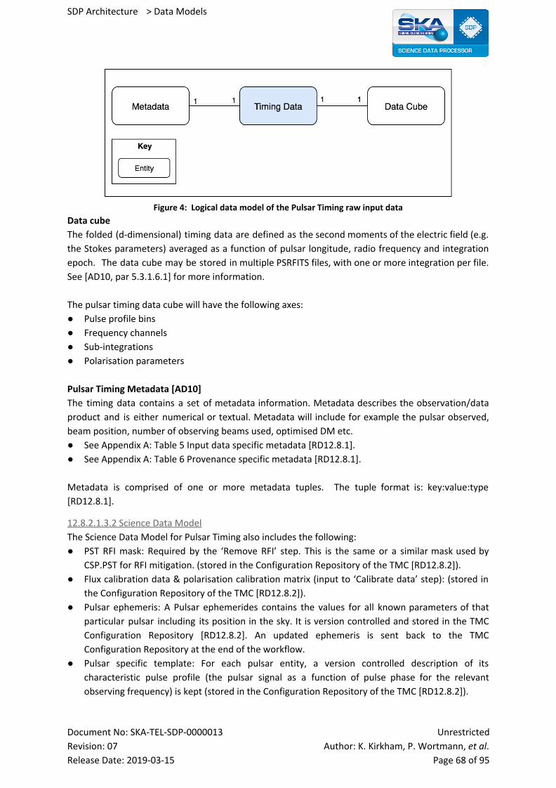
SDP Architecture > Data Models
Figure 4: Logical data model of the Pulsar Timing raw input data
Data cube
The folded (d-dimensional) timing data are defined as the second moments of the electric field (e.g.
the Stokes parameters) averaged as a function of pulsar longitude, radio frequency and integration
epoch. The data cube may be stored in multiple PSRFITS files, with one or more integration per file.
See [AD10, par 5.3.1.6.1] for more information.
The pulsar timing data cube will have the following axes:
● Pulse profile bins
● Frequency channels
● Sub-integrations
● Polarisation parameters
Pulsar Timing Metadata [AD10]
The timing data contains a set of metadata information. Metadata describes the observation/data
product and is either numerical or textual. Metadata will include for example the pulsar observed,
beam position, number of observing beams used, optimised DM etc.
● See Appendix A: Table 5 Input data specific metadata [RD12.8.1].
● See Appendix A: Table 6 Provenance specific metadata [RD12.8.1].
Metadata is comprised of one or more metadata tuples. The tuple format is: key:value:type
[RD12.8.1].
12.8.2.1.3.2 Science Data Model
The Science Data Model for Pulsar Timing also includes the following:
● PST RFI mask: Required by the ‘Remove RFI’ step. This is the same or a similar mask used by
CSP.PST for RFI mitigation. (stored in the Configuration Repository of the TMC [RD12.8.2]).
● Flux calibration data & polarisation calibration matrix (input to ‘Calibrate data’ step): (stored in
the Configuration Repository of the TMC [RD12.8.2]).
● Pulsar ephemeris: A Pulsar ephemerides contains the values for all known parameters of that
particular pulsar including its position in the sky. It is version controlled and stored in the TMC
Configuration Repository [RD12.8.2]. An updated ephemeris is sent back to the TMC
Configuration Repository at the end of the workflow.
● Pulsar specific template: For each pulsar entity, a version controlled description of its
characteristic pulse profile (the pulsar signal as a function of pulse phase for the relevant
observing frequency) is kept (stored in the Configuration Repository of the TMC [RD12.8.2]).
Document No: SKA-TEL-SDP-0000013 Unrestricted
Revision: 07 Author: K. Kirkham, P. Wortmann, et al. Release Date: 2019-03-15 Page 68 of 95

SDP Architecture > Data Models
● List of TOAs (from previous observations) stored in the Configuration Repository of the TMC
[RD12.8.2]. An updated list of TOAs is sent back to the TMC Configuration Repository at the end
of the workflow.
● Processing Block Configuration: Configuration of the different processing steps in the processing
workflow.
○ Configuration for all the processing steps, e.g. calibration, averaging etc.
● The SDM contains a set of QA metrics to determine the quality of the Pulsar Timing Data
Products. These include, but are not limited to:
○ S/N of the total observation
○ S/N of each sub-integration
○ Number of channels/sub-integrations/samples removed by RFI mitigation
○ Reduced chi-square of the timing fit.
○ etc. (TBD)
12.8.2.1.3.3 Pulsar Timing SDP Data Products
The Pulsar Timing SDP Data Product [RD12.8.1] consists of the following:
● Original input data.
● Averaged timing data products: Much of the pulsar timing pipeline uses full-resolution data
cubes during data processing. This is because interference mitigation and calibration greatly
benefit from high resolution data. However some processing steps require higher S/N values
rather than high resolution. This requires partly averaged (also known as summed or
‘scrunched’) data products. One or more averaged intermediate data cubes will be included in
the SDP Data Product along with the original data cube. This information is saved for future
post-processing. The quantity and size of the averaged cubes is scan specific, but will likely
include cubes averaged over frequency (1 x Nbin x Nsub x Npol x Nbit), time (Nchan x Nbin x 1 x Npol x
Nbit), frequency & time (1 x Nbin x 1 x Npol x Nbit), or some combination [RD12.8.1].
● TOA list: A Time-of-arrival (TOA) list describes pulse arrival times for a pulsar with respect to
some time reference. There is 1 TOA recorded per sub-integration and frequency channel, as an
intermediate data product in the pulsar timing pipeline. The TOA list is represented by a row
vector of size Nchan x 1 (or cube of Nchan x 1 x Nsub) [RD12.8.1].
● Timing Residuals describe the difference [modulo the spin period] between the expected pulse
arrival times and the actual pulse arrival times. The residuals are represented by a row vector of
size Nchan x 1 (or cube of Nchan x 1 x Nsub) [RD12.8.1].
Table 3: List of Pulsar Timing parameters
Parameter Description
Nbin Number of phase bins
Nsub Number of temporal sub-integrations
Npol Number of polarisations
Nbit Number of bits per sample in the cube
Nchan Number of frequency channels
Document No: SKA-TEL-SDP-0000013 Unrestricted
Revision: 07 Author: K. Kirkham, P. Wortmann, et al. Release Date: 2019-03-15 Page 69 of 95
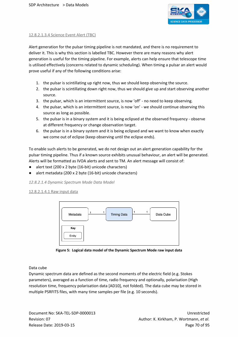
SDP Architecture > Data Models
12.8.2.1.3.4 Science Event Alert (TBC)
Alert generation for the pulsar timing pipeline is not mandated, and there is no requirement to
deliver it. This is why this section is labelled TBC. However there are many reasons why alert
generation is useful for the timing pipeline. For example, alerts can help ensure that telescope time
is utilised effectively (concerns related to dynamic scheduling). When timing a pulsar an alert would
prove useful if any of the following conditions arise:
1. the pulsar is scintillating up right now, thus we should keep observing the source.
2. the pulsar is scintillating down right now, thus we should give up and start observing another
source.
3. the pulsar, which is an intermittent source, is now ‘off’ - no need to keep observing.
4. the pulsar, which is an intermittent source, is now ‘on’ - we should continue observing this
source as long as possible.
5. the pulsar is in a binary system and it is being eclipsed at the observed frequency - observe
at different frequency or change observation target.
6. the pulsar is in a binary system and it is being eclipsed and we want to know when exactly
we come out of eclipse (keep observing until the eclipse ends).
To enable such alerts to be generated, we do not design out an alert generation capability for the
pulsar timing pipeline. Thus if a known source exhibits unusual behaviour, an alert will be generated.
Alerts will be formatted as IVOA alerts and sent to TM. An alert message will consist of:
● alert text (200 x 2 byte (16-bit) unicode characters)
● alert metadata (200 x 2 byte (16-bit) unicode characters)
12.8.2.1.4 Dynamic Spectrum Mode Data Model
12.8.2.1.4.1 Raw input data
Figure 5: Logical data model of the Dynamic Spectrum Mode raw input data
Data cube
Dynamic spectrum data are defined as the second moments of the electric field (e.g. Stokes
parameters), averaged as a function of time, radio frequency and optionally, polarisation (High
resolution time, frequency polarisation data [AD10], not folded). The data cube may be stored in
multiple PSRFITS files, with many time samples per file (e.g. 10 seconds).
Document No: SKA-TEL-SDP-0000013 Unrestricted
Revision: 07 Author: K. Kirkham, P. Wortmann, et al. Release Date: 2019-03-15 Page 70 of 95
SDP Architecture > Data Models
The dynamic spectrum data cube will have the following axes:
● frequency channels
● samples
● stokes (polarisation) parameters
Dynamic Spectrum Metadata [AD10]
The dynamic spectrum data contains a set of metadata information. Metadata describes the
observation/data product and is either numerical or textual. Metadata will include for example the
pulsar observed, beam position, number of observing beams used, optimised DM etc.
● See Appendix A: Table 5: Input data specific metadata [RD12.8.1]
● See Appendix A: Table 6: Provenance specific metadata [RD12.8.1]
Metadata is comprised of one or more metadata tuples. The tuple format is: key:value:type
[RD12.8.1].
12.8.2.1.4.2 Science Data Model
The Science Data Model for Dynamic Spectrum mode also includes the following:
● PST RFI mask (input to the ‘Remove RFI’ step): (stored in Configuration Repository of the TMC)
[RD12.8.2].
● Flux calibration data & polarisation calibration matrix (input to ‘Calibrate data’ step): (stored in
Configuration Repository of the TMC [RD12.8.2]).
● Processing Block Configuration: Configuration of the different processing steps in the processing
workflow.
○ Configuration for all the processing steps, e.g. calibration, averaging etc. as appropriate.
● SDM contains a set of QA metrics to determine the quality of the Dynamic Spectrum Data
Products. These QA metrics may be a subset of the QA metrics used for the Pulsar Timing
Workflow (see par 2.1.3.2).
12.8.2.1.4.3 Dynamic Spectrum SDP Data Products
Dynamic Spectrum mode (DSM) allows the high resolution data product recorded during pulsar
timing mode, to be preserved for off-line analysis. This data is called the Channelized Detected Time
Series data (CDTS) by the science community. The DSM data is not processed within SDP, simply
archived for later use by the science community (e.g. can be searched for pulsars etc.).
The data product is structurally identical to that used for pulsar timing. There are some practical
differences: i) DSM data cubes are much higher resolution than pulsar timing data products making
them significantly larger in size, and ii) DSM data is not folded [RD12.8.1].
The Dynamic Spectrum SDP Data Product consists of the following [RD12.8.1]:
● Original input data.
● High resolution data product (after RFI mitigation and Calibration).
Document No: SKA-TEL-SDP-0000013 Unrestricted
Revision: 07 Author: K. Kirkham, P. Wortmann, et al. Release Date: 2019-03-15 Page 71 of 95
SDP Architecture > Data Models
12.8.2.1.5 Flow Through Mode Data Model
12.8.2.1.5.1 Raw input data
Data cube
The raw beam-formed voltage data are defined as the instantaneous samples of the electric field,
with no temporal or spectral averaging, but optional re-quantisation.
The flow through mode data cube will have the following axes:
● frequency channels
● samples
● polarisations
● dimensions
The flow through mode (beamformer) weights cube will have the following axes:
● frequency channels
● time samples
Flow Through Metadata
The dynamic spectrum data contains a set of metadata information. Metadata describes the
observation/data product and is either numerical or textual. Metadata will include eg the pulsar
observed, beam position, number of observing beams used, optimised dispersion measure (DM),
etc.
● See Appendix A: Table 5: Input data specific metadata [RD12.8.1]
● See Appendix A: Table 6: Provenance specific metadata [RD12.8.1]
Metadata is comprised of one or more metadata tuples. The tuple format is: key:value:type
[RD12.8.1].
12.8.2.1.5.2 Science Data Model
No Science Data Model for Flow Through Mode is needed, because the data is not processed within
SDP; rather it simply passed through the SDP for storage and offline analysis.
12.8.2.1.5.3 Flow Through Mode SDP Data Products
The Flow Through SDP Data Product consists of the following:
● Raw beam-formed voltages (no processing done on input data).
12.8.2.2 Relations and Their Properties
Not applicable
12.8.2.3 Element Interfaces
Not applicable
12.8.2.4 Element Behavior
Not applicable
12.8.2.5 Indices and Keys
Not applicable
Document No: SKA-TEL-SDP-0000013 Unrestricted
Revision: 07 Author: K. Kirkham, P. Wortmann, et al. Release Date: 2019-03-15 Page 72 of 95
SDP Architecture > Data Models
12.8.2.6 Structure and Access Patterns
Not applicable.
12.8.3 Context Diagram
Refer to Figure 1 for the Non-Imaging Context diagram.
12.8.4 Variability Guide
Not applicable.
12.8.5 Rationale
The Non-Imaging Data Model has been defined by the following drivers:
● How the data is received by SDP from CSP.
● How the Pulsar Search, Single Pulse/Fast Transient, Pulsar Timing, Dynamic Spectrum and Flow
Through Mode workflows are defined.
● The current implementation of the workflows.
● The System-level Data Model View
12.8.6 Related Views
● Pulsar Search and Single Pulse/Fast Transient Workflow View packet
● Pulsar Timing and Dynamic Spectrum Workflow View packet
● System-level Data Model View
12.8.7 Reference Documents
The following documents are referenced in this document. In the event of conflict between the
contents of the referenced documents and this document, this document shall take precedence.
[RD12.8.1] SDP Memo 42: Data Model Summary for Pulsar/Transient Search & Timing; RevC1
[RD12.8.2] SKA-TEL-TM-0000242: TMC Software Architecture document
[RD12.8.3] Keras: The Python Deep Learning library,
https://keras.io/getting-started/faq/
[RD12.8.4] Scikit-Learn Documentation, “3.4 Model Persistence”,
http://scikit-learn.org/stable/modules/model_persistence.html
[RD12.8.5] Lorimer D. R. & Kramer M., “Handbook of pulsar astronomy”,
Cambridge University Press, 2005.
[RD12.8.6] McLaughlin et al. 2006, Nature, 439, 817
[RD12.8.7] Thornton et al. 2013, Science, 341, 53
[RD12.8.8] Hotan A. W., van Straten W., and Manchester R. N., 2004, arXiv:astro-ph/0404549v1.
[RD12.8.9] van Straten W. et. al ., 2009, arXiv:0912.1662.
[RD12.8.10] Roy A. E. & Clarke D. “Astronomy: Principles and Practice”, 4th Edition, CRC Press,
2003.
Document No: SKA-TEL-SDP-0000013 Unrestricted
Revision: 07 Author: K. Kirkham, P. Wortmann, et al. Release Date: 2019-03-15 Page 73 of 95

SDP Architecture > Data Models
12.9 Visibility Data Model Contributors: T. J. Dijkema
12.9.1 Scope, Terminology
In this document we will refer to Visibility Model as the entity that holds visibility data. The exact
properties of the Visibility Model shall be described later. We will refer to the existing storage
system for visibilities, the Measurement Set, as MSv2 [RD1].
The Measurement Standard was defined around 2000 and is widely used, and well defined [RD1]. It
is used for many telescopes, e.g. LOFAR, VLA, MeerKAT, MWA. The most popular software package
CASA is built around the measurement set, but also many other data reduction packages use the
measurement set standard. This makes software designed for different telescopes easily usable for
the others.
SKA and NRAO have a Memorandum of Understanding [AD19] to work on a new standard of the
Measurement Set. We will refer to the standard being developed by the project started by this
Memorandum of Understanding as MSv3. This document is not intended to duplicate the work on
MSv3, but rather to describe the SKA architectural requirements on the Visibility Model, which may
be realized as the Measurement Set.
The Visibility Model shall contain both data and metadata. The logical data model, treated in this
document, shall describe which data and metadata goes into the Visibility Model. The physical data
model shall prescribe how data is stored. This document will focus on the logical data model, but will
touch on some aspects of the physical data format.
The current MSv2 format supports single dish data, and per [AD19] MSv3 shall also support single
dish data. The data model used for single-dish observations will be MSv3 and not a separate data
model. In terms of the pipelines, these are not exhaustive and new pipelines can be created as
required.In this document however, we will concentrate on interferometric data.
Document No: SKA-TEL-SDP-0000013 Unrestricted
Revision: 07 Author: K. Kirkham, P. Wortmann, et al. Release Date: 2019-03-15 Page 74 of 95
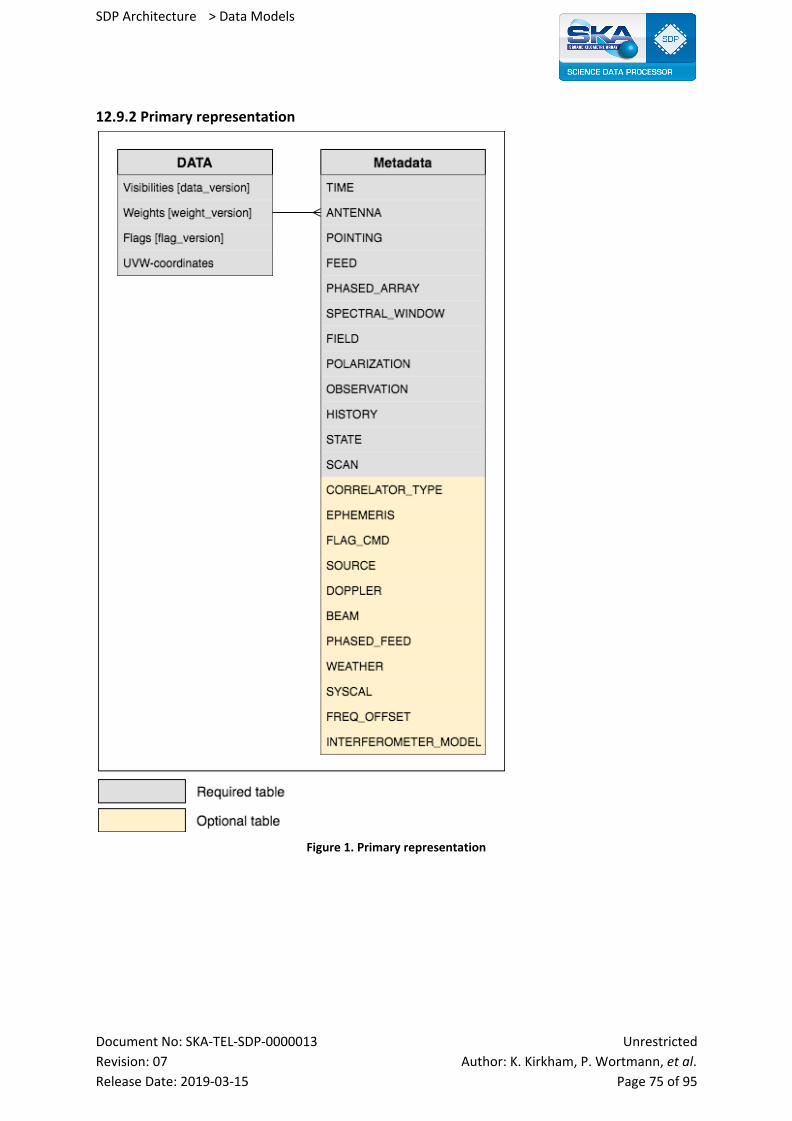
SDP Architecture > Data Models
12.9.2 Primary representation
Figure 1. Primary representation
Document No: SKA-TEL-SDP-0000013 Unrestricted
Revision: 07 Author: K. Kirkham, P. Wortmann, et al. Release Date: 2019-03-15 Page 75 of 95
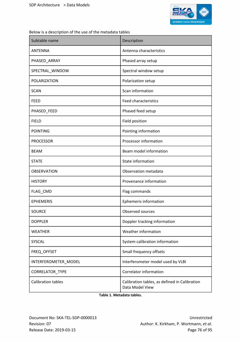
SDP Architecture > Data Models
Below is a description of the use of the metadata tables
Subtable name Description
ANTENNA Antenna characteristics
PHASED_ARRAY Phased array setup
SPECTRAL_WINDOW Spectral window setup
POLARIZATION Polarization setup
SCAN Scan information
FEED Feed characteristics
PHASED_FEED Phased feed setup
FIELD Field position
POINTING Pointing information
PROCESSOR Processor information
BEAM Beam model information
STATE State information
OBSERVATION Observation metadata
HISTORY Provenance information
FLAG_CMD Flag commands
EPHEMERIS Ephemeris information
SOURCE Observed sources
DOPPLER Doppler tracking information
WEATHER Weather information
SYSCAL System calibration information
FREQ_OFFSET Small frequency offsets
INTERFEROMETER_MODEL Interferometer model used by VLBI
CORRELATOR_TYPE Correlator information
Calibration tables Calibration tables, as defined in Calibration Data Model View
Table 1. Metadata tables.
Document No: SKA-TEL-SDP-0000013 Unrestricted
Revision: 07 Author: K. Kirkham, P. Wortmann, et al. Release Date: 2019-03-15 Page 76 of 95

SDP Architecture > Data Models
12.9.2.1 Versioning
All tables should be treated as append-only, to make it possible to go back one step. Also, pipeline
frameworks typically expect a distinct input and output file. Note that this is not a hard requirement;
if file size is a limiting factor, visibilities can be changed in-place.
It should be possible to associate multiple versions of e.g. WEIGHTS with one version of DATA
without duplicating data. The way to store these versions is TBD.
Note that this is versioning scheme generalizes typical use of MSv2 [RD12.9.1] where a
CORRECTED_DATA is stored next to the DATA column.
For example, to calibrate data (from original DATA[0] column) are read (not changed), and
calibration solution are deduced. Applying these solutions will generate a new column DATA[1]. If
the calibration does not change the weights, DATA[1] is still associated with WEIGHTS[0] and
FLAGS[0].
12.9.2.2 Keywords
Both tables and columns can contain keywords. The value of a keyword can be of a simple type
(boolean, integer, float, complex, string), a combination of these, or even a table. If the value of a
keyword is a table, we call this a subtable. That is, the main table of a measurement set has a
keyword “ANTENNA” which points to the antenna subtable.
Column keywords are used to store information about e.g. units or reference frames. For
implementation details in Casacore, see [RD12.9.2].
12.9.3 Element Catalogue
12.9.3.1 Elements and Their Properties
12.9.3.1.1 Data
The main data elements in the Visibility Model shall be visibilities, weights, flags and
UVW-coordinates. Visibilities, weights and flags shall have the same number axes, namely
polarization and channel.
For different applications, the optimal ordering of visibilities may differ. The main operations on
visibilities are flagging, calibration and averaging. For flagging and calibration, typically the data is
stored in time-order, as it comes off the telescope. For imaging, where the UVW is the dominant
axis, the order is different. In the Algorithm Reference Library (ARL), the two formats are referred to
as BlockVisibility and Visibility. The format we describe is intended to support both.
Visibilities can be seen as a high-dimensional cube of data, with the following axes:
● TIME
● ANTENNA1 and ANTENNA2
● FEED1, FEED2
● SPECTRAL_WINDOW_ID
● POLARIZATION_ID
● PROCESSOR_ID
● FIELD_ID
● SCAN_NUMBER
● STATE_ID
Document No: SKA-TEL-SDP-0000013 Unrestricted
Revision: 07 Author: K. Kirkham, P. Wortmann, et al. Release Date: 2019-03-15 Page 77 of 95
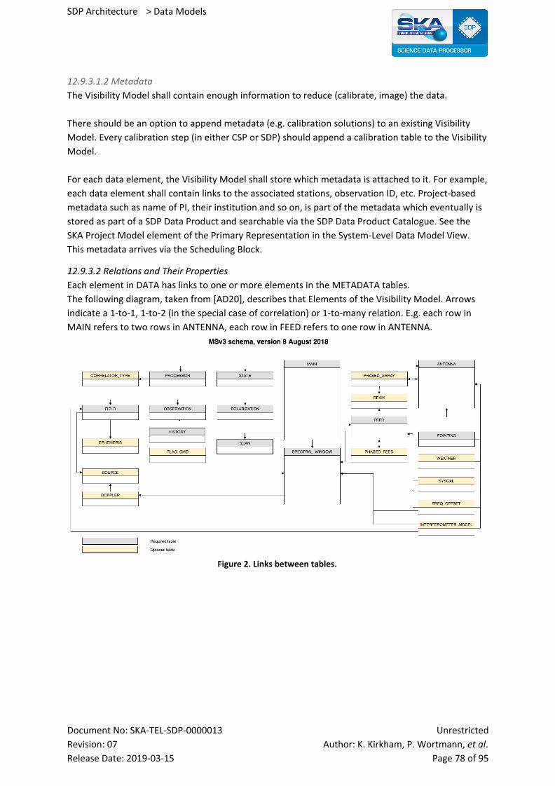
SDP Architecture > Data Models
12.9.3.1.2 Metadata
The Visibility Model shall contain enough information to reduce (calibrate, image) the data.
There should be an option to append metadata (e.g. calibration solutions) to an existing Visibility
Model. Every calibration step (in either CSP or SDP) should append a calibration table to the Visibility
Model.
For each data element, the Visibility Model shall store which metadata is attached to it. For example,
each data element shall contain links to the associated stations, observation ID, etc. Project-based
metadata such as name of PI, their institution and so on, is part of the metadata which eventually is
stored as part of a SDP Data Product and searchable via the SDP Data Product Catalogue. See the
SKA Project Model element of the Primary Representation in the System-Level Data Model View.
This metadata arrives via the Scheduling Block.
12.9.3.2 Relations and Their Properties
Each element in DATA has links to one or more elements in the METADATA tables.
The following diagram, taken from [AD20], describes that Elements of the Visibility Model. Arrows
indicate a 1-to-1, 1-to-2 (in the special case of correlation) or 1-to-many relation. E.g. each row in
MAIN refers to two rows in ANTENNA, each row in FEED refers to one row in ANTENNA.
Figure 2. Links between tables.
Document No: SKA-TEL-SDP-0000013 Unrestricted
Revision: 07 Author: K. Kirkham, P. Wortmann, et al. Release Date: 2019-03-15 Page 78 of 95
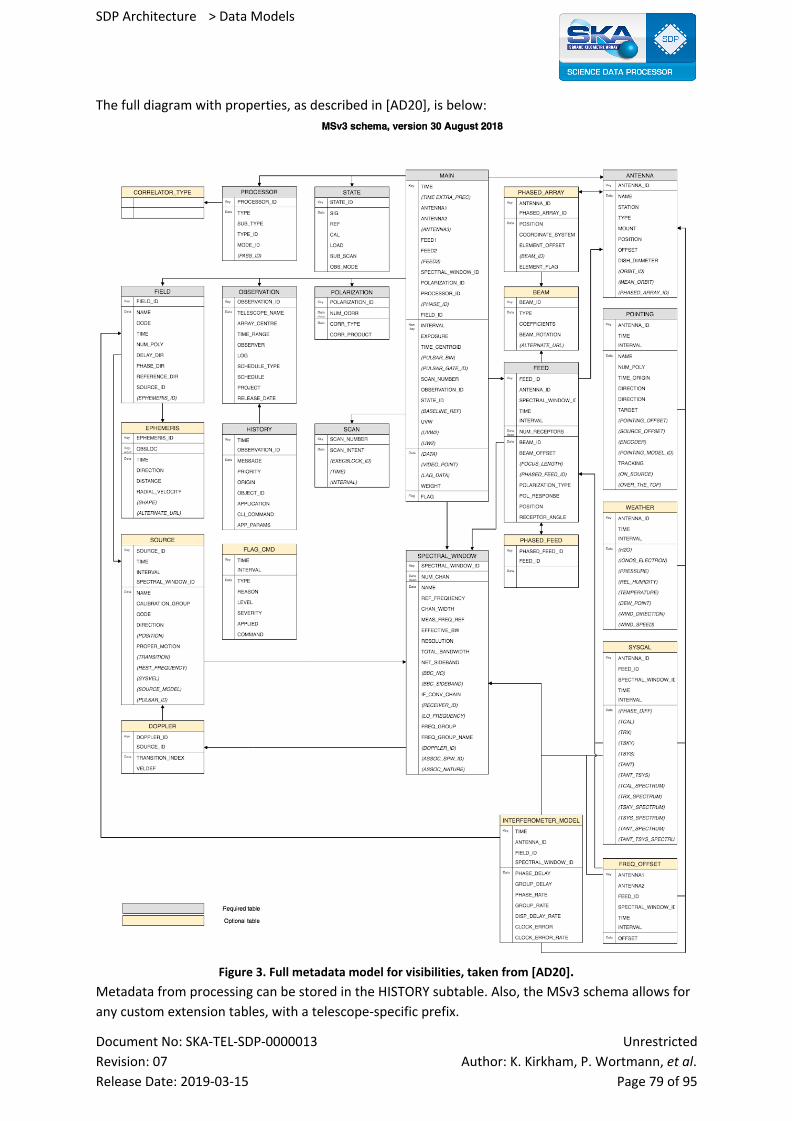
SDP Architecture > Data Models
The full diagram with properties, as described in [AD20], is below:
Figure 3. Full metadata model for visibilities, taken from [AD20]. Metadata from processing can be stored in the HISTORY subtable. Also, the MSv3 schema allows for
any custom extension tables, with a telescope-specific prefix.
Document No: SKA-TEL-SDP-0000013 Unrestricted
Revision: 07 Author: K. Kirkham, P. Wortmann, et al. Release Date: 2019-03-15 Page 79 of 95

SDP Architecture > Data Models
12.9.3.3 Element Interfaces
The interface to the Visibility Data Model is very rich, and complex . The interfaces of the visibility 3
data should support the following:
● Visibility Data can be generated by the correlator, or in simulations.
● Bad data flagging: Visibility Data is searched for RFI, which is then flagged (storing an
updated version of the FLAG column).
● Calibration: Visibility Data is compared to modeled visibilities to fit parameters of
instrumental and atmospheric models are fitted (which are then stored in Calibration Data).
● Subtracting of bright sources: visibility data as input and visibility data as output (with a new
version of the DATA column), where strong sources are subtracted.
● Subtraction of degridded data: subtract visibilities from imaged data from existing visibilities.
● Gridding: Visibility data is converted to Gridded Visibility Data.
● Degridding: Gridded UV Data is converted to visibility data.
● Predict: Convert discrete fourier transforms (DFTs) of components in the Local Sky Model
(LSM).
● Conversion to Science Data Product.
12.9.3.4 Element Behavior
Not applicable.
12.9.3.5 Indices and Keys
Each metadata table shall have an explicit key (this differs from MSv2 where row numbers are
implicit keys). This is to facilitate coalescing and splitting visibilities for parallelization, as well as
combining (joining). These indices and keys are highlighted as such in Figure 3.
12.9.3.6 Structure and Access Patterns
It should be possible to tune the underlying physical data format to a given access pattern.
In view of distributed processing, it should be possible to split a set of visibilities into many smaller
sets that can be processed independently. It should also be possible to recombine these smaller sets.
The axes over which sets of visibilities are allowed to be split or coalesced can be a subset of all axes.
The storage of the data shall be such that it can be optimized for various access patterns. Some
examples of typical access patterns, ranging from slowest to fastest varying axis (where we ignore
other axes like ‘scan’ and ‘feed’):
● Calibration: time, spectral window, channel, baseline
● Flagging: spectral window, baseline, spectral channel, time
● Imaging: baseline, spectral window, channel, time (in this way the best ordering in
UVW-coordinates is achieved without reading the UVW-coordinates, which are treated as
data)
Visibilities are not stored as a full data cube. That is because a generic data format can not assume
that they form a full cube, e.g. every scan has the same number of spectral windows, or every
baseline has the same number of integrations (baseline dependent averaging).
3 The interface to the existing MSv2 is documented here.
Document No: SKA-TEL-SDP-0000013 Unrestricted
Revision: 07 Author: K. Kirkham, P. Wortmann, et al. Release Date: 2019-03-15 Page 80 of 95
SDP Architecture > Data Models
To elaborate this example: note that because <V_p, V_q> = conj(<V_q, V_p>), only half of the
correlations need to be stored.
Instead of storing a full data cube, one element of data shall be a cube of polarizations and channels,
with attached to to it links to all other axes, pointing to the metadata.
In computations, it can be efficient to temporarily store visibilities as a full data cube, filling gaps
with flagged visibilities. For example, baseline averaged visibilities can be duplicated (upsampled) to
the resolution of the longest baseline to get a regular cube of data. In those cases, it is important to
retain sufficient metadata to be able to export to the original data format.
12.9.4 Context Diagram
Not applicable.
12.9.5 Variability Guide
● Correlator - Generates visibilities at the highest time resolution
● Flagging, removing strong sources, averaging - Create a new instance of visibilities at
reduced resolution
● Direction independent calibration - Create new data column where calibration has been
applied
Between LOW and MID telescopes, the main difference is how the location of the different antenna
/ telescope locations are stored. For the MID telescope, telescope locations are stored in the
ANTENNA location. For LOW: the ANTENNA table contains one location per station, the individual
antenna locations are stored in the PHASED_ARRAY table.
12.9.6 Rationale We have followed the existing storage of visibilities quite closely. This will make it easy to use
existing software. We envision that the architecture of CTDS [RD12.9.2] is sufficient to allow efficient
storage managers to be written to guarantee good I/O performance on various hardware platforms.
12.9.7 Related Views ● Gridded Data Model View
● Calibration Data Model View
● Beam Data Model View
12.9.8 References
The following documents are referenced in this document. In the event of conflict between the
contents of the referenced documents and this document, this document shall take precedence.
Document No: SKA-TEL-SDP-0000013 Unrestricted
Revision: 07 Author: K. Kirkham, P. Wortmann, et al. Release Date: 2019-03-15 Page 81 of 95

SDP Architecture > Data Models
[RD12.9.1] MeasurementSet definition version 2.0. A.J. Kemball and M.H. Wieringa, eds. 2000. http://casacore.github.io/casacore-notes/229.pdf
[RD12.9.2] Casacore Table Data System and its use in the MeasurementSet. Ger van Diepen, Astronomy & Computing, 2015, 12. 10.1016/j.ascom.2015.06.002
[RD12.9.3] Data Models for the SDP Pipeline Components. Ger van Diepen, Chris Skipper, Robert Lyon et al. SDP Design Report, 2016-12-02 https://docs.google.com/document/d/1UPZQn8hVv7TDtFm8G3DxTJx0cf0yan_NrBZylwXr8mM/edit .
Document No: SKA-TEL-SDP-0000013 Unrestricted
Revision: 07 Author: K. Kirkham, P. Wortmann, et al. Release Date: 2019-03-15 Page 82 of 95
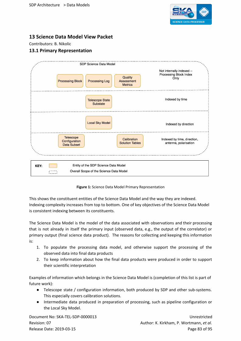
SDP Architecture > Data Models
13 Science Data Model View Packet Contributors: B. Nikolic
13.1 Primary Representation
Figure 1: Science Data Model Primary Representation
This shows the constituent entities of the Science Data Model and the way they are indexed.
Indexing complexity increases from top to bottom. One of key objectives of the Science Data Model
is consistent indexing between its constituents.
The Science Data Model is the model of the data associated with observations and their processing
that is not already in itself the primary input (observed data, e.g., the output of the correlator) or
primary output (final science data product). The reasons for collecting and keeping this information
is:
1. To populate the processing data model, and otherwise support the processing of the
observed data into final data products
2. To keep information about how the final data products were produced in order to support
their scientific interpretation
Examples of information which belongs in the Science Data Model is (completion of this list is part of
future work):
● Telescope state / configuration information, both produced by SDP and other sub-systems.
This especially covers calibration solutions.
● Intermediate data produced in preparation of processing, such as pipeline configuration or
the Local Sky Model.
Document No: SKA-TEL-SDP-0000013 Unrestricted
Revision: 07 Author: K. Kirkham, P. Wortmann, et al. Release Date: 2019-03-15 Page 83 of 95
SDP Architecture > Data Models
● Secondary outputs of processing, such as Science Event Alerts or logs.
The primary goal of the Science Data Model is to unify all of this information in a common
hierarchical name space. This is to enable queries into the data, both while processing as well as
after the fact. The latter allows the Science Data Model to become a Data Product documenting a
finished processing run. To serve this function effectively in the face of changing software
requirements both from Processing Components and Delivery, the Science Data Model must remain
open to modification.
To this end, the Science Data Schema is specified by the Workflow template used by a concrete
Processing Block. The Schema defines a hierarchy of Science Model Paths that contain Science Model
Fields of certain types. Both paths and fields have names as well as associated indices, which not
only allows representing collections of data, but also tracking multiple versions of values (e.g. if they
get updated while processing).
13.2 Element Catalogue
13.2.1 Elements and Their Properties
Elements of this view are data entities. Properties:
● Type of data entity
● Indexing requirements, in particular ones which may drive the design
● Representations details the primary ways in which the data entity will get represented in the
operational SDP system.
13.2.1.1 Processing Block
Type: Configuration data -- specification of what processing was requested by
TM to be done by SDP
Indexing Not required
Representations: Markup language with simple schema
13.2.1.2 Processing Log
Type: Logging data -- auxiliary data about the processing, i.e., data not known
to be required but kept because it may be useful for problem solving or
scientific interpretation in complex cases.
Indexing Not required. Data are time stamped and marked by the ID of where
produced in workflow.
Representations: Stream based representation, probably mixed text & structured data
(arrays and tables)
13.2.1.3 Quality Assessment Metrics
Type: Metrics -- quantitative measurement of quality of the observation,
telescope systems and processing.
Indexing Not required
Representations: Markup language with simple schema
Document No: SKA-TEL-SDP-0000013 Unrestricted
Revision: 07 Author: K. Kirkham, P. Wortmann, et al. Release Date: 2019-03-15 Page 84 of 95

SDP Architecture > Data Models
13.2.1.4 Telescope State Subset
Type: Numerical and configuration data -- details of the actual (as opposed to
commanded) telescope configuration as function of time during
observing
Indexing Time
Representations: Markup language with simple schema, tables
13.2.1.5 Local Sky Model
Type: Numerical Data -- relevant information about known sources in the
region being observed
Indexing Direction on celestial sphere
Representations: Mixed hierarchical representation with code in the in-memory
data-model module to interpret the representation which may be both
simple (tabular), wide-field (HealPix) and complex (using basis set
expansion or rasterised image representations. See the Sky Model Data
Model view packet
13.2.1.6 Telescope Configuration Data Subset
Type: Mixture of computational models and their parameters
Indexing Time, array element (i.e., antenna or station), direction on sky,
polarisation, feed (for Mid)
Representations: Mostly tables, some markup language with simple schema
13.2.1.7 Calibration Solution Tables
Type: Numerical Data -- corrections from calibrations computed in SDP
Indexing Time, array element (i.e., antenna or station), direction on sky,
polarisation, feed (for Mid)
Representations: High efficiency table representations (an example are CASA tables)
13.2.2 Relations and Their Properties
The relations between elements is their common indexing scheme. The top level index is by
processing block ID, followed by time (defined on a common basis for elements), and direction and
antenna/polarisation at the lowest level.
13.2.3 Element Interfaces Not applicable
13.2.4 Element Behavior
No behaviour to document
Document No: SKA-TEL-SDP-0000013 Unrestricted
Revision: 07 Author: K. Kirkham, P. Wortmann, et al. Release Date: 2019-03-15 Page 85 of 95
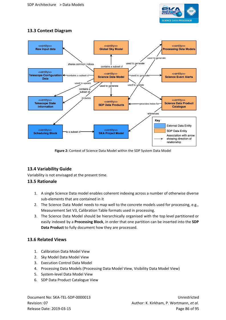
SDP Architecture > Data Models
13.3 Context Diagram
Figure 2: Context of Science Data Model within the SDP System Data Model
13.4 Variability Guide Variability is not envisaged at the present time.
13.5 Rationale
1. A single Science Data model enables coherent indexing across a number of otherwise diverse
sub-elements that are contained in it
2. The Science Data Model needs to map well to the concrete models used for processing, e.g.,
Measurement Set V3, Calibration Table formats used in processing.
3. The Science Data Model should be hierarchically organised with the top level partitioned or
easily indexed by a Processing Block, in order that one partition can be inserted into the SDP
Data Product to fully document how they are processed.
13.6 Related Views
1. Calibration Data Model View
2. Sky Model Data Model View
3. Execution Control Data Model
4. Processing Data Models (Processing Data Model View, Visibility Data Model View)
5. System-level Data Model View
6. SDP Data Product Catalogue View
Document No: SKA-TEL-SDP-0000013 Unrestricted
Revision: 07 Author: K. Kirkham, P. Wortmann, et al. Release Date: 2019-03-15 Page 86 of 95
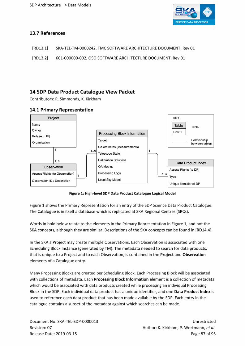
SDP Architecture > Data Models
13.7 References
[RD13.1] SKA-TEL-TM-0000242, TMC SOFTWARE ARCHITECTURE DOCUMENT, Rev 01
[RD13.2] 601-000000-002, OSO SOFTWARE ARCHITECTURE DOCUMENT, Rev 01
14 SDP Data Product Catalogue View Packet Contributors: R. Simmonds, K. Kirkham
14.1 Primary Representation
Figure 1: High-level SDP Data Product Catalogue Logical Model
Figure 1 shows the Primary Representation for an entry of the SDP Science Data Product Catalogue.
The Catalogue is in itself a database which is replicated at SKA Regional Centres (SRCs).
Words in bold below relate to the elements in the Primary Representation in Figure 1, and not the
SKA concepts, although they are similar. Descriptions of the SKA concepts can be found in [RD14.4].
In the SKA a Project may create multiple Observations. Each Observation is associated with one
Scheduling Block Instance (generated by TM). The metadata needed to search for data products,
that is unique to a Project and to each Observation, is contained in the Project and Observation
elements of a Catalogue entry.
Many Processing Blocks are created per Scheduling Block. Each Processing Block will be associated
with collections of metadata. Each Processing Block Information element is a collection of metadata
which would be associated with data products created while processing an individual Processing
Block in the SDP. Each individual data product has a unique identifier, and one Data Product Index is
used to reference each data product that has been made available by the SDP. Each entry in the
catalogue contains a subset of the metadata against which searches can be made.
Document No: SKA-TEL-SDP-0000013 Unrestricted
Revision: 07 Author: K. Kirkham, P. Wortmann, et al. Release Date: 2019-03-15 Page 87 of 95

SDP Architecture > Data Models
14.2 Element Catalogue
14.2.1 Elements and Their Properties
14.2.1.1 Project
Project contains all information about the body which successfully proposed the Observing Project,
i.e. data relating to the person(s) and institution(s) who requested the observation.
14.2.1.2 Observation
Each Observation has a relationship to the Project class and each Observation is unique and related
to a single Scheduling Block Instance, with a unique Scheduling Block ID within SKA. The Observation
class also contains data access rights for the person(s) who proposed the observing Project, which
governs access to the metadata in this element of the Catalogue.
Related to each Observation there may be an Image Preview (TBD) so the catalogue browser can see
a small snapshot (thumbnail/postage stamp) of the image(s) in the final data product. This is not
shown in Figure 1.
14.2.1.3 Processing Block Information
This contains all material required for the astronomer to assess the conditions of the observation,
processing, and associated metadata. It includes all necessary elements from the IVOA ObsCore
model. Each Processing Block Information element may have several data products associated with it
depending on what data products were created during the processing of the associated Processing
Block in the SDP.
14.2.1.4 Data Product Index
Each individual data product has a unique identifier, and one Data Product Index references one
data product. Note that there are two sub-elements (or classes in the logical model) containing
access rights (see Section 2.2.1). The Observation sub-element contains access rights for the
metadata relating to this observation. The Data Product Index also contains access rights but for the
individual data product it represents in the Catalogue.
14.2.2 Relations and Their Properties
14.2.2.1 Access Rights
This contains an Access Control List (ACL) of groups that can access the entity containing this Access
Rights object. It also contains the Proprietary period, which is the time after which the entity is
considered to be in the public domain. These objects are contained in Observation and Data Product
Index objects in the Catalogue elements (see [RD14.1] and [RD14.2]).
Document No: SKA-TEL-SDP-0000013 Unrestricted
Revision: 07 Author: K. Kirkham, P. Wortmann, et al. Release Date: 2019-03-15 Page 88 of 95
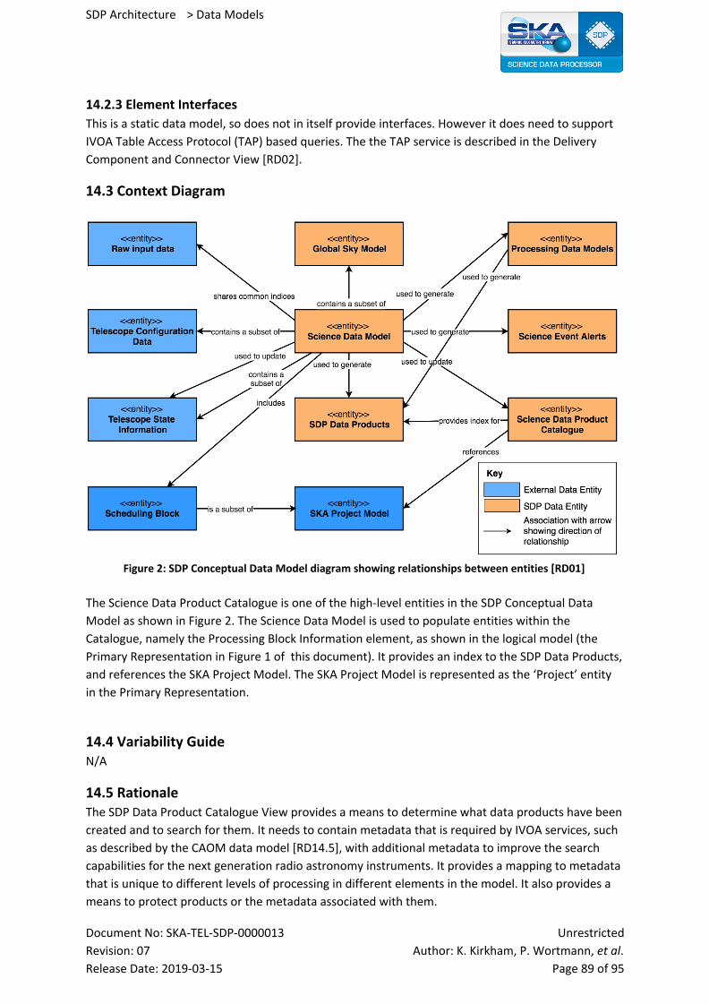
SDP Architecture > Data Models
14.2.3 Element Interfaces
This is a static data model, so does not in itself provide interfaces. However it does need to support
IVOA Table Access Protocol (TAP) based queries. The the TAP service is described in the Delivery
Component and Connector View [RD02].
14.3 Context Diagram
Figure 2: SDP Conceptual Data Model diagram showing relationships between entities [RD01]
The Science Data Product Catalogue is one of the high-level entities in the SDP Conceptual Data
Model as shown in Figure 2. The Science Data Model is used to populate entities within the
Catalogue, namely the Processing Block Information element, as shown in the logical model (the
Primary Representation in Figure 1 of this document). It provides an index to the SDP Data Products,
and references the SKA Project Model. The SKA Project Model is represented as the ‘Project’ entity
in the Primary Representation.
14.4 Variability Guide N/A
14.5 Rationale The SDP Data Product Catalogue View provides a means to determine what data products have been
created and to search for them. It needs to contain metadata that is required by IVOA services, such
as described by the CAOM data model [RD14.5], with additional metadata to improve the search
capabilities for the next generation radio astronomy instruments. It provides a mapping to metadata
that is unique to different levels of processing in different elements in the model. It also provides a
means to protect products or the metadata associated with them.
Document No: SKA-TEL-SDP-0000013 Unrestricted
Revision: 07 Author: K. Kirkham, P. Wortmann, et al. Release Date: 2019-03-15 Page 89 of 95

SDP Architecture > Data Models
14.6 Related Views The System Level Data Model provides the context for this View, as shown in section 3.
The Delivery Component and Connector View describes components associated with this view.
14.7 Reference Documents
The following documents are referenced in this document. In the event of conflict between the
contents of the referenced documents and this document, this document shall take precedence.
[RD14.1] SKA-TEL-SKO-0000307, Rev02, SKA1 Operational Concept Document, G.R. Davis, A. Chrysostomou, C. Taljaard,
[RD14.2] SKA-TEL-SKO-0000958, SKA1 SDP - SRC INTERFACE DEFINITION DOCUMENT,
[RD14.3] Data Access Rules and Regulations, A. Chrysostomou (TBC).
[RD14.4] T4000-0000-AR-002, OSO SOFTWARE ARCHITECTURE DOCUMENT
[RD14.5] CAOM-2.0: The Inevitable Evolution of a Data Model, Dowler, P. (2011)
Document No: SKA-TEL-SDP-0000013 Unrestricted
Revision: 07 Author: K. Kirkham, P. Wortmann, et al. Release Date: 2019-03-15 Page 90 of 95
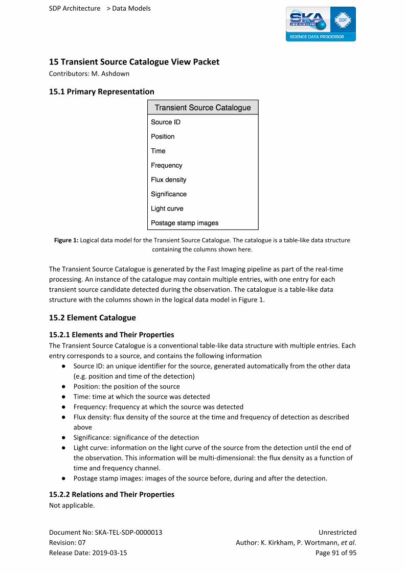
SDP Architecture > Data Models
15 Transient Source Catalogue View Packet Contributors: M. Ashdown
15.1 Primary Representation
Figure 1: Logical data model for the Transient Source Catalogue. The catalogue is a table-like data structure
containing the columns shown here.
The Transient Source Catalogue is generated by the Fast Imaging pipeline as part of the real-time
processing. An instance of the catalogue may contain multiple entries, with one entry for each
transient source candidate detected during the observation. The catalogue is a table-like data
structure with the columns shown in the logical data model in Figure 1.
15.2 Element Catalogue
15.2.1 Elements and Their Properties
The Transient Source Catalogue is a conventional table-like data structure with multiple entries. Each
entry corresponds to a source, and contains the following information
● Source ID: an unique identifier for the source, generated automatically from the other data
(e.g. position and time of the detection)
● Position: the position of the source
● Time: time at which the source was detected
● Frequency: frequency at which the source was detected
● Flux density: flux density of the source at the time and frequency of detection as described
above
● Significance: significance of the detection
● Light curve: information on the light curve of the source from the detection until the end of
the observation. This information will be multi-dimensional: the flux density as a function of
time and frequency channel.
● Postage stamp images: images of the source before, during and after the detection.
15.2.2 Relations and Their Properties
Not applicable.
Document No: SKA-TEL-SDP-0000013 Unrestricted
Revision: 07 Author: K. Kirkham, P. Wortmann, et al. Release Date: 2019-03-15 Page 91 of 95
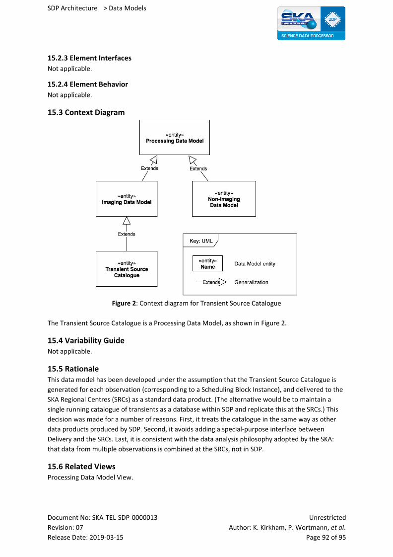
SDP Architecture > Data Models
15.2.3 Element Interfaces
Not applicable.
15.2.4 Element Behavior
Not applicable.
15.3 Context Diagram
Figure 2: Context diagram for Transient Source Catalogue
The Transient Source Catalogue is a Processing Data Model, as shown in Figure 2.
15.4 Variability Guide Not applicable.
15.5 Rationale This data model has been developed under the assumption that the Transient Source Catalogue is
generated for each observation (corresponding to a Scheduling Block Instance), and delivered to the
SKA Regional Centres (SRCs) as a standard data product. (The alternative would be to maintain a
single running catalogue of transients as a database within SDP and replicate this at the SRCs.) This
decision was made for a number of reasons. First, it treats the catalogue in the same way as other
data products produced by SDP. Second, it avoids adding a special-purpose interface between
Delivery and the SRCs. Last, it is consistent with the data analysis philosophy adopted by the SKA:
that data from multiple observations is combined at the SRCs, not in SDP.
15.6 Related Views Processing Data Model View.
Document No: SKA-TEL-SDP-0000013 Unrestricted
Revision: 07 Author: K. Kirkham, P. Wortmann, et al. Release Date: 2019-03-15 Page 92 of 95
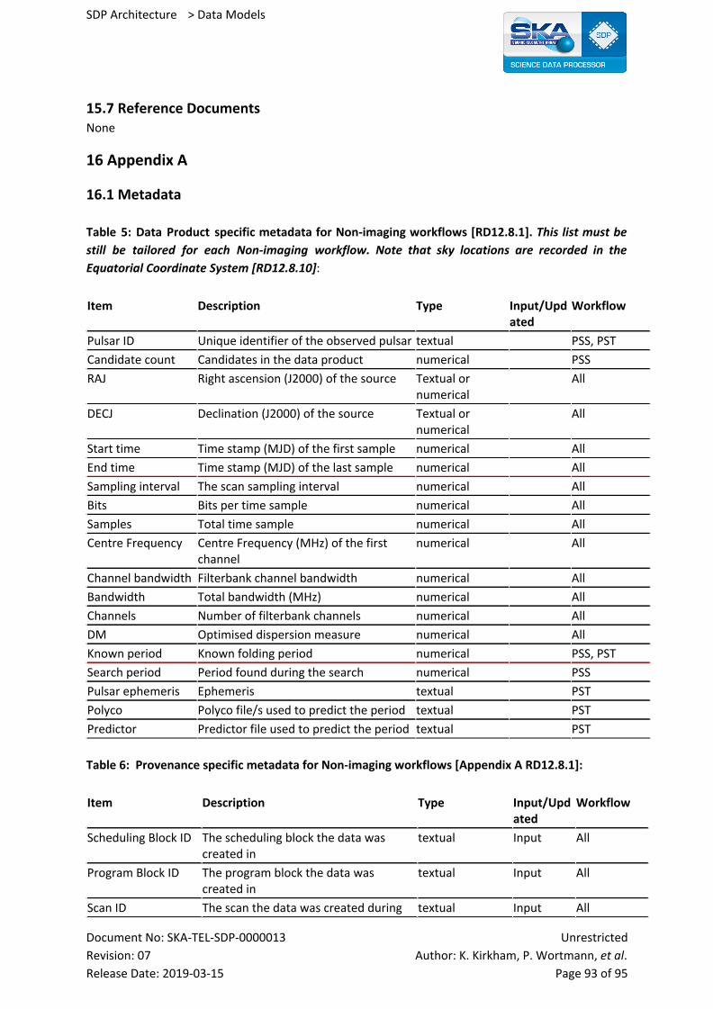
SDP Architecture > Data Models
15.7 Reference Documents None
16 Appendix A
16.1 Metadata Table 5: Data Product specific metadata for Non-imaging workflows [RD12.8.1]. This list must be
still be tailored for each Non-imaging workflow. Note that sky locations are recorded in the
Equatorial Coordinate System [RD12.8.10]:
Item Description Type Input/Updated
Workflow
Pulsar ID Unique identifier of the observed pulsar textual PSS, PST
Candidate count Candidates in the data product numerical PSS
RAJ Right ascension (J2000) of the source Textual or numerical
All
DECJ Declination (J2000) of the source Textual or numerical
All
Start time Time stamp (MJD) of the first sample numerical All
End time Time stamp (MJD) of the last sample numerical All
Sampling interval The scan sampling interval numerical All
Bits Bits per time sample numerical All
Samples Total time sample numerical All
Centre Frequency Centre Frequency (MHz) of the first channel
numerical All
Channel bandwidth Filterbank channel bandwidth numerical All
Bandwidth Total bandwidth (MHz) numerical All
Channels Number of filterbank channels numerical All
DM Optimised dispersion measure numerical All
Known period Known folding period numerical PSS, PST
Search period Period found during the search numerical PSS
Pulsar ephemeris Ephemeris textual PST
Polyco Polyco file/s used to predict the period textual PST
Predictor Predictor file used to predict the period textual PST
Table 6: Provenance specific metadata for Non-imaging workflows [Appendix A RD12.8.1]:
Item Description Type Input/Updated
Workflow
Scheduling Block ID The scheduling block the data was created in
textual Input All
Program Block ID The program block the data was created in
textual Input All
Scan ID The scan the data was created during textual Input All
Document No: SKA-TEL-SDP-0000013 Unrestricted
Revision: 07 Author: K. Kirkham, P. Wortmann, et al. Release Date: 2019-03-15 Page 93 of 95

SDP Architecture > Data Models
Subarray ID The sub-array configuration, if applicable
textual Input All
Product ID The data product identifier textual Updated All
CBF Pipeline Version Pipeline processing the data numerical Input All
CSP Pipeline Version Pipeline processing the data numerical Input All
SDP Pipeline Version Pipeline processing the data numerical Updated All
History Description of the steps applied to the data
textual Input & Updated
All
Size Size of the product in bits integer Input & Updated
All
Intermediate Products
Flag indicating if there are child products
textual ? All
17 Applicable Documents The following documents are applicable to the extent stated herein. In the event of conflict between
the contents of the applicable documents and this document, the applicable documents shall take
precedence.
This list of applicable documents applies to the whole of the SDP Architecture.
[AD01] SKA-TEL-SKO-0000002 SKA1 System Baseline Design V2, Rev 03 4
[AD02] SKA-TEL-SKO-0000008 SKA1 Phase 1 System Requirement Specification, Rev 11
[AD03] SKA-TEL-SDP-0000033 SDP Requirements Specification and Compliance Matrix, Rev 04
[AD04] SKA-TEL-SKO-0000307 SKA1 Operational Concept Documents, Rev 02
[AD05] 000-000000-010 SKA1 Control System Guidelines, Rev 01
[AD06] 100-000000-002 SKA1 LOW SDP to CSP ICD, Rev 06
[AD07] 100-000000-025 SKA1 LOW SDP to SaDT ICD, Rev 05
[AD08] 100-000000-029 SKA1 LOW SDP to TM ICD, Rev 05
[AD09] 100-000000-033 SKA1 LOW SDP to LFAA Interface Control Document (ICD), Rev 02
[AD10] 300-000000-002 SKA1 MID SDP to CSP ICD, Rev 06
[AD11] 300-000000-025 SKA1 MID SDP to SaDT ICD, Rev 05
[AD12] 300-000000-029 SKA1 MID SDP to TM ICD, Rev 05
[AD13] SKA-TEL-SKO-0000484 SKA1 SDP to INFRA-AUS and SKA SA Interface Control Document, Rev 02
4 This document is still a draft version and therefore not truly applicable, but will be replaced by an applicable version by System CDR.
Document No: SKA-TEL-SDP-0000013 Unrestricted
Revision: 07 Author: K. Kirkham, P. Wortmann, et al. Release Date: 2019-03-15 Page 94 of 95

SDP Architecture > Data Models
[AD14] SKA-TEL-SKO-0000661 Fundamental SKA Software and Hardware Description Language Standards
[AD15] http://www.ivoa.net/documents/TAP/
[AD16] http://www.ivoa.net/documents/latest/SIA.html
[AD17] http://www.ivoa.net/documents/DataLink/
[AD18] http://www.ivoa.net/documents/SSA/
[AD19] Memorandum of Understanding between the SKA organisation and National Radio Astronomy Observatory relating to a work package for the study and design of a new data model for the CASA software package
[AD20] MeasurementSet definition version 3.0. MSv3 team, eds. 2018. http://casacore.github.io/casacore-notes/264
[AD22] Shibboleth Authentication Service from Interenet2 https://www.internet2.edu/products-services/trust-identity/shibboleth/
[AD23] COmanage Authorization Service from Interenet2 https://www.internet2.edu/products-services/trust-identity/comanage/
[AD24] SKA-TEL-SKO-0000990 SKA Software Verification and Testing Plan
© Copyright 2019 University of Cambridge
This work is licensed under a Creative Commons Attribution 4.0 International License.
Document No: SKA-TEL-SDP-0000013 Unrestricted
Revision: 07 Author: K. Kirkham, P. Wortmann, et al. Release Date: 2019-03-15 Page 95 of 95