School of Education, Culture and CommunicationDivision of Applied Mathematics

MASTER THESIS IN MATHEMATICS / APPLIED MATHEMATICS

The Mathematical Formulation and Practical Implementation ofMarkowitz 2.0

by

Erick Mokaya Momanyi

MALARDALEN UNIVERSITY

SE-721 23 VASTERAS, SWEDEN

School of Education, Culture and CommunicationDivision of Applied Mathematics

Master thesis in mathematics / applied mathematics

Date:

January 22, 2017

Project name:

The Mathematical Formulation and Practical Implementation of Markowitz 2.0

Author:

Erick Mokaya Momanyi

Supervisors:

Lars Pettersson and Anatoliy Malyarenko

Reviewer:

Ying Ni

Examiner:

Linus Carlsson

Comprising:

30 ECTS credits

Abstract

Standard Deviation is a commonly used risk measures in risk management and port-folio optimization. Optimal portfolios have normally been computed using standarddeviation as the measure of choice for risk. However, ever since the Great Recession,it has come up short in capturing tail risk leading practitioners and investors alike tolook for alternative measures such as Value-at-Risk (VaR) and conditional Value-at-Risk (CVaR). Further, given that it is a coherent risk measure and that it allows for asimplification of the portfolio optimization process, CVaR is preferable to VaR.

This thesis analyzes the financial model referred to as Markowitz 2.0 which adoptsCVaR as the risk measure of choice. Tapping into the extensive literature on portfoliooptimization using CVaR and VaR, we give historical context to the model and make amathematical formulation of the model. Moreover, we present a practical implementa-tion of the model using data drawn from the Dow Jones Industrial Average, generateoptimal portfolios and draw the efficient frontier. The results obtained are comparedwith those obtained through the Mean-Variance optimization framework.

Keywords: Value-at-Risk, Conditional Value-at-Risk, Markowitz 2.0, Optimization,Mean-Variance optimization

To Josephine Mwango, my mother,

for her unwavering support to and strong belief in me.

Acknowledgements

This project would not have been possible without the support of many people. Firstand foremost, I would like to thank my thesis supervisors Lars Pettersson and AnatoliyMalyarenko who have walked with me throughout the process and offered remarkableguidance and support.

My very profound appreciation to the many friends I made while studying in Swedenwith a special mention to those I met at the Bible Study group at Malardalen Univer-sity. Specifically, special thanks to my close friends Carolyne Ogutu, James Omweno,Shedrack Lutembeka, Polite Mpofu, Katarına Skrabakova, Asmund Skomedal, Re-becca Njuguna, Grace Oliver, Mary Wanja, Nora Austad Sværen, Mahalet Haile Se-lasie and Anna Katharine Shelby for their unwavering encouragement and support. Iwould also like to thank my program mates who have helped me a lot.

Further, my regards to the Swedish Institute for affording me the incredible oppor-tunity to study Financial Engineering with a generous scholarship. You opened myworld to a world of wonder and learning.

Finally, a big thank you to my mother Josephine Mwango and my brother EliudMageto and the rest of the extended family for their love and support. Never for-get you are my source of motivation to live life to the fullest.

Contents

1 Introduction 1

1.1 Motivation and Context . . . . . . . . . . . . . . . . . . . . . . . . . . . . 1

1.2 Thesis Contribution . . . . . . . . . . . . . . . . . . . . . . . . . . . . . . . 2

1.3 Research Aim and Objectives . . . . . . . . . . . . . . . . . . . . . . . . . 3

1.4 Overview and Outline . . . . . . . . . . . . . . . . . . . . . . . . . . . . . 3

2 Modern Portfolio Theory 4

2.1 The Foundations of Modern Portfolio Theory . . . . . . . . . . . . . . . 4

2.2 Markowitz 1.0 . . . . . . . . . . . . . . . . . . . . . . . . . . . . . . . . . . 5

2.2.1 Model Concepts . . . . . . . . . . . . . . . . . . . . . . . . . . . . 5

2.2.2 Model Limitations . . . . . . . . . . . . . . . . . . . . . . . . . . . 7

2.3 Measuring Risk . . . . . . . . . . . . . . . . . . . . . . . . . . . . . . . . . 8

2.3.1 Value-at-Risk (VaR) . . . . . . . . . . . . . . . . . . . . . . . . . . . 9

2.3.2 Conditional Value-at-Risk (CVaR) . . . . . . . . . . . . . . . . . . 10

2.4 Measuring Returns . . . . . . . . . . . . . . . . . . . . . . . . . . . . . . . 13

3 Markowitz 2.0 16

3.1 Model Overview . . . . . . . . . . . . . . . . . . . . . . . . . . . . . . . . 16

3.2 Model Concepts . . . . . . . . . . . . . . . . . . . . . . . . . . . . . . . . . 17

3.3 Mathematical Formulation . . . . . . . . . . . . . . . . . . . . . . . . . . . 19

3.3.1 Smooth Multivariate Discrete Distribution (SMDD) . . . . . . . . 19

3.3.2 Portfolio Utility and Returns . . . . . . . . . . . . . . . . . . . . . 22

3.3.3 Portfolio Optimization with CVaR . . . . . . . . . . . . . . . . . . 24

3.3.4 The Efficient Frontier . . . . . . . . . . . . . . . . . . . . . . . . . . 26

iii

3.3.5 Incorporating Additional Constraints . . . . . . . . . . . . . . . . 28

4 Numerical Implementation 29

4.1 Data Description . . . . . . . . . . . . . . . . . . . . . . . . . . . . . . . . 29

4.2 Model Implementation, Results and Analysis . . . . . . . . . . . . . . . . 30

5 Conclusion and Further Research 36

5.1 Review and Conclusion . . . . . . . . . . . . . . . . . . . . . . . . . . . . 36

5.2 Further Research . . . . . . . . . . . . . . . . . . . . . . . . . . . . . . . . 37

Bibliography 37

List of Acronyms 41

A More mathematics 42

A.1 Mathematical Formulation of Markowitz 1.0 . . . . . . . . . . . . . . . . 42

A.2 The Dow Jones Industrial Average (DJIA) Companies . . . . . . . . . . . 44

A.3 Matlab Mean-CVaR Optimization Code . . . . . . . . . . . . . . . . . . . 45

A.4 Notes on fulfillment of Thesis objectives . . . . . . . . . . . . . . . . . . 47

iv

Chapter 1

Introduction

This chapter gives an introduction to the thesis.

1.1 Motivation and Context

Ever since the Great Recession started in 2008, extreme market events have become anorm rather than the exception. A quick glance at a couple of Bloomberg headlinesin 2015 and 2016 as highlighted in Figure 1.1 shows how these unexpected events justkeep happening. Such kind of events have not just started happening recently but haveonly been noticed more keenly. A name for such events has been given to be BlackSwans. A black swan is an outlier event with an extreme impact and which seemsto have a good explanation, but only after-the-fact Taleb (2010). It therefore combinesrarity, extreme impact and retrospective predictability. Such events have an impact onportfolios that is very significant.

Figure 1.1: Bloomberg articles highlighting non-normal market events in 2015.

Further, there is empirical proof that market returns are not normally distributed asmost commonly assumed. The tails has been found to be fatter and the distributionsmore peaked than the normal distribution implies, see Sheikh and Qiao (2009). Asmost financial models assume a normal distribution, there has been a significant fail-ure to capture the tail risk in most financial models.

In 2016 alone, such non-normal market events have been prevalent with such events

1

as Brexit, the election of Donald Trump as president of the United States, and yieldson highly rated government bonds like the German Bunds falling below zero beingviewed as unexpected. In one of the articles cited in Figure 1.1, Alloway (2015b),details six non-normal events that were happening as of that date of the article includ-ing negative swap spreads and corporate bond inventories below zero. In essence,market moves that aren’t supposed to happen often kept happening. In the other ar-ticle, Alloway (2015a), encourages investors to consider Value-at-Risk (VaR) as a keycomponent of their risk analysis measures.

When it comes to portfolio optimization, VaR, as we will see, is not a coherent measureof risk as it lacks both subadditivity and convexity and presents a bit of challenge inoptimizing optimize. The preferable coherent measure of risk is Conditional Value-at-Risk (CVaR). This proposition is central point to our approach in optimization inthis thesis. The thesis is motivated by the need to consider such non-normal marketevents and incorporate them in a risk analysis and portfolio management. The focusof the thesis is Markowitz 2.0, a model developed in Kaplan and Savage (2011) whichincorporates CVaR in generating optimal portfolios.

1.2 Thesis Contribution

To the author’s best knowledge, this thesis is the first to review Markowitz 2.0 andattempt to reformulate it in a manner that taps into the rich historical context that isVaR and CVaR optimization. As a result, a significant part of the thesis is therefore areview of other peoples works. The author seeks to present seemingly complex worksin a manner understandable to the reader in a single framework of optimization innon-normal markets so as to make the adoption of the concepts underlying the thesisby practitioners is not only possible but more likely.

To the best knowledge of the author, the key insights that are new in this thesis are:

• The detailed mathematical formulation of Markowitz 2.0 while drawing on theworks of Palmquist et al. (2002), Boyd and Vandenberghe (2004) and Kaplan andSavage (2011), see Section 3.3.

• The mathematical proof on how the kurtosis and skewness in the Discrete Mul-tivariate Model relates to that in the Smooth Multivariate Discrete MultivariateModel (SMDD), see Section 3.3.1.

• The proposition of the weighted estimator as an alternative to the geometricmean and arithmetic mean in the mean-CVaR optimization framework, see Sub-section 2.4.

• The implementation of Markowitz 2.0 in MATLAB using data from the DowJones Industrial Average (DJIA) index, see Section 4.2.

2

1.3 Research Aim and Objectives

The overall aim of this thesis is to make a contribution towards a better understandingof the theoretical and practical underpinnings of Markowitz 2.0. Special focus is givento the use of the coherent risk measure CVaR.

The thesis sets out to achieve this aim by fulfilling the following specific objectives:

1. To review the literature concerning asset allocation models and, in the process, givehistorical context and perspective to Markowitz 2.0

2. To draw on relevant literature to make a mathematical formulation on Markowitz 2.0.

3. To implement Markowitz 2.0 in a programming language of choice and conduct a prac-tical assessment of the model.

In doing all this, the thesis seeks to add to the rich body of knowledge on portfoliooptimization using CVaR.

1.4 Overview and Outline

The thesis is organized as follows: Chapter 1 has briefly introduced the topic forresearch together with the motivation and context for it. Chapter 2 reviews modernportfolio theory and discusses the various measures of risk and returns used in financetogether with their strengths and drawbacks and seeks to make a case for using CVaRas a coherent risk measure.

Further, Chapter 3 introduces Markowitz 2.0, gives an overview and an analysis ofkey concepts in the model and lays out the mathematical formulation of the model.Chapter 4 implements the model using data from the DJIA) and generates both opti-mal portfolios and an efficient frontier. It further provides an analysis and discussionof the results. Finally, Chapter 5 provides a review and summary of the thesis andprovides some conclusions and makes a case for areas that warrants further research.

Throughout this paper, we adopt a convention of using bold-face lower case letters forvectors (x, ...), bold-faced capital letters for matrices (Σ, ...) and ordinary letters (c) forscalars.

3

Chapter 2

Modern Portfolio Theory

This chapter explores the foundations of Modern Portfolio Theory and analyses vari-ous risk and returns measures.

2.1 The Foundations of Modern Portfolio Theory

The foundations of Modern Portfolio Theory were laid out succinctly when Markowitzpublished his seminal paper Portfolio Selection in 1952. Prior to this, even thoughinvestors suspected that there were benefits to holding a diversified portfolio, theyhad no way of quantifying these benefits to help them assess the impact that theindividual assets had on the portfolio risk or how additional assets changed the risk-return mix of the portfolio. As a result, the construction of portfolios was a highlysubjective business coupled with an inability to assess the performance of investmentmanagers (Fabozzi et al., 2011). The main challenge was one of allocating resourcesamong the assets in a portfolio so as to maximize returns and maximize risk and thisis the central portfolio optimization problem.

Along came Markowitz (1952) to shift the landscape of portfolio management by pos-tulating that portfolio risk and returns could not only be assessed but also managedby using three key elements: means, variances and covariances. As a result, Mean-Variance Optimization (MVO) was born. It’s naming is apt given its reliance on mean(a proxy for expected returns) and variance (a proxy for risk). The Expected Returnsare defined as the expected excess returns of an asset above the risk free rate.

Central to MVO is the thesis that investors can maximize returns and minimize riskby paying keen attention to the correlation between assets and thereby construct op-timal portfolios. In this way, they can allocate their resources among asset and assetclasses so as to create optimal portfolios (as opposed to holding individual assets) thatmaximize returns and mitigate risk. Investors could do this by maximizing expectedreturns given a particular level of risk or minimizing risk at a given level of expected

4

return.

This is the foundation upon which later models like the Black-Litterman and Markowitzbuild up. It gave investors a new way to examine their portfolios and allowed for theobjectives and constraints of the investor to be taken into account when constructingportfolios, the control of risk exposures in the portfolio, an organization to reflect itsstyle and positioning in the market in the portfolio and for strategic portfolio changesas needed (Michaud, 1989). The central goal of this dissertation is to study and analysetwo models that help deal with the limitations of the MVO.

2.2 Markowitz 1.0

2.2.1 Model Concepts

The Mean-Variance Optimization (MVO) framework, here referred to as the Markowitz1.0, is a one-period concept in that it maximizes returns over one period only. The pa-rameters needed are expected returns, variances and covariances of the assets to beassessed.

Markowitz 1.0 begins with the assumption that the investor has beliefs about futureperformances, that is they have the expected returns, variances and covariances Fig-ured out, see Markowitz (1952). These are mostly obtained from historical data mak-ing the further assumption that the past is a good indicator of the future. The investormust have these beliefs in place at the outset. Intuitively, when given a choice betweentwo assets with similar returns but one of which has lower variance, the rational in-vestor opts for the one lower variance. However, when considering choices betweenportfolios, the investor must consider the covariances and correlations among assets.In using only the means, variances, and covariances to derive the optimal portfolio,MVO takes the first two moments as sufficient and fails to take into account extremeevents in the tails.

To model risk and return in an MVO framework, assume an investment universe withn securities. Let rj be the expected return of the n assets in the portfolio, σjk be thecovariance between assets j and k, ρjk be the correlation coefficient between assets jand k and xj be the weight of the investors allocation to the jth security. The return ofa portfolio is the weighted average returns of the individual asset, that is

rp =n

∑j=1

xjrj. (2.1)

However, the risk of a portfolio as measured by standard deviation (square root of

5

variance) is not calculated as an average but rather as

σ2p =

n

∑j=1

x2j σ2

j +n

∑j=1

n

∑k=1j 6=k

xjxkσjσkρjk.

Further, take x to be the n × 1 vector of portfolio weights, σ2p the portfolio variance,

rp the portfolio expected return, r the 1× n vector of expected returns of the assetsand Σ the symmetric n× n covariance matrix. We assume the covariance matrix (Σ)to be a positive definite matrix, x>Σx 0 to ensure it is invertible. All the assets andcombinations of assets that make up a portfolio lie the first or fourth quadrant in themean-standard deviation space. The convex upper boundary where all the efficientcombinations lie is called the efficient frontier.

Figure 2.1: An example of the mean-variance efficient frontier.

To derive the efficient frontier, we minimize risk for a given level of return (Equa-tion 2.2) or maximize return for a given level of risk (equation 2.3).

minimize x>Σxsubject to rp = x>R

(2.2)

maximize x>Rsubject to σ2

p = x>Σx (2.3)

Additional constraints like no short selling and a minimum desired return can be in-troduced at the discretion of the investor making the model even more robust. Should

6

the set of constraints have only linear equality and inequality constraints as definedin Definition 2.1, then the problem is a quadratic program that can be solved usingstandard numerical optimization software (Kolm et al., 2014).

Definition 2.1. A quadratic program (QP) is a convex optimization problem with a quadraticobjective function and affine constraint functions (Boyd and Vandenberghe, 2004). Given thatP is a positive semidefinite matrix, then the QP is expressed as

minimize12

x>Px + q>x + r

subject to Gx hAx = 0

(2.4)

Mankert and Seiler (2011) prove that solving Equation 2.5 is equivalent to solvingequations 2.2 or 2.3 with the added parameter δ being the risk aversion parameter andµ being the excess return vector (expected returns in excess of the risk free rate, R f ).

max x>µ− 12

δx>Σx. (2.5)

The resulting solution to these equations is the Markowitz optimal portfolio given as

x∗ =(δΣ)−1µ. (2.6)

A more detailed formulation of equation 2.6 is given in Appendix A.1.

2.2.2 Model Limitations

Given general intuitiveness and simplicity in application of the MVO model, one canwonder why the uptake of this model has been limited, see (Michaud, 1989; Kolmet al., 2014). Several issues have been identified that have limited its practical useful-ness.

• It yields unintuitive, highly concentrated portfolios. It tends to place the greatestweights on assets that have the highest expected returns and lowest correlation.As Mankert and Seiler (2011) indicate, this may not be a surprise given thatinvestors predicted those very assets to be prone to high returns and would,therefore, be inclined to placing greater weights on them. The challenge of unin-tuitive portfolios persists though. Some of the portfolios generated by the modelare quite difficult to make sense of due to the fact that “they don’t make invest-ment sense and don’t have investment value” because “they were often found to beunmarketable either internally or externally” (Michaud, 1989).

• It generates portfolios that can be extremely sensitive to changes in asset means(Best and Grauer, 1991) and views (Black and Litterman, 1991). In one instance,

7

Best and Grauer showed that a slight increase in any one asset’s returns ofaround say 2%, removed more than half the securities from the equally weightedportfolio with little or no change in the portfolio’s risk-return characteristics.Further, they noted that the higher the correlations between the assets in a port-folio, the more sensitive the portfolios to changes in inputs. Therefore, theres aneed to pay attention to the inputs one is feeding the optimizer and one cannotafford not to pay attention to this.

• As identified by Michaud, Mean-Variance Optimization tends to maximize theerrors in the inputs, that is in expected returns, variances and covariances. Theinputs are estimates. Often times, the greatest weight on securities is placedon the assets with the largest expected returns,most negative correlations andsmallest variances, which incidentally tend to have the greatest estimation errors,the resulting portfolios have optimal errors in as much as they are optimal in therisk-return space.

Other limitations of the model include problems with estimating covariances, modelinstability, focus on single periods, failure to account for market capitalization weightsand failure to differentiate between the levels of uncertainty in the inputs (Elton andGruber, 1997; Mankert and Seiler, 2011; Michaud, 1989).

Given these weaknesses that have been identified, investigated and discussed exten-sively, the model still retains its universal appeal being prominently used by manypractitioners in portfolio management. Elton and Gruber (1997) believe that this isbecause “the implications of mean variance portfolio theory are well developed, widely known,and have great intuitive appeal” such that “professionals who have never run an optimizerhave learned that correlations as well as means and variances are necessary to understand theimpact of adding a security to a portfolio”. It seems then that the model is here to stay.

2.3 Measuring Risk

Risk in finance is the uncertainty in future returns. There are several measures thatare taken to be proxies to risk.

Definition 2.2. A risk measure: Given a set, V, of real-value random variables, a riskmeasure is a function ρ that maps the random variables in V to R, that is ρ : V → R.

The measures of risk commonly utilized include standard deviation, value-at-risk(VaR) and conditional value-at-risk (CVaR), all of which are defined in this thesis.Standard Deviation has already been defined and has also been found wanting be-cause of it penalizes risk and loss equally. In this section, we formally define andexplore VaR and CVaR.

8

2.3.1 Value-at-Risk (VaR)

Value-at-Risk (VaR) is a risk measure that has found wide application in finance sinceits formulation in early 1990s, becoming so popular as to be adopted by banks andbank regulators such as the Bank for International Settlements (BIS).

Definition 2.3. Value-at-Risk: Let X be a random variable representing loss. The α-VaRwith probability level α ∈ (0, 1) is defined as

VaRα(X) := min c ∈ R : P(X ≤ c) ≥ α . (2.7)

VaR considers how much an investment is likely to lose in a certain interval of timewith a given degree of confidence. For instance, having invested 10 million, the ques-tion one would like to answer using VaR is this: how much can we expect to lose witha given level of confidence?. One answer to this question would be that with a 95%degree of confidence, we estimate that we would lose 2 million or more over a periodof 6 months. This amount of 2 million or more is the VaR and describes the left tail ofthe distribution.

VaR is not considered a coherent risk measure as defined by Artzner et al. (1999).

Definition 2.4. A coherent risk measure: A function ρ : V → R is called a coherentrisk measure if it meets the axioms of translation invariance, monotonicity, subadditivity andpositive homogeneity.

Axiom 2.1. Subadditivity: For bounded random variables Y and Z with Y, Z ∈ V, thenρ(Y + Z) ≤ ρ(Y) + ρ(Z).

The subadditivity axiom implies that the risk of holding both assets Y and Z simulta-neously should be less than or equal to the risk of holding the two assets separately.this is the essence of portfolio diversification where the risk of individual assets heldtogether should be less than the risk of individual assets held separately. Therefore, ifthe axiom does not hold, the investor is better off opening separate accounts for eachasset Y and Z because the margin requirement, ρ(Y) + ρ(Z), would be lower than ifhe held both assets in one account, ρ(Y + Z), see Artzner et al. (1999).

Axiom 2.2. Translation Invariance: If c ∈ R, then ρ(Z + c) = ρ(Z)− c.

Axiom 2.3. Monotonicity: If Z ≥ Y, then ρ(Z) ≤ ρ(Y).

Translation invariance means that that should we add a certain amount of cash to theportfolio, the portfolio risk should decrease by a similar amount while monotonicityimplies that if an investment Y generates worse outcomes than an investment Z, thenthe former should be considered riskier.

Axiom 2.4. Positive Homogeneity: If λ ≥ 0, then ρ(λZ) = λρ(Z).

9

A risk measure that has positive homogeneity axiom allows for the risk of a portfolioto be proportional to its size. VaR is translation invariant, motononic and positivelyhomogeneous. VaR, however, does not satisfy the subadditivity axiom. Convexity is anatural result of the axioms of subadditivity and positive homogeneity and is central tosolving portfolio optimization problems.

VaR is difficult to use in optimization because it results in multiple local maximaand in non-convex, non-smooth functions (Palmquist et al., 2002). A unique and welldiversified optimal solution is only possible in situations where the surfaces are convex(Acerbi and Tasche, 2002).

There are several methodologies employed in calculating VaR. One of the ways is usingthe α-Quantile. The quantile function can be used to determine the VaR.

Definition 2.5. VaR as a quantile function: For a random variable X with a cumulativedistribution function (cdf) given by FX(u) = PX ≤ u whose left continuous inverse isgiven by F−1

X (α) = minu : FX(u) ≥ v, the VaR for a fixed level α, is defined as

VaRα(X) = F−1X (α).

Given that the quantile function is determined from the distribution function, then ifthe cdf is known, the VaR is calculated as the quantile function of the given proba-bility distribution. However, since it is not common to find the cdf as well defined,RiskMetrics, a methodology that assumes that the continuous compound daily returnof the portfolio are conditional normally distributed, is used.

Although a popular measure, VaR is rarely used in solving optimization problems. Forinstance, in calculating VaR using RiskMetrics, return distributions are assumed to benormal making the analysis very simple and easy to interpret. Since these return dis-tributions are far from normal in real life and are often skewed with heavy tails, thereis need to improve on this tool. VaR has the further defect of being unable to estimatethe amounts that can be lost in case the limit is breached as it fails to recognize theconcentration of risks beyond the threshold. For other methods for computing VaR, werefer the reader to the Gloria-Mundi website (http://gloria-mundi.com/) wherethe methods are extensively covered.

2.3.2 Conditional Value-at-Risk (CVaR)

Conditional Value-at-Risk (CVaR) captures the losses that can be incurred should theVaR be breached. In essence, while VaR captures returns at some specific point, theCVaR captures the probability weighted return of the whole tail. As such the CVaRis always more than the VaR meaning that portfolios with low CVaR have low VaRas well, see Rockafellar and Uryasev (2000). Figure 2.4 compares VaR to CVaR. CVaRis also referred to as Mean Excess Loss, Mean Shortfall, or Tail VaR in continuousdistributions, see Palmquist et al. (2002). CVaR is normally looked at as the weighted

10

Figure 2.2: VaR is the left end point depicted by a red line while CVaR the area afterthat point breached bounded by the blue and red lines.

average of tail VaR and loss that strictly exceeding VaR. For continuous distributions,CVaRα(X) is defined as the weighted average of CVaR+

α (X), i.e. losses strictly exceed-ing VaR and CVaR−α (X), i.e. VaR which can be depicted as

CVaRα(X) = (1− θα(X))CVaR+α (X) + θα(X)VaR(

αX),

where

θα(X) =FX(VaR(

αX))− α

1− α.

For a generalized distribution, Sarykalin et al. (2008) defines CVaR as

Definition 2.6. General CVaR definition: For a random variable X with a cumulativedistribution function given by FX(u) = PX ≤ u, the CVaR for the probability level α ∈(0, 1) is defined as

CVaRα(X) =∫ +∞

−∞udFα

X(u),

where

FαX(u) =

0 if when u < VaRα(X),FX(u)−α

1−α when u ≥ VaRα(X).

Specifically, for a loss random variable X with a continuous distribution function it isdefined as

Definition 2.7. CVaR: For a loss random variable X with a continuous distribution function,the α-CVaR at the probability level α ∈ (0, 1) is defined as

CVaRα(X) := E[X|X ≥ VaRα(X)]. (2.8)

Rockafellar and Uryasev (2000) provide another definition. They consider CVaR to bea solution to the function below that will be used in the formulation of Markowitz 2.0.

CVaRα(X) = inf

a +1

1− αE[[X− a]+]

, where [z]+ = max0, z. (2.9)

11

Another equivalent formulation of CVaR is given by Acerbi and Tasche (2002) andAcerbi (2002) who show that under certain conditions, CVaR is equal to the expectedshortfall as defined by

CVaRα(X) =1α

∫ α

0VaRβ(X)dβ.

There is another formulation of CVaR to be given in Section 3.3.3.

CVaRα is a coherent measure of risk as it fulfills all the four conditions in Definition 2.4.These and other properties of CVaR are summarized as (see Pflug (2000) for proofs)

(a) CVaRα is subadditive: For λ ∈ [0, 1], then CVaRα(λY + (1− λ)Z) ≤ λCVaRα(Y) +(1− λ)CVaRα(Z).

(b) CVaRα is translation invariant: If c ∈ R then CVaRα(Z + c) = CVaRα(Z)− c.

(c) CVaRα is monotonic: If Z ≥ Y, then CVaRα(Z) ≤ CVaRα(Y).

(d) CVaRα is positively homogeneous: If λ ≥ 0, then CVaRα(λZ) = λCVaRα(Z).

(e) Other Property: If Z is a continuous random variable, then E(Z) = (1− α)CVaRα(Z)−αCVaR1−α(−Z).

Proof. To provide proof for (a), we use Equation 2.9 to define CVaRα(Y) = a +1

1−α E[[Y − a]+] and CVaRα(Z) = b + 11−α E[[Z − b]+]. Given that y 7→ [y − a]+ is

convex, then

CVaRα(λY + (1− λ)Z) ≤ λa + (1− λ)b +1

1− αE[[λY + (1− λ)Z− λa + (1− λ)b]+]

≤ λa + (1− λ)b +λ

1− αE[[Y− a]+] +

1− λ

1− αE[[Z− b]+]

≤ λCVaRα(Y) + (1− λ)CVaRα(Z).

Proofs for (b) and (d) are obvious from the definition of CVaR. In addition to beingconvex, y 7→ [y− a]+ is also monotone. Proof for (c) follows as a result. To provideprof for (e), we have

CVaR1−α(−Z) = E(−Z| − Z > VaR1−α(−Z))= E(−Z| − Z > −VaRα(Z))= −E(Z|Z < VaRα(Z))

which means

E(Z) = E(Z|Z < VaRα(Z)) +−(1− α)E(Z|Z > VaRα(Z))= (1− α)CVaRα(Z)− αCVaR1−α(−Z).

12

CVaRα has proved to be a useful tool in measuring risk especially because of the con-vexity property that allows the optimization problem to be succinctly expressed as aminimization formula solvable via convex programming methods. Although VaR andCVaR concentrate on different properties of the distribution (VaR does not considerlosses exceeding VaR while CVaR accounts for them), they can coincide if the tails iscut off (Pflug, 2000). Further, optimal solutions derived when minimizing CVaR arealso near optimal as regards to VaR such that portfolios with a low CVaR might alsohave low VaR (Rockafellar and Uryasev, 2000). Caution must, however, be exercisedin that although in some cases the two measures yield similar results, they can yielddifferent portfolios as tested by Gaivoronski and Pflug (2004).

2.4 Measuring Returns

The arithmetic mean and the geometric mean of the return series are used to measurereturns.

Definition 2.8. Arithmetic mean return: For a series of returns r1, r2, .., rn, the arithmeticmean return (AM) is defined as

AM =1n

n

∑i=1

ri. (2.10)

Although it is an unbiased estimator of the expected return, the probability of achiev-ing it is low given that it is too optimistic a measure (Mindlin, 2011). The geometricmean, on the other hand, is concerned with maximizing the growth of the portfolioover a longer period of time.

Definition 2.9. Geometric mean return: For a series of returns r1, r2, .., rn, the geometricmean return is defined as

GM =[ n

∏i=1

(1 + ri)] 1

n − 1. (2.11)

This can also be written as

ln(1 + GM) =1n

n

∑i=1

ln(1 + ri). (2.12)

The strategy of maximizing the geometric means is also referred to as the Kelly cri-terion, the growth optimal portfolio, the capital growth theory of investment, the ge-ometric mean strategy, investment for the long run, maximum expected log, and ge-ometric mean maximization, see Estrada (2010). Given that investors and fund man-agers focus on capital growth over their investment horizon, there is a tendency to usethe GM to measure returns with many practitioners preferring geometric averages, seeJacquier et al. (2003) and Kaplan and Savage (2011).

13

Mindlin (2011) provides proofs for four formulas that connect the arithmetic and ge-ometric mean, one of which is of interest. This is the one that gives the relationshipbetween GM and GM as

GM = −1 + (1 + AM) exp(− V

2(1 + AM)−2

). (2.13)

Proof. A Taylor series expansion for the function f (x) = ln(1 + x) around point AMto the second degree generates

ln(1 + x) = ln(1 + AM) +x− AM1 + AM

− (x− AM)2

2(1 + AM)2 + · · · . (2.14)

Define sample variance of a series of returns as

V =1n

n

∑i=1

(ri − AM)2, (2.15)

and apply Equation 2.14 to Equation 2.12 to get

ln(1 + GM) =1n

n

∑i=1

ln(1 + ri)

≈ ln(1 + AM) +1

n(1 + AM)

n

∑i=1

(ri − AM)− 12(1 + AM)2

1n

n

∑i=1

(ri − AM)2

≈ ln(1 + AM) +V

2(1 + AM)2 .

The other relationship of note is

GM ≈ AM− V2

. (2.16)

Proof. A Maclaurin series expansion for the function f (x) = (1 + x)1n to the second

degree generates

(1 + x)1n = 1 +

1n

x +1− n2n2 x2 + · · · . (2.17)

Substitute Equation 2.17 into Equation 2.11 and using Equation 2.15 and Equation 2.10

14

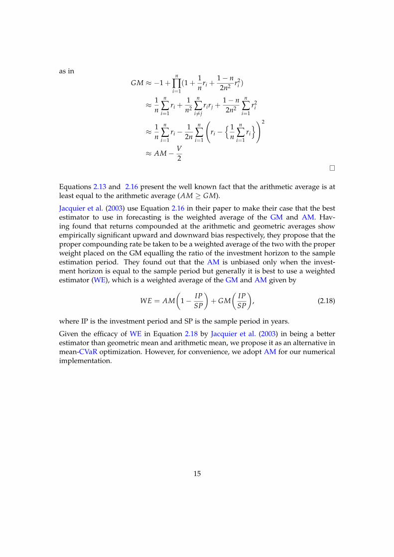
as in

GM ≈ −1 +n

∏i=1

(1 +1n

ri +1− n2n2 r2

i )

≈ 1n

n

∑i=1

ri +1n2

n

∑i 6=j

rirj +1− n2n2

n

∑i=1

r2i

≈ 1n

n

∑i=1

ri −1

2n

n

∑i=1

(ri −

1n

n

∑i=1

ri

)2

≈ AM− V2

Equations 2.13 and 2.16 present the well known fact that the arithmetic average is atleast equal to the arithmetic average (AM ≥ GM).

Jacquier et al. (2003) use Equation 2.16 in their paper to make their case that the bestestimator to use in forecasting is the weighted average of the GM and AM. Hav-ing found that returns compounded at the arithmetic and geometric averages showempirically significant upward and downward bias respectively, they propose that theproper compounding rate be taken to be a weighted average of the two with the properweight placed on the GM equalling the ratio of the investment horizon to the sampleestimation period. They found out that the AM is unbiased only when the invest-ment horizon is equal to the sample period but generally it is best to use a weightedestimator (WE), which is a weighted average of the GM and AM given by

WE = AM(

1− IPSP

)+ GM

(IPSP

), (2.18)

where IP is the investment period and SP is the sample period in years.

Given the efficacy of WE in Equation 2.18 by Jacquier et al. (2003) in being a betterestimator than geometric mean and arithmetic mean, we propose it as an alternative inmean-CVaR optimization. However, for convenience, we adopt AM for our numericalimplementation.

15

Chapter 3

Markowitz 2.0

This chapter gives an overview of Markowitz 2.0, explores its core concepts and con-tributions and derives it mathematically.

3.1 Model Overview

Motivated by the need to cure some of the flaws in the MVO model while leveragingdevelopments in technology and probability distribution, Kaplan and Savage (2011)developed Markowitz 2.0 (hereafter Markowitz 2.0 ). Just like the BL model, the start-ing point is the MVO framework as they add afterburners in order to overcome thelimitations identified in the MVO model. For instance, they replace the covariancematrix, the arithmetic mean and standard deviation with a scenario-based model gen-erated via Monte Carlo simulation, the GM and Conditional Value-at-Risk (CVaR) re-spectively. The result is the new efficient frontier which they believe to be more relevantto investors than the one from MVO.

Not much literature is available on Markowitz 2.0. The main material to be gleanedfor this model are found in the original article and two chapters of a book written byone of the authors. We will therefore seek to develop the mathematical underpinningsof this model in this thesis while drawing on the insights gained through a host ofliterature dealing with CVaR and optimization.

The need for Markowitz 2.0 can be traced back to Markowitz 1.0. In the time beforeMarkowitz (1952) and his Markowitz 1.0 model, investors did not have a way to choosebetween two assets with similar returns, a problem that Savage (2009) calls the the weakform of the flaw of averages. The assessment of assets were based solely on the averagereturns of assets resulting in systematic errors. Averages are insufficient in giving acomplete picture of the assets. A tale of the mathematician once drowned in a streamof averagely 2 inches illustrates this well. MVO gave investors a way of choosingbetween two assets with similar returns by helping them pay attention to variance and

16

with that Markowitz introduced the idea of risk. However, the use of variances andcovariances introduced other flaws since they too are averages. Markowitz 2.0 seeksto be more robust by dealing with flaws found in the MVO model for instance byallowing for fat-tailed distributions.

3.2 Model Concepts

Markowitz 2.0 incorporates five key afterburners that Kaplan and Savage (2011) addedto make the portfolio optimization process more robust.

Figure 3.1: A histogram of the distribution of historical returns over a ten year period2006-2016 on four stocks Intel, Exxon Mobil, Goldman Sachs and JP Morgani Chase &Co overlayed with a standard normal distribution.

(a) Incorporates Scenario Analysis

In using the mean and variance of asset returns in optimization, the MVO frame-work has the implicit assumption that asset returns are normally distributed.The well known symbol of a normal distribution is the bell-curve shape. Thenormal distribution underestimates the likelihood of extreme events since thereturns are concentrated around one or two standard deviations from the mean.Sheikh and Qiao (2009), however, show that the historical returns have beenknown not to be normally distributed. They also found that historical returnsare non-normally distributed with fatter tails (specifically negative skewness and

17

leptokurtosis), serial correlations and correlations that break down in periods ofeconomic distress. A normal distribution fit on some historical returns over theten year period 2006-2016 for some four stocks is plotted in Figure 3.1 and itshows the normal distribution to be a poor fit. Further analysis to prove this isdone in Chapter 4.

Markowitz 2.0 utilizes the scenario-based approach to allow for the incorporationof the fat tails. The scenario approach incorporates high peaks and fat tailsmaking it more reflective of real-world assumptions, see Gosling (2010). Notably,the resulting return distributions are best illustrated using histograms whichcan be smoothed out because no precise graphical presentation could suffice tocapture it. There are different ways of generating scenarios including MonteCarlo simulation.

The model assumes that a particular joint distribution holds for the price-returnprocess and generates the scenarios using Monte-Carlo simulation or quasi-random simulation or such other similar simulations. Markowitz 2.0 uses theSmooth Multivariate Discrete Distribution (SMDD) as the underlying distribu-tion. For convenience in using the inbuilt MATLAB function PortfolioCVaRobject, we use the Multivariate normal distribution. Although the underlyingprobability distribution is the multivariate normal, the asset returns generatedare sufficiently non-normal.

(b) Eliminates Covariance Matrices and Correlations

MVO also uses covariance matrices which assume a linear relationship betweenvariables to capture the relationship between the asset classes being modelled.Covariance matrices are, however, deficient in capturing the relationships be-tween the assets completely and effectively. For one, the use of a single Figure,the correlation coefficient derived from the covariance matrix, to represent thecomplex relationship between two assets introduces the flaw of averages.

Further, when complex securities such as options are introduced into the portfo-lio, the covariance matrix becomes ineffective by failing to capture the resultantnon-linear relationships between asset classes. Moreover, in market downturnsor during crisis events like the Great Recession and the Great Depression, thecorrelations between various assets and asset classes tend to increase. Notablythen, Markowitz 2.0 uses scenarios to model the non-linear relationships and toallow for more dynamic relationships between variables.

(c) Estimates Returns using Arithmetic and Geometric Mean

Kaplan and Savage (2011) present two measures of mean returns to be used ingenerating optimal portfolios. They seem to prefer the use of the GM because itis seen as a measure of returns that is more focused on the long term, in line withmost investors who want to invest for the long run. The age-old debate betweenthese two measures has been explored in Section 2.4. There we also make a case

18

for the use of an alternative measure known as the weighted estimator. In thisthesis, however, we make use of the arithmetic mean.

(d) Provides alternatives to Standard Deviation

Having noted the deficiencies of the standard deviation, this model explores theuse of several alternatives such as CVaR, the First Lower Partial Moment belowa target, the First Lower Partial Moment below the mean, Downside Deviationbelow a target and Downside Deviation below the mean. We will specificallyfocus on the CVaR.

(e) Utilizes data management techniques

The main drawback of the scenario-based approach is the need for the stor-age and processing of significant amounts of data. The number of scenariosneeded to generate a tractable solution to the optimization problem is signif-icantly large begging the need for an adequate data management technique.The model then leverages Sam Savage’s Distribution String (DIST), now calledStochastic Information Packet (SIPmathTM), data management technique whichallows many trials as a single data element to be made conveniently and speed-ily just by adding it to Microsoft Excel. Details of SIPmathTMare available atwww.probabilitymanagement.org/.

3.3 Mathematical Formulation

In this section, we formulate Markowitz 2.0 mathematically as we draw from the in-sights of Kaplan and Savage (2011) and Rockafellar and Uryasev (2000).

3.3.1 Smooth Multivariate Discrete Distribution (SMDD)

We begin with the Smooth Multivariate Discrete Distribution (SMDD) which under-pins this model. Assume there are m asset classes and n scenarios. Let R be a matrixwith m rows and n columns. The jth column of R,

rj = (r1j, . . . , rmj)>, 1 ≤ j ≤ n,

represents the returns of the assets under scenario number j.

The probability that the jth scenario occurs, is equal to wj, which obviously sum up to

1 (n∑

j=1wi = 1). Denote w = (w1, . . . , wn)> and let J be a random variable with

P J = j = wj, 1 ≤ j ≤ n.

Then r J is a random vector with

Pr J = rj = wj, 1 ≤ j ≤ n.

19

Definition 3.1. The random vector r J is called the Discrete Multivariate Model, hereafterknown as the discrete model.

The expected value of the discrete model is

E[r J ] = r =n

∑j=1

wjrj. (3.1)

The covariance matrix of the discrete model is

Σ[r J ] := E[(r J − E[r J ])(r J − E[r J ])>] = E[r Jr

>J ]− E[r J ](E[r J ])

>. (3.2)

The (ij)th entry of the random matrix r Jr>J takes value rikrjk with probability wk, 1 ≤

k ≤ n. We obtain

(E[r Jr>J ])ij =

n

∑k=1

wkrikrjk. (3.3)

orE[r Jr

>J ] = RWR>, (3.4)

where W is the n× n matrix with elements Wkl = wkδkl with

δkl =

1, if k = l0, if k 6= l.

Finally,Σ[r J ] = RWR> − r r>. (3.5)

Let ε be an m-dimensional centred normal random vector with covariance matrix Ωindependent on J.

Definition 3.2. The Smooth Multivariate Discrete Distributions Model (SMDD) is given by

r = r J + ε. (3.6)

Let x = (x1, . . . , xm)> be a vector representing an asset mix, that is xi ≥ 0 and∑m

i=1 xi = 1, the return of the asset mix is given by

r = x>r = x>(r J + ε) = x>r J + x>ε. (3.7)

The first term in the right hand side is the return of the portfolio under the discrete model,while the second term is called the disturbance term. We define our reward function as

R(x) = x>r.

Another name for this reward function is the arithmetic mean, see Kaplan and Savage(2011). They also define an alternative reward function, geometric mean.

20

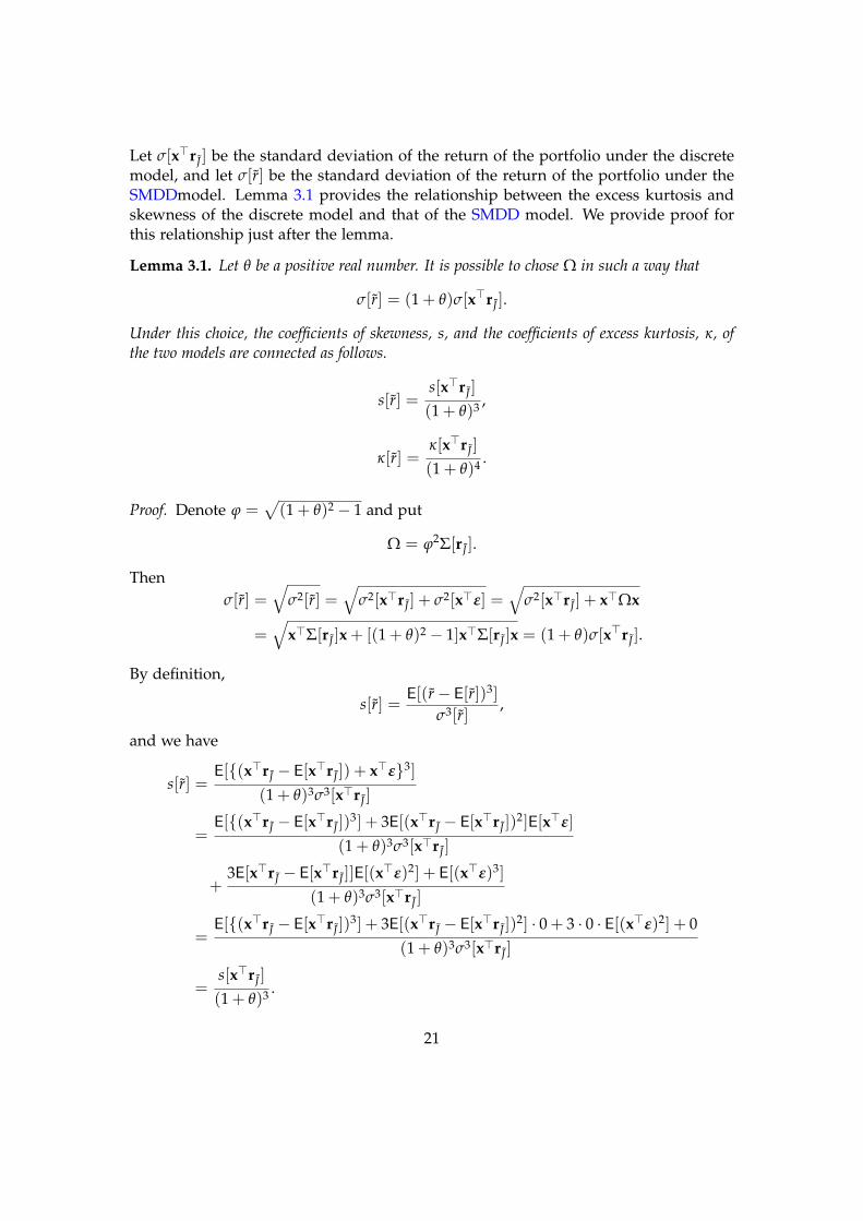
Let σ[x>r J ] be the standard deviation of the return of the portfolio under the discretemodel, and let σ[r] be the standard deviation of the return of the portfolio under theSMDDmodel. Lemma 3.1 provides the relationship between the excess kurtosis andskewness of the discrete model and that of the SMDD model. We provide proof forthis relationship just after the lemma.

Lemma 3.1. Let θ be a positive real number. It is possible to chose Ω in such a way that

σ[r] = (1 + θ)σ[x>r J ].

Under this choice, the coefficients of skewness, s, and the coefficients of excess kurtosis, κ, ofthe two models are connected as follows.

s[r] =s[x>r J ]

(1 + θ)3 ,

κ[r] =κ[x>r J ]

(1 + θ)4 .

Proof. Denote ϕ =√(1 + θ)2 − 1 and put

Ω = ϕ2Σ[r J ].

Thenσ[r] =

√σ2[r] =

√σ2[x>r J ] + σ2[x>ε] =

√σ2[x>r J ] + x>Ωx

=√

x>Σ[r J ]x + [(1 + θ)2 − 1]x>Σ[r J ]x = (1 + θ)σ[x>r J ].

By definition,

s[r] =E[(r− E[r])3]

σ3[r],

and we have

s[r] =E[(x>r J − E[x>r J ]) + x>ε3]

(1 + θ)3σ3[x>r J ]

=E[(x>r J − E[x>r J ])

3] + 3E[(x>r J − E[x>r J ])2]E[x>ε]

(1 + θ)3σ3[x>r J ]

+3E[x>r J − E[x>r J ]]E[(x

>ε)2] + E[(x>ε)3]

(1 + θ)3σ3[x>r J ]

=E[(x>r J − E[x>r J ])

3] + 3E[(x>r J − E[x>r J ])2] · 0 + 3 · 0 · E[(x>ε)2] + 0

(1 + θ)3σ3[x>r J ]

=s[x>r J ]

(1 + θ)3 .

21

Similarly, by definition,

κ[r] =E[(r− E[r])4]

σ4[r]− 3,

and we have

κ[r] =E[(x>r J − E[x>r J ]) + x>ε4]

(1 + θ)4σ4[x>r J ]− 3

=E[(x>r J − E[x>r J ])

4] + 4E[(x>r J − E[x>r J ])3]E[x>ε]

(1 + θ)4σ4[x>r J ]

+6E[(x>r J − E[x>r J ])

2]E[(x>ε)2] + 4E[x>r J − E[x>r J ]]E[(x>ε)3] + E[(x>ε)4]

(1 + θ)4σ4[x>r J ]− 3

=E[(x>r J − E[x>r J ])

4]

(1 + θ)4σ4[x>r J ]− 3

(1 + θ)4 +3

(1 + θ)4 − 3 +4E[(x>r J − E[x>r J ])

3] · 0(1 + θ)4σ4[x>r J ]

+4E[x>r J − E[x>r J ]] · 0

(1 + θ)4σ4[x>r J ]+

6σ2[x>r J ]x>Ωx + 3(x>Ωx)2

(1 + θ)4σ4[x>r J ]

=κ[x>r J ]

(1 + θ)4 +3

(1 + θ)4 − 3 +6(2θ + θ2) + 3(2θ + θ2)2

(1 + θ)4

=κ[x>r J ]

(1 + θ)4 .

The last equality in the proof follows after some manipulations.

As noted from lemma 3.1, as volatility increases, the SMDD model has a reducedskewness and kurtosis when compared to the discrete model.

3.3.2 Portfolio Utility and Returns

Investors are often assumed to be risk averse such that they are faced with a concaveand increasing utility function, u(·). Given that u(·) is concave with respect to the meanand standard deviation, Jensen’s inequality helps us express the investors risk aversionas

u[E(X)] ≥ E[u(X)].

Let u(·) be a twice differentiable von Neumann-Morgenstern utility function. Levy andMarkowitz (1979) show that to approximate the expected utility (EU) by a function thatdepends on mean (E) and variance (V) only, one can use the Taylor-series expansionof u(·) around E given as

u(R) = u(E) + u′(E)(R− E) +12

u′′(E)(R− E)2 + · · · .

22

The EU can then be approximated by

EU ≈ u(E) +12

u′′(E)V. (3.8)

Let the return of the portfolio be given by r and its expectation by E[r]. The Taylorseries expansion of u(1+ r) around 1+ E[r] using a process similar to the one resultingin Equation 3.8 results in

E[u(1 + r)] ≈ u(1 + E[r]) +12

u′′(1 + E[r])σ2[r]. (3.9)

where σ2[r] is the variance of the returns of the portfolio. Given that u(.) is concave,its second derivative in Equation 3.9 is negative meaning that the investor shouldconsider portfolios along the efficient frontier as these have minimum risk for a givenlevel of return or maximum return for a given level of risk (Kaplan and Savage, 2011).

For simplicity, take the mean return under the Discrete model expressed in Equa-tion 3.7 as x>r J to be rPj and its standard deviation to be ωP for this section. TheSMDD model expressed in Equation 3.7 involves first drawing randomly one of the nscenarios J and then drawing a portfolio from a normal distribution , N (r J , ωP). Theexpected utility of the portfolio is the weighted average of the expected utilities of thescenarios as

E[u(1 + r)] =n

∑j=1

wjE[u(1 + r)| J = j].

which can be approximated using Equation 3.8 as

E[u(1 + r)] ≈n

∑j=1

wj[u(1 + rPj) +12

.u′′(1 + rPj)ω2P]. (3.10)

Define the certainty equivalent rate of return (CE) for a risky portfolio as the returnthat makes one indifferent between that portfolio and earning a certain return. UsingEquation 3.10, Kaplan and Savage (2011) express the certainty equivalent return forthe SMDD portfolio as

CE[r] ≈ u−1

(n

∑j=1

wj[u(1 + rPj) +12

.u′′(1 + rPj)ω2P

)− 1. (3.11)

using Equation 3.10. Kaplan and Savage (2011) applies the assumption that the geo-metric mean, GM [r], is the CER given a logarithmic utility function to Equation 3.11,to get

GM[r] ≈ exp

(n

∑j=1

wj

[ln(1 + rPj)−

12

(ωP

1 + rPj

)2])− 1.

23

3.3.3 Portfolio Optimization with CVaR

Given the insufficiency of the standard deviation as a measure of risk, several measureof risk have been explored especially those that measure downside risk. While Kaplanand Savage (2011) explored 6 different risk measures, we will mostly deal with CVaRand its closely related measure VaR.

Let f (x, r) = −x>r J − x>ε be the loss associated with the asset mix x. Let p(r) be theprobability density function of the portfolio return. The probability that the loss doesnot exceed a threshold ζ is

Ψ(x, ζ) = P f (x, r) ≤ ζ =∫

f (x,r)≤ζp(r)dr.

Following Palmquist et al. (2002), assume that Ψ(x, ζ) is everywhere continuous withrespect to ζ. The α-VaR with probability level α ∈ (0, 1) is defined as

ζα(x) = min ζ ∈ R : Ψ(x, ζ) ≥ α ,

The α-CVaR is defined as

ϕα(x) =1

1− α

∫f (x,r)≥ζα(x)

f (x, r)p(r)dr.

In what follows, we define α-CVaR as our risk function. By our assumption, Ψ(x, ζ)is everywhere continuous with respect to ζ. Moreover, for any fixed x ∈ Rm thefunction Ψ(x, ζ) is the cumulative distribution function for the loss associated with xand therefore is nondecreasing. The set

ζ ∈ R : Ψ(x, ζ) = α

is closed as the inverse image of the closed set α under continuous map Ψ(x, ζ) andconnected because Ψ(x, ζ) is nondecreasing. In other words, the above set is either asingle point if Ψ(x, ζ) is strictly increasing at ζ = α or a closed interval if there is a“flat spot” around the point ζ = α, that is, an interval surrounding the above pointwhere the function Ψ(x, ζ) is a constant in ζ. In the last case, ζα(x) is the left endpointof this interval. It follows that

P f (x, r) ≥ ζα(x) = 1− α,

and the CVaR is the conditional expectation of the loss under condition that the lossis not less than ζα(x).

Following Rockafellar and Uryasev (2000) and Palmquist et al. (2002), consider thefunction

Fα(x, ζ) = ζ +1

1− α

∫ ∞

−∞max f (x, r)− ζ, 0p(r)dr.

Rockafellar and Uryasev (2000) proved the following result.

24

Theorem 3.1. The function Fα(x, ζ) is convex and continuously differentiable as a function ofζ. The α-CVaR is determined by the formula

ϕα(x) = minζ∈R

Fα(x, ζ).

The set Aα(x) consisting of the values of ζ for which the minimum is attained, is either a singlepoint or a nonempty closed bounded interval. The α-VaR of the loss is either that point or theleft endpoint of the interval Aα(x). In particular,

ϕα(x) = Fα(x, ζα(x)).

Recall that a function is called convex if its graph lies under any secant line. Mathe-matically, let ζ1 and ζ2 be two real numbers. When a real number λ runs from 0 to1, the number ζ = λζ1 + (1− λ)ζ2 runs from ζ2 to ζ1. Fix an admissible portfoliox0. The y-coordinate of the point on the secant line that corresponds to ζ, is equal toλFα(x0, ζ1) + (1− λ)Fα(x0, ζ2), while the value of the function Fα at the point ζ is equalto Fα(x0, λζ1 + (1− λ)ζ2). The definition of convexity takes the form

Fα(x0, λζ1 + (1− λ)ζ2) ≤ Fα(x0, ζ1) + (1− λ)Fα(x0, ζ2),

see a comprehensive treatment of the subject in Rockafellar (1997). In particular, alocal minimum of a convex function is always equal to its global minimum.

Denote by X ⊂ Rm the set of admissible portfolios. The problem of minimising theα-CVaR of the loss associated with x over all x ∈ X is solved by the following result ofRockafellar and Uryasev (2000).

Theorem 3.2. We haveminx∈X

ϕα(x) = min(x,ζ)∈X×R

Fα(x, ζ).

Moreover, a pair (x∗, ζ∗) achieves the right hand side minimum if and only if x∗ achieves the lefthand side minimum and ζ∗ ∈ Aα(x∗). In particular, if the set Aα(x∗) is a single point, then theminimisation of Fα(x, ζ) over (x, ζ) ∈ X×R produces a pair (x∗, ζ∗), not necessarily unique,such that x∗ minimises the α-CVaR and ζ∗ gives the corresponding α-VaR. Furthermore, iff (x, r) is convex with respect to x, then Fα(x, ζ) and ϕα(x) are convex functions.

The economical sense of this result is as follows. Instead of solving very complicatedproblem of minimisation the α-CVaR, ϕα(x), we can solve much easier problem ofminimisation the simpler function Fα(x, ζ). Under very mild additional conditions,namely, if f (x, r) is convex with respect to x and if X is a convex set:

λx1 + (1− λ)x2 ∈ X if x1, x2 ∈ X, λ ∈ [0, 1],

the minimisation problem belongs to the area of convex minimisation, which is muchsimpler to deal with than with the minimisation of the original function ϕα(x).

25

3.3.4 The Efficient Frontier

The optimisation problem using CVaR can be formulated in three equivalent formu-lations. The equivalence holds for any concave reward and convex risk functions withconvex constraints, see Palmquist et al. (2002) for proof of equivalence. First, one canfind a minimal risk portfolio among all possible portfolios with reward not less than a givenvalue ρ which can be formulated as

minx∈X

ϕα(x), R(x) ≥ ρ. (3.12)

The second formulation is that of finding a maximal reward portfolio among all portfolioswith risk not greater than a given value ω and is given by

minx∈X

(−R(x)), ϕα(x) ≤ ω. (3.13)

The last problem isminx∈X

(ϕα(x)− µR(x)), µ ≥ 0. (3.14)

As ρ, ω and µ vary in the problems (3.12), (3.13) and (3.14) respectively, a curve istraced on the risk-reward plane. This curve is nothing but the celebrated efficientfrontier of the optimisation problem (3.12).

In order to formulate the next result from Palmquist et al. (2002), we need to explainthe following expression:

. . . constraints R(x) ≥ ρ, ϕ(x) ≤ ω have internal points.

To do this, we use Boyd and Vandenberghe (2004). First a few definitions.

Definition 3.3. Affine Set: A set C ⊆ Rm is called affine if the line through any two distinctpoints in C lies in C, that is, for any x1, x2 ∈ C and θ ∈ R,

θx1 + (1− θ)x2 ∈ C.

Definition 3.4. Affine Hull: The affine hull of a set C, aff C, is the intersection of all affinesets containing C, or equivalently, the smallest affine set that contains C.

Definition 3.5. Relative Interior: The relative interior of the set C is its interior relativeto its affine hull, that is, a point x ∈ C lies in the relative interior of C if and only if there is apositive real number r such that the intersection of the closed ball of radius r and centre x withthe affine hull of C is a subset of C.

As an example, let C be the interval [0, ∞) of the x-axis in the plane. The affine hull ofC is the x-axis, the interior of C relative to the plane is empty, but the relative interiorof C is the interval (0, ∞).

The constraint R(x) ≥ ρ satisfies Slater’s condition if there exists a point x in the relativeinterior of X with R(x) > ρ. This is the exact sense of the above citation.

26

Theorem 3.3. Suppose that constraints R(x) ≥ ρ and ϕ(x) ≤ ω satisfy Slater’s condition.If ϕ(x) is convex, R(x) is concave (that is, −R(x) is convex) and the set X is convex, then theoptimisation problems (3.12)–(3.14) generate the same efficient frontier.

Slater’s condition is just an example of the class of conditions called constraint qualifi-cations, see Boyd and Vandenberghe (2004). Theorem 3.3 remains true under any kindof constraint qualification.

In Markowitz 2.0, the loss function f (x, r) is linear with respect to x. By Theorem 3.2,the CVaR risk function ϕα(x) is convex with respect to x. The reward function R(x) isalso linear with respect to x. The set X is defined as

X = (x1, . . . , xm)> : xi ≥ 0, x1 + · · ·+ xm = 1 .

This set is convex. If Slater’s condition is satisfied, then by Theorem 3.3 maximisingthe reward under a CVaR constraint generates the same efficient frontier as minimisingthe CVaR under a reward constraint.

The optimisation problems (3.12)–(3.14) are still complicated. However, Theorem 3.2shows that the convex function Fα(x, ζ) can be used instead of much more complicatedfunction ϕα(x) in problem (3.12). Is this possible for problems (3.13) and (3.14)? Theanswer is yes as can be seen in Theorems (3.4) and (3.5). See Palmquist et al. (2002) forproofs.

Theorem 3.4. The minimisation problem (3.13) is equivalent to the problem

min(x,ζ)∈X×R

(−R(x)), Fα(x, ζ) ≤ ω. (3.15)

in the following sense. A pair (x∗, ζ∗) achieves the minimum in the problem (3.15) if and onlyif x∗ achieves the minimum in the problem (3.13) and ζ∗ ∈ Aα(x∗). In particular, if the setAα(x∗) is a single point, then the minimisation of −R(x) over (x, ζ) ∈ X×R produces a pair(x∗, ζ∗) such that x∗ maximises the return and ζ∗ gives the corresponding α-VaR.

Theorem 3.5. The minimisation problem (3.14) is equivalent to the problem

min(x,ζ)∈X×R

(Fα(x, ζ)− µR(x)), µ ≥ 0. (3.16)

in the following sense. A pair (x∗, ζ∗) achieves the minimum in the problem (3.16) if andonly if x∗ achieves the minimum in the problem (3.14) and ζ∗ ∈ Aα(x∗). In particular, ifthe set Aα(x∗) is a single point, then the minimisation of Fα(x, ζ) − µR(x) over (x, ζ) ∈X ×R produces a pair (x∗, ζ∗) such that x∗ minimises Fα(x, ζ) − µR(x) and ζ∗ gives thecorresponding α-VaR.

The numerical implementation in this thesis uses the formulation (3.12) but as we havenoted we could just as well as used (3.13) or (3.14).

27

3.3.5 Incorporating Additional Constraints

In generating the efficient frontier, the investor can face a host of constraints. Specifi-cally, there are three types of constraints which can expressed as

l ≤ x ≥ uMx ≤ bQx = c

(3.17)

where the lower and upper bounds of the m elements of x make up the vectors l and u,the left and right hand coefficients of inequality constraints are M and b respectivelyand those of equality constraints, including the budget constraint, are Q and c, seeKaplan and Savage (2011).

The types of constraints an investor faces include loss and reward functions, CVaRconstraints, transaction costs, budget constraints, value constraints (a singular assetcannot exceed a given percentage in an optimal portfolio) and liquidity constraints.These constraints can be easily incorporated in the mean-CVaR optimization problemjust like it would be in a mean-variance optimization exercise.

For instance, given that the optimization will use CVaR and AM, the efficient frontierfunction is drawn by solving, for given levels of returns drawn from the interval (ρmin,ρmax), the nonlinear program given by

minimize CVaRα(x)

subject to

AM = ρ

(3.17)(3.18)

For simplicity, we do not incorporate any additional constraints in the numerical im-plementation in this thesis.

28

Chapter 4

Numerical Implementation

This chapter discusses the numerical implementation of Markowitz 2.0.

4.1 Data Description

The data for the study is the sample of daily stock prices of 30 blue chip UnitedStates equities that make up the The Dow Jones Industrial AverageTM(DJIA)1 Indexoperated by S&P Dow Jones Indices. It is also referred to as the Dow Jones, theDow Jones Industrial, the Dow 30 or simply the Dow. The Dow is composed ofcompanies from varied sectors except for transportation and utilities. The selectionof the constituents does take into sector balance and company reputation, growthtrack record and level of interest among investors among other considerations. Theindex is a price-weighted measure, is one of the oldest indexes as it was launched on26th May 1896 and is calculated every 2 seconds during U.S. stock exchange tradinghours while being rebalanced as and when needed.

The ProShares Ultra Dow30 ETF2, developed and maintained by ProShares, is an Elec-tronically Traded Fund (ETF) that mimics the Dow and offers investors daily grossinvestment results corresponding to two times (2x) the Dow’s daily performance. ThisETF constitutes our source for the constituents of the Dow as of 23rd November 2016.We then used Bulk Stock Data Series Download by Jason Strimpel 3 to get the adjustedclosing price, in effect the total returns data, on the 30 index constituents relating tothe 10 year period from 1st December 2006 to 30th November 2016, a total of 2193observations. One Stock, Visa, was omitted over insufficient data.

We converted the stock prices into price returns and plotted the daily logarithmicreturns for one of the asset in our portfolio: JP Morgan Chase & Co. This can be

1http://us.spindices.com/indices/equity/dow-jones-industrial-average2http://www.proshares.com/funds/ddm.html3http://finance.jasonstrimpel.com/bulk-stock-download/

29

seen in Figure 4.1. The volatility was notably significantly higher during the 2008-2009financial crisis also known as the Great Recession.

Figure 4.1: Time series plot of daily logarithmic price returns on JP Morgan Chase &Co stock.

4.2 Model Implementation, Results and Analysis

In conducting a Mean-CVaR portfolio optimization, there is need to generate such asignificant number of scenarios as to to allow for asymptotic convergence of samplestatistics. The scenarios are samples from the underlying multivariate normal proba-bility distribution of asset returns. To generate the scenarios, we ran n Monte Carlosimulations on the historical portfolio data. In our case, n is a million scenarios.

The model has been implemented in Matlab using the built-in PortfolioCVaR functionthat implements mean-CVaR portfolio optimization. The codes are in the appendix.The PortfolioCVaR object simulates multivariate normal scenarios from our momentsof the historical data we input. The implementation was performed on a MacBook Prowith a 2.9 GHz Intel Core i5 processor and 8 GB of RAM. The total time to perfom theone million simulations was

A CVaR optimization problem is completely specified when we have a universe ofassets or asset classes that have scenarios of asset returns for a given period, a portfolioset that includes a set of equality and non-equality constraints and a probability levelwhere the loss is less than or equal to the VaR. The commonly used probability levelsare 0.99, 0.95 and 0.9 which are indicative of 1%, 5% and 10% probabilities of loss

30

Figure 4.2: Fitting distributions to on JP Morgan Chase & Co stock logarithmic pricereturns.

respectively. We use 0.95 in this case.

We implemented the model in a number of steps aimed at creating the efficient frontier.First, we define the asset universe as specified in Section 4.1 and generate the historicalreturn matrix. Then, we generate scenarios for portfolio asset returns. After that, wespecify portfolio constraints such as budget, cost and value constraints as necessary.Finally, we estimate the efficient portfolios and efficient frontiers.

We tested the data of return distributions for normality and both tests came negative atthe 5% significance level. We used the one-sample Kolmogorov-Smirnov and Jarque-Bera tests. They test the null hypothesis that the data comes from a standard normaldistribution against the alternative that it does not. We fitted the normal and ExtremeValue distributions to one of the stocks in the portfolio as can be seen in Figure 4.2.

On implementing the model using the data set described in Section 4.1, we generatethe efficient frontier seen in Figure 4.3. The algorithm starts with an initial portfolioand works its way to an optimal one. We implemented the mean-variance optimizationbased on the same set of data and obtained the efficient frontier in Figure 4.4 which

31

can be compared to the Mean-CVaR Frontier as in Figure 4.5. In both cases, we addedthe additional constraint of no short selling and another to ensure the asset mix addsup to 1.

Figure 4.3: A plot of the mean - CVaR efficient frontier using the simulated data of theDJIA.

The portfolios on the mean-CVaR frontier also seem to result in a mean-variance effi-cient frontier as seen in Figure 4.5 meaning that portfolios on the mean-CVaR frontierare optimal in the mean-variance framework as well. The asset allocation weights onthe efficient frontier portfolios from the mean-Variance and mean-CVaR portfolios areshown in Figure 4.6.

32

Figure 4.4: Mean-variance efficient frontier using the same simulated data of the DJIA.

33

Figure 4.5: Mean-CVaR and mean-variance efficient frontiers: The blue line has beensubsumed by the red line in this case.

34

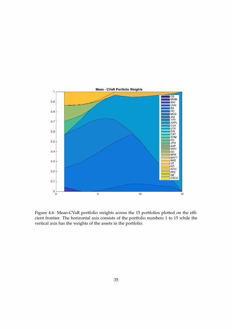
Figure 4.6: Mean-CVaR portfolio weights across the 15 portfolios plotted on the effi-cient frontier. The horizontal axis consists of the portfolio numbers 1 to 15 while thevertical axis has the weights of the assets in the portfolio.

35

Chapter 5

Conclusion and Further Research

This chapter presents the conclusion to the analysis and provides some recommenda-tions for further research.

5.1 Review and Conclusion

The thesis has covered several areas. It is meant to be an introduction to Markowitz 2.0covering the motivation for it, its formulation and a guidance to its formulation meantto enhance appreciation of the model and to enable its practical implementation. Thevarious chapters aim to accomplish this by focusing on various areas.

Chapter 1 began by briefly introducing the topic for our research together with themotivation and context for it and even noting the research objectives. Chapter 2reviewed modern portfolio theory and discussed the various measures of risk andreturns in terms of overview, strengths and drawbacks. We noted that Standard De-viation, Value-at-Risk (VaR) and conditional Value-at-Risk (CVaR) are frequently usedas risk measures in risk management. Ever since the Great Recession, their has beenincreased focus on tail risks. Optimal portfolios have normally been computed usingstandard deviation as the measure of choice for risk which assumes a normal distribu-tion. This means underestimates tail risk leading practitioners to consider CVaR andVaR as alternative risk measures. We noted that CVaR is preferable to VaR given thatit is a coherent risk measure especially because of its fulfilment of the convexity axiomand simplifies the optimization process.

Chapter 3 introduces Markowitz 2.0 while giving an overview and an analysis of keyconcepts in the model before laying out the mathematical formulation of the model.We analyzed the portfolio optimization model referred to as Markowitz 2.0 that usesCVaR as the risk measure of choice in portfolio optimization. We drew on the extensiveliterature on portfolio optimization techniques related to CVaR and VaR to formulatethe model mathematically, in the process giving the model historical perspective. We

36

noted in the formulation that the model is not entirely new, the techniques for it havingbeen developed by Palmquist et al. (2002).

Chapter 4 implements the model using data from the DJIA and generates optimalportfolios and the efficient frontier. It further provides an analysis and discussion ofthe results. We presented a practical implementation of the model using data fromthe DJIA and generated optimal portfolios while drawing the efficient frontier. Theresulting portfolio weights were similar to those obtained through the Mean-Varianceoptimization on the same data set. Given all these, we tend to see Markowitz 2.0 asappealing both in theory and practice.

5.2 Further Research

The author proposes further research in the area of mean-CVaR optimization withSIPmathTMdeveloped by Sam Savage and can be found at probability managementwebsite (www.probabilitymanagement.org/sip-math.html). The tool aims atsimplifying the portfolio optimization process using scenario analysis for the masseswho do not have access to such proprietary and sophisticated software as Matlab.There is little available information on conducting this kind of optimisation and step-by-step guide would be appropriate. Further works needs to be done to simplify themean-CVaR optimization process so as to make it as easily usable as the precedingmean-variance Framework.

37

Bibliography

Acerbi, C. (2002). Spectral measures of risk: A coherent representation of subjectiverisk aversion, Journal of Banking & Finance 26(7): 1505–1518.URL: http://EconPapers.repec.org/RePEc:eee:jbfina:v:26:y:2002:i:7:p:1505-1518

Acerbi, C. and Tasche, D. (2002). Expected shortfall: a natural coherent alternative tovalue at risk, Economic Notes 31(2): 379–388.

Alloway, T. (2015a). Market moves that are supposed to happen every half-decadekeep happening. Online; posted 13-May-2015.URL: https://www.bloomberg.com/news/articles/2015-05-13/market-moves-that-are-supposed-to-happen-every-half-decade-keep-happening

Alloway, T. (2015b). Six strange things that have been happening in financial markets.Online; posted 12-November-2015.URL: https://www.bloomberg.com/news/articles/2015-11-12/five-strange-things-that-have-been-happening-in-financial-markets

Artzner, P., Delbae, F., Eber, J.-M. and Heath, D. (1999). Coherent measures of risk,Mathematical Finance 9(203-228).

Best, M. J. and Grauer, R. R. (1991). On the sensitivity of mean variance-efficientportfolios to changes in asset means: Some analytical and computational results,The Review of Financial Studies 4(2): 315–342.

Black, F. and Litterman, R. (1991). Asset allocation: Combining investor views withmarket equilibrium, The Journal of Fixed Income 1(2): 7–18.

Boyd, S. and Vandenberghe, L. (2004). Convex optimization, Cambridge UniversityPress, Cambridge.

Elton, E. J. and Gruber, M. J. (1997). Modern portfolio theory, 1950 to date, Journal ofBanking and Finance 21: 1743–1759.

Estrada, J. (2010). Geometric mean maximization: An overlooked portfolio approach?,The Journal of Investing 19(4): 134–147.

38

Fabozzi, F. J., Markowitz, H. M., Kolm, P. N. and Gupta, F. (2011). Portfolio selection,in F. J. Fabozzi and H. M. Markowitz (eds), The Theory and Practice of InvestmentManagement: Asset Allocation, Valuation, Portfolio Construction, and Strategies, JohnWiley & Sons, Inc., chapter 3, pp. 45–78.

Gaivoronski, A. A. and Pflug, G. (2004). Value-at-risk in portfolio optimization: Prop-erties and computational approach, Journal of Risk, 7(2): 1–31.

Gosling, S. (2010). A scenarios approach to asset allocation, The Journal of PortfolioManagement 37(1): 53–66.

Jacquier, E., Kane, A. and Marcus, A. J. (2003). Geometric or arithmetic mean: Areconsideration, Financial Analysts Journal 59(6): 46–53.

Kaplan, P. D. and Savage, S. (2011). Markowitz 2.0, in P. D. Kaplan (ed.), Frontiers ofModern Asset Allocation, John Wiley & Sons, Inc., chapter 26, pp. 325–349.

Kolm, P. N., Tutuncu, R. and Fabozzi, F. J. (2014). 60 years of portfolio optimiza-tion: Practical challenges and current trends, European Journal of Operational Research234(2): 356–371.

Levy, H. and Markowitz, H. M. (1979). Approximating expected utility by a functionof mean and variance,, American Economic Review 69: 308–17.

Mankert, C. and Seiler, M. J. (2011). Mathematical derivations and practical implica-tions for the use of the black-litterman model, Journal of Real Estate Portfolio Manage-ment 17(2): 139–159.

Markowitz, H. (1952). Portfolio selection, The Journal of Finance 7(1): 77–91.

Michaud, R. O. (1989). The markowitz optimization enigma: is ’optimized’ optimal?,Financial Analysts Journal 45(1): 31–42.

Mindlin, D. (2011). On the relationship between arithmetic and geometric returns,SSRN Electronic Journal .

Palmquist, J., Uryasev, S. and Krokhmal, P. (2002). Portfolio optimization with condi-tional value-at-risk objective and constraints, Journal of Risk 4(2): 43–68.

Pflug, G. (2000). Some remarks on the value-at-risk and the conditional value-at-risk.,in S. Uryasev (ed.), Probabilistic Constrained Optimization: Methodology and Applica-tions, 49, Springer US.

Rockafellar, R. T. (1997). Convex analysis, Princeton Landmarks in Mathematics, Prince-ton University Press, Princeton, NJ. Reprint of the 1970 original, Princeton Paper-backs.

Rockafellar, R. T. and Uryasev, S. (2000). Optimization of conditional value-at-risk,Journal of risk 2(3): 21–42.

39

Sarykalin, S., Serraino, G. and Uryasev, S. (2008). Value-at-Risk vs. Conditional Value-at-Risk in Risk Management and Optimization, INFORMS, chapter 13, pp. 270–294.URL: http://pubsonline.informs.org/doi/abs/10.1287/educ.1080.0052

Savage, S. (2009). The Flaw of Averages: Why We Underestimate Risk in the Face of Uncer-tainty, John Wiley & Sons, Inc.

Sheikh, A. Z. and Qiao, H. (2009). Non-normality of market returns: A framework forasset allocation, The Journal of Alternative Investments 12(3): 8–35.

Taleb, N. N. (2010). The black swan : the impact of the highly improbable, Random HousePublishing Group.

40

List of Acronyms

AM Arithmetic Mean.

CVaR Conditional Value-at-Risk.

DJIA The Dow Jones Industrial Average.

GM Geometric Mean.

MVO Mean-Variance Optimization.

SMDD Smooth Multivariate Discrete Distribution.

VaR Value-at-Risk.

WE Weighted Estimator.

41

Appendix A

More mathematics

A.1 Mathematical Formulation of Markowitz 1.0

Assume we have n risky assets. Let x be the column vector of portfolio weights, σ2 bethe portfolio variance, ri be the expected return of asset i and rp be the expected returnof the portfolio. Also let R be the column vector of expected returns of the n assetsin the portfolio, Σ be the variance-covariance matrix, δ be the risk aversion parameterand 1 be a column vector of n ones.

Generating the efficient frontier means solving either problem A.1 or problem A.2which are equivalent:

minimize x>Σxsubject to rp = x>R

(A.1)

ormaximize x>Rsubject to σ2 = x>Σx

(A.2)

Apply the Lagrange multiplier to problem A.2, we get:

L = x>R− λ(x>Σx− σ2)

Take the derivative and setting it to zero

∂L∂x

= 1R− 2λ1Σx = 0

Define λ = δ2 , then

1R− δ1Σx = 0

And thenR = δΣx

42

The optimal portfolio weights are given by

x∗ = (δΣ)−1R

43

A.2 The Dow Jones Industrial Average (DJIA) Companies

The Dow Jones Industrial Average (DJIA) was composed of the following stocks as of30th November 2016.

44

A.3 Matlab Mean-CVaR Optimization Code

%plot(Dow)%Load Dow Dataload(’Dow.mat’)%Convert prices to logarithmic returnsA = fts2mat(Dow);returnDow = price2ret(A);returnDow(end);

%Calculate the mean of asset returns from historical datameanDow = mean(A);meanDow;

%Create PortfolioCVaR object.dowPortfolio = PortfolioCVaR;%Simulate Scenarios from Dow DatadowPortfolio = simulateNormalScenariosByData(dowPortfolio,

returnDow, 100000);%check the returns on scenarios 999 to 1001scenarioSubset = dowPortfolio.localScenarioHandle(999,1001);scenarioSubset%Set names of Assets and display them with their numbersdowPortfolio = setAssetList(dowPortfolio, ...’GS’, ’MMM’, ’IBM’, ’UNH’, ’BA’, ’HD’, ’MCD’, ’JNJ’, ’TRV’,

’AAPL’,...’CVX’, ’UTX’, ’DIS’, ’CAT’, ’XOM’, ’PG’, ’JPM’, ’AXP’, ’WMT’, ’DD’,

...’MRK’, ’MSFT’, ’NKE’, ’VZ’, ’KO’, ’INTC’, ’PFE’, ’GE’, ’CSCO’);disp(dowPortfolio.AssetList);disp(dowPortfolio.NumAssets);%Constraints%For Non-negative WeightsdowPortfolio = PortfolioCVaR(dowPortfolio,’lowerBound’,0);%For weights to add up to 1dowPortfolio =

PortfolioCVaR(dowPortfolio,’lowerBudget’,1,’UpperBudget’,1) ;%Set probability leveldowPortfolio = setProbabilityLevel(dowPortfolio, 0.95);%Calculate scenario means and covariances[passetmean, passetcovar] = estimateScenarioMoments(dowPortfolio)%plot the CVaR efficient frontierfigure;[dowPortfolioRisk,dowPortfolioReturns] =

dowPortfolio.plotFrontier(15);%Obtain efficient portfolios with given number of points%cvarFrontier = estimateFrontier(dowPortfolio,15);%display(cvarFrontier)

45

%Mean-variance optimization based on same data.q = Portfolio(’AssetList’, dowPortfolio.AssetList);q = estimateAssetMoments(q, dowPortfolio.getScenarios);%Constraint to ensure Non-negative Weightsq = Portfolio(q,’lowerBound’,0);%Constraint to ensure weights add up to 1q = Portfolio(q,’lowerBudget’,1,’UpperBudget’,1) ;%plot the mean-Variance efficient frontierfigure; q.plotFrontier(15);

%Add CVaR porfolios to Mean-Variance Plot%Calculate the Mean-Variance risk of the 15 CVaR portfoliosqStdDev =

dowPortfolio.estimatePortStd(dowPortfolio.estimateFrontier(15));figure;q.plotFrontier(15);hold onplot(qStdDev,dowPortfolioReturns, ’-r’, ’LineWidth’, 2);legend(’Mean-Variance Efficient Frontier’,...

’Mean-CVaR Efficient Frontier’,...’Location’, ’SouthEast’)

%Compare Weights of Mean-Variance to those of Mean-CVaRmeanCvarWeights = dowPortfolio.estimateFrontier(15);meanStdWeights = q.estimateFrontier(15);

figure;subplot(1,2,1);area(meanCvarWeights’);title(’Mean - CVaR Portfolio Weights’);

subplot(1,2,2);area(meanStdWeights’);title(’Mean - Variance Portfolio Weights’);

set(get(gcf,’Children’),’YLim’, [0 1]);legend(dowPortfolio.AssetList);

46

A.4 Notes on fulfillment of Thesis objectives

This section analyses how the requirements of the Swedish National Agency for HigherEducation to master theses have been fulfilled in this thesis.

Objective 1: Knowledge and understanding in the major field

The thesis starts with an introduction that places helps the reader appreciate the extentof progress made in Modern Portfolio theory. It then evaluates the measures or riskand return used with a special focus on CVaR. Markowitz 2.0 is then presented indetail with a mathematical formulation followed by a practical implementation. Wethen present our findings and discussions on them. All this serves to demonstratethe authors firm grasp of the key concepts in Modern Portfolio Theory and financialmathematics by extension.

Objective 2: Deep methodological knowledge

By providing a practical application of the model, the author demonstrates the practi-cal usefulness of Markowitz 2.0 as a portfolio management tool. Before this, the authorformulates the mean-CVaR optimization problem adequately.

Objective 3: Critical thinking and systematic integration of knowledge

Tail risk is an area of significant interest in financial circles especially in the periodafter the Great Recession with numerous tools being developed to help manage it. Theauthor has demonstrated the ability to bring together results from different papers indeveloping a coherent case for the adoption of CVaR as a key risk measure. To supportthis, one has to understand deficiencies in current risk measures and the advantages ofCVaR. This line of thought is arrived through authors ability to question assumptionsin the existing modelling framework.

Objective 4: Ability to critically, independently and creatively formulate issues witha plan to carry out advanced tasks

At the time of beginning the project, the author made a project plan with specifictime lines for each phase of the project which has helped in giving guidance to theentire project. Further, the model was implemented in MATLAB to provide a practicalapplication of the theoretical analysis advanced in the thesis.

Objective 5: Knowledge presentation in both national and international contexts

The language and concepts used in the thesis are universal to any reader of financialmathematics and especially to anyone familiar with basic concepts in portfolio analysisand investment management. The thesis will be presented on 19th January 2017 wherethe author field questions from the audience.

Objective 6: Ability to make judgement considering the relevant scientific, socialand ethical aspects

The thesis is focused on challenging the blind adoption of risk measures without due

47

regard to their effectiveness. By presenting a model that considers downside risk ina non-normal market, the author intends to help the reader make informed decisionsin portfolio management. Finally the author carefully make reference to the ideas,research and results from different authors that have been used as input in this thesis.

48