Scanning the Science-Society Horizon - CORE
584
Scanning the Science-Society Horizon Brenda R Moon A thesis submitted for the degree of Doctor of Philosophy at The Australian National University Australian National Centre for the Public Awareness of Science (CPAS) January 2015
-
Upload
khangminh22 -
Category
Documents
-
view
0 -
download
0
Transcript of Scanning the Science-Society Horizon - CORE

Scanning the Science-Society
Horizon
Brenda R Moon
A thesis submitted for the degree of
Doctor of Philosophy at
The Australian National University
Australian National Centre
for the
Public Awareness of Science (CPAS)
January 2015

© Brenda R Moon
Typeset in Palatino by TEX and LATEX 2ε.

This thesis contains no material that has been accepted for the award of any other
degree or diploma in any university. To the best of the author’s knowledge and belief it
contains no material previously published or written by another person, except where
due reference is made in the text.
Brenda R Moon
20 April 2016


Acknowledgements
First of all I would like to thank my supervisors Sue Stocklmayer, Rod Lamberts and
Will Grant for their excellent advice and guidance throughout the PhD process.
I feel that I have been very privileged to undertake my PhD at CPAS which brings
together people from diverse backgrounds and interests and so provides a very stim-
ulating environment for research. Thank you to all of my friends and colleagues at
CPAS for your help and support during this PhD.
I am grateful to the many other people at the ANU who provided me with assis-
tance.
This PhD would not have been possible without the amazing open source software
projects that have created most of the research tools that I used. I would like to thank
the people involved in many of those projects for their prompt and helpful answers to
my questions about how to use the software.
Finally I would like to thank my family for their support during the many years I
have been working on this thesis.
v

vi

Abstract
Science communication approaches have evolved over time gradually placing more im-
portance on understanding the context of the communication and audience.
The increase in people participating in social media on the Internet offers a new
resource for monitoring what people are discussing. People self publish their views
on social media, which provides a rich source of every day, every person thinking.
This introduces the possibility of using passive monitoring of this public discussion to
find information useful to science communicators, to allow them to better target their
communications about different topics.
This research study is focussed on understanding what open source intelligence,
in the form of public tweets on Twitter, reveals about the contexts in which the word
‘science’ is used by the English speaking public. By conducting a series of studies based
on simpler questions, I gradually build up a view of who is contributing on Twitter,
how often, and what topics are being discussed that include the keyword ‘science’.
An open source a data gathering tool for Twitter data was developed and used to
collect a dataset from Twitter with the keyword ‘science’ during 2011. After collection
was completed, data was prepared for analysis by removing unwanted tweets. The
size of the dataset (12.2 million tweets by 3.6 million users (authors)) required the
use of mainly quantitative approaches, even though this only represents a very small
proportion, about 0.02%, of the total tweets per day on Twitter
Fourier analysis was used to create a model of the underlying temporal pattern of
tweets per day and revealed a weekly pattern. The number of users per day followed a
similar pattern, and most of these users did not use the word ‘science’ often on Twitter.
vii

viii
An investigation of types of tweets suggests that people using the word ‘science’
were engaged in more sharing of both links, and other peoples tweets, than is usual on
Twitter.
Consideration of word frequency and bigrams in the text of the tweets found that
while word frequencies were not particularly effective when trying to understand such
a large dataset, bigrams were able to give insight into the contexts in which ‘science’
is being used in up to 19.19% of the tweets.
The final study used Latent Dirichlet Allocation (LDA) topic modelling to identify
the contexts in which ‘science’ was being used and gave a much richer view of the whole
corpus than the bigram analysis.
Although the thesis has focused on the single keyword ‘science’ the techniques
developed should be applicable to other keywords and so be able to provide science
communicators with a near real time source of information about what issues the public
is concerned about, what they are saying about those issues and how that is changing
over time.
Contents
Acknowledgements v
Abstract vii
1 Introduction 1
1.1 Background to the Study . . . . . . . . . . . . . . . . . . . . . . . . . . 1
1.2 Research Questions . . . . . . . . . . . . . . . . . . . . . . . . . . . . . . 6
1.3 Overview of the Method . . . . . . . . . . . . . . . . . . . . . . . . . . . 7
1.4 Outline of chapters . . . . . . . . . . . . . . . . . . . . . . . . . . . . . . 7
1.5 Significance of thesis . . . . . . . . . . . . . . . . . . . . . . . . . . . . . 9
1.6 Limitations . . . . . . . . . . . . . . . . . . . . . . . . . . . . . . . . . . 10
2 Literature Review 11
2.1 Science Communication . . . . . . . . . . . . . . . . . . . . . . . . . . . 12
2.2 Twitter Research . . . . . . . . . . . . . . . . . . . . . . . . . . . . . . . 18
2.2.1 Why do people use Social Media . . . . . . . . . . . . . . . . . . 19
2.2.2 Who uses Twitter . . . . . . . . . . . . . . . . . . . . . . . . . . 20
2.2.3 Expression of the public’s views on Twitter . . . . . . . . . . . . 23
2.2.4 Topic detection . . . . . . . . . . . . . . . . . . . . . . . . . . . . 33
2.2.5 Sentiment Analysis . . . . . . . . . . . . . . . . . . . . . . . . . . 40
2.2.6 Social network analysis in Twitter . . . . . . . . . . . . . . . . . 44
2.3 New literature since 2011 . . . . . . . . . . . . . . . . . . . . . . . . . . 48
2.3.1 Science Communication . . . . . . . . . . . . . . . . . . . . . . . 49
2.3.2 Twitter Research . . . . . . . . . . . . . . . . . . . . . . . . . . . 54
ix

x Contents
2.3.3 Conclusion . . . . . . . . . . . . . . . . . . . . . . . . . . . . . . 72
3 Research Design - Data Collection 75
3.1 Description of Twitter . . . . . . . . . . . . . . . . . . . . . . . . . . . . 75
3.2 Data Collection Software . . . . . . . . . . . . . . . . . . . . . . . . . . . 77
3.3 Database design . . . . . . . . . . . . . . . . . . . . . . . . . . . . . . . 78
3.4 Data collection . . . . . . . . . . . . . . . . . . . . . . . . . . . . . . . . 85
3.4.1 Changes in Data Collection Search Terms - SearchAPI . . . . . . 89
3.4.2 Changes in Data Collection Search Terms - StreamAPI . . . . . 90
3.4.3 Changes in keywords collected . . . . . . . . . . . . . . . . . . . 90
3.4.4 Trend over StreamAPI period . . . . . . . . . . . . . . . . . . . . 93
3.4.5 Tweets dropped from StreamAPI . . . . . . . . . . . . . . . . . . 93
3.4.6 Collected Tweets as a Proportion of Total Tweets on Twitter . . 96
4 Data cleaning and filtering 101
4.1 Filtering out non-English tweets . . . . . . . . . . . . . . . . . . . . . . 102
4.1.1 Accuracy of language detection . . . . . . . . . . . . . . . . . . . 105
4.1.2 Filtering Unicode characters . . . . . . . . . . . . . . . . . . . . . 110
4.1.3 Comparison of accuracy of language detection with and without
unicode filtering . . . . . . . . . . . . . . . . . . . . . . . . . . . 116
4.1.4 Determining which languages to discard from corpus . . . . . . . 121
4.1.5 Filtered by Language . . . . . . . . . . . . . . . . . . . . . . . . . 127
4.2 Filtering out spam . . . . . . . . . . . . . . . . . . . . . . . . . . . . . . 128
4.2.1 Noun spam . . . . . . . . . . . . . . . . . . . . . . . . . . . . . . 128
4.3 Final data set . . . . . . . . . . . . . . . . . . . . . . . . . . . . . . . . . 135
5 Tweets per day 137
5.1 Comparing ‘science’ tweets to total tweets on Twitter . . . . . . . . . . 138

Contents xi
5.2 Simple model of tweets per day . . . . . . . . . . . . . . . . . . . . . . . 140
5.3 Using Fourier analysis to improve the fit of the model . . . . . . . . . . 145
5.4 Conclusion . . . . . . . . . . . . . . . . . . . . . . . . . . . . . . . . . . 152
6 Authors 155
6.1 Tweets per author . . . . . . . . . . . . . . . . . . . . . . . . . . . . . . 156
6.2 Authors per day . . . . . . . . . . . . . . . . . . . . . . . . . . . . . . . 156
6.3 Days per Author . . . . . . . . . . . . . . . . . . . . . . . . . . . . . . . 160
6.4 Conclusion . . . . . . . . . . . . . . . . . . . . . . . . . . . . . . . . . . 161
7 Types of Tweets 163
7.1 Retweets . . . . . . . . . . . . . . . . . . . . . . . . . . . . . . . . . . . . 164
7.2 Mentions . . . . . . . . . . . . . . . . . . . . . . . . . . . . . . . . . . . 168
7.3 Replies . . . . . . . . . . . . . . . . . . . . . . . . . . . . . . . . . . . . . 170
7.4 Hashtags . . . . . . . . . . . . . . . . . . . . . . . . . . . . . . . . . . . . 172
7.5 URLs . . . . . . . . . . . . . . . . . . . . . . . . . . . . . . . . . . . . . 173
7.6 Conclusion . . . . . . . . . . . . . . . . . . . . . . . . . . . . . . . . . . 175
8 Word frequency and word co-occurence 177
8.1 Introducing Tokenisation . . . . . . . . . . . . . . . . . . . . . . . . . . . 178
8.2 Tokenisation of January 2011 Science Tweets . . . . . . . . . . . . . . . 180
8.3 Tokenisation of all 2011 Science Tweets . . . . . . . . . . . . . . . . . . 189
8.4 Word frequencies . . . . . . . . . . . . . . . . . . . . . . . . . . . . . . . 190
8.4.1 Science and Retweet tokens . . . . . . . . . . . . . . . . . . . . . 192
8.4.2 URL Shorteners . . . . . . . . . . . . . . . . . . . . . . . . . . . 193
8.4.3 Remaining Word tokens . . . . . . . . . . . . . . . . . . . . . . . 194
8.4.4 Conclusions about single word frequency . . . . . . . . . . . . . . 228
8.5 Word co-occurrence . . . . . . . . . . . . . . . . . . . . . . . . . . . . . . 231

xii Contents
8.5.1 Bigrams by raw frequency . . . . . . . . . . . . . . . . . . . . . . 233
8.5.2 Bigrams by likelihood ratio . . . . . . . . . . . . . . . . . . . . . 234
8.5.3 Bigrams by likelihood ratio with window size of 3 . . . . . . . . . 240
8.5.4 Sample tweets for top 70 likelihood ratio bigrams . . . . . . . . . 245
8.5.5 Conclusions about Word co-occurrence . . . . . . . . . . . . . . . 286
8.6 Conclusion . . . . . . . . . . . . . . . . . . . . . . . . . . . . . . . . . . 293
9 Topic analysis approaches 295
9.1 Initial experiments with Gensim . . . . . . . . . . . . . . . . . . . . . . 301
9.1.1 Dictionary filtering . . . . . . . . . . . . . . . . . . . . . . . . . . 304
9.1.2 New Gensim version . . . . . . . . . . . . . . . . . . . . . . . . . 307
9.1.3 Batch processing . . . . . . . . . . . . . . . . . . . . . . . . . . . 309
9.1.4 Mallet from Gensim . . . . . . . . . . . . . . . . . . . . . . . . . 311
9.1.5 Iterate over different parameter values . . . . . . . . . . . . . . . 314
9.1.6 Remove retweets . . . . . . . . . . . . . . . . . . . . . . . . . . . 318
9.1.7 Number of iterations for Gensim Mallet . . . . . . . . . . . . . . 323
9.2 January 2011 LDA Topic Model Results . . . . . . . . . . . . . . . . . . 326
9.3 Full Year 2011 LDA Model . . . . . . . . . . . . . . . . . . . . . . . . . 358
9.4 Conclusion . . . . . . . . . . . . . . . . . . . . . . . . . . . . . . . . . . 393
10 Conclusion 397
10.1 Significance of Thesis . . . . . . . . . . . . . . . . . . . . . . . . . . . . . 403
10.2 Limitations of Study . . . . . . . . . . . . . . . . . . . . . . . . . . . . . 404
10.3 Areas for Further Research . . . . . . . . . . . . . . . . . . . . . . . . . 405
A Database Structures 409
A.1 Twitter_Stream_Archive Database . . . . . . . . . . . . . . . . . . . . . 409
A.2 twitterArchive Database . . . . . . . . . . . . . . . . . . . . . . . . . . . 415

Contents xiii
B Twitter Search API search queries 419
C Data Collection Software 423
C.1 tStreamingArchiver . . . . . . . . . . . . . . . . . . . . . . . . . . . . . . 423
C.1.1 How To Get Started . . . . . . . . . . . . . . . . . . . . . . . . . 425
C.1.2 Bugs / Requests . . . . . . . . . . . . . . . . . . . . . . . . . . . 425
C.1.3 Citing this work . . . . . . . . . . . . . . . . . . . . . . . . . . . 425
D Languages detected using langid.py 427
E Multi-character emoticons filtered 465
F Authors per day extra graphs 487
G Types of Tweets CouchDB View Code 489
G.1 Retweets . . . . . . . . . . . . . . . . . . . . . . . . . . . . . . . . . . . . 489
G.2 Mentions . . . . . . . . . . . . . . . . . . . . . . . . . . . . . . . . . . . 492
G.3 Replies . . . . . . . . . . . . . . . . . . . . . . . . . . . . . . . . . . . . . 493
G.4 Hashtags . . . . . . . . . . . . . . . . . . . . . . . . . . . . . . . . . . . . 494
G.5 Urls . . . . . . . . . . . . . . . . . . . . . . . . . . . . . . . . . . . . . . 496
H Word Frequency Analysis Code 497
I Word Frequency Results 507
J Bigrams 509
K Topic Analysis 513
K.1 Create Gensim corpus . . . . . . . . . . . . . . . . . . . . . . . . . . . . 513
K.2 Filter Gensim corpus . . . . . . . . . . . . . . . . . . . . . . . . . . . . . 515
K.3 Gensim Model tests . . . . . . . . . . . . . . . . . . . . . . . . . . . . . 517

xiv Contents
K.4 Iterate over different parameter values . . . . . . . . . . . . . . . . . . . 522
K.5 Checking retweets . . . . . . . . . . . . . . . . . . . . . . . . . . . . . . 525
K.6 Number of iterations for Gensim Mallet . . . . . . . . . . . . . . . . . . 526
K.7 Top documents per topic . . . . . . . . . . . . . . . . . . . . . . . . . . . 527
K.8 Representation of topic in corpus . . . . . . . . . . . . . . . . . . . . . . 531
References 535

List of Figures
1.1 ‘Atlas of Now’ prototype . . . . . . . . . . . . . . . . . . . . . . . . . . . 5
2.1 Interest in Twitter over time based . . . . . . . . . . . . . . . . . . . . . 21
2.2 Measuring Twitter (Weil, 2010) . . . . . . . . . . . . . . . . . . . . . . . 22
2.3 Interest in Twitter over time - updated . . . . . . . . . . . . . . . . . . . 49
3.1 Data collection — tweets per day . . . . . . . . . . . . . . . . . . . . . . 88
3.2 Data collection — tweets per day — SearchAPI . . . . . . . . . . . . . . 88
3.3 Data collection - tweets per day - StreamAPI trend . . . . . . . . . . . . 93
3.4 Data collection - tweets per day - StreamAPI Weekly Pattern (April to
July 2011) . . . . . . . . . . . . . . . . . . . . . . . . . . . . . . . . . . . 94
3.5 Tweets matching my search terms that were not received (dropped) . . . 96
3.6 Cumulative sum of dropped tweets . . . . . . . . . . . . . . . . . . . . . 97
3.7 Total Tweets per day on Twitter . . . . . . . . . . . . . . . . . . . . . . 99
3.8 Total Tweets per day on Twitter - outlier removed . . . . . . . . . . . . 99
3.9 Collected Tweets (monthly average) and Total Tweets on Twitter (in-
terpolated) . . . . . . . . . . . . . . . . . . . . . . . . . . . . . . . . . . 100
3.10 Collected tweets (StreamAPI) as a Percentage of Total Tweets on Twitter100
4.1 Science keyword Tweets per day before filtering . . . . . . . . . . . . . . 102
4.2 Population proportion of English tweets in foreign languages as identified
by langid.py . . . . . . . . . . . . . . . . . . . . . . . . . . . . . . . . . 112
4.3 Population proportion (p) of English tweets for langid1 and langid2
(sorted by langid1 p) . . . . . . . . . . . . . . . . . . . . . . . . . . . . . 118
xv

xvi List of Figures
4.4 Cumulative population proportion (p) of Non-English tweets for langid2
(sorted by langid2 p) . . . . . . . . . . . . . . . . . . . . . . . . . . . . . 123
4.5 Science keyword tweets per day removed by language filtering . . . . . . 128
4.6 Science keyword tweets per day identified as Noun spam . . . . . . . . . 132
4.7 Science keyword Tweets per day after filtering . . . . . . . . . . . . . . . 136
5.1 Science keyword tweets per day . . . . . . . . . . . . . . . . . . . . . . . 138
5.2 Total tweets on Twitter and science keyword tweets per day (monthly
averages) . . . . . . . . . . . . . . . . . . . . . . . . . . . . . . . . . . . 139
5.3 Percentage of science keyword tweets to total tweets on Twitter per day
(monthly averages) . . . . . . . . . . . . . . . . . . . . . . . . . . . . . . 140
5.4 Science keyword tweets per week . . . . . . . . . . . . . . . . . . . . . . 141
5.5 Science keyword tweets model vs actual data . . . . . . . . . . . . . . . 142
5.6 Science keyword tweets model vs actual - detail . . . . . . . . . . . . . . 143
5.7 Science keyword tweets model and residual . . . . . . . . . . . . . . . . 145
5.8 Science keyword tweets Fourier analysis . . . . . . . . . . . . . . . . . . 146
5.9 Science keyword tweets normalised to around 0 by subtracting linear
growth. . . . . . . . . . . . . . . . . . . . . . . . . . . . . . . . . . . . . 146
5.10 Science keyword Fourier analysis of normalised tweets. . . . . . . . . . . 147
5.11 Science keyword tweets two sine model vs actual - detail . . . . . . . . . 150
5.12 Science keyword tweets comparison of residuals from each model . . . . 152
6.1 Histogram of science tweets per author in 2011 . . . . . . . . . . . . . . 156
6.2 Science tweets per day vs authors per day in 2011 . . . . . . . . . . . . 157
6.3 Science authors grouped by number of science tweets sent on each day . 159
6.4 Histograms of number of science tweet authors with different numbers
of days of tweets . . . . . . . . . . . . . . . . . . . . . . . . . . . . . . . 161
8.1 Science and retweet tokens in top 20 tokens per month 2011 . . . . . . . 193

List of Figures xvii
8.2 Short urls in top 20 tokens per month 2011 . . . . . . . . . . . . . . . . 195
8.3 Remaining tokens in top 20 tokens per month 2011 . . . . . . . . . . . . 196
8.4 Remaining tokens that appear every month in top 20 tokens per month
2011 . . . . . . . . . . . . . . . . . . . . . . . . . . . . . . . . . . . . . . 198
8.5 Remaining tokens that appear in more than two months but not every
month in top 20 tokens per month 2011 . . . . . . . . . . . . . . . . . . 200
8.6 Remaining tokens that only appear for one or two months in top 20
tokens per month 2011 . . . . . . . . . . . . . . . . . . . . . . . . . . . . 201
8.7 Change in ranking of bigrams appearing in both raw frequency and
likelihood ratio top 70. Note: gaps appear where bigrams of equal weight
have been shown on the line above. . . . . . . . . . . . . . . . . . . . . . 238
8.8 Percentage of 2011 science tweets for each Bigram . . . . . . . . . . . . 292
9.1 Perplexity per number of topics (Gensim multicore i10 symmetric alpha) 317
9.2 Perplexity per number of topics (Gensim multicore i10 asymmetric alpha)317
9.3 Perplexity per number of topics (asymmetric vs symmetric alpha) . . . 320
9.4 Mallet Perplexity and Beta by iterations January 2011) . . . . . . . . . 325
9.5 Mallet Perplexity by iterations January 2011 (detail) . . . . . . . . . . . 325
9.6 Mallet Perplexity and Beta - January 2011 (30 Topics, 4000 iterations) . 326
9.7 Mallet Perplexity and Beta - January 2011 - detail (30 Topics, 4000
iterations) . . . . . . . . . . . . . . . . . . . . . . . . . . . . . . . . . . . 327
9.8 Weight of topics in LDA Model of January 2011 corpus . . . . . . . . . 357
9.9 Mallet Perplexity and Beta (30 Topics, 4000 iterations) whole year 2011 359
9.10 Weight of topics in LDA Model of whole year 2011 corpus . . . . . . . . 391
F.1 Science authors grouped by number of science tweets sent on each day
(106 per day and above) . . . . . . . . . . . . . . . . . . . . . . . . . . . 487

xviii List of Figures

List of Tables
2.1 Types of Social Media . . . . . . . . . . . . . . . . . . . . . . . . . . . . 18
2.2 Top Social Media Sites by Growth in Number of Unique Visitors in the
USA (source: Nielsen NetView, 2/09, U.S., Home andWork) (McGiboney,
n.d.) . . . . . . . . . . . . . . . . . . . . . . . . . . . . . . . . . . . . . . 18
3.1 Data Collection Software Modules . . . . . . . . . . . . . . . . . . . . . 78
3.2 Twitter_Stream_Archive database tables . . . . . . . . . . . . . . . . . 79
3.3 twitterArchive database tables (SearchAPI data only) . . . . . . . . . . 80
3.4 Example of database Tweets table entry - SearchAPI source . . . . . . . 81
3.5 Example of database Tweets table entry - StreamAPI source . . . . . . 82
3.6 Example of database Users table entry - StreamAPI source . . . . . . . 83
3.7 How Twitter user names can be swapped over time . . . . . . . . . . . . 86
3.8 Search API query changes over time . . . . . . . . . . . . . . . . . . . . 89
3.9 Changes to searches.txt file (29/9/2010) . . . . . . . . . . . . . . . . . . 91
3.10 Changes to searches.txt file (8/11/2010) . . . . . . . . . . . . . . . . . . 91
3.11 Changes to searches.txt file (1/10/2011) . . . . . . . . . . . . . . . . . . 92
3.12 Changes to searches.txt file (9/12/2011) . . . . . . . . . . . . . . . . . . 92
3.13 Days on which dropped tweets are more than 1% of total tweets matching
StreamAPI search terms . . . . . . . . . . . . . . . . . . . . . . . . . . . 96
3.14 Twitter total Tweets per day . . . . . . . . . . . . . . . . . . . . . . . . 98
4.1 Use of ‘science fiction’ as a loanword . . . . . . . . . . . . . . . . . . . . 103
4.2 Science Tweets by User Preferred Language in 2011 . . . . . . . . . . . . 104
4.3 Location fields by Number of Science tweets . . . . . . . . . . . . . . . . 104
xix

xx List of Tables
4.4 Top 10 Languages by number of tweets with ‘science’ keyword (language
detection using langid) . . . . . . . . . . . . . . . . . . . . . . . . . . . . 106
4.5 Sample sizes for first 10 languages identified by langid.py . . . . . . . . 108
4.6 Recalculated Sample sizes for first 10 languages after 2nd round of sampling108
4.7 Population proportion of English coded tweets in tweets identified as
English by langid.py . . . . . . . . . . . . . . . . . . . . . . . . . . . . . 110
4.8 Additional samples required after 2nd round of sampling . . . . . . . . . 111
4.9 Unicode Symbol Blocks included in filter . . . . . . . . . . . . . . . . . . 114
4.10 Top 10 languages by number of tweets identified by langid.py with
emoticon filtering of tweets. Shows number of tweets identified in each
language with filtering (langid2) and without filtering (langid1) . . . . . 115
4.11 Comparison of Langid1 and Langid2 . . . . . . . . . . . . . . . . . . . . 120
4.12 Comparison of Langid1 and Langid2 - Proportion of English . . . . . . . 120
4.13 . . . . . . . . . . . . . . . . . . . . . . . . . . . . . . . . . . . . . . . . . 120
4.14 Cumulative population proportion of non-English for langid2 . . . . . . 124
4.15 Examples of noun spam . . . . . . . . . . . . . . . . . . . . . . . . . . . 129
7.1 Total tweets per month in 2011 . . . . . . . . . . . . . . . . . . . . . . . 164
7.2 Retweets . . . . . . . . . . . . . . . . . . . . . . . . . . . . . . . . . . . . 167
7.3 Types of Retweets . . . . . . . . . . . . . . . . . . . . . . . . . . . . . . 168
7.4 Mentions . . . . . . . . . . . . . . . . . . . . . . . . . . . . . . . . . . . 170
7.5 Replies . . . . . . . . . . . . . . . . . . . . . . . . . . . . . . . . . . . . . 171
7.6 Hashtags . . . . . . . . . . . . . . . . . . . . . . . . . . . . . . . . . . . . 173
7.7 URLs . . . . . . . . . . . . . . . . . . . . . . . . . . . . . . . . . . . . . 175
8.1 Characters used to split words . . . . . . . . . . . . . . . . . . . . . . . 183
8.2 NTLK English Stop Words . . . . . . . . . . . . . . . . . . . . . . . . . 184
8.3 Additional Stop words showing occurrence in January 2011 . . . . . . . 186

List of Tables xxi
8.4 Additional Normalisation filters . . . . . . . . . . . . . . . . . . . . . . . 187
8.5 Reduction in variation of tokens . . . . . . . . . . . . . . . . . . . . . . . 188
8.6 Reduction in variation of tokens by month in 2011 . . . . . . . . . . . . 190
8.7 Tokens appearing in Twenty most frequent tokens per month in 2011
ranked by mean frequency per month (percent of total tokens) . . . . . 192
8.8 Percentage occurrence of science and rt in top 20 tokens per month 2011 193
8.9 Percentage occurance of short urls in top 20 tokens per month 2011 . . 194
8.10 Percentage occurrence of remaining tokens in top 20 tokens per month
2011 above minimum frequency . . . . . . . . . . . . . . . . . . . . . . . 197
8.11 Random sample of tweets containing token ‘day’ in 2011 . . . . . . . . . 202
8.12 Random sample of tweets containing token ‘fair’ in January 2011 . . . . 203
8.13 Random sample of tweets containing token ‘new’ in 2011 . . . . . . . . . 204
8.14 Random sample of tweets containing token ‘math’ in 2011 . . . . . . . . 205
8.15 Random sample of tweets containing token ‘like’ in 2011 . . . . . . . . . 206
8.16 Random sample of tweets containing token ‘fiction’ in 2011 . . . . . . . 207
8.17 Random sample of tweets containing token ‘class’ in 2011 . . . . . . . . 208
8.18 Random sample of tweets containing token ‘get’ in 2011 . . . . . . . . . 208
8.19 Random sample of tweets containing token ‘year’ in 2011 . . . . . . . . 209
8.20 Random sample of tweets containing token ‘news’ in 2011 . . . . . . . . 210
8.21 Random sample of tweets containing token ‘teacher’ in 2011 . . . . . . . 211
8.22 Random sample of tweets containing token ‘got’ in 2011 . . . . . . . . . 212
8.23 Random sample of tweets containing token ‘good’ in 2011 . . . . . . . . 212
8.24 Random sample of tweets containing token ‘school’ in 2011 . . . . . . . 213
8.25 Random sample of tweets containing token ‘love’ in 2011 . . . . . . . . . 214
8.26 Random sample of tweets containing token ‘art’ in 2011 . . . . . . . . . 215
8.27 Random sample of tweets containing token ‘computer’ in 2011 . . . . . . 216
8.28 Random sample of tweets containing token ‘time’ in 2011 . . . . . . . . 217

xxii List of Tables
8.29 Random sample of tweets containing token ‘test’ in 2011 . . . . . . . . . 218
8.30 Random sample of tweets containing token ‘one’ in 2011 . . . . . . . . . 218
8.31 Random sample of tweets containing token ‘technology’ in 2011 . . . . . 219
8.32 Random sample of tweets containing token ‘study’ in 2011 . . . . . . . . 220
8.33 Random sample of tweets containing token ‘exam’ in 2011 . . . . . . . . 221
8.34 Random sample of tweets containing token ‘series’ in 2011 . . . . . . . . 222
8.35 Random sample of tweets containing token ‘people’ in 2011 . . . . . . . 222
8.36 Random sample of tweets containing token ‘lol’ in 2011 . . . . . . . . . 223
8.37 Random sample of tweets containing token ‘bill’ in 2011 . . . . . . . . . 225
8.38 Random sample of tweets containing token ‘history’ in 2011 . . . . . . . 226
8.39 Random sample of tweets containing token ‘know’ in 2011 . . . . . . . . 226
8.40 Random sample of tweets containing token ‘project’ in 2011 . . . . . . . 227
8.41 Random sample of tweets containing token ‘book’ in 2011 . . . . . . . . 228
8.42 Top 70 Bigrams sorted by raw frequency . . . . . . . . . . . . . . . . . 234
8.43 Top 70 Bigrams sorted by likelihood ratio (Scores bigrams using likeli-
hood ratios as in Manning and Schutze 5.3.4) . . . . . . . . . . . . . . . 235
8.44 Bigrams appearing in raw frequency but not in likelihood ratio top 70
(by raw frequency) . . . . . . . . . . . . . . . . . . . . . . . . . . . . . . 236
8.45 Bigrams appearing in both likelihood ratio and raw frequency top 70 . 237
8.46 Change in ranking of bigrams appearing in both likelihood ratio and raw
frequency top 70. . . . . . . . . . . . . . . . . . . . . . . . . . . . . . . . 239
8.47 Bigrams appearing in likelihood ratio but not in raw frequency top 70 . 241
8.48 Top 70 Bigrams sorted by likelihood ratio, with window size of 3 . . . . 242
8.49 Bigrams in both likelihood ratio & likelihood ratio with window size of 3 243
8.50 Bigrams in likelihood ratio but not in likelihood ratio with window size
of 3 . . . . . . . . . . . . . . . . . . . . . . . . . . . . . . . . . . . . . . 244

List of Tables xxiii
8.51 Bigrams in likelihood ratio but not in likelihood ratio with window size
of 3 . . . . . . . . . . . . . . . . . . . . . . . . . . . . . . . . . . . . . . 244
8.52 Bigrams in both likelihood ratio with window size of 3 and in raw frequency244
8.53 Sample of tweets containing bigram ‘science fiction’ . . . . . . . . . . . . 246
8.54 Sample of tweets containing bigram ‘fiction fantasy’ . . . . . . . . . . . 246
8.55 Sample of tweets containing bigram ‘bill nye’ . . . . . . . . . . . . . . . 247
8.56 Sample of tweets containing bigram ‘nye science’ . . . . . . . . . . . . . 248
8.57 Sample of tweets containing bigram ‘science guy’ . . . . . . . . . . . . . 248
8.58 Sample of tweets containing bigram ‘computer science’ . . . . . . . . . . 249
8.59 Sample of tweets containing bigram ‘t.co via’ . . . . . . . . . . . . . . . 249
8.60 Sample of tweets containing bigram ‘rocket science’ . . . . . . . . . . . . 250
8.61 Sample of tweets containing bigram ‘science fair’ . . . . . . . . . . . . . 251
8.62 Sample of tweets containing bigram ‘fair project’ . . . . . . . . . . . . . 252
8.63 Sample of tweets containing bigram ‘science project’ . . . . . . . . . . . 252
8.64 Sample of tweets containing bigram ‘science class’ . . . . . . . . . . . . . 253
8.65 Sample of tweets containing bigram ‘science teacher’ . . . . . . . . . . . 253
8.66 Sample of tweets containing bigram ‘#science #news’ . . . . . . . . . . 254
8.67 Sample of tweets containing bigram ‘political science’ . . . . . . . . . . . 255
8.68 Sample of tweets containing bigram ‘history battle’ . . . . . . . . . . . . 256
8.69 Sample of tweets containing bigram ‘problem history’ . . . . . . . . . . 256
8.70 Sample of tweets containing bigram ‘math problem’ . . . . . . . . . . . 257
8.71 Sample of tweets containing bigram ‘reaction heart’ . . . . . . . . . . . . 257
8.72 Sample of tweets containing bigram ‘love math’ . . . . . . . . . . . . . . 258
8.73 Sample of tweets containing bigram ‘christian science’ . . . . . . . . . . 258
8.74 Sample of tweets containing bigram ‘science monitor’ . . . . . . . . . . . 258
8.75 Sample of tweets containing bigram ‘got ta’ . . . . . . . . . . . . . . . . 259
8.76 Sample of tweets containing bigram ‘science technology’ . . . . . . . . . 260
xxiv List of Tables
8.77 Sample of tweets containing bigram ‘climate change’ . . . . . . . . . . . 261
8.78 Sample of tweets containing bigram ‘global warming’ . . . . . . . . . . . 261
8.79 Sample of tweets containing bigram ‘rt science’ . . . . . . . . . . . . . . 262
8.80 Sample of tweets containing bigram ‘via @addthis’ . . . . . . . . . . . . 263
8.81 Sample of tweets containing bigram ‘science test’ . . . . . . . . . . . . . 264
8.82 Sample of tweets containing bigram ‘science exam’ . . . . . . . . . . . . 264
8.83 Sample of tweets containing bigram ‘test tomorrow’ . . . . . . . . . . . 264
8.84 Sample of tweets containing bigram ‘wish luck’ . . . . . . . . . . . . . . 265
8.85 Sample of tweets containing bigram ‘t.co science’ . . . . . . . . . . . . . 266
8.86 Sample of tweets containing bigram ‘t.co #science’ . . . . . . . . . . . . 266
8.87 Sample of tweets containing bigram ‘bit.ly #science’ . . . . . . . . . . . 267
8.88 Sample of tweets containing bigram ‘high school’ . . . . . . . . . . . . . 268
8.89 Sample of tweets containing bigram ‘share friend’ . . . . . . . . . . . . . 268
8.90 Sample of tweets containing bigram ‘math science’ . . . . . . . . . . . . 269
8.91 Sample of tweets containing bigram ‘considered insanity’ . . . . . . . . . 271
8.92 Sample of tweets containing bigram ‘weight loss’ . . . . . . . . . . . . . 271
8.93 Sample of tweets containing bigram ‘science rt’ . . . . . . . . . . . . . . 272
8.94 Sample of tweets containing bigram ‘science center’ . . . . . . . . . . . . 273
8.95 Sample of tweets containing bigram ‘social medium’ . . . . . . . . . . . 274
8.96 Sample of tweets containing bigram ‘newly tagged’ . . . . . . . . . . . . 274
8.97 Sample of tweets containing bigram ‘lecture note’ . . . . . . . . . . . . . 275
8.98 Sample of tweets containing bigram ‘science lab’ . . . . . . . . . . . . . 276
8.99 Sample of tweets containing bigram ‘getting rich’ . . . . . . . . . . . . . 277
8.100Sample of tweets containing bigram ‘science behind’ . . . . . . . . . . . 277
8.101Sample of tweets containing bigram ‘art science’ . . . . . . . . . . . . . 278
8.102Sample of tweets containing bigram ‘bbc news’ . . . . . . . . . . . . . . 278
8.103Sample of tweets containing bigram ‘year old’ . . . . . . . . . . . . . . . 279

List of Tables xxv
8.104Sample of tweets containing bigram ‘big bang’ . . . . . . . . . . . . . . . 280
8.105Sample of tweets containing bigram ‘@1nf1d3lc4str0 #blamethemuslims’ 281
8.106Sample of tweets containing bigram ‘#blamethemuslims advance’ . . . . 281
8.107Sample of tweets containing bigram ‘forensic science’ . . . . . . . . . . . 282
8.108Sample of tweets containing bigram ‘science homework’ . . . . . . . . . 282
8.109Sample of tweets containing bigram ‘physical science’ . . . . . . . . . . . 283
8.110Sample of tweets containing bigram ‘Albert Einstein’ . . . . . . . . . . . 284
8.111Sample of tweets containing bigram ‘look like’ . . . . . . . . . . . . . . . 284
8.112Sample of tweets containing bigram ‘new york’ . . . . . . . . . . . . . . 285
8.113Sample of tweets containing bigram ‘environmental science’ . . . . . . . 286
8.114Sample of tweets containing bigram ‘@youtube video’ . . . . . . . . . . 286
9.1 Sample Gensim LDA topics from unfiltered January 2011 corpus . . . . 304
9.2 Sample Gensim LDA topics with iterations=10, auto alpha and filtered
January 2011 corpus . . . . . . . . . . . . . . . . . . . . . . . . . . . . . 306
9.3 Sample Gensim LDA topics with iterations=10, auto alpha, and final
filtered January 2011 corpus . . . . . . . . . . . . . . . . . . . . . . . . . 308
9.4 Sample Gensim LDA topics with batch mode, passes=10, iterations=10,
symmetric alpha, and final filtered January 2011 corpus . . . . . . . . . 310
9.5 Sample Gensim LDA topics with online mode, passes=10, iterations=10,
symmetric alpha, and final filtered January 2011 corpus . . . . . . . . . 312
9.6 Sample Gensim LDA topics with online mode, passes=10, iterations=10,
symmetric alpha, and final filtered January 2011 corpus . . . . . . . . . 313
9.7 Gensim LDA summary of perplexity and run times . . . . . . . . . . . . 314
9.8 Sample of tweets (cleaned words) with ‘rt’ not at first position . . . . . 319
9.9 Comparing topics with and without retweets at 30 topics . . . . . . . . 321
9.10 Gensim Mallet 30 Topics - January 2011 . . . . . . . . . . . . . . . . . . 334
9.11 Weight of topics in LDA Model of January 2011 corpus . . . . . . . . . 358

xxvi List of Tables
9.12 Gensim Mallet 30 Topics 2011 whole year . . . . . . . . . . . . . . . . . 366
9.13 Topic weight ranges in top 100 tweets for each topic for full year 2011 . 389
9.14 Weight of topics in LDA Model of January 2011 corpus . . . . . . . . . 392
B.1 Twitter Search API Queries . . . . . . . . . . . . . . . . . . . . . . . . . 419
B.1 Search API Queries (continued) . . . . . . . . . . . . . . . . . . . . . . . 420
B.1 Search API Queries (continued) . . . . . . . . . . . . . . . . . . . . . . . 421
B.1 Search API Queries (continued) . . . . . . . . . . . . . . . . . . . . . . . 422
D.1 Languages by number of tweets with ‘science’ keyword (language detec-
tion using langid) . . . . . . . . . . . . . . . . . . . . . . . . . . . . . . . 427
D.2 Sample sizes required for each language (language detection using langid)431
D.3 Sample sizes required for each language - after 2nd Round of Sampling
(language detection using langid) . . . . . . . . . . . . . . . . . . . . . . 436
D.4 Proportion of English tweets per language identified by langid.py with-
out filtering . . . . . . . . . . . . . . . . . . . . . . . . . . . . . . . . . . 440
D.5 Comparison of number of tweets with ‘science’ keyword per language
without filtering (langid1) and with filtering (langid2) . . . . . . . . . . 444
D.6 Summary of langid1 and langid2 sampling . . . . . . . . . . . . . . . . . 449
D.7 Population proportion of English for langid1 and langid2 . . . . . . . . . 457
I.1 Percentage occurance of remaining tokens in top 20 tokens per month
2011 . . . . . . . . . . . . . . . . . . . . . . . . . . . . . . . . . . . . . . 507
J.1 Sample of tweets containing bigram ‘stop believing’ . . . . . . . . . . . . 509
J.2 Sample of tweets containing bigram ‘believing magic’ . . . . . . . . . . . 509
J.3 Sample of tweets containing bigram ‘idea considered’ . . . . . . . . . . . 510
J.4 Sample of tweets containing bigram ‘every original’ . . . . . . . . . . . . 510
J.5 Sample of tweets containing bigram ‘original idea’ . . . . . . . . . . . . 511

List of Tables xxvii
J.6 Sample of tweets containing bigram ‘user-heavyd never’ . . . . . . . . . 511
J.7 Sample of tweets containing bigram ‘insanity first’ . . . . . . . . . . . . 512
J.8 Sample of tweets containing bigram ‘never stop’ . . . . . . . . . . . . . . 512

xxviii List of Tables

List of Program Code
4.1 First version of nounSpam.py view creator for couchdb . . . . . . . . . . 129
4.2 Second version of nounSpam.py view creator for couchdb . . . . . . . . 131
4.3 Fourth version of nounSpam.py view creator for couchdb . . . . . . . . . 133
9.1 Gensim LDA 100 topics . . . . . . . . . . . . . . . . . . . . . . . . . . . 302
9.2 Gensim LDA 100 topics & auto alpha . . . . . . . . . . . . . . . . . . . 302
9.3 Python code to split the filtered corpus in to training and test . . . . . . 315
E.1 Python list of multi-character emoticons filtered . . . . . . . . . . . . . . 465
G.1 retweets2/retweets view in CouchDB . . . . . . . . . . . . . . . . . . . . 489
G.2 retweets4/all_retweets view in CouchDB . . . . . . . . . . . . . . . . . . 489
G.3 retweets5/manual_retweets view in CouchDB . . . . . . . . . . . . . . . 490
G.4 retweets6/retweetId_not_regex view in CouchDB . . . . . . . . . . . . 490
G.5 retweets7/all_retweets_with_url view in CouchDB . . . . . . . . . . . . 491
G.6 retweets8/types_of_retweets view in CouchDB . . . . . . . . . . . . . . 491
G.7 mentions/mentions view in CouchDB . . . . . . . . . . . . . . . . . . . . 492
G.8 mentions4/all_mentions view in CouchDB . . . . . . . . . . . . . . . . . 492
G.9 mentions6/all_mentions_not_pos1 view in CouchDB . . . . . . . . . . 493
G.10 replies2/replies_with_inReplyTo view in CouchDB . . . . . . . . . . . . 493
G.11 replies2/replies_without_inReplyTo view in CouchDB . . . . . . . . . . 494
G.12 hashtag2/hashtagEntities view in CouchDB . . . . . . . . . . . . . . . . 494
G.13 hashtag3/hashtags_with_URLs view in CouchDB . . . . . . . . . . . . 494
G.14 hashtag2/all_hashtags view in CouchDB . . . . . . . . . . . . . . . . . . 495
G.15 url/urlEntities view in CouchDB . . . . . . . . . . . . . . . . . . . . . . 496
xxix

xxx List of Program Code
G.16 url2/allurls view in CouchDB . . . . . . . . . . . . . . . . . . . . . . . . 496
H.1 Python code used to tokenise twitter entities and abbreviations . . . . . 497
H.2 Python code used to split words with character seperators . . . . . . . . 500
H.3 Python code used to normalise words . . . . . . . . . . . . . . . . . . . . 501
H.4 Python code for final stopwords . . . . . . . . . . . . . . . . . . . . . . . 505
K.1 Python code for creating Gensim corpus . . . . . . . . . . . . . . . . . . 513
K.2 Python code for Gensim dictionary filtering . . . . . . . . . . . . . . . . 515
K.3 Python code for Gensim dictionary filtering and stopwords . . . . . . . 516
K.4 Python code for Gensim LDA test (symmetric alpha) . . . . . . . . . . 517
K.5 Python code for Gensim LDA test (auto alpha) . . . . . . . . . . . . . . 518
K.6 Python code for Gensim LDA test (auto alpha & 10 iterations) . . . . . 518
K.7 Python code for Gensim LDA test (auto alpha & 10 iterations) filtered
corpus . . . . . . . . . . . . . . . . . . . . . . . . . . . . . . . . . . . . . 519
K.8 Python code for Gensim LdaMulticore test (symmetric alpha & 10 iter-
ations) filtered corpus . . . . . . . . . . . . . . . . . . . . . . . . . . . . 520
K.9 Python code for Gensim LdaMulticore test (load previous alpha values
& 10 iterations) filtered corpus . . . . . . . . . . . . . . . . . . . . . . . 520
K.10 Python code for Gensim LdaMulticore test (batch / 10 passes / sym-
metric alpha / 10 iterations) filtered corpus . . . . . . . . . . . . . . . . 521
K.11 Python code for Gensim LdaMallet test (optimize_interval 10 / 1000
iterations) filtered corpus . . . . . . . . . . . . . . . . . . . . . . . . . . 521
K.12 Python code to split the filtered corpus in to training and test . . . . . . 522
K.13 Python code for iterating over different numbers of topics for LdaMul-
ticore (i10) . . . . . . . . . . . . . . . . . . . . . . . . . . . . . . . . . . 523
K.14 Python code check for retweets in the cleaned words . . . . . . . . . . . 525
K.15 Python to code check for retweets in the cleaned words . . . . . . . . . . 525
K.16 Python code for Gensim Mallet iterations testing . . . . . . . . . . . . . 526

List of Program Code xxxi
K.17 Python code to create table of topics with top 8 tweets for each topic . 527
K.18 Python code to get top n documents for each topic . . . . . . . . . . . . 528
K.19 Python code to create table of topics with top 8 tweets for each topic . 529
K.20 Python code to find the proportion of each topic in January 2011 corpus 531
K.21 Python code to find the proportion of each topic in whole year 2011 corpus532

xxxii List of Program Code

Chapter 1
Introduction
1.1 Background to the Study
Science communication approaches have evolved over time gradually placing more im-
portance on understanding the context of the communication and audience.
In 1985 a report of the Royal Society1 linked national prosperity and cultural rich-
ness to scientific literacy saying:
A basic thesis of this report is that better public understanding of science
can be a major element in promoting national prosperity, in raising the
quality of public and private decision-making and in enriching the life of
the individual. (The Royal Society, 1985, p. 9)
The ‘Bodmer report’ recommended approaches to achieve the Public Understanding
of Science (PUS). Over time, however, there was increasing recognition that the PUS
approaches were not achieving the desired improvement in science literacy outcomes.
The PUS approach was critiqued as being based on a ‘deficit model’ (Wynne, 1993) of
science communication which views the pubic as having a deficit of scientific informa-
tion that can be resolved by simple one way transmission of science knowledge from
experts to lay people. Miller (2001) discusses the lack of success of ‘deficit model’ of
science communication on improving public understanding of science between 1988 and1Royal Society of London for Improving Natural Knowledge
1

2 Introduction
1996 and concludes “The deficit model did not deliver” (Miller, 2001, p. 117). He goes
on to stress the importance of understanding the intended audience:
What the past decade or so has brought to the fore, however, is that where
science is being communicated, communicators need to be much more aware
of the nature and existing knowledge of the intended audience. They need
to know why the facts being communicated are required by the listeners,
what their implications may be for the people on the receiving end, what
the receivers might feel about the way those facts were gleaned, and where
future research might lead. (Miller, 2001, p. 118)
In 2000 The House of Lords report “Science and Society”2 responded to the BSE3
crisis in England by putting forward a new “contextual approach” to science commu-
nication (Miller, 2001). Salter (2003) agrees with Miller (2001) on the importance of
understanding the audience; “attention must be paid to the problem of audience. What
does this public understand to be their information needs? When (and why) do they
think they need information?” (Salter, 2003, p. 4).
The need for understanding of the audience is also the case when using free-choice
learning as a way to improve public awareness of science. Falk, Storksdieck, and Dierk-
ing (2007) claim that the “key to future success in public science education depends
upon achieving a more accurate understanding of the where, when, how, why and with
whom of the public’s science learning” (p. 464).
Continuing the development of the contextual approach to science communication,
Burns, O’Connor, and Stocklmayer (2003) define Public Awareness of Science (PAS)
as “a set of positive attitudes toward science (and technology) that are evidenced by
a series of skills and behavioral intentions” (p. 186) and go on to say that “PAS is
predominantly about attitudes toward science” (p. 187). They develop a definition2http://www.publications.parliament.uk/pa/ld199900/ldselect/ldsctech/38/3801.htm3Bovine spongiform encephalopathy or ‘mad cow disease’

§1.1 Background to the Study 3
of science communication based on personal responses to science described through
a ‘vowel analogy’ (Awareness, Enjoyment, Interest, Opinions, Understanding) which
“personalizes the impersonal aims of scientific awareness, understanding, literacy and
culture, and thereby defines the purpose of science communication” (p. 190).
Apart from media monitoring, traditional methods of understanding an audience
are based on some form of active sampling of the public’s viewpoint. This may result
in people giving answers that they think the surveyor wants to hear, or responding on
issues that are not really of interest to them. Traditional survey methods of people’s
attitudes are not able to explain why people hold a particular view about an issue and
usually assess their views only at one point in time. They “will not provide sufficient
information as to why members of the community may have formed either a positive
or a negative attitude to a new technology and how that may alter in the face of new
developments” (Fisher, Cribb, & Peacock, 2007, p. 1268).
The increase in people participating in various forms of social media on the Internet
offers a new resource for monitoring what topics people are discussing and what they
are saying about particular topics. People self publish their views on subjects that
interest them using a variety of social media tools, which provides a rich source of
every day, every person thinking.
This introduces the possibility of using passive monitoring of this public discus-
sion to look for trends in the importance of different issues. This has been called
“Open Source Intelligence”: finding, selecting and acquiring information from publicly
available sources in order to produce actionable intelligence (Stalder & Hirsh, 2002;
Kingsbury, 2008).
This information would be useful to science communicators to allow them to better
target their communications about different topics. Knowing what the public are saying
about a particular topic supports a tailored communication strategy for that topic. It
is also possible that a greater level of engagement can be achieved by communicating

4 Introduction
on social media at times when people are already discussing that topic, they are already
listening to the conversation.
At the start of this research, therefore, I was interested in discovering whether open
source intelligence could be used to inform science communicators of public attitudes
to science and technology issues and in changes to these over time. I began with the
question:
How effective can a science communication “Atlas of Now”, based on open
source intelligence, be in revealing geographical and temporal changes in
attitudes to science and technology issues throughout society?
I aimed to develop an online application for science communicators based on data
from a range of social media sources such as Facebook, Google Trends and Twitter.
Information from the different sources would be combined using weightings reflect-
ing the strengths and weaknesses of each source depending on the information being
retrieved. An initial prototype of the online application was developed to show the
number of mentions of particular keywords on Twitter over time and it allowed users
to drill down into the raw information for each keyword to see the most common words,
bigrams and even the individual tweets. Figure 1.1 shows the layout of the first screen
of the prototype.
Twitter was selected as the initial data source because it is relatively easy to collect
data, has clearer information about the constraints on data collection than Google
Trends, and unlike Facebook, people publish their tweets in public4. Messages on
Twitter (tweets) are restricted to 140 characters which encourages a very concise form
of writing.
There were no suitable software tools available to collect Twitter data at the time
the research was started (in 2008), so I developed and released as open source the4people can set their account to private, but in that case their tweets are not visible to the public
or researchers

§1.1 Background to the Study 5
Figure 1.1: ‘Atlas of Now’ prototype
Twitter Streaming Archiver (Section 3.2). Data collection was begun in November 2009
but changes in the data provision policy by Twitter in mid 2010 required a substantial
change in my data collection as both the way of requesting the data and the data
provided were different. After some overlap between the two data collection approaches,
the old data collection approach discontinued at the end of September 2010. Although
I explored ways to reconcile the data changes I decided it was more reliable to just use
data collected after October 2010 in this thesis.
When using the prototype application I realised that the meaning of the various
simple metrics being displayed were not easy to interpret. The apparently simple time
line of short messages (tweets) selected by each keyword is made complex by many
factors including the rich meta data available with each tweet, the way people interact
through Twitter, their use of colloquial, abbreviated language and sarcasm, and changes
in Twitter over time.
The research was therefore refocused on investigating what information regarding

6 Introduction
science communication can be obtained from the tweets for each keyword, and I realised
that this could be done using a single keyword instead of the range of keywords that
were being collected. I selected ‘science’ as the keyword for this detailed evaluation as
understanding the contexts in which it is used is valuable to science communication
as well as providing a useful case study for the evaluation of different metrics. In
early 2012 I was ready to proceed with the analysis of the tweets containing the word
‘science’, and had rephrased my research question.
1.2 Research Questions
The research question addressed by this thesis is:
What does open source intelligence, in the form of public tweets on Twitter,
reveal about the contexts in which the word ‘science’ is used by the English
speaking public?
I approached this question by answering a series of simpler questions that could
gradually build up a view of who is contributing on Twitter, how often, and what
topics are being discussed.
1. How many tweets are sent containing the word ‘science’ and what is the temporal
pattern?
2. Who sends these tweets, and how does that change over time?
3. What is the breakdown of types of tweets?
4. What topics are discussed in these tweets?
(a) what is the frequency of words used?
(b) what words co-occur?
(c) what topics are identified by topic analysis?

§1.3 Overview of the Method 7
1.3 Overview of the Method
In order to answer these questions a dataset was collected from Twitter using the
StreamAPI with the keyword ‘science’ during 2011. After collection was completed it
was prepared for analysis by removing unwanted tweets. The attributes of the cleaned
dataset were then explored in order to answer the research quesions.
The size of the dataset (12.2 million tweets by 3.6 million authors) requires the use
of quantitative approaches to gain an overview of the characteristics of the dataset. I
begin with numeric analysis of the temporal changes in the total number of tweets and
authors and continued with the numeric analysis of different types of tweets. I then
moved onto investigations of the semantic content of the tweets through text analysis.
The relationship of these studies to the individual research questions is outlined
below.
1.4 Outline of chapters
In Chapter 2, ‘Literature Review’ I begin by looking at the history of science com-
munication and the growing focus on understanding public attitudes to science and
technology issues as a key to effective science communication. To provide context for
social media approaches, I briefly review studies of public views of science and tech-
nology that do not use social media, then move on to the few papers which discuss
the use social media data specifically from a science communication perspective. The
rest of the chapter looks at studies which use data from social media in understanding
public attitudes to various topics including science and technology. The initial section
of the literature review was completed in 2011 and informed the initial phases of my
research. In section Section 2.3, I survey more recent literature. I have chosen to keep
this separate so that it is clear to the reader which information was available at the
time the research was being initiated.

8 Introduction
In Chapter 3, ‘Research Design - Data Collection’ I describe the types of data
available from Twitter, how I have collected data from Twitter, and the overall quality
of that data collection.
In Chapter 4, ‘Data cleaning and filtering’ I focus on a subset of my collected data,
tweets which contain the word ‘science’ collected during 2011. By focussing on a single
keyword the amount of data to be analysed is significantly reduced, although still large.
I describe the techniques used to prepare the collected data for analysis and the process
of deciding which tweets are outside the scope of the study.
In Chapter 5, ‘Tweets per day’ I begin the analysis of how Twitter users use the
word ‘science’ by considering my first research question “How many tweets are sent
containing the word ‘science’ and what is the temporal pattern?”. I start by describing
the filtered dataset and then explore the simple metric of the number of tweets being
sent over time.
In Chapter 6, ‘Authors’ I address my second research question “Who sends these
tweets, and how does that change over time?” by exploring the information available
about the authors of the ‘science’ dataset tweets and the largest number of tweets sent
by any author. I then describe the distribution of the number of tweets per author, the
variation in the number of authors writing tweets per day, and finally the distribution
of the number of consecutive days authors write tweets on.
The third research question “What is the breakdown of types of tweets?” is ad-
dressed in Chapter 7 where I find the proportion of different types of tweets based on
their features, following the categories used by Boyd, Golder, and Lotan (2010) which
were ‘mention’, ‘hashtag’, ‘URL’, ‘retweet’.
In Chapter 8, ‘Word frequency and word co-occurence’ I begin the analysis of
the tweet text, starting to build an understanding of how people have used the word
science on Twitter and what topics they have been discussing in order to answer my

§1.5 Significance of thesis 9
fourth research question “What topics are discussed in these tweets?”. In particular
this chapter addresses the first two sub questions: Question 4a “what is the frequency
of words used?” and Question 4b “what words co-occur?”.
In Chapter 9, ‘Topic analysis approaches’ I apply techniques which use a combi-
nation of word frequency and word co-location to look for the “hidden” topics which
describe the texts in order to answer Question 4c “what topics are identified by topic
analysis?”.
In Chapter 10, ‘Conclusion’ I summarise what the different types of analysis of the
‘science’ tweets dataset have been able to contribute towards revealing the contexts in
which the word ‘science’ is used by the English speaking public. I then consider whether
these techniques can be applied to other keywords and make recommendations about
areas for further research.
1.5 Significance of thesis
The significance of this thesis is a contribution to the understanding of how to inter-
pret public conversations about science topics on Twitter in order to inform science
communication on these topics. I investigate what different Twitter metrics can reveal
about the contexts in which the word ‘science’ is used by the English speaking public.
I explore potential analysis approaches and metrics from other disciplines, adapt these
from a science communication perspective, and develop computer programs to perform
the analysis.
By considering a range of metrics for the same dataset, where previous studies
have predominately looked at each metric in isolation, I will provide insight into the
interaction between the metrics. Although the thesis focuses on the single keyword
‘science’ the intention is to use techniques which can be extended to other keywords so
as to provide science communicators with a near real time source of information about

10 Introduction
what issues the public is concerned about, what they are saying about those issues and
how that is changing over time.
1.6 Limitations
By electing to use a single social media source (Twitter) I have restricted the demo-
graphic of the people contributing to the discussion to Twitter users and the style of
their contribution to 140 character tweets. There are many other forms of social media,
such as Facebook, that could also be used as “Open Source Intelligence” and would
give access to different types of information and other demographic groups.
Restrictions that apply to collection of Twitter data impact on the quality of data
available for this study. It is difficult to localise tweets which limits my ability to con-
sider regional or national differences in conversations. People use Twitter in languages
other than English but my study is limited to English. It is also difficult to filter out
non English tweets and some of these may remain as ‘noise’ in the collected data. The
restrictions by Twitter on obtaining past tweets5 means that it is necessary to wait for
tweets to be created by people on Twitter before they can be collected as data.
Although it is intended that the techniques developed in this thesis should be able
to be applied to other Twitter datasets, and possibly even other social media datasets,
testing this is beyond the scope of this thesis.
In the next chapter I conduct a literature review to provide the context for this
thesis.
5Searching for past tweets is limited to 1,500 tweets per search term.

Chapter 2
Literature Review
In this chapter I survey the literature concerning ways to evaluate public views of
science and technology issues.
I begin by looking at the history of science communication and the growing focus
on understanding public attitudes to science and technology issues as a key to effective
science communication. To provide context for social media approaches, I briefly review
studies of public views of science and technology that do not use social media, then
move on to the few papers which discuss the use social media data specifically from a
science communication perspective. The rest of the chapter looks at studies which use
data from social media in understanding public attitudes to various topics including
science and technology. Literature that describes why people use social media and
the demographics of Twitter is used to give context to data from Twitter. With this
context set, I then consider studies of public opinion on Twitter. I finish by looking in
more detail at three of the main techniques used in studying public views on Twitter,
namely Topic Detection, Sentiment Analysis and Social Network Analysis.
The initial section of this literature review was completed in 2011 and informed the
initial phases of my research. The final section of this chapter, Section 2.3, looks at
more recent literature. I have chosen to keep this separate so that it is clear to the
reader which information was available at the time the research was being conducted.
11

12 Literature Review
2.1 Science Communication
One of the foundations of modern science communication was the 1985 report of the
Royal Society known as the ‘Bodmer report’ after the chair of the working group Sir
Walter Bodmer. The report linked (British) national prosperity and cultural richness
to scientific literacy saying:
A basic thesis of this report is that better public understanding of science
can be a major element in promoting national prosperity, in raising the
quality of public and private decision-making and in enriching the life of
the individual. (The Royal Society, 1985, p. 9)
Over the next 15 years the Public Understanding of Science approaches recom-
mended in the Bodmer report were applied but over time there was increasing recogni-
tion that they were not achieving the improved science literacy outcomes they aspired
to. In 2000 The House of Lords report “Science and Society”1 responded to the BSE2
crisis in England by putting forward a new “contextual approach” to science commu-
nication (Miller, 2001).
Miller (2001) discusses the lack of success of the ‘deficit model’ of science com-
munication on improving public understanding of science between 1988 and 1996 and
concludes “The deficit model did not deliver” (Miller, 2001, p. 117). He goes on to
stress the importance of understanding the intended audience:
What the past decade or so has brought to the fore, however, is that where
science is being communicated, communicators need to be much more aware
of the nature and existing knowledge of the intended audience. They need
to know why the facts being communicated are required by the listeners,1http://www.publications.parliament.uk/pa/ld199900/ldselect/ldsctech/38/3801.htm2Bovine spongiform encephalopathy or ‘mad cow disease’

§2.1 Science Communication 13
what their implications may be for the people on the receiving end, what
the receivers might feel about the way those facts were gleaned, and where
future research might lead. (Miller, 2001, p. 118)
Salter (2003) supports this by introducing the changes in communication theory
which increase the focus on the context and recipient of communication:
communication theory today places as much emphasis on the “reader” of
information as on its author, and as much upon the context in which the
communication occurs as on the message. (p. 4)
but suggests that science communicators have not yet learnt from this; “communicators
of science rarely take seriously the good reasons that members of the public have for
relying on the information they already have” (p. 4). Salter (2003) agrees with Miller
(2001) on the importance of understanding the audience; “attention must be paid to
the problem of audience. What does this public understand to be their information
needs? When (and why) do they think they need information?” (Salter, 2003, p. 4).
The need for understanding of the audience is also the case when using free-choice
learning as a way to improve public awareness of science. Free-choice learning is defined
by Falk et al. (2007) as “science learning driven by intrinsic rather than extrinsic
motivations” (p. 456). Falk et al. (2007) claim that the “key to future success in
public science education depends upon achieving a more accurate understanding of the
where, when, how, why and with whom of the public’s science learning” (p. 464). They
found that the majority of life long science learning occurs through free-choice learning,
and that this means that science communicators need to “take into account individual
differences and the unique personal and context-specific nature of knowledge” (Falk et
al., 2007, p. 465).
Continuing the development of the contextual approach ot science communication,
Burns et al. (2003) define Public Awareness of Science (PAS) as “a set of positive

14 Literature Review
attitudes toward science (and technology) that are evidenced by a series of skills and
behavioral intentions” (p. 186) and go on to say that “PAS is predominantly about
attitudes toward science” (p. 187). They develop a definition of science communication
based on personal responses to science described through a ‘vowel analogy’ (AEIOU)
which “personalizes the impersonal aims of scientific awareness, understanding, literacy
and culture, and thereby defines the purpose of science communication” (p. 190). Their
definition of science communication and the vowel analogy is:
SCIENCE COMMUNICATION (SciCom) may be defined as the use of
appropriate skills, media, activities, and dialogue to produce one or more
of the following personal responses to science (the vowel analogy)
Awareness, including familiarity with new aspects of science
Enjoyment or other affective responses, e.g. appreciating science as enter-
tainment or art
Interest, as evidenced by voluntary involvement with science or its commu-
nication
Opinions, the forming, reforming, or confirming of science-related attitudes
Understanding of science, its content, processes, and social factors
Science communication may involve science practitioners, mediators, and
other members of the general public, either peer-to-peer or between groups.
(Burns et al., 2003, p. 191)
The phrase ‘public understanding of science’ has continued to be widely used along-
side ‘public awareness of science’. However in many cases the definition of ‘public un-
derstanding of science’ used by authors has shifted towards that of ‘public awareness
of science’ as shown in Bauer and Jensen (2011) where they say that public engage-
ment “has taken the specific meaning of communicative action, to establish a dialogue
between science and various publics” (Bauer & Jensen, 2011, p. 3) and that ‘public

§2.1 Science Communication 15
understanding of science’ “carries a double meaning; the public’s understanding of sci-
ence on one hand, and the mobilization of scientists and other resources to engage the
public with science on the other” (Bauer & Jensen, 2011, p. 3).
The questionnaire based survey of scientific literacy published in the journal Nature
in 1989 by Durant, Evans, and Thomas (1989) was grounded in, and contributed to,
the ‘public understanding of science’ movement. The questions from this survey have
been used as the basis for longitudinal studies since then: “versions of the 1989 survey
have provided a mechanism for comparing countries, socio-economic groups and gender
for over 20 years” (Stocklmayer & Bryant, 2011, p. 6). (Stocklmayer & Bryant, 2011)
concluded that such studies do not provide useful information about the scientific
knowledge of the public:
At present, we do not know what knowledge is valued by the public or what
they find useful to know. ... we would seek to understand what science
knowledge does matter in a cultural and environmental framework which
understands local contexts and renders invidious any attempt to compare
countries or communities through a deficit lens. (Stocklmayer & Bryant,
2011, p. 19)
Gauchat (2011) is also critical of these longitudinal surveys, suggesting that “the public
may have multiple understandings of “what science is” or “what makes something
scientific”” (p. 755) and that the absence of questions to help to define the publics’
meaning of science such as “what makes something scientific” (p. 756) limit the ability
to interpret the responses to these surveys.
Traditional survey methods of people’s attitudes are not able to explain why people
hold a particular view about an issue and usually assess their views only at one point
in time. They “will not provide sufficient information as to why members of the com-
munity may have formed either a positive or a negative attitude to a new technology
and how that may alter in the face of new developments” (Fisher et al., 2007, p. 1268).

16 Literature Review
Fisher et al. (2007) have addressed these problems by developing a survey and focus
group method based on a well established marketing process for monitoring customer
satisfaction called “Customer Value Analysis” (Fisher et al., 2007, p. 1263). They have
applied this to the concept of value added to the community instead of focusing on
value added for customers and called the result “Community Value Analysis”.
A survey instrument is developed by first creating a community value tree which
shows the key drivers (benefits and concerns) of community value. Fisher et al. (2007)
use focus groups to develop the value tree by elucidating the drivers of community
attitudes to particular science issues. The root community value for the specific project
under scrutiny in their study was found to be “worthwhile research project”.
The value tree is then used as the basis of a series of questions with a rating scale of
1 to 10 where a higher score indicates a higher community value outcome: for example,
rating between ‘poor to excellent’ for benefits or ‘unconcerned to very concerned’ for
concerns. The survey includes a top level question rating the overall project, taking into
account all the benefits and concerns. In addition, including some ‘business impact’
questions allows “the overall value score to be linked to higher-level business drivers”
(Fisher et al., 2007, p. 1264). Fisher et al. (2007) give an example of a business impact
question as “On a scale of 1 to 10, where 1 is ‘unwilling’ and 10 is ‘very willing’, please
rate your willingness to support eventual deployment of a genetically modified agent
to manage pest mice” (p. 1264). An important aspect of the tree structure is that it
supports statistical validation of the survey and allows detection of missing business
drivers or attributes in the survey (p. 1265)
Fisher et al. (2007) state that repeating the focus groups at regular intervals can
then monitor trends in the importance of different issues: “Finally, a significant benefit
of the community value approach is its ability to monitor the drivers of community
attitude on an ongoing basis and respond by fine-tuning public outreach accordingly”
(Fisher et al., 2007, p. 1268).

§2.1 Science Communication 17
A key feature of their approach is that it uses changes in attitudes over time as a
way of gaining a better understanding of the public’s views. This provides much more
information than traditional survey methods.
Apart from media monitoring, traditional methods of assessing public attitudes are
based on some form of active sampling of the public’s viewpoint. This may result in
people giving answers that they think the surveyor wants to hear, or responding on
issues that are not really of interest to them.
The increase in people participating in various forms of social media on the Internet
offers a new resource for monitoring. People self publish their views on subjects that
interest them using a variety of social media tools.
This introduces the possibility of using passive monitoring of this public discus-
sion to look for trends in the importance of different issues. This has been called
“Open Source Intelligence”: finding, selecting and acquiring information from publicly
available sources in order to produce actionable intelligence (Stalder & Hirsh, 2002;
Kingsbury, 2008). At the time of writing in 2011, some analysis tools for social media
are already available (Google Trends, Twitter Search) but these are mainly focused
on marketing and brand monitoring (Baram-Tsabari & Segev, 2009). There are no
analysis tools that focus on monitoring public discussion of science and technology
controversies and pseudoscience understandings (Baram-Tsabari & Segev, 2009).
Baram-Tsabari and Segev (2009) studied public interest in science by “analyzing
tools designed to probe what the public is interested in knowing about science” (Baram-
Tsabari & Segev, 2009, p. 2). This is not entirely accurate as the three tools they
studied, Google Trends, Google Zeitgeist and Google Insights for Search, are actually
designed for general information and not specifically targeted at science. They acknowl-
edge this later in their paper saying; “the present study describes the potentials and
limitations for public understanding of science (PUS) research of three existing web-
based tools which analyze trends in online search queries” (Baram-Tsabari & Segev,

18 Literature Review
2009, p. 3).
2.2 Twitter Research
There is a wide variety of social media platforms which allow different types of social
interactions and target different groups of people. Table 2.1 shows the different focuses
of social media content and gives examples of social media platforms with those focuses.
Table 2.1: Types of Social Media
Main content focus ExamplesBlogs WordPress, BloggerMicro-blogging Twitter, FacebookDiscussion groups Google GroupsSocial news/bookmarking reddit, Delicious, DiggPhotographs Flickr, PicassaVideo YouTube, Vimeo
The social media sites with the fastest growth in number of visitors from within
the USA in February 2009 are given in Table 2.2.
Table 2.2: Top Social Media Sites by Growth in Number of Unique Visitors in theUSA (source: Nielsen NetView, 2/09, U.S., Home and Work) (McGiboney,n.d.)
rank Site Number of visitors % growthFeb 08 Feb 09
1 Twitter.com 475,000 7,038,000 1,382%2 Zimbio 809,000 2,752,000 240%3 Facebook 20,043,000 65,704,000 228%4 Multiply 821,000 2,394,000 192%5 Wikia 1,381,000 3,758,000 172%
Of these, I have selected Twitter as the focus of my research both because its mode
of use is one of public posting of updates and profiles, and because it provides the
greatest level of access to information exchanged within it.
Twitter makes it clear to people using it that their posts and profile information

§2.2 Twitter Research 19
are publicly accessible unless they specifically choose to make them all private. Twit-
ter provides an extensive Application Programming Interface (API) that allows access
to all public information within Twitter. A detailed description of the data available
from Twitter is provided in Chapter 3: Research Design - Data Collection (Page 75).
Although Facebook has a significantly larger number of people using it, most of the
information exchanged on Facebook is kept private to the “friends” of the people pub-
lishing it. In addition, the usage agreement of Facebook does not allow the harvesting
of information from it, even if that information is publicly accessible.
Another source of information about people’s interests, as indicated by their activity
on the Internet, is the popularity of different search terms. This is what Google Trends
and Google Insights for Search provide access to. The popularity of different search
terms is not as useful as Twitter from a research perspective because they only provide
the information that Google has elected to provide and this is at a summary level.
Ovadia (2009) compare Twitter and Google Trends:
The Google Trends tool (http://www.google.com/trends) allows users to
track search terms, but it does not necessarily tell you what people are
saying about an event. So while it does give researchers some semblance of
what certain people are interested in via the search volume of keywords, it
does not really convey what the masses are saying about the idea. (Ovadia,
2009, p. 203)
2.2.1 Why do people use Social Media
People use social media for a wide variety of reasons and as a result may use it in very
different ways.
D. Zhao and Rosson (2009) conducted an exploratory study of Twitter based on a
small sample of eleven people who were using Twitter. They found that the purposes

20 Literature Review
for using Twitter include “(1) keeping in touch with friends and colleagues; (2) raising
visibility of interesting things to one’s social networks; (3) gathering useful information
for one’s profession or other personal interests; (4) seeking for helps and opinions; and
(5) releasing emotional stress” (D. Zhao & Rosson, 2009, p. 245). Even with their small
sample size they found a wide diversity in the types of content people published on
Twitter. The types of content ranged from “personal whereabouts information, links
to articles and news, and opinions to headline news” (D. Zhao & Rosson, 2009, p. 245).
The 140-character limitation imposed by Twitter on messages is seen as a benefit
by most users, as it reduces the cost of sharing, both in composing messages and in
reading updates from other people (D. Zhao & Rosson, 2009). These authors found
that “Easy access to Twitter services is another important technology feature that
allows users to post updates frequently and in real time” (D. Zhao & Rosson, 2009,
p. 248) and this accessibility allows people to keep up with updates from other people.
They summarised it thus:
In sum, micro-blogging was viewed3 as a quick and easy way to share inter-
esting and fun things happening in daily life activities; it lets users keep in
touch with friends and colleagues, especially who are outside our life cycles
[sic]. Because the length of tweets are restricted and there is very little
overhead to sending or receiving tweets, users see it as a low-cost way to
share updates that might otherwise not be seen as worth the effort. (p. 246)
2.2.2 Who uses Twitter
Having looked in the previous section at why people might use social media in general,
and Twitter in particular, I now consider the demographics of Twitter to see how
representative it is of the wider community.3by the participants in their study
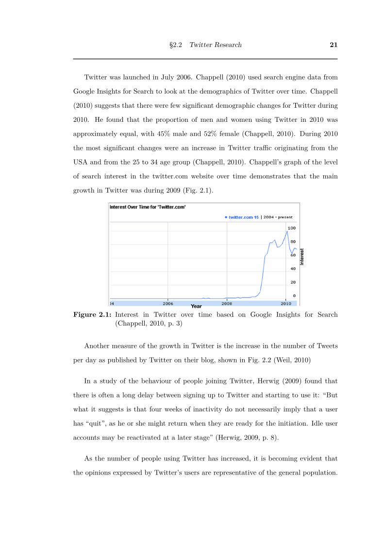
§2.2 Twitter Research 21
Twitter was launched in July 2006. Chappell (2010) used search engine data from
Google Insights for Search to look at the demographics of Twitter over time. Chappell
(2010) suggests that there were few significant demographic changes for Twitter during
2010. He found that the proportion of men and women using Twitter in 2010 was
approximately equal, with 45% male and 52% female (Chappell, 2010). During 2010
the most significant changes were an increase in Twitter traffic originating from the
USA and from the 25 to 34 age group (Chappell, 2010). Chappell’s graph of the level
of search interest in the twitter.com website over time demonstrates that the main
growth in Twitter was during 2009 (Fig. 2.1).
Figure 2.1: Interest in Twitter over time based on Google Insights for Search(Chappell, 2010, p. 3)
Another measure of the growth in Twitter is the increase in the number of Tweets
per day as published by Twitter on their blog, shown in Fig. 2.2 (Weil, 2010)
In a study of the behaviour of people joining Twitter, Herwig (2009) found that
there is often a long delay between signing up to Twitter and starting to use it: “But
what it suggests is that four weeks of inactivity do not necessarily imply that a user
has “quit”, as he or she might return when they are ready for the initiation. Idle user
accounts may be reactivated at a later stage” (Herwig, 2009, p. 8).
As the number of people using Twitter has increased, it is becoming evident that
the opinions expressed by Twitter’s users are representative of the general population.
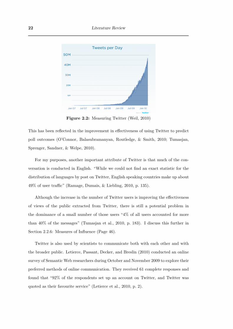
22 Literature Review
Figure 2.2: Measuring Twitter (Weil, 2010)
This has been reflected in the improvement in effectiveness of using Twitter to predict
poll outcomes (O’Connor, Balasubramanyan, Routledge, & Smith, 2010; Tumasjan,
Sprenger, Sandner, & Welpe, 2010).
For my purposes, another important attribute of Twitter is that much of the con-
versation is conducted in English. “While we could not find an exact statistic for the
distribution of languages by post on Twitter, English speaking countries make up about
49% of user traffic” (Ramage, Dumais, & Liebling, 2010, p. 135).
Although the increase in the number of Twitter users is improving the effectiveness
of views of the public extracted from Twitter, there is still a potential problem in
the dominance of a small number of those users “4% of all users accounted for more
than 40% of the messages” (Tumasjan et al., 2010, p. 183). I discuss this further in
Section 2.2.6: Measures of Influence (Page 46).
Twitter is also used by scientists to communicate both with each other and with
the broader public. Letierce, Passant, Decker, and Breslin (2010) conducted an online
survey of Semantic Web researchers during October and November 2009 to explore their
preferred methods of online communication. They received 61 complete responses and
found that “92% of the respondents set up an account on Twitter, and Twitter was
quoted as their favourite service” (Letierce et al., 2010, p. 2).

§2.2 Twitter Research 23
2.2.3 Expression of the public’s views on Twitter
This section describes a range of studies that use Twitter to look for expression of the
views of the public. Most studies focus on a single topic area of public discussion such
as politics, earthquake detection or influenza detection. There is a growing number
of studies which use Twitter as a source of information about the views of the public.
Twitter can “provide access to thoughts, intentions and activities of millions of users
in real-time” (Phelan, McCarthy, & Smyth, 2009, p. 385).
An important aspect of Twitter is that anyone with access to it can express their
views, and although some users have more influence than others, “a trend can be
initiated by anyone, and if the environment is right, it will spread” (Cha, Haddadi,
Benevenuto, & Gummadi, 2010, p. 11).
One of the attributes of the Twitter environment is competition for attention which
Romero, Galuba, Asur, and Huberman (2010) describe as; “ideas, opinions, and prod-
ucts compete with all other content for the scarce attention of the user community.”
(Romero et al., 2010, p. 1) They go on to say “in spite of the seemingly chaotic fashion
with which all these interactions take place, certain topics manage to get an inordinate
amount of attention, thus bubbling to the top in terms of popularity and contributing
to new trends and to the public agenda of the community” (p. 1).
Yardi and Boyd (2010a) suggest that one factor by which topics are spread is that
people enjoy spreading news, especially if it is new and interesting. “Indeed, the large
spike and subsequent decays in tweets following immediately after any event breaks
out on Twitter suggests that people enjoy spreading news that are novel and popular”
(Yardi & Boyd, 2010a, p. 325). This supports the earlier study by D. Zhao and Rosson
(2009) which showed that people use Twitter because it provides an informal way to
keep up with friends and colleagues: “Real-time information posted through micro-
blogging is considered a quick and interesting source of news. It can also provide

24 Literature Review
valuable context information that may prompt catching-up conversations with distant
friends and colleagues” (D. Zhao & Rosson, 2009, p. 247).
Because Twitter provides access to the individual public messages (tweets)4 that
make up a conversation, it can be used not just to see what topics are popular, but to
see what individuals are saying:
This type of usage has tremendous potential for social and behavioral sci-
ences researchers, in terms of seeing both what topics are reverberating
with the public as well as what Twitter users are actually saying about the
topic. Twitter gives the ability to track both the subject and content of
conversations (Ovadia, 2009, p. 203).
Ovadia (2009) found that Twitter can act as a filter to focus discourse about a
conference saying “Whereas most conference Websites will display some representation
of what was discussed without much filtering or analysis, searching tweets will connect
users to content deemed interesting enough to tweet about” (Ovadia, 2009, p. 204).
This was confirmed by a study of conference tweets by Letierce et al. (2010) looking at
“how researchers use it for spreading information” (Letierce et al., 2010, p. 3) which
“showed that studying streams of scientific conferences provide means to figure out
trend topics of the event” (p. 8) and that “people use Twitter as a background commu-
nication channel during conferences, focussing mainly on other people attending the
conference” (p. 6). Although they found main focus is on other people at the confer-
ence, they also “believe that Twitter has this potential to help the erosion of boundaries
between researchers and a broader audience” (Letierce et al., 2010, p. 1).
Boyd et al. (2010)5 looked at how people use retweets as a form of conversation on
Twitter. They describe retweeting as “the Twitter-equivalent of email forwarding where4it is not possible to access any private tweets (private messages) that might also be part of the
conversation5Note: danah michele boyd asks that people use lower case for her name - http://www.danah.org/
name.html

§2.2 Twitter Research 25
users post messages originally posted by others” (Boyd et al., 2010, p. 1). They stress
the importance of retweeting in helping to provide a sense of community on Twitter:
While retweeting can simply be seen as the act of copying and rebroad-
casting, the practice contributes to a conversational ecology in which con-
versations are composed of a public interplay of voices that give rise to an
emotional sense of shared conversational context. (Boyd et al., 2010, p. 1)
Retweeting allows people to “have a sense of being surrounded by a conversation,
despite perhaps not being an active contributor” (Boyd et al., 2010, p. 1).
“as more scholars begin examining Twitter, it is important to have a grounded
understanding of the core practices.” (Boyd et al., 2010, p. 1).
Boyd et al. (2010) collected three datasets. The first dataset was a “random sample
of 720,000 tweets captured at 5-minute intervals from the public timeline over the period
1/26/09-6/13/09” (Boyd et al., 2010, p. 3). They used this to identify the proportion
of different types of tweets in the dataset and found that:
• 36% of tweets mention a user in the form ‘@user’; 86% of tweets with
@user begin with @user and are presumably a directed @reply
• 5% of tweets contain a hashtag (#) with 41% of these also containing
a URL
• 22% of tweets include a URL (‘http:’)
• 3% of tweets are likely to be retweets in that they contain ‘RT’,
‘retweet’ and/or ‘via’ (88% include ‘RT’, 11% include ‘via’ and 5%
include ‘retweet’)
(Boyd et al., 2010, p. 4)

26 Literature Review
Because the proportion of retweets in the random sample was quite low, Boyd et al.
(2010) created a second data set, a “random sample of 203,371 retweets captured from
the Twitter public timeline using the search API over the period 4/20/09-6/13/09.”
(p. 4) collected using “explicit queries for retweets of the form ‘RT’ and ‘via”’ (p. 4).
They used this to identify the proportion of retweets with particular features and found:
• 18% of retweets contain a hashtag
• 52% of retweets contain a URL
• 11% of retweets contain an encapsulated retweet (RT @user1 RT @user2
...message..)
• 9% of retweets contain an @reply that refers to the person retweeting
the post
(Boyd et al., 2010, p. 4)
Based on these results, they concluded that “compared to the random sample of tweets,
hashtag usage and linking are overrepresented in retweets” (Boyd et al., 2010, p. 4).
The 9% of retweets which contain a reference to the person retweeting the post indicate
that person “A retweets B when B’s message refers to A. We call these ‘ego retweets’ ”
(Boyd et al., 2010, p. 4).
Boyd et al. (2010) studied a third data set containing “qualitative comments on
Twitter practices stemming from responses we received to a series of questions on
@zephoria’s public Twitter account, which has over 12,000 followers” (p. 4) asking:
• “What do you think are the different reasons for why people RT some-
thing?” [99 responses]
• “If, when RTing, you alter a tweet to fit under 140 chars, how do you
decide what to alter from the original tweet?” [96 responses]

§2.2 Twitter Research 27
• “What kinds of content are you most likely to retweet? (Why?)” [73
responses]”
(Boyd et al., 2010, p. 4)
While they acknowlege that “the responses we received from this convenience sam-
ple are not representative of all Twitter users nor do they reflect all possible answers”
(Boyd et al., 2010, p. 4) they were able to obtain some interesting results. Some of the
motivations for retweeting found in responses to danah boyd’s (@zephoria) questions
include: (all from (Boyd et al., 2010, p. 6))
• “To amplify or spread tweets to new audiences”
• “entertain or inform”
• “to comment”
• “to make one’s presence as a listener visible”
• “to publicly agree”
• “validate others’ thoughts”
• “an act of friendship, loyalty, or homage”
• “recognize or refer to less popular people or less visible content”
• “self-gain”
• “save tweets for future personal access”
Boyd et al. (2010) found that “not all retweets are an accurate portrayal of the
original message” (p. 9) and that “conversations on Twitter can sometimes take the
form of a glorified game of “Broken Telephone” as individuals whisper what they re-
member to their neighbor and the message is corrupted as it spreads” (p. 10). However

28 Literature Review
most messages are not corrupted and “retweets can knit together tweets and provide a
valuable conversational infrastructure” (p. 7). On Twitter, “rather than participating
in an ordered exchange of interactions, people instead loosely inhabit a multiplicity of
conversational contexts at once” (Boyd et al., 2010, p. 10).
Letierce et al. (2010) found that the proportion of tweets that were repeated
(retweets) compared to original tweets from each of three Semantic Web scientific
conferences they studied was between 15% to 20% and note that this is much higher
than the 3% found by Boyd et al. (2010) (Letierce et al., 2010, p. 3).
Having considered these general studies of how people communicate on Twitter I
now move on to research that looks at specific topic areas, the first of which is politics.
Politics
Politics has been an active area of study of expression of the views of the public on
Twitter, with researchers looking at predicting election outcomes, using Twitter as an
alternative to polling, using public mood states on Twitter to predict stock market
movements and investigating how public converations about a contiversial issue plays
out on Twitter.
In a study of the 2009 German federal election Tumasjan et al. (2010) found that
even a simple analysis of the number of tweets mentioning a political party can be
almost as accurate in predicting election outcomes as traditional election polling, this
may be affected by the system of voting and so may not apply in countries with a
different system than Germany. Analysis of the joint mentions of political parties in
individual tweets was able to describe the complex relationships between the different
parties in Germany; “joint mentions of two parties are in line with real world political
ties and coalitions” (Tumasjan et al., 2010, p. 178). Tumasjan et al. (2010) were
surprised that their sample of the German electorate through Twitter still predicted the
§2.2 Twitter Research 29
election outcome “despite the fact that the Twittersphere is no representative sample
of the German electorate, the activity prior to the election seems to validly reflect the
election outcome” (Tumasjan et al., 2010, p. 183).
Tumasjan et al. (2010) found that in Germany “Twitter is indeed used extensively
for political deliberation” (p. 178) and this was also reported for Australia by Grant,
Moon, and Busby Grant (2010) who found that “Twitter is becoming, ever more, the
political space in Australia in which ideas, issues and policies are first announced,
discussed, debated and framed” (Grant et al., 2010, p. 599).
Another political study was conducted by O’Connor, Balasubramanyan, et al.
(2010) who looked at whether two years of Twitter data could be mined for partic-
ular topics (consumer confidence and political opinion) and the sentiment within these
topics used to replicate traditional telephone based polling. They suggested that “min-
ing public opinion from freely available text content could be a faster and less expensive
alternative to traditional polls” (p. 122) . They go on to suggest that an important
advantage of Twitter analysis over polling is that the topics that can be considered are
much broader than what can be covered by a traditional poll: “Such analysis would
also permit us to consider a greater variety of polling questions, limited only by the
scope of topics and opinions people broadcast” (p. 122).
An investigation of whether homophily was present on Twitter was conducted by
Yardi and Boyd (2010a) by examining the conversation in Twitter in the first 24 hours
after a polarising news event, in this case, the shooting in the USA of a doctor at an
abortion clinic. They defined homophily as “the principle that interactions between
similar people occur more often than among dissimilar people” (p. 318). They captured
approximately 30,000 tweets about the shooting by using the Twitter Search API with
search terms like “#tiller, pro-life, pro-choice, abortion, and George Tiller” over the
60 days following the event (p. 319). For this study they “focus on the first 24 hours
because traffic is heaviest at this point and later use is subject to anomalies among

30 Literature Review
heavy users and outliers” (p. 319). This resulted in a dataset of 11,017 Tweets from
6,803 Twitter accounts. They found that within this dataset there were 1,447 reply
pairs where one Twitter account had replied to another. They manually coded each of
these Twitter accounts as being ‘strong pro-life’, ‘pro-life’, ‘moderate/can’t tell’, ‘pro-
choice’, or ‘strong pro-choice’ and looked at the number of reply pairs between each
of these categories. They also used the LIWC text analysis tool6 to look at changes
in emotions expressed in the Tweets over the 24 hours. They found that people with
pro-abortion and anti-abortion views did interact through Twitter and that “The kinds
of interactions we observed suggest that Twitter is exposing people to multiple diverse
points of view but that the medium is insufficient for reasoned discourse and debate,
instead privileging haste and emotion” (p. 325).
Earthquake detection
Another topic that researchers have studied on Twitter is earthquake detection. In
this topic area researchers have been more explicit about treating tweets as sensor
data rather than as part of a discourse. Real world events can be detected by using
location and timing of tweets. Each user is considered to be a sensor, and their tweets
are reports from that sensor (Earle, 2010; Sakaki, Okazaki, & Matsuo, 2010).
Earle (2010) used the timing and geographic location of Twitter messages about
earthquakes to supplement instrument based estimates of earthquake location and mag-
nitude. He found that tweets about earthquakes were available very quickly “generally
within 20 seconds of widely felt events in tech-savvy regions” (Earle, 2010, p. 221).
They compared this to the official U.S. Geological Survey (USGS) data; “tweets are
often available before the 2 to 20 minutes it takes the USGS to publically distribute
instrumentally derived estimates of location and magnitude” (Earle, 2010, p. 221).
A similar study by Sakaki et al. (2010) in Japan also found tweets to be faster than6Linguistic Inquiry and Word Count (LIWC) – http://www.liwc.net/

§2.2 Twitter Research 31
the official Japan Meteorological Agency (JMA) announcements, although by a much
smaller margin.
Our system sent e-mails mostly within a minute, sometimes within 20s.
The delivery time is far faster than the rapid broadcast of announcements of
JMA, which are widely broadcast on TV; on average, a JMA announcement
is broadcast 6 min after an earthquake occurs. (Sakaki et al., 2010, p. 858)
An interesting aspect of the study by Sakaki et al. (2010) is that they applied
statistical filtering techniques that are used to account for inaccuracies in distributed
physical sensors, to the tweets in their study. They considered each Twitter user to be
a different sensor, and the tweets they sent were sensor observations; “Each Twitter
user is regarded as a sensor. A sensor detects a target event and makes a report
probabilistically” (p. 853). Semantic analysis was used to classify tweets as positive
or negative observations. They then tested the accuracy of results produced using a
variety of algorithms for filtering distributed physical sensors such as “Kalman filters,
multihypothesis tracking, grid-based, and topological approaches, and particle filters”
(p. 859). They found that “Particle filters perform well compared to other methods”
(p. 859). Sakaki et al. (2010) went on to use the same techniques to detect rainbow
locations.
Health information
Scanfeld, Scanfeld, and Larson (2010) studied the discussion of health information on
Twitter. They used the Twitter search API to get a sample of tweets mentioning
“antibiotic” and “antibiotics” and used text analysis to categorise these. One of their
categories was “abuse/misuse” which looked at the proportion of tweets that were
conveying misinformation. They propose that automated responses to key phrases
might be one way to address misinformation;

32 Literature Review
To disseminate information to those exhibiting confusion or sharing mis-
information, online services are available to monitor and auto-respond to
trigger word combinations, such as ‘flu + antibiotics.’ (Scanfeld et al., 2010,
p. 187)
Scanfeld et al. (2010) conclude that “this study confirmed that Twitter is a space for
the informal sharing of health information and advice” (p. 186).
As well as the discussion of health related information on Twitter another health
topic that has been investigated is the use of Twitter to detect the spread of diseases.
Influenza detection using Twitter
Culotta (2010) conducted a study of the detection influenza outbreaks by analysing
Twitter messages. He used eight months of data from September 2009 to May 2010
containing over 570 million Twitter messages. He determined which keywords gave the
best correlation with national health statistics (US Out-patient Influenza-like Illness
Surveillance Network (ILINet)). Culotta (2010) found that Twitter based detection was
able to give almost real-time results at relatively low costs, while ILINet is expensive
and reporting is delayed by one to two weeks.
His study provides strong support for the usefulness of simple keyword matching
as a technique for assessing public interest in a topic on Twitter by showing that the
level of discussion of a flu on Twitter does correlate well with the incidence of flu in
the community.
Culotta (2010) was surprised by the level of correlation obtained using a single key-
word. He found that just by using “flu” they obtained an 84% held-out correlation and
the addition of a few other flu-related terms (cough, headache, sore throat) increased
this to 95%. Culotta (2010) warned that a problem with their methodology is that it is

§2.2 Twitter Research 33
very likely to detect false correlations, “the phrase “flu shot” has a correlation greater
than 90%, but certainly this is not a good term to monitor, as it may spike in frequency
without a corresponding spike in influenza rates” (p. 2). He partially addresses this
problem by adding a document classifier which can “reduce error rates by over half in
simulated false alarm experiments” (p. 1), although its effectiveness decreased in very
high noise simulations.
Lampos, De Bie, and Cristianini (2010) developed a web based automated Flu
Detector for the UK. They used geolocated tweets from Twitter search across 49 urban
centres in the UK (using the ability to search within a 10km radius) to develop a
regression model against the official Influenza-like Illness (ILI) rates from the Health
Protection Agency (HPA).
The research discussed in this section has shown that Twitter can be used to inves-
tigate the expression of the views of the public over a range of topics including politics
and health information. In contrast, the approach of treating tweets on certain topics
as sensor data rather than discourse was shown to be useful in detecting events like
earthquakes and influenza outbreaks. The next section describes one technique that
can be used to extract the views of the public from Twitter data, topic detection.
2.2.4 Topic detection
Topic detection looks at the content of tweets and uses various semantic techniques
to assign them to topics. There has been an increasing recognition of the ability of
Twitter to provide information about trends in topics of public discussion;
Once [Twitter] users began to understand that tweets, in the aggregate,
provided rich real-time information about specific issues, they began to
build tools to help filter and highlight trending topics (Huang, Thornton,
& Efthimiadis, 2010, p. 2).

34 Literature Review
There are a number of attributes of tweets that can be used for topic detection
including twitter hashtags and word co-occurance.
Twitter hashtags
Hashtags are the keywords or tags that people add to their tweets to add context or
indicate what topic they are discussing. They are known as hashtags because the hash
symbol # is used at the start of each tag. One of the most straight forward approaches
to topic detection is to look at the tags that people add to their Tweets.
People began publishing tweets with tags in them spontaneously, probably influ-
enced by the rise in tagging (folksonomies) in other social media tools such as Delicious.
“One year after Twitter went live, members of the community, without involvement
or support from Twitter administrators, began tagging their tweets” (Huang et al.,
2010, p. 3). However, Huang et al. (2010) found that the way in which tagging was
used in Twitter was unlike that used elsewhere and they named this “conversational
tagging”. They say “In conversational tagging, the tag itself is an important piece of
the message” (Huang et al., 2010, p. 3). They contrasted this with the use of tagging
for organising information in Delicious and many other social media tools.
The first tweet with a hashtag was sent on August 23, 2007 by Chris Messina
(@factoryjoe):
how do you feel about using # (pound) for groups. As in #barcamp [msg]?
https://twitter.com/chrismessina/status/223115412
He followed this up with a blog post7 two days later discussing how he thought
hashtags could improve conversations on Twitter.7http://factoryjoe.com/blog/2007/08/25/groups-for-twitter-or-a-proposal-for-twitter-tag-
channels/

§2.2 Twitter Research 35
Unlike organisational tags, which are used for organising and retrieving stored in-
formation, the Twitter hashtags are used in real time to “provide synchronic metadata
used to funnel related tweets into common streams” (Huang et al., 2010, p. 3). Ser-
vices which allow searching of past tweets have become available, and some of these
use hashtags as if they were organisational tags. Huang et al. (2010) suggests that
this may change the way people use hashtags in Twitter, perhaps moving to using tags
to help people find their tweets later instead of for participating in current streams of
conversation. This is explored by H. C. Chang (2010) who used diffusion of information
(DoI) theory to examine the adoption and non-adoption of hashtags on Twitter with
a view to improving the archiving of tweets, saying that;
DoI theory facilitates the investigation of the competing dynamics between
Twitter trending topics with and without hashtags during certain time pe-
riods. (p. 4)
Michelson and Macskassy (2010) found that hashtags were not useful in determining
the topics of interest of a single Twitter user. The most frequently used hashtags by
a user only gave some indication of their topics of interest in one out of their three
studied users. Because of this they excluded Twitter hashtags from their analysis saying
that “they are often not general enough and do not form an ontology” (Michelson &
Macskassy, 2010, p. 77).
Twitter hashtag time series
Hashtags can be studied over time resulting in hashtag time series. Huang et al. (2010)
used hashtag time series to study the emergence and decline of topics. They define this
as a micro-meme; “Twitter micro-meme: emergent topics for which a tag is created,
used widely for a few days, then disappears.” (p. 1) and go on to say

36 Literature Review
A micro-meme is a small-scale meme emerging around a Twitter hash-
tag. As more users adopt the hashtag, they add to an asynchronous, mas-
sively multi-person conversation by tweeting their thoughts about the topic
prompted by the hashtag. (p. 2)
They suggest that people are inspired to contribute to a trending topic because
they notice the hashtag associated with it, and otherwise might not have written on
that topic: “it is overwhelmingly likely that they might never have written the tweet
if they had not been inspired to participate in the micro-meme phenomenon” (Huang
et al., 2010, p. 1).
Word co-occurrence models
Another approach to topic detection is to look at word co-occurrence models. These
models look at the distribution of words in the text, in particular their co-occurrence.
The advantage of this approach is that it can be used to look at any text because it
doesn’t rely on the text matching a particular style. In this approach, words which
co-occur frequently are referred to as topics.
Ramage et al. (2010) provide a clear description of this type of model:
Latent variable topic models have been applied widely to problems in text
modeling, and require no manually constructed training data. These mod-
els distill collections of text documents (here, tweets) into distributions of
words that tend to co-occur in similar documents – these sets of related
words are referred to as “topics.” (p. 130)
Ramage et al. (2010) used latent variable topic modelling in a large scale study
of the content posted by people on Twitter. They initially conducted interviews with
Twitter users to try to determine “what needs drive following and reading behavior on
§2.2 Twitter Research 37
Twitter, and to what extent does Twitter satisfy them” (Ramage et al., 2010, p. 131).
Based on these interviews they found that people decided who was worth following
using four criteria;
1. Substance: “for the subjects they write about (substance, e.g. about a hobby or
professional interest)”
2. Social: “because of some social value (social, e.g. for making plans with friends)”
3. Status: “because of (dis)interest in personal life updates from the poster (status,
e.g. where someone is or what they are doing)”
4. Style: “because of the tone or style of the posts (style, e.g. humor or wit)”
(Ramage et al., 2010, p. 131)
Ramage et al. (2010) named these the 4S categories (substance / status / style /
social). They then used these categories (with the edition of an ‘other’ category) to
label (group) the top 200 latent topics that were detected when training the system on
the first day of data. Topics could be allocated to more than one of the 4S categories.
They give an example of this labeling; “the most frequent words in “Topic 1” are:
“watching tv show watch channel youtube episode and season,” which was labeled as
substance” (Ramage et al., 2010, p. 133).
Labels were also created for any hashtag occurring in the tweets for posts that
contained emoticons; “Emoticon-specific labels were applied to posts that used any of
a set of nine canonical emoticons: smile, frown, wink, big grin, tongue, heart, surprise,
awkward, and confused” (Ramage et al., 2010, p. 134). All of these created labels were
also allocated to the 4S categories.
This then allowed them to measure the proportion of Tweets that fell into each of
the 4S categories by using labeled latent topic analysis of the tweets and they found
that “At the word level, Twitter is 11% substance, 5% status, 16% style, 10% social,

38 Literature Review
and 56% other. Despite the common perception to the contrary, usage of substance
dimensions outnumbers status dimensions on Twitter by two to one.” (Ramage et al.,
2010, p. 135).
Griffiths and Steyvers (2004) use topic detection techniques to analyse abstracts
from papers in scientific journals in order to identify the most active topics in them.
They suggest that by finding the active topics in a textual data set the structure of the
data can be understood and trends over time discovered.
Petrovic, Osborne, and Lavrenko (2010) only focused on detecting tweets that
match news events: “We address the problem of detecting new events from a stream of
Twitter posts” (Petrovic et al., 2010, p. 181). This research is not focused on anything
that is not related to news: “The majority of tweets are not real stories, but rather
updates on one’s personal life, conversations, or spam” (p. 184). Their news events
category is similar to the substance category defined by Ramage et al. (2010). They
use First Story Detection (FSD) which aims to identify the first story (in this case a
tweet in a thread of related tweets) that discusses a particular event (Petrovic et al.,
2010). First Story Detection has mainly been used to look back at documents such as
newspapers, where each new story is compared to previously seen stories. This takes
too long in the context of Twitter where a constant stream of tweets is arriving in
real time (Petrovic et al., 2010). These authors solved this problem by developing an
algorithm which “takes constant time to process each new document, while also using
constant space” (p. 181). Petrovic et al. (2010) defined the most interesting topics
as those that grow the fastest, “Once we have threads of tweets, we are interested in
which threads grow fastest, as this will be an indication that news of a new event is
spreading.” (p. 181)
Another application of topic detection is for search and TweetMotif is a Twitter
search engine developed by O’Connor, Krieger, and Ahn (2010) that demonstrates the
use of topic detection to group tweets by significant terms to facilitate faceted search:

§2.2 Twitter Research 39
TweetMotif groups messages by frequent significant terms — a result set’s
subtopics — which facilitate navigation and drill down through a faceted
search (p. 384).
A related application to search is news story recommendation. Phelan et al. (2009)
used topic detection in Twitter to discover emerging topics and select the ones that
match recent news in a RSS feed in order to provide recommended reading for users.
They found this approach promising; “early evaluation results suggest that users do
benefit from the recommendations that are derived from the Twitter data” (p. 388).
“TwitterStand” is another news recommendation application which was developed by
Sankaranarayanan, Samet, Lieberman, and Sperling (2009) which uses real time filter-
ing and clustering of tweets to detect news topics. They used a selected set of Twitter
users as a ‘seeders’ group to help filter the noise from the main body of their Twitter
feeds. Seeders were selected as people who mainly tweeted news items, so their tweets
were used to start new clusters. Other people’s tweets could also start a cluster, but
that cluster would not be considered as an active news item cluster until a tweet from
a seeder was added to it. They also provide a method for determining the geographic
location(s) of the topic cluster.
The hashtag timeseries topic detection and some of the word co-occurance topic
detection methods have included consideration of changes in topics over time and con-
cepts of the rise and fall of the popularity of topics. Cataldi, Di Caro, and Schifanella
(2010) extend this by applying a biological metaphor to the change in topics over time.
Biological metaphor
Cataldi et al. (2010) use a biological metaphor with an aging algorithm. Each occur-
rence of a term acts as ‘food’ increasing the ‘energy’ metric of the term and the energy
decreases at a constant rate (to maintain the organism). The contribution of each

40 Literature Review
tweet, containing a term, to the term metric is weighted by the authority of the person
sending the tweet. The authority of each person was based on a Page Rank algorithm8.
The terms are then linked to topics using semantically related keywords. They define a
topic as “a coherent set of semantically related terms that express a single argument”
(Cataldi et al., 2010, p. 2). A topic is emergent in a particular time period if “it has
been extensively treated within it but rarely in the past” (Cataldi et al., 2010, p. 1).
They found that emerging topics appeared on Twitter before newspapers; “Twitter
can provide a real-time system that can also predate the best newspapers in informing
the web community about the emerging topics” (Cataldi et al., 2010, p. 1). Using
longer time steps (sampling windows) increases the statistical significance of the topics
detected but reduces the lead Twitter has over traditional sources (Cataldi et al., 2010).
2.2.5 Sentiment Analysis
A further refinement of topic detection is to analyse the sentiments being expressed
in tweets. The simplest form of sentiment analysis categorises views as expressing
positive, negative or neutral sentiment. A more complex sentiment analysis measures
the sentiments across a wider range of emotions.
O’Connor, Balasubramanyan, et al. (2010) demonstrated a correlation between the
sentiments expressed in Tweets and contemporaneous public opinion polls during 2008
and 2009. They “find that a relatively simple sentiment detector based on Twitter
data replicates consumer confidence and presidential job approval polls” (p. 128) and
conclude that “it is encouraging that expensive and time-intensive polling can be sup-
plemented or supplanted with the simple-to-gather text data that is generated from
online social networking” (p. 128-129). Their approach looked for positive or negative
sentiment words9 in tweets which contained a topic keyword. The topic keywords used8see Section 2.2.6: Measures of Influence (Page 46) for further discussion of influence9using subjectivity lexicon from OpinionFinder (http://www.cs.pitt.edu/mpqa/opinionfinderrelease/).
They did not use OpinionFinder’s distinctions between weak and strong words.

§2.2 Twitter Research 41
were;
• For consumer confidence: economy, job, and jobs
• For presidential approval: obama
• For elections: obama and mccain
(O’Connor, Balasubramanyan, et al., 2010, p. 124).
They found that text sentiment information from Twitter was volatile compared to
poll data, and that matching poll data required smoothing of the Twitter data in order
to detect long-term trends: “Smoothing is a critical issue. It causes the sentiment
ratio to respond more slowly to recent changes, thus forcing consistent behavior to
appear over longer periods of time” (p. 125). O’Connor, Balasubramanyan, et al.
(2010) suggest that sentiment analysis of social media might be improved by using the
demographic information from people’s online profiles to obtain a more representative
sample of the population.
They are optimistic about the future of sentiment analysis of social media sources:
Eventually, we see this research progressing to align with the more general
goal of query-driven sentiment analysis where one can ask more varied ques-
tions of what people are thinking based on text they are already writing
(p. 129).
Bollen, Mao, and Zeng (2010) come to a similar conclusion, saying that compared
to other public mood tracking tools, “Public mood analysis from Twitter feeds on
the other hand offers an automatic, fast, free and large-scale addition to this toolkit
that may in addition be optimized to measure a variety of dimensions of the public
mood state” (Bollen et al., 2010, p. 7). However, Bifet and Frank (2010) warn that
sentiment analysis of Twitter is particularly difficult due to the 140 character limitation;
42 Literature Review
“a tweet can contain a significant amount of information in very compressed form, and
simultaneously carry positive and negative feelings” (Bifet & Frank, 2010, p. 4)
Bollen et al. (2010) explored whether measuring public mood states, by using Twit-
ter sentiment analysis, could be used to predict the Dow Jones Industrial Average
(DJIA). They found that although there was a strong predictive correlation shown in
the results they could not provide any explanation of causative mechanisms:
these results are strongly indicative of a predictive correlation between mea-
surements of the public mood states from Twitter feeds, but offer no infor-
mation on the causative mechanisms that may connect public mood states
with DJIA values in this manner. (Bollen et al., 2010, p. 7)
Bollen et al. (2010) note that this correlation was found even though the data they
used were world wide, whereas the DIJA is a measure of the USA stock market and
suggest that further research using geographically selected data would be interesting.
Davidov, Tsur, and Rappoport (2010) developed a supervised sentiment classifi-
cation framework based on Twitter, extending a Natural Language Processing (NLP)
approach to sentiment analysis of Twitter content by considering Twitter hashtags and
smileys instead of predefined lists of sentiment words in determining sentiment earn-
ing from Tweets. Their approach removed the manual effort in developing sentiment
classification for new data sets:
The substantial coverage and size of the processed Twitter data allowed us
to identify dozens of sentiment types without any labor-intensive manually
labeled training sets or pre-provided sentiment-specific features or senti-
ment words. (p. 248)
A weakness of their paper is that they do not provide the number of ‘judges’ used
in their human evaluation of the sentiment encoding of the tweets. They compare the
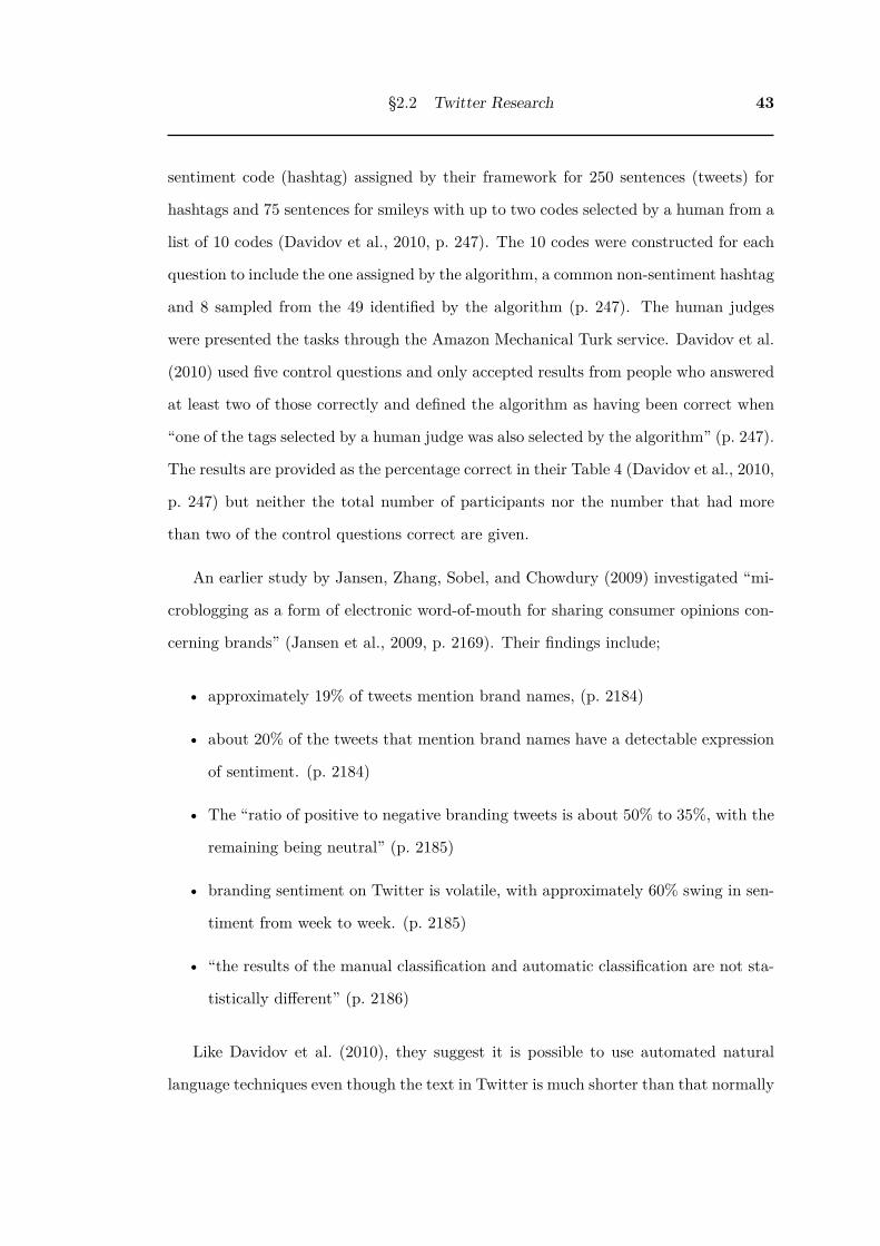
§2.2 Twitter Research 43
sentiment code (hashtag) assigned by their framework for 250 sentences (tweets) for
hashtags and 75 sentences for smileys with up to two codes selected by a human from a
list of 10 codes (Davidov et al., 2010, p. 247). The 10 codes were constructed for each
question to include the one assigned by the algorithm, a common non-sentiment hashtag
and 8 sampled from the 49 identified by the algorithm (p. 247). The human judges
were presented the tasks through the Amazon Mechanical Turk service. Davidov et al.
(2010) used five control questions and only accepted results from people who answered
at least two of those correctly and defined the algorithm as having been correct when
“one of the tags selected by a human judge was also selected by the algorithm” (p. 247).
The results are provided as the percentage correct in their Table 4 (Davidov et al., 2010,
p. 247) but neither the total number of participants nor the number that had more
than two of the control questions correct are given.
An earlier study by Jansen, Zhang, Sobel, and Chowdury (2009) investigated “mi-
croblogging as a form of electronic word-of-mouth for sharing consumer opinions con-
cerning brands” (Jansen et al., 2009, p. 2169). Their findings include;
• approximately 19% of tweets mention brand names, (p. 2184)
• about 20% of the tweets that mention brand names have a detectable expression
of sentiment. (p. 2184)
• The “ratio of positive to negative branding tweets is about 50% to 35%, with the
remaining being neutral” (p. 2185)
• branding sentiment on Twitter is volatile, with approximately 60% swing in sen-
timent from week to week. (p. 2185)
• “the results of the manual classification and automatic classification are not sta-
tistically different” (p. 2186)
Like Davidov et al. (2010), they suggest it is possible to use automated natural
language techniques even though the text in Twitter is much shorter than that normally
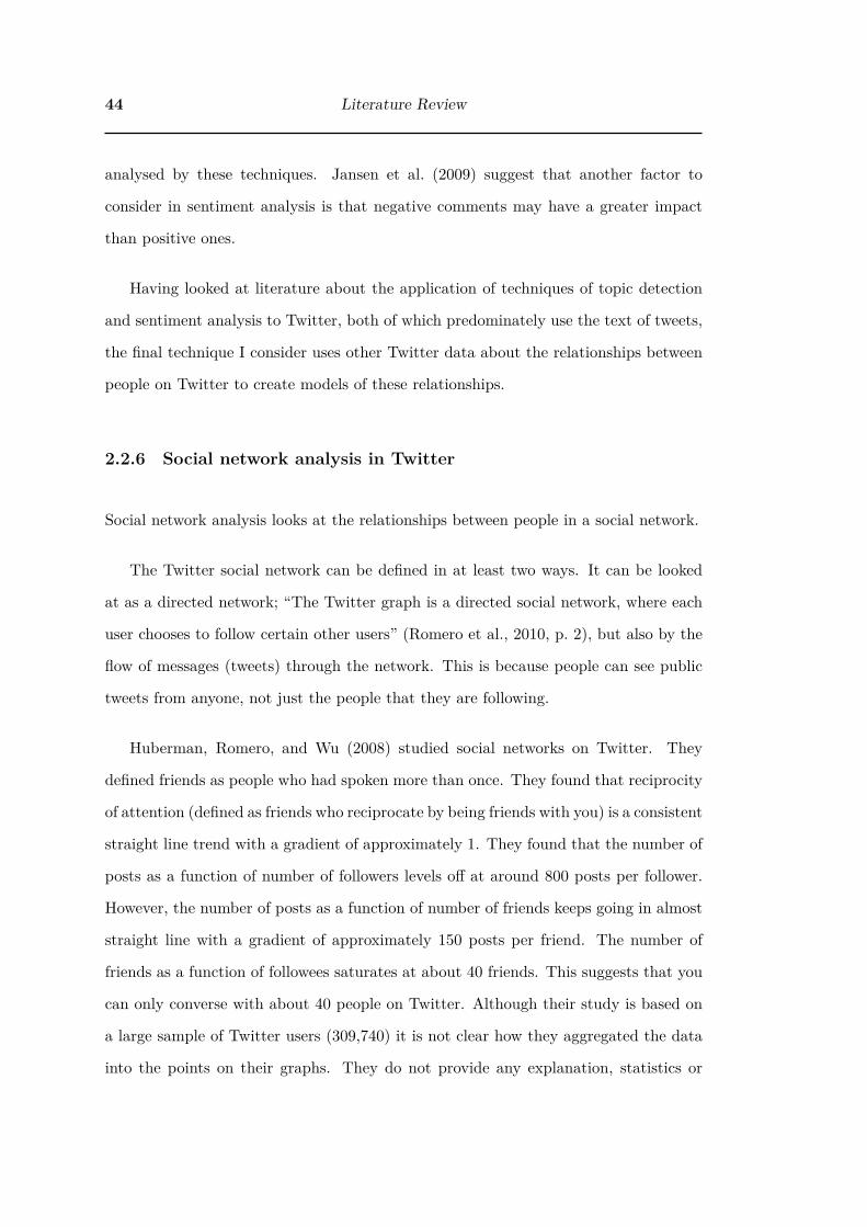
44 Literature Review
analysed by these techniques. Jansen et al. (2009) suggest that another factor to
consider in sentiment analysis is that negative comments may have a greater impact
than positive ones.
Having looked at literature about the application of techniques of topic detection
and sentiment analysis to Twitter, both of which predominately use the text of tweets,
the final technique I consider uses other Twitter data about the relationships between
people on Twitter to create models of these relationships.
2.2.6 Social network analysis in Twitter
Social network analysis looks at the relationships between people in a social network.
The Twitter social network can be defined in at least two ways. It can be looked
at as a directed network; “The Twitter graph is a directed social network, where each
user chooses to follow certain other users” (Romero et al., 2010, p. 2), but also by the
flow of messages (tweets) through the network. This is because people can see public
tweets from anyone, not just the people that they are following.
Huberman, Romero, and Wu (2008) studied social networks on Twitter. They
defined friends as people who had spoken more than once. They found that reciprocity
of attention (defined as friends who reciprocate by being friends with you) is a consistent
straight line trend with a gradient of approximately 1. They found that the number of
posts as a function of number of followers levels off at around 800 posts per follower.
However, the number of posts as a function of number of friends keeps going in almost
straight line with a gradient of approximately 150 posts per friend. The number of
friends as a function of followees saturates at about 40 friends. This suggests that you
can only converse with about 40 people on Twitter. Although their study is based on
a large sample of Twitter users (309,740) it is not clear how they aggregated the data
into the points on their graphs. They do not provide any explanation, statistics or

§2.2 Twitter Research 45
error bars on their graphs to indicate how well the raw data maps onto the points on
their graphs.
Cha et al. (2010) suggests that connections in social media can have a range of mean-
ings: “Directed links in social media could represent anything from intimate friendships
to common interests, or even a passion for breaking news or celebrity gossip” (Cha et
al., 2010, p. 10). Noordhuis, Heijkoop, and Lazovik (2010) say that on Twitter links
mostly indicate shared interests rather than real life connections.
Twitter is less focused on friendship and more on interest: a user is more
likely to be connected to another user because he is interested in what
this user has to say and less because they happen to be friends in real life
(Noordhuis et al., 2010, p. 107).
Noordhuis et al. (2010) also found that Twitter users often read Tweets written by
people that they are not connected to by using keyword search to find the tweets.
Ediger, Jiang, Riedy, Bader, and Corley (2010) describe a method based on large
scale social network analysis (using parallel processing on a super computer) to rank
actors within conversations in the network. This approach allows a much smaller data
subset of the ‘key players’ to be identified for use in more detailed studies that could
not easily be calculated on the full data set.
Yardi and Boyd (2010b) looked at whether the social network graph on Twitter
reflected the geographic location of the participants. They found that it did, with both
people who are geographically closer having more links between them and individuals
who are central in the Twitter network also being geographically central to the same
group.
An important attribute of social networks is how people in the network influence
each other.
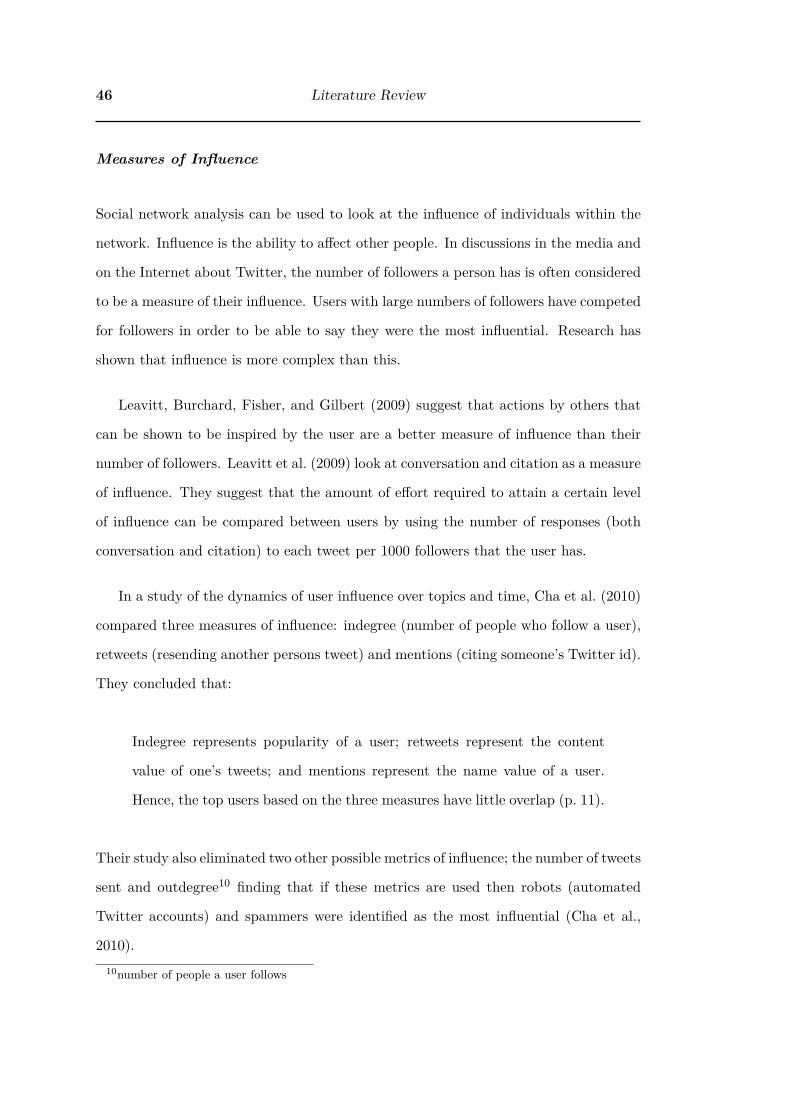
46 Literature Review
Measures of Influence
Social network analysis can be used to look at the influence of individuals within the
network. Influence is the ability to affect other people. In discussions in the media and
on the Internet about Twitter, the number of followers a person has is often considered
to be a measure of their influence. Users with large numbers of followers have competed
for followers in order to be able to say they were the most influential. Research has
shown that influence is more complex than this.
Leavitt, Burchard, Fisher, and Gilbert (2009) suggest that actions by others that
can be shown to be inspired by the user are a better measure of influence than their
number of followers. Leavitt et al. (2009) look at conversation and citation as a measure
of influence. They suggest that the amount of effort required to attain a certain level
of influence can be compared between users by using the number of responses (both
conversation and citation) to each tweet per 1000 followers that the user has.
In a study of the dynamics of user influence over topics and time, Cha et al. (2010)
compared three measures of influence: indegree (number of people who follow a user),
retweets (resending another persons tweet) and mentions (citing someone’s Twitter id).
They concluded that:
Indegree represents popularity of a user; retweets represent the content
value of one’s tweets; and mentions represent the name value of a user.
Hence, the top users based on the three measures have little overlap (p. 11).
Their study also eliminated two other possible metrics of influence; the number of tweets
sent and outdegree10 finding that if these metrics are used then robots (automated
Twitter accounts) and spammers were identified as the most influential (Cha et al.,
2010).10number of people a user follows

§2.2 Twitter Research 47
Cha et al. (2010) found that influential users can exert influence across a range of
topics and that it required effort to obtain influence, saying “influence is not gained
spontaneously or accidentally, but through concerted effort such as limiting tweets to
a single topic” (p. 10). They agree with Leavitt et al. (2009) that actions by other
users is a better measure of influence: “We have empirically demonstrated that having
a million followers does not always mean much in the Twitter world. Instead, we claim
that it is more influential to have an active audience who retweets or mentions the
user” (Cha et al., 2010, p. 11).
Lee, Kwak, Park, and Moon (2010) extend the idea of measuring influence by the
actions of users to tracking the diffusion of information in Twitter and saying that the
people who affect the spread of information are the ones who are influential. They also
show that most diffusion happens early in the spread of an idea, so people who tweet
earlier are more influential than those who join the conversation later.
Romero et al. (2010) also used the diffusion of information through the network as
their approach to influence. They found that the aspects which control the amount of
attention content generated by a user receives were:
1. “popularity and status of given members of these social networks, which is mea-
sured by the level of attention they receive in the form of followers” (p. 1),
2. “influence that these individuals wield, which is determined by the actual prop-
agation of their content through the network” (p. 1), and
3. “the passivity of members of the network which provides a barrier to propagation
that is often hard to overcome” (p. 1).
Romero et al. (2010) compared three measures of influence; their proposed Influence-
Passivity algorithm, PageRank and The Hirsch Index. They evaluated each approach
against information about how many people accessed URLs mentioned by users:
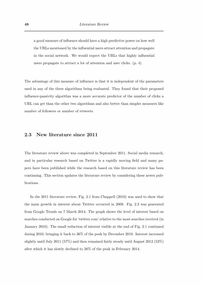
48 Literature Review
a good measure of influence should have a high predictive power on how well
the URLs mentioned by the influential users attract attention and propagate
in the social network. We would expect the URLs that highly influential
users propagate to attract a lot of attention and user clicks. (p. 4)
The advantage of this measure of influence is that it is independent of the parameters
used in any of the three algorithms being evaluated. They found that their proposed
influence-passivity algorithm was a more accurate predictor of the number of clicks a
URL can get than the other two algorithms and also better than simpler measures like
number of followers or number of retweets.
2.3 New literature since 2011
The literature review above was completed in September 2011. Social media research,
and in particular research based on Twitter is a rapidly moving field and many pa-
pers have been published while the research based on this literature review has been
continuing. This section updates the literature review by considering these newer pub-
lications.
In the 2011 literature review, Fig. 2.1 from Chappell (2010) was used to show that
the main growth in interest about Twitter occurred in 2009. Fig. 2.3 was generated
from Google Trends on 7 March 2014. The graph shows the level of interest based on
searches conducted on Google for ‘twitter.com’ relative to the most searches received (in
January 2010). The small reduction of interest visible at the end of Fig. 2.1 continued
during 2010, bringing it back to 36% of the peak by December 2010. Interest increased
slightly until July 2011 (57%) and then remained fairly steady until August 2012 (53%)
after which it has slowly declined to 26% of the peak in February 2014.

§2.3 New literature since 2011 49
Figure 2.3: Interest in Twitter over time based on Google Insights for Search(http://www.google.com.au/trends/explore#q=twitter.com) – as atMarch 2014 – extended from graph in Fig. 2.1 by (Chappell, 2010)
2.3.1 Science Communication
Bray, France, and Gilbert (2012) conducted a Delphi process with 10 experts to de-
fine the essential elements of science communication as a focus for developing a post
graduate Science Communication course. Of relevance for this thesis, they found that
understanding the audience is key to effective science communication: “an effective sci-
ence communicator needed to be aware of the needs of and outcomes for the audience”
and further that “science communicators need to be aware of the social, political and
cultural milieu in which science is embedded” (Bray et al., 2012, p. 32).
In a national survey of how Australian’s engage with science Searle (2014) found
that “a third (34%) reported having commented about science or technology issues
through social media in the last 12 months” (p. 36).
The study by Fisher et al. (2007) of a new way of assessing the publics views of
science over time, using a technique they call ‘Community Value Analysis’, has been
run over three years and Fisher, Lee, and Cribb (2013) have published their final
results. Fisher et al. (2013) look at public attitudes to pest animal management and
show that by using random sampling without replacement from an ‘ethical Internet
panel’ for a weekly online survey, that “a real-time ‘moving picture’ of public opinion

50 Literature Review
was developed over the lifetime of the study” (Fisher et al., 2013, Abstract), even with
the small sample size of 40 per week. Fisher et al. (2013) defines an ‘ethical internet
panel’ as having these characteristics:
• people are approached and invited to participate, they are not able
to apply (e.g. by responding to an advertisement for panellists on an
Internet dating site);
• there is no guarantee of any reward for panellists, whose motivation is
generally an ethical one based on a wish to help society;
• panels are refreshed reasonably frequently; and
• there has to be some altruistic purpose for the survey.
(p. 7)
Following on from their work looking at public interest in science using Google
search trends (Baram-Tsabari & Segev, 2009), Segev and Baram-Tsabari (2012) have
again used data from Google, this time to look at the correlation between the share of
searches for scientific topics, their news coverage, and the academic calendar to evaluate
science information seeking behaviours. They include the academic calendar to “reflect
the role of the education system” but note that the “academic calendar differs between
countries and hemispheres and we could not use it as a measure”, instead using the
keyword ‘science’ as a proxy for it. In this study they used Google Trends for both the
scientific topics and the trend for the keyword ‘science’, but in addition used Google
News to find the amount of news coverage for the scientific topics.
Segev and Baram-Tsabari (2012) confirmed their hypothesis that the “top searches
for science-related information between 2004 and 2010 would be correlated with the
academic calendar, while rising searches (searches that increased their share consid-
erably over a period) during that period would be correlated with media coverage.”
(p. 824). They also note that some search terms correlate with seasonal changes, not

§2.3 New literature since 2011 51
news events or the academic calendar, giving the example of ‘Full Moon’ which fol-
lowed a monthly cycle, this leads to the interesting insight that “motivation of people
to look for information on the full moon phenomenon each month does not stem from
reading about it in the news or learning about it in school, but rather from their direct
experience of this event” (p. 824). Their discussion of the limitations of their study
include some limitations that apply to this thesis. They note that the search queries
people use are a ‘Behavioural Measure’: “By entering a search query people reveal
that they are thinking about a topic but we do not know the nature of their thoughts.”
(p. 825) which is also a limitation of studying what people write in Tweets. They
go on to say “Online research tools represent to some degree the interests of people
from industrialized societies, usually from middle and upper class families, who use the
internet’s resources to pursue their science interests” (p. 825).
There has been increasing interest in the impact of social media on science commu-
nication. Brossard and Scheufele (2013) state that “a better understanding is needed
about how the online environment affects the communication of science information to
the public” (p. 40) and that “the new realities of an online information environment will
increasingly force scientists and social scientists to rethink the interface between the
science community” (p. 40). Mandavilli (2011) say that social media is changing how
communication between scientists occurs “Papers are increasingly being taken apart
in blogs, on Twitter and on other social media within hours rather than years, and in
public, rather than at small conferences or in private conversation” (p. 286).
A number of researchers have been looking at whether citations and references
to scientific publications in social media can be used as infometric or scientometric
measures of the value of the publication. Weller, Dröge, and Puschmann (2011) looked
at how scientists used Twitter during scientific conferences “this paper is the first
to focus on Twitter citations in the context of scientific conferences” (p. 3). The
found that “scientists use two types of Twitter citations during scientific conferences.
Users cite external sources in form of URLs and quote statements within Twitter via

52 Literature Review
RTs” (p. 11). They have gone on to extend their original data set with tweets by
scientific twitterers and focus on whether “scientific tweets include citation structures
similar to traditional information flows in scientific literature” (p. 2). Eysenbach (2011)
compared the citation rates articles in the Journal of Medical Internet Research (JMIR)
on Twitter from July 2008 to November 2011, in the form of URL links to articles
(which they call ‘Tweetations’), within a range of periods up ot 30 days after the
publication of the article with their Scopus and Google Scholar citation rates 17 to 29
months later and found that “a fascinating and compelling finding that the collective
intelligence of Twitter users can, within limitations, predict citations, which normally
take years to accumulate” (p. 16). They found that there was significant correlation
between Tweetations as early as 3 days after the publication of an article, and that
the optimal period of measurement was 7 days after the date of publication. They
defined “twimpact factor twn as a metric for immediate impact in social media, which
is defined as the cumulative number of tweetations within n days after publication (eg,
tw7 means total number of tweetations after n = 7 days).” (p. 13). JMIR intends to
use this as a metric on their website as a standard ‘Twimpact factor’.
Veltri (2012) conducted “one of the first studies on the use of the social web in
the context of the public understanding of science” (p. 833), an “exploratory study
of the use of the social web platform Twitter to share and discuss news on a ‘new’
technology: nanotechnology” (p. 833). They describe the history of the study of the
role of mass media in science communication through “the theoretical shift from a linear
diffusion model to a more interpretative approach” (p. 834) and the parallel move from
printed media to other mass media. They highlight “social media’s dual nature of
information source and conversation enabler” (p. 835) and conclude that “studying
how mass media frame an emerging technology is important for observing definitions
and associated meanings that are legitimised or stigmatised” (p. 832).
Veltri (2012) compared the discussion of nanotechnology with previous studies of
nanotechnology in mainstream mass media. They used a “mixed research design”

§2.3 New literature since 2011 53
(p. 836) combining web metrics, automated text analysis and sentiment analysis using
“T-Lab 7.3 and IBM Text Analytics” (p. 837). The “upper computational limit of
the two types of software used in the analysis roughly corresponded to 30,000 tweets”
(p. 837) so they collected 24,634 tweets from 60 randomly selected days in 2011 using
the “keywords and hashtags ‘nanotechnology’, ‘nano’ or ‘nanotechnologies”’ (p. 836).
The breakdown of types of tweets collected was found to be “92% new messages, 7%
‘re-tweets’ (a message forwarded to each of the user’s followers) and 1% ‘mentions”’
(p. 838) and “94% of tweets contained a link to a website.” (p. 838). They define the
reach and exposure of messages as follows:
Reach is the total number of unique Twitter users who received tweets about
the search term. Exposure is the total number of times tweets about the
search term were delivered to Twitter users. (p. 839)
and find that for their corpus the reach/exposure ratio was 0.489 which “suggests a
power law distribution of tweets, re-tweets and amplification” (p. 839) where “some
people are tweeting multiple times; some influencers are tweeting to lots of followers;
and most people are tweeting once or twice to their smaller set of followers” (p. 839).
They confirm this by looking at the number of tweets per user for their corpus. From
the low percentage of retweets and mentions they conclude that “nanotechnology is
not an object of conversation on Twitter but rather that Twitter is another channel of
diffusion for nanotechnology” (p. 844).
They used Latent Semantic Analysis to detect clusters in the tweets about Nan-
otechnology and found seven clusters that were “labelled as: ‘Fight Cancer’, ‘News/-
Conference’, ‘Mobile Phone’, ‘Science Projects’, ‘Applications’, ‘Opposition’ and ‘Resid-
ual’ ” (p. 841). Their sentiment analysis found that “positive feelings about nanotech-
nology are related in particular to business, medicine and science in general” (p. 843)
and that “negative tweets about nanotechnology were few in number” (p. 844). The

54 Literature Review
negative tweets were associated with uncertainty about the technology, dystopian views
of the future and hype.
Veltri (2012) showed that there is “a remarkable similarity with the findings of
previous studies on the discussion and representation of nanotechnology in the national
press of different countries” (p. 844).
2.3.2 Twitter Research
In an overview of the use of Twitter for research, Burgess and Bruns (2012) say that data
from Twitter requires “new methodological choices in the processing and analysis of
such large datasets on mediated social interaction” (p. 1). They go on to describe their
own work in which they collect tweets using the open source tool your Twapperkeeper11
and then process the data using scripts they have written in Gawk12. They use the
open source application Gephi13 for network analysis.
Burgess and Bruns (2012) discuss the history of the Twitter API and related regula-
tory instruments and the effects that changes in these over time have had on researchers.
The changes have all resulted in reductions on the amount and ease of access to Twitter
data:
First, the company locked out developers and researchers from direct “fire-
hose” (very high volume) access to the Twitter feed; this was accompanied
by a crackdown on free and public Twitter archiving services like 140Kit and
the Web version of Twapperkeeper (Sample), and coincided with the estab-
lishment of what was at the time a monopoly content licensing arrangement
between Twitter and Gnip, a company which charges commercial rates for
high-volume API access to tweets (and content from other social media11https://github.com/jobrieniii/yourTwapperKeeper12http://www.gnu.org/software/gawk/13http://gephi.org

§2.3 New literature since 2011 55
platforms). A second wave of controversy among the developer community
occurred in August 2012 in response to Twitter’s release of its latest API
rules (Sippey), which introduce further, significant limits to API use and
usability in certain circumstances. (p. 2)
Burgess and Bruns (2012) say that these changes to Twitter “undermines scholarly
research efforts to examine actual Twitter uses at least temporarily – meaning that
researchers are increasingly forced to invest time and resources in finding workarounds
for the new restrictions imposed by the Twitter API” (p. 3). They go on to suggest
that an underlying problem of Twitter research is that researchers “have no access to
an original set of texts – we can access only what Twitter’s proprietary and frequently
changing API will provide.” (p. 3) and “in providing an API, Twitter is driven not by
scholarly concerns but by an attempt to serve a range of potentially value-generating
end-users – particularly those with whom Twitter can create business-to-business rela-
tionships” (p. 3). These problems mean that it is “impossible for us to say with any
certainty that we are capturing a complete archive or even a ‘representative’ sample”
(p. 3). Burgess and Bruns (2012) conclude that this uncertainty cannot be fixed even
with best practice in data collection:
The total yield of even the most robust capture system (using the Streaming
API and not relying only on Search) depends on a number of variables:
rate limiting, the filtering and spam-limiting functions of Twitter’s search
algorithm, server outages and so on; further, because Twitter prohibits the
sharing of data sets it is difficult to compare notes with other research
teams. (p. 3)
Burgess and Bruns (2012) discuss the importance of understanding the way in which
the data made available by the Twitter API affects the choices made by researchers,
warning that “datapoints that are hardwired into the data naturally become the most
salient” (p. 3) and concluding:

56 Literature Review
Understanding how something like the Twitter API mediates the cultures
of use of the platform, as well as reflexively engaging with its mediating role
in data-driven Twitter research, promotes a much more materialist critical
understanding of the politics of the social media platforms. (p. 4)
Gerlitz and Rieder (2013) build on the work by Burgess and Bruns (2012) and look
at large scale sampling methodologies for Twitter from a humanities and social sciences
perspective. They discuss the “material/technical conditions of platforms” (Gerlitz &
Rieder, 2013, p. 1) which are “drawing attention to the performative capacities of
platform protocols to enable and structure specific activities” (p. 1). For Twitter these
include “elements such as tweets, retweets, @replies, favourites, follows, and lists” (p. 1).
They suggest that:
using these elements as basis for building a collection of tweets, users, etc.
to be analysed has significant epistemic weight: these sampling methods
come with specific notions of use scenarios built into them (p. 2).
They illustrate this with the example of the common practice of using hashtags to
select a corpus of Tweets which “assumes that a) the conversation is held together by
hashtags and b) the chosen hashtags are indeed the most relevant ones” (p. 2). Gerlitz
and Rieder (2013) say that the use of such assumptions do not just raise statistical
sampling bias issues but also involve information recall and precision, providing a nice
analogy to fishing;
Such assumptions go beyond the statistical question of sampling bias and
concern the fundamental problem of how to go fishing in a pond that is
big, opaque, and full of quickly evolving populations of fish. The classic
information retrieval concepts of recall (How many of the relevant fish did
I get?) and precision (How many fish caught are relevant?) fully apply in
this context. (p. 2)

§2.3 New literature since 2011 57
They describe selection techniques such as topic-based sampling, snowball sampling,
marker-based sampling and suggest that;
Non-probability selection techniques, topic-, marker-, and basic graph-based
sampling struggle with representativeness (Are my results generalisable?),
exhaustiveness (Did I capture all the relevant units?), cleanness (How many
irrelevant units did I capture?), and scoping (How “big” is my set compared
to others?), which does – of course – not invalidate results. It does, how-
ever, raise questions about the generality of derived claims, as case-based
approaches only allow for sense-making from inside the sample and not in
relation to the entire population of tweets. (p. 3)
To overcome these concerns, they suggest using the statuses/sample endpoint which
returns a 1% random sample of the full stream. Based on 450 million tweets per day
the “1% endpoint would provide a representative and high resolution sample with a
maximum margin of error of 0.06 at a confidence level of 99%, making the study of
even relatively small subpopulations within that sample a realistic option” (p. 4)
They agree with other authors that there is limited information available from
Twitter about the way in which this 1% sample is generated and perform a technical
analysis of the stream to check some of the concerns that have been expressed. They
conclude that “while more testing is needed, various elements indicate that the status-
es/sample endpoint provides data that are indeed representative of all public tweets.”
(Gerlitz & Rieder, 2013, p. 4) and “in the absence of access to a full sample, we propose
that the random sample provided through the Streaming API can serve as baseline for
case approaches in principle” (p. 12).
Like Burgess and Bruns (2012), Black, Mascaro, Gallagher, and Goggins (2012)
suggest that researchers need to have a “more reflexive stance towards the application
programming interfaces twitter provides” (p. 229) saying;
58 Literature Review
The two key gaps in analysis of social media generally, and Twitter in
particular, then, are 1) Each study constructs its own approach to gathering
Twitter data and 2) Attempts to explain the Twitter API through analysis
are difficult to verify because the data delivered by API may be changing
over time. (p. 229)
They go on to propose a “integrated methodological approach and technology architec-
ture for the standard capture, social transformation and analysis of Twitter interactions
using the Search API” (p. 229) which they call TwitterZombie. It is interesting to note
that Twitter has since encouraged developers ( including researchers) to move away
from the Search API to the Streaming API.
In March 2014 Lazer, Kennedy, King, and Vespignani (2014) challenged the Google
Flu Trends paper which has been used by many authors as evidence of the usefulness
of big data in prediction of societal events like the spread of disease, election outcomes
and the rise and fall of share markets. The original paper by Ginsberg et al. (2009)
reported on an algorithm called Google Flu Trends (GFT) which used Google search
engine queries to predict the level of the Influenza-like Illness (ILI) in the community
before the official Centers for Disease Control and Prevention (CDC) ILI reports:
we were able to estimate consistently the current ILI percentage 1-2 weeks
ahead of the publication of reports by the CDC’s US Influenza Sentinel
Provider Surveillance Network (Ginsberg et al., 2009, p. 1013)
Lazer et al. (2014) look at the causes of the large prediction error of GFT with “more
than double the proportion of doctor visits” (Lazer et al., 2014, p. 1203) for ILI than
that reported by the CDC, an error which was originally reported by Butler (2013).
Lazer et al. (2014) “explore two issues that contributed to GFT’s mistakes— big data
hubris and algorithm dynamics— and offer lessons for moving forward in the big data
age.” (p. 1203) They define ‘big data hubris’ as “the often implicit assumption that

§2.3 New literature since 2011 59
big data are a substitute for, rather than a supplement to, traditional data collection
and analysis.” (p. 1203) The initial version of GFT was flawed in that it selected for
search queries that were correlated with ILI in the training data but were not actually
related to ILI “the initial version of GFT was part flu detector, part winter detector”
(p. 1203). The GFT algorithm was updated in 2009 and Lazer et al. (2014) find that,
even before the 2013 critism by Butler (2013), the “new GFT has been persistently
overestimating flu prevalence” (Lazer et al., 2014, p. 1203) and show that the “GFT
also missed by a very large margin in the 2011–2012 flu season and has missed high for
100 out of 108 weeks starting with August 2011” (p. 1203).
Lazer et al. (2014) consider the problem of the effects of ‘algorithm dynamics’ on
GFT. They define ‘algorithm dynamics’ as “the changes made by engineers to improve
the commercial service and by consumers in using that service.” (p. 1204). Both
Burgess and Bruns (2012) and Black et al. (2012) report on the problems for researchers
caused by changes in the Twitter API, and changing patterns of user behaviour, which
align with this definition of algorithm dynamics. Lazer et al. (2014) acknowledge that
this problem extends beyond GFT and Google data sources such as Google Trends and
Google Correlate to other social media services:
Platforms such as Twitter and Facebook are always being re-engineered,
and whether studies conducted even a year ago on data collected from these
platforms can be replicated in later or earlier periods is an open question.
(p. 1204)
Lazer et al. (2014) are critical of Google and Ginsberg et al. (2009) for not providing
details of the GFT algorithms to allow the replication or validation of the Ginsberg et
al. (2009) study. They call for improvements in transparency and replicability of big
data research, pointing out that the “supporting materials for the GFT-related papers
did not meet emerging community standards” (Lazer et al., 2014, p. 1205). As well
as not providing access to the data that would be needed to replicate the GFT study,

60 Literature Review
Lazer et al. (2014) conclude that there appears to be a lack of transparency even in
the search terms included in the Ginsberg et al. (2009) paper;
Oddly, the few search terms offered in the papers ... do not seem to be
strongly related with either GFT or the CDC data (SM) – we surmise that
the authors felt an unarticulated need to cloak the actual search terms
identified. (Lazer et al., 2014, p. 1205)
Lazer et al. (2014) say that to mitigate the effects of algorithm dynamics it is
important to replicate findings based on big data sources “across time and using other
data sources to ensure that they are observing robust patterns and not evanescent
trends.” (p. 1205)
Even with these difficulties, Lazer et al. (2014) are still positive about the use of
big data for research:
Big data offer enormous possibilities for understanding human interactions
at a societal scale, with rich spatial and temporal dynamics, and for de-
tecting complex interactions and nonlinearities among variables. We con-
tend that these are the most exciting frontiers in studying human behavior.
(p. 1205)
Who uses Twitter
Since writing Section 2.2.2 (Who uses Twitter) there has been new literature published
showing that as the use of Twitter has become more prevalent, interest has developed
in how it can be applied in Education. Greenhow and Gleason (2012) review a range
of literature to support their argument that Twitter is a new form of literacy “A tweet
stream is a constantly evolving, co-constructed conversation.” (p. 472), and coin the
phrase ‘Twiteracy’ to describe this literacy. They suggest that

§2.3 New literature since 2011 61
Twitter use in higher education may facilitate increased student engagement
with course content and increased student-to-student or student-instructor
interactions — potentially leading to stronger positive relationships that
improve learning and to the design of richer experiential or authentic learn-
ing experiences. (p. 472)
Expression of the public’s views on Twitter
Extending the earlier studies by Boyd et al. (2010) and Letierce et al. (2010), Bruns
and Stieglitz (2012) and Bruns and Stieglitz (2013) looked a the proportions of dif-
ferent types of tweets in a wide range of hashtags and keywords in order to develop
a “catalogue of metrics for describing the communicative patterns which may be ob-
served for each hashtag” (Bruns & Stieglitz, 2012, p. 166). They found a range of
between 15% and 65% retweets and a correlation between the number of retweets and
number of urls, but found that the proportion of @replies did not seem to follow any
particular pattern. They compared the respective percentages of URLs and retweets
in the datasets because those measures
relate specifically to the two key practices of user engagement with informa-
tion which are postulated by the gatewatching model: finding information
online (i.e. identifying and posting relevant URLs), and sharing informa-
tion with other users (i.e. retweeting relevant messages). (Bruns & Stieglitz,
2013, p. 14)
Kosala and Adi (2012) harvested tweets about traffic in Jakata to provide real time
traffic data to enable “a map for users to easily get an overall understanding of any
given traffic situation in Jakarta in real time” (p. 2). They identified a problem in
parsing Indonesian tweets:

62 Literature Review
Based on an observation of 1000 sample tweets, it was found out that 946
did not use the grammatical language of Bahasa Indonesia. Thus around
95% of the tweets about traffic information were ungrammatical. (p. 2)
This problem was partly addressed by adding ‘abbreviations’ of keywords as well as
keywords to the analysis. Their initial study also used traffic CCTV to determine how
long traffic observations on Twitter remained valid and found that “traffic information
on Twitter will become irrelevant after 34 minutes, on average” (p. 8).
DiGrazia, McKelvey, Bollen, and Rojas (2013) used a large random sample of
Tweets from between 1 August 2010 and 1 November 2010 from which they “extracted
113,985 tweets that contained the name of the Republican or Democratic candidate for
Congress” (p. 2). They combined these with the “2010 election outcomes and sociode-
mographic variables from all 435 U.S. House districts” (p. 2) to investigate “whether
social media activity can be used to assess offline political behavior” (p. 2). They
develop a Ordinary Least Squares regression (OLS) model comparing the election out-
comes with the interest in each candidate on Twitter as expressed by the number of
tweets containing the name of each candidate and the number of users making those
tweets. They use the sociodemographic information such as district population, income,
incumbency as additional controls for their model.
After removing any election districts that do not have an opposition candidate they
“estimate the effect of the tweet and user share variables with two models: a bivariate
model and a full model including all controls” (DiGrazia et al., 2013, p. 4) and find
statistically significant (P < 0.001) effects for both tweet share and user share in both
models. They also found that both models “fit the data well; the R2adj for the bivariate
model is .283 and increases to .871 in the full model” (p. 4). DiGrazia et al. (2013)
suggest that “the robust effect of tweet content on electoral outcomes is consistent with
prior psycho-linguistic research ... people are more likely to say a word when it has a
positive connotation within the mind of the speaker” (p. 5-6) and that this allows for
§2.3 New literature since 2011 63
the success of the model even though it does not look at the sentiment expressed in
the tweets mentioning the candidates, “the relative share of attention compared to the
opponent is all that is needed” (p. 6).
Morgan, Lampe, and Shafiq (2013) look at whether the perceived ideology of a news
outlet effects the consumption and sharing of news from that outlet on Twitter. They
found that “people seem to share news in similar ways, regardless of outlet, and the
traits we examined did not indicate a substantial difference between outlets” (p. 894)
and that “people who share more than one tweet seem pretty quickly to include news
from different ideologies in the news they share, the opposite of what selective exposure
would predict” (p. 894).
Topic detection
Jung (2012) used Twitter for a case study of named entity recognition (NER). He
generated training data for the maximum entropy NER model by asking a group of
76 Twitter users to tag all named entities in their own tweets and tweets from their
followers for one week (p. 8069). The same users are involved for the following week in
“testing the proposed NER tasks” (p. 8069), it is unclear how they do this, although it
may be using the same tagging as a ground truth dataset instead of a training data set.
The study found that they could improve the accuracy of the NER model by clustering
the tweets using the meta data associated with a tweet. The best improvement was
by using temporal clustering, which is “is quite similar to event-based text clustering”
(p. 8079).
Wilkinson and Thelwall (2012) used the ‘time series scanning method’ developed
by one of the authors (Thelwall) to identify the top 50 trending topics in a dataset
consisting of “9 months of English-language Tweets from the United Kingdom, United
States, India, South Africa, New Zealand, and Australia” (Wilkinson & Thelwall, 2012,
p. 1631), collected using the geolocation options of the Twitter Streaming API. These

64 Literature Review
keywords were used to “identify the typical types of topic found and to identify in-
ternational differences” (p. 1637). The main topics of interest were grouped by type
with the most common being ‘Festival or religious occasion’ followed by ‘Media’ (TV
shows, concerts, films) then ‘Political Events’, ‘Human Interest Stories’ and ‘Sports’.
India showed the most variation from the other countries in the study, “having many
festivals and political events, but few media events, human interest stories, and natural
events” (p. 1637) while “topics of most interest to the United States tend to also be
found interesting by other countries” (p. 1638,) They say this is similar to the interna-
tional variation found in news reporting but that this “is not surprising because news
coverage presumably impacts what people Tweet about” (p. 1639) and that the Twit-
ter using public seems to reflect the “international imbalances in news media agenda
setting rather than combating them” (p. 1631).
Weng, Yao, Leonardi, Lee, and Lee (2011) developed a novel approach to event
detection on Twitter “EDCoW (Event Detection with Clustering of Wavelet-based
Signals)” (p. 401). The researchers capture bursts in the occurrence of words, filter
out trivial words and detect events by clustering words with similar wavelet functions.
Where the Discrete Fourier Transform (DFT) “converts the signals from the time
domain into the frequency domain” (p. 402) the Wavelet transformation “converts
signal from the time domain to the time-scale domain (scale can be considered as the
inverse of frequency)” (p. 402). The time-scale domain allows the time period in which
the burst happened to be determined “Unlike the sine and cosine used in the DFT,
which are localized in frequency but extend infinitely in time, wavelets are localized in
both time and frequency domain” (p. 402). The study was based on tweets published
in June 2010 by a snowball sample of 19,256 unique Twitter users connected to the
top 1,000 Singapore-based users (those with the most followers) initially selected using
http://twitaholic.com/. The raw dataset contained 4,331,937 tweets. The tweets were
then tokenised into words and then filtered to remove stop-words, words with non-
English characters and words with less than four characters. The tweets were further

§2.3 New literature since 2011 65
reduced by applying word stemming. Resulting in “638,457 unique words in total after
filtering and stemming” (p. 406). Words that were not considered to be useful in event
detection were removed before applying EDCoW, reducing the dataset to 8,140 unique
words:
First of all, rare words are filtered, since they are less possible to be associ-
ated with an event. A threshold of five appearances every day by average is
applied. We further filter words with certain patterns being repeated more
than two times, e.g. “booooo” (“o” being repeated 5 times) and “haha-
haah” (“ha” being repeated 3 times). Such words are mainly used for emo-
tional expression, and not useful in defining events. There are 8,140 unique
words left after cleaning up. (p. 406)
They set the time sampling parameters to capture the “hourly change of individual
words’ appearance patterns.” (Weng et al., 2011, p. 406) and the threshold for event
detection to be ϵ > 0.1 then “manually check the events detected by EDCoW one by
one” (p. 406). There were 21 events detected of which 3 were not able to be matched
to any real-life event and one that matched teams for the World Cup 2010 but didn’t
correspond to any event at that time. This means that “the precision of EDCoW in
this case is 76.2%” (p. 406). EDCoW has one tunable parameter (γ) which was set to
40 for this initial result. The authors repeated the event detection with γ values of 10,
20, 30, 50 and found that the precision was 0%, 14.3%, 16.3% and 22.5% respectively,
showing that the initial value of 40 performs the best.
Weng et al. (2011) also compared their model with other models. They aggregated
all of the tweets for each day into a single document per day and then used a Latent
Dirichlet Allocation (LDA) topic model on the 30 documents for June 2010. They
suggest that because LDA represents each topic as a mix of weighted words, it is more
difficult to identify what each topic is than with their EDCoW model and point out

66 Literature Review
another disadvantage of LDA in that it requires the specification of the number of
events to detect:
Further processing is required to improve the results generated by LDA in
the context of event detection, e.g. applying threshold-based heuristics to
filter non-eventful topics and words. In contrast, EDCoW has the ability to
filter trivial words away before applying clustering technique to detect the
events. More importantly, it requires no parameter to specify the number
of events. It will automatically generate different number of events based
on users’ discussions in the tweets. (p. 407)
W. X. Zhao, Jiang, Weng, He, and Lim (2011) used topic models to compare the
topics found on Twitter with the topics found in a traditional news medium, The New
York Times. They found that although “Twitter and traditional news media cover
a similar range of topic categories” (p. 339) the distributions of the topics differ and
“Twitter users tweet more on personal life and pop culture than world events.” (p. 339).
Twitter users do “retweet (forward) world event topics” (p. 339) leading them to suggest
that “Retweets can also be used to indicate trendy topics” (p. 339). The prevalence of
pop culture tweets mean that “Twitter can be a good source of entity-oriented topics
that have low coverage in traditional news media” (p. 349).
A Technical Report by Strnadova, Jurgens, and Lu (2013) based on Twitter data
proposes a new method to “identify quantitative measures of driving factors behind
a discussion and to discover those features which reveal significant differences in the
types of discussion” (p. 91). To create the corpus for the study, they define “four topic
categories: sports teams, popular musicians, companies, and countries” (p. 92) and for
each category select five terms that “might best exhibit different network characteris-
tics” (p. 92). From a “10% sample of all the Tweets which appear on Twitter” (p. 92)
they select all of the tweets containing their terms. If the number of tweets for any
term exceeds 15,000 on a day they use random sampling without replacement within

§2.3 New literature since 2011 67
that day’s tweets for that term to limit the number of tweets to 15,000 for “compu-
tational efficiency” (p. 92). They use a “network to model the relationships between
participants, locations, and discussion points” (p. 91) for the corpus. Network statistics
for the different terms are compared. They used four network statistics proposed in an
earlier study; “node type distribution, the number of connected components, PageR-
ank, and node degree” (p. 97) and added two new features “the normalized diameter
and the nodes’ closeness distribution” (p. 97). While their two new features “offered
superior insight into the discussions” (p. 97) they found that node degree and PageR-
ank “are easily reducible to simple frequency counts” (p. 97) and so do not need to be
considered as a network and further that their “distributions are stationary over time,
and therefore neither aid in discussion analysis nor in prediction” (p. 97).
Strnadova et al. (2013) suggest that the interdependence of the relationships be-
tween locations, people and topics means that “a structural analysis that moves beyond
basic graph metrics is needed” (p. 98) to better reveal the properties of online discourse.
Posch, Wagner, Singer, and Strohmaier (2013) “investigate to what extent prag-
matic characteristics of a hashtag (which capture how a large group of users uses
a hashtag) may reveal information about its semantics” (p. 621). They found that
“although our results show that lexical features work best within the semantic classifi-
cation task, those features are text and language dependent” (p. 628) while “pragmatic
features on the other hand rely on usage information which is independent of the type of
content which is shared in social streams and can therefore also be computed for social
video or image streams” (p. 628). However in their study they did not find a significant
performance increase when using pragmatic features to supplement lexical features and
think that this is because “in our setup lexical features alone already achieved good
performance” (p. 629). They still conclude that “our work suggests that the collective
usage of hashtags indeed reveals information about their semantics” (p. 629).

68 Literature Review
Sentiment Analysis
Nguyen, Wu, Chan, and Field (2012) looked at sentiment evolution on Twitter using
Tweets collected between January 2011 to March 2011 via the “Twitter Gardenhose
streaming API, which is said to sample 10% of all public tweets” (p. 4). From the
12 million tweets received, they extracted 7 million English tweets using “language
detection tools powered by Cybozu Labs [3], which employs Naive Bayes to classify
documents into different language categories and with an accuracy of approximately
99%” (p. 4). They further reduced these to “tweets that contained at least one of these
words: ‘android’ (1 million tweets), ‘blackberry’ (0.8 million tweets), or ‘iphone’ (2.5
million tweets) or one of their inflected forms such as plural” (p. 4). Using these tweets
and the meta data associated with them, they developed a “machine learning model
to predict the change of sentiment of a given topic over time” (p. 8). Rather than
consider the individual tweets, they “perform ‘aggregated statistical analysis’ at the
time series level” (p. 4) with the smallest time slice being 1 hour. Meta data like the
number of Twitter followers of the author of a tweet is aggregated over all the tweets
in a time slice. They hope that this aggregation will also allow errors in the automated
sentiment analysis to cancel out:
The sentiment classifier might have relatively high error rate on the indi-
vidual tweet level. However, on the global level with a large data set the
errors tend to cancel out as pointed out by O’Connor et al. (p. 5)
Nguyen et al. (2012) optimised their model by comparing various combinations of
parameters for the model with a “simple approach of predicting the change of future
sentiment ratio using heuristics” (p. 5). They divided the data set into “two timely
non-overlapping data sets A and B with an equal number of tweets” (p. 5) and used
the first set as training data and the second set for evaluation. Parameters that they
look at include the length of history window available to the model, ‘bandwidth of

§2.3 New literature since 2011 69
prediction’ (the length of time over which the model tries to predict the sentiment
ratio) and ‘response time’ (the speed at which social media responds to events in the
history). For the ‘bandwidth of prediction’ they found that the F1 score increases
significantly from 0 to 12 hours, and continues to increase up to 24 hours after which
it does not increase further. This leads them to infer that the “model performs the
best at predicting the sentiment dynamics occurring in the next 12 to 24 hours” (p. 6)
while for ‘response time’ the “best prediction can be achieved with the response time
of 12 hours” (p. 6). The ‘response time’ results show “local maxima at 12, 36, 60, 84
hours, etc., which corresponds to 12 hours and N days where N start from 0” (p. 6).
They suggest that the “underlying sentiment daytime pattern [in] our Twitter data”
(p. 6) may be based on the observation that “people tend to be more positive in the
morning hours and change their sentiment towards the end of the day” (p. 6).
Having determined the optimal settings for the parameters for the model, Nguyen
et al. (2012) went on to assess different machine learning models; SVM, Logistic Regres-
sion and Decision Tree and found that “SVM and logistic regression have a similar result
and outperform the decision tree” (p. 6-7). By using “Weka’s InfoGainAttributeEval
algorithm to evaluate the importance of an attribute by measuring the information gain
with respect to the output class” (p. 7) they found that “the change of sentiment is
influenced by a set of multiple features and the sentiment evolution cannot be predicted
by using one individual feature” (p. 7). They then extended their binary classification
which predicts sentiment either going up or down into a multi-class classification able
to predict the range of sentiment change as well as the direction. As the number of
classification classes increased, the model complexity increased and prediction accuracy
decreased.
Nguyen et al. (2012) conclude that they “are able to predict directional sentiment
ratio change with accuracy above 85% using SVM.” (p. 8) and that “using multiclass
SVM we can achieve an accuracy around 55% to 70% depending on the granularity of
sentiment quantity classification desired.” (p. 8).

70 Literature Review
Salathé and Khandelwal (2011) conducted a six month study of public attitudes
to the then newly introduced H1N1 vaccine in the second half of 2009 by collecting
tweets from different regions of the USA. They reinforce the new affordances of social
media compared to surveys, saying they provide a “fundamental shift in measurement
methodology because the study population is not responding to a survey, but rather
shares data in a survey-free context, often in real time.” (p. 1) They classify the
sentiments of Tweets about H1N1 vaccine as positive, negative, neutral or irrelevant
using supervised machine learning with a training dataset coded by students. After
evaluating three different classifier algorithms they found the best result was with an
“ensemble method combining the Naive Bayes and the Maximum Entropy classifiers”
(p. 5). The Naive Bayes classifier was used for the positive and negative tweets and
the Maximum Entropy classifier used for neutral and irrelevant tweets, achieving a
classification accuracy of 84.29%.
Salathé and Khandelwal (2011) assume that the information flow within the Twitter
network is a directed graph where people ‘listen’ to the people the follow. Based on this
they then “measured assortative mixing of users with a qualitatively similar opinion
on vaccination (homophily) by calculating the assortativity coefficient r” (p. 2). An
interesting aspect of their study was that they checked the significance of their identified
sentiment networks by using randomised opinion on the networks (using bootstrap
with replacement) to provide a baseline assortativity coefficient r value allowing them
to “demonstrate that there is significantly more information flow between users who
share the same sentiments than expected based on the distribution of sentiments”
(p. 3).
Maynard (2012) developed a method for the automatic detection of political opin-
ions in tweets using a complex approach to sentiment analysis based on a combination
of “detecting positive, negative and neutral words (Affect annotations), identifying fac-
tual or opinionated versus questions or doubtful statements, identifying negatives, and
detecting extra-linguistic clues such as smileys.” (p. 86) Using these signals Maynard

§2.3 New literature since 2011 71
(2012) attempted to identify a triple of Author, Opinion, and Political Party for each
tweet. The rules used to create the opinion triple from the signals are restricted to
“rules which are very likely to be successful, thus achieving high Precision at the ex-
pense of Recall.” (p. 88) She identifies ‘Affect annotations’ using a gazetteer of words
(sentiment dictionary) but then “a check is performed to ensure that the part of speech
of the gazetteer entry matched and the word in the text are the same, otherwise no
match is produced.” (p. 86) A gazetteer of commonly used hashtags and the opinion
they indicate is used to supplement the words gazetteer.
Maynard (2012) evaluated her methodology on a random sample of 1,000 tweets
from a large political corpus from the 2010 UK pre-election period. Her system iden-
tified 143 of the tweets as being opinionated about a political party. The main UK
political parties considered were the Conservatives, Labour and Liberal. These 143
tweets were then classified manually into 8 categories, the first 6 of which matched the
automated categories: “ProCon, AntiCon, ProLab, AntiLab, ProLib, AntiLib, Un-
known and Irrelevant.” (p. 88). The first of the two additional categories ‘Unknown’
was used “when either a political opinion is not expressed or where it is unclear what
the political opinion expressed is” (p. 88) while the second additional category ‘Irrel-
evant’ was used when the tweet was not about politics and should not have been in
the original corpus. Only 2 tweets out of the 143 were coded as ‘Irrelevant’ while 29
were ‘Unknown’ a total of around 20% of the tweets identified as opinionated. Ap-
proximately 80% of the opinionated tweets were coded as expressing an opinion, and
a confusion matrix was used to determine that the precision of the system was 62.2%
(p. 88). She states that “unfortunately, it was not feasible in this preliminary evalu-
ation to manually annotate 1000 tweets” (p. 88) but does not explain why this is not
possible. Instead she codes a sample of 150 of the tweets that were not identified as
opinionated. Using both coded sets, she obtained an overall precision of 62% and recall
of 37% for her model.

72 Literature Review
Social network analysis in Twitter
Karnik, Saroop, and Borkar (2013) investigate “how information propagates in on-line
social networks (OSNs), such as Facebook and Twitter” (p. 271) by using theoretical
modelling of information diffusion. They are “interested in understanding how and
why some messages become popular, or ‘viral’ as they are called, whereas many others
do not” (p. 271). They “model forwarding behavior as a response to content stickiness
and/or social influence” (p. 272) and “analyze our model in a mean-field regime that
gives an approximation to the diffusion dynamics in the limit of large N, the number
of individuals forming the OSN” (p. 272). Their “main results are threshold theorems”
(p. 272) where the “presence of a threshold means that a message is required to cross
a barrier to become viral” (p. 282) and further, “the higher the rate of generation of
(competing) messages, the higher is this barrier” (p. 282). This better matches the
“low incidence of outbreaks observed in OSNs” (p. 283) than other models that have
been proposed.
Lim and Datta (2012) use conversation on Twitter to refine communities of in-
terest initially detected by linkage to ‘celebrities’ (people with > 10,000 followers)
with particular interests. They extend the Common Interest Community Detection
(CICD) method which uses only topological links between users into their proposed
Highly Interactive Community Detection (HICD) method which “detects a highly in-
teractive community using the communication pattern and frequency among the users”
(p. 215). By using the “frequency of direct tweets between users to construct a network
of weighted links” (p. 221) they can then “detect the highly interactive communities
based on a pre-determined threshold” (p. 221).
2.3.3 Conclusion
This literature review has considered literature from both Science Communication and
Social Media research. The Science Communication literature shows that there is an

§2.3 New literature since 2011 73
imperative for science communicators to better understand the publics’ views on science
and technology issues and that there has been limited research on using social media
for this purpose. Social Media research is being conducted across a range of disciplines
including social science, humanities, computer science and political science and this
adds complexity to the identification of results, approaches and methods that may be
applicable to Science Communication research. The literature shows that although
there has been progress in understanding public attitudes to topics including science
and technology there have been few studies with a specific science communication
focus. I identified three of the main techniques used in studying public views on
Twitter, namely Topic Detection, Sentiment Analysis and Social Network Analysis as
likely to be useful for science communication research. The rapid pace of research in
Social Media necessitated an update to the literature review during the progress of my
research, and this was done in a separate section to make it clear which information
was available at the time the research was being conducted.

74 Literature Review

Chapter 3
Research Design - Data
Collection
This chapter describes the types of data available from Twitter, how I have collected
data from Twitter, and the overall quality of that data collection. Finally it compares
the quantity of tweets that I have collected with the total sent over the same period
on Twitter.
3.1 Description of Twitter
Twitter provides an extensive API (Application Programming Interface) that allows
access to all public information within Twitter.
Twitter has two forms of public information;
1. The user profile with user name, name, picture, location, brief description and
the following and followers lists. All fields except the user name are optional.
The ‘following list’ is a list of other Twitter users that the person wants to see
the tweets from in their Twitter timeline. The ‘followers list’ contains the Twit-
ter users that have included this person in their following list. People can set
their profile to ‘protected’ which blocks access to their tweets, ‘following list’ and
‘followers list’ for anyone who is not on their ‘followers list’.
75

76 Research Design - Data Collection
2. Tweets: messages of 140 characters in length. As well as text, tweets can include
links (urls). The text often contains abbreviations and colloquial language, partly
to achieve more compact messages. Users of Twitter have adopted abbreviations
with specific meanings for use within Twitter such as;
• ‘RT’ — Retweet. Indicates that the text following ‘RT’ is copied from a
different tweet. It can include comments about the tweet as in this example:
Whoa....RT @leojacket: In a Cosmology Breakthrough, Astronomers
Measure a Filament of Dark Matter http://bit.ly/PhfH1P 1
• ‘#’ — Hash tag. Using # in front of a word (e.g. #asc20122) allows
searching for tweets that include that tag.
• ‘via’ or ‘ht’ (hat tip) followed by at Twitter user name (e.g. ‘via @brendam’)
— attribute the source of the information.
Tweets can be categorised as a number of types;
• Normal tweet — public message of 140 characters.
• Reply — public message starting with the Twitter user name of the person
you are replying to / talking to.
• Mention — public message with a Twitter user name in the text. Twitter
notifies people of any tweets that include their user name.
• Retweet — public message resending an existing tweet. These were originally
signified by having ‘RT’ at the front of the original tweet text. Twitter
introduced a ‘new style’ retweet which doesn’t have the ‘RT’ tag and instead
uses a separate field in the Tweet to signify that it is a retweet. A second
variation of the new style retweets is the ‘Quote retweet’ which allows you
to add a comment about the tweet you are resending.
1https://twitter.com/cate_long/status/2214078173058334732#asc2012 was the hashtag used at the Australian Science Communicators 2012 conference

§3.2 Data Collection Software 77
• Direct message — a private message to another Twitter user. These are not
accessible to anyone but the sender and recipient and so are not included in
this research.
Both the Twitter API and the user culture of Twitter are constantly evolving,
therefore the usage described above is likely to change over time.
3.2 Data Collection Software
In November 2009, when data collection was started, there was not any software avail-
able to collect data from Twitter so I developed my own data collection software using
the Twitter API.
Since then there have been some publicly available options for the collection of
Twitter data such as TwapperKeeper, but in 2011 Twitter changed its licensing of
Twitter data, greatly restricting the sharing of gathered data sets. This resulted in all
of the free public services that provided the ability to collect large datasets being shut
down, although some of these made their software available to be run on researchers’
own computers. Another effect of this change was that all of the publicly available
corpuses of Twitter data that researchers had made available (linked to published
papers) have been removed from the internet at the request of Twitter.
The data collection software uses a suite of programs to gather and process the
Twitter data into a mySQL database. The software was written in the Java program-
ming language and uses the Twitter4J library3 by Yusuke Yamamoto to connect to
Twitter.
Separate programs are used for data collection and data processing to ensure that
the data collecting program can keep up with the real-time data stream provided by
Twitter. The TwitterStreamArchiver program modules are described in Table 3.1.3http://twitter4j.org/en/index.html (change to citation?)

78 Research Design - Data Collection
Table 3.1: Data Collection Software Modules
Program DescriptiontUtils Shared code used by the different modulesMain modulestStreamingArchiver Use twitter streamingAPI to get tweets into text files
on hard disk.tDiskToSQL Import tweets from disk into mySQL databaseIndexing modulestUpdateSearchTermIndexing Create indexes in mySQL for the search terms from
the searches table.Other modulestArchiver Original module that uses the SearchAPI to get tweets
and write them directly to a mySQL database.tSearchImport Import tweets from older SearchAPI mySQL database.tGetMissingUsers Fill in any missing users for tweets imported from
SearchAPI or twapperkeeper.Discontinued modulestTwapperKeeperImport Import twapperKeeper archives.tBuildWordLists Create word co-occurance lists in mySQL.
Detailed documentation of the data collection software is provided in Appendix C.
The software was released for use by other researchers on 4 August 2012 under an open
source GPL licence and is available on GitHub4.
3.3 Database design
The databases were designed with a view to the large amount of data it was ex-
pected would be gathered. Additional tables were used as indexes to allow faster
look up of tweets matching each keyword. Table 3.2 describes each of the Twit-
ter_Stream_Archive database tables. Table 3.3 describes each of the earlier twitterAr-
chive database tables. The twitterArchive database was used with the SearchAPI data
collection. The Twitter_Stream_Archive database contains data collected through the
SearchAPI, the StreamAPI and from TwapperKeeper archives.4https://github.com/brendam/tStreamingArchiver

§3.3 Database design 79
The full description of the fields in each table in both the Twitter_Stream_Archive
database and twitterArchive database are provided in Appendix A.
Table 3.2: Twitter_Stream_Archive database tables
Table DescriptionMain Tables
tweets The full tweet data for each tweet.users The full user record for each user who has sent a col-
lected tweet.
Supporting TablesapiOverlap Which API(s) each tweet was obtained through.dataGaps Record each time there is a gap of more than 1 minute
between tweets received.dNotices List of Twitter deletion notices (requests to delete a
tweet) and whether they have been acted on. Requiredbecause tweets can sometimes arrive after the deletionrequest asking for them to be removed.
SearchAPIids Search user-id to screenName lookup table.searches List of searches (both queries and phrases). Includes
whether they are active, when they were created andability to group them into type and subtype.
searchTermIndex Index of tweets for each ‘searches’ table record.trackLimitations Record of the trackLimitations reported by Twitter.
TrackLimitation notices give the number of tweetsnot sent since the current StreamAPI connection wasopened.
Experimental tablesCoOccuranceList List of the frequency of co-occurring words for a par-
ticular search term and date. (no longer used)WordList List of the frequency of individual words for a partic-
ular search term and date. (no longer used)WordListTweetsLookup Index of tweets that have the words from the WordList
table in them. (no longer used)
Two examples of the database record for a Tweet are provided; Table 3.4 shows
a tweet collected via the SearchAPI and Table 3.5 shows a tweet collected via the
StreamAPI. An example of the database record for a Twitter User is provided in Ta-
ble 3.6. Note that the Twitter User data was saved at the time each user record was
first added to the database (dateAddedToDatabase), and was not updated when new

80 Research Design - Data Collection
Table 3.3: twitterArchive database tables (SearchAPI data only)
Table DescriptionMain Tables
tweets The full SearchAPI tweet data for each tweet. Thereare fewer fields than those returned by the streamAPI.
Supporting Tablessearches List of searches (both queries and phrases). Includes
whether they are active, when they were created andability to group them into type and subtype.
archive Index of tweets for each ‘searches’ record. (equiva-lent of ‘searchTermIndex’ in Twitter_Stream_Archivedatabase)
tweets are seen from the user. All of the fields except the id and created_at_GMT can
change over time. Because the StreamAPI includes the full user record with the re-
turned tweet and the SearchAPI does not, the database only has user records collected
using the StreamAPI.
Even with the focus on performance when designing the database, as the size of the
database grew it became too slow for queries that required accessing a large number of
records. This was a problem both for this research, and may also affect the usability of
the ‘Atlas of Now’ web based tool for science communicators that is being developed
based on this research (shown in Figure 1.1). The ‘Atlas of Now’ aims to allow science
communicators to interactively explore what is being said about science and technology
on Twitter.
I investigated different options for improving the performance of the database. One
possibility was to use a more powerful computer, or to spread the database over different
servers. Both of these options required resources that were not available within the
scope of this project. Another option was to use external indexing software to improve
access to the data rather than more resources. This approach was used during the
initial analysis of the data. The external indexing software, Apache Solr5 was selected5http://lucene.apache.org/solr/

§3.3 Database design 81
for this indexing.
Apache Solr is a high performance, open source, search platform based on Apache
Lucene. It can be used to create external indexes to the database that are much faster
to read than the ones internal to the mySQL database. Queries such as looking at
the number of tweets per day can be performed directly on the Apache Solr indexes
without needing to access the mySQL database at all.
Even though using Apache Solr made exploring the data much quicker, the large
size of the database also meant that copying it from the data gathering computer to
my research computer and creating or updating the Apache Solr indexes still took a
Table 3.4: Example of database Tweets table entry - SearchAPI source
Field Dataid 5773603811source <a href=“http://twitterfeed.com”
rel=“nofollow”>twitterfeed</a>text One-Quarter Of Canadians Have Received H1N1 Shot:
Canada�s top doctor credits the success of the vacci-nation prog... http://bit.ly/1plWp2
createdAt Mon, 16 Nov 2009 19:39:35 +0000created_at_GMT 2009-11-16 19:39:35to_user_id 0to_user_id_Search -1to_userfrom_user_id 0from_user_id_Search 144766from_user CityNewshasGeoCode 0latitude 0longitude 0isTruncated 0inReplyToStatusId 0retweetedStatus 0retweetedId 0contributorsplaceisFavoritedsourceAPI Searchrecord_add_date 2010-09-27 21:23:36

82 Research Design - Data Collection
long time.
For the detailed analysis of the ‘science’ keyword tweets, a new approach was im-
plemented to further improve the performance of queries. The original raw data as
collected by the TwitterStreamArchiver program was imported directly into a new
database, Apache CouchDB 6.
Apache CouchDB was a new database, the first stable version of it was released in
July 2010. CouchDB uses the ‘MapReduce’ approach developed at Google by Dean
and Ghemawat (2004). Dean and Ghemawat (2004) describe MapReduce as:
6http://couchdb.apache.org/
Table 3.5: Example of database Tweets table entry - StreamAPI source
Field Dataid 221592825303810048source <a href=“http://twitter.com/tweetbutton”
rel=“nofollow”>Tweet Button</a>text Diet investigative panel: Fukushima nuclear accident
was man-made http://t.co/oz4mUPrOcreatedAt Sat Jul 07 23:13:41 EST 2012created_at_GMT 2012-07-07 13:13:41to_user_id -1to_user_id_Search 0to_userfrom_user_id 27524029from_user_id_Search 0from_user WishAponAStarhasGeoCode 0latitude 0longitude 0isTruncated 0inReplyToStatusId -1retweetedStatus 0retweetedId 0contributorsplaceisFavorited 0sourceAPI Streamrecord_add_date 2012-07-08 12:12:18

§3.3 Database design 83
“a programming model and an associated implementation for processing
and generating large data sets. Users specify a map function that processes
a key/value pair to generate a set of intermediate key/value pairs, and
a reduce function that merges all intermediate values associated with the
Table 3.6: Example of database Users table entry - StreamAPI source
Field Dataid 12993222name CityNews.cascreenName CityNewslocation Toronto, Ontario, Canadadescription Headlines from CityNews.caprofileImageUrlurl http://www.citynews.caisProtected 0followersCount 6758statusprofileBackgroundColor ffffffprofileTextColor 333333profileLinkColor 2c4058profileSidebarFillColor efefefprofileSidebarBorderColor fcfcfcfriendsCount 752created_at_GMT 2008-02-02 22:56:28favouritesCount 11utcOffset -21600timeZone Central Time (US & Canada)profileBackgroundImageUrl http://a1.twimg.com/profile_background_images/
148749344/twitter_citynews.jpgprofileBackgroundTile 0statusesCount 7031geoEnabled 0verified 0listedCount NULLgetLang NULLcontributorsEnabled NULLuseProfileBackgroundImage NULLshowInlineMedia NULLisTranslator NULLdateAddedToDatabase 2010-11-04 14:01:39sourceAPI Stream

84 Research Design - Data Collection
same intermediate key”(Dean & Ghemawat, 2004).
In this approach, raw data is stored and then views of it are built by ‘mapping’ each
record into the new view and ‘reducing’ the view to provide various summary views. For
the Twitter data this meant that each tweet was stored in the raw JSON format that
was received from the Twitter streamAPI, and this was then processed into different
views as required.
In CouchDB, views are stored in a way that optimises access to the different sum-
mary levels defined by the reduce function which results in very fast access to that
information.
In part the performance of access to the ‘science’ keyword tweets was improved
by using only the small subset of the collected data, only that collected using the
keyword ‘science’. However a number of other features of CouchDB, such as the way
it stores new data, how it updates existing views and populates new views, also made
the exploration of the data much quicker than with mySQL and Apache Solr.
The way it preserved the raw data and then allowed the creation of ‘views’ of
the data also helped to provide a robust research environment. Another advantage of
CouchDB is that it is very scalable, it is easy to replicate the database to other servers.
This will be important for the future implementation of the ‘Atlas of Now’ tool for
science communicators to explore social media discussion of science topics that was the
original focus of my research.
When I moved to using CouchDB I began using the iPython environment for inter-
active scientific computing (Perez & Granger, 2007), in particular the iPython Note-
book, which allowed me to combine my research notes, program code and results in
web page based ‘notebooks’ during analysis and to produce the graphs and tables used
in this thesis.

§3.4 Data collection 85
3.4 Data collection
Data collection started on 6 November 2009 using the Twitter Search API (SearchAPI).
In mid 2010 Twitter introduced a new API called the Twitter Streaming API (StreamAPI).
Once this was available they announced that developers (including researchers) should
change to using it, and that they would be limiting the amount of data available through
the SearchAPI. I started using the StreamAPI on 18 August 2010. It was initially run
in parallel with the SearchAPI in order to confirm that all the SearchAPI tweets were
being found by the StreamAPI. Once this was confirmed the SearchAPI collection
was turned off on 30 September 2010. The ongoing StreamAPI data collection was
continued even when collection of dataset selected for this thesis was completed.
The StreamAPI differed from the SearchAPI in that it only supported single key-
words, not phrases. It was possible in the SearchAPI to use a search phrase like ‘science
theatre’ which has quite a narrow scope. In 2010 the StreamAPI required single key-
words, so the phrase ‘science theatre’ had to be changed to either ‘science’ or ‘theatre’,
both of which had a much broader scope. In this case I decided to use ‘science’. The
same decision had to be made for all of the phrases used with the SearchAPI (given
in Table B.1 in Appendix B). This broadening of the search scope resulted in a much
larger amount of data being collected.
Another major difference was that until 7th November 2011, the SearchAPI did
not return the unique user-id for each user (Roomann-Kurrick, 2011; Taylor, 2011).
It did return the user name and full name, but the user-id it returned was linked
to the user name text, not the unique user. So if a person changed their Twitter user
name, they were given a different user-id in the SearchAPI and appeared to be different
person. During the overlap period where tweets were being obtained through both the
StreamAPI and the SearchAPI it was possible to match up the user names from the
SearchAPI to a unique TwitterId. This cross-reference was recorded in the database.
This was not completely reliable, because although unusual, it is possible for people

86 Research Design - Data Collection
to effectively swap Twitter user names over time as shown in Table 3.7, where Person1
and Person2 start with Name1 and Name2 respectively. Person1 then changes their
name to Name3 and then at a later time Person2 changes their name to Name1, the
name that Person1 started with. Finally Person1 can now user Name2 which is no
longer in use by Person2.
Table 3.7: How Twitter user names can be swapped over time
Time Step Person1 Person21 Name1 Name22 Name3 Name23 Name3 Name14 Name2 Name1
It would be possible to request all of the SearchAPI tweets using another Twitter
API, the Tweet API which would then return the tweet with the unique Twitter user-
id as part of the embedded user record. But this would have required computing and
Twitter API access resources beyond those that were available to me.
During both the SearchAPI and StreamAPI data collection, new keywords (or
phrases for the SearchAPI) were gradually added over time. It is important to take
into account the date a keyword or phrase was added when looking at the results for
that term. It can be confusing because there may be some tweets that include a key-
word/phrase, before it was added, that were collected using a different keyword/phrase.
For example ‘wind mills’ or ‘wind turbines’ (which were added on the 22/3/2010) might
be included in a tweet that also contained the earlier start date phrase ‘solar energy’
(which was added on the 4/12/2009).
In September 2010, during the SearchAPI collection period, I noticed that multi-
byte characters in tweets were not being saved correctly. To understand what a multi-
byte character is, we have to look at how individual characters (letters and digits in the
case of English) are stored on computers. When computers were first developed, the
storage of text was approached from an Anglo-centric point of view. One of the most

§3.4 Data collection 87
prevalent early character encoding is ASCII (American Standard Code for Information
Interchange) characters, which only covers the English alphabet and was developed
from earlier telegraphic codes. It covers 128 characters including 33 non-printing con-
trol characters. This small number of characters allows it to be represented within a
single byte (8 bits) of storage. Eight bits can store a maximum of binary 11111111
which is 28 or 256 characters. Many programming languages still default to working
with this encoding. A new character encoding, Unicode, has been developed to allow
a single encoding for all character sets. It defines a code-space of 1,114,112 characters.
Languages like Japanese are represented further down the Unicode lookup table than
English characters and these higher positions in the table require more than one byte
to store. Unicode characters are represented by ‘U’ followed by the number of the char-
acter in hexadecimal notation. Hexadecimal notation is used because by using base 8
each hexadecimal digit can be represented by one byte. For example the range for the
Japanese hiragana kana is U+3040 to U+309F and so they require 4 bytes to store.
On 20 September 2010 I changed TwitterArchiver to use multi-byte encoding (UTF-
87), instead of plain text, to fix this problem. Data collected prior to this has the
Tweets, including the English keyword that caused them to be collected, but any
foreign text characters that require multiple bytes to encode them have been corrupted.
However, they do include the tweet id, and so could be requested again from Twitter
using the Tweet API if required for a study.
In order to compare results before and after the change in data collection method
it was necessary to use the original keyword phrases to search within the new results,
not the new single word keywords. But there was still some variation in the tweets
found by each approach around the cross over date. It is much more reliable to study
within the SearchAPI period using the search phrases and then separately within the
StreamAPI period using the new keywords.
7An unfortunate side effect of this change is that UTF8 storage prevents the built in MySQL freetext search from being used to search the data.

88 Research Design - Data Collection
The number of tweets collected per day, and changes to the search terms and
collection method are shown on Fig. 3.1. These changes are explained further in the
following section. Figure 3.2 magnifies the detail of the SearchAPI period, which is
difficult to see at the scale of the overall graph in Fig. 3.1.
Jan2010
Apr Jul Oct Jan2011
Apr Jul Oct0
200,000
400,000
600,000
800,000
1,000,000
1,200,000
1,400,000
1,600,000
Tw
eets
per
day
18 Aug -27 SepStream andSearch APIin parallel
27 SepChange toStream API
30 SepCorrectedStream APIparameters
8 Novsmallupdate tosearches.txt
31 Mar to 12 Aprdata outage(out of disk space)
1 Octsmallupdate tosearches.txt
Figure 3.1: Data collection — tweets per day
Dec Jan2010
Feb Mar Apr May Jun Jul Aug Sep0
20,000
40,000
60,000
80,000
100,000
120,000
140,000
Tw
eets
per
day
18 Aug -27 SepStream andSearch APIin parallel
Figure 3.2: Data collection — tweets per day — SearchAPI

§3.4 Data collection 89
3.4.1 Changes in Data Collection Search Terms - SearchAPI
For the SearchAPI the dates of additions to the search terms were recorded in the
‘searches’ table of the database. The date of the last time the search was used is also
recorded in the ‘searches’ database table. The gradual addition of search queries into
the SearchAPI searches is shown in Table 3.8. More detail, including the search queries
is given in Table B.1 in Appendix B. The table includes the search query, the date that
query was created and the last date that the search was used.
Table 3.8: Search API query changes over time
Date QueriesAdded
Notes
15 Nov 2009 12 Initial queries4 Dec 2009 1416 Dec 2009 211 Feb 2010 115 Feb 2010 822 Mar 2010 1026 Mar 2010 319 Apr 2010 15 Jun 2010 21 Jul 2010 67 Jul 2010 1
31 Jul 2010 112 Aug 2010 21 Oct 2010 5 Never used in SearchAPI, added to match StreamAPI
searches.20 Oct 2010 4 Phrase ‘murray darling’ added, and still collected us-
ing SearchAPI. Other 3 queries used SearchAPI forsingle search to get older tweets for new searches addedto StreamAPI.
7 Nov 2010 1 Used SearchAPI for single search3 Aug 2011 1 Used SearchAPI for single search28 Nov 2011 2 Used SearchAPI for single search
TOTAL 76

90 Research Design - Data Collection
3.4.2 Changes in Data Collection Search Terms - StreamAPI
Changes made to the searches.txt file used by the StreamAPI were tracked using a
version control system starting on the 29 September 2010. This history and other
major events affecting the data collection are described below.
3.4.3 Changes in keywords collected
From the 18 August 2010 the StreamAPI was run in parallel with the SearchAPI,
however I initially had not realised that only single words were accepted by that version
of the StreamAPI, and still had some phrases as search terms. On the 29 September
2010 the search terms for the StreamAPI were corrected to use single words instead of
phrases. Words like “wind”, “science”, “nuclear” became individual keywords instead
of being part of much narrower phrases like “nuclear power”, “wind power”, “science
theatre”. This resulted in a large change in volume of tweets received. In this first
correction, I overlooked the phrase “9/11 Truth”and left it in the file. These changes
are shown in Table 3.9.
On 8 November 2010 a second set of changes to the StreamAPI search terms were
made, correcting the “9/11 truth” phrase error, and removing the searches that were
looking at the conspiracy theories about President Obama’s birth8. At the same time I
added new search terms looking at the Murray-Darling basin and the “worldometers”
keyword. The SearchAPI collection tool was reactivated to just look for the phrase
“Murray Darling” as using either of the individual words in the StreamAPI resulted in
collecting too many unrelated items. These changes are shown in Table 3.10.
On 1 October 2011 three new keywords were added to the search terms as shown in
Table 3.11. Science Scramble (sciencescramble) was an Australian Science Week public
event, MakeHackVoid is a hackerspace located in Canberra and ‘SocMedSci’ was used8https://en.wikipedia.org/wiki/Barack_Obama_citizenship_conspiracy_theories
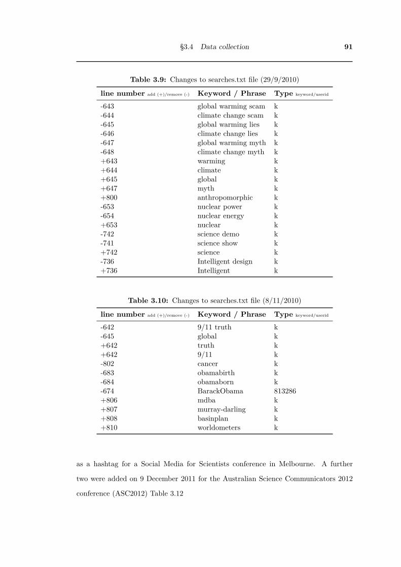
§3.4 Data collection 91
Table 3.9: Changes to searches.txt file (29/9/2010)
line number add (+)/remove (-) Keyword / Phrase Type keyword/userid
-643 global warming scam k-644 climate change scam k-645 global warming lies k-646 climate change lies k-647 global warming myth k-648 climate change myth k+643 warming k+644 climate k+645 global k+647 myth k+800 anthropomorphic k-653 nuclear power k-654 nuclear energy k+653 nuclear k-742 science demo k-741 science show k+742 science k-736 Intelligent design k+736 Intelligent k
Table 3.10: Changes to searches.txt file (8/11/2010)
line number add (+)/remove (-) Keyword / Phrase Type keyword/userid
-642 9/11 truth k-645 global k+642 truth k+642 9/11 k-802 cancer k-683 obamabirth k-684 obamaborn k-674 BarackObama 813286+806 mdba k+807 murray-darling k+808 basinplan k+810 worldometers k
as a hashtag for a Social Media for Scientists conference in Melbourne. A further
two were added on 9 December 2011 for the Australian Science Communicators 2012
conference (ASC2012) Table 3.12

92 Research Design - Data Collection
Table 3.11: Changes to searches.txt file (1/10/2011)
line number add (+)/remove (-) Keyword / Phrase Type keyword/userid
+815 sciencescramble k+816 makehackvoid k+817 SocMedSci k
Table 3.12: Changes to searches.txt file (9/12/2011)
line number add (+)/remove (-) Keyword / Phrase Type keyword/userid
+835 #asc2012 k+836 asc2012convener 422954978
Outages in data collection
On 1 April 2011 (30 May 2011 GMT) the data collection computer ran out of hard disk
space. This was not noticed immediately, and once it was noticed it still took some
time to obtain and install a larger hard disk. The result was the loss of twelve days of
data, from 1 April 2011 to 11 April 2011 inclusive. There was partial data available
on the 1st and the 11th of April, but these days were excluded from any analysis of
tweets per day.
A small outage of less than one hour occurred at around 3:30 pm AEST on 3 April
2012 due to out of date Java SSL security certificates.
Another outage of less than 8 minutes occurred at 3:00 pm AEST on 24 July 2012
during the change over to a new versions of both the StreamAPI and SearchAPI pro-
grams. This change integrated the SearchAPI program into the new suite of programs
and used the latest version of Twitter4j9 to add the new “Stall Warning” feature to
the StreamAPI program. This feature provides a warning if the tStreamingArchiver
program is not keeping up with the stream of tweets sent by the StreamAPI from
Twitter.
9twitter4j 3.0.0 SNAPSHOT 23/7/2012

§3.4 Data collection 93
3.4.4 Trend over StreamAPI period
Oct2010
Nov Dec Jan2011
Feb Mar Apr May Jun Jul Aug Sep Oct Nov Dec0
200,000
400,000
600,000
800,000
1,000,000
1,200,000
1,400,000
1,600,000
Tw
eets
per
day
8 Novsmallupdate tosearches.txt
31 Mar to 12 Aprdata outage(out of disk space)
1 Octsmallupdate tosearches.txt
tweets per day
trend line (least squares)
Figure 3.3: Data collection - tweets per day - StreamAPI trend
Figure 3.3 shows that there was an overall linear growth in the number of tweets
collected per day by the StreamAPI for my set of search terms. The increase over the
whole period is 696 tweets/day, around 21,000 tweets/month from the base of 159,822
tweets in October 2010 to 459,768 in December 2011. As expected, the small changes
to the search terms (searches.txt) on 8 November 2010 (Page 90) and 1 October 2011
(Page 90) have not altered the overall number of tweets being collected very much.
There is a strong weekly pattern visible on the graph. Figure 3.4 magnifies April to
July of 2011 showing that the weekly pattern for this set of keywords has a peak in
the middle of the week and is low on the weekends. This pattern matches that found
on Twitter overall, people use Twitter more during the week at work and less on the
weekends.
3.4.5 Tweets dropped from StreamAPI
Twitter restricts the amount of data it will send through the StreamAPI. I applied for
and was given a higher level of access for research, but the StreamAPI still dropped

94 Research Design - Data Collection
03TueMay
10Tue
17Tue
24Tue
31Tue
07TueJun
14Tue
21Tue
28Tue
05TueJul
12Tue
19Tue
26Tue
2011
0
100,000
200,000
300,000
400,000
500,000Tw
eets
per
day
Figure 3.4: Data collection - tweets per day - StreamAPI Weekly Pattern (April toJuly 2011)
some tweets when Twitter was experiencing load problems. When this happens Twitter
sends a special record in the StreamAPI, a track limitation notice (trackLimitation).
The raw trackLimitation has no date information, just a number of statuses skipped.
It looks like this:
TrackLimitationNotice: number of statuses skipped by rate limiting = 34715
The Twitter documentation defines a trackLimitation as:
Track streams may also contain limitation notices, where the integer track is
an enumeration of statuses that, since the start of the connection, matched
the track predicate but were rate limited.10
When processing the data files, I included the date and time of the previous tweet
in the data file as part of the trackLimitation record in the database. This gave an
approximate time for the trackLimitation. Using the details of the tweet before the10Twitter documentation: https://dev.twitter.com/overview/documentation

§3.4 Data collection 95
trackLimitation, it was also possible to find the tweet after it. Most of the gaps between
the tweet before and after the trackLimitation notice were zero seconds, indicating that
Twitter was still sending a continuous stream of Tweets but had skipped some.
To get the number of tweets skipped by trackLimitation at any point I subtracted
the previous trackLimitation from the current one. If that gave a negative number,
it indicated that the stream connection had been reset and so just the value from the
current trackLimitation notice was used.
Figure 3.5 shows the number of tweets per day that matched my search term but
were not received based on the trackLimitations information from Twitter. This shows
that on most days there were very few tweets restricted from the stream by Twitter. By
adding the number of tweets skipped by trackLimitation per day (dropped tweets) to
the number of tweets received that day (collected tweets) it is possible to get the total
number of tweets that matched all of the search terms being used in my StreamAPI
data gathering (matched tweets). There are only a few days between August 2010 and
November 2011 with more than 1% of total tweets matching the StreamAPI search
terms dropped (12 days out of 16 months). These are shown in Table 3.13. Only three
of these days have significant losses; 17 August 2011 and 3rd and 4th of October 2011,
and these also stand out on Fig. 3.5. Care must be taken when analysing time series
which include these days. The cumulative sum of tweets dropped per day is given
in Fig. 3.6 and shows that the number of tweets dropped on normal days increased
after each of the major outages, suggesting changes in the underlying algorithm used
by Twitter. But even the more recent, higher rate, was still less than 1% of the total
tweets matching the StreamAPI search terms. This shows that apart from the three
days with significant losses, my dataset includes almost all of the tweets containing the
SearchAPI keywords in 2011.

96 Research Design - Data Collection
Table 3.13: Days on which dropped tweets are more than 1% of total tweets matchingStreamAPI search terms
Date Tweets Dropped2010-12-19 2.8%2011-02-15 2.9%2011-02-28 3.2%2011-03-23 4.0%2011-03-30 2.4%2011-04-27 1.6%2011-08-17 34.1%2011-08-25 1.4%2011-09-07 1.1%2011-09-27 1.4%2011-10-03 14.7%2011-10-04 11.9%
Oct2010
Nov Dec Jan2011
Feb Mar Apr May Jun Jul Aug Sep Oct Nov Dec0
50,000
100,000
150,000
200,000
Tw
eets
ski
pped p
er
day
Figure 3.5: Tweets matching my search terms that were not received (dropped)
3.4.6 Collected Tweets as a Proportion of Total Tweets on Twitter
It is difficult to get figures for the total number of tweets sent on Twitter per day.
Twitter has occasionally published some numbers on their blog, and there have been
some other numbers reported from business meetings. On 22 February 2010 Twitter
published a graph (shown in Fig. 2.2 (Weil, 2010)), but the scale at which it was created
limits the accuracy with which the numbers can be read from it.

§3.4 Data collection 97
Oct2010
Nov Dec Jan2011
Feb Mar Apr May Jun Jul Aug Sep Oct Nov Dec0
100,000
200,000
300,000
400,000
500,000
600,000
700,000
Tw
eets
ski
pped p
er
day
Figure 3.6: Cumulative sum of dropped tweets
On 14 March 2011 Twitter stated these numbers:
50 million.
The average number of Tweets people sent per day, one year ago.
140 million.
The average number of Tweets people sent per day, in the last month.
177 million.
Tweets sent on March 11, 2011.
(Twitter, 2011c).
On 21 March 2011 Twitter co-founder, Biz Stone wrote “people send more than
140,000,000 tweets per day” (Stone, 2011).
In June 2011, Twitter stated the approximate numbers as:
Halfway through 2011, users on Twitter are now sending 200 million Tweets
per day. For context on the speed of Twitter’s growth, in January of 2009,
users sent two million Tweets a day, and one year ago they posted 65 million
a day.

98 Research Design - Data Collection
Table 3.14: Twitter total Tweets per day
Date Reported Number of Tweets per Day Notes31 January 2009 2,000,0001 January 2010 30,000,000 (from graph)14 March 2010 50,000,00030 June 2010 65,000,000
11 March 2011 177,000,000 (one day peak)21 March 2011 140,000,00030 June 2011 200,000,000
9 Sep 2011 230,000,00017 Oct 2011 250,000,000
21 March 2012 340,000,0006 June 2012 400,000,000
(Twitter, 2011b)
Two more data points come from speeches by Twitter CEO Dick Costolo. During a
media briefing on 9 September 2011 he is reported as saying that there are 230 million
tweets per day (Dugan, 2011). TechCrunch reports that he said “Twitter is at 250
million tweets per day as of now” at a dinner on 17 October 2011 (Tsotsis, 2011).
On 21 March 2012 Twitter stated that “And at last check, there are more than
140 million active users (there’s that number again) — and today we see 340 million
Tweets a day” (Twitter, 2012)
A report by CNET on the 6 June 2012 says that Twitter CEO Dick Costolo indi-
cated that there are now “more than 400 million tweets per day” in an interview at
the ‘Ideas Economy: Information 2012’ conference (Twitter hits 400 million tweets per
day, mostly mobile | Internet & Media - CNET News, 2012).
These data points are summarised in Table 3.14, and graphed in Fig. 3.7. The jump
in the graph on the 11 March 2011 in Fig. 3.7 is caused by the inclusion of the peak
day data for that date, where the other figures are averages for a period. Figure 3.8
shows the same graph with this outlier removed. All of the subsequent comparisons of
my data to the total tweets on Twitter also exclude that data point.

§3.4 Data collection 99
2009 2010 2011 2012Jan Jul Jan Jul Jan Jul Jan Jul
0
50
100
150
200
250
300
350
400
450
Tw
eets
per
day (
mill
ions)
single day peak11 Mar 2011
Figure 3.7: Total Tweets per day on Twitter
2009 2010 2011 2012Jan Jul Jan Jul Jan Jul Jan Jul
0
50
100
150
200
250
300
350
400
450
Tw
eets
per
day (
mill
ions)
Figure 3.8: Total Tweets per day on Twitter - outlier removed
Because the figures for the total tweets sent on Twitter per day are based on monthly
averages, I also use monthly averages of the number of tweets collected per day using
the StreamAPI in order to compare rates of growth. Figure 3.9 shows that the gradual
increase in the number of tweets received shown in the StreamAPI data is similar to
the overall increase in the number of tweets sent per day on Twitter. Note the large
difference in the two y-axis scales; the tweets I collected ranged from just over 150
thousand to 450 thousand while the total tweets sent on twitter start at 100 million
and go up to 250 million in the same period. Another way of comparing these is to
graph the ratio between the monthly average of the total daily tweets on Twitter and
the monthly average of the daily tweets received using my keywords. This ratio is

100 Research Design - Data Collection
Jan2011
Oct Apr Jul Oct150,000
200,000
250,000
300,000
350,000
400,000
450,000
500,000
Collected Tweets (monthly average)
31 Mar - 12 Aprdata outage
collected tweets
total tweets 100,000,000
150,000,000
200,000,000
250,000,000
300,000,000
Total Tweets on Twitter (interpolated)
Figure 3.9: Collected Tweets (monthly average) and Total Tweets on Twitter (inter-polated)
shown as a percentage in Fig. 3.10. It shows that all of my science related searches
are only a very small proportion of the total discussion on Twitter, returning between
0.16% and 0.24% of the total tweets sent on Twitter in the same period, averaging
0.18%. What is interesting is that it was staying more or less constant up until a jump
in March 2011 and then gradually declining back towards the previous level. I think
that this jump was caused by my gathering tweets about the Japanese earthquake
through my ‘nuclear’ keyword.
Jan2011
Oct Apr Jul Oct0.0
0.1
0.2
0.3
0.4
0.5
% Tweets Collected (monthly average)
31 Mar - 12 Aprdata outage
Figure 3.10: Collected tweets (StreamAPI) as a Percentage of Total Tweets on Twit-ter

Chapter 4
Data cleaning and filtering
Having looked at the details and quality of the overall data collection in the previous
chapter, I will now focus on a subset of my collected data, tweets which contain the
word ‘science’ collected during 2011 (with the start and end of year based on UTC
time). By focussing in on a single keyword the amount of data to be analysed is
significantly reduced, although still large. The dataset collected using the keyword
‘science’ during 2011 includes a total of 13 million tweets by 4 million different authors
(Tweets: 13,537,096 Authors: 3,912,982). Although these are large numbers, the total
number of tweets sent on Twitter in this same period was much higher, around 72
billion (estimated by interpolation of the numbers in Table 3.14). The large size of the
dataset means that it is not possible to manually analyse the data and so computer
based analysis, ‘data mining’, must be used.
This chapter describes how the ‘science’ data set was prepared for analysis by
removing unwanted tweets. Two types of filtering were applied, one that excludes
tweets that are not written in English, and another that excludes tweets that are
identified as spam - nonsense collections of words generated by automated programs
(spambots) to get people to follow links to pages. This filtering removes tweets which
are outside the scope of the study, which act as noise if left in. Their removal is critical
for the success and accuracy of studies based on text analysis in Chapters 8 to 9.
There was one day with only partial data caused by the major outage in data
collection in April, described in Section 3.4.3 (Page 92). 12 April 2011 only has 444
101

102 Data cleaning and filtering
tweets recorded and these have been removed so that it is treated as missing data
instead of partial data. This is important for the studies that look at the number of
tweets per day and number of authors per day. Figure 4.1 shows the science keyword
tweets per day before filtering.
Jan Feb Mar Apr May Jun Jul Aug Sep Oct Nov Dec
2011
10,000
20,000
30,000
40,000
50,000
60,000
70,000
80,000
Tw
eets
per
day
31 Mar - 12 Aprdata outage
Figure 4.1: Science keyword Tweets per day before filtering
4.1 Filtering out non-English tweets
Some of the tweets that contain the word ‘science’ are not written in English except
for the keyword ‘science’. These foreign language tweets act as noise when trying
to understand the topics that people are discussing about science using the English
language. For example the term ‘science fiction’ is used as a loanword in a number
of foreign languages such as Danish, Dutch, French, German, Norwegian and Swedish
(although often with the addition of a hyphen — ‘science-fiction’). In all of these
languages except French, there is a different word for science, as shown in Table 4.1.
The use of this loanword causes the occurrence of the term ‘science fiction’ to be
much more frequent in the science keyword corpus than if only tweets in English are
considered.

§4.1 Filtering out non-English tweets 103
Table 4.1: Use of ‘science fiction’ as a loanword
Language Science Fiction ScienceDanish Science Fiction videnskabDutch Science Fiction wetenschapFrench Science-Fiction scienceGerman Science-Fiction WissenschaftNorwegian Science Fiction vitenskapNorwegian Science Fiction vetenskap
In addition, many of the techniques used to exploring the meaning of the tweets
assume that they are in a single language:
Natural language processing techniques typically pre-suppose that all doc-
uments being processed are written in a given language (e.g. English), but
as focus shifts onto processing documents from internet sources such as mi-
croblogging services, this becomes increasingly difficult to guarantee. (Lui
& Baldwin, 2012, p. 25)
In April 2011 Twitter introduced a new field into the Twitter User record - Lan-
guage. This records the preferred language of the user. In my dataset there are 10.3
million (10,299,583) tweets with the language field set, and 3.3 million (3,247,513)
without. The number of tweets made by users with the preferred language field set,
grouped by preferred language, is shown in Table 4.2.
However, Carter, Weerkamp, and Tsagkias (2012) found that the Twitter location
related fields are not reliable for language detection;
We have demonstrated that the language and country meta data fields that
come with the microblog posts make poor signals for language identification,
with the language field greatly over-or-underestimating the true underlying
language distribution, and the geo-location field being too sparsely used to
be relied upon for language identification. (Carter et al., 2012, p. 214)

104 Data cleaning and filtering
Table 4.2: Science Tweets by User Preferred Language in 2011
code Language Number of Tweetsda Danish 3de German 46,854en English 9,792,564es Spanish; Castilian 120,949fi Finnish 3fil Filipino; Pilipino 386fr French 98,680hi Hindi 202id Indonesian 6,188it Italian 19,899ja Japanese 134,804ko Korean 9,053msa Malay 222nl Dutch; Flemish 10,296no Norwegian 5pl Polish 31pt Portuguese 23,612ru Russian 19,833tr Turkish 11,557zh-cn Chinese; China 3,081zh-tw Chinese; Taiwan 1,361Total 10,299,583
Like Carter et al. (2012), I found that the geo-location fields are rarely used, oc-
curring in only around 1% of tweets as shown in Table 4.3.
Table 4.3: Location fields by Number of Science tweets
Field Name Number of Tweets Percentage of TotalgeoL 132,982 0.98%place 173,622 1.28%
Given that the location and preferred language fields from Twitter could not be used
to filter out the foreign language tweets, an alternative approach was to try to identify
the language based on the text of each tweet. The algorithms available for language
detection improved during the period of this thesis to a stage where they were able to
be useful. However Carter et al. (2012) point out that tweets still represent a challenge
to automatic language detection;

§4.1 Filtering out non-English tweets 105
We have demonstrated that, given the short nature of the posts, the rather
idiomatic language in these (due to abbreviations, spelling variants, etc.),
and mixed language usage, language identification is a difficult task. (Carter
et al., 2012, p. 213)
I have selected the language identifier langid.py developed by Lui and Baldwin
(2012) because it is available as a Python module which integrates well with my other
analysis tools. Lui and Baldwin (2012) state the accuracy of langid.py on tweets as “In
its off-the-shelf configuration, langid.py attains an accuracy of 0.94” (Lui & Baldwin,
2012). They also compared the performance of two other language identification tools
by using their tweet dataset and found that the tuned (using priors) TextCat approach
of Carter et al. (2012) had an accuracy of 0.90 - 0.92 and the more complex approach of
Tromp (2011) gave an accuracy of 0.92-0.98. Another advantage of langid.py is that it
did not require any configuration or training in order to be used on different datasets.
4.1.1 Accuracy of language detection
Using langid.py, without constraining the set of languages, I identified 97 languages
in the ‘science’ keyword dataset. Table 4.4 shows the top 10 languages by number of
tweets. The full table of all 97 languages detected is available in Appendix D with
their ISO 639-1 codes.
In order to check the accuracy of the language detection by langid.py, a random
sample of tweets from each detected language were checked and coded as English or
Other. Any that were in mixed language were manually coded as Other. Tweets with
emoticons and other patterns made of characters were coded as English if only English
words were included. No attempt was made to determine if the detected language
was the actual language of the foreign language tweets. For each language identified

106 Data cleaning and filtering
Table 4.4: Top 10 Languages by number of tweets with ‘science’ keyword (languagedetection using langid)
code Language Number of tweetsen English 12,285,213fr French 201,566ja Japanese 174,194id Indonesian 123,944it Italian 93,029es Spanish; Castilian 85,743nl Dutch; Flemish 77,733de German 74,735pt Portuguese 54,242tl Tagalog 42,239Total 13,212,638
by langid.py, the Python1 Random module (random.sample()) was used to select a
random sample of tweet ids from all of the tweet ids for that language.
For languages other than English, the initial sample size checked was 30 tweets,
or all of the tweets if the language had fewer than 30 tweets, giving a total of 2,838
tweets manually coded across the 96 languages (excluding English). The proportion
found using this sample was used to determine the sample size required to achieve a
standard error for the sample estimate of the population proportion of no more than
±0.10 at the 95% confidence level. The calculation was based on the formula derived
in Cochran (1977);
The required margin of error d for my proportion estimate can be expressed as;
Pr(| p − P |≥ d) = α
where p = sample proportion, P = population proportion, α = 0.05 for 95% confidence
and d = margin of error.
Assuming that p is normally distributed, we also have;1Python version 2.7.2
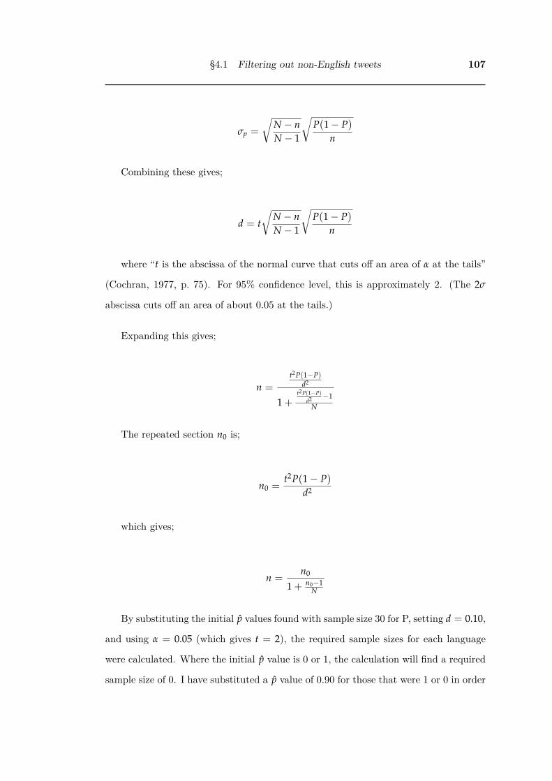
§4.1 Filtering out non-English tweets 107
σp =
√N − nN − 1
√P(1 − P)
n
Combining these gives;
d = t√
N − nN − 1
√P(1 − P)
n
where “t is the abscissa of the normal curve that cuts off an area of α at the tails”
(Cochran, 1977, p. 75). For 95% confidence level, this is approximately 2. (The 2σ
abscissa cuts off an area of about 0.05 at the tails.)
Expanding this gives;
n =t2P(1−P)
d2
1 +t2P(1−P)
d2 −1N
The repeated section n0 is;
n0 =t2P(1 − P)
d2
which gives;
n =n0
1 + n0−1N
By substituting the initial p values found with sample size 30 for P, setting d = 0.10,
and using α = 0.05 (which gives t = 2), the required sample sizes for each language
were calculated. Where the initial p value is 0 or 1, the calculation will find a required
sample size of 0. I have substituted a p value of 0.90 for those that were 1 or 0 in order

108 Data cleaning and filtering
to find a required sample size. The results for the first 10 languages by language code
are given in Table 4.5, the complete list is provided in Table D.2 in Appendix D.
Where the required sample size was higher than the initial sample of 30, an addi-
tional random sample excluding the already coded tweets was made to bring the total
sample size up to the required number. The new total sample size for all languages
except English is 5,383.
Table 4.5: Sample sizes for first 10 languages identified by langid.py
lang English Not-English n p N n0 Required n
af 22 8 30 0.733 9,345 78.222 78am 16 14 30 0.533 545 99.556 85an 10 20 30 0.333 1,387 88.889 84ar 2 28 30 0.067 5,691 24.889 25as 7 6 13 0.538 13 99.408 12az 22 8 30 0.733 756 78.222 71be 2 28 30 0.067 136 24.889 22bg 0 30 30 0.000 845 36.000 35bn 24 6 30 0.800 356 64.000 55br 23 6 29 0.793 3,324 65.636 65
Repeating the sample size calculations using the updated ratio after the second
round of sampling, the results for the first 10 languages are given in Table 4.6, the
complete list is provided in Table D.3 in Appendix D.
Table 4.6: Recalculated Sample sizes for first 10 languages after 2nd round of sam-pling
lang English Not-English n p N n0 Required n
af 60 29 89 0.674 9,345 87.868 88am 55 30 85 0.647 545 91.349 79an 27 57 84 0.321 1,387 87.245 83ar 2 28 30 0.067 5,691 24.889 25as 7 6 13 0.538 13 99.408 12az 56 15 71 0.789 756 66.653 62be 2 28 30 0.067 136 24.889 22bg 0 35 35 0.000 845 36.000 35
Although the normal approach when using sampling by proportion is to stop after
the second round of sampling to the sizes calculated using Cochran (1977, p. 75),

§4.1 Filtering out non-English tweets 109
I repeated the supplemental random sampling until the desired standard error was
achieved. Where the sample proportion (p) moves towards the middle (0.5) due to
the new sample data, it increases the standard error and so may need a larger sample
to achieve the target standard error. The sample size calculations and sampling were
repeated until the standard error for the proportion of English tweets in each language
was less than or equal to the selected 0.10 at the 95% confidence level. Table 4.8 shows
the additional samples required as calculated after each round of sampling. The final,
sixth round, of sampling resulted in only one more tweet being required for language
Urdu (ur) as it was not above 0.10 after rounding the lci and uci to 3 significant digits.
The final sample sizes, sample proportions and standard errors for each language are
give in Table D.4 in Appendix D. The final sample size after six rounds was 5,899.
The population proportion of English tweets found in each of the foreign languages
identified by langid.py covered the full range from 0 (no English) to 1 (all English), as
shown on Fig. 4.2. Table D.4 contains the detailed data that Fig. 4.2 is based on. For
all of the languages identified by langid.py except English, I measured the occurrence
of English tweets in what langid.py identified as not English, not checking whether
they were actually in the language identified. Although I was measuring one type of
incorrect identification, there may actually be many other errors (such as tweets in
other languages being wrongly included) not measured by me. This means that my
measure may give a higher accuracy than one that checks the actual language of the
tweets. But even on my measure of English tweets misidentified as another language,
the accuracy of language detection by langid.py varies dramatically across languages
and many languages were outside the stated accuracy of langid.py of 0.94 (Lui &
Baldwin, 2012).
A sample of 1,000 was randomly selected from the 12.3 million tweets identified
as English by langid.py. These were coded in the same way as the tweets detected
as other languages by langid.py. However in the case of English, the meaning of the
coding for accuracy is reversed, the ones coded as English have been correctly classified

110 Data cleaning and filtering
by langid.py while the ones coded as Other are errors. It was also different in that
as a native English speaker it was possible for me to say that the tweets coded as
English were actually in English. The population proportion (p) of English for the
tweets identified as English by langid.py was 0.988± 0.003 at the 95% confidence level
as shown in Table 4.7.
Table 4.7: Population proportion of English coded tweets in tweets identified as En-glish by langid.py
Language n N English other p SE lci uci
English 1000 12,285,213 988 12 0.988 0.003 0.981 0.995
Given the variation in accuracy across languages it was necessary to find a way to
decide on a language by language basis which tweets should be retained in the corpus
and which should be excluded.
4.1.2 Filtering Unicode characters
Having created samples of tweets from each language to check the accuracy of langid.py,
I looked in detail at the results for each language to decide whether to keep or discard
that language from my corpus. During the initial stages of this, I noticed that the
false positives, that is the tweets identified as being not English by langid.py, that I
had coded as English, often contained character sequences other than those used for
English. For example, this sequence which seems to depict faces with arms is used in
9 out of the 55 sample Aramaic tweets coded as English: ƪ(˘⌣˘)┐ ƪ(˘⌣˘)ʃ ┌(˘⌣˘)ʃ These
are ‘eastern style’, upright emoticons in this case showing ‘happy dancing’ characters.
Others contain emoji ‘picture characters’ first developed for mobile phone use in Japan
but now used more widely (for example: 🎈🎉👍👏😃💓). Another type of character used
in tweets are Unicode symbols such as ✗✔☑❒♪. To find out whether language detection
accuracy could be improved by filtering out these special characters, I developed a filter
that removes a range of Unicode symbols, the Japanese emoji and a number of other
‘eastern style’ emoticons.
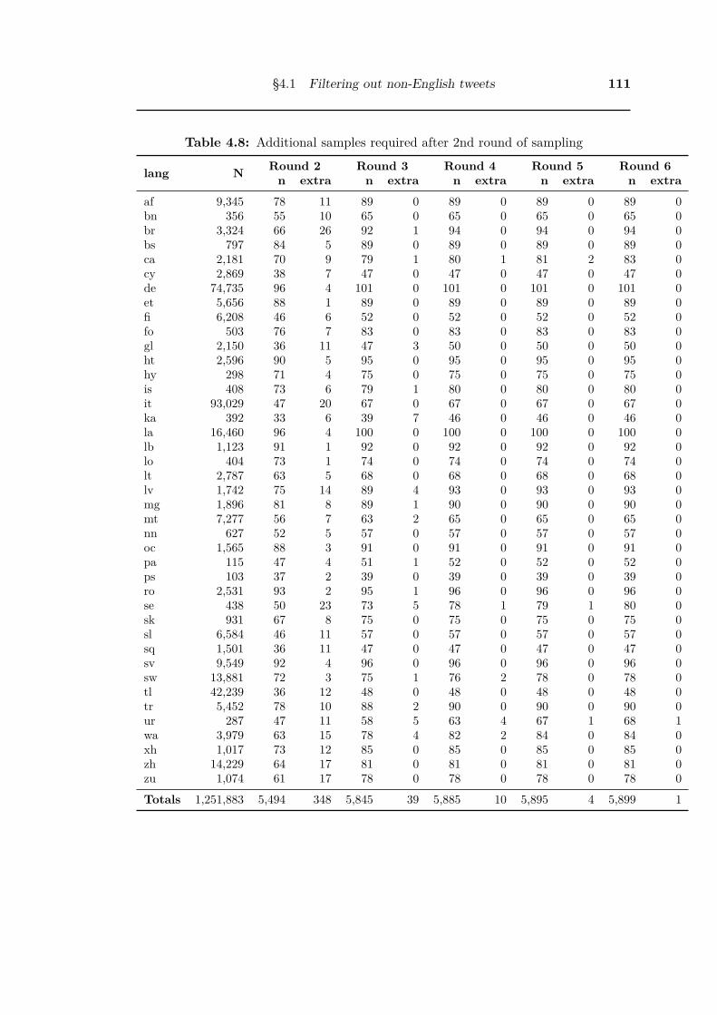
§4.1 Filtering out non-English tweets 111
Table 4.8: Additional samples required after 2nd round of sampling
lang N Round 2 Round 3 Round 4 Round 5 Round 6n extra n extra n extra n extra n extra
af 9,345 78 11 89 0 89 0 89 0 89 0bn 356 55 10 65 0 65 0 65 0 65 0br 3,324 66 26 92 1 94 0 94 0 94 0bs 797 84 5 89 0 89 0 89 0 89 0ca 2,181 70 9 79 1 80 1 81 2 83 0cy 2,869 38 7 47 0 47 0 47 0 47 0de 74,735 96 4 101 0 101 0 101 0 101 0et 5,656 88 1 89 0 89 0 89 0 89 0fi 6,208 46 6 52 0 52 0 52 0 52 0fo 503 76 7 83 0 83 0 83 0 83 0gl 2,150 36 11 47 3 50 0 50 0 50 0ht 2,596 90 5 95 0 95 0 95 0 95 0hy 298 71 4 75 0 75 0 75 0 75 0is 408 73 6 79 1 80 0 80 0 80 0it 93,029 47 20 67 0 67 0 67 0 67 0ka 392 33 6 39 7 46 0 46 0 46 0la 16,460 96 4 100 0 100 0 100 0 100 0lb 1,123 91 1 92 0 92 0 92 0 92 0lo 404 73 1 74 0 74 0 74 0 74 0lt 2,787 63 5 68 0 68 0 68 0 68 0lv 1,742 75 14 89 4 93 0 93 0 93 0mg 1,896 81 8 89 1 90 0 90 0 90 0mt 7,277 56 7 63 2 65 0 65 0 65 0nn 627 52 5 57 0 57 0 57 0 57 0oc 1,565 88 3 91 0 91 0 91 0 91 0pa 115 47 4 51 1 52 0 52 0 52 0ps 103 37 2 39 0 39 0 39 0 39 0ro 2,531 93 2 95 1 96 0 96 0 96 0se 438 50 23 73 5 78 1 79 1 80 0sk 931 67 8 75 0 75 0 75 0 75 0sl 6,584 46 11 57 0 57 0 57 0 57 0sq 1,501 36 11 47 0 47 0 47 0 47 0sv 9,549 92 4 96 0 96 0 96 0 96 0sw 13,881 72 3 75 1 76 2 78 0 78 0tl 42,239 36 12 48 0 48 0 48 0 48 0tr 5,452 78 10 88 2 90 0 90 0 90 0ur 287 47 11 58 5 63 4 67 1 68 1wa 3,979 63 15 78 4 82 2 84 0 84 0xh 1,017 73 12 85 0 85 0 85 0 85 0zh 14,229 64 17 81 0 81 0 81 0 81 0zu 1,074 61 17 78 0 78 0 78 0 78 0Totals 1,251,883 5,494 348 5,845 39 5,885 10 5,895 4 5,899 1

112 Data cleaning and filtering
Serb
ian
Kore
an
Kaza
khB
ulg
ari
an
Mala
yJa
panese
Russ
ian
Thai
Tam
ilM
ongolia
nU
krain
ian
Hin
di
Mace
donia
nA
rabic
Indonesi
an
Bela
rusi
an
Javanese
Tagalo
gU
ighur
Mala
yala
mG
alic
ian
Dutc
hN
epali
Pers
ian
Port
uguese
Spanis
hM
ara
thi
Quech
ua
Sw
ahili
Chin
ese
Zulu
Cata
lan0.0
0.2
0.4
0.6
0.8
1.0popula
tion p
roport
ion (
p)
proportion coded as EnglishA
ragonese
Xhosa
Turk
ish
Gre
ek
Vie
tnam
ese
Kin
yarw
anda
Sw
edis
hH
ait
ian
French
Esp
era
nto
Arm
enia
nG
erm
an
Kannada
Luxem
bourg
ish
Bosn
ian
Kir
ghiz
Ass
am
ese
Lati
nR
om
ania
nFa
roese
Icela
ndic
Latv
ian
Nort
hern
Sam
iO
ccit
an
Bre
ton
Punja
bi
Mala
gasy
Am
hari
cU
rdu
Lao
Est
onia
nA
frik
aans0.0
0.2
0.4
0.6
0.8
1.0
popula
tion p
roport
ion (
p)
Wallo
on
Telu
gu
Cro
ati
an
Guja
rati
Cze
chSlo
vak
Bengali
Iris
hN
orw
egia
n B
okm
ål
Vola
pük
Basq
ue
Norw
egia
nLi
thuania
nA
zerb
aija
ni
Malt
ese
Italia
nPush
toN
orw
egia
n N
ynors
kSin
hala
Slo
venia
nFi
nnis
hG
eorg
ian
Ori
ya
Danis
hK
urd
ish
Alb
ania
nW
els
hPolis
hH
ebre
wC
entr
al K
hm
er
Dzo
ngkh
aH
ungari
an0.0
0.2
0.4
0.6
0.8
1.0
popula
tion p
roport
ion (
p)
Figure 4.2: Population proportion of English tweets in foreign languages as identifiedby langid.py

§4.1 Filtering out non-English tweets 113
The Japanese emoji were identified using the patterns in the python e4u module2
which is based on the Emoji Symbol translation standards defined by the Unicode
Consortium3. These also include the Unicode emoticons symbol block.
In addition to the Unicode emoticons symbol block, there is a number of other
Unicode symbol blocks which were included in the filter. These are listed in Table 4.9.
These are all blocks that do not represent text in any language.
The final types of emoticon were the most difficult to filter because they were made
up of multiple characters combined to create an image of a face or face and body. There
is a huge number of possible combinations of characters. Here are a few examples; ತಟತ
(•_•)
ƪ(˘⌣˘)┐
(ノ≥∇≤)ノ
ԅ(°▿▿▿▿▿▿° )ԅ
(˘⌣˘ƪ)
( -˛ - )
This type of upright emoticon are called ‘eastern style’ emoticons in contrast to the
‘western style’ sideways smiley faces made using English punctuation characters, for
example; :-) 8-) ;)
I based my initial list of multi-character emoticons on a list maintained by the
account called ‘Endolith’ on GitHub in a ‘gist’. A ‘gist’ is the name for a version
controlled segment of text or source code stored on the GitHub website. This particular
gist was available online at https://gist.github.com/endolith/157796 4. It contained a
number of separate files, two of which I have not included (Multiline stuff.txt and
Assimilate these.txt). I supplemented the initial list with additional emoticons found2http://pypi.python.org/pypi/e4u3http://www.unicode.org/~scherer/emoji4unicode/snapshot/full.html4Accesssed 29 December 2012 - gist157796-ac480a955cc680e1965bdd6c3ddb9d9bbd59ca95
(This version can be viewed by using https://gist.github.com/157796/ac480a955cc680e1965bdd6c3ddb9d9bbd59ca95)

114 Data cleaning and filtering
on other pages and in the sampled tweets. The final list of multi-character emoticons
included in the filter is given in listing E.1 in Appendix E. An interesting area for
further study would be to either create a more comprehensive list by searching for new
emoticons in my corpus or by attempting to define a pattern or components needed for
multi-character emoticons such as needing two eyes, a mouth or nose and a number of
optional additional components like ears, arms and sides of faces. If the filtering does
result in an improvement in language detection accuracy, it might be possible to make
some further gains in accuracy by improving the list of filtered emoticons.
Table 4.9: Unicode Symbol Blocks included in filter
Unicode Block Name start and end characters unicode code pointDingbats ✀-➿ U+2700-U+27bfDomino Tiles 🀰-🂓 U+1f030-U+1f09FOptical Character Recognition ⑀-⑊ U+2440-U+245fGeometric Shapes ■-◿ U+25a0-U+25ffNumber Forms ⅐- U+2150-U+218fEnclosed Alphanumerics ①-⓿ U+2460-U+24ffControl Pictures ␀- U+2400-U+243fMiscellaneous Technical ⌀- U+2300-U+23ffMathematical Operators ∀-⋿ U+2200-U+22ffByzantine Musical Symbols 𝀀-𝃵 U+1d000-U+1d0fFSuperscripts and Subscripts ⁰- U+2070-U+209fMiscellaneous Symbols ☀-⛿ U+2600-U+26ffCurrency Symbols ₠- U+20a0-U+20cfMiscellaneous Symbols and Arrows ⬀- U+2b00-U+2bffMusical Symbols �-� U+1d100-U+1d1fFMahjong Tiles �-� U+1f000-U+1f02FAncient Greek Musical Notation 𝈀-𝉅 U+1d200-U+1d24FMiscellaneous Mathematical Symbols-A ⟀-⟯ U+27c0-U+27efMiscellaneous Mathematical Symbols-B ⦀-⧿ U+2980-U+29ffSupplemental Mathematical Operators ⨀-⫿ U+2a00-U+2affArrows ←-⇿ U+2190-U+21ffBlock Elements ▀-▟ U+2580-U+259fMathematical Alphanumeric Symbols 𝐀-𝟿 U+1d400-U+1d7fFLetterlike Symbols ℀-⅏ U+2100-U+214fCombining Diacritical Marks for Symbols - U+20d0-U+20ffPlaying Cards 🂠-🃟 U+1f0a0-U+1f0fFBox Drawing ─-╿ U+2500-U+257fSupplemental Arrows-B ⤀-⥿ U+2900-U+297fSupplemental Arrows-A ⟰-⟿ U+27f0-U+27ff
The filter was applied to each tweet and then the langid.py language identification
was repeated using the filtered tweet. The original langid.py language identification

§4.1 Filtering out non-English tweets 115
is henceforth referred to as langid1 and the new langid.py identification based on the
filtered tweet is called langid2.
The number of tweets identified in each language did not change very much using
the filter. The largest change was to the largest language, English, where 12,157 more
tweets were identified as English. The top 10 languages identified with filtering and
the comparison with the previous number of tweets identified in each of them without
filtering is shown in Table 4.10. The complete list of languages, sorted by language
code, is given in Table D.5 in Appendix D.
Table 4.10: Top 10 languages by number of tweets identified by langid.py with emoti-con filtering of tweets. Shows number of tweets identified in each languagewith filtering (langid2) and without filtering (langid1)
Code Language langid1 langid2 deltatweets (a) tweets (b) (b-a)
en English 12,285,213 12,297,370 12,157fr French 201,566 201,630 64ja Japanese 174,194 173,445 -749id Indonesian 123,944 124,700 756it Italian 93,029 93,384 355es Spanish 85,743 86,241 498nl Dutch 77,733 77,726 -7de German 74,735 74,830 95pt Portuguese 54,242 54,500 258tl Tagalog 42,239 42,832 593
The previously sampled tweets, both identified by langid1 as English and as other
languages, were merged into a single dataset. They were then checked to see which
language each was identified as using langid2. The sample size calculations described
in Section 4.1.1 were repeated using all of these sample tweets as the starting sample.
A single round of additional random sampling within each language (as identified by
langid2) was performed based on the required sample size calculations. This resulted
in a final coded sample of 8,622 tweets.

116 Data cleaning and filtering
4.1.3 Comparison of accuracy of language detection with and without
unicode filtering
The summary of the final coded sample of 8,622 tweets for both langid without filtering
(langid1) and with filtering of unicode characters (langid2) is given in Table D.6 in
Appendix D. The table is sorted by language code and for both langid1 and langid2
gives a breakdown by language of the total tweets found (N), sample sizes manual
coded (n) and the number of tweets manually coded as English within each sample
(Coded English).
Using this data the population proportion of English in each language and the
standard error for the sample estimate at the 95% confidence level can be calculated
for both langid1 and langid2. The results, sorted by language name, are given in
Table D.7 (Page 457). The population proportions and population sizes are plotted
in Fig. 4.3 (Page 118), sorted by population proportion. In Fig. 4.3 the right y-axis
for the number of tweets (N) is using log scale to allow the huge variation the largest
language, English and the others to be shown. The number of English tweets is much
larger than the other languages with 12,285,213 identified by langid1 and 12,297,370
identified by langid2 (12,157 more).
Figure 4.3 (Page 118) shows that for most languages the emoticon filtering (langid2)
did not significantly change the population proportion (the langid1 and langid2 pro-
portions overlap for most of their confidence interval) or number of tweets identified
as being each language. In languages where the langid1 and langid2 proportion of En-
glish do differ significantly, most of them show an improvement (reduction in English
proportion) using langid2 with the green triangle (langid2) and error bars appearing
below the blue langid1 one.
The languages that have improved in accuracy are (reading across the panels):
Hindi, Belarusian, Uighur, Nepali, Persian, Marathi, Vietnamese, Chinese, Armenian,

§4.1 Filtering out non-English tweets 117
Kannada, Latin, Amharic, Urdu, Punjabi, Pushtu, Gujarati, Georgian and Central
Khmer. Of these, only Latin and Chinese have many tweets with Latin having 16,460
identified by langid1, reducing to 12,496 identified by langid2 and Chinese having 14,229
identified by langid1 and 12,283 identified by langid2.
Two languages which have significantly worse accuracy with langid2 are Russian and
French. French is the second largest language detected with 201,566 tweets identified
by langid1 and 64 more by langid2. Russian has 26,335 identified by langid1 and
164 fewer by langid2. Generally the languages which had no English tweets found in
langid1, shown in the first panel of the figure, performed worse in langid2 (Russian,
Bulgarian, Malay and Japanese).
In the case of English, a higher population proportion is an improvement as it means
that more of the tweets identified as English were found to be English. Both the larger
sample size for English and being at the upper end of the population proportion mean
that the confidence interval is very narrow. For English, langid1 performed slightly
better than langid2.

118 Data cleaning and filtering
Russ
ian
Bulg
ari
an
Mala
yJa
panese
Serb
ian
Tam
ilThai
Ukr
ain
ian
Kore
an
Mongolia
nK
aza
khM
ace
donia
nH
indi
Bela
rusi
an
Ara
bic
Indonesi
an
Javanese
Uig
hur
Mala
yala
mN
epali
Tagalo
gPers
ian
Galic
ian
Port
uguese
Dutc
hM
ara
thi
Spanis
hSw
ahili
Quech
ua
Zulu
Cata
lan
Ara
gonese
0.0
0.2
0.4
0.6
0.8
1.0
popula
tion p
roport
ion (
p)
Gre
ek
Vie
tnam
ese
Chin
ese
Xhosa
Turk
ish
Kin
yarw
anda
Sw
edis
hH
ait
ian
French
Esp
era
nto
Germ
an
Arm
enia
nLu
xem
bourg
ish
Kannada
Lati
nB
osn
ian
Am
hari
cA
ssam
ese
Rom
ania
nU
rdu
Latv
ian
Kir
ghiz
Icela
ndic
Occ
itan
Nort
hern
Sam
iPunja
bi
Lao
Mala
gasy
Bre
ton
Faro
ese
Est
onia
nSlo
vak0.0
0.2
0.4
0.6
0.8
1.0
popula
tion p
roport
ion (
p)
Afr
ikaans
Cze
chPush
toG
uja
rati
Cro
ati
an
Telu
gu
Wallo
on
Bengali
Norw
egia
nH
ebre
wN
orw
egia
n B
okm
ål
Basq
ue
Vola
pük
Aze
rbaija
ni
Lith
uania
nN
orw
egia
n N
ynors
kIr
ish
Ori
ya
Georg
ian
Italia
nD
zongkh
aC
entr
al K
hm
er
Malt
ese
Polis
hD
anis
hSlo
venia
nFi
nnis
hK
urd
ish
Sin
hala
Wels
hA
lbania
nEnglis
hH
ungari
an0.0
0.2
0.4
0.6
0.8
1.0
popula
tion p
roport
ion (
p)
101
102
103
104
105
106
log N
langid1 (p)
langid2 (p)
langid1 (N)
langid2 (N)
101
102
103
104
105
106
log N
100
101
102
103
104
105
106
107
108
log N
Figure 4.3: Population proportion (p) of English tweets for langid1 and langid2(sorted by langid1 p)

§4.1 Filtering out non-English tweets 119
The summary statistics for langid1 and langid2 across all languages identified by
langid.py can also be calculated. As stated above, my manual coding for accuracy
checking is either English or not English, which can be considered as ‘English versus the
rest’. This same definition can be applied to the langid1 and langid2 identification by
grouping all the languages other than English together giving four different treatments
as shown in Table 4.11. The proportion manually coded as English for each of these
and the confidence interval is shown in Table 4.12. The confidence interval at the 95%
confidence level is calculated using the formula:
p ± 1.96
√p(1 − p)
n
Langid1 codes more tweets as foreign languages than langid2 (7,604 vs 7,177) but
50.9% are actually English compared with 48.6%. Langid2 codes more tweets to English
(1,445 vs 1,018) but only 95.6% of the 1,445 are actually English compared with 98.2%
of the 1,018.
The confidence interval for English coding was very narrow because the proportion
of English tweets found to be English is at the upper end. For langid1, n = 1,018 and p
= 0.982 giving a confidence interval of (0.974, 0.990). For langid2, n= 1,445, p = 0.956
giving a confidence interval of (0.945, 0.967). So for tweets coded as English, langid1
is more accurate than langid2. The confidence interval for all the foreign languages is
wider because the population proportion falls near the middle of the range. For foreign
languages, a smaller proportion of English represents greater accuracy. For langid1, n
= 7,604 and p = 0.509 giving a confidence interval of (0.498, 0.520). For langid2, n=
7,177, p = 0.486 giving a confidence interval of (0.474, 0.498). So for tweets identified
as English, langid1 is more accurate than langid2, but for tweets identified as foreign,
langid2 is probably more accurate (the upper confidence interval of langid2 overlaps the
lower confidence interval of langid1 at 0.498). One way of comparing two population
proportions is using the log odds ratio.

120 Data cleaning and filtering
Table 4.11: Comparison of Langid1 and Langid2
Coded Other Coded English Total (n)
langid1rest 3,735 3,869 7,604English 18 1,000 1,018Total 3,753 4,869 8,622
langid2rest 3,689 3,488 7,177English 64 1,381 1,445Total 3,753 4,869 8,622
Table 4.12: Comparison of Langid1 and Langid2 - Proportion of English
n p SE lci uci
langid1rest 7,604 0.509 0.011 0.498 0.520English 1,018 0.982 0.008 0.974 0.990
langid2rest 7,177 0.486 0.012 0.474 0.498English 1,445 0.956 0.011 0.945 0.967
Odds of being English
To calculate the log odds ratio, Table 4.11 is rotated to have langid classification across
the top and the manual coding down the side giving the layout shown in Table 4.13
for each of langid1 and langid2.
Table 4.13
langid.py classificationManual coding English Not EnglishEnglish n11 n12 n1.Not English n21 n22 n2.
n.1 n.2 n..
Ideally all of the n.. sampled tweets would be in the (English-English) or (Not
English- Not English) diagonal. The estimated probability of a tweet classified as
English being English is n11n.1
. The odds of being English for those classified as English
are:n11n.1
( 1−n11n.1
)=
n11
n21
The estimated probability of a tweet classified as not English being English is n12n.2
.

§4.1 Filtering out non-English tweets 121
The odds of being English for this group are n12n22
. The odds ratio compares the odds
of being English for those tweets classified as English versus those classified as foreign
language and is given by (n11∗n22)(n21∗n12)
. The natural log odds ratio is:
ln(n11 ∗ n22)
(n21 ∗ n12)
with standard error: √1
n11+
1n12
+1
n21+
1n22
Calculation of log odds ratio
For langid1, n11 = 1, 000, n21 = 18, n.1 = 1, 018, while n12 = 3, 870, n22 = 3, 734
and n.2 = 7, 604. The odds of being English for tweets classified as English by langid1
versus tweets classified as non-English by langid1 are 1000x373418x3870 = 53.6. The log odds
ratio is 1.729 with standard error 0.2389. A 95% CI is (1.2609, 2.1974).
For langid2, n11 = 1381, n21 = 64, n12 = 3488, n22 = 3689 The odds of being
English for tweets classified as English by langid2 versus tweets classified as non-English
by langid2 are 1381∗368964∗3488 = 22.8. The log odds ratio is 1.3579 with standard error 0.1300.
The 95% CI is (1.1031, 1.6128).
A larger odds ratio represents a more accurate result, so it seems that langid1
has performed better, however the standard error at the 95% confidence for langid1
is nearly twice that of langid2 which indicates there is a larger degree of uncertainty
about the actual log odds ratio. The log odds ratios for langid1 and langid2 overlap,
so again it is not possible to say one is performing significantly better than the other.
4.1.4 Determining which languages to discard from corpus
Given the large number of tweets in the corpus, one choice might be to just discard
all of the tweets identified as not English by langid1 or langid2. Another option is to

122 Data cleaning and filtering
decide on whether to keep each individual language in the corpus. This is the approach
I decided to use. Although the overall results for langid2 were not significantly different
from langid1, it did work better for some languages as shown on Fig. 4.3. Based on
this, I decided use langid2 as the basis for deciding which languages to discard.
By sorting the languages by the proportion of English tweets they contain when
identified by langid2, and then looking at the cumulative total of non English tweets,
a large change in the cumulative total occured between Latvian and French. This is
shown in Table 4.14. Figure 4.4 (Page 123) shows the cumulative non-English popula-
tion proportion and has the discontinuity between Latvian and French marked. Based
on this, all languages up to and including Latvian in Table 4.14 have been retained in
the corpus and the ones from French down have been excluded from the corpus. This
results in the exclusion of 1,025,389 tweets from the 2011 corpus of 13,537,096 giving
a new corpus of 12,511,707 tweets.

§4.1 Filtering out non-English tweets 123
0.00 0.02 0.04 0.06 0.08 0.10 0.12cumulative population proportion of not english (p)
HindiBelarusianUkrainian
TamilSerbian
DzongkhaNepaliMalay
ThaiJapaneseBulgarian
MongolianKazakhUighurArabic
MacedonianRussianKoreanPersianMarathi
IndonesianTagalogGalician
UrduJavanese
MalayalamChinese
PortugueseDutch
SpanishVietnamese
KannadaSwahili
AmharicZulu
Central KhmerQuechuaCatalan
AragoneseArmenian
XhosaGreek
KinyarwandaTurkish
LatinSwedishHaitian
LuxembourgishEsperanto
GermanPushtoPunjabi
BosnianFrench
LatvianGeorgian
RomanianLao
AssameseNorthern Sami
KirghizOccitanGujarati
IcelandicMalagasy
BretonFaroese
AfrikaansSlovakTeluguCzech
EstonianCroatianHebrewWalloonBengaliBasque
NorwegianNorwegian Bokmål
Norwegian NynorskLithuanian
IrishVolapük
AzerbaijaniItalianOriya
MaltesePolish
SlovenianDanishKurdishSinhalaFinnishWelsh
AlbanianEnglish
Hungarian
language
keep all languages above here
Figure 4.4: Cumulative population proportion (p) of Non-English tweets for langid2(sorted by langid2 p)

124 Data cleaning and filtering
Table 4.14: Cumulative population proportion of non-English for langid2
lang N nCoded English Other Cumulative
English p (N ∗ (1 − p)) Other Total NE p
hu 6,922 36 35 0.972 192 192 6,922 0.028
en 12,297,370 1,445 1381 0.956 544,659 544,851 12,304,292 0.044
sq 1,166 60 53 0.883 136 544,987 12,305,458 0.044
cy 2,956 63 55 0.873 375 545,362 12,308,414 0.044
fi 6,062 61 53 0.869 795 546,157 12,314,476 0.044
si 419 80 68 0.850 63 546,220 12,314,895 0.044
ku 558 52 44 0.846 86 546,306 12,315,453 0.044
da 12,059 69 58 0.841 1,922 548,228 12,327,512 0.044
sl 6,650 71 59 0.831 1,124 549,352 12,334,162 0.045
pl 11,826 54 44 0.815 2,190 551,542 12,345,988 0.045
mt 7,195 92 74 0.804 1,408 552,950 12,353,183 0.045
or 35 25 20 0.800 7 552,957 12,353,218 0.045
it 93,384 95 75 0.789 19,660 572,617 12,446,602 0.046
az 755 79 62 0.785 162 572,779 12,447,357 0.046
vo 255 84 65 0.774 58 572,837 12,447,612 0.046
ga 2,775 106 81 0.764 654 573,491 12,450,387 0.046
lt 2,687 92 70 0.761 643 574,134 12,453,074 0.046
nn 569 75 57 0.760 137 574,271 12,453,643 0.046
nb 604 75 57 0.760 145 574,416 12,454,247 0.046
no 14,644 83 63 0.759 3,529 577,945 12,468,891 0.046
eu 3,026 107 81 0.757 735 578,680 12,471,917 0.046
bn 320 77 57 0.740 83 578,763 12,472,237 0.046
wa 3,536 107 79 0.738 925 579,688 12,475,773 0.046
he 672 88 63 0.716 191 579,879 12,476,445 0.046
hr 3,439 106 74 0.698 1,038 580,917 12,479,884 0.047
et 5,618 109 75 0.688 1,752 582,669 12,485,502 0.047
cs 2,329 102 70 0.686 731 583,400 12,487,831 0.047
Continued on next page...

§4.1 Filtering out non-English tweets 125
Table 4.14 – continued from previous page
lang N nCoded English Other Cumulative
English p (N ∗ (1 − p)) Other Total NE p
te 26 25 17 0.680 8 583,408 12,487,857 0.047
sk 769 90 60 0.667 256 583,664 12,488,626 0.047
af 9,510 101 67 0.663 3,201 586,865 12,498,136 0.047
fo 484 104 68 0.654 168 587,033 12,498,620 0.047
br 3,370 128 82 0.641 1,211 588,244 12,501,990 0.047
mg 1,981 110 70 0.636 720 588,964 12,503,971 0.047
is 394 96 59 0.615 152 589,116 12,504,365 0.047
gu 70 46 28 0.609 27 589,143 12,504,435 0.047
oc 1,510 112 67 0.598 607 589,750 12,505,945 0.047
ky 763 102 59 0.578 322 590,072 12,506,708 0.047
se 342 90 52 0.578 144 590,216 12,507,050 0.047
as 14 14 8 0.571 6 590,222 12,507,064 0.047
lo 319 85 48 0.565 139 590,361 12,507,383 0.047
ro 2,590 119 66 0.555 1,154 591,515 12,509,973 0.047
ka 67 38 21 0.553 30 591,545 12,510,040 0.047
lv 1,667 117 64 0.547 755 592,300 12,511,707 0.047
fr 201,630 148 80 0.541 92,641 684,941 12,713,337 0.054
bs 820 113 59 0.522 392 685,333 12,714,157 0.054
pa 69 46 24 0.522 33 685,366 12,714,226 0.054
ps 84 39 20 0.513 41 685,407 12,714,310 0.054
de 74,830 135 68 0.504 37,138 722,545 12,789,140 0.056
eo 5,651 121 60 0.496 2,849 725,394 12,794,791 0.057
lb 1,059 122 59 0.484 547 725,941 12,795,850 0.057
ht 2,526 116 50 0.431 1,437 727,378 12,798,376 0.057
sv 9,427 130 53 0.408 5,584 732,962 12,807,803 0.057
la 12,496 130 52 0.400 7,498 740,460 12,820,299 0.058
tr 5,488 120 45 0.375 3,430 743,890 12,825,787 0.058
Continued on next page...

126 Data cleaning and filtering
Table 4.14 – continued from previous page
lang N nCoded English Other Cumulative
English p (N ∗ (1 − p)) Other Total NE p
rw 4,079 112 41 0.366 2,586 746,476 12,829,866 0.058
el 4,999 126 46 0.365 3,174 749,650 12,834,865 0.058
xh 1,046 106 38 0.358 671 750,321 12,835,911 0.058
hy 149 54 18 0.333 99 750,420 12,836,060 0.058
an 1,390 107 34 0.318 948 751,368 12,837,450 0.059
ca 2,210 104 32 0.308 1,530 752,898 12,839,660 0.059
qu 835 79 24 0.304 581 753,479 12,840,495 0.059
km 11 10 3 0.300 8 753,487 12,840,506 0.059
zu 1,110 101 29 0.287 791 754,278 12,841,616 0.059
am 131 51 14 0.275 95 754,373 12,841,747 0.059
sw 13,806 110 29 0.264 10,166 764,539 12,855,553 0.059
kn 21 19 5 0.263 15 764,554 12,855,574 0.059
vi 477 81 20 0.247 359 764,913 12,856,051 0.059
es 86,241 100 24 0.240 65,543 830,456 12,942,292 0.064
nl 77,726 97 22 0.227 60,097 890,553 13,020,018 0.068
pt 54,500 96 21 0.219 42,578 933,131 13,074,518 0.071
zh 12,283 96 19 0.198 9,852 942,983 13,086,801 0.072
ml 58 38 7 0.184 47 943,030 13,086,859 0.072
jv 6,422 79 14 0.177 5,284 948,314 13,093,281 0.072
ur 99 46 8 0.174 82 948,396 13,093,380 0.072
gl 2,168 68 11 0.162 1,817 950,213 13,095,548 0.073
tl 42,832 57 7 0.123 37,572 987,785 13,138,380 0.075
id 124,700 49 5 0.102 111,976 1,099,761 13,263,080 0.083
mr 48 34 2 0.059 45 1,099,806 13,263,128 0.083
fa 148 37 2 0.054 140 1,099,946 13,263,276 0.083
ko 11,858 38 2 0.053 11,234 1,111,180 13,275,134 0.084
ru 26,171 39 2 0.051 24,829 1,136,009 13,301,305 0.085
mk 425 45 2 0.044 406 1,136,415 13,301,730 0.085
Continued on next page...

§4.1 Filtering out non-English tweets 127
Table 4.14 – continued from previous page
lang N nCoded English Other Cumulative
English p (N ∗ (1 − p)) Other Total NE p
ar 5,624 46 2 0.043 5,379 1,141,794 13,307,354 0.086
ug 88 28 1 0.036 85 1,141,879 13,307,442 0.086
kk 79 32 1 0.031 77 1,141,956 13,307,521 0.086
mn 112 37 1 0.027 109 1,142,065 13,307,633 0.086
bg 876 37 1 0.027 852 1,142,917 13,308,509 0.086
ja 173,445 37 1 0.027 168,757 1,311,674 13,481,954 0.097
th 14,518 49 1 0.020 14,222 1,325,896 13,496,472 0.098
ms 39,089 50 1 0.020 38,307 1,364,203 13,535,561 0.101
ne 54 32 0 0.000 54 1,364,257 13,535,615 0.101
dz 1 1 0 0.000 1 1,364,258 13,535,616 0.101
sr 524 47 0 0.000 524 1,364,782 13,536,140 0.101
ta 219 40 0 0.000 219 1,365,001 13,536,359 0.101
uk 415 44 0 0.000 415 1,365,416 13,536,774 0.101
be 122 36 0 0.000 122 1,365,538 13,536,896 0.101
hi 200 37 0 0.000 200 1,365,738 13,537,096 0.101
4.1.5 Filtered by Language
Figure 4.5 shows the number of tweets per day removed by filtering languages with a
higher population proportion of English than Latvian.
Removing these tweets gave a reduced data set of 12,511,707 tweets and 3,621,346
authors. This is the dataset that was used for all subsequent filtering.

128 Data cleaning and filtering
Jan Feb Mar Apr May Jun Jul Aug Sep Oct Nov Dec
2011
0
1,000
2,000
3,000
4,000
5,000
6,000
Tw
eets
per
day
Figure 4.5: Science keyword tweets per day removed by language filtering
4.2 Filtering out spam
During my initial analysis I identified some of the tweets containing the keyword science
as being a type of advertising containing only random collections of words (mainly
nouns) and a link. I have called this ‘noun spam’. The reason to filter these out is that
they contain a series of unrelated nouns which will disrupt attempts to identify topics
of discussion in the tweets by connecting unrelated terms. I decided to remove them
from the dataset before beginning the main analysis.
4.2.1 Noun spam
During the language coding, it was noticed that a lot of the English tweets that had
been detected as foreign languages were spam, so further sampling was done to look
for different types of spam.
Examples of ‘noun spam’ tweets are give in Table 4.15

§4.2 Filtering out spam 129
Table 4.15: Examples of noun spam
Tweet text1 http://t.co/gIZ0ZOu mini car science fair experiments anxiety disorder
anti inflammatories2 http://t.co/vbYxCtw Rasta Science Teacher3 http://t.co/C3RJKPj detox gateway amphitheatre club animation sci-
ence fair experiments4 http://t.co/g9I0INz #Emotional Intelligence Vegetable #First Person
Shooter Sesame Street Health Science
My first attempt at filtering the noun-spam shown in listing 4.1 was very slow,
taking 5 days to process all 13.5 million 2011 tweets (before langid2 filtering) and
checking the results showed that their were a number of tweets that were not spam
included in the found set.
1 def fun(doc):
2 import nltk
3 import ttp
4 import pytz
5 from dateutil.parser import parse
6 if doc['text'] and doc['createdAt'] and doc['user']:
7 p = ttp.Parser()
8 result = p.parse(doc['text'])
9 # need at least one url
10 if len(result.urls) > 0:
11 # strip urls and hashtags
12 text = doc['text']
13 for url in result.urls:
14 text = text.replace(url, '')
15 text = text.replace('#', '')
16 notNouns = [taggedWord for taggedWord in
nltk.pos_tag(nltk.word_tokenize(text)) if not
taggedWord[1].startswith('NN')]
17 if len(notNouns) == 0:

130 Data cleaning and filtering
18 utime = parse(doc['createdAt'], tzinfos={'EST':
10*3600}).astimezone(pytz.utc)
19 yield [utime.year, utime.month, utime.day, doc['user']['id']], None
Listing 4.1: First version of nounSpam.py view creator for couchdb
Profiling the performance of the program showed that the performance problems
were due to having to load the python modules for every tweet (the import statements
inside the function), importing whole modules when only a part was needed, and the
large amount of computing needed for line 16 which starts with ‘notNouns=’. By using
a new version of the couchpy python module developed by Alexander Shorin5 it was
possible to move the import statements outside of the function so that the modules were
only loaded once. He also suggested importing only the parts of the imported modules
that were required. Additional performance gains were made by introducing additional
tests to eliminate candidate tweets before the slow ‘notNouns=’ line. The new code
shown in listing 4.2 reduced the running time down to about 6 hours. Inspection of
a sample of the 255,763 matching tweets showed that some were still not noun spam
so an additional test was added to enforce the tweet having a ‘http://t.co/’ url at the
start. This further reduced the running time of the query to 4 hours. This final version
found 210,826 tweets which on sampling all seemed to match the noun spam pattern.
A new version of the program was created to check options for relaxing the selection
criteria to allow the noun spam tweet to contain adjectives as well as nouns and up to
two words which are not nouns or adjectives, as long as the number of these words is
less than the number of nouns. This program is show in listing 4.3.
There were 14,544 tweets identified as possible noun spam that contain adjectives
and nouns but no other types of words. Sampling these showed that they were nearly
all noun spam. There were 58,183 tweets identified as possible noun spam that have
5https://github.com/kxepal

§4.2 Filtering out spam 131
up to two words which are not nouns or adjectives, but more nouns than other words.
Sampling these showed that they were also nearly all noun spam.
The program identified 876 tweets which were possible noun spam but had more
words which were not nouns or adjectives than nouns. Sampling these showed that
they were mostly not noun spam. There were also 7,115 tweets which had three or
more words that were not nouns or adjectives or which had more words that were not
nouns or adjectives than nouns. Sampling these found very few that were noun spam.
A fifth version of the program was created that relaxed the requirement for the tweet
to start with the ‘http://t.co//’ url. Sampling the 423,626 tweets identified by this
program found that very few were noun spam. This confirms that the tweets identified
as noun spam fit a very specific pattern of starting with ‘http://t.co’, containing no
foreign characters, and having only nouns and adjectives or at most two words which
were not nouns or adjectives.
The final filtering included the original 210,826 noun only noun spam and an addi-
tional 14,544 tweets that contained adjectives and nouns and 58,183 that had up to two
words which were not nouns or adjectives (but more nouns than these). This brought
the final total of noun spam to be filtered to 283,553. The number of noun spam tweets
per day is shown in Fig. 4.6. This shows that noun spam only started being published
in quantity during the first week of June 2011 and has had large variation in the volume
per day. It is possible that a factor in this is the spam policies and filtering of spam
by Twitter.
1 import nltk
2 import ttp
3 import pytz
4 import dateutil.parser
5 import re
6

132 Data cleaning and filtering
Feb2011
Mar Apr May Jun Jul Aug Sep Oct Nov Dec0
1,000
2,000
3,000
4,000
5,000
Tw
eets
per
day
31 Mar - 12 Aprdata outage
Figure 4.6: Science keyword tweets per day identified as Noun spam
7 def fun(doc, nltk=nltk, utc=pytz.utc, parse=dateutil.parser.parse,
p=ttp.Parser(), urlre=ttp.URL_REGEX, search=re.compile(r'[^A-Za-z_\-0-9#
]').search):
8 # if document field will be missed, don't panic and raise errors
9 if not (doc.get('text') or doc.get('createdAt') or doc.get('user')):
10 return
11
12 text = doc['text']
13
14 # some magic from ttp.Parser() internals
15 urls = p._urls = []
16 urlre.sub(p._parse_urls, text)
17
18 # need at least one url
19 if not urls:
20 return
21
22 # strip urls and hashtags
23 for url in urls:
24 text = text.replace(url, '')
25 text = text.replace('#', '').strip()
26 if len(text) <= 1:

§4.2 Filtering out spam 133
27 return
28
29 # check for non-english characters - the noun spam doesn't have any
30 if bool(search(text)):
31 return
32
33 # next version differs from here
34 notNouns = [taggedWord
35 for taggedWord in nltk.pos_tag(nltk.word_tokenize(text))
36 if not taggedWord[1].startswith('NN')]
37 if notNouns:
38 return
39
40 utime = parse(doc['createdAt'], tzinfos={'EST': 10*3600}).astimezone(utc)
41 yield [utime.year, utime.month, utime.day, doc['user']['id']], None
Listing 4.2: Second version of nounSpam.py view creator for couchdb
1 import nltk
2 import ttp
3 import pytz
4 import dateutil.parser
5 import re
6
7 def fun(doc, nltk=nltk, utc=pytz.utc, parse=dateutil.parser.parse,
p=ttp.Parser(), urlre=ttp.URL_REGEX, search=re.compile(r'[^A-Za-z_\-0-9#
]').search):
8 # if document field will be missed, don't panic and raise errors
9 if not (doc.get('text') or doc.get('createdAt') or doc.get('user')):
10 return
11
12 text = doc['text']
13

134 Data cleaning and filtering
14 # this is the extra constaint added after version 2
15 if not text.startswith('http://t.co/'):
16 return
17
18 # some magic from ttp.Parser() internals
19 urls = p._urls = []
20 urlre.sub(p._parse_urls, text)
21
22 # need at least one url
23 if not urls:
24 return
25
26 # strip urls and hashtags
27 for url in urls:
28 text = text.replace(url, '')
29 text = text.replace('#', '').strip()
30 if len(text) <= 1:
31 return
32
33 # check for non-english characters - the noun spam doesn't have any
34 if bool(search(text)):
35 return
36
37 # program was identical as previous version down to here
38
39 taggedWords = nltk.pos_tag(nltk.word_tokenize(text))
40 notNouns = [taggedWord
41 for taggedWord in taggedWords
42 if not taggedWord[1].startswith('NN')]
43 if notNouns:
44 # check those that have some words which aren't nouns, they still
might be 'nounspam'

§4.3 Final data set 135
45 nounCount = len(taggedWords) - len(notNouns)
46 if nounCount < 3: # need at least 3 nouns
47 return
48
49 # look for words which are not adjectives or punctuation
50 notjj = [taggedWord for taggedWord in notNouns if not taggedWord[1] in
['JJ',':','.']]
51
52 if len(notjj) > nounCount:
53 # more not nouns and not jj etc than nouns
54 yield ["maybeok"], text
55 elif len(notjj) == 0:
56 # only adjectives as well as nouns
57 yield ["newSpam"], text
58 elif len(notjj) < 3:
59 # adjectives, nouns and up to two other words
60 yield ["probablySpam"], text
61 else:
62 # either more 'other' words than nouns or more than two 'other'
words
63 yield ["maybeSpam"], text
64 else:
65 # same as previously selected
66 yield ["Noun-spam"], None
Listing 4.3: Fourth version of nounSpam.py view creator for couchdb
4.3 Final data set
The data cleaning process described in this chapter has sought to remove the tweets
that were most likely to act as ‘noise’ in the later analysis, particularly in topic analysis.

136 Data cleaning and filtering
These were the ones written in languages other than English, and those containing one
type of advertising tweet that I have called noun spam. The language filtering process
is an area for possible improvement, the available language filtering tools were still not
very accurate. It is acknowledged that there are still some tweets written in foreign
languages in the data set, but on balance it was decided to be better to leave some
foreign tweets rather than filter too many English tweets. The noun spam filtering is
more complete, although there may be other types of tweets, as yet unidentified, still
in the corpus that will also act as noise in the topic analysis stage.
After filtering both of these, the final 2011 data set has 12,227,737 tweets by
3,579,429 authors. This is the dataset that will be used for all subsequent analysis.
Figure 4.7 shows the science keyword tweets per day after filtering.
Jan Feb Mar Apr May Jun Jul Aug Sep Oct Nov Dec
2011
10,000
20,000
30,000
40,000
50,000
60,000
70,000
Tw
eets
per
day
31 Mar - 12 Aprdata outage
Figure 4.7: Science keyword Tweets per day after filtering

Chapter 5
Tweets per day
This chapter begins the analysis of how Twitter users use the word ‘science’. I start
by describing the filtered dataset and then explore the simple metric of the number of
tweets being sent over time. This addresses my first research question: “How many
tweets are sent containing the word ‘science’ and what is the temporal pattern?”
After data cleaning, the dataset of 2011 tweets containing ‘science’ consisted of a
total of 12 million tweets by 3.6 million different authors. (Tweets: 12,227,737 Authors:
3,579,429). Although these are large numbers, the total number of tweets sent on Twit-
ter in this same period was much higher, around 72 billion (estimated by interpolation
of the numbers in Table 3.14). For this chapter, the partial day1 of tweets sent on the
31/03/2011 (32,252 tweets) were removed leaving a dataset of 12,195,485 tweets.
Figure 5.1 shows the tweets per day for the science keyword. The strong weekly
pattern characteristic of Twitter is again visible on this graph, showing that people
use twitter more during the middle of the week than on weekends. This dataset was
collected world wide, from different time zones, which spreads the effect of a daily
pattern out. Time zones vary from UTC-12 to UTC+14, so midday on Wednesday
occurs at a different UTC time in different timezones, with up to 26 hours difference.
The dip near the end of the year is around Christmas day and the dip at the start
is around New Year, people are not mentioning science as much on these days. This1due to the April data collection outage
137

138 Tweets per day
is global data, so the different time zones mean that the effect of these days is spread
over more than twenty-four hours. At this stage the cause of the three large peaks, 26
January 2011 (48,072 tweets), on 8 September 2011 (59,754 tweets) and 09 November
2011 (67,375 tweets), are not known. Sometimes the peaks may not be caused by
an event related to the keyword being collected, but due to another event that has
attracted people to use twitter more on that day during which time they also tweet
about other topics.
Jan Feb Mar Apr May Jun Jul Aug Sep Oct Nov Dec
2011
10,000
20,000
30,000
40,000
50,000
60,000
70,000
Tw
eets
per
day
31 Mar - 12 Aprdata outage
Figure 5.1: Science keyword tweets per day
5.1 Comparing ‘science’ tweets to total tweets on Twitter
Comparing the number of science tweets to the total tweets on Twitter on a daily basis
is not possible because as discussed in Section 3.4.6 (Page 96), the data for the total
tweets on Twitter is not published very often, and when it is, it is as an average of
daily tweets over the previous month. Because the figures for the total tweets sent on
Twitter per day were based on monthly averages, I also used monthly averages of the
number of science tweets collected per day in order to compare rates of growth. The
comparison is shown in Fig. 5.2. The number of science tweets per day moves from
around 26 thousand to around 45 thousand over the year. At the same time the total

§5.1 Comparing ‘science’ tweets to total tweets on Twitter 139
tweets on Twitter rises from around 125 million to 280 million. The number of science
tweets is only a very small proportion of the total tweets on Twitter.
By re-plotting the number of science tweets as a percentage of the total tweets on
Twitter it is even clearer that they are growing at similar rates as shown in Fig. 5.3
(again using the monthly average of tweets per day). The proportion remains almost
constant at around 0.02 percent, which reinforces that the use of the word ‘science’
is a very small part of the overall conversation on Twitter but does scale with overall
usage.
Jan2011
Feb Mar Apr May Jun Jul Aug Sep Oct Nov Dec25,000
30,000
35,000
40,000
45,000
50,000
Sci
ence
Tw
eets
(m
onth
ly a
vera
ge) 31 Mar - 12 Apr
data outage
'science' tweets
total tweets100,000,000
150,000,000
200,000,000
250,000,000
300,000,000
Tota
l Tw
eets
on T
wit
ter
(inte
rpola
ted)
Figure 5.2: Total tweets on Twitter and science keyword tweets per day (monthlyaverages)

140 Tweets per day
Jan2011
Feb Mar Apr May Jun Jul Aug Sep Oct Nov Dec0.00
0.02
0.04
0.06
0.08
0.10
% S
cience
Tw
eets
(m
onth
ly a
vera
ge)
31 Mar - 12 Aprdata outage
Figure 5.3: Percentage of science keyword tweets to total tweets on Twitter per day(monthly averages)
5.2 Simple model of tweets per day
Developing a model of the underlying patterns in the data serves both to better identify
and describe trends in the data and also to allow these trends to be used as a filter to
expose features which are not part of the underlying pattern.
Smoothing can be used as a way to find an underlying pattern. The problem with
smoothing approaches for my data was that the peaks often only occur over a day or
two. The Nyquist sampling theorem (Marks II, Robert, 2009, p. 252) shows that the
sampling rate for sinusoidal data must be more than twice the maximum frequency
of interest to correctly describe the frequency of the data. This can be restated for
smoothing as the smoothing period must be less than half of the period of the shortest
event you want to detect. So for a peak that only lasts 1 day, the most smoothing that
can be applied is half a day. Because of the spread of day time around the world, most
of the peaks of interest in my data are spread over more than one day and so do still
appear when smoothed per day. It would be possible to use a higher sampling rate to
detect peaks which occur over 24 hours or less. The results of weekly smoothing (using

§5.2 Simple model of tweets per day 141
the mean number of tweets sent per week instead of per day) is shown in Fig. 5.4 and
shows that this has hidden all of the peaks in the data.
Jan2011
Feb Mar Apr May Jun Jul Aug Sep Oct Nov Dec Jan2012
10,000
15,000
20,000
25,000
30,000
35,000
40,000
45,000
50,000
55,000
Sci
ence
Tw
eets
(w
eekl
y a
vera
ge)
31 Mar - 12 Aprdata outage
Figure 5.4: Science keyword tweets per week
Another approach is to create a model of the pattern and then subtract this from
the data. One of the simplest ways to make a model is by fitting simple mathematical
equation like sine and linear equations to model the data. I developed a model using a
sine wave to represent the weekly variation, a linear component for the overall growth
in number of tweets over time and another component for the growth in the amplitude
of the weekly pattern. The parameters were set by estimating them from the graph of
the data. The equation used is:

142 Tweets per day
f (t) =
Amplitude growth︷ ︸︸ ︷(Amin + ka(t + t0))×
Sine︷ ︸︸ ︷sin
2π(t + t0)
T+
Linear growth︷ ︸︸ ︷k(t + t0) + z
Where:t the time in days
t0 = 4.5days phase shift in days, adjusts to have midweek peak
T = 7days the period of the sine wave
Amin = 7, 000 amplitude at start of year
Amax = 13, 000 amplitude at end of year
ka =Amin−Amax
365 amplitude growth
z = 23, 000 y intercept at start of year
k = 64 growth in tweets per day
The pattern resulting from the model compared with the actual data for the whole
year is shown in Fig. 5.5. By focussing on the start, middle and end of year at an
increased scale it is easier to see the fit of the data to the model as shown in Fig. 5.6.
2011Jan Feb Mar Apr May Jun Jul Aug Sep Oct Nov Dec
0
10,000
20,000
30,000
40,000
50,000
60,000
70,000
Sci
ence
Tw
eets
per
day
31 Mar - 12 Aprdata outage
'science' tweets
weekly sine curve with growth
Figure 5.5: Science keyword tweets model vs actual data
The weekly pattern is present in overall Twitter data and is explained as people
tweeting more at work than on the weekend. The tweets per day reduce during July
and August and this was not included in the model, so those months are not as good

§5.2 Simple model of tweets per day 143
Jan2011
Feb
2803 10 17 24 31 07 14 210
10,000
20,000
30,000
40,000
50,000
60,000
70,000
Sci
ence
Tw
eets
per
day
'science' tweets
weekly sine curve with growth
Jun2011
Jul
06 13 20 27 04 11 18 250
10,000
20,000
30,000
40,000
50,000
60,000
70,000
Nov2011
Dec
07 14 21 28 05 12 19 260
10,000
20,000
30,000
40,000
50,000
60,000
70,000
Figure 5.6: Science keyword tweets model vs actual - detail

144 Tweets per day
a fit. This reduction may be due to a similar effect to the weekend one, perhaps
people (particularly students) tweet less about science during the Northern hemisphere
summer holidays. The big drop in tweets on New Years day and Christmas day, which
are not included in the model, can also be explained in the same way. I have shown that
the approximately linear growth in tweets per day is very close to matching the overall
rate of growth of Twitter. The increase in the gap between the number of tweets on the
weekend and the middle of the week (the amplitude of the sine wave), as the overall
number increased, was unexpected. It suggests that as the number of people tweeting
about science increases, more of them are tweeting mid week and not on the weekend.
To decide whether patterns like the dip in the middle of the year and the Christmas day
and New Years day drops are seasonal events and part of the underlying pattern rather
than one off events is only possible by using multi year data. The Nyquist sampling
theorem applies here too, to detect an annual dip in the middle of the year, we would
have to have more than 2 years of data to be sure we had characterised it correctly.
Figure 5.7 shows the resulting tweets per day after the weekly pattern has been
removed. Once this is done the resulting graph shows the residual variation that is
not explained by the model. Although the model appears to have a good fit, it is
not good enough to be used to identify points of interest. The peak in January has
been preserved however the peaks in September and November are no longer visible in
Fig. 5.7. There does still appear to be some structure in the residuals, which suggests
the model could be improved by tuning the parameters better or by adding more terms.

§5.3 Using Fourier analysis to improve the fit of the model 145
2011Jan Feb Mar Apr May Jun Jul Aug Sep Oct Nov Dec
-20,000
0
20,000
40,000
60,000
80,000Sci
ence
Tw
eets
per
day
'science' tweets
weekly sine curve with growth
residual
Figure 5.7: Science keyword tweets model and residual
5.3 Using Fourier analysis to improve the fit of the model
The asymetry in the raw data with more rounded peaks and sharper troughs compared
with a pure sine wave suggests the presence of higher order harmonics in frequency.
One technique for identifying the frequencies present in sinusoidal data is Fourier
analysis(Marks II, Robert, 2009, p. 3). The Fourier transform decomposes the raw
time series data into its component frequencies producing a frequency distribution.
The frequency distribution produced by using the Python numpy.fft.rfft() function
on the science tweets per day dataset is shown in Fig. 5.8. The horizontal axis is in
Hertz, cycles per second and the vertical axis is the amplitude in number of tweets.
The large peak around zero Hz is a result of the noise caused by variations in the
data that are not part of the sinusoidal pattern and is making the scale of the y axis
large. One of the sources of this noise is the linear growth described earlier, so this was
removed by subtracting it from the tweets per day as shown in Fig. 5.9. The result of
repeating Fourier analysis on the normalised dataset is given in Fig. 5.10. The peak
around zero is greatly reduced making the y axis scale more reasonable and revealing

146 Tweets per day
the peaks of interest. The graph still shows both low and high frequency noise. The
low frequency noise can be attributed to the mid year dip and the missing data during
April. High frequency components might be attributed to the rapid fluctuations around
Christmas and New Year. This means that the absolute values of the amplitude are
not reliable, but can be used to compare the relative strength of each peak.
0.000000 0.000001 0.000002 0.000003 0.000004 0.000005 0.000006Hz (cycles/sec)
0.0
0.2
0.4
0.6
0.8
1.0
1.2
1.4
am
plit
ude (
tweets
)
1e7
Figure 5.8: Science keyword tweets Fourier analysis
2011Jan Feb Mar Apr May Jun Jul Aug Sep Oct Nov Dec
-40,000
-20,000
0
20,000
40,000
60,000
80,000
100,000
tweets
31 Mar - 12 Aprdata outage
tweets
linear growth
normalised tweets
Figure 5.9: Science keyword tweets normalised to around 0 by subtracting lineargrowth.
Figure 5.10 shows two peaks which represent the main frequencies in the data. One

§5.3 Using Fourier analysis to improve the fit of the model 147
0.000000 0.000001 0.000002 0.000003 0.000004 0.000005 0.000006Hz (cycles/sec)
0
200,000
400,000
600,000
800,000
1,000,000
1,200,000am
plit
ude (
tweets
)
Figure 5.10: Science keyword Fourier analysis of normalised tweets.
is at 1.67 × 10⁻⁶ Hz and the other at 3.31 × 10⁻⁶ Hz. These can be converted from
cycles/second to cycles/week by multiplying by 60× 60× 24× 7 (seconds × minutes ×
hours × days). Doing this gives 1.010 cycles/week and 1.995 cycles per week, which
show a weekly and half weekly cycle. Fourier analysis has detected that there is a
second, twice a week, cycle in the data as well as the weekly one I had already identified.
Any additional cycles have to be harmonics of each other if the pattern in the data
remains consistent over time. If they are not harmonics, then they would get out of
phase over time and change the shape of the pattern.
The Fourier analysis also gives the relative strength (amplitude) of each of the
frequency peaks. To compare the peaks, you measure from the middle of the ‘noise
floor’, the middle of the pattern to each side of the frequency peak. Reading from
Fig. 5.10, the noise floor for the first frequency peak, the weekly cycle (week1), is
118,514 and the noise floor for the second peak, the twice weekly cycle (week 12), is
56,293. The amplitude at frequency week1 is 1,057,176 and at frequency week 12is

148 Tweets per day
525,510. This gives:
week1 = 1, 057, 176 − 118, 514 = 938, 662
week 12= 525, 510 − 56, 293 = 469, 217
week 12
week1= 0.5
The amplitude of the twice weekly cycle (week 12) is 1
2 the size of the weekly cycle
(week1).
The final information from Fourier analysis is the phase of each peak. The phase
determines where the cycle starts along the time axis. In my previous model I had a
phase shift of 4.5 days to make the peak of the weekly pattern happen on Wednesday.
The phase is calculated by getting the angle in radians of each point returned by the
np.rfft function (np.angle(np.fft.rfft(data)[i])). The phase of weekly cycle, week1,
is 1.24 radians, the phase of the twice weekly cycle, week 12, is 2.89 radians. To add
the twice weekly cycle into my model, I should phase shift it by 1.65 radians from the
weekly cycle. To convert these from radians to days of offset, we can use the fact that
there are 2π radians per cycle. So for the 7 day cycle it is 1.24 × 72π = 1.38 days. For
the twice weekly cycle it is 2.89 × 3.52π = 3.22 days. However how the starting point for
the Fourier phase results relate to days of the week in my data is not known, so these
can only be used to find the phase difference, not to set the phase shift for my time
line. For the phase shift to move the peaks to mid week, I reused the 4.5 day phase
shift from the previous model, but found through experimenting that adjusting it to
4.8 days resulted in a better fit of the model and so used that value.
Using the information obtained from Fourier analysis, the new equation for a two
sine model of the data is:

§5.3 Using Fourier analysis to improve the fit of the model 149
f (t) =
Amplitude growth︷ ︸︸ ︷(Amin + kat) ×
( Sine weekly︷ ︸︸ ︷sin(
2πt + t0
T1) +
Sine twice weekly︷ ︸︸ ︷S sin(
2πt + t0
T2+ t1)
)+
Linear growth︷ ︸︸ ︷kt + z
Where:t the time in days
t0 = 4.8days phase shift in days, adjusts to have midweek peak
t1 = 1.65radians phase difference between the two sine waves in radians
T1 = 7days the period of the weekly sine wave
T2 = 3.5days the period of the twice weekly sine wave
S = 0.5 the scaling factor for twice weekly sine wave amplitude
Amin = 7, 000 amplitude at start of year
Amax = 14, 000 amplitude at end of year
ka =Amin−Amax
365 amplitude growth
z = 24, 000 y intercept at start of year
k = 26000/365 = 71 growth in tweets per day
The resulting graph of this two sine model for the start, middle and end of year
are given in Fig. 5.11. Compared to the single sine wave model shown on Fig. 5.6, the
new model has narrower dips and broader peaks providing in a closer fit to the actual
data.

150 Tweets per day
Jan2011
Feb
2803 10 17 24 31 07 14 2110,000
20,000
30,000
40,000
50,000
60,000
70,000
Sci
ence
Tw
eets
per
day
'science' tweets
two sine curves with growth
Jun2011
Jul
06 13 20 27 04 11 18 2510,000
20,000
30,000
40,000
50,000
60,000
70,000
Nov2011
Dec
07 14 21 28 05 12 19 2610,000
20,000
30,000
40,000
50,000
60,000
70,000
Figure 5.11: Science keyword tweets two sine model vs actual - detail

§5.3 Using Fourier analysis to improve the fit of the model 151
In order to compare the residuals of the two models I first refined the parameters
for single sine model, based on better fit of two sine model. The new parameters for
the single sine wave model used to compare the residuals are:
t the time in days
t0 = 4.8days phase shift in days, adjusts to have midweek peak (was 4.5)
T = 7days the period of the sine wave
Amin = 7, 000 amplitude at start of year
Amax = 14, 000 amplitude at end of year (was 13,000)
ka =Amin−Amax
365 amplitude growth
z = 24, 000 y intercept at start of year (was 23,000)
k = 71 growth in tweets per day (was 64)
The final comparison of the residuals of the two models is shown in Fig. 5.12. The
improved parameters for the single sine model have revealed the September peak that
was not visible in the original residuals for that model (Fig. 5.7), but the November
peak is still not visible. The residuals from the new two sine model show the three
peaks in January, September and November. There is also a peak visible in late July
that corresponds to a dip in the tweets per day, and a similar one in December. This
demonstrates that the new, two sine wave model is better at revealing exceptions to
the underlying pattern as well as preserving the previously visible peaks in the data.
The models can also be compared by looking at the change in the Root Mean Square
Error (RMSE) of the models. The best comparison is during a period where there
were no obvious ‘features’ or other unmodelled variation in the raw data. Based on
the residuals graphs in Fig. 5.12, I selected 1 February 2011 through to 30 March 2011
(31 March is the start of the April outage) as having residuals centred around zero
and no obvious spikes in the raw data. For this period the two sine model gives a
19% improvement in fit over the single sine model, with a RMSE of 2,475 and 3,057
respectively.

152 Tweets per day
Jan Feb Mar Apr May Jun Jul Aug Sep Oct Nov Dec
2011
10,000
20,000
30,000
40,000
50,000
60,000
70,000tweets per day
Jan2011
Feb Mar Apr May Jun Jul Aug Sep Oct Nov Dec-30,000
-20,000
-10,000
0
10,000
20,0001 sine wave model residuals
Jan2011
Feb Mar Apr May Jun Jul Aug Sep Oct Nov Dec-30,000
-20,000
-10,000
0
10,000
20,0002 sine wave model residuals
Figure 5.12: Science keyword tweets comparison of residuals from each model
5.4 Conclusion
In this chapter I have considered my first research question “How many tweets are sent
containing the word ‘science’ and what is the temporal pattern?”. Although the number
of tweets per day containing the word ‘science’ seems large, it is only 0.02% of the total
tweets on Twitter, and this ratio remain constistant during 2011 as the number of tweets
sent on Twitter increases. The temporal pattern of tweets per day containing the word

§5.4 Conclusion 153
‘science’ followed the weekly pattern found in other Twitter datasets. I have shown
that by using Fourier analysis to determine the component sine waves, a more accurate
model of this underlying pattern can be created than by either simple smoothing or by
a model based on a single sine wave with linear and amplitude growth. The resulting
model can then be used to filter the data to reveal temporal changes that were masked
by the weekly pattern. There also appears to be a decrease in the middle and end of
the year, but this could only be confirmed by studying multiple year data2.
Having gained an overview of the number of science tweets per day, the next metrics
to consider are who are writing the tweets and how often.
2Nyquist sampling theorem shows that more than 2 years would be needed for this.

154 Tweets per day

Chapter 6
Authors
In this chapter I address my second research question “Who sends these tweets, and
how does that change over time?” by exploring the information available about the
authors of the ‘science’ dataset tweets. I begin with the total number of authors and
the largest number of tweets sent by any author. I then describe the distribution of
the number of tweets per author, the variation in the number of authors writing tweets
per day, and finally the distribution of the number of consecutive days authors write
tweets on.
There were 3.6 million (3,579,429) different twitter users who used the word science
in at least one tweet during 2011. The same person can have more than one twitter id,
and many people can share an id, so it is not possible to be sure how many different
people this represents. The largest number of science tweets in 2011 by a single user
is 26,760 by userid 68919156 (username: Alltop_science). The most tweets sent on
a single day by a single user is 574 sent by user 367623967 (username: science_m8y)
on 4 September 2011. Alltop (alltop.com) is a site which aggregates web content by
topic, and Alltop_science tweets about the top new science items. Atmy8 (atmy8.com)
seems to have been a similar service, with lots of twitter accounts for different topics
although as at 20 August 2013 the science_m8y twitter account has been suspended
and the website is blank, so it is possible they were sending spam. In September 2011
Twitter stated that there were 100 million active Twitter users (Twitter, 2011a), so the
3.6 million unique users that used the keyword ‘science’ during 2011 represent 3.6% of
the active Twitter user base.
155

156 Authors
6.1 Tweets per author
The number of tweets per user per year in 2011 is very skewed, with most users sending
only a single tweet containing the word science (2,089,136 or 58%) and then a few users
sending a large number of tweets. The mean number of tweets containing science sent
per user is 3.4, but the median is 1 because of the skew. The skew is so extreme that
unless a log scale is used for the number of authors (y-axis) it will only show a single bin
at the lowest end. The histogram of log number of authors against number of tweets
sent is shown on Fig. 6.1. The tweets per year (x-axis) extends to 30,000 because of
the few authors with large numbers of tweets. Only 4.6% of authors have more than
10 tweets per year.
0 5000 10000 15000 20000 25000 30000
Tweets per year
100
101
102
103
104
105
106
107
Num
ber
of
auth
ors
Figure 6.1: Histogram of science tweets per author in 2011
6.2 Authors per day
The number of authors per day follows the same weekly overall growth pattern as the
number of tweets per day, and the ratio between them is around 0.8 as shown in Fig. 6.2.
Overlapping the two graphs for comparison has been achieved by using different y-axis

§6.2 Authors per day 157
for each with the same scale but moving the number of tweets graph down by starting
the y-axis 10,000 above the y-axis for number of authors. The ratio between authors
per day and tweets per day being 0.8 indicates that 20% of the tweets are sent by users
sending more than one tweet per day. The consistency of the ratio suggests that the
people sending additional tweets per day are doing so in similar proportions per day
and that even prolific individual authors have little effect on the overall pattern.
0
10,000
20,000
30,000
40,000
50,000
60,000
num
ber
of
auth
ors
10,000
20,000
30,000
40,000
50,000
60,000
70,000
num
ber
of
tweets
authors
tweets
Jan 2011
Feb 2011
Mar 2011
Apr 2011
May 2011
Jun 2011
Jul 2011
Aug 2011
Sep 2011
Oct 2011
Nov 2011
Dec 2011
0.00.20.40.60.81.0
rati
o
Figure 6.2: Science tweets per day vs authors per day in 2011
To further explore the impact of authors with larger numbers of tweets I looked at
the number of authors per day for different levels of tweets. Each author may have a
different number of tweets on different days and so may be counted in one of the levels
on one day and a different level on another day. Because there are 3.6 million different
authors it is not possible to show how the number of tweets per day changes for each
individual. Figure 6.3 compares the total authors per day with the number of authors
per day with different levels of tweets. The top graph in Fig. 6.3 shows the total authors
per day in green. The subsequent graphs down Fig. 6.3 show the number of authors
each day who sent between 1-15, 16-30, 31-40, 46-50, 61-75, 76-90 and 91-105 tweets
on that day. I have not included a line between points after the second graph because

158 Authors
joining the gaps between the days when authors send the required number of tweets
gives a misleading impression that there were tweets on those days.
The second graph in Fig. 6.3 of the number of authors who had 1-15 tweets each
day is almost identical to the overall total authors per day graph. This again confirms
what we already knew from the histogram in Fig. 6.1, that most of the authors send
only a few tweets per day. The similarity to the first graph also shows that most of the
pattern in the total tweets per day is explained by these authors who send only a few
tweets.
The subsequent graphs down Fig. 6.1 show the dramatic drop off in number of
authors sending each level of tweets and the decline in the number of days on which
they send the larger number of tweets. Above 105 tweets per day the number of
authors is very low, with few authors on very few days, and so no patterns can be seen
in them. The plots of authors per day sending above 105 tweets available in Fig. F.1
in Appendix F. As the number of authors decline, the pattern becomes increasingly
random. There does seem to be an unexpected increase in the number of authors
sending more than 31 tweets per day during November 2011 with a peak around the
same day as the peak in the 0-10 tweets per day authors and overall authors per day
(9 November 2011, 67,375 tweets total). However because there are so few authors,
the total number of tweets sent by these more prolific authors is still not significant
compared to the total sent by the people sending few tweets. The earlier peaks on 6
January 2011 (48,072 tweets) and 8 September 2011 (59,754 tweets) do not appear in
the graphs of authors sending more than 15 tweets per day.

§6.2 Authors per day 159
0
70,000
total numberof authors withtweets on day
31 Mar - 12 Aprdata outage
0
70,000
authors with1 to 15
tweets on day
0
160
authors with16 to 30
tweets on day
0
25
authors with31 to 45
tweets on day
0
16
authors with46 to 60
tweets on day
0
14
authors with61 to 75
tweets on day
0
14
authors with76 to 90
tweets on day
Jan 2011
Feb 2011
Mar 2011
Apr 2011
May 2011
Jun 2011
Jul 2011
Aug 2011
Sep 2011
Oct 2011
Nov 2011
Dec 2011
0
9
authors with91 to 105
tweets on day
Figure 6.3: Science authors grouped by number of science tweets sent on each day

160 Authors
6.3 Days per Author
The final attribute of authors that I want to consider is how consistently they send
tweets containing the word science. The measure I have used for consistency is the
number of days in the year that a user sends science tweets and also by the number
of consecutive days on which they send tweets. Less than half of all the authors sent
science tweets on more than one day in 2011 (41.6%, 1,490,293). Of these, 223,060
authors sent tweets on consecutive days, which is only 6.2% of the total authors.
The distribution of the number of authors grouped by number of days they send
tweets on is again highly skewed with only a few users tweeting over many of days and
even fewer tweeting for a large number of consecutive days. The mean number of days
with tweets for all authors with more than one day of tweets was 5.0, with a median of
3.0 and standard deviation of 9.2. For those with consecutive days of tweets the mean
number of days was 15.3 with a median of 10.0 and standard deviation of 20.0. For all
authors with more than one day of tweets the mean maximum consecutive day of tweets
is 0.3 with a median of 0 and standard deviation of 1.73. For the subset of authors
who sent tweets on consecutive days, the mean maximum number of consecutive days
is 2.0 with a median of 1.0 and standard deviation of 4.1. In this case one consecutive
days means that they sent tweets for two days in a row, two consecutive days indicates
tweets being sent three days in a row.
The skew again made it necessary to use a log scale on the y-axis in order to see the
range of values. Figure 6.4 shows three histograms, the top one is showing the number
of authors with more than one tweet grouped by the numbers of days they sent tweets
on per year, the second one is the subset of the first who send tweets on consecutive
days and the final one is showing the same authors who tweet on consecutive days, but
only their maximum number of consecutive days with tweets, grouped by maximum
number of consecutive days of tweets within the year. The smaller area under the
third graph is partly due to it representing consecutive days of tweets, which means

§6.4 Conclusion 161
that each bar is one day less than the number of days in a row that the consecutive
days represent, and partly shows that most of the people sending consecutive days of
tweets send tweets outside of the period of their maximum consecutive days of tweets.
0 50 100 150 200 250 300 350 400
101
102
103
104
105
106
107
Num
ber
of
auth
ors
days with tweets (authors with more than 1 tweet)
0 50 100 150 200 250 300 350 400
101
102
103
104
105
106
107
Num
ber
of
auth
ors
days with tweets (authors with consecutive tweets)
0 50 100 150 200 250 300 350 400
Number of days
100
101
102
103
104
105
106
107
Num
ber
of
auth
ors
max consecutive days with tweets
Figure 6.4: Histograms of number of science tweet authors with different numbers ofdays of tweets
6.4 Conclusion
In this chapter I have answered my second research question “Who sends these tweets,
and how does that change over time?” by describing the broad pattern of the 3.6

162 Authors
million users sending tweets containing the word science in 2011. Most users only sent
a single tweet (58%) and only 4.6% sent more than 10 tweets per year. The pattern
of authors per day is very similar to the pattern of tweets per day, and most of the
pattern is made by those sending less than 15 tweets per year. Almost half of the users
that sent science tweets sent science tweets on more than one day (41.6%), although
only 6.2% of them sent science tweets on consecutive days.
Having looked at the overall patterns of numbers of tweets and numbers of authors,
I now move onto looking at the numbers of different types of tweets with the word
science.

Chapter 7
Types of Tweets
In this chapter I address my third research question by looking at the breakdown of
types of tweets based on their features, following the categories used by Boyd et al.
(2010) which were ‘mention’, ‘hashtag’, ‘URL’, ‘retweet’. Boyd et al. (2010) studied
tweets collected in 2009. At that stage Twitter had not introduced any metadata fields
to formalise these different features of tweets, they were just applied by people using
them in the text of their tweets. Over time Twitter has introduced metadata fields for
replies (inReplyToUserId), mentions (userMentionEntities (introduced in April 2011)
but has now been changed to user_mentions), retweets (retweeted_status), URLs
(doc.urlEntities) and hashtags (doc.hashtagEntities). I have looked for each feature
using both the metadata and in the text of the tweet.
mention tweets with the mention of a user in the form ‘@user’
reply subset of mentions that are directed to a particular user by having the ‘@user’
at the start of the tweet
hashtag tweets which contain a hashtag ‘#’
URL tweets which contain a Uniform Resource Locator (URL) ‘http://’, also called
a link.
retweets tweets which contain ‘RT’, ‘retweet’ and/or ‘via’
163

164 Types of Tweets
The overall number of tweets per month in the dataset is provided in Table 7.1 and
is used to calculate the percentage of tweets of with each feature. Tweets can contain
more than one of the features being studied, so the percentages of each feature in this
chapter do not sum to 100%.
Table 7.1: Total tweets per month in 2011
Month Number of tweets1 802,8352 743,4923 954,4534 565,4155 1,053,9926 1,018,4337 931,8458 987,1499 1,156,10410 1,284,41511 1,403,91612 1,325,688
Total 12,227,737
7.1 Retweets
Retweets are used as a way of sharing tweets that a person thinks will be of interest
to their followers. They can be created by manually copying or replying to a tweet
and adding the text ‘rt’, ‘retweet’ or ‘via’, or by selecting the retweet option in many
Twitter clients. They usually include the Twitter name of the person being retweeted
and so are also a type of mention. Example of a retweet:
RT @NatGeoSociety: Lightning Captured by X-Ray Camera—A First:
http://on.natgeo.com/gGjpc1 #camera #science
tweetid: 21458941292584960
The number of tweets with the doc.retweetedId field present and not empty were
found using the CouchDB view given in listing G.1 in Appendix G. The number of

§7.1 Retweets 165
tweets per month and percentage of all tweets per month with doc.retweetedId are
shown in the ‘Retweets’ column of Table 7.2. The doc.retweetedId search found results
throughout 2011 indicating that it was introduced before 2011. The percentage of
science tweets containing doc.retweetedId varied between 11.1% and 15.3% per month
during 2011.
A second report was created to find manual retweets, that is, tweets with a retweet
feature in the tweet text not the doc.retweetedId metadata. This report checked tweets
that do not have the doc.retweetedId field for the text ‘rt’ or ‘via’ or ‘retweet’ with
a word boundary (space or punctuation) on each side of it in the tweet text. The
requirement for a word boundary each side of the text may exclude some tweets which
were intended as retweets, but not having the word boundary finds text fragments
that do not appear to be intended as retweets. The CouchDB view is provided in
listing G.3 and the results are shown in the ‘Manual Retweets’ column of Table 7.2.
The percentage of science tweets that were manual retweets varied between 5.2% and
7.8% per month during 2011.
Another report was created to find the inverse of this, that is, how many tweets with
the doc.retweetedId field did not contain the text ‘rt’, ‘via’ or ‘retweet’. The CouchDB
view is provided in listing G.4 and found no tweets, which shows that all of the tweets
with the doc.retweetedId field did also contain one of ‘rt’, ‘via’ or ‘retweet’.
The total number of retweets was found by combining the manual and metadata
retweets. The CouchDB view used for finding all retweets is given in listing G.2 in
Appendix G and the results are shown in the ‘All Retweets’ column of Table 7.2. The
percentage of science tweets that were retweets varied between 17.8% and 21.1% per
month during 2011.
Over the whole year, 19.5% of the science tweets were retweets compared to the
3% found in a random sample of tweets from 2009 by Boyd et al. (2010). Letierce et
al. (2010) found that the proportion of tweets that were repeated (retweets) compared

166 Types of Tweets
to original tweets from each of three Semantic Web scientific conferences held in 2009
that they studied was between 15% to 20% (Letierce et al., 2010, p. 3) which is much
closer to my findings. This makes it more likely that the higher proportion of retweets
in my dataset than in the random sample by Boyd et al. (2010) does reflect a different
pattern of usage by people sending science tweets, with people doing more sharing of
tweets containing the keyword science, rather being due to a change in the ways in
which people use Twitter between 2009 and 2011.
The number of retweets that contained URLs was checked by looking for the text
‘http://’ in the tweet text. The CouchDB view provided in listing G.5 in Appendix G
found that 1,219,136 of the retweets in my dataset contained urls which is 51.2% of the
total number of retweets. This is very close to the 52% found by Boyd et al. (2010) in
their sample of retweets from 2009. This proportion of URL’s was found by Bruns and
Stieglitz (2012), in a study of a wide range of hashtag and keyword based data sets,
but only for hashtags with more than 50% retweets, whereas my data only has 20%
hashtags. They say “On average, half of all tweets in hashtags with more than 50%
retweets contain URLs” (Bruns & Stieglitz, 2012, p. 174).
The breakdown of retweets by the text used to indicate the retweet (‘rt’ or ‘via’ or
‘retweet’) is shown in Table 7.3. The CouchDB view used to obtain these numbers is
provided in listing G.6 in Appendix G. This looks for each of ‘rt’ or ‘via’ or ‘retweet’ in
the tweet text, and so may count a single tweet up to three times if it includes all of the
terms. There were 9,406 retweets with the full word ‘retweet’, 2,139,070 retweets with
‘rt’ and 310,596 retweets with ‘via’. Expressing these as a percentage of the number
of retweets gives 0.4% with ‘retweet’, 89.8% with ‘rt’ and 13.0% with ‘via’. The sum
of these is 103.2% which indicates that some of the retweets do contain more than one
of these terms in the tweet text. Boyd et al. (2010) found very similar proportions in
their sample of retweets from 2009 reporting that “88% include ‘RT’, 11% include ‘via’
and 5% include ‘retweet”’ (Boyd et al., 2010, p. 4). The sum of their results is 104%,
indicating that they also had tweets with more than one of the terms present.

§7.1 Retweets 167
Although my 2011 science tweets contain many more retweets than found in the
random sample of 2009 tweets by Boyd et al. (2010) (19.5% compared to 3%), the
characteristics of the retweets (proportion of retweets with ‘via’, ‘rt’ or ‘retweet’ and
the number of retweets containing URLs) are very similar. This suggests that people
were probably using them in a similar way, with many of them being used to share links
to information outside of Twitter. Boyd et al. (2010) concluded that “compared to the
random sample of tweets, hashtag usage and linking are overrepresented in retweets”
(Boyd et al., 2010, p. 4).
Table 7.2: Retweets
2011 Retweets Manual Retweets All RetweetsJan 91,955 11.5% 58,229 7.3% 150,184 18.7%Feb 82,686 11.1% 53,899 7.2% 136,585 18.4%Mar 118,920 12.5% 71,897 7.5% 190,817 20.0%Apr 63,075 11.2% 38,807 6.9% 101,882 18.0%May 123,714 11.7% 71,765 6.8% 195,479 18.5%Jun 113,832 11.2% 67,413 6.6% 181,245 17.8%Jul 129,981 13.9% 66,838 7.2% 196,819 21.1%Aug 150,627 15.3% 77,399 7.8% 228,026 23.1%Sep 154,622 13.4% 73,950 6.4% 228,572 19.8%Oct 175,125 13.6% 76,851 6.0% 251,976 19.6%Nov 191,731 13.7% 75,454 5.4% 267,185 19.0%Dec 181,656 13.7% 72,467 5.5% 254,123 19.2%Totals 1,577,924 12.9% 804,969 6.6% 2,382,893 19.5%

168 Types of Tweets
Table 7.3: Types of Retweets
2011 ‘retweet’ ‘rt’ ‘via’Jan 488 134,764 19,752Feb 309 121,539 18,491Mar 495 168,589 27,877Apr 418 90,419 14,232May 1,030 174,229 26,434Jun 1,706 161,612 25,292Jul 490 175,993 28,044Aug 1,087 204,869 31,899Sep 691 206,256 27,605Oct 698 228,845 28,972Nov 738 242,644 30,294Dec 1,256 229,311 31,704Totals 9,406 (0.4%) 2,139,070 (89.8%) 310,596 (13.0%)
7.2 Mentions
Mentions are used as a way of getting the attention of another Twitter user. The
Twitter name of the person being mentioned is included in the tweet text in the form
‘@user’. Their name can be included for a number of reasons; in order to have a
conversation with them, to give credit to them for some information you are passing
on or to draw their attention to something you are saying. Conversations often use a
subset of mentions where the mention is at the start of the tweet text, called a reply
(see Section 7.3 below). Example of a mention tweet:
Woohoo! @mythbusters marathon! Starting the new year with science!
tweetid: 21237697750237184
The number of tweets with the doc.userMentionEntities field present and not empty
was found using the CouchDB view given in listing G.7 in Appendix G. The number
of tweets per month and percentage of all tweets per month that these represent are
shown in the ‘Mention Entities’ column of Table 7.4. There are no tweets found in
my dataset with the doc.userMentionEntities field until April 2011, indicating that

§7.2 Mentions 169
it was not introduced by Twitter until this time. Instead of relying on the Twitter
doc.userMentionEntities field, a second report was created that looked for one or more
occurrences of words starting with ‘@’ in the tweet text. The CouchDB view used for
this is given in listing G.8 in Appendix G and the results shown in the ‘All Mentions’
column of Table 7.4. Even once the doc.userMentionEntities field was introduced, there
were slightly more tweets each month found using the search for words starting with
‘@’ in the tweet text than by the doc.userMentionEntities field.
The percentage of science tweets containing mentions of users varied between 34.6%
and 42.2% per month. For the whole year 37.8% of the science tweets contained
mentions of users. This is very close to the 36% found in a random sample of tweets
from 2009 by Boyd et al. (2010).
Tweets which are mentions but not just replies, that is they have a mention other
than at the start of the tweet text, are shown in the ‘All Mentions not Reply’ column of
Table 7.4. The CouchDB view used to find these is given in listing G.9 in Appendix G.
The percentage of science tweets that are mentions which are not just replies varied
between 22.5% and 28.4% per month and was 24.7% for the whole year. This included
tweets which are replies (begin with ‘@’) but have a second mention of a user in the
reply. All mentions which are replies are considered further below in Section 7.3 where
I find that 14.8% of science tweets are replies.

170 Types of Tweets
Table 7.4: Mentions
2011 Mention Entities All Mentions All Mentions not ReplyJan 0 0.0% 297,444 37.0% 187,319 23.3%Feb 0 0.0% 262,418 35.3% 169,803 22.8%Mar 0 0.0% 356,693 37.4% 235,988 24.7%Apr 28,711 5.1% 195,430 34.6% 127,449 22.5%May 386,424 36.7% 389,167 36.9% 247,835 23.5%Jun 361,212 35.5% 364,000 35.7% 229,560 22.5%Jul 339,376 36.4% 341,864 36.7% 241,241 25.9%Aug 414,599 42.0% 417,011 42.2% 280,539 28.4%Sep 464,119 40.1% 466,827 40.4% 299,487 25.9%Oct 496,121 38.6% 499,069 38.9% 325,072 25.3%Nov 526,475 37.5% 529,919 37.7% 347,224 24.7%Dec 496,045 37.4% 499,218 37.7% 328,099 24.7%Totals 3,513,082 28.7% 4,619,060 37.8% 3,019,616 24.7%
7.3 Replies
Replies are a subset of mentions where the mention is at the start of the tweet text.
The Twitter name of the person being replied to is included at the start of the tweet
text in the form ‘@user’. Example of a reply tweet:
@ScientistMags Unless it’s shopping for science equipment or toys! I love
shopping for science toys :-)
tweetid: 21493289857318913
The number of tweets with the doc.inReplyToUserId field present and not empty
were found using the CouchDB view given in listing G.10 in Appendix G. The number
of tweets per month and percentage of all tweets per month that these represent are
shown in the ‘Replies’ column of Table 7.4. A second report was created that looked for
tweets that start with ‘@’ in the tweet text but do not have the doc.inReplyToUserId
field set - old style replies, not new Twitter replies. The CouchDB view used for this is
given in listing G.11 in Appendix G and the results are shown in the ‘Manual Replies’
column of Table 7.4. There are very few tweets in my dataset that start with ‘@’ but
do not have the doc.inReplyToUserId field set: only 9,759 or 0.1% of the total tweets.

§7.3 Replies 171
Table 7.5: Replies
2011 Replies Manual RepliesJan 121,875 15.2% 595 0.1%Feb 102,806 13.8% 995 0.1%Mar 136,284 14.3% 675 0.1%Apr 76,786 13.6% 343 0.1%May 159,139 15.1% 607 0.1%Jun 151,639 14.9% 641 0.1%Jul 117,192 12.6% 495 0.1%Aug 156,661 15.9% 528 0.1%Sep 189,304 16.4% 727 0.1%Oct 197,113 15.3% 1,010 0.1%Nov 206,739 14.7% 1,587 0.1%Dec 194,494 14.7% 1,556 0.1%Totals 1,810,032 14.8% 9,759 0.1%
Boyd et al. (2010) found that of the 36% of tweets that mention a user, 86% ‘begin
with @user and are presumably a directed @reply’ (Boyd et al., 2010, p. 4), which
means that 31% (36x0.86) of all their tweets were replies. This is much higher than my
finding of 14.9% for tweets which either start with @user or have doc.inReplyToUserId
set. The higher proportion of retweets in my dataset is likely to contribute to this
difference because mentions occurring in retweets are unlikely to be replies as most
retweets start with ‘RT’. Across their many hashtag data sets, Bruns and Stieglitz
(2012) found genuine @replies “generally accounts only for a relatively small percentage
of tweets in each data set” (p. 174) without giving an actual percentage, and go onto
say that;
a limitation of our hashtag-based Twitter research approach must be noted:
As users respond to hashtagged tweets, they frequently do not again include
the hashtag in their @replies, and such non-hashtagged replies are therefore
not included in our data sets. (p. 174)

172 Types of Tweets
7.4 Hashtags
Hashtags are the keywords or tags that people add to their tweets to add context or
indicate what topic they are discussing or add emphasis. They are known as hashtags
because the hash symbol # is used at the start of each tag. They mainly provide a way
to let people search for all the tweets with that hashtag. Example of a hashtag tweet:
New open access publication SAGE Open is now accepting manuscripts
www.sageopen.com #science #publications #openaccess
tweetid: 23363709166428160
The number of tweets with the doc.hashtagEntities field present and not empty was
found using the CouchDB view given in listing G.12 in Appendix G. The number of
tweets per month and percentage of all tweets per month that these represent are shown
in the ‘Hashtag Entities’ column of Table 7.6. There are no tweets found in my dataset
with the doc.hashtagEntities field until April 2011, indicating that it was not introduced
by Twitter until this time. Instead of relying on the Twitter doc.hashtagEntities fields,
a second report was created that looked for one or more occurrences of hashtags (a
word starting with ‘#’) in the tweet text. The CouchDB view used for this is given in
listing G.14 in Appendix G. Even once the doc.hashtagEntities field was introduced,
there were slightly more tweets each month found using the search for words starting
with ‘#’ in the tweet text than by the doc.hashtagEntities field. A third report was
created to find out how many tweets with hashtags contained URLs. The CouchDB
view is provided in listing G.13 and the results are shown in the ‘Hashtags with URLs’
column of Table 7.6.
The percentage of science tweets containing hashtags varied between 18.9% and
21.5% per month. For the whole year, just over one fifth (20.5%) of the science tweets
in 2011 contained hashtags. This is much higher than the 5% found in a random
sample Tweets from 2009 by Boyd et al. (2010), much closer to their results from at a
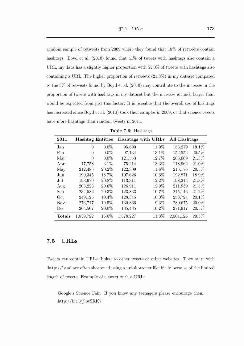
§7.5 URLs 173
random sample of retweets from 2009 where they found that 18% of retweets contain
hashtags. Boyd et al. (2010) found that 41% of tweets with hashtags also contain a
URL, my data has a slightly higher proportion with 55.0% of tweets with hashtags also
containing a URL. The higher proportion of retweets (21.8%) in my dataset compared
to the 3% of retweets found by Boyd et al. (2010) may contribute to the increase in the
proportion of tweets with hashtags in my dataset but the increase is much larger than
would be expected from just this factor. It is possible that the overall use of hashtags
has increased since Boyd et al. (2010) took their samples in 2009, or that science tweets
have more hashtags than random tweets in 2011.
Table 7.6: Hashtags
2011 Hashtag Entities Hashtags with URLs All HashtagsJan 0 0.0% 95,690 11.9% 153,279 19.1%Feb 0 0.0% 97,134 13.1% 152,552 20.5%Mar 0 0.0% 121,553 12.7% 203,669 21.3%Apr 17,758 3.1% 75,214 13.3% 118,962 21.0%May 212,486 20.2% 122,309 11.6% 216,176 20.5%Jun 190,345 18.7% 107,626 10.6% 192,871 18.9%Jul 193,979 20.8% 113,311 12.2% 198,215 21.3%Aug 203,223 20.6% 126,911 12.9% 211,939 21.5%Sep 234,582 20.3% 123,833 10.7% 245,146 21.2%Oct 249,125 19.4% 128,345 10.0% 258,724 20.1%Nov 273,717 19.5% 130,866 9.3% 280,675 20.0%Dec 264,507 20.0% 135,435 10.2% 271,917 20.5%Totals 1,839,722 15.0% 1,378,227 11.3% 2,504,125 20.5%
7.5 URLs
Tweets can contain URLs (links) to other tweets or other websites. They start with
‘http://’ and are often shortened using a url-shortener like bit.ly because of the limited
length of tweets. Example of a tweet with a URL:
Google’s Science Fair. If you know any teenagers please encourage them
http://bit.ly/hwSRK7

174 Types of Tweets
tweetid: 24824515498352640
In this example http://bit.ly/hwSRK7 expands to http://www.theguardian.com/science/
punctuated-equilibrium/2011/jan/11/1, an article with the headline “The world’s first
international online science fair”.
The number of tweets with the doc.urlEntities field present and not empty were
found using the CouchDB view given in listing G.15 in Appendix G. The number of
tweets per month and percentage of all tweets per month these represent are shown
in the ‘URL Entities’ column of Table 7.7. There are no tweets found in my dataset
with the doc.urlEntities field until April 2011, indicating that it was not introduced
by Twitter until this time. Instead of relying on the Twitter doc.urlEntities fields, a
second report was created that looked for one or more occurrences of ‘http://’ in the
tweet text. The CouchDB view used for this is given in listing G.16 in Appendix G.
Even once the doc.urlEntities field was introduced, there were slightly more tweets each
month found using the search for ‘http://’ in the tweet text than by the doc.urlEntities
field.
The percentage of science tweets containing URLs varied between 38.6% and 57.4%
per month. For the whole year just under half (46.0%) of the science tweets contained
links. This is much higher than the 22% found in a random sample of Tweets from
2009 by Boyd et al. (2010), and is much closer to their results from a random sample
of retweets from 2009, where they found that 52% of retweets contained URLs. The
higher proportion of retweets (21.8%) in my dataset compared to the 3% of retweets
found by Boyd et al. (2010) may contribute to the increase in the proportion of science
tweets containing URLs but the increase is much larger than would be expected from
just this factor. It is possible that the use of overall use of URLs has increased since
Boyd et al. (2010) took their samples in 2009, or that science tweets have more URLs
than random tweets in 2011.

§7.6 Conclusion 175
Table 7.7: URLs
2011 URL Entities All URLsJan 0 0.0% 384,255 47.9%Feb 0 0.0% 370,579 49.8%Mar 0 0.0% 450,584 47.2%Apr 46,252 8.2% 296,347 52.4%May 485,127 46.0% 490,280 46.5%Jun 504,542 49.5% 509,825 50.1%Jul 529,440 56.8% 535,117 57.4%Aug 477,831 48.4% 483,964 49.0%Sep 439,832 38.0% 446,057 38.6%Oct 501,180 39.0% 508,067 39.6%Nov 563,812 40.2% 572,959 40.8%Dec 572,116 43.2% 581,203 43.8%Totals 4,120,132 33.7% 5,629,237 46.0%
7.6 Conclusion
The science tweets dataset contains a lot more retweets (19.5%) than found in a random
sample of tweets (3%) by Boyd et al. (2010), but is much closer to the retweets found in
a sample of tweets from a scientific conference (15% to 20%) by Letierce et al. (2010).
The study by Bruns and Stieglitz (2012) of a wide range of hashtags and keywords were
found to contain between 15% and 65% retweets. My result of 17% for ‘science’ was
close to that found by Bruns and Stieglitz (2012) for TV shows like #mkr (My Kitchen
Rules), #masterchef, #eurovision and #angryboys, however these all had very low
numbers of links (less than 15%) while my dataset had nearly 50%. The proportion of
links (URLs) in the retweets and the proportion of retweets with ‘via’, ‘rt’ or ‘retweet’
was almost identical to that found by Boyd et al. (2010) suggesting that people tweeting
about science are engaged in considerably more re-sharing of information than average
on Twitter but that the actual retweets are used in a similar way.
The overall proportion of mentions (37.8%) was also very similar to that found by
Boyd et al. (2010) (36%). However the proportion of a subtype of mentions, replies,
found in my dataset (14.9%) is only half that found by Boyd et al. (2010) (31%). The
176 Types of Tweets
higher proportion of retweets in my dataset is likely to contribute to this difference
because mentions occurring in retweets are unlikely to be replies as most retweets start
with ‘RT’.
The use of hashtags and urls was much more prevalent in my dataset (hashtags:
20.5%, urls: 46.0%) than in the random sample of tweets by Boyd et al. (2010) (hash-
tags: 5%, urls: 22%), but close to the use of hashtags and urls Boyd et al. (2010) found
in retweets (hashtags: 18%, urls: 52%). This increase is larger than would be expected
from the higher proportion of retweets in my dataset and indicates that another factor
is present, possibly an increase in the overall use of urls and hashtags on Twitter or
perhaps science tweets have more urls and hashtags than random tweets.
Having looked at the overall patterns of numbers of tweets, numbers of authors and
types of tweets I will begin looking at the text of the tweets with the word science.

Chapter 8
Word frequency and word
co-occurence
This chapter begins the analysis of the tweet text, starting to build an understanding
of how people have used the word science on Twitter and what topics they have been
discussing in order to answer my fourth research question “What topics are discussed
in these tweets?”. In the first part of this chapter Question 4a – “what is the frequency
of words used?” – is addressed by using one of the simplest forms of text analysis:
word frequency, looking at how often different words appear in the corpus. Question
4b – “what words co-occur?” – is addressed in the second part of this chapter where
I look at word co-occurance which starts to capture some of the patterns of usage of
words, or grammar, without actually needing to know anything about grammar.
The language used in tweets makes word frequency analysis more difficult than other
written sources because people often use abbreviations, informal or colloquial language
and slang in tweets, partly to fit their messages into the 140 character restriction of
Twitter. This means that the list of words in the corpus obtained by splitting the tweets
into words will contain many variations on each word. The unusual language can also
make the process of splitting the tweets into words less reliable as word boundaries
may not follow normal English grammar rules.
177
178 Word frequency and word co-occurence
8.1 Introducing Tokenisation
The process of splitting the text up to find words and punctuation is called tokenisation.
The resulting tokens can be words, punctuation characters, symbols like the emoticons
discussed in 4.1.2 or special twitter entities like web addresses (urls), twitter user names
and twitter hashtags.
Before word frequencies can be determined it is necessary to decide which of the
tokens are useful for this particular analysis, and what degree of reduction in the
variation of tokens with the same or similar meanings should be applied. Too much
reduction can result in missing interesting information in the data. With such a large
dataset, too little reduction leaves too much information to be considered.
The reduction in variation can be achieved by applying a combination of text anal-
ysis techniques such as stop word removal, word stemming, lemmatisation, entity anal-
ysis, normalisation and case-folding.
Word stemming is a process that reduces each word to a root token (which does not
have to be a valid English word) by using grammatical rules to chop off the endings
of words. Endings like ‘s’, ‘ing’, ‘ed’ are removed so that only the base version of the
token remains. There are two difficulties with this approach for my dataset: it may
reduce words of different meanings to the same stem, and if it is applied to tokens which
are not words it may result in misleading stems. An example of what can go wrong
when using stemming is provided by Manning, Raghavan, and Schütze (2009) “the
Porter stemmer stems all of the following words: operate operating operates operation
operative operatives operational to oper” (Manning et al., 2009, p. 34).
Lemmatisation is a more complex approach which uses the linguistic morphology
of a word and a vocabulary to find the lemma of each word. A lemma is the base
or dictionary form of a word (Manning et al., 2009, p. 32). I have chosen to use
lemmatisation because it only acts on words which are included in the vocabulary of

§8.1 Introducing Tokenisation 179
English words, leaving all other tokens unchanged. Using the previous example of
operate operating operates operation operative operatives operational, the Word Net
lemmatiser returns operate operating operate operation operative operative operational,
retaining more information about the use of the word at the cost of less reduction of
tokens.
Another way of reducing the number of tokens is to remove common tokens that
do not help understand the topics of the text. These are called stop words. A simple
approach to this is to remove all tokens that are two characters or less. This included
words like a, I, in, on, to, is. It is also possible to use a list of words that are very
common in the English language, and most natural language analysis tools include stop
word lists. In this data set, every text must include the word ‘science’, either as a word
or a twitter hashtag because that is the keyword that was used to collect the data. For
some types of text analysis, such as word frequency, it will make sense to remove this
word as it is very common in this dataset. However the position in which it occurs
may be useful in identifying the words in the text most closely related to it. I use this
proximity to the word ‘science’ later in this chapter when I look at the frequency of
bi-grams (pairs of words) and n-grams (groups of adjacent words) in the tweet texts.
In the case of Twitter text, there is an additional set of tokens that represent
twitter entities like web addresses (urls), twitter user names, twitter hash tags, old
style retweet signs (RT). There is also other special language commonly used in tweets
such as internet slang, for example lol for ‘laugh out loud’ and emoticons. Decisions
about how to reduce each of these need to be made.
Normalisation is the process of merging together tokens which are determined to
have the same meaning. This can be applied to tokens which are of the same Twitter
entity type, so for example all twitter user names could be merged into a token ‘twitter-
user-name’. It can also be applied to words which are determined to have the same
meaning. Which tokens are decided to be synonyms will depend on the dataset and

180 Word frequency and word co-occurence
what is being looked for in the analysis. In my dataset it is common for internet slang
to be repeated for emphasis, so lol might be extended to lololololol or grr extended to
grrrrrrrrrrr and it may be useful to normalise these to their base forms.
A final type of reduction is case-folding, where mixed case letters are changed to
a single case, usually lower case. This can cause some proper nouns to be confused
with words that are spelt in the same way and can also make sentence detection more
difficult. In the case of Twitter text analysis, the tweets are very short so sentences are
not usually of interest. It is also common for people to write tweets in all lower case,
or to use capitalisation to show they are ‘yelling’. I decided that the advantage of the
reduction in tokens gained by using lower case was much greater than the information
loss and so all of the analysis has been conducted with lower case text.
Once all of these approaches have been used, the remaining tokens can be reviewed
and the entity detection and stop word lists recursively refined by excluding any tokens
that are determined to be unhelpful and by folding additional synonym tokens detected
into already existing ones.
The text analysis in this chapter was carried out using the Python Natural Language
Tool Kit (NLTK)1 (Bird, Klein, & Loper, 2009) which is a well recognised tool for text
analysis (Layton, 2015; Rehuvrek & Sojka, 2010).
8.2 Tokenisation of January 2011 Science Tweets
For performance reasons, the reduction in variation of the tokens was developed us-
ing just the first month of data from 2011. There are 802,821 tweets in the dataset
for January 2011. The tweets were tokenised using the NLTK sentence tokenise
(sent_tokenize()) followed by the NTLK word tokenise (word_tokenize()). The token
frequencies are found using the NLTK FreqDist() module. From the raw tweets, there1NLTK version 1.7.1(http://nltk.org/)

§8.2 Tokenisation of January 2011 Science Tweets 181
were a total of 15,796,566 tokens found, 691,902 unique tokens of which 478,854 oc-
curred only once. Table 8.5 shows the reduction in number of tokens achieved by each
processing step. Each step includes the processing from the previous step. Making text
lower case gives a 9.5% reduction in unique tokens, a 7.5% reduction in unique tokens
that appear only once and a 14% reduction in unique tokens that appear more than
once.
The Twitter Entity processing uses the python twitter tweet parser (ttp)2 to detect
the entities in the raw tweet. The Twitter user names detected are modified by adding
‘user-’ to them so they will be distinguished from matching words, so ‘@RealClimate’
becomes ‘user-realclimate’. This may actually increase the number of unique tokens,
but preserves the meta information that they are user names. The largest reduction
in tokens in this step is achieved by the recognition of web addresses (urls) and trun-
cation of them to their base domain names. For example ‘http://bit.ly/fm4Dlo’ will
be reduced to ‘bit.ly’. The string ‘www.’ is also removed from urls so that just the
main domain is left (‘www.futurity.org’ becomes ‘futurity.org’). The final Twitter en-
tity that I’m processing is the Twitter hashtag, words starting with a ‘#’ which are
used as keywords to find groups of tweets. These are modified by adding ‘hashtag-’
to them, so ‘#health’ will become ‘hashtag-health’. Like the user name processing,
this preserves meta information that may be useful for later analysis, even though it
potentially increases the number of unique tokens.
During the implementation of the Twitter Entity processing it was found that the
url detection performed by ttp does not find all urls. It fails to recognise urls that do
not start with either ‘http://’ or ‘www.’. Twitter specifies that Twitter entity parsers
should be able to detect urls which do not have these prefixes, so this is a problem in
the current version of ttp.
To address this problem, the url detection performed by ttp was supplemented
checking any tokens that contain a full stop using python Top Level Domain Extract2twitter-text-python (ttp), version 1.0.1.0, (https://pypi.python.org/pypi/twitter-text-python/)

182 Word frequency and word co-occurence
(tldextract)3, to see if they contained a valid top level domain (TLD). If they did, the
token was replaced by just the TLD part of the token. Otherwise, it was assumed that
the fullstops are separators rather than part of a url. If the fullstops are separating
single letters, then I have considered the token to be an abbreviation and removed
the full stops creating a single token. Abbreviations were detected using a regular
expression4. Remaining fullstops in the text were used to split the token into multiple
tokens - for example ‘science.lol’ was changed to three tokens ‘science’, ‘.’ and ‘lol’.
The final code used for the Twitter Entity Processing is given in listing H.1 in
Appendix H. Processing the Twitter entities gained a further 39.1% reduction in unique
tokens (44.8% total reduction), a further 47.7% reduction in unique tokens that appear
only once (51.6% overall) and an additional 18.1% reduction in unique tokens that
appear more than once (29.6% overall). The resulting numbers of tokens are shown in
Table 8.5.
The next normalisation applied was to split the tokens detected by NTLK word
tokenise on other separators not used by NLTK word tokenise. During this step, tokens
which are Twitter Entities are not split and tokens that are only a single character
after splitting are discarded. The additional seperators used are shown in Table 8.1
and Python code is provided in listing H.2 in Appendix H. Including digits 0 to 9 in
the charactes to split on effectively filters out all numbers from the tokens. This, and
the other filter characters used, may remove some emoticons and text written in ‘leet
speak’5 but should not remove any English words. Because tokens are being split, this
step can actually increase the number of tokens, but in this case more of the tokens
created by splitting were either existing tokens or removed because they were only a
single character, so there was a reduction in the number of tokens. Splitting on these
characters gained a further 13.9% reduction in unique tokens (52.5% total reduction),
3tldextract, version 1.2.2, (https://pypi.python.org/pypi/tldextract)4regular expression: r'((?:[^.0-9]\.){2,})' compiled with the regex module, version 2.4.28
(https://pypi.python.org/pypi/regex)5leet speak uses an alternative alphabet for English words - for example leet can be spelled as ‘1337’

§8.2 Tokenisation of January 2011 Science Tweets 183
a further 15.8% reduction in unique tokens that appear only once (59.3% overall) and
an additional 11.1% reduction in unique tokens that appear more than once (37.4%
overall). The resulting numbers of tokens are shown in Table 8.5.
Table 8.1: Characters used to split words
character char in regex‘ ‘/ /* *\ \- -“ \u201c– \u2013” \u201d: :’ \u2019… \u2026— \u2014☑ \u2611☐ \u2610‘ \u2018´ \u00B4| |~= =+ +’ ’, ,0-9 0-9^ ^_ _
The stop word processing was applied before lemmatisation because it was found
that some of the stop words were being reduced to their lemma and then not removed
by the stop word processing. The NLTK English stop word list which contains 127
tokens shown in Table 8.2 was used. At the same time all single character tokens were
removed. The stop word processing resulted in a 29.5% reduction in the total number
of tokens from 11.2 million to 7.9 million. It had only a very small effect on the number
of unique tokens (only reduced by 123 tokens) and no effect on tokens that appear only

184 Word frequency and word co-occurence
once. The ‘Stop words’ row in Table 8.5 gives the tokens remaining after stop word
processing.
Table 8.2: NTLK English Stop Words
a about above after again against all aman and any are as at be becausebeen before being below between both but bycan did do does doing don down duringeach few for from further had has havehaving he her here hers herself him himselfhis how i if in into is itits itself just me more most my myselfno nor not now of off on onceonly or other our ours ourselves out overown s same she should so some sucht than that the their theirs them themselvesthen there these they this those through totoo under until up very was we werewhat when where which while who whom whywill with you your yours yourself yourselves
The next step in processing the corpus for word frequency analysis was lemma-
tisation. The NLTK WordNet Lemmatizer (nltk.WordNetLemmatizer()) was applied
to each token remaining in the corpus after the stop word processing. Lemmatisation
altered 631,208 instances of 9,674 unique tokens, reducing them to 9,038 unique to-
kens. The resulting number of tokens is given in the ‘Lemmatisation’ row of Table 8.5.
The reduction produced by Lemmatisation after the stop words step was a 2.6% in the
number of unique tokens, 1.3% in tokens appearing only once, and a 4.5% reduction in
tokens that appear more than once. This gave an overall reduction of 53.8% in unique
tokens, 59.8% in tokens appearing only once and 40.3% in tokens appearing more than
once as compared to the raw corpus.
The stop word processing using the NTLK English stopwords was performed a
second time to check if the lemmatisation had transformed any tokens into ones which
are stop words. The results in ‘2nd stop words’ in Table 8.5 show a very small reduction
in tokens, so some of the lemmas were stop words. Total tokens were reduced by

§8.2 Tokenisation of January 2011 Science Tweets 185
27,781 and unique tokens by 55. Only 1 token appearing only once was removed, so
the reduction in unique tokens was mostly those that appear more than once (reduced
by 54).
Reviewing the first 4,000 most frequent tokens showed a number of tokens that do
not help with understanding the topics being discussed. Individual tokens that should
be removed by adding them to stop words are given in Table 8.3. These are mostly
fragments of words or variations on stop words. There were also some tokens that
should be normalised back to a standard base word, or removed by matching a pattern
rather than a stop word string. These are shown in Table 8.4. The normalisation is
applied first, because the normalised token may be a stop word.
The Python code for the normalisation is provided in listing H.3 in Appendix H.
This normalisation step only resulted in a small reduction in the number of tokens,
reducing unique tokens by 739, unique tokens that appear only once by 291 and tokens
that appear more than once by 448. The resulting numbers of tokens are shown in
Table 8.5.
The additional stop words were combined with the standard NTLK English stop-
words and then applied the normalised words as shown in listing H.4 in Appendix H.
Applying these removed an additional 37 unique tokens, all of which appeared more
than once. The resulting numbers of tokens are shown in the final row of Table 8.5
labeled ‘3rd Stopwords’.
The overall reduction in numbers of tokens compared to the raw words split just
using NLTK sentence tokenise and NLTK word tokenise was 50.7% in total instances
of tokens, 53.9% in number of unique tokens, 59.9% in unique tokens appearing only
once and 40.5% in unique tokens appearing more than once.

186 Word frequency and word co-occurence
Table 8.3: Additional Stop words showing occurrence in January 2011
Token Instancesna 10,708im 10,705ca 9,778th 9,382http 8,000ve 7,701ll 7,109dont 4,140le 2,821cant 2,047la 1,879others 1,849thats 1,837htt 1,584tho 1,322didnt 1,268al 1,153aint 1,042doin 928ive 869whats 723dnt 646ii 642havent 554tha 518wont 459isnt 454doesnt 443aaa 441yall 392ish 388xii 308wasnt 294havin 125havnt 117youre 112isnot 59

§8.2 Tokenisation of January 2011 Science Tweets 187
Table 8.4: Additional Normalisation filters
Type Examples New word/removesingle char repeated xxxxx, xxxx, ooooo reduce to 3 charactersvariants of lol lolol, loool, lolz reduce to lolvariants of haha haha, hah, hehe reduce to hahavariants of ah ahhh reduce to ahvariants of oh ohhh, oooh reduce to ohvariants of so or no nooooo, sooo, sooooo removevariants of umm um, ummmm ummvariants of hmm hm, hmmmm hmmvariants of ugh ughh, urgh reduce to ughvariants of science sci, scienc, science’s, science-y sciencevariants of people ppl peoplevariants of fucking fuckin fuckingvariants of please plz pleasevariants of day today, daii, dayy dayvariants of tonight nite, tonight, nights nightvariants of tomorrow tomorow, morrow tomorrowvariants of hour hr, hour, hrs hourvariants of world world’s worldvariants of minute min, minutes, mins minutevariants of year yr, yo, yro yearvariants of pound lb, pounds poundvariants of point pt, points, pts pointvariants of hell helllll, hella hellvariants of drop droppin dropvariants of going goin goingvariants of yeah yeahh, yeh, aye yesvariants of obama obama’s obamavariants of congratulations congrats congratulationsvariants of school skool schoolvariants of working workin work

188 Word frequency and word co-occurence
Table 8.5: Reduction in variation of tokens
Processing step Total Unique Tokens that Tokens thatTokens Tokens appear once appear > once
Raw tweets 15,796,566 691,902 478,854 213,048Lowercase Tweets 15,796,566 626,285 442,950 183,335Twitter Entities 15,124,566 381,633 231,563 150,070Split words 11,205,410 328,429 195,040 133,389Stopwords 7,902,230 328,306 195,040 133,266Lemmatisation 7,902,230 319,654 192,428 127,2262nd Stopwords 7,874,449 319,599 192,427 127,172Normalise 7,871,687 318,860 192,136 126,7243rd Stopwords 7,778,828 318,823 192,136 126,687

§8.3 Tokenisation of all 2011 Science Tweets 189
8.3 Tokenisation of all 2011 Science Tweets
The same processing steps were then applied to the other months of data in 2011.
The initial and final numbers of tokens for each month are shown in Table 8.6. After
processing, the total number of unique tokens over the whole year is 2,732,171 with
a total of 117,206,868 instances. Of these 1,659,308 tokens appear only once and the
total of unique tokens appearing more than once is 1,072,863.
Now that we have the filtered tokens, the simplest way to look at them is to sort
them by frequency and look at the most frequent ones. Looking at samples of tweets
containing the most frequent tokens to see how they are being used is very time con-
suming which limits the number of tokens that can be considered. I have looked at
the most frequent 20 tokens in each month of 2011. This is an extremely small sample
when it is considered that there were just over one million tokens appearing more than
once in 2011.

190 Word frequency and word co-occurence
Table 8.6: Reduction in variation of tokens by month in 2011
Month Step Total Unique Tokens that Tokens thatTokens Tokens appear once appear > once
Jan Raw tweets 15,796,566 691,902 478,854 213,048Final 7,778,828 318,823 192,136 126,687
Feb Raw tweets 14,526,242 664,072 460,160 203,912Final 7,224,131 304,459 183,192 121,267
Mar Raw tweets 18,668,719 797,478 553,912 243,566Final 9,237,619 372,833 226,196 146,637
Apr Raw tweets 11,007,854 541,160 369,374 171,786Final 5,475,076 249,934 150,703 99,231
May Raw tweets 20,176,303 896,450 626,667 269,783Final 9,989,991 412,675 251,336 161,339
Jun Raw tweets 19,453,485 840,754 560,408 280,346Final 9,610,652 393,337 237,594 155,743
Jul Raw tweets 18,465,948 786,984 524,363 262,621Final 9,188,592 344,353 205,334 139,019
Aug Raw tweets 19,788,050 924,928 668,707 256,221Final 9,760,601 401,322 246,604 154,718
Sep Raw tweets 22,270,578 1,009,629 736,305 273,324Final 10,920,821 473,933 299,274 174,659
Oct Raw tweets 24,603,604 1,101,174 808,068 293,106Final 12,049,148 502,469 315,343 187,126
Nov Raw tweets 26,872,178 1,197,122 886,753 310,369Final 13,362,825 535,269 337,009 198,260
Dec Raw tweets 25,487,083 1,170,646 874,222 296,424Final 12,608,584 515,892 326,762 189,130
8.4 Word frequencies
The tokens which appear in the twenty most frequent tokens per month in 2011 are
shown in Table 8.7 ordered by their average frequency over the year (expressed as the
percentage of all tokens). As expected, the keyword used to collect the tweets, ‘science’
is much more frequent than the next token. The gap increases if the ‘hashtag-science’
token is merged with the science token. The two tokens have not been normalised
(merged) because using a hashtag of science indicates the person is talking about the
topic science instead of just using the word science.
The second most frequent token is the URL ‘t.co’ which is the default link shortener

§8.4 Word frequencies 191
used by Twitter. This indicates that a lot of the tweets included links that had been
shortened by t.co to save characters in the tweet. The data normalisation has reduced
all links to their base domain. It is possible to look up each ‘t.co’ URL and find out
what the actual domain it expands to (although in some cases the short link will have
been deleted since 2011). At this stage I do not think resolving the actual domains
improves the understanding of the topics being discussed enough to justify the large
resources required to expand all the links. The frequency of different URL shorteners
appearing in the top 20 tokens varies a lot from month to month. In the overall rankings
the next most frequent URL shortener ‘bit.ly’ appears fourth, followed by ‘amzn.to’
which is the tenth most frequent token. To simplify the analysis of the other tokens, I
have considered all the URL shorteners separately in Section 8.4.2 and excluded them
from the main analysis of most frequent tokens.
The third most frequent token was ‘rt’ which is used to indicate that people are
retweeting someone else’s tweet - they are sending a tweet they found interesting onto
their followers. These tweets can just be the original tweet unchanged, or in some cases
users may add a comment when they retweet. Another commonly used indicator in
tweets is ‘via’ which is used to give credit to someone when passing on information.
This was the 16th most frequent token over the whole of 2011. The token ‘rt’ can be
considered to be a meta-token indicating the type of tweet.
The fourth and fifth most frequent tokens are the previously mentioned ‘bit.ly’ and
‘hashtag-science’. The first five tokens occur much more frequently than the subsequent
tokens. Even within these tokens, if ‘hashtag-science’ and ‘science’ are merged, then
their combined frequency is 10.77%, much more frequently than the next most frequent
token ‘t.co’ at 2.03%. There is another large decrease in frequency between the fourth
token ‘bit.ly’ and the sixth token ‘day’ compared to that between the second and third
tokens (‘t.co’ and ‘rt’). After these first five, the remaining tokens show a gradual
decrease in frequency without any other large steps.

192 Word frequency and word co-occurence
Because of their much higher occurrence and status as meta-tokens, I have consid-
ered the first five tokens separately from the remaining tokens in the most frequent 20
per month in 2011. The token ‘via’ (rank 16) has been included with ‘rt’ and ‘amzn.to’
(rank 10) has been included with the URL shorteners even though they do not have as
high occurrence.
Table 8.7: Tokens appearing in Twenty most frequent tokens per month in 2011ranked by mean frequency per month (percent of total tokens)
rank word frequency rank word frequency1 science 10.12% 20 one 0.25%2 t.co 2.03% 21 love 0.25%3 rt 1.96% 22 school 0.25%4 bit.ly 1.13% 23 study 0.23%5 hashtag-science 0.65% 24 year 0.23%6 day 0.49% 25 time 0.23%7 math 0.45% 26 lol 0.23%8 new 0.40% 27 test 0.23%9 like 0.39% 28 know 0.22%
10 amzn.to 0.36% 29 news 0.22%11 fiction 0.36% 30 good 0.22%12 class 0.34% 31 book 0.21%13 computer 0.30% 32 project 0.20%14 get 0.29% 33 history 0.20%15 teacher 0.27% 34 people 0.17%16 via 0.27% 35 fair 0.17%17 art 0.26% 36 exam 0.14%18 got 0.25% 37 bill 0.13%19 technology 0.25% 38 series 0.11%
8.4.1 Science and Retweet tokens
The percentage occurrence in the total tokens of the individual science and retweet
tokens that appeared in the top 20 tokens in each month is given in Table 8.8. The
table also gives the combined frequency of the science tokens and retweet tokens and
the minimum frequency required for a token to appear in the top 20 tokens in each
month. Their individual frequencies and the minimum frequency needed to appear in
the top 20 tokens are shown on Fig. 8.1. The ‘via’ token stays in the top 20 tokens

§8.4 Word frequencies 193
in every month as shown by comparing its frequency with the minimum frequency in
Table 8.8, this can be seen on Fig. 8.1 with the red ‘via’ line staying just above the
black ‘minimum frequency’ line. The frequency of these tokens is very stable over the
year with only small variations from month to month.
Jan Feb Mar Apr May Jun Jul Aug Sep Oct Nov Dec
2011
0.00
0.02
0.04
0.06
0.08
0.10
0.12
Frequency
science
hashtag-science
rt
via
minimum for top 20
Figure 8.1: Science and retweet tokens in top 20 tokens per month 2011
Table 8.8: Percentage occurrence of science and rt in top 20 tokens per month 2011
Jan Feb Mar Apr May Jun Jul Aug Sep Oct Nov Decscience 9.9 9.8 9.8 9.8 10.2 10.3 9.9 9.9 10.4 10.6 10.5 10.5hashtag-science 0.7 0.7 0.7 0.9 0.7 0.6 0.7 0.7 0.6 0.6 0.5 0.5rt 1.9 1.8 2.0 1.8 1.9 1.8 2.1 2.3 2.0 2.0 1.9 1.9via 0.3 0.3 0.3 0.3 0.3 0.3 0.3 0.3 0.3 0.2 0.2 0.3science & #science 10.5 10.5 10.5 10.7 10.8 10.9 10.6 10.5 11.0 11.1 11.0 11.0rt & via 2.1 2.1 2.3 2.1 2.2 2.1 2.4 2.6 2.3 2.3 2.2 2.2Minimum Freq. 0.3 0.2 0.3 0.2 0.3 0.3 0.2 0.2 0.3 0.3 0.2 0.3
8.4.2 URL Shorteners
The percentage occurrence in the total tokens of each of the different URL shorteners
that appeared in the top 20 tokens in each month is given in Table 8.9 and the fre-
quencies and the minumum frequency needed to appear in the top 20 tokens are shown
on Fig. 8.2. Where the individual lines go below the black line showing the minimum

194 Word frequency and word co-occurence
frequency the token is not in the top 20 tokens for that month. The ‘bit.ly’ shortener
is the most common until july where it is rapidly replaced by ‘t.co’ which goes onto
be used more than twice as the highest ‘bit.ly’ use towards the end of the year. This
reflects a change made by Twitter where they originally supported bit.ly but then in-
troduced their own URL shortener ‘t.co’ in June 20106 and gradually increased their
use of it. On 10 October 2011 Twitter announced7 that all links regardless of length
will be wrapped in the t.co URL shortener. Amazon introduced amzn.to in April 2010
by using the ‘Pro service’ provided by bit.ly8. The growth in the use of the amazon.com
URL shortener in Tweets containing ‘science’ starts in March and then reduces in the
same way as bit.ly as Twitter forces the use of the t.co link shortener. Many of the
tweets with the amzn.co URL shortener seem to be spam generated by robots trying
to make money on Amazon affiliates. Amazon affiliates gives a commission to people
when products are bought through links the affiliate has provided. The use of Amazon
affiliates links for spam in was also found in a study of Twitter spam sent during 2010
by Thomas, Grier, Paxson, and Song (2011, p. 254).
Table 8.9: Percentage occurance of short urls in top 20 tokens per month 2011
Jan Feb Mar Apr May Jun Jul Aug Sep Oct Nov Decbit.ly 2.1 2.2 2.0 2.1 1.8 1.4 1.4 0.5 0.0 0.0 0.0 0.0t.co 0.3 0.3 0.4 0.4 0.4 0.9 1.1 3.4 3.9 4.2 4.4 4.7amzn.to 0.0 0.0 0.1 0.7 0.5 1.3 1.5 0.2 0.0 0.0 0.0 0.0
8.4.3 Remaining Word tokens
After removing the science, retweet and URL shortener tokens there were 31 tokens
remaining that appear in the 20 most frequent tokens in at least one month of 2011.
The percentage occurrence of each token in the top 20 for each month are given in
Table 8.10 and shown on Fig. 8.3. Only the January tokens are in decreasing frequency
order. New tokens appearing in each month are added to the bottom of the table in6https://blog.twitter.com/2010/links-and-twitter-length-shouldn\%E2\%80\%99t-matter7https://dev.twitter.com/discussions/28068http://techcrunch.com/2010/04/14/amazon-goes-pro-with-bit-ly/

§8.4 Word frequencies 195
Jan Feb Mar Apr May Jun Jul Aug Sep Oct Nov Dec
2011
0.00
0.01
0.02
0.03
0.04
0.05
Frequency
bit.ly
t.co
amzn.to
minimum for top 20
Figure 8.2: Short urls in top 20 tokens per month 2011
decreasing frequency order within that month. This means that any tokens frequencies
for a month which are above the new ones may not be in decreasing frequency order.
The percentage occurrence for the tokens in every month and the minimum frequency
required for a token to be in the top 20 for that month are given in Table I.1 in
Appendix I.
Although Fig. 8.3 gives an overview of the relative frequencies of the different
tokens, the number of tokens make it difficult to interpret so I have split them into
three groups; the tokens that appear in top 20 tokens per month in 2011 every month
are shown on Fig. 8.4, those that appear in more than two months but not every month
are shown on Fig. 8.5 and those that appear only in one or two months are shown on
Fig. 8.6.
The first group contains the tokens that are in the 20 most frequent tokens for
every month during 2011. Figure 8.4 shows that they are amongst the most frequent
tokens, with the lowest being ‘math’ with a frequency of 0.003 in July. Interestingly,
‘math’ also has the highest frequency of 0.0062 in September and October. The token
‘day’ also shows a high variation, it is the most frequent token (in all groups) during

196 Word frequency and word co-occurence
Jan Feb Mar Apr May Jun Jul Aug Sep Oct Nov Dec
2011
0.0025
0.0030
0.0035
0.0040
0.0045
0.0050
0.0055
0.0060
0.0065
Frequency
day
fair
new
math
like
fiction
class
get
year
news
teacher
got
good
school
love
art
computer
time
test
one
technology
study
exam
series
people
lol
bill
history
know
project
book
minimum for top 20
Figure 8.3: Remaining tokens in top 20 tokens per month 2011

§8.4 Word frequencies 197
Table 8.10: Percentage occurrence of remaining tokens in top 20 tokens per month2011 above minimum frequency
Jan Feb Mar Apr May Jun Jul Aug Sep Oct Nov Decday 0.50 0.56 0.56 0.50 0.55 0.49 0.37 0.39 0.54 0.53 0.49 0.44fair 0.46new 0.45 0.43 0.39 0.44 0.38 0.40 0.42 0.37 0.36 0.37 0.37 0.37math 0.41 0.43 0.39 0.35 0.43 0.39 0.30 0.48 0.62 0.62 0.48 0.50like 0.39 0.36 0.38 0.34 0.40 0.38 0.37 0.43 0.46 0.43 0.38 0.41fiction 0.36 0.34 0.34 0.38 0.37 0.36 0.42 0.45 0.32 0.34 0.31 0.35class 0.34 0.34 0.32 0.28 0.31 0.35 0.53 0.41 0.40 0.34get 0.32 0.29 0.28 0.30 0.31 0.25 0.29 0.32 0.30 0.28 0.28year 0.28 0.32 0.29news 0.28 0.32 0.28 0.26teacher 0.28 0.28 0.29 0.29 0.36 0.30 0.30 0.27got 0.27 0.24 0.26 0.28 0.24 0.29 0.28 0.27 0.28good 0.26school 0.26 0.26 0.30 0.27 0.25love 0.30 0.26 0.27 0.32 0.26 0.27art 0.30 0.28 0.26 0.26 0.27 0.29 0.27computer 0.26 0.28 0.29 0.33 0.35 0.28 0.28 0.32 0.36 0.34time 0.27 0.23test 0.26 0.23 0.25 0.32 0.31 0.29one 0.27 0.26 0.26 0.24 0.26 0.26technology 0.27 0.28 0.33 0.37 0.24study 0.24 0.25 0.28 0.27exam 0.42series 0.25 0.28people 0.25lol 0.28 0.25bill 0.35history 0.29know 0.25project 0.25 0.27book 0.27Min. Freq. 0.25 0.24 0.26 0.23 0.25 0.25 0.23 0.24 0.25 0.25 0.25 0.25
January to June (between 0.005 and 0.0055) and then drops to the middle this group
during July and August before returning to a high level for September and October
and it is again the most frequent of these remaining tokens in November. The other
tokens in this group are ‘like’, ‘new’ and ‘fiction’ and they show less variation over the
months, with their frequencies moving between 0.0032 and 0.0045.
The second group is the tokens that are not in the most frequent 20 tokens every
month but are in the top 20 for more than two months in 2011. Figure 8.5 shows

198 Word frequency and word co-occurence
Jan Feb Mar Apr May Jun Jul Aug Sep Oct Nov Dec
2011
0.0025
0.0030
0.0035
0.0040
0.0045
0.0050
0.0055
0.0060
0.0065
Frequency
day
new
math
like
fiction
minimum for top 20
Figure 8.4: Remaining tokens that appear every month in top 20 tokens per month2011
that most of these remain at the lower end of the frequencies in the top 20 per month,
staying below 0.0035. The exception is ‘class’ which is the most frequent of this group
from August to December with a frequency as high as 0.0053 in September. From
January to March the fequency of ‘class’ is below 0.0035, but still the most frequent
token of this group, then it drops to second most frequent in April and May and does
not appear in the top 20 during June and July. The token ‘computer’ is not in the top
20 during January and March but appears for the rest of the year and is second most
frequent in this group for June, July, November and December. The token ‘get’ appears
in every month except July and is most frequent in this group in April and May and
second most frequent in this group in January and August. The related token ‘got’ is
not in the most frequent tokens in April, June and July. It is always less frequent than
‘get’ and at its highest frequency in September it is still only the fourth most frequent
in this group. Although the token ‘news’ only appears in the most frequent tokens in
four months - January, February, March and July, it is the second most frequent in this
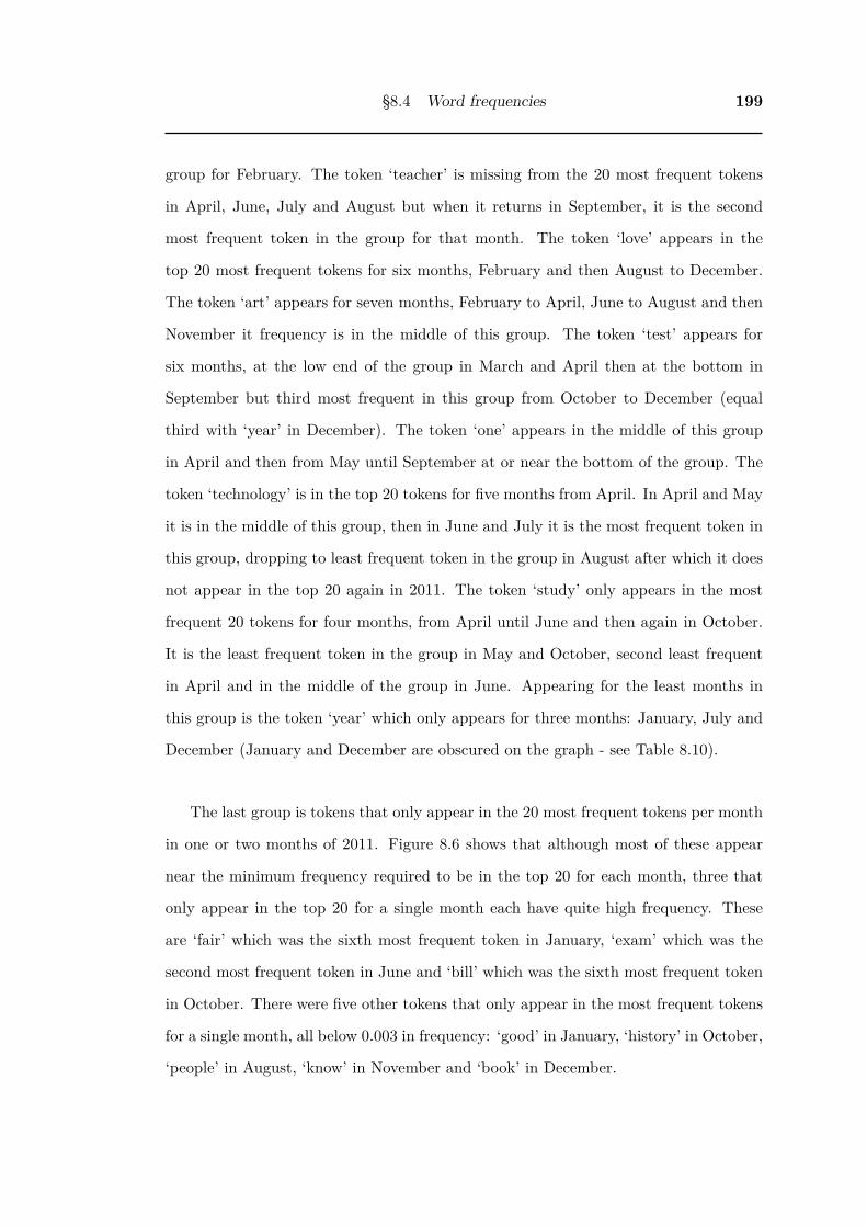
§8.4 Word frequencies 199
group for February. The token ‘teacher’ is missing from the 20 most frequent tokens
in April, June, July and August but when it returns in September, it is the second
most frequent token in the group for that month. The token ‘love’ appears in the
top 20 most frequent tokens for six months, February and then August to December.
The token ‘art’ appears for seven months, February to April, June to August and then
November it frequency is in the middle of this group. The token ‘test’ appears for
six months, at the low end of the group in March and April then at the bottom in
September but third most frequent in this group from October to December (equal
third with ‘year’ in December). The token ‘one’ appears in the middle of this group
in April and then from May until September at or near the bottom of the group. The
token ‘technology’ is in the top 20 tokens for five months from April. In April and May
it is in the middle of this group, then in June and July it is the most frequent token in
this group, dropping to least frequent token in the group in August after which it does
not appear in the top 20 again in 2011. The token ‘study’ only appears in the most
frequent 20 tokens for four months, from April until June and then again in October.
It is the least frequent token in the group in May and October, second least frequent
in April and in the middle of the group in June. Appearing for the least months in
this group is the token ‘year’ which only appears for three months: January, July and
December (January and December are obscured on the graph - see Table 8.10).
The last group is tokens that only appear in the 20 most frequent tokens per month
in one or two months of 2011. Figure 8.6 shows that although most of these appear
near the minimum frequency required to be in the top 20 for each month, three that
only appear in the top 20 for a single month each have quite high frequency. These
are ‘fair’ which was the sixth most frequent token in January, ‘exam’ which was the
second most frequent token in June and ‘bill’ which was the sixth most frequent token
in October. There were five other tokens that only appear in the most frequent tokens
for a single month, all below 0.003 in frequency: ‘good’ in January, ‘history’ in October,
‘people’ in August, ‘know’ in November and ‘book’ in December.
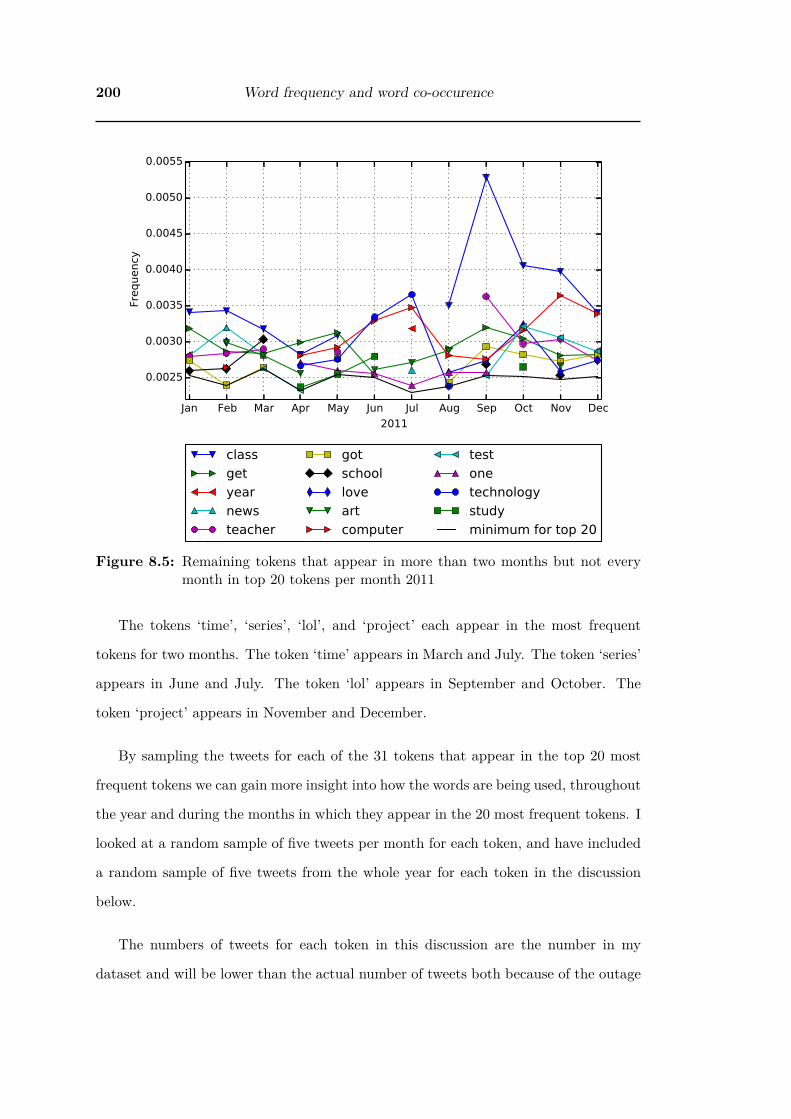
200 Word frequency and word co-occurence
Jan Feb Mar Apr May Jun Jul Aug Sep Oct Nov Dec
2011
0.0025
0.0030
0.0035
0.0040
0.0045
0.0050
0.0055
Frequency
class
get
year
news
teacher
got
school
love
art
computer
test
one
technology
study
minimum for top 20
Figure 8.5: Remaining tokens that appear in more than two months but not everymonth in top 20 tokens per month 2011
The tokens ‘time’, ‘series’, ‘lol’, and ‘project’ each appear in the most frequent
tokens for two months. The token ‘time’ appears in March and July. The token ‘series’
appears in June and July. The token ‘lol’ appears in September and October. The
token ‘project’ appears in November and December.
By sampling the tweets for each of the 31 tokens that appear in the top 20 most
frequent tokens we can gain more insight into how the words are being used, throughout
the year and during the months in which they appear in the 20 most frequent tokens. I
looked at a random sample of five tweets per month for each token, and have included
a random sample of five tweets from the whole year for each token in the discussion
below.
The numbers of tweets for each token in this discussion are the number in my
dataset and will be lower than the actual number of tweets both because of the outage

§8.4 Word frequencies 201
Jan Feb Mar Apr May Jun Jul Aug Sep Oct Nov Dec
2011
0.0025
0.0030
0.0035
0.0040
0.0045
0.0050
Frequency
fair
good
time
exam
series
people
lol
bill
history
know
project
book
minimum for top 20
Figure 8.6: Remaining tokens that only appear for one or two months in top 20 tokensper month 2011
in data collection during April, and very small number of tweets missed due to Twitter
restricting the number of tweets received by my data collection during times of high
load (‘track limitation’). The April outage will have a larger impact on the numbers
for any tokens that appear in the top 20 most frequent tokens in April, especially those
that do not stay in the top 20 for many other months.
Token ‘day’
There were 540,614 tweets containing normalised token ‘day’ in 2011. As described
in Section 8.2 the tokenisation is a complex process. In the case of ‘day’, any tokens
that when cleaned and lemmatised match one of ‘day’, ‘todaay’, ‘daii’, ‘dai’, ‘dayy’,
‘dayyy’, ‘today’, ‘days’ are then changed to the token ‘day’. The token ‘day’ appears
in the top 20 tokens throughout 2011. The tweets with token ‘day’ frequently have the

202 Word frequency and word co-occurence
actual word ‘day’ or ‘today’ being used by people to say what they are doing today.
Many of the tweets appear to be students talking about having science classes, science
fair or science tests today. Some tweets use ‘day’ in the sense of ‘picture of the day’,
for example:
RT @EarthPic: Earth Science Picture of the Day: Rays Above Madison,
Wisconsin http://t.co/wO4nbvUM
tweetid: 123685125019009024
. Table 8.11 has a random sample of 5 tweets containing the token ‘day’ from 2011.
Table 8.11: Random sample of tweets containing token ‘day’ in 2011
tweet id tweet text128888539361456128 It take 3 day to fall in, and 28 days to chemically fall out
love. popular science48545552618618880 @JenSchwalbach @ThatKevinSmith just wanted to say I
love Jen’s science corner and I heard it shouted out todayon sex & other human activies
146204037010817024 RT @tnechols: Science sol today. #ahh63578269533999104 Gonna take the science TAKS today!! Oh Lord please help
me!:)75685981369536512 I have a confession. We were learning about heart attacks
in science today and...I, er...got really worried about people.._.
Token ‘fair’
The token ‘fair’ only occurred in the top 20 in January 2011, where it was the sixth
most frequent word, occurring 35,956 times in 34,756 tweets. The phrase ‘science fair’
accounts for 95.8% of the occurrences of ‘fair’ in January 2011, with only 1,459 uses of
‘fair’ without ‘science’ in front of it. Of the 34,756 tweets containing ‘fair’ in January
2011, the word ‘google’ also occurs in 11,531 (33%). Looking at these, most are about
Google’s announcement of the worlds largest science fair launched on January 11 2011.
It is likely that this event is what caused ‘fair’ to appear in the top 20 tokens in
January 2011. Table 8.12 has a random sample of 5 tweets containing the token ‘fair’
from January 2011.

§8.4 Word frequencies 203
Table 8.12: Random sample of tweets containing token ‘fair’ in January 2011
tweet id tweet text30090238726508545 MY GOD TODAY!!! ‘It’s not just the winner of the su-
perbowl that needs to be celebrated, but the winner of thescience fair’ - Obama
24882909529776128 The world’s first international online science fair for science-loving kids http://t.co/BKFGMKe via @guardian
24658274859098112 RT @mashable: Google Is Holding a Global, Web-BasedScience Fair - http://on.mash.to/eWPk5S #Google #Sci-ence
21755213098516480 Im Screwed Still Didnt Start On Science Fair Ehh O SHoot:/ Its All Due In Like 3 Wks... Looks Like Ima Be StandinThere Trippin On My Words
30520135169085440 @viperhbkluvr752 No! My stupid science fair project! Itsannoying!! Lol
Token ‘new’
The token ‘new’ appears in the top 20 most frequent tokens for all months of 2011,
appearing in 437,034 (3.6%) of the tweets containing ‘science’ for the year, averaging
around 36,000 tweets per month. From January to April, and June and July it is the
second most frequent token in the group appearing in all months. In May it drops to
second least frequent, in August it is the least frequent of this group and then from
September to December it is again second least frequent. The token ‘new’ appears to be
used in its standard English meaning in tweets containing the word science, although
in many of them the ‘new’ thing is a blog post, show, a book, schools, maps, job, or a
proper noun (New Yorker, New Zealand) rather than the science being new. A random
sample of 5 tweets containing the token ‘new’ from all months 2011 in Table 8.13
illustrates this usage.
Token ‘math’
From January to June, the token ‘math’ is in the middle of the group of tokens that
appear in the top 20 tokens throughout 2011. It also shows the largest variation in
frequency of this group, ranging between 0.3% in July to 0.62% in September and

204 Word frequency and word co-occurence
Table 8.13: Random sample of tweets containing token ‘new’ in 2011
tweet id tweet text80470273970806784 new book, science: THE PHYSICIAN’S ROLE IN DI-
RECTING LONG-TERM CARE: Understanding the rulesis important for protect… http://amzn.to/k7qQPG
145299066992078848 American Museum of Natural History in NYC in-troduces new master’s program for science teachers.http://t.co/vS78y6aQ via @WSJ
121324848449458176 Excellent New Youk Magazine article: ‘Tweet Science:Twitter as a global consciousness’ http://t.co/kNLspqWs
108174092477280256 Pilates: A well-studied and effective workout: I have a Mas-ter of Science degree from New York University and ha...http://t.co/ysDsEry
26327324714602496 Science Online -Session – Harnessing New Media:This writing while things are going on feels l...http://bit.ly/h1ZyPl #science #chicago
October. In July it is the least frequent token in this group, and then from August
to October, and again in December it is the most frequent while in November it is
second most frequent. Many of the tweets appear to be students discussing studying
maths, while some are recommending students should study maths like this tweet from
a #NASAtweetup:
.@astro_wheels to get a job @NASA or become astronaut, students should
have interest in math, science, life sciences #NASAtweetup
tweetid: 48126862521667584
The drop in June is probably due to midyear school holidays in countries following
the American school year. With the small sample sizes being used to look at how
‘math’ is used in tweets, the change in usage of the word math during July was not
apparent.
The token ‘math’ appears in 523,858 (4.3%) of the tweets containing science in
2011, an average of 43,654 tweets per month. Of these, there are around 49,000 tweets,
spread through the year, based on this poem/meme:
‘WHAT IS LOVE?????
In math, it’s a problem

§8.4 Word frequencies 205
In history, it’s a battle
In science, it’s a reaction
But in my heart, it’s you’
(attribution uncertain, possibly to the rap artist Tyga)
Searching for ‘in history’ in the ‘math’ token tweets finds 49,751 tweets, ‘love?’
finds 42,847 tweets.
One example of this type of tweet is included in the random sample of 5 tweets
containing the token ‘math’ from all months in 2011 given in Table 8.14. These poem
based tweets will also be appearing under the token ‘love’ Section 8.4.3 and ‘history’
Section 8.4.3.
Table 8.14: Random sample of tweets containing token ‘math’ in 2011
tweet id tweet text149530857701511169 RT @girlposts: What is love? In math...it’s a problem. In
history...it’s a battle. In science...it’s a reaction. In art...it’sa heart.
148781039119122432 Want to teach science or math? With a $30K STEM teach-ing stipend & incredible preparation offered by the WW..sponsored http://t.co/g6kGjcGe
126300528312467456 I have the same stuff to do xD! RT @SMS_ALK: @7amdwhquiz review + math + science + arabic ! :/
100028747440328704 @ChaTheWanted Taa <3 I’ve had my maths and scienceGCSE’s which were pretty crap... but they’re finished now:’) Hoepfully I’ve done good xx
73142761779494912 I need to. Do my nails, study for science, study for math...oh boi.
Token ‘like’
The token ‘like’ appears in the top 20 most frequent tokens throughout 2011. It shows
less variation in frequency than ‘math’, moving between 0.34% and 0.46%. There were
439,164 (3.6%) tweets containing the word ‘science’ that also had the token ‘like’, an
average of 36,597 per month. Most of the tweets containing the token ‘like’ appear to
be using it as an adjective, comparing things with similar properties rather than in a

206 Word frequency and word co-occurence
verb or noun sense conveying enjoyment or preference for something. Table 8.15 has a
random sample of 5 tweets containing the token ‘like’ from all months in 2011.
Table 8.15: Random sample of tweets containing token ‘like’ in 2011
tweet id tweet text62407802718650368 Did some Science notes today in class.Wondering whether
i should continue doing like this or not since it’s not hardto memorize like Sej :3
114405211547762689 my science teacher has swag. why? he supports brightonand hove albion like me. top of the champions league baby!#goodoldsussexbythesea
48416881547296768 RT @adactio: I like that the top three tags frommy @huffduffer collective are music, science and design.http://huffduffer.com/adactio/ ...
40628823070351360 looks like its just me, forensic files & environmental sciencetonight....
111867972271878144 @EdDrain wooah! ogodd. i have science to do aswel! dontwanna get on the wrong side of piggy;) apperently my hairlooks like hers? no!
Token ‘fiction’
The last token to appear in the top 20 most frequent tokens for every month of 2011 is
‘fiction’. It appears in 386,652 (3.2%) of the science tweets during 2011, with an average
of 32,221 tweets per month. Nearly all of the tweets containing the token ‘fiction’ have
one of the variations of science fiction that was tokenised to science and fiction (for
example ‘science fiction’, ‘sci-fi’ or ‘scifi’). Only 15,733 tweets do not have the token
‘science’ immediately before the token ‘fiction’, and of these only 11,162 do not have
‘#science fiction’, ‘science fiction’ with a special character at one end or ‘science and
fantasy fiction’ in the tweet text. A random sample of 5 tweets containing the token
‘fiction’ from all months 2011 is provided in Table 8.16.
Token ‘class’
The token ‘class’ appears in the top 20 most frequent tokens for all except two months
of 2011, occurring in 381,268 (3.1%) of the tweets containing science. It does not appear

§8.4 Word frequencies 207
Table 8.16: Random sample of tweets containing token ‘fiction’ in 2011
tweet id tweet text98285001744986112 Lost creator JJ Abrams: ’now geek means someone who
likes science-fiction http://t.co/v7iU9P858244563357282304 The Surprising Growth of Magic in A Song of Ice and
Fire | tor.com | Science fiction and fantasy | Blog postshttp://bit.ly/eeZyFs
133919096935948289 Do Science Fiction Books Stimulate the Mind?http://t.co/CkI7YU6e
138760324391243776 RT @io9: Gift ideas for ten major species of science fictionfan http://t.co/NamiAAjK
80033123869540352 dear twitter, I need to hear every SCIENCE FICTION IN-NUENDO you have. please? I need some help with thisscript! #inyourendo
in the 20 most frequent tweets during June and July, which are the summer vacation
months for students in the Northern hemisphere. However there are still 22,339 tweets
in June and 15,610 tweets in July with the token ‘class’. The average number of tweets
per month containing the token ‘class’ was 31,772. Most of the tweets containing
the token ‘class’ appear to be students discussing which classes they have or what is
happening in class. Some tweets appear to be adults reflecting on earlier experiences
in class, for example:
RT @As_Kids: #AsKids we looked forward to watching The Magic School
Bus in Science class
tweetid: 129325046765338625
The ‘math’ token discussed above, which similarly appeared to be mainly discussion
by students, also had a dip in July although unlike ‘class’ it remained in the top 20.
Like ‘math’, there is no obvious difference in the tweets containing ‘class’ sent during
June and July compared to the rest of the year. Table 8.17 has a random sample of 5
tweets containing the token ‘class’ from all months in 2011.

208 Word frequency and word co-occurence
Table 8.17: Random sample of tweets containing token ‘class’ in 2011
tweet id tweet text116572741083217920 Want to rant. Don’t have the energy to. Exhausted but
it’s time for science class...101941775396118529 Today Science lesson was super boring, cos that stupid go-
rilla joined our class. Asshole.52697058032877568 Tweeting from science class. #swag46114501501784064 @firexbomb Lots of production classes, media theory stuff.
And science classes (but easy stuff like environmental issueswith no math!)
119851551119515648 Science classsssss -.-
Token ‘get’
The token ‘get’ is in the 20 most frequent tokens for every month except July in 2011,
occurring in 325,644 (2.7%) of the tweets that contained science, an average of 27,137
per month. The token ‘get’ is mainly used by people saying they will get something.
Table 8.18 has a random sample of 5 tweets containing the token ‘get’ from all months in
2011. Having looked at the tweets containing the token ‘get’ I think it should probably
be included in the stopwords list as it does not seem to be helping to define a topic of
conversation about science.
Table 8.18: Random sample of tweets containing token ‘get’ in 2011
tweet id tweet text75595505861799936 @tylerdkeenan once you get enough #hookswag, you can
then have a #hookswagparty. Everyone drinks rum, andacts like #hook. It’s science.
27566484515454976 MAYBE, just MAYBE, I should get my ass off Twitter, andstudy for french exam, and science test tomorrow. -_-
143575553553870849 Success is a science; if you have the conditions, you get theresult. Oscar Wilde
137325162931560449 #news: Hawaii schools get National Math and ScienceInitiative http://t.co/VnMCWN3x @USArmyCC #haw#communitycovenant
107553361737424896 New to environmental science? This is 4 you. Book aboutcarbon footprint of everything Get book from the librarytho :) http://t.co/WNKn5We

§8.4 Word frequencies 209
Token ‘year’
The token ‘year’ only appears in the top 20 tokens in three months of 2011, January,
July and December. During the whole year there are 257,018 (2.1%) tweets with the
keyword ‘science’ and token ‘year’, an average of 21,418 per month. Table 8.19 has a
random sample of 5 tweets containing the token ‘year’ from all months in 2011.
There are 12,155 tweets based on this tweet that appears in July:
I #blamethemuslims for advances in science, mathematics, medicine &
chemistry. And for developing these 100’s of years before #Christianity.
tweetid: 95094589739905024
of these, all but 27 are also in July, and probably explain the appearance of ‘year’ in
the most frequent 20 tokens in July. They are either retweets, or modified versions of
the original tweet.
Table 8.19: Random sample of tweets containing token ‘year’ in 2011
tweet id tweet text87936230033076224 Okay So Im Sitting In Science And Reading Through My
21 Pages Of Case Study That I Did In Year 9...Oh MyDayss ; It’ll Be The Death Of ME[!]
95298628884758528 RT @1nf1d3lC4str0: I #blamethemuslims for advances inscience, mathematics, medicine & chemistry. And for de-veloping these 100’s of year ...
88434435925622784 RT @SethMacFarlane: RT @hcastano: What don’t you likeabout Bachmann? // Her desire to set science educationback 500 years is a danger ...
95127412723023872 RT #blamethemuslims for advances in science, mathemat-ics, medicine & chemistry.And for developing these 100’s ofyears before #Christianity.
150082001528033281 Magazine Subscriptions: Wired $4/yr, Family Handyman$5/yr, GQ $4/yr, Men’s Health $7/yr, Popular Science$5/yr, Car… http://t.co/5HZoeQil
Token ‘news’
The token ‘news’ appears for four months in the top 20 most frequent tokens for
2011 during January to March and then in July. The total number of ‘science’ tweets

210 Word frequency and word co-occurence
containing the token ‘news’ in all months of 2011 is 224,408 (1.84%), an average of
18,700 per month. The tweets including the token ‘news’ appear to be mostly tweets
or retweets by or about news organisations coverage of science. There does not seem
to be any difference in the tweets during the months where ‘news’ is in the top 20 most
frequent tokens compared to those were it is not. Table 8.20 has a random sample of
5 tweets containing the token ‘news’ from all months in 2011.
Table 8.20: Random sample of tweets containing token ‘news’ in 2011
tweet id tweet text45593293995786240 nsf.gov - National Science Foundation (NSF) News - Re-
searchers Selectively Control Anxiety Pathways in theBrain -.. http://safe.mn/2SJ2
46637432925466625 Middle-schoolers excel at social science - Savannah MorningNews http://tinyurl.com/6fxp8jb
135276774547398656 Pristine Big Bang gas found › News in Science (ABC Sci-ence) http://t.co/kk2NQH9L
119650533849051136 news: Croucher Fellowships for Postdoctoral Re-search in Natural Science, Medicine or Technologyhttp://t.co/gVrS5GpH
101670986725867521 Reprehensibly wrong - “@TreeHugger: Fox News GivesScienceLesson on Why Humans Aren’t Causing GlobalWarming. http://t.co/x1h9ilA”
Token ‘teacher’
The token ‘teacher’ appears in the top 20 for 8 months of 2011, in January to March,
then again in May and finally in September to December. The total number of science
tweets containing ‘teacher’ in all months of 2011 is 301,068 (2.5%) with an average
of 25,089 tweets per month. They appear to be mainly students talking about their
teachers with a smaller number where teachers talking about teaching, offers of teaching
qualifications and offers of teaching jobs. Table 8.21 has a random sample of 5 tweets
containing the token ‘teacher’ from all months in 2011.

§8.4 Word frequencies 211
Table 8.21: Random sample of tweets containing token ‘teacher’ in 2011
tweet id tweet text88634592965308416 RT @OGxZayHunnids: i remember when Coach Broughton
was just a Science teacher lmfao..bitch ass nigga..140909618019835904 @BigTimeDiiane LOL. All the guys in my school think our
science teacher is so hot. But she like a huge bitch.30626351945879552 @thebirdsisters @bookingmama Found researching latex al-
lergies as teacher, would need to eliminate all art supplies& lots of science stuff.
141204927816007680 RT @sickoditto: My science teacher told me that bloodcauses the penis to become erect. What a weird fetish hehad.
149667623230128129 GACE Political Science 032, 033 Teacher Certification TestPrep Study Guide: Do you know the methods of data gat...http://t.co/AhXaXa84
Token ‘got’
The token ‘got’ appears in the top 20 most frequent tokens in 9 months of 2011, not
present in April, June or July. It occurs in 288,010 (2.4%) of tweets containing ‘science’
in 2011, an average of 24,000 tweets per month. Of these, 44,811 contain the word
‘gotta’ that has been normalised to ‘got’. The phrase ‘got ... down to a science’ where
‘...’ is ‘it’ or some words describing a topic like ‘baking chicken’ or ‘this iPhone’ occurs
in 13,841 of the tweets with the token ‘got’. Many of these appear to be song lyrics.
Like the token ‘get’ this token does not appear to help in understanding the topic of
conversation and so perhaps should be included in the stopwords list. Table 8.22 has
a random sample of 5 tweets containing the token got’ from all months in 2011.
Token ‘good’
The token ‘good’ only appears in the top 20 most frequent tokens in January of 2011,
and is near the minimum required even in this month. The number of tweets containing
the token ‘good’ is actually higher in some of the other months, but below the number
needed to appear in the 20 most frequent tokens. The total number of science tweets
containing ‘good’ in all months is 248,377 (2.0%), an average of 20,698 per month.

212 Word frequency and word co-occurence
Table 8.22: Random sample of tweets containing token ‘got’ in 2011
tweet id tweet text134060876864045056 English is done , next is science then gotta start studying
for science tn :) this is actually going well #proudtweet142698791601049600 If you got enough time to photoshop an ass on you, why
not open a graphic design business? You’ve got photomanipdown to a science
131727355398991872 Catch Zarrella’s Science of PR Webinar... It’s got somegood best practices. http://t.co/CnzoFNXX
32312434463084544 RT @K_I_Y_A: I played both sides of the fence. I wasonce a player and once the one gettin played. So I got thisgame down to a science
92730546198818816 RT @neiltyson: The two greatest acts of creativity? Whyelse do we say, “They’ve raised it to an art” & “They’vegot it down to a science”
There were 19,574 tweets containing the token ‘good’ in January 2011. The use of the
word good in the tweets seems to be spread over the range of meanings of good, as can
be seen even in the small random sample of 5 tweets containing the token ‘good’ from
all months 2011 in Table 8.23. There did not appear to be any difference in the usage
of good in the months that it was not in the top 20 most frequent tokens.
Table 8.23: Random sample of tweets containing token ‘good’ in 2011
tweet id tweet text45193709498810368 Science: Science in the Neighborhood: how to make a really
good coffee (Scientific American) http://feedzil.la/hfEMUn148957158153789442 #stoplying RT @NazihahAnuar To all the form 3 students,
if your results are good, do take pure science ’cause Biologyis fun. Like seriously
141011685237473280 When you’re good at languages but suck at math and sci-ence, while your best friend is the opposite, and you helpeach other #BFFL
82923542328524801 @ChewChewToyiii good girl xD hows science revision go-ing?
136595770882269186 RT @sciam: RT @ShipLives: Good news from Congressabout science: http://t.co/ak4hObuD #SITT #scio12#Unexpected

§8.4 Word frequencies 213
Token ‘school’
The token ‘school’ appears in the top 20 most frequent tweets containing ‘science’ in five
months of 2011, January to March and September and November. There were 276,593
(2.3%) science tweets in 2011 containing the token ‘school’, an average of 23,049 per
month. Table 8.24 has a random sample of 5 tweets containing the token ‘school’ from
all months in 2011. There is no obvious difference between the content of the tweets in
the months in which it is in the top 20 and those when it is not. Compared to the usage
of ‘class’, the usage of ‘school’ seems to have more adults reflecting on experiences in
school as well as students discussing school and a few more general posts about schools
and school. It also reflects the American use of ‘school’ to refer to University.
Table 8.24: Random sample of tweets containing token ‘school’ in 2011
tweet id tweet text83263837486321664 YAY!! Im officially out of school :) my science teacher let
me play Party Rock Anthem at the last 5 minutes of classbest way to end 7 grade
103234234038226944 Huizenga School Students Receive Scholarships to AttendReal Estate: Six Master of Science, Real Estate Developm...http://t.co/S1JLnnw
126669964450070528 I’m so irritated! I hate school. I hate science. Fuck asianteachers.
83236732832722944 Yahoo! News: Science News: Federal Agencies LaunchPlan to Reduce Radon in Homes, Schools (Contributor-Netwo... http://bit.ly/jAKkTv
125994661482471424 RT @hola_sky: During my secondary school days, i hada crush on my Agricultural Science Teacher! Damn, thatbitch’s got a Fine Ass+She’s ...
Token ‘love’
The token ‘love’ appears in the 20 most frequent tokens in science tweets for six months
in 2011, in February and then from August through December 2011. There were
271,934 (2.2%) science tweets containing the token ‘love’ in 2011, an average of 22,661
per month. Table 8.25 has a random sample of 5 tweets containing the token ‘love’
from all months in 2011.

214 Word frequency and word co-occurence
As noted in Section 8.4.3 above, a large number of the tweets containing the token
‘love’ are based on a poem. The 47,290 found using search for ‘battle’ in tweets con-
taining token ‘love’. As with the token ‘math’ this one meme has contributed to ‘love’
appearing in the top 20 most frequent tokens.
Another section of song lyric, this one by the rap artist Lil Wayne, appears in 1,691
tweets:
Love is blind and hope is dark
But why does pain feel so good
Love is science, live for you
Die for you, and I’ll die smiling
Lil Wayne, ‘Grenade’ (section of lyrics)
Table 8.25: Random sample of tweets containing token ‘love’ in 2011
tweet id tweet text121777779279802368 @mirandacosgrove What is love? In math, its a problem.
In history, it’s a battle. In science, it’s a reaction. But inmy heart, its you. ❤
135541017532317697 @NinaQawasmi @idreamofshady @mohamedaboss2 I lovemath especially and like science =)
142039372982788096 RT @funnyorfact: What is love? In math, its a problem.In history, it’s a battle. In science, it’s a reaction. ...http://t.co/u8dSFcO3
76654891128459264 @possawat but science more important then social. We lovescience.. :P
144380047325794305 @28Lollipop Hey ! Missing you loads. love sarahand alex ( in science ) xxxxxxxxxxxxxxxxxxxxxxxxxxxxxxxxxxxxxxxxxxxxxxxxxxxxxxxxxxxxxxx
Token ‘art’
The token ‘art’ appears in the 20 most frequent tokens in science tweets for seven
months in 2011, from February to April, then from June to August and again in
November. There were 289,345 (2.4%) science tweets containing the token ‘art’ in
2011, an average of 24,112 per month. Many of these tweets use the phrase ‘the art

§8.4 Word frequencies 215
and science of...’ (38,367 for an exact match on ‘art and science of’ or ‘art & science
of’), others contrast art and science:
One key to successful job seeking is to embrace the art of it. It’s not a
science. You cannot check off a list of 10... http://t.co/cK83hIZ
tweetid: 111024051471925248
As with the token ‘love’, the poem mentioned in the discussion of token ‘math’
above Section 8.4.3 and is again part of the tweets containing the token ‘art’ as it
includes the line ‘In art, a heart’. Searching on ‘battle’ finds 13,515 tweets with this
poem. This is much lower than the number found using earlier keywords in the poem
because many of the variants are truncated before the token ‘art’. Table 8.26 has a
random sample of 5 tweets containing the token ‘art’ from all months in 2011.
Table 8.26: Random sample of tweets containing token ‘art’ in 2011
tweet id tweet text135145491217387522 The Science of Passion, The Art of Romance: This book is
a must-read for husbands who are in solid marriages, ye...http://t.co/21lKCDmW
103197733032173568 A Celebration of Tak Miyagishima: The Academy of Mo-tion Picture Arts and Sciences’ Science and TechnologyCounci... http://t.co/rcBAToX
45185454554882049 5 day intensive training: Art & Science of Starting aNew Cooperative Business http://tinyurl.com/4d7f4bu in#Madison #Wisoconsin #gocoop
138871254324219904 @bennSaxx maaci. because medicine is about science andart. science bs kita plajari. tp kl art ga bs. tp bs di dpt drmusik :)
87223556924116992 RT @adam_loony: ‘The most beautiful thing we can expe-rience is the mysterious. It is the source of all true art andscience.’ - Albert E ...
Token ‘computer’
The token ‘computer’ appears in the 20 most frequent tokens in science tweets for ten
months in 2011, all except January and May. There were 329,671 (2.7%) science tweets
containing the token ‘computer’ in 2011, an average of 27,472 per month.

216 Word frequency and word co-occurence
Most of these contain the phrase ‘computer science’ (285,735 out of 329,671, 87%).
They are mainly talking about courses, mostly at the university level rather than high
school. A large number are links to computer science books available on Amazon
(32,185 contain ‘amzn.to’), probably generated by robots trying to get commission as
discussed in Section 8.4.2. Table 8.27 has a random sample of 5 tweets containing the
token ‘computer’ from all months in 2011.
Table 8.27: Random sample of tweets containing token ‘computer’ in 2011
tweet id tweet text92751402690031616 Networks and Imaging Systems in a Windowed En-
vironment (Artech House Computer Science Library):http://amzn.to/kXzggj
62640003951509504 This computer science crap takes THEE longest to load!Keep playin wit me... NOT bout get done! lol JESS
68315859315195904 100 million Android devices now activated…: eXWorldHeadline News – Technology, Science and Computer In-dustry News http://bit.ly/k5m24m
144825112061935616 I never do anything in computer science.129953878803361794 Software Engineering 3: Domains, Requirements, and Soft-
ware Design (Texts in Theoretical Computer Science. AnEA... http://t.co/X6NQMGBt
Token ‘time’
The token ‘time’ appears in the 20 most frequent tokens in science tweets for only two
months in 2011, August and November. There were 260,074 (2.1%) science tweets with
the token ‘time’ in 2011, an average of 21,672 per month. There are a diverse range of
topics covered in tweets containing the token ‘time’ and no obvious difference in the
tweets for the months that it appears in the top 20 most frequent tokens compared
to the month it does not. Table 8.28 has a random sample of 5 tweets containing the
token ‘time’ from all months in 2011.

§8.4 Word frequencies 217
Table 8.28: Random sample of tweets containing token ‘time’ in 2011
tweet id tweet text94138763990663168 Google’s lobbying bill tops $2M for 1st time in 2Q: (AP) –
Google Inc.’s quarterly lobbying exp... http://bit.ly/o6Vrc7#Science #News
24126593915944960 Started a new book: Hyperspace... by Michio Kaku. Onlyjust started but I’m enjoying it. About time I did someheavier reading. #science
81371880925315072 @Smikey1123 Remember: The Aperture Science ”BringYour Daughter to Work Day” is the perfect time to haveher tested
30709142524002304 @io9: 10 Biggest Time-Sinks in Science Fiction andFantasy http://j.mp/g6zPZR - if you’re interested -http://j.mp/3W1iDR -
82279342884913152 @KJ1MUTHAFUKA has it been the whole time? mineswas computer science but im not really feelin it like ithought i would
Token ‘test’
The token ‘test’ appears in the 20 most frequent tokens in science tweets for six months
in 2011, March and April, then September to December. There were 254,219 (2.1%)
science tweets containing the token ‘test’ in 2011, an average of 21,184 per month. This
token shows more monthly variation than most, with a low point of 8,076 tweets in
July 2011 and maximum of 38,047 in November 2011. Like the similar token ‘exam’
in Section 8.4.3, this token appears to be mainly tweets sent by students. There were
153,975 tweets containing the phrase ‘science test’, 61% of the total tweets with this
token. There were 2,162 tweets with the phrase ‘test tube’. Table 8.29 has a random
sample of 5 tweets containing the token ‘test’ from all months in 2011.
Token ‘one’
The token ‘one’ appears in the 20 most frequent tokens in science tweets for six months
in 2011, from April to September. There are 276,403 (2.3%) science tweets with the
token ‘one’ in 2011, an average of 23,033 per month. There is no apparent difference
between the content of the tweets with the token ‘one’ in the months that it is in the

218 Word frequency and word co-occurence
Table 8.29: Random sample of tweets containing token ‘test’ in 2011
tweet id tweet text142051816031518720 RT @JewellAll21: Can’t wait to fail the science test in kei-
ths class tomorrow.45143263375671296 so i have a test on thurs. for ap comp science & homework
-__- thisss fuckingg guy gets me so pissed ?! JUNE 12HURRY THE FUCK UP !!!
58873822190911489 Wingin the science test. :( just cuz I was to lazy to study145157318345109504 best sleep ever. Fuck you science test #welp74167912516157440 RT @LLrosada: #foronceiwould like to do good on a sci-
ence test!!
top 20 most frequent tokens and those where it is not. The topics covered in tweets
containing the token ‘one’ is very diverse. Table 8.30 has a random sample of 5 tweets
containing the token ‘one’ from all months of 2011.
Table 8.30: Random sample of tweets containing token ‘one’ in 2011
tweet id tweet text102237030137868288 @VashtiToronto now it’s acceptable _Maybe one day sci-
ence will be advanced enough for us to procreate :)146707704822509568 @Swagg_yoBitch the one in yo science class ? & i juss
txted you .141932882242437120 @yasminn_jmalik i dont know iv left it at school in my
science book :/ can u send me a pic or post one of the hwplz x
102742568693006337 @CamronJK @discovery creation and evolution are boththeories. Presenting one or the other as science is wrong.
116255319600021504 One of the science ‘geniuses’ who got $500,000grant is my fav, @JadAbumrad of @wnycradiolabhttp://t.co/nL4QkiaF
Token ‘technology’
The token ‘technology’ appears in the 20 most frequent tokens in science tweets for
five months in 2011, from April to August. There were 279,652 (2.3%) science tweets
containing the token ‘technology’ in 2011, an average of 23,304 per month. The phrase
‘science and technology’ (or ‘science & technology’) appears in 140,374 (50.2%) of the
tweets containing the token ‘technology’ and another 28,859 (10%) have ‘technology and
science’ (or technology & science). Many of the tweets containing the token ‘technology’
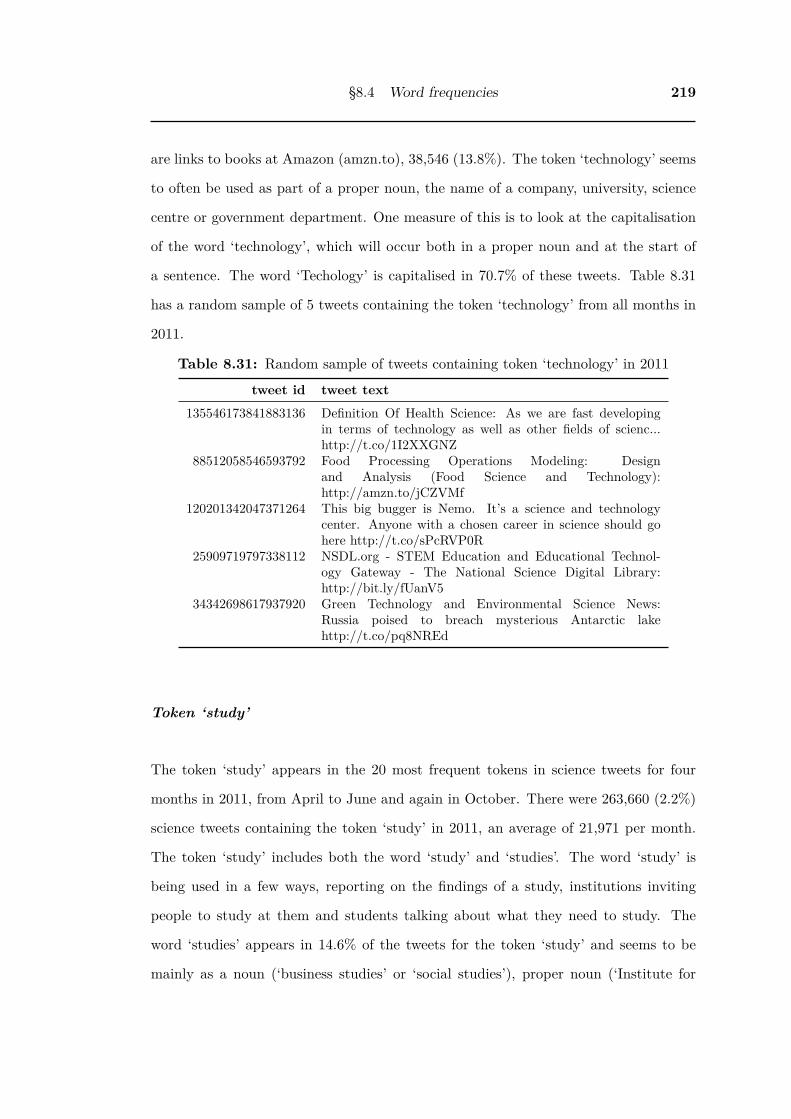
§8.4 Word frequencies 219
are links to books at Amazon (amzn.to), 38,546 (13.8%). The token ‘technology’ seems
to often be used as part of a proper noun, the name of a company, university, science
centre or government department. One measure of this is to look at the capitalisation
of the word ‘technology’, which will occur both in a proper noun and at the start of
a sentence. The word ‘Techology’ is capitalised in 70.7% of these tweets. Table 8.31
has a random sample of 5 tweets containing the token ‘technology’ from all months in
2011.
Table 8.31: Random sample of tweets containing token ‘technology’ in 2011
tweet id tweet text135546173841883136 Definition Of Health Science: As we are fast developing
in terms of technology as well as other fields of scienc...http://t.co/1I2XXGNZ
88512058546593792 Food Processing Operations Modeling: Designand Analysis (Food Science and Technology):http://amzn.to/jCZVMf
120201342047371264 This big bugger is Nemo. It’s a science and technologycenter. Anyone with a chosen career in science should gohere http://t.co/sPcRVP0R
25909719797338112 NSDL.org - STEM Education and Educational Technol-ogy Gateway - The National Science Digital Library:http://bit.ly/fUanV5
34342698617937920 Green Technology and Environmental Science News:Russia poised to breach mysterious Antarctic lakehttp://t.co/pq8NREd
Token ‘study’
The token ‘study’ appears in the 20 most frequent tokens in science tweets for four
months in 2011, from April to June and again in October. There were 263,660 (2.2%)
science tweets containing the token ‘study’ in 2011, an average of 21,971 per month.
The token ‘study’ includes both the word ‘study’ and ‘studies’. The word ‘study’ is
being used in a few ways, reporting on the findings of a study, institutions inviting
people to study at them and students talking about what they need to study. The
word ‘studies’ appears in 14.6% of the tweets for the token ‘study’ and seems to be
mainly as a noun (‘business studies’ or ‘social studies’), proper noun (‘Institute for

220 Word frequency and word co-occurence
Advanced Studies’), although it is also used as a plural as in ‘good studies of’, ‘proven
studies’, ‘case studies’. Table 8.32 has a random sample of 5 tweets containing the
token ‘study’ from all months in 2011.
Table 8.32: Random sample of tweets containing token ‘study’ in 2011
tweet id tweet text145992603035377664 physical science study guide. #nomegusta129827427697430529 okay. i shall now study Science while listening to Switch-
foot, Brooke Fraser and The Script. this is so fun!42799269371056128 TRYING TO study .. i haute science gosh.. Hope I
do well gonna go rest my brains! Yes brains not brainhttp://yfrog.com/gyjohshj
63359551285641216 Your Perception of Gravity Is All Relative, Study Finds(LiveScience.com) http://yhoo.it/j84m30 Science.alltop
79400308119314432 now watching waktu rehat and study science -.-
Token ‘exam’
The token ‘exam’ appears in the 20 most frequent tokens in science tweets only in June
2011. There are 158,348 (1.3%) science tweets that contain the token ‘exam’ in 2011,
an average of 13,195 per month. In June 2011, when it appears in the top 20 most
frequent tokens, there are 37,877 tweets with the token ‘exam’. Like the similar token
‘test’ in Section 8.4.3, this token appears to be mainly tweets sent by students. Another
similarity is that proportion of tweets with the word ‘science’ directly before the token
(‘exam’ or ‘test’) is nearly the same. Sixty three percent (99,585 tweets) of tweets with
token ‘exam’ contain the phrase ‘science exam’ and 61% of token ‘test’ tweets have the
phrase ‘science test’. Table 8.33 has a random sample of 5 tweets containing the token
‘exam’ from all months of 2011.
Token ‘series’
The token ‘series’ appears in the 20 most frequent tokens in science tweets only in
June and July 2011. There were 117,489 (1.0%) science tweets with the token ‘series’

§8.4 Word frequencies 221
Table 8.33: Random sample of tweets containing token ‘exam’ in 2011
tweet id tweet text152344169963196416 @MidnightSunSC17 SAME :( I have to prepare for my Sci-
ence Exams in January :L69487363176398848 @erupta remember when i had my science exam nd u said
i was gonna fail well FUCK U i just gt ma results i gottaB #SAYSUMFIN :-)
78051145079209984 History exam wasn’t too bad, still science exams to go, ohwell
65509529021988864 sooo imma fail the physical science exam tonight lol...i gotan A soooo I kinda dnt care lol
43561093930561536 Science exam is at 8:30am.... Why that early!?!?
in 2011, an average of 9,791 per month. This token shows a huge variation in the
number of tweets per month, ranging from 1,938 in February to 23,151 in July. The
average number of tweets for June and July is 22,306 while for the rest of the year it
is 7,288 tweets per month.
The usage of ‘series’ includes book series, tv, radio or podcast series, lecture series,
machine model series and time series. More than half of them look like links to books
with 47% (55,240) of the tweets with token ‘series’ having ‘amzn.to’ links and a further
35% (40,769) of them having ‘t.co’ links, many of which appear to refer to books. A lot
of these are probably what is called ‘link spam’, where people try to make money on
the referral commission that Amazon pays if a book is purchased by someone following
a link, as discussed in Section 8.4.2. Table 8.34 has a random sample of 5 tweets
containing the token ‘series’ from all months in 2011.
Token ‘people’
The token ‘people’ appears in the 20 most frequent tokens in science tweets only in
August 2011. There were 195,724 (1.6%) science tweets with the token ‘people’ in
2011, an average of 16,310 per month. This token has a wide variation in number of
tweets per month, although not as great as that for the previous token ‘series’. There
were 23,829 tweets in August, the only month the token is in the top 20, while the

222 Word frequency and word co-occurence
Table 8.34: Random sample of tweets containing token ‘series’ in 2011
tweet id tweet text89165752279629824 Early Experience and the Development of Competence
(Jossey Bass Social and Behavioral Science Series):http://amzn.to/lfx7Yc
134446408739729408 Who Needs Emotions?: The Brain Meets the Robot (Seriesin Affective Science): The idea that some day robots may... http://t.co/d01r1I5s
147572395916525569 So I just remembered science today. We were talking aboutthe hunger game series and how they all are 27 chapters. Iwas like ”maybe
91351863387099136 Words, Science and Learning (Developing Science andTechnology Education Series): http://amzn.to/jdLwns
146398525188612098 Diffusion in Materials (NATO Science Series E: (closed)):http://t.co/zkNZrLKp
lowest number was 9,855 in April. The average number of tweets per month excluding
August is 15,626. The abbreviation ‘ppl’ has been normalised to the token ‘people’ and
occurs in 18,739 (9.6%) of the tweets for this token. There does not appear to be any
difference between the tweets containing the token ‘people’ during August as compared
to the rest of the year. Table 8.35 has a random sample of 5 tweets containing the
token ‘people’ from all months 2011.
Table 8.35: Random sample of tweets containing token ‘people’ in 2011
tweet id tweet text91243737912578048 Smartphones May Strain Eyesight: According to the Jour-
nal of Optometry and Vision Science, people may holdtheir... http://bit.ly/nPCdFB
108288221447852032 @brianjameswalsh- I know you right-wing fanatics hatescience but are all you people also incapable of reading?http://t.co/rguneca
60836286482759682 Too lazy to learn #science? Not bothered about #truth?Want to feel superior to other people? You need #Religion.#Atheism
127357142293417984 RT @philoquotes: Man has to awaken to wonder - and soperhaps do peoples. Science is a way of sending him tosleep again. Wittgenstein ...
89656738382491648 RT @bengoldacre Amazon ban science book because itsideas upset some people? *If* true this is massive.http://t.co/u5jEGqr via @markgfh

§8.4 Word frequencies 223
Token ‘lol’
The token ‘lol’ appears in the 20 most frequent tokens in science tweets in September
and October 2011. This token is an abbreviation of ‘laugh out loud’. There were
257,301 (2.1%) science tweets containing the token ‘lol’ in 2011, an average of 21,442
per month. In November the token ‘lol’ is not in the 20 most frequent tokens, even
though that month has the most tweets per month containing the token ‘lol’ (31,079).
The topics of the tweets is very diverse and a mixture of positive and negative sentiment
about science. Table 8.36 has a random sample of 5 tweets containing the token ‘lol’
from all months of 2011.
Table 8.36: Random sample of tweets containing token ‘lol’ in 2011
tweet id tweet text82990602219831296 Not like that bro u know u a computer science major RT
@IM|_KONRAD: @loveleenae @FreakoSwava lol I’m not acomputer geek!
58146238633230337 @EpiphanyReality loool nopee! Prom is the least of myworries at the moment its all about maths nd science
40315362532659200 @_BooFTNoise lol study hard all week get wAt I needa outda way party Friday Saturday sleep Sunday got it down toa science ;P
111954268382179328 @FredGeorge94 ouch! I hate science lol weird... O.o144480510444453888 and @bridjet21 <3 lol @ndivirgilio24 RT @eosterhaus
When you try and study with non science majors and theycan’t even pronounce the words.
Token ‘bill’
The token ‘bill’ appears in the 20 most frequent tokens in science tweets only in October
2011. There are 100,363 (0.8%) science tweets with the token ‘bill’ in 2011, an average
of 8,364 per month. There were 14,506 tweets in October when the token ‘bill’ appears
in the top 20 most frequent tokens. The most tweets containing the token ‘bill’ was
18,058 in November, even though it was not in the top 20 most frequent tokens in
that month, and the least was 3,668 in January. Most of the tweets with the token
‘bill’ are about Bill Nye, an American science educator. Searching for ‘nye’ in the
224 Word frequency and word co-occurence
tweets containing the token ‘bill’ finds 80,370 tweets, which is 80.1% of the total tweets
containing the token ‘bill’. He is known as ‘Bill Nye the Science Guy’ which is the name
of an award-winning television series which he was writer, producer and host of from
1992 to 1998. He has produced many other television series and children’s books about
science. Most of the tweets about him are adults reflecting on having seen the original
shows (particularly remembering the theme song) and a few are people mentioning him
appearing as a commentator in the news or students watching shows by him in science
class. In March he is mentioned because he was a guest on CNN’s coverage of the
Japanese Fukushima reactor problems after the earthquake:
RT @waitinthevan: Guys. @CNN has brought in Bill Nye, the Science Guy
as an expert on this nuclear issue in Japan. Bill. Nye. SCIENCE GUY.
tweetid: 46773389473480704
and less flatteringly:
Bill Nye ”The Science Guy” is on CNN talking about the Japan reactor. I
thought Bill died in the late 90’s. Oh wait, that was his career.
tweetid: 46773732152320000
In the tweets with the token ‘bill’ which do not contain ‘nye’, there are many
different topics discussed; some are about legislature, some about money, some mention
other people like Bill Gates and Bill Bryson. Table 8.37 has a random sample of 5 tweets
containing the token ‘bill’ from all months in 2011.
Token ‘history’
The token ‘history’ only appears in the top 20 most frequent tokens in science tweets
for 2011 in October. There were 230,676 (1.9%) science tweets with the token ‘history’

§8.4 Word frequencies 225
Table 8.37: Random sample of tweets containing token ‘bill’ in 2011
tweet id tweet text109466223623929856 Jed Lowrie looks like a young Bill Nye the Science Guy...68117444945915904 #childhoodmemories watching Bill Nye The Science Guy120686792142880769 Bill nye the science guy135404450465591296 RT @90sgirlproblem: Everything I know about science I
learned from Bill Nye. #90sgirlsolutions35774395192451072 Etc: Science Guy Bill Nye on teaching evolution: ”The
main idea in all of biology is evo... http://nxy.in/ix8yg[ARS Science]
in 2011, an average of 19,223 per month. In October there were 34,708 science tweets
containing the token ‘history’.
The tweets for the token ‘history’ include the poem first mentioned in the discussion
of token ‘math’ Section 8.4.3 which also occurs in the tokens ‘love’ Section 8.4.3, and
‘art’ Section 8.4.3 because it has the line ‘In history, it’s a battle’. Searching on ‘battle’
finds 47,531 tweets with this poem. Searching for the phrase ‘in history’ finds 55,439
tweets in token ‘history’ which is 5,688 more than the 49,751 tweets found in the ‘math’
token tweets for the same search. These 5,688 tweets are not related to the poem, and
talk about other things ‘in history’. The high occurrence of this poem brings the token
‘history’ into the top 20 most frequent tokens in science tweets for October 2011.
Many of the tweets with token ‘history’ are student giving lists of which subjects
they are studying, with the list including another subject with the token ‘science’ like
‘science’, ‘social science’ or ‘political science’. Others are about the history of something
containing the ‘science’ keyword, this can include the school subjects just mentioned
and other things like the history of science fiction:
RT @lensassaman: Wondrous, detailed map of the history of science fiction
http://feedly.com/k/gvcZ7Q
tweetid: 45607700939288576
Table 8.38 has a random sample of 5 tweets containing the token ‘history’ from all
months in 2011.

226 Word frequency and word co-occurence
Table 8.38: Random sample of tweets containing token ‘history’ in 2011
tweet id tweet text144458476658233344 Why u think colin powell left from being secretary of state
nd condeleeza tuve cañete through study history or policialscience before speak
78170067573022720 I can’t remember what my tenth GCSE was. English Lit &Lang, Double Science, Maths, French, Italian, R.E., History- WHAT AM I MISSING?
77808147699478529 Revising for the history and science exams tomorrow :( xx122555768464609281 RT @SeanKingston: What is love? In math, its a problem.
In history, it’s a battle. In science, it’s a reaction. But inmy heart, its you.
49148652337381377 http://www.best-seller-books.com/history-of-science-antiquity-to-1700.html History of Science: Antiquity to1700
Token ‘know’
The token ‘know’ appears in the 20 most frequent tokens in science tweets only in
November 2011. There were 248,377 (2.0%) science tweets with the token ‘know’ in
2011, an average of 20,698 per month. In November there were 32,209 science tweets
with the token ‘know’. There does not appear to be any difference in the type of tweets
with the token ‘know’ in November compared to the rest of the year. The phrase ‘I
know’ was found in 53,237 (21.4%) of the science tweets with the token ‘know’, and
the phrase ‘don’t know’ occurred in 26,231 (10.6%) of them. Table 8.39 has a random
sample of 5 tweets containing the token ‘know’ from all months in 2011.
Table 8.39: Random sample of tweets containing token ‘know’ in 2011
tweet id tweet text133928989143212032 science is pretty scary, it makes me want to be dead, they
know too much.82341864946155520 Get to know Obama’s appointed science czar. You’ll be
surprised. Maybe not. http://t.co/xq5FN7D47102752702218240 Everything you wanted to know about the science and tech-
nique of making Parisian macarons. Recipes & more here:http://trunc.it/f5uru
86129588991836161 This chick herre nigga, this chick herre nigga @amburgerr_know #whatmakesablackguymad ...she got it down to ascience
129805151044239360 @whyhellothere_ I know. I miss science from last year haha:)

§8.4 Word frequencies 227
Token ‘project’
The token ‘project’ appears in the 20 most frequent tokens in science tweets in both
November and December 2011. There were 220,918 (1.8 %) of science tweets with the
token ‘project’ in 2011, an average of 18,410 tweets per month. There were 31,282
science tweets in November and 31,599 in December with the token ‘project’. Student
science projects seem to be the main topic being discussed in these tweets. In 2011 there
were 123,738 (56.0%) science tweets with token ‘project’ that had the phrase ‘science
project’ and a further 38,719 (17.5%) that had the phrase ‘science fair project’, and
7,085 (0.3%) that had the phrase ‘science fair’ not followed immediately by ‘project’.
Table 8.40 has a random sample of 5 tweets containing the token ‘project’ from all
months of 2011.
Table 8.40: Random sample of tweets containing token ‘project’ in 2011
tweet id tweet text116218982977114112 @maria_paps No and your science project is due on october
5th :)88695199462731776 @AstronomyCast I hae to cute science, but mismanagement
seems to be SOP with this project. Ho to fund but alsoclean up the mess?
63295522227761152 My second grader has a Science project on Friday so I or-dered her tri-fold, some supplies and snacks from Staplesfree shipping, no FL heat!
138713990204370944 chillin out lookin over my project for my presenttation to-day in science. wish me luck :)
39439943189270528 Helping my little brother out with his science project...
Token ‘book’
The token ‘book’ appears in the 20 most frequent tokens in science tweets only in
December 2011. There are 224,006 (1.8%) science tweets with the token ‘book’, an
average of 18,667 tweets per month. There were 30,293 tweets in December containing
the token ‘book’. There is a wide range of topics in the tweets containing the token
‘book’; book reviews, book recommendations, describing people as having ‘written a
book’ and students mentioning that it’s the first time they have opened their text book.

228 Word frequency and word co-occurence
There was no obvious difference between the topics in December when the token ‘book’
was in the top 20 most frequent tokens and the topics in the rest of the year. Table 8.41
has a random sample of 5 tweets containing the token ‘book’ from all months in 2011.
Table 8.41: Random sample of tweets containing token ‘book’ in 2011
tweet id tweet text52717476949131265 in the 8th grade, i threw a science book at some kid’s eye
because he talked about my momma134991192499818496 The Rough Guide to the Future by Jon Turney – re-
view | Royal Society science book prize: A meticulo...http://t.co/9Cr1vFyM #books #read
90955082035765249 Opportunities in Forensic Science: Each book offers: Thelatest information on a field ofinterest Training and e...http://bit.ly/nncuk8
142656954060386304 RT @p8riot: @brandondarby I recently examined a 1904Book loaded with Eugenic ”science” people like Sanger be-lieved in. Disturbing. http ...
142372127671193600 Downloads CSL ’89 Computer Science Logic 3 conf e-book:CSL ’89 Computer Science Logic 3 conf book downloadEgon... http://t.co/qfczWmsp
8.4.4 Conclusions about single word frequency
By looking at the most frequent tokens used in tweets containing the word ‘science’ I
can now provide some insight into them:
The short form posting of Twitter encourages people to report on what they are
doing at the time, and so it is not surprising that many of the tweets containing
‘science’ also contain the token ‘day’. The token ‘year’ appears in the top 20 tokens
per month in December and January, possibly because this is around the end of the
year, although this was not clear from the sampled tweets. It also appears in the top
20 in July, and this seems to be due to a variations on a single tweet using the ironic
tag ‘#blamethemuslims’ shown in Section 8.4.3 which contains the word ‘years’. The
token ‘time’ only appear in the most frequent 20 tokens in August and November but
there was not any clear difference between these tweets and those with ‘time’ in other
months, and the range of topics covered was very diverse.

§8.4 Word frequencies 229
The token ‘new’ is in the top 20 throughout the year which suggests a relation
between science and newness, although the ‘new’ thing referred to is often not the
science. It is unknown how this compares to the overall usage of ‘new’ on Twitter.
Google hosting the first international ‘science fair’ brought the token ‘fair’ into the
most frequent 20 tokens in January.
Many of the top 20 most frequent tokens in tweets containing ‘science’ are related
to school and most of the tweets using these tokens appear to be sent by school stu-
dents. These include the tokens ‘math’, ‘class’, ‘teacher’, ‘school’, ‘computer’, ‘history’,
‘project’, ‘test’ and ‘exam’. As well as being used by school students, the tokens ‘class’
and ‘school’ are used to some extent by adults discussing their experiences in school,
and the token ‘school’ is also used in talking about University.
The token ‘computer’ is most often used in tweets about university level computer
science and in links to computer science books on Amazon.
The tokens ‘test’ and ‘exam’ are used in very similar ways. Sixty one percent of the
tweets with the token ‘test’ contain the phrase ‘science test’ while 63% of tweets with
the token ‘exam’ contain the phrase ‘science exam’. The token ‘project’ only appear
in the top 20 most frequent tokens in November and December. Of science tweets
containing the token ‘project’ during 2011, 73.8% have the phrases ‘science project’ or
‘science fair’.
The tokens ‘math’, ‘history’ and ‘love’ all contain a significant number of tweets
based on the poem giving in Section 8.4.3. The token ‘art’ is mainly used in tweets
that contrast art and science, but also contains a number of examples of tweets about
this poem. There are less than for the other words because the poem is often truncated
before the line containing the word ‘art’.
Although the token ‘study’ is often used by students discussing what they are
studying, it is also used to refer to scientific studies, institutions inviting people to
study at them and to the names of institutions such as ‘Institute for Advanced Studies’.
230 Word frequency and word co-occurence
The token ‘fiction’ is almost exclusively used discussing science fiction, and was one
of the most common words, appearing in 3.2% of the science tweets in 2011.
Like the token ‘fiction’, the token ‘technology’ is mainly used in a phrase containing
the word ‘science’, in this case either ‘science and technology’ or to a lesser extent
‘technology and science’. It is usually capitalised, indicating that it is being used as a
proper noun, naming courses and places of study, research or science centers.
The token ‘series’ appears to have been pushed into the top 20 most frequent tokens
during June and July by links to Amazon books and occurred at a very low rate for
the rest of the year. These links were probably automatically generated and stopped
after Twitter detected and blocked them.
The token ‘news’ is mainly used in tweets discussing news organisations or by news
organisations.
The token ‘bill’ mostly occurs in tweets referring to the science educator Bill Nye
and is only in the most frequent tokens in October 2011.
The related tokens ‘get’ and ‘got’, although appearing in the top 20 most frequent
tokens per month in 2011 are used in a very diverse way and so should probably be
added to the stopwords list. The token ‘one’ also does not seem to help in understanding
the topics of the tweets that contain it and so should be added to the stopwords list,
perhaps along with the other words for numbers.
The token ‘good’ appeared to be mostly associated with positive sentiment while
the token ‘lol’ (laugh out loud) has a mixture of positive and negative sentiment about
science. As with ‘get’, ‘got’ and ‘one’ they do not help in understanding the topic of
the tweet in most cases, but may be useful for sentiment analysis.
The token ‘know’ has the phrase ‘I know’ at twice the rate of the phrase ‘don’t
know’ (21.4% and 10.4% of science tweets with the token ‘know’ respectively). It only

§8.5 Word co-occurrence 231
occurs in the top 20 most frequent tokens in November although there does not appear
to be any difference in the topics of the tweets containing it from the rest of the year.
The token ‘people’ only occurs in the top 20 during July, and even then there is a
very diverse range of topics discussed in tweets containing this token.
The token ‘book’ only appears in the top 20 most frequent tokens in December, has
a diverse range of topics about reading books, using books and writing books. There is
not any obvious difference between the topics covered in tweets with this token during
December and the rest of the year.
Although single word frequency has given some insight into how the word science
is being used, on such a large dataset the number of most frequent tokens that can
be looked at compared to the total number of tokens limits the usefulness of this
approach. The arbitrary limit used here of looking at the top 20 most frequent tokens
per month out of 2.7 million tokens means that many words that may be more useful in
understanding how the word science is being used have been ignored. The appearance
of so many school related topics in the top 20 tokens does show that school students
send a lot of the tweets about ‘science’ and to a lesser extent university students and
people reminiscing about school.
While looking at individual word frequencies, many of the more interesting findings
involved a pair of words or a phrase. In the next section I build on this by looking for the
most frequent co-occurring words to see how they can help develop our understanding
of how the word science is being used.
8.5 Word co-occurrence
By looking at pairs of words instead of single words we start to capture some of the
patterns of usage of words, or grammar, without actually needing to know anything

232 Word frequency and word co-occurence
about grammar. The Python NLTK toolkit does provide tools for working with gram-
mar (such as part of text classifiers) but these may not work well with the informal and
brief text used in tweets. Pairs of words (bigrams) can be extended to consider more
words that occur together, known as n-grams. Just looking at the frequency of n-grams
will tend to give similar results to word frequency, because very frequent words will
also tend to occur together in the same text. This can be overcome by looking at the
frequency with which the words occur together compared the frequency that they are
not together. A number of different association measures are described by Manning
and Schütze (1999) such as t-test, Pearson’s chi-square test and likelihood ratio. Bi-
grams found using these comparative frequency approaches instead of raw frequency
are more likely to be a collocation, “an expression consisting of two or more words that
correspond to some conventional way of saying things.” (Manning & Schütze, 1999,
p. 141). The strict linguistic definition of a collocation also requires that the definition
of the meaning of a collocation is different from the definitions of the individual words
in that collocation. Manning and Schütze (1999) use the concept of compositionality
to define collocations;
“Collocations are characterized by limited compositionality. We call a nat-
ural language expression compositional if the meaning of the expression
can be predicted from the meaning of the parts. Collocations are not fully
compositional in that there is usually an element of meaning added to the
combination.” (Manning & Schütze, 1999, p. 141)
Examples of collocations which show this limited compositionality are “strong tea” and
the idiom “kick the bucket” (Manning & Schütze, 1999, p. 141). The common English
meaning of the collocation ‘kick the bucket’ is to die, not the compositional meaning,
to literally kick a bucket.
In order to compare the bigrams found using raw frequency to those found using a
measure of the co-dependence of the words in the bigram, I have chosen the likelihood

§8.5 Word co-occurrence 233
ratio because Manning and Schütze (1999) recommend that the “likelihood ratio test
is in general more appropriate than Pearson’s χ2 for collocation discovery” (Manning
& Schütze, 1999, p. 164).
8.5.1 Bigrams by raw frequency
The top 70 bigrams sorted by raw frequency are given in Table 8.42. As expected
when using raw frequency to select the most frequent bigrams, most of these bigrams
include words that occurred in the most frequent words in 2011; for 33 of them both
words in the bigram appear in the top 20 most frequent words each month of 2011 and
another 36 have one most frequent word, only one bigram has both words not in the
most frequent words - ‘climate change’. I have used emphasis to highlight the words
in the bigrams in Table 8.42 that are not in the most frequent words. Because the
dataset was collected using the word ‘science’, all but 10 of the top bigrams by raw
frequency include the word ‘science’ or ‘#science’. The ones which do not are: ‘t.co
via’, ‘bill nye’, ‘history battle’, ‘problem history’, ‘love math’, ‘got ta’, ‘math problem’,
‘climate change’, ‘fair project’ and ‘high school’. Four of these, ‘history battle’, ‘problem
history’, ‘love math’ and ‘math problem’ show the effect of the popularity of retweeting
the poem on Page 204. Two of the most frequent bigrams containing the word science
are also probably a result of this poem; ‘battle science’ and ‘science reaction’, and they
have very similar raw frequency to the other bigrams from the poem.

234 Word frequency and word co-occurence
Table 8.42: Top 70 Bigrams sorted by raw frequency
Bigram Score Bigram Scorescience fiction 0.00308 #science #news 0.000525science t.co 0.0023 new science 0.000489computer science 0.00229 science book 0.000487science class 0.00194 science museum 0.000478science teacher 0.00167 love science 0.000464math science 0.00159 environmental science 0.000464rocket science 0.00152 science engineering 0.000463t.co via 0.00147 physical science 0.000456science technology 0.00142 study science 0.000452science fair 0.00139 got science 0.000451science test 0.00122 day science 0.000449political science 0.00109 sport science 0.000429art science 0.00103 forensic science 0.000416science project 0.00102 science day 0.000404christian science 0.00102 science faith 0.000392science monitor 0.000871 health science 0.000382science amzn.to 0.000859 science experiment 0.00038science exam 0.000787 science art 0.000367science bit.ly 0.000767 popular science 0.000366t.co #science 0.00076 history battle 0.000362bit.ly #science 0.000754 battle science 0.000362science math 0.000742 science reaction 0.000358science lab 0.000725 problem history 0.000355science center 0.000698 love math 0.000353bill nye 0.000635 science channel 0.000352science guy 0.000625 got ta 0.000352earth science 0.000611 science education 0.000351social science 0.000611 math problem 0.000347science homework 0.000606 climate change 0.000346science behind 0.000599 science history 0.00034like science 0.000587 school science 0.000334hate science 0.000585 science series 0.000328life science 0.000558 fair project 0.000325science news 0.000544 weird science 0.00032nye science 0.00053 high school 0.000313Note: emphasis indicates the words in the bigrams that are not in the most frequent words.
8.5.2 Bigrams by likelihood ratio
Table 8.43 has the Top 70 Bigrams sorted by the likelihood ratio score described above.
This brings up words that are less frequent overall, but very likely to appear together
as a bigram. Comparing the two sets of bigrams, there are 33 bigrams that appear in
the top 70 by raw frequency that are not in the top 70 by likelihood ratio and these

§8.5 Word co-occurrence 235
all contain the most frequent word, ‘science’, as shown in Table 8.44.
Table 8.43: Top 70 Bigrams sorted by likelihood ratio (Scores bigrams using likeli-hood ratios as in Manning and Schutze 5.3.4)
Bigram Score Bigram Scorescience fiction 3.48e+06 social medium 5.68e+05bill nye 2.24e+06 newly tagged 5.64e+05computer science 2.24e+06 stop believing 5.61e+05t.co via 2.13e+06 believing magic 5.6e+05rocket science 1.7e+06 science exam 5.48e+05science fair 1.51e+06 lecture note 5.36e+05science class 1.39e+06 science lab 5.25e+05science teacher 1.29e+06 getting rich 5.19e+05#science #news 1.16e+06 science behind 5.06e+05political science 1.13e+06 art science 5.05e+05history battle 1.1e+06 love math 5.04e+05christian science 1.08e+06 idea considered 5.04e+05got ta 1.05e+06 bbc news 5.02e+05science technology 1.04e+06 every original 5.01e+05climate change 1.02e+06 original idea 4.96e+05science monitor 1.02e+06 year old 4.95e+05problem history 9.15e+05 nye science 4.94e+05rt science 8.57e+05 @heavyd never 4.9e+05via @addthis 8.43e+05 big bang 4.75e+05science test 8.12e+05 @1nf1d3lc4str0 #blamethemuslims 4.61e+05t.co science 8.09e+05 test tomorrow 4.45e+05global warming 7.97e+05 forensic science 4.37e+05high school 7.51e+05 science guy 4.36e+05bit.ly #science 7.4e+05 science homework 4.33e+05share friend 7.37e+05 physical science 4.32e+05math problem 7.28e+05 wish luck 4.31e+05reaction heart 7.15e+05 insanity first 4.28e+05fiction fantasy 7.06e+05 albert einstein 4.24e+05fair project 6.71e+05 look like 4.23e+05science project 6.56e+05 new york 4.21e+05math science 6.54e+05 environmental science 4.16e+05considered insanity 6.33e+05 t.co #science 4.14e+05weight loss 6.15e+05 never stop 4.1e+05science rt 6.05e+05 @youtube video 4.08e+05science center 5.85e+05 #blamethemuslims advance 3.97e+05
Table 8.45 shows the 37 bigrams that appear in both the top 70 by likelihood and
by raw frequency. There are 10 bigrams in this group that do not contain the word
‘science’ and they are the same 10 that did not contain ‘science’ in the top 70 by raw
frequency. The table is sorted by the raw frequency score and looking at the likelihood
ratio score we can see that some of the bigrams are in a very different order when ranked

236 Word frequency and word co-occurence
Table 8.44: Bigrams appearing in raw frequency but not in likelihood ratio top 70(by raw frequency)
Bigram F Bigram FScore Score
science t.co 0.002300 day science 0.000449science amzn.to 0.000859 sport science 0.000429science bit.ly 0.000767 science day 0.000404science math 0.000742 science faith 0.000392earth science 0.000611 health science 0.000382social science 0.000611 science experiment 0.000380like science 0.000587 science art 0.000367hate science 0.000585 popular science 0.000366life science 0.000558 battle science 0.000362science news 0.000544 science reaction 0.000358new science 0.000489 science channel 0.000352science book 0.000487 science education 0.000351science museum 0.000478 science history 0.000340love science 0.000464 school science 0.000334science engineering 0.000463 science series 0.000328study science 0.000452 weird science 0.000320got science 0.000451
by likelihood ratio, with ‘science fiction’ still in the first position but ‘bill nye’ ranked
equal second with ‘computer science’. The changes in rank between the two scoring
methods can be seen more clearly in Fig. 8.7, which has these 37 bigrams with the raw
frequency ranking of the bigrams of the left side and the likelihood ratio ranking of the
bigrams on the right side. The bigrams are ordered from most common at the top and
least common at the bottom in each case. The lines between the bigrams on each side
make it easy to see which bigrams have moved up the ranking and which have moved
down. The colours of the lines do not indicate anything, and are just used to make it
easier to follow the lines where they cross each other. Where two bigrams are equally
ranked they are shown on the same line with a blank line below them.
It should be noted that the ranking does not give any indication of how large the
raw frequency or likelihood ratio gaps are between the ranked bigrams. In Table 8.45 it
can be seen that the bigrams have a very large variation in raw frequency ranging from
‘science fiction’ at 0.00308 through to ‘high school’ at 0.000313, an order of magnitude
less frequent. The same wide range is still visible in the likelihood ratio with ‘science

§8.5 Word co-occurrence 237
Table 8.45: Bigrams appearing in both likelihood ratio and raw frequency top 70
Bigram F LH Bigram F LHScore Score Score Score
science fiction 0.003080 3.48e+06 science center 0.000698 5.85e+05computer science 0.002290 2.24e+06 bill nye 0.000635 2.24e+06science class 0.001940 1.39e+06 science guy 0.000625 4.36e+05science teacher 0.001670 1.29e+06 science homework 0.000606 4.33e+05math science 0.001590 6.54e+05 science behind 0.000599 5.06e+05rocket science 0.001520 1.70e+06 nye science 0.000530 4.94e+05t.co via 0.001470 2.13e+06 #science #news 0.000525 1.16e+06science technology 0.001420 1.04e+06 environmental science 0.000464 4.16e+05science fair 0.001390 1.51e+06 physical science 0.000456 4.32e+05science test 0.001220 8.12e+05 forensic science 0.000416 4.37e+05political science 0.001090 1.13e+06 history battle 0.000362 1.10e+06art science 0.001030 5.05e+05 problem history 0.000355 9.15e+05science project 0.001020 6.56e+05 love math 0.000353 5.04e+05christian science 0.001020 1.08e+06 got ta 0.000352 1.05e+06science monitor 0.000871 1.02e+06 math problem 0.000347 7.28e+05science exam 0.000787 5.48e+05 climate change 0.000346 1.02e+06t.co #science 0.000760 4.14e+05 fair project 0.000325 6.71e+05bit.ly #science 0.000754 7.40e+05 high school 0.000313 7.51e+05science lab 0.000725 5.25e+05
fiction’ at 3.48e+06 and ‘t.co #science’ at 4.14e+05, again almost an order of magnitude
different.
The changes in rank shown on Fig. 8.7 are summarised in Table 8.46. Only three
bigrams stay at the same rank, ‘science fiction’ at the top, ‘computer science’ second
and ‘science monitor’ in the middle. Five move up slightly (up to 3 positions) when
ranked by likelihood ratio; ‘t.co via’, ‘science fair’, ‘political science’, ‘christian science’
and ‘love math’ but only two, ‘bit.ly #science’ and ‘forensic science’, move down slightly
(2 and 3 positions respectively). Three others move down 4 positions; ‘science class’,
‘science teacher’ and ‘science behind’. There are nine bigrams that move up 13 or
more positions; ‘bill nye’, ‘#science #news’, ‘history battle’, ‘problem history’, ‘got
ta’, ‘math problem’, ‘climate change’, ‘fair project’ and ‘high school’ and 14 that move
down between 5 and 19 positions; ‘science technology’, ‘science test’, ‘science project’,
‘math science’, ‘science centre’, ‘science exam’, ‘science lab’, ‘art science’, ‘nye science’,
‘science guy’, ‘science homework’, ‘physical science’, ‘environmental science’ and ‘t.co

238 Word frequency and word co-occurence
#science’.
rawfrequency
likelihoodratio
high school
fair project
climate change
math problem
got ta
love math
problem history
history battle
forensic science
physical science
environmental science
hashtag-science hashtag-news
nye science
science behind
science homework
science guy
bill nye
science center
science lab
bit.ly hashtag-science
t.co hashtag-science
science exam
science monitor
science project & christian science
art science
political science
science test
science fair
science technology
t.co via
rocket science
math science
science teacher
science class
computer science
science fiction
t.co hashtag-science
environmental science
physical science
science homework
science guy
forensic science
nye science
love math
art science
science behind
science lab
science exam
science center
math science
science project
fair project
math problem
bit.ly hashtag-science
high school
science test
problem history
science monitor & climate change
science technology
got ta
christian science
history battle
political science
hashtag-science hashtag-news
science teacher
science class
science fair
rocket science
t.co via
computer science & bill nye
science fiction
Figure 8.7: Change in ranking of bigrams appearing in both raw frequency and like-lihood ratio top 70. Note: gaps appear where bigrams of equal weighthave been shown on the line above.
Although these changes illustrate the decrease of the effect of the most common
word ‘science’ on the ranking of the bigrams by likelihood ratio, it is not clear that
the improved ranking of the bigrams that appear in both raw frequency and likelihood
ratio helps with understanding how the word science is being used.

§8.5 Word co-occurrence 239
Table 8.46: Change in ranking of bigrams appearing in both likelihood ratio and rawfrequency top 70.
∆ Rank Bigrams-20 ‘t.co #science’-19 ‘math science’-17 ‘art science’-11 ‘science guy’, ‘science homework’-10 ‘science project’, ‘science exam’-9 ‘environmental science’-8 ‘science test’, ‘science lab’-7 ‘physical science’-6 ‘science technology’, ‘nye science’-5 ‘science center’-4 ‘science class’, ‘science teacher’, ‘science behind’-3 ‘forensic science’-2 ‘bit.ly #science’no change ‘science fiction’, ‘computer science’, ‘science monitor’+1 ‘rocket science’, ‘political science’, ‘christian science’+2 ‘love math’+3 ‘t.co via’, ‘science fair’+13 ‘math problem’+14 ‘problem history’, ‘fair project’+17 ‘#science #news’+18 ‘high school’+19 ‘bill nye’, ‘history battle’+20 ‘got ta’, ‘climate change’
There are also 33 bigrams that appear in the top 70 by likelihood ratio that were
not in the top 70 by raw frequency and these are shown in Table 8.47. Only three of
these bigrams contain the word science. This is where the improvement in gaining an
understanding of how people are using the word science though using bigrams selected
by likelihood ratio rather than raw frequency can be seen. The bigrams that include
twitter meta information like retweet attribution (‘rt’, ‘via’) or links (‘t.co’) tell us
that a lot of the tweets are people sharing information or links, but does not tell us
anything about their understanding of the word ‘science’. The appearance of twitter
user in the top bigrams is surprising. The bigram ‘@1nf1d3lc4str0 #blamethemuslims’
indicates that a lot of the tweets with the ironic hashtag ‘#blamethemuslims’ must also
include the username ‘@1nf1d3lc4str0’ (which translates to ‘Infidel Castro’ from ‘leet-
speak’). As discussed in Section 8.4.3 (Page 209) the high number of tweets containing
‘#blamethemuslims’ were probably responsible for token ‘year’ appearing in the top

240 Word frequency and word co-occurence
20 tokens per month in July 2011.
Another twitter user, @youtube, appears automatically in links shared from youtube
to twitter and so the bigram ‘@youtube video’ appears frequently. Another user,
@heavyd, appears in the bigram ‘@heavyd never’. This is the Twitter username of the
rapper Heavy D and is due to many people retweeting a tweet from him as a memorial
after he died on November 8, 2011.
@heavyd: Never stop believing.. Magic is just science we don’t understand..
Every original idea was considered insanity at first..
As with the most frequent words, some bigrams appear to relate to school and ed-
ucation - ‘lecture note’, ‘test tomorrow’, ‘wish luck’ and ‘albert einstein’. The bigrams
‘idea considered’, ‘original idea’, ‘every original’ suggest an association of science with
ideas. Others suggest a juxtaposition of belief and science; ‘stop believing’, ‘believing
magic’. Or madness; ‘considered insanity’, ‘insanity first’. Other bigrams are recog-
nisable as topics; ‘global warming’, ‘weight loss’, ‘fiction fantasy’ (probably as part of
‘science fiction fantasy’ trigram) and ‘getting rich’. The ‘bbc news’ bigram suggests
that BBC News sends a lot of tweets about science, or people link to BBC News articles
about science. A more detailed understanding of these can be gained by sampling the
individual tweets that contain them as I have done below in Section 8.5.4.
8.5.3 Bigrams by likelihood ratio with window size of 3
I investigated extending the likelihood ratio approach by using a window size of 3
to allow a single word to appear between the words making up the bigram. This is
much slower to compute because it doubles the number of bigrams to be considered.
The results are shown in Table 8.48. There is less difference between the results of
likelihood ratio and of likelihood ratio with window size of 3 than there was between

§8.5 Word co-occurrence 241
Table 8.47: Bigrams appearing in likelihood ratio but not in raw frequency top 70
Bigram Score Bigram Scorert science 8.57e+05 bbc news 5.02e+05via @addthis 8.43e+05 every original 5.01e+05t.co science 8.09e+05 original idea 4.96e+05global warming 7.97e+05 year old 4.95e+05share friend 7.37e+05 @heavyd never 4.90e+05reaction heart 7.15e+05 big bang 4.75e+05fiction fantasy 7.06e+05 @1nf1d3lc4str0 #blamethemuslims 4.61e+05considered insanity 6.33e+05 test tomorrow 4.45e+05weight loss 6.15e+05 wish luck 4.31e+05science rt 6.05e+05 insanity first 4.28e+05social medium 5.68e+05 albert einstein 4.24e+05newly tagged 5.64e+05 look like 4.23e+05stop believing 5.61e+05 new york 4.21e+05believing magic 5.60e+05 never stop 4.10e+05lecture note 5.36e+05 @youtube video 4.08e+05getting rich 5.19e+05 #blamethemuslims advance 3.97e+05idea considered 5.04e+05
the raw frequency and likelihood ratio. There are 52 bigrams that are common between
the top 70 by likelihood ratio and likelihood ratio with window size 3 (Table 8.49) and
18 bigrams that are unique to each (Table 8.50 and Table 8.51). The new bigrams
in Table 8.51 found by using the window size of 3 for likelihood ratio do not appear
particularly informative. There are 4 bigrams that appear in the top 70 by LR window
3 and in original raw freq but not in the top 70 by likelihood ratio (Table 8.52).
Using a window also introduces a problem of finding bigrams across the boundaries
between tweets which is not valid with this dataset as although the tweets are in the
time sequence order by when they were sent it is unlikely that any two consecutive
tweets are part of the same conversation.

242 Word frequency and word co-occurence
Table 8.48: Top 70 Bigrams sorted by likelihood ratio, with window size of 3
Bigram Score Bigram Scorescience fiction 3.54e+06 high school 7.56e+05christian monitor 3.25e+06 fiction fantasy 7.53e+05computer science 2.34e+06 share friend 7.39e+05bill nye 2.25e+06 art science 7.26e+05t.co via 2.17e+06 fair project 7.17e+05nye guy 1.74e+06 science exam 6.96e+05rocket science 1.72e+06 wired wired.com 6.91e+05science class 1.62e+06 science center 6.66e+05science fair 1.58e+06 considered insanity 6.33e+05science teacher 1.51e+06 weight loss 6.16e+05battle reaction 1.42e+06 original considered 6.16e+05science t.co 1.32e+06 science lab 5.88e+05t.co rt 1.28e+06 social medium 5.71e+05problem battle 1.26e+06 newly tagged 5.64e+05#science #news 1.26e+06 stop believing 5.61e+05science project 1.24e+06 believing magic 5.6e+05science technology 1.24e+06 science behind 5.51e+05political science 1.18e+06 love math 5.45e+05christian science 1.12e+06 nato series 5.38e+05history battle 1.11e+06 lecture note 5.37e+05got ta 1.06e+06 @heavyd stop 5.33e+05math science 1.05e+06 nye science 5.24e+05reaction heart 1.03e+06 getting rich 5.19e+05climate change 1.03e+06 idea insanity 5.13e+05science monitor 1.03e+06 bbc news 5.1e+05science test 1.02e+06 hate science 5.05e+05science amzn.to 1.01e+06 wish luck 5.05e+05bit.ly #science 1e+06 science homework 5.05e+05t.co #science 9.43e+05 idea considered 5.04e+05math history 9.22e+05 never believing 5.03e+05problem history 9.19e+05 every original 5.01e+05love problem 8.47e+05 year old 4.97e+05via @addthis 8.44e+05 original idea 4.96e+05math problem 8.01e+05 earth science 4.92e+05global warming 7.97e+05 understand original 4.91e+05

§8.5 Word co-occurrence 243
Table 8.49: Bigrams in both likelihood ratio & likelihood ratio with window size of 3
Bigram LR LRW3 Bigram LR LRW3Score Score Score Score
science fiction 3.48e+06 3.54e+06 problem history 9.15e+05 9.19e+05computer science 2.24e+06 2.34e+06 love math 5.04e+05 5.45e+05science class 1.39e+06 1.62e+06 got ta 1.05e+06 1.06e+06science teacher 1.29e+06 1.51e+06 math problem 7.28e+05 8.01e+05math science 6.54e+05 1.05e+06 climate change 1.02e+06 1.03e+06rocket science 1.70e+06 1.72e+06 fair project 6.71e+05 7.17e+05t.co via 2.13e+06 2.17e+06 high school 7.51e+05 7.56e+05science technology 1.04e+06 1.24e+06 via @addthis 8.43e+05 8.44e+05science fair 1.51e+06 1.58e+06 global warming 7.97e+05 7.97e+05science test 8.12e+05 1.02e+06 share friend 7.37e+05 7.39e+05political science 1.13e+06 1.18e+06 reaction heart 7.15e+05 1.03e+06art science 5.05e+05 7.26e+05 fiction fantasy 7.06e+05 7.53e+05science project 6.56e+05 1.24e+06 considered insanity 6.33e+05 6.33e+05christian science 1.08e+06 1.12e+06 weight loss 6.15e+05 6.16e+05science monitor 1.02e+06 1.03e+06 social medium 5.68e+05 5.71e+05science exam 5.48e+05 6.96e+05 newly tagged 5.64e+05 5.64e+05t.co #science 4.14e+05 9.43e+05 stop believing 5.61e+05 5.61e+05bit.ly #science 7.40e+05 1.00e+06 believing magic 5.60e+05 5.60e+05science lab 5.25e+05 5.88e+05 lecture note 5.36e+05 5.37e+05science center 5.85e+05 6.66e+05 getting rich 5.19e+05 5.19e+05bill nye 2.24e+06 2.25e+06 idea considered 5.04e+05 5.04e+05science homework 4.33e+05 5.05e+05 bbc news 5.02e+05 5.10e+05science behind 5.06e+05 5.51e+05 every original 5.01e+05 5.01e+05nye science 4.94e+05 5.24e+05 original idea 4.96e+05 4.96e+05#science #news 1.16e+06 1.26e+06 year old 4.95e+05 4.97e+05history battle 1.10e+06 1.11e+06 wish luck 4.31e+05 5.05e+05

244 Word frequency and word co-occurence
Table 8.50: Bigrams in likelihood ratio but not in likelihood ratio with window sizeof 3
Bigram LR Scorescience guy 4.36e+05environmental science 4.16e+05physical science 4.32e+05forensic science 4.37e+05rt science 8.57e+05t.co science 8.09e+05science rt 6.05e+05@heavyd never 4.90e+05big bang 4.75e+05@1nf1d3lc4str0 #blamethemuslims 4.61e+05test tomorrow 4.45e+05insanity first 4.28e+05albert einstein 4.24e+05look like 4.23e+05new york 4.21e+05never stop 4.10e+05@youtube video 4.08e+05#blamethemuslims advance 3.97e+05
Table 8.51: Bigrams in likelihood ratio but not in likelihood ratio with window sizeof 3
Bigram LRW3 Score Bigram LRW3 Scorescience t.co 1.32e+06 math history 9.22e+05science amzn.to 1.01e+06 love problem 8.47e+05earth science 4.92e+05 wired wired.com 6.91e+05hate science 5.05e+05 original considered 6.16e+05christian monitor 3.25e+06 nato series 5.38e+05nye guy 1.74e+06 @heavyd stop 5.33e+05battle reaction 1.42e+06 idea insanity 5.13e+05t.co rt 1.28e+06 never believing 5.03e+05problem battle 1.26e+06 understand original 4.91e+00
Table 8.52: Bigrams in both likelihood ratio with window size of 3 and in raw fre-quency
Bigram Raw Freq Score LRW3 Scorescience t.co 0.002300 1.32e+06science amzn.to 0.000859 1.01e+06earth science 0.000611 4.92e+05hate science 0.000585 5.05e+05

§8.5 Word co-occurrence 245
8.5.4 Sample tweets for top 70 likelihood ratio bigrams
In this section I look at a random sample of five tweets for each of the top 70 bigrams by
likelihood ratio in 2011. The bigrams are considered in their rank order by likelihood
ratio except where I have grouped later bigrams with the most frequently occurring
one (highest ranked) on the same or similar topic. As discussed in the introduction
to Section 8.5 (Page 231), the likelihood ratio is the likelihood that the pair of words
appears in the bigram, divided by the likelihood that they appear separately. Unlike
the raw frequency ranking, some of the top bigrams by likelihood ratio ranking may
only occur in a relatively small number of tweets, if the words in the bigram do not
appear separately.
Bigrams ‘science fiction’ and ‘fiction fantasy’
The most frequent bigram by Likelihood ratio is ‘science fiction’ and it occurs in 3.06%
of the 2011 ‘science’ tweets (374,165). As the word used to collect the tweets, the token
‘science’ was in the top 20 tokens in every month of 2011. As discussed in Section 8.4.3
(Page 206) the individual token ‘fiction’ also appeared in the top 20 tokens in every
month and most of the tweets sampled for the individual token ‘fiction’ contained a
variation on the bigram ‘science fiction’. The number of tweets per month containing
the bigram ‘science fiction’ was fairly consistent through the year, apart from April
where the data outages means that there is less than a full month collected. Table 8.53
has a random sample of 5 tweets containing the bigram ‘science fiction’ from all months
2011. The bigram ‘science fiction’ seems to be used in it’s common English usage in
discussing science fiction genre books and movies.
The related bigram ‘fiction fantasy’ was ranked 28th and appeared in 0.29% (35,875)
of the tweets in the dataset. Table 8.54 has a random sample of 5 tweets containing
the bigram ‘fiction fantasy’ from the dataset. All of the sample tweets also have the
bigram ‘science fiction’.

246 Word frequency and word co-occurence
Table 8.53: Sample of tweets containing bigram ‘science fiction’
tweet id tweet text89808149929922561 Looking fwd to seein Capt Jack Harkness agn!>With Mir-
acle Day, Torchwood Becomes First-Rate Science FictionAbout Ideas| http://t.co/D8Ta7wA
144622962941771778 RT @andrewdcarlson: ’This science fiction work is afantastic story’ 5 star review of SUE’S FINGERPRINThttp://t.co/xwyQsYQV #scifi #kin ...
67221543146618881 worldnewzen: THRILLER,SCIENCE FICTION NOVELSAND STORIES they are very good. http://t.co/OHL9khS
72567928943427584 Science Fiction and Fantasy Book Review Index, 1986(Science Fiction and Fantasy Book Review Index):http://amzn.to/mCwRUs
51057255608614912 MidSouthCon 29: Memphis’ Other Fantasy Warehouse:MidSouthCon 29 – the 29th annual gathering of sciencefiction... http://bit.ly/h21qBo
Table 8.54: Sample of tweets containing bigram ‘fiction fantasy’
tweet id tweet text134511934891503616 @jaymgates Year’s Best books. Year’s Best Horror. Year’s
Best Science Fiction and Fantasy. Year’s Best Dark Fan-tasy, etc.
127111003321270272 RT @Theresa_Weir: fiction. nonfiction. horror. suspense.romance. science fiction. fantasy. mystery. memoir. writ-ing is the search for t ...
95715792422830081 How to Write Tales of Horror, Science Fiction and Fantasy:http://amzn.to/jSsdg2
22797428855930880 Science fiction or fantasy? — Uhmm , neither really .http://4ms.me/gpxaP6
110922590184419328 RT @Rob_Thurman: Being Rob Thurman: Appreciat-ing Science Fiction/Fantasy’s Hardest Working Authorhttp://t.co/g5yT8GF
Bigrams ‘bill nye’, ‘nye science’ and ‘science guy’
There is a big drop in occurrence to the next most frequent bigram, ‘bill nye’, which only
occurs in 0.65% of tweets (78,956) in the dataset. I’ve grouped the three bigrams ‘bill
nye’, ‘nye science’ and ‘science guy’ because when the stop word ‘the’ is removed from
the phrase ‘bill nye the science guy’ the bigrams remaining are ‘bill nye’, ‘nye science’
and ‘science guy’. These tweets were also identified by the word frequency approach
token ‘bill’ and discussed in Section 8.4.3 (Page 223). It is possible for ‘science guy’
to appear in tweets that do not mention Bill Nye, however it is an indication of the

§8.5 Word co-occurrence 247
success of his marketing that this does not seem to occur very often.
There is a large non-linear variation in the number of tweets with the bigram ‘bill
nye’ per month, with a low in January of 2,255 and peak of 16,246 in November 2011.
Table 8.55 has a random sample of 5 tweets containing the bigram ‘bill nye’ from all
months 2011. These indicate the strength of the ‘Bill Nye’ brand for both adults and
school students.
The bigram ‘nye science’ is ranked 52nd by likelihood ratio and appears in 66,640
tweets in all months, only 0.55% of the dataset. The variation of tweets per month is
similar to that of the bigram ‘bill nye’, but a lower number of tweets per month, with a
low in January of 2,100 tweets and peak in October of 11,584 (there were 10,370 tweets
in November). Table 8.56 has a random sample of 5 tweets containing the bigram ‘nye
science’ from all months 2011.
The bigram ‘science guy’ is ranked 58th by likelihood ratio and appears in 78,741
tweets, 0.64% of the dataset. It has a low of 2,764 in January and peak of 12,501 in
October. Table 8.57 has a random sample of 5 tweets containing the bigram ‘science
guy’ from all months 2011.
Table 8.55: Sample of tweets containing bigram ‘bill nye’
tweet id tweet text117466520950542336 RT @KidCheeno: True 90s kids will always remember Bill
Nye The Science Guy!!!112885348299849728 Bill Nye The Science Guy!85547392811794432 RT @JYatesAKAJYates: RT @MadamProper . bill nye the
science guy- i bet someone just started singing the song.Lol/*raises hand* #guilty <-:)
86859193981739008 Bill Nye The Science Guy !81747689846489090 Ayee that was that shit..! RT @coolinYO__ Bill Nye the
Science Guy!

248 Word frequency and word co-occurence
Table 8.56: Sample of tweets containing bigram ‘nye science’
tweet id tweet text46775736358543360 Bill Nye the Science Guy is now a tsunami expert! Who
knew!?86667976480276480 Bill Bill bill bill bill bill bill bill bill bill bill billl Bill nye the
science Guy106399020662005760 How lucky!! RT @ThinkAtheist: Bill Nye (the science guy)
was taught as an undergraduate at Cornell by Carl Sagan#awesome! #science
46775066519810048 Bill Nye the science guy! Haha used to watch that in allmy classes in HS! #memories
149017632237035520 Bill Nye the Science Guy : PROBABILITY: There is agood chance this will be one of Bill’s best episodes! Infact... http://t.co/wKTI9KTs
Table 8.57: Sample of tweets containing bigram ‘science guy’
tweet id tweet text125846169199984640 Safety Smart Science with Bill Nye the Science Guy Class-
room Edition: Go on location with Bill Nye at Underwrite...http://t.co/B8sBhVnh
131214548085645313 Bill Nye the Science Guy > #RIP #youweredabest129002240739508224 RT @ItsAYYSIAN: Bill Nye the science guy! BILL! BILL!
BILL! BILL! Who remembers this?!138051929669509120 RT @Nicolee_E: Bill nye the science guy dieed ? :o81390804601540609 i dnt care wut BILL NY THE SCIENCE GUY
says..opposites do not always ATTRACT!!!
Bigram ‘computer science’
The third ranked bigram was ‘computer science’ and it occurred in 2.36% (288,701)
tweets in the dataset. Table 8.58 has a random sample of 5 tweets containing the bigram
‘computer science’ from all months 2011. The first of these is a computer science joke,
the second links to a text book and the rest appear to be discussing computer science
university courses.
Bigram ‘t.co via’
The bigram ‘t.co via’ occurs in 1.55% (190,018) of tweets in the dataset. Table 8.59 has
a random sample of 5 tweets containing the bigram ‘t.co via’ from all months 2011. The

§8.5 Word co-occurrence 249
Table 8.58: Sample of tweets containing bigram ‘computer science’
tweet id tweet text53300092169502720 RT @secretGeek: There are 2 hard problems in computer
science: cache invalidation, naming things, and off-by-1 er-rors.
72495433452228610 Software Engineering: An Engineering Ap-proach (Worldwide Series in Computer Science):http://amzn.to/jnwDYX
51210285146583040 TicketPrinting.com and TicketRiver.com Announce TwoNew MSU Computer Science Scholarships: BOZEMAN,Mont., March... http://prn.to/gfFMi2
137913566819917824 @imsobeauTIFFul im in da back wit da computer science109385480323346432 I need to join NSBE since I’m officially a Computer Science
major.
bigram occurs when a Twitter short link is followed by an attribution to someone else
for the information ‘via’. The ones in the sample all appear to be links to information,
either blog posts, newspaper articles or video and indicate people sharing information
about science that interests them.
Table 8.59: Sample of tweets containing bigram ‘t.co via’
tweet id tweet text115817014462906368 Check this video out – Blue Buffalo vs science diet. Taste
test http://t.co/NVOhkhBi via @youtube40513835215355905 Bill O’Reilly Fails At Science and Becomes a Meme - You
Can’t Explain That! - Urlesque http://t.co/EWcbYpK via@Urlesque
136116227495047168 Arts and #Crafts Activity - Sand Art for Kids and Adultshttp://t.co/5NGseLAt via @LearningWR #ece #preschool#science #homeschool #weteach
137289129368104961 Alan Alda on his new play about Marie Curie #science#theater http://t.co/0PkKAQxT via @SmithsonianMag
148393423550947328 RT @CryptoDream: The science of poetry, the poetry ofscience http://t.co/J7oToSYe via @guardian
Bigram ‘rocket science’
The 5th ranked bigram was ‘rocket science’ and appeared in 1.59% (194,525) tweets in
the dataset. Table 8.60 has a random sample of 5 tweets containing the bigram ‘rocket
science’ from all months 2011. It is part of the longer phrase ‘it’s not rocket science’

250 Word frequency and word co-occurence
which is used to imply that something is simple, straight forward or easy to do. It is
used in contexts that may not be related to science at all. Even in the small sample
of five tweets the topics discussed include sport (football), making money and love.
However by using the idiom, people do imply that they find science, or at least rocket
science, complex.
Table 8.60: Sample of tweets containing bigram ‘rocket science’
tweet id tweet text139100923451555841 @NeilArmstrong61 @missingman1961 it’s not rocket sci-
ence what is wrong. Central midfield. !!51486014727929856 Come on, AT&T. Releasing #NoDo isn’t rocket science. If
you botch this, you are seriously going to piss me off andalso screw Windows Phone.
138709559232569344 It ain’t rocket science.30790000605921281 It’s not rocket science. Anyone can be successful
online given the correct tools, assistance and desire.http://makemoneyonlinewithjc.com
143818056978792448 RT @REEwindThatBack: It’s not rocket science babe, ei-ther you love me or you don’t.
Bigrams ‘science fair’, ‘fair project’ and ‘science project’
The bigram ‘science fair’ appears in 1.41% (171,991) of tweets in 2011. Table 8.61 has
a random sample of 5 tweets containing the bigram ‘science fair’ from all months 2011.
American schools hold science fairs for students to demonstrate a science project. In
January 2011 Google sponsored a national science fair and there is a corresponding
peak in the use of the bigram ‘science fair’ on Twitter during January with 33,820
tweets containing ‘science fair’ compared to the average of 14,332 tweets per month.
This was also picked up by the individual word frequency of the word ‘fair’ discussed
in Section 8.4.3 (Page 202) and ‘project’ Section 8.4.3 (Page 227).
Although the related bigram ‘fair project’ was ranked 29th by likelihood ratio, it
occurs much less frequently, appearing in only 0.33% (39,879) of tweets in the dataset.
Because the dataset was collected using the word ‘science’ there may be tweets that
contain the bigram ‘fair project’ that did not contain ‘science’ and so were not collected.

§8.5 Word co-occurrence 251
The sample of 5 tweets containing the bigram ‘fair project’ shown in Table 8.62. All of
these are about school science fairs although one looks like it maybe spam, with ‘earn
60% commission’. The frequency of this bigram is more stable around the average of
3,323 per month and shows a peak in November and December, not January.
Another related bigram ‘science project’ was ranked 30th by likelihood ratio but
appeared more frequently than the 29th ranked ‘fair project’, much closer to ‘science
fair’, appearing in 1.02% (124,707) of tweets in the dataset, an average of 10,392 per
month. However like ‘fair project’ it has peaks in the number of tweets using it in
November (18,173) and December (17,602) not January (8,179). Table 8.63 has a
random sample of 5 tweets containing the bigram ‘science project’ from all months
2011. Four of these appear to be from students talking about science projects and one
is a link to a book about science projects.
Most of the tweets about science fairs and science projects seem to be sent by
students discussing their science fair project in a range of ways; asking for ideas, saying
they hate it, like it or sharing what home work they have. In January there are a lot
more tweets by adults supporting the Google national science fair or talking about the
winners of it. In particular, a tweet by the American President Barack Obama saying
“It’s not just the winner of the Super Bowl who deserves to be celebrated, but the
winner of the science fair.” was retweeted by a lot of people in January 2011.
Table 8.61: Sample of tweets containing bigram ‘science fair’
tweet id tweet text42296885091893248 RT @WildflowerBread: Don’t forget to RSVP for Yelp’s
Ultimate Science Fair, featuring Wildflower favorites!http://ow.ly/40CUM
91418588212244480 RT @EdComs: EdComs and the 2011 Google Science Fairhttp://goo.gl/fb/myWJc
121484680762626048 @annaisonfire hey please can I ask u a few questions forthis science fair survey projectthing at my school sry plz
42466295291191296 RT @sciam: Talking Science and the Google Science Fairhttp://bit.ly/hB07bO
137288137868181504 this is what happend to 13-year olds who stay up all nightw/ science fair http://t.co/6az2aOz5

252 Word frequency and word co-occurence
Table 8.62: Sample of tweets containing bigram ‘fair project’
tweet id tweet text34673670832001025 RT @manila_bulletin: Materials Needed in Making
a PicoTurbine Windmill for a Science Fair Projecthttp://bit.ly/hhkD9U
82693187730276352 What are some great science fair projects for ”http://t.co/RFi66Jj
88178260663484416 1 day Science Fair Projects- Earn 60% Commission: 12 Ex-citing Science Fair Projects you can complete in 24 hours...http://bit.ly/lmJyJX
52381597470691328 Detailed, Step-by-step Instructions On How To Do AnAward Winning Science Fair Project. A Parent’s Guidehttp://tiny.ly/moVt
140917679522463746 i took some fake pictures of vivian doing her science fairproject. lol
Table 8.63: Sample of tweets containing bigram ‘science project’
tweet id tweet text121515281465081856 done my science project woooot :D This rocks slept at 12
:( now im up at 5 doin math haha43005312843792384 Got onto a bus with a science project bigger than an ele-
phant today. You should’ve seen some of the facial expres-sions people gave us.
145039765752905728 Just did my sisters science project«86157569428684800 101 Easy Science Projects.: Downloadable E-book With
Step By Step Instructions For Lots Of Easy ScienceProjects... http://bit.ly/jqNx7u
151892380822413312 RT @ExxonKEV: RT @kariLOU88: Socks on, off, or doesntmatter while doing the do?? Im only asking this cuz I havea science project due o ...
Bigram ‘science class’
The bigram ‘science class’ appeared in 2.05% (250,263) of the tweets in the dataset, an
average of 20,855 tweets per month. These tweets were nearly all written by students
and many appear to be written during science class. This is supported by a dip to
a low of 9,546 tweets being sent in July when many schools are on summer vacation.
Table 8.64 has a random sample of 5 tweets containing the bigram ‘science class’ from
all months 2011.

§8.5 Word co-occurrence 253
Table 8.64: Sample of tweets containing bigram ‘science class’
tweet id tweet text29559555268542464 Sitting in the libray watin for my 11 o clock evnivormental
science class..just spent almost 500 in books an still got onemore to get! Fml
78506706375684096 Chilling in Science class... Borinnnnnnnggg... I just no-ticed all my classes dont bring out the slightest amount ofexcitement in me lol
43109716087410688 @Elise_Renee_ O lol! I see the confusion. Girl U ofI kicked me out for violating ”code” by going to scienceclasses while pregnant!
108343891450802177 I always preferred the science classes though.. Idk who iam anymore!! D:
90468102638276608 Girl I’m in letters to lol but true thts what’s up..so ur gunnab taking all them science classes o__O?? Blehh! @beeguer-rero
Bigram ‘science teacher’
The bigram ‘science teacher’ appears in 1.74% (213,333) of tweets in the 2011 dataset.
It has a drop in April to 8,139 tweets/month from an average of 17,778 tweets per
month and a second reduction to 10,324 tweets per month in July. Table 8.65 has a
random sample of 5 tweets containing the bigram ‘science teacher’ from all months
2011. Four of these are students talking about their science teachers and one is not in
English.
Table 8.65: Sample of tweets containing bigram ‘science teacher’
tweet id tweet text128157419326017536 @LuceyKelford1D yeah same! in science my teacher kept
saying one dirction and I was like HDIDNRHJ! No one un-derstands!:’) or I always (c)
141130509911724032 I have the cutest science teacher ever!141748569802674176 gonna be in alot of shit with my science teacher tommorow
-.- ...#fml75898424247058433 http://tinyurl.com/6gk6lep / FUNNY QUOTES / Science
teacher:agar kisi ladki ko mirgi ka attack ho to use lambetime takkiss karo isse wo thi
151845033702735873 watching some shit programme about stars, presented myscience teacher’s crush Brian Cox..

254 Word frequency and word co-occurence
Bigram ‘#science #news’
The bigram ‘#science #news’ is another example of a bigram that ranks highly by
likelihood ratio but is not very common in tweets, occurring in only 0.56% (67,904)
of the dataset. There is an average of 5,658 tweets per month for this bigram, with
January and February lower at 1,144 and 1,552 respectively and a peak of 9,607 during
July. Hashtags are used on twitter as a way to make tweets findable by people looking
for that topic. Table 8.66 has a random sample of 5 tweets containing the bigram
‘#science #news’ from all months 2011. The sample tweets show that tags #science
#news are used to tag links to current articles about science.
Table 8.66: Sample of tweets containing bigram ‘#science #news’
tweet id tweet text133291414435004416 Infratil to raise up to $75 mln in new infrastructure
bond: Monday, 7 November 2011, 9:23 am Arti...http://t.co/hdErXV9g #Science #News
74875044106473473 Bayer unveils a faster-acting aspirin: Bayer AG islooking for a speedy remedy for stagnant aspir...http://bit.ly/mJuDUL #Science #News
150957480552300544 Bid to host Square Kilometre Array telescope: SouthAfrica and Australia are the last two remaini...http://t.co/Nol25xTu #Science #News
48032377380929536 High blood pressure linked to steeper decline inwalking speeds in seniors: Researchers have foun...http://bit.ly/h92hxI #Science #News
109359284348928000 #Science #News Iceland Directs Avalanche Funds Into Vol-cano Risk Studies (Sciencemag): Share With Friends: ...http://t.co/CehZuw1
Bigram ‘political science’
The bigram ‘political science’ appeared in 1.14% (135,987) of tweets in the dataset.
There are between 7,705 and 9,257 tweets per month with the bigram ‘political science’
in January to July and then the number per month increases to a peak of 19,226
in September decreasing to around 16,000 per month in October and November and
14,725 in December. The random sample of 5 tweets containing ‘political science’ from

§8.5 Word co-occurrence 255
all months in 2011 in Table 8.67 has two tweets by students studying political science,
two others that may be from students and one linking to a conference about political
science.
Table 8.67: Sample of tweets containing bigram ‘political science’
tweet id tweet text104078240943050752 they really didn’t have my political science book at the
student store. nobody wants to buy it via web -__-146736289889267712 Just finished my political science final. Two down, two to
go!72730925238198272 RT @iapss: 22nd World Congress of Political Sci-
ence : Reshaping Power, Shifting Boundarieshttp://fb.me/12C1NFYlT
139105039372398592 @JasonJohnson18 political science?133506922761551872 political science make me confused now.......
Bigrams ‘history battle’, ‘problem history’, ‘math problem’, ‘reaction heart’,
‘love math’
The 11th ranked token by likelihood ratio ‘history battle’ appears in only 0.38%
(46,874) of tweets in the dataset. This is the highest ranked bigram by likelihood
ratio of the bigrams from the retweeting of the poem on Page 204. In decreasing fre-
quency by likelihood ratio, the other bigrams in the top 70 probably associated with
the poem are ‘problem history’ (17), ‘math problem’ (26), ‘reaction heart’ (27) and
‘love math’ (46). Because these other bigrams mostly appear in the same tweets they
occur at a similar frequency in the data set as ‘history battle’ with ‘problem history’
the same at 0.38%, ‘math problem’ and ‘love math’ slightly lower at 0.37% and ‘reac-
tion heart’ lower at 0.23%. The sample tweets show that there is variation in way the
tweets show the later part of the poem with some having ‘In science, it’s a reaction.
In art, it’s a heart.’ and others having ‘In science, it’s a reaction. But in my heart, its
you.’ which explains the lower frequency of the bigram ‘reaction heart’.
The random sample of 5 tweets from 2011 containing each of the bigrams are shown
in Tables 8.68 to 8.72.

256 Word frequency and word co-occurence
There are only two tweets in these samples that are not based on the poem, in the
sample for ‘love math’ (Table 8.72) which are about students saying they love maths.
Table 8.68: Sample of tweets containing bigram ‘history battle’
tweet id tweet text117161221836390400 What is love? In math, a problem. In history, a battle. In
science, a reaction. In art, its a heart. But to me? Lovewill always be, you.
122503569223057408 What is love? In math, its a problem. In history, it’s abattle. In science, it’s a reaction. But in my heart, its you.
35016544509493248 RT @SheLuvTheDreadz What is love? in math....it’s aproblem,in history....it’s a battle,in science...it’s a (cont)http://tl.gd/8mlsge
142885277201993728 RT @mythaLestari: What is love? In math, it’s a problem.In history, it’s a battle. In science, It’s a reaction. But inmy heart, it’s o ...
68522895445475329 RT @ohteenquotes: What is love? In math, a problem. Inhistory, a battle. In science, it’s a reaction. In art, it’s aheart. But to me? ...
Table 8.69: Sample of tweets containing bigram ‘problem history’
tweet id tweet text149364505070149632 RT @girlposts: What is love? In math...it’s a problem. In
history...it’s a battle. In science...it’s a reaction. In art...it’sa heart.
120176258448494592 RT @Tyga_YMCMB: What is love? In math, its a prob-lem. In history, it’s a battle. In science, it’s a reaction.But in my heart, its you.
35235302050246656 RT @itsTEENA: RT @jaejaemarie: What is love? In math,a problem. In history, a battle. In science, it’s a reaction.In art, it’s a ♥. Bu ...
42115856934633472 RT @Quotephrases: What is love? In math, a problem. Inhistory, a battle. In science, it’s a reaction. In art, it’s ...http://tmi.me/7c3xj
120222276917534722 RT @SayingsForGirls: What is love? In math, its a prob-lem. In history, it’s a battle. In science, it’s a reaction.But in my heart, its you.
Bigram ‘christian science’ and ‘science monitor’
The bigram ‘christian science’ occurs in 1.05% (127,913) of tweets in the dataset. Ta-
ble 8.73 has a random sample of 5 tweets containing the bigram ‘christian science’
from all months 2011. In four of the sample tweets the bigram ‘christian science’ is

§8.5 Word co-occurrence 257
Table 8.70: Sample of tweets containing bigram ‘math problem’
tweet id tweet text119772895575670784 What is love? In math, its a problem. In history, it’s a
battle. In science, it’s a reaction, but in my heart, its you♥119669773549314048 RT @TheNoteboook What is love? In math, its a problem.
In history, it’s a battle. In science, it’s a reaction. But inmy heart, its you.
111430497980264448 RT @iQuoteComedy: What is love? Well In math, It’s aproblem. In history, It’s a battle. In science, It’s a reaction.But in my heart, I ...
37567606416220160 Perfect RT @TheLoveStories: What’s LOVE? In math, aproblem. In history, a battle. In science, it’s a reaction. Inart, it’s a heart. #TLS
119972607436144640 RT @Ithinkthatway: What is love? In math, its a problem.In history, it’s a battle. In science, it’s a reaction. But inmy heart, its you.
Table 8.71: Sample of tweets containing bigram ‘reaction heart’
tweet id tweet text119978399245664259 RT @Tyga_YMCMB: What is love? In math, its a prob-
lem. In history, it’s a battle. In science, it’s a reaction.But in my heart, its you.
122490875203952642 RT @SeanKingston: What is love? In math, its a problem.In history, it’s a battle. In science, it’s a reaction. But inmy heart, its you.
119730510879653888 RT @TheNoteboook: What is love? In math, its a problem.In history, it’s a battle. In science, it’s a reaction. But inmy heart, its you.
119985100233523200 RT @Tyga_YMCMB: What is love? In math, its a prob-lem. In history, it’s a battle. In science, it’s a reaction.But in my heart, its you.
121045939514376192 RT @DamnDatzHim: What is love? In math, its a problem.In history, it’s a battle. In science, it’s a reaction. But inmy heart, its you.
part of the name of a news service, the Christian Science Monitor, in one it is a tweet
containing ‘Christian Science Fiction’.
A second bigram ‘science monitor’ also come from tweets about the Christian Sci-
ence Monitor. It occurs slightly less frequently, appearing in 0.92% (111,996) of the
tweets in the dataset. The random sample of five tweets for this bigram is given in
Table 8.74.

258 Word frequency and word co-occurence
Table 8.72: Sample of tweets containing bigram ‘love math’
tweet id tweet text94676118765977600 @Sammikie ME TOO!!!I LOVE MATH I HATE SCI-
ENCE...... WE SHOULD START A UNION!!!119668521331462144 RT @TheNoteboook: What is love? In math, its a problem.
In history, it’s a battle. In science, it’s a reaction. But inmy heart, its you.
120388500330790912 RT @Ithinkthatway: What is love? In math, its a problem.In history, it’s a battle. In science, it’s a reaction. But inmy heart, its you.
146773935860621312 Overheard: What are your favorite subjects in school? -Ray Ray: I love math and science. Prodigy: Science...http://t.co/0hkHeheT
125348120971329536 RT @hajaratheninja: ” What is love? In math, its a prob-lem. In history, it’s a battle. In science, it’s a reaction.But in my heart, its ...
Table 8.73: Sample of tweets containing bigram ‘christian science’
tweet id tweet text103902553632288768 No Christian Science Fiction What to Expect In These Last
Days http://lx.im/1emZs - spon149378053389295616 Online Sites For Dating Prisoners On The Rise: Christian
Science Monitor reports that the online prisoner dating...http://t.co/hVAwuDlo
140915317412073472 Russia’s new threats may endanger Obama’s ’reset’ policy- Christian Science Monitor http://t.co/OLcHoRFH
37175084569329665 Palestinian PM announces full cabinet overhaul (ChristianScience Monitor) http://feedzil.la/fKpYX0
134812638424215552 Sergeant seen as ’kill team’ leader found guilty inAfghanistan atrocities - Christian Science Monitorhttp://t.co/mIVP9Epn
Table 8.74: Sample of tweets containing bigram ‘science monitor’
tweet id tweet text59414036521029632 Crackdown on Full Tilt Poker clouds future of online gam-
bling Christian Science Monitor http://ow.ly/1cdCk2111575863241355265 #Science #News Supernova ’of a generation’: how you
can see it with binoculars (Christian Science Monitor): ...http://t.co/1Wr21cn
71355773959155712 Obama’s Middle East speech missed ’historic opportunity,’say many Arabs (Christian Science Monitor): While ...http://feedzil.la/jp63ZL
139163338126000128 Obama visits New Hampshire, but is the state swingingagainst him? - Christian Science Monitor
137398676262887424 Benetton ads draw criticism from White House, Vatican -Christian Science Monitor http://t.co/uHnu3a8x #world

§8.5 Word co-occurrence 259
Bigram ‘got ta’
The bigram ‘got ta’ occurs in only a very small proportion of the dataset, 0.37%
(44,730). The random sample of 5 tweets containing the bigram ‘got ta’ Table 8.75 has
a random sample of 5 tweets containing the bigram ‘got ta’ from all months 2011. The
word ‘gotta’ is split into two tokens ‘got’ and ‘ta’ in the word tokenisation step using
NTLK word tokenise (word_tokenize()).
Table 8.75: Sample of tweets containing bigram ‘got ta’
tweet id tweet text139670628662902784 Studying for science...gotta get better than 88 on finals.
#realshit148424466119143424 RT @active_neurons: You gotta be a little loopy to ignore
science for the sake of believing that a woman came from arib. No offense....
129406729162211328 I gotta go to either DK or SF on Saturday, before I leaveto science camp, okay
60197881633701888 Excited for tomorrow buh gotta take my science exam. Iknow for a fact that i’m not guna do well on it. x(
35746582708232192 baha tweeting in science..on the laptops...gotta love havinggibby sub ;)
Bigram ‘science technology’
The bigram ‘science technology’ appears in 1.48% (180,435) of the tweets in the dataset.
The number of tweets per month varies from 8,813 to 21,471 with an average of 15,036
but does not appear to have any pattern. Table 8.76 has a random sample of 5 tweets
containing the bigram ‘science technology’ from all months 2011.
The sample tweets have a mixture of proper nouns containing the bigram ‘science
technology’ such as ‘Science and Technology Park’ and others using the phrase ‘science
and technology’ to indicate a topic.

260 Word frequency and word co-occurence
Table 8.76: Sample of tweets containing bigram ‘science technology’
tweet id tweet text64037499110039552 Nano Engineering In Science And Technology Pdf Torrent
Download ...: Nano Engineering In Science And Technology... http://bit.ly/iWTzWr
131372091541962752 I’m at Gulf University for Science & Technologyhttp://t.co/kv7CZjuD
142769615863422977 Physics for Chemists: The development of science, technol-ogy and industry in the near future requires new materi...http://t.co/FcqqdjxI
139274407662198784 The Merit of GHD Hair Straighteners: With the progressof science and technology the world of hair straightening...http://t.co/O5HoQXzy
119649167231565824 Filipino Time Is On Time. A campaign by the Depart-ment of Science and Technology to sync all clocks in the...http://t.co/TLteb3F8
Bigrams ‘climate change’ and ‘global warming’
The 15th ranked token was ‘climate change’ and it occurred in 0.36% (43,786) of the
tweets in the dataset. Like the other bigrams that do not include the keyword ‘science’
used to collect the data, there are likely to be a lot of tweets that contain the bigram
‘climate change’ that are not in the dataset. Table 8.77 has a random sample of 5
tweets containing the bigram ‘climate change’ from all months 2011.
All but one of the sample tweets seem to be positive about the science of climate
change.
The related bigram ‘global warming’ is ranked 22nd and appears in 0.22% (26,505)
of tweets in the dataset. Table 8.78 has a random sample of 5 tweets containing the
bigram ‘global warming’ from all months 2011. The tweets in this sample also seem
to be positive about the science of climate change, but there are a lot of tweets with
‘global warming’ and ‘climate change’ that are dismissive of the science. It would be
interesting to compare the number of positive and negative tweets using each of these
bigrams.

§8.5 Word co-occurrence 261
Table 8.77: Sample of tweets containing bigram ‘climate change’
tweet id tweet text103835961678512128 RT @wildlifeaction: Polar Bears and Climate Change: The
Science Speaks for Itself http://t.co/3tavzeF84380460641296384 RT @nytimesscience: Grasping Climate Change at a
Garden-Plot Level http://bit.ly/jxSvAQ111096682355232768 RT @skepticscience: Am blown away, @skepticscience
just won Eureka Prize 4 Advancement of Climate ChangeKnowledge
141646944769540097 Report warns of deadly climate change: A new re-port is warning Australians face dying in heatwa...http://t.co/MQqwwuCO #Earth #Sciences
146189878231711744 Good piece: Bash In Durban Ends. But The Great ClimateChange Scam Rolls On: http://t.co/VE9U6WT2 #satire#Durban #climate #science
Table 8.78: Sample of tweets containing bigram ‘global warming’
tweet id tweet text98383930809520129 RT @TheMightyCE: If you think the global warming is a
myth you must disbelieve science. Thus you have no rightto use a computer to tell ...
98911728162701312 RT @Dr_RyanJones: To all my physical science studentswhom i led to believe global warming was a hoax: ummsorry bout that #worldismelting
39228733521002496 RT @artiofab: #itsscientificallyproven that if you thinkglobal warming is not human-influenced, you probablydon’t know much science.
76024216872435712 With global warming, Arctic access will diminish by landbut improve by sea - Science Daily http://goo.gl/fb/Nv6Al
132412806720012288 Biggest jump ever seen in global warming gaseshttp://t.co/nvTOsP9z #Environment #Global #Science#FooZools #Green
Bigram ‘rt science’
The bigram ‘rt science’ is ranked 18th by likelihood ratio but only occurs in an in-
significant number of tweets; 1,934 tweets or 0.02% of the dataset. The ‘rt’ in the text
is a manual retweet, forwarding of someone else’s tweet or sometimes a request for
people to retweet the current tweet. The normal form for a retweet is ‘RT @username’
followed by the original tweet from the person. Table 8.79 has a random sample of 5
tweets containing the bigram ‘rt science’ from all months 2011. None of these follow
the normal pattern for a retweet. The ones that start with a username seem to be

262 Word frequency and word co-occurence
asking that user to either take action by retweeting the information, or to be passing
information from a retweet onto the user.
Table 8.79: Sample of tweets containing bigram ‘rt science’
tweet id tweet text71524332073005056 RT @fierAries: RT @cresevation: social RT ! Science RW!71991177599127552 I hate project doing on rt now for science ahhh104935761509498880 @donttrythis how about a RT for why science is truly amaz-
ing: http://t.co/mzPK65O ; Mythbusters = GREATESTSHOW EVER! STEM forever!
46674483578273793 whoa RT@science: CNN iReport video shows cracks open-ing in ground and releasing water during Japan earthquake.http://bit.ly/fY5Dum
131799850118418433 RT @Erotica_scott: @RalphGarman can I get a RT formy science fiction erotica book Slave of the Galaxieshttp://t.co/hHXwjLrI busted to ...
Bigram ‘via @addthis’
The bigram ‘via @addthis’ occurs in 0.29% (35,106) tweets in the dataset. The user
@addthis is a content distribution service that lets people have buttons on their website
to share content to social media. The user description for the @addthis twitter account
is:
AddThis is the leading content engagement platform for maximizing content
distribution, discovery and monetization.
https://twitter.com/addthis (retrieved 22 June 2014)
The resulting tweets all end in the attribution ‘via @addthis’ as can be seen in the
random sample of 5 tweets for this bigram in Table 8.80.
Bigrams ‘science test’, ‘science exam’, ‘test tomorrow’ and ‘wish luck’
The bigram ‘science test’ occurred in 1.29% (157,523) of tweets in the dataset and was
ranked 20th by likelihood ratio. As with the other school related bigrams, it shows a

§8.5 Word co-occurrence 263
Table 8.80: Sample of tweets containing bigram ‘via @addthis’
tweet id tweet text113424188798287872 We said this 2 years ago!!! Sea lice linked to wild
salmon mortality - Technology & Science - CBC News:http://t.co/csfWW40 via @AddThis
152553642006814721 Does team training save lives? A new science gives it arigorous evaluation: http://t.co/VqQEqlGd via @AddThis
44106364666122240 What is ”social science”? http://t.co/H5Hlm03 via @Ad-dThis
44968434907357184 RT @Revkin: Live-blogging the climate science hearings:http://bit.ly/i8nE1S via @addthis
123499326772232192 All About the Periodic Table Of Elements! Science Fun!http://t.co/4tc0Wp16 via @AddThis
dip to a low of 3,202 tweets in July from the average of 13,126 per month. October,
November and December have between 25,440 and 22,039 tweets, perhaps indicating
that more tests occur towards the end of the year. Table 8.81 has a random sample
of 5 tweets containing the bigram ‘science test’ from all months 2011. They all appear
to be from students talking about science tests they are about to have or have just
finished. Most seem to be expressing negative sentiment about not knowing enough for
the test, but one is a tweet from a more relaxed student; “science test =#pieceofcake”.
The related bigram ‘science exam’ ranked 40th by likelihood ratio and occurs in
0.83% (101,630) of tweets in the dataset. It also shows a low point in tweets per month
in July but no October peak, instead it has a large peak in June of 27,049 compared
to the average of 8,469 tweets per month. This suggests that ‘science exam’ may be
being used by a different group of students than ‘science test’ rather than being an
interchangeable term. Table 8.82 has a random sample of 5 tweets containing the
bigram ‘science exam’ from all months 2011. These use more moderate language than
the sample tweets for ‘science test’.
A third bigram ‘test tomorrow’ was ranked 56th by likelihood ratio and appeared
in only 0.26% (32,270) of tweets in the dataset. There is a low point in the tweets
per month for this bigram in July and August and a peak in October to December.
The random sample of 5 tweets containing the bigram ‘test tomorrow’ in Table 8.83

264 Word frequency and word co-occurence
all appear to have been sent by students saying they have a science test tomorrow.
Although it is not obvious that the ‘wish luck’ bigram is related to the other bigrams
in this section, the random sample of 5 tweets with the bigram shown in Table 8.84
seem to relate to students asking for luck for tests although a larger sample would be
required to be sure. The bigram ‘wish luck’ was ranked 61st by likelihood ratio and
occurred in 0.14% (17,381) of tweets in the dataset, an average of 1,413 tweets per
month with a dip to 275 and 399 tweets per month for July and August.
Table 8.81: Sample of tweets containing bigram ‘science test’
tweet id tweet text52715061646602240 My science test I’m aiming at least a 20 ‘140886685192949761 Remember year 9 triple science have a test on Tuesday.
P1def. All the stuff on light, lasers, digital, microwaves,communication etc
134598805474643968 Ehhh, Science test today. Didn’t study. Couldn’t study.42230065882349569 science test =#pieceofcake79603339591036928 Really enjoyed that extra science test #act
Table 8.82: Sample of tweets containing bigram ‘science exam’
tweet id tweet text75888356201992193 @cambo97 CAMPBELL JAMES CARSLEY! please wish
me good luck today, I hav my spanish & science exams!81669988045438976 Science exam..... Yaaay this should be fun.82509063707049985 Nvmm. found it :) lol studying for my science exam on
wednesday64842130375458816 Debating if I should even study for this environmental sci-
ence exam, it seems kinda pointless at the moment23349311714631680 Year 10 GCSE Science exam is on 13th January 2011
Table 8.83: Sample of tweets containing bigram ‘test tomorrow’
tweet id tweet text70607554102820864 Geography science English and bible tests tomorrow #fail-
ing42376894129258496 ugh geo and science test tomorrow...35835201204666368 Still never started my homework and i got a science test
tomorrow.. Bet i’m gonna fail :(96218411796934656 Wish me luck for science test tomorrow ;p24586897959428097 Wish me luck in my maths,geography and science tests to-
morrow X_x

§8.5 Word co-occurrence 265
Table 8.84: Sample of tweets containing bigram ‘wish luck’
tweet id tweet text32197000518705153 Wish me luck today science & english ☺
79734741057810432 @ArianaGrande please wish me luck on my regions for sci-ence I love you! 2
139477056210735104 Goodmorning! Wish me luck peeps, for paper 1 and 2 sci-ence today :)
45894424349257728 Please wish me luck as I will be writting a science test in30 mins. May your thoughts and prayers be with me andlitmous paper
83687698036043776 @ZachAllStar I wish I could watch but I gotta study formy Science exam tomorrow. You should wish me luck! :)
Bigram ‘t.co science’, ‘t.co #science’ and ‘bit.ly #science’
The bigram ‘t.co science’ was ranked 22nd and appears in only 0.15% (18,287) of
tweets in the dataset. ‘t.co’ is base url of the Twitter link shortener url to which all
links using it have been normalised. Without this normalisation it is unlikely that ‘t.co’
would appear in the top 70 bigrams because most of the links will be to different urls
and so have different ‘short codes’. This variation in urls can be seen in the random
sample of 5 tweets for this bigram in Table 8.85, these tweets are links to blog posts,
videos or other information but other than that the topics they cover are not related.
The related bigram ‘t.co #science’ was ranked 67th but appears in more tweets
than the bigram ‘t.co science’, occuring in 0.8% (98,307) of tweets in the dataset. The
same caveats about the token ‘t.co’ apply to this bigram. Table 8.86 has a random
sample of 5 tweets containing the bigram ‘t.co #science’ from all months 2011. The
sample suggest that when the ‘t.co’ link is followed by ‘science’ used as a hashtag to
label the topic of a tweet, the tweet is more likely to be a link to a news article or
publication rather than the variety of links for the bigram ‘t.co science’. However a
larger sample size would be needed to confirm this.
The 25th ranked bigram, ‘bit.ly #science’, uses the bit.ly url shortening service
instead of the t.co one. As discussed in Section 8.4.2 , Twitter transitioned to shortening
all links with the t.co url shortener during 2011 and this can be seen in the drop from

266 Word frequency and word co-occurence
the average of 8,106 tweets per month with this bigram to 42 in September, further
reducing to 37 in October, 26 in November and 19 in December. Even with this
drop off, there were 0.8% (97,551) of the tweets in the dataset contained this bigram.
Table 8.87 has a random sample of 5 tweets containing the bigram ‘bit.ly #science’
from all months 2011. As with ‘t.co #science’ these tweets seem to be news articles
rather than the more varied links for the bigram ‘t.co science’.
Table 8.85: Sample of tweets containing bigram ‘t.co science’
tweet id tweet text98419612198244353 Check out this site: http://t.co/5rtqnyN - the science be-
hind high expextations. Not to disappoint- my best workyet
114542471853248513 http://t.co/NVbjI9nl Science and science education criti-cal for Haiti’s future, says international team convened byAAAS
110671174484242432 http://t.co/0IXeDup In science, doctor’s guidance, familyfinds hope
146930500429283328 You can watch me here :) http://t.co/ZfPCuYkM ScienceGallery #2012
85407901031739393 Now you can subscribe to our blog & get posts sent to youvia email! Subscribe at http://t.co/meiNEwd. Science &health care news & updates.
Table 8.86: Sample of tweets containing bigram ‘t.co #science’
tweet id tweet text63971831840907264 Cool! “@rosettastone: Sing along! Symphony of Sci-
ence: Ode to the #Brain (where our #language is stored!)http://t.co/Q4i3XFG #science”
135852543761858560 Knocking on Heaven’s Door: great interview withLisa Randall on #CBC Radio’s Quirks & Quarks.http://t.co/APGULdqR #science #creativity
114454018767589376 RT @sciencecodex: Early detection is key in the fightagainst ovarian cancer http://t.co/rgSIQBLQ #science
128791026537209856 Japan parliament hit by China-based cyberattackhttp://t.co/0Y5qkiEf #science
133909059282796544 Goalie Kuszczak attacks Man Utd for treating himlike a slave: Manchester United’s goalkeeper Tom...http://t.co/Xd3WUFT5 #Science #News

§8.5 Word co-occurrence 267
Table 8.87: Sample of tweets containing bigram ‘bit.ly #science’
tweet id tweet text88376726043885569 Frozen embryo transfer leads to larger and heavier babies
http://bit.ly/qmXzJ1 #science72766675673554945 Firefox 5 beta released for desktop, mobile:
(PhysOrg.com) – The beta version of Firefox 5, apo... http://bit.ly/mGMJ3l #Science #News
52709544836603904 Victor Blanco, Stargazer, Dies at 92 http://bit.ly/gKmpxl#Science #news #allbreakingnews #breakingnews
83254373731401728 Slowing down stars: One of the long standing chal-lenges in stellar astronomy, is explaining why s...http://bit.ly/iCPP5I #Science #News
39509427056947200 RT @sci_illustrated: How snakes got leglesshttp://bit.ly/hkEWvP #science #snakes #x-rays
Bigram ‘high school’
The bigram ‘high school’ appeared in 0.32% (39,695) of tweets in the data set. It
appears at a very low rate, with an average of 3,307 tweets per month. As with other
bigrams that do not include ‘science’, there may be many tweets that contain ‘high
school’ that were not collected in this dataset. Although July has the lowest number of
tweets per month at 2,322, it is not as large a dip as the other school related bigrams
(April is lower, but the data outage makes the monthly total inaccurate).
Table 8.88 has a random sample of 5 tweets containing the bigram ‘high school’
from the dataset. Looking at these tweets, most of them may not be from current
students, which may explain why there is not as large a dip in this bigram during July.
Bigram ‘share friend’
Although the bigram ‘share friend’ was ranked 25th by likelihood ratio it has a low
occurrence in the dataset, appearing in only 0.24% (29,235) of tweets. As with other
bigrams that do not include ‘science’, there may be many tweets that contain ‘share
friend’ that were not collected in this dataset. Table 8.89 has a random sample of
5 tweets containing the bigram ‘share friend’ from the dataset. These tweets appear
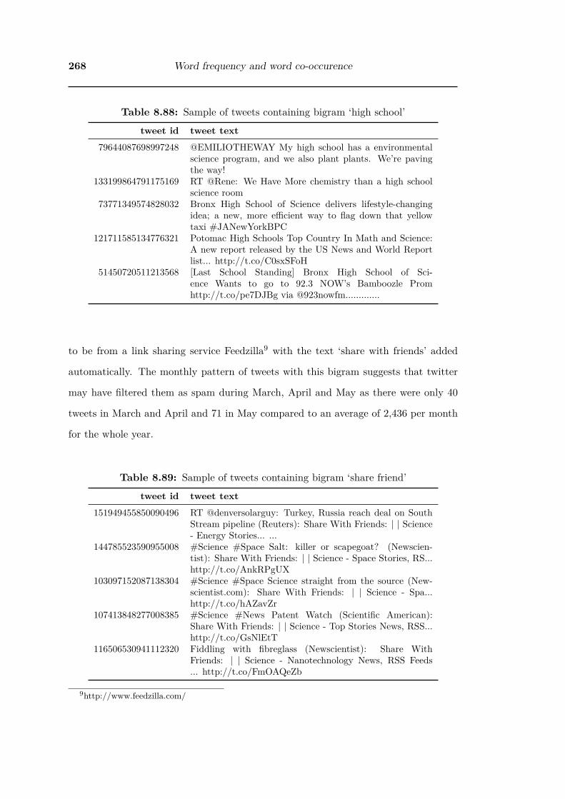
268 Word frequency and word co-occurence
Table 8.88: Sample of tweets containing bigram ‘high school’
tweet id tweet text79644087698997248 @EMILIOTHEWAY My high school has a environmental
science program, and we also plant plants. We’re pavingthe way!
133199864791175169 RT @Rene: We Have More chemistry than a high schoolscience room
73771349574828032 Bronx High School of Science delivers lifestyle-changingidea; a new, more efficient way to flag down that yellowtaxi #JANewYorkBPC
121711585134776321 Potomac High Schools Top Country In Math and Science:A new report released by the US News and World Reportlist... http://t.co/C0sxSFoH
51450720511213568 [Last School Standing] Bronx High School of Sci-ence Wants to go to 92.3 NOW’s Bamboozle Promhttp://t.co/pe7DJBg via @923nowfm.............
to be from a link sharing service Feedzilla9 with the text ‘share with friends’ added
automatically. The monthly pattern of tweets with this bigram suggests that twitter
may have filtered them as spam during March, April and May as there were only 40
tweets in March and April and 71 in May compared to an average of 2,436 per month
for the whole year.
Table 8.89: Sample of tweets containing bigram ‘share friend’
tweet id tweet text151949455850090496 RT @denversolarguy: Turkey, Russia reach deal on South
Stream pipeline (Reuters): Share With Friends: | | Science- Energy Stories... ...
144785523590955008 #Science #Space Salt: killer or scapegoat? (Newscien-tist): Share With Friends: | | Science - Space Stories, RS...http://t.co/AnkRPgUX
103097152087138304 #Science #Space Science straight from the source (New-scientist.com): Share With Friends: | | Science - Spa...http://t.co/hAZavZr
107413848277008385 #Science #News Patent Watch (Scientific American):Share With Friends: | | Science - Top Stories News, RSS...http://t.co/GsNlEtT
116506530941112320 Fiddling with fibreglass (Newscientist): Share WithFriends: | | Science - Nanotechnology News, RSS Feeds... http://t.co/FmOAQeZb
9http://www.feedzilla.com/

§8.5 Word co-occurrence 269
Bigram ‘math science’
The bigram ‘math science’ appears in 1.67% (203,628) of tweets in the 2011 dataset, an
average of 16,969 per month. Table 8.90 has a random sample of 5 tweets containing
the bigram ‘math science’ from all months 2011. One of these appears to be from a
student complaining about maths and science while the others seem more positive but
probably not written by students
Table 8.90: Sample of tweets containing bigram ‘math science’
tweet id tweet text136764103313199104 I don’t have a good background in math and science. Now
I can learn every day. Thank you so much.”116397277265920000 English, Maths, I.T, Science then History, omg kill me now
:-(((((127195954968412160 math science history unraveling the mystery that all lead to
a big bang #alwaysmakesmelaugh #obsessed #teamshel-don
108340129189462016 @qc2 hahah no for really basic stuff like geography, math,science - more for kids or brushing up
144575701855637504 Two Altamont School seniors win top awards in AdvancedPlacement math, science: Altamont’s Haley Hurowitz andRakesh... http://t.co/klpFn4G5
Bigrams ‘considered insanity’, ‘stop believing’, ‘believing magic’, ‘idea con-
sidered’, ‘every original’, ‘original idea’, ‘@heavyd never’, ‘insanity first’
and ‘never stop’
The bigram ‘considered insanity’ is the highest ranked by likelihood ratio of a series
of bigrams based on the retweeting of a tweet by rapper Heavy D (@heavyd) as a
memorial after he died on November 8, 2011. It was ranked 32nd but occurs in only
0.14% (17,623) tweets in the dataset, all but 19 of these occur in November, with
19 in December. Table 8.91 has a random sample of 5 tweets containing the bigram
‘considered insanity’ from all months 2011. This shows that they are all retweets of
the original tweet:

270 Word frequency and word co-occurence
@heavyd: Never stop believing.. Magic is just science we don’t understand..
Every original idea was considered insanity at first..
The next two bigrams that are in the top 70 by likelihood ratio because of these
retweets are ‘stop believing’ and ‘believing magic’ which were ranked 38th, 39th re-
spectively. They both appeared in 0.16% of tweets in the dataset, 19,222 tweets with
‘stop believing’ and 18,994 tweets with ‘believing magic’. The monthly pattern of ‘be-
lieving magic’ is similar to that of ‘considered insanity’ with almost all of the tweets
(18,965) appearing in November. The bigram ‘stop believing’ shows that this was used
in between 5 and 26 tweets per month before the peak of 18,996 in November which
suggests it is occasionally used in science tweets other than this retweeted one. The
random samples of 5 tweets from the dataset containing these bigrams are given in
Tables J.1 and J.2 in Appendix J (Page 509) and are all retweets of the same tweet,
some with added text like ‘RIP’.
The remaining bigrams in the top 70 as a result of these retweets are; ‘idea con-
sidered’ at rank 47, ‘every original’ at rank 49, ‘original idea’ at rank 50, ‘@heavyd
never’ at rank 53, ‘insanity first’ at rank 62 and ‘never stop’ at rank 68. The all occur
in between 0.14% (16,808) and 0.16% (19,568) of the tweets in the dataset. Like the
bigram ‘stop believing’, the bigrams ‘original idea’ and ‘never stop’ both have a low
occurrence leading up to November which indicates they are sometimes used in other
tweets. A random sample of 5 tweets from the 2011 dataset for each of these bigrams
are shown in Tables J.3 to J.8 in Appendix J (Page 509). There is one tweet in Ta-
ble J.1 that is not based on the poem ‘RT @internet_hindus: Biggest joke of d century
http://t.co/i2lf06WQ Wait till they stop believing medical science coz koran told thm
ta ...’.

§8.5 Word co-occurrence 271
Table 8.91: Sample of tweets containing bigram ‘considered insanity’
tweet id tweet text134054245946228736 RT @heavyd: Never stop believing.. Magic is just science
we don’t understand.. Every original idea was consideredinsanity at first..
134097070104641536 R.I.P ”@heavyd: Never stop believing.. Magic is just sci-ence we don’t understand.. Every original idea was consid-ered insanity at first..”
134081298972151808 RT @heavyd: Never stop believing.. Magic is just sciencewe don’t understand.. Every original idea was consideredinsanity at first..
134361656808579072 RT @heavyd: Never stop believing.. Magic is just sciencewe don’t understand.. Every original idea was consideredinsanity at first..
134040005189439489 RT @heavyd: Never stop believing.. Magic is just sciencewe don’t understand.. Every original idea was consideredinsanity at first..
Bigram ‘weight loss’
The bigram ‘weight loss’ was ranked 33rd by likelihood ratio and appears in 0.15%
(17,756) of tweets in the dataset, an average of 1,421 per month. Table 8.92 has a
random sample of 5 tweets containing the bigram ‘weight loss’ from the dataset. The
tweets are links to articles or books about weight loss.
Table 8.92: Sample of tweets containing bigram ‘weight loss’
tweet id tweet text145466510415114240 Rethinking Thin: The New Science of Weight Loss—
and the Myths and Realities of Dieting (Paperback)http://t.co/Qc52LPjW
73052639180496896 Weight loss the science not the fads: Measurements of fatlevels and body girths or circumferences (eg waist and...http://bit.ly/l8qdPa
23053826156142593 Sciennce Daily: Weight-loss surgery improved femaleurinary problems but male erection issues got worse...http://bit.ly/gQOQeP #science
130066848338280448 UWeight Loss Clinics - The Science Behind Emotional Eat-ing http://t.co/XiqmUDgV
48813849280905216 Diet News: Slow Eating and Weight Loss: Does the ScienceSupport It? - The ... http://ow.ly/1bPgRf

272 Word frequency and word co-occurence
Bigram ‘science rt’
The bigram ‘science rt’ appears in 0.18% (21,801) of the tweets containing ‘science’ in
2011, an average of 1,816 per month. The change in the number of tweets per month
through the year is small. The tweets all are in the form of a comment containing the
word science in front of a manual retweet, but cover a wide range of topics, as can
be seen in the random sample of 5 tweets containing the bigram ‘science rt’ from all
months 2011 shown in table Table 8.93.
Table 8.93: Sample of tweets containing bigram ‘science rt’
tweet id tweet text104590759801528320 5th and 6th grade math/science RT @cookayemonster:
@theteachERINme what grade do you teach?133987129691881472 Nautical Science RT @DavidQuartz: What course is mak-
ing u tweet all this? ”@tomkadelik: Brazil-Singapore-SouthAfrica-Sri Lanka- Australia”
115924049812652032 What a fun piece - It’s not Rocket Science! RT @ginidi-etrich Tips on exceptional client service by @thingcreatorhttp://t.co/4v9K6Ej5
104575422762725376 LOL. It shldve been said by ’Weird Science’. RT@mikethornsbury: w/ ths & my hrs of watchg TV i’m done!RT @ho… (cont) http://t.co/JAu5Qsz
132813281097302016 Wkwkwkwk .. Kocakk stiap pljran science RT @chelvi-etanadii: @sherina_khoen enakkkk
Bigram ‘science center’
The bigram ‘science center’ was ranked 35th by likelihood ratio and occurred in 0.73%
(89,009) of tweets in 2011. These were spread fiarly evenly through the year with an
average of 7,417 per month. Table 8.94 has a random sample of 5 tweets containing
the bigram ‘science center’ from all months 2011. In some these the use of ‘science
center’ is a science center in the sense of a informal learning institution that people can
visit while others are talking about University science precincts. There is a mixture of
proper nouns naming science centers and references to the local science center.

§8.5 Word co-occurrence 273
Table 8.94: Sample of tweets containing bigram ‘science center’
tweet id tweet text136852231789101056 Got hour and half 2 finish 1 paper, do a outline 4 anone,
and make it cross 501 to science center30764218751918080 Winter Nature Walk at Hill-Stead; Mind Games at Science
Center; ’Piano Lesson ...: In 1987, August Wilson’s play...http://bit.ly/fxaiW5
107182779430739968 Family Astronomy Weekend - Join Pacific Science Centerfor our annual weekend of astronomy and natural discov-ery.... http://t.co/vnd03yi
96789889928015873 RT @eVoloMagazine: Floating Canopy Defines the NewBeijing Science Center http://su.pr/AYnnmD
106519470788444160 @Addy_UP noooooooo! i absolutely will not allow that..go to the science center and watch a space movie in theimax theater lol
Bigram ‘social medium’
The bigram ‘social medium’ appears in 0.22% (27,039) of tweets in the dataset, an
average of 2,253 per month. The random sample of 5 tweets containing it given in
Table 8.95 shows that the bigram in the raw tweets is ‘social media’ and ‘media’ has
been changed to ‘medium’ during the normalisation and lemmatisation of the individual
tokens. There is a peak of 8,583 tweets in August, and this is probably due to promotion
of the ‘Science of Social Media webinar’ shown in one of the tweets in the sample. This
was held on August the 23rd partly as an attempt to gain a Guinness World Record
for largest online marketing webinar, which it did10.
Bigram ‘newly tagged’
The bigram ‘newly tagged’ was ranked 37th by likelihood ratio and occurs in 0.13%
(15,651) of tweets in the dataset. Table 8.96 has a random sample of 5 tweets con-
taining the bigram ‘newly tagged’ from all months 2011. They are all links to Amazon
books and are probably link spam or at best links generated when users on Ama-
zon add tags to books. The ones using the ‘goo.gl’ link shortner resolve to a website10http://www.guinnessworldrecords.com/news/hubspot-set-new-largest-online-marketing-seminar-
record/
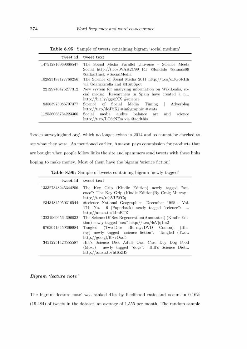
274 Word frequency and word co-occurence
Table 8.95: Sample of tweets containing bigram ‘social medium’
tweet id tweet text147512816969068547 The Social Media Parallel Universe – Science Meets
Social http://t.co/0VAK2C99 RT @fondalo @kunals89@arkarthick #SocialMedia
102823188177760256 The Science of Social Media 2011 http://t.co/oDG6RHhvia @danzarrella and @HubSpot
22129740475277312 New system for analyzing information on WikiLeaks, so-cial media: Researchers in Spain have created a n...http://bit.ly/ggoxXX #science
83563975085797377 Science of Social Media Timing | Adverbloghttp://t.co/dcJ7iKj #infographic #stats
112556066734223360 Social media audits balance art and sciencehttp://t.co/LC6tNFm via @addthis
‘books.surveyingland.org’, which no longer exists in 2014 and so cannot be checked to
see what they were. As mentioned earlier, Amazon pays commission for products that
are bought when people follow links the site and spammers send tweets with these links
hoping to make money. Most of them have the bigram ‘science fiction’.
Table 8.96: Sample of tweets containing bigram ‘newly tagged’
tweet id tweet text133327348245344256 The Key Grip (Kindle Edition) newly tagged ”sci-
ence”: The Key Grip (Kindle Edition)By Craig Murray...http://t.co/rcbVUWCq
83434845950316544 #science National Geographic: December 1988 - Vol.174, No. 6 (Paperback) newly tagged ”science”: ...http://amzn.to/kImRTZ
132319696564396032 The Science Of Sex Regeneration(Annotated) (Kindle Edi-tion) newly tagged ”sex” http://t.co/4sVjq1m2
67630413459369984 Tangled (Two-Disc Blu-ray/DVD Combo) (Blu-ray) newly tagged ”science fiction”: Tangled (Two…http://goo.gl/fb/vOxd5
34512251423555587 Hill’s Science Diet Adult Oral Care Dry Dog Food(Misc.) newly tagged ”dogs”: Hill’s Science Diet...http://amzn.to/htRZHS
Bigram ‘lecture note’
The bigram ‘lecture note’ was ranked 41st by likelihood ratio and occurs in 0.16%
(19,484) of tweets in the dataset, an average of 1,555 per month. The random sample

§8.5 Word co-occurrence 275
of 5 tweets containing the bigram ‘lecture note’ in Table 8.97 all refer to a series of
‘Lecture Notes in Computer Science’ on Amazon. Those with links link to Amazon
Japan. There are very few tweets with ‘lecture note’ in January to March (less than
86), then varying from month to month between 275 and 4886 for the rest of the year
with peaks in June, July, November and December.
Table 8.97: Sample of tweets containing bigram ‘lecture note’
tweet id tweet text151787135618396160 New Frontiers in Artificial Intelligence: JSAI 2006 Confer-
ence andWorkshops (Lecture Notes in Computer Science /Le.. error: either unsuppor
103253746498285569 Advances in Web-age Information Management (LectureNotes in Computer Science): http://t.co/mPr4nNk
133646004179312640 Modular Specification and Verification of Object-OrientedPrograms (Lecture Notes in Computer Science) – PeterMüller download, read,
90034218612174848 Intelligent Tutoring Systems (Lecture Notes in ComputerScience): http://amzn.to/lWZYzm
76964591258705920 Finite Representations of Ccs and Tcsp Programs by Au-tomata and Petri Nets (Lecture Notes in Computer Sci-ence): http://amzn.to/lTHOSX
Bigram ‘science lab’
The bigram ‘science lab’ occurs in 0.76% (93,227) of tweets in 2011. The number per
month varies between 2,718 and 3,583 during January to August (excluding the partial
month of April) then increases to 6,814 in September and between 17,487 and 21,412
in October to December. Table 8.98 has a random sample of 5 tweets containing the
bigram ‘science lab’ from all months 2011. Three of the sample tweets are advertise-
ments linking to laboratory equipment, mainly on Amazon. It is likely that the big
increase towards the end of the year is due to spam accounts on Twitter but I have not
investigated this.

276 Word frequency and word co-occurence
Table 8.98: Sample of tweets containing bigram ‘science lab’
tweet id tweet text139816621819691008 RT @spacefuture: Ambitious Mars Science Lab rover set
for Saturday launch #space http://t.co/OZ00IlWf143947130015449089 Tissue Culture Filters. Pack of five.: science-lab-pipettor-
accessories http://t.co/vSfYUhPg115386975044894720 PROBE; RDO; 30M; SS GUARD: science-lab-dissolved-
oxygen-meters http://t.co/2Bj6DCLS123399096202559488 Adjustable occlusion three-stop minicartridge: science-lab-
peristaltic-pumps http://t.co/jjmMPKmp58528287395287040 This old lady is in my science lab is about to blow me...go
home grandma!
Bigram ‘getting rich’
The bigram ‘getting rich’ appears in 0.15% (18,214) of tweets in the dataset, an average
of 1,518 per month. The number of tweets per month is fairly even during the year.
Table 8.99 has a random sample of 5 tweets containing the bigram ‘getting rich’ from
all months 2011. Most of them are links promoting a book by Wallace Wattles or
mentions of it. One tweet in a different sample (which also was mainly tweets with
links to places to buy the book) uses ‘richer’ in the sense of ‘more interesting’ and links
to an article on SlashDot11:
Physicists Devise Magnetic Shield: sciencehabit writes The sneaky science
of ‘cloaking’ just keeps getting rich... http://t.co/Jj6wea6p 117018003614334976
Bigram ‘science behind’
The bigram ‘science behind’ occurs in 0.63% (76,993) of the tweets in 2011, an average
of 6,416 per month. The random sample of 5 tweets containing the bigram ‘science
behind’ Table 8.100 are all discussing the ‘science behind’ different science topics.
11http://science.slashdot.org/story/11/09/22/2216241/Physicists-Devise-Magnetic-Shield

§8.5 Word co-occurrence 277
Table 8.99: Sample of tweets containing bigram ‘getting rich’
tweet id tweet text111085076367937536 Wallace D. Wattles ”The Science of Getting Rich” Chapter
14 http://t.co/pQdYsjU #belief #commitment147099951430762496 Listening to my Science of getting Rich audio... #Person-
alDevelopment is a must105990369107390465 The Science of Getting Rich - Bob Proctor (The Secret)
http://t.co/jA13IAy25314465956241408 Marked as to-read: The Science of Getting Rich by Wallace
D. Wattles http://bit.ly/hTI9SD95852159127658496 ”Desire is power seeking to manifest.” - Wallace Wattles,
The Science of Getting Rich
Table 8.100: Sample of tweets containing bigram ‘science behind’
tweet id tweet text72960371207573504 Great day ! @ coffee chemistry with Joseph Rivera ! If you
want the science behind coffee check him out !50219876454907904 Dangers of Leaving No Resident Behind: As the Japanese
are learning, the science behind herding thousands, some...http://nyti.ms/fw3ita
95410752680235008 Applied Food Sciences Builds Science Behind Coffee Com-pounds for Weight Loss ...: Applied Food Sciences Inc.(AF... http://bit.ly/oYlBfA
32169750922526721 RT @AmwayUS: Amway scientists work to provide themost innovative beauty products possible. See the sciencebehind the beauty: http://co ...
126326280818925568 RT @adrianatweeting: Scientists break down the brain sci-ence behind bullying by testing BULLIED MICE! See howin today’s @ChannelOneNews ...
Bigram ‘art science’
The bigram ‘art science’ appears in 1.07% (130,557) of tweets in 2011. Table 8.101 has
a random sample of 5 tweets containing the bigram ‘art science’ from all months 2011.
Many of the tweets suggest the strength of combining art and science. Although the
last one suggests art is greater than science.
Bigram ‘bbc news’
The bigram ‘bbc news’ was ranked 48th by likelihood ratio and occurs in 0.19% (22,702)
of the tweets in the dataset, an average of 1,891 per month. The number of tweets

278 Word frequency and word co-occurence
Table 8.101: Sample of tweets containing bigram ‘art science’
tweet id tweet text129467007463727104 the art and science of shameless self promotion: ...65904461654134784 It is the source of all true art and science131717829010534400 Democracy is the art and science of running the circus from
the monkey cage. H. L. Mencken122310259560808449 ERIC SCHMIDT ON STEVE JOBS: ”He Perfectly
Merged Art And Science” – Like Michaelangelohttp://t.co/rCLQld48 #IEEE #IEEEGreen
71434757170409472 @DontFollow_Mi the power of art …..science equationscan’t do that…
per month is higher in January to March and again in November and December than
during the middle of the year. Table 8.102 has a random sample of 5 tweets containing
the bigram ‘bbc news’ from all months 2011. Not surprisingly, these are all links to
BBC New reports about science. In most of them the word ‘science’ is part of the url
‘science-environment’ or a title in the tweet of ‘Science & Environment’ indicating that
the article is in the science and environment section of the BBC News website.
Table 8.102: Sample of tweets containing bigram ‘bbc news’
tweet id tweet text42590322500435968 BBC News - Are humans still evolving by Darwin’s
natural selection? http://www.bbc.co.uk/news/science-environment-12535647
113261566429896704 BBC News - Science & Environment: ’European GPS’ready for launch: BBC News - Science & Envir...http://t.co/x2cQn2s
48135706526224384 BBC News - X-ray machine from 1896 compared to modernversion http://www.bbc.co.uk/news/science-environment-12745194
110633713146150912 BBC News - Science & Environment: Crabs keepcool with giant claws: BBC News - Science & Envi...http://t.co/AJBObhT
66108047231156224 Science Cave of death – BBC News http://bit.ly/impMZN
Bigram ‘year old’
The bigram ‘year old’ is ranked 51st and appears in 0.21% (26,080) of tweets in the
dataset. The normalisation and lemmatisation of individual tokens has added to the
occurrence of this bigram by transforming various forms of year into the token ‘year’.

§8.5 Word co-occurrence 279
Most of the tweets in the random sample of 5 tweets containing the bigram ‘year old’
in Table 8.103 are talking about the age of students while two are talking about the
age of things - a 6,000 year old wine press. The science topics being discussed are very
broad.
Table 8.103: Sample of tweets containing bigram ‘year old’
tweet id tweet text24704641799299072 Reuters Science News At 6,000 years old, wine
press is oldest yet found: WASHINGTON (Reuter...http://bit.ly/hKYrZO http://bit.ly/fxidPd
146227742604673025 Science: Awesome 17-Year-Old Girl Invents NanoparticleThat Kills Cancer Cells - @Jezebel http://t.co/Me8gNtBh
78657125345271808 /trying to Understanding girls is like understanding Uni-versity level Science at the age of 5 years old.. It’s just notgonna happen #fact
129613755331002368 Our science teacher just told us Elmo is a 40 somethingyear old black man....
33577680452456449 The Google Science Fair starts today! Tell all your 13-18year-old friends to learn more and follow @googlescifair forupdates.
Bigram ‘big bang’
The bigram ‘big bang’ is ranked 54th and appears in 0.14% (17,612) of the tweets in
the dataset, an average of 1,467 per month. Table 8.104 has a random sample of 5
tweets containing the bigram ‘big bang’ from all months 2011. Four of the 5 tweets
appear to be referring to the TV show “Big Bang Theory”. Two of these are retweets
of a tweet saying ‘Maths science history, unravelling the mystery and it all started with
the big bang! BANG!’, which is the theme song of the show, another seems to be a
variation of that and one is about the show making science cool. The remaining tweet
in the sample seems to be part of a conversation about atheism.

280 Word frequency and word co-occurence
Table 8.104: Sample of tweets containing bigram ‘big bang’
tweet id tweet text28545873902313472 @Flighto math science history and reviled all the misery ,
it all started with big bang76886810806067201 the big bang theory made science geeks cool135448790009249793 Math, science, history, unraveling the mysteries, That all
started with the big bang!121294167098920962 Math, science, history, unraveling the mystery, That all
started with a big bang!52127202627686400 @DENISE_IAB ur choice of weapon was science ms lady
n da big bang theory is da only way an atheist can explainlife.
Bigrams ‘@1nf1d3lc4str0 #blamethemuslims’ and ‘#blamethemuslims ad-
vance’
The bigram ‘@1nf1d3lc4str0 #blamethemuslims’ was ranked 55th and appeared in 0.1%
(11,741) tweets in the dataset. As previously mentioned, the user name @1nf1d3lc4str0
translates to ‘Infidel Castro’ from ‘leet-speak’. There are no tweets with this bigram
until July. In July there are 11,719 tweets, reducing to 16 in August and three or
less in September to November. A second bigram ‘#blamethemuslims advance’ was
ranked 70th by likelihood ratio and also appeared in 0.1% of tweets in the dataset with
a slightly higher (12,745) number of tweets. All of the additional tweets occurred in
July and the pattern for the rest of the year was identical.
Tables 8.105 and 8.106 has a random sample of 5 tweets containing each ‘#blamethe-
muslims’ bigram from all months 2011. These are all retweets of a single ironic tweet
sent in July. Some have additional comments added to the retweets.
Bigram ‘forensic science’
The bigram ‘forensic science’ was ranked 57th appearing in 0.42% (51,946) of tweets in
2011, an average of 4,328 tweets per month. The number of tweets per month remains
fairly even through the year. Table 8.107 has a random sample of 5 tweets containing

§8.5 Word co-occurrence 281
Table 8.105: Sample of tweets containing bigram ‘@1nf1d3lc4str0 #blamethemus-lims’
tweet id tweet text95168576494903296 RT @1nf1d3lC4str0: I #blamethemuslims for advances in
science, mathematics, medicine & chemistry. And for de-veloping these 100’s of year ...
95123252837490688 RT @debyprima: WTF RT @danujaka: GO TO HELL !!RT @1nf1d3lC4str0: I #blamethemuslims for advances inscience, mathematics, ... http://tmi
95229895638122496 RT @1nf1d3lC4str0: I #blamethemuslims for advances inscience, mathematics, medicine & chemistry. And for de-veloping these 100’s of year ...
95183711158534144 RT @1nf1d3lC4str0: I #blamethemuslims for advances inscience, mathematics, medicine & chemistry. And for de-veloping these 100’s of year ...
95109779395051521 RT @1nf1d3lC4str0: I #blamethemuslims for advances inscience, mathematics, medicine & chemistry. And for de-veloping these 100’s of year ...
Table 8.106: Sample of tweets containing bigram ‘#blamethemuslims advance’
tweet id tweet text95154737434988544 RT @1nf1d3lC4str0: I #blamethemuslims for advances in
science, mathematics, medicine & chemistry. And for de-veloping these 100’s of year ...
95160301367988224 RT @1nf1d3lC4str0: I #blamethemuslims for advances inscience, mathematics, medicine & chemistry. And for de-veloping these 100’s of year ...
95201670488793088 RT @1nf1d3lC4str0: I #blamethemuslims for advances inscience, mathematics, medicine & chemistry. And for de-veloping these 100’s of year ...
95357944094396416 RT @1nf1d3lC4str0: I #blamethemuslims for advances inscience, mathematics, medicine & chemistry. And for de-veloping these 100’s of year ...
95113024356102144 RT @1nf1d3lC4str0: I #blamethemuslims for advances inscience, mathematics, medicine & chemistry. And for de-veloping these 100’s of year ...
the bigram ‘forensic science’ from all months 2011. Two of them appear to be talking
about the TV shows ‘CSI’ and ‘NCIS’. One is from a student studying forensic science,
one about getting a degree in forensic science and one is a link to a book about forensic
science on Amazon.

282 Word frequency and word co-occurence
Table 8.107: Sample of tweets containing bigram ‘forensic science’
tweet id tweet text70213625347964928 @GTG_heem lol, nothing in forensic science class. bored
like a muggg. Wbu?113328992039354368 RT @gratser: How to get a degree in Forensic Science:
http://t.co/9Nigmiw #Forensics103935851721007105 Abby: I am the Energizer bunny of forensic science: I never
sleep and I never give up. #ncis86269705962258432 Forensic Science Experiments on File:
http://amzn.to/ltFexU150096582858113026 This is slack of CSI....I’m glad I didn’t go into forensic sci-
ence
Bigram ‘science homework’
The bigram ‘science homework’ appears in 0.64% (78,200) of tweets in 2011, an average
of 6,328 per month. As with other school related bigrams there is a low point in July
with only 1,485 tweets. There is a peak in September of 14,207 tweets, decreasing to
11,523 in October and 11,248 in November. Without sampling more tweets in these
months it is not possible to say why there is such a large increase in the discussion of
science homework during them. Table 8.108 has a random sample of 5 tweets containing
the bigram ‘science homework’ from all months 2011. All appear to have been sent by
students discussing their science homework. Most them seem negative about science
homework.
Table 8.108: Sample of tweets containing bigram ‘science homework’
tweet id tweet text113442827542855680 I’m not doing my earth science homework, fuck that.44451364360814592 Have to finish my speech and science homework.146425682984050688 wondering if @_JessicaParillo did her science homework?143468653277491200 Need help with this science homework smfh cuzz123514466485796864 right better make a start on enviro science homework, -.-
im off twittterrrr peaceee

§8.5 Word co-occurrence 283
Bigram ‘physical science’
The bigram ‘physical science’ occurs in 0.48% (58,225) of tweets in 2011. Unlike most
of the school related bigrams, there is very little reduction in the number of tweets
with this bigram during July and August. The random sample of 5 tweets containing
the bigram ‘physical science’ in Table 8.109 all appear to have been sent by students
and most are negative about it.
Table 8.109: Sample of tweets containing bigram ‘physical science’
tweet id tweet text77908143039979520 Guess I’ll study physical science80105890237251584 @_AngelBabee um the physical science building :o139836259437785090 My uncle thought physical science was P.E. lol52421040059584512 @2da4thpower probably physical science. If im not mis-
taken thats like the class bout climate n earthquakes n crap134768403905921025 Bam! Just killed that rebuttal paper. On to Physical Sci-
ence.
Bigram ‘Albert Einstein’
The bigram ‘Albert Einstein’ was ranked 63rd by likelihood ratio and appeared in
0.11% (12,992) of tweets in the dataset. Four of the tweets in the random sample of 5
tweets containing the bigram ‘Albert Einstein’ in Table 8.110 are people quoting him.
The other is a link to a news article about his grandaughter trying to get a share of his
estate profits. The dataset only contains tweets with the word science, so there may
be other tweets quoting Albert Einstein that are not in this dataset.
Bigram ‘look like’
The bigram ‘look like’ appears in 0.24% (29,942) of tweets in the dataset. In most cases
it appears as the bigram ‘looks like’ in the raw tweet, ‘looks’ has been lemmatised to
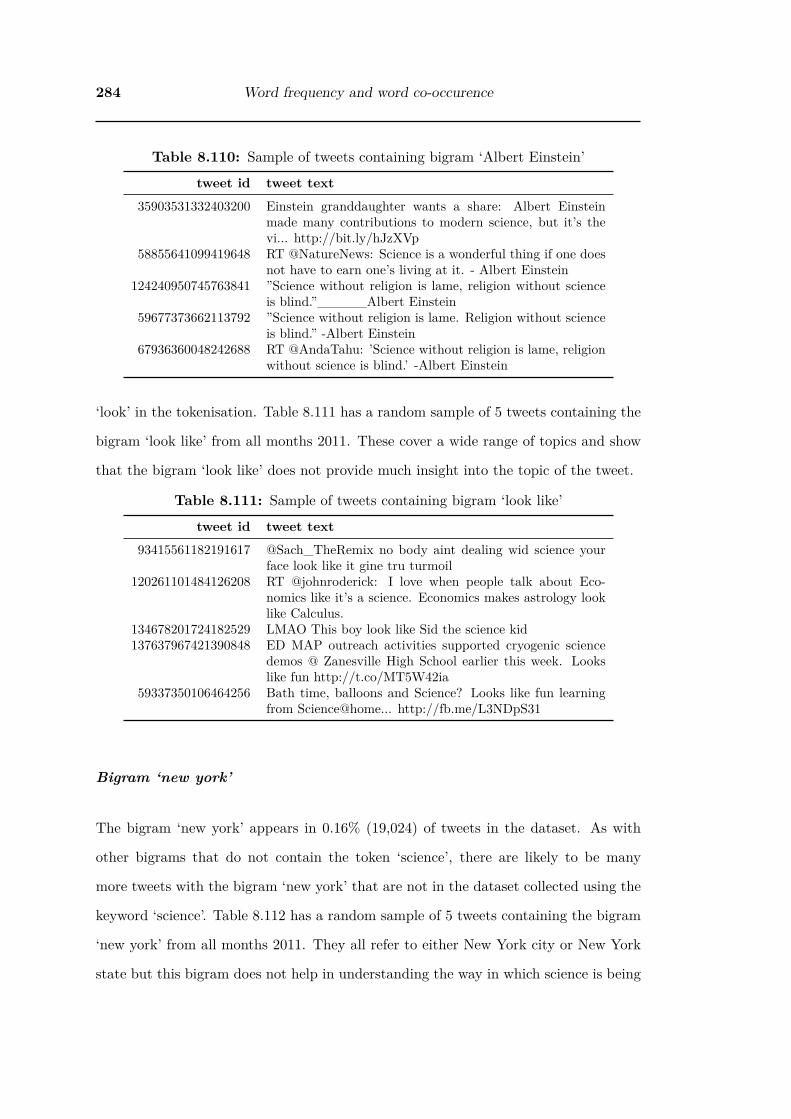
284 Word frequency and word co-occurence
Table 8.110: Sample of tweets containing bigram ‘Albert Einstein’
tweet id tweet text35903531332403200 Einstein granddaughter wants a share: Albert Einstein
made many contributions to modern science, but it’s thevi... http://bit.ly/hJzXVp
58855641099419648 RT @NatureNews: Science is a wonderful thing if one doesnot have to earn one’s living at it. - Albert Einstein
124240950745763841 ”Science without religion is lame, religion without scienceis blind.”_____Albert Einstein
59677373662113792 ”Science without religion is lame. Religion without scienceis blind.” -Albert Einstein
67936360048242688 RT @AndaTahu: ’Science without religion is lame, religionwithout science is blind.’ -Albert Einstein
‘look’ in the tokenisation. Table 8.111 has a random sample of 5 tweets containing the
bigram ‘look like’ from all months 2011. These cover a wide range of topics and show
that the bigram ‘look like’ does not provide much insight into the topic of the tweet.
Table 8.111: Sample of tweets containing bigram ‘look like’
tweet id tweet text93415561182191617 @Sach_TheRemix no body aint dealing wid science your
face look like it gine tru turmoil120261101484126208 RT @johnroderick: I love when people talk about Eco-
nomics like it’s a science. Economics makes astrology looklike Calculus.
134678201724182529 LMAO This boy look like Sid the science kid137637967421390848 ED MAP outreach activities supported cryogenic science
demos @ Zanesville High School earlier this week. Lookslike fun http://t.co/MT5W42ia
59337350106464256 Bath time, balloons and Science? Looks like fun learningfrom Science@home... http://fb.me/L3NDpS31
Bigram ‘new york’
The bigram ‘new york’ appears in 0.16% (19,024) of tweets in the dataset. As with
other bigrams that do not contain the token ‘science’, there are likely to be many
more tweets with the bigram ‘new york’ that are not in the dataset collected using the
keyword ‘science’. Table 8.112 has a random sample of 5 tweets containing the bigram
‘new york’ from all months 2011. They all refer to either New York city or New York
state but this bigram does not help in understanding the way in which science is being

§8.5 Word co-occurrence 285
used.
Table 8.112: Sample of tweets containing bigram ‘new york’
tweet id tweet text65111957254057984 RT @PIPIL4LIFE: #Geoengineering: Are They Trying to
Control the Weather? | The New York Academy of Scienceshttp://t.co/rIXIzvt #Chemtrails
142293492511674368 So all through Science today, I was singing Fairytale of NewYork with Grace...
149023753454620672 Cornell Chosen to Build Science School in New York City- http://t.co/Fg6I90gj http://t.co/DVBd7L6g
119267166624296961 #PRJobs Computer Science Editor, Journals - SpringerScience + Business Media - NEW YORK, NY USAhttp://t.co/KYHK1tVv
129990778331205632 ’Until’ wins at the Imagine Science Film Festival, New York- watch it here: http://t.co/9xae2qrK
Bigram ‘environmental science’
The bigram ‘environmental science’ was ranked 66th by likelyhood ratio and appears
in 0.48% (59,202) of tweets in 2011. Table 8.113 has a random sample of 5 tweets
containing the bigram ‘environmental science’ from all months 2011. Most appear
to have been sent by students discussing environmental science classes. Unlike other
student related bigrams there is no low in the number of tweets per month in July
or August which suggests that the term ‘environmental science’ may be used in more
non-school tweets than indicated in the sample.
Bigram ‘@youtube video’
The final bigram to be discussed is ‘@youtube video’ which was ranked 69th by likeli-
hood ratio and appeared in 0.16% (19,084) of tweets in the dataset. The user @youtube
is the official account of the YouTube video sharing website. All of the tweets in the
random sample of 5 tweets containing the bigram ‘@youtube video’ in Table 8.114 are
tweets automatically sent on behalf of users by YouTube when they mark a video as

286 Word frequency and word co-occurence
Table 8.113: Sample of tweets containing bigram ‘environmental science’
tweet id tweet text69269709031350272 Beautiful Saturday and I am inside reading about environ-
mental science. TOO EXCITING30252105218396162 Climate Change and Careers in Atmospheric and Environ-
mental Science: His Ph.D. research involved using globalcl... http://bit.ly/gvSBPD
114352283197779968 My new novel is based on a true story from my Environ-mental Science class. It’s called ”The Hipster & The Bro.”It’s about a rare friendship
105734126228881409 Hopefully this next class won’t put me to sleep, I’m coolwith environmental science though #nerd
126533367209537536 Last night was good but I could’ve been a whoooole lotbetter... time for environmental science!
liked or favorited using their account. It appears that YouTube only introduced this
service in April 2011 as their were very few tweets containing ‘@youtube video’ before
April. Because the tweets all contain the token ‘science’, the videos are all relate to
science, but there are a wide range of topics. However it does show that people are
marking some science videos are ‘liked’ or ‘favorited’.
Table 8.114: Sample of tweets containing bigram ‘@youtube video’
tweet id tweet text65740540561465344 I favorited a @YouTube video
http://youtu.be/3An7JQubQhs?a Planetary Science:Exploring The Solar System
144217735746945024 I liked a @YouTube video http://t.co/wocPcn45 ScienceSaved My Soul.
136213765631918080 I liked a @YouTube video http://t.co/bAEqsiPT ScienceBulletins: Down and Dirty Biodiversity
88734194062209024 I liked a @YouTube video http://youtu.be/JB7jSFeVz1U?aOde to the Brain! by Symphony of Science
115108368649162753 I liked a @YouTube video http://t.co/veRrOdB9 You Can’tTrust Science!
8.5.5 Conclusions about Word co-occurrence
Some of the bigrams identified by likelihood ratio have given more insight into how
the word ‘science’ is used by people on Twitter while others are not as useful in under-
standing the usage of the word ‘science’ because they occur across tweets expressing a

§8.5 Word co-occurrence 287
wide range of science topics.
The bigram ‘science fiction’ was the highest ranked by both likelihood ratio and raw
frequency. It is the most frequently occurring bigram in the dataset. It is also one of
the most narrowly focused uses of the word ‘science’, with the sample tweets for both
the bigram and the earlier sample for the individual token ‘fiction’ in Section 8.4.3
(Page 206) both showing it being used to mean the science fiction genre of books,
movies and games. The bigram ‘fiction fantasy’ is also used in the same context, but
is less useful as it co-occurs with the bigram ‘science fiction’ in most tweets and is less
frequent.
The bigram ranked equal second by likelihood ratio, ‘Bill Nye’, was ranked much
lower by raw frequency. It is again a very narrow topic with people talking about the
science presenter Bill Nye. Most of these tweets are by students talking about watching
his shows as part of their science education although some are by adults reflecting back
on their education or discussing appearances of Bill Nye as a science commentator on
television. On balance they seem to indicate that students enjoy watching his science
shows. The related bigrams ‘nye science’ and ‘science guy’ are lower ranked and largely
refer to the same tweets.
The other equal second ranked bigram by likelihood ratio is ‘computer science’. It
is the first in a group of bigrams where the bigram is the name of an area of study and
the tweets with it support that it is being used with this meaning. The sample tweets
for ‘computer science’ discuss the topic computer science, although the small sample
looked at seemed to be more specifically talking about university level computer science
courses. The bigram ‘political science’ is used in a similar way for the topic political
science, although it is not as clear what level of students are sending the tweets. The
low ranking bigram ‘forensic science’ is used in tweets about the topic forensic science,
with the sample showing a mixture of tweets about studying forensic science and TV
shows like CSI and NCIS. The sample tweets for the bigram ‘environmental science’

288 Word frequency and word co-occurence
show it is used by students discussing studying environmental science and as a link to
text books about environmental science. The sample tweets for the bigram ‘physical
science’ also show it being used by students discussing physical science as an area of
study.
Another group of bigrams appear in tweets where people are sharing information
on a range of science topics. The bigram ‘t.co via’ and the lower ranked bigrams
‘#science #news’, ‘t.co science’, ‘t.co #science’, ‘bit.ly #science’ and ‘science rt’ all
show that people share science information and links to science information but do
not provide insight into what they mean by ‘science’. Another lower ranked bigram
‘via @addthis’ is added by a content sharing service and again shows that people share
science information but not what they are sharing. The ‘share friend’ bigram is a
suggestion to share the tweets with friends added by another content sharing service,
Feedzilla. Tweets containing the bigram ‘newly tagged’ appear to be generated by the
action of tagging books on Amazon, although may be a form of link spam. As with the
other sharing tools there is no pattern to the topics of science books shared, except that
many of them are science fiction, but these will be picked up by the ‘science fiction’
bigram. The bigram ‘science behind’ is also used in tweets sharing information about
the science behind a wide range of topics. The bigram which ranked 70th by likelihood
ratio is ‘@youtube video’ and appears in tweets created for a user when they like a
video on youtube.
The bigram ‘rocket science’ appears from the phrase ‘it’s not rocket science’ in
tweets with a wide range of topics, most not about science. The use of it does imply
that people find science complex.
The bigram ‘science fair’ and related lower ranked bigrams ‘fair project’ and ‘science
project’ mostly appear in tweets sent by students about doing school science projects.
They show that a major form of engagement with science is through science fairs and
that student science projects. However they do not provide much insight into what

§8.5 Word co-occurrence 289
people mean by ‘science’. The same can be said of the next two bigrams by likelihood
ratio ranking, ‘science class’ and ‘science teacher’. They are both mostly written by
students and tell us that they attend science classes, but again do not provide insight
into what people mean by ‘science’. The bigrams ‘science test’, ‘science exam’, ‘test
tomorrow’ and ‘wish luck’ are also used mainly by students reporting that they are
about to have a test or are preparing for one. As with ‘science class’, they are about
the activity of having a science test rather than helping understand what people mean
by ‘science’. The bigram ‘high school’ also belongs in this group although the small
sample of tweets suggest it may be used more by people looking back at high school
instead of by students. Another school class related bigram is ‘math science’ and the
use of this indicates that maths and science are considered to be separate subjects in
school. A low ranked bigram ‘science homework’ also belongs in this group as it is
mainly sent by students complaining about having science homework.
There are three sets of tweets in the dataset that use an unusual pattern of words
and are repeated (retweeted) often enough to cause many of the word pairs in them
to appear in the top 70 by likelihood ratio. The first set of tweets based on the poem
on Page 204 results in the bigrams ‘history battle’, ‘problem history’, ‘math problem’,
‘reaction heart’ and ‘love math’ to appear in the top 70 by likelihood ratio. The sample
tweets show the use of the word science in a poem about love, and imply that the core
science is chemistry saying ‘in science, it’s a reaction’. Another group of bigrams result
from the retweeting of a tweet by @heavyd as a memorial after his death in November
2011. The bigrams are ‘considered insanity’, ‘stop believing’, ‘believing magic’, ‘idea
considered’, ‘every original’, ‘original idea’, ‘@heavyd never’, ‘insanity first’ and ‘never
stop’. The reason for people repeating this tweet was to memorialise Heavy D, and it
could just as easily been a tweet that did not contain the word science. Another set
of tweets was based on a tweet giving credit to Muslim culture for historic advances in
science while using the ironic hashtag #blamethemuslims which was retweeted 11,741
times. It brought the bigrams ‘@1nf1d3lc4str0 #blamethemuslims’ and ‘#blamethe-

290 Word frequency and word co-occurence
muslims advance’ into the top 70 by likelihood ratio. These bigrams highlight the
ability of bigrams by likelihood ratio to pick up on unusual word usage even when it
only occurs in a very small sample of the dataset.
The bigrams ‘Christian Science’ and ‘Science Monitor’ from the Christian news
service Christian Science Monitor are about a range of news topics including science.
The name does highlight the term ‘Christian science’, although all of the small sample
of tweets for this bigram were from the newspaper, not a more general use of the term.
Another news service related bigram ‘BBC news’ appears in tweets about science from,
or linking to, the BBC news service.
The bigram ‘got ta’ appears in tweets for a wide range of topics and both words
should probably be added to the stop word list. The bigram ‘rt science’ occurs in too
few tweets to be useful, only 1,476 tweets for the whole year. The bigrams ‘year old’,
‘look like’ (raw phrase ‘looks like’) and ‘New York’ also occur in tweets on a wide range
of science topics and so should probably be added to the stop words if bigrams are
going to be used to find science topics.
The bigram ‘science technology’ comes from the phrase ‘science and technology’
which is used as both a proper noun and a topic in the tweets containing it. The
phrase ‘science and techology’ can be considered to imply that technology is separate
from ‘science’.
The bigrams ‘climate change’ and ‘global warming’ are both used in tweets dis-
cussing the topic of climate science, but in the small sample looked at, the ones with
the bigram ‘global warming’ seem to be more negative about the science. The number
of tweets for each of these bigrams is quite low because they have only been collected
in the dataset if the word ‘science’ also appears in the tweet.
Tweets with the bigram ‘weight loss’ appear to be mostly links to information
about weight loss, although in other samples there were a lot of tweets which were
spam advertising links to weight loss products.

§8.5 Word co-occurrence 291
The bigram ‘getting rich’ seems to be mostly spam links trying to get people to
buy books. The sample tweets contain the phrase ‘the science of getting rich’ which
indicates that the advertisers think that associating with science will help sell their
products.
The bigram ‘science center’ is used to refer to both informal science learning centers
and university science precincts. Like the school related terms above it is referring to
a type of institution rather than a meaning of the word science.
The bigram ‘social medium’ is used in tweets about a Science of Social Media
seminar, which suggests ‘science of social media’ could be indicative of a area of science
like ‘computer science’, however it seems to only appear in the dataset though the
promotion of this one small event and so is probably not significant.
The bigram ‘lecture note’ only appears in 18,660 tweets in the dataset and the
sample suggests that it is mainly links to lecture notes about computer science on
Amazon Japan. These will also be picked up by the bigram ‘computer science’, so this
bigram does not appear to be useful in discovering new topics.
The small sample of tweets for bigram ‘science lab’ suggests it is mainly used in
link spam tweets linking to laboratory equipment for sale (possibly generated by bots),
not by people in science labs or discussing science labs.
The bigram ‘art science’ appears in 1.04% of tweets in the dataset and the sample
tweets suggest it is used when comparing art to science, discussing the strength of
combining art and science and also talking about the band Art Vs Science.
The bigram ‘big bang’ occurs mainly in tweets discussing the TV show The Big
Bang Theory and some tweets about the physics big bang.
The bigram ‘Albert Einstein’ is a persons name like the bigram ‘Bill Nye’. Many of
the ‘Bill Nye’ tweets are just the theme song from his show whereas the bigram ‘Albert
Einstein’ occurs in tweets based on many different quotes from Albert Einstein.

292 Word frequency and word co-occurence
From this discussion, the bigrams that are most useful in understanding how peo-
ple use the word science are; ‘science fiction’, ‘bill nye’, ‘computer science’, ‘political
science’, ‘forensic science’, ‘environmental science’, ‘physical science’, ‘rocket science’,
‘climate change’, ‘global warming’, ‘science center’, ‘art science’, ‘albert einstein’ and
‘science technology’. The relative frequency of each of these bigrams is shown in Fig. 8.8
based on the percentage of tweets each bigram appears in. This clearly shows domi-
nance of ‘science fiction’. The sum of the individual percentage of tweets for each of
these may be greater than the total percentage of tweets that contain these bigrams
because tweets can contain more than one of the bigrams. In total these bigrams ap-
pear in 1,711,352 tweets, or 14.0% of the dataset, so these topics may explain 14.0%
of the conversation on Twitter containing the word science in 2011. Four of these bi-
grams do not contain the word ‘science’ and yet are useful in identifying a topic area
of discussion about science. Bigrams that also indicate a science activity are; ‘science
fair’, ‘science test’, ‘science exam’, ‘science class’. Adding these bigrams extends the
coverage of the bigrams by 5.19%, giving a total of 19.19% of science tweets including
one of the topic and activity bigrams.
0.0 0.5 1.0 1.5 2.0 2.5 3.0 3.5
%
science fiction
computer science
rocket science
science technology
political science
art science
science center
bill nye
physical science
environmental science
forensic science
climate change
global warming
albert einstein
Big
ram
s
Figure 8.8: Percentage of 2011 science tweets for each Bigram

§8.6 Conclusion 293
8.6 Conclusion
In this chapter I have begun the process of understanding how people are using the word
‘science’ but have found the raw word frequencies considered in response to research
question Question 4a “what is the frequency of words used?” are not particularly ef-
fective when trying to understand such a large dataset, and do not contribute towards
answering the main question “What topics are discussed in these tweets?”. The second
subquestion addressed in this chapter, Question 4b “what words co-occur?”, did con-
tribute more towards answering the main question. I found that Bigrams are able to
give some insight into the contexts in which ‘science’ is being used in around 14% to
19.19% of the tweets. In the next chapter I address the third subquestion question 4b
“what topics are identified by topic analysis?” to see if I can get a better answer to
how people use the word ‘science’ on Twitter.

294 Word frequency and word co-occurence

Chapter 9
Topic analysis approaches
This chapter addresses research question 4c “what topics are identified by topic anal-
ysis?”. Having found that word co-occurrence bigram frequencies can describe the
context of the use of the word ‘science’ in up to 19.2% of the tweets I move on to use
techniques which use a combination of word frequency and word co-location to look
for the topics which describe the texts, to see if this approach can explain more of the
conversations in the dataset:
producing a human-interpretable decomposition of the texts can be a goal
in itself, as when browsing or summarizing a large collection of documents.
(J. Chang, Gerrish, Boyd-Graber, Wang, & Blei, 2009, p. 1)
There is a number of supervised and unsupervised machine learning techniques
available for detecting topics in documents. I have chosen to investigate unsupervised
approaches because they do not require human coding of the dataset, which may make
them easier to apply to new datasets in the future.
Latent Dirichlet Allocation (LDA) was announced in 2003 by Blei, Ng, and Jordan
(2003). It is an unsupervised machine learning approach that identifies the topics
present in a text. Each text is considered to be a bag-of-words, that is only the
frequency of the words in the text is used, not the word order or meaning of the words.
The word counts in each document of the training corpus are transformed by LDA
into a topic space of lower dimensionality. A LDA topic is expressed as a Bayesian
295

296 Topic analysis approaches
probability distribution across all the words in the corpus, with the contribution of
each word towards that topic. Blei et al. (2003) defined LDA as:
Latent Dirichlet Allocation (LDA) is a generative probabilistic model of a
corpus. The basic idea is that documents are represented as random mix-
tures over latent topics, where each topic is characterized by a distribution
over words. (p. 996)
If the model is successful, the most important words in each topic should appear
coherent to a human reader, “but the top few words in a topic only give a small
sense of the thousands of the words that constitute the whole probability distribution”
(Schmidt, 2012, p. 51).
Each document in a corpus can be interpreted as having a mixture of topics and
this allows the identification of both the most significant documents for a topic and
the prevalence of a topic in the corpus.
I chose to use LDA instead of another unsupervised approach, Latent Semantic
Indexing (LSI), because the topics created by LSI are very difficult to interpret, with
words given both positive and negative weights, and are more useful for document
similarity or search applications rather than as a way of gaining insight into the content
of a corpus.
Topic analysis is a rapidly moving field, and there are newer extensions of LDA that
incorporate additional information or relax the assumptions on which LDA is based.
Dynamic Topic Analysis is an example which relaxes the assumption that the order
of the documents do not matter by respecting the time order in which the documents
were created (Blei, 2012, p. 82). The Author-Topic model (Rosen-Zvi, Chemudugunta,
Griffiths, Smyth, & Steyvers, 2009) uses meta data about the author of the documents
to extend the LDA model; “topic proportions are attached to authors; papers with

297
multiple authors are assumed to attach each word to an author, drawn from a topic
drawn from his or her topic proportions” (Blei, 2012, p. 83).
Due to this rapid change, the software tools available for people using topic mod-
elling (rather than developing topic modelling techniques) are often hard to use and
do not have all of the newest approaches. The new approaches are usually published
as mathematical specifications in academic papers, some of which include links to aca-
demic demonstration code, but even these take some time to be included in more
general tools like Mallet or Gensim.
I considered three tools for topic modelling; Mallet (McCallum, 2002), WEKA
(Hall et al., 2009) and Gensim (Rehuvrek & Sojka, 2010). I selected Gensim because
it implemented a range of the topic modelling algorithms, can be used to call Mallet
on the same data, and is written in Python which made it easy to use with the format
of my cleaned tweets corpus.
Gensim uses the online variational Bayes algorithm for LDA developed by Hoffman,
Bach, and Blei (2010). An ‘online’ algorithm allows the topic model to be updated as
each document in a stream of documents is seen, whereas a ‘batch’ algorithm requires
all of the training documents to be seen before updating the model. By updating the
model as documents are seen the model can become more accurate (converge) with
fewer passes over the corpus. However, this approach requires that the distribution of
topics and distribution of words in topics remains the same over time (is stationary).
When either of these changes it is called topic drift. Topic drift can confuse an online
model and degrade the quality of the topics it identifies. Topic drift can also be a
problem when updating the model with new documents over time.
Evaluation of machine learning is often based on splitting the data into training
and testing sets. The training set is used to train the model and then the test set is
used to evaluate it. For supervised learning this is straight forward because you can
compare the manual coding of the test set with the coding predicted by the model to

298 Topic analysis approaches
see how well the model is working. With unsupervised learning the test dataset does
not have any expected results encoded and so evaluation is more difficult. One measure
that can be used for evaluating LDA models is ‘perplexity’ (Blei et al., 2003; J. Chang
et al., 2009) which is a measure of how well the word counts of the test documents
are represented by the word distributions of the topics. Blei et al. (2003) described
perplexity as:
The perplexity, used by convention in language modeling, is monotonically
decreasing in the likelihood of the test data, and is algebraicly equivalent
to the inverse of the geometric mean per-word likelihood. (Blei et al., 2003,
p. 1008)
Perplexity is useful for comparing models or parameter options, but may not be an
accurate measure of the quality of the topics, “there is no technical reason to suppose
that held-out accuracy corresponds to better organization or easier interpretation”
(Blei, 2012, p. 83).
J. Chang et al. (2009) look at how to measure the interpretability of a LDA topic
model. They developed “two human evaluation tasks to explicitly evaluate both the
quality of the topics inferred by the model and how well the model assigns topics to
documents” (p. 2). The first is “called word intrusion, as subjects must identify a
spurious word inserted into a topic” (p. 3) and measures whether a “topic has human-
identifiable semantic coherence” (p. 3). The second is called ‘topic intrusion’ as the
“subject must identify a topic that was not associated with the document by the model”
(p. 3) and “tests whether a topic model’s decomposition of documents into a mixture
of topics agrees with human judgements of the document’s content” (p. 4). They
conducted a large scale human study of this approach and found that:
For three topic models, we demonstrated that traditional metrics do not
capture whether topics are coherent or not. Traditional metrics are, indeed,

299
negatively correlated with the measures of topic quality developed in this
paper. Our measures enable new forms of model selection and suggest that
practitioners developing topic models should thus focus on evaluations that
depend on real-world task performance rather than optimizing likelihood-
based measures. (J. Chang et al., 2009, p. 8)
I followed this advice and used the concepts of word intrusion and topic intrusion
when evaluating the topics modelled from my corpus. I manually checked the highest
likelihood words in each topic to see if they formed a recognisable, coherent topic
instead of appearing random. When checking the topics that the model assigns to
unseen documents (held out from training), I manually inspected the documents to see
what topics appeared in each tweet.
Blei and Lafferty (2009) conclude with a warning about the interpretation of topic
models:
The topics and topical decomposition found with LDA and other topic
models are not “definitive.” Fitting a topic model to a collection will
yield patterns within the corpus whether or not they are “naturally” there.
(And starting the procedure from a different place will yield different pat-
terns!) Rather, topic models are a useful exploratory tool. The topics
provide a summary of the corpus that is impossible to obtain by hand; the
per-document decomposition and similarity metrics provide a lens through
which to browse and understand the documents. A topic model analysis
may yield connections between and within documents that are not obvi-
ous to the naked eye, and find co-occurrences of terms that one would not
expect a priori. (p. 17).
Brett (2012) adds to this saying that “Topic modeling is not an exact science by
any means. The only way to know if your results are useful or wildly off the mark is
to have a general idea of what you should be seeing” (Brett, 2012, p. 14).

300 Topic analysis approaches
A key parameter for LDA is the number of topics that the model should find,
however “choosing the number of topics is a persistent problem in topic modeling and
other latent variable analysis” (Blei & Lafferty, 2009, p. 11). If too few topics are
used in the model they will be broad and their most frequent words may not appear
coherent. If the model is set to look for too many topics then “as topics become more
fine-grained in models with larger number of topics, they are less useful for humans”
(J. Chang et al., 2009, p. 4). Perplexity can be used to help find the optimum number
of topics by creating a series of models varying the number of topics and looking for
the lowest perplexity estimate:
When the goal is qualitative, such as corpus exploration, one can use cross
validation on predictive likelihood, essentially choosing the number of topics
that provides the best language model. (Blei & Lafferty, 2009, p. 12)
Tuning the LDA hyperparameters used for the LDA model is also critical for good
results. One of these hyperparameters (also referred to as a Dirichlet prior or con-
centration parameter) is the expected underlying distribution of ‘topics in documents’
(alpha). The other Dirichlet prior is the ‘words in topic’ distribution (called beta in
Mallet or eta in Gensim LDA), which is recommended in the Gensim documentation
to be left to the default of ‘symmetric’. Gensim gives four options for the setting of the
Dirichlet alpha priors: Symmetric, Asymmetric, Auto, or the provision of user selected
alpha value for each topic. Symmetric sets them all to the same value, this implies
that all topics are expected to appear with equal weight in the corpus. Asymmetric
sets them to a range of values from low to high and implies that topics are expected to
occur in a range of weights in the corpus. The ‘auto’ option tells the model to learn the
alpha value for each topic as the model is developed which allows it to more accurately
match the distribution of topics in a corpus.
§9.1 Initial experiments with Gensim 301
9.1 Initial experiments with Gensim
Having provided an overview of the topic modelling approach I intended to use, I took
note of the advice of Brett (2012) who said:
If you imagine topic modeling as a switchboard, there are a large number
of knobs and dials which can be adjusted. These have to be tuned, mostly
through trial and error, before the results are useful. (p. 14)
and
Don’t be afraid to fail or to get bad results, because those will help you find
the settings which give you good results. Plug in some data and see what
happens. (p. 15)
and began to explore my corpus.
To reduce the computer run time required for each test, I carried out my initial
experiments with Gensim on a single month of data, January 2011. The tokenised and
cleaned words from Chapter 8 were used to create a bag of words corpus in Gensim
using the code in listing K.1 in Appendix K. For January 2011 this resulted in a corpus
of 802,821 documents (tweets) containing 318,823 features (words or tokens).
In the Gensim documentation it recommends begining by using the default param-
eters as they have been selected to work well with a wide range of different types of
documents. The default parameters for gensim.models.LdaModel1 are:
models.LdaModel(self, corpus=None, num_topics=100, id2word=None, distributed=False,
chunksize=2000, passes=1, update_every=1, alpha='symmetric', eta=None, decay=0.5,
eval_every=10, iterations=50, gamma_threshold=0.001)
1Gensim online documentation http://radimrehurek.com/gensim/models/ldamodel.html

302 Topic analysis approaches
I have described the meaning of the number of topics (num_topics) and the Dirichlet
priors alpha and eta in the introduction above. Rather than going through the meaning
of the other parameters here, I describe each parameter where I choose to vary it from
the default value.
In my initial trials I did not split my corpus into test and training, instead relying on
the estimated perplexity calculated by Gensim and output to the log file for each trial.
The estimated perplexity provided during training by Gensim is based on the varia-
tional Evidence Lower BOund (ELBO) of a held out sample which is adjusted2. This
adjusted perplexity is better for comparing different models than the raw perplexity
values.
Gensim can use a technology called BLAS (Basic Linear Algebra Subprograms)
to gain significant improvement in speed in model calculation. In order to use this, I
changed from a directly installed version of Python to using a pre-packaged distribution
called Anaconda3 which includes pre-configured BLAS for the research in this chapter.
Using the January corpus I ran Gensim LDA leaving all the parameters to their
default values including the number of topics at 100 topics (listing 9.1) and then re-
peated this test varying the alpha parameter to ‘auto’ (listing 9.2) from the default of
‘symmetric’. The full code for each of these is provided in listing K.4 and listing K.5
in Appendix K.
1 models.LdaModel(bow_corpus, id2word=dictionary, num_topics=100)
Listing 9.1: Gensim LDA 100 topics
1 models.LdaModel(bow_corpus, id2word=dictionary, alpha='auto', num_topics=100)
Listing 9.2: Gensim LDA 100 topics & auto alpha
2The perplexity is re-weighted as if the held-out corpus was the entire training corpus -http://radimrehurek.com/2013/12/python-lda-in-Gensim-christmas-edition/
3https://store.continuum.io/cshop/anaconda/

§9.1 Initial experiments with Gensim 303
The topics generated by LDA are not ordered, that is there is no natural order of
importance of the topics. When evaluating the topics, it is easy to think that the ones
that have more recognisable most frequent words are the ‘better’ topics, but this is not
correct.
The most frequently occurring 10 words for 5 topics from the 100 topics modelled
by each trial is shown in Table 9.1. The number preceding each word is the probability
of that word in that topic. Each topic is a distribution over all of the 318,823 words
in the corpus, but many of the words will have a very low probability of contributing
to that topic. The topics in Table 9.1 are not very coherent, it is very difficult to
understand what most of the topics might represent. This is reflected in the high final
perplexity estimate for both models; the symmetric alpha model perplexity estimate
was 13168.3 (-13.685 per-word bound) and for the auto alpha model the perplexity
estimate was slightly lower at 9940.6 (-13.279 per-word bound). Both estimates were
based on a Gensim held-out corpus of 821 documents with 8088 words.

304 Topic analysis approaches
Table 9.1: Sample Gensim LDA topics from unfiltered January 2011 corpus
alpha Topic (top 10 words)
symmetric
1 0.251*know, 0.079*science, 0.044*morning, 0.036*rt, 0.030*febru-ary, 0.029*creationism, 0.028*expert, 0.022*huff.to, 0.020*classroom,0.016*suggestion
2 0.184*video, 0.130*tinyurl.com, 0.124*science, 0.075*youtube,0.056*youtu.be, 0.036*point, 0.028*liked, 0.027*tea, 0.020*prof,0.020*humanity
3 0.142*science, 0.062*building, 0.057*ever, 0.053*real, 0.047*rt,0.042*result, 0.033*bit.ly, 0.033*event, 0.032*without, 0.029*success
4 0.173*study, 0.138*science, 0.108*oh, 0.093*shit, 0.079*gon,0.041*subject, 0.019*conference, 0.019*rule, 0.014*tired, 0.011*as-trology
5 0.186*computer, 0.156*one, 0.142*science, 0.061*engineering,0.060*job, 0.040*bit.ly, 0.030*ta, 0.027*hashtag-jobs, 0.023*enough,0.019*pioneer
auto
1 0.065*rt, 0.030*website, 0.029*bit.ly, 0.025*science, 0.023*skin,0.022*astrology, 0.021*posted, 0.015*host, 0.015*effort, 0.015*rat
2 0.089*science, 0.073*bit.ly, 0.058*rt, 0.057*magic, 0.056*scien-tific, 0.046*wired, 0.043*far, 0.032*wired.com, 0.027*researcher,0.020*walking
3 0.198*teacher, 0.144*science, 0.142*time, 0.103*work, 0.036*awe-some, 0.023*xx, 0.020*image, 0.020*user-sethmacfarlane, 0.015*later,0.014*seriously
4 0.206*math, 0.174*science, 0.116*lol, 0.081*english, 0.067*yes,0.019*monday, 0.016*hell, 0.015*city, 0.014*finally, 0.011*score
5 0.230*science, 0.139*school, 0.101*test, 0.053*shit, 0.052*would,0.046*ugh, 0.045*back, 0.032*tomorrow, 0.016*wait, 0.015*midterm
9.1.1 Dictionary filtering
On further reading of the Gensim documentation I found that it is important for
LDA to filter the extremes of the words in the corpus, both the most frequently
and least frequently occurring words. The way to do this in Gensim is by using the
filter_extremes() function which has these parameters:
Filter out tokens that appear in
less than no_below documents (absolute number) or
more than no_above documents (fraction of total corpus size, not
§9.1 Initial experiments with Gensim 305
absolute number).
after (1) and (2), keep only the first keep_n most frequent tokens
(or keep all if None).
from http://radimrehurek.com/gensim/corpora/dictionary.html
The default values for this function are no_below=5, no_above=0.5, keep_n=100000.
Applying these defaults to my corpus reduced the dictionary from 318,823 words to
50,350 words which were in no less than 5 and no more than 401,410 (50.0%) of docu-
ments. The code for the filtering is shown in listing K.2 in Appendix K.
Reducing the size of the dictionary also has the benefit of reducing the time required
to calculate the model and the size of the model. The probability distribution for each
topic is modelled over 50,350 words instead of 318,823 words.
For Gensim LDA, the ‘iterations’ parameter should be set to around the average
number of words in each document and I found suggestions that adjusting this may
help the speed and model quality. For my dataset I found the average number of
cleaned words per tweet and used this as the ‘iterations’ parameter.
The average length of documents in the corpus is not the length of the original
tweets, because even the first Gensim corpus I created was based on the tokenized and
cleaned words from Chapter 8, not the words in the raw tweets. In a Gensim corpus,
only words in the dictionary are counted. So for the initial tests the dictionary has
318,823 words and when I filtered this to 50,230 words the document lengths also went
down because many words are no longer included. The average document length in the
318,823 word corpus was 9.4 words, and the maximum document length was 25 words.
This reduced to 8.0 words and a maximum length of 22 in the filtered corpus of 50,350
words.
To test the impact of changing the interations parameter and the default filtering
of the corpus, Gensim LDA models were created for both the filtered and unfiltered

306 Topic analysis approaches
corpus with the iterations parameter set to 10 and alpha set to ‘auto’. The code for
these is given in listing K.6 and listing K.7 in Appendix K. The perplexity and run
time results from this and subsequent tests are summarised in Table 9.7 (p. 314). The
perplexity results for these tests are shown in lines 3 and 4 of Table 9.7. Compar-
ing these to the original two trials on lines 1 and 2 of Table 9.7 shows that reducing
the iterations from 50 to 10 gave a small improvement in the perplexity and run-
time. Filtering the corpus resulted in a dramatic improvement in both the perplexity
and runtime, although some of the reduction in perplexity may have been due to the
smaller vocabulary, there were only 6,914 words remaining in the test corpus instead
of 8,088. The sample of 5 topics from the 100 topic, 10 iteration, filtered corpus model
in Table 9.2 shows that although the perplexity is lower, the topics are still difficult to
understand. Looking at the 100 topics, I noticed that there were still words that I did
not think were useful in topics including urls, ‘rt’ and ‘hashtag-science’. I decided to
do some additional filtering of the dictionary to remove these words and to filter more
of the rare words.
Table 9.2: Sample Gensim LDA topics with iterations=10, auto alpha and filteredJanuary 2011 corpus
Topic (top 10 words)1 0.082*using, 0.070*diet, 0.037*bit.ly, 0.033*brian, 0.032*air,
0.030*revision, 0.030*training, 0.028*method, 0.022*horse, 0.022*fig-ure
2 0.233*good, 0.107*come, 0.057*learn, 0.049*join, 0.036*wow,0.035*around, 0.028*pound, 0.025*model, 0.024*rt, 0.024*important
3 0.100*getting, 0.093*bit.ly, 0.068*based, 0.067*public, 0.053*result,0.041*law, 0.039*rich, 0.036*success, 0.036*team, 0.035*secret
4 0.163*take, 0.134*dlvr.it, 0.035*practice, 0.030*da, 0.029*ei-ther, 0.028*discussion, 0.026*bed, 0.025*cocktail, 0.023*lead,0.021*present
5 0.168*ow.ly, 0.097*guy, 0.079*bill, 0.053*nation, 0.052*rt, 0.045*nye,0.040*due, 0.028*okay, 0.024*hashtag-science, 0.023*ten

§9.1 Initial experiments with Gensim 307
I increased rare word threshold from 5 to 20, so each word had to appear in at least
20 tweets to be included. There were 50,350 tokens in previous filtered dictionary,
increasing rare word from 5 to 20 reduced this to 18,934 tokens. I also removed two
more words that were appearing in as frequent words in many topics, ‘rt’ and ‘hashtag-
science’, and removed all of the remaining 580 urls from the dictionary. This reduced
the final number of words in new dictionary to 18,351. The code for this filtering is
provided in listing K.3 in Appendix K. The reduction in the dictionary decreased the
average document length to 6.9 words and the maximum document length to 21.
Using the new dictionary and corpus I repeated the 100 topic, auto alpha and 10
iterations test. Only two lines in the code from the previous test given in listing K.7
in Appendix K were changed to load the new corpus:
bow_corpus = corpora.MmCorpus(data_path +
'words_cleaned_corpus_jan_filtered3.mm')
dictionary = corpora.Dictionary.load(data_path +
'words_cleaned_corpus_jan_filtered3.dict')
The perplexity results for this test is shown in line 5 of Table 9.7 and had another large
improvement in perplexity and runtime over the previous test. The sample of 5 topics
from the 100 topic, 10 iteration, newly filtered corpus model in Table 9.3 shows that
although the perplexity is lower, the topics were still difficult to understand.
9.1.2 New Gensim version
In September 2014 a new version of Gensim was released (version 0.10.2) and included
a faster version of the LDA model that was able to use multiple processors on the same
computer called models.LdaMulticore4. This model has all but three parameters the
same as the models.LdaModel described earlier.
The default parameters for models.LdaMulticore5 are:4http://radimrehurek.com/2014/09/multicore-lda-in-python-from-over-night-to-over-lunch/5Gensim online documentation http://radimrehurek.com/gensim/models/ldamulticore.html

308 Topic analysis approaches
Table 9.3: Sample Gensim LDA topics with iterations=10, auto alpha, and final fil-tered January 2011 corpus
Topic (top 10 words)1 0.148*grade, 0.086*daily, 0.069*fail, 0.045*midterm, 0.035*young,
0.033*site, 0.029*discussion, 0.025*resource, 0.023*beauty,0.021*user-virtualastro
2 0.086*teaching, 0.068*information, 0.064*law, 0.060*library,0.054*secret, 0.052*trick, 0.040*ready, 0.031*uploaded, 0.026*attrac-tion, 0.026*ebook
3 0.175*center, 0.104*please, 0.103*always, 0.091*use, 0.079*mind,0.056*remember, 0.040*turn, 0.026*air, 0.019*shut, 0.019*fit
4 0.248*need, 0.073*reading, 0.060*business, 0.046*phd, 0.039*au-tomatic, 0.029*publishing, 0.025*audio, 0.023*africa, 0.023*along,0.017*suggestion
5 0.215*scientist, 0.078*truth, 0.054*bored, 0.047*snow, 0.045*break,0.041*bird, 0.039*researcher, 0.038*winter, 0.031*bible, 0.025*james
models.LdaMulticore(corpus=None, num_topics=100, id2word=None, workers=None,
chunksize=2000, passes=1, batch=False, alpha='symmetric', eta=None, decay=0.5,
eval_every=10, iterations=50, gamma_threshold=0.001)
The changed parameters were the addition of a new parameter workers to control
the number of processors to be used, a new batch parameter instead of the update_every
parameter for choosing between online or batch learning, and the removal of the pa-
rameter distributed because the multicore LDA does not have the option to use the
distributed processing approach available in models.LdaModel. One option that is not
available in multicore LDA is setting alpha to auto to learn the alpha values, it only
supports setting it to ‘symmetric’, ‘asymmetric’ or to an array of alpha values.
LdaMulticore was tested using the same settings as the last test of LdaModel, except
that because alpha='auto' is not available the default alpha='symmetric' was used.
The workers parameter was left at the default setting so that it would use the full
resources of the test computer. The code is available in listing K.8 in Appendix K. The
perplexity and runtime results for this test are shown in line 6 of Table 9.7 and show
that although perplexity increased slightly the run time was almost halved.
I conducted a second test of LdaMulticore using the final alpha values from the

§9.1 Initial experiments with Gensim 309
previous LDA model (results on line 5 of Table 9.7) using the code shown in listing K.9
in Appendix K. The results on line 7 of Table 9.7 show that using the learned alpha
values allowed the new LdaMulticore to achieve the same perplexity in half the time,
although part of this improvement may be because it did not have to preform the alpha
optimisation at the same time.
A final online LdaMulticore test was run with alpha='asymmetric' and the perplex-
ity and runtime results for this test are shown in line 8 of Table 9.7. Although the
runtime was similar the perplexity was worse than the results using symmetric alpha.
The topics for these three tests were still difficult to understand and appeared very
similar to the previous examples so I have not included them here.
9.1.3 Batch processing
One possibility is that there is topic drift in my corpus and this was preventing clear
topics being found. Gensim LDA can be run in batch instead of online mode, only
updating the model after every full pass of the corpus instead of after each chunk
which avoids any problems caused by changes in topics over time.
Using online mode, the number of updates to the model is controlled by how many
chunks the corpus is split into and number of passes. The ‘passes’ parameter is the
number of complete passes over the whole corpus the model training should make.
The previous tests described above used the default single pass and default chunksize
of 2,000. For my corpus of 802,821 documents this gave 401 (802,821/2,000) updates
to the model. This suggests that batch mode would require 401 passes for the same
amount of training, which would take a long time to run, but initial tests found that
updating the model for the whole corpus seemed to result in a lower perplexity for far
fewer updates.

310 Topic analysis approaches
In batch mode the chunk size is only used for managing how much memory is used,
not for how often updates are made, so for the batch test I set the chunk size much
higher to 200,000 documents. As a starting point I tried 10 passes using the code shown
in listing K.10 in Appendix K. This took 44 minutes to run and had a final perplexity
of 438.4 as shown in line 9 of Table 9.7, similar to that of the equivalent online mode
LdaMulticore run (465.4) shown on line 6 of Table 9.7, although the run time was 10
times slower. However the resulting topics seemed to be more coherent than any of the
previous tests as can be seen in the sample in Table 9.4. This suggests that there may
be topic drift in my corpus, although it is possible that it is the increasing training
time that was also a factor.
Table 9.4: Sample Gensim LDA topics with batch mode, passes=10, iterations=10,symmetric alpha, and final filtered January 2011 corpus
Topic (top 10 words)1 0.107*google, 0.100*fair, 0.084*online, 0.036*global, 0.025*first,
0.020*world, 0.017*come, 0.015*push, 0.014*gone, 0.014*launch2 0.116*christian, 0.094*monitor, 0.028*news, 0.009*winter,
0.009*iphone, 0.008*obama, 0.008*egypt, 0.007*year, 0.006*protest,0.006*shark
3 0.125*stupid, 0.065*bracelet, 0.041*homeopathy, 0.033*pseudo,0.029*user-donttrythis, 0.029*debunk, 0.014*toy, 0.012*still,0.008*behind, 0.007*hashtag-agw
4 0.070*state, 0.031*union, 0.025*phone, 0.023*obama, 0.017*chris-tian, 0.016*address, 0.014*monitor, 0.013*mobile, 0.010*blast,0.010*baby
5 0.044*week, 0.035*thank, 0.027*essay, 0.017*think, 0.014*done,0.014*due, 0.012*english, 0.011*sleep, 0.010*day, 0.008*re

§9.1 Initial experiments with Gensim 311
I reran the online LdaMulticore with symmetric alpha for 10 passes to check whether
increasing it to a similar training time improved the topic model. The changes made
to the code shown in listing K.8 in Appendix K were to update the names of the log
file6 and the results file7 and to change the model creation call to:
lda_model = models.LdaMulticore(corpus=bow_corpus, workers=None, passes=10,
id2word=dictionary, alpha='symmetric', num_topics=100, iterations=10)
This took 36 minutes to run and the final perplexity was 492.5 as shown in line 10
of Table 9.7. Perplexity at end of passes decreased to a low at the end of the third pass
at 446.9 (held out corpus of 821 docs and 5,962 words) and then increased or stayed
the same at the end of the rest of passes. Perplexity is evaluated by Gensim at the end
of each chunk and varies within each pass. The lowest perplexity for any chunk was
at the end of the first chunk of the eighth pass with 283.1 perplexity (held out corpus
of 2,000 docs and 15,026 words). The resulting topics again did not appear coherent
as can be seen in the sample in Table 9.5. The lack of coherent topics combined with
the increasing end of pass perplexity after the third pass supports the conjecture that
I have topic drift in my corpus. I think that topic drift in my corpus may be caused
by both new topics being discussed, and by the way in which some words are used
changing as these new topics appear.
9.1.4 Mallet from Gensim
The final LDA model option in Gensim is to call the Mallet topic modelling tool to cre-
ate the model using Gensim models.LdaMallet. The default parameters for this model
are different from the other two options because it passes them through to the external
Mallet software to do the processing. The default parameters are:
models.LdaMallet(self, mallet_path, corpus=None, num_topics=100, id2word=None,
workers=4, prefix=prefix, optimize_interval=0, iterations=1000)
6changed to gensim_ldamulticore_symmetric_i10_online_p10_filtered3.log7changed to lda_multicore_test_symmetric_jan_i10_online_p10_filtered3.lda

312 Topic analysis approaches
Table 9.5: Sample Gensim LDA topics with online mode, passes=10, iterations=10,symmetric alpha, and final filtered January 2011 corpus
Topic (top 10 words)1 0.083*home, 0.063*channel, 0.043*already, 0.040*set, 0.040*nerd,
0.034*soon, 0.033*new, 0.033*planet, 0.024*astrology, 0.024*mom2 0.222*google, 0.144*online, 0.103*found, 0.041*dead, 0.039*issue,
0.036*available, 0.020*mother, 0.019*gift, 0.018*find, 0.017*poor3 0.077*looking, 0.073*lot, 0.049*half, 0.038*park, 0.037*break,
0.025*wanted, 0.024*biggest, 0.024*kinda, 0.024*forward, 0.023*five4 0.409*fair, 0.180*project, 0.061*grade, 0.047*feel, 0.019*need,
0.016*south, 0.016*work, 0.015*method, 0.014*applied, 0.011*quote5 0.129*teach, 0.095*philosophy, 0.059*sex, 0.051*baby, 0.038*phd,
0.035*cuz, 0.032*symphony, 0.030*eat, 0.020*bear, 0.017*indeed
For models.LdaMallet the iterations parameter controls what was the number of
passes in the previous models. The prefix parameter sets the path and file name prefix
of the Mallet files created. Setting the optimize_interval enables hyperparameter
optimisation and I used the suggested value of 108. This is similar to the alpha='auto'
option in the other Gensim LDA models. Goldstone and Underwood (2012) describe
the optimisation in Mallet:
MALLET also has a “hyperparameter optimization” option ... “hyperpa-
rameters” are just dials that control how much fuzziness is allowed in a
topic’s distribution across words (beta) or across documents (alpha). Al-
lowing alpha to vary allows greater differentiation between the sizes of large
topics (often with common words), and smaller (often more specialized)
topics. (p. 47-48)
I increased the memory available to Mallet from 1G to 12G, even though it did not
appear to be using much memory.
I compared the Mallet corpus generated from GenSim with the corpus in Gensim
and the original cleaned words to make sure that they all have the same words. Word8Mallet documentation - http://mallet.cs.umass.edu/topics.php

§9.1 Initial experiments with Gensim 313
order is not preserved in either corpus because they are bag of words, albeit they are
the same.
I ran Gensim LDAMallet with the optimize_interval set to 10 and 1,000 iterations
(passes) as shown in the code in listing K.11 in Appendix K. The perplexity and runtime
results for this test are shown in line 11 of Table 9.7 and indicate that the 18 minute run
time is slower than the online Gensim LdaModel and LdaMulticore but faster than the
Gensim LdaMulticore batch mode. Mallet returns the perplexity as the log likelihood
per token: LL/token: -7.64326. The per word perplexity is 2−LL/token which in this
case was 27.64326 = 199.9. This was much lower than the perplexity of any of the
other tests, however, because the underlying algorithms are different; it may not be
directly comparable to the previous perplexity results from Gensim. The resulting
topics appeared to have similar coherence to the better, previous, tests as can be seen
in a random sample of five of the 100 topics shown in Table 9.6.
Table 9.6: Sample Gensim LDA topics with online mode, passes=10, iterations=10,symmetric alpha, and final filtered January 2011 corpus
Topic (top 10 words)1 0.062*space, 0.041*nasa, 0.020*year, 0.019*hashtag-space,
0.015*earth, 0.014*news, 0.014*challenger, 0.013*mar, 0.012*shuttle,0.011*moon
2 0.040*mad, 0.038*mammoth, 0.018*art, 0.016*mind, 0.015*health,0.015*celebrity, 0.015*year, 0.014*reveals, 0.014*cloning, 0.012*list
3 0.062*exam, 0.058*test, 0.039*tomorrow, 0.030*day, 0.028*math,0.021*study, 0.017*fail, 0.017*studying, 0.014*english, 0.013*gon
4 0.182*stupid, 0.159*bracelet, 0.079*user-donttrythis, 0.078*debunk,0.020*mental, 0.017*health, 0.016*prof, 0.015*modern, 0.013*dianet-ics, 0.009*love
5 0.085*god, 0.078*problem, 0.066*philosophy, 0.064*class, 0.061*pro-fessor, 0.061*atheist, 0.060*speaking, 0.056*overheard, 0.054*cure,0.052*found

314 Topic analysis approaches
Table 9.7: Gensim LDA summary of perplexity and run times
word alpha iter- test corpus time perplexitycount ations (docs/words) (hrs)100 topics, online training, models.LdaModel1. 318,823 symmetric 50 821 / 8,088 1.5 13,168.32. 318,823 auto 50 821 / 8,088 1.24 9,940.63. 318,823 auto 10 821 / 8,088 1.21 9,851.34. 50,350 auto 10 821 / 6,914 0.28 662.15. 18,351 auto 10 821 / 5,962 0.12 391.6100 topics, online training, models.LdaMulticore6. 18,351 symmetric 10 821 / 5,962 0.07 465.47. 18,351 loaded 10 821 / 5,962 0.06 384.68. 18,351 asymmetric 10 821 / 5,962 0.07 571.8100 topics, batch training with 10 passes, models.LdaMulticore9. 18,351 symmetric 10 2,821 / 20,589 0.73 438.4100 topics, online training with 10 passes, models.LdaMulticore10. 18,351 symmetric 10 821 / 5,962 0.60 492.5100 topics, 1,000 iterations (passes), models.LdaMallet11. 18,351 optimize 10 unknown 0.31 199.9∗
∗ Mallet perplexity
These experiments using the default settings with small variations explored the
different LDA model tools available in Gensim, but even the clearest topics were still
not coherent enough to be useful. In the next section I followed the advice of Blei
(2012):
First, hold out a sub-set of your corpus as the test set. Then, fit a variety of
topic models to the rest of the corpus and approximate a measure of model
fit (for example, probability) for each trained model on the test set. (p. 83)
to see if clearer topics could be achieved.
9.1.5 Iterate over different parameter values
The first parameter value I wanted to optimise was the number of topics. Based on the
results in Table 9.7, the lowest perplexity results were for LdaMallet with alpha='auto'

§9.1 Initial experiments with Gensim 315
followed by LdaMulticore batch mode with 10 passes and then LdaMulticore online
mode with alpha='symmetric'. However the first two were much slower than the last,
and speed is important when iterating over a range of parameters. I have not considered
the LdaMulticore with loaded alpha option for the iteration testing because it requires
LdaMallet to be run with alpha='auto' to learn the alpha values first. When the
LdaMulticore online with alpha='symmetric' mode test was repeated with 10 passes,
the lowest perplexity (446.9) was reached after three passes, but was not much lower
than the single pass perplexity of 465.4. On this basis I decided to do the initial topic
number testing using these parameters:
models.LdaMulticore(corpus=train_corpus, id2word=dictionary,
num_topics=parameter_value, iterations=10)
The first step was to split the corpus into a testing and a training component so
that the perplexity could be calculated using the same held out documents for each
model. I wanted to preserve the order of the tweets in the corpus so that the sample
is suitable for testing models that incorporate time like the dynamic topic model in
the future. This was done by using Python random.sample() to take a random sample
of 80% of the corpus for training and leaving the remaining 20% for testing, using the
code in listing 9.3 (the full program is available in listing K.12 in Appendix K).
1 # split into train and test − random sample, but preserving order
2 train_size = int(round(len(bow_corpus)*0.8))
3 train_index = sorted(random.sample(xrange(len(bow_corpus)), train_size))
4 test_index = sorted(set(xrange(len(bow_corpus)))−set(train_index))
5 train_corpus = [bow_corpus[i] for i in train_index]
6 test_corpus = [bow_corpus[j] for j in test_index]
Listing 9.3: Python code to split the filtered corpus in to training and test
The training corpus was then used to train the a Gensim LdaMulticore model with
iterations set to 10 and the other parameters at their default values as shown here:

316 Topic analysis approaches
models.LdaMulticore(corpus=train_corpus, workers=None, id2word=dictionary,
num_topics=parameter_value, iterations=10)
The perplexity of the held out test corpus was then calculated using the Gensim
perplex = model.bound(test_corpus) function. The per word perplexity that has been
used above was calculated with np.exp2(-perplex/number_of_words) which is based on
the formula 2−LL/token described above (the number of words is the sum of all the words
appearing in the test corpus). This was repeated with the number of topics varying
from 5 to 150 in steps of 5 and the results stored at each step. The full code is available
in listing K.13 in Appendix K.
The results from this test were not what I expected. Perplexity is expected to
decrease as the number of topics increases whereas my results on Fig. 9.1 show it was
increasing. I repeated the iteration test with alpha='asymmetric' but the results were
almost identical as shown in Fig. 9.2. I contacted the lead developer of Gensim and
found out that other people have “been reporting strange relationship between perplex-
ity and number of topics for some time” (Dr R. Řehůřek, personal communication, 16
November 2014) and that there was probably an error in Gensim. The lack of accurate
perplexity calculations made it impossible to use the approach I was trying to use of
testing each parameter over a range to find the minimum perplexity.
One alternative is manually looking at the topics for each run of the model. I printed
a sample of 20 topics from each run of both the symmetric alpha and asymmetric alpha
models at each number of topics. The increase in detail of the topics as the number
of topics increased was recognisable in these samples. Up to around 20 topics, most
of the topics were too broad to make sense. The quality of the topics from this model
was still too low to be useful, as discussed above in the initial testing, and so I have
not included them here. The problem with manual checking is that it is very time
consuming. For higher topic number models looking at a sample of topics may not
give a true impression because LDA is known to create some poor quality catch all

§9.1 Initial experiments with Gensim 317
0 20 40 60 80 100 120 140
topics
300
350
400
450
500
550
600
Perp
lexit
y
Figure 9.1: Perplexity per number of topics (Gensim multicore i10 symmetric alpha)
20 40 60 80 100 120 140
topics
300
350
400
450
500
550
600
650
700
750
Perp
lexit
y
Figure 9.2: Perplexity per number of topics (Gensim multicore i10 asymmetric alpha)

318 Topic analysis approaches
topics for large numbers of topics and these may be the ones sampled. Looking at all
of the topics at each level, however, and for each parameter to be optimised, is too
time consuming.
I looked for alternative ways to calculate the perplexity or to apply other topic
quality metrics such as those developed by Mimno and Blei (2011) but was not able to
find any simple way of doing so. I decided to proceed by using the Gensim LdaMallet
interface to Mallet because it makes use of the built in ‘hyperparameter optimization’
in Mallet and only needs to have the number of iterations and the number of topics
set.
While I was working on the number of topic iterations it was suggested to me that
I look at the effect of removing retweets from the corpus on the quality of the topics.
I report on that investigation here.
9.1.6 Remove retweets
Having retweets in the corpus may be reducing the quality of the topic model be-
cause the repeated documents can pull the repeated words into the same topics in an
unreasonable way (I. Wood, personal communication, 14 November, 2014). To test
this I removed the retweets to see if the model improved. These tests were conducted
using the Gensim models.LdaMulticore model before I decided to move to using the
models.LdaMallet model.
In Chapter 7 I found that using pattern matching in the tweet text to find the
retweets included all of the tweets with the metadata field doc.retweetedId set, so
instead of going back to the CouchDB database to create an index of the tweets that
were identified in CouchDB as retweets, I have used pattern matching in the cleaned
words to identify those that were still in the corpus. I first created a report to see
how many retweets were still present in the corpus and which types they were. The

§9.1 Initial experiments with Gensim 319
code for this report is available in listing K.14 in Appendix K. Of the 802,821 tweets in
the January 2011 corpus, 118,349 were retweets that started with the text ‘rt’. Of the
remaining 684,472 tweets, 15,574 contained the word ‘via’, 16,298 contained the word
‘rt’ (but not at the start of the tweet) and only 223 contained the word ‘retweet’. A
sample of tweets with ‘rt’ not as the first word shown in Table 9.8 suggests that the
words ahead of the ‘rt’ are often a comment on the tweet that is being retweeted. I
decided that this indicated more engagement on the part of people writing them than
a pure retweet and so these should not be removed. The same applied to tweets which
use the word ‘via’, they were usually a rewording of the original tweet giving credit
back to the original author. Based on this I decided to only remove the 118,349 tweets
that started with ‘rt’.
Table 9.8: Sample of tweets (cleaned words) with ‘rt’ not at first position
Cleaned Words1 mom, always, know, best, rt, user-lolagoheen, good, deed, day,
science, found, best, way, cure, hangover, t.co
2 oh, hashtag-dead, rt, user-lexcorleone, girl, political, science, class,jersey, dress, say, baby, gurl
3 user-rayi_putra, rt, user-time, science, hip, hop, rapper, brain, look,like, creating, improv, rhyme, su.pr
4 lol, exactly, rt, user-rainnwilson, hate, science, get, way, cockamamie,superstition
5 interesting, rt, user-ghostwrittn, science, penetrating, brain, injury,bit.ly
The code to generate a Gensim corpus from the cleaned words (listing K.1 in
Appendix K) was modified to exclude tweets that started with ‘rt’ by updating the
inter_documents function as shown in listing K.15 in Appendix K. The final dictionary
filter (listing K.3 in Appendix K) was then applied to the resulting corpus to filter high
frequency and low frequency terms and additional stop words. The resulting dictionary
had 15,906 tokens, 2,445 less than the 18,351 tokens for the January 2011 corpus with

320 Topic analysis approaches
retweets. This indicated that 2,445 tokens had only occurred in retweets.
The filtered corpus without retweets was split into test and training and used
to create a series of models at different numbers of topics in the same way as the
tests described in the previous section. In this case each model was created with
models.LdaMulticore with default parameters, except for setting iterations to 10 (to
match my document lengths) and varying the number of topics over the range between
5 and 150 in steps of 5.
The perplexity results without retweets (green) is compared with the perplexity
results with retweets (purple) from the previous section on Fig. 9.3 and shows that
there was only a small gain in perplexity by removing the retweets. This change can
probably be explained by the reduction of the number of documents from 802,821 to
684,472 between the two models. However these results are not reliable as they exhibit
the unexpected increase in perplexity as the number of topics increases discussed above.
0 20 40 60 80 100 120 140
Topics
0
100
200
300
400
500
600
Perp
lexit
y
not RT
with RT
Figure 9.3: Perplexity per number of topics (asymmetric vs symmetric alpha)
The topics generated with and without retweets were compared by looking at the
model results at 30 topics. The topics without retweets (A) were sorted alphabetically
on the most important word in the topic (first word) and then the topics from the
model with retweets (B) that appeared to be a similar topic were inserted below the

§9.1 Initial experiments with Gensim 321
first topic. The twelve topics with retweets that did not appear to have a similar topic
in the model without retweets are included at the bottom of the list. The results are
shown in Table 9.9 with the first four words from each topic and the weight of each
word. Some topics match quite closely, while others are much less similar. These
results are inconclusive, there does not seem to be a clear difference in the quality of
the models using Gensim LDAMulticore, but perhaps there would be a more obvious
difference with a better tuned model.
Table 9.9: Comparing topics with and without retweets at 30 topics
Model Cleaned Words
Model: A=without Retweet, B=with RT
A 0.047*award, 0.033*shorty, 0.032*nominate, 0.028*fact
B 0.053*award, 0.037*shorty, 0.036*nominate, 0.034*must
A 0.050*blog, 0.038*post, 0.032*new, 0.026*twitter
A 0.057*book, 0.045*read, 0.029*bowl, 0.029*global
B 0.080*fiction, 0.049*book, 0.037*kid, 0.033*read
A 0.027*business, 0.021*nature, 0.019*history, 0.019*natural
A 0.025*child, 0.020*wow, 0.014*black, 0.014*reuters
A 0.066*christian, 0.058*political, 0.054*monitor, 0.035*obama
B 0.060*christian, 0.049*monitor, 0.043*bowl, 0.024*channel
A 0.082*class, 0.035*like, 0.029*people, 0.023*fuck
B 0.112*class, 0.024*talk, 0.020*evolution, 0.019*biology
A 0.048*climate, 0.038*change, 0.020*new, 0.019*game
B 0.062*museum, 0.062*climate, 0.042*change, 0.035*brain
A 0.104*computer, 0.029*engineering, 0.022*learn, 0.021*degree
B 0.109*computer, 0.041*student, 0.021*course, 0.019*major
A 0.124*fair, 0.071*project, 0.029*gon, 0.026*need
B 0.123*fair, 0.073*lol, 0.069*project, 0.044*got
A 0.142*fiction, 0.078*haha, 0.031*movie, 0.027*watch
B 0.052*best, 0.035*ever, 0.032*watch, 0.031*fiction
Continued on next page...

322 Topic analysis approaches
Table 9.9 – continued from previous page
Model Cleaned Words
A 0.037*free, 0.036*faith, 0.023*result, 0.020*email
A 0.039*god, 0.039*food, 0.034*guy, 0.033*teach
B 0.033*guy, 0.033*faith, 0.027*philosophy, 0.025*religion
A 0.057*got, 0.056*exam, 0.051*test, 0.037*tomorrow
B 0.055*exam, 0.051*love, 0.039*done, 0.036*first
A 0.031*hashtag-news, 0.030*every, 0.018*hashtag-health, 0.018*john
A 0.066*hate, 0.039*getting, 0.030*space, 0.023*big
A 0.060*health, 0.041*art, 0.033*online, 0.029*paper
A 0.033*hour, 0.028*easy, 0.025*experiment, 0.020*looking
B 0.036*free, 0.031*hour, 0.029*building, 0.028*easy
A 0.045*human, 0.043*may, 0.028*woman, 0.027*celebrated
A 0.075*kid, 0.034*music, 0.028*french, 0.022*forensic
A 0.069*love, 0.041*show, 0.040*studying, 0.037*much
A 0.074*math, 0.059*school, 0.046*teacher, 0.038*go
B 0.062*day, 0.054*teacher, 0.038*go, 0.032*haha
B 0.059*know, 0.055*math, 0.043*want, 0.043*social
A 0.046*museum, 0.032*building, 0.025*tell, 0.017*street
A 0.052*life, 0.026*education, 0.025*physical, 0.022*biology
B 0.050*education, 0.041*look, 0.038*political, 0.035*technology
A 0.046*sport, 0.045*religion, 0.031*system, 0.023*without
A 0.058*student, 0.046*help, 0.040*bbc, 0.037*news
B 0.101*news, 0.046*world, 0.034*bbc, 0.032*via
A 0.043*super, 0.025*union, 0.025*star, 0.017*follow
A 0.086*via, 0.054*technology, 0.033*university, 0.016*shower
A 0.085*video, 0.049*top, 0.047*friend, 0.042*story
B 0.071*video, 0.052*super, 0.035*getting, 0.025*check
A 0.076*winner, 0.041*hashtag-sotu, 0.034*behind, 0.024*marketing
B 0.098*winner, 0.034*shit, 0.024*real, 0.022*problem
B 0.059*hashtag-sotu, 0.048*space, 0.035*fair, 0.030*global
Continued on next page...

§9.1 Initial experiments with Gensim 323
Table 9.9 – continued from previous page
Model Cleaned Words
Not matched
B 0.058*behind, 0.034*weight, 0.031*stupid, 0.030*yet
B 0.059*earth, 0.041*lab, 0.030*food, 0.016*sex
B 0.110*good, 0.027*also, 0.024*environmental, 0.019*field
B 0.033*hard, 0.028*paper, 0.024*looking, 0.021*keep
B 0.043*music, 0.027*join, 0.023*challenger, 0.019*truth
B 0.045*national, 0.035*feel, 0.031*system, 0.024*hit
B 0.064*obama, 0.049*scientist, 0.023*moment, 0.020*master
B 0.064*rocket, 0.026*photo, 0.025*online, 0.025*google
B 0.059*school, 0.041*english, 0.031*post, 0.030*new
B 0.083*test, 0.034*center, 0.019*state, 0.018*research
B 0.106*year, 0.047*god, 0.024*tell, 0.021*result
B 0.045*yes, 0.043*fuck, 0.037*watching, 0.027*found
While I was investigating the removal of retweets I discovered that the Gensim
perplexity results were unreliable as described at the end of 9.1.5 and so I then moved
onto using the Gensim interface to Mallet, model.LdaMallet, starting by considering
the appropriate setting for the number of iterations.
9.1.7 Number of iterations for Gensim Mallet
To find the appropriate number of iterations9 for Mallet I ran LdaMallet with iterations=10,000
and collected both the LL/token and beta estimates provided by Mallet every 10 iter-
ations using the code shown in listing K.16 in Appendix K.9The iterations parameter in Mallet matches what is called passes in Gensim LdaModel and
LdaMulticore where the iterations parameter sets how many times each document should belooked at.

324 Topic analysis approaches
I converted the collected LL/token data to perplexity using the formula 2−LL/token
to allow it to be compared to the perplexity from the earlier results.
Decreasing perplexity should indicate improving model quality. As described above,
the ‘beta’ value controls “how much fuzziness is allowed in a topic’s distribution across
words (beta)” (Goldstone & Underwood, 2012, p. 47-48) and the model quality is better
when it has stabilised rather than still changing for each iteration. The perplexity and
beta both improve with increasing iterations and selecting the number of iterations is
a trade off between the quality of the model and the time required to create it.
The beta estimates were not displayed by Mallet until after the 10th sampling. The
perplexity results did show the expected decrease as the number of topics increased for
this model.
The default setting for Mallet of 1,000 iterations gave quite good model quality as
shown on the plot of perplexity and beta between 5 and 4,000 topics in Fig. 9.4. I
did not include the values above 4,000 because both the beta and perplexity continue
approximately flat and compressing the x-axis hides the detail at the lower values (the
perplexity at 4,000 iterations was 194.5 and by 10,000 it had only reduced to 192.9).
By considering the detailed results around the inflection point as shown in Fig. 9.5 I
decided to use 4,000 iterations for my modelling.
With the number of iterations set, I then looked at the topics generated at the
default 100 topics and after inspecting them decided that there appeared to be too
much overlap in words between the topics, and that 100 topics would take to long
to look at in detail. I generated a second set of topics using 30 topics and these are
discussed in the next section.

§9.1 Initial experiments with Gensim 325
0 500 1,000 1,500 2,000 2,500 3,000 3,500 4,000
Iterations
0
1,000
2,000
3,000
4,000
5,000
Perp
lexit
y
0.000
0.005
0.010
0.015
0.020
0.025
Betaperplexity
beta
Figure 9.4: Mallet Perplexity and Beta by iterations January 2011)
2,000 4,000 6,000 8,000 10,000
Iterations
190
192
194
196
198
200
202
204
206
Perp
lexit
y
Figure 9.5: Mallet Perplexity by iterations January 2011 (detail)

326 Topic analysis approaches
9.2 January 2011 LDA Topic Model Results
The code used to find the number of iterations for LdaMallet (listing K.16 in Ap-
pendix K) was modified to use iterations=4000 and topics=30 to generate a 30 topic
model. The beta and LL/token reported by Mallet were again collected to check that
the change to 30 topics from the previous 100 topics had not affected the number of
iterations required. The overall results are shown in 9.6 and the detail around the
inflection point is shown in 9.7 and both confirmed that 4,000 iterations was allowing
the beta and perplexity to stabilise.
0 500 1,000 1,500 2,000 2,500 3,000 3,500 4,000
Iterations
0
500
1,000
1,500
2,000
2,500
3,000
Perp
lexit
y
0.010
0.015
0.020
0.025
0.030
0.035
0.040
0.045
Betaperplexity
beta
Figure 9.6: Mallet Perplexity and Beta - January 2011 (30 Topics, 4000 iterations)
The 30 topics identified by this model are shown in Table 9.10 and seem to be more
coherent than any previously found. The most significant tweets for a topic are the
ones that have the highest proportion of that topic. These were calculated using the
code shown in listing K.17 in Appendix K and the first eight of these are included in
summary Table 9.10 (pp. 334-356) under each topic. Using the top tweets for each
topic I gave each topic a title describing what I thought was being discussed and these
are shown above the word frequency for the topic in 9.10. The ordering of the topics
from a LDA model has no meaning: topic 1 may be closer to topic 29 than to topic 2
and all the topics are equally important.

§9.2 January 2011 LDA Topic Model Results 327
1,000 1,500 2,000 2,500 3,000 3,500 4,000
Iterations
220
225
230
235
240
Perp
lexit
y
Figure 9.7: Mallet Perplexity and Beta - January 2011 - detail (30 Topics, 4000 iter-ations)
Topic 1 appeared to be about ScienceOnline2011 (#scio11), an international meet-
ing on Science and the Web held on January 13-15th 2011 in North Carolina. There
were also mentions of ScienceOnline London (#solo11) which was not held until Septem-
ber 2011, so perhaps they were announcing it at the January conference. It looks like
this topic may have pulled in other tweets about science writing on the internet.
The top documents for Topic 2 at first appeared to be almost pure collections of
hashtags about climate and environment, I then noticed that the links were using the
Stumble Upon url shortener http://su.pr/. I think this topic had collected tweets that
were shared by clicking a share button at StumbleUpon and that the tags used on
StumbleUpon have been included as hashtags in the generated tweet. All of the short
urls in the top 7 tweets for this topic expanded to links on StumbleUpon blogs run by
the same person. For example, the short url http://su.pr/AZt0cb expands to
http://www.stumbleupon.com/su/AZt0cb/deepgreendesign.blogspot.com/2009/11/green-killing
-machines-please.html. This short url appeared in tweets 2, 3, and 7 even though the
original article, “Green Killing Machines”, was published in November 2009.
Topic 3 contained tweets about Bill Nye ‘the science guy’, but also ESPN and
Science news. Perhaps Bill Nye had appeared on ESPN and this has pulled Science

328 Topic analysis approaches
news, Bill Nye and ESPN programs in general into this topic. This might be able
to be determined by looking at more tweets for this topic. Tweets 9 to 35 are all
retweets of the same tweet: “RT @BorowitzReport: Science news: Women’s tears send
a ”no sex” message to men. And men’s tears are a result of receiving that message.”
which suggests retweets could be distorting the topic given the importance of the words
woman (0.023), men (0.022) and tear (0.018) in the topic.
It appeared that the fourth topic was also the result of retweeting of a tweet, in
this case one by twitter account @fakeMOE, as more than the first 100 tweets for
this topic were identical. The 2nd most important tweet in this topic appeared to be
the original tweet: “#sgworstnightmare Your teachers are: Ris Low (Eng/Lit), Gary
Ng (Science), Zhou Jieming (Maths/Chi), Steven Lim (Music/PE). #sgedu”10. The
@fakeMOE account was a parody account of the Ministry of Education, Singapore.
Topic 5 did not seem to be as dominated by retweets and as the top words for
the topic suggested, it was about climate change and other general science news. It
is interesting that some of the science news items appeared to be quite diverse for
example “RT @sciencenewsorg: Reviving the taste of an Iron Age beer: Barley grains
offer savory insights into ancient Celtic malt beverage” and “RT @science: Orange
Alligator: Florida Fish & Wildlife says gator prob orange from “paint, stain, iron
oxide or some other element” http ...”. It would be interesting to see if these were
brought into the topic because they were tweeted by ‘@science’ and ‘@sciencenewsorg’
- perhaps those users had many tweets about climate change and their names are closely
associated with those words.
Topic 6 had a mixture of genuine science news from media news services like BBC
science and what appeared to be advertising spam sites such as ‘Osprey Port News
Network’. Topic 7 is similar, with a mixture of space news and links to spam sites, or
tweets that seemed to be spam. Topic 8 again has a mixture of health news and spam.10https://twitter.com/fakeMOE/status/28840268929171457

§9.2 January 2011 LDA Topic Model Results 329
There were a large number of tweets with “Stem Cell Therapy Cream Science Opens
Door for Anti-Aging Creams and Anti ...: The ant-wrinkle and skin cream in...” that
linked to the same url11 but had different short urls, I suspect they may have been
computer generated as part of a campaign. The seventh tweet for this topic was not
about health but contained “Anti-reflective film”, the word ‘anti’ may have increased its
importance in this category. This pattern of topics containing a mixture of legitimate
science news and spam may indicate that spammers were targeting successful hashtags.
The ninth topic appeared to be mainly about jobs. Many of these included lists
of USA states and this has pulled in some other tweets that are not job related like
the sixth tweet for this topic. I think that the words and locations in job titles may
have brought in other tweets about energy (power) research and Power Balance wrist
bands. There were also quite a few tweets about school boards sacking a teacher and
various uses of ‘contract’ that are not directly job related.
Topic 10 was students tweeting about what classes, exams or projects they have
today or soon. This was the first topic that contained mainly unique tweets.
Topic 11 was another job related topic but this time was focussed more on promotion
of university jobs, PhD positions and courses rather than the locations and titles of
jobs. There were some non university jobs that had university degrees as required
qualifications included in this topic. There were also tweets announcing details and
deadlines for NSF grants. This topic included a tweet about the release of new dietary
guidelines which was retweeted many times: “RT @USDAgov: Countdown to USDA &
@HHSgov 2010 Dietary Guidelines TODAY at 10am - science-based recs for a healthier
life. Links soon!”.
Topic 12 appeared to be mainly book promotion with links. The first 79 tweets
for this topic all began with ‘Read Featured Books’ and linked to a web site www11http://www.prnewswire.com/news-releases/stem-cell-therapy-cream-science-opens-door-for-anti-aging
-creams-and-anti-wrinkle-creams-113341759.html

330 Topic analysis approaches
.readfeaturedbooks.com that no longer existed in 2014. I think these were spam because
they had Amazon book links and the Amazon referral system was a known target
for spammers. The tweets appeared to be computer generated with the same tweet
repeated many times.
The highest weighted 21 tweets in topic 13 contained ‘Google Science Fair’ but were
actually spam using a popular hashtag to be seen. Below that more of the tweets were
genuinely talking about the science fair, although the same spam tweets also continued.
As discussed in Section 8.5.4, in January 2011 Google sponsored a national science fair
for the first time and there were many tweets about it in the January 2011 corpus.
The top tweets for topic 14 were either by user @science or retweets those tweets.
News about the follow up to the Gulf oil spill, which occurred in April 2010, were also
prominent in this topic.
Although the top words for topic 15 looked like it was again about the Google
Science Fair, the top 100 tweets in the topic contained a mixture of archaeology news,
dinosaur discovery news, NASA Mars mission news and a series of tweets about ‘THE
SACRED PROMISE UNIVERSE, Science and Spirit’ videos. It is likely that the name
of the NASAMars rover ‘spirit’ has caused this strange linkage. The NASA mars tweets
may have been linked to the history ones through the words in tweets like this “RT
@airandspace: Jan 13: Mars Update! Experts from @airandspace, @NASA, @ESA+
discuss Mars science past, present & future”.
Topic 15 included tweets about weight loss diets, the ‘Hill’s Science Diet’ dog food
and even stranger tweets like “Best Diet Plan for Weight Loss with Meal Plans and
Easy Recipes: science diet cat food reviews puppy diets diet ... http://bit.ly/hnog0H”
many of these appeared to be spam. Tweets from the news service Christian Science
Monitor also appeared in this topic, perhaps due to tweets like this one “Health care
reform: House marches toward repeal vote – Christian Science Monitor”.

§9.2 January 2011 LDA Topic Model Results 331
Many of the tweets and retweets in topic 16 contained links to this article “Arkansas
birds died of trauma”12 published on the 3rd January 2011. The name of that section
of science news was ‘Deleted Scenes’ and perhaps this is why the topic also included
quite a few film review tweets. Three of the frequent words for the topic ‘channel’,
‘idiot’ and ‘abroad’ seem to be based on tweets announcing a new TV show “Please
watch ‘An Idiot Abroad’ on Science Channel Saturday nights. Gervais & Merchant
send Carl The Round Headed Buffoon round the world”.
Topic 17 had tweets about the announcement by the Royal Society that the MMR
Vaccine/Autism link paper was fraudulent and tweets promoting a Horizon TV episode
about the fraud. The British Medical Journal publish the first in a series of articles by
the journalist Brian Deer on 5 January 2011, which exposed the Autism MMR research
fraud13. The topic had tweets about other frauds and crimes, including damage and
looting of museums in Cairo, Egypt based on Reuters news released on 29th January
201114. There were also other tweets about vaccination and anti vaccination, not only
the MMR vaccine.
The focus of topic 19 is science fiction with tweets about books, films, music, car-
toons and artwork.
Topic 20 contained mainly announcements about opening times and events at Sci-
ence Centres. There were also some tweets by people visiting science centres. These
included mention of other cultural institutions like Art Galleries and perhaps this is
why there were also tweets about Art and Science events and exhibits (sometimes
Science and Art).
Topic 21 had tweets about nominations for the Shorty Awards15 which are annual
awards for the ‘best of social media’. The 2011 awards were held on March 28, 2011,12https://www.sciencenews.org/blog/deleted-scenes/arkansas-birds-died-trauma?utm_medium=
twitter&utm_source=twitterfeed13http://www.bmj.com/content/342/bmj.c5347.full14http://af.reuters.com/article/egyptNews/idAFLDE70S0KB2011012915http://shortyawards.com/

332 Topic analysis approaches
and nominations opened three months before that and were made through tweets. It
also had tweets advertising for iPads. There were many tweets and retweets around
3rd January 2011 about the photographs of the announcement of the National Science
Congress in India having politicians in front of Nobel laureates and scientists. The
congress ran from the 3 to 7 January 2011.
Topic 22 had tweets discussing the differences between science and religion. The
topic also contained many Amazon link spam from the same ‘Read Featured Books’
site as mentioned above.
Topic 23 appeared to be split between education outreach by the USA National Sci-
ence Foundation (NSF) and reports about science education performance assessment.
Like topic 16, topic 24 mentioned the dead birds in Arkansas which died on New
Years Eve 2011, but the tweets were based on a large fish kill which occurred a few
days later. The @science user sent a tweet on the 3rd of January saying “100,000+
dead fish found floating in Arkansas River - 125 miles west of Beebe, where 5,000 birds
fell dead from sky http://bit.ly/hWYYtx”16 and many retweets of this appeared in the
top tweets for topic 24. The top words for this topic suggested that it must also include
the tweet from the USA @WhiteHouse twitter account on the 26 Jan 2011, ““it’s not
just the winner of the Super Bowl who deserves to be celebrated, but the winner of the
science fair” #SOTU”17 which was widely retweeted, but it did not occur in the top
100 tweets that I checked for this topic.
The top tweets for topic 25 do not seem to match the top words for the topic very
well. There were many retweets of science news headlines “Week in science: peak
travel, tree rings, and methane-eating bacteria...” and detailed tweets about each of
these news items and other tweets about trees. There were tweets about the importance
of school field trips or excursions for science education which may have contributed to16https://twitter.com/science/status/2175345021577625617https://twitter.com/WhiteHouse/status/30090034447122433

§9.2 January 2011 LDA Topic Model Results 333
‘field’ and ‘important’ being top words for this topic. Weight loss spam containing
‘weight loss and peak energy is NO Rocket Science’ also appeared in this topic.
Topic 26 had top tweets about the ‘Dirty Science Records’18 record label, tweets
about an album called ‘Science and Faith’ which was released in September 2010 and
other music related tweets containing the word science. It also had tweets about the
‘science of social media’.
The top tweets in topic 27 were mostly individual tweets sent by people saying they
are attending a science event, doing a science activity or in some other way mentioning
science in relation to what they are doing right then. These tweets seemed very positive
about the experience the authors were having with science and many contained the
word ‘love’. Retweets of a tweet by @science “RT @science: Panda Cow: A miniature
cow with markings resembling a panda bear was born on a farm in northern Colorado.
http://bit.ly/embjfO” appeared in the top 100.
Topic 28 contained many tweets in colloquial language and odd spelling, for example
“knw wen um lyin , knw um cryin , it’s like yu qot it down to a science , y am I trying
know yu ain dying , I try 2 fite it bk wid defiance” which appeared to be lyrics to a
song. Similar to topic 27 many of the tweets were about current experiences of science
class or activities, but in this case more seemed to be school based, and they were
mostly negative.
The 2011 USA State of the Union address was delivered by President Obama on
25th January 2011. Many tweets about it appeared in topic 29. The tax cuts mentioned
in the top 10 tweets for this topic were suggested in a post on The Heritage Foundation
website19 in October 2010 and it is not clear why this was being tweeted in January
2011.
18http://www.thedirtyscience.com/19http://www.heritage.org/research/reports/2010/10/how-to-cut-343-billion-from-the-federal-budget

334 Topic analysis approaches
The final topic, topic 30, again seemed to have the highest weighted tweets dom-
inated by retweets. The 49th to the 100th top tweets were all retweets of a serious
tweet: “ RT @TheEconomist: Science in Singapore: Real time data about a city en-
ables inhabitants (& authorities) to make more informed decisions ...” Many of the
higher weighted tweets for the topic were less serious with phrases like ‘epic fail’, ‘mad
science’, ‘mob science’, ‘bad science’, but it is difficult to see a coherent pattern between
these tweets.
A tweet, and retweets of it, about home brewed beer “Enjoying a Dirty American
Ale by Mad Science Brewing Company at Mad Science Brewing Company (aka my
house) — http://untpd.it/CFLUZk” was in the top tweets for this topic.
The strange combinations in some topics suggested that the number of topics may
have been too low. It would be interesting to see if these would separate out into
separate topics in a model with more topics.
Table 9.10: Gensim Mallet 30 Topics - January 2011
rank Topic / Top documents
1 Science Online 2011 Conference / writing / blogging
0.020*blog, 0.019*hashtag-scio11, 0.012*post, 0.010*woman, 0.009*online,
0.009*writing, 0.008*article, 0.007*great, 0.007*good, 0.007*blogging
1 RT @lonibarrett: Writing a great classified ad headline is part science and
part art. Read tips for crafting a catchy ad headline at www ...
2 Writing a great classified ad headline is part science and part art. Read tips
for crafting a catchy ad headline at www.backpagepromo.com
3 Mark your calendars: Science Online London, Sept 2-3, British Library.
Organisers+info: @LouWoodley @mfenner @kaythaney #solo11 #scio11
4 Writing a great classified ad headline is part science and part art. Read tips
for crafting a catchy ad headline at www.backpagepromo.com
5 Ocean tweeps: Special live broadcast of NPR’s Science Friday w/ Ira Flatow
from the #NCSEconf on Our Changing Oceans here in DC. Tune in!
Continued on next page...

§9.2 January 2011 LDA Topic Model Results 335
Table 9.10 – continued from previous page
no. Topic
6 Cosmic Log: Chase the eclipse on the Web: Science editor Alan Boyle’s
Weblog: Find out ho... http://on.msnbc.com/ffBmEO #Technology #BRK
7 RT @getreading: Sir David Attenborough, Robert Winston & Steve Jones
among the guests at Rdg Uni science education conference: http://bi ...
8 RT @getreading: Sir David Attenborough, Robert Winston & Steve Jones
among the guests at Rdg Uni science education conference: http://bi ...
2 Tweets shared from StumbleUpon - possibly spam
0.026*brain, 0.020*jan, 0.019*birth, 0.017*moral, 0.017*compass, 0.013*health,
0.011*free, 0.009*scientific, 0.009*fact, 0.008*hip
1 Ad-Free #Blog:“#Tarsand” http://su.pr/AJhatM #toronto #green #sci-
ence #environment #toxic #abpoli #water #eco #cdnpoli #ethics
#iearth1st U?
2 Ad-Free #Blog: #Green Killin’ Machines? http://su.pr/AZt0cb #eco
#COP16 #climatechange #science #military #energy #un #toronto
#iearth1st
3 Ad-Free #Blog: #Green Killin’ Machines? http://su.pr/AZt0cb #eco
#COP17 #climatechange #science #military #energy #un #toronto
#iearth1st
4 Ad-Free #Blog: #Infinity #Time! http://su.pr/1Tf3sJ #psychology
#brain #math #science #fun #brights #toronto #energy #topology
#iearth1st
5 @imadnaffa Ad-Free #Blog: #Infinity #Time! http://su.pr/1Tf3sJ #psy-
chology #brain #math #science #fun #brights #energy #topology
#iearth1st
6 RT @DougBench: Brain science breakthrough-Train your brain to create
money-making idea after idea. Get the brain secret facts http://bud ...
7 Ad-Free #Blog: #Green Killin’ Machines? http://su.pr/AZt0cb #eco
#COP16 #climatechange #science #military #cdnpoli #un #toronto
#iearth1st
Continued on next page...

336 Topic analysis approaches
Table 9.10 – continued from previous page
no. Topic
8 Ad-Free #Blog: #Green Killin’ #Machine? http://su.pr/AZt0cb #eco
#COP17 #climatechange #science #military #energy #un #toronto
#iearth1st
3 Bill Nye / ESPN / Science News
0.056*bill, 0.043*sport, 0.041*guy, 0.038*nye, 0.023*woman, 0.022*men, 0.018*tear,
0.018*system, 0.016*betting, 0.010*professional
1 Bill Nye the Science Guy... BILL BILL BILL BILL BILL BILL BILL BILL-
BILL BILL BILL BILLBILL BILL BILL BILLBILL BILL BILL BILLBILL
BILL BILL
2 Sport Science: Cam Newton - ESPN Video - ESPN: ESPN Video: Sport
Science analyzes Heisman Trophy winner Cam Newton http://bit.ly/h0l2Sg
3 Bill Nye the science guy... bill-bill-bill-bill-bill-bill-biiiiillll nyyyye the sciiii-
ience guuuuy... BILL! BILL! BILL! BILL! BILL! BILL!
4 Sport Science: Winter Classic - ESPN Video - ESPN: ESPN Video: With
rain expected in Saturday’s outdoor NHL game... http://bit.ly/hvhM7q
5 Sport Science: Winter Classic - ESPN Video - ESPN: ESPN Video: With
rain expected in Saturday’s outdoor NHL game... http://bit.ly/euglMG
6 Bill Nye the science guy bill bill bill bill bill bill bill bill Bill Nye the science
guy
7 Bill Nye the science Guy Bill Bill Bill Bill bill Nye the science guy SCIENCE
RULES Bill Nye the science guy
8 RT @Scott_McFly: Bill Nye the science Guy Bill Bill Bill Bill bill Nye the
science guy SCIENCE RULES Bill Nye the science guy
4 Singapore Education (parody)
0.074*math, 0.053*english, 0.034*religion, 0.031*history, 0.026*art, 0.019*teach,
0.013*subject, 0.013*language, 0.013*french, 0.012*pe
Continued on next page...

§9.2 January 2011 LDA Topic Model Results 337
Table 9.10 – continued from previous page
no. Topic
1 RT @fakeMOE #sgworstnightmare Your teachers are:Ris Low (Eng/Lit),
Gary Ng (Science), Zhou Jieming (Maths/Chi), Steven Lim (Music/PE)
#sgedu
2 #sgworstnightmare Your teachers are: Ris Low (Eng/Lit), Gary Ng (Sci-
ence), Zhou Jieming (Maths/Chi), Steven Lim (Music/PE). #sgedu
3 RT @fakeMOE: #sgworstnightmare Your teachers are: Ris Low (Eng/Lit),
Gary Ng (Science), Zhou Jieming (Maths/Chi), Steven Lim (Music/PE). ...
4 RT @fakeMOE: #sgworstnightmare Your teachers are: Ris Low (Eng/Lit),
Gary Ng (Science), Zhou Jieming (Maths/Chi), Steven Lim (Music/PE). ...
5 RT @fakeMOE: #sgworstnightmare Your teachers are: Ris Low (Eng/Lit),
Gary Ng (Science), Zhou Jieming (Maths/Chi), Steven Lim (Music/PE). ...
6 RT @fakeMOE: #sgworstnightmare Your teachers are: Ris Low (Eng/Lit),
Gary Ng (Science), Zhou Jieming (Maths/Chi), Steven Lim (Music/PE). ...
7 RT @fakeMOE: #sgworstnightmare Your teachers are: Ris Low (Eng/Lit),
Gary Ng (Science), Zhou Jieming (Maths/Chi), Steven Lim (Music/PE). ...
8 RT @fakeMOE: #sgworstnightmare Your teachers are: Ris Low (Eng/Lit),
Gary Ng (Science), Zhou Jieming (Maths/Chi), Steven Lim (Music/PE). ...
5 Climate change, Global Warming and general science news
0.038*climate, 0.018*change, 0.017*global, 0.016*warming, 0.010*news, 0.009*energy,
0.008*hashtag-climate, 0.008*hashtag-news, 0.007*scientist, 0.007*year
1 UK science group calls 4 shale gas moratorium, cites climate change risk and
water problems in USA: RATE_LIMIT_EXCEEDED #fracking #drilling
2 Biblical floods in Australia. US bees declining in past decade. GOP mocks
climate change & science. Follow those fools at our peril. #tcot
3 #Climate Science’s Dirtiest Secret: Resilient Earth http://bit.ly/cJH8xb
#agw #globalwarming #agw #co2 #news #cnn #pbs #tcot #sgp
#twisters
Continued on next page...

338 Topic analysis approaches
Table 9.10 – continued from previous page
no. Topic
4 MrExcel Today: ”Filter Search in Excel 2010”- http://bit.ly/dUgVzT #BI
#CEO#CIO #CFO#CMO#COO#cpa #gov #mkt #science #statistics
#free
5 RT @sciencenewsorg: Reviving the taste of an Iron Age beer: Barley grains
offer savory insights into ancient Celtic malt beverage http:/ ...
6 RT @sciencenewsorg: Reviving the taste of an Iron Age beer: Barley grains
offer savory insights into ancient Celtic malt beverage http:/ ...
7 RT @sciencenewsorg: Reviving the taste of an Iron Age beer: Barley grains
offer savory insights into ancient Celtic malt beverage http:/ ...
8 RT @sciencenewsorg: Reviving the taste of an Iron Age beer: Barley grains
offer savory insights into ancient Celtic malt beverage http:/ ...
6 Science media news links (CBC News, BBC Science, CBS News
etc) / spam
0.047*news, 0.023*top, 0.022*technology, 0.017*story, 0.016*friend, 0.015*share,
0.012*bbc, 0.011*world, 0.010*tech, 0.008*day
1 CBC News - Technology & Science - Apple’s iPhone alarm glitch hits users:
Apple’s iPhone alarm glitch hits user... http://twal.kr/esphdm
2 #msnbc LG display in LCD screen supply deal with Sony: * LG Display
resumes TV panel supply... http://on.msnbc.com/ig3viQ #tech #science
3 Latest twist in high-tech story of WikiLeaks: Twitter is subpoenaed - Chris-
tian Science Monitor: CTV.ca Latest twist in high-tech story of…
4 #art Tunisia according to Le Health Science Environment Technology Na-
ture local navigation news; Sources Abou BBC BBC News Homepage.
5 RT #art Tunisia according to Le Health Science Environment Technology
Nature local navigation news; Sources Abou BBC BBC News Homepage.
6 [BBC-Science] Abu Dhabi: A pioneer for clean energy?: Abu Dhabi plays
host to the World Future Energy Summit thi... http://bbc.in/fFnzJa
7 Visit Osprey Port Blog Network! http://bit.ly/fzv7Zr Apple, Google, tech-
nology, banking, stock market, economy, science, environment, future
Continued on next page...

§9.2 January 2011 LDA Topic Model Results 339
Table 9.10 – continued from previous page
no. Topic
8 Science News: Device mimics complex bird-song: A simple rubber device
that replicates complex bird-songs is deve... http://bbc.in/hyppaR
7 Space science news / spam
0.029*space, 0.017*nasa, 0.016*earth, 0.015*news, 0.014*hashtag-art, 0.013*hashtag-
philosophy, 0.013*hashtag-space, 0.012*year, 0.012*hashtag-knp, 0.011*solar
1 Earth, Space Earth, Science Technology Earth, Origin of Earth, Earth Moon
and Sun, Earth Solar System Planets http://goo.gl/c9G3H #follow
2 Earth, Space Earth, Science Technology Earth, Origin of Earth, Earth Moon
and Sun, Earth Solar System Planets http://goo.gl/c9G3H #follow
3 Orbital-Built Glory Earth Science Satellite Arrives at Vandenberg Air Force
Base Launch Site: Source: www.centre... http://bit.ly/gDIFiK
4 RT @science: Hubble Telescope sheds light on mysterious, green space blob
- a twisting rope of gas about 300,000 light-years long http:/ ...
5 RT @science: Hubble Telescope sheds light on mysterious, green space blob
- a twisting rope of gas about 300,000 light-years long http:/ ...
6 RT @science: Hubble Telescope sheds light on mysterious, green space blob
- a twisting rope of gas about 300,000 light-years long http:/ ...
7 RT @science: Hubble Telescope sheds light on mysterious, green space blob
- a twisting rope of gas about 300,000 light-years long http:/ ...
8 RT @science: Hubble Telescope sheds light on mysterious, green space blob
- a twisting rope of gas about 300,000 light-years long http:/ ...
8 Health science news (cancer, anti-aging, fertility) / spam
0.011*news, 0.011*cell, 0.011*study, 0.009*alltop, 0.009*cancer, 0.008*daily,
0.008*brain, 0.007*scientist, 0.006*anti, 0.006*human
1 RT @sciencedaily: Mothers key to college-age women receiving HPV vaccine,
study suggests: Even after young women reach adulthood, ... ht ...
2 RT @sciencedaily: Call for truth in trans fats labeling by US FDA: Study
shows how deceptive food labels lead to increased risk of... ht ...
Continued on next page...

340 Topic analysis approaches
Table 9.10 – continued from previous page
no. Topic
3 Stem Cell Therapy Face Cream | Anti Aging Products: Stem cell therapy
face cream is a new science based anti wri... http://bit.ly/fSuXWR
4 Anti-Aging News: Stem Cell Therapy Cream Science Opens Door for Anti-
Aging Creams and Anti ... http://bit.ly/hPGqqN Chocolate Anti-Aging
5 Anti-Aging News: Stem Cell Therapy Cream Science Opens Door for Anti-
Aging Creams and Anti ... http://bit.ly/eEWVd6 Chocolate Anti-Aging
6 Anti-Aging News: Stem Cell Therapy Cream Science Opens Door for Anti-
Aging Creams and Anti ... http://bit.ly/eEWVd6 Chocolate Anti-Aging
7 Latest Cream Anti Aging News: Stem Cell Therapy Cream Science Opens
Door for Anti-Aging Creams and Anti-Wrinkle ... http://bit.ly/igJjAc
8 RT @sciencedaily: Insect eyes inspire improved solar cells: Anti-reflective
film based on moth eyes increases efficiency of photov... ht ...
9 Jobs / school boards / power / contracts
0.023*technology, 0.022*job, 0.019*teacher, 0.017*hashtag-jobs, 0.014*math,
0.012*school, 0.011*power, 0.010*education, 0.009*engineering, 0.008*research
1 UK Job Post Science Sales Jobs: UK Product - - Googlyfish UK’s blog: UK
Job Post Science Sales Jobs: UK Product ... http://bit.ly/fX43Pz
2 House sci cmte renamed Cmte on Science, Space, and Technology; Ralph
Hall (R-TX) selected Chairman, Eddie Johnson (D-TX) as Ranking Member
3 EdWeek: Pres Obama signs legislation to reauthorize America COMPETES
Act to renew nation’s focus on science, education & technology, Jan 4
4 Ohio school board fires teacher in crosses case: MOUNT VERNON, Ohio
(AP) — An Ohio science teacher accused of bu... http://bit.ly/gP4Jx3
5 AP News: Ohio school board fires teacher in crosses case: MOUNT VER-
NON, Ohio (AP) – An Ohio science teache... http://apne.ws/eZuVyK
6 Avon #Jobs: SAS/SAS - Retail Decision Science - Manager Basel II -
SAS/SAS/SAS: Bristol - SAS/SAS - A leading... http://dlvr.it/DCqkm
Jobs
Continued on next page...

§9.2 January 2011 LDA Topic Model Results 341
Table 9.10 – continued from previous page
no. Topic
7 Obama emphasized science and tech at the #SOTU. The 10 states leading
the charge: http://is.gd/s2BNq1 DE CT VA NH WA UT CA CO MD and...
MA!
8 sea jobs , sap job , sales jobs , science job , security , scientist , secretary ,
site engineer http://bit.ly/click-
10 Students tweeting about lessons / exams / projects (today/tomorrow)
0.035*exam, 0.027*day, 0.026*tomorrow, 0.023*math, 0.023*test, 0.014*homework,
0.013*english, 0.013*study, 0.012*project, 0.012*good
1 orchestra BLEH BLEH BLEH. lunch. then french BLEH BLEH BLEH.
science. math BLEH BLEH BLEH. gym BLEH BLEH BLEH. then home
ec.
2 Today: study study study study study, marine science homework, study
study study study study, do first essay, study study study study study.
3 gunna wake up early. gunna pass science test. gunna wake up early. gunna
pass science test. gunna wake up early. gunna pass science test.
4 Holy Shit...Mon: English Essay; Tues: Science Quiz & English Vocab Quiz;
Wed: English Reading Comp Test; Thurs: Science Unit D Final
5 aah english assesment starts 2day, business exam tommorow, science exam
thurs, art mock till the end of the term & dance exam at the end...
6 hahaha 3 more days till chinese new year....... picture day tomorrow stupid
getaclue due today science project due today math hw due today
7 geog hw + 2 chinese essays + lit hw + history hw + science hw + math hw
+ piano theory papers + science tuition hw.. and list goes on..
8 cant skip this week -_- monday - math quiz. tuesday - science & geo test.
mon/tues/wed/thurs - gym fitness test worth like 15% of mark -_-
11 University jobs and courses / NSF grants / qualifications for jobs
0.033*computer, 0.013*technology, 0.013*university, 0.010*engineering, 0.009*politi-
cal, 0.009*student, 0.008*degree, 0.008*research, 0.008*art, 0.008*social
Continued on next page...

342 Topic analysis approaches
Table 9.10 – continued from previous page
no. Topic
1 1st choice: intl Law, UCC. 2nd: Law&Political science, TCD. 3rd: European
studies, TCD. 4th: intl commerce, UCD. 5th&6th: intl commerce, UCC
2 CLEMSON JOB LINK: AT&T ”Network Engineering Technical De-
velopment Program Internship (NE” INTERNSHIP (seeking: EE, IE,
Comp.Science) lo
3 -Java Professional Required-Lahore & USA POST: Account Manager ED-
UCATION: Masters in Computer Science/Engineering SPECIALTY: Java
Pro…
4 Assistant VP Systems Monitoring Tools - Degree/ Diploma in Computer
Science or a related. With min 5yrs relevant exp. Exp with BMC tools
5 Listing: Online Human Resources Graduate Programs . Drexel University
Online Master of Science in Human Resource Development Graduate Pr...
6 RT @USDAgov Countdown to USDA & @HHSgov Dietary Guidelines re-
lease science-based recs for a healthier life. Follow #DGA2010 4 news &
updates
7 Civic Job: STEM Program Coordinator (Lynn Ma) - Operation
SMART Program Coordinator Operation SMART (Science, Math ...
http://ow.ly/1aIKgy
8 RT @NSF: Upcoming Due Dates: Ecosystem Science: Full Proposal Dead-
line Date: January 9, 2011Program Guidelines: PD 04-73... http://bit. ...
12 Amazon book promotion spam links
0.059*book, 0.030*read, 0.027*rich, 0.016*pound, 0.015*tea, 0.014*love, 0.014*shed,
0.013*secret, 0.012*day, 0.011*law
1 Read Featured Books: Cooking for Geeks: Real Science, Great Hacks,
and Good Food http://t.co/7rb98FF Cookbooks Kindle Books NPR PBS
YouTube
2 Read Featured Books: Cooking for Geeks: Real Science, Great Hacks,
and Good Food http://t.co/7rb98FF Cookbooks Kindle Books NPR PBS
YouTube
Continued on next page...
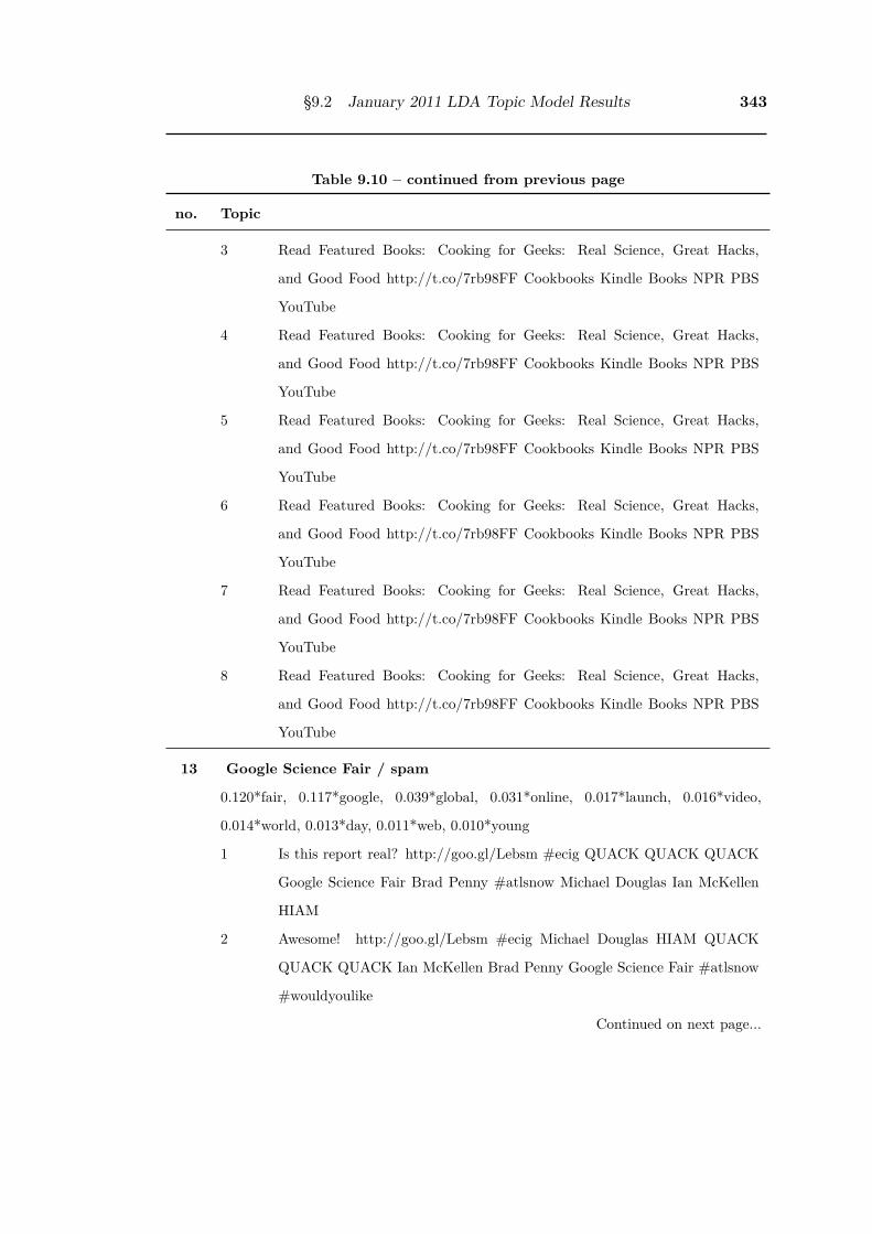
§9.2 January 2011 LDA Topic Model Results 343
Table 9.10 – continued from previous page
no. Topic
3 Read Featured Books: Cooking for Geeks: Real Science, Great Hacks,
and Good Food http://t.co/7rb98FF Cookbooks Kindle Books NPR PBS
YouTube
4 Read Featured Books: Cooking for Geeks: Real Science, Great Hacks,
and Good Food http://t.co/7rb98FF Cookbooks Kindle Books NPR PBS
YouTube
5 Read Featured Books: Cooking for Geeks: Real Science, Great Hacks,
and Good Food http://t.co/7rb98FF Cookbooks Kindle Books NPR PBS
YouTube
6 Read Featured Books: Cooking for Geeks: Real Science, Great Hacks,
and Good Food http://t.co/7rb98FF Cookbooks Kindle Books NPR PBS
YouTube
7 Read Featured Books: Cooking for Geeks: Real Science, Great Hacks,
and Good Food http://t.co/7rb98FF Cookbooks Kindle Books NPR PBS
YouTube
8 Read Featured Books: Cooking for Geeks: Real Science, Great Hacks,
and Good Food http://t.co/7rb98FF Cookbooks Kindle Books NPR PBS
YouTube
13 Google Science Fair / spam
0.120*fair, 0.117*google, 0.039*global, 0.031*online, 0.017*launch, 0.016*video,
0.014*world, 0.013*day, 0.011*web, 0.010*young
1 Is this report real? http://goo.gl/Lebsm #ecig QUACK QUACK QUACK
Google Science Fair Brad Penny #atlsnow Michael Douglas Ian McKellen
HIAM
2 Awesome! http://goo.gl/Lebsm #ecig Michael Douglas HIAM QUACK
QUACK QUACK Ian McKellen Brad Penny Google Science Fair #atlsnow
#wouldyoulike
Continued on next page...
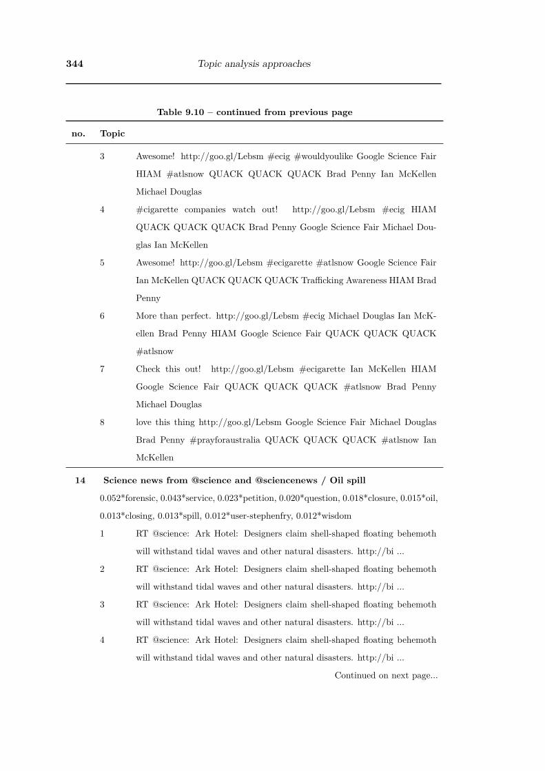
344 Topic analysis approaches
Table 9.10 – continued from previous page
no. Topic
3 Awesome! http://goo.gl/Lebsm #ecig #wouldyoulike Google Science Fair
HIAM #atlsnow QUACK QUACK QUACK Brad Penny Ian McKellen
Michael Douglas
4 #cigarette companies watch out! http://goo.gl/Lebsm #ecig HIAM
QUACK QUACK QUACK Brad Penny Google Science Fair Michael Dou-
glas Ian McKellen
5 Awesome! http://goo.gl/Lebsm #ecigarette #atlsnow Google Science Fair
Ian McKellen QUACK QUACK QUACK Trafficking Awareness HIAM Brad
Penny
6 More than perfect. http://goo.gl/Lebsm #ecig Michael Douglas Ian McK-
ellen Brad Penny HIAM Google Science Fair QUACK QUACK QUACK
#atlsnow
7 Check this out! http://goo.gl/Lebsm #ecigarette Ian McKellen HIAM
Google Science Fair QUACK QUACK QUACK #atlsnow Brad Penny
Michael Douglas
8 love this thing http://goo.gl/Lebsm Google Science Fair Michael Douglas
Brad Penny #prayforaustralia QUACK QUACK QUACK #atlsnow Ian
McKellen
14 Science news from @science and @sciencenews / Oil spill
0.052*forensic, 0.043*service, 0.023*petition, 0.020*question, 0.018*closure, 0.015*oil,
0.013*closing, 0.013*spill, 0.012*user-stephenfry, 0.012*wisdom
1 RT @science: Ark Hotel: Designers claim shell-shaped floating behemoth
will withstand tidal waves and other natural disasters. http://bi ...
2 RT @science: Ark Hotel: Designers claim shell-shaped floating behemoth
will withstand tidal waves and other natural disasters. http://bi ...
3 RT @science: Ark Hotel: Designers claim shell-shaped floating behemoth
will withstand tidal waves and other natural disasters. http://bi ...
4 RT @science: Ark Hotel: Designers claim shell-shaped floating behemoth
will withstand tidal waves and other natural disasters. http://bi ...
Continued on next page...

§9.2 January 2011 LDA Topic Model Results 345
Table 9.10 – continued from previous page
no. Topic
5 RT @science: Ark Hotel: Designers claim shell-shaped floating behemoth
will withstand tidal waves and other natural disasters. http://bi ...
6 RT @science: Ark Hotel: Designers claim shell-shaped floating behemoth
will withstand tidal waves and other natural disasters. http://bi ...
7 RT @science: Ark Hotel: Designers claim shell-shaped floating behemoth
will withstand tidal waves and other natural disasters. http://bi ...
8 RT @science: Ark Hotel: Designers claim shell-shaped floating behemoth
will withstand tidal waves and other natural disasters. http://bi ...
15 Dinosaurs / Archeology / NASA mars news / Science and Spirit
0.031*year, 0.021*email, 0.021*marketing, 0.019*hour, 0.014*sun, 0.014*fair,
0.013*day, 0.013*mammoth, 0.012*google, 0.011*project
1 RT @sciencenewsorg: Early meat-eating dinosaur unearthed: Pint-sized,
two-legged runner dates back to the dawn of the dinos http://bit.l ...
2 RT @sciencenewsorg: Early meat-eating dinosaur unearthed: Pint-sized,
two-legged runner dates back to the dawn of the dinos http://bit.l ...
3 RT @sciencenewsorg: Early meat-eating dinosaur unearthed: Pint-sized,
two-legged runner dates back to the dawn of the dinos http://bit.l ...
4 RT @sciencenewsorg: Early meat-eating dinosaur unearthed: Pint-sized,
two-legged runner dates back to the dawn of the dinos http://bit.l ...
5 RT @sciencenewsorg: Early meat-eating dinosaur unearthed: Pint-sized,
two-legged runner dates back to the dawn of the dinos http://bit.l ...
6 RT @sciencenewsorg: Early meat-eating dinosaur unearthed: Pint-sized,
two-legged runner dates back to the dawn of the dinos http://bit.l ...
7 Latest Science News Early meat-eating dinosaur unearthed: Pint-sized, two-
legged runner dates back to the dawn o... http://bit.ly/fbETBY
8 Martin Luther King Day: How much do you know about MLK? Take our
quiz - Christian Science Monitor: ABC News Martin Luther King Day:
How…
Continued on next page...

346 Topic analysis approaches
Table 9.10 – continued from previous page
no. Topic
16 Hill’s Science Diet / weight loss / Christian Science Monitor news
0.071*christian, 0.059*monitor, 0.022*weight, 0.017*diet, 0.014*loss, 0.013*news,
0.011*food, 0.010*health, 0.008*egypt, 0.008*hill
1 weight loss meal plan: The Low GI Diet Revolution: The Definitive Science-
Based Weight Loss Plan: http://weight-loss-meal-plan.fatbash.c...
2 Hill’s Science Diet Adult Lamb Meal & Rice Recipe Small Bites Dog Food:
Hill’s Science Diet Adult Lamb Meal & Ri... http://bit.ly/gLkxbu
3 @SpeakerBoehner JOBS JOBS JOBS! POTUS remind 2 digit IQ #tcot JFK
believed in science! GOP boast JFK while ignore SCIENCE #greenenergy
#P2
4 Weight Loss, Best Diet Plan, Meal Plans and Easy Recipes: san diego weight
loss club science diet w d diabetic d gt1rWw http://bit.ly/hyCG26
5 Funeral protest: Arizona rallies to foil Westboro Baptist Church - Christian
Science Monitor: Daily Mail Funeral protest: Arizona rallies…
6 Public rallies to help rescued dogs at Mat-Su shelter: The Mat-Su animal
shelter is seeking donations of Hills Science Diet Advanced ...
7 Hill’s Science Diet Puppy Large Breed Lamb Meal and Rice Formula Dry
Dog Food: Hill’s Science Diet Puppy Large B... http://bit.ly/fNsEIq
8 Pet Supplies Hills Pet Nutrition - Adult Large Breed Oral Care Dog Treats
200g: Hills Science Plan Oral Care Sna... http://bit.ly/f6EbWF
17 Bird Death / Life Science / Idiot Abroad show (Science Channel)
/ Films
0.026*channel, 0.016*fiction, 0.016*kissing, 0.015*newly, 0.015*tagged, 0.014*idiot,
0.014*abroad, 0.013*magic, 0.012*nature, 0.012*area
1 RT @sciencenewsorg: Deleted Scenes: Arkansas birds died of trauma:
Necropsies suggest loud noise caused panicked flock to f... http://bi ...
2 RT @sciencenewsorg: Deleted Scenes: Arkansas birds died of trauma:
Necropsies suggest loud noise caused panicked flock to f... http://bi ...
Continued on next page...

§9.2 January 2011 LDA Topic Model Results 347
Table 9.10 – continued from previous page
no. Topic
3 RT @sciencenewsorg: Deleted Scenes: Arkansas birds died of trauma:
Necropsies suggest loud noise caused panicked flock to f... http://bi ...
4 RT @sciencenewsorg: Deleted Scenes: Arkansas birds died of trauma:
Necropsies suggest loud noise caused panicked flock to f... http://bi ...
5 RT @sciencenewsorg: Deleted Scenes: Arkansas birds died of trauma:
Necropsies suggest loud noise caused panicked flock to f... http://bi ...
6 RT @sciencenewsorg: Deleted Scenes: Arkansas birds died of trauma:
Necropsies suggest loud noise caused panicked flock to f... http://bi ...
7 RT @sciencenewsorg: Deleted Scenes: Arkansas birds died of trauma:
Necropsies suggest loud noise caused panicked flock to f... http://bi ...
8 RT @sciencenewsorg: Deleted Scenes: Arkansas birds died of trauma:
Necropsies suggest loud noise caused panicked flock to f... http://bi ...
18 Fraud (including MMR and Autism) / vaccination / anti vacci-
nation / Crime
0.024*museum, 0.023*vaccine, 0.018*autism, 0.016*bbc, 0.015*study, 0.015*horizon,
0.012*attack, 0.010*fraud, 0.009*news, 0.008*paul
1 ATTENTION SCIENCE COMMUNITY, RAMIRO MURATA, NYU COL-
LEGE OF DENTISTRY STAFF, INVOLVED IN CHILD ABDUCTION,
ABUSE, ROBBERY, FRAUDS IN NEW YORK.
2 ATTENTION SCIENCE COMMUNITY, RAMIRO MURATA, NYU-
POLY STAFF, INVOLVED IN CHILD ABDUCTION, ABUSE, APART-
MENT ROBBERY, FRAUDS IN NEW YORK.
3 ATTENTION SCIENCE COMMUNITY, RAMIRO MURATA, NYU-
POLY STAFF, INVOLVED IN CHILD ABDUCTION, ABUSE, APART-
MENT ROBBERY, FRAUDS IN NEW YORK.
4 9PM on BBC Two: BBC Horizon. Nobel Prize winner Sir Paul Nurse
examines why science appears to be under attack #bbc #horizon
5 RT @bbc_horizon: 9PM on BBC Two: BBC Horizon Nobel Prize winner Sir
Paul Nurse examines why science appears to be under attack #bbc #horizon
Continued on next page...

348 Topic analysis approaches
Table 9.10 – continued from previous page
no. Topic
6 ATTENTION SCIENCE COMMUNITY, RAMIRO MURATA, NYU-
POLY STAFF, INVOLVED IN CHILD ABDUCTION, ABUSE, APART-
MENT ROBBERY, FRAUDS IN NEW YORK.
7 RT @AutismScienceFd: ”Wakefield Paper Linking MMR Vaccine and
Autism a Fraud on the Scale of Piltdown Man, BMJ Editorial Says”- LA
Times ...
8 RT @AutismScienceFd: ”Wakefield Paper Linking MMR Vaccine and
Autism a Fraud on the Scale of Piltdown Man, BMJ Editorial Says”- LA
Times ...
19 Science Fiction (books / film / art / music)
0.112*fiction, 0.020*movie, 0.019*fantasy, 0.015*film, 0.013*book, 0.008*nasa,
0.007*time, 0.007*watch, 0.007*story, 0.006*video
1 Call it techno-thriller, science fiction, call terrific story-telling Terry Brooks
1 #NYT #author ref #Atlantis http://bit.ly/99yNaN #kindle
2 Call it techno-thriller, science fiction, call terrific story-telling Terry Brooks
1 #NYT #author ref #Atlantis http://bit.ly/99yNaN #kindle
3 Call it techno-thriller, science fiction, call terrific story-telling Terry Brooks
1 #NYT #author ref #Atlantis http://bit.ly/99yNaN #kindle
4 Call it techno-thriller, science fiction, call terrific story-telling Terry Brooks
1 #NYT #author ref #Atlantis http://bit.ly/99yNaN #kindle
5 Call it techno-thriller, science fiction, call terrific story-telling Terry Brooks
1 #NYT #author ref #Atlantis http://bit.ly/99yNaN #kindle
6 Call it techno-thriller, science fiction, call terrific story-telling Terry Brooks
#NYT #author ref #Atlantis http://bit.ly/99yNaN #kindle
7 Call it techno-thriller, science fiction, call terrific story-telling Terry Brooks
1 #NYT #author ref #Atlantis http://bit.ly/99yNaN #kindle
8 Call it techno-thriller, science fiction, call terrific story-telling Terry Brooks
1 #NYT #author ref #Atlantis http://bit.ly/99yNaN #kindle
Continued on next page...
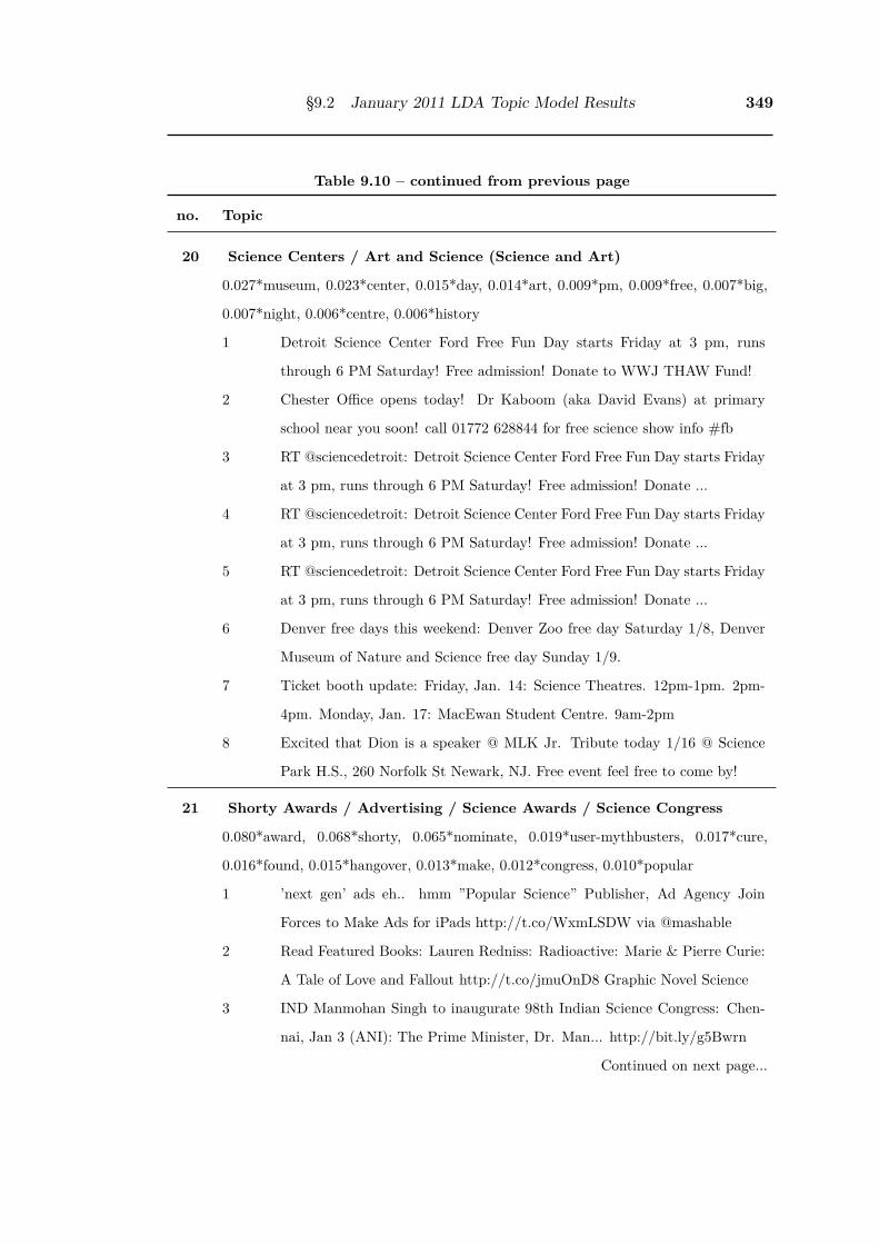
§9.2 January 2011 LDA Topic Model Results 349
Table 9.10 – continued from previous page
no. Topic
20 Science Centers / Art and Science (Science and Art)
0.027*museum, 0.023*center, 0.015*day, 0.014*art, 0.009*pm, 0.009*free, 0.007*big,
0.007*night, 0.006*centre, 0.006*history
1 Detroit Science Center Ford Free Fun Day starts Friday at 3 pm, runs
through 6 PM Saturday! Free admission! Donate to WWJ THAW Fund!
2 Chester Office opens today! Dr Kaboom (aka David Evans) at primary
school near you soon! call 01772 628844 for free science show info #fb
3 RT @sciencedetroit: Detroit Science Center Ford Free Fun Day starts Friday
at 3 pm, runs through 6 PM Saturday! Free admission! Donate ...
4 RT @sciencedetroit: Detroit Science Center Ford Free Fun Day starts Friday
at 3 pm, runs through 6 PM Saturday! Free admission! Donate ...
5 RT @sciencedetroit: Detroit Science Center Ford Free Fun Day starts Friday
at 3 pm, runs through 6 PM Saturday! Free admission! Donate ...
6 Denver free days this weekend: Denver Zoo free day Saturday 1/8, Denver
Museum of Nature and Science free day Sunday 1/9.
7 Ticket booth update: Friday, Jan. 14: Science Theatres. 12pm-1pm. 2pm-
4pm. Monday, Jan. 17: MacEwan Student Centre. 9am-2pm
8 Excited that Dion is a speaker @ MLK Jr. Tribute today 1/16 @ Science
Park H.S., 260 Norfolk St Newark, NJ. Free event feel free to come by!
21 Shorty Awards / Advertising / Science Awards / Science Congress
0.080*award, 0.068*shorty, 0.065*nominate, 0.019*user-mythbusters, 0.017*cure,
0.016*found, 0.015*hangover, 0.013*make, 0.012*congress, 0.010*popular
1 ’next gen’ ads eh.. hmm ”Popular Science” Publisher, Ad Agency Join
Forces to Make Ads for iPads http://t.co/WxmLSDW via @mashable
2 Read Featured Books: Lauren Redniss: Radioactive: Marie & Pierre Curie:
A Tale of Love and Fallout http://t.co/jmuOnD8 Graphic Novel Science
3 IND Manmohan Singh to inaugurate 98th Indian Science Congress: Chen-
nai, Jan 3 (ANI): The Prime Minister, Dr. Man... http://bit.ly/g5Bwrn
Continued on next page...
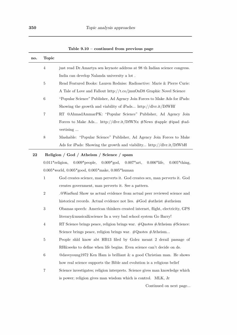
350 Topic analysis approaches
Table 9.10 – continued from previous page
no. Topic
4 just read Dr.Amartya sen keynote address at 98 th Indian science congress.
India can develop Nalanda university a lot .
5 Read Featured Books: Lauren Redniss: Radioactive: Marie & Pierre Curie:
A Tale of Love and Fallout http://t.co/jmuOnD8 Graphic Novel Science
6 “Popular Science” Publisher, Ad Agency Join Forces to Make Ads for iPads:
Showing the growth and viability of iPads... http://dlvr.it/DfWHf
7 RT @AhmadAmmarPK: “Popular Science” Publisher, Ad Agency Join
Forces to Make Ads... http://dlvr.it/DfWNx #News #apple #ipad #ad-
vertising ...
8 Mashable: “Popular Science” Publisher, Ad Agency Join Forces to Make
Ads for iPads: Showing the growth and viability... http://dlvr.it/DfWbH
22 Religion / God / Atheism / Science / spam
0.011*religion, 0.009*people, 0.009*god, 0.007*art, 0.006*life, 0.005*thing,
0.005*world, 0.005*good, 0.005*make, 0.005*human
1 God creates science, man perverts it. God creates sex, man perverts it. God
creates government, man perverts it. See a pattern.
2 .@WasSaul Show us actual evidence from actual peer reviewed science and
historical records. Actual evidence not lies. #God #atheist #atheism
3 Obamas speech: American thinkers created internet, flight, electricity, GPS
literary&musical&science In a very bad school system Go Barry!
4 RT Science brings peace, religion brings war. #Quotes #Atheism #Science:
Science brings peace, religion brings war. #Quotes #Atheism...
5 People shld know abt HB13 filed by Golez meant 2 derail passage of
RH&seeks to define when life begins. Even science can’t decide on ds.
6 @daveyoung1972 Ken Ham is brilliant & a good Christian man. He shows
how real science supports the Bible and evolution is a religious belief
7 Science investigates; religion interprets. Science gives man knowledge which
is power; religion gives man wisdom which is control. MLK, Jr
Continued on next page...

§9.2 January 2011 LDA Topic Model Results 351
Table 9.10 – continued from previous page
no. Topic
8 Science investigates, religion interprets. Science gives man knowledge which
is power, religion gives man wisdom which is control. MLK Jr.
23 National Science Foundation (education outreach) / Science ed-
ucation assessment
0.046*student, 0.030*video, 0.026*youtube, 0.017*national, 0.015*test, 0.013*report,
0.013*school, 0.011*american, 0.010*score, 0.010*show
1 NSF Leader to Researchers: Explore Post-High School Transitions: A top
National Science Foundation official beli... http://bit.ly/hwxZVY
2 RT @milesobrien: New NSF ”Science Nation” - Virtual Reality Maps: re-
building the world one pixel at a time. Miles O’Brien, reporter. htt ...
3 RT @milesobrien: New NSF ”Science Nation” - Virtual Reality Maps: re-
building the world one pixel at a time. Miles O’Brien, reporter. htt ...
4 RT @milesobrien: New NSF ”Science Nation” - Virtual Reality Maps: re-
building the world one pixel at a time. Miles O’Brien, reporter. htt ...
5 RT @milesobrien: New NSF ”Science Nation” - Virtual Reality Maps: re-
building the world one pixel at a time. Miles O’Brien, reporter. htt ...
6 RT @milesobrien: New NSF ”Science Nation” - Virtual Reality Maps: re-
building the world one pixel at a time. Miles O’Brien, reporter. htt ...
7 Study shows students lack science skills: Study shows students lack science
skills College students might find t... http://bit.ly/emSNzE
8 Writing About Anxiety Helps Students Ace Exams - Kansas City infoZine
News #school #edu #education #science #NSF http://t.co/0MzFVHN
24 Arkansas river dead fish / (@WhiteHouse science fair winner tweet?)
0.098*fair, 0.098*winner, 0.045*hashtag-sotu, 0.041*bowl, 0.041*super, 0.035*cele-
brated, 0.017*deserves, 0.016*dead, 0.015*bird, 0.015*obama
1 MT @science: 100,000+ dead fish found dead in Ark. River, 125 miles west
of Beebe, where 5,000 birds fell dead from sky http://bit.ly/hWYYtx
Continued on next page...

352 Topic analysis approaches
Table 9.10 – continued from previous page
no. Topic
2 100,000+ dead fish found floating in AR River - 125 miles west of Beebe,
whr 5,000 birds fell dead from sky http://bit.ly/hWYYtx By @science
3 Apocalypse?RT @science: 100,000+ dead fish found floating in Arkansas
River - 125 miles west of Beebe, where 5,000 birds fell dead from sky
4 RT @science: 100,000+ dead fish found floating in Arkansas River - 125
miles w of Beebe, whr 5K birds fell dead frm sky http://bit.ly/hWYYtx
5 @science: 100,000+ dead fish found floating in Arkansas River - 125 miles
w of Beebe, whr 5K birds fell dead frm sky http://bit.ly/hWYYtx
6 Honey West actress dies aged 80: Actress Anne Francis, who played the love
interest in the 1950s science-fiction classic Forbidden Pl...
7 Honey West actress dies aged 80: Actress Anne Francis, who played the love
interest in the 1950s science-fiction classic Forbidden Pl...
8 Honey West actress dies aged 80: Actress Anne Francis, who played the love
interest in the 1950s science-fiction classic Forbidden Pl...
25 Science news (trees / bacteria / travel) / Science excursions (students)
0.046*good, 0.043*heart, 0.042*field, 0.039*politics, 0.037*motivation, 0.036*impor-
tant, 0.036*develop, 0.035*agriculture, 0.033*user-dalailama, 0.022*hashtag
1 Week in science: peak travel, tree rings, and methane-eating bacteria:
Trends suggest industrialized world may be hitting peak travel...
2 Week in science: peak travel, tree rings, and methane-eating bacteria - Ars
Technica: National Geographic Week in science: peak travel,...
3 Week in science: peak travel, tree rings, and methane-eating bacteria:
Trends suggest industrialized world may be hitting peak travel...
4 #Tech #TechNews Week in science: peak travel, tree rings, and methane-
eating bacteria - Ars Technica http://bit.ly/emXY8K #DhilipSiva
5 Travel Week in science: peak travel, tree rings, and methane-eating bacteria:
Trends suggest industrialized worl... http://bit.ly/exMA6o
6 Ars Technica| Week in science: peak t...: Ars Technica| Week in science:
peak travel, tree rings, and methane-ea... http://bit.ly/gJpbgK
Continued on next page...

§9.2 January 2011 LDA Topic Model Results 353
Table 9.10 – continued from previous page
no. Topic
7 -bbc science- Fall of Rome ’recorded in trees’: An extensive study of tree
growth rings suggest that rise and fa... http://bbc.in/fIQg72
8 [BBC Science] Fall of Rome ’recorded in trees’: An extensive study of tree
growth rings suggest that rise and fa... http://bbc.in/gbmPQT
26 Music with word science’ in name or company / Science of Social Media
0.067*faith, 0.030*script, 0.028*album, 0.021*user-thescript, 0.016*medium,
0.015*social, 0.011*song, 0.010*textbook, 0.009*video, 0.009*hashtag-nowplaying
1 brian tracy video » Free torrent and rapidshare downloads, free ...: brian
tracy video Brian Tracy - The Science of Positive Focus En...
2 Radio Free Dystopia. Exile x Dirty Science - Watch Out! False Prophet [ft.
Dagsavage & Turtle] on Wub-Fur Internet Radio
3 Radio Free Dystopia. Exile x Dirty Science - Watch Out! False Prophet [ft.
Dagsavage & Turtle] on Wub-Fur Internet Radio
4 Radio Free Dystopia. Exile x Dirty Science - Watch Out! False Prophet [ft.
Dagsavage & Turtle] on Wub-Fur Internet Radio
5 Radio Free Dystopia. Exile x Dirty Science - In Love (Kan Kick Remix) on
Wub-Fur Internet Radio
6 Radio Free Dystopia. Exile x Dirty Science - In Love (Kan Kick Remix) on
Wub-Fur Internet Radio
7 Radio Free Dystopia. Exile x Dirty Science - In Love (Kan Kick Remix) on
Wub-Fur Internet Radio
8 Buy Cheap Science & Faith (US Bonus Track Version) The Script 276%
Sales Rank in Music: 1... http://amzn.to/fCkFqG #deal #sale #coupon
27 People participating in science events / science actities / men-
tioning science
0.012*day, 0.009*love, 0.008*project, 0.008*teacher, 0.008*make, 0.007*class,
0.007*rocket, 0.006*time, 0.006*kid, 0.006*watching
Continued on next page...

354 Topic analysis approaches
Table 9.10 – continued from previous page
no. Topic
1 Watched the Star Gazing last night: rarely watch any TV enjoyed Dara &
the Prof, frustrated by cloudy sky! TV Science at a level I cd enjoy
2 Spent all day at the Space Science Centre, then ate great food, drank good
wine, watched movies, cuddled, kissed good night. life’s good.
3 Jessica’s party was AWESOME! Cotton candy, fireworks, dry ice, epic Mad
Science show, beach ball fight and giant Allie’s donut cake!
4 @daraobriain love that ur a science geek!! Sexy dara!! Lol and u make
women laugh... O and ur irish! Loving ur work mister!
5 right plan. have bath&wash hair. dry&straighteb hair. get dressed. write
science reports. go on wii fit. watch TW on YouTube. day sorted!;)
6 Fuck Flowers, Fuck Candy... - science fiction holidays Valentine’s Day gift
present sex toy sex machine robot lover http://t.co/3IyXw6c
7 Just ran my bath water. That shit is like a science project. Lol! I be pouring
in a a gang of shit. Bubbles, sea salt, vinegar, and oil lol!
8 Tags: break science, Glass Hits, Ideal Fathers, Julio Enriquez, lefse, Mike
Marchant, Night of Joy, paper diamond, Pretty Lights, tal...
28 Students not liking science classes (colloquial spelling and language)
0.037*class, 0.024*lol, 0.019*teacher, 0.017*haha, 0.015*math, 0.013*hate,
0.010*school, 0.009*computer, 0.008*political, 0.008*year
1 ”@mcchizzy:Ur lazy man y r u nw a science student?@deputyp:i jus wnt 2
do onli maths,eng nd pe.i hate bio d physics.dt 1 iz evn worse”iono o
2 @mym8fanciesyou oppss..i loved physics 4rm da 3 f it..hated bio bcoz of ma
stupid bio mam lol..chemistry gone case! :D enjoy ur science lol
3 JESUS BE WIT ME DIS SEMESTER...9 classes=17 hrs...dey all in da
science building so u knw wat dat means hmmmm...nun bt science...yay
ha!!!
4 IN ENVIORNMENTAL SCIENCE I FXKIN HATE DIZ CLASS DA
TEACHER SLOW AF & ION FXKWIT NOBODI IN DIZ CLASS LYK
DAT #ugh #fml READY FA COSMETOLOGY
Continued on next page...

§9.2 January 2011 LDA Topic Model Results 355
Table 9.10 – continued from previous page
no. Topic
5 @aaomnt tae hai pj print hai laew don’t worry huhi chun tum science mai
sed td nae a kae mai wai laew ja pai sleep la nhu mai norn ror ya?
6 DEY SHOULDA TESTED ERRTHANG IN DIS NEW SCIENCE BUILDIN
B4 DEY PUT US IN HUR. ITS KOLD IN DIS LAB & DA TEACHER DNT
KNO HW 2 PLUG UP DA STUFF
7 @superathilah tak. Malas nak stay back. And the science part tak susah,
the english part of est yg susah. Tak capital je terus potong marks
8 I Got An A On Mii Reading Nd Math Xam Juss Passed History Wiff A 76
Mii Mom Gonna Lecture Mii How Iculd Do Betta DK Bout Science Hope
Idid G
29 USA Obama State of the Union Address / Politics
0.052*stupid, 0.047*bracelet, 0.040*problem, 0.031*state, 0.030*god, 0.027*union,
0.026*class, 0.026*professor, 0.025*philosophy, 0.024*speaking
1 CUT #TAXES: #Save $86 MILLION by eliminating Natl Science Fdn (
#NSF ) spending on elementary & secondary #education. #youcut @GO-
PLeader
2 CUT #TAXES: #Save $86 MILLION by eliminating Natl Science Fdn (
#NSF ) spending on elementary & secondary #education. #youcut @GO-
PLeader
3 CUT #TAXES: #Save $86 MILLION by eliminating Natl Science Fdn (
#NSF ) spending on elementary & secondary #education. #youcut @GO-
PLeader
4 CUT #TAXES: #Save $86 MILLION by eliminating Natl Science Fdn (
#NSF ) spending on elementary & secondary #education. #youcut @GO-
PLeader
5 CUT #TAXES: #Save $86 MILLION by eliminating Natl Science Fdn (
#NSF ) spending on elementary & secondary #education. #youcut @GO-
PLeader
Continued on next page...

356 Topic analysis approaches
Table 9.10 – continued from previous page
no. Topic
6 CUT #TAXES: #Save $86 MILLION by eliminating Natl Science Fdn (
#NSF ) spending on elementary & secondary #education. #youcut @GO-
PLeader
7 CUT #TAXES: #Save $86 MILLION by eliminating Natl Science Fdn (
#NSF ) spending on elementary & secondary #education. #youcut @GO-
PLeader
8 CUT #TAXES: #Save $86 MILLION by eliminating Natl Science Fdn (
#NSF ) spending on elementary & secondary #education. #youcut @GO-
PLeader
30 unclear - very diverse tweets
0.024*time, 0.016*scientist, 0.015*quantum, 0.014*make, 0.013*mad, 0.012*sign,
0.012*real, 0.011*data, 0.009*life, 0.009*wired
1 Tasty Science FAIL - Epic Fail Funny Videos and Funny Pictures: epic fail
photos - Tasty Science FAIL.Epic Fail ... http://bit.ly/hMBcpn
2 Enjoying a Black Death Imperial IPA by Mad Science Brewing Company at
Mad Science Brewing Company (aka my house) — http://untpd.it/Fetxz2
3 Enjoying a Black Death Imperial IPA by Mad Science Brewing Company at
Mad Science Brewing Company (aka my house) — http://untpd.it/BDEKPl
4 Scientists Create Real-Life Pac-Man Using Microorganisms [Science] - Sci-
entists Create Real-Life Pac-Man... http://tumblr.com/xbl1aa5crr
5 Enjoying a Black Death Imperial IPA by Mad Science Brewing Company at
Mad Science Brewing Company (aka my house) — http://untpd.it/HPSknr
6 Led Bulb | Lighting Science Group Makes Its One Millionth U.S. LED Bulb
– An Ultra-Efficient And Affordable 60 Watt... http://dlvr.it/Clq4N
7 Led Bulb | Lighting Science Group Makes Its One Millionth U.S. LED Bulb
– An Ultra-Efficient And Affordable 60 Watt... http://dlvr.it/Clq4S
8 Led Bulb | Lighting Science Group Makes Its One Millionth U.S. LED Bulb
– An Ultra-Efficient And Affordable 60 Watt... http://dlvr.it/Clq4X

§9.2 January 2011 LDA Topic Model Results 357
The overall representation of each topic in the corpus can be calculated by summing
the weight of each topic in each document to get the total weight for the topic. The
code to do this is shown in listing K.20 in Appendix K. The topic weights for each of
the 30 LDA topics for January 2011 are shown on Fig. 9.8 and in Table 9.11. Using
the total weight of each topic in the corpus gives an indication of how much of the
conversation is about that topic. For January 2011, Topics 10 (students tweeting about
lessons / exams / projects (today/tomorrow)), 27 (people participating in science) and
28 (students not liking science classes (colloquial spelling and language)) are highly
represented in the corpus, followed by 22 (Religion / God / Atheism / Science / spam)
and 11 (University jobs and courses / NSF grants / qualifications for jobs).
1 2 3 4 5 6 7 8 910
11
12
13
14
15
16
17
18
19
20
21
22
23
24
25
26
27
28
29
30
Topic Number
0.00
0.02
0.04
0.06
0.08
0.10
0.12
0.14
Weig
ht
Figure 9.8: Weight of topics in LDA Model of January 2011 corpus
Having looked in detail at the 30 topics from the LDA Model for January 2011 I
finish this chapter by building a 30 topic model for all of the science tweets in 2011.

358 Topic analysis approaches
Table 9.11: Weight of topics in LDA Model of January 2011 corpus
Topic Weight Topic Description1 0.030 Science Online 2011 Conference / writing / blogging2 0.014 Tweets shared from StumbleUpon - possibly spam3 0.012 Bill Nye / ESPN / Science News4 0.013 Singapore Education (parody)5 0.028 Climate change, Global Warming and general science news6 0.029 Science media news links (CBC News, BBC Science, CBS News etc.) /
spam7 0.023 Space science news / spam8 0.039 Health science news (cancer, anti-aging, fertility) / spam9 0.032 Jobs / school boards / power / contracts
10 0.130 Students tweeting about lessons / exams / projects (today/tomorrow)11 0.063 University jobs and courses / NSF grants / qualifications for jobs12 0.014 Kindle book promotion spam links13 0.019 Google Science Fair / spam14 0.010 Science news from @science and @sciencenews / Oil spill15 0.011 Dinosaurs / Archaeology / NASA Mars news / Science and Spirit16 0.020 Hill’s Science Diet / weight loss / Christian Science Monitor news17 0.014 Bird Death / Life Science / Idiot Abroad show (Science Channel) /
Films18 0.012 Fraud (including MMR and Autism) / vaccination / anti vaccination /
Crime19 0.034 Science Fiction (books / film / art / music)20 0.044 Science Centers / Art and Science (Science and Art)21 0.014 Shorty Awards / Advertising / Science Awards / Science Congress22 0.076 Religion / God / Atheism / Science / spam23 0.018 National Science Foundation (education outreach) / Science education
assessment24 0.016 Arkansas river dead fish / (@WhiteHouse science fair winner tweet?)25 0.010 Science news (trees / bacteria / travel) / Science excursions (students)26 0.015 Music with word ‘science’ in name or company / Science of Social Media27 0.124 People participating in science events / science activities / mentioning
science28 0.110 Students not liking science classes (colloquial spelling and language)29 0.010 USA Obama State of the Union Address / Politics30 0.015 unclear - very diverse tweets
9.3 Full Year 2011 LDA Model
The corpus creation and filtering code used for the January corpus was extended to
create a single corpus for the whole year. The number of months to process in the
corpus creation software in listing K.1 in Appendix K were extended to the whole year:
months = range(1,13) and the names of the output files changed to reflect their being
for the whole year. The filtering code (listing K.3 in Appendix K) had the input and

§9.3 Full Year 2011 LDA Model 359
output file names changed to be for the whole year. The corpus creation from the
previous cleaned tweets took 1.5 hours and the filtering took 28 minutes.
The unfiltered whole year corpus had 12,227,439 documents (tweets) with 2,732,171
unique tokens (words) and a total of 113,102,102 tokens. The number of unique tokens
was reduced to 97,709 by the filtering and the total number of tokens to 87,335,786.
When Mallet imported the documents it applied further stop word processing and
reduced the number of tokens to 78,541,806.
The code used to find the number of iterations for LdaMallet (listing K.16 in Ap-
pendix K) as modified for January 30 topic model (iterations=4000 and topics=30)
was used with the full year filtered corpus to generate a 30 topic model. This took
11.7 hours to run. The beta and LL/token reported by Mallet was again collected to
check that the change to the full year from the previous single month had not affected
the number of iterations required. The overall results are shown in 9.9 confirmed that
4,000 iterations allowed the beta and perplexity to stabilise for the whole year corpus.
0 500 1,000 1,500 2,000 2,500 3,000 3,500 4,000
Iterations
0
500
1,000
1,500
2,000
2,500
3,000
3,500
4,000
4,500
Perp
lexit
y
0.005
0.010
0.015
0.020
0.025
0.030
0.035
Betaperplexity
beta
Figure 9.9: Mallet Perplexity and Beta (30 Topics, 4000 iterations) whole year 2011
The code used to find and report the most significant tweets for each topic for
January 2011 (code shown in listing K.17 in Appendix K) was not memory efficient
and failed to work with the much larger full year dataset. A new program was written

360 Topic analysis approaches
(listing K.18 in Appendix K) that found the top documents by iterating over the
document weights one document at a time instead of loading the full year and sorting
in memory to get the top ones. It took 5.1 hours to run after which the final report was
generated by the code shown in listing K.19 in Appendix K. The 30 topics identified
by this model are shown in Table 9.12 (pp. 366-388) with the first eight tweets for each
topic. As for the January 2011 corpus, I examined the highest weight 100 tweets for
each topic and gave each topic a title describing what I thought was being discussed
and these are shown above the word frequency for the topic in 9.12.
The first topic was technology news with companies like Google, Apple, Facebook,
Paypal and Nokia mentioned. Many of the tweets were about phones and tablets, but
the top 100 tweets also included mentions of mobile science applications for phones,
citizen science, data science, open data, and the launch of an early-stage science research
funding body.
Topic 2 was health and medical science. The top 100 tweets covered many health
and medical science topics and the topic was very coherent. Although it was similar
to topic 8 in January 2011 it does not contain much spam and was more focussed on
science rather than health services or product promotion.
The third topic had tweets about science fiction and was very similar to topic 19
from the January 2011 model. There were quite a few tweets in the top 100 that looked
like spam because they contained lists of other unrelated keywords as well as ‘science
fiction’ and seemed likely to be using the phrase ‘science fiction’ to try to be seen by
readers.
The fourth topic was more diverse with discussion of climate change, the Fukushima
nuclear disaster, marine and freshwater science and household energy and had some
overlap with fifth topic in the January 2011 model. Two of the highest weighted tweets
were about ‘White Snow on Green Leaves’ and ‘Autumn colours’ and it is not clear
what brought them into the topic, although perhaps the both might be mentioned in

§9.3 Full Year 2011 LDA Model 361
other tweets as being due to climate change effects. There were some anthropology
tweets in the top 100. This topic had many of what looked like automated tweets from
home energy meters: “Household energy used:natural gas:5 m3/51.8 kWh, electrical
energy:20.2 kWh Total energy used:72 kWh WX:oc #solar #energy #citizenscience”
Topic 5 had many tweets about university jobs and jobs with university qualifica-
tions. Many of these seemed to be generated tweets from a company called Simply
Hired. There were also tweets about research linkages across states and countries. It
had some similarity to topic 11 in January 2011.
The sixth topic was very coherent and had tweets about a wide range of space news
and space science.
The most significant 100 tweets for the seventh topic included many that should
have been removed as ‘noun spam’ in Chapter 4 where I filtered out 283,553 tweets
identified as ‘noun spam’. These included tweets 7 and 8 under topic 7 in listing K.17.
Another tweet that appeared to be spam is repeated with small variations;
Watch MST3K Vs. Gamera: Mystery Science Theater 3000, Vol. XXI
[Deluxe Edition] - Joel Hodgson (Actor), Kevin Murphy (Di http://adf.ly/1WPsl
many times in the top 100. The few non-spam tweets in the top 100 were about the
Big Bang theory TV show and retweets of news about CERN Higgs Boson research:
RT @dailygalaxy: NewsFlash: Rumor Sweeping World’s Science Commu-
nity that CERN’s LHC has Detected the Higgs Boson -The ”God Particle”
ht ...”.
Most of the top 100 tweets in topic 8 and all of the top 100 tweets in topic 9 were
not in English. Of the ones in topic 8 that were in English quite a few were lists of
equipment or steps in simple science experiments like these ones:

362 Topic analysis approaches
Vinegar, lemon juice, baking soda, bleach, red cabbage juice, sunscreen,
color-changing beads & string. Another fun day of Science @ work.
and
Soccer, football, dance, baby naps, dog poop, cook lunch, laundry, toddler
poop, science project, [husband duty], shower.... Ughhhhhhhh
These and the other English tweets in topic 8 contained diverse collections of words
that are not often used together. Most of the foreign tweets in topic 9 appeared to
be in Indonesian and should have been removed by language filtering as described in
Chapter 4.
The first two tweets in topic 10 were in English, then the next 25 tweets by topic
weight were not in English, and appeared to be variations on the same tweet. After
the 32nd tweet most of them were in English and seemed to be mainly tweets by high
school students. Some tweets in this topic showed that the students did not like science,
like topic 28 in January, but there were also positive ones about science class and funny
incidents in science class. There were a number of tweets by students commenting on
the appearance of their teachers, what their teachers say and conversations with their
teachers.
Most of the highest weight tweets in topic 11 were high school students listing the
subjects they are going to study for senior year, many of them with ‘AP’ - Advanced
Placement as can be seen in the sample tweets for topic 11 in Table 9.12. There
were some tweets that were lists of courses students are taking or planing to take at
University along with some promoting University degrees.
Topic 12 contained many tweets of the theme for the Bill Nye show as shown in
Table 9.12.

§9.3 Full Year 2011 LDA Model 363
Many of the top 100 tweets for topic 13 were not in English, and most of these
appeared to be Norwegian. The English tweets included many announcements about
TV shows with links to buy, download or watch them on YouTube.
The highest weighted 16 tweets for topic 14 were promoting shows by performer
DJ Science and there were many more of this type of tweet in the top 100. They
appeared to be computer generated promotional tweets. Other tweets in the top 100
were similar to those for topic 20 in January 2011; promotion of opening times of
museums and science centres and people tweeting about visits to science centres and
museums, although there was less mention of art.
The top weighted words for topic 15 were almost identical to topic 10 in January
2011. The tweets in this topic were very similar too. There were more non-English
tweets in the whole year, three in the top 8 for the whole year, and quite a few more
in the top 100, although these all had some English words in them like ‘good luck’ or
‘exam’.
Topic 16 appeared to be computer generated Amazon book link spam like topic
12 in January 2011. The first 7 tweets shown for topic 18 in Table 9.12 all contained
computer error messages that appeared to have been included as part of the text by a
program creating them. This type of error message could be a useful indicator of spam
tweets.
The tweets in the top 100 for topic 17 had most words as hashtags. They were
nearly all repeats of two tweets, one promoting twitter user @iamlogiq (for example
tweets 2-5 and 8 in Table 9.12) and one linking to the same StumbleUpon account
found in topic 2 of January 2011.
Topic 18 was mainly about climate change, similar to topic 4 in January 2011. It
also included some other controversial science issues but unlike topic 4 in January, did
not include any general science news in the top 100 tweets.
364 Topic analysis approaches
Topic 19 included many retweets of two celebrities, one by Indian film director and
producer Ram Gopal Varma (@RGVzoomin) sent on 30 Sep 2011:
Aftr lots of struggle nd time I managed to undrstnd logarithms nd evn
rocket science bt evn aftr almost a life time I can’t understand women
https://twitter.com/RGVzoomin/status/119446080487297025
and another by political satirist Stephen Colbert (@StephenAtHome) sent on 24 Mar
2011:
Science and food ARE linked. True story: Jonas Salk stumbled upon the
polio vaccine while perfecting a gravy recipe.
https://twitter.com/StephenAtHome/status/50768636108996608
There were also tweets about the rap lyric by Lil Wayne ‘choppers dissect a nigga lik
science’ as shown in tweet 1 in Table 9.12. Tweets similar to tweets 3 and 4 were
repeated in the top 100 and also appeared to be song lyrics.
The most significant 100 tweets for topic 20 were mainly lists of the names of songs
by rock band ‘System of a Down’ which was reunited in November 2010 and toured
during May to October 2011. The band asked people to submit sets of 6 songs they
would like to hear during the reunion tour20. Some of their song titles include the word
science and so have been collected as part of my corpus.
Like topic 22 in January 2011, topic 21 for the full year had tweets about religion
and science. The top 100 tweets did not contain any of the Amazon link spam seen
in January. There were more tweets about pro-choice and pro-life than in the January
topic.
Topic 22 was nearly all Hill’s Science Diet pet food advertisements.20http://www.systemofadown.com/yoursetlist/us/

§9.3 Full Year 2011 LDA Model 365
The top 100 tweets for topic 23 were mainly about USA politics. Some of these
were from the Christian Science News service and there were other science news tweets
from this service in the top 100.
Topic 24 contained tweets about weight loss, diet and cosmetics and although some
were links to information, most appeared to be product advertising or spam links.
Some of the most significant tweets for topic 25 again contained the computer error
texts in what was probably Amazon book link spam. There were many repeats of
the 8th retweet promoting the ‘NYT Science Times: The Future of Computing issue’
in the top 100. The highest weighted words for this topic were similar to topic 1 in
January 2011 and near the end of the top 100 tweets there was one about the Science
Online 2011 Conference, so it is likely that this topic included more tweets about the
conference and science blogging.
Topic 26 looked very similar to topic 28 from January. In both cases they con-
tained tweets by students not liking science classes, many using colloquial spelling and
language.
The first 61 tweets in topic 27 were similar to those in topic 4 in January 2011,
retweets of a tweet by the @fakeMOE account which was a parody account of the
Ministry of Education, Singapore. The highest weighted words for topic 27 suggest
that it also contained the ‘what is love’ poem tweets identified in Chapter 8 (Page 204),
although none of them appeared in the most significant 100 tweets for this topic.
Topic 28 contained mainly science toy and science equipment advertising links in
the top 100 tweets. Strangely, tweets 2-4 were reports of heavy rainfall events.
Topic 29 was similar to the education component of topic 23 in January and had
tweets with news about science education; science teachers joining schools, teaching
science, and students, teachers or schools winning science education awards.

366 Topic analysis approaches
The top 100 tweets for the last topic, topic 30, were mainly about the winners of
the Google Science Fair although there were some tweets about other student science
competitions. More than half (63) of the tweets were retweets of a tweet from the
@whitehouse account with a picture of the winners being congratulated by President
Obama in the Oval office, as shown by top tweet numbers 1 to 3, 5 and 7 to 8 for the
topic in Table 9.12.
Table 9.12: Gensim Mallet 30 Topics 2011 whole year
rank Topic / Top documents
1 Technology news (Google/Apple/Facebook/Nokia etc.) phones and
tablets
0.021*technology, 0.013*popular, 0.012*news, 0.010*data, 0.007*tech, 0.006*com-
puter, 0.006*year, 0.006*magazine, 0.006*apple, 0.006*fiction
1 Sidus Group launches Life Science and EHR/EMR Health Data Hosting ...:
Sidus Group, LLC, leading provider of Managed Hosting and Clou...
2 science forum buy brand new unlocked htc evo shift 4g$300usd. Apple iPad
2 Wi-Fi 32GB–$1200. Apple iPad 2 Wi-Fi +... http://dlvr.it/PD2dB
3 iFive: Space Business and Science, Google Strict on Apps, iPad 2 Rumors,
Gaddafi Jams Sat Phones, YouTube Subscription Movies: 1. Whi...
4 RT @fastcompany: iFive: Obama’s ”Fun” Science, Facebook Lost iPhone
Deal, Iran’s Space Monkey, Foursquare-Apple Rumors, Nokia-Microsoft ...
5 RT @fastcompany: iFive: Obama’s ”Fun” Science, Facebook Lost iPhone
Deal, Iran’s Space Monkey, Foursquare-Apple Rumors, Nokia-Microsoft ...
6 RT @fastcompany: iFive: Obama’s ”Fun” Science, Facebook Lost iPhone
Deal, Iran’s Space Monkey, Foursquare-Apple Rumors, Nokia-Microsoft ...
7 RT @fastcompany: iFive: Obama’s ”Fun” Science, Facebook Lost iPhone
Deal, Iran’s Space Monkey, Foursquare-Apple Rumors, Nokia-Microsoft ...
8 RT @fastcompany: iFive: Obama’s ”Fun” Science, Facebook Lost iPhone
Deal, Iran’s Space Monkey, Foursquare-Apple Rumors, Nokia-Microsoft ...
2 Health and medical science
Continued on next page...

§9.3 Full Year 2011 LDA Model 367
Table 9.12 – continued from previous page
no. Topic
0.012*brain, 0.012*cancer, 0.011*news, 0.011*study, 0.010*cell, 0.008*hashtag-news,
0.006*medical, 0.006*health, 0.006*research, 0.006*daily
1 RT @NeuroNow: Science News » NIH-funded study shows pre-birth brain
growth problems linked to autism: Children with autism ha... http:/ ...
2 Anal Sex In Islam Health Benefits Of Anal Sex Bisexual Anal Hf Antenna
Analyzer Danger Of Anal Sex http://t.co/LrkFhzeu anal sex science
3 Important info from Dr. Mark!-Low-Carb, High-Protein Diets May Reduce
Tumor Growth Rates and Cancer Risk-Science Daily- http://bit.l
4 #health,science long time said that lack of copper produces imbalances in
the body immune system causing:anemia,low body temp.brittle bones
5 RT @ScienceNewsOrg: Body attacks lab-made stem cells: In mice, the im-
mune system targets and destroys reprogrammed adult sk... http://bi ...
6 RT @ScienceNewsOrg: Body attacks lab-made stem cells: In mice, the im-
mune system targets and destroys reprogrammed adult sk... http://bi ...
7 RT @sciencedaily: Low-fat yogurt intake when pregnant may lead to child
asthma and hay fever, study suggests: Eating low-fat... http://t ...
8 ”Running&science draw on similar traits-
Stamina,Ambition,Patience,&Ability to overcome limits”Wolfgang Ket-
terle,Nobel Laureate&MIT Professor
3 Science fiction
0.116*fiction, 0.023*book, 0.018*fantasy, 0.011*story, 0.010*movie, 0.007*film,
0.007*read, 0.006*star, 0.005*newly, 0.005*tagged
1 SF. not talking about Science Fiction. SF SF SF SF SF SF SF SF SF SF
SF SF SF SF SF SF SF SF SF SF SF SF SF SF SF SF SF SF SF SF SF SF
SF SF
2 @smpfilms Cory.Cory.Cory.Cory.Cory.Cory.Cory.Cory.Cory.Cory.Cory.
Cory.Cory.Cory.Cory.Cory.Cory.Cory.Cory.Cory.Cory.Cory.Cory.Cory.
science.
Continued on next page...

368 Topic analysis approaches
Table 9.12 – continued from previous page
no. Topic
3 #Amazon 57 pct off! Star Wars: http://ping.fm/yYDtj clone wars star wars
blu-ray tv series high definition science fiction star wars clone
4 Paul Di Filippo reviews Cult of Lego: Science Fiction author and bOING
bOING contributor Paul Di Filippo reviewed The Cult of Lego, ...
5 Science Fiction Porn Transexual Porn Dvd Dvd Porn Cheap Reality Kings
Porno Porn Za http://t.co/vjBhYLd7 free black anal porn movies
6 Sci Fi lovers.... Science Fiction back on the shelves - Isaac Asimov, Craig
Shaw Gardner, Frank Herbert, Anne McCaffrey + loads of Star Trek
7 Paul Di Filippo reviews Cult of Lego: Science Fiction author and bOING
bOING contributor Paul Di Filippo reviewed The Cult of Lego, ...
8 make science Fiction E-book free, ufo http://t.co/wvwyEnEC Pixar Disney
Avatar fun cute doll for kids books free stories movie browse
4 Climate change / Fukushima / Marine science / Autumn / House-
hold Energy
0.027*news, 0.009*bbc, 0.007*top, 0.007*story, 0.006*hashtag-news, 0.006*share,
0.006*climate, 0.006*nuclear, 0.006*earth, 0.006*friend
1 North Sea oil leak: BBC- Shell divers switch off North Sea oil leak valve
http://t.co/WP83vgj #North #Sea #oil #science #industry #research
2 Remains of fish hooks and large pelagic fish form earliest evidence of open-
ocean #fishing by early humans 42.000 years ago, reports Science
3 Dot Earth Blog: October Surprise: White Snow on Green Leaves (NY
Times) Share With Friends: | | Top News - Science News , RSS Feeds and
4 ”Missing” global heat may hide in deep oceans http://t.co/cMNhIzuF #SCI-
ENCE#EGYPT#EUROPE#JAPAN#EU#USA#LONDON#OTTAWA
#WORLD#NEWS#UK#AFRICA
5 RT @science: Orange Alligator: Florida Fish & Wildlife gator prob orange
from”paint, stain, iron oxide or some other element”)big orange spy
6 North Icelandic Jet: New Ocean Current Clogs Climate Picture | Global
Warming & Climate Change, Giant Ocean Conveyor Belt | LiveScience http
Continued on next page...

§9.3 Full Year 2011 LDA Model 369
Table 9.12 – continued from previous page
no. Topic
7 Short Sharp Science: Autumn colours in North America and Europe: A
Polish scene shows birch trees turning yellow and beech red in autumn,...
8 RT @scienceprogress: #Climate change poses big risks to great lakes water
level, milk production, alpine forests, say 50 NY scientists | ...
5 University jobs / Research linkages across states and countries
0.021*university, 0.019*technology, 0.017*hashtag-jobs, 0.016*job, 0.011*computer,
0.010*research, 0.007*teacher, 0.006*hashtag-job, 0.006*engineering, 0.006*school
1 Next Generation Science Standards Lead State Partners are AZ, CA, GA,
IA, KS, KY, ME, MD, MA, MI, MN, NJ, NY, OH, RI, SD, TN, VT, WA
and WV!
2 Untuk Asia = Univ. of Tokyo, Univ. of Hongkong, NUS, Peking Univ,
Kyoto Univ, Postech, HK univ. of science tech, Tsinghua Univ dan KAIST
3 CLEMSON JOB LINK: Infor Global Solutions. ”Associate Software Engi-
neer” FULL-TIME (Loc: Greenville, SC) Major: Computer Science or MIS;
CES
4 RT @AchieveInc: Next Generation Science Standards Lead State Partners
are AZ, CA, GA, IA, KS, KY, ME, MD, MA, MI, MN, NJ, NY, OH, RI,
SD ...
5 Sr. Medical Science Liaison, Southeast - home-based, Oncology or Immunol-
ogy, Mgmt/Sup exp req. Base range to $155K, annual bonus, full ben…
6 San Jose schools win top honors in national science, math contest - San Jose
Mercury News: San Jose schools win ... http://t.co/Hg9t1fRh
7 ...Chief Revenue Officer, Chief Risk Officer, Chief Sales Officer, Chief Science
Officer, Chief Search Officer, Chief Security Officer...
8 Hong Kong News HK science park plans $643 mn green tech
hub: HONG KONG: Hong Kong Science & Technology Parks, wh...
http://t.co/P0evpDJE
6 Space news (NASA/Soyuz/Space station/Hubble)
Continued on next page...

370 Topic analysis approaches
Table 9.12 – continued from previous page
no. Topic
0.031*space, 0.024*nasa, 0.016*earth, 0.015*hashtag-space, 0.014*mar, 0.012*magic,
0.010*understand, 0.010*stop, 0.010*news, 0.009*idea
1 NASA techs to begin loading payload aboard Space Shuttle Endeavour for
STS-134 #space #science #nasa #sts134 #iss #esa #roscosmos #jaxa
2 NASA techs to begin loading payload aboard Space Shuttle Endeavour for
STS-134 #space #science #nasa #sts134 #iss #esa #roscosmos #jaxa
3 ”Suicide” Comet Storm Hits Sun—Bigger Sun-Kisser Coming?: ”Suicide”
Comet Storm Hits Sun—Bigger ... http://bit.ly/hVOykk #science #space
4 Cosmic Log: Planet probe spots hot prospects: Science editor Alan Boyle’s
Weblog: NASA’s Kepler planet-hu... http://bit.ly/ihR9aH #snasm
5 Soyuz progress cargo ship lost in space #Roskosmos says soyuz 3rd stage
shut down early #space #science #nasa #jaxa #esa #iss
6 Cosmic Log: Planet probe spots hot prospects - Science editor Alan Boyle’s
Weblog: NASA’s Kepler planet-hunting prob... http://ow.ly/1bpSJL
7 RT @abcStarStuff: NASA techs to begin loading payload aboard Space
Shuttle Endeavour for STS-134 #space #science #nasa #sts134 #iss #esa
...
8 Cosmic Log: Planet probe spots hot prospects Science editor Alan Boyle’s
Weblog: NASA’s Kepler planet-hunting probe has http://tiny.ly/xwHE
7 spam / Big Bang Theory (tv show) / Higgs Boson news
0.034*mystery, 0.022*life, 0.021*bang, 0.020*big, 0.015*theater, 0.015*history,
0.013*math, 0.012*light, 0.012*knowledge, 0.012*started
1 Discovery Science = Big bang,Big bang, Big bang, Big bang, Big bang, Big
bang, Big bang, Big bang, Big bang, Big bang, Big bang
2 RT @thinkerspad: Forensic Science gives clues that D K Bose song is written
by Rajiv Gandhi for Rahul Gandhi...Sabun ki shakal mein, bet ...
3 RT @thinkerspad: Forensic Science gives clues that D K Bose song is written
by Rajiv Gandhi for Rahul Gandhi...Sabun ki shakal mein, bet ...
Continued on next page...

§9.3 Full Year 2011 LDA Model 371
Table 9.12 – continued from previous page
no. Topic
4 RT @thinkerspad: Forensic Science gives clues that D K Bose song is written
by Rajiv Gandhi for Rahul Gandhi...Sabun ki shakal mein, bet ...
5 RT @thinkerspad: Forensic Science gives clues that D K Bose song is written
by Rajiv Gandhi for Rahul Gandhi...Sabun ki shakal mein, bet ...
6 RT @thinkerspad: Forensic Science gives clues that D K Bose song is written
by Rajiv Gandhi for Rahul Gandhi...Sabun ki shakal mein, bet ...
7 http://t.co/Ftx0lQXO Yahoo! Matt Damon Civil Law Video Cards Gold
China Life Science Telephone Cancer Actor PC Game Surfing
8 http://t.co/qt0qZuF3 Yahoo! Life Science LLC NBC Nightly News Supreme
Court Hotel Swimming Hobby Stock Index BMW USB Skiing
8 Non-English / descriptions of simple experiments or experiences
0.009*make, 0.009*day, 0.008*experiment, 0.008*rocket, 0.007*time, 0.006*kid,
0.006*love, 0.005*good, 0.005*project, 0.005*people
1 ”Science ki Reserch k mutabik bohat thanda pani penay say dil k waal band
ho jatay hain Follow sMs_Guru Plz bohat thanda pani mat piyien,
2 ”Science ki Reserch k mutabik boht thanda pani peny sy dil k wall band ho
jate hain plz boht thanda pani mat pijiye send 2 all Ur friends,
3 Tip of da DAY: ”Science ki Reserch k mutabik bohat thanda pani peeny sy
dil k wall band ho jate hain plz bohat thanda paani mat pijiye..
4 Science ki Reserch k mutabik boht thanda pani peny sy dil k wall band ho
jate hain plz boht thanda pani mat pijiye (send 2 all Ur friends.
5 ”Science ki Reserch k mutabik boht thanda pani peny sy dil k wall band ho
jate hain plz boht thanda pani mat pijiye (send 2 all Ur frien ...
6 ”Science ki Reserch k mutabik boht thanda pani peny sy dil k wall band ho
jate hain plz boht thanda pani mat pijiye send 2 all Ur friends,
7 ”Science ki Reserch k mutabik boht thanda pani peny sy dil k wall band ho
jate hain plz boht thanda pani mat pijiye (send 2 all)###info###
8 ”Science ki Reserch k mutabik bohat thanda pani penay say dil k waal band
ho jatay hain.Plz bohat thanda pani mat piyien, A1_sMs 03329403602
Continued on next page...

372 Topic analysis approaches
Table 9.12 – continued from previous page
no. Topic
9 Non-English
0.032*series, 0.025*technology, 0.017*chemistry, 0.017*nato, 0.016*advance,
0.013*material, 0.013*food, 0.012*mathematics, 0.010*medicine, 0.009*year
1 Bg sy PMR & SPM yg penting. Kalau PMR tk dpt bnyk A nnt tk dpt msuk
pure science, hancur ah harapan sy nk jd doktor en en.
2 @ateenteenteen taw xpe..ak pn nk apply fd science/nutrition tp syarat die
cm harem..nk background sc.-..- t tp ak xkesah la kos ni pon ;)
3 ESOK AKU TAK AMBIK CHEMIST DKT SEKOLAH. KPD BUDAK SCI-
ENCE, AKU MINTAK MAAF BNYAK2 KALAU ADA BUAT SALAH.
DAH TAK JUMPA DAH KORANG LEPASNI :’(
4 RT @yuriyuso: DAK DAK PURE SCIENCE NI, BERLAGAK MERDEKA
AWAL. SEMPAT KE STUDY MLM NI?? TAK GUNA JUGAK
MERDEKA AWAL KALAU BIO GAGAL NANTI.
5 klo di Liga Indonesia SFC: Sriwijaya FC. klo di FIB, SFC: Sastra FC. klo
di MIPA?? SFC mau Science FC gk?? hahahaha
6 @amrhmn owh yg tu ka...tu laaa..nk bgi bdk science jual bnda mmg ssh
laa..ak still xdpt cri kpentingn bnda tu.tp at least dpt knai kwn bru.
7 @Yayajohan elly dulu mana amek acc. dulu elly science physical ni kat univ
baru amek business studies ;) eh tak lah elly kptm bangi ;)
8 RT @yuriyuso: DAK DAK PURE SCIENCE NI, BERLAGAK MERDEKA
AWAL. SEMPAT KE STUDY MLM NI?? TAK GUNA JUGAK
MERDEKA AWAL KALAU BIO GAGAL NANTI.
10 Non-English / high school students (science class/teachers)
0.031*teacher, 0.026*class, 0.019*day, 0.015*lol, 0.014*haha, 0.011*love, 0.010*school,
0.007*mr, 0.006*watching, 0.006*kid
1 Science next. #Ew #Ew #Ew #Ew #Ew #Ew #Ew #Ew #Ew #Ew
#Ew #Ew #Ew #Ew #Ew #Ew #Ew #Ew #Ew #Ew #Ew #Ew #Ew
#Ew #Ew #Ew #Ew #Ew #Ew #Ew #Ew!!
Continued on next page...

§9.3 Full Year 2011 LDA Model 373
Table 9.12 – continued from previous page
no. Topic
2 In earth science is fun fun fun fun fun fun fun fun fun fun fun fun fun fun
fun fun v fun fun fun fun fun fun fun fun fun fun fun
3 Kia Koi INSAN Science Parhe Bina Engenier Ban Sakta Hai ? Medical pare
Bina Doctor ban sakta hai? Wakalat pare Bina wakeel ban sakta hai?
4 Koi be INSAN Science Parhe bina Doctor ban Sakta hai? Nahi na! To
Sochiye K Hum QURAAN Aur NAMAZ parhe Bina MUSALMAN kasay
Banain Gay?
5 Koi be INSAN Science Parhe bina Doctor ban Sakta hai? Nahi na! To
Sochiye K Hum QURAAN Aur NAMAZ parhe Bina MUSALMAN kasay
Banain Gay?
6 Koi be INSAN Science Parhe bina Doctor ban Sakta hai? Nahi na! To
Sochiye K Hum QURAAN Aur NAMAZ parhe Bina MUSALMAN kasay
Banain Gay?
7 Koi be INSAN Science Parhe bina Doctor ban Sakta hai? Nahi na! To
Sochiye K Hum QURAAN Aur NAMAZ parhe Bina MUSALMAN kasay
Banain Gay?
8 Koi be INSAN Science Parhe bina Doctor ban Sakta hai? Nahi na! To
Sochiye K Hum QURAAN Aur NAMAZ parhe Bina MUSALMAN kasay
Banain Gay?
11 Student course choices (senior year highschool/university)
0.034*computer, 0.020*major, 0.019*degree, 0.017*political, 0.012*class, 0.012*stu-
dent, 0.010*college, 0.010*art, 0.010*math, 0.009*year
1 @CarlosSummers b/c idk. I only took 2 science classes all 4 yrs. Hon bio
freshman yr hon chem sophomore yr ap chem jr yr & ap bio sr yr lol.
2 Senior Year Schedule: AP Literature, AP Spanish, AP Government, AP
Calc AB, AP Economics, AP Environmental Science, College Business Law
3 Next year schedule will def. include: Pre-AP English 9, Pre-AP Geometry,
Pre-AP Physical Science, and Pre-AP Civics/Economics. And band.
Continued on next page...

374 Topic analysis approaches
Table 9.12 – continued from previous page
no. Topic
4 Ap euro, ap gov, ap micro econ, prob & stats hnrs, marine science hnrs, ap
literature, and maybe 2 dual enrollment classes. Lol. F me.
5 1) Spanish III 2&3) Health Science - Clinical Rotation 4) Pre-AP Physics I
5) Pre-AP Pre-Cal 6) AP U.S. History 7) AP English III -____-
6 My schedule. 1.Pre-AP Pre-Calc 2.AP Enviro Science 3.Debate 4.AP Gov’t
5.AP English 6.Pre-AP Spanish IV. We have any classes together? #fb
7 Schedule kinda tough. pre calc honors, comparative economics honors, gov-
erment college prep, enviromental science honors,social issues honor
8 @heyzeus_13 AP US Hist, AP Spanish 4, AP Art Hist, AP Eng 3, PAP pre
cal, law enforcement, forensic science, & physics :P not in that order
12 Bill Nye the Science Guy
0.205*bill, 0.114*nye, 0.107*guy, 0.011*remembers, 0.008*learned, 0.008*nuclear,
0.007*user-90sgirlproblem, 0.007*hashtag-90sgirlsolutions, 0.006*school, 0.005*japan
1 Bill Bill Bill Bill Bill Bill Bill Bill Bill Bill Bill Bill Bill Bill Bill Bill Bill Bill
Bill Bill Bill Bill Bill Bill Nye the science guy
2 BILL NYE THE SCIENCE GUY BILL BILL BILL BILL BILL BILL BILL
BILL BILL BILL BILL BILL BILL BILL BILL BILL BILL BILL BILL
BILL BILL BILL BILL
3 Bill Nye the science guy. BILL BILL BILL BILL BILL BILL BILL BILL
BILL BILL BILL BILL BILL BILL BILL BILL BILL BILL BILL BILL
BILL BILL BILL
4 Bill Nye the science guy. BILL BILL BILL BILL BILL BILL BILL BILL
BILL BILL BILL BILL BILL BILL BILL BILL BILL BILL BILL BILL
BILL BILL BILL
5 BILL NYE THE SCIENCE GUY! BILL BILL BILL BILL BILL BILL BILL
BILL BILL BILL BILL BILL BILL BILL BILL BILL BILL BILL BILL BILL
BILL BILL BILL
Continued on next page...

§9.3 Full Year 2011 LDA Model 375
Table 9.12 – continued from previous page
no. Topic
6 bill nye the science guy. BILL BILL BILL BILL BILL BILL BILL BILL
BILL BILL BILL BILL BILL BILL BILL BILL BILL BILL BILL BILL
BILL BILL BILL
7 BILL BILL BILL BILL BILL BILL BILL BILL BILL BILL BILL BILL
BILL BILL BILL BILL BILL BILL BILL BILL BILL BILL BILL BILL
NYE THE SCIENCE GUY
8 BILL BILL BILL BILL BILL BILL BILL BILL BILL BILL BILL BILL
BILL BILL BILL BILL BILL BILL BILL BILL BILL BILL BILL BILL
NYE THE SCIENCE GUY
13 Non-English / TV Shows (fiction and non-fiction)
0.027*video, 0.020*channel, 0.017*sport, 0.012*user-youtube, 0.011*show,
0.011*watching, 0.007*watch, 0.006*check, 0.006*tv, 0.006*discovery
1 *Memory Range in Cmputr Science Bytes KB-Kilo Byte MB-Mega Byte
GB-Giga Byte TB-Terra Byte PB-Petta Byte EB-Exa Byte.
2 Memory Range in Cmputr Science Bytes KB- Kilo Byte MB- Mega Byte
GB- Giga Byte TB- Terra Byte PB- Petta Byte EB- Exa Byte
3 @MetteNo det er en den bedste bog jeg har læst(har alligevel læst en del)!!
Det er science fiction men på en unik måde. Filmen kommer snart
4 @magnusbugge Det burde bare vært en tid for alle rundt om i verden: Earth
time. Skal det bli science fiction så må vi starte å leke det nå!
5 FAQ AIA 2 on Science channel in the US in Jan DVD out in UK 21 Nov
RG Show S3 HBO Jan Life’s Too Short BBC2 Early Nov, HBO late Feb.
6 Hvis I er til rock og beats, så skal I altså høre Steen Rock’s ”Rock Science”
mix tape en dag. Det er sgu’ fee’, for saaat’n.
7 Føler at jeg nettopp så Star Trek på Tv2 science fiction, men det får jeg nok
aldri vite siden de ikke har programmoversikt noen plass
8 En del av klippene på Det fantastiske livet på NRK er så hinsides at de får
science fiction-film til å se ut som Norge anno 1857.
Continued on next page...

376 Topic analysis approaches
Table 9.12 – continued from previous page
no. Topic
14 Science Centres / Museums / DJ Science
0.029*museum, 0.020*center, 0.018*day, 0.010*pm, 0.007*night, 0.007*art,
0.007*event, 0.007*free, 0.007*festival, 0.006*centre
1 REGGAE4US FRIDAY: DJ SCIENCE 5pm-8pm (GMT) 12noon-3pm EST,
DJ P.DIDDY 8pm-10pm (GMT) 3pm-5pm EST, YOSEF TAFARI 10pm-
12mid (GMT) 5pm-7pm EST
2 REGGAE4US TUESDAY: SS UK E17 3pm-7pm (GMT) 10am-2pm (EST),
DJ SCIENCE 7pm-10pm (GMT) 2pm-5pm (EST), TG ROCK 10pm-12mid
(GMT) 5pm-7pm (EST)
3 REGGAE4US FRIDAY: DJ SCIENCE 5pm-8pm (GMT) 12noon-3pm
(EST), DJ P.DIDDY 8pm-10pm (GMT) 3pm-5pm YOSEF TAFARI 10pm-
12mid (GMT) 5pm-7pm (EST).
4 REGGAE4US FRIDAY: HOMEFRONT 3pm-5pm (GMT) DJ SCIENCE
5pm-8pm (GMT) DJ P.DIDDY 8pm-10pm (GMT) DJ KISH 10pm-1am
(GMT) SKANKADAN 1am-4am (GMT)
5 REGGAE4US FRIDAY: HOMEFRONT 3pm-5pm (GMT) DJ SCIENCE
5pm-8pm (GMT) DJ P.DIDDY 8pm-10pm (GMT) DJ KISH 10pm-1am
(GMT) SKANKADAN 1am-4am (GMT)
6 shwWowMON=World info Tue=Pak Info Wed=Science Info THU=Sad Po-
etry Fri=Islamic SAT=Lot of FUN Sun= Chat&trx Get all F @PrinceNo01
snd 40404
7 REGGAE4US FRIDAY: HOMEFRONT 3pm-5pm (GMT) DJ SCIENCE
5pm-8pm (GMT) DJ P.DIDDY 8pm-10pm (GMT) DJ KISH 10pm-1am
(GMT) SKANKADAN 1am-4am (GMT)
8 REGGAE4US TUESDAY: SPECIAL K 10am-12noon (GMT), DJ BENGE
12noon-3pm, REPLAY SHOWS 3pm-7pm, DJ SCIENCE 7pm-10pm, TG
ROCK 10pm-12mid (GMT)
15 Students tweeting about lessons / exams / projects (today/tomorrow)
Continued on next page...

§9.3 Full Year 2011 LDA Model 377
Table 9.12 – continued from previous page
no. Topic
0.034*math, 0.029*test, 0.023*tomorrow, 0.023*day, 0.021*exam, 0.020*english,
0.015*study, 0.012*homework, 0.011*good, 0.010*history
1 nao science and english #fml #fml #fml #fml #fml #fml #fml #fml #fml
#fml #fml #fml #fml #fml #fml #fml #fml #fml #fml #fml #fml #fml
#fml
2 OK NA SANA EH. BAKIT GANUN PA SA EARTH SCIENCE? TAKTE.
MAS MABABA PA NGA BENE EXAM KO DUN EH. TAPOS. TAPOS
MAS MABABA GRADE KO SA ERTSCI.
3 happy test day! happy test day! happy test day! happy test day! happy
test day! happy test day! happy test day! dear all xi science
4 La ta ta ta ta ta ta (history) ooh ooh oh ooh oh oh (biology) woo la ta ta
ta ta ta ta (science book) ooh ooh oh ooh oh (french I took)
5 WALA NA AKONG TIME PARA MAG-ARAL/MAG-REVIEW NG SCI-
ENCE PARA BUKAS SA TEST KO. GOOD LUCK NA LANG SA AKIN.
KAYA KO YAN. GOD WILL HELP ME..
6 nao science and english fml fml fml fml fml fml fml fml fml fml fml fml fml
fml fml fml fml fml fml lQxW
7 Nakaka-OP pala kapag puro science high school mga kasama mo sa klase.
Recite sila ng recite when all I do is just nod. Mm-hmm. Uh-huh. :))
8 Math-practice SOL, folder due friday, Science-none, VA Studies-finish pack-
et/WS, WL-essay, GL-essy, TL-essay, EL-essay,vocab thurs, spel fri
16 Amazon book promotion spam links
0.045*computer, 0.016*series, 0.015*engineering, 0.013*international, 0.011*lecture,
0.011*technology, 0.010*note, 0.009*system, 0.009*social, 0.008*information
1 Basic Radiology (LANGE Clinical Science) 8211 Michael Chen Thomas
Pope David Ott download, read, buy online <br /><b>Warning</b>:
mysql_con
Continued on next page...

378 Topic analysis approaches
Table 9.12 – continued from previous page
no. Topic
2 Free and Moving Boundary Problems (Oxford Science Publications) 8211
John Crank download, read, buy online <br /><b>Warning</b>:
mysql_conn
3 The Facts on File Earth Science Handbook 8211 Diagram Group down-
load, read, buy online <br /><b>Warning</b>: mysql_connect() [<a
href=’func
4 Conceptual Integrated Science 8211 Paul G. Hewitt Suzanne Lyons John A.
Suchocki Jennifer Yeh download, read, buy o.. <title>Blocked URL</ti
5 Science Integrated Level Blue Laboratory Manual ebook <br
/><b>Warning</b>: mysql_connect() [<a href=’function.mysql-
connect’>function.mysq
6 Formal Syntax and Semantics of Java (Lecture Notes in Computer Science)
8211 Jim Alves-Foss download, read, buy onl.. error: either unsuppor
7 Formal Syntax and Semantics of Java (Lecture Notes in Computer Science)
8211 Jim Alves-Foss download, read, buy onl.. <br /><b>Warning</b>:
8 The A-Z of Social Research: A Dictionary of Key Social Science Research
Concepts – Dr Robert Lee Miller; Dr. John D. Brewer download,
17 Tweets shared from StumbleUpon - possibly spam
0.013*human, 0.010*brain, 0.007*scientist, 0.007*hashtag-news, 0.007*hashtag-
technology, 0.007*hashtag-health, 0.006*make, 0.006*hashtag-tech, 0.005*hashtag-
education, 0.005*world
1 1842 PRINT Hway: slow from Sect 17 – the NKVE Dsara toll & Taman
Tun, fr the National Science Centre – Mont Kiara, & fr Kiara to Jln Maarof.
2 Logiq (@iamlogiq) is multidisciplinary! TRUE LOVE 4 KNOWLEDGE
#Science #Music #Film #GFX#Writing #Tech #People #Cosmos #Love
#Universe #fb
3 Logiq (@iamlogiq) is multidisciplinary! TRUE LOVE 4 KNOWLEDGE
#Science #Music #Film #GFX#Writing #Tech #People #Cosmos #Love
#Universe #fb
Continued on next page...

§9.3 Full Year 2011 LDA Model 379
Table 9.12 – continued from previous page
no. Topic
4 Logiq (@iamlogiq) is multidisciplinary! TRUE LOVE 4 KNOWLEDGE
#Science #Music #Film #GFX#Writing #Tech #People #Cosmos #Love
#Universe #fb
5 Logiq (@iamlogiq) is multidisciplinary! TRUE LOVE 4 KNOWLEDGE
#Science #Music #Film #GFX#Writing #Tech #People #Cosmos #Love
#Universe #fb
6 RT @GaryPHayes: Online gamers crack AIDS virus enzyme puzzle, 1st time
gamers have solved a long standing science problem | PET http://t ...
7 RT @GaryPHayes: Online gamers crack AIDS virus enzyme puzzle, 1st time
gamers have solved a long standing science problem | PET http://t ...
8 Logiq (@iamlogiq) is multidisciplinary! TRUE LOVE 4 KNOWLEDGE
#Science #Music #Film #GFX#Writing #Tech #People #Cosmos #Love
#Universe #fb
18 Climate change and Global Warming / science controversies
0.026*climate, 0.014*change, 0.009*global, 0.007*warming, 0.007*scientist,
0.005*anti, 0.005*bad, 0.005*political, 0.004*research, 0.004*public
1 COMPARE & CONTRAST: Anti-Science, Anti-Govt GOP Disaster Re-
sponse = Katrina. Pro-Science, Pro-Govt Dem Disaster Response = Irene.
#p2 #tcot
2 Memo 2 Prez Obama #p2 Filthy #AIR & #WATER fr #Oil & #Coal
cost $$! YOUR JOB is 2 Protect ppl, not 2 Pander 2 Corpor Anti-Science
#Rhetoric
3 In 88’ Rick Perry led Al Gore’s campaign in TX.He now calls Gore a false
prophet and climate change science a secular carbon cult.Flip-Flop?
4 Study funded by agenda driven leftist groups #p2 #Fail MT @mmfa A
study confirms Fox is more chatty on climate change, it’s all anti-science
5 @OttawaDaddy anti-knowledge anti-travel anti-science anti-global anti-
success anti-innovation anti-ideas: Canadian Conservative #cpc #lpc
Continued on next page...

380 Topic analysis approaches
Table 9.12 – continued from previous page
no. Topic
6 African food security,global corruption,low-level nuclear waste&env.change
reported, reviewed&explored next issue Science, People&Politics.
7 @sevenish #GOP #TeaParty rewrite HISTORY,refute SCIENCE,repeal
PUB EDUCATN b/c facts,evidence n truth DO NOT VERIFY #GOP LIES
n GREED #tcot
8 Ont Lib gov’t funds grape growers climate science - Fed Con cuts funds
Environ Can uses to collect data scientists need to do prov study.
19 Celebrity retweets / Rap songs
0.075*rocket, 0.031*understand, 0.021*great, 0.020*planet, 0.016*people, 0.015*re-
search, 0.014*interested, 0.012*recommend, 0.012*bot, 0.012*tweeter
1 choppers dissect a nigga lik science put a end tu ya world lik tha Mayans
this a celebration bitches Mazel Tov its a slim chance i fall
2 Aftr lots of struggle & time managed to undrstnd logarithms & evn rocket
science bt evn aftr almost a life time I can’t understand women-RGV
3 Is yu crzy, are yu looney, are yu stupid, are yu foolish? Boy im da only one
lik me on da planet it dnt tke rocket science to undrstnd it !
4 Is yu crazy.did yu lose it?..r yu stupid.r yu foolish?.Boy Im da only one lik
me on da planet..it don’t tak rocket science to understand it
5 Aftr lots of struggle nd time I managed to undrstnd logarithms nd evn rocket
science bt evn aftr almost a life time I can’t understand women
6 Im abt 2 go Andre Da Gaint. U a sellout but I ain’t buying.... Chop or
dissect a Nigga like science. Put a end 2 yo world like da Mayans....
7 Boutta Go Andre Da Giant u A Sell Out Nigga & I Ain’t Buyin I Have DA
Choppa Disect u Niggaz Like Science & End ur World Like The Mayans!
8 RT @RGVzoomin: Aftr lots of struggle nd time I managed to undrstnd
logarithms nd evn rocket science bt evn aftr almost a life time I can’t u
20 System of a Down song set lists
Continued on next page...

§9.3 Full Year 2011 LDA Model 381
Table 9.12 – continued from previous page
no. Topic
0.024*religion, 0.012*philosophy, 0.009*art, 0.009*modern, 0.008*history, 0.008*hu-
man, 0.008*study, 0.007*book, 0.007*life, 0.007*day
1 Kill Rock N’ Roll Forest Science Mind Innervision Holy Mountains Aerials
Vicinity Of Obscenity Tentative Cigaro Suite-Pee War Toxicity Sugar
2 Psycho Chop Suey! Lonely Day Bounce Lost In Hollywood Kill Rock N’
Roll Forest Science Mind Innervision Holy Mountains Aerials Vicinity
3 Lonely Day Bounce Kill Rock ’n Roll Lost in Hollywood Forest Science Darts
Aerials Tentative Cigaro Suite-Pee War? Toxicity Sugar
4 Suggestions, Psycho, Chop suey, Lonely day, Bounce, Lost in hollywood,
Kill rock n roll, Forest, Science, Mind, Innervision, Holy mountains,
5 Suggestions, Psycho, Chop suey, Lonely day, Bounce, Lost in hollywood,
Kill rock n roll, Forest, Science, Mind, Innervision, Holy mountains
6 Kill rock n roll, Forest, Science, Mind, Innervision, Holy mountains, Aerials,
Vicinity, Tentative, Cigaro,Suite pee,War? ,Toxicity e Sugar.
7 Suggestions, Psycho, Chop suey, Lonely day, Bounce, Lost in hollywood,
Kill rock n roll, Forest, Science, Mind, Innervision, Holy mountains
8 Chop suey, Lonely day, Bounce, Lost in hollywood, Kill rock n roll, Forest,
Science, Mind, Innervision, Holy mountains, Aerials, Vicinity..
21 pro-choice / pro-life / religion / atheism
0.017*god, 0.013*religion, 0.012*people, 0.009*thing, 0.008*make, 0.007*fact,
0.007*faith, 0.006*woman, 0.006*man, 0.006*world
1 #prochoice leap to legal/moral OPINION is a HUGE leap from sci-
ence&biological FACT:human fetus=human beings;be sure 2teach ur kids
#prolife
2 I am pro-science, pro-feminism, pro-choice, anti-war, gay and atheist. I am
basically the devil. #atheism #antitheism #atheist #gay #lgbt
3 sum young men/women inspired *hope*.Now they follow sum1 who makes
no qualms abt secularism& opposes science & reason in favor of religion!
Continued on next page...
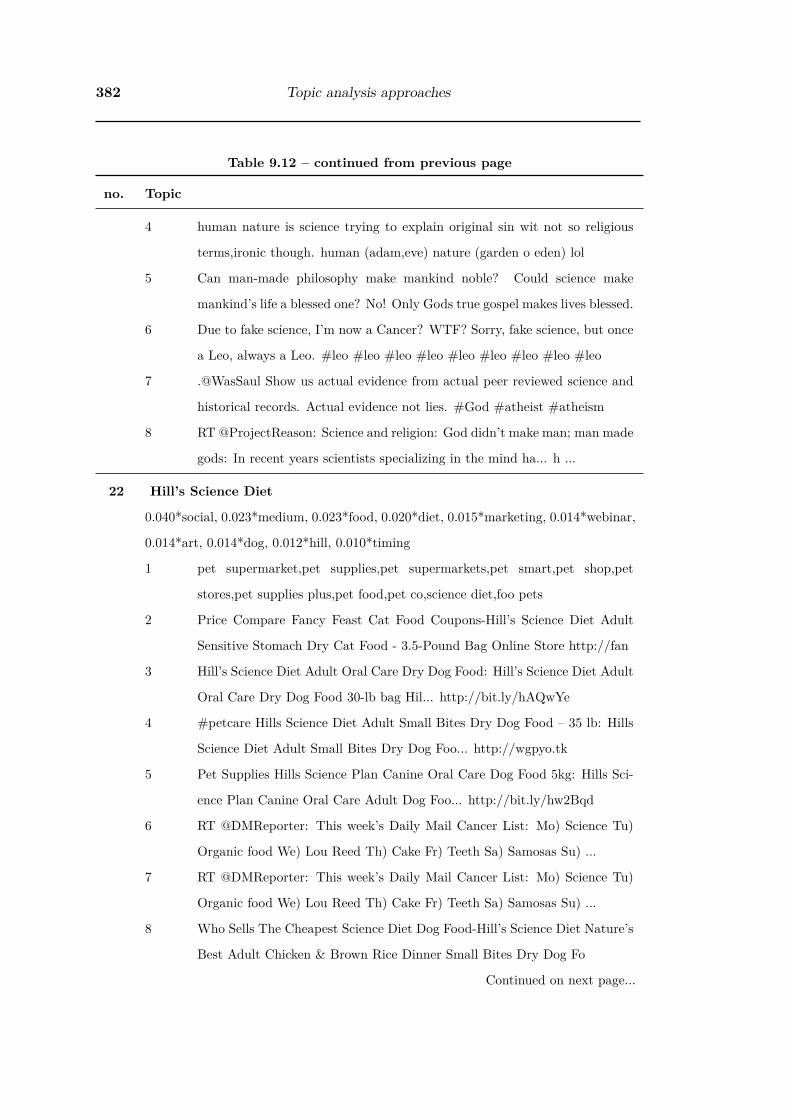
382 Topic analysis approaches
Table 9.12 – continued from previous page
no. Topic
4 human nature is science trying to explain original sin wit not so religious
terms,ironic though. human (adam,eve) nature (garden o eden) lol
5 Can man-made philosophy make mankind noble? Could science make
mankind’s life a blessed one? No! Only Gods true gospel makes lives blessed.
6 Due to fake science, I’m now a Cancer? WTF? Sorry, fake science, but once
a Leo, always a Leo. #leo #leo #leo #leo #leo #leo #leo #leo #leo
7 .@WasSaul Show us actual evidence from actual peer reviewed science and
historical records. Actual evidence not lies. #God #atheist #atheism
8 RT @ProjectReason: Science and religion: God didn’t make man; man made
gods: In recent years scientists specializing in the mind ha... h ...
22 Hill’s Science Diet
0.040*social, 0.023*medium, 0.023*food, 0.020*diet, 0.015*marketing, 0.014*webinar,
0.014*art, 0.014*dog, 0.012*hill, 0.010*timing
1 pet supermarket,pet supplies,pet supermarkets,pet smart,pet shop,pet
stores,pet supplies plus,pet food,pet co,science diet,foo pets
2 Price Compare Fancy Feast Cat Food Coupons-Hill’s Science Diet Adult
Sensitive Stomach Dry Cat Food - 3.5-Pound Bag Online Store http://fan
3 Hill’s Science Diet Adult Oral Care Dry Dog Food: Hill’s Science Diet Adult
Oral Care Dry Dog Food 30-lb bag Hil... http://bit.ly/hAQwYe
4 #petcare Hills Science Diet Adult Small Bites Dry Dog Food – 35 lb: Hills
Science Diet Adult Small Bites Dry Dog Foo... http://wgpyo.tk
5 Pet Supplies Hills Science Plan Canine Oral Care Dog Food 5kg: Hills Sci-
ence Plan Canine Oral Care Adult Dog Foo... http://bit.ly/hw2Bqd
6 RT @DMReporter: This week’s Daily Mail Cancer List: Mo) Science Tu)
Organic food We) Lou Reed Th) Cake Fr) Teeth Sa) Samosas Su) ...
7 RT @DMReporter: This week’s Daily Mail Cancer List: Mo) Science Tu)
Organic food We) Lou Reed Th) Cake Fr) Teeth Sa) Samosas Su) ...
8 Who Sells The Cheapest Science Diet Dog Food-Hill’s Science Diet Nature’s
Best Adult Chicken & Brown Rice Dinner Small Bites Dry Dog Fo
Continued on next page...

§9.3 Full Year 2011 LDA Model 383
Table 9.12 – continued from previous page
no. Topic
23 USA Politics / Christian Science Monitor news service
0.060*christian, 0.051*monitor, 0.011*obama, 0.007*anti, 0.006*gop, 0.005*perry,
0.005*news, 0.005*republican, 0.004*house, 0.004*rick
1 TX Gov Rick Perry has turned his state into a Libertarian paradise. High
pollution, anti poor, low law suit risk, anti-women, anti science
2 Libya+Sudan+Gaza+Bahrain+USA+Europe+Africa+Israel+Asia
need science+free-markets+pragmatism+hope+jobs+logic+fairness+
peace+freedom+&—
3 RT @rkref: House GOP shows true colors on contrived Solyndra outrage.
House Science Comm letter urges SuperComm to kill DOE’s clean ener ...
4 @nytimesworld JOBS JOBS JOBS! POTUS remind 2 digit IQ #tcot JFK
believed in science! GOP boast JFK while ignore SCIENCE #greenenergy
#P2
5 UTSA Political Science and Geography Chair Mansour El-Kikhia Discusses
Osama Bin Laden’s Death on WOAI-TV and KSAT-TV newscasts tonight.
6 DrudgeReport: Fla gov scraps high-speed rail plan pushed by Obama...: Fla
gov scraps high-speed ra... http://bit.ly/givhOR #biz #science
7 Herman Cain denies report of sexual harassment - Christian Science Monitor
ABC News Herman Cain denies report of sexual harassment Christ
8 @JohnCornyn JOBS JOBS JOBS! POTUS remind 2 digit IQ #tcot JFK
believed in science! GOP boast JFK while ignore SCIENCE #greenenergy
#P2
24 Weight Loss / Diet / Cosmetics - mainly advertising/spam links
0.025*weight, 0.020*loss, 0.020*health, 0.012*fat, 0.011*diet, 0.009*skin, 0.008*lose,
0.008*academy, 0.008*food, 0.007*based
1 Low carb diet low carb food list:All natural detox diet: science diet cat food
plan, starting a weight loss gym, healthy weight its n...
Continued on next page...

384 Topic analysis approaches
Table 9.12 – continued from previous page
no. Topic
2 Don’t Starve Fuel Body with High Quality #Nutrients! High lean Protein
High Fiber Diets reduce Cholesterol,Belly Fat & Weight Loss #Science
3 Health- Low-carb, higher-fat diets add no arterial health risks to obese peo-
ple seeking to lose weight, studies suggest (Science Daily)
4 Watermans Applied Science SPF 55 Face Stick � Skin Tone Reviews ...:
Tips For Facial Hair Remover. Tips For Facial Hair Remover? sk...
5 Watermans Applied Science SPF 55 Face Stick � Skin Tone Reviews ...:
Tips For Facial Hair Remover. Tips For Facial Hair Remover? sk...
6 Medical Science Provd: *Long Sajda: No Heart Prob Increase Eye sight,
Brain work & Face beauty *Rukoo with straight legs: No knees/joints
7 weight loss meal plan: The Low GI Diet Revolution: The Definitive Science-
Based Weight Loss Plan: http://weight-loss-meal-plan.fatbash.c...
8 Hair treatments:hot oil,aloe Vera,fruit smoothies,l’oreal absolute re-
pair,l’oreal vitamin,miracle oil,morrocan oil,caviar,science of10
25 Science writing / Science blogging / Amazon Book spam
0.029*art, 0.009*book, 0.009*blog, 0.008*thing, 0.008*read, 0.007*great, 0.006*good,
0.006*post, 0.006*story, 0.005*day
1 RT @heysayaezra: Art vs Science : ART ART ART ART ART ART ART
ART ART ART ART ART ART ART ART ART ART ART ART
2 MT @AutismScienceFd: Join Good Morning America’s Dr. Richard Besser
& USA Today Liz Szabo for Tweet chat re: autism http://t.co/ECNRHmUb
-SR
3 WIR- Aura Portraits Make Good Art, Bad Science: Carlo Van de Roer’s
Portrait Machine Project is shot with a piec... http://bit.ly/gwWk9m
4 The Science of Orgasm 8211 Barry R. Komisaruk Carlos Beyer-Flores Bev-
erly Whipple download, read, buy online <title>Blocked URL</title><ifra
5 The Science of Orgasm 8211 Barry R. Komisaruk Carlos Beyer-Flores Bev-
erly Whipple download, read, buy online <title>Blocked URL</title><ifra
Continued on next page...

§9.3 Full Year 2011 LDA Model 385
Table 9.12 – continued from previous page
no. Topic
6 Space Science 8211 Louise K. Harra Keith O. Mason download, read, buy on-
line <br /><b>Warning</b>: mysql_connect() [<a href=’function.mysql
7 The Art and Science of CSS 8211 Jonathan Snook Steve Smith Jina
Bolton Cameron Adams David Johnson download, read, .. <br
/><b>Warning</b>:
8 RT @edge: NYT Science Times: The Future of Computing issue -Fantastic!!!
Markoff, Zachary, Smarr, Ito, G.Dyson, Endy, Ted Nelson http:// ...
26 Students not liking science classes (colloquial spelling and language)
0.033*class, 0.023*lol, 0.017*hate, 0.015*fuck, 0.013*teacher, 0.012*project,
0.011*rocket, 0.011*shit, 0.011*fair, 0.009*math
1 Hate hate hate hate hate hate hate hate hate hate hate hate hate hate hate
hate hate hate hate hate hate hate hate hate hate hate science!!!
2 I hate hate hate hate hate hate hate hate hate hate hate hate hate hate hate
hate hate hate hate hate hate hate hate hate hate science.-.-
3 : I hate hate hate hate hate hate hate hate hate hate hate hate hate hate
hate hate hate hate hate hate hate hate hate hate hate science !
4 Fuck Fuck Fuck Fuck Fuck Fuck Fuck Fuck Fuck Fuck Fuck Fuck Fuck Fuck
Fuck Fuck Fuck Fuck Fuck Fuck Fuck Fuck Fuck forgot science
5 cnt do dis sht boi wat i tld u bout u dat wrd cnt shldnt b n a manz vocab
n u nt cz wen u sai cnt u ain a man #im a grl sayn ion ds science!
6 Omg! Mong pai hen history leaw mai yark read por mong pai eik tee hen
science gor mai yark read hen thai yhing mai yark read!!! -____-
7 @aaomnt tae hai pj print hai laew don’t worry huhi chun tum science mai
sed td nae a kae mai wai laew ja pai sleep la nhu mai norn ror ya?
8 @mystmm tae rao huay science makmakkk hahah kor loey kid yoo wa ja
rean food sci d maii :( tae thai his tem rew mak loey naa tong pai kor aj
27 Singapore Education (parody) / Education
Continued on next page...

386 Topic analysis approaches
Table 9.12 – continued from previous page
no. Topic
0.097*math, 0.094*love, 0.085*history, 0.078*problem, 0.068*heart, 0.068*battle,
0.067*reaction, 0.025*art, 0.014*progress, 0.012*philosophy
1 RT @fakeMOE: #sgworstnightmare Your teachers are: Ris Low (Eng/Lit),
Gary Ng (Science), Zhou Jieming (Maths/Chi), Steven Lim (Music/PE). ...
2 RT @fakeMOE: #sgworstnightmare Your teachers are: Ris Low (Eng/Lit),
Gary Ng (Science), Zhou Jieming (Maths/Chi), Steven Lim (Music/PE). ...
3 RT @fakeMOE: #sgworstnightmare Your teachers are: Ris Low (Eng/Lit),
Gary Ng (Science), Zhou Jieming (Maths/Chi), Steven Lim (Music/PE). ...
4 RT @fakeMOE: #sgworstnightmare Your teachers are: Ris Low (Eng/Lit),
Gary Ng (Science), Zhou Jieming (Maths/Chi), Steven Lim (Music/PE). ...
5 RT @fakeMOE: #sgworstnightmare Your teachers are: Ris Low (Eng/Lit),
Gary Ng (Science), Zhou Jieming (Maths/Chi), Steven Lim (Music/PE). ...
6 RT @fakeMOE: #sgworstnightmare Your teachers are: Ris Low (Eng/Lit),
Gary Ng (Science), Zhou Jieming (Maths/Chi), Steven Lim (Music/PE). ...
7 RT @fakeMOE: #sgworstnightmare Your teachers are: Ris Low (Eng/Lit),
Gary Ng (Science), Zhou Jieming (Maths/Chi), Steven Lim (Music/PE). ...
8 RT @fakeMOE: #sgworstnightmare Your teachers are: Ris Low (Eng/Lit),
Gary Ng (Science), Zhou Jieming (Maths/Chi), Steven Lim (Music/PE). ...
28 Science toy and Science equipment advertising links / Rainfall
0.058*lab, 0.044*faith, 0.022*script, 0.019*pump, 0.016*kit, 0.011*tubing,
0.010*user-thescript, 0.009*album, 0.009*scientific, 0.007*explorer
1 Solar Bag: Solar Bag solar bags solar science kit solar educational kit solar
education toy solar toy This solar... http://bit.ly/piobCV
2 RT @Karen_DaviLa: WOW. RT @dost_pagasa: Amount of Rainfall sa
Science Garden sa Quezon City ay 44.4mm /3hrs..equivalent na heavy rains
3 24 HR Rainfall from PAGASA Station over Metro Manila Port Area : 199.8
mm,Sangley Point :147.0 mm, Science Garden :147.3 mm,NAIA :151.5 mm
4 RT @Karen_DaviLa: WOW. RT @dost_pagasa: Amount of Rainfall sa
Science Garden sa Quezon City ay 44.4mm /3hrs..equivalent na heavy rains
Continued on next page...

§9.3 Full Year 2011 LDA Model 387
Table 9.12 – continued from previous page
no. Topic
5 #science #5: Pyrex Large Vol Burette 250 ml: Pyrex Large Vol Burette
250 ml by PYREX Sales Rank in Indu... http://amzn.to/iRpDVU #stuff
6 Autofill Valve Box (High Pressure) for Cole-Parmer Syringe Pump, Infusion
and Withdrawal design, Tou: science-lab-pumps http://bit.ly/jaOMQy
7 Toys; toys; toys! Play sets; dolls; toy trains; novelties; games | Airsoft guns;
RC items; Science; Electronics; More http://ow.ly/61H4B
8 Toys; toys; toys! Play sets; dolls; toy trains; novelties; games - Science;
Airsoft guns; Electronics; RC items; More http://ow.ly/61pYZ
29 News about Science Education: (teachers, teaching, awards (stu-
dents/teachers/schools)
0.030*math, 0.019*school, 0.017*student, 0.014*education, 0.013*teacher, 0.010*tech-
nology, 0.009*teaching, 0.009*teach, 0.007*learning, 0.007*kid
1 Science, social studies, foreign language teacher Nicole Keegan, Dakota Mid-
dle in Rapid City, SD joins Milken Educator family today. #MEA25
2 Nice work!! RT @shellykramer: $5k winner - Science City ER. Blue Springs
High School. Smart kids focused on healthcare and tech via @BOTBKC
3 Awesome Educator! #FF @mrsd5107 5th gr tchr-
Math/Science/English/Reading-Instructional Tech Specialist,Teacher
Support Specialist,Presenter
4 RT @WeAreTeachers: Hear Dr Sally Ride discuss #STEM education plus
learn effective STEM teaching strategies & promote science careers ht ...
5 Congrats: Basis Charter, Tucson; Sonoran Science Academy Tucson Char-
ter; University High, TUSD (Tucson) in top 50 of WA Post Challenge Index
6 RT @NCSE: Louisiana Science Education Act vs. high school senior? Check
radio chat with Zack Kopplin & NCSE’s Barbara Forrest. http://bi ...
7 Fostering Stars Learning & Resource Ctr. Tutoring youth, SAT/ACT test
prep, call 713.741.2400 Sheryl Garner #math #science #reading
8 RT @WeAreTeachers: Hear Dr Sally Ride discuss #STEM education plus
learn effective STEM teaching strategies & promote science careers ht ...
Continued on next page...

388 Topic analysis approaches
Table 9.12 – continued from previous page
no. Topic
30 Google science fair (winners) / other student science competitions
0.065*fair, 0.037*project, 0.026*google, 0.019*winner, 0.018*award, 0.013*prize,
0.012*win, 0.011*easy, 0.011*step, 0.011*rich
1 RT @whitehouse: Photo of the Day: Obama congratulates @Google Science
Fair winners Naomi Shah, Shree Bose & Lauren Hodge in the Oval: ht ...
2 RT @whitehouse: Photo of the Day: Obama congratulates @Google Science
Fair winners Naomi Shah, Shree Bose & Lauren Hodge in the Oval: ht ...
3 RT @whitehouse: Photo of the Day: Obama congratulates @Google Science
Fair winners Naomi Shah, Shree Bose & Lauren Hodge in the Oval: ht ...
4 Today at MrExcel: ”Changing Case in Excel w/ VBA”- http://bit.ly/giqVlU
#BI #CEO #CIO #CFO #CMO #COO #cpa #gov #science #statistics
#free
5 RT @VendiCRM: Girls Rock!!! Pres. Obama congratulates @Google Science
Fair winners Naomi Shah, Shree Bose & Lauren Hodge in the Oval: ht ...
6 Live Webcast w/ MrExcel & CFO(.)com 22Feb2011- http://bit.ly/fk4jRq
#BI #CEO #CIO #CFO #CMO #COO #cpa #gov #Fed #science
#statistics #edtech
7 RT @whitehouse: Photo of the Day: Obama congratulates @Google Science
Fair winners Naomi Shah, Shree Bose & Lauren Hodge in the Oval: ht ...
8 RT @whitehouse: Photo of the Day: Obama congratulates @Google Science
Fair winners Naomi Shah, Shree Bose & Lauren Hodge in the Oval: ht ...
The full year topics seemed more coherent than the January 2011 single month
topics, although perhaps this was an artefact of only checking the top 100 tweets;
with so many more tweets the higher weighted ones for a topic were more likely to be

§9.3 Full Year 2011 LDA Model 389
coherent. The range of weights for most significant 100 tweets for the full year was very
small, the least being a range of 0.0006 for topic 30 and the most being 0.0056 for topic
3 as shown in Table 9.13. For some topics this has resulted in the lowest weighted of
the most significant tweets being likely to be randomly selected from a larger group of
tweets at the cut off weight for the top 100. Where this occured, it may have reduced
the number of duplicated retweets in the top 100.
Table 9.13: Topic weight ranges in top 100 tweets for each topic for full year 2011
weight_min weight_max weight_range1 0.9904 0.9915 0.00112 0.9898 0.9916 0.00183 0.9905 0.9961 0.00564 0.9905 0.9921 0.00165 0.9905 0.9932 0.00276 0.9904 0.9915 0.00117 0.9896 0.9936 0.00418 0.9913 0.9934 0.00209 0.9915 0.9937 0.002210 0.9909 0.9956 0.004711 0.9898 0.9929 0.003012 0.9927 0.9943 0.001713 0.9905 0.9932 0.002714 0.9912 0.9938 0.002715 0.9923 0.9948 0.002416 0.9904 0.9920 0.001617 0.9896 0.9914 0.001818 0.9905 0.9921 0.001619 0.9888 0.9919 0.003120 0.9910 0.9920 0.001021 0.9899 0.9912 0.001222 0.9909 0.9927 0.001823 0.9904 0.9924 0.002024 0.9903 0.9927 0.002425 0.9898 0.9928 0.003026 0.9920 0.9947 0.002827 0.9902 0.9914 0.001128 0.9902 0.9914 0.001129 0.9898 0.9921 0.002230 0.9903 0.9909 0.0006
The presence of large numbers of ‘noun spam’ in the top tweets for topic 7 and

390 Topic analysis approaches
non-English tweets in topics 8, 9 and 13 showed that my data cleaning was not as
successful as I had hoped but does suggest that topic analysis could be used to check
and improve data cleaning.
It is interesting that some topics were mainly individuals tweeting while others were
dominated by news services or advertising or computer generated spam tweets. The
topics with individuals tweeting sometimes appeared to be by a specific demographic
group, like high school student or university students. This suggests that topic analysis
may also be useful in locating the tweets of particular demographic groups.
As for the January 2011 corpus, the overall representation of each topic in the corpus
can be calculated by summing the weight of each topic in each document to get the
total weight for the topic. The code used for January 2011 (listing K.20 in Appendix K)
was modified to create the results for the full year (listing K.21 in Appendix K). The
topic weights for each of the 30 LDA topics for the whole year 2011 are shown on
Fig. 9.10 and in Table 9.14.
For the whole of 2011, topic 15 (Students tweeting about lessons / exams / projects
(today/tomorrow)) was by far the most represented in the corpus with almost twice
the weight of the next three topics. The second most frequent topic was 26 (Stu-
dents not liking science classes (colloquial spelling and language)) followed by topic
10 (Non-English / high school students (science class/teachers)) and 8 (Non-English /
descriptions of simple experiments or experiences). That two of the most frequent four
topics were ones badly affected by non-English content is an indication that more work
needed to be done at the data cleaning stage. The two most frequent topics (15 and
26) were both based on tweets sent by high school students, as is the English portion
of the third most frequent topic (10). This suggests that school students sent many
more tweets containing the words science than any other demographic group.
As described above, the topics for the full year 2011 were coherent enough to provide
useful information about the contexts in which the word science was being used on

§9.3 Full Year 2011 LDA Model 391
1 2 3 4 5 6 7 8 91
01
11
21
31
41
51
61
718
19
20
21
22
23
24
25
26
27
28
29
30
Topic Number
0.00
0.02
0.04
0.06
0.08
0.10
0.12
0.14
Weig
ht
Figure 9.10: Weight of topics in LDA Model of whole year 2011 corpus
Twitter during 2011 and show that these were very diverse, both in who was speaking
and what was being said.
There are topics that appeared to be mostly sent by high school students about
a range of issues identified by topics 10 (comments about teachers), 12 (Bill Nye), 15
(lessons/exams) and 26 (Students not liking science classes). Some topics were sent by
both university and high school students, like topic 11 about course choices.
There are other education focussed topics that were not mainly sent by students
such as topic 29 (News about Science Education), topic 5 (university jobs / research
linkages), topic 30 (Google science fair) and topic 14 (science centres).
Another source of tweets containing the word science was news services, and al-
though some of the tweets in the topics containing these were sent directly by a news
service, most were retweets by people who had found the news interesting enough to
pass on. It would be possible to look at the Twitter profiles of those people to try to
understand their demographic but this was not done as part of this study. Topics 1,
2, 4, 6 and 23 appeared to have many news related tweets. Topic 29 (News about Sci-

392 Topic analysis approaches
Table 9.14: Weight of topics in LDA Model of January 2011 corpus
Topic Weight Topic Description1 0.025 Technology news (Google/Apple/Facebook/Nokia etc.) phones and
tablets2 0.031 Health and medical science3 0.037 Science fiction4 0.037 Climate change / Fukushima / Marine science / Autumn / Household
Energy5 0.036 University jobs / Research linkages across states and countries6 0.025 Space news (NASA/Soyuz/Space station/Hubble)7 0.011 spam / Big Bang Theory (tv show) / Higgs Boson news8 0.063 Non-English / descriptions of simple experiments or experiences9 0.018 Non-English
10 0.072 Non-English / high school students (science class/teachers)11 0.036 Student course choices (senior year highschool/university)12 0.009 Bill Nye the Science Guy13 0.033 Non-English / TV Shows (fiction and non-fiction)14 0.044 Science Centres / Museums / DJ Science15 0.125 Students tweeting about lessons / exams / projects (today/tomorrow)16 0.030 Amazon book promotion spam links17 0.015 Tweets shared from StumbleUpon - possibly spam18 0.038 Climate change and Global Warming / science controversies19 0.010 Celebrity retweets / Rap songs20 0.023 System of a Down song set lists21 0.048 pro-choice / pro-life / religion / atheism22 0.014 Hill’s Science Diet23 0.022 USA Politics / Christian Science Monitor news service24 0.015 Weight Loss / Diet / Cosmetics - mainly advertising/spam links25 0.030 Science writing / Science blogging / Amazon Book spam26 0.079 Students not liking science classes (colloquial spelling and language)27 0.008 Singapore Education (parody) / Education28 0.011 Science toy and Science equipment advertising links / Rainfall29 0.038 News about Science Education: (teachers, teaching, awards (stu-
dents/teachers/schools)30 0.016 Google science fair (winners) / other student science competitions
ence Education) also had many tweets from news services, but perhaps because many
of the news reports were about awards, it also had more tweets sent by individuals
congratulating the winners of the awards.
Some topics were very specific like topic 27 (Singapore Education (parody)) and
topic 20 (‘System of a Down’ song set lists). A broader but still recognisably single
focus topic was topic 3 (science fiction). Topic 19 (Celebrity retweets / Rap songs)
may be in this group based on the top 100 tweets, although even in these it contained

§9.4 Conclusion 393
tweets from two very different celebrities.
Topic 18 (climate change/global warming) was interesting in that it had tweets
from both sides of a range of science controversies, as did the somewhat similar topic
21 (pro-choice / pro-life / religion / atheism).
There are topics that contained advertising or spam like topic 22 (Hill’s Science
Diet), topic 7 (spam / Big Bang Theory (tv show) / Higgs Boson news), topic 24
(Weight Loss / Diet), topic 28 (Science toy and Science equipment advertising), topic
16 (Amazon book promotion spam links), topic 17 (Tweets shared from StumbleUpon)
and topic 25 (Science writing / Science blogging / Amazon Book spam).
Like the spam and advertising topics, the non-English dominated topics (8, 9 and
13) also seemed to be of less use, although topic 8 had a subset of interesting descrip-
tions by individuals doing science experiments at school or home that would hopefully
become a topic if the non-English tweets were removed. As noted above, a number of
the more popular topics also seemed to have spam tweets in them.
9.4 Conclusion
In this chapter I have developed an approach to applying LDA topic modelling to a
corpus of tweets to identify the contexts in which the key word ‘science’ used to collect
the corpus was being used, in this case the word ‘science’. Topic analysis has given a
much richer view of the contexts in which the word ‘science’ was being tweeted than
the Bigram analysis in the previous chapter. While the bigrams were only present in
19.2% of the tweets, the topic analysis covers the whole corpus at whichever number
of topics has been chosen.
The LDA topics in both the final January 2011 and full year 30 topic LDA models
demonstrate that these models are useful in identifying the topics being tweeted about,

394 Topic analysis approaches
and that for some topics the demographics of the people sending the tweets can also
be inferred. They revealed previously unknown details about the contexts in which the
word science was being used in the corpus.
There is a number of ideas for further research in topic modelling of this corpus
that I would like to follow up but were outside the scope of this thesis. These are
discussed below:
In Section 9.1.6 I looked at the topics produced with and without retweets and they
seemed to be of similar quality so I did not proceed with removing retweets. In the
final sections of this chapter, however, where I examined the most significant tweets for
each topic, there did seem to be some topics in which retweets were very prominent -
a strategy for identifying and removing those may also be worth considering for future
investigation.
There were more spam tweets and foreign language tweets in the topics than I ex-
pected to find given that I had filtered spam and languages as described in Chapter 4.
The concentration of spam tweets and foreign language tweets in particular topics sug-
gested that the topic modelling was picking up on a different use of words in those
tweets. I would like to conduct more filtering based on the spam and languages iden-
tified in these topics and see what affect that has on the quality of a new topic model.
Perhaps this would need to be an iterative process as more spam was revealed.
It would be interesting to look in more detail at what is being said within a single
topic, particularly in topics that are coherent, but then show variation in the detail
within the topic, like the science centre topic in January 2011 appeared to. Another way
to approach this would be to investigate the changes in detail with changing numbers
of topics. The models with different number of topics for the same corpus should be
consistent with each other but reveal different aspects of the corpus;
“As you change the number of topics (and other parameters), models pro-
vide different pictures of the same underlying collection. But this doesn’t

§9.4 Conclusion 395
mean that topic modeling is an indeterminate process, unreliable as evi-
dence. All of those pictures will be valid. They are taken (so to speak) at
different distances, and with different levels of granularity.” (Goldstone &
Underwood, 2012, p. 47)
In this thesis I have used perplexity as the measure for refining the settings of
the Dirichlet priors, but this may not be a good measure of the usefulness of the
topics for humans. An alternative approach developed by Mimno and Blei (2011) is
Bayesian model checking method for probabilistic topic models, based on ‘posterior
predictive checking’ which “can show where the model fits and doesn’t fit the observa-
tions” (Mimno & Blei, 2011, p. 227). They develop discrepancy functions for LDA that
“measure how well its statistical assumptions about the topics are matched in the ob-
served corpus and inferred topics” (Mimno & Blei, 2011, p. 228). Applying these tests
to my models would be worth considering for future investigation, and also provide a
way to visualise topic models.
Returning to my original aim of developing a tool for exploring and analysing
streams of tweets, another area I would like to investigate is the visualisation and
presentation of the results of topic modelling. I identified a number of existing tools
for visualising topic models but decided that evaluating them was outside the scope of
this thesis. These tools are:
The TMVE tool developed by Chaney and Blei (2012) which allows users to “explore
the corpus, moving between high level discovered summaries (the “topics”) and the
documents themselves,” (Chaney & Blei, 2012, p. 1).
Termite is an active research project by Jason Chuang and Ashley Jin, a ‘visual
analysis tool for inspecting the output of statistical topic models’, which is open source
and available on GitHub21(Chuang, Manning, & Heer, 2012).21https://github.com/uwdata/termite-visualizations
396 Topic analysis approaches
There are also open source scripts available to use the Gelphi22 network visualisation
tool with networks from LDA topics such those used by Goldstone and Underwood
(2012). When considering visualisations of topic models Goldstone and Underwood
(2012) warn that:
“A topic model isn’t a network, and mapping one onto a network can be
misleading. For instance, topics that are physically distant from each other
in this visualization are not necessarily unrelated. Connections below a
certain threshold go unrepresented.” (p. 44)
Another tool that looks useful is “TopicNets, a system for interactive visual anal-
ysis of large document corpora, based on the associations formed by topic modeling.”
(Gretarsson et al., 2009).
In this chapter I have answered research question 4c “what topics are identified by
topic analysis?” and shown that topic analysis techniques can be used to identify useful
and coherent topics in a Twitter corpus collected using a single keyword, I have now
completed my analysis of the ‘science’ keyword corpus. In the next chapter I conclude
this thesis by summarising how the different aspects of the corpus I have examined
contribute towards an understanding of the contexts in which the word ‘science’ is
used by the English speaking public.
22http://gephi.github.io/

Chapter 10
Conclusion
In this thesis I have conducted a study of a number of different aspects of a large
corpus of tweets collected using the single keyword ‘science’ throughout 2011, in order
to answer my research question: “What does open source intelligence, in the form of
public tweets on Twitter, reveal about the contexts in which the word ‘science’ is used
by the English speaking public?”. This chapter summarises the research findings for
those differerent aspects and shows that taken together they do provide an answer
to the research question, and that these answers provide both information useful for
science communication about the use of the word ‘science’ on Twitter during 2011 and
the potential to apply this approach to other text sources.
I approached the research question by answering a series of simpler questions that
inform the view of who is contributing on Twitter, how often, and what topics are
being discussed.
Before these questions could be considered, a dataset had to be collected from
Twitter. This was done using the Twitter StreamAPI with the keyword ‘science’ during
2011 using a flexible data gathering tool, tStreamingArchiver, which I developed and
released as open source1.
After data collection was completed the corpus was prepared for analysis by re-
moving unwanted tweets, those that were considered likely to be ‘noise’. I developed1https://github.com/brendam/tStreamingArchiver
397
398 Conclusion
and documented robust and repeatable techniques for filtering a dataset of tweets col-
lected using a keyword in Chapter 4, ‘Data cleaning and filtering’. The tweets removed
were the ones written in languages other than English, and those containing one type
of advertising tweet that I have called ‘noun spam’. In both cases the uncertainty in
the identification of tweets to be filtered meant that a decision had to be made as to
the level of filtering to apply, balancing the advantages of removing tweets written in
foreign languages and spam with the possibility of removing too many useful tweets.
The attributes of the cleaned dataset were then explored in order to answer the
research questions.
The first research question “How many tweets are sent containing the word ‘science’
and what is the temporal pattern?” was answered for the 2011 dataset of tweets
containing the word ‘science’ in Chapter 5 by looking at the number of tweets per
day. The number of tweets per day containing the word ‘science’ moved from around
26 thousand to around 45 thousand over the year, at a rate that reflected the overall
growth in Twitter. However, these tweets only represented a very small proportion,
about 0.02%, of the total tweets on Twitter. I demonstrated that Fourier analysis
can be used to create a more accurate model of the underlying temporal pattern of
tweets per day containing the keyword ‘science’ than by either simple smoothing or by
a model based on a single sine wave with linear and amplitude growth. I identified a
weekly pattern with more tweets sent during the week than on weekends. The temporal
model was then used to filter the tweets per day data, to reveal temporal changes that
were masked by the weekly pattern, with a view to highlighting changes in the rates of
conversation that may be useful to allow science communicators to release information
at a time when the conversation of that topic is increasing on Twitter. The underlying
regular mid week increase in conversation using the keyword ‘science’ may result in
science communicators getting greater engagement if they release their information
mid week. Both of these suggestions are based on the assumption that the increase in
rate of conversation on Twitter for a topic indicates that the audience is more receptive
399
to the topics at these times, but this is not tested in this thesis.
The second research question “Who sends these tweets, and how does that change
over time?” was answered for 2011 in Chapter 6. There were 3.6 million users who sent
tweets containing the word science in 2011 and most of these only sent a single tweet
containing the keyword ‘science’ (58%), with only 4.6% sending more than 10 tweets
with ‘science’ in 2011. The pattern of authors per day in 2011 was very similar to the
pattern of tweets per day, and most of the pattern was contributed to by those sending
less than 15 ‘science’ tweets per year. Of those that sent more than one ‘science’ tweet,
approximately half sent them on different days (41.6%), but only 6.2% of them sent
them on consecutive days. From a science communication perspective this tells us that
the tweets containing the keywords ‘science’ are predominately coming from different
Twitter user accounts, and that each account does not use the word ‘science’ very often.
The third research question “What is the breakdown of types of tweets?” was
addressed in Chapter 7 where I found that people tweeting using the keyword ‘science’
were engaged in considerably more re-sharing (retweeting) of information than average
on Twitter, but that the actual retweets were used in a similar way to that found in
other studies. The proportion of tweets that mention other users in my data set was
similar to that found in other studies, although there were fewer mentions which were
directed replies, perhaps because while retweets are always mentions they are unlikely
to be replies, as most retweets start with ‘RT’.
The use of hashtags and urls was more prevalent in my dataset, closer to the rate
found in retweets by Boyd et al. (2010) than normal tweets, and this increase is larger
than would be expected from the higher proportion of retweets in my dataset, which
indicates that another factor is present, possibly an increase in the overall use of urls
and hashtags on Twitter since her study, or perhaps ‘science’ tweets have more urls
and hashtags than random tweets. In the topic analysis I found some topics that had
messages from Pinterest that were almost completely made up of hashtags (and may be

400 Conclusion
considered as spam). Perhaps these have contributed to the high rate of hashtags in my
corpus. My result of 17% retweets for ‘science’ was close to that found by Bruns and
Stieglitz (2012) for datasets containing tweets about TV shows like #mkr (My Kitchen
Rules), #masterchef, #eurovision and #angryboys, however these all had very low
numbers of links (less than 15%) while my dataset had nearly 50%.
Both the higher proportion of retweets and higher use of urls and hashtags suggest
that people using the word ‘science’ are engaged in more sharing of both links, and
other peoples tweets, than is present in a random sample of tweets. This high rate
of re-sharing may indicate that although people are interested in sharing science re-
lated information, they do not feel as comfortable in generating new tweets or replies
containing the word ‘science’.
In Chapter 8, ‘Word frequency and word co-occurence’ I found that the raw word
frequencies considered in response to research question Question 4a “what is the fre-
quency of words used?” are not particularly effective when trying to understand such
a large dataset. Question 4b “what words co-occur?”, which was answered by looking
at Bigrams, was able to give some insight into the contexts in which ‘science’ is being
used in up to 19.19% of the tweets. Of the top 70 bigrams identified, 18 were able to
be understood from a science communication perspective as describing either activities
or topic areas related to the word ‘science’. The science keyword topic area bigrams
identified in 2011 were:
• science fiction
• bill nye
• computer science
• political science
• forensic science
• environmental science
• physical science
• rocket science
• climate change
• global warming

401
• science center
• art science
• albert einstein
• science technology
and the science activity bigrams were:
• science fair
• science test
• science exam
• science class
These topics indicate that much of the activity on Twitter around the keyword
‘science’ is about science education.
Research question 4c “what topics are identified by topic analysis?” was answered
in Chapter 9 by using LDA topic modelling to identify the contexts in which the key
word used to collect the corpus, ‘science’, was being used. Topic analysis provided a
much richer view of the contexts in which the word ‘science’ was being tweeted than
the Bigram analysis in the previous chapter. While the bigrams were only present in
19.2% of the tweets, topic analysis covers the whole corpus for whatever number of
topics is chosen. Topics were identified for two time periods, January 2011 and the
full year 2011, both looking for 30 Topics, using Gensim model.LdaMallet. The topics
for the full year 2011 were coherent enough to provide useful information about the
contexts in which the word science was being used on Twitter during 2011 and showed
that these were very diverse, both in who was speaking and what was being said.
While the demographics of the authors of most topics were unclear, it was possible
to infer the authors of some topics based on examination of the top tweets in the
topic. For example, the inferred authors of the topics characterised as ‘comments about
teachers’ (topic 10), ‘Bill Nye’ (topic 12), ‘lessons/exams’ (topic 15) and ‘students not
liking science class’ (topic 26) in the full year results were high school students. Other
topics appeared to be sent by university as well as high school students (topic 11 ‘course
choices’) or by news services (topics 1, 2, 4, 6 and 23).

402 Conclusion
There were also education focussed topics that appeared to be sent by diverse
authors, such as ‘news about science education’ (topic 29), ‘university jobs/research
linkages’ (topic 5), ‘Google science fair’ (topic 30) and ‘science centres’ (topic 14).
Some topics were very specific like ‘Singapore education (parody)’ (topic 27) and
‘System of a Down song set lists’ (topic 20) or single focus ‘science fiction’ (topic 3).
Two topics about controversial issues both had a mixture of tweets expressing views
on both sides of the controversy; ‘climate change/global warming’ (Topic 18) and ‘pro-
choice/pro-life/religion/atheism’ (topic 21).
The topic analysis also created some topics mainly characterised by unfiltered spam
(topics 22, 7, 24, 28, 17 and 25) or foreign language tweets (topics 8, 9 and 13). Based
on the highest weighted words for these topics, it appeared that many of them may
have contained useful tweets outside the top 100 that were checked. To retain these
tweets it would be better to use these topics to identify the characteristics of unwanted
tweets and refine the filtering of the dataset rather than discarding the whole topics.
The LDA topics in both the final January 2011 and full year 30 topic LDA models
demonstrate that these models are useful in identifying the topics being tweeted about,
and that for some topics the demographics of the people sending the tweets can also
be inferred. They revealed previously unknown details about the contexts in which the
word science was being used in tweets during 2011.
The information provided by topic analysis about the topics being discussed, and
the detail available in the tweets contained within each topic, could be useful to science
communicators to allow them to better target their communications about different
topics. Knowing what the public are saying about a particular topic supports a tailored
communication strategy for that topic. By combining this with the filtered tweets per
day information, to see when the level of conversation about a particular topic is rising,
it is possible that a greater level of engagement could be achieved because people are
already listening to the conversation.

§10.1 Significance of Thesis 403
Putting these different results together, I can say that most people sent tweets
containing the word ‘science’ during the middle of the week. If they were students then
the tweet was probably either complaining about science class, or asking for luck in
completing a science test or project. Other individuals were likely to retweet interesting
science news they had received in a retweet themselves, or perhaps received directly
from a science news service like @science or @sciencenews.
10.1 Significance of Thesis
This thesis has contributed to the understanding of how to interpret public conversa-
tions about science topics on Twitter in order to inform science communication on these
topics. I have shown that the combination of different Twitter metrics can reveal more
about the contexts in which a keyword like ‘science’ is used by the English speaking
public than any single metric alone. At the time of writing, I am not aware of any
other studies that have investigated such a wide range of metrics for a single Twitter
corpus.
I identified suitable analysis approaches and metrics from other disciplines and
adapted and combined these from a science communication perspective, including de-
veloping computer programs to perform the analysis. The techniques developed are
novel in science communication research.
By examining a range of metrics for the same corpus, I have provided insight into
what each metrics can contribute to understanding public conversations as well as into
the interaction between the metrics.
Although the thesis has focused on the single keyword ‘science’ the techniques
developed should be applicable to other keywords and so able to provide science com-
municators with a near real time source of information about what issues the Twitter

404 Conclusion
using public is concerned about, what they are saying about those issues and how that
is changing over time.
I developed and released as open source a flexible data gathering tool for collecting
Twitter data using either the Twitter Search API or the Twitter Streaming API.
At the time of writing, the use of Fourier analysis to determine the component sine
waves for the temporal modelling of the number of tweets per day is novel to this thesis.
10.2 Limitations of Study
The main limitation of this thesis was the scale of Twitter data. This has meant that
even considering a year of data gathered using the single keyword ‘science’ required
learning a range of multidisciplinary approaches to data analysis. Although it is in-
tended that the techniques developed should be able to be applied to other Twitter
datasets, and possibly even other social media datasets, testing this was beyond the
scope of this thesis. Another limitation was the restrictions by Twitter on obtaining
past tweets2 which meant that it was necessary to wait for data to be collected as it
was generated by people posting on Twitter.
At the time I started collecting data there were very few tweets with embedded
location information and other options for localising tweets were not considered to be
reliable enough to use. Because of this my analysis was worldwide and did not look at
regional or country differences.
The study only looked at a single year of Twitter data and this prevents identifica-
tion of any underlying annual patterns in the data.
The large number of metrics available with tweets meant that not all of them could
be studied. Possible sources of useful information about the context of a keyword used2Searching for past tweets is limited to 1,500 tweets per search term.

§10.3 Areas for Further Research 405
on Twitter such as social network information or the path of individual tweets though
the network have not be included in this study.
This research is also constrained by the overall limitations of the representativeness
of social media research, reflected on by many authors. (danah Boyd & Crawford,
2012; Bruns, 2013; Busch, 2014; Crawford, Gray, & Miltner, 2014; Bruns & Stieglitz,
2015; Burgess & Bruns, 2015)
10.3 Areas for Further Research
For each of the metrics I investigated there were additional areas for research that
became apparent during the study, and these are discussed here:
In my tweets per day analysis I identified weekly patterns in the number tweets
being sent per day. There also appeared to be seasonal patterns, and these could
be investigated by extending the study over three years. However, it is possible that
changes in Twitter over time may effect these longer term patterns or make detecting
them difficult. Using a shorter time frame for grouping the tweets, such as hourly,
could possibly be used as a way to tell where the tweets were from by looking for time
zone patterns in the numbers of tweets sent. A correlation between time zone and
number of tweets sent could be investigated by using the few tweets that have their
geolocation information set.
The author analysis I conducted could be extended to look the social network
between the authors and patterns of transmission of tweets. Both of these would
require a different data gathering approach that collected tweets that were replies to,
or retweets of, the tweets containing the keywords even if they did not themselves
contain the keywords.
It would be interesting to build on the finding concerning the types of tweets per
day that the higher proportion of retweets and higher use of urls and hashtags for

406 Conclusion
tweets containing the word ‘science’ may imply more sharing of those tweets, to see if
this means that Tweets sent by science communicators can be effective in reaching a
large audience.
In the topic analysis, I put forward a number of ideas for further research in topic
modelling of this corpus which are summarised here: repeat the topic modelling with
retweets removed from the corpus; improve the spam and foreign language filtering by
iteratively using topic modelling to identify tweets which should be excluded; investi-
gate the changes in detail with changing numbers of topics; investigate the application
of posterior predictive checking to my models; and explore options for the visualisation
and presentation of the results of topic modelling. There is also a number of more
recent extensions to LDA topic modelling like author-topic models and dynamic topic
models which would be interesting to apply to this corpus.
This thesis focussed on a single keyword ‘science’. Research is needed to determine
whether the techniques developed in this thesis can be applied to different Twitter
keywords or groups of keywords, to see if they can be applied more broadly.
Beyond these extensions to the individual studies in this thesis, there is also scope
for investigating the ways in which the metrics can be combined and used to create an
online tool for interactively exploring a larger Twitter dataset, with multiple keywords
and longer time frame. I continued to collect a larger Twitter dataset, using many
science related keywords over a number of years, and it would be interesting to see
whether a tool for exploring these is useful for informing science communicators of the
discussions taking place on Twitter.
Recent Twitter studies have had some success at developing approaches to localise
Twitter data. In particular the Mapping Online Publics project at Queensland Uni-
versity of Technology which has developed a ‘map of the Australian Twittersphere’3,3http://mappingonlinepublics.net/2014/08/04/first-steps-in-exploring-the-australian-
twittersphere/

§10.3 Areas for Further Research 407
opens up the possibility of looking at national or regional Twitter datasets instead
being limited to considering the whole world at once.
The techniques developed in this thesis can be extended in a number of ways in-
cluding;
• to different Twitter datasets, to other social media sources and even to other
types of documents
• by looking at different time periods
• by incorporating other metrics both from within and outside Twitter
• by applying interactive visualisation techniques to combine, filter and explore the
results
I hope that the techniques developed in this thesis, and in particular the topic
analysis approaches, are applied in the future to contribute new insights for science
communication where there are text based materials to be explored and understood.

408 Conclusion

Appendix A
Database Structures
A.1 Twitter_Stream_Archive Database
-- Create syntax for TABLE 'apiOverlap'
CREATE TABLE `apiOverlap` (
`tweetId` bigint(20) NOT NULL DEFAULT '0',
`inStream` tinyint(1) DEFAULT NULL,
`inSearch` tinyint(1) DEFAULT NULL,
`inTwapperKeeper` tinyint(1) DEFAULT NULL,
PRIMARY KEY (`tweetId`)
) ENGINE=MyISAM DEFAULT CHARSET=utf8;
-- Create syntax for TABLE 'CoOccuranceList'
CREATE TABLE `CoOccuranceList` (
`id` int(11) NOT NULL AUTO_INCREMENT,
`searchId` int(11) DEFAULT NULL,
`date` date DEFAULT NULL,
`word1` varchar(30) DEFAULT NULL,
`word2` varchar(30) DEFAULT NULL,
`frequency` int(11) DEFAULT NULL,
PRIMARY KEY (`id`),
UNIQUE KEY `coListKey` (`searchId`,`date`,`word1`,`word2`)
409

410 Database Structures
) ENGINE=MyISAM AUTO_INCREMENT=316915 DEFAULT CHARSET=utf8;
-- Create syntax for TABLE 'dataGaps'
CREATE TABLE `dataGaps` (
`id` int(11) NOT NULL AUTO_INCREMENT,
`startGapTime` datetime DEFAULT NULL,
`endGapTime` datetime DEFAULT NULL,
`startGapTweetId` bigint(20) DEFAULT NULL,
`endGapTweetId` bigint(20) DEFAULT NULL,
`timeGap` bigint(20) DEFAULT NULL,
PRIMARY KEY (`id`)
) ENGINE=MyISAM AUTO_INCREMENT=72298 DEFAULT CHARSET=utf8;
-- Create syntax for TABLE 'dNotices'
CREATE TABLE `dNotices` (
`id` bigint(20) NOT NULL DEFAULT '0',
`userId` bigint(20) DEFAULT NULL,
`isDeleted` tinyint(1) DEFAULT NULL,
PRIMARY KEY (`id`)
) ENGINE=MyISAM DEFAULT CHARSET=utf8;
-- Create syntax for TABLE 'SearchAPIids'
CREATE TABLE `SearchAPIids` (
`searchUserId` bigint(20) NOT NULL,
`screenName` varchar(32) DEFAULT NULL,
`sourceAPI` varchar(20) DEFAULT NULL,
PRIMARY KEY (`searchUserId`),
KEY `screenName` (`screenName`)

§A.1 Twitter_Stream_Archive Database 411
) ENGINE=MyISAM DEFAULT CHARSET=utf8;
-- Create syntax for TABLE 'searches'
CREATE TABLE `searches` (
`id` int(11) NOT NULL AUTO_INCREMENT,
`query` varchar(140) NOT NULL,
`active` tinyint(1) NOT NULL DEFAULT '1',
`created_on` datetime DEFAULT NULL,
`type` varchar(20) DEFAULT NULL,
`subtype` varchar(20) DEFAULT NULL,
PRIMARY KEY (`id`)
) ENGINE=MyISAM AUTO_INCREMENT=837 DEFAULT CHARSET=latin1;
-- Create syntax for TABLE 'searchTermIndex'
CREATE TABLE `searchTermIndex` (
`id` int(11) NOT NULL AUTO_INCREMENT,
`searchId` int(11) DEFAULT NULL,
`date` date DEFAULT NULL,
`tweetId` bigint(20) DEFAULT NULL,
PRIMARY KEY (`id`),
KEY `date` (`date`),
KEY `searchId` (`searchId`),
KEY `tweetId` (`tweetId`)
) ENGINE=MyISAM AUTO_INCREMENT=171062733 DEFAULT CHARSET=utf8;
-- Create syntax for TABLE 'trackLimitations'
CREATE TABLE `trackLimitations` (
`id` int(11) NOT NULL AUTO_INCREMENT,

412 Database Structures
`numberLimited` int(11) DEFAULT NULL,
`lastTweetDateBeforeLimit` datetime DEFAULT NULL,
`lastTweetIdBeforeLimit` bigint(20) DEFAULT NULL,
PRIMARY KEY (`id`)
) ENGINE=MyISAM AUTO_INCREMENT=16853 DEFAULT CHARSET=utf8;
-- Create syntax for TABLE 'tweets'
CREATE TABLE `tweets` (
`id` bigint(20) NOT NULL,
`source` varchar(300) DEFAULT NULL,
`text` varbinary(450) DEFAULT NULL,
`createdAt` varchar(64) DEFAULT NULL,
`created_at_GMT` datetime DEFAULT NULL,
`to_user_id` bigint(20) DEFAULT NULL,
`to_user_id_Search` bigint(11) DEFAULT NULL,
`to_user` varchar(32) DEFAULT NULL,
`from_user_id` bigint(20) DEFAULT NULL,
`from_user_id_Search` bigint(11) DEFAULT NULL,
`from_user` varchar(32) DEFAULT NULL,
`hasGeoCode` tinyint(1) DEFAULT NULL,
`latitude` double DEFAULT NULL,
`longitude` double DEFAULT NULL,
`isTruncated` tinyint(1) DEFAULT NULL,
`inReplyToStatusId` bigint(20) DEFAULT NULL,
`retweetedStatus` tinyint(1) DEFAULT NULL,
`retweetedId` bigint(20) DEFAULT NULL,
`contributors` varchar(300) DEFAULT NULL,
`place` varchar(700) DEFAULT NULL,

§A.1 Twitter_Stream_Archive Database 413
`isFavorited` tinyint(1) DEFAULT NULL,
`sourceAPI` varchar(20) DEFAULT NULL,
`record_add_date` datetime DEFAULT NULL,
PRIMARY KEY (`id`),
KEY `from_user` (`from_user`),
KEY `from_user_id` (`from_user_id`),
KEY `from_user_id_Search` (`from_user_id_Search`),
KEY `to_user_id` (`to_user_id`),
KEY `to_user_id_Search` (`to_user_id_Search`),
KEY `to_user` (`to_user`),
KEY `created_at_GMT` (`created_at_GMT`)
) ENGINE=MyISAM DEFAULT CHARSET=utf8;
-- Create syntax for TABLE 'users'
CREATE TABLE `users` (
`id` bigint(20) NOT NULL DEFAULT '0',
`name` varbinary(100) DEFAULT NULL,
`screenName` varchar(32) DEFAULT NULL,
`location` varbinary(110) DEFAULT NULL,
`description` varbinary(500) DEFAULT NULL,
`profileImageUrl` varchar(320) DEFAULT NULL,
`url` varchar(255) DEFAULT NULL,
`isProtected` tinyint(1) DEFAULT NULL,
`followersCount` int(11) DEFAULT NULL,
`status` varchar(200) DEFAULT NULL,
`profileBackgroundColor` varchar(6) DEFAULT NULL,
`profileTextColor` varchar(6) DEFAULT NULL,
`profileLinkColor` varchar(6) DEFAULT NULL,

414 Database Structures
`profileSidebarFillColor` varchar(6) DEFAULT NULL,
`profileSidebarBorderColor` varchar(6) DEFAULT NULL,
`friendsCount` int(11) DEFAULT NULL,
`created_at_GMT` datetime DEFAULT NULL,
`favouritesCount` int(11) DEFAULT NULL,
`utcOffset` int(11) DEFAULT NULL,
`timeZone` varchar(40) DEFAULT NULL,
`profileBackgroundImageUrl` varchar(315) DEFAULT NULL,
`profileBackgroundTile` varchar(255) DEFAULT NULL,
`statusesCount` bigint(20) DEFAULT NULL,
`geoEnabled` tinyint(1) DEFAULT NULL,
`verified` tinyint(1) DEFAULT NULL,
`listedCount` int(11) DEFAULT NULL,
`getLang` varchar(100) DEFAULT NULL,
`contributorsEnabled` tinyint(1) DEFAULT NULL,
`useProfileBackgroundImage` tinyint(1) DEFAULT NULL,
`showInlineMedia` tinyint(1) DEFAULT NULL,
`isTranslator` tinyint(1) DEFAULT NULL,
`dateAddedToDatabase` datetime DEFAULT NULL,
`sourceAPI` varchar(20) DEFAULT NULL,
PRIMARY KEY (`id`),
KEY `screenName` (`screenName`)
) ENGINE=MyISAM DEFAULT CHARSET=utf8;
-- Create syntax for TABLE 'WordList'
CREATE TABLE `WordList` (
`id` int(11) NOT NULL AUTO_INCREMENT,
`searchId` int(11) DEFAULT NULL,

§A.2 twitterArchive Database 415
`date` date DEFAULT NULL,
`word` varchar(30) DEFAULT NULL,
`frequency` int(11) DEFAULT NULL,
PRIMARY KEY (`id`),
UNIQUE KEY `wordKey` (`searchId`,`date`,`word`)
) ENGINE=MyISAM AUTO_INCREMENT=76146 DEFAULT CHARSET=utf8;
-- Create syntax for TABLE 'WordListTweetsLookup'
CREATE TABLE `WordListTweetsLookup` (
`id` int(11) NOT NULL AUTO_INCREMENT,
`wordListId` int(11) DEFAULT NULL,
`tweetId` bigint(20) DEFAULT NULL,
PRIMARY KEY (`id`),
KEY `wordListId` (`wordListId`),
KEY `tweetId` (`tweetId`)
) ENGINE=MyISAM AUTO_INCREMENT=3945102 DEFAULT CHARSET=utf8;
A.2 twitterArchive Database
-- Create syntax for TABLE 'archive'
CREATE TABLE `archive` (
`id` bigint(20) NOT NULL AUTO_INCREMENT,
`search_id` int(11) NOT NULL,
`tweet_id` bigint(20) NOT NULL,
`record_add_date` datetime DEFAULT NULL,
PRIMARY KEY (`id`),
KEY `FK_SEARCHES_ARCHIVE` (`search_id`),
KEY `FK_TWEETS_ARCHIVE` (`tweet_id`)

416 Database Structures
) ENGINE=MyISAM AUTO_INCREMENT=27845 DEFAULT CHARSET=utf8;
-- Create syntax for TABLE 'searches'
CREATE TABLE `searches` (
`id` int(11) NOT NULL AUTO_INCREMENT,
`query` varchar(140) NOT NULL,
`active` tinyint(1) NOT NULL DEFAULT '1',
`lastFoundCount` int(4) DEFAULT NULL,
`lastSearchDate` datetime DEFAULT NULL,
`created_on` datetime DEFAULT NULL,
`type` varchar(20) DEFAULT NULL,
`subtype` varchar(20) DEFAULT NULL,
PRIMARY KEY (`id`)
) ENGINE=MyISAM AUTO_INCREMENT=838 DEFAULT CHARSET=latin1;
-- Create syntax for TABLE 'tweets'
CREATE TABLE `tweets` (
`id` bigint(20) NOT NULL,
`iso_language_code` char(3) DEFAULT NULL,
`source` varchar(255) DEFAULT NULL,
`text` varchar(200) DEFAULT NULL,
`created_at` varchar(64) DEFAULT NULL,
`to_user_id` bigint(20) DEFAULT NULL,
`to_user` varchar(32) DEFAULT NULL,
`from_user_id` bigint(20) DEFAULT NULL,
`from_user` varchar(32) DEFAULT NULL,
`hasGeoCode` int(1) DEFAULT NULL,
`latitude` double DEFAULT NULL,

§A.2 twitterArchive Database 417
`longitude` double DEFAULT NULL,
`record_add_date` datetime DEFAULT NULL,
PRIMARY KEY (`id`)
) ENGINE=MyISAM DEFAULT CHARSET=utf8;

418 Database Structures

Appendix B
Twitter Search API search
queries
Table B.1 shows the search queries used for data collection with the Twitter Search
API. The date that the search query was created on and the last date that the search
was used are shown. If the Last Search Date is ‘NULL’ then that search was never run
using the searchAPI.
Table B.1: Twitter Search API Queries
id Query Last Search Date Created On
636 Vaccine NULL 2009-11-15 00:00:00
637 Vaccination 2010-09-21 13:40:19 2009-11-15 00:00:00
638 Fluoride 2010-09-21 13:40:21 2009-11-15 00:00:00
639 Fluoridation 2010-09-21 13:40:24 2009-11-15 00:00:00
640 Autism MMR 2010-09-21 13:40:26 2009-11-15 00:00:00
642 9/11 truth 2010-09-21 13:40:29 2009-11-15 00:00:00
643 global warming scam 2010-09-21 13:40:31 2009-11-15 00:00:00
644 climate change scam 2010-09-21 13:40:34 2009-11-15 00:00:00
645 global warming lies 2010-09-21 13:40:36 2009-11-15 00:00:00
646 climate change lies 2010-09-21 13:40:40 2009-11-15 00:00:00
647 global warming myth 2010-09-21 13:40:42 2009-11-15 00:00:00
648 climate change myth 2010-09-21 13:40:44 2009-11-15 00:00:00
Continued overleaf419

420 Twitter Search API search queries
Table B.1: Search API Queries (continued)
id Query Last Search Date Created On
649 irradiation 2010-09-21 13:40:49 2009-12-04 13:01:56
650 cloning 2010-09-21 13:40:54 2009-12-04 13:01:56
651 stem cells 2010-09-21 13:40:59 2009-12-04 13:01:56
652 xenotransplants 2010-09-21 13:41:03 2009-12-04 13:01:56
653 nuclear power 2010-09-21 13:41:08 2009-12-04 13:01:56
654 nuclear energy 2010-09-21 13:41:12 2009-12-04 13:01:56
655 nanotechnology 2010-09-21 13:41:18 2009-12-04 13:01:56
656 frankenfood 2010-09-21 13:41:22 2009-12-04 13:01:56
657 genetically modified 2010-09-21 13:41:27 2009-12-04 13:01:56
658 GMO 2010-09-21 13:41:32 2009-12-04 13:01:56
659 solar power 2010-09-21 13:41:37 2009-12-04 13:01:56
660 solar energy 2010-09-21 13:41:43 2009-12-04 13:01:56
661 visualization 2010-09-21 13:41:48 2009-12-04 13:01:56
662 visualisation 2010-09-21 13:41:52 2009-12-04 13:01:56
663 nocleanfeed 2010-09-21 13:41:55 2009-12-16 10:09:00
664 openinternet 2010-09-21 13:41:57 2009-12-16 11:49:00
665 asc2010 2010-09-21 13:42:00 2010-02-11 13:15:00
666 climategate 2010-09-21 13:42:03 2010-02-15 16:45:00
667 alarmism 2010-09-21 13:42:05 2010-02-15 16:45:00
668 AGW scam 2010-09-21 13:42:07 2010-02-15 16:45:00
669 flouride 2010-09-21 13:42:10 2010-02-15 16:45:00
670 AGW lies 2010-09-21 13:42:12 2010-02-15 16:45:00
671 AGW lie 2010-09-21 13:42:15 2010-02-15 16:45:00
672 AGW myth 2010-09-21 13:42:17 2010-02-15 16:45:00
674 BarackObama 2010-09-21 13:43:00 2010-02-15 18:19:00
Continued overleaf

421
Table B.1: Search API Queries (continued)
id Query Last Search Date Created On
677 hayfever 2010-09-21 13:42:31 2010-03-22 11:49:00
678 hay fever 2010-09-21 13:42:25 2010-03-22 11:49:00
679 epigenetics 2010-09-21 13:42:43 2010-03-22 11:49:00
680 Transformational Biology 2010-09-21 13:42:46 2010-03-22 11:49:00
681 wind turbines 2010-09-21 13:42:50 2010-03-22 11:49:00
682 abortion breast cancer 2010-09-21 13:42:38 2010-03-22 11:49:00
683 obama birth 2010-09-21 13:42:41 2010-03-22 11:49:00
684 obama born 2010-09-21 13:42:55 2010-03-22 11:49:00
685 windmills 2010-09-21 13:42:36 2010-03-22 13:06:00
686 wind mills 2010-09-21 13:43:05 2010-03-22 13:06:00
702 geoengineering 2010-09-21 13:43:48 2010-03-26 18:31:00
722 anbg 2010-09-21 13:44:43 2010-03-26 18:31:00
723 RBGSydney 2010-09-21 13:44:45 2010-03-26 18:31:00
732 sneeze 2010-09-21 13:45:03 2010-04-19 14:31:00
736 Intelligent design 2010-09-21 13:45:38 2010-06-05 02:20:40
737 darwinist 2010-09-21 13:45:40 2010-06-05 02:20:40
738 whaling 2010-09-21 13:45:45 2010-07-01 12:40:41
739 iwc 2010-09-21 13:45:10 2010-07-01 12:40:41
740 science theatre 2010-09-21 13:45:48 2010-07-01 12:40:41
741 science show 2010-09-21 13:45:08 2010-07-01 12:40:41
742 science demo 2010-09-21 13:45:05 2010-07-01 12:40:41
743 nanotech 2010-09-21 13:45:50 2010-07-01 14:19:28
744 ANMMuseum 2010-09-21 13:45:55 2010-07-07 11:46:34
745 ausvotes 2010-09-21 13:45:27 2010-07-31 20:25:46
746 #tlines 2010-09-21 13:45:57 2010-08-12 12:00:00
Continued overleaf
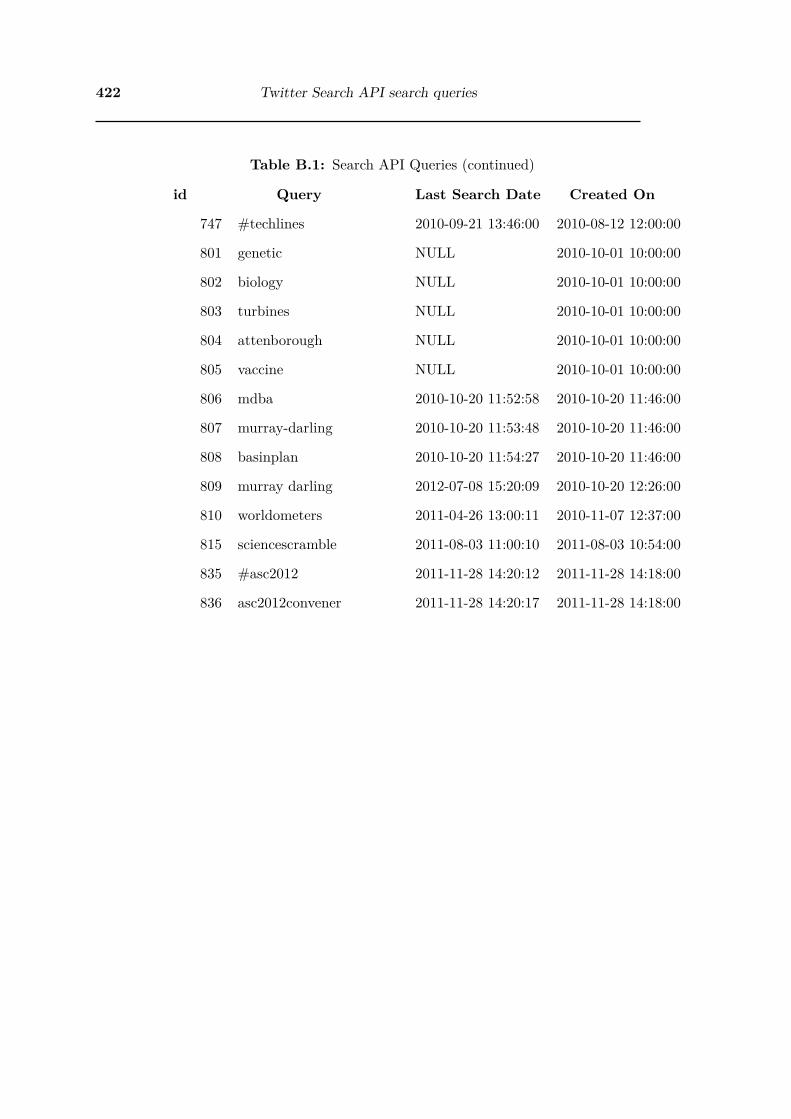
422 Twitter Search API search queries
Table B.1: Search API Queries (continued)
id Query Last Search Date Created On
747 #techlines 2010-09-21 13:46:00 2010-08-12 12:00:00
801 genetic NULL 2010-10-01 10:00:00
802 biology NULL 2010-10-01 10:00:00
803 turbines NULL 2010-10-01 10:00:00
804 attenborough NULL 2010-10-01 10:00:00
805 vaccine NULL 2010-10-01 10:00:00
806 mdba 2010-10-20 11:52:58 2010-10-20 11:46:00
807 murray-darling 2010-10-20 11:53:48 2010-10-20 11:46:00
808 basinplan 2010-10-20 11:54:27 2010-10-20 11:46:00
809 murray darling 2012-07-08 15:20:09 2010-10-20 12:26:00
810 worldometers 2011-04-26 13:00:11 2010-11-07 12:37:00
815 sciencescramble 2011-08-03 11:00:10 2011-08-03 10:54:00
835 #asc2012 2011-11-28 14:20:12 2011-11-28 14:18:00
836 asc2012convener 2011-11-28 14:20:17 2011-11-28 14:18:00

Appendix C
Data Collection Software
C.1 tStreamingArchiver
tStreamingArchiver is a set of programs for archiving Tweets using the Twitter API
and moving them into a mySQL database. It is written in the Java language and li-
censed under GPL 2.0. The code is available on Github at https://github.com/brendam/
tStreamingArchiver.
tStreamingArchiver uses external libraries - twitter4j1, mysql-connector-java and
javax.mail. The Maven dependencies load these for you.
It is setup as a group of 10 eclipse projects using maven to bring in their depen-
dencies.
• gpl-2.0.txt - the terms of license of this software
• readme.md - this file
• tUtils - shared code used by different modules
• Example - sample setup with shell scripts, configuration files and runnable jar
files
• Main modules:1http://twitter4j.org/en/index.html
423

424 Data Collection Software
– tStreamingArchiver - use Twitter streamingAPI to get Tweets into text
files on disk
– tDiskToSQL - import the Tweets from disk into mySQL
• Indexing modules: (better to use Apache Solr instead)
– tUpdateSearchTermIndexing - create indexes in mySQL for the search
terms from the searches table. Has some hard coded search terms which
should be adjusted for your purposes and a new jar file created.
– tBuildWordLists - create word co-occurance lists in mySQL. Has hard
coded search terms which should be adjusted for your purposes and a new
jar file created.
– tSearchArchiver - user Twitter searchAPI to get Tweets and put them di-
rectly into a mySQL database. This is an older module and hasn’t been fully
refactored into the new suite. Use tSearchImport to bring the searchAPI
Tweets into the main mySQL database.
• Other modules:
– tSearchImport - import Tweets from Twitter searchAPI mySQL database.
Before the streamAPI existed, I was collecting data using the searchAPI.
– tGetMissingUsers - fill in any missing users for Tweets imported from
searchAPI or TwapperKeeper
• Discontinued modules:
– tTwapperKeeperImport - import twapperKeeper archives

§C.1 tStreamingArchiver 425
C.1.1 How To Get Started
If you want to build the source code, it is setup to work with Eclipse2 and Maven
Eclipse (m2e)3. To build the project, setup a “Run as Maven Build” run option with
Goals set to clean install javadoc:javadoc.
If you just want to use the programs, then you only need the Example directory
and the instructions in the README.md file in that directory. You do need to have
Java installed (for example Sun Java4.
C.1.2 Bugs / Requests
If you find any bugs or have any suggestions for improvements, please use the issues
section on GitHub.
C.1.3 Citing this work
If you use tStreamingArchiver in publications, please cite the following...
Moon B.R. (2012). tStreamingArchiver <version number> [Software]. Available
from https://github.com/brendam/tStreamingArchiver, <date of access>
BibTex: tStreamingArchiver.bib5
2http://eclipse.org/3http://www.eclipse.org/m2e/4http://java.com/en/download/index.jsp5https://github.com/brendam/tStreamingArchiver/blob/master/tStreamingArchiver.bib

426 Data Collection Software

Appendix D
Languages detected using
langid.py
Table of the 97 languages detected in tweets with ‘science’ keyword in 2011. Language
detection using langid.py (Lui & Baldwin, 2012) with unconstrained set of languages.
Table D.1: Languages by number of tweets with ‘science’ keyword (language detectionusing langid)
code Language Number of Tweets
dz Dzongkha 5
as Assamese 13
kn Kannada 31
te Telugu 33
mr Marathi 54
ml Malayalam 58
ne Nepali 67
or Oriya 80
kk Kazakh 82
ug Uighur; Uyghur 89
gu Gujarati 92
ps Pushto; Pashto 103
Continued on next page...427

428 Languages detected using langid.py
Table D.1 – continued from previous page
code Language Number of Tweets
mn Mongolian 112
pa Panjabi; Punjabi 115
be Belarusian 136
fa Persian 162
ta Tamil 219
hi Hindi 240
vo Volapük 259
ur Urdu 287
hy Armenian 298
bn Bengali 356
ka Georgian 392
lo Lao 404
is Icelandic 408
km Central Khmer 415
uk Ukrainian 422
se Northern Sami 438
mk Macedonian 444
si Sinhala; Sinhalese 476
fo Faroese 503
sr Serbian 524
am Amharic 545
vi Vietnamese 580
nb Bokmål, Norwegian; Norwegian Bokmål 613
nn Norwegian Nynorsk; Nynorsk, Norwegian 627
ku Kurdish 662
Continued on next page...

429
Table D.1 – continued from previous page
code Language Number of Tweets
az Azerbaijani 756
bs Bosnian 797
ky Kirghiz; Kyrgyz 800
bg Bulgarian 845
sk Slovak 931
xh Xhosa 1,017
zu Zulu 1,074
qu Quechua 1,111
lb Luxembourgish; Letzeburgesch 1,123
an Aragonese 1,387
sq Albanian 1,501
oc Occitan (post 1500) 1,565
lv Latvian 1,742
mg Malagasy 1,896
he Hebrew 2,011
gl Galician 2,150
ca Catalan; Valencian 2,181
cs Czech 2,441
ro Romanian 2,531
ht Haitian; Haitian Creole 2,596
lt Lithuanian 2,787
ga Irish 2,845
cy Welsh 2,869
eu Basque 2,982
br Breton 3,324
Continued on next page...

430 Languages detected using langid.py
Table D.1 – continued from previous page
code Language Number of Tweets
hr Croatian 3,548
wa Walloon 3,979
rw Kinyarwanda 4,147
el Greek, Modern (1453-) 4,968
tr Turkish 5,452
eo Esperanto 5,648
et Estonian 5,656
ar Arabic 5,691
fi Finnish 6,208
sl Slovenian 6,584
jv Javanese 7,090
mt Maltese 7,277
hu Hungarian 7,397
af Afrikaans 9,345
sv Swedish 9,549
pl Polish 11,704
ko Korean 12,056
da Danish 12,488
sw Swahili 13,881
zh Chinese 14,229
th Thai 14,517
no Norwegian 15,857
la Latin 16,460
ru Russian 26,335
ms Malay 38,786
Continued on next page...

431
Table D.1 – continued from previous page
code Language Number of Tweets
tl Tagalog 42,239
pt Portuguese 54,242
de German 74,735
nl Dutch; Flemish 77,733
es Spanish; Castilian 85,743
it Italian 93,029
id Indonesian 123,944
ja Japanese 174,194
fr French 201,566
en English 12,285,213
Total 13,212,638
Table showing the calculations of required sample sizes based on sample proportions
from initial samples of 30 tweets per language.
Table D.2: Sample sizes required for each language (language detection using langid)
lang English Not-English n p N n0 Required n
af 22 8 30 0.733 9,345 78.222 78
am 16 14 30 0.533 545 99.556 85
an 10 20 30 0.333 1,387 88.889 84
ar 2 28 30 0.067 5,691 24.889 25
as 7 6 13 0.538 13 99.408 12
Continued on next page...

432 Languages detected using langid.py
Table D.2 – continued from previous page
lang English Not-English n p N n0 Required n
az 22 8 30 0.733 756 78.222 71
be 2 28 30 0.067 136 24.889 22
bg 0 30 30 0.000 845 36.000 35
bn 24 6 30 0.800 356 64.000 55
br 23 7 30 0.767 3,324 71.556 71
bs 19 11 30 0.633 797 92.889 84
ca 7 23 30 0.233 2,181 71.556 70
cs 20 10 30 0.667 2,441 88.889 86
cy 27 3 30 0.900 2,869 36.000 36
da 25 5 30 0.833 12,488 55.556 56
de 18 12 30 0.600 74,735 96.000 96
dz 5 0 5 1.000 5 36.000 5
el 14 16 30 0.467 4,968 99.556 98
eo 15 15 30 0.500 5,648 100.000 99
es 7 23 30 0.233 85,743 71.556 72
et 20 10 30 0.667 5,656 88.889 88
eu 22 8 30 0.733 2,982 78.222 77
fa 5 25 30 0.167 162 55.556 42
fi 26 4 30 0.867 6,208 46.222 46
fo 10 20 30 0.333 503 88.889 76
fr 14 16 30 0.467 201,566 99.556 100
ga 21 9 30 0.700 2,845 84.000 82
gl 3 27 30 0.100 2,150 36.000 36
gu 19 11 30 0.633 92 92.889 47
he 28 2 30 0.933 2,011 24.889 25
Continued on next page...

433
Table D.2 – continued from previous page
lang English Not-English n p N n0 Required n
hi 2 28 30 0.067 240 24.889 23
hr 18 12 30 0.600 3,548 96.000 94
ht 11 19 30 0.367 2,596 92.889 90
hu 30 0 30 1.000 7,397 36.000 36
hy 19 11 30 0.633 298 92.889 71
id 2 28 30 0.067 123,944 24.889 25
is 20 10 30 0.667 408 88.889 73
it 26 4 30 0.867 93,029 46.222 47
ja 0 30 30 0.000 174,194 36.000 36
jv 2 28 30 0.067 7,090 24.889 25
ka 27 3 30 0.900 392 36.000 33
kk 0 30 30 0.000 82 36.000 26
km 29 1 30 0.967 415 12.889 13
kn 15 15 30 0.500 31 100.000 24
ko 0 30 30 0.000 12,056 36.000 36
ku 26 4 30 0.867 662 46.222 44
ky 16 14 30 0.533 800 99.556 89
la 18 12 30 0.600 16,460 96.000 96
lb 13 17 30 0.433 1,123 98.222 91
lo 20 10 30 0.667 404 88.889 73
lt 24 6 30 0.800 2,787 64.000 63
lv 22 8 30 0.733 1,742 78.222 75
mg 21 9 30 0.700 1,896 84.000 81
mk 2 28 30 0.067 444 24.889 24
ml 4 26 30 0.133 58 46.222 26
Continued on next page...

434 Languages detected using langid.py
Table D.2 – continued from previous page
lang English Not-English n p N n0 Required n
mn 1 29 30 0.033 112 12.889 12
mr 8 22 30 0.267 54 78.222 32
ms 0 30 30 0.000 38,786 36.000 36
mt 25 5 30 0.833 7,277 55.556 56
nb 22 8 30 0.733 613 78.222 70
ne 5 25 30 0.167 67 55.556 31
nl 6 24 30 0.200 77,733 64.000 64
nn 25 5 30 0.833 627 55.556 52
no 23 7 30 0.767 15,857 71.556 72
oc 19 11 30 0.633 1,565 92.889 88
or 25 5 30 0.833 80 55.556 33
pa 22 8 30 0.733 115 78.222 47
pl 27 3 30 0.900 11,704 36.000 36
ps 25 5 30 0.833 103 55.556 37
pt 7 23 30 0.233 54,242 71.556 72
qu 10 20 30 0.333 1,111 88.889 83
ro 18 12 30 0.600 2,531 96.000 93
ru 0 30 30 0.000 26,335 36.000 36
rw 15 15 30 0.500 4,147 100.000 98
se 25 5 30 0.833 438 55.556 50
si 24 6 30 0.800 476 64.000 57
sk 23 7 30 0.767 931 71.556 67
sl 26 4 30 0.867 6,584 46.222 46
sq 27 3 30 0.900 1,501 36.000 36
sr 0 30 30 0.000 524 36.000 34
Continued on next page...

435
Table D.2 – continued from previous page
lang English Not-English n p N n0 Required n
sv 11 19 30 0.367 9,549 92.889 92
sw 7 23 30 0.233 13,881 71.556 72
ta 0 30 30 0.000 219 36.000 31
te 21 9 30 0.700 33 84.000 24
th 0 30 30 0.000 14,517 36.000 36
tl 3 27 30 0.100 42,239 36.000 36
tr 8 22 30 0.267 5,452 78.222 78
ug 4 26 30 0.133 89 46.222 31
uk 1 29 30 0.033 422 12.889 13
ur 25 5 30 0.833 287 55.556 47
vi 13 17 30 0.433 580 98.222 84
vo 20 10 30 0.667 259 88.889 67
wa 24 6 30 0.800 3,979 64.000 63
xh 8 22 30 0.267 1,017 78.222 73
zh 6 24 30 0.200 14,229 64.000 64
zu 6 24 30 0.200 1,074 64.000 61
Total 5,383
Table showing the recalculation of required sample sizes based the new sample
proportions after the 2nd round of sampling.

436 Languages detected using langid.py
Table D.3: Sample sizes required for each language - after 2nd Round of Sampling(language detection using langid)
lang English other n p N n0 Required n
af 60 29 89 0.674 9,345 87.868 88
am 55 30 85 0.647 545 91.349 79
an 27 57 84 0.321 1,387 87.245 83
ar 2 28 30 0.067 5,691 24.889 25
as 7 6 13 0.538 13 99.408 12
az 56 15 71 0.789 756 66.653 62
be 2 28 30 0.067 136 24.889 22
bg 0 35 35 0.000 845 36.000 35
bn 48 17 65 0.738 356 77.254 64
br 56 36 92 0.609 3,324 95.274 93
bs 46 43 89 0.517 797 99.886 89
ca 23 56 79 0.291 2,181 82.551 80
cs 63 23 86 0.733 2,441 78.367 76
cy 42 5 47 0.894 2,869 38.026 38
da 48 8 56 0.857 12,488 48.980 49
de 49 52 101 0.485 74,735 99.912 100
dz 5 0 5 1.000 5 36.000 5
el 35 63 98 0.357 4,968 91.837 91
eo 46 53 99 0.465 5,648 99.500 98
es 16 56 72 0.222 85,743 69.136 70
et 59 30 89 0.663 5,656 89.383 88
eu 59 18 77 0.766 2,982 71.648 70
fa 7 35 42 0.167 162 55.556 42
fi 44 8 52 0.846 6,208 52.071 52
Continued on next page...

437
Table D.3 – continued from previous page
lang English other n p N n0 Required n
fo 46 37 83 0.554 503 98.824 83
fr 44 56 100 0.440 201,566 98.560 99
ga 61 21 82 0.744 2,845 76.205 75
gl 7 40 47 0.149 2,150 50.702 50
gu 34 13 47 0.723 92 80.036 43
he 28 2 30 0.933 2,011 24.889 25
hi 2 28 30 0.067 240 24.889 23
hr 66 28 94 0.702 3,548 83.658 82
ht 39 56 95 0.411 2,596 96.798 94
hu 36 0 36 1.000 7,397 36.000 36
hy 35 40 75 0.467 298 99.556 75
id 2 28 30 0.067 123,944 24.889 25
is 45 34 79 0.570 408 98.061 80
it 54 13 67 0.806 93,029 62.553 63
ja 0 36 36 0.000 174,194 36.000 36
jv 2 28 30 0.067 7,090 24.889 25
ka 33 6 39 0.846 392 52.071 46
kk 0 30 30 0.000 82 36.000 26
km 29 1 30 0.967 415 12.889 13
kn 15 15 30 0.500 31 100.000 24
ko 0 36 36 0.000 12,056 36.000 36
ku 38 6 44 0.864 662 47.107 44
ky 47 42 89 0.528 800 99.684 89
la 54 46 100 0.540 16,460 99.360 99
lb 46 46 92 0.500 1,123 100.000 92
Continued on next page...

438 Languages detected using langid.py
Table D.3 – continued from previous page
lang English other n p N n0 Required n
lo 49 25 74 0.662 404 89.481 74
lt 53 15 68 0.779 2,787 68.772 68
lv 52 37 89 0.584 1,742 97.159 93
mg 55 34 89 0.618 1,896 94.433 90
mk 2 28 30 0.067 444 24.889 24
ml 4 26 30 0.133 58 46.222 26
mn 1 29 30 0.033 112 12.889 12
mr 8 24 32 0.250 54 75.000 32
ms 0 36 36 0.000 38,786 36.000 36
mt 50 13 63 0.794 7,277 65.508 65
nb 53 17 70 0.757 613 73.551 66
ne 5 26 31 0.161 67 54.110 30
nl 10 54 64 0.156 77,733 52.734 53
nn 47 10 57 0.825 627 57.864 53
no 56 16 72 0.778 15,857 69.136 69
oc 55 36 91 0.604 1,565 95.641 91
or 28 5 33 0.848 80 51.423 32
pa 32 19 51 0.627 115 93.502 52
pl 33 3 36 0.917 11,704 30.556 31
ps 32 7 39 0.821 103 58.909 38
pt 14 58 72 0.194 54,242 62.654 63
qu 21 62 83 0.253 1,111 75.599 71
ro 52 43 95 0.547 2,531 99.102 96
ru 0 36 36 0.000 26,335 36.000 36
rw 37 61 98 0.378 4,147 94.002 92
Continued on next page...

439
Table D.3 – continued from previous page
lang English other n p N n0 Required n
se 45 28 73 0.616 438 94.577 78
si 48 9 57 0.842 476 53.186 48
sk 55 20 75 0.733 931 78.222 73
sl 48 9 57 0.842 6,584 53.186 53
sq 41 6 47 0.872 1,501 44.545 44
sr 0 34 34 0.000 524 36.000 34
sv 38 58 96 0.396 9,549 95.660 95
sw 19 56 75 0.253 13,881 75.662 76
ta 0 31 31 0.000 219 36.000 31
te 21 9 30 0.700 33 84.000 24
th 0 36 36 0.000 14,517 36.000 36
tl 6 42 48 0.125 42,239 43.750 44
tr 31 57 88 0.352 5,452 91.271 90
ug 4 27 31 0.129 89 44.953 30
uk 1 29 30 0.033 422 12.889 13
ur 42 16 58 0.724 287 79.905 63
vi 30 54 84 0.357 580 91.837 80
vo 51 16 67 0.761 259 72.711 57
wa 55 23 78 0.705 3,979 83.169 82
xh 29 56 85 0.341 1,017 89.910 83
zh 21 60 81 0.259 14,229 76.818 77
zu 22 56 78 0.282 1,074 80.999 76
Total 5,574

440 Languages detected using langid.py
Table D.4: Proportion of English tweets per language identified by langid.py withoutfiltering
lang English other N n p SE lci uci
af 60 29 9,345 89 0.674 0.049 0.575 0.773
am 55 30 545 85 0.647 0.048 0.552 0.742
an 27 57 1,387 84 0.321 0.049 0.223 0.420
ar 2 28 5,691 30 0.067 0.045 -0.024 0.158
as 7 6 13 13 0.538 0.000 0.538 0.538
az 56 15 756 71 0.789 0.046 0.697 0.881
be 2 28 136 30 0.067 0.040 -0.014 0.147
bg 0 35 845 35 0.000 0.000 0.000 0.000
bn 48 17 356 65 0.738 0.049 0.640 0.837
br 57 37 3,324 94 0.606 0.050 0.507 0.706
bs 46 43 797 89 0.517 0.050 0.417 0.617
ca 26 57 2,181 83 0.313 0.050 0.213 0.413
cs 63 23 2,441 86 0.733 0.047 0.639 0.826
cy 42 5 2,869 47 0.894 0.045 0.804 0.983
da 48 8 12,488 56 0.857 0.047 0.764 0.950
de 49 52 74,735 101 0.485 0.050 0.386 0.585
dz 5 0 5 5 1.000 0.000 1.000 1.000
el 35 63 4,968 98 0.357 0.048 0.261 0.453
eo 46 53 5,648 99 0.465 0.050 0.365 0.564
es 16 56 85,743 72 0.222 0.049 0.124 0.320
et 59 30 5,656 89 0.663 0.050 0.563 0.762
eu 59 18 2,982 77 0.766 0.048 0.671 0.861
fa 7 35 162 42 0.167 0.049 0.068 0.266
fi 44 8 6,208 52 0.846 0.050 0.747 0.946
Continued on next page...

441
Table D.4 – continued from previous page
lang English other N n p SE lci uci
fo 46 37 503 83 0.554 0.050 0.455 0.654
fr 44 56 201,566 100 0.440 0.050 0.341 0.539
ga 61 21 2,845 82 0.744 0.048 0.649 0.839
gl 7 43 2,150 50 0.140 0.048 0.043 0.237
gu 34 13 92 47 0.723 0.046 0.632 0.815
he 28 2 2,011 30 0.933 0.045 0.843 1.024
hi 2 28 240 30 0.067 0.043 -0.019 0.152
hr 66 28 3,548 94 0.702 0.047 0.609 0.795
ht 39 56 2,596 95 0.411 0.050 0.311 0.510
hu 36 0 7,397 36 1.000 0.000 1.000 1.000
hy 35 40 298 75 0.467 0.050 0.367 0.566
id 2 28 123,944 30 0.067 0.046 -0.024 0.158
is 46 34 408 80 0.575 0.050 0.476 0.674
it 54 13 93,029 67 0.806 0.048 0.709 0.903
ja 0 36 174,194 36 0.000 0.000 0.000 0.000
jv 2 28 7,090 30 0.067 0.045 -0.024 0.158
ka 39 7 392 46 0.848 0.050 0.748 0.947
kk 0 30 82 30 0.000 0.000 0.000 0.000
km 29 1 415 30 0.967 0.032 0.904 1.030
kn 15 15 31 30 0.500 0.016 0.467 0.533
ko 0 36 12,056 36 0.000 0.000 0.000 0.000
ku 38 6 662 44 0.864 0.050 0.764 0.964
ky 47 42 800 89 0.528 0.050 0.428 0.628
la 54 46 16,460 100 0.540 0.050 0.441 0.639
lb 46 46 1,123 92 0.500 0.050 0.400 0.600
Continued on next page...

442 Languages detected using langid.py
Table D.4 – continued from previous page
lang English other N n p SE lci uci
lo 49 25 404 74 0.662 0.050 0.563 0.762
lt 53 15 2,787 68 0.779 0.050 0.680 0.879
lv 54 39 1,742 93 0.581 0.050 0.481 0.680
mg 56 34 1,896 90 0.622 0.050 0.522 0.722
mk 2 28 444 30 0.067 0.044 -0.021 0.155
ml 4 26 58 30 0.133 0.043 0.047 0.220
mn 1 29 112 30 0.033 0.028 -0.023 0.089
mr 8 24 54 32 0.250 0.049 0.152 0.348
ms 0 36 38,786 36 0.000 0.000 0.000 0.000
mt 52 13 7,277 65 0.800 0.049 0.701 0.899
nb 53 17 613 70 0.757 0.048 0.661 0.854
ne 5 26 67 31 0.161 0.048 0.064 0.258
nl 10 54 77,733 64 0.156 0.045 0.066 0.247
nn 47 10 627 57 0.825 0.048 0.728 0.921
no 56 16 15,857 72 0.778 0.049 0.680 0.876
oc 55 36 1,565 91 0.604 0.050 0.505 0.704
or 28 5 80 33 0.848 0.048 0.753 0.944
pa 32 20 115 52 0.615 0.050 0.516 0.715
pl 33 3 11,704 36 0.917 0.046 0.825 1.009
ps 32 7 103 39 0.821 0.048 0.724 0.917
pt 14 58 54,242 72 0.194 0.047 0.101 0.288
qu 21 62 1,111 83 0.253 0.046 0.161 0.345
ro 52 44 2,531 96 0.542 0.050 0.442 0.641
ru 0 36 26,335 36 0.000 0.000 0.000 0.000
rw 37 61 4,147 98 0.378 0.048 0.281 0.474
Continued on next page...

443
Table D.4 – continued from previous page
lang English other N n p SE lci uci
se 48 32 438 80 0.600 0.050 0.501 0.699
si 48 9 476 57 0.842 0.045 0.751 0.933
sk 55 20 931 75 0.733 0.049 0.635 0.831
sl 48 9 6,584 57 0.842 0.048 0.746 0.938
sq 41 6 1,501 47 0.872 0.048 0.777 0.968
sr 0 34 524 34 0.000 0.000 0.000 0.000
sv 38 58 9,549 96 0.396 0.050 0.297 0.495
sw 20 58 13,881 78 0.256 0.049 0.158 0.355
ta 0 31 219 31 0.000 0.000 0.000 0.000
te 21 9 33 30 0.700 0.025 0.650 0.750
th 0 36 14,517 36 0.000 0.000 0.000 0.000
tl 6 42 42,239 48 0.125 0.048 0.030 0.220
tr 31 59 5,452 90 0.344 0.050 0.245 0.444
ug 4 27 89 31 0.129 0.049 0.032 0.226
uk 1 29 422 30 0.033 0.032 -0.030 0.097
ur 45 23 287 68 0.662 0.050 0.562 0.762
vi 30 54 580 84 0.357 0.048 0.260 0.454
vo 51 16 259 67 0.761 0.045 0.671 0.851
wa 58 26 3,979 84 0.690 0.050 0.591 0.790
xh 29 56 1,017 85 0.341 0.049 0.243 0.440
zh 21 60 14,229 81 0.259 0.049 0.162 0.356
zu 22 56 1,074 78 0.282 0.049 0.184 0.380
Total 1,251,883 5,899
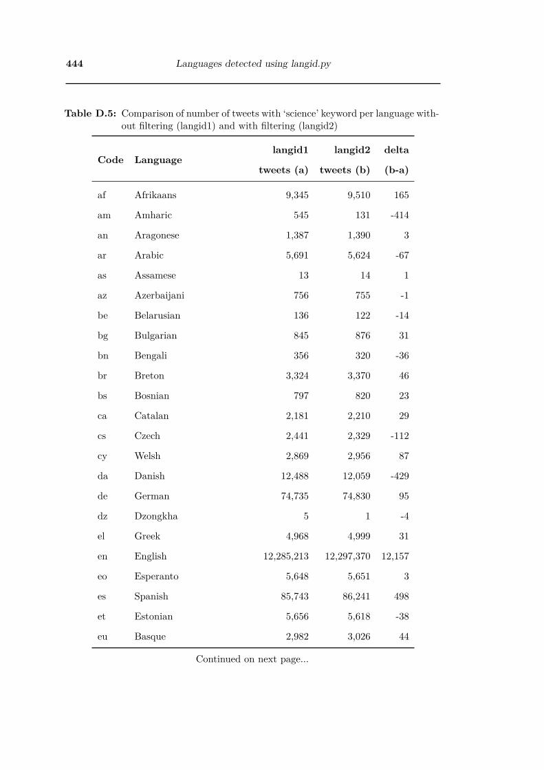
444 Languages detected using langid.py
Table D.5: Comparison of number of tweets with ‘science’ keyword per language with-out filtering (langid1) and with filtering (langid2)
Code Languagelangid1 langid2 delta
tweets (a) tweets (b) (b-a)
af Afrikaans 9,345 9,510 165
am Amharic 545 131 -414
an Aragonese 1,387 1,390 3
ar Arabic 5,691 5,624 -67
as Assamese 13 14 1
az Azerbaijani 756 755 -1
be Belarusian 136 122 -14
bg Bulgarian 845 876 31
bn Bengali 356 320 -36
br Breton 3,324 3,370 46
bs Bosnian 797 820 23
ca Catalan 2,181 2,210 29
cs Czech 2,441 2,329 -112
cy Welsh 2,869 2,956 87
da Danish 12,488 12,059 -429
de German 74,735 74,830 95
dz Dzongkha 5 1 -4
el Greek 4,968 4,999 31
en English 12,285,213 12,297,370 12,157
eo Esperanto 5,648 5,651 3
es Spanish 85,743 86,241 498
et Estonian 5,656 5,618 -38
eu Basque 2,982 3,026 44
Continued on next page...

445
Table D.5 – continued from previous page
Code Languagelangid1 langid2 delta
tweets (a) tweets (b) (b-a)
fa Persian 162 148 -14
fi Finnish 6,208 6,062 -146
fo Faroese 503 484 -19
fr French 201,566 201,630 64
ga Irish 2,845 2,775 -70
gl Galician 2,150 2,168 18
gu Gujarati 92 70 -22
he Hebrew 2,011 672 -1,339
hi Hindi 240 200 -40
hr Croatian 3,548 3,439 -109
ht Haitian 2,596 2,526 -70
hu Hungarian 7,397 6,922 -475
hy Armenian 298 149 -149
id Indonesian 123,944 124,700 756
is Icelandic 408 394 -14
it Italian 93,029 93,384 355
ja Japanese 174,194 173,445 -749
jv Javanese 7,090 6,422 -668
ka Georgian 392 67 -325
kk Kazakh 82 79 -3
km Central Khmer 415 11 -404
kn Kannada 31 21 -10
ko Korean 12,056 11,858 -198
ku Kurdish 662 558 -104
Continued on next page...

446 Languages detected using langid.py
Table D.5 – continued from previous page
Code Languagelangid1 langid2 delta
tweets (a) tweets (b) (b-a)
ky Kirghiz 800 763 -37
la Latin 16,460 12,496 -3,964
lb Luxembourgish 1,123 1,059 -64
lo Lao 404 319 -85
lt Lithuanian 2,787 2,687 -100
lv Latvian 1,742 1,667 -75
mg Malagasy 1,896 1,981 85
mk Macedonian 444 425 -19
ml Malayalam 58 58 0
mn Mongolian 112 112 0
mr Marathi 54 48 -6
ms Malay 38,786 39,089 303
mt Maltese 7,277 7,195 -82
nb Norwegian Bokmål 613 604 -9
ne Nepali 67 54 -13
nl Dutch 77,733 77,726 -7
nn Norwegian Nynorsk 627 569 -58
no Norwegian 15,857 14,644 -1,213
oc Occitan 1,565 1,510 -55
or Oriya 80 35 -45
pa Punjabi 115 69 -46
pl Polish 11,704 11,826 122
ps Pashto 103 84 -19
pt Portuguese 54,242 54,500 258
Continued on next page...

447
Table D.5 – continued from previous page
Code Languagelangid1 langid2 delta
tweets (a) tweets (b) (b-a)
qu Quechua 1,111 835 -276
ro Romanian 2,531 2,590 59
ru Russian 26,335 26,171 -164
rw Kinyarwanda 4,147 4,079 -68
se Northern Sami 438 342 -96
si Sinhalese 476 419 -57
sk Slovak 931 769 -162
sl Slovenian 6,584 6,650 66
sq Albanian 1,501 1,166 -335
sr Serbian 524 524 0
sv Swedish 9,549 9,427 -122
sw Swahili 13,881 13,806 -75
ta Tamil 219 219 0
te Telugu 33 26 -7
th Thai 14,517 14,518 1
tl Tagalog 42,239 42,832 593
tr Turkish 5,452 5,488 36
ug Uyghur 89 88 -1
uk Ukrainian 422 415 -7
ur Urdu 287 99 -188
vi Vietnamese 580 477 -103
vo Volapük 259 255 -4
wa Walloon 3,979 3,536 -443
xh Xhosa 1,017 1,046 29
Continued on next page...

448 Languages detected using langid.py
Table D.5 – continued from previous page
Code Languagelangid1 langid2 delta
tweets (a) tweets (b) (b-a)
zh Chinese 14,229 12,283 -1,946
zu Zulu 1,074 1,110 36
Total 13,537,096 13,537,096 0
Table D.6 (next page) shows the summary of results for langid without filtering
(langid1) and with filtering of unicode characters applied first (langid2). For each
language identified by langid the table shows the total tweets found for that language
(N), sample sizes of manual coding (n) and the number of tweets manually coded as
English (Coded English).

449
Tabl
eD
.6:Su
mmaryof
lang
id1an
dlang
id2sampling
code
Lang
uage
nC
oded
Eng
lish
N
lang
id1
lang
id2
lang
id1
lang
id2
lang
id1
lang
id2
afAfrika
ans
9710
167
679,34
59,51
0
amAmha
ric11
951
6414
545
131
anArago
nese
110
107
3634
1,38
71,39
0
arArabic
4946
32
5,69
15,62
4
asAssam
ese
1314
78
1314
azAzerbaijani
8379
6462
756
755
beBe
larusia
n38
362
013
612
2
bgBu
lgarian
3537
01
845
876
bnBe
ngali
8377
6257
356
320
brBr
eton
130
128
8482
3,32
43,37
0
bsBo
snian
115
113
5959
797
820
caCatalan
104
104
3232
2,18
12,21
0
csCzech
103
102
7270
2,44
12,32
9
cyWelsh
6363
5655
2,86
92,95
6
Con
tinuedon
next
page...

450 Languages detected using langid.pyTa
ble
D.6
–co
ntin
ued
from
prev
ious
page
code
Lang
uage
nC
oded
Eng
lish
N
lang
id1
lang
id2
lang
id1
lang
id2
lang
id1
lang
id2
daDan
ish69
6958
5812
,488
12,059
deGerman
123
135
5868
74,735
74,830
dzDzong
kha
51
40
51
elGreek
122
126
4246
4,96
84,99
9
enEn
glish
1,01
81,44
51,00
01,38
112
,285
,213
12,297
,370
eoEs
peranto
126
121
5960
5,64
85,65
1
esSp
anish
8110
019
2485
,743
86,241
etEs
tonian
106
109
7275
5,65
65,61
8
euBa
sque
107
107
8281
2,98
23,02
6
faPe
rsian
4337
72
162
148
fiFinn
ish60
6151
536,20
86,06
2
foFa
roese
105
104
6868
503
484
frFrench
101
148
4580
201,56
620
1,63
0
gaIrish
109
106
8581
2,84
52,77
5
Con
tinuedon
next
page...

451
Tabl
eD
.6–
cont
inue
dfr
ompr
evio
uspa
ge
code
Lang
uage
nC
oded
Eng
lish
N
lang
id1
lang
id2
lang
id1
lang
id2
lang
id1
lang
id2
glGalician
6668
1111
2,15
02,16
8
guGujarati
5746
4028
9270
heHebrew
100
8876
632,01
167
2
hiHindi
3937
20
240
200
hrCroatian
109
106
7774
3,54
83,43
9
htHaitia
n12
511
655
502,59
62,52
6
huHun
garia
n37
3637
357,39
76,92
2
hyArm
enian
9354
4418
298
149
idIndo
nesia
n41
493
512
3,94
412
4,70
0
isIcelan
dic
101
9660
5940
839
4
itItalian
7095
5575
93,029
93,384
jaJa
panese
3837
01
174,19
417
3,44
5
jvJavanese
7679
714
7,09
06,42
2
kaGeorgian
6038
4721
392
67
Con
tinuedon
next
page...

452 Languages detected using langid.pyTa
ble
D.6
–co
ntin
ued
from
prev
ious
page
code
Lang
uage
nC
oded
Eng
lish
N
lang
id1
lang
id2
lang
id1
lang
id2
lang
id1
lang
id2
kkKazak
h32
321
182
79
kmCentral
Khm
er40
1032
341
511
knKan
nada
3019
155
3121
koKorean
3838
12
12,056
11,858
kuKurdish
6252
5344
662
558
kyKirg
hiz
106
102
6159
800
763
laLa
tin15
113
077
5216
,460
12,496
lbLu
xembo
urgish
126
122
6259
1,12
31,05
9
loLa
o10
785
6748
404
319
ltLithua
nian
8592
6670
2,78
72,68
7
lvLa
tvian
125
117
7164
1,74
21,66
7
mg
Malag
asy
110
110
7070
1,89
61,98
1
mk
Macedon
ian
4745
22
444
425
ml
Malayalam
3838
57
5858
Con
tinuedon
next
page...

453
Tabl
eD
.6–
cont
inue
dfr
ompr
evio
uspa
ge
code
Lang
uage
nC
oded
Eng
lish
N
lang
id1
lang
id2
lang
id1
lang
id2
lang
id1
lang
id2
mn
Mon
golia
n37
371
111
211
2
mr
Marathi
3734
82
5448
ms
Malay
3850
01
38,786
39,089
mt
Maltese
9092
7474
7,27
77,19
5
nbNorwe
gian
Bokm
ål76
7558
5761
360
4
neNepali
3732
50
6754
nlDutch
9497
1822
77,733
77,726
nnNorwe
gian
Nyn
orsk
8175
6357
627
569
noNorwe
gian
8783
6663
15,857
14,644
ocOccita
n11
611
269
671,56
51,51
0
orOriy
a41
2532
2080
35
paPu
njab
i64
4640
2411
569
plPo
lish
5654
4744
11,704
11,826
psPa
shto
5039
3520
103
84
Con
tinuedon
next
page...
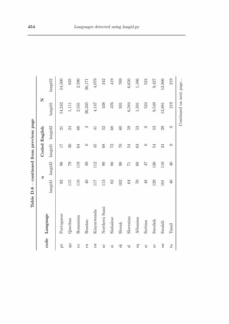
454 Languages detected using langid.pyTa
ble
D.6
–co
ntin
ued
from
prev
ious
page
code
Lang
uage
nC
oded
Eng
lish
N
lang
id1
lang
id2
lang
id1
lang
id2
lang
id1
lang
id2
ptPo
rtug
uese
9296
1721
54,242
54,500
quQuechua
115
7930
241,11
183
5
roRom
anian
118
119
6466
2,53
12,59
0
ruRussia
n40
390
226
,335
26,171
rwKinyarw
anda
117
112
4541
4,14
74,07
9
seNorthernSa
mi
113
9068
5243
834
2
siSinh
alese
8280
7268
476
419
skSlovak
102
9070
6093
176
9
slSlovenian
6471
5459
6,58
46,65
0
sqAlban
ian
7060
6353
1,50
11,16
6
srSerbian
4847
00
524
524
svSw
edish
129
130
5453
9,54
99,42
7
swSw
ahili
101
110
2429
13,881
13,806
taTa
mil
4040
00
219
219
Con
tinuedon
next
page...

455
Tabl
eD
.6–
cont
inue
dfr
ompr
evio
uspa
ge
code
Lang
uage
nC
oded
Eng
lish
N
lang
id1
lang
id2
lang
id1
lang
id2
lang
id1
lang
id2
teTe
lugu
3125
2217
3326
thTha
i49
491
114
,517
14,518
tlTa
galog
4957
77
42,239
42,832
trTu
rkish
118
120
4445
5,45
25,48
8
ugUyg
hur
3128
41
8988
ukUkrainian
4544
10
422
415
urUrdu
8746
488
287
99
viVietnam
ese
9581
3320
580
477
voVo
lapü
k87
8467
6525
925
5
waWalloon
125
107
9379
3,97
93,53
6
xhXho
sa10
510
639
381,01
71,04
6
zhChinese
142
9651
1914
,229
12,283
zuZu
lu97
101
2729
1,07
41,11
0
Totals
8,62
28,62
24,86
94,86
913
,537
,096
13,537
,096

456 Languages detected using langid.py

457
Tabl
eD
.7:Po
pulatio
nprop
ortio
nof
English
forlang
id1an
dlang
id2
Lang
uage
lang
id1
lang
id2
Np
SElc
iuc
iN
pSE
lci
uci
Afrika
ans
9,34
50.69
10.04
70.59
70.78
49,51
00.66
30.04
70.57
00.75
7
Alban
ian
1,50
10.90
00.03
50.83
00.97
01,16
60.88
30.04
00.80
30.96
4
Amha
ric54
50.53
80.04
00.45
70.61
913
10.27
50.04
90.17
70.37
2
Arabic
5,69
10.06
10.03
4-0.007
0.12
95,62
40.04
30.03
0-0.016
0.10
3
Arago
nese
1,38
70.32
70.04
30.24
10.41
31,39
00.31
80.04
30.23
10.40
4
Arm
enian
298
0.47
30.04
30.38
70.55
914
90.33
30.05
10.23
10.43
6
Assam
ese
130.53
80.00
00.53
80.53
814
0.57
10.00
00.57
10.57
1
Azerbaijani
756
0.77
10.04
40.68
40.85
875
50.78
50.04
40.69
70.87
2
Basque
2,98
20.76
60.04
00.68
60.84
73,02
60.75
70.04
10.67
60.83
8
Belarusia
n13
60.05
30.03
1-0.009
0.11
412
20.00
00.00
00.00
00.00
0
Beng
ali
356
0.74
70.04
20.66
30.83
132
00.74
00.04
40.65
30.82
7
Bosnian
797
0.51
30.04
30.42
70.59
982
00.52
20.04
40.43
50.60
9
Breton
3,32
40.64
60.04
10.56
40.72
83,37
00.64
10.04
20.55
70.72
4
Bulgarian
845
0.00
00.00
00.00
00.00
087
60.02
70.02
6-0.025
0.07
9
Con
tinuedon
next
page...

458 Languages detected using langid.pyTa
ble
D.7
–co
ntin
ued
from
prev
ious
page
Lang
uage
lang
id1
lang
id2
Np
SElc
iuc
iN
pSE
lci
uci
Catalan
2,18
10.30
80.04
40.21
90.39
62,21
00.30
80.04
40.21
90.39
6
Central
Khm
er41
50.80
00.06
00.68
00.92
011
0.30
00.04
40.21
30.38
7
Chinese
14,229
0.35
90.04
00.27
90.43
912
,283
0.19
80.04
10.11
70.27
9
Croatian
3,54
80.70
60.04
30.62
10.79
23,43
90.69
80.04
40.61
00.78
6
Czech
2,44
10.69
90.04
40.61
10.78
72,32
90.68
60.04
50.59
60.77
6
Dan
ish12
,488
0.84
10.04
40.75
30.92
812
,059
0.84
10.04
40.75
30.92
8
Dutch
77,733
0.19
10.04
10.11
00.27
377
,726
0.22
70.04
20.14
20.31
2
Dzong
kha
50.80
00.00
00.80
00.80
01
0.00
00.00
00.00
00.00
0
English
12,285
,213
0.98
20.00
40.97
40.99
112
,297
,370
0.95
60.00
50.94
50.96
7
Espe
ranto
5,64
80.46
80.04
40.38
00.55
65,65
10.49
60.04
50.40
60.58
6
Estonian
5,65
60.67
90.04
50.58
90.76
95,61
80.68
80.04
40.60
00.77
6
Faroese
503
0.64
80.04
10.56
50.73
148
40.65
40.04
10.57
10.73
7
Finn
ish6,20
80.85
00.04
60.75
80.94
26,06
20.86
90.04
30.78
30.95
5
French
201,56
60.44
60.04
90.34
70.54
420
1,63
00.54
10.04
10.45
90.62
2
Con
tinuedon
next
page...

459
Tabl
eD
.7–
cont
inue
dfr
ompr
evio
uspa
ge
Lang
uage
lang
id1
lang
id2
Np
SElc
iuc
iN
pSE
lci
uci
Galician
2,15
00.16
70.04
50.07
60.25
72,16
80.16
20.04
40.07
40.25
0
Georgian
392
0.78
30.04
90.68
50.88
167
0.55
30.05
30.44
60.65
9
German
74,735
0.47
20.04
50.38
20.56
174
,830
0.50
40.04
30.41
80.59
0
Greek
4,96
80.34
40.04
20.25
90.42
94,99
90.36
50.04
20.28
00.45
0
Gujarati
920.70
20.03
70.62
70.77
770
0.60
90.04
20.52
40.69
3
Haitia
n2,59
60.44
00.04
30.35
30.52
72,52
60.43
10.04
50.34
10.52
1
Heb
rew
2,01
10.76
00.04
20.67
70.84
367
20.71
60.04
50.62
60.80
6
Hindi
240
0.05
10.03
2-0.013
0.11
620
00.00
00.00
00.00
00.00
0
Hun
garia
n7,39
71.00
00.00
01.00
01.00
06,92
20.97
20.02
70.91
81.02
7
Icelan
dic
408
0.59
40.04
20.50
90.67
939
40.61
50.04
30.52
80.70
1
Indo
nesia
n12
3,94
40.07
30.04
1-0.008
0.15
412
4,70
00.10
20.04
30.01
60.18
9
Irish
2,84
50.78
00.03
90.70
20.85
82,77
50.76
40.04
00.68
30.84
5
Italian
93,029
0.78
60.04
90.68
80.88
493
,384
0.78
90.04
20.70
60.87
3
Japa
nese
174,19
40.00
00.00
00.00
00.00
017
3,44
50.02
70.02
7-0.026
0.08
0
Con
tinuedon
next
page...

460 Languages detected using langid.pyTa
ble
D.7
–co
ntin
ued
from
prev
ious
page
Lang
uage
lang
id1
lang
id2
Np
SElc
iuc
iN
pSE
lci
uci
Javanese
7,09
00.09
20.03
30.02
60.15
86,42
20.17
70.04
30.09
20.26
3
Kan
nada
310.50
00.01
60.46
70.53
321
0.26
30.03
10.20
10.32
6
Kazak
h82
0.03
10.02
4-0.017
0.07
979
0.03
10.02
4-0.016
0.07
9
Kinyarw
anda
4,14
70.38
50.04
40.29
60.47
34,07
90.36
60.04
50.27
60.45
6
Kirg
hiz
800
0.57
50.04
50.48
60.66
576
30.57
80.04
60.48
70.66
9
Korean
12,056
0.02
60.02
6-0.026
0.07
811
,858
0.05
30.03
6-0.020
0.12
5
Kurdish
662
0.85
50.04
30.77
00.94
055
80.84
60.04
80.75
10.94
1
Lao
404
0.62
60.04
00.54
60.70
631
90.56
50.04
60.47
30.65
7
Latin
16,460
0.51
00.04
00.42
90.59
112
,496
0.40
00.04
30.31
50.48
5
Latvian
1,74
20.56
80.04
30.48
30.65
31,66
70.54
70.04
40.45
80.63
6
Lithua
nian
2,78
70.77
60.04
40.68
70.86
52,68
70.76
10.04
40.67
30.84
8
Luxembo
urgish
1,12
30.49
20.04
20.40
80.57
61,05
90.48
40.04
30.39
80.56
9
Macedon
ian
444
0.04
30.02
8-0.013
0.09
842
50.04
40.02
9-0.014
0.10
3
Malagasy
1,89
60.63
60.04
50.54
70.72
51,98
10.63
60.04
50.54
70.72
6
Con
tinuedon
next
page...

461
Tabl
eD
.7–
cont
inue
dfr
ompr
evio
uspa
ge
Lang
uage
lang
id1
lang
id2
Np
SElc
iuc
iN
pSE
lci
uci
Malay
38,786
0.00
00.00
00.00
00.00
039
,089
0.02
00.02
0-0.020
0.06
0
Malayalam
580.13
20.03
20.06
70.19
658
0.18
40.03
70.11
00.25
8
Maltese
7,27
70.82
20.04
00.74
20.90
27,19
50.80
40.04
10.72
20.88
7
Marathi
540.21
60.03
80.14
00.29
248
0.05
90.02
20.01
50.10
2
Mon
golia
n11
20.02
70.02
2-0.017
0.07
111
20.02
70.02
2-0.017
0.07
1
Nepali
670.13
50.03
80.06
00.21
054
0.00
00.00
00.00
00.00
0
NorthernSa
mi
438
0.60
20.04
00.52
20.68
134
20.57
80.04
50.48
80.66
7
Norwe
gian
15,857
0.75
90.04
60.66
70.85
014
,644
0.75
90.04
70.66
50.85
3
Norwe
gian
Bokm
ål61
30.76
30.04
60.67
20.85
460
40.76
00.04
60.66
80.85
2
Norwe
gian
Nyn
orsk
627
0.77
80.04
30.69
20.86
456
90.76
00.04
60.66
80.85
2
Occita
n1,56
50.59
50.04
40.50
70.68
31,51
00.59
80.04
50.50
90.68
7
Oriy
a80
0.78
00.04
50.69
00.87
135
0.80
00.04
30.71
40.88
6
Persian
162
0.16
30.04
80.06
60.25
914
80.05
40.03
2-0.010
0.11
8
Polish
11,704
0.83
90.04
90.74
10.93
711
,826
0.81
50.05
30.70
90.92
0
Con
tinuedon
next
page...

462 Languages detected using langid.pyTa
ble
D.7
–co
ntin
ued
from
prev
ious
page
Lang
uage
lang
id1
lang
id2
Np
SElc
iuc
iN
pSE
lci
uci
Portug
uese
54,242
0.18
50.04
00.10
40.26
654
,500
0.21
90.04
20.13
40.30
3
Punjab
i11
50.62
50.04
00.54
40.70
669
0.52
20.04
30.43
70.60
7
Pushto
103
0.70
00.04
60.60
70.79
384
0.51
30.05
90.39
60.63
0
Quechua
1,11
10.26
10.03
90.18
30.33
883
50.30
40.04
90.20
50.40
2
Rom
anian
2,53
10.54
20.04
50.45
30.63
22,59
00.55
50.04
50.46
60.64
4
Russia
n26
,335
0.00
00.00
00.00
00.00
026
,171
0.05
10.03
5-0.019
0.12
2
Serbian
524
0.00
00.00
00.00
00.00
052
40.00
00.00
00.00
00.00
0
Sinh
ala
476
0.87
80.03
30.81
20.94
441
90.85
00.03
60.77
80.92
2
Slovak
931
0.68
60.04
30.60
00.77
376
90.66
70.04
70.57
30.76
0
Slovenian
6,58
40.84
40.04
50.75
30.93
46,65
00.83
10.04
40.74
30.91
9
Span
ish85
,743
0.23
50.04
70.14
00.32
986
,241
0.24
00.04
30.15
50.32
5
Swah
ili13
,881
0.23
80.04
20.15
30.32
213
,806
0.26
40.04
20.18
00.34
7
Swedish
9,54
90.41
90.04
30.33
20.50
59,42
70.40
80.04
30.32
20.49
3
Tagalog
42,239
0.14
30.05
00.04
30.24
342
,832
0.12
30.04
30.03
60.21
0
Con
tinuedon
next
page...

463
Tabl
eD
.7–
cont
inue
dfr
ompr
evio
uspa
ge
Lang
uage
lang
id1
lang
id2
Np
SElc
iuc
iN
pSE
lci
uci
Tamil
219
0.00
00.00
00.00
00.00
021
90.00
00.00
00.00
00.00
0
Telugu
330.71
00.02
00.67
00.75
026
0.68
00.01
80.64
30.71
7
Tha
i14
,517
0.02
00.02
0-0.020
0.06
114
,518
0.02
00.02
0-0.020
0.06
1
Turkish
5,45
20.37
30.04
40.28
50.46
15,48
80.37
50.04
40.28
80.46
2
Uighu
r89
0.12
90.04
90.03
20.22
688
0.03
60.02
9-0.022
0.09
4
Ukrainian
422
0.02
20.02
1-0.019
0.06
441
50.00
00.00
00.00
00.00
0
Urdu
287
0.55
20.04
50.46
30.64
199
0.17
40.04
10.09
20.25
6
Vietnam
ese
580
0.34
70.04
50.25
80.43
747
70.24
70.04
40.16
00.33
4
Volapü
k25
90.77
00.03
70.69
70.84
425
50.77
40.03
70.69
90.84
9
Walloon
3,97
90.74
40.03
80.66
70.82
13,53
60.73
80.04
20.65
50.82
2
Welsh
2,86
90.88
90.03
90.81
10.96
72,95
60.87
30.04
10.79
00.95
6
Xho
sa1,01
70.37
10.04
50.28
20.46
11,04
60.35
80.04
40.27
00.44
7
Zulu
1,07
40.27
80.04
30.19
20.36
51,11
00.28
70.04
30.20
10.37
3

464 Languages detected using langid.py

Appendix E
Multi-character emoticons
filtered
Many of the characters used to create the emoticons are difficult to include in a printed
document because they use characters that are not available in many fonts. Because
of this, the list of multi-character emoticons that were used in the emoticon filter are
represented as Unicode in python code that can be used to recreate the list.
1 # python code to re-create multi-character emoticons set for filter
2 emoticons = [u'\u05bc_\u05d1\u05bc',
3 u'\u05d1\u05bc_\u05d1\u05bc',
4 u'\u05d8\u05bc_\u05d8\u05bc',
5 u'\u05db\u05bc\u2017\u05db\u05bc',
6 u'\u05dc\u05bc_\u05dc\u05bc',
7 u'\u05de\u05bc_\u05de\u05bc',
8 u'\u05e1\u05bc_\u05e1\u05bc',
9 u'\u05ea\u05bc_\u05ea\u05bc',
10 u'\u0669(\xd7\u032f\xd7)\u06f6',
11 u'\u0669(\u033e\u25cf\u032e\u032e\u0303\u033e\u2022\u0303\u033e)\u06f6',
12 u'\u0669(-\u032e\u032e\u0303\u2022\u0303)\u06f6',
13 u'\u0669(-\u032e\u032e\u0303-\u0303)\u06f6',
14 u'\ufb31_\ufb31',
15 u'\ufb38_\ufb38',
16 u'\ufb3c_\ufb3c',
465

466 Multi-character emoticons filtered
17 u'\ufb3e_\ufb3e',
18 u'\ufb41_\ufb41',
19 u'\ufb4a_\ufb4a',
20 u'\u2a00_\ua668',
21 u'\ua668\u2335\ua668',
22 u'\ua668_\ua668',
23 u'\ua669_\ua669',
24 u'\ua66a_\ua66a',
25 u'\ua66b_\ua66b',
26 u'\ua66e_\ua66e',
27 u'\ufeff\xaf\\(\xba\u0434\u0ca0)/\xaf',
28 u'\u0669(\u0ca5_\u0ca5)\u06f6',
29 u'\u0c20_\u0c20',
30 u'\u0ca0\xbf\u0ca0i',
31 u'\u0ca0\u203f\u0ca0',
32 u'\u0ca0\u2583\u0ca0',
33 u'\u0ca0\u76ca\u0ca0',
34 u'\u0ca0\ufa17\u0ca0',
35 u'\u0ca0\ufe35\u0ca0\u51f8',
36 u'\u0ca0_\u0ca0',
37 u'\u0ca1_\u0ca1',
38 u'\u0ca4_\u0ca4',
39 u'\u0ca5\u0434\u0ca5',
40 u'\u0ca5\ufe4f\u0ca5',
41 u'\u0ca5_\u0ca5',
42 u'\u0cad_\u0cad',
43 u'\u0cb8_\u0cb8',
44 u'\u0d15_\u0d15',
45 u'\u0ed6_\u0ed6',
46 u'\u250c( \u0ca0_\u0ca0)\u2518',
47 u'\u250c( \u0ca5_\u0ca5)\u2518',
48 u'\u51f8\u0ca0\u76ca\u0ca0)\u51f8',

467
49 u'(\u0ca0\u203e\u0ca0\ufeff)',
50 u'(\u0ca0\u203f\u0298)',
51 u'(\u0ca0\u203f\u0ca0)',
52 u'(\u0ca0\u76ca\u0ca0)',
53 u'(\u0ca0_\u0ca0)',
54 u'(\u0ca5_\u0ca5)',
55 u'(\u256c\u0ca0\u76ca\u0ca0)',
56 u'\\(\u0ca0 \u1f61 \u0ca0 )/',
57 u'\ufeff\xa2\u203f\xa2',
58 u'\xa9\xbf\xa9 o',
59 u'\xaa{\u2022\u0303\u033e_\u2022\u0303\u033e}\xaa',
60 u'\xac_\xac',
61 u'\xaf\uff3c(\xba_o)/\xaf',
62 u'\xaf\\(\xba o)/\xaf',
63 u'\xaf\\_(\u2299\ufe3f\u2299)_/\xaf',
64 u'\xaf\\_(\u30c4)_/\xaf',
65 u'\xb0\u03c9\xb0',
66 u'\xb0\u0414\xb0',
67 u'\xb0\u203f\u203f\xb0',
68 u'\xb0\ufe91\xb0',
69 u'\xbf\u24e7_\u24e7\ufb8c',
70 u'\xd2,\xf3',
71 u'\xf3\u203f\xf3',
72 u'\xf4\u2310\xf4',
73 u'\xf4\u30ee\xf4',
74 u'\u014e\u05dd\u014e',
75 u'\u014f\ufea1\xf3',
76 u'\u0295\u2022\u032b\u0361\u2022\u0294',
77 u'\u0295\u2022\u1d25\u2022\u0294',
78 u'\u0298\u203f\u0298',
79 u'\u02da\u2022_\u2022\u02da',
80 u'\u02da\u2307\u02da',

468 Multi-character emoticons filtered
81 u'\u02da\u25b1\u02da',
82 u"\u033f
\u033f\u033f'\u033f'\\\u0335\u0347\u033f\u033f\\=(\u2022\u032a\u25cf)=/\u0335"
+
83 u"\u0347\u033f\u033f/'\u033f\u033f \u033f \u033f \u033f\n",
84 u'\u03a3 \u25d5 \u25e1 \u25d5',
85 u'\u03a3(\uff9f\u0414\uff9f )',
86 u'\u03a6,\u03a6',
87 u'\u03b4\ufea1\u03cc',
88 u'\u03c3_\u03c3',
89 u'\u0434_\u0434',
90 u'\u0444_\u0444',
91 u'\u0449\uff08\uff9f\u0414\uff9f\u0449\uff09',
92 u'\u053e_\u053e',
93 u'\u0623\u203f\u0623',
94 u'\u0628_\u0628',
95 u'\u062d\u02da\u0bf0\u02da\u3065',
96 u'\u062d\u02da\u11ba\u02da\u0e27',
97 u'\u062d\u11c2\ufb8c\u11c2)',
98 u'\u0669\u0e4f\u032f\u0361\u0e4f\u06f6',
99 u'\u0669\u0e4f\u032f\u0361\u0e4f)\u06f6',
100 u'\u0669\u25d4\u032f\u25d4\u06f6',
101 u'\u0669(\u0361\u0e4f\u032f\u0361\u0e4f)\u06f6',
102 u'\u0669(\u0361\u0e4f\u032f \u0361\u0e4f)\u06f6',
103 u'\u0669(\u2022\u032e\u032e\u0303\u2022\u0303)\u06f6',
104 u'\u0669(\u25cf\u032e\u032e\u0303\u2022\u0303)\u06f6',
105 u'\u0669(\u25cf\u032e\u032e\u0303\u25cf\u0303)\u06f6',
106 u'\u0669(\uff61\u0361\u2022\u203f\u2022\uff61)\u06f6',
107 u'\u0669(-\u032e\u032e\u0303\u2022\u0303)\u06f6',
108 u'\u0669(-\u032e\u032e\u0303-\u0303)\u06f6',
109 u'\u06de_\u06de',
110 u'\u06de_\u06df\u06de',
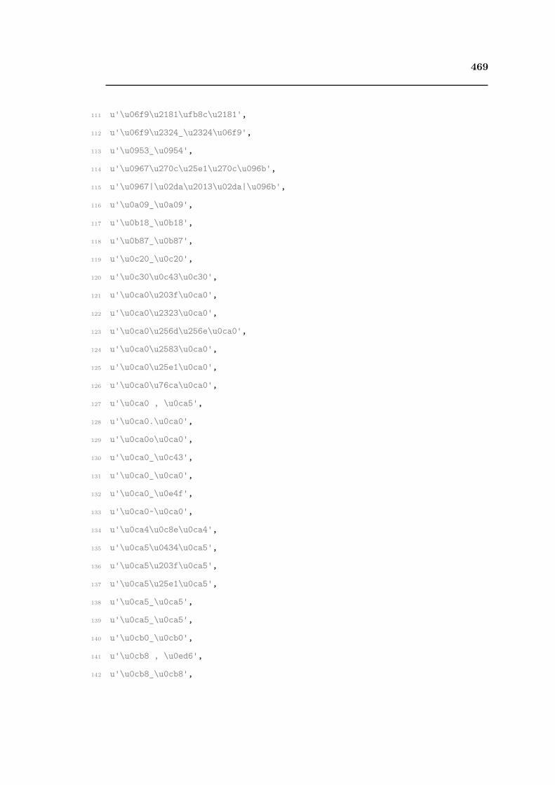
469
111 u'\u06f9\u2181\ufb8c\u2181',
112 u'\u06f9\u2324_\u2324\u06f9',
113 u'\u0953_\u0954',
114 u'\u0967\u270c\u25e1\u270c\u096b',
115 u'\u0967|\u02da\u2013\u02da|\u096b',
116 u'\u0a09_\u0a09',
117 u'\u0b18_\u0b18',
118 u'\u0b87_\u0b87',
119 u'\u0c20_\u0c20',
120 u'\u0c30\u0c43\u0c30',
121 u'\u0ca0\u203f\u0ca0',
122 u'\u0ca0\u2323\u0ca0',
123 u'\u0ca0\u256d\u256e\u0ca0',
124 u'\u0ca0\u2583\u0ca0',
125 u'\u0ca0\u25e1\u0ca0',
126 u'\u0ca0\u76ca\u0ca0',
127 u'\u0ca0 , \u0ca5',
128 u'\u0ca0.\u0ca0',
129 u'\u0ca0o\u0ca0',
130 u'\u0ca0_\u0c43',
131 u'\u0ca0_\u0ca0',
132 u'\u0ca0_\u0e4f',
133 u'\u0ca0~\u0ca0',
134 u'\u0ca4\u0c8e\u0ca4',
135 u'\u0ca5\u0434\u0ca5',
136 u'\u0ca5\u203f\u0ca5',
137 u'\u0ca5\u25e1\u0ca5',
138 u'\u0ca5_\u0ca5',
139 u'\u0ca5_\u0ca5',
140 u'\u0cb0_\u0cb0',
141 u'\u0cb8 , \u0ed6',
142 u'\u0cb8_\u0cb8',

470 Multi-character emoticons filtered
143 u'\u0e2d\u0e49_\u0e2d\u0e49',
144 u'\u0e2d_\u0e2d',
145 u'\u0e42\u0e4f\u0bf0\u0e4f\u0e43 \u0e37',
146 u'\u0e4f\u032f\u0361\u0e4f\ufd3f',
147 u'\u0e4f\u032f\u0361\u0e4f',
148 u'\u0e4f\u0361\u032f\u0e4f\ufd3f',
149 u'\u0e4f[-\u0e34\u0e34_\u2022\u0e34]\u0e4f',
150 u'\u0e4f_\u0e4f',
151 u'\u0ed6_\u0ed6',
152 u'\u0f3a\u203f\u0f3b',
153 u'\u10da(\xb4\u06a1`\u10da)',
154 u'\u10da(\u0ca0\u76ca\u0ca0\u10da)',
155 u'\u10da(\u25c9\u25de\u0c6a\u25df\u25c9\u2035\u10da)',
156 u'\u10da,\u1511\u2022\ufeaa\u035f\u0360\u2022\u1510.\u10da',
157 u'\u113d\u1f41\u020d \u032a \u0151\u1f40\u113f',
158 u'\u1559(\u21c0\u2038\u21bc\u2036)\u1557',
159 u'\u2022\u25b1\u2022',
160 u'\u2022\u271e_\u271e\u2022',
161 u'\u2022\ufe91\u2022',
162 u'\u2022(\u231a_\u231a)\u2022',
163 u'\u2022_\u2022)',
164 u'\u2037\u0317\u2182\u51f8\u2182\u2034\u0316',
165 u'\u2039\u2022.\u2022\u203a',
166 u'\u2039\u203a \u2039(\u2022\xbf\u2022)\u203a \u2039\u203a',
167 u'\u2039(\u1d52\u1d25\u1d52\xad\xad\xad\xad\xad)\u203a\ufeff',
168 u'\u2181_\u2181',
169 u'\u21ce_\u21ce',
170 u'\u2267\u30ee\u2266',
171 u'\u2282\u2022\u2283_\u2282\u2022\u2283',
172 u'\u2282(\u25c9\u203f\u25c9)\u3064',
173 u'\u2299\u03c9\u2299',
174 u'\u2299\u2582\u2299',

471
175 u'\u2299\u2583\u2299',
176 u'\u2299\u25b3\u2299',
177 u'\u2299\ufe3f\u2299',
178 u'\u2299\ufe4f\u2299',
179 u'\u2299\uff10\u2299',
180 u'\u229b\u0920\u032f\u229b',
181 u'\u22cb\u014d_\u014d`',
182 u'\u2501\u2501\u2501\u30fd(\u30fd(\uff9f\u30fd(\uff9f\u2200\u30fd(\uff9f\u2200\uff9f'
+
183 u'\u30fd(\uff9f\u2200\uff9f)\uff89\uff9f\u2200\uff9f)\uff89\u2200\uff9f)\uff89\uff9f)'
+
184 u'\uff89)\uff89\u2501\u2501\u2501',
185 u'\u250c\u2229\u2510(\u25d5_\u25d5)\u250c\u2229\u2510',
186 u'\u250c( \u0ca0_\u0ca0)\u2518',
187 u'\u255a(\u2022\u2302\u2022)\u255d',
188 u'\u256d\u256e\u256d\u256e\u261c{\u2022\u0303\u033e_\u2022\u0303\u033e}\u261e\u256d'
+
189 u'\u256e\u256d\u256e',
190 u'\u256d\u272c\u2322\u272c\u256e',
191 u'\u256f\u2035\u0414\u2032)\u256f\u5f61\u253b\u2501\u253b',
192 u'\u2570\u2606\u256e',
193 u'\u25a1_\u25a1',
194 u'\u25ba_\u25c4',
195 u'\u25c3\u2506\u25c9\u25e1\u25c9\u2506\u25b7',
196 u'\u25c9\u25b3\u25c9',
197 u'\u25c9\ufe35\u25c9',
198 u'\u25c9_\u25c9',
199 u'\u25cb_\u25cb',
200 u'\u25cf\xbf\u25cf\\ ~',
201 u'\u25cf_\u25cf',
202 u'\u25d4\u032f\u25d4',
203 u'\u25d4\u1d17\u25d4',

472 Multi-character emoticons filtered
204 u'\u25d4 \u2323 \u25d4',
205 u'\u25d4_\u25d4',
206 u'\u25d5\u03c9\u25d5',
207 u'\u25d5\u203f\u25d5',
208 u'\u25d5\u25e1\u25d5',
209 u'\u25d5 \u25e1 \u25d5',
210 u'\u25d6\u266a_\u266a|\u25d7',
211 u'\u25d6|\u25d4\u25e1\u25c9|\u25d7',
212 u'\u25d8_\u25d8',
213 u'\u25d9\u203f\u25d9',
214 u'\u25dc\u3355\u25dd',
215 u'\u25ea_\u25ea',
216 u'\u25ee_\u25ee',
217 u'\u2601 \u261d\u02c6~\u02c6\u2602',
218 u'\u2606\xb8\u2606',
219 u'\u2609\u203f\u2299',
220 u'\u2609_\u2609',
221 u'\u261c\u0642\u2742\u10c2\u2742\u0642\u261e',
222 u'\u261c(\u2312\u25bd\u2312)\u261e',
223 u'\u261c(\uff9f\u30ee\uff9f\u261c)',
224 u'\u261c-(\u0398L\u0398)-\u261e',
225 u'\u261d\u261e\u270c',
226 u'\u262e\u2581\u2582\u2583\u2584\u263e \u265b \u25e1 \u265b
\u263d\u2584\u2583' +
227 u'\u2582\u2581\u262e',
228 u'\u2639_\u2639',
229 u'\u263b_\u263b',
230 u'\u263c.\u263c',
231 u'\u263e\u02d9\u2740\u203f\u2740\u02d9\u263d',
232 u'\u2640\u062d\u2640\u30fe',
233 u'\u2665\u203f\u2665',
234 u'\u2665\u256d\u256e\u2665',

473
235 u'\u2665\u25e1\u2665',
236 u'\u270c\u266b\u266a\u02d9\u2764\u203f\u2764\u02d9\u266b\u266a\u270c',
237 u'\u270c.\u0295\u0298\u203f\u0298\u0294.\u270c',
238 u'\u270c.|\u2022\u0361\u02d8\u203f\u2022\u0361\u02d8|.\u270c',
239 u'\u2716_\u2716',
240 u'\u2750\u203f\u2751',
241 u'\u2a00_\u2a00',
242 u'\u2a02_\u2a02',
243 u'\u3006(\u30fb\u2200\u30fb\uff20)',
244 u'\u300a\u3020_\u3020\u300b',
245 u'\u3010\u2022\u3011_\u3010\u2022\u3011',
246 u'\u3020_\u3020',
247 u'\u3034\u22cb_\u22cc\u3035',
248 u'\u306e\u30ee\u306e',
249 u'\u30cb\u30ac\u30fc?
\u2501\u2501\u2501\u2501\u2501\u2501(\uff9f\u2200\uff9f)\u2501' +
250 u'\u2501\u2501\u2501\u2501\u2501 \u30cb\u30ac\u30fc?',
251 u'\u30da\u3355\u02da\\',
252 u'\u30fd(\xb4\uff70\uff40 )\uff89',
253 u'\u30fd(\uff40\u0414\xb4)\uff89',
254 u'\u30fd(\uff4f`\u76bf\u2032\uff4f)\uff89',
255 u'\u314e_\u314e',
256 u'\u4e42\u25dc\u25ec\u25dd\u4e42',
257 u'\u53e5_\u53e5',
258 u'\ua66e_\ua66e',
259 u'\ud76b_\ud76b',
260 u'\uf906_\uf906',
261 u"\ufd3e\u0361\u0e4f\u032f\u0361\u0e4f\ufd3f O'RLY?\n",
262 u'\uff08\xb7\xd7\xb7\uff09',
263 u'\uff08\u2312\u0414\u2312\uff09',
264 u'\uff08\u266f\u30fb\u2200\u30fb\uff09\u2283',
265 u'\uff08\u309c\u0414\u309c\uff09',

474 Multi-character emoticons filtered
266 u'\uff08\uff9f\u2200\uff9f\uff09',
267 u'\uff08 \xb4\u2623///_\u309d///\u2623\uff40\uff09',
268 u'\uff08 \u3064 \u0414 \uff40\uff09',
269 u'\uff3f\u2606\uff08 \xb4_\u2283\uff40\uff09\u2606\uff3f',
270 u'\uff61\u25d5\u203f\u203f\u25d5\uff61',
271 u'\uff61\u25d5 \u203f \u25d5\uff61',
272 u'!\u2448\u02c6~\u02c6!\u2448',
273 u'!(\uff40\uff65\u03c9\uff65\uff61)',
274 u'(\xac_\xac)',
275 u'(\xb0\u2107 \xb0)',
276 u'(\xb0\u2200\xb0)',
277 u'(\xb4\u25c9\u25de\u0c6a\u25df\u25c9)',
278 u'(\xb4\u30fb\u03c9\u30fb\uff40)',
279 u'(\u0298\u203f\u0298)',
280 u'(\u0298_\u0298)',
281 u'(\u02da\u0b87\u02da)',
282 u'(\u0361\u0e4f\u032f\u0361\u0e4f)',
283 u'(\u0398\u03b5\u0398;)',
284 u'(\u053e\u2038 \u053e)',
285 u'(\u0966 \u094d\u0966)',
286 u'(\u0bc1\u096e\u0bc1_ .:)',
287 u'(\u0ca0\u203f\u0ca0)',
288 u'(\u0ca0\u2323\u0ca0)',
289 u'(\u0ca0\u76ca\u0ca0 \u256c)',
290 u'(\u0ca0_\u0c43)',
291 u'(\u0ca0_\u0ca0)',
292 u'(\u0ca5\ufe4f\u0ca5)',
293 u'(\u0ca5_\u0ca5)',
294 u'(\u0e4f\u032f\u0361\u0e4f )',
295 u'(\u1d54\u1d25\u1d54)',
296 u'(\u2022\u03c9\u2022)',
297 u'(\u2022\u203f\u2022)',

475
298 u'(\u2022 \u03b5 \u2022)',
299 u'(\u2267\u30ed\u2266)',
300 u'(\u2310\u25a0_\u25a0)',
301 u'(\u251b\u25c9\u0414\u25c9)\u251b\u253b\u2501\u253b',
302 u'(\u256c\u25e3\u0434\u25e2)',
303 u'(\u256c \u0ca0\u76ca\u0ca0)',
304 u'(\u256f\xb0\u25a1\xb0\uff09\u256f\ufe35 \u253b\u2501\u253b',
305 u'(\u25b0\u02d8\u25e1\u02d8\u25b0)',
306 u'(\u25cf\xb4\u03c9\uff40\u25cf)',
307 u'(\u25d1\u25e1\u25d1)',
308 u'(\u25d5\u203f\u25d5)',
309 u'(\u25d5\ufe35\u25d5)',
310 u'(\u25d5 ^ \u25d5)',
311 u'(\u25d5_\u25d5)',
312 u'(\u25dc\u0bf0\u25dd)',
313 u'(\u25e3_\u25e2)',
314 u'(\u261e\uff9f\u2200\uff9f)\u261e',
315 u'(\u261e\uff9f\u30ee\uff9f)\u261e',
316 u'(\u261e\uff9f \u2200\uff9f )\u261e',
317 u'(\u263c\u25e1\u263c)',
318 u'(\u263c_\u263c)',
319 u'(\u270c\uff9f\u2200\uff9f)\u261e',
320 u'(\u3000\u30fb\u2200\u30fb)',
321 u'(\u3000\uff65\u0e31\u03c9\uff65\u0e31)\uff1f',
322 u'(\u3000\uff9f\u2200\uff9f)o\u5f61\u309c\u3048\u30fc\u308a\u3093\u3048\u30fc'
+
323 u'\u308a\u3093!!',
324 u'(\u3065\uff61\u25d5\u203f\u203f\u25d5\uff61)\u3065',
325 u'(\u30ce\u0ca0\u76ca\u0ca0)\u30ce\u5f61\u253b\u2501\u253b',
326 u'(\u30ce \u25d1\u203f\u25d1)\u30ce',
327 u'(\ufea7\u76ca\ufea8)',
328 u'(\uff1b\u4e00_\u4e00)',

476 Multi-character emoticons filtered
329 u'(\uff61\u25d5\u203f\u203f\u25d5\uff61)',
330 u'(\uff61\u25d5\u203f\u25d5\uff61)',
331 u'(\uff61\u25d5 \u203f \u25d5\uff61)',
332 u'(\uff61\uff65\u03c9..\uff65)\u3063',
333 u'(\uff89\u25d5\u30ee\u25d5)\uff89*:\uff65\uff9f\u2727',
334 u'(\uff9f\u2200\uff9f)',
335 u'(\uff9f\u30ee\uff9f)',
336 u'(\uffe3\u30fc\uffe3)',
337 u'( \xb0\u0662\xb0 )',
338 u'( \u2022_\u2022)>\u2310\u25a0-\u25a0',
339 u'( \uff65\u0e34\u0437\uff65\u0e34)',
340 u'(*..\u0414\uff40)',
341 u'(*..\u0434\uff40*)',
342 u'(-\u2019\u0e4f_\u0e4f\u2019-)',
343 u'(/\u25d4 \u25e1 \u25d4)/',
344 u'(///_\u0ca5)',
345 u"(>'o')> \u2665 <('o'<)\n",
346 u'(V)(\xb0,,\xb0)(V)',
347 u'(\\/) (\xb0,,\xb0) (\\/)',
348 u'(`\uff65\u03c9\uff65\xb4)',
349 u'/\u2572/\\\u256d\xbao\ua358o\xba\u256e/\\\u2571\\',
350 u'<\u3010\u262f\u3011\u203f\u3010\u262f\u3011>',
351 u'=(\uff9f\u0434\uff9f)\uff73',
352 u'@_@',
353 u'd(*\u2312\u25bd\u2312*)b',
354 u'o(\u2267\u2200\u2266)o',
355 u'q(\u2742\u203f\u2742)p',
356 u'\\\u02da\u3125\u02da\\',
357 u'\\\u11c2_\u11c2\\',
358 u'\\(\u25d5 \u25e1 \u25d5\\)',
359 u'^\u032e^',
360 u'^\u3142^',

477
361 u'_(\u0361\u0e4f\u032f\u0361\u0e4f)_',
362 u'{\xb4\u25d5 \u25e1 \u25d5\uff40}',
363 u'{\u0ca0_\u0ca0}__,,|,',
364 u'{\u25d5 \u25e1 \u25d5}',
365 u'\u2610_\u2610',
366 u'\u25a1_\u25a1',
367 u'\u01b8\u0335\u0321\u04dc\u0335\u0328\u0304\u01b7',
368 u'\u031c\u2009\u0333 \u0333 \u0333 \u0333\u2009\u0359 \u06aa\u200a',
369 u'\u0334\u0131\u0334\u0334\u0321\u0321\u0321
\u0321\u034cl\u0321\u0321\u0321' +
370 u'\u0321\u034cl\u0321*\u0321\u0321 \u0334\u0321\u0131\u0334\u0334\u0321
\u0321' +
371 u'\u0321\u0361|\u0332\u0332\u0332\u0361\u0361\u0361
\u0332\u25ab\u0332\u0361' +
372 u'\u0321\u0361|\u0332\u0332\u0332\u0361\u0361\u0361
\u0332\u25ab\u0332\u0361' +
373 u'\u0332\u0332\u0332\u0361\u0361\u03c0\u0332\u0332\u0361\u0361
\u0332\u0332' +
374 u'\u0332\u0332\u0332\u0361\u0361\u03c0\u0332\u0332\u0361\u0361
\u0332\u0332' +
375 u'\u0361\u25ab\u0332\u0332\u0361\u0361 \u0332|\u0321\u0321\u0321 \u0321
\u0334' +
376 u'\u0321\u0131\u0334\u0321\u0321 \u0321\u034cl\u0321\u0321\u0321\u0321.',
377 u'\u2584\ufe3b\u0337\u033f\u253b\u033f\u2550\u2501\u4e00',
378 u'\u2661+\u2661=\u2764\xb2',
379 u'\u2704---------\u2764',
380 u'[\u0332\u0305$\u0332\u0305(\u0332\u03055\u0332\u0305)\u0332\u0305$\u0332\u0305]',
381 u'\xa6\xac)',
382 u'\xa6-)',
383 u'\xa63',
384 u'\u3013D',
385 u'/:\u20ac',

478 Multi-character emoticons filtered
386 u':\u2309',
387 u'=\u2309',
388 u'\u04ec',
389 u'\u04ed',
390 u'\u2324',
391 u'\u2362',
392 u'\u2363',
393 u'\u2364',
394 u'\u2365',
395 u'\u2368',
396 u'\u2369',
397 u'\u2603',
398 u'\u2639',
399 u'\u263a',
400 u'\u263b',
401 u'\u267e',
402 u'\u3020',
403 u'\u30c4',
404 u'\u32e1',
405 u'\u01aa(\u02d8\u2323\u02d8)\u2510',
406 u'\u01aa(\u02d8\u2323\u02d8)\u0283',
407 u'\u250c(\u02d8\u2323\u02d8)\u0283',
408 u'o_0',
409 u'\u250c\u2229\u2510(~_~)\u250c\u2229\u2510',
410 u'\u0429(\xba\u0414\xba\u0449)',
411 u"\u2510('\u2323'\u2510) (\u250c'\u2323')\u250c",
412 u'(" `.\xb4 )_,/"(>_<!)',
413 u'\u200e\u200b\u01aa(\xb4\u02db`\u201c)\u0283',
414 u'(\u02d8\u2323\u02d8)\u03b5 \u02d8)',
415 u'\u01b8(\u02c7\u25bd\u02c7)\u01b7',
416 u'\u01aa(\u02d8\u25bd\u02d8)\u0283',
417 u'\u250c(\u02d8\u2022\u02d8)\u0283',

479
418 u'\u01aa(\u02d8\u2323\u02d8)\u0283',
419 u'(\u02d8\u2323\u02d8)\u0283\u01aa(\u02d8\u2323\u02d8)',
420 u'\u01aa(\u2022\u02d8\u2323\u02d8)\u2510',
421 u'\u250c(\u02d8\u2323\u02d8\u2022)\u0283',
422 u'(\u0254 \u02d8\u2323\u02d8)\u02d8\u2323\u02d8 c)',
423 u'\u01aa(\u02d8\u2323\u02d8)\u0283',
424 u'\u250c(\u02d8\u2323\u02d8)\u0283',
425 u'(\u02d8\u2323\u02d8)\u2510',
426 u'(\u02d8\u2323\u02d8)',
427 u'\u0505(\u02c6\u2323\u02c6\u0505)',
428 u'\u01aa(\u02c6\u2323\u02c6)\u0283',
429 u'(\u2323\u0301_\u2323\u0300)',
430 u"\u2512('o'\u2512)",
431 u"(\u250c','\u2510)",
432 u'\u2512(\u2323\u02db\u2323)\u250e',
433 u'\u200b(\xaf\u2015\xaf\u0665)',
434 u'(\u30ce^^)\u30ce',
435 u"'')",
436 u'\u250c(\u02d8\u2022\u02d8)\u0283',
437 u'\xb0\\(^\u25bf^)/\xb0',
438 u'~(\u203e\u25bf\u203e~)',
439 u'~(\u203e\u25bf\u203e)~',
440 u'-(\u02c6\u25bf\u02c6)-',
441 u'(~\u203e\u25bf\u203e)~',
442 u'( -\u0329\u0329\u0329\u0361\u02db -\u0329\u0329\u0329\u0361 )',
443 u'(-\u0329\u0329\u0329\u0361\u02db -\u0329\u0329\u0329\u0361)',
444 u'(-\u0329\u0329\u0329\u0361\u02db-\u0329\u0329\u0329\u0361)',
445 u'(\u203e\u0283\u01aa\u203e)',
446 u'(\u02d8\u0329\u0329\u0329\u0283\u01aa\u02d8\u0329\u0329\u0329)',
447 u'\u01aa(\u02c7\u25bf\u02c7)\xac',
448 u'(\u02d8\u0283\u01aa\u02d8)',
449 u'\u01aa(\u02c7\u25bc\u02c7)\xac',

480 Multi-character emoticons filtered
450 u'\u01aa(\xb0\u0361\u25bf\u25bf\u25bf\u25bf\u25bf\u25bf\xb0")\u0361\u01aa',
451 u'(\u2022\u0329\u0329\u0329\u0329\u0361\u02db\u02d8\u2022\u0329\u0329\u0329\u0329\u0361)',
452 u'(\u2022\u0361\u02d8\u02db\u02d8 \u2022\u0361)',
453 u'(\u02d8\u0329\u0329\u0329.\u02d8\u0329\u01aa)',
454 u'(\u02d8\u0329\u0329\u0329\u256d\u256e\u02d8\u0329\u01aa)',
455 u'*\\(\u02d8\u25bd\u02d8)/*',
456 u'\uf8e7-(\u02d8\u25bd\u02d8)/*',
457 u'*\\(\u02d8\u25bd\u02d8)-\uf8e7',
458 u'\u01aa(\u02c6\u25bd\u02c6)\u2510',
459 u'\u01aa(\u02c6\u25bd\u02c6)\u0283',
460 u'\u250c(\u02c6\u25bd\u02c6)\u0283',
461 u'(\uff34\u25bd\uff34)',
462 u'(\u02d8\u0329\u0329\u0329^\u02d8\u0329\u01aa)',
463 u'\u2022_\u2022',
464 u'\u2022',
465 u'(\u0283\u02d8\u0329\u0329\u0329\ufe4f\u02d8\u0329\u0329\u0329\u01aa)',
466 u'(\u2015\u02db\u2015\u201c)',
467 u'(\u02d8O\u01aa)',
468 u'(\u0283\u2323\u01aa)',
469 u'(\u02d8\u0329\u0329\u0329\u2323\u02d8\u0329\u0329\u0329\u01aa)\u200e\u200b',
470 u'(\u02d8\u0329\u0329\u0329.\u02d8\u0329\u0329\u0329\u01aa)',
471 u'(\u02d8\u0329\u0329\u0329\u0283\u01aa\u02d8\u0329\u0329\u0329)',
472 u'(-\u0329\u0329\u0329-\u0361__ --\u0329\u0329\u0329\u0361)',
473 u'(\u02d8\u0329\u0329\u0329^\u02d8\u0329\u0329\u01aa)',
474 u'(\u02d8\u0329\u0329~\u02d8\u0329\u01aa)',
475 u'(\u02d8\u0329\u0329\u0329~\u02d8\u0329\u0329\u0329\u01aa)',
476 u'(\u02d8\u2323\u02d8\u0283\u01aa)',
477 u'(\u02d8\u0329\u0329\u0329\u2323\u02d8\u0329\u0329\u0329)',
478 u'(\xba\u0329\u0329\u0301_\xba\u0329\u0329\u0300)(\u01a0\u0334\u0334\u0334\u0334\u0334'
+
479 u'\u0334\u0361.\u032e\u01a0\u0334\u0334\u0361)',
480 u'\u01a0\u0334\u0334\u0334\u0334\u0334\u0334\u0361.\u032e\u01a0\u0334\u0334\u0361

481
',
481 u'(O\u0334\u0334\u0334\u0334\u032f\u0361 .\u032e
O\u0334\u0334\u0334\u0334\u032f\u0361)',
482 u'(>\u0334\u0334\u0334\u0334\u0334\u0361.\u032e\u01a0\u0334\u0361)',
483 u'(\u2022\u032f\u0361.\u2022\u032f\u0361)',
484 u'(\u2022\u032f\u0361.\u2022\u032f\u0361)',
485 u'>\u0334\u0334\u0334\u0334\u0334\u0361.\u032e\u01a0\u0334\u0361*',
486 u'>\u0334\u0334\u0334\u0334\u0334\u0361.\u032e\u01a0\u0334\u0361',
487 u'\\(\u203e\u25bf\u203e\\)',
488 u'\\(\xb4\u25bd`)/',
489 u'(/\u203e\u25bf\u203e)/',
490 u'(\u2022\u0361. \u2022\u0361)',
491 u'(\u2022\u0361.\u2022\u0361)',
492 u'(\u2022\u0303-\u032e\u2022\u0303)',
493 u'(\xac-\u032e\xac)',
494 u'(..\u2022\u0361\u02d8_\u02d8 \u2022\u0361..)',
495 u'(..\u2022\u0361\u02d8_\u02d8 \u2022\u0361..',
496 u'\u250c\u041f\u2510',
497 u'(\u2323\u0334\u0361\u0361\u062f\u0332\u2323\u0334\u0361\u0361)',
498 u'(\u203e\u203e \u2323 \u203e\u203e)',
499 u'\u0505(\xb0\u0361\u25bf\u25bf\u25bf\u25bf\u25bf\u25bf\xb0 )\u0361\u0505',
500 u'\u01aa(\xb0\u0361\u25bf\u25bf\u25bf\u25bf\u25bf\u25bf\xb0)\u0361\u01aa',
501 u'\u256d(\u2032\u25bd`)\u256f',
502 u'\u2514(^\u02db^)\u2510',
503 u'~(\u02d8\u25bd\u02d8~)',
504 u'~(\u02d8\u25bd\u02d8)~',
505 u'(~\u02d8\u25bd\u02d8)~',
506 u'\xb0\\(^\u25bf^)/',
507 u'~(\u02d8\u25be\u02d8~)',
508 u'~(\u02d8\u25be\u02d8)~',
509 u'(~\u02d8\u25be\u02d8)~',
510 u"(\u25ba\u02db\u25c4'!)",

482 Multi-character emoticons filtered
511 u'\\(\u2267\u25bd\u2266)/',
512 u'\\(\u2022\u02c6\u2323\u02c6\u200e\u200b\u200b\u200b\u200b\u2022)/',
513 u'(\u2022\u02c6 \u25bd \u02c6\u2022)\u200e\u200b',
514 u'(\u2022\u02c6\u25bd\u02c6\u2022)\u200e\u200b',
515 u'( \u02d8\u0336\u0300\u2022 \u032f\u2022\u02d8\u0336\u0301)',
516 u'(\u02d8\u0336\u0300\u2022 \u032f\u2022\u02d8\u0336\u0301)',
517 u'-_______-',
518 u'-__-',
519 u'.____.',
520 u'\xac___\xac',
521 u'-___-\u200e\u200b\u200b\u01aa(\u203e\u03b5\u203e\u201c)\u0283',
522 u'(\u1d55.\u1d55)',
523 u'\u0669(\u0e51`\u020f\xb4\u0e51)\u06f6',
524 u'\u0449(\u0ca5\u0414\u0ca5\u0449)',
525 u'\u0429(\xba\u0329\u0329\u0301\u2323\xba\u0329\u0329\u0300\u0449)',
526 u'\u0449(\xba\u0414\xba\u0449)"',
527 u'\u0ca5\u2323\u0ca5',
528 u"( '\u2323')\u4eba('\u2323' )",
529 u'(\u2323\u0301.\u2323\u0300)',
530 u'\xac\xac',
531 u'(-\u0329\u0329\u0329-\u0329\u0329\u0329-\u0329\u0329\u0329-\u0329\u0329\u0329-'
+
532 u'\u0329\u0329\u0329___-\u0329\u0329\u0329-\u0329\u0329\u0329-\u0329\u0329\u0329-'
+
533 u'\u0329\u0329\u0329-\u0329\u0329\u0329)',
534 u'(-\u0329\u0329\u0329-\u0329\u0329\u0329-\u0329\u0329-\u0329\u0329\u0329\u0329__-'
+
535 u'\u0329\u0329\u0329-\u0329\u0329\u0329-\u0329\u0329\u0329-\u0329\u0329\u0329)',
536 u'\u01aa\u200b\u200b\u200b(-\u0329\u0329\u0329-\u0329\u0329\u0329-\u0329\u0329\u0329__-'
+
537 u'\u0329\u0329\u0329-\u0329\u0329\u0329-\u0329\u0329\u0329)\u0283!',
538 u'\u04a8(\xb0 \u032f\u02da)\u04a8',

483
539 u'\u02c6\u2323\u02c6',
540 u'(\u06f3\u02da\u0414\u02da)\u06f3',
541 u'(\u06f3\xba\u0329\u0329\u0301\u0414\xba\u0329\u0329\u0300)\u06f3(\xba\u0329\u0329\u0301'
+
542 u'\u0414\xba\u0329\u0329\u0300)',
543 u'\xba\u0329\u0329\u0301\u0414\xba\u0329\u0329\u0300)',
544 u'\u01aa(\u203e\u03b5\u203e\u201c)\u0283',
545 u'(\u2022\u0300_\u2022\u0301)\u0e07',
546 u'o_o\u201d',
547 u'o_o',
548 u'(\u02d8\u0336\u0300 \u032f \u02d8\u0336\u0301 )',
549 u'(\u02d8\u0336\u0300 \u032f \u02d8\u0336\u0301)',
550 u'(\u02d8\u0336\u0300 \u032f\u02d8\u0336\u0301)',
551 u'\\(!!\u02da\u2610\u02da)/',
552 u'\\(\u02da\u2610\u02da!!)/',
553 u"(\u0e07 '\u0300\u2323'\u0301 )\u0e07",
554 u'\xbb\xbb\u2500\u2500\u2500\u2500\u2500\u2500\u25ba',
555 u'\uff3c(^o^)\uff0f',
556 u'=_=',
557 u'(\xb4\u25bd`\u0283\u01aa)',
558 u'(*\u309d\u03c9\uff65)\uff89',
559 u'\u0ca0_\u0cb0\u0cc3',
560 u'\U0001d107\u2940.\u2940\U0001d106',
561 u'\u2299_\u0298',
562 u'\u25f4_\u25f6',
563 u'(',
564 u'\u25d5\ufe35\u25d5',
565 u'\u25cf\ufe35\u2022',
566 u'\u0ca2_\u0ca2',
567 u'\u0ca2_\u0ca5',
568 u'( \uff9fo\uff9f)',
569 u'\u22cb_\u22cc',

484 Multi-character emoticons filtered
570 u'\u200e(\u30ce\u2265\u2207\u2264)\u30ce',
571 u'(\ufe36\u03b5\ufe36\u30e1)',
572 u'(\xb4\u30fc`)',
573 u'(\xb4\u25bd`)',
574 u'(\uff9f\uff0a\uff9f)',
575 u'(\uff61\uff65_\uff65\uff61)',
576 u'\u2256\u25e1\u0c8e\u2256',
577 u'(\u2265_<)',
578 u'\u0295\u0294',
579 u':-\xfe',
580 u':^\xde',
581 u'\u30d8(\u25d5\u3002\u25d5\u30d8)',
582 u'\u263c_\u263c',
583 u'_',
584 u'\u262f\u203f\u262f',
585 u'(\uff9f\u30fc\uff9f)',
586 u'\u0c86_\u0c86',
587 u'\u0c8a_\u0c8a',
588 u'\u0cb9_\u0cb9',
589 u'\\(\u2022 \u25e1 \u2022)/',
590 u'\\( \uff9f\u25e1\uff9f)/',
591 u'\u261c\uff61\uff61\u261e',
592 u'\u10da( \u10da)',
593 u'( \u2018-\u2019)\u4eba(\uff9f_\uff9f )',
594 u'( _)=mm=(^_^ )',
595 u"(>'o\u2019)> <('o\u2019<)",
596 u'\u239d\u23e0\u23dd\u23e0\u23a0',
597 u'( \xb4_\u2283\uff40\uff09',
598 u'(\u014c_\u0186\u014e)',
599 u'\u2256_\u2256',
600 u'\uff3c| \uffe3\u30d8\uffe3|\uff0f',
601 u'\u033f\u2019\u033f\u2019\\\u0335\u0347\u033f\u033f\\' +

485
602 u'\u0437=(\u2022\u032a\u25cf)=\u03b5/\u0335\u0347\u033f\u033f/' +
603 u'\u2019\u033f\u2019\u033f',
604 u"< ('o'<) ( '-\u2019 ) (>\u2018o\u2019)> v( \u2018.\u2019 )v < (' .' )> <
('.'<) " +
605 u"( '.\u2019 ) (>\u2018.\u2019)> v( \u2018.\u2019 )v < (' .' )>",
606 u'\u266a\u250f(\u30fbo\uff65)\u251b\u266a\u2517 ( \uff65o\uff65)
\u2513\u266a\u250f' +
607 u'( ) \u251b\u266a\u2517 (\uff65o\uff65 )
\u2513\u266a\u250f(\uff65o\uff65)\u251b\u266a',
608 u'(* \uff65(\uff74)\uff65 *)',
609 u'\u0ca4\u0c9f\u0ca4',
610 u'\u2019;\u2018',
611 u'\u0c88_\u0c88',
612 u'\u24e7_\u24e7',
613 u'\xd7\u032f\xd7',
614 u'\xa2\u203f\xa2',
615 u'\u0ca4_\u0c8e\u0ca4',
616 u'\u0ca0\ufb5b\u0ca0',
617 u'\u23e0\u23dd\u23e0',
618 u'\u25f7_\u0bf0\u25f4',
619 u'\u25ce\u072b\u25ce',
620 u'(\u02da\u3125_\u02da)',
621 u'\u1ed9_\u1ed9',
622 u'\u2742\u203f\u2742',
623 u'(\u0398L_\u0398)',
624 u'\u25cf\xbf_\u25cf',
625 u'\u250c\u2229\u2510(>_<)\u250c\u2229\u2510',
626 u'\u2039^\u203a \u2039(\u2022\xbf\u2022)\u203a \u2039^\u203a',
627 u'\u2704\u2014\u2014\u2014\u2014-',
628 u'\u2570\u2584\ufe3b\u2584\u256f',
629 u'\u2584\ufe3b\u253b\u2533\u2550\u4e00',
630 u'(\u0305_\u0305_\u0305_\u0305(\u0305_\u0305_\u0305_\u0305_\u0305_\u0305_\u0305\u0305_'

486 Multi-character emoticons filtered
+
631 u'\u0305()\u06aa\u06d2',
632 u'( \u0332\u0305:\u0332\u0305:\u0332\u0305:\u0332\u0305[\u0332\u0305
\u0332\u0305]' +
633 u'\u0332\u0305:\u0332\u0305:\u0332\u0305:\u0332\u0305',
634 u'\u0131\u0334\u0334\u0321\u0321\u0321 \u0321\u034cl\u0321\u0321\u0321
\u0321\u034cl' +
635 u'\u0321*\u0321\u0321 \u0334\u0321\u0131\u0334\u0334\u0321
\u0321\u0321\u0361|\u0332' +
636 u'\u0332\u0332\u0361\u0361\u0361 \u0332\u0332\u0361
\u0332\u0332\u0332\u0361\u0361' +
637 u'\u03c0\u0332\u0332\u0361\u0361 \u0332\u0332\u0332\u0332\u0361\u0361\u0361
\u0332|' +
638 u'\u0321\u0321\u0321 \u0321 \u0334\u0321\u0131\u0334\u0321\u0321
\u0321\u034cl\u0321\u0321\u0321',
639 u'l\u0131ll\u0131
((((|\u0332\u0305\u0305\u25cf\u0332\u0305\u0305|\u0332\u0305\u0305=' +
640 u'\u0332\u0305\u0305|\u0332\u0305\u0305\u25cf\u0332\u0305\u0305|))))
\u0131ll\u0131',
641 u'\u2523\u2587\u2587\u2587\u2550\u2500\u2500',
642 u'\u2523\u2587\u2587\u2587\u2550\u2500\u2500\u2500\u2500\u2500\u2500\u2500' +
643 u'\u2500\u2500\u2500\u2500',
644 u'\u03df']
Listing E.1: Python list of multi-character emoticons filtered

Appendix F
Authors per day extra graphs
0
3authors with106 to 120
tweets on day
0
2authors with121 to 135
tweets on day
0
2authors with136 to 150
tweets on day
0
1authors with151 to 165
tweets on day
0
3authors with166 to 180
tweets on day
0
1authors with181 to 195
tweets on day
0
1authors with196 to 210
tweets on day
0
1authors with211 to 225
tweets on day
0
2authors with226 to 240
tweets on day
0
2authors with241 to 255
tweets on day
0
2authors with256 to 270
tweets on day
0
1authors with271 to 285
tweets on day
0
1authors with301 to 315
tweets on day
0
1authors with316 to 330
tweets on day
0
1authors with346 to 360
tweets on day
Jan 2011
Feb 2011
Mar 2011
Apr 2011
May 2011
Jun 2011
Jul 2011
Aug 2011
Sep 2011
Oct 2011
Nov 2011
Dec 2011
0
1authors with571 to 585
tweets on day
Figure F.1: Science authors grouped by number of science tweets sent on each day(106 per day and above)
487

488 Authors per day extra graphs

Appendix G
Types of Tweets CouchDB View
Code
This appendix provides details of the JavaScript source code used in the CouchDB
views to count the number of different types of tweets for Chapter 7. All of these views
have the built in reduce function of _count set.
G.1 Retweets
1 function(doc) {
2 if (doc.retweetedId) {
3 var jsDate = new
Date(Date.parse(doc.createdAt.replace("EST","GMT+1000")));
4 emit([jsDate.getUTCFullYear(), (jsDate.getUTCMonth()+1),
jsDate.getUTCDate()],doc.text);
5 }
6 }
Listing G.1: retweets2/retweets view in CouchDB
1 function(doc) {
2 var rt_pattern = /\b(rt|via|retweet)\b/gi;
3 var retweets = doc.text.match(rt_pattern);
4 if (doc.retweetedId || retweets) {
5 var jsDate = new
Date(Date.parse(doc.createdAt.replace("EST","GMT+1000")));
489

490 Types of Tweets CouchDB View Code
6 emit([jsDate.getUTCFullYear(), (jsDate.getUTCMonth()+1),
jsDate.getUTCDate()],retweets);
7 }
8 }
Listing G.2: retweets4/all_retweets view in CouchDB
1 function(doc) {
2 var rt_pattern = /\b(rt|via|retweet)\b/gi;
3 var retweets = doc.text.match(rt_pattern);
4 if (!doc.retweetedId && retweets) {
5 var jsDate = new
Date(Date.parse(doc.createdAt.replace("EST","GMT+1000")));
6 emit([jsDate.getUTCFullYear(), (jsDate.getUTCMonth()+1),
jsDate.getUTCDate()],retweets);
7 }
8 }
Listing G.3: retweets5/manual_retweets view in CouchDB
1 function(doc) {
2 var rt_pattern = /(^|\B)(rt|via|retweet)\B/gi;
3 var retweets = doc.text.match(rt_pattern);
4 if (doc.retweetedId && !retweets) {
5 var jsDate = new
Date(Date.parse(doc.createdAt.replace("EST","GMT+1000")));
6 emit([jsDate.getUTCFullYear(), (jsDate.getUTCMonth()+1),
jsDate.getUTCDate()],retweets);
7 }
8 }
Listing G.4: retweets6/retweetId_not_regex view in CouchDB

§G.1 Retweets 491
1 function(doc) {
2 var rt_pattern = /\b(rt|via|retweet)\b/gi;
3 var retweets = doc.text.match(rt_pattern);
4 if (doc.retweetedId || retweets) {
5 if (doc.text.toLowerCase().indexOf('http://') > -1 ) {
6 var jsDate = new
Date(Date.parse(doc.createdAt.replace("EST","GMT+1000")));
7 emit([jsDate.getUTCFullYear(), (jsDate.getUTCMonth()+1)],retweets);
8 }
9 }
10 }
Listing G.5: retweets7/all_retweets_with_url view in CouchDB
1 function(doc) {
2 var rt_pattern = /\b(rt|via|retweet)\b/gi;
3 var retweets = doc.text.toLowerCase().match(rt_pattern);
4 if (retweets) {
5 var jsDate = new
Date(Date.parse(doc.createdAt.replace("EST","GMT+1000")));
6 if (retweets.indexOf('rt') > -1) {
7 emit([jsDate.getUTCFullYear(), (jsDate.getUTCMonth()+1), 'rt'], null);
8 }
9 if (retweets.indexOf('via') > -1) {
10 emit([jsDate.getUTCFullYear(), (jsDate.getUTCMonth()+1), 'via'], null);
11 }
12 if (retweets.indexOf('retweet') > -1) {
13 emit([jsDate.getUTCFullYear(), (jsDate.getUTCMonth()+1), 'retweet'],
null);
14 }
15 }
16 }
Listing G.6: retweets8/types_of_retweets view in CouchDB

492 Types of Tweets CouchDB View Code
G.2 Mentions
1 function(doc) {
2 if (doc.userMentionEntities) {
3 var count = (doc.userMentionEntities.match(/UserMentionEntityJSONImpl/g)
|| []).length
4 if (count > 0) {
5 var jsDate = new
Date(Date.parse(doc.createdAt.replace("EST","GMT+1000")));
6 emit([jsDate.getUTCFullYear(), (jsDate.getUTCMonth()+1)],count);
7 }
8 }
9 }
Listing G.7: mentions/mentions view in CouchDB
1 function(doc) {
2 var pattern = /@[^@\s]+/gi;
3 var mentions = doc.text.match(pattern);
4 var count = 0
5 if (doc.userMentionEntities) {
6 count = (doc.userMentionEntities.match(/UserMentionEntityJSONImpl/g) ||
[]).length
7 }
8 if (count > 0 || mentions) {
9 var jsDate = new
Date(Date.parse(doc.createdAt.replace("EST","GMT+1000")));
10 emit([jsDate.getUTCFullYear(), (jsDate.getUTCMonth()+1)],mentions);
11 }
12 }
Listing G.8: mentions4/all_mentions view in CouchDB

§G.2 Mentions 493
1 function(doc) {
2 var pattern = /@[^@\s]+/gi;
3 var mentions = doc.text.substring(1).match(pattern);
4 var count = 0
5 if (doc.userMentionEntities) {
6 var count = (doc.userMentionEntities.match(/UserMentionEntityJSONImpl/g)
|| []).length
7
8 }
9 if ((count > 0 && !(doc.text.charAt(0) == '@' && count < 2)) || mentions) {
10 var jsDate = new
Date(Date.parse(doc.createdAt.replace("EST","GMT+1000")));
11 emit([jsDate.getUTCFullYear(), (jsDate.getUTCMonth()+1),
jsDate.getUTCDate()],count);
12 }
13
14 }
Listing G.9: mentions6/all_mentions_not_pos1 view in CouchDB
G.3 Replies
1 function(doc) {
2 if (doc.inReplyToUserId) {
3 var jsDate = new
Date(Date.parse(doc.createdAt.replace("EST","GMT+1000")));
4 emit([jsDate.getUTCFullYear(), (jsDate.getUTCMonth()+1),
jsDate.getUTCDate()],doc.text);
5 }
6 }
Listing G.10: replies2/replies_with_inReplyTo view in CouchDB

494 Types of Tweets CouchDB View Code
1 function(doc) {
2 if (!doc.inReplyToUserId && doc.text.charAt(0) == '@') {
3 var jsDate = new
Date(Date.parse(doc.createdAt.replace("EST","GMT+1000")));
4 emit([jsDate.getUTCFullYear(), (jsDate.getUTCMonth()+1),
jsDate.getUTCDate()],doc.text);
5 }
6 }
Listing G.11: replies2/replies_without_inReplyTo view in CouchDB
G.4 Hashtags
1 function(doc) {
2 if (doc.hashtagEntities) {
3 var count = (doc.hashtagEntities.match(/HashtagEntityJSONImpl/g) ||
[]).length
4 if (count > 0) {
5 var jsDate = new
Date(Date.parse(doc.createdAt.replace("EST","GMT+1000")));
6 emit([jsDate.getUTCFullYear(),
(jsDate.getUTCMonth()+1)],doc.hashtagEntities);
7 }
8 }
9 }
Listing G.12: hashtag2/hashtagEntities view in CouchDB
1 function(doc) {
2 var pattern = /#[^#\s]+/gi;
3 var hashtags = doc.text.match(pattern);

§G.4 Hashtags 495
4 var count = 0;
5 if (doc.hashtagEntities) {
6 count = (doc.hashtagEntities.match(/HashtagEntityJSONImpl/g) ||
[]).length;
7 }
8 if (count > 0 || hashtags) {
9 if (doc.text.toLowerCase().indexOf('http://') > -1 ) {
10 var jsDate = new
Date(Date.parse(doc.createdAt.replace("EST","GMT+1000")));
11 emit([jsDate.getUTCFullYear(), (jsDate.getUTCMonth()+1),
jsDate.getUTCDate()],hashtags);
12 }
13 }
14 }
Listing G.13: hashtag3/hashtags_with_URLs view in CouchDB
1 function(doc) {
2 var pattern = /#[^#\s]+/gi;
3 var hashtags = doc.text.match(pattern);
4 var count = 0;
5 if (doc.hashtagEntities) {
6 count = (doc.hashtagEntities.match(/HashtagEntityJSONImpl/g) ||
[]).length;
7 }
8 if (count > 0 || hashtags) {
9 var jsDate = new
Date(Date.parse(doc.createdAt.replace("EST","GMT+1000")));
10 emit([jsDate.getUTCFullYear(), (jsDate.getUTCMonth()+1)],hashtags);
11 }
12 }
Listing G.14: hashtag2/all_hashtags view in CouchDB
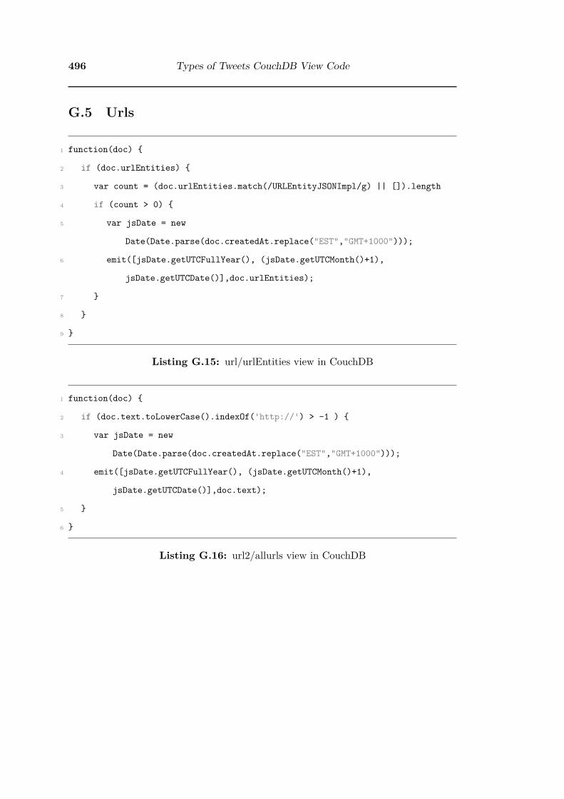
496 Types of Tweets CouchDB View Code
G.5 Urls
1 function(doc) {
2 if (doc.urlEntities) {
3 var count = (doc.urlEntities.match(/URLEntityJSONImpl/g) || []).length
4 if (count > 0) {
5 var jsDate = new
Date(Date.parse(doc.createdAt.replace("EST","GMT+1000")));
6 emit([jsDate.getUTCFullYear(), (jsDate.getUTCMonth()+1),
jsDate.getUTCDate()],doc.urlEntities);
7 }
8 }
9 }
Listing G.15: url/urlEntities view in CouchDB
1 function(doc) {
2 if (doc.text.toLowerCase().indexOf('http://') > -1 ) {
3 var jsDate = new
Date(Date.parse(doc.createdAt.replace("EST","GMT+1000")));
4 emit([jsDate.getUTCFullYear(), (jsDate.getUTCMonth()+1),
jsDate.getUTCDate()],doc.text);
5 }
6 }
Listing G.16: url2/allurls view in CouchDB

Appendix H
Word Frequency Analysis Code
1 from nltk.tokenize import word_tokenize, sent_tokenize
2 import itertools
3 import pandas
4 import tldextract
5 from ttp import ttp
6 import regex
7
8 def fix_abbrevs(text, abbrev_re=regex.compile(r'((?:[^.0-9]\.){2,})')):
9 # abbrev looks for single characters that are not numbers followed by a
10 # fullstop. It works for sentences as well as single words
11 abbrevs = abbrev_re.findall(text)
12 # reverse alpha sort the abbreviations so that shorter ones that are also
13 # part of longer ones don't double replace
14 if abbrevs:
15 unique_abbrevs = sorted(set(abbrevs), reverse=True)
16 for abbrev in unique_abbrevs:
17 if abbrev == 'u.s.':
18 text = text.replace(abbrev, 'usa')
19 else:
20 text = text.replace(abbrev, abbrev.replace('.', ''))
21 return text
22
23
24 def update_entities(tweet, p=ttp.Parser(include_spans=True)):
497

498 Word Frequency Analysis Code
25 # uses ttp to parse the tweet.
26 # count = 0
27 result = p.parse(tweet, html=False)
28 # available entities in result are users, urls, tags, lists, reply
29 entities = []
30 for i, user in enumerate(result.users):
31 entities.append(('user-' + tweet[(user[1][0] + 1):user[1][1]],
32 user[1]))
33
34 for i, url in enumerate(result.urls):
35 clean_url = url[0]
36 if clean_url.startswith('http://'):
37 clean_url = clean_url[7:]
38 if clean_url.startswith('www.'):
39 clean_url = clean_url[4:]
40 ext = tldextract.extract(clean_url.encode('ascii', 'ignore'))
41 if ext.registered_domain:
42 clean_url = ext.registered_domain
43 entities.append((clean_url, url[1]))
44
45 for i, tag in enumerate(result.tags):
46 entities.append(('hashtag-' + tweet[(tag[1][0] + 1):tag[1][1]],
47 tag[1]))
48
49 # sort entities by start position in tweet
50 entities.sort(key=lambda x: x[1][0])
51
52 if entities:
53 # update the tweet with updated entities
54 text = ''
55 start_pos = 0
56 for i, entity in enumerate(entities):

499
57 text += tweet[start_pos:entity[1][0]] + entity[0]
58 if i == len(entities) - 1:
59 text += tweet[entity[1][1]:]
60 else:
61 start_pos = entity[1][1]
62 else:
63 text = tweet
64 return text
65
66
67 def check_urls(words, full_stops_re=regex.compile('(\.)')):
68 # this deals with urls that haven't been found during twitter
69 # entitity detection
70 new_words = []
71 for word in words:
72 if len(word) > 1:
73 # separate off '/', '.', "'" non text characters?
74 # - maybe generalise this to all not [a-z]?
75 while word.startswith('/'):
76 new_words.append('/')
77 word = word[1:]
78 while word.startswith('\''):
79 new_words.append('\'')
80 word = word[1:]
81 while word.startswith('.'):
82 new_words.append('.')
83 word = word[1:]
84 if len(word) > 1 and '.' in word:
85 ext = tldextract.extract(word.encode('ascii', 'ignore'))
86 if ext.registered_domain:
87 word = ext.registered_domain
88 else:
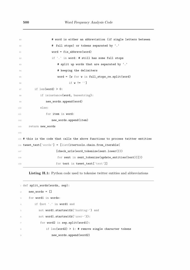
500 Word Frequency Analysis Code
89 # word is either an abbreviation (if single letters between
90 # full stops) or tokens separated by '.'
91 word = fix_abbrevs(word)
92 if '.' in word: # still has some full stops
93 # split up words that are separated by '.'
94 # keeping the delimiters
95 word = [w for w in full_stops_re.split(word)
96 if w != '']
97 if len(word) > 0:
98 if isinstance(word, basestring):
99 new_words.append(word)
100 else:
101 for item in word:
102 new_words.append(item)
103 return new_words
104
105 # this is the code that calls the above functions to process twitter entities
106 tweet_text['words'] = [list(itertools.chain.from_iterable(
107 [check_urls(word_tokenize(sent.lower()))
108 for sent in sent_tokenize(update_entities(text))]))
109 for text in tweet_text['text']]
Listing H.1: Python code used to tokenise twitter entities and abbreviations
1 def split_words(words, sep):
2 new_words = []
3 for word1 in words:
4 if (not '.' in word1 and
5 not word1.startswith('hashtag-') and
6 not word1.startswith('user-')):
7 for word2 in sep.split(word1):
8 if len(word2) > 1: # remove single character tokens
9 new_words.append(word2)

501
10 elif len(word1) > 1:
11 new_words.append(word1)
12 return new_words
13
14 # remove seperators and split up words if more than one word
15 # this will delete some emoticons and '1337 speak'
16 regex_string = r'[`\/*\\\-\u201c\u2013\u201d\:\u2019\u2026\u2014\u2611' \
17 '\u2610\u2018\xb4|~=,+\'0-9^_]+'
18 sep = regex.compile(regex_string)
19 tweet_text['words_split'] = [split_words(words, sep)
20 for words in tweet_text['words']]
Listing H.2: Python code used to split words with character seperators
1 # Normalise - define regexes outside function so they only get declared once
2 # numbers = regex.compile(r'^\d+\S?\d+\S?$') # remove any numbers with a
3 # single character at end
4 # placings_and_times = regex.compile(r'^\d+(st|rd|nd|th|am|pm)+$') # remove
5 hour = regex.compile(r'^(hour|hr){1}s?$') # return 'hour'
6 minute = regex.compile(r'^(minute|min){1}s?$') # return 'minute'
7 year = regex.compile(r'^(year|yr|yo|yro){1}s?$') # return 'year'
8 pound = regex.compile(r'^(pound|lb){1}s?$') # return 'pound'
9 point = regex.compile(r'^(point|pt){1}s?$') # return 'point'
10 question = regex.compile(r'^(question){1}s?$') # return 'question'
11 three_chars = regex.compile(r'^(\S)\1{3,}$') # > 3 of any character, return 3
12 lol = regex.compile(r'^lo{1}((o+l)|(l)|((lo)+l))$') # return 'lol'
13 haha = regex.compile(r'^(ha|ah){2,}(h|a){0,}$') # 'haha' or 'ahahah'
14 hehe = regex.compile(r'^(he|eh){2,}(h|e){0,}$') # 'hehe' or 'eheh'
15 ahoh = regex.compile(r'^(a+|o+){1}h+$') # return 'ah' or 'oh' (use 1st letter)
16 so = regex.compile(r'^(s|n){1}o+$') # remove 'so' and 'no' with number of 'o'
17 # no = regex.compile(r'^n{1}o+$') # remove
18 umm = regex.compile(r'^u{1}m+$') # return 'umm'
19 hmm = regex.compile(r'^h{1}m+$') # return 'hmm'

502 Word Frequency Analysis Code
20 ugh = regex.compile(r'^u{1}r?g{0,}h{0,}$') # return 'ugh'
21 # qhc = regex.compile(u“”'^[\*:\-]?(\w+)“”[\*:\-]?$') # return middle word
22 # age = regex.compile(u'^(\d+\-)?year\-old$') # return 2 tokens ['year',
'old']
23 hell = regex.compile(r'^hel+a?$') # return hell
24 yes = regex.compile(r'^ye(s+|ah+|h+)$') # return yes
25
26 def normalise_words(words):
27 newwords = []
28 # changed = False
29 for word in words:
30 # u‘'science',
31 if word in ['sci', 'scienc', 'scien', 'sy', 'scie',
32 'sciennce', 'sciency', 'sciencee']:
33 newwords.append('science')
34 elif word in ['fi', 'fy']:
35 newwords.append('fiction')
36 elif word == u'–rocketscience': # separator not noticed earlier
37 newwords.append('rocket')
38 newwords.append('science')
39 elif word == 'workin':
40 newwords.append('work')
41 elif word == 'livescience':
42 newwords.append('live')
43 newwords.append('science')
44 # elif word == u'’earths':
45 # newwords.append('earth')
46 elif word in ['scifi', 'syfi', 'scify', 'syfy']:
47 newwords.append('science')
48 newwords.append('fiction')
49 elif word == 'ppl':
50 newwords.append('people')

503
51 elif word in ['fucking', 'fuckin', 'efing',
52 'effing', 'fucken', 'fuckk']:
53 newwords.append('fuck')
54 elif word == 'plz':
55 newwords.append('please')
56 elif word in ['day', 'todaay', 'daii', 'dai', 'dayy',
57 'dayyy', 'today', 'days']:
58 newwords.append('day')
59 elif word in ['night', 'nite', 'nites', 'nights', 'tonight']:
60 newwords.append('night')
61 elif word in ['morrow', 'tomorow']:
62 newwords.append('tomorrow')
63 # elif word == u'’worlds':
64 # newwords.append('world')
65 elif word == 'droppin':
66 newwords.append('drop')
67 elif word == 'goin':
68 newwords.append('going')
69 elif word == 'lookin':
70 newwords.append('look')
71 elif word in ['skool', 'skools', 'skoolin', 'skooling']:
72 newwords.append('school')
73 elif hell.search(word):
74 newwords.append('hell')
75 elif yes.search(word):
76 newwords.append('yes')
77 elif word == 'yeh':
78 newwords.append('yes')
79 elif word == 'congrats':
80 newwords.append('congratulations')
81 # elif numbers.search(word):
82 # print 'numbers', word

504 Word Frequency Analysis Code
83 # elif placings_and_times.search(word):
84 # print 'placings', word
85 elif hour.search(word):
86 newwords.append('hour')
87 elif minute.search(word):
88 newwords.append('minute')
89 elif year.search(word):
90 newwords.append('year')
91 elif pound.search(word):
92 newwords.append('pound')
93 elif point.search(word):
94 newwords.append('point')
95 elif question.search(word):
96 newwords.append('question')
97 elif three_chars.search(word):
98 newwords.append(word[0:3])
99 elif lol.search(word) or word == 'lolz':
100 newwords.append('lol')
101 elif haha.search(word) or hehe.search(word):
102 newwords.append('haha')
103 elif so.search(word):
104 None
105 elif umm.search(word):
106 newwords.append('umm')
107 elif hmm.search(word):
108 newwords.append('hmm')
109 elif ugh.search(word):
110 newwords.append('ugh')
111 else:
112 temp = ahoh.search(word)
113 if temp:
114 newwords.append(temp.group(1) + 'h')

505
115 else:
116 newwords.append(word)
117 return newwords
118
119 tweet_text['words_normalised'] = [normalise_words(words)
120 for words in
121 tweet_text['words_stopped2']]
Listing H.3: Python code used to normalise words
1 my_stopwords = ['na', 'im', 'ca', 'th', 'http', 've',
2 'll', 'dont', 'le', 'cant', 'la', 'others',
3 'thats', 'htt', 'tho', 'didnt', 'al', 'aint',
4 'doin', 'ive', 'whats', 'dnt', 'ii', 'havent',
5 'tha', 'wont', 'isnt', 'doesnt', 'aaa', 'yall',
6 'ish', 'xii', 'wasnt', 'havin', 'havnt',
7 'youre', 'isnot']
8 stopwords = nltk_stopwords + my_stopwords
9 tweet_text['words_stopped3'] = [[word for word in words
10 if ((len(word) > 1) and
11 (word not in stopwords))]
12 for words in
13 tweet_text['words_normalised']]
Listing H.4: Python code for final stopwords

506 Word Frequency Analysis Code

Appendix I
Word Frequency Results
Table I.1: Percentage occurance of remaining tokens in top 20 tokens per month 2011
Jan Feb Mar Apr May Jun Jul Aug Sep Oct Nov Decday 0.50 0.56 0.56 0.50 0.55 0.49 0.37 0.39 0.54 0.53 0.49 0.44fair 0.46 0.24 0.18 0.14 0.15 0.09 0.19 0.08 0.08 0.11 0.17 0.19new 0.45 0.43 0.39 0.44 0.38 0.40 0.42 0.37 0.36 0.37 0.37 0.37math 0.41 0.43 0.39 0.35 0.43 0.39 0.30 0.48 0.62 0.62 0.48 0.50like 0.39 0.36 0.38 0.34 0.40 0.38 0.37 0.43 0.46 0.43 0.38 0.41fiction 0.36 0.34 0.34 0.38 0.37 0.36 0.42 0.45 0.32 0.34 0.31 0.35class 0.34 0.34 0.32 0.28 0.31 0.25 0.18 0.35 0.53 0.41 0.40 0.34get 0.32 0.29 0.28 0.30 0.31 0.25 0.22 0.29 0.32 0.30 0.28 0.28year 0.28 0.19 0.23 0.20 0.20 0.21 0.32 0.23 0.24 0.19 0.20 0.29news 0.28 0.32 0.28 0.22 0.21 0.19 0.26 0.21 0.21 0.16 0.17 0.18teacher 0.28 0.28 0.29 0.23 0.29 0.23 0.18 0.24 0.36 0.30 0.30 0.27got 0.27 0.24 0.26 0.22 0.28 0.25 0.16 0.24 0.29 0.28 0.27 0.28good 0.26 0.22 0.23 0.21 0.23 0.23 0.18 0.21 0.23 0.22 0.23 0.21school 0.26 0.26 0.30 0.22 0.25 0.23 0.19 0.23 0.27 0.24 0.25 0.24love 0.22 0.30 0.24 0.22 0.21 0.18 0.21 0.26 0.27 0.32 0.26 0.27art 0.24 0.30 0.28 0.26 0.25 0.26 0.27 0.29 0.24 0.25 0.27 0.24computer 0.24 0.26 0.23 0.28 0.29 0.33 0.35 0.28 0.28 0.32 0.36 0.34time 0.23 0.23 0.27 0.21 0.23 0.22 0.23 0.23 0.25 0.24 0.22 0.22test 0.20 0.23 0.26 0.23 0.25 0.16 0.09 0.11 0.25 0.32 0.31 0.29one 0.24 0.22 0.25 0.27 0.26 0.26 0.24 0.26 0.26 0.25 0.24 0.24technology 0.21 0.24 0.22 0.27 0.28 0.33 0.37 0.24 0.19 0.22 0.24 0.21study 0.22 0.21 0.22 0.24 0.25 0.28 0.22 0.22 0.23 0.27 0.22 0.23exam 0.23 0.08 0.12 0.08 0.22 0.42 0.03 0.04 0.05 0.09 0.15 0.17series 0.03 0.03 0.03 0.13 0.11 0.25 0.28 0.10 0.03 0.08 0.11 0.11people 0.15 0.15 0.17 0.19 0.17 0.16 0.17 0.25 0.18 0.17 0.15 0.17lol 0.24 0.23 0.22 0.20 0.24 0.22 0.17 0.23 0.28 0.25 0.25 0.24bill 0.06 0.13 0.21 0.09 0.08 0.06 0.09 0.10 0.09 0.35 0.19 0.13history 0.15 0.19 0.18 0.15 0.18 0.20 0.17 0.22 0.24 0.29 0.20 0.21know 0.22 0.20 0.21 0.19 0.25 0.23 0.19 0.23 0.25 0.23 0.25 0.23project 0.21 0.22 0.21 0.22 0.22 0.16 0.15 0.14 0.15 0.22 0.25 0.27book 0.20 0.18 0.18 0.20 0.20 0.23 0.18 0.21 0.19 0.20 0.23 0.27Minimum Freq. 0.25 0.24 0.26 0.23 0.25 0.25 0.23 0.24 0.25 0.25 0.25 0.25
507

508 Word Frequency Results

Appendix J
Bigrams
Table J.1: Sample of tweets containing bigram ‘stop believing’
tweet id tweet text134126461627019264 RT @MshotHANDz: ”@heavyd Never stop believing..
Magic is just science we don’t understand.. Every origi-nal idea was considered insanity ...
134058838067392512 RT @heavyd: Never stop believing.. Magic is just sciencewe don’t understand.. Every original idea was consideredinsanity at first..
137564597174542336 RT @heavyd Never stop believing.. Magic is just sciencewe don’t understand.. Every original idea was consideredinsanity at first..
141600386288066560 RT @internet_hindus: Biggest joke of d centuryhttp://t.co/i2lf06WQ Wait till they stop believing medicalscience coz koran told thm ta ...
134044565329018881 RT @heavyd: Never stop believing.. Magic is just sciencewe don’t understand.. Every original idea was consideredinsanity at first..
Table J.2: Sample of tweets containing bigram ‘believing magic’
tweet id tweet text134063144426409985 RT @heavyd: Never stop believing.. Magic is just science
we don’t understand.. Every original idea was consideredinsanity at first..
134168381648674816 RT @heavyd: Never stop believing.. Magic is just sciencewe don’t understand.. Every original idea was consideredinsanity at first..
134040511894925316 RT @heavyd: Never stop believing.. Magic is just sciencewe don’t understand.. Every original idea was consideredinsanity at first..
134038558246834177 RT @heavyd: Never stop believing.. Magic is just sciencewe don’t understand.. Every original idea was consideredinsanity at first..
134204285826252800 RT @heavyd: Never stop believing.. Magic is just sciencewe don’t understand.. Every original idea was consideredinsanity at first..
509

510 Bigrams
Table J.3: Sample of tweets containing bigram ‘idea considered’
tweet id tweet text134047275163992064 RT @heavyd: Never stop believing.. Magic is just science
we don’t understand.. Every original idea was consideredinsanity at first..
134055339124473856 Never stop believing.. Magic is just science we don’t un-derstand.. Every original idea was considered insanity atfirst..
134189977994149888 RT @heavyd: Never stop believing.. Magic is just sciencewe don’t understand.. Every original idea was consideredinsanity at first..
134042477664542720 RIP RT @heavyd Never stop believing.. Magic is just sci-ence we don’t understand.. Every original idea was consid-ered insanity at first..
134103516183666688 RT @heavyd: Never stop believing.. Magic is just sciencewe don’t understand.. Every original idea was consideredinsanity at first..
Table J.4: Sample of tweets containing bigram ‘every original’
tweet id tweet text134062882257256449 RT @heavyd: Never stop believing.. Magic is just science
we don’t understand.. Every original idea was consideredinsanity at first..
134058313628389376 RT @heavyd: Never stop believing.. Magic is just sciencewe don’t understand.. Every original idea was consideredinsanity at first..
136977639624810497 RT @heavyd: Never stop believing.. Magic is just sciencewe don’t understand.. Every original idea was consideredinsanity at first..
134735759608528896 RT @heavyd: Never stop believing.. Magic is just sciencewe don’t understand.. Every original idea was consideredinsanity at first..
134308329001463808 RT @heavyd: Never stop believing.. Magic is just sciencewe don’t understand.. Every original idea was consideredinsanity at first..

511
Table J.5: Sample of tweets containing bigram ‘original idea’
tweet id tweet text138462580376215552 RT @ohteenquotes: Never stop believing.. Magic is just
science we don’t understand.. Every original idea was con-sidered insanity at first..
134039238772658176 RT @heavyd: Never stop believing.. Magic is just sciencewe don’t understand.. Every original idea was consideredinsanity at first..
134090150450966528 “@heavyd: Never stop believing.. Magic is just sciencewe don’t understand.. Every original idea was consideredinsanity at first..” #RIP
134188672764493824 RT @heavyd: Never stop believing.. Magic is just sciencewe don’t understand.. Every original idea was consideredinsanity at first..
134114782067433473 RT @heavyd: Never stop believing.. Magic is just sciencewe don’t understand.. Every original idea was consideredinsanity at first..
Table J.6: Sample of tweets containing bigram ‘user-heavyd never’
tweet id tweet text134041750036684800 RT @heavyd: Never stop believing.. Magic is just science
we don’t understand.. Every original idea was consideredinsanity at first..
134040259037110272 RT @heavyd: Never stop believing.. Magic is just sciencewe don’t understand.. Every original idea was consideredinsanity at first..
134081065542365184 RT @heavyd: Never stop believing.. Magic is just sciencewe don’t understand.. Every original idea was consideredinsanity at first..
134043399815835648 RT @heavyd: Never stop believing.. Magic is just sciencewe don’t understand.. Every original idea was consideredinsanity at first..
137398348788404224 RT @heavyd: Never stop believing.. Magic is just sciencewe don’t understand.. Every original idea was consideredinsanity at first..

512 Bigrams
Table J.7: Sample of tweets containing bigram ‘insanity first’
tweet id tweet text134046372172279808 RT @heavyd: Never stop believing.. Magic is just science
we don’t understand.. Every original idea was consideredinsanity at first..
134063283324993536 RT @heavyd: Never stop believing.. Magic is just sciencewe don’t understand.. Every original idea was consideredinsanity at first..
134713197549719553 RT @heavyd: Never stop believing.. Magic is just sciencewe don’t understand.. Every original idea was consideredinsanity at first..
134109089092481024 RT @heavyd: Never stop believing.. Magic is just sciencewe don’t understand.. Every original idea was consideredinsanity at first..
134040062743674880 RT @heavyd: Never stop believing.. Magic is just sciencewe don’t understand.. Every original idea was consideredinsanity at first..
Table J.8: Sample of tweets containing bigram ‘never stop’
tweet id tweet text134290967607001088 RT @MsTaniaTorres: RT @heavyd: Never stop believing..
Magic is just science we don’t understand.. Every originalidea was considered ins ...
134048954223570944 RT @heavyd: Never stop believing.. Magic is just sciencewe don’t understand.. Every original idea was consideredinsanity at first..
134061721269710848 RT @heavyd: Never stop believing.. Magic is just sciencewe don’t understand.. Every original idea was consideredinsanity at first..
134057622478401536 RT @heavyd: Never stop believing.. Magic is just sciencewe don’t understand.. Every original idea was consideredinsanity at first..
134287866976141314 RT @heavyd: Never stop believing.. Magic is just sciencewe don’t understand.. Every original idea was consideredinsanity at first..

Appendix K
Topic Analysis
K.1 Create Gensim corpus
1 import logging
2 import pandas
3 from gensim import corpora, models, similarities
4
5 # Timing code so I can see how long each process takes.
6 def timer(the_time = 0):
7 if the_time == 0:
8 the_time = pandas.datetime.now()
9 print the_time
10 print
11 else:
12 end_time = pandas.datetime.now()
13 print "\n\nOverall Elapsed time: ", (end_time - the_time).seconds, "
seconds =", (end_time - the_time).seconds/60, "minutes"
14 print end_time
15 print
16 the_time = end_time
17 return the_time
18
19
513

514 Topic Analysis
20 # setup logging (not working unless set logging.root.level to WARN, but then
it appears in the notebook too)
21 logger = logging.getLogger()
22 formatter = logging.Formatter('%(asctime)s : %(levelname)s : %(message)s')
23
24 fh = logging.FileHandler('gensim_lda.log')
25 fh.setLevel(logging.INFO)
26 fh.setFormatter(formatter)
27 logger.addHandler(fh)
28 logging.root.level = logging.WARN
29
30 logging.basicConfig(format='%(asctime)s : %(levelname)s : %(message)s',
level=logging.DEBUG)
31
32 start_time = timer()
33
34 data_path = '/Users/brenda/pyDev/text_analysis_data/'
35 #data_path = '/Volumes/HDD/text_analysis_data/'
36
37 def iter_documents(months):
38 for month in months:
39 print 'processing month', month
40 tweet_text = pandas.read_pickle(data_path +
'tweet_text_cleaned_month_' + str(month) + '.pkl')
41 for words in tweet_text['words_clean']:
42 yield words
43
44 class MyCorpus(object):
45 def __init__(self, months):
46 self.months = months
47 self.dictionary = corpora.Dictionary(iter_documents(months))
48

§K.2 Filter Gensim corpus 515
49 def __iter__(self):
50 for tokens in iter_documents(self.months):
51 yield self.dictionary.doc2bow(tokens)
52
53 months = range(1,2)
54 corpus_memory_friendly = MyCorpus(months) # create a dictionary
55
56 corpora.MmCorpus.serialize(data_path + 'words_cleaned_corpus_jan.mm',
corpus_memory_friendly)
57 corpus_memory_friendly.dictionary.save(data_path +
'words_cleaned_corpus_jan.dict')
58
59 timer(start_time)
Listing K.1: Python code for creating Gensim corpus
K.2 Filter Gensim corpus
1 import copy
2 from gensim.models import VocabTransform
3 start_time = timer()
4
5 # filter the dictionary
6 old_dict = corpora.Dictionary.load(data_path +
'words_cleaned_corpus_jan.dict')
7 new_dict = copy.deepcopy(old_dict)
8 new_dict.filter_extremes()
9 new_dict.save(data_path + 'words_cleaned_corpus_jan_filtered.dict')
10
11 print 'number of words', len(new_dict) # expect 100,000 at most
12

516 Topic Analysis
13 # now transform the corpus
14 corpus = corpora.MmCorpus(data_path + 'words_cleaned_corpus_jan.mm')
15 old2new = {old_dict.token2id[token]:new_id for new_id, token in
new_dict.iteritems()}
16 vt = VocabTransform(old2new)
17 corpora.MmCorpus.serialize(data_path +
'words_cleaned_corpus_jan_filtered_corpus.mm',
18 vt[corpus],
19 id2word=new_dict)
20
21 end_time = timer(start_time)
Listing K.2: Python code for Gensim dictionary filtering
1 import copy
2 from gensim.models import VocabTransform
3 start_time = timer()
4
5 # filter the dictionary
6 old_dict = corpora.Dictionary.load(data_path +
'words_cleaned_corpus_jan.dict')
7 new_dict = copy.deepcopy(old_dict)
8 new_dict.filter_extremes(no_below=20, no_above=0.5, keep_n=100000)
9
10 # filter out additional stopwords
11 stopwords = ['rt', 'hashtag-science']
12
13 # add all urls to stopwords
14 for word in new_dict.token2id:
15 if '.' in word:
16 stopwords.append(word)
17
18 bad_ids = []

§K.3 Gensim Model tests 517
19 for word in stopwords:
20 if new_dict.token2id[word]:
21 bad_ids.append(new_dict.token2id[word])
22
23 new_dict.filter_tokens(bad_ids=bad_ids)
24 new_dict.compactify()
25 new_dict.save(data_path + 'words_cleaned_corpus_jan_filtered3.dict')
26
27 print 'number of words', len(new_dict) # expect 100,000 at most
28
29 # now transform the corpus
30 corpus = corpora.MmCorpus(data_path + 'words_cleaned_corpus_jan.mm')
31 old2new = {old_dict.token2id[token]:new_id for new_id, token in
new_dict.iteritems()}
32 vt = VocabTransform(old2new)
33 corpora.MmCorpus.serialize(data_path +
'words_cleaned_corpus_jan_filtered3.mm',
34 vt[corpus],
35 id2word=new_dict)
36
37 end_time = timer(start_time)
Listing K.3: Python code for Gensim dictionary filtering and stopwords
K.3 Gensim Model tests
1 from gensim import corpora, models, similarities
2 data_path = '/Users/brenda/pyDev/text_analysis_data/'
3 start_time = timer()
4 bow_corpus = corpora.MmCorpus(data_path + 'words_cleaned_corpus_jan.mm')

518 Topic Analysis
5 dictionary = corpora.Dictionary.load(data_path +
'words_cleaned_corpus_jan.dict')
6
7 lda_model = models.LdaModel(bow_corpus, id2word=dictionary, num_topics=100)
8
9 lda_model.save(data_path + 'lda_model_test_jan.lda')
10 end_time = timer(start_time)
Listing K.4: Python code for Gensim LDA test (symmetric alpha)
1 import logging
2 import pandas
3 from gensim import corpora, models, similarities
4 logging.basicConfig(format='%(asctime)s : %(levelname)s : %(message)s',
level=logging.INFO)
5 data_path = '/Users/brenda/pyDev/text_analysis_data/'
6 start_time = timer()
7 bow_corpus = corpora.MmCorpus(data_path + 'words_cleaned_corpus_jan.mm')
8 dictionary = corpora.Dictionary.load(data_path +
'words_cleaned_corpus_jan.dict')
9
10 lda_model = models.LdaModel(bow_corpus, id2word=dictionary, alpha='auto',
num_topics=100)
11
12 lda_model.save(data_path + 'lda_model_test_auto_jan.lda')
13 end_time = timer(start_time)
Listing K.5: Python code for Gensim LDA test (auto alpha)
1 import logging
2 import pandas
3 from gensim import corpora, models, similarities
4 logging.basicConfig(format='%(asctime)s : %(levelname)s : %(message)s',

§K.3 Gensim Model tests 519
level=logging.INFO)
5 data_path = '/Users/brenda/pyDev/text_analysis_data/'
6 start_time = timer()
7 bow_corpus = corpora.MmCorpus(data_path + 'words_cleaned_corpus_jan.mm')
8 dictionary = corpora.Dictionary.load(data_path +
'words_cleaned_corpus_jan.dict')
9
10 lda_model = models.LdaModel(bow_corpus, id2word=dictionary, alpha='auto',
num_topics=100, iterations=10)
11
12 lda_model.save(data_path + 'lda_model_test_auto_jan.lda')
13 end_time = timer(start_time)
Listing K.6: Python code for Gensim LDA test (auto alpha & 10 iterations)
1 import logging
2 import pandas
3 from gensim import corpora, models, similarities
4 logging.basicConfig(format='%(asctime)s : %(levelname)s : %(message)s',
level=logging.INFO)
5 data_path = '/Users/brenda/pyDev/text_analysis_data/'
6 start_time = timer()
7 bow_corpus = corpora.MmCorpus(data_path +
'words_cleaned_corpus_jan_filtered_corpus.mm')
8 dictionary = corpora.Dictionary.load(data_path +
'words_cleaned_corpus_jan_filtered_corpus.dict')
9
10 lda_model = models.LdaModel(bow_corpus, id2word=dictionary, alpha='auto',
num_topics=100, iterations=10)
11
12 lda_model.save(data_path + 'lda_model_test_auto_jan.lda')
13 end_time = timer(start_time)

520 Topic Analysis
Listing K.7: Python code for Gensim LDA test (auto alpha & 10 iterations) filtered
corpus
1 fh = logging.FileHandler('gensim_ldamulticore_symmetric_i10_filtered3.log')
2 data_path = '/Users/brenda/pyDev/text_analysis_data/'
3 start_time = timer()
4 bow_corpus = corpora.MmCorpus(data_path +
'words_cleaned_corpus_jan_filtered3.mm')
5 dictionary = corpora.Dictionary.load(data_path +
'words_cleaned_corpus_jan_filtered3.dict')
6
7 lda_model = models.LdaMulticore(corpus=bow_corpus, workers=None,
id2word=dictionary, alpha='symmetric', num_topics=100, iterations=10)
8
9 lda_model.save(data_path +
'lda_multicore_test_symmetric_jan_i10_filtered3.lda')
10 end_time = timer(start_time)
Listing K.8: Python code for Gensim LdaMulticore test (symmetric alpha & 10
iterations) filtered corpus
1 fh = logging.FileHandler('gensim_ldamulticore_load_alpha_i10_filtered3.log')
2 data_path = '/Users/brenda/pyDev/text_analysis_data/'
3 start_time = timer()
4 bow_corpus = corpora.MmCorpus(data_path +
'words_cleaned_corpus_jan_filtered3.mm')
5 dictionary = corpora.Dictionary.load(data_path +
'words_cleaned_corpus_jan_filtered3.dict')
6
7 lda_auto_model = models.LdaModel.load(data_path +
'lda_model_test_auto_jan_i10_filtered3.lda')
8
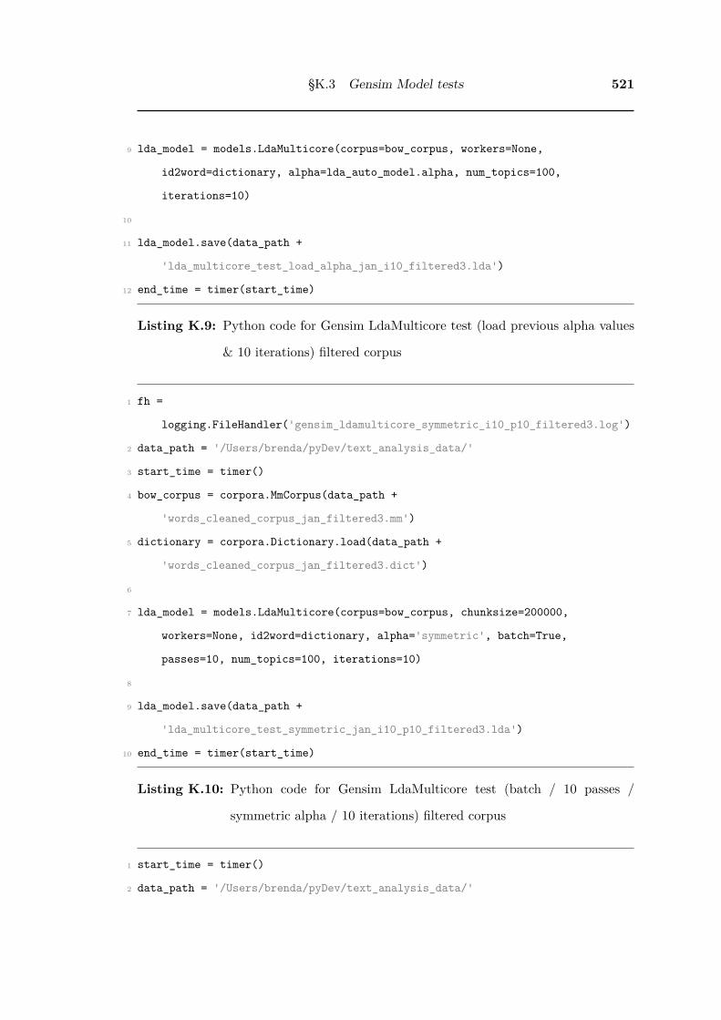
§K.3 Gensim Model tests 521
9 lda_model = models.LdaMulticore(corpus=bow_corpus, workers=None,
id2word=dictionary, alpha=lda_auto_model.alpha, num_topics=100,
iterations=10)
10
11 lda_model.save(data_path +
'lda_multicore_test_load_alpha_jan_i10_filtered3.lda')
12 end_time = timer(start_time)
Listing K.9: Python code for Gensim LdaMulticore test (load previous alpha values
& 10 iterations) filtered corpus
1 fh =
logging.FileHandler('gensim_ldamulticore_symmetric_i10_p10_filtered3.log')
2 data_path = '/Users/brenda/pyDev/text_analysis_data/'
3 start_time = timer()
4 bow_corpus = corpora.MmCorpus(data_path +
'words_cleaned_corpus_jan_filtered3.mm')
5 dictionary = corpora.Dictionary.load(data_path +
'words_cleaned_corpus_jan_filtered3.dict')
6
7 lda_model = models.LdaMulticore(corpus=bow_corpus, chunksize=200000,
workers=None, id2word=dictionary, alpha='symmetric', batch=True,
passes=10, num_topics=100, iterations=10)
8
9 lda_model.save(data_path +
'lda_multicore_test_symmetric_jan_i10_p10_filtered3.lda')
10 end_time = timer(start_time)
Listing K.10: Python code for Gensim LdaMulticore test (batch / 10 passes /
symmetric alpha / 10 iterations) filtered corpus
1 start_time = timer()
2 data_path = '/Users/brenda/pyDev/text_analysis_data/'

522 Topic Analysis
3 bow_corpus = corpora.MmCorpus(data_path +
'words_cleaned_corpus_jan_filtered3.mm')
4 dictionary = corpora.Dictionary.load(data_path +
'words_cleaned_corpus_jan_filtered3.dict')
5 prefix = data_path+'mallet_ldamallet_test_defaults_oi10_newcorpus3'
6
7 model = models.LdaMallet('/usr/local/bin/mallet', corpus=bow_corpus,
id2word=dictionary, prefix=prefix, optimize_interval=10)
8
9 model.save(data_path + 'ldamallet_test_defaults_oi10_newcorpus3.lda')
10 end_time = timer(start_time)
Listing K.11: Python code for Gensim LdaMallet test (optimize_interval 10 / 1000
iterations) filtered corpus
K.4 Iterate over different parameter values
1 import cPickle as pickle
2 bow_corpus = corpora.MmCorpus(data_path +
'words_cleaned_corpus_jan_filtered3.mm')
3
4 # split into train and test - random sample, but preserving order
5 train_size = int(round(len(bow_corpus)*0.8))
6 train_index = sorted(random.sample(xrange(len(bow_corpus)), train_size))
7 test_index = sorted(set(xrange(len(bow_corpus)))-set(train_index))
8 train_corpus = [bow_corpus[i] for i in train_index]
9 test_corpus = [bow_corpus[j] for j in test_index]
10
11 with open( "train_corpus_jan.pkl", "wb" ) as f:
12 pickle.dump( train_corpus, f)
13

§K.4 Iterate over different parameter values 523
14 with open( "test_corpus_jan.pkl", "wb" ) as f:
15 pickle.dump( test_corpus, f)
16
17 # check against originals
18 with open( 'train_corpus_jan.pkl', "rb" ) as f:
19 test = pickle.load(f)
20 if test != train_corpus:
21 print "Pickling failed - train_corpus"
22
23 with open( 'test_corpus_jan.pkl', "rb" ) as f:
24 test = pickle.load(f)
25 if test != test_corpus:
26 print "Pickling failed - test_corpus"
Listing K.12: Python code to split the filtered corpus in to training and test
1 import numpy as np
2 from collections import defaultdict
3
4 start_time = timer()
5 grid = defaultdict(list)
6 data_path = '/Users/brenda/pyDev/text_analysis_data/'
7 dictionary = corpora.Dictionary.load(data_path +
'words_cleaned_corpus_jan_filtered3.dict')
8 train_corpus = []
9 with open( 'train_corpus_jan.pkl', "rb" ) as f:
10 train_corpus = pickle.load(f)
11
12 test_corpus = []
13 with open( 'test_corpus_jan.pkl', "rb" ) as f:
14 test_corpus = pickle.load(f)
15
16 number_of_words = sum(cnt for document in test_corpus for _, cnt in document)

524 Topic Analysis
17
18 print 'Testing different numbers of topics'
19
20 parameter_list = range(5, 151, 5)
21
22 for parameter_value in parameter_list:
23
24 print "starting pass for parameter_value = %.3f" % parameter_value
25 loop_time = timer()
26
27 model = models.LdaMulticore(corpus=train_corpus, workers=None,
id2word=dictionary, num_topics=parameter_value, iterations=10)
28
29 perplex = model.bound(test_corpus)
30 print "Total Perplexity: %s" % perplex
31 grid[parameter_value].append(perplex)
32 per_word_perplex = np.exp2(-perplex / number_of_words)
33 print "Per-word Perplexity: %s" % per_word_perplex
34 grid[parameter_value].append(per_word_perplex)
35 model.save(data_path + 'ldaMulticore_i10_T' + str(parameter_value) +
'_training_corpus.lda')
36 end_time = timer(loop_time)
37 print
38
39 for numtopics in parameter_list:
40 print numtopics, '\t', grid[numtopics]
41
42 df = pandas.DataFrame(grid)
43 df.to_pickle(data_path + 'gensim_multicore_i10_topic_perplexity.df')
44
45 %run '../graphLayoutFunctions.py'
46 ax = plt.figure(figsize=(7, 4), dpi=300).add_subplot(111)

§K.5 Checking retweets 525
47 df.iloc[1].transpose().plot(ax=ax, color=lineColor)
48 plt.xlim(0,150)
49 plt.ylabel('Perplexity')
50 plt.xlabel('topics')
51 plt.title('')
52 plt.savefig('gensim_multicore_i10_topic_perplexity.pdf', format='pdf',
bbox_inches='tight', pad_inches=0.1)
53 plt.show()
54
55 end_time = timer(start_time)
Listing K.13: Python code for iterating over different numbers of topics for
LdaMulticore (i10)
K.5 Checking retweets
1 not_rt_index = tweet_text.words_clean.map(lambda x: x[0] != 'rt')
2 print 'total tweets:', len(not_rt_index)
3 print 'not retweets:', not_rt_index.sum()
4 print 'rt at start:', len(not_rt_index) - not_rt_index.sum()
5 print 'Other retweets:'
6 print '\ttweets with via', len([words for words in
tweet_text[not_rt_index].words_clean if 'via' in words])
7 print '\ttweets with retweet', len([words for words in
tweet_text[not_rt_index].words_clean if 'retweet' in words])
8 print '\ttweets with rt', len([words for words in
tweet_text[not_rt_index].words_clean if 'rt' in words])
Listing K.14: Python code check for retweets in the cleaned words
1 def iter_documents(months):
2 for month in months:

526 Topic Analysis
3 print 'processing month', month
4 tweet_text = pandas.read_pickle(data_path +
'tweet_text_cleaned_month_' + str(month) + '.pkl')
5 not_rt_index = tweet_text.words_clean.map(lambda x: x[0] != 'rt')
6 for words in tweet_text[not_rt_index]['words_clean']:
7 yield words
Listing K.15: Python to code check for retweets in the cleaned words
K.6 Number of iterations for Gensim Mallet
1 start_time = timer()
2 data_path = '/Users/brenda/pyDev/text_analysis_data/'
3 bow_corpus = corpora.MmCorpus(data_path +
'words_cleaned_corpus_jan_filtered3.mm')
4 dictionary = corpora.Dictionary.load(data_path +
'words_cleaned_corpus_jan_filtered3.dict')
5 prefix = data_path+'mallet_ldamallet_test_defaults_oi10_filtered3'
6
7 model = models.LdaMallet('/usr/local/bin/mallet', corpus=bow_corpus,
iterations=10000, id2word=dictionary, prefix=prefix, optimize_interval=10)
8
9 model.save(data_path + 'ldamallet_test_defaults_oi10_i10000_filtered3.lda')
10 end_time = timer(start_time)
Listing K.16: Python code for Gensim Mallet iterations testing

§K.7 Top documents per topic 527
K.7 Top documents per topic
1 start_time = timer()
2 data_path = '/Users/brenda/pyDev/text_analysis_data/'
3 ldaMallet_model = models.LdaMallet.load(data_path +
'ldamallet_final_defaults_oi10_T30_i4000_filtered3.lda')
4 bow_corpus = corpora.MmCorpus(data_path +
'words_cleaned_corpus_jan_filtered3.mm')
5 dictionary = corpora.Dictionary.load(data_path +
'words_cleaned_corpus_jan_filtered3.dict')
6 all_documents = ldaMallet_model[bow_corpus]
7 tweet_text = pandas.read_pickle(data_path + 'tweet_text_cleaned_month_' +
str(1) + '.pkl')
8
9 N = 7 # number of documents to show (zero based, so = 8 docs)
10 topic_names = ['INSERT TOPIC DESCRIPTION HERE'] * ldaMallet_model.num_topics
11 for topic_number in range(ldaMallet_model.num_topics):
12 print '\\multirow{'+ str(N+1) + '}{*}{', topic_number + 1, '} &
\\multicolumn{2}{l}{\textbf{', topic_names[topic_number] ,'}} \\\\'
13 print '& \\multicolumn{2}{p{0.9\\linewidth}}{',
ldaMallet_model.print_topic(topic_number).replace(' +', ','), '}\\\\'
14 my_ids = range(len(all_documents))
15 # topic mixtures of the top docs for the selected topic
16 # with index back to BOW for that document
17 tops = sorted(zip(my_ids, all_documents), reverse=True, key=lambda
(my_id, doc): abs(dict(doc).get(topic_number, 0.0)))
18 for i, document in enumerate(tops[ : N]):
19 # print ' &', str(i+1), '&', ', '.join([dictionary[word[0]] for word
in bow_corpus[document[0]]]), '\\\\'
20 print ' &', str(i+1), tweet_text.text[document[0]], '\\\\'
21 print '\\midrule'
Listing K.17: Python code to create table of topics with top 8 tweets for each topic

528 Topic Analysis
1 def read_doctopics(fname, eps=1e-6):
2 # code from Gensim - models.LdaMallet
3 """
4 Yield document topic vectors from MALLET's "doc-topics" format, as sparse
gensim vectors.
5
6 """
7 with utils.smart_open(fname) as fin:
8 next(fin) # skip the header line
9 for lineno, line in enumerate(fin):
10 parts = line.split()[2:] # skip "doc" and "source" columns
11 if len(parts) % 2 != 0:
12 raise RuntimeError("invalid doc topics format at line %i in %s"
% (lineno + 1, fname))
13 doc = [(int(id), float(weight)) for id, weight in zip(parts[::2],
parts[1::2]) if abs(float(weight)) > eps]
14 # explicitly normalize probs to sum up to 1.0, just to be sure...
15 weights = float(sum([weight for _, weight in doc]))
16 yield [] if weights == 0 else sorted((id, 1.0 * weight / weights)
for id, weight in doc)
17
18 start_time = timer()
19
20 dd = {}
21 n = 100
22 for i in range(30):
23 name = 'topic' + str(i)
24 dd[name] = pandas.DataFrame(columns={'doc_no', 'weight'}, index=xrange(n),
data=[[0, 0.0] for x in range(n)])
25 top_docs = pandas.Panel(data=dd)
26

§K.7 Top documents per topic 529
27 all_documents = read_doctopics(data_path +
'ldamallet_final_2011_oi10_T30_filtered3_brm_doctopics.txt.1.infer')
28
29 for i, doc in enumerate(all_documents):
30 if i % 500000 == 0:
31 print 'processing document', i
32 print
33 for topic in doc:
34 name = 'topic' + str(topic[0])
35 if top_docs[name].weight.min() < topic[1]:
36 min_index = top_docs[name].weight.argmin()
37 top_docs[name].iloc[min_index].weight = topic[1]
38 top_docs[name].iloc[min_index].doc_no = i
39 for topic in top_docs:
40 print topic
41 print top_docs[topic].iloc[0:8]
42
43 end_time = timer(start_time)
Listing K.18: Python code to get top n documents for each topic
1 import re
2 start_time = timer()
3
4 def atoi(text):
5 return int(text) if text.isdigit() else text
6
7 def natural_keys(text):
8 '''
9 alist.sort(key=natural_keys) sorts in human order
10 http://nedbatchelder.com/blog/200712/human_sorting.html
11 (See Toothy's implementation in the comments)
12 '''

530 Topic Analysis
13 return [ atoi(c) for c in re.split('(\d+)', text) ]
14
15 N = 8
16 print table_head
17
18 # load all the original tweet texts for the year (this is still big - 1.6Gb!)
19 whole_year = pandas.read_pickle(data_path + 'tweetid_tweettext_2011.pkl')
20 top_docs = pandas.read_pickle(data_path +
'top_docs_per_topic_2011_not_sorted.pkl')
21 ldaMallet_model = models.LdaMallet.load(data_path +
'ldamallet_final_2011_oi10_T30_i4000_filtered3_brm.lda')
22
23 bow_corpus = corpora.MmCorpus(data_path +
'words_cleaned_corpus_2011_filtered3.mm')
24 dictionary = corpora.Dictionary.load(data_path +
'words_cleaned_corpus_2011_filtered3.dict')
25 topic_names = ['INSERT TOPIC DESCRIPTION HERE'] * ldaMallet_model.num_topics
26
27 topics = top_docs.items.tolist()
28 topics.sort(key=natural_keys)
29
30 for topic_number, topic in enumerate(topics):
31 print '\\multirow{'+ str(N+1) + '}{*}{', topic_number + 1, '} &
\\multicolumn{2}{l}{\\textbf{', topic_names[topic_number] ,'}} \\\\'
32 print '& \\multicolumn{2}{p{0.9\\linewidth}}{',
ldaMallet_model.print_topic(topic_number).replace(' +', ','), '}\\\\'
33 # need to get the rows sorted by weight.
34 top_docs[topic].sort(columns='weight', ascending=False, inplace=True)
35 for row in list(top_docs.major_axis)[0:N]:
36 print ' &', str(row+1), '&',
whole_year.iloc[int(top_docs[topic].iloc[row].doc_no)].text.replace('#','\\#')
.replace('_','\\_').replace('$','\\$').replace('&',
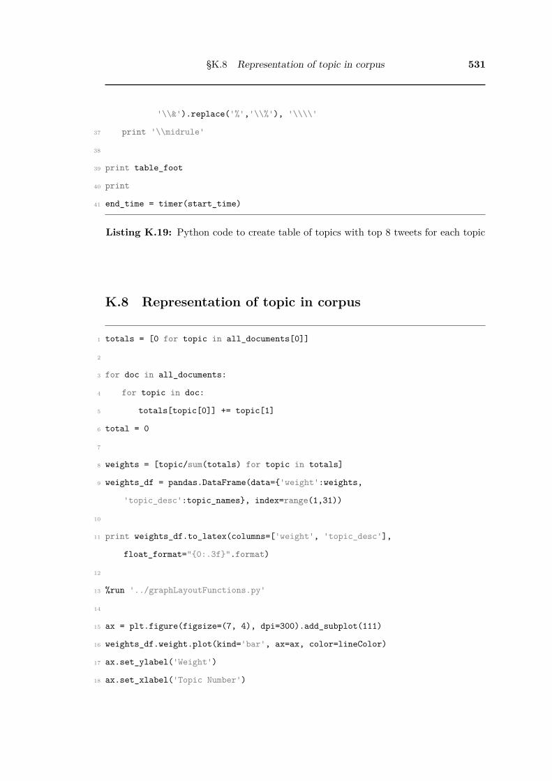
§K.8 Representation of topic in corpus 531
'\\&').replace('%','\\%'), '\\\\'
37 print '\\midrule'
38
39 print table_foot
40 print
41 end_time = timer(start_time)
Listing K.19: Python code to create table of topics with top 8 tweets for each topic
K.8 Representation of topic in corpus
1 totals = [0 for topic in all_documents[0]]
2
3 for doc in all_documents:
4 for topic in doc:
5 totals[topic[0]] += topic[1]
6 total = 0
7
8 weights = [topic/sum(totals) for topic in totals]
9 weights_df = pandas.DataFrame(data={'weight':weights,
'topic_desc':topic_names}, index=range(1,31))
10
11 print weights_df.to_latex(columns=['weight', 'topic_desc'],
float_format="{0:.3f}".format)
12
13 %run '../graphLayoutFunctions.py'
14
15 ax = plt.figure(figsize=(7, 4), dpi=300).add_subplot(111)
16 weights_df.weight.plot(kind='bar', ax=ax, color=lineColor)
17 ax.set_ylabel('Weight')
18 ax.set_xlabel('Topic Number')

532 Topic Analysis
19 ax.grid(False)
20 plt.title('')
21 plt.savefig('January30Topics_TopicWeights.pdf', format='pdf',
bbox_inches='tight', pad_inches=0.1)
22 plt.show()
Listing K.20: Python code to find the proportion of each topic in January 2011 corpus
1
2 start_time = timer()
3 totals = [0 for topic in range(30)]
4 all_documents = read_doctopics(data_path +
'ldamallet_final_2011_oi10_T30_filtered3_brm_doctopics.txt.1.infer')
5
6 for doc in all_documents:
7 for topic in doc:
8 totals[topic[0]] += topic[1]
9 total = 0
10 weights = [topic/sum(totals) for topic in totals]
11 weights_df = pandas.DataFrame(data={'weight':weights,
'topic_desc':topic_names}, index=range(1,31))
12 print weights_df.to_latex(columns=['weight', 'topic_desc'],
float_format="{0:.3f}".format)
13
14 %run '../graphLayoutFunctions.py'
15 ax = plt.figure(figsize=(7, 4), dpi=300).add_subplot(111)
16 weights_df.weight.plot(kind='bar', ax=ax, color=lineColor)
17 # ax.xaxis.set_major_formatter(plt.FuncFormatter(commaNumbers))
18 # ax.yaxis.set_major_formatter(plt.FuncFormatter(commaNumbers))
19 ax.set_ylabel('Weight')
20 ax.set_xlabel('Topic Number')
21 ax.grid(False)
22 plt.title('')

§K.8 Representation of topic in corpus 533
23 plt.savefig('2011Topics_TopicWeights.pdf', format='pdf', bbox_inches='tight',
pad_inches=0.1)
24 plt.show()
25 end_time = timer(start_time)
Listing K.21: Python code to find the proportion of each topic in whole year 2011
corpus

534 Topic Analysis

References
Baram-Tsabari, A., & Segev, E. (2009, oct). Exploring new web-based tools to
identify public interest in science. Public Understanding of Science, Pub-
lished(October 2009). Retrieved from http://pus.sagepub.com/cgi/doi/10.1177/
0963662509346496 doi: 10.1177/0963662509346496
Bauer, M. W., & Jensen, P. (2011, feb). The mobilization of scientists for pub-
lic engagement. Public Understanding of Science, 20(1), 3–11. Retrieved
from http://pus.sagepub.com/cgi/doi/10.1177/0963662510394457 doi: 10.1177/
0963662510394457
Bifet, A., & Frank, E. (2010). Sentiment Knowledge Discovery in Twitter Streaming
Data. cswaikatoacnz, 1–15. Retrieved from http://www.cs.waikato.ac.nz/{~}eibe/
pubs/Twitter-crc.pdf
Bird, S., Klein, E., & Loper, E. (2009). Natural Language Processing with Python
(Vol. 43). Retrieved from http://nltk.org/book/ doi: 10.1097/00004770
-200204000-00018
Black, A., Mascaro, C., Gallagher, M., & Goggins, S. P. (2012). Twitter zombie.
In Proceedings of the 17th acm international conference on supporting group
work - group ’12 (p. 229). New York, New York, USA: ACM Press. Re-
trieved from http://dl.acm.org/citation.cfm?id=2389211http://dl.acm.org/citation
.cfm?doid=2389176.2389211 doi: 10.1145/2389176.2389211
Blei, D. M. (2012). Topic modeling and digital humanities. Journal of Dig-
ital Humanities, 2(1), 8–11. Retrieved from http://scholar.google.com/
scholar?hl=en{\&}btnG=Search{\&}q=intitle:Topic+Modeling+and+Digital+
Humanities{\#}1
535

536 References
Blei, D. M., & Lafferty, J. D. (2009). Topic models. In A. Srivastava & M. Sahami
(Eds.), Text mining: Classification, clustering, and applications (chap. Topic
mode). Chapman & Hall/CRC Data Mining and Knowledge Discovery Series.
Retrieved from http://www.cs.princeton.edu/{~}blei/papers/BleiLafferty2009.pdf
Blei, D. M., Ng, A., & Jordan, M. (2003). Latent dirichlet allocation. the Journal
of machine Learning research, 3, 993–1022. Retrieved from http://dl.acm.org/
citation.cfm?id=944937
Bollen, J., Mao, H., & Zeng, X.-J. (2010). Twitter mood predicts the stock market.
Computer, 1010(3003v1), 1–8. Retrieved from http://arxiv.org/abs/1010.3003
Boyd, d. m., Golder, S., & Lotan, G. (2010). Tweet, Tweet, Retweet: Conversa-
tional Aspects of Retweeting on Twitter. In 2010 43rd hawaii international con-
ference on system sciences (Vol. 0, pp. 1–10). IEEE. Retrieved from http://
www.computer.org/portal/web/csdl/doi/10.1109/HICSS.2010.412 doi: 10.1109/
HICSS.2010.412
Bray, B., France, B., & Gilbert, J. K. (2012). Identifying the Essential Elements
of Effective Science Communication: What do the experts say? International
Journal of Science Education Part B Communication and Public Engagement,
2(February 2013), 37–41. Retrieved from http://www.tandfonline.com/doi/abs/
10.1080/21548455.2011.611627 doi: 10.1080/21548455.2011.611627
Brett, M. R. (2012). Topic Modeling: A Basic Introduction. Journal of Digital
Humanities, 2(1), 12–16.
Brossard, D., & Scheufele, D. A. (2013, jan). Science, New Media, and the Public.
Science, 339(6115), 40–41. Retrieved from http://www.sciencemag.org/cgi/doi/
10.1126/science.1232329 doi: 10.1126/science.1232329
Bruns, A. (2013, oct). Faster than the speed of print: Reconciling ‘big data’ so-
cial media analysis and academic scholarship. First Monday, 18(10). Retrieved
from http://journals.uic.edu/ojs/index.php/fm/article/view/4879 doi: 10.5210/
fm.v18i10.4879

References 537
Bruns, A., & Stieglitz, S. (2012). Quantitative Approaches to Comparing Commu-
nication Patterns on Twitter. Journal of Technology in Human Services, 30(3-
4), 160–185. Retrieved from http://www.tandfonline.com.proxy.uba.uva.nl:2048/
doi/full/10.1080/15228835.2012.744249{\#}.Ut{\_}HMBA1hD8 doi: 10.1080/
15228835.2012.744249
Bruns, A., & Stieglitz, S. (2013). Towards more systematic Twitter analysis:
metrics for tweeting activities. International Journal of Social Research
Methodology, 16(2), 91–108. Retrieved from http://www.tandfonline.com/doi/
abs/10.1080/13645579.2012.756095$\backslash$nhttp://www.tandfonline.com
.ezproxy.ub.gu.se/doi/abs/10.1080/13645579.2012.756095$\backslash$nhttp://
www.tandfonline.com.ezproxy.ub.gu.se/doi/pdf/10.1080/13645579.2012.756095
doi: 10.1080/13645579.2012.756095
Bruns, A., & Stieglitz, S. (2015). Twitter Data: What Do They Represent? Information
Technology, 57 , 1–7.
Burgess, J., & Bruns, A. (2012, nov). Twitter Archives and the Challenges of ”Big
Social Data” for Media and Communication Research. M/C Journal, 15(5),
8. Retrieved from http://journal.media-culture.org.au/index.php/mcjournal/
article/view/561http://search.ebscohost.com/login.aspx?direct=true{\&}db=
ufh{\&}AN=89110439{\&}site=ehost-live
Burgess, J., & Bruns, A. (2015). Easy Data, Hard Data: The Politics and Pragmatics
of Twitter Research after the Computational Turn. In Compromised data: From
social media to big data (pp. 93–111).
Burns, T. W., O’Connor, D. J., & Stocklmayer, S. M. (2003, apr). Science Communica-
tion: A Contemporary Definition. Public Understanding of Science, 12(2), 183–
202. Retrieved from http://pus.sagepub.com/cgi/doi/10.1177/09636625030122004
doi: 10.1177/09636625030122004
Busch, L. (2014). Big Data, Big Questions| A Dozen Ways to Get Lost in Translation:
Inherent Challenges in Large Scale Data Sets. International Journal of Commu-

538 References
nication, 8(0). Retrieved from http://ijoc.org/index.php/ijoc/article/view/2160
Butler, D. (2013). When Google got flu wrong. Nature, 494(7436), 155–156. Retrieved
from http://search.proquest.com/docview/1319460535?accountid=8330 doi: 10
.1038/494155a
Carter, S., Weerkamp, W., & Tsagkias, M. (2012, jun). Microblog
language identification: overcoming the limitations of short, unedited
and idiomatic text. Language Resources and Evaluation, 47(1), 195–
215. Retrieved from http://www.springerlink.com/index/10.1007/s10579-012-9195
-yhttp://link.springer.com/10.1007/s10579-012-9195-y doi: 10.1007/s10579-012
-9195-y
Cataldi, M., Di Caro, L., & Schifanella, C. (2010). Emerging topic detection on Twitter
based on temporal and social terms evaluation. Search, 1–10. Retrieved from
http://portal.acm.org/citation.cfm?id=1814245.1814249 doi: 10.1145/1814245
.1814249
Cha, M., Haddadi, H., Benevenuto, F., & Gummadi, K. P. (2010). Measuring User
Influence in Twitter: The Million Follower Fallacy. In Artificial intelligence (pp.
10–17). Fourth International AAAI Conference on Weblogs and Social Media. Re-
trieved from http://www.aaai.org/ocs/index.php/ICWSM/ICWSM10/paper/view/
1538http://twitter.mpi-sws.org/
Chaney, A., & Blei, D. M. (2012). Visualizing Topic Models. ICWSM .
Retrieved from http://www.aaai.org/ocs/index.php/ICWSM/ICWSM12/paper/
viewPDFInterstitial/4645/5021
Chang, H. C. (2010). A new perspective on Twitter hashtag use: Diffusion of innovation
theory. In Proceedings of the asist annual meeting (Vol. 47). doi: 10.1002/
meet.14504701295
Chang, J., Gerrish, S., Boyd-Graber, J., Wang, C., & Blei, D. M. (2009). Reading Tea
Leaves: How Humans Interpret Topic Models. In Neural information processing
systems. Vancouver, British Columbia. Retrieved from http://machinelearning

References 539
.wustl.edu/mlpapers/paper{\_}files/NIPS2009{\_}0125.pdf
Chappell, B. (2010). 2010 Social Network Analysis Report - Geographic - Demographic
and Traffic Data Revealed. Retrieved from http://www.ignitesocialmedia.com/
2010-social-network-analysis-report/
Chuang, J., Manning, C. D., & Heer, J. (2012). Termite: Visualization Techniques
for Assessing Textual Topic Models. Advanced Visual Interfaces. Retrieved from
http://vis.stanford.edu/papers/termite
Cochran, W. G. (1977). Sampling Techniques (Third Edit ed.). JOHN WILEY &
SONS INC.
Crawford, K., Gray, M., & Miltner, K. (2014). Big Data| Critiquing Big Data: Politics,
Ethics, Epistemology | Special Section Introduction. International Journal of
Communication, 8(0). Retrieved from http://ijoc.org/index.php/ijoc/article/view/
2167
Culotta, A. (2010). Detecting influenza outbreaks by analyzing Twitter messages.
Science(May), 1–11. Retrieved from http://arxiv.org/abs/1007.4748
danah Boyd, & Crawford, K. (2012, jun). CRITICAL QUESTIONS FOR BIG
DATA. Information, Communication & Society, 15(5), 662–679. Retrieved
from http://www.tandfonline.com/doi/abs/10.1080/1369118X.2012.678878 doi:
10.1080/1369118X.2012.678878
Davidov, D., Tsur, O., & Rappoport, A. (2010). Enhanced Sentiment Learning Using
Twitter Hashtags and Smileys. In Coling ’10 proceedings of the 23rd international
conference on computational linguistics: Posters (pp. 241–249). Beijing, China:
Association for Computational Linguistics. Retrieved from http://dl.acm.org/
citation.cfm?id=1944566.1944594 doi: 10.1.1.185.3112
Dean, J., & Ghemawat, S. (2004). MapReduce: Simplified Data Processing on Large
Clusters. In Osdi ’04: 6th symposium on operating systems design and implemen-
tation (pp. 137–149). San Francisco, CA. Retrieved from http://static.usenix.org/
events/osdi04/tech/dean.html

540 References
DiGrazia, J., McKelvey, K., Bollen, J., & Rojas, F. (2013). More Tweets, More
Votes: Social Media as a Quantitative Indicator of Political Behavior. SSRN
Electronic Journal, 1–11. Retrieved from http://www.ssrn.com/abstract=2235423
doi: 10.2139/ssrn.2235423
Dugan, L. (2011). 230 Million Tweets Per Day, 50 Million Daily
Users And Other Twitter Stats - AllTwitter. Retrieved 2012-06-13,
from http://www.mediabistro.com/alltwitter/230-million-tweets-per-day-50-million
-daily-users-and-other-twitter-stats{\_}b13518
Durant, J., Evans, G., & Thomas, G. (1989). The public understanding of science.
Nature, 340(6 July 1989). Retrieved from http://www.nature.com.virtual.anu.edu
.au/nature/journal/v340/n6228/pdf/340011a0.pdf
Earle, P. (2010). Earthquake Twitter. Nature Geoscience, 3(4), 221–222. Retrieved
from http://dx.doi.org/10.1038/ngeo832 doi: 10.1038/ngeo832
Ediger, D., Jiang, K., Riedy, J., Bader, D. A., & Corley, C. (2010). Massive Social
Network Analysis : Mining Twitter for Social Good. 2010 39th International
Conference on Parallel Processing, 583–593. Retrieved from http://ieeexplore.ieee
.org/lpdocs/epic03/wrapper.htm?arnumber=5599247 doi: 10.1109/ICPP.2010.66
Eysenbach, G. (2011, jan). Can tweets predict citations? Metrics of
social impact based on Twitter and correlation with traditional met-
rics of scientific impact. Journal of medical Internet research, 13(4),
e123. Retrieved from http://www.pubmedcentral.nih.gov/articlerender.fcgi?artid=
3278109{\&}tool=pmcentrez{\&}rendertype=abstract doi: 10.2196/jmir.2012
Falk, J. H., Storksdieck, M., & Dierking, L. D. (2007, oct). Investigating pub-
lic science interest and understanding: evidence for the importance of free-
choice learning. Public Understanding of Science, 16(4), 455–469. Retrieved
from http://pus.sagepub.com/cgi/doi/10.1177/0963662506064240 doi: 10.1177/
0963662506064240
Fisher, N. I., Cribb, J. H. J., & Peacock, A. J. (2007). Reading the public mind: a novel

References 541
approach to improving the adoption of new science and technology. Australian
Journal of Experimental Agriculture, 47(11), 1262. Retrieved from http://www
.publish.csiro.au/?paper=EA07004 doi: 10.1071/EA07004
Fisher, N. I., Lee, A. J., & Cribb, J. H. (2013, mar). A Scientific Approach to Mon-
itoring Public Perceptions of Scientific Issues. International Journal of Science
Education, Part B, 3(1), 25–51. Retrieved from http://www.tandfonline.com/doi/
abs/10.1080/09500693.2011.652364 doi: 10.1080/09500693.2011.652364
Gauchat, G. (2011). The cultural authority of science: Public trust and acceptance
of organized science. Public Understanding of Science, 20(6), 751–770. Re-
trieved from http://pus.sagepub.com/content/20/6/751.abstract doi: 10.1177/
0963662510365246
Gerlitz, C., & Rieder, B. (2013). Mining One Percent of Twitter: Collections, Baselines,
Sampling. M/C Journal, 16(2). Retrieved from http://www.journal.media-culture
.org.au/index.php/mcjournal/article/view/620
Ginsberg, J., Mohebbi, M. H., Patel, R. S., Brammer, L., Smolinski, M. S., & Brilliant,
L. (2009). Detecting influenza epidemics using search engine query data. Nature,
457(7232), 1012–1014. Retrieved from http://www.nature.com/nature/journal/
v457/n7232/suppinfo/nature07634{\_}S1.html doi: 10.1038/nature07634
Goldstone, A., & Underwood, T. (2012). What Can Topic Models of PMLA Teach Us
about the History of Literary Scholarship? Journal of Digital Humanities, 2(1),
39–48. Retrieved from http://journalofdigitalhumanities.org/files/jdh{\_}2{\_}1
Grant, W. J., Moon, B., & Busby Grant, J. (2010, dec). Digital Dialogue? Australian
Politicians’ use of the Social Network Tool Twitter. Australian Journal of Political
Science, 45(4), 579–604. Retrieved from http://www.informaworld.com/10.1080/
10361146.2010.517176 doi: 10.1080/10361146.2010.517176
Greenhow, C., & Gleason, B. (2012, oct). Twitteracy: Tweeting as a New Literacy
Practice. The Educational Forum, 76(4), 464–478. Retrieved from http://www

542 References
.tandfonline.com/doi/abs/10.1080/00131725.2012.709032 doi: 10.1080/00131725
.2012.709032
Gretarsson, B., O’Donovan, J., Bostandjiev, S., Hollerer, T., Asuncion, A., Newman,
D., & Smyth, P. (2009). Topicnets: Visual analysis of large text corpora with
topic modeling. ACM Transactions on Information Systems, V , 1–26. Retrieved
from http://dl.acm.org/citation.cfm?id=2089099
Griffiths, T. L., & Steyvers, M. (2004). Finding scientific topics. Proceedings of the
National Academy of Sciences of the United States of America, 101 Suppl(Suppl
1), 5228–5235. Retrieved from http://www.pubmedcentral.nih.gov/articlerender
.fcgi?artid=387300{\&}tool=pmcentrez{\&}rendertype=abstract
Hall, M., Frank, E., Holmes, G., Pfahringer, B., Reutemann, P., & Witten, I. (2009).
The WEKA Data Mining Software: An Update. ACM SIGKDD Explorations
Newsletter, 11(1), 10–18. Retrieved from http://portal.acm.org/citation.cfm?id=
1656274.1656278
Herwig, J. (2009). Liminality and Communitas in Social Media: The Case of Twitter.
Internet Critical Internet Research. Retrieved from http://homepage.univie.ac.at/
jana.herwig/PDF/herwig{\_}ir10{\_}liminalitycommunitastwitter{\_}v5oct09
Hoffman, M. D., Bach, F., & Blei, D. M. (2010). Online learning for latent dirichlet
allocation. advances in neural information …, 1–9. Retrieved from http://papers
.nips.cc/paper/3902-online-learning-for-latent-dirichlet-allocation
Huang, J., Thornton, K. M., & Efthimiadis, E. N. (2010). Conversational tagging in
twitter. Proceedings of the 21st ACM conference on Hypertext and hypermedia
HT 10, 173–177. Retrieved from http://portal.acm.org/citation.cfm?doid=1810617
.1810647 doi: 10.1145/1810617.1810647
Huberman, B. A., Romero, D. M., & Wu, F. (2008). Social networks that matter:
Twitter under the microscope. First Monday, 14(1), 1–9. Retrieved from http://
arxiv.org/abs/0812.1045

References 543
Jansen, B. J., Zhang, M., Sobel, K., & Chowdury, A. (2009, nov). Twitter Power:
Tweets as Electronic Word of Mouth. Journal of the American Society For Infor-
mation Science and Technology, 60(11), 2169–2188. doi: DOI10.1002/asi.21149
Jung, J. J. (2012, jul). Online named entity recognition method for microtexts in
social networking services: A case study of twitter. Expert Systems with Applica-
tions, 39(9), 8066–8070. Retrieved from http://linkinghub.elsevier.com/retrieve/
pii/S0957417412001546 doi: 10.1016/j.eswa.2012.01.136
Karnik, A., Saroop, A., & Borkar, V. (2013, apr). On the diffusion of messages in on-line
social networks. Performance Evaluation, 70(4), 271–285. Retrieved from http://
linkinghub.elsevier.com/retrieve/pii/S0166531612001320 doi: 10.1016/j.peva.2012
.12.002
Kingsbury, A. (2008). Spy Agencies Turn to Newspapers, NPR, and Wikipedia for In-
formation. Retrieved from http://www.usnews.com/news/national/articles/2008/
09/12/spy-agencies-turn-to-newspapers-npr-and-wikipedia-for-information.html
Kosala, R., & Adi, E. (2012, jan). Harvesting Real Time Traffic Information from
Twitter. Procedia Engineering, 50(Icasce), 1–11. Retrieved from http://linkinghub
.elsevier.com/retrieve/pii/S1877705812046516 doi: 10.1016/j.proeng.2012.10.001
Lampos, V., De Bie, T., & Cristianini, N. (2010). Flu Detector - Tracking Epidemics
on Twitter. Machine Learning and Knowledge, 6323, 599–602. Retrieved from
http://dx.doi.org/10.1007/978-3-642-15939-8{\_}42
Layton, R. (2015). Learning Data Mining with Python. Packt Publishing.
Lazer, D., Kennedy, R., King, G., & Vespignani, A. (2014, mar). Big data. The parable
of Google Flu: traps in big data analysis. Science (New York, N.Y.), 343(6176),
1203–5. Retrieved from http://www.ncbi.nlm.nih.gov/pubmed/24626916 doi: 10
.1126/science.1248506
Leavitt, A., Burchard, E., Fisher, D., & Gilbert, S. (2009). The Influentials: New Ap-
proaches for Analyzing Influence on Twitter. Webecology Project, 04(September).
Retrieved from http://www.webecologyproject.org/2009/09/analyzing-influence-on

544 References
-twitter/
Lee, C., Kwak, H., Park, H., & Moon, S. (2010). Finding influentials based on
the temporal order of information adoption in twitter. Proceedings of the
19th international conference on World wide web WWW 10, 1137. Retrieved
from http://portal.acm.org/citation.cfm?doid=1772690.1772842 doi: 10.1145/
1772690.1772842
Letierce, J., Passant, A., Decker, S., & Breslin, J. G. (2010). Understanding how
Twitter is used to spread scientific messages. October, 8. Retrieved from http://
journal.webscience.org/314/
Lim, K. H., & Datta, A. (2012, dec). Tweets Beget Propinquity: Detecting Highly Inter-
active Communities on Twitter Using Tweeting Links. 2012 IEEE/WIC/ACM
International Conferences on Web Intelligence and Intelligent Agent Technol-
ogy, 214–221. Retrieved from http://ieeexplore.ieee.org/lpdocs/epic03/wrapper
.htm?arnumber=6511887 doi: 10.1109/WI-IAT.2012.53
Lui, M., & Baldwin, T. (2012). langid.py: An Off-the-shelf Language Identification
Tool. In Proceedings of the 50th annual meeting of the association for compu-
tational linguistics (pp. 25–30). Jeju, Republic of Korea: Association for Com-
putational Linguistics. Retrieved from http://www.aclweb.org/anthology-new/P/
P12/P12-3005.pdf
Mandavilli, A. (2011). Trial by Twitter. Nature, 469(7330), 286–287. Retrieved
from http://www.nature.com/news/2011/110119/full/469286a.html doi: 10.1038/
469286a
Manning, C. D., Raghavan, P., & Schütze, H. (2009). Introduction to Infor-
mation Retrieval (Online edi ed.). Cambridge University Press. Retrieved
from http://www-nlp.stanford.edu/IR-book/http://nlp.stanford.edu/IR-book/pdf/
irbookonlinereading.pdf
Manning, C. D., & Schütze, H. (1999). Foundations of Statistical Natural Language
Processing. Retrieved from http://nlp.stanford.edu/fsnlp/

References 545
Marks II, Robert, J. (2009). Handbook of Fourier Analysis & its applications. New
York: Oxford University Press.
Maynard, D. (2012). Automatic detection of political opinions in tweets. The Semantic
Web: ESWC 2011 Workshops, 81–92. Retrieved from http://www.springerlink
.com/index/F3H0J8N38010R730.pdf
McCallum, A. K. (2002). MALLET: A Machine Learning for Language Toolkit. Re-
trieved from http://mallet.cs.umass.edu
McGiboney, M. N. O. (n.d.). Twitter’s Tweet Smell Of Success | Nielsen Wire.
Retrieved 2009-04-21, from http://blog.nielsen.com/nielsenwire/online{\_}mobile/
twitters-tweet-smell-of-success/
Michelson, M., & Macskassy, S. A. (2010). Discovering Users’ Topics of Interest on
Twitter: A First Look. In D. Lopresti, C. Ringlstetter, S. Roy, K. Schulz, &
L. V. Subramaniam (Eds.), Proceedings of the workshop on analytics for noisy,
unstructured text data (and) (pp. 73–79). ACM Press. Retrieved from http://
www.mmichelson.com/paps/and2010.pdf
Miller, S. (2001). Public Understanding of Science Public understanding of science at
the crossroads. Public Understanding of Science, 10(1), 115–120. doi: 10.1088/
0963-6625/10/1/308
Mimno, D., & Blei, D. M. (2011). Bayesian Checking for Topic Models. In Proceedings
of the conference on empirical methods in natural language processing (pp. 227–
237). Retrieved from http://dl.acm.org/citation.cfm?id=2145432.2145459
Morgan, J. S., Lampe, C., & Shafiq, M. Z. (2013). Is news sharing on Twit-
ter ideologically biased? In Proceedings of the 2013 conference on computer
supported cooperative work - cscw ’13 (p. 887). New York, New York, USA:
ACM Press. Retrieved from http://dl.acm.org/citation.cfm?id=2441877http://
dl.acm.org/citation.cfm?doid=2441776.2441877 doi: 10.1145/2441776.2441877
Nguyen, L. T., Wu, P., Chan, W., & Field, M. (2012). Predicting Collective Sentiment
Dynamics from Time-series Social Media Categories and Subject Descriptors. In

546 References
Wisdom’12 at kdd’2012. Beijing, China: ACM. Retrieved from http://kdd2012
.sigkdd.org
Noordhuis, P., Heijkoop, M., & Lazovik, A. (2010). Mining Twitter in the Cloud:
A Case Study. 2010 IEEE 3rd International Conference on Cloud Comput-
ing, 107–114. Retrieved from http://ieeexplore.ieee.org/lpdocs/epic03/wrapper
.htm?arnumber=5558003 doi: 10.1109/CLOUD.2010.59
O’Connor, B., Balasubramanyan, R., Routledge, B. R., & Smith, N. A. (2010).
From Tweets to polls: Linking text sentiment to public opinion time series.
In Proceedings of the international aaai conference on weblogs and social me-
dia (pp. 122–129). Retrieved from http://www.aaai.org/ocs/index.php/ICWSM/
ICWSM10/paper/viewPDFInterstitial/1536/1842
O’Connor, B., Krieger, M., & Ahn, D. (2010). TweetMotif: Exploratory search and
topic summarization for twitter. In International aaai conference on weblogs and
social media, washington, dc (pp. 384–385). Retrieved from http://www.aaai.org/
ocs/index.php/ICWSM/ICWSM10/paper/viewPDFInterstitial/1540/1907
Ovadia, S. (2009). Exploring the Potential of Twitter as a Research
Tool. Behavioral Social Sciences Librarian, 28(4), 202–205. Retrieved
from http://www.informaworld.com/openurl?genre=article{\&}doi=10.1080/
01639260903280888{\&}magic=crossref doi: 10.1080/01639260903280888
Perez, F., & Granger, B. E. (2007). IPython: A System for Interactive Scientific
Computing. Computing in Science & Engineering, 9(3), 21–29. Retrieved from
http://ieeexplore.ieee.org/lpdocs/epic03/wrapper.htm?arnumber=4160251 doi: 10
.1109/MCSE.2007.53
Petrovic, S., Osborne, M., & Lavrenko, V. (2010). Streaming First Story Detection
with application to Twitter. Proceedings of NAACL(June), 181–189. Retrieved
from http://www.aclweb.org/anthology/N10-1021
Phelan, O., McCarthy, K., & Smyth, B. (2009). Using twitter to recommend real-time
topical news. Proceedings of the third ACM conference on Recommender systems

References 547
RecSys 09, systemspag, 385. Retrieved from http://portal.acm.org/citation.cfm
?doid=1639714.1639794 doi: 10.1145/1639714.1639794
Posch, L., Wagner, C., Singer, P., & Strohmaier, M. (2013). Meaning as collective use:
predicting semantic hashtag categories on twitter. In Proceedings of the 22nd
international conference on world wide web companion (pp. 621–628). Rio de
Janeiro, Brazil: International World Wide Web Conferences Steering Committee.
Retrieved from http://dl.acm.org/citation.cfm?id=2488008
Ramage, D., Dumais, S., & Liebling, D. (2010). Characterizing microblogs
with topic models. In International aaai conference on weblogs and social
media. Retrieved from http://www.aaai.org/ocs/index.php/ICWSM/ICWSM10/
paper/viewPDFInterstitial/1528/1846
Rehuvrek, R., & Sojka, P. (2010, may). Software Framework for Topic Modelling with
Large Corpora. In Proceedings of the lrec 2010 workshop on new challenges for
nlp frameworks (pp. 45–50). Valletta, Malta: ELRA. Retrieved from http://
radimrehurek.com/gensim/lrec2010{\_}final.pdf
Romero, D. M., Galuba, W., Asur, S., & Huberman, B. A. (2010, aug). Influence and
Passivity in Social Media. papers.ssrn.com, 1–9. Retrieved from http://arxiv.org/
abs/1008.1253
Roomann-Kurrick, A. (2011). Important Search Changes: real user IDs & support
for URL, media, hashtag entities. Retrieved 2015-12-01, from https://blog.twitter
.com/2011/user-ids-and-tweet-entities-in-search
Rosen-Zvi, M., Chemudugunta, C., Griffiths, T., Smyth, P., & Steyvers, M. (2009).
Learning author-topic models from text corpora. ACM Transactions on Infor-
mation Systems, V (March), 1–38. Retrieved from http://dl.acm.org/citation.cfm
?id=1658381
Sakaki, T., Okazaki, M., & Matsuo, Y. (2010). Earthquake shakes Twitter users: real-
time event detection by social sensors. In Proceedings of the 19th international
conference on world wide web (pp. 851–860). ACM. Retrieved from http://

548 References
portal.acm.org/citation.cfm?id=1772690.1772777 doi: 10.1145/1772690.1772777
Salathé, M., & Khandelwal, S. (2011, oct). Assessing vaccination sentiments with
online social media: implications for infectious disease dynamics and control.
PLoS computational biology, 7(10), e1002199. Retrieved from http://dx.plos.org/
10.1371/journal.pcbi.1002199 doi: 10.1371/journal.pcbi.1002199
Salter, L. (2003). Science and Public Discourse. History of Intellectual Culture, 3(1),
19. Retrieved from http://www.ucalgary.ca/hic/files/hic/salterpdf.pdf
Sankaranarayanan, J., Samet, H., Lieberman, M. D., & Sperling, J. (2009).
TwitterStand : News in Tweets. Information Storage and Retrieval, 42–51.
Retrieved from http://portal.acm.org/citation.cfm?id=1653781 doi: 10.1145/
1653771.1653781
Scanfeld, D., Scanfeld, V., & Larson, E. L. (2010, apr). Dissemination of health
information through social networks: twitter and antibiotics. American journal
of infection control, 38(3), 182–8. Retrieved from http://www.ncbi.nlm.nih.gov/
pubmed/20347636 doi: 10.1016/j.ajic.2009.11.004
Schmidt, B. M. (2012). Words Alone: Dismantling Topic Models in the Human-
ities. Journal of Digital Humanities, 2(1), 49–65. Retrieved from http://
journalofdigitalhumanities.org/files/jdh{\_}2{\_}1.pdf
Searle, S. D. (2014). How do Australians engage with science? Preliminary results
from a national survey. (Tech. Rep. No. April). Canberra, Australia: Australian
National Centre for the Public Awareness of Science (CPAS), The Australian
National University.
Segev, E., & Baram-Tsabari, A. (2012, oct). Seeking science information online:
Data mining Google to better understand the roles of the media and the ed-
ucation system. Public understanding of science (Bristol, England), 21(7),
813–29. Retrieved from http://www.ncbi.nlm.nih.gov/pubmed/23832560 doi:
10.1177/0963662510387560
Stalder, F., & Hirsh, J. (2002, jun). Open source intelligence. First Monday, 7(6). Re-

References 549
trieved from http://firstmonday.org/htbin/cgiwrap/bin/ojs/index.php/fm/article/
viewArticle/961/882 doi: http://dx.doi.org/10.1080/03071840408522977
Stocklmayer, S. M., & Bryant, C. (2011, apr). Science and the Public—What should
people know? International Journal of Science Education, Part B(November), 1–
21. Retrieved from http://www.tandfonline.com/doi/abs/10.1080/09500693.2010
.543186 doi: 10.1080/09500693.2010.543186
Stone, B. (2011). Twitter Blog: Happy Birthday Twitter! Retrieved 2012-06-13, from
http://blog.twitter.com/2011/03/happy-birthday-twitter.html
Strnadova, V., Jurgens, D., & Lu, T. (2013). Characterizing Online Discussions in
Microblogs Using Network Analysis. 2013 AAAI Spring Symposium Series,
91–98. Retrieved from http://www.aaai.org/ocs/index.php/SSS/SSS13/paper/
viewPDFInterstitial/5800/5917
Taylor, S. (2011). Issue 214: Search API ”from_user_id” doesn’t match up with the
proper Twitter ”user_id”. Retrieved 2015-12-01, from https://code.google.com/
p/twitter-api/issues/detail?id=214{\#}c73
The Royal Society. (1985). The Public Understanding of Science (Tech. Rep.). London:
The Royal Society. Retrieved from https://royalsociety.org/policy/publications/
1985/public-understanding-science/
Thomas, K., Grier, C., Paxson, V., & Song, D. (2011). Suspended Accounts in
Retrospect: An Analysis of Twitter Spam Categories and Subject Descrip-
tors. In Proceedings of the 2011 acm sigcomm conference on internet mea-
surement conference (pp. 243–258). Berlin, Germany: ACM. Retrieved from
http://conferences.sigcomm.org/imc/2011/docs/p243.pdf
Tromp, E. (2011). Graph-Based N-gram Language Identification on Short
Texts. In Proceedings of the 20th machine learning conference of belgium
and the netherlands (pp. 27–34). The Hague, Belgium. Retrieved from
http://www.win.tue.nl/{~}mpechen/publications/pubs/TrompPechenizkiy{\
_}LIGA{\_}Benelearn11.pdfhttp://www.liacs.nl/{~}putten/benelearn2011/

550 References
Benelearn2011{\_}Proceedings.pdf
Tsotsis, A. (2011). Twitter Is At 250 Million Tweets Per Day, iOS 5 Integration
Made Signups Increase 3x | TechCrunch. Retrieved 2012-06-13, from http://
techcrunch.com/2011/10/17/twitter-is-at-250-million-tweets-per-day/
Tumasjan, A., Sprenger, T. O., Sandner, P. G., & Welpe, I. M. (2010). Predicting
elections with Twitter: What 140 characters reveal about political sentiment. In
International aaai conference on weblogs and social media, washington, dc (pp.
178–185). Washington, DC: AAAI Press. Retrieved from http://www.aaai.org/
ocs/index.php/ICWSM/ICWSM10/paper/viewFile/1441/1852
Twitter. (2011a). One hundred million voices. Retrieved 2015-12-30, from https://
blog.twitter.com/2011/one-hundred-million-voices
Twitter. (2011b). Twitter Blog: 200 million Tweets per day. Retrieved 2012-06-13,
from http://blog.twitter.com/2011/06/200-million-tweets-per-day.html
Twitter. (2011c). Twitter Blog: #numbers. Retrieved 2012-06-13, from http://blog
.twitter.com/2011/03/numbers.html
Twitter. (2012). Twitter Blog: Twitter turns six. Retrieved 2012-09-17, from http://
blog.twitter.com/2012/03/twitter-turns-six.html
Twitter hits 400 million tweets per day, mostly mobile | Internet & Media - CNET
News. (2012). Retrieved 2012-09-17, from http://news.cnet.com/8301-1023{\_}3
-57448388-93/twitter-hits-400-million-tweets-per-day-mostly-mobile/
Veltri, G. A. (2012, nov). Microblogging and nanotweets: Nanotechnology on Twitter.
Public understanding of science (Bristol, England). Retrieved from http://www
.ncbi.nlm.nih.gov/pubmed/23825265 doi: 10.1177/0963662512463510
Weil, K. T. (2010). Twitter Blog: Measuring Tweets. Retrieved 2011-03-21, from
http://blog.twitter.com/2010/02/measuring-tweets.html
Weller, K., Dröge, E., & Puschmann, C. (2011). Citation Analysis in Twitter. Ap-
proaches for Defining and Measuring Information Flows within Tweets during Sci-
entific Conferences. In M. Rowe, M. Stankovic, A.-s. Dadzie, & M. Hardey (Eds.),

References 551
Proceedings of the eswc2011 workshop on ’making sense of microposts’ (pp. 1–
12). Heraklion, Crete. Retrieved from http://files.ynada.com/papers/msm2011
.pdfhttp://sunsite.informatik.rwth-aachen.de/Publications/CEUR-WS/Vol-718/
Weng, J., Yao, Y., Leonardi, E., Lee, F., & Lee, B.-s. (2011). Event Detection in
Twitter. Development(98), 401–408. Retrieved from http://www.aaai.org/ocs/
index.php/ICWSM/ICWSM11/paper/download/2767/3299 doi: 10.1109/ICTAI
.2007.23
Wilkinson, D., & Thelwall, M. (2012, aug). Trending Twitter topics in English: An in-
ternational comparison. Journal of the American Society for Information Science
and Technology, 63(8), 1631–1646. Retrieved from http://doi.wiley.com/10.1002/
asi.22713 doi: 10.1002/asi.22713
Wynne, B. (1993). Public uptake of science: a case for institutional reflexivity. Public
Understanding of Science, 2, 321–337. Retrieved from http://pus.sagepub.com
.virtual.anu.edu.au/content/2/4/321 doi: 10.1088/0963-6625/2/4/003
Yardi, S., & Boyd, d. m. (2010a). Dynamic Debates: An Analysis of Group Polarization
Over Time on Twitter. Bulletin of Science Technology Society, 30(5), 316–327.
Retrieved from http://bst.sagepub.com/cgi/doi/10.1177/0270467610380011 doi:
10.1177/0270467610380011
Yardi, S., & Boyd, d. m. (2010b). Tweeting from the Town Square: Measuring Geo-
graphic Local Networks. In International aaai conference on weblogs and social
media. Retrieved from http://www.aaai.org/ocs/index.php/ICWSM/ICWSM10/
paper/download/1490/1853
Zhao, D., & Rosson, M. B. (2009). How and why people Twitter. In Proceedings of
the acm 2009 international conference on supporting group work group 09 (pp.
243–252). ACM Press. Retrieved from http://portal.acm.org/citation.cfm?doid=
1531674.1531710 doi: 10.1145/1531674.1531710
Zhao, W. X., Jiang, J., Weng, J., He, J., & Lim, E.-p. (2011). Comparing Twitter
and Traditional Media using Topic Models. In P. Clough et al. (Eds.), Advances

552 References
in information retrieval (Vol. 6611, pp. 338–349). Springer Berlin / Heidelberg.
Retrieved from http://www.springerlink.com/index/9614610Q7Q13M4K6.pdf doi:
10.1007/978-3-642-20161-5_34