arX

iv:1

203.

0009

v2 [

astr

o-ph

.CO

] 3

1 Ju

l 201

2Mon. Not. R. Astron. Soc. 000, 1–?? (2011) Printed 1 August 2012 (MN LATEX style file v2.2)

Satellite abundances around bright isolated galaxies

Wenting Wang1,2,3, Simon D.M. White21Key Laboratory for Research in Galaxies and Cosmology of Chinese Academy of Sciences, Max-Panck-Institute Partner

Group, Shanghai Astronomical Observatory, Nandan Road 80, Shanghai 200030, China2Max Planck Institut fur Astrophysik, Karl-Schwarzschild-Str. 1, 85741 Garching b. Munchen, Germany3Graduate School of the Chinese Academy of Sciences, 19A, Yuquan Road, Beijing, China, 100080

Submitted to MNRAS

ABSTRACT

We study satellite galaxy abundances by counting photometric galaxies from theEighth Data Release of the Sloan Digital Sky Survey (SDSS/DR8) around isolatedbright primary galaxies from SDSS/DR7. We present results as a function of the lu-minosity, stellar mass and colour of the satellites, and of the stellar mass and colourof the primaries. For massive primaries (logM⋆/M⊙ > 11.1) the luminosity and stel-lar mass functions of satellites with logM⋆/M⊙ > 8 are similar in shape to thoseof field galaxies, but for lower mass primaries they are significantly steeper, evenaccounting for exclusion effects due to the isolation criteria. The steepening is par-ticularly marked for the stellar mass function. Satellite abundance increases stronglywith primary stellar mass, approximately in proportion to expected dark halo mass.For logM⋆/M⊙ > 10.8, red primaries have more satellites than blue ones of the samestellar mass. The effect exceeds a factor of two at logM⋆/M⊙ ∼ 11.2. Satellite galaxiesare systematically redder than field galaxies of the same stellar mass, except aroundprimaries with logM⋆/M⊙ < 10.8 where their colours are similar or even bluer. Satel-lites are also systematically redder around more massive primaries. At fixed primarymass, they are redder around red primaries. We select similarly isolated galaxies frommock catalogues based on the galaxy formation simulations of Guo et al. and analyzethem in parallel with the SDSS data. The simulation reproduces all the above trendsqualitatively, except for the steepening of the satellite luminosity and stellar massfunctions with decreasing primary mass. Model satellites, however, are systematicallyredder than in the SDSS, particularly at low mass and around low-mass primaries.Simulated haloes of a given mass have satellite abundances that are independent ofcentral galaxy colour, but red centrals tend to have lower stellar masses, reflectingearlier quenching of star formation by feedback. This explains the correlation betweensatellite abundance and primary colour in the simulation. The correlation betweensatellite colour and primary colour arises because red centrals live in haloes which aremore massive, older and more gas-rich, so that satellite quenching is more efficient.

Key words: galaxies:abundances-galaxies:evolution-galaxies:luminosity function,mass function-galaxies:statistics-cosmology:observations-cosmology:dark matter

1 INTRODUCTION

Clustering studies provide insights into the formation andevolution of galaxies that complement those coming from thejoint distribution of intrinsic properties – mass, size, mor-phology, gas content, star-formation rate, nuclear activity,characteristic velocity and metallicity. In particular, clus-tering studies connect galaxies to their unseen dark matterhaloes and indicate how these were assembled. Accordingto the current standard ΛCDM paradigm, galaxies form asgas cools and condenses at the centres of a hierarchicallyaggregating population of dark matter haloes, as originally

outlined by White & Rees (1978). As smaller haloes fall intomore massive ones, their central galaxies become satellitesof these new hosts, occasionally merging at some later timeinto the new central galaxies in their cores. Thus, each halocontains a dominant galaxy at the bottom of its potentialwell, and a set of satellites which were the central galax-ies of smaller progenitors. Observational studies of satellitepopulations provide a check on this picture, indicating howcentral galaxy properties relate to halo mass, and how theseproperties are modified when a halo falls into a bigger sys-tem.

c© 2011 RAS

2 Wang et al.

The abundance of satellites, their spatial distributionand their intrinsic properties are thus intimately bound upwith halo merger histories, which are themselves closely re-lated to the underlying cosmology. For example, the evolu-tion of merger rates is sensitive to the cosmic matter den-sity, while the mass distribution of merging objects dependson the linear power spectrum of initial density fluctuations(Lacey & Cole 1993). Thus, satellite properties can, in prin-ciple, be used to constrain cosmological parameters. On theother hand, the physical processes driving galaxy evolutionhave strong effects on satellites. For example, their coloursare affected by stripping of the gas reservoirs which supplystar formation, and both gravitational and hydrodynamicalprocesses can modify their structure, changing their mor-phology and partially or even totally disrupting them. Mod-ern evolutionary models for the galaxy population attemptto include such processes and can be tested by comparisonwith the abundances, colours and spatial distributions ofsatellites.

The “missing satellite problem” is a particularly strik-ing example of how satellite galaxy studies can constraincosmology and galaxy evolution. The problem highlights anapparent mismatch between the large number of self-boundsubhaloes found in ΛCDM simulations of the formation ofhaloes like those of the Milky Way and M 31, and the muchsmaller number of satellite galaxies observed around thesetwo Local Group galaxies (Klypin et al. 1999; Moore et al.1999; Kravtsov, Gnedin, & Klypin 2004). This discrepancyhas traditionally been addressed by claiming that photoion-isation and supernova feedback suppress cooling and starformation in low-mass haloes, so that only the most massiveMilky Way subhaloes were able to make stars, the rest re-maining dark (e.g. Kauffmann, White, & Guiderdoni 1993;Bullock, Kravtsov, & Weinberg 2000; Benson et al. 2002;Somerville 2002; Maccio et al. 2010; Guo et al. 2011). Re-cent analyses of the kinematics of Galactic satellites sug-gest, however, that their dark matter haloes are not denseenough to correspond to the most massive subhaloes ina ΛCDM universe (Boylan-Kolchin, Bullock, & Kaplinghat2012; Ferrero et al. 2011). Such problems have led a num-ber of authors to invoke warm dark matter (WDM) toeliminate subhaloes less massive than a few billion solarmasses, and to reduce the central density of subhaloes abovethis cut-off (e.g. Moore et al. 2000; Spergel & Steinhardt2000; Yoshida et al. 2000; Bode, Ostriker, & Turok 2001;Zavala et al. 2009; Lovell et al. 2012). Others claim thatpart of the problem may be incompleteness of theobserved satellite population (e.g., Willman et al. 2004;Simon & Geha 2007; Koposov et al. 2008; Tollerud et al.2008; Walsh, Willman, & Jerjen 2009).

Two kinds of methods are now commonly used tocompare galaxy clustering in large redshift surveys tothe predictions of high-resolution simulations of cosmicstructure formation. The Halo Occupation Distribution(HOD; e.g., Jing, Mo, & Boerner 1998; Jing & Boerner1998; Peacock & Smith 2000; Ma & Fry 2000; Seljak2000; Berlind and Weinberg 2002; Cooray & Sheth 2002;Zheng et al. 2005) and the closely related Conditional Lu-minosity Function (CLF; Yang, Mo, & van den Bosch 2003)approaches determine the central and satellite galaxy pop-ulations of haloes as a function of mass by optimizing thefit to abundance and clustering observations, typically lumi-

nosity and correlation functions. In a non-parametric vari-ant, the observed abundance of central galaxies is matcheddirectly to the simulated abundance of haloes to obtaina monotonic relation between galaxy luminosity and halomass (Abundance Matching, AM: Tasitsiomi et al. 2004;Vale & Ostriker 2004; Conroy, Wechsler, & Kravtsov 2006;Moster et al. 2010; Guo et al. 2010). This relation can beused to populate both main and satellite subhaloes, if it isassumed to hold when satellites first fall into more massivesystems. By construction, these methods fit observed lumi-nosity functions perfectly. The same is true for observed cor-relation functions for HOD and CLF, whereas these serve asa test for AM. None of these schemes explains why haloes ofgiven mass have central galaxies with specific properties.

In contrast, semi-analytic models use simplified rep-resentations of the relevant astrophysics to follow galaxygrowth within the evolving dark halo population, andso attempt to predict the detailed properties of bothcentral and satellite galaxies (SAM; e.g., White & Frenk1991; Kauffmann, White, & Guiderdoni 1993; Cole et al.1994; Kauffmann et al. 1999; Somerville & Primack 1999;Springel et al. 2001; Kang et al. 2005). Here, adjustable pa-rameters correspond to the efficiencies of poorly under-stood processes like star formation or AGN feedback, sothat the values derived from fitting to observation are in-teresting in their own right. In recent years, ever moredetailed astrophysical models have been incorporated intoever larger and higher resolution simulations of dark matterevolution, leading to increasingly faithful representation ofthe observed galaxy population (e.g. Springel et al. 2005;Croton et al. 2006; Bower et al. 2006; De Lucia & Blaizot2007; Guo et al. 2011).

Many studies of satellite galaxy populations have fo-cused on the Local Group (LG) because of the greaterdepth and detail with which nearby galaxies can bestudied (see Grebel (2000, 2001, 2007, 2011) and refer-ences therein). Recent work has been particularly con-cerned with comparing ΛCDM predictions to the abun-dance and internal structure of dwarf spheroidal galaxiesand to the orbital and internal properties of the Mag-ellanic Clouds (e.g. Koposov et al. 2009; Liu et al. 2011;Font et al. 2011; Tollerud et al. 2011; Sales et al. 2011;Boylan-Kolchin, Bullock, & Kaplinghat 2011). Such stud-ies are limited by the fact that the LG contains onlytwo large spirals, since considerable scatter is expectedamong the satellite populations of similar mass haloes (e.g.Boylan-Kolchin et al. 2010; Guo et al. 2011).

Beyond the LG, many observational studies of satel-lite populations have estimated their luminosity functionsand their radial distribution around their primaries, butrather few have compared directly with theoretical expec-tations. Some studies have used redshift surveys to investi-gate the projected number density profiles of satellites (e.g.Vader & Sandage 1991; Sales & Lambas 2005; Chen et al.2006) usually fitting power laws Σ(r) ∼ rα, and obtainingslopes α between −0.5 and −1.2. The availability of redshiftsfor all galaxies facilitates discrimination between satellitesand background objects, but, for most objects, satellites aredetectable only one or two magnitudes fainter than theirprimaries. An important application made possible by theredshifts is the measurement of mean dynamical masses forhaloes as a function of central galaxy luminosity and colour

c© 2011 RAS, MNRAS 000, 1–??

Satellite abundances 3

(Zaritsky et al. 1993, 1997; Prada et al. 2003; Conroy et al.2005, 2007; More et al. 2011). The last of these papers findsthat, at given luminosity, red central galaxies have moremassive haloes than blue ones, but that this difference goesaway if red and blue primaries are compared at the samestellar mass. We will return to this issue below.

The abundance of satellites at magnitudes much fainterthan their primaries is most easily studied by combin-ing a redshift survey with a photometric survey whichcatalogues galaxies several magnitudes below the spectro-scopic limit. In the absence of redshifts, it is not pos-sible, of course, to distinguish true satellites from back-ground galaxies. Results can therefore be obtained onlyby stacking large samples of primaries so that a statisti-cal substraction of the background population is possible(Holmberg 1969; Phillipps & Shanks 1987; Lorrimer et al.1994; Smith, Martınez, & Graham 2004; Tal et al. 2012). Inparticular, Lorrimer et al. (1994) counted the number offaint images on Schmidt survey plates around primaries ofknown redshift, using a “bootstrap” method to remove thebackground and fitting the projected surface density to apower law Σ(rp) ∼ r−α

p , finding α ∼ 0.9. They showed thatsatellites are more abundant and are concentrated to smallerradii around early-type primaries than around late-types.

Most recent work has taken advantage of the enor-mous increase in data provided by the Sloan Digital SkySurvey (SDSS; York et al. 2000). Weinmann et al. (2006)used the group catalogue of Yang et al. (2007), constructedfrom the SDSS spectroscopic data, to study in detail howthe properties of satellite galaxies depend on the colour,luminosity, and morphology of the central galaxy and ontheir inferred dark halo mass. They compared their obser-vational results with a mock redshift survey based on theSAM of Croton et al. (2006), finding significant discrepan-cies. In particular, the model overpredicted the number offaint satellites in massive haloes and produced too manyred satellites. The fraction of blue central galaxies was alsotoo high at high luminosities. Weinmann et al. (2006) ar-gued that the satellite problems most likely reflect an im-proper treatment of tidal stripping or of the truncation ofstar formation, while the central problem may reflect anoverly simple treatment of dust or of AGN feedback. InWeinmann et al. (2011) a mock catalog based on the morerecent model of Guo et al. (2011) was compared with severalnearby galaxy clusters as well as with the group catalogue ofYang et al. (2007). Discrepancies were weaker than for theearlier model, but the predicted fraction of red dwarf satel-lites remains higher than in the Virgo cluster or in the groupcatalogue of Yang et al. (2007), although agreeing with thefractions found in the Coma and Perseus clusters.

Studies of satellite galaxies based on both spec-troscopic and photometric data from the SDSS havebeen published recently by Lares, Lambas, & Domınguez(2011), by Guo et al. (2011) and by Tal et al. (2012);Tal, Wake, & van Dokkum (2012). The first of these investi-gated how the luminosity function and number density pro-file of satellites depend on the colour and luminosity of theircentral galaxy, finding the abundance of satellites to dependstrongly on primary luminosity, and the faint-end slope oftheir luminosity function to be consistent with that of thefield. Using similar datasets, Guo et al. (2011) investigatedthe satellite luminosity function and its dependence on pri-

mary luminosity, colour and concentration. Their satelliteluminosity function estimates are not well fit by Schechterfunctions, tending to be flat at bright luminosities but verysteep at faint luminosities, apparently at odds with theconclusions of Lares, Lambas, & Domınguez (2011). For theprimary magnitude range (MV = −21.25 ± 0.5) the meanluminosity function of Guo et al. (2011)is similar in shapeto that of the MW and M31, but the abundance of satel-lites is about a factor two lower. Tal et al. (2012) studiedsatellites of SDSS Luminous Red Galaxies using, in partic-ular, the deep Stripe 82 data finding a luminosity functionwith a shallow faint end slope and a very different shapefrom those of Guo et al. (2011). Tal, Wake, & van Dokkum(2012) constructed radial number density profiles for thesesame systems, concluding that they are well fitted by a NFWmodel (Navarro, Frenk, & White 1996, 1997) on large scaleswhile at small radii there is an excess of satellites comparedwith the NFW profile, which can be well dscribed by a Sersicmodel. Using data from the Galaxy and Mass Assembly Sur-vey (GAMA; Driver et al. 2009, 2011), Prescott et al. (2011)also studied satellite number density profiles and red frac-tions as functions of projected separation and the masses ofboth satellite and primary, arguing that their results favourremoval of gas reservoirs as the main mechanism quench-ing star formation in satellites. Finally, Nierenberg et al.(2012) use HST data from the Cosmological Evolution Sur-vey (COSMOS) to study similar issues for smaller samplesof galaxies, but out to z ∼ 0.8.

In the present paper we return to many of these ques-tions, using the full SDSS spectroscopic and photometricdatabases in conjunction with the galaxy population sim-ulations of Guo et al. (2011, hereafter G11). The simula-tions allow us to compare expectations based on our cur-rent understanding of galaxy formation in a ΛCDM universewith the observed dependences of satellite luminosity, stel-lar mass and colour on primary galaxy properties. By usingmock catalogues from the simulations, we are able to explorehow satellite populations relate to the dark matter haloes inwhich they are embedded, to gain insight into the effect ofphysical processes like quenching and tidal stripping on theirobservable properties, and to explore how the observationalcriteria defining isolated primary galaxies impact the clus-tering of other galaxies around them (see Fall et al. (1976)for an old example of the potential strength of such effects).

We describe the datasets we use and the selection cri-teria which define our primary and satellite galaxy samplesin section 2. In section 3 we introduce our background sub-traction method. We present our SDSS results and comparethem directly with the G11 simulation in sections 4 and 5.Further discussion and comparison with previous work isgiven in our concluding section. An appendix describes avariety of tests for systematics in the SDSS photometricdata and in the techniques we use to correct satellite countsfor contamination by foreground and background galaxies.Throughout this paper, we convert observational to intrinsicproperties assuming a cosmology with Ωm = 0.25, ΩΛ = 0.75and h = 0.73. We quote all masses in units of M⊙ ratherthan h−1M⊙.

c© 2011 RAS, MNRAS 000, 1–??

4 Wang et al.

2 DATA AND SAMPLE SELECTION

2.1 Primary Selection

We wish to study the satellite populations of bright iso-lated galaxies out to distances ∼ 0.5 Mpc. We begin byconsidering all galaxies brighter than r = 16.6 (r-band ex-tinction corrected Petrosian magnitude) in the spectroscopicgalaxy catalogue of the New York University Value AddedGalaxy Catalog (NYU-VAGC)1 (Aihara et al. 2011). Thiscatalogue was built by Blanton et al. (2005) on the basis ofthe seventh Data Release of the Sloan Digital Sky Survey(SDSS/DR7; Abazajian et al. 2009). This apparent magni-tude limit provides us with a parent catalogue of 145070objects. We select isolated galaxies from this sample by re-quiring that there should be no companion in the spectro-scopic sample at rp < 0.5 Mpc and |∆z| < 1000 km/s thatis less than a magnitude fainter in r than the central object,and no companion at rp < 1 Mpc and |∆z| < 1000 km/sthat is brighter than it. These isolation criteria reduce oursample to 66285 objects.

The SDSS spectroscopic sample is incomplete, becauseobserving efficiency constraints made it impossible to put afibre on all candidates or to re-observe objects where aninitial spectrum yielded an unreliable redshift. The com-pleteness varies with position on the sky and has a meanof 91.5% for our parent sample. Thus ∼ 10% of our “iso-lated” galaxies will not, in fact, be isolated according to ourcriteria, because their companion was missed by the spec-troscopic survey. To eliminate such systems we apply anadditional cut using the SDSS photometric data. The pho-tometric redshift 2 catalogue (photoz2; Cunha et al. 2009)on the SDSS website provides redshift probability distribu-tions for all galaxies in the SDSS footprint down to apparentmagnitude limits much fainter than we require. These dis-tributions are tabulated for 100 redshift bins, centered fromz1 = 0.03 to z2 = 1.47 with spacing dz = 1.44/99. We findall the objects in our candidate isolated galaxy list whichhave a companion in the photoz2 catalogue satisfying theabove projected separation and magnitude difference crite-ria, and we discard those where the companion has a pho-tometrically estimated redshift distribution compatible withthe spectroscopic redshift of the primary. Our definition of“compatible” is that the probability for the companion tohave a redshift equal to or less than that of the primary ex-ceeds 0.1. Apparent companions which fail this test usuallydo so because their colours are too red to be consistent witha redshift as low as that of the primary. After applying thisadditional cut, 41883 objects remain in our isolated galaxysample.

Finally, we exclude any object for which more than 20%of a surrounding disc of radius rp = 1Mpc lies outside thesurvey footprint. Such objects could have bright companionswhich are not included in the SDSS databases. To evaluatethese overlaps we made use of the set of “spherical poly-gons” provided on the NYU-VAGC website. These accountboth for the survey boundary and for masked areas aroundbright stars. We generate a large number of points uniformlyand randomly over the 1 Mpc disc surrounding each galaxyand discard any which lie outside the .survey boundary. A

1 http://sdss.physics.nyu.edu/vagc/

galaxy is eliminated from the sample if more than 20% of itspoints are discarded in this way. This last cut removes about1.5% of our objects, leaving a final sample of 41271 brightisolated galaxies. The set of randomly generated points sur-rounding each of these “primaries” is kept for later use whenestimating background corrections to the counts of its faintcompanions (see below).

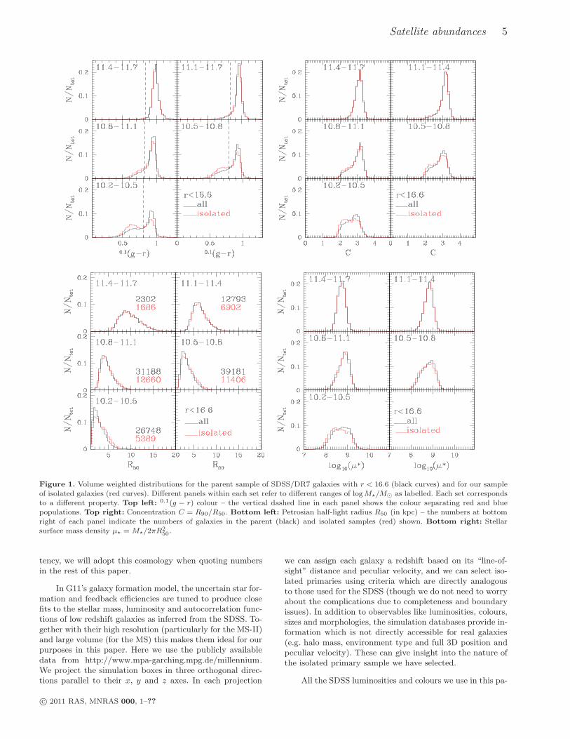
Figure 1 compares the distributions of colour, Petrosianhalf-light radius R50, concentration C = R90/R50 and stellarsurface mass density µ⋆ = M⋆/2πR

250 for our parent galaxy

sample (all 145070 galaxies with r < 16.6) and for our 41271isolated primaries, separated into bins of galaxy stellar mass.These quantities were taken directly from the NYU-VAGCcatalogue. The stellar masses were estimated by fitting stel-lar population synthesis models to the K-corrected galaxycolours assuming a Chabrier (2003) initial mass function asin Blanton & Roweis (2007). The sensitivity of the stellarmasses to assumptions underlying the estimation techniqueis explored in the Appendix of Li & White (2009). Each stel-lar mass bin is a factor of two wide, and we show data forthe five mass bins on which we will concentrate our analy-sis throughout the rest of this paper. The numbers in thelower right of the R50 plots indicate the number of isolatedprimaries in each mass bin. Volume corrections have beenapplied to all the histograms in this figure by calculatingthe total volume Vmax of the survey over which each indi-vidual galaxy would be brighter than the flux limit, r = 16.6,and accumulating counts weighted by 1/Vmax. It turns outthat our isolated primaries are slightly bluer than the par-ent sample, particularly at low masses. In addition, they areslightly more concentrated than the parent sample. Our se-lection procedure appears to have no significant effect onthe distributions of the other two properties, and the sameis true for the redshift distributions which we do not show.To a very good approximation our isolated primary galax-ies are typical objects of their stellar mass, although as wewill see below, our selection has a strong influence on theirrelation to their environment. Vertical dashed lines in thecolour plots indicate the split we adopt when separating ourprimaries into red and blue populations. This split is slightlydependent on stellar mass.

2.2 The mock catalogue

In the analysis and interpretation of our results for satellitegalaxy populations we will make considerable use of mockcatalogues built from the galaxy formation simulations ofGuo et al. (2011, hereafter G11). These are implementedon two very large dark matter simulations, the MillenniumSimulation (MS; Springel et al. 2005) and the Millennium-II Simulation (MS-II; Boylan-Kolchin et al. 2009). The MSfollows the evolution of structure within a cube of side500h−1Mpc (comoving) and its merger trees are complete forsubhaloes above a mass resolution limit of 1.7×1010h−1M⊙.The MS-II follows a cube of side 100h−1Mpc but with125 times better mass resolution (subhalo masses greaterthan 1.4 × 108h−1M⊙). Both adopt the same WMAP1-based ΛCDM cosmology (Spergel et al. 2003) with param-eters h = 0.73,Ωm = 0.25,ΩΛ = 0.75, n = 1 and σ8 = 0.9.These are outside the region preferred by more recent anal-yses (in particular, σ8 appears too high) but this is of noconsequence for the issues we study in this paper. For consis-

c© 2011 RAS, MNRAS 000, 1–??

Satellite abundances 5

Figure 1. Volume weighted distributions for the parent sample of SDSS/DR7 galaxies with r < 16.6 (black curves) and for our sampleof isolated galaxies (red curves). Different panels within each set refer to different ranges of logM⋆/M⊙ as labelled. Each set correspondsto a different property. Top left: 0.1(g − r) colour – the vertical dashed line in each panel shows the colour separating red and bluepopulations. Top right: Concentration C = R90/R50. Bottom left: Petrosian half-light radius R50 (in kpc) – the numbers at bottomright of each panel indicate the numbers of galaxies in the parent (black) and isolated samples (red) shown. Bottom right: Stellarsurface mass density µ⋆ = M⋆/2πR2

50.

tency, we will adopt this cosmology when quoting numbersin the rest of this paper.

In G11’s galaxy formation model, the uncertain star for-mation and feedback efficiencies are tuned to produce closefits to the stellar mass, luminosity and autocorrelation func-tions of low redshift galaxies as inferred from the SDSS. To-gether with their high resolution (particularly for the MS-II)and large volume (for the MS) this makes them ideal for ourpurposes in this paper. Here we use the publicly availabledata from http://www.mpa-garching.mpg.de/millennium.We project the simulation boxes in three orthogonal direc-tions parallel to their x, y and z axes. In each projection

we can assign each galaxy a redshift based on its “line-of-sight” distance and peculiar velocity, and we can select iso-lated primaries using criteria which are directly analogousto those used for the SDSS (though we do not need to worryabout the complications due to completeness and boundaryissues). In addition to observables like luminosities, colours,sizes and morphologies, the simulation databases provide in-formation which is not directly accessible for real galaxies(e.g. halo mass, environment type and full 3D position andpeculiar velocity). These can give insight into the nature ofthe isolated primary sample we have selected.

All the SDSS luminosities and colours we use in this pa-

c© 2011 RAS, MNRAS 000, 1–??

6 Wang et al.

per are rest-frame quantities K-corrected to the 0.1r band.The absolute magnitudes in our mock catalogues are in thetrue z = 0 r band, because this is what is directly pro-vided by the database and the difference between the 0.1rand r bands is too small to significantly affect luminosities.We do, however, transform the database (g − r) colours tothe 0.1(g − r) band using the empirical fitting formula ofBlanton & Roweis (2007) because here the shifts seem largeenough to cause (minor) differences.

Structure in the MS and MS-II is characterized us-ing Friends-of Friends (FoF) groups partitioned into setsof disjoint self-bound subhaloes. The subhalo populationsat neighboring output times are linked to build merger treeswhich record the assembly history of all nonlinear structuresand provide the framework for the galaxy formation simu-lations. In these simulations galaxy evolution is affected byenvironment in several ways. The galaxy at the centre ofthe most massive subhalo of each FoF group (which usuallycontains most of its mass) is considered the “central galaxy”and is the only one to accrete material from the diffuse gasassociated with the group. When evolution joins two FoFgroups, G11 continue to treat the galaxy at the centre of theless massive subhalo as a central galaxy until it falls withinthe nominal virial radius2 of the new FoF group. After thispoint the infalling galaxy is considered as a “satellite”, themass of its dark halo starts dropping as a result of tidalstripping, and its diffuse gas is assumed to be removed inproportion to the subhalo dark matter. Such satellites maylater lose their subhaloes entirely through tidal disruption.At this point they are either disrupted themselves or (morecommonly) they become “orphan satellites” which continueto orbit until dynamical friction causes a merger with theircentral galaxy. In this paper we will follow G11, consideringtogether the two kinds of satellites (with and without a darkmatter subhalo) and the two kinds of centrals (in dominantand in newly accreted, distant subhaloes).

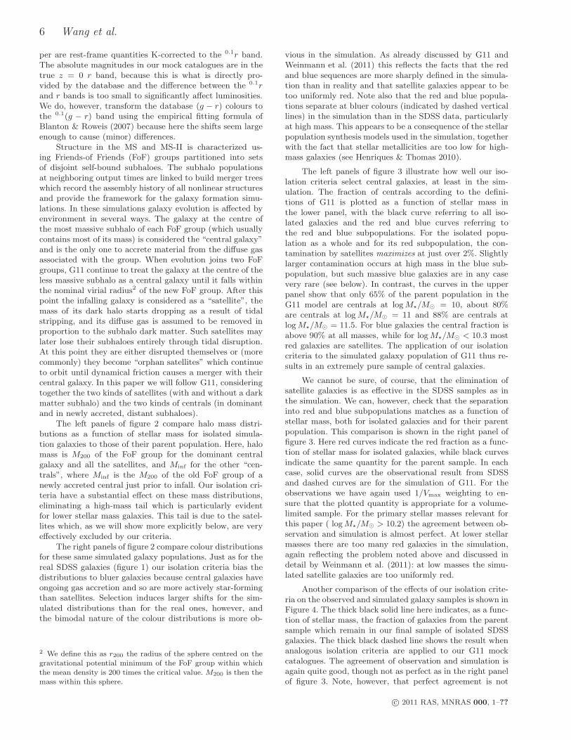
The left panels of figure 2 compare halo mass distri-butions as a function of stellar mass for isolated simula-tion galaxies to those of their parent population. Here, halomass is M200 of the FoF group for the dominant centralgalaxy and all the satellites, and Minf for the other “cen-trals”, where Minf is the M200 of the old FoF group of anewly accreted central just prior to infall. Our isolation cri-teria have a substantial effect on these mass distributions,eliminating a high-mass tail which is particularly evidentfor lower stellar mass galaxies. This tail is due to the satel-lites which, as we will show more explicitly below, are veryeffectively excluded by our criteria.

The right panels of figure 2 compare colour distributionsfor these same simulated galaxy populations. Just as for thereal SDSS galaxies (figure 1) our isolation criteria bias thedistributions to bluer galaxies because central galaxies haveongoing gas accretion and so are more actively star-formingthan satellites. Selection induces larger shifts for the sim-ulated distributions than for the real ones, however, andthe bimodal nature of the colour distributions is more ob-

2 We define this as r200 the radius of the sphere centred on thegravitational potential minimum of the FoF group within whichthe mean density is 200 times the critical value. M200 is then themass within this sphere.

vious in the simulation. As already discussed by G11 andWeinmann et al. (2011) this reflects the facts that the redand blue sequences are more sharply defined in the simula-tion than in reality and that satellite galaxies appear to betoo uniformly red. Note also that the red and blue popula-tions separate at bluer colours (indicated by dashed verticallines) in the simulation than in the SDSS data, particularlyat high mass. This appears to be a consequence of the stellarpopulation synthesis models used in the simulation, togetherwith the fact that stellar metallicities are too low for high-mass galaxies (see Henriques & Thomas 2010).

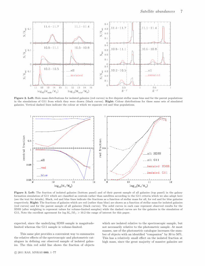
The left panels of figure 3 illustrate how well our iso-lation criteria select central galaxies, at least in the sim-ulation. The fraction of centrals according to the defini-tions of G11 is plotted as a function of stellar mass inthe lower panel, with the black curve referring to all iso-lated galaxies and the red and blue curves referring tothe red and blue subpopulations. For the isolated popu-lation as a whole and for its red subpopulation, the con-tamination by satellites maximizes at just over 2%. Slightlylarger contamination occurs at high mass in the blue sub-population, but such massive blue galaxies are in any casevery rare (see below). In contrast, the curves in the upperpanel show that only 65% of the parent population in theG11 model are centrals at logM⋆/M⊙ = 10, about 80%are centrals at logM⋆/M⊙ = 11 and 88% are centrals atlogM⋆/M⊙ = 11.5. For blue galaxies the central fraction isabove 90% at all masses, while for logM⋆/M⊙ < 10.3 mostred galaxies are satellites. The application of our isolationcriteria to the simulated galaxy population of G11 thus re-sults in an extremely pure sample of central galaxies.

We cannot be sure, of course, that the elimination ofsatellite galaxies is as effective in the SDSS samples as inthe simulation. We can, however, check that the separationinto red and blue subpopulations matches as a function ofstellar mass, both for isolated galaxies and for their parentpopulation. This comparison is shown in the right panel offigure 3. Here red curves indicate the red fraction as a func-tion of stellar mass for isolated galaxies, while black curvesindicate the same quantity for the parent sample. In eachcase, solid curves are the observational result from SDSSand dashed curves are for the simulation of G11. For theobservations we have again used 1/Vmax weighting to en-sure that the plotted quantity is appropriate for a volume-limited sample. For the primary stellar masses relevant forthis paper ( logM⋆/M⊙ > 10.2) the agreement between ob-servation and simulation is almost perfect. At lower stellarmasses there are too many red galaxies in the simulation,again reflecting the problem noted above and discussed indetail by Weinmann et al. (2011): at low masses the simu-lated satellite galaxies are too uniformly red.

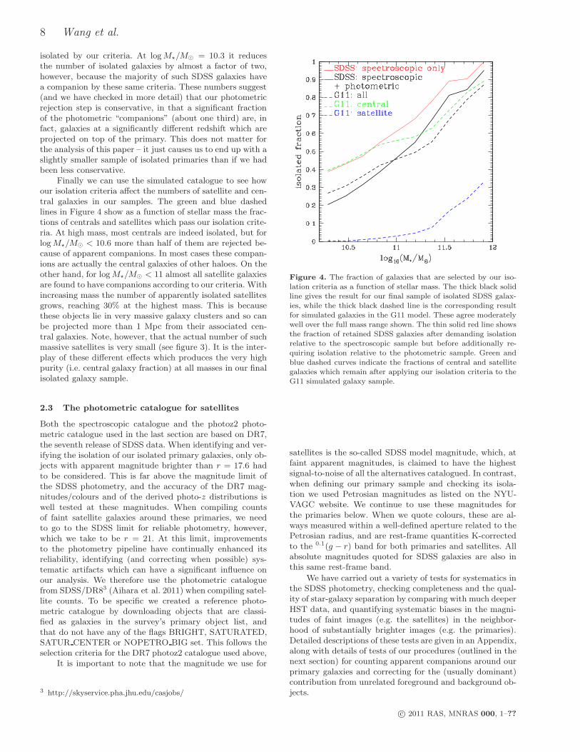
Another comparison of the effects of our isolation crite-ria on the observed and simulated galaxy samples is shown inFigure 4. The thick black solid line here indicates, as a func-tion of stellar mass, the fraction of galaxies from the parentsample which remain in our final sample of isolated SDSSgalaxies. The thick black dashed line shows the result whenanalogous isolation criteria are applied to our G11 mockcatalogues. The agreement of observation and simulation isagain quite good, though not as perfect as in the right panelof figure 3. Note, however, that perfect agreement is not

c© 2011 RAS, MNRAS 000, 1–??

Satellite abundances 7

Figure 2. Left: Halo mass distributions for isolated galaxies (red curves) in five disjoint stellar mass bins and for the parent populationsin the simulations of G11 from which they were drawn (black curves). Right: Colour distributions for these same sets of simulatedgalaxies. Vertical dashed lines indicate the colour at which we separate red and blue populations.

Figure 3. Left: The fraction of isolated galaxies (bottom panel) and of their parent sample of all galaxies (top panel) in the galaxyformation simulation of G11 which are classified as centrals rather than satellites according to the G11 criteria which we also adopt here(see the text for details). Black, red and blue lines indicate the fractions as a function of stellar mass for all, for red and for blue galaxiesrespectively. Right: The fractions of galaxies which are red (rather than blue) are shown as a function of stellar mass for isolated galaxies(red curves) and for the parent sample of all galaxies (black curves). The solid curves in each case represent observed results for theSDSS (after weighting to represent values for volume-limited samples) while the dashed curves are for the galaxies in the simulation ofG11, Note the excellent agreement for logM⋆/M⊙ > 10.2 the range of interest for this paper.

expected, since the underlying SDSS sample is magnitude-limited whereas the G11 sample is volume-limited.

This same plot provides a convenient way to summariesthe relative effects of the spectroscopic and photometric cat-alogues in defining our observed sample of isolated galax-ies. The thin red solid line shows the fraction of objects

which are isolated relative to the spectroscopic sample, butnot necessarily relative to the photometric sample. At mostmasses, use of the photometric catalogue increases the num-ber of objects with an identified “companion” by 30 to 50%.This has a relatively small effect on the isolated fraction athigh mass, since the great majority of massive galaxies are

c© 2011 RAS, MNRAS 000, 1–??

8 Wang et al.

isolated by our criteria. At logM⋆/M⊙ = 10.3 it reducesthe number of isolated galaxies by almost a factor of two,however, because the majority of such SDSS galaxies havea companion by these same criteria. These numbers suggest(and we have checked in more detail) that our photometricrejection step is conservative, in that a significant fractionof the photometric “companions” (about one third) are, infact, galaxies at a significantly different redshift which areprojected on top of the primary. This does not matter forthe analysis of this paper – it just causes us to end up with aslightly smaller sample of isolated primaries than if we hadbeen less conservative.

Finally we can use the simulated catalogue to see howour isolation criteria affect the numbers of satellite and cen-tral galaxies in our samples. The green and blue dashedlines in Figure 4 show as a function of stellar mass the frac-tions of centrals and satellites which pass our isolation crite-ria. At high mass, most centrals are indeed isolated, but forlogM⋆/M⊙ < 10.6 more than half of them are rejected be-cause of apparent companions. In most cases these compan-ions are actually the central galaxies of other haloes. On theother hand, for logM⋆/M⊙ < 11 almost all satellite galaxiesare found to have companions according to our criteria. Withincreasing mass the number of apparently isolated satellitesgrows, reaching 30% at the highest mass. This is becausethese objects lie in very massive galaxy clusters and so canbe projected more than 1 Mpc from their associated cen-tral galaxies. Note, however, that the actual number of suchmassive satellites is very small (see figure 3). It is the inter-play of these different effects which produces the very highpurity (i.e. central galaxy fraction) at all masses in our finalisolated galaxy sample.

2.3 The photometric catalogue for satellites

Both the spectroscopic catalogue and the photoz2 photo-metric catalogue used in the last section are based on DR7,the seventh release of SDSS data. When identifying and ver-ifying the isolation of our isolated primary galaxies, only ob-jects with apparent magnitude brighter than r = 17.6 hadto be considered. This is far above the magnitude limit ofthe SDSS photometry, and the accuracy of the DR7 mag-nitudes/colours and of the derived photo-z distributions iswell tested at these magnitudes. When compiling countsof faint satellite galaxies around these primaries, we needto go to the SDSS limit for reliable photometry, however,which we take to be r = 21. At this limit, improvementsto the photometry pipeline have continually enhanced itsreliability, identifying (and correcting when possible) sys-tematic artifacts which can have a significant influence onour analysis. We therefore use the photometric cataloguefrom SDSS/DR83 (Aihara et al. 2011) when compiling satel-lite counts. To be specific we created a reference photo-metric catalogue by downloading objects that are classi-fied as galaxies in the survey’s primary object list, andthat do not have any of the flags BRIGHT, SATURATED,SATUR CENTER or NOPETRO BIG set. This follows theselection criteria for the DR7 photoz2 catalogue used above,

It is important to note that the magnitude we use for

3 http://skyservice.pha.jhu.edu/casjobs/

Figure 4. The fraction of galaxies that are selected by our iso-lation criteria as a function of stellar mass. The thick black solidline gives the result for our final sample of isolated SDSS galax-ies, while the thick black dashed line is the corresponding resultfor simulated galaxies in the G11 model. These agree moderatelywell over the full mass range shown. The thin solid red line showsthe fraction of retained SDSS galaxies after demanding isolationrelative to the spectroscopic sample but before additionally re-quiring isolation relative to the photometric sample. Green andblue dashed curves indicate the fractions of central and satellitegalaxies which remain after applying our isolation criteria to theG11 simulated galaxy sample.

satellites is the so-called SDSS model magnitude, which, atfaint apparent magnitudes, is claimed to have the highestsignal-to-noise of all the alternatives catalogued. In contrast,when defining our primary sample and checking its isola-tion we used Petrosian magnitudes as listed on the NYU-VAGC website. We continue to use these magnitudes forthe primaries below. When we quote colours, these are al-ways measured within a well-defined aperture related to thePetrosian radius, and are rest-frame quantities K-correctedto the 0.1(g − r) band for both primaries and satellites. Allabsolute magnitudes quoted for SDSS galaxies are also inthis same rest-frame band.

We have carried out a variety of tests for systematics inthe SDSS photometry, checking completeness and the qual-ity of star-galaxy separation by comparing with much deeperHST data, and quantifying systematic biases in the magni-tudes of faint images (e.g. the satellites) in the neighbor-hood of substantially brighter images (e.g. the primaries).Detailed descriptions of these tests are given in an Appendix,along with details of tests of our procedures (outlined in thenext section) for counting apparent companions around ourprimary galaxies and correcting for the (usually dominant)contribution from unrelated foreground and background ob-jects.

c© 2011 RAS, MNRAS 000, 1–??

Satellite abundances 9

3 SATELLITE COUNTING METHODOLOGY

We want to study the abundance of satellites as a func-tion of their luminosity, stellar mass and colour around oursample of isolated bright primaries, and to see how theseabundances depend on the stellar mass and colour of theprimary. We will need to use the SDSS data down to theirreliable photometric limit (which we take to be r = 21) andas a result the great majority of the potential satellites donot have a spectroscopically measured redshift. Hence it isnecessary to count all apparent neighbours around our pri-maries and to correct statistically for unassociated objectswhich happen to be projected near them. The number ofsuch (mainly) background objects can substantially exceedthe number of true satellites, so it is important to take con-siderable care in making these corrections. We adopt thefollowing procedure.

For each isolated bright galaxy, we identify all photo-metric galaxies with apparent projected separation rp <0.5 Mpc and we accumulate counts in bins of projected sep-aration rp, apparent magnitude r and observed colour g−r.From the count in each (rp,r,g − r) bin, we subtract theexpected number of background galaxies which we take tobe N(r, g − r)A(rp, z)f/Atot, where N(r, g − r) is the totalnumber of galaxies in the (r,g− r) bin in the full photomet-ric catalogue, Atot is the solid angle of the survey footprint,A(rp, zpri) is the solid angle corresponding to the annular rpbin at the redshift zpri of the primary galaxy, and f is theincompleteness factor, the fraction of this annulus which lieswithin the survey footprint (we estimate this using the ran-dom points generated around the position of each primaryduring the selection process – see above). We then use theredshift of the primary galaxy to convert observed appar-ent magnitudes and colours into rest-frame luminosities andcolours (in the 0.1r and 0.1(g − r) system)4 and we transferthe background-subtracted satellite counts from our narrowbins of r and g−r into substantially broader bins of the rest-frame quantities. Finally we average these counts for eachrp bin over the set of all primaries in the desired range ofstellar mass (and sometimes colour) and we sum the resultover the desired range in rp. Uncertainties in the resultingnumbers are estimated from the scatter among results for100 bootstrap resamplings of the set of primaries.

Some apparent companions are too red to be at the red-shift of the primary galaxy. It is useful to exclude them whenaccumulating counts since they add noise without addingsignal. Hence, we exclude all bins redder than 0.1(g − r) =0.032log10M⋆+0.73, a fit to the upper envelope of the distri-bution of rest-frame colour against stellar mass for galaxiesof measured redshift. The stellar mass M⋆ of the apparentcompanion is estimated by assuming it to be at the primary’sredshift and adopting

(M/L)r = −1.08190.1(g−r)2+4.11830.1(g−r)−0.7837 (1)

This empirical relation is a fit to a flux-limited(r < 17.6) galaxy sample from the NYU-VAGC web-site for which stellar masses were estimated from the K-corrected galaxy colours by fitting stellar population synthe-

4 We use the empirical fitting formula of Westra et al. (2010)which gives the K-correction as a function of redshift and observedcolour.

sis models assuming a Chabrier (2003) initial mass function(Blanton & Roweis 2007). For this sample the 1-σ scatter in(M/L)r of this simple relation is about 0.1.

The photometric catalogue we use is complete down toan r-band apparent model magnitude of 21. This limit cor-responds, of course, to different satellite luminosities andstellar masses for different primary redshifts and differentsatellite colours. In order to ensure that our samples arecomplete when compiling satellite luminosity functions, weallow a particular primary to contribute counts to a partic-ular luminosity bin only if the K-corrected absolute lumi-nosity corresponding to r = 21 for a galaxy at the redshiftof the primary and lying on the red envelope of the intrinsiccolour distribution is fainter than the lower luminosity limitof the bin. Thus only the nearest primaries will contribute tothe faintest luminosity bins of our satellite luminosity func-tions, and different numbers of primaries will contribute toeach bin. We follow an exactly analogous procedure whencompiling stellar mass functions for satellites.

For each individual satellite luminosity/stellar mass bin,this treatment is equivalent to imposing an upper limit onprimary redshift. Thus there is a maximum volume which issurveyed for satellites in the jth luminosity/stellar mass binwhich we denote Vmax,bin,j .

On the other hand, our primary sample is flux-limitedat r = 16.6, so for brighter satellite bins where Vmax,bin,j

is large, intrinsically faint primaries will not be visible tothe redshift limit. The effective volume surveyed is thenVmax,pri,i, the total survey volume over which the ith pri-mary would lie above the flux limit. Note that because ofK-corrections, this volume depends on the intrinsic colourof the primary as well as its intrinsic luminosity. We presentour final results in the form of the mean number of satellitesper primary for a volume-limited primary sample

Nsat,j =ΣiNsat,i,j/Vmax,ij

Σi1/Vmax,ij

, (2)

where

Vmax,ij = min[

Vmax,pri,i, Vmax,bin,j

]

. (3)

Thus, for satellite luminosity/stellar mass bin j, we sumsatellite counts over all primaries i that are within Vmax,bin,j .At the bright end of the satellite luminosity function, weexpect Vmax,ij = Vmax,pri,i because satellites are less than4.4 magnitudes fainter than their primaries and so can beseen around all primaries. For intrinsically faint satellites,however, Vmax,ij = Vmax,bin,j because primaries can be seento well beyond the distance at which r = 21 for the satellites.

We apply similar selection criteria to our mock cata-logues based on G11. Since we know the absolute magni-tude, rest-frame colour and stellar mass of all galaxies, thebackground subtraction can be carried out directly usingrest-frame quantities. In addition, the effective depth of thesatellite catalogue is the same for all primaries so that allprimaries can contribute to all satellite luminosity or stellarmass bins and we do not need any weighting in order to ob-tain proper volume-weighted statistics. Note that we do notuse any information about the redshift difference betweenprimary and apparent companion, so projection effects oc-cur over ∆z = 50, 000 km/s corresponding to the side of theMillennium Simulation “box”. Both for the simulation andfor the real SDSS data we use a global background estimate

c© 2011 RAS, MNRAS 000, 1–??

10 Wang et al.

based on the full survey in order to minimize the statisticaluncertainty in the correction.

Previous work often estimated a background density lo-cally for each primary (e.g. Lorrimer et al. 1994; Guo et al.2011). This not only substantially increases the noise, it alsointroduces a significant bias since galaxies are correlated onall scales and the “background” fields are, in fact, expectedto have faint galaxy densities significantly above the mean.The extent of the bias is, in fact, strongly dependent on theisolation criteria and can be of either sign (see, for exam-ple, Fall et al. 1976). The large-scale uniformity of the SDSSphotometry is such that there appears to be no advantage toadopt a local estimate, provided all photometric quantitiesare properly corrected for Galactic extinction. The accuracyof our method is confirmed by the accurate convergence tounity at large angular scale in the left panel of figure A1and by a variety of tests which we describe in detail in theAppendix.

4 LUMINOSITY AND MASS FUNCTIONS OF

SATELLITE GALAXIES

4.1 Luminosity functions

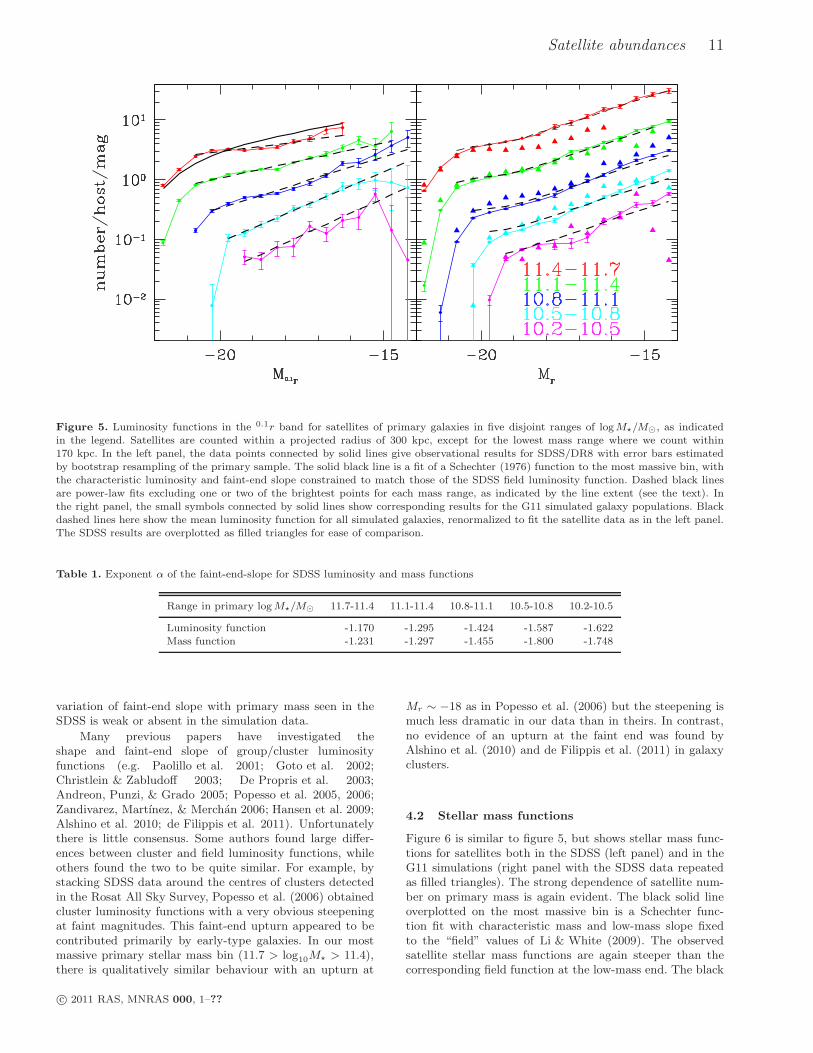
In figure 5 we present 0.1r-band luminosity functions forsatellites projected within 300 kpc of their primaries, exceptfor the faintest bin, where the halo virial radius is muchsmaller than 300 kpc and we estimate the luminosity func-tion within 170 kpc in order to increase the signal-to-noise.In the left panel, data points connected by solid lines showour observational results for SDSS/DR8. As indicated in thelegend, colours encode the range in logM⋆/M⊙ of the pri-maries contributing to each luminosity function estimate.Error bars are derived by bootstrap resampling the primarysample. At the faint end we lose higher redshift primariesbecause of the apparent magnitude limit of our photomet-ric catalogue. We do not plot data for bins with fewer thaneight primaries. It is evident that satellite numbers increasestrongly with primary mass.

The black solid line in the left panel shows a Schechter(1976) function fit to the data for the most massive pri-maries. We have fixed the characteristic luminosity andfaint-end slope to be those of the SDSS field luminosity func-tion in 0.1r (Montero-Dorta & Prada 2009). The result is amoderately good fit to the satellite data, although these ap-pear steeper than the field luminosity function at the faintestmagnitudes. The satellite luminosity functions clearly be-come steeper for lower mass primaries. Power-law fits tothe faint-end data are shown as dashed lines in the figureand give the slopes α listed in the first row of table 1. Thebright end of each function is cut off by our requirementthat every satellite be at least one magnitude fainter thanits primary. We therefore exclude one or two of the brightestpoints when making these fits. Specifically, we find the me-dian absolute magnitude Mmed for primaries in each massrange, and we include only points for which the correspond-ing absolute magnitude bin lies entirely below Mmed+1. Theranges fitted in each case are indicated by the extents of thedashed black straight lines.5 The faint-end slope decreases

5 We have checked that the remaining points are indeed unaf-

from α ∼ −1.2 for logM⋆,p/M⊙ ∼ 11.5 to α ∼ −1.6 forlogM⋆,p/M⊙ ∼ 10.3.

Guo et al. (2011) divided their primaries into threeluminosity ranges (Mr = −23.0 ± 0.5, −23.0 ± 0.5 and−23.0 ± 0.5) and compiled satellite luminosity functions inbins of satellite-primary magnitude difference rather thansatellite absolute magnitude. They quote faint-end slopes of-1.45, -1.725 and -1.96 for these three sets of primaries, withthe fainter primaries having steeper luminosity functions.For the largest measured magnitude differences (∆m ∼ 8)they found similar numbers of satellites independent of pri-mary luminosity. These α values are substantially more neg-ative than ours, particularly for the faintest primaries. In or-der to compare with their results, we adopt similar isolationcriteria, we take the same ranges of primary luminosity, andwe also accumulate satellite number as a function of mag-nitude difference. Fitting the faint-end slope over the samesatellite magnitude range as in figure 7 of Guo et al. (2011),we find α values of -1.189, -1.376 and -1.588, substantiallyshallower than those of Guo et al. (2011) and quite com-patible with those we quote in Table 1. Detailed tests showthis inconsistency to be due partly to the local backgroundsubtraction scheme of Guo et al. (2011) which removes partof the signal 6, but mainly to the fact that they use modelmagnitudes K-corrected to z = 0 for their primaries, ratherthan the 0.1r Petrosian magnitudes which we use here.

In the right panel of figure 5, the small symbolsjoined by solid lines show analogous results for the galaxyformation model of G11, based on the Millennium andMillennium-II simulations. Points brighter than Mr = −18are MS data. At fainter magnitudes, resolution effects causethe MS to underestimate galaxy abundances and we take ourdata from the MS-II. (The two simulations agree very well inthe range −18 > Mr > −20.) To facilitate comparison, wereplot the SDSS data from the left panel as filled triangles.Agreement of model and observation is fair but far fromperfect. The simulation overpredicts the number of satel-lites around the most massive primaries by 25 to 50% forMr > −19.5. In the two lower primary stellar mass ranges,the simulation underpredicts the number of satellites by 20to 30% . As we will see below, the latter discrepancy reflectsa problem with the colours of the simulated satellites ratherthan with their stellar masses. The black dashed lines in thispanel are the “field” luminosity function for the full simula-tions renormalized to fit the satellite data for each primarymass range. Here also there is a trend for the faint-end slopeto be steeper for satellites than in the field, but the effect ismuch less marked than for the SDSS data. Furthermore the

fected by rebinning our data as a function of the r-band absolutemagnitude of the primaries. In this case we know exactly whichbins are unaffected by our isolation criterion. When primary abso-lute magnitude and stellar mass are matched appropriately, theresulting satellite luminosity functions match those of figure 5very closely over the full range used to determine the faint-endslope and are unaffected by the isolation criterion over this range.6 Guo et al. (2011) used photometry from SDSS/DR7 while ourown tests, similar to those discussed in section A1 of the Ap-pendix, showed to suffer from substantially more serious system-atics for faint images close to brighter ones than is the case forthe SDSS/DR8 catalogues used here.

c© 2011 RAS, MNRAS 000, 1–??

Satellite abundances 11

Figure 5. Luminosity functions in the 0.1r band for satellites of primary galaxies in five disjoint ranges of logM⋆/M⊙, as indicatedin the legend. Satellites are counted within a projected radius of 300 kpc, except for the lowest mass range where we count within170 kpc. In the left panel, the data points connected by solid lines give observational results for SDSS/DR8 with error bars estimatedby bootstrap resampling of the primary sample. The solid black line is a fit of a Schechter (1976) function to the most massive bin, withthe characteristic luminosity and faint-end slope constrained to match those of the SDSS field luminosity function. Dashed black linesare power-law fits excluding one or two of the brightest points for each mass range, as indicated by the line extent (see the text). Inthe right panel, the small symbols connected by solid lines show corresponding results for the G11 simulated galaxy populations. Blackdashed lines here show the mean luminosity function for all simulated galaxies, renormalized to fit the satellite data as in the left panel.The SDSS results are overplotted as filled triangles for ease of comparison.

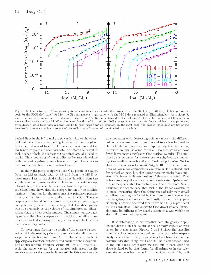
Table 1. Exponent α of the faint-end-slope for SDSS luminosity and mass functions

Range in primary logM⋆/M⊙ 11.7-11.4 11.1-11.4 10.8-11.1 10.5-10.8 10.2-10.5

Luminosity function -1.170 -1.295 -1.424 -1.587 -1.622Mass function -1.231 -1.297 -1.455 -1.800 -1.748

variation of faint-end slope with primary mass seen in theSDSS is weak or absent in the simulation data.

Many previous papers have investigated theshape and faint-end slope of group/cluster luminosityfunctions (e.g. Paolillo et al. 2001; Goto et al. 2002;Christlein & Zabludoff 2003; De Propris et al. 2003;Andreon, Punzi, & Grado 2005; Popesso et al. 2005, 2006;Zandivarez, Martınez, & Merchan 2006; Hansen et al. 2009;Alshino et al. 2010; de Filippis et al. 2011). Unfortunatelythere is little consensus. Some authors found large differ-ences between cluster and field luminosity functions, whileothers found the two to be quite similar. For example, bystacking SDSS data around the centres of clusters detectedin the Rosat All Sky Survey, Popesso et al. (2006) obtainedcluster luminosity functions with a very obvious steepeningat faint magnitudes. This faint-end upturn appeared to becontributed primarily by early-type galaxies. In our mostmassive primary stellar mass bin (11.7 > log10M⋆ > 11.4),there is qualitatively similar behaviour with an upturn at

Mr ∼ −18 as in Popesso et al. (2006) but the steepening ismuch less dramatic in our data than in theirs. In contrast,no evidence of an upturn at the faint end was found byAlshino et al. (2010) and de Filippis et al. (2011) in galaxyclusters.

4.2 Stellar mass functions

Figure 6 is similar to figure 5, but shows stellar mass func-tions for satellites both in the SDSS (left panel) and in theG11 simulations (right panel with the SDSS data repeatedas filled triangles). The strong dependence of satellite num-ber on primary mass is again evident. The black solid lineoverplotted on the most massive bin is a Schechter func-tion fit with characteristic mass and low-mass slope fixedto the “field” values of Li & White (2009). The observedsatellite stellar mass functions are again steeper than thecorresponding field function at the low-mass end. The black

c© 2011 RAS, MNRAS 000, 1–??

12 Wang et al.

Figure 6. Similar to figure 5 but showing stellar mass functions for satellites projected within 300 kpc (or 170 kpc) of their primaries,both for the SDSS (left panel) and for the G11 simulations (right panel with the SDSS data repeated as filled triangles). As in figure 5,the primaries are grouped into five disjoint ranges of logM⋆/M⊙, as indicated by the colours. A black solid line in the left panel is arenormalized version of the “field” stellar mass function of Li & White (2009) overplotted on the data for the highest mass primaries,while dashed black lines show a power law fit to each mass function estimate. In the right panel the dashed black lines are fits of thesatellite data to renormalized versions of the stellar mass function of the simulation as a whole.

dashed lines in the left panel are power-law fits to the obser-vational data. The corresponding faint-end-slopes are givenin the second row of table 1. Here also we have ignored thefew brightest points in each estimate. As before the extent ofeach dashed black line indicates the points actually used inthe fit. The steepening of the satellite stellar mass functionswith decreasing primary mass is even stronger than was thecase for the satellite luminosity functions.

In the right panel of figure 6, the G11 points are takenfrom the MS at logM⋆/M⊙ > 9.5 and from the MS-II atlower mass. Fits to the field stellar mass function from thesimulations are shown as dashed lines and indicate no sig-nificant shape difference between the two. Comparison withthe SDSS data shows that the overprediction of the satelliteluminosity function for the most massive primaries persistsin very similar form in their stellar mass function, The un-derprediction found for the two lower primary mass rangeshas gone away, however, indicating that the discrepancywas due primarily to the colours of the simulated satellites,rather than to their stellar masses. The simulation does notreproduce the clear steepening of the SDSS satellite massfunctions with decreasing primary mass. Any effect in thisdirection is very weak.

To investigate further the origin of the observed steep-ening with decreasing primary mass, we take all spectro-scopic galaxies brighter than 16.6 in the r-band, withoutapplying any isolation criterion, and calculate the mass func-tion of surrounding satellites within 300 (or 170) kpc in ex-actly the same way as for our isolated primaries. Resultsare shown as solid curves in figure A6. In this case there is

no steepening with decreasing primary mass – the differentcolour curves are more or less parallel to each other and tothe field stellar mass function. Apparently, the steepeningis caused by our isolation criteria – isolated galaxies havefewer lower mass neighbours than typical galaxies. The sup-pression is stronger for more massive neighbours, steepen-ing the satellite mass functions of isolated primaries. Noticethat for primaries with logM⋆/M⊙ > 10.8, the mean num-bers of low-mass companions are similar for isolated andfor typical objects, but that lower mass primaries have sub-stantially fewer such companions if they are isolated. Thisis because many of the lower mass non-isolated ”primaries”are, in fact, satellites themselves, and their low-mass “com-panions” are fellow satellites within the larger system. Itis quite interesting that the abundance of relatively smallsatellites is strongly affected by the presence or absence of anearby galaxy comparable in luminosity to the primary, par-ticularly since the observed trends are not fully reproducedby the simulation. This suggests that dwarf galaxy forma-tion may be influenced by nearby giants in a way which thesimulation does not represent.

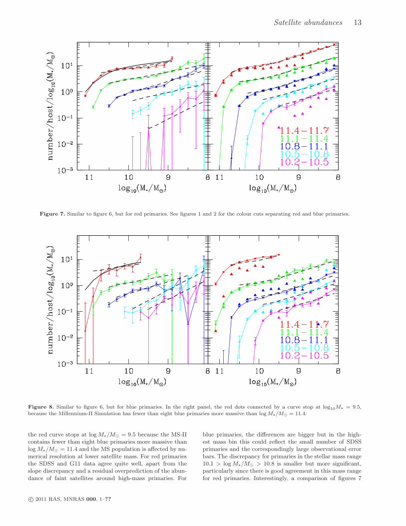
It is interesting to see whether satellite galaxy popu-lations depend on the colour of the primary galaxy as wellas on its stellar mass. Figures 7 and 8 show the satellitemass functions surrounding red and blue primaries respec-tively, where the primary populations have been split at thecolours indicated in figures 1 and 2. The black dashed linesin the left panels are power-law fits, but in each case theslope is fixed to be that found for all primaries in the rele-vant stellar mass bin (table 1). In the right panel of figure 8

c© 2011 RAS, MNRAS 000, 1–??

Satellite abundances 13

Figure 7. Similar to figure 6, but for red primaries. See figures 1 and 2 for the colour cuts separating red and blue primaries.

Figure 8. Similar to figure 6, but for blue primaries. In the right panel, the red dots connected by a curve stop at log10M⋆ = 9.5,because the Millennium-II Simulation has fewer than eight blue primaries more massive than logM⋆/M⊙ = 11.4.

the red curve stops at logM⋆/M⊙ = 9.5 because the MS-IIcontains fewer than eight blue primaries more massive thanlogM⋆/M⊙ = 11.4 and the MS population is affected by nu-merical resolution at lower satellite mass. For red primariesthe SDSS and G11 data agree quite well, apart from theslope discrepancy and a residual overprediction of the abun-dance of faint satellites around high-mass primaries. For

blue primaries, the differences are bigger but in the high-est mass bin this could reflect the small number of SDSSprimaries and the correspondingly large observational errorbars. The discrepancy for primaries in the stellar mass range10.1 > logM⋆/M⊙ > 10.8 is smaller but more significant,particularly since there is good agreement in this mass rangefor red primaries. Interestingly, a comparison of figures 7

c© 2011 RAS, MNRAS 000, 1–??

14 Wang et al.

and 8 shows that the amplitude of the satellite luminosityfunction is higher around red primaries than around blueprimaries of the same stellar mass. We analyze this result inmore detail in the following subsections.

4.3 Satellite abundance as a function of primary

stellar mass and colour

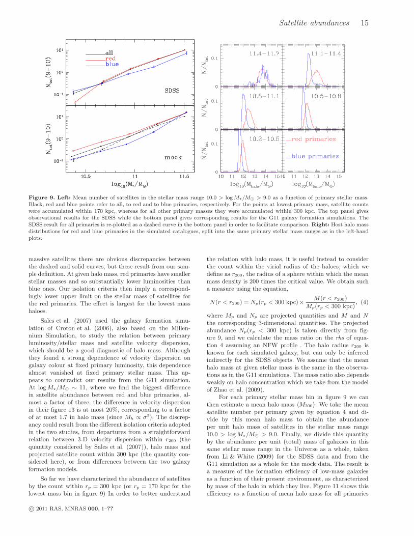
In order to better display how the abundance of satellitesdepends on the stellar mass and colour of the primary, we usethe power-law fits shown as dashed lines in figures 6, 7 and 8to predict the mean number of satellites per primary in thestellar mass range 10.0 > logM⋆/M⊙ > 9.0 and at projectedseparation rp < 300 kpc (rp < 170 kpc for the lowest massprimaries). This has the advantage of producing a robustmeasure of satellite abundance which is little affected eitherby selection-induced cut-offs (most important for low-massand red primaries) or by incompleteness (most importantfor high-mass and blue primaries). The results are shownin the left panels of figure 9, where black dots and linesgive results for all primaries, while red and blue dots andlines give results for red and blue primaries, respectively.The top panel presents results for the SDSS and the lowerpanel results for the G11 simulations. The SDSS result forall primaries is repeated in the lower panel, showing that thesimulation overpredicts the number of satellites in this massand projected radius range both for the highest mass andfor the lowest mass primaries. Note that because the low-mass slopes differ in simulation and observation, the resultfor low-mass primaries depends on the satellite mass rangechosen for the comparison.

At high mass the black and red curves in figure 9 areclose to each other, reflecting the fact that the fraction of redprimaries is large (see figure 3). At the highest mass, the bluecurve indicates a consistent number of satellites around blueprimaries, although with considerable uncertainty becausesuch primaries are rare. At somewhat lower mass, however,blue primaries have significantly fewer satellites than redprimaries of the same stellar mass, both in the SDSS dataand in the simulation. This is a primary result of our paper.The effect is a factor of two to three in satellite abundancefor primaries with logM⋆/M⊙ ∼ 11. In the SDSS data thereis some indication that the the colour dependence may getsmaller again for lower mass primaries, but this does nothappen in the simulation, where there is still more than afactor of two difference for M⋆ ∼ 2 × 1010M⊙. Overall, thedifferences appear somewhat larger in the model than in thereal data.

The cause of this effect in the G11 simulation is easyto track down. In the right-hand panels of figure 9 we plothistograms of host halo mass for isolated galaxies as a func-tion of their stellar mass and colour. (As shown in figure 3,almost all isolated galaxies in the simulation are the centralgalaxies of their haloes.) For all except the highest stellarmass range, red primaries have significantly more massivedark haloes than blue ones. The shift between the peaks ofthe two distribution is an order of magnitude for primarieswith 11.4 > logM⋆/M⊙ ∼ 11.1, dropping to a factor of twofor 10.5 > logM⋆/M⊙ ∼ 10.2. In the simulation red pri-maries have more satellites because they live in more mas-sive haloes. A direct indication that the same may hold forreal galaxies comes from the galaxy-galaxy lensing study of

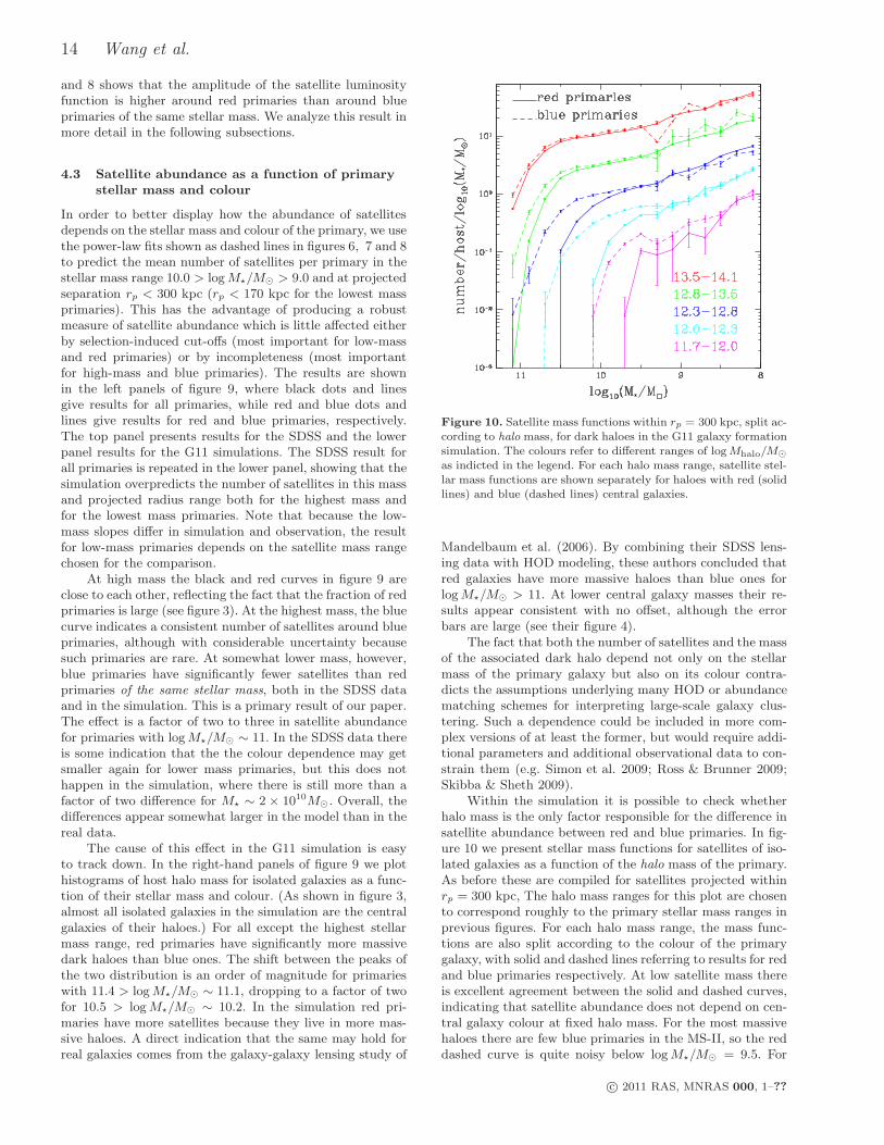
Figure 10. Satellite mass functions within rp = 300 kpc, split ac-cording to halo mass, for dark haloes in the G11 galaxy formationsimulation. The colours refer to different ranges of logMhalo/M⊙

as indicted in the legend. For each halo mass range, satellite stel-lar mass functions are shown separately for haloes with red (solidlines) and blue (dashed lines) central galaxies.

Mandelbaum et al. (2006). By combining their SDSS lens-ing data with HOD modeling, these authors concluded thatred galaxies have more massive haloes than blue ones forlogM⋆/M⊙ > 11. At lower central galaxy masses their re-sults appear consistent with no offset, although the errorbars are large (see their figure 4).

The fact that both the number of satellites and the massof the associated dark halo depend not only on the stellarmass of the primary galaxy but also on its colour contra-dicts the assumptions underlying many HOD or abundancematching schemes for interpreting large-scale galaxy clus-tering. Such a dependence could be included in more com-plex versions of at least the former, but would require addi-tional parameters and additional observational data to con-strain them (e.g. Simon et al. 2009; Ross & Brunner 2009;Skibba & Sheth 2009).

Within the simulation it is possible to check whetherhalo mass is the only factor responsible for the difference insatellite abundance between red and blue primaries. In fig-ure 10 we present stellar mass functions for satellites of iso-lated galaxies as a function of the halo mass of the primary.As before these are compiled for satellites projected withinrp = 300 kpc, The halo mass ranges for this plot are chosento correspond roughly to the primary stellar mass ranges inprevious figures. For each halo mass range, the mass func-tions are also split according to the colour of the primarygalaxy, with solid and dashed lines referring to results for redand blue primaries respectively. At low satellite mass thereis excellent agreement between the solid and dashed curves,indicating that satellite abundance does not depend on cen-tral galaxy colour at fixed halo mass. For the most massivehaloes there are few blue primaries in the MS-II, so the reddashed curve is quite noisy below logM⋆/M⊙ = 9.5. For

c© 2011 RAS, MNRAS 000, 1–??

Satellite abundances 15

Figure 9. Left: Mean number of satellites in the stellar mass range 10.0 > logM⋆/M⊙ > 9.0 as a function of primary stellar mass.Black, red and blue points refer to all, to red and to blue primaries, respectively. For the points at lowest primary mass, satellite countswere accumulated within 170 kpc, whereas for all other primary masses they were accumulated within 300 kpc. The top panel givesobservational results for the SDSS while the bottom panel gives corresponding results for the G11 galaxy formation simulations. TheSDSS result for all primaries is re-plotted as a dashed curve in the bottom panel in order to facilitate comparison. Right: Host halo massdistributions for red and blue primaries in the simulated catalogues, split into the same primary stellar mass ranges as in the left-handplots.

massive satellites there are obvious discrepancies betweenthe dashed and solid curves, but these result from our sam-ple definition. At given halo mass, red primaries have smallerstellar masses and so substantially lower luminosities thanblue ones. Our isolation criteria then imply a correspond-ingly lower upper limit on the stellar mass of satellites forthe red primaries. The effect is largest for the lowest masshaloes.

Sales et al. (2007) used the galaxy formation simu-lation of Croton et al. (2006), also based on the Millen-nium Simulation, to study the relation between primaryluminosity/stellar mass and satellite velocity dispersion,which should be a good diagnostic of halo mass. Althoughthey found a strong dependence of velocity dispersion ongalaxy colour at fixed primary luminosity, this dependencealmost vanished at fixed primary stellar mass. This ap-pears to contradict our results from the G11 simulation.At logM⋆/M⊙ ∼ 11, where we find the biggest differencein satellite abundance between red and blue primaries, al-most a factor of three, the difference in velocity dispersionin their figure 13 is at most 20%, corresponding to a factorof at most 1.7 in halo mass (since Mh ∝ σ3). The discrep-ancy could result from the different isolation criteria adoptedin the two studies, from departures from a straightforwardrelation between 3-D velocity dispersion within r200 (thequantity considered by Sales et al. (2007)), halo mass andprojected satellite count within 300 kpc (the quantity con-sidered here), or from differences between the two galaxyformation models.

So far we have characterized the abundance of satellitesby the count within rp = 300 kpc (or rp = 170 kpc for thelowest mass bin in figure 9) In order to better understand

the relation with halo mass, it is useful instead to considerthe count within the virial radius of the haloes, which wedefine as r200, the radius of a sphere within which the meanmass density is 200 times the critical value. We obtain sucha measure using the equation,

N(r < r200) = Np(rp < 300 kpc)×M(r < r200)

Mp(rp < 300 kpc), (4)

where Mp and Np are projected quantities and M and Nthe corresponding 3-dimensional quantities. The projectedabundance Np(rp < 300 kpc) is taken directly from fig-ure 9, and we calculate the mass ratio on the rhs of equa-tion 4 assuming an NFW profile . The halo radius r200 isknown for each simulated galaxy, but can only be inferredindirectly for the SDSS objects. We assume that the meanhalo mass at given stellar mass is the same in the observa-tions as in the G11 simulations. The mass ratio also dependsweakly on halo concentration which we take from the modelof Zhao et al. (2009).

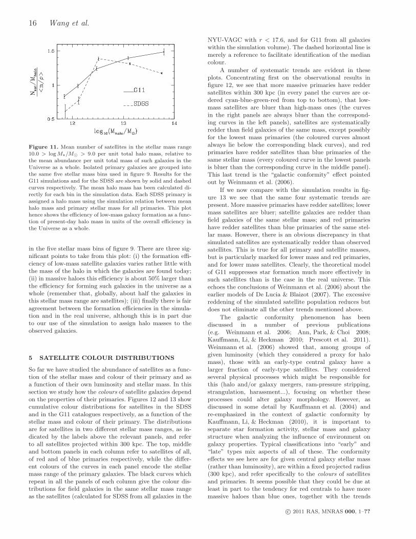
For each primary stellar mass bin in figure 9 we canthen estimate a mean halo mass 〈M200〉. We take the meansatellite number per primary given by equation 4 and di-vide by this mean halo mass to obtain the abundanceper unit halo mass of satellites in the stellar mass range10.0 > logM⋆/M⊙ > 9.0. Finally, we divide this quantityby the abundance per unit (total) mass of galaxies in thissame stellar mass range in the Universe as a whole, takenfrom Li & White (2009) for the SDSS data and from theG11 simulation as a whole for the mock data. The result isa measure of the formation efficiency of low-mass galaxiesas a function of their present environment, as characterizedby mass of the halo in which they live. Figure 11 shows thisefficiency as a function of mean halo mass for all primaries

c© 2011 RAS, MNRAS 000, 1–??

16 Wang et al.

Figure 11. Mean number of satellites in the stellar mass range10.0 > logM⋆/M⊙ > 9.0 per unit total halo mass, relative tothe mean abundance per unit total mass of such galaxies in theUniverse as a whole. Isolated primary galaxies are grouped intothe same five stellar mass bins used in figure 9. Results for theG11 simulations and for the SDSS are shown by solid and dashedcurves respectively. The mean halo mass has been calculated di-rectly for each bin in the simulation data. Each SDSS primary isassigned a halo mass using the simulation relation between meanhalo mass and primary stellar mass for all primaries. This plothence shows the efficiency of low-mass galaxy formation as a func-tion of present-day halo mass in units of the overall efficiency inthe Universe as a whole.

in the five stellar mass bins of figure 9. There are three sig-nificant points to take from this plot: (i) the formation effi-ciency of low-mass satellite galaxies varies rather little withthe mass of the halo in which the galaxies are found today;(ii) in massive haloes this efficiency is about 50% larger thanthe efficiency for forming such galaxies in the universe as awhole (remember that, globally, about half the galaxies inthis stellar mass range are satellites); (iii) finally there is fairagreement between the formation efficiencies in the simula-tion and in the real universe, although this is in part dueto our use of the simulation to assign halo masses to theobserved galaxies.

5 SATELLITE COLOUR DISTRIBUTIONS

So far we have studied the abundance of satellites as a func-tion of the stellar mass and colour of their primary and asa function of their own luminosity and stellar mass. In thissection we study how the colours of satellite galaxies dependon the properties of their primaries. Figures 12 and 13 showcumulative colour distributions for satellites in the SDSSand in the G11 catalogues respectively, as a function of thestellar mass and colour of their primary. The distributionsare for satellites in two different stellar mass ranges, as in-dicated by the labels above the relevant panels, and referto all satellites projected within 300 kpc. The top, middleand bottom panels in each column refer to satellites of all,of red and of blue primaries respectively, while the differ-ent colours of the curves in each panel encode the stellarmass range of the primary galaxies. The black curves whichrepeat in all the panels of each column give the colour dis-tributions for field galaxies in the same stellar mass rangeas the satellites (calculated for SDSS from all galaxies in the

NYU-VAGC with r < 17.6, and for G11 from all galaxieswithin the simulation volume). The dashed horizontal line ismerely a reference to facilitate identification of the mediancolour.

A number of systematic trends are evident in theseplots. Concentrating first on the observational results infigure 12, we see that more massive primaries have reddersatellites within 300 kpc (in every panel the curves are or-dered cyan-blue-green-red from top to bottom), that low-mass satellites are bluer than high-mass ones (the curvesin the right panels are always bluer than the correspond-ing curves in the left panels), satellites are systematicallyredder than field galaxies of the same mass, except possiblyfor the lowest mass primaries (the coloured curves almostalways lie below the corresponding black curves), and redprimaries have redder satellites than blue primaries of thesame stellar mass (every coloured curve in the lowest panelsis bluer than the corresponding curve in the middle panel).This last trend is the “galactic conformity” effect pointedout by Weinmann et al. (2006).

If we now compare with the simulation results in fig-ure 13 we see that the same four systematic trends arepresent. More massive primaries have redder satellites; lowermass satellites are bluer; satellite galaxies are redder thanfield galaxies of the same stellar mass; and red primarieshave redder satellites than blue primaries of the same stel-lar mass. However, there is an obvious discrepancy in thatsimulated satellites are systematically redder than observedsatellites. This is true for all primary and satellite masses,but is particularly marked for lower mass and red primaries,and for lower mass satellites. Clearly, the theoretical modelof G11 suppresses star formation much more effectively insuch satellites than is the case in the real universe. Thisechoes the conclusions of Weinmann et al. (2006) about theearlier models of De Lucia & Blaizot (2007). The excessivereddening of the simulated satellite population reduces butdoes not eliminate all the other trends mentioned above.

The galactic conformity phenomenon has beendiscussed in a number of previous publications(e.g. Weinmann et al. 2006; Ann, Park, & Choi 2008;Kauffmann, Li, & Heckman 2010; Prescott et al. 2011).Weinmann et al. (2006) showed that, among groups ofgiven luminosity (which they considered a proxy for halomass), those with an early-type central galaxy have alarger fraction of early-type satellites. They consideredseveral physical processes which might be responsible forthis (halo and/or galaxy mergers, ram-pressure stripping,strangulation, harassment...), focusing on whether theseprocesses could alter galaxy morphology. However, asdiscussed in some detail by Kauffmann et al. (2004) andre-emphasized in the context of galactic conformity byKauffmann, Li, & Heckman (2010), it is important toseparate star formation activity, stellar mass and galaxystructure when analyzing the influence of environment ongalaxy properties. Typical classifications into “early” and“late” types mix aspects of all of these. The conformityeffects we see here are for given central galaxy stellar mass(rather than luminosity), are within a fixed projected radius(300 kpc), and refer specifically to the colours of satellitesand primaries. It seems possible that they could be due atleast in part to the tendency for red centrals to have moremassive haloes than blue ones, together with the trends

c© 2011 RAS, MNRAS 000, 1–??

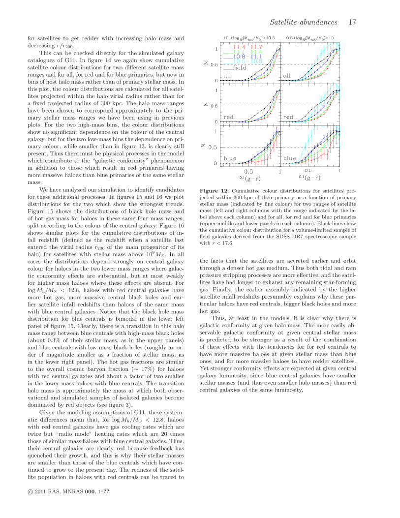
Satellite abundances 17

for satellites to get redder with increasing halo mass anddecreasing r/r200.

This can be checked directly for the simulated galaxycatalogues of G11. In figure 14 we again show cumulativesatellite colour distributions for two different satellite massranges and for all, for red and for blue primaries, but now inbins of host halo mass rather than of primary stellar mass. Inthis plot, the colour distributions are calculated for all satel-lites projected within the halo virial radius rather than fora fixed projected radius of 300 kpc. The halo mass rangeshave been chosen to correspond approximately to the pri-mary stellar mass ranges we have been using in previousplots. For the two high-mass bins, the colour distributionsshow no significant dependence on the colour of the centralgalaxy, but for the two low-mass bins the dependence on pri-mary colour, while smaller than in figure 13, is clearly stillpresent. Thus there must be physical processes in the modelwhich contribute to the “galactic conformity” phenomenonin addition to those which result in red primaries havingmore massive haloes than blue primaries of the same stellarmass.

We have analyzed our simulation to identify candidatesfor these additional processes. In figures 15 and 16 we plotdistributions for the two which show the strongest trends.Figure 15 shows the distributions of black hole mass andof hot gas mass for haloes in these same four mass ranges,split according to the colour of the central galaxy. Figure 16shows similar plots for the cumulative distributions of in-fall redshift (defined as the redshift when a satellite lastentered the virial radius r200 of the main progenitor of itshalo) for satellites with stellar mass above 109M⊙. In allcases the distributions depend strongly on central galaxycolour for haloes in the two lower mass ranges where galac-tic conformity effects are substantial, but at most weaklyfor higher mass haloes where these effects are absent. ForlogMh/M⊙ < 12.8, haloes with red central galaxies havemore hot gas, more massive central black holes and ear-lier satellite infall redshifts than haloes of the same masswith blue central galaxies. Notice that the black hole massdistribution for blue centrals is bimodal in the lower leftpanel of figure 15. Clearly, there is a transition in this halomass range between blue centrals with high-mass black holes(about 0.3% of their stellar mass, as in the upper panels)and blue centrals with low-mass black holes (roughly an or-der of magnitude smaller as a fraction of stellar mass, asin the lower right panel). The hot gas fractions are similarto the overall cosmic baryon fraction (∼ 17%) for haloeswith red central galaxies and about a factor of two smallerin the lower mass haloes with blue centrals. The transitionhalo mass is approximately the mass at which both obser-vational and simulated samples of isolated galaxies becomedominated by red objects (see figure 3).

Given the modeling assumptions of G11, these system-atic differences mean that, for logMh/M⊙ < 12.8, haloeswith red central galaxies have gas cooling rates which aretwice but “radio mode” heating rates which are 20 timesthose of similar mass haloes with blue central galaxies. Thus,their central galaxies are clearly red because feedback hasquenched their growth, and this is why their stellar massesare smaller than those of the blue centrals which have con-tinued to grow to the present day. The redness of the satel-lite population in haloes with red centrals can be traced to

Figure 12. Cumulative colour distributions for satellites pro-jected within 300 kpc of their primary as a function of primarystellar mass (indicated by line colour) for two ranges of satellitemass (left and right columns with the range indicated by the la-bel above each column) and for all, for red and for blue primaries(upper middle and lower panels in each column). Black lines showthe cumulative colour distribution for a volume-limited sample offield galaxies derived from the SDSS DR7 spectroscopic samplewith r < 17.6.

the facts that the satellites are accreted earlier and orbitthrough a denser hot gas medium. Thus both tidal and rampressure stripping processes are more effective, and the satel-lites have had longer to exhaust any remaining star-forminggas. Finally, the earlier assembly indicated by the highersatellite infall redshifts presumably explains why these par-ticular haloes have red centrals, bigger black holes and morehot gas.

Thus, at least in the models, it is clear why there isgalactic conformity at given halo mass. The more easily ob-servable galactic conformity at given central stellar massis predicted to be stronger as a result of the combinationof these effects with the tendencies for for red centrals tohave more massive haloes at given stellar mass than blueones, and for more massive haloes to have redder satellites.Yet stronger conformity effects are expected at given centralgalaxy luminosity, since blue central galaxies have smallerstellar masses (and thus even smaller halo masses) than redcentral galaxies of the same luminosity.

c© 2011 RAS, MNRAS 000, 1–??

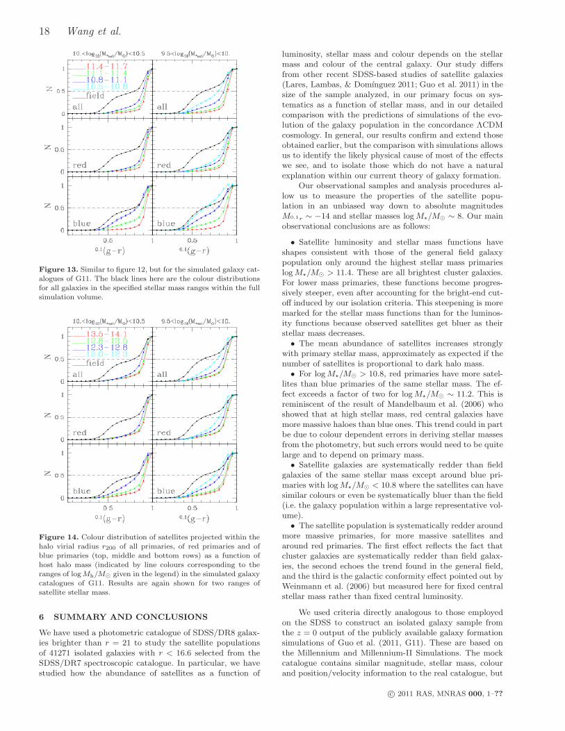
18 Wang et al.

Figure 13. Similar to figure 12, but for the simulated galaxy cat-alogues of G11. The black lines here are the colour distributionsfor all galaxies in the specified stellar mass ranges within the fullsimulation volume.

Figure 14. Colour distribution of satellites projected within thehalo virial radius r200 of all primaries, of red primaries and ofblue primaries (top, middle and bottom rows) as a function ofhost halo mass (indicated by line colours corresponding to theranges of logMh/M⊙ given in the legend) in the simulated galaxycatalogues of G11. Results are again shown for two ranges ofsatellite stellar mass.

6 SUMMARY AND CONCLUSIONS

We have used a photometric catalogue of SDSS/DR8 galax-ies brighter than r = 21 to study the satellite populationsof 41271 isolated galaxies with r < 16.6 selected from theSDSS/DR7 spectroscopic catalogue. In particular, we havestudied how the abundance of satellites as a function of

luminosity, stellar mass and colour depends on the stellarmass and colour of the central galaxy. Our study differsfrom other recent SDSS-based studies of satellite galaxies(Lares, Lambas, & Domınguez 2011; Guo et al. 2011) in thesize of the sample analyzed, in our primary focus on sys-tematics as a function of stellar mass, and in our detailedcomparison with the predictions of simulations of the evo-lution of the galaxy population in the concordance ΛCDMcosmology. In general, our results confirm and extend thoseobtained earlier, but the comparison with simulations allowsus to identify the likely physical cause of most of the effectswe see, and to isolate those which do not have a naturalexplanation within our current theory of galaxy formation.

Our observational samples and analysis procedures al-low us to measure the properties of the satellite popu-lation in an unbiased way down to absolute magnitudesM0.1r ∼ −14 and stellar masses logM⋆/M⊙ ∼ 8. Our mainobservational conclusions are as follows:

• Satellite luminosity and stellar mass functions haveshapes consistent with those of the general field galaxypopulation only around the highest stellar mass primarieslogM⋆/M⊙ > 11.4. These are all brightest cluster galaxies.For lower mass primaries, these functions become progres-sively steeper, even after accounting for the bright-end cut-off induced by our isolation criteria. This steepening is moremarked for the stellar mass functions than for the luminos-ity functions because observed satellites get bluer as theirstellar mass decreases.

• The mean abundance of satellites increases stronglywith primary stellar mass, approximately as expected if thenumber of satellites is proportional to dark halo mass.

• For logM⋆/M⊙ > 10.8, red primaries have more satel-lites than blue primaries of the same stellar mass. The ef-fect exceeds a factor of two for logM⋆/M⊙ ∼ 11.2. This isreminiscent of the result of Mandelbaum et al. (2006) whoshowed that at high stellar mass, red central galaxies havemore massive haloes than blue ones. This trend could in partbe due to colour dependent errors in deriving stellar massesfrom the photometry, but such errors would need to be quitelarge and to depend on primary mass.

• Satellite galaxies are systematically redder than fieldgalaxies of the same stellar mass except around blue pri-maries with logM⋆/M⊙ < 10.8 where the satellites can havesimilar colours or even be systematically bluer than the field(i.e. the galaxy population within a large representative vol-ume).

• The satellite population is systematically redder aroundmore massive primaries, for more massive satellites andaround red primaries. The first effect reflects the fact thatcluster galaxies are systematically redder than field galax-ies, the second echoes the trend found in the general field,and the third is the galactic conformity effect pointed out byWeinmann et al. (2006) but measured here for fixed centralstellar mass rather than fixed central luminosity.

We used criteria directly analogous to those employedon the SDSS to construct an isolated galaxy sample fromthe z = 0 output of the publicly available galaxy formationsimulations of Guo et al. (2011, G11). These are based onthe Millennium and Millennium-II Simulations. The mockcatalogue contains similar magnitude, stellar mass, colourand position/velocity information to the real catalogue, but

c© 2011 RAS, MNRAS 000, 1–??

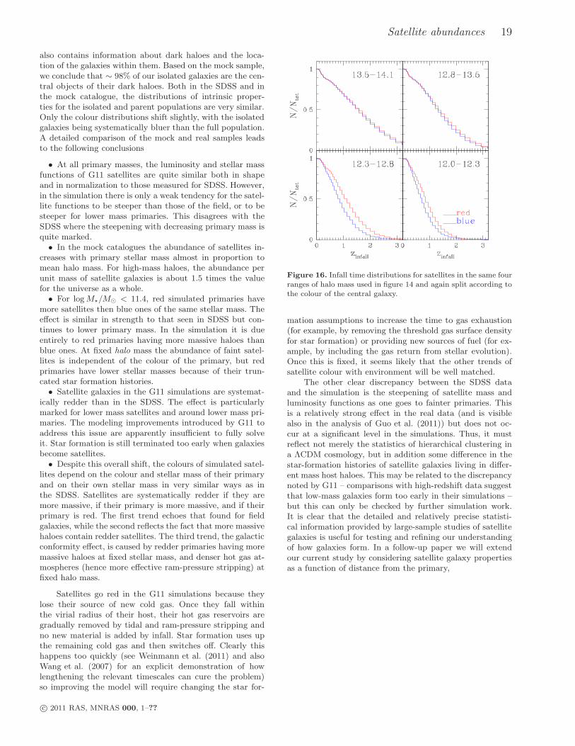
Satellite abundances 19

also contains information about dark haloes and the loca-tion of the galaxies within them. Based on the mock sample,we conclude that ∼ 98% of our isolated galaxies are the cen-tral objects of their dark haloes. Both in the SDSS and inthe mock catalogue, the distributions of intrinsic proper-ties for the isolated and parent populations are very similar.Only the colour distributions shift slightly, with the isolatedgalaxies being systematically bluer than the full population.A detailed comparison of the mock and real samples leadsto the following conclusions

• At all primary masses, the luminosity and stellar massfunctions of G11 satellites are quite similar both in shapeand in normalization to those measured for SDSS. However,in the simulation there is only a weak tendency for the satel-lite functions to be steeper than those of the field, or to besteeper for lower mass primaries. This disagrees with theSDSS where the steepening with decreasing primary mass isquite marked.

• In the mock catalogues the abundance of satellites in-creases with primary stellar mass almost in proportion tomean halo mass. For high-mass haloes, the abundance perunit mass of satellite galaxies is about 1.5 times the valuefor the universe as a whole.

• For logM⋆/M⊙ < 11.4, red simulated primaries havemore satellites then blue ones of the same stellar mass. Theeffect is similar in strength to that seen in SDSS but con-tinues to lower primary mass. In the simulation it is dueentirely to red primaries having more massive haloes thanblue ones. At fixed halo mass the abundance of faint satel-lites is independent of the colour of the primary, but redprimaries have lower stellar masses because of their trun-cated star formation histories.

• Satellite galaxies in the G11 simulations are systemat-ically redder than in the SDSS. The effect is particularlymarked for lower mass satellites and around lower mass pri-maries. The modeling improvements introduced by G11 toaddress this issue are apparently insufficient to fully solveit. Star formation is still terminated too early when galaxiesbecome satellites.

• Despite this overall shift, the colours of simulated satel-lites depend on the colour and stellar mass of their primaryand on their own stellar mass in very similar ways as inthe SDSS. Satellites are systematically redder if they aremore massive, if their primary is more massive, and if theirprimary is red. The first trend echoes that found for fieldgalaxies, while the second reflects the fact that more massivehaloes contain redder satellites. The third trend, the galacticconformity effect, is caused by redder primaries having moremassive haloes at fixed stellar mass, and denser hot gas at-mospheres (hence more effective ram-pressure stripping) atfixed halo mass.

Satellites go red in the G11 simulations because theylose their source of new cold gas. Once they fall withinthe virial radius of their host, their hot gas reservoirs aregradually removed by tidal and ram-pressure stripping andno new material is added by infall. Star formation uses upthe remaining cold gas and then switches off. Clearly thishappens too quickly (see Weinmann et al. (2011) and alsoWang et al. (2007) for an explicit demonstration of howlengthening the relevant timescales can cure the problem)so improving the model will require changing the star for-

Figure 16. Infall time distributions for satellites in the same fourranges of halo mass used in figure 14 and again split according tothe colour of the central galaxy.

mation assumptions to increase the time to gas exhaustion(for example, by removing the threshold gas surface densityfor star formation) or providing new sources of fuel (for ex-ample, by including the gas return from stellar evolution).Once this is fixed, it seems likely that the other trends ofsatellite colour with environment will be well matched.

The other clear discrepancy between the SDSS dataand the simulation is the steepening of satellite mass andluminosity functions as one goes to fainter primaries. Thisis a relatively strong effect in the real data (and is visiblealso in the analysis of Guo et al. (2011)) but does not oc-cur at a significant level in the simulations. Thus, it mustreflect not merely the statistics of hierarchical clustering ina ΛCDM cosmology, but in addition some difference in thestar-formation histories of satellite galaxies living in differ-ent mass host haloes. This may be related to the discrepancynoted by G11 – comparisons with high-redshift data suggestthat low-mass galaxies form too early in their simulations –but this can only be checked by further simulation work.It is clear that the detailed and relatively precise statisti-cal information provided by large-sample studies of satellitegalaxies is useful for testing and refining our understandingof how galaxies form. In a follow-up paper we will extendour current study by considering satellite galaxy propertiesas a function of distance from the primary,

c© 2011 RAS, MNRAS 000, 1–??

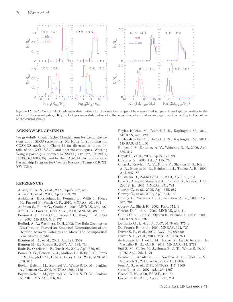
20 Wang et al.

Figure 15. Left: Central black hole mass distributions for the same four ranges of halo mass used in figure 14 and split according to thecolour of the central galaxy. Right: Hot gas mass distributions for the same four sets of haloes and again split according to the colourof the central galaxy.

ACKNOWLEDGEMENTS

We gratefully thank Rachel Mandelbaum for useful discus-sions about SDSS systematics, Xu Kong for supplying theCOSMOS mask and Cheng Li for discussions about de-tails of the NYU-VAGC and photoz2 catalogues. WentingWang is partially supported by NSFC (11121062, 10878001,11033006,11003035), and by the CAS/SAFEA InternationalPartnership Program for Creative Research Teams (KJCX2-YW-T23).

REFERENCES

Abazajian K. N., et al., 2009, ApJS, 182, 543Aihara H., et al., 2011, ApJS, 193, 29Alshino A., Khosroshahi H., Ponman T., Willis J., PierreM., Pacaud F., Smith G. P., 2010, MNRAS, 401, 941

Andreon S., Punzi G., Grado A., 2005, MNRAS, 360, 727Ann H. B., Park C., Choi Y.-Y., 2008, MNRAS, 389, 86Benson A. J., Frenk C. S., Lacey C. G., Baugh C. M., ColeS., 2002, MNRAS, 333, 177

Berlind, A. A., Weinberg, D. H. 2002. The Halo OccupationDistribution: Toward an Empirical Determination of theRelation between Galaxies and Mass. The AstrophysicalJournal 575, 587-616.

Blanton M. R., et al., 2005, AJ, 129, 2562Blanton M. R., Roweis S., 2007, AJ, 133, 734Bode P., Ostriker J. P., Turok N., 2001, ApJ, 556, 93Bower R. G., Benson A. J., Malbon R., Helly J. C., FrenkC. S., Baugh C. M., Cole S., Lacey C. G., 2006, MNRAS,370, 645

Boylan-Kolchin M., Springel V., White S. D. M., JenkinsA., Lemson G., 2009, MNRAS, 398, 1150

Boylan-Kolchin M., Springel V., White S. D. M., JenkinsA., 2010, MNRAS, 406, 896

Boylan-Kolchin M., Bullock J. S., Kaplinghat M., 2012,MNRAS, 422, 1203

Boylan-Kolchin M., Bullock J. S., Kaplinghat M., 2011,MNRAS, 415, L40

Bullock J. S., Kravtsov A. V., Weinberg D. H., 2000, ApJ,539, 517

Capak P., et al., 2007, ApJS, 172, 99Chabrier G., 2003, PASP, 115, 763Chen J., Kravtsov A. V., Prada F., Sheldon E. S., KlypinA. A., Blanton M. R., Brinkmann J., Thakar A. R., 2006,ApJ, 647, 86

Christlein D., Zabludoff A. I., 2003, ApJ, 591, 764Cole S., Aragon-Salamanca A., Frenk C. S., Navarro J. F.,Zepf S. E., 1994, MNRAS, 271, 781

Conroy C., et al., 2005, ApJ, 635, 982Conroy C., et al., 2007, ApJ, 654, 153Conroy C., Wechsler R. H., Kravtsov A. V., 2006, ApJ,647, 201

Cooray A., Sheth R., 2002, PhR, 372, 1Croton D. J., et al., 2006, MNRAS, 365, 11Cunha C. E., Lima M., Oyaizu H., Frieman J., Lin H., 2009,MNRAS, 396, 2379

De Lucia G., Blaizot J., 2007, MNRAS, 375, 2De Propris R., et al., 2003, MNRAS, 342, 725Driver S. P., et al., 2009, A&G, 50, 050000Driver S. P., et al., 2011, MNRAS, 413, 971de Filippis E., Paolillo M., Longo G., La Barbera F., deCarvalho R. R., Gal R., 2011, MNRAS, 414, 2771

Fall S. M., Geller M. J., Jones B. J. T., White S. D. M.,1976, ApJ, 205, L121

Ferrero I., Abadi M. G., Navarro J. F., Sales L. V.,Gurovich S., 2011, arXiv, arXiv:1111.6609

Font A. S., et al., 2011, MNRAS, 417, 1260Goto T., et al., 2002, AJ, 123, 1807Grebel E. K., 2000, ESASP, 445, 87Grebel E. K., 2001, ApSSS, 277, 231

c© 2011 RAS, MNRAS 000, 1–??

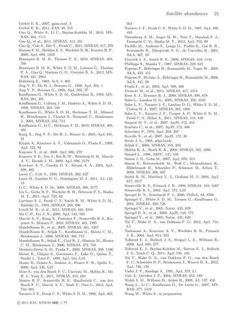
Satellite abundances 21

Grebel E. K., 2007, ggnu.conf, 3Grebel E. K., 2011, EAS, 48, 315Guo Q., White S., Li C., Boylan-Kolchin M., 2010, MN-RAS, 404, 1111

Guo Q., et al., 2011, MNRAS, 413, 101Guo Q., Cole S., Eke V., Frenk C., 2011, MNRAS, 417, 370Hansen S. M., Sheldon E. S., Wechsler R. H., Koester B. P.,2009, ApJ, 699, 1333

Henriques B. M. B., Thomas P. A., 2010, MNRAS, 403,768

Henriques B. M. B., White S. D. M., Lemson G., ThomasP. A., Guo Q., Marleau G.-D., Overzier R. A., 2012, MN-RAS, 421, 2904

Holmberg E., 1969, ArA, 5, 305Jing Y. P., Mo H. J., Boerner G., 1998, ApJ, 494, 1Jing Y. P., Boerner G., 1998, ApJ, 503, 37Kauffmann G., White S. D. M., Guiderdoni B., 1993, MN-RAS, 264, 201

Kauffmann G., Colberg J. M., Diaferio A., White S. D. M.,1999, MNRAS, 303, 188

Kauffmann G., White S. D. M., Heckman T. M., MenardB., Brinchmann J., Charlot S., Tremonti C., BrinkmannJ., 2004, MNRAS, 353, 713

Kauffmann G., Li C., Heckman T. M., 2010, MNRAS, 409,491

Kang X., Jing Y. P., Mo H. J., Borner G., 2005, ApJ, 631,21

Klypin A., Kravtsov A. V., Valenzuela O., Prada F., 1999,ApJ, 522, 82

Koposov S., et al., 2008, ApJ, 686, 279Koposov S. E., Yoo J., Rix H.-W., Weinberg D. H., MaccioA. V., Escude J. M., 2009, ApJ, 696, 2179

Kravtsov A. V., Gnedin O. Y., Klypin A. A., 2004, ApJ,609, 482

Lacey C., Cole S., 1993, MNRAS, 262, 627Lares M., Lambas D. G., Domınguez M. J., 2011, AJ, 142,13

Li C., White S. D. M., 2009, MNRAS, 398, 2177Liu L., Gerke B. F., Wechsler R. H., Behroozi P. S., BushaM. T., 2011, ApJ, 733, 62

Lorrimer S. J., Frenk C. S., Smith R. M., White S. D. M.,Zaritsky D., 1994, MNRAS, 269, 696

Lovell M. R., et al., 2012, MNRAS, 420, 2318Ma C.-P., Fry J. N., 2000, ApJ, 543, 503Maccio A. V., Kang X., Fontanot F., Somerville R. S., Ko-posov S., Monaco P., 2010, MNRAS, 402, 1995

Mandelbaum R., et al., 2005, MNRAS, 361, 1287Mandelbaum R., Seljak U., Kauffmann G., Hirata C. M.,Brinkmann J., 2006, MNRAS, 368, 715

Mandelbaum R., Seljak U., Cool R. J., Blanton M., HirataC. M., Brinkmann J., 2006, MNRAS, 372, 758

Montero-Dorta A. D., Prada F., 2009, MNRAS, 399, 1106Moore B., Ghigna S., Governato F., Lake G., Quinn T.,Stadel J., Tozzi P., 1999, ApJ, 524, L19

Moore B., Gelato S., Jenkins A., Pearce F. R., Quilis V.,2000, ApJ, 535, L21

More S., van den Bosch F. C., Cacciato M., Skibba R., MoH. J., Yang X., 2011, MNRAS, 410, 210

Moster B. P., Somerville R. S., Maulbetsch C., van denBosch F. C., Maccio A. V., Naab T., Oser L., 2010, ApJ,710, 903

Navarro J. F., Frenk C. S., White S. D. M., 1996, ApJ, 462,

563

Navarro J. F., Frenk C. S., White S. D. M., 1997, ApJ, 490,493

Nierenberg A. M., Auger M. W., Treu T., Marshall P. J.,Fassnacht C. D., Busha M. T., 2012, ApJ, 752, 99

Paolillo M., Andreon S., Longo G., Puddu E., Gal R. R.,Scaramella R., Djorgovski S. G., de Carvalho R., 2001,A&A, 367, 59

Peacock J. A., Smith R. E., 2000, MNRAS, 318, 1144

Phillipps S., Shanks T., 1987, MNRAS, 229, 621

Popesso P., Bohringer H., Romaniello M., Voges W., 2005,A&A, 433, 415

Popesso P., Biviano A., Bohringer H., Romaniello M., 2006,A&A, 445, 29

Prada F., et al., 2003, ApJ, 598, 260Prescott M., et al., 2011, MNRAS, 417, 1374

Ross A. J., Brunner R. J., 2009, MNRAS, 399, 878

Sales L., Lambas D. G., 2005, MNRAS, 356, 1045

Sales L. V., Navarro J. F., Lambas D. G., White S. D. M.,Croton D. J., 2007, MNRAS, 382, 1901

Sales L. V., Navarro J. F., Cooper A. P., White S. D. M.,Frenk C. S., Helmi A., 2011, MNRAS, 418, 648

Sargent M. T., et al., 2007, ApJS, 172, 434

Scarlata C., et al., 2007, ApJS, 172, 406

Schechter P., 1976, ApJ, 203, 297

Scoville N., et al., 2007, ApJS, 172, 38

Sersic J. L., 1968, adga.book,

Seljak U., 2000, MNRAS, 318, 203

Skibba R. A., Sheth R. K., 2009, MNRAS, 392, 1080

Simard L., 1998, ASPC, 145, 108

Simon J. D., Geha M., 2007, ApJ, 670, 313

Simon P., Hetterscheidt M., Wolf C., Meisenheimer K.,Hildebrandt H., Schneider P., Schirmer M., Erben T.,2009, MNRAS, 398, 807

Smith R. M., Martınez V. J., Graham M. J., 2004, ApJ,617, 1017

Somerville R. S., Primack J. R., 1999, MNRAS, 310, 1087

Somerville R. S., 2002, ApJ, 572, L23

Spergel D. N., Steinhardt P. J., 2000, PhRvL, 84, 3760

Springel V., White S. D. M., Tormen G., Kauffmann G.,2001, MNRAS, 328, 726

Springel V., et al., 2005, Natur, 435, 629Spergel D. N., et al., 2003, ApJS, 148, 175

Springel V., et al., 2005, Natur, 435, 629

Tal T., Wake D. A., van Dokkum P. G., 2012, ApJ, 751,L5

Tasitsiomi A., Kravtsov A. V., Wechsler R. H., PrimackJ. R., 2004, ApJ, 614, 533

Tollerud E. J., Bullock J. S., Strigari L. E., Willman B.,2008, ApJ, 688, 277

Tollerud E. J., Boylan-Kolchin M., Barton E. J., BullockJ. S., Trinh C. Q., 2011, ApJ, 738, 102

Tal T., Wake D. A., van Dokkum P. G., van den BoschF. C., Schneider D. P., Brinkmann J., Weaver B. A., 2012,ApJ, 746, 138

Vader J. P., Sandage A., 1991, ApJ, 379, L1

Vale A., Ostriker J. P., 2004, MNRAS, 353, 189

Walsh S. M., Willman B., Jerjen H., 2009, AJ, 137, 450

Wang L., Li C., Kauffmann G., De Lucia G., 2007, MN-RAS, 377, 1419

Wang W., White S., in preparation

c© 2011 RAS, MNRAS 000, 1–??

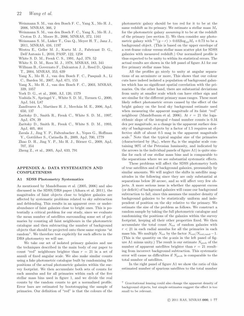
22 Wang et al.

Weinmann S. M., van den Bosch F. C., Yang X., Mo H. J.,2006, MNRAS, 366, 2

Weinmann S. M., van den Bosch F. C., Yang X., Mo H. J.,Croton D. J., Moore B., 2006, MNRAS, 372, 1161

Weinmann S. M., Lisker T., Guo Q., Meyer H. T., Janz J.,2011, MNRAS, 416, 1197

Westra E., Geller M. J., Kurtz M. J., Fabricant D. G.,Dell’Antonio I., 2010, PASP, 122, 1258

White S. D. M., Frenk C. S., 1991, ApJ, 379, 52White S. D. M., Rees M. J., 1978, MNRAS, 183, 341Willman B., Governato F., Dalcanton J. J., Reed D., QuinnT., 2004, MNRAS, 353, 639

Yang X., Mo H. J., van den Bosch F. C., Pasquali A., LiC., Barden M., 2007, ApJ, 671, 153

Yang X., Mo H. J., van den Bosch F. C., 2003, MNRAS,339, 1057

York D. G., et al., 2000, AJ, 120, 1579Yoshida N., Springel V., White S. D. M., Tormen G., 2000,ApJ, 544, L87

Zandivarez A., Martınez H. J., Merchan M. E., 2006, ApJ,650, 137

Zaritsky D., Smith R., Frenk C., White S. D. M., 1997,ApJ, 478, 39

Zaritsky D., Smith R., Frenk C., White S. D. M., 1993,ApJ, 405, 464

Zavala J., Jing Y. P., Faltenbacher A., Yepes G., HoffmanY., Gottlober S., Catinella B., 2009, ApJ, 700, 1779

Zhao D. H., Jing Y. P., Mo H. J., Borner G., 2009, ApJ,707, 354

Zheng Z., et al., 2005, ApJ, 633, 791

APPENDIX A: DATA SYSTEMATICS AND

COMPLETENESS

A1 SDSS Photometry Systematics

As mentioned by Mandelbaum et al. (2005, 2006) and alsodiscussed in the SDSS/DR8 paper (Aihara et al. 2011), themagnitudes of faint objects close to brighter galaxies areaffected by systematic problems related to sky subtractionand deblending. This results in an apparent over- or under-abundance of faint galaxies close to bright ones. This is po-tentially a critical problem for our study, since we evaluatethe mean number of satellites surrounding some set of pri-maries by counting all faint neighbours in the photometriccatalogue and then subtracting the number of backgroundobjects that should be projected onto these same regions “atrandom”. We therefore test explicitly for such affects in theDR8 photometry we will use.

We take our set of isolated primary galaxies and usethe techniques described in the main body of our paper tocount “red” neighbours brighter than r = 21 in a set ofannuli of fixed angular scale. We also make similar countsusing a fake photometric catalogue built by randomizing thepositions of the actual photometric galaxies within the sur-vey footprint. We then accumulate both sets of counts foreach annulus and for all primaries within each of the fivestellar mass bins used in figure 1, and we divide the realcounts by the random counts to get a normalized profile.Error bars are estimated by bootstrapping the sample ofprimaries. Our definition of “red” is that the colours of the

photometric galaxy should be too red for it to be at thesame redshift as its primary. We estimate a stellar mass M⋆

for the photometric galaxy assuming it to be at the redshiftof the primary (see section 3). We then consider any photo-metric galaxy with 0.1(g− r) > 0.032log10M⋆ +0.73 to be abackground object. (This is based on the upper envelope ofa rest-frame colour versus stellar mass scatter plot for SDSSgalaxies with measured redshift.) Our normalized profile isthus expected to be unity to within its statistical errors. Theactual results are shown in the left panel of figure A1 for ourfive primary stellar mass bins.

All the profiles go nicely to unity at angular separa-tions of an arcminute or more, This shows that our colourcuts have indeed isolated a population of background galax-ies which has no significant spatial correlation with the pri-maries. On the other hand, there are substantial deviationsfrom unity at smaller scale which can have either sign andare similar for the different primary mass ranges. These mostlikely reflect photometric errors caused by the effect of thebright galaxy on the local sky background estimate usedwhen measuring the apparent magnitude of its faint “red”neighbour (Mandelbaum et al. 2006). At r = 21 the loga-rithmic slope of the integral r-band number counts is 0.34dex per magnitude, so a change in the apparent surface den-sity of background objects by a factor of 1.5 requires an ef-fective shift of about 0.5 mag in the apparent magnitudescale.7 Note that the typical angular size of the primaries(characterized by 〈θ90〉, where θ90 is the angular scale con-taining 90% of the Petrosian luminosity, and indicated bythe arrows in the individual panels of figure A1) is quite sim-ilar for each of our stellar mass bins and is comparable tothe separations where we see substantial systematic effects.

These problems will affect the SDSS photometry bothof true satellites and of background galaxies, presumably bysimilar amounts. We will neglect the shifts in satellite mag-nitudes in the following since they are only substantial atseparations below 20 arcsec, and so will affect very few ob-jects. A more serious issue is whether the apparent excess(or deficit) of background galaxies will cause our backgroundsubtraction to fail, since this assumes the number density ofbackground galaxies to be statistically uniform and inde-pendent of position on the sky relative to the primary. Weestimate the size of the problem as follows. We construct arandom sample by taking the full photometric catalogue andrandomizing the positions of the galaxies within the surveyfootprint, keeping all their other properties fixed. We thenaccumulate the total count Ntot of random galaxies withr < 21 in each radial annulus for all the primaries in eachmass bin. We multiply Ntot by the factor Nred/Nred,rand−1.(This is the quantity on the y-axis in the left panel of fig-ure A1 minus unity.) The result is our estimate Nprob of thenumber of apparent satellites brighter than r = 21 result-ing from incorrect background subtraction. This systematicerror will cause us difficulties if Nprob is comparable to thetotal number of satellites.

In the right panel of figure A1 we show the ratio of thisestimated number of spurious satellites to the total number

7 Gravitational lensing could also change the apparent density ofbackground objects, but simple estimates suggest the effect is toosmall to be relevant.

c© 2011 RAS, MNRAS 000, 1–??

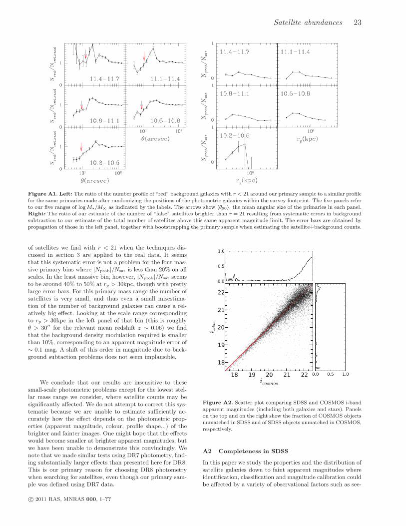
Satellite abundances 23

Figure A1. Left: The ratio of the number profile of “red” background galaxies with r < 21 around our primary sample to a similar profilefor the same primaries made after randomizing the positions of the photometric galaxies within the survey footprint. The five panels referto our five ranges of logM⋆/M⊙ as indicated by the labels. The arrows show 〈θ90〉, the mean angular size of the primaries in each panel.Right: The ratio of our estimate of the number of “false” satellites brighter than r = 21 resulting from systematic errors in backgroundsubtraction to our estimate of the total number of satellites above this same apparent magnitude limit. The error bars are obtained bypropagation of those in the left panel, together with bootstrapping the primary sample when estimating the satellite+background counts.

of satellites we find with r < 21 when the techniques dis-cussed in section 3 are applied to the real data. It seemsthat this systematic error is not a problem for the four mas-sive primary bins where |Nprob|/Nsat is less than 20% on allscales. In the least massive bin, however, |Nprob|/Nsat seemsto be around 40% to 50% at rp > 30kpc, though with prettylarge error-bars. For this primary mass range the number ofsatellites is very small, and thus even a small misestima-tion of the number of background galaxies can cause a rel-atively big effect. Looking at the scale range correspondingto rp > 30kpc in the left panel of that bin (this is roughlyθ > 30′′ for the relevant mean redshift z ∼ 0.06) we findthat the background density modulation required is smallerthan 10%, corresponding to an apparent magnitude error of∼ 0.1 mag. A shift of this order in magnitude due to back-ground subtaction problems does not seem implausible.

We conclude that our results are insensitive to thesesmall-scale photometric problems except for the lowest stel-lar mass range we consider, where satellite counts may besignificantly affected. We do not attempt to correct this sys-tematic because we are unable to estimate sufficiently ac-curately how the effect depends on the photometric prop-erties (apparent magnitude, colour, profile shape...) of thebrighter and fainter images. One might hope that the effectswould become smaller at brighter apparent magnitudes, butwe have been unable to demonstrate this convincingly. Wenote that we made similar tests using DR7 photometry, find-ing substantially larger effects than presented here for DR8.This is our primary reason for choosing DR8 photometrywhen searching for satellites, even though our primary sam-ple was defined using DR7 data.

18 19 20 21 22icosmos

18

19

20

21

22

i sdss

0.0

0.5

1.0

0.0 0.5 1.0

Figure A2. Scatter plot comparing SDSS and COSMOS i-bandapparent magnitudes (including both galaxies and stars). Panelson the top and on the right show the fraction of COSMOS objectsunmatched in SDSS and of SDSS objects unmatched in COSMOS,respectively.

A2 Completeness in SDSS

In this paper we study the properties and the distribution ofsatellite galaxies down to faint apparent magnitudes whereidentification, classification and magnitude calibration couldbe affected by a variety of observational factors such as see-

c© 2011 RAS, MNRAS 000, 1–??

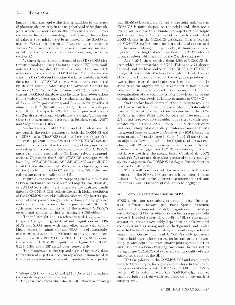
24 Wang et al.

ing, sky brightness and extinction, in addition to the issuesof photometric accuracy in the neighborhood of brighter ob-jects which we addressed in the previous section. In thissection we focus on estimating quantitatively the fractionof galaxies that might have been missed in the SDSS cat-alogues. We test the accuracy of star-galaxy separation insection A3, of our background galaxy subtraction methodsin A4 and the influence of additional observing factors insection A5.

We investigate the completeness of the SDSS/DR8 pho-tometric catalogue using the much deeper HST data avail-able for the 2 squ.deg. COSMOS survey. We cross-matchgalaxies and stars in the COSMOS field 8 to galaxies andstars in SDSS/DR8 and examine the failed matches in bothdirections. The COSMOS survey was initially conductedby HST in broad I-band using the Advanced Camera forSurveys (ACS) Wide-Field Channel (WFC) detector. Thecurrent COSMOS database also includes later observationsfrom a variety of telescopes. It reaches a limiting magnitudeof IAB = 28 for point source, and IAB = 26 for galaxies ofdiameter ∼ 0.5′′ (Scoville et al. 2007). This is much deeperthan SDSS. The specific COSMOS catalogue used here isthe Zurich Structure and Morphology catalogue9, which con-tains the measurements presented in Scarlata et al. (2007)and Sargent et al. (2007).

We further excluded COSMOS and SDSS objects whichare outside the region common to both the COSMOS andthe SDSS masks. The SDSS mask used here is made up of the“spherical polygons” provided on the NYU-VAGC website,and is the same as used in the main body of our paper whenevaluating and correcting for edge effects. The COSMOSmask was kindly provided by Xu Kong (private communi-cation). Objects in the Zurich COSMOS catalogue whichhave flag ACS CLEAN=0, ACS MU CLASS=3 or JUNK-FLAG=1 are also excluded. We consider objects (galaxiesor stars) to be matched in COSMOS and SDSS if their an-gular separation is smaller than 1.5′′.

Figure A2 is a scatter plot comparing the COSMOS andSDSS i-band magnitudes of matched objects. For about 4%of SDSS objects with r < 21 there are two matched candi-dates in COSMOS. This reflects the much higher resolutionof the COSMOS data which allows substantially better sepa-ration of close pairs of images, double stars, merging galaxiesand chance superpositions, than is possible with SDSS. Insuch cases, we sum the flux of all the matched COSMOSobjects and compare to that of the single SDSS object.

The red straight line is a reference with icosmos = isdssto guide the eye. In general, i-band magnitudes in COS-MOS and SDSS agree with each other quite well, with abigger scatter for fainter objects. SDSS r-band magnitudesof r = 19, 20, 20.5 and 21 correspond roughly to i-band mag-nitudes, i = 18.6, 19.6, 20.1 and 20.6. For these SDSS valuesthe scatter in COSMOS magnitudes in figure A2 is 0.277,0.293, 0.360 and 0.367 magnitudes, respectively.

The histograms at the top and right of figure A2 showthe fraction of objects in each survey which is unmatched inthe other as a function of i-band magnitude. It is expected

8 We use 150.7 > ra > 149.5 and 2.72 > dec > 1.65 to excludethe irregular edge of the full survey.9 http://irsa.ipac.caltech.edu/data/COSMOS/tables/morphology/

that SDSS objects should be lost at the faint end, becauseCOSMOS is much deeper. At the bright end, there are afew spikes, but the total number of objects at the brightend is small. For i < 20.5, we fail to match about 1% ofSDSS objects in the COSMOS catalogue. This is becausethe COSMOS mask we are using is not identical to that usedfor the Zurich catalogue. In particular, it eliminates smallerregions around bright stars so we find a few SDSS objectsin such regions which are not in the Zurich catalogue.

At i ∼ 20.5, there are also about 1.5% of COSMOS ob-jects which are unmatched in SDSS. This is only 71 objectsin total, and we have looked at both SDSS and COSMOSimages of these fields. We found that about 31 of these 71objects failed to match because the angular separation be-tween their centroid coordinates was bigger than 1.5′′. Insome cases the objects are quite extended or have a closeneighbour. Given the relatively poor seeing in SDSS, thedetermination of the coordinates of faint objects can be un-certain and so can result in failure to match to COSMOS.

On the other hand, about 40 of the 71 objects really donot have a match in SDSS. Of these, about 1/3 do indeedhave an object at or close to their coordinates in the COS-MOS image which SDSS failed to recognize. The remaining2/3 do not, however, have an object at or close to their coor-dinates even in the COSMOS image. The Zurich Structureand Morphology catalogue also provides a cross-match withthe ground based catalogue of Capak et al. (2007). Using thecross-match information provided, we found 15 out of these40 objects do have a match in the Capak et al. (2007) cat-alogue, with 12 having angular separation between the twomatched objects bigger than 1.5′′. The remaining objects donot have a match in the ground-based Capak et al. (2007)catalogue. We are not clear what produced these seeminglyspurious objects in the COSMOS catalogue, but the fractionis indeed small (< 1%).

The overall conclusion of this exercise is that incom-pleteness in the SDSS/DR8 photometric catalogue is at orbelow the 1% level at the apparent magnitude limit relevantfor our analysis. This is small enough to be negligible.

A3 Star-Galaxy Separation in SDSS

SDSS carries out star-galaxy separation using the mea-sured difference between psf (Point Spread Function)and cmodel (Composite Model) magnitudes. If psfMag-cmodelMag > 0.145, an object is classified as a galaxy, oth-erwise it is called a star. The quality of SDSS star-galaxyseparation is thus unavoidably dependent on observationalconditions such as seeing and sky background, and is alsoexpected to be a function of galaxy apparent magnitude andangular size. On the other hand, COSMOS should give muchmore reliable star-galaxy separation because of its substan-tially greater depth, its much smaller point-spread functionand its more uniform observing conditions. In this sectionwe again use COSMOS data to evaluate the quality of star-galaxy separation in the SDSS.

We take galaxies in the COSMOS field and cross-matchthem to SDSS images, both galaxies and stars. In the match,we again used objects with 150.7 > ra > 149.5 and 2.72 >dec > 1.65 in order to avoid the COSMOS edge, and weagain excluded objects which are obscured by the mask ofeither survey.

c© 2011 RAS, MNRAS 000, 1–??

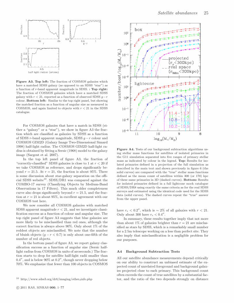
Satellite abundances 25

Figure A3. Top left: The fraction of COSMOS galaxies whichhave a matched SDSS galaxy (as opposed to an SDSS “star”) asa function of r-band apparent magnitude in SDSS. : Top right:

The fraction of COSMOS galaxies which have a matched SDSSgalaxy with r < 21, reported as a function of observed SDSS g−rcolour. Bottom left: Similar to the top right panel, but showingthe matched fraction as a function of angular size as measured inCOSMOS, and again limited to objects with r < 21 in the SDSScatalogue.

For COSMOS galaxies that have a match in SDSS (ei-ther a “galaxy” or a “star”), we show in figure A3 the frac-tion which are classified as galaxies by SDSS as a functionof SDSS r-band apparent magnitude, SDSS g−r colour andCOSMOS GIM2D (Galaxy Image Two-Dimensional Simard1998) half-light radius. The COSMOS GIM2D half-light ra-dius is obtained by fitting a Sersic (1968) model to the galaxyimage (Sargent et al. 2007).

In the top left panel of figure A3, the fraction of“correctly-classified” SDSS galaxies is close to 1 at r < 20 ifwe take COSMOS as reference, and drops significantly be-yond r = 21.5. At r = 21, the fraction is about 95%. Thereis some discussion about star-galaxy separation on the offi-cial SDSS website10. SDSS/DR1 was compared against theCOMBO-17 survey (Classifying Objects by Medium-BandObservations in 17 Filters). This much older completenesscurve also drops significantly beyond r = 21.5, and the frac-tion at r = 21 is about 95%, in excellent agreement with ourCOSMOS test here.

We now consider all COSMOS galaxies with matchedSDSS apparent magnitude r < 21, and we investigate classi-fication success as a function of colour and angular size. Thetop right panel of figure A3 suggests that blue galaxies aremore likely to be misclassified than red ones, although thecorrect fraction is always above 90%. Only about 1% of thereddest objects are misclassified. We note that the numberof bluish objects (g − r < 0.7) is only about one-fifth of thenumber of red objects.

In the bottom panel of figure A3, we report galaxy clas-sification success as a function of angular size (Sersic half-light radius from COSMOS in units of arcseconds.) The frac-tion starts to drop for satellite half-light radii smaller than0.4′′, and is below 90% at 0.2′′, though never dropping below70%. We emphasize that fewer than 100 objects in COSMOS

10 http://www.sdss3.org/dr8/imaging/other info.php

Figure A4. Tests of our background subtraction algorithms us-ing stellar mass functions for satellites of isolated primaries inthe G11 simulation separated into five ranges of primary stellarmass as indicated by colour in the legend. Top: Results for iso-lated primaries defined in a projection of the full simulation asdescribed in the main text and shown previously in figure 6 (thesolid curves) are compared with the “true” stellar mass functionsdefined as the mean count of satellites within 300 (or 170) kpcof these same primaries in 3D (dashed curves). Bottom: Resultsfor isolated primaries defined in a full lightcone mock catalogueof SDSS/DR8 using exactly the same criteria as for the real SDSSsurveys and estimated using the identical code used for the SDSSdata (solid curves). The dashed curves repeat the “true” answerfrom the upper panel.

have re < 0.2′′, which is ∼ 2% of all galaxies with r < 21.Only about 300 have re < 0.4′′.

In summary, these results together imply that not morethan about 1% of galaxies brighter than r = 21 are misclas-sified as stars by SDSS, which is a remarkably small numberfor a 2.5m telescope working on a less than perfect site. Theyalso imply that misclassification is a negligible problem forour purposes.

A4 Background Subtraction Tests

All our satellite abundance measurements depend criticallyon our ability to construct an unbiased estimate of the ex-pected count of unrelated foreground and background galax-ies projected close to each primary. This background countoften exceeds the count of true satellites by a substantial fac-tor, and the ratio of the two depends strongly on distance

c© 2011 RAS, MNRAS 000, 1–??

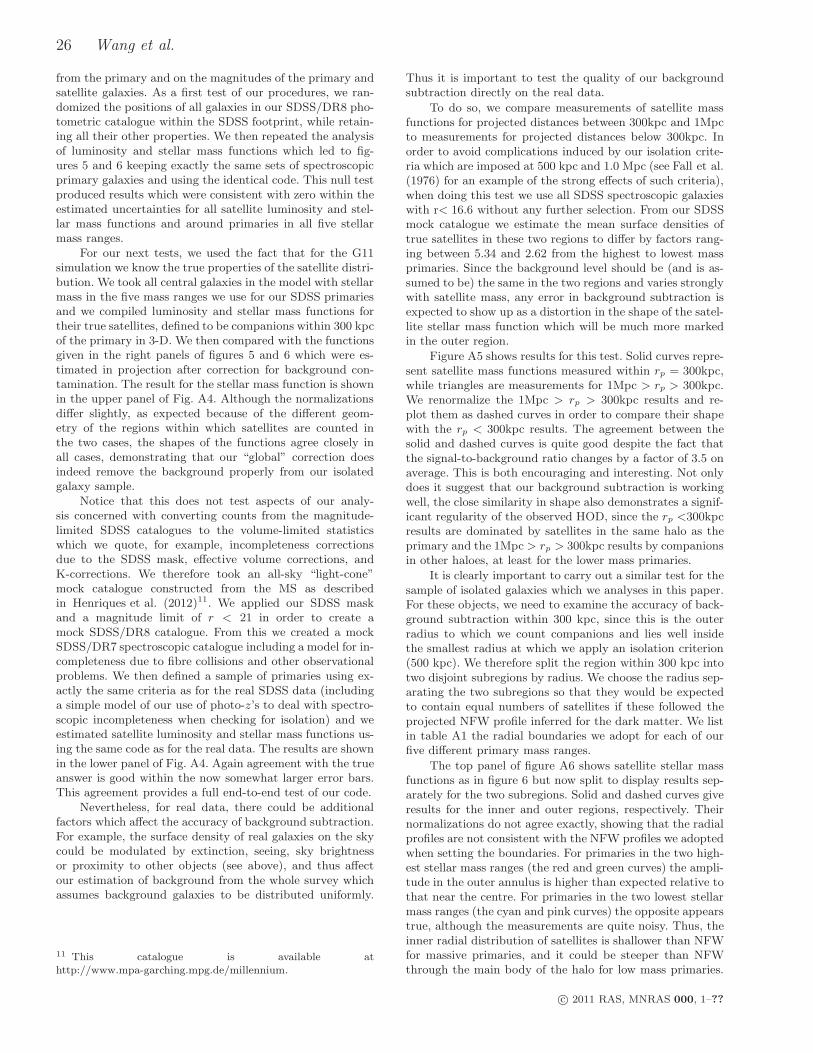
26 Wang et al.

from the primary and on the magnitudes of the primary andsatellite galaxies. As a first test of our procedures, we ran-domized the positions of all galaxies in our SDSS/DR8 pho-tometric catalogue within the SDSS footprint, while retain-ing all their other properties. We then repeated the analysisof luminosity and stellar mass functions which led to fig-ures 5 and 6 keeping exactly the same sets of spectroscopicprimary galaxies and using the identical code. This null testproduced results which were consistent with zero within theestimated uncertainties for all satellite luminosity and stel-lar mass functions and around primaries in all five stellarmass ranges.

For our next tests, we used the fact that for the G11simulation we know the true properties of the satellite distri-bution. We took all central galaxies in the model with stellarmass in the five mass ranges we use for our SDSS primariesand we compiled luminosity and stellar mass functions fortheir true satellites, defined to be companions within 300 kpcof the primary in 3-D. We then compared with the functionsgiven in the right panels of figures 5 and 6 which were es-timated in projection after correction for background con-tamination. The result for the stellar mass function is shownin the upper panel of Fig. A4. Although the normalizationsdiffer slightly, as expected because of the different geom-etry of the regions within which satellites are counted inthe two cases, the shapes of the functions agree closely inall cases, demonstrating that our “global” correction doesindeed remove the background properly from our isolatedgalaxy sample.

Notice that this does not test aspects of our analy-sis concerned with converting counts from the magnitude-limited SDSS catalogues to the volume-limited statisticswhich we quote, for example, incompleteness correctionsdue to the SDSS mask, effective volume corrections, andK-corrections. We therefore took an all-sky “light-cone”mock catalogue constructed from the MS as describedin Henriques et al. (2012)11. We applied our SDSS maskand a magnitude limit of r < 21 in order to create amock SDSS/DR8 catalogue. From this we created a mockSDSS/DR7 spectroscopic catalogue including a model for in-completeness due to fibre collisions and other observationalproblems. We then defined a sample of primaries using ex-actly the same criteria as for the real SDSS data (includinga simple model of our use of photo-z’s to deal with spectro-scopic incompleteness when checking for isolation) and weestimated satellite luminosity and stellar mass functions us-ing the same code as for the real data. The results are shownin the lower panel of Fig. A4. Again agreement with the trueanswer is good within the now somewhat larger error bars.This agreement provides a full end-to-end test of our code.

Nevertheless, for real data, there could be additionalfactors which affect the accuracy of background subtraction.For example, the surface density of real galaxies on the skycould be modulated by extinction, seeing, sky brightnessor proximity to other objects (see above), and thus affectour estimation of background from the whole survey whichassumes background galaxies to be distributed uniformly.

11 This catalogue is available athttp://www.mpa-garching.mpg.de/millennium.

Thus it is important to test the quality of our backgroundsubtraction directly on the real data.

To do so, we compare measurements of satellite massfunctions for projected distances between 300kpc and 1Mpcto measurements for projected distances below 300kpc. Inorder to avoid complications induced by our isolation crite-ria which are imposed at 500 kpc and 1.0 Mpc (see Fall et al.(1976) for an example of the strong effects of such criteria),when doing this test we use all SDSS spectroscopic galaxieswith r< 16.6 without any further selection. From our SDSSmock catalogue we estimate the mean surface densities oftrue satellites in these two regions to differ by factors rang-ing between 5.34 and 2.62 from the highest to lowest massprimaries. Since the background level should be (and is as-sumed to be) the same in the two regions and varies stronglywith satellite mass, any error in background subtraction isexpected to show up as a distortion in the shape of the satel-lite stellar mass function which will be much more markedin the outer region.

Figure A5 shows results for this test. Solid curves repre-sent satellite mass functions measured within rp = 300kpc,while triangles are measurements for 1Mpc > rp > 300kpc.We renormalize the 1Mpc > rp > 300kpc results and re-plot them as dashed curves in order to compare their shapewith the rp < 300kpc results. The agreement between thesolid and dashed curves is quite good despite the fact thatthe signal-to-background ratio changes by a factor of 3.5 onaverage. This is both encouraging and interesting. Not onlydoes it suggest that our background subtraction is workingwell, the close similarity in shape also demonstrates a signif-icant regularity of the observed HOD, since the rp <300kpcresults are dominated by satellites in the same halo as theprimary and the 1Mpc > rp > 300kpc results by companionsin other haloes, at least for the lower mass primaries.

It is clearly important to carry out a similar test for thesample of isolated galaxies which we analyses in this paper.For these objects, we need to examine the accuracy of back-ground subtraction within 300 kpc, since this is the outerradius to which we count companions and lies well insidethe smallest radius at which we apply an isolation criterion(500 kpc). We therefore split the region within 300 kpc intotwo disjoint subregions by radius. We choose the radius sep-arating the two subregions so that they would be expectedto contain equal numbers of satellites if these followed theprojected NFW profile inferred for the dark matter. We listin table A1 the radial boundaries we adopt for each of ourfive different primary mass ranges.

The top panel of figure A6 shows satellite stellar massfunctions as in figure 6 but now split to display results sep-arately for the two subregions. Solid and dashed curves giveresults for the inner and outer regions, respectively. Theirnormalizations do not agree exactly, showing that the radialprofiles are not consistent with the NFW profiles we adoptedwhen setting the boundaries. For primaries in the two high-est stellar mass ranges (the red and green curves) the ampli-tude in the outer annulus is higher than expected relative tothat near the centre. For primaries in the two lowest stellarmass ranges (the cyan and pink curves) the opposite appearstrue, although the measurements are quite noisy. Thus, theinner radial distribution of satellites is shallower than NFWfor massive primaries, and it could be steeper than NFWthrough the main body of the halo for low mass primaries.

c© 2011 RAS, MNRAS 000, 1–??

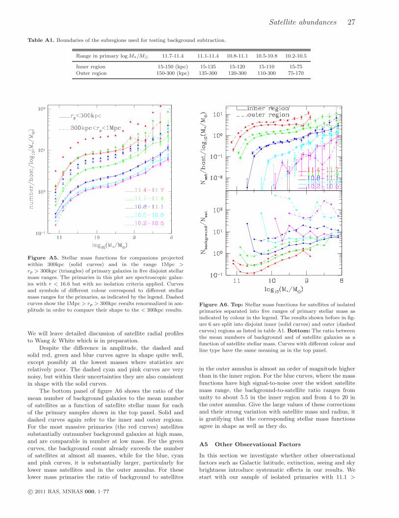
Satellite abundances 27

Table A1. Boundaries of the subregions used for testing background subtraction.

Range in primary logM∗/M⊙ 11.7-11.4 11.1-11.4 10.8-11.1 10.5-10.8 10.2-10.5

Inner region 15-150 (kpc) 15-135 15-120 15-110 15-75Outer region 150-300 (kpc) 135-300 120-300 110-300 75-170

Figure A5. Stellar mass functions for companions projectedwithin 300kpc (solid curves) and in the range 1Mpc >rp > 300kpc (triangles) of primary galaxies in five disjoint stellarmass ranges. The primaries in this plot are spectroscopic galax-ies with r < 16.6 but with no isolation criteria applied. Curvesand symbols of different colour correspond to different stellarmass ranges for the primaries, as indicated by the legend. Dashedcurves show the 1Mpc > rp > 300kpc results renormalized in am-plitude in order to compare their shape to the < 300kpc results.

We will leave detailed discussion of satellite radial profilesto Wang & White which is in preparation.

Despite the difference in amplitude, the dashed andsolid red, green and blue curves agree in shape quite well,except possibly at the lowest masses where statistics arerelatively poor. The dashed cyan and pink curves are verynoisy, but within their uncertainties they are also consistentin shape with the solid curves.

The bottom panel of figure A6 shows the ratio of themean number of background galaxies to the mean numberof satellites as a function of satellite stellar mass for eachof the primary samples shown in the top panel. Solid anddashed curves again refer to the inner and outer regions.For the most massive primaries (the red curves) satellitessubstantially outnumber background galaxies at high mass,and are comparable in number at low mass. For the greencurves, the background count already exceeds the numberof satellites at almost all masses, while for the blue, cyanand pink curves, it is substantially larger, particularly forlower mass satellites and in the outer annulus. For theselower mass primaries the ratio of background to satellites

Figure A6. Top: Stellar mass functions for satellites of isolatedprimaries separated into five ranges of primary stellar mass asindicated by colour in the legend. The results shown before in fig-ure 6 are split into disjoint inner (solid curves) and outer (dashedcurves) regions as listed in table A1. Bottom: The ratio betweenthe mean numbers of background and of satellite galaxies as afunction of satellite stellar mass. Curves with different colour andline type have the same meaning as in the top panel.

in the outer annulus is almost an order of magnitude higherthan in the inner region. For the blue curves, where the massfunctions have high signal-to-noise over the widest satellitemass range, the background-to-satellite ratio ranges fromunity to about 5.5 in the inner region and from 4 to 20 inthe outer annulus. Give the large values of these correctionsand their strong variation with satellite mass and radius, itis gratifying that the corresponding stellar mass functionsagree in shape as well as they do.

A5 Other Observational Factors

In this section we investigate whether other observationalfactors such as Galactic latitude, extinction, seeing and skybrightness introduce systematic effects in our results. Westart with our sample of isolated primaries with 11.1 >

c© 2011 RAS, MNRAS 000, 1–??

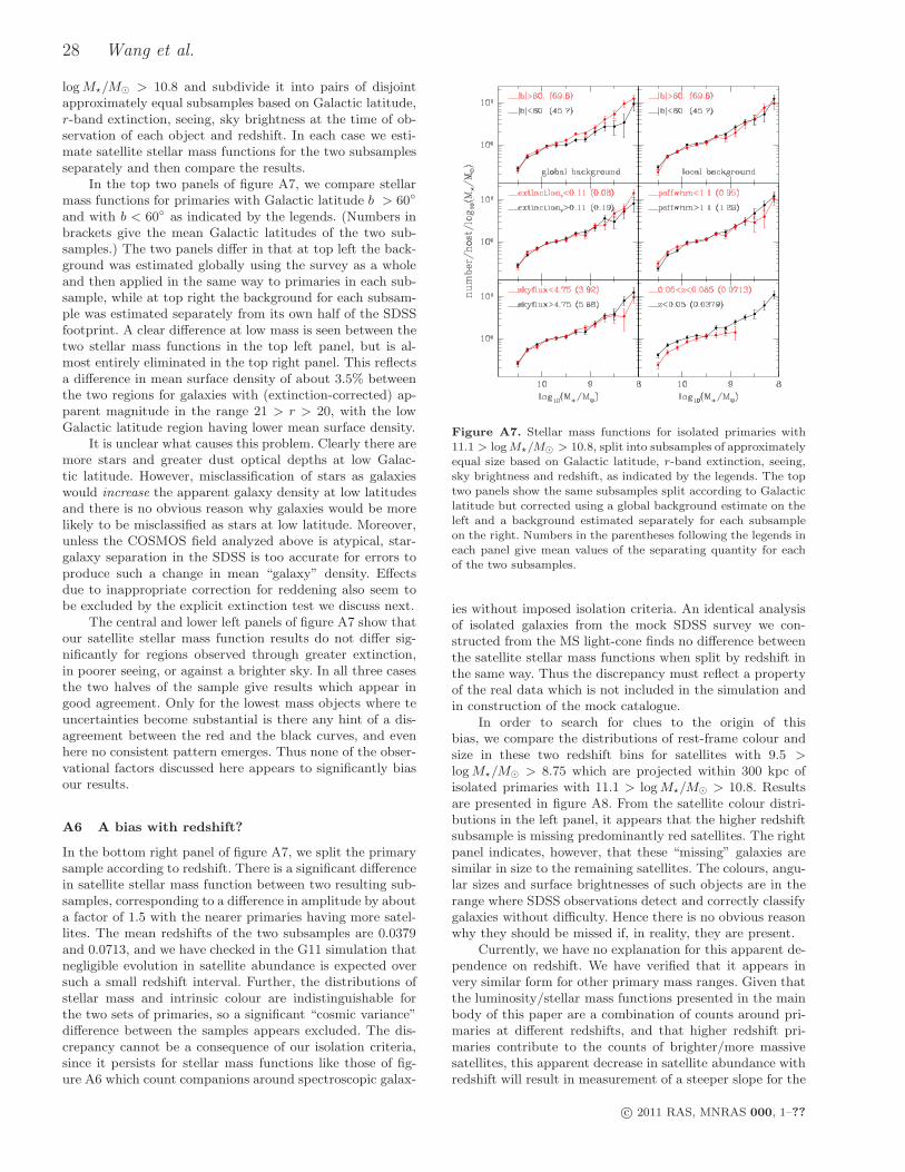
28 Wang et al.

logM⋆/M⊙ > 10.8 and subdivide it into pairs of disjointapproximately equal subsamples based on Galactic latitude,r-band extinction, seeing, sky brightness at the time of ob-servation of each object and redshift. In each case we esti-mate satellite stellar mass functions for the two subsamplesseparately and then compare the results.

In the top two panels of figure A7, we compare stellarmass functions for primaries with Galactic latitude b > 60

and with b < 60 as indicated by the legends. (Numbers inbrackets give the mean Galactic latitudes of the two sub-samples.) The two panels differ in that at top left the back-ground was estimated globally using the survey as a wholeand then applied in the same way to primaries in each sub-sample, while at top right the background for each subsam-ple was estimated separately from its own half of the SDSSfootprint. A clear difference at low mass is seen between thetwo stellar mass functions in the top left panel, but is al-most entirely eliminated in the top right panel. This reflectsa difference in mean surface density of about 3.5% betweenthe two regions for galaxies with (extinction-corrected) ap-parent magnitude in the range 21 > r > 20, with the lowGalactic latitude region having lower mean surface density.

It is unclear what causes this problem. Clearly there aremore stars and greater dust optical depths at low Galac-tic latitude. However, misclassification of stars as galaxieswould increase the apparent galaxy density at low latitudesand there is no obvious reason why galaxies would be morelikely to be misclassified as stars at low latitude. Moreover,unless the COSMOS field analyzed above is atypical, star-galaxy separation in the SDSS is too accurate for errors toproduce such a change in mean “galaxy” density. Effectsdue to inappropriate correction for reddening also seem tobe excluded by the explicit extinction test we discuss next.

The central and lower left panels of figure A7 show thatour satellite stellar mass function results do not differ sig-nificantly for regions observed through greater extinction,in poorer seeing, or against a brighter sky. In all three casesthe two halves of the sample give results which appear ingood agreement. Only for the lowest mass objects where teuncertainties become substantial is there any hint of a dis-agreement between the red and the black curves, and evenhere no consistent pattern emerges. Thus none of the obser-vational factors discussed here appears to significantly biasour results.

A6 A bias with redshift?

In the bottom right panel of figure A7, we split the primarysample according to redshift. There is a significant differencein satellite stellar mass function between two resulting sub-samples, corresponding to a difference in amplitude by abouta factor of 1.5 with the nearer primaries having more satel-lites. The mean redshifts of the two subsamples are 0.0379and 0.0713, and we have checked in the G11 simulation thatnegligible evolution in satellite abundance is expected oversuch a small redshift interval. Further, the distributions ofstellar mass and intrinsic colour are indistinguishable forthe two sets of primaries, so a significant “cosmic variance”difference between the samples appears excluded. The dis-crepancy cannot be a consequence of our isolation criteria,since it persists for stellar mass functions like those of fig-ure A6 which count companions around spectroscopic galax-

Figure A7. Stellar mass functions for isolated primaries with11.1 > logM⋆/M⊙ > 10.8, split into subsamples of approximatelyequal size based on Galactic latitude, r-band extinction, seeing,sky brightness and redshift, as indicated by the legends. The toptwo panels show the same subsamples split according to Galacticlatitude but corrected using a global background estimate on theleft and a background estimated separately for each subsampleon the right. Numbers in the parentheses following the legends ineach panel give mean values of the separating quantity for eachof the two subsamples.

ies without imposed isolation criteria. An identical analysisof isolated galaxies from the mock SDSS survey we con-structed from the MS light-cone finds no difference betweenthe satellite stellar mass functions when split by redshift inthe same way. Thus the discrepancy must reflect a propertyof the real data which is not included in the simulation andin construction of the mock catalogue.

In order to search for clues to the origin of thisbias, we compare the distributions of rest-frame colour andsize in these two redshift bins for satellites with 9.5 >logM⋆/M⊙ > 8.75 which are projected within 300 kpc ofisolated primaries with 11.1 > logM⋆/M⊙ > 10.8. Resultsare presented in figure A8. From the satellite colour distri-butions in the left panel, it appears that the higher redshiftsubsample is missing predominantly red satellites. The rightpanel indicates, however, that these “missing” galaxies aresimilar in size to the remaining satellites. The colours, angu-lar sizes and surface brightnesses of such objects are in therange where SDSS observations detect and correctly classifygalaxies without difficulty. Hence there is no obvious reasonwhy they should be missed if, in reality, they are present.

Currently, we have no explanation for this apparent de-pendence on redshift. We have verified that it appears invery similar form for other primary mass ranges. Given thatthe luminosity/stellar mass functions presented in the mainbody of this paper are a combination of counts around pri-maries at different redshifts, and that higher redshift pri-maries contribute to the counts of brighter/more massivesatellites, this apparent decrease in satellite abundance withredshift will result in measurement of a steeper slope for the

c© 2011 RAS, MNRAS 000, 1–??

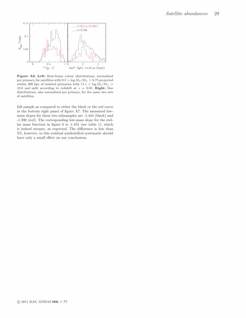
Satellite abundances 29

Figure A8. Left: Rest-frame colour distributions, normalizedper primary, for satellites with 9.5 > logM⋆/M⊙ > 8.75 projectedwithin 300 kpc of isolated primaries with 11.1 > logM⋆/M⊙ >10.8 and split according to redshift at z = 0.05. Right: Sizedistributions, also normalized per primary, for the same two setsof satellites.

full sample as compared to either the black or the red curvein the bottom right panel of figure A7. The measured low-mass slopes for these two subsamples are -1.444 (black) and-1.390 (red). The corresponding low-mass slope for the stel-lar mass function in figure 6 is -1.455 (see table 1), whichis indeed steeper, as expected. The difference is less than5%, however, so this residual unidentified systematic shouldhave only a small effect on our conclusions.

c© 2011 RAS, MNRAS 000, 1–??