Computational historical linguistics and language diversity in ...
Upload
khangminh22Category
view
0download
0
NAACL HLT 2018
Lexical and Computational Semantics(*SEM 2018)
Proceedings of the 7th Conference
June 5-6, 2018New Orleans

*SEM 2018 is sponsored by:
Association for Computational Linguistics
Special Interest Group on Computational Semantics
Special Interest Group on the Lexicon
c©2018 The Association for Computational Linguistics
ii

Order copies of this and other ACL proceedings from:
Association for Computational Linguistics (ACL)209 N. Eighth StreetStroudsburg, PA 18360USATel: +1-570-476-8006Fax: [email protected]
ISBN 978-1-948087-22-3
iii
Introduction
Preface by the General Chair
*SEM, the Joint Conference on Lexical and Computational Semantics is the major venue for researchon all aspects of semantics since 2012. This 2018 edition is therefore the seventh in a series that weenvisage to be a lot longer in the future.
As in previous years, *SEM 2018 has attracted a substantial number of submissions, and offers ahigh quality programme covering a wide spectrum of semantic areas. The overall goal of the *SEMseries, which is bringing together different communities that treat the computational modeling ofsemantics from different angles, is beautifully met in this year’s edition, which includes distributionaland formal/linguistic semantics approaches, spanning from lexical to discourse issues, with an eye toapplications.
We hope that the diversity and richness of the programme will provide not only an interesting eventfor a broad audience of NLP researchers, but also serve to stimulate new ideas and synergies that cansignificantly impact the field.
As always, *SEM would not have been possible without the active involvement of our community. Asidefrom our dedicated programme committee, to whom we give an extended acknowledgement further inthis introduction, we are very thankful to Johannes Bjerva (Publicity Chair) and Emmanuele Chersoni(Publication Chair) for their efficiency and hard work in making the conference a visible and sharedevent, from website to proceedings. We are grateful to ACL SIGLEX and SIGSEM for endorsing andstaying behind this event, and to Google, who thanks to its sponsorship to *SEM 2018, made it possibleto assign a few student grants, as a partial reimbursement of the *SEM participation costs.
As General Chair, I am particularly grateful to the Programme Chairs, Jonathan Berant and AlessandroLenci, to whom we all owe the excellence and variety of the programme, and to whom I personally owea very rewarding experience in sharing responsibility for this important event. I hope you will enjoy*SEM 2018 in all its diversity, and you will find it as stimulating and enriching as it strives to be.
Malvina NissimGeneral Chair of *SEM 2018
iv
Preface by the Program Chairs
We are pleased to present this volume containing the papers accepted at the Seventh Joint Conference onLexical and Computational Semantics (*SEM 2018, co-located with NAACL in New Orleans, USA, onJune 5-6, 2018). Like for the last edition, *SEM received a high number of submissions, which allowedus to compile a diverse and high-quality program. The number of submissions was 82. Out of these, 35papers were accepted (22 long, 14 short). Thus, the acceptance rate was 35.6% overall, 42.3% for thelong papers and 28.6% for the short submissions. Some of the papers were withdrawn after acceptance,due to multiple submissions to other conferences (the 2018 schedule was particularly complicated, withsignificant intersection of *SEM with ACL, COLING, and other venues). The final number of papers inthe program is 32 (19 long, 13 short).Submissions were reviewed in 5 different areas: Distributional Semantics, Discourse and Dialogue,Lexical Semantics, Theoretical and Formal Semantics, and Applied Semantics.The papers were evaluated by a program committee of 10 area chairs from Europe and North America,assisted by a panel of 115 reviewers. Each submission was reviewed by three reviewers, who werefurthermore encouraged to discuss any divergence in evaluation. The papers in each area weresubsequently ranked by the area chairs. The final selection was made by the program co-chairs afteran independent check of all reviews and discussion with the area chairs. Reviewers’ recommendationswere also used to shortlist a set of papers nominated for the Best Paper Award.The final *SEM 2018 program consists of 18 oral presentations and 14 posters, as well as two keynotetalks by Ellie Pavlick (Brown University & Google Research, joint keynote with SemEval 2018) andChristopher Potts (Stanford University).We are deeply thankful to all area chairs and reviewers for their help in the selection of the program, fortheir readiness in engaging in thoughtful discussions about individual papers, and for providing valuablefeedback to the authors. We are also grateful to Johannes Bjerva for his precious help in publicizingthe conference, and to Emmanuele Chersoni for his dedication and thoroughness in turning the programinto the proceedings you now have under your eyes. Last but not least, we are indebted to our GeneralChair, Malvina Nissim, for her continuous guidance and support throughout the process of organizingthis installment of *SEM.
We hope you enjoy the conference!Jonathan Berant and Alessandro Lenci
v


General Chair:
Malvina Nissim, University of Groningen
Program Chairs:
Jonathan Berant, Tel-Aviv UniversityAlessandro Lenci, University of Pisa
Publication Chair:
Emmanuele Chersoni, Aix-Marseille University
Publicity Chair:
Johannes Bjerva, University of Copenaghen
Area Chairs:
Distributional SemanticsOmer Levy, University of WashingtonSebastian Padó, University of Stuttgart
Discourse and DialogueAni Nenkova, University of PennsylvaniaMarta Recasens, Google Research
Lexical SemanticsNúria Bel, Pompeu Fabra UniversityEnrico Santus, Massachusetts Institute of Technology
Theoretical and Formal SemanticsSam Bowman, New York UniversityKilian Evang, University of Düsseldorf
Applied SemanticsSvetlana Kiritchenko, National Research Council CanadaLonneke van der Plas, University of Malta
vii
Reviewers:
Lasha Abzianidze, Eneko Agirre, Alan Akbik, Domagoj Alagic, Ron Artstein, Yoav Artzi, ChrisBarker, Raffaella Bernardi, Eduardo Blanco, Johan Bos, Teresa Botschen, António Branco, PaulBuitelaar, Jose Camacho-Collados, Tommaso Caselli, Emmanuele Chersoni, Eunsol Choi, Woo-Jin Chung, Paul Cook, Claudio Delli Bovi, Vera Demberg, Valeria dePaiva, Georgiana Dinu,Jakub Dotlacil, Aleksandr Drozd, Guy Emerson, Katrin Erk, Masha Esipova, Luis Espinosa Anke,Fabrizio Esposito, Benamara Farah, Raquel Fernandez, Kathleen C. Fraser, Daniel Fried, Al-bert Gatt, Kevin Gimpel, Luís Gomes, Edgar Gonzàlez Pellicer, Dagmar Gromann, Jiang Guo,Matthias Hartung, Iris Hendrickx, Aurélie Herbelot, Felix Hill, Veronique Hoste, Julie Hunter,Thomas Icard, Filip Ilievski, Gianina Iordachioaia, Sujay Kumar Jauhar, Hans Kamp, DouweKiela, Roman Klinger, Gregory Kobele, Alexander Koller, Valia Kordoni, Maximilian Köper,Mathieu Lafourcade, Gabriella Lapesa, Jochen L. Leidner, Nikola Ljubešic, Louise McNally,Oren Melamud, Tomas Mikolov, Ashutosh Modi, Saif Mohammad, Alessandro Moschitti, NikolaMrkšic, Preslav Nakov, Vivi Nastase, Guenter Neumann, Alexis Palmer, Martha Palmer, Alexan-der Panchenko, Denis Paperno, Panupong Pasupat, Sandro Pezzelle, Nghia The Pham, Mas-simo Poesio, Christopher Potts, Ciyang Qing, Marek Rei, Steffen Remus, Laura Rimell, AnnaRogers, Stephen Roller, Mats Rooth, Sara Rosenthal, Michael Roth, Sascha Rothe, Josef Ruppen-hofer, Mehrnoosh Sadrzadeh, Magnus Sahlgren, Efsun Sarioglu Kayi, Dominik Schlechtweg, RoySchwartz, Marco Silvio Giuseppe Senaldi, Jennifer Sikos, Stefan Thater, Sara Tonelli, Judith Ton-hauser, Yulia Tsvetkov, Martin Tutek, Lyle Ungar, Dmitry Ustalov, Benjamin Van Durme, NoortjeVenhuizen, Yannick Versley, Bonnie Webber, Kellie Webster, Hongzhi Xu, Roberto Zamparelli,Yue Zhang, Michael Zock, Pierre Zweigenbaum
viii

Invited Talk: Why Should we Care about Linguistics?Ellie Pavlick
(Joint Invited Speaker with SemEval 2018)
Brown University & Google Research
In just the past few months, a flurry of adversarial studies have pushed back on the apparentprogress of neural networks, with multiple analyses suggesting that deep models of text fail tocapture even basic properties of language, such as negation, word order, and compositionality.Alongside this wave of negative results, our field has stated ambitions to move beyond task-specificmodels and toward "general purpose" word, sentence, and even document embeddings. This is atall order for the field of NLP, and, I argue, marks a significant shift in the way we approach ourresearch. I will discuss what we can learn from the field of linguistics about the challenges ofcodifying all of language in a "general purpose" way. Then, more importantly, I will discuss whatwe cannot learn from linguistics. I will argue that the state-of-the-art of NLP research is operatingclose to the limits of what we know about natural language semantics, both within our field andoutside it. I will conclude with thoughts on why this opens opportunities for NLP to advance bothtechnology and basic science as it relates to language, and the implications for the way we shouldconduct empirical research.
ix
Invited Talk: Linguists for Deep Learning; or How I Learned to StopWorrying and Love Neural Networks
Christopher PottsStanford University, USA
The rise of deep learning (DL) might seem initially to mark a low point for linguists hoping tolearn from, and contribute to, the field of statistical NLP. In building DL systems, the decisivefactors tend to be data, computational resources, and optimization techniques, with domain ex-pertise in a supporting role. Nonetheless, at least for semantics and pragmatics, I argue that DLmodels are potentially the best computational implementations of linguists’ ideas and theories thatwe’ve ever seen. At the lexical level, symbolic representations are inevitably incomplete, whereaslearned distributed representations have the potential to capture the dense interconnections thatexist between words, and DL methods allow us to infuse these representations with informationfrom contexts of use and from structured lexical resources. For semantic composition, previousapproaches tended to represent phrases and sentences in partial, idiosyncratic ways; DL modelssupport comprehensive representations and might yield insights into flexible modes of semanticcomposition that would be unexpected from the point of view of traditional logical theories. Andwhen it comes to pragmatics, DL is arguably what the field has been looking for all along: a flex-ible set of tools for representing language and context together, and for capturing the nuanced,fallible ways in which langage users reason about each other’s intentions. Thus, while linguistsmight find it dispiriting that the day-to-day work of DL involves mainly fund-raising to supporthyperparameter tuning on expensive machines, I argue that it is worth the tedium for the insightsinto language that this can (unexpectedly) deliver.
x

Table of Contents
Resolving Event Coreference with Supervised Representation Learning and Clustering-Oriented Regu-larization
Kian Kenyon-Dean, Jackie Chi Kit Cheung and Doina Precup . . . . . . . . . . . . . . . . . . . . . . . . . . . . . . . . 1
Learning distributed event representations with a multi-task approachXudong Hong, Asad Sayeed and Vera Demberg . . . . . . . . . . . . . . . . . . . . . . . . . . . . . . . . . . . . . . . . . . . .11
Assessing Meaning Components in German Complex Verbs: A Collection of Source-Target Domains andDirectionality
Sabine Schulte im Walde, Maximilian Köper and Sylvia Springorum. . . . . . . . . . . . . . . . . . . . . . . . .22
Learning Neural Word Salience ScoresKrasen Samardzhiev, Andrew Gargett and Danushka Bollegala . . . . . . . . . . . . . . . . . . . . . . . . . . . . . . 33
Examining Gender and Race Bias in Two Hundred Sentiment Analysis SystemsSvetlana Kiritchenko and Saif Mohammad . . . . . . . . . . . . . . . . . . . . . . . . . . . . . . . . . . . . . . . . . . . . . . . . 43
Graph Algebraic Combinatory Categorial GrammarSebastian Beschke and Wolfgang Menzel . . . . . . . . . . . . . . . . . . . . . . . . . . . . . . . . . . . . . . . . . . . . . . . . . 54
Mixing Context Granularities for Improved Entity Linking on Question Answering Data across EntityCategories
Daniil Sorokin and Iryna Gurevych . . . . . . . . . . . . . . . . . . . . . . . . . . . . . . . . . . . . . . . . . . . . . . . . . . . . . . . 65
Quantitative Semantic Variation in the Contexts of Concrete and Abstract WordsDaniela Naumann, Diego Frassinelli and Sabine Schulte im Walde . . . . . . . . . . . . . . . . . . . . . . . . . . .76
EmoWordNet: Automatic Expansion of Emotion Lexicon Using English WordNetGilbert Badaro, Hussein Jundi, Hazem Hajj and Wassim El-Hajj . . . . . . . . . . . . . . . . . . . . . . . . . . . . . 86
The Limitations of Cross-language Word Embeddings EvaluationAmir Bakarov, Roman Suvorov and Ilya Sochenkov . . . . . . . . . . . . . . . . . . . . . . . . . . . . . . . . . . . . . . . . 94
How Gender and Skin Tone Modifiers Affect Emoji Semantics in TwitterFrancesco Barbieri and Jose Camacho-Collados . . . . . . . . . . . . . . . . . . . . . . . . . . . . . . . . . . . . . . . . . . 101
Element-wise Bilinear Interaction for Sentence MatchingJihun Choi, Taeuk Kim and Sang-goo Lee . . . . . . . . . . . . . . . . . . . . . . . . . . . . . . . . . . . . . . . . . . . . . . . . 107
Named Graphs for Semantic RepresentationRichard Crouch and Aikaterini-Lida Kalouli . . . . . . . . . . . . . . . . . . . . . . . . . . . . . . . . . . . . . . . . . . . . . 113
Learning Patient Representations from TextDmitriy Dligach and Timothy Miller . . . . . . . . . . . . . . . . . . . . . . . . . . . . . . . . . . . . . . . . . . . . . . . . . . . . .119
Polarity Computations in Flexible Categorial GrammarHai Hu and Larry Moss . . . . . . . . . . . . . . . . . . . . . . . . . . . . . . . . . . . . . . . . . . . . . . . . . . . . . . . . . . . . . . . . 124
Coarse Lexical Frame Acquisition at the Syntax–Semantics Interface Using a Latent-Variable PCFGModel
Laura Kallmeyer, Behrang QasemiZadeh and Jackie Chi Kit Cheung . . . . . . . . . . . . . . . . . . . . . . . 130
xi

Halo: Learning Semantics-Aware Representations for Cross-Lingual Information ExtractionHongyuan Mei, Sheng Zhang, Kevin Duh and Benjamin Van Durme . . . . . . . . . . . . . . . . . . . . . . . . 142
Exploiting Partially Annotated Data in Temporal Relation ExtractionQiang Ning, Zhongzhi Yu, Chuchu Fan and Dan Roth . . . . . . . . . . . . . . . . . . . . . . . . . . . . . . . . . . . . . 148
Predicting Word Embeddings VariabilityBenedicte Pierrejean and Ludovic Tanguy . . . . . . . . . . . . . . . . . . . . . . . . . . . . . . . . . . . . . . . . . . . . . . . . 154
Integrating Multiplicative Features into Supervised Distributional Methods for Lexical EntailmentTu Vu and Vered Shwartz . . . . . . . . . . . . . . . . . . . . . . . . . . . . . . . . . . . . . . . . . . . . . . . . . . . . . . . . . . . . . . .160
Deep Affix Features Improve Neural Named Entity RecognizersVikas Yadav, Rebecca Sharp and Steven Bethard . . . . . . . . . . . . . . . . . . . . . . . . . . . . . . . . . . . . . . . . . . 167
Fine-grained Entity Typing through Increased Discourse Context and Adaptive Classification ThresholdsSheng Zhang, Kevin Duh and Benjamin Van Durme. . . . . . . . . . . . . . . . . . . . . . . . . . . . . . . . . . . . . . .173
Hypothesis Only Baselines in Natural Language InferenceAdam Poliak, Jason Naradowsky, Aparajita Haldar, Rachel Rudinger and Benjamin Van Durme180
Quality Signals in Generated StoriesManasvi Sagarkar, John Wieting, Lifu Tu and Kevin Gimpel . . . . . . . . . . . . . . . . . . . . . . . . . . . . . . . 192
Term Definitions Help Hypernymy DetectionWenpeng Yin and Dan Roth . . . . . . . . . . . . . . . . . . . . . . . . . . . . . . . . . . . . . . . . . . . . . . . . . . . . . . . . . . . . 203
Agree or Disagree: Predicting Judgments on Nuanced AssertionsMichael Wojatzki, Torsten Zesch, Saif Mohammad and Svetlana Kiritchenko . . . . . . . . . . . . . . . . 214
A Multimodal Translation-Based Approach for Knowledge Graph Representation LearningHatem Mousselly Sergieh, Teresa Botschen, Iryna Gurevych and Stefan Roth . . . . . . . . . . . . . . . . 225
Putting Semantics into Semantic RolesJames Allen and Choh Man Teng. . . . . . . . . . . . . . . . . . . . . . . . . . . . . . . . . . . . . . . . . . . . . . . . . . . . . . . .235
Measuring Frame Instance RelatednessValerio Basile, Roque Lopez Condori and Elena Cabrio . . . . . . . . . . . . . . . . . . . . . . . . . . . . . . . . . . . 245
Solving Feature Sparseness in Text Classification using Core-Periphery DecompositionXia Cui, Sadamori Kojaku, Naoki Masuda and Danushka Bollegala . . . . . . . . . . . . . . . . . . . . . . . . .255
Robust Handling of Polysemy via Sparse RepresentationsAbhijit Mahabal, Dan Roth and Sid Mittal . . . . . . . . . . . . . . . . . . . . . . . . . . . . . . . . . . . . . . . . . . . . . . . 265
Multiplicative Tree-Structured Long Short-Term Memory Networks for Semantic RepresentationsNam Khanh Tran and Weiwei Cheng . . . . . . . . . . . . . . . . . . . . . . . . . . . . . . . . . . . . . . . . . . . . . . . . . . . . 276
xii

Conference Program
June 5th, 2018
9:00–10:30 Session 1
9:15–9:30 Opening Remarks
9:30–10:30 Invited Talk by Ellie Pavlick (Brown University): Why Should we Care about Lin-guistics?
10:30–11:00 Coffee Break
11:00–12:30 Session 2
11:00–11:30 Resolving Event Coreference with Supervised Representation Learning andClustering-Oriented RegularizationKian Kenyon-Dean, Jackie Chi Kit Cheung and Doina Precup
11:30–12:00 Learning distributed event representations with a multi-task approachXudong Hong, Asad Sayeed and Vera Demberg
12:00–12:15 Assessing Meaning Components in German Complex Verbs: A Collection of Source-Target Domains and DirectionalitySabine Schulte im Walde, Maximilian Köper and Sylvia Springorum
12:15–12:30 Learning Neural Word Salience ScoresKrasen Samardzhiev, Andrew Gargett and Danushka Bollegala
12:30–14:00 Lunch Break
xiii
June 5th, 2018 (continued)
14:00–15:30 Session 3
14:00–14:30 Examining Gender and Race Bias in Two Hundred Sentiment Analysis SystemsSvetlana Kiritchenko and Saif Mohammad
14:30–15:00 Graph Algebraic Combinatory Categorial GrammarSebastian Beschke and Wolfgang Menzel
15:00–15:15 Mixing Context Granularities for Improved Entity Linking on Question AnsweringData across Entity CategoriesDaniil Sorokin and Iryna Gurevych
15:15–15:30 Quantitative Semantic Variation in the Contexts of Concrete and Abstract WordsDaniela Naumann, Diego Frassinelli and Sabine Schulte im Walde
15:30–16:00 Coffee Break
16:00–18:00 Session 4
16:00–16:50 Poster Booster
16:50–18:00 Poster Session
EmoWordNet: Automatic Expansion of Emotion Lexicon Using English WordNetGilbert Badaro, Hussein Jundi, Hazem Hajj and Wassim El-Hajj
The Limitations of Cross-language Word Embeddings EvaluationAmir Bakarov, Roman Suvorov and Ilya Sochenkov
How Gender and Skin Tone Modifiers Affect Emoji Semantics in TwitterFrancesco Barbieri and Jose Camacho-Collados
Element-wise Bilinear Interaction for Sentence MatchingJihun Choi, Taeuk Kim and Sang-goo Lee
xiv

June 5th, 2018 (continued)
Named Graphs for Semantic RepresentationRichard Crouch and Aikaterini-Lida Kalouli
Learning Patient Representations from TextDmitriy Dligach and Timothy Miller
Polarity Computations in Flexible Categorial GrammarHai Hu and Larry Moss
Coarse Lexical Frame Acquisition at the Syntax–Semantics Interface Using aLatent-Variable PCFG ModelLaura Kallmeyer, Behrang QasemiZadeh and Jackie Chi Kit Cheung
Halo: Learning Semantics-Aware Representations for Cross-Lingual InformationExtractionHongyuan Mei, Sheng Zhang, Kevin Duh and Benjamin Van Durme
Exploiting Partially Annotated Data in Temporal Relation ExtractionQiang Ning, Zhongzhi Yu, Chuchu Fan and Dan Roth
Predicting Word Embeddings VariabilityBenedicte Pierrejean and Ludovic Tanguy
Integrating Multiplicative Features into Supervised Distributional Methods for Lex-ical EntailmentTu Vu and Vered Shwartz
Deep Affix Features Improve Neural Named Entity RecognizersVikas Yadav, Rebecca Sharp and Steven Bethard
Fine-grained Entity Typing through Increased Discourse Context and AdaptiveClassification ThresholdsSheng Zhang, Kevin Duh and Benjamin Van Durme
xv
June 6th, 2018
9:00–10:30 Session 5
9:00–10:00 Invited Talk by Christopher Potts (Stanford University): Linguists for Deep Learn-ing; or How I Learned to Stop Worrying and Love Neural Networks
10:00–10:30 Hypothesis Only Baselines in Natural Language InferenceAdam Poliak, Jason Naradowsky, Aparajita Haldar, Rachel Rudinger and BenjaminVan Durme
10:30–11:00 Coffee Break
11:00–12:15 Session 6
11:00–11:30 Quality Signals in Generated StoriesManasvi Sagarkar, John Wieting, Lifu Tu and Kevin Gimpel
11:30–12:00 Term Definitions Help Hypernymy DetectionWenpeng Yin and Dan Roth
12:00–12:15 Agree or Disagree: Predicting Judgments on Nuanced AssertionsMichael Wojatzki, Torsten Zesch, Saif Mohammad and Svetlana Kiritchenko
12:15–14:00 Lunch Break
xvi

June 6th, 2018 (continued)
14:00–15:30 Session 7
14:00–14:30 A Multimodal Translation-Based Approach for Knowledge Graph RepresentationLearningHatem Mousselly Sergieh, Teresa Botschen, Iryna Gurevych and Stefan Roth
14:30–15:30 Putting Semantics into Semantic RolesJames Allen and Choh Man Teng
15:00–15:30 Measuring Frame Instance RelatednessValerio Basile, Roque Lopez Condori and Elena Cabrio
15:30–16:00 Coffee Break
16:00–16:30 Solving Feature Sparseness in Text Classification using Core-Periphery Decompo-sitionXia Cui, Sadamori Kojaku, Naoki Masuda and Danushka Bollegala
16:30–17:00 Robust Handling of Polysemy via Sparse RepresentationsAbhijit Mahabal, Dan Roth and Sid Mittal
17:00–17:30 Multiplicative Tree-Structured Long Short-Term Memory Networks for SemanticRepresentationsNam Khanh Tran and Weiwei Cheng
xvii


Proceedings of the 7th Joint Conference on Lexical and Computational Semantics (*SEM), pages 1–10New Orleans, June 5-6, 2018. c©2018 Association for Computational Linguistics
Resolving Event Coreference with Supervised Representation Learningand Clustering-Oriented Regularization
Kian Kenyon-DeanSchool of Computer Science
McGill [email protected]
Jackie Chi Kit CheungSchool of Computer Science
McGill [email protected]
Doina PrecupSchool of Computer Science
McGill [email protected]
Abstract
We present an approach to event coreferenceresolution by developing a general frameworkfor clustering that uses supervised representa-tion learning. We propose a neural networkarchitecture with novel Clustering-OrientedRegularization (CORE) terms in the objectivefunction. These terms encourage the model tocreate embeddings of event mentions that areamenable to clustering. We then use agglom-erative clustering on these embeddings to buildevent coreference chains. For both within-and cross-document coreference on the ECB+corpus, our model obtains better results thanmodels that require significantly more pre-annotated information. This work provides in-sight and motivating results for a new generalapproach to solving coreference and clusteringproblems with representation learning.
1 Introduction
Event coreference resolution is the task of deter-mining which event mentions expressed in lan-guage refer to the same real-world event in-stances. The ability to resolve event coreferencehas improved the quality of downstream taskssuch as automatic text summarization (Vander-wende et al., 2004), questioning-answering (Be-rant et al., 2014), headline generation (Sun et al.,2015), and text-mining in the medical domain(Ferracane et al., 2016).
Event mentions are comprised of an actioncomponent (or, head) and surrounding arguments.Consider the following passages, drawn from twodifferent documents; the heads of the event men-tions are in boldface and the subscripts indicatemention IDs:
(1) The president’s speechm1 shockedm2 the au-dience. He announcedm3 several new con-troversial policies.
(2) The policies proposedm4 by the presidentwill not surprisem5 those who followedm6
his campaignm7.
In this example, m1, m3, and m4 form a chainof coreferent event mentions (underlined), becausethey refer to the same real-world event in whichthe president gave a speech. The other four aresingletons, meaning that they all refer to separateevents and do not corefer with any other mention.
This work investigates how to learn useful rep-resentations of event mentions. Event mentionsare complex objects, and both the event mentionheads and the surrounding arguments are impor-tant for the event coreference resolution task. Inour example above, the head words of mentionsm2, shocked, and m5, surprise, are lexically sim-ilar, but the event mentions do not corefer. Thistask therefore necessitates a model that can cap-ture the distributional relationships between eventmentions and their surrounding contexts.
We hypothesize that prior knowledge about thetask itself can be usefully encoded into the rep-resentation learning objective. For our task, thisprior means that the embeddings of corefentialevent mentions should have similar embeddings toeach other (a “natural clustering”, using the termi-nology of Bengio et al. (2013)). With this prior,our model creates embeddings of event mentionsthat are directly conducive for the clustering taskof building event coreference chains. This is con-trary to the indirect methods of previous work thatrely on pairwise decision making followed by aseparate model that aggregates the sometimes in-consistent decisions into clusters (Section 2).
We demonstrate these points by proposing amethod that learns to embed event mentions intoa space that is tuned specifically for clustering.The representation learner is trained to predictwhich event cluster the event mention belongs to,
1
using an hourglass-shaped neural network. Wepropose a mechanism to modulate this trainingby introducing Clustering-Oriented Regulariza-tion (CORE) terms into the objective function ofthe learner; these terms impel the model to pro-duce similar embeddings for coreferential eventmentions, and dissimilar embeddings otherwise.
Our model obtains strong results on within-and cross-document event coreference resolution,matching or outperforming the system of Cybul-ska and Vossen (2015) on the ECB+ corpus on allsix evaluation measures. We achieve these gainsdespite the fact that our model requires signifi-cantly less pre-annotated or pre-detected informa-tion in terms of the internal event structure. Ourmodel’s improvements upon the baselines showthat our supervised representation learning frame-work creates new embeddings that capture the ab-stract distributional relations between samples andtheir clusters, suggesting that our framework canbe generalized to other clustering tasks1.
2 Related Work
The recent work on event coreference can be cat-egorized according to the assumed level of eventrepresentation. In the predicate-argument align-ment paradigm (Roth and Frank, 2012; Wolfeet al., 2013), links are simply drawn between pred-icates in different documents. This work only con-siders cross-document event coreference (Wolfeet al., 2013, 2015), and no within-document coref-erence. At the other extreme, the ACE and EREdatasets annotate rich internal event structure, withspecific taxonomies that describe the annotatedevents and their types (Linguistic Data Consor-tium, 2005, 2016). In these datasets, only within-document coreference is annotated.
The creators of the ECB (Bejan and Harabagiu,2008) and ECB+ (Cybulska and Vossen, 2014),annotate events according to a level of abstractionbetween that of the predicate-argument approachand the ACE approach, being most similar to theTimeML paradigm (Pustejovsky et al., 2003). Inthese datasets, both within-document and cross-document coreference relations are annotated. Weuse the ECB+ corpus in our experiments becauseit solves the lack of lexical diversity found withinthe ECB by adding 502 new annotated documents,providing a total of 982 documents.
1All code used in this paper can be found here:https://github.com/kiankd/events
Previous work on model design for event coref-erence has focused on clustering over a linguis-tically rich set of features. Most models require apairwise-prediction based supervised learning stepwhich predicts whether or not a pair of event men-tions is coreferential (Bagga and Baldwin, 1999;Chen et al., 2009; Cybulska and Vossen, 2015).Other work focuses on the clustering step itself,aggregating local pairwise decisions into clusters,for example by graph partitioning (Chen and Ji,2009). There has also been work using non-parametric Bayesian clustering techniques (Bejanand Harabagiu, 2014; Yang et al., 2015), as wellas other probabilistic models (Lu and Ng, 2017).Some recent work uses intuitions combining rep-resentation learning with clustering, but does notaugment the loss function for the purpose ofbuilding clusterable representations (Krause et al.,2016; Choubey and Huang, 2017).
3 Event Coreference Resolution Model
We formulate the task of event coreference resolu-tion as creating clusters of event mentions whichrefer to the same event. For the purposes of thiswork, we define an event mention to be a set of to-kens that correspond to the action of some event.Consider the sentence below (borrowed from Cy-bulska and Vossen (2014)):
(3) On Monday Lindsay Lohan checked into re-hab in Malibu, California after a car crash.
Our model would take, as input, feature vectors(see Section 4) extracted from the two event men-tions (in bold) independently. In this paper, we usethe gold-standard event mentions provided by thedataset, and leave mention detection to other work.
3.1 Model Overview
Our approach to resolving event coreference con-sists of the following steps:
1. Train a supervised neural network model whichlearns event mention embeddings by predictingthe event cluster in the training set to which themention belongs (Figure 1).
2. At test time, use the previously trained model’sembedding layer to derive representations ofunseen event mentions. Then, perform agglom-erative clustering with these embeddings to cre-ate event coreference chains (Figure 2).
2

Figure 1: Our supervised representation learning modelduring the training step. Dashed arrows indicate contri-butions to the loss function.
Figure 2: Our trained model at inference time, used forvalidation tuning and final testing. Note that H3 and Yare not used in this step.
3.2 Supervised Representation Learning
We propose a representation learning frameworkbased on training a multi-layer artificial neural net-work, with one layer He chosen to be the embed-ding layer. In the training set, there are a certainnumber of event mentions, each of which belongsto some gold standard cluster, makingC total non-singleton clusters in the training set. The networkis trained as if it were encountering a C+1-classclassification problem, where the class of an eventmention corresponds to a single output node, andall singleton mentions belong to class C+12.
When using this model to cluster a new set ofmentions, the final layer’s output will not be di-rectly informative since the output node structurecorresponds to the clusters within the training set.However, we hypothesize that the trained modelwill have learned to capture the abstract distribu-tional relationships between event mentions andclusters in the intermediate layer He. We thus usethe activations in He as the embedding of an eventmention for the clustering step (see Figure 2). Asimilar hourglass-like neural architecture designhas been successful in automatic speech recogni-
2If each singleton mention (i.e., a mention that does notcorefer with anything else) had its own class then the modelwould be confronted with a classification problem with thou-sands of classes, many of which would only have one sample;this is much too ill-posed, so we merge all singletons togetherduring the training step.
tion (Grezl et al., 2007; Gehring et al., 2013), buthas not to our knowledge been used to pre-trainembeddings for clustering.
3.3 Categorical-Cross-Entropy (CCE)Using CCE as the loss function trains the modelto correctly predict a training set mention’s corre-sponding cluster. With model prediction yic as theprobability that sample i belongs to class c, and in-dicator variable tic = 1 if sample i belongs to classc (else tic = 0), we have the mean categorical-cross entropy loss over a randomly sampled train-ing input batch X:
(1)LCCE = − 1
|X|
|X|∑
i=1
C+1∑
c=1
tic log(yic)
3.4 Clustering-Oriented Regularization(CORE)
With CCE, the model may overfit towards accurateprediction performance for those particular clus-ters found in the training set without learning anembedding that captures the nature of events ingeneral. This therefore motivates introducing reg-ularization terms based on the intuition that em-beddings of mentions belonging to the same clus-ter should be similar, and that embeddings of men-tions belonging to different clusters should be dis-similar. Accordingly, we define dissimilarity be-tween two vector embeddings (~e1, ~e2) according
3

to the cosine-distance function d:
d(~e1, ~e2) =1
2
(1− ~e1 · ~e2||~e1||||~e2||
)(2)
Given input batch X, we create two sets S andD, where S is the set of all pairs (a, b) of men-tions in X that belong to the same cluster, andD isthe set of all pairs (c, d) in X that belong to differ-ent clusters. Note that all vector embeddings ~ei =He(i); i.e., they are obtained by feeding the eventmention i’s features through to embedding layerHe. We now define the following Attractive andRepulsive CORE terms.
3.4.1 Attractive RegularizationThe first desirable property for the embeddingsis that mentions that belong to the same clustershould have low cosine distance between each oth-ers’ embeddings, since the agglomerative cluster-ing algorithm uses cosine distance to make coref-erence decisions.
Formally, for all pairs of mentions a and b thatbelong to the same cluster, we would like to min-imize the distance between their embeddings ~eaand ~eb. We call this “attractive” regularizationbecause we want to attract embeddings closer toeach other by minimizing their distance d(~ea, ~eb)so that they will be as similar as possible.
(3)Lattract =1
|S|∑
(a,b)∈Sd(~ea, ~eb)
3.4.2 Repulsive RegularizationThe second desirable property is that the embed-dings corresponding to mentions that belong todifferent clusters should have high cosine distancebetween each other. Thus, for all pairs of mentionsc and d that belong to different clusters, the goal isto maximize their distance d(~ec, ~ed). This is “re-pulsive” because we train the model to push awaythe embeddings from each other to be as distant aspossible.
(4)Lrepulse = 1− 1
|D|∑
(c,d)∈Dd(~ec, ~ed)
3.5 Loss FunctionEquation 5 below shows the final loss function3.The attractive and repulsive terms are weighted by
3Note that, while we present Equations 3 and 4 as sum-mations over pairs from the input batch, the computation isactually reasonable when written in terms of matrix multipli-cations. The most expensive operation multiplying the em-bedded batch of input samples times its transpose.
hyperparameter constants λ1 and λ2 respectively:
(5)L = LCCE + λ1Lattract + λ2Lrepulse
By adding these regularization terms to the lossfunction, we hypothesize that the new embeddingsof test set mentions (obtained by feeding-forwardtheir features into the trained model) will exem-plify the desired properties represented by the lossfunction, thus assisting the agglomerative cluster-ing task in producing correct coreference-chains.
3.6 Agglomerative Clustering
Agglomerative clustering is a non-parametric“bottom-up” approach to hierarchical clustering,in which each sample starts as its own cluster,and at each step, the two most similar clustersare merged, where similarity between two clus-ters is measured according to some similarity met-ric. After each merge, clustering similarities arerecomputed according to a preset criterion (e.g.,single- or complete-linkage). In our models, clus-tering proceeds until a pre-determined similaritythreshold, τ , is reached. We tuned τ on the vali-dation set, doing grid search for τ ∈ [0, 1] to max-imize B3 accuracy4. Preliminary experimentationled us to use cosine-similarity (see cosine distancein Equation 2) to measure vector similarity, andsingle-linkage for clustering decisions.
We experimented with two initializationschemes for agglomerative clustering. In the firstscheme, each event mention is initialized as itsown cluster, as is standard. In the second, weinitialized clusters using the lemma-δ baselinedefined by Upadhyay et al. (2016). This baselinemerges all event mentions with the same headlemma that are in documents with document-levelsimilarity that is higher than a threshold δ. Upad-hyay et al. showed that it is a strong indicator ofevent coreference, so we experimented with ini-tializing our clustering algorithm in this way. Wecall this model variant CORE+CCE+LEMMA,and describe the parameter tuning procedures inmore detail in Section 5.
4 Feature Extraction
We extract features that do not require the pre-processing step of event-template construction torepresent the context (unlike Cybulska and Vossen
4We optimize with B3 F1-score because the other mea-sures are either too expensive to compute (CEAF-M, CEAF-E, BLANC), or are less discriminative (MUC).
4
1.action checked into, crash2.time On Monday3.location rehab in Malibu, California4.participant Lindsay Lohan (human)
car (non-human)
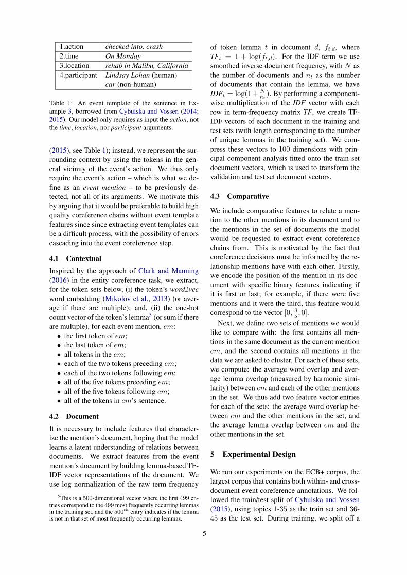
Table 1: An event template of the sentence in Ex-ample 3, borrowed from Cybulska and Vossen (2014;2015). Our model only requires as input the action, notthe time, location, nor participant arguments.
(2015), see Table 1); instead, we represent the sur-rounding context by using the tokens in the gen-eral vicinity of the event’s action. We thus onlyrequire the event’s action – which is what we de-fine as an event mention – to be previously de-tected, not all of its arguments. We motivate thisby arguing that it would be preferable to build highquality coreference chains without event templatefeatures since since extracting event templates canbe a difficult process, with the possibility of errorscascading into the event coreference step.
4.1 Contextual
Inspired by the approach of Clark and Manning(2016) in the entity coreference task, we extract,for the token sets below, (i) the token’s word2vecword embedding (Mikolov et al., 2013) (or aver-age if there are multiple); and, (ii) the one-hotcount vector of the token’s lemma5 (or sum if thereare multiple), for each event mention, em:• the first token of em;• the last token of em;• all tokens in the em;• each of the two tokens preceding em;• each of the two tokens following em;• all of the five tokens preceding em;• all of the five tokens following em;• all of the tokens in em’s sentence.
4.2 Document
It is necessary to include features that character-ize the mention’s document, hoping that the modellearns a latent understanding of relations betweendocuments. We extract features from the eventmention’s document by building lemma-based TF-IDF vector representations of the document. Weuse log normalization of the raw term frequency
5This is a 500-dimensional vector where the first 499 en-tries correspond to the 499 most frequently occurring lemmasin the training set, and the 500th entry indicates if the lemmais not in that set of most frequently occurring lemmas.
of token lemma t in document d, ft,d, whereTFt = 1 + log(ft,d). For the IDF term we usesmoothed inverse document frequency, with N asthe number of documents and nt as the numberof documents that contain the lemma, we haveIDFt = log(1+ N
nt). By performing a component-
wise multiplication of the IDF vector with eachrow in term-frequency matrix TF, we create TF-IDF vectors of each document in the training andtest sets (with length corresponding to the numberof unique lemmas in the training set). We com-press these vectors to 100 dimensions with prin-cipal component analysis fitted onto the train setdocument vectors, which is used to transform thevalidation and test set document vectors.
4.3 Comparative
We include comparative features to relate a men-tion to the other mentions in its document and tothe mentions in the set of documents the modelwould be requested to extract event coreferencechains from. This is motivated by the fact thatcoreference decisions must be informed by the re-lationship mentions have with each other. Firstly,we encode the position of the mention in its doc-ument with specific binary features indicating ifit is first or last; for example, if there were fivementions and it were the third, this feature wouldcorrespond to the vector [0, 35 , 0].
Next, we define two sets of mentions we wouldlike to compare with: the first contains all men-tions in the same document as the current mentionem, and the second contains all mentions in thedata we are asked to cluster. For each of these sets,we compute: the average word overlap and aver-age lemma overlap (measured by harmonic simi-larity) between em and each of the other mentionsin the set. We thus add two feature vector entriesfor each of the sets: the average word overlap be-tween em and the other mentions in the set, andthe average lemma overlap between em and theother mentions in the set.
5 Experimental Design
We run our experiments on the ECB+ corpus, thelargest corpus that contains both within- and cross-document event coreference annotations. We fol-lowed the train/test split of Cybulska and Vossen(2015), using topics 1-35 as the train set and 36-45 as the test set. During training, we split off a
5
validation set6 for hyperparameter tuning.Following Cybulska and Vossen, we used the
portion of the corpus that has been manually re-viewed and checked for correctness. Some pre-vious work (Yang et al., 2015; Upadhyay et al.,2016; Choubey and Huang, 2017) do not appearto have followed this guideline from the corpuscreators, as they report different corpus statis-tics compared to those reported by Cybulska andVossen. As a result, those papers may report re-sults on a data set with known annotation errors.
5.1 Evaluation Measures
Since there is no consensus in the coreference res-olution literature on the best evaluation measure,we present results obtained according to six differ-ent measures, as is common in previous work. Weuse the scorer presented by Pradhan et al. (2014).In this task, the term “coreference chain” is syn-onymous with “cluster”.
MUC (Vilain et al., 1995). Link-level mea-sure which counts the minimum number of linkchanges required to obtain the correct clusteringfrom the predictions; it does not account for cor-rectly predicted singletons.
B3 (Bagga and Baldwin, 1998). Mention-levelmeasure which computes precision and recall foreach individual mention, overcoming the singletonproblem of MUC, but can problematically countthe same coreference chain multiple times.
CEAF-M (Luo, 2005). Mention-level measurewhich reflects the percentage of mentions that arein the correct coreference chains. Note that preci-sion and recall are the same in this measure sincewe use pre-annotated mentions.
CEAF-E (Luo, 2005). Entity-level measure com-puted by aligning predicted with the gold chains,not allowing one chain to have more than onealignment, overcoming the problem of B3.
BLANC (Luo et al., 2014). Computes two F-scores in terms of the pairwise quality of corefer-ence decisions and non-coreference decisions, andaverages these scores together for the final results.
CoNLL. The mean of MUC, B3, and CEAF-E.
5.2 Models
We compare our representation-learning modelvariants to three baselines: a deterministic lemma-
6Topics 2, 5, 12, 18, 21, 23, 34, 35 (randomly chosen).
based baseline, a lemma-δ baseline, and an unsu-pervised baseline which clusters the originally ex-tracted features. We also compare with the resultsof Cybulska and Vossen (2015).
5.2.1 BaselinesLEMMA. This algorithm clusters event mentionswhich share the same head word lemma into thesame coreference chains across all documents.
LEMMA-δ. Proposed by Upadhyay et al. (2016),this method provides a difficult baseline to beat.A δ-similarity threshold is introduced, and wemerge two mentions with the same head-lemma ifand only if the cosine-similarity between the TF-IDF vectors of their corresponding documents isgreater than δ. This δ parameter is tuned to maxi-mize B3 performance on the validation set, whichwe found occurs when δ = 0.67.
UNSUPERVISED. This is the result obtainedby agglomerative clustering over the original un-weighted features. Again, we optimize the τ sim-ilarity threshold over the validation set.
5.2.2 Sentence Templates (CV2015)Cybulska and Vossen (2015) propose a model thatuses sentence-level event templates (see Table 1),requiring more annotated information than ourmodels. See (Vossen and Cybulska, 2017) for fur-ther elaboration of this model. To our knowledge,this is the best previous model on ECB+ using thesame data and evaluation criteria as our work.
5.2.3 Representation Learning.We test four different model variants:
• CCE: uses only categorical-cross-entropy in theloss function (Equation 1);
• CORE: uses only clustering-oriented regular-ization; i.e., the attract and repulse terms (Equa-tions 3 and 4);
• CORE+CCE: includes categorical-cross-entropy and the attract and repulse terms(Equation 5);
• CORE+CCE+LEMMA: initializes the agglom-erative clustering with clusters computed bylemma-δ (with a differently tuned value of δthan the baseline) and continues the clusteringprocess using the similarities between the em-beddings created by CORE+CCE.
6
Model λ1 λ2 B3 τ
BaselinesUNSUPERVISED - - 0.590 0.657LEMMA - - 0.597 -LEMMA-δ - - 0.612 -Model VariantsCORE+CCE+L 2.0 0.0 0.678 0.843
CORE+CCE 2.0 2.0 0.663 0.7762.0 1.0 0.666 0.7732.0 0.1 0.665 0.8432.0 0.0 0.669 0.8430.0 2.0 0.662 0.710
CORE 2.0 2.0 0.631 0.7011.0 1.0 0.625 0.689
CCE - - 0.644 0.853
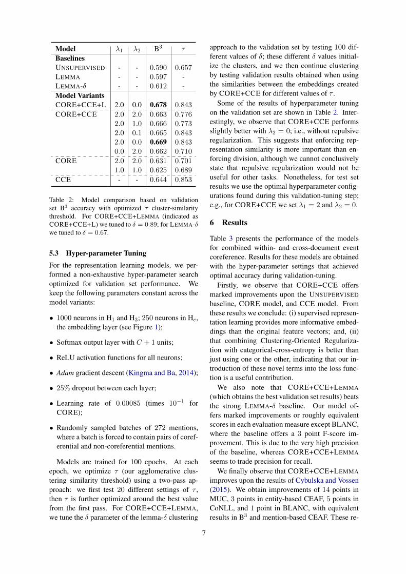
Table 2: Model comparison based on validationset B3 accuracy with optimized τ cluster-similaritythreshold. For CORE+CCE+LEMMA (indicated asCORE+CCE+L) we tuned to δ = 0.89; for LEMMA-δwe tuned to δ = 0.67.
5.3 Hyper-parameter TuningFor the representation learning models, we per-formed a non-exhaustive hyper-parameter searchoptimized for validation set performance. Wekeep the following parameters constant across themodel variants:
• 1000 neurons in H1 and H3; 250 neurons in He,the embedding layer (see Figure 1);
• Softmax output layer with C + 1 units;
• ReLU activation functions for all neurons;
• Adam gradient descent (Kingma and Ba, 2014);
• 25% dropout between each layer;
• Learning rate of 0.00085 (times 10−1 forCORE);
• Randomly sampled batches of 272 mentions,where a batch is forced to contain pairs of coref-erential and non-coreferential mentions.
Models are trained for 100 epochs. At eachepoch, we optimize τ (our agglomerative clus-tering similarity threshold) using a two-pass ap-proach: we first test 20 different settings of τ ,then τ is further optimized around the best valuefrom the first pass. For CORE+CCE+LEMMA,we tune the δ parameter of the lemma-δ clustering
approach to the validation set by testing 100 dif-ferent values of δ; these different δ values initial-ize the clusters, and we then continue clusteringby testing validation results obtained when usingthe similarities between the embeddings createdby CORE+CCE for different values of τ .
Some of the results of hyperparameter tuningon the validation set are shown in Table 2. Inter-estingly, we observe that CORE+CCE performsslightly better with λ2 = 0; i.e., without repulsiveregularization. This suggests that enforcing rep-resentation similarity is more important than en-forcing division, although we cannot conclusivelystate that repulsive regularization would not beuseful for other tasks. Nonetheless, for test setresults we use the optimal hyperparameter config-urations found during this validation-tuning step;e.g., for CORE+CCE we set λ1 = 2 and λ2 = 0.
6 Results
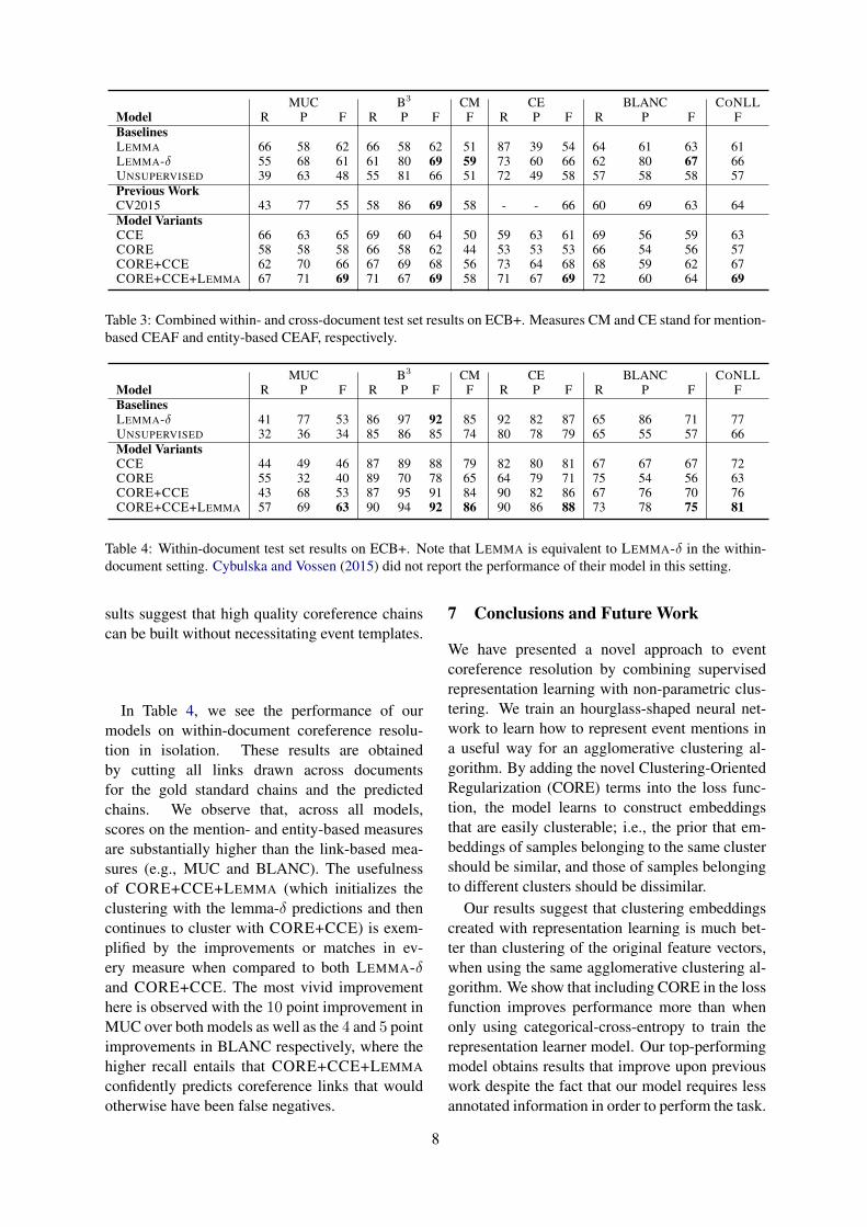
Table 3 presents the performance of the modelsfor combined within- and cross-document eventcoreference. Results for these models are obtainedwith the hyper-parameter settings that achievedoptimal accuracy during validation-tuning.
Firstly, we observe that CORE+CCE offersmarked improvements upon the UNSUPERVISED
baseline, CORE model, and CCE model. Fromthese results we conclude: (i) supervised represen-tation learning provides more informative embed-dings than the original feature vectors; and, (ii)that combining Clustering-Oriented Regulariza-tion with categorical-cross-entropy is better thanjust using one or the other, indicating that our in-troduction of these novel terms into the loss func-tion is a useful contribution.
We also note that CORE+CCE+LEMMA
(which obtains the best validation set results) beatsthe strong LEMMA-δ baseline. Our model of-fers marked improvements or roughly equivalentscores in each evaluation measure except BLANC,where the baseline offers a 3 point F-score im-provement. This is due to the very high precisionof the baseline, whereas CORE+CCE+LEMMA
seems to trade precision for recall.We finally observe that CORE+CCE+LEMMA
improves upon the results of Cybulska and Vossen(2015). We obtain improvements of 14 points inMUC, 3 points in entity-based CEAF, 5 points inCoNLL, and 1 point in BLANC, with equivalentresults in B3 and mention-based CEAF. These re-
7
MUC B3 CM CE BLANC CONLLModel R P F R P F F R P F R P F FBaselinesLEMMA 66 58 62 66 58 62 51 87 39 54 64 61 63 61LEMMA-δ 55 68 61 61 80 69 59 73 60 66 62 80 67 66UNSUPERVISED 39 63 48 55 81 66 51 72 49 58 57 58 58 57Previous WorkCV2015 43 77 55 58 86 69 58 - - 66 60 69 63 64Model VariantsCCE 66 63 65 69 60 64 50 59 63 61 69 56 59 63CORE 58 58 58 66 58 62 44 53 53 53 66 54 56 57CORE+CCE 62 70 66 67 69 68 56 73 64 68 68 59 62 67CORE+CCE+LEMMA 67 71 69 71 67 69 58 71 67 69 72 60 64 69
Table 3: Combined within- and cross-document test set results on ECB+. Measures CM and CE stand for mention-based CEAF and entity-based CEAF, respectively.
MUC B3 CM CE BLANC CONLLModel R P F R P F F R P F R P F FBaselinesLEMMA-δ 41 77 53 86 97 92 85 92 82 87 65 86 71 77UNSUPERVISED 32 36 34 85 86 85 74 80 78 79 65 55 57 66Model VariantsCCE 44 49 46 87 89 88 79 82 80 81 67 67 67 72CORE 55 32 40 89 70 78 65 64 79 71 75 54 56 63CORE+CCE 43 68 53 87 95 91 84 90 82 86 67 76 70 76CORE+CCE+LEMMA 57 69 63 90 94 92 86 90 86 88 73 78 75 81
Table 4: Within-document test set results on ECB+. Note that LEMMA is equivalent to LEMMA-δ in the within-document setting. Cybulska and Vossen (2015) did not report the performance of their model in this setting.
sults suggest that high quality coreference chainscan be built without necessitating event templates.
In Table 4, we see the performance of ourmodels on within-document coreference resolu-tion in isolation. These results are obtainedby cutting all links drawn across documentsfor the gold standard chains and the predictedchains. We observe that, across all models,scores on the mention- and entity-based measuresare substantially higher than the link-based mea-sures (e.g., MUC and BLANC). The usefulnessof CORE+CCE+LEMMA (which initializes theclustering with the lemma-δ predictions and thencontinues to cluster with CORE+CCE) is exem-plified by the improvements or matches in ev-ery measure when compared to both LEMMA-δand CORE+CCE. The most vivid improvementhere is observed with the 10 point improvement inMUC over both models as well as the 4 and 5 pointimprovements in BLANC respectively, where thehigher recall entails that CORE+CCE+LEMMA
confidently predicts coreference links that wouldotherwise have been false negatives.
7 Conclusions and Future Work
We have presented a novel approach to eventcoreference resolution by combining supervisedrepresentation learning with non-parametric clus-tering. We train an hourglass-shaped neural net-work to learn how to represent event mentions ina useful way for an agglomerative clustering al-gorithm. By adding the novel Clustering-OrientedRegularization (CORE) terms into the loss func-tion, the model learns to construct embeddingsthat are easily clusterable; i.e., the prior that em-beddings of samples belonging to the same clustershould be similar, and those of samples belongingto different clusters should be dissimilar.
Our results suggest that clustering embeddingscreated with representation learning is much bet-ter than clustering of the original feature vectors,when using the same agglomerative clustering al-gorithm. We show that including CORE in the lossfunction improves performance more than whenonly using categorical-cross-entropy to train therepresentation learner model. Our top-performingmodel obtains results that improve upon previouswork despite the fact that our model requires lessannotated information in order to perform the task.
8
Future work involves applying our model to au-tomatically annotated event mentions and otherevent coreference datasets, and extending thisframework toward a full end-to-end system thatdoes not rely on manual feature engineering at theinput level. Additionally, our model may be use-ful for other clustering tasks, such as entity coref-erence and document clustering. Lastly, we seekto determine how CORE and its imposition of aclusterable latent space structure may or may notassist in improving the quality of latent represen-tations in general.
Acknowledgements
This work was funded with grants from the Natu-ral Sciences and Engineering Research Council ofCanada (NSERC) and the Fonds de recherche duQuebec - Nature et Technologies (FRQNT). Wethank the anonymous reviewers for their helpfulcomments and suggestions.
ReferencesAmit Bagga and Breck Baldwin. 1998. Algorithms
for scoring coreference chains. In The first in-ternational conference on language resources andevaluation workshop on linguistics coreference, vol-ume 1, pages 563–566.
Amit Bagga and Breck Baldwin. 1999. Cross-document event coreference: Annotations, exper-iments, and observations. In Proceedings of theWorkshop on Coreference and its Applications,pages 1–8. ACL.
Cosmin Adrian Bejan and Sanda Harabagiu. 2014. Un-supervised Event Coreference Resolution. Compu-tational Linguistics, 40(2):311–347.
Cosmin Adrian Bejan and Sanda M Harabagiu. 2008.A Linguistic Resource for Discovering Event Struc-tures and Resolving Event Coreference. In LREC.
Yoshua Bengio, Aaron Courville, and Pascal Vincent.2013. Representation learning: A review and newperspectives. IEEE transactions on pattern analysisand machine intelligence, 35(8):1798–1828.
Jonathan Berant, Vivek Srikumar, Pei-Chun Chen,Abby Vander Linden, Brittany Harding, BradHuang, Peter Clark, and Christopher D Manning.2014. Modeling Biological Processes for ReadingComprehension. In Proceedings of the 2014 Con-ference on EMNLP, pages 1499–1510.
Zheng Chen and Heng Ji. 2009. Graph-based eventcoreference resolution. In Proceedings of the 2009Workshop on Graph-based Methods for NLP, pages54–57. ACL.
Zheng Chen, Heng Ji, and Robert Haralick. 2009. APairwise Event Coreference Model, Feature Impactand Evaluation for Event Coreference Resolution.In Proceedings of the workshop on events in emerg-ing text types, pages 17–22. ACL.
Prafulla Kumar Choubey and Ruihong Huang. 2017.Event coreference resolution by iteratively un-folding inter-dependencies among events. arXivpreprint arXiv:1707.07344.
Kevin Clark and Christopher D Manning. 2016. Im-proving Coreference Resolution by Learning Entity-Level Distributed Representations. arXiv preprintarXiv:1606.01323.
Agata Cybulska and Piek Vossen. 2014. Using asledgehammer to crack a nut? Lexical diversity andevent coreference resolution. In LREC, pages 4545–4552.
Agata Cybulska and Piek Vossen. 2015. TranslatingGranularity of Event Slots into Features for EventCoreference Resolution. In Proceedings of the 3rdWorkshop on EVENTS at the NAACL-HLT, pages 1–10.
Elisa Ferracane, Iain Marshall, Byron C Wallace, andKatrin Erk. 2016. Leveraging coreference to iden-tify arms in medical abstracts: An experimentalstudy. EMNLP, pages 86–95.
Jonas Gehring, Yajie Miao, Florian Metze, and AlexWaibel. 2013. Extracting deep bottleneck featuresusing stacked auto-encoders. In Acoustics, Speechand Signal Processing (ICASSP), 2013 IEEE Inter-national Conference on, pages 3377–3381. IEEE.
Frantisek Grezl, Martin Karafiat, Stanislav Kontar, andJan Cernocky. 2007. Probabilistic and bottle-neckfeatures for LVCSR of meetings. In Acoustics,Speech and Signal Processing, 2007. ICASSP 2007.IEEE International Conference on, volume 4, pagesIV–757. IEEE.
Diederik Kingma and Jimmy Ba. 2014. Adam: Amethod for stochastic optimization. arXiv preprintarXiv:1412.6980.
Sebastian Krause, Feiyu Xu, Hans Uszkoreit, and DirkWeissenborn. 2016. Event linking with sententialfeatures from convolutional neural networks. InProceedings of the 20th SIGNLL Conference onComputational Natural Language Learning, pages239–249.
Linguistic Data Consortium. 2005. ACE (AutomaticContent Extraction) English Annotation Guidelinesfor Events. Version 5.4.3 2005.07.01.
Linguistic Data Consortium. 2016. Rich ERE Annota-tion Guidelines Overview. V4.2.
Jing Lu and Vincent Ng. 2017. Learning antecedentstructures for event coreference resolution. In Ma-chine Learning and Applications (ICMLA), 2017
9
16th IEEE International Conference on, pages 113–118. IEEE.
Xiaoqiang Luo. 2005. On coreference resolution per-formance metrics. In Proceedings of the confer-ence on Human Language Technology and EMNLP,pages 25–32. ACL.
Xiaoqiang Luo, Sameer Pradhan, Marta Recasens, andEduard H Hovy. 2014. An Extension of BLANC toSystem Mentions. In ACL (2), pages 24–29.
Tomas Mikolov, Ilya Sutskever, Kai Chen, Greg S Cor-rado, and Jeff Dean. 2013. Distributed representa-tions of words and phrases and their compositional-ity. In Advances in neural information processingsystems, pages 3111–3119.
Sameer Pradhan, Xiaoqiang Luo, Marta Recasens, Ed-uard H Hovy, Vincent Ng, and Michael Strube.2014. Scoring coreference partitions of predictedmentions: A reference implementation. In ACL (2),pages 30–35.
James Pustejovsky, Jose M Castano, Robert Ingria,Roser Sauri, Robert J Gaizauskas, Andrea Set-zer, Graham Katz, and Dragomir R Radev. 2003.TimeML: Robust specification of event and tempo-ral expressions in text. New directions in questionanswering, 3:28–34.
Michael Roth and Anette Frank. 2012. Aligning predi-cate argument structures in monolingual comparabletexts: A new corpus for a new task. In Proceedingsof the First Joint Conference on Lexical and Com-putational Semantics-Volume 1: Proceedings of themain conference and the shared task, and Volume 2:Proceedings of the Sixth International Workshop onSemantic Evaluation, pages 218–227. ACL.
Rui Sun, Yue Zhang, Meishan Zhang, and DonghongJi. 2015. Event-driven headline generation. In Pro-ceedings of ACL, pages 462–472.
Shyam Upadhyay, Nitish Gupta, ChristosChristodoulopoulos, and Dan Roth. 2016. Re-visiting the Evaluation for Cross Document EventCoreference. In COLING.
Lucy Vanderwende, Michele Banko, and ArulMenezes. 2004. Event-centric summary generation.Working notes of DUC, pages 127–132.
Marc Vilain, John Burger, John Aberdeen, Dennis Con-nolly, and Lynette Hirschman. 1995. A model-theoretic coreference scoring scheme. In Proceed-ings of the 6th conference on Message understand-ing, pages 45–52. ACL.
Piek Vossen and Agata Cybulska. 2017. Identityand granularity of events in text. arXiv preprintarXiv:1704.04259.
Travis Wolfe, Mark Dredze, and Benjamin Van Durme.2015. Predicate argument alignment using a global
coherence model. In Proceedings of the 2015 Con-ference of NAACL: Human Language Technologies,pages 11–20.
Travis Wolfe, Benjamin Van Durme, Mark Dredze,Nicholas Andrews, Charley Beller, Chris Callison-Burch, Jay DeYoung, Justin Snyder, JonathanWeese, Tan Xu, et al. 2013. PARMA: A PredicateArgument Aligner. In ACL (2), pages 63–68.
Bishan Yang, Claire Cardie, and Peter Frazier. 2015.A Hierarchical Distance-dependent Bayesian Modelfor Event Coreference Resolution. Transactionsof the Association for Computational Linguistics,3:517–528.
10
Proceedings of the 7th Joint Conference on Lexical and Computational Semantics (*SEM), pages 11–21New Orleans, June 5-6, 2018. c©2018 Association for Computational Linguistics
Learning Distributed Event Representations with a Multi-Task Approach
Xudong Hong†, Asad Sayeed*, Vera Demberg††Dept. of Language Science and Technology, Saarland University
{xhong,vera}@coli.uni-saarland.de*Dept. of Philosophy, Linguistics, and Theory of Science, University of Gothenburg
AbstractHuman world knowledge contains informa-tion about prototypical events and their partic-ipants and locations. In this paper, we trainthe first models using multi-task learning thatcan both predict missing event participants andalso perform semantic role classification basedon semantic plausibility. Our best-performingmodel is an improvement over the previousstate-of-the-art on thematic fit modelling tasks.The event embeddings learned by the modelcan additionally be used effectively in an eventsimilarity task, also outperforming the state-of-the-art.
1 Introduction
Event representations consist, at minimum, of apredicate, the entities that participate in the event,and the thematic roles of those participants (Fill-more, 1968). The cook cut the cake with the knifeexpresses an event of cutting in which a cook is the“agent”, the cake is the “patient”, and the knife isthe “instrument” of the action. Experiments haveshown that event knowledge, in terms of the proto-typical participants of events and their structuredcompositions, plays a crucial role in human sen-tence processing, especially from the perspectiveof thematic fit: the extent to which humans per-ceive given event participants as “fitting” givenpredicate-role combinations (Ferretti et al., 2001;McRae et al., 2005; Bicknell et al., 2010). There-fore, computational models of language process-ing should also consist of event representationsthat reflect thematic fit. To evaluate this aspect em-pirically, a popular approach in previous work hasbeen to compare model output to human judge-ments (Sayeed et al., 2016).
The best-performing recent work has been themodel of Tilk et al. (2016), who effectively simu-late thematic fit via selectional preferences: gener-ating a probability distribution over the full vocab-
ulary of potential role-fillers. Given event contextas input, including a predicate and a given set ofsemantic roles and their role-fillers as well as onetarget role, its training objective is to predict thecorrect role-filler for the target role. The objectiveof predicting upcoming role-fillers is cognitivelyplausible: there is ample evidence that humans an-ticipate upcoming input during sentence process-ing and learn from prediction error (Kuperbergand Jaeger, 2016; Friston, 2010) (even if other de-tails of the implementation like back-propagationmay not have much to do with how errors are prop-agated in humans).
An analysis of role filler predictions by Tilk etal.’s model shows that the model does not makesufficient use of the thematic role input. For in-stance, the representation of apple eats boy is sim-ilar to the representation of boy eats apple, eventhough the events are very dissimilar from one an-other. Interestingly, humans have been found tomake similar errors. For instance, humans havebeen shown to frequently misinterpret a sentencewith inverse role assignment, when the plausibil-ity of the sentence with swapped role assignmentis very high, as in The mother gave the candle thedaughter, which is often erroneously interpretedas the daughter receiving the candle, instead of theliteral syntax which says that the candle receivesthe daughter (Gibson et al., 2013).
Tilk et al.’s model design makes it more sus-ceptible to this type of error than humans. Themodel lacks the ability to process in both direc-tions, i.e., to both comprehend and produce the-matic role marking (approximated here as the-matic role assignment). We therefore propose toadd a secondary role prediction task to the model,training it to both produce and comprehend lan-guage.
In this paper, we train the first model usingmulti-task learning (Caruana, 1998) which can ef-
11
fectively predict semantic roles for event partic-ipants as well as perform role-filler prediction1.Furthermore, we obtain significant improvementsand better-performing event embeddings by an ad-justment to the architecture (parametric weightedaverage of role-filler embeddings) which helpsto capture role-specific information for partici-pants during the composition process. The newevent embeddings exhibit state-of-the-art perfor-mance on a correlation task with human thematicfit judgements and an event similarity task.
Our model is the first joint model for selec-tional preferences (SPs) prediction and seman-tic role classification (SRC) to the best of ourknowledge. Previous works used distributionalsimilarity-based (Zapirain et al., 2013) or LDA-based (Wu and Palmer, 2015) SPs for semanticrole labelling to leverage lexical sparsity. How-ever, when it comes to a situation with domainshift, single task SP models that rely heavily onsyntax have high generalisation error. We showthat the multi-task architecture is better suited togeneralise in that situation and can be potentiallyapplied to improve current semantic role labellingsystems which rely on small annotated corpora.
Our approach is a conceptual improvementon previous models because we address mul-tiple event-representation tasks in a singlemodel: thematic fit evaluation, role-filler predic-tion/generation, semantic role classification, eventparticipant composition, and structured event sim-ilarity evaluation.
2 Role-Filler Prediction Model
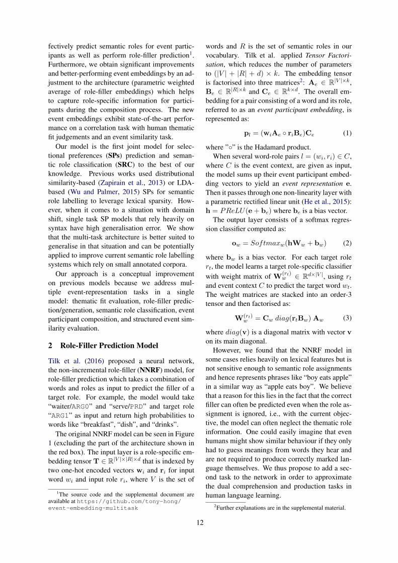
Tilk et al. (2016) proposed a neural network,the non-incremental role-filler (NNRF) model, forrole-filler prediction which takes a combination ofwords and roles as input to predict the filler of atarget role. For example, the model would take“waiter/ARG0” and “serve/PRD” and target role“ARG1” as input and return high probabilities towords like “breakfast”, “dish”, and “drinks”.
The original NNRF model can be seen in Figure1 (excluding the part of the architecture shown inthe red box). The input layer is a role-specific em-bedding tensor T ∈ R|V |×|R|×d that is indexed bytwo one-hot encoded vectors wi and ri for inputword wi and input role ri, where V is the set of
1The source code and the supplemental document areavailable at https://github.com/tony-hong/event-embedding-multitask
words and R is the set of semantic roles in ourvocabulary. Tilk et al. applied Tensor Factori-sation, which reduces the number of parametersto (|V | + |R| + d) × k. The embedding tensoris factorised into three matrices2: Ae ∈ R|V |×k,Be ∈ R|R|×k and Ce ∈ Rk×d. The overall em-bedding for a pair consisting of a word and its role,referred to as an event participant embedding, isrepresented as:
pl = (wiAe ◦ riBe)Ce (1)
where ”◦” is the Hadamard product.When several word-role pairs l = (wi, ri) ∈ C,
where C is the event context, are given as input,the model sums up their event participant embed-ding vectors to yield an event representation e.Then it passes through one non-linearity layer witha parametric rectified linear unit (He et al., 2015):h = PReLU(e+ be) where be is a bias vector.
The output layer consists of a softmax regres-sion classifier computed as:
ow = Softmaxw(hWw + bw) (2)
where bw is a bias vector. For each target rolert, the model learns a target role-specific classifierwith weight matrix of W(rt)
w ∈ Rd×|V |, using rtand event context C to predict the target word wt.The weight matrices are stacked into an order-3tensor and then factorised as:
W(rt)w = Cw diag(rtBw) Aw (3)
where diag(v) is a diagonal matrix with vector von its main diagonal.
However, we found that the NNRF model insome cases relies heavily on lexical features but isnot sensitive enough to semantic role assignmentsand hence represents phrases like “boy eats apple”in a similar way as “apple eats boy”. We believethat a reason for this lies in the fact that the correctfiller can often be predicted even when the role as-signment is ignored, i.e., with the current objec-tive, the model can often neglect the thematic roleinformation. One could easily imagine that evenhumans might show similar behaviour if they onlyhad to guess meanings from words they hear andare not required to produce correctly marked lan-guage themselves. We thus propose to add a sec-ond task to the network in order to approximatethe dual comprehension and production tasks inhuman language learning.
2Further explanations are in the supplemental material.
12
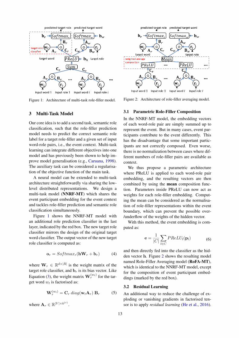
Figure 1: Architecture of multi-task role-filler model.
3 Multi-Task Model
Our core idea is to add a second task, semantic roleclassification, such that the role-filler predictionmodel needs to predict the correct semantic rolelabel for a target role-filler and a given set of inputword-role pairs, i.e., the event context. Multi-tasklearning can integrate different objectives into onemodel and has previously been shown to help im-prove model generalisation (e.g., Caruana, 1998).The auxiliary task can be considered a regularisa-tion of the objective function of the main task.
A neural model can be extended to multi-taskarchitecture straightforwardly via sharing the low-level distributed representations. We design amulti-task model (NNRF-MT) which shares theevent participant embedding for the event contextand tackles role-filler prediction and semantic roleclassification simultaneously.
Figure 1 shows the NNRF-MT model withan additional role prediction classifier in the lastlayer, indicated by the red box. The new target roleclassifier mirrors the design of the original targetword classifier. The output vector of the new targetrole classifier is computed as:
or = Softmaxr(hWr + br) (4)
where Wr ∈ Rd×|R| is the weight matrix of thetarget role classifier, and br is its bias vector. LikeEquation (3), the weight matrix W
(wt)r for the tar-
get word wt is factorised as:
W(wt)r = Cr diag(wtAr) Br (5)
where Ar ∈ R|V |×k(r) .
Figure 2: Architecture of role-filler averaging model.
3.1 Parametric Role-Filler CompositionIn the NNRF-MT model, the embedding vectorsof each word-role pair are simply summed up torepresent the event. But in many cases, event par-ticipants contribute to the event differently. Thishas the disadvantage that some important partic-ipants are not correctly composed. Even worse,there is no normalization between cases where dif-ferent numbers of role-filler pairs are available ascontext.
We thus propose a parametric architecturewhere PReLU is applied to each word-role pairembedding, and the resulting vectors are thencombined by using the mean composition func-tion. Parameters inside PReLU can now act asweights for each role-filler embedding. Comput-ing the mean can be considered as the normalisa-tion of role-filler representations within the eventboundary, which can prevent the possible over-/underflow of the weights of the hidden vector.
With this method, the event embedding is com-puted as:
e =1
|C|∑
l∈CPReLUl(pl) (6)
and then directly fed into the classifier as the hid-den vector h. Figure 2 shows the resulting modelnamed Role-Filler Averaging model (RoFA-MT),which is identical to the NNRF-MT model, exceptfor the composition of event participant embed-dings (marked by the red box).
3.2 Residual LearningAn additional way to reduce the challenge of ex-ploding or vanishing gradients in factorised ten-sor is to apply residual learning (He et al., 2016).
13
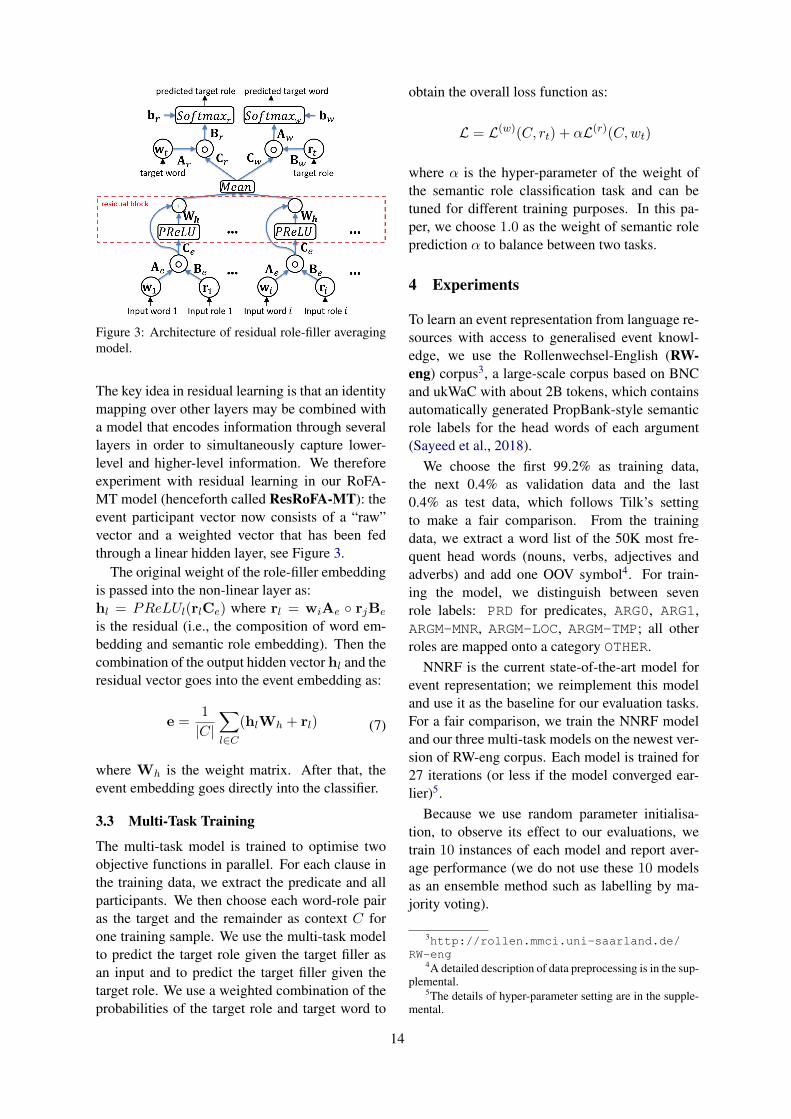
Figure 3: Architecture of residual role-filler averagingmodel.
The key idea in residual learning is that an identitymapping over other layers may be combined witha model that encodes information through severallayers in order to simultaneously capture lower-level and higher-level information. We thereforeexperiment with residual learning in our RoFA-MT model (henceforth called ResRoFA-MT): theevent participant vector now consists of a “raw”vector and a weighted vector that has been fedthrough a linear hidden layer, see Figure 3.
The original weight of the role-filler embeddingis passed into the non-linear layer as:hl = PReLUl(rlCe) where rl = wiAe ◦ rjBe
is the residual (i.e., the composition of word em-bedding and semantic role embedding). Then thecombination of the output hidden vector hl and theresidual vector goes into the event embedding as:
e =1
|C|∑
l∈C(hlWh + rl) (7)
where Wh is the weight matrix. After that, theevent embedding goes directly into the classifier.
3.3 Multi-Task Training
The multi-task model is trained to optimise twoobjective functions in parallel. For each clause inthe training data, we extract the predicate and allparticipants. We then choose each word-role pairas the target and the remainder as context C forone training sample. We use the multi-task modelto predict the target role given the target filler asan input and to predict the target filler given thetarget role. We use a weighted combination of theprobabilities of the target role and target word to
obtain the overall loss function as:
L = L(w)(C, rt) + αL(r)(C,wt)
where α is the hyper-parameter of the weight ofthe semantic role classification task and can betuned for different training purposes. In this pa-per, we choose 1.0 as the weight of semantic roleprediction α to balance between two tasks.
4 Experiments
To learn an event representation from language re-sources with access to generalised event knowl-edge, we use the Rollenwechsel-English (RW-eng) corpus3, a large-scale corpus based on BNCand ukWaC with about 2B tokens, which containsautomatically generated PropBank-style semanticrole labels for the head words of each argument(Sayeed et al., 2018).
We choose the first 99.2% as training data,the next 0.4% as validation data and the last0.4% as test data, which follows Tilk’s settingto make a fair comparison. From the trainingdata, we extract a word list of the 50K most fre-quent head words (nouns, verbs, adjectives andadverbs) and add one OOV symbol4. For train-ing the model, we distinguish between sevenrole labels: PRD for predicates, ARG0, ARG1,ARGM-MNR, ARGM-LOC, ARGM-TMP; all otherroles are mapped onto a category OTHER.
NNRF is the current state-of-the-art model forevent representation; we reimplement this modeland use it as the baseline for our evaluation tasks.For a fair comparison, we train the NNRF modeland our three multi-task models on the newest ver-sion of RW-eng corpus. Each model is trained for27 iterations (or less if the model converged ear-lier)5.
Because we use random parameter initialisa-tion, to observe its effect to our evaluations, wetrain 10 instances of each model and report aver-age performance (we do not use these 10 modelsas an ensemble method such as labelling by ma-jority voting).
3http://rollen.mmci.uni-saarland.de/RW-eng
4A detailed description of data preprocessing is in the sup-plemental.
5The details of hyper-parameter setting are in the supple-mental.
14

Model Accuracy p-valueNNRF-MT 89.1 -RoFA-MT 94.8 < 0.0001ResRoFA-MT 94.7 < 0.0001
Table 1: Semantic role classification results for thethree multi-task architectures.
5 Evaluation: Semantic RoleClassification
We begin by testing the new component of themodel in terms of how well the model can predictsemantic role labels.
5.1 Role Prediction Given Event Context
We evaluate our models on semantic role predic-tion accuracy given the predicate and other argu-ments with their roles on the test dataset of theRW-eng corpus. Table 1 shows that the RoFA-MTand ResRoFA-MT models outperform the NNRF-MT model by a statistically significant margin(tested with McNemar’s test), showing that theparametric weighted average composition methodleads to significant improvements.
5.2 Classification for Verb-Head Pairs
Semantic role classification systems make heavyuse of syntactic features but can be further im-proved by integrating models of selectional pref-erences (Zapirain et al., 2009). Here we comparethe semantics-based role assignments produced byour model to predictions made by various selec-tional preference (SP) models in the first evalua-tion of Zapirain et al. (2013). E.g., the model is topredict ARG1 for the pair (eatverb, apple) withoutany other feature.
Zapirain et al. (2013) combined a verb-role SPmodel built on training data and an additionaldistributional similarity model trained on a largescale corpus for estimating the fit between verbsand their arguments for different roles. These the-matic fit estimates are used to select the best rolelabel for each predicate-argument pair.
We consider only following best variants asbaselines:Zapirain13Pado07: This variant uses a distri-butional similarity model constructed on a gen-eral corpus (BNC) with Pado and Lapata (2007)’ssyntax-based method.Zapirain13Lin98in−domain: This variant containsLin (1998)’s distributional similarity model which
uses syntax-based clustering. The model is pre-computed on a mixed corpus (including WSJ)which is in the same domain as the WSJ test set.
We apply our trained role labelling model di-rectly to the test set, without touching the WSJtraining/validation set. Following the baselines,for semantic roles which are not represented in ourmodel, we do not make any prediction (this is re-flected in lower recall for those cases).
The model is evaluated on the data set from theCoNLL-2005 shared task (Carreras and Marquez,2005), which contains the WSJ corpus as part ofits training/validation/test sets and the Brown cor-pus as an out-of-domain test set (marked in Table 2as Brown). We estimate 99% confidence intervalsusing the bootstrapping method, with 100 replica-tions. We also construct a trivial baseline model,the ZeroR classifier, which predicts the majorityclass ARG1 given any input.
Table 2 shows that the baseline model usingLin’s similarities (Zapirain13Lin98in−domain) worksbest on the WSJ test dataset, statistically signif-icantly outperforming each of the other methods(p < 0.01). However, this can be explained by thefact that this model is using semantic similaritiesobtained from the same domain as the WSJ testset. Among the models without using in-domainsemantic similarity, ResRoFA-MT is significantlybetter than all others (p < 0.01).
On the Brown data, which is out-of-domain forall models, the ResRoFA-MT model achieves thebest result and outperforms previous baselines sig-nificantly (p < 0.01). Without any training on theWSJ corpus, our best model has a much smallergap between test and ood dataset (only about 3 F1
points), which indicates that our multi-task modelsgeneralise better than previous baselines.
5.3 End-to-End Semantic Role Labelling
Future work will need to investigate in more de-tail whether the multi-task models proposed herecan be used to improve the performance of exist-ing semantic role labellers. While our model can-not be directly applied to a standard semantic rolelabelling task (because it assigns roles only to headwords), we were able to combine the model withan existing semantic role labeller and obtainedpromising results. Adding embeddings based onthe predicate and target word hCrdiag(wtAr)from the NNRF-MT model (see Equation (4), (5))as a feature to the MATE semantic role labeller
15
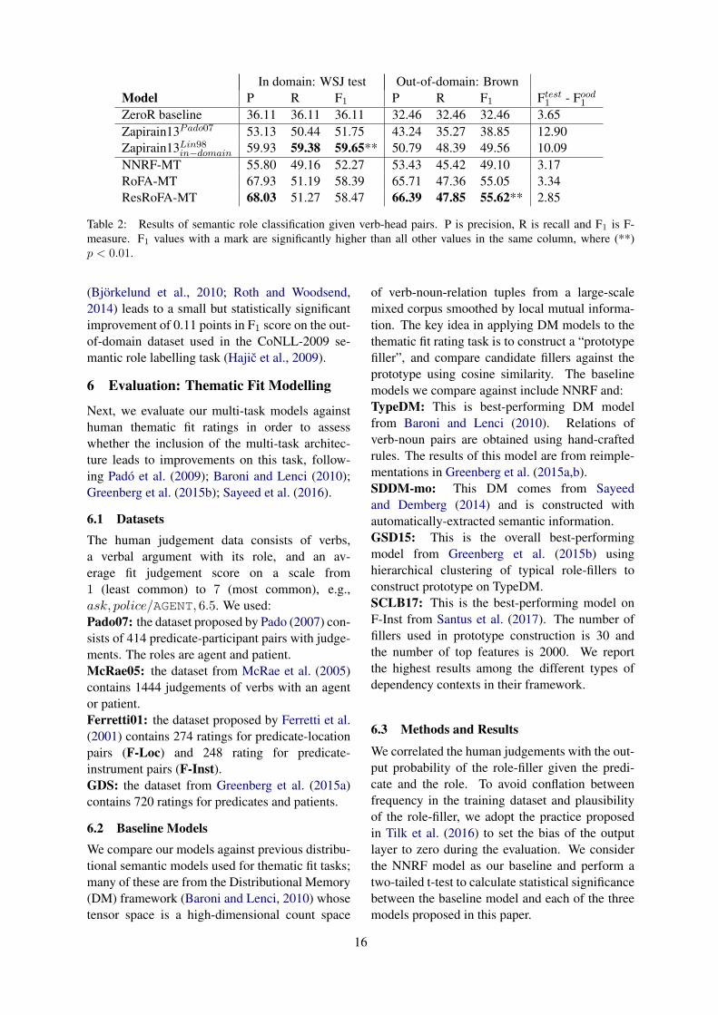
In domain: WSJ test Out-of-domain: BrownModel P R F1 P R F1 Ftest
1 - Food1
ZeroR baseline 36.11 36.11 36.11 32.46 32.46 32.46 3.65Zapirain13Pado07 53.13 50.44 51.75 43.24 35.27 38.85 12.90Zapirain13Lin98in−domain 59.93 59.38 59.65** 50.79 48.39 49.56 10.09NNRF-MT 55.80 49.16 52.27 53.43 45.42 49.10 3.17RoFA-MT 67.93 51.19 58.39 65.71 47.36 55.05 3.34ResRoFA-MT 68.03 51.27 58.47 66.39 47.85 55.62** 2.85
Table 2: Results of semantic role classification given verb-head pairs. P is precision, R is recall and F1 is F-measure. F1 values with a mark are significantly higher than all other values in the same column, where (**)p < 0.01.
(Bjorkelund et al., 2010; Roth and Woodsend,2014) leads to a small but statistically significantimprovement of 0.11 points in F1 score on the out-of-domain dataset used in the CoNLL-2009 se-mantic role labelling task (Hajic et al., 2009).
6 Evaluation: Thematic Fit Modelling
Next, we evaluate our multi-task models againsthuman thematic fit ratings in order to assesswhether the inclusion of the multi-task architec-ture leads to improvements on this task, follow-ing Pado et al. (2009); Baroni and Lenci (2010);Greenberg et al. (2015b); Sayeed et al. (2016).
6.1 DatasetsThe human judgement data consists of verbs,a verbal argument with its role, and an av-erage fit judgement score on a scale from1 (least common) to 7 (most common), e.g.,ask, police/AGENT, 6.5. We used:Pado07: the dataset proposed by Pado (2007) con-sists of 414 predicate-participant pairs with judge-ments. The roles are agent and patient.McRae05: the dataset from McRae et al. (2005)contains 1444 judgements of verbs with an agentor patient.Ferretti01: the dataset proposed by Ferretti et al.(2001) contains 274 ratings for predicate-locationpairs (F-Loc) and 248 rating for predicate-instrument pairs (F-Inst).GDS: the dataset from Greenberg et al. (2015a)contains 720 ratings for predicates and patients.
6.2 Baseline ModelsWe compare our models against previous distribu-tional semantic models used for thematic fit tasks;many of these are from the Distributional Memory(DM) framework (Baroni and Lenci, 2010) whosetensor space is a high-dimensional count space
of verb-noun-relation tuples from a large-scalemixed corpus smoothed by local mutual informa-tion. The key idea in applying DM models to thethematic fit rating task is to construct a “prototypefiller”, and compare candidate fillers against theprototype using cosine similarity. The baselinemodels we compare against include NNRF and:TypeDM: This is best-performing DM modelfrom Baroni and Lenci (2010). Relations ofverb-noun pairs are obtained using hand-craftedrules. The results of this model are from reimple-mentations in Greenberg et al. (2015a,b).SDDM-mo: This DM comes from Sayeedand Demberg (2014) and is constructed withautomatically-extracted semantic information.GSD15: This is the overall best-performingmodel from Greenberg et al. (2015b) usinghierarchical clustering of typical role-fillers toconstruct prototype on TypeDM.SCLB17: This is the best-performing model onF-Inst from Santus et al. (2017). The number offillers used in prototype construction is 30 andthe number of top features is 2000. We reportthe highest results among the different types ofdependency contexts in their framework.
6.3 Methods and Results
We correlated the human judgements with the out-put probability of the role-filler given the predi-cate and the role. To avoid conflation betweenfrequency in the training dataset and plausibilityof the role-filler, we adopt the practice proposedin Tilk et al. (2016) to set the bias of the outputlayer to zero during the evaluation. We considerthe NNRF model as our baseline and perform atwo-tailed t-test to calculate statistical significancebetween the baseline model and each of the threemodels proposed in this paper.
16

Model Pado07 McRae05 F-Loc F-Inst GDS avgTypeDM 53 33 23 36 46 40.8SDDM-mo 56 27 13 28 - -GSD15 50 36 29 42 48 40.5SCLB17 49 28 37 50 - -NNRF 43.3 35.9 46.5 52.1 57.6 44.2NNRF-MT 43.2 36.1 46.3 50.0* 57.2 44.0RoFA-MT 52.2** 41.9** 45.9 49.4* 60.7** 48.6**ResRoFA-MT 53.0** 42.5** 46.3 47.7** 60.8** 48.9**
Table 3: Results on human thematic fit judgement correlation task (Spearman’s ρ × 100) compared to previouswork. The last column reports the weighted average results by numbers of entries of all five datasets. Values witha mark are significantly different from the baseline model (NNRF), where (*) p < 0.05, (**) p < 0.01.
Table 3 shows results for all models anddatasets. The ResRoFA-MT model performs bestoverall, improving more than 4 points over thebaseline. The multi-task model (NNRF-MT) hasperformance similar to baseline (NNRF). Our newarchitecture using a parametric weighted averageover event participant embeddings (RoFA-MT)outperforms simple summation (NNRF-MT), es-pecially on the Pado07, McRae05 and GDSdatasets. The residual method leads to furtherminor improvements on the Pado07, F-Loc andGDS datasets. However, on predicate-instrumentpairs of the F-Inst dataset, NNRF outperformsother models significantly. We think that multi-task models are biased towards roles with a largerfrequency like ARG0 or ARG1, which is proved inthe ablation study (see Section 8).
7 Evaluation: Compositionality
The thematic fit judgements from the tasks dis-cussed in section 6 only contain ratings of the fitbetween the predicate and one role-filler. How-ever, other event participants contained in a clausecan affect human expectations of the upcomingrole-fillers. For instance, mechanics are likely tocheck tires, while journalists are likely to checkspellings. The B10 dataset (Bicknell et al., 2010)contains human judgements for 64 pairs of agent-verb-patient triples, where one triple in each pairis plausible (e.g., “journalist check spelling”), andone is implausible (e.g., “journalist check type”).A model is evaluated based on whether it success-fully assigns a higher likelihood/rating to the plau-sible than to the implausible object (also referredto as the Accuracy 1 metric in Tilk et al. (2016)).The baseline models are NNRF as well as:Random: The naive baseline model consists of
choosing the tags uniformly at random.Lenci11: Lenci (2011) proposed a compositionmodel for TypeDM.
Table 4 shows that our new composition methodbased on parametric weighted average outper-forms previous models; the RoFA-MT modelachieves the highest accuracy overall and outper-forms the baseline (NNRF) significantly.
7.1 Event Similarity
Lastly, we evaluate the quality of the event embed-dings learned via the multi-task network models.While word embeddings from tools like word2vec(Mikolov et al., 2013) are standard methods forobtaining word similarities, identifying a suitablemethod for more general event similarity estima-tion is still a relevant problem. The model pro-posed here constitutes an interesting method forobtaining event embeddings, as it is trained on twosemantics-focused prediction tasks.
For evaluation, we use the sentence similar-ity task proposed by Grefenstette and Sadrzadeh(2015) (second experiment in their paper). Forevaluation, we use the re-annotated dataset, namedGS13, constructed in 2013 by Kartsaklis andSadrzadeh (2014). Each row in the dataset con-tains a participant ID, two sentences, a humanevaluation score of their similarity from 1 to 7, anda HIGH/LOW tag indicating the similarity group oftwo sentences. An example entry is:
p1, (table, draw, eye), (table, attract, eye), 7, HIGH
where p1 is the participant ID. We compare ourmodels’ performance to NNRF, as well as:Kronecker: The best-performing model inGrefenstette and Sadrzadeh (2015) using Kro-necker product as its composition method.W2V: The sentence representations in W2V are
17
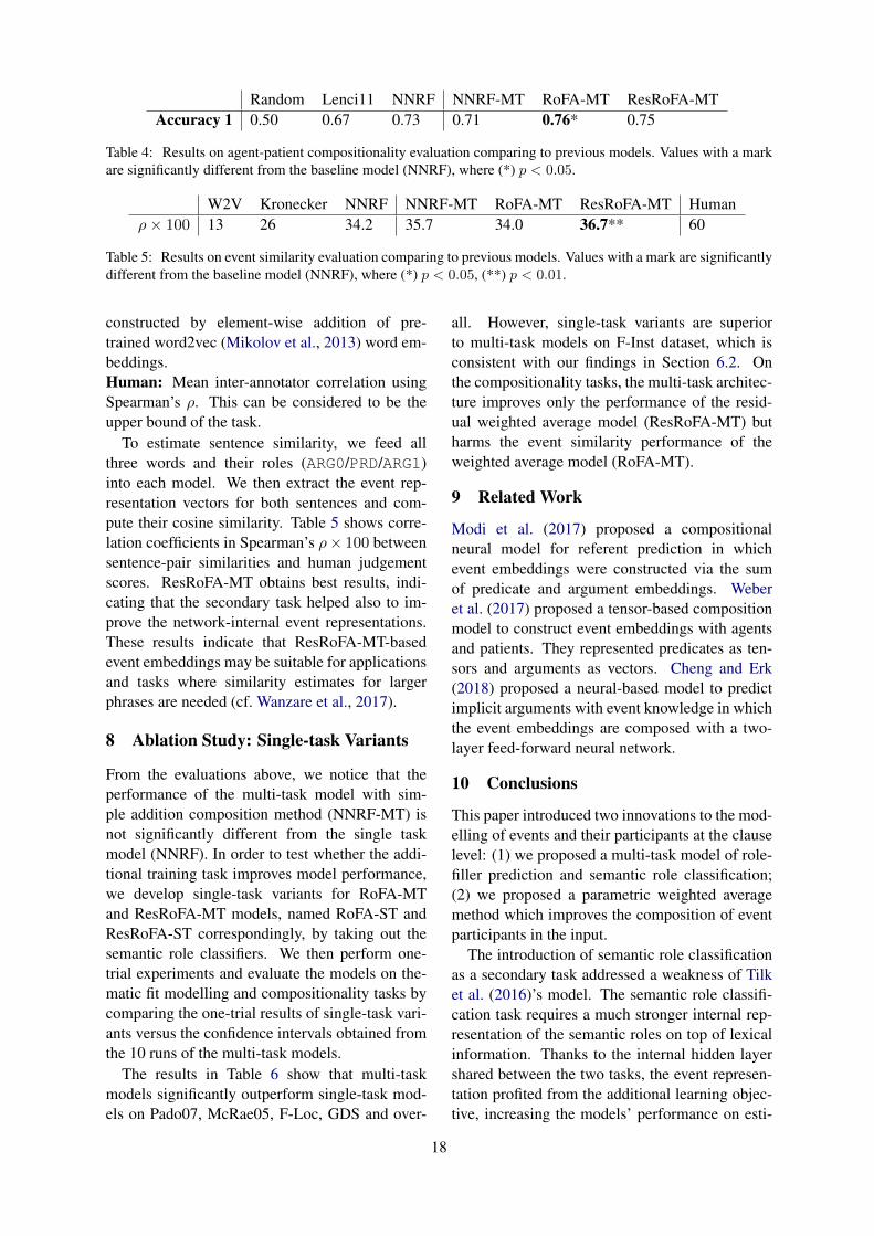
Random Lenci11 NNRF NNRF-MT RoFA-MT ResRoFA-MTAccuracy 1 0.50 0.67 0.73 0.71 0.76* 0.75
Table 4: Results on agent-patient compositionality evaluation comparing to previous models. Values with a markare significantly different from the baseline model (NNRF), where (*) p < 0.05.
W2V Kronecker NNRF NNRF-MT RoFA-MT ResRoFA-MT Humanρ× 100 13 26 34.2 35.7 34.0 36.7** 60
Table 5: Results on event similarity evaluation comparing to previous models. Values with a mark are significantlydifferent from the baseline model (NNRF), where (*) p < 0.05, (**) p < 0.01.
constructed by element-wise addition of pre-trained word2vec (Mikolov et al., 2013) word em-beddings.Human: Mean inter-annotator correlation usingSpearman’s ρ. This can be considered to be theupper bound of the task.
To estimate sentence similarity, we feed allthree words and their roles (ARG0/PRD/ARG1)into each model. We then extract the event rep-resentation vectors for both sentences and com-pute their cosine similarity. Table 5 shows corre-lation coefficients in Spearman’s ρ× 100 betweensentence-pair similarities and human judgementscores. ResRoFA-MT obtains best results, indi-cating that the secondary task helped also to im-prove the network-internal event representations.These results indicate that ResRoFA-MT-basedevent embeddings may be suitable for applicationsand tasks where similarity estimates for largerphrases are needed (cf. Wanzare et al., 2017).
8 Ablation Study: Single-task Variants
From the evaluations above, we notice that theperformance of the multi-task model with sim-ple addition composition method (NNRF-MT) isnot significantly different from the single taskmodel (NNRF). In order to test whether the addi-tional training task improves model performance,we develop single-task variants for RoFA-MTand ResRoFA-MT models, named RoFA-ST andResRoFA-ST correspondingly, by taking out thesemantic role classifiers. We then perform one-trial experiments and evaluate the models on the-matic fit modelling and compositionality tasks bycomparing the one-trial results of single-task vari-ants versus the confidence intervals obtained fromthe 10 runs of the multi-task models.
The results in Table 6 show that multi-taskmodels significantly outperform single-task mod-els on Pado07, McRae05, F-Loc, GDS and over-
all. However, single-task variants are superiorto multi-task models on F-Inst dataset, which isconsistent with our findings in Section 6.2. Onthe compositionality tasks, the multi-task architec-ture improves only the performance of the resid-ual weighted average model (ResRoFA-MT) butharms the event similarity performance of theweighted average model (RoFA-MT).
9 Related Work
Modi et al. (2017) proposed a compositionalneural model for referent prediction in whichevent embeddings were constructed via the sumof predicate and argument embeddings. Weberet al. (2017) proposed a tensor-based compositionmodel to construct event embeddings with agentsand patients. They represented predicates as ten-sors and arguments as vectors. Cheng and Erk(2018) proposed a neural-based model to predictimplicit arguments with event knowledge in whichthe event embeddings are composed with a two-layer feed-forward neural network.
10 Conclusions
This paper introduced two innovations to the mod-elling of events and their participants at the clauselevel: (1) we proposed a multi-task model of role-filler prediction and semantic role classification;(2) we proposed a parametric weighted averagemethod which improves the composition of eventparticipants in the input.
The introduction of semantic role classificationas a secondary task addressed a weakness of Tilket al. (2016)’s model. The semantic role classifi-cation task requires a much stronger internal rep-resentation of the semantic roles on top of lexicalinformation. Thanks to the internal hidden layershared between the two tasks, the event represen-tation profited from the additional learning objec-tive, increasing the models’ performance on esti-
18

Model Pado07 McRae05 F-Loc F-Inst GDS avg B10 GS13RoFA-ST 44.1*** 36.6*** 44.4* 56.7*** 57.3*** 44.5*** 75.0 36.3**RoFA-MT 52.2 41.9 45.9 49.4 60.7 48.6 76.1 34.0ResRoFA-ST 42.3*** 35.8*** 44.5** 50.4* 56.9*** 43.6*** 67.2*** 32.5***ResRoFA-MT 53.0 42.5 46.3 47.7 60.8 48.9 74.5 36.7
Table 6: Ablation study of single task variants. Underlined values indicate the best values with the same com-position method, and bold values indicate the best values on that data set. Values with a mark are significantlydifferent from the multi-task baseline models (RoFA-MT / ResRoFA-MT), where (*) p < 0.05, (**) p < 0.01,(***) p < 0.001.
mating event similarity.We also performed a study regarding the useful-
ness of our purely semantics-based representationsfor semantic role labelling. While many seman-tic role labellers rely predominantly on syntax, ourapproach addresses the likelihood that a semanticrole should be assigned purely based on its plausi-bility to fill that role content-wise. We showed thatthe semantics-based role label predictions gener-ated by our multi-task model outperform the onesbased on earlier syntax-based selectional prefer-ence methods and observe promising results forintegrating the model with a semantic role labelleron out-of-domain data.
Our parametric composition method (RoFA-MT) composes event embeddings in the hiddenlayer, which captures role-specific informationduring the composition process and reduces therisk of overflow and underflow of the hidden layerweights. We additionally included the residuallearning method alongside RoFA-MT (ResRoFA-MT), further mitigating the vanishing/explodinggradient problem and allowing the transmissionof information from lower levels directly into theevent embedding. This approach provided theoverall best result of all models on the thematicfit human judgement task as well as the event sim-ilarity task and competitive results on the tasks in-dividually.
10.1 Future Work
In future work, the model may be improvedby including visual information from photos andvideos. Common-sense reasoning is becominga new focus (Mostafazadeh et al., 2016; Baroniet al., 2017). One characteristic of common-senseknowledge is that it is often not explicitly men-tioned in language precisely because it constitutescommon-sense knowledge and is hence uninfor-mative as it can easily be inferred (Mukuze et al.,
2018). Syntactically optional event participants(such as the kitchen as location for the predicate“cook”) are thus often omitted in text; this sets alimit to what can be learned from text only.
The prospect of applying our models indepen-dently to SRL tasks suggests an area of poten-tial future work. Our models currently use onlythe predicates and head words of arguments. In-stead of depending on corpora with extracted headwords, we can integrate an attention mechanism(Vaswani et al., 2017) to capture the position ofsyntactic heads. We are working on extending ourmodels to use all words, which will enable testingas an SRL tool.
Finally, the predictive nature of this type ofmodel can potentially enable its deployment in in-cremental semantic parsing (Konstas et al., 2014;Konstas and Keller, 2015) by combining the multi-task design with the incremental architecture in(Tilk et al., 2016). We are continuing to developthis and other ways of employing models of eventrepresentation that simultaneously predict eventparticipants and assess the fit of given participants.
Acknowledgements
This research was funded in part by the Ger-man Research Foundation (DFG) as part of SFB1102 “Information Density and Linguistic En-coding”, EXC 284 Cluster of Excellence “Multi-modal Computing and Interaction”, and a SwedishResearch Council (VR) grant for the Centrefor Linguistic Theory and Studies in Probability(CLASP). We thank Dr. Michael Roth for con-ducting the semantic role labelling evaluation us-ing features from our model to see whether it isbeneficial. We sincerely thank the anonymous re-viewers for their insightful comments that helpedus to improve this paper.
19
References
Marco Baroni, Armand Joulin, Allan Jabri, GermanKruszewski, Angeliki Lazaridou, Klemen Simonic,and Tomas Mikolov. 2017. CommAI: Evaluatingthe first steps towards a useful general AI. arXivpreprint arXiv:1701.08954 .
Marco Baroni and Alessandro Lenci. 2010. Dis-tributional memory: A general framework forcorpus-based semantics. Computational Linguistics36(4):673–721.
Klinton Bicknell, Jeffrey L Elman, Mary Hare, KenMcRae, and Marta Kutas. 2010. Effects of eventknowledge in processing verbal arguments. Journalof memory and language 63(4):489–505.
Anders Bjorkelund, Bernd Bohnet, Love Hafdell, andPierre Nugues. 2010. A high-performance syntac-tic and semantic dependency parser. In Proceedingsof the 23rd International Conference on Computa-tional Linguistics: Demonstrations. Association forComputational Linguistics, pages 33–36.
Xavier Carreras and Lluıs Marquez. 2005. Introduc-tion to the CoNLL-2005 shared task: Semanticrole labeling. In Proceedings of the Ninth Confer-ence on Computational Natural Language Learning(CoNLL-2005). Association for Computational Lin-guistics, Ann Arbor, Michigan, pages 152–164.
Rich Caruana. 1998. Multitask learning. In Learningto learn, Springer, pages 95–133.
Pengxiang Cheng and Katrin Erk. 2018. Implicit ar-gument prediction with event knowledge. arXivpreprint arXiv:1802.07226 .
Todd R Ferretti, Ken McRae, and Andrea Hatherell.2001. Integrating verbs, situation schemas, and the-matic role concepts. Journal of Memory and Lan-guage 44(4):516–547.
C. J. Fillmore. 1968. The case for case. Universals inLinguistic Theory pages 1–25(Part Two).
Karl Friston. 2010. The free-energy principle: a uni-fied brain theory? Nature Reviews Neuroscience11(2):127.
Edward Gibson, Leon Bergen, and Steven T Pianta-dosi. 2013. Rational integration of noisy evidenceand prior semantic expectations in sentence interpre-tation. Proceedings of the National Academy of Sci-ences 110(20):8051–8056.
Clayton Greenberg, Vera Demberg, and Asad Say-eed. 2015a. Verb polysemy and frequency effectsin thematic fit modeling. In Proceedings of the6th Workshop on Cognitive Modeling and Compu-tational Linguistics. Association for ComputationalLinguistics, Denver, Colorado, pages 48–57.
Clayton Greenberg, Asad Sayeed, and Vera Demberg.2015b. Improving unsupervised vector-space the-matic fit evaluation via role-filler prototype clus-tering. In Proceedings of the 2015 Conference ofthe North American Chapter of the Association forComputational Linguistics: Human Language Tech-nologies. Association for Computational Linguis-tics, Denver, Colorado, pages 21–31.
Edward Grefenstette and Mehrnoosh Sadrzadeh. 2015.Concrete models and empirical evaluations for thecategorical compositional distributional model ofmeaning. Computational Linguistics 41(1):71–118.
Jan Hajic, Massimiliano Ciaramita, Richard Johans-son, Daisuke Kawahara, Maria Antonia Martı, LluısMarquez, Adam Meyers, Joakim Nivre, SebastianPado, Jan Stepanek, Pavel Stranak, Mihai Surdeanu,Nianwen Xue, and Yi Zhang. 2009. The CoNLL-2009 shared task: Syntactic and semantic dependen-cies in multiple languages. In Proceedings of theThirteenth Conference on Computational NaturalLanguage Learning (CoNLL 2009): Shared Task.Association for Computational Linguistics, Boulder,Colorado, pages 1–18.
Kaiming He, Xiangyu Zhang, Shaoqing Ren, and JianSun. 2015. Delving deep into rectifiers: Surpass-ing human-level performance on imagenet classifi-cation. In Proceedings of the IEEE internationalconference on computer vision. pages 1026–1034.
Kaiming He, Xiangyu Zhang, Shaoqing Ren, and JianSun. 2016. Deep residual learning for image recog-nition. In Proceedings of the IEEE conference oncomputer vision and pattern recognition. pages 770–778.
Dimitri Kartsaklis and Mehrnoosh Sadrzadeh. 2014. Astudy of entanglement in a categorical framework ofnatural language. arXiv preprint arXiv:1405.2874 .
Ioannis Konstas and Frank Keller. 2015. Semantic rolelabeling improves incremental parsing. In Proceed-ings of the 53rd Annual Meeting of the Associationfor Computational Linguistics and the 7th Interna-tional Joint Conference on Natural Language Pro-cessing (Volume 1: Long Papers). Association forComputational Linguistics, Beijing, China, pages1191–1201.
Ioannis Konstas, Frank Keller, Vera Demberg, andMirella Lapata. 2014. Incremental semantic role la-beling with Tree Adjoining Grammar. In Proceed-ings of the 2014 Conference on Empirical Methodsin Natural Language Processing (EMNLP). Asso-ciation for Computational Linguistics, Doha, Qatar,pages 301–312.
Gina R Kuperberg and T Florian Jaeger. 2016. What dowe mean by prediction in language comprehension?Language, cognition and neuroscience 31(1):32–59.
Alessandro Lenci. 2011. Composing and updatingverb argument expectations: A distributional seman-tic model. In Proceedings of the 2nd Workshop on
20

Cognitive Modeling and Computational Linguistics.Association for Computational Linguistics, Strouds-burg, PA, USA, CMCL 2011, pages 58–66.
Dekang Lin. 1998. Automatic retrieval and clusteringof similar words. In Proceedings of the 17th inter-national conference on Computational linguistics-Volume 2. Association for Computational Linguis-tics, pages 768–774.
Ken McRae, Mary Hare, Jeffrey L Elman, and ToddFerretti. 2005. A basis for generating expectan-cies for verbs from nouns. Memory & Cognition33(7):1174–1184.
Tomas Mikolov, Ilya Sutskever, Kai Chen, Greg S Cor-rado, and Jeff Dean. 2013. Distributed representa-tions of words and phrases and their compositional-ity. In Advances in neural information processingsystems. pages 3111–3119.
Ashutosh Modi, Ivan Titov, Vera Demberg, Asad Say-eed, and Manfred Pinkal. 2017. Modelling seman-tic expectation: Using script knowledge for referentprediction. Transactions of the Association of Com-putational Linguistics 5(1):31–44.
Nasrin Mostafazadeh, Nathanael Chambers, XiaodongHe, Devi Parikh, Dhruv Batra, Lucy Vanderwende,Pushmeet Kohli, and James Allen. 2016. A cor-pus and evaluation framework for deeper under-standing of commonsense stories. arXiv preprintarXiv:1604.01696 .
Nelson Mukuze, Anna Rohrbach, Vera Demberg, andBernt Schiele. 2018. A vision-grounded dataset forpredicting typical locations for verbs. In The 11thedition of the Language Resources and EvaluationConference (LREC).
Sebastian Pado and Mirella Lapata. 2007.Dependency-based construction of semantic spacemodels. Computational Linguistics 33(2):161–199.
Ulrike Pado. 2007. The Integration of Syntax and Se-mantic Plausibility in a Wide-Coverage Model ofHuman Sentence Processing. Ph.D. thesis, SaarlandUniversity.
Ulrike Pado, Matthew W Crocker, and Frank Keller.2009. A probabilistic model of semantic plausi-bility in sentence processing. Cognitive Science33(5):794–838.
Michael Roth and Kristian Woodsend. 2014. Composi-tion of word representations improves semantic rolelabelling. In Proceedings of the 2014 Conference onEmpirical Methods in Natural Language Processing(EMNLP). pages 407–413.
Enrico Santus, Emmanuele Chersoni, AlessandroLenci, and Philippe Blache. 2017. Measuring the-matic fit with distributional feature overlap. In Pro-ceedings of the 2017 Conference on Empirical Meth-ods in Natural Language Processing. Associationfor Computational Linguistics, Copenhagen, Den-mark, pages 659–669.
Asad Sayeed and Vera Demberg. 2014. Combiningunsupervised syntactic and semantic models of the-matic fit. In Proceedings of the first Italian Confer-ence on Computational Linguistics (CLiC-it 2014).
Asad Sayeed, Clayton Greenberg, and Vera Demberg.2016. Thematic fit evaluation: an aspect of selec-tional preferences. In Proceedings of the 1st Work-shop on Evaluating Vector-Space Representationsfor NLP. Association for Computational Linguistics,Berlin, Germany, pages 99–105.
Asad Sayeed, Pavel Shkadzko, and Vera Demberg.2018. Rollenwechsel-English: a large-scale seman-tic role corpus. In Proceedings of the 11th editionof the Language Resources and Evaluation Confer-ence.
Ottokar Tilk, Vera Demberg, Asad Sayeed, DietrichKlakow, and Stefan Thater. 2016. Event participantmodelling with neural networks. In Proceedings ofthe 2016 Conference on Empirical Methods in Nat-ural Language Processing. Association for Compu-tational Linguistics, Austin, Texas, pages 171–182.
Ashish Vaswani, Noam Shazeer, Niki Parmar, JakobUszkoreit, Llion Jones, Aidan N Gomez, ŁukaszKaiser, and Illia Polosukhin. 2017. Attention is allyou need. In Advances in Neural Information Pro-cessing Systems. pages 6000–6010.
Lilian DA Wanzare, Alessandra Zarcone, StefanThater, and Manfred Pinkal. 2017. Inducing scriptstructure from crowdsourced event descriptions viasemi-supervised clustering. LSDSem 2017 page 1.
Noah Weber, Niranjan Balasubramanian, andNathanael Chambers. 2017. Event represen-tations with tensor-based compositions. arXivpreprint arXiv:1711.07611 .
Shumin Wu and Martha Palmer. 2015. Can selectionalpreferences help automatic semantic role labeling?In Proceedings of the Fourth Joint Conference onLexical and Computational Semantics. pages 222–227.
Benat Zapirain, Eneko Agirre, and Lluıs Marquez.2009. Generalizing over lexical features: Selec-tional preferences for semantic role classification. InProceedings of the ACL-IJCNLP 2009 conferenceshort papers. Association for Computational Lin-guistics, pages 73–76.
Benat Zapirain, Eneko Agirre, Lluis Marquez, and Mi-hai Surdeanu. 2013. Selectional preferences for se-mantic role classification. Computational Linguis-tics 39(3):631–663.
21

Proceedings of the 7th Joint Conference on Lexical and Computational Semantics (*SEM), pages 22–32New Orleans, June 5-6, 2018. c©2018 Association for Computational Linguistics
Assessing Meaning Components in German Complex Verbs:A Collection of Source–Target Domains and Directionality
Sabine Schulte im Walde and Maximilian Koper and Sylvia SpringorumInstitut fur Maschinelle Sprachverarbeitung
Universitat Stuttgart, Germany{schulte,maximilian.koeper,sylvia.springorum}@ims.uni-stuttgart.de
Abstract
This paper presents a collection to assessmeaning components in German complexverbs, which frequently undergo meaningshifts. We use a novel strategy to obtain sourceand target domain characterisations via sen-tence generation rather than sentence annota-tion. A selection of arrows adds spatial dir-ectional information to the generated contexts.We provide a broad qualitative description ofthe dataset, and a series of standard classifica-tion experiments verifies the quantitative reli-ability of the presented resource. The setup forcollecting the meaning components is applic-able also to other languages, regarding com-plex verbs as well as other language-specifictargets that involve meaning shifts.
1 Introduction
German particle verbs (PVs) are complex verbstructures such as anstrahlen ‘to beam/smile at’that combine a prefix particle (an) with a baseverb (strahlen ‘to beam’). PVs represent a typeof multi-word expressions, which are generallyknown as a “pain in the neck for NLP” (Saget al., 2002). Even more, German PVs pose aspecific challenge for NLP tasks and applications,because the particles are highly ambiguous; e.g.,the particle an has a partitive meaning in anbeißen’to take a bite’, a cumulative meaning in anhaufen’to pile up’, and a topological meaning in an-binden ’to tie to’ (Springorum, 2011). In addi-tion, they often trigger meaning shifts of the baseverbs (BVs), cf. Springorum et al. (2013); e.g.,the PV abschminken with the BV schminken ’toput on make-up’ has a literal meaning (’to removemake-up’) and a shifted, non-literal meaning (’toforget about something’).1
1We deliberately make use of the general term “meaningshift” in comparison to specific instances such as metaphor
With PVs representing a large and challen-ging class in the lexicon, their meaning com-ponents and their mechanisms of compositional-ity have received a considerable amount of in-terdisciplinary research interest. For example, aseries of formal-semantic analyses manually clas-sified German PVs (with particles ab, an, auf,nach) into soft semantic classes (Lechler andRoßdeutscher, 2009; Haselbach, 2011; Kliche,2011; Springorum, 2011). Corpus studies and an-notations demonstrated the potential of GermanPVs to appear in non-literal language usage, andto trigger meaning shifts (Springorum et al., 2013;Koper and Schulte im Walde, 2016b). Regard-ing computational models, the majority of exist-ing approaches to PV meaning addressed the auto-matic prediction of German PV compositionality(Salehi et al., 2014; Bott and Schulte im Walde,2015; Koper and Schulte im Walde, 2017b), in asimilar vein as computational approaches for Eng-lish PVs (Baldwin et al., 2003; Bannard, 2005;McCarthy et al., 2003; Kim and Baldwin, 2007;Salehi and Cook, 2013; Salehi et al., 2014). Onlyfew approaches to German and English PVs haveincluded the meaning contributions of the particlesinto the prediction of PV meaning (Bannard, 2005;Cook and Stevenson, 2006; Koper et al., 2016).
Overall, we are faced with a variety of interdis-ciplinary approaches to identifying and modellingthe meaning components and the composite mean-ings of German PVs. Current and future researchactivities are however hindered by a lack of re-sources that go beyond PV–BV compositionalityand can serve as gold standards for assessing
(i) the meaning contributions of the notoriouslyambiguous particles, and
(ii) meaning shifts of PVs in comparison to theirBVs.
and metonymy because non-literal language usage of PVs isnot restricted to a specific type of meaning shift.
22

In this paper, we present a new collection forGerman PVs that aims to improve on this situ-ation. The dataset includes 138 German BVs andtheir 323 existing PVs with particle prefixes ab,an, auf, aus. For all target verbs, we collected
1. sentences from 15 human participants acrossa specified set of domains, to address theirambiguity in context; and
2. spatial directional information (UP, DOWN,RIGHT, LEFT), also in context.
Meaning shifts are typically represented as a map-ping from a rather concrete source-domain mean-ing to a rather abstract target-domain meaning(Lakoff and Johnson, 1980). For example, the ab-stract conceptual domain TIME may be illustratedin terms of the structurally similar, more con-crete domain MONEY, enabling non-literal lan-guage such as to save time and to spend time. ForGerman PVs, meaning shifts frequently take placewhen combining a BV from a concrete source do-main with a particle (as in the abschminken ex-ample above, where the BV schminken is takenfrom the domain HUMAN BODY), resulting in aPV meaning (possibly among other meanings) re-lated to an abstract target domain such as DESIRE.
Targeting the representation of meaning shiftswith our collection, we specified source domainsfor the BVs (such as MENSCHLICHER KORPER
’HUMAN BODY’) and target domains for the PVs(such as ZEIT ’TIME’). In this way, our data-set offers source–target domain combinations forassessing BV–PV meaning shifts across PVs andparticle types. Our domains were taken from con-ceptual specifications in (Kovecses, 2002), whichcluster semantically and encyclopedically relatedconcepts to ensure a generally applicable set ofdomains involved in meaning shifts. The spatialdirectional information is captured through simpledirectional arrows and enables a view on spatialmeaning components of particle types and PVs,which supposedly represent core meaning dimen-sions of PVs (Frassinelli et al., 2017).
While the collection focuses on German PVs,the representation of the meaning components(source and target domains, as well as directions)is language-independent. Therefore, the setupfor collecting the meaning components that wepresent below should also be applicable to otherlanguages, regarding complex verbs as well asregarding other language-specific targets that un-dergo meaning shifts.
2 Related Work
PV Meaning Components and ClassificationsSo far, the most extensive manual resources re-garding German PV meaning components rely onformal semantic research within the frameworkof Discourse Representation Theory (DRT), cf.Kamp and Reyle (1993). Here, detailed word-syntactic analyses and soft classifications werecreated for German PVs with the particles auf(Lechler and Roßdeutscher, 2009), nach (Hasel-bach, 2011), ab (Kliche, 2011), and an (Sprin-gorum, 2011).
PV Compositionality Most manual and com-putational research on PV meaning addressed themeaning of a PV through its degree of composi-tionality, for German as well as for English com-plex verbs. McCarthy et al. (2003) exploited vari-ous measures on distributional descriptions andnearest neighbours to predict the degree of com-positionality of English PVs with regard to theirBVs. Baldwin et al. (2003) defined Latent Se-mantic Analysis (LSA) models (Deerwester et al.,1990) for English PVs and their constituents, todetermine the degree of compositionality throughdistributional similarity, and evaluated the predic-tions against various WordNet-based gold stand-ards. Bannard (2005) defined the compositional-ity of an English PV as an entailment relation-ship between the PV and its constituents, andcompared four distributional models against hu-man entailment judgements. Cook and Steven-son (2006) addressed not only the compositional-ity but also the meanings of English particles andPVs. Focusing on the particle up, they performeda type-based classification using window-drivenand syntactic distributional information about thePVs, particles and BVs. Kim and Baldwin (2007)combined standard distributional similarity meas-ures with WordNet-based hypernymy informationto predict English PV compositionality. Kuhnerand Schulte im Walde (2010), Bott and Schulte imWalde (2017) and Koper and Schulte im Walde(2017a) used unsupervised (soft) clustering andmulti-sense embeddings to determine the degreeof compositionality of German PVs. Salehi andCook (2013) and Salehi et al. (2014) relied ontranslations into multiple languages in order topredict the degree of compositionality for Eng-lish PVs. Bott and Schulte im Walde (2014) andBott and Schulte im Walde (2015) explored and
23

compared word-based and syntax-based distribu-tional models in the prediction of German PVs.Koper and Schulte im Walde (2017b) integratedvisual information into a similar textual distribu-tional model.
Altogether, most PV gold standards that areused for evaluation within the above approachesto compositionality rate the similarity between PVand BV, ignoring the contribution of the particlemeaning. Exceptions to this is the gold standardby Bannard (2005), rating the entailment betweenthe PV and its particle as well as between the PVand its BV. In addition, all PV gold standards aretype-based, i.e., rating the compositionality for aPV type, rather than for PV senses in context.
Spatial Meaning Components The GroundingTheory indicates that the mental representationof a concept is built not only through linguisticexposure but also incorporating multi-modal in-formation extracted from real-world situations,including auditory, visual, etc. stimuli (Bars-alou, 1999; Glenberg and Kaschak, 2002; Shapiro,2007). Spatial meaning plays an important rolein grounding information. For example, Richard-son et al. (2003) showed an interaction betweenspatial properties of verbs and their positions inlanguage comprehension. Dudschig et al. (2012)and Kaup et al. (2012) demonstrated effects of typ-ical locations of a word’s referent in language pro-cessing. Specifically for German PVs, Frassinelliet al. (2017) found spatial meaning (mis)matchesfor PVs with particles an and auf, when combiningthem with primarily vertical vs. horizontal BVs.The spatial information in our dataset providesan opportunity to further explore spatial meaningcomponents in German BVs and PVs.
Meaning Shift Datasets Lakoff and Johnson(1980) and Gentner (1983) were the first to specifysystematic conceptual mappings between two do-mains, within their theories of conventional meta-phors and analogy by structure-mapping, respect-ively. In contrast, practical advice and projectson the actual annotation of source/domain categor-isations or meaning shifts are sparse. The Mas-ter Metaphor List (MML) represents an extens-ive manual collection of metaphorical mappingsbetween source and target domains (Lakoff et al.,1991) but from a practical point of view has beencritised for its incoherent levels of specificity andits lack of coverage by Lonneker-Rodman (2008),
who relied on the MML next to EuroWordNetwhen annotating a total of 1,650 French and Ger-man metaphor instances. Similarly, Shutova andTeufel (2010) used the source and target domainsfrom the MML but relied only on a subset of thedomains, which they then extended for their an-notation purposes.
As to our knowledge, there is no previous data-set on meaning shifts of complex verbs, other thana smaller-scale collection developed in parallel byourselves, which however focuses on analogies inmeaning shifts rather than source–target domains(Koper and Schulte im Walde, 2018). Some data-sets include non-literal meanings of verbs (Birkeand Sarkar, 2006; Turney et al., 2011; Shutovaet al., 2013; Koper and Schulte im Walde, 2016b),and the MML-based meaning shift annotationsby Lonneker-Rodman (2008) and Shutova andTeufel (2010) also include verbs but are less target-specific than our work. In addition, while bothLonneker-Rodman (2008) and Shutova and Teufel(2010) asked their annotators to label words intheir corpus data, we follow a different strategyand ask our participants to generate sentences ac-cording to domain-specific target senses.
3 Target Verbs, Domains, Directionalities
In this section, we describe our selections and rep-resentations of BV and PV targets (Section 3.1),the source and target domains (Section 3.2), andthe directional arrows (Section 3.3).
3.1 German Base and Particle VerbsBased on the source domain descriptions byKovecses (2002), cf. Section 3.2 below, we iden-tified BVs which (i) supposedly belong to the re-spective source domain, and (ii) we expected toundergo meaning shifts when combined with oneof our target particle types, as based on our lin-guistic expertise from previous work (see relatedwork above).
All of the BVs were systematically combinedwith the four prefix particles ab, an, auf, aus, res-ulting in a total of 552 PVs. Since we did not wantto include neologisms into our PV targets, we thenchecked the PV existence in the online version ofthe German dictionary DUDEN2. The final list oftarget PVs that were found in the dictionary com-prised 323 verbs.
2www.duden.de/suchen/dudenonline/
24

Source Domains Target DomainsMenschlicher Korper Human Body Emotion und Gefuhl Emotion and FeelingGesundheit und Krankheit Health and Illness Wunsch und Sehnsucht DesireTiere Animals Moral MoralityPflanzen Plants Gedanke ThoughtGebaude und Konstruktion Buildings and Construction Gesellschaft und Nation Society and NationMaschinen und Werkzeuge Machines and Tools Wirtschaft und Okonomie EconomySpiele und Sport Games and Sports Menschliche Beziehungen Human RelationshipsGeld und Handel Money and Economic Transaction Kommunikation CommunicationKochen und Essen Cooking and Food Zeit TimeHitze und Kalte Heat and Cold Leben und Tod Life and DeathLicht und Dunkelheit Light and Darkness Religion ReligionKrafte Forces Ereignis und Handlung Event and ActionBewegung und Richtung Movement and DirectionGerausch und Klang Sound
Table 1: Source and target domains.
3.2 Domains of Meaning Shifts
The Master Metaphor List (MML) provides themost extensive list of source–domain shift defin-itions but has been criticised for being incompleteregarding corpus annotations (Lonneker-Rodman,2008; Shutova and Teufel, 2010), cf. Section 2.In addition, we found the MML and an extendedsubset as provided by Shutova and Teufel (2010)impractical to apply because the lists use too manycategories that are based on too diverse motiva-tions, such as event structures (e.g., change, caus-ality, existence, creation) vs. event types (e.g.,mental objects, beliefs, social forces).
Instead, our source and target domains weretaken from specifications in (Kovecses, 2002),which we assumed to ensure a more stratified andgenerally applicable set of domains involved inmeaning shifts. Table 1 lists all 13 source and12 target domains by Kovecses (2002), includ-ing both the original English terms from Kovecses(2002) and the German translations that we usedin our collection. Regarding the source domains,we added one domain to Kovecses’ original list,i.e., SOUND, which we expected to play a role inBV–PV meaning shifts (Springorum et al., 2013).
3.3 Spatial Directionality Arrows
According to Viberg (1983), spatial experienceprovides a cognitive structure for the concepts un-derlying language. Given that we focus on PVswith prepositional particles (ab, an, auf, aus), weassume that the particles are spatially grounded,similar to preposition meanings which indicatespatial fundamentals (Herskovits, 1986; Dirven,1993) and structure space regarding location, ori-entation, and direction (Zwarts, 2017).
We decided to focus on directionality as a cent-ral function in space, and to use arrows as visualexpressions of directional meaning, given that (i)visual expressions are supposedly analogous ex-pressions in language and categorise meaning, cf.Tversky (2011); (ii) arrows are asymmetric linesthat “fly in the direction of the arrowhead” andprovide structural organisation (Heiser and Tver-sky, 2006; Tversky, 2011); and (iii) directed ar-rows provide a simple but unambiguous depictiveexpression for direction in space. Our selection ofarrows uses the four basic directions
UP ↑DOWN ↓
LEFT←RIGHT→
4 Dataset3
In this section, we describe our collection of mean-ing components from three different perspectives:the instructions for annotators (Section 4.1), abroad qualitative description of the dataset (Sec-tion 4.2), and classification experiments to verifythe quantitative value of the resource (Section 4.3).
4.1 Annotation InstructionsWe randomly distributed BVs and PVs over listswith 35 verbs each. The annotators were asked
(i) to choose one or more pre-defined semanticdomain classes for each verb,
(ii) to provide an example sentence to illustratethe class assignment, and
(iii) to select an arrow that intuitively corres-ponds to the generated example sentence.
3The dataset is publicly available from www.ims.uni-stuttgart.de/data/pv-bv-domains/.
25
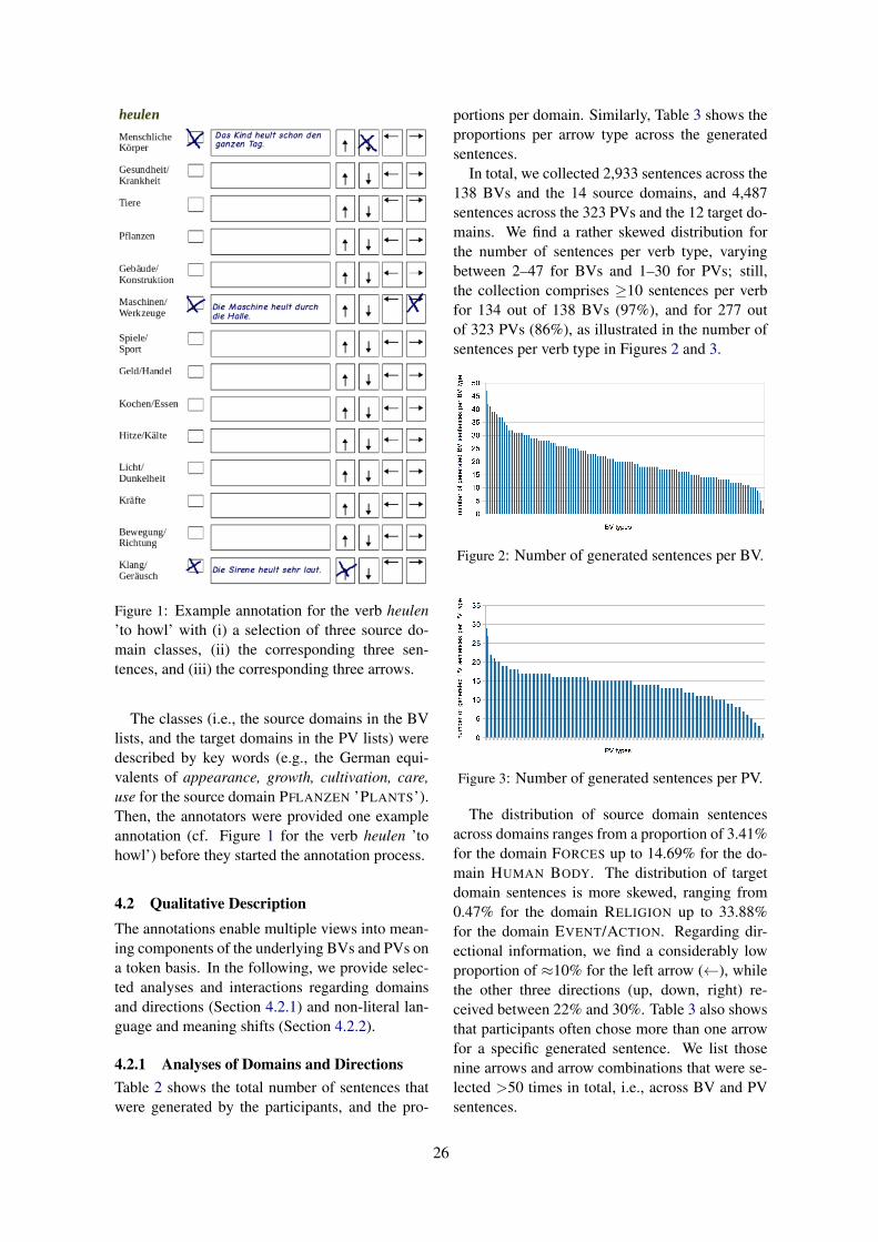
Figure 1: Example annotation for the verb heulen’to howl’ with (i) a selection of three source do-main classes, (ii) the corresponding three sen-tences, and (iii) the corresponding three arrows.
The classes (i.e., the source domains in the BVlists, and the target domains in the PV lists) weredescribed by key words (e.g., the German equi-valents of appearance, growth, cultivation, care,use for the source domain PFLANZEN ’PLANTS’).Then, the annotators were provided one exampleannotation (cf. Figure 1 for the verb heulen ’tohowl’) before they started the annotation process.
4.2 Qualitative DescriptionThe annotations enable multiple views into mean-ing components of the underlying BVs and PVs ona token basis. In the following, we provide selec-ted analyses and interactions regarding domainsand directions (Section 4.2.1) and non-literal lan-guage and meaning shifts (Section 4.2.2).
4.2.1 Analyses of Domains and DirectionsTable 2 shows the total number of sentences thatwere generated by the participants, and the pro-
portions per domain. Similarly, Table 3 shows theproportions per arrow type across the generatedsentences.
In total, we collected 2,933 sentences across the138 BVs and the 14 source domains, and 4,487sentences across the 323 PVs and the 12 target do-mains. We find a rather skewed distribution forthe number of sentences per verb type, varyingbetween 2–47 for BVs and 1–30 for PVs; still,the collection comprises ≥10 sentences per verbfor 134 out of 138 BVs (97%), and for 277 outof 323 PVs (86%), as illustrated in the number ofsentences per verb type in Figures 2 and 3.
Figure 2: Number of generated sentences per BV.
Figure 3: Number of generated sentences per PV.
The distribution of source domain sentencesacross domains ranges from a proportion of 3.41%for the domain FORCES up to 14.69% for the do-main HUMAN BODY. The distribution of targetdomain sentences is more skewed, ranging from0.47% for the domain RELIGION up to 33.88%for the domain EVENT/ACTION. Regarding dir-ectional information, we find a considerably lowproportion of ≈10% for the left arrow (←), whilethe other three directions (up, down, right) re-ceived between 22% and 30%. Table 3 also showsthat participants often chose more than one arrowfor a specific generated sentence. We list thosenine arrows and arrow combinations that were se-lected >50 times in total, i.e., across BV and PVsentences.
26

Source Domains No. of Sentences Target Domains No. of SentencesHuman Body 431 14.69% Event/Action 1,520 33.88%Animals 322 10.98% Economy 460 10.25%Health/Illness 251 8.56% Emotion/Feeling 452 10.07%Machines/Tools 242 8.25% Human Relationships 383 8.54%Games/Sports 211 7.19% Life/Death 365 8.13%Cooking/Food 210 7.16% Time 292 6.51%Plants 207 7.06% Thought 284 6.33%Economic Transaction 190 6.48% Communication 280 6.24%Buildings/Construction 167 5.69% Society/Nation 181 4.03%Sound 165 5.63% Desire 150 3.34%Heat/Cold 156 5.32% Morality 99 2.21%Movement/Direction 154 5.25% Religion 21 0.47%Light/Darkness 127 4.33%Forces 100 3.41%Total: 2,933 100.00% Total: 4,487 100.00%
Table 2: Source and target domains: number and proportions of generated sentences per domain.
Source Domain Directions No. of Sentences Target Domain Directions No. of Sentences↓ 879 29.97% → 1,300 28.97%↑ 782 26.66% ↓ 1,218 27.15%→ 648 22.09% ↑ 1,113 24.80%← 270 9.21% ← 462 10.30%↔ 128 4.36% ↔ 178 3.97%↔ l 58 1.98% ↓ → 52 1.16%l 50 1.70% ↑ → 44 0.98%↑ → 16 0.55% l ↔ 28 0.62%↓ → 12 0.41% l 27 0.60%
other combinations 69 0.24% other combinations 54 1.20%no choice 21 0.72% no choice 21 0.47%
Total: 2,933 100.00% Total: 4,487 100.00%
Table 3: Directional information: number and proportions of selected arrows and arrow combinations.
BV/PV Domain Direction SentenceBV LIGHT/DARKNESS ↑ Der Diamant funkelt im Licht.
‘The diamond sparkles in the light.’BV PLANTS ↓ Die Blatter fallen von den Baumen.
‘The leaves fall from the trees.’BV FORCES ← Er bog das Kupferrohr.
‘He bent the copper pipe.’BV ANIMALS ↔ Die Bullen fechten miteinander.
‘The bulls fence with each other.’BV HEAT/COLD ↔ l Das Feuer brennt heiß.
‘The fire is burning hot.’PV MORALITY ↓ Du solltest von deinem hohen Ross absteigen.
‘You should step down off your pedestal.’PV EMOTION/FEELING ↑ Der Druck wachst kurz vor der Prasentation an.
‘The pressure increases shortly before the presentation.’PV HUMAN-RELATIONSHIPS → Sie lasst ihn eiskalt abblitzen.
‘She turns him down cold-bloodedly.’PV LIFE/DEATH l Musst du mein ganzes Leben aufwuhlen?
‘Do you have to chum up my whole life?’PV COMMUNICATION ↔ Er kauft ihr die Luge problemlos ab.
‘He believes her lie without any doubts.’
Table 4: Example BV and PV sentences with selected domains and directions.
27
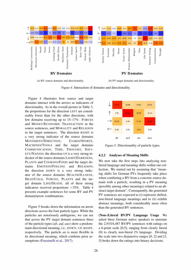
25.34 41.54 31.91 12.71 23.75 16.32 15.42 35 25 28.98 40.21 11.19 25.39 17.39
28.08 22.31 24.11 38.12 42.5 34.21 50.66 34.5 37.21 34.28 19.05 45.45 34.29 26.09
14.38 13.85 9.22 5.52 15 10.53 9.69 12 16.28 6.36 11.11 8.39 12.57 2.61
32.19 22.31 34.75 43.65 18.75 38.95 24.23 18.5 21.51 30.39 29.63 34.97 27.75 53.91
right
down
left
upB
uild
ings
/C
onst
ruct
ion
Mov
emen
t/D
irec
tion
Soun
d
Plan
ts
Forc
es
Coo
king
/Fo
od
Hea
lth/
Illn
ess
Mac
hine
s/To
ols
Eco
nom
ic−
Tran
sact
ion
Ani
mal
s
Gam
es/
Spor
ts
Hea
t/C
old
Hum
an−
Bod
y
Lig
ht/
Dar
knes
s
BV Domains
Dir
ecti
on ↑←↓→
(a) BV source domains and directionality.
35.15 29.36 31.18 33.58 34.4 26.5 25 37.02 28.32 21.38 37.84 36.43
32.73 29.83 32.26 29.2 28.85 27.64 20 26.72 46.31 28.03 22.78 26.74
9.7 13.37 17.2 6.57 12.34 11.4 15 9.16 10.03 8.55 13.9 8.91
22.42 27.45 19.35 30.66 24.4 34.47 40 27.1 15.34 42.04 25.48 27.91
right
down
left
up
Soci
ety/
Nat
ion
Eco
nom
y
Mor
alit
y
Des
ire
Eve
nt/
Act
ion
Hum
an−
Rel
atio
nshi
ps
Rel
igio
n
Tim
e
Lif
e/D
eath
Em
otio
n/Fe
elin
g
Com
mun
icat
ion
Tho
ught
PV Domains
Dir
ecti
on
↑←↓→
(b) PV target domains and directionality.
Figure 4: Interaction of domains and directionality.
Figure 4 illustrates how source and targetdomains interact with the arrows as indicators ofdirectionality. As in the overall picture in Table 3,the proportions for the direction LEFT are consid-erably lower than for the other directions, withfew domains receiving up to 15–17%: FORCES
and MONEY/ECONOMIC TRANSACTION in thesource sentences, and MORALITY and RELIGION
in the target sentences. The direction RIGHT isa very strong indicator of the source domainsMOVEMENT/DIRECTION, GAMES/SPORTS,MACHINES/TOOLS and the target domainsCOMMUNICATION, TIME, THOUGHT, SOCI-ETY/NATION; the direction UP is a very strong in-dicator of the source domains LIGHT/DARKNESS,PLANTS and COOKING/FOOD and the target do-mains EMOTION/FEELING and RELIGION;the direction DOWN is a very strong indic-ator of the source domains HEALTH/ILLNESS,HEAT/COLD, FORCES, PLANTS and the tar-get domain LIFE/DEATH; all of these strongindicators received proportions >35%. Table 4presents example sentences for some BV and PVdomain/arrow combinations.
Figure 5 breaks down the information on arrowdirections across the four particle types. While theparticles are notoriously ambiguous, we can seethat across the PV target domain sentences threeof the particle types (ab, auf, aus) show a predom-inant directional meaning, i.e., DOWN, UP, RIGHT,respectively. The particle an is more flexible inits directional meaning, which confirms prior as-sumptions (Frassinelli et al., 2017).
8.39 5.59 25.8 5.05
25.35 9.49 27.54 62.54
7.82 65.93 26.86 12.11
58.44 18.99 19.81 20.31
left
right
up
down
ab auf an aus
Particle
Dir
ecti
on
↓↑→←
Figure 5: Directionality of particle types.
4.2.2 Analyses of Meaning Shifts
We now take the first steps into analysing non-literal language and meaning shifts within our col-lection. We started out by assuming that “mean-ing shifts for German PVs frequently take placewhen combining a BV from a concrete source do-main with a particle, resulting in a PV meaning(possibly among other meanings) related to an ab-stract target domain”. Consequently, the generatedPV sentences are expected to (i) represent shifted,non-literal language meanings and to (ii) exhibitabstract meanings, both considerably more oftenthan the generated BV sentences.
(Non-)Literal BV/PV Language Usage Weasked three German native speakers to annotatethe 2,933/4,487 BV/PV sentences with ratings ona 6-point scale [0,5], ranging from clearly literal(0) to clearly non-literal (5) language. Dividingthe scale into two disjunctive ranges [0, 2] and [3,5] broke down the ratings into binary decisions.
28

Table 5 shows the numbers and proportionsof BV/PV sentences that were annotated as lit-eral vs. non-literal language usage, distinguishingbetween full agreement (i.e., all annotators agreedon the binary category) and majority agreement(i.e., at least two out of three annotators agreedon the binary category). We can see that the pro-portions of non-literal sentences are indeed con-siderably larger for PVs than for BVs (14.8% vs.3.2% for full agreement, and 29.5% vs. 14.8%for majority agreement), thus indicating a strongernon-literal language potential for German PVs incomparison to their BVs. Contrary to our assump-tions, the participants in the generation experimentalso produced a large number of literal sentencesfor PVs. In our opinion this indicates (a) the am-biguity of German PVs, which led participants torefer to literal as well as non-literal senses; and(b) that the presumably strongly abstract target do-main definitions did not necessarily enforce non-literal senses.
literal non-literalBVs full 2,443 83.3% 94 3.2%
maj 2,674 91.2% 259 8.8%PVs full 2,174 48.5% 666 14.8%
maj 3,150 70.2% 1,337 29.5%
Table 5: (Non-)literal language usage in generatedBV/PV sentences.
Abstractness in BV/PV Sentences As meaningshifts typically take place as a mapping from asource to a target domain, where the target do-main is supposedly more abstract than the sourcedomain, we expect our sentences in the target do-mains to be more abstract than those in the sourcedomains. Figure 6 shows that this is the case:
●
●
●●
●
●●●
● ●
●
BV PV
down left right up down left right up
2
4
6
8
2
4
6
8
Avg
. Abs
trac
tnes
s sc
ore
LIT NLIT
Figure 6: Average concreteness of nouns in BV/PVsentences, categorised by directionality.
Relying on abstractness/concreteness ratings ofa semi-automatically created database (Koper andSchulte im Walde, 2016a), we looked up and aver-aged over the ratings of all nouns in a sentence.
The ratings range from 0 (very abstract) to 10(very concrete). We can see that across directionsthe literal sentences are more concrete than thenon-literal sentences. In addition, we can see thatthe differences in abstractness are much strongerfor the PV target-domain sentences than for theBV source-domain sentences.
Particle Meaning Shifts Figure 7 once moreillustrates preferences in arrow directions acrossthe four particle types, but is –in contrast to Fig-ure 5– restricted to the non-literal PV sentences(full agreement). For particles ab and auf wehardly find differences when specifying on non-literal language usage; for both an and aus we findan increase of DOWN meanings in non-literal lan-guage usage, which goes along with a decrease ofLEFT meanings for an and a decrease of RIGHT
meanings for aus. So within our collection we findsome evidence for meaning shifts within PV typesfor the two particle types an and aus but not for aband auf, which seem to stay with their predomin-ant vertical meanings also in non-literal language.
8.442 4.926 18.621 5.263
25.974 4.434 26.897 53.383
7.143 73.399 25.517 13.534
58.442 17.241 28.965 27.82
left
right
up
down
ab auf an aus
Particle
Dir
ecti
on
↓↑→←
Figure 7: Directionality of particle types restrictedto non-literal sentences.
Source–Target Domain Meaning Shifts Fig-ure 8 presents meaning shifts as strengths of re-lationships between source and target domains,when looking at only literal BV sentences andnon-literal PV sentences. The cells in the heat mappresent the results of multiplying the target do-main degrees of membership across all PVs withthe source domain degrees of membership of theirrespective BVs. We applied positive pointwisemutual information (PPMI) weighting to avoid abias towards popular classes. Examples of partic-ularly strong combinations are PLANTS → TIME
(e.g., bluhen→ aufbluhen); and SOUND→ COM-MUNICATION (e.g., bellen→ anbellen).
29
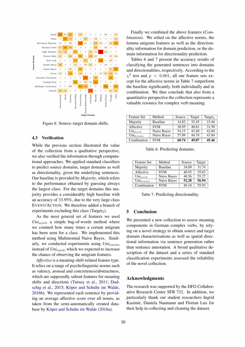
0.25
0
0
0
0.07
0
0.28
0
0.17
0.18
0.17
0.01
0
0.68
0.2
0
0
0
0
0
0
0
0
0.23
0.49
0
0.57
0.07
0
0.09
0
0
0.44
0.11
0
0
0.22
0
0.29
0.05
0.23
0.41
0
0
0.53
0
0
0
0.11
0.44
0
0.41
0
0
0
0
0
0.54
0
0
0.19
0.42
0
0
0.46
0
0
0.84
0
0.19
0
0.39
0.09
0.84
0
0
0.06
0.3
0
0
0
0.01
0.24
0
0.97
0
0.02
0
0
0
0.17
0
0.33
0.18
0
0
0
0
0
0
0.61
0.34
0
0
0
0
0.07
0.04
0.26
0.28
0.08
0
0
0
0
0
0.02
0
0
0.69
0
1.62
0
0.08
0
0
0
0.63
0
0
0.17
0
0.04
0
0
0.08
0.06
0
0
0.04
0.14
0
0
0.49
0.26
0.17
0
0.08
0.07
0
0
0.16
0
0
0.19
0.48
0
0
0.02
0.55
0
0
0.08
0
0
0.48
0.15
0.08
Animals
Buildings/Construction
Cooking/Food
Economic−Transaction
Forces
Games/Sports
Health/Illness
Heat/Cold
Human−Body
Light/Darkness
Machines/Tools
Movement/Direction
Plants
Sound
Com
mun
icat
ion
Des
ire
Eco
nom
y
Em
otio
n.Fe
elin
g
Eve
nt.A
ctio
n
Hum
an.R
elat
ions
hips
Lif
e.D
eath
Mor
alit
y
Rel
igio
n
Soci
ety.
Nat
ion
Tho
ught
Tim
eTarget Domain
Sou
rce
Dom
ain
Figure 8: Source–target domain shifts.
4.3 Verification
While the previous section illustrated the valueof the collection from a qualitative perspective,we also verified the information through computa-tional approaches. We applied standard classifiersto predict source domains, target domains as wellas directionality, given the underlying sentences.Our baseline is provided by Majority, which refersto the performance obtained by guessing alwaysthe largest class. For the target domains this ma-jority provides a considerably high baseline withan accuracy of 33.95%, due to the very large classEVENT/ACTION. We therefore added a branch ofexperiments excluding this class (Target2).
As the most general set of features we usedUniword, a simple bag-of-words method wherewe counted how many times a certain unigramhas been seen for a class. We implemented thismethod using Multinomial Naive Bayes. Simil-arly, we conducted experiments using Unilemma
instead of Uniword, which we expected to increasethe chance of observing the unigram features.
Affective is a meaning-shift-related feature type.It relies on a range of psycholinguistic norms suchas valency, arousal and concreteness/abstractness,which are supposedly salient features for meaningshifts and directions (Turney et al., 2011; Dud-schig et al., 2015; Koper and Schulte im Walde,2016b). We represented each sentence by provid-ing an average affective score over all nouns, astaken from the semi-automatically created data-base by Koper and Schulte im Walde (2016a).
Finally we combined the above features (Com-bination). We relied on the affective norms, thelemma unigram features as well as the direction-ality information for domain prediction, or the do-main information for directionality prediction.
Tables 6 and 7 present the accuracy results ofclassifying the generated sentences into domainsand directionalities, respectively. According to theχ2 test and p < 0.001, all our feature sets ex-cept for the affective norms in Table 7 outperformthe baseline significantly, both individually and incombination. We thus conclude that also from aquantitative perspective the collection represents avaluable resource for complex verb meaning.
Feature Set Method Source Target Target2Majority Baseline 14.82 33.45 15.46Affective SVM 30.95 40.61 31.50Uniword Naive Bayes 54.15 43.40 42.60Unilemma Naive Bayes 57.09 44.74 43.84Combination SVM 60.74 49.87 45.46
Table 6: Predicting domains.
Feature Set Method Source TargetMajority Baseline 34.09 31.74Affective SVM 40.93 35.63Uniword Naive Bayes 48.56 55.27Unilemma Naive Bayes 52.28 56.94Combination SVM 49.18 55.93
Table 7: Predicting directionality.
5 Conclusion
We presented a new collection to assess meaningcomponents in German complex verbs, by rely-ing on a novel strategy to obtain source and targetdomain characterisations as well as spatial direc-tional information via sentence generation ratherthan sentence annotation. A broad qualitative de-scription of the dataset and a series of standardclassification experiments assessed the reliabilityof the novel collection.
Acknowledgments
The research was supported by the DFG Collabor-ative Research Centre SFB 732. In addition, weparticularly thank our student researchers IngridKasimir, Daniela Naumann and Florian Lux fortheir help in collecting and cleaning the dataset.
30
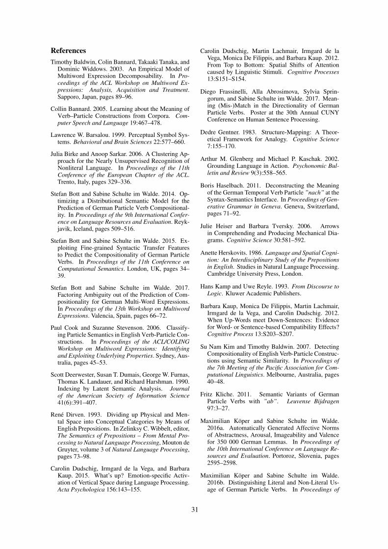
ReferencesTimothy Baldwin, Colin Bannard, Takaaki Tanaka, and
Dominic Widdows. 2003. An Empirical Model ofMultiword Expression Decomposability. In Pro-ceedings of the ACL Workshop on Multiword Ex-pressions: Analysis, Acquisition and Treatment.Sapporo, Japan, pages 89–96.
Collin Bannard. 2005. Learning about the Meaning ofVerb–Particle Constructions from Corpora. Com-puter Speech and Language 19:467–478.
Lawrence W. Barsalou. 1999. Perceptual Symbol Sys-tems. Behavioral and Brain Sciences 22:577–660.
Julia Birke and Anoop Sarkar. 2006. A Clustering Ap-proach for the Nearly Unsupervised Recognition ofNonliteral Language. In Proceedings of the 11thConference of the European Chapter of the ACL.Trento, Italy, pages 329–336.
Stefan Bott and Sabine Schulte im Walde. 2014. Op-timizing a Distributional Semantic Model for thePrediction of German Particle Verb Compositional-ity. In Proceedings of the 9th International Confer-ence on Language Resources and Evaluation. Reyk-javik, Iceland, pages 509–516.
Stefan Bott and Sabine Schulte im Walde. 2015. Ex-ploiting Fine-grained Syntactic Transfer Featuresto Predict the Compositionality of German ParticleVerbs. In Proceedings of the 11th Conference onComputational Semantics. London, UK, pages 34–39.
Stefan Bott and Sabine Schulte im Walde. 2017.Factoring Ambiguity out of the Prediction of Com-positionality for German Multi-Word Expressions.In Proceedings of the 13th Workshop on MultiwordExpressions. Valencia, Spain, pages 66–72.
Paul Cook and Suzanne Stevenson. 2006. Classify-ing Particle Semantics in English Verb-Particle Con-structions. In Proceedings of the ACL/COLINGWorkshop on Multiword Expressions: Identifyingand Exploiting Underlying Properties. Sydney, Aus-tralia, pages 45–53.
Scott Deerwester, Susan T. Dumais, George W. Furnas,Thomas K. Landauer, and Richard Harshman. 1990.Indexing by Latent Semantic Analysis. Journalof the American Society of Information Science41(6):391–407.
Rene Dirven. 1993. Dividing up Physical and Men-tal Space into Conceptual Categories by Means ofEnglish Prepositions. In Zelinksy C. Wibbelt, editor,The Semantics of Prepositions – From Mental Pro-cessing to Natural Language Processing, Mouton deGruyter, volume 3 of Natural Language Processing,pages 73–98.
Carolin Dudschig, Irmgard de la Vega, and BarbaraKaup. 2015. What’s up? Emotion-specific Activ-ation of Vertical Space during Language Processing.Acta Psychologica 156:143–155.
Carolin Dudschig, Martin Lachmair, Irmgard de laVega, Monica De Filippis, and Barbara Kaup. 2012.From Top to Bottom: Spatial Shifts of Attentioncaused by Linguistic Stimuli. Cognitive Processes13:S151–S154.
Diego Frassinelli, Alla Abrosimova, Sylvia Sprin-gorum, and Sabine Schulte im Walde. 2017. Mean-ing (Mis-)Match in the Directionality of GermanParticle Verbs. Poster at the 30th Annual CUNYConference on Human Sentence Processing.
Dedre Gentner. 1983. Structure-Mapping: A Theor-etical Framework for Analogy. Cognitive Science7:155–170.
Arthur M. Glenberg and Michael P. Kaschak. 2002.Grounding Language in Action. Psychonomic Bul-letin and Review 9(3):558–565.
Boris Haselbach. 2011. Deconstructing the Meaningof the German Temporal Verb Particle ”nach” at theSyntax-Semantics Interface. In Proceedings of Gen-erative Grammar in Geneva. Geneva, Switzerland,pages 71–92.
Julie Heiser and Barbara Tversky. 2006. Arrowsin Comprehending and Producing Mechanical Dia-grams. Cognitive Science 30:581–592.
Anette Herskovits. 1986. Language and Spatial Cogni-tion: An Interdisciplinary Study of the Prepositionsin English. Studies in Natural Language Processing.Cambridge University Press, London.
Hans Kamp and Uwe Reyle. 1993. From Discourse toLogic. Kluwer Academic Publishers.
Barbara Kaup, Monica De Filippis, Martin Lachmair,Irmgard de la Vega, and Carolin Dudschig. 2012.When Up-Words meet Down-Sentences: Evidencefor Word- or Sentence-based Compatibility Effects?Cognitive Process 13:S203–S207.
Su Nam Kim and Timothy Baldwin. 2007. DetectingCompositionality of English Verb-Particle Construc-tions using Semantic Similarity. In Proceedings ofthe 7th Meeting of the Pacific Association for Com-putational Linguistics. Melbourne, Australia, pages40–48.
Fritz Kliche. 2011. Semantic Variants of GermanParticle Verbs with ”ab”. Leuvense Bijdragen97:3–27.
Maximilian Koper and Sabine Schulte im Walde.2016a. Automatically Generated Affective Normsof Abstractness, Arousal, Imageability and Valencefor 350 000 German Lemmas. In Proceedings ofthe 10th International Conference on Language Re-sources and Evaluation. Portoroz, Slovenia, pages2595–2598.
Maximilian Koper and Sabine Schulte im Walde.2016b. Distinguishing Literal and Non-Literal Us-age of German Particle Verbs. In Proceedings of
31
the Conference of the North American Chapter ofthe Association for Computational Linguistics: Hu-man Language Technologies. San Diego, California,USA, pages 353–362.
Maximilian Koper and Sabine Schulte im Walde.2017a. Applying Multi-Sense Embeddings for Ger-man Verbs to Determine Semantic Relatedness andto Detect Non-Literal Language. In Proceedings ofthe 15th Conference of the European Chapter of theAssociation for Computational Linguistics. Valen-cia, Spain, pages 535–542.
Maximilian Koper and Sabine Schulte im Walde.2017b. Complex Verbs are Different: Exploring theVisual Modality in Multi-Modal Models to PredictCompositionality. In Proceedings of the 13th Work-shop on Multiword Expressions. Valencia, Spain,pages 200–206.
Maximilian Koper and Sabine Schulte im Walde. 2018.Analogies in Complex Verb Meaning Shifts: TheEffect of Affect in Semantic Similarity Models.In Proceedings of the 16th Annual Conference ofthe North American Chapter of the Association forComputational Linguistics: Human Language Tech-nologies. New Orleans, LA, USA. To appear.
Maximilian Koper, Sabine Schulte im Walde, MaxKisselew, and Sebastian Pado. 2016. ImprovingZero-Shot-Learning for German Particle Verbs byusing Training-Space Restrictions and Local Scal-ing. In Proceedings of the 5th Joint Conference onLexical and Computational Semantics. Berlin, Ger-many, pages 91–96.
Zolzan Kovecses. 2002. Metaphor: A Practical Intro-duction. Oxford University Press, New York.
Natalie Kuhner and Sabine Schulte im Walde. 2010.Determining the Degree of Compositionality of Ger-man Particle Verbs by Clustering Approaches. InProceedings of the 10th Conference on Natural Lan-guage Processing. Saarbrucken, Germany, pages47–56.
George Lakoff, Jane Espenson, and Alan Schwartz.1991. Master Metaphor List. Technical Report.
George Lakoff and Mark Johnson. 1980. Metaphorswe live by. University of Chicago Press.
Andrea Lechler and Antje Roßdeutscher. 2009. Ger-man Particle Verbs with ”auf”. Reconstructing theirComposition in a DRT-based Framework. Lin-guistische Berichte 220:439–478.
Birte Lonneker-Rodman. 2008. The Hamburg Meta-phor Database Project: Issues in Resource Creation.Language Resources and Evaluation 42:293–318.
Diana McCarthy, Bill Keller, and John Carroll. 2003.Detecting a Continuum of Compositionality inPhrasal Verbs. In Proceedings of the ACL Work-shop on Multiword Expressions: Analysis, Acquisi-tion and Treatment. Sapporo, Japan, pages 73–80.
Daniel C. Richardson, Michael J. Spivey, Lawrence W.Barsalou, and Ken McRae. 2003. Spatial Represent-ations activated during Real-Time Comprehensionof Verbs. Cognitive Science 27:767–780.
Ivan A. Sag, Timothy Baldwin, Francis Bond, AnnCopestake, and Dan Flickinger. 2002. MultiwordExpressions: A Pain in the Neck for NLP. InProceedings of the Conference on Intelligent TextProcessing and Computational Linguistics. MexicoCity, Mexico.
Bahar Salehi and Paul Cook. 2013. Predicting theCompositionality of Multiword Expressions UsingTranslations in Multiple Languages. In Proceedingsof the 2nd Joint Conference on Lexical and Compu-tational Semantics. Atlanta, GA, USA, pages 266–275.
Bahar Salehi, Paul Cook, and Timothy Baldwin. 2014.Using Distributional Similarity of Multi-way Trans-lations to Predict Multiword Expression Composi-tionality. In Proceedings of the 14th Conference ofthe European Chapter of the Association for Com-putational Linguistics. Gothenburg, Sweden, pages472–481.
Larry Shapiro. 2007. The Embodied Cognition Re-search Programme. Philosophy Compass 2(2):338–346.
Ekaterina Shutova and Simone Teufel. 2010. Meta-phor Corpus Annotated for Source – Target DomainMappings. In Proceedings of the 7th InternationalConference on Language Resources and Evaluation.Valletta, Malta, pages 3255–3261.
Ekaterina Shutova, Simone Teufel, and AnnaKorhonen. 2013. Statistical Metaphor Processing.Computational Linguistics 39(2):301–353.
Sylvia Springorum. 2011. DRT-based Analysis of theGerman Verb Particle ”an”. Leuvense Bijdragen97:80–105.
Sylvia Springorum, Jason Utt, and Sabine Schulte imWalde. 2013. Regular Meaning Shifts in GermanParticle Verbs: A Case Study. In Proceedings ofthe 10th International Conference on ComputationalSemantics. Potsdam, Germany, pages 228–239.
Peter Turney, Yair Neuman, Dan Assaf, and Yohai Co-hen. 2011. Literal and Metaphorical Sense Identi-fication through Concrete and Abstract Context. InProceedings of the Conference on Empirical Meth-ods in Natural Language Processing. Edinburgh,UK, pages 680–690.
Barbara Tversky. 2011. Visualizing Thought. Topicsin Cognitive Science 3:499–535.
Ake Viberg. 1983. The Verbs of Perception: A Typo-logical Study. Linguistics 21(1):123–162.
Joost Zwarts. 2017. Spatial semantics: Modeling themeaning of prepositions. Language and LinguisticsCompass 11(5):1–20.
32

Proceedings of the 7th Joint Conference on Lexical and Computational Semantics (*SEM), pages 33–42New Orleans, June 5-6, 2018. c©2018 Association for Computational Linguistics
Learning Neural Word Salience Scores
Krasen Samardzhiev Andrew GargettDepartment of Computer Science, University of Liverpool
Science and Technology Facilities [email protected], [email protected]
Danushka Bollegala
Abstract
Measuring the salience of a word is an essen-tial step in numerous NLP tasks. Heuristic ap-proaches such as tfidf have been used so farto estimate the salience of words. We proposeNeural Word Salience (NWS) scores, unlikeheuristics, are learnt from a corpus. Specifi-cally, we learn word salience scores such that,using pre-trained word embeddings as the in-put, can accurately predict the words that ap-pear in a sentence, given the words that ap-pear in the sentences preceding or succeed-ing that sentence. Experimental results on sen-tence similarity prediction show that the learntword salience scores perform comparably orbetter than some of the state-of-the-art ap-proaches for representing sentences on bench-mark datasets for sentence similarity, while us-ing only a fraction of the training and predic-tion times required by prior methods. More-over, our NWS scores positively correlate withpsycholinguistic measures such as concrete-ness, and imageability implying a close con-nection to the salience as perceived by hu-mans.
1 Introduction
Humans can easily recognise the words that con-tribute to the meaning of a sentence (i.e. contentwords) from words that serve only a grammaticalfunctionality (i.e. functional words). For example,functional words such as the, an, a etc. have lim-ited contributions towards the overall meaning ofa document and are often filtered out as stop wordsin information retrieval systems (Salton and Buck-ley, 1983). We define the salience q(w) of a wordw in a given text T as the semantic contributionmade by w towards the overall meaning of T . Ifwe can accurately compute the salience of words,then we can develop better representations of textsthat can be used in downstream NLP tasks such assimilarity measurement (Arora et al., 2017) or text
(e.g. sentiment, entailment) classification (Socheret al., 2011).
As described later in section 2, existing meth-ods for detecting word salience can be classi-fied into two groups: (a) lexicon-based filter-ing methods such as stop word lists, or (b)word frequency-based heuristics such as the pop-ular term-frequency inverse document frequency(tfidf) (Jones, 1972) measure and its variants. Un-fortunately, two main drawbacks can be identifiedin common to both stop words lists and frequency-based salience scores.
First, such methods do not take into account thesemantics associated with individual words whendetermining their salience. For example, considerthe following two adjacent sentences extractedfrom a newspaper article related to the visit of theJapanese Prime Minister, Shinzo Abe, to the WhiteHouse in Washington, to meet the US PresidentDonald Trump.
(a) Abe visited Washington in February and metTrump in the White House.
(b) Because the trade relations between US andJapan have been fragile after the recent com-ments by the US President, the Prime Minis-ter’s visit to the US can be seen as an attemptto reinforce the trade relations.
In Sentence (a), the Japanese person name Abe orAmerican person name Trump would occur lessin a corpus than the US state name Washington.Nevertheless, for the main theme of this sentence,Japanese Prime minister met US President, thetwo person names are equally important as the lo-cation they met. Therefore, we must look into thesemantics of the individual words when comput-ing their saliences.
Second, words do not occur independently ofone another in a text, and methods that compute
33

word salience using frequency or pre-compiledstop words lists alone do not consider the contex-tual information. For example, the two sentences(a) and (b) in our previous example are extractedfrom the same newspaper article and are adjacent.The words in the two sentences are highly re-lated. For example, Abe in sentence (a) refers tothe Prime Minister in sentence (b), and Trump insentence (a) is refers to the US President in sen-tence (b). A human reader who reads sentence (a)before sentence (b) would expect to see some re-lationship between the topic discussed in (a) andthat in the next sentence (b). Unfortunately, meth-ods that compute word salience scores consideringeach word independently from all other words innear by contexts, ignore such proximity relation-ships.
To overcome the above-mentioned disfluenciesin existing word salience scores, we propose anunsupervised method that first randomly initialisesword salience scores, and subsequently updatesthem such that we can accurately predict the wordsin local contexts. Specifically, we train a two-layerneural network where in the first layer we takepre-trained word embeddings of the words in asentence Si as the input and compute a represen-tation for Si (here onwards referred to as a sen-tence embedding) as the weighted average of theinput word embeddings. The weights correspondto the word salience scores of the words in Si.Likewise, we apply the same approach to computethe sentence embedding for the sentence Si−1 pre-ceding Si and Si+1 succeeding Si in a sentence-ordered corpus. Because Si−1, Si and Si+1 are ad-jacent sentences, we would expect the sentencepairs (Si, Si−1) and (Si, Si+1) to be topically re-lated.1
We would expect a high degree of cosine sim-ilarity between si and si−1, and si and si+1,where boldface symbols indicate vectors. Like-wise, for a randomly selected sentence Sj /∈{Si−1, Si, Si+1}, the expect similarity between Sjand Si would be low. We model this as a super-vised similarity prediction task and use backprop-agation to update the word salience scores, keep-ing word embeddings fixed. We refer to the word
1Si−1 and Si+1 could also be topically related and pro-duce a positive training examples in some cases. However,they are non-adjacent and possibly less related compared toadjacent sentence pairs. Because we have an abundant supplyof sentences, and we want to reduce label noise in positiveexamples, we do not consider (Si−1, Si+1) as a positive ex-ample.
salience scores learnt by the proposed method asthe Neural Word Salience (NWS) scores. We willuse the contextual information of a word to learnits salience. However, once learnt, we considersalience as a property of a word that holds inde-pendently of its context. This enables us to use thesame salience score for a word after training, with-out having to modify it considering the context inwhich it occurs.
Several remarks can be made about the pro-posed method for learning NWS scores. First, wedo not require labelled data for learning NWSscores. Although we require semantically similar(positive) and semantically dissimilar (negative)pairs of sentences for learning the NWS scores,both positive and negative examples are automati-cally extracted from the given corpus. Second, weuse pre-trained word embeddings as the input, anddo not learn the word embeddings as part of thelearning process. This design choice differentiatesour work from previously proposed sentence em-bedding learning methods that jointly learn wordembeddings as well as sentence embeddings (Hillet al., 2016; Kiros et al., 2015; Kenter et al., 2016).Moreover, it decouples the word salience scorelearning problem from word or sentence embed-ding learning problem, thereby simplifying the op-timisation task and speeding up the learning pro-cess.
We use the NWS scores to compute sen-tence embeddings and measure the similarity be-tween two sentences using 18 benchmark datasetsfor semantic textual similarity in past SemEvaltasks (Agirre et al., 2012). Experimental resultsshow that the sentence similarity scores com-puted using the NWS scores and pre-trained wordembeddings show a high degree of correlationwith human similarity ratings in those bench-mark datasets. Moreover, we compare the NWSscores against the human ratings for psycholin-guistic properties of words such as arousal, va-lence, dominance, imageability, and concreteness.Our analysis shows that NWS scores demonstratea moderate level of correlation with concretenessand imageability ratings, despite not being specifi-cally trained to predict such psycholinguistic prop-erties of words.
2 Related Work
Word salience scores have long been studied inthe information retrieval community (Salton and
34
Buckley, 1983). Given a user query described interms of one or more keywords, an informationretrieval system must find the most relevant doc-uments to the user query from a potentially largecollection of documents. Word salience scoresbased on term frequency, document frequency, anddocument length have been proposed such as tfidfand BM25 (Robertson, 1997).
Our proposed method learns word saliencescores by creating sentence embeddings. Next, webriefly review such sentence embedding methodsand explain the differences between the sentenceembedding learning problem and word saliencelearning problem.
Sentences have a syntactic structure and the or-dering of words affects the meaning expressedin the sentence. Consequently, compositional ap-proaches for computing sentence-level semanticrepresentations from word-level semantic repre-sentations have used numerous linear algebraicoperators such as vector addition, element-wisemultiplication, multiplying by a matrix or a ten-sor (Blacoe and Lapata, 2012; Mitchell and Lap-ata, 2008).
Alternatively to applying nonparametric opera-tors on word embeddings to create sentence em-beddings, recurrent neural networks can learn theoptimal weight matrix that can produce an ac-curate sentence embedding when repeatedly ap-plied to the constituent word embeddings. For ex-ample, skip-thought vectors (Kiros et al., 2015)use bi-directional LSTMs to predict the words inthe order they appear in the previous and nextsentences given the current sentence. Althoughskip-thought vectors have shown superior perfor-mances in supervised tasks, its performance onunsupervised tasks has been sub-optimal (Aroraet al., 2017). Moreover, training bi-directionalLSTMs from large datasets is time consuming andwe also need to perform LSTM inference in or-der to create the embedding for unseen sentencesat test time, which is time consuming compared toweighted addition of the input word embeddings.FastSent (Hill et al., 2016) was proposed as analternative lightweight approach for sentence em-bedding where a softmax objective is optimised topredict the occurrences of words in the next andthe previous sentences, ignoring the ordering ofthe words in the sentence.
Surprisingly, averaging word embeddings tocreate sentence embeddings has shown compara-
Figure 1: Overview of the proposed neural word saliencelearning method. Given two sentences (Si, Sj), we learn thesalience scores of words q(w) such that we can predict thesimilarity between the two sentences using their embeddingssi, sj . Difference between predicted similarity and actual la-bel is considered as the error and its gradient is backpropa-gated through the network to update q(w).
ble performances to sentence embeddings that arelearnt using more sophisticated word-order sen-sitive methods. For example, (Arora et al., 2017)proposed a method to find the optimal weights forcombining word embeddings when creating sen-tence embeddings using unigram probabilities, bymaximising the likelihood of the occurrences ofwords in a corpus. Siamese CBOW (Kenter et al.,2016) learns word embeddings such that we canaccurately compute sentence embeddings by aver-aging the word embeddings. Although averagingis an order insensitive operator, (Adi et al., 2016)empirically showed that it can accurately predictthe content and word order in sentences. This canbe understood intuitively by recalling that wordsthat appear between two words are often differentin contexts where those two words are swapped.For example, in the two sentences “Ostrich is alarge bird that lives in Africa” and “Large birdssuch as Ostriches live in Africa”, the words thatappear in between ostrich and bird are different,giving rise to different sentence embeddings evenwhen sentence embeddings are computed by aver-aging the individual word embeddings. Instead ofconsidering all words equally for sentence embed-ding purposes, attention-based models (Hahn andKeller, 2016; Yin et al., 2016; Wang et al., 2016)learn the amount of weight (attention) we must as-sign to each word in a given context.
Our proposed method for learning NWS scoresis based on the prior observation that averagingis an effective heuristic for creating sentence em-beddings from word embeddings. However, unlikesentence embedding learning methods that do notlearn word salience scores (He and Lin, 2016; Yin
35
et al., 2016) , our goal in this paper is to learn wordsalience scores and not sentence embeddings. Wecompute sentence embeddings only for the pur-pose of evaluating the word salience scores welearn. Moreover, our work differs from SiameseCBOW (Kenter et al., 2016) in that we do not learnword embeddings but take pre-trained word em-beddings as the input for learning word saliencescores. NWS scores we learn in this paper are alsodifferent from the salience scores learnt by (Aroraet al., 2017) because they do not constrain theirword salience scores such that they can be used topredict the words that occur in adjacent sentences.
3 Neural Word Salience Scores
Let us consider a vocabulary V of words w ∈ V .For the simplicity of exposition, we limit the vo-cabulary to unigrams but note that the proposedmethod can be used to learn salience scores forarbitrary length n-grams. We assume that we aregiven d-dimensional pre-trained word embeddingsw ∈ Rd for the words in V . Let us denotethe NWS score of w by q(w) ∈ R. We learnq(w) such that the similarity between two adja-cent sentences Si and Si−1, or Si and Si+1 ina sentence-ordered corpus C is larger than thatbetween two non-adjacent sentences Si and Sj ,where j /∈ {i − 1, i, i + 1}. Let us further rep-resent the two sentence Si = {wi1, . . . , win} andSj = {wj1, . . . , wjm} by the sets of words inthose sentences. Here, we assume the corpus tocontain sequences of ordered sentence such as in anewspaper article, a book chapter or a blog post.
The neural network we use for learning q(w) isshown in Figure 1. The first layer computes theembedding of a sentence S, s ∈ Rd using Equa-tion 1, which is the weighted-average of the indi-vidual word embeddings.
s =∑
w∈Sq(w)w (1)
We use (1) to compute embeddings for two sen-tences Si and Sj denoted respectively by si andsj . Here, the same set of salience scores q(w) areused for computing both si and sj , which resem-bles a Siamese neural network architecture.
The root node computes the similarity h(si, sj)between two sentence embeddings. Different sim-ilarity (alternatively dissimilarity or divergence)functions such as cosine similarity, `1 distance, `2distance, Jenson-Shannon divergence etc. can be
used as h. As a concrete example, here we usesoftmax of the inner-products as follows:
h(si, sj) =exp
(si>sj)
∑Sk∈C exp (si>sk)
(2)
Ideally, the normalisation term in the denominatorin the softmax must be taken over all the sentencesSk in the corpus (Andreas and Klein, 2015). How-ever, this is computationally expensive in mostcases except for extremely small corpora. There-fore, following noise-contrastive estimation (Gut-mann and Hyvärinen, 2012), we approximate thenormalisation term using a randomly sampled setof K sentences, where K is typically less than10. Because the similarity between two randomlysampled sentences is likely to be smaller than, forexample, two adjacent sentences, we can see thissampling process as randomly sampling negativetraining instances from the corpus.
For two sentences Si and Sj we consider themto be similar (positive training instance) if j ∈{i − 1, i + 1}, and denote this by the target labelt = 1. On the other hand, if the two sentences arenon-adjacent (i.e. j /∈ {i−1, i+1}), then we con-sider the pair (Si,Sj) to form a negative traininginstance, and denote this by t = 0.2 This assump-tion enables us to use a sentence-ordered corpusfor selecting both positive and negative training in-stances required for learning NWS scores.
Specifically, the model is trained using the twoadjacent sentences to Si - {i − 1, i + 1} as posi-tive examples, and K=2 negative examples not in{i− 1, i + 1}. These are sampled from the wholetext corpus using a uniformly. Similar to (Kenteret al., 2016), we found that increasing the numberof negative examples increases the training time,but does not have a significant impact on modelaccuracy.
Using t and h(si, sj) above, we compute thecross-entropy error E(t, (Si,Sj)) for an instance(t, (Si,Sj)) as follows:
E(t, (Si,Sj)) = t log (h(si, sj))+(1−t) log (1− h(si, sj))(3)
Next, we backpropagate the error gradients via thenetwork to compute the updates as follows:
∂E
∂q(w)=
(t− h(si, sj))
h(si, sj)(1− h(si, sj))
∂h(si, sj)
∂q(w)(4)
2It is possible in theory that two non-adjacent sentencescould be similar, but the likelihood of this event is small andcan be safely ignored in practice.
36
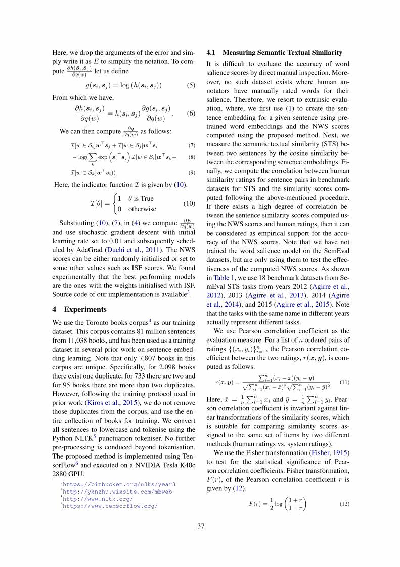
Here, we drop the arguments of the error and sim-ply write it as E to simplify the notation. To com-pute ∂h(si,sj)
∂q(w) let us define
g(si, sj) = log (h(si, sj)) (5)
From which we have,
∂h(si, sj)
∂q(w)= h(si, sj)
∂g(si, sj)
∂q(w). (6)
We can then compute ∂g∂q(w) as follows:
I[w ∈ Si]w>sj + I[w ∈ Sj ]w>si (7)
− log(∑
k
exp(si>sj
)I[w ∈ Si]w>sk+ (8)
I[w ∈ Sk]w>si)) (9)
Here, the indicator function I is given by (10).
I[θ] =
{1 θ is True0 otherwise
(10)
Substituting (10), (7), in (4) we compute ∂E∂q(w)
and use stochastic gradient descent with initiallearning rate set to 0.01 and subsequently sched-uled by AdaGrad (Duchi et al., 2011). The NWSscores can be either randomly initialised or set tosome other values such as ISF scores. We foundexperimentally that the best performing modelsare the ones with the weights initialised with ISF.Source code of our implementation is available3.
4 Experiments
We use the Toronto books corpus4 as our trainingdataset. This corpus contains 81 million sentencesfrom 11,038 books, and has been used as a trainingdataset in several prior work on sentence embed-ding learning. Note that only 7,807 books in thiscorpus are unique. Specifically, for 2,098 booksthere exist one duplicate, for 733 there are two andfor 95 books there are more than two duplicates.However, following the training protocol used inprior work (Kiros et al., 2015), we do not removethose duplicates from the corpus, and use the en-tire collection of books for training. We convertall sentences to lowercase and tokenise using thePython NLTK5 punctuation tokeniser. No furtherpre-processing is conduced beyond tokenisation.The proposed method is implemented using Ten-sorFlow6 and executed on a NVIDIA Tesla K40c2880 GPU.
3https://bitbucket.org/u3ks/year34http://yknzhu.wixsite.com/mbweb5http://www.nltk.org/6https://www.tensorflow.org/
4.1 Measuring Semantic Textual SimilarityIt is difficult to evaluate the accuracy of wordsalience scores by direct manual inspection. More-over, no such dataset exists where human an-notators have manually rated words for theirsalience. Therefore, we resort to extrinsic evalu-ation, where, we first use (1) to create the sen-tence embedding for a given sentence using pre-trained word embeddings and the NWS scorescomputed using the proposed method. Next, wemeasure the semantic textual similarity (STS) be-tween two sentences by the cosine similarity be-tween the corresponding sentence embeddings. Fi-nally, we compute the correlation between humansimilarity ratings for sentence pairs in benchmarkdatasets for STS and the similarity scores com-puted following the above-mentioned procedure.If there exists a high degree of correlation be-tween the sentence similarity scores computed us-ing the NWS scores and human ratings, then it canbe considered as empirical support for the accu-racy of the NWS scores. Note that we have nottrained the word salience model on the SemEvaldatasets, but are only using them to test the effec-tiveness of the computed NWS scores. As shownin Table 1, we use 18 benchmark datasets from Se-mEval STS tasks from years 2012 (Agirre et al.,2012), 2013 (Agirre et al., 2013), 2014 (Agirreet al., 2014), and 2015 (Agirre et al., 2015). Notethat the tasks with the same name in different yearsactually represent different tasks.
We use Pearson correlation coefficient as theevaluation measure. For a list of n ordered pairs ofratings {(xi, yi)}ni=1, the Pearson correlation co-efficient between the two ratings, r(x,y), is com-puted as follows:
r(x,y) =
∑ni=1(xi − x)(yi − y)√∑n
i=1(xi − x)2√∑n
i=1(yi − y)2(11)
Here, x = 1n
∑ni=1 xi and y = 1
n
∑ni=1 yi. Pear-
son correlation coefficient is invariant against lin-ear transformations of the similarity scores, whichis suitable for comparing similarity scores as-signed to the same set of items by two differentmethods (human ratings vs. system ratings).
We use the Fisher transformation (Fisher, 1915)to test for the statistical significance of Pear-son correlation coefficients. Fisher transformation,F (r), of the Pearson correlation coefficient r isgiven by (12).
F (r) =1
2log
(1 + r
1− r
)(12)
37
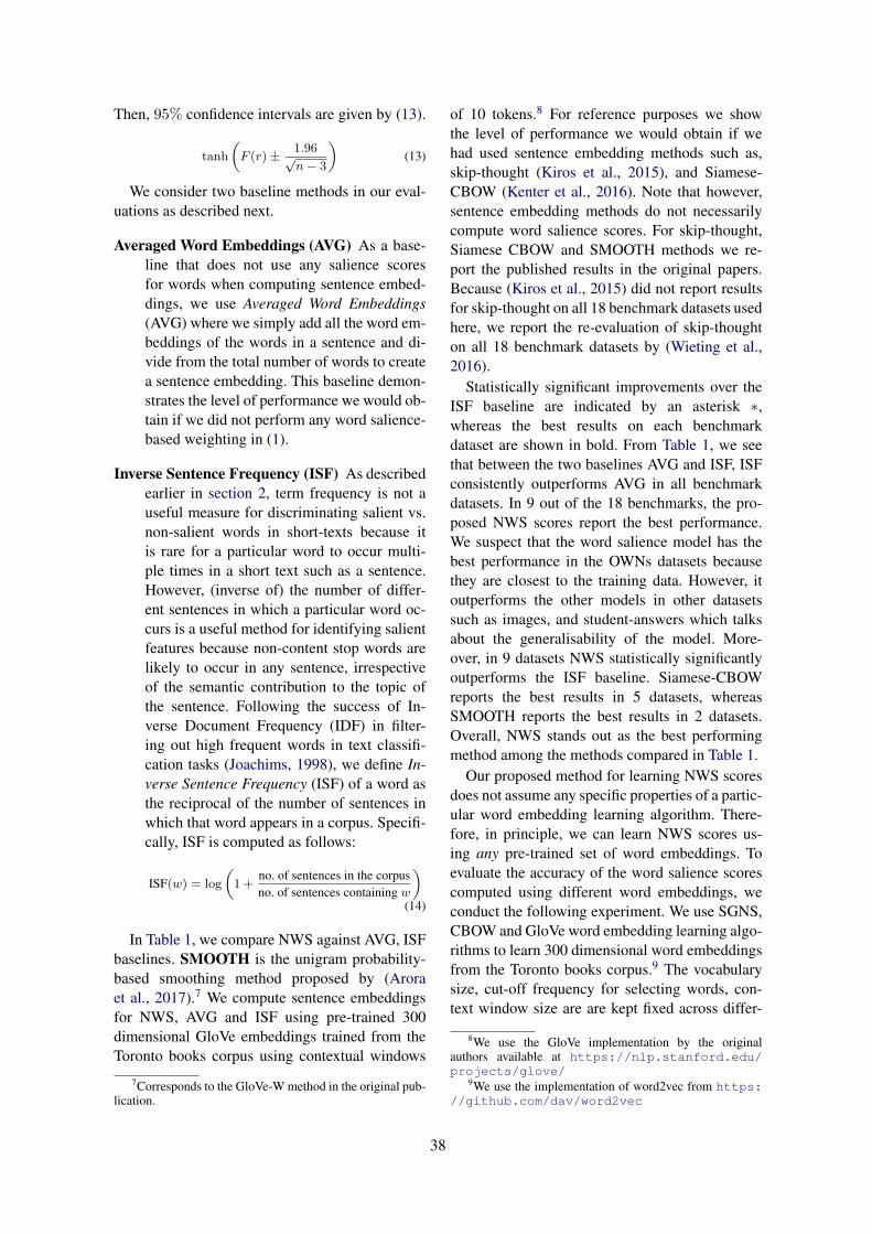
Then, 95% confidence intervals are given by (13).
tanh
(F (r)± 1.96√
n− 3
)(13)
We consider two baseline methods in our eval-uations as described next.
Averaged Word Embeddings (AVG) As a base-line that does not use any salience scoresfor words when computing sentence embed-dings, we use Averaged Word Embeddings(AVG) where we simply add all the word em-beddings of the words in a sentence and di-vide from the total number of words to createa sentence embedding. This baseline demon-strates the level of performance we would ob-tain if we did not perform any word salience-based weighting in (1).
Inverse Sentence Frequency (ISF) As describedearlier in section 2, term frequency is not auseful measure for discriminating salient vs.non-salient words in short-texts because itis rare for a particular word to occur multi-ple times in a short text such as a sentence.However, (inverse of) the number of differ-ent sentences in which a particular word oc-curs is a useful method for identifying salientfeatures because non-content stop words arelikely to occur in any sentence, irrespectiveof the semantic contribution to the topic ofthe sentence. Following the success of In-verse Document Frequency (IDF) in filter-ing out high frequent words in text classifi-cation tasks (Joachims, 1998), we define In-verse Sentence Frequency (ISF) of a word asthe reciprocal of the number of sentences inwhich that word appears in a corpus. Specifi-cally, ISF is computed as follows:
ISF(w) = log
(1 +
no. of sentences in the corpusno. of sentences containing w
)
(14)
In Table 1, we compare NWS against AVG, ISFbaselines. SMOOTH is the unigram probability-based smoothing method proposed by (Aroraet al., 2017).7 We compute sentence embeddingsfor NWS, AVG and ISF using pre-trained 300dimensional GloVe embeddings trained from theToronto books corpus using contextual windows
7Corresponds to the GloVe-W method in the original pub-lication.
of 10 tokens.8 For reference purposes we showthe level of performance we would obtain if wehad used sentence embedding methods such as,skip-thought (Kiros et al., 2015), and Siamese-CBOW (Kenter et al., 2016). Note that however,sentence embedding methods do not necessarilycompute word salience scores. For skip-thought,Siamese CBOW and SMOOTH methods we re-port the published results in the original papers.Because (Kiros et al., 2015) did not report resultsfor skip-thought on all 18 benchmark datasets usedhere, we report the re-evaluation of skip-thoughton all 18 benchmark datasets by (Wieting et al.,2016).
Statistically significant improvements over theISF baseline are indicated by an asterisk ∗,whereas the best results on each benchmarkdataset are shown in bold. From Table 1, we seethat between the two baselines AVG and ISF, ISFconsistently outperforms AVG in all benchmarkdatasets. In 9 out of the 18 benchmarks, the pro-posed NWS scores report the best performance.We suspect that the word salience model has thebest performance in the OWNs datasets becausethey are closest to the training data. However, itoutperforms the other models in other datasetssuch as images, and student-answers which talksabout the generalisability of the model. More-over, in 9 datasets NWS statistically significantlyoutperforms the ISF baseline. Siamese-CBOWreports the best results in 5 datasets, whereasSMOOTH reports the best results in 2 datasets.Overall, NWS stands out as the best performingmethod among the methods compared in Table 1.
Our proposed method for learning NWS scoresdoes not assume any specific properties of a partic-ular word embedding learning algorithm. There-fore, in principle, we can learn NWS scores us-ing any pre-trained set of word embeddings. Toevaluate the accuracy of the word salience scorescomputed using different word embeddings, weconduct the following experiment. We use SGNS,CBOW and GloVe word embedding learning algo-rithms to learn 300 dimensional word embeddingsfrom the Toronto books corpus.9 The vocabularysize, cut-off frequency for selecting words, con-text window size are are kept fixed across differ-
8We use the GloVe implementation by the originalauthors available at https://nlp.stanford.edu/projects/glove/
9We use the implementation of word2vec from https://github.com/dav/word2vec
38

Table 1: Performance on STS benchmarks.
Dataset SMOOTH skip-thought Siamese-CBOW AVG ISF NWS2012MSRpar 43.6 5.6 43.8 28.4 39.1 28.5OnWN 54.3 60.5 64.4 47.1 60.5 65.5∗
SMTeuroparl 51.1∗ 42.0 45.0 37.1 44.5 50.1SMTnews 42.2 39.1 39.0 32.2 34.9 44.7∗
2013FNWN 23.0 31.2 23.2 26.9 29.4 25.2OnWN 68.0∗ 24.2 49.9 25.0 63.2 78.1∗
headlines 63.8 38.6 65.3∗ 40.2 59.4 57.02014OnWN 68.0 46.8 60.7 41.1 68.5 80.8∗
deft-forum 29.1 37.4 40.8 27.1 37.1 29.9deft-news 68.5 46.2 59.1 48.8 63.6 65.4headlines 59.3 40.3 63.6∗ 41.9 58.8 56.2images 74.1∗ 42.6 65.0 35.3 66.3 75.9∗
tweet-news 57.3 51.4 73.2∗ 41.7 57.1 64.5∗
2015answers-forums 41.4 27.8 21.8 25.7 37.6 49.6∗
answers-students 61.5 26.6 36.7 56.5 67.1 68.0belief 47.7 45.8 47.7 29.3 43.2 54.3∗
headlines 64.0 12.5 21.5 49.3 65.4 65.3images 75.4∗ 21 25.6 49.8 66.1 76.6∗
Overall Average 55.1 35.5 47.0 38.0 53.4 57.6
ent word embedding learning methods for the con-sistency of the evaluation. We then trained NWSwith each set of word embeddings. Performanceon STS benchmarks is shown in Table 2, wherethe best performance is bolded.
From Table 2, we see that GloVe is the bestamong the three word embedding learning meth-ods compared in Table 2 for producing pre-trainedword embeddings for the purpose of learningNWS scores. In particular, NWS scores reportsbest results with GloVe embeddings in 10 out ofthe 18 benchmark datasets, whereas with CBOWembeddings it obtains the best results in the re-maining 8 benchmark datasets.
Figures 2a and 2b show the Pearson correla-tion coefficients on STS benchmarks obtained byNWS scores computed respectively for GloVe andSGNS embeddings. We plot training curves for theaverage correlation over each year’s benchmarksas well as the overall average over the 18 bench-marks. We see that for both embeddings the train-ing saturates after about five or six epochs. Thisability to learn quickly with a small number ofepochs is attractive because it reduces the training
time.
4.2 Correlation with Psycholinguistic Scores
Prior work in psycholinguistics show that there isa close connection between the emotions felt byhumans and the words they read in a text. Va-lence (the pleasantness of the stimulus), arousal(the intensity of emotion provoked by the stim-ulus), and dominance (the degree of control ex-erted by the stimulus) contribute to how the mean-ings of words affect human psychology, and of-ten referred to as the affective meanings of words.(Mandera et al., 2015) show that by using SGNSembeddings as features in a k-Nearest Neighbourclassifier, it is possible to accurately extrapolatethe affective meanings of words. Moreover, per-ceived psycholinguistic properties of words suchas concreteness (how “palpable” the object theword refers to) and imageability (the intensity withwhich a word arouses images) have been success-fully predicted using word embeddings (Turneyet al., 2011; Paetzold and Specia, 2016). For ex-ample, (Turney et al., 2011) used the cosine simi-larity between word embeddings obtained via La-
39

Table 2: Effect of word embeddings.
Dataset NWS with pre-trainedSGNS CBOW GloVe
2012MSRpar 14.27 24.15 28.47OnWN 59.76 61.25 65.50SMTeuroparl 41.04 45.51 50.12SMTnews 43.42 46.94 44.732013FNWN 21.47 29.31 25.21OnWN 67.37 70.04 78.06headlines 57.05 57.46 57.022014OnWN 73.06 73.71 80.83deft-forum 28.62 32.49 29.90deft-news 59.63 61.95 65.35headlines 56.05 55.64 56.20images 76.94 78.08 75.88tweet-news 61.49 66.41 64.462015answers-forums 36.35 46.78 49.65answers-students 59.53 59.92 68.01belief 51.97 55.65 54.27headlines 61.24 63.04 65.32images 77.67 78.39 76.55Overall Average 52.60 55.92 57.52
(a) GloVe
(b) SGNS
Figure 2: Pearson correlations on STS benchmarks againstthe number of training epochs
tent Semantic Analysis (LSA) (Deerwester et al.,1990) to predict the concreteness and imageability
Table 3: Pearson correlation coefficients against Psycholin-guistic ratings of words in the ANEW and MRC databases.
Embed. Arousal Conc. Dom. Img. ValanceGloVe 0.03 0.26 0.09 0.25 0.03CBOW 0.04 -0.35 -0.04 -0.37 0.04SGNS -0.01 0.27 0.06 0.27 -0.01
ratings of words.On the other hand, prior work studying the re-
lationship between human reading patterns usingeye-tracking devices show that there exist a highpositive correlation between word salience andreading times (Dziemianko et al., 2013; Hahn andKeller, 2016). For example, humans pay more at-tention to words that carry meaning as indicatedby the longer fixation times. Therefore, an inter-esting open question is that what psycholinguis-tic properties of words, if any, are related to theNWS scores we learn in a purely unsupervisedmanner from a large corpus? To answer this ques-tion empirically, we conduct the following exper-iment. We used the Affected Norms for EnglishWords (ANEW) dataset created by Warriner et al.(2013), which contains valence, arousal, and dom-inance ratings collected via crowd sourcing for13,915 words. Moreover, we obtained concrete-ness and imageability ratings for 3364 words fromthe MRC psycholinguistic database. We then mea-sure the Pearson correlation coefficient betweenNWS scores and each of the psycholinguistic rat-ings as shown in Table 3.
We see a certain degree of correlation betweenNWS scores computed for all three word embed-dings and the concreteness scores. Both GloVeand SGNS show moderate positive correlationsfor concreteness, whereas CBOW shows a mod-erate negative correlation for the same. A similartrend can be observed for imageability ratings inTable 3, where GloVe and SGNS correlates posi-tively with imageability, while CBOW correlatesnegatively. Moreover, no correlation could be ob-served for arousal, valance and dominance ratings.This result shows that NWS scores are not corre-lated with affective meanings of words (arousal,dominance, and valance), but show a moderatelevel of correlation with perceived meaning scores(concreteness and imageability).
4.3 Sample Salience ScoresTables 4 and 5 show respectively low and highsalient words for ISF, NWS (ISF initialised) andNWS (randomly initialised) methods. words) se-
40
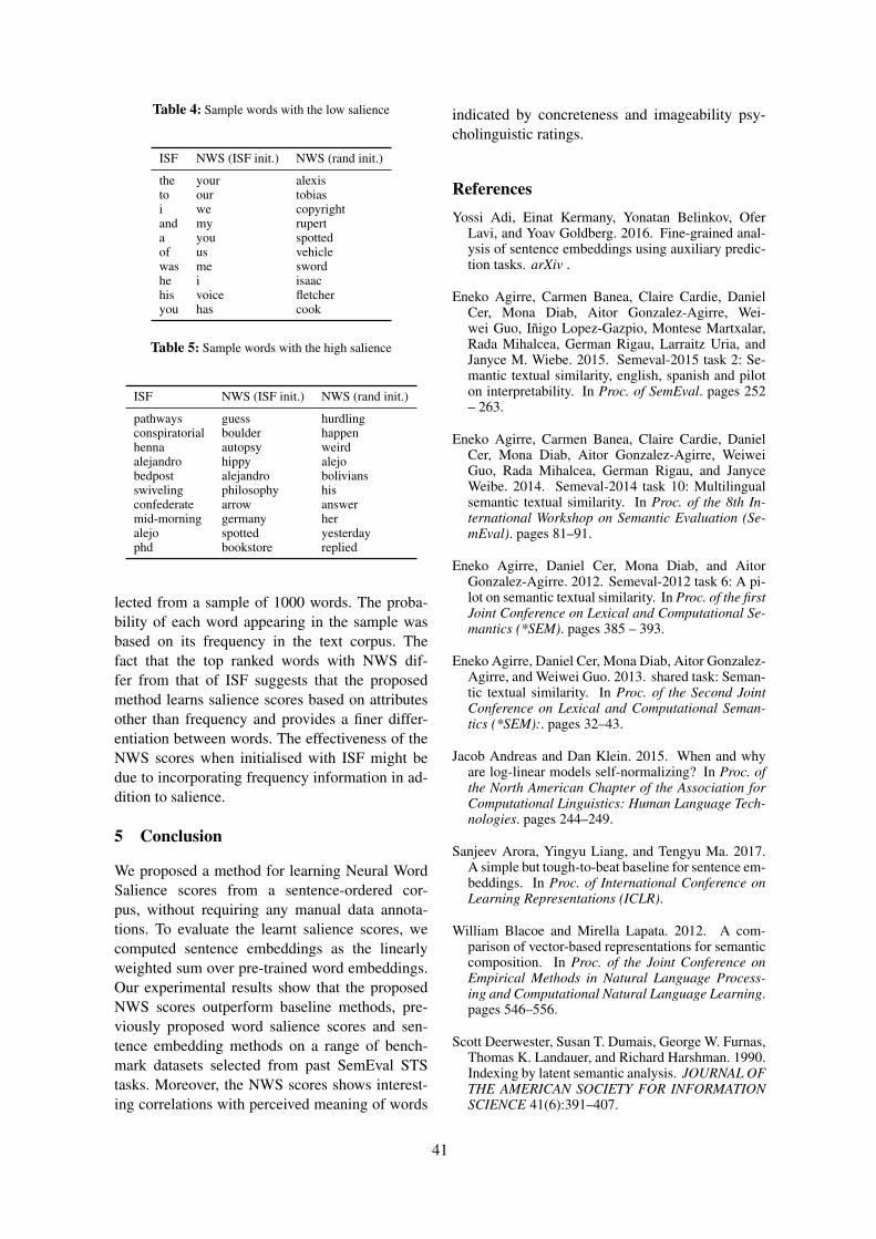
Table 4: Sample words with the low salience
ISF NWS (ISF init.) NWS (rand init.)
the your alexisto our tobiasi we copyrightand my ruperta you spottedof us vehiclewas me swordhe i isaachis voice fletcheryou has cook
Table 5: Sample words with the high salience
ISF NWS (ISF init.) NWS (rand init.)
pathways guess hurdlingconspiratorial boulder happenhenna autopsy weirdalejandro hippy alejobedpost alejandro boliviansswiveling philosophy hisconfederate arrow answermid-morning germany heralejo spotted yesterdayphd bookstore replied
lected from a sample of 1000 words. The proba-bility of each word appearing in the sample wasbased on its frequency in the text corpus. Thefact that the top ranked words with NWS dif-fer from that of ISF suggests that the proposedmethod learns salience scores based on attributesother than frequency and provides a finer differ-entiation between words. The effectiveness of theNWS scores when initialised with ISF might bedue to incorporating frequency information in ad-dition to salience.
5 Conclusion
We proposed a method for learning Neural WordSalience scores from a sentence-ordered cor-pus, without requiring any manual data annota-tions. To evaluate the learnt salience scores, wecomputed sentence embeddings as the linearlyweighted sum over pre-trained word embeddings.Our experimental results show that the proposedNWS scores outperform baseline methods, pre-viously proposed word salience scores and sen-tence embedding methods on a range of bench-mark datasets selected from past SemEval STStasks. Moreover, the NWS scores shows interest-ing correlations with perceived meaning of words
indicated by concreteness and imageability psy-cholinguistic ratings.
ReferencesYossi Adi, Einat Kermany, Yonatan Belinkov, Ofer
Lavi, and Yoav Goldberg. 2016. Fine-grained anal-ysis of sentence embeddings using auxiliary predic-tion tasks. arXiv .
Eneko Agirre, Carmen Banea, Claire Cardie, DanielCer, Mona Diab, Aitor Gonzalez-Agirre, Wei-wei Guo, Iñigo Lopez-Gazpio, Montese Martxalar,Rada Mihalcea, German Rigau, Larraitz Uria, andJanyce M. Wiebe. 2015. Semeval-2015 task 2: Se-mantic textual similarity, english, spanish and piloton interpretability. In Proc. of SemEval. pages 252– 263.
Eneko Agirre, Carmen Banea, Claire Cardie, DanielCer, Mona Diab, Aitor Gonzalez-Agirre, WeiweiGuo, Rada Mihalcea, German Rigau, and JanyceWeibe. 2014. Semeval-2014 task 10: Multilingualsemantic textual similarity. In Proc. of the 8th In-ternational Workshop on Semantic Evaluation (Se-mEval). pages 81–91.
Eneko Agirre, Daniel Cer, Mona Diab, and AitorGonzalez-Agirre. 2012. Semeval-2012 task 6: A pi-lot on semantic textual similarity. In Proc. of the firstJoint Conference on Lexical and Computational Se-mantics (*SEM). pages 385 – 393.
Eneko Agirre, Daniel Cer, Mona Diab, Aitor Gonzalez-Agirre, and Weiwei Guo. 2013. shared task: Seman-tic textual similarity. In Proc. of the Second JointConference on Lexical and Computational Seman-tics (*SEM):. pages 32–43.
Jacob Andreas and Dan Klein. 2015. When and whyare log-linear models self-normalizing? In Proc. ofthe North American Chapter of the Association forComputational Linguistics: Human Language Tech-nologies. pages 244–249.
Sanjeev Arora, Yingyu Liang, and Tengyu Ma. 2017.A simple but tough-to-beat baseline for sentence em-beddings. In Proc. of International Conference onLearning Representations (ICLR).
William Blacoe and Mirella Lapata. 2012. A com-parison of vector-based representations for semanticcomposition. In Proc. of the Joint Conference onEmpirical Methods in Natural Language Process-ing and Computational Natural Language Learning.pages 546–556.
Scott Deerwester, Susan T. Dumais, George W. Furnas,Thomas K. Landauer, and Richard Harshman. 1990.Indexing by latent semantic analysis. JOURNAL OFTHE AMERICAN SOCIETY FOR INFORMATIONSCIENCE 41(6):391–407.
41

John Duchi, Elad Hazan, and Yoram Singer. 2011.Adaptive subgradient methods for online learningand stochastic optimization. Journal of MachineLearning Research 12:2121 – 2159.
Michal Dziemianko, Alasdair Clarke, and Frank Keller.2013. Object-based saliency as a predictor of atten-tion in visual tasks. In Proc. of the 35thth AnnualConference of the Cognitive Science Society. pages2237–2242.
R. A. Fisher. 1915. Frequency distribution of the val-ues of the correlation coefficient in samples of an in-definitely large population. Biometrika 10(4):507–521.
Michael U. Gutmann and Aapo Hyvärinen. 2012.Noise-contrastive estimation of unnormalized sta-tistical models, with applications to natural imagestatistics. Journal of Machine Learning Research13:307 – 361.
Michael Hahn and Frank Keller. 2016. Modeling hu-man reading with neural attention. In Proc. of Em-pirical Methods in Natural Language Processing(EMNLP). pages 85–95.
Hua He and Jimmy Lin. 2016. Pairwise word interac-tion modeling with deep neural networks for seman-tic similarity measurement. In Proc. of the NorthAmerican Chapter of the Association for Computa-tional Linguistics: Human Language Technologies.pages 937–948.
Felix Hill, Kyunghyun Cho, and Anna Korhonen.2016. Learning disributed representations of sen-tences from unlabelled data. In Proc. of the NorthAmerican Chapter of the Association for Computa-tional Linguistics: Human Language Technologies.pages 1367–1377.
Thorsten Joachims. 1998. Text categorization withsupport vector machines: Learning with many rel-evant features. In Proc. of the European Conferenceon Machine Learning (ECML). pages 137–142.
Karen Spärck Jones. 1972. A statistical interpretationof term specificity and its application in retrieval.Journal of Documentation 28:11–21.
Tom Kenter, Alexey Borisov, and Maarten de Rijke.2016. Siamese cbow: Optimizing word embeddingsfor sentence representations. In Proc, of the AnnualMeeting of the Association for Computational Lin-guistics (Volume 1: Long Papers). pages 941–951.
Ryan Kiros, Yukun Zhu, Ruslan Salakhutdinov,Richard S. Zemel, Antonio Torralba, Raquel Urta-sun, and Sanja Fidler. 2015. Skip-thought vectors.In Proc. of Advances in Neural Information Process-ing Systems (NIPS). pages 3276–3284.
Pawel Mandera, Emmanuel Keuleers, and Marc Brys-baret. 2015. How useful are corpus-based meth-ods for extrapolating psycholinguistic variables?The Quarterly Journal of Experimental Pscychology68(8):1623–1642.
Jeff Mitchell and Mirella Lapata. 2008. Vector-basedmodels of semantic composition. In Proc. of AnnualMeeting of the Association for Computational Lin-guistics. pages 236 – 244.
Gustavi Henrique Paetzold and Lucia Specia. 2016.Inferring psycholinguistic properties of words. InProc. of the North American Chapter of the Asso-ciation for Computational Linguistics: Human Lan-guage Technologies. pages 435–440.
S. E. Robertson. 1997. Overview of the okapi projects.Journal of Documentation 53(1):3 – 7.
G. Salton and C. Buckley. 1983. Introduction toModern Information Retreival. McGraw-Hill BookCompany.
Richard Socher, Jeffrey Pennington, Eric H. Huang,Andrew Y. Ng, and Christopher D. Manning.2011. Semi-supervised recursive autoencoders forpredicting sentiment distributions. In Proceed-ings of the 2011 Conference on Empirical Meth-ods in Natural Language Processing. Associationfor Computational Linguistics, Edinburgh, Scotland,UK., pages 151–161. http://www.aclweb.org/anthology/D11-1014.
Peter D. Turney, Yair Neuman, Dan Assaf, and YohaiCohen. 2011. Literal and metaphorical sense identi-fication through concrete and abstract context. InProc. of Empirical Methods in Natural LanguageProcessing (EMNLP). pages 27 – 31.
Yashen Wang, Heyan Huang, Chong Feng, QiangZhou, Jiahui Gu, and Xion Gao. 2016. Cse: Concep-tutal sentence embeddings based on attention model.In Proc. of Annual Meeting of the Association forComputational Linguistics. pages 505–515.
Amy Beth Warriner, Victor Kuperman, and Marc Brys-baret. 2013. Norms of valence, arousal, and domi-nance for 13,915 enlish lemmas. Behavior ResearchMethods 45(4):1191–1207.
John Wieting, Mohit Bansal, Kevin Gimpel, and KarenLivescu. 2016. Towards universal paraphrastic sen-tence embeddings. In Proc. of International Confer-ence on Learning Representations (ICLR).
Wenpeng Yin, Hinrich Schütze, Bing Xiang, andBowen Zhou. 2016. Abcnn: Attention-based convo-lutional neural network for modeling sentence pairs.Transactions of Association for Computational Lin-guistics pages 259–272.
42

Proceedings of the 7th Joint Conference on Lexical and Computational Semantics (*SEM), pages 43–53New Orleans, June 5-6, 2018. c©2018 Association for Computational Linguistics
Examining Gender and Race Biasin Two Hundred Sentiment Analysis Systems
Svetlana Kiritchenko and Saif M. MohammadNational Research Council Canada
{svetlana.kiritchenko,saif.mohammad}@nrc-cnrc.gc.ca
AbstractAutomatic machine learning systems can in-advertently accentuate and perpetuate inappro-priate human biases. Past work on examin-ing inappropriate biases has largely focusedon just individual systems. Further, there isno benchmark dataset for examining inappro-priate biases in systems. Here for the firsttime, we present the Equity Evaluation Cor-pus (EEC), which consists of 8,640 Englishsentences carefully chosen to tease out biasestowards certain races and genders. We usethe dataset to examine 219 automatic senti-ment analysis systems that took part in a re-cent shared task, SemEval-2018 Task 1 ‘Affectin Tweets’. We find that several of the systemsshow statistically significant bias; that is, theyconsistently provide slightly higher sentimentintensity predictions for one race or one gen-der. We make the EEC freely available.
1 Introduction
Automatic systems have had a significant and ben-eficial impact on all walks of human life. Somuch so that it is easy to overlook their potentialto benefit society by promoting equity, diversity,and fairness. For example, machines do not takebribes to do their jobs, they can determine eligi-bility for a loan without being influenced by thecolor of the applicant’s skin, and they can pro-vide access to information and services withoutdiscrimination based on gender or sexual orien-tation. Nonetheless, as machine learning systemsbecome more human-like in their predictions, theycan also perpetuate human biases. Some learnedbiases may be beneficial for the downstream appli-cation (e.g., learning that humans often use someinsect names, such as spider or cockroach, to referto unpleasant situations). Other biases can be in-appropriate and result in negative experiences forsome groups of people. Examples include, loan el-igibility and crime recidivism prediction systems
that negatively assess people belonging to a cer-tain pin/zip code (which may disproportionatelyimpact people of a certain race) (Chouldechova,2017) and resume sorting systems that believe thatmen are more qualified to be programmers thanwomen (Bolukbasi et al., 2016). Similarly, senti-ment and emotion analysis systems can also per-petuate and accentuate inappropriate human bi-ases, e.g., systems that consider utterances fromone race or gender to be less positive simply be-cause of their race or gender, or customer supportsystems that prioritize a call from an angry maleover a call from the equally angry female.
Predictions of machine learning systems havealso been shown to be of higher quality when deal-ing with information from some groups of peopleas opposed to other groups of people. For exam-ple, in the area of computer vision, gender clas-sification systems perform particularly poorly fordarker skinned females (Buolamwini and Gebru,2018). Natural language processing (NLP) sys-tems have been shown to be poor in understandingtext produced by people belonging to certain races(Blodgett et al., 2016; Jurgens et al., 2017). ForNLP systems, the sources of the bias often includethe training data, other corpora, lexicons, andword embeddings that the machine learning algo-rithm may leverage to build its prediction model.
Even though there is some recent work high-lighting such inappropriate biases (such as thework mentioned above), each such past work haslargely focused on just one or two systems and re-sources. Further, there is no benchmark datasetfor examining inappropriate biases in natural lan-guage systems. In this paper, we describe howwe compiled a dataset of 8,640 English sentencescarefully chosen to tease out biases towards cer-tain races and genders. We will refer to it asthe Equity Evaluation Corpus (EEC). We usedthe EEC as a supplementary test set in a recent
43
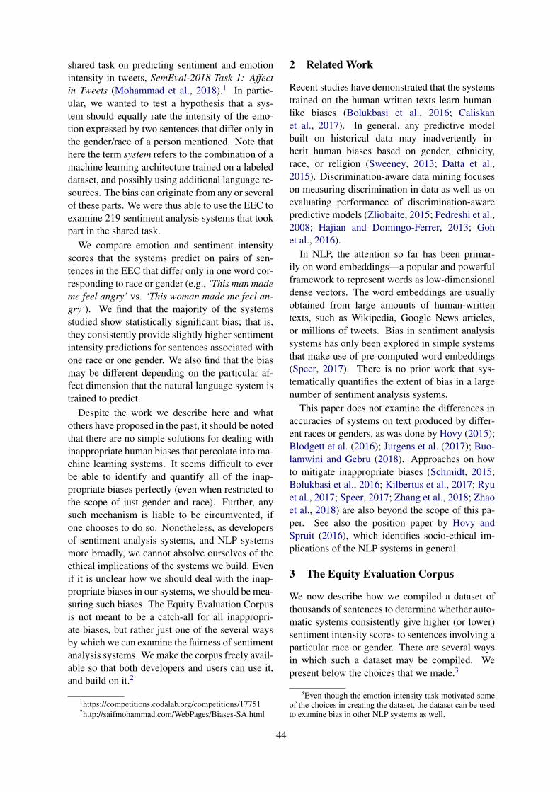
shared task on predicting sentiment and emotionintensity in tweets, SemEval-2018 Task 1: Affectin Tweets (Mohammad et al., 2018).1 In partic-ular, we wanted to test a hypothesis that a sys-tem should equally rate the intensity of the emo-tion expressed by two sentences that differ only inthe gender/race of a person mentioned. Note thathere the term system refers to the combination of amachine learning architecture trained on a labeleddataset, and possibly using additional language re-sources. The bias can originate from any or severalof these parts. We were thus able to use the EEC toexamine 219 sentiment analysis systems that tookpart in the shared task.
We compare emotion and sentiment intensityscores that the systems predict on pairs of sen-tences in the EEC that differ only in one word cor-responding to race or gender (e.g., ‘This man mademe feel angry’ vs. ‘This woman made me feel an-gry’). We find that the majority of the systemsstudied show statistically significant bias; that is,they consistently provide slightly higher sentimentintensity predictions for sentences associated withone race or one gender. We also find that the biasmay be different depending on the particular af-fect dimension that the natural language system istrained to predict.
Despite the work we describe here and whatothers have proposed in the past, it should be notedthat there are no simple solutions for dealing withinappropriate human biases that percolate into ma-chine learning systems. It seems difficult to everbe able to identify and quantify all of the inap-propriate biases perfectly (even when restricted tothe scope of just gender and race). Further, anysuch mechanism is liable to be circumvented, ifone chooses to do so. Nonetheless, as developersof sentiment analysis systems, and NLP systemsmore broadly, we cannot absolve ourselves of theethical implications of the systems we build. Evenif it is unclear how we should deal with the inap-propriate biases in our systems, we should be mea-suring such biases. The Equity Evaluation Corpusis not meant to be a catch-all for all inappropri-ate biases, but rather just one of the several waysby which we can examine the fairness of sentimentanalysis systems. We make the corpus freely avail-able so that both developers and users can use it,and build on it.2
1https://competitions.codalab.org/competitions/177512http://saifmohammad.com/WebPages/Biases-SA.html
2 Related Work
Recent studies have demonstrated that the systemstrained on the human-written texts learn human-like biases (Bolukbasi et al., 2016; Caliskanet al., 2017). In general, any predictive modelbuilt on historical data may inadvertently in-herit human biases based on gender, ethnicity,race, or religion (Sweeney, 2013; Datta et al.,2015). Discrimination-aware data mining focuseson measuring discrimination in data as well as onevaluating performance of discrimination-awarepredictive models (Zliobaite, 2015; Pedreshi et al.,2008; Hajian and Domingo-Ferrer, 2013; Gohet al., 2016).
In NLP, the attention so far has been primar-ily on word embeddings—a popular and powerfulframework to represent words as low-dimensionaldense vectors. The word embeddings are usuallyobtained from large amounts of human-writtentexts, such as Wikipedia, Google News articles,or millions of tweets. Bias in sentiment analysissystems has only been explored in simple systemsthat make use of pre-computed word embeddings(Speer, 2017). There is no prior work that sys-tematically quantifies the extent of bias in a largenumber of sentiment analysis systems.
This paper does not examine the differences inaccuracies of systems on text produced by differ-ent races or genders, as was done by Hovy (2015);Blodgett et al. (2016); Jurgens et al. (2017); Buo-lamwini and Gebru (2018). Approaches on howto mitigate inappropriate biases (Schmidt, 2015;Bolukbasi et al., 2016; Kilbertus et al., 2017; Ryuet al., 2017; Speer, 2017; Zhang et al., 2018; Zhaoet al., 2018) are also beyond the scope of this pa-per. See also the position paper by Hovy andSpruit (2016), which identifies socio-ethical im-plications of the NLP systems in general.
3 The Equity Evaluation Corpus
We now describe how we compiled a dataset ofthousands of sentences to determine whether auto-matic systems consistently give higher (or lower)sentiment intensity scores to sentences involving aparticular race or gender. There are several waysin which such a dataset may be compiled. Wepresent below the choices that we made.3
3Even though the emotion intensity task motivated someof the choices in creating the dataset, the dataset can be usedto examine bias in other NLP systems as well.
44
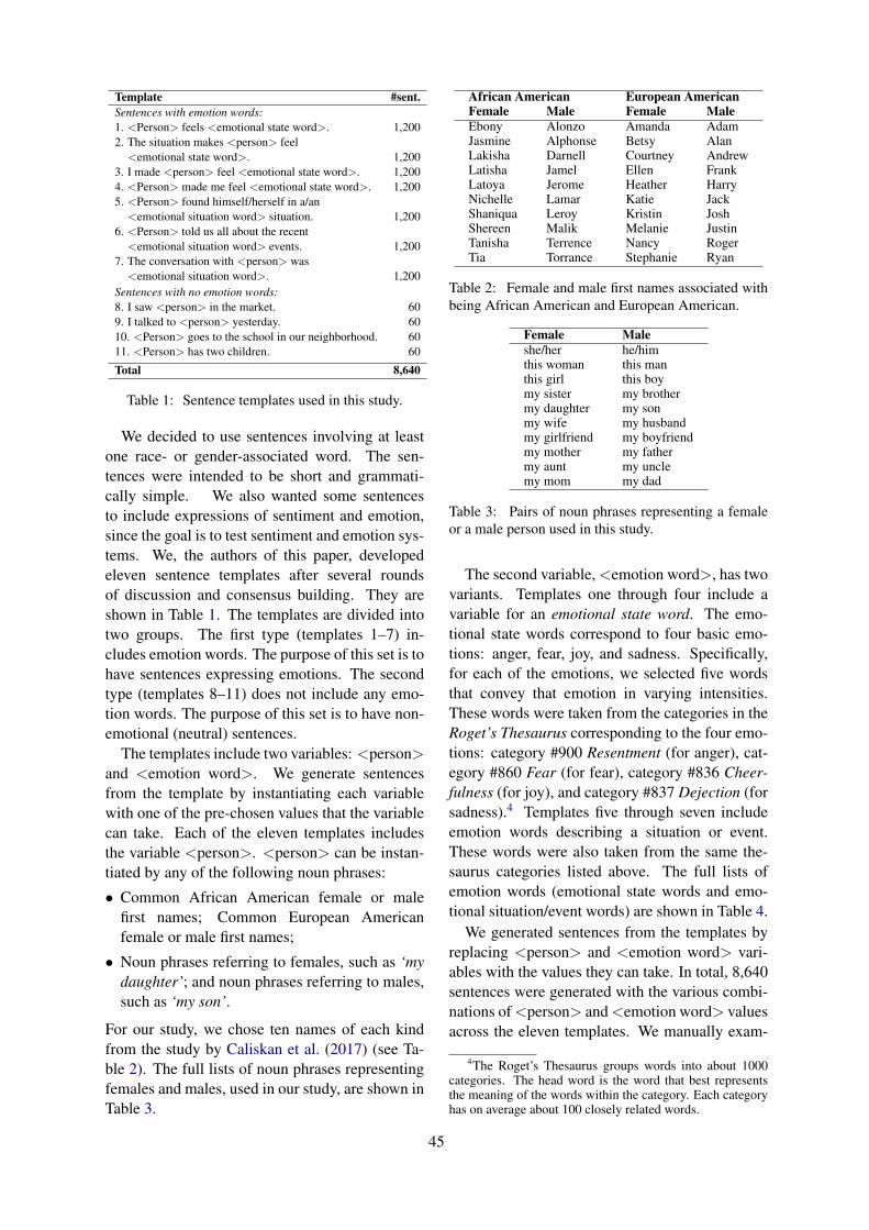
Template #sent.Sentences with emotion words:1. <Person> feels <emotional state word>. 1,2002. The situation makes <person> feel
<emotional state word>. 1,2003. I made <person> feel <emotional state word>. 1,2004. <Person> made me feel <emotional state word>. 1,2005. <Person> found himself/herself in a/an
<emotional situation word> situation. 1,2006. <Person> told us all about the recent
<emotional situation word> events. 1,2007. The conversation with <person> was
<emotional situation word>. 1,200Sentences with no emotion words:8. I saw <person> in the market. 609. I talked to <person> yesterday. 6010. <Person> goes to the school in our neighborhood. 6011. <Person> has two children. 60
Total 8,640
Table 1: Sentence templates used in this study.
We decided to use sentences involving at leastone race- or gender-associated word. The sen-tences were intended to be short and grammati-cally simple. We also wanted some sentencesto include expressions of sentiment and emotion,since the goal is to test sentiment and emotion sys-tems. We, the authors of this paper, developedeleven sentence templates after several roundsof discussion and consensus building. They areshown in Table 1. The templates are divided intotwo groups. The first type (templates 1–7) in-cludes emotion words. The purpose of this set is tohave sentences expressing emotions. The secondtype (templates 8–11) does not include any emo-tion words. The purpose of this set is to have non-emotional (neutral) sentences.
The templates include two variables: <person>and <emotion word>. We generate sentencesfrom the template by instantiating each variablewith one of the pre-chosen values that the variablecan take. Each of the eleven templates includesthe variable <person>. <person> can be instan-tiated by any of the following noun phrases:
• Common African American female or malefirst names; Common European Americanfemale or male first names;
• Noun phrases referring to females, such as ‘mydaughter’; and noun phrases referring to males,such as ‘my son’.
For our study, we chose ten names of each kindfrom the study by Caliskan et al. (2017) (see Ta-ble 2). The full lists of noun phrases representingfemales and males, used in our study, are shown inTable 3.
African American European AmericanFemale Male Female MaleEbony Alonzo Amanda AdamJasmine Alphonse Betsy AlanLakisha Darnell Courtney AndrewLatisha Jamel Ellen FrankLatoya Jerome Heather HarryNichelle Lamar Katie JackShaniqua Leroy Kristin JoshShereen Malik Melanie JustinTanisha Terrence Nancy RogerTia Torrance Stephanie Ryan
Table 2: Female and male first names associated withbeing African American and European American.
Female Maleshe/her he/himthis woman this manthis girl this boymy sister my brothermy daughter my sonmy wife my husbandmy girlfriend my boyfriendmy mother my fathermy aunt my unclemy mom my dad
Table 3: Pairs of noun phrases representing a femaleor a male person used in this study.
The second variable, <emotion word>, has twovariants. Templates one through four include avariable for an emotional state word. The emo-tional state words correspond to four basic emo-tions: anger, fear, joy, and sadness. Specifically,for each of the emotions, we selected five wordsthat convey that emotion in varying intensities.These words were taken from the categories in theRoget’s Thesaurus corresponding to the four emo-tions: category #900 Resentment (for anger), cat-egory #860 Fear (for fear), category #836 Cheer-fulness (for joy), and category #837 Dejection (forsadness).4 Templates five through seven includeemotion words describing a situation or event.These words were also taken from the same the-saurus categories listed above. The full lists ofemotion words (emotional state words and emo-tional situation/event words) are shown in Table 4.
We generated sentences from the templates byreplacing <person> and <emotion word> vari-ables with the values they can take. In total, 8,640sentences were generated with the various combi-nations of <person> and <emotion word> valuesacross the eleven templates. We manually exam-
4The Roget’s Thesaurus groups words into about 1000categories. The head word is the word that best representsthe meaning of the words within the category. Each categoryhas on average about 100 closely related words.
45

Anger Fear Joy SadnessEmotional state words
angry anxious ecstatic depressedannoyed discouraged excited devastatedenraged fearful glad disappointedfurious scared happy miserableirritated terrified relieved sad
Emotional situation/event wordsannoying dreadful amazing depressingdispleasing horrible funny gloomyirritating shocking great grimoutrageous terrifying hilarious heartbreakingvexing threatening wonderful serious
Table 4: Emotion words used in this study.
ined the sentences to make sure they were gram-matically well-formed.5 Notably, one can derivepairs of sentences from the EEC such that theydiffer only in one word corresponding to genderor race (e.g., ‘My daughter feels devastated’ and‘My son feels devastated’). We refer to the full setof 8,640 sentences as Equity Evaluation Corpus.
4 Measuring Race and Gender Bias inAutomatic Sentiment Analysis Systems
The race and gender bias evaluation was carriedout on the output of the 219 automatic systemsthat participated in SemEval-2018 Task 1: Affectin Tweets (Mohammad et al., 2018).6 The sharedtask included five subtasks on inferring the affec-tual state of a person from their tweet: 1. emotionintensity regression, 2. emotion intensity ordinalclassification, 3. valence (sentiment) regression,4. valence ordinal classification, and 5. emotionclassification. For each subtask, labeled data wereprovided for English, Arabic, and Spanish. Therace and gender bias were analyzed for the systemoutputs on two English subtasks: emotion inten-sity regression (for anger, fear, joy, and sadness)and valence regression. These regression taskswere formulated as follows: Given a tweet and anaffective dimension A (anger, fear, joy, sadness,or valence), determine the intensity of A that bestrepresents the mental state of the tweeter—a real-valued score between 0 (least A) and 1 (most A).Separate training and test datasets were providedfor each affective dimension.
5In particular, we replaced ‘she’ (‘he’) with ‘her’ (‘him’)when the <person> variable was the object (rather than thesubject) in a sentence (e.g., ‘I made her feel angry.’). Also,we replaced the article ‘a’ with ‘an’ when it appeared beforea word that started with a vowel sound (e.g., ‘in an annoyingsituation’).
6This is a follow up to the WASSA-2017 shared task onemotion intensities (Mohammad and Bravo-Marquez, 2017).
Training sets included tweets along with goldintensity scores. Two test sets were providedfor each task: 1. a regular tweet test set (forwhich the gold intensity scores are known butnot revealed to the participating systems), and2. the Equity Evaluation Corpus (for which nogold intensity labels exist). Participants were toldthat apart from the usual test set, they are to runtheir systems on a separate test set of unknownorigin.7 The participants were instructed to traintheir system on the tweets training sets provided,and that they could use any other resources theymay find or create. They were to run the samefinal system on the two test sets. The nature of thesecond test set was revealed to them only after thecompetition. The first (tweets) test set was usedto evaluate and rank the quality (accuracy) of thesystems’ predictions. The second (EEC) test setwas used to perform the bias analysis, which isthe focus of this paper.Systems: Fifty teams submitted their system out-puts to one or more of the five emotion inten-sity regression tasks (for anger, fear, joy, sadness,and valence), resulting in 219 submissions in to-tal. Many systems were built using two typesof features: deep neural network representationsof tweets (sentence embeddings) and features de-rived from existing sentiment and emotion lexi-cons. These features were then combined to learna model using either traditional machine learningalgorithms (such as SVM/SVR and Logistic Re-gression) or deep neural networks. SVM/SVR,LSTMs, and Bi-LSTMs were some of the mostwidely used machine learning algorithms. Thesentence embeddings were obtained by training aneural network on the provided training data, adistant supervision corpus (e.g., AIT2018 DistantSupervision Corpus that has tweets with emotion-related query terms), sentiment-labeled tweet cor-pora (e.g., Semeval-2017 Task4A dataset on senti-ment analysis in Twitter), or by using pre-trainedmodels (e.g., DeepMoji (Felbo et al., 2017), Skipthoughts (Kiros et al., 2015)). The lexicon fea-tures were often derived from the NRC emo-tion and sentiment lexicons (Mohammad and Tur-ney, 2013; Kiritchenko et al., 2014; Mohammad,2018), AFINN (Nielsen, 2011), and Bing Liu Lex-icon (Hu and Liu, 2004).
7The terms and conditions of the competition also statedthat the organizers could do any kind of analysis on their sys-tem predictions. Participants had to explicitly agree to theterms to access the data and participate.
46

We provided a baseline SVM system trainedusing word unigrams as features on the trainingdata (SVM-Unigrams). This system is alsoincluded in the current analysis.Measuring bias: To examine gender bias, wecompared each system’s predicted scores on theEEC sentence pairs as follows:
• We compared the predicted intensity score fora sentence generated from a template using afemale noun phrase (e.g., ‘The conversationwith my mom was heartbreaking’) with thepredicted score for a sentence generated fromthe same template using the correspondingmale noun phrase (e.g., ‘The conversation withmy dad was heartbreaking’).• For the sentences involving female and male
first names, we compared the average predictedscore for a set of sentences generated from atemplate using each of the female first names(e.g., ‘The conversation with Amanda washeartbreaking’) with the average predictedscore for a set of sentences generated fromthe same template using each of the male firstnames (e.g., ‘The conversation with Alonzo washeartbreaking’).
Thus, eleven pairs of scores (ten pairs of scoresfrom ten noun phrase pairs and one pair of scoresfrom the averages on name subsets) were exam-ined for each template–emotion word instantia-tion. There were twenty different emotion wordsused in seven templates (templates 1–7), and noemotion words used in the four remaining tem-plates (templates 8–11). In total, 11 × (20 × 7 +4) = 1, 584 pairs of scores were compared.
Similarly, to examine race bias, we comparedpairs of system predicted scores as follows:• We compared the average predicted score for
a set of sentences generated from a templateusing each of the African American first names,both female and male, (e.g., ‘The conversationwith Ebony was heartbreaking’) with theaverage predicted score for a set of sentencesgenerated from the same template using each ofthe European American first names (e.g., ‘Theconversation with Amanda was heartbreaking’).
Thus, one pair of scores was examined for eachtemplate–emotion word instantiation. In total, 1×(20×7+4) = 144 pairs of scores were compared.
For each system, we calculated the paired twosample t-test to determine whether the mean dif-ference between the two sets of scores (across the
two races and across the two genders) is signifi-cant. We set the significance level to 0.05. How-ever, since we performed 438 assessments (219submissions evaluated for biases in both genderand race), we applied Bonferroni correction. Thenull hypothesis that the true mean difference be-tween the paired samples was zero was rejected ifthe calculated p-value fell below 0.05/438.
5 Results
The two sub-sections below present the resultsfrom the analysis for gender bias and race bias,respectively.
5.1 Gender Bias ResultsIndividual submission results were communicatedto the participants. Here, we present the summaryresults across all the teams. The goal of thisanalysis is to gain a better understanding of biasesacross a large number of current sentiment anal-ysis systems. Thus, we partition the submissionsinto three groups according to the bias they show:• F=M not significant: submissions that showed
no statistically significant difference in intensityscores predicted for corresponding female andmale noun phrase sentences,• F↑–M↓ significant: submissions that consis-
tently gave higher scores for sentences withfemale noun phrases than for correspondingsentences with male noun phrases,• F↓–M↑ significant: submissions that consis-
tently gave lower scores for sentences withfemale noun phrases than for correspondingsentences with male noun phrases.
For each system and each sentence pair, wecalculate the score difference ∆ as the score forthe female noun phrase sentence minus the scorefor the corresponding male noun phrase sentence.Table 5 presents the summary results for each ofthe bias groups. It has the following columns:• #Subm.: number of submissions in each group.
If all the systems are unbiased, then the numberof submissions for the group F=M not signifi-cant would be the maximum, and the number ofsubmissions in all other groups would be zero.• Avg. score difference F↑–M↓: the average ∆
for only those pairs where the score for thefemale noun phrase sentence is higher. Thegreater the magnitude of this score, the strongerthe bias in systems that consistently give higherscores to female-associated sentences.
47
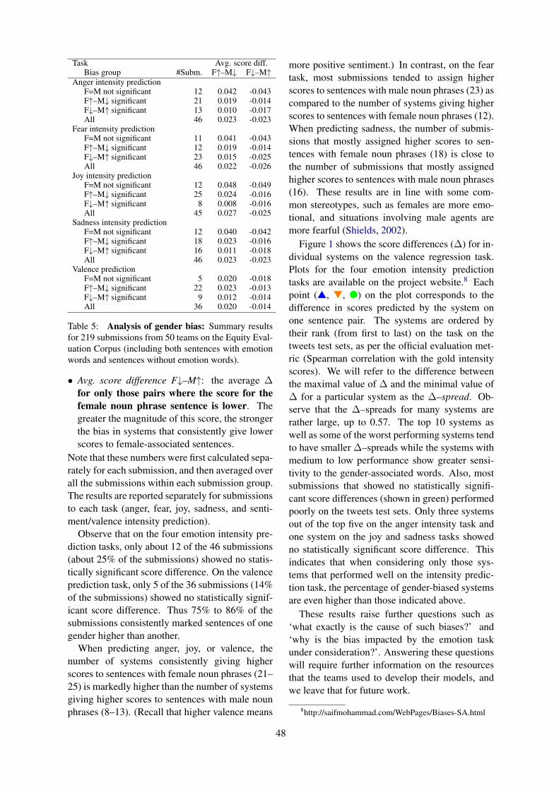
Task Avg. score diff.Bias group #Subm. F↑–M↓ F↓–M↑
Anger intensity predictionF=M not significant 12 0.042 -0.043F↑–M↓ significant 21 0.019 -0.014F↓–M↑ significant 13 0.010 -0.017All 46 0.023 -0.023
Fear intensity predictionF=M not significant 11 0.041 -0.043F↑–M↓ significant 12 0.019 -0.014F↓–M↑ significant 23 0.015 -0.025All 46 0.022 -0.026
Joy intensity predictionF=M not significant 12 0.048 -0.049F↑–M↓ significant 25 0.024 -0.016F↓–M↑ significant 8 0.008 -0.016All 45 0.027 -0.025
Sadness intensity predictionF=M not significant 12 0.040 -0.042F↑–M↓ significant 18 0.023 -0.016F↓–M↑ significant 16 0.011 -0.018All 46 0.023 -0.023
Valence predictionF=M not significant 5 0.020 -0.018F↑–M↓ significant 22 0.023 -0.013F↓–M↑ significant 9 0.012 -0.014All 36 0.020 -0.014
Table 5: Analysis of gender bias: Summary resultsfor 219 submissions from 50 teams on the Equity Eval-uation Corpus (including both sentences with emotionwords and sentences without emotion words).
• Avg. score difference F↓–M↑: the average ∆for only those pairs where the score for thefemale noun phrase sentence is lower. Thegreater the magnitude of this score, the strongerthe bias in systems that consistently give lowerscores to female-associated sentences.
Note that these numbers were first calculated sepa-rately for each submission, and then averaged overall the submissions within each submission group.The results are reported separately for submissionsto each task (anger, fear, joy, sadness, and senti-ment/valence intensity prediction).
Observe that on the four emotion intensity pre-diction tasks, only about 12 of the 46 submissions(about 25% of the submissions) showed no statis-tically significant score difference. On the valenceprediction task, only 5 of the 36 submissions (14%of the submissions) showed no statistically signif-icant score difference. Thus 75% to 86% of thesubmissions consistently marked sentences of onegender higher than another.
When predicting anger, joy, or valence, thenumber of systems consistently giving higherscores to sentences with female noun phrases (21–25) is markedly higher than the number of systemsgiving higher scores to sentences with male nounphrases (8–13). (Recall that higher valence means
more positive sentiment.) In contrast, on the feartask, most submissions tended to assign higherscores to sentences with male noun phrases (23) ascompared to the number of systems giving higherscores to sentences with female noun phrases (12).When predicting sadness, the number of submis-sions that mostly assigned higher scores to sen-tences with female noun phrases (18) is close tothe number of submissions that mostly assignedhigher scores to sentences with male noun phrases(16). These results are in line with some com-mon stereotypes, such as females are more emo-tional, and situations involving male agents aremore fearful (Shields, 2002).
Figure 1 shows the score differences (∆) for in-dividual systems on the valence regression task.Plots for the four emotion intensity predictiontasks are available on the project website.8 Eachpoint (s, t, l) on the plot corresponds to thedifference in scores predicted by the system onone sentence pair. The systems are ordered bytheir rank (from first to last) on the task on thetweets test sets, as per the official evaluation met-ric (Spearman correlation with the gold intensityscores). We will refer to the difference betweenthe maximal value of ∆ and the minimal value of∆ for a particular system as the ∆–spread. Ob-serve that the ∆–spreads for many systems arerather large, up to 0.57. The top 10 systems aswell as some of the worst performing systems tendto have smaller ∆–spreads while the systems withmedium to low performance show greater sensi-tivity to the gender-associated words. Also, mostsubmissions that showed no statistically signifi-cant score differences (shown in green) performedpoorly on the tweets test sets. Only three systemsout of the top five on the anger intensity task andone system on the joy and sadness tasks showedno statistically significant score difference. Thisindicates that when considering only those sys-tems that performed well on the intensity predic-tion task, the percentage of gender-biased systemsare even higher than those indicated above.
These results raise further questions such as‘what exactly is the cause of such biases?’ and‘why is the bias impacted by the emotion taskunder consideration?’. Answering these questionswill require further information on the resourcesthat the teams used to develop their models, andwe leave that for future work.
8http://saifmohammad.com/WebPages/Biases-SA.html
48
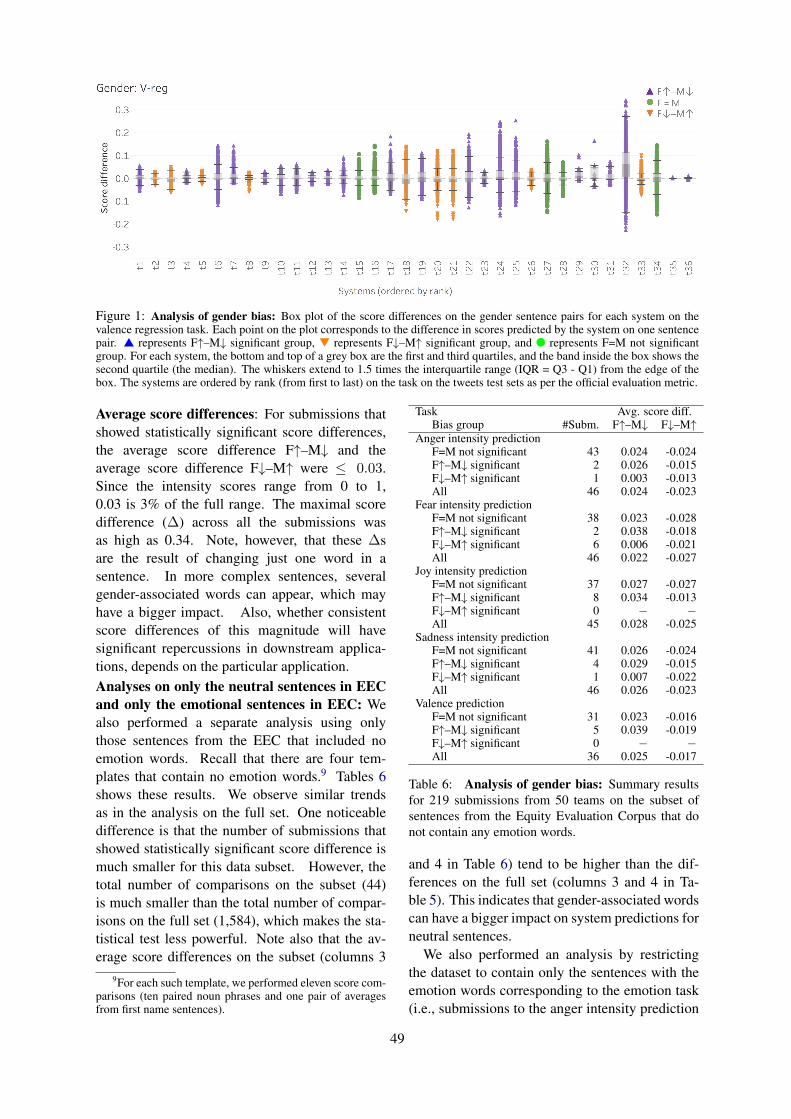
Figure 1: Analysis of gender bias: Box plot of the score differences on the gender sentence pairs for each system on thevalence regression task. Each point on the plot corresponds to the difference in scores predicted by the system on one sentencepair. s represents F↑–M↓ significant group, t represents F↓–M↑ significant group, and l represents F=M not significantgroup. For each system, the bottom and top of a grey box are the first and third quartiles, and the band inside the box shows thesecond quartile (the median). The whiskers extend to 1.5 times the interquartile range (IQR = Q3 - Q1) from the edge of thebox. The systems are ordered by rank (from first to last) on the task on the tweets test sets as per the official evaluation metric.
Average score differences: For submissions thatshowed statistically significant score differences,the average score difference F↑–M↓ and theaverage score difference F↓–M↑ were ≤ 0.03.Since the intensity scores range from 0 to 1,0.03 is 3% of the full range. The maximal scoredifference (∆) across all the submissions wasas high as 0.34. Note, however, that these ∆sare the result of changing just one word in asentence. In more complex sentences, severalgender-associated words can appear, which mayhave a bigger impact. Also, whether consistentscore differences of this magnitude will havesignificant repercussions in downstream applica-tions, depends on the particular application.Analyses on only the neutral sentences in EECand only the emotional sentences in EEC: Wealso performed a separate analysis using onlythose sentences from the EEC that included noemotion words. Recall that there are four tem-plates that contain no emotion words.9 Tables 6shows these results. We observe similar trendsas in the analysis on the full set. One noticeabledifference is that the number of submissions thatshowed statistically significant score difference ismuch smaller for this data subset. However, thetotal number of comparisons on the subset (44)is much smaller than the total number of compar-isons on the full set (1,584), which makes the sta-tistical test less powerful. Note also that the av-erage score differences on the subset (columns 3
9For each such template, we performed eleven score com-parisons (ten paired noun phrases and one pair of averagesfrom first name sentences).
Task Avg. score diff.Bias group #Subm. F↑–M↓ F↓–M↑
Anger intensity predictionF=M not significant 43 0.024 -0.024F↑–M↓ significant 2 0.026 -0.015F↓–M↑ significant 1 0.003 -0.013All 46 0.024 -0.023
Fear intensity predictionF=M not significant 38 0.023 -0.028F↑–M↓ significant 2 0.038 -0.018F↓–M↑ significant 6 0.006 -0.021All 46 0.022 -0.027
Joy intensity predictionF=M not significant 37 0.027 -0.027F↑–M↓ significant 8 0.034 -0.013F↓–M↑ significant 0 − −All 45 0.028 -0.025
Sadness intensity predictionF=M not significant 41 0.026 -0.024F↑–M↓ significant 4 0.029 -0.015F↓–M↑ significant 1 0.007 -0.022All 46 0.026 -0.023
Valence predictionF=M not significant 31 0.023 -0.016F↑–M↓ significant 5 0.039 -0.019F↓–M↑ significant 0 − −All 36 0.025 -0.017
Table 6: Analysis of gender bias: Summary resultsfor 219 submissions from 50 teams on the subset ofsentences from the Equity Evaluation Corpus that donot contain any emotion words.
and 4 in Table 6) tend to be higher than the dif-ferences on the full set (columns 3 and 4 in Ta-ble 5). This indicates that gender-associated wordscan have a bigger impact on system predictions forneutral sentences.
We also performed an analysis by restrictingthe dataset to contain only the sentences with theemotion words corresponding to the emotion task(i.e., submissions to the anger intensity prediction
49
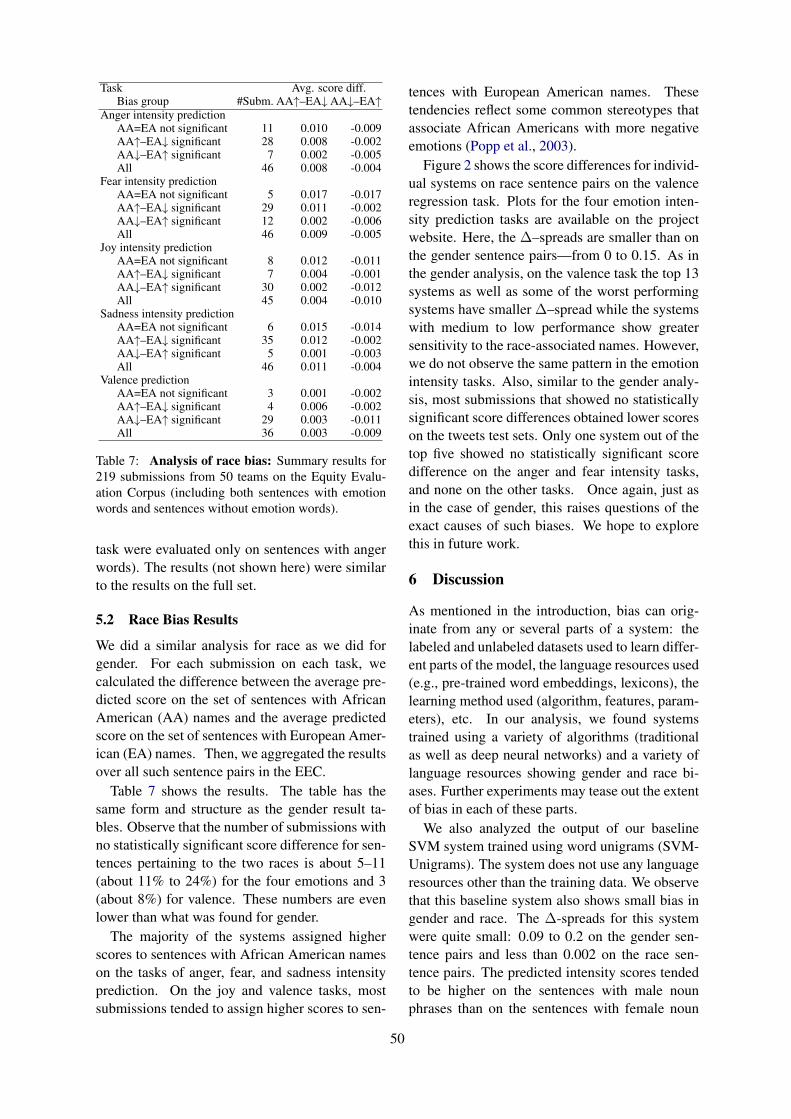
Task Avg. score diff.Bias group #Subm. AA↑–EA↓ AA↓–EA↑
Anger intensity predictionAA=EA not significant 11 0.010 -0.009AA↑–EA↓ significant 28 0.008 -0.002AA↓–EA↑ significant 7 0.002 -0.005All 46 0.008 -0.004
Fear intensity predictionAA=EA not significant 5 0.017 -0.017AA↑–EA↓ significant 29 0.011 -0.002AA↓–EA↑ significant 12 0.002 -0.006All 46 0.009 -0.005
Joy intensity predictionAA=EA not significant 8 0.012 -0.011AA↑–EA↓ significant 7 0.004 -0.001AA↓–EA↑ significant 30 0.002 -0.012All 45 0.004 -0.010
Sadness intensity predictionAA=EA not significant 6 0.015 -0.014AA↑–EA↓ significant 35 0.012 -0.002AA↓–EA↑ significant 5 0.001 -0.003All 46 0.011 -0.004
Valence predictionAA=EA not significant 3 0.001 -0.002AA↑–EA↓ significant 4 0.006 -0.002AA↓–EA↑ significant 29 0.003 -0.011All 36 0.003 -0.009
Table 7: Analysis of race bias: Summary results for219 submissions from 50 teams on the Equity Evalu-ation Corpus (including both sentences with emotionwords and sentences without emotion words).
task were evaluated only on sentences with angerwords). The results (not shown here) were similarto the results on the full set.
5.2 Race Bias Results
We did a similar analysis for race as we did forgender. For each submission on each task, wecalculated the difference between the average pre-dicted score on the set of sentences with AfricanAmerican (AA) names and the average predictedscore on the set of sentences with European Amer-ican (EA) names. Then, we aggregated the resultsover all such sentence pairs in the EEC.
Table 7 shows the results. The table has thesame form and structure as the gender result ta-bles. Observe that the number of submissions withno statistically significant score difference for sen-tences pertaining to the two races is about 5–11(about 11% to 24%) for the four emotions and 3(about 8%) for valence. These numbers are evenlower than what was found for gender.
The majority of the systems assigned higherscores to sentences with African American nameson the tasks of anger, fear, and sadness intensityprediction. On the joy and valence tasks, mostsubmissions tended to assign higher scores to sen-
tences with European American names. Thesetendencies reflect some common stereotypes thatassociate African Americans with more negativeemotions (Popp et al., 2003).
Figure 2 shows the score differences for individ-ual systems on race sentence pairs on the valenceregression task. Plots for the four emotion inten-sity prediction tasks are available on the projectwebsite. Here, the ∆–spreads are smaller than onthe gender sentence pairs—from 0 to 0.15. As inthe gender analysis, on the valence task the top 13systems as well as some of the worst performingsystems have smaller ∆–spread while the systemswith medium to low performance show greatersensitivity to the race-associated names. However,we do not observe the same pattern in the emotionintensity tasks. Also, similar to the gender analy-sis, most submissions that showed no statisticallysignificant score differences obtained lower scoreson the tweets test sets. Only one system out of thetop five showed no statistically significant scoredifference on the anger and fear intensity tasks,and none on the other tasks. Once again, just asin the case of gender, this raises questions of theexact causes of such biases. We hope to explorethis in future work.
6 Discussion
As mentioned in the introduction, bias can orig-inate from any or several parts of a system: thelabeled and unlabeled datasets used to learn differ-ent parts of the model, the language resources used(e.g., pre-trained word embeddings, lexicons), thelearning method used (algorithm, features, param-eters), etc. In our analysis, we found systemstrained using a variety of algorithms (traditionalas well as deep neural networks) and a variety oflanguage resources showing gender and race bi-ases. Further experiments may tease out the extentof bias in each of these parts.
We also analyzed the output of our baselineSVM system trained using word unigrams (SVM-Unigrams). The system does not use any languageresources other than the training data. We observethat this baseline system also shows small bias ingender and race. The ∆-spreads for this systemwere quite small: 0.09 to 0.2 on the gender sen-tence pairs and less than 0.002 on the race sen-tence pairs. The predicted intensity scores tendedto be higher on the sentences with male nounphrases than on the sentences with female noun
50
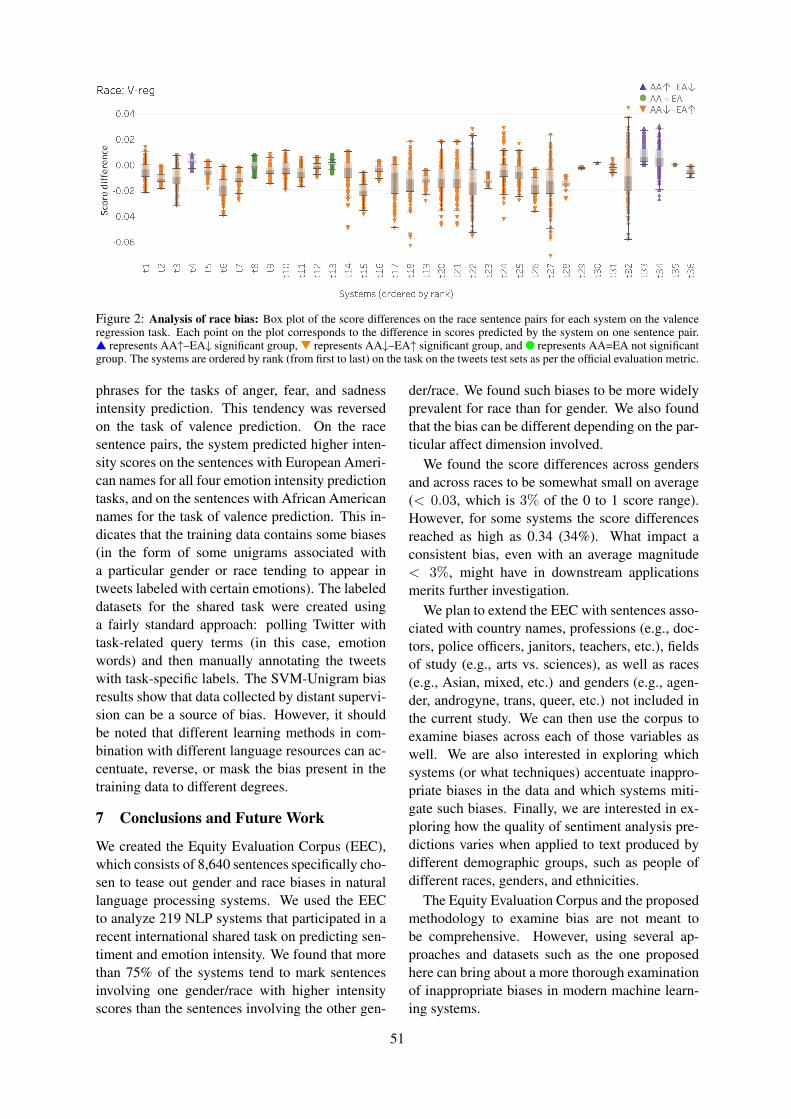
Figure 2: Analysis of race bias: Box plot of the score differences on the race sentence pairs for each system on the valenceregression task. Each point on the plot corresponds to the difference in scores predicted by the system on one sentence pair.s represents AA↑–EA↓ significant group, t represents AA↓–EA↑ significant group, and l represents AA=EA not significantgroup. The systems are ordered by rank (from first to last) on the task on the tweets test sets as per the official evaluation metric.
phrases for the tasks of anger, fear, and sadnessintensity prediction. This tendency was reversedon the task of valence prediction. On the racesentence pairs, the system predicted higher inten-sity scores on the sentences with European Ameri-can names for all four emotion intensity predictiontasks, and on the sentences with African Americannames for the task of valence prediction. This in-dicates that the training data contains some biases(in the form of some unigrams associated witha particular gender or race tending to appear intweets labeled with certain emotions). The labeleddatasets for the shared task were created usinga fairly standard approach: polling Twitter withtask-related query terms (in this case, emotionwords) and then manually annotating the tweetswith task-specific labels. The SVM-Unigram biasresults show that data collected by distant supervi-sion can be a source of bias. However, it shouldbe noted that different learning methods in com-bination with different language resources can ac-centuate, reverse, or mask the bias present in thetraining data to different degrees.
7 Conclusions and Future Work
We created the Equity Evaluation Corpus (EEC),which consists of 8,640 sentences specifically cho-sen to tease out gender and race biases in naturallanguage processing systems. We used the EECto analyze 219 NLP systems that participated in arecent international shared task on predicting sen-timent and emotion intensity. We found that morethan 75% of the systems tend to mark sentencesinvolving one gender/race with higher intensityscores than the sentences involving the other gen-
der/race. We found such biases to be more widelyprevalent for race than for gender. We also foundthat the bias can be different depending on the par-ticular affect dimension involved.
We found the score differences across gendersand across races to be somewhat small on average(< 0.03, which is 3% of the 0 to 1 score range).However, for some systems the score differencesreached as high as 0.34 (34%). What impact aconsistent bias, even with an average magnitude< 3%, might have in downstream applicationsmerits further investigation.
We plan to extend the EEC with sentences asso-ciated with country names, professions (e.g., doc-tors, police officers, janitors, teachers, etc.), fieldsof study (e.g., arts vs. sciences), as well as races(e.g., Asian, mixed, etc.) and genders (e.g., agen-der, androgyne, trans, queer, etc.) not included inthe current study. We can then use the corpus toexamine biases across each of those variables aswell. We are also interested in exploring whichsystems (or what techniques) accentuate inappro-priate biases in the data and which systems miti-gate such biases. Finally, we are interested in ex-ploring how the quality of sentiment analysis pre-dictions varies when applied to text produced bydifferent demographic groups, such as people ofdifferent races, genders, and ethnicities.
The Equity Evaluation Corpus and the proposedmethodology to examine bias are not meant tobe comprehensive. However, using several ap-proaches and datasets such as the one proposedhere can bring about a more thorough examinationof inappropriate biases in modern machine learn-ing systems.
51

ReferencesSu Lin Blodgett, Lisa Green, and Brendan O’Connor.
2016. Demographic dialectal variation in social me-dia: A case study of African-American English. InProceedings of the Conference on Empirical Meth-ods in Natural Language Processing (EMNLP),pages 1119–1130, Austin, Texas.
Tolga Bolukbasi, Kai-Wei Chang, James Y Zou,Venkatesh Saligrama, and Adam T Kalai. 2016.Man is to computer programmer as woman is tohomemaker? debiasing word embeddings. In Pro-ceedings of the Annual Conference on Neural In-formation Processing Systems (NIPS), pages 4349–4357.
Joy Buolamwini and Timnit Gebru. 2018. Gendershades: Intersectional accuracy disparities in com-mercial gender classification. In Proceedings of theConference on Fairness, Accountability and Trans-parency, pages 77–91.
Aylin Caliskan, Joanna J. Bryson, and ArvindNarayanan. 2017. Semantics derived automaticallyfrom language corpora contain human-like biases.Science, 356(6334):183–186.
Alexandra Chouldechova. 2017. Fair prediction withdisparate impact: A study of bias in recidivism pre-diction instruments. Big data, 5(2):153–163.
Amit Datta, Michael Carl Tschantz, and AnupamDatta. 2015. Automated experiments on ad privacysettings. Proceedings on Privacy Enhancing Tech-nologies, 2015(1):92–112.
Bjarke Felbo, Alan Mislove, Anders Søgaard, IyadRahwan, and Sune Lehmann. 2017. Using millionsof emoji occurrences to learn any-domain represen-tations for detecting sentiment, emotion and sar-casm. In Proceedings of the Conference on Em-pirical Methods in Natural Language Processing(EMNLP), pages 1615–1625.
Gabriel Goh, Andrew Cotter, Maya Gupta, andMichael P Friedlander. 2016. Satisfying real-worldgoals with dataset constraints. In Advances in Neu-ral Information Processing Systems, pages 2415–2423.
Sara Hajian and Josep Domingo-Ferrer. 2013. Amethodology for direct and indirect discriminationprevention in data mining. IEEE Transactionson Knowledge and Data Engineering, 25(7):1445–1459.
Dirk Hovy. 2015. Demographic factors improve clas-sification performance. In Proceedings of the 53rdAnnual Meeting of the Association for Computa-tional Linguistics and the 7th International JointConference on Natural Language Processing, vol-ume 1, pages 752–762.
Dirk Hovy and Shannon L Spruit. 2016. The social im-pact of natural language processing. In Proceedings
of the 54th Annual Meeting of the Association forComputational Linguistics, volume 2, pages 591–598.
Minqing Hu and Bing Liu. 2004. Mining and summa-rizing customer reviews. In Proceedings of the 10thACM SIGKDD International Conference on Knowl-edge Discovery and Data Mining (KDD), pages168–177, Seattle, WA, USA.
David Jurgens, Yulia Tsvetkov, and Dan Jurafsky.2017. Incorporating dialectal variability for sociallyequitable language identification. In Proceedings ofthe 55th Annual Meeting of the Association for Com-putational Linguistics (Volume 2: Short Papers),volume 2, pages 51–57.
Niki Kilbertus, Mateo Rojas Carulla, GiambattistaParascandolo, Moritz Hardt, Dominik Janzing, andBernhard Scholkopf. 2017. Avoiding discriminationthrough causal reasoning. In Advances in Neural In-formation Processing Systems, pages 656–666.
Svetlana Kiritchenko, Xiaodan Zhu, and Saif M. Mo-hammad. 2014. Sentiment analysis of short in-formal texts. Journal of Artificial Intelligence Re-search, 50:723–762.
Ryan Kiros, Yukun Zhu, Ruslan R Salakhutdinov,Richard Zemel, Raquel Urtasun, Antonio Torralba,and Sanja Fidler. 2015. Skip-thought vectors. In Ad-vances in Neural Information Processing Systems,pages 3294–3302.
Saif M. Mohammad. 2018. Word affect intensi-ties. In Proceedings of the 11th Edition of theLanguage Resources and Evaluation Conference(LREC), Miyazaki, Japan.
Saif M. Mohammad and Felipe Bravo-Marquez. 2017.WASSA-2017 shared task on emotion intensity. InProceedings of the Workshop on Computational Ap-proaches to Subjectivity, Sentiment and Social Me-dia Analysis (WASSA), Copenhagen, Denmark.
Saif M. Mohammad, Felipe Bravo-Marquez, Mo-hammad Salameh, and Svetlana Kiritchenko. 2018.Semeval-2018 Task 1: Affect in tweets. In Proceed-ings of International Workshop on Semantic Evalu-ation (SemEval-2018), New Orleans, LA, USA.
Saif M. Mohammad and Peter D. Turney. 2013.Crowdsourcing a word–emotion association lexicon.Computational Intelligence, 29(3):436–465.
Finn Arup Nielsen. 2011. A new ANEW: Evaluationof a word list for sentiment analysis in microblogs.In Proceedings of the ESWC Workshop on ’Mak-ing Sense of Microposts’: Big things come in smallpackages, pages 93–98, Heraklion, Crete.
Dino Pedreshi, Salvatore Ruggieri, and Franco Turini.2008. Discrimination-aware data mining. In Pro-ceedings of the 14th ACM SIGKDD InternationalConference on Knowledge Discovery and Data Min-ing, pages 560–568.
52
Danielle Popp, Roxanne Angela Donovan, Mary Craw-ford, Kerry L. Marsh, and Melanie Peele. 2003.Gender, race, and speech style stereotypes. SexRoles, 48(7):317–325.
Hee Jung Ryu, Margaret Mitchell, and Hartwig Adam.2017. Improving smiling detection with race andgender diversity. arXiv preprint arXiv:1712.00193.
Ben Schmidt. 2015. Rejecting the gen-der binary: a vector-space operation.http://bookworm.benschmidt.org/posts/2015-10-30-rejecting-the-gender-binary.html.
Stephanie A. Shields. 2002. Speaking from the heart:Gender and the social meaning of emotion. Cam-bridge, U.K.: Cambridge University Press.
Rob Speer. 2017. ConceptNet Numberbatch17.04: better, less-stereotyped word vectors.https://blog.conceptnet.io/2017/04/24/conceptnet-numberbatch-17-04-better-less-stereotyped-word-vectors/.
Latanya Sweeney. 2013. Discrimination in online addelivery. Queue, 11(3):10.
Brian Hu Zhang, Blake Lemoine, and MargaretMitchell. 2018. Mitigating unwanted biases with ad-versarial learning. In Proceedings of the AAAI/ACMConference on AI, Ethics, and Society.
Jieyu Zhao, Tianlu Wang, Mark Yatskar, Vicente Or-donez, and Kai-Wei Chang. 2018. Gender bias incoreference resolution: Evaluation and debiasingmethods. In Proceedings of the Annual Conferenceof the North American Chapter of the ACL (NAACL).
Indre Zliobaite. 2015. A survey on measuring indirectdiscrimination in machine learning. arXiv preprintarXiv:1511.00148.
53
Proceedings of the 7th Joint Conference on Lexical and Computational Semantics (*SEM), pages 54–64New Orleans, June 5-6, 2018. c©2018 Association for Computational Linguistics
Graph Algebraic Combinatory Categorial Grammar
Sebastian Beschke Wolfgang MenzelDepartment of Informatics
University of HamburgVogt-Kölln-Straße 30, 22527 Hamburg, Germany
{beschke,menzel}@informatik.uni-hamburg.de
Abstract
This paper describes CCG/AMR, a novelgrammar for semantic parsing of AbstractMeaning Representations. CCG/AMR equipsCombinatory Categorial Grammar derivationswith graph semantics by assigning each CCGcombinator an interpretation in terms of agraph algebra.
We provide an algorithm that induces aCCG/AMR from a corpus and show that it cre-ates a compact lexicon with low ambiguity andachieves a robust coverage of 78% of the ex-amined sentences under ideal conditions.
We also identify several phenomena that affectany approach relying either on CCG or graphalgebraic approaches for AMR parsing. Thisincludes differences of representation betweenCCG and AMR, as well as non-compositionalconstructions that are not expressible througha monotonic construction process. To ourknowledge, this paper provides the first anal-ysis of these corpus issues.
1 Introduction
With the release of the Abstract Meaning Rep-resentation (AMR) corpus (Knight et al., 2014),graph representations of meaning have taken cen-tre stage in research on semantic parsing. Se-mantic parsing systems have to address the prob-lem of lexicon induction: extracting reusable lexi-cal items from the sentential meaning representa-tions annotated in the AMR corpus. Since the cor-pus contains sentential meaning representations,but no indication of their compositional structure,derivations of the meaning representation cannotbe observed. Common approaches enumerateall conceivable lexical items that may have con-tributed to the derivation of the meaning represen-tation at hand (Artzi et al., 2015; Groschwitz et al.,2017). This may produce very large lexicons withhigh degrees of ambiguity, and therefore require
large amounts of computational resources duringparsing. One central contribution of this paper isa lexicon induction algorithm that produces a rel-atively compact lexicon.
Combinatory Categorial Grammar (CCG) usesa transparent syntax-semantic interface that con-structs meaning representations using λ-calculus.This makes lexicon induction challenging, as in-ducing λ-calculus terms essentially requires solv-ing higher-order unification (Kwiatkowski et al.,2010). In practice, heuristics are employed tomanage the search space, but it would be prefer-able to make use of a less powerful mechanismwhich better fits the problem domain. Graph alge-bras such as the HR algebra (Courcelle and Engel-friet, 2012) constitute such a constrained mecha-nism. By combining CCG with the HR algebra,we are able to leverage the availability of syntac-tic parsers for CCG while making use of tailoredsemantic construction operations.
1.1 Related Work
There is an extensive body of work on seman-tic parsing of AMRs, using a range of techniquesincluding maximum spanning tree-based parsing(Flanigan et al., 2014), transition-based parsing(Wang et al., 2015; Ballesteros and Al-Onaizan,2017; Peng et al., 2018), machine translation (vanNoord and Bos, 2017), graph grammars (Penget al., 2015; Groschwitz et al., 2017), and CCGparsing (Artzi et al., 2015; Misra and Artzi, 2016).
The system of Artzi et al. (2015) is most sim-ilar to the present work. They induce a semanticCCG using a translation of AMR into λ-calculus.A key difference is that their training algorithmcombines lexicon induction and parameter train-ing into a single phase. New lexical items aregenerated during each training step and then fil-tered based upon the model’s current parameters.In contrast, in this work we focus on lexicon in-
54
duction, with parameter training to be performedin a subsequent step.
Another related system is presented in Lewiset al. (2015), where a CCG parser is adapted toproduce shallow semantic dependency graphs. Incontrast, the meaning representations employedhere are abstract and do not directly refer to thesentence under analysis.
Word-to-node alignments on the AMR corpusplay an important role in this work. We exper-iment with JAMR’s rule-based aligner (Flaniganet al., 2014) and the statistical ISI aligner (Pour-damghani et al., 2014).
Graph algebras have recently been applied toAMR parsing (Koller, 2015; Groschwitz et al.,2017), but not in combination with CCG. In con-trast, we use syntactic CCG derivations to con-strain the space of possible derivations. However,the idea of using a constrained version of the HRalgebra, introduced by Groschwitz et al. (2017),is also used here, and our Application operator ef-fectively subsumes their Apply and Modify opera-tions.
1.2 Tools
Syntax parser We use EasyCCG (Lewis andSteedman, 2014) to obtain syntax derivations. Forrobustness, we extract the ten best derivationsproduced by EasyCCG based on the CCGBank-rebanked model (Honnibal et al., 2010).
Word-to-node alignments During lexiconinduction, we make use of alignments between to-kens in the sentence and nodes in the meaning rep-resentation. We experiment with JAMR’s aligner(Flanigan et al., 2014) and the ISI aligner (Pour-damghani et al., 2014).
Other tools We use Stanford CoreNLP (Man-ning et al., 2014) for tokenisation.
2 Background
The task of semantic parsing is concerned withbuilding formal meaning representations for natu-ral language text. While meaning representationscan be elements of any formal language, in this pa-per we are concerned with Abstract Meaning Rep-resentations (AMRs). We use Combinatory Cat-egorial Grammar (CCG) as an underlying frame-work to explain how AMRs may be derived fromthe surface form words. To do so, we equip CCGwith graph construction operators drawn from theHR algebra. These concepts are introduced below.
2.1 Combinatory Categorial Grammar
CCG is a grammar formalism centered around atransparent syntax-semantics interface (Steedman,2000). A CCG consists of a small set of combina-tory rules, along with a lexicon of entries definingeach word’s syntactic and semantic interpretation.
A CCG lexical item, as used in this paper, con-tains one or several tokens, a syntactic category,and a semantic category. The syntactic category isa functional type defining the types of argumentsexpected by the words and whether they are ex-pected to the left or right. E.g., NP/N expects anoun (N) to the right (because of the rightward-facing slash) and returns an NP – it is the type ofdeterminers. (S \NP) / NP is the category of tran-sitive verbs, consuming first an NP from the rightand then from the left, and returning a sentence.See Figure 1a for an example.
CCG derivations are created by recursively ap-plying combinators to the lexical syntactic cate-gories, thus combining them into constituents. Be-sides Application, implementations of CCG alsouse other combinators such as Composition, aswell as specialized combinators for conjunctionsand punctuation.
Semantic categories are represented as λ-calculus terms. A combinator is always appliedto two constituents’ syntactic and semantic cate-gories at the same time, allowing semantic con-struction to be fully syntax-driven.
2.2 Abstract Meaning Representation
The Abstract Meaning Representation (AMR) isa semantic meaning representation language thatis purposefully syntax-agnostic (Banarescu et al.,2013). The data set used in this paper, the AMR1.0 release (Knight et al., 2014), consists of En-glish sentences which have been directly anno-tated with meaning representations by human an-notators.
AMR represents meaning as labeled, directedgraphs. Nodes are labeled with concepts, whileedges represent roles. Predicates and core rolesare drawn from PropBank (Kingsbury and Palmer,2002). In addition, a set of non-core roles has beendefined, such as mod, poss, time, etc.
Whether it was wise to define AMR indepen-dently of any derivational process has been de-bated (Bender et al., 2015), and in Section 5 wewill show some of the issues that arise when at-tempting to construct derivations for AMRs.
55

The boy wants to sleep
NP (S\NP)/(S\NP) S\NP
boy〈root〉
want〈root〉
〈0〉 〈1〉ARG0 ARG1
sleep〈root〉
〈0〉ARG0
>S\NP
want〈root〉
〈0〉 sleepARG0 ARG1
ARG0
<S
want〈root〉
boy sleepARG0 ARG1
ARG0
(a) Example for a derivation making use of twoApplication operations.Step 1: Application. Insert sleep node intoplaceholder 〈1〉; merge 〈0〉 placeholders.Step 2: Application. Insert boy into placeholder〈0〉.
met and married
(S\NP)/NP conj (S\NP)/NP
meet〈root〉
〈0〉 〈1〉ARG0 ARG1
and〈root〉
〈0〉 〈1〉op1 op2
marry〈root〉
〈0〉 〈1〉ARG0 ARG1
conj((S\NP)/NP)\((S\NP)/NP)
and〈root〉
〈2〉 marry
〈0〉 〈1〉
op1 op2
ARG0 ARG1
<(S\NP)/NP)
and〈root〉
meet marry
〈0〉 〈1〉
op1 op2
ARG0ARG1
ARG0ARG1
(b) Example for a derivation containing one Conjunctionand one Application operation.Step 1: Conjunction. Insert marry node into placeholder〈1〉 of and; shift placeholder 〈0〉 of and to 〈2〉.Step 2: Application of the phrase and married to met; theoperands’ same-numbered placeholders are merged.
Figure 1: Examples for the semantic operations Application and Conjunction.
2.3 The HR Algebra
During semantic parsing, a complete meaning rep-resentation needs to be built out of smaller compo-nents. To formalise this process, known as seman-tic construction, an algebra may be defined that de-scribes the permitted operations on meaning repre-sentations. The HR algebra has first been definedin the context of graph grammars (Courcelle andEngelfriet, 2012) and has been applied to seman-tic construction of AMR graphs (Koller, 2015).
The HR algebra operates on graphs withsources, or s-graphs. Given a set of labels A, ans-graph is a pair (G, slabG) where G = (VG, EG)is a graph and slabG : VG → A is a partial in-jective function. The nodes contained within thedomain of slabG are called the sources of G, andthe elements of A are called source labels.
The HR algebra defines three basic operationsover s-graphs:• Parallel composition creates the union of
two disjoint s-graphs and fuses nodes thatshare a source label. slabG is defined to re-tain all source labels.• Forgetting removes a source from the do-
main of slabG, effectively deleting its label.• Renaming modifies slabG to change source
labels according to a specified mapping.The HR algebra provides the building blocks for
the manipulation of s-graphs. In the following sec-tion, we apply these basic operations to CCG.
3 Graph Semantics for CCG
In CCG, semantic construction is syntax-driven inthat the construction operations that are appliedto lexical units of meaning are determined by thecombinatory operations that make up a CCG syn-tax tree. To define CCG derivations over graphsemantics, we must therefore define the semanticconstruction operators invoked by each CCG com-binator.
We will use a restricted version of the HR alge-bra, where we only consider a subset of possible s-graphs, and only some of the possible operations.To represent incomplete meaning representations,we define CCG/AMR s-graphs.
3.1 CCG/AMR S-Graphs
As an extension of AMR graphs, CCG/AMR s-graphs may contain unlabeled nodes called place-holders. In addition to the AMR labels, a sourcelabelling function is employed, as defined in Sec-tion 2.3. Source labels used in CCG/AMR s-graphs take one of two forms:• 〈r, i〉 with r ∈ {root, ∅} and i ∈ N ∪ {∅},
which marks a node as root if r = root, andassigns it an index i if i ∈ N. However, wedisallow 〈∅, ∅〉 as a source label.• 〈s〉, used temporarily to label a placeholder-
argument pair.Sources with r = root are called root-sources,
and sources with i ∈ N are called i-sources. For
56

CCG combinator Semantic operator
(F/B) Application (F/B) Application(F/B) [Gen.] [Cr.] Comp. (F/B) ApplicationConjunction F Conjunction(Left/Right) Punctuation (F/B) Identity
Table 1: The mapping from CCG combinators tosemantic operators. F and B stand for Forwardand Backward, Gen. stands for Generalised, Cr.stands for Crossed, and Comp. stands for compo-sition. All variants of Composition are mapped tothe Application operation.
simplicity, we abbreviate 〈root, ∅〉 to 〈root〉 and〈∅, i〉 to 〈i〉 for i ∈ N.
The following constraints apply:• A CCG/AMR s-graph must have exactly one
root-source.• For every i ∈ N, there may be at most onei-source, and for every i-source with i > 0,there must also be an (i− 1)-source.• The i-sources of a CCG/AMR s-graph must
be exactly its placeholders.The outermost placeholder of a CCG/AMR s-
graph is defined to be the placeholder with thehighest index i.
3.2 Semantic Operators
We now define three semantic operators based onthe building blocks of the HR algebra. They are bi-nary operators, with a left and a right operand. Ifthe operator is used in forward direction, we callthe left operand the function graph and the rightoperand the argument graph. In backward direc-tion, these roles are reversed.• Application Relabels both the outermost
placeholder of the function graph and the rootof the argument graph to 〈s〉. Then performsparallel composition of both graphs. Finally,forgets 〈s〉. Requires the function graph tohave at least one placeholder.• Conjunction The function graph of a con-
junction operator is required to have exactlytwo placeholders. Placeholder 〈1〉 and theroot of the function graph are both renamedto 〈s〉. Placeholder 〈0〉 of the function graphis relabelled to 〈i+ 1〉, where i is the index ofthe argument graph’s outermost placeholder.Then, parallel composition is applied to the
relabelled graphs and 〈s〉 forgotten.• Identity A special case of Application
where the function graph must consist of asingle placeholder and the argument graph istherefore always returned unchanged.
Examples for the Application and Conjunctionoperators are given in Figure 1.
For our definition of CCG/AMR, we use thecombinator set of the EasyCCG parser (Lewis andSteedman, 2014), which is small and achievesgood coverage. The Application operator is suffi-cient to cover almost all CCG combinators, withthe exception of conjunctions. The mapping ofCCG combinators to semantic operators used inthis paper is summarised in Table 1.
All unary combinators, including type raisingand the various type-changing rules used by Easy-CCG, are defined to have no effect on the semanticrepresentation.
We add a single rule that is non-compositionalin terms of the semantic operators. Since n-aryconjunctions are frequent in the AMR corpus,this rule combines two nested conjunction nodes,merging their operands into a single contiguousoperand list.
3.3 Induction of CCG/AMR Lexicons
To induce a CCG/AMR lexicon, we propose asimple recursive algorithm, described in Algo-rithm 1. It starts with a full-sentence meaningrepresentation, a syntax tree, and a set of word-to-node alignments. Starting from the root, it re-curses down the syntax tree and splits the meaningrepresentation into smaller parts by applying theinverse of one of the semantic operators at eachnode.
Constraints We impose two constraints onthe generated lexical items:
1. The alignments must not be violated.2. The number of placeholders must not exceed
the arity of the lexical item’s syntactic cat-egory. E. g., the meaning representation forthe syntactic category (S\NP)/NP must nothave more than two placeholders.
Soundness Algorithm 1 requires findingz1, z2 with o(z1, z2) = z. This equation statesthat a parser would be able to produce the parseobserved in the data based on the induced thelexical items, thus ensuring the soundness of theinduction algorithm.
Implementation We examine all ways of par-
57

titioning the meaning representation into a func-tion subgraph and an argument subgraph, providedthat no alignments are violated. Nodes that sit atthe boundary between both subgraphs – belongingto the argument subgraph but connected by edgesto the function subgraph – are unmerged, meaningthat a placeholder is created in the function sub-graph to which those edges are moved.
Phrasal items Intermediate items are emittedby the algorithm even if they can be further de-composed. The rationale behind this behaviour isthat some lexical entries legitimately span multipletokens. E.g., one could argue that a named entitysuch as New York should be kept as a lexical item.
Coreferences Since there are many caseswhere graphs are connected more densely than al-lowed by the arity constraint, we allow <coref>nodes to be created by unmerging additionalnodes. They are treated just like regular nodes. Inparticular, they are not sources and do not counttowards the function graph’s placeholder count. Inthe experiments in this paper, we only allow cre-ation of a single <coref> node per splitting step.
Splitting failures The algorithm may en-counter situations where splitting cannot continuebecause it is impossible to further decompose themeaning representation without violating one ofthe constraints. In such cases, its output is incom-plete, emitting a lexical item only for the deriva-tion node at which the problem was encountered –which may span a long constituent of the sentence– but not for any of its sub-nodes.
4 Analysis of Lexicon Induction
We begin by analysing the statistical properties oflarge-scale grammar induction on the 6,603 sen-tences of the proxy-train subset of the AMRcorpus, which consists of newswire texts. Wealso examine the influence that different alignmentstrategies have on the produced lexicon.
We then turn to the consensus-dev sub-set, which consists of 100 sentences taken fromthe Wall Street Journal corpus. Therefore, goldstandard syntax parses for these sentences canbe obtained from CCGBank (Hockenmaier andSteedman, 2007). In addition, Pourdamghaniet al. (2014) have released gold-standard word-to-meaning alignments for these sentences. This al-lows us to examine the effect of tool-derived align-ments and syntax parses on the induction algo-rithm’s behaviour.
Algorithm 1 Recursive Splitting
Input: syntax derivation node y, CCG/AMR s-graph z
Definitions: OPERATOR returns the semantic op-erator matching a derivation node’s combina-tor. CHILDREN returns the sub-nodes of a syn-tax derivation node. VALID tests whether apair of a derivation node and a meaning repre-sentation fulfill the constraints of Section 3.3.EMIT adds an item to the lexicon. EMITTED
tests whether an equivalent item is already inthe lexicon.
1: function SPLITREC(y, z)2: if ¬EMITTED(y, z) ∧ VALID(y, z) then3: EMIT(y, z)4: y1, y2 ← CHILDREN(y)5: o← OPERATOR(y)6: for z1, z2 such that o(z1, z2) = z do7: SPLITREC(y1, z1)8: SPLITREC(y2, z2)9: end for
10: end if11: end function
4.1 Quantitative Analysis
We run lexicon induction on the fullproxy-train subcorpus. To limit thecomputational effort and reduce the extraction ofpoorly generalisable lexical items, we apply thefollowing limitations:1
1. If more than 1,000 lexical items are extractedfrom a derivation, it is skipped entirely.
2. Sentences with more than ten unalignednodes are skipped.
3. If at any derivation node, more than ten lexi-cal items are generated, none of them are in-cluded in the lexicon (but induction may stillproceed recursively from these nodes).
We measure results by examining the distribu-tion of maximum span lengths over the corpus.The maximum span length of a sentence is de-fined as the length of its longest subspan whichthe induction algorithm was not able to split anyfurther. Ideally, we would like to achieve a maxi-mum span length of 1 for every sentence, meaningthat each individual token is assigned at least onelexical item.
1Constraints 1 and 2 will tend to penalise longer sentencesmore frequently. While this skews our results towards shortersentences, we have found them necessary to keep the runtimeof the algorithm manageable.
58
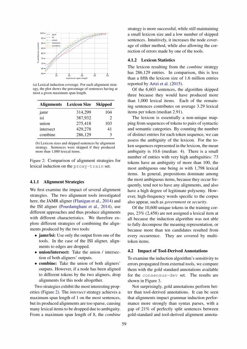
10 20 30 40 50maximum span length
60
65
70
75
80
85
90
95
100
% se
nten
ces c
over
edjamrisiunionintersectcombine
(a) Lexical induction coverage. For each alignment strat-egy, the plot shows the percentage of sentences having atmost a given maximum span length.
Alignments Lexicon Size Skipped
jamr 314,299 104isi 387,932 2union 275,418 103intersect 429,278 41combine 286,129 3
(b) Lexicon sizes and skipped sentences by alignmentstrategy. Sentences were skipped if they producedmore than 1,000 lexical items.
Figure 2: Comparison of alignment strategies forlexical induction on the proxy-train set.
4.1.1 Alignment Strategies
We first examine the impact of several alignmentstrategies. The two alignment tools investigatedhere, the JAMR aligner (Flanigan et al., 2014) andthe ISI aligner (Pourdamghani et al., 2014), usedifferent approaches and thus produce alignmentswith different characteristics. We therefore ex-plore different strategies of combining the align-ments produced by the two tools:• jamr/isi: Use only the output from one of the
tools. In the case of the ISI aligner, align-ments to edges are dropped.• union/intersect: Take the union / intersec-
tion of both aligners’ outputs.• combine: Take the union of both aligners’
outputs. However, if a node has been alignedto different tokens by the two aligners, dropalignments for this node altogether.
Two strategies exhibit the most interesting prop-erties (Figure 2). The intersect strategy achieves amaximum span length of 1 on the most sentences,but its produced alignments are too sparse, causingmany lexical items to be dropped due to ambiguity.From a maximum span length of 8, the combine
strategy is more successful, while still maintaininga small lexicon size and a low number of skippedsentences. Intuitively, it increases the node cover-age of either method, while also allowing the cor-rection of errors made by one of the tools.
4.1.2 Lexicon StatisticsThe lexicon resulting from the combine strategyhas 286,129 entries. In comparison, this is lessthan a fifth the lexicon size of 1.6 million entriesreported by Artzi et al. (2015).
Of the 6,603 sentences, the algorithm skippedthree because they would have produced morethan 1,000 lexical items. Each of the remain-ing sentences contributes on average 3.29 lexicalitems per token (median 2.91).
The lexicon is essentially a non-unique map-ping from sequences of tokens to pairs of syntacticand semantic categories. By counting the numberof distinct entries for each token sequence, we canassess the ambiguity of the lexicon. For the to-ken sequences represented in the lexicon, the meanambiguity is 10.6 (median: 4). There is a smallnumber of entries with very high ambiguities: 73tokens have an ambiguity of more than 100, themost ambiguous one being in with 1,798 lexicalitems. In general, prepositions dominate amongthe most ambiguous items, because they occur fre-quently, tend not to have any alignments, and alsohave a high degree of legitimate polysemy. How-ever, high-frequency words specific to the corpusalso appear, such as government or security.
Of the 10,600 unique tokens in the training cor-pus, 23% (2,458) are not assigned a lexical item atall because the induction algorithm was not ableto fully decompose the meaning representation, orbecause more than ten candidates resulted fromevery occurrence. They are covered by multi-token items.
4.2 Impact of Tool-Derived Annotations
To examine the induction algorithm’s sensitivity toerrors propagated from external tools, we comparethem with the gold standard annotations availablefor the consensus-dev set. The results areshown in Figure 3.
Not surprisingly, gold annotations perform bet-ter than tool-derived annotations. It can be seenthat alignments impact grammar induction perfor-mance more strongly than syntax parses, with agap of 21% of perfectly split sentences betweengold-standard and tool-derived alignment annota-
59
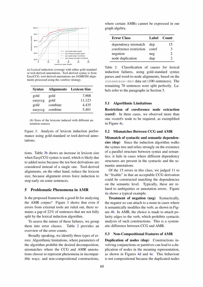
0 10 20 30 40 50maximum span length
50
60
70
80
90
100se
nten
ces c
over
ed
syn=gold align=goldsyn=easyccg align=goldsyn=gold align=combinesyn=easyccg align=combine
(a) Lexical induction coverage with either gold-standardor tool-derived annotations. Tool-derived syntax is fromEasyCCG, tool-derived annotations are JAMR/ISI align-ments processed using the combine strategy.
Syntax Alignments Lexicon Size
gold gold 7,908easyccg gold 11,123gold combine 4,435easyccg combine 5,401
(b) Sizes of the lexicons induced with different an-notation sources.
Figure 3: Analysis of lexicon induction perfor-mance using gold-standard or tool-derived anno-tations.
tions. Table 3b shows an increase in lexicon sizewhen EasyCCG syntax is used, which is likely dueto added noise because the ten best derivations areconsidered instead of a single one. Tool-derivedalignments, on the other hand, reduce the lexiconsize, because alignment errors force induction tostop early on some sentences.
5 Problematic Phenomena in AMR
Is the proposed framework a good fit for analysingthe AMR corpus? Figure 3 shows that even iferrors from external tools are ruled out, there re-mains a gap of 22% of sentences that are not fullysplit by the lexical induction algorithm.
To assess the nature of these failures, we groupthem into error classes. Table 2 provides anoverview of the error counts.
Broadly speaking, we identify three types of er-rors: Algorithmic limitations, where parameters ofthe algorithm prohibit the desired decomposition;mismatches where the CCG and AMR annota-tions choose to represent phenomena in incompat-ible ways; and non-compositional constructions,
where certain AMRs cannot be expressed in ourgraph algebra.
Error Class Label Count
dependency mismatch dep 15coreference restriction coref 3negation neg 2node duplication dup 2
Table 2: Classification of causes for lexicalinduction failures, using gold-standard syntaxparses and word-to-node alignments, based on theconsensus-dev data set (100 sentences). Theremaining 78 sentences were split perfectly. La-bels refer to the paragraphs in Section 5.
5.1 Algorithmic Limitations
Restriction of coreference node extraction(coref) In three cases, we observed more thanone <coref> node to be required, as exemplifiedin Figure 4c.
5.2 Mismatches Between CCG and AMR
Mismatch of syntactic and semantic dependen-cies (dep) Since the induction algorithm walksthe syntax tree and relies strongly on the existenceof a parallel structure between syntax and seman-tics, it fails in cases where different dependencystructures are present in the syntactic and the se-mantic annotations.
Of the 15 errors in this class, we judged 11 tobe “fixable” in that an acceptable CCG derivationcould be constructed matching the dependencieson the semantic level. Typically, these are re-lated to ambiguities or annotation errors. Figure4a shows a typical example.
Treatment of negation (neg) Syntactically,the negator no can attach to a noun in cases whereit semantically modifies the verb, as shown in Fig-ure 4b. In AMR, the choice is made to attach po-larity edges to the verb, which prohibits syntacticanalysis of such constructions. This is a system-atic difference between CCG and AMR.
5.3 Non-Compositional Features of AMR
Duplication of nodes (dup) Constructions in-volving conjunctions or partitives can lead to a du-plication of nodes in the meaning representation,as shown in Figures 4d and 4e. This behaviouris not compositional because the duplicated nodes
60

bear-06〈root〉
force
work-01
today
-we
ARG2
ARG0
time
polarityposs
no bearing on our work force today
NP (NP\NP)/NP NP NP\NP<
NP>
(NP\NP)<
NP
(a) Example for mismatching syntactic / semantic dependen-cies. Syntactically, a dependency between work force andtoday is annotated, but semantically, today is dependent onbearing. While a syntax derivation matching the semanticdependencies could be constructed, it has not been annotatedin CCGbank. From wsj_0003.30.
have-03〈root〉
we
information
useful-ARG0
ARG1
modpolarity
We have no useful information
NP (S [dcl ]\NP)/NP NP [nb]/N N>
NP>
S [dcl ]\NP<
S[dcl]
(b) Example for the incompatible treatment of negation. Thepolarity edge of have-03 does not match the dependency be-tween no and information. Simplified from wsj_0003.9
settle-01〈root〉
〈0〉
Indianapolis
meet-03
board
ARG1
ARG0 part ARG0
location
settled on Indianapolis for its board meeting
(S [dcl ]\NP)/PP PP (S\NP)\(S\NP)>
S [dcl ]\NP<
S [dcl ]\NP(c) Example for a phrase with more than one coreference.The phrase its board meeting contains coreferences both viathe location and part edges. The Indianapolis node is an ab-breviation for a multi-node named entity subgraph. Simpli-fied from wsj_0010.3.
and〈root〉
operation
sell-01
operation
service-01
operation
part
operation
market-01
op1 op2 op3 op4
mod mod mod mod
(d) Example for the duplication of nodes due to coordination.The phrase is sales, service, parts and marketing operations.Even though the token operations occurs only once, a sepa-rate operation node is introduced for each operand of the andconjunction. From wsj_0009.2.
chef〈root〉
include-91 chef town
hot most
ARG1 ARG2 location
mod degree
(e) Example for the duplication of nodes due to a partitive.The phrase is some of the hottest chefs in town. The ex-ample illustrate how quantification can lead to nodes be-ing duplicated, such as the chef nodes in this AMR. Fromwsj_0010.17
Figure 4: Corpus examples for the phenomena described in Section 5: mismatching dependencies, treat-ment of negations, number of coreferences, duplication of nodes due to coordination and partitives.Syntax annotations are taken from CCGbank, and semantic annotations are taken from the AMR corpus.
〈root〉tell-01
〈0〉
boy
sleep
ARG0
ARG2
ARG1ARG0
(a) Meaning representation fortold the boy to sleep.
〈root〉tell-01
〈0〉
boy
〈1〉
ARG0
ARG2
ARG1 ARG0
(b) Induced meaning represen-tation for told the boy.
〈root〉tell-01
〈0〉
〈2〉
〈1〉
ARG0
ARG2
ARG1ARG0
boy〈root〉
sleep〈root〉
(c) Induced meaning representations fortold, boy, and sleep.
Figure 5: Example for the induction of lexical items from an object control verb construction. Thesentence is [The girl] told the boy to sleep. Since sleep is an argument to tell, it is not assigned anyplaceholders and is extracted as a 0-ary lexical item. The control structure is encoded in the lexical itemfor tell.
61

scenario〈root〉
and
kidnap-01 take-01
hostage
mod
op1 op2
ARG1
(a) AMR for the phrasekidnapping and hostage-taking scenarios.
kidnapping and hostage-taking scenarios
N /N conj N /N Nconj
(N /N )\(N /N )<
N /N>
N
(b) CCG derivation showing the lexical entries forthe modifiers kidnapping and hostage-taking.
〈root, 0〉
kidnap-01mod
〈root, 0〉
take-01
hostage
mod
ARG1
(c) The lexical entries forthe modifiers kidnappingand hostage-taking.
Figure 6: Corpus example for conjunctions of modifiers. The AMR in Figure 6a cannot be com-positionally constructed from the modifier interpretations of kidnapping and hostage-taking becausethe mod edges present in the lexical entries would have to be destructively modified. Example fromPROXY_AFP_ENG_20020105_0162.12.
are introduced only once lexically, and then copiedbased on the syntactic context.
Coordination of modifiers2 When modifiersare the arguments of a conjunction, the conjunc-tion node itself is connected to the modifiee via amod edge, as shown in Figure 6. Given that eachof the conjoined modifiers itself has a mod edge,these edges need to be merged, moved, or deletedsomehow.
6 Conclusion
We have presented a new variant of CCG whichperforms semantic construction using the opera-tions of a graph algebra instead of combinatoryoperations on λ-calculus terms. This allows thegrammar to construct graph representations di-rectly without going through intermediate repre-sentations. It also restricts the set of possibleoperations, leading to a compact lexicon. Wehave demonstrated that under ideal conditions, ourgrammar achieves a robust coverage of 78% onWSJ sentences.
Our experiments suggest that CCG/AMR is agood overall match for representing the derivationof AMRs. There remain several possibilities forimprovement which we leave for future work:• Allowing the induction algorithm to search
over possible derivations and alignmentswould reduce the influence of both tool er-rors and mismatching annotations. To keepthe lexicon manageable, an optimizing induc-tion algorithm would be needed, e.g. usingEM.
2This phenomenon has not been observed in theconsensus data set and is therefore not represented in Ta-ble 2.
• An attempt could me made to more stronglyidentify placeholders with the argument po-sitions of the corresponding syntactic cate-gories. Among others, this would allow fora more canonical treatment of object con-trol verbs, which is somewhat ad hoc, requir-ing an interpretation of verbs as 0-ary lexicalitems (see Figure 5 for an example).• Additional rules could be introduced to deal
with non-compositional phenomena such asthe conjunction of modifiers. Statistically,such phenomena appear to be rare, affectingonly 2% of the examined corpus.• Other differences in representation might be
resolved statistically or using heuristics. E.g.,the fact that negators that attach to a nounsyntactically attach to the verb in AMR couldbe mitigated by a rule that allows for themovement of polarity edges.
Our results represent a promising step towardsa more complete grammatical treatment of AMR.Although AMR has not been designed with com-positionality in mind, we have shown that it is pos-sible to construct linguistically motivated compo-sitional derivations.
7 Acknowledgements
We thank Alexander Koller and his group, Chris-tine and Arne Köhn, and the anonymous reviewersfor their helpful comments. Part of this work wassupported by the DFG (IGK 1247).
ReferencesYoav Artzi, Kenton Lee, and Luke Zettlemoyer. 2015.
Broad-coverage CCG Semantic Parsing with AMR.
62
In Proceedings of the 2015 Conference on Empiri-cal Methods in Natural Language Processing, pages1699–1710, Lisbon, Portugal. Association for Com-putational Linguistics.
Miguel Ballesteros and Yaser Al-Onaizan. 2017. AMRParsing using Stack-LSTMs. In Proceedings of the2017 Conference on Empirical Methods in Natu-ral Language Processing, pages 1269–1275, Copen-hagen, Denmark. Association for ComputationalLinguistics.
Laura Banarescu, Claire Bonial, Shu Cai, MadalinaGeorgescu, Kira Griffitt, Ulf Hermjakob, KevinKnight, Philipp Koehn, Martha Palmer, and NathanSchneider. 2013. Abstract Meaning Representationfor Sembanking. In Proceedings of the 7th Linguis-tic Annotation Workshop and Interoperability withDiscourse, pages 178–186, Sofia, Bulgaria. Associ-ation for Computational Linguistics.
Emily M. Bender, Dan Flickinger, Stephan Oepen,Woodley Packard, and Ann Copestake. 2015. Lay-ers of Interpretation: On Grammar and Compo-sitionality. In Proceedings of the 11th Inter-national Conference on Computational Semantics,pages 239–249, London, UK. Association for Com-putational Linguistics.
Bruno Courcelle and Joost Engelfriet. 2012. GraphStructure and Monadic Second-Order Logic: ALanguage-Theoretic Approach, 1st edition. Cam-bridge University Press, New York, NY, USA.
Jeffrey Flanigan, Sam Thomson, Jaime Carbonell,Chris Dyer, and Noah A. Smith. 2014. A Discrimi-native Graph-Based Parser for the Abstract MeaningRepresentation. In Proceedings of the 52nd AnnualMeeting of the Association for Computational Lin-guistics, pages 1426–1436, Baltimore, Maryland.Association for Computational Linguistics.
Jonas Groschwitz, Meaghan Fowlie, Mark Johnson,and Alexander Koller. 2017. A constrained graph al-gebra for semantic parsing with AMRs. In Proceed-ings of the 12th International Conference on Com-putational Semantics, Montpellier, France. Associa-tion for Computational Linguistics.
Julia Hockenmaier and Mark Steedman. 2007. CCG-bank: a corpus of CCG derivations and dependencystructures extracted from the Penn Treebank. Com-putational Linguistics, 33(3):355–396.
Matthew Honnibal, James R. Curran, and Johan Bos.2010. Rebanking CCGbank for Improved NP Inter-pretation. In Proceedings of the 48th Annual Meet-ing of the Association for Computational Linguis-tics, pages 207–215, Uppsala, Sweden. Associationfor Computational Linguistics.
Paul Kingsbury and Martha Palmer. 2002. From Tree-Bank to PropBank. In Proceedings of the Third In-ternational Conference on Language Resources andEvaluation, pages 1989–1993, Las Palmas, Spain.European Language Resources Association.
Kevin Knight, Laura Baranescu, Claire Bonial,Madalina Georgescu, Kira Griffitt, Ulf Hermjakob,Daniel Marcu, Martha Palmer, and Nathan Schnei-der. 2014. Abstract Meaning Representation (AMR)Annotation Release 1.0 LDC2014T12. LinguisticData Consortium, Philadelphia.
Alexander Koller. 2015. Semantic construction withgraph grammars. In Proceedings of the 11th Inter-national Conference on Computational Semantics,pages 228–238, London, UK. Association for Com-putational Linguistics.
Tom Kwiatkowski, Luke Zettlemoyer, Sharon Goldwa-ter, and Mark Steedman. 2010. Inducing Probabilis-tic CCG Grammars from Logical Form with Higher-Order Unification. In Proceedings of the 2010 Con-ference on Empirical Methods in Natural LanguageProcessing, pages 1223–1233, Cambridge, MA. As-sociation for Computational Linguistics.
Mike Lewis, Luheng He, and Luke Zettlemoyer. 2015.Joint A* CCG Parsing and Semantic Role Labelling.In Proceedings of the 2015 Conference on Empiri-cal Methods in Natural Language Processing, pages1444–1454, Lisbon, Portugal. Association for Com-putational Linguistics.
Mike Lewis and Mark Steedman. 2014. A* CCG Pars-ing with a Supertag-factored Model. In Proceed-ings of the 2014 Conference on Empirical Methodsin Natural Language Processing (EMNLP), pages990–1000, Doha, Qatar. Association for Computa-tional Linguistics.
Christopher D. Manning, Mihai Surdeanu, John Bauer,Jenny Finkel, Steven J. Bethard, and David Mc-Closky. 2014. The Stanford CoreNLP Natural Lan-guage Processing Toolkit. In Association for Com-putational Linguistics (ACL) System Demonstra-tions, pages 55–60.
Kumar Dipendra Misra and Yoav Artzi. 2016. NeuralShift-Reduce CCG Semantic Parsing. In Proceed-ings of the 2016 Conference on Empirical Methodsin Natural Language Processing, pages 1775–1786,Austin, Texas. Association for Computational Lin-guistics.
Rik van Noord and Johan Bos. 2017. Neural Se-mantic Parsing by Character-based Translation: Ex-periments with Abstract Meaning Representations.Computational Linguistics in the Netherlands Jour-nal, 7:93–108.
Xiaochang Peng, Daniel Gildea, and Giorgio Satta.2018. AMR Parsing with Cache Transition Systems.In Proceedings of the Thirty-Second AAAI Confer-ence on Artificial Intelligence, New Orleans, USA.Association for the Advancement of Artificial Intel-ligence.
Xiaochang Peng, Linfeng Song, and Daniel Gildea.2015. A Synchronous Hyperedge Replacement
63

Grammar based approach for AMR parsing. In Pro-ceedings of the Nineteenth Conference on Compu-tational Natural Language Learning, pages 32–41,Beijing, China. Association for Computational Lin-guistics.
Nima Pourdamghani, Yang Gao, Ulf Hermjakob, andKevin Knight. 2014. Aligning English Strings withAbstract Meaning Representation Graphs. In Pro-ceedings of the 2014 Conference on Empirical Meth-ods in Natural Language Processing (EMNLP),pages 425–429, Doha, Qatar. Association for Com-putational Linguistics.
Mark Steedman. 2000. The Syntactic Process. MITPress, Cambridge, MA, USA.
Chuan Wang, Nianwen Xue, and Sameer Pradhan.2015. A Transition-based Algorithm for AMR Pars-ing. In Proceedings of the 2015 Conference ofthe North American Chapter of the Association forComputational Linguistics: Human Language Tech-nologies, pages 366–375, Denver, Colorado. Asso-ciation for Computational Linguistics.
64

Proceedings of the 7th Joint Conference on Lexical and Computational Semantics (*SEM), pages 65–75New Orleans, June 5-6, 2018. c©2018 Association for Computational Linguistics
Mixing Context Granularities for Improved Entity Linkingon Question Answering Data across Entity Categories
Daniil Sorokin and Iryna GurevychUbiquitous Knowledge Processing Lab (UKP) and Research Training Group AIPHES
Department of Computer Science, Technische Universitat Darmstadtwww.ukp.tu-darmstadt.de
{sorokin|gurevych}@ukp.informatik.tu-darmstadt.de
Abstract
The first stage of every knowledge basequestion answering approach is to link en-tities in the input question. We investigateentity linking in the context of a questionanswering task and present a jointly opti-mized neural architecture for entity men-tion detection and entity disambiguationthat models the surrounding context on dif-ferent levels of granularity.
We use the Wikidata knowledge base andavailable question answering datasets tocreate benchmarks for entity linking onquestion answering data. Our approachoutperforms the previous state-of-the-artsystem on this data, resulting in an average8% improvement of the final score. We fur-ther demonstrate that our model delivers astrong performance across different entitycategories.
1 Introduction
Knowledge base question answering (QA) requiresa precise modeling of the question semanticsthrough the entities and relations available in theknowledge base (KB) in order to retrieve the cor-rect answer. The first stage for every QA approachis entity linking (EL), that is the identification ofentity mentions in the question and linking themto entities in KB. In Figure 1, two entity mentionsare detected and linked to the knowledge base ref-erents. This step is crucial for QA since the correctanswer must be connected via some path over KBto the entities mentioned in the question.
The state-of-the-art QA systems usually rely onoff-the-shelf EL systems to extract entities fromthe question (Yih et al., 2015). Multiple EL sys-tems are freely available and can be readily applied
what are taylor swift’s albums ?
Taylor Swift Q462 album Q24951125
Red, 1989, etc.
PERFORMERINSTANCE OF
Figure 1: An example question from a QA datasetthat shows the correct entity mentions and theirrelationship with the correct answer to the question,Qxxx stands for a knowledge base identifier
for question answering (e.g. DBPedia Spotlight1,AIDA2). However, these systems have certain draw-backs in the QA setting: they are targeted at longwell-formed documents, such as news texts, andare less suited for typically short and noisy ques-tion data. Other EL systems focus on noisy data(e.g. S-MART, Yang and Chang, 2015), but arenot openly available and hence limited in their us-age and application. Multiple error analyses of QAsystems point to entity linking as a major externalsource of error (Berant and Liang, 2014; Reddyet al., 2014; Yih et al., 2015).
The QA datasets are normally collected from theweb and contain very noisy and diverse data (Be-rant et al., 2013), which poses a number of chal-lenges for EL. First, many common features usedin EL systems, such as capitalization, are not mean-ingful on noisy data. Moreover, a question is ashort text snippet that does not contain broader con-text that is helpful for entity disambiguation. TheQA data also features many entities of various cat-egories and differs in this respect from the Twitterdatasets that are often used to evaluate EL systems.
1http://www.dbpedia-spotlight.org2https://www.mpi-inf.mpg.de/yago-naga/aida/
65
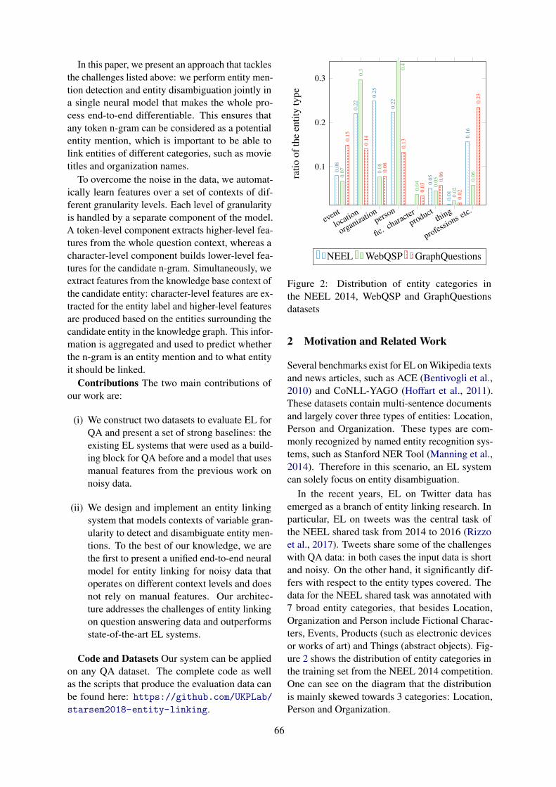
In this paper, we present an approach that tacklesthe challenges listed above: we perform entity men-tion detection and entity disambiguation jointly ina single neural model that makes the whole pro-cess end-to-end differentiable. This ensures thatany token n-gram can be considered as a potentialentity mention, which is important to be able tolink entities of different categories, such as movietitles and organization names.
To overcome the noise in the data, we automat-ically learn features over a set of contexts of dif-ferent granularity levels. Each level of granularityis handled by a separate component of the model.A token-level component extracts higher-level fea-tures from the whole question context, whereas acharacter-level component builds lower-level fea-tures for the candidate n-gram. Simultaneously, weextract features from the knowledge base context ofthe candidate entity: character-level features are ex-tracted for the entity label and higher-level featuresare produced based on the entities surrounding thecandidate entity in the knowledge graph. This infor-mation is aggregated and used to predict whetherthe n-gram is an entity mention and to what entityit should be linked.
Contributions The two main contributions ofour work are:
(i) We construct two datasets to evaluate EL forQA and present a set of strong baselines: theexisting EL systems that were used as a build-ing block for QA before and a model that usesmanual features from the previous work onnoisy data.
(ii) We design and implement an entity linkingsystem that models contexts of variable gran-ularity to detect and disambiguate entity men-tions. To the best of our knowledge, we arethe first to present a unified end-to-end neuralmodel for entity linking for noisy data thatoperates on different context levels and doesnot rely on manual features. Our architec-ture addresses the challenges of entity linkingon question answering data and outperformsstate-of-the-art EL systems.
Code and Datasets Our system can be appliedon any QA dataset. The complete code as wellas the scripts that produce the evaluation data canbe found here: https://github.com/UKPLab/
starsem2018-entity-linking.
fic. characterevent
location
organization
professions etc.
person
productthing
0.1
0.2
0.3
0.4
0.08
0.22
0.25
0.16
0.22
0.05
0.01
0.04
0.07
0.3
0.08
0.06
0.05
0.020.
03
0.15
0.14
0.08
0.23
0.13
0.06
0.02
ratio
ofth
een
tity
type
NEEL WebQSP GraphQuestions
Figure 2: Distribution of entity categories inthe NEEL 2014, WebQSP and GraphQuestionsdatasets
2 Motivation and Related Work
Several benchmarks exist for EL on Wikipedia textsand news articles, such as ACE (Bentivogli et al.,2010) and CoNLL-YAGO (Hoffart et al., 2011).These datasets contain multi-sentence documentsand largely cover three types of entities: Location,Person and Organization. These types are com-monly recognized by named entity recognition sys-tems, such as Stanford NER Tool (Manning et al.,2014). Therefore in this scenario, an EL systemcan solely focus on entity disambiguation.
In the recent years, EL on Twitter data hasemerged as a branch of entity linking research. Inparticular, EL on tweets was the central task ofthe NEEL shared task from 2014 to 2016 (Rizzoet al., 2017). Tweets share some of the challengeswith QA data: in both cases the input data is shortand noisy. On the other hand, it significantly dif-fers with respect to the entity types covered. Thedata for the NEEL shared task was annotated with7 broad entity categories, that besides Location,Organization and Person include Fictional Charac-ters, Events, Products (such as electronic devicesor works of art) and Things (abstract objects). Fig-ure 2 shows the distribution of entity categories inthe training set from the NEEL 2014 competition.One can see on the diagram that the distributionis mainly skewed towards 3 categories: Location,Person and Organization.
66

Figure 2 also shows the entity categories presentin two QA datasets. The distribution over the cate-gories is more diverse in this case. The WebQues-tions dataset includes the Fictional Character andThing categories which are almost absent from theNEEL dataset. A more even distribution can be ob-served in the GraphQuestion dataset that featuresmany Events, Fictional Characters and Professions.This means that a successful system for EL on ques-tion data needs to be able to recognize and to linkall categories of entities. Thus, we aim to showthat comprehensive modeling of different contextlevels will result in a better generalization and per-formance across various entity categories.
Existing Solutions The early machine learningapproaches to EL focused on long well-formeddocuments (Bunescu and Pasca, 2006; Cucerzan,2007; Han and Sun, 2012; Francis-Landau et al.,2016). These systems usually rely on an off-the-shelf named entity recognizer to extract entity men-tions in the input. As a consequence, such ap-proaches can not handle entities of types other thanthose that are supplied by the named entity rec-ognizer. Named entity recognizers are normallytrained to detect mentions of Locations, Organiza-tions and Person names, whereas in the context ofQA, the system also needs to cover movie titles,songs, common nouns such as ‘president’ etc.
To mitigate this, Cucerzan (2012) has introducedthe idea to perform mention detection and entitylinking jointly using a linear combination of man-ually defined features. Luo et al. (2015) haveadopted the same idea and suggested a probabilis-tic graphical model for the joint prediction. This isessential for linking entities in questions. For exam-ple in “who does maggie grace play in taken?”, it ishard to distinguish between the usage of the word‘taken’ and the title of a movie ‘Taken’ withoutconsulting a knowledge base.
Sun et al. (2015) were among the first to useneural networks to embed the mention and the en-tity for a better prediction quality. Later, Francis-Landau et al. (2016) have employed convolutionalneural networks to extract features from the doc-ument context and mixed them with manually de-fined features, though they did not integrate it withmention detection. Sil et al. (2018) continued thework in this direction recently and applied convo-lutional neural networks to cross-lingual EL.
The approaches that were developed for Twit-ter data present the most relevant work for EL
on QA data. Guo et al. (2013b) have created anew dataset of around 1500 tweets and suggested aStructured SVM approach that handled mention de-tection and entity disambiguation together. Changet al. (2014) describe the winning system of theNEEL 2014 competition on EL for short texts: Thesystem adapts a joint approach similar to Guo et al.(2013b), but uses the MART gradient boosting al-gorithm instead of the SVM and extends the fea-ture set. The current state-of-the-art system forEL on noisy data is S-MART (Yang and Chang,2015) which extends the approach from Chang et al.(2014) to make structured predictions. The samegroup has subsequently applied S-MART to extractentities for a QA system (Yih et al., 2015).
Unfortunately, the described EL systems forshort texts are not available as stand-alone tools.Consequently, the modern QA approaches mostlyrely on off-the-shelf entity linkers that were de-signed for other domains. Reddy et al. (2016) haveemployed the Freebase online API that was sincedeprecated. A number of question answering sys-tems have relied on DBPedia Spotlight to extractentities (Lopez et al., 2016; Chen et al., 2016). DB-Pedia Spotlight (Mendes et al., 2011) uses doc-ument similarity vectors, word embeddings andmanually defined features such as entity frequency.We are addressing this problem in our work by pre-senting an architecture specifically targeted at ELfor QA data.
The Knowledge Base Throughout the ex-periments, we use the Wikidata3 open-domainKB (Vrandecic and Krotzsch, 2014). Among theprevious work, the common choices of a KB in-clude Wikipedia, DBPedia and Freebase. Theentities in Wikidata directly correspond to theWikipedia articles, which enables us to work withdata that was previously annotated with DBPedia.Freebase was discontinued and is no longer up-to-date. However, most entities in Wikidata have beenannotated with identifiers from other knowledgesources and databases, including Freebase, whichestablishes a link between the two KBs.
3 Entity Linking Architecture
The overall architecture of our entity linking systemis depicted in Figure 3. From the input questionx we extract all possible token n-grams N up to a
3 At the moment, Wikidata contains more than 40 millionentities and 350 million relation instances:https://www.wikidata.org/wiki/Special:Statistics
67

x = what are taylor swift’s albums?
Step 1. consider all n-grams
N = ngrams(x), i = 0
i < |N |,n = N [i]
Step 2. entity candidates for an n-gram
C = entity candidates(n)
wikidata
Full textsearch
Step 3. score the n-gram with the model
pn,pc = M(x, n, C)
i = i+ 1
Step 4. compute the global assignment of entities
G = global assignment(pn,pc, n,x|n ∈ N)
Figure 3: Architecture of the entity linking system
certain length as entity mention candidates (Step 1).For each n-gram n, we look it up in the knowledgebase using a full text search over entity labels (Step2). That ensures that we find all entities that containthe given n-gram in the label. For example fora unigram ‘obama’, we retrieve ‘Barack Obama’,‘Michelle Obama’ etc. This step produces a set ofentity disambiguation candidates C for the given n-gram n. We sort the retrieved candidates by lengthand cut off after the first 1000. That ensures thatthe top candidates in the list would be those thatexactly match the target n-gram n.
In the next step, the list of n-grams N and thecorresponding list of entity disambiguation candi-dates are sent to the entity linking model (Step 3).The model jointly performs the detection of correctmentions and the disambiguation of entities.
3.1 Variable Context Granularity Network
The neural architecture (Variable Context Granular-ity, VCG) aggregates and mixes contexts of differ-ent granularities to perform a joint mention detec-tion and entity disambiguation. Figure 4 showsthe layout of the network and its main compo-nents.granularity level. The input to the model is alist of question tokens x, a token n-gram n and a listof candidate entities C. Then the model is a func-tion M(x,n,C) that produces a mention detectionscore pn for each n-gram and a ranking score pc foreach of the candidates c ∈C: pn,pc = M(x,n,C).
Dilated Convolutions To process sequentialinput, we use dilated convolutional networks
(DCNN). Strubell et al. (2017) have recently shownthat DCNNs are faster and as effective as recurrentmodels on the task of named entity recognition.We define two modules: DCNNw and DCNNc forprocessing token-level and character-level inputrespectively. Both modules consist of a series ofconvolutions applied with an increasing dilation, asdescribed in Strubell et al. (2017). The output ofthe convolutions is averaged and transformed by afully-connected layer.
Context Components The token componentcorresponds to sentence-level features normallydefined for EL and encodes the list of questiontokens x into a fixed size vector. It maps the tokensin x to dw-dimensional pre-trained word embed-dings, using a matrix W ∈ R|Vw|×dw , where |Vw| isthe size of the vocabulary. We use 50-dimensionalGloVe embeddings pre-trained on a 6 billion to-kens corpus (Pennington et al., 2014). The wordembeddings are concatenated with dp-dimensionalposition embeddings Pw ∈ R3×dp that are used todenote the tokens that are part of the target n-gram.The concatenated embeddings are processed byDCNNw to get a vector os.
The character component processes the target to-ken n-gram n on the basis of individual characters.We add one token on the left and on the right to thetarget mention and map the string of characters todz-character embeddings, Z∈R|Vz|×dz . We concate-nate the character embeddings with dp-dimensionalposition embeddings Pz ∈R|x|×dp and process themwith DCNNc to get a feature vector on.
We use the character component with the samelearned parameters to encode the label of a candi-date entity from the KB as a vector ol. The param-eter sharing between mention encoding and entitylabel encoding ensures that the representation of amention is similar to the entity label.
The KB structure is the highest context levelincluded in the model. The knowledge base struc-ture component models the entities and relationsthat are connected to the candidate entity c. First,we map a list of relations r of the candidate en-tity to dr-dimensional pre-trained relations embed-dings, using a matrix R ∈ R|Vr|×dr , where |Vr| isthe number of relation types in the KB. We trans-form the relations embeddings with a single fully-connected layer fr and then apply a max poolingoperation to get a single relation vector or per en-tity. Similarly, we map a list of entities that areimmediately connected to the candidate entity e
68

w1 p1 w2 p2 w3 p3 w4 p4 . . . wn pn
what are taylor swift . . . ?
DCNNw
W , Pw
x
Token-level Context
z1 p1 z2 p2 z3 p3 z4 p4 z5 p5 z6 p6 . . . zn pn
t a y l o r . . . t
DCNNc
Z, Pz
n
Character-level Context
what are taylor swift’s albums?
c =Taylor Swift Q26876
T a y l o r . . . t
c1 p1 c2 p2 c3 p3 c4 p4 c5 p5 c6 p6 . . . cn
Entity Labels Context
DCNNc
Z, Pz
l r1 r2 r3 . . . rn
KB Relations Labels Context
xr1
xr2
xr3
xr1
xr2
xr3
xr1
xr2
xr3
xr1
xr2
xr3
W W W W
frl
r1 r2 r3 r4 . . . rn
KB Relations Context
R
fr
e1 e2 e3 e4 . . . en
KB Entities Context
E
fe
c
fe
KB Entity Context
oc
ot
pcs
pn
gc
gn
od ol orl or oe
os om
os on
Figure 4: The architecture of the Variable Context Granularity Network for a single n-gram and an entitycandidate. The output vectors (oc,ot) are aggregated over all n-grams for the global assignment
to de-dimensional pre-trained entity embeddings,using a matrix E ∈ R|Ve|×de , where |Ve| is the num-ber of entities in the KB. The entity embeddingsare transformed by a fully-connected layer fe andthen also pooled to produce the output oe. The em-bedding of the candidate entity itself is also trans-formed with fe and is stored as od. To train theknowledge base embeddings, we use the TransEalgorithm (Bordes et al., 2013).
Finally, the knowledge base lexical componenttakes the labels of the relations in r to computelexical relation embeddings. For each r ∈ r, wetokenize the label and map the tokens xr to wordembeddings, using the word embedding matrix W.To get a single lexical embedding per relation, weapply max pooling and transform the output witha fully-connected layer frl . The lexical relationembeddings for the candidate entity are pooled intothe vector orl.
Context Aggregation The different levels ofcontext are aggregated and are transformed by asequence of fully-connected layers into a final vec-tor oc for the n-gram n and the candidate entity c.The vectors for each candidate are aggregated intoa matrix O = [oc|c ∈C]. We apply element-wise
max pooling on O to get a single summary vectors for all entity candidates for n.
To get the ranking score pc for each entity candi-date c, we apply a single fully-connected layer gc
on the concatenation of oc and the summary vec-tor s: pc = gc(oc‖s). For the mention detectionscore for the n-gram, we separately concatenate thevectors for the token context os and the charactercontext on and transform them with an array offully-connected layers into a vector ot. We con-catenate ot with the summary vector s and applyanother fully-connected layer to get the mentiondetection score pn = σ(gn(ot‖s)).
3.2 Global Entity Assignment
The first step in our system is extracting all possi-ble overlapping n-grams from the input texts. Weassume that each span in the input text can only re-fer to a single entity and therefore resolve overlapsby computing a global assignment using the modelscores for each n-gram (Step 4 in Figure 3).
If the mention detection score pn is above the0.5-threshold, the n-gram is predicted to be a cor-rect entity mention and the ranking scores pc areused to disambiguate it to a single entity candidate.
69

N-grams that have pn lower than the threshold arefiltered out.
We follow Guo et al. (2013a) in computing theglobal assignment and hence, arrange all n-gramsselected as mentions into non-overlapping combi-nations and use the individual scores pn to computethe probability of each combination. The com-bination with the highest probability is selectedas the final set of entity mentions. We have ob-served in practice a similar effect as descirbed byStrubell et al. (2017), namely that DCNNs are ableto capture dependencies between different entitymentions in the same context and do not tend toproduce overlapping mentions.
3.3 Composite Loss FunctionOur model jointly computes two scores for eachn-gram: the mention detection score pn and the dis-ambiguation score pc. We optimize the parametersof the whole model jointly and use the loss functionthat combines penalties for the both scores for alln-grams in the input question:
L = ∑n∈N
∑c∈Cn
M (tn, pn) + tnD(tc, pc),
where tn is the target for mention detection and iseither 0 or 1, tc is the target for disambiguation andranges from 0 to the number of candidates |C|.
For the mention detection loss M , we include aweighting parameter α for the negative class as themajority of the instances in the data are negative:
M (tn, pn)=−tn log pn−α(1−tn) log(1− pn)
The disambiguation detection loss D is a maxi-mum margin loss:
D(tc, pc) =∑|C|i=0 max(0,(m− pc[tc]+ pc[i]))
|C| ,
where m is the margin value. We set m = 0.5,whereas the α weight is optimized with the otherhyper-parameters.
3.4 Architecture ComparisonOur model architecture follows some of the ideaspresented in Francis-Landau et al. (2016): they sug-gest computing a similarity score between an entityand the context for different context granularities.Francis-Landau et al. (2016) experiment on entitylinking for Wikipedia and news articles and con-sider the word-level and document-level contexts
#Questions #Entities
WebQSP Train 3098 3794WebQSP Test 1639 2002
GraphQuestions Test 2608 4680
Table 1: Dataset statistics
for entity disambiguation. As described above, wealso incorporate different context granularities witha number of key differences: (1) we operate onsentence level, word level and character level, thusincluding a more fine-grained range of contexts;(2) the knowledge base contexts that Francis-Lan-dau et al. (2016) use are the Wikipedia title andthe article texts — we, on the other hand, employthe structure of the knowledge base and encoderelations and related entities; (3) Francis-Landauet al. (2016) separately compute similarities foreach type of context, whereas we mix them in asingle end-to-end architecture; (4) we do not relyon manually defined features in our model.
4 Datasets
We compile two new datasets for entity linkingon questions that we derive from publicly avail-able question answering data: WebQSP (Yih et al.,2016) and GraphQuestions (Su et al., 2016).
WebQSP contains questions that were originallycollected for the WebQuestions dataset from websearch logs (Berant et al., 2013). They were man-ually annotated with SPARQL queries that can beexecuted to retrieve the correct answer to each ques-tion. Additionally, the annotators have also selectedthe main entity in the question that is central to find-ing the answer. The annotations and the query useidentifiers from the Freebase knowledge base.
We extract all entities that are mentioned in thequestion from the SPARQL query. For the mainentity, we also store the correct span in the text,as annotated in the dataset. In order to be able touse Wikidata in our experiments, we translate theFreebase identifiers to Wikidata IDs.
The second dataset, GraphQuestions, was cre-ated by collecting manual paraphrases for automat-ically generated questions (Su et al., 2016). Thedataset is meant to test the ability of the systemto understand different wordings of the same ques-tion. In particular, the paraphrases include variousreferences to the same entity, which creates a chal-lenge for an entity linking system. The following
70

P R F1
Heuristic baseline 0.286 0.621 0.392Simplified VCG 0.804 0.654 0.721
VCG 0.823 0.646 0.724
Table 2: Evaluation results on the WEBQSP devel-opment dataset (all entities)
are three example questions from the dataset thatcontain a mention of the same entity:
(1) a. what is the rank of marvel’s ironman?
b. iron-man has held what ranks?c. tony stark has held what ranks?
GraphQuestions does not contain main entityannotations, but includes a SPARQL query struc-turally encoded in JSON format. The queries wereconstructed manually by identifying the entities inthe question and selecting the relevant KB relations.We extract gold entities for each question from theSPARQL query and map them to Wikidata.
We split the WebQSP training set into train anddevelopment subsets to optimize the neural model.We use the GraphQuestions only in the evaluationphase to test the generalization power of our model.The sizes of the constructed datasets in terms of thenumber of questions and the number of entities arereported in Table 1. In both datasets, each questioncontains at least one correct entity mention.
5 Experiments
5.1 Evaluation Methodology
We use precision, recall and F1 scores to evaluateand compare the approaches. We follow Carmelet al. (2014) and Yang and Chang (2015) and definethe scores on a per-entity basis. Since there areno mention boundaries for the gold entities, anextracted entity is considered correct if it is presentin the set of the gold entities for the given question.We compute the metrics in the micro and macrosetting. The macro values are computed per entityclass and averaged afterwards.
For the WebQSP dataset, we additionally per-form a separate evaluation using only the informa-tion on the main entity. The main entity has theinformation on the boundary offsets of the correctmentions and therefore for this type of evaluation,we enforce that the extracted mention has to over-
emb. size filter sizedw dz de dr dp DCNNw DCNNc α
50 25 50 50 5 64 64 0.5
Table 3: Best configuration for the VCG model
lap with the correct mention. QA systems need atleast one entity per question to attempt to find thecorrect answer. Thus, evaluating using the mainentity shows how the entity linking system fulfillsthis minimum requirement.
5.2 Baselines
Existing Systems In our experiments, we compareto DBPedia Spotlight that was used in several QAsystems and represents a strong baseline for entitylinking4. In addition, we are able to compare to thestate-of-the-art S-MART system, since their outputon the WebQSP datasets was publicly released5.The S-MART system is not openly available, it wasfirst trained on the NEEL 2014 Twitter dataset andlater adapted to the QA data (Yih et al., 2015).
We also include a heuristics baseline that rankscandidate entities according to their frequency inWikipedia. This baseline represents a reasonablelower bound for a Wikidata based approach.
Simplified VCG To test the effect of the end-to-end context encoders of the VCG network, we de-fine a model that instead uses a set of features com-monly suggested in the literature for EL on noisydata. In particular, we employ features that cover(1) frequency of the entity in Wikipedia, (2) edit dis-tance between the label of the entity and the tokenn-gram, (3) number of entities and relations imme-diately connected to the entity in the KB, (4) wordoverlap between the input question and the labelsof the connected entities and relations, (5) lengthof the n-gram. We also add an average of the wordembeddings of the question tokens and, separately,an average of the embeddings of tokens of entitiesand relations connected to the entity candidate. Wetrain the simplified VCG model by optimizing thesame loss function in Section 3.3 on the same data.
5.3 Practical Considerations
The hyper-parameters of the model, such as thedimensionality of the layers and the size of embed-
4We use the online end-point: http://www.dbpedia-spotlight.org/api
5https://github.com/scottyih/STAGG
71
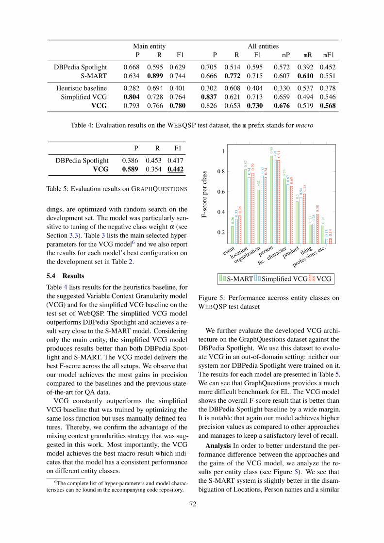
Main entity All entitiesP R F1 P R F1 mP mR mF1
DBPedia Spotlight 0.668 0.595 0.629 0.705 0.514 0.595 0.572 0.392 0.452S-MART 0.634 0.899 0.744 0.666 0.772 0.715 0.607 0.610 0.551
Heuristic baseline 0.282 0.694 0.401 0.302 0.608 0.404 0.330 0.537 0.378Simplified VCG 0.804 0.728 0.764 0.837 0.621 0.713 0.659 0.494 0.546
VCG 0.793 0.766 0.780 0.826 0.653 0.730 0.676 0.519 0.568
Table 4: Evaluation results on the WEBQSP test dataset, the m prefix stands for macro
P R F1
DBPedia Spotlight 0.386 0.453 0.417VCG 0.589 0.354 0.442
Table 5: Evaluation results on GRAPHQUESTIONS
dings, are optimized with random search on thedevelopment set. The model was particularly sen-sitive to tuning of the negative class weight α (seeSection 3.3). Table 3 lists the main selected hyper-parameters for the VCG model6 and we also reportthe results for each model’s best configuration onthe development set in Table 2.
5.4 ResultsTable 4 lists results for the heuristics baseline, forthe suggested Variable Context Granularity model(VCG) and for the simplified VCG baseline on thetest set of WebQSP. The simplified VCG modeloutperforms DBPedia Spotlight and achieves a re-sult very close to the S-MART model. Consideringonly the main entity, the simplified VCG modelproduces results better than both DBPedia Spot-light and S-MART. The VCG model delivers thebest F-score across the all setups. We observe thatour model achieves the most gains in precisioncompared to the baselines and the previous state-of-the-art for QA data.
VCG constantly outperforms the simplifiedVCG baseline that was trained by optimizing thesame loss function but uses manually defined fea-tures. Thereby, we confirm the advantage of themixing context granularities strategy that was sug-gested in this work. Most importantly, the VCGmodel achieves the best macro result which indi-cates that the model has a consistent performanceon different entity classes.
6The complete list of hyper-parameters and model charac-teristics can be found in the accompanying code repository.
fic. characterevent
location
organization
professions etc.
person
productthing
0.2
0.4
0.6
0.8
1
0.73
0.26
0.82
0.62
0.26
0.95
0.5
0.27
0.67
0.33
0.74 0.75
0.13
0.91
0.54
0.28
0.65
0.36
0.79
0.74
0.14
0.91
0.58
0.38
F-sc
ore
perc
lass
S-MART Simplified VCG VCG
Figure 5: Performance accross entity classes onWEBQSP test dataset
We further evaluate the developed VCG archi-tecture on the GraphQuestions dataset against theDBPedia Spotlight. We use this dataset to evalu-ate VCG in an out-of-domain setting: neither oursystem nor DBPedia Spotlight were trained on it.The results for each model are presented in Table 5.We can see that GraphQuestions provides a muchmore difficult benchmark for EL. The VCG modelshows the overall F-score result that is better thanthe DBPedia Spotlight baseline by a wide margin.It is notable that again our model achieves higherprecision values as compared to other approachesand manages to keep a satisfactory level of recall.
Analysis In order to better understand the per-formance difference between the approaches andthe gains of the VCG model, we analyze the re-sults per entity class (see Figure 5). We see thatthe S-MART system is slightly better in the disam-biguation of Locations, Person names and a similar
72

Main entity All entitiesP R F1 P R F1 mP mR mF1
VCG 0.793 0.766 0.780 0.826 0.653 0.730 0.676 0.519 0.568w/o token context 0.782 0.728 0.754 0.812 0.618 0.702 0.664 0.474 0.530
w/o character context 0.802 0.684 0.738 0.820 0.573 0.675 0.667 0.404 0.471w/o KB structure context 0.702 0.679 0.690 0.728 0.576 0.643 0.549 0.427 0.461
w/o KB lexical context 0.783 0.732 0.756 0.807 0.617 0.699 0.643 0.454 0.508
Table 6: Ablation experiments for the VCG model on WEBQSP
category of Fictional Character names, while it hasa considerable advantage in processing of Profes-sions and Common Nouns. Our approach has anedge in such entity classes as Organization, Thingsand Products. The latter category includes movies,book titles and songs, which are particularly hardto identify and disambiguate since any sequenceof words can be a title. VCG is also considerablybetter in recognizing Events. We conclude thatthe future development of the VCG architectureshould focus on the improved identification anddisambiguation of professions and common nouns.
To analyze the effect that mixing various contextgranularities has on the model performance, weinclude ablation experiment results for the VCGmodel (see Table 6). We report the same scores asin the main evaluation but without individual modelcomponents that were described in Section 3.
We can see that the removal of the KB structureinformation encoded in entity and relation embed-dings results in the biggest performance drop ofalmost 10 percentage points. The character-level in-formation also proves to be highly important for thefinal state-of-the-art performance. These aspects ofthe model (the comprehensive representation of theKB structure and the character-level information)are two of the main differences of our approach tothe previous work. Finally, we see that excludingthe token-level input and the lexical informationabout the related KB relations also decrease theresults, albeit less dramatically.
6 Conclusions
We have described the task of entity linking onQA data and its challenges. The suggested newapproach for this task is a unifying network thatmodels contexts of variable granularity to extractfeatures for mention detection and entity disam-biguation. This system achieves state-of-the-artresults on two datasets and outperforms the pre-
vious best system used for EL on QA data. Theresults further verify that modeling different typesof context helps to achieve a better performanceacross various entity classes (macro f-score).
Most recently, Peng et al. (2017) and Yu et al.(2017) have attempted to incorporate entity linkinginto a QA model. This offers an exciting future di-rection for the Variable Context Granularity model.
Acknowledgments
This work has been supported by the German Re-search Foundation as part of the Research TrainingGroup Adaptive Preparation of Information fromHeterogeneous Sources (AIPHES) under grant No.GRK 1994/1, and via the QA-EduInf project (grantGU 798/18-1 and grant RI 803/12-1).
We gratefully acknowledge the support ofNVIDIA Corporation with the donation of the TitanX Pascal GPU used for this research.
ReferencesLuisa Bentivogli, Pamela Forner, Claudio Giu-
liano, Alessandro Marchetti, Emanuele Pianta, andKateryna Tymoshenko. 2010. Extending EnglishACE 2005 corpus annotation with ground-truth linksto Wikipedia. In Proceedings of the 2nd Workshopon Collaboratively Constructed Semantic Resourcesat the 23rd International Conference on Computa-tional Linguistics (Coling). Beijing, China, pages19–26. http://www.aclweb.org/anthology/W10-3503.
Jonathan Berant, Andrew Chou, Roy Frostig, and PercyLiang. 2013. Semantic Parsing on Freebase fromQuestion-Answer Pairs. In Proceedings of the Con-ference on Empirical Methods in Natural LanguageProcessing (EMNLP). Seattle, WA, USA, pages1533–1544. http://www.aclweb.org/anthology/D13-1160.
Jonathan Berant and Percy Liang. 2014. Seman-tic Parsing via Paraphrasing. In Proceedings of52nd Annual Meeting of the Association for Com-putational Linguistics (ACL). Baltimore, MD, USA,
73
pages 1415–1425. https://doi.org/10.3115/v1/P14-1133.
Antoine Bordes, Nicolas Usunier, Jason Weston, andOksana Yakhnenko. 2013. Translating Embeddingsfor Modeling Multi-Relational Data. In C. J. C.Burges, L. Bottou, M. Welling, Z. Ghahramani, andK. Q. Weinberger, editors, Advances in Neural In-formation Processing Systems (NIPS). Curran As-sociates, Inc., Lake Tahoe, NV, USA, volume 26,pages 2787–2795.
Razvan Bunescu and Marius Pasca. 2006. Using Ency-clopedic Knowledge for Named Entity Disambigua-tion. In Proceedings of the 11th Conference of theEuropean Chapter of the Association for Computa-tional Linguistics (EACL). Trento, Italy, pages 9–16.http://aclweb.org/anthology/E06-1002.
David Carmel, Ming-Wei Chang, Evgeniy Gabrilovich,Bo-June (Paul) Hsu, and Kuansan Wang. 2014.ERD’14: Entity Recognition and DisambiguationChallenge. In ACM SIGIR Forum. volume 48, pages63–77. https://doi.org/10.1145/2600428.2600734.
Ming-Wei Chang, Bo-June Hsu, Hao Ma, Ricky Loynd,and Kuansan Wang. 2014. E2E: An End-to-End En-tity Linking System for Short and Noisy text. In Pro-ceedings of the the 4thWorkshop on Making Senseof Microposts co-located with the 23rd InternationalWorld Wide Web Conference (WWW). Seoul, Korea,pages 62–63.
Long Chen, Joemon M. Jose, Haitao Yu, Fa-jie Yuan, and Dell Zhang. 2016. A Se-mantic Graph based Topic Model for Ques-tion Retrieval in Community Question Answer-ing. In Proceedings of the 9th ACM Interna-tional Conference on Web Search and Data Mining(WSDM). San Francisco, CA, USA, pages 287–296.https://doi.org/10.1145/2835776.2835809.
Silviu Cucerzan. 2007. Large-Scale Named EntityDisambiguation Based on Wikipedia Data. In Pro-ceedings of the 2007 Joint Conference on EmpiricalMethods in Natural Language Processing and Com-putational Natural Language Learning (EMNLP-CoNLL). Prague, Czech Republic, pages 708–716.http://aclweb.org/anthology/D07-1074.
Silviu Cucerzan. 2012. The MSR System for En-tity Linking at TAC 2012. In Proceedings of theText Analysis Conference (TAC). Gaithersburg, MD,USA, pages 14–15.
Matthew Francis-Landau, Greg Durrett, and Dan Klein.2016. Capturing Semantic Similarity for EntityLinking with Convolutional Neural Networks. InAnnual Conference of the North American Chap-ter of the Association for Computational Linguistics(NAACL). San Diego, CA, USA, pages 1256–1261.https://doi.org/10.18653/v1/N16-1150.
Stephen Guo, Ming-Wei Chang, and Emre Kcman.2013a. To Link or Not to Link? A Study
on End-to-End Tweet Entity Linking. In Pro-ceedings of the 2013 Conference of the NorthAmerican Chapter of the Association for Compu-tational Linguistics: Human Language Technolo-gies (NAACL-HLT). Atlanta, GA, USA, pages 1020–1030. http://www.aclweb.org/anthology/N13-1122.
Yuhang Guo, Bing Qin, Ting Liu, and Sheng Li.2013b. Microblog entity linking by leverag-ing extra posts. In Proceedings of the 2013Conference on Empirical Methods in NaturalLanguage Processing (EMNLP). pages 863–868.http://www.aclweb.org/anthology/D13-1085.
Xianpei Han and Le Sun. 2012. An entity-topicmodel for entity linking. In Proceedings ofthe 2012 Joint Conference on Empirical Meth-ods in Natural Language Processing and Com-putational Natural Language Learning (EMNLP-CoNLL). Jeju Island, Korea, pages 105–115.http://www.aclweb.org/anthology/D12-1010.
Johannes Hoffart, Mohamed Amir Yosef, Ilaria Bor-dino, Hagen Furstenau, Manfred Pinkal, Marc Span-iol, Bilyana Taneva, Stefan Thater, and GerhardWeikum. 2011. Robust Disambiguation of NamedEntities in Text. In Proceedings of the 2011 Con-ference on Empirical Methods in Natural LanguageProcessing (EMNLP). Edinburgh, UK, pages 782–792. http://www.aclweb.org/anthology/D11-1072.
Vanessa Lopez, Pierpaolo Tommasi, Spyros Kotoulas,and Jiewen Wu. 2016. QuerioDALI: Question an-swering over dynamic and linked knowledge graphs.In The Semantic Web - 15th International Seman-tic Web Conference (ISWC 2016). Springer Inter-national Publishing, Kobe, Japan, pages 363–382.https://doi.org/10.1007/978-3-319-46547-0 32.
Gang Luo, Xiaojiang Huang, Chin-Yew Lin, and Za-iqing Nie. 2015. Joint Named Entity Recogni-tion and Disambiguation. In Proceedings of the2015 Conference on Empirical Methods in NaturalLanguage Processing (EMNLP). Lisbon, Portugal.https://doi.org/10.18653/v1/D15-1104.
Christopher D. Manning, John Bauer, Jenny Finkel,Steven J. Bethard, Mihai Surdeanu, and DavidMcClosky. 2014. The Stanford CoreNLP Nat-ural Language Processing Toolkit. In Proceed-ings of 52nd Annual Meeting of the Associa-tion for Computational Linguistics (ACL): SystemDemonstrations. Baltimore, MD, USA, pages 55–60.https://doi.org/10.3115/v1/P14-5010.
Pablo N. Mendes, Max Jakob, Andres Garcıa-Silva, and Christian Bizer. 2011. DBpediaSpotlight: Shedding Light on the Web of Doc-uments. In Proceedings of the 7th Inter-national Conference on Semantic Systems (I-Semantics). Graz, Austria, volume 95, pages 1–8.https://doi.org/10.1145/2063518.2063519.
Haoruo Peng, Ming-Wei Chang, and Wen-Tau Yih.2017. Maximum Margin Reward Networks for
74

Learning from Explicit and Implicit Supervision.In Proceedings of the 2017 Conference on Em-pirical Methods in Natural Language Processing(EMNLP). Copenhagen, Denmark, pages 2358–2368. https://doi.org/10.18653/v1/D17-1252.
Jeffrey Pennington, Richard Socher, and Christo-pher D. Manning. 2014. GloVe: Global Vectorsfor Word Representation. In Proceedings of the2014 Conference on Empirical Methods in NaturalLanguage Processing (EMNLP). pages 1532–1543.https://doi.org/10.3115/v1/D14-1162.
Siva Reddy, Mirella Lapata, and Mark Steedman.2014. Large-scale Semantic Parsing withoutQuestion-Answer Pairs. Transactions of the As-sociation for Computational Linguistics 2:377–392.http://aclweb.org/anthology/Q14-1030.
Siva Reddy, Oscar Tackstrom, Michael Collins,Tom Kwiatkowski, Dipanjan Das, Mark Steed-man, and Mirella Lapata. 2016. Transform-ing Dependency Structures to Logical Forms forSemantic Parsing. Transactions of the Asso-ciation for Computational Linguistics 4:127–140.http://aclweb.org/anthology/Q16-1010.
Giuseppe Rizzo, Bianca Pereira, Andrea Varga,Marieke Van Erp, and Amparo Elizabeth CanoBasave. 2017. Lessons learnt from the NamedEntity rEcognition and Linking (NEEL) Chal-lenge Series. Semantic Web 8(5):667–700.https://doi.org/10.3233/SW-170276.
Avirup Sil, Gourab Kundu, Radu Florian, and WaelHamza. 2018. Neural Cross-Lingual Entity Linking.In Association for the Advancement of Artificial In-telligence (AAAI). New Orleans, LA, US.
Emma Strubell, Patrick Verga, David Belanger, andAndrew McCallum. 2017. Fast and AccurateEntity Recognition with Iterated Dilated Convolu-tions. In Proceedings of the 2017 Conference onEmpirical Methods in Natural Language Process-ing (EMNLP). Copenhagen, Denmark, pages 2670–2680. https://doi.org/10.18653/v1/D17-1283.
Yu Su, Huan Sun, Brian Sadler, Mudhakar Srivatsa,Izzeddin Gur, Zenghui Yan, and Xifeng Yan. 2016.On Generating Characteristic-rich Question Sets forQA Evaluation. In Proceedings of the 2016 Con-ference on Empirical Methods in Natural LanguageProcessing (EMNLP). Austin, Texas, pages 562–572. https://doi.org/10.18653/v1/D16-1054.
Yaming Sun, Lei Lin, Duyu Tang, Nan Yang, ZhenzhouJi, and Xiaolong Wang. 2015. Modeling mention,context and entity with neural networks for entitydisambiguation. In Proceedings of the InternationalJoint Conference on Artificial Intelligence (IJCAI).Buenos Aires, Argentina, pages 1333–1339.
Denny Vrandecic and Markus Krotzsch. 2014.Wikidata: A Free Collaborative Knowledge-base. Communications of the ACM 57(10):78–85.https://doi.org/10.1021/ac60289a702.
Yi Yang and Ming-Wei Chang. 2015. S-MART:Novel Tree-based Structured Learning AlgorithmsApplied to Tweet Entity Linking. In Proceed-ings of the 53rd Annual Meeting of the Associationfor Computational Linguistics and the 7th Interna-tional Joint Conference on Natural Language Pro-cessing (ACL-IJCNLP). Beijing, China, pages 504–513. https://doi.org/10.3115/v1/P15-1049.
Wen-tau Yih, Ming-Wei Chang, Xiaodong He, andJianfeng Gao. 2015. Semantic Parsing via StagedQuery Graph Generation: Question Answeringwith Knowledge Base. In Proceedings of the53rd Annual Meeting of the Association for Com-putational Linguistics and the 7th InternationalJoint Conference on Natural Language Processing(ACL-IJCNLP). Beijing, China, pages 1321–1331.https://doi.org/10.3115/v1/P15-1128.
Wen-tau Yih, Matthew Richardson, Christopher Meek,Ming-Wei Chang, and Jina Suh. 2016. The Value ofSemantic Parse Labeling for Knowledge Base Ques-tion Answering. In Proceedings of the 54th An-nual Meeting of the Association for ComputationalLinguistics (ACL). Berlin, Germany, pages 201–206.https://doi.org/10.18653/v1/P16-2033.
Mo Yu, Wenpeng Yin, Kazi Saidul Hasan, Cicero dosSantos, Bing Xiang, and Bowen Zhou. 2017. Im-proved Neural Relation Detection for KnowledgeBase Question Answering. In Proceedings of the55th Annual Meeting of the Association for Com-putational Linguistics (ACL). Vancouver, Canada,pages 571–581. https://doi.org/10.18653/v1/P17-1053.
75

Proceedings of the 7th Joint Conference on Lexical and Computational Semantics (*SEM), pages 76–85New Orleans, June 5-6, 2018. c©2018 Association for Computational Linguistics
Quantitative Semantic Variationin the Contexts of Concrete and Abstract Words
Daniela Naumann Diego Frassinelli Sabine Schulte im WaldeInstitut fur Maschinelle Sprachverarbeitung, Universitat Stuttgart
{naumanda,frassinelli,schulte}@ims.uni-stuttgart.de
Abstract
Across disciplines, researchers are eager togain insight into empirical features of abstractvs. concrete concepts. In this work, we pro-vide a detailed characterisation of the distri-butional nature of abstract and concrete wordsacross 16,620 English nouns, verbs and ad-jectives. Specifically, we investigate the fol-lowing questions: (1) What is the distribu-tion of concreteness in the contexts of con-crete and abstract target words? (2) What arethe differences between concrete and abstractwords in terms of contextual semantic diver-sity? (3) How does the entropy of concreteand abstract word contexts differ? Overall, ourstudies show consistent differences in the dis-tributional representation of concrete and ab-stract words, thus challenging existing theoriesof cognition and providing a more fine-graineddescription of their nature.
1 Introduction
The complete understanding of the cognitivemechanisms behind the processing of concreteand abstract meanings represents a key and stillopen question in cognitive science (Barsalou andWiemer-Hastings, 2005). More specifically, thepsycholinguistic literature reports extensive analy-ses of how concrete concepts are processed, how-ever there is still little consensus about the na-ture of abstract concepts (Barsalou and Wiemer-Hastings, 2005; McRae and Jones, 2013; Hillet al., 2014; Vigliocco et al., 2014).
The Context Availability Theory represents oneof the earliest theoretical approaches aiming to ac-count for the differences between concrete andabstract concepts (Schwanenflugel and Shoben,1983). This theory suggests that meaning arisesfrom the ability to create an appropriate contextfor a concept, which has proven to be more chal-lenging (i.e., enforcing higher reaction times and
larger number of errors) for abstract than for con-crete concepts. In a computational study, Hillet al. (2014) quantitatively analysed the distinc-tion between concrete and abstract words in alarge corpus. Overall, they showed that abstractwords occur within a broad range of context wordswhile concrete words occur within a smaller set ofcontext words. Similarly, Hoffman et al. (2013)and Hoffman and Woollams (2015) analysed theconcrete vs. abstract dichotomy in terms of theirsemantic diversity, demonstrating that concretewords occur within highly similar contexts whileabstract words occur in a broad range of less asso-ciated contexts (i.e., exhibiting high semantic di-versity). These computational findings are fullyin line with the Context Availability Theory: theprocessing time of concrete words is generallyshorter than the processing time of abstract words,as abstract words are attached to a broad range ofloosely associated words.
More recently, embodied theories of cogni-tion have suggested that word meanings aregrounded in the sensory-motor system (Barsa-lou and Wiemer-Hastings, 2005; Glenberg andKaschak, 2002; Hill et al., 2014; Pecher et al.,2011). According to this account, concrete con-cepts have a direct referent in the real world,while abstract concepts have to activate a series ofconcrete concepts that provide the necessary sit-uational context required to successfully processtheir meanings (Barsalou, 1999).
These interdisciplinary outcomes are not fullysupported by recent computational studies show-ing different contextual patterns for concrete andabstract words in text compared to the literature(Bhaskar et al., 2017; Frassinelli et al., 2017). Itis becoming clear, however, that the inclusion ofinformation regarding the concreteness of wordsplays a key role in the automatic identification ofnon-literal language usage (Turney et al., 2011;
76

Koper and Schulte im Walde, 2016, 2017).The aim of the current study is thus to provide
a contextual description of the distributional rep-resentation of these two classes of words, to gaininsight into empirical features of abstract vs. con-crete concepts. This would represent an essentialcontribution to the resolution of the debate aboutmeaning representation within the human mind,and thereby also help to enhance computationallyderived models that are concerned with meaningderivation from text.
2 Hypotheses
Based on the existing psycholinguistic and com-putational evidence reported in the previous sec-tion, we formulate three hypotheses regardingthe distributional nature of concrete and abstractwords that we will test in the following studies.
(1) The contexts of both concrete and abstractwords are mainly composed of concretewords.
This first hypothesis directly tests the generalclaim of grounding theories: both concrete andabstract words require the activation of a layerof situational (concrete) information in order tobe successfully processed (Barsalou and Wiemer-Hastings, 2005). According to the DistributionalHypothesis (Harris, 1954; Firth, 1968), similar lin-guistic contexts tend to imply similar meanings ofwords. Thus, we suggest to perform a distribu-tional semantic analysis in order to quantitativelyinvestigate the contexts that concrete and abstractwords frequently co-occur within.
(2) Abstract words occur in a broad range of dis-tinct contexts whereas concrete words appearin a limited set of contexts.
Based on the computational study by Hill et al.(2014), we expect to find concrete words appear-ing in a more restricted set of contexts in compar-ison to abstract words, which should occur in abroad range of contexts. This second hypothesisis explored by providing two fine-grained analysesof the extension and variety in contexts of concreteand abstract words.
(3) Abstract words are more difficult to predictthan concrete words, due to their higher con-textual variability.
Building upon the previous hypothesis and on thestudies by Hoffman et al. (2013) and Hoffman andWoollams (2015), we aim to show that concretewords are easier to predict than abstract words.Specifically, we expect higher entropy values forabstract than for concrete contexts, indicating thaton average, we need more information to uniquelyencode an abstract word than a concrete word(Shannon, 2001). The reason resides within thehigh context variability of abstract words: there isa large number of highly probable words satisfy-ing these contexts. In contrast, we expect concretewords to occur in a limited set of different contextsbecause there is only a restricted amount of wordsthat have a high probability to fit a specific con-text. Thus, we estimate the entropy value of con-crete contexts to be lower than the entropy valueof abstract contexts.
In the three studies reported in this paper, wesystematically test these three hypotheses regard-ing concrete vs. abstract words, by performingquantitative analyses of the distributional repre-sentations across the word classes of nouns, verbsand adjectives.
3 Materials and Method
For our studies, we selected nouns, verbs and ad-jectives from the Brysbaert et al. (2014) collectionof concreteness ratings for 40,000 English words.In total we used 16,620 target words including9,240 nouns, 3,976 verbs and 3,404 adjectives.1
Each word in this collection has been scored byhumans according to its concreteness on a scalefrom 1 (abstract) to 5 (concrete).
Our distributional semantic representationsof the target words were built by extractingco-occurrences from the POS-tagged version(Schmid, 1994) of the sentence-shuffled EnglishCOW corpus ENCOW16AX (Schafer and Bild-hauer, 2012). We originally constructed three dif-ferent spaces with window sizes of 2, 10, and20 context words surrounding the target, and per-formed parallel analyses for all the three spaces.Since we did not find any relevant differences be-tween the three spaces, we will report only theanalyses based on the distributional space from awindow size of 20 context words. Moreover, we
1The reason why we only used a subset of the availabletargets was that these were also covered in an extensive selec-tion of behavioural measures, such as valency scores (War-riner et al., 2013) and reaction times (Balota et al., 2007)which we aim to include in further analyses.
77

restricted the dimensions in our matrix to 16,620× 16,620 (target words × context words). By us-ing the target words also as context words, we hadknowledge about the concreteness score of eachcontext word. In a follow-up study, we performedthe same analyses extracting co-occurrences fromthe British National Corpus (Burnard, 2000). Eventhough both the size and the nature of these twocorpora are extremely different, the results did notshow any significant difference.
In order to get a clearer picture about empiricaldistributional differences for concrete vs. abstracttargets, we focused some of our analyses only onthe most concrete and abstract targets, expectingwords with mid-range concreteness scores to bemore difficult in their generation by humans andconsequently noisier in their distributional repre-sentation. For this reason, we analysed the 1,000most concrete (concreteness range: 4.82 - 5.00)and the 1,000 most abstract (1.07 - 2.17) nouns,the 500 most concrete (4.71 - 5.00) and most ab-stract (1.12 - 2.21) verbs, and the 200 most con-crete (4.34 - 5.00) and most abstract (1.19 - 1.64)adjectives. On the other hand, context was notsubset and consisted of the complete set of 16,620nouns, verbs and adjectives.
4 Study 1: Analysis of Concrete vs.Abstract Co-Occurrences
In this study we test the validity of hypothesis (1):the contexts of both concrete and abstract wordsare mainly concrete. For this purpose, we analysethe distributions of the 16,620 context dimensionsfor their concreteness, by the parts-of-speech oftarget and context words.
Noun Targets Figure 1 reports the distributionof noun, verb and adjective contexts for the 1,000most abstract target nouns (Figure 1a) in com-parison to the 1,000 most concrete target nouns(Figure 1b). As clearly shown in Figure 1a, themajority of contexts of an abstract noun are alsoabstract: noun, verb and adjective context wordsall show the maximum peak at low concretenessscores. On the contrary, the distributions of thecontexts of concrete nouns shown in Figure 1bvary according to POS. The nouns in the contextof concrete noun targets are also very concrete asshown by the high red bar at concreteness 4.5–5.
1.0 1.5 2.0 2.5 3.0 3.5 4.0 4.5 5.0
Concreteness of Contexts
0
5
10
15
20
25
30
35
40
Freq
uenc
y (in
%)
NounsVerbsAdjectives
(a) Contexts of abstract noun targets.
1.0 1.5 2.0 2.5 3.0 3.5 4.0 4.5 5.0
Concreteness of Contexts
0
5
10
15
20
25
30
35
40
Freq
uenc
y (in
%)
NounsVerbsAdjectives
(b) Contexts of concrete noun targets.
Figure 1: Concreteness scores of context words(nouns, verbs, adjectives) of the 1,000 most ab-stract and concrete noun targets.
1.0 1.5 2.0 2.5 3.0 3.5 4.0 4.5 5.0
Concreteness of Contexts
0
5
10
15
20
25
30
35
40
Freq
uenc
y (in
%)
NounsVerbsAdjectives
(a) Contexts of abstract verb targets.
1.0 1.5 2.0 2.5 3.0 3.5 4.0 4.5 5.0
Concreteness of Contexts
0
5
10
15
20
25
30
35
40
Freq
uenc
y (in
%)
NounsVerbsAdjectives
(b) Contexts of concrete verb targets.
Figure 2: Concreteness scores of context words(nouns, verbs, adjectives) of the 500 most abstractand concrete verb targets.
78

On the other hand, verbs and adjectives show asimilar pattern to Figure 1a: a greater distributionwith low concreteness scores.
Verb Targets Figure 2 shows a very compara-ble pattern to the one described for noun targets.Contexts of abstract verbs are, on average, also ab-stract, regardless of their POS. On the other hand,the verbs and adjectives in the contexts of concreteverb targets are mainly abstract, while the nounsare mainly concrete.
Adjective Targets Again, Figure 3 shows thesame pattern as the one reported for nouns andverbs.
1.0 1.5 2.0 2.5 3.0 3.5 4.0 4.5 5.0
Concreteness of Contexts
0
5
10
15
20
25
30
35
40
Freq
uenc
y (in
%)
NounsVerbsAdjectives
(a) Contexts of abstract adjective targets.
1.0 1.5 2.0 2.5 3.0 3.5 4.0 4.5 5.0
Concreteness of Contexts
0
5
10
15
20
25
30
35
40
Freq
uenc
y (in
%)
NounsVerbsAdjectives
(b) Contexts of concrete adjective targets.
Figure 3: Concreteness scores of context words(nouns, verbs, adjectives) of the 200 most abstractand concrete adjective targets.
Discussion Table 1 reports an overview of theoutcomes of this first study. The “X” indicatesthe predominant contextual class (abstract vs. con-crete words) for each target class by POS. Allin all, our results partly disagree with our firsthypothesis induced from observations in the lit-erature, within the scope of which we expectedthe context of concrete and abstract words to bemostly composed of concrete words.
Target Words Context Wordsabst.
NN
abst.
V
abst
ADJ
conc.
NN
conc.
V
conc.
ADJ
abstract NN X X Xabstract V X X X
abstract ADJ X X Xconcrete NN X X X
concrete V X X Xconcrete ADJ X X XX = most frequent context type
Table 1: Evaluation of hypothesis (1).
More specifically, our first hypothesis is con-firmed, on the one hand, by the contextual distri-bution of concrete target nouns, due to the fact thatthey frequently appear with other concrete nouns.On the contrary, it is rejected by the contextualratio of abstract nouns as they primarily co-occurwith other abstract nouns. Thus, as we based ourhypothesis on the theory of embodied cognition,the observed contextual pattern of abstract nounschallenges this theory.
Another evidence in favour of our hypothesiscomes from the nouns in the context of concreteverbs and adjectives that are mainly concrete. Incontrast, concrete and abstract nouns, verbs andadjectives elicit the same contextual pattern re-garding context verbs and adjectives. They co-occur with abstract verbs and abstract adjectivesto a large extent, which does not support the ex-pectations based on the existing literature.
5 Study 2: Semantic Diversity of Context
In this study, we test our second hypothesis: ab-stract words occur in a broad range of distinct con-texts whereas concrete words appear in a limitedset of different contexts. In the following sectionswe report two studies where we analyse (i) thenumber of non-zero dimensions in the represen-tation of concrete vs. abstract words, and (ii) thedegree of semantic variability in their contexts.
5.1 Non-Zero DimensionsThe analysis of the number of non-zero dimen-sions in the vector representation of concrete andabstract words provides a first indicator of thecontextual richness of our targets. Based on Hillet al. (2014), we expect concrete target words tohave significantly less diverse context dimensionsthan abstract target words, as the former shouldco-occur within a restricted set of context words.Therefore, we expect the portion of non-zero con-text dimensions to be smaller for concrete than forabstract target words.
79
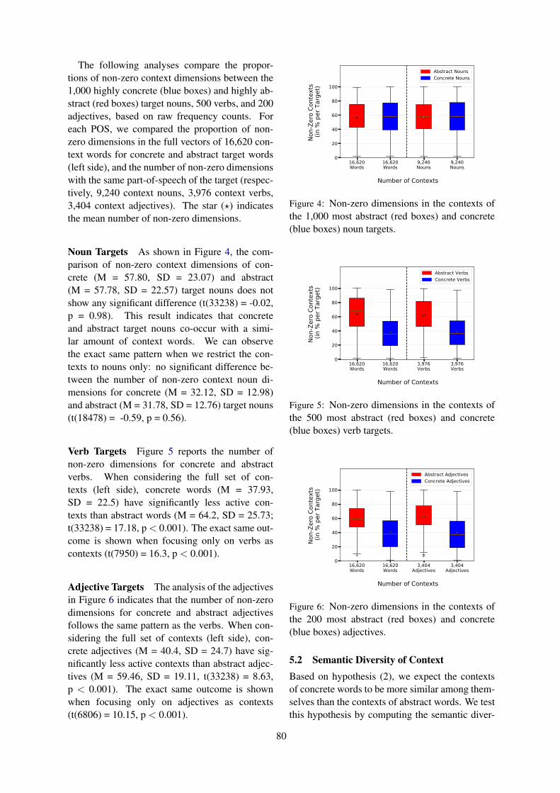
The following analyses compare the propor-tions of non-zero context dimensions between the1,000 highly concrete (blue boxes) and highly ab-stract (red boxes) target nouns, 500 verbs, and 200adjectives, based on raw frequency counts. Foreach POS, we compared the proportion of non-zero dimensions in the full vectors of 16,620 con-text words for concrete and abstract target words(left side), and the number of non-zero dimensionswith the same part-of-speech of the target (respec-tively, 9,240 context nouns, 3,976 context verbs,3,404 context adjectives). The star (?) indicatesthe mean number of non-zero dimensions.
Noun Targets As shown in Figure 4, the com-parison of non-zero context dimensions of con-crete (M = 57.80, SD = 23.07) and abstract(M = 57.78, SD = 22.57) target nouns does notshow any significant difference (t(33238) = -0.02,p = 0.98). This result indicates that concreteand abstract target nouns co-occur with a simi-lar amount of context words. We can observethe exact same pattern when we restrict the con-texts to nouns only: no significant difference be-tween the number of non-zero context noun di-mensions for concrete (M = 32.12, SD = 12.98)and abstract (M = 31.78, SD = 12.76) target nouns(t(18478) = -0.59, p = 0.56).
Verb Targets Figure 5 reports the number ofnon-zero dimensions for concrete and abstractverbs. When considering the full set of con-texts (left side), concrete words (M = 37.93,SD = 22.5) have significantly less active con-texts than abstract words (M = 64.2, SD = 25.73;t(33238) = 17.18, p < 0.001). The exact same out-come is shown when focusing only on verbs ascontexts (t(7950) = 16.3, p < 0.001).
Adjective Targets The analysis of the adjectivesin Figure 6 indicates that the number of non-zerodimensions for concrete and abstract adjectivesfollows the same pattern as the verbs. When con-sidering the full set of contexts (left side), con-crete adjectives (M = 40.4, SD = 24.7) have sig-nificantly less active contexts than abstract adjec-tives (M = 59.46, SD = 19.11, t(33238) = 8.63,p < 0.001). The exact same outcome is shownwhen focusing only on adjectives as contexts(t(6806) = 10.15, p < 0.001).
16,620Words
16,620Words
9,240Nouns
9,240Nouns
Number of Contexts
0
20
40
60
80
100
Non-
Zero
Con
text
s (i
n %
per
Tar
get)
Abstract NounsConcrete Nouns
Figure 4: Non-zero dimensions in the contexts ofthe 1,000 most abstract (red boxes) and concrete(blue boxes) noun targets.
16,620Words
16,620Words
3,976Verbs
3,976Verbs
Number of Contexts
0
20
40
60
80
100
Non-
Zero
Con
text
s (i
n %
per
Tar
get)
Abstract VerbsConcrete Verbs
Figure 5: Non-zero dimensions in the contexts ofthe 500 most abstract (red boxes) and concrete(blue boxes) verb targets.
16,620Words
16,620Words
3,404Adjectives
3,404Adjectives
Number of Contexts
0
20
40
60
80
100
Non-
Zero
Con
text
s (i
n %
per
Tar
get)
Abstract AdjectivesConcrete Adjectives
Figure 6: Non-zero dimensions in the contexts ofthe 200 most abstract (red boxes) and concrete(blue boxes) adjectives.
5.2 Semantic Diversity of ContextBased on hypothesis (2), we expect the contextsof concrete words to be more similar among them-selves than the contexts of abstract words. We testthis hypothesis by computing the semantic diver-
80
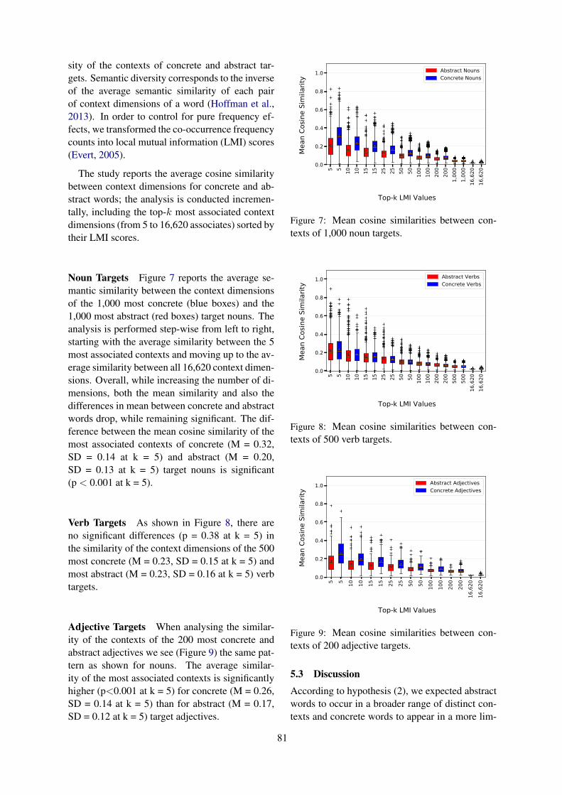
sity of the contexts of concrete and abstract tar-gets. Semantic diversity corresponds to the inverseof the average semantic similarity of each pairof context dimensions of a word (Hoffman et al.,2013). In order to control for pure frequency ef-fects, we transformed the co-occurrence frequencycounts into local mutual information (LMI) scores(Evert, 2005).
The study reports the average cosine similaritybetween context dimensions for concrete and ab-stract words; the analysis is conducted incremen-tally, including the top-k most associated contextdimensions (from 5 to 16,620 associates) sorted bytheir LMI scores.
Noun Targets Figure 7 reports the average se-mantic similarity between the context dimensionsof the 1,000 most concrete (blue boxes) and the1,000 most abstract (red boxes) target nouns. Theanalysis is performed step-wise from left to right,starting with the average similarity between the 5most associated contexts and moving up to the av-erage similarity between all 16,620 context dimen-sions. Overall, while increasing the number of di-mensions, both the mean similarity and also thedifferences in mean between concrete and abstractwords drop, while remaining significant. The dif-ference between the mean cosine similarity of themost associated contexts of concrete (M = 0.32,SD = 0.14 at k = 5) and abstract (M = 0.20,SD = 0.13 at k = 5) target nouns is significant(p < 0.001 at k = 5).
Verb Targets As shown in Figure 8, there areno significant differences (p = 0.38 at k = 5) inthe similarity of the context dimensions of the 500most concrete (M = 0.23, SD = 0.15 at k = 5) andmost abstract (M = 0.23, SD = 0.16 at k = 5) verbtargets.
Adjective Targets When analysing the similar-ity of the contexts of the 200 most concrete andabstract adjectives we see (Figure 9) the same pat-tern as shown for nouns. The average similar-ity of the most associated contexts is significantlyhigher (p<0.001 at k = 5) for concrete (M = 0.26,SD = 0.14 at k = 5) than for abstract (M = 0.17,SD = 0.12 at k = 5) target adjectives.
5 5 10 10 15 15 25 25 50 50 100
100
200
200
1,00
01,
000
16,6
2016
,620
Top-k LMI Values
0.0
0.2
0.4
0.6
0.8
1.0
Mea
n Co
sine
Sim
ilarit
y
Abstract NounsConcrete Nouns
Figure 7: Mean cosine similarities between con-texts of 1,000 noun targets.
5 5 10 10 15 15 25 25 50 50 100
100
200
200
500
500
16,6
2016
,620
Top-k LMI Values
0.0
0.2
0.4
0.6
0.8
1.0
Mea
n Co
sine
Sim
ilarit
y
Abstract VerbsConcrete Verbs
Figure 8: Mean cosine similarities between con-texts of 500 verb targets.
5 5 10 10 15 15 25 25 50 50 100
100
200
200
16,6
2016
,620
Top-k LMI Values
0.0
0.2
0.4
0.6
0.8
1.0
Mea
n Co
sine
Sim
ilarit
y
Abstract AdjectivesConcrete Adjectives
Figure 9: Mean cosine similarities between con-texts of 200 adjective targets.
5.3 Discussion
According to hypothesis (2), we expected abstractwords to occur in a broader range of distinct con-texts and concrete words to appear in a more lim-
81

ited set of different contexts. Moreover, the con-texts of concrete words should be more restrictedand more similar to each other compared to thecontexts of abstract words. The results discussedonly partially support this hypothesis.
The analysis of the number of non-zero contextdimensions for concrete and abstract target verbsand adjectives show results in line with hypothe-sis (2). On the contrary, concrete and abstract tar-get nouns share the same number of non-zero di-mensions. The analysis of the similarity betweencontexts of concrete and abstract target nouns andadjectives supports our hypothesis; while we donot see any significant difference when analysingthe verbs.
6 Study 3: Entropy of Concrete andAbstract Words
In this study we test our third hypothesis: abstractwords are more difficult to predict than concretewords, due to their higher contextual variability. Instudy 2 we already started investigating this phe-nomenon using semantic diversity. In the currentstudy we will use entropy as a measure of variabil-ity (Shannon, 2001):
H(X) = −∑
x∈Xp(x)log2p(x) (1)
Based on the assumption that abstract words oc-cur within a high number of distinct contexts, weexpect the entropy of abstract words to be higherthan the entropy of concrete words.
Noun Targets Figure 10 reports the average en-tropy in the context of the top 1,000 most abstract(on the left side) and most concrete (on the rightside) target nouns. Regarding the 1,000 most ab-stract target nouns, the entropy of the 1,000 mostabstract context nouns (M = 7.42, SD = 0.58)is significantly higher (p < 0.001) than the en-tropy of the 1,000 most concrete context nouns(M = 6.44, SD = 0.77). A similar pattern emergesin the analysis of the entropy of the contexts ofthe 1,000 most concrete target nouns: the differ-ence between concrete (M = 6.64, SD = 0.61) andabstract contexts (M = 7.21, SD = 0.54) is statisti-cally significant (p < 0.001).
Verb Targets Similarly to nouns (see Fig-ure 11), also the abstract contexts of both con-crete and abstract target verbs show significantly(p < 0.001) higher entropy (concrete target:
M = 6.1, SD = 0.58; abstract target: M = 6.55,SD = 0.49) than the entropy of their concrete con-texts (concrete target: M = 4.70, SD = 0.89; ab-stract target: M = 5.50, SD = 0.86).
1,000 AbstractNouns
1,000 Concrete
Nouns
1,000AbstractNouns
1,000Concrete
Nouns
Number of Contexts
0
2
4
6
8
10
12
Entro
py V
alue
Abstract NounsConcrete Nouns
Figure 10: Entropy of 1,000 most abstract (leftside) and 1,000 most concrete (right side) nountargets.
500 Abstract
Verbs
500 Concrete
Verbs
500Abstract
Verbs
500Concrete
Verbs
Number of Contexts
0
2
4
6
8
10
12
Entro
py V
alue
Abstract VerbsConcrete Verbs
Figure 11: Entropy of 500 most abstract (left side)and 500 most concrete (right side) verbs targets.
200 Abstract
Adjectives
200 ConcreteAdjectives
200Abstract
Adjectives
200ConcreteAdjectives
Number of Contexts
0
2
4
6
8
10
12
Entro
py V
alue
Abstract AdjectivesConcrete Adjectives
Figure 12: Entropy of 200 most abstract (left side)and 200 most concrete (right side) adjectives tar-gets.
Adjective Targets The same pattern seen fornouns and verbs (see Figure 12) describes also
82
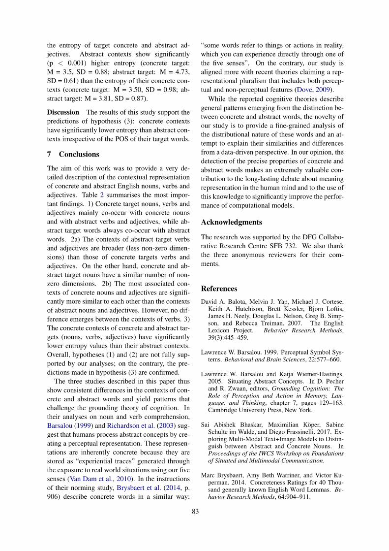
the entropy of target concrete and abstract ad-jectives. Abstract contexts show significantly(p < 0.001) higher entropy (concrete target:M = 3.5, SD = 0.88; abstract target: M = 4.73,SD = 0.61) than the entropy of their concrete con-texts (concrete target: M = 3.50, SD = 0.98; ab-stract target: M = 3.81, SD = 0.87).
Discussion The results of this study support thepredictions of hypothesis (3): concrete contextshave significantly lower entropy than abstract con-texts irrespective of the POS of their target words.
7 Conclusions
The aim of this work was to provide a very de-tailed description of the contextual representationof concrete and abstract English nouns, verbs andadjectives. Table 2 summarises the most impor-tant findings. 1) Concrete target nouns, verbs andadjectives mainly co-occur with concrete nounsand with abstract verbs and adjectives, while ab-stract target words always co-occur with abstractwords. 2a) The contexts of abstract target verbsand adjectives are broader (less non-zero dimen-sions) than those of concrete targets verbs andadjectives. On the other hand, concrete and ab-stract target nouns have a similar number of non-zero dimensions. 2b) The most associated con-texts of concrete nouns and adjectives are signifi-cantly more similar to each other than the contextsof abstract nouns and adjectives. However, no dif-ference emerges between the contexts of verbs. 3)The concrete contexts of concrete and abstract tar-gets (nouns, verbs, adjectives) have significantlylower entropy values than their abstract contexts.Overall, hypotheses (1) and (2) are not fully sup-ported by our analyses; on the contrary, the pre-dictions made in hypothesis (3) are confirmed.
The three studies described in this paper thusshow consistent differences in the contexts of con-crete and abstract words and yield patterns thatchallenge the grounding theory of cognition. Intheir analyses on noun and verb comprehension,Barsalou (1999) and Richardson et al. (2003) sug-gest that humans process abstract concepts by cre-ating a perceptual representation. These represen-tations are inherently concrete because they arestored as “experiential traces” generated throughthe exposure to real world situations using our fivesenses (Van Dam et al., 2010). In the instructionsof their norming study, Brysbaert et al. (2014, p.906) describe concrete words in a similar way:
“some words refer to things or actions in reality,which you can experience directly through one ofthe five senses”. On the contrary, our study isaligned more with recent theories claiming a rep-resentational pluralism that includes both percep-tual and non-perceptual features (Dove, 2009).
While the reported cognitive theories describegeneral patterns emerging from the distinction be-tween concrete and abstract words, the novelty ofour study is to provide a fine-grained analysis ofthe distributional nature of these words and an at-tempt to explain their similarities and differencesfrom a data-driven perspective. In our opinion, thedetection of the precise properties of concrete andabstract words makes an extremely valuable con-tribution to the long-lasting debate about meaningrepresentation in the human mind and to the use ofthis knowledge to significantly improve the perfor-mance of computational models.
Acknowledgments
The research was supported by the DFG Collabo-rative Research Centre SFB 732. We also thankthe three anonymous reviewers for their com-ments.
ReferencesDavid A. Balota, Melvin J. Yap, Michael J. Cortese,
Keith A. Hutchison, Brett Kessler, Bjorn Loftis,James H. Neely, Douglas L. Nelson, Greg B. Simp-son, and Rebecca Treiman. 2007. The EnglishLexicon Project. Behavior Research Methods,39(3):445–459.
Lawrence W. Barsalou. 1999. Perceptual Symbol Sys-tems. Behavioral and Brain Sciences, 22:577–660.
Lawrence W. Barsalou and Katja Wiemer-Hastings.2005. Situating Abstract Concepts. In D. Pecherand R. Zwaan, editors, Grounding Cognition: TheRole of Perception and Action in Memory, Lan-guage, and Thinking, chapter 7, pages 129–163.Cambridge University Press, New York.
Sai Abishek Bhaskar, Maximilian Koper, SabineSchulte im Walde, and Diego Frassinelli. 2017. Ex-ploring Multi-Modal Text+Image Models to Distin-guish between Abstract and Concrete Nouns. InProceedings of the IWCS Workshop on Foundationsof Situated and Multimodal Communication.
Marc Brysbaert, Amy Beth Warriner, and Victor Ku-perman. 2014. Concreteness Ratings for 40 Thou-sand generally known English Word Lemmas. Be-havior Research Methods, 64:904–911.
83

POS PrimaryCo-Occurrence
Semantic Diversityof Context
Entropy
concrete nounsconcrete nouns similar number of contexts;
high context similaritylowabstract verbs
abstract adjectives
abstract nounsabstract nouns similar number of contexts;
low context similarityhighabstract verbs
abstract adjectives
concrete verbsconcrete nouns low number of contexts;
similar context similaritylowabstract verbs
abstract adjectives
abstract verbsabstract nouns high number of contexts;
similar context similarityhighabstract verbs
abstract adjectives
concrete adjectivesconcrete nouns low number of contexts;
high context similaritylowabstract verbs
abstract adjectives
abstract adjectivesabstract nouns high number of contexts;
low context similarityhighabstract verbs
abstract adjectives
Table 2: Overview of our main findings.
L. Burnard. 2000. Reference Guide for the British Na-tional Corpus (world edition).
Guy Dove. 2009. Beyond Perceptual Symbols: aCall for Representational Pluralism. Cognition,110(3):412–31.
Stefan Evert. 2005. The Statistics of Word Co-Occurrences: Word Pairs and Collocations. Ph.D.thesis, Institut fur Maschinelle Sprachverarbeitung,Universitat Stuttgart.
John R. Firth. 1968. A Synopsis of Linguistic Theory,1930–55. In Frank R. Palmer, editor, Selected Pa-pers of J.R. Firth 1952–59, Longman’s LinguisticsLibrary, pages 168–205. Longmans.
Diego Frassinelli, Daniela Naumann, Jason Utt, andSabine Schulte im Walde. 2017. Contextual Char-acteristics of Concrete and Abstract Words. In Pro-ceedings of the 12th International Conference onComputational Semantics, Montpellier, France.
Arthur M. Glenberg and Michael P. Kaschak. 2002.Grounding Language in Action. Psychonomic Bul-letin and Review, 9(3):558–565.
Zellig S. Harris. 1954. Distributional structure. Word,10(2-3):146–162.
Felix Hill, Anna Korhonen, and Christian Bentz.2014. A Quantitative Empirical Analysis of theAbstract/Concrete Distinction. Cognitive Science,38(1):162–177.
Paul Hoffman, Matthew A. Lambon Ralph, and Tim-othy T. Rogers. 2013. Semantic Diversity: A Mea-sure of Semantic Ambiguity Based on Variability inthe Contextual Usage of Words. Behavior ResearchMethods, 45(3):718–730.
Paul Hoffman and Anna M. Woollams. 2015. Oppos-ing Effects of Semantic Diversity in Lexical and Se-mantic Relatedness Decisions. Journal of Experi-mental Psychology: Human Perception and Perfor-mance, 41(2):385.
Maximilian Koper and Sabine Schulte im Walde. 2016.Distinguishing Literal and Non-Literal Usage ofGerman Particle Verbs. In Proceedings of the Con-ference of the North American Chapter of the As-sociation for Computational Linguistics: HumanLanguage Technologies, pages 353–362, San Diego,California, USA.
Maximilian Koper and Sabine Schulte im Walde. 2017.Improving Verb Metaphor Detection by Propagat-ing Abstractness to Words, Phrases and IndividualSenses. In Proceedings of the 1st Workshop onSense, Concept and Entity Representations and theirApplications, pages 24–30, Valencia, Spain.
Ken McRae and Michael Jones. 2013. Semantic Mem-ory. The Oxford Handbook of Cognitive Psychology,206.
Diane Pecher, Inge Boot, and Saskia Van Dantzig.2011. Abstract Concepts. Sensory-Motor Ground-ing, Metaphors, and Beyond. Psychology of Learn-
84
ing and Motivation – Advances in Research and The-ory, 54:217–248.
Daniel C. Richardson, Michael J. Spivey, Lawrence W.Barsalou, and Ken McRae. 2003. Spatial Represen-tations Activated during Real-Time Comprehensionof Verbs. Cognitive Science, 27(5):767–780.
Roland Schafer and Felix Bildhauer. 2012. BuildingLarge Corpora from the Web Using a New EfficientTool Chain. In Proceedings of the 8th InternationalConference on Language Resources and Evaluation,pages 486–493, Istanbul, Turkey.
Helmut Schmid. 1994. Probabilistic Part-of-SpeechTagging Using Decision Trees. In Proceedings ofthe 1st International Conference on New Methods inLanguage Processing.
Paula J Schwanenflugel and Edward J Shoben. 1983.Differential context effects in the comprehension ofabstract and concrete verbal materials. Journal ofExperimental Psychology: Learning, Memory, andCognition, 9(1):82.
Claude E. Shannon. 2001. A Mathematical Theory ofCommunication. ACM SIGMOBILE Mobile Com-puting and Communications Review, 5(1):3–55.
Peter Turney, Yair Neuman, Dan Assaf, and Yohai Co-hen. 2011. Literal and Metaphorical Sense Identi-fication through Concrete and Abstract Context. InProceedings of the Conference on Empirical Meth-ods in Natural Language Processing, pages 680–690, Edinburgh, UK.
Wessel O. Van Dam, Shirley-Ann Rueschemeyer,Oliver Lindemann, and Harold Bekkering. 2010.Context effects in embodied lexical-semantic pro-cessing. Frontiers in Psychology, 1.
Gabriella Vigliocco, Stavroula-Thaleia Kousta,Pasquale Anthony Della Rosa, David P. Vinson,Marco Tettamanti, Joseph T. Devlin, and Stefano F.Cappa. 2014. The Neural Representation of Ab-stract Words: The Role of Emotion. CerebralCortex, 24(7):1767–1777.
Amy Beth Warriner, Victor Kuperman, and Marc Brys-baert. 2013. Norms of Valence, Arousal, and Dom-inance for 13,915 English Lemmas. Behavior Re-search Methods, 45(4):1191–1207.
85

Proceedings of the 7th Joint Conference on Lexical and Computational Semantics (*SEM), pages 86–93New Orleans, June 5-6, 2018. c©2018 Association for Computational Linguistics
EmoWordNet: Automatic Expansion of Emotion Lexicon Using EnglishWordNet
Gilbert Badaro, Hussein Jundi†, Hazem Hajj, Wassim El-Hajj†Department of Electrical & Computer Engineering
†Department of Computer ScienceAmerican University of Beirut
Beirut, Lebanon{ggb05;haj14;hh63;we07}@aub.edu.lb
Abstract
Nowadays, social media have become a plat-form where people can easily express theiropinions and emotions about any topic suchas politics, movies, music, electronic prod-ucts and many others. On the other hand,politicians, companies, and businesses are in-terested in analyzing automatically people’sopinions and emotions. In the last decade, alot of efforts has been put into extracting sen-timent polarity from texts. Recently, the focushas expanded to also cover emotion recogni-tion from texts. In this work, we expand anexisting emotion lexicon, DepecheMood, byleveraging semantic knowledge from EnglishWordNet (EWN). We create an expanded lex-icon, EmoWordNet, consisting of 67K termsaligned with EWN, almost 1.8 times the size ofDepecheMood. We also evaluate EmoWord-Net in an emotion recognition task using Se-mEval 2007 news headlines dataset and weachieve an improvement compared to the useof DepecheMood. EmoWordNet is publiclyavailable to speed up research in the field onhttp://oma-project.com.
1 Introduction
Emotion recognition models have been exten-sively explored based on different modalities suchas human computer interaction (Cowie et al.,2001; Pantic and Rothkrantz, 2003; Fragopanagosand Taylor, 2005; Jaimes and Sebe, 2007; Hibbelnet al., 2017; Patwardhan and Knapp, 2017; Con-stantine et al., 2016) and facial images and ex-pressions (Goldman and Sripada, 2005; Gunes andPiccardi, 2007; Trad et al., 2012; Wegrzyn et al.,2017). Recently, special attention has been givento emotion recognition from text (Wu et al., 2006;Alm et al., 2005; Shaheen et al., 2014; Abdul-Mageed and Ungar, 2017; Badaro et al., 2018b,a).In fact, a tremendous amount of opinionated andemotionally charged text data is nowadays avail-
able on the Internet due to the increase of num-ber of users of social networks such as Twitter andFacebook. For instance, Facebook reached morethan 2 billion users on September 2017.1 Rec-ognizing emotions from text has several applica-tions: first, it helps companies and businesses inshaping their marketing strategies based on con-sumers’ emotions (Bougie et al., 2003); second,it allows improving typical collaborative filteringbased recommender systems (Badaro et al., 2013,2014c,d) in terms of products or advertisementsrecommendations (Mohammad and Yang, 2011);third, politicians can learn how to adapt their polit-ical speech based on people emotions (Pang et al.,2008) and last but not least emotion classificationhelps in stock market predictions (Bollen et al.,2011).
While plenty of works exist for sentiment anal-ysis for different languages including analysisof social media data for sentiment characteris-tics (Al Sallab et al., 2015; Baly et al., 2014,2017b,a), few works focused on emotion recogni-tion from text. Since sentiment lexicons helpedin improving the accuracy of sentiment classifi-cation models (Liu and Zhang, 2012; Al-Sallabet al., 2017; Badaro et al., 2014a,b, 2015), sev-eral researchers are working on developing emo-tion lexicons for different languages such as En-glish, French, Polish and Chinese (Mohammad,2017; Bandhakavi et al., 2017; Yang et al., 2007;Poria et al., 2012; Mohammad and Turney, 2013;Das et al., 2012; Mohammad et al., 2013; Abdaouiet al., 2017; Staiano and Guerini, 2014; Maziarzet al., 2016; Janz et al., 2017). While sentimentis usually represented by three labels namely pos-itive, negative or neutral, several representationmodels exist for emotions such as Ekman repre-sentation (Ekman, 1992) (happiness, sadness, fear,
1https://www.statista.com/statistics/272014/global-social-networks-ranked-by-number-of-users/
86

anger, surprise and disgust) or Plutchik model(Plutchik, 1994) that includes trust and anticipa-tion in addition to Ekman’s six emotions. De-spite the efforts for creating large scale emotionlexicons for English, the size of existing emo-tion lexicons remain much smaller compared tosentiment lexicons. For example, DepecheMood(Staiano and Guerini, 2014), one of the largestpublicly available emotion lexicon for English,includes around 37K terms while SentiWordNet(SWN) (Esuli and Sebastiani, 2007; Baccianellaet al., 2010), a large scale English sentimentlexicon semi-automatically generated using En-glish WordNet (EWN) (Fellbaum, 1998), includesaround 150K terms annotated with three sentimentscores: positive, negative and objective.
In this paper, we focus on expanding cov-erage of existing emotion lexicon, namely De-pecheMood, using the synonymy semantic rela-tion available in English WordNet. We decide toexpand DepecheMood since it is one of the largestemotion lexicon publicly available, and since itsterms are aligned with EWN, thus allowing us tobenefit from powerful semantic relations in EWN.
The paper is organized as follows. In section2, we conduct a brief literature survey on existingemotion lexicons. In section 3, we describe theexpansion approach to build EmoWordNet. In sec-tion 4, we compare the performance of EmoWord-Net against DepecheMood using SemEval 2007dataset and in section 5, we present a conclusionof our results and future work.
2 Literature Review
Strapparava et al. (2004) developed WordNet Af-fect by tagging specific synsets with affectivemeanings in EWN. They identified first a corenumber of synsets that represent emotions of alexical database for emotions. They expandedthen the coverage of the lexicon by checking se-mantically related synsets compared to the coreset. They were able to annotate 2,874 synsets and4,787 words. WordNet Affect was also tested indifferent applications such as affective text sens-ing systems and computational humor. WordNetAffect is of good quality given that it was manu-ally created and validated, however, it is of limitedsize. Mohammad and Turney (2013) presentedchallenges that researchers face for developingemotion lexicons and devised an annotation strat-egy to create a good quality and inexpensive emo-
tion lexicon, EmoLex, by utilizing crowdsourc-ing. To create EmoLex, the authors first identifiedtarget terms for annotation extracted from Mac-quarie Thesaurus (Bernard and Bernard, 1986),WordNet Affect and the General Inquirer (Stoneet al., 1966). Then, they launched the annota-tion task on Amazon’s Mechanical Turk. EmoLexhas around 10K terms annotated for emotions aswell as for sentiment polarities. They evaluatedthe annotation quality using different techniquessuch as computing inter-annotator agreement andcomparing a subsample of EmoLex with existinggold data. AffectNet (Cambria et al., 2012), partof the SenticNet project, includes also around 10Kterms extracted from ConceptNet (Liu and Singh,2004) and aligned with WordNet Affect. Theyextended WordNet Affect using the concepts inConceptNet. While WordNet Affect, EmoLex andAffectNet include terms with emotion labels, Af-fect database (Neviarouskaya et al., 2007) and De-pecheMood (Staiano and Guerini, 2014) includewords that have emotion scores instead, whichcan be useful for compositional computations ofemotion scores. Affect database extends SentiFuland covers around 2.5K words presented in theirlemma form along with the corresponding part ofspeech (POS) tag. DepecheMood was automat-ically built by harvesting social media data thatwere implicitly annotated with emotions. Staianoand Guerini (2014) utilized news articles from rap-pler.com. The articles are accompanied by Rap-pler’s Mood Meter, which allows readers to ex-press their emotions about the article they are read-ing. DepecheMood includes around 37K lemmasalong with their part of speech tags and the lem-mas are aligned with EWN. Staiano and Guerinialso evaluated DepecheMood in emotion regres-sion and classification tasks in unsupervised set-tings. They claim that although they utilized anaıve unsupervised model, they were able to out-perform existing lexicons when applied on Se-mEval 2007 dataset (Strapparava and Mihalcea,2007). Since DepecheMood is aligned with EWN,is publicly available and has a better coverage andclaimed performance compared to existing emo-tion lexicons, we decide to expand it using EWNsemantic relations as described below in section 3.
To summarize, there are mainly two approachesthat have been followed for building emotion lex-icons for English. The first set of methods relieson manual annotation either done by specific indi-
87

viduals or through crowdsourcing, where the listof words is extracted from lexical resources. Thesecond approach is automatic or semi-automaticand is based on annotated corpora for emotion.The first approach tends to produce limited sizeand highly accurate emotion lexicons but it is rel-atively expensive. On the other hand, the secondapproach is cheap and results in large scale emo-tion lexicons but with lower accuracy compared tomanually developed emotion lexicons in terms ofaccurately representing the emotion of the term.
3 EmoWordNet
In this section, we describe the approach wefollowed in order to expand DepecheMood andbuild EmoWordNet. DepecheMood consists of37,771 lemmas along with their correspondingPOS tags where each entry is appended withscores for 8 emotion labels: afraid, amused, an-gry, annoyed, don’t care, happy, inspired andsad. Three variations of score representations ex-ist for DepecheMood. We select to expand theDepecheMood variation with normalized scoressince this variation performed best according tothe presented results in (Staiano and Guerini,2014).
In Fig. 1, we show an overview of the stepsfollowed to expand DepecheMood.
Figure 1: Overview of DepecheMood Expansion Ap-proach.
Step 1: EWN synsets that include lemmas ofDepecheMood were retrieved. A score was thencomputed for each retrieved synset, s. Let S de-notes the set of all such synsets. Two cases mightappear: either the retrieved synset included onlyone lemma from DepecheMood, in this case thesynset was assigned the same score of the lemma,or, the synset included multiple lemmas that exist
in DepecheMood, in this case the synset’s scorewas the average of the scores of its correspondinglemmas. Step 2: A synset, s, includes two set ofterms: T, terms that are in DepecheMood, and T ,terms not in DepecheMood. Using the synonymysemantic relation in EWN, and based on the con-cept that synonym words would likely share thesame emotion scores, we assigned the synset’sscores to its corresponding terms T . Again, a termt in T might appear in one or multiple synsets fromS. Hence, the score assigned to t would be eitherthe one of its corresponding synset or the averageof the scores of its corresponding synsets that be-long to S. Step 3: after performing step 2, newsynsets might be explored. Terms in T might alsoappear in synsets s that do not belong to S. s wouldget the score of its corresponding terms. Step 2and 3 were repeated until no new terms or synsetswere added and scores of added terms converged.It is important to note that we decided to consideronly synonyms for expansion since synonymy isthe only semantic relation that mostly preservesthe emotion orientation and does not require man-ual validation as described by Strapparava et al.(2004).
As a walking example of the steps describedabove, let us consider the DepecheMood term“bonding” having noun as POS tag. “bond-ing” can be found in three different EWN nounsynsets with the following offset IDs: “00148653;05665769; 13781820”. Since “bonding” is theonly term having a DepecheMood representationin the three synsets, the three synsets will have thesame emotion scores as “bonding”. While synsets“05665769; 13781820” have only the term “bond-ing”, “00148653” includes as well the lemma “sol-dering” which is not in DepecheMood. Thus, fromstep 2, “soldering” will have the same scores as“bonding”. “soldering” does not appear in anyother EWN synset so there are no more iterations.
Using the described automatic expansion ap-proach, we were able to extend the size of De-pecheMood by a factor of 1.8. We obtained emo-tion scores for an additional 29,967 EWN termsand for 59,952 EWN synsets. Overall, we con-struct EmoWordNet, an emotion lexicon consist-ing of 67,738 EWN terms and of 59,952 EWNsynsets annotated with emotion scores.
Next, we present a simple extrinsic evaluationof EmoWordNet similar to the one performed forDepecheMood.
88

4 Evaluation of EmoWordNet
In this section, we evaluate the effectiveness ofEmoWordNet in emotion recognition task fromtext. We evaluate regression as well as classi-fication of emotions in unsupervised settings us-ing similar techniques used for evaluating De-pecheMood.
4.1 Dataset & Coverage
We utilized the dataset provided publicly by Se-mEval 2007 task on Affective text (Strapparavaand Mihalcea, 2007). The dataset consists of onethousand news headlines annotated with six emo-tion scores: anger, disgust, fear, joy, sadness andsurprise. For the regression task, a score between0 and 1 is provided for each emotion. For theclassification task, a threshold is applied on theemotion scores to get a binary representation ofthe emotions: if the score of a certain emotionis greater than 0.5, the corresponding emotion la-bel is set to 1, otherwise it is 0. The emotion la-bels used in the dataset correspond to the six emo-tions of the Ekman model (Ekman, 1992) whilethose in EmoWordNet, as well as DepecheMood,follow the ones provided by Rappler Mood Me-ter. We considered the same emotion mapping as-sumptions presented in the work of (Staiano andGuerini, 2014): Fear→ Afraid, Anger→ Angry,Joy → Happy, Sadness → Sad and Surprise →Inspired. Disgust was not aligned with any emo-tion in EmoWordNet and hence was discarded asalso assumed in (Staiano and Guerini, 2014). Oneimportant aspect of the extrinsic evaluation waschecking the coverage of EmoWordNet againstSemEval dataset. In order to compute coverage,we performed lemmatization of the news head-lines using WordNet lemmatizer available throughPython NLTK package. We excluded all wordswith POS tags different than noun, verb, adjec-tive and adverb. EmoWordNet achieved a cover-age of 68.6% while DepecheMood had a cover-age of 67.1%. An increase in coverage was ex-pected but since the size of the dataset is rela-tively small, the increase was only around 1.5%.In terms of headline coverage, only one headline(“Toshiba Portege R400”) was left without anyemotion scores when using both EmoWordNet andDepecheMood since none of its terms were foundin any of the two lexicons.
4.2 Regression and Classification Results
We followed an approach similar to the one pre-sented for evaluating DepecheMood. For prepro-cessing, we first lemmatized the headlines usingWordNet lemmatizer available in Python NLTKpackage. We also accounted for multi-word termsthat were solely available in EmoWordNet bylooking at n-grams (up to n=3) after lemmatiza-tion. We then removed all terms that did not be-long to any of the four POS tags: noun, verb,adjective and adverbs. For features computation,we considered two variations: the sum and theaverage of the emotion scores for the five emo-tion labels that overlapped between EmoWordNetand SemEval dataset. Using average turned out toperform better than when using sum for both lex-icons. As stated in (Staiano and Guerini, 2014)paper, ‘Disgust’ emotion was excluded since therewas no corresponding mapping in EmoWord-Net/DepecheMood. The first evaluation consistedof measuring Pearson Correlation between thescores computed using the lexicons and those pro-vided in SemEval. The results are reported in Ta-ble 1. We could see that the results are relativelyclose to each other: EmoWordNet slightly outper-formed DepecheMood for the five different emo-tions. It was expected to have close results giventhat the coverage of EmoWordNet is very close toDepecheMood. Given the slight improvement, weexpect EmoWordNet to perform much better onlarger datasets.
For the classification task, we first transformedthe numerical emotion scores of the headlines to abinary representation. We applied min-max nor-malization on the computed emotion scores perheadline, and then assigned a ‘1’ for the emotionlabel with score greater than ‘0.5’, and a ‘0’ other-wise. We used F1 measure for evaluation. Resultsare shown in Table 2. More significant improve-ment was observed in classification task comparedto regression task when using EmoWordNet.
4.3 Results Analysis
In this section, we present some quantitative andqualitative analyses of the results. For quantita-tive analysis, we checked first whether the countof terms in a headline is correlated with having acorrect emotion classification. Overall, the lengthof headlines was varying between 2 and 15 terms.Headlines with length between 5 and 10 termswere mostly correctly classified. Hence, one can
89
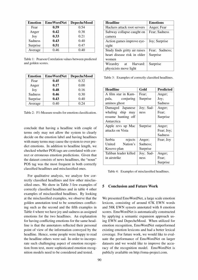
Emotion EmoWordNet DepecheMoodFear 0.59 0.54
Anger 0.42 0.38Joy 0.33 0.21
Sadness 0.43 0.40Surprise 0.51 0.47Average 0.46 0.40
Table 1: Pearson Correlation values between predictedand golden scores.
Emotion EmoWordNet DepecheMoodFear 0.45 0.32
Anger 0.17 0.00Joy 0.48 0.16
Sadness 0.46 0.30Surprise 0.43 0.40Average 0.40 0.24
Table 2: F1-Measure results for emotion classification.
conclude that having a headline with couple ofterms only may not allow the system to clearlydecide on the emotion label and having headlineswith many terms may cause the system to over pre-dict emotions. In addition to headline length, wechecked whether POS tags are correlated with cor-rect or erroneous emotion predictions. Given thatthe dataset consists of news headlines, the “noun”POS tag was the most frequent in both correctlyclassified headlines and misclassified ones.
For qualitative analysis, we analyze few cor-rectly classified headlines and few other misclas-sified ones. We show in Table 3 few examples ofcorrectly classified headlines and in table 4 otherexamples of misclassified headlines. By lookingat the misclassified examples, we observe that thegolden annotation tend to be sometimes conflict-ing such as the second and the fifth examples inTable 4 where we have joy and sadness as assignedemotions for the two headlines. An explanationfor having conflicting emotions for the same head-line is that the annotators reflected their personalpoint of view of the information conveyed by theheadline. Hence, some people were happy to readthe headline others were sad. In order to incorpo-rate such challenging aspect of emotion recogni-tion from text, more sophisticated emotion recog-nition models need to be considered and tested.
Headline EmotionsHackers attack root servers Anger; FearSubway collapse caught oncamera
Fear; Sadness
Action games improve eye-sight
Joy; Surprise
Study finds gritty air raisesheart disease risk in olderwomen
Fear; Sadness;Surprise
Wizardry at Harvard:physicists move light
Surprise
Table 3: Examples of correctly classified headlines.
Headline Gold PredictedA film star in Kam-pala, conjuringaminos ghost
Fear;Surprise
Anger;Joy;Sadness
Damaged Japanesewhaling ship mayresume hunting offAntarctica
Joy; Sad-ness
Anger;Fear;Surprise
Apple revs up Macattacks on Vista
Surprise Anger;Fear; Joy;Sadness
Serbia rejectsUnited Nation’sKosovo plan
Anger;Sadness;Surprise
Fear; Joy
Taliban leader killedin airstrike
Joy; Sad-ness
Anger;Fear;Surprise
Table 4: Examples of misclassified headlines.
5 Conclusion and Future Work
We presented EmoWordNet, a large scale emotionlexicon, consisting of around 67K EWN wordsand 58K EWN synsets annotated with 8 emotionscores. EmoWordNet is automatically constructedby applying a semantic expansion approach us-ing EWN and DepecheMood. When utilized foremotion recognition, EmoWordNet outperformedexisting emotion lexicons and had a better lexicalcoverage. For future work, we would like to eval-uate the performance of EmoWordNet on largerdatasets and we would like to improve the accu-racy of the recognition model. EmoWordNet ispublicly available on http://oma-project.com.
90

References
Amine Abdaoui, Jerome Aze, Sandra Bringay,and Pascal Poncelet. 2017. Feel: a french ex-panded emotion lexicon. Language Resourcesand Evaluation, 51(3):833–855.
Muhammad Abdul-Mageed and Lyle Ungar. 2017.Emonet: Fine–grained emotion detection withgated recurrent neural networks. In Proceedingsof the 55th Annual Meeting of the Associationfor Computational Linguistics (Volume 1: LongPapers), volume 1, pages 718–728.
Ahmad Al-Sallab, Ramy Baly, Hazem Hajj,Khaled Bashir Shaban, Wassim El-Hajj, andGilbert Badaro. 2017. Aroma: A recursive deeplearning model for opinion mining in arabic asa low resource language. ACM Transactionson Asian and Low-Resource Language Informa-tion Processing (TALLIP), 16(4):25.
Ahmad A Al Sallab, Ramy Baly, Gilbert Badaro,Hazem Hajj, Wassim El Hajj, and Khaled BShaban. 2015. Deep learning models for sen-timent analysis in arabic. In ANLP Workshop,volume 9.
Cecilia Ovesdotter Alm, Dan Roth, and RichardSproat. 2005. Emotions from text: machinelearning for text-based emotion prediction. InProceedings of the conference on human lan-guage technology and empirical methods in nat-ural language processing, pages 579–586. As-sociation for Computational Linguistics.
Stefano Baccianella, Andrea Esuli, and FabrizioSebastiani. 2010. Sentiwordnet 3.0: An en-hanced lexical resource for sentiment analysisand opinion mining. In LREC, volume 10, pages2200–2204.
Gilbert Badaro, Ramy Baly, Rana Akel, LindaFayad, Jeffrey Khairallah, Hazem Hajj, KhaledShaban, and Wassim El-Hajj. 2015. A lightlexicon-based mobile application for sentimentmining of arabic tweets. In Proceedings of theSecond Workshop on Arabic Natural LanguageProcessing, pages 18–25.
Gilbert Badaro, Ramy Baly, Hazem Hajj, NizarHabash, and Wassim El-Hajj. 2014a. A largescale Arabic sentiment lexicon for Arabic opin-ion mining. ANLP 2014, 165.
Gilbert Badaro, Ramy Baly, Hazem Hajj, NizarHabash, Wassim El-hajj, and Khaled Shaban.2014b. An efficient model for sentiment classi-fication of Arabic tweets on mobiles. In QatarFoundation Annual Research Conference, 1,page ITPP0631.
Gilbert Badaro, Obeida El Jundi, Alaa Khaddaj,Alaa Maarouf, Raslan Kain, Hazem Hajj, andWassim El-Hajj. 2018a. Ema at semeval-2018task 1: Emotion mining for arabic. In Pro-ceedings of International Workshop on Seman-tic Evaluation (SemEval-2018).
Gilbert Badaro, Hazem Hajj, Wassim El-Hajj, andLama Nachman. 2013. A hybrid approachwith collaborative filtering for recommendersystems. In Wireless Communications and Mo-bile Computing Conference (IWCMC), 2013 9thInternational, pages 349–354. IEEE.
Gilbert Badaro, Hazem Hajj, Ali Haddad, WassimEl-Hajj, and Khaled Bashir Shaban. 2014c. Amultiresolution approach to recommender sys-tems. In Proceedings of the 8th Workshop onSocial Network Mining and Analysis, page 9.ACM.
Gilbert Badaro, Hazem Hajj, Ali Haddad, Was-sim El-Hajj, and Khaled Bashir Shaban. 2014d.Recommender systems using harmonic analy-sis. In Data Mining Workshop (ICDMW), 2014IEEE International Conference on, pages 1004–1011. IEEE.
Gilbert Badaro, Hussein Jundi, Hazem Hajj, Was-sim El-Hajj, and Nizar Habash. 2018b. Arsel:A large scale arabic sentiment and emotion lex-icon. In Proceedings of the 3rd Workshop onOpen-Source Arabic Corpora and ProcessingTools (OSACT3) co-located with LREC2018.
Ramy Baly, Gilbert Badaro, Georges El-Khoury,Rawan Moukalled, Rita Aoun, Hazem Hajj,Wassim El-Hajj, Nizar Habash, and KhaledShaban. 2017a. A characterization study of ara-bic twitter data with a benchmarking for state-of-the-art opinion mining models. In Proceed-ings of the Third Arabic Natural Language Pro-cessing Workshop, pages 110–118.
Ramy Baly, Gilbert Badaro, Hazem Hajj, NizarHabash, Wassim El Hajj, and Khaled Shaban.
91

2014. Semantic model representation for hu-man’s pre-conceived notions in arabic text withapplications to sentiment mining. In QatarFoundation Annual Research Conference, 1,page ITPP1075.
Ramy Baly, Gilbert Badaro, Ali Hamdi, RawanMoukalled, Rita Aoun, Georges El-Khoury,Ahmad Al Sallab, Hazem Hajj, Nizar Habash,Khaled Shaban, et al. 2017b. Omam at semeval-2017 task 4: Evaluation of english state-of-the-art sentiment analysis models for arabic and anew topic-based model. In Proceedings of the11th International Workshop on Semantic Eval-uation (SemEval-2017), pages 603–610.
Anil Bandhakavi, Nirmalie Wiratunga, StewartMassie, and Deepak Padmanabhan. 2017. Lexi-con generation for emotion detection from text.IEEE intelligent systems, 32(1):102–108.
John Rupert Lyon-Bowes Bernard and John Ru-pert Lyon-Bowes Bernard. 1986. The Mac-quarie Thesaurus. Macquarie.
Johan Bollen, Huina Mao, and Xiaojun Zeng.2011. Twitter mood predicts the stock market.Journal of computational science, 2(1):1–8.
Roger Bougie, Rik Pieters, and Marcel Zeelen-berg. 2003. Angry customers don’t come back,they get back: The experience and behavioralimplications of anger and dissatisfaction in ser-vices. Journal of the Academy of Marketing Sci-ence, 31(4):377–393.
Erik Cambria, Catherine Havasi, and Amir Hus-sain. 2012. Senticnet 2: A semantic and affec-tive resource for opinion mining and sentimentanalysis. In FLAIRS conference, pages 202–207.
Layale Constantine, Gilbert Badaro, Hazem Hajj,Wassim El-Hajj, Lama Nachman, MohamedBenSaleh, and Abdulfattah Obeid. 2016. Aframework for emotion recognition from humancomputer interaction in natural setting. 22ndACM SIGKDD Conference on Knowledge Dis-covery and Data Mining (KDD 2016), Work-shop on Issues of Sentiment Discovery andOpinion Mining (WISDOM 2016).
Roddy Cowie, Ellen Douglas-Cowie, NicolasTsapatsoulis, George Votsis, Stefanos Kollias,
Winfried Fellenz, and John G Taylor. 2001.Emotion recognition in human-computer in-teraction. IEEE Signal processing magazine,18(1):32–80.
Dipankar Das, Soujanya Poria, and Sivaji Bandy-opadhyay. 2012. A classifier based approach toemotion lexicon construction. In NLDB, pages320–326. Springer.
Paul Ekman. 1992. An argument for basic emo-tions. Cognition & emotion, 6(3-4):169–200.
Andrea Esuli and Fabrizio Sebastiani. 2007. Sen-tiwordnet: A high-coverage lexical resource foropinion mining. Evaluation, pages 1–26.
Christiane Fellbaum. 1998. WordNet. Wiley On-line Library.
N Fragopanagos and John G Taylor. 2005. Emo-tion recognition in human–computer interac-tion. Neural Networks, 18(4):389–405.
Alvin I Goldman and Chandra Sekhar Sripada.2005. Simulationist models of face-based emo-tion recognition. Cognition, 94(3):193–213.
Hatice Gunes and Massimo Piccardi. 2007. Bi-modal emotion recognition from expressiveface and body gestures. Journal of Network andComputer Applications, 30(4):1334–1345.
Martin Hibbeln, Jeffrey L Jenkins, ChristophSchneider, Joseph S Valacich, and MarkusWeinmann. 2017. How is your user feeling?inferring emotion through human–computer in-teraction devices. MIS Quarterly, 41(1).
Alejandro Jaimes and Nicu Sebe. 2007. Mul-timodal human–computer interaction: A sur-vey. Computer vision and image understanding,108(1):116–134.
Arkadiusz Janz, Jan Kocon, Maciej Piasecki, andMonika Zasko-Zielinska. 2017. plwordnet as abasis for large emotive lexicons of polish.
Bing Liu and Lei Zhang. 2012. A survey of opin-ion mining and sentiment analysis. In Miningtext data, pages 415–463. Springer.
Hugo Liu and Push Singh. 2004. Conceptnetapractical commonsense reasoning tool-kit. BTtechnology journal, 22(4):211–226.
92
Marek Maziarz, Maciej Piasecki, Ewa Rud-nicka, Stan Szpakowicz, and Paweł Kedzia.2016. plwordnet 3.0–a comprehensive lexical-semantic resource. In Proceedings of COL-ING 2016, the 26th International Conference onComputational Linguistics: Technical Papers,pages 2259–2268.
Saif M Mohammad. 2017. Word affect intensities.arXiv preprint arXiv:1704.08798.
Saif M Mohammad, Svetlana Kiritchenko, and Xi-aodan Zhu. 2013. Nrc-canada: Building thestate-of-the-art in sentiment analysis of tweets.arXiv preprint arXiv:1308.6242.
Saif M Mohammad and Peter D Turney. 2013.Crowdsourcing a word–emotion associa-tion lexicon. Computational Intelligence,29(3):436–465.
Saif M Mohammad and Tony Wenda Yang. 2011.Tracking sentiment in mail: How genders differon emotional axes. In Proceedings of the 2ndworkshop on computational approaches to sub-jectivity and sentiment analysis, pages 70–79.Association for Computational Linguistics.
Alena Neviarouskaya, Helmut Prendinger, andMitsuru Ishizuka. 2007. Textual affect sensingfor sociable and expressive online communica-tion. Affective Computing and Intelligent Inter-action, pages 218–229.
Bo Pang, Lillian Lee, et al. 2008. Opinion min-ing and sentiment analysis. Foundations andTrends R© in Information Retrieval, 2(1–2):1–135.
Maja Pantic and Leon JM Rothkrantz. 2003. To-ward an affect-sensitive multimodal human-computer interaction. Proceedings of the IEEE,91(9):1370–1390.
Amol S Patwardhan and Gerald M Knapp. 2017.Multimodal affect analysis for product feedbackassessment. arXiv preprint arXiv:1705.02694.
Robert Plutchik. 1994. The psychology and biol-ogy of emotion. HarperCollins College Publish-ers.
Soujanya Poria, Alexander Gelbukh, DipankarDas, and Sivaji Bandyopadhyay. 2012. Fuzzyclustering for semi-supervised learning–case
study: Construction of an emotion lexicon. InMexican International Conference on ArtificialIntelligence, pages 73–86. Springer.
Shadi Shaheen, Wassim El-Hajj, Hazem Hajj, andShady Elbassuoni. 2014. Emotion recogni-tion from text based on automatically generatedrules. In Data Mining Workshop (ICDMW),2014 IEEE International Conference on, pages383–392. IEEE.
Jacopo Staiano and Marco Guerini. 2014. De-pechemood: A lexicon for emotion analysisfrom crowd-annotated news. arXiv preprintarXiv:1405.1605.
Philip J Stone, Dexter C Dunphy, and Marshall SSmith. 1966. The general inquirer: A computerapproach to content analysis.
Carlo Strapparava and Rada Mihalcea. 2007.Semeval-2007 task 14: Affective text. In Pro-ceedings of the 4th International Workshop onSemantic Evaluations, pages 70–74. Associa-tion for Computational Linguistics.
Carlo Strapparava, Alessandro Valitutti, et al.2004. Wordnet affect: an affective extensionof wordnet. In LREC, volume 4, pages 1083–1086.
Chadi Trad, Hazem M Hajj, Wassim El-Hajj, andFatima Al-Jamil. 2012. Facial action unit andemotion recognition with head pose variations.In ADMA, pages 383–394. Springer.
Martin Wegrzyn, Maria Vogt, Berna Kireclioglu,Julia Schneider, and Johanna Kissler. 2017.Mapping the emotional face. how individualface parts contribute to successful emotionrecognition. PloS one, 12(5):e0177239.
Chung-Hsien Wu, Ze-Jing Chuang, and Yu-ChungLin. 2006. Emotion recognition from text usingsemantic labels and separable mixture models.ACM transactions on Asian language informa-tion processing (TALIP), 5(2):165–183.
Changhua Yang, Kevin Hsin-Yih Lin, and Hsin-Hsi Chen. 2007. Building emotion lexicon fromweblog corpora. In Proceedings of the 45th An-nual Meeting of the ACL on Interactive Posterand Demonstration Sessions, pages 133–136.Association for Computational Linguistics.
93
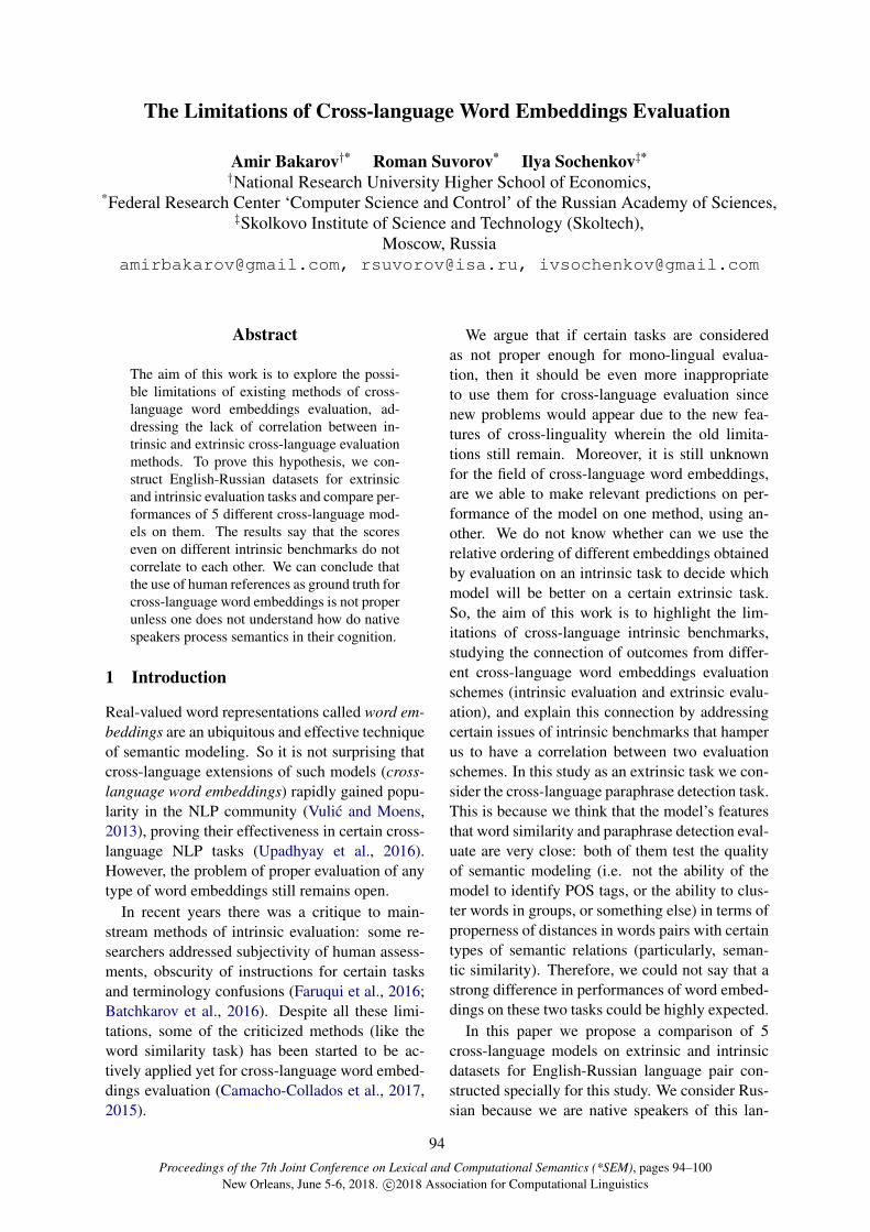
Proceedings of the 7th Joint Conference on Lexical and Computational Semantics (*SEM), pages 94–100New Orleans, June 5-6, 2018. c©2018 Association for Computational Linguistics
The Limitations of Cross-language Word Embeddings Evaluation
Amir Bakarov†* Roman Suvorov* Ilya Sochenkov‡*†National Research University Higher School of Economics,
*Federal Research Center ‘Computer Science and Control’ of the Russian Academy of Sciences,‡Skolkovo Institute of Science and Technology (Skoltech),
Moscow, [email protected], [email protected], [email protected]
Abstract
The aim of this work is to explore the possi-ble limitations of existing methods of cross-language word embeddings evaluation, ad-dressing the lack of correlation between in-trinsic and extrinsic cross-language evaluationmethods. To prove this hypothesis, we con-struct English-Russian datasets for extrinsicand intrinsic evaluation tasks and compare per-formances of 5 different cross-language mod-els on them. The results say that the scoreseven on different intrinsic benchmarks do notcorrelate to each other. We can conclude thatthe use of human references as ground truth forcross-language word embeddings is not properunless one does not understand how do nativespeakers process semantics in their cognition.
1 Introduction
Real-valued word representations called word em-beddings are an ubiquitous and effective techniqueof semantic modeling. So it is not surprising thatcross-language extensions of such models (cross-language word embeddings) rapidly gained popu-larity in the NLP community (Vulic and Moens,2013), proving their effectiveness in certain cross-language NLP tasks (Upadhyay et al., 2016).However, the problem of proper evaluation of anytype of word embeddings still remains open.
In recent years there was a critique to main-stream methods of intrinsic evaluation: some re-searchers addressed subjectivity of human assess-ments, obscurity of instructions for certain tasksand terminology confusions (Faruqui et al., 2016;Batchkarov et al., 2016). Despite all these limi-tations, some of the criticized methods (like theword similarity task) has been started to be ac-tively applied yet for cross-language word embed-dings evaluation (Camacho-Collados et al., 2017,2015).
We argue that if certain tasks are consideredas not proper enough for mono-lingual evalua-tion, then it should be even more inappropriateto use them for cross-language evaluation sincenew problems would appear due to the new fea-tures of cross-linguality wherein the old limita-tions still remain. Moreover, it is still unknownfor the field of cross-language word embeddings,are we able to make relevant predictions on per-formance of the model on one method, using an-other. We do not know whether can we use therelative ordering of different embeddings obtainedby evaluation on an intrinsic task to decide whichmodel will be better on a certain extrinsic task.So, the aim of this work is to highlight the lim-itations of cross-language intrinsic benchmarks,studying the connection of outcomes from differ-ent cross-language word embeddings evaluationschemes (intrinsic evaluation and extrinsic evalu-ation), and explain this connection by addressingcertain issues of intrinsic benchmarks that hamperus to have a correlation between two evaluationschemes. In this study as an extrinsic task we con-sider the cross-language paraphrase detection task.This is because we think that the model’s featuresthat word similarity and paraphrase detection eval-uate are very close: both of them test the qualityof semantic modeling (i.e. not the ability of themodel to identify POS tags, or the ability to clus-ter words in groups, or something else) in terms ofproperness of distances in words pairs with certaintypes of semantic relations (particularly, seman-tic similarity). Therefore, we could not say that astrong difference in performances of word embed-dings on these two tasks could be highly expected.
In this paper we propose a comparison of 5cross-language models on extrinsic and intrinsicdatasets for English-Russian language pair con-structed specially for this study. We consider Rus-sian because we are native speakers of this lan-
94
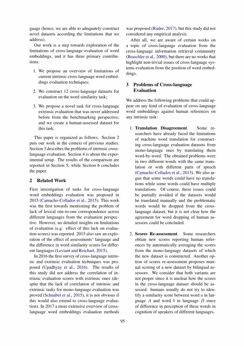
guage (hence, we are able to adequately constructnovel datasets according the limitations that weaddress).
Our work is a step towards exploration of thelimitations of cross-language evaluation of wordembeddings, and it has three primary contribu-tions:
1. We propose an overview of limitations ofcurrent intrinsic cross-language word embed-dings evaluation techniques;
2. We construct 12 cross-language datasets forevaluation on the word similarity task;
3. We propose a novel task for cross-languageextrinsic evaluation that was never addressedbefore from the benchmarking perspective,and we create a human-assessed dataset forthis task.
This paper is organized as follows. Section 2puts our work in the context of previous studies.Section 3 describes the problems of intrinsic cross-language evaluation. Section 4 is about the exper-imental setup. The results of the comparison arereported in Section 5, while Section 6 concludesthe paper.
2 Related Work
First investigation of tasks for cross-languageword embeddings evaluation was proposed in2015 (Camacho-Collados et al., 2015). This workwas the first towards mentioning the problem oflack of lexical one-to-one correspondence acrossdifferent languages from the evaluation perspec-tive. However, no detailed insights on limitationsof evaluation (e.g. effect of this lack on evalua-tion scores) was reported. 2015 also saw an explo-ration of the effect of assessments’ language andthe difference in word similarity scores for differ-ent languages (Leviant and Reichart, 2015).
In 2016 the first survey of cross-language intrin-sic and extrinsic evaluation techniques was pro-posed (Upadhyay et al., 2016). The results ofthis study did not address the correlation of in-trinsic evaluation scores with extrinsic ones (de-spite that the lack of correlation of intrinsic andextrinsic tasks for mono-language evaluation wasproved (Schnabel et al., 2015), it is not obvious ifthis would also extend to cross-language evalua-tion). In 2017 a more extensive overview of cross-language word embeddings evaluation methods
was proposed (Ruder, 2017), but this study did notconsidered any empirical analysis.
After all, we are aware of certain works ona topic of cross-language evaluation from thecross-language information retrieval community(Braschler et al., 2000), but there are no works thathighlight non-trivial issues of cross-language sys-tems evaluation from the position of word embed-dings.
3 Problems of Cross-languageEvaluation
We address the following problems that could ap-pear on any kind of evaluation of cross-languageword embeddings against human references onany intrinsic task:
1. Translation Disagreement. Some re-searchers have already faced the limitationsof machine word translation for construct-ing cross-language evaluation datasets frommono-language ones by translating themword-by-word. The obtained problems werein two different words with the same trans-lation or with different parts of speech(Camacho-Collados et al., 2015). We also ar-gue that some words could have no transla-tions while some words could have multipletranslations. Of course, these issues couldbe partially avoided if the datasets wouldbe translated manually and the problematicwords would be dropped from the cross-language dataset, but it is not clear how theagreement for word dropping of human as-sessors could be concluded.
2. Scores Re-assessment. Some researchersobtain new scores reporting human refer-ences by automatically averaging the scoresfrom the mono-language datasets of whichthe new dataset is constructed. Another op-tion of scores re-assessment proposes man-ual scoring of a new dataset by bilingual as-sessors. We consider that both variants arenot proper since it is unclear how the scoresin the cross-language dataset should be as-sessed: humans usually do not try to iden-tify a similarity score between word a in lan-guage A and word b in language B sinceof difference in perception of these words incognition of speakers of different languages.
95

3. Semantic Fields. According to the theoriesof lexical typology, the meaning of a prop-erly translated word could denote a bit differ-ent things in a new languages. Such effectis called semantic shift, and there is a pos-sibility that the actual meanings of two cor-responding words could be different even ifthey are correctly translated and re-assessed(Ryzhova et al., 2016). One of the ways ofavoiding this problem is to exclude relationalnouns which are words with non-zero va-lency (Koptjevskaja-Tamm et al., 2015) fromthe dataset, so it should consist only of zerovalency nouns that are more properly linkedwith real world objects. However, the distinc-tion of words on relational and non-relationalones is fuzzy, and such assessments could bevery subjective (also, since verbs are usuallyhighly relational, they should not be used incross-language evaluation).
4. New Factors for Bias. It is already knownthat existence of connotative associationsfor certain words in mono-language datasetscould introduce additional subjectivity in thehuman assessments (Liza and Grzes, 2016).We argue that yet more factors could be thecause of assessors’ bias in the cross-languagedatasets. For example, words five and clockcould be closely connected in minds of En-glish speakers (since of the common fiveo’clock tea collocation), but not in minds ofspeakers of other languages, and we thinkthat a native English speaker could assess bi-ased word similarity scores for this word pair.
4 Experimental Setup
4.1 Distributional ModelsTo propose a comparison, we used 5 cross-language embedding models.
1. MSE (Multilingual Supervised Embeddings).Trains using a bilingual dictionary and learnsa mapping from the source to the target spaceusing Procrustes alignment (Conneau et al.,2017).
2. MUE (Multilingual Unsupervised Embed-dings). Trains learning a mapping from thesource to the target space using adversarialtraining and Procrustes refinement (Conneauet al., 2017).
3. VecMap. Maps the source into the tar-get space using a bilingual dictionary orshared numerals minimizing the squared Eu-clidean distance between embedding matri-ces (Artetxe et al., 2018).
4. BiCCA (Bilingual Canonical CorrelationAnalysis). Projects vectors of two differ-ent languages in the same space using CCA(Faruqui and Dyer, 2014).
5. MFT (Multilingual FastText). Uses SVD tolearn a linear transformation, which alignsmonolingual vectors from two languages ina single vector space (Smith et al., 2017).
We mapped vector spaces of Russian and En-glish FastText models trained on a dump ofWikipedia (Bojanowski et al., 2016) with anEnglish-Russian bilingual dictionary (Conneauet al., 2017) (only one translation for a singleword).
4.2 Intrinsic TasksWord Semantic Similarity. The task is to predictthe similarity score for a word a in language Aand a word b in language B. All three publiclyavailable datasets for cross-language word simi-larity (Camacho-Collados et al., 2015, 2017) arenot available for Russian, so we created the cross-language datasets ourselves. We used 5 Englishdatasets assessed by semantic similarity of nounsand adjectives (S), 3 datasets assessed by seman-tic similarity of verbs (V), and 3 datasets assessedby semantic relatedness of nouns and adjectives(R); we labeled each with a letter reporting thetype of relations. We translated these datasets,merged into cross-language sets (the first word ofeach word pair was English, and the second wasRussian), dropped certain words pairs according tolimitations addressed by us (in the Section 2), andre-assessed the obtained cross-languages datasetswith the help of 3 English-Russian volunteers,having Krippendorff’s alpha 0.5 (final amount ofword pairs and ratio to original datasets is reportedat Table 1). Then we compared human referencesof these datasets with cosine distances of cross-language word vectors, and computed Spearman’srank correlation coefficient (p− value in all caseswas lower than 0.05).
Dictionary Induction (also called word trans-lation). The second task is to translate a word inlanguage A into language B, so for the seed word
96
MSE MUE VM BCCA MFT
S.RareWord-958 (56.3%) (Luong et al., 2013) 0.44 0.42 0.43 0.43 0.43S.SimLex-739 (95.9%) (Hill et al., 2016) 0.34 0.32 0.35 0.34 0.34S.SemEval-243 (88.0%) (Camacho-Collados et al., 2017) 0.6 0.56 0.35 0.34 0.34S.WordSim-193 (96.4%) (Agirre et al., 2009) 0.69 0.67 0.72 0.67 0.71S.RG-54 (83.1%) (Rubenstein and Goodenough, 1965) 0.68 0.67 0.63 0.61 0.61S.MC-28 (93.3%) (Miller and Charles, 1991) 0.66 0.7 0.71 0.72 0.7
V. SimVerb-3074 (87.8%) (Gerz et al., 2016) 0.2 0.2 0.23 0.22 0.21V.Verb-115 (85.4%) (Baker et al., 2014) 0.24 0.39 0.27 0.27 0.27V.YP-111 (88.5%) (Yang and Powers, 2006) 0.22 0.37 0.25 0.25 0.25
R.MEN-1146 (94.7%) (Bruni et al., 2014) 0.68 0.66 0.69 0.66 0.68R.MTurk-551 (91.7%) (Halawi et al., 2012) 0.56 0.51 0.57 0.54 0.57R.WordSim-193 (96.4%) (Agirre et al., 2009) 0.55 0.53 0.57 0.53 0.55
P@1, dictionary induction 0.31 0.16 0.32 0.29 0.21P@5, dictionary induction 0.53 0.34 0.52 0.49 0.38P@10, dictionary induction 0.61 0.42 0.5 0.55 0.45
F1, paraphrase detection, our dataset 0.82 0.77 0.84 0.83 0.86F1, paraphrase detection, parallel sentences 0.55 0.45 0.57 0.6 0.59
Table 1: Performance of the compared models across different tasks. Evaluation on first 11 datasetsindicate Spearman’s rank correlation. For word similarity task: words before the hyphen in datasets
name report the name of the original English dataset, the number after the hyphen report the amount ofword pairs, the numbers in brackets report ratio to its English original and the prefix before the dot in
the name report type of assessments.
the model generates a list of the closest word inother language, and we need to find the correcttranslation in it. As a source of correct transla-tions we used English-Russian dictionary of 53186 translation pairs (Conneau et al., 2017). Theevaluation on this measure was proposed as a pre-cision on k nearest vectors of a word embeddingmodel for k = 1, 5, 10.
4.3 Extrinsic Task and Our Dataset
Cross-language Paraphrase Detection. In ananalogy with a monolingual paraphrase detectiontask (also called sentence similarity identification)(Androutsopoulos and Malakasiotis, 2010), thetask is to identify whether sentence a in languageA and sentence b in language B are paraphrasesor not. This task is highly scalable, and usuallyfigures as a sub-task of bigger tasks like cross-language plagiarism detection.
We are not aware of any dataset for this task, sowe designed a benchmark ourselves for English-Russian language pair. The dataset was con-structed on the base of Wikipedia articles covering
wide range of topics from technology to sports. Itcontains 8 334 sentences with a balanced class dis-tribution. The assessments and translations weredone by 3 bilingual assessors. The negative resultswere obtained by automatically randomly sam-pling another sentence in the same domain fromthe datasets.
Translations were produced manually by a poolof human translators. Translators could para-phrase the translations using different techniques(according to our guidelines), and the assessorshad to verify paraphrase technique labels and an-notate similarity of English-Russian sentences inbinary labels. We invited 3 assessors to estimateinter-annotator agreement. To obtain the evalua-tion scores, we conducted 3-fold cross validationand trained Logistic Regression with only one fea-ture: cosine similarity of two sentence vectors.Sentence representations were built by averagingtheir word vectors.
In order to validate the correctness of results onour dataset, we automatically constructed a para-phrase set from a corpus of 1 million English-
97
Figure 1: Clustermap of different evaluationtechniques. Lighter color correspond to stronger
positive correlation. Each row and column islabeled according to benchmark type: red –
extrinsic, blue – verbs, purple – word translation,green – word relatedness, yellow – word
similarity.
Russian parallel sentences from WMT’16∗, gen-erating for each sentence pair a semantic nega-tive sample, searching for nearest sentence with amonolingual FastText model.
5 Results and Discussion
The results of the experiments with intrinsic andextrinsic evaluation are presented in Table 1. De-spite the difference in scores for different modelsin one dataset could be minuscule, the scores fordifferent intrinsic datasets vary a lot, and modelsthat achieve higher results on one task often havelower results on other tasks.
Figure 1 shows mutual similarities betweendatasets (measured as Spearman’s rank correlationbetween evaluation scores from Table 1). Onecan see that there are at least 4 clusters: ex-trinsic+SemEval; word relations; word transla-tion+some word similarities; others.
Interestingly, SemEval behaves similarly to ex-trinsic tasks: this benchmark contains not onlysingle words but also two-word expressions (e.g.Borussia Dortmund), so evaluation on this datasetis more similar to paraphrase detection task. Sur-prisingly, other word similarity datasets yield verydifferent metrics. This is kind of unexpected, be-cause paraphrase detection task relies on similarityof word senses.
Notably, many datasets from the same group(marked using color in the leftmost column onFigure 1) have difference in models’ behavior (e.g.
∗https://translate.yandex.ru/corpus
SimLex and WordSim both being word similaritybenchmarks are clustered away from each other).
Our datasets, aligned models and code to repro-duce the experiments are available at our GitHub †.
6 Conclusions and Future Work
In this work we explored primary limitationsof evaluation methods of intrinsic cross-languageword embeddings. We proposed experiments on 5models in order to answer the question ‘could wesomehow estimate extrinsic performance of cross-language embeddings given some intrinsic met-rics?’. Currently, the short answer is ‘No’, but thelonger is ‘maybe yes, if we understand the cogni-tive and linguistic regularities that take place in thebenchmarks we use. Our point is that we not onlyneed intrinsic datasets of different types if we wantto robustly predict the performance of different ex-trinsic tasks, but we also should overthink the de-sign and capabilities of existing extrinsic bench-marks.
Our research does not address some evaluationmethods (like MultiQVEC (Ammar et al., 2016))and word embeddings models (for instance, Bivec(Luong et al., 2015)) since Russian do not haveenough linguistic resources: there are certainparallel corpora available at http://opus.nlpl.eu, but a merge of all English-Russian cor-pora has 773.0M/710.5M tokens, while the mono-lingual Russian model that we used in this studywas trained on Wikipedia of 5B tokens (and En-glish Wikipedia has a triple of this size). A for-tiori, these corpora have different nature (subtitles,corpus of Europar speeches, etc), and we thinkthat merging them would yield a dataset of unpre-dictable quality.
In future we plan to make a comparison withother languages giving more insights about perfor-mance of compared models. We also plan to inves-tigate cross-language extensions of other intrinsicmonolingual tasks (like the analogical reasoningtask) to make our findings more generalizable.
Acknowledgments
The reported study was funded by the RussianFoundation for Basic Research project 16-37-60048 mol a dk and by the Ministry of Educa-tion and Science of the Russian Federation (grant14.756.31.0001).
†https://github.com/bakarov/cross-lang-embeddings
98
ReferencesEneko Agirre, Enrique Alfonseca, Keith Hall, Jana
Kravalova, Marius Pasca, and Aitor Soroa. 2009. Astudy on similarity and relatedness using distribu-tional and wordnet-based approaches. In Proceed-ings of Human Language Technologies: The 2009Annual Conference of the North American Chap-ter of the Association for Computational Linguistics,pages 19–27. Association for Computational Lin-guistics.
Waleed Ammar, George Mulcaire, Yulia Tsvetkov,Guillaume Lample, Chris Dyer, and Noah A Smith.2016. Massively multilingual word embeddings.arXiv preprint arXiv:1602.01925.
Ion Androutsopoulos and Prodromos Malakasiotis.2010. A survey of paraphrasing and textual entail-ment methods. Journal of Artificial Intelligence Re-search, 38:135–187.
Mikel Artetxe, Gorka Labaka, and Eneko Agirre. 2018.Generalizing and improving bilingual word embed-ding mappings with a multi-step framework of lin-ear transformations. In Proceedings of the Thirty-Second AAAI Conference on Artificial Intelligence(AAAI-18).
Simon Baker, Roi Reichart, and Anna Korhonen. 2014.An unsupervised model for instance level subcate-gorization acquisition. In EMNLP, pages 278–289.
Miroslav Batchkarov, Thomas Kober, Jeremy Reffin,Julie Weeds, and David Weir. 2016. A critique ofword similarity as a method for evaluating distribu-tional semantic models.
Piotr Bojanowski, Edouard Grave, Armand Joulin,and Tomas Mikolov. 2016. Enriching word vec-tors with subword information. arXiv preprintarXiv:1607.04606.
Martin Braschler, Donna Harman, Michael Hess,Michael Kluck, Carol Peters, and Peter Schauble.2000. The evaluation of systems for cross-languageinformation retrieval. In LREC.
Elia Bruni, Nam-Khanh Tran, and Marco Baroni. 2014.Multimodal distributional semantics. J. Artif. Intell.Res.(JAIR), 49(2014):1–47.
Jose Camacho-Collados, Mohammad Taher Pilehvar,Nigel Collier, and Roberto Navigli. 2017. Semeval-2017 task 2: Multilingual and cross-lingual semanticword similarity. In Proceedings of the 11th Interna-tional Workshop on Semantic Evaluation (SemEval-2017), pages 15–26.
Jose Camacho-Collados, Mohammad Taher Pilehvar,and Roberto Navigli. 2015. A framework for theconstruction of monolingual and cross-lingual wordsimilarity datasets. In Proceedings of the 53rd An-nual Meeting of the Association for ComputationalLinguistics and the 7th International Joint Confer-ence on Natural Language Processing (Volume 2:Short Papers), volume 2, pages 1–7.
Alexis Conneau, Guillaume Lample, Marc’AurelioRanzato, Ludovic Denoyer, and Herve Jegou. 2017.Word translation without parallel data. arXivpreprint arXiv:1710.04087.
Manaal Faruqui and Chris Dyer. 2014. Improving vec-tor space word representations using multilingualcorrelation. In Proceedings of EACL.
Manaal Faruqui, Yulia Tsvetkov, Pushpendre Rastogi,and Chris Dyer. 2016. Problems with evaluation ofword embeddings using word similarity tasks. arXivpreprint arXiv:1605.02276.
Daniela Gerz, Ivan Vulic, Felix Hill, Roi Reichart, andAnna Korhonen. 2016. Simverb-3500: A large-scale evaluation set of verb similarity. arXiv preprintarXiv:1608.00869.
Guy Halawi, Gideon Dror, Evgeniy Gabrilovich, andYehuda Koren. 2012. Large-scale learning of wordrelatedness with constraints. In Proceedings ofthe 18th ACM SIGKDD international conference onKnowledge discovery and data mining, pages 1406–1414. ACM.
Felix Hill, Roi Reichart, and Anna Korhonen. 2016.Simlex-999: Evaluating semantic models with (gen-uine) similarity estimation. Computational Linguis-tics.
Maria Koptjevskaja-Tamm, Ekaterina Rakhilina, andMartine Vanhove. 2015. The semantics of lexicaltypology. The Routledge Handbook of Semantics,page 434.
Ira Leviant and Roi Reichart. 2015. Separated by anun-common language: Towards judgment languageinformed vector space modeling. arXiv preprintarXiv:1508.00106.
Farhana Ferdousi Liza and Marek Grzes. 2016. Animproved crowdsourcing based evaluation techniquefor word embedding methods. ACL 2016, page 55.
Minh-Thang Luong, Hieu Pham, and Christopher D.Manning. 2015. Bilingual word representationswith monolingual quality in mind. In NAACL Work-shop on Vector Space Modeling for NLP.
Thang Luong, Richard Socher, and Christopher DManning. 2013. Better word representations withrecursive neural networks for morphology. InCoNLL, pages 104–113.
George A Miller and Walter G Charles. 1991. Contex-tual correlates of semantic similarity. Language andcognitive processes, 6(1):1–28.
Herbert Rubenstein and John B Goodenough. 1965.Contextual correlates of synonymy. Communica-tions of the ACM, 8(10):627–633.
Sebastian Ruder. 2017. A survey of cross-lingual em-bedding models. arXiv preprint arXiv:1706.04902.
99
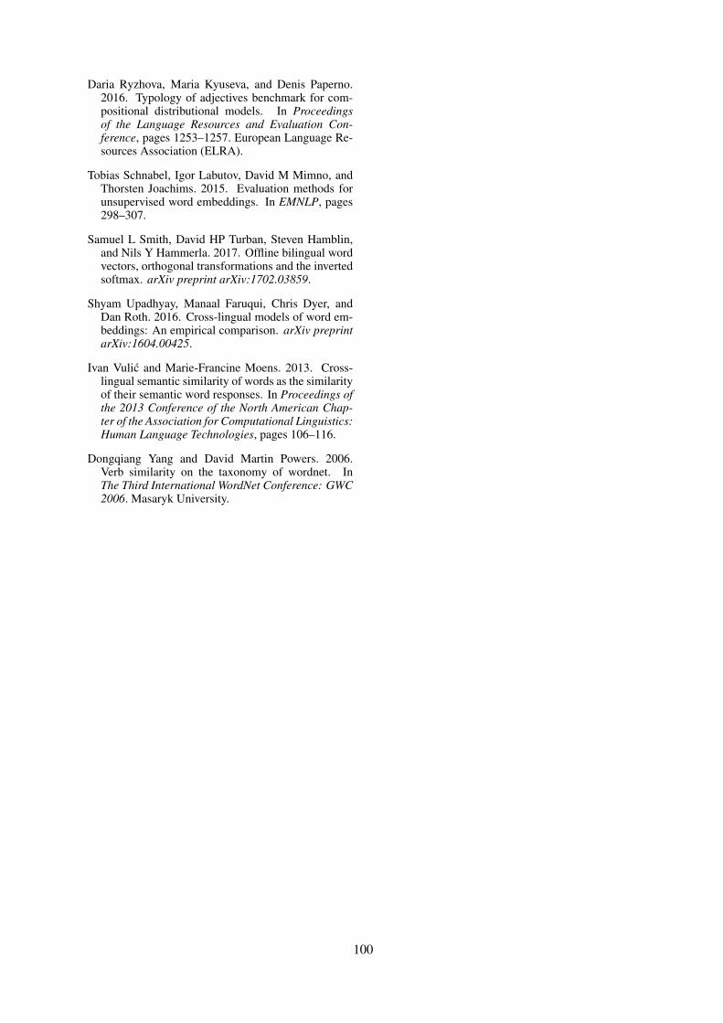
Daria Ryzhova, Maria Kyuseva, and Denis Paperno.2016. Typology of adjectives benchmark for com-positional distributional models. In Proceedingsof the Language Resources and Evaluation Con-ference, pages 1253–1257. European Language Re-sources Association (ELRA).
Tobias Schnabel, Igor Labutov, David M Mimno, andThorsten Joachims. 2015. Evaluation methods forunsupervised word embeddings. In EMNLP, pages298–307.
Samuel L Smith, David HP Turban, Steven Hamblin,and Nils Y Hammerla. 2017. Offline bilingual wordvectors, orthogonal transformations and the invertedsoftmax. arXiv preprint arXiv:1702.03859.
Shyam Upadhyay, Manaal Faruqui, Chris Dyer, andDan Roth. 2016. Cross-lingual models of word em-beddings: An empirical comparison. arXiv preprintarXiv:1604.00425.
Ivan Vulic and Marie-Francine Moens. 2013. Cross-lingual semantic similarity of words as the similarityof their semantic word responses. In Proceedings ofthe 2013 Conference of the North American Chap-ter of the Association for Computational Linguistics:Human Language Technologies, pages 106–116.
Dongqiang Yang and David Martin Powers. 2006.Verb similarity on the taxonomy of wordnet. InThe Third International WordNet Conference: GWC2006. Masaryk University.
100

Proceedings of the 7th Joint Conference on Lexical and Computational Semantics (*SEM), pages 101–106New Orleans, June 5-6, 2018. c©2018 Association for Computational Linguistics
How Gender and Skin Tone Modifiers AffectEmoji Semantics in Twitter
Francesco BarbieriLASTUS Lab, TALN
Universitat Pompeu FabraBarcelona, Spain
Jose Camacho-ColladosSchool of Computer Science and Informatics
Cardiff UniversityUnited Kingdom
Abstract
In this paper we analyze the use of emojis insocial media with respect to gender and skintone. By gathering a dataset of over twentytwo million tweets from United States somefindings are clearly highlighted after perform-ing a simple frequency-based analysis. More-over, we carry out a semantic analysis on theusage of emojis and their modifiers (e.g. gen-der and skin tone) by embedding all words,emojis and modifiers into the same vectorspace. Our analyses reveal that some stereo-types related to the skin color and gender seemto be reflected on the use of these modifiers.For example, emojis representing hand ges-tures are more widely utilized with lighter skintones, and the usage across skin tones differssignificantly. At the same time, the vector cor-responding to the male modifier tends to besemantically close to emojis related to busi-ness or technology, whereas their female coun-terparts appear closer to emojis about love ormakeup.
1 Introduction
Gender and race stereotypes are still present inmany places of our lives. These stereotype-basedbiases are directly reflected on the data that canbe gathered from different sources such as vi-sual or textual contents. In fact, it has beenshown how these biases can lead to problematicbehaviours such as an increase in discrimination(Podesta et al., 2014). These biases have alreadybeen studied in diverse text data sources (Zhaoet al., 2017), and have been proved to propagate tosupervised and unsupervised techniques learningfrom them, including word embeddings (Boluk-basi et al., 2016; Caliskan et al., 2017; Zhao et al.,2018) and end-user applications like online ads(Sweeney, 2013).
In this paper we study the biases produced ina newer form of communication in social media
from an analytical point of view. We focus on theuse of emojis and their interaction with the textualcontent within a social network (i.e. Twitter). Westudy emojis as another part of the message, as itcould be words. An interesting feature about emo-jis, apart from their increasing use in diverse socialmedia platforms, is that they enable us to numeri-cally measure some biases with respect to genderand race. Recently, emojis have introduced mod-ifiers as part of their encoding. With these mod-ifiers the same emoji can be used with differentfeatures: as male or female, or with different skincolors, for example.
We approach the problem from two method-ological perspectives. First, we analyze the use ofemojis and their modifiers from a numerical pointof view, counting their occurrences in a corpus.This already gives us important hints of how theseemojis are used. Then, we leverage the SW2V(Senses and Words to Vectors) embedding model(Mancini et al., 2017) to train a joint vector spacein which emojis and their modifiers are encodedtogether, enabling us to analyze their semantic in-terpretation. While there have been approaches at-tempting to model emojis with distributional se-mantics (Aoki and Uchida, 2011; Barbieri et al.,2016; Eisner et al., 2016; Ljubesic and Fiser, 2016;Wijeratne et al., 2017), to the best of our knowl-edge this is the first work that semantically ana-lyzes modifiers as well. In fact, even though the in-formation provided by modifiers can be extremelyuseful (for the modeling of emojis in particular,and of messages in social media in general), thishas been neglected by previous approaches mod-eling and predicting emojis (Barbieri et al., 2017;Felbo et al., 2017).
Following our two complementary methodolog-ical perspectives, we reached similar conclusions:many stereotypes related to gender and race arealso present in this new form of communication.
101
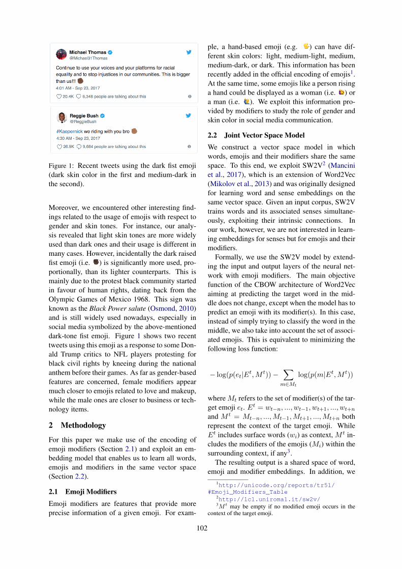
Figure 1: Recent tweets using the dark fist emoji(dark skin color in the first and medium-dark inthe second).
Moreover, we encountered other interesting find-ings related to the usage of emojis with respect togender and skin tones. For instance, our analy-sis revealed that light skin tones are more widelyused than dark ones and their usage is different inmany cases. However, incidentally the dark raisedfist emoji (i.e. ) is significantly more used, pro-portionally, than its lighter counterparts. This ismainly due to the protest black community startedin favour of human rights, dating back from theOlympic Games of Mexico 1968. This sign wasknown as the Black Power salute (Osmond, 2010)and is still widely used nowadays, especially insocial media symbolized by the above-mentioneddark-tone fist emoji. Figure 1 shows two recenttweets using this emoji as a response to some Don-ald Trump critics to NFL players protesting forblack civil rights by kneeing during the nationalanthem before their games. As far as gender-basedfeatures are concerned, female modifiers appearmuch closer to emojis related to love and makeup,while the male ones are closer to business or tech-nology items.
2 Methodology
For this paper we make use of the encoding ofemoji modifiers (Section 2.1) and exploit an em-bedding model that enables us to learn all words,emojis and modifiers in the same vector space(Section 2.2).
2.1 Emoji ModifiersEmoji modifiers are features that provide moreprecise information of a given emoji. For exam-
ple, a hand-based emoji (e.g. ) can have dif-ferent skin colors: light, medium-light, medium,medium-dark, or dark. This information has beenrecently added in the official encoding of emojis1.At the same time, some emojis like a person risinga hand could be displayed as a woman (i.e. ) ora man (i.e. ). We exploit this information pro-vided by modifiers to study the role of gender andskin color in social media communication.
2.2 Joint Vector Space ModelWe construct a vector space model in whichwords, emojis and their modifiers share the samespace. To this end, we exploit SW2V2 (Manciniet al., 2017), which is an extension of Word2Vec(Mikolov et al., 2013) and was originally designedfor learning word and sense embeddings on thesame vector space. Given an input corpus, SW2Vtrains words and its associated senses simultane-ously, exploiting their intrinsic connections. Inour work, however, we are not interested in learn-ing embeddings for senses but for emojis and theirmodifiers.
Formally, we use the SW2V model by extend-ing the input and output layers of the neural net-work with emoji modifiers. The main objectivefunction of the CBOW architecture of Word2Vecaiming at predicting the target word in the mid-dle does not change, except when the model has topredict an emoji with its modifier(s). In this case,instead of simply trying to classify the word in themiddle, we also take into account the set of associ-ated emojis. This is equivalent to minimizing thefollowing loss function:
− log(p(et|Et,M t))−∑
m∈Mt
log(p(m|Et,M t))
where Mt refers to the set of modifier(s) of the tar-get emoji et. Et = wt−n, ..., wt−1, wt+1, ..., wt+n
and M t = Mt−n, ...,Mt−1,Mt+1, ...,Mt+n bothrepresent the context of the target emoji. WhileEt includes surface words (wi) as context, M t in-cludes the modifiers of the emojis (Mi) within thesurrounding context, if any3.
The resulting output is a shared space of word,emoji and modifier embeddings. In addition, we
1http://unicode.org/reports/tr51/#Emoji_Modifiers_Table
2http://lcl.uniroma1.it/sw2v/3M t may be empty if no modified emoji occurs in the
context of the target emoji.
102
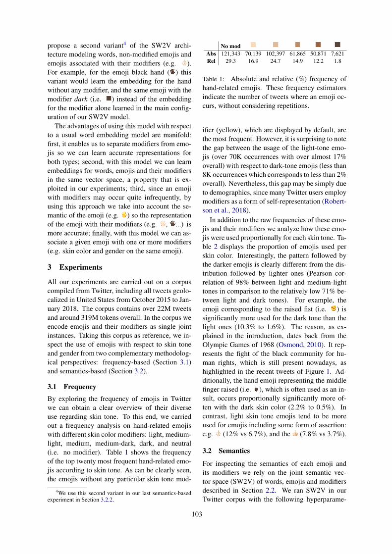
propose a second variant4 of the SW2V archi-tecture modeling words, non-modified emojis andemojis associated with their modifiers (e.g. ).For example, for the emoji black hand ( ) thisvariant would learn the embedding for the handwithout any modifier, and the same emoji with themodifier dark (i.e. ) instead of the embeddingfor the modifier alone learned in the main config-uration of our SW2V model.
The advantages of using this model with respectto a usual word embedding model are manifold:first, it enables us to separate modifiers from emo-jis so we can learn accurate representations forboth types; second, with this model we can learnembeddings for words, emojis and their modifiersin the same vector space, a property that is ex-ploited in our experiments; third, since an emojiwith modifiers may occur quite infrequently, byusing this approach we take into account the se-mantic of the emoji (e.g. ) so the representationof the emoji with their modifiers (e.g. , ...) ismore accurate; finally, with this model we can as-sociate a given emoji with one or more modifiers(e.g. skin color and gender on the same emoji).
3 Experiments
All our experiments are carried out on a corpuscompiled from Twitter, including all tweets geolo-calized in United States from October 2015 to Jan-uary 2018. The corpus contains over 22M tweetsand around 319M tokens overall. In the corpus weencode emojis and their modifiers as single jointinstances. Taking this corpus as reference, we in-spect the use of emojis with respect to skin toneand gender from two complementary methodolog-ical perspectives: frequency-based (Section 3.1)and semantics-based (Section 3.2).
3.1 Frequency
By exploring the frequency of emojis in Twitterwe can obtain a clear overview of their diverseuse regarding skin tone. To this end, we carriedout a frequency analysis on hand-related emojiswith different skin color modifiers: light, medium-light, medium, medium-dark, dark, and neutral(i.e. no modifier). Table 1 shows the frequencyof the top twenty most frequent hand-related emo-jis according to skin tone. As can be clearly seen,the emojis without any particular skin tone mod-
4We use this second variant in our last semantics-basedexperiment in Section 3.2.2.
No modAbs 121,343 70,139 102,397 61,865 50,871 7,621Rel 29.3 16.9 24.7 14.9 12.2 1.8
Table 1: Absolute and relative (%) frequency ofhand-related emojis. These frequency estimatorsindicate the number of tweets where an emoji oc-curs, without considering repetitions.
ifier (yellow), which are displayed by default, arethe most frequent. However, it is surprising to notethe gap between the usage of the light-tone emo-jis (over 70K occurrences with over almost 17%overall) with respect to dark-tone emojis (less than8K occurrences which corresponds to less than 2%overall). Nevertheless, this gap may be simply dueto demographics, since many Twitter users employmodifiers as a form of self-representation (Robert-son et al., 2018).
In addition to the raw frequencies of these emo-jis and their modifiers we analyze how these emo-jis were used proportionally for each skin tone. Ta-ble 2 displays the proportion of emojis used perskin color. Interestingly, the pattern followed bythe darker emojis is clearly different from the dis-tribution followed by lighter ones (Pearson cor-relation of 98% between light and medium-lighttones in comparison to the relatively low 71% be-tween light and dark tones). For example, theemoji corresponding to the raised fist (i.e. ) issignificantly more used for the dark tone than thelight ones (10.3% to 1.6%). The reason, as ex-plained in the introduction, dates back from theOlympic Games of 1968 (Osmond, 2010). It rep-resents the fight of the black community for hu-man rights, which is still present nowadays, ashighlighted in the recent tweets of Figure 1. Ad-ditionally, the hand emoji representing the middlefinger raised (i.e. ), which is often used as an in-sult, occurs proportionally significantly more of-ten with the dark skin color (2.2% to 0.5%). Incontrast, light skin tone emojis tend to be moreused for emojis including some form of assertion:e.g. (12% vs 6.7%), and the (7.8% vs 3.7%).
3.2 Semantics
For inspecting the semantics of each emoji andits modifiers we rely on the joint semantic vec-tor space (SW2V) of words, emojis and modifiersdescribed in Section 2.2. We ran SW2V in ourTwitter corpus with the following hyperparame-
103

13.0 15.7 14.9 16.1 17.5 12.212.9 8.8 11.3 13.7 14.2 13.512.5 12.0 10.9 9.0 7.8 6.712.0 9.9 9.0 15.0 18.5 20.011.4 12.8 15.0 10.6 8.8 8.610.3 7.8 5.3 3.5 2.9 3.76.0 14.1 14.3 11.0 7.8 8.34.6 4.5 4.6 3.9 2.6 3.54.1 3.9 3.3 3.0 2.5 2.22.4 3.1 2.9 2.6 2.0 1.42.3 1.1 1.0 1.4 1.5 1.72.2 1.6 2.4 4.4 7.7 10.32.0 1.3 1.7 1.7 1.7 2.11.0 0.8 0.8 0.9 0.9 0.90.8 0.4 0.6 0.7 0.6 0.70.7 0.6 0.5 0.5 0.4 0.70.6 0.2 0.3 0.4 0.5 0.40.5 0.8 0.7 1.2 1.6 2.20.5 0.3 0.3 0.2 0.2 0.30.5 0.3 0.2 0.4 0.5 0.7
Table 2: Relative frequency (%) of the top twentyhand-related emojis with respect to skin modifiers(from left to right: no modifier, light, medium-light, medium, medium-dark, dark).
ters: 100 dimensions and window size of 6 tokens.We performed two kinds of experiment: one rely-ing on the nearest neighbours in the vector spaceto understand the main semantics of skin tone andgender modifiers (Section 3.2.1) and another ex-periment in which we analyze the main semanticdivergences between opposing modifiers (Section3.2.2), i.e. dark vs. light (skin tone) and male vs.female (gender).
3.2.1 Nearest Neighbours
For this experiment we analyze the nearest neigh-bours of skin tone and gender modifiers in theSW2V vector space using cosine similarity ascomparison measure. Table 3 shows the fifteennearest neighbours for the five skin tone and twogender modifiers. For the skin tone modifiers it isnoteworthy the fact that while lighter tones containlove-related emojis as nearest neighbours, these donot appear on the list of darker tones. Instead, wecan see some money-related (e.g. , or )and electric-related emojis (e.g. a battery or aplug ) as nearest neighbours of dark tone emo-jis. These two electric emojis are often used inthe context of music, sport or motivational tweets
Table 3: Fifteen emoji nearest neighbours of theseven modifiers in our analysis.
along with hashtags like #energy or #chargedup(e.g. The GRIND begins!!! Refuse to settle foraverage!! #chargedup). As a possiblymore worrying trend we found many versions ofthe (often derogatory) word nigger and gang asnearest neighbours of dark tone modifiers. A morefocused analysis on this issue would be requiredin order to understand the possible racist implica-tions.
As far as gender modifiers are concerned,business-related emojis (e.g. a briefcase , a suit
or a handshake ) are among the closest emo-jis to the man modifier in the SW2V vector space,while nail polishing (i.e. ) or the selfie emoji (i.e.
), for example, are among the nearest neighboursof the female modifier.
3.2.2 Semantic Divergences
In addition to the nearest neighbours experiments,we analyze the highest semantic similarity gap be-tween skin tone and gender modifiers. In Table 4we display in each row the emojis with the highestsimilarity gap with respect to the opposite mod-ifier (light vs. dark and male vs. female), be-ing more similar to the corresponding modifierrow. In this case we can see a similar pattern asin the nearest neighbours experiment. A money-related emoji appears again semantically close tothe dark-skin modifier ( ) but far from the lightskin modifier, and love-related emojis closer to thelight skin modifier (e.g. , and ). Likewise,
104
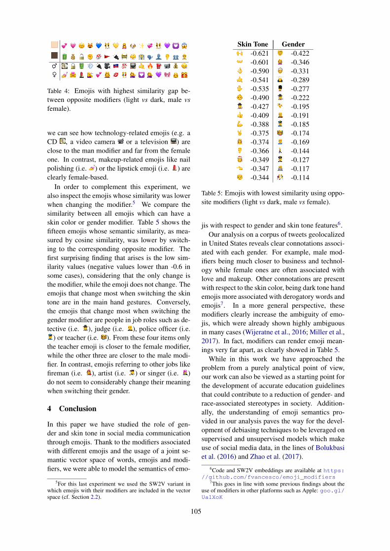
Table 4: Emojis with highest similarity gap be-tween opposite modifiers (light vs dark, male vsfemale).
we can see how technology-related emojis (e.g. aCD , a video camera or a television ) areclose to the man modifier and far from the femaleone. In contrast, makeup-related emojis like nailpolishing (i.e. ) or the lipstick emoji (i.e. ) areclearly female-based.
In order to complement this experiment, wealso inspect the emojis whose similarity was lowerwhen changing the modifier.5 We compare thesimilarity between all emojis which can have askin color or gender modifier. Table 5 shows thefifteen emojis whose semantic similarity, as mea-sured by cosine similarity, was lower by switch-ing to the corresponding opposite modifier. Thefirst surprising finding that arises is the low sim-ilarity values (negative values lower than -0.6 insome cases), considering that the only change isthe modifier, while the emoji does not change. Theemojis that change most when switching the skintone are in the main hand gestures. Conversely,the emojis that change most when switching thegender modifier are people in job roles such as de-tective (i.e. ), judge (i.e. ), police officer (i.e.
) or teacher (i.e. ). From these four items onlythe teacher emoji is closer to the female modifier,while the other three are closer to the male modi-fier. In contrast, emojis referring to other jobs likefireman (i.e. ), artist (i.e. ) or singer (i.e. )do not seem to considerably change their meaningwhen switching their gender.
4 Conclusion
In this paper we have studied the role of gen-der and skin tone in social media communicationthrough emojis. Thank to the modifiers associatedwith different emojis and the usage of a joint se-mantic vector space of words, emojis and modi-fiers, we were able to model the semantics of emo-
5For this last experiment we used the SW2V variant inwhich emojis with their modifiers are included in the vectorspace (cf. Section 2.2).
Skin Tone Gender-0.621 -0.422-0.601 -0.346-0.590 -0.331-0.541 -0.289-0.535 -0.277-0.490 -0.222-0.427 -0.195-0.409 -0.191-0.388 -0.185-0.375 -0.174-0.374 -0.169-0.366 -0.144-0.349 -0.127-0.347 -0.117-0.344 -0.114
Table 5: Emojis with lowest similarity using oppo-site modifiers (light vs dark, male vs female).
jis with respect to gender and skin tone features6.Our analysis on a corpus of tweets geolocalized
in United States reveals clear connotations associ-ated with each gender. For example, male mod-ifiers being much closer to business and technol-ogy while female ones are often associated withlove and makeup. Other connotations are presentwith respect to the skin color, being dark tone handemojis more associated with derogatory words andemojis7. In a more general perspective, thesemodifiers clearly increase the ambiguity of emo-jis, which were already shown highly ambiguousin many cases (Wijeratne et al., 2016; Miller et al.,2017). In fact, modifiers can render emoji mean-ings very far apart, as clearly showed in Table 5.
While in this work we have approached theproblem from a purely analytical point of view,our work can also be viewed as a starting point forthe development of accurate education guidelinesthat could contribute to a reduction of gender- andrace-associated stereotypes in society. Addition-ally, the understanding of emoji semantics pro-vided in our analysis paves the way for the devel-opment of debiasing techniques to be leveraged onsupervised and unsupervised models which makeuse of social media data, in the lines of Bolukbasiet al. (2016) and Zhao et al. (2017).
6Code and SW2V embeddings are available at https://github.com/fvancesco/emoji_modifiers
7This goes in line with some previous findings about theuse of modifiers in other platforms such as Apple: goo.gl/Ua1XoK
105

Acknowledgments
We thank Roberto Carlini for the initial idea of thepaper, and Luis Espinox-Anke for fruitful discus-sions on this topic. Francesco B. acknowledgessupport from the TUNER project (TIN2015-65308-C5-5-R, MINECO/FEDER, UE) and theMaria de Maeztu Units of Excellence Programme(MDM-2015-0502).
ReferencesSho Aoki and Osamu Uchida. 2011. A method for
automatically generating the emotional vectors ofemoticons using weblog articles. In Proceedingsof the 10th WSEAS International Conference onApplied Computer and Applied Computational Sci-ence, Stevens Point, Wisconsin, USA, pages 132–136.
Francesco Barbieri, Miguel Ballesteros, and HoracioSaggion. 2017. Are emojis predictable? In Pro-ceedings of the 15th Conference of the EuropeanChapter of the Association for Computational Lin-guistics: Volume 2, Short Papers, volume 2, pages105–111.
Francesco Barbieri, German Kruszewski, FrancescoRonzano, and Horacio Saggion. 2016. How cos-mopolitan are emojis?: Exploring emojis usage andmeaning over different languages with distributionalsemantics. In Proceedings of the 2016 ACM on Mul-timedia Conference, pages 531–535. ACM.
Tolga Bolukbasi, Kai-Wei Chang, James Y Zou,Venkatesh Saligrama, and Adam T Kalai. 2016.Man is to computer programmer as woman is tohomemaker? debiasing word embeddings. In Ad-vances in Neural Information Processing Systems,pages 4349–4357.
Aylin Caliskan, Joanna J Bryson, and ArvindNarayanan. 2017. Semantics derived automaticallyfrom language corpora contain human-like biases.Science, 356(6334):183–186.
Ben Eisner, Tim Rocktaschel, Isabelle Augenstein,Matko Bosnjak, and Sebastian Riedel. 2016.emoji2vec: Learning emoji representations fromtheir description. In Proceedings of The FourthInternational Workshop on Natural Language Pro-cessing for Social Media, pages 48–54, Austin, TX,USA. Association for Computational Linguistics.
Bjarke Felbo, Alan Mislove, Anders Søgaard, IyadRahwan, and Sune Lehmann. 2017. Using millionsof emoji occurrences to learn any-domain represen-tations for detecting sentiment, emotion and sar-casm. In Proceedings of the 2017 Conference onEmpirical Methods in Natural Language Process-ing, pages 1615–1625.
Nikola Ljubesic and Darja Fiser. 2016. A global anal-ysis of emoji usage. In Proceedings of the 10th Webas Corpus Workshop (WAC-X) and the EmpiriSTShared Task, pages 82–89, Berlin, Germany. Asso-ciation for Computational Linguistics.
Massimiliano Mancini, Jose Camacho-Collados, Igna-cio Iacobacci, and Roberto Navigli. 2017. Embed-ding words and senses together via joint knowledge-enhanced training. In Proceedings of CoNLL, Van-couver, Canada.
Tomas Mikolov, Kai Chen, Greg Corrado, and JeffreyDean. 2013. Efficient estimation of word represen-tations in vector space. CoRR, abs/1301.3781.
Hannah Miller, Daniel Kluver, Jacob Thebault-Spieker,Loren Terveen, and Brent Hecht. 2017. Understand-ing emoji ambiguity in context: The role of textin emoji-related miscommunication. In 11th In-ternational Conference on Web and Social Media,ICWSM 2017. AAAI Press.
Gary Osmond. 2010. Photographs, materiality andsport history: Peter norman and the 1968 mexicocity black power salute. Journal of Sport History,37(1):119–137.
John Podesta, Penny Pritzker, Ernest J. Moniz, JohnHoldren, and Jefrey Zients. 2014. Big data: Seiz-ing opportunities, preserving values. White House,Executive Office of the President.
Alexander Robertson, Walid Magdy, and Sharon Gold-water. 2018. Self-representation on twitter us-ing emoji skin color modifiers. arXiv preprintarXiv:1803.10738.
Latanya Sweeney. 2013. Discrimination in online addelivery. Queue, 11(3):10.
Sanjaya Wijeratne, Lakshika Balasuriya, Amit Sheth,and Derek Doran. 2016. Emojinet: Building a ma-chine readable sense inventory for emoji. In Interna-tional Conference on Social Informatics, pages 527–541. Springer.
Sanjaya Wijeratne, Lakshika Balasuriya, Amit Sheth,and Derek Doran. 2017. A semantics-based mea-sure of emoji similarity. In Proceedings of the In-ternational Conference on Web Intelligence, pages646–653. ACM.
Jieyu Zhao, Tianlu Wang, Mark Yatskar, Vicente Or-donez, and Kai-Wei Chang. 2017. Men also likeshopping: Reducing gender bias amplification us-ing corpus-level constraints. In Proceedings of the2017 Conference on Empirical Methods in NaturalLanguage Processing, pages 2979–2989.
Jieyu Zhao, Tianlu Wang, Mark Yatskar, Vicente Or-donez, and Kai-Wei Chang. 2018. Gender bias incoreference resolution: Evaluation and debiasingmethods. In Proceedings of NAACL, New Orleans,LA, United States.
106

Proceedings of the 7th Joint Conference on Lexical and Computational Semantics (*SEM), pages 107–112New Orleans, June 5-6, 2018. c©2018 Association for Computational Linguistics
Element-wise Bilinear Interaction for Sentence Matching
Jihun Choi, Taeuk Kim, Sang-goo LeeDepartment of Computer Science and Engineering
Seoul National University, Seoul, Korea{jhchoi,taeuk,sglee}@europa.snu.ac.kr
Abstract
When we build a neural network model pre-dicting the relationship between two sen-tences, the most general and intuitive approachis to use a Siamese architecture, where thesentence vectors obtained from a shared en-coder is given as input to a classifier. For theclassifier to work effectively, it is importantto extract appropriate features from the twovectors and feed them as input. There existseveral previous works that suggest heuristic-based function for matching sentence vectors,however it cannot be said that the heuris-tics tailored for a specific task generalize toother tasks. In this work, we propose anew matching function, ElBiS, that learns tomodel element-wise interaction between twovectors. From experiments, we empiricallydemonstrate that the proposed ElBiS matchingfunction outperforms the concatenation-basedor heuristic-based matching functions on nat-ural language inference and paraphrase identi-fication, while maintaining the fused represen-tation compact.
1 Introduction
Identifying the relationship between two sentencesis a key component for various natural languageprocessing tasks such as paraphrase identification,semantic relatedness prediction, textual entailmentrecognition, etc. The most general and intuitiveapproach to these problems would be to encodeeach sentence using a sentence encoder networkand feed the encoded vectors to a classifier net-work.1
For a model to predict the relationship correctly,it is important for the input to the classifier tocontain appropriate information. The most naıve
1 The encoded vectors can also be fed into a regressionnetwork, however in this work we focus only on classifica-tion.
method is to concatenate the two vectors and del-egate the role of extracting features to subsequentnetwork components. However, despite the theo-retical fact that even a single-hidden layer feedfor-ward network can approximate any arbitrary func-tion (Cybenko, 1989; Hornik, 1991), the space ofnetwork parameters is too large, and it is helpfulto narrow down the search space by directly giv-ing information about interaction to the classifiermodel, as empirically proven in previous worksbuilt for various tasks (Ji and Eisenstein, 2013;Mou et al., 2016; Xiong et al., 2016, to name but afew).
In this paper, we propose a matching functionwhich learns from data to fuse two sentence vec-tors and extract useful features. Unlike bilinearpooling methods designed for matching vectorsfrom heterogeneous domain (e.g. image and text),our proposed method utilizes element-wise bilin-ear interaction between vectors rather than interdi-mensional interaction. In §3, we will describe theintuition and assumption behind the restriction ofinteraction.
This paper is organized as follows. In §2, webriefly introduce previous work related to our ob-jective. The detailed explanation of the proposedmodel is given in §3, and we show its effectivenessin extracting compact yet powerful features in §4.§5 concludes the paper.
2 Related Work
As stated above, matching sentences is a com-mon component in various tasks in natural lan-guage processing. Ji and Eisenstein (2013) empir-ically prove that the use of element-wise multipli-cation and absolute difference as matching func-tion substantially improve performance on para-phrase identification, and Tai et al. (2015) applythe same matching scheme to the semantic related-
107
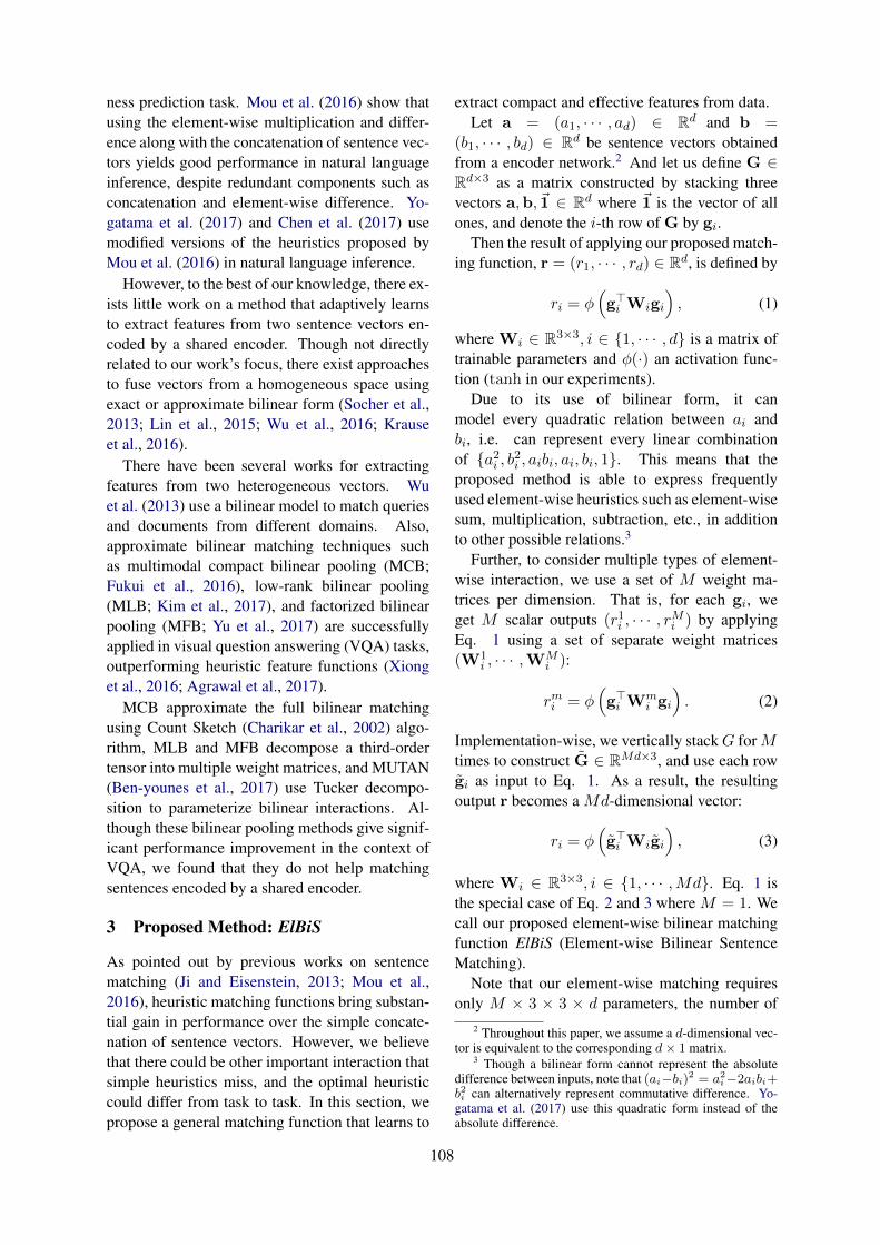
ness prediction task. Mou et al. (2016) show thatusing the element-wise multiplication and differ-ence along with the concatenation of sentence vec-tors yields good performance in natural languageinference, despite redundant components such asconcatenation and element-wise difference. Yo-gatama et al. (2017) and Chen et al. (2017) usemodified versions of the heuristics proposed byMou et al. (2016) in natural language inference.
However, to the best of our knowledge, there ex-ists little work on a method that adaptively learnsto extract features from two sentence vectors en-coded by a shared encoder. Though not directlyrelated to our work’s focus, there exist approachesto fuse vectors from a homogeneous space usingexact or approximate bilinear form (Socher et al.,2013; Lin et al., 2015; Wu et al., 2016; Krauseet al., 2016).
There have been several works for extractingfeatures from two heterogeneous vectors. Wuet al. (2013) use a bilinear model to match queriesand documents from different domains. Also,approximate bilinear matching techniques suchas multimodal compact bilinear pooling (MCB;Fukui et al., 2016), low-rank bilinear pooling(MLB; Kim et al., 2017), and factorized bilinearpooling (MFB; Yu et al., 2017) are successfullyapplied in visual question answering (VQA) tasks,outperforming heuristic feature functions (Xionget al., 2016; Agrawal et al., 2017).
MCB approximate the full bilinear matchingusing Count Sketch (Charikar et al., 2002) algo-rithm, MLB and MFB decompose a third-ordertensor into multiple weight matrices, and MUTAN(Ben-younes et al., 2017) use Tucker decompo-sition to parameterize bilinear interactions. Al-though these bilinear pooling methods give signif-icant performance improvement in the context ofVQA, we found that they do not help matchingsentences encoded by a shared encoder.
3 Proposed Method: ElBiS
As pointed out by previous works on sentencematching (Ji and Eisenstein, 2013; Mou et al.,2016), heuristic matching functions bring substan-tial gain in performance over the simple concate-nation of sentence vectors. However, we believethat there could be other important interaction thatsimple heuristics miss, and the optimal heuristiccould differ from task to task. In this section, wepropose a general matching function that learns to
extract compact and effective features from data.Let a = (a1, · · · , ad) ∈ Rd and b =
(b1, · · · , bd) ∈ Rd be sentence vectors obtainedfrom a encoder network.2 And let us define G ∈Rd×3 as a matrix constructed by stacking threevectors a,b, ~1 ∈ Rd where ~1 is the vector of allones, and denote the i-th row of G by gi.
Then the result of applying our proposed match-ing function, r = (r1, · · · , rd) ∈ Rd, is defined by
ri = φ(g>i Wigi
), (1)
where Wi ∈ R3×3, i ∈ {1, · · · , d} is a matrix oftrainable parameters and φ(·) an activation func-tion (tanh in our experiments).
Due to its use of bilinear form, it canmodel every quadratic relation between ai andbi, i.e. can represent every linear combinationof {a2i , b2i , aibi, ai, bi, 1}. This means that theproposed method is able to express frequentlyused element-wise heuristics such as element-wisesum, multiplication, subtraction, etc., in additionto other possible relations.3
Further, to consider multiple types of element-wise interaction, we use a set of M weight ma-trices per dimension. That is, for each gi, weget M scalar outputs (r1i , · · · , rMi ) by applyingEq. 1 using a set of separate weight matrices(W1
i , · · · ,WMi ):
rmi = φ(g>i W
mi gi
). (2)
Implementation-wise, we vertically stackG forMtimes to construct G ∈ RMd×3, and use each rowgi as input to Eq. 1. As a result, the resultingoutput r becomes a Md-dimensional vector:
ri = φ(g>i Wigi
), (3)
where Wi ∈ R3×3, i ∈ {1, · · · ,Md}. Eq. 1 isthe special case of Eq. 2 and 3 where M = 1. Wecall our proposed element-wise bilinear matchingfunction ElBiS (Element-wise Bilinear SentenceMatching).
Note that our element-wise matching requiresonly M × 3 × 3 × d parameters, the number of
2 Throughout this paper, we assume a d-dimensional vec-tor is equivalent to the corresponding d× 1 matrix.
3 Though a bilinear form cannot represent the absolutedifference between inputs, note that (ai−bi)2 = a2
i−2aibi+b2i can alternatively represent commutative difference. Yo-gatama et al. (2017) use this quadratic form instead of theabsolute difference.
108

which is substantially less than that of full bilin-ear matching, Md3. For example, in the case ofd = 300 and Md = 1200 (the frequently usedset of hyperparameters in NLI), the full bilinearmatching needs 108 million parameters, while theelement-wise matching needs only 10,800 param-eters.
Why element-wise? In the scenario we are fo-cusing on, sentence vectors are computed from aSiamese network, and thus it can be said that thevectors are in the same semantic space. There-fore, the effect of considering interdimensional in-teraction is less significant than that of multimodalpooling (e.g. matching a text and a image vector),so we decided to model more powerful interactionwithin the same dimension instead. We also wouldlike to remark that our preliminary experiments,where MFB (Yu et al., 2017) or MLB (Kim et al.,2017) was adopted as matching function, were notsuccessful.
4 Experiments
We evalute our proposed ElBiS model on the nat-ural language inference and paraphrase identifica-tion task. Implementation for experiments will bemade public.
4.1 Natural Language Inference
Natural language inference (NLI), also called rec-ognizing textual entailment (RTE), is a task whoseobjective is to predict the relationship between apremise and a hypothesis sentence. We conductexperiments using Stanford Natural Language In-ference Corpus (SNLI; Bowman et al., 2015), oneof the most famous dataset for the NLI task. TheSNLI dataset consists of roughly 570k premise-hypothesis pairs, each of which is annotated witha label (entailment, contradiction, or neutral).
For sentence encoder, we choose the en-coder based on long short-term memory (LSTM;Hochreiter and Schmidhuber, 1997) architectureas baseline model, which is similar to that of Bow-man et al. (2015) and Bowman et al. (2016). Itconsists of a single layer unidirectional LSTM net-work that reads a sentence from left to right, andthe last hidden state is used as the sentence vector.We also conduct experiments using a more elab-orated encoder model, Gumbel Tree-LSTM (Choiet al., 2018). As a classifier network, we use anMLP with a single hidden layer. In experiments
Matching Fn. # Params. Acc. (%)Concat 1.34M 81.6Heuristic 1.96M 83.9ElBiS (M = 1) 1.04M 84.4ElBiS (M = 2) 1.35M 84.5ElBiS (M = 3) 1.66M 85.0ElBiS (M = 4) 1.97M 84.6
Table 1: Results on the SNLI task using LSTM-basedsentence encoders.
Matching Fn. # Params. Acc. (%)Concat 2.25M 82.4Heuristic 2.86M 84.6ElBiS (M = 1) 1.94M 84.8ElBiS (M = 2) 2.25M 85.6ElBiS (M = 3) 2.56M 85.9ElBiS (M = 4) 2.87M 85.6
Table 2: Results on the SNLI task using Gumbel Tree-LSTM-based sentence encoders.
with heuristic matching we use the heuristic fea-tures proposed by Mou et al. (2016) and adoptedin many works on the NLI task: [a;b;a−b;a�b],where a and b are encoded sentence vectors. Formore detailed experimental settings, we refer read-ers to §A.1.
Table 1 and 2 contain results on the SNLI task.We can see that models that adopt the proposedElBiS matching function extract powerful featuresleading to a performance gain, while keeping simi-lar or less number of parameters. Also, though notdirectly related to our main contribution, we foundthat, with elaborated initialization and regulariza-tion, simple LSTM models (even the one with theheuristic matching function) achieve competitiveperformance with those of state-of-the-art mod-els.4
4.2 Paraphrase Identification
Another popular task on identifying relationshipbetween a sentence pair is paraphrase identifica-tion (PI). The objective of the PI task is to pre-dict whether a given sentence pair has the samemeaning or not. To correctly identify the para-phrase relationship, an input to a classifier shouldcontain the semantic similarity and difference be-tween sentences.
For evaluation of paraphrase identification, we
4https://nlp.stanford.edu/projects/snli
109
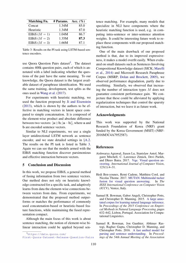
Matching Fn. # Params. Acc. (%)Concat 1.34M 85.0Heuristic 1.34M 87.0ElBiS (M = 1) 1.04M 86.7ElBiS (M = 2) 1.35M 87.3ElBiS (M = 3) 1.66M 87.1
Table 3: Results on the PI task using LSTM-based sen-tence encoders.
use Quora Question Pairs dataset5. The datasetcontains 400k question pairs, each of which is an-notated with a label indicating whether the ques-tions of the pair have the same meaning. To ourknowledge, the Quora dataset is the largest avail-able dataset of paraphrase identification. We usedthe same training, development, test splits as theones used in Wang et al. (2017).
For experiments with heuristic matching, weused the function proposed by Ji and Eisenstein(2013), which is shown by the authors to be ef-fective in matching vectors in latent space com-pared to simple concatenation. It is composed ofthe element-wise product and absolute differencebetween two vectors: [a�b; |a−b|], where a andb are encoded sentence vectors.
Similar to NLI experiments, we use a singlelayer unidirectional LSTM network as sentenceencoder, and we state detailed settings in §A.2.The results on the PI task is listed in Table 3.Again we can see that the models armed with theElBiS matching function discover parsimoniousand effective interaction between vectors.
5 Conclusion and Discussion
In this work, we propose ElBiS, a general methodof fusing information from two sentence vectors.Our method does not rely on heuristic knowl-edge constructed for a specific task, and adaptivelylearns from data the element-wise connections be-tween vectors from data. From experiments, wedemonstrated that the proposed method outper-forms or matches the performance of commonlyused concatenation-based or heuristic-based fea-ture functions, while maintaining the fused repre-sentation compact.
Although the main focus of this work is aboutsentence matching, the notion of element-wise bi-linear interaction could be applied beyond sen-
5https://data.quora.com/First-Quora-Dataset-Release-Question-Pairs
tence matching. For example, many models thatspecialize in NLI have components where theheuristic matching function is used, e.g. in com-puting intra-sentence or inter-sentence attentionweights. It could be interesting future work to re-place these components with our proposed match-ing function.
One of the main drawback of our proposedmethod is that, due to its improved expressive-ness, it makes a model overfit easily. When evalu-ated on small datasets such as Sentences InvolvingCompositional Knowledge dataset (SICK; Marelliet al., 2014) and Microsoft Research ParaphraseCorpus (MSRP; Dolan and Brockett, 2005), weobserved performance degradation, partly due tooverfitting. Similarly, we observed that increas-ing the number of interaction types M does notguarantee consistent performance gain. We con-jecture that these could be alleviated by applyingregularization techniques that control the sparsityof interaction, but we leave it as future work.
Acknowledgments
This work was supported by the NationalResearch Foundation of Korea (NRF) grantfunded by the Korea Government (MSIT) (NRF-2016M3C4A7952587).
References
Aishwarya Agrawal, Jiasen Lu, Stanislaw Antol, Mar-garet Mitchell, C. Lawrence Zitnick, Devi Parikh,and Dhruv Batra. 2017. Vqa: Visual question an-swering. International Journal of Computer Vision,123(1):4–31.
Hedi Ben-younes, Remi Cadene, Matthieu Cord, andNicolas Thome. 2017. MUTAN: Multimodal tuckerfusion for visual question answering. In TheIEEE International Conference on Computer Vision(ICCV), Venice, Italy.
Samuel R. Bowman, Gabor Angeli, Christopher Potts,and Christopher D. Manning. 2015. A large anno-tated corpus for learning natural language inference.In Proceedings of the 2015 Conference on Empiri-cal Methods in Natural Language Processing, pages632–642, Lisbon, Portugal. Association for Compu-tational Linguistics.
Samuel R. Bowman, Jon Gauthier, Abhinav Ras-togi, Raghav Gupta, Christopher D. Manning, andChristopher Potts. 2016. A fast unified model forparsing and sentence understanding. In Proceed-ings of the 54th Annual Meeting of the Association
110
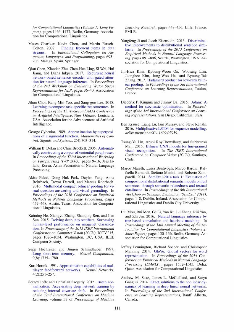
for Computational Linguistics (Volume 1: Long Pa-pers), pages 1466–1477, Berlin, Germany. Associa-tion for Computational Linguistics.
Moses Charikar, Kevin Chen, and Martin Farach-Colton. 2002. Finding frequent items in datastreams. In International Colloquium on Au-tomata, Languages, and Programming, pages 693–703, Malaga, Spain. Springer.
Qian Chen, Xiaodan Zhu, Zhen-Hua Ling, Si Wei, HuiJiang, and Diana Inkpen. 2017. Recurrent neuralnetwork-based sentence encoder with gated atten-tion for natural language inference. In Proceedingsof the 2nd Workshop on Evaluating Vector SpaceRepresentations for NLP, pages 36–40. Associationfor Computational Linguistics.
Jihun Choi, Kang Min Yoo, and Sang-goo Lee. 2018.Learning to compose task-specific tree structures. InProceedings of the Thirty-Second AAAI Conferenceon Artificial Intelligence, New Orleans, Louisiana,USA. Association for the Advancement of ArtificialIntelligence.
George Cybenko. 1989. Approximation by superposi-tions of a sigmoidal function. Mathematics of Con-trol, Signals and Systems, 2(4):303–314.
William B. Dolan and Chris Brockett. 2005. Automati-cally constructing a corpus of sentential paraphrases.In Proceedings of the Third International Workshopon Paraphrasing (IWP 2005), pages 9–16, Jeju Is-land, Korea. Asian Federation of Natural LanguageProcessing.
Akira Fukui, Dong Huk Park, Daylen Yang, AnnaRohrbach, Trevor Darrell, and Marcus Rohrbach.2016. Multimodal compact bilinear pooling for vi-sual question answering and visual grounding. InProceedings of the 2016 Conference on EmpiricalMethods in Natural Language Processing, pages457–468, Austin, Texas. Association for Computa-tional Linguistics.
Kaiming He, Xiangyu Zhang, Shaoqing Ren, and JianSun. 2015. Delving deep into rectifiers: Surpassinghuman-level performance on imagenet classifica-tion. In Proceedings of the 2015 IEEE InternationalConference on Computer Vision (ICCV), ICCV ’15,pages 1026–1034, Washington, DC, USA. IEEEComputer Society.
Sepp Hochreiter and Jurgen Schmidhuber. 1997.Long short-term memory. Neural Computation,9(8):1735–1780.
Kurt Hornik. 1991. Approximation capabilities of mul-tilayer feedforward networks. Neural Networks,4(2):251–257.
Sergey Ioffe and Christian Szegedy. 2015. Batch nor-malization: Accelerating deep network training byreducing internal covariate shift. In Proceedingsof the 32nd International Conference on MachineLearning, volume 37 of Proceedings of Machine
Learning Research, pages 448–456, Lille, France.PMLR.
Yangfeng Ji and Jacob Eisenstein. 2013. Discrimina-tive improvements to distributional sentence simi-larity. In Proceedings of the 2013 Conference onEmpirical Methods in Natural Language Process-ing, pages 891–896, Seattle, Washington, USA. As-sociation for Computational Linguistics.
Jin-Hwa Kim, Kyoung-Woon On, Woosang Lim,Jeonghee Kim, Jung-Woo Ha, and Byoung-TakZhang. 2017. Hadamard product for low-rank bilin-ear pooling. In Proceedings of the 5th InternationalConference on Learning Representations, Toulon,France.
Diederik P. Kingma and Jimmy Ba. 2015. Adam: Amethod for stochastic optimization. In Proceed-ings of the 3rd International Conference on Learn-ing Representations, San Diego, California, USA.
Ben Krause, Liang Lu, Iain Murray, and Steve Renals.2016. Multiplicative LSTM for sequence modelling.arXiv preprint arXiv:1609.07959.
Tsung-Yu Lin, Aruni RoyChowdhury, and SubhransuMaji. 2015. Bilinear CNN models for fine-grainedvisual recognition. In The IEEE InternationalConference on Computer Vision (ICCV), Santiago,Chile.
Marco Marelli, Luisa Bentivogli, Marco Baroni, Raf-faella Bernardi, Stefano Menini, and Roberto Zam-parelli. 2014. SemEval-2014 task 1: Evaluation ofcompositional distributional semantic models on fullsentences through semantic relatedness and textualentailment. In Proceedings of the 8th InternationalWorkshop on Semantic Evaluation (SemEval 2014),pages 1–8, Dublin, Ireland. Association for Compu-tational Linguistics and Dublin City University.
Lili Mou, Rui Men, Ge Li, Yan Xu, Lu Zhang, Rui Yan,and Zhi Jin. 2016. Natural language inference bytree-based convolution and heuristic matching. InProceedings of the 54th Annual Meeting of the As-sociation for Computational Linguistics (Volume 2:Short Papers), pages 130–136, Berlin, Germany. As-sociation for Computational Linguistics.
Jeffrey Pennington, Richard Socher, and ChristopherManning. 2014. GloVe: Global vectors for wordrepresentation. In Proceedings of the 2014 Con-ference on Empirical Methods in Natural LanguageProcessing (EMNLP), pages 1532–1543, Doha,Qatar. Association for Computational Linguistics.
Andrew M. Saxe, James L. McClelland, and SuryaGanguli. 2014. Exact solutions to the nonlinear dy-namics of learning in deep linear neural networks.In Proceedings of the 2nd International Confer-ence on Learning Representations, Banff, Alberta,Canada.
111
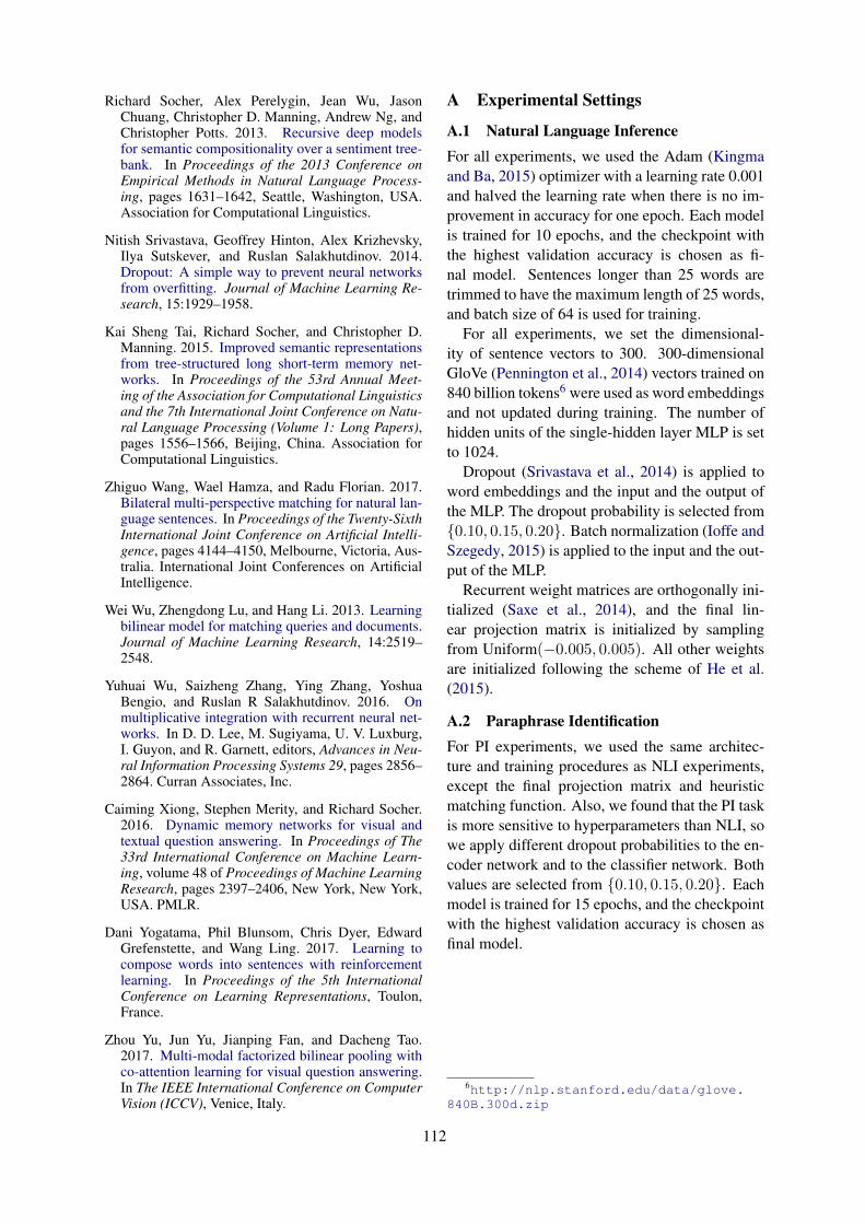
Richard Socher, Alex Perelygin, Jean Wu, JasonChuang, Christopher D. Manning, Andrew Ng, andChristopher Potts. 2013. Recursive deep modelsfor semantic compositionality over a sentiment tree-bank. In Proceedings of the 2013 Conference onEmpirical Methods in Natural Language Process-ing, pages 1631–1642, Seattle, Washington, USA.Association for Computational Linguistics.
Nitish Srivastava, Geoffrey Hinton, Alex Krizhevsky,Ilya Sutskever, and Ruslan Salakhutdinov. 2014.Dropout: A simple way to prevent neural networksfrom overfitting. Journal of Machine Learning Re-search, 15:1929–1958.
Kai Sheng Tai, Richard Socher, and Christopher D.Manning. 2015. Improved semantic representationsfrom tree-structured long short-term memory net-works. In Proceedings of the 53rd Annual Meet-ing of the Association for Computational Linguisticsand the 7th International Joint Conference on Natu-ral Language Processing (Volume 1: Long Papers),pages 1556–1566, Beijing, China. Association forComputational Linguistics.
Zhiguo Wang, Wael Hamza, and Radu Florian. 2017.Bilateral multi-perspective matching for natural lan-guage sentences. In Proceedings of the Twenty-SixthInternational Joint Conference on Artificial Intelli-gence, pages 4144–4150, Melbourne, Victoria, Aus-tralia. International Joint Conferences on ArtificialIntelligence.
Wei Wu, Zhengdong Lu, and Hang Li. 2013. Learningbilinear model for matching queries and documents.Journal of Machine Learning Research, 14:2519–2548.
Yuhuai Wu, Saizheng Zhang, Ying Zhang, YoshuaBengio, and Ruslan R Salakhutdinov. 2016. Onmultiplicative integration with recurrent neural net-works. In D. D. Lee, M. Sugiyama, U. V. Luxburg,I. Guyon, and R. Garnett, editors, Advances in Neu-ral Information Processing Systems 29, pages 2856–2864. Curran Associates, Inc.
Caiming Xiong, Stephen Merity, and Richard Socher.2016. Dynamic memory networks for visual andtextual question answering. In Proceedings of The33rd International Conference on Machine Learn-ing, volume 48 of Proceedings of Machine LearningResearch, pages 2397–2406, New York, New York,USA. PMLR.
Dani Yogatama, Phil Blunsom, Chris Dyer, EdwardGrefenstette, and Wang Ling. 2017. Learning tocompose words into sentences with reinforcementlearning. In Proceedings of the 5th InternationalConference on Learning Representations, Toulon,France.
Zhou Yu, Jun Yu, Jianping Fan, and Dacheng Tao.2017. Multi-modal factorized bilinear pooling withco-attention learning for visual question answering.In The IEEE International Conference on ComputerVision (ICCV), Venice, Italy.
A Experimental Settings
A.1 Natural Language InferenceFor all experiments, we used the Adam (Kingmaand Ba, 2015) optimizer with a learning rate 0.001and halved the learning rate when there is no im-provement in accuracy for one epoch. Each modelis trained for 10 epochs, and the checkpoint withthe highest validation accuracy is chosen as fi-nal model. Sentences longer than 25 words aretrimmed to have the maximum length of 25 words,and batch size of 64 is used for training.
For all experiments, we set the dimensional-ity of sentence vectors to 300. 300-dimensionalGloVe (Pennington et al., 2014) vectors trained on840 billion tokens6 were used as word embeddingsand not updated during training. The number ofhidden units of the single-hidden layer MLP is setto 1024.
Dropout (Srivastava et al., 2014) is applied toword embeddings and the input and the output ofthe MLP. The dropout probability is selected from{0.10, 0.15, 0.20}. Batch normalization (Ioffe andSzegedy, 2015) is applied to the input and the out-put of the MLP.
Recurrent weight matrices are orthogonally ini-tialized (Saxe et al., 2014), and the final lin-ear projection matrix is initialized by samplingfrom Uniform(−0.005, 0.005). All other weightsare initialized following the scheme of He et al.(2015).
A.2 Paraphrase IdentificationFor PI experiments, we used the same architec-ture and training procedures as NLI experiments,except the final projection matrix and heuristicmatching function. Also, we found that the PI taskis more sensitive to hyperparameters than NLI, sowe apply different dropout probabilities to the en-coder network and to the classifier network. Bothvalues are selected from {0.10, 0.15, 0.20}. Eachmodel is trained for 15 epochs, and the checkpointwith the highest validation accuracy is chosen asfinal model.
6http://nlp.stanford.edu/data/glove.840B.300d.zip
112
Proceedings of the 7th Joint Conference on Lexical and Computational Semantics (*SEM), pages 113–118New Orleans, June 5-6, 2018. c©2018 Association for Computational Linguistics
Named Graphs for Semantic Representations
Richard CrouchA9.com
Aikaterini-Lida KalouliUniversity of Konstanz
AbstractA position paper arguing that purely graphicalrepresentations for natural language semanticslack a fundamental degree of expressiveness,and cannot deal with even basic Boolean op-erations like negation or disjunction, let aloneintensional phenomena. Moving from graphsto named graphs leads to representations thatstand some chance of having sufficient expres-sive power. Named FL0 graphs are of partic-ular interest.
1 Introduction
Graphs are popular for both (semantic web)knowledge representation (Screiber and Raimond,2014; Dong et al., 2014; Rospocher et al., 2016)and natural language semantics (Banarescu et al.,2013; Perera et al., 2018; Wities et al., 2017). Thecasual observer might assume there is substantialoverlap between the two activities, but there is lessthan meets the eye. This paper attempts to makethree points:
1. Knowledge graphs, which are designed torepresent facts about the world rather than humanknowledge, are not well set up to represent nega-tion, disjunction, and conditional or hypotheticalcontexts. Arguably, the world contains no nega-tive, disjunctive, or hypothetical facts; just posi-tive facts that make them true. Natural languagesemantics has to deal with more partial assertions,where all that is known are the negations, dis-junctions, or hypotheticals, and not the underlyingfacts that make them true.
2. Named graphs (Carroll et al., 2005) are anextension of RDF graphs (Screiber and Raimond,2014), primarily introduced to record provenanceinformation. They are worthy of further study,since they promise a way of bridging between therelentlessly positive world of knowledge represen-tation and the more partial, hypothetical world ofnatural language. In RDF-OWL graphs (Hitzleret al., 2012), the subject-predicate-object triples
forming the nodes and arcs of the graph corre-spond to atomic propositions. Beyond conjunc-tion, no direct relations between these proposi-tions can be expressed. Named graphs allow sub-graphs (i.e. collections of atomic propositions) tobe placed in relationships with other sub-graphs,and thus allow for negative, disjunctive and hypo-thetical relations between complex propositions.
3. Named graphs illustrate a certain way offactoring out complexity, in this case betweenpredicate-argument structure and Boolean / modalstructure. As a semantic representation, thepredicate-argument structure is correct, but notcomplete. Adding a named, Boolean layer re-quires no adjustment to the syntax or semanticsof the predicate-argument structure; it just embedsit in a broader environment. This often is not thecase; e.g. in moving from unquantified predicatelogic to first-order quantified logic, to first-odermodal logic, to higher-order intensional logic.
After reviewing RDF graphs and named graphs,we discuss how they could be applied to a (some-what incestuous) family of layered, graphical, se-mantic representations (Boston et al., forthcom-ing; Shen et al., 2018; Bobrow et al., 2007) (seeour companion paper (Kalouli and Crouch, 2018)for an introduction to these representations). Thisoffers the prospect of a formal semantics that takesgraphs to be first class semantic objects, which dif-fers from approaches like AMR (Banarescu et al.,2013), where the graphs are descriptions of under-lying semantic objects.
2 Graphs and Named Graphs
A graph is a collection of binary relationshipsbetween entities. Since any n-ary relationshipcan be decomposed into n + 1 binary relation-ships through the introduction of an extra entitythat serves as a “pivot” (this is the basis of neo-Davidsonian event semantics (Parsons, 1990)), alln-ary relationships can be represented in graphical
113

form as a collection of entity-relation triples.
2.1 RDF
This graphical approach to n-ary relationships hasseen perhaps its fullest use in the Resource De-scription Framework (RDF) (Screiber and Rai-mond, 2014), where subject-relation-object triplescan be stored to treat complex ontologies asgraphs. But since the triples form a conjunctiveset, RDF has to go through some contortions toemulate negation and disjunction.
Unadorned, RDF is lax about what kinds of en-tity can occur in triples, and individuals, relations,and classes can intermingle freely. One can statefacts about how classes relate to other classes (e.g.one is a subclass of the other), how relations relateto other relations, and how individual relate to re-lations and classes. Successive restrictions, suchas RDFS (Brickley and Guha, 2014) and OWL(Hitzler et al., 2012) tighten up on this freedomof expression, for the resulting gain in inferentialtractability.
OWL provides a number of class constructionoperations that mimic Booleans at a class level:complement (negation), intersection (conjunction)and union (disjunction). One could therefore as-sert that Rosie is not a cat by saying that she isan instance of the cat-complement class, and onecould assert that Rosie is a cat or a dog by assertingthat she is an instance of the class formed by tak-ing the union of cats and dogs. Additionally, OWLand RDFS allow negative properties as a way ofstating that a particular relation does not hold be-tween two entities (i.e. a form of atomic negation).
The semantic web is geared toward capturingpositive facts about what is known. Two positivefacts can establish a negative, e.g. that cats anddogs are disjoint classes and that Rosie is a dogestablishes that Rosie is not a cat. But the need toassert a negative rarely arises: better to wait untilthe corresponding incompatible positive is known,or as a last resort make up a positive fact that is in-compatible with negative (e.g. that Rosie is a non-cat). Natural language, by contrast, is full of neg-ative, disjunctive, and hypothetical assertions forwhich the justifying positive facts are not known.And these Boolean and modal assertions expressrelationships between propositions (i.e. collec-tions of triples), and not between classes.
Moreover, Gardenfors (2014) makes the casefor restricting semantics to natural concepts within
a conceptual space. A conceptual space consistsof a set of quality dimensions (c.f. dimensions inword vectors). A point in the space is a particularvector along these dimensions. A natural conceptis a region (collection of points in the space) that isconnected and convex. This essentially means thatthe shortest path from one sub-region of a naturalconcept to another does not pass outside of the re-gion defined by the concept: natural concepts areregions that are not gerrymandered. OWL unionsof classes can arbitrarily combine disconnected re-gions, whereas complements can tear holes in themiddle of regions: they can produce gerrymander-ing that would make the most partisan blush.
2.2 Named GraphsNamed graphs were introduced by Carroll et al.(2005) as a small extension on top of RDF, primar-ily with the goal of recording provenance meta-data for different parts of a complex graph, such assource, access restrictions, or ontology versions.However, applications to stating propositional at-titudes and capturing logical relationships betweengraphs were also mentioned in passing. A namedgraph simply associates an extra identifier with aset of triples. For example, a propositional attitudelike Fred believes John does not like Mary couldbe represented as follows1:
:g1 { :john :like :mary }:g2 :not :g1:fred :belive :g2
where :g1 is the name given to the graph express-ing the proposition that John likes Mary, and :g2
to the graph expressing its negation. Disjunctionlikewise can be expressed as a relationship be-tween named graphs:
:g1 { :john :like :mary }:g2 { :fred :like :mary }:g0 :or :g1:g0 :or :g2
where the graph :g0 expresses the disjunction of:g1 and :g2.
The graph semantics for named graphs is a sim-ple extension of the basic semantics (Carroll et al.,2005). The meaning of a named graph is the mean-ing of the graph, and sub-graph relations betweennamed graphs must reflect the underlying relationsbetween the graphs that are named. But signif-icantly, named graphs are not automatically as-serted — there is no presumption that the triples
1Using the TriG format (Bizer and Cyganiak, 2014), withthe prefix definition for : omitted for brevity.
114
Figure 1: GKR for Fred believes John likes Mary
occurring in a named graph are true. This is some-what inconvenient if your main goal is to assertpositive, true facts. But this looks ideal for deal-ing with negation, disjunction and hypotheticals innatural language. In particular, the named graphabove asserts neither that John likes Mary nor thatJohn doesn’t like Mary.
Reification in RDF was an earlier approachto dealing with provenance meta-data (Screiberand Raimond, 2014). This turns every tripleinto four triples that describe it, so that :john
:like :mary becomes :t :type :statement;
:t :subj :john; :t :pred :like; :t :obj
:mary. The reified graph is graphical descriptionof the original graph. Naming preserves theunderlying graph in a way that reification doesnot.
3 Layered Graphs and the GraphicalKnowledge Representation
A recent proposal for semantic representation hasmade use of so-called “layered-graphs” (GKR,(Kalouli and Crouch, 2018), see also (Bostonet al., forthcoming; Shen et al., 2018)), with theclaim that this gives a good way of handlingBoolean, hypothetical, and modal relations2. Theproposal is based on earlier work on an AbstractKnowledge Representtions (AKR, (Bobrow et al.,2007)), which imposes a separation between con-ceptual / predicate-argument structure and contex-tual structure. The GKR representation (simpli-fied) for Fred believes John likes Mary is shownin Figure 1. This comprises two sub-graphs: aconcept/predicate-argument graph on the left, anda context graph on the right. The concept graphcan be read conjunctively as stating the following,but where variables range over (sub)concepts andnot over individuals:
∃b,l,f,j,m.2This section does not attempt to motivate GKR in terms
of coverage of phenomena or support of natural language in-ference: see the cited papers for this.
believe(b) & like(l) & fred(f)& sub(b,f) & comp(b,l)& mary(m) & john(j)& subj(l,j) & obj(l,m)
Thus b denotes a sub-concept of believe, that isfurther constrained to have as a subject role somesub-concept of fred, and as a complement somesub-concept of like. The concept graph makesno assertions about whether any of these conceptshave individuals instantiating them: it asserts nei-ther that Fred has a belief, nor that John likesMary. It is a level at which semantic similarity canbe assessed, but not one at which — on its own— logical entailments can be judged. The conceptgraph is a correct characterization of the sentence,but an incomplete one.
Entailment requires existential commitmentsthat are introduced by the context graph shownon the right of Figure 1. There are two contexts.The top level, “true”, context top states the com-mitments of the sentence’s speaker. The arc con-necting it to the believe node means that thespeaker is asserting that there is an instance of thebelieve concept. The second context, bel is lex-ically induced by the word “believes”. The arcfrom bel to the like node means that in thiscontext there is asserted to be an instance of thelike context. However, bel is marked as beingaveridical with respect to top. This means thatwe cannot lift the existential commitments of belup into top. Hence Figure 1 does not entail thatJohn likes Mary (nor that he doesn’t).
Other words introduce different context rela-tions. For example know creates a veridical lowercontext, which means that the lower existentialcommitments can be lifted up. Whereas nega-tion creates an anti-veridical lower context, whichspecifically says that the concept that is instan-tiated in the lower context is uninstantiated inthe upper one. Following the work of (Nairnet al., 2006), these instantiation raising rules allowcomplex intensional inference to be drawn (see(Boston et al., forthcoming) for a fuller descrip-tion).
4 Named FL0 Graphs
The semantics for GKR has yet to be clearly laidout. Our claim is that the layered graphs are bet-ter seen in terms of named graphs. First, thatthe context graph simply expresses relationshipsbetween named concept graphs, so that contexts
115
C,D ⇒ A | C uD | ∀R.Cwhere A ∈ Atomic concept
R ∈ Atomic roleC,D ∈ concept
Figure 2: Concept Construction in FL0
are nothing more than concept (sub-)graphs. Sec-ond, that the concept graph corresponds to theFL0 description logic (Baader and Nutt, 2003),for which subsumption is decidable in polynomialtime. FL0 is a simple logic that is generally re-garded as too inexpressive to deal with interestinglanguage-related phenomena. But in combinationwith graph naming it becomes much more expres-sive.
The FL0 description logic allows concepts tobe constructed as shown in Figure 2. Given astock of atomic concepts, complex concepts canbe formed by (i) intersection, e.g. (Adult u Maleu Person) ≡ Man; and ii) slot/role restriction, e.g.Bite u ∀subj.Dog u ∀obj.Man (the class of bitingsby dogs of men). The concept graphs of GKR cor-respond to the application of FL0 operations toatomic lexical concepts. The concept of the like
node in Figure 1 is thus like u ∀subj.j u ∀obj.m3.In order to keep the concept graphs of GKR
within FL0, it is important that context nodes arenot allowed to participate in role restrictions. Thisrules out the kind of free intermingling of graphnodes and other nodes that was presented in Sec-tion 2.2. The GKR treatment of Fred believes Johnlikes Mary is shown in Figure 1. Expressed as anamed graph, this corresponds to:
top: {b v Believef v Fredb v ∀subj.fb v ∀comp.l }
bel: {l v Likej v Johnm v Maryl v ∀subj.jl v ∀obj.m }
:top averidical :bel
This named-graph formulation of GKR inherits astandard graph semantics, as described by Carrollet al. (2005). The graph semantics is complemen-tary to the kind of truth-conditional semantics setout for AKR (and by analogy, GKR) by Bobrow
3GKR extends its concept graph with a property graphthat captures the effect of morpho-syntactic features like car-dinality. This corresponds to extending the logic to FLN 0
by introducing cardinality restrictions.
et al. (2005). More work, however, is needed toexplore the connections between the graph andtruth-conditional semantics.
5 Abstract Meaning Representation(AMR)
AMR is best seen as a graphical notation for de-scribing logical forms, which is the view taken byBos (2016) and Stabler (2017) in their augmen-tations of AMR to increase its expressive power.This can be seen by considering the AMR for Fredbelieves John likes Mary:
(b / believe:arg0 (f / Fred):arg1 (l / like
:arg0 (j / John):arg1 (m / Mary)))
Expressed as a set of triples, this becomesb instance believe; l instance like;f instance Fred; j instance John;b :arg0 f; m instance Mary;b :arg1 l; l :arg0 j;
l :arg1 m;
Since a graph is a conjunction of triples, and be-cause A ∧ B |= A, all the triples on the leftcan be validly eliminated to leave those on theright, which correspond to the graph for John likesMary. The inference from Fred believes John likesMary to John likes Mary is clearly not semanti-cally valid. Consequently the AMR triples cannotbe interpreted as stating semantic-web style facts;rather they state sub-formulas of a logical form.
There is nothing wrong in having a more hab-itable, graphical notation for logical formulas, es-pecially if large amounts of annotation are to bedone. But this is different from a goal of havinggraphs as first class semantic objects.
6 Concluding Observations
This paper attempts to make the case for namedgraphs as an interesting tool for natural languagesemantics. The first task in exploring this furtherwould be to provide a truth-conditional, graph-based semantics for GKR. A positive outcomewould enable closer links between semantic andknowledge graphs.
By naming graphs, it appears that an inexpres-sive, conjunctive concept logic, FL0, can be em-ployed to handle a wide variety of more complexphenomena including Booleans and hypotheticals.However, one should not assume that the inferen-tial tractability of FL0 carries across to a systemthat combines it with named graphs.
116
We conjecture that the restriction of concept for-mation to FL0 will satisfy (Gardenfors, 2014) re-quirements on the connectedness and convexity ofconcepts. Additionally, the restricted operationsmay be better for the operations inherent in deal-ing with vector spaces used in distributed seman-tic representation; it is currently unclear what cor-responds to negation in vector spaces, though see(Bowman et al., 2015). The strategy of having acorrect but incomplete conceptual structure maymake it easier to reconcile logical and distribi-tional accounts of semantics if distributional se-mantics is relieved of the burden of having to ac-count for Boolean structure.
Naming a graph essentially boxes it off, to beevaluated or asserted within a different context.GKR focuses on the analogue between these con-texts and switching assignments to possible worldsin standard Kripke semantics for modal logics.With regard to distributional quantification it ob-serves that assignments to variables in standardfirst-order logic plays a similar role, and suggestsusing this to account for quantifier scope via con-texts. This does not exhaust the space of evalua-tive contexts. Named graphs were primarily mo-tivated by the desire to record (provenance) meta-data about triples. They provide an ideal meansof associating meta-data with semantic relation-ships, such as the confidence that a particular rolerestriction is correct. This can be extended torecord inter-dependencies between collections ofambiguous relationships, using the packing mech-anism of (Maxwell and Kaplan, 1993): choices be-tween alternate interpretations also set up differentevaluation contexts.
The embedding of boxes in Discourse Rep-resentation Theory (Kamp and Reyle, 1993) isstrongly reminiscent of embedding sub-graphs.We speculate that DRT could be given a graph-based semantics, in which discourse representa-tion structures (DRSs) are seen as first class graph-ical and semantic objects. However, one differ-ence between DRT and GKR is that GKR imposesa strict separation between concepts and contexts.This essentially means that contexts cannot be re-ferred to in conceptual predicate-argument struc-tures. In DRT, this would correspond to not per-mitting DRSs to serve as arguments of predicates.
With regard to AMR, naming some of thegraphs and expressing context relations betweenthem seems a relatively conservative extension in
terms of notation. But doing so offers the prospectof lifting AMRs out of being graphical descrip-tions of some other semantic object (like a logicalform), and becoming much closer to RDF graphsas first-class semantic objects.
Ackowledgements
This paper does not describe any work done bythe first author in his role at A9. We are grateful toTagyoung Chung and Valeria de Paiva for helpfulcomments on presentation, though they should notbe held responsible for the views expressed.
ReferencesFranz Baader and Werner Nutt. 2003. The description
logic handbook. chapter Basic Description Log-ics, pages 43–95. Cambridge University Press, NewYork, NY, USA.
Laura Banarescu, Claire Bonial, Shu Cai, MadalinaGeorgescu, Kira Griffitt, Ulf Hermjakob, KevinKnight, Philipp Koehn, Martha Palmer, and NathanSchneider. 2013. Abstract Meaning Representationfor Sembanking. In Proceedings of the LinguisticAnnotation Workshop.
Chris Bizer and Richard Cyganiak. 2014. RDF 1.1TriG, https://www.w3.org/tr/trig/.
Danny G. Bobrow, Cleo Condoravdi, Richard Crouch,Valeria de Paiva, Lauri Karttunen, Tracy Holloway-King, Rowan Nairn, Charlotte Price, and AnnieZaenen. 2007. Precision-focused Textual Infer-ence. In Proceedings of the ACL-PASCAL Work-shop on Textual Entailment and Paraphrasing, RTE’07, pages 16–21, Stroudsburg, PA, USA. Associa-tion for Computational Linguistics.
Danny G. Bobrow, Richard Crouch, Valeria de Paiva,Ron Kaplan, Lauri Karttunen, Tracy King-Holloway, and Annie Zaenen. 2005. A basiclogic for textual inference. In Proceedings of theAAAI Workshop on Inference for Textual QuestionAnswering.
Johan Bos. 2016. Expressive Power of Abstract Mean-ing Representations. Computational Linguistics,42(3):527–535.
Marisa Boston, Richard Crouch, Erdem Ozcan, and Pe-ter Stubley. forthcoming. Natural language infer-ence using an ontology. In Cleo Condoravdi, editor,Lauri Karttunen Festschrift.
Samuel R. Bowman, Christopher Potts, and Christo-pher D. Manning. 2015. Recursive neural networkscan learn logical semantics. In Proceedings of the3rd Workshop on Continuous Vector Space Modelsand their Compositionality.
117
Dan Brickley and R. V. Guha. 2014. RDF Schema 1.1,https://www.w3.org/tr/rdf-schema/.
Jeremy Carroll, Christian Bizer, Pat Hayes, and PatrickStickler. 2005. Named Graphs. Web Semantics: Sci-ence, Services and Agents on the World Wide Web,3(4).
Xin Luna Dong, Evgeniy Gabrilovich, Geremy Heitz,Wilko Horn, Ni Lao, Kevin Murphy, ThomasStrohmann, Shaohua Sun, and Wei Zhang. 2014.Knowledge Vault: A Web-Scale Approach to Prob-abilistic Knowledge Fusion. In The 20th ACMSIGKDD International Conference on KnowledgeDiscovery and Data Mining, KDD ’14, New York,NY, USA - August 24 - 27, 2014, pages 601–610.
Peter Gardenfors. 2014. The Geometry of Meaning:Semantics Based on Conceptual Spaces. MIT Press.
Pascal Hitzler, Markus Krotzsch, Bijan Parsia, Pe-ter F. Patel-Schneider, and Sebastian Rudolph.2012. OWL 2 Web Ontology Language Primer,https://www.w3.org/tr/owl2-primer.
Aikaterini-Lida Kalouli and Richard Crouch. 2018.GKR: the graphical knowledge representation. InSemBEaR-18.
Hans Kamp and Uwe Reyle. 1993. From Discourseto Logic. Introduction to Modeltheoretic Semanticsof Natural Language, Formal Logic and DiscourseRepresentation Theory. Kluwer, Dordrecht.
John T. Maxwell and Ronald M. Kaplan. 1993. Theinterface between phrasal and functional constraints.Computational Linguistics, 19(4).
Rowan Nairn, Cleo Condoravdi, and Lauri Karttunen.2006. Computing relative polarity for textual infer-ence. Inference in Computational Semantics (ICoS-5), pages 20–41.
Terence Parsons. 1990. Events in the semantics of En-glish. MIT Press.
Vittorio Perera, Tagyoung Chung, Thomas Kollar, andEmma Strubell. 2018. Multi-Task Learning forparsing the Alexa Meaning Representation Lan-guage. In Proc AAAI.
Marco Rospocher, Marieke van Erp, Piek Vossen,Antske Fokkens, Itziar Aldabe, German Rigau,Aitor Soroa, Thomas Ploeger, and Tessel Bogaard.2016. Building event-centric knowledge graphsfrom news. 37.
Guus Screiber and Yves Raimond. 2014. RDF 1.1primer, https://www.w3.org/tr/rdf-primer/.
Jiaying Shen, Henk Harkema, Richard Crouch, Cia-ran O’Reilly, and Peng Yu. 2018. Layered semanticgraphs for dialogue management. In SigDial.
Ed Stabler. 2017. Reforming AMR. In Formal Gram-mar 2017. Lecture Notes in Computer Science, vol-ume 10686. Springer.
Rachel Wities, Vered Shwartz, Gabriel Stanovsky,Meni Adler, Ori Shapira, Shyam Upadhyay, DanRoth, Eugenio Martınez-Camara, Iryna Gurevych,and Ido Dagan. 2017. A consolidated open knowl-edge representation for multiple texts. In Proceed-ings of the 2nd Workshop on Linking Models of Lexi-cal, Sentential and Discourse-level Semantics, pages12–24.
118

Proceedings of the 7th Joint Conference on Lexical and Computational Semantics (*SEM), pages 119–123New Orleans, June 5-6, 2018. c©2018 Association for Computational Linguistics
Learning Patient Representations from Text
Dmitriy Dligach1 and Timothy Miller2
1Loyola University Chicago2Boston Children’s Hospital and Harvard Medical School
[email protected]@childrens.harvard.edu
Abstract
Mining electronic health records for patientswho satisfy a set of predefined criteria isknown in medical informatics as phenotyping.Phenotyping has numerous applications suchas outcome prediction, clinical trial recruit-ment, and retrospective studies. Supervisedmachine learning for phenotyping typically re-lies on sparse patient representations such asbag-of-words. We consider an alternative thatinvolves learning patient representations. Wedevelop a neural network model for learn-ing patient representations and show that thelearned representations are general enough toobtain state-of-the-art performance on a stan-dard comorbidity detection task.
1 Introduction
Mining electronic health records for patients whosatisfy a set of predefined criteria is known inmedical informatics as phenotyping. Phenotypinghas numerous applications such as outcome pre-diction, clinical trial recruitment, and retrospec-tive studies. Supervised machine learning is cur-rently the predominant approach to automatic phe-notyping and it typically relies on sparse patientrepresentations such as bag-of-words and bag-of-concepts (Shivade et al., 2013). We consider analternative that involves learning patient represen-tations. Our goal is to develop a conceptually sim-ple method for learning lower dimensional densepatient representations that succinctly capture theinformation about a patient and are suitable fordownstream machine learning tasks. Our methoduses cheap supervision in the form of billing codesand thus has representational power of a largedataset. The learned representations can be usedto train phenotyping classifiers with much smallerdatasets.
Recent trends in machine learning have usedneural networks for representation learning, and
these ideas have propagated into the clinical in-formatics literature, using information from elec-tronic health records to learn dense patient repre-sentations (Choi et al., 2016, 2017; Lipton et al.,2016; Miotto et al., 2016; Nguyen et al., 2017;Pham et al., 2016). Most of this work to date hasused only codified variables, including ICD (Inter-national Classification of Diseases) codes, proce-dure codes, and medication orders, often reducedto smaller subsets. Recurrent neural networksare commonly used to represent temporality (Choiet al., 2016, 2017; Lipton et al., 2016; Pham et al.,2016), and many methods map from code vocab-ularies to dense embedding input spaces (Choiet al., 2016, 2017; Nguyen et al., 2017; Pham et al.,2016).
One of the few patient representation learningsystems to incorporate electronic medical record(EMR) text is DeepPatient (Miotto et al., 2016).This system takes as input a variety of features,including coded diagnoses as the above systems,but also uses topic modeling on the text to gettopic features, and applies a tool that maps textspans to clinical concepts in standard vocabularies(SNOMED and RxNorm). To learn the represen-tations they use a model consisting of stacked de-noising autoencoders. In an autoencoder network,the goal of training is to reconstruct the input usinghidden layers that compress the size of the input.The output layer and the input layer therefore havethe same size, and the loss function calculates re-construction error. The hidden layers thus formthe patient representation. This method is used topredict novel ICD codes (from a reduced set with78 elements) occurring in the next 30, 60, 90, and180 days.
Our work extends these methods by building aneural network system for learning patient rep-resentations using text variables only. We trainthis model to predict billing codes, but solely as
119
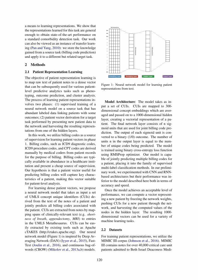
a means to learning representations. We show thatthe representations learned for this task are generalenough to obtain state-of-the-art performance ona standard comorbidity detection task. Our workcan also be viewed as an instance of transfer learn-ing (Pan and Yang, 2010): we store the knowledgegained from a source task (billing code prediction)and apply it to a different but related target task.
2 Methods
2.1 Patient Representation Learning
The objective of patient representation learning isto map raw text of patient notes to a dense vectorthat can be subsequently used for various patient-level predictive analytics tasks such as pheno-typing, outcome prediction, and cluster analysis.The process of learning patient representations in-volves two phases: (1) supervised training of aneural network model on a source task that hasabundant labeled data linking patients with someoutcomes; (2) patient vector derivation for a targettask performed by presenting new patient data tothe network and harvesting the resulting represen-tations from one of the hidden layers.
In this work, we utilize billing codes as a sourceof supervision for learning patient vectors in phase1. Billing codes, such as ICD9 diagnostic codes,ICD9 procedure codes, and CPT codes are derivedmanually by medical coders from patient recordsfor the purpose of billing. Billing codes are typi-cally available in abundance in a healthcare insti-tution and present a cheap source of supervision.Our hypothesis is that a patient vector useful forpredicting billing codes will capture key charac-teristics of a patient, making this vector suitablefor patient-level analysis.
For learning dense patient vectors, we proposea neural network model that takes as input a setof UMLS concept unique identifiers (CUIs) de-rived from the text of the notes of a patient andjointly predicts all billing codes associated withthe patient. CUIs are extracted from notes by map-ping spans of clinically-relevant text (e.g. short-ness of breath, appendectomy, MRI) to entriesin the UMLS Metathesaurus. CUIs can be eas-ily extracted by existing tools such as ApachecTAKES (http://ctakes.apache.org). Our neuralnetwork model (Figure 1) is inspired by Deep Av-eraging Network (DAN) (Iyyer et al., 2015), Fast-Text (Joulin et al., 2016), and continuous bag-of-words (CBOW) (Mikolov et al., 2013a,b) models.
Embedding Layer Averaging Layer Hidden Layer Output Layer
CUI1
CUI2
CUI3
•
•
•
•
•
•
•
•
•
•
•
CUIn
300 dimensions
300 dimensions
1000 dimensions
Figure 1: Neural network model for learning patientrepresentations from text.
Model Architecture: The model takes as in-put a set of CUIs. CUIs are mapped to 300-dimensional concept embeddings which are aver-aged and passed on to a 1000-dimensional hiddenlayer, creating a vectorial representation of a pa-tient. The final network layer consists of n sig-moid units that are used for joint billing code pre-diction. The output of each sigmoid unit is con-verted to a binary (1/0) outcome. The number ofunits n in the output layer is equal to the num-ber of unique codes being predicted. The modelis trained using binary cross-entropy loss functionusing RMSProp optimizer. Our model is capa-ble of jointly predicting multiple billing codes fora patient, placing it into the family of supervisedmulti-label classification methods. In our prelimi-nary work, we experimented with CNN and RNN-based architectures but their performance was in-ferior to the model described here both in terms ofaccuracy and speed.
Once the model achieves an acceptable level ofperformance, we can compute a vector represent-ing a new patient by freezing the network weights,pushing CUIs for a new patient through the net-work, and harvesting the computed values of thenodes in the hidden layer. The resulting 1000-dimensional vectors can be used for a variety ofmachine learning tasks.
2.2 Datasets
For training patient representations, we utilize theMIMIC III corpus (Johnson et al., 2016). MIMICIII contains notes for over 40,000 critical care unitpatients admitted to Beth Israel Deaconess Medi-
120

cal Center as well as ICD9 diagnostic, procedure,and Current Procedural Terminology (CPT) codes.Since our goal is learning patient-level representa-tions, we concatenate all available notes for eachpatient into a single document. We also combineall ICD9 and CPT codes for a patient to form thetargets for the prediction task. Finally, we pro-cess the patient documents with cTAKES to ex-tract UMLS CUIs. cTAKES is an open-sourcesystem for processing clinical texts which has anefficient dictionary lookup component for identi-fying CUIs, making it possible to process a largenumber of patient documents.
To decrease training time, we reduce the com-plexity of the prediction task as follows: (1) wecollapse all ICD9 and CPT codes to their moregeneral category (e.g. first three digits for ICD9diagnostic codes), (2) we drop all CUIs that ap-pear fewer than 100 times, (3) we discard patientsthat have over 10,000 CUIs, (4) we discard allbilling codes that have fewer than 1,000 examples.This preprocessing results in a dataset consistingof 44,211 patients mapped to multiple codes (174categories total). We randomly split the patientsinto a training set (80%) and a validation set (20%)for tuning hyperparameters.
For evaluating our patient representations, weuse a publicly available dataset from the Informat-ics for Integrating Biology to the Bedside (i2b2)Obesity challenge (Uzuner, 2009). Obesity chal-lenge data consisted of 1237 discharge summariesfrom the Partners HealthCare Research PatientData Repository annotated with respect to obesityand its fifteen most common comorbidities. Eachpatient was thus labeled for sixteen different cate-gories. We focus on the more challenging intuitivetask (Uzuner, 2009; Miller et al., 2016), containingthree label types (present, absent, questionable),where annotators labeled a diagnosis as presentif its presence could be inferred (i.e., even if notexplicitly mentioned). This task involves compli-cated decision-making and inference.
Importantly, our patient representations areevaluated in sixteen different classification taskswith patient data originating from a healthcare in-stitution different from the one our representationswere trained on. This setup is challenging yet itpresents a true test of robustness of the learnedrepresentations.
2.3 ExperimentsOur first baseline is an SVM classifier trained withbag-of-CUIs features. Our second baseline in-volves linear dimensionality reduction performedby running singular value decomposition (SVD)on a patient-CUI matrix derived from the MIMICcorpus, reducing the space by selecting the 1000largest singular values, and mapping the target in-stances into the resulting 1000-dimensional space.
Our multi-label billing code classifier is trainedto maximize the macro F1 score for billing codeprediction on the validation set. We train themodel for 75 epochs with a learning rate of 0.001and batch size of 50. These hyperparameters areobtained by tuning the model’s macro F1 on thevalidation set. Observe that tuning of hyperpa-rameters occurred independently from the targettask. Also note that since our goal is not to ob-tain the best possible performance on a held outset, we are not allocating separate developmentand test sets. Once we determine the best valuesof these hyperparameters, we combine the train-ing and validation sets and retrain the model. Wetrain two version of the model: (1) with randomlyinitialized CUI embeddings, (2) with word2vec-pretrained CUI embeddings. Pre-trained embed-dings are learned using word2vec (Mikolov et al.,2013a) by extracting all CUIs from the text ofMIMIC III notes and using the CBOW methodwith windows size of 5 and embedding dimensionof 300.
We then create a 1000-dimensional vector rep-resentation for each patient in the i2b2 obesitychallenge data by giving the sparse (CUI-based)representation for each patient as input to the ICDcode classifier. Rather than reading the classifier’spredictions, we harvest the hidden layer outputs,forming a 1000-dimensional dense vector. Wethen train multi-class SVM classifiers for each dis-ease (using one-vs.-all strategy), building sixteenSVM classifiers. Following the i2b2 obesity chal-lenge, the models are evaluated using macro pre-cision, recall, and F1 scores (Uzuner, 2009).
We make the code available for use by the re-search community 1.
3 Results
Our billing code classifier achieves the macro F1score on the source task (billing code prediction)
1https://github.com/dmitriydligach/starsem2018-patient-representations
121

Disease Sparse SVD LearnedP R F1 P R F1 P R F1
Asthma 0.894 0.736 0.787 0.888 0.854 0.870 0.910 0.920 0.915CAD 0.583 0.588 0.585 0.593 0.602 0.596 0.596 0.596 0.596CHF 0.558 0.564 0.561 0.571 0.575 0.573 0.558 0.564 0.561Depression 0.797 0.685 0.715 0.723 0.727 0.725 0.781 0.773 0.777Diabetes 0.859 0.853 0.856 0.611 0.624 0.617 0.907 0.919 0.913GERD 0.530 0.466 0.485 0.533 0.482 0.499 0.528 0.539 0.533Gallstones 0.814 0.640 0.678 0.747 0.721 0.732 0.645 0.663 0.653Gout 0.975 0.811 0.871 0.955 0.834 0.882 0.928 0.910 0.919Hypercholesterolemia 0.781 0.784 0.782 0.789 0.793 0.790 0.865 0.868 0.866Hypertension 0.680 0.650 0.662 0.711 0.763 0.728 0.825 0.879 0.847Hypertriglyceridemia 0.933 0.679 0.748 0.580 0.610 0.591 0.604 0.650 0.621OA 0.514 0.448 0.466 0.479 0.442 0.454 0.511 0.508 0.510OSA 0.596 0.511 0.542 0.626 0.568 0.592 0.611 0.618 0.615Obesity 0.825 0.791 0.798 0.883 0.844 0.853 0.872 0.873 0.872PVD 0.594 0.542 0.564 0.599 0.557 0.576 0.568 0.599 0.582Venous Insufficiency 0.797 0.649 0.694 0.669 0.757 0.700 0.638 0.717 0.665Average 0.733 0.650 0.675 0.685 0.672 0.674 0.709 0.725 0.715
Table 1: Comorbidity challenge results (intuitive task). SVM trained using sparse representations (bag-of-CUIs)is compared to SVM trained using SVD-based representations and learned dense patient representations.
of 0.447 when using randomly initialized CUI em-beddings and macro F1 of 0.473 when using pre-trained CUI embeddings. This is not directly com-parable to existing work because it is a uniquesetup; but we note that this is likely a difficult taskbecause of the large output space. However, it isinteresting to note that pre-training CUI embed-ding has a positive relative impact on performance.
Classifier performance for the target pheno-typing task is shown in Table 1, which showsthe performance of the baseline SVM classifiertrained using the standard bag-of-CUIs approach(Sparse), the baseline using 1000-dimensionalvectors obtained via dimensionality reduction(SVD), and our system using dense patient vec-tors derived from the source task. Since a sepa-rate SVM classifier was trained for each disease,we present classifier performance for each SVMmodel.
Both of our baseline approaches showed ap-proximately the same performance (F1=0.675) asthe best reported i2b2 system (Solt et al., 2009)(although they used a rule-based approach). Ourdense patient representations outperformed bothbaseline approaches by four percentage points onaverage (F1=0.715). The difference is statisticallysignificant (t-test, p=0.03).
Out of the sixteen diseases, our dense represen-
tations performed worse (with one tie) than thesparse baseline only for three: gallstones, hyper-triglyceridemia, venous insufficiency. The likelycause is the scarcity of positive training examples;two of these diseases have the smallest number ofpositive training examples.
4 Discussion and Conclusion
For most diseases and on average our dense pa-tient representations outperformed sparse patientrepresentations. Importantly, patient representa-tions were learned from a task (billing code pre-diction) that is different from the evaluation task(comorbidity prediction), presenting evidence thatuseful representations can be derived in this trans-fer learning scenario.
Furthermore, the data from which the represen-tations were learned (BI medical center) and theevaluation data (Partners HealthCare) originatedfrom two different healthcare institutions provid-ing evidence of robustness of our patient represen-tations.
Our future work will include exploring the useof other sources of supervision for learning patientrepresentations, alternative neural network archi-tectures, tuning the learned patient representationsto the target task, and evaluating the patient repre-sentations on other phenotyping tasks.
122
Acknowledgments
The Titan X GPU used for this research wasdonated by the NVIDIA Corporation. TimothyMiller’s effort was supported by National Insti-tute of General Medical Sciences (NIGMS) of theNational Institutes of Health under award numberR01GM114355. The content is solely the respon-sibility of the authors and does not necessarily rep-resent the official views of the National Institutesof Health.
ReferencesEdward Choi, Mohammad Taha Bahadori, Andy
Schuetz, Walter F Stewart, and Jimeng Sun. 2016.Doctor ai: Predicting clinical events via recurrentneural networks. In Machine Learning for Health-care Conference. pages 301–318.
Edward Choi, Mohammad Taha Bahadori, Le Song,Walter F Stewart, and Jimeng Sun. 2017. GRAM:Graph-based attention model for healthcare repre-sentation learning. In Proceedings of the 23rd ACMSIGKDD International Conference on KnowledgeDiscovery and Data Mining. ACM, pages 787–795.
Mohit Iyyer, Varun Manjunatha, Jordan Boyd-Graber,and Hal Daume III. 2015. Deep unordered com-position rivals syntactic methods for text classifica-tion. In Proceedings of the 53rd Annual Meeting ofthe Association for Computational Linguistics andthe 7th International Joint Conference on NaturalLanguage Processing (Volume 1: Long Papers). vol-ume 1, pages 1681–1691.
Alistair EW Johnson, Tom J Pollard, Lu Shen, Li-wei H Lehman, Mengling Feng, Mohammad Ghas-semi, Benjamin Moody, Peter Szolovits, Leo An-thony Celi, and Roger G Mark. 2016. Mimic-iii,a freely accessible critical care database. Scientificdata 3.
Armand Joulin, Edouard Grave, Piotr Bojanowski, andTomas Mikolov. 2016. Bag of tricks for efficient textclassification. arXiv preprint arXiv:1607.01759 .
ZC Lipton, David Kale, Charles Elkan, and RandallWetzel. 2016. Learning to Diagnose with LSTMRecurrent Neural Networks. In Proceedings ofICLR 2016. San Juan, Puerto Rico.
Tomas Mikolov, Kai Chen, Greg Corrado, and Jef-frey Dean. 2013a. Efficient estimation of wordrepresentations in vector space. arXiv preprintarXiv:1301.3781 .
Tomas Mikolov, Wen-tau Yih, and Geoffrey Zweig.2013b. Linguistic regularities in continuous spaceword representations. In hlt-Naacl. volume 13,pages 746–751.
Timothy Miller, Dmitriy Dligach, and GuerganaSavova. 2016. Unsupervised document classifica-tion with informed topic models. In Proceedings ofthe 15th Workshop on Biomedical Natural LanguageProcessing. pages 83–91.
Riccardo Miotto, Li Li, Brian A Kidd, and Joel TDudley. 2016. Deep Patient: An UnsupervisedRepresentation to Predict the Future of Patientsfrom the Electronic Health Records. Scientific re-ports 6:26094. https://doi.org/10.1038/srep26094.
Phuoc Nguyen, Truyen Tran, Nilmini Wickramas-inghe, and Svetha Venkatesh. 2017. Deepr: A Con-volutional Net for Medical Records. IEEE Journalof Biomedical and Health Informatics https://doi.org/10.1109/JBHI.2016.2633963.
Sinno Jialin Pan and Qiang Yang. 2010. A survey ontransfer learning. IEEE Transactions on knowledgeand data engineering 22(10):1345–1359.
Trang Pham, Truyen Tran, Dinh Phung, and SvethaVenkatesh. 2016. Deepcare: A deep dynamic mem-ory model for predictive medicine. In Pacific-AsiaConference on Knowledge Discovery and Data Min-ing. Springer, pages 30–41.
Chaitanya Shivade, Preethi Raghavan, Eric Fosler-Lussier, Peter J Embi, Noemie Elhadad, Stephen BJohnson, and Albert M Lai. 2013. A review ofapproaches to identifying patient phenotype co-horts using electronic health records. Journalof the American Medical Informatics Association21(2):221–230.
Illes Solt, Domonkos Tikk, Viktor Gal, and Zsolt TKardkovacs. 2009. Semantic classification of dis-eases in discharge summaries using a context-awarerule-based classifier. Journal of the American Med-ical Informatics Association 16(4):580–584.
Ozlem Uzuner. 2009. Recognizing obesity and co-morbidities in sparse data. Journal of the AmericanMedical Informatics Association 16(4):561–570.
123
Proceedings of the 7th Joint Conference on Lexical and Computational Semantics (*SEM), pages 124–129New Orleans, June 5-6, 2018. c©2018 Association for Computational Linguistics
Polarity Computations in Flexible Categorial Grammar
Hai HuLinguistics Department
Indiana UniversityBloomington, IN 47405 [email protected]
Lawrence S. MossMathematics Department
Indiana UniversityBloomington, IN 47405 [email protected]
Abstract
This paper shows how to take parse trees inCCG and algorithmically find the polarities ofall the constituents. Our work uses the well-known polarization principle corresponding tofunction application, and we have extendedthis with principles for type raising and com-position. We provide an algorithm, extendingthe polarity marking algorithm of van Ben-them. We discuss how our system works inpractice, taking input from the C&C parser.
1 Introduction
The main goal of this work is to take input fromtext and then to automatically determine the polar-ity of all the words. For example, we aim to findthe arrows in sentences like Every dog↓ scares ↑ atleast two↓ cats↑, Every dog↓ and no cat↓ sleeps=,and Most rabbits= hop↑. The ↑ notation meansthat whenever we use the given sentence truth-fully, if we replace the marked word w with an-other word which is “≥ w,” then the resulting sen-tence will still be true. So we have a semanticinference. The ↓ notation means the same thing,except that when we substitute using a word ≤ w,we again preserve truth. Finally, the = notationmeans that we have neither property in general; ina valid semantic inference statement, we can onlyreplace the word with itself rather than with some-thing larger or smaller.
For example, if we had a collection of back-ground facts like cats ≤ animals, beagles ≤ dogs,scares ≤ startles, and one ≤ two, then our ↑ and↓ notations on Every dog↓ scares ↑ at least two↓
cats↑ would allow us to conclude Every beaglestartles at least one animal.
The goal of the paper is to provide a computa-tional system to determine the notations ↑, ↓,= oninput text to the best extent possible, either usinghand-created parses, or output from a popular and
freely available CCG parser C&C (Clark and Cur-ran, 2007).
Using our polarity tool, we get a very easy firststep on automatic inference done with little or norepresentation. We discuss potential applicationsto textual inference.
Theory We extend polarity determination forcategorial grammar (CG) (see Sanchez-Valencia(1991); van Benthem (1986); van Eijck (2007);Lavalle-Martınez et al. (2017)). These papers onlyconsider the Ajdukiewicz/Bar-Hillel (AB) flavorof CG, where the rules are restricted to applica-tion rules (>) and (<). There is a consensus thatapplication rules alone are too restrictive to givewide-coverage grammars. We thus extend thiswork to the full set of flexible combinators usedin CCG. We prove that our system is sound, in aprecise sense. Further, we show how to incorpo-rate boolean reasoning (Keenan and Faltz, 1984)to get a more complete system.
A working system We have implemented ouralgorithm in Python. This implementation handlessentences from the C&C parser (Clark and Curran,2007). This is a non-trivial step on top of the the-oretical advance because the parses delivered bythe C&C parser deviate in several respects fromthe semantically-oriented input that one would likefor this kind of work.
2 An Ordered Syntax-semanticsInterface
The basis of the semantics is the syntax-semanticsinterface in formal semantics, especially in CGand CCG (Keenan and Faltz, 1984; Carpenter,1998; Steedman, 2000; Jacobson, 2014).
Our syntax in this small paper will consist of thelexicon shown in our examples. Here is an exam-
124

ple of a CCG derivation:
Fido : npr
Fido: s/(s\npr)T
ch: (s\npr)/npr
Fido chased : s/nprB
Felix : npr
Fido chased Felix : s>
(1)This tree is not the simplest one for Fido chasedFelix. We chose it to remind the reader of the CCGrules of type-raising (T) and composition (B).
Let us fix a semantics. We first select the basetypes e and t. We generate complex types fromthese by using function types x → y. We adopta few standard abbreviations. We then fix a mapfrom the CG categories into the types. We chooses 7→ t, n 7→ e→ t, npr 7→ e, np 7→ (e→ t)→ t,etc. (We use npr for proper names.)
A model M is a set M together with interpre-tations of all the lexical items by objects of theappropriate semantic type. We use M as the se-mantic space for the type e, 2 = {F,T} for typet, and the full set of functions for higher types.The interpretations of some words are fixed: deter-miners, conjunctions and relative pronouns. Themodel thus interprets intransitive verbs by (et, t)t,and transitive verbs by (et, t)((et, t)t). By the Jus-tification Theorem in Keenan and Faltz (1984), wein fact may obtain these using simpler and morenatural data: for proper names we need only ob-jects of type e, for intransitive verbs we need onlyet, and for transitive verbs eet.
Let S be a sentence in our fragment, and let Πbe a parse tree for S. Associated to Π we havea semantic parse tree, giving us a term tS in thetyped lambda calculus over the base types e andt. This term may be interpreted in each modelM.For example, the interpretation corresponding to(1) is the boolean value in the model
(λx.x[[Fido]] ◦ [[chased]])[[Felix]].
Polarities ↑ and ↓ In order to say what the polar-ity symbols mean, we need to enrich our semanticspaces from sets to preorders (Moss, 2012; Icardand Moss, 2014).
A preorder P = (P,≤) is a set P with a rela-tion ≤ on P which is reflexive and transitive. Fixa modelM. Then each type x gives rise to a pre-order Px. We order Pt by F < T. For Pe we takethe flat preorder on the universe set M underlyingthe model. For the higher types x → y, we takethe set (Px → Py) of all functions and endow it
with the pointwise order. In this way every one ofour semantic types is naturally endowed with thestructure of a preorder in every model.
A function f : P → Q is monotone (or orderpreserving) if p ≤ q in P implies f(p) ≤ f(q) inQ. And f is antitone (or order inverting) if p ≤ qin P implies f(q) ≤ f(p) inQ.
Each sentence S in our fragment is now inter-preted in an ordered setting. This is the (math-ematical) meaning of our ↑ and ↓ arrows in thispaper. For example, when we write every dog↓
barks↑, this means: for all models M, all m1 ≤m2 in Pet (for dog), and all n1 ≤ n2 in P(et)t
(for barks), we have in 2 that [[every]] m2 n1 ≤[[every]] m1 n2.
Order-enriched types using +, −, and · Fol-lowing Dowty (1994) we incorporate monotonic-ity information into the types. Function typesx→ y split into three versions: the monotone ver-sion x +→ y, the antitone version x −→ y, and thefull version x
·→ y. (What we wrote before asx → y is now x
·→ y.) These are all preordersusing the pointwise order. We must replace all ofthe ordinary slash types by versions of them whichhave markings on them.
Lexicon with order-enriched types We use Sfor t, N or et for e ·→ t = e
+→ t, NP for N ·→ t,NP+ for N +→ t, and NP− for N −→ t. Note thatwe have a different font than our syntactic types s,n, and np. Then we use NP +→ S for intransitiveverbs, NP+ or NP− for noun phrases with deter-miners, e for proper names. For the determiners,our lexicon then uses the order-enriched types indifferent ways:
word type
every N −→ NP+
some N +→ NP+
word type
no N −→ NP−
most N ·→ NP+
3 Polarizing a Parse Tree
In this section, we specify the rules (see Fig-ure 1) by which we put markings and polaritieson each node of a CCG parse tree, based on amarked/order-enriched lexicon. The next sectiondiscusses the algorithm.
Input A parse tree T in CCG as in (1), and amarked lexicon.
Output We aim to convert T to a different treeT ∗ satisfying the following properties: (1) The se-mantic terms in T and T ∗ should denote the same
125
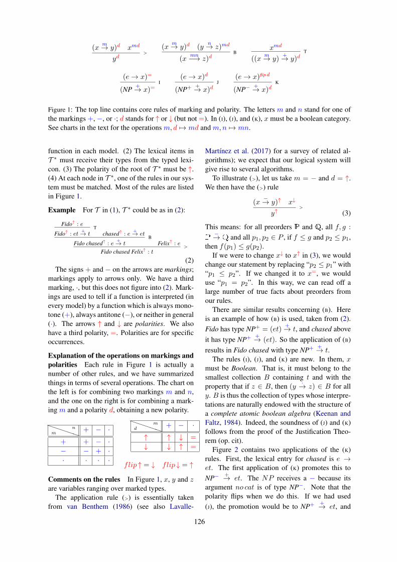
(xm→ y)d xmd
yd>
(xm→ y)d (y
n→ z)md
(xmn−→ z)d
Bxmd
((xm→ y)
+→ y)dT
(e→ x)=
(NP +→ x)=I
(e→ x)d
(NP+ +→ x)dJ
(e→ x)flip d
(NP− +→ x)dK
Figure 1: The top line contains core rules of marking and polarity. The letters m and n stand for one ofthe markings +, −, or ·; d stands for ↑ or ↓ (but not =). In (I), (J), and (K), x must be a boolean category.See charts in the text for the operations m, d 7→ md and m,n 7→ mn.
function in each model. (2) The lexical items inT ∗ must receive their types from the typed lexi-con. (3) The polarity of the root of T ∗ must be ↑.(4) At each node in T ∗, one of the rules in our sys-tem must be matched. Most of the rules are listedin Figure 1.
Example For T in (1), T ∗ could be as in (2):
Fido↑ : e
Fido↑ : et +→ tT
chased↑ : e +→ et
Fido chased↑ : e +→ tB
Felix↑ : eFido chased Felix↑ : t
>
(2)The signs + and − on the arrows are markings;
markings apply to arrows only. We have a thirdmarking, ·, but this does not figure into (2). Mark-ings are used to tell if a function is interpreted (inevery model) by a function which is always mono-tone (+), always antitone (−), or neither in general(·). The arrows ↑ and ↓ are polarities. We alsohave a third polarity, =. Polarities are for specificoccurrences.
Explanation of the operations on markings andpolarities Each rule in Figure 1 is actually anumber of other rules, and we have summarizedthings in terms of several operations. The chart onthe left is for combining two markings m and n,and the one on the right is for combining a mark-ing m and a polarity d, obtaining a new polarity.
PPPPPmn + − ·
+ + − ·− − + ·· · · ·
PPPPPdm + − ·
↑ ↑ ↓ =
↓ ↓ ↑ =
flip ↑ = ↓ flip ↓ = ↑
Comments on the rules In Figure 1, x, y and zare variables ranging over marked types.
The application rule (>) is essentially takenfrom van Benthem (1986) (see also Lavalle-
Martınez et al. (2017) for a survey of related al-gorithms); we expect that our logical system willgive rise to several algorithms.
To illustrate (>), let us take m = − and d = ↑.We then have the (>) rule
(x−→ y)↑ x↓
y↑>
(3)
This means: for all preorders P and Q, all f, g :
P−→ Q and all p1, p2 ∈ P , if f ≤ g and p2 ≤ p1,
then f(p1) ≤ g(p2).If we were to change x↓ to x↑ in (3), we would
change our statement by replacing “p2 ≤ p1” with“p1 ≤ p2”. If we changed it to x=, we woulduse “p1 = p2”. In this way, we can read off alarge number of true facts about preorders fromour rules.
There are similar results concerning (B). Hereis an example of how (B) is used, taken from (2).Fido has type NP+ = (et)
+→ t, and chased aboveit has type NP+ +→ (et). So the application of (B)results in Fido chased with type NP+ +→ t.
The rules (I), (J), and (K) are new. In them, xmust be Boolean. That is, it must belong to thesmallest collection B containing t and with theproperty that if z ∈ B, then (y
·→ z) ∈ B for ally. B is thus the collection of types whose interpre-tations are naturally endowed with the structure ofa complete atomic boolean algebra (Keenan andFaltz, 1984). Indeed, the soundness of (J) and (K)follows from the proof of the Justification Theo-rem (op. cit).
Figure 2 contains two applications of the (K)rules. First, the lexical entry for chased is e →et. The first application of (K) promotes this toNP− +→ et. The NP receives a − because itsargument no cat is of type NP−. Note that thepolarity flips when we do this. If we had used(J), the promotion would be to NP+ +→ et, and
126

no dog↓
no dog↑ : NP−>
ch↑ : e→ et
ch↓ : NP− +→ etK no cat↑
no cat↓ : NP−>
chased no cat↓ : e→ t>
chased no cat↑ : NP− +→ SK
no dog chased no cat↑ : S<
Figure 2: Two applications of the (K) rules.
there would be no polarity flipping. This wouldbe used in sentence where the object VP was somecat or every cat. The second application promotedchased no cat from the type et to NP− +→ S, againwith a polarity flip. If we had used (I), we wouldhave obtained NP +→ S. However, this would havetrivialized the polarity to =, and this effect wouldhave been propagated up the tree. Rule (I) wouldbe needed for the sentence most dogs chased nocat.
Several rules are not shown including “back-wards” versions of (>), (B), and (T), and also ver-sions where all polarizations are =. This is a tech-nical point that is not pertinent to this short ver-sion. We should mention that due to these rules,every tree may be polarized in a trivial way, by us-ing = at all nodes. So we are really interested inthe maximally informative polarizations, the onesthat make the most predictions.
Boolean connectives, etc. We take and and orto be polymorphic of the types B m→ (B
m→ B),when B is a Boolean category and m = +,−, or·. Negation flips polarities. Relative pronouns andrelative clauses also can be handled. Adjectivesare taken to be N +→ N.
Other combinators This paper only discusses(T) and (B), but we also have rules for the othercombinators used in CG, such as (S) and (W). Forexample, the (S) combinator is defined by Sfg =λx.(fx)(gx). In our system, the correspondingpolarization rule is
(xm→ (y
n→ z))d (xmn−→ y)nd
(xm→ z)d
S
This combinator is part of the standard presenta-tion of CCG, but it is less important in this paperbecause the C&C parser does not deliver parsesusing it.
4 Algorithmic Aspects
We have an algorithm1 that takes as input a CCGtree as in (1) and outputs some tree with markingsand polarities, a tree which satisfies the conditionsthat we have listed. The algorithm has two phases,similar to van Benthem’s algorithm (van Benthem,1986) for work with the Ajdukiewicz/Bar-Hillelvariant of CG (only application rules). Phase 1goes down the tree from leaves to root and addsthe markings, based on the rules in Figure 1. Themarkings on the leaves are given in the lexicon.The rest of Phase 1 is non-deterministic. We cansee this from our set of rules: there are many caseswhere one conclusion (on top of the line) permitsseveral possible conclusions. As we go down thetree, we frequently need to postpone the choice.
Phase 2 of the algorithm computes the polar-ities, again following the rules, starting with theroot. One always puts ↑ on the root, and then goesup the tree. This part of the algorithm is straight-forward.
The overall algorithm is in fact non-deterministic for two reasons. As we explained,Phase 1 has a non-deterministic feature. In addi-tion, it is always possible to polarize everythingwith = and make similar uninformative choicesfor the markings. We are really interested in themost informative polarization, the one with thefewest number of = polarities.
Soundness We have proved a soundness theo-rem for the system. Though too complicated tostate in full, it might be summarized informally,as follows. Suppose we have a sentence S in En-glish, and suppose that the lexical items in S aregiven semantics that conform to our assumptions.(This means that the semantics of the lexical en-tries must belong to the appropriate types.) Thenany semantic statement about the ↑, ↓, = mark-ing predicted by our system is correct. See Moss(2018) for details.
Completeness We have not proven the com-pleteness of our system/algorithm, and indeed thisis an open question. What completeness wouldmean for a system like ours is that whenever wehave an input CCG parse tree and a polarizationof its words which is semantically valid in thesense that it holds no matter how the nouns, verbs,etc. are interpreted, then our algorithm would de-tect this. This completeness would be a property
1https://github.com/huhailinguist/ccg2mono
127
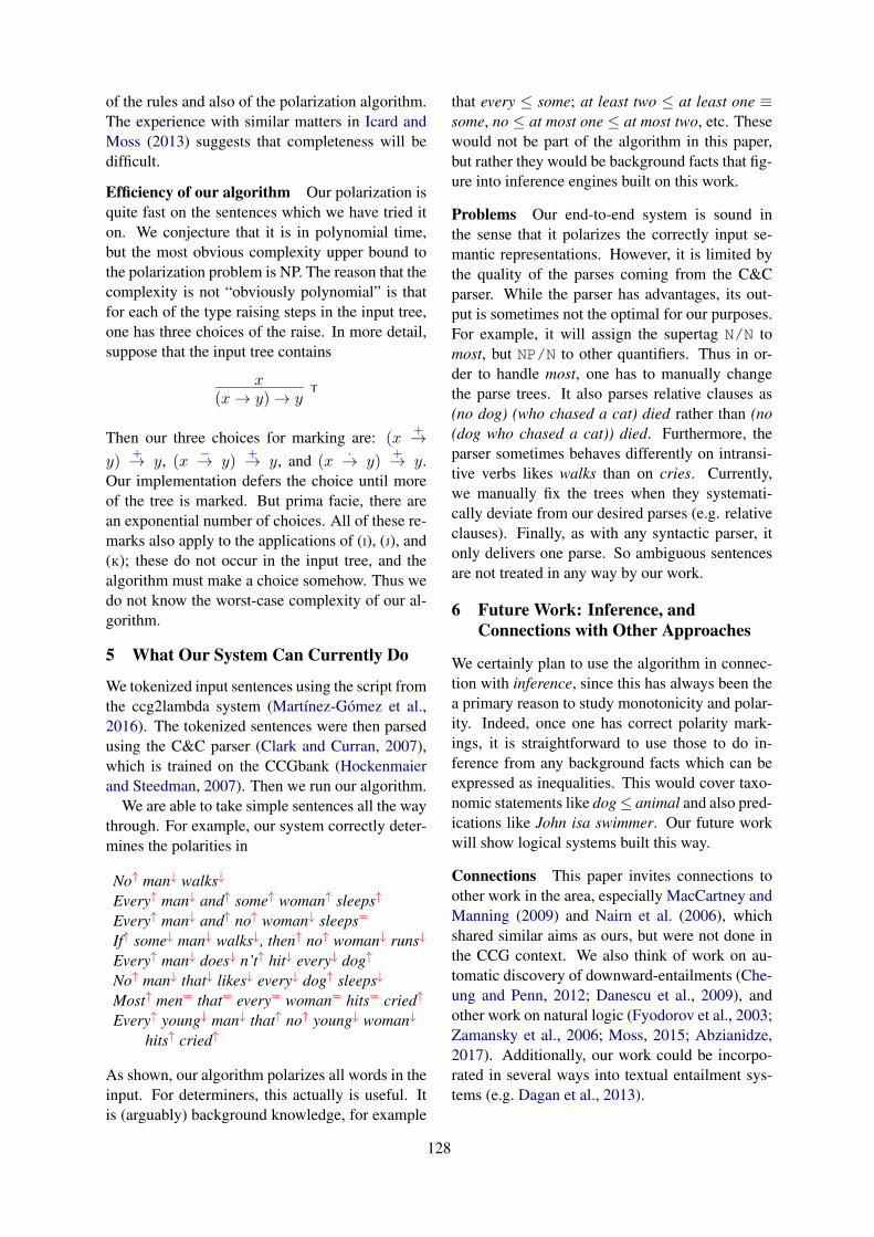
of the rules and also of the polarization algorithm.The experience with similar matters in Icard andMoss (2013) suggests that completeness will bedifficult.
Efficiency of our algorithm Our polarization isquite fast on the sentences which we have tried iton. We conjecture that it is in polynomial time,but the most obvious complexity upper bound tothe polarization problem is NP. The reason that thecomplexity is not “obviously polynomial” is thatfor each of the type raising steps in the input tree,one has three choices of the raise. In more detail,suppose that the input tree contains
x(x→ y)→ y
T
Then our three choices for marking are: (x+→
y)+→ y, (x
−→ y)+→ y, and (x
·→ y)+→ y.
Our implementation defers the choice until moreof the tree is marked. But prima facie, there arean exponential number of choices. All of these re-marks also apply to the applications of (I), (J), and(K); these do not occur in the input tree, and thealgorithm must make a choice somehow. Thus wedo not know the worst-case complexity of our al-gorithm.
5 What Our System Can Currently Do
We tokenized input sentences using the script fromthe ccg2lambda system (Martınez-Gomez et al.,2016). The tokenized sentences were then parsedusing the C&C parser (Clark and Curran, 2007),which is trained on the CCGbank (Hockenmaierand Steedman, 2007). Then we run our algorithm.
We are able to take simple sentences all the waythrough. For example, our system correctly deter-mines the polarities in
No↑ man↓ walks↓
Every↑ man↓ and↑ some↑ woman↑ sleeps↑
Every↑ man↓ and↑ no↑ woman↓ sleeps=
If↑ some↓ man↓ walks↓, then↑ no↑ woman↓ runs↓
Every↑ man↓ does↓ n’t↑ hit↓ every↓ dog↑
No↑ man↓ that↓ likes↓ every↓ dog↑ sleeps↓
Most↑ men= that= every= woman= hits= cried↑
Every↑ young↓ man↓ that↑ no↑ young↓ woman↓
hits↑ cried↑
As shown, our algorithm polarizes all words in theinput. For determiners, this actually is useful. Itis (arguably) background knowledge, for example
that every ≤ some; at least two ≤ at least one ≡some, no ≤ at most one ≤ at most two, etc. Thesewould not be part of the algorithm in this paper,but rather they would be background facts that fig-ure into inference engines built on this work.
Problems Our end-to-end system is sound inthe sense that it polarizes the correctly input se-mantic representations. However, it is limited bythe quality of the parses coming from the C&Cparser. While the parser has advantages, its out-put is sometimes not the optimal for our purposes.For example, it will assign the supertag N/N tomost, but NP/N to other quantifiers. Thus in or-der to handle most, one has to manually changethe parse trees. It also parses relative clauses as(no dog) (who chased a cat) died rather than (no(dog who chased a cat)) died. Furthermore, theparser sometimes behaves differently on intransi-tive verbs likes walks than on cries. Currently,we manually fix the trees when they systemati-cally deviate from our desired parses (e.g. relativeclauses). Finally, as with any syntactic parser, itonly delivers one parse. So ambiguous sentencesare not treated in any way by our work.
6 Future Work: Inference, andConnections with Other Approaches
We certainly plan to use the algorithm in connec-tion with inference, since this has always been thea primary reason to study monotonicity and polar-ity. Indeed, once one has correct polarity mark-ings, it is straightforward to use those to do in-ference from any background facts which can beexpressed as inequalities. This would cover taxo-nomic statements like dog≤ animal and also pred-ications like John isa swimmer. Our future workwill show logical systems built this way.
Connections This paper invites connections toother work in the area, especially MacCartney andManning (2009) and Nairn et al. (2006), whichshared similar aims as ours, but were not done inthe CCG context. We also think of work on au-tomatic discovery of downward-entailments (Che-ung and Penn, 2012; Danescu et al., 2009), andother work on natural logic (Fyodorov et al., 2003;Zamansky et al., 2006; Moss, 2015; Abzianidze,2017). Additionally, our work could be incorpo-rated in several ways into textual entailment sys-tems (e.g. Dagan et al., 2013).
128
ReferencesLasha Abzianidze. 2017. Langpro: Natural language
theorem prover. CoRR, abs/1708.09417.
Johan van Benthem. 1986. Essays in Logical Seman-tics. Reidel, Dordrecht.
Bob Carpenter. 1998. Type-Logical Semantics. MITPress.
Jackie Cheung and Gerald Penn. 2012. Unsuperviseddetection of downward-entailing operators by maxi-mizing classification certainty. In Proc. 13th EACL,pages 696–705.
Stephen Clark and James R Curran. 2007. Wide-coverage efficient statistical parsing with ccg andlog-linear models. Computational Linguistics,33(4):493–552.
Ido Dagan, Dan Roth, Mark Sammons, and Fabio Mas-simo Zanzotto. 2013. Recognizing Textual Entail-ment. Synthesis Lectures on Human LanguageTechnologies. Morgan & Claypool Publishers.
Cristian Danescu, Lillian Lee, and Richard Ducott.2009. Without a ‘doubt’? Unsupervised discoveryof downward-entailing operators. In Proceedings ofNAACL HLT.
David Dowty. 1994. The role of negative polarityand concord marking in natural language reasoning.In Proceedings of Semantics and Linguistic Theory(SALT) IV.
Jan van Eijck. 2007. Natural logic for natural language.In Logic, Language, and Computation, volume 4363of LNAI, pages 216–230. Springer-Verlag.
Yaroslav Fyodorov, Yoad Winter, and Nissim Fyo-dorov. 2003. Order-based inference in natural logic.Log. J. IGPL, 11(4):385–417. Inference in compu-tational semantics: the Dagstuhl Workshop 2000.
Julia Hockenmaier and Mark Steedman. 2007. Ccg-bank: a corpus of ccg derivations and dependencystructures extracted from the Penn Treebank. Com-putational Linguistics, 33(3):355–396.
Thomas F. Icard and Lawrence S. Moss. 2013. Acomplete calculus of monotone and antitone higher-order functions. In Proceedings, TACL 2013, vol-ume 23 of EPiC Series, pages 96–99. VanderbiltUniversity.
Thomas F. Icard and Lawrence S. Moss. 2014. Recentprogress on monotonicity. Linguistic Issues in Lan-guage Technology, 9(7):167–194.
Pauline Jacobson. 2014. An Introduction to the Syn-tax/Semantics Interface. Oxford University Press.
Edward L. Keenan and Leonard M. Faltz. 1984.Boolean Semantics for Natural Language. Springer.
Jose-de-Jesus Lavalle-Martınez, Manuel Montes-yGomez, Luis Villasenor-Pineda, Hector Jimenez-Salazar, and Ismael-Everardo Barcenas-Patino.2017. Equivalences among polarity algorithms.Studia Logica.
Bill MacCartney and Christopher D. Manning. 2009.An extended model of natural logic. In IWCS-8,Proceedings of the Eighth International Conferenceon Computational Semantics, pages 140–156.
Pascual Martınez-Gomez, Koji Mineshima, YusukeMiyao, and Daisuke Bekki. 2016. ccg2lambda: Acompositional semantics system. In Proceedingsof ACL 2016 System Demonstrations, pages 85–90, Berlin, Germany. Association for ComputationalLinguistics.
Lawrence S. Moss. 2012. The soundness of internal-ized polarity marking. Studia Logica, 100(4):683–704.
Lawrence S. Moss. 2015. Natural logic. In Handbookof Contemporary Semantic Theory, Second Edition,pages 646–681. Wiley-Blackwell.
Lawrence S. Moss. 2018. Foundations of polarity de-termination for flexible categorial grammars. Un-published ms.
Rowan Nairn, Cleo Condoravdi, and Lauri Karttunen.2006. Computing relative polarity for textual infer-ence. In Proceedings of ICoS-5 (Inference in Com-putational Semantics), Buxton, UK.
Victor Sanchez-Valencia. 1991. Studies on NaturalLogic and Categorial Grammar. Ph.D. thesis, Uni-versiteit van Amsterdam.
Mark Steedman. 2000. The Syntactic Process. MITPress.
Anna Zamansky, Nissim Francez, and Yoad Winter.2006. A ‘natural logic’ inference system using theLambek calculus. Journal of Logic, Language, andInformation, 15(3):273–295.
129

Proceedings of the 7th Joint Conference on Lexical and Computational Semantics (*SEM), pages 130–141New Orleans, June 5-6, 2018. c©2018 Association for Computational Linguistics
Coarse Lexical Frame Acquisition at the Syntax–Semantics InterfaceUsing a Latent-Variable PCFG Model
Laura Kallmeyer* & Behrang Q. Zadeh*
SFB991, Heinrich-Heine-Universitat [email protected] [email protected]
Jackie Chi Kit CheungMcGill University
AbstractWe present a method for unsupervised lexi-cal frame acquisition at the syntax–semanticsinterface. Given a set of input strings de-rived from dependency parses, our methodgenerates a set of clusters that resemble lex-ical frame structures. Our work is motivatednot only by its practical applications (e.g., tobuild, or expand the coverage of lexical framedatabases), but also to gain linguistic insightinto frame structures with respect to lexicaldistributions in relation to grammatical struc-tures. We model our task using a hierarchicalBayesian network and employ tools and meth-ods from latent variable probabilistic contextfree grammars (L-PCFGs) for statistical infer-ence and parameter fitting, for which we pro-pose a new split and merge procedure. Weshow that our model outperforms several base-lines on a portion of the Wall Street Journalsentences that we have newly annotated forevaluation purposes.
1 Introduction
We propose a method for building coarse lexi-cal frames automatically from dependency parsedsentences; i.e., without using any explicit seman-tic information as training data. The task involvesgrouping verbs that evoke the same frame (i.e., areconsidered to be the head of this frame) and fur-ther clustering their syntactic arguments into latentsemantic roles. Hence, our target structures standbetween FrameNet (Ruppenhofer et al., 2016) andPropBank (Palmer et al., 2005) frames. Similarto FrameNet and in contrast to PropBank, we as-sume a many-to-many relationship between verbtypes and frame types. But similar to PropBank,we aim to cluster syntactic arguments into gen-eral semantic roles instead of frame-specific slot
*Both authors contributed equally to this work.
types in FrameNet. This allows us to generalizeacross frames concerning semantic roles. As partof this, we study possible ways to automaticallygenerate more abstract lexical-semantic represen-tations from lexicalized dependency structures.
In our task, grouping verb tokens into framesrequires not only distinguishing between differ-ent senses of verbs, but also identifying a rangeof lexical relationships (e.g., synonymy, oppositeverbs, troponymy, etc.) among them. Hence (asModi et al., 2012; Green et al., 2004), our prob-lem definition differs from most work on unsu-pervised fine-grained frame induction using verbsense disambiguation (e.g., Kawahara et al., 2014;Peng et al., 2017). Similarly, forming role clustersyields generalization from several alternate link-ings between semantic roles and their syntactic re-alization. Given, for instance, an occurrence of theverb pack and its syntactic arguments, not only dowe aim to distinguish different senses of the verbpack (e.g., as used to evoke the FILLING frame, orthe PLACING frame), but also to group these in-stances of ‘pack’ with other verbs that evoke thesame frame (e.g., to group instances of pack thatevoke the frame PLACING with instances of verbsload, pile, place, and so on when used to evoke thesame PLACING frame).
The motivation for this work is twofold. On theone hand, the frame induction techniques we pro-pose can be useful in the context of applicationssuch as text summarization (Cheung and Penn,2013), question answering (Frank et al., 2007;Shen and Lapata, 2007), and so on, for languageswhere we lack a frame-annotated resource for su-pervised frame induction, or to expand the cov-erage of already existing resources. On the otherhand, we are interested in theoretical linguisticinsights into frame structure. In this sense, our
130
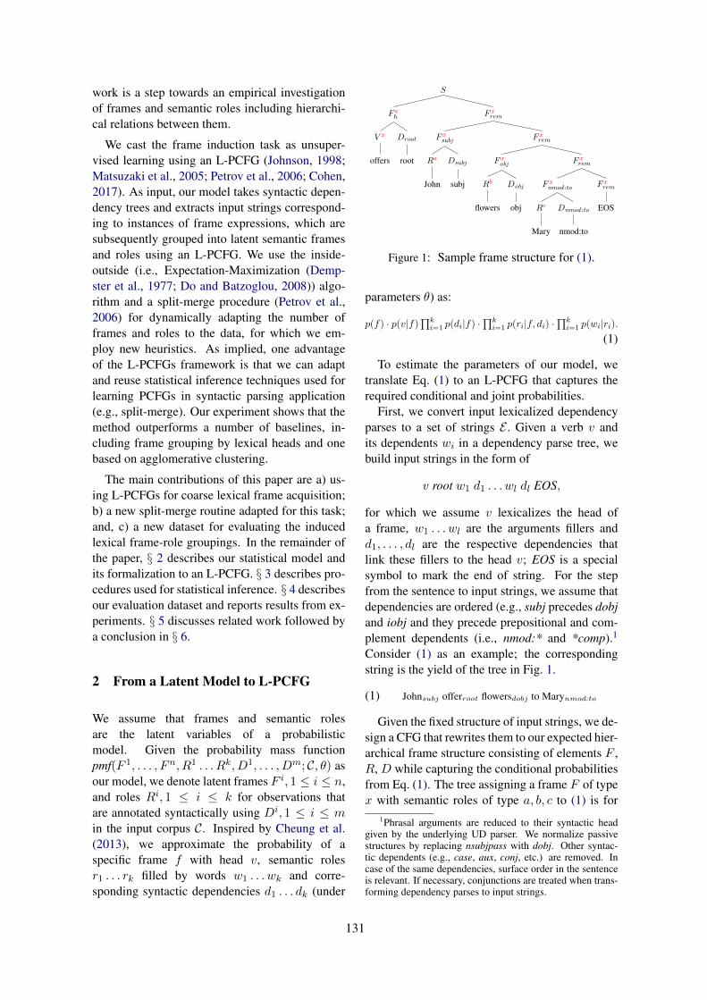
work is a step towards an empirical investigationof frames and semantic roles including hierarchi-cal relations between them.
We cast the frame induction task as unsuper-vised learning using an L-PCFG (Johnson, 1998;Matsuzaki et al., 2005; Petrov et al., 2006; Cohen,2017). As input, our model takes syntactic depen-dency trees and extracts input strings correspond-ing to instances of frame expressions, which aresubsequently grouped into latent semantic framesand roles using an L-PCFG. We use the inside-outside (i.e., Expectation-Maximization (Demp-ster et al., 1977; Do and Batzoglou, 2008)) algo-rithm and a split-merge procedure (Petrov et al.,2006) for dynamically adapting the number offrames and roles to the data, for which we em-ploy new heuristics. As implied, one advantageof the L-PCFGs framework is that we can adaptand reuse statistical inference techniques used forlearning PCFGs in syntactic parsing application(e.g., split-merge). Our experiment shows that themethod outperforms a number of baselines, in-cluding frame grouping by lexical heads and onebased on agglomerative clustering.
The main contributions of this paper are a) us-ing L-PCFGs for coarse lexical frame acquisition;b) a new split-merge routine adapted for this task;and, c) a new dataset for evaluating the inducedlexical frame-role groupings. In the remainder ofthe paper, § 2 describes our statistical model andits formalization to an L-PCFG. § 3 describes pro-cedures used for statistical inference. § 4 describesour evaluation dataset and reports results from ex-periments. § 5 discusses related work followed bya conclusion in § 6.
2 From a Latent Model to L-PCFG
We assume that frames and semantic rolesare the latent variables of a probabilisticmodel. Given the probability mass functionpmf(F 1, . . . , Fn, R1 . . . Rk, D1, . . . , Dm; C, θ) asour model, we denote latent frames F i, 1 ≤ i ≤ n,and roles Ri, 1 ≤ i ≤ k for observations thatare annotated syntactically using Di, 1 ≤ i ≤ min the input corpus C. Inspired by Cheung et al.(2013), we approximate the probability of aspecific frame f with head v, semantic rolesr1 . . . rk filled by words w1 . . . wk and corre-sponding syntactic dependencies d1 . . . dk (under
S
F xrem
F xrem
F xrem
F xrem
EOS
F xnmod :to
Dnmod :to
nmod:to
Rc
Mary
F xobj
Dobj
obj
Rb
flowers
F xsubj
Dsubj
subj
Ra
John
F xh
Droot
root
V x
offers
Figure 1: Sample frame structure for (1).
parameters θ) as:
p(f) · p(v|f)∏ki=1 p(di|f) ·
∏ki=1 p(ri|f, di) ·
∏ki=1 p(wi|ri).
(1)
To estimate the parameters of our model, wetranslate Eq. (1) to an L-PCFG that captures therequired conditional and joint probabilities.
First, we convert input lexicalized dependencyparses to a set of strings E . Given a verb v andits dependents wi in a dependency parse tree, webuild input strings in the form of
v root w1 d1 . . . wl dl EOS,
for which we assume v lexicalizes the head ofa frame, w1 . . . wl are the arguments fillers andd1, . . . , dl are the respective dependencies thatlink these fillers to the head v; EOS is a specialsymbol to mark the end of string. For the stepfrom the sentence to input strings, we assume thatdependencies are ordered (e.g., subj precedes dobjand iobj and they precede prepositional and com-plement dependents (i.e., nmod:* and *comp).1
Consider (1) as an example; the correspondingstring is the yield of the tree in Fig. 1.
(1) Johnsubj offerroot flowersdobj to Marynmod:to
Given the fixed structure of input strings, we de-sign a CFG that rewrites them to our expected hier-archical frame structure consisting of elements F ,R, D while capturing the conditional probabilitiesfrom Eq. (1). The tree assigning a frame F of typex with semantic roles of type a, b, c to (1) is for
1Phrasal arguments are reduced to their syntactic headgiven by the underlying UD parser. We normalize passivestructures by replacing nsubjpass with dobj. Other syntac-tic dependents (e.g., case, aux, conj, etc.) are removed. Incase of the same dependencies, surface order in the sentenceis relevant. If necessary, conjunctions are treated when trans-forming dependency parses to input strings.
131

instance given in Fig. 1. More generally, given fi-nite sets of frames F and of semantic rolesR, ourunderlying CFG G = 〈N,T, P, S〉 is as follows:
• T = Tv∪Tn∪D∪{root, EOS}, where Tv is theset of possible verbal heads, Tn is the set of pos-sible lexicalizations (fillers) for arguments, andD is a finite set of dependency relations; rootand EOS are special symbols.• N = {S} ∪ {F fh | f ∈ F} ∪ {F
frem | f ∈ F} ∪
{F fg | f ∈ F , g ∈ D}∪{Rr|r ∈ R}∪{V f | f ∈F} ∪ {Dg | g ∈ D}.• P contains the following rules:
– S → F fhFfrem for all f ∈ F ;
– F fh → V f Droot for all f ∈ F ;
– F frem → F fg Ffrem for all f ∈ F , g ∈ D;
– F frem → EOS for all f ∈ F ;– F fg → Rr Dg for all f ∈ F , r ∈ R, g ∈ D;– V f → v for all f ∈ F , v ∈ Tv;– Rr → n for all r ∈ R, n ∈ Tn;– Dg → g for all g ∈ D ∪ {root}.
With this grammar, an input string derived from adependency parsed sentence fully determines theshape of the tree and the node labels are fixed ex-cept for the choice of the frame f and the semanticroles r of the k fillers (i.e., x, a, b, and c in Fig. 1).
The probabilities of the rules correspond to theconditional probabilities in Eq. (1). The probabil-ity of S → F fh F frem gives p(F = f), the prob-ability of V f → v gives p(V = v|F = f), andso on. During the subsequent inside-outside (IO)split-and-merge training procedure, the inventoryof frames and roles and the probabilities corre-sponding to our rules are estimated so that theoverall likelihood of observations is maximized.
3 Method
This section describes statistical inference meth-ods used for inducing latent frame clusters frominput strings. The scenario we used for parame-ter fitting (split, merge, smoothing, and generatingclusters) is described in § 3.1. In § 3.2, we describeour method for computing embedding-based sim-ilarity between frames, which we use during themerge process and in our baseline system.
3.1 Parameter FittingGiven an input corpus parsed into universal de-pendencies (UD) and converted into a set of input
strings E , we instantiate a model G according to§ 2. We set |F| = 1 and |R| = |D|, and D, Tvand Tn are automatically extracted from E . Start-ing from this, we iteratively perform split-mergesequences (with an IO parameter estimation in be-tween), and cluster E to disjoint subsets Ei by find-ing the most-likely derivations that G yields. Wedetail this process in the following subsections.
3.1.1 The IO AlgorithmAs a solution to sparsity of observations, we mod-ify the IO algorithm slightly. We adapt the proce-dures described in (Eisner, 2016) with the excep-tion that for computing inside and outside prob-abilities, instead of mapping terminals to nonter-minals using an exact matching of the right-hand-sides of the rules (and respectively their assignedparameters), we use embedding-based similarities.I.e., for computing inside probabilities, given sym-bol a as input, instead of considering A →θ asrewrite rules and updating the parse chart only byasserting θ in it, we also consider B →θ bs inwhich instead of θ we assert α × θs in the IO ta-ble, where α is the r2 coefficient correlations ofembeddings for a and bs. During the outside pro-cedure, θs are updated proportionally w.r.t. to αsused during the inside parameter estimation pro-cedure.
3.1.2 SplitWe alter the splitting procedure from (Klein andManning, 2003a; Petrov et al., 2006) for our ap-plication. In (Klein and Manning, 2003b; Petrovet al., 2006), during split, a non-terminal symbol(which represents a random variable in the under-lying probabilistic model) is split and its relatedproduction rules are duplicated independently ofits parent, or sibling nodes. We can apply sucha context-independent split only to the Rr non-terminals but the F f...s must split dependently w.r.t.their sibling nodes that define the frame structure.Therefore, to split frame x to two frames y and z,we replace the entire set {S → F xhF
xrem, F xh →
V x Droot, F xrem → EOS, F xrem → F xg F xrem,F xg → Rr Dg, and V x → v} with two similar setswhere x gets replaced with y and z, respectively.The parameters for the new rules are set to half ofthe value of the parameters of the rules that theyoriginated from with the addition (or subtraction)of a random ε (e.g., 1e-7) to break symmetry.
Moreover, in our application, training the splitgrammar on the whole input is ineffective and at
132
a certain point, computationally intractable. Theproblem is due to the scope of the split grammarand the large portion of input strings E that theyspan. Splitting a frame’s rules, unlike parameterfitting for syntactic rules, increases the number ofpossible derivations for all E , to the extent that af-ter a number of split iterations the computationof the derivations becomes intractable even for asmall E of short length. We address this problemby using a new strategy for splitting: we not onlysplit the grammar, but also the input training data.
Before each split, we cluster input strings E toclusters Ei that G gives (§ 3.1.4) at that point. Forinput strings in each cluster Ei, we instantiate anew Gi and perform parameter fitting and split-ting independently of other Eis. The correspond-ing probabilistic Gi is initialized by assigning ran-dom parameters to its rules and then smoothingthem (§ 3.1.3) by the fitted parameters for G. Weapply the aforementioned process several times,until the number of independently generated clus-ters is at least twice as large as |Tv|. At the end ofeach split iteration, we collect the elicited Ei clus-ters (and their respective Gis) for the next mergeprocess. Given the independence assumption be-tween roles and frames, pre-terminals that rewriteroles are split similar to (Petrov et al., 2006).
3.1.3 SmoothingWe apply a notion of smoothing by interpolatingparameters that are obtained in the n−1th iterationof split-merge with parameters that are randomlyinitialized at the beginning of each split-merge it-eration and, as mentioned earlier in § 3.1.2, whenderiving new Gis from G: For each rule in Gi orGn with parameters θ (i.e., the G instantiated forthe next split-merge iteration), we smooth θs usingθ = αθ + (1− α)θn−1, where θn−1 is the alreadyknown and fitted parameter for the correspondingrule in G. We choose α = 0.1.
3.1.4 Generating Clusters from G
After fitting parameters of G, the frame struc-ture for an input string is given by its most-likelyviterbi derivation with respect to G. The verbwhich is rewritten by F fh is placed to frame-type/cluster f . Similarly, lexical items that are ar-gument fillers are assigned to type/cluster r wherer is the structural annotation for pre-terminal Rr
that rewrite them. For example, assuming Fig 1is the most likely derivation for (1), the verb ‘of-fer’ is categorized as frame x and its arguments as
roles a, b, and c.
3.1.5 MergeThe model resulting from the split process gen-erates a relatively large number of ‘homoge-neous’ clusters that are ‘incomplete’. A subse-quent merge process unifies these homogeneous-but-incomplete clusters to achieve a clustering thatis both homogeneous and complete. To this end,we use heuristics which are based on both the es-timated loss in likelihood from merging two sym-bols that span the same input sequence (as pro-posed previously in Petrov et al. (2006)) as wellas the ‘discriminative similarities’ between the ob-tained clusters.
Merge by likelihoods does not work: Theheuristics for merge in (Petrov et al., 2006) (i.e.,minimizing the loss in training likelihood using‘locally’ estimated inside and outside probabili-ties) are based on the assumptions that a) pre-terminals appearing in different places in deriva-tions are nearly independent, and b) that their ap-proximation (according to the method proposedby Petrov et al. (2006)) requires less computa-tion than computing full derivation trees. How-ever, neither of these hold in our case: a) mostpre-terminals in our model are dependent on eachother and, b) to compute the loss in likelihoodfrom a cluster merge requires computation of fullderivation trees (given the interdependence be-tween pre-terminals that define frame structures).More importantly, in our application, the outsideprobabilities for clusters are always 1.0 and dif-ferences in the sum of inside probabilities is oftennegligible since input strings are spanned more-or-less by the same set of derivations. For thesereasons (i.e., computation cost and the lack of suf-ficient statistics), the ‘estimated loss in likelihood’heuristics is a futile method for guiding the mergeprocess in our application. We resolve this prob-lem by leveraging discriminative similarities be-tween the obtained frame clusters and proposing ahybrid method.
Our merge approach: In the beginning of amerge process, we conflate Gis that are obtainedfrom the previous split procedure to form a G thatspans all input strings. Where applicable, we setparameters of rules in G to the arithmetic meanof corresponding ones obtained from the split pro-cess and normalize them such that sum of the pa-rameters of rules with the same pre-terminal is 1.0.
133
We go through an iterative process: Using themethod proposed in § 3.2 below, the frame in-stances in the clusters are converted to tensors andsimilarities among them are computed. Motivatedby the assumption that split clusters are homoge-neous, for every pair of clusters cx and cy (x 6= y)with instances ai ∈ cx and bj ∈ cy, we findargmaxi,j sim(ai, bj) and argmini,j sim(ai, bj)(sim is given by Eq. 2 below) and calculate theirharmonic mean as the similarity sc between cx andcy. Cluster pairs are sorted in a descending orderby sc. Given a threshold δ, for all sc(cx, cy) > δ,their corresponding production rules (i.e., the sim-ilar set of rules mentioned in the split procedure)are merged and their parameters are updated to thearithmetic mean of their origin rules.
Parameters for this new merged G are updatedthrough a few IO iterations (in an incrementalfashion (Liang and Klein, 2009)), and finally Gis used to obtain a new clustering. The processis repeated for this newly obtained clustering untilall the resulting cluster-wise sc similarities are lessthan a threshold β.
Computing all derivations for each input stringis time consuming and makes the merge processcomputationally expensive, particularly in the firstfew iterations. We resolve this issue using astratified random sampling and by performing theaforementioned iterations only on a random sub-set of input strings in each cluster. Each cluster inthe output of the split process is taken as a stratumand its size is reduced by 90% by applying a ran-dom sampling; this random sampling is updatedin each iteration (we use a similar strategy for pa-rameter estimation, i.e., we update samples in eachestimation iteration). This process reduces the re-quired time for merge drastically without hurtingthe overall outcome of the merge process. It isworth to mention that after merging clusters cx andcy, the output does not necessarily contain a clus-ter cx∪cy. Instead, the resulting clustering reflectsthe effect of merging the rules that rewrite cx andcy in the whole model.
To merge Rr categories, we use the mergemethod from (Petrov et al., 2006) based on the ob-tained likelihoods. After merging frame clusters,we reduce the number of Rrs by 50%. Since ourmethod for merging role categories is similar to(Petrov et al., 2006), we do not describe it here.
3.2 Similarity Between Frame Instances
When necessary (such as during merge), we com-pute embedding-based similarities between frameinstances similar to methods proposed in (Mitchelland Lapata, 2008; Clark, 2013). We build a n-dimensional embedding for each word appear-ing in our input strings from large web corpora.Each frame instance is then represented using a(m+ 1, n)-tensor, in which m is the total numberof argument types/clusters given by our model atits current stage and n is the dimensionality of theembeddings that represent words that fill these ar-guments. To this, we add the embedding for theverb that lexicalizes the head of the frame, whichgives us the final (m+ 1, n)-tensor.
For two frame-instances represented by tensorsa and b, the similarity for their arguments is
sim-arg(a, b) =1
k
m∑
i=1
r2(a~vi, b~vi),
in which ~vis are embeddings for the ith argumentfiller (
∑nj=1
~vij 6= 0), r2 is the coefficient of de-
termination, and k =∑
i[r2(a~vi, b~vi) 6= 0]. If an
argument is lexicalized by more than one filler, wereplace r2 with the arithmetic mean of r2s com-puted over each distinct pair of fillers. The overallsim between a and b is:
sim(a, b) = w1.r2(a ~vh, b ~vh) + w2.sim-arg(a, b),
(2)where ~vhs are the embeddings for the lex-ical heads (i.e., verbs), and w1 and w2
are two hyper-parameters which can betuned. For instance, for two hypotheticalstructures of Fa:[Head:travel, [Arg1:John,Arg2:London]] and Fb:[Head:walk, [Arg1:Mary,Arg3:home]], the similarity between Fa andFb is w1r
2( ~travel, ~walk) + w2r2( ~John, ~Mary),
given that the all these vectors have at leastone nonzero component. During merge we usew1 = w2 = 0.50.
We build our lexical embeddings of dimension-ality n = 900 using the hash-based embeddinglearning technique proposed in (QasemiZadeh andKallmeyer, 2017); before using these embeddings,we weight them using positive pointwise mutualinformation. During evaluation, this combinationof PPMI-weighted hash-based embeddings andthe r2 estimator consistently yielded better resultsthan using other popular choices such as the co-
134
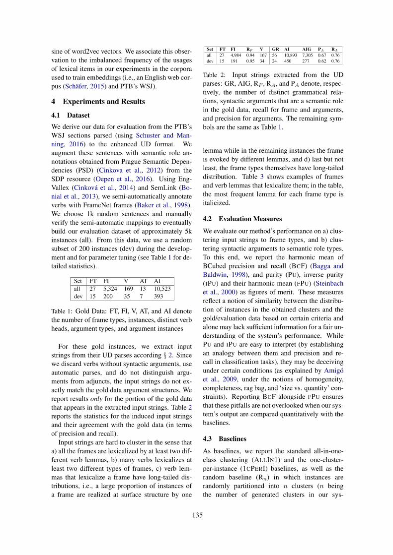
sine of word2vec vectors. We associate this obser-vation to the imbalanced frequency of the usagesof lexical items in our experiments in the corporaused to train embeddings (i.e., an English web cor-pus (Schafer, 2015) and PTB’s WSJ).
4 Experiments and Results
4.1 DatasetWe derive our data for evaluation from the PTB’sWSJ sections parsed (using Schuster and Man-ning, 2016) to the enhanced UD format. Weaugment these sentences with semantic role an-notations obtained from Prague Semantic Depen-dencies (PSD) (Cinkova et al., 2012) from theSDP resource (Oepen et al., 2016). Using Eng-Vallex (Cinkova et al., 2014) and SemLink (Bo-nial et al., 2013), we semi-automatically annotateverbs with FrameNet frames (Baker et al., 1998).We choose 1k random sentences and manuallyverify the semi-automatic mappings to eventuallybuild our evaluation dataset of approximately 5kinstances (all). From this data, we use a randomsubset of 200 instances (dev) during the develop-ment and for parameter tuning (see Table 1 for de-tailed statistics).
Set FT FI V AT AIall 27 5,324 169 13 10,523dev 15 200 35 7 393
Table 1: Gold Data: FT, FI, V, AT, and AI denotethe number of frame types, instances, distinct verbheads, argument types, and argument instances
For these gold instances, we extract inputstrings from their UD parses according § 2. Sincewe discard verbs without syntactic arguments, useautomatic parses, and do not distinguish argu-ments from adjuncts, the input strings do not ex-actly match the gold data argument structures. Wereport results only for the portion of the gold datathat appears in the extracted input strings. Table 2reports the statistics for the induced input stringsand their agreement with the gold data (in termsof precision and recall).
Input strings are hard to cluster in the sense thata) all the frames are lexicalized by at least two dif-ferent verb lemmas, b) many verbs lexicalizes atleast two different types of frames, c) verb lem-mas that lexicalize a frame have long-tailed dis-tributions, i.e., a large proportion of instances ofa frame are realized at surface structure by one
Set FT FI RF V GR AI AIG PA RA
all 27 4,984 0.94 167 56 10,893 7,305 0.67 0.76dev 15 191 0.95 34 24 450 277 0.62 0.76
Table 2: Input strings extracted from the UDparses: GR, AIG, RF , RA, and PA denote, respec-tively, the number of distinct grammatical rela-tions, syntactic arguments that are a semantic rolein the gold data, recall for frame and arguments,and precision for arguments. The remaining sym-bols are the same as Table 1.
lemma while in the remaining instances the frameis evoked by different lemmas, and d) last but notleast, the frame types themselves have long-taileddistribution. Table 3 shows examples of framesand verb lemmas that lexicalize them; in the table,the most frequent lemma for each frame type isitalicized.
4.2 Evaluation Measures
We evaluate our method’s performance on a) clus-tering input strings to frame types, and b) clus-tering syntactic arguments to semantic role types.To this end, we report the harmonic mean ofBCubed precision and recall (BCF) (Bagga andBaldwin, 1998), and purity (PU), inverse purity(IPU) and their harmonic mean (FPU) (Steinbachet al., 2000) as figures of merit. These measuresreflect a notion of similarity between the distribu-tion of instances in the obtained clusters and thegold/evaluation data based on certain criteria andalone may lack sufficient information for a fair un-derstanding of the system’s performance. WhilePU and IPU are easy to interpret (by establishingan analogy between them and precision and re-call in classification tasks), they may be deceivingunder certain conditions (as explained by Amigoet al., 2009, under the notions of homogeneity,completeness, rag bag, and ‘size vs. quantity’ con-straints). Reporting BCF alongside FPU ensuresthat these pitfalls are not overlooked when our sys-tem’s output are compared quantitatively with thebaselines.
4.3 Baselines
As baselines, we report the standard all-in-one-class clustering (ALLIN1) and the one-cluster-per-instance (1CPERI) baselines, as well as therandom baseline (Rn) in which instances arerandomly partitioned into n clusters (n beingthe number of generated clusters in our sys-
135
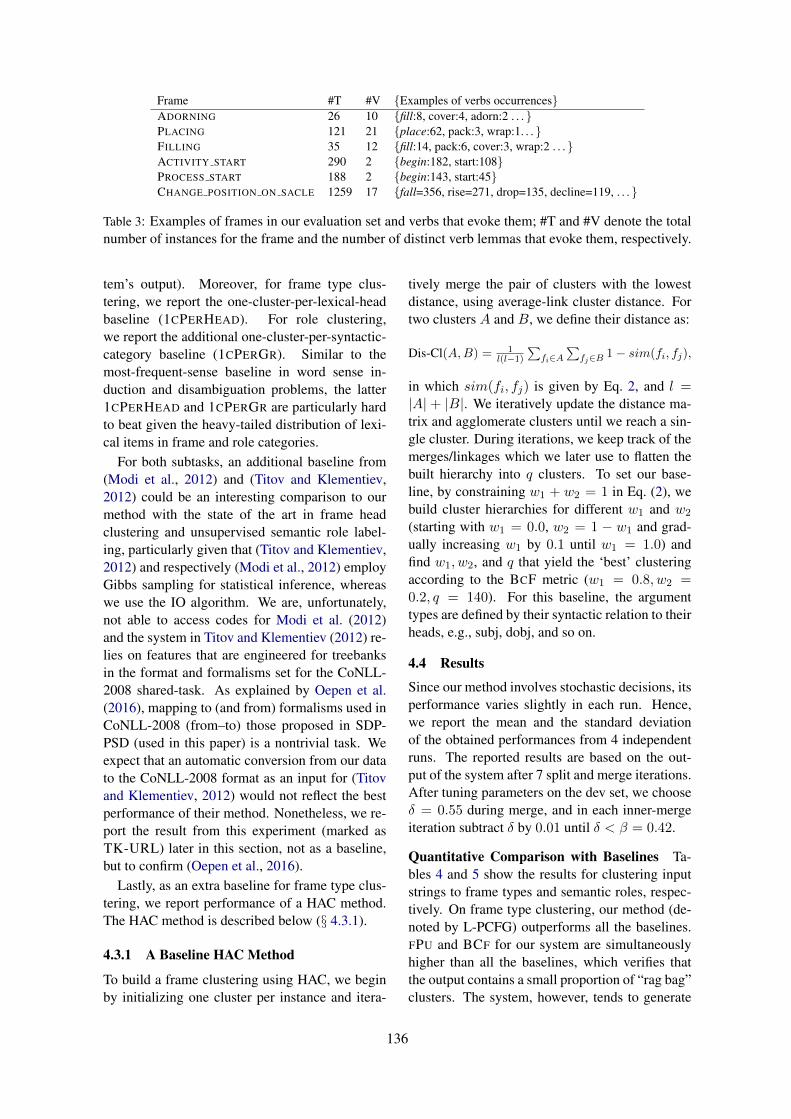
Frame #T #V {Examples of verbs occurrences}ADORNING 26 10 {fill:8, cover:4, adorn:2 . . . }PLACING 121 21 {place:62, pack:3, wrap:1. . . }FILLING 35 12 {fill:14, pack:6, cover:3, wrap:2 . . .}ACTIVITY START 290 2 {begin:182, start:108}PROCESS START 188 2 {begin:143, start:45}CHANGE POSITION ON SACLE 1259 17 {fall=356, rise=271, drop=135, decline=119, . . .}
Table 3: Examples of frames in our evaluation set and verbs that evoke them; #T and #V denote the totalnumber of instances for the frame and the number of distinct verb lemmas that evoke them, respectively.
tem’s output). Moreover, for frame type clus-tering, we report the one-cluster-per-lexical-headbaseline (1CPERHEAD). For role clustering,we report the additional one-cluster-per-syntactic-category baseline (1CPERGR). Similar to themost-frequent-sense baseline in word sense in-duction and disambiguation problems, the latter1CPERHEAD and 1CPERGR are particularly hardto beat given the heavy-tailed distribution of lexi-cal items in frame and role categories.
For both subtasks, an additional baseline from(Modi et al., 2012) and (Titov and Klementiev,2012) could be an interesting comparison to ourmethod with the state of the art in frame headclustering and unsupervised semantic role label-ing, particularly given that (Titov and Klementiev,2012) and respectively (Modi et al., 2012) employGibbs sampling for statistical inference, whereaswe use the IO algorithm. We are, unfortunately,not able to access codes for Modi et al. (2012)and the system in Titov and Klementiev (2012) re-lies on features that are engineered for treebanksin the format and formalisms set for the CoNLL-2008 shared-task. As explained by Oepen et al.(2016), mapping to (and from) formalisms used inCoNLL-2008 (from–to) those proposed in SDP-PSD (used in this paper) is a nontrivial task. Weexpect that an automatic conversion from our datato the CoNLL-2008 format as an input for (Titovand Klementiev, 2012) would not reflect the bestperformance of their method. Nonetheless, we re-port the result from this experiment (marked asTK-URL) later in this section, not as a baseline,but to confirm (Oepen et al., 2016).
Lastly, as an extra baseline for frame type clus-tering, we report performance of a HAC method.The HAC method is described below (§ 4.3.1).
4.3.1 A Baseline HAC Method
To build a frame clustering using HAC, we beginby initializing one cluster per instance and itera-
tively merge the pair of clusters with the lowestdistance, using average-link cluster distance. Fortwo clusters A and B, we define their distance as:
Dis-Cl(A,B) = 1l(l−1)
∑fi∈A
∑fj∈B 1− sim(fi, fj),
in which sim(fi, fj) is given by Eq. 2, and l =|A| + |B|. We iteratively update the distance ma-trix and agglomerate clusters until we reach a sin-gle cluster. During iterations, we keep track of themerges/linkages which we later use to flatten thebuilt hierarchy into q clusters. To set our base-line, by constraining w1 + w2 = 1 in Eq. (2), webuild cluster hierarchies for different w1 and w2
(starting with w1 = 0.0, w2 = 1 − w1 and grad-ually increasing w1 by 0.1 until w1 = 1.0) andfind w1, w2, and q that yield the ‘best’ clusteringaccording to the BCF metric (w1 = 0.8, w2 =0.2, q = 140). For this baseline, the argumenttypes are defined by their syntactic relation to theirheads, e.g., subj, dobj, and so on.
4.4 Results
Since our method involves stochastic decisions, itsperformance varies slightly in each run. Hence,we report the mean and the standard deviationof the obtained performances from 4 independentruns. The reported results are based on the out-put of the system after 7 split and merge iterations.After tuning parameters on the dev set, we chooseδ = 0.55 during merge, and in each inner-mergeiteration subtract δ by 0.01 until δ < β = 0.42.
Quantitative Comparison with Baselines Ta-bles 4 and 5 show the results for clustering inputstrings to frame types and semantic roles, respec-tively. On frame type clustering, our method (de-noted by L-PCFG) outperforms all the baselines.FPU and BCF for our system are simultaneouslyhigher than all the baselines, which verifies thatthe output contains a small proportion of “rag bag”clusters. The system, however, tends to generate
136

Method #C PU IPU FPU BCFALLIN1 1 22.35 100 36.54 17.431CPERI 4984 100 0.54 1.08 1.08
1CPERHEAD 167 94.38 59.59 73.06 63.53R235 235 24.7 2.03 3.75 1.79HAC 140 75.07 65.52 69.97 61.74
L-PCFG (Avg.) 230.25 86.2 73.64 79.4 71.29L-PCFG (Std. Dev.) ±6.24 ±3.07 ±0.96 ±1.17 ±1.49
Table 4: Results for head groupings: #C de-notes the number of induced clusters by eachmethod/baseline; the last two rows reports the av-erage and the standard deviation for the obtainedresults using the L-PCFG model.The remainingabbreviations are introduced in § 4.2 and 4.3.
Method #C PU IPU FPU BCFALLIN1 1 47.73 100 64.62 55.431CPERI 7257 100 0.18 0.36 0.36
1CPERGR 32 92.89 79.83 85.86 76.71R24 24 47.73 5.36 9.64 7.79
TK-URL 333 85.7 15.01 25.54 11.71L-PCFG (Avg.) 24 90.36 79.25 84.44 74.65
L-PCFG (Std. Dev.) ±5.29 ±0.33 ±1.31 ±0.61 ±1.38
Table 5: Results on clustering of syntactic argu-ments to semantic roles.
many incomplete yet homogeneous clusters (as wediscuss below). With respect to roles, however, themethod’s performance and its output remains verysimilar to the syntactic baseline (BCF=97.3).
What is in the clusters? The ability of the sys-tem to successfully cluster instances varies fromone gold frame category to another one. Themost problematic cases are the frame types AC-TIVITY START and PROCESS START, as well asPLACING. While the system put instances of‘start’ and ‘begin’ verbs in one cluster, it fails todistinguish between ACTIVITY START and PRO-CESS START. Regarding the PLACING frame, thesystem places verbs that evoke this frame in dif-ferent clusters; each cluster consists of instancesfrom one verb lemma. In our opinion, this is dueto the frequent idiomatic usages of these verbs,e.g., ‘to lay claim’, ‘to place listing’, ‘to positiononeself as’ and so on. This being said, however,the system is capable of distinguishing betweendifferent readings of polysemous verbs, e.g., in-stances of the verb ‘pack’ that evoke the FILLING
frame end up in different clusters than those evok-ing the PLACING frame. Additionally, for a num-ber of frame types, we observe that the systemcan successfully group synonymous (and oppo-site) verbs that evoke the same frame into one clus-ter: representative examples are the instances of
the CHANGE POSITION ON A SCALE frame thatare evoked by different verb lemmas such as ‘de-cline’, ‘drop’, ‘fall’, ‘gain’, ‘jump’, ‘rise’, . . . ,which all end up in one cluster. The output of thesystem also contains a large number of small clus-ters (consisting of only one or two instances): weobserve that these instances are usually those withwrong (and incomplete) dependency parses.
5 Related Work
Our work differs from most work on word senseinduction (WSI), e.g. (Goyal and Hovy, 2014; Lauet al., 2012; Manandhar et al., 2010; Van de Cruysand Apidianaki, 2011), in that not only do we dis-cern different senses of a lexical item but also wegroup the induced senses into more general mean-ing categories (i.e., FrameNet’s grouping). Hence,our model must be able to capture lexical rela-tionships other than polysemy, e.g., synonymy,antonymy (opposite verbs), troponymy, etc.. How-ever, our method can be adapted to WSI, too.Firstly, we can assume that word senses are ‘in-compatible’ and thus they necessarily evoke dif-ferent frames; subsequently, the induced frameclusters can be seen directly as clusters of wordsenses. Otherwise, the proposed method can beadapted for WSI by altering its initialization, e.g.,by building one-model-at-a-time for each wordform (i.e., simply altering the input).
Despite similarities between our method andthose proposed previously to address unsupervisedsemantic role induction (Carreras and Marquez,2005; Lang and Lapata, 2010, 2011; Titov andKlementiev, 2012; Swier and Stevenson, 2004),our method differs from them in that we at-tempt to include frame head grouping informationfor inducing roles associated to them. In otherwords, these methods leave out the problem ofsense/frame grouping in their models.
Our work differs in objective from methods forunsupervised template induction in informationextraction (IE) (e.g., MUC-style frames in Cham-bers and Jurafsky (2009, 2011) and its later refine-ments such as (Chambers, 2013; Cheung et al.,2013; Balasubramanian et al., 2013), and in abroader sense attempts towards ontology learn-ing and population from text (Cimiano et al.,2005)). Our focus is on lexicalized elementarysyntactic structures, identifying lexical semanticrelationships, and thereby finding salient patternsin syntax–semantic interface. However, in IE
137
tasks the aim is to build structured summariesof text. Therefore, the pre-and post-processingin these induction models are often more com-plex/different than our method (e.g., they requireanaphora resolution, identifying discourse rela-tions, etc.). Lastly, we deal with a broader set ofverbs and domains and more general frame defini-tions than these methods.
As stated earlier, Modi et al. (2012) propose themost similar work to ours. They adapt (Titov andKlementiev, 2012) to learn FrameNet-style headand role groupings. Modi et al. (2012) assumeroles to be frame-specific, while our role clustersare defined independently of frame groupings (asexpressed in Eq. 1). Last, with respect to researchsuch as (Pennacchiotti et al., 2008; Green et al.,2004) in which lexical resources such as Word-Net are used (in supervised or unsupervised set-tings) to refine and extend existing frame reposito-ries such as FrameNet, our model learns and boot-straps a frame repository from text annotated onlywith syntactic structure in an unsupervised way.
6 Conclusion
We proposed an unsupervised method for coarse-lexical frame induction from dependency parsedsentences using L-PCFG. We converted lexical-ized dependency trees of sentences to a set of in-put strings of fixed, predetermined structure con-sisting of a verbal head, its arguments and theirsyntactic dependencies. We then use a CFGmodel (subsequently L-PCFG) to shape/captureframe structures from these strings. We adaptedEM parameter estimation techniques from PCFGwhile relaxing independence assumptions, includ-ing appropriate methods for splitting and mergingframes and semantic roles and using word embed-dings for better generalization. In empirical eval-uations, our model outperforms several baselines.
Acknowledgments
We would like to thank Dr. Curt Anderson andDr. Rainer Osswlad for valuable comments on thepaper and analysis of frame clusters. The workdescribed in this paper is funded by the DeutscheForschungsgemeinschaft (DFG) through the ‘Col-laborative Research Centre 991 (CRC 991): TheStructure of Representations in Language, Cogni-tion, and Science’.
ReferencesEnrique Amigo, Julio Gonzalo, Javier Artiles, and
Felisa Verdejo. 2009. A comparison of extrinsicclustering evaluation metrics based on formal con-straints. Inf. Retr. 12(4):461–486. https://doi.org/10.1007/s10791-008-9066-8.
Amit Bagga and Breck Baldwin. 1998. Entity-based cross-document coreferencing using the vec-tor space model. In Proceedings of the 17th In-ternational Conference on Computational Linguis-tics - Volume 1. Association for ComputationalLinguistics, Stroudsburg, PA, USA, COLING ’98,pages 79–85. https://doi.org/10.3115/980451.980859.
Collin F. Baker, Charles J. Fillmore, and John B. Lowe.1998. The Berkeley FrameNet project. In Pro-ceedings of the 36th Annual Meeting of the Associ-ation for Computational Linguistics and 17th Inter-national Conference on Computational Linguistics -Volume 1. Association for Computational Linguis-tics, Stroudsburg, PA, USA, ACL ’98, pages 86–90. https://doi.org/10.3115/980845.980860.
Niranjan Balasubramanian, Stephen Soderland,Mausam, and Oren Etzioni. 2013. Generating co-herent event schemas at scale. In Proceedings of the2013 Conference on Empirical Methods in NaturalLanguage Processing. Association for Compu-tational Linguistics, Seattle, Washington, USA,pages 1721–1731. http://www.aclweb.org/anthology/D13-1178.
Claire Bonial, Kevin Stowe, and Martha Palmer. 2013.Renewing and revising SemLink. In Proceedingsof the 2nd Workshop on Linked Data in Linguis-tics (LDL-2013): Representing and linking lexicons,terminologies and other language data. Associationfor Computational Linguistics, Pisa, Italy, pages 9 –17. http://www.aclweb.org/anthology/W13-5503.
X. Carreras and L. Marquez. 2005. Introductionto the CoNLL-2005 shared task: Semantic rolelabeling. In Proceedings of the Ninth Confer-ence on Computational Natural Language Learning.pages 152–164. http://www.aclweb.org/anthology/W05-0620.
Nathanael Chambers. 2013. Event schema induc-tion with a probabilistic entity-driven model.In EMNLP. volume 13, pages 1797–1807.https://aclweb.org/anthology/D/D13/D13-1185.pdf.
Nathanael Chambers and Dan Jurafsky. 2009. Un-supervised learning of narrative schemas and theirparticipants. In Proceedings of the Joint Confer-ence of the 47th Annual Meeting of the ACL andthe 4th International Joint Conference on NaturalLanguage Processing of the AFNLP. Associationfor Computational Linguistics, Suntec, Singapore,pages 602–610. http://www.aclweb.org/anthology/P/P09/P09-1068.
138

Nathanael Chambers and Dan Jurafsky. 2011.Template-based information extraction withoutthe templates. In Proceedings of the 49th AnnualMeeting of the Association for ComputationalLinguistics: Human Language Technologies - Vol-ume 1. Association for Computational Linguistics,Stroudsburg, PA, USA, HLT ’11, pages 976–986.http://dl.acm.org/citation.cfm?id=2002472.2002595.
Jackie Chi Kit Cheung and Gerald Penn. 2013. To-wards robust abstractive multi-document summa-rization: A caseframe analysis of centrality and do-main. In Proceedings of the 51st Annual Meet-ing of the Association for Computational Lin-guistics (Volume 1: Long Papers). Associationfor Computational Linguistics, Sofia, Bulgaria,pages 1233–1242. http://www.aclweb.org/anthology/P13-1121.
J.C.K. Cheung, H. Poon, and L. Vanderwende. 2013.Probabilistic frame induction. In Proceedings ofNAACL-HLT . pages 837–846. http://www.aclweb.org/anthology/N13-1104.
Philipp Cimiano, Andreas Hotho, and Steffen Staab.2005. Learning concept hierarchies from text cor-pora using formal concept analysis. J. Artif. Int.Res. 24(1):305–339. http://dl.acm.org/citation.cfm?id=1622519.1622528.
Silvie Cinkova, Eva Fucıkova, Jana Sindlerova, andJan Hajic. 2014. EngVallex - English valency lex-icon. LINDAT/CLARIN digital library at the Insti-tute of Formal and Applied Linguistics, Charles Uni-versity. http://hdl.handle.net/11858/00-097C-0000-0023-4337-2.
Silvie Cinkova, Marie Mikulova, Lucie Mladova, AnjaNedoluzko, Petr Pajas, Jarmila Panevova, Jiri Se-mecky, Jana Sindlerova, Zdenka Uresova, ZdenekZabokrtsky, Jiri Semecky, Jana Sindlerova, JosefToman, Zdenka Uresova, and Zdenek Zabokrtsky.2012. Annotation of English on the tectogram-matical level: Reference book. https://ufal.mff.cuni.cz/techrep/tr35.pdf.
Stephen Clark. 2013. Quantum Physics and Linguis-tics, Oxford University Press, chapter Type-DrivenSyntax and Semantics for Composing Mean-ing Vectors. https://doi.org/http://dx.doi.org/10.1093/acprof:oso/9780199646296.003.0013.
Shay Cohen. 2017. Latent-variable PCFGs: Back-ground and applications. In Proceedings of the15th Meeting on the Mathematics of Language. As-sociation for Computational Linguistics, London,UK, pages 47–58. http://www.aclweb.org/anthology/W17-3405.
A. P. Dempster, N. M. Laird, and D. B. Rubin. 1977.Maximum likelihood from incomplete data via theEM algorithm. Journal of the Royal Statistical So-ciety 39(1):1–21.
Chuong B. Do and Serafim Batzoglou. 2008. What isthe expectation maximization algorithm? NatureBiotechnology https://doi.org/10.1038/nbt1406.
Jason Eisner. 2016. Inside-outside and forward-backward algorithms are just backprop. In Proceed-ings of the EMNLP Workshop on Structured Predic-tion for NLP. Austin, TX.
Anette Frank, Hans-Ulrich Krieger, Feiyu Xu,Hans Uszkoreit, Berthold Crysmann, Brigitte Jrg,and Ulrich Schfer. 2007. Question answer-ing from structured knowledge sources. Jour-nal of Applied Logic 5(1):20 – 48. Questionsand Answers: Theoretical and Applied Perspec-tives. https://doi.org/https://doi.org/10.1016/j.jal.2005.12.006.
Kartik Goyal and Eduard Hovy. 2014. Unsupervisedword sense induction using distributional statistics.In Proceedings of COLING 2014, the 25th Inter-national Conference on Computational Linguistics:Technical Papers. Dublin City University and Asso-ciation for Computational Linguistics, Dublin, Ire-land, pages 1302–1310. http://www.aclweb.org/anthology/C14-1123.
Rebecca Green, Bonnie J. Dorr, and Philip Resnik.2004. Inducing frame semantic verb classes fromwordnet and LDOCE. In Proceedings of the 42NdAnnual Meeting on Association for ComputationalLinguistics. Association for Computational Linguis-tics, Stroudsburg, PA, USA, ACL ’04. https://doi.org/10.3115/1218955.1219003.
Mark Johnson. 1998. PCFG models of linguistictree representations. Comput. Linguist. 24(4):613–632. http://dl.acm.org/citation.cfm?id=972764.972768.
Daisuke Kawahara, Daniel Peterson, OctavianPopescu, and Martha Palmer. 2014. Inducingexample-based semantic frames from a massiveamount of verb uses. In Proceedings of the 14thConference of the European Chapter of the Associa-tion for Computational Linguistics. Association forComputational Linguistics, Gothenburg, Sweden,pages 58–67. http://www.aclweb.org/anthology/E14-1007.
Dan Klein and Christopher D. Manning. 2003a. A*parsing: Fast exact Viterbi parse selection. In Pro-ceedings of the 2003 Conference of the North Amer-ican Chapter of the Association for ComputationalLinguistics on Human Language Technology - Vol-ume 1. Association for Computational Linguistics,Stroudsburg, PA, USA, NAACL ’03, pages 40–47. https://doi.org/10.3115/1073445.1073461.
Dan Klein and Christopher D. Manning. 2003b. Ac-curate unlexicalized parsing. In Proceedings of the41st Annual Meeting on Association for Computa-tional Linguistics - Volume 1. Association for Com-putational Linguistics, Stroudsburg, PA, USA, ACL
139
’03, pages 423–430. https://doi.org/10.3115/1075096.1075150.
Joel Lang and Mirella Lapata. 2010. Unsupervisedinduction of semantic roles. In Human LanguageTechnologies: The 2010 Annual Conference of theNorth American Chapter of the Association forComputational Linguistics. Association for Compu-tational Linguistics, Stroudsburg, PA, USA, HLT’10, pages 939–947. http://dl.acm.org/citation.cfm?id=1857999.1858135.
Joel Lang and Mirella Lapata. 2011. Unsupervisedsemantic role induction via split-merge cluster-ing. In Proceedings of the 49th Annual Meet-ing of the Association for Computational Lin-guistics: Human Language Technologies - Vol-ume 1. Association for Computational Linguistics,Stroudsburg, PA, USA, HLT ’11, pages 1117–1126. http://dl.acm.org/citation.cfm?id=2002472.2002614.
Jey Han Lau, Paul Cook, Diana McCarthy, DavidNewman, and Timothy Baldwin. 2012. Wordsense induction for novel sense detection. In Pro-ceedings of the 13th Conference of the EuropeanChapter of the Association for Computational Lin-guistics. Association for Computational Linguistics,pages 591–601. http://www.aclweb.org/anthology/E12-1060.
Percy Liang and Dan Klein. 2009. Online EMfor unsupervised models. In Proceedings ofHuman Language Technologies: The 2009 An-nual Conference of the North American Chap-ter of the Association for Computational Linguis-tics. Association for Computational Linguistics,Stroudsburg, PA, USA, NAACL ’09, pages 611–619. http://dl.acm.org/citation.cfm?id=1620754.1620843.
Suresh Manandhar, Ioannis Klapaftis, Dmitriy Dli-gach, and Sameer Pradhan. 2010. SemEval-2010Task 14: Word sense induction & disambiguation.In Proceedings of the 5th International Workshopon Semantic Evaluation. Association for Compu-tational Linguistics, Uppsala, Sweden, pages 63–68. http://www.aclweb.org/anthology/S10-1011.
Takuya Matsuzaki, Yusuke Miyao, and Jun’ichi Tsu-jii. 2005. Probabilistic CFG with latent annota-tions. In Proceedings of the 43rd Annual Meet-ing on Association for Computational Linguistics.Association for Computational Linguistics, Strouds-burg, PA, USA, ACL ’05, pages 75–82. https://doi.org/10.3115/1219840.1219850.
Jeff Mitchell and Mirella Lapata. 2008. Vector-basedmodels of semantic composition. In Proceedingsof ACL-08: HLT . Association for ComputationalLinguistics, Columbus, Ohio, pages 236–244.http://www.aclweb.org/anthology/P08-1028.
Ashutosh Modi, Ivan Titov, and Alexandre Klementiev.2012. Unsupervised induction of frame-semantic
representations. In Proceedings of the NAACL-HLT Workshop on the Induction of Linguistic Struc-ture. Association for Computational Linguistics,Montreal, Canada, pages 1–7. http://www.aclweb.org/anthology/W12-1901.
Stephan Oepen, Marco Kuhlmann, Yusuke Miyao,Daniel Zeman, Silvie Cinkova, Dan Flickinger,Jan Hajic, Angelina Ivanova, and Zdenka Uresova.2016. Towards comparability of linguistic graphbanks for semantic parsing. In Nicoletta Calzo-lari (Conference Chair), Khalid Choukri, ThierryDeclerck, Sara Goggi, Marko Grobelnik, BenteMaegaard, Joseph Mariani, Helene Mazo, Asun-cion Moreno, Jan Odijk, and Stelios Piperidis, edi-tors, Proceedings of the Tenth International Confer-ence on Language Resources and Evaluation (LREC2016). European Language Resources Association(ELRA), Paris, France.
Martha Palmer, Daniel Gildea, and Paul Kingsbury.2005. The Proposition Bank: An annotated cor-pus of semantic roles. Computational Linguistics31(1):71–106.
Haoruo Peng, Snigdha Chaturvedi, and Dan Roth.2017. A joint model for semantic sequences:Frames, entities, sentiments. In Proceedingsof the 21st Conference on Computational Natu-ral Language Learning (CoNLL 2017). Associa-tion for Computational Linguistics, pages 173–183. https://doi.org/10.18653/v1/K17-1019.
Marco Pennacchiotti, Diego De Cao, Roberto Basili,Danilo Croce, and Michael Roth. 2008. Automaticinduction of framenet lexical units. In Proceedingsof the Conference on Empirical Methods in Natu-ral Language Processing. Association for Computa-tional Linguistics, Stroudsburg, PA, USA, EMNLP’08, pages 457–465. http://dl.acm.org/citation.cfm?id=1613715.1613773.
Slav Petrov, Leon Barrett, Romain Thibaux, and DanKlein. 2006. Learning accurate, compact, and in-terpretable tree annotation. In ACL 2006, 21st In-ternational Conference on Computational Linguis-tics and 44th Annual Meeting of the Association forComputational Linguistics, Proceedings of the Con-ference, Sydney, Australia, 17-21 July 2006. http://aclweb.org/anthology/P06-1055.
Behrang QasemiZadeh and Laura Kallmeyer. 2017.HHU at SemEval-2017 Task 2: Fast hash-basedembeddings for semantic word similarity assess-ment. In Proceedings of the 11th InternationalWorkshop on Semantic Evaluation (SemEval-2017).Association for Computational Linguistics, pages250–255. https://doi.org/10.18653/v1/S17-2039.
Josef Ruppenhofer, Michael Ellsworth, Miriam R. L.Petruck, Christopher R. Johnson, Collin F. Baker,and Jan Scheffczyk. 2016. FrameNet II: ExtendedTheory and Practice. ICSI, Berkeley.
140

Roland Schafer. 2015. Processing and querying largeweb corpora with the COW14 architecture. In Pi-otr Baski, Hanno Biber, Evelyn Breiteneder, MarcKupietz, Harald Lngen, and Andreas Witt, editors,Proceedings of Challenges in the Management ofLarge Corpora 3 (CMLC-3). UCREL, IDS, Lan-caster. http://rolandschaefer.net/?p=749.
Sebastian Schuster and Christopher D. Manning. 2016.Enhanced english universal dependencies: An im-proved representation for natural language under-standing tasks. In Nicoletta Calzolari (Confer-ence Chair), Khalid Choukri, Thierry Declerck,Sara Goggi, Marko Grobelnik, Bente Maegaard,Joseph Mariani, Helene Mazo, Asuncion Moreno,Jan Odijk, and Stelios Piperidis, editors, Proceed-ings of the Tenth International Conference on Lan-guage Resources and Evaluation (LREC 2016). Eu-ropean Language Resources Association (ELRA),Paris, France.
Dan Shen and Mirella Lapata. 2007. Using seman-tic roles to improve question answering. In Pro-ceedings of the 2007 Joint Conference on Em-pirical Methods in Natural Language Processingand Computational Natural Language Learning(EMNLP-CoNLL). Association for ComputationalLinguistics, Prague, Czech Republic, pages 12–21. http://www.aclweb.org/anthology/D07-1002.
M. Steinbach, G. Karypis, and V. Kumar. 2000.A comparison of document clustering tech-niques. In KDD Workshop on Text Min-ing. http://citeseer.ist.psu.edu/steinbach00comparison.html.
Robert S. Swier and Suzanne Stevenson. 2004. Un-supervised semantic role labelling. In DekangLin and Dekai Wu, editors, Proceedings ofEMNLP 2004. Association for ComputationalLinguistics, Barcelona, Spain, pages 95–102.http://www.aclweb.org/anthology/W/W04/W04-3213.pdf.
Ivan Titov and Alexandre Klementiev. 2012. ABayesian approach to unsupervised semantic roleinduction. In EACL 2012, 13th Conference ofthe European Chapter of the Association for Com-putational Linguistics, Avignon, France, April 23-27, 2012. pages 12–22. http://aclweb.org/anthology/E/E12/E12-1003.pdf.
Tim Van de Cruys and Marianna Apidianaki. 2011.Latent semantic word sense induction and disam-biguation. In Proceedings of the 49th AnnualMeeting of the Association for Computational Lin-guistics: Human Language Technologies. Associa-tion for Computational Linguistics, Portland, Ore-gon, USA, pages 1476–1485. http://www.aclweb.org/anthology/P11-1148.
141
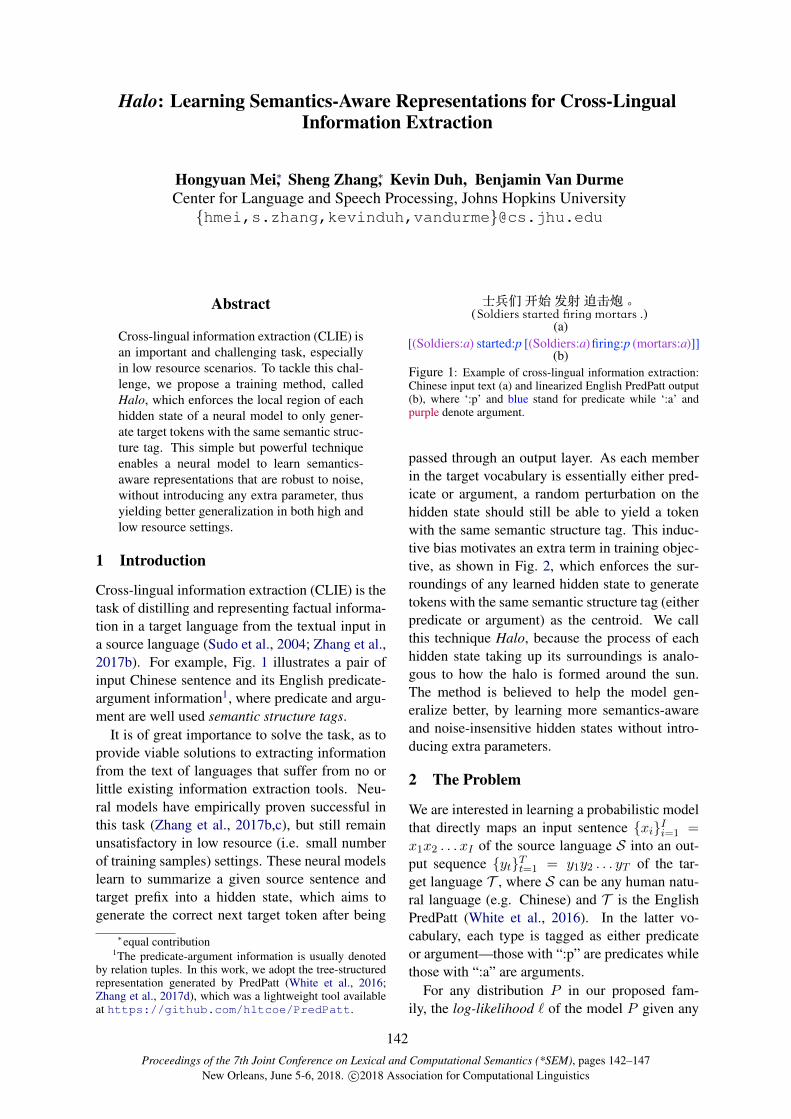
Proceedings of the 7th Joint Conference on Lexical and Computational Semantics (*SEM), pages 142–147New Orleans, June 5-6, 2018. c©2018 Association for Computational Linguistics
Halo: Learning Semantics-Aware Representations for Cross-LingualInformation Extraction
Hongyuan Mei∗, Sheng Zhang∗, Kevin Duh, Benjamin Van DurmeCenter for Language and Speech Processing, Johns Hopkins University{hmei,s.zhang,kevinduh,vandurme}@cs.jhu.edu
Abstract
Cross-lingual information extraction (CLIE) isan important and challenging task, especiallyin low resource scenarios. To tackle this chal-lenge, we propose a training method, calledHalo, which enforces the local region of eachhidden state of a neural model to only gener-ate target tokens with the same semantic struc-ture tag. This simple but powerful techniqueenables a neural model to learn semantics-aware representations that are robust to noise,without introducing any extra parameter, thusyielding better generalization in both high andlow resource settings.
1 Introduction
Cross-lingual information extraction (CLIE) is thetask of distilling and representing factual informa-tion in a target language from the textual input ina source language (Sudo et al., 2004; Zhang et al.,2017b). For example, Fig. 1 illustrates a pair ofinput Chinese sentence and its English predicate-argument information1, where predicate and argu-ment are well used semantic structure tags.
It is of great importance to solve the task, as toprovide viable solutions to extracting informationfrom the text of languages that suffer from no orlittle existing information extraction tools. Neu-ral models have empirically proven successful inthis task (Zhang et al., 2017b,c), but still remainunsatisfactory in low resource (i.e. small numberof training samples) settings. These neural modelslearn to summarize a given source sentence andtarget prefix into a hidden state, which aims togenerate the correct next target token after being
∗equal contribution1The predicate-argument information is usually denoted
by relation tuples. In this work, we adopt the tree-structuredrepresentation generated by PredPatt (White et al., 2016;Zhang et al., 2017d), which was a lightweight tool availableat https://github.com/hltcoe/PredPatt.
Figure 1: Example of cross-lingual information extraction:Chinese input text (a) and linearized English PredPatt output(b), where ‘:p’ and blue stand for predicate while ‘:a’ andpurple denote argument.
passed through an output layer. As each memberin the target vocabulary is essentially either pred-icate or argument, a random perturbation on thehidden state should still be able to yield a tokenwith the same semantic structure tag. This induc-tive bias motivates an extra term in training objec-tive, as shown in Fig. 2, which enforces the sur-roundings of any learned hidden state to generatetokens with the same semantic structure tag (eitherpredicate or argument) as the centroid. We callthis technique Halo, because the process of eachhidden state taking up its surroundings is analo-gous to how the halo is formed around the sun.The method is believed to help the model gen-eralize better, by learning more semantics-awareand noise-insensitive hidden states without intro-ducing extra parameters.
2 The Problem
We are interested in learning a probabilistic modelthat directly maps an input sentence {xi}Ii=1 =x1x2 . . . xI of the source language S into an out-put sequence {yt}Tt=1 = y1y2 . . . yT of the tar-get language T , where S can be any human natu-ral language (e.g. Chinese) and T is the EnglishPredPatt (White et al., 2016). In the latter vo-cabulary, each type is tagged as either predicateor argument—those with “:p” are predicates whilethose with “:a” are arguments.
For any distribution P in our proposed fam-ily, the log-likelihood ` of the model P given any
142

mortars:afiring:pstarted:p ?:p?:a
output layer
decoder unit
hidden space
Figure 2: Visualization of Halo method. While a neuralmodel learns to summarizes the current known informationinto a hidden state and predict the next target token, thesurroundings of this hidden state in the same space (two-dimensional in this example) are supervised to generate to-kens with the same semantic structure tag. For example, atthe last shown step, the centroid of purple area is the summa-rized hidden state and learns to predict ‘mortars:a’, while arandomly sampled neighbor is enforced to generate an argu-ment, although it may not be ‘mortars’ (thus denoted by ‘?’).Similar remarks apply to the blue regions.
({yt}Tt=1 | {xi}Ii=1) pair is:
T∑
t=1
logP(yt | yt−1, . . . , y0, {xi}Ii=1
)(1)
where y0 is a special beginning of sequence token.We denote vectors by bold lowercase Roman
letters such as h, and matrices by bold capital Ro-man letters such as W throughout the paper. Sub-scripted bold letters denote distinct vectors or ma-trices (e.g., pt). Scalar quantities, including vec-tor and matrix elements such as hd and pt,yt , arewritten without bold. Capitalized scalars representupper limits on lowercase scalars, e.g., 1 ≤ d ≤D. Function symbols are notated like their returntype. All R → R functions are extended to applyelementwise to vectors and matrices.
3 The Method
In this section, we first briefly review how thebaseline neural encoder-decoder models work onthis task, and then introduce our novel and well-suited training method Halo.
3.1 Baseline Neural Models
Previous neural models on this task (Zhang et al.,2017b,c) all adopt an encoder-decoder architec-ture with recurrent neural networks, particularlyLSTMs (Hochreiter and Schmidhuber, 1997). Ateach step t in decoding, the models summarize theinput {xi}Ii=1 and output prefix y1, . . . , yt−1 intoa hidden state ht ∈ (−1, 1)D, and then projectit with a transformation matrix W ∈ R|V|×D toa distribution pt over the target English PredPatt
vocabulary V:
pt = ot/(1>ot) (2a)
ot = expWht ∈ R|V|+ (2b)
where 1 is a |V|-dimensional one vector such thatpt is a valid distribution.
Suppose that the ground truth target token at thisstep is yt, the probability of generating yt underthe current model is pt,yt , obtained by accessingthe yt-th element in the vector pt. Then the log-likelihood is constructed as ` =
∑Tt=1 log pt,yt ,
and the model is trained by maximizing this ob-jective over all the training pairs.
3.2 Halo
Our method adopts a property of this task—the vo-cabulary V is partitioned into P , set of predicatesthat end with “:p”, and A, set of arguments thatend with “:a”. As a neural model would summa-rize everything known up to step t into ht, woulda perturbation h′t around ht still generate the sametoken yt? This bias seems too strong, but we canstill reasonably assume that h′t would generate atoken with the same semantic structure tag (i.e.predicate or argument). That is, the predictionmade by h′t should end with “:p” if yt is a pred-icate, and with “:a” otherwise.
This inductive bias provides us with anotherlevel of supervision. Suppose that at step t, aneighboring h′t is randomly sampled around ht,and is then used to generate a distribution p′t inthe same way as equation (2). Then we can geta distribution q′t over C = {predicate, argument},by summing all the probabilities of predicates andthose of arguments:
q′t,predicate =∑
v∈Pp′t,v (3a)
q′t,argument =∑
v∈Ap′t,v (3b)
This aggregation is shown in Fig. 3. Then the ex-tra objective is `′ =
∑Tt=1 log q
′t,ct , where ct =
predicate if the target token yt ∈ P (i.e. endingwith “:p”) and ct = argument otherwise.
Therefore, we get the joint objective to maxi-mize by adding ` and `′:
`+ `′ =T∑
t=1
log pt,yt +
T∑
t=1
log q′t,ct (4)
143

Pv2P pt,v
Pv2A pt,v
pt
qt
| {z } | {z }
V
C
Figure 3: Visualization of how q (distribution over C) is ob-tained by aggregating p (distribution over V).
which enables the model to learn more semantics-aware and noise-insensitive hidden states by en-forcing the hidden states within a region to sharethe same semantic structure tag.2
3.2.1 Sampling NeighborsSampling a neighbor around ht is essentiallyequivalent to adding noise to it. Note that in aLSTM decoder that previous work used, ht ∈(−1, 1)D because ht = ot� tanh(ct) where ot ∈(0, 1)D and tanh(ct) ∈ (−1, 1)D. Therefore, ex-tra work is needed to ensure h′t ∈ (−1, 1)D. Forthis purpose, we follow the recipe3:
• Sample h′′t ∈ (−1, 1)D by independentlysampling each entry from an uniform distri-bution over (−1, 1);• Sample a scalar λt ∈ (0, 1) from a Beta dis-
tribution B(α, β) where α and β are hyper-parameters to be tuned;• Compute h′t = ht + λt(h
′′t − ht) such that
h′t ∈ (−1, 1)D lies on the line segment be-tween ht and h′′t .
Note that the sampled hidden state h′t is onlyused to compute q′t, but not to update the LSTMhidden state, i.e., ht+1 is independent of h′t.
3.2.2 Roles of HyperparametersThe Halo technique adds an inductive bias into themodel, and its magnitude is controlled by λt:
• λt ∈ (0, 1) to ensure h′t ∈ (−1, 1)D;• λt → 0 makes h′t → ht, thus providing no
extra supervision on the model;
2One can also sample multiple, rather than one, neighborsfor one hidden state and then average their log q′t,ct . In ourexperimental study, we only try one for computational costand found it effective enough.
3Alternatives do exist. For example, one can transform ht
from (−1, 1)D to (−∞,∞)D , add random (e.g. Gaussian)noise in the latter space and then transform back to (−1, 1)D .These tricks are valid as long as they find neighbors within thesame space (−1, 1)D as ht is.
• λt → 1 makes h′t uniformly sampled in entire(−1, 1)D, and causes underfitting just like aL-2 regularization coefficient goes to infinity.
We sample a valid λt from a Beta distributionwith α > 0 and β > 0, and their magnitude canbe tuned on the development set:
• When α→ 0 and β is finite, or α is finite andβ →∞, we have λt → 0;• When α → ∞ and β is finite, or α is finite
and β → 0, we have λt → 1;• Larger α and β yield larger variance of λt,
and setting λt to be a constant is a specialcase that α→∞, β →∞ and α/β is fixed.
Besides α and β, the way of partitioning V (i.e.the definition of C) also serves as a knob for tuningthe bias strength. Although on this task, the pred-icate and argument tags naturally partition the vo-cabulary, we are still able to explore other possibil-ities. For example, an extreme is to partition V into|V| different singletons, meaning that C = V—a perturbation around ht should still predict thesame token. But this extreme case does not workwell in our experiments, verifying the importanceof the semantic structure tags on this task.
4 Related Work
Cross-lingual information extraction has drawna great deal of attention from researchers.Some (Sudo et al., 2004; Parton et al., 2009; Ji,2009; Snover et al., 2011; Ji and Nothman, 2016)worked in closed domains, i.e. on a predefinedset of events and/or entities, Zhang et al. (2017b)explored this problem in open domain and their at-tentional encoder-decoder model significantly out-performed a baseline system that does translationand parsing in a pipeline. Zhang et al. (2017c)further improved the results by inventing a hier-archical architecture that learns to first predict thenext semantic structure tag and then select a tag-dependent decoder for token generation. Orthog-onal to these efforts, Halo aims to help all neuralmodels on this task, rather than any specific modelarchitecture.
Halo can be understood as a data augmentationtechnique (Chapelle et al., 2001; Van der Maatenet al., 2013; Srivastava et al., 2014; Szegedyet al., 2016; Gal and Ghahramani, 2016). Suchtricks have been used in training neural net-works to achieve better generalization, in appli-cations like image classification (Simard et al.,
144
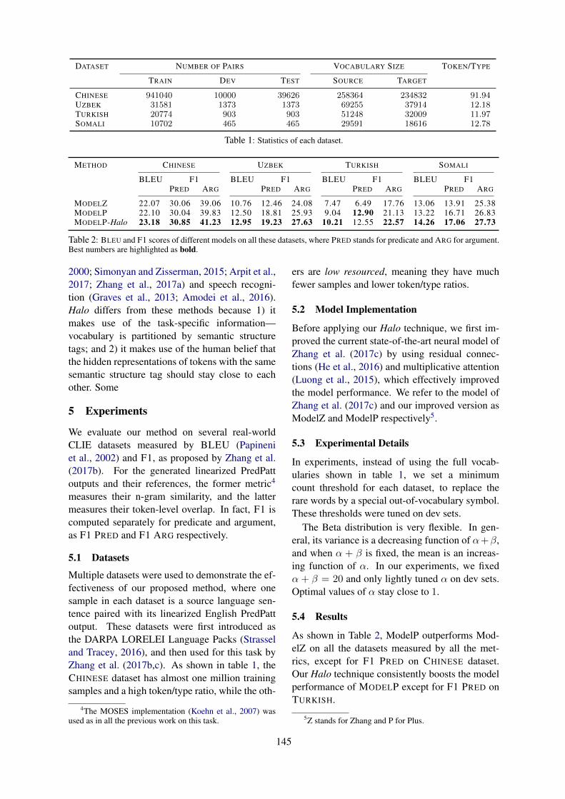
DATASET NUMBER OF PAIRS VOCABULARY SIZE TOKEN/TYPE
TRAIN DEV TEST SOURCE TARGET
CHINESE 941040 10000 39626 258364 234832 91.94UZBEK 31581 1373 1373 69255 37914 12.18TURKISH 20774 903 903 51248 32009 11.97SOMALI 10702 465 465 29591 18616 12.78
Table 1: Statistics of each dataset.
METHOD CHINESE UZBEK TURKISH SOMALI
BLEU F1 BLEU F1 BLEU F1 BLEU F1PRED ARG PRED ARG PRED ARG PRED ARG
MODELZ 22.07 30.06 39.06 10.76 12.46 24.08 7.47 6.49 17.76 13.06 13.91 25.38MODELP 22.10 30.04 39.83 12.50 18.81 25.93 9.04 12.90 21.13 13.22 16.71 26.83MODELP-Halo 23.18 30.85 41.23 12.95 19.23 27.63 10.21 12.55 22.57 14.26 17.06 27.73
Table 2: BLEU and F1 scores of different models on all these datasets, where PRED stands for predicate and ARG for argument.Best numbers are highlighted as bold.
2000; Simonyan and Zisserman, 2015; Arpit et al.,2017; Zhang et al., 2017a) and speech recogni-tion (Graves et al., 2013; Amodei et al., 2016).Halo differs from these methods because 1) itmakes use of the task-specific information—vocabulary is partitioned by semantic structuretags; and 2) it makes use of the human belief thatthe hidden representations of tokens with the samesemantic structure tag should stay close to eachother. Some
5 Experiments
We evaluate our method on several real-worldCLIE datasets measured by BLEU (Papineniet al., 2002) and F1, as proposed by Zhang et al.(2017b). For the generated linearized PredPattoutputs and their references, the former metric4
measures their n-gram similarity, and the lattermeasures their token-level overlap. In fact, F1 iscomputed separately for predicate and argument,as F1 PRED and F1 ARG respectively.
5.1 Datasets
Multiple datasets were used to demonstrate the ef-fectiveness of our proposed method, where onesample in each dataset is a source language sen-tence paired with its linearized English PredPattoutput. These datasets were first introduced asthe DARPA LORELEI Language Packs (Strasseland Tracey, 2016), and then used for this task byZhang et al. (2017b,c). As shown in table 1, theCHINESE dataset has almost one million trainingsamples and a high token/type ratio, while the oth-
4The MOSES implementation (Koehn et al., 2007) wasused as in all the previous work on this task.
ers are low resourced, meaning they have muchfewer samples and lower token/type ratios.
5.2 Model Implementation
Before applying our Halo technique, we first im-proved the current state-of-the-art neural model ofZhang et al. (2017c) by using residual connec-tions (He et al., 2016) and multiplicative attention(Luong et al., 2015), which effectively improvedthe model performance. We refer to the model ofZhang et al. (2017c) and our improved version asModelZ and ModelP respectively5.
5.3 Experimental Details
In experiments, instead of using the full vocab-ularies shown in table 1, we set a minimumcount threshold for each dataset, to replace therare words by a special out-of-vocabulary symbol.These thresholds were tuned on dev sets.
The Beta distribution is very flexible. In gen-eral, its variance is a decreasing function of α+β,and when α + β is fixed, the mean is an increas-ing function of α. In our experiments, we fixedα + β = 20 and only lightly tuned α on dev sets.Optimal values of α stay close to 1.
5.4 Results
As shown in Table 2, ModelP outperforms Mod-elZ on all the datasets measured by all the met-rics, except for F1 PRED on CHINESE dataset.Our Halo technique consistently boosts the modelperformance of MODELP except for F1 PRED onTURKISH.
5Z stands for Zhang and P for Plus.
145

Additionally, experiments were also conductedon two other low resource datasets AMHARIC andYORUBA that Zhang et al. (2017c) included, andα = 0 in Halo was found optimal on the dev sets.In such cases, this regularization was not helpfulso no comparison need be made on the held-outtest sets.
6 Conclusion and Future Work
We present a simple and effective training tech-nique Halo for the task of cross-lingual informa-tion extraction. Our method aims to enforce thelocal surroundings of each hidden state of a neu-ral model to only generate tokens with the samesemantic structure tag, thus enabling the learnedhidden states to be more aware of semantics androbust to random noise. Our method providesnew state-of-the-art results on several benchmarkcross-lingual information extraction datasets, in-cluding both high and low resource scenarios.
As future work, we plan to extend this techniqueto similar tasks such as POS tagging and SemanticRole Labeling. One straightforward way of work-ing on these tasks is to define the vocabularies asset of ‘word-type:POS-tag’ (so ct = POS tag) and‘word-type:SR’ (so ct = semantic role), such thatour method is directly applicable. It would also beinteresting to apply Halo widely to other tasks asa general regularization technique.
Acknowledgments
This work was supported in part by the JHU Hu-man Language Technology Center of Excellence(HLTCOE), and DARPA LORELEI. The U.S.Government is authorized to reproduce and dis-tribute reprints for Governmental purposes. Theviews and conclusions contained in this publica-tion are those of the authors and should not beinterpreted as representing official policies or en-dorsements of DARPA or the U.S. Government.
ReferencesDario Amodei, Sundaram Ananthanarayanan, Rishita
Anubhai, Jingliang Bai, Eric Battenberg, Carl Case,Jared Casper, Bryan Catanzaro, Qiang Cheng, Guo-liang Chen, et al. 2016. Deep speech 2: End-to-endspeech recognition in english and mandarin. In In-ternational Conference on Machine Learning. pages173–182.
Devansh Arpit, Stanislaw Jastrzkebski, Nicolas Bal-las, David Krueger, Emmanuel Bengio, Maxin-
der S Kanwal, Tegan Maharaj, Asja Fischer, AaronCourville, Yoshua Bengio, et al. 2017. A closer lookat memorization in deep networks. In InternationalConference on Machine Learning. pages 233–242.
Olivier Chapelle, Jason Weston, Leon Bottou, andVladimir Vapnik. 2001. Vicinal risk minimization.In Advances in neural information processing sys-tems. pages 416–422.
Yarin Gal and Zoubin Ghahramani. 2016. A theoret-ically grounded application of dropout in recurrentneural networks. In Advances in neural informationprocessing systems. pages 1019–1027.
Alex Graves, Abdel-rahman Mohamed, and GeoffreyHinton. 2013. Speech recognition with deep recur-rent neural networks. In Acoustics, speech and sig-nal processing (icassp), 2013 ieee international con-ference on. IEEE, pages 6645–6649.
Kaiming He, Xiangyu Zhang, Shaoqing Ren, and JianSun. 2016. Deep residual learning for image recog-nition. In The IEEE Conference on Computer Visionand Pattern Recognition (CVPR).
Sepp Hochreiter and Jurgen Schmidhuber. 1997.Long short-term memory. Neural computation9(8):1735–1780.
Heng Ji. 2009. Cross-lingual predicate cluster acquisi-tion to improve bilingual event extraction by induc-tive learning. In Proceedings of the Workshop onUnsupervised and Minimally Supervised Learningof Lexical Semantics. Association for ComputationalLinguistics, Boulder, Colorado, USA, pages 27–35. http://www.aclweb.org/anthology/W09-1704.
Heng Ji and Joel Nothman. 2016. Overview of TAC-KBP2016 Tri-lingual EDL and its impact on end-to-end cold-start KBP. In Proceedings of the TextAnalysis Conference (TAC).
Philipp Koehn, Hieu Hoang, Alexandra Birch, ChrisCallison-Burch, Marcello Federico, Nicola Bertoldi,Brooke Cowan, Wade Shen, Christine Moran,Richard Zens, et al. 2007. Moses: Open sourcetoolkit for statistical machine translation. In Pro-ceedings of the 45th annual meeting of the ACL oninteractive poster and demonstration sessions. As-sociation for Computational Linguistics, pages 177–180.
Minh-Thang Luong, Hieu Pham, and Christopher DManning. 2015. Effective approaches to attention-based neural machine translation. In Proceedings ofthe 2015 Conference on Empirical Methods in Nat-ural Language Processing.
Kishore Papineni, Salim Roukos, Todd Ward, and Wei-Jing Zhu. 2002. Bleu: a method for automatic eval-uation of machine translation. In Proceedings ofthe 40th annual meeting on association for compu-tational linguistics. Association for ComputationalLinguistics, pages 311–318.
146
Kristen Parton, Kathleen R. McKeown, Bob Coyne,Mona T. Diab, Ralph Grishman, Dilek Hakkani-Tur, Mary Harper, Heng Ji, Wei Yun Ma, AdamMeyers, Sara Stolbach, Ang Sun, Gokhan Tur, WeiXu, and Sibel Yaman. 2009. Who, what, when,where, why? comparing multiple approaches to thecross-lingual 5w task. In Proceedings of the JointConference of the 47th Annual Meeting of the ACLand the 4th International Joint Conference on Nat-ural Language Processing of the AFNLP. Associa-tion for Computational Linguistics, Suntec, Singa-pore, pages 423–431. http://www.aclweb.org/anthology/P/P09/P09-1048.
Patrice Y Simard, Yann A Le Cun, John S Denker, andBernard Victorri. 2000. Transformation invariancein pattern recognition: Tangent distance and prop-agation. International Journal of Imaging Systemsand Technology 11(3):181–197.
Karen Simonyan and Andrew Zisserman. 2015. Verydeep convolutional networks for large-scale imagerecognition. In International Conference on Learn-ing Representations.
Matthew Snover, Xiang Li, Wen-Pin Lin, Zheng Chen,Suzanne Tamang, Mingmin Ge, Adam Lee, Qi Li,Hao Li, Sam Anzaroot, and Heng Ji. 2011. Cross-lingual slot filling from comparable corpora. InProceedings of the 4th Workshop on Building andUsing Comparable Corpora: Comparable Corporaand the Web. Association for Computational Lin-guistics, Stroudsburg, PA, USA, BUCC ’11, pages110–119. http://dl.acm.org/citation.cfm?id=2024236.2024256.
Nitish Srivastava, Geoffrey E Hinton, Alex Krizhevsky,Ilya Sutskever, and Ruslan Salakhutdinov. 2014.Dropout: a simple way to prevent neural networksfrom overfitting. Journal of Machine Learning Re-search 15(1):1929–1958.
Stephanie Strassel and Jennifer Tracey. 2016. Loreleilanguage packs: Data, tools, and resources fortechnology development in low resource languages.In Nicoletta Calzolari (Conference Chair), KhalidChoukri, Thierry Declerck, Sara Goggi, Marko Gro-belnik, Bente Maegaard, Joseph Mariani, HeleneMazo, Asuncion Moreno, Jan Odijk, and SteliosPiperidis, editors, Proceedings of the Tenth Interna-tional Conference on Language Resources and Eval-uation (LREC 2016). European Language ResourcesAssociation (ELRA), Paris, France.
Kiyoshi Sudo, Satoshi Sekine, and Ralph Grishman.2004. Cross-lingual information extraction systemevaluation. In Proceedings of the 20th internationalConference on Computational Linguistics. Associa-tion for Computational Linguistics, page 882.
Christian Szegedy, Vincent Vanhoucke, Sergey Ioffe,Jon Shlens, and Zbigniew Wojna. 2016. Rethinkingthe inception architecture for computer vision. InProceedings of the IEEE Conference on ComputerVision and Pattern Recognition. pages 2818–2826.
Laurens Van der Maaten, Minmin Chen, StephenTyree, and Kilian Weinberger. 2013. Learning withmarginalized corrupted features. In Proceedingsof The 30th International Conference on MachineLearning.
Aaron Steven White, Drew Reisinger, Keisuke Sak-aguchi, Tim Vieira, Sheng Zhang, Rachel Rudinger,Kyle Rawlins, and Benjamin Van Durme. 2016.Universal Decompositional Semantics on UniversalDependencies. In Proceedings of the 2016 Con-ference on Empirical Methods in Natural LanguageProcessing. Association for Computational Linguis-tics, Austin, Texas, pages 1713–1723. https://aclweb.org/anthology/D16-1177.
Hongyi Zhang, Moustapha Cisse, Yann N Dauphin,and David Lopez-Paz. 2017a. mixup: Be-yond empirical risk minimization. arXiv preprintarXiv:1710.09412 .
Sheng Zhang, Kevin Duh, and Benjamin Van Durme.2017b. MT/IE: Cross-lingual Open Information Ex-traction with Neural Sequence-to-Sequence Mod-els. In Proceedings of the 15th Conference of theEuropean Chapter of the Association for Compu-tational Linguistics: Volume 2, Short Papers. As-sociation for Computational Linguistics, Valencia,Spain, pages 64–70. http://www.aclweb.org/anthology/E17-2011.
Sheng Zhang, Kevin Duh, and Benjamin Van Durme.2017c. Selective Decoding for Cross-lingual OpenInformation Extraction. In Proceedings of theEighth International Joint Conference on NaturalLanguage Processing (Volume 1: Long Papers).Asian Federation of Natural Language Processing,Taipei, Taiwan, pages 832–842. http://www.aclweb.org/anthology/I17-1084.
Sheng Zhang, Rachel Rudinger, and Benjamin VanDurme. 2017d. An Evaluation of PredPatt and OpenIE via Stage 1 Semantic Role Labeling. In IWCS2017 — 12th International Conference on Com-putational Semantics — Short papers. http://aclweb.org/anthology/W17-6944.
147
Proceedings of the 7th Joint Conference on Lexical and Computational Semantics (*SEM), pages 148–153New Orleans, June 5-6, 2018. c©2018 Association for Computational Linguistics
Exploiting Partially Annotated Data for Temporal Relation Extraction
Qiang Ning,1 Zhongzhi Yu,2 Chuchu Fan,1 Dan Roth1,2,3
1Department of Electrical and Computer Engineering, 2Department of Computer ScienceUniversity of Illinois at Urbana-Champaign, Urbana, IL 61801, USA
3Department of Computer Science, University of Pennsylvania, Philadelphia, PA 19104, USA{qning2,zyu19,cfan10}@illinois.edu, [email protected]
Abstract
Annotating temporal relations (TempRel) be-tween events described in natural language isknown to be labor intensive, partly becausethe total number of TempRels is quadratic inthe number of events. As a result, only asmall number of documents are typically an-notated, limiting the coverage of various lexi-cal/semantic phenomena. In order to improveexisting approaches, one possibility is to makeuse of the readily available, partially annotateddata (P as in partial) that cover more docu-ments. However, missing annotations in P areknown to hurt, rather than help, existing sys-tems. This work is a case study in exploringvarious usages of P for TempRel extraction.Results show that despite missing annotations,P is still a useful supervision signal for thistask within a constrained bootstrapping learn-ing framework. The system described in thissystem is publicly available.1
1 Introduction
Understanding the temporal information in natu-ral language text is an important NLP task (Ver-hagen et al., 2007, 2010; UzZaman et al., 2013;Minard et al., 2015; Bethard et al., 2016, 2017). Acrucial component is temporal relation (TempRel;e.g., before or after) extraction (Mani et al., 2006;Bethard et al., 2007; Do et al., 2012; Chamberset al., 2014; Mirza and Tonelli, 2016; Ning et al.,2017, 2018a,b).
The TempRels in a document or a sentence canbe conveniently modeled as a graph, where thenodes are events, and the edges are labeled byTempRels. Given all the events in an instance,TempRel annotation is the process of manually la-beling all the edges – a highly labor intensive taskdue to two reasons. One is that many edges re-quire extensive reasoning over multiple sentences
1https://cogcomp.org/page/publication_view/832
and labeling them is time-consuming. Perhapsmore importantly, the other reason is that #edgesis quadratic in #nodes. If labeling an edge takes 30seconds (already an optimistic estimation), a typi-cal document with 50 nodes would take more than10 hours to annotate. Even if existing annotationschemes make a compromise by only annotatingedges whose nodes are from a same sentence oradjacent sentences (Cassidy et al., 2014), it stilltakes more than 2 hours to fully annotate a typ-ical document. Consequently, the only fully an-notated dataset, TB-Dense (Cassidy et al., 2014),contains only 36 documents, which is rather smallcompared with datasets for other NLP tasks.
A small number of documents may indicate thatthe annotated data provide a limited coverage ofvarious lexical and semantic phenomena, sincea document is usually “homogeneous” within it-self. In contrast to the scarcity of fully annotateddatasets (denoted by F as in full), there are ac-tually some partially annotated datasets as well(denoted by P as in partial); for example, Time-Bank (Pustejovsky et al., 2003) and AQUAINT(Graff, 2002) cover in total more than 250 docu-ments. Since annotators are not required to labelall the edges in these datasets, it is less labor inten-sive to collect P than to collect F . However, ex-isting TempRel extraction methods only work onone type of datasets (i.e., either F or P), withouttaking advantage of both. No one, as far as weknow, has explored ways to combine both types ofdatasets in learning and whether it is helpful.
This work is a case study in exploring varioususages of P in the TempRel extraction task. Weempirically show that P is indeed useful withina (constrained) bootstrapping type of learning ap-proach. This case study is interesting from twoperspectives. First, incidental supervision (Roth,2017). In practice, supervision signals may not al-ways be perfect: they may be noisy, only partial,
148

based on different annotation schemes, or even ondifferent (but relevant) tasks; incidental supervi-sion is a general paradigm that aims at makinguse of the abundant, naturally occurring data, assupervision signals. As for the TempRel extrac-tion task, the existence of many partially annotateddatasets P is a good fit for this paradigm and theresult here can be informative for future investi-gations involving other incidental supervision sig-nals. Second, TempRel data collection. The factthat P is shown to provide useful supervision sig-nals poses some further questions: What is the op-timal data collection scheme for TempRel extrac-tion, fully annotated, partially annotated, or a mix-ture of both? For partially annotated data, whatis the optimal ratio of annotated edges to unanno-tated edges? The proposed method in this workcan be readily extended to study these questionsin the future, as we further discuss in Sec. 5.
2 Existing Datasets and Methods
TimeBank (Pustejovsky et al., 2003) is a classicTempRel dataset, where the annotators were givena whole article and allowed to label TempRels be-tween any pairs of events. Annotators in this setupusually focus only on salient relations but overlooksome others. It has been reported that many eventpairs in TimeBank should have been annotatedwith a specific TempRel but the annotators failedto look at them (Chambers, 2013; Cassidy et al.,2014; Ning et al., 2017). Consequently, we cate-gorize TimeBank as a partially annotated dataset(P). The same argument applies to other datasetsthat adopted this setup, such as AQUAINT (Graff,2002), CaTeRs (Mostafazadeh et al., 2016) andRED (O’Gorman et al., 2016). Most existing sys-tems make use of P , including but not limited to,(Mani et al., 2006; Bramsen et al., 2006; Cham-bers et al., 2007; Bethard et al., 2007; Verhagenand Pustejovsky, 2008; Chambers and Jurafsky,2008; Denis and Muller, 2011; Do et al., 2012);this applies also to the TempEval workshops sys-tems, e.g., (Laokulrat et al., 2013; Bethard, 2013;Chambers, 2013).
To address the missing annotation issue, Cas-sidy et al. (2014) proposed a dense annotationscheme, TB-Dense. Edges are presented one-by-one and the annotator has to choose a label forit (note that there is a vague label in case theTempRel is not clear or does not exist). As a re-sult, edges in TB-Dense are considered as fullyannotated in this paper. The first system on TB-
Dense was proposed in Chambers et al. (2014).Two recent TempRel extraction systems (Mirzaand Tonelli, 2016; Ning et al., 2017) also re-ported their performances on TB-Dense (F) andon TempEval-3 (P) separately. However, thereare no existing systems that jointly train on both.Given that the annotation guidelines of F and Pare obviously different, it may not be optimal tosimply treat P and F uniformly and train on theirunion. This situation necessitates further investi-gation as we do here.
Before introducing our joint learning approach,we have a few remarks about our choice of F andP datasets. First, we note that TB-Dense is actu-ally not fully annotated in the strict sense becauseonly edges within a sliding, two-sentence windoware presented. That is, distant event pairs are in-tentionally ignored by the designers of TB-Dense.However, since such distant pairs are consistentlyruled out in the training and inference phase inthis paper, it does not change the nature of theproblem being investigated here. At this point,TB-Dense is the only fully annotated dataset thatcan be adopted in this study, despite the aforemen-tioned limitation.
Second, the partial annotations in datasets likeTimeBank were not selected uniformly at randomfrom all possible edges. As described earlier, onlysalient and non-vague TempRels (which may oftenbe those easy ones) are labeled in these datasets.Using TimeBank as P might potentially createsome bias and we will need to keep this in mindwhen analyzing the results in Sec. 4. Recent ad-vances in TempRel data annotation (Ning et al.,2018c) can be used in the future to collect both Fand P more easily.
3 Joint Learning on F and PIn this work, we study two learning paradigms thatmake use of both F and P . In the first, we simplytreat those edges that are annotated in P as edgesin F so that the learning process can be performedon top of the union of F and P . This is the moststraightforward approach to using F and P jointlyand it is interesting to see if it already helps.
In the second, we use bootstrapping: we use Fas a starting point and learn a TempRel extractionsystem on it (denoted by SF ), and then fill thosemissing annotations in P based on SF (thus obtain“fully” annotated P); finally, we treat P as F andlearn from both. Algorithm 1 is a meta-algorithmof the above.
149
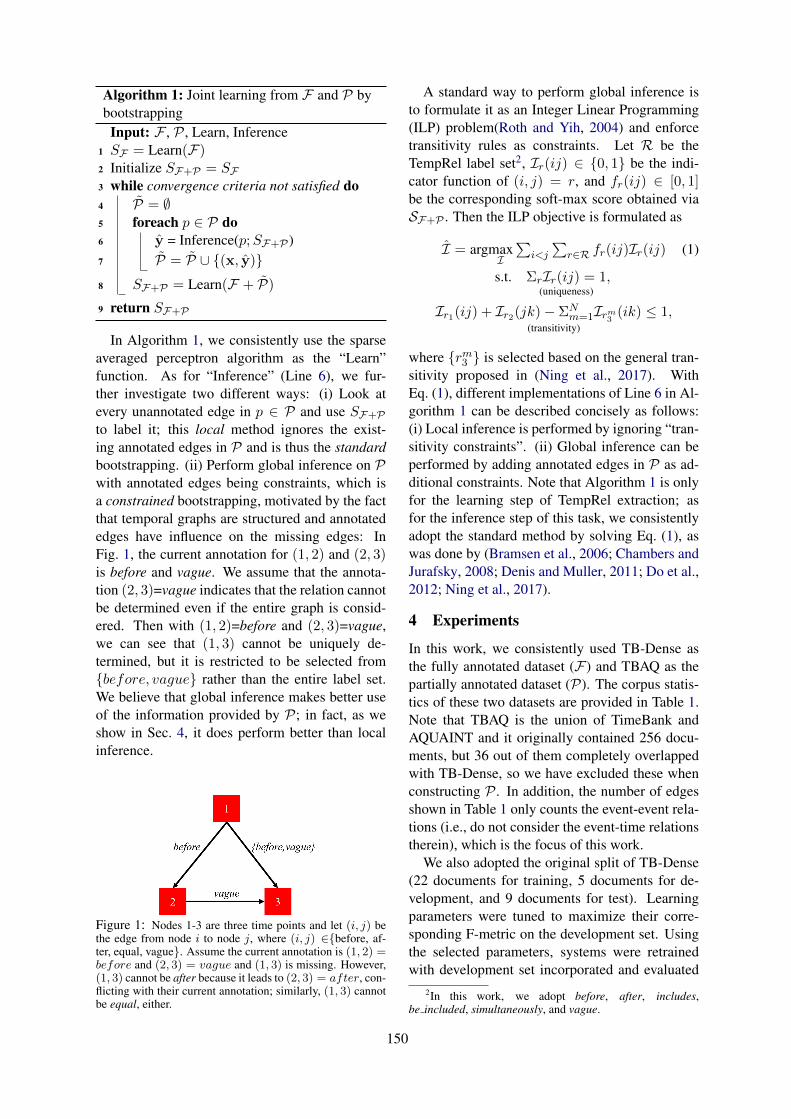
Algorithm 1: Joint learning from F and P bybootstrapping
Input: F , P , Learn, Inference1 SF = Learn(F)2 Initialize SF+P = SF3 while convergence criteria not satisfied do4 P = ∅5 foreach p ∈ P do6 y = Inference(p; SF+P )7 P = P ∪ {(x, y)}8 SF+P = Learn(F + P)
9 return SF+P
In Algorithm 1, we consistently use the sparseaveraged perceptron algorithm as the “Learn”function. As for “Inference” (Line 6), we fur-ther investigate two different ways: (i) Look atevery unannotated edge in p ∈ P and use SF+Pto label it; this local method ignores the exist-ing annotated edges in P and is thus the standardbootstrapping. (ii) Perform global inference on Pwith annotated edges being constraints, which isa constrained bootstrapping, motivated by the factthat temporal graphs are structured and annotatededges have influence on the missing edges: InFig. 1, the current annotation for (1, 2) and (2, 3)is before and vague. We assume that the annota-tion (2, 3)=vague indicates that the relation cannotbe determined even if the entire graph is consid-ered. Then with (1, 2)=before and (2, 3)=vague,we can see that (1, 3) cannot be uniquely de-termined, but it is restricted to be selected from{before, vague} rather than the entire label set.We believe that global inference makes better useof the information provided by P; in fact, as weshow in Sec. 4, it does perform better than localinference.
Figure 1: Nodes 1-3 are three time points and let (i, j) bethe edge from node i to node j, where (i, j) ∈{before, af-ter, equal, vague}. Assume the current annotation is (1, 2) =before and (2, 3) = vague and (1, 3) is missing. However,(1, 3) cannot be after because it leads to (2, 3) = after, con-flicting with their current annotation; similarly, (1, 3) cannotbe equal, either.
A standard way to perform global inference isto formulate it as an Integer Linear Programming(ILP) problem(Roth and Yih, 2004) and enforcetransitivity rules as constraints. Let R be theTempRel label set2, Ir(ij) ∈ {0, 1} be the indi-cator function of (i, j) = r, and fr(ij) ∈ [0, 1]be the corresponding soft-max score obtained viaSF+P . Then the ILP objective is formulated as
I = argmaxI
∑i<j
∑r∈R fr(ij)Ir(ij) (1)
s.t. ΣrIr(ij) = 1(uniqueness)
,
Ir1(ij) + Ir2(jk) − ΣNm=1Irm
3(ik) ≤ 1,
(transitivity)
where {rm3 } is selected based on the general tran-
sitivity proposed in (Ning et al., 2017). WithEq. (1), different implementations of Line 6 in Al-gorithm 1 can be described concisely as follows:(i) Local inference is performed by ignoring “tran-sitivity constraints”. (ii) Global inference can beperformed by adding annotated edges in P as ad-ditional constraints. Note that Algorithm 1 is onlyfor the learning step of TempRel extraction; asfor the inference step of this task, we consistentlyadopt the standard method by solving Eq. (1), aswas done by (Bramsen et al., 2006; Chambers andJurafsky, 2008; Denis and Muller, 2011; Do et al.,2012; Ning et al., 2017).
4 Experiments
In this work, we consistently used TB-Dense asthe fully annotated dataset (F) and TBAQ as thepartially annotated dataset (P). The corpus statis-tics of these two datasets are provided in Table 1.Note that TBAQ is the union of TimeBank andAQUAINT and it originally contained 256 docu-ments, but 36 out of them completely overlappedwith TB-Dense, so we have excluded these whenconstructing P . In addition, the number of edgesshown in Table 1 only counts the event-event rela-tions (i.e., do not consider the event-time relationstherein), which is the focus of this work.
We also adopted the original split of TB-Dense(22 documents for training, 5 documents for de-velopment, and 9 documents for test). Learningparameters were tuned to maximize their corre-sponding F-metric on the development set. Usingthe selected parameters, systems were retrainedwith development set incorporated and evaluated
2In this work, we adopt before, after, includes,be included, simultaneously, and vague.
150
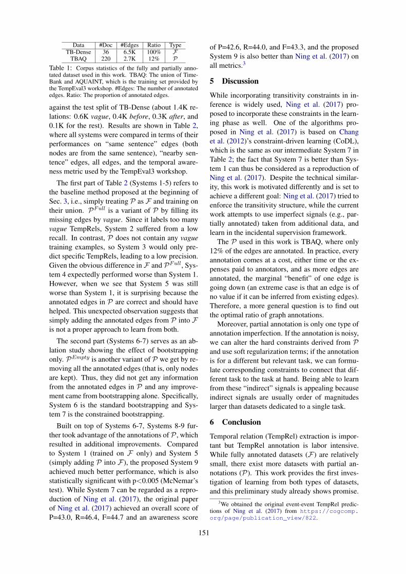
Data #Doc #Edges Ratio TypeTB-Dense 36 6.5K 100% F
TBAQ 220 2.7K 12% PTable 1: Corpus statistics of the fully and partially anno-tated dataset used in this work. TBAQ: The union of Time-Bank and AQUAINT, which is the training set provided bythe TempEval3 workshop. #Edges: The number of annotatededges. Ratio: The proportion of annotated edges.
against the test split of TB-Dense (about 1.4K re-lations: 0.6K vague, 0.4K before, 0.3K after, and0.1K for the rest). Results are shown in Table 2,where all systems were compared in terms of theirperformances on “same sentence” edges (bothnodes are from the same sentence), “nearby sen-tence” edges, all edges, and the temporal aware-ness metric used by the TempEval3 workshop.
The first part of Table 2 (Systems 1-5) refers tothe baseline method proposed at the beginning ofSec. 3, i.e., simply treating P as F and training ontheir union. PFull is a variant of P by filling itsmissing edges by vague. Since it labels too manyvague TempRels, System 2 suffered from a lowrecall. In contrast, P does not contain any vaguetraining examples, so System 3 would only pre-dict specific TempRels, leading to a low precision.Given the obvious difference in F and PFull, Sys-tem 4 expectedly performed worse than System 1.However, when we see that System 5 was stillworse than System 1, it is surprising because theannotated edges in P are correct and should havehelped. This unexpected observation suggests thatsimply adding the annotated edges from P into Fis not a proper approach to learn from both.
The second part (Systems 6-7) serves as an ab-lation study showing the effect of bootstrappingonly. PEmpty is another variant of P we get by re-moving all the annotated edges (that is, only nodesare kept). Thus, they did not get any informationfrom the annotated edges in P and any improve-ment came from bootstrapping alone. Specifically,System 6 is the standard bootstrapping and Sys-tem 7 is the constrained bootstrapping.
Built on top of Systems 6-7, Systems 8-9 fur-ther took advantage of the annotations of P , whichresulted in additional improvements. Comparedto System 1 (trained on F only) and System 5(simply adding P into F), the proposed System 9achieved much better performance, which is alsostatistically significant with p<0.005 (McNemar’stest). While System 7 can be regarded as a repro-duction of Ning et al. (2017), the original paperof Ning et al. (2017) achieved an overall score ofP=43.0, R=46.4, F=44.7 and an awareness score
of P=42.6, R=44.0, and F=43.3, and the proposedSystem 9 is also better than Ning et al. (2017) onall metrics.3
5 Discussion
While incorporating transitivity constraints in in-ference is widely used, Ning et al. (2017) pro-posed to incorporate these constraints in the learn-ing phase as well. One of the algorithms pro-posed in Ning et al. (2017) is based on Changet al. (2012)’s constraint-driven learning (CoDL),which is the same as our intermediate System 7 inTable 2; the fact that System 7 is better than Sys-tem 1 can thus be considered as a reproduction ofNing et al. (2017). Despite the technical similar-ity, this work is motivated differently and is set toachieve a different goal: Ning et al. (2017) tried toenforce the transitivity structure, while the currentwork attempts to use imperfect signals (e.g., par-tially annotated) taken from additional data, andlearn in the incidental supervision framework.
The P used in this work is TBAQ, where only12% of the edges are annotated. In practice, everyannotation comes at a cost, either time or the ex-penses paid to annotators, and as more edges areannotated, the marginal “benefit” of one edge isgoing down (an extreme case is that an edge is ofno value if it can be inferred from existing edges).Therefore, a more general question is to find outthe optimal ratio of graph annotations.
Moreover, partial annotation is only one type ofannotation imperfection. If the annotation is noisy,we can alter the hard constraints derived from Pand use soft regularization terms; if the annotationis for a different but relevant task, we can formu-late corresponding constraints to connect that dif-ferent task to the task at hand. Being able to learnfrom these “indirect” signals is appealing becauseindirect signals are usually order of magnitudeslarger than datasets dedicated to a single task.
6 Conclusion
Temporal relation (TempRel) extraction is impor-tant but TempRel annotation is labor intensive.While fully annotated datasets (F) are relativelysmall, there exist more datasets with partial an-notations (P). This work provides the first inves-tigation of learning from both types of datasets,and this preliminary study already shows promise.
3We obtained the original event-event TempRel predic-tions of Ning et al. (2017) from https://cogcomp.org/page/publication_view/822.
151
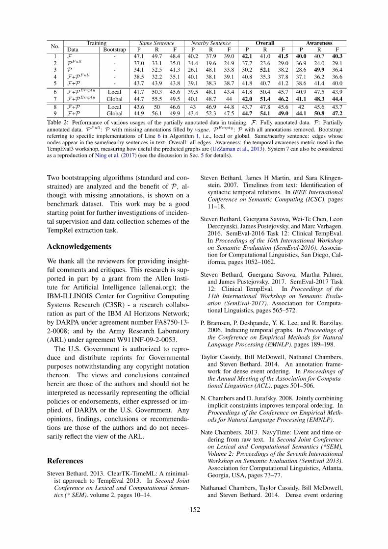
No. Training Same Sentence Nearby Sentence Overall AwarenessData Bootstrap P R F P R F P R F P R F
1 F - 47.1 49.7 48.4 40.2 37.9 39.0 42.1 41.0 41.5 40.0 40.7 40.32 PFull - 37.0 33.1 35.0 34.4 19.6 24.9 37.7 23.6 29.0 36.9 24.0 29.13 P - 34.1 52.5 41.3 26.1 48.1 33.8 30.2 52.1 38.2 28.6 49.9 36.44 F+PFull - 38.5 32.2 35.1 40.1 38.1 39.1 40.8 35.3 37.8 37.1 36.2 36.65 F+P - 43.7 43.9 43.8 39.1 38.3 38.7 41.8 40.7 41.2 38.6 41.4 40.06 F+PEmpty Local 41.7 50.3 45.6 39.5 48.1 43.4 41.8 50.4 45.7 40.9 47.5 43.97 F+PEmpty Global 44.7 55.5 49.5 40.1 48.7 44 42.0 51.4 46.2 41.1 48.3 44.48 F+P Local 43.6 50 46.6 43 46.9 44.8 43.7 47.8 45.6 42 45.6 43.79 F+P Global 44.9 56.1 49.9 43.4 52.3 47.5 44.7 54.1 49.0 44.1 50.8 47.2
Table 2: Performance of various usages of the partially annotated data in training. F : Fully annotated data. P: Partiallyannotated data. PFull: P with missing annotations filled by vague. PEmpty: P with all annotations removed. Bootstrap:referring to specific implementations of Line 6 in Algorithm 1, i.e., local or global. Same/nearby sentence: edges whosenodes appear in the same/nearby sentences in text. Overall: all edges. Awareness: the temporal awareness metric used in theTempEval3 workshop, measuring how useful the predicted graphs are (UzZaman et al., 2013). System 7 can also be consideredas a reproduction of Ning et al. (2017) (see the discussion in Sec. 5 for details).
Two bootstrapping algorithms (standard and con-strained) are analyzed and the benefit of P , al-though with missing annotations, is shown on abenchmark dataset. This work may be a goodstarting point for further investigations of inciden-tal supervision and data collection schemes of theTempRel extraction task.
Acknowledgements
We thank all the reviewers for providing insight-ful comments and critiques. This research is sup-ported in part by a grant from the Allen Insti-tute for Artificial Intelligence (allenai.org); theIBM-ILLINOIS Center for Cognitive ComputingSystems Research (C3SR) - a research collabo-ration as part of the IBM AI Horizons Network;by DARPA under agreement number FA8750-13-2-0008; and by the Army Research Laboratory(ARL) under agreement W911NF-09-2-0053.
The U.S. Government is authorized to repro-duce and distribute reprints for Governmentalpurposes notwithstanding any copyright notationthereon. The views and conclusions containedherein are those of the authors and should not beinterpreted as necessarily representing the officialpolicies or endorsements, either expressed or im-plied, of DARPA or the U.S. Government. Anyopinions, findings, conclusions or recommenda-tions are those of the authors and do not neces-sarily reflect the view of the ARL.
ReferencesSteven Bethard. 2013. ClearTK-TimeML: A minimal-
ist approach to TempEval 2013. In Second JointConference on Lexical and Computational Seman-tics (* SEM). volume 2, pages 10–14.
Steven Bethard, James H Martin, and Sara Klingen-stein. 2007. Timelines from text: Identification ofsyntactic temporal relations. In IEEE InternationalConference on Semantic Computing (ICSC). pages11–18.
Steven Bethard, Guergana Savova, Wei-Te Chen, LeonDerczynski, James Pustejovsky, and Marc Verhagen.2016. SemEval-2016 Task 12: Clinical TempEval.In Proceedings of the 10th International Workshopon Semantic Evaluation (SemEval-2016). Associa-tion for Computational Linguistics, San Diego, Cal-ifornia, pages 1052–1062.
Steven Bethard, Guergana Savova, Martha Palmer,and James Pustejovsky. 2017. SemEval-2017 Task12: Clinical TempEval. In Proceedings of the11th International Workshop on Semantic Evalu-ation (SemEval-2017). Association for Computa-tional Linguistics, pages 565–572.
P. Bramsen, P. Deshpande, Y. K. Lee, and R. Barzilay.2006. Inducing temporal graphs. In Proceedings ofthe Conference on Empirical Methods for NaturalLanguage Processing (EMNLP). pages 189–198.
Taylor Cassidy, Bill McDowell, Nathanel Chambers,and Steven Bethard. 2014. An annotation frame-work for dense event ordering. In Proceedings ofthe Annual Meeting of the Association for Computa-tional Linguistics (ACL). pages 501–506.
N. Chambers and D. Jurafsky. 2008. Jointly combiningimplicit constraints improves temporal ordering. InProceedings of the Conference on Empirical Meth-ods for Natural Language Processing (EMNLP).
Nate Chambers. 2013. NavyTime: Event and time or-dering from raw text. In Second Joint Conferenceon Lexical and Computational Semantics (*SEM),Volume 2: Proceedings of the Seventh InternationalWorkshop on Semantic Evaluation (SemEval 2013).Association for Computational Linguistics, Atlanta,Georgia, USA, pages 73–77.
Nathanael Chambers, Taylor Cassidy, Bill McDowell,and Steven Bethard. 2014. Dense event ordering
152
with a multi-pass architecture. Transactions of theAssociation for Computational Linguistics 2:273–284.
Nathanael Chambers, Shan Wang, and Dan Juraf-sky. 2007. Classifying temporal relations betweenevents. In Proceedings of the 45th Annual Meetingof the ACL on Interactive Poster and DemonstrationSessions. pages 173–176.
M. Chang, L. Ratinov, and D. Roth. 2012. Structuredlearning with constrained conditional models. Ma-chine Learning 88(3):399–431.
Pascal Denis and Philippe Muller. 2011. Predictingglobally-coherent temporal structures from texts viaendpoint inference and graph decomposition. InProceedings of the International Joint Conferenceon Artificial Intelligence (IJCAI). volume 22, page1788.
Q. Do, W. Lu, and D. Roth. 2012. Joint inference forevent timeline construction. In Proc. of the Con-ference on Empirical Methods in Natural LanguageProcessing (EMNLP).
David Graff. 2002. The AQUAINT corpus of englishnews text. Linguistic Data Consortium, Philadel-phia .
Natsuda Laokulrat, Makoto Miwa, Yoshimasa Tsu-ruoka, and Takashi Chikayama. 2013. UTTime:Temporal relation classification using deep syntac-tic features. In Second Joint Conference on Lexicaland Computational Semantics (* SEM). volume 2,pages 88–92.
Inderjeet Mani, Marc Verhagen, Ben Wellner,Chong Min Lee, and James Pustejovsky. 2006.Machine learning of temporal relations. In Proceed-ings of the Annual Meeting of the Association forComputational Linguistics (ACL). pages 753–760.
Anne-Lyse Minard, Manuela Speranza, EnekoAgirre, Itziar Aldabe, Marieke van Erp, BernardoMagnini, German Rigau, Ruben Urizar, and Fon-dazione Bruno Kessler. 2015. SemEval-2015 Task4: TimeLine: Cross-document event ordering. InProceedings of the 9th International Workshopon Semantic Evaluation (SemEval 2015). pages778–786.
Paramita Mirza and Sara Tonelli. 2016. CATENA:CAusal and TEmporal relation extraction from NAt-ural language texts. In The 26th International Con-ference on Computational Linguistics. pages 64–75.
Nasrin Mostafazadeh, Alyson Grealish, NathanaelChambers, James Allen, and Lucy Vanderwende.2016. CaTeRS: Causal and temporal relationscheme for semantic annotation of event structures.In Proceedings of the 4th Workshop on Events: Def-inition, Detection, Coreference, and Representation.pages 51–61.
Qiang Ning, Zhili Feng, and Dan Roth. 2017. A struc-tured learning approach to temporal relation extrac-tion. In Proceedings of the Conference on Em-pirical Methods for Natural Language Processing(EMNLP). Copenhagen, Denmark.
Qiang Ning, Zhili Feng, Hao Wu, and Dan Roth.2018a. Joint reasoning for temporal and causal rela-tions. In Proceedings of the Annual Meeting of theAssociation for Computational Linguistics (ACL).
Qiang Ning, Hao Wu, Haoruo Peng, and Dan Roth.2018b. Improving temporal relation extraction witha globally acquired statistical resource. In Proceed-ings of the Annual Meeting of the North AmericanAssociation of Computational Linguistics (NAACL).Association for Computational Linguistics.
Qiang Ning, Hao Wu, and Dan Roth. 2018c. A multi-axis annotation scheme for event temporal relations.In Proceedings of the Annual Meeting of the Associ-ation for Computational Linguistics (ACL).
Tim O’Gorman, Kristin Wright-Bettner, and MarthaPalmer. 2016. Richer event description: Integratingevent coreference with temporal, causal and bridg-ing annotation. In Proceedings of the 2nd Workshopon Computing News Storylines (CNS 2016). Associ-ation for Computational Linguistics, Austin, Texas,pages 47–56.
James Pustejovsky, Patrick Hanks, Roser Sauri, An-drew See, Robert Gaizauskas, Andrea Setzer,Dragomir Radev, Beth Sundheim, David Day, LisaFerro, et al. 2003. The TIMEBANK corpus. In Cor-pus linguistics. volume 2003, page 40.
D. Roth and W. Yih. 2004. A linear programmingformulation for global inference in natural languagetasks. In Hwee Tou Ng and Ellen Riloff, editors,Proc. of the Conference on Computational NaturalLanguage Learning (CoNLL). pages 1–8.
Dan Roth. 2017. Incidental supervision: Moving be-yond supervised learning. In AAAI.
Naushad UzZaman, Hector Llorens, James Allen, LeonDerczynski, Marc Verhagen, and James Pustejovsky.2013. SemEval-2013 Task 1: TempEval-3: Evaluat-ing time expressions, events, and temporal relations.In Second Joint Conference on Lexical and Compu-tational Semantics. volume 2, pages 1–9.
Marc Verhagen, Robert Gaizauskas, Frank Schilder,Mark Hepple, Graham Katz, and James Pustejovsky.2007. SemEval-2007 Task 15: TempEval temporalrelation identification. In SemEval. pages 75–80.
Marc Verhagen and James Pustejovsky. 2008. Tem-poral processing with the TARSQI toolkit. In 22ndInternational Conference on on Computational Lin-guistics: Demonstration Papers. pages 189–192.
Marc Verhagen, Roser Sauri, Tommaso Caselli, andJames Pustejovsky. 2010. SemEval-2010 Task 13:TempEval-2. In SemEval. pages 57–62.
153
Proceedings of the 7th Joint Conference on Lexical and Computational Semantics (*SEM), pages 154–159New Orleans, June 5-6, 2018. c©2018 Association for Computational Linguistics
Predicting Word Embeddings Variability
Benedicte Pierrejean and Ludovic TanguyCLLE: CNRS & University of Toulouse
Toulouse, France{benedicte.pierrejean,ludovic.tanguy}@univ-tlse2.fr
Abstract
Neural word embeddings models (such asthose built with word2vec) are known to havestability problems: when retraining a modelwith the exact same hyperparameters, wordsneighborhoods may change. We propose amethod to estimate such variation, based onthe overlap of neighbors of a given word intwo models trained with identical hyperparam-eters. We show that this inherent variation isnot negligible, and that it does not affect everyword in the same way. We examine the influ-ence of several features that are intrinsic to aword, corpus or embedding model and providea methodology that can predict the variability(and as such, reliability) of a word representa-tion in a semantic vector space.
1 Introduction
Word embeddings are dense representations of themeaning of words that are efficient and easy to use.Embeddings training methods such as word2vec(Mikolov et al., 2013), are based on neural net-works methods that imply random processes (ini-tialization of the network, sampling, etc.). Assuch, they display stability problems (Hellrich andHahn, 2016) meaning that retraining a model withthe exact same hyperparameters will give differentword representations, with a word possibly havingdifferent nearest neighbors from one model to theother.
Benchmarks test sets such as WordSim-353(Finkelstein et al., 2002) are commonly used toevaluate word embeddings since they provide afast and easy way to quickly evaluate a model(Nayak et al., 2016). However, the instability ofword embeddings is not detected by these test setssince only selected pairs of words are evaluated.A model showing instability could get very sim-ilar performance results when evaluated on suchbenchmarks.
Hyperparameters selected when training wordembeddings impact the semantic representation ofa word. Among these hyperparameters we findsome hyperparameters internal to the system suchas the architecture used, the size of the contextwindow or the dimensions of the vectors as well assome external hyperparameters such as the corpusused for training (Asr et al., 2016; Baroni et al.,2014; Chiu et al., 2016; Li et al., 2017; Mela-mud et al., 2016; Roberts, 2016). In this work,we adopt a corpus linguistics approach in a simi-lar way to Antoniak and Mimno (2018), Hamiltonet al. (2016) and Hellrich and Hahn (2016) mean-ing that observing the semantic representation ofa word consists in observing the nearest neighborsof this word. Corpus tools such as Sketch Engine(Kilgarriff et al., 2014) use embeddings trained onseveral corpora1 to provide users with most similarwords as a lexical semantic information on a tar-get word. In order to make accurate observations,it thus seems important to understand the stabilityof these embeddings.
In this paper, we measure the variation that ex-ists between several models trained with the samehyperparameters in terms of nearest neighbors forall words in a corpus. A word having the samenearest neighbors across several models is consid-ered stable.
Based on a set of selected features, we also at-tempt to predict the stability of a word. Such a pre-diction is interesting to understand what featureshave an impact on a word representation variabil-ity. It could also be used to certify the reliabil-ity of the given semantic representation of a wordwithout having to retrain several models to makesure the representation is accurate. This will be auseful method to give more reliability to observa-tions made in corpus linguistics using word em-
1https://embeddings.sketchengine.co.uk/static/index.html
154
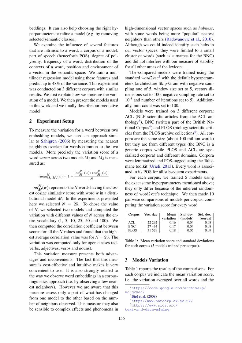
beddings. It can also help choosing the right hy-perparameters or refine a model (e.g. by removingselected semantic classes).
We examine the influence of several featuresthat are intrinsic to a word, a corpus or a model:part of speech (henceforth POS), degree of pol-ysemy, frequency of a word, distribution of thecontexts of a word, position and environment ofa vector in the semantic space. We train a mul-tilinear regression model using these features andpredict up to 48% of the variance. This experimentwas conducted on 3 different corpora with similarresults. We first explain how we measure the vari-ation of a model. We then present the models usedin this work and we finally describe our predictivemodel.
2 Experiment Setup
To measure the variation for a word between twoembedding models, we used an approach simi-lar to Sahlgren (2006) by measuring the nearestneighbors overlap for words common to the twomodels. More precisely the variation score of aword varnn across two models M1 and M2 is mea-sured as:
varnnNM1,M2
(w) = 1−|nnN
M1(w) ∩ nnN
M2(w)|
N
nnNM(w) represents the N words having the clos-
est cosine similarity score with word w in a distri-butional model M. In the experiments presentedhere we selected N = 25. To chose the valueof N, we selected two models and computed thevariation with different values of N across the en-tire vocabulary (1, 5, 10, 25, 50 and 100). Wethen computed the correlation coefficient betweenscores for all the N values and found that the high-est average correlation value was for N = 25. Thevariation was computed only for open classes (ad-verbs, adjectives, verbs and nouns).
This variation measure presents both advan-tages and inconvenients. The fact that this mea-sure is cost-effective and intuitive makes it veryconvenient to use. It is also strongly related tothe way we observe word embeddings in a corpus-linguistics approach (i.e. by observing a few near-est neighbors). However we are aware that thismeasure assess only a part of what has changedfrom one model to the other based on the num-ber of neighbors observed. This measure may alsobe sensible to complex effects and phenomena in
high-dimensional vector spaces such as hubness,with some words being more “popular” nearestneighbors than others (Radovanovic et al., 2010).Although we could indeed identify such hubs inour vector spaces, they were limited to a smallcluster of words (such as surnames for the BNC)and did not interfere with our measure of stabilityfor all other areas of the lexicon.
The compared models were trained using thestandard word2vec2 with the default hyperparam-eters (architecture Skip-Gram with negative sam-pling rate of 5, window size set to 5, vectors di-mensions set to 100, negative sampling rate set to10-3 and number of iterations set to 5). Addition-ally, min-count was set to 100.
Models were trained on 3 different corpora:ACL (NLP scientific articles from the ACL an-thology3), BNC (written part of the British Na-tional Corpus4) and PLOS (biology scientific arti-cles from the PLOS archive collections5). All cor-pora are the same size (about 100 million words)but they are from different types (the BNC is ageneric corpus while PLOS and ACL are spe-cialized corpora) and different domains. Corporawere lemmatized and POS-tagged using the Talis-mane toolkit (Urieli, 2013). Every word is associ-ated to its POS for all subsequent experiments.
For each corpus, we trained 5 models usingthe exact same hyperparameters mentioned above;they only differ because of the inherent random-ness of word2vec’s technique. We then made 10pairwise comparisons of models per corpus, com-puting the variation score for every word.
Corpus Voc. size Mean Std. dev. Std. dev.variation (models) (words)
ACL 22 292 0.16 0.04 0.08BNC 27 434 0.17 0.04 0.08PLOS 31 529 0.18 0.05 0.09
Table 1: Mean variation score and standard deviationsfor each corpus (5 models trained per corpus).
3 Models Variation
Table 1 reports the results of the comparisons. Foreach corpus we indicate the mean variation score,i.e. the variation averaged over all words and the
2https://code.google.com/archive/p/word2vec/
3Bird et al. (2008)4http://www.natcorp.ox.ac.uk/5https://www.plos.org/
text-and-data-mining
155
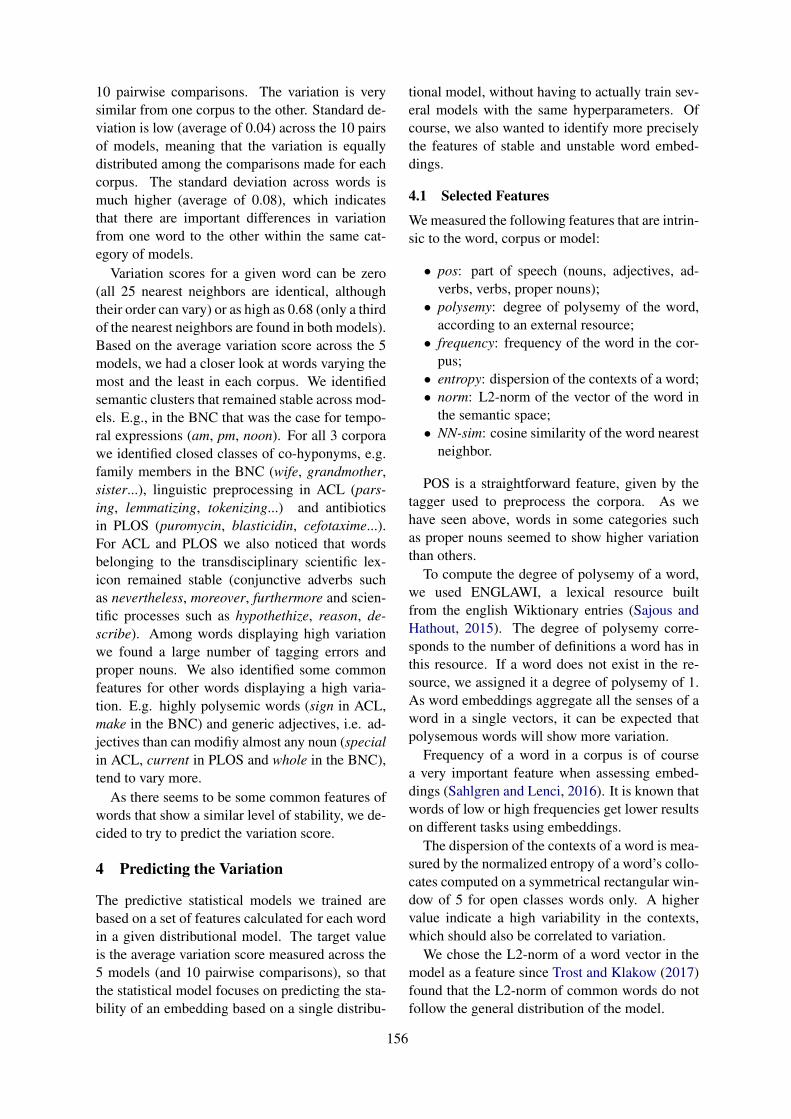
10 pairwise comparisons. The variation is verysimilar from one corpus to the other. Standard de-viation is low (average of 0.04) across the 10 pairsof models, meaning that the variation is equallydistributed among the comparisons made for eachcorpus. The standard deviation across words ismuch higher (average of 0.08), which indicatesthat there are important differences in variationfrom one word to the other within the same cat-egory of models.
Variation scores for a given word can be zero(all 25 nearest neighbors are identical, althoughtheir order can vary) or as high as 0.68 (only a thirdof the nearest neighbors are found in both models).Based on the average variation score across the 5models, we had a closer look at words varying themost and the least in each corpus. We identifiedsemantic clusters that remained stable across mod-els. E.g., in the BNC that was the case for tempo-ral expressions (am, pm, noon). For all 3 corporawe identified closed classes of co-hyponyms, e.g.family members in the BNC (wife, grandmother,sister...), linguistic preprocessing in ACL (pars-ing, lemmatizing, tokenizing...) and antibioticsin PLOS (puromycin, blasticidin, cefotaxime...).For ACL and PLOS we also noticed that wordsbelonging to the transdisciplinary scientific lex-icon remained stable (conjunctive adverbs suchas nevertheless, moreover, furthermore and scien-tific processes such as hypothethize, reason, de-scribe). Among words displaying high variationwe found a large number of tagging errors andproper nouns. We also identified some commonfeatures for other words displaying a high varia-tion. E.g. highly polysemic words (sign in ACL,make in the BNC) and generic adjectives, i.e. ad-jectives than can modifiy almost any noun (specialin ACL, current in PLOS and whole in the BNC),tend to vary more.
As there seems to be some common features ofwords that show a similar level of stability, we de-cided to try to predict the variation score.
4 Predicting the Variation
The predictive statistical models we trained arebased on a set of features calculated for each wordin a given distributional model. The target valueis the average variation score measured across the5 models (and 10 pairwise comparisons), so thatthe statistical model focuses on predicting the sta-bility of an embedding based on a single distribu-
tional model, without having to actually train sev-eral models with the same hyperparameters. Ofcourse, we also wanted to identify more preciselythe features of stable and unstable word embed-dings.
4.1 Selected Features
We measured the following features that are intrin-sic to the word, corpus or model:
• pos: part of speech (nouns, adjectives, ad-verbs, verbs, proper nouns);• polysemy: degree of polysemy of the word,
according to an external resource;• frequency: frequency of the word in the cor-
pus;• entropy: dispersion of the contexts of a word;• norm: L2-norm of the vector of the word in
the semantic space;• NN-sim: cosine similarity of the word nearest
neighbor.
POS is a straightforward feature, given by thetagger used to preprocess the corpora. As wehave seen above, words in some categories suchas proper nouns seemed to show higher variationthan others.
To compute the degree of polysemy of a word,we used ENGLAWI, a lexical resource builtfrom the english Wiktionary entries (Sajous andHathout, 2015). The degree of polysemy corre-sponds to the number of definitions a word has inthis resource. If a word does not exist in the re-source, we assigned it a degree of polysemy of 1.As word embeddings aggregate all the senses of aword in a single vectors, it can be expected thatpolysemous words will show more variation.
Frequency of a word in a corpus is of coursea very important feature when assessing embed-dings (Sahlgren and Lenci, 2016). It is known thatwords of low or high frequencies get lower resultson different tasks using embeddings.
The dispersion of the contexts of a word is mea-sured by the normalized entropy of a word’s collo-cates computed on a symmetrical rectangular win-dow of 5 for open classes words only. A highervalue indicate a high variability in the contexts,which should also be correlated to variation.
We chose the L2-norm of a word vector in themodel as a feature since Trost and Klakow (2017)found that the L2-norm of common words do notfollow the general distribution of the model.
156
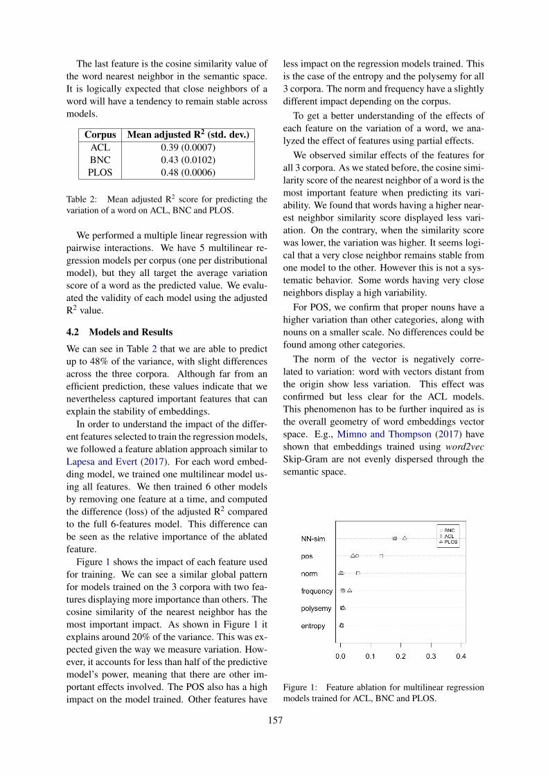
The last feature is the cosine similarity value ofthe word nearest neighbor in the semantic space.It is logically expected that close neighbors of aword will have a tendency to remain stable acrossmodels.
Corpus Mean adjusted R2 (std. dev.)ACL 0.39 (0.0007)BNC 0.43 (0.0102)PLOS 0.48 (0.0006)
Table 2: Mean adjusted R2 score for predicting thevariation of a word on ACL, BNC and PLOS.
We performed a multiple linear regression withpairwise interactions. We have 5 multilinear re-gression models per corpus (one per distributionalmodel), but they all target the average variationscore of a word as the predicted value. We evalu-ated the validity of each model using the adjustedR2 value.
4.2 Models and Results
We can see in Table 2 that we are able to predictup to 48% of the variance, with slight differencesacross the three corpora. Although far from anefficient prediction, these values indicate that wenevertheless captured important features that canexplain the stability of embeddings.
In order to understand the impact of the differ-ent features selected to train the regression models,we followed a feature ablation approach similar toLapesa and Evert (2017). For each word embed-ding model, we trained one multilinear model us-ing all features. We then trained 6 other modelsby removing one feature at a time, and computedthe difference (loss) of the adjusted R2 comparedto the full 6-features model. This difference canbe seen as the relative importance of the ablatedfeature.
Figure 1 shows the impact of each feature usedfor training. We can see a similar global patternfor models trained on the 3 corpora with two fea-tures displaying more importance than others. Thecosine similarity of the nearest neighbor has themost important impact. As shown in Figure 1 itexplains around 20% of the variance. This was ex-pected given the way we measure variation. How-ever, it accounts for less than half of the predictivemodel’s power, meaning that there are other im-portant effects involved. The POS also has a highimpact on the model trained. Other features have
less impact on the regression models trained. Thisis the case of the entropy and the polysemy for all3 corpora. The norm and frequency have a slightlydifferent impact depending on the corpus.
To get a better understanding of the effects ofeach feature on the variation of a word, we ana-lyzed the effect of features using partial effects.
We observed similar effects of the features forall 3 corpora. As we stated before, the cosine simi-larity score of the nearest neighbor of a word is themost important feature when predicting its vari-ability. We found that words having a higher near-est neighbor similarity score displayed less vari-ation. On the contrary, when the similarity scorewas lower, the variation was higher. It seems logi-cal that a very close neighbor remains stable fromone model to the other. However this is not a sys-tematic behavior. Some words having very closeneighbors display a high variability.
For POS, we confirm that proper nouns have ahigher variation than other categories, along withnouns on a smaller scale. No differences could befound among other categories.
The norm of the vector is negatively corre-lated to variation: word with vectors distant fromthe origin show less variation. This effect wasconfirmed but less clear for the ACL models.This phenomenon has to be further inquired as isthe overall geometry of word embeddings vectorspace. E.g., Mimno and Thompson (2017) haveshown that embeddings trained using word2vecSkip-Gram are not evenly dispersed through thesemantic space.
Figure 1: Feature ablation for multilinear regressionmodels trained for ACL, BNC and PLOS.
157

The effect of the frequency over the predictabil-ity of the variation is not linear. Words having verylow or very high frequency are more affected byvariation than words in the mid-frequency range.This partly infirms the common knowledge thatembeddings of more frequent words are of betterquality. We actually found a number of frequentwords displaying instability words in each corpus(e.g. gene and protein in PLOS, language in ACLand make in BNC etc.).
The degree of polysemy of a word also has aslight effect on the predictability of the variation ofa word. The more polysemic a word is, the morelikely its variation score is to be high.
As for the entropy, we observed for ACL andthe BNC, that words having higher entropy withtheir contexts display more variation.
Concerning these two last features (polysemyand entropy) experiments confirm that distribu-tional semantics has more difficulty in represent-ing the meaning of words that appear in a varietyof contexts.
5 Conclusion
In this paper, we wanted to get a better understand-ing of the intrinsic stability of neural-based wordembeddings models. We agree with Antoniak andMimno (2018) when saying that word embeddingsshould be used with care when used as tools forcorpus linguistics, as any phenomenon observedin such models could be simply due to random.
We proposed a method that measures the vari-ation of a word, along with a technique to predictthe variation of a word by using simple features.We have seen that not all features have the sameimportance when predicting the variability, promi-nent features being the cosine similarity score ofthe nearest neighbor of a word and its POS. Theother features we considered, while having a lesserpredictive power, helped to shed some light onwhich areas of the lexicon are more or less af-fected by the variation. This means that we canhope to assess which words (in a given corpus) canbe more reliably represented by embeddings, andwhich one should be analyzed with more caution.
Beyond the practical insterest of this prediction,this work is a step towards a better understandingof the conditions in which distributional semanticscapture and represent the meaning of words. Wealready observed that some words or meanings aremore challenging than others. In this way we as-
sume that stability attest the quality of a semanticrepresentation.
In this work, the embeddings models used weretrained with default hyperparameters. In the fu-ture, we want to know if hyperparameters usedwhen training word embeddings have an impacton the variation. We also want to make sure thatthe identified features explaining the variation willbe the same when varying the hyperparameters. Inthe long run, this could lead to an alternative tobenchmark test sets when selecting the hyperpa-rameter values.
Acknowledgments
We are thankful to the anonymous reviewers fortheir suggestions and comments. Experimentspresented in this paper were carried out usingthe OSIRIM computing platform6 that is admin-istered by the IRIT computer science lab andsupported by the National Center for ScientificResearch (CNRS), the Region Midi-Pyrenees, theFrench Government, and the European RegionalDevelopment Fund (ERDF).
References
Maria Antoniak and David Mimno. 2018. Evaluatingthe stability of embedding-based word similarities.Transactions of the Association for ComputationalLinguistics, 6:107–119.
Fatemeh Torabi Asr, Jon A. Willits, and Michael N.Jones. 2016. Comparing predictive and co-occurrence based models of lexical semanticstrained on child-directed speech. In Proceedings ofthe 37th Meeting of the Cognitive Science Society.
Marco Baroni, Georgiana Dinu, and GermanKruszewski. 2014. Don’t count, predict! Asystematic comparison of context-counting vs.context-predicting semantic vectors. In Proceedingsof the 52nd Annual Meeting of the Associationfor Computational Linguistics, pages 238–247,Baltimore, Maryland, USA.
Steven Bird, Robert Dale, Bonnie Dorr, Bryan Gibson,Mark Joseph, Min-Yen Kan, Dongwon Lee, BrettPowley, Dragomir Radev, and Yee Fan Tan. 2008.The ACL Anthology Reference Corpus: A referencedataset for bibliographic research in computationallinguistics. In Proceedings of Language Resourcesand Evaluation Conference (LREC 08), Marrakesh,Morrocco.
6See http://osirim.irit.fr/site/en
158

Billy Chiu, Gamal Crichton, Anna Korhonen, andSampo Pyysalo. 2016. How to train good word em-beddings for biomedical NLP. In Proceedings ofthe 15th Workshop on Biomedical Natural LanguageProcessing, pages 166–174, Berlin, Germany.
Lev Finkelstein, Evgeniy Gabrilovich, Yossi Matias,Ehud Rivlin, Zach Solan, Gadi Wolfman, and EytanRuppin. 2002. Placing search in context: The con-cept revisited. In ACM Transactions on InformationSystems, volume 20, page 116:131.
William L. Hamilton, Jure Leskovec, and Dan Jurafsky.2016. Diachronic word embeddings reveal statisti-cal laws of semantic change. In Proceedings of the54th Annual Meeting of the Association for Compu-tational Linguistics, pages 1489–1501, Berlin, Ger-many.
Johannes Hellrich and Udo Hahn. 2016. Bad com-pany - neighborhoods in neural embedding spacesconsidered harmful. In Proceedings of COLING2016, the 26th International Conference on Compu-tational Linguistics: Technical Papers, pages 2785–2796, Osaka, Japan.
Adam Kilgarriff, Vıt Baisa, Jan Busta, MilosJakubıcek, Vojtech Kovar, Jan Michelfeit, PavelRychly, and Vıt Suchomel. 2014. The Sketch En-gine: Ten years on. Lexicography, 1(1):7–36.
Gabriella Lapesa and Stefan Evert. 2017. Large-scaleevaluation of dependency-based DSMs: Are theyworth the effort? In Proceedings of the 15th Confer-ence of the European Chapter of the Association forComputational Linguistics, volume 2, Short papers,pages 394–400, Valencia, Spain.
Bofang Li, Tao Liu, Zhe Zhao, Buzhou Tang, Alek-sandr Drozd, Anna Rogers, and Xiaoyong Du. 2017.Investigating different syntactic context types andcontext representations for learning word embed-dings. In Proceedings of the 2017 Conference onEmpirical Methods in Natural Language Process-ing, pages 2411–2421.
Oren Melamud, David McClosky, Siddharth Patward-han, and Mohit Bansal. 2016. The role of contexttypes and dimensionality in learning word embed-dings. In Proceedings of NAACL-HLT 2016, SanDiego, California.
Tomas Mikolov, Kai Chen, Greg Corrado, and JeffreyDean. 2013. Efficient estimation of word represen-tations in vector space. CoRR, abs/1301.3781.
David Mimno and Laure Thompson. 2017. The strangegeometry of skip-gram with negative sampling. InProceedings of the 2017 Conference on EmpiricalMethods in Natural Language Processing, pages2873–2878, Copenhagen, Denmark.
Neha Nayak, Gabor Angeli, and Christopher D. Man-ning. 2016. Evaluating word embeddings using arepresentative suite of practical tasks. In Proceed-ings of the 1st Workshop on Evaluating Vector Space
Representations for NLP, pages 19–23, Berlin, Ger-many.
Milos Radovanovic, Alexandros Nanopoulos, and Mir-jana Ivanovic. 2010. Hubs in space: Popular nearestneighbors in high-dimensional data. Journal of Ma-chine Learning Research, 11:2487–2531.
Kirk Roberts. 2016. Assessing the corpus size vs.similarity trade-off for word embeddings in clinicalNLP. In Proceedings of the Clinical Natural Lan-guage Processing Workshop, pages 54–63, Osaka,Japan.
Magnus Sahlgren. 2006. The Word-Space Model.Ph.D. thesis, Stockholm University, Sweden.
Magnus Sahlgren and Alessandro Lenci. 2016. The ef-fects of data size and frequency range on distribu-tional semantic models. In Proceedings of the 2016Conference on Empirical Methods in Natural Lan-guage Processing, pages 975–980, Austin, Texas.
Franck Sajous and Nabil Hathout. 2015. GLAWI,a free XML-encoded machine-readable dictionarybuilt from the French Wiktionary. In Proceedingsof the eLex 2015 conference, pages 405–426, Herst-monceux, England.
Thomas A. Trost and Dietrich Klakow. 2017. Parame-ter free hierarchical graph-based clustering for ana-lyzing continuous word embeddings. In Proceed-ings of TextGraphs-11: the Workshop on Graph-based Methods for Natural Language Processing,Vancouver, Canada.
Assaf Urieli. 2013. Robust French syntax analysis:reconciling statistical methods and linguistic knowl-edge in the Talismane toolkit. Ph.D. thesis, Univer-sity of Toulouse, France.
159

Proceedings of the 7th Joint Conference on Lexical and Computational Semantics (*SEM), pages 160–166New Orleans, June 5-6, 2018. c©2018 Association for Computational Linguistics
Integrating Multiplicative Featuresinto Supervised Distributional Methods for Lexical Entailment
Tu VuCollege of Information and Computer Sciences
University of Massachusetts AmherstAmherst, MA, USA
Vered ShwartzComputer Science Department
Bar-Ilan UniversityRamat-Gan, Israel
Abstract
Supervised distributional methods are appliedsuccessfully in lexical entailment, but recentwork questioned whether these methods ac-tually learn a relation between two words.Specifically, Levy et al. (2015) claimed thatlinear classifiers learn only separate propertiesof each word. We suggest a cheap and easyway to boost the performance of these meth-ods by integrating multiplicative features intocommonly used representations. We providean extensive evaluation with different classi-fiers and evaluation setups, and suggest a suit-able evaluation setup for the task, eliminatingbiases existing in previous ones.
1 Introduction
Lexical entailment is concerned with identifyingthe semantic relation, if any, holding between twowords, as in (pigeon, hyponym, animal). The pop-ularity of the task stems from its potential rele-vance to various NLP applications, such as ques-tion answering and recognizing textual entailment(Dagan et al., 2013) that often rely on lexical se-mantic resources with limited coverage like Word-net (Miller, 1995). Relation classifiers can be usedeither within applications or as an intermediatestep in the construction of lexical resources whichis often expensive and time-consuming.
Most methods for lexical entailment are distri-butional, i.e., the semantic relation holding be-tween x and y is recognized based on theirdistributional vector representations. While thefirst methods were unsupervised and used high-dimensional sparse vectors (Weeds and Weir,2003; Kotlerman et al., 2010; Santus et al., 2014),in recent years, supervised methods became popu-lar (Baroni et al., 2012; Roller et al., 2014; Weedset al., 2014). These methods are mostly basedon word embeddings (Mikolov et al., 2013b; Pen-nington et al., 2014a) utilizing various vector com-
binations that are designed to capture relational in-formation between two words.
While most previous work reported success us-ing supervised methods, some questions remainunanswered: First, several works suggested thatsupervised distributional methods are incapable ofinferring the relationship between two words, butrather rely on independent properties of each word(Levy et al., 2015; Roller and Erk, 2016; Shwartzet al., 2016), making them sensitive to trainingdata; Second, it remains unclear what is the mostappropriate representation and classifier; previ-ous studies reported inconsistent results with Con-cat〈 ~vx⊕ ~vy〉 (Baroni et al., 2012) and Diff〈~vy− ~vx〉(Roller et al., 2014; Weeds et al., 2014; Fu et al.,2014), using various classifiers.
In this paper, we investigate the effectiveness ofmultiplicative features, namely, the element-wisemultiplication Mult〈 ~vx� ~vy〉, and the squared dif-ference Sqdiff〈(~vy − ~vx) � (~vy − ~vx)〉. Thesefeatures, similar to the cosine similarity and theEuclidean distance, might capture a different no-tion of interaction information about the relation-ship holding between two words. We directly inte-grate them into some commonly used representa-tions. For instance, we consider the concatenationDiff⊕Mult 〈(~vy− ~vx)⊕( ~vx� ~vy)〉 that might cap-ture both the typicality of each word in the relation(e.g., if y is a typical hypernym) and the similaritybetween the words.
We experiment with multiple supervised distri-butional methods and analyze which representa-tions perform well in various evaluation setups.Our analysis confirms that integrating multiplica-tive features into standard representations can sub-stantially boost the performance of linear classi-fiers. While the contribution over non-linear clas-sifiers is sometimes marginal, they are expensiveto train, and linear classifiers can achieve the sameeffect “cheaply” by integrating multiplicative fea-
160

tures. The contribution of multiplicative featuresis mostly prominent in strict evaluation settings,i.e., lexical split (Levy et al., 2015) and out-of-domain evaluation that disable the models’ abil-ity to achieve good performance by memorizingwords seen during training. We find that Concat⊕Mult performs consistently well, and suggest itas a strong baseline for future research.
2 Related Work
Available Representations In supervised distri-butional methods, a pair of words (x, y) is rep-resented as some combination of the word em-beddings of x and y, most commonly Concat〈~vx ⊕ ~vy〉 (Baroni et al., 2012) or Diff 〈~vy − ~vx〉(Weeds et al., 2014; Fu et al., 2014).
Limitations Recent work questioned whethersupervised distributional methods actually learnthe relation between x and y or only separate prop-erties of each word. Levy et al. (2015) claimedthat they tend to perform “lexical memorization”,i.e., memorizing that some words are prototypicalto certain relations (e.g., that y = animal is a hy-pernym, regardless of x). Roller and Erk (2016)found that under certain conditions, these methodsactively learn to infer hypernyms based on sep-arate occurrences of x and y in Hearst patterns(Hearst, 1992). In either case, they only learnwhether x and y independently match their cor-responding slots in the relation, a limitation whichmakes them sensitive to the training data (Shwartzet al., 2017; Sanchez and Riedel, 2017).
Non-linearity Levy et al. (2015) claimed thatthe linear nature of most supervised methods lim-its their ability to capture the relation betweenwords. They suggested that using support vectormachine (SVM) with non-linear kernels slightlymitigates this issue, and proposed KSIM, a customkernel with multiplicative integration.
Multiplicative Features The element-wise mul-tiplication has been studied by Weeds et al. (2014),but models that operate exclusively on it were notcompetitive to Concat and Diff on most tasks.Roller et al. (2014) found that the squared differ-ence, in combination with Diff, is useful for hyper-nymy detection. Nevertheless, little to no work hasfocused on investigating combinations of repre-sentations obtained by concatenating various baserepresentations for the more general task of lexicalentailment.
Base representations CombinationsOnly-x〈 ~vx〉 Diff⊕MultOnly-y〈~vy〉 Diff⊕ Sqdiff
Diff〈~vy − ~vx〉 Sum⊕MultSum〈 ~vx + ~vy〉 Sum⊕ Sqdiff
Concat〈 ~vx ⊕ ~vy〉 Concat⊕MultMult〈 ~vx � ~vy〉 Concat⊕ Sqdiff
Sqdiff〈(~vy − ~vx)� (~vy − ~vx)〉
Table 1: Word pair representations.
3 Methodology
We classify each word pair (x, y) to a specificsemantic relation that holds for them, from a setof pre-defined relations (i.e., multiclass classifica-tion), based on their distributional representations.
3.1 Word Pair Representations
Given a word pair (x, y) and their embeddings~vx, ~vy, we consider various compositions as fea-ture vectors for classifiers. Table 1 displays baserepresentations and combination representations,achieved by concatenating two base representa-tions.
3.2 Word Vectors
We used 300-dimensional pre-trained word em-beddings, namely, GloVe (Pennington et al.,2014b) containing 1.9M word vectors trained on acorpus of web data from Common Crawl (42B to-kens),1 and Word2vec (Mikolov et al., 2013a,c)containing 3M word vectors trained on a part ofGoogle News dataset (100B tokens).2 Out-of-vocabulary words were initialized randomly.
3.3 Classifiers
Following previous work (Levy et al., 2015; Rollerand Erk, 2016), we trained different types of clas-sifiers for each word-pair representation outlinedin Section 3.1, namely, logistic regression withL2 regularization (LR), SVM with a linear kernel(LIN), and SVM with a Gaussian kernel (RBF). Inaddition, we trained multi-layer perceptrons witha single hidden layer (MLP). We compare our mod-els against the KSIM model found to be successfulin previous work (Levy et al., 2015; Kruszewskiet al., 2015). We do not include Roller and Erk(2016)’s model since it focuses only on hyper-nymy. Hyper-parameters are tuned using gridsearch, and we report the test performance of the
1http://nlp.stanford.edu/projects/glove/
2http://code.google.com/p/word2vec/
161

Dataset Relations #Instances #DomainsBLESS attri (attribute), coord (co-hyponym), event, hyper (hypernymy), mero (meronymy), random 26,554 17K&H+N hypo (hypernymy), mero (meronymy), sibl (co-hyponym), false (random) 63,718 3ROOT09 hyper (hypernymy), coord (co-hyponym), random 12,762 –
EVALutionHasProperty (attribute), synonym, HasA (possession),
7,378 –MadeOf (meronymy), IsA (hypernymy), antonym, PartOf (meronymy)
Table 2: Metadata on the datasets. Relations are mapped to corresponding WordNet relations, if available.
hyper-parameters that performed best on the vali-dation set. Below are more details about the train-ing procedure:
• For LR, the inverse of regularization strengthis selected from {2−1, 21, 23, 25}.• For LIN, the penalty parameter C of the error
term is selected from {2−5, 2−3, 2−1, 21}.• For RBF, C and γ values are selected from{21, 23, 25, 27} and {2−7, 2−5, 2−3, 2−1}, re-spectively.• For MLP, the hidden layer size is either 50 or
100, and the learning rate is fixed at 10−3. Weuse early stopping based on the performanceon the validation set. The maximum numberof training epochs is 100.• For KSIM, C and α values are selected from{2−7, 2−5, . . . , 27} and {0.0, 0.1, . . . , 1.0},respectively.
3.4 DatasetsWe evaluated the methods on four common se-mantic relation datasets: BLESS (Baroni and Lenci,2011), K&H+N (Necsulescu et al., 2015), ROOT09
(Santus et al., 2016), and EVALution (Santus et al.,2015). Table 2 provides metadata on the datasets.Most datasets contain word pairs instantiating dif-ferent, explicitly typed semantic relations, plus anumber of unrelated word pairs (random). In-stances in BLESS and K&H+N are divided into anumber of topical domains.3
3.5 Evaluation SetupWe consider the following evaluation setups:
Random (RAND) We randomly split eachdataset into 70% train, 5% validation and 25% test.
Lexical Split (LEX) In line with recent work(Shwartz et al., 2016), we split each dataset intotrain, validation and test sets so that each con-tains a distinct vocabulary. This differs from Levyet al. (2015) who dedicated a subset of the train
3We discarded two relations in EVALution with too fewinstances and did not include its domain information sinceeach word pair can belong to multiple domains at once.
set for evaluation, allowing the model to memo-rize when tuning hyper-parameters. We tried tokeep the same ratio 70 : 5 : 25 as in the randomsetup.
Out-of-domain (OOD) To test whether themethods capture a generic notion of each semanticrelation, we test them on a domain that the clas-sifiers have not seen during training. This setupis more realistic than the random and lexical splitsetups, in which the classifiers can benefit frommemorizing verbatim words (random) or regionsin the vector space (lexical split) that fit a specificslot of each relation.
Specifically, on BLESS and K&H+N, one domain isheld out for testing whilst the classifiers are trainedand validated on the remaining domains. This pro-cess is repeated using each domain as the test set,and each time, a randomly selected domain amongthe remaining domains is left out for validation.The average results are reported.
4 Experiments
Table 3 summarizes the best performing base rep-resentations and combinations on the test setsacross the various datasets and evaluation setups.4
The results across the datasets vary substantiallyin some cases due to the differences between thedatasets’ relations, class balance, and the sourcefrom which they were created. For instance, K&H+Nis imbalanced between the number of instancesacross relations and domains. ROOT09 was de-signed to mitigate the lexical memorization issueby adding negative switched hyponym-hypernympairs to the dataset, making it an inherently moredifficult dataset. EVALution contains a richer setof semantic relations. Overall, the addition ofmultiplicative features improves upon the perfor-mance of the base representations.
Classifiers Multiplicative features substantiallyboost the performance of linear classifiers. How-ever, the gain from adding multiplicative features
4Due to the space limitation, we only show the results ob-tained with Glove. The trend is similar across the word em-beddings.
162

Setup Dataset Linear classifiers (LR, LIN) Non-linear classifiers (RBF, MLP)KSIM
~vy Base Combination ~vy Base Combination
RAND
BLESS 84.4LRConcat
83.8LRConcat ⊕ Mult
89.5 (+5.7) 89.3RBFConcat
94.0RBFConcat ⊕ Mult
94.3 (+0.3) 70.2
K&H-N 89.1LRConcat
95.4LRConcat ⊕ SqDiff
96.1 (+0.7) 96.4RBFConcat
98.6RBFConcat ⊕ Mult
98.6 (0.0) 82.4
ROOT09 68.5LINSum
65.9LINSum ⊕ Mult
84.6 (+18.7) 66.1RBFSum
87.3RBFSum ⊕ SqDiff
88.8 (+1.5) 72.3
EVALution 49.7LINConcat
56.7LINConcat ⊕ Mult
56.8 (+0.1) 52.1RBFConcat
61.1RBFConcat ⊕ Mult
60.6 (-0.5) 50.5
LEX
BLESS 69.9LINConcat
70.6LINConcat ⊕ Mult
74.5 (+3.9) 69.8MLPConcat
63.0MLPConcat ⊕ Mult
73.8 (+10.8) 65.8
K&H-N 78.3LINSum
74.0LINSum ⊕ SqDiff
76.1 (+2.1) 83.2RBFSum
82.0RBFSum ⊕ Mult
81.7 (-0.3) 77.5
ROOT09 66.7LRConcat
66.0LRConcat ⊕ Mult
77.9 (+11.9) 64.5RBFConcat
76.8RBFConcat ⊕ Mult
81.6 (+4.8) 66.7
EVALution 35.0LRConcat
37.9LRConcat ⊕ Mult
40.2 (+2.3) 35.5RBFConcat
43.1RBFConcat ⊕ Mult
44.9 (+1.8) 35.9
OOD
BLESS 70.9LINConcat
69.9LINConcat ⊕ Mult
77.0 (+7.1) 69.9RBFDiff
78.7RBFDiff ⊕ Mult
81.5 (+2.8) 57.8
K&H-N 38.5LINConcat
38.6LINConcat ⊕ Mult
39.7 (+1.1) 48.6MLPSum
44.7MLPSum ⊕ Mult
47.9 (+3.2) 48.9
Table 3: Best test performance (F1) across different datasets and evaluation setups, using Glove. The number inbrackets indicates the performance gap between the best performing combination and base representation setups.
Vector/ RAND OOD
Classifier ~vy Diff Diff ⊕ Mult Sum Sum ⊕ Mult Concat Concat ⊕ Mult ~vy Diff Diff ⊕ Mult Sum Sum ⊕ Mult Concat Concat ⊕ Mult
Glo
Ve
LR 84.4 81.5 87.6 (+6.1) 81.5 87.0 (+5.5) 83.8 89.5 (+5.7) 70.9 64.5 74.7 (+10.2) 59.2 68.9 (+9.7) 69.5 76.5 (+7.0)
LIN 84.1 81.5 87.7 (+6.2) 81.3 87.2 (+5.9) 83.8 89.2 (+5.4) 70.7 64.6 74.8 (+10.2) 59.3 69.4 (+10.1) 69.9 77.0 (+7.1)
RBF 89.3 93.8 94.1 (+0.3) 94.4 94.2 (-0.2) 94.0 94.3 (+0.3) 67.8 78.7 81.5 (+2.8) 65.3 66.4 (+1.1) 69.5 75.7 (+6.2)
MLP 84.4 87.4 89.2 (+1.8) 87.2 89.9 (+2.7) 90.5 90.5 (0.0) 69.9 67.4 77.7 (+10.3) 57.3 66.1 (+8.8) 71.5 77.3 (+5.8)
Wor
d2ve
c
LR 83.5 81.0 85.4 (+4.4) 80.0 84.6 (+4.6) 83.6 87.1 (+3.5) 71.2 62.4 69.0 (+6.6) 59.0 65.3 (+6.3) 71.8 76.1 (+4.3)
LIN 83.3 80.8 84.6 (+3.8) 80.4 84.5 (+4.1) 83.3 86.5 (+3.2) 71.5 62.8 69.1 (+6.3) 59.8 65.2 (+5.4) 72.1 76.0 (+3.9)
RBF 89.1 93.7 93.7 (0.0) 93.7 93.8 (+0.1) 93.6 93.8 (+0.2) 69.2 75.6 76.0 (+0.4) 64.7 66.3 (+1.6) 71.4 75.3 (+3.9)
MLP 81.6 81.0 84.6 (+3.6) 79.6 85.2 (+5.6) 81.3 84.7 (+3.4) 70.2 63.4 69.3 (+5.9) 56.2 60.0 (+3.8) 70.5 74.6 (+4.1)
Table 4: Test performance (F1) on BLESS in the RAND and OOD setups, using Glove and Word2vec.
is smaller when non-linear classifiers are used,since they partially capture such notion of inter-action (Levy et al., 2015). Within the same repre-sentation, there is a clear preference to non-linearclassifiers over linear classifiers.
Evaluation Setup The Only-y representationindicates how well a model can perform withoutconsidering the relation between x and y (Levyet al., 2015). Indeed, in RAND, this method per-forms similarly to the others, except on ROOT09,which by design disables lexical memorization.As expected, a general decrease in performance isobserved in LEX and OOD, stemming from themethods’ inability to benefit from lexical memo-rization. In these setups, there is a more signifi-cant gain from using multiplicative features whennon-linear classifiers are used.
Word Pair Representations Among the baserepresentations Concat often performed best,while Mult seemed to be the preferred multiplica-tive addition. Concat ⊕ Mult performed consis-
tently well, intuitively because Concat capturesthe typicality of each word in the relation (e.g.,if y is a typical hypernym) and Mult captures thesimilarity between the words (where Concat alonemay suggest that animal is a hypernym of apple).To take a closer look at the gain from adding Mult,Table 4 shows the performance of the various baserepresentations and combinations with Mult usingdifferent classifiers on BLESS.5
5 Analysis of Multiplicative Features
We focus the rest of the discussion on the OODsetup, as we believe it is the most challengingsetup, forcing methods to consider the relation be-tween x and y. We found that in this setup, allmethods performed poorly on K&H+N, likely dueto its imbalanced domain and relation distribution.Examining the per-relation F1 scores, we see thatmany methods classify all pairs to one relation.Even KSIM, the best performing method in this
5We also tried ~vx with multiplicative features but they per-formed worse.
163

x relation y similarity Concat Concat ⊕Multcloak-n random good-j 0.195 attribute randomcloak-n random hurl-v 0.161 event randomcloak-n random stop-v 0.186 event randomcoat-n event wear-v 0.544 random eventcloak-n mero silk-n 0.381 random merodress-n attri feminine-j 0.479 random attri
Table 5: Example pairs which were incorrectly classified by Concat while being correctly classified by Concat ⊕Mult in BLESS, along with their cosine similarity scores.
setup, classifies pairs as either hyper or random,effectively only determining if they are related ornot. We therefore focus our analysis on BLESS.
To get a better intuition of the contribution ofmultiplicative features, Table 5 exemplifies pairsthat were incorrectly classified by Concat (RBF)while correctly classified by Concat ⊕ Mult(RBF), along with their cosine similarity scores. Itseems that Mult indeed captures the similarity be-tween x and y. While Concat sometimes relieson properties of a single word, e.g. classifying anadjective y to the attribute relation and a verb y tothe event relation, adding Mult changes the clas-sification of such pairs with low similarity scoresto random. Conversely, pairs with high similarityscores which were falsely classified as random byConcat are assigned specific relations byConcat ⊕Mult.
Interestingly, we found that across domains,there is an almost consistent order of relations withrespect to mean intra-pair cosine similarity:
coord meronym attribute event hypernym random0.426 0.323 0.304 0.296 0.279 0.141
Table 6: Mean pairwise cosine similarity in BLESS.
Since the difference between random (0.141)and other relations (0.279-0.426) was the mostsignificant, it seems that multiplicative featureshelp distinguishing between related and unrelatedpairs. This similarity is possibly also used to dis-tinguish between other relations.
6 Conclusion
We have suggested a cheap way to boost theperformance of supervised distributional methodsfor lexical entailment by integrating multiplica-tive features into standard word-pair representa-tions. Our results confirm that the multiplicativefeatures boost the performance of linear classi-fiers, and in strict evaluation setups, also of non-linear classifiers. We performed an extensive eval-uation with different classifiers and evaluation se-
tups, and suggest the out-of-domain evaluationas the most suitable for the task. Directions forfuture work include investigating other composi-tions, and designing a neural model that can auto-matically learn such features.
7 Acknowledgements
We would like to thank Wei Lu for his involve-ment and advice in the early stage of this project,Stephen Roller and Omer Levy for valuable dis-cussions, and the anonymous reviewers for theirinsightful comments and suggestions.
Vered is supported in part by an IntelICRI-CI grant, the Israel Science Foundationgrant 1951/17, the German Research Foundationthrough the German-Israeli Project Cooperation(DIP, grant DA 1600/1-1), the Clore Scholars Pro-gramme (2017), and the AI2 Key Scientific Chal-lenges Program (2017).
ReferencesMarco Baroni, Raffaella Bernardi, Ngoc-Quynh Do,
and Chung-chieh Shan. 2012. Entailment above theword level in distributional semantics. In Proceed-ings of the 13th Conference of the European Chap-ter of the Association for Computational Linguis-tics, pages 23–32, Avignon, France. Association forComputational Linguistics.
Marco Baroni and Alessandro Lenci. 2011. How weblessed distributional semantic evaluation. In Pro-ceedings of the GEMS 2011 Workshop on GEomet-rical Models of Natural Language Semantics, pages1–10. Association for Computational Linguistics.
Ido Dagan, Dan Roth, Mark Sammons, and Fabio Mas-simo Zanzotto. 2013. Recognizing textual entail-ment: Models and applications. Synthesis Lectureson Human Language Technologies, 6(4):1–220.
Ruiji Fu, Jiang Guo, Bing Qin, Wanxiang Che, HaifengWang, and Ting Liu. 2014. Learning semantic hier-archies via word embeddings. In Proceedings of the52nd Annual Meeting of the Association for Compu-tational Linguistics (Volume 1: Long Papers), pages1199–1209, Baltimore, Maryland. Association forComputational Linguistics.
164
Marti A. Hearst. 1992. Automatic acquisition of hy-ponyms from large text corpora. In Proceedings ofthe 14th Conference on Computational Linguistics -Volume 2, COLING ’92, pages 539–545.
Lili Kotlerman, Ido Dagan, Idan Szpektor, and MaayanZhitomirsky-geffet. 2010. Directional distributionalsimilarity for lexical inference. Natural LanguageEngineering, 16(4):359–389.
Germn Kruszewski, Denis Paperno, and Marco Baroni.2015. Deriving boolean structures from distribu-tional vectors. Transactions of the Association forComputational Linguistics, 3:375–388.
Omer Levy, Steffen Remus, Chris Biemann, and IdoDagan. 2015. Do supervised distributional meth-ods really learn lexical inference relations? In Pro-ceedings of the 2015 Conference of the North Amer-ican Chapter of the Association for ComputationalLinguistics: Human Language Technologies, pages970–976, Denver, Colorado. Association for Com-putational Linguistics.
Tomas Mikolov, Kai Chen, Greg Corrado, and JeffreyDean. 2013a. Efficient estimation of word represen-tations in vector space. Proceedings of Workshop atICLR, 2013.
Tomas Mikolov, Ilya Sutskever, Kai Chen, Greg S Cor-rado, and Jeff Dean. 2013b. Distributed representa-tions of words and phrases and their compositional-ity. In Advances in neural information processingsystems, pages 3111–3119.
Tomas Mikolov, Ilya Sutskever, Kai Chen, Greg S Cor-rado, and Jeff Dean. 2013c. Distributed represen-tations of words and phrases and their composition-ality. In C. J. C. Burges, L. Bottou, M. Welling,Z. Ghahramani, and K. Q. Weinberger, editors, Ad-vances in Neural Information Processing Systems26, pages 3111–3119. Curran Associates, Inc.
George A. Miller. 1995. Wordnet: A lexicaldatabase for english. Communications of the ACM,38(11):39–41.
Silvia Necsulescu, Sara Mendes, David Jurgens, NuriaBel, and Roberto Navigli. 2015. Reading betweenthe lines: Overcoming data sparsity for accurateclassification of lexical relationships. In Proceed-ings of the Fourth Joint Conference on Lexical andComputational Semantics, pages 182–192, Denver,Colorado. Association for Computational Linguis-tics.
Jeffrey Pennington, Richard Socher, and ChristopherManning. 2014a. Glove: Global vectors for wordrepresentation. In Proceedings of the 2014 Con-ference on Empirical Methods in Natural LanguageProcessing (EMNLP), pages 1532–1543. Associa-tion for Computational Linguistics.
Jeffrey Pennington, Richard Socher, and ChristopherManning. 2014b. Glove: Global vectors for word
representation. In Proceedings of the 2014 Con-ference on Empirical Methods in Natural LanguageProcessing (EMNLP), pages 1532–1543, Doha,Qatar. Association for Computational Linguistics.
Stephen Roller and Katrin Erk. 2016. Relations suchas hypernymy: Identifying and exploiting hearst pat-terns in distributional vectors for lexical entailment.In Proceedings of the 2016 Conference on Empiri-cal Methods in Natural Language Processing, pages2163–2172, Austin, Texas. Association for Compu-tational Linguistics.
Stephen Roller, Katrin Erk, and Gemma Boleda. 2014.Inclusive yet selective: Supervised distributional hy-pernymy detection. In Proceedings of COLING2014, the 25th International Conference on Compu-tational Linguistics: Technical Papers, pages 1025–1036, Dublin, Ireland. Dublin City University andAssociation for Computational Linguistics.
Ivan Sanchez and Sebastian Riedel. 2017. How wellcan we predict hypernyms from word embeddings?a dataset-centric analysis. In Proceedings of the15th Conference of the European Chapter of the As-sociation for Computational Linguistics: Volume 2,Short Papers, pages 401–407, Valencia, Spain. As-sociation for Computational Linguistics.
Enrico Santus, Alessandro Lenci, Tin-Shing Chiu, QinLu, and Chu-Ren Huang. 2016. Nine features ina random forest to learn taxonomical semantic re-lations. In Proceedings of the Tenth InternationalConference on Language Resources and Evaluation(LREC 2016), Paris, France.
Enrico Santus, Alessandro Lenci, Qin Lu, and SabineSchulte im Walde. 2014. Chasing hypernyms in vec-tor spaces with entropy. In Proceedings of the 14thConference of the European Chapter of the Associa-tion for Computational Linguistics, volume 2: ShortPapers, pages 38–42, Gothenburg, Sweden. Associ-ation for Computational Linguistics.
Enrico Santus, Frances Yung, Alessandro Lenci, andChu-Ren Huang. 2015. Evalution 1.0: an evolvingsemantic dataset for training and evaluation of dis-tributional semantic models. In Proceedings of the4th Workshop on Linked Data in Linguistics (LDL-2015), pages 64–69.
Vered Shwartz, Yoav Goldberg, and Ido Dagan. 2016.Improving hypernymy detection with an integratedpath-based and distributional method. In Proceed-ings of the 54th Annual Meeting of the Associationfor Computational Linguistics (Volume 1: Long Pa-pers), pages 2389–2398, Berlin, Germany. Associa-tion for Computational Linguistics.
Vered Shwartz, Enrico Santus, and DominikSchlechtweg. 2017. Hypernyms under siege:Linguistically-motivated artillery for hypernymydetection. In Proceedings of the 15th Conferenceof the European Chapter of the Association forComputational Linguistics: Volume 1, Long Papers,
165

pages 65–75, Valencia, Spain. Association forComputational Linguistics.
Julie Weeds, Daoud Clarke, Jeremy Reffin, David Weir,and Bill Keller. 2014. Learning to distinguish hyper-nyms and co-hyponyms. In Proceedings of COL-ING 2014, the 25th International Conference onComputational Linguistics: Technical Papers, pages2249–2259, Dublin, Ireland. Dublin City Universityand Association for Computational Linguistics.
Julie Weeds and David Weir. 2003. Proceedings ofthe 2003 Conference on Empirical Methods in Natu-ral Language Processing, chapter A General Frame-work for Distributional Similarity.
166

Proceedings of the 7th Joint Conference on Lexical and Computational Semantics (*SEM), pages 167–172New Orleans, June 5-6, 2018. c©2018 Association for Computational Linguistics
Deep Affix Features Improve Neural Named Entity Recognizers
Vikas Yadav†, Rebecca Sharp‡, Steven Bethard††School of Information, ‡ Dept. of Computer Science
University of Arizona, Tucson, AZ, USA{vikasy,bsharp,bethard}@email.arizona.edu
Abstract
We propose a practical model for named en-tity recognition (NER) that combines wordand character-level information with a specificlearned representation of the prefixes and suf-fixes of the word. We apply this approachto multilingual and multi-domain NER andshow that it achieves state of the art resultson the CoNLL 2002 Spanish and Dutch andCoNLL 2003 German NER datasets, consis-tently achieving 1.5-2.3 percent over the stateof the art without relying on any dictionary fea-tures. Additionally, we show improvement onSemEval 2013 task 9.1 DrugNER, achievingstate of the art results on the MedLine datasetand the second best results overall (-1.3% fromstate of the art). We also establish a new bench-mark on the I2B2 2010 Clinical NER datasetwith 84.70 F-score.
1 Introduction
Named entity recognition (NER), or identifyingthe specific named entities (eg. person, location,organization etc) in a text, is a precursor to other in-formation extraction tasks such as event extraction.The oldest and perhaps most common approach toNER is based on dictionary lookups, and indeed,when the resources are available, this is very useful(e.g., Uzuner et al., 2011). However, hand-craftingthese lexicons is time-consuming and expensiveand so these resources are often either unavailableor sparse for many domains and languages.
Neural network (NN) approaches to NER, on theother hand, do not necessitate these resources, andadditionally do not require complex feature engi-neering, which can also be very costly and may notport well from domain to domain and language tolanguage. Commonly, these NN architectures forNER include a learned representation of individualwords as well as an encoding of the word’s char-acters. However, neither of these representations
makes explicit use of the semantics of sub-wordunits, i.e., morphemes.
Here we propose a simple neural network archi-tecture that learns a custom representation for af-fixes, allowing for a richer semantic representationof words and allowing the model to better approxi-mate the meaning of words not seen during train-ing1. While a full morphological analysis mightbring further benefits, to ease re-implementationwe take advantage of the Zipfian distribution of lan-guage and focus here on a simple approximation ofmorphemes as high-frequency prefixes and suffixes.Our approach thus requires no language-specificaffix lexicon or morphological tools.
Our contributions are:
1. We propose a simple yet robust extension ofcurrent neural NER approaches that allowsus to learn a representation for prefixes andsuffixes of words. We employ an inexpensiveand language-independent method to approxi-mate affixes of a given language using n-gramfrequencies. This extension is able to be ap-plied directly to new languages and domainswithout any additional resource requirementsand it allows for a more compositional, andhence richer, representation of words.
2. We demonstrate the utility of including a ded-icated representation for affixes. Our modelshows as much as a 2.3% F1 improvementover an recurrent neural network model withonly words and characters, demonstrating thatwhat our model learns about affixes is comple-mentary to a recurrent layer over characters.We find filtering to high-frequency affixes isessential, as simply using all word-boundarycharacter trigrams degrades performance insome cases.
1All code required for reproducibility is available at:https://github.com/vikas95/Pref_Suff_Span_NN
167
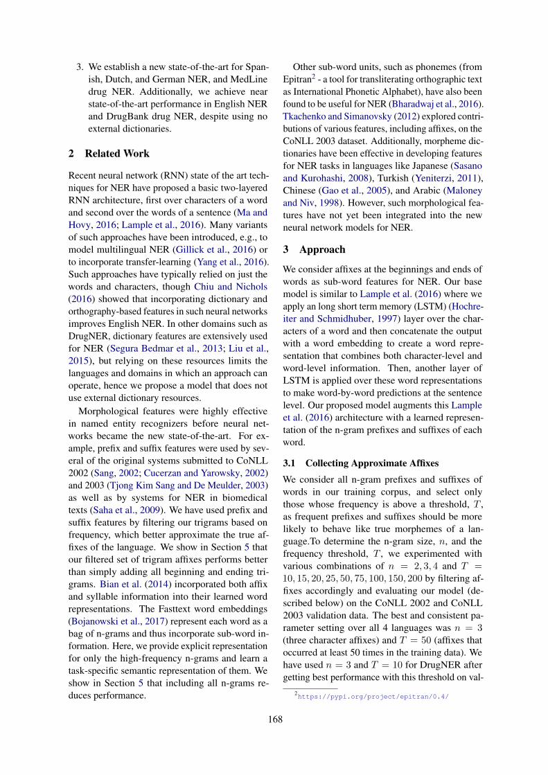
3. We establish a new state-of-the-art for Span-ish, Dutch, and German NER, and MedLinedrug NER. Additionally, we achieve nearstate-of-the-art performance in English NERand DrugBank drug NER, despite using noexternal dictionaries.
2 Related Work
Recent neural network (RNN) state of the art tech-niques for NER have proposed a basic two-layeredRNN architecture, first over characters of a wordand second over the words of a sentence (Ma andHovy, 2016; Lample et al., 2016). Many variantsof such approaches have been introduced, e.g., tomodel multilingual NER (Gillick et al., 2016) orto incorporate transfer-learning (Yang et al., 2016).Such approaches have typically relied on just thewords and characters, though Chiu and Nichols(2016) showed that incorporating dictionary andorthography-based features in such neural networksimproves English NER. In other domains such asDrugNER, dictionary features are extensively usedfor NER (Segura Bedmar et al., 2013; Liu et al.,2015), but relying on these resources limits thelanguages and domains in which an approach canoperate, hence we propose a model that does notuse external dictionary resources.
Morphological features were highly effectivein named entity recognizers before neural net-works became the new state-of-the-art. For ex-ample, prefix and suffix features were used by sev-eral of the original systems submitted to CoNLL2002 (Sang, 2002; Cucerzan and Yarowsky, 2002)and 2003 (Tjong Kim Sang and De Meulder, 2003)as well as by systems for NER in biomedicaltexts (Saha et al., 2009). We have used prefix andsuffix features by filtering our trigrams based onfrequency, which better approximate the true af-fixes of the language. We show in Section 5 thatour filtered set of trigram affixes performs betterthan simply adding all beginning and ending tri-grams. Bian et al. (2014) incorporated both affixand syllable information into their learned wordrepresentations. The Fasttext word embeddings(Bojanowski et al., 2017) represent each word as abag of n-grams and thus incorporate sub-word in-formation. Here, we provide explicit representationfor only the high-frequency n-grams and learn atask-specific semantic representation of them. Weshow in Section 5 that including all n-grams re-duces performance.
Other sub-word units, such as phonemes (fromEpitran2 - a tool for transliterating orthographic textas International Phonetic Alphabet), have also beenfound to be useful for NER (Bharadwaj et al., 2016).Tkachenko and Simanovsky (2012) explored contri-butions of various features, including affixes, on theCoNLL 2003 dataset. Additionally, morpheme dic-tionaries have been effective in developing featuresfor NER tasks in languages like Japanese (Sasanoand Kurohashi, 2008), Turkish (Yeniterzi, 2011),Chinese (Gao et al., 2005), and Arabic (Maloneyand Niv, 1998). However, such morphological fea-tures have not yet been integrated into the newneural network models for NER.
3 Approach
We consider affixes at the beginnings and ends ofwords as sub-word features for NER. Our basemodel is similar to Lample et al. (2016) where weapply an long short term memory (LSTM) (Hochre-iter and Schmidhuber, 1997) layer over the char-acters of a word and then concatenate the outputwith a word embedding to create a word repre-sentation that combines both character-level andword-level information. Then, another layer ofLSTM is applied over these word representationsto make word-by-word predictions at the sentencelevel. Our proposed model augments this Lampleet al. (2016) architecture with a learned represen-tation of the n-gram prefixes and suffixes of eachword.
3.1 Collecting Approximate Affixes
We consider all n-gram prefixes and suffixes ofwords in our training corpus, and select onlythose whose frequency is above a threshold, T ,as frequent prefixes and suffixes should be morelikely to behave like true morphemes of a lan-guage.To determine the n-gram size, n, and thefrequency threshold, T , we experimented withvarious combinations of n = 2, 3, 4 and T =10, 15, 20, 25, 50, 75, 100, 150, 200 by filtering af-fixes accordingly and evaluating our model (de-scribed below) on the CoNLL 2002 and CoNLL2003 validation data. The best and consistent pa-rameter setting over all 4 languages was n = 3(three character affixes) and T = 50 (affixes thatoccurred at least 50 times in the training data). Wehave used n = 3 and T = 10 for DrugNER aftergetting best performance with this threshold on val-
2https://pypi.org/project/epitran/0.4/
168
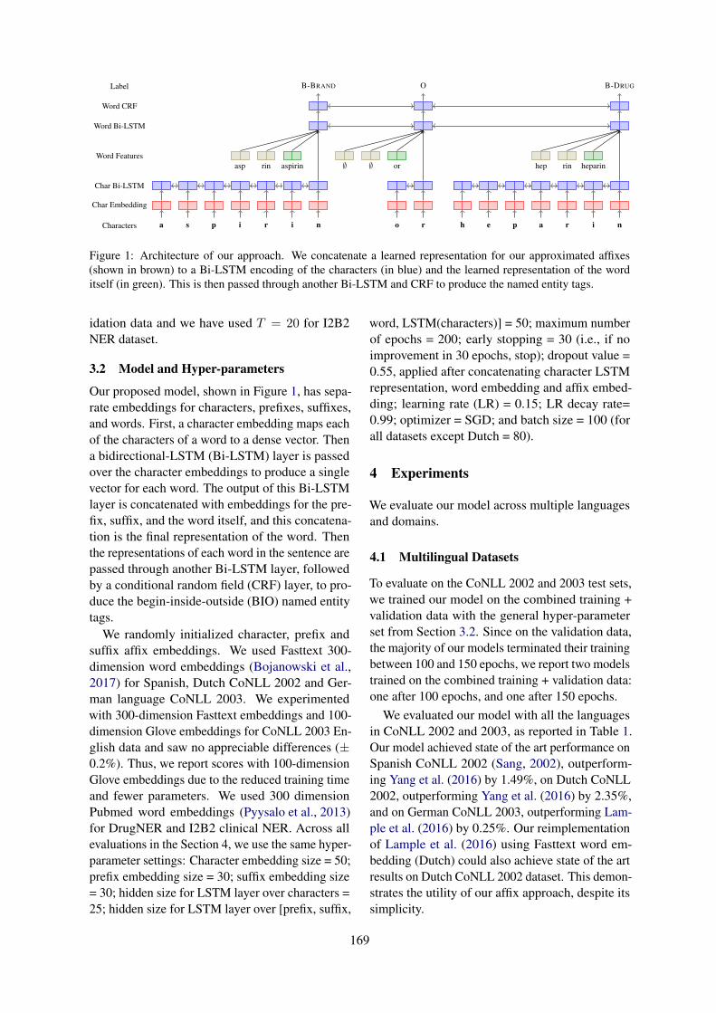
Characters
Char Embedding
Char Bi-LSTM
Word Features
Word Bi-LSTM
Word CRF
Label
a s p i r i n
asp rin aspirin
B-BRAND
o r
∅ ∅ or
O
h e p a r i n
hep rin heparin
B-DRUG
Figure 1: Architecture of our approach. We concatenate a learned representation for our approximated affixes(shown in brown) to a Bi-LSTM encoding of the characters (in blue) and the learned representation of the worditself (in green). This is then passed through another Bi-LSTM and CRF to produce the named entity tags.
idation data and we have used T = 20 for I2B2NER dataset.
3.2 Model and Hyper-parameters
Our proposed model, shown in Figure 1, has sepa-rate embeddings for characters, prefixes, suffixes,and words. First, a character embedding maps eachof the characters of a word to a dense vector. Thena bidirectional-LSTM (Bi-LSTM) layer is passedover the character embeddings to produce a singlevector for each word. The output of this Bi-LSTMlayer is concatenated with embeddings for the pre-fix, suffix, and the word itself, and this concatena-tion is the final representation of the word. Thenthe representations of each word in the sentence arepassed through another Bi-LSTM layer, followedby a conditional random field (CRF) layer, to pro-duce the begin-inside-outside (BIO) named entitytags.
We randomly initialized character, prefix andsuffix affix embeddings. We used Fasttext 300-dimension word embeddings (Bojanowski et al.,2017) for Spanish, Dutch CoNLL 2002 and Ger-man language CoNLL 2003. We experimentedwith 300-dimension Fasttext embeddings and 100-dimension Glove embeddings for CoNLL 2003 En-glish data and saw no appreciable differences (±0.2%). Thus, we report scores with 100-dimensionGlove embeddings due to the reduced training timeand fewer parameters. We used 300 dimensionPubmed word embeddings (Pyysalo et al., 2013)for DrugNER and I2B2 clinical NER. Across allevaluations in the Section 4, we use the same hyper-parameter settings: Character embedding size = 50;prefix embedding size = 30; suffix embedding size= 30; hidden size for LSTM layer over characters =25; hidden size for LSTM layer over [prefix, suffix,
word, LSTM(characters)] = 50; maximum numberof epochs = 200; early stopping = 30 (i.e., if noimprovement in 30 epochs, stop); dropout value =0.55, applied after concatenating character LSTMrepresentation, word embedding and affix embed-ding; learning rate (LR) = 0.15; LR decay rate=0.99; optimizer = SGD; and batch size = 100 (forall datasets except Dutch = 80).
4 Experiments
We evaluate our model across multiple languagesand domains.
4.1 Multilingual Datasets
To evaluate on the CoNLL 2002 and 2003 test sets,we trained our model on the combined training +validation data with the general hyper-parameterset from Section 3.2. Since on the validation data,the majority of our models terminated their trainingbetween 100 and 150 epochs, we report two modelstrained on the combined training + validation data:one after 100 epochs, and one after 150 epochs.
We evaluated our model with all the languagesin CoNLL 2002 and 2003, as reported in Table 1.Our model achieved state of the art performance onSpanish CoNLL 2002 (Sang, 2002), outperform-ing Yang et al. (2016) by 1.49%, on Dutch CoNLL2002, outperforming Yang et al. (2016) by 2.35%,and on German CoNLL 2003, outperforming Lam-ple et al. (2016) by 0.25%. Our reimplementationof Lample et al. (2016) using Fasttext word em-bedding (Dutch) could also achieve state of the artresults on Dutch CoNLL 2002 dataset. This demon-strates the utility of our affix approach, despite itssimplicity.
169
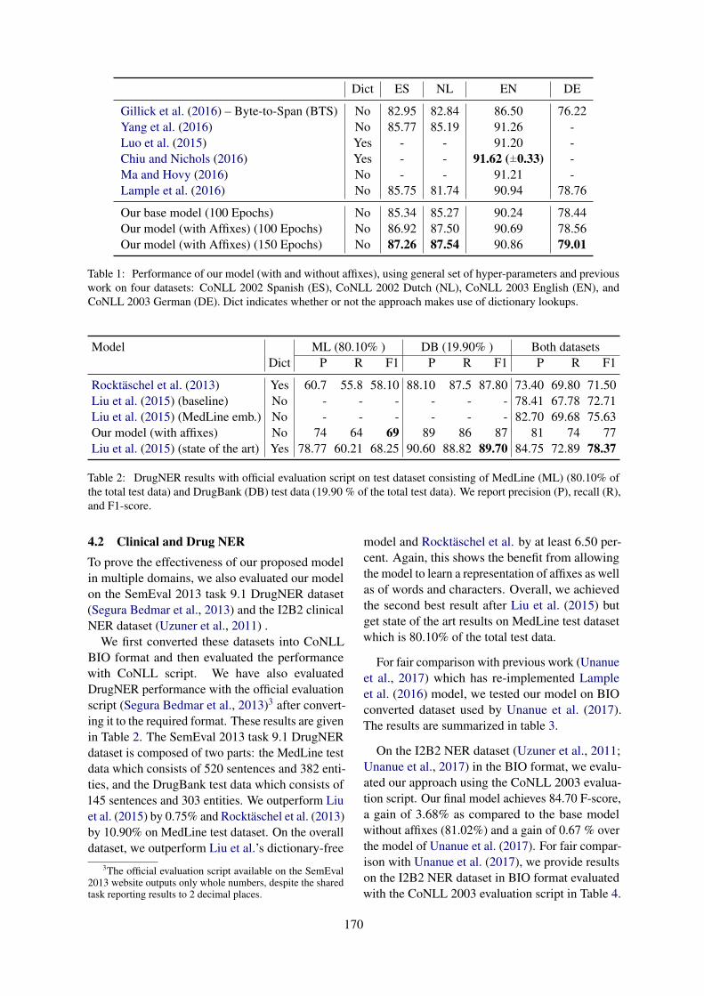
Dict ES NL EN DE
Gillick et al. (2016) – Byte-to-Span (BTS) No 82.95 82.84 86.50 76.22Yang et al. (2016) No 85.77 85.19 91.26 -Luo et al. (2015) Yes - - 91.20 -Chiu and Nichols (2016) Yes - - 91.62 (±0.33) -Ma and Hovy (2016) No - - 91.21 -Lample et al. (2016) No 85.75 81.74 90.94 78.76
Our base model (100 Epochs) No 85.34 85.27 90.24 78.44Our model (with Affixes) (100 Epochs) No 86.92 87.50 90.69 78.56Our model (with Affixes) (150 Epochs) No 87.26 87.54 90.86 79.01
Table 1: Performance of our model (with and without affixes), using general set of hyper-parameters and previouswork on four datasets: CoNLL 2002 Spanish (ES), CoNLL 2002 Dutch (NL), CoNLL 2003 English (EN), andCoNLL 2003 German (DE). Dict indicates whether or not the approach makes use of dictionary lookups.
Model ML (80.10% ) DB (19.90% ) Both datasetsDict P R F1 P R F1 P R F1
Rocktaschel et al. (2013) Yes 60.7 55.8 58.10 88.10 87.5 87.80 73.40 69.80 71.50Liu et al. (2015) (baseline) No - - - - - - 78.41 67.78 72.71Liu et al. (2015) (MedLine emb.) No - - - - - - 82.70 69.68 75.63Our model (with affixes) No 74 64 69 89 86 87 81 74 77Liu et al. (2015) (state of the art) Yes 78.77 60.21 68.25 90.60 88.82 89.70 84.75 72.89 78.37
Table 2: DrugNER results with official evaluation script on test dataset consisting of MedLine (ML) (80.10% ofthe total test data) and DrugBank (DB) test data (19.90 % of the total test data). We report precision (P), recall (R),and F1-score.
4.2 Clinical and Drug NERTo prove the effectiveness of our proposed modelin multiple domains, we also evaluated our modelon the SemEval 2013 task 9.1 DrugNER dataset(Segura Bedmar et al., 2013) and the I2B2 clinicalNER dataset (Uzuner et al., 2011) .
We first converted these datasets into CoNLLBIO format and then evaluated the performancewith CoNLL script. We have also evaluatedDrugNER performance with the official evaluationscript (Segura Bedmar et al., 2013)3 after convert-ing it to the required format. These results are givenin Table 2. The SemEval 2013 task 9.1 DrugNERdataset is composed of two parts: the MedLine testdata which consists of 520 sentences and 382 enti-ties, and the DrugBank test data which consists of145 sentences and 303 entities. We outperform Liuet al. (2015) by 0.75% and Rocktaschel et al. (2013)by 10.90% on MedLine test dataset. On the overalldataset, we outperform Liu et al.’s dictionary-free
3The official evaluation script available on the SemEval2013 website outputs only whole numbers, despite the sharedtask reporting results to 2 decimal places.
model and Rocktaschel et al. by at least 6.50 per-cent. Again, this shows the benefit from allowingthe model to learn a representation of affixes as wellas of words and characters. Overall, we achievedthe second best result after Liu et al. (2015) butget state of the art results on MedLine test datasetwhich is 80.10% of the total test data.
For fair comparison with previous work (Unanueet al., 2017) which has re-implemented Lampleet al. (2016) model, we tested our model on BIOconverted dataset used by Unanue et al. (2017).The results are summarized in table 3.
On the I2B2 NER dataset (Uzuner et al., 2011;Unanue et al., 2017) in the BIO format, we evalu-ated our approach using the CoNLL 2003 evalua-tion script. Our final model achieves 84.70 F-score,a gain of 3.68% as compared to the base modelwithout affixes (81.02%) and a gain of 0.67 % overthe model of Unanue et al. (2017). For fair compar-ison with Unanue et al. (2017), we provide resultson the I2B2 NER dataset in BIO format evaluatedwith the CoNLL 2003 evaluation script in Table 4.
170

Model drug brand group drug n ML drug brand group drug n DB Both
Unanue et al. (2017) 75.57 28.57 64.37 37.19 60.66 91.83 87.27 84.67 0 88.38 -BASE 72 41.67 75.86 4.88 60.86 89.92 79.12 86.13 0 86.52 72.31BASE+Affix(10) 79.25 44.44 85.39 32.73 69.71 92.09 86.60 87.41 20 88.93 78.39
Table 3: DrugNER results on test data using CoNLL evaluation script. ML indicates the results for MedLine testdata and DB indicates results for DrugBank test data. We have reported F1 scores for each entity type in MedLine,DrugBank and overall dataset (Both). The last column (Both) provides performance on the the combined dataset.
Model Problem Test TreatmentP R F1 P R F1 P R F1
Unanue et al. (2017) 81.29 83.62 82.44 84.74 85.01 84.87 83.36 83.55 83.46Base Model 82.45 77.88 80.10 87.24 77.96 82.34 85.53 76.97 81.02Base+Affix(20) 84.35 84.27 84.31 87.37 84.34 85.82 85.73 82.58 84.13
Table 4: Performance on I2B2 2010 NER (Uzuner et al., 2011) test data 5 using CoNLL evaluation script. Wehave reported precision (P), recall (R), and F1-score.
5 Analysis
To better understand the performance of our model,we conducted several analyses on the EnglishCoNLL 2003 dataset.
To determine if the performance gains were trulydue to the affix embeddings, and not simply due tohaving more model parameters, we re-ran our basemodel (without affixes), increasing the characterembeddings from 25 to 55 to match the increase of30 of our affix embeddings. This model’s F-score(90.28%) was similar to the original base model(90.24%), and was more than a half a point belowour model with affixes (90.86%).
To determine the contribution of filtering ouraffixes based on frequency (as compared to sim-ply using all word-boundary n-grams) we ran ourmodel with the full set of affixes found in train-ing. The performance without filtering (89.87%F1) was even lower than the base model withoutaffixes (90.24% F1), which demonstrates that fil-tering based on frequency is beneficial for affixselection.
6 ConclusionOur results across multiple languages and do-mains show that sub-word features such as pre-fixes and suffixes are complementary to characterand word-level information. Our straight-forwardand language-independent approach shows perfor-mance gains compared to other neural systems forNER, achieving a new state of the art on Spanish,Dutch, and German NER as well as the MedLineportion of DrugNER, despite our lack of dictionaryresources. Additionally, we also achieve 3.67% im-provement in the I2B2 clinical NER dataset which
points towards potential applications in biomedi-cal NER. While our model proposes a very simpleidea of using filtered affixes as an approximationof morphemes, we suggest there are further gainsto be had with better methods for deriving truemorphemes (e.g., the supervised neural model ofLuong et al., 2013). We leave this exploration tofuture work.
ReferencesAkash Bharadwaj, David R. Mortensen, Chris Dyer,
and Carlos de Juan Carbonell. 2016. Phonologicallyaware neural model for named entity recognition inlow resource transfer settings. In EMNLP.
Jiang Bian, Bin Gao, and Tie-Yan Liu. 2014.Knowledge-powered deep learning for word embed-ding. In Joint European Conference on MachineLearning and Knowledge Discovery in Databases.Springer, pages 132–148.
Piotr Bojanowski, Edouard Grave, Armand Joulin, andTomas Mikolov. 2017. Enriching word vectors withsubword information. Transactions of the Associa-tion for Computational Linguistics 5:135–146.
Jason Chiu and Eric Nichols. 2016. Named entityrecognition with bidirectional LSTM-CNNs. Trans-actions of the Association for Computational Lin-guistics 4:357–370.
Silviu Cucerzan and David Yarowsky. 2002. Lan-guage independent ner using a unified model of in-ternal and contextual evidence. In proceedings ofthe 6th conference on Natural language learning-Volume 20. Association for Computational Linguis-tics, pages 1–4.
Jianfeng Gao, Mu Li, Andi Wu, and Chang-NingHuang. 2005. Chinese word segmentation and
171
named entity recognition: A pragmatic approach.Computational Linguistics 31(4):531–574.
Daniel Gillick, Cliff Brunk, Oriol Vinyals, and Amar-nag Subramanya. 2016. Multilingual language pro-cessing from bytes. In HLT-NAACL.
Sepp Hochreiter and Jurgen Schmidhuber. 1997. Longshort-term memory. Neural computation 9(8):1735–1780.
Guillaume Lample, Miguel Ballesteros, Sandeep Sub-ramanian, Kazuya Kawakami, and Chris Dyer. 2016.Neural architectures for named entity recognition.In Proceedings of the 2016 Conference of the NorthAmerican Chapter of the Association for Computa-tional Linguistics: Human Language Technologies.Association for Computational Linguistics, pages260–270.
Shengyu Liu, Buzhou Tang, Qingcai Chen, and Xiao-long Wang. 2015. Effects of semantic features onmachine learning-based drug name recognition sys-tems: word embeddings vs. manually constructeddictionaries. Information 6(4):848–865.
Gang Luo, Xiaojiang Huang, Chin-Yew Lin, and Za-iqing Nie. 2015. Joint entity recognition and disam-biguation. In Proceedings of the 2015 Conferenceon Empirical Methods in Natural Language Process-ing. pages 879–888.
Thang Luong, Richard Socher, and Christopher D Man-ning. 2013. Better word representations with recur-sive neural networks for morphology. In CoNLL.pages 104–113.
Xuezhe Ma and Eduard Hovy. 2016. End-to-endsequence labeling via bi-directional LSTM-CNNs-CRF. In Proceedings of the 54th Annual Meeting ofthe Association for Computational Linguistics. As-sociation for Computational Linguistics, Berlin, Ger-many, pages 1064–1074.
John Maloney and Michael Niv. 1998. Tagarab: afast, accurate arabic name recognizer using high-precision morphological analysis. In Proceedingsof the Workshop on Computational Approaches toSemitic Languages. Association for ComputationalLinguistics, pages 8–15.
Sampo Pyysalo, Filip Ginter, Hans Moen, TapioSalakoski, and Sophia Ananiadou. 2013. Distribu-tional semantics resources for biomedical text pro-cessing. In Languages in Biology and medicine.LBM.
Tim Rocktaschel, Torsten Huber, Michael Weidlich,and Ulf Leser. 2013. Wbi-ner: The impact ofdomain-specific features on the performance of iden-tifying and classifying mentions of drugs. In Se-mEval@ NAACL-HLT . pages 356–363.
Sujan Kumar Saha, Sudeshna Sarkar, and Pabitra Mitra.2009. Feature selection techniques for maximumentropy based biomedical named entity recognition.
Journal of Biomedical Informatics 42(5):905 – 911.Biomedical Natural Language Processing.
Erik F Tjong Kim Sang. 2002. Introduction to theCoNLL-2002 shared task: language-independentnamed entity recognition, proceedings of the 6thconference on natural language learning. August31:1–4.
Ryohei Sasano and Sadao Kurohashi. 2008. Japanesenamed entity recognition using structural natural lan-guage processing. In IJCNLP. pages 607–612.
Isabel Segura Bedmar, Paloma Martınez, and MarıaHerrero Zazo. 2013. Semeval-2013 task 9: Ex-traction of drug-drug interactions from biomedicaltexts (ddiextraction 2013). Association for Compu-tational Linguistics.
Erik F Tjong Kim Sang and Fien De Meulder.2003. Introduction to the CoNLL-2003 shared task:Language-independent named entity recognition. InProceedings of the seventh conference on Naturallanguage learning at HLT-NAACL 2003-Volume 4.Association for Computational Linguistics, pages142–147.
Maksim Tkachenko and Andrey Simanovsky. 2012.Named entity recognition: Exploring features. InKONVENS. pages 118–127.
Inigo Jauregi Unanue, Ehsan Zare Borzeshi, andMassimo Piccardi. 2017. Recurrent neural net-works with specialized word embeddings for health-domain named-entity recognition. Journal ofbiomedical informatics 76:102–109.
Ozlem Uzuner, Brett R South, Shuying Shen, andScott L DuVall. 2011. 2010 i2b2/va challenge onconcepts, assertions, and relations in clinical text.Journal of the American Medical Informatics Asso-ciation 18(5):552–556.
Zhilin Yang, Ruslan Salakhutdinov, and William W.Cohen. 2016. Transfer learning for sequence tag-ging with hierarchical recurrent networks. CoRRabs/1703.06345.
Reyyan Yeniterzi. 2011. Exploiting morphology inTurkish named entity recognition system. In Pro-ceedings of the ACL 2011 Student Session. Associa-tion for Computational Linguistics, pages 105–110.
172
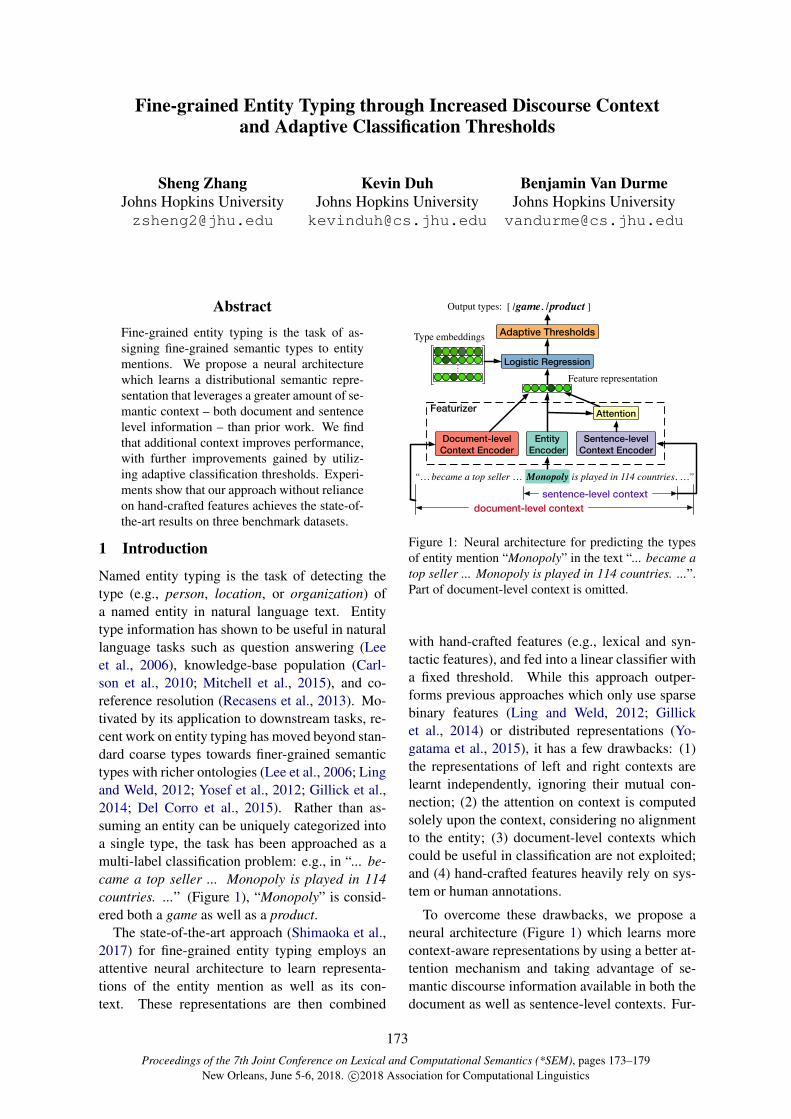
Proceedings of the 7th Joint Conference on Lexical and Computational Semantics (*SEM), pages 173–179New Orleans, June 5-6, 2018. c©2018 Association for Computational Linguistics
Fine-grained Entity Typing through Increased Discourse Contextand Adaptive Classification Thresholds
Sheng ZhangJohns Hopkins [email protected]
Kevin DuhJohns Hopkins [email protected]
Benjamin Van DurmeJohns Hopkins [email protected]
AbstractFine-grained entity typing is the task of as-signing fine-grained semantic types to entitymentions. We propose a neural architecturewhich learns a distributional semantic repre-sentation that leverages a greater amount of se-mantic context – both document and sentencelevel information – than prior work. We findthat additional context improves performance,with further improvements gained by utiliz-ing adaptive classification thresholds. Experi-ments show that our approach without relianceon hand-crafted features achieves the state-of-the-art results on three benchmark datasets.
1 Introduction
Named entity typing is the task of detecting thetype (e.g., person, location, or organization) ofa named entity in natural language text. Entitytype information has shown to be useful in naturallanguage tasks such as question answering (Leeet al., 2006), knowledge-base population (Carl-son et al., 2010; Mitchell et al., 2015), and co-reference resolution (Recasens et al., 2013). Mo-tivated by its application to downstream tasks, re-cent work on entity typing has moved beyond stan-dard coarse types towards finer-grained semantictypes with richer ontologies (Lee et al., 2006; Lingand Weld, 2012; Yosef et al., 2012; Gillick et al.,2014; Del Corro et al., 2015). Rather than as-suming an entity can be uniquely categorized intoa single type, the task has been approached as amulti-label classification problem: e.g., in “... be-came a top seller ... Monopoly is played in 114countries. ...” (Figure 1), “Monopoly” is consid-ered both a game as well as a product.
The state-of-the-art approach (Shimaoka et al.,2017) for fine-grained entity typing employs anattentive neural architecture to learn representa-tions of the entity mention as well as its con-text. These representations are then combined
EntityEncoder
Sentence-level Context Encoder
Document-level Context Encoder
sentence-level contextdocument-level context
Attention
Feature representation
Type embeddings… Logistic Regression
Adaptive Thresholds
[ /game, /product ]Output types:
Featurizer
“… became a top seller … is played in 114 countries. …”Monopoly
Figure 1: Neural architecture for predicting the typesof entity mention “Monopoly” in the text “... became atop seller ... Monopoly is played in 114 countries. ...”.Part of document-level context is omitted.
with hand-crafted features (e.g., lexical and syn-tactic features), and fed into a linear classifier witha fixed threshold. While this approach outper-forms previous approaches which only use sparsebinary features (Ling and Weld, 2012; Gillicket al., 2014) or distributed representations (Yo-gatama et al., 2015), it has a few drawbacks: (1)the representations of left and right contexts arelearnt independently, ignoring their mutual con-nection; (2) the attention on context is computedsolely upon the context, considering no alignmentto the entity; (3) document-level contexts whichcould be useful in classification are not exploited;and (4) hand-crafted features heavily rely on sys-tem or human annotations.
To overcome these drawbacks, we propose aneural architecture (Figure 1) which learns morecontext-aware representations by using a better at-tention mechanism and taking advantage of se-mantic discourse information available in both thedocument as well as sentence-level contexts. Fur-
173
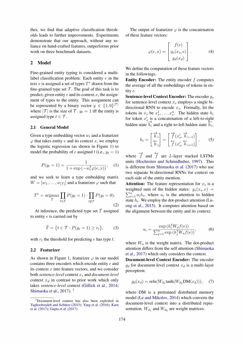
ther, we find that adaptive classification thresh-olds leads to further improvements. Experimentsdemonstrate that our approach, without any re-liance on hand-crafted features, outperforms priorwork on three benchmark datasets.
2 Model
Fine-grained entity typing is considered a multi-label classification problem: Each entity e in thetext x is assigned a set of types T ∗ drawn from thefine-grained type set T . The goal of this task is topredict, given entity e and its context x, the assign-ment of types to the entity. This assignment canbe represented by a binary vector y ∈ {1, 0}|T |where |T | is the size of T . yt = 1 iff the entity isassigned type t ∈ T .
2.1 General Model
Given a type embedding vector wt and a featurizerϕ that takes entity e and its context x, we employthe logistic regression (as shown in Figure 1) tomodel the probability of e assigned t (i.e., yt = 1)
P (yt = 1) =1
1 + exp (−wᵀt ϕ(e, x))
, (1)
and we seek to learn a type embedding matrixW = [w1, . . . , w|T |] and a featurizer ϕ such that
T ∗ = argmaxT
∏
t∈TP (yt = 1) ·
∏
t/∈TP (yt = 0).
(2)At inference, the predicted type set T assigned
to entity e is carried out by
T ={t ∈ T : P (yt = 1) ≥ rt
}, (3)
with rt the threshold for predicting e has type t.
2.2 Featurizer
As shown in Figure 1, featurizer ϕ in our modelcontains three encoders which encode entity e andits context x into feature vectors, and we considerboth sentence-level context xs and document-levelcontext xd in contrast to prior work which onlytakes sentence-level context (Gillick et al., 2014;Shimaoka et al., 2017). 1
1Document-level context has also been exploited inYaghoobzadeh and Schutze (2015); Yang et al. (2016); Karnet al. (2017); Gupta et al. (2017).
The output of featurizer ϕ is the concatenationof these feature vectors:
ϕ(e, x) =
f(e)
gs(xs, e)
gd(xd)
. (4)
We define the computation of these feature vectorsin the followings.Entity Encoder: The entity encoder f computesthe average of all the embeddings of tokens in en-tity e.Sentence-level Context Encoder: The encoder gsfor sentence-level context xs employs a single bi-directional RNN to encode xs. Formally, let thetokens in xs be x1s, . . . , x
ns . The hidden state hi
for token xis is a concatenation of a left-to-righthidden state
−→hi and a right-to-left hidden state
←−hi ,
hi =
[−→h i
←−h i
]=
[−→f (xis,
−→h i−1)
←−f (xis,
←−h i+1)
], (5)
where−→f and
←−f are L-layer stacked LSTMs
units (Hochreiter and Schmidhuber, 1997). Thisis different from Shimaoka et al. (2017) who usetwo separate bi-directional RNNs for context oneach side of the entity mention.Attention: The feature representation for xs is aweighted sum of the hidden states: gs(xs, e) =∑n
i=1 aihi, where ai is the attention to hiddenstate hi. We employ the dot-product attention (Lu-ong et al., 2015). It computes attention based onthe alignment between the entity and its context:
ai =exp (hᵀiWaf(e))∑nj=1 exp (h
ᵀjWaf(e))
, (6)
where Wa is the weight matrix. The dot-productattention differs from the self attention (Shimaokaet al., 2017) which only considers the context.Document-level Context Encoder: The encodergd for document-level context xd is a multi-layerperceptron:
gd(xd) = relu(Wd1 tanh(Wd2DM(xd))), (7)
where DM is a pretrained distributed memorymodel (Le and Mikolov, 2014) which converts thedocument-level context into a distributed repre-sentation. Wd1 and Wd2 are weight matrices.
174

2.3 Adaptive Thresholds
In prior work, a fixed threshold (rt = 0.5) isused for classification of all types (Ling and Weld,2012; Shimaoka et al., 2017). We instead assigna different threshold to each type that is optimizedto maximize the overall strict F1 on the dev set.We show the definition of strict F1 in Section 3.1.
3 Experiments
We conduct experiments on three publicly avail-able datasets.2 Table 1 shows the statistics of thesedatasets.OntoNotes: Gillick et al. (2014) sampled sen-tences from OntoNotes (Weischedel et al., 2011)and annotated entities in these sentences using 89types. We use the same train/dev/test splits in Shi-maoka et al. (2017). Document-level contexts areretrieved from the original OntoNotes corpus.BBN: Weischedel and Brunstein (2005) annotatedentities in Wall Street Journal using 93 types. Weuse the train/test splits in Ren et al. (2016b) andrandomly hold out 2,000 pairs for dev. Documentcontexts are retrieved from the original corpus.FIGER: Ling and Weld (2012) sampled sentencesfrom 780k Wikipedia articles and 434 news re-ports to form the train and test data respectively,and annotated entities using 113 types. The splitswe use are the same in Shimaoka et al. (2017).
Train Dev Test Types
OntoNotes 251,039 2,202 8,963 89BBN 84,078 2,000 13,766 93FIGER 2,000,000 10,000 563 113
Table 1: Statistics of the datasets.
3.1 Metrics
We adopt the metrics used in Ling and Weld(2012) where results are evaluated via strict, loosemacro, loose micro F1 scores. For the i-th in-stance, let the predicted type set be Ti, and thereference type set Ti. The precision (P ) and re-call (R) for each metric are computed as follow.Strict:
P = R =1
N
N∑
i=1
δ(Ti = Ti)
2 We made the source code and data publicly available athttps://github.com/sheng-z/figet.
Loose Macro:
P =1
N
N∑
i=1
|Ti ∩ Ti||Ti|
R =1
N
N∑
i=1
|Ti ∩ Ti||Ti|
Loose Micro:
P =
∑Ni=1 |Ti ∩ Ti|∑N
i=1 |Ti|
R =
∑Ni=1 |Ti ∩ Ti|∑N
i=1 |Ti|
3.2 HyperparametersWe use open-source GloVe vectors (Penningtonet al., 2014) trained on Common Crawl 840Bwith 300 dimensions to initialize word embed-dings used in all encoders. All weight parame-ters are sampled from U(−0.01, 0.01). The en-coder for sentence-level context is a 2-layer bi-directional RNN with 200 hidden units. The DMoutput size is 50. Sizes of Wa, Wd1 and Wd2 are200×300, 70×50, and 50×70 respectively. Adamoptimizer (Kingma and Ba, 2014) and mini-batchgradient is used for optimization. Batch size is200. Dropout (rate=0.5) is applied to three featurefunctions. To avoid overfitting, we choose modelswhich yield the best strict F1 on dev sets.
3.3 ResultsWe compare experimental results of our approachwith previous approaches3, and study contribu-tion of our base model architecture, document-level contexts and adaptive thresholds via ablation.To ensure our findings are reliable, we run eachexperiment twice and report the average perfor-mance.
Overall, our approach significantly increasesthe state-of-the-art macro F1 on both OntoNotesand BBN datasets.
On OntoNotes (Table 3), our approach im-proves the state of the art across all three met-rics. Note that (1) without adaptive thresholds ordocument-level contexts, our approach still out-performs other approaches on macro F1 and microF1; (2) adding hand-crafted features (Shimaokaet al., 2017) does not improve the performance.
3For PLE (Ren et al., 2016b), we were unable to replicatethe performance benefits reported in their work, so we reportthe results after running their codebase.
175
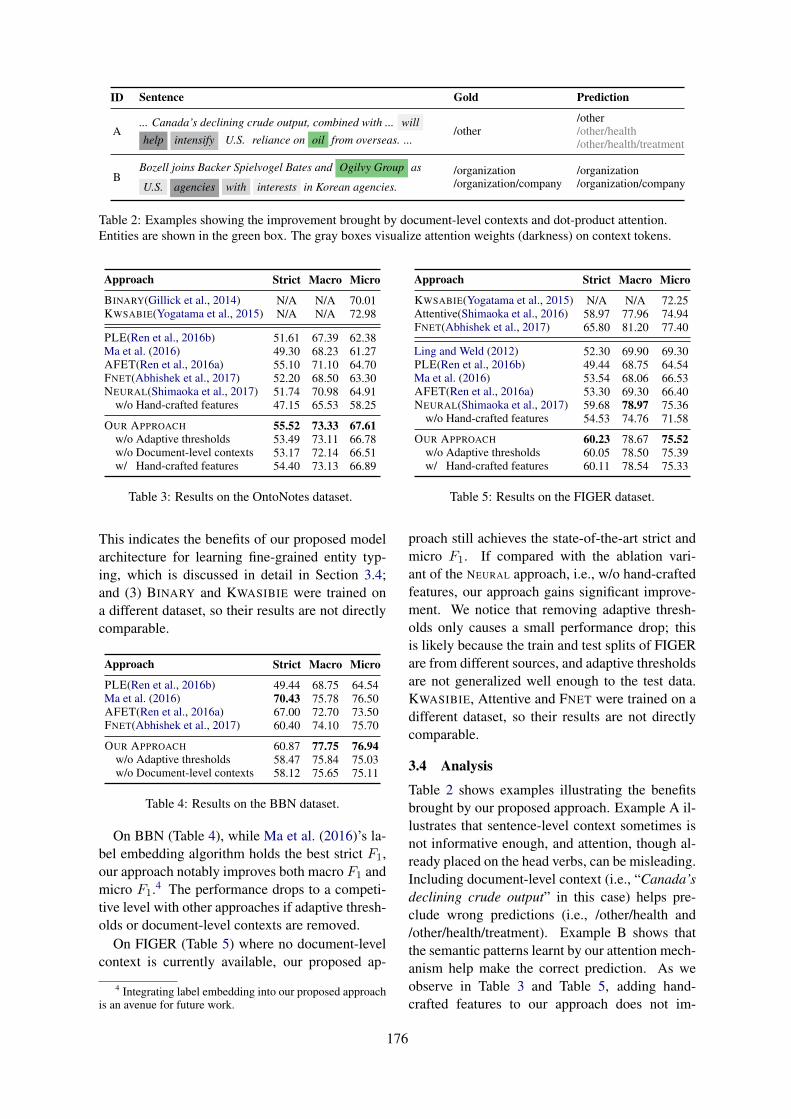
ID Sentence Gold Prediction
A... Canada’s declining crude output, combined with ... willhelp intensify U.S. reliance on oil from overseas. ...
/other/other/other/health/other/health/treatment
BBozell joins Backer Spielvogel Bates and Ogilvy Group as
U.S. agencies with interests in Korean agencies./organization/organization/company
/organization/organization/company
Table 2: Examples showing the improvement brought by document-level contexts and dot-product attention.Entities are shown in the green box. The gray boxes visualize attention weights (darkness) on context tokens.
Approach Strict Macro Micro
BINARY(Gillick et al., 2014) N/A N/A 70.01KWSABIE(Yogatama et al., 2015) N/A N/A 72.98
PLE(Ren et al., 2016b) 51.61 67.39 62.38Ma et al. (2016) 49.30 68.23 61.27AFET(Ren et al., 2016a) 55.10 71.10 64.70FNET(Abhishek et al., 2017) 52.20 68.50 63.30NEURAL(Shimaoka et al., 2017) 51.74 70.98 64.91
w/o Hand-crafted features 47.15 65.53 58.25
OUR APPROACH 55.52 73.33 67.61w/o Adaptive thresholds 53.49 73.11 66.78w/o Document-level contexts 53.17 72.14 66.51w/ Hand-crafted features 54.40 73.13 66.89
Table 3: Results on the OntoNotes dataset.
This indicates the benefits of our proposed modelarchitecture for learning fine-grained entity typ-ing, which is discussed in detail in Section 3.4;and (3) BINARY and KWASIBIE were trained ona different dataset, so their results are not directlycomparable.
Approach Strict Macro Micro
PLE(Ren et al., 2016b) 49.44 68.75 64.54Ma et al. (2016) 70.43 75.78 76.50AFET(Ren et al., 2016a) 67.00 72.70 73.50FNET(Abhishek et al., 2017) 60.40 74.10 75.70
OUR APPROACH 60.87 77.75 76.94w/o Adaptive thresholds 58.47 75.84 75.03w/o Document-level contexts 58.12 75.65 75.11
Table 4: Results on the BBN dataset.
On BBN (Table 4), while Ma et al. (2016)’s la-bel embedding algorithm holds the best strict F1,our approach notably improves both macro F1 andmicro F1.4 The performance drops to a competi-tive level with other approaches if adaptive thresh-olds or document-level contexts are removed.
On FIGER (Table 5) where no document-levelcontext is currently available, our proposed ap-
4 Integrating label embedding into our proposed approachis an avenue for future work.
Approach Strict Macro Micro
KWSABIE(Yogatama et al., 2015) N/A N/A 72.25Attentive(Shimaoka et al., 2016) 58.97 77.96 74.94FNET(Abhishek et al., 2017) 65.80 81.20 77.40
Ling and Weld (2012) 52.30 69.90 69.30PLE(Ren et al., 2016b) 49.44 68.75 64.54Ma et al. (2016) 53.54 68.06 66.53AFET(Ren et al., 2016a) 53.30 69.30 66.40NEURAL(Shimaoka et al., 2017) 59.68 78.97 75.36
w/o Hand-crafted features 54.53 74.76 71.58
OUR APPROACH 60.23 78.67 75.52w/o Adaptive thresholds 60.05 78.50 75.39w/ Hand-crafted features 60.11 78.54 75.33
Table 5: Results on the FIGER dataset.
proach still achieves the state-of-the-art strict andmicro F1. If compared with the ablation vari-ant of the NEURAL approach, i.e., w/o hand-craftedfeatures, our approach gains significant improve-ment. We notice that removing adaptive thresh-olds only causes a small performance drop; thisis likely because the train and test splits of FIGERare from different sources, and adaptive thresholdsare not generalized well enough to the test data.KWASIBIE, Attentive and FNET were trained on adifferent dataset, so their results are not directlycomparable.
3.4 Analysis
Table 2 shows examples illustrating the benefitsbrought by our proposed approach. Example A il-lustrates that sentence-level context sometimes isnot informative enough, and attention, though al-ready placed on the head verbs, can be misleading.Including document-level context (i.e., “Canada’sdeclining crude output” in this case) helps pre-clude wrong predictions (i.e., /other/health and/other/health/treatment). Example B shows thatthe semantic patterns learnt by our attention mech-anism help make the correct prediction. As weobserve in Table 3 and Table 5, adding hand-crafted features to our approach does not im-
176

prove the results. One possible explanation is thathand-crafted features are mostly about syntactic-head or topic information, and such informationare already covered by our attention mechanismand document-level contexts as shown in Table 2.Compared to hand-crafted features that heavilyrely on system or human annotations, attentionmechanism requires significantly less supervision,and document-level or paragraph-level contextsare much easier to get.
Through experiments, we observe no improve-ment by encoding type hierarchical informa-tion (Shimaoka et al., 2017).5 To explain this, wecompute cosine similarity between each pair offine-grained types based on the type embeddingslearned by our model, i.e., wt in Eq. (1). Table 6shows several types and their closest types: thesetypes do not always share coarse-grained typeswith their closest types, but they often co-occurin the same context.
Type Closest Types
/other/event/accident /location/transit/railway/location/transit/bridge
/person/artist/music /organization/music/person/artist/director
/other/product/mobile phone /location/transit/railway/other/product/computer
/other/event/sports event /location/transit/railway/other/event
/other/product/car /organization/transit/other/product
Table 6: Type similarity.
4 Conclusion
We propose a new approach for fine-grained en-tity typing. The contributions are: (1) we pro-pose a neural architecture which learns a distribu-tional semantic representation that leverage bothdocument and sentence level information, (2) wefind that context increased with document-level in-formation improves performance, and (3) we uti-lize adaptive classification thresholds to furtherboost the performance. Experiments show ourapproach achieves new state-of-the-art results onthree benchmarks.
5The type embedding matrix W for the logistic regres-sion is replaced by the product of a learnt weight matrix Vand the constant sparse binary matrix S which encodes typehierarchical information.
Acknowledgments
This work was supported in part by the JHU Hu-man Language Technology Center of Excellence(HLTCOE), and DARPA LORELEI. The U.S.Government is authorized to reproduce and dis-tribute reprints for Governmental purposes. Theviews and conclusions contained in this publica-tion are those of the authors and should not beinterpreted as representing official policies or en-dorsements of DARPA or the U.S. Government.
ReferencesAbhishek Abhishek, Ashish Anand, and Amit Awekar.
2017. Fine-grained entity type classification byjointly learning representations and label embed-dings. In Proceedings of the 15th Conference of theEuropean Chapter of the Association for Computa-tional Linguistics: Volume 1, Long Papers, pages797–807, Valencia, Spain. Association for Compu-tational Linguistics.
Andrew Carlson, Justin Betteridge, Richard C Wang,Estevam R Hruschka Jr, and Tom M Mitchell. 2010.Coupled semi-supervised learning for informationextraction. In Proceedings of the third ACM inter-national conference on Web search and data mining,pages 101–110. ACM.
Luciano Del Corro, Abdalghani Abujabal, RainerGemulla, and Gerhard Weikum. 2015. Finet:Context-aware fine-grained named entity typing. InProceedings of the 2015 Conference on EmpiricalMethods in Natural Language Processing, pages868–878, Lisbon, Portugal. Association for Compu-tational Linguistics.
Dan Gillick, Nevena Lazic, Kuzman Ganchev, JesseKirchner, and David Huynh. 2014. Context-dependent fine-grained entity type tagging. arXivpreprint arXiv:1412.1820.
Nitish Gupta, Sameer Singh, and Dan Roth. 2017. En-tity linking via joint encoding of types, descriptions,and context. In Proceedings of the 2017 Conferenceon Empirical Methods in Natural Language Pro-cessing, pages 2681–2690, Copenhagen, Denmark.Association for Computational Linguistics.
Sepp Hochreiter and Jurgen Schmidhuber. 1997.Long short-term memory. Neural computation,9(8):1735–1780.
Sanjeev Karn, Ulli Waltinger, and Hinrich Schutze.2017. End-to-end trainable attentive decoder for hi-erarchical entity classification. In Proceedings of the15th Conference of the European Chapter of the As-sociation for Computational Linguistics: Volume 2,Short Papers, pages 752–758, Valencia, Spain. As-sociation for Computational Linguistics.
177

Diederik Kingma and Jimmy Ba. 2014. Adam: Amethod for stochastic optimization. arXiv preprintarXiv:1412.6980.
Quoc Le and Tomas Mikolov. 2014. Distributed repre-sentations of sentences and documents. In Proceed-ings of the 31st International Conference on Ma-chine Learning (ICML-14), pages 1188–1196.
Changki Lee, Yi-Gyu Hwang, Hyo-Jung Oh, SoojongLim, Jeong Heo, Chung-Hee Lee, Hyeon-Jin Kim,Ji-Hyun Wang, and Myung-Gil Jang. 2006. Fine-Grained Named Entity Recognition Using Con-ditional Random Fields for Question Answering.Springer Berlin Heidelberg, Berlin, Heidelberg.
Xiao Ling and Daniel S. Weld. 2012. Fine-grainedentity recognition. In Proceedings of the Twenty-Sixth AAAI Conference on Artificial Intelligence,AAAI’12, pages 94–100. AAAI Press.
Minh-Thang Luong, Hieu Pham, and Christopher D.Manning. 2015. Effective approaches to attention-based neural machine translation. In Proceedings ofthe 2015 Conference on Empirical Methods in Nat-ural Language Processing, pages 1412–1421, Lis-bon, Portugal. Association for Computational Lin-guistics.
Yukun Ma, Erik Cambria, and SA GAO. 2016. La-bel embedding for zero-shot fine-grained named en-tity typing. In Proceedings of COLING 2016, the26th International Conference on ComputationalLinguistics: Technical Papers, pages 171–180. TheCOLING 2016 Organizing Committee.
Tom M. Mitchell, William W. Cohen, Estevam R. Hr-uschka Jr., Partha Pratim Talukdar, Justin Bet-teridge, Andrew Carlson, Bhavana Dalvi Mishra,Matthew Gardner, Bryan Kisiel, Jayant Krishna-murthy, Ni Lao, Kathryn Mazaitis, Thahir Mo-hamed, Ndapandula Nakashole, Emmanouil Anto-nios Platanios, Alan Ritter, Mehdi Samadi, Burr Set-tles, Richard C. Wang, Derry Tanti Wijaya, Abhi-nav Gupta, Xinlei Chen, Abulhair Saparov, MalcolmGreaves, and Joel Welling. 2015. Never-endinglearning. In Proceedings of the Twenty-Ninth AAAIConference on Artificial Intelligence, January 25-30, 2015, Austin, Texas, USA., pages 2302–2310.
Jeffrey Pennington, Richard Socher, and Christo-pher D. Manning. 2014. Glove: Global vectors forword representation. In Empirical Methods in Nat-ural Language Processing (EMNLP), pages 1532–1543.
Marta Recasens, Marie-Catherine de Marneffe, andChristopher Potts. 2013. The life and death of dis-course entities: Identifying singleton mentions. InProceedings of the 2013 Conference of the NorthAmerican Chapter of the Association for Computa-tional Linguistics: Human Language Technologies,pages 627–633, Atlanta, Georgia. Association forComputational Linguistics.
Xiang Ren, Wenqi He, Meng Qu, Lifu Huang, HengJi, and Jiawei Han. 2016a. Afet: Automatic fine-grained entity typing by hierarchical partial-labelembedding. In Proceedings of the 2016 Conferenceon Empirical Methods in Natural Language Pro-cessing, pages 1369–1378, Austin, Texas. Associ-ation for Computational Linguistics.
Xiang Ren, Wenqi He, Meng Qu, Clare R. Voss, HengJi, and Jiawei Han. 2016b. Label noise reduction inentity typing by heterogeneous partial-label embed-ding. In Proceedings of the 22Nd ACM SIGKDDInternational Conference on Knowledge Discoveryand Data Mining, KDD ’16, pages 1825–1834, NewYork, NY, USA. ACM.
Sonse Shimaoka, Pontus Stenetorp, Kentaro Inui, andSebastian Riedel. 2016. An attentive neural ar-chitecture for fine-grained entity type classification.In Proceedings of the 5th Workshop on AutomatedKnowledge Base Construction, pages 69–74, SanDiego, CA. Association for Computational Linguis-tics.
Sonse Shimaoka, Pontus Stenetorp, Kentaro Inui, andSebastian Riedel. 2017. Neural architectures forfine-grained entity type classification. In Proceed-ings of the 15th Conference of the European Chap-ter of the Association for Computational Linguistics:Volume 1, Long Papers, pages 1271–1280, Valencia,Spain. Association for Computational Linguistics.
Ralph Weischedel and Ada Brunstein. 2005. Bbn pro-noun coreference and entity type corpus. LinguisticData Consortium, Philadelphia, 112.
Ralph Weischedel, Eduard Hovy, Mitchell Mar-cus, Martha Palmer, Robert Belvin, Sameer Prad-han, Lance Ramshaw, and Nianwen Xue. 2011.Ontonotes: A large training corpus for enhancedprocessing. Handbook of Natural Language Pro-cessing and Machine Translation. Springer.
Yadollah Yaghoobzadeh and Hinrich Schutze. 2015.Corpus-level fine-grained entity typing using con-textual information. In Proceedings of the 2015Conference on Empirical Methods in Natural Lan-guage Processing, pages 715–725, Lisbon, Portugal.Association for Computational Linguistics.
Zichao Yang, Diyi Yang, Chris Dyer, Xiaodong He,Alex Smola, and Eduard Hovy. 2016. Hierarchi-cal attention networks for document classification.In Proceedings of the 2016 Conference of the NorthAmerican Chapter of the Association for Computa-tional Linguistics: Human Language Technologies,pages 1480–1489, San Diego, California. Associa-tion for Computational Linguistics.
Dani Yogatama, Daniel Gillick, and Nevena Lazic.2015. Embedding methods for fine grained entitytype classification. In Proceedings of the 53rd An-nual Meeting of the Association for ComputationalLinguistics and the 7th International Joint Confer-ence on Natural Language Processing (Volume 2:
178

Short Papers), pages 291–296, Beijing, China. As-sociation for Computational Linguistics.
Mohamed Amir Yosef, Sandro Bauer, Johannes Hof-fart, Marc Spaniol, and Gerhard Weikum. 2012.HYENA: Hierarchical type classification for entitynames. In Proceedings of COLING 2012: Posters,pages 1361–1370, Mumbai, India. The COLING2012 Organizing Committee.
179
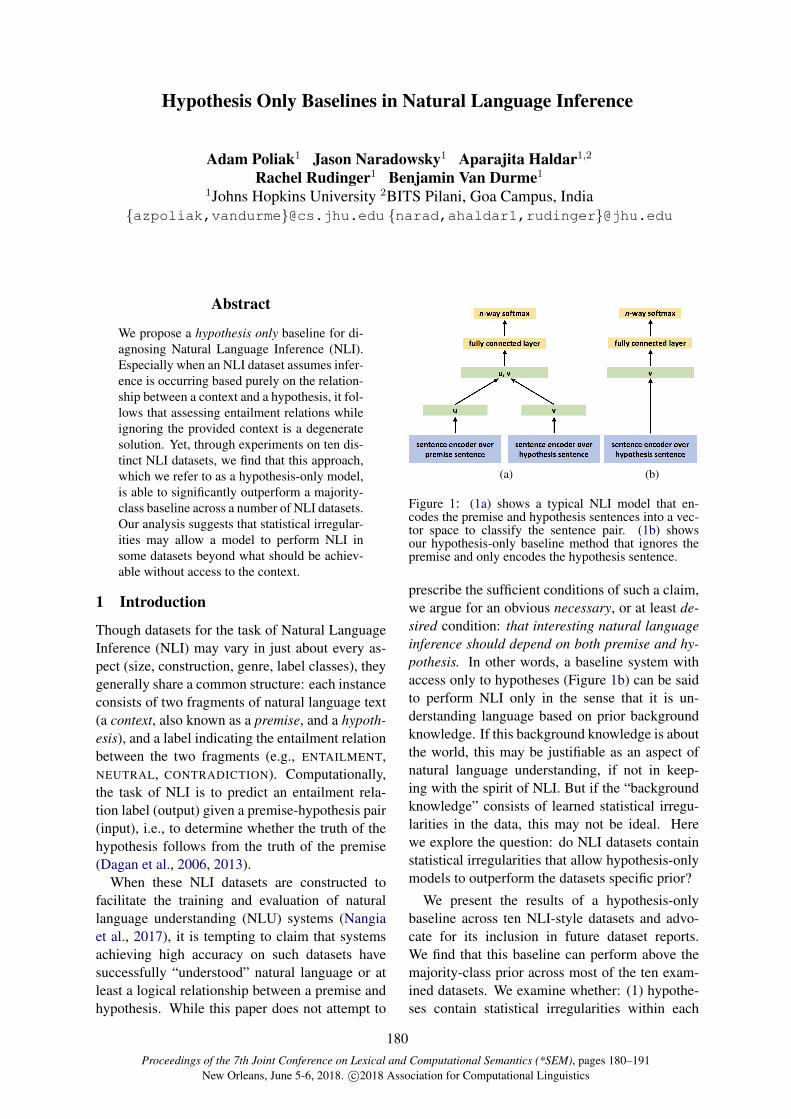
Proceedings of the 7th Joint Conference on Lexical and Computational Semantics (*SEM), pages 180–191New Orleans, June 5-6, 2018. c©2018 Association for Computational Linguistics
Hypothesis Only Baselines in Natural Language Inference
Adam Poliak1 Jason Naradowsky1 Aparajita Haldar1,2Rachel Rudinger1 Benjamin Van Durme1
1Johns Hopkins University 2BITS Pilani, Goa Campus, India{azpoliak,vandurme}@cs.jhu.edu {narad,ahaldar1,rudinger}@jhu.edu
Abstract
We propose a hypothesis only baseline for di-agnosing Natural Language Inference (NLI).Especially when an NLI dataset assumes infer-ence is occurring based purely on the relation-ship between a context and a hypothesis, it fol-lows that assessing entailment relations whileignoring the provided context is a degeneratesolution. Yet, through experiments on ten dis-tinct NLI datasets, we find that this approach,which we refer to as a hypothesis-only model,is able to significantly outperform a majority-class baseline across a number of NLI datasets.Our analysis suggests that statistical irregular-ities may allow a model to perform NLI insome datasets beyond what should be achiev-able without access to the context.
1 Introduction
Though datasets for the task of Natural LanguageInference (NLI) may vary in just about every as-pect (size, construction, genre, label classes), theygenerally share a common structure: each instanceconsists of two fragments of natural language text(a context, also known as a premise, and a hypoth-esis), and a label indicating the entailment relationbetween the two fragments (e.g., ENTAILMENT,NEUTRAL, CONTRADICTION). Computationally,the task of NLI is to predict an entailment rela-tion label (output) given a premise-hypothesis pair(input), i.e., to determine whether the truth of thehypothesis follows from the truth of the premise(Dagan et al., 2006, 2013).
When these NLI datasets are constructed tofacilitate the training and evaluation of naturallanguage understanding (NLU) systems (Nangiaet al., 2017), it is tempting to claim that systemsachieving high accuracy on such datasets havesuccessfully “understood” natural language or atleast a logical relationship between a premise andhypothesis. While this paper does not attempt to
(a) (b)
Figure 1: (1a) shows a typical NLI model that en-codes the premise and hypothesis sentences into a vec-tor space to classify the sentence pair. (1b) showsour hypothesis-only baseline method that ignores thepremise and only encodes the hypothesis sentence.
prescribe the sufficient conditions of such a claim,we argue for an obvious necessary, or at least de-sired condition: that interesting natural languageinference should depend on both premise and hy-pothesis. In other words, a baseline system withaccess only to hypotheses (Figure 1b) can be saidto perform NLI only in the sense that it is un-derstanding language based on prior backgroundknowledge. If this background knowledge is aboutthe world, this may be justifiable as an aspect ofnatural language understanding, if not in keep-ing with the spirit of NLI. But if the “backgroundknowledge” consists of learned statistical irregu-larities in the data, this may not be ideal. Herewe explore the question: do NLI datasets containstatistical irregularities that allow hypothesis-onlymodels to outperform the datasets specific prior?
We present the results of a hypothesis-onlybaseline across ten NLI-style datasets and advo-cate for its inclusion in future dataset reports.We find that this baseline can perform above themajority-class prior across most of the ten exam-ined datasets. We examine whether: (1) hypothe-ses contain statistical irregularities within each
180
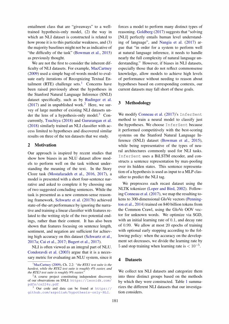
entailment class that are “giveaways” to a well-trained hypothesis-only model, (2) the way inwhich an NLI dataset is constructed is related tohow prone it is to this particular weakness, and (3)the majority baselines might not be as indicative of“the difficulty of the task” (Bowman et al., 2015)as previously thought.
We are not the first to consider the inherent dif-ficulty of NLI datasets. For example, MacCartney(2009) used a simple bag-of-words model to eval-uate early iterations of Recognizing Textual En-tailment (RTE) challenge sets.1 Concerns havebeen raised previously about the hypotheses inthe Stanford Natural Language Inference (SNLI)dataset specifically, such as by Rudinger et al.(2017) and in unpublished work.2 Here, we sur-vey of large number of existing NLI datasets un-der the lens of a hypothesis-only model.3 Con-currently, Tsuchiya (2018) and Gururangan et al.(2018) similarly trained an NLI classifier with ac-cess limited to hypotheses and discovered similarresults on three of the ten datasets that we study.
2 Motivation
Our approach is inspired by recent studies thatshow how biases in an NLU dataset allow mod-els to perform well on the task without under-standing the meaning of the text. In the StoryCloze task (Mostafazadeh et al., 2016, 2017), amodel is presented with a short four-sentence nar-rative and asked to complete it by choosing oneof two suggested concluding sentences. While thetask is presented as a new common-sense reason-ing framework, Schwartz et al. (2017b) achievedstate-of-the-art performance by ignoring the narra-tive and training a linear classifier with features re-lated to the writing style of the two potential end-ings, rather than their content. It has also beenshown that features focusing on sentence length,sentiment, and negation are sufficient for achiev-ing high accuracy on this dataset (Schwartz et al.,2017a; Cai et al., 2017; Bugert et al., 2017).
NLI is often viewed as an integral part of NLU.Condoravdi et al. (2003) argue that it is a neces-sary metric for evaluating an NLU system, since it
1MacCartney (2009), Ch. 2.2: “the RTE1 test suite is thehardest, while the RTE2 test suite is roughly 4% easier, andthe RTE3 test suite is roughly 9% easier.”
2A course project constituting independent discoveryof our observations on SNLI: https://leonidk.com/pdfs/cs224u.pdf
3 Our code and data can be found at https://github.com/azpoliak/hypothesis-only-NLI.
forces a model to perform many distinct types ofreasoning. Goldberg (2017) suggests that “solving[NLI] perfectly entails human level understand-ing of language”, and Nangia et al. (2017) ar-gue that “in order for a system to perform wellat natural language inference, it needs to handlenearly the full complexity of natural language un-derstanding.” However, if biases in NLI datasets,especially those that do not reflect commonsenseknowledge, allow models to achieve high levelsof performance without needing to reason abouthypotheses based on corresponding contexts, ourcurrent datasets may fall short of these goals.
3 Methodology
We modify Conneau et al. (2017)’s InferSentmethod to train a neural model to classify justthe hypotheses. We choose InferSent becauseit performed competitively with the best-scoringsystems on the Stanford Natural Language In-ference (SNLI) dataset (Bowman et al., 2015),while being representative of the types of neu-ral architectures commonly used for NLI tasks.InferSent uses a BiLSTM encoder, and con-structs a sentence representation by max-poolingover its hidden states. This sentence representa-tion of a hypothesis is used as input to a MLP clas-sifier to predict the NLI tag.
We preprocess each recast dataset using theNLTK tokenizer (Loper and Bird, 2002). Follow-ing Conneau et al. (2017), we map the resulting to-kens to 300-dimensional GloVe vectors (Penning-ton et al., 2014) trained on 840 billion tokens fromthe Common Crawl, using the GloVe OOV vec-tor for unknown words. We optimize via SGD,with an initial learning rate of 0.1, and decay rateof 0.99. We allow at most 20 epochs of trainingwith optional early stopping according to the fol-lowing policy: when the accuracy on the develop-ment set decreases, we divide the learning rate by5 and stop training when learning rate is < 10−5.
4 Datasets
We collect ten NLI datasets and categorize theminto three distinct groups based on the methodsby which they were constructed. Table 1 summa-rizes the different NLI datasets that our investiga-tion considers.
181

Creation Protocol Dataset Size Classes Example Hypothesis
RecastDPR 3.4K 2 People raise dogs because dogs are afraid of thieves
SPR 150K 2 The judge was aware of the dismissing
FN+ 150K 2 the irish are actually principling to come home
Judged
ADD-1 5K 2 A small child staring at a young horse and a pony
SCITAIL 25K 2 Humans typically have 23 pairs of chromosomes
SICK 10K 3 Pasta is being put into a dish by a woman
MPE 10K 3 A man smoking a cigarette
JOCI 30K 3 The flooring is a horizontal surface
ElicitedSNLI 550K 3 An animal is jumping to catch an object
MNLI 425K 3 Kyoto has a kabuki troupe and so does Osaka
Table 1: Basic statistics about the NLI datasets we consider. ‘Size’ refers to the total number of labeled premise-hypothesis pairs in each dataset (for datasets with > 100K examples, numbers are rounded down to the nearest25K). The ‘Creation Protocol’ column indicates how the dataset was created. The ‘Class’ column reports thenumber of class labels/tags. The last column shows an example hypothesis from each dataset.
4.1 Human Elicited
In cases where humans were given a context andasked to generate a corresponding hypothesis andlabel, we consider these datasets to be elicited. Al-though we consider only two such datasets, theyare the largest datasets included in our study andare currently popular amongst researchers. Theelicited NLI datasets we look at are:
Stanford Natural Language Inference (SNLI)To create SNLI, Bowman et al. (2015) showedcrowdsourced workers a premise sentence(sourced from Flickr image captions), and askedthem to generate a corresponding hypothesis sen-tence for each of the three labels (ENTAILMENT,NEUTRAL, CONTRADICTION). SNLI is known tocontain stereotypical biases based on gender, race,and ethnic stereotypes (Rudinger et al., 2017).Furthermore, Zhang et al. (2017) commentedthat this “elicitation protocols can lead to biasedresponses unlikely to contain a wide range ofpossible common-sense inferences.”
Multi-NLI Multi-NLI is a recent expansion ofSNLI aimed to add greater diversity to the existingdataset (Williams et al., 2017). Premises in Multi-NLI can originate from fictional stories, personalletters, telephone speech, and a 9/11 report.
4.2 Human Judged
Alternatively, if hypotheses and premises were au-tomatically paired but labeled by a human, weconsider the dataset to be judged. Our human-judged data sets are:
Sentences Involving Compositional Knowledge(SICK) To evaluate how well compositional dis-tributional semantic models handle “challengingphenomena”, Marelli et al. (2014) introducedSICK, which used rules to expand or normalizeexisting premises to create more difficult exam-ples. Workers were asked to label the relatednessof these resulting pairs, and these labels were thenconverted into the same three-way label space asSNLI and Multi-NLI.
Add-one RTE This mixed-genre dataset testswhether NLI systems can understand adjective-noun compounds (Pavlick and Callison-Burch,2016). Premise sentences were extracted fromAnnotated Gigaword (Napoles et al., 2012), im-age captions (Young et al., 2014), the InternetArgument Corpus (Walker et al., 2012), and fic-tional stories from the GutenTag dataset (Mac Kimand Cassidy, 2015). To create hypotheses, ad-jectives were removed or inserted before nounsin a premise, and crowd-sourced workers wereasked to provide reliable labels (ENTAILED, NOT-ENTAILED).
SciTail Recently released, SciTail is an NLIdataset created from 4th grade science ques-tions and multiple-choice answers (Khot et al.,2018). Hypotheses are assertions convertedfrom question-answer pairs found in SciQ (Welblet al., 2017). Hypotheses are automati-cally paired with premise sentences from do-main specific texts (Clark et al., 2016), andlabeled (ENTAILMENT, NEUTRAL) by crowd-sourced workers. Notably, the construction
182
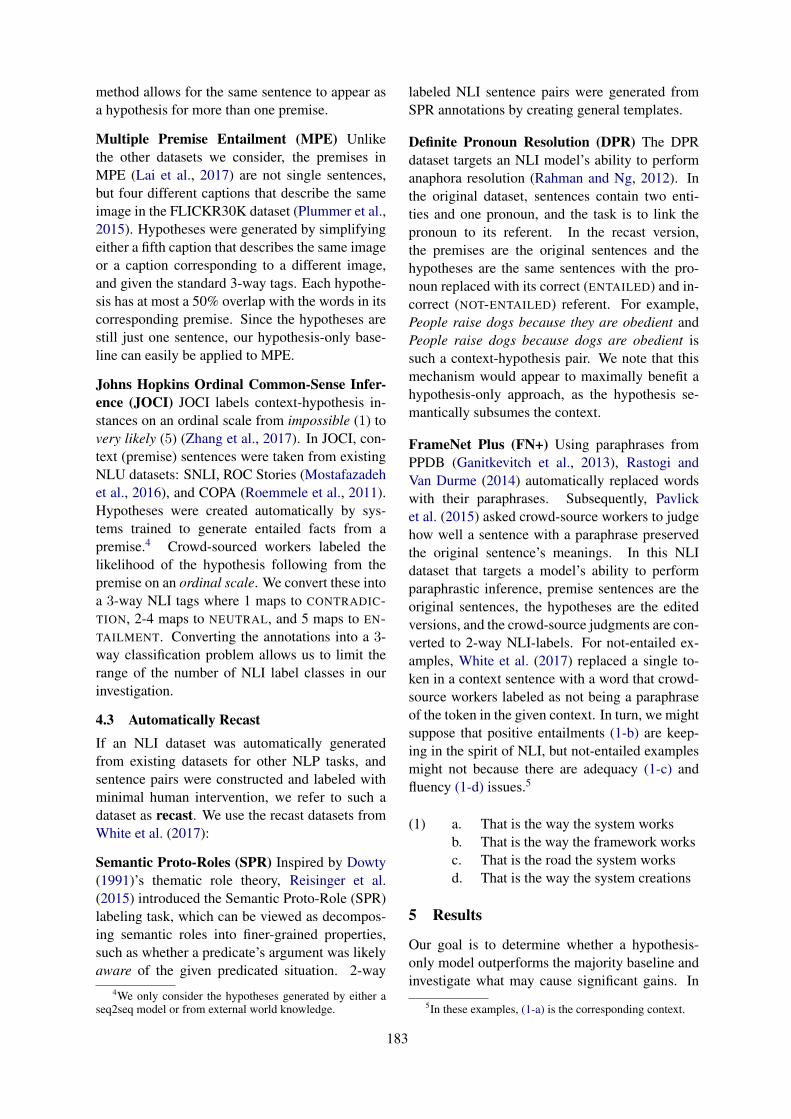
method allows for the same sentence to appear asa hypothesis for more than one premise.
Multiple Premise Entailment (MPE) Unlikethe other datasets we consider, the premises inMPE (Lai et al., 2017) are not single sentences,but four different captions that describe the sameimage in the FLICKR30K dataset (Plummer et al.,2015). Hypotheses were generated by simplifyingeither a fifth caption that describes the same imageor a caption corresponding to a different image,and given the standard 3-way tags. Each hypothe-sis has at most a 50% overlap with the words in itscorresponding premise. Since the hypotheses arestill just one sentence, our hypothesis-only base-line can easily be applied to MPE.
Johns Hopkins Ordinal Common-Sense Infer-ence (JOCI) JOCI labels context-hypothesis in-stances on an ordinal scale from impossible (1) tovery likely (5) (Zhang et al., 2017). In JOCI, con-text (premise) sentences were taken from existingNLU datasets: SNLI, ROC Stories (Mostafazadehet al., 2016), and COPA (Roemmele et al., 2011).Hypotheses were created automatically by sys-tems trained to generate entailed facts from apremise.4 Crowd-sourced workers labeled thelikelihood of the hypothesis following from thepremise on an ordinal scale. We convert these intoa 3-way NLI tags where 1 maps to CONTRADIC-TION, 2-4 maps to NEUTRAL, and 5 maps to EN-TAILMENT. Converting the annotations into a 3-way classification problem allows us to limit therange of the number of NLI label classes in ourinvestigation.
4.3 Automatically RecastIf an NLI dataset was automatically generatedfrom existing datasets for other NLP tasks, andsentence pairs were constructed and labeled withminimal human intervention, we refer to such adataset as recast. We use the recast datasets fromWhite et al. (2017):
Semantic Proto-Roles (SPR) Inspired by Dowty(1991)’s thematic role theory, Reisinger et al.(2015) introduced the Semantic Proto-Role (SPR)labeling task, which can be viewed as decompos-ing semantic roles into finer-grained properties,such as whether a predicate’s argument was likelyaware of the given predicated situation. 2-way
4We only consider the hypotheses generated by either aseq2seq model or from external world knowledge.
labeled NLI sentence pairs were generated fromSPR annotations by creating general templates.
Definite Pronoun Resolution (DPR) The DPRdataset targets an NLI model’s ability to performanaphora resolution (Rahman and Ng, 2012). Inthe original dataset, sentences contain two enti-ties and one pronoun, and the task is to link thepronoun to its referent. In the recast version,the premises are the original sentences and thehypotheses are the same sentences with the pro-noun replaced with its correct (ENTAILED) and in-correct (NOT-ENTAILED) referent. For example,People raise dogs because they are obedient andPeople raise dogs because dogs are obedient issuch a context-hypothesis pair. We note that thismechanism would appear to maximally benefit ahypothesis-only approach, as the hypothesis se-mantically subsumes the context.
FrameNet Plus (FN+) Using paraphrases fromPPDB (Ganitkevitch et al., 2013), Rastogi andVan Durme (2014) automatically replaced wordswith their paraphrases. Subsequently, Pavlicket al. (2015) asked crowd-source workers to judgehow well a sentence with a paraphrase preservedthe original sentence’s meanings. In this NLIdataset that targets a model’s ability to performparaphrastic inference, premise sentences are theoriginal sentences, the hypotheses are the editedversions, and the crowd-source judgments are con-verted to 2-way NLI-labels. For not-entailed ex-amples, White et al. (2017) replaced a single to-ken in a context sentence with a word that crowd-source workers labeled as not being a paraphraseof the token in the given context. In turn, we mightsuppose that positive entailments (1-b) are keep-ing in the spirit of NLI, but not-entailed examplesmight not because there are adequacy (1-c) andfluency (1-d) issues.5
(1) a. That is the way the system worksb. That is the way the framework worksc. That is the road the system worksd. That is the way the system creations
5 Results
Our goal is to determine whether a hypothesis-only model outperforms the majority baseline andinvestigate what may cause significant gains. In
5In these examples, (1-a) is the corresponding context.
183

DEV TESTDataset Hyp-Only MAJ |∆| ∆% Hyp-Only MAJ |∆| ∆% Baseline SOTA
Recast
DPR 50.21 50.21 0.00 0.00 49.95 49.95 0.00 0.00 49.5 49.5SPR 86.21 65.27 +20.94 +32.08 86.57 65.44 +21.13 +32.29 80.6 80.6FN+ 62.43 56.79 +5.64 +9.31 61.11 57.48 +3.63 +6.32 80.5 80.5
Human JudgedADD-1 75.10 75.10 0.00 0.00 85.27 85.27 0.00 0.00 92.2 92.2SciTail 66.56 50.38 +16.18 +32.12 66.56 60.04 +6.52 +10.86 70.6 77.3SICK 56.76 56.76 0.00 0.00 56.87 56.87 0.00 0.00 56.87 84.6MPE 40.20 40.20 0.00 0.00 42.40 42.40 0.00 0.00 41.7 56.3JOCI 61.64 57.74 +3.90 +6.75 62.61 57.26 +5.35 +9.34 – –
Human ElicitedSNLI 69.17 33.82 +35.35 +104.52 69.00 34.28 +34.72 +101.28 78.2 89.3
MNLI-1 55.52 35.45 +20.07 +56.61 – 35.6 – – 72.3 80.60MNLI-2 55.18 35.22 +19.96 +56.67 – 36.5 – – 72.1 83.21
Table 2: NLI accuracies on each dataset. Columns ‘Hyp-Only’ and ‘MAJ’ indicates the accuracy of the hypothesis-only model and the majority baseline. |∆| and ∆% indicate the absolute difference in percentage points and thepercentage increase between the Hyp-Only and MAJ. Blue numbers indicate that the hypothesis-model outper-forms MAJ. In the right-most section, ‘Baseline’ indicates the original baseline on the test when the dataset wasreleased and ‘SOTA’ indicates current state-of-the-art results. MNLI-1 is the matched version and MNLI-2 is themismatched for MNLI. The names of datasets are italicized if containing ≤ 10K labeled examples.
such cases a hypothesis-only model should beused as a stronger baseline instead of the ma-jority class baseline. For all experiments exceptfor JOCI, we use each NLI dataset’s standardtrain, dev, and test splits.6 Table 2 compares thehypothesis-only model’s accuracy with the major-ity baseline on each dataset’s dev and test set.7
Criticism of the Majority Baseline Across sixof the ten datasets, our hypothesis-only modelsignificantly outperforms the majority-baseline,even outperforming the best reported results onone dataset, recast SPR. This indicates that thereexists a significant degree of exploitable signal thatmay help NLI models perform well on their cor-responding test set without considering NLI con-texts. From Table 2, it is unclear whether the con-struction method is responsible for these improve-ments. The largest relative gains are on human-elicited models where the hypothesis-only modelmore than doubles the majority baseline.
However, there are no obvious unifying trendsacross these datasets: Among the judged and re-cast datasets, where humans do not generate theNLI hypothesis, we observe lower performancemargins between majority and hypothesis-onlymodels compared to the elicited data sets. How-ever, the baseline performances of these modelsare noticeably larger than on SNLI and Multi-NLI.
6JOCI was not released with such splits so we randomlysplit the dataset into such a partition with 80:10:10 ratios.
7We only report results on the Multi-NLI development setsince the test labels are only accessible on Kaggle.
The drop between SNLI and Multi-NLI suggeststhat by including multiple genres, an NLI datasetmay contain less biases. However, adding addi-tional genres might not be enough to mitigate bi-ases as the hypothesis-only model still drasticallyoutperforms the majority-baseline. Therefore, webelieve that models tested on SNLI and Multi-NLIshould include a baseline version of the model thatonly accesses hypotheses.
We do not observe general trends across thedatasets based on their construction methodology.On three of the five human judged datasets, thehypothesis-only model defaults to labeling eachinstance with the majority class tag. We find thesame behavior in one recast dataset (DPR). How-ever, across both these categories we find smallerrelative improvements than on SNLI and Multi-NLI. These results suggest the existence of ex-ploitable signal in the datasets that is unrelated toNLI contexts. Our focus now shifts to identifyingprecisely what these signals might be and under-standing why they may appear in NLI hypotheses.
6 Statistical Irregularities
We are interested in determining what character-istics in the datasets may be responsible for thehypothesis-only model often outperforming themajority baseline. Here, we investigate the impor-tance of specific words, grammaticality, and lexi-cal semantics.
184
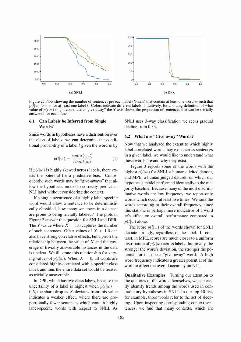
0.0 0.2 0.4 0.6 0.8 1.0500
1000
1500
2000
2500
3000
(a) SNLI
0.0 0.2 0.4 0.6 0.8 1.00
50
100
150
200
250
(b) DPR
Figure 2: Plots showing the number of sentences per each label (Y-axis) that contain at least one word w such thatp(l|w) >= x for at least one label l. Colors indicate different labels. Intuitively, for a sliding definition of whatvalue of p(l|w) might constitute a “give-away” the Y-axis shows the proportion of sentences that can be triviallyanswered for each class.
6.1 Can Labels be Inferred from SingleWords?
Since words in hypotheses have a distribution overthe class of labels, we can determine the condi-tional probability of a label l given the word w by
p(l|w) =count(w, l)
count(w)(1)
If p(l|w) is highly skewed across labels, there ex-ists the potential for a predictive bias. Conse-quently, such words may be “give-aways” that al-low the hypothesis model to correctly predict anNLI label without considering the context.
If a single occurrence of a highly label-specificword would allow a sentence to be deterministi-cally classified, how many sentences in a datasetare prone to being trivially labeled? The plots inFigure 2 answer this question for SNLI and DPR.The Y -value where X = 1.0 captures the numberof such sentences. Other values of X < 1.0 canalso have strong correlative effects, but a priori therelationship between the value of X and the cov-erage of trivially answerable instances in the datais unclear. We illustrate this relationship for vary-ing values of p(l|w). When X = 0, all words areconsidered highly-correlated with a specific classlabel, and thus the entire data set would be treatedas trivially answerable.
In DPR, which has two class labels, because theuncertainty of a label is highest when p(l|w) =0.5, the sharp drop as X deviates from this valueindicates a weaker effect, where there are pro-portionally fewer sentences which contain highlylabel-specific words with respect to SNLI. As
SNLI uses 3-way classification we see a gradualdecline from 0.33.
6.2 What are “Give-away” Words?
Now that we analyzed the extent to which highlylabel-correlated words may exist across sentencesin a given label, we would like to understand whatthese words are and why they exist.
Figure 3 reports some of the words with thehighest p(l|w) for SNLI, a human elicited dataset,and MPE, a human judged dataset, on which ourhypothesis model performed identically to the ma-jority baseline. Because many of the most discrim-inative words are low frequency, we report onlywords which occur at least five times. We rank thewords according to their overall frequency, sincethis statistic is perhaps more indicative of a wordw’s effect on overall performance compared top(l|w) alone.
The score p(l|w) of the words shown for SNLIdeviate strongly, regardless of the label. In con-trast, in MPE, scores are much closer to a uniformdistribution of p(l|w) across labels. Intuitively, thestronger the word’s deviation, the stronger the po-tential for it to be a “give-away” word. A highword frequency indicates a greater potential of theword to affect the overall accuracy on NLI.
Qualitative Examples Turning our attention tothe qualities of the words themselves, we can eas-ily identify trends among the words used in con-tradictory hypotheses in SNLI. In our top-10 list,for example, three words refer to the act of sleep-ing. Upon inspecting corresponding context sen-tences, we find that many contexts, which are
185

Word Score Freq
instrument 0.90 20touching 0.83 12
least 0.90 10Humans 0.88 8
transportation 0.86 7speaking 0.86 7
screen 0.86 7arts 0.86 7
activity 0.86 7opposing 1.00 5
(a) entailment
SNLIWord Score Freq
tall 0.93 44competition 0.88 24
because 0.83 23birthday 0.85 20
mom 0.82 17win 0.88 16got 0.81 16trip 0.93 15tries 0.87 15
owner 0.87 15
(b) neutral
Word Score Freq
sleeping 0.88 108driving 0.81 53Nobody 1.00 52
alone 0.90 50cat 0.84 49
asleep 0.91 43no 0.84 31
empty 0.93 28eats 0.83 24
sleeps 0.95 20
(c) contradiction
Word Score Freq
an 0.57 21gathered 0.58 12
girl 0.50 12trick 0.55 11Dogs 0.55 11
watches 0.60 10field 0.60 10
singing 0.50 10outside 0.67 9
something 0.62 8
(d) entailment
MPEWord Score Freq
smiling 0.56 16An 0.60 10for 0.56 9
front 0.75 8camera 0.62 8waiting 0.50 8posing 0.50 8Kids 0.57 7smile 0.83 6wall 0.50 6
(e) neutral
Word Score Freq
sitting 0.51 88woman 0.55 80
men 0.56 34Some 0.62 26doing 0.59 22
Children 0.50 22boy 0.67 21
having 0.65 20sit 0.60 15
children 0.53 15
(f) contradiction
Figure 3: Lists of the most highly-correlated words in each dataset for given labels, thresholded to the top 10 andranked according to frequency.
sourced from Flickr, naturally deal with activi-ties. This leads us to believe that as a commonstrategy, crowd-source workers often do not gen-erate contradictory hypotheses that require fine-grained semantic reasoning, as a majority of suchactivities can be easily negated by removing anagent’s agency, i.e. describing the agent as sleep-ing. A second trend we notice is that universalnegation constitutes four of the remaining seventerms in this list, and may also be used to simi-lar effect.8 The human-elicited protocol does notguide, nor incentivize crowd-source workers tocome up with less obvious examples. If not prop-erly controlled, elicited datasets may be prone tomany label-specific terms. The existence of label-specific terms in human-elicited NLI datasets doesnot invalidate the datasets nor is surprising. Stud-
8These are “Nobody”, “alone”, “no”, and “empty”.
ies in eliciting norming data are prone to repeatedresponses across subjects (McRae et al., 2005)(see discussion in §2 of (Zhang et al., 2017)).
6.3 On the Role of Grammaticality
Like MPE, FN+ contains few high frequencywords with high p(l|w). However, unlike onMPE, our hypothesis-only model outperforms themajority-only baseline. If these gains do not arisefrom “give-away” words, then what is the statisti-cal irregularity responsible for this discriminativepower?
Upon further inspection, we notice an interest-ing imbalance in how our model performs for eachof the two classes. The hypothesis-only modelperforms similarly to the majority baseline for en-tailed examples, while improving by over 34%those which are not entailed, as shown in Table 3.
As shown by White et al. (2017) and noticed
186

label Hyp-Only MAJ ∆%entailed 44.18 43.20 +2.27
not-entailed 76.31 56.79 +34.37
Table 3: Accuracies on FN+ for each class label.
by Poliak et al. (2018), FN+ contains more gram-matical errors than the other recast datasets. Weexplore whether grammaticality could be the sta-tistical irregularity exploited in this case. Wemanually sample a total of 200 FN+ sentencesand categorize them based on their gold label andour model’s prediction. Out of 50 sentences thatthe model correctly labeled as ENTAILED, 88%of them were grammatical. On the other-hand,of the 50 hypotheses incorrectly labeled as EN-TAILED, only 38% of them were grammatical.Similarly, when the model correctly labeled 50NOT-ENTAILED hypotheses, only 20% were gram-matical, and 68% when labeled incorrectly. Thissuggests that a hypothesis-only model may be ableto discover the correlation between grammatical-ity and NLI labels on this dataset.
6.4 Lexical Semantics
A survey of gains (Table 4) in the SPR dataset sug-gest a number of its property-driven hypotheses,such as X was sentient in [the event], can be accu-rately guessed based on lexical semantics (back-ground knowledge learned from training) of theargument. For example, the hypothesis-only base-line correctly predicts the truth of hypotheses inthe dev set such as: Experts were sentient ... orMr. Falls was sentient ..., and the falsity of Thecampaign was sentient, while failing on referringexpressions like Some or Each side. A model ex-ploiting regularities of the real world would seemto be a different category of dataset bias: whilenot strictly wrong from the perspective of NLU,one should be aware of what the hypothesis-onlybaseline is capable of, to recognize those caseswhere access to the context is required and there-fore more interesting under NLI.
6.5 Open Questions
There may remain statistical irregularities, whichwe leave for future work to explore. For ex-ample, are there correlation between sentencelength and label class in these data sets? Is therea particular construction method that minimizesthe amount of “give-away” words present in thedataset? And lastly, our study is another in aline of research which looks for irregularities at
Proto-Role H-model MAJ ∆%
aware 88.70 59.94 +47.99used in 77.30 52.72 +46.63
volitional 87.45 64.96 +34.62physically existed 87.97 65.38 +34.56
caused 82.11 63.08 +30.18sentient 94.35 76.26 +23.73
existed before 80.23 65.90 +21.75changed 72.18 64.85 +11.29
chang. state 71.76 64.85 +10.65existed after 79.29 72.91 +8.75
existed during 90.06 85.67 +5.13location 93.83 91.21 +2.87
physical contact 89.33 86.92 +2.77chang. possession 94.87 94.46 +0.44
moved 93.51 93.20 +0.34stationary during 96.44 96.34 +0.11
Table 4: NLI accuracies on the SPR development data;each property appears in 956 hypotheses.
the word level (MacCartney et al., 2008; Mac-Cartney, 2009). Beyond bag-of-words, are theremulti-word expressions or syntactic phenomenathat might encode label biases?
7 Related Work
Non-semantic information to help NLI In NLIdatasets, non-semantic linguistic features havebeen used to improve NLI models. Vanderwendeand Dolan (2006) and Blake (2007) demonstratehow sentence structure alone can provide a highsignal for NLI. Instead of using external sourcesof knowledge, which was a common trend at thetime, Blake (2007) improved results on RTE bycombining syntactic features. More recently, Bar-Haim et al. (2015) introduce an inference formal-ism based on syntactic-parse trees.
World Knowledge and NLI As mentioned ear-lier, hypothesis-only models that perform with-out exploiting statistical irregularities may be per-forming NLI only in the sense that it is understand-ing language based on prior background knowl-edge. Here, we take the approach that interest-ing NLI should depend on both premise and hy-potheses. Prior work in NLI reflect this approach.For example, Glickman and Dagan (2005) arguethat “the notion of textual entailment is relevantonly” for hypothesis that are not world facts, e.g.“Paris is the capital of France.” Glickman et al.(2005a,b), introduce a probabilistic framework forNLI where the premise entails a hypothesis if, andonly if, the probability of the hypothesis being trueincreases as a result of the premise.
187
NLI’s resurgence Starting in the mid-2000’s,multiple community-wide shared tasks focused onNLI, then commonly referred to as RTE, i.e, rec-ognizing textual entailment. Starting with Da-gan et al. (2006), there have been eight itera-tions of the PASCAL RTE challenge with themost recent being Dzikovska et al. (2013).9 NLIdatasets were relatively small, ranging from thou-sands to tens of thousands of labeled sentencepairs. In turn, NLI models often used alignment-based techniques (MacCartney et al., 2008) ormanually engineered features (Androutsopoulosand Malakasiotis, 2010). Bowman et al. (2015)sparked a renewed interested in NLI, particularlyamong deep-learning researchers. By developingand releasing a large NLI dataset containing over550K examples, Bowman et al. (2015) enabledthe community to successfully apply deep learn-ing models to the NLI problem.
8 Conclusion
We introduced a stronger baseline for ten NLIdatasets. Our baseline reduces the task from label-ing the relationship between two sentences to clas-sifying a single hypothesis sentence. Our experi-ments demonstrated that in six of the ten datasets,always predicting the majority-class label is not astrong baseline, as it is significantly outperformedby the hypothesis-only model. Our analysis sug-gests that statistical irregularities, including wordchoice and grammaticality, may reduce the dif-ficulty of the task on popular NLI datasets bynot fully testing how well a model can determinewhether the truth of a hypothesis follows from thetruth of a corresponding premise.
We hope our findings will encourage the devel-opment of new NLI datasets which exhibit lessexploitable irregularities, and that encourage thedevelopment of richer models of inference. Asa baseline, new NLI models should be comparedagainst a corresponding version that only accesseshypotheses. In future work, we plan to apply asimilar hypothesis-only baseline to multi-modaltasks that attempt to challenge a system to under-stand and classify the relationship between two in-puts, e.g. Visual QA (Antol et al., 2015).
9Technically Bentivogli et al. (2011) was the last chal-lenge under PASCAL’s aegis but Dzikovska et al. (2013) wasbranded as the 8th RTE challenge.
Acknowledgements
This work was supported by Johns Hopkins Uni-versity, the Human Language Technology Cen-ter of Excellence (HLTCOE), DARPA LORELEI,and the NSF Graduate Research Fellowships Pro-gram (GRFP). We would also like to thank threeanonymous reviewers for their feedback. Theviews and conclusions contained in this publica-tion are those of the authors and should not beinterpreted as representing official policies or en-dorsements of DARPA or the U.S. Government.
ReferencesIon Androutsopoulos and Prodromos Malakasiotis.
2010. A survey of paraphrasing and textual entail-ment methods. Journal of Artificial Intelligence Re-search, 38:135–187.
Stanislaw Antol, Aishwarya Agrawal, Jiasen Lu, Mar-garet Mitchell, Dhruv Batra, C Lawrence Zitnick,and Devi Parikh. 2015. Vqa: Visual question an-swering. In Proceedings of the IEEE InternationalConference on Computer Vision, pages 2425–2433.
Roy Bar-Haim, Ido Dagan, and Jonathan Berant. 2015.Knowledge-based textual inference via parse-treetransformations. Journal of Artificial IntelligenceResearch, 54:1–57.
Luisa Bentivogli, Peter Clark, Ido Dagan, and DaniloGiampiccolo. 2011. The seventh pascal recognizingtextual entailment challenge.
Catherine Blake. 2007. The role of sentence structurein recognizing textual entailment. In Proceedingsof the ACL-PASCAL Workshop on Textual Entail-ment and Paraphrasing, RTE ’07, pages 101–106,Stroudsburg, PA, USA. Association for Computa-tional Linguistics.
Samuel R. Bowman, Gabor Angeli, Christopher Potts,and Christopher D. Manning. 2015. A large an-notated corpus for learning natural language infer-ence. In Proceedings of the 2015 Conference onEmpirical Methods in Natural Language Processing(EMNLP). Association for Computational Linguis-tics.
Michael Bugert, Yevgeniy Puzikov, Andreas Ruckle,Judith Eckle-Kohler, Teresa Martin, EugenioMartınez-Camara, Daniil Sorokin, Maxime Peyrard,and Iryna Gurevych. 2017. Lsdsem 2017: Exploringdata generation methods for the story cloze test. InProceedings of the 2nd Workshop on Linking Modelsof Lexical, Sentential and Discourse-level Seman-tics, pages 56–61.
Zheng Cai, Lifu Tu, and Kevin Gimpel. 2017. Pay at-tention to the ending: Strong neural baselines for the
188

roc story cloze task. In Proceedings of the 55th An-nual Meeting of the Association for ComputationalLinguistics (Volume 2: Short Papers), volume 2,pages 616–622.
Peter Clark, Oren Etzioni, Tushar Khot, Ashish Sab-harwal, Oyvind Tafjord, Peter D Turney, and DanielKhashabi. 2016. Combining retrieval, statistics, andinference to answer elementary science questions.In AAAI.
Cleo Condoravdi, Dick Crouch, Valeria De Paiva,Reinhard Stolle, and Daniel G Bobrow. 2003. En-tailment, intensionality and text understanding. InProceedings of the HLT-NAACL 2003 workshop onText meaning-Volume 9, pages 38–45. Associationfor Computational Linguistics.
Alexis Conneau, Douwe Kiela, Holger Schwenk, LoıcBarrault, and Antoine Bordes. 2017. Supervisedlearning of universal sentence representations fromnatural language inference data. In Proceedings ofthe 2017 Conference on Empirical Methods in Nat-ural Language Processing, pages 670–680, Copen-hagen, Denmark. Association for ComputationalLinguistics.
Ido Dagan, Oren Glickman, and Bernardo Magnini.2006. The pascal recognising textual entailmentchallenge. In Machine learning challenges. evalu-ating predictive uncertainty, visual object classifica-tion, and recognising tectual entailment, pages 177–190. Springer.
Ido Dagan, Dan Roth, Mark Sammons, and Fabio Mas-simo Zanzotto. 2013. Recognizing textual entail-ment: Models and applications. Synthesis Lectureson Human Language Technologies, 6(4):1–220.
David Dowty. 1991. Thematic proto-roles and argu-ment selection. Language, pages 547–619.
Myroslava Dzikovska, Rodney Nielsen, Chris Brew,Claudia Leacock, Danilo Giampiccolo, Luisa Ben-tivogli, Peter Clark, Ido Dagan, and Hoa TrangDang. 2013. Semeval-2013 task 7: The joint stu-dent response analysis and 8th recognizing textualentailment challenge. In Second Joint Conferenceon Lexical and Computational Semantics (*SEM),Volume 2: Proceedings of the Seventh InternationalWorkshop on Semantic Evaluation (SemEval 2013),pages 263–274, Atlanta, Georgia, USA. Associationfor Computational Linguistics.
Juri Ganitkevitch, Benjamin Van Durme, and ChrisCallison-Burch. 2013. Ppdb: The paraphrasedatabase. In Proceedings of the 2013 Conference ofthe North American Chapter of the Association forComputational Linguistics: Human Language Tech-nologies, pages 758–764.
Oren Glickman and Ido Dagan. 2005. A probabilisticsetting and lexical cooccurrence model for textualentailment. In Proceedings of the ACL Workshop onEmpirical Modeling of Semantic Equivalence and
Entailment, pages 43–48. Association for Compu-tational Linguistics.
Oren Glickman, Ido Dagan, and Moshe Koppel. 2005a.A probabilistic classification approach for lexicaltextual entailment. In AAAI.
Oren Glickman, Ido Dagan, and Moshe Koppel. 2005b.A probabilistic lexical approach to textual entail-ment. In IJCAI.
Yoav Goldberg. 2017. Neural network methods for nat-ural language processing. Synthesis Lectures on Hu-man Language Technologies, 10(1):1–309.
Suchin Gururangan, Swabha Swayamdipta, OmerLevy, Roy Schwartz, Samuel Bowman, and Noah A.Smith. 2018. Annotation artifacts in natural lan-guage inference data. In Proc. of NAACL.
Tushar Khot, Ashish Sabharwal, and Peter Clark. 2018.SciTail: A textual entailment dataset from sciencequestion answering. In AAAI.
Alice Lai, Yonatan Bisk, and Julia Hockenmaier. 2017.Natural language inference from multiple premises.In Proceedings of the Eighth International JointConference on Natural Language Processing (Vol-ume 1: Long Papers), pages 100–109, Taipei, Tai-wan. Asian Federation of Natural Language Pro-cessing.
Edward Loper and Steven Bird. 2002. Nltk: The natu-ral language toolkit. In Proceedings of the ACL-02Workshop on Effective tools and methodologies forteaching natural language processing and computa-tional linguistics-Volume 1, pages 63–70. Associa-tion for Computational Linguistics.
Sunghwan Mac Kim and Steve Cassidy. 2015. Find-ing names in trove: Named entity recognition foraustralian historical newspapers. In Proceedings ofthe Australasian Language Technology AssociationWorkshop 2015, pages 57–65.
Bill MacCartney. 2009. Natural language inference.Ph.D. thesis, Stanford University.
Bill MacCartney, Michel Galley, and Christopher DManning. 2008. A phrase-based alignment modelfor natural language inference. In Proceedings ofthe conference on empirical methods in natural lan-guage processing, pages 802–811. Association forComputational Linguistics.
Marco Marelli, Stefano Menini, Marco Baroni, LuisaBentivogli, Raffaella bernardi, and Roberto Zampar-elli. 2014. A sick cure for the evaluation of compo-sitional distributional semantic models. In Proceed-ings of the Ninth International Conference on Lan-guage Resources and Evaluation (LREC’14), pages216–223, Reykjavik, Iceland. European LanguageResources Association (ELRA). ACL AnthologyIdentifier: L14-1314.
189
Ken McRae, George S Cree, Mark S Seidenberg, andChris McNorgan. 2005. Semantic feature produc-tion norms for a large set of living and nonlivingthings. Behavior research methods, 37(4):547–559.
Nasrin Mostafazadeh, Nathanael Chambers, XiaodongHe, Devi Parikh, Dhruv Batra, Lucy Vanderwende,Pushmeet Kohli, and James Allen. 2016. A cor-pus and cloze evaluation for deeper understanding ofcommonsense stories. In Proceedings of the 2016Conference of the North American Chapter of theAssociation for Computational Linguistics: HumanLanguage Technologies, pages 839–849, San Diego,California. Association for Computational Linguis-tics.
Nasrin Mostafazadeh, Michael Roth, Annie Louis,Nathanael Chambers, and James Allen. 2017. Ls-dsem 2017 shared task: The story cloze test. In Pro-ceedings of the 2nd Workshop on Linking Models ofLexical, Sentential and Discourse-level Semantics,pages 46–51, Valencia, Spain. Association for Com-putational Linguistics.
Nikita Nangia, Adina Williams, Angeliki Lazaridou,and Samuel Bowman. 2017. The repeval 2017shared task: Multi-genre natural language inferencewith sentence representations. In Proceedings of the2nd Workshop on Evaluating Vector Space Repre-sentations for NLP, pages 1–10.
Courtney Napoles, Matthew Gormley, and BenjaminVan Durme. 2012. Annotated Gigaword. In Pro-ceedings of the Joint Workshop on Automatic Knowl-edge Base Construction and Web-scale Knowl-edge Extraction (AKBC-WEKEX), pages 95–100,Montreal, Canada. Association for ComputationalLinguistics.
Ellie Pavlick and Chris Callison-Burch. 2016. Most“babies” are “little” and most “problems” are“huge”: Compositional entailment in adjective-nouns. In Proceedings of the 54th Annual Meet-ing of the Association for Computational Linguistics(Volume 1: Long Papers), pages 2164–2173. Asso-ciation for Computational Linguistics.
Ellie Pavlick, Travis Wolfe, Pushpendre Rastogi,Chris Callison-Burch, Mark Dredze, and BenjaminVan Durme. 2015. Framenet+: Fast paraphrastictripling of framenet. In Proceedings of the 53rd An-nual Meeting of the Association for ComputationalLinguistics and the 7th International Joint Confer-ence on Natural Language Processing (Volume 2:Short Papers), pages 408–413, Beijing, China. As-sociation for Computational Linguistics.
Jeffrey Pennington, Richard Socher, and Christo-pher D. Manning. 2014. Glove: Global vectors forword representation. In Empirical Methods in Nat-ural Language Processing (EMNLP), pages 1532–1543.
Bryan A Plummer, Liwei Wang, Chris M Cervantes,Juan C Caicedo, Julia Hockenmaier, and Svet-
lana Lazebnik. 2015. Flickr30k entities: Col-lecting region-to-phrase correspondences for richerimage-to-sentence models. In Computer Vision(ICCV), 2015 IEEE International Conference on,pages 2641–2649. IEEE.
Adam Poliak, Yonatan Belinkov, James Glass, andBenjamin Van Durme. 2018. On the evaluation ofsemantic phenomena in neural machine translationusing natural language inference. In Proceedings ofthe Annual Meeting of the North American Associa-tion of Computational Linguistics (NAACL).
Altaf Rahman and Vincent Ng. 2012. Resolvingcomplex cases of definite pronouns: The winogradschema challenge. In Proceedings of the 2012 JointConference on Empirical Methods in Natural Lan-guage Processing and Computational Natural Lan-guage Learning, pages 777–789, Jeju Island, Korea.Association for Computational Linguistics.
Pushpendre Rastogi and Benjamin Van Durme. 2014.Augmenting framenet via ppdb. In Proceedings ofthe Second Workshop on EVENTS: Definition, De-tection, Coreference, and Representation, pages 1–5.
Drew Reisinger, Rachel Rudinger, Francis Ferraro,Craig Harman, Kyle Rawlins, and Benjamin VanDurme. 2015. Semantic proto-roles. Transactionsof the Association for Computational Linguistics,3:475–488.
Melissa Roemmele, Cosmin Adrian Bejan, and An-drew S Gordon. 2011. Choice of plausible alterna-tives: An evaluation of commonsense causal reason-ing. In AAAI Spring Symposium: Logical Formal-izations of Commonsense Reasoning.
Rachel Rudinger, Chandler May, and Benjamin VanDurme. 2017. Social Bias in Elicited Natural Lan-guage Inferences. In The 15th Conference of theEuropean Chapter of the Association for Compu-tational Linguistics (EACL): Workshop on Ethics inNLP.
Roy Schwartz, Maarten Sap, Ioannis Konstas, LeilaZilles, Yejin Choi, and Noah A Smith. 2017a. Theeffect of different writing tasks on linguistic style:A case study of the roc story cloze task. In Pro-ceedings of the 21st Conference on ComputationalNatural Language Learning (CoNLL 2017), pages15–25.
Roy Schwartz, Maarten Sap, Ioannis Konstas, LeilaZilles, Yejin Choi, and Noah A Smith. 2017b. Storycloze task: Uw nlp system. In Proceedings of the2nd Workshop on Linking Models of Lexical, Sen-tential and Discourse-level Semantics, pages 52–55.
Masatoshi Tsuchiya. 2018. Performance impactcaused by hidden bias of training data for recog-nizing textual entailment. In 11th InternationalConference on Language Resources and Evaluation(LREC2018).
190

Lucy Vanderwende and William B Dolan. 2006. Whatsyntax can contribute in the entailment task. InMachine Learning Challenges. Evaluating Predic-tive Uncertainty, Visual Object Classification, andRecognising Tectual Entailment, pages 205–216.Springer.
Marilyn A Walker, Pranav Anand, Robert Abbott, andRicky Grant. 2012. Stance classification using dia-logic properties of persuasion. In Proceedings of the2012 Conference of the North American Chapter ofthe Association for Computational Linguistics: Hu-man Language Technologies, pages 592–596. Asso-ciation for Computational Linguistics.
Johannes Welbl, Nelson F Liu, and Matt Gardner. 2017.Crowdsourcing multiple choice science questions.In Proceedings of the 3rd Workshop on Noisy User-generated Text, pages 94–106.
Aaron Steven White, Pushpendre Rastogi, Kevin Duh,and Benjamin Van Durme. 2017. Inference is ev-erything: Recasting semantic resources into a uni-fied evaluation framework. In Proceedings of theEighth International Joint Conference on NaturalLanguage Processing (Volume 1: Long Papers),pages 996–1005, Taipei, Taiwan. Asian Federationof Natural Language Processing.
Adina Williams, Nikita Nangia, and Samuel R Bow-man. 2017. A broad-coverage challenge corpus forsentence understanding through inference. arXivpreprint arXiv:1704.05426.
Peter Young, Alice Lai, Micah Hodosh, and JuliaHockenmaier. 2014. From image descriptions tovisual denotations: New similarity metrics for se-mantic inference over event descriptions. Transac-tions of the Association for Computational Linguis-tics, 2:67–78.
Sheng Zhang, Rachel Rudinger, Kevin Duh, and Ben-jamin Van Durme. 2017. Ordinal common-sense in-ference. Transactions of the Association for Com-putational Linguistics, 5:379–395.
191
Proceedings of the 7th Joint Conference on Lexical and Computational Semantics (*SEM), pages 192–202New Orleans, June 5-6, 2018. c©2018 Association for Computational Linguistics
Quality Signals in Generated Stories
Manasvi Sagarkar∗ John Wieting† Lifu Tu‡ Kevin Gimpel‡
∗University of Chicago, Chicago, IL, 60637, USA†Carnegie Mellon University, Pittsburgh, PA, 15213, USA
‡Toyota Technological Institute at Chicago, Chicago, IL, 60637, USA
[email protected], [email protected], {lifu,kgimpel}@ttic.edu
Abstract
We study the problem of measuring the qual-ity of automatically-generated stories. We fo-cus on the setting in which a few sentences ofa story are provided and the task is to generatethe next sentence (“continuation”) in the story.We seek to identify what makes a story con-tinuation interesting, relevant, and have highoverall quality. We crowdsource annotationsalong these three criteria for the outputs ofstory continuation systems, design features,and train models to predict the annotations.Our trained scorer can be used as a rich featurefunction for story generation, a reward func-tion for systems that use reinforcement learn-ing to learn to generate stories, and as a partialevaluation metric for story generation.
1 Introduction
We study the problem of automatic story gen-eration in the climate of neural network natu-ral language generation methods. Story genera-tion (Mani, 2012; Gervas, 2012) has a long his-tory, beginning with rule-based systems in the1970s (Klein et al., 1973; Meehan, 1977). Moststory generation research has focused on mod-eling the plot, characters, and primary action ofthe story, using simplistic methods for producingthe actual linguistic form of the stories (Turner,1993; Riedl and Young, 2010). More recent worklearns from data how to generate stories holisti-cally without a clear separation between contentselection and surface realization (McIntyre andLapata, 2009), with a few recent methods basedon recurrent neural networks (Roemmele and Gor-don, 2015; Huang et al., 2016).
We follow the latter style and focus on a settingin which a few sentences of a story are provided(the context) and the task is to generate the nextsentence in the story (the continuation). Our goal
is to produce continuations that are both interest-ing and relevant given the context.
Neural networks are increasingly employedfor natural language generation, most often withencoder-decoder architectures based on recurrentneural networks (Cho et al., 2014; Sutskever et al.,2014). However, while neural methods are effec-tive for generation of individual sentences condi-tioned on some context, they struggle with coher-ence when used to generate longer texts (Kiddonet al., 2016). In addition, it is challenging to applyneural models in less constrained generation taskswith many valid solutions, such as open-domaindialogue and story continuation.
The story continuation task is difficult to formu-late and evaluate because there can be a wide va-riety of reasonable continuations for typical storycontexts. This is also the case in open-domain dia-logue systems, in which common evaluation met-rics like BLEU (Papineni et al., 2002) are onlyweakly correlated with human judgments (Liuet al., 2016). Another problem with metrics likeBLEU is the dependence on a gold standard. Instory generation and open-domain dialogue, therecan be several equally good continuations for anygiven context which suggests that the quality ofa continuation should be computable without re-liance on a gold standard.
In this paper, we study the question of iden-tifying the characteristics of a good continuationfor a given context. We begin by building sev-eral story generation systems that generate a con-tinuation from a context. We develop simplesystems based on recurrent neural networks andsimilarity-based retrieval and train them on theROC story dataset (Mostafazadeh et al., 2016). Weuse crowdsourcing to collect annotations of thequality of the continuations without revealing thegold standard. We ask annotators to judge continu-ations along three distinct criteria: overall quality,
192
relevance, and interestingness. We collect mul-tiple annotations for 4586 context/continuationpairs. These annotations permit us to comparemethods for story generation and to study the re-lationships among the criteria. We analyze our an-notated dataset by developing features of the con-text and continuation and measuring their correla-tion with each criterion.
We combine these features with neural net-works to build models that predict the humanscores, thus attempting to automate the processof human quality judgment. We find that ourpredicted scores correlate well with human judg-ments, especially when using our full feature set.Our scorer can be used as a rich feature functionfor story generation or a reward function for sys-tems that use reinforcement learning to learn togenerate stories. It can also be used as a partialevaluation metric for story generation.1 Examplesof contexts, generated continuations, and qualitypredictions from our scorer are shown in Table 3.The annotated data and trained scorer are availableat the authors’ websites.
2 Related Work
Research in automatic story generation has a longhistory, with early efforts driven primarily byhand-written rules (Klein et al., 1973; Meehan,1977; Dehn, 1981; Lebowitz, 1985; Turner, 1993),often drawing from theoretical analysis of sto-ries (Propp, 1968; Schank and Abelson, 1975;Thorndyke, 1977; Wilensky, 1983). Later meth-ods were based on various methods of planningfrom artificial intelligence (Theune et al., 2003;Oinonen et al., 2006; Riedl and Young, 2010)or commonsense knowledge resources (Liu andSingh, 2002; Winston, 2014). A detailed summaryof this earlier work is beyond our scope; for sur-veys, please see Mani (2012), Gervas (2012), orGatt and Krahmer (2017).
More recent work in story generation has fo-cused on data-driven methods (McIntyre and La-pata, 2009, 2010; McIntyre, 2011; Elson, 2012;Daza et al., 2016; Roemmele, 2016). The gener-ation problem is often constrained via anchoringto some other input, such as a topic or list of key-words (McIntyre and Lapata, 2009), a sequenceof images (Huang et al., 2016), a set of loosely-
1However, since our scorer does not use a gold standard,it is possible to “game” the metric by directly optimizing thepredicted score, so if used as an evaluation metric, it shouldstill be validated with a small-scale manual evaluation.
connected sentences (Jain et al., 2017), or settingsin which a user and agent take turns adding sen-tences to a story (Swanson and Gordon, 2012;Roemmele and Gordon, 2015; Roemmele, 2016).
Our annotation criteria—relevance, interesting-ness, and overall quality—are inspired by thosefrom prior work. McIntyre and Lapata (2009) sim-ilarly obtain annotations for story interestingness.They capture coherence in generated stories by us-ing an automatic method based on sentence shuf-fling. We discuss the relationship between rele-vance and coherence below in Section 3.2.
Roemmele et al. (2017) use automated linguis-tic analysis to evaluate story generation systems.They explore the various factors that affect thequality of a story by measuring feature values fordifferent story generation systems, but they do notobtain any quality annotations as we do here.
Since there is little work in automatic evalua-tion of story generation, we can turn to the relatedtask of open-domain dialogue. Evaluation of dia-logue systems often uses perplexity or metrics likeBLEU (Papineni et al., 2002), but Liu et al. (2016)show that most common evaluation metrics for di-alog systems are correlated very weakly with hu-man judgments. Lowe et al. (2017) develop an au-tomatic metric for dialog evaluation by training amodel to predict crowdsourced quality judgments.While this idea is very similar to our work, onekey difference is that their annotators were shownboth system outputs and the gold standard for eachcontext. We fear this can bias the annotations byturning them into a measure of similarity to thegold standard, so we do not show the gold stan-dard to annotators.
Wang et al. (2017) use crowdsourcing (upvoteson Quora) to obtain quality judgments for shortstories and train models to predict them. One dif-ference is that we obtain annotations for three dis-tinct criteria, while they only use upvotes. An-other difference is that we collect annotations forboth manually-written continuations and a rangeof system-generated continuations, with the goalof using our annotations to train a scorer that canbe used within training.
3 Data Collection
Our goal is to collect annotations of the quality ofa sentence in a story given its preceding sentences.We use the term context to refer to the preced-ing sentences and continuation to refer to the next
193
sentence being generated and evaluated. We nowdescribe how we obtain 〈context, continuation〉pairs from automatic and human-written storiesfor crowdsourcing quality judgments.
We use the ROC story corpus (Mostafazadehet al., 2016), which contains 5-sentence storiesabout everyday events. We use the initial data re-lease of 45,502 stories. The first 45,002 storiesform our training set (TRAIN) for story generationmodels and the last 500 stories form our develop-ment set (DEV) for tuning hyperparameters whiletraining story generation models. For collectingannotations, we compile a dataset of 4586 context-continuation pairs, drawing contexts from DEV aswell as the 1871-story validation set from the ROCStory Cloze task (Mostafazadeh et al., 2016).
For contexts, we use 3- and 4-sentence prefixesfrom the stories in this set of 4586. We use both 3and 4 sentence contexts as we do not want our an-notated dataset to include only story endings (forthe 4-sentence contexts, the original 5th sentenceis the ending of the story) but also more general in-stances of story continuation. We did not use 1 or2 sentence contexts because we consider the spaceof possible continuations for these short contextsto be too unconstrained and thus it would be diffi-cult for both systems and annotators.
We generated continuations for each context us-ing a variety of systems (described in Section 3.1)as well as simply taking the human-written contin-uation from the original story. We then obtainedannotations for the continuation with its contextvia crowdsourcing, described in Section 3.2.
3.1 Story Continuation Systems
In order to generate a dataset with a range ofqualities, we consider six ways of generating thecontinuation of the story, four based on neu-ral sequence-to-sequence models and two usinghuman-written sentences. To lessen the possibil-ity of annotators seeing the same context multipletimes, which could bias the annotations, we usedat most two methods out of six for generating thecontinuation for a particular context.
3.1.1 Sequence-to-Sequence ModelsWe used a standard sequence-to-sequence(SEQ2SEQ) neural network model (Sutskeveret al., 2014) to generate continuations givencontexts. We trained the models on TRAIN andtuned on DEV. We generated 180,008 〈context,continuation〉 pairs from TRAIN, where the contin-
uation is always a single sentence and the contextconsists of all previous sentences in the story.We trained a 3-layer bidirectional SEQ2SEQ
model, with each layer having hidden vectordimensionality 1024. The size of the vocabularywas 31,220. We used scheduled sampling (Bengioet al., 2015), using the previous ground truth wordin the decoder with probability 0.5t, where t is theindex of the mini-batch processed during training.We trained the model for 20,000 epochs with abatch size of 100. We began training the modelon consecutive sentence pairs (so the context wasonly a single sentence), then shifted to training onfull story contexts.
We considered four different methods for thedecoding function of our SEQ2SEQ model:
• SEQ2SEQ-GREEDY: return the highest-scoringoutput under greedy (argmax) decoding.
• SEQ2SEQ-DIV: return the kth-best output us-ing a diverse beam search (Vijayakumar et al.,2016) with beam size k = 10.
• SEQ2SEQ-SAMPLE: sample words from thedistribution over output words at each step us-ing a temperature parameter τ = 0.4.
• SEQ2SEQ-REVERSE: reverse input sequence(at test time only) and use greedy decoding.
Each decoding rule contributes one eighth ofthe total data generated for annotation, so theSEQ2SEQ models account for one half of the〈context, continuation〉 pairs to be annotated.
3.1.2 Human Generated OutputsFor human generated continuations, we use twomethods. The first is simply the gold standard con-tinuation from the ROC stories dataset, which wecall HUMAN. The second finds the most similarcontext in the ROC training corpus, then returnsthe continuation for that context. To compute sim-ilarity between contexts, we use the sum of twosimilarity scores: BLEU score (Papineni et al.,2002) and the overall sentence similarity describedby Li et al. (2006). Since this method is similarto an information retrieval-based story generationsystem, we refer to it as RETRIEVAL. HUMAN andRETRIEVAL each contribute a fourth of the totaldata generated for annotation.
3.2 Crowdsourcing AnnotationsWe used Amazon Mechanical Turk to collect an-notations of continuations paired with their con-
194

texts. We collected annotations for 4586 context-continuation pairs, collecting the following threecriteria for each pair:
• Overall quality (O): a subjective judgment bythe annotator of the quality of the continuation,i.e., roughly how much the annotator thinks thecontinuation adds to the story.
• Relevance (R): a measure of how relevant thecontinuation is to the context. This addressesthe question of whether the continuation fitswithin the world of the story.
• Interestingness (I): a measure of the amount ofnew (but still relevant) information added to thestory. We use this to measure whether the con-tinuation makes the story more interesting.
Our criteria follow McIntyre and Lapata (2009)who used interestingness and coherence as twoquality criteria for story generation. Our notionof relevance is closely related to coherence; whenthinking of judging a continuation, we believedthat it would be more natural for annotators tojudge the relevance of the continuation to its con-text, rather than judging the coherence of the re-sulting story. That is, coherence is a property of adiscourse, while relevance is a property of a con-tinuation (in relation to the context).
Our overall quality score was intended to cap-ture any remaining factors that determine humanquality judgment. In preliminary annotation ex-periments, we found that the overall score tendedto capture a notion of fluency/grammaticality,hence we decided not to annotate this criterionseparately. We asked annotators to forgive minorungrammaticalities in the continuations and ratethem as long as they could be understood. If an-notators could not understand the continuation, weasked them to assign a score of 0 for all criteria.
We asked the workers to rate the continuationson a scale of 1 to 10, with 10 being the high-est score. We obtained annotations from two dis-tinct annotators for each pair and for each crite-rion, adding up to a total of 4586×2×3 = 27516judgments. We asked annotators to annotate allthree criteria for a given pair simultaneously inone HIT.2 We required workers to be located inthe United States, to have a HIT approval rating
2In a preliminary study, we experimented with asking foreach criterion separately to avoid accidental correlation of thecriteria, but found that it greatly reduced cumulative cognitiveload for each annotator to do all three together.
Criterion Mean Std. IA MAD IA SDADOverall 5.2 2.5 2.1 1.6Relevance 5.2 3.0 2.3 1.8Interestingness 4.6 2.5 2.1 1.9
Table 1: Means and standard deviations for each cri-terion, as well as inter-annotator (IA) mean absolutedifferences (MAD) and standard deviations of absolutedifferences (SDAD).
greater than 97%, and to have had at least 500HITs approved. We paid $0.08 per HIT. Sincetask duration can be difficult to estimate fromHIT times (due to workers becoming distracted orworking on multiple HITs simultaneously), we re-port the top 5 modes of the time duration data inseconds. For pairs with 3 sentences in the context,the most frequent durations are 11, 15, 14, 17, and21 seconds. For 4 sentences, the most frequent du-rations are 18, 20, 19, 21, and 23 seconds.
We required each worker to annotate no morethan 150 continuations so as not to bias the datacollected. After collecting all annotations, we ad-justed the scores to account for how harshly or le-niently each worker scored the sentences on av-erage. We did this by normalizing each score bythe absolute value of the difference between theworker’s mean score and the average mean scoreof all workers for each criterion. We only normal-ized scores of workers who annotated more than10 pairs in order to ensure reliable worker means.We then averaged the two adjusted sets of scoresfor each pair to get a single set of scores.
4 Dataset Analysis
Table 1 shows means and standard deviations forthe three criteria. The means are similar across thethree, though interestingness has the lowest, whichaligns with our expectations of the ROC stories.For measuring inter-annotator agreement, we con-sider the mean absolute difference (MAD) of thetwo judgments for each pair.3 Table 1 shows theMADs for each criterion and the correspondingstandard deviations (SDAD). Overall quality andinterestingness showed slightly lower MADs thanrelevance, though all three criteria are similar.
The average scores for each data source areshown in Table 2. The ranking of the systems is
3Cohen’s Kappa is not appropriate for our data because,while we obtained two annotations for each pair, they werenot always from the same pair of annotators. In this case,an annotator-agnostic metric like MAD (and its associatedstandard deviation) is a better measure of agreement.
195

System # O R ISEQ2SEQ-GREEDY 596 4.18 4.09 3.81SEQ2SEQ-DIV 584 3.36 3.50 3.00SEQ2SEQ-SAMPLE 578 3.69 3.70 3.42SEQ2SEQ-REVERSE 577 4.61 4.39 4.02RETRIEVAL 1086 5.68 4.93 5.15HUMAN 1165 7.22 8.05 6.33
Table 2: Average criteria scores for each system (O =overall, R = relevance, I = interestingness).
consistent across criteria. Human-written contin-uations are best under all three criteria. The HU-MAN relevance average is higher than interesting-ness. This matches our intuitions about the ROCcorpus: the stories were written to capture com-monsense knowledge about everyday events ratherthan to be particularly surprising or interesting sto-ries in their own right. Nonetheless, we do findthat the HUMAN continuations have higher inter-estingness scores than all automatic systems.
The RETRIEVAL system actually outperformsall SEQ2SEQ systems on all criteria, though thegap is smallest on relevance. We found that theSEQ2SEQ systems often produced continuationsthat fit topically within the world suggested bythe context, though they were often generic ormerely topically relevant without necessarily mov-ing the story forward. We found S2S-GREEDY
produced outputs that were grammatical and rele-vant but tended to be more mundane whereas S2S-REVERSE tended to produce slightly more inter-esting outputs that were still grammatical and rel-evant on average. The sampling and diverse beamsearch outputs were frequently ungrammatical andtherefore suffer under all criteria.
We show sample outputs from the different sys-tems in Table 3. We also show predicted criteriascores from our final automatic scoring model (seeSection 6 for details). We show predicted ratherthan annotated scores here because for a givencontext, we did not obtain annotations for all con-tinuations for that context. We can see some of thecharacteristics of the different models and under-stand how their outputs differ. The RETRIEVAL
outputs are sometimes more interesting than theHUMAN outputs, though they often mention newentities that were not contained in the context, orthey may be merely topically related to the contextwithout necessarily resulting in a coherent story.This affects interestingness as well, as a continua-tion must first be relevant in order to be interesting.
4.1 Relationships Among CriteriaTable 4 shows correlations among the criteria fordifferent sets of outputs. RETRIEVAL outputsshow a lower correlation between overall scoreand interestingness than HUMAN outputs. This islikely because the RETRIEVAL outputs with highinterestingness scores frequently contained moresurprising content such as new character namesor new actions/events that were not found in thecontext. Therefore, a high interestingness scorewas not as strongly correlated with overall qual-ity as with HUMAN outputs, for which interestingcontinuations were less likely to contain erroneousnew material.
HUMAN continuations have a lower correlationbetween relevance and interestingness than theRETRIEVAL or SEQ2SEQ models. This is likelybecause nearly all HUMAN outputs are relevant, sotheir interestingness does not depend on their rel-evance. For SEQ2SEQ, the continuations can onlybe interesting if they are first somewhat relevant tothe context; nonsensical output was rarely anno-tated as interesting. Thus the SEQ2SEQ relevanceand interestingness scores have a higher correla-tion than for HUMAN or RETRIEVAL.
The lower rows show correlations for differentlevels of overall quality. For stories whose over-all quality is greater than 7.5, the correlations be-tween the overall score and the other two criteria ishigher than when the overall quality is lower. Thecorrelation between relevance and interestingnessis not as high (0.34). The stories at this qualitylevel are already at least somewhat relevant andunderstandable, hence like HUMAN outputs, theinterestingness score is not as dependent on therelevance score. For stories with overall qualitybelow 2.5, the stories are often not understandableso annotators assigned low scores to all three cri-teria, leading to higher correlation among them.
4.2 FeaturesWe also analyze our dataset by designing featuresof the 〈context, continuation〉 pair and measuringtheir correlation with each criterion.
4.2.1 Shallow FeaturesWe consider simple features designed to capturesurface-level characteristics of the continuation:
• Length: number of tokens in the continuation.
• Relative length: the length of the continuationdivided by the length of the context.
196

Context 1: Tripp wanted to learn how to put a topspin on his serve . He was a more advanced tennis player . He sought outa tennis pro to help him . He finally perfected his topspin .System Continuation O R IS2S-GREEDY He won the game . 4.12 4.99 3.45S2S-DIV Now he had the game. 4.25 5.04 3.60S2S-SAMPLE Now , he is able to play his . 4.48 4.88 3.94S2S-REVERSE He took a few minutes . 4.92 5.77 4.22RETRIEVAL Lyn now has a great backhand . 6.05 7.14 5.34HUMAN His game improved even more. 5.05 6.16 4.36Context 2: Neil had just entered the country of Oman . He found the desert land to be enchanting . The women dressedbeautifully and the men were friendly . Neil felt very comfortable in Oman .S2S-GREEDY Neil decided to try the best man. 5.47 6.13 4.74S2S-DIV They were days and decided 4.66 5.65 3.96S2S-SAMPLE Neil Neil the trip trip of the trip of the trip 4.95 5.66 4.72S2S-REVERSE He took a tour of the city. 3.97 4.83 3.64RETRIEVAL Neil saw that South Koreans were a very kind people ! 6.26 6.94 5.66HUMAN He wished he could stay forever! 6.24 7.22 5.58Context 3: Ed and Emma were twins and wanted to have matching Halloween costumes . But they couldn ’t agree on acostume ! Ed wanted to be a superhero and Emma wanted to be a mermaid .S2S-GREEDY He took out and could make to work . 4.60 5.11 4.11S2S-DIV So , s ’ and they would learn . 4.71 5.41 4.18S2S-SAMPLE They decided went their great time and they their family . s house . 4.86 5.50 4.58S2S-REVERSE They decided to try to their local home . 4.74 5.21 4.22RETRIEVAL Then their mom offered a solution to please them both . 5.59 6.11 5.05HUMAN Then their mom said she could make costumes that ’d please them both . 6.17 6.71 5.69
Table 3: Sample system outputs for different contexts. Final three columns show predicted scores from our trainedscorer (see Section 6 for details).
Corr(O,R) Corr(O,I) Corr(R,I)HUMAN 0.70 0.63 0.44RETRIEVAL 0.68 0.52 0.47HUMAN + RET. 0.76 0.61 0.53SEQ2SEQ-ALL 0.72 0.70 0.59Overall > 7.5 0.46 0.47 0.345 < Overall < 7.5 0.44 0.31 0.242.5 < Overall < 5 0.38 0.35 0.38Overall < 2.5 0.41 0.41 0.38Overall > 2.5 0.76 0.69 0.59
Table 4: Pearson correlations between criteria for dif-ferent subsets of the annotated data.
• Language model: perplexity from a 4-gramlanguage model with modified Kneser-Neysmoothing estimated using KenLM (Heafield,2011) from the Personal Story corpus (Gordonand Swanson, 2009), which includes about 1.6million personal stories from weblogs.
• IDF: the average of the inverse document fre-quencies (IDFs) across all tokens in the contin-uation. The IDFs are computed using Wikipediasentences as “documents”.
4.2.2 PMI FeaturesWe use features based on pointwise mutual infor-mation (PMI) of word pairs in the context and con-tinuation. We take inspiration from methods de-veloped for the Choice of Plausible Alternatives(COPA) task (Roemmele et al., 2011), in whicha premise is provided with two alternatives. Gor-
don et al. (2011) obtained strong results by usingPMIs to compute a score that measures the causalrelatedness between a premise and its potential al-ternatives. For a 〈context, continuation〉 pair, wecompute the following score (Gordon et al., 2011):
spmi =
∑u∈context
∑v∈continuation PMI(u, v)
NcontextNcontination
where Ncontext and Ncontinuation are the numbers oftokens in the context and continuation. We cre-ate 6 versions of the above score, combining threewindow sizes (10, 25, and 50) with both stan-dard PMI and positive PMI (PPMI). To computePMI/PPMI, we use the Personal Story corpus.4
For efficiency and robustness, we only computePMI/PPMI of a word pair if the pair appears morethan 10 times in the corpus using the particularwindow size.
4.2.3 Entity Mention FeaturesWe compute several features to capture howrelevant the continuation is to the input. In
4We use Wikipedia for IDFs and the Personal Story cor-pus for PMIs. IDF is a simpler statistic which is presumed tobe similar across a range of large corpora for most words; weuse Wikipedia because it has broad coverage in terms of vo-cabulary. PMIs require computing word pair statistics and aretherefore expected to be more data-dependent, so we chosethe Personal Story corpus due to its effectiveness for relatedtasks (Gordon et al., 2011).
197
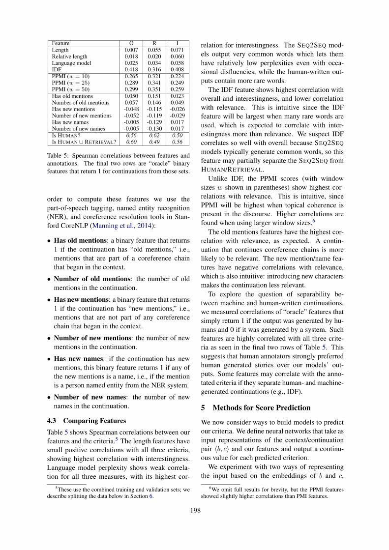
Feature O R ILength 0.007 0.055 0.071Relative length 0.018 0.020 0.060Language model 0.025 0.034 0.058IDF 0.418 0.316 0.408PPMI (w = 10) 0.265 0.321 0.224PPMI (w = 25) 0.289 0.341 0.249PPMI (w = 50) 0.299 0.351 0.259Has old mentions 0.050 0.151 0.023Number of old mentions 0.057 0.146 0.049Has new mentions -0.048 -0.115 -0.026Number of new mentions -0.052 -0.119 -0.029Has new names -0.005 -0.129 0.017Number of new names -0.005 -0.130 0.017Is HUMAN? 0.56 0.62 0.50Is HUMAN ∪ RETRIEVAL? 0.60 0.49 0.56
Table 5: Spearman correlations between features andannotations. The final two rows are “oracle” binaryfeatures that return 1 for continuations from those sets.
order to compute these features we use thepart-of-speech tagging, named entity recognition(NER), and coreference resolution tools in Stan-ford CoreNLP (Manning et al., 2014):
• Has old mentions: a binary feature that returns1 if the continuation has “old mentions,” i.e.,mentions that are part of a coreference chainthat began in the context.
• Number of old mentions: the number of oldmentions in the continuation.
• Has new mentions: a binary feature that returns1 if the continuation has “new mentions,” i.e.,mentions that are not part of any coreferencechain that began in the context.
• Number of new mentions: the number of newmentions in the continuation.
• Has new names: if the continuation has newmentions, this binary feature returns 1 if any ofthe new mentions is a name, i.e., if the mentionis a person named entity from the NER system.
• Number of new names: the number of newnames in the continuation.
4.3 Comparing FeaturesTable 5 shows Spearman correlations between ourfeatures and the criteria.5 The length features havesmall positive correlations with all three criteria,showing highest correlation with interestingness.Language model perplexity shows weak correla-tion for all three measures, with its highest cor-
5These use the combined training and validation sets; wedescribe splitting the data below in Section 6.
relation for interestingness. The SEQ2SEQ mod-els output very common words which lets themhave relatively low perplexities even with occa-sional disfluencies, while the human-written out-puts contain more rare words.
The IDF feature shows highest correlation withoverall and interestingness, and lower correlationwith relevance. This is intuitive since the IDFfeature will be largest when many rare words areused, which is expected to correlate with inter-estingness more than relevance. We suspect IDFcorrelates so well with overall because SEQ2SEQ
models typically generate common words, so thisfeature may partially separate the SEQ2SEQ fromHUMAN/RETRIEVAL.
Unlike IDF, the PPMI scores (with windowsizes w shown in parentheses) show highest cor-relations with relevance. This is intuitive, sincePPMI will be highest when topical coherence ispresent in the discourse. Higher correlations arefound when using larger window sizes.6
The old mentions features have the highest cor-relation with relevance, as expected. A contin-uation that continues coreference chains is morelikely to be relevant. The new mention/name fea-tures have negative correlations with relevance,which is also intuitive: introducing new charactersmakes the continuation less relevant.
To explore the question of separability be-tween machine and human-written continuations,we measured correlations of “oracle” features thatsimply return 1 if the output was generated by hu-mans and 0 if it was generated by a system. Suchfeatures are highly correlated with all three crite-ria as seen in the final two rows of Table 5. Thissuggests that human annotators strongly preferredhuman generated stories over our models’ out-puts. Some features may correlate with the anno-tated criteria if they separate human- and machine-generated continuations (e.g., IDF).
5 Methods for Score Prediction
We now consider ways to build models to predictour criteria. We define neural networks that take asinput representations of the context/continuationpair 〈b, c〉 and our features and output a continu-ous value for each predicted criterion.
We experiment with two ways of representingthe input based on the embeddings of b and c,
6We omit full results for brevity, but the PPMI featuresshowed slightly higher correlations than PMI features.
198
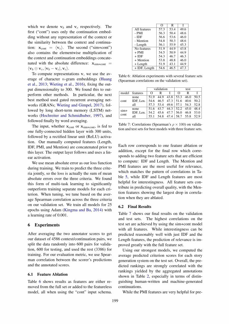
which we denote vb and vc respectively. Thefirst (“cont”) uses only the continuation embed-ding without any representation of the context orthe similarity between the context and continua-tion: xcont = 〈vc〉. The second (“sim+cont”)also contains the elementwise multiplication ofthe context and continuation embeddings concate-nated with the absolute difference: xsim+cont =〈vb � vc, |vb − vc|,vc〉.
To compute representations v, we use the av-erage of character n-gram embeddings (Huanget al., 2013; Wieting et al., 2016), fixing the out-put dimensionality to 300. We found this to out-perform other methods. In particular, the nextbest method used gated recurrent averaging net-works (GRANs; Wieting and Gimpel, 2017), fol-lowed by long short-term memory (LSTM) net-works (Hochreiter and Schmidhuber, 1997), andfollowed finally by word averaging.
The input, whether xcont or xsim+cont, is fed toone fully-connected hidden layer with 300 units,followed by a rectified linear unit (ReLU) activa-tion. Our manually computed features (Length,IDF, PMI, and Mention) are concatenated prior tothis layer. The output layer follows and uses a lin-ear activation.
We use mean absolute error as our loss functionduring training. We train to predict the three crite-ria jointly, so the loss is actually the sum of meanabsolute errors over the three criteria. We foundthis form of multi-task learning to significantlyoutperform training separate models for each cri-terion. When tuning, we tune based on the aver-age Spearman correlation across the three criteriaon our validation set. We train all models for 25epochs using Adam (Kingma and Ba, 2014) witha learning rate of 0.001.
6 Experiments
After averaging the two annotator scores to getour dataset of 4586 context/continuation pairs, wesplit the data randomly into 600 pairs for valida-tion, 600 for testing, and used the rest (3386) fortraining. For our evaluation metric, we use Spear-man correlation between the scorer’s predictionsand the annotated scores.
6.1 Feature Ablation
Table 6 shows results as features are either re-moved from the full set or added to the featurelessmodel, all when using the “cont” input schema.
O R IAll features 57.3 53.4 49.6- PMI 56.3 50.4 48.6- IDF 56.6 53.6 46.0- Mention 54.8 50.3 48.6- Length 56.1 55.9 45.3No features 51.9 44.9 43.8+ PMI 54.5 50.9 44.9+ IDF 54.3 46.7 46.3+ Mention 53.8 48.8 46.0+ Length 51.9 43.1 44.9+ IDF, Length 54.6 46.5 47.3
Table 6: Ablation experiments with several feature sets(Spearman correlations on the validation set).
validation testmodel features O R I O R I
none 51.9 44.9 43.8 53.3 46.0 50.5cont IDF, Len. 54.6 46.5 47.3 51.6 40.6 50.2
all 57.3 53.4 49.6 57.1 54.3 52.8
sim+ none 51.6 43.7 44.3 52.2 45.0 48.4
cont IDF, Len. 54.2 45.6 47.7 56.0 46.8 53.0all 55.1 54.8 47.4 58.7 55.8 52.9
Table 7: Correlations (Spearman’s ρ× 100) on valida-tion and test sets for best models with three feature sets.
Each row corresponds to one feature ablation oraddition, except for the final row which corre-sponds to adding two feature sets that are efficientto compute: IDF and Length. The Mention andPMI features are the most useful for relevance,which matches the pattern of correlations in Ta-ble 5, while IDF and Length features are mosthelpful for interestingness. All feature sets con-tribute in predicting overall quality, with the Men-tion features showing the largest drop in correla-tion when they are ablated.
6.2 Final Results
Table 7 shows our final results on the validationand test sets. The highest correlations on thetest set are achieved by using the sim+cont modelwith all features. While interestingness can bepredicted reasonably well with just IDF and theLength features, the prediction of relevance is im-proved greatly with the full feature set.
Using our strongest models, we computed theaverage predicted criterion scores for each storygeneration system on the test set. Overall, the pre-dicted rankings are strongly correlated with therankings yielded by the aggregated annotationsshown in Table 2, especially in terms of distin-guishing human-written and machine-generatedcontinuations.
While the PMI features are very helpful for pre-
199
dicting relevance, they do have demanding spacerequirements due to the sheer number of wordpairs with nonzero counts in large corpora. We at-tempted to replace the PMI features by similar fea-tures based on word embedding similarity, follow-ing the argument that skip-gram embeddings withnegative sampling form an approximate factoriza-tion of a PMI score matrix (Levy and Goldberg,2014). However, we were unable to find the sameperformance by doing so; the PMI scores were stillsuperior.
For the automatic scores shown in Table 3, weused the sim+cont model with IDF and Lengthfeatures. Since this model does not require PMIsor NLP analyzers, it is likely to be the one usedmost in practice by other researchers within train-ing/tuning settings. We release this trained scoreras well as our annotated data to the research com-munity.
7 Conclusion
We conducted a manual evaluation of neuralsequence-to-sequence and retrieval-based storycontinuation systems along three criteria: overallquality, relevance, and interestingness. We ana-lyzed the annotations and identified features thatcorrelate with each criterion. These annotationsalso provide a new story understanding task: pre-dicting the quality scores of generated continua-tions. We took initial steps toward solving thistask by developing an automatic scorer that usesfeatures, compositional architectures, and multi-task training. Our trained continuation scorer canbe used as a rich feature function for story gen-eration or a reward function for systems that usereinforcement learning to learn to generate stories.The annotated data and trained scorer are availableat the authors’ websites.
Acknowledgments
We thank Melissa Roemmele and the anonymousreviewers for their comments. We also thankNVIDIA Corporation for donating GPUs used inthis research.
ReferencesSamy Bengio, Oriol Vinyals, Navdeep Jaitly, and
Noam Shazeer. 2015. Scheduled sampling for se-quence prediction with recurrent neural networks.In Advances in Neural Information Processing Sys-tems. pages 1171–1179.
Kyunghyun Cho, Bart van Merrienboer, Caglar Gul-cehre, Dzmitry Bahdanau, Fethi Bougares, HolgerSchwenk, and Yoshua Bengio. 2014. Learningphrase representations using RNN encoder–decoderfor statistical machine translation. In Proceedings ofthe 2014 Conference on Empirical Methods in Nat-ural Language Processing (EMNLP). pages 1724–1734.
Angel Daza, Hiram Calvo, and Jesus Figueroa-Nazuno.2016. Automatic text generation by learning fromliterary structures. In Proceedings of the Fifth Work-shop on Computational Linguistics for Literature.pages 9–19.
Natalie Dehn. 1981. Story generation after TALE-SPIN. In Proceedings of the 9th International JointConference on Artificial Intelligence (IJCAI). pages16–18.
David K. Elson. 2012. Modeling Narrative Discourse.Ph.D. thesis, Columbia University.
Albert Gatt and Emiel Krahmer. 2017. Survey of thestate of the art in natural language generation: Coretasks, applications and evaluation. arXiv preprintarXiv:1703.09902 .
Pablo Gervas. 2012. Story generator algorithms. TheLiving Handbook of Narratology 19.
Andrew S. Gordon, Cosmin Adrian Bejan, and KenjiSagae. 2011. Commonsense causal reasoning usingmillions of personal stories. In 25th Conference onArtificial Intelligence (AAAI-11).
Andrew S. Gordon and Reid Swanson. 2009. Identi-fying personal stories in millions of weblog entries.In Third International Conference on Weblogs andSocial Media, Data Challenge Workshop.
Kenneth Heafield. 2011. KenLM: faster and smallerlanguage model queries. In Proceedings of theEMNLP 2011 Sixth Workshop on Statistical Ma-chine Translation.
Sepp Hochreiter and Jurgen Schmidhuber. 1997. Longshort-term memory. Neural computation 9(8).
Po-Sen Huang, Xiaodong He, Jianfeng Gao, Li Deng,Alex Acero, and Larry Heck. 2013. Learning deepstructured semantic models for web search usingclickthrough data. In Proceedings of the 22nd ACMinternational conference on Conference on informa-tion & knowledge management. ACM, pages 2333–2338.
Ting-Hao (Kenneth) Huang, Francis Ferraro, NasrinMostafazadeh, Ishan Misra, Aishwarya Agrawal, Ja-cob Devlin, Ross Girshick, Xiaodong He, Push-meet Kohli, Dhruv Batra, C. Lawrence Zitnick,Devi Parikh, Lucy Vanderwende, Michel Galley, andMargaret Mitchell. 2016. Visual storytelling. InProceedings of the 2016 Conference of the NorthAmerican Chapter of the Association for Computa-tional Linguistics: Human Language Technologies.pages 1233–1239.
200

Parag Jain, Priyanka Agrawal, Abhijit Mishra, Mo-hak Sukhwani, Anirban Laha, and Karthik Sankara-narayanan. 2017. Story generation from sequence ofindependent short descriptions. In Workshop on Ma-chine Learning for Creativity, at the 23rd SIGKDDConference on Knowledge Discovery and Data Min-ing (KDD 2017).
Chloe Kiddon, Luke Zettlemoyer, and Yejin Choi.2016. Globally coherent text generation with neuralchecklist models. In Proceedings of the 2016 Con-ference on Empirical Methods in Natural LanguageProcessing. pages 329–339.
Diederik Kingma and Jimmy Ba. 2014. Adam: Amethod for stochastic optimization. arXiv preprintarXiv:1412.6980 .
Sheldon Klein, John F. Aeschlimann, David F. Bal-siger, Steven L. Converse, Claudine Court, MarkFoster, Robin Lao, John D. Oakley, and Joel Smith.1973. Automatic novel writing: A status report.Technical Report 186, University of Wisconsin-Madison.
Michael Lebowitz. 1985. Story-telling as planning andlearning. Poetics 14(6):483–502.
Omer Levy and Yoav Goldberg. 2014. Neural wordembedding as implicit matrix factorization. In Ad-vances in Neural Information Processing Systems27.
Yuhua Li, David McLean, Zuhair A Bandar, James DO’shea, and Keeley Crockett. 2006. Sentence sim-ilarity based on semantic nets and corpus statistics.IEEE transactions on knowledge and data engineer-ing 18(8):1138–1150.
Chia-Wei Liu, Ryan Lowe, Iulian Serban, Mike Nose-worthy, Laurent Charlin, and Joelle Pineau. 2016.How NOT to evaluate your dialogue system: An em-pirical study of unsupervised evaluation metrics fordialogue response generation. In Proceedings of the2016 Conference on Empirical Methods in NaturalLanguage Processing. pages 2122–2132.
Hugo Liu and Push Singh. 2002. MAKEBELIEVE:Using commonsense knowledge to generate stories.In Proceedings of the Eighteenth National Confer-ence on Artificial Intelligence (AAAI). pages 957–958.
Ryan Lowe, Michael Noseworthy, Iulian V. Ser-ban, Nicolas Angelard-Gontier, Yoshua Bengio, andJoelle Pineau. 2017. Towards an automatic Turingtest: Learning to evaluate dialogue responses. InProceedings of the 55th Annual Meeting of the As-sociation for Computational Linguistics.
Inderjeet Mani. 2012. Computational modeling ofnarrative. Synthesis Lectures on Human LanguageTechnologies 5(3):1–142.
Christopher D. Manning, Mihai Surdeanu, John Bauer,Jenny Rose Finkel, Steven Bethard, and David Mc-Closky. 2014. The Stanford CoreNLP natural lan-guage processing toolkit. In ACL (System Demon-strations). pages 55–60.
Neil McIntyre and Mirella Lapata. 2009. Learning totell tales: A data-driven approach to story genera-tion. In Proceedings of the Joint Conference of the47th Annual Meeting of the ACL and the 4th Interna-tional Joint Conference on Natural Language Pro-cessing of the AFNLP. pages 217–225.
Neil McIntyre and Mirella Lapata. 2010. Plot induc-tion and evolutionary search for story generation. InProceedings of the 48th Annual Meeting of the Asso-ciation for Computational Linguistics. pages 1562–1572.
Neil Duncan McIntyre. 2011. Learning to tell tales:automatic story generation from Corpora. Ph.D.thesis, The University of Edinburgh.
James R. Meehan. 1977. TALE-SPIN, an interactiveprogram that writes stories. In Proceedings of the5th International Joint Conference on Artificial In-telligence (IJCAI). pages 91–98.
Nasrin Mostafazadeh, Nathanael Chambers, XiaodongHe, Devi Parikh, Dhruv Batra, Lucy Vanderwende,Pushmeet Kohli, and James Allen. 2016. A cor-pus and cloze evaluation for deeper understanding ofcommonsense stories. In Proceedings of the 2016Conference of the North American Chapter of theAssociation for Computational Linguistics: HumanLanguage Technologies. pages 839–849.
K.M. Oinonen, Mariet Theune, Antinus Nijholt, andJ.R.R. Uijlings. 2006. Designing a story databasefor use in automatic story generation, Springer Ver-lag, pages 298–301. Lecture Notes in Computer Sci-ence.
Kishore Papineni, Salim Roukos, Todd Ward, and Wei-Jing Zhu. 2002. BLEU: a method for automaticevaluation of machine translation. In Proceedingsof the 40th annual meeting on association for com-putational linguistics. pages 311–318.
Vladimir Propp. 1968. Morphology of the Folktale,volume 9. University of Texas Press.
Mark O. Riedl and Robert Michael Young. 2010. Nar-rative planning: Balancing plot and character. Jour-nal of Artificial Intelligence Research 39:217–268.
Melissa Roemmele. 2016. Writing stories with helpfrom recurrent neural networks. In Thirtieth AAAIConference on Artificial Intelligence. pages 4311 –4312.
Melissa Roemmele, Cosmin Adrian Bejan, and An-drew S. Gordon. 2011. Choice of Plausible Alterna-tives: An Evaluation of Commonsense Causal Rea-soning. In AAAI Spring Symposium on Logical For-malizations of Commonsense Reasoning. StanfordUniversity.
201

Melissa Roemmele and Andrew S. Gordon. 2015. Cre-ative help: a story writing assistant. In Inter-national Conference on Interactive Digital Story-telling. Springer, pages 81–92.
Melissa Roemmele, Andrew S. Gordon, and ReidSwanson. 2017. Evaluating story generation sys-tems using automated linguistic analyses. In Work-shop on Machine Learning for Creativity, at the 23rdSIGKDD Conference on Knowledge Discovery andData Mining (KDD 2017).
Roger C. Schank and Robert P. Abelson. 1975. Scripts,plans, and knowledge. In Proceedings of the 4thInternational Joint Conference on Artificial Intelli-gence (IJCAI). pages 151–157.
Ilya Sutskever, Oriol Vinyals, and Quoc V. Le. 2014.Sequence to sequence learning with neural net-works. In Advances in neural information process-ing systems. pages 3104–3112.
Reid Swanson and Andrew S. Gordon. 2012. Say any-thing: Using textual case-based reasoning to enableopen-domain interactive storytelling. ACM Trans.Interact. Intell. Syst. 2(3):16:1–16:35.
Mariet Theune, Sander Faas, Anton Nijholt, and DirkHeylen. 2003. The virtual storyteller: story cre-ation by intelligent agents. In Proceedings of the1st International Conference on Technologies forInteractive Digital Storytelling and Entertainment.Springer, pages 204–215.
Perry W. Thorndyke. 1977. Cognitive structures incomprehension and memory of narrative discourse.Cognitive psychology 9(1):77–110.
Scott R. Turner. 1993. Minstrel: a computer model ofcreativity and storytelling. Ph.D. thesis, Universityof California at Los Angeles.
Ashwin K Vijayakumar, Michael Cogswell, Ram-prasath R Selvaraju, Qing Sun, Stefan Lee, DavidCrandall, and Dhruv Batra. 2016. Diverse beamsearch: Decoding diverse solutions from neural se-quence models. arXiv preprint arXiv:1610.02424 .
Tong Wang, Ping Chen, and Boyang Li. 2017. Pre-dicting the quality of short narratives from socialmedia. In Proceedings of the Twenty-Sixth Inter-national Joint Conference on Artificial Intelligence(IJCAI).
John Wieting, Mohit Bansal, Kevin Gimpel, and KarenLivescu. 2016. Charagram: Embedding words andsentences via character n-grams. In Proceedings ofthe 2016 Conference on Empirical Methods in Nat-ural Language Processing. pages 1504–1515.
John Wieting and Kevin Gimpel. 2017. Revisiting re-current networks for paraphrastic sentence embed-dings. In Proceedings of the 55th Annual Meeting ofthe Association for Computational Linguistics (Vol-ume 1: Long Papers). pages 2078–2088.
Robert Wilensky. 1983. Story grammars versus storypoints. Behavioral and Brain Sciences 6(4):579–591.
Patrick Henry Winston. 2014. The Genesis story un-derstanding and story telling system: A 21st centurystep toward artificial intelligence. Memo 019, Cen-ter for Brains Minds and Machines, MIT.
202

Proceedings of the 7th Joint Conference on Lexical and Computational Semantics (*SEM), pages 203–213New Orleans, June 5-6, 2018. c©2018 Association for Computational Linguistics
Term Definitions Help Hypernymy Detection
Wenpeng Yin and Dan RothUniversity of Pennsylvania
{wenpeng,danroth}@seas.upenn.edu
Abstract
Existing methods of hypernymy detectionmainly rely on statistics over a big corpus, ei-ther mining some co-occurring patterns like“animals such as cats” or embedding wordsof interest into context-aware vectors. Theseapproaches are therefore limited by the avail-ability of a large enough corpus that cancover all terms of interest and provide suffi-cient contextual information to represent theirmeaning. In this work, we propose a newparadigm, HYPERDEF, for hypernymy de-tection – expressing word meaning by en-coding word definitions, along with contextdriven representation. This has two mainbenefits: (i) Definitional sentences express(sense-specific) corpus-independent meaningsof words, hence definition-driven approachesenable strong generalization – once trained,the model is expected to work well in open-domain testbeds; (ii) Global context from alarge corpus and definitions provide comple-mentary information for words. Consequently,our model, HYPERDEF, once trained on task-agnostic data, gets state-of-the-art results inmultiple benchmarks1.
1 Introduction
Language understanding applications like textualentailment (Dagan et al., 2013), question answer-ing (Saxena et al., 2007) and relation extraction(Mintz et al., 2009), benefit from the identificationof lexical entailment relations. Lexical inferenceencompasses several semantic relations, with hy-pernymy being one of the prevalent (Roller et al.,2014; Shwartz et al., 2016), an i.e., “Is-A” relationthat holds for a pair of terms2 (x, y) for specificterms’ senses.
Two families of approaches have been studiedfor identifying term hypernymy. (i) Pattern match-
1cogcomp.org/page/publication_view/8362This paper uses “term” to refer to any words or phrases.
ing exploits patterns such as “animals such as cats”to indicate a hypernymy relation from “cat” to “an-imal” (Hearst, 1992; Snow et al., 2004). How-ever, it requires the co-occurrence of the two termsin the same sentence, which limits the recall ofthis method; (ii) Term representation learning de-pends on a vector embedding of each term, whereeach entry in the vector expresses an explicit con-text feature (Baroni et al., 2012a; Roller and Erk,2016; Shwartz et al., 2017) or a latent semantic(Fu et al., 2014; Vulic and Mrksic, 2017; Glavasand Ponzetto, 2017).
Both approaches hinge on acquiring context-aware term meaning in a large corpus. The gen-eralization of these corpus-based representationlearning paradigms, however, is limited due to thedomain specificity of the training data. For ex-ample, an IT corpus hardly mentions “apple” asa fruit. Furthermore, the surrounding context ofa term may not convey subtle differences in termmeaning – “he” and “she” have highly similar con-text that may not reveal the important differencebetween them. Moreover, rare words are poorlyexpressed by their sparse global context and, moregenerally, these methods would not generalize tothe low resource language setting.
Humans can easily determine the hypernymyrelation between terms even for words they havenot been exposed to a lot, given a definition of it interms of other words. For example, one can imag-ine a “teaching” scenario that consists of defininga term, potentially followed by a few examples ofthe term usage in text.
Motivated by these considerations and the goalof eventually develop an approach that could gen-eralize to unseen words and even to the low re-source languages scenario, we introduce the fol-lowing hypernymy detection paradigm, HYPER-DEF, where we augment distributional contextualmodels with that of learning terms representations
203

from their definitions. This paradigm has an im-portant advantage in its powerful generalization,as definitions are agnostic to specific domains andbenchmarks, and are equally available for wordsregardless of their frequency in a given data set.Consequently, the task of identifying the relationbetween two terms is enhanced by the knowl-edge of the terms’ definitions. Our model can beapplied to any new terms in any domain, givensome context of the term usage and their domain-agnostic definitions. Moreover, given our learningapproach – we learn also the notion of lexical en-tailment between terms – we can generalize to anylexical relation between terms.
Technically, we implement HYPERDEF bymodifying the AttentiveConvNet (Yin andSchutze, 2017), a top-performing system on atextual entailment benchmark (Bowman et al.,2015), to model the input (x, dx; y, dy), where di(i = x, y) is the definition of term i. In contrastto earlier work which mostly built separate repre-sentations for terms x and y, HYPERDEF insteaddirectly models the representation for each pairin {(x, y), (x, dy), (dx, y), (dx, dy)}, and thenaccumulates the four-way representations to forman overall representation for the input.
In our experiments, we train HYPERDEF on atask-agnostic annotated dataset, Wordnet, and testit on a broad array of open-domain hypernymy de-tection datasets. The results show the outstandingperformance and strong generalization of the HY-PERDEF model.
Overall, our contributions are as follows:
• To our knowledge, this is the first work in hy-pernymy detection that makes use of term def-initions. Definitions provide complementaryknowledge to distributional context, so that ourmodel better tolerates unseen words, rare wordsand words with biased sense distribution.
• HYPERDEF accounts for word sense when in-ferring the hypernymy relation. This differsfrom much of the literature, which usually de-rives sense-unaware representative vectors forterms – earlier approaches would say ‘yes’ ifthe relation holds for some combination of theterms’ senses.
• HYPERDEF has strong generalization capabil-ity – once trained on a task-agnostic definitiondataset, it can be used in different testbeds, andshows state-of-the-art results.
2 Related Work
The main novelty of our HYPERDEF lies in theinformation resource that is employed to representthe terms. Prior work in exploring informationresources can be put into two categories: under-standing terms by the co-occurring context in rawtext, or grounding the terms in open-domain ob-jects.
2.1 Mining Distributional Context from Text
Window-based Context Baroni et al. (2012b)build distributional semantic vectors for termsfrom a concatenation of three corpora: the BritishNational Corpus, WackyPedia and ukWac. Eachentry in the vector is the PMI-formulated scorefrom co-occurrence counts. Dimension reductionis conducted by Singular Value Decomposition(SVD) before feeding representation vectors to aclassifier.
Dependency-based Context Roller and Erk(2016) compute a syntactic distributional spacefor terms by counting their dependency neighborsacross the corpus.
Shwartz et al. (2017) further compare (i) con-texts being parent and daughter nodes in the de-pendency tree, and (ii) contexts being the parent-sister pairs in the dependency tree.
Term Embeddings Unspecialized term embed-dings are not informative signals for detectingspecific lexico-semantic relations. Hence, com-munity often explicitly build transformation func-tions from unspecialized embeddings to relation-specialized embeddings. Fu et al. (2014) firstuse the skip-gram model (Mikolov et al., 2013)to learn generic term embeddings from a largeChinese encyclopedia corpus, then learn a projec-tion function from the generic space to hypernymyspace by annotated hypernymy pairs. Other worktrying to specify the generic word embeddings tohypernymy detection task include (Vulic and Mrk-sic, 2017; Glavas and Ponzetto, 2017).
Other advanced types of term embeddings spe-cific to the hypernymy detection problem in-clude Gaussian distributed embeddings (Vilnisand McCallum, 2015), non-negative embeddings(Chang et al., 2017), magnitude-oriented embed-dings (Nguyen et al., 2017), and so on.
In our work, distributional context model is alsoapplied. More specifically, we will directly use
204
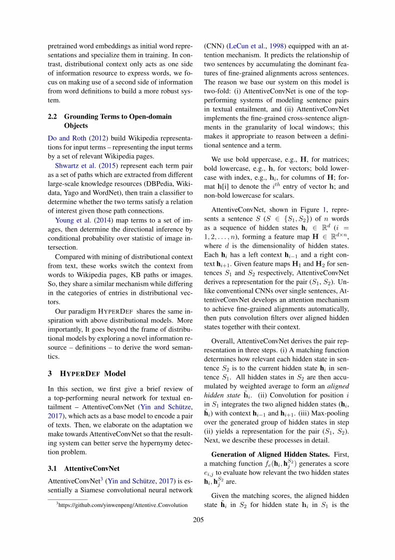
pretrained word embeddings as initial word repre-sentations and specialize them in training. In con-trast, distributional context only acts as one sideof information resource to express words, we fo-cus on making use of a second side of informationfrom word definitions to build a more robust sys-tem.
2.2 Grounding Terms to Open-domainObjects
Do and Roth (2012) build Wikipedia representa-tions for input terms – representing the input termsby a set of relevant Wikipedia pages.
Shwartz et al. (2015) represent each term pairas a set of paths which are extracted from differentlarge-scale knowledge resources (DBPedia, Wiki-data, Yago and WordNet), then train a classifier todetermine whether the two terms satisfy a relationof interest given those path connections.
Young et al. (2014) map terms to a set of im-ages, then determine the directional inference byconditional probability over statistic of image in-tersection.
Compared with mining of distributional contextfrom text, these works switch the context fromwords to Wikipedia pages, KB paths or images.So, they share a similar mechanism while differingin the categories of entries in distributional vec-tors.
Our paradigm HYPERDEF shares the same in-spiration with above distributional models. Moreimportantly, It goes beyond the frame of distribu-tional models by exploring a novel information re-source – definitions – to derive the word seman-tics.
3 HYPERDEF Model
In this section, we first give a brief review ofa top-performing neural network for textual en-tailment – AttentiveConvNet (Yin and Schutze,2017), which acts as a base model to encode a pairof texts. Then, we elaborate on the adaptation wemake towards AttentiveConvNet so that the result-ing system can better serve the hypernymy detec-tion problem.
3.1 AttentiveConvNet
AttentiveConvNet3 (Yin and Schutze, 2017) is es-sentially a Siamese convolutional neural network
3https://github.com/yinwenpeng/Attentive Convolution
(CNN) (LeCun et al., 1998) equipped with an at-tention mechanism. It predicts the relationship oftwo sentences by accumulating the dominant fea-tures of fine-grained alignments across sentences.The reason we base our system on this model istwo-fold: (i) AttentiveConvNet is one of the top-performing systems of modeling sentence pairsin textual entailment, and (ii) AttentiveConvNetimplements the fine-grained cross-sentence align-ments in the granularity of local windows; thismakes it appropriate to reason between a defini-tional sentence and a term.
We use bold uppercase, e.g., H, for matrices;bold lowercase, e.g., h, for vectors; bold lower-case with index, e.g., hi, for columns of H; for-mat h[i] to denote the ith entry of vector h; andnon-bold lowercase for scalars.
AttentiveConvNet, shown in Figure 1, repre-sents a sentence S (S ∈ {S1, S2}) of n wordsas a sequence of hidden states hi ∈ Rd (i =1, 2, . . . , n), forming a feature map H ∈ Rd×n,where d is the dimensionality of hidden states.Each hi has a left context hi−1 and a right con-text hi+1. Given feature maps H1 and H2 for sen-tences S1 and S2 respectively, AttentiveConvNetderives a representation for the pair (S1, S2). Un-like conventional CNNs over single sentences, At-tentiveConvNet develops an attention mechanismto achieve fine-grained alignments automatically,then puts convolution filters over aligned hiddenstates together with their context.
Overall, AttentiveConvNet derives the pair rep-resentation in three steps. (i) A matching functiondetermines how relevant each hidden state in sen-tence S2 is to the current hidden state hi in sen-tence S1. All hidden states in S2 are then accu-mulated by weighted average to form an alignedhidden state hi. (ii) Convolution for position iin S1 integrates the two aligned hidden states (hi,hi) with context hi−1 and hi+1. (iii) Max-poolingover the generated group of hidden states in step(ii) yields a representation for the pair (S1, S2).Next, we describe these processes in detail.
Generation of Aligned Hidden States. First,a matching function fe(hi,hS2
j ) generates a scoreei,j to evaluate how relevant the two hidden stateshi,hS2
j are.
Given the matching scores, the aligned hiddenstate hi in S2 for hidden state hi in S1 is the
205

hi
mi
S1 S2
alignedhidden state
attentiveconvolution
p
row-wisemax-pooling
Representation for pair ( , )S1 S2
h˜i
hi−1 hi+1
Figure 1: AttentiveConvNet models a sent. pair (S1, S2). Inour work, Si (i=1,2) can be the definition sentence orthe term itself (we treat a term as a short sentence.)
weighted average of all hidden states in S2:
hi =∑
j
softmax(ei)[j] · hS2j (1)
Attentive Convolution. A position i in S1 hashidden state hi, left context hi−1, right contexthi+1 and aligned hidden state hi from S2. At-tentive convolution then generates the higher-levelrepresentation for this combination:
mi = tanh(W · [hi−1,hi,hi+1, hi] + b) (2)
where parameters W ∈ Rd×4d, b ∈ Rd.Pair Representation Generation. As Equation
2 shows, each mi denotes the inference featuresbetween hi and its alignment hi in context. Atten-tiveConvNet uses max-pooling over {mi} to getthe overall representation p for the pair:
p[i] = max(m1[i],m2[i], · · · ,mn[i]) (3)
Finally, the representation p is used in classifi-cation. The whole model is learned in an end-to-end training4.
3.2 Four-way AttentiveConvNetAttentiveConvNet originally works on sentencepairs. We formulate the hypernymy detection
4For more details, please refer to (Yin and Schutze, 2017).
Figure 2: HYPERDEF – combining distributionalmodel with definition encoding
problem as {(x, dx; y, dy; 1/0)}. Just as in(Shwartz et al., 2016) which directly concatenatesthe term path representation vector with term em-bedding vectors as the classifier input, a simplecombination of distributional models and defini-tion encoding for us could be: separately learn-ing the distributional model over term embeddingpairs and an AttentiveConvNet model over def-inition pairs, then concatenate their output rep-resentations. However, the analysis over dataset{(x, dx; y, dy; 1/0)} hints that HYPERDEF canobtain more indicative features by modeling (term,definition), which crosses the distributional mod-els and definition encoding. For example, the def-inition of term “cat” in WordNet is: feline mam-mal usually having thick soft fur and no ability toroar: domestic cats; wildcats. Intuitively, whenthe system meets the pair (cat, mammal), it shouldbe trivial to get the “hypernymy” decision since“mammal” appears in the definition sentence.
Inspired by this observation, we implement theHYPERDEF paradigm as four-way AttentiveCon-vNets, as Figure 2 shows, i.e., treating the twoterms as word sequences as well, then do Atten-tiveConvNet over all four combinations: (x, y),(x, dy), (dx, y) and (dx, dy).
Assume we get four separate representations:pww from (x, y), pwd from (x, dy), pdw from(dx, y) and pdd from (dx, dy), as Section 3.1 de-scribed. We construct the final representation for
206

random split lexical splitall –pww –pwd –pdw – pdd all –pww –pwd – pdw –pdd
HYPERDEF (F1) .905 .874 .896 .876 .881 .887 .875 .870 .849 .862HYPERDEF (AP) .933 .902 .921 .905 .909 .900 .890 .883 .880 .877w/o attention (F1) .825 .743w/o definition (F1) .734 .619LSTM+atten. (F1) .757 .685
Table 1: Tune HyperDef on wn dev
(x, dx; y, dy) via concatenation:
p = [pww,pwd,pdw,pdd] (4)
then p is fed to the final classifier.AttentiveConvNet over (x, y) resembles the
conventional hypernymy classifiers which taketwo representation vectors (one for x, the otherfor y) as input and output the label. Note thatAttentiveConvNet puts filter weights over (x, y)to learn more abstract representations; this actu-ally is in common with some literature such as (Fuet al., 2014; Vulic and Mrksic, 2017; Glavas andPonzetto, 2017), which utilize weights to projectgeneric word representations into specified repre-sentations towards hypernymy annotations.
AttentiveConvNet over (x, dy) and (dx, y) com-pares a term with the descriptive sentence of theother term; this might provide direct clues, as wediscussed in the beginning of this subsection.
AttentiveConvNet over (dx, dy) resembles lit-erature (Do and Roth, 2012; Young et al., 2014).HYPERDEF provides an alternative resource forinterpreting terms, resorting to definitional expres-sions instead of Wikipedia pages or images.
Overall, our HYPERDEF combines strengths of(i) conventional supervised classifiers over contextdistributions, and (ii) rich interpretation of termsin broader knowledge bases.
3.3 Analysis of HYPERDEF
Our HYPERDEF has the following properties:
• HYPERDEF combines distributional modelswith definition encoding, but it is not simplya concatenation of two independent subsys-tems. HYPERDEF enables modeling across(distributional context, definition). This isexpected to generate more indicative fea-tures than a similar work (Shwartz et al.,2016), which simply concatenated distribu-tional models with path-based models;
• HYPERDEF employs definitions to providericher information for the terms. But it doesnot generate an auxiliary term representationvector from the definitive sentence as the lit-erature (Hill et al., 2016) did. Instead, HY-PERDEF formulates a pair of input elements– each can be a distributional vector or a def-inition representation – into a cross-sentenceattention mechanism, which directly yields acompact representation to the pair rather thantwo separate vectors for the two input ele-ments. This is shown more effective to modelthe relationship of two pieces of text (Yin andSchutze, 2017);
• Distributional models and definitive sen-tences in HYPERDEF provide complemen-tary knowledge. For terms which can not re-trieve a definition, HYPERDEF still works –just turning into a basic distributional model.This work uses WordNet and Wikipedia asexample resources for the definition retrieval,more splendid resources will be developedgradually in released HYPERDEF models.We will also provide users the option to typeinto their definitions;
• WordNet provides term definitions in thesense level, so theHYPERDEF model is es-sentially trained in the sense level. For poly-semy cases in testing, HYPERDEF can sim-ply test on all combinations of definitions,then pick the pair with the highest probabil-ity;
• For terms that were never observed in train-ing, we expect context distributions, suchas pretrained embeddings, and definitionsare available, so HYPERDEF is hardly influ-enced in this case. This is exactly the mainadvantage of HYPERDEF: generalization.
207

4 Experiments
4.1 Pre-training of HYPERDEF
Dataset Preparation. As we aim to build astrongly generalizing hypernymy detector, thetraining data we collect here is expected to betask-agnostic. Hence, extracting from structuredknowledge resources, such as WordNet (Fell-baum, 1998), Wikidata (Vrandecic, 2012), DB-Pedia (Auer et al., 2007), and Yago (Suchaneket al., 2007), is preferred. Some literature, e.g.,(Shwartz et al., 2015), claim that there is limitedcoverage for almost all knowledge resources. Forexample, WordNet does not cover many proper-names (Donald Trump → president) or recentterminology (AlphaGo → computer program).Our data tends to alleviate this challenge, sincein testing, descriptive sentences in the HYPER-DEF paradigm can provide the precise and dis-tinct features for terms even if these terms areOOV and in new types.
In this work, we pick one of those knowl-edge resources – WordNet – to collect trainingdata. Specifically, our positive instances consistof (i) all direct hypernymy pairs, and (ii) switchedterms from the original hyponymy pairs. Neg-ative instances include (i) pairs with other rela-tions such as antonym, synonym, and (ii) pairs ofpositive instances after exchanging the two terms.Note that each term is accompanied by its defini-tion in sense level. So we get instances in form(x, dx; y, dy; 1/0), where the binary value “1/0”indicates whether y is x’s hypernymy or not. Al-together, we collect about 900K instances withroughly a 8:1 ratio between negative and positiveinstances.
In testing, we implement HYPERDEF to re-trieve definitions and distributional context forterms automatically5.
Random and Lexical Dataset Splits. In our pri-mary dataset, we perform a random split, with80% train, 10% dev, and 10% test.
As pointed out by Levy et al. (2015), super-vised distributional lexical inference methods tendto perform “lexical memorization”, i.e., instead oflearning a relation between the two terms, theymostly learn an independent property of term y inthe pair: whether y is a “prototypical hypernym”or not. Levy et al. (2015) suggest to splitting the
5In the released HYPERDEF model, we will provide anoption for users to input definitions.
train and test sets such that each will contain a dis-tinct vocabulary (“lexical split”), in order to pre-vent the model from overfitting by lexical memo-rization.
In the current phase, we use notations wn train,wn dev, and wn test to refer to the three parts.Note that wn train and wn dev will be used to trainand tune the HYPERDEF model, while wn test isset to show how well the model performs in Word-Net domain – it is not expected to act as a testbedin real benchmarks. In experiments, we will com-pare our model in random and lexical splits.
Training Setup. Given wn train in form {(x,dx; y, dy; 1/0)}, a binary classifier via logistic re-gression is trained over the pair representation pobtained from Equation 4, predicting 1 or 0 for thehypernymy relation. The objective function is im-plemented through negative log-likelihood. Termsand words in definitions are initialized by 300dWord2Vec embeddings (Mikolov et al., 2013) andkept unchanged in training. This benefits the gen-eralization as it ensures that the words in train-ing and the new words in test data lie in the samespace. All hidden sizes are 300 as well. The wholesystem is trained by AdaGrad (Duchi et al., 2011)with initial learning rate 0.02.
We first run the HYPERDEF in wn test to checkif it is effective in the WordNet domain. Then wetest it in some open-domain benchmarks. Notethat all experiments use the HYPERDEF modelspretrained over wn train.
4.2 Performance within WordNet
As mentioned in Section 4.1, wn train, wn devand wn test have two distinct setups: “randomsplit” and “lexical split”, inspired by the “lexicalmemorization” observation (Levy et al., 2015).
We first tune the parameters in wn train andsearch the best system layout based on wn dev.F1 and average precision (AP) are reported. Ta-ble 1 lists the performance records, with the firstblock for “random split” and the second block for“lexical split”.
We first discuss three baselines: (i) “w/o defi-nition”: We discard definitions and only use dis-tributional model, i.e., a logistic regression clas-sifier (LR) over the concatenated (x, y) embed-dings from Word2Vec. Its performance drops11.5% from “random split” to “lexical split”.This is within expectation as Levy et al. (2015)concluded that this baseline is not effective in
208

learning genuine term relations; (ii) “w/o atten-tion”: We discard the attention mechanism inAttentiveConvNet, resulting in a bi-CNN struc-ture. It works on instances {(x, dx; y, dy; 1/0)},a vanilla CNN is used to encode the definitionsentence into a dense representation vector. So,each term in (x, y) will get two separate rep-resentation vectors (one is from Word2Vec, theother from the definition); finally totally four rep-resentation vectors are concatenated and fed tothe LR. This baseline works much better than“w/o definition” (improvements of 9% ∼ 11%).Their comparison shows that incorporating termdefinitions in reasoning process is promising;(iii) “LSTM+attention” (Rocktaschel et al., 2016).A representative attention mechanism in LSTM(Hochreiter and Schmidhuber, 1997) for textualentailment. We apply it in the same way asour four-way AttentiveConvNet, however, foundit performs poorly. We suspect that this is due totwo reasons: i) Though there is entailment or hy-pernymy relation between a term pair, e.g., (“cat”,“animal”), unfortunately there is no clear clue ofthat relation between their definition pair if consid-ering all the information contained in the defini-tions. For example, “cat” – “a small domesticatedcarnivorous mammal with soft fur, a short snout,and retractile claws. It is widely kept as a pet orfor catching mice, and many breeds have been de-veloped”, and “animal” – “a living organism thatfeeds on organic matter, typically having special-ized sense organs and nervous system and ableto respond rapidly to stimuli”. Apparently, wecan not infer the whole definition of “animal” bycat’s definition. Instead, their help mainly comesfrom some key-phrases, such as “domesticatedcarnivorous mammal”, “living organism” and soon. LSTM, encoding the whole word sequencesin attention, potentially would be misled. Ourapproach relies on convolution filters and max-pooling, excelling in modeling keywords-drivingfeatures (Yin et al., 2017). This baseline indicatesthe overall strength of our system comes from thedefinition incorporation as well as an appropriateencoder.
Considering the whole table, we observe that:(i) HYPERDEF models have pretty close perfor-mances in “random split” and “lexical split” –mostly within 2∼3%. This strongly indicatesthat HYPERDEF is less influenced by the “lexicalmemorization” problem. Our systems, equipped
random lexicalF1 .902 .881AP .915 .891
Table 2: Pretrained HyperDef on wn test
with definition encoding, show promising general-ization (at least in WordNet domain); (ii) ThoughHYPERDEF models in “all” setup behave simi-larly in random split and lexical split, the detailedcontributions of pww, pwd, pdw and pdd differ inthe two settings. To be specific, in “wn dev (ran-dom split)”, there is no clear winner among {pww,pdw, pdd}, pwd contributes consistently less thanthe other three. In “wn dev (lexical split)”, in-stead, pwd, pdw and pdd perform similarly whilepww performs worst. This indicates that whendealing with unseen terms, definition-based com-ponents in HYPERDEF play a dominant role.
Experiments on wn dev enable to store the bestHYPERDEF models – concatenation over the fourrepresentations: pww, pwd, pdw and pdd. Thenwe reload the pretrained models and report theirperformance on wn test, as shown in Table 2.From Table 1 to Table 2, we observe pretty smalldrop in performance – mostly∼ 1% . This prelim-inarily demonstrates the strong generalization.
Next, we test the best HYPERDEF models pre-trained on “wn train (lexical split)” in open do-main benchmarks.
4.3 Performance in Open-domain Datasets
First, we use four widely-explored datasets:BLESS (Baroni and Lenci, 2011), EVALution(Santus et al., 2015), Lenci/Benotto (Benotto,2015), and Weeds (Weeds et al., 2014). They wereconstructed either using knowledge resources (e.g.WordNet, Wikipedia), crowd-sourcing or both.The instance sizes of hypernymy and “other” re-lation types are detailed in Table 3. We also re-port “#OOV pair”, the proportions of unseen termpairs in above four datasets regarding the train-ing set of HYPERDEF, i.e., wn train in Section4.1. We notice that most term pairs in BLESS andLenci/Benotto datasets are unseen in wn train.
First, we extract the term’s all sense definitionsfrom WordNet based on the term string. For afew instances which contain terms not coveredby WordNet, such as proper noun “you”, “ev-erybody” etc, we set definitions the same as theterm strings (this preprocessing does not influenceresults, just for making the system uniformed).
209
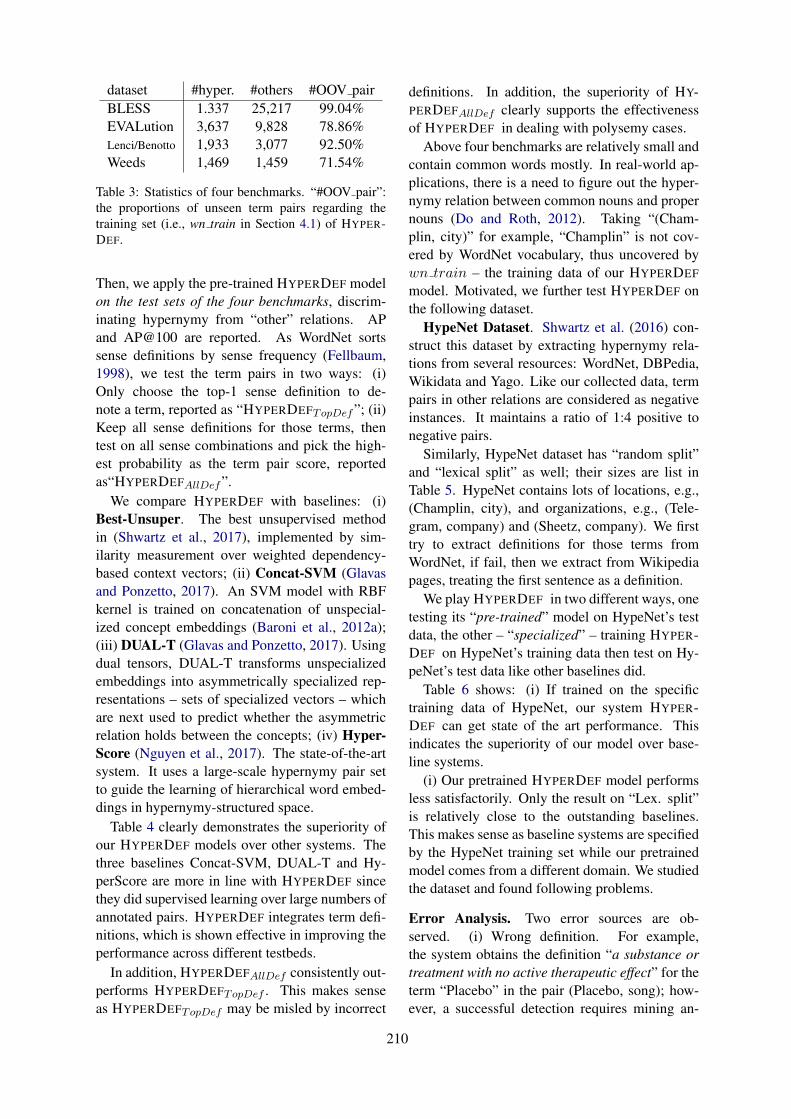
dataset #hyper. #others #OOV pairBLESS 1.337 25,217 99.04%EVALution 3,637 9,828 78.86%Lenci/Benotto 1,933 3,077 92.50%Weeds 1,469 1,459 71.54%
Table 3: Statistics of four benchmarks. “#OOV pair”:the proportions of unseen term pairs regarding thetraining set (i.e., wn train in Section 4.1) of HYPER-DEF.
Then, we apply the pre-trained HYPERDEF modelon the test sets of the four benchmarks, discrim-inating hypernymy from “other” relations. APand AP@100 are reported. As WordNet sortssense definitions by sense frequency (Fellbaum,1998), we test the term pairs in two ways: (i)Only choose the top-1 sense definition to de-note a term, reported as “HYPERDEFTopDef”; (ii)Keep all sense definitions for those terms, thentest on all sense combinations and pick the high-est probability as the term pair score, reportedas“HYPERDEFAllDef”.
We compare HYPERDEF with baselines: (i)Best-Unsuper. The best unsupervised methodin (Shwartz et al., 2017), implemented by sim-ilarity measurement over weighted dependency-based context vectors; (ii) Concat-SVM (Glavasand Ponzetto, 2017). An SVM model with RBFkernel is trained on concatenation of unspecial-ized concept embeddings (Baroni et al., 2012a);(iii) DUAL-T (Glavas and Ponzetto, 2017). Usingdual tensors, DUAL-T transforms unspecializedembeddings into asymmetrically specialized rep-resentations – sets of specialized vectors – whichare next used to predict whether the asymmetricrelation holds between the concepts; (iv) Hyper-Score (Nguyen et al., 2017). The state-of-the-artsystem. It uses a large-scale hypernymy pair setto guide the learning of hierarchical word embed-dings in hypernymy-structured space.
Table 4 clearly demonstrates the superiority ofour HYPERDEF models over other systems. Thethree baselines Concat-SVM, DUAL-T and Hy-perScore are more in line with HYPERDEF sincethey did supervised learning over large numbers ofannotated pairs. HYPERDEF integrates term defi-nitions, which is shown effective in improving theperformance across different testbeds.
In addition, HYPERDEFAllDef consistently out-performs HYPERDEFTopDef . This makes senseas HYPERDEFTopDef may be misled by incorrect
definitions. In addition, the superiority of HY-PERDEFAllDef clearly supports the effectivenessof HYPERDEF in dealing with polysemy cases.
Above four benchmarks are relatively small andcontain common words mostly. In real-world ap-plications, there is a need to figure out the hyper-nymy relation between common nouns and propernouns (Do and Roth, 2012). Taking “(Cham-plin, city)” for example, “Champlin” is not cov-ered by WordNet vocabulary, thus uncovered bywn train – the training data of our HYPERDEF
model. Motivated, we further test HYPERDEF onthe following dataset.
HypeNet Dataset. Shwartz et al. (2016) con-struct this dataset by extracting hypernymy rela-tions from several resources: WordNet, DBPedia,Wikidata and Yago. Like our collected data, termpairs in other relations are considered as negativeinstances. It maintains a ratio of 1:4 positive tonegative pairs.
Similarly, HypeNet dataset has “random split”and “lexical split” as well; their sizes are list inTable 5. HypeNet contains lots of locations, e.g.,(Champlin, city), and organizations, e.g., (Tele-gram, company) and (Sheetz, company). We firsttry to extract definitions for those terms fromWordNet, if fail, then we extract from Wikipediapages, treating the first sentence as a definition.
We play HYPERDEF in two different ways, onetesting its “pre-trained” model on HypeNet’s testdata, the other – “specialized” – training HYPER-DEF on HypeNet’s training data then test on Hy-peNet’s test data like other baselines did.
Table 6 shows: (i) If trained on the specifictraining data of HypeNet, our system HYPER-DEF can get state of the art performance. Thisindicates the superiority of our model over base-line systems.
(i) Our pretrained HYPERDEF model performsless satisfactorily. Only the result on “Lex. split”is relatively close to the outstanding baselines.This makes sense as baseline systems are specifiedby the HypeNet training set while our pretrainedmodel comes from a different domain. We studiedthe dataset and found following problems.
Error Analysis. Two error sources are ob-served. (i) Wrong definition. For example,the system obtains the definition “a substance ortreatment with no active therapeutic effect” for theterm “Placebo” in the pair (Placebo, song); how-ever, a successful detection requires mining an-
210
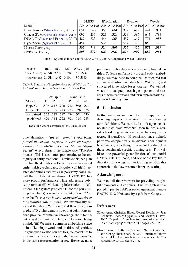
BLESS EVALuation Benotto WeedsModel AP AP@100 AP AP@100 AP AP@100 AP AP@100Best-Unsuper (Shwartz et al., 2017) .051 .540 .353 .661 .382 .617 .441 .911Concat-SVM (Glavas and Ponzetto, 2017) .097 .235 .321 .329 .523 .586 .644 .793DUAL-T (Glavas and Ponzetto, 2017) .487 .823 .446 .866 .557 .847 .774 .985HyperScore (Nguyen et al., 2017) .454 – .538 – .574 – .850 –HYPERDEFTopDef .595 .749 .524 .867 .557 .825 .872 .989HYPERDEFAllDef .508 .872 .623 .927 .576 .909 .889 .991
Table 4: System comparison on BLESS, EVALution, Benotto and Weeds datasets
Dataset train dev test #OOV pairHypeNet (rnd) 49.5K 3.5K 17.7K 95.56%HypeNet (lex) 20.3K 1.4K 6.6K 95.33%
Table 5: Statistics of HypeNet dataset. “#OOV pair” isfor “test” regarding the “wn train” of HYPERDEF.
Lex. split Rand. splitModel P R F1 P R F1
HypeNet .809 .617 .700 .913 .890 .901DUAL-T .705 .785 .743 .933 .826 .876pre-trained .572 .717 .637 .474 .601 .530specialized .670 .914 .773 .892 .935 .913
Table 6: System comparison on HypeNet test
other definition – “are an alternative rock band,formed in London, England in 1994 by singer-guitarist Brian Molko and guitarist-bassist StefanOlsdal” which depicts the article title “Placebo(band)”. This is a common problem due to the am-biguity of entity mentions. To relieve this, we planto refine the definition retrieval by more advancedentity linking techniques, or retrieve all highly re-lated definitions and test as in polysemy cases (re-call that in Table 4 we showed HYPERDEF hasmore robust performance while addressing poly-semy terms); (ii) Misleading information in defi-nitions. Our system predicts “1” for the pair (Au-rangabad, India); we analyze the definition of “Au-rangabad”: is a city in the Aurangabad district ofMaharashtra state in India. We intentionally re-moved the phrase “in India”, and then the systempredicts “0”. This demonstrates that definitions in-deed provide informative knowledge about terms,but a system must be intelligent to avoid beingmisled; (iii) We miss a common embedding spaceto initialize single words and (multi-word) entities.To generalize well to new entities, the model has topresume the new entities and the known terms liein the same representation space. However, most
pretrained embedding sets cover pretty limited en-tities. To learn uniformed word and entity embed-dings, we may need to combine unstructured textcorpus, semi-structured data (e.g., Wikipedia) andstructured knowledge bases together. We will ad-vance this data preprocessing component – the ac-cess of term definitions and term representations –in our released system.
5 Conclusion
In this work, we introduced a novel approach todetecting hypernymy relations by incorporatingterm definitions. We extracted a task-agnostic an-notated data from WordNet, then trained a neu-ral network to generate a universal hypernymy de-tector, HYPERDEF. HYPERDEF, once trained,performs competitively in diverse open-domainbenchmarks, even though it was not fine-tuned onthose benchmark-specific training sets. This val-idates the powerful generalization of our modelHYPERDEF. Our hope, and one of the key futuredirections following this work is to generalize thisapproach to the low-resource language setting.
Acknowledgments
We thank all the reviewers for providing insight-ful comments and critiques. This research is sup-ported in part by DARPA under agreement numberFA8750-13-2-0008, and by a gift from Google.
References
Soren Auer, Christian Bizer, Georgi Kobilarov, JensLehmann, Richard Cyganiak, and Zachary G. Ives.2007. Dbpedia: A nucleus for a web of open data.In Proceedings of ISWC/ASWC. pages 722–735.
Marco Baroni, Raffaella Bernardi, Ngoc-Quynh Do,and Chung-chieh Shan. 2012a. Entailment abovethe word level in distributional semantics. In Pro-ceedings of EACL. pages 23–32.
211
Marco Baroni, Raffaella Bernardi, Ngoc-Quynh Do,and Chung-chieh Shan. 2012b. Entailment abovethe word level in distributional semantics. In Pro-ceedings of EACL. pages 23–32.
Marco Baroni and Alessandro Lenci. 2011. How weBLESSed distributional semantic evaluation. InProceedings of the GEMS 2011 Workshop on GE-ometrical Models of Natural Language Semantics.pages 1–10.
Giulia Benotto. 2015. Distributional models forsemantic relations: A study on hyponymy andantonymy. PhD Thesis, University of Pisa .
Samuel R. Bowman, Gabor Angeli, Christopher Potts,and Christopher D. Manning. 2015. A large anno-tated corpus for learning natural language inference.In Proceedings of EMNLP. pages 632–642.
Haw-Shiuan Chang, ZiYun Wang, Luke Vilnis, andAndrew McCallum. 2017. Unsupervised hypernymdetection by distributional inclusion vector embed-ding. CoRR abs/1710.00880.
Ido Dagan, Dan Roth, Mark Sammons, and Fabio Mas-simo Zanzoto. 2013. Recognizing textual entail-ment: Models and applications.
Quang Xuan Do and Dan Roth. 2012. Exploiting thewikipedia structure in local and global classificationof taxonomic relations. Natural Language Engi-neering 18(2):235–262.
John Duchi, Elad Hazan, and Yoram Singer. 2011.Adaptive subgradient methods for online learningand stochastic optimization. JMLR 12:2121–2159.
Christiane Fellbaum. 1998. WordNet: An ElectronicLexical Database. MIT Press.
Ruiji Fu, Jiang Guo, Bing Qin, Wanxiang Che, HaifengWang, and Ting Liu. 2014. Learning semantic hi-erarchies via word embeddings. In Proceedings ofACL. pages 1199–1209.
Goran Glavas and Simone Paolo Ponzetto. 2017.Dual tensor model for detecting asymmetric lexico-semantic relations. In Proceedings of EMNLP.pages 1757–1767.
Marti A. Hearst. 1992. Automatic acquisition of hy-ponyms from large text corpora. In Proceedings ofCOLING. pages 539–545.
Felix Hill, KyungHyun Cho, Anna Korhonen, andYoshua Bengio. 2016. Learning to understandphrases by embedding the dictionary. TACL 4:17–30.
Sepp Hochreiter and Jurgen Schmidhuber. 1997.Long short-term memory. Neural computation9(8):1735–1780.
Yann LeCun, Leon Bottou, Yoshua Bengio, and PatrickHaffner. 1998. Gradient-based learning applied todocument recognition. In Proceedings of the IEEE.pages 2278–2324.
Omer Levy, Steffen Remus, Chris Biemann, and IdoDagan. 2015. Do supervised distributional methodsreally learn lexical inference relations? In Proceed-ings of NAACL. pages 970–976.
Tomas Mikolov, Ilya Sutskever, Kai Chen, Greg S Cor-rado, and Jeff Dean. 2013. Distributed representa-tions of words and phrases and their compositional-ity. In Proceedings of NIPS. pages 3111–3119.
Mike Mintz, Steven Bills, Rion Snow, and Daniel Ju-rafsky. 2009. Distant supervision for relation extrac-tion without labeled data. In Proceedings of ACL.pages 1003–1011.
Kim Anh Nguyen, Maximilian Koper, Sabine Schulteim Walde, and Ngoc Thang Vu. 2017. Hierarchicalembeddings for hypernymy detection and direction-ality. In Proceedings of EMNLP. pages 233–243.
Tim Rocktaschel, Edward Grefenstette, Karl MoritzHermann, Tomas Kocisky, and Phil Blunsom. 2016.Reasoning about entailment with neural attention.In Proceedings of ICLR.
Stephen Roller and Katrin Erk. 2016. Relations suchas hypernymy: Identifying and exploiting hearst pat-terns in distributional vectors for lexical entailment.In Proceedings of EMNLP. pages 2163–2172.
Stephen Roller, Katrin Erk, and Gemma Boleda. 2014.Inclusive yet selective: Supervised distributional hy-pernymy detection. In Proceedings of COLING.pages 1025–1036.
Enrico Santus, Frances Yung, Alessandro Lenci, andChu-Ren Huang. 2015. EVALution 1.0: An evolv-ing semantic dataset for training and evaluation ofdistributional semantic models. In Proceedings ofthe 4th Workshop on Linked Data in Linguistics.pages 64–69.
Ashish Kumar Saxena, Ganesh Viswanath Sambhu,Saroj Kaushik, and L. Venkata Subramaniam. 2007.IITD-IBMIRL system for question answering usingpattern matching, semantic type and semantic cate-gory recognition. In Proceedings of TREC.
Vered Shwartz, Yoav Goldberg, and Ido Dagan. 2016.Improving hypernymy detection with an integratedpath-based and distributional method. In Proceed-ings of ACL.
Vered Shwartz, Omer Levy, Ido Dagan, and JacobGoldberger. 2015. Learning to exploit structuredresources for lexical inference. In Proceedings ofCoNLL. pages 175–184.
Vered Shwartz, Enrico Santus, and DominikSchlechtweg. 2017. Hypernyms under siege:Linguistically-motivated artillery for hypernymydetection. In Proceedings of EACL. pages 65–75.
Rion Snow, Daniel Jurafsky, and Andrew Y. Ng. 2004.Learning syntactic patterns for automatic hypernymdiscovery. In Proceedings of NIPS. pages 1297–1304.
212

Fabian M. Suchanek, Gjergji Kasneci, and GerhardWeikum. 2007. Yago: A core of semantic knowl-edge. In Proceedings of WWW. pages 697–706.
Luke Vilnis and Andrew McCallum. 2015. Word rep-resentations via gaussian embedding. In Proceed-ings of ICLR.
Denny Vrandecic. 2012. Wikidata: A new platformfor collaborative data collection. In Proceedings ofWWW. pages 1063–1064.
Ivan Vulic and Nikola Mrksic. 2017. Specialis-ing word vectors for lexical entailment. CoRRabs/1710.06371.
Julie Weeds, Daoud Clarke, Jeremy Reffin, David J.Weir, and Bill Keller. 2014. Learning to distinguishhypernyms and co-hyponyms. In Proceedings ofCOLING. pages 2249–2259.
Wenpeng Yin, Katharina Kann, Mo Yu, and Hin-rich Schutze. 2017. Comparative study of CNNand RNN for natural language processing. CoRRabs/1702.01923.
Wenpeng Yin and Hinrich Schutze. 2017. Attentiveconvolution. CoRR abs/1710.00519.
Peter Young, Alice Lai, Micah Hodosh, and JuliaHockenmaier. 2014. From image descriptions to vi-sual denotations: New similarity metrics for seman-tic inference over event descriptions. TACL 2:67–78.
213

Proceedings of the 7th Joint Conference on Lexical and Computational Semantics (*SEM), pages 214–224New Orleans, June 5-6, 2018. c©2018 Association for Computational Linguistics
Agree or Disagree: Predicting Judgments on Nuanced Assertions
Michael Wojatzki Torsten ZeschLanguage Technology Lab
University of Duisburg-Essen, [email protected]
Saif M. Mohammad Svetlana KiritchenkoNational Research Council Canada
Ottawa, [email protected]
Abstract
Being able to predict whether people agree ordisagree with an assertion (i.e. an explicit, self-contained statement) has several applicationsranging from predicting how many people willlike or dislike a social media post to classi-fying posts based on whether they are in ac-cordance with a particular point of view. Weformalize this as two NLP tasks: predictingjudgments of (i) individuals and (ii) groupsbased on the text of the assertion and previ-ous judgments. We evaluate a wide range ofapproaches on a crowdsourced data set con-taining over 100,000 judgments on over 2,000assertions. We find that predicting individualjudgments is a hard task with our best resultsonly slightly exceeding a majority baseline.Judgments of groups, however, can be morereliably predicted using a Siamese neural net-work, which outperforms all other approachesby a wide margin.
1 Introduction
One of the most basic reactions when reading asentence is to agree or disagree with it.1 Mech-anisms that allow us to express agreement (e.g.thumb-up, like, up-vote, ♥) or disagreement (e.g.thumb-down, dislike, down-vote) towards postsof other users can be found in almost all socialnetworking sites. The judgments associated withposts that discuss controversial political or socialissues, such as legalization of drug, immigrationpolicy, or gun rights, are a rich source of infor-mation for those interested in the opinions of in-dividuals or groups. For instance, public opinionregarding an issue is often illustrated by the num-ber of retweets, likes, or upvotes that a politicianor influential person receives.
1You are probably thinking about whether you agree withthat statement right now.
Hence, especially for controversial issues, be-ing able to predict how people judge posts has sev-eral applications: people at large could automati-cally anticipate if politicians, companies or otherdecision makers would agree or disagree with anew perspective on a problem or how they wouldevaluate a new possible solution. The method canalso be used by journalists to more accurately ana-lyze the homogeneity of opinions or to detect filterbubbles in social media. Decision makers them-selves would be able to evaluate in advance howcitizens, customers, or employees react to a pressannouncement, a new regulation, or tweet. Socialmedia users could be enabled to search, sort or fil-ter posts based on whether they are in accordancewith or contrary to their personal world view. Suchpredictions could also be used to augment chat ap-plications by indicating to a user if her recipientswill agree or disagree with a message to be sent,enabling to choose a more or less confrontationaldiscussion style.
In this paper, we describe how the outlined usecases can be framed as two inference tasks: pre-dicting individual judgments and predicting judg-ments of whole groups. As a first step, we restrictourselves to judgments on textual utterances thatare explicit, relevant, and that do not contain mul-tiple positions. We will refer to such utterances asassertions. For solving the tasks, we define the de-gree to which two assertions are judged similar asjudgment similarity. This similarity allows us topredict a judgment based on other judgments thathave been made on similar, known assertions.
Across both tasks, we compare this strategyagainst several baselines and reference approacheson a newly crowdsourced data set containing over100 000 judgments on assertions. We find that,for predicting individual judgments, our best re-sults only slightly exceed a majority baseline, butthat judgments of groups can be more reliably pre-
214

Figure 1: Overview on the two prediction tasks.
dicted using a Siamese neural network, which out-performs all other approaches by a wide margin.
2 Predicting Judgments
In order to predict if someone will agree withan assertion, we need knowledge about that per-son. Ideally, we would have access to a large setof other assertions which the person has alreadyjudged. We could then measure the similarity be-tween previous assertions and the new assertionand hypothesize that the judgment on the new as-sertion should be the same as for a highly similarone. In Figure 1, we show this case for binary(yes/no) predictions on individuals and argue thatthis can be also generalized to probabilistic pre-dictions on groups of people. Thus, we formulatetwo prediction tasks:
In the first task, we want to predict judgmentsof individuals on assertions based on other judg-ments by the same person. Thus, the first task isformulated as follows: given a set of assertionsa1, ..., an relevant to an issue and the judgmentsof a person pi on a1, ..., an−1 an automatic systemhas to predict pi’s judgment on the assertion an.
In the second task, we want to predict judg-ments of groups on assertions based on averagedjudgments of other assertions. Hence, this taskcan be formalized as follows: given a set of judg-ments of a group of persons p1, ..., pk on the asser-tions a1, ..., an−1, an automatic systems must pre-dict the judgment on the assertion an for the samegroup of persons. Judgments of groups can beexpressed by an aggregated agreement score be-tween -1 and 1, where -1 means that every persondisagrees to an assertion and 1 that every personagrees to the assertion.
For measuring the similarity between two asser-tions, we propose to compare how a large groupof people judges them. We define the degree towhich two assertions are judged similarly by alarge group as the judgment similarity of the twoassertions. However, judgments of other persons
are not easily available – e.g. if we want to predicta judgment on a new, unseen assertion. To over-come this limitation, we propose to use methodsthat consider the texts of the assertions to mimicjudgment similarity and have thus the ability togeneralize from existing data collections.
3 Related Work
Measuring the judgment similarity of two asser-tions is related to several NLP tasks such as thedetection of semantic text similarity (STS) (Agirreet al., 2012), paraphrase recognition (Bhagat andHovy, 2013), and textual entailment (Dagan et al.,2009).
Unlike semantic text similarity, we do not usea notation of similarity based on the intuition ofhumans, but one that derives from the context ofjudgments. Hence, we define that the judgmentsimilarity of two assertions is 1 if two assertionsare consistently judged the same and are thus in-terchangeable in the context of our task.
There are several reasons why assertions arejudged similarly: their text may convey similar se-mantics such as in the assertions ‘Marijuana alle-viates the suffering of chronically ill patients’ and‘Marijuana helps chronically ill persons’. Thistype of similarity corresponds to what methodsof semantic text similarity capture. However, astrong judgment similarity of two assertions canalso be due to semantically entailed relationshipsbetween assertions. For instance, if people agreewith ‘Marijuana is a gateway drug for teenagersand damages growing brains’ most of them alsoagree to ‘Marijuana is dangerous for minors’, de-spite the texts being different in content and hav-ing thus low semantic text similarity. In addition,two assertions can also have a strong judgmentsimilarity because of underlying socio-cultural,political, or personal factors. For instance, the as-sertions ‘Consuming Marijuana has no impact onyour success at work’ and ‘Marijuana is not ad-dictive’ describe different arguments for legalizingmarijuana, but judgments made on these assertionsare often correlated.
Our work also relates to other attempts on pre-dicting reactions to text, such as predicting thenumber of retweets (Suh et al., 2010; Petrovicet al., 2011), the number of likes on tweets (Tanet al., 2014), the number of karma points of red-dit posts (Wei et al., 2016), or sales from prod-uct descriptions (Pryzant et al., 2017). What those
215
works have in common is that they measure somekind of popularity, which differs significantly fromour task: even if one agrees with a text, one mightdecide not to retweet or like it for any number ofreasons. There are also cases in which one mayretweet a post with which one disagrees in orderto flag someone or something from the opposingcommunity. Furthermore, there are effects suchas the author’s followers affecting the visibilityof posts and thereby the likelihood of a like or aretweet (Suh et al., 2010).
In addition, we relate to works that aim at pre-dicting whether two texts (Menini and Tonelli,2016) or sequences of utterances (Wang andCardie, 2014; Celli et al., 2016) express agreementor disagreement with each other. More broadly,we also relate to works that analyze stance (Mo-hammad et al., 2016; Xu et al., 2016; Taule et al.,2017), sentiment (Pang and Lee, 2008; Liu, 2012;Mohammad, 2016), or arguments (Habernal andGurevych, 2016; Boltuzic and Snajder, 2016; Bar-Haim et al., 2017) that are expressed via text. Incontrast to these works, we do not examine whatjudgment, sentiment, or claim is expressed by atext, but whether we can infer agreement or dis-agreement based on judgments which were madeon other assertions.
Finally, we relate to work on analyzing and pre-dicting outcomes of congressional roll-call voting.These works constantly find that votes of politi-cians can be explained by a low number of under-lying, ideological dimensions such as being leftor right (Heckman and Snyder, 1996; Poole andRosenthal, 1997, 2001). Our work is differentfrom these attempts, as we do not consider politi-cians who might have incentives to vote in accor-dance with the ideological views of their party, andas we base our prediction on the text of assertions.
4 Data Collection
For exploring how well the two tasks can be solvedautomatically, we use the dataset Nuanced Asser-tions on Controversial Issues (NAoCI) created byWojatzki et al. (2018). The dataset contains as-sertions judged on a wide range of controversialissues.2 The NAoCI dataset mimics a commonsituation in many social media sites, where peo-ple e.g. up- or downvote social media posts. How-ever, it does not have the experimental problems
2The dataset is accessible from https://sites.google.com/view/you-on-issues/
of using social media data directly. These prob-lems include legal reasons of scraping social me-dia data and moderator variables such as the defi-nition of issues, the influence of previous posts, orthe question of whether someone is not judging anassertion because she does not want to judge it orbecause she did not perceive it.
The data was collected using crowdsourcingconducted on crowdflower.com in two steps.First, participants were asked to generate a largeset of assertions relevant to controversial issues.The set of assertions was created using crowd-sourcing, as a manual creation of assertions wouldbe potentially incomplete and subject to personalbias. We provided instructions to make sure thatthe assertions are natural, self-contained state-ments about an issue. Next, a large number ofpeople was asked to indicate whether they agreeor disagree with these assertions.
The process was reviewed and approved by theinstitutional ethics board of the National ResearchCouncil Canada.
Generating Assertions In order to obtain real-istic assertions, 69 participants were asked to gen-erate assertions for sixteen predefined issues (seeTable 1). For each issue, the subjects were givendefinition of the issue and a few example asser-tions. In addition, the instructions state that as-sertions should be explicit, relevant to an issue,self-contained, and only contain a single position.Specifically, the use of co-reference or hedging in-dicated by words such as perhaps, maybe, or pos-sibly was not permitted. After a removal of dupli-cates and instances that did not follow the rules,this process resulted in about 150 unique asser-tions per issue (2,243 in total).
Judging Assertions Next, 230 subjects wereasked to indicate whether they agree or disagreewith an assertion, resulting in over 100 000 judg-ments (see Table 1). The participants were freeto judge as many assertions on as many issues asthey wanted. On average each assertion is judgedby about 45 persons and each participant judgedover 400 assertions. For each person, agreement isencoded with 1, disagreement with −1, and miss-ing values with 0 (as not all subjects judged allassertions). Additionally, we can also computethe aggregated agreement score for each assertionby simply subtracting the percentage of partici-pants that disagreed with the assertion from the
216
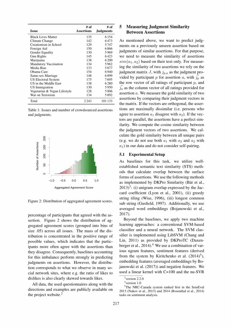
# of # ofIssue Assertions Judgments
Black Lives Matter 135 6 154Climate Change 142 6 473Creationism in School 129 5 747Foreign Aid 150 6 866Gender Equality 130 5 969Gun Rights 145 6 423Marijuana 138 6 200Mandatory Vaccination 134 5 962Media Bias 133 5 877Obama Care 154 6 940Same-sex Marriage 148 6 899US Electoral System 175 7 695US in the Middle East 138 6 280US Immigration 130 5 950Vegetarian & Vegan Lifestyle 128 5 806War on Terrorism 134 5 892
Total 2 243 101 133
Table 1: Issues and number of crowdsourced assertionsand judgments.
Aggregated Agreement Score
Num
ber
of A
sser
tions
−1.0 −0.5 0.0 0.5 1.0
050
100
150
200
Figure 2: Distribution of aggregated agreement scores.
percentage of participants that agreed with the as-sertion. Figure 2 shows the distribution of ag-gregated agreement scores (grouped into bins ofsize .05) across all issues. The mass of the dis-tribution is concentrated in the positive range ofpossible values, which indicates that the partic-ipants more often agree with the assertions thanthey disagree. Consequently, baselines accountingfor this imbalance perform strongly in predictingjudgments on assertions. However, the distribu-tion corresponds to what we observe in many so-cial network sites, where e.g. the ratio of likes todislikes is also clearly skewed towards likes.
All data, the used questionnaires along with thedirections and examples are publicly available onthe project website.2
5 Measuring Judgment SimilarityBetween Assertions
As mentioned above, we want to predict judg-ments on a previously unseen assertion based onjudgments of similar assertions. For that purpose,we need to measure the similarity of assertionssim(a1, a2) based on their text only. For measur-ing the similarity of two assertions we rely on thejudgment matrix J , with jp,a as the judgment pro-vided by participant p for assertion a, with ~jp asthe row vector of all ratings of participant p, and~ja as the column vector of all ratings provided forassertion a. We measure the gold similarity of twoassertions by comparing their judgment vectors inthe matrix. If the vectors are orthogonal, the asser-tions are maximally dissimilar (i.e. persons whoagree to assertion a1 disagree with a2). If the vec-tors are parallel, the assertions have a perfect sim-ilarity. We compute the cosine similarity betweenthe judgment vectors of two assertions. We cal-culate the gold similarity between all unique pairs(e.g. we do not use both a1 with a2 and a2 witha1) in our data and do not consider self-pairing.
5.1 Experimental SetupAs baselines for this task, we utilize well-established semantic text similarity (STS) meth-ods that calculate overlap between the surfaceforms of assertions. We use the following methodsas implemented by DKPro Similarity (Bar et al.,2013)3: (i) unigram overlap expressed by the Jac-card coefficient (Lyon et al., 2001), (ii) greedystring tiling (Wise, 1996), (iii) longest commonsub string (Gusfield, 1997). Additionally, we useaveraged word embeddings (Bojanowski et al.,2017).
Beyond the baselines, we apply two machinelearning approaches: a conventional SVM-basedclassifier and a neural network. The SVM clas-sifier is implemented using LibSVM (Chang andLin, 2011) as provided by DKProTC (Daxen-berger et al., 2014).4 We use a combination of var-ious ngram features, sentiment features (derivedfrom the system by Kiritchenko et al. (2014)5),embedding features (averaged embeddings by Bo-janowski et al. (2017)) and negation features. Weused a linear kernel with C=100 and the nu-SVR
3version 2.2.04version 1.05The NRC-Canada system ranked first in the SemEval
2013 (Nakov et al., 2013) and 2014 (Rosenthal et al., 2014)tasks on sentiment analysis.
217

regression model. Iterative experiments showedthat this configuration gave the most stable resultsacross the issues. For the neural approach, weadapt Siamese neural networks (SNN), which con-sist of two identical branches or sub-networks thattry to extract useful representations of the asser-tions and a final layer that merges these branches.SNNs have been successfully used to predict textsimilarity (Mueller and Thyagarajan, 2016; Necu-loiu et al., 2016) and match pairs of sentences (e.g.a tweet to reply) (Hu et al., 2014). In our SNN, abranch consists of a layer that translates the asser-tions into sequences of word embeddings, whichis followed by a convolution layer with a filtersize of two, max pooling over time layer, and adense layer. To merge the branches, we calculatethe cosine similarity of the extracted vector repre-sentations. The SNN was implemented using thedeep learning framework deepTC (Horsmann andZesch, 2018) in conjunction with Keras6 and Ten-sorflow (Abadi et al., 2016). In order to ensure fullreproducibility of our results, the source code forboth approaches is publicly available.7 We eval-uate all approaches using 10-fold cross validationand calculate Pearson correlation between the pre-diction and the gold similarity.
5.2 Results
Table 2 shows the correlation of all approaches av-eraged over all sixteen issues.8 Overall, the STSbaselines result in very low correlation coefficientsbetween .02 and .07, while the trained models ob-tain coefficients around .6. This shows that thesystems can learn useful representations that cap-ture judgment similarity and that this representa-tion is indeed different from semantic similarity.Since both models are purely lexical and still yieldreliable performance, we suspect that the relation-ship between a pair of assertions and their judg-ment similarity also has a lexical nature.
While STS baselines obtain consistently low re-sults, we observe largely differing results per is-sues (ranging from .32 to .72) with SVM and SNNbehaving alike. Detailed results for each issue arelisted in Table 3.
In order to better understand the results, we ex-
6https://keras.io/
7https://github.com/muchafel/judgmentPrediction
8As Pearsons r is defined in a probabilistic space it can-not be averaged directly. Therefore, we first z-transform thescores, average them and then transform them back into theoriginal range of values.
Method r
SNN .61SVM .58Embedding distance .07Jaccard .07Greedy string tiling .06Longest common sub string .05
Table 2: Pearson correlation (averaged over all issues)of text-based approaches for approximating similarityof assertion judgments.5
Issue SVM SNN
Climate Change .70 .72Gender Equality .67 .73Mandatory Vaccination .68 .74Obama Care .66 .70Black Lives Matter .66 .74Media Bias .63 .63US Electoral System .63 .59Same-sex Marriage .59 .61War on Terrorism .56 .59Foreign Aid .54 .46US in the Middle East .52 .55US Immigration .52 .57Gun Rights .51 .64Creationism in school .48 .51Vegetarian and Vegan Lifestyle .43 .40Legalization of Marijuana .37 .32
Table 3: Correlation coefficients of the similarity pre-diction by the SVM and the SNN, obtained in 10 foldcross-validation.
amine the scatter-plots that visualize assignmentof gold to prediction (x–Axis: gold, y–Axis: pre-diction) and investigate cases that deviate stronglyfrom an ideal correlation. Figure 3 shows the scat-ter plot for the issue Climate Change for both clas-sifiers. For the SVM we observe that there is agroup of pairs that is predicted inversely propor-tional, i.e. their gold value is positive, but the re-gression assigns a clearly negative value. We ob-serve that these instances mainly correspond topairs in which both assertions have high negativeword scores. For instance the pair, ‘There is nota real contribution of human activities in Climatechange’ and ‘Climate change was made up by thegovernment to keep people in fear’, have a com-parable high similarity of .20. The SVM, how-ever, assigns them a similarity score of −.38. Wesuspect that this effect results from the distribu-tion of similarity scores that is skewed to the posi-tive range of possible scores. Therefore, the SVMprobably assigns too much weight to ngrams thatsignal a negative score. Far less pronounced, forthe neural approach, we find instances whose gold
218
values are negative, but which are assigned a pos-itive value. When inspecting these pairs we findthat many of them contain one assertion whichuses a negation (e.g. not, unsure, or unlikely). Anexample for this is the pair, ‘There has been an in-crease in tropical storms of greater intensity whichcan be attributed to climate change’ and ‘Differentchanges in weather does not mean global warm-ing’, that have a low similarity in the gold data(−0.19), but get assigned a rather high similarityscore (.20).
6 Predicting Judgments of Individuals
Now that we have means for quite reliably esti-mating the judgment similarity of assertions, wecan try to predict judgments on individual asser-tions. We compare the judgment similarity meth-ods against several baselines and collaborative fil-tering methods (that make use of judgments thatare made by other persons to calculate person andassertion similarity).
Baselines (BL) The random baseline predictsagree or disagree for each assertion. We alsodefine the all agree baseline, which always pre-dicts agree. As the data contains substantiallymore agree judgments than disagree judgments(c.f. Figure 2), this is a strong baseline. As athird baseline, we average all known judgments ofa person and predict agree if this value is positiveand predict disagree otherwise. We refer to thisbaseline as tendency.
Judgment Similarity (JS) We use the above de-fined judgment similarity methods to calculate thesimilarity between each of the assertions previ-ously judged by that person and the assertion forwhich we want to make the prediction. Then wesimply transfer the judgment of the most similarassertion to the assertion of interest.9 To preventleakage, the scores of the prediction are taken fromthe models that have been trained in the cross val-idation. This means, for predicting the score ofa pair of assertions we use the model which doesnot include the pair in the training set. As the ma-trix is missing one entry for each prediction (i.e.the judgment on the assertion for which we wantto make the prediction), one could theoreticallyform a new matrix for each prediction and then
9Note that the subjects have all rated different numbers ofassertions. Thus, for the sake of comparability, we restrictourselves to the most similar assertion (as opposed to averag-ing a judgment over the n most similar assertions.)
re-calculate all cosines. However, we find thatthe judgment similarity between assertions doesnot change significantly when a single entry inthe vectors of the assertions is removed or added.Hence, due to computational complexity, the goldsimilarity was calculated over the entire matrix ofjudgments.
There are several assertions that do not have tex-tual overlap, which is why the STS methods oftenreturn a zero similarity. In such a case, we fallback on the all agree baseline. We refer to strate-gies which are based on judgment similarity asmost similar assertion (method), where methodindicates how the similarity is computed.
All strategies use all available context. For in-stance, if we want to predict the judgment of theassertion an and a prediction strategy considersother judgments, the strategy uses all the judg-ments on the assertions a1, ..., an−1.
Collaborative Filtering (CF) Collaborative fil-tering (Adomavicius and Tuzhilin, 2005; Schaferet al., 2007; Su and Khoshgoftaar, 2009) uses pre-viously made judgments and judgments made byothers to predict future judgments. Collaborativefiltering has been successfully used in applica-tion areas such shopping recommendations (Lin-den et al., 2003), or personalization of news (Daset al., 2007). Note that collaborative filtering re-quires knowledge of how others judged the asser-tion for which the system tries to make a predic-tion. Therefore, these strategies are not applicableif we want to predict judgments on a previouslyunseen assertion. Nevertheless, they represent anupper bound for our text-based predictions.
As a simple collaborative filtering strategy, wepredict how the majority of other persons judgedan assertion. Therefore, we average the judgmentsof all other users and predict agree if this valueis positive and disagree if the value is negative.This strategy will be referred to as mean other. Inaddition, we compute the similarity between pairsof people by calculating the cosine similarity be-tween the vector that corresponds to all judgmentsa person has made. We use this person–personsimilarity to determine the most similar personand then transfer the judgment on an of the userwhich is most similar to pi. We refer to this strat-egy as most similar user. We also use the (gold)judgment similarity between assertions to predictagree or disagree based on how the assertion thatis most similar to an has been judged. We call this
219

−0.4 −0.2 0.0 0.2 0.4 0.6
−0.
4−
0.2
0.0
0.2
0.4
0.6
gold judgment similarity
pred
icte
d ju
dgm
ent s
imila
rity
(a) SVM
−0.4 −0.2 0.0 0.2 0.4 0.6
−0.
4−
0.2
0.0
0.2
0.4
0.6
gold judgment similarity
pred
icte
d ju
dgm
ent s
imila
rity
(b) SNN
Figure 3: Comparison of gold judgment similarity and judgment similarity as predicted by the SVM and the SNNfor the issue Climate Change.
Strategy Type Accuracy
most similar user CF .85most similar assertion (gold) CF .76tendency BL .75mean other CF .74most similar assertion (SNN) JS .73most similar assertion (SVM) JS .72all agree BL .71most similar assertion (jaccard) JS .70most similar assertion (embedding) JS .68most similar assertion (gst) JS .69most similar assertion (lcss) JS .67random BL .50
Table 4: Accuracy of different approaches for predict-ing judgments of individuals.
strategy most similar assertion (gold).
6.1 Results
Table 4 shows the accuracy of the strategies acrossall issues obtained using leave-one-out cross val-idation. We observe that all strategies are signif-icantly better than the random baseline. On av-erage, the all agree strategy is more than 20%above the random baseline and thus represents ahighly competitive baseline. The tendency base-line, which is a refinement of all agree, is even4% higher. Only the collaborative filtering strate-gies most similar assertion and most similar userbeat this baseline. With an accuracy of about 85%the most similar user strategy performs best. Themethods that use the learned judgment similar-ity beat the all agree but fall behind the tendencybaseline. The fact that methods based on judgment
similarity are already close to their upper-bound(most similar assertion (gold)) shows that theirpotential is limited, even if measuring judgmentsimilarity can be significantly improved. One pos-sible explanation for comparably low performanceof most similar assertion is that the past assertionsare not sufficient to make a meaningful prediction.For instance, if only a few assertions have beenjudged in the past and none of them is similar toa new assertion, then a prediction becomes guess-ing. As expected from their poor performance ofapproximating judgment similarity, the methodsrelying on STS measures fall behind the all agree.
7 Predicting Judgments of Groups
We now turn to predicting judgments of groups,i.e. the task of estimating what percentage of agroup of people are likely to agree to an asser-tion. We illustrate the prediction task in the fol-lowing example: From the assertion ‘Marijuana isalmost never addictive’ with an aggregated agree-ment score of 0.9 we want to predict a compara-tively lower value for the assertion ‘Marijuana issometimes addictive’.
Direct Prediction (DP) As a reference ap-proach, we train different regression models thatpredict the aggregated agreement score directlyfrom the text of the assertion. We train each modelover all issues in order to achieve the necessarygeneralization.
Again, we compare more traditional modelsbased on feature engineering and neural models.
220
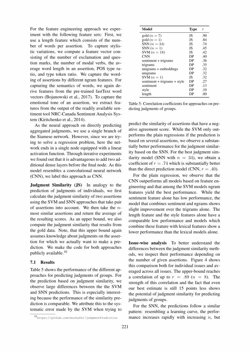
For the feature engineering approach we exper-iment with the following feature sets: First, weuse a length feature which consists of the num-ber of words per assertion. To capture stylis-tic variations, we compute a feature vector con-sisting of the number of exclamation and ques-tion marks, the number of modal verbs, the av-erage word length in an assertion, POS type ra-tio, and type token ratio. We capture the word-ing of assertions by different ngram features. Forcapturing the semantics of words, we again de-rive features from the pre-trained fastText wordvectors (Bojanowski et al., 2017). To capture theemotional tone of an assertion, we extract fea-tures from the output of the readily available sen-timent tool NRC-Canada Sentiment Analysis Sys-tem (Kiritchenko et al., 2014).
As the neural approach on directly predictingaggregated judgments, we use a single branch ofthe Siamese network. However, since we are try-ing to solve a regression problem, here the net-work ends in a single node equipped with a linearactivation function. Through iterative experimentswe found out that it is advantageous to add two ad-ditional dense layers before the final node. As thismodel resembles a convolutional neural network(CNN), we label this approach as CNN.
Judgment Similarity (JS) In analogy to theprediction of judgments of individuals, we firstcalculate the judgment similarity of two assertionsusing the SVM and SNN approaches that take pairof assertions into account. We then take the n-most similar assertions and return the average ofthe resulting scores. As an upper bound, we alsocompute the judgment similarity that results fromthe gold data. Note, that this upper bound againassumes knowledge about judgments on the asser-tion for which we actually want to make a pre-diction. We make the code for both approachespublicly available.10
7.1 ResultsTable 5 shows the performance of the different ap-proaches for predicting judgments of groups. Forthe prediction based on judgment similarity, weobserve large differences between the the SVMand SNN predictions. This is especially interest-ing because the performance of the similarity pre-diction is comparable. We attribute this to the sys-tematic error made by the SVM when trying to
10https://github.com/muchafel/judgmentPrediction
Model Type r
gold (n = 7) JS .90gold (n = 1) JS .84SNN (n = 34) JS .74SNN (n = 1) JS .45SVM (n = 18) JS .42CNN DP .40sentiment + trigrams DP .36trigrams DP .35unigrams + embeddings DP .32unigrams DP .32SVM (n = 1) JS .32sentiment + trigrams + style DP .27sentiment DP .13style DP .10length DP .00
Table 5: Correlation coefficients for approaches on pre-dicting judgments of groups.
predict the similarity of assertions that have a neg-ative agreement score. While the SVM only out-performs the plain regressions if the prediction isbased on several assertions, we observe a substan-tially better performance for the judgment similar-ity based on the SNN. For the best judgment sim-ilarity model (SNN with n = 34), we obtain acoefficient of r = .74 which is substantially betterthan the direct prediction model (CNN, r = .40).
For the plain regression, we observe that theCNN outperforms all models based on feature en-gineering and that among the SVM models ngramfeatures yield the best performance. While thesentiment feature alone has low performance, themodel that combines sentiment and ngrams showsslight improvement over the trigrams alone. Thelength feature and the style features alone have acomparable low performance and models whichcombine these feature with lexical features show alower performance than the lexical models alone.
Issue-wise analysis To better understand thedifferences between the judgment similarity meth-ods, we inspect their performance depending onthe number of given assertions. Figure 4 showsthis comparison both for individual issues and av-eraged across all issues. The upper-bound reachesa correlation of up to r = .89 (n = 8). Thestrength of this correlation and the fact that evenour best estimate is still 15 points less showsthe potential of judgment similarity for predictingjudgments of groups.
For the SNN, the predictions follow a similarpattern: resembling a learning curve, the perfor-mance increases rapidly with increasing n, but
221
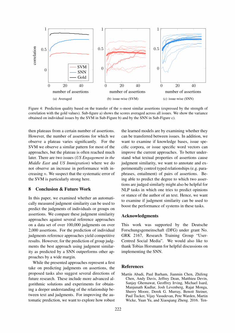
0 20 40
0
0.5
1
number of assertions
corr
elat
ion
SVMSNNGold
(a) Averaged
0 20 40
0
0.5
1
number of assertions
(b) issue-wise (SVM)
0 20 40
0
0.5
1
number of assertions
(c) issue-wise (SNN)
Figure 4: Prediction quality based on the transfer of the n-most similar assertions (expressed by the strength ofcorrelation with the gold values). Sub-figure a) shows the scores averaged across all issues. We show the varianceobtained on individual issues by the SVM in Sub-Figure b) and by the SNN in Sub-Figure c).
then plateaus from a certain number of assertions.However, the number of assertions for which weobserve a plateau varies significantly. For theSVM we observe a similar pattern for most of theapproaches, but the plateau is often reached muchlater. There are two issues (US Engagement in theMiddle East and US Immigration) where we donot observe an increase in performance with in-creasing n. We suspect that the systematic error ofthe SVM is particularly strong here.
8 Conclusion & Future Work
In this paper, we examined whether an automati-cally measured judgment similarity can be used topredict the judgments of individuals or groups onassertions. We compare these judgment similarityapproaches against several reference approacheson a data set of over 100,000 judgments on over2,000 assertions. For the prediction of individualjudgments reference approaches yield competitiveresults. However, for the prediction of group judg-ments the best approach using judgment similar-ity as predicted by a SNN outperforms other ap-proaches by a wide margin.
While the presented approaches represent a firsttake on predicting judgments on assertions, theproposed tasks also suggest several directions offuture research. These include more advanced al-gorithmic solutions and experiments for obtain-ing a deeper understanding of the relationship be-tween text and judgments. For improving the au-tomatic prediction, we want to explore how robust
the learned models are by examining whether theycan be transferred between issues. In addition, wewant to examine if knowledge bases, issue spe-cific corpora, or issue specific word vectors canimprove the current approaches. To better under-stand what textual properties of assertions causejudgment similarity, we want to annotate and ex-perimentally control typed relationships (e.g. para-phrases, entailment) of pairs of assertions. Be-ing able to predict the degree to which two asser-tions are judged similarly might also be helpful forNLP tasks in which one tries to predict opinionsor stance of the author of an text. Hence, we wantto examine if judgment similarity can be used toboost the performance of systems in these tasks.
Acknowledgments
This work was supported by the DeutscheForschungsgemeinschaft (DFG) under grant No.GRK 2167, Research Training Group “User-Centred Social Media”. We would also like tothank Tobias Horsmann for helpful discussions onimplementing the SNN.
ReferencesMartın Abadi, Paul Barham, Jianmin Chen, Zhifeng
Chen, Andy Davis, Jeffrey Dean, Matthieu Devin,Sanjay Ghemawat, Geoffrey Irving, Michael Isard,Manjunath Kudlur, Josh Levenberg, Rajat Monga,Sherry Moore, Derek G. Murray, Benoit Steiner,Paul Tucker, Vijay Vasudevan, Pete Warden, MartinWicke, Yuan Yu, and Xiaoqiang Zheng. 2016. Ten-
222
sorFlow: A System for Large-scale Machine Learn-ing. In Proceedings of the 12th USENIX Conferenceon Operating Systems Design and Implementation,OSDI’16, pages 265–283, Savannah, USA.
Gediminas Adomavicius and Alexander Tuzhilin.2005. Toward the next generation of recommendersystems: A survey of the state-of-the-art and pos-sible extensions. IEEE Transactions on Knowledgeand Data Engineering, 17(6):734–749.
Eneko Agirre, Mona Diab, Daniel Cer, and AitorGonzalez-Agirre. 2012. Semeval-2012 task 6: A pi-lot on semantic textual similarity. In Proceedings ofthe SemEval, pages 385–393, Montreal, Canada.
Daniel Bar, Torsten Zesch, and Iryna Gurevych. 2013.DKPro Similarity: An Open Source Framework forText Similarity. In Proceedings of the 51st AnnualMeeting of the Association for Computational Lin-guistics: System Demonstrations, pages 121–126,Sofia, Bulgaria.
Roy Bar-Haim, Indrajit Bhattacharya, Francesco Din-uzzo, Amrita Saha, and Noam Slonim. 2017. StanceClassification of Context-Dependent Claims. InProceedings of the 15th Conference of the EuropeanChapter of the Association for Computational Lin-guistics (EACL, pages 251–261, Valencia, Spain.
Rahul Bhagat and Eduard Hovy. 2013. What is a para-phrase? Computational Linguistics, 39(3):463–472.
Piotr Bojanowski, Edouard Grave, Armand Joulin, andTomas Mikolov. 2017. Enriching word vectors withsubword information. Transactions of the Associa-tion for Computational Linguistics, 5:135–146.
Filip Boltuzic and Jan Snajder. 2016. Fill the gap! an-alyzing implicit premises between claims from on-line debates. In Proceedings of the Third Workshopon Argument Mining (ArgMining2016), pages 124–133, Berlin, Germany.
Fabio Celli, Evgeny Stepanov, Massimo Poesio, andGiuseppe Riccardi. 2016. Predicting Brexit: Clas-sifying agreement is better than sentiment and poll-sters. In Proceedings of the Workshop on Computa-tional Modeling of People’s Opinions, Personality,and Emotions in Social Media (PEOPLES), pages110–118, Osaka, Japan.
Chih-Chung Chang and Chih-Jen Lin. 2011. LIB-SVM: A library for support vector machines. ACMTransactions on Intelligent Systems and Technol-ogy, 2:27:1–27:27. Software available at http://www.csie.ntu.edu.tw/˜cjlin/libsvm.
Ido Dagan, Bill Dolan, Bernardo Magnini, and DanRoth. 2009. Recognizing textual entailment: Ratio-nal, evaluation and approaches. Natural LanguageEngineering, 15(4):i–xvii.
Abhinandan S. Das, Mayur Datar, Ashutosh Garg, andShyam Rajaram. 2007. Google News Personaliza-tion: Scalable Online Collaborative Filtering. In
Proceedings of the 16th International Conference onWorld Wide Web (WWW ’07), pages 271–280, Banff,Canada.
Johannes Daxenberger, Oliver Ferschke, IrynaGurevych, and Torsten Zesch. 2014. DKPro TC:A Java-based Framework for Supervised LearningExperiments on Textual Data. In Proceedings of52nd Annual Meeting of the Association for Compu-tational Linguistics: System Demonstrations, pages61–66, Baltimore, Maryland.
Dan Gusfield. 1997. Algorithms on strings, trees andsequences: computer science and computational bi-ology. Cambridge university press.
Ivan Habernal and Iryna Gurevych. 2016. Which Ar-gument is More Convincing? Analyzing and Pre-dicting Convincingness of Web Arguments UsingBidirectional LSTM. In Proceedings of the 54th An-nual Meeting of the Association for ComputationalLinguistics, pages 1589–1599, Berlin, Germany.
James J. Heckman and James M. Snyder. 1996. Lin-ear Probability Models of the Demand for Attributeswith an Empirical Application to Estimating thePreferences of Legislators. The RAND Journal ofEconomics, 28:142–189.
Tobias Horsmann and Torsten Zesch. 2018. DeepTC– An Extension of DKPro Text Classification forFostering Reproducibility of Deep Learning Ex-periments. In Proceedings of the InternationalConference on Language Resources and Evaluation(LREC), Miyazaki, Japan.
Baotian Hu, Zhengdong Lu, Hang Li, and QingcaiChen. 2014. Convolutional Neural Network Ar-chitectures for Matching Natural Language Sen-tences. In Advances in Neural Information Process-ing Systems (NIPS 27), pages 2042–2050, Montreal,Canada.
Svetlana Kiritchenko, Xiaodan Zhu, and Saif M Mo-hammad. 2014. Sentiment Analysis of Short In-formal Texts. Journal of Artificial Intelligence Re-search (JAIR), 50:723–762.
Greg Linden, Brent Smith, and Jeremy York. 2003.Amazon.com recommendations: Item-to-item Col-laborative Filtering. IEEE Internet computing,7(1):76–80.
Bing Liu. 2012. Sentiment analysis and opinion min-ing. Synthesis lectures on human language tech-nologies, 5(1):1–167.
Caroline Lyon, James Malcolm, and Bob Dickerson.2001. Detecting short passages of similar text inlarge document collections. In Proceedings of Con-ference on Empirical Methods in Natural LanguageProcessing, pages 118–125, Pittsburgh, USA.
Stefano Menini and Sara Tonelli. 2016. Agreement andDisagreement: Comparison of Points of View in the
223
Political Domain. In Proceedings of the 26th Inter-national Conference on Computational Linguistics(COLING), pages 2461–2470, Osaka, Japan.
Saif M. Mohammad. 2016. Sentiment analysis: De-tecting valence, emotions, and other affectual statesfrom text. Emotion Measurement, pages 201–238.
Saif M. Mohammad, Svetlana Kiritchenko, ParinazSobhani, Xiaodan Zhu, and Colin Cherry. 2016.SemEval-2016 Task 6: Detecting Stance in Tweets.In Proceedings of the SemEval, pages 31–41, SanDiego, USA.
Jonas Mueller and Aditya Thyagarajan. 2016. SiameseRecurrent Architectures for Learning Sentence Sim-ilarity. In Proceedings of the Thirtieth AAAI Con-ference on Artificial Intelligence, AAAI’16, pages2786–2792, Phoenix, USA.
Preslav Nakov, Sara Rosenthal, Zornitsa Kozareva,Veselin Stoyanov, Alan Ritter, and Theresa Wilson.2013. SemEval-2013 Task 2: Sentiment Analysis inTwitter. In Proceedings of the SemEval, pages 312–320, Atlanta, USA.
Paul Neculoiu, Maarten Versteegh, and Mihai Rotaru.2016. Learning text similarity with siamese recur-rent networks. In Proceedings of the 1st Workshopon Representation Learning for NLP, pages 148–157.
Bo Pang and Lillian Lee. 2008. Opinion mining andsentiment analysis. Foundations and Trends R© in In-formation Retrieval, 2(1–2):1–135.
Sasa Petrovic, Miles Osborne, and Victor Lavrenko.2011. RT to Win! Predicting Message Propaga-tion in Twitter. Proceedings of the Fifth Interna-tional AAAI Conference on Weblogs and Social Me-dia, 11:586–589.
Keith T. Poole and Howard Rosenthal. 1997.Congress: A Political-economic History of Roll CallVoting. Oxford University Press.
Keith T. Poole and Howard Rosenthal. 2001. D-Nominate after 10 Years: A Comparative Updateto Congress: A Political-Economic History of Roll-Call Voting. Legislative Studies Quarterly, 26(1):5–29.
Reid Pryzant, Young-joo Chung, and Dan Jurafsky.2017. Predicting Sales from the Language of Prod-uct Descriptions. In Proceedings of the SIGIR2017 Workshop on eCommerce (ECOM 17), Tokyo,Japan.
Sara Rosenthal, Alan Ritter, Preslav Nakov, andVeselin Stoyanov. 2014. Semeval-2014 task 9: Sen-timent analysis in twitter. In Proceedings of the Se-mEval, pages 73–80, Dublin, Ireland.
J. Ben Schafer, Dan Frankowski, Jon Herlocker, andShilad Sen. 2007. Collaborative Filtering Recom-mender Systems. The Adaptive Web, pages 291–324.
Xiaoyuan Su and Taghi M. Khoshgoftaar. 2009. ASurvey of Collaborative Filtering Techniques. Ad-vances in Artificial Intelligence, pages 4:2–4:2.
Bongwon Suh, Lichan Hong, Peter Pirolli, and Ed H.Chi. 2010. Want to be Retweeted? Large Scale An-alytics on Factors Impacting Retweet in Twitter Net-work. In Proceedings of the Second IEEE Interna-tional Conference on Social Computing, pages 177–184, Washington, USA.
Chenhao Tan, Lillian Lee, and Bo Pang. 2014. The Ef-fect of Wording on Message Propagation: Topic-andAuthor-controlled Natural Experiments on Twitter.In Proceedings of the ACL, pages 175–185, Balti-more, USA.
Mariona Taule, M Antonia Martı, Francisco Rangel,Paolo Rosso, Cristina Bosco, and Viviana Patti.2017. Overview of the task of stance and gender de-tection in tweets on catalan independence at ibereval2017. In Notebook Papers of 2nd SEPLN Work-shop on Evaluation of Human Language Technolo-gies for Iberian Languages (IBEREVAL), Murcia,Spain, September, volume 19.
Lu Wang and Claire Cardie. 2014. Improving Agree-ment and Disagreement Identification in Online Dis-cussions with A Socially-Tuned Sentiment Lexicon.In Proceedings of the 5th Workshop on Computa-tional Approaches to Subjectivity, Sentiment and So-cial Media Analysis (WASSA ’14), pages 97–106.
Zhongyu Wei, Yang Liu, and Yi Li. 2016. Is This PostPersuasive? Ranking Argumentative Comments inthe Online Forum. In Proceedings of the ACL, pages195–200, Berlin, Germany.
Michael J. Wise. 1996. Yap3: Improved detectionof similarities in computer program and other texts.ACM SIGCSE Bulletin, 28(1):130–134.
Michael Wojatzki, Saif M. Mohammad, Torsten Zesch,and Svetlana Kiritchenko. 2018. Quantifying Qual-itative Data for Understanding Controversial Is-sues. In Proceedings of the 11th Edition of theLanguage Resources and Evaluation Conference(LREC-2018), Miyazaki, Japan.
Ruifeng Xu, Yu Zhou, Dongyin Wu, Lin Gui, JiachenDu, and Yun Xue. 2016. Overview of NLPCCShared Task 4: Stance Detection in Chinese Mi-croblogs. In International Conference on ComputerProcessing of Oriental Languages, pages 907–916,Kunming, China.
224
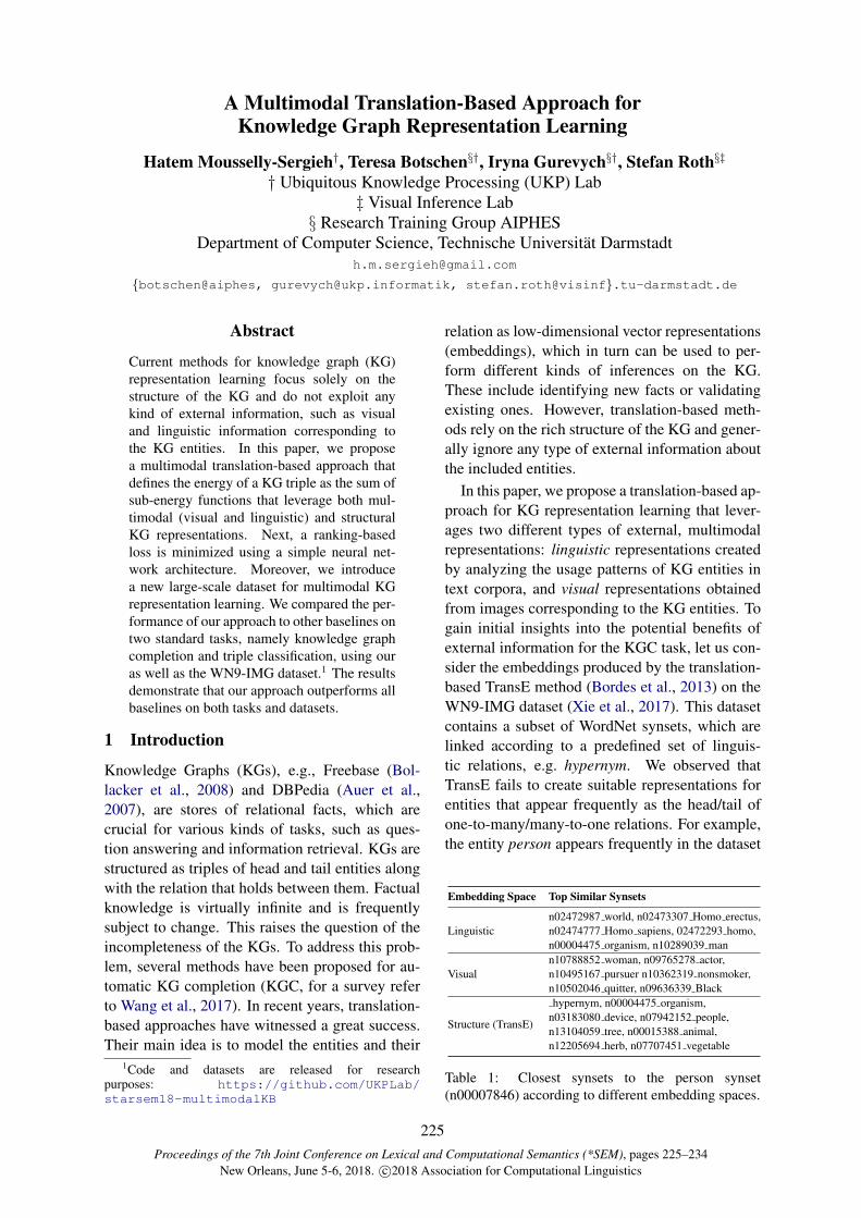
Proceedings of the 7th Joint Conference on Lexical and Computational Semantics (*SEM), pages 225–234New Orleans, June 5-6, 2018. c©2018 Association for Computational Linguistics
A Multimodal Translation-Based Approach forKnowledge Graph Representation Learning
Hatem Mousselly-Sergieh†, Teresa Botschen§†, Iryna Gurevych§†, Stefan Roth§‡
† Ubiquitous Knowledge Processing (UKP) Lab‡ Visual Inference Lab
§ Research Training Group AIPHESDepartment of Computer Science, Technische Universitat Darmstadt
{botschen@aiphes, [email protected], stefan.roth@visinf}.tu-darmstadt.de
Abstract
Current methods for knowledge graph (KG)representation learning focus solely on thestructure of the KG and do not exploit anykind of external information, such as visualand linguistic information corresponding tothe KG entities. In this paper, we proposea multimodal translation-based approach thatdefines the energy of a KG triple as the sum ofsub-energy functions that leverage both mul-timodal (visual and linguistic) and structuralKG representations. Next, a ranking-basedloss is minimized using a simple neural net-work architecture. Moreover, we introducea new large-scale dataset for multimodal KGrepresentation learning. We compared the per-formance of our approach to other baselines ontwo standard tasks, namely knowledge graphcompletion and triple classification, using ouras well as the WN9-IMG dataset.1 The resultsdemonstrate that our approach outperforms allbaselines on both tasks and datasets.
1 Introduction
Knowledge Graphs (KGs), e.g., Freebase (Bol-lacker et al., 2008) and DBPedia (Auer et al.,2007), are stores of relational facts, which arecrucial for various kinds of tasks, such as ques-tion answering and information retrieval. KGs arestructured as triples of head and tail entities alongwith the relation that holds between them. Factualknowledge is virtually infinite and is frequentlysubject to change. This raises the question of theincompleteness of the KGs. To address this prob-lem, several methods have been proposed for au-tomatic KG completion (KGC, for a survey referto Wang et al., 2017). In recent years, translation-based approaches have witnessed a great success.Their main idea is to model the entities and their
1Code and datasets are released for researchpurposes: https://github.com/UKPLab/starsem18-multimodalKB
relation as low-dimensional vector representations(embeddings), which in turn can be used to per-form different kinds of inferences on the KG.These include identifying new facts or validatingexisting ones. However, translation-based meth-ods rely on the rich structure of the KG and gener-ally ignore any type of external information aboutthe included entities.
In this paper, we propose a translation-based ap-proach for KG representation learning that lever-ages two different types of external, multimodalrepresentations: linguistic representations createdby analyzing the usage patterns of KG entities intext corpora, and visual representations obtainedfrom images corresponding to the KG entities. Togain initial insights into the potential benefits ofexternal information for the KGC task, let us con-sider the embeddings produced by the translation-based TransE method (Bordes et al., 2013) on theWN9-IMG dataset (Xie et al., 2017). This datasetcontains a subset of WordNet synsets, which arelinked according to a predefined set of linguis-tic relations, e.g. hypernym. We observed thatTransE fails to create suitable representations forentities that appear frequently as the head/tail ofone-to-many/many-to-one relations. For example,the entity person appears frequently in the dataset
Embedding Space Top Similar Synsets
Linguisticn02472987 world, n02473307 Homo erectus,n02474777 Homo sapiens, 02472293 homo,n00004475 organism, n10289039 man
Visualn10788852 woman, n09765278 actor,n10495167 pursuer n10362319 nonsmoker,n10502046 quitter, n09636339 Black
Structure (TransE)
hypernym, n00004475 organism,n03183080 device, n07942152 people,n13104059 tree, n00015388 animal,n12205694 herb, n07707451 vegetable
Table 1: Closest synsets to the person synset(n00007846) according to different embedding spaces.
225

as a head/tail of the hyponym/hypernym relation;the same holds for entities like animal or tree.TransE represents such entities as points that arevery close to each other in the embedding space(cf. Tab. 1). Furthermore, the entity embeddingstend to be very similar to the embeddings of rela-tions in which they frequently participate. Conse-quently, such a representation suffers from limiteddiscriminativeness and can be considered a mainsource of error for different KG inference tasks.
To understand how multimodal representationsmay help to overcome this issue, we performed thesame analysis by considering two types of externalinformation: linguistic and visual. The linguisticrepresentations are created using word embeddingtechniques (Mikolov et al., 2013), and the visualones, called visual embeddings, are obtained fromthe feature layers of deep networks for image clas-sification (e.g., Chatfield et al., 2014) on imagesthat correspond to the entities of the dataset. Forthe same category of entities discussed above, weobserved that both the visual and the linguistic em-beddings are much more robust than the structure-based embeddings of TransE. For instance, per-son is closer to other semantically related con-cepts, such as Homo erectus in the linguistic em-bedding space, and to concepts with common vi-sual characteristics (e.g., woman, actor) in the vi-sual embedding space (cf. Tab. 1). Furthermore,the linguistic and the visual embeddings seem tocomplement each other and hence are expected toenhance KG representations if they can be lever-aged during the representation learning process.
The contributions of this paper can be summa-rized as follows: (1) We propose an approach forKG representation learning that incorporates mul-timodal (visual and linguistic) information in atranslation-based framework and extends the def-inition of triple energy to consider the new mul-timodal representations; (2) we investigate dif-ferent methods for combining multimodal rep-resentations and evaluate their performance; (3)we introduce a new large-scale dataset for multi-modal KGC based on Freebase; (4) we experimen-tally demonstrate that our approach outperformsbaseline approaches including the state-of-the-artmethod of Xie et al. (2017) on the link predictionand triple classification tasks.
2 Related Work
2.1 Translation ModelsTransE (Bordes et al., 2013) is among the earli-est translation-based approaches for KG represen-tation learning. TransE represents entities and re-lations as vectors in the same space, where the re-lation is considered a translation operation fromthe representation of the head to that of the tailentity. For a correct triple, TransE assumes thath + r ≈ t, where h, r, t are the vector represen-tations of the head, relation, and tail, respectively.Additionally, TransE use a dissimilarity measure dto define the energy of a given triple as d(h+r, t).Finally, the representations of KG entities and re-lations are learned by minimizing a margin-basedranking objective that aims to score positive tripleshigher than negative triples based on their energiesand a predefined margin.
TransE is a simple and effective method, how-ever, the simple translational assumption con-strains the performance when dealing with com-plex relations, such as one-to-many or many-to-one. To address this limitation, some exten-sions of TransE have been proposed. Wang et al.(2014) introduced TransH, which uses translationson relation-specific hyperplanes and applies ad-vanced methods for sampling negative triples. Linet al. (2015b) proposed TransR, which uses sep-arate spaces for modeling entities and relations.Entities are projected from their space to the cor-responding relation space by relation-specific ma-trices. Moreover, they propose an extension calledCTransR, in which instances of pairs of head andtail for a specific relation are clustered such thatthe members of the clusters exhibit similar mean-ings of this relation. Lin et al. (2015a) proposedanother extension of TransE, called PTransE, thatleverages multi-step relation path information inthe process of representation learning.
The above models rely only on the structure ofthe KG, and learning better KG representationsis dependent upon the complexity of the model.In this paper, however, we follow a different ap-proach for improving the quality of the learnedKG representation and incorporate external mul-timodal information in the learning process, whilekeeping the model as simple as possible.
2.2 Multimodal MethodsRecent advances in natural language processinghave witnessed a greater interest in leveraging
226

multimodal information for a wide range of tasks.For instance, Shutova et al. (2016) showed thatbetter metaphor identification can be achieved byfusing linguistic and visual representations. Col-lell et al. (2017) demonstrated the effectivenessof combining linguistic and visual embeddingsin the context of word relatedness and similaritytasks. Regarding KG representation learning, thefirst and, to the best of our knowledge, only at-tempt that considers multimodal data is the workof Xie et al. (2017). Their IKRL approach extendsTransE based on visual representations extractedfrom images that correspond to the KG entities. InIKRL, the energy of a triple is defined in terms ofthe structure of the KG as well as the visual repre-sentation of the entities. Our work, while buildingupon the foundations of Xie et al. (2017), sets it-self apart based on the following properties: (1) inaddition to images, our model integrates anotherkind of external representation, namely linguisticembeddings for KG entities – thus, adding multi-modal information; (2) we base our approach ona simple and easily extensible neural network ar-chitecture; (3) we introduce an additional energyfunction that considers the multimodal represen-tation of the KG entities; (4) we introduce a newlarge-scale dataset for multimodal KG representa-tion learning.
3 Proposed Approach
We denote the knowledge graph as G = (E ,R, T ),where E is the set of entities, R is the set of rela-tions, and T = {(h, r, t)|h, t ∈ E , r ∈ R} theset of KG triples. For each head and tail entityh, r ∈ E , we define three kinds of representations(embeddings): structural hI
s, tIs ∈ IRN , linguistic
hIw, t
Iw ∈ IRM , and visual hI
i , tIi ∈ IRP , where
N , M and P are the corresponding numbers ofdimensions. Furthermore, we represent each rela-tion r ∈ R as a vector rIs ∈ IRN in the space ofthe structural information. The superscript I de-notes that these are the input embeddings. Sincethe different embeddings do not live in the samespace, we assume from now on that they can betransformed into a common space using a multi-layer network (e.g., hI
s into hs, cf. Fig. 1). Fol-lowing the translational assumption, given a triple(h, r, t), we have
hs + rs ≈ ts. (1)
3.1 Model
In general, previous works such as (Bordes et al.,2013) start from Eq. (1) and build models for min-imizing a ranking loss between positive and nega-tive triples that are sampled from the KG. Conven-tionally, negative triples are sampled by corruptingthe head, the tail, or the relation of correct triples.We follow this idea and make it explicit by takingtwo different “views” on the translational assump-tion. Apart from the first view through Eq. (1), wecan also rewrite the translational assumption as
ts − rs ≈ hs. (2)
We will learn the two views jointly. For each view,we sample specific kinds of negative triples ac-cording to which part of the triple has to be pre-dicted. For the head-centric view, we define T ′
tail,a set of negative triples that is sampled by cor-rupting the tail of gold triples. Similarly, for thetail-centric view, we define T ′
head, a set of negativetriples sampled by corrupting the head of the goldtriples:
T ′tail = {(h, r, t′)|h, t′∈E ∧ (h, r, t′) /∈T } (3a)
T ′head = {(h′, r, t)|h′, t∈E ∧ (h′, r, t) /∈T }. (3b)
Next, we extend the definition of triple energy inorder to integrate both the structural and the multi-modal representations of the KG entities. For eachkind of representation as well as their combina-tion, we define a specific energy function. Subse-quently, the final energy of a triple is defined as thesum of the individual energies defined below.
Structural Energy: The structure-based energyof a triple is defined in terms of the structure of theKG as proposed by the TransE approach (Bordeset al., 2013). Accordingly, we define
ES = ‖hs + rs − ts‖. (4)
Multimodal Energies: The multimodal repre-sentation of a KG entity is defined by combin-ing the corresponding linguistic and visual repre-sentations. Let ⊕ denote the combination opera-tor (more details in Section 3.2). Now, we definethe multimodal representations hm and tm of thehead and the tail entities, respectively, as
hm = hw ⊕ hi (5a)
tm = tw ⊕ ti. (5b)
227

rs
hs
ts
hm
tm
shared weights
shared weights
Dense layers Dense layers
Triple energy Input Input
+
+
+
+
ES
||ℎ𝑆 + 𝑟𝑠 − 𝑡𝑠||
EMS ||ℎ𝑚 + 𝑟𝑠 − 𝑡𝑠||
ESM ||ℎ𝑠 + 𝑟𝑠 − 𝑡𝑚||
EM1
||ℎ𝑚 + 𝑟𝑠 − 𝑡𝑚||
EM2
||(ℎ𝑚 + ℎ𝑠) + 𝑟𝑠 − (𝑡𝑚 + 𝑡𝑠)||
hs
rs
ts
hm
tm
structural embeddings multimodal
embeddings
fully connected fully
connected
hs
rs
ts
I
I
I
hm
tm
I
I
Figure 1: Overview of the neural network architecture for calculating the total triple energy from the differentmodels. The fully connected networks transform the respective input embeddings into a common space.
Next, we transfer the structure-based energy func-tion from Eq. (4) to the multimodal case where itincorporates the multimodal representations underthe translational assumption, i.e.
EM1 = ‖hm + rs − tm‖. (6)
We then extend the previous energy from Eq. (6)to define another energy function that considersthe structural embeddings in addition to the multi-modal ones as follows:
EM2 = ‖(hm + hs) + rs − (tm + ts)‖. (7)
These presented multimodal energies can be un-derstood as additional constraints for the trans-lation model. M1 states that the relation corre-sponds to a translation operation between the mul-timodal representation of the head and the tail en-tities once projected into the structural space. M2enforces that same constraint, however, on the sumof the multimodal and the structural embeddingsof the head and the tail entities. While Eqs. (4),(6), and (7) cannot be fulfilled at the same time, wefound that combining these complementary ener-gies makes the results more robust.
Structural-Multimodal Energies: Next, to en-sure that the structural and the multimodal repre-sentations are learned in the same space, we followthe proposal of Xie et al. (2017) and define the fol-lowing energy functions:
ESM = ‖hs + rs − tm‖ (8a)
EMS = ‖hm + rs − ts‖. (8b)
Finally, the overall energy of a triple for thehead and the tail views are defined as
E(h, r, t) = ES + EM1 + EM2
+ESM + EMS . (9a)
Objective Function: For both the head and thetail view, we aim to minimize a margin-basedranking loss between the energies of the positiveand the negative triples. The corresponding lossfunctions are finally defined as
Lhead =∑
(h,r,t)∈T
∑
(h,r,t′)∈T ′tail
max(γ + E(h, r, t)
−E(h, r, t′), 0)
(10)
Ltail =∑
(h,r,t)∈T
∑
(h′,r,t)∈T ′head
max(γ + E(t,−r, h)
−E(t,−r, h′), 0). (11)
Here, γ is a margin parameter, which controls theamount of energy difference between the positiveand the negative triples. Finally, we aim to mini-mize the global loss
L = Lhead + Ltail. (12)
To bring the different representations (structural,linguistic, visual) into the same space, we em-ploy a simple feed-forward neural network archi-tecture. The input of the network consists of thestructural and the multimodal embeddings of theheads, the tails, and the relations (Fig. 1); the fully-connected layers map these inputs into a commonspace. Furthermore, we share the weights between
228

𝒆𝒊
Mapping function
𝒆𝒎
𝒆𝒘
Figure 2: The DeViSE method (Frome et al., 2013).
those fully-connected layers that receive the samekind of input. Additionally, the weights are alsoshared across the head and the tail views.
3.2 Combining Multimodal RepresentationsTo complete the description of our approach, westill need to define the ⊕ operator used in Eq. (5)to combine the linguistic and visual embeddingsinto a single one. To that end, we identified threemethods for multimodal representation learningand adapted them to KG entities.
Concatenation Method: The simplest methodto create multimodal representations for KG enti-ties is to combine the multimodal embedding vec-tors by concatenation. Given the linguistic ew andthe visual ei embeddings of an entity e, we de-fine the multimodal representation em = ew
_ei,where _ is the concatenation operator.
DeViSE Method: Next, we consider the deepvisual-semantic embedding model (DeViSE) ofFrome et al. (2013), which leverages textual datato explicitly map images into a rich semantic em-bedding space. Given the visual representationof some concept, the goal is to learn a mappinginto the linguistic (word) embedding space. Themapped representation can then be used as a mul-timodal representation for the target entity. Fig. 2illustrates the application of DeViSE to generatingmultimodal representations for KG entities.
Imagined Method: Finally, we consider theImagined method of Collell et al. (2017) for creat-ing multimodal representations of concepts basedon their linguistic and visual embeddings. Imag-ined is similar to DeViSE, however, it applies thereverse procedure. That is, for a given conceptImagined aims to learn a mapping from the lin-guistic embedding space of that concept into the
Dataset #Rel #Ent #Train #Valid #Test
WN9-IMG 9 6555 11 741 1337 1319FB-IMG 1231 11 757 285 850 29 580 34 863
Table 2: Datasets statistics
𝒆𝒘
Mapping function
𝒆𝒘 𝒆𝒘𝒊
𝒆𝒎 = 𝒆𝒘𝒊 𝒆𝒘
𝒆𝒊
Figure 3: The Imagined method (Collell et al., 2017).
visual embedding space. The mapping can be for-mulated as a linear or nonlinear transformation us-ing a simple neural network, and the objective isto minimize the distance between the mapped lin-guistic representation and the visual representationof the entities. Subsequently, a multimodal repre-sentation is created by applying the learned map-ping function on the linguistic representation ofthe entity and then concatenating the resulting vec-tor with the original linguistic embedding (Fig. 3).
4 Experiments
4.1 Datasets
WN9-IMG: This dataset provided by Xie et al.(2017) is based on WordNet. It contains a col-lection of triples, where the entities correspond toword senses (synsets) and the relations define thelexical relationships between the entities. Further-more, for each synset a collection of up to ten im-ages obtained from ImageNet (Deng et al., 2009)is provided.
FB-IMG: To demonstrate the scalability of ourapproach to larger datasets, we created anotherdataset based on FB15K (Bordes et al., 2013),which consists of triples extracted from Freebase.For each entity, we crawled 100 images from theweb using text search based on the entity labels.To ensure that the crawled images are representa-tive of the corresponding entities, we applied anapproach for image filtering based on the Page-Rank algorithm (Page et al., 1999). First, wecreated a vector representation (embedding) foreach image by feeding it into a pre-trained VGG19neural network for image classification (Simonyanand Zisserman, 2014). The image embeddingsconsist of the 4096-dimensional activation of thelast layer (before the softmax). Next, for eachentity we create a similarity graph for the corre-sponding images based on the cosine similaritybetween their embedding vectors. Finally, we cal-culated the PageRank score for each image in the
229

graph and kept the top 10 results. Tab. 2 gives ba-sic statistics of the two datasets.
4.2 Representations
We now discuss the procedure we followed to ob-tain different kinds of representations for the enti-ties and relations of the two evaluation datasets.
Structural Representation: This baseline rep-resentation is created based on the structure of theKG only, without any external information. In ourexperiments we created structure representationsfor the entity and the relations of the two datasetsusing the TransE algorithm. For both datasets, wetrained TransE with 100 dimensions and used thesame values for the other hyperparameters as rec-ommended by Bordes et al. (2013).
Linguistic Representation: The linguistic rep-resentations of the entities are obtained by ap-plying word embedding techniques. For the FB-IMG dataset, we used a pre-trained word embed-ding model for Freebase entities as provided bythe word2vec framework (Mikolov et al., 2013).The provided embeddings are 1000 dimensionaland are trained using the skipgram model over theGoogle 100B token news dataset. We applied L2-normalization on the generated embeddings.
The entities of the WN9-IMG dataset corre-spond to word senses rather than to individ-ual words. In order to create embeddings forthe synsets, we used the AutoExtend framework(Rothe and Schutze, 2015), which enables cre-ating sense embeddings for a given sense basedon the embeddings of the contained lemmas. Forthis purpose, we initialized AutoExtend with pre-trained 300-dimensional GloVe embeddings (Pen-nington et al., 2014). In case where no pre-trainedembeddings are found for the sense lemmas, Au-toExtend generates zero initialized vectors for thecorresponding synsets. In order to provide bet-ter representations, we define the embeddings ofsuch synsets by copying the embeddings of thefirst hyperonym synset that has non-zero AutoEx-tend embeddings. The linguistic embeddings ofWN9-IMG entities (synsets) are 300-dimensionalvectors, which were also L2-normalized.
Visual Representation: For each image of agiven KG entity, we created a visual embeddingvector using the same procedure as for creat-ing the FB-IMG dataset. This was done usinga pre-trained VGG model (Simonyan and Zis-
serman, 2014). For the WN9-IMG dataset, weused the VGG19 model and extracted the 4096-dimensional vector of the last fully-connectedlayer before the softmax. For the FB-IMGdataset, which contains much more data thanWN9-IMG and in order to speed up the train-ing, we used the more compact VGG-m-128CNN model (Chatfield et al., 2014), which pro-duces 128-dimensional embedding vector for eachimage. Next, the visual embeddings are L2-normalized. We investigated two ways of combin-ing the embedding vectors corresponding to im-ages of a given entity. The first method definesthe visual embedding of an entity as the averageof the embeddings of all corresponding images.The second method uses the dimension-wise max-imum. In our experiments we observed that av-eraging the embedding vectors outperforms themaximum method. Hence, we only report the re-sults obtained with averaging.
4.3 Experimental Setup
We investigated different sets of hyperparametersfor training the model. The best results were ob-tained using the Adam optimizer (Kingma andBa, 2014) with a fixed learning rate of 0.001 andbatch size of 100. We used the hyperbolic tan-gent function (tanh) for the activation and onefully-connected layer of 100 hidden units. We ob-served that regularization has a minor effect. Inthe case of WN9-IMG, we used dropout regular-ization (Srivastava et al., 2014) with a dropout ra-tio of 10%; we applied no regularization on theFB-IMG dataset. Regarding the margin of the lossfunction, we experimented with several values forboth datasets γ ∈ {4, 6, 8, 10, 12}. The best re-sults for both datasets were obtained with γ = 10.
We investigated different configurations of ourapproach: (1) Ling considers the linguistic em-beddings only, (2) Vis considers the visual em-beddings only, (3) multimodal where the visualand the linguistic embeddings are considered ac-cording to the presented multimodal combinationmethods: DeViSE, Imagined, and the Concatena-tion methods (cf. Sec. 3.2), and (4) only head inwhich we use the head view only and the concate-nation method for combining the multimodal rep-resentations. Here, negative samples are producedby randomly corrupting the head, the tail, or therelation of gold triples.
We compared our approach to other baseline
230
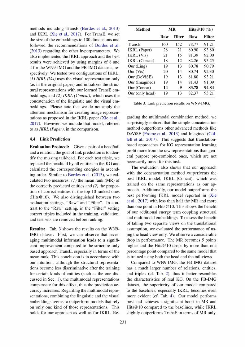
methods including TransE (Bordes et al., 2013)and IKRL (Xie et al., 2017). For TransE, we setthe size of the embeddings to 100 dimensions andfollowed the recommendations of Bordes et al.(2013) regarding the other hyperparameters. Wealso implemented the IKRL approach and the bestresults were achieved by using margins of 8 and4 for the WN9-IMG and the FB-IMG datasets, re-spectively. We tested two configurations of IKRL:(1) IKRL (Vis) uses the visual representation only(as in the original paper) and initializes the struc-tural representations with our learned TransE em-beddings, and (2) IKRL (Concat), which uses theconcatenation of the linguistic and the visual em-beddings. Please note that we do not apply theattention mechanism for creating image represen-tations as proposed in the IKRL paper (Xie et al.,2017). However, we include that model, referredto as IKRL (Paper), in the comparison.
4.4 Link Prediction
Evaluation Protocol: Given a pair of a head/tailand a relation, the goal of link prediction is to iden-tify the missing tail/head. For each test triple, wereplaced the head/tail by all entities in the KG andcalculated the corresponding energies in ascend-ing order. Similar to Bordes et al. (2013), we cal-culated two measures: (1) the mean rank (MR) ofthe correctly predicted entities and (2) the propor-tion of correct entities in the top-10 ranked ones(Hits@10). We also distinguished between twoevaluation settings, “Raw” and “Filter”. In con-trast to the “Raw” setting, in the “Filter” settingcorrect triples included in the training, validation,and test sets are removed before ranking.
Results: Tab. 3 shows the results on the WN9-IMG dataset. First, we can observe that lever-aging multimodal information leads to a signifi-cant improvement compared to the structure-onlybased approach TransE, especially in terms of themean rank. This conclusion is in accordance withour intuition: although the structural representa-tions become less discriminative after the trainingfor certain kinds of entities (such as the one dis-cussed in Sec. 1), the multimodal representationscompensate for this effect, thus the prediction ac-curacy increases. Regarding the multimodal repre-sentations, combining the linguistic and the visualembeddings seems to outperform models that relyon only one kind of those representations. Thisholds for our approach as well as for IKRL. Re-
Method MR Hits@10 (%)
Raw Filter Raw Filter
TransE 160 152 78.77 91.21IKRL (Paper) 28 21 80.90 93.80IKRL (Vis) 21 15 81.39 92.00IKRL (Concat) 18 12 82.26 93.25Our (Ling) 19 13 80.78 90.79Our (Vis) 20 14 80.74 92.30Our (DeViSE) 19 13 81.80 93.21Our (Imagined) 19 14 81.43 91.09Our (Concat) 14 9 83.78 94.84Our (only head) 19 13 82.37 93.21
Table 3: Link prediction results on WN9-IMG.
garding the multimodal combination method, wesurprisingly noticed that the simple concatenationmethod outperforms other advanced methods likeDeViSE (Frome et al., 2013) and Imagined (Col-lell et al., 2017). This suggests that translation-based approaches for KG representation learningprofit more from the raw representations than gen-eral purpose pre-combined ones, which are notnecessarily tuned for this task.
The evaluation also shows that our approachwith the concatenation method outperforms thebest IKRL model, IKRL (Concat), which wastrained on the same representations as our ap-proach. Additionally, our model outperforms thebest performing IKRL model reported in (Xieet al., 2017) with less than half the MR and morethan one point in Hits@10. This shows the benefitof our additional energy term coupling structuraland multimodal embeddings. To assess the benefitof taking two separate views on the translationalassumption, we evaluated the performance of us-ing the head view only. We observe a considerabledrop in performance. The MR becomes 5 pointshigher and the Hits@10 drops by more than onepercentage point compared to the same model thatis trained using both the head and the tail views.
Compared to WN9-IMG, the FB-IMG datasethas a much larger number of relations, entities,and triples (cf. Tab. 2), thus it better resemblesthe characteristics of real KG. On the FB-IMGdataset, the superiority of our model comparedto the baselines, especially IKRL, becomes evenmore evident (cf. Tab. 4). Our model performsbest and achieves a significant boost in MR andHits@10 compared to the baselines, while IKRLslightly outperforms TransE in terms of MR only.
231

Method MR Hits@10 (%)
Raw Filter Raw Filter
TransE 205 121 37.83 49.39IKRL (Concat) 179 104 37.48 47.87Our (Concat) 134 53 47.19 64.50
Table 4: Link prediction results on FB-IMG.
Therefore, the results confirm the robustness ofour method for large-scale datasets.
Finally, we observe that, in general, the perfor-mance boost on the FB-IMG dataset is lower thanin the case of the WN9-IMG dataset. This canbe explained by the higher scale and complexityof the FB-IMG dataset. Furthermore, the visualrepresentations of the FB-IMG entities are basedon images that are automatically crawled from theWeb. Accordingly, some of the crawled imagesmay not be representative enough or even noisy,while the images in WN9-IMG have better qualitysince they are obtained from ImageNet, which is amanually created dataset.
4.5 Triple Classification
Evaluation Protocol: Triple classification is abinary classification task, in which the KG triplesare classified as correct or not according to a givendissimilarity measure (Socher et al., 2013). Forthis purpose a threshold for each relation δr islearned. Accordingly, a triple (h, r, t) is consid-ered correct if its energy is less than δr, and incor-rect otherwise. Since the dataset did not containnegative triples, we followed the procedure pro-posed by Socher et al. (2013) to sample negativetriples for both the validation and the test sets. Asa dissimilarity measure, we used the total energyof the triple and determined the relation thresholdusing the validation set and then calculated the ac-curacy on the test set.
Results: We measured the triple classificationaccuracy of our approach using ten test runs. Ineach run, we sampled new negative triples for boththe validation and the test sets. We report the max-imum, the minimum, the average, and the standarddeviation of the triple classification accuracy.
For WN9-IMG, the results (cf. Tab. 5) show thatour approach outperforms the baselines with up totwo points in maximum accuracy and around threepoints in average accuracy. Please note that a di-rect comparison with IKRL (Paper) is not possi-
Method Accuracy(%)
max min avg ± std
TransE 95.38 89.67 93.35± 1.54IKRL (Paper) 96.90 – –IKRL (Vis) 95.16 88.75 92.57± 1.78IKRL (Concat) 95.40 91.77 93.56± 1.03Our (Concat) 97.16 94.93 96.10 ± 0.87Our (only head) 95.58 91.78 93.14± 1.09
Table 5: Triple classification results on WN9-IMG.
Method Accuracy(%)
max min avg ± std
TransE 67.13 66.47 66.81± 0.21IKRL (Concat) 66.68 66.03 66.34± 0.20Our (Concat) 69.04 68.16 68.62 ± 0.25
Table 6: Triple classification results on FB-IMG.
ble since we do not have access to the same set ofnegative samples. Still, the maximum classifica-tion accuracy of our approach is higher than that ofby IKRL (Paper). Finally, the results confirm thatusing separate head and tail views leads to betterresults than using the head view only.
Regarding the FB-IMG dataset, the results inTab. 6 emphasize the advantage of our approach.Compared to the multimodal approach IKRL,which fails to outperform TransE, our model em-ploys multimodal information more effectivelyand leads to more than one point improvement inaverage accuracy compared to TransE.
In conclusion, the conducted evaluation demon-strates the robustness of our approach on bothevaluation tasks and on different evaluationdatasets.
5 Conclusion
In this paper, we presented an approach for KGrepresentation learning that leverages multimodaldata about the KG entities including linguistic aswell as visual representations. The proposed ap-proach confirms the advantage of multimodal datafor learning KG representations. In future work,we will investigate the effect of multimodal datain the context of advanced translation methods andconduct further research on combining visual andlinguistic features for KGs.
232

Acknowledgments
The first author was supported by the German Fed-eral Ministry of Education and Research (BMBF)under the promotional reference 01UG1416B(CEDIFOR). Other than this, the work has beensupported by the DFG-funded research traininggroup “Adaptive Preparation of Information formHeterogeneous Sources” (AIPHES, GRK 1994/1).Finally, we gratefully acknowledge the supportof NVIDIA Corporation with the donation of theTesla K40 GPU used for this research.
ReferencesSoren Auer, Christian Bizer, Georgi Kobilarov, Jens
Lehmann, Richard Cyganiak, and Zachary Ives.2007. DBpedia: A nucleus for a web of open data.In The Semantic Web, pages 722–735. Springer.
Kurt Bollacker, Colin Evans, Praveen Paritosh, TimSturge, and Jamie Taylor. 2008. Freebase: A col-laboratively created graph database for structuringhuman knowledge. In Proceedings of the Interna-tional Conference on Management of Data (ACMSIGMOD), pages 1247–1250.
Antoine Bordes, Nicolas Usunier, Alberto Garcia-Duran, Jason Weston, and Oksana Yakhnenko.2013. Translating embeddings for modeling multi-relational data. In Proceedings of the 26th Interna-tional Conference on Advances in Neural Informa-tion Processing Systems (NIPS), pages 2787–2795.
Ken Chatfield, Karen Simonyan, Andrea Vedaldi, andAndrew Zisserman. 2014. Return of the devil in thedetails: Delving deep into convolutional nets. InProceedings of the British Machine Vision Confer-ence (BMVC).
Guillem Collell, Ted Zhang, and Marie-FrancineMoens. 2017. Imagined visual representations asmultimodal embeddings. In Proceedings of the 31stConference on Artificial Intelligence (AAAI), pages4378–4384.
Jia Deng, Wei Dong, Richard Socher, Li-Jia Li, KaiLi, and Li Fei-Fei. 2009. ImageNet: A large-scalehierarchical image database. In Proceedings of theIEEE Conference on Computer Vision and PatternRecognition (CVPR), pages 248–255.
Andrea Frome, Greg S Corrado, Jon Shlens, SamyBengio, Jeff Dean, Tomas Mikolov, et al. 2013. De-ViSE: A deep visual-semantic embedding model. InProceedings of the 26th International Conference onAdvances in Neural Information Processing Systems(NIPS), pages 2121–2129.
Diederik Kingma and Jimmy Ba. 2014. Adam: Amethod for stochastic optimization. arXiv preprintarXiv:1412.6980.
Yankai Lin, Zhiyuan Liu, Huan-Bo Luan, MaosongSun, Siwei Rao, and Song Liu. 2015a. Modelingrelation paths for representation learning of knowl-edge bases. In Proceedings of the Conference onEmpirical Methods in Natural Language Processing(EMNLP), pages 705–714.
Yankai Lin, Zhiyuan Liu, Maosong Sun, Yang Liu, andXuan Zhu. 2015b. Learning entity and relation em-beddings for knowledge graph completion. In Pro-ceedings of the 29th Conference on Artificial Intelli-gence (AAAI).
Tomas Mikolov, Kai Chen, Greg Corrado, and Jef-frey Dean. 2013. Efficient estimation of wordrepresentations in vector space. arXiv preprintarXiv:1301.3781.
Lawrence Page, Sergey Brin, Rajeev Motwani, andTerry Winograd. 1999. The PageRank citation rank-ing: Bringing order to the web. Technical report,Stanford InfoLab.
Jeffrey Pennington, Richard Socher, and Christo-pher D. Manning. 2014. GloVe: Global vectors forword representation. In Proceedings of the Con-ference on Empirical Methods in Natural LanguageProcessing (EMNLP), pages 1532–1543.
Sascha Rothe and Hinrich Schutze. 2015. AutoEx-tend: Extending word embeddings to embeddingsfor synsets and lexemes. In Proceedings of the 53rdAnnual Meeting of the Association for Computa-tional Linguistics (ACL), pages 1793–1803.
Ekaterina Shutova, Douwe Kiela, and Jean Maillard.2016. Black holes and white rabbits: Metaphoridentification with visual features. In Proceedingsof the Conference of the North American Chapter ofthe Association for Computational Linguistics: Hu-man Language Technologies (NAACL-HLT), pages160–170.
Karen Simonyan and Andrew Zisserman. 2014. Verydeep convolutional networks for large-scale imagerecognition. arXiv preprint arXiv:1409.1556.
Richard Socher, Danqi Chen, Christopher D Manning,and Andrew Ng. 2013. Reasoning with neural ten-sor networks for knowledge base completion. InProceedings of the 26th International Conference onAdvances in Neural Information Processing Systems(NIPS), pages 926–934.
Nitish Srivastava, Geoffrey E. Hinton, AlexKrizhevsky, Ilya Sutskever, and Ruslan Salakhutdi-nov. 2014. Dropout: A simple way to prevent neuralnetworks from overfitting. Journal of MachineLearning Research (JMLR), 15(1):1929–1958.
Quan Wang, Zhendong Mao, Bin Wang, and Li Guo.2017. Knowledge graph embedding: A survey ofapproaches and applications. IEEE Transactionson Knowledge and Data Engineering, 29(12):2724–2743.
233

Zhen Wang, Jianwen Zhang, Jianlin Feng, and ZhengChen. 2014. Knowledge graph embedding by trans-lating on hyperplanes. In Proceedings of the 28thConference on Artificial Intelligence (AAAI), pages1112–1119.
Ruobing Xie, Zhiyuan Liu, Huanbo Luan, andMaosong Sun. 2017. Image-embodied knowledgerepresentation learning. In Proceedings of the 26thInternational Joint Conference on Artificial Intelli-gence (IJCAI), pages 3140–3146.
234
Proceedings of the 7th Joint Conference on Lexical and Computational Semantics (*SEM), pages 235–244New Orleans, June 5-6, 2018. c©2018 Association for Computational Linguistics
Putting Semantics into Semantic Roles
James F. Allen1,2 and Choh Man Teng1 1Institute for Human and Machine Cognition, 40 S. Alcaniz St., Pensacola FL 32502, USA
2Department of Computer Science, University of Rochester, Rochester NY 14627, USA [email protected], [email protected]
Abstract
While there have been many proposals for theories of semantic roles over the years, these models are mostly justified by intui-tion and the only evaluation methods have been inter-annotator agreement. We ex-plore three different ideas for providing more rigorous theories of semantic roles. These ideas give rise to more objective cri-teria for designing role sets, and lend themselves to some experimental evalua-tion. We illustrate the discussion by exam-ining the semantic roles in TRIPS.
1 Introduction
Semantic roles play a foundational role in most computational approaches to encoding meaning, yet they remain surprisingly ill-defined. For the most part, a role taxonomy is defined by an in-formal gloss and some examples. In other cases, semantic roles act purely as convenient names for arguments of a predicate, frame or event, but are otherwise uninterpreted. This paper starts from the belief that if we are going to base a representation on semantic roles, they should have consequences independent of the predicate or event they are used in. In particular, we will explore three differ-ent aspects that identify criteria one might want in a theory of semantic roles: 1. Entailment: We should be able to identify en-
tailments from a role independent of the type that has such roles
2. Integration with ontology: Roles should obey the typical entailments in an ontology (e.g., inheritance of properties from parents in the ontology)
3. Derivability: The roles that a type has should be derivable from its semantic properties, as revealed by definitions of the type in sources such as dictionaries.
The first property helps ensure that roles are used consistently in a semantic lexicon, the second en-sures consistency with an ontology used for rea-
soning, and the third evaluates the semantic inter-dependence of roles and the types they occur in.
This paper will examine a particular role set, the TRIPS roles sketched in Allen & Teng, (2017)1. The first two properties are more formal in nature, but the third allows empirical evalua-tion, namely, whether the roles of an unknown word sense can be derived from its definition.
2 Preliminaries
Semantic roles have a long history, originating in linguistics as thematic roles (e.g., Fillmore, 1968; Dowty, 1991) and widely adopted in computa-tional linguistics for semantic representations be-cause of their compatibility with frame-based and graph-based (i.e., semantic networks) representa-tions of meaning.
Very roughly, computational approaches can be divided into two classes based on whether one be-lieves there is a single universal set of roles (e.g., LiRICS (Bunt & Rosemary, 2002; Petukhova & Bunt, 2008), VerbNet (Kipper et al., 2008; Bonial et al., 2011)), or whether one believes each type may identify its own unique roles (e.g., FrameNet (Baker et al., 1998)). Straddling a middle ground is PropBank (Palmer et al., 2005), which uses a universal set of role names, but allows each type to define what their roles mean. Our interest is in defining a universal set of roles across all types.
A key distinction that most frameworks make is between the inner (or core or argument) roles and the outer (or relational or adjunct) roles. The core roles identify objects that are typically re-quired to fully specify the content of the type, while relational roles are typically optional but add additional information. For instance, in
The snow melted into a puddle.
The subject of this sentence is clearly a critical ar-gument to the melting event. In fact, we cannot 1 More detail can be found in the TRIPS LF documentation: trips.ihmc.us/parser/LF%20Documentation.pdf
235
describe a melting event in a well-formed sen-tence without mentioning what melted (even if it is vague, as in something melted). On the other hand, the result construction realized by into a puddle is optional. Typically, roles of time and lo-cation are relational roles as they can be applied to almost any event and are usually optional.
But there are differences that go beyond op-tionality. The core roles semantically are like ar-guments to a predicate, although they might be optional. The relational roles semantically denote a relationship between an event and some other condition, not an argument. For instance, the phrase into a puddle above denotes first a seman-tic relationship called RESULTING-OBJECT (one of the senses of the word into) that takes as one argument the melting event and the other ar-gument the object that the snow becomes, i.e., a puddle. We will elaborate on this later in the pa-per.
This paper describes three possible ways to es-tablish a more rigorous semantics for a set of semantic roles, and explores each method in terms of the TRIPS semantic roles. In Section 4 we describe the start of an axiomatization of the roles. In Section 5 we describe the integration of the roles with an ontology. And in Section 6 we describe experiments involving derivability, i.e., can the roles that a given verb sense has be de-rived from its dictionary definition.
3 Overview of TRIPS Semantic Roles
The TRIPS core roles are shown in Table 1. These roles are defined to reflect the causal relationship between the role values and the events they are in. Informally, an AGENT of an event necessarily ex-erts causal influence to bring about the event. An AFFECTED of an event is necessarily affected or changed in some way by the event but does not cause the event. Objects filling the NEUTRAL and FORMAL roles are acausal, i.e., not neces-sarily causing or changed by the event. NEU-TRAL objects are existent and can be created or destroyed. These include both physical (e.g., a box) and abstract (e.g., an idea) objects. In con-trast, FORMAL objects have no temporal exist-ence (e.g., a proposition). Finally, EXPERI-ENCER is a special class for sentient objects in stative events involving perceptual or cognitive states.
Table 1 summarizes the distinguishing features of each of the roles, and shows correspondences with VerbNet and LiRICS. Note the mappings are nowhere near one-to-one, reflecting differing cri-teria that are used to define each of the role sets. In some cases, the LiRICS role is not completely clear and is marked with a question mark.
Some differences are differences of granularity (cf: the hierarchical roles in Bonial et al. (2001) and Allen (1995)). For instance, the TRIPS AGENT role only requires a causal relationship to the event, and does not require intentionality of the agent (as in LiRICS which distinguishes be-tween its AGENT and CAUSE roles). TRIPS takes this stance as it seems most verbs with agents would also allow non-intentional causes as well. We believe the intentionality distinction is not signaled in linguistic usage, and should be de-rived based on commonsense knowledge and rea-soning. Thus, we do not make the distinction in the role set.
As another example, VerbNet identifies classes of STIMULUS/EXPERIENCER verbs, as in The clown amused the children. Roughly, the STIM-ULUS role plays a causal role similar to AGENT and the EXPERIENCER plays an AFFECTED role where the object is affected in some cognitive fashion. The TRIPS roleset stays at an abstract level of representation, assigning the clown to AGENT and children to AFFECTED. For similar reasons, TRIPS does not have INSTRUMENT as a core role (although there is a sense of the prepo-sition with that captures accomplishing actions with a tool – e.g., He opened the door with a key).
Note TRIPS and VerbNet agree on the EXPE-RIENCER role in some cases, namely with stative verbs. In TRIPS, EXPERIENCER only occurs with stative verbs of perception and cognition.
There is a surprising variety in the VerbNet roles corresponding to the TRIPS roles, partly due to the principle in VerbNet that objects should fill the same role across all the different constructions supported by the verb. For instance, in The horse jumped over the fence, the horse is assigned a THEME role because jump supports another con-struction where the horse plays that role, as in He jumped the horse over the fence. Using the TRIPS criteria, however, the horse is clearly an AGENT in the first, and an AFFECTED in the second.
236
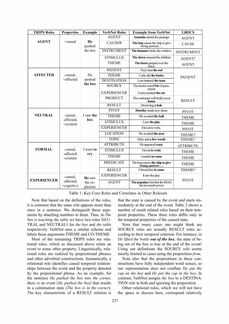
Note that based on the definitions of the roles, it is common that the same role appears more than once in a sentence. We distinguish these argu-ments by attaching numbers to them. Thus, in The box is touching the table we have two roles NEU-TRAL and NEUTRAL1 for the box and the table respectively. VerbNet uses a similar scheme and labels these arguments THEME and CO-THEME.
Most of the remaining TRIPS roles are rela-tional roles, which as discussed above relate an event to some other property. Linguistically, rela-tional roles are realized by prepositional phrases and other adverbial constructions. Semantically, a relational role identifies causal temporal relation-ships between the event and the property denoted by the prepositional phrase. As an example, for the sentence He pushed the box into the corner, there is an event (He pushed the box) that results in a culmination state (The box is in the corner). The key characteristic of a RESULT relation is
that the state is caused by the event and starts im-mediately at the end of the event. Table 2 shows a number of result related roles based on their tem-poral properties. These three roles differ only in the temporal properties of the caused state.
Note that many cases one might think are SOURCE roles are actually RESULT roles ac-cording to their temporal criterion. For instance, in He lifted the bottle out of the box, the state of be-ing out of the box is true at the end of the event! Using our definitions the SOURCE role seems mostly limited to cases using the preposition from.
Note also that the prepositions in these con-structions have fully independent word senses, so our representation does not conflate He put the cup on the box and He put the cup in the box. In contrast, VerbNet assigns the box to a DESTINA-TION role in both and ignoring the preposition.
Other relational roles, which we will not have the space to discuss here, correspond relatively
TRIPS Roles Properties Example VerbNet Roles Example from VerbNet LiRICS
AGENT +causal He pushed the box
AGENT Amanda carried the package AGENT CAUSER The bug causes the chip to give
wrong answers … CAUSE
INSTRUMENT The hammer broke the window INSTRUMENT STIMULUS The clown amused the children AGENT?
THEME The horse jumped over the fence AGENT
AFFECTED -causal, +affected
He pushed the box
PATIENT Tony bent the rod
PATIENT THEME Carla slid the books DESTINATION Lora buttered the toast
SOURCE The doctor cured Pat of pneu-monia
EXPERIENCER Carrie touched the cat PRODUCT The contractor will build you a
house RESULT RESULT David dug a hole
NEUTRAL -causal, -affected, +existent
I saw the box
PIVOT Dorothy needs new shoes PIVOT THEME We avoided the ball THEME
STIMULUS I saw the play THEME EXPERIENCER I loved to write. PIVOT
LOCATION We avoided the area THEME? TOPIC Ellen said a few words THEME?
FORMAL -causal, -affected -existent
I want to cry
ATTRIBUTE He appeared crazy ATTRIBUTE STIMULUS I loved to write THEME
THEME I needed to come THEME PREDICATE The bug causes the chip to give
wrong answers … THEME RESULT I forced him to come THEME?
EXPERIENCER -causal,
-affected, +cognitive
He saw the ex-plosion
EXPERIENCER I saw the play PIVOT AGENT The populace feel that the RIAA
has too much power
Table 1: Key Core Roles and Correlates in Other Rolesets
237
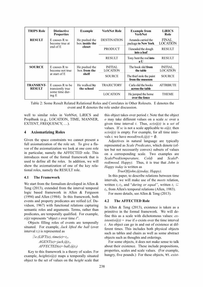
well to similar roles in VerbNet, LiRICS and PropBank (e.g., LOCATION, TIME, MANNER, EXTENT, FREQUENCY, …).
4 Axiomatizing Roles
Given the space constraints we cannot present a full axiomatization of the role set. To give a fla-vor of the axiomatization we look at one core role in particular, namely the AFFECTED role. This introduces most of the formal framework that is used to define all the roles. In addition, we will show the axiomatization of one of the key rela-tional roles, namely the RESULT role.
4.1 The Framework
We start from the formalism developed in Allen & Teng (2013), extended from the interval temporal logic based framework in Allen & Ferguson (1994) and Allen (1984). In this framework, both events and property predicates are reified (cf. Da-vidson, 1967) with functional relations capturing semantic roles and arguments. Terms, rather than predicates, are temporally qualified. For example, x@t represents “object x over time t”.
Objects filling roles of events are temporally situated. For example, Jack lifted the ball (over interval t1) is represented as ∃e.(LIFT(e),time(e)=t1,
AGENT(e)=jack1@t1,AFFECTED(e)=ball1@t1)
Key to this framework is a theory of scales. For example, height(o@t) maps a temporally situated object to the set of values on the height scale that
this object takes over period t. Note that the object o may take different values on a scale sc over a given time interval t. Thus, sc(o@t) is a set of values. If sc is not a scale applicable to o@t, then sc(o@t) is empty. For example, for all time inter-vals t, we have mood(rock1@t) =∅.
Adjectives in natural language are typically represented as Scale Predicates, which denote (of-ten but not necessarily convex) subsets of values on a corresponding scale. Two examples are ScalePred(temperature, Cold) and ScaleP-red(mood, Happy). Thus, it is true that John is Happy today is written as
TrueOf(john1@today, Happy). In this paper, to describe relations between time
intervals, we will make use of the meets relation, written t1:t2, and “during or equal”, written t1 ⊆ t2, from Allen's temporal relations (Allen, 1983).
For more details, see Allen & Teng (2013).
4.2 The AFFECTED Role
In Allen & Teng (2013), existence is taken as a primitive in the formal framework. We will de-fine this as a scale with dichotomous values: ex-istent(o@t) = true if o exists over the time interval t. An object can go in and out of existence at dif-ferent times. This includes both physical objects such as tables and chairs as well as some abstract objects such as thoughts and orderings.
For some objects, it does not make sense to talk about their existence. These include propositions, properties, scales and scale values. (For example, hungry, five pounds.) For these objects, ∀𝑡. exist-
TRIPS Role Distinctive Properties
Example VerbNet Role Example from VerbNet
LiRICS Role
RESULT E causes R to become true at end of E
He pushed the box inside the
closet
DESTINATION Amanda carried the package to New York
FINAL_ LOCATION
PRODUCT I kneaded the dough into a loaf
RESULT
RESULT Tony bent the rod into a U
RESULT
SOURCE E causes R to become not true at start of E
He pushed the box from the
shelf
INITIAL LOCATION
The book slid from the table
INITIAL_ LOCATION
SOURCE The thief stole the paint from the museum
SOURCE
TRANSIENT-RESULT
E causes R to be transiently true some time dur-ing E
He walked by the school
TRAJECTORY Carla slid the books across the table
ATTRIBUTE
LOCATION He jumped the horse over the fence
THEME
Table 2: Some Result Related Relational Roles and Correlates in Other Rolesets. E denotes the event and R denotes the role under discussion.
238
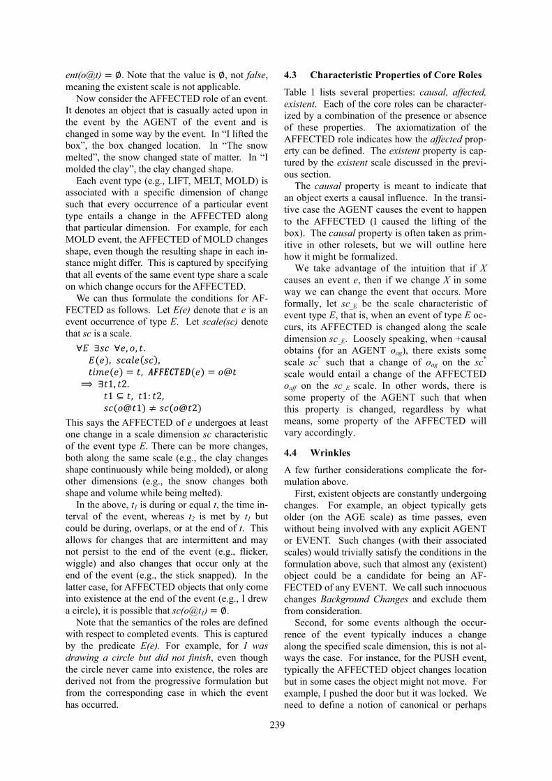
ent(o@t) = ∅. Note that the value is ∅, not false, meaning the existent scale is not applicable.
Now consider the AFFECTED role of an event. It denotes an object that is casually acted upon in the event by the AGENT of the event and is changed in some way by the event. In “I lifted the box”, the box changed location. In “The snow melted”, the snow changed state of matter. In “I molded the clay”, the clay changed shape.
Each event type (e.g., LIFT, MELT, MOLD) is associated with a specific dimension of change such that every occurrence of a particular event type entails a change in the AFFECTED along that particular dimension. For example, for each MOLD event, the AFFECTED of MOLD changes shape, even though the resulting shape in each in-stance might differ. This is captured by specifying that all events of the same event type share a scale on which change occurs for the AFFECTED.
We can thus formulate the conditions for AF-FECTED as follows. Let E(e) denote that e is an event occurrence of type E. Let scale(sc) denote that sc is a scale. ∀𝐸∃𝑠𝑐∀𝑒, 𝑜, 𝑡.
𝐸(𝑒), 𝑠𝑐𝑎𝑙𝑒 𝑠𝑐 , 𝑡𝑖𝑚𝑒(𝑒) = 𝑡, 𝑨𝑭𝑭𝑬𝑪𝑻𝑬𝑫(𝑒) = 𝑜@𝑡 ⟹∃𝑡1, 𝑡2. 𝑡1 ⊆ 𝑡, 𝑡1: 𝑡2,𝑠𝑐(𝑜@𝑡1) ≠ 𝑠𝑐(𝑜@𝑡2)This says the AFFECTED of e undergoes at least one change in a scale dimension sc characteristic of the event type E. There can be more changes, both along the same scale (e.g., the clay changes shape continuously while being molded), or along other dimensions (e.g., the snow changes both shape and volume while being melted).
In the above, t1 is during or equal t, the time in-terval of the event, whereas t2 is met by t1 but could be during, overlaps, or at the end of t. This allows for changes that are intermittent and may not persist to the end of the event (e.g., flicker, wiggle) and also changes that occur only at the end of the event (e.g., the stick snapped). In the latter case, for AFFECTED objects that only come into existence at the end of the event (e.g., I drew a circle), it is possible that sc(o@t1) = ∅.
Note that the semantics of the roles are defined with respect to completed events. This is captured by the predicate E(e). For example, for I was drawing a circle but did not finish, even though the circle never came into existence, the roles are derived not from the progressive formulation but from the corresponding case in which the event has occurred.
4.3 Characteristic Properties of Core Roles
Table 1 lists several properties: causal, affected, existent. Each of the core roles can be character-ized by a combination of the presence or absence of these properties. The axiomatization of the AFFECTED role indicates how the affected prop-erty can be defined. The existent property is cap-tured by the existent scale discussed in the previ-ous section.
The causal property is meant to indicate that an object exerts a causal influence. In the transi-tive case the AGENT causes the event to happen to the AFFECTED (I caused the lifting of the box). The causal property is often taken as prim-itive in other rolesets, but we will outline here how it might be formalized.
We take advantage of the intuition that if X causes an event e, then if we change X in some way we can change the event that occurs. More formally, let sc_E be the scale characteristic of event type E, that is, when an event of type E oc-curs, its AFFECTED is changed along the scale dimension sc_E. Loosely speaking, when +causal obtains (for an AGENT oag), there exists some scale sc* such that a change of oag on the sc* scale would entail a change of the AFFECTED oaff on the sc_E scale. In other words, there is some property of the AGENT such that when this property is changed, regardless by what means, some property of the AFFECTED will vary accordingly.
4.4 Wrinkles
A few further considerations complicate the for-mulation above.
First, existent objects are constantly undergoing changes. For example, an object typically gets older (on the AGE scale) as time passes, even without being involved with any explicit AGENT or EVENT. Such changes (with their associated scales) would trivially satisfy the conditions in the formulation above, such that almost any (existent) object could be a candidate for being an AF-FECTED of any EVENT. We call such innocuous changes Background Changes and exclude them from consideration.
Second, for some events although the occur-rence of the event typically induces a change along the specified scale dimension, this is not al-ways the case. For instance, for the PUSH event, typically the AFFECTED object changes location but in some cases the object might not move. For example, I pushed the door but it was locked. We need to define a notion of canonical or perhaps
239
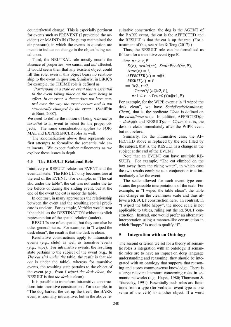
counterfactual change. This is especially pertinent for events such as PREVENT (I prevented the ac-cident) or MAINTAIN (The pump maintained the air pressure), in which the events in question are meant to induce no change in the object being act-ed upon.
Third, the NEUTRAL role mostly entails the absence of properties: not causal and not affected. It would seem then that any existent object could fill this role, even if this object bears no relation-ship to the event in question. Similarly, in LiRICS for example, the THEME role is defined as
“Participant in a state or event that is essential to the event taking place or the state being in effect. In an event, a theme does not have con-trol over the way the event occurs and is not structurally changed by the event.” (Schiffrin & Bunt, 2007).
We need to define the notion of being relevant or essential to an event to select for the proper ob-jects. The same consideration applies to FOR-MAL and EXPERIENCER roles as well.
The axiomatization above thus represents our first attempts to formalize the semantic role en-tailments. We expect further refinements as we explore these issues in depth.
4.5 The RESULT Relational Role
Intuitively a RESULT relates an EVENT and the eventual state. The RESULT only becomes true at the end of the EVENT. For example, in “The cat slid under the table”, the cat was not under the ta-ble before or during the sliding event, but at the end of the event the cat is under the table.
In contrast, in many approaches the relationship between the event and the resulting spatial predi-cate is unclear. For example, VerbNet would treat “the table” as the DESTINATION without explicit representation of the spatial relation (under).
RESULTs are often spatial, but they can also be other general states. For example, in “I wiped the desk clean”, the result is that the desk is clean.
Resultative constructions apply to intransitive events (e.g., slide) as well as transitive events (e.g., wipe). For intransitive events, the resulting state pertains to the subject of the event (e.g., In The cat slid under the table, the result is that the cat is under the table), whereas for transitive events, the resulting state pertains to the object of the event (e.g., from I wiped the desk clean, the RESULT is that the desk is clean).
It is possible to transform intransitive construc-tions into transitive constructions. For example, in “The dog barked the cat up the tree”, the BARK event is normally intransitive, but in the above re-
sultative construction, the dog is the AGENT of the BARK event, the cat is the AFFECTED and the RESULT is that the cat is up the tree. (For a treatment of this, see Allen & Teng (2017).)
Thus, the RESULT role can be formalized as follows for a transitive event type E. ∃𝑠𝑐∀𝑒, 𝑜, 𝑡, 𝑃.
𝐸 𝑒 , 𝑠𝑐𝑎𝑙𝑒 𝑠𝑐 , 𝑆𝑐𝑎𝑙𝑒𝑃𝑟𝑒𝑑(𝑠𝑐, 𝑃), 𝑡𝑖𝑚𝑒 𝑒 = 𝑡, 𝑨𝑭𝑭𝑬𝑪𝑻𝑬𝑫(𝑒) = 𝑜@𝑡, 𝑹𝑬𝑺𝑼𝑳𝑻(𝑒) = 𝑃 ⟹ ∃𝑡2.𝑡: 𝑡2, 𝑇𝑟𝑢𝑒𝑂𝑓 𝑜@𝑡2, 𝑃 , ∀𝑡1 ⊆ 𝑡.~𝑇𝑟𝑢𝑒𝑂𝑓(𝑜@𝑡1, 𝑃) For example, for the WIPE event e in “I wiped the desk clean”, we have ScalePred(cleanliness, Clean), that is, the predicate Clean is defined on the cleanliness scale. In addition, AFFECTED(e) = desk1@t and RESULT(e) = Clean; that is, the desk is clean immediately after the WIPE event but not before.
Similarly, for the intransitive case, the AF-FECTED above is replaced by the role filled by the subject, that is, the RESULT is a change in the subject at the end of the EVENT.
Note that an EVENT can have multiple RE-SULTs. For example, “The cat climbed on the box away from the rising water”, in which case the two results combine as a conjunction true im-mediately after the event.
The scale allowed for each event type con-strains the possible interpretations of the text. For example, in “I wiped the table clean”, the table can change on the cleanliness scale and thus al-lows a RESULT construction here. In contrast, in “I wiped the table happy”, the mood scale is not applicable to tables, ruling out the RESULT con-struction. Instead, one would prefer an alternative interpretation using a manner-like construction in which “happy” is used to qualify “I”.
5 Integration with an Ontology
The second criterion we set for a theory of seman-tic roles is integration with an ontology. If seman-tic roles are to have an impact on deep language understanding and reasoning, they should be inte-grated with an ontology that supports that reason-ing and stores commonsense knowledge. There is a large relevant literature concerning roles in se-mantic networks (e.g., Hayes, 1980; Thomason & Touretsky, 1991). Essentially such roles are func-tions from a type (for verbs an event type is one sense of the verb) to another object. If a word
240

sense S has a semantic role R, then for all instanc-es of S there is an object that fills the R role, i.e.,
∀𝑠.𝑆 𝑠 ⟹ ∃𝑟.𝑅 𝑠, 𝑟
This axiom captures what is sometimes called an essential role (Palmer, 2006), i.e., a semantic role that must exist even if not specified in the input sentence. Palmer notes that other roles are obliga-tory, that is, they are both essential and linguisti-cally required, and still others are simply optional and may or may not be realized at either the lin-guistic or inferential levels.
A critical foundation of semantic networks is inheritance down type hierarchies, where a sub-type “inherits” all properties of its parent types. When viewing this from the perspective of se-mantic roles, this means any role that is essential for a given type T must also then be essential for all subtypes of T.
Surprisingly, the predominant models of se-mantic roles do not address such issues in any depth. VerbNet, for instance, creates its classes based on clustering by verb usage patterns, rather than semantic entailments, and has a very limited hierarchical structure defined in terms of exten-sions in allowed usages. Within these hierar-chies, though, it does have inheritance of roles. Propbank, on the other hand, is word based and even semantically very similar verbs have differ-ent rolesets (e.g., compare the rolesets for the verbs constrict, compress and squeeze, which
one would expect would be clustered to-gether in an ontology).
The TRIPS role set is fully integrated with a rich ontology. In this ontology, the concepts are organized both by entailment as well as the semantic roles the verb sens-es take. Table 3 shows a small part of the upper ontology for events and the roles that are defined for each type and inherited from ancestor types. Note TRIPS allows both essential and optional roles. Both are inherited down the hierarchy, and lower types can make an inherited optional role essential, but not vice versa. Whether a role is obligatory or not is not specified in the ontology, but rather in the lexicon where the words and the argument struc-tures they allow are defined. Furthermore, it employs explanation closure techniques (Schubert, 1994) – if a role is not defined as possible in the ontology then the role is not possible.
The integration of roles with an ontolo-gy mutually constrains the assignment of
roles to verb sense predicates and constrains the ontology itself. For instance, if we believe that the verb disappear takes the AFFECTED role and not an AGENT role, then its word sense can-not be under the EVENT-OF-ACTION or EVENT-OF-STATE hierarchies, but it looks like a good candidate for being under the EVENT-OF-UNDERGOING-ACTION category. Like-wise, although you might think the verb analyze might take an EXPERIENCER role, if you be-lieve that analyze falls under EVENT-OF-ACTION, then it should take the AGENT role instead.
One other aspect that relates to the ontology is selectional preferences. As in many semantic networks, one can also constrain the semantic type of the arguments that can fill a role. For in-stance, one might say that the event type EAT typically concerns an animate entity (as AGENT) and some comestible substance (as the AF-FECTED role). Such knowledge is critical for driving semantic disambiguation during parsing. The TRIPS restrictions are soft constraints, i.e., the parser prefers interpretations that satisfy the constraints, but can construct interpretations that do not. As with roles, the selectional preferences are inherited down the hierarchy, with more spe-cific event types accumulating all the constraints imposed on their ancestors in the hierarchy. We do not have the space to discuss this further here.
Type New roles/ Inherited roles
Verbs (often in sub-classes)
EVENT-OF-ACTION AGENT EVENT-OF-AGENT-INTERACTION
AGENT1 AGENT
Meet, collabo-rate, …
EVENT-OF-CREATION
AFFECTED AGENT
Bake, establish, …
EVENT-OF-CAUSATION
AFFECTED, AGENT
Push, control, …
MOTION RESULT AGENT AFFECTED
Go, disperse, move, …
EVENT-OF-UNDERGOING-ACTION
AFFECTED Die, inherit, …
EVENT-OF-STATE NEUTRAL
POSSESS NEUTRAL1 NEUTRAL
Own, possess, …
HAVE-PROPERTY FORMAL NEUTRAL
Be, seem, …
EVENT-OF-EXPERIENCE
EXPERIENCER NEUTRAL
Appreciate, be-lieve, …
Table 3: Some Roles in the Event Ontology (Showing Role Inheritance)
241

6 Derivability in Definitions
The third criterion we explore is derivability. The motivation is as follows: If semantic roles have a semantics independent of their predicates/events, then the semantic properties of roles would not change between a predicate and its definition. For example, consider the word sense corresponding to the predicate for kill, defined as cause to die. According to our analysis above, kill would take two essential roles: AGENT and AFFECTED. The definition, on the other hand, involves a predicate cause that takes an AGENT, AFFECTED and a FORMAL role (to die). A highly abbreviated logi-cal form for this definition is shown in Figure 1. While cause has three roles, only the FORMAL role is fixed by the definition (i.e., it is the die event). The unfilled essential roles in the defini-tion are AGENT and AFFECTED, exactly the roles for kill.
Our hypothesis is that given a good definition of a word sense, the essential roles can be de-rived from that definition automatically. This, of course, has significant impact. If the definitions in WordNet (Fellbaum, 1998) are generally rea-sonable, we can bootstrap from the items prede-fined in the TRIPS ontology and lexicon, and de-rive the semantic roles for any verb in WordNet. Our preliminary evaluation described here indi-cates that this is a very feasible goal.
To implement this we need a strategy for iden-tifying unfilled semantic roles in a definition. The most common case we have encountered in
WordNet definitions is that the unfilled roles are elided in the definition. The TRIPS parser instan-tiates such gaps in the logical form using its IM-PRO construct. Other cases include indicating the unfilled roles by an indefinite pronoun, such as someone or something.
More complicated cases occur when the roles do not occur at the top level but in an embedded clause, as in one definition of approach (move towards), shown in Figure 2. The roles for the predicate Towards are FIGURE and GROUND, and an IMPRO fills the GROUND role of the predicate. Thus we have a role chain, from the head verb through RESULT and GROUND. We have analyzed such role patterns and created a mapping based on the semantics of the roles. In this case, it would indicate a NEUTRAL role, as the GROUND role is not changed by the event. Table 4 summarizes a few of the most common rules for identifying roles from role chains.
6.1 Experimental Evaluation of Derivability
To test this technique, we built a customized TRIPS system to parse definitions. The main cus-tomization was the addition of about a dozen top level syntactic rules that capture the common forms of definitions, which as we have seen con-tain much ellipsis. Otherwise, the grammar and lexicon are exactly the same as in all the other variants of the TRIPS parser. Our experiment also takes advantage of the fact that the TRIPS ontolo-gy has an extensive mapping to WordNet synsets, and uses the WordNet hypernym hierarchy to
Role Chain Role Identified
Example Word and Defi-nition
Justification
R wolf : f eat f An unfilled direct role R of
the head verb is R
NEUTRAL near: f move towards f The ground of the property
is not affected by the verb
AFFECTED jump: f cause [ f to jump] The agent of the embedded
event is changed by under-going the cause event
Table 4: A few sample rules for deriving roles from definitions.
V ArgR
V V1RESULT ArgGROUND
Figure 1: Key aspects of the LF for to cause to
die
Figure 2: Key aspects of the LF for to
move towards
242
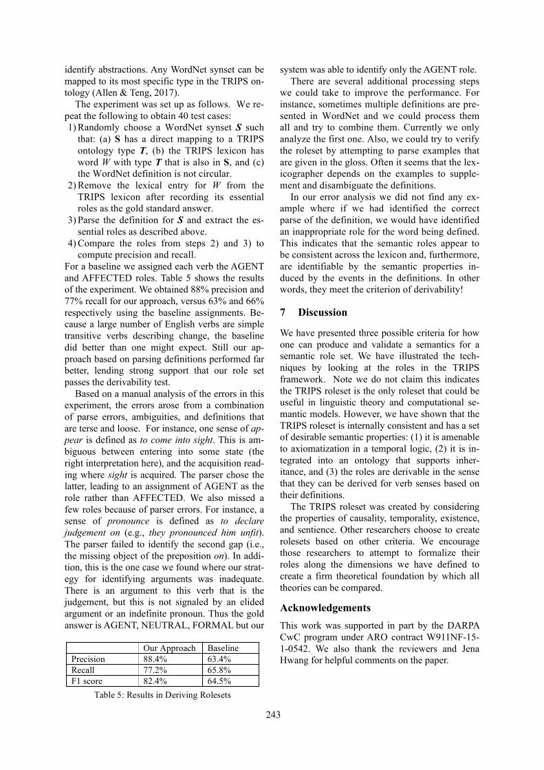
identify abstractions. Any WordNet synset can be mapped to its most specific type in the TRIPS on-tology (Allen & Teng, 2017).
The experiment was set up as follows. We re-peat the following to obtain 40 test cases: 1) Randomly choose a WordNet synset S such
that: (a) S has a direct mapping to a TRIPS ontology type T, (b) the TRIPS lexicon has word W with type T that is also in S, and (c) the WordNet definition is not circular.
2) Remove the lexical entry for W from the TRIPS lexicon after recording its essential roles as the gold standard answer.
3) Parse the definition for S and extract the es-sential roles as described above.
4) Compare the roles from steps 2) and 3) to compute precision and recall.
For a baseline we assigned each verb the AGENT and AFFECTED roles. Table 5 shows the results of the experiment. We obtained 88% precision and 77% recall for our approach, versus 63% and 66% respectively using the baseline assignments. Be-cause a large number of English verbs are simple transitive verbs describing change, the baseline did better than one might expect. Still our ap-proach based on parsing definitions performed far better, lending strong support that our role set passes the derivability test.
Based on a manual analysis of the errors in this experiment, the errors arose from a combination of parse errors, ambiguities, and definitions that are terse and loose. For instance, one sense of ap-pear is defined as to come into sight. This is am-biguous between entering into some state (the right interpretation here), and the acquisition read-ing where sight is acquired. The parser chose the latter, leading to an assignment of AGENT as the role rather than AFFECTED. We also missed a few roles because of parser errors. For instance, a sense of pronounce is defined as to declare judgement on (e.g., they pronounced him unfit). The parser failed to identify the second gap (i.e., the missing object of the preposition on). In addi-tion, this is the one case we found where our strat-egy for identifying arguments was inadequate. There is an argument to this verb that is the judgement, but this is not signaled by an elided argument or an indefinite pronoun. Thus the gold answer is AGENT, NEUTRAL, FORMAL but our
system was able to identify only the AGENT role. There are several additional processing steps
we could take to improve the performance. For instance, sometimes multiple definitions are pre-sented in WordNet and we could process them all and try to combine them. Currently we only analyze the first one. Also, we could try to verify the roleset by attempting to parse examples that are given in the gloss. Often it seems that the lex-icographer depends on the examples to supple-ment and disambiguate the definitions.
In our error analysis we did not find any ex-ample where if we had identified the correct parse of the definition, we would have identified an inappropriate role for the word being defined. This indicates that the semantic roles appear to be consistent across the lexicon and, furthermore, are identifiable by the semantic properties in-duced by the events in the definitions. In other words, they meet the criterion of derivability!
7 Discussion
We have presented three possible criteria for how one can produce and validate a semantics for a semantic role set. We have illustrated the tech-niques by looking at the roles in the TRIPS framework. Note we do not claim this indicates the TRIPS roleset is the only roleset that could be useful in linguistic theory and computational se-mantic models. However, we have shown that the TRIPS roleset is internally consistent and has a set of desirable semantic properties: (1) it is amenable to axiomatization in a temporal logic, (2) it is in-tegrated into an ontology that supports inher-itance, and (3) the roles are derivable in the sense that they can be derived for verb senses based on their definitions.
The TRIPS roleset was created by considering the properties of causality, temporality, existence, and sentience. Other researchers choose to create rolesets based on other criteria. We encourage those researchers to attempt to formalize their roles along the dimensions we have defined to create a firm theoretical foundation by which all theories can be compared.
Acknowledgements This work was supported in part by the DARPA CwC program under ARO contract W911NF-15-1-0542. We also thank the reviewers and Jena Hwang for helpful comments on the paper.
Our Approach Baseline Precision 88.4% 63.4% Recall 77.2% 65.8% F1 score 82.4% 64.5%
Table 5: Results in Deriving Rolesets
243

8 References
Allen, J. F. (1983). Maintaining Knowledge About Temporal intervals. Communications of the ACM 26(11):832-843.
Allen, J. F. (1984). Towards a general theory of ac-tion and time. Artificial Intelligence, 23(2):123-154.
Allen, J.F. (1995). Natural Language Understanding, Benjamin Cummings, Second Edition.
Allen, J. F. and G. Ferguson (1994). Actions and events in interval temporal logic. Journal of Logic and Computation, 4(5):531-579.
Allen, J. F. and C. M. Teng (2013). Becoming differ-ent: A language-driven formalism for com-monsense knowledge. In the 11th International Symposium on Logical Formalizations of Com-monsense Reasoning, Cyprus.
Allen, J., and C. M. Teng (2017). Broad coverage, domain-generic deep semantic parsing. AAAI Workshop on Construction Grammar, March, Stan-ford University.
Baker, Collin F., Charles J. Fillmore, and John B. Lowe. (1998). The Berkeley FrameNet Project. In Proceedings of COLING-ACL’98, pages 86–90, Montréal, Canada.
Bonial, C., et al. (2011). A Hierarchical Unification of LIRICS and VerbNet Semantic Roles. 5th IEEE Conf. on Semantic Computing (ICSC), Palo Alto, CA.
Bunt, H. C. and L. Romary (2002). Requirements on multimodal semantic representations. Proceedings of ISO TC37/SC4 Preliminary Meeting, pages 59–68.
Davidson, D. (1967). The Logical Form of Action Sentences. The Logic of Decision and Action. N. Rescher. Pittsburgh, University of Pittsburgh Press.
Dowty, D. (1991). Thematic Proto-Roles and Argu-ment Selection, Language, Vol 67-3, pp547-619
Fellbaum, C. (1998, ed.) WordNet: An Electronic Lexical Database. Cambridge, MA: MIT Press.
Fillmore, Charles (1968) “The case for case”, in E. Bach and R. Harms, (eds) Universals in Linguistic Theory, Holt, Rinehart, and Winston, New York, 1–90.
Hayes, Pat (1980). The Logic of Frames. In Reading in Artificial Intelligence, Margan Kaufman.
Kipper, K., A. Korhonen, N. Ryant, and M. Palmer (2008). A large-scale classification of English verbs. Language Resources and Evaluation Jour-nal, vol. 42, pp. 21–40, 2008.
Palmer, M. (2006). Semantic Processing for Finite Domains, Cambridge University Press.
Palmer, M., Gildea, D. and Kingsbury, P. (2005). The Proposition Bank: A corpus annotated with seman-tic roles, Computational Linguistics Journal, 31:1.
Petukhova, V. and Bunt, H. (2008). LIRICS Semantic Role Annotation: Design and Evaluation of a Set of Data Categories. LREC.
Schiffrin A. and H. C. Bunt (2007). LIRICS Delivera-ble D4.3. Documented compilation of semantic da-ta categories. http://lirics.loria.fr
Schubert, L.K. (1994). Explanation closure, action closure, and the Sandewall test suite for reasoning about change, J. of Logic and Computation 4(5), Special Issue on Actions and Processes, pp. 679-799
Thomason R. and D. Touretsky (1991). Inheritance Theory and Networks with Roles, in Principles of Semantic Networks, Morgan-Kaufmann.
244

Proceedings of the 7th Joint Conference on Lexical and Computational Semantics (*SEM), pages 245–254New Orleans, June 5-6, 2018. c©2018 Association for Computational Linguistics
Measuring Frame Instance Relatedness
Valerio BasileUniversity of Turin
Roque Lopez CondoriUniversité Côte d’Azur,
Inria, CNRS, I3S, [email protected]
Elena CabrioUniversité Côte d’Azur,
Inria, CNRS, I3S, [email protected]
Abstract
Frame semantics is a well-establishedframework to represent the meaning of nat-ural language in computational terms. Inthis work, we aim to propose a quantita-tive measure of relatedness between pairsof frame instances. We test our methodon a dataset of sentence pairs, highlightingthe correlation between our metric and hu-man judgments of semantic similarity. Fur-thermore, we propose an application of ourmeasure for clustering frame instances toextract prototypical knowledge from natu-ral language.
1 Introduction
Frame Semantics has been a staple of artificialintelligence and cognitive linguistics since itsfirst formulation in the ’70s (Fillmore, 1976).In particular, frame semantics has been widelyadopted as a theoretical backbone for the inter-pretation of natural language, in order to repre-sent its meaning with formal structures suitedfor computation. In a nutshell, according toframe semantics, the meaning of a sentence canbe represented as a set of situations (frames)and the entities involved in them (frame ele-ments), each with their own role.
Several approaches have proposed in thepast years to automatically interpret naturallanguage in terms of frame semantics (Gildeaand Jurafsky, 2002; Thompson et al., 2003;Erk and Padó, 2006, among others). How-ever, the vast majority of these approaches fo-cuses on the extraction of the structure of theframes evoked in the natural language fragment(frames and roles), while leaving the frame el-ements either underspecified or simply repre-senting them as spans of the original text. Inthis work, we propose to fully represent themeaning of a natural language sentence with
instantiated frames, where the frame elementsare nodes in a knowledge graph.
Moreover, while a great deal of effort hasbeen directed towards the extraction of framesfrom natural language, not many systems pro-cess frames further, to solve downstream tasksin NLP and AI — an example is Sentilo (Recu-pero et al., 2015), a sentiment analysis systembuilt on top of the frame-based machine read-ing tool FRED by Presutti et al. (2012).
In this paper we define a quantitative mea-sure to compute the semantic relatedness of apair of frame instances, and apply it to the taskof creating a commonsense knowledge base.
The main contributions of this paper are:
• A novel measure of relatedness betweenframe instances (Section 3).
• A high-quality data set of natural lan-guage sentences aligned to the frame in-stances evoked by them (Sections 4 and5).
• A pilot study on the extraction of pro-totypical knowledge based on frame in-stance clustering (Section 6).
Before introducing the novel contributions, wedescribe related work (Section 2), while Sec-tion 7 summarizes our conclusions.
2 Related Work
The most relevant to our research is the workof Pennacchiotti and Wirth (2009), which in-troduces the notion of “frame relatedness” andproposes different types of measures to assesit. These measures are grouped in three cate-gories: i) based on the hypothesis that framesare related if their lexical units are semanti-cally related; ii) corpus-based measures, whichsuggest that related frames tend to occur in
245
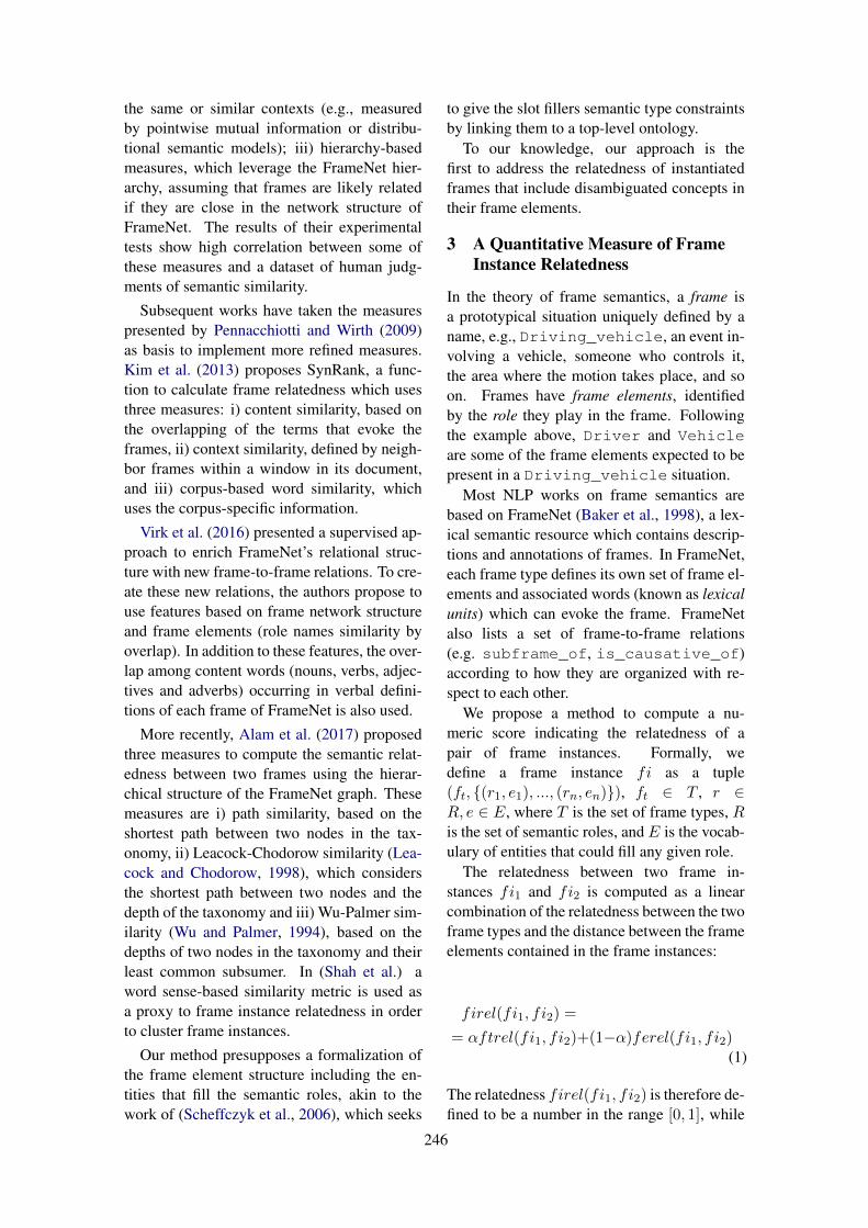
the same or similar contexts (e.g., measuredby pointwise mutual information or distribu-tional semantic models); iii) hierarchy-basedmeasures, which leverage the FrameNet hier-archy, assuming that frames are likely relatedif they are close in the network structure ofFrameNet. The results of their experimentaltests show high correlation between some ofthese measures and a dataset of human judg-ments of semantic similarity.
Subsequent works have taken the measurespresented by Pennacchiotti and Wirth (2009)as basis to implement more refined measures.Kim et al. (2013) proposes SynRank, a func-tion to calculate frame relatedness which usesthree measures: i) content similarity, based onthe overlapping of the terms that evoke theframes, ii) context similarity, defined by neigh-bor frames within a window in its document,and iii) corpus-based word similarity, whichuses the corpus-specific information.
Virk et al. (2016) presented a supervised ap-proach to enrich FrameNet’s relational struc-ture with new frame-to-frame relations. To cre-ate these new relations, the authors propose touse features based on frame network structureand frame elements (role names similarity byoverlap). In addition to these features, the over-lap among content words (nouns, verbs, adjec-tives and adverbs) occurring in verbal defini-tions of each frame of FrameNet is also used.
More recently, Alam et al. (2017) proposedthree measures to compute the semantic relat-edness between two frames using the hierar-chical structure of the FrameNet graph. Thesemeasures are i) path similarity, based on theshortest path between two nodes in the tax-onomy, ii) Leacock-Chodorow similarity (Lea-cock and Chodorow, 1998), which considersthe shortest path between two nodes and thedepth of the taxonomy and iii) Wu-Palmer sim-ilarity (Wu and Palmer, 1994), based on thedepths of two nodes in the taxonomy and theirleast common subsumer. In (Shah et al.) aword sense-based similarity metric is used asa proxy to frame instance relatedness in orderto cluster frame instances.
Our method presupposes a formalization ofthe frame element structure including the en-tities that fill the semantic roles, akin to thework of (Scheffczyk et al., 2006), which seeks
to give the slot fillers semantic type constraintsby linking them to a top-level ontology.
To our knowledge, our approach is thefirst to address the relatedness of instantiatedframes that include disambiguated concepts intheir frame elements.
3 A Quantitative Measure of FrameInstance Relatedness
In the theory of frame semantics, a frame isa prototypical situation uniquely defined by aname, e.g., Driving_vehicle, an event in-volving a vehicle, someone who controls it,the area where the motion takes place, and soon. Frames have frame elements, identifiedby the role they play in the frame. Followingthe example above, Driver and Vehicleare some of the frame elements expected to bepresent in a Driving_vehicle situation.
Most NLP works on frame semantics arebased on FrameNet (Baker et al., 1998), a lex-ical semantic resource which contains descrip-tions and annotations of frames. In FrameNet,each frame type defines its own set of frame el-ements and associated words (known as lexicalunits) which can evoke the frame. FrameNetalso lists a set of frame-to-frame relations(e.g. subframe_of, is_causative_of)according to how they are organized with re-spect to each other.
We propose a method to compute a nu-meric score indicating the relatedness of apair of frame instances. Formally, wedefine a frame instance fi as a tuple(ft, {(r1, e1), ..., (rn, en)}), ft ∈ T , r ∈R, e ∈ E, where T is the set of frame types, Ris the set of semantic roles, and E is the vocab-ulary of entities that could fill any given role.
The relatedness between two frame in-stances fi1 and fi2 is computed as a linearcombination of the relatedness between the twoframe types and the distance between the frameelements contained in the frame instances:
firel(fi1, fi2) =
= αftrel(fi1, fi2)+(1−α)ferel(fi1, fi2)(1)
The relatedness firel(fi1, fi2) is therefore de-fined to be a number in the range [0, 1], while
246
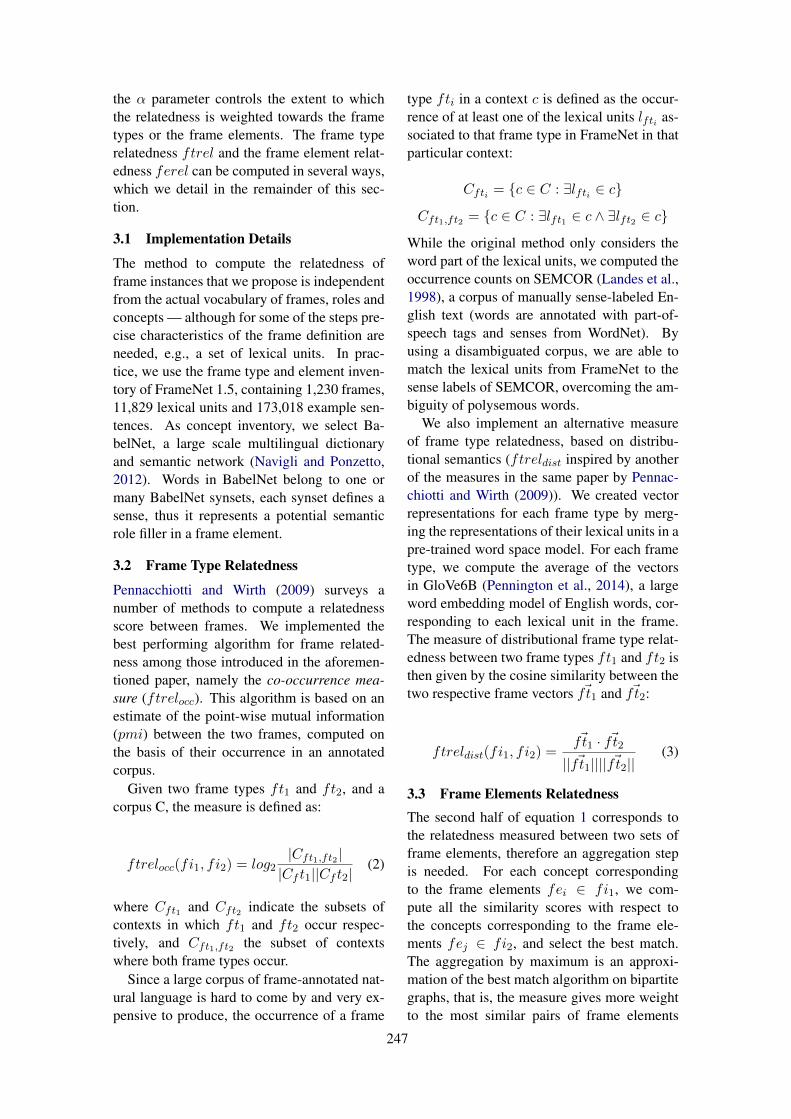
the α parameter controls the extent to whichthe relatedness is weighted towards the frametypes or the frame elements. The frame typerelatedness ftrel and the frame element relat-edness ferel can be computed in several ways,which we detail in the remainder of this sec-tion.
3.1 Implementation Details
The method to compute the relatedness offrame instances that we propose is independentfrom the actual vocabulary of frames, roles andconcepts — although for some of the steps pre-cise characteristics of the frame definition areneeded, e.g., a set of lexical units. In prac-tice, we use the frame type and element inven-tory of FrameNet 1.5, containing 1,230 frames,11,829 lexical units and 173,018 example sen-tences. As concept inventory, we select Ba-belNet, a large scale multilingual dictionaryand semantic network (Navigli and Ponzetto,2012). Words in BabelNet belong to one ormany BabelNet synsets, each synset defines asense, thus it represents a potential semanticrole filler in a frame element.
3.2 Frame Type Relatedness
Pennacchiotti and Wirth (2009) surveys anumber of methods to compute a relatednessscore between frames. We implemented thebest performing algorithm for frame related-ness among those introduced in the aforemen-tioned paper, namely the co-occurrence mea-sure (ftrelocc). This algorithm is based on anestimate of the point-wise mutual information(pmi) between the two frames, computed onthe basis of their occurrence in an annotatedcorpus.
Given two frame types ft1 and ft2, and acorpus C, the measure is defined as:
ftrelocc(fi1, fi2) = log2|Cft1,ft2 ||Cf t1||Cf t2|
(2)
where Cft1 and Cft2 indicate the subsets ofcontexts in which ft1 and ft2 occur respec-tively, and Cft1,ft2 the subset of contextswhere both frame types occur.
Since a large corpus of frame-annotated nat-ural language is hard to come by and very ex-pensive to produce, the occurrence of a frame
type fti in a context c is defined as the occur-rence of at least one of the lexical units lfti as-sociated to that frame type in FrameNet in thatparticular context:
Cfti = {c ∈ C : ∃lfti ∈ c}Cft1,ft2 = {c ∈ C : ∃lft1 ∈ c ∧ ∃lft2 ∈ c}
While the original method only considers theword part of the lexical units, we computed theoccurrence counts on SEMCOR (Landes et al.,1998), a corpus of manually sense-labeled En-glish text (words are annotated with part-of-speech tags and senses from WordNet). Byusing a disambiguated corpus, we are able tomatch the lexical units from FrameNet to thesense labels of SEMCOR, overcoming the am-biguity of polysemous words.
We also implement an alternative measureof frame type relatedness, based on distribu-tional semantics (ftreldist inspired by anotherof the measures in the same paper by Pennac-chiotti and Wirth (2009)). We created vectorrepresentations for each frame type by merg-ing the representations of their lexical units in apre-trained word space model. For each frametype, we compute the average of the vectorsin GloVe6B (Pennington et al., 2014), a largeword embedding model of English words, cor-responding to each lexical unit in the frame.The measure of distributional frame type relat-edness between two frame types ft1 and ft2 isthen given by the cosine similarity between thetwo respective frame vectors ~ft1 and ~ft2:
ftreldist(fi1, fi2) =~ft1 · ~ft2
|| ~ft1|||| ~ft2||(3)
3.3 Frame Elements RelatednessThe second half of equation 1 corresponds tothe relatedness measured between two sets offrame elements, therefore an aggregation stepis needed. For each concept correspondingto the frame elements fei ∈ fi1, we com-pute all the similarity scores with respect tothe concepts corresponding to the frame ele-ments fej ∈ fi2, and select the best match.The aggregation by maximum is an approxi-mation of the best match algorithm on bipartitegraphs, that is, the measure gives more weightto the most similar pairs of frame elements
247
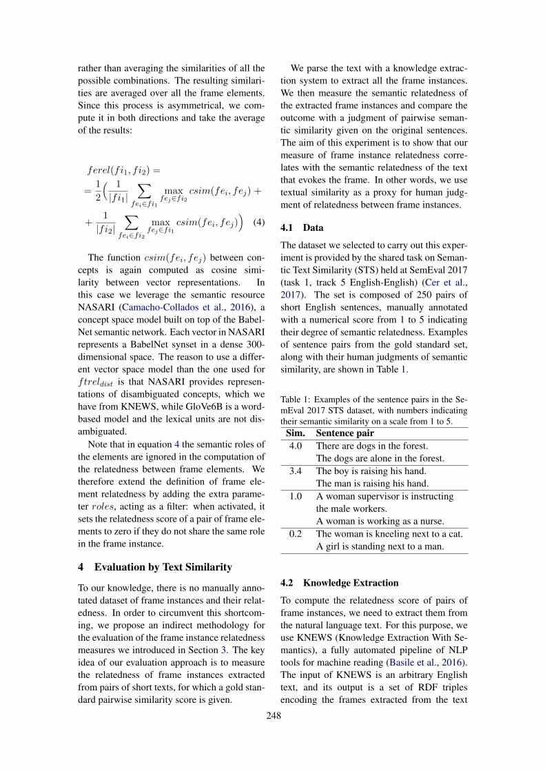
rather than averaging the similarities of all thepossible combinations. The resulting similari-ties are averaged over all the frame elements.Since this process is asymmetrical, we com-pute it in both directions and take the averageof the results:
ferel(fi1, fi2) =
=1
2
( 1
|fi1|∑
fei∈fi1max
fej∈fi2csim(fei, fej) +
+1
|fi2|∑
fei∈fi2max
fej∈fi1csim(fei, fej)
)(4)
The function csim(fei, fej) between con-cepts is again computed as cosine simi-larity between vector representations. Inthis case we leverage the semantic resourceNASARI (Camacho-Collados et al., 2016), aconcept space model built on top of the Babel-Net semantic network. Each vector in NASARIrepresents a BabelNet synset in a dense 300-dimensional space. The reason to use a differ-ent vector space model than the one used forftreldist is that NASARI provides represen-tations of disambiguated concepts, which wehave from KNEWS, while GloVe6B is a word-based model and the lexical units are not dis-ambiguated.
Note that in equation 4 the semantic roles ofthe elements are ignored in the computation ofthe relatedness between frame elements. Wetherefore extend the definition of frame ele-ment relatedness by adding the extra parame-ter roles, acting as a filter: when activated, itsets the relatedness score of a pair of frame ele-ments to zero if they do not share the same rolein the frame instance.
4 Evaluation by Text Similarity
To our knowledge, there is no manually anno-tated dataset of frame instances and their relat-edness. In order to circumvent this shortcom-ing, we propose an indirect methodology forthe evaluation of the frame instance relatednessmeasures we introduced in Section 3. The keyidea of our evaluation approach is to measurethe relatedness of frame instances extractedfrom pairs of short texts, for which a gold stan-dard pairwise similarity score is given.
We parse the text with a knowledge extrac-tion system to extract all the frame instances.We then measure the semantic relatedness ofthe extracted frame instances and compare theoutcome with a judgment of pairwise seman-tic similarity given on the original sentences.The aim of this experiment is to show that ourmeasure of frame instance relatedness corre-lates with the semantic relatedness of the textthat evokes the frame. In other words, we usetextual similarity as a proxy for human judg-ment of relatedness between frame instances.
4.1 Data
The dataset we selected to carry out this exper-iment is provided by the shared task on Seman-tic Text Similarity (STS) held at SemEval 2017(task 1, track 5 English-English) (Cer et al.,2017). The set is composed of 250 pairs ofshort English sentences, manually annotatedwith a numerical score from 1 to 5 indicatingtheir degree of semantic relatedness. Examplesof sentence pairs from the gold standard set,along with their human judgments of semanticsimilarity, are shown in Table 1.
Table 1: Examples of the sentence pairs in the Se-mEval 2017 STS dataset, with numbers indicatingtheir semantic similarity on a scale from 1 to 5.
Sim. Sentence pair4.0 There are dogs in the forest.
The dogs are alone in the forest.3.4 The boy is raising his hand.
The man is raising his hand.1.0 A woman supervisor is instructing
the male workers.A woman is working as a nurse.
0.2 The woman is kneeling next to a cat.A girl is standing next to a man.
4.2 Knowledge Extraction
To compute the relatedness score of pairs offrame instances, we need to extract them fromthe natural language text. For this purpose, weuse KNEWS (Knowledge Extraction With Se-mantics), a fully automated pipeline of NLPtools for machine reading (Basile et al., 2016).The input of KNEWS is an arbitrary Englishtext, and its output is a set of RDF triplesencoding the frames extracted from the text
248

by Semafor (Das et al., 2014). KNEWS in-tegrates the Word Sense Disambiguation toolBabelfy (Moro et al., 2014) to extract con-cept and entities from the input sentences, andmaps them to the frame roles provided bySemafor, creating frame instances where theframe types are from FrameNet 1.5 and theframe roles are filled with concepts from Ba-belNet. An example of the extraction of frameinstances from natural language performed byKNEWS is shown in Figure 1. In the exam-ple, three frame instances are extracted fromthe sentence “two men sit on a bench”, withframe types People, Cardinal_numbersand Being_located. The frame elementsare completed with BabelNet synset identi-fiers, e.g., the Theme of Being_locatedis bn:00001533n (man, adult male, male:An adult person who is male (as opposed toa woman)1) and the Location of the sameframe instance is bn:00009850n (bench: Along seat for more than one person2).
We ran KNEWS on the 500 sentences fromthe STS dataset and extracted 1,650 frame in-stances of 178 different frame types. Eachframe instance has on average 1.2 frame ele-ments, for a total of 2,107 roles filled by 457different types of concepts.
4.3 Frame-based Sentence SimilarityOur aim in this experiment is to assess the re-latedness of sentences by measuring the relat-edness of their corresponding frame instances.Since we have defined (in Section 3) a methodto compute the relatedness of frame instances,an extra step of aggregation is needed in orderto reconcile the measurement for the evalua-tion. We define the similarity ssim(s1, s2) be-tween two sentences s1 = {fi11, ..., fi1n} ands2 = {fi21, ..., fi2m} as follows:
ssim(s1, s2) =
=1
2
( 1
|s1|∑
fi1i∈s1
maxfi2j∈s2
firel(fi1i , fi2j ) +
+1
|s2|∑
fi2i∈s2
maxfi1j∈s1
firel(fi1i , fi2j ))
(5)
1http://babelnet.org/synset?word=bn:00001533n
2http://babelnet.org/synset?word=bn:00009850n
Table 2: Pearson correlation between sentence pairsimilarity scores predicted by frame instance relat-edness and the SemEval STS reference set.
without role filter with role filterftrel: occ dist occ distalpha
1.0 0.526 0.455 0.526 0.4550.9 0.529 0.465 0.536 0.4770.8 0.529 0.471 0.544 0.4950.7 0.525 0.473 0.550 0.5100.6 0.517 0.471 0.555 0.5220.5 0.503 0.463 0.558 0.5310.4 0.484 0.451 0.558 0.5380.3 0.461 0.436 0.557 0.5420.2 0.436 0.418 0.554 0.5440.1 0.410 0.400 0.550 0.5450.0 0.381 0.381 0.543 0.543
We tested the effect of the α parameter, theframe type relatedness measures ftrelocc andftreldist, and the filter on semantic roles to in-vestigate their impact on the quality of the re-latedness measurement. The result is given inTable 2 in terms of Pearson correlation betweenthe gold standard relatedness scores and the re-latedness scores predicted by our method.
Overall, the occ measure of frame type re-latedness produces better results than dist. Wefind that both halves of equation 1 contributeto the final result, with a sweet stop aroundα = 0.4 that achieves the best performanceon this benchmark with ftrel = occ and thefilter on the semantic roles. Indeed, enforcingthe matching constraint on the semantic rolesproves to be a successful strategy. The differ-ence in terms of adherence to the text similarityscores with and without such constraint is sig-nificant and consistent across every variation ofthe other parameters.
4.4 Discussion
It must be stressed that the aim of the experi-ment presented in this section is not to achievestate of the art performance on the STS task,for which better algorithms based on word sim-ilarity and other techniques have been pro-posed. In fact, many tasks that rely on sen-tence level semantics can be solved withoutthe need of extracting frame instances. Rather,we show that our method to compute a relat-edness score between frame instances works
249
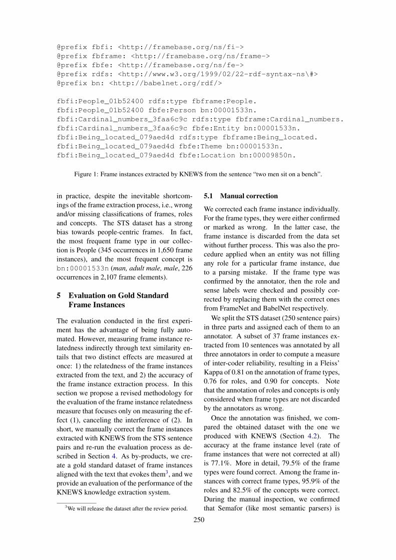
@prefix fbfi: <http://framebase.org/ns/fi->@prefix fbframe: <http://framebase.org/ns/frame->@prefix fbfe: <http://framebase.org/ns/fe->@prefix rdfs: <http://www.w3.org/1999/02/22-rdf-syntax-ns\#>@prefix bn: <http://babelnet.org/rdf/>
fbfi:People_01b52400 rdfs:type fbframe:People.fbfi:People_01b52400 fbfe:Person bn:00001533n.fbfi:Cardinal_numbers_3faa6c9c rdfs:type fbframe:Cardinal_numbers.fbfi:Cardinal_numbers_3faa6c9c fbfe:Entity bn:00001533n.fbfi:Being_located_079aed4d rdfs:type fbframe:Being_located.fbfi:Being_located_079aed4d fbfe:Theme bn:00001533n.fbfi:Being_located_079aed4d fbfe:Location bn:00009850n.
Figure 1: Frame instances extracted by KNEWS from the sentence “two men sit on a bench”.
in practice, despite the inevitable shortcom-ings of the frame extraction process, i.e., wrongand/or missing classifications of frames, rolesand concepts. The STS dataset has a strongbias towards people-centric frames. In fact,the most frequent frame type in our collec-tion is People (345 occurrences in 1,650 frameinstances), and the most frequent concept isbn:00001533n (man, adult male, male, 226occurrences in 2,107 frame elements).
5 Evaluation on Gold StandardFrame Instances
The evaluation conducted in the first experi-ment has the advantage of being fully auto-mated. However, measuring frame instance re-latedness indirectly through text similarity en-tails that two distinct effects are measured atonce: 1) the relatedness of the frame instancesextracted from the text, and 2) the accuracy ofthe frame instance extraction process. In thissection we propose a revised methodology forthe evaluation of the frame instance relatednessmeasure that focuses only on measuring the ef-fect (1), canceling the interference of (2). Inshort, we manually correct the frame instancesextracted with KNEWS from the STS sentencepairs and re-run the evaluation process as de-scribed in Section 4. As by-products, we cre-ate a gold standard dataset of frame instancesaligned with the text that evokes them3, and weprovide an evaluation of the performance of theKNEWS knowledge extraction system.
3We will release the dataset after the review period.
5.1 Manual correction
We corrected each frame instance individually.For the frame types, they were either confirmedor marked as wrong. In the latter case, theframe instance is discarded from the data setwithout further process. This was also the pro-cedure applied when an entity was not fillingany role for a particular frame instance, dueto a parsing mistake. If the frame type wasconfirmed by the annotator, then the role andsense labels were checked and possibly cor-rected by replacing them with the correct onesfrom FrameNet and BabelNet respectively.
We split the STS dataset (250 sentence pairs)in three parts and assigned each of them to anannotator. A subset of 37 frame instances ex-tracted from 10 sentences was annotated by allthree annotators in order to compute a measureof inter-coder reliability, resulting in a Fleiss’Kappa of 0.81 on the annotation of frame types,0.76 for roles, and 0.90 for concepts. Notethat the annotation of roles and concepts is onlyconsidered when frame types are not discardedby the annotators as wrong.
Once the annotation was finished, we com-pared the obtained dataset with the one weproduced with KNEWS (Section 4.2). Theaccuracy at the frame instance level (rate offrame instances that were not corrected at all)is 77.1%. More in detail, 79.5% of the frametypes were found correct. Among the frame in-stances with correct frame types, 95.9% of theroles and 82.5% of the concepts were correct.During the manual inspection, we confirmedthat Semafor (like most semantic parsers) is
250

biased towards the most dominant frame forambiguous forms. The final gold standardset comprises 1,261 frame instances and 1,579frame elements.
5.2 Text Similarity Experiment with GoldStandard Frame Instances
We repeated the experiment in 4.3, this timecomputing the pair-wise frame relatedness onthe manually corrected frame instances. Toprovide a fair comparison, we removed theframe instances from the original set corre-sponding to the frame instances removed dur-ing the manual correction. We used the filteron semantic roles described in 4.3 and ftrelocc(the performance patterns we observed werethe same as in the original experiment). Theresults of the experiment are shown in Fig-ure 2. The overall performance is slightlylower than the previous experiment. This canbe explained by observing that in this versionof the experiment we are using less data, al-though of higher quality. Due to the struc-ture of the correlation-based evaluation, incor-rect frame instances extracted from a pair ofsentences contribute to their relatedness scoremore than missing some frame instances. Also,the dominance bias could play a role, in thatwe mostly discarded low-frequency frames, forwhich the relatedness metric we defined couldperform less than optimally. An in-depth anal-ysis of this phenomenon (i.e., how does lexicalambiguity interplay with the variance in relat-edness scores?) is left for future work.
6 Clustering Frame Instances toExtract Prototypical Knowledge
In the previous sections, we proved that ourmethod for computing a relatedness score be-tween two frame instances correlates well withhuman judgments of semantic similarity basedon the natural language expression of such in-stances. What we presented is a kind of intrin-sic evaluation, which, while helpful in assess-ing the quality of the solution, does not pro-vide an insight into the motivation to imple-ment a measure of frame instance relatedness,and what open problems could benefit fromour approach down the line. To fill this gap,we propose a pilot study on the application ofthe method introduced in this paper to a down-
● ●●●●
● ●●
●
●
●
0.400
0.425
0.450
0.475
0.500
0.00 0.25 0.50 0.75 1.00alpha
Pear
son
set
● correctedoriginal
Figure 2: Pearson correlation between sentence pairsimilarity scores predicted by frame instance relat-edness on corrected frame instances and the Se-mEval STS reference set.
stream task, namely the extraction of commonsense knowledge from text, in line with the pro-totypical knowledge building method in (Shahet al.).
We start by observing that defining a quan-titative distance metric between homogeneousinstances allows us to apply a clustering algo-rithm. The result of such clustering is a par-tition of the original set into subsets that canbe either overlapping (soft clustering) or non-overlapping (hard clustering). Moreover, clus-ters have a definite shape, with one of the el-ements being the most central one (called theclustroid), and the others being more or lessfar from the center. We perform a hard clus-tering of the frame instances collected fromthe STS dataset and used for the experimentin Section 4.3, and formulate three hypotheses:i) elements close to the center of their respec-tive clusters are the best candidates to repre-sent prototypical frame instances; ii) elementsnear the border of their respective clusters areless likely to represent prototypical frame in-stances, and therefore can be filtered out; iii)the size of each cluster influences the prototyp-icality degree of the elements in its central re-gion, with larger clusters containing more pro-totypical frame instances near its center.
To cluster the frame instances, we follow
251
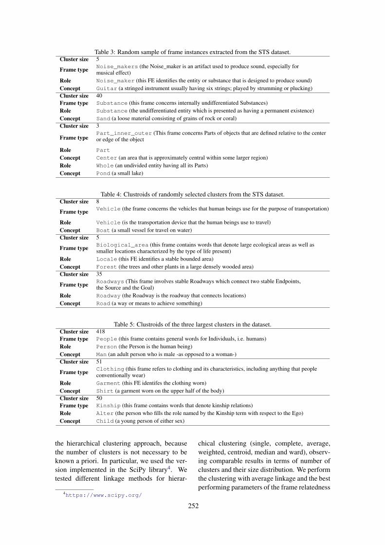
Table 3: Random sample of frame instances extracted from the STS dataset.Cluster size 5
Frame type Noise_makers (the Noise_maker is an artifact used to produce sound, especially formusical effect)
Role Noise_maker (this FE identifies the entity or substance that is designed to produce sound)Concept Guitar (a stringed instrument usually having six strings; played by strumming or plucking)Cluster size 40Frame type Substance (this frame concerns internally undifferentiated Substances)Role Substance (the undifferentiated entity which is presented as having a permanent existence)Concept Sand (a loose material consisting of grains of rock or coral)Cluster size 3
Frame typePart_inner_outer (This frame concerns Parts of objects that are defined relative to the centeror edge of the object
Role Part
Concept Center (an area that is approximately central within some larger region)Role Whole (an undivided entity having all its Parts)Concept Pond (a small lake)
Table 4: Clustroids of randomly selected clusters from the STS dataset.Cluster size 8
Frame type Vehicle (the frame concerns the vehicles that human beings use for the purpose of transportation)
Role Vehicle (is the transportation device that the human beings use to travel)Concept Boat (a small vessel for travel on water)Cluster size 5
Frame type Biological_area (this frame contains words that denote large ecological areas as well assmaller locations characterized by the type of life present)
Role Locale (this FE identifies a stable bounded area)Concept Forest (the trees and other plants in a large densely wooded area)Cluster size 35
Frame type Roadways (This frame involves stable Roadways which connect two stable Endpoints,the Source and the Goal)
Role Roadway (the Roadway is the roadway that connects locations)Concept Road (a way or means to achieve something)
Table 5: Clustroids of the three largest clusters in the dataset.Cluster size 418Frame type People (this frame contains general words for Individuals, i.e. humans)Role Person (the Person is the human being)Concept Man (an adult person who is male -as opposed to a woman-)Cluster size 51
Frame type Clothing (this frame refers to clothing and its characteristics, including anything that peopleconventionally wear)
Role Garment (this FE identifes the clothing worn)Concept Shirt (a garment worn on the upper half of the body)Cluster size 50Frame type Kinship (this frame contains words that denote kinship relations)Role Alter (the person who fills the role named by the Kinship term with respect to the Ego)Concept Child (a young person of either sex)
the hierarchical clustering approach, becausethe number of clusters is not necessary to beknown a priori. In particular, we used the ver-sion implemented in the SciPy library4. Wetested different linkage methods for hierar-
4https://www.scipy.org/
chical clustering (single, complete, average,weighted, centroid, median and ward), observ-ing comparable results in terms of number ofclusters and their size distribution. We performthe clustering with average linkage and the bestperforming parameters of the frame relatedness
252
measure (the distance metric for the clustering)according to the experiments in Section 4.
While giving an objective assessment aboutthe prototypicality of a frame instance is some-what hard, we observe different behavior inline with our hypothesis. The examples re-ported in Table 3 include quite arbitrary, albeitcorrect, frame instances. On the other hand, theexamples in Table 5 are indeed highly proto-typical, e.g., a shirt is a prototypical piece ofclothing, while the examples in Table 4 can beplaced somewhere in the middle of the proto-typicality scale.
7 Conclusion and Future Work
We presented a novel method to computea quantitative relatedness measure betweenframe instances, that takes into account thetype of the frames, the semantic role of theframe elements, and the entities involved in theframe instances. Based on a test conducted ona gold standard set of sentence pairs, the mea-sure we defined correlates positively with hu-man judgments of semantic similarity. We fur-ther apply the relatedness measure to the taskof extracting prototypical knowledge from nat-ural language.
One clear bottleneck of our experimentalsetup is given by the automatic parsing, thatdoes not always reach optimal performances.We believe that a stable measure of relatednessbetween frame instances will in fact boost theperformance of a disambiguation system, act-ing as a coherence measure for an all-word dis-ambiguation approach. We intend to test suchstrategy in future work.
The experiment on frame instance cluster-ing for prototypical knowledge extraction pre-sented in Section 6 showed promising results.In future work, we plan to conduct a large-scaleexperiment following the same principles in-cluding an extensive systematic evaluation ofthe quality of the resulting dataset.
References
Mehwish Alam, Diego Reforgiato Recupero, Mis-ael Mongiovì, Aldo Gangemi, and Petar Ris-toski. 2017. Event-based Knowledge Reconcili-ation using Frame Embeddings and Frame Simi-larity. Knowledge-Based Systems, 135:192–203.
Collin F. Baker, Charles J. Fillmore, and John B.Lowe. 1998. The Berkeley FrameNet Project. InProceedings of the 36th Annual Meeting of theAssociation for Computational Linguistics and17th International Conference on ComputationalLinguistics - Volume 1, ACL ’98, pages 86–90,Stroudsburg, PA, USA. Association for Compu-tational Linguistics.
Valerio Basile, Elena Cabrio, and Claudia Schon.2016. KNEWS: Using Logical and Lexical Se-mantics to Extract Knowledge from Natural Lan-guage. In Proceedings of the European Confer-ence on Artificial Intelligence (ECAI) 2016.
José Camacho-Collados, Mohammad Taher Pile-hvar, and Roberto Navigli. 2016. Nasari: Inte-grating explicit knowledge and corpus statisticsfor a multilingual representation of concepts andentities. Artificial Intelligence, 240:36–64.
Daniel Cer, Mona Diab, Eneko Agirre, InigoLopez-Gazpio, and Lucia Specia. 2017.Semeval-2017 task 1: Semantic textual sim-ilarity multilingual and crosslingual focusedevaluation. In Proceedings of the 11th Inter-national Workshop on Semantic Evaluation(SemEval-2017), Vancouver, Canada.
Dipanjan Das, Desai Chen, André F. T. Martins,Nathan Schneider, and Noah A. Smith. 2014.Frame-semantic parsing. Computational Lin-guistics, 40:1:9–56.
Katrin Erk and Sebastian Padó. 2006. SHAL-MANESER - A Toolchain For Shallow SemanticParsing. In Proceedings of LREC 2006.
Charles J. Fillmore. 1976. Frame semantics andthe nature of language. Annals of the New YorkAcademy of Sciences: Conference on the Ori-gin and Development of Language and Speech,280(1):20–32.
Daniel Gildea and Daniel Jurafsky. 2002. Auto-matic labeling of semantic roles. Comput. Lin-guist., 28(3):245–288.
H. Kim, X. Ren, Y. Sun, C. Wang, and J. Han. 2013.Semantic Frame-Based Document Representa-tion for Comparable Corpora. In Proceedings ofthe 13th International Conference on Data Min-ing, pages 350–359.
Shari Landes, Claudia Leacock, and Randee ITengi. 1998. Building semantic concordances.WordNet: An electronic lexical database,199(216):199–216.
C. Leacock and M. Chodorow. 1998. Combininglocal context and wordnet similarity for wordsense identification. In MIT Press, pages 265–283, Cambridge, Massachusetts.
253

Andrea Moro, Alessandro Raganato, and RobertoNavigli. 2014. Entity Linking meets Word SenseDisambiguation: a Unified Approach. Transac-tions of the Association for Computational Lin-guistics (TACL), 2:231–244.
Roberto Navigli and Simone Paolo Ponzetto. 2012.BabelNet: The automatic construction, evalua-tion and application of a wide-coverage multi-lingual semantic network. Artificial Intelligence,193:217–250.
Marco Pennacchiotti and Michael Wirth. 2009.Measuring Frame Relatedness. In Proceedingsof the 12th Conference of the European Chapterof the Association for Computational Linguis-tics, EACL ’09, pages 657–665, Stroudsburg,PA, USA. Association for Computational Lin-guistics.
Jeffrey Pennington, Richard Socher, and Christo-pher D. Manning. 2014. Glove: Global vec-tors for word representation. In Empirical Meth-ods in Natural Language Processing (EMNLP),pages 1532–1543.
Valentina Presutti, Francesco Draicchio, and AldoGangemi. 2012. Knowledge extraction basedon discourse representation theory and linguisticframes. In Knowledge Engineering and Knowl-edge Management, pages 114–129, Berlin, Hei-delberg. Springer Berlin Heidelberg.
Diego Reforgiato Recupero, Valentina Presutti, Ser-gio Consoli, Aldo Gangemi, and Andrea Gio-vanni Nuzzolese. 2015. Sentilo: Frame-basedsentiment analysis. Cognitive Computation,7(2):211–225.
Jan Scheffczyk, Adam Pease, and MichaelEllsworth. 2006. Linking framenet to the sug-gested upper merged ontology. In Proceed-ings of the 2006 Conference on Formal Ontol-ogy in Information Systems: Proceedings of theFourth International Conference (FOIS 2006),pages 289–300, Amsterdam, The Netherlands,The Netherlands. IOS Press.
Avijit Shah, Valerio Basile, Elena Cabrio, andSowmya Kamath S. Frame instance extractionand clustering for default knowledge building.pages 1–10.
Cynthia A Thompson, Roger Levy, and Christo-pher D Manning. 2003. A generative model forsemantic role labeling. In European Conferenceon Machine Learning, pages 397–408. Springer.
Shafqat Mumtaz Virk, Philippe Muller, and Juli-ette Conrath. 2016. A Supervised Approach forEnriching the Relational Structure of Frame Se-mantics in FrameNet. In Proceedings of the 26thInternational Conference on Computational Lin-guistics: Technical Papers, pages 3542–3552,Osaka, Japan. The COLING 2016 OrganizingCommittee.
Zhibiao Wu and Martha Palmer. 1994. Verbssemantics and lexical selection. In Proceed-ings of the 32Nd Annual Meeting on Associa-tion for Computational Linguistics, ACL ’94,pages 133–138, Stroudsburg, PA, USA. Associ-
ation for Computational Linguistics.
254
Proceedings of the 7th Joint Conference on Lexical and Computational Semantics (*SEM), pages 255–264New Orleans, June 5-6, 2018. c©2018 Association for Computational Linguistics
Solving Feature Sparseness in Text Classificationusing Core-Periphery Decomposition
Xia Cui, Sadamori Kojaku, Naoki Masuda, and Danushka BollegalaDepartment of Computer Science, University of Liverpool
Department of Engineering Mathematics, University of Bristol{xia.cui, danushka.bollegala}@liverpool.ac.uk{sadamori.koujaku, naoki.masuda}@bristol.ac.uk
Abstract
Feature sparseness is a problem commonto cross-domain and short-text classificationtasks. To overcome this feature sparsenessproblem, we propose a novel method basedon graph decomposition to find candidate fea-tures for expanding feature vectors. Specif-ically, we first create a feature-relatednessgraph, which is subsequently decomposed intocore-periphery (CP) pairs and use the periph-eries as the expansion candidates of the cores.We expand both training and test instancesusing the computed related features and usethem to train a text classifier. We observethat prioritising features that are common toboth training and test instances as cores dur-ing the CP decomposition to further improvethe accuracy of text classification. We evalu-ate the proposed CP-decomposition-based fea-ture expansion method on benchmark datasetsfor cross-domain sentiment classification andshort-text classification. Our experimental re-sults show that the proposed method consis-tently outperforms all baselines on short-textclassification tasks, and perform competitivelywith pivot-based cross-domain sentiment clas-sification methods.
1 Introduction
Short-texts are abundant on the Web and ap-pear in various different formats such as micro-blogs (Kwak et al., 2010), Question and Answer(QA) forums, review sites, Short Message Ser-vice (SMS), email, and chat messages (Cong et al.,2008; Thelwall et al., 2010). Unlike lengthy re-sponses that take time to both compose and toread, short responses have gained popularity par-ticularly in social media contexts. Considering thesteady growth of mobile devices that are physi-cally restricted to compact keyboards, which aresuboptimal for entering lengthy text inputs, it issafe to predict that the amount of short-texts will
continue to grow in the future. Considering theimportance and the quantity of the short-texts invarious web-related tasks, such as text classifica-tion (kun Wang et al., 2012; dos Santos and Gatti,2014), and event prediction (Sakaki et al., 2010), itis important to be able to accurately represent andclassify short-texts.
Compared to performing text mining on longertexts (Guan et al., 2009; Su et al., 2011; Yogatamaand Smith, 2014), for which dense and diverse fea-ture representations can be created relatively eas-ily, handling of shorter texts poses several chal-lenges. The number of features that are presentin a given short-text will be a small fraction ofthe set of all features that exist in all of the traininstances. Moreover, frequency of a feature in ashort-text will be small, which makes it difficultto reliably estimate the salience of a feature usingterm frequency-based methods. This is known asthe feature sparseness problem in text classifica-tion.
Feature sparseness is not unique to short-text classification but also encountered in cross-domain text classification (Blitzer et al., 2006,2007; Bollegala et al., 2014), where the train-ing and test data are selected from different do-mains with small intersection of feature spaces.In the domain adaptation (DA) setting, a classifiertrained on one domain (source) might be agnosticto the features that are unique to a different do-main (target), which results in a feature mismatchproblem similar to the feature-sparseness problemdiscussed above.
To address the feature sparseness problem en-countered in short-text and cross-domain classi-fication tasks, we propose a novel method thatcomputes related features that can be appended tothe feature vectors to reduce the sparsity. Specif-ically, we decompose a feature-relatedness graphinto core-periphery (CP) structures, where a core
255
feature (a vertex) is linked to a set of periph-eries (also represented by vertices), indicating theconnectivity of the graph. This graph decompo-sition problem is commonly known as the CP-decomposition (Csermely et al., 2013; Rombachet al., 2017; Kojaku and Masuda, 2018, 2017).
Our proposed CP-decomposition algorithmsignificantly extends existing CP-decompositionmethods in three important ways.
• First, existing CP-decomposition methodsconsider unweighted graphs, whereas edgesin feature-relatedness graphs are weighted(possibly nonnegative) real-valued feature-relatedness scores such as positive pointwisemutual information (PPMI). Our proposedCP-decomposition method can operate onedge-weighted graphs.
• Second, considering the fact that in text clas-sification a particular periphery can be relatedto more than one core, we relax the hard as-signment constraints on peripheries and al-low a particular periphery attach to multiplecores.
• Third, prior work on pivot-based cross-domain sentiment classification methodshave used features that are frequent in train-ing (source) and test (target) data as ex-pansion candidates to overcome the featuremismatch problem. Inspired by this, wedefine coreness of a feature as the point-wise mutual information between a featureand the source/target domains. The CP-decomposition algorithm we propose willthen compute the set of cores consideringboth structural properties of the graph as wellas the coreness values computed from thetrain/test data.
To perform feature vector expansion, we firstconstruct a feature-relatedness graph, where ver-tices correspond to features and the weight of theundirected edge connecting two features repre-sent the relatedness between those two features.Different features and relatedness measures canbe flexibly used in the proposed graph construc-tion. In our experiments, we use the simple (yetpopular and effective) setting of n-gram featuresas vertices and compute their relatedness usingPPMI. We compute the coreness of features as thesum of the two PPMI values between the feature
and the source, and the feature and the target do-mains.1 Next, CP-decomposition is performed onthis feature-relatedness graph to obtain a set ofcore-periphery structures. We then rank the set ofperipheries of a particular core by their PPMI val-ues, and select the top-ranked peripheries as theexpansion features of the core. We expand the corefeatures in training and train a logistic regression-based binary classifier using the expanded featurevectors, and evaluate its performance on the ex-panded test feature vectors.
We evaluate the effectiveness of the proposedmethod using benchmark datasets for two dif-ferent tasks: short-text classification and cross-domain sentiment classification. Experimentalresults on short-text classification show that theproposed method consistently outperforms pre-viously proposed feature expansion-based meth-ods for short-text classification and even some ofthe sentence embedding learning-based methods.Moreover, the consideration of coreness duringthe CP-decomposition improves the text classifi-cation accuracy. In cross-domain sentiment clas-sification experiments, the proposed method out-performs previously proposed pivot-based meth-ods such as the structural correspondence learning(SCL) (Blitzer et al., 2006).
2 Related Work
Two complementary approaches for overcomingfeature sparseness in text classification can beidentified in the literature: (a) expanding the in-stances by predicting the missing features, and(b) projecting the instances to a dense (poten-tially lower-dimensional) space and performingthe classification task in this projected space. Ourwork can be categorised to the first group of meth-ods. We next review prior work on both types ofapproaches.
Man (2014) proposed a feature vector expan-sion based on frequent term sets (FTS), wherethey first define the co-occurrence among the fea-tures and then the expansion candidates are se-lected by a pre-defined threshold on frequency. Fi-nally, the features in the original feature vectorsare expanded using these frequently co-occurringfeatures. Ma et al. (2016) proposed an improve-ment based on FTS by introducing the support andconfidence to the co-occurrence relationship when
1In short-text classification experiments, coreness is com-puted using unlabelled training and test instances.
256
they create the frequent term sets for expansion.
Our proposed method is related to the pivot se-lection methods proposed in prior work on un-supervised cross-domain sentiment classification,where common features (called the pivots) are firstidentified using some heuristic measure, and pre-dictors are learnt that can accurately predict thosepivots using the other (non-pivot) features. For ex-ample, in spectral feature alignment (SFA) (Panet al., 2010), a bipartite graph is created be-tween non-pivots (domain-specific) and pivots(domain-independent) then spectral methods areused to learn a projection from domain-specific todomain-independent feature spaces. Blitzer et al.(2006) proposed the frequency (FREQ) of a fea-ture in the source and the target domain as thecriterion for selecting pivots for structural corre-spondence learning (SCL) when performing cross-domain named entity recognition. However, theyfound (Blitzer et al., 2007) that mutual informa-tion (MI) to be a better pivot selection criterion forcross-domain sentiment classification tasks. Bol-legala et al. (2015) proposed a feature expansion-based domain adaptation method, where a senti-ment sensitive thesaurus (SST) is built using thepointwise mutual information (PMI) between afeature and the source/target domains. The coresidentified by CP-decomposition can be seen asplaying the role of pivots in cross-domain textclassification tasks because cores get expanded bytheir corresponding peripheries during the featureexpansion step. However, one notable characteris-tic in the proposed method is that we induce coresvia CP-decomposition instead of applying heuris-tic measures such as MI or PMI. As we later seein the experiments, the proposed method outper-forms the previous pivot-based feature expansionmethods in cross-domain sentiment classificationbenchmarks.
A complementary approach to overcomefeature-sparseness is to learn a (potentiallylower dimensional) dense feature representationfor the training and test instances that sufferfrom feature sparseness, and train and evaluateclassifiers in this dense feature space instead ofthe original sparse feature space. Skip-thoughtvectors (Kiros et al., 2015) encodes a sentenceinto a lower-dimensional dense vector usingbidirectional long short-term memory (bi-LSTM),whereas FastSent (Hill et al., 2016) learns sen-tence embeddings by predicting the words in the
adjacent sentences in a corpus, ignoring the wordordering. Paragraph2Vec (Le and Mikolov, 2014)jointly learns sentence and word embeddings thatcan mutually predict each other in a short-textsuch as a paragraph in a document. SequentialDenoising Autoencoder (SDAE) (Hill et al., 2016)transforms an input sentence into an embeddingby a look-up table consisting of pre-trained wordembeddings and attempts to reconstruct the orig-inal sentence embedding from a masked version.Sentence embedding learning methods such asskip-thought vectors, FastSent, SDAE etc. requirea large amount of unlabelled texts for trainingsuch as 80 million sentence Toronto books corpus,which might not be available for specialiseddomains. As shown in our experiments, the pro-posed methods perform competitively with theseembedding-based methods, while not requiringany additional training data, other than the small(typically less than 50,000 sentences) benchmarktraining datasets.
In the CP-decomposition problem, one seeksa partition of vertices into two groups called acore and a periphery. The core vertices aredensely interconnected and the peripheral verticesare sparsely interconnected. The core and pe-ripheral vertices may be densely interconnected orsparsely interconnected. Various algorithms havebeen developed to find a single core-peripherystructure (Csermely et al., 2013; Rombach et al.,2017) or multiple core-periphery structures (Ko-jaku and Masuda, 2018, 2017) in a graph. Manyexisting algorithms assume that each vertex be-longs to only one core-periphery structure. Thisassumption is problematic for text classificationbecause a peripheral vertex can belong to multi-ple core-periphery structures. To circumvent thisproblem, here we present a novel algorithm forthe CP-decomposition that allows a peripheral ver-tex to belong to more than one core-peripherystructures. Some existing CP-decomposition algo-rithms allow peripheral vertices to belong to multi-ple core-periphery structures (Yan and Luo, 2016;Sardana and Bhatnagar, 2016; Xiang et al., 2018).These algorithms detect non-overlapping commu-nities (i.e., groups of densely interconnected ver-tices) in a graph. Then, they regard vertices thatdo not belong to any community as peripheral ver-tices. Therefore, the detected peripheries mightnot be strongly related to the associated cores be-cause they are not densely interconnected with the
257
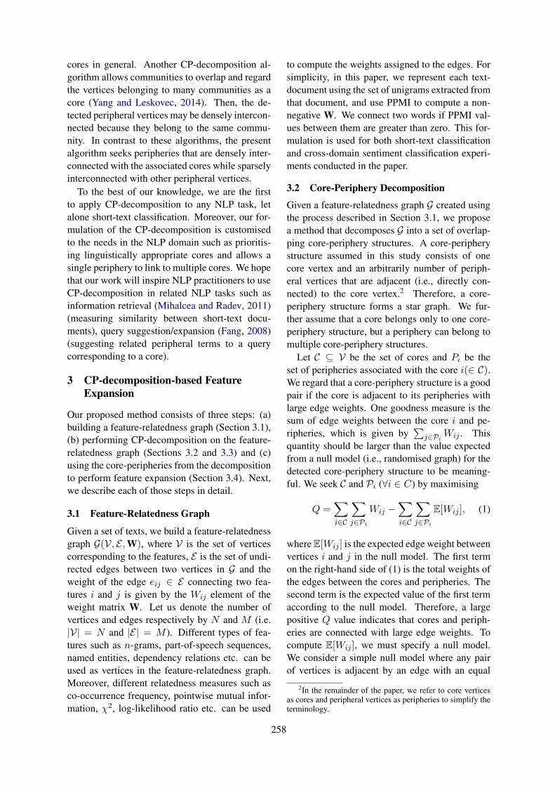
cores in general. Another CP-decomposition al-gorithm allows communities to overlap and regardthe vertices belonging to many communities as acore (Yang and Leskovec, 2014). Then, the de-tected peripheral vertices may be densely intercon-nected because they belong to the same commu-nity. In contrast to these algorithms, the presentalgorithm seeks peripheries that are densely inter-connected with the associated cores while sparselyinterconnected with other peripheral vertices.
To the best of our knowledge, we are the firstto apply CP-decomposition to any NLP task, letalone short-text classification. Moreover, our for-mulation of the CP-decomposition is customisedto the needs in the NLP domain such as prioritis-ing linguistically appropriate cores and allows asingle periphery to link to multiple cores. We hopethat our work will inspire NLP practitioners to useCP-decomposition in related NLP tasks such asinformation retrieval (Mihalcea and Radev, 2011)(measuring similarity between short-text docu-ments), query suggestion/expansion (Fang, 2008)(suggesting related peripheral terms to a querycorresponding to a core).
3 CP-decomposition-based FeatureExpansion
Our proposed method consists of three steps: (a)building a feature-relatedness graph (Section 3.1),(b) performing CP-decomposition on the feature-relatedness graph (Sections 3.2 and 3.3) and (c)using the core-peripheries from the decompositionto perform feature expansion (Section 3.4). Next,we describe each of those steps in detail.
3.1 Feature-Relatedness Graph
Given a set of texts, we build a feature-relatednessgraph G(V, E ,W), where V is the set of verticescorresponding to the features, E is the set of undi-rected edges between two vertices in G and theweight of the edge eij ∈ E connecting two fea-tures i and j is given by the Wij element of theweight matrix W. Let us denote the number ofvertices and edges respectively by N and M (i.e.|V| = N and |E| = M ). Different types of fea-tures such as n-grams, part-of-speech sequences,named entities, dependency relations etc. can beused as vertices in the feature-relatedness graph.Moreover, different relatedness measures such asco-occurrence frequency, pointwise mutual infor-mation, χ2, log-likelihood ratio etc. can be used
to compute the weights assigned to the edges. Forsimplicity, in this paper, we represent each text-document using the set of unigrams extracted fromthat document, and use PPMI to compute a non-negative W. We connect two words if PPMI val-ues between them are greater than zero. This for-mulation is used for both short-text classificationand cross-domain sentiment classification experi-ments conducted in the paper.
3.2 Core-Periphery Decomposition
Given a feature-relatedness graph G created usingthe process described in Section 3.1, we proposea method that decomposes G into a set of overlap-ping core-periphery structures. A core-peripherystructure assumed in this study consists of onecore vertex and an arbitrarily number of periph-eral vertices that are adjacent (i.e., directly con-nected) to the core vertex.2 Therefore, a core-periphery structure forms a star graph. We fur-ther assume that a core belongs only to one core-periphery structure, but a periphery can belong tomultiple core-periphery structures.
Let C ⊆ V be the set of cores and Pi be theset of peripheries associated with the core i(∈ C).We regard that a core-periphery structure is a goodpair if the core is adjacent to its peripheries withlarge edge weights. One goodness measure is thesum of edge weights between the core i and pe-ripheries, which is given by
∑j∈Pi
Wij . Thisquantity should be larger than the value expectedfrom a null model (i.e., randomised graph) for thedetected core-periphery structure to be meaning-ful. We seek C and Pi (∀i ∈ C) by maximising
Q =∑
i∈C
∑
j∈Pi
Wij −∑
i∈C
∑
j∈Pi
E[Wij ], (1)
where E[Wij ] is the expected edge weight betweenvertices i and j in the null model. The first termon the right-hand side of (1) is the total weights ofthe edges between the cores and peripheries. Thesecond term is the expected value of the first termaccording to the null model. Therefore, a largepositive Q value indicates that cores and periph-eries are connected with large edge weights. Tocompute E[Wij ], we must specify a null model.We consider a simple null model where any pairof vertices is adjacent by an edge with an equal
2In the remainder of the paper, we refer to core verticesas cores and peripheral vertices as peripheries to simplify theterminology.
258
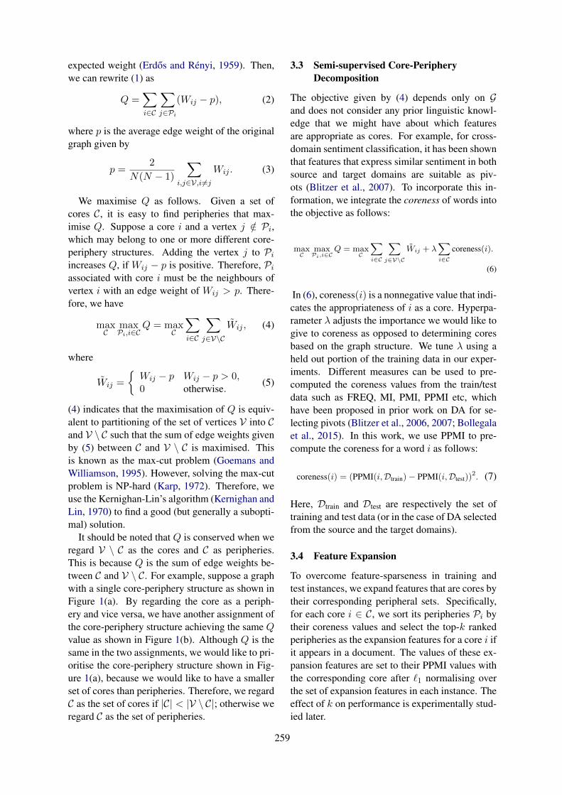
expected weight (Erdos and Rényi, 1959). Then,we can rewrite (1) as
Q =∑
i∈C
∑
j∈Pi
(Wij − p), (2)
where p is the average edge weight of the originalgraph given by
p =2
N(N − 1)
∑
i,j∈V,i 6=j
Wij . (3)
We maximise Q as follows. Given a set ofcores C, it is easy to find peripheries that max-imise Q. Suppose a core i and a vertex j /∈ Pi,which may belong to one or more different core-periphery structures. Adding the vertex j to Piincreases Q, if Wij − p is positive. Therefore, Piassociated with core i must be the neighbours ofvertex i with an edge weight of Wij > p. There-fore, we have
maxC
maxPi,i∈C
Q = maxC
∑
i∈C
∑
j∈V\CWij , (4)
where
Wij =
{Wij − p Wij − p > 0,0 otherwise.
(5)
(4) indicates that the maximisation of Q is equiv-alent to partitioning of the set of vertices V into Cand V \ C such that the sum of edge weights givenby (5) between C and V \ C is maximised. Thisis known as the max-cut problem (Goemans andWilliamson, 1995). However, solving the max-cutproblem is NP-hard (Karp, 1972). Therefore, weuse the Kernighan-Lin’s algorithm (Kernighan andLin, 1970) to find a good (but generally a subopti-mal) solution.
It should be noted that Q is conserved when weregard V \ C as the cores and C as peripheries.This is because Q is the sum of edge weights be-tween C and V \ C. For example, suppose a graphwith a single core-periphery structure as shown inFigure 1(a). By regarding the core as a periph-ery and vice versa, we have another assignment ofthe core-periphery structure achieving the same Qvalue as shown in Figure 1(b). Although Q is thesame in the two assignments, we would like to pri-oritise the core-periphery structure shown in Fig-ure 1(a), because we would like to have a smallerset of cores than peripheries. Therefore, we regardC as the set of cores if |C| < |V \ C|; otherwise weregard C as the set of peripheries.
3.3 Semi-supervised Core-PeripheryDecomposition
The objective given by (4) depends only on Gand does not consider any prior linguistic knowl-edge that we might have about which featuresare appropriate as cores. For example, for cross-domain sentiment classification, it has been shownthat features that express similar sentiment in bothsource and target domains are suitable as piv-ots (Blitzer et al., 2007). To incorporate this in-formation, we integrate the coreness of words intothe objective as follows:
maxC
maxPi,i∈C
Q = maxC
∑
i∈C
∑
j∈V\CWij + λ
∑
i∈Ccoreness(i).
(6)
In (6), coreness(i) is a nonnegative value that indi-cates the appropriateness of i as a core. Hyperpa-rameter λ adjusts the importance we would like togive to coreness as opposed to determining coresbased on the graph structure. We tune λ using aheld out portion of the training data in our exper-iments. Different measures can be used to pre-computed the coreness values from the train/testdata such as FREQ, MI, PMI, PPMI etc, whichhave been proposed in prior work on DA for se-lecting pivots (Blitzer et al., 2006, 2007; Bollegalaet al., 2015). In this work, we use PPMI to pre-compute the coreness for a word i as follows:
coreness(i) = (PPMI(i,Dtrain)− PPMI(i,Dtest))2. (7)
Here, Dtrain and Dtest are respectively the set oftraining and test data (or in the case of DA selectedfrom the source and the target domains).
3.4 Feature Expansion
To overcome feature-sparseness in training andtest instances, we expand features that are cores bytheir corresponding peripheral sets. Specifically,for each core i ∈ C, we sort its peripheries Pi bytheir coreness values and select the top-k rankedperipheries as the expansion features for a core i ifit appears in a document. The values of these ex-pansion features are set to their PPMI values withthe corresponding core after `1 normalising overthe set of expansion features in each instance. Theeffect of k on performance is experimentally stud-ied later.
259
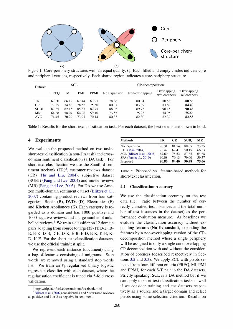
(a) (b)
Core
Periphery
Figure 1: Core-periphery structures with an equal quality, Q. Each filled and empty circles indicate coreand peripheral vertices, respectively. Each shared region indicates a core-periphery structure.
Dataset SCL CP-decomposition
FREQ MI PMI PPMI No Expansion Non-overlapping Overlappingw/o coreness
Overlappingw/ coreness
TR 67.60 66.12 67.44 63.21 78.86 80.34 80.56 80.86CR 77.85 74.83 78.52 75.50 80.87 83.89 83.89 84.40SUBJ 87.65 82.15 85.65 82.75 88.05 89.75 90.15 90.48MR 64.68 58.07 64.26 59.10 73.55 75.23 74.95 75.66AVG 74.45 70.29 73.97 70.14 80.33 82.30 82.39 82.85
Table 1: Results for the short-text classification task. For each dataset, the best results are shown in bold.
4 Experiments
We evaluate the proposed method on two tasks:short-text classification (a non-DA task) and cross-domain sentiment classification (a DA task). Forshort-text classification we use the Stanford sen-timent treebank (TR)3, customer reviews dataset(CR) (Hu and Liu, 2004), subjective dataset(SUBJ) (Pang and Lee, 2004) and movie reviews(MR) (Pang and Lee, 2005). For DA we use Ama-zon multi-domain sentiment dataset (Blitzer et al.,2007) containing product reviews from four cat-egories: Books (B), DVDs (D), Electronics (E)and Kitchen Appliances (K). Each category is re-garded as a domain and has 1000 positive and1000 negative reviews, and a large number of unla-belled reviews.4 We train a classifier on 12 domainpairs adapting from source to target (S-T): B-D, B-E, B-K, D-B, D-E, D-K, E-B, E-D, E-K, K-B, K-D, K-E. For the short-text classification datasets,we use the official train/test split.
We represent each instance (document) usinga bag-of-features consisting of unigrams. Stopwords are removed using a standard stop wordslist. We train an `2 regularised binary logisticregression classifier with each dataset, where theregularisation coefficient is tuned via 5-fold crossvalidation.
3https://nlp.stanford.edu/sentiment/treebank.html4Blitzer et al. (2007) considered 4 and 5 star rated reviews
as positive and 1 or 2 as negative in sentiment.
Methods TR CR SUBJ MR
No Expansion 76.31 81.54 88.05 73.35FTS (Man, 2014) 76.47 62.41 50.15 66.83SCL (Blitzer et al., 2006) 67.60 78.52 87.65 64.68SFA (Pan et al., 2010) 60.08 70.13 79.00 59.57Proposed 80.86 84.40 90.48 75.66
Table 3: Proposed vs. feature-based methods forshort-text classification.
4.1 Classification Accuracy
We use the classification accuracy on the testdata (i.e. ratio between the number of cor-rectly classified test instances and the total num-ber of test instances in the dataset) as the per-formance evaluation measure. As baselines weevaluate the classification accuracy without ex-panding features (No Expansion), expanding thefeatures by a non-overlapping version of the CP-decomposition method where a single peripherywill be assigned to only a single core, overlappingCP-decomposition with and without the consider-ation of coreness (described respectively in Sec-tions 3.2 and 3.3). We apply SCL with pivots se-lected from four different criteria (FREQ, MI, PMIand PPMI) for each S-T pair in the DA datasets.Strictly speaking, SCL is a DA method but if wecan apply to short-text classification tasks as wellif we consider training and test datasets respec-tively as a source and a target domain and selectpivots using some selection criterion. Results on
260
S-T SCL CP-decomposition
FREQ MI PMI PPMI No Expansion Non-overlapping Overlappingw/o coreness
Overlappingw/ coreness
B-D 72.75 65.50 71.50 69.25 75.00 75.75 76.75 76.38B-E 72.75 71.00 74.50 66.00 71.00 71.00 69.75 69.75B-K 77.25 64.00 80.50 77.25 78.25 78.25 77.75 78.00D-B 71.00 53.00 66.25 65.50 74.00 74.25 74.25 75.25D-E 72.00 67.00 72.75 74.75 74.75 73.75 73.00 74.75D-K 79.75 57.50 79.00 76.75 79.25 78.00 79.25 79.25E-B 62.75 57.25 66.25 60.25 69.50 68.50 68.75 68.75E-D 64.50 62.75 65.50 62.75 73.25 71.75 73.25 73.50E-K 82.00 77.75 81.25 79.50 84.25 84.00 82.50 84.00K-B 65.75 52.50 68.00 68.75 70.00 70.00 69.75 69.50K-D 67.25 53.75 66.75 68.50 72.75 72.00 72.75 73.63K-E 77.25 74.50 74.50 74.75 79.00 79.75 79.00 80.50AVG 72.08 63.04 72.23 70.33 75.08 74.75 74.73 75.27
Table 2: Results for DA tasks. For each S-T pair, the best results are shown in bold. The last row showsthe average of performance over the 12 S-T pairs.
the short-text and DA tasks are summarised re-spectively in Tables 1 and 2.
As shown in Table 1, all variants of theCP-decomposition outperform the No Expansionbaseline and the best performance is reportedby the overlapping CP-decomposition consideringthe coreness values. According to binomial test re-sults, there is no statistical significance in Table 1.SCL performs poorly on this non-DA task, indicat-ing that it is specifically customised for DA tasks.
Table 3 compares the performance of the pro-posed method (i.e., overlapping version of the CP-decomposition with coreness) against FTS, a pre-viously proposed feature expansion method andDA methods such as SCL and SFA applied toshort-text classification. We see that the proposedmethod consistently outperforms FTS, which usesfrequently occurring features as expansion candi-dates. This result implies that frequency of a fea-ture alone does not enable us to find useful featuresfor expanding sparse feature vectors. The subop-timal performance of SFA and SCL for short-textclassification indicates that, despite the fact thatthe feature-mismatch problem in DA has some re-semblance to the feature-sparseness problem inshort-text classification, applying DA methods toshort-text classification is not effective. On theother hand, as shown in Table 2, proposed methodreports equal or the best performance for 10 outof 12 domain pairs indicating that it is effectivenot only for short-text classification but also forDA. However, the improvements reported in Ta-ble 2 are not statistically significant (accordingto Clopper-Pearson confidence intervals (Clopper
Methods MR CR SUBJ
Skip-thought (Kiros et al., 2015) 76.5 80.1 93.6Paragraph2Vec (Le and Mikolov, 2014) 74.8 78.1 90.5FastSent (Hill et al., 2016) 70.8 78.4 88.7SDAE (Hill et al., 2016) 74.6 78.0 90.8CNN (Kim, 2014) 76.1 79.8 89.6Proposed 75.7 84.4 90.5
Table 4: Proposed vs. document-level embedding-based methods for short-text classification.
and Pearson, 1934) computed at p < 0.01), im-plying that CP-decomposition is less effective onDA datasets, which contain longer (on average 5-10 sentence reviews) texts.
We compare the proposed method against thestate-of-the-art embedding-based short-text classi-fication methods in Table 4. For skip-thought vec-tors (Kiros et al., 2015), Paragraph2Vec (Le andMikolov, 2014), FastSent (Hill et al., 2016) andSDAE (Hill et al., 2016) provided by Hill et al.(2016), we show the published results on MR,CR and SUBJ.5 CNN represents the convolutionalneural network-based document-level embeddinglearning method proposed by Kim (2014). Theproposed method reports the best results on CR,whereas skip-thought does so for MR and SUBJdatasets. An interesting future research directionwould be to combine feature-expansion methodand document-level embedding methods to furtherimprove the accuracy of short-text classification.
An example feature expansion is shown in Ta-ble 5, where 6 cores are expanded by the over-lapping version of the CP-decomposition method
5These methods have not been evaluated on the TRdataset.
261
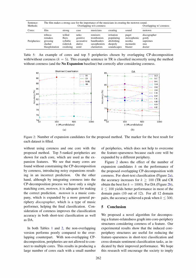
Sentence: The film makes a strong case for the importance of the musicians in creating the motown sound.Methods: Overlapping w/o coreness Overlapping w/ coreness
Cores: film strong case musicians creating sound motown
Peripheries:
tribecaremakesgrossingslasherblaxploitation
willedflierssyllabicroderickoxidizing
nekogenitiveaccusativedativeeeml
remixerstrombonistsbandleaderssaxophonistsclarinetists
irritationpopulatingabolishingduopolysoundscapes
pugetstereophonicnootkamcmurdoblaster
discographergordysupremesstaxdozier
Table 5: An example of cores and top 5 peripheries chosen by overlapping CP-decompositionwith/without coreness (k = 5). This example sentence in TR is classified incorrectly using the methodwithout coreness (and the No Expansion baseline) but correctly after considering coreness.
(a) (b)
Figure 2: Number of expansion candidates for the proposed method. The marker for the best result foreach dataset is filled.
without using coreness and one core with theproposed method. Top 5-ranked peripheries areshown for each core, which are used as the ex-pansion features. We see that many cores arefound without constraining the CP-decompositionby coreness, introducing noisy expansions result-ing in an incorrect prediction. On the otherhand, although by integrating coreness into theCP-decomposition process we have only a singlematching core, motown, it is adequate for makingthe correct prediction. motown is a music com-pany, which is expanded by a more general pe-riphery discographer, which is a type of musicperformer, helping the final classification. Con-sideration of coreness improves the classificationaccuracy in both short-text classification as wellas DA.
In both Tables 1 and 2, the non-overlappingversion performs poorly compared to the over-lapping counterpart. With non-overlapping CP-decomposition, peripheries are not allowed to con-nect to multiple cores. This results in producing alarge number of cores each with a small number
of peripheries, which does not help to overcomethe feature-sparseness because each core will beexpanded by a different periphery.
Figure 2 shows the effect of the number ofexpansion candidates k on the performance ofthe proposed overlapping CP-decomposition withcoreness. For short-text classification (Figure 2a),the accuracy increases for k ≥ 100 (TR and CRobtain the best for k = 1000). For DA (Figure 2b),k ≤ 100 yields better performance in most of thedomain pairs (10 out of 12). For all 12 domainpairs, the accuracy achieved a peak when k ≤ 500.
5 Conclusion
We proposed a novel algorithm for decompos-ing a feature-relatedness graph into core-peripherystructures considering coreness of a feature. Ourexperimental results show that the induced core-periphery structures are useful for reducing thefeature-sparseness in short-text classification andcross-domain sentiment classification tasks, as in-dicated by their improved performance. We hopethis research will encourage the society to imply
262

different CP decomposition methods with differ-ent tasks in NLP.
ReferencesJohn Blitzer, Mark Dredze, and Fernando Pereira.
2007. Biographies, bollywood, boom-boxes andblenders: Domain adaptation for sentiment classi-fication. In Proc. of ACL. pages 440–447.
John Blitzer, Ryan McDonald, and Fernando Pereira.2006. Domain adaptation with structural correspon-dence learning. In Proc. of EMNLP. pages 120–128.
Danushka Bollegala, Takanori Maehara, and Ken ichiKawarabayashi. 2015. Unsupervised cross-domainword representation learning. In Proc. of ACL.pages 730–740.
Danushka Bollegala, David Weir, and John Carroll.2014. Learning to predict distributions of wordsacross domains. In Proc. of ACL. pages 613–623.
C. J. Clopper and E. S. Pearson. 1934. The use of con-fidence or fiducial limits illustrated in the case of thebinomial. Biometrika 26(4):403–413.
Gao Cong, Long Wang, Chin-Yew Lin, Young-In Song,and Yueheng Sun. 2008. Finding question-answerpairs from online forums. In Proc. of SIGIR. pages467–474.
Peter Csermely, András London, Ling-Yun Wu, andBrian Uzzi. 2013. Structure and dynamics ofcore/periphery networks. Journal of Complex Net-works 1(2):93–123.
Cicero dos Santos and Maira Gatti. 2014. Deep con-volutional neural networks for sentiment analysis ofshort texts. In Proc. of COLING. pages 69–78.
P Erdos and A Rényi. 1959. On random graphs i.Publ. Math. 6:290–297.
Hui Fang. 2008. A re-examination of query expansionusing lexical resources. In Proc. of ACL. pages 139–147.
Michel X Goemans and David P Williamson. 1995.Improved approximation algorithms for maximumcut and satisfiability problems using semidefiniteprogramming. Journal of the ACM (JACM)42(6):1115–1145.
Hu Guan, Jinguy Zhou, and Minyi Guo. 2009. A class-feature-centroid classifier for text categorization. InProc. of WWW. pages 201–210.
Felix Hill, Kyunghyun Cho, and Anna Korhonen. 2016.Learning distributed representations of sentencesfrom unlabelled data. In Proceedings of NAACL-HLT . pages 1367–1377.
Minqing Hu and Bing Liu. 2004. Mining and summa-rizing customer reviews. In KDD 2004. pages 168–177.
Richard. M. Karp. 1972. Reducibility among Combi-natorial Problems. Springer US, Boston, MA.
Brian W Kernighan and Shen Lin. 1970. An efficientheuristic procedure for partitioning graphs. The BellSystem Technical Journal 49(2):291–307.
Yoon Kim. 2014. Convolutional neural networks forsentence classification. In Proceedings of the 2014Conference on Empirical Methods in Natural Lan-guage Processing (EMNLP). pages 1746–1751.
Ryan Kiros, Yukun Zhu, Ruslan R Salakhutdinov,Richard Zemel, Raquel Urtasun, Antonio Torralba,and Sanja Fidler. 2015. Skip-thought vectors. InAdvances in neural information processing systems.pages 3294–3302.
Sadamori Kojaku and Naoki Masuda. 2017. Findingmultiple core-periphery pairs in networks. PhysicalReview E 96(5):052313.
Sadamori Kojaku and Naoki Masuda. 2018. Core-periphery structure requires something else in thenetwork. New Journal of Physics 40:043012.
Bing kun Wang, Yong feng Huang, Wan xia Yang,and Xing Li. 2012. Short text classification basedon strong feature thesaurus. Journal of ZhejiangUniversity-SCIENCE C (Computers and Electron-ics) 13(9):649–659.
Haewoon Kwak, Changhyun Lee, Hosung Park, andSue Moon. 2010. What is twitter, a social networkor a news media? In Proc. of WWW. pages 591–600.
Quoc Le and Tomas Mikolov. 2014. Distributed rep-resentations of sentences and documents. In Inter-national Conference on Machine Learning. pages1188–1196.
Huifang Ma, Lei Di, Xiantao Zeng, Li Yan, and YuyiMa. 2016. Short text feature extension based on im-proved frequent term sets. In Zhongzhi Shi, SunilVadera, and Gang Li, editors, Intelligent InformationProcessing VIII. Springer International Publishing,Cham, pages 169–178.
Yuan Man. 2014. Feature extension for short text cate-gorization using frequent term sets. Procedia Com-puter Science 31:663–670. 2nd International Con-ference on Information Technology and QuantitativeManagement, ITQM 2014.
Rada Mihalcea and Dragomir Radev. 2011. Graph-based Natural Language Processing and Informa-tion Retrieval. Cambridge University Press.
Sinno Jialin Pan, Xiaochuan Ni, Jian-Tao Sun, QiangYang, and Zheng Chen. 2010. Cross-domain senti-ment classification via spectral feature alignment. InProc. of WWW. pages 751–760.
Bo Pang and Lillian Lee. 2004. A sentimental educa-tion: Sentiment analysis using subjectivity summa-rization based on minimum cuts. In Proceedings of
263
the 42nd annual meeting on Association for Compu-tational Linguistics. Association for ComputationalLinguistics, page 271.
Bo Pang and Lillian Lee. 2005. Seeing stars: Ex-ploiting class relationships for sentiment categoriza-tion with respect to rating scales. In Proceedings ofthe 43rd annual meeting on association for compu-tational linguistics. Association for ComputationalLinguistics, pages 115–124.
Puck Rombach, Mason A. Porter, James H. Fowler, andPeter J. Mucha. 2017. Core-periphery structure innetworks (revisited). SIAM Review 59(3):619–646.
Takeshi Sakaki, Makoto Okazaki, and Yutaka Matsuo.2010. Earthquake shakes twitter uers: Real-timeevent detection by social sensors. In Proc. of WWW.pages 851–860.
Divya Sardana and Raj Bhatnagar. 2016. Core pe-riphery structures in weighted graphs using greedygrowth. In Proc. 2016 IEEE/WIC/ACM Int. Conf.Web Intelligence Core. ACM, New York, pages 1–8.
Jiang Su, Jelber Sayyad-Shirabad, and Stan Matwin.2011. Large scale text classification using semi-supervised multinomial naive bayes. In Proc. ofICML.
Mike Thelwall, Kevan Buckley, Georgios Paltoglou,Di Cai, and Arvid Kappas. 2010. Sentiment strengthdetection in short informal text. Journal of the As-sociation for Information Science and Technology61(12):2544–2558.
Bing-Bing Xiang, Zhong-Kui Bao, Chuang Ma, XingyiZhang, Han-Shuang Chen, and Hai-Feng Zhang.2018. A unified method of detecting core-peripherystructure and community structure in networks.Chaos: An Interdisciplinary Journal of NonlinearScience 28(1):013122.
Bowen Yan and Jianxi Luo. 2016. Multicore-peripherystructure in networks. Preprint arXiv:1605.03286.
Jaewon Yang and Jure Leskovec. 2014. Overlappingcommunities explain core–periphery organization ofnetworks. Proc. IEEE 102(12):1892–1902.
Dani Yogatama and Noah A. Smith. 2014. Making themost of bag of words: Sentence regularization withalternating direction method of multipliers. In Proc.of ICML. pages 656–664.
264

Proceedings of the 7th Joint Conference on Lexical and Computational Semantics (*SEM), pages 265–275New Orleans, June 5-6, 2018. c©2018 Association for Computational Linguistics
Robust Handling of Polysemy via Sparse Representations
Abhijit A. MahabalGoogle
Dan RothUniversity of [email protected]
Sid MittalGoogle
Abstract
Words are polysemous and multi-faceted,with many shades of meanings. We sug-gest that sparse distributed representations aremore suitable than other, commonly used,(dense) representations to express these mul-tiple facets, and present Category Builder, aworking system that, as we show, makes use ofsparse representations to support multi-facetedlexical representations. We argue that the setexpansion task is well suited to study thesemeaning distinctions since a word may be-long to multiple sets with a different reason formembership in each. We therefore exhibit theperformance of Category Builder on this task,while showing that our representation capturesat the same time analogy problems such as“the Ganga of Egypt” or “the Voldemort ofTolkien”. Category Builder is shown to bea more expressive lexical representation andto outperform dense representations such asWord2Vec in some analogy classes despite be-ing shown only two of the three input terms.
1 Introduction
Word embeddings have received much attentionlately because of their ability to represent similarwords as nearby points in a vector space, thus sup-porting better generalization when comparisonsof lexical items are needed, and boosting the ro-bustness achieved by some deep-learning systems.However, a given surface form often has multiplemeanings, complicating this simple picture. Aroraet al. (2016) showed that the vector correspondingto a polysemous term often is not close to any ofthat of its individual senses, thereby breaking thesimilar-items-map-to-nearby-points promise. Thepolysemy wrinkle is not merely an irritation but,in the words of Pustejovsky and Boguraev (1997),“one of the most intractable problems for languageprocessing studies”.
Our notion of Polysemy here is quite broad,since words can be similar to one another alonga variety of dimensions. The following three pairseach has two similar items: (a) {ring, necklace},(b) {ring, gang}, and (c) {ring, beep}. Note thatring is similar to all words that appear as secondwords in these pairs, but for different reasons, de-fined by the second token in the pairs. While thisexample used different senses of ring, it is easy tofind examples where a single sense has multiplefacets: Clint Eastwood, who is both an actor anda director, shares different aspects with directorsthan with actors, and Google, both a website anda major corporation, is similar to Wikipedia andGeneral Electric along different dimensions.
Similarity has typically been studied pairwise:that is, by asking how similar item A is to itemB. A simple modification sharply brings to forethe issues of facets and polysemy. This modifi-cation is best viewed through the task of set ex-pansion (Wang and Cohen, 2007; Davidov et al.,2007; Jindal and Roth, 2011), which highlights thesimilarity of an item (a candidate in the expansion)to a set of seeds in the list. Given a few seeds (say,{Ford, Nixon}), what else belongs in the set? Notehow this expansion is quite different from the ex-pansion of {Ford, Chevy}, and the difference isone of Similar How, since whether a word (say,BMW or FDR) belongs in the expansion dependsnot just on how much commonality it shares withFord but on what commonality it shares. Conse-quently, this task allows the same surface form tobelong to multiple sets, by virtue of being similarto items in distinct sets for different reasons. Thefacets along which items are similar is implicitlydefined by the members in the set.
In this paper, we propose a context sensitiveversion of similarity based on highlighting sharedfacets. We do this by developing a sparse repre-sentation of words that simultaneously captures all
265
facets of a given surface form. This allows us todefine a notion of contextual similarity, in whichFord is similar to Chevy (e.g., when Audi or BMWis in the context) but similar to Obama when Bushor Nixon is in the context (i.e., in the seed list).In fact, it can even support multi-granular similar-ity since while {Chevy, Chrysler, Ford} representthe facet of AMERICAN CARS, {Chevy, Audi, Ford}define that of CARS. Our contextual similarity isbetter able to mold itself to this variety since itmoves away from the one-size-fits-all nature of co-sine similarity.
We exhibit the strength of the representationand the contextual similarity metric we develop bycomparing its performance on both set expansionand analogy problems with dense representations.
2 Senses and Facets
The present work does not attempt to resolvethe Word Sense Disambiguation (WSD) problem.Rather, our goal is to advance a lexical represen-tation and a corresponding context sensitive sim-ilarity metric that, together, get around explicitlysolving WSD.
Polysemy is intimately tied to the well-exploredfield of WSD so it is natural to expect techniquesfrom WSD to be relevant. If WSD could neatlyseparate senses, the set expansion problem couldbe approached thus. Ford would split into, say,two senses: Ford-1 for the car, and Ford-2 for thepresident, and expanding {Ford, Nixon} could betranslated to expanding {Ford-2, Nixon}. Such arepresentational approach is taken by many au-thors when they embed the different senses ofwords as distinct points in an embedding space(Reisinger and Mooney, 2010; Huang et al., 2012;Neelakantan et al., 2014; Li and Jurafsky, 2015).
Such approaches run into what we term theFixed Inventory Problem. Either senses are ob-tained from a hand curated resource such as a dic-tionary, or are induced from the corpus directlyby mapping contexts clusters to different senses.In either case, however, by the time the final rep-resentation (e.g., the embedding) is obtained, thenumber of different senses of each term has be-come fixed: all decisions have been made relatingto how finely or coarsely to split senses.
How to split senses is a hard problem: dictionar-ies such as NOAD list coarse senses and split thesefurther into fine senses, and it is unclear what gran-ularity to use: should each fine sense correspond
to a point in the vector space, or should, instead,each coarse sense map to a point? Many authors(Hofstadter and Sander, 2013, for example) dis-cuss how the various dictionary senses of a termare not independent. Further, if context clustersmap to senses, the word whale, which is seen bothin mammal-like contexts (e.g., “whales have hair”)and water-animal contexts (“whales swim”), couldget split into separate points. Thus, the differentsenses that terms are split into may instead be dis-tinct facets. This is not an idle theoretical worry:such facet-based splitting is evident in Neelakan-tan et al. (2014, Table 3). Similarly, in the vec-tors they released, november splits into ten senses,likely based on facets. Once split, for subsequentprocessing, the points are independent.
In contrast to such explicit, prior, splitting, inthe Category Builder approach developed here,relevant contexts are chosen given the task at hand,and if multiple facets are relevant (as happens, forexample, in {whale, dolphin, seal}, whose expan-sion should rank aquatic mammals highest), allthese facets influence the expansion; if only onefacet is of relevance (as happens in {whale, shark,seahorse}), the irrelevant facets get ignored.
3 Related Work
In this section, we situate our approach within therelevant research landscape. Both Set Expansionand Analogies have a long history, and both de-pend on Similarity, with an even longer history.
3.1 Set Expansion
Set Expansion is the well studied problem of ex-panding a given set of terms by finding other se-mantically related terms. Solutions fall into twolarge families, differing on whether the expansionis based on a preprocessed, limited corpus (Shenet al., 2017, for example) or whether a much largercorpus (such as the entire web) is accessed on de-mand by making use of a search engine such asGoogle (Wang and Cohen, 2007, for example).
Each family has its advantages and disadvan-tages. “Open web” techniques that piggyback onGoogle can have coverage deep into the tail. Thesetypically rely on some form of Wrapper Induc-tion, and tend to work better for sets whose in-stances show up in lists or other repeated structureon the web, and thus perform much better on setsof nouns than on sets of verbs or adjectives. Bycontrast, “packaged” techniques that work off a
266
preprocessed corpus are faster (no Google lookupneeded) and can work well for any part of speech,but are of course limited to the corpus used. Thesetypically use some form of distributional similar-ity, which can compute similarity between itemsthat have never been seen together in the samedocument; approaches based on shared member-ships in lists would need a sequence of overlap-ping lists to achieve this. Our work is in the “pack-aged” family, and we use sparse representationsused for distributional similarity.
Gyllensten and Sahlgren (2018) compares twosubfamilies within the packaged family: central-ity-based methods use a prototype of the seeds(say, the centroid) as a proxy for the entire seedset and classification-based methods (a strict su-perset), which produce a classifier by using theseeds. Our approach is classification-based.
It is our goal to be able to expand nuancedcategories. For example, we want our solutionto expand the set {pluto, mickey}—both Disneycharacters—to other Disney characters. That is,the context mickey should determine what is con-sidered ‘similar’ to pluto, rather than being biasedby the more dominant sense of pluto, to determinethat neptune is similar to it. Earlier approachessuch as Rong et al. (2016) approach this problemdifferently: they expand to both planets and Dis-ney characters, and then attempt to cluster the ex-pansion into meaningful clusters.
3.2 Analogies
Solving analogy problems usually refers to pro-portional analogies, such as hand:glove::foot:?.Mikolov et al. (2013) showed how word embed-dings such as Word2Vec capture linguistic regu-larities and thereby solve this. Turney (2012) useda pair of similarity functions (one for function andone for domain) to address the same problem.
There is a sense, however, that the problem isoverdetermined: in many such problems, peoplecan solve it even if the first term is not shown.That is, people easily answer “What is the glovefor the foot?”. People also answer questions suchas “What is the Ganga of Egypt?” without firsthaving to figure out the unprovided term India (oris the missing term Asia? It doesn’t matter.) Hof-stadter and Sander (2013) discuss how our abilityto do these analogies is central to cognition.
The current work aims to tackle these non-proportional analogies and in fact performs bet-
ter than Word2Vec on some analogy classes usedby Mikolov et al. (2013), despite being shown onefewer term.
The approach is rather close to that used by Tur-ney (2012) for a different problem: word com-pounds. Understanding what a dog house is canbe phrased as “What is the house of a dog?”, withkennel being the correct answer. This is solvedusing the pair of similarity functions mentionedabove. The evaluations provided in that paperare for ranking: which of five provided terms isa match. Here, we apply it to non-proportionalanalogies and evaluate for retrieval, where we areranking over all words, a significantly more chal-lenging problem.
To our knowledge, no one has presented a com-putational model for analogies where only twoterms are provided. We note, however, that Linzen(2016) briefly discusses this problem.
3.3 Similarity
Both Set Expansion and Analogies depend on anotion of similarity. Set Expansion can be seenas finding items most similar to a category, andAnalogies can be seen as directly dependent onsimilarities (e.g., in the work of Turney (2012)).
Most current approaches, such as word embed-dings, produce a context independent similarity. Insuch an approach, the similarity between, say, kingand twin is some fixed value (such as their cosinesimilarity). However, depending on whether weare talking about bed sizes, these two items are ei-ther closely related or completely unrelated, andthus context dependent.
Psychologists and Philosophers of Languagehave long pointed out that similarity is subtle.It is sensitive to context and subject to prim-ing effects. Even the very act of categorizationcan change the perceived similarity between items(Goldstone et al., 2001). Medin et al. (1993, p.275) tell a story, from the experimental psychol-ogy trenches, that supports representation morph-ing when they conclude that “the effective rep-resentations of constituents are determined in thecontext of the comparison, not prior to it”.
Here we present a malleable notion of similar-ity that can adapt to the wide range of human cat-egories, some of which are based on narrow, su-perficial similarities (e.g., BLUE THINGS) while oth-ers share family resemblances (a la Wittgenstein).Even in a small domain such as movies, in differ-
267

ent contexts, similarity may be driven by who thedirector is, or the cast, or the awards won. Fur-thermore, to the extent that the contexts we useare human readable, we also have a mechanismfor explaining what makes the terms similar.
There is a lot of work on the context-dependence of human categories and similaritiesin Philosophy, in Cognitive Anthropology andin Experimental Psychology (Lakoff, 1987; Ellis,1993; Agar, 1994; Goldstone et al., 2001; Hof-stadter and Sander, 2013, for example, surveythis space from various theoretical standpoints),but there are not, to our knowledge, unsupervisedcomputational models of these phenomena.
4 Representations and Algorithms
This section describes the representation and cor-responding algorithms that perform set expansionin Category Builder (CB).
4.1 Sparse Representations for Expansion
We use the traditional word representation thatdistributional similarity uses (Turney and Pantel,2010), and that is commonly used in fields suchas context sensitive spelling correction and gram-matical correction (Golding and Roth, 1999; Ro-zovskaya and Roth, 2014); namely,words are asso-ciated with some ngrams that capture the contextsin which they occur – all contexts are representedin a sparse vector corresponding to a word. Fol-lowing Levy and Goldberg (2014a), we call thisrepresentation explicit.
Generating Representations. We start withweb pages and extract words and phrases fromthese, as well as the contexts they appear in. Anaggregation step then calculates the strengths ofword to context and context to word associations.
Vocabulary. The vocabulary is made up ofwords (nouns, verbs, adjectives, and adverbs) andsome multi-word phrases. To go beyond words,we use a named entity recognizer to find multi-word phrases such as New York. We also use oneheuristic rule to add certain phrasal verbs (e.g.,take shower), when a verb is directly followed byits direct object. We lowercase all phrases, anddrop those phrases seen infrequently. The set ofall words is called the vocabulary, V .
Contexts. Many kinds of contexts have beenused in literature. Levy (2018) provides a compre-hensive overview. We use contexts derived fromsyntactic parse trees using about a dozen heuris-
tic rules. For instance, one rule deals with nounsmodified by an adjective, say, red followed bycar. Here, one of the contexts of car is MODI-FIEDBY#RED, and one of the contexts of red isMODIFIES#CAR. Two more examples of contexts:OBJECTOF#EAT and SUBJECTOF#WRITE. Theset of all contexts is denoted C.
The Two Vocabulary⇔Context matrices. Forvocabulary V and contextsC, we produce two ma-trices, MV→C and MC→V . Many measures of as-sociation between a word and a context have beenexplored in the literature, usually based on somevariant of pointwise mutual information.
PPMI (Positive PMI) is the typically used mea-sure. If P (w), P (c) and P (w, c) respectively rep-resent the probabilities that a word is seen, a con-text is seen and the word is seen in that context,then
PMI(w, c) = logP (w, c)
P (w)P (c)(1)
PPMI(w, c) = max(0,PMI(w, c)) (2)
PPMI is widely used, but comments are in orderregarding the ad-hocness of the “0” in Equation 2.There is seemingly a good reason to choose 0 asa threshold: if a word is seen in a context morethan by chance, the PMI is positive, and a 0 thresh-old seems sensible. However, in the presence ofpolysemy, especially lopsided polysemy such asCancer (disease and star sign), a “0” threshold isarbitrary: even if every single occurrence of thestar sign sense of cancer was seen in some con-text c (thereby crying out for a high PMI), be-cause of the rarity of that sense, the overall PMIbetween c and (non-disambiguated) Cancer maywell be negative. Relatedly, Shifted PPMI (Levyand Goldberg, 2014b) uses a non-0 cutoff.
Another well known problem with PPMI is itslarge value when the word or the context is rare,and even a single occurrence of a word-contextpair can bloat the PMI (see Role and Nadif, 2011,for fixes that have been proposed). We introducea new variant we call Asymmetric PMI, whichtakes frequency into account by adding a secondlog term, and is asymmetric because in generalP (w|c) 6= P (c|w):
APMI(w, c) = PMI(w, c) + logP (w, c)
P (w)
= logP (w, c)2
P (w)2P (c)
(3)
268

This is asymmetric because APMI(c, w) hasP (c) in the denominator of the extra log term.
What benefit does this modification to PMI pro-vide? Consider a word and two associated con-texts, c1 and c2, where the second context is sig-nificantly rarer. Further, imagine that the PMI ofthe word with either feature is the same. The wordwould have been seen in the rarer context only afew times, and this is more likely to have been astatistical fluke. In this case, the APMI with themore frequent term is higher: we reward the factthat the PMI is high despite its prevalence; this isless likely to be an artifact of chance.
Note that the rearranged expression seen inthe second line of Equation 3 is reminiscent ofPPMI0.75 from Levy et al. (2015).
The second log term in APMI is always nega-tive, and we thus shift all values by a constant k(chosen based on practical considerations of datasize: the smaller the k, the larger the size of thesparse matrices; based on experimenting with vari-ous values of k, it appears that expansion quality isnot very sensitive to k). Clipping this shifted valueat 0 produces Asymmetrical PPMI (APPMI):
APPMI(w, c) = max(0,APMI(w, c) + k) (4)
The two matrices thus produced are shown inEquation 5. If we use PPMI instead of APPMI,these are transposes of each other.
MV→Cw,c = APPMI(w, c)
MC→Vc,w = APPMI(c, w)(5)
4.2 Focused Similarity and Set Expansion
We now come to the central idea of this paper:the notion of focused similarity. Typically, simi-larity is based on the dot product or cosine simi-larity of the context vectors. The pairwise simi-larity among all terms can be expressed as a ma-trix multiplication as shown in Equation 6. Notethat if we had used PPMI in Equation 5, the ma-trices would be each other’s transposes and eachentry in SimMatrix in Equation 6 would be thedot-product-based similarity for a word pair.
SimMatrix =MC→VMV→C (6)
We introduce context weighting by inserting asquare matrix W between the two (see Equation7). Similarity is unchanged if W is the identitymatrix. IfW is a non-identity diagonal matrix, this
is equivalent to treating some contexts as more im-portant than others. It is by appropriately choosingweights in W that we achieve the context depen-dent similarity. If, for instance, all contexts otherthan those indicative of cars are zeroed out in W ,ford and obama will have no similarity.
SimMatrix =MC→VWMV→C (7)
4.3 Set Expansion via Matrix Multiplication
To expand a set of k seeds, we can construct thek-hot column vector S with a 1 corresponding toeach seed, and a 0 elsewhere. Given S, we calcu-late the focus matrix, WS . Then the expansion Eis a column vector that is just:
E =MC→VWSMV→CS (8)
The score for a term in E is the sum of its fo-cused similarity to each seed.
4.4 Motivating Our Choice of W
When expanding the set {taurus, cancer}—the setof star signs, or perhaps the constellations—we arefaced with the presence of a polysemous term witha lopsided polysemy. The disease sense is muchmore prevalent than the star sign sense for cancer,and the associated contexts are also unevenly dis-tributed. If we attempt to use Equation 8 with theidentity matrix W , the expansion is dominated bydiseases.
The contexts we care about are those that areshared. Note that restricting ourselves to the in-tersection is not sensible, since if we are givena dozen seeds it is entirely possible that theyshare family resemblances and have a high pair-wise overlap in contexts between any two seedsbut where there are almost no contexts shared byall. We thus require a soft intersection, and this weachieve by downweighting contexts based on whatfraction of the seeds are associated with that con-text. The parameter ρ described in the next sectionachieves this.
This modification helps, but it is not enough.Each disease-related context for cancer is nowweakened, but their large number causes manydiseases to rank high in the expansion. To addressthis, we can limit ourselves to only the top n con-texts (typically, n = 100 is used). This way, ifthe joint contexts are highly ranked, the expansionwill be based only on such contexts.
269
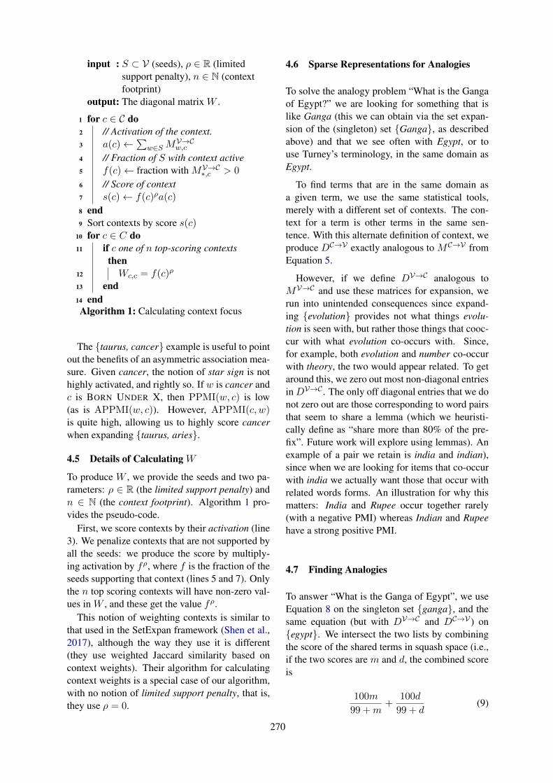
input : S ⊂ V (seeds), ρ ∈ R (limitedsupport penalty), n ∈ N (contextfootprint)
output: The diagonal matrix W .
1 for c ∈ C do2 // Activation of the context.3 a(c)←∑
w∈SMV→Cw,c
4 // Fraction of S with context active5 f(c)← fraction with MV→C∗,c > 0
6 // Score of context7 s(c)← f(c)ρa(c)
8 end9 Sort contexts by score s(c)
10 for c ∈ C do11 if c one of n top-scoring contexts
then12 Wc,c = f(c)ρ
13 end14 endAlgorithm 1: Calculating context focus
The {taurus, cancer} example is useful to pointout the benefits of an asymmetric association mea-sure. Given cancer, the notion of star sign is nothighly activated, and rightly so. If w is cancer andc is BORN UNDER X, then PPMI(w, c) is low(as is APPMI(w, c)). However, APPMI(c, w)is quite high, allowing us to highly score cancerwhen expanding {taurus, aries}.
4.5 Details of Calculating W
To produce W , we provide the seeds and two pa-rameters: ρ ∈ R (the limited support penalty) andn ∈ N (the context footprint). Algorithm 1 pro-vides the pseudo-code.
First, we score contexts by their activation (line3). We penalize contexts that are not supported byall the seeds: we produce the score by multiply-ing activation by fρ, where f is the fraction of theseeds supporting that context (lines 5 and 7). Onlythe n top scoring contexts will have non-zero val-ues in W , and these get the value fρ.
This notion of weighting contexts is similar tothat used in the SetExpan framework (Shen et al.,2017), although the way they use it is different(they use weighted Jaccard similarity based oncontext weights). Their algorithm for calculatingcontext weights is a special case of our algorithm,with no notion of limited support penalty, that is,they use ρ = 0.
4.6 Sparse Representations for Analogies
To solve the analogy problem “What is the Gangaof Egypt?” we are looking for something that islike Ganga (this we can obtain via the set expan-sion of the (singleton) set {Ganga}, as describedabove) and that we see often with Egypt, or touse Turney’s terminology, in the same domain asEgypt.
To find terms that are in the same domain asa given term, we use the same statistical tools,merely with a different set of contexts. The con-text for a term is other terms in the same sen-tence. With this alternate definition of context, weproduce DC→V exactly analogous to MC→V fromEquation 5.
However, if we define DV→C analogous toMV→C and use these matrices for expansion, werun into unintended consequences since expand-ing {evolution} provides not what things evolu-tion is seen with, but rather those things that cooc-cur with what evolution co-occurs with. Since,for example, both evolution and number co-occurwith theory, the two would appear related. To getaround this, we zero out most non-diagonal entriesinDV→C . The only off diagonal entries that we donot zero out are those corresponding to word pairsthat seem to share a lemma (which we heuristi-cally define as “share more than 80% of the pre-fix”. Future work will explore using lemmas). Anexample of a pair we retain is india and indian),since when we are looking for items that co-occurwith india we actually want those that occur withrelated words forms. An illustration for why thismatters: India and Rupee occur together rarely(with a negative PMI) whereas Indian and Rupeehave a strong positive PMI.
4.7 Finding Analogies
To answer “What is the Ganga of Egypt”, we useEquation 8 on the singleton set {ganga}, and thesame equation (but with DV→C and DC→V ) on{egypt}. We intersect the two lists by combiningthe score of the shared terms in squash space (i.e.,if the two scores are m and d, the combined scoreis
100m
99 +m+
100d
99 + d(9)
270

5 Set Expansion Experiments andEvaluation
5.1 Experimental Setup
We report data on two different corpora.The Comparison Corpus. We begin with
20 million English web pages randomly sampledfrom a set of popular web pages (high pagerankaccording to Google). We run Word2Vec on thetext of these pages, producing a 200 dimensionalembeddings. We also produce MV→C and MC→V
according to Equation 5. We use this corpus tocompare Category Builder with Word2Vec-basedtechniques. Note that these web-pages may benoisier than Wikipedia. Word2Vec was chosen be-cause it was deemed “comparable”: mathemati-cally, it is an implicit factorization of the PMI ma-trix (Levy and Goldberg, 2014b).
Release Corpus. We also ran Category Builderon a much larger corpus. The generated matri-ces are restricted to the most common words andphrases (around 200,000). The matrices and asso-ciated code are publicly available1.
Using Word2Vec for Set Expansion. Twoclasses of techniques are considered, representingmembers of both families described by Gyllenstenand Sahlgren (2018). The centroid method findsthe centroid of the seeds and expands to its neigh-bors based on cosine similarity. The other meth-ods first find similarity of a candidate to each seed,and combines these scores using arithmetic, geo-metric, and harmonic means.
Mean Average Precision (MAP). MAP com-bines both precision and recall into a sin-gle number. The gold data to evaluateagainst is presented as sets of synsets, e.g.,{{California,CA}, {Indiana, IN}, . . .}.
An expansion L consists of an ordered list ofterms (which may include the seeds). DefinePreci(L) to be the fraction of items in the first iitems inL that belong to at least one golden synset.We can also speak of the precision at a synset,PrecS(L) = Precj(L), where j is the smallestindex where an element in S was seen in L. Ifno element in the synset S was ever seen, thenPrecS = 0. MAP(L) = avg(PrecS(L)) is theaverage precision over all synsets.
Generalizations of MAP. While MAP is an ex-cellent choice for closed sets (such as U.S. STATES),it is less applicable to open sets (say, POLITICAL
1https://github.com/google/categorybuilder
IDEOLOGIES or SCIENTISTS). For such cases, we pro-pose a generalization of MAP that preserves its at-tractive properties of combining precision and re-call while accounting for variant names. The pro-posed score is MAPn(L), which is the average ofprecision for the first n synsets seen. That it is astrict generalization of MAP can be seen by ob-serving that in the case of US STATES, MAP(L) ≡MAP50(L).
5.2 Evaluation Sets
We produced three evaluation sets, two closedand one open. For closed sets, following Wangand Cohen (2007), we use US States and Na-tional Football League teams. To increase the dif-ficulty, for NFL teams, we do not use as seedsdismabiguated names such as Detroit Lions orGreen Bay Packers, instead using the polysemouslions and packers. The synsets were produced byadding all variant names for the teams. For exam-ple, Atlanta Falcons are also known as falcs, andso this was added to the synset.
For the open set, we use verbs that indicatethings breaking or failing in some way. We choseten popular instances (e.g., break, chip, shatter)and these act as seeds. We expanded the set bymanual evaluation: any correct item produced byany of the evaluated systems was added to the list.There is an element of subjectivity here, and wetherefore provide the lists used (Appendix A.1).
5.3 Evaluation
For each evaluation set, we did 50 set expansions,each starting with three randomly selected seeds.
Effect of ρ and APPMI. Table 1 reveals thatAPPMI performs better than PPMI — signifi-cantly better on two sets, and slightly worse onone. Penalizing contexts that are not shared bymost seeds (i.e., using ρ > 0) also has a markedpositive effect.
Effect of n. Table 2 reveals a curious effect. Aswe increase n, for US STATES, performance dropssomewhat but for BREAK VERBS it improves quite abit. Our analysis shows that pinning down whata state is can be done with very few contexts,and other shared contexts (such as LIVE IN X)are shared also with semantically related entitiessuch as states in other countries. At the other end,BREAK VERBS is based on a large number of sharedcontexts and using more contexts is beneficial.
271
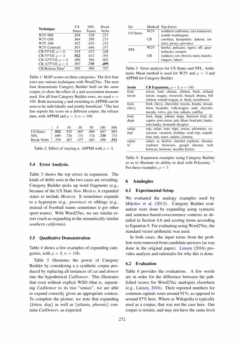
Technique US NFL BreakStates Teams Verbs
W2V HM .858 .528 .231W2V GM .864 .589 .273W2V AM .852 .653 .332W2V Centroid .851 .646 .337CB:PPMI; ρ = 0 .918 .473 .248CB:PPMI; ρ = 3 .922 .612 .393CB:APPMI; ρ = 0 .900 .584 .402CB:APPMI; ρ = 3 .907 .735 .499CB:Release Data† .959 .999 .797
Table 1: MAP scores on three categories. The first fourrows use various techniques with Word2Vec. The nextfour demonstrate Category Builder built on the samecorpus, to show the effect of ρ and association measureused. For all four Category Builder rows, we used n =100. Both increasing ρ and switching to APPMI can beseen to be individually and jointly beneficial. †The lastline reports the score on a different corpus, the releasedata, with APPMI and ρ = 3, n = 100.
5 10 30 50 100 500US States .932 .925 .907 .909 .907 .903NFL .699 .726 .731 .734 .735 .733Break Verbs .339 .407 .477 .485 .496 .511
Table 2: Effect of varying n. APPMI with ρ = 3.
5.4 Error Analysis.
Table 3 shows the top errors in expansion. Thekinds of drifts seen in the two cases are revealing.Category Builder picks up word fragments (e.g.,because of the US State New Mexico, it expandedstates to include Mexico). It sometimes expandsto a hypernym (e.g., province) or siblings (e.g.,instead of Football teams sometimes it got othersport teams). With Word2Vec, we see similar er-rors (such as expanding to the semantically similarsouthern california).
5.5 Qualitative Demonstration
Table 4 shows a few examples of expanding cate-gories, with ρ = 3, n = 100.
Table 5 illustrates the power of CategoryBuilder by considering a a synthetic corpus pro-duced by replacing all instances of cat and denverinto the hypothetical CatDenver. This illustratesthat even without explicit WSD (that is, separat-ing CatDenver to its two “senses”, we are ableto expand correctly given an appropriate context.To complete the picture, we note that expanding{kitten, dog} as well as {atlanta, phoenix} con-tains CatDenver, as expected.
Set Method Top Errors
US States W2V southern california; east tennessee;seattle washington
CB carolina; hampshire; dakota; on-tario; jersey; province
NFL W2V hawks; pelicans; tigers; nfl; quar-terbacks; sooners
CB yankees; sox; braves; mets; knicks;rangers, lakers
Table 3: Error analysis for US States and NFL. Arith-metic Mean method is used for W2V and ρ = 3 andAPPMI for Category Builder
Seeds CB Expansion, ρ = 3, n = 100ford,nixon
nixon, ford, obama, clinton, bush, richardnixon, reagan, roosevelt, barack obama, billclinton, ronald reagan, w. bush, eisenhower
ford,chevy
ford, chevy, chevrolet, toyota, honda, nissan,bmw, hyundai, volkswagen, audi, chrysler,mazda, volvo, gm, kia, subaru, cadillac
ford,depp
ford, depp, johnny depp, harrison ford, di-caprio, tom cruise, pitt, khan, brad pitt, hanks,tom hanks, leonardo dicaprio
safari,trip†
trip, safari, tour, trips, cruise, adventure, ex-cursion, vacation, holiday, road trip, expedi-tion, trek, tours, safaris, journey,
safari,ie†
safari, ie, firefox, internet explorer, chrome,explorer, browsers, google chrome, webbrowser, browser, mozilla firefox
Table 4: Expansion examples using Category Builderso as to illustrate its ability to deal with Polysemy. †
For these examples, ρ = 5
6 Analogies
6.1 Experimental Setup
We evaluated the analogy examples used byMikolov et al. (2013). Category Builder eval-uation were done by expanding using syntacticand sentence-based-cooccurrence contexts as de-tailed in Section 4.6 and scoring items accordingto Equation 9. For evaluating using Word2Vec, thestandard vector arithmetic was used.
In both cases, the input terms from the prob-lem were removed from candidate answers (as wasdone in the original paper). Linzen (2016) pro-vides analysis and rationales for why this is done.
6.2 Evaluation
Table 6 provides the evaluations. A few wordsare in order for the difference between the pub-lished scores for Word2Vec analogies elsewhere(e.g., Linzen, 2016). Their reported numbers forcommon capitals were around 91%, as opposed toaround 87% here. Where as Wikipedia is typicallyused as a corpus, that was not the case here. Ourcorpus is noisier, and may not have the same level
272

Seeds CB Expansion, ρ = 3, n = 100CatDenver,dog
dogs, cats, puppy, pet, rabbit, kitten, ani-mal, animals, pup, pets, puppies, horse
CatDenver,phoenix
chicago, atlanta, seattle, dallas, boston,portland, angeles, los angeles
CatDenver,TigerAndroid
cats, lion, dog, tigers, kitten, animal,dragon, wolf, dogs, bear, leopard, rabbit
Table 5: Expansion examples with synthetic polysemyby replacing all instances of cat and denver into thehypothetical CatDenver (similarly, TigerAndroid). Asingle other term is enough to pick out the right sense.
a:b::c:? Harder :b::c:?(a withheld)Method W2V CB:APPMICorpus Comp Comp Release†
common capitals .872 .957 .941city-in-state .657 .972 .955currency .030 .037 .122nationality .515 .615 .655world capitals .472 .789 .668family .617 .217 .306
Table 6: Performance on Analogy classes fromMikolov et al. (2013). The first two columns are de-rived from the same corpus, whereas the last columnreports numbers on the data we will release. For cate-gory builder, we used ρ = 3, n = 100
of country-based factual coverage as Wikipedia,and almost all non-grammar based analogy prob-lems are of that nature.
A second matter to point out is why grammarbased rows are missing from Table 6. Grammarbased analogy classes cannot be solved with justtwo terms. For boy:boys::king:?, dropping the firstterm boy takes away information crucial to thesolution in a way that dropping the first term ofUS:dollar::India:? does not. The same is true forthe family class of analogies.
6.3 Qualitative DemonstrationTable 7 provides a sampler of analogies solved us-ing Category Builder.
7 Limitations
Much work remains, of course. The analogy workpresented here (and also the corresponding workusing vector offsets) is no match for the sub-tlety that people can bring to bear when they seedeep connections via analogy. Some progress herecould come from the ability to discover and usemore semantically meaningful contexts.
There is currently no mechanism to automati-cally choose n and ρ. Standard settings of n =100 and ρ = 3 work well for the many appli-cations we use it for, but clearly there are cate-
term1 term2 What is the term1 of term2?voldemort tolkien sauronvoldemort star wars vader
ganga egypt niledollar india rupee
football india cricketcivic toyota corolla
Table 7: A sampler of analogies solved by CategoryBuilder.
gories that benefit from very small n (such as BLUE
THINGS) or very large n. Similarly, as can be seenin Equation 9, analogy also uses a parameter forcombining the results, with no automated way yetto choose it. Future work will prioritize this.
The current work suggests, we believe, that itis beneficial to not collapse the large dimensionalsparse vector space that implicitly underlies manyembeddings. Having the ability to separately ma-nipulate contexts can help differentiate betweenitems that differ on that context. That said, thesmoothing and generalization that dimensionalityreduction provides has its uses, so finding a com-bined solution might be best.
8 Conclusions
Given that natural categories vary in their degreeof similarities and their kinds of coherence, we be-lieve that solutions that can adapt to these wouldperform better than context independent notions ofsimilarity.
As we have shown, Category Builder displaysthe ability to implicitly deal with polysemy anddetermine similarity in a context sensitive manner,as exhibited in its ability to expand a set by latch-ing on to what is common among the seeds.
In developing it we proposed a new measureof association between words and contexts anddemonstrated its utility in set expansion and a hardversion of the analogy problem. In particular, ourresults show that sparse representations deserveadditional careful study.
Acknowledgments
We are thankful to all the reviewers for their help-ful comments and critiques. In particular, Ido Da-gan, Yoav Goldberg, Omer Levy, Praveen Pari-tosh, and Chris Waterson gave us insightful com-ments on earlier versions of this write up. Theresearch of Dan Roth is partly supported by aGoogle gift and by DARPA, under agreementnumber FA8750-13-2-008.
273

ReferencesMichael Agar. 1994. Language shock: Understand-
ing the culture of conversation. William Morrow &Company.
Sanjeev Arora, Yuanzhi Li, Yingyu Liang, Tengyu Ma,and Andrej Risteski. 2016. Linear algebraic struc-ture of word senses, with applications to polysemy.arXiv preprint arXiv:1601.03764.
Dmitry Davidov, Ari Rappoport, and Moshe Koppel.2007. Fully unsupervised discovery of concept-specific relationships by web mining. In Proceed-ings of the 45th Annual Meeting of the Associa-tion of Computational Linguistics, pages 232–239,Prague, Czech Republic. Association for Computa-tional Linguistics.
John M. Ellis. 1993. Language, Thought, and Logic.Northwestern University Press.
A. R. Golding and D. Roth. 1999. A winnow based ap-proach to context-sensitive spelling correction. Ma-chine Learning, 34(1-3):107–130.
Robert L Goldstone, Yvonne Lippa, and Richard MShiffrin. 2001. Altering object representationsthrough category learning. Cognition, 78(1):27–43.
Amaru Cuba Gyllensten and Magnus Sahlgren. 2018.Distributional term set expansion.
Douglas Hofstadter and Emmanuel Sander. 2013. Sur-faces and Essences: Analogy as the Fuel and Fire ofThinking. Basic Books.
Eric H Huang, Richard Socher, Christopher D Man-ning, and Andrew Y Ng. 2012. Improving wordrepresentations via global context and multiple wordprototypes. In Proceedings of the 50th Annual Meet-ing of the Association for Computational Linguis-tics: Long Papers-Volume 1, pages 873–882. Asso-ciation for Computational Linguistics.
P. Jindal and D. Roth. 2011. Learning from negativeexamples in set-expansion. In ICDM, pages 1110–1115.
George Lakoff. 1987. Women, Fire, and DangerousThings: What Categories Reveal about the Mind.University of Chicago Press.
Omer Levy. 2018. The Oxford handbook of computa-tional linguistics, second edition, chapter Word Rep-resentaion. Oxford University Press.
Omer Levy and Yoav Goldberg. 2014a. Linguistic reg-ularities in sparse and explicit word representations.In Proceedings of the eighteenth conference on com-putational natural language learning, pages 171–180.
Omer Levy and Yoav Goldberg. 2014b. Neuralword embedding as implicit matrix factorization.In Z. Ghahramani, M. Welling, C. Cortes, N. D.Lawrence, and K. Q. Weinberger, editors, Advances
in Neural Information Processing Systems 27, pages2177–2185. Curran Associates, Inc.
Omer Levy, Yoav Goldberg, and Ido Dagan. 2015. Im-proving distributional similarity with lessons learnedfrom word embeddings. Transactions of the Associ-ation for Computational Linguistics, 3:211–225.
Jiwei Li and Dan Jurafsky. 2015. Do multi-sense em-beddings improve natural language understanding?
Tal Linzen. 2016. Issues in evaluating seman-tic spaces using word analogies. arXiv preprintarXiv:1606.07736.
Douglas L Medin, Robert L Goldstone, and DedreGentner. 1993. Respects for similarity. Psychologi-cal review, 100(2):254.
Tomas Mikolov, Wen-tau Yih, and Geoffrey Zweig.2013. Linguistic regularities in continuous spaceword representations. In Proceedings of the 2013Conference of the North American Chapter of theAssociation for Computational Linguistics: HumanLanguage Technologies, pages 746–751.
Arvind Neelakantan, Jeevan Shankar, Alexandre Pas-sos, and Andrew McCallum. 2014. Efficient non-parametric estimation of multiple embeddings perword in vector space. In Proceedings of the 2014Conference on Empirical Methods in Natural Lan-guage Processing.
James Pustejovsky and Bran Boguraev. 1997. Lexi-cal semantics: The problem of polysemy. ClarendonPress.
Joseph Reisinger and Raymond J Mooney. 2010.Multi-prototype vector-space models of word mean-ing. In Human Language Technologies: The 2010Annual Conference of the North American Chap-ter of the Association for Computational Linguistics,pages 109–117. Association for Computational Lin-guistics.
Francois Role and Mohamed Nadif. 2011. Handlingthe impact of low frequency events on co-occurrencebased measures of word similarity. In InternationalConference on Knowledge Discovery and Informa-tion Retrieval, pages 226–231.
Xin Rong, Zhe Chen, Qiaozhu Mei, and Eytan Adar.2016. Egoset: Exploiting word ego-networks anduser-generated ontology for multifaceted set expan-sion. In Proceedings of the Ninth ACM InternationalConference on Web Search and Data Mining, pages645–654. ACM.
A. Rozovskaya and D. Roth. 2014. Building a state-of-the-art grammatical error correction system.
Jiaming Shen, Zeqiu Wu, Dongming Lei, JingboShang, Xiang Ren, and Jiawei Han. 2017. Setexpan:Corpus-based set expansion via context feature se-lection and rank ensemble. In Joint European Con-ference on Machine Learning and Knowledge Dis-covery in Databases, pages 288–304. Springer.
274

Peter D Turney. 2012. Domain and function: A dual-space model of semantic relations and compositions.Journal of Artificial Intelligence Research, 44:533–585.
Peter D Turney and Patrick Pantel. 2010. From fre-quency to meaning: Vector space models of se-mantics. Journal of artificial intelligence research,37:141–188.
Richard C Wang and William W Cohen. 2007.Language-independent set expansion of named en-tities using the web. In Data Mining, 2007. ICDM2007. Seventh IEEE International Conference on,pages 342–350. IEEE.
A Supplemental Material
A.1 Lists Used in Evaluating Set Expansion
US States. Any of the 50 states could be used asa seed. The 50 golden synsets were the 50 pairsof state name and abbreviation (e.g., {California,CA}).
NFL Teams. Any of the first termsin these 32 synsets could be used as aseed. The golden synsets are: {Bills, Buf-falo Bills}, {Dolphins, Miami Dolphins, Phins},{Patriots, New England Patriots, Pats}, {Jets,New York Jets}, {Ravens, Baltimore Ravens},{Bengals, Cincinnati Bengals}, {Browns, Cleve-land Browns}, {Steelers, Pittsburgh Steelers},{Texans, Houston Texans}, {Colts, Indianapo-lis Colts}, {Jaguars, Jacksonville Jaguars, Jags},{Titans, Tennessee Titans}, {Broncos, Den-ver Broncos}, {Chiefs, Kansas City Chiefs},{Chargers, Los Angeles Chargers}, {Raiders,Oakland Raiders}, {Cowboys, Dallas Cowboys},{Giants, New York Giants}, {Eagles, Philadel-phia Eagles}, {Redskins, Washington Redskins},{Bears, Chicago Bears}, {Lions, Detroit Lions},{Packers, Green Bay Packers}, {Vikings, Min-nesota Vikings, Vikes}, {Falcons, Atlanta Falcons,Falcs}, {Panthers, Carolina Panthers}, {Saints,New Orleans Saints}, {Buccaneers, Tampa BayBuccaneers, Bucs}, {Cardinals, Arizona Cardi-nals}, {Rams, Los Angeles Rams}, {49ers, SanFrancisco 49ers, Niners}, and {Seahawks, SeattleSeahawks}
Break Verbs. Seeds are chosen from amongthese ten items: break, chip, shatter, rot, melt,scratch, crush, smash, rip, fade. Evaluation isdone for MAP30 (see Section 5.1). The follow-ing items are accepted in the expansion: breakup, break down, tip over, splinter, tear, come off,
crack, disintegrate, deform, crumble, burn, dis-solve, bend, chop, stain, destroy, smudge, tarnish,explode, derail, deflate, corrode, trample, ruin,suffocate, obliterate, topple, scorch, crumple, pul-verize, fall off, cut, dry out, split, deteriorate, hit,blow, damage, wear out, peel, warp, shrink, evap-orate, implode, scrape, sink, harden, abrade, un-hinge, erode, calcify, vaporize, sag, shred, de-grade, collapse, annihilate. In the synsets, we alsoadded the morphological variants (e.g., {break,breaking, broke, breaks}).
A.2 Word2Vec Model DetailsThe word2vec model on the “comparison corpus”created 200 dimensional word embeddings. Weused a skip-gram model with a batch size of 100,a vocabulary of 600k ngrams, and negative sam-pling with 100 examples. It was trained using alearning rate of 0.2 with Adagrad optimizer for 70million steps.
275

Proceedings of the 7th Joint Conference on Lexical and Computational Semantics (*SEM), pages 276–286New Orleans, June 5-6, 2018. c©2018 Association for Computational Linguistics
Multiplicative Tree-Structured Long Short-Term Memory Networks forSemantic Representations
Nam Khanh Tran∗L3S Research [email protected]
Weiwei ChengAmazon
Abstract
Tree-structured LSTMs have shown advan-tages in learning semantic representations byexploiting syntactic information. Most exist-ing methods model tree structures by bottom-up combinations of constituent nodes using thesame shared compositional function and oftenmaking use of input word information only.The inability to capture the richness of com-positionality makes these models lack expres-sive power. In this paper, we propose multi-plicative tree-structured LSTMs to tackle thisproblem. Our model makes use of not onlyword information but also relation informationbetween words. It is more expressive, as dif-ferent combination functions can be used foreach child node. In addition to syntactic trees,we also investigate the use of Abstract Mean-ing Representation in tree-structured models,in order to incorporate both syntactic and se-mantic information from the sentence. Experi-mental results on common NLP tasks show theproposed models lead to better sentence repre-sentation and AMR brings benefits in complextasks.
1 Introduction
Learning the distributed representation for longspans of text from its constituents has been acrucial step of various NLP tasks such as textclassification (Zhao et al., 2015; Kim, 2014), se-mantic matching (Liu et al., 2016), and machinetranslation (Cho et al., 2014). Seminal workuses recurrent neural networks (RNN) (Elman,1990), convolutional neural networks (Kalchbren-ner et al., 2014), and tree-structured neural net-works (Socher et al., 2011; Tai et al., 2015) forsequence and tree modeling. Long Short-TermMemory (LSTM) (Hochreiter and Schmidhuber,1997) networks are a type of recurrent neural net-
∗ Work done as an intern at Amazon.
𝑐"#$
ℎ"#$
𝑐"
ℎ"
𝑥"#$ 𝑥"
𝑐"#$'
ℎ"#$'
𝑐"#$(
ℎ"#$(
𝑐"
ℎ"
𝑥"
𝑥"#$'
𝑥"#$(
(a) (b)
Figure 1: Topology of sequential LSTM andTreeLSTM: (a) nodes in sequential LSTM and (b)nodes in tree-structured LSTM
work that are capable of learning long-term de-pendencies across sequences and have achievedsignificant improvements in a variety of sequencetasks. LSTM has been extended to model treestructures (e.g., TreeLSTM) and produced promis-ing results in tasks such as sentiment classification(Tai et al., 2015; Zhu et al., 2015) and relation ex-traction (Miwa and Bansal, 2016).
Figure 1 shows the topologies of the con-ventional chain-structured LSTM (Hochreiter andSchmidhuber, 1997) and the TreeLSTM (Tai et al.,2015), illustrating the input (x), cell (c) and hid-den node (h) at a time step t. The key differencebetween Figure 1 (a) and (b) is the branching fac-tor. While a cell in the sequential LSTM only de-pends on the single previous hidden node, a cell inthe tree-structured LSTM depends on the hiddenstates of child nodes.
Despite their success, the tree-structured mod-els have a limitation in their inability to fully cap-ture the richness of compositionality (Socher et al.,2013a). The same combination function is usedfor all kinds of semantic compositions, though the
276

compositions have different characteristics in na-ture. For example, the composition of the ad-jective and the noun differs significantly from thecomposition of the verb and the noun.
To alleviate this problem, some researcherspropose to use multiple compositional functions,which are predefined according to some parti-tion criterion (Socher et al., 2012, 2013a; Donget al., 2014). Socher et al. (2013a) defined dif-ferent compositional functions in terms of syntac-tic categories, and a suitable compositional func-tion is selected based on the syntactic categories.Dong et al. (2014) introduced multiple composi-tional functions and a proper one is selected basedon the input information. These models accom-plished their objective to a certain extent but theystill face critical challenges. The predefined com-positional functions cannot cover all the compo-sitional rules and they add much more learnableparameters, bearing the risk of overfitting.
In this paper, we propose multiplicative TreeL-STM, an extension to the TreeLSTM model, whichinjects relation information into every node in thetree. It allows the model to have different semanticcomposition matrices to combine child nodes. Toreduce the model complexity and keep the numberof parameters manageable, we define the compo-sition matrices using the product of two dense ma-trices shared across relations, with an intermediatediagonal matrix that is relation dependent.
Though the syntactic-based models have shownto be promising for compositional semantics, theydo not make full use of the linguistic informa-tion. For example, semantic nodes are often theargument of more than one predicate (e.g., coref-erence) and it is generally useful to exclude se-mantically vacuous words like articles or comple-mentizers, i.e., leave nodes unattached that do notadd further meaning to the resulting representa-tions. Recently, Banarescu et al. (2013) introducedAbstract Meaning Representation (AMR), singlerooted, directed, acyclic graphs that incorporatesemantic roles, correference, negation, and otherlinguistic phenomena. In this paper, we investigatea combination of the semantic process provided byTreeLSTM model with the lexical semantic rep-resentation of the AMR formalism. This differsfrom most of existing work in this area, wheresyntactic rather than semantic information is in-corporated to the tree-structured models. We seekto answer the question: To what extent can we do
better with AMR as opposed to syntactic represen-tations, such as constituent and dependency trees,in tree-structured models?
We evaluate the proposed models on three com-mon tasks: sentiment classification, sentence re-latedness, and natural language inference. The re-sults show that the multiplicative TreeLSTM mod-els outperform TreeLSTM models on the sametree structures. The results further suggest that us-ing AMR as the backbone for tree-structured mod-els is helpful in the complex task such as for longersentences in natural language inference but not insentiment classification, where lexical informationalone suffices.
In short, our contribution is twofold:
1. We propose the new multiplicative TreeL-STM model that effectively learns distributedrepresentation of a given sentence from itsconstituents, utilizing not only the lexical in-formation of words, but also the relation in-formation between the words.
2. We conduct an extensive investigation onthe usefulness of lexical semantic represen-tation induced by AMR formalism in tree-structured models.
2 Tree-Structured LSTM
A standard LSTM processes a sentence in a se-quential order, e.g., from left to right. It esti-mates a sequence of hidden vectors given a se-quence of input vectors, through the calculationof a sequence of hidden cell vectors using a gatemechanism. Extending the standard LSTM fromlinear chains to tree structures leads to TreeL-STM. Unlike the standard LSTM, TreeLSTM al-lows richer network topologies, where each LSTMunit is able to incorporate information from multi-ple child units.
As in standard LSTM units, each TreeLSTMunit contains input gate ij , output gate oj , a mem-ory cell cj , and hidden state hj for node j. Unlikethe standard LSTM, in TreeLSTM the gating vec-tors and the memory cell updates are dependenton the states of one or more child units. In addi-tion, the TreeLSTM unit contains one forget gatefjk for each child k instead of having a single for-get gate. The transition equations of node j are as
277
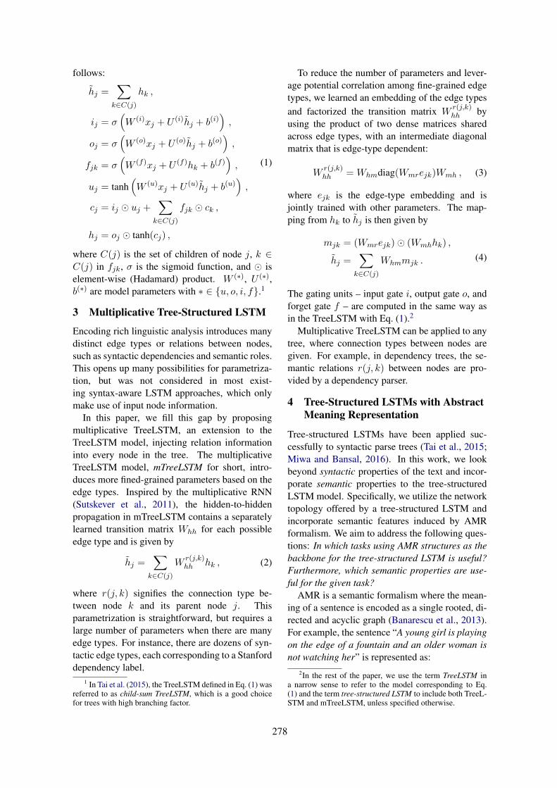
follows:
hj =∑
k∈C(j)
hk ,
ij = σ(W (i)xj + U (i)hj + b(i)
),
oj = σ(W (o)xj + U (o)hj + b(o)
),
fjk = σ(W (f)xj + U (f)hk + b(f)
),
uj = tanh(W (u)xj + U (u)hj + b(u)
),
cj = ij � uj +∑
k∈C(j)
fjk � ck ,
hj = oj � tanh(cj) ,
(1)
where C(j) is the set of children of node j, k ∈C(j) in fjk, σ is the sigmoid function, and � iselement-wise (Hadamard) product. W (∗), U (∗),b(∗) are model parameters with ∗ ∈ {u, o, i, f}.1
3 Multiplicative Tree-Structured LSTM
Encoding rich linguistic analysis introduces manydistinct edge types or relations between nodes,such as syntactic dependencies and semantic roles.This opens up many possibilities for parametriza-tion, but was not considered in most exist-ing syntax-aware LSTM approaches, which onlymake use of input node information.
In this paper, we fill this gap by proposingmultiplicative TreeLSTM, an extension to theTreeLSTM model, injecting relation informationinto every node in the tree. The multiplicativeTreeLSTM model, mTreeLSTM for short, intro-duces more fined-grained parameters based on theedge types. Inspired by the multiplicative RNN(Sutskever et al., 2011), the hidden-to-hiddenpropagation in mTreeLSTM contains a separatelylearned transition matrix Whh for each possibleedge type and is given by
hj =∑
k∈C(j)
Wr(j,k)hh hk , (2)
where r(j, k) signifies the connection type be-tween node k and its parent node j. Thisparametrization is straightforward, but requires alarge number of parameters when there are manyedge types. For instance, there are dozens of syn-tactic edge types, each corresponding to a Stanforddependency label.
1 In Tai et al. (2015), the TreeLSTM defined in Eq. (1) wasreferred to as child-sum TreeLSTM, which is a good choicefor trees with high branching factor.
To reduce the number of parameters and lever-age potential correlation among fine-grained edgetypes, we learned an embedding of the edge typesand factorized the transition matrix W
r(j,k)hh by
using the product of two dense matrices sharedacross edge types, with an intermediate diagonalmatrix that is edge-type dependent:
Wr(j,k)hh =Whmdiag(Wmrejk)Wmh , (3)
where ejk is the edge-type embedding and isjointly trained with other parameters. The map-ping from hk to hj is then given by
mjk = (Wmrejk)� (Wmhhk) ,
hj =∑
k∈C(j)
Whmmjk . (4)
The gating units – input gate i, output gate o, andforget gate f – are computed in the same way asin the TreeLSTM with Eq. (1).2
Multiplicative TreeLSTM can be applied to anytree, where connection types between nodes aregiven. For example, in dependency trees, the se-mantic relations r(j, k) between nodes are pro-vided by a dependency parser.
4 Tree-Structured LSTMs with AbstractMeaning Representation
Tree-structured LSTMs have been applied suc-cessfully to syntactic parse trees (Tai et al., 2015;Miwa and Bansal, 2016). In this work, we lookbeyond syntactic properties of the text and incor-porate semantic properties to the tree-structuredLSTM model. Specifically, we utilize the networktopology offered by a tree-structured LSTM andincorporate semantic features induced by AMRformalism. We aim to address the following ques-tions: In which tasks using AMR structures as thebackbone for the tree-structured LSTM is useful?Furthermore, which semantic properties are use-ful for the given task?
AMR is a semantic formalism where the mean-ing of a sentence is encoded as a single rooted, di-rected and acyclic graph (Banarescu et al., 2013).For example, the sentence “A young girl is playingon the edge of a fountain and an older woman isnot watching her” is represented as:
2In the rest of the paper, we use the term TreeLSTM ina narrow sense to refer to the model corresponding to Eq.(1) and the term tree-structured LSTM to include both TreeL-STM and mTreeLSTM, unless specified otherwise.
278
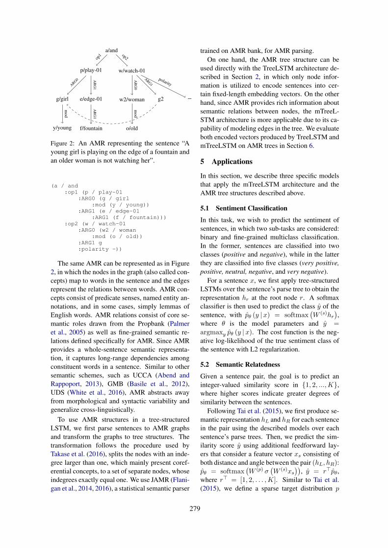
a/and
p/play-01 w/watch-01
e/edge-01g/girl
y/young f/fountain
w2/woman
o/old
g2 –
op1 op2
ARG0 AR
G1
mod
AR
G0
ARG1
AR
G1
polarity
mod
Figure 2: An AMR representing the sentence “Ayoung girl is playing on the edge of a fountain andan older woman is not watching her”.
(a / and:op1 (p / play-01
:ARG0 (g / girl:mod (y / young))
:ARG1 (e / edge-01:ARG1 (f / fountain)))
:op2 (w / watch-01:ARG0 (w2 / woman
:mod (o / old)):ARG1 g:polarity -))
The same AMR can be represented as in Figure2, in which the nodes in the graph (also called con-cepts) map to words in the sentence and the edgesrepresent the relations between words. AMR con-cepts consist of predicate senses, named entity an-notations, and in some cases, simply lemmas ofEnglish words. AMR relations consist of core se-mantic roles drawn from the Propbank (Palmeret al., 2005) as well as fine-grained semantic re-lations defined specifically for AMR. Since AMRprovides a whole-sentence semantic representa-tion, it captures long-range dependencies amongconstituent words in a sentence. Similar to othersemantic schemes, such as UCCA (Abend andRappoport, 2013), GMB (Basile et al., 2012),UDS (White et al., 2016), AMR abstracts awayfrom morphological and syntactic variability andgeneralize cross-linguistically.
To use AMR structures in a tree-structuredLSTM, we first parse sentences to AMR graphsand transform the graphs to tree structures. Thetransformation follows the procedure used byTakase et al. (2016), splits the nodes with an inde-gree larger than one, which mainly present coref-erential concepts, to a set of separate nodes, whoseindegrees exactly equal one. We use JAMR (Flani-gan et al., 2014, 2016), a statistical semantic parser
trained on AMR bank, for AMR parsing.On one hand, the AMR tree structure can be
used directly with the TreeLSTM architecture de-scribed in Section 2, in which only node infor-mation is utilized to encode sentences into cer-tain fixed-length embedding vectors. On the otherhand, since AMR provides rich information aboutsemantic relations between nodes, the mTreeL-STM architecture is more applicable due to its ca-pability of modeling edges in the tree. We evaluateboth encoded vectors produced by TreeLSTM andmTreeLSTM on AMR trees in Section 6.
5 Applications
In this section, we describe three specific modelsthat apply the mTreeLSTM architecture and theAMR tree structures described above.
5.1 Sentiment Classification
In this task, we wish to predict the sentiment ofsentences, in which two sub-tasks are considered:binary and fine-grained multiclass classification.In the former, sentences are classified into twoclasses (positive and negative), while in the latterthey are classified into five classes (very positive,positive, neutral, negative, and very negative).
For a sentence x, we first apply tree-structuredLSTMs over the sentence’s parse tree to obtain therepresentation hr at the root node r. A softmaxclassifier is then used to predict the class y of thesentence, with pθ (y |x) = softmax
(W (s)hr
),
where θ is the model parameters and y =argmaxy pθ (y |x). The cost function is the neg-ative log-likelihood of the true sentiment class ofthe sentence with L2 regularization.
5.2 Semantic Relatedness
Given a sentence pair, the goal is to predict aninteger-valued similarity score in {1, 2, ...,K},where higher scores indicate greater degrees ofsimilarity between the sentences.
Following Tai et al. (2015), we first produce se-mantic representation hL and hR for each sentencein the pair using the described models over eachsentence’s parse trees. Then, we predict the sim-ilarity score y using additional feedforward lay-ers that consider a feature vector xs consisting ofboth distance and angle between the pair (hL, hR):pθ = softmax
(W (p) σ
(W (s)xs
)), y = r>pθ,
where r> = [1, 2, . . . ,K]. Similar to Tai et al.(2015), we define a sparse target distribution p
279
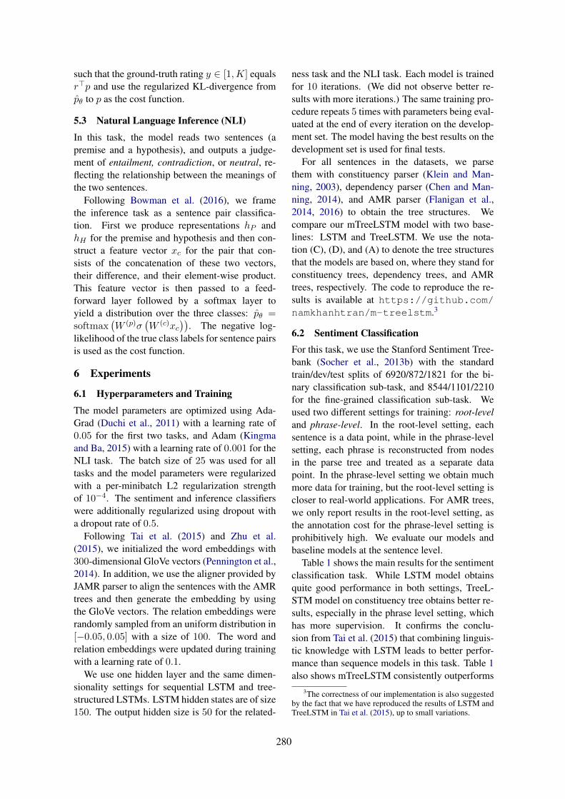
such that the ground-truth rating y ∈ [1,K] equalsr>p and use the regularized KL-divergence frompθ to p as the cost function.
5.3 Natural Language Inference (NLI)
In this task, the model reads two sentences (apremise and a hypothesis), and outputs a judge-ment of entailment, contradiction, or neutral, re-flecting the relationship between the meanings ofthe two sentences.
Following Bowman et al. (2016), we framethe inference task as a sentence pair classifica-tion. First we produce representations hP andhH for the premise and hypothesis and then con-struct a feature vector xc for the pair that con-sists of the concatenation of these two vectors,their difference, and their element-wise product.This feature vector is then passed to a feed-forward layer followed by a softmax layer toyield a distribution over the three classes: pθ =softmax
(W (p)σ
(W (c)xc
)). The negative log-
likelihood of the true class labels for sentence pairsis used as the cost function.
6 Experiments
6.1 Hyperparameters and Training
The model parameters are optimized using Ada-Grad (Duchi et al., 2011) with a learning rate of0.05 for the first two tasks, and Adam (Kingmaand Ba, 2015) with a learning rate of 0.001 for theNLI task. The batch size of 25 was used for alltasks and the model parameters were regularizedwith a per-minibatch L2 regularization strengthof 10−4. The sentiment and inference classifierswere additionally regularized using dropout witha dropout rate of 0.5.
Following Tai et al. (2015) and Zhu et al.(2015), we initialized the word embeddings with300-dimensional GloVe vectors (Pennington et al.,2014). In addition, we use the aligner provided byJAMR parser to align the sentences with the AMRtrees and then generate the embedding by usingthe GloVe vectors. The relation embeddings wererandomly sampled from an uniform distribution in[−0.05, 0.05] with a size of 100. The word andrelation embeddings were updated during trainingwith a learning rate of 0.1.
We use one hidden layer and the same dimen-sionality settings for sequential LSTM and tree-structured LSTMs. LSTM hidden states are of size150. The output hidden size is 50 for the related-
ness task and the NLI task. Each model is trainedfor 10 iterations. (We did not observe better re-sults with more iterations.) The same training pro-cedure repeats 5 times with parameters being eval-uated at the end of every iteration on the develop-ment set. The model having the best results on thedevelopment set is used for final tests.
For all sentences in the datasets, we parsethem with constituency parser (Klein and Man-ning, 2003), dependency parser (Chen and Man-ning, 2014), and AMR parser (Flanigan et al.,2014, 2016) to obtain the tree structures. Wecompare our mTreeLSTM model with two base-lines: LSTM and TreeLSTM. We use the nota-tion (C), (D), and (A) to denote the tree structuresthat the models are based on, where they stand forconstituency trees, dependency trees, and AMRtrees, respectively. The code to reproduce the re-sults is available at https://github.com/namkhanhtran/m-treelstm.3
6.2 Sentiment ClassificationFor this task, we use the Stanford Sentiment Tree-bank (Socher et al., 2013b) with the standardtrain/dev/test splits of 6920/872/1821 for the bi-nary classification sub-task, and 8544/1101/2210for the fine-grained classification sub-task. Weused two different settings for training: root-leveland phrase-level. In the root-level setting, eachsentence is a data point, while in the phrase-levelsetting, each phrase is reconstructed from nodesin the parse tree and treated as a separate datapoint. In the phrase-level setting we obtain muchmore data for training, but the root-level setting iscloser to real-world applications. For AMR trees,we only report results in the root-level setting, asthe annotation cost for the phrase-level setting isprohibitively high. We evaluate our models andbaseline models at the sentence level.
Table 1 shows the main results for the sentimentclassification task. While LSTM model obtainsquite good performance in both settings, TreeL-STM model on constituency tree obtains better re-sults, especially in the phrase level setting, whichhas more supervision. It confirms the conclu-sion from Tai et al. (2015) that combining linguis-tic knowledge with LSTM leads to better perfor-mance than sequence models in this task. Table 1also shows mTreeLSTM consistently outperforms
3The correctness of our implementation is also suggestedby the fact that we have reproduced the results of LSTM andTreeLSTM in Tai et al. (2015), up to small variations.
280

Model Phrase-level Root-level
5-class 2-class 5-class 2-class
LSTM 48.0 (1.0) 86.7 (0.7) 45.6 (1.1) 85.6 (0.5)
TreeLSTM(C) 49.8 (0.8) 87.9 (0.9) 46.3 (0.7) 85.8 (0.5)TreeLSTM(D) 46.9 (0.2) 85.5 (0.4) 46.0 (0.3) 85.0 (0.4)TreeLSTM(A) n/a n/a 44.4 (0.2) 82.9 (0.6)
mTreeLSTM(A) n/a n/a 45.2 (0.5) 83.2 (0.5)mTreeLSTM(D) 47.5 (0.7) 85.7 (0.1) 46.7 (0.8) 85.7 (0.8)
Table 1: Accuracy on the Stanford Sentiment Tree-bank dataset with standard deviation in parenthe-ses (numbers in percentage)
.
TreeLSTM on the same tree structures in both set-tings – Whenever a tree structure is applicableto both mTreeLSTM and TreeLSTM, the perfor-mance of mTreeLSTM with that tree structure isbetter. That is, in phrase-level setting, mTreeL-STM (D) outperforms TreeLSTM (D) and simi-larly in root-level setting, mTreeLSTM (D) andmTreeLSTM (A) perform better than TreeLSTM(D) and TreeLSTM (A), respectively. It demon-strates the effectiveness of the relation multipli-cation mechanism and the importance of mod-eling relation information. The TreeLSTM andmTreeLSTM models with AMR trees do not per-form well on this task. Synthetic informationalong goes a long way in determining the senti-ment of a sentence. Noisy sentences in this taskalso impact the accuracy of the AMR parser.
We now dive deep into what the models learn,by listing the composition matrices W r(j,k)
hh withthe largest Frobenius norms. These matrices havelearned larger weights, which are in turn beingmultiplied with the child hidden states. Thatchild will therefore have more weight in the com-posed parent vector. In decreasing order of Frobe-nius norm, the relationship matrices for mTreeL-STM on dependency trees are: conjunction, ad-jectival modifier, object of a preposition, negationmodifier, verbal modifier. The relationship ma-trices for mTreeLSTM on AMR trees are: nega-tion (:polarity), attribute (:ARG3, :ARG2),modifier (:mod), conjunction (:opN). The modellearns that verbal and adjective modifiers are moreimportant than nouns, as they tend to affect thesentiment of sentences.
6.3 Sentence Relatedness
For this task, we use the Sentences InvolvingCompositional Knowledge (SICK) dataset, con-
Model Pearson Spearman MSE
LSTM .841 (.004) .778 (.006) .304 (.003)
TreeLSTM (C) .849 (.005) .790 (.004) .286 (.010)TreeLSTM (D) .863 (.003) .803 (.002) .260 (.005)TreeLSTM (A) .842 (.002) .774 (.001) .299 (.005)
mTreeLSTM (A) .853 (.001) .788 (.001) .279 (.002)mTreeLSTM (D) .872 (.004) .814 (.005) .244 (.007)
Table 2: Results on the SICK dataset for semanticrelatedness task with standard deviation in paren-theses
sisting of 9927 sentence pairs with the standardtrain/dev/test split of 4500/500/4927. Each pair isannotated with a relatedness score y ∈ [1, 5], with1 indicating the two sentences are completely un-related, and 5 indicating they are very related. Fol-lowing Tai et al. (2015), we use Pearson, Spear-man correlations and mean squared error (MSE)as evaluation metrics.
Our results are summarized in Table 2. The tree-structured LSTMs, both TreeLSTM and mTreeL-STM, reach better performance than the standardLSTM. The model using dependency tree as thebackbone achieves best results. The mTreeL-STM with AMR trees obtain slightly better resultsthan the TreeLSTM with constituency trees. Themultiplicative TreeLSTM models outperform theTreeLSTM models on the same parse trees, illus-trating again the usefulness of incorporating rela-tion information into the model.
Similar to the previous experiment, we listthe composition matrices W r(j,k)
hh with the largestFrobenius norms. The relationship matricesfor dependency trees include: indirect object,marker for introducing a finite clause subordi-nate to another clause, negation modifier, ad-jectival modifier, phrasal verb particle, conjunc-tion. The relationship matrices for AMR trees are:patient (:ARG1), comparatives and superlatives(:degree), agent (:ARG0), attribute (:ARG3),medium (:medium), possession (:poss), man-ner (:manner).
6.4 Natural Language Inference
In this task, we first look at the SICK dataset de-scribed in the previous section. In this setting eachsentence pair is classified into three labels, entail-ment, contradiction, and neutral.
In addition to the standard test set, we also re-port performances of our models on two different
281

Model All LS Negation
LSTM 77.3 (0.5) 74.6 (1.4) 77.5 (0.4)
TreeLSTM (C) 79.0 (1.4) 78.1 (2.9) 85.3 (1.2)TreeLSTM (D) 82.9 (0.3) 81.0 (2.6) 84.3 (1.2)TreeLSTM (A) 82.6 (0.2) 84.0 (1.5) 88.2 (0.4)
mTreeLSTM (A) 83.3 (0.2) 85.3 (0.4) 88.5 (0.8)mTreeLSTM (D) 84.0 (0.5) 81.6 (1.3) 87.8 (0.8)
Table 3: Accuracy on the SICK dataset for the NLItask with standard deviation in parentheses (num-bers in percentage)
subsets. The first subset, Long Sentence (LS), con-sists of sentence pairs in the test set where thepremise sentence contains at least 18 words. Wehypothesize that long sentences are more difficultto handle by sequential models as well as tree-structured models. The second subset, Negation,is a set of sentence pairs where negation words(not, n’t or no) do not appear in the premise butappear in the hypothesis. In the test set, 58.7% ofthese examples are labeled as contradiction.
Table 3 summarizes the results of our mod-els on different test sets. The mTreeLSTM mod-els obtain highest results, followed by TreeLSTMmodels. The standard LSTM model does notwork well on this task. The results reconfirm thebenefit of using the structure information of sen-tences in learning semantic representations. In ad-dition, Table 3 shows that TreeLSTM on depen-dency trees and AMR trees outperform the mod-els with constituency trees. The dependency treesprovide some semantic information, i.e., semanticrelations between words at some degrees, whileAMR trees present more semantic information.The multiplicative TreeLSTM on AMR trees per-form much better than other models on the LS andNegation subsets. The results on the LS subsetshows that mTreeLSTM on AMR trees can han-dle long-range dependencies in a sentence moreeffectively. For example, only mTreeLSTM (A)is able to predict the following example correctly:Premise: The grotto with a pink interior is be-ing climbed by four middle eastern children, threegirls and one boy.Hypothesis: A group of kids is playing on a col-orful structure.Label: entailment
Similar to previous experiments, we list thecomposition matrices with the largest Frobeniusnorms to get some insights into what the mod-
Model Acc (%)
LSTM (Bowman et al., 2015) 77.6Syntax TreeLSTM (Yogatama et al., 2017) 80.5CYK TreeLSTM (Maillard et al., 2017) * 81.6Gumbel TreeLSTM (Choi et al., 2018) 81.8Gumbel TreeLSTM + leaf LSTM (Choi et al., 2018) 82.6
TreeLSTM (D) 81.0mTreeLSTM (D) 81.9
Table 4: Results on the SNLI dataset. The firstgroup contains results of some best-performingtree-structured LSTM models on this data. (*: apreprint)
Model rDim # Params Acc (%)
TreeLSTM (A) n/a 301K 82.6
mTreeLSTM (A) 50 354K 82.7mTreeLSTM (A) 75 358K 83.1mTreeLSTM (A) 100 361K 83.6mTreeLSTM (A) 200 376K 83.0
Table 5: Effects of the relation embedding size onSICK dataset for the NLI task
els learn. The relationship matrices for mTreeL-STM on dependency trees are: negation modifier,nominal subject, adjectival modifier, direct object,passive auxiliary, adverb modifier. These matri-ces for mTreeLSTM on AMR trees are: attribute(:ARG2), patient (:ARG1), conjunction (:opN),location, negation (:polarity), domain. Incontrast to the sentiment classification task, whereadjectives are crucial, the model learns that sub-jects and objects are important to determine themeaning of sentences.
Furthermore, we evaluate our mTreeLSTMmodel with SNLI (Stanford Natural Language In-ference), a larger NLI dataset (Bowman et al.,2015). It is composed of about 550K/10K/10Ksentence pairs in train/dev/test sets. We use de-pendency tree as the backbone for tree-structuredLSTMs. All models in Table 4 use a hidden sizeof 100 for a fair comparison. The table showsthat mTreeLSTM (D) outperforms many othersyntax-based TreeLSTM models including TreeL-STM (D), reconfirming our conclusion drawn withSICK.
6.5 Additional Tests and Discussions
Incorporating relation information in the tree-structured LSTM increases model complexity. Inthis experiment, we analyze the impact of the di-mensionality of relation embedding on the model
282

Model # Params Acc (%)
TreeLSTM (D) 301K 82.9
addTreeLSTM (D) 361K 83.4fullTreeLSTM (D) 1.1M 83.5mTreeLSTM (D) 361K 84.0
Table 6: Comparison between different methodsusing relation information on the SICK dataset forthe NLI task
size and accuracy. Table 5 shows the model withthe relation embedding size of 100 achieves thebest accuracy, while the overall impact of the em-bedding size is mild. The multiplicative TreeL-STM has only 1.2 times the number of weightsin TreeLSTM (with the same number of hiddenunits). We did not count the number of parametersin the embedding models since these parametersare the same for all models.
Table 6 shows a comparison between mTreeL-STM and two other plausible methods for inte-grating relation information with TreeLSTM. InaddTreeLSTM, a relation is treated as an addi-tional node input in the TreeLSTM model; InfullTreeLSTM, the model corresponds to Eq. (2),where each edge type has a separate transitionmatrix. Both models achieve better results thanTreeLSTM, indicating the usefulness of relationinformation. While addTreeLSTM and fullTreeL-STM obtain comparable performances, mTreeL-STM outperforms both of them. It is also to notethat the number of parameters of mTreeLSTM ismuch less than those of fullTreeLSTM.
7 Other Related Work
There is a line of research that extends the standardLSTM (Hochreiter and Schmidhuber, 1997) in or-der to model more complex structures. Tai et al.(2015) and Zhu et al. (2015) extended sequen-tial LSTMs to tree-structured LSTMs by addingbranching factors. They showed such extensionsoutperform competitive LSTM baselines on sev-eral tasks such as sentiment classification and se-mantic relatedness prediction (which is also con-firmed in this paper). Li et al. (2015) further inves-tigated the effectiveness of TreeLSTMs on varioustasks and discussed when tree structures are neces-sary. Chen et al. (2017) combined sequential andtree-structured LSTM for NLI and has achievedstate-of-the-art results on the benchmark dataset.Their approach uses n-ary TreeLSTM based on
syntactic constituency parsers. In contrast, we fo-cus more on child-sum TreeLSTM which is bettersuited for trees with high branching factor.
Previous works have studied the use of relationinformation. Dyer et al. (2015) considered eachsyntactic relation as an additional node and in-cluded its embedding to their composition func-tion for dependency parsing. Peng et al. (2017)introduced a different set of parameters for eachedge-type in their LSTM-based approach for re-lation extraction. In contrast to these works, ourmTreeLSTM model incorporates relation informa-tion via a multiplicative mechanism, which wehave shown is more effective and uses less param-eters.
AMR has been successfully applied to a num-ber of NLP tasks, besides the ones we consideredin this paper. For example, Mitra and Baral (2016)made use of AMR to improve question answering;Liu et al. (2015) utilized AMR to produce promis-ing results toward abstractive summarization. Us-ing AMR as the backbone in TreeLSTM has beeninvestigated in Takase et al. (2016). They incor-porated AMR information by a neural encoder tothe attention-based summarization method (Rushet al., 2015) and it performed well on headlinegeneration. Our work differs from these studiesin the sense that we aim to investigate how seman-tic information induced by AMR formalism canbe incorporated to tree-structured LSTM models,and study which properties introduced by AMRturn out to be useful in various tasks. In this paper,we use the start-of-the-art AMR parser providedby Flanigan et al. (2016) which additionally pro-vides the alignment between words and nodes inthe tree.
Though we have considered AMR in this paper,we believe the conclusions we drew here largelyapply to other semantic schemes, such as GMBand UCCA, as well. Abend and Rappoport (2017)has recently noted that the differences betweenthese schemes are not critical, and the main dis-tinguishing factors between them are their relationto syntax, their degree of universality, and the ex-pertise they require from annotators.
8 Conclusions
We presented multiplicative TreeLSTM, an exten-sion of existing tree-structured LSTMs to incor-porate relation information between nodes in thetree. Multiplicative TreeLSTM allows different
283
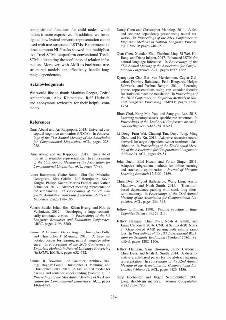
compositional functions for child nodes, whichmakes it more expressive. In addition, we inves-tigated how lexical semantic representation can beused with tree-structured LSTMs. Experiments onthree common NLP tasks showed that multiplica-tive TreeLSTMs outperform conventional TreeL-STMs, illustrating the usefulness of relation infor-mation. Moreover, with AMR as backbone, tree-structured models can effectively handle long-range dependencies.
Acknowledgments
We would like to thank Matthias Seeger, CedricArchambeau, Alex Klementiev, Ralf Herbrich,and anonymous reviewers for their helpful com-ments.
ReferencesOmri Abend and Ari Rappoport. 2013. Universal con-
ceptual cognitive annotation (UCCA). In Proceed-ings of the 51st Annual Meeting of the Associationfor Computational Linguistics. ACL, pages 228–238.
Omri Abend and Ari Rappoport. 2017. The state ofthe art in semantic representation. In Proceedingsof the 55th Annual Meeting of the Association forComputational Linguistics. ACL, pages 77–89.
Laura Banarescu, Claire Bonial, Shu Cai, MadalinaGeorgescu, Kira Griffitt, Ulf Hermjakob, KevinKnight, Philipp Koehn, Martha Palmer, and NathanSchneider. 2013. Abstract meaning representationfor sembanking. In Proceedings of the 7th Lin-guistic Annotation Workshop & Interoperability withDiscourse. pages 178–186.
Valerio Basile, Johan Bos, Kilian Evang, and NoortjeVenhuizen. 2012. Developing a large semanti-cally annotated corpus. In Proceedings of the 8thLanguage Resources and Evaluation Conference.LREC, pages 3196–3200.
Samuel R. Bowman, Gabor Angeli, Christopher Potts,and Christopher D Manning. 2015. A large an-notated corpus for learning natural language infer-ence. In Proceedings of the 2015 Conference onEmpirical Methods in Natural Language Processing(EMNLP). EMNLP, pages 632–642.
Samuel R. Bowman, Jon Gauthier, Abhinav Ras-togi, Raghav Gupta, Christopher D. Manning, andChristopher Potts. 2016. A fast unified model forparsing and sentence understanding (volume 1). InProceedings of the 54th Annual Meeting of the Asso-ciation for Computational Linguistics. ACL, pages1466–1477.
Danqi Chen and Christopher Manning. 2014. A fastand accurate dependency parser using neural net-works. In Proceedings of the 2014 Conference onEmpirical Methods in Natural Language Process-ing. EMNLP, pages 740–750.
Qian Chen, Xiaodan Zhu, Zhenhua Ling, Si Wei, HuiJiang, and Diana Inkpen. 2017. Enhanced LSTM fornatural language inference. In Proceedings of the55th Annual Meeting of the Association for Compu-tational Linguistics. ACL, pages 1657–1668.
Kyunghyun Cho, Bart van Merrienboer, Caglar Gul-cehre, Dzmitry Bahdanau, Fethi Bougares, HolgerSchwenk, and Yoshua Bengio. 2014. Learningphrase representations using rnn encoder-decoderfor statistical machine translation. In Proceedings ofthe 2014 Conference on Empirical Methods in Nat-ural Language Processing. EMNLP, pages 1724–1734.
Jihun Choi, Kang Min Yoo, and Sang goo Lee. 2018.Learning to compose task-specific tree structures. InProceedings of the 32nd AAAI Conference on Artifi-cial Intelligence (AAAI-18). AAAI.
Li Dong, Furu Wei, Chuanqi Tan, Duyu Tang, MingZhou, and Ke Xu. 2014. Adaptive recursive neuralnetwork for target-dependent twitter sentiment clas-sification. In Proceedings of the 52nd Annual Meet-ing of the Association for Computational Linguistics(Volume 2). ACL, pages 49–54.
John Duchi, Elad Hazan, and Yoram Singer. 2011.Adaptive subgradient methods for online learningand stochastic optimization. Journal of MachineLearning Research 12:2121–2159.
Chris Dyer, Miguel Ballesteros, Wang Ling, AustinMatthews, and Noah Smith. 2015. Transition-based dependency parsing with stack long short-term memory. In Proceedings of the 53rd AnnualMeeting of the Association for Computational Lin-guistics. ACL, pages 334–343.
Jeffrey L. Elman. 1990. Finding structure in time.Cognitive Science 14:179–211.
Jeffrey Flanigan, Chris Dyer, Noah A. Smith, andJaime Carbonell. 2016. CMU at SemEval-2016 task8: Graph-based AMR parsing with infinite ramploss. In Proceedings of the 10th International Work-shop on Semantic Evaluation (SemEval-2016). Se-mEval, pages 1202–1206.
Jeffrey Flanigan, Sam Thomson, Jaime Carbonell,Chris Dyer, and Noah A. Smith. 2014. A discrim-inative graph-based parser for the abstract meaningrepresentation. In Proceedings of the 52nd AnnualMeeting of the Association for Computational Lin-guistics (Volume 1). ACL, pages 1426–1436.
Sepp Hochreiter and Jurgen Schmidhuber. 1997.Long short-term memory. Neural Computation9(8):1735–1780.
284

Nal Kalchbrenner, Edward Grefenstette, and Phil Blun-som. 2014. A convolutional neural network formodelling sentences. In Proceedings of the 52ndAnnual Meeting of the Association for Computa-tional Linguistics (Volume 1). ACL, pages 655–665.
Yoon Kim. 2014. Convolutional neural networks forsentence classification. In Proceedings of the 2014Conference on Empirical Methods in Natural Lan-guage Processing. EMNLP, pages 1746–1751.
Diederik P. Kingma and Jimmy Ba. 2015. Adam:A method for stochastic optimization. In The 3rdInternational Conference on Learning Representa-tions. ICLR.
Dan Klein and Christopher D. Manning. 2003. Ac-curate unlexicalized parsing. In Proceedings of the41st Annual Meeting of the Association for Compu-tational Linguistics. ACL, pages 423–430.
Jiwei Li, Minh-Thang Luong, Dan Jurafsky, and Ed-uard Hovy. 2015. When are tree structures nec-essary for deep learning of representations? InProceedings of the 2015 Conference on EmpiricalMethods in Natural Language Processing. EMNLP,pages 2304–2314.
Fei Liu, Jeffrey Flanigan, Sam Thomson, Norman M.Sadeh, and Noah A. Smith. 2015. Toward abstrac-tive summarization using semantic representations.In Proceedings of the Conference of the North Amer-ican Chapter of the Association for ComputationalLinguistics. NAACL.
Pengfei Liu, Xipeng Qiu, Yaqian Zhou, Jifan Chen,and Xuanjing Huang. 2016. Modelling interactionof sentence pair with coupled-LSTMs. In Proceed-ings of the 2016 Conference on Empirical Methodsin Natural Language Processing. EMNLP, pages1703–1712.
Jean Maillard, Stephen Clark, and Dani Yogatama.2017. Jointly learning sentence embeddings andsyntax with unsupervised tree-LSTMs. CoRR .
Arindam Mitra and Chitta Baral. 2016. Addressing aquestion answering challenge by combining statisti-cal methods with inductive rule learning and reason-ing. In Proceedings of the 13th AAAI Conference onArtificial Intelligence. AAAI, pages 2779–2785.
Makoto Miwa and Mohit Bansal. 2016. End-to-end re-lation extraction using LSTMs on sequences and treestructures. In Proceedings of the 54th Annual Meet-ing of the Association for Computational Linguistics(Volume 1). ACL, pages 1105–1116.
Martha Palmer, Daniel Gildea, and Paul Kingsbury.2005. The proposition bank: An annotated corpus ofsemantic roles. Computational Linguistics 31:71–106.
Nanyun Peng, Hoifung Poon, Chris Quirk, KristinaToutanova, and Wen-tau Yih. 2017. Cross-sentence
n-ary relation extraction with graph LSTMs. Trans-actions of the Association for Computational Lin-guistics pages 101–115.
Jeffrey Pennington, Richard Socher, and Christo-pher D. Manning. 2014. GloVe: Global vectors forword representation. In Proceedings of the 2014Conference on Empirical Methods in Natural Lan-guage Processing. EMNLP, pages 1532–1543.
Alexander Rush, Sumit Chopra, and Jason Weston.2015. A neural attention model for abstractive sen-tence summarization. In Proceedings of the 2015Conference on Empirical Methods in Natural Lan-guage Processing. EMNLP, pages 379–389.
Richard Socher, John Bauer, Christopher D. Manning,and Ng Andrew Y. 2013a. Parsing with composi-tional vector grammars. In Proceedings of the 51stAnnual Meeting of the Association for Computa-tional Linguistics (Volume 1). ACL, pages 455–465.
Richard Socher, Brody Huval, Christopher D. Man-ning, and Andrew Y. Ng. 2012. Semantic compo-sitionality through recursive matrix-vector spaces.In Proceedings of the 2012 Joint Conference onEmpirical Methods in Natural Language Process-ing and Computational Natural Language Learning.EMNLP-CoNLL, pages 1201–1211.
Richard Socher, Cliff C. Lin, Andrew Y. Ng, andChristopher D. Manning. 2011. Parsing naturalscenes and natural language with recursive neu-ral networks. In Proceedings of the 28th Inter-national Conference on Machine Learning. ICML,pages 129–136.
Richard Socher, Alex Perelygin, Jean Wu, JasonChuang, Christopher D. Manning, Andrew Y. Ng,and Christopher Potts. 2013b. Recursive deep mod-els for semantic compositionality over a sentimenttreebank. In Proceedings of the 2013 Conference onEmpirical Methods in Natural Language Process-ing. ACL, pages 1631–1642.
Ilya Sutskever, James Martens, and Geoffrey Hinton.2011. Generating text with recurrent neural net-works. In Proceedings of the 28th InternationalConference on Machine Learning. ICML, pages1017–1024.
Kai Sheng Tai, Richard Socher, and Christopher D.Manning. 2015. Improved semantic representationsfrom tree-structured long short-term memory net-works. In Proceedings of the 53rd Annual Meet-ing of the Association for Computational Linguisticsand the 7th International Joint Conference on Natu-ral Language Processing. ACL, pages 1556–1566.
Sho Takase, Jun Suzuki, Naoaki Okazaki, Tsutomu Hi-rao, and Masaaki Nagata. 2016. Neural headlinegeneration on abstract meaning representation. InProceedings of the 2016 Conference on EmpiricalMethods in Natural Language Processing. EMNLP,pages 1054–1059.
285

Aaron Steven White, Drew Reisinger, Keisuke Sak-aguchi, Tim Vieira, Sheng Zhang, Rachel Rudinger,Kyle Rawlins, and Benjamin Van Durme. 2016.Universal decompositional semantics on universaldependencies. In Proceedings of the 2016 Confer-ence on Empirical Methods in Natural LanguageProcessing. EMNLP, pages 1713–1723.
Dani Yogatama, Phil Blunsom, Chris Dyer, EdwardGrefenstette, and Wang Ling. 2017. Learning tocompose words into sentences with reinforcementlearning. In Proceedings of the 5th InternationalConference on Learning Representations. ICLR.
Han Zhao, Zhengdong Lu, and Pascal Poupart. 2015.Self-adaptive hierarchical sentence model. In Pro-ceedings of the 24th International Joint Conferenceon Artificial Intelligence. IJCAI, pages 4069–4076.
Xiaodan Zhu, Parinaz Sobhani, and Hongyu Guo.2015. Long short-term memory over recursivestructures. In Proceedings of the 32nd InternationalConference on Machine Learning. ICML, pages1604–1612.
286

Author Index
Allen, James, 235
Badaro, Gilbert, 86Bakarov, Amir, 94Barbieri, Francesco, 101Basile, Valerio, 245Beschke, Sebastian, 54Bethard, Steven, 167Bollegala, Danushka, 33, 255Botschen, Teresa, 225
Cabrio, Elena, 245Camacho-Collados, Jose, 101Cheng, Weiwei, 276Cheung, Jackie Chi Kit, 1, 130Choi, Jihun, 107Crouch, Richard, 113Cui, Xia, 255
Demberg, Vera, 11Dligach, Dmitriy, 119Duh, Kevin, 142, 173
El-Hajj, Wassim, 86
Fan, Chuchu, 148Frassinelli, Diego, 76
Gargett, Andrew, 33Gimpel, Kevin, 192Gurevych, Iryna, 65, 225
Hajj, Hazem, 86Haldar, Aparajita, 180Hong, Xudong, 11Hu, Hai, 124
Jundi, Hussein, 86
Köper, Maximilian, 22Kallmeyer, Laura, 130Kalouli, Aikaterini-Lida, 113Kenyon-Dean, Kian, 1Kim, Taeuk, 107Kiritchenko, Svetlana, 43, 214Kojaku, Sadamori, 255
Lee, Sang-goo, 107Lopez Condori, Roque, 245
Mahabal, Abhijit, 265Masuda, Naoki, 255Mei, Hongyuan, 142Menzel, Wolfgang, 54Miller, Timothy, 119Mittal, Sid, 265Mohammad, Saif, 43, 214Moss, Larry, 124Mousselly Sergieh, Hatem, 225
Naradowsky, Jason, 180Naumann, Daniela, 76Ning, Qiang, 148
Pierrejean, Benedicte, 154Poliak, Adam, 180Precup, Doina, 1
QasemiZadeh, Behrang, 130
Roth, Dan, 148, 203, 265Roth, Stefan, 225Rudinger, Rachel, 180
Sagarkar, Manasvi, 192Samardzhiev, Krasen, 33Sayeed, Asad, 11Schulte im Walde, Sabine, 22, 76Sharp, Rebecca, 167Shwartz, Vered, 160Sochenkov, Ilya, 94Sorokin, Daniil, 65Springorum, Sylvia, 22Suvorov, Roman, 94
Tanguy, Ludovic, 154Teng, Choh Man, 235Tran, Nam Khanh, 276Tu, Lifu, 192
Van Durme, Benjamin, 142, 173, 180Vu, Tu, 160
287

Wieting, John, 192Wojatzki, Michael, 214
Yadav, Vikas, 167Yin, Wenpeng, 203Yu, Zhongzhi, 148
Zesch, Torsten, 214Zhang, Sheng, 142, 173
Copyright © 2022 FDOKUMEN