Rules of Origin in North-South Preferential Trading

Arrangements with an Application to NAFTA*

José Anson♠, Olivier Cadot

Antoni Estevadeordal♦ Jaime de Melo♣

Akiko Suwa-Eisenmann♥ Bolorma Tumurchudur•

January 25, 2004

Abstract

All preferential trading agreements (PTAs) short of a customs union use

Rules of Origin (RoO) to prevent trade deflection. RoO raise production

costs and create administrative costs. This paper argues that in the case

of the recent wave of North-South PTAs, the presence of RoO virtually

limits the market access that these PTAs confer to the Southern partners.

In the case of NAFTA, it is estimated that up to 45% of Mexico’s

preferential access to the US market in 2000 (estimated at 4%) was absorbed

by RoO-related administrative costs with non-administrative costs for

Mexican firms of about 3% US of import value. These findings are coherent

with the view that North-South PTAs could well be viewed like a principal-

agent problem in which the Southern partners are just about left on their

participation constraint.

JEL Classification : F10,F11, and F13.

Keywords : Rules of origin, FTAs, NAFTA.

*This paper draws on Cadot et al. (2002). Cadot, Suwa-Eisenmann and de Melo are thankful for partial financial support from the World Bank. We thank two referees, David Colin for assistance, Céline Carrère, Alberto Portugal-Perez, Luis Serven, and participants at a workshop at the World Bank for comments on an earlier draft. An earlier version appeared as CEPR DP #4166. ♠University of LausanneUniversity of Lausanne, CERDI and CEPR: e-mail-Olivier.Cadot@hec.unil.ch

♦Inter-American Development Bank: e-mail-ANTONIE@iadb.org ♣Université of Geneva, CERDI and CEPR: e-mail-jaime.demelo@ecopo.unige.ch ♥Institut National de Recherche Agronomique and DELTA-e-mail: Suwa@java.Ens.Fr •University of Lausanne

1

1. Introduction

With the proliferation of preferential trading arrangements

(PTAs), much interest is being focussed on the effects of rules

of origin (RoO), especially at the theoretical level (Krueger

(1997), Krueger and Krishna (1995), Falvey and Reed (2000),

Krishna and Krueger (1995), Krishna (2003)). Work has also been

carried out on the detailed aspects of their implementation

(Estevadeordal (2000), Estevadeordal and Suominen (2003))) as

well as on the political-economy aspects (Duttagupta and

Panagariya (2002), Flatters (2002)). To our knowledge, beyond

the observation that RoO raise costs of production by

constraining producers in their choice of inputs, there is

little recent empirical work on these costs.1

At the same time, most recent PTAs have been of the North-South

(or ‘vertical’) type involving one (or several) rich Northern

partners and one (or several) substantially poorer Southern

partners. This is the pattern for the myriad EU PTAs, but also

for those involving the US. While it has been recognized that

recent vertical PTAs are perceived as bringing several ‘non-

traditional’ gains from integration for the Southern partner

(see e.g. Fernandez and Portes (1999)), there is concern that

little market access is in fact being provided by these

agreements, both because MFN tariffs are falling, but also

because of the complexity of RoO that invariably accompany all

PTAs short of full CUs.2 Taking the case of the recent

1 Early estimates were for EFTA. Koskinen (1983) estimated administrative compliance costs under the EFTA-EC FTA at between 1.4% and 5.7% of the value of export transactions, while according to Holmes and Shephard (1983) the average export transaction from EFTA to the EC required 35 documents and 360 copies. Also see Herin (1986). For recent work, see Estevadeordal (2000), Estevadeordal and Suominen (2003), Brenton and Manchin (2003)), and Augier, Gasiorek and Lai-Tong (2003). 2 For example, the EAs provided duty and quota free access to clothing products coming from the CEECs presumably an improvement over OPT status which deducted from the tariff, the duty paid on textile exports from the

2

implementation of NAFTA where substantial market access was

provided to Mexican firms selling in the US market, this paper

sets out to give estimates of the likely costs of RoO in the

case of NAFTA and argues that these may be representative of a

North-South PTA.

The remainder of the paper is organized as follows. Section 2

describes the general features of RoO operating under PANEURO

and NAFTA, the two main examples of North-South PTAs and gives

an estimate of their potential impact on the volume of trade.

Section 3 then summarizes the standard positive theory of RoO

which is subsequently applied to NAFTA. Section 4 provides

indirect estimates of the likely compliance costs of RoO under

NAFTA along with an attempt to disentangle administrative costs

from costs associated with the rules themselves. Section 5 then

examines to what extent the pattern of trade in manufactures

between Mexico and the US was affected by NAFTA along the lines

predicted in section 3. Section 6 concludes.

2. Rules of origin and trade patterns

RoO are in principle meant to ensure that goods being exported

from one of the partners to another truly originate from the

area and are not superficially assembled from components

originating from third countries (henceforth “non-

originating”). Two criteria are used to identify origin: the

“wholly-obtained or produced” category which asks whether

commodities and related products have been entirely grown,

harvested or extracted from the soil in the territory or

manufactured there from any of these products, thereby

EU. Yet, Brenton and Manchin (2003) conclude that the use of OPT privileges rather than switching to the FTA status indicates that the costs of compliance with RoO was denying any additional market access beyond that obtained under OPT status. On AGOA, see Mattoo et al. (2002).

3

precluding the use of second-country components, and the more

complex “substantial transformation” criterion which is used

most frequently. Five basic components of RoO are used at the

product level to substantiate the transformation criterion

across PTAs, including the two most notable North-South PTAs:

the EU FTAs now being negotiated under the PANEURO system which

is in place since 1997, and NAFTA.

First is a Change of Tariff Classification (CTC) which requires

the product to change either: its chapter (CC at the 2 digit

level under the Harmonized System (HS)); or its heading (CH at

the 4 digit level); or change its sub-heading (CS at the 6

digit level); or its item (CI at the 8-10 digit). In terms of

restrictiveness, following Estevadeordal (2000), one can assume

that the change at the item [chapter] level is the least [most]

restrictive, i.e. that CI<CS<CH<CC. Next is an exception

attached to a particular CTC (called an ECTC), usually

forbidding the use of non-originating materials from certain

subheadings, headings or chapters. Third is Value Content (VC)

which specifies the minimum percentage value that must be added

by the exporting country. VC can be expressed in one of three

ways: (i) a minimum Regional Value content (RVC); (ii) a

minimum difference between the value of the final good and the

costs of imported inputs (import content, MC); (iii) a minimum

Value of originating Parts (VP). Finally, the Technical

requirement (TECH) criterion requires the product to undergo

certain manufacturing operations.3

3 On the one hand, the restrictiveness of these criteria is relaxed by the following: de minimis rules allowing for a specified maximum percentage of non-originating materials to be used without affecting origin; a roll-up or absorption principle that allows materials that have acquired origin by meeting specific processing requirements to be considered originating when used as inputs in subsequent transformation; cumulation (bilateral, diagonal or full) that allows producers of one PTA to use non-originating materials from another PTA member without losing the preferential status. On the other hand, the restrictiveness of RoO is increased because all PTAs impose administrative costs via the method used for certifying origin. Most PTAs require a two-step certification (public and private) while NAFTA is

4

Table 1 summarizes the structure of RoO in a typical EU FTA

under the PANEURO system and under NAFTA according to the

criteria described above (the PANEURO system applies for

virtually all EU FTAs and NAFTA is likely to be the model for

future FTAs involving the US). The table gives the percentage

of HS-6 tariff line headings that fall under each of the broad

categories of RoO presented above. Comparing PANEURO and NAFTA,

one notices the high degree of selectivity. Both use the whole

gamut of criteria although PANEURO relies more heavily on a CH

rule (33% vs. 17%) while NAFTA relies mostly on a CC rule (2%

vs 31%). Finally, the third column gives the value of a

restrictiveness index ri, (1≤ri≤7) constructed from an

extension of Estevadeordal’s (2000) observation rule.4 Perhaps

the most important point to retain from that table is that,

indeed, RoO are complex, and vary enormously in their details.

Insert table 1: Structure of RoO in Selected FTAs

As a first inquiry into the effects of RoO, we estimate a

standard gravity model on cross-section data using average data

for 1999-2001:

an exception since it only requires self-certification. Krishna (2003) points out the importance of the specific details of RoO. 4 More precisely, the observation rule, y*, is carried out at the tariff line level i. The value of the RoO index, ri, takes a value according to the following criterion: ri=1 if y*≤CI (i.e. if the change of classification is at the item level); ri=2 if CI< y* ≤CS; ri=3 if CS< y* ≤CS+VC; ri=4 if CS+VC< y* ≤CH; ri=5 if CH< y* ≤CH+VC; ri=6 if CH+VC< y* ≤CC; ri=7 if CC< y* ≤CC+TECH. Finally, in the case of those EU RoO for which no CTC is specified, the following changes modifications are brought to the above rule. First, RoO based on the import content rule are equated to a change in heading (value 4) if the content requirement allows up to 50 percent of non-originating inputs of the ex-works price of the product. Value 5 is assigned when the share of permitted non-originating inputs is below 50 percent, as well as when an import content criterion is combined with a technical requirement. Second, RoO featuring an exception alone is assigned value 1 if exception concerns a heading or a number of headings, and 2 if the exception concerns

5

0 1 2

3 4 5

ln ln( ) ln( )

ln( ) ln(1 )ij i j i j ij

kk ij ij ij ij

M YY DIST

DUM PTA CU ROO ij

α δ δ α α

α α α β

= + + + +

+ + + + + µ+

[1]

The dependent variable is total bilateral imports of i from j,

Mij. Explanatory variables include the logarithm of the product

of partners’ GDPs (YiYj), also averaged over the 1999-2001

period, the logarithm of distance DISTij, a vector of dummy

variables, DUMkij, that take a value of 1 (zero otherwise) if

the partners share a common border, a common language, or a

common colonizer. The remaining variables are constructed from

Estevadeordal and Suominen (2003 in progress) and are specific

to this exercise. They include dummies that take a value of 1

(zero otherwise) if the partners belong to a PTA (1400 pairs of

countries in the sample), or to a “perfect” PTA, i.e. a CU (318

pairs of countries in the sample)5. Finally, (1+ROOij) is the

value of the restrictiveness index (an unweighted average of

the rij values measured at the 6-digit HS level of

disaggregation) if there is a PTA between i and j (but not a

CU).

To conform to the recommended formulation of the gravity model

in cross-section (see Anderson and Van Wincoop, 2003), the

formulation [1] should also include a term that measures

multilateral resistance (or relative distance) when estimated

with ordinary least squares (OLS). An alternative approach to

estimating the gravity equation, while using OLS, is to use

fixed effects to take account of these unobserved multilateral

resistance terms (see Anderson and Van Wincoop 2003, Feenstra

2003, chapter 5, p.35). Hence table 2 presents the results both

in OLS and with country fixed effects (these are captured by

the δi and δj dummies in equation [1]).

a chapter or a number of chapters. Third, RoO based on the wholly-obtained criterion are assigned value 7. 5 The PTAij dummy take the value one if the two countries i and j belong to the same PTA, except if the PTA is a “perfect” one, i.e. a CU.

6

Insert table 2:

Bilateral Trade and RoO Restrictiveness: A Cross-country

Gravity analysis

Estimation of [1] is for 149 countries for 15280 observations.6

For well-known reasons, one would expect the following signs:

1 2 3ˆ ˆ ˆ0; 0; 0α α α> < > . However of interest here, is the value of β .

After controlling for the effects of a CU (where RoO do not

play the potential role of restricting trade) and after

controlling for PTA partnership, both of which would be

expected to yield positive estimates ( 4 5ˆ ˆ, 0α α > ), one would

expect if indeed, other things equal, ROO are impediments

to trade.

ˆ 0β <

As is customary in gravity estimates with a large number of

observations, the coefficient estimates are stable across

specifications, including several not reported here to save

space. As predicted by the theory, the signs and values of the

standard gravity coefficients on income, on distance, and on

the vector of dummies are close to those in the literature,

even though the estimated value of the income coefficient in

the theoretically correct specification (column 2) departs from

an expected coefficient close to unity.

Of particular interest here are the values for the coefficients

on the PTA, CU, and restrictiveness index variables. According

to the estimates in columns 1 and 2, a PTA augments

significantly trade between countries as does a CU [except in

6 The sample size is determined by the data collection in Estevadeordal and Suominen (2003). Trade data is from the IMF trade statistics, the GDP’s are in 1995 constant dollars from the World Bank Indicators. A small value is assigned for zero values for bilateral imports. We do not report results from Tobit estimations since they yield very close values for all coefficient estimates.

7

column 2 where the coefficient is not significant which

suggests that one should not place too much emphasis on the

relative magnitude of the coefficients on these dummy

variables]. Most importantly, the coefficient of the

restrictiveness index has a negative, stable and statistically

significant sign. If one is willing to accept the

multiplicative form in [1], the net effect of a PTA is positive

since the positive impact captured by the PTA dummy dominates

the negative impact of the RoO variable.7

These results are only suggestive, since robustness to omitted

variable bias8 and potential endogeneity of right-side

variables could modify the results. Yet, given the large

sample, and the difficulty in obtaining the relevant omitted

variables that might be correlated with the endogenous variable

(those omitted variables that are correlated with the

explanatory variables are controlled for with the bilateral

dummies), it is likely that the results in table 2 would

survive these checks.

3 The simple analytics of RoO

Table 1 indicates that value content (VC) and technical

requirements (TECH) are pervasive across PTAs. To illustrate

how VC (and TECH) reduce the gains from market access, suppose

that a final good, denoted by the subscript F, is produced with

7 If we run the regression without the ln(ROO+1) variable, the coefficient for the PTA dummy is 1.37 by OLS and 1.09 with country fixed effects, both significant at 1%. The coefficient estimate is still larger than the corresponding coefficient for the CU dummy which is surprising but could be partly explained by the effects captured by the other dummy variables controlling. 8 If we introduce the logarithm of the product of the populations, ln(NiNj) in addition to the logarithm of the GDP’s product, notably to take into account the Balassa-Samuelson effect, the results are still very similar to those in column 2.

8

labor (l) and an intermediate good, denoted by the subscript I,

according to the following Leontief technology:

*min ( );( ) /F F I IX f l X X a= + [2]

where a is an input-output coefficient, IX represents the

quantity of intermediate originating from the free-trade area

(henceforth called “home-made”) and *IX the quantity imported

from the rest of the world. The formulation in [2] presupposes

that the home-made and imported varieties of the intermediate

good are perfect substitutes in production, an assumption

maintained throughout. Due to the presence of a fixed factor

omitted from the formulation, technology f effectively produces

value-added with labor under decreasing returns to scale. To

represent the Mexican situation under NAFTA (and other

‘vertical’ PTAs), suppose that two countries, North (N) and

South (S) form an FTA whereby goods produced in one of the two

countries can be exported to the other at preferential

(reduced) tariff rates, provided that they satisfy the RoO

criterion here reduced to a VC criterion.

To keep things simple, suppose that the South does not produce

the intermediate good and hence does not protect it. Let *Fp

and Ft be respectively the final good's world price and ad-

valorem external tariff in the North, *Ip and Ip be the

intermediate good's world price and domestic price in the FTA,

the latter being determined endogenously by the RoO.

Let the VC take the form of a regional value content (RVC)

expressed by weight which is a constraint on the quantity

(volume) of the imported variety that can be used by the final-

good producer in order to qualify for preferential treatment.

9

Let the RoO specify that a proportion α of intermediate

consumption must originate from the area. Formally, the rule

then takes the form:

( )*I I IX X Xα≥ + [3]

If the Northern intermediate-good industry is inefficient at

world prices, the RoO is binding, in which case [3] can be

written as:

*

1I IX Xαα

=−

[4]

Using this, the total value of intermediate consumption at

domestic prices is

* * * * *( )1

II I I I I I I I

p1

p X p X p p X Xαϕ αα

⎡ ⎤= + = + =⎢ ⎥−⎣ ⎦ α− [5]

where *(1 )I I Ip pα α= + − p is the price index of the composite

intermediate good in the presence of a RoO. Because the RoO

segments the intermediate-good market in the free-trade area,

the price of the home-made one is determined endogenously by

supply and demand. Let then ( )NI IX p be its supply (in the North,

since the South does not produce it) and ( )( )*, 1 ,I I F FX p p t α+ its

demand. Demand for the home-made intermediate comes only from

the South, since Northern producers won't bother to use it when

its price is higher than ( )* 1I Ip t+ . That price is determined by9

( )( )*, 1 , (NI I F F I I )X p p t X pα+ = [6]

9 Several cases must be considered, but in order to avoid a taxonomy of little interest here we will suppose that the price satisfying the market-equilibrium condition is above pI*(1+tI).

10

Suppose first that Southern producers of the final good enjoy

tariff-free access to the Northern market (i.e. they obtain

(* 1F F )p t+ if they satisfy the RoO). Unit value added is then

( ) ( )*, 1I F F Iv t p t ap ( )α α= + −

whereas, under an MFN regime . The benefit from using

the preferential regime, b, is thus

* *Fv p ap= − *

I

( ) ( ) ( )* * * * *,I F F I I F F Ib v t v p t a p p p t a p pα= − = − − = − − Iα

*I

[7]

Let *( ) /I I Ip p pρ = − be the ad-valorem equivalent (AVE) of the

premium on the home-made intermediate good generated by the

RoO. Expression [7] can be rewritten in an effective rate of

protection (ERP) format as:

*F F I Ib p t ap*α ρ= − [8]

Expression [8] states that the net incentives to Southern

producers granted under the application of the RoO is positive

(negative) if the gain in terms of market access resulting from

a higher price obtained for the final good exceeds the extra

costs on intermediate goods due to the application of the RoO,

so that a profit maximizing Southern producer of a final good

will avail himself of duty-free access to the Northerner’s

market under the FTA, only if b>0.10

10 Note that when α < 1, the preferential regime can be profitable (b > 0) even when the rate of effective protection given tariff equivalents tF and ρI is negative. This is because α <1 implies that the tariff equivalent on the composite intermediate good, xI + xI*, is less than ρI, the tariff equivalent on the home-made intermediate good. Herin (1986) used this insight to develop a revealed-preference approach to detecting the extent of market access provided by an FTA, which we use in section 4.

11

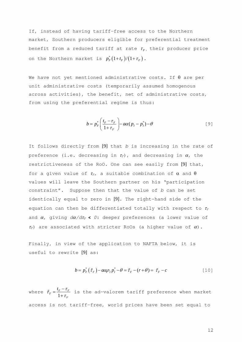
If, instead of having tariff-free access to the Northern

market, Southern producers eligible for preferential treatment

benefit from a reduced tariff at rate Fτ , their producer price

on the Northern market is ( ) ( )* 1 / 1F F Fp t τ+ + .

We have not yet mentioned administrative costs. If θ are per

unit administrative costs (temporarily assumed homogenous

across activities), the benefit, net of administrative costs,

from using the preferential regime is thus:

* ( )1F F

F IF

tb p a p pτ *Iα θ

τ⎛ ⎞−

= − −⎜ ⎟+⎝ ⎠−

−

[9]

It follows directly from [9] that b is increasing in the rate of

preference (i.e. decreasing in τF), and decreasing in α, the

restrictiveness of the RoO. One can see easily from [9] that,

for a given value of τF, a suitable combination of α and θ

values will leave the Southern partner on his “participation

constraint”. Suppose then that the value of b can be set

identically equal to zero in [9]. The right-hand side of the

equation can then be differentiated totally with respect to τF

and α, giving dα/dτF < 0: deeper preferences (a lower value of

τF) are associated with stricter RoOs (a higher value of α).

Finally, in view of the application to NAFTA below, it is

useful to rewrite [9] as:

[10] ( )* * ( )F F I I F Fb p a p r cτ αρ θ τ θ τ= − − = − + =

where 1F F

FF

t τττ−

=+

is the ad-valorem tariff preference when market

access is not tariff-free, world prices have been set equal to

12

unity by choice of units, the costs of RoO are replaced by the

proxy value given by the restrictiveness index presented in

table 1 (rescaled since the choice of units here imply

), and c represents total RoO-related compliance costs. 0 ri< <1

If the participation-constraint view is indeed prevalent in

North-South PTAs, one would expect that there is

substitutability between tariffs and RoO as instruments of

intra-bloc protection. If so, suppose that Southern

final-good producers used to purchase their intermediate inputs

outside of the bloc before the preferential agreement. Then, as

RoO are substituted for tariff protection, they start

purchasing within the bloc, say in the North if the South does

not produce the intermediate inputs. As a result, their costs

go up and they enjoy only marginally improved market access.

But Northern producers of intermediates now enjoy a captive

market and emerge as the winners. Thus, Northern (US, EU)

intermediate-good producers can be expected to lobby in favor

of RoO. Taking the argument one step further, as stiffer RoO

require deeper tariff preferences along the Southern member’s

participation constraint (because dα/dτF < 0 along b = 0, see

supra and the dotted indifferent participation curves drawn in

figure 1), Northern intermediate-good producers can be expected

to lobby in favor of deeper tariff preferences in their

downstream sectors. When they succeed, tariff revenue for the

Northern country is replaced by rents and inefficiencies at the

level of intermediate-good producers.11

11 While this outcome can be derived from common agency political economy models (see e.g. Cadot et al. 2003), it can also be viewed as an application of the obfuscation principle in the endogenous tariff literature. See Magee, Brock and Young (1989, chp. 18). Alternatively, one may take as exogenously given that all intra-bloc tariffs must go to zero, which then implies that the rate of tariff preference is equal to the rate of MFN tariffs. Then, if MFN tariffs proxy for lobbying power, ROOs will be positively correlated with them (and with tariff preference since the two

13

With specific functional forms, one can get an idea of the

trade-offs involved between preference rates, τ , and the costs

associated with a VC of the type analyzed here. Portugal-Perez

(2003), simulates a modified version of [10] in which Southern-

partner producers purchase intermediates from the Northern

partner and from the ROW under the assumption of a Leontief

technology for intermediates, a CES technology (with elasticity

of substitution σ) for intermediates by country of origin, a

CES technology for value-added using capital and labor (with

elasticity of substitution σV) and a CET (constant elasticity

of transformation function with transformation elasticity Ω).

To reflect the partial equilibrium set-up, assume also that

prior of the FTA, half of the exports go to the (future)

Northern FTA partner, and that the Southern partner faces an

infinitely elastic demand for its exports, and an infinitely

elastic supply of capital and labor. Let 0 1,α α represent the

Northern partner's share in intermediate imports before and

after the FTA respectively. Portugal-Perez obtains the

following preference values for the final good, Fτ , (which are

plausible in light of the Mexican experience discussed below)

that will leave the Southern partner on his participation

constraint:

0 1[ .2, .3 ( 1, 1, 1) 5.1%]V Fα α σ σ τ= = = = Ω = → = ;

0 1[ .2, .3 ( 2, 1, 2) 2.7%]V Fα α σ σ τ= = = = Ω = → = .

To summarize, we may ask how the above analysis could help

predict how the application of RoO would affect the pattern of

trade in manufactures under a typical FTA like NAFTA. At the

minimum we must consider three countries: two forming an FTA

(intra-FTA trade), and a third (the rest-of-the-world (ROW).

are just the same thing) but for a reason that is unrelated to the Southern member’s participation constraint.

14

Suppose then that manufacturing trade is aggregated into

intermediates goods and final goods trade. Then, in the absence

of a change in tariffs, the application of RoO would be

expected to have the following effects:

1) Final goods producers would shift their purchases of

intermediates to intra-FTA intermediates.

2) If final goods are imperfect substitutes by origin,

consumers will shift towards (away from) intra-FTA from (to)

ROW trade if b>0 (b<0) in [8].

3) Should there be a shift in consumer goods consumption

towards FTA partners that is not too strong (τF not too

large relative to ρI), an FTA would be expected to raise the

share of intermediates goods trade in total intra-FTA trade.

Alternatively, if market-access is substantial (τF is large and

ρI is small) then predictions 1) and 3) would not be borne out

in the data, intra-partners final goods trade would rise

markedly. Below, we shall examine whether or not these

predictions were borne out in the case of NAFTA using the WTO

classification of goods into raw materials, intermediates and

final goods classification.

4. Assessing the costs of NAFTA’s RoO

The remaining sections use NAFTA to assess the costs of RoO and

to see whether trade patterns have been altered along the lines

predicted above.12 This section provides estimates of total

compliance costs and section 5 looks for changes in the pattern

of manufacturing trade.

12 NAFTA has four broad types or RoO (see Cadot et al. (2002) for a detailed description).

15

Tariff preferences granted under NAFTA are substantial. In 1998

(about half-way down the tariff phase-out) [in 2000, near

completion], the US average tariff on Mexican goods was 0.28%

[0.08%], whereas the US average MFN tariff on the same goods

was 4.8% [4.02%], giving a preference for Mexican exports to

the US of 4.51% [3.94].13 As a result, it would seem that

Mexican products enjoy substantial access to the US market.14

However, in spite of these preferences, as shown in table 3, in

2000, NAFTA’s utilization rates, Ui, computed at the HS-6 level

varied widely across sectors, being sometimes substantially

below 100% in sectors with deep tariff preferences, suggests

that hidden barriers associated with RoO-related compliance

costs undid the positive effect of tariff preferences, and that

firm heterogeneity may be important.

Following Herin’s (1986) approach in the case of EFTA, in

sectors where NAFTA’s ui=100%, the benefit of tariff preference

is revealed larger than total compliance costs (including

administrative costs), while for sectors where ui=0%, tariff

preference rates, τi, provide a lower bound on total compliance

costs. Finally, for sectors with 0%≤ui≤100%, if Mexican

exporters had identical (homogeneous) compliance costs they

would be revealed indifferent between shipping under NAFTA or

MFN, so the rate of tariff preference would be revealed equal

to compliance costs.15 Recognizing that compliance costs are

13 Average tariffs are ad-valorem equivalents weighted by shares in Mexican exports to the US. Thus, the weighted-average MFN tariff reported here is computed using the product shares in Mexican exports to the US as weights, rather than product shares in total US imports. Mexico’s maquiladora exports amounted to $223 million in 2000 (see Cadot et al. 2002 for details). 14 For specific examples, in 1998, Mexican apparel products faced a tariff of less than 1% whereas similar products from China and Hong-Kong faced tariffs of 12.7% and 17.5% respectively. For automobile products the corresponding tariff rates were 0.4% for Mexican products, against 2.7% for German products. 15 Out of a total of 3641 lines, 1471 lines had 0%<ui<100%, accounting for 75.6% of the total value of exports to the US.

16

likely to be heterogeneous even within sectors (some firms are

better at dealing with compliance costs than others), all that

can be said is that the tariff preference gives a rough

estimate of compliance costs in the sense that at least some

firms have higher compliance costs whereas others have lower

ones.

According to table 3, NAFTA's overall utilization rate, u was

64% in 2000, with the utilization rate computed at the HTS-6

level, measuring the share of Mexican exports to the US that

entered under the NAFTA regime. When tariff lines with zero US

MFN tariffs (and hence no tariff preferences) are excluded

(last column of Table 4), 83%u = . Among sectors with

significant exports, despite substantial preferential access,

the T&A sector (HTS2 chapters 50-63, $10.3 billion) had a

slightly lower-than average utilization rate. At the other end

of the spectrum, the lowest utilization rates among significant

sectors were ui=20% for furniture (HTS chapter 94, $3.8

billion), ui=42% for optics (HTS2 90,$4.6 billion), ui=48% for

knitting products (HTS2 61,$ 3.5 billion), the lowest rate in

the textile-clothing sector.

Insert table 3 here Mexican exports to the US and NAFTA’s regime

Further inspection of Table 3 suggests much heterogeneity in

compliance costs, justifying exploring further sources of this

heterogeneity using the restrictiveness index, r, introduced in

table 1. For example, in T&A (sector 11 in table 3),

(weighted at the 6-digit level by the value of

Mexican exports) and , yet u

16.69%MFNi it t= =

0.06%NAFTAi it τ= = i=66.7% but ri=6.9.

The transport equipment (HTS17) and leather goods (HTS8)

sectors have similar tariff preferences (τi=6.28%; τi=6.38%),

yet utilization rates are very different, though in the

17

direction predicted by values of ri ([ui=94.9%; ri=4.8] versus

[ui=57%; ri=5.6]).

To construct a ‘rule-of-thumb’ estimate for the share of

administrative costs in total compliance costs, we assume that

differences in administrative costs, θ, in equation [10] are

mostly related to differences in administrative capabilities to

deal with red tape compliance across firms, rather than to

differences across sectors (at least when the severity of the

RoO is supposedly the same as measured by the index, r).

By revealed preference, for those tariff headings that are

eligible for NAFTA treatment and where 100% of Mexico's exports

to the US enter under the NAFTA regime (i.e. ui=100%), the

combined cost of complying with RoO and other NAFTA-related

administrative procedures cannot be greater than the benefit

conferred by preferential tariff access. In other words, the

value of b in [9] is positive. For those tariff headings, thus,

the rate of preference gives an upper bound on total

compliance. By the same reasoning, for those tariff headings

where none of Mexico's exports enter the US under NAFTA regime

(i.e. ui=0%), the rate of preference gives a lower bound on

those costs.

The first approximation on combined ROO and administrative

costs associated with the preferential regime is given by the

rate of tariff preference for the remaining sectors (i.e.

0%<ui<100%). This is because, as explained above one can

suppose that, at least for the marginal firms (administrative

and ROO compliance costs may vary across firms), b = 0. Thus,

for those tariff headings, the rate of preference

would be an upper bound estimate on

combined ROO and administrative costs. Eliminating tariff

( ) (/ 1MFN NAFTA NAFTAi i i it t tτ ⎡= − +⎣ )⎤⎦

18

headings with either ui= 100% or ui= 0%, the import-weighted

average of the rate of preference is 6.13% (1471 tariff line

observations, standard error 0.58%).16 In terms of [10] total

compliance costs, ci, for sectors on the participation

constraint are: bi=0 ⇔ 0%<ui<100% ⇒ ( ) 6.13%i i i ir cθ τ+ = = = .

When can we consider administrative costs to be negligible? For

those tariff lines corresponding to industries that are on

their participation constraint (i.e. 0%<ui<100%),

administrative costs should be low when it is easy to comply,

which should correspond to easy-to-document 'proof of origin'

(e.g. a change of classification at the item level or at the

sub-heading), i.e. for tariff lines for whom the value of ri is

low. We take as a cut-off r* of 2 (only one tariff line has a

value of 1), i.e. R = i: ri ≤ r*=2. This corresponds to the

case where the RoO boils down to a change of tariff subheading,

CS, or at the item level, CI.

A calculation of the average, minimum and maximum values of

tariff preferences for three different sets R∩U (low

restrictiveness values defined above cum different cut-off

utilization rates values) corresponding to cut-offs for u* of

90%, 95% and 99% gives average values for preference margins

between 4.18% (u*=90%) and 4.69% (u*=99%) and robust to changes

in u*.17 Take then the average tariff-preference level for u* =

95% ( 4.30%iτ = ) as the closest upper bound on non-ROO

administrative costs. In terms of [10] if bi=0 ⇔ 0%<ui<100% ⇒

16 In the calculations, we have eliminated 5 outlier observations with

100%iτ > belonging to chapter 24 (Tobacco) and 12 (vegetables). Excluding

outliers, the average margin of preference was 4.1%. 17 As a further check, the frequency distribution of tariff preference levels by intervals of two percentage points in R∩U (218 observations) for u* = 95% and confirms that the range 2-4% is not only the average but also the mode of the distribution.

19

6.13% 4.3% 1.83%i i icθ τ= − = − = , or close to 45% of the preference

margin.18

This estimate should be interpreted with caution. Referring

back to [10], if firms that export at the HS-8 level are

heterogenous (which must certainly be the case), then some

firms will not meet the RoO, which Ju and Krishna (2003) call a

heterogenous regime. In evaluating the average administrative

costs, we obviously ignore regime switches as estimates of the

restrictiveness change. Fortunately this problem is not too

important in these non-parametric estimates, since all but one

of the values of the ri index are equal to 2. However, since we

are taking averages across industries, some observations that

enter the calculation must include firms for which b>0.

Finally recent estimates of compliance costs (Carrère and de

Melo (2004)) using the same data set, but distinguishing the

cost-raising effects of different RoO (change of chapter

heading, regional value content, and technical requirements)

yields both estimates that justify the observation rule used by

Estevadeordal (2000). They also find that for each of three

broad product categories (raw materials, intermediates and

final goods), unconstrained cost estimates within the zero-one

range), are lower than the average preference margin for

products with a utilization rate of 100%. They also find, as

expected, that total compliance costs are greater for final

goods than for intermediates, and fairly close to the non-

parametric estimates reported here.

5. Tariff Preferences and RoO: Offsetting instruments?

18 Carrère and de Melo (2003) repeated these non-parametric estimates for 2001 data when the average preference margin and utilization rates were

20

If RoO and tariff preferences largely offset each other, one

would only expect marginal changes in trade patterns between

the US and Mexico following NAFTA, with these changes being

along the lines suggested in section 3. To see if NAFTA shifted

patterns of purchases and sales along the lines predicted

above, we computed several indices of the regional intensity of

trade according to the following formulas. Let ijkx be country

i’s exports of good k to country (or region) j, ij k ijkx x= Σ

country i’s exports aggregated over all goods to country (or

region) j, ik j ijkx x= Σ country i’s exports of good k to the world,

and i k j ijkx x= Σ Σ . Then, letting i be Mexico, j the US, a regional

intensity of trade index, ijkR would indicate the intensity of

exports of good k by Mexico to the US (an index greater (less)

than 1 indicating concentration (lack of concentration)):

//

ijk ijijk

ik i

x xR

x x= [11]

Using the same notation, let denote Mexican imports from

the US of good k, and let k=I denote the set of intermediate

goods, k=F the set of final goods, and period (0) 0=92-94 and

(1), 1=98-00, the pre and post-NAFTA two year average values.

Then, according to the discussion in section 3, and as shown in

the first two inequalities, R

ijkm

I and RF in [12], we would expect

imports of intermediates to shift towards the US, and exports

of final goods to the US. Alternatively, if one views NAFTA as

specializing Mexico-US trade into a ‘vertical exchange’ of the

offshore-assembly type whereby the US ships semi-finished goods

for assembly in Mexico and then re-imports them as finished

products, then, as shown in the third inequality, V, in [12],

6.16% 4.44% 1.72%i i icslightly higher. Their corresponding estimates for 2001 are:

θ τ= − = − =

21

one would expect the pattern of Mexican revealed comparative

advantage towards the US to shift away from finished towards

intermediates:

(1) / (1) (1) / (1)1; 1;

(0) / (0) (0) / (0)

(1) (0)(1) (0)

(1) (0)

ijI ij ijF ijI F

ijI ij ijF ij

ijI ijI

ijF ijF

m m x xR R

m m x x

R RV V

R R

= > =

= > =

>

i

[12]

Computation of [12] shows a strong shift in sales of final goods

towards the US (RF=1.12), but only a small change in the

pattern of intermediate purchases (RI=0.98) away from the US,

and little evidence of ‘vertical exchange’ at the aggregate

level. However, stronger patterns of specialization along the

lines predicted in section 3 are apparent for textiles and

apparel (T&A) (784 tariff lines). For the T&A tariff lines, the

above indices take the values: RI= 1.24>1; RF=1.02>1;

V(1)=0.57>V(0)=0.33.

Figure 1 explores the issue further by reporting data on tariff

preferences and the restrictiveness estimate of the costs of

RoO at the HTS1 level from Cadot et al. (2002).19

Insert figure 1 here Mexico: Exports to the US in PREF/ROO ( /i rτ ) space, 2000

According to [10], 450 lines would trace equal benefit curves in

preference-restrictiveness space, with lines closer to the

North-West corner indicating higher market access values since

they would correspond to large preferences and low RoO

compliance costs. On the assumption that r integer values are

an approximation of RoO compliance costs, it is immediately

19 These data are aggregated from ITC data on US imports from Mexico (overall and under NAFTA regime) at the HTS 6-digit with ad-valorem tariff equivalents computed at the 8-digit level using US ad-valorem and specific tariffs under MFN and NAFTA regimes and aggregated to the 6-digit level using US imports from Mexico as weights.

22

apparent that the attractiveness of the high-preference, high-

RoO package offered by NAFTA to HTS 11 (T&A) cannot be directly

compared with the low-preference, low-ROO package offered to

HTS 16 (machinery & electrical equipment) since they could be

on the same b ‘indifference locus’, but one can say that the

latter is unambiguously better than that offered to HTS 2

(vegetable products) and probably better than that offered to

HTS15 (base metals). At the HTS1 level, figure 1 clearly

suggests a 'frontier' in terms of tariff preferences and RoO

with all points lying Southeast of that frontier.

As a final check, we ran the following double-log ad-hoc

specification:

(10.15) (70.33) (9.57) (7.10)

2

ln 5.48 0.54 ln 0.015ln (0.338) ln

3,617; 0.831

i i i iXUS XROW r

NOBS R

τ= + + −

= = [13]

where XUSi (XROWi) stands for exports to the US (rest of the

world) at the HS 6 level in 2000, iτ stands for the rate of

tariff preference under NAFTA, ri is the restrictiveness index,

and where a vector of dummy variables at the HS 2 level that

controls for omitted variables have not been reported in [13].

As can be seen, the coefficients have the expected signs,

suggesting that preferences and RoO have opposite effects on

exports to the US, and if one were to trust the relative

magnitude of the coefficients, that preferential access has a

quantitatively smaller effect than increases in the stringency

of RoO.20 But, alternative specifications in which changes in

export shares (post vs. pre NAFTA) to the US were regressed on

the same set of variables yielded generally statistically

20 Tariff lines with 0iτ = were assigned a value arbitrarily close to zero

(10E-13). Strictly speaking, one cannot compare the magnitude of the coefficients since the values taken by r are ordinal rather than cardinal.

23

insignificant coefficients suggesting both little systematic

changes in the destination composition of Mexican manufacturing

exports, as would be expected under the ‘participation

constraint’ view of North-South PTAs.

6. Concluding remarks

This paper has described and analyzed the functioning of RoO

present in all PTAs. Having developed the basic analytics of

RoO in a typical North-South PTA, we have argued that in the

predominantly North-South recent wave of PTAs these RoO have

been set up in a complex and non-uniform manner, so that in

practice these PTAs provide little market access. As a result,

compliance costs have largely eroded the preferential access

afforded by the PTA, leading us to suggest that Southern

partners are effectively left on their ‘participation

constraint’.

To estimate the likely effects of RoO, we have modified an

existing index of ‘restrictiveness’ of RoO based on an

observation rule on the various criteria used to establish

origin. A cross-country regression on determinants of the

volume of bilateral trade indicates (after controlling for

several factors affecting the volume of trade) that if the

presence of PTAs increased the volume of trade, the

restrictiveness of RoO had a negative impact on the volume of

trade.

The second part of the paper was devoted to estimating the

likely effects of NAFTA on the pattern of Mexican exports to

the US in 2000, a year when the treaty was almost in full

force. At that time, Mexican exports were getting an average

Interpreting the coefficient of r as an elasticity would thus be

24

preferential access of 4% in the US market. Based on

utilization rates, Ui, computed at the HS-6 tariff

classification level, for sectors on the participation

constraint (i.e. with 0%<Ui<100%), we estimated total

compliance costs of 5% with up to 40% attributable to

administrative costs. Turning to the pattern of trade,

calculations of indices of comparative advantage at the HS-6

level revealed (with few exceptions like textiles & apparel),

only marginal changes in trade patterns although sectoral

exports to the US were positively (negatively) related to

preferential access (the restrictveness of RoO). Taken

together, it would seem that for NAFTA, RoO largely undid

preferential tariff access, suggesting that North-South PTAs

may well offer little market access to the Southern partners.

misleading.

25

References Anderson, J., and E. Van Wincoop, (2003), “Gravity with Gravitas: A Solution to the Border Puzzle”, American Economic Review, 93, 170-92. Augier, P., M. Gasiorek and C. Lai-Tong (2003), “The Impact of Rules of Origin on Trade Flows”, mimeo, University of Sussex. Brenton, P., and M. Manchin (2003), “Making EU Trade Agreements Work: The Role of Rules of Origin”, World Economy, forthcoming, also CEPS #183. Cadot, O., A. Estevadeordal, J. de Melo, A. Suwa-Eisenmann, and Bolorma Tumurchudur, (2002), “Assessing the Effect of NAFTA’s Rules of Origin”, mimeo, University of Lausanne. Cadot, O., A. Estevadeordal and Akiko Suwa-Eisenmann (2003), “ Assessing the Effect of NAFTA’s Rules of Origin”, mimeo, University of Lausanne. Carrère, C. and J. de Melo (2004), "North-South FTAs: Any Gains for the South?", mimeo in progress, University of Geneva. Duttagupta, R., and A. Panagariya, (2002), “Free Trade Areas and Rules of Origin: Economics and Politics”, mimeo, University of Maryland. Estevadeordal, A. (2000), “Negotiating Preferential Market Access: The Case of the North American Free Trade Agreement”, Journal of World Trade 34, 141-66. Estevadeordal, A., and K. Suominen (2003), “Rules of Origin: A World Map and Trade Effects”, mimeo, IDB, Washington, D.C. Falvey, R. and G. Reed, (2000), Economic Effects of Rules of Origin, Weltwirtchafliches Archiv, 143(4), 209-29. Feenstra, R. (2003), Advanced International Trade, Princeton University Press, forthcoming. Fernandez, R. and R. Portes, (1999), “The Non-Traditional Gains from Regionalism”, World Bank Economic Review, 12, 197-220. Flatters, F. (2002), “SADC Rules of Origin: Undermining Free Trade” mimeo, Queens University. Herin, J. (1986), “Rules of Origin and Differences Between Tariff Levels in EFTA and in the EC”, EFTA Occasional Paper 13.

26

Holmes, P. and G. Sheppard (1983), “Protectionism in the Economic Community”, International Economics Study Group, 8th annual conference. Ju, J., and K. Krishna (2002), "Regulation, Regime Switches and Non-Monotonicity when Non-Compliance is an Option: An Application to Content Protection and Preference", Economic Letters, 77, 315-21. Ju, J., and K. Krishna (2003), "Firm Behavior and Market Access in a Free Trade Area with Rules of Origin", mimeo, Penn State University. Koskinen, M. (1983), “Excess Documentation Costs as a Non-tariff Measure: an Empirical Analysis of the Import Effects of Documentation Costs”, Working Paper, Swedish School of Economics and Business Administration. Krishna, K., 2003, “Understanding Rules of Origin”, mimeo, Pennsylvania State University. Krishna, K. and A. Krueger (1995), “Implementing Free Trade Areas: Rules of Origin as Hidden Protection”, in A. Deardorff, J. Levinsohn and R. Stern eds. New Directions in Trade Theory, 149-87. Krueger, Anne. (1997),“Free Trade Areas versus Customs Union”, Journal of Development Economics, 54, 169-97. Magee, S.P., W.A. Brock et al. (1989), Black Hole Tariffs and Endogenous Policy Theory: Political Economy in General Equilibrium:, New York, Cambridge University Press. Matoo, A. D. Roy and A. Subramanian (2002), “ The Africa Growth Opportunities Act and its Rules of Origin: Generosity Undermined?”, IMF Working Paper # WP/02/158. Portugal-Perez, L. A. (2003), "Rules of Origin in a North-South Type of PTA: An Empirical Investigation from NAFTA", M.A. Thesis, University of Geneva. US Customs (1998), NAFTA for Textiles and Textile Articles, 1998. USTR (2000), 1999 Annual Report of the President of the United States on the Trade Agreements Program, www.ustr.gov/html/2000tpaT.

27

Table 1: Structure of RoO in Selected FTAs (calculated at the HS-6 level tariff line)

EUROPE AMERICAS Requirement PANEURO NAFTA ROO INDEXPPa

NC 0.39 0.54 1 NC+ECTC 2.39 1-2 NC+TECH 1.39 2 NC+ECTC+TECH 0.00 2 NC+VC 11.46 4-5 NC+ECTC+VC 1.57 5 NC+VC+TECH 0.08 7 NC+WHOLLY OBTAINED CHAPTER 7.62 7 NC+WHOLLY OBTAINED HEADING 0.70 SUBTOTAL 25.60 0.54 CI CI+ECTC 0.02 1 CI+TECH CI+ECTC+TECH CI+VC CI+ECTC+VC 0.02 2 CI+VC+TECH SUBTOTAL 0.00 0.04 CS 0.20 1.29 2 CS+ECTC 0.00 2.52 2 CS+TECH 1.90 0.04 2 CS+ECTC+TECH 0.00 0.40 2 CS+VC 0.27 3 CS+ECTC+VC 0.00 0.10 3 CS+VC+TECH 0.00 3 CS+ECTC+VC+TECH 0.00 3 SUBTOTAL 2.37 4.35 CH 32.99 17.09 4 CH+ECTC 4.60 19.18 4 CH+TECH 0.00 0.02 4 CH+ECTC+TECH 6.66 0.14 4 CH+VC 13.01 3.54 5 CH+ECTC+VC 0.37 0.58 5 CH+VC+TECH 0.00 0.10 5 CH+ECTC+VC+TECH 0.02 5 SUBTOTAL 57.65 40.65 CC 2.16 30.95 6 CC+ECTC 1.02 17.71 6 CC+TECH 0.04 0.02 6 CC+ECTC+TECH 11.02 5.76 6 CC+VC 0.00 7 CC+ECTC+VC 0.00 7 CC+VC+TECH 0.00 7 CC+ECTC+VC+TECH 0.00 7 SUBTOTAL 14.24 54.44 TOTAL 100 100 Sources: Cols.1-3 from Estevadeordal and Suominen (2003, table --) and authors' computations NC= No change; ECTC=exception to change of tariff classification; TECH= technical requirement; VC= value content; CI=Change of item; CS= change of subheading; CH=change of heading; CC=change of chapter a The index ri is calculated at the HS-6 level following Estevadeordal (2000) and takes a value in the range 1<ri<7, a higher value indicating a more restrictive RoO (see text).

28

Table 2: Bilateral Imports and RoO Restrictiveness: A Cross-Country Gravity Analysis

Dependent variable: Ln (Average Bilateral Imports 1999-2001)

Column 1 2 OLS Country Fixed

Effects

Ln(YiYj) 0.95 0.80 (158.4) (13.6)

Ln(DISTij) -0.75 -0.98 (29.3) (32.8)

Former colony 1.28 1.14 (12.5) (10.6)

Common colonizer 0.64 0.77 (9.4) (12.1)

Common language 0.60 0.43 (10.8) (7.9)

Common border 1.08 1.10 (10.3) (10.2)

PTA 3.67 3.38 (9.4) (10.4) Perfect CU 0.60 0.11 (7.3) (1.2) Ln (RoOij+1) -1.46 -2.11

(6.3) (8.3)

Constant -24.88 -15.90

(72.0) (5.6)

Observations 15,280 15,280 Adjusted/Pseudo R-sq. 0.67 0.76

Source: Authors’ estimation; data from Estevadeordal and Suominen (2003) Notes: Absolute value of t-statistics in parentheses.

29

Table 3: Mexican exports to the US and NAFTA's regime

Mexican exports to the US ($ million)

US Ad-valorem tariff equivalents (%)

ROO index

NAFTA utilization Rates [ui] (%)

Section All

regimes NAFTA MFN NAFTA Preference rate [ri]

All tariff lines

Positive preference

a B C D (c-d) /

(1+d) e F g

1. Live animals 974 434 0.41 0.00 0.41 (0.0066)

6.0 44.60 (23.97)

85.82 (10.74)

2. Veg. Products 3'070 2'210 4.73 0.75 3.92 (0.246)

6.0 71.95 (15.04)

85.30 (6.12)

3. Fats and Oils 30 18 4.35 0.00 4.35 (0.056)

6.0 58.60 (7.64)

62.51 (5.71)

4. Food, Bev & Tob 2'130 1'520 3.96 0.34 3.56 (4.891)

4.7 71.18 (16.30)

74.18 (14.82)

5. Min. prod. 12'700 10'500 0.40 0.08 0.32 (0.000)

6.0 82.62 (1.57)

84.76 (0.01)

6. Chemicals 1'640 928 3.42 0.21 3.19 (0.067)

5.3 56.47 (20.46)

79.10 (10.76)

7. Plastics 1'800 1'530 4.21 0.01 4.20 (0.043)

4.8 84.69 (8.16)

93.08 (1.17)

8. Leather goods 289 165 9.13 2.49 6.38 (0.180)

5.6 56.97 (17.32)

58.74 (16.82)

9. Wood products 389 208 2.66 0.08 2.58 (0.071)

4.0 53.57 (22.59)

68.06 (18.84)

10. Pulp & paper 685 462 1.34 0.00 1.34 (0.082)

4.8 67.45 (18.44)

84.76 (8.50)

11. Text.& apparel 10'300 6'790 16.75 0.06 16.69 (0.628)

6.9 65.70 (4.40)

66.72 (4.29)

12. Footwear 414 333 10.69 4.07 6.13 (0.173)

4.9 80.39 (9.73)

82.16 (8.48)

13. Stone & glass 1'540 1'050 5.01 1.45 3.50 (0.068)

4.9 67.80 (16.34)

77.53 (11.14)

14. Jewelry 507 191 2.18 0.00 2.18 (0.081)

5.3 37.70 (20.51)

40.74 (20.93)

15. Base metals 4'940 3'580 2.34 0.41 1.92 (0.031)

4.6 72.47 (14.90)

82.13 (8.96)

16. Mach. & elec. 53'000 25'300 1.86 0.00 1.86 (0.038)

3.2 47.78 (17.00)

75.60 (5.82)

17. Trans. equip. 26'800 25'400 6.31 0.03 6.28 (0.717)

4.8 94.93 (2.73)

97.64 (0.16)

18. Optics 4'610 1'950 1.14 0.00 1.14 (0.030)

4.0 42.25 (20.02)

85.99 (3.14)

19. Arms & ammun. 13 2 0.87 0.00 0.87 (0.018)

4.7 12.82 (9.50)

40.81 (18.80)

20. Miscellaneous 4'770 1'130 1.72 0.01 1.71 (0.113)

5.1 23.72 (17.05)

91.22 (4.00)

Total 130'601 83'700 4.02 0.10 3.92* 4.5† 64.03 82.68 Standard deviations in parentheses * StanSource: Cadot et al. (2002, table 1).

dard deviation: 0.49 † Standard deviation: 2.35

30

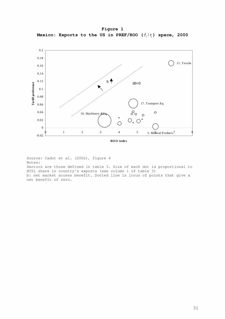
Figure 1 Mexico: Exports to the US in PREF/ROO ( /i riτ ) space, 2000

11. Textile

17. Transport Eq.

5. Mineral Products

16. Machinery &Eq.

-0.02

0

0.02

0.04

0.06

0.08

0.1

0.12

0.14

0.16

0.18

0.2

0 1 2 3 4 5 6 7 8

RO O index

Tari

ff p

refe

renc

e b db=0

Source: Cadot et al. (2002), figure 4 Notes: Sectors are those defined in table 3. Size of each dot is proportional to HTS1 share in country’s exports (see column 1 of table 3) b: net market access benefit. Dotted line is locus of points that give a net benefit of zero.

31