Roman lead and copper mining in Germany

their origin and development through time,

deduced from lead and copper isotope provenance studies

Dissertation zur Erlangen des Doktorgrades

Der Naturwissenschaften

Vorgelegt beim Fachbereich Geowissenschaften der Johann Wolfgang Goethe-Universität

in Frankfurt am Main

von Soodabeh Durali-Müller

aus Tehran/Iran

Frankfurt (2005)

Von Fachbereich .............................................................................................. der Johann Wolfgang Goethe – Universität als Dissertation angenommen. Dekan: ................................................................................................ Gutachter: ........................................................................................... Datum der Disputation: .......................................................................

ACKNOWLEDGEMENTS I would like to express my gratitude to Prof. G. Brey for his support and guidance. I profited much from discussions with Prof. S. Weyer, Prof. W. Püttmann and Prof. H.M. von Kaenel. Dr. D. Wigg-Wolf is specially thanked for his valuable comments and for finding me very useful contacts and I thank Dr. Y. Lahaye, Dr. H. Höfer, Dr. Ch. Bendall and A. K. Neumann for helping me in the laboratory and with measurements. I like to thank Dr. H.M. Seitz and Dr. Ch. Bendall for reviewing the German and English text respectively. I would also like to thank those people and institutions, which provided artifacts and ore samples for analysis: For artifacts: Dr. D. Wigg-Wolf: Akademie der Wissenschaften und der Literatur Mainz Prof. G. Fingerlin: Archäologische Denkmalpflege, Freiburg Dr. G. Rasbach and Dr. K.-F. Rittershofer: Römisch-Germanische Kommision, Frankfurt Dr. A. Heising: Archäologie und Geschichte der römischen Provinzen, Johann Wolfgang Goethe Universität Frankfurt Dr. G. Rupprecht and Dr. J. Dolata: Landesamt für Denkmalpflege, Mainz Dr. S. Faust and Dr. L. Schwinden: Landesmuseum, Trier Dr. H. Merten: Bischofliches Museum, Trier Dr. C. Nickel and Dr. M. Thoma: Landesamt für Denkmalpflege, Außenstelle Koblenz Dr. D. Krausse: University of Kiel For ores: Dr. L. Krahn: Fraunhofer IZM, Paderborn Dr. A. Hauptmann and Dr. M. Ganzelewski: Bergbau Museum, Bochum Dr. A. Wiechowski: Institut für Mineralogie und Lagerstättenlehre RWTH, Aachen Dr. K. Schürmann: Mineralogisches Museum der Philipps Universität, Marburg Dr. R. Schumacher: Rheinische Friedrich Wilhelms Universität, Bonn Dr. R.T. Schmitt: Museum für Naturkunde, Universität zu Berlin Dr. Dr. H. Lutz and C. Poser: Naturhistorisches Museum, Mainz Dr. M. Günter: Senckenberg Museum, Frankfurt Dr. U. Neumann: Institut für Geowissenschaften, Universität Tübingen Prof. W. Püttmann: Institut für Atmosphäre und Umwelt, Universität Frankfurt Dr. A. Bechtel: Montanuniversität Leoben, Österreich Above all I wish to thank my parents and my husband, Thomas, for their love, patience and encouragement.

ACKNOWLEDGEMENTS

ABSTRACT

KURZFASSUNG

GERMAN SUMMARY

INTRODUCTION

CHAPTER 1 GEOLOGY AND METALLURGY OF LEAD .....................1

1.1 GEOLOGICAL SETTING........................................................................1

1.2 ORE MINERALIZATION............................................................................1

1.2.1 VARISCAN VEIN-TYPE MINERALIZATION ................................................1

1.2.2 POST-VARISCAN VEIN-TYPE MINERALIZATION IN PALEOZOIC SEDIMENTS...........................................................................................................2

1.2.3 POST-VARISCAN CARBONATE-HOSTED LEAD-ZINC MINERALIZATION OF AACHEN-STOLBERG AND EASTERN BELGIUM .........4

1.2.4 TRIASSIC SANDSTONE-HOSTED ORE IMPREGNATIONS OF MAUBACH-MECHERNICH ...................................................................................4

1.3 METAL OCCURRENCE AND METALLURGY OF LEAD IN ROMAN PERIOD...........................................................................................................6

1.3.1 THE SOURCES OF LEAD IN ROMAN PERIOD ...........................................6

1.3.2 METAL REFINING PROCESSES ...............................................................10

1.4 USE OF LEAD IN ROMAN PERIOD ........................................................12

CHAPTER 2 ANALYTICAL METHODS...............................................14

2.1 ELEMENTAL ANALYSIS ........................................................................14

2.1.1 INSTRUMENTATION ..................................................................................14

2.1.2 SAMPLE PREPARATION...........................................................................14

2.2 LEAD ISOTOPE ANALYSIS....................................................................14

2.2.1 INSTRUMENTATION ..................................................................................14

2.2.2 SAMPLE PREPARATION...........................................................................15

2.2.3 STANDARD.................................................................................................15

2.3.4 COMPARING THE RESULTS OF THE MEASUREMENTS WITH TIMS AND MC-ICP-MS ..........................................................................................................16

2.3.5 COMPARING THE LASER MC-ICP-MS AND SOLUTION MC-ICP-MS RESULTS OF LEAD ISOTOPE ANALYSIS.........................................................19

2.4 COPPER ISOTOPE ANAYLSIS ..............................................................20

2.4.1 SAMPLE SELECTION AND ANALYSIS.....................................................20

2.4.2 MEASUREMENT AND STANDARDIZATION ............................................21

2.5 ZINC ISOTOPE ANAYLSIS.....................................................................22

2.5.1 INTRODUCTION .........................................................................................22

2.5.1 SAMPLE PREPARATION AND ANALYSIS ...............................................23

CHAPTER 3 ELEMENTAL ANALYSIS................................................24

3.1 ELEMENTAL ANALYSIS OF GALENA FROM THE RHEINISCHE SCHIEFERGEBIRGE....................................................................................24

3.1.1 INTRODUCTION .........................................................................................24

3.1.2 RESULTS AND DISCUSSION ....................................................................25

3.2 ELEMENTAL ANALYSIS OF LEAD OBJECTS FROM MAINZ WORKSHOP AND WALDGIRMES...............................................................29

3.2.1 RESULTS ....................................................................................................29

3.2.2 DISCUSSION ..............................................................................................30

CHAPTER 4 LEAD ISOTOPE ANALYSIS...........................................31

4.1 LEAD ISOTOPE ANALYSIS OF GERMAN ORES .................................. 31

4.1.1 INTRODUCTION .........................................................................................31

4.1.2 RESULTS AND DISCUSSION ....................................................................32

4.2 LEAD ISOTOPE ANALYSIS OF LEAD OBJECTS.................................. 35

4.2.1 INTRODUCTION .........................................................................................35

4.2.2 RESULTS ....................................................................................................38

DANGSTETTEN .............................................................................................38

WALDGIRMES ...............................................................................................39

MAINZ.............................................................................................................41

MARTBERG ...................................................................................................44

TRIER..............................................................................................................48

WALLENDORF...............................................................................................54

DÜNSBERG....................................................................................................55

4.2.3 DISCUSSION ..............................................................................................57

4.2.4 CONCLUSION.............................................................................................59

CHAPTER 5 ELEMENTAL AND ISOTOPIC ANALYSIS OF COPPER ORES AND ALLOYS............................................................................62

5.1 METALLURGY OF COPPER .................................................................. 62

5.1.1 INTRODUCTION .........................................................................................62

5.1.2 MINING AND MINERALS............................................................................62

5.1.3 COPPER ALLOYS ......................................................................................64

5.2 ELEMENTAL ANALYSIS ........................................................................67

5.2.1 INTRODUCTION .........................................................................................67

5.2.2 RESULTS ....................................................................................................68

5.2.3 DISCUSSION ..............................................................................................70

5.3 COPPER ISOTOPE ANALYSIS ..............................................................71

5.3.1 INTRODUCTION .........................................................................................71

5.3.2 RESULTS ....................................................................................................72

5.4 LEAD ISOTOPE ANALYSIS AND PROVENANCING THE COPPER ALLOYS FROM THE MAINZ WORKSHOP .................................................. 80

5.5 COPPER AND LEAD ISOTOPES IN KUPFERSCHIEFER...................... 82

5.5.1 INTRODUCTION .........................................................................................82

5.5.2 METAL ACCUMULATION MECHANISM ...................................................82

5.5.3 SAMPLE PREPARATION AND ANALYSIS ...............................................84

5.5.4 RESULTS ....................................................................................................85

5.5.4 DISSCUSION........................................................................................90

REFERENCES......................................................................................95

APPENDIX 1 LEAD ISOTOPE RATIOS.............................................106

APPENDIX 2 COPPER ISOTOPE ANALYSIS ..................................124

i

ABSTRACT The present work was devised to address the systematic analysis of samples from a range of Roman non-ferrous metal artefacts from different archaeological contexts and sites in the Roman provinces of Germania Superior. One of the focal points of this study is the provenancing of different lead objects from five important Roman settlements between 15 BC and the beginning of fourth century AD. For this purpose, measurements were made on lead and copper ore samples from the Siegerland, Eifel, Hunsrück and Lahn-Dill area in Germany and supplemented with data from the literature to create a data bank of lead isotope ratios of European deposits. Compositional analysis of lead objects by Electron Microprobe analysis showed that Romans were able to purify lead from ore up to 99%. Multi-Collector Inductively Coupled Plasma Mass-Spectrometry was used to determine the source of lead, which played an important role in nearly all aspects of Roman life. Lead isotope ratios were measured for ore samples from German deposits from the eastern side of the Rhine (Siegerland, Lahn-Dill, Ems) and the western side of the Rhine (Eifel, Hunsrück), which contained enough ore reserves to answer the increasing local demand and are believed to have been mined during the Roman period. This data together with those from Mediterranean ore deposits from the literature was used to establish a data bank. The Mediterranean ore deposits range from Cambrian (high 207Pb/206Pb) to tertiary (lower 207Pb/206Pb) values. In particular, the Cypriot deposits are younger, while the Spanish deposits fall either with the younger Sardic ores or close to the older Cypriot ores (Klein et al. 2004). The lead isotope ratios of most German ore deposits fall in between the 208Pb/206Pb vs. 207Pb/206Pb ratios of Sardinia and Cyprus, where the lead isotope signature of ore deposits from France and Britain are also found. Over 240 lead objects were measured from Wallendorf (second century BC to first century AD) Dangstetten (15-8 BC), Waldgirmes (AD 1-10), Mainz (AD 1-300), Martberg (first to fourth centuries AD) & Trier (third to fourth centuries AD). Comparing the lead isotope ratios of lead objects and those from German ores shows that the source of over 85 percent of objects are Eifel ore deposits, but the Roman’s had also imported lead from the Southern Massif Central and from Great Britain. A further topic of this work was the systematic study of the variation of copper isotope ratios in different copper minerals and the mechanisms, which controls copper isotope fractionation in ores deposits.

ii

For this purpose, copper isotope analyses were made by Multi-Collector Inductively Coupled Plasma Mass-Spectrometry from a series of hydrothermal copper sulphides and their alteration products. Copper and lead isotope ratios were measured in coexisting phases of chalcopyrite and malachite and also coexisting malachite and azurite. No significant fractionation was observed in malachite-azurite phases, but in chalcopyrite-malachite coexisting phases, malachite always shows a positive fractionation to heavier isotope values. Zhu et al. (2000) and Larson et al. (2003) showed that isotopic variations in copper principally reflect mass fractionation in response to low temperature processes rather than source heterogeneity. The low temperature ore formation processes are mostly represented by weathering of primary sulphide ores to produce secondary carbonate phases and therefore are usually observed on the surface of ore deposits, which were probably removed during the early Bronze Age. Using this concept, copper isotope ratios were measured in some Early Bronze Age copper alloys and Roman copper alloys. However, no large copper isotope fractionation has been observed. Lead and copper isotope ratios were measured on samples from the Kupferschiefer. Two profiles were investigated; 1) Sangerhausen, which was not directly influenced by the oxidizing brines of Rote Fäule and 2) Oberkatz, where both Rote Fäule-controlled and structure-controlled mineralization were observed. Results from maturation studies of organic matter suggest the maximum temperature affecting the Kupferschiefer did not exceed 130°C (Sun 1996). δ65Cu ranges between -0.78-+0.58‰, shows a positive correlation with copper concentration. Maximum temperature in the Kupferschiefer profile from Oberkatz is supposed to be around 150°C. δ65Cu in this profile ranges between -0.71-+0.68‰. The pattern of copper isotope fractionation and copper concentration is same as the for profile of Sangerhausen. Origina lead isotope ratios are strongly overprinted by high concentrations of uranium in bottom of both profiles causing more radiogenic lead. Klein S.; Lahaye Y.; Brey G.P.; Von Kaenel H.M. (2004). Archaeometry 46, 3 (2004) 469-480. Larson P.B., Maher K., Ramos F.C., Chang Z., Gaspar M., Meinert L.D. (2003). Chemical Geology, 201, 337-350. Sun Y. (1996). Geochemical Evidence for Multi-Stage Base Metal Enrichment in Kupferschiefer. PhD Thesis, Shaker Verlag, Aachen. Zhu X.K., O'Nions R.K., Guo Y., Belshaw N.S. and Rickard D. (2000). Chemical Geology 163, 139-149.

iii

KURZFASSUNG Die vorliegende Arbeit wurde geplant, um eine systematische Datenbasis römischer Buntmetallartefakte aus unterschiedlichen archäologischen Kontexten und verschiedenen Gebieten in Germania Superior zu schaffen. Einer der Schwerpunkte dieser Studie ist die Herkunftsbestimmung von Bleiartefakten, die aus funf wichtigen römischen Lagern, zwischen 15 v. Ch. und dem Anfang des vierten Jahrhunderts n. Ch., stammen. Das Blei spielte eine wichtige Rolle in fast allen Aspekten des römischen Lebens. Elementaranalysen von Blei mit der Elektronenstrahl-Mikrosonde zeigen, dass die Römer in der Lage waren, das Blei vom Erz bis zu einer Reinheit von 99% zu trennen. Um die Herkunft des Bleis zu bestimmen wurde mittels MC ICP-MS (Multi-Collector Inductively Coupeld Plasma Mass-Spectrometry) die Bleiisotopie bestimmt. Bleiisotopenverhältnisse wurden an Erzproben verschiedener Lagerstätten östlich des Rheins (Siegerland, Lahn-Dill, Ems) und westlich des Rheins (Eifel, Hunsrück) bestimmt. Archäologische Funde deuten darauf hin, dass die Erze zu römischen Zeiten möglicherweise aus diesen Lagerstätten gewonnen wurden. Zusammen mit Literaturdaten vom Mittelmeerraum bilden sie eine umfassende Datenbank. Die Mittelmeerlagerstätten liegen im Bleiisotopendiagramm in einem zeitlichen Bereich, der sich vom Kambrium (hohes 207Pb/206Pb) bis zum Tertiär (niedrigeres 207Pb/206Pb) erstreckt (Klein et al. 2004). Die Bleiisotopenverhältnisse der deutschen Lagerstätten liegen im 208Pb/206Pb gegen 207Pb/206Pb Diagramm zwischen Sardinien und Zypern, und fallen teilweise mit den Bleiisotopenverhältnisse von Frankreich und Großbritannien zusammen. Die Bleiisotopenverhältnisse wurden an 240 Blei Artefakten von Wallendorf (2. Jh. v. Chr. bis 1. Jh. n. Chr), Dangstetten (15-8 v. Ch.), Waldgirmes (1-10 n. Ch.), Mainz (1-300 n. Ch.), Martberg (1. bis 4. Jh. n. Ch.) und Trier (3. bis 4. Jh. n. Ch.) gemessen. Beim Vergleich der Bleiisotopenverhältnisse der Bleiartefakte und der deutschen Lagerstätten wird deutlich, dass die Römer zur Herstellung der Artefakte bis zu 85‰ Blei aus den Eifel – Erzlagerstätten verwendet haben, dass aber auch Blei aus dem südlichen Zentralmassiv und aus Großbritannien dafür importiert wurde. Ein weiterer Schwerpunkt dieser Arbeit ist die systematische Studie der Fraktionierung der Kupferisotope in unterschiedlichen Kupfermineralien und die Frage, welcher Mechanismus die Kupferisotopenfraktionierung in den Erzen und in den Kupferlegierungen steuert. Zu diesem Zweck wurde die Kupferisotopie an hydrothermalen Kupfersulfiden und Karbonaten mittels MC-ICP-MS gemessen. Kupfer- und Bleiisotopenverhältnisse wurden in den koexistierenden Phasen

iv

Kupferkies und Malachit, sowie Malachit und Azurit gemessen. Während zwischen Malachit- und Azurit keine Fraktionierung zu beobachten ist, so ist zwischen Kupferkies und Malachit eine Fraktionierung festzustellen, wobei Malachit immer isotopisch schwerer ist. Zhu et al. (2000) und Larson et al. (2003) zeigten, dass die Isotopenfraktionierung hauptsächlich bei der Erzbildung unter niedrigen Temperaturbedingungen stattfindet und weniger eine Heterogenität der Lagerstätten darstellt . Der Erzbildungsprozess bei niedrigen Temperaturen tritt in Oberflächennähe einer Erzlagerstätte auf. Die oberen Schichten wurden vermutlich in der frühen Bronzezeit abgebaut. Mit diesem Hintergrund wurde die Kupferisotopie an Artefakten aus der frühen Bronzezeit und an römischen Kupferlegierungen gemessen. Die Untersuchungen zeigten, dass keine große Kupferisotopfraktionierung stattfindet. Kupferisotopenverhältnisse wurden auch in Kupferschiefer gemessen. Zwei Profile wurden dafür ausgewählt: 1. Sangerhausen, das nicht direkt durch oxidierende Salzlösungen (Rote Fäule) beeinflusst wurde, und 2. Oberkatz, in dem Rote Fäule- und Struktur-Kontrollierte Mineralisierung vorkommt. Die Ergebnisse der Maturations - Studien organischer Materialien zeigen, dass die maximale Temperatur, die den Kupferschiefer beeinflusste, 130°C nicht überstieg (Sun 1996). δ65Cu schwankt zwischen -0.78-+0.58‰ und zeigt eine positive Korrelation mit der Kupferkonzentration. Im Kupferschiefer von Oberkatz schwankt δ65Cu zwischen -0.71-+0.68‰ und eine maximale Temperatur von 150°C wurde abgeschätzt. Die gleiche Korrelation ist zwischen der Kupferisotopie und Kupferkonzentration zu beobachten. Bleiisotopenverhältnisse sind sehr stark von der hohen Urankonzentrationen der untersten Schicht beeinflußt und zeigen mehr radiogenes Blei. Klein S.; Lahaye Y.; Brey G.P.; Von Kaenel H.M. (2004). Archaeometry 46, 3 (2004) 469-480. Larson P.B., Maher K., Ramos F.C., Chang Z., Gaspar M., Meinert L.D. (2003). Chemical Geology, 201, 337-350. Sun Y. (1996). Geochemical Evidence for Multi-Stage Base Metal Enrichment in Kupferschiefer. PhD Thesis, Shaker Verlag, Aachen. Zhu X.K., O'Nions R.K., Guo Y., Belshaw N.S. and Rickard D. (2000). Chemical Geology 163, 139-149.

v

GERMAN SUMMARY

EINLEITUNG

Die Zielsetzung der Arbeit ist im Folgenden zusammengefasst:

1. Zusammenstellung einer ausreichend großen und vollständigen Bleiisotopendatenbank, sowohl für archäologische Bleiobjekte, als auch für deutsche Lagerstätten. Literaturdaten der Mittelmeerlagestätten sollen die Datenbank ergänzen.

2. Herkunftsbestimmung der Bleifunde aus römischen Siedlungen in Süd-

und Zentraldeutschland. Das Ziel ist, herauszufinden, aus welchen Rohstoffquellen innerhalb und außerhalb Deutschlands sich die Römer mit Buntmetallen versorgten.

3. Ermittlung des Bleibergbaus und Metallurgie des römischen Reiches in

Zentral- und Süddeutschland in einem Zeitraum von 400 Jahren.

4. Kupfer- und Bleiisotopie des Kupferschiefers, sowie verschiedener Kupferminerale.

5. Möglichkeit der Verwendung der Kupferisotopie zur

Herkunftsbestimmung des Kupfers in Artefakten. PROBEN Insgesamt sind im Zuge dieser Arbeit über 80 Kupferlagerstätten innerhalb- und außerhalb Deutschlands, 100 Bleilagerstätten aus dem Rheinischen Schiefergebirge, drei Kupferschieferprofile, 242 römische und keltische Bleiobjekte und 24 Kupferlegierungen beprobt und analysiert worden. Die Artefakte stammen aus verschiedenen archäologischen Fundkomplexen aus unterschiedlichen Altersperioden. Die Gesamtheit dieser Artefakte deckt eine Zeitspanne von mehr als vierhundert Jahren ab.

- Aus der spätkeltischen, frührömischen Siedlung in Wallendorf wurden 28 Rouelle und Bleiperlen beprobt.

- Von dem frührömischen Legionslager Dangstetten (15-9 v.Ch.) in

Südwestdeutschland wurden 30 Proben analysiert, unter anderem 2 Bleibarren und einige bestimmbare Gegenstände. In diesen Proben finden sich viele abgeschrotete Reststücke und mehrere Werkstattbelege, jedoch kaum ganze, sicher erkennbare Alltagsobjekte.

- Von Waldgirmes (0-10 n.Ch.) nordwestlich von Lahnau-Dolar (Lahn-Dill-

Kreis) sind keine identifizierbaren Bleigegenstände vorhanden. Die als Bleiobjekte bezeichneten Gegenstände sind unförmige Bleiplatten verschiedener Größe. Der Grund ist, dass die Bleiartefakte durch einen

vi

Brand geschmolzen wurden und nun nur noch als amorpher Bleifluss erhalten sind.

- Von Mainz und Umgebung (10-300 n.Ch.) wurden 23 Bleiobjekte beprobt,

darunter Wasserleitungen und Bleiklammern aus einer Werkstatt sowie kleine Gegenstände und unförmige Bleiplatten.

- Die Proben aus Trier stammen von mehr als 10 Särgen. Dazu kommen

zahlreiche Fluchttäfelchen und Bleietiketten die aus dem Landesmuseum stammen. Eine Minerva Statue und andere kleine Gegenstände stellte das Bischöfliche Museum bereit. Alle Proben datieren in das 3. und 4. Jahrhundert n. Ch.

- Aus Martberg bei Pommern an der Mosel wurden verschiedene Proben

analysiert, die allerdings nicht genau datierbar sind. Sie umfassen mehr als 15 Opfermünzen, 14 Phallusamulette, Minerva Statuen, Rouelle und zahlreiche Werkstattabfälle (schätzungsweise 1. bis 4. Jahrhundert n. Ch.).

Mit Hilfe modernster analytischer Meßtechnik (ICP-MS mit multi-collector Faraday Detektoren und Thallium-Fraktionierungskorrektur), wurde eine schnelle Meßmethode mit minimaler Trennung des Bleis entwickelt. Zur Korrektur der Massenfraktionierung im Gerät wurden die Proben mit einer 50 ppb Thallium Standardlösung vermischt (Alpha ICP Standard). Das Verhältnis 2.3871 von 205Tl/203Tl von Dunstan et al. (1980) wurde verwendet. Die Bleiisotppe 204Pb, 206Pb, 207Pb und 208Pb werden gleichzeitig mit den Thalliumisotopen 203Tl und 205Tl gemessen. Zusätzlich wird das Isotop 202Hg gemessen, um die Interferenz von 204Hg auf 204Pb auszugleichen. ERGEBNISSE Die Bleiisotope besitzen die Massen 204, 206, 207 und 208. Anhand dieser vier Isotope kann man eine Bleilagerstätte charakterisieren. Gewisse geologische Prozesse beeinflussen die Bleiisotopenzusammensetzung: a) das Alter der Vererzung und b) die Quelle des Bleis. Im Gegensatz zu diesen geologischen Prozessen haben die metallurgischen Prozesse keinen Einfluss auf die Bleiisotopenzusammensetzung. Das hat zur Folge, dass die Bleiisotopenzusammensetzung des Objekts mit jener des Erzes, aus dem das Metall gewonnen wurde, übereinstimmt. Durch den Vergleich der Bleiisotopenzusammensetzungen von Objekt und Erz kann die Herkunft des Bleis bestimmt werden. Die Isotopenzusammensetzung der deutschen Lagerstätten, die als mögliche Erzquellen für die Bleiartefakte in Frage kommen, wurde mit der isotopischen Signatur der Lagerstätten aus dem Mittelmeerraum (Literaturdaten) verglichen.

vii

Die Ergebnisse sind in der Abbildung 1 dargestellt. In disesem Diagramm reflektiert der Wert 207Pb/206Pb das Alter der Erzablagerungen und das Verhältnis von 208Pb/206Pb spiegelt das ursprüngliche U/Th-Verhältnis der erzbildenden Schmelze wider. Die Werte für die Mittelmeerlagerstätten schwanken zwischen Kambrium (hohe Werte 207Pb/206Pb) und Tertiär (niedrigerer Wert 207Pb/206Pb). Die zypriotischen Lagerstätten sind jünger, während die Werte der spanischen Lagerstätten entweder mit den jüngeren sardinischen Lagerstätten zusammenfallen oder nah an den älteren zypriotischen Erzen zu liegen kommen (Klein et al. 2004). Die Isotopenzusammensetzungen der deutschen Lagerstätten liegen zwischen Sardinien und Zypern und überlappen z.T. mit denen von Frankreich und Großbritannien. Deutsche Erzlagerstätten haben 207Pb/206Pb-Verhältnisse zwischen 0.845 und 0.860, das die Erzbildung im Zeitraum von etwa 330 bis 150 Ma reflektiert - die Zeitspanne zwischen dem Variszikum und der frühen alpinen Orogenese. Aus der zusammenfassenden Bearbeitung von zahlreichen Bleiobjekten aus süd- und zentraldeutschen römischen Siedlungen ergaben sich einige neue Ergebnisse über die Metallurgie und den Bergbau und Einblick in die wirtschaftsgeschichtlichen Hintergründe. Auf der Basis der Bleiisotopie lassen sich die Proben in fünf Gruppen unterteilen (Abb. 1):

- Eine Hauptgruppe, die fast 85% der Proben umfasst. Die eng begrenzte Zusammensetzung ihrer Bleiisotope stimmt mit den Lagerstätten aus der Eifel überein.

- Die Bleiartefakte aus Dangstetten (Werkstattabfälle) haben eine

Signatur (208Pb/206Pb liegt zwischen 2.089 und 2.104) die mit der Isotopie der Lagerstätten des südlichen Zentral Massiv übereinstimmt.

- Die Gruppe mit 207Pb/206Pb-Werten zwischen 0.848 und 0.846,

die aus Martberg und Trier (3. bis 4. Jahrhundert v. Ch.) stammen, haben eine Isotopie ähnlich den Lagerstätten in den britischen South Pennines.

- Eine kleine Gruppe von Rouelle aus Martberg, die

möglicherweise aus der keltischen Zeit stammen, zeigen ähnliche Werte wie das Blei aus der Toskana.

viii

- Dei restlichen Proben zeigen eine ziemlich große Streuung in ihrer Bleiisotopien und fallen in den Bereich der deutschen Lagerstätten.

2.05

2.06

2.07

2.08

2.09

2.1

2.11

2.12

2.13

2.14

0.825 0.835 0.845 0.855 0.865 0.875207Pb/206Pb

208 Pb

/206 Pb

Deutsche LagerstättenRömische und Keltische Bleiartefakte

Abbildung 1 Vergleich der Bleiisotopie von römischen und keltischen Bleiartefakten mit Lagerstätten aus Deutschland und Mittelmeerraum

Bei der Untersuchung von verschiedenen römischen Bleiobjekten aus Wallendorf, Waldgirmes, Dangstetten, Mainz, Martberg und Trier wurde aufgrund der Bleiisotopenanalysen festgestellt, dass das Blei im 1. und 2. Jahrhunderts zum großen Teil aus lokaler Produktion in der Eifel abgebaut wurde. Im 3. und 4. Jahrhundert wurde der Bleibedarf vorwiegend aus den Lagerstätten der Eifel, aber auch aus Großbritannien importiert. Die Ergebnisse zeigen, dass kein Blei aus den Bergwerken des Mittelmeerraums zur Herstellung von Artefakten verwendet wurde. Ausnahme sind vier Radamulette aus Martberg, die aus toskanischem Blei hergestellt wurden. All dies sind Indizien dafür, dass die Römer im betrachteten Zeitraum von 400 Jahren vornehmlich, Eifelblei förderten. Die Bleiisotopenanalyse der keltischen Siedlung Wallendorf zeigt, dass das Blei schon in keltischer Zeit aus der Eifel abgebaut wurde und die Römer den keltischen Bergbau einfach weiterführten.

Sardinien

Toskana Frankreich

Zypern

Ägäis

Großbritannien

ix

KUPFERISOTOPIE In dieser Arbeit wird auch über die ersten Ergebnisse der Kupferisotopie in Kupfermineralien und Kupfererzlagerstätten, sowie in frühen Bronzezeitartefakten und römischen Kupferlegierungen aus der Mainzer Werkstatt berichtet. Diese Daten, zusammen mit anderen Kupferisotopenverhältnissen aus der Literatur, ermöglichen es, die Quellen des Kupfers aus hydrothermalen Erzablagerungen näher zu bestimmen. δ65Cu der Kupfersulfide schwankt zwischen -1.5 bis +0.75‰, während die Kupferkarbonate größere Variationen der Isotopenverhältnisse zeigen (1.0 bis +3.5‰). Abbildung 2 zeigt die Variation der Kupferisotopenverhältnisse von koexistierenden Malachit und Kupferkies. In allen untersuchten Fällen zeigt Kupferkarbonat eine positive Tendenz zu höheren Deltawerten in Bezug auf Kupfersulfid.

-4 -3 -2 -1 0 1 2 3 4Delta 65Cu/63Cu

ChalcopyriteMalachite

Dillenburg, Nassau, Germany

Lauterberg, Harz, Germany

Falkenstein

Dillenburg, Nassau, Germany

Bad Lauternberg, Germany

Rio Marina, Spain

Hachelbach, Westerwald, Germany

Abbildung 2 δ65Cu von Kupferkies und Malachit von gleichbestehenden Phasen. Maréchal et al. (1999) und Larson et al. (2003) stimmen überein, dass bei niedrigen Temperaturen Mineralie wie Chrysocolle, Lasurstein, Malachit, Kuprit größere Variationen der Kupferisotopenverhältnisse zeigen (-3.0‰ in Mineralien von Ray und Arizona bis zu +5.6‰ für Mineralien von Morenci, vom Arizona). Wenn das Kupferkarbonat, das durch hydrothermale Hochtemperaturprozesse gebildet wurde, wieder mobilisiert und bei niedrigerer Temperatur ausgefällt wird, kommt es zur Fraktionierung der Kupferisotope. Es ist wahscheinlich, dass diese oberflächennahen Kupferkarbonate in einer früheren Bergbauphase abgetragen und zur Herstellung der ersten Werkzeuge bestehend aus Kupfer und Kupferlegierung verwendet wurden. Während des Einschmelzens und der

x

weiteren Verarbeitung des Metalls kommt es zu keiner Fraktionierung Kupferisotope (Gale et al. 1999). Die Isotopenfraktionierung bei niedrigen Temperaturen könnte daher ein wichtiges archäometrisches Hilfsmittel zur Bestimmung früher bronzezeitlicher Kupferlegierungen darstellen. Zu diesem Zweck wurden zehn Äxte aus der frühen Bronzezeit (Landesmuseum in Mainz) beprobt. Die mit dem MC-ICP-MS bestimmten δ65Cu Werte zeigen jedoch keine große Fraktionierung an. Kupfer- und Bleiisotopenverhältnisse wurden auch in Kupferschiefer gemessen. Zwei Profile wurden dafür ausgewählt: 1) Sangerhausen, das nicht direkt durch oxidierende Salzlösungen (Rote Fäule) beeinflusst wurde, und 2) Oberkatz, in dem Rote Fäule- und Struktur-Kontrollierte Mineralisierung vorkommt. Die Ergebnisse der Maturation Studien organischer Materialien zeigen, dass die maximale Temperatur, die den Kupferschiefer beeinflusste, 130°C nicht überstieg (Sun 1996). δ65Cu schwankt zwischen -0.78-+0.58‰ und zeigt eine positive Korrelation mit der Kupferkonzentration. Im Kupferschiefer von Oberkatz schwankt δ65Cu zwischen -0.81-+0.68‰ und eine maximale Temperatur von 150°C wurde abgeschätzt. Die gleiche Korrelation ist zwischen der Kupferisotopie und Kupferkonzentration zu beobachten. Bleiisotopenverhältnisse sind sehr stark von der hohen Urankonzentration der untersten Schicht beeinflußt und zeigen mehr radiogenes Blei. Die Ergebnisse sind auch ein Hinweis dafür, dass im Kupferschiefer keine synsedimentären, sondern sekundäre Vererzungen auftreten. Dunstan L.P., Gramlich J.W., Barnes I.L., Purdy W.C., (1980). J. Res. Natl. Bur. Stand., 85, 1, 1-10. Klein S.; Lahaye Y.; Brey G.P.; Von Kaenel H.M. (2004). Archaeometry 46, 3 (2004) 469-480. Larson P.B., Maher K., Ramos F.C., Chang Z., Gaspar M., Meinert L.D. (2003). Chemical Geology, 201, 337-350. Maréchal C.N., Telouk P., Albarede F. (1999). Chemical Geology 156, 252-273. Gale N.H., Woodhead A.P., Stos-Gale Z.A., Walder A., Bowen I., (1999). International Journal of Mass Spectrometry, 184, 1-9.

xi

INTRODUCTION

Two main topics will be investigated in the present work: a) the provenancing of the Roman lead artefacts and b) the systematic copper isotope analysis to find the possible use of natural variation in the isotopic composition of copper to provenance the copper alloy artefacts. The first part is contrived to acquire the metal trade routes between Germany and neighbouring countries. While Spain, Britain and Sardinia counted as the main metal producer in the Roman time, Germany, with numerous archaeological lead artefacts, was not considered as an important metal resource. Therefore, this part of the work is motivated to find out the relation of Germany to the rich Mediterranean metal sources and to the role of regional mines as the potential of local sources to meet the increasing demand. The focus of this part is lead objects from the excavations in Roman sites from the western side of the Rhine River. The sites selected for this study includ associated civilian settlements, towns, villas, temples, ritual hoards and workshops to cover the whole variety of the application of lead. They comprise a period of about 400 years of Roman history as follows:

1) Dangstetten, which was a civilian settlement on the border between Germany and Gaul and active from 15-9 B.C. It is important as one of the oldest Roman military camps in Germany to show the beginning of mining and metallurgy in Roman time.

2) Waldgirmes, which is located on the eastern side of the Rhine River was chosen because of its historical importance. Waldgirmes was a potential center of Romans at the border with the Germans about AD 1-10, which was however, after a very short blooming time, ruined because of a battle.

3) Mainz, the capital of the province Germania Superior and the most important Roman metal production center in the Central Germany, with several production phases.

4) Trier was built by the Romans around 16 BC and became the Roman emperor residence and the capital of the western Empire towards the end of third century AD.

5) Martberg with Celtic establishment around the last century BC bacame later a Roman settlement, which lasted up to the end of fourth century AD.

Two Celtic sites were also studied to investigate the relationship between mining in both periods:

1) Wallendorf, a Celtic site, with lead objects from second century BC to first centuy AD.

2) Dünsberg, one of the last Celtic settlements to the north of the Main River, which fell to the Romans after Caesar’s conquest.

xii

In the second part copper isotope analysis is used to provide insights into some questions associated with hydrothermal systems and their possible use of it in provenancing the copper in ancient alloys. Copper isotope ratios were measured in copper ore samples from different sources together with copper alloy artifacts from Early Bronze Age and Roman time.

AIMS

a) lead isotope analysis:

1- To measure the isotope ratios of lead ores from German ore deposits, as the possible local source.

2- To make a data bank from the above measurements together with data from Mediterranean and other European ore deposits from the literature.

3- To measure the lead isotope ratios of lead artifacts from Roman provinces in Central and Southern Germany during a period of 400 years, to compare with the data bank and find the metal sources and provide a pattern of metal trade routs.

4- To specify the certain ore deposits mined within Germany or other resources, where lead or fabricated artifacts were imported from.

5- To define the relationship between Roman metal exploration and Celtic mining activities.

b) copper isotope analysis

1- To measure the isotopic fractionation between co-existing copper mineral phases.

2- To measure the copper isotope ratios in Roman copper alloys and artifacts from Early Bronze Age, to find possible variations to address different hydrothermal copper sources.

3- To study the variation of copper and lead isotope ratios in Kupferschiefer and the parameters that control the isotopic fractionation.

1

CHAPTER 1 GEOLOGY AND METALLURGY OF LEAD

1.1 GEOLOGICAL SETTING1 The Rhenish massif is part of the Rheno-Hercynian zone that represents the external fold-and-thrust belt of the Late Paleozoic variscan orogen in central Europe (Figure 1.1). This zone is made up of Lower Devonian to Lower Carboniferous rocks. Epi-continental platform sediments with carbonates prevail in the west of the belt (Ardenne Mountains), while the eastern basinal areas (Rhenish Massif, Harz Mountains) consist of a rock sequence comprising former pelitic sediments, bimodal submarine volcanites and volcaniclastites and reef carbonates (Franke 1989). The Rheno-Hercynian zone is juxtaposed against the autochthonous foreland along the variscan front. During Late Carboniferous crustal shortening the sediments were folded and stacked along a system of internal listric thrusts (Weber 1981). The main part of the Rheno-Hercynian consists of rocks of very low metamorphic grade (Ahrendt et al. 1978). In a small belt (“phyllite zone”) at the southeastern margin of the zone, the rocks of the Rheno-Hercynian were affected by prograde metamorphism of lower greenschist facies (Anderle et al. 1990). Peak metamorphic conditions attained maximum temperatures of 300-350°C and maximum pressures of 2-3 kbar, as defined by facies-critical minerals (prehnite-pumpellyite, pyrophyllite; Meisl 1970; Weber 1981). Metamorphic grade decreases from southeast to north-west. In the Upper Carboniferous of the Ruhr area, north of the Rhenish Massif, maximum temperatures were below 200°C (Buntebarth et al. 1982). Mesozoic and Cenozoic sedimentary rocks rest unconformably on the variscan basement, especially at the margins of the western Rhenish Massif. The late tectonic development was characterized by deep-reaching fault systems caused by regional-scale movements related to the opening of the North Atlantic Ocean (Jurassic) and the Alpine orogeny in Tertiary times.

1.2 ORE MINERALIZATION

1.2.1 VARISCAN VEIN-TYPE MINERALIZATION

The variscan veins contain siderite, sphalerite and silver-bearing galena as the main ore minerals. In contrast to post-variscan mineralization, the ores typically display Fe-rich sphalerite and Ag-rich tetrahedrite and are barren in barite (Schaeffer 1984; Krahn 1988). Variscan mineralization is restricted to host rocks of Early Devonian age, with the exception of the Ramsbeck district where mineralized veins occur in Mid-Devonian shales and quartzites. Vein formation took place in already cleaved psammopelitic sequences of large anticlines as a consequence of variable rock competencies and changing deformation patterns 1 This part was taken without changes from: Jochum J. (2000). Figures are from Dallmeyer 1995.

2

(e.g. Hannak 1964; Weber 1977). Typical textural features which were formed during the variscan orogeny are, for instance, mineralized breccia vein filling cut by variscan thrusts (Hesemann 1978), mylonitization of sulfide ore in variscan thrusts (Weber 1977), and drag and distortion of siderite veinlets into cleavage planes (Fenchel et al. 1985). Siderite veins formed from CO2-undersaturated fluids of low salinity and precipitated at temperatures between 180 and 320°C, immediately after the peak metamorphism predating the postkinematic magmatism of the Rheno-Hercynian Belt (Hein 1993) (Figure 1.2). Despite local peculiarities, the mineralization shows widely uniform parageneses on a regional scale: An early stage with host-rock silification and sulfide mineralization (arsenopyrite, pyrrhotite) is followed by the depositions of siderite (Siegerland type) during a main stage, and of Pb-Zn sulfides (Hunsrück type, Ramsbeck, Bensberg district) during a late stage (sulfide stage). A final rejuvenation stage is documented by partial remobilization or hydrothermal alteration of pre-existing mineralization. The Siegerland veins are up to 12 km long, up to 10m wide and are proved to extend down to depth of 1000m (Walther and Dill 1995). The main ore minerals of the veins in the Bensberg district are sphalerite, galena and siderite, accompanied by a variety of accessory Pb, Cu, Fe, As and Sb minerals (Lehmann and Pietzner 1970). At Ramsbeck, the veins are composed of quartz, calcite, ankerite and siderite with the main ore minerals sphalerite, pyrite and galena (Bauer et al. 1979). In the southern Rhenish Massif, the Siegerland vein-type mineralization of the Ems district and the Mühlenbach mine yielded Zn und Pb ores (with 900 ppm Ag), and the so-called schistosity veins of the Hunsrück-Lower Lahn district (Holzappel, Werlau, Tellig and Altlay mines) produced Zn-Pb-Cu-Ag ore (Werner and Walter 1995).

1.2.2 POST-VARISCAN VEIN-TYPE MINERALIZATION IN PALEOZOIC SEDIMENTS

The post-variscan (Saxonian) vein mineralization in the Rhenish Massif received little attention in the past due to its minor economic importance. An exception is the Eifel North-South Zone, where important mineralization occurs, especially in the western and eastern margin areas (Figure 1.2). In contrast to the synorogenic veins described above, these ores are generally coarse grained, and barite is an abundant gangue mineral. The main mineral is coarse crystalline galena. Sphalerite is rare and occurs as resin jack (honey-colored sphalerite) a variety of sphalerite with low iron contents (Krahn 1988). The post-variscan occurrences of the eastern Rhenisch Massif are composed of calcite, quartz, barite, hematite and silver-poor Pb, Fe, Zn sulfides (Schaeffer 1984, 1986).

3

Figure 1.1 The generalized pattern of mineralization in the Rhenohercynian Fold Belt. The Figure depicts the metallogenetic classification of the main mineral districts, vein fields, and of some selected occurrences as well as regionally extending structures, which are important for mineralization. Ch Chaudfontaine; Be Bensberg district; Br Brilon district; D Dreislar; Di Dillenbrg; E Elbingerode; G Günterod; Is Iserlohn district; Lb Lauterberg; Lo Lohrheim; M Meggen; Ma Marsberg; Me Mettmann; Mech Mechernich, Ob Oberhundem; P Plettenberg; R Rammelsberg; Ra Ramsbeck district; Sch Schwelm; A.L. Altenbüren Linement; M.-O.L. Menden-Oberscheld Lineament; wavy line likely continuation of the volcanic rise Lahn-Dill Kellerwald Central Harz Mts (after Dallmeyer 1995).

4

1.2.3 POST-VARISCAN CARBONATE-HOSTED LEAD-ZINC MINERALIZATION OF AACHEN-STOLBERG AND EASTERN BELGIUM Epigenetic lead-zinc mineralization in Devonian and Lower Carboniferous carbonate rocks, in the Aachen-Stolberg area and eastern Belgium, is associated with NW-SE-striking faults which cross-cut the NE-SW-trending rocks. At Plombieres and La Calamine (eastern Belgium) mineralization additionally occurs in organic-matter-rich clay stones of Late Carboniferous (Namurian) age. The mineralization in the Aachen area is confined to fault structures that evidently provided high-permeability fluid conduits within low-permeability carbonate rocks. The mineral paragenesis includes colloform sphalerite and wurtzite (schalenblende), galena, marcasite, melnikovite, pyrite and bravoite (Gussone 1964; Krahn and Baumann 1996).

1.2.4 TRIASSIC SANDSTONE-HOSTED ORE IMPREGNATIONS OF MAUBACH-MECHERNICH The sandstone-hosted lead-zinc deposits of Maubach and Mechernich occur at the western and eastern margins of the so-called Triassic Triangle, which represents a graben-like depression along the northern margin of the Rhenish Massif (Eifel Mountains). The Triassic Triangle was formed at the northern extension of the Eifel North-South Zone due to the reactivation of this old variscan lineament. Fluvatile sandstone and conglomerates and Aeolian sandstones of the Middle Bunter host the mineralization. They unconformably overlie folded clastic sedimentary rocks of the Lower Devonian. The ore minerals (mainly galena and sphalerite) occur as cement within the highly porous sandstones and conglomerates. Base metal mineralization is proceeded by carbonization and bleaching of the red-colored sandstones within the ore zones (Schachner 1960, 1961; Germann et al. 1997). The largest ore deposit at Mechernich covers an area of 9x1 km and the ore body reaches a maximum thickness of 60 m. About 3 Mt of Pb were mined in the Mechernich district until 1969 (Henneke 1977), and some 0.27 Mt Pb and 0.1 Mt Zn at Maubach (Siemes and Breuer 1992).

5

Figure 1.2 Metallotectonic map of the Central European Variscides illustrating the characteristic metal associations in Precambrian to Late Paleozoic syngenetic, variscan and post-variscan epigenetic mineral deposits (after Dallmeyer 1995).

6

1.3 METAL OCCURRENCE AND METALLURGY OF LEAD IN ROMAN PERIOD

1.3.1 THE SOURCES OF LEAD IN ROMAN PERIOD

In the year AD 90, Germania was divided into two provinces: Germania inferior and Germania superior. The first province covered parts of Germany on the left side of the Rhine including parts of North Rhine-Westphalia, Belgium, Hessen, Baden-Wuerttemberg, France (Elsass) and the Netherlands, while Germania superior included parts of today's Rhineland-Palatinate, as well as central Switzerland. Germania contained some lead zinc occurrences, which had already been mined by Celtic miners during the Lateen period (500-100 BC). At that time, the most important lead mines were in Spain, Great Britain, Aegean and Sardinia (Figure 1.3) (Meier 1995): - SPAIN

Spain was the most important country for extraction of the metal ores. Over 560 mines and smelting places from Bronze Age and Roman time are found in this area. The Romans won a great deal of silver and lead, gold, copper and mercury. Spain had not only a political importance for Rome, but also an economical meaning, since Italy was not rich in metal resources. Starting from the second century AD Spain lost its great importance in lead production due to the intensive extraction during the earlier years. - FRANCE

The most important districts of mining in Gallia were concentrated in the southern part country, on today's Lot, Aveyron, Lozere, Herault and Gard. These lie in the area of the Roman provinces Gallia, Narbonensis and Aquitania. Already before-Roman time, lead and silver had been mined in these areas. However, Gallia was not important for Republican Rome neither for the silver nor for the lead production. There is up to now no evidence that lead ingots had been exported from Gallia. Nevertheless, the local lead production might have been large enough to sature the local demands. shipwrecks in the Fretum Gallicum (road of Bonifacio) had exclusively lead ingots from Spanish provinces on board (Liou 1982) and further one near Sept Iles (off the north coast of Bretagne) had 271 lead ingots on board not from Gallia, but from northern Britannia (L'Hour 1987). - GREAT BRITAIN

Although Britannia was far away from the center of Roman Empire, it played an important role as a source of raw material particularly for lead and tin. Britain became a main lead exporter in the Roman Empire because the Spanish mines were exhausted at that time and it forced Rome to the development more lead sources. Gradually, Britain became an convenient reference for exploration, delivery, smelting and also the transport of lead because:

7

- The occurrences in Britannia were often near the surface or even opencast pits. Therefore, the extraction from British mines was cheaper and easier to compare with underground mining in Spain and Greece.

- The mining places were near rivers and transport distances to the sea were short.

So far 80 lead ingots were found in Britain most likely made for export. The evidence for this hypothesis are the British lead ingots found at the riverbank in Gallia (L'Hour 1987). -AEGEAN

The Aegean area exhibits over 30 lead occurrences. In some localities, the ore has been extracted over extensive deep mines, whereby many, today still well preserved pits and lug as well as heaps of slag are evidences for an immense mining and smelting industry. Begin of the lead mining in this area of goes back to thirteenth century BC. [Laureion (Kalcyk 1983), Siphon (Weisgerber 1985)]. In the Roman Age, the mining activities were reduced because of exhausted mines and insufficient wood for smelting processes. Only with the change of political conditions at the beginning of fourth century AD, the Byzantines increased again the mining activities in this region. - GERMANY

The Romans obtained gold, silver, lead, copper and above all iron from the occupied regions of Germany. The Romans mined and used local lead. Archaeological evidence for Roman lead-silver mining in Germany is sparse, and confined to the Rhine River basin, particularly to the Eifel district and the Lahn and Sieg valley. The Rhine zone had an important role during the Roman period because:

1. The Rhine zone was a military frontier zone, 2. It belonged to the rich Gaul, 3. It has the Rhine as 1200 km long route for transportation.

The most important lead ore deposits mined in the Roman time are as follows:

a) NORTH EIFEL

This mine zone, beside that at the Lahn in the area of Germania inferior, was probably the most important mining area. It extended from Aachen southeastward over Ruhr valley to Mechernich. Lead and zinc ores from these mines has been already used by the Celts at the end of the first century AD to produce brass and/or lead brass (Bayley and Butcher 1990). At the following districts ancient mining is archaeologically provable:

- Gressenich, 15 km east of Aachen, There is evidence of mining activities from the first to third century A.D (Davies 1935). Starting from AD 74-77 a large metal working

8

center had been established in this area, which flourished to approximately the third century AD (Bayley 1990).

- South of Berg vor Nideggen. Open mining, and remains of smelting furnaces testify the mining activities. Lead ingots have been found in this area (Petrikovits 1958). Some of which show very high litharge contents as well as copper and other oxides. The slags came probably from smelting processes for silver production (Bachmann 1969). The Roman mining industry and smelting activities lasted from the second to the fourth century AD (Petrikovits 1956).

- Mechernich and surrounding; Cerussite was mined in this area. In a 20m deep pit near Kommern (2,5 km north of Mechernich) coins were found from the Lateen epoch (Davies 1935). In fourth century AD and after the marsh of the Germanic tribes, mining activities must have stopped (Preuschen 1957).

b) LOWER LAHN

Although to the close to the Limes, lead mining and smelting existed. The mining zone extends from Arzbach at the limes over Bad Ems on the Lahn to Braubach on the Rhine. People looked for lead already before the establishment of the limes. The high bloom of the mining activities lay however from second and third century AD. - Bad Ems, at Blaeskopf, 2,5 km north of Ems, had a Roman metal work shop with two smelting ovens. In its ruins, heaps of lead ores and slags from all stages of smelting have been found.

- Braubach; can be specified as an expanded Roman estate. The ores were mined in the open pits. There is evidences for mining activities in the second and third century AD (Meier 1995).

c) NUSSLOCH-WIESLOCH

The district lies 11 km south of Heidelberg. The deposit contains mainly zinc sulfide and galena. The galena contains about 300-400 g/t silver, occasionally up to 940 g/t (Hildebrandt 1989) as well as up to 30000 g/t antimony (Ostwald and Lieber 1957). Roman coins have been found in one of the pits in a depth of 37 m. The ancient mining had probably Celtic roots. Roman have mined in this area from the first to the third century AD.

d) SOUTH BADEN

Two Roman-mining districts were in the southern Black Forest, about 30 km north of Basel. First lies near Sulzburg, about 7 km northeast from Müllheim, where lead ores and slags have been found in a Roman site (Maus 1977). Several lead objects and evidence for silver extraction have been found. This site was probably active at about second century AD.

9

Figure 1.3 Map showing the main metal ores of the Mediterranean region (modified after M. Gelzer in Putzger F.W. 1970)

10

1.3.2 METAL REFINING PROCESSES

The ancients have long known the metal lead, but little value was placed on extracting it from its ores. While the “fresh” metal is bright bluish-white, it rapidly oxidizes in the atmosphere to a dull gray. Since it is too soft for tools and too dull to impress as jewelry, lead was often for ballast e.g. weighting down anglers’ nets. Lead does not occur native except in very rare and limited circumstances, but the ores are easy to smelt. These are abundant, easy to collect to an almost pure concentration and they can be reduced to metal at low temperature and under quite moderate reducing conditions. Lead medallions have been found in Egyptian excavations, and it is believed to have been the first metal extracted from its ore, accidentally discovered in a fire-ring using lead-bearing stones. Around 2400 BC people of Mesopotamia discovered that many galena deposits also contained silver. By roasting galena until the lead was volatized (driven off) or absorbed in the ashes, the silver was left behind as pure metallic silver, or ‘silver button’. This could be recovered from the ashes by washing. While the process does not recover lead, it was found that silver could be refined by mixing the silver ore with galena, resulting in a much purer silver metal button. This would have been a necessary step before silver could be used in coinage of guaranteed purity. Later it was found that other minerals also reduced silver and both metals could be recovered. It is important to remember that the ancients did not know when their product was refined and pure. They processed the ores until they acquired as much of the metal as possible with the techniques at hand. Often they were not aware that other impurities were present, and did not know how to remove them. There was no reason at the time to believe lead from one area should not resemble lead from another. Lead played an important role during the Roman period, as lead is a common by-product of silver mining. Lead was transported all over the ancient world. Spanish billions have been found in Tunisia, Algeria, Sicily, Livorno, Westphalia, Savignano, Latium, Basel; British ones near Worms, St. Valery, Sassenay and Lillebonne (Boulakia 1972). The main lead ore is galena (lead sulphide, PbS), which is easily recognised by its high density and its dark lustre. Galena is undoubtedly the mineral primitive man could most easily smelt. Lead melts at 327°C and its oxide can be reduced below 800°C in a domestic fire burning charcoal or dry wood. Since galena is lead sulphide and not an oxide ore it must be first converted to oxide by roasting. A separate process is not required, since this conversion occurs in the more oxidising zones at the top of a furnace or domestic fire. Once part of the galena is roasted to its oxide (PbO) it reacts with the unroasted part according to the simple reaction:

PbO + PbS 3Pb + SO2 (1.1)

11

and produces lead, which sinks to the bottom of the fire. This is known as a double decomposition reaction. In reality, the sulphide is acting as the reducing agent and the fuel takes no part in the reaction, it merely maintains a sufficiently high temperature. The processes do seem to have been very different depending on whether ore was smelted primarily for lead, or for silver, which it also contained. If silver was the wanted product, then the lead ores were smelted under much more rigorous conditions to ensure that all silver minerals were reduced and absorbed by the lead. After the silver had been extracted from the lead by cupellation, the litharge (which had absorbed any other metals present) could be remelted. However, the resulting lead would contain significant quantities of metals such as arsenic, bismuth, antimony and copper, which rendered it much harder. The silver content of lead ores is generally higher in the upper layers of a deposit, probably owing to pre-concentration of the lead by dissolution and reprecipitation processes related to the weathering of the deposit. Metallurgical treatment of the ore was usually conducted near the mines. The metal was melted after cupellation once more, and moulded into bullion or pigs. The melted lead was then cooled in a clay mould, which was engraved with stamps. Usually the inscription gave the name of the mine's owner, exploiter, emperor, citizen or company, the origin of the lead: country, mountain or tribe and a trademark (Tylecote, 1962).

12

1.4 USE OF LEAD IN ROMAN PERIOD

Lead seemed to be the least attractive metal in antiquity. Because of its softness and lack of lustre, it found little application in weaponry or jewellery. However, lead possessed other unique properties, which made it one of the most useful industrial metals in the Roman period. Because of its corrosion resistance and formability, it was extensively used in plumbing, building and ship construction. Its density and malleability made it attractive as plummets and sinkers for fishing nets and lines. Its low melting point, further reduced by the addition of tin, ensured its use as solder. The utilization of lead reached such an impressive level during Roman period that lead is often referred to as the “Roman metal” (Nriagu 1983). According to the record from coins it is assumed that the Mediterranean ore deposits contiued toto play an important role in the lead supply. This was in the form of lead ingots for the northwest provinces as shown by Nriagu (1983). The fields of most important useage of lead in the Roman world were as follows: - ALLOYS

Alloys with lead were widely known and used. The most common lead alloys are solder and pewter. These required the addition of tin, a metal, first written about by Pliny.

• Solder is an alloy of lead and tin. A small percentage of tin determined the melting point and hardness of the solder. Solder was frequently used to fuse copper, bronze and occasionally lead sheets together. Using solder the ancients could make tableware such as cups and bowls with handles which did not leak.

• Pewter is also an alloy of lead with a much higher percentage of tin. This alloy was used by the Romans for cast tableware. Cups and bowls could be cast in elaborate shapes, could be a highly polished, and were relatively inexpensive.

• Type Metal; an alloy of lead and antimony, made a hard, durable cast product. This was essentially ‘hard lead’ to the ancients, and was dependent upon the source of the lead and whether antimony was naturally present. Later technology identified antimony and deliberately added it creating what we call type metal.

Ancient metallurgists discovered that a small percentage of lead added to bronze allows the bronze to flow easier. In bronze casting, the fluid metal hardened frequently (became viscous) before completely filling the mold, leaving voids which ruined the product. The addition of lead overcame this probably keeping the metal fluid much longer. Now, complex molds could be created and bronze casting entered a new era. Bronze products became more intricate and varied as the lost-wax method could now be used.

13

- ARCHITECTURE

In columns, the Romans cuts square holes in adjoining column drums and a special channel into which to pour lead. This locked the drums and was used in very tall columns, as in the temple of Bacchus at Baalbek. A later improvement was the insertion of loose iron rods back-filled with lead. The final joint was much stronger as the iron did the work in tension and shear, while the lead worked best in compression. Even in far-flung areas, lead was used to secure the foundation stones, as at the tomb of Pozo Moro. - COINAGE

Although lead coins were forbidden by law in Rome, most bronze coins of Roman period contain lead. Lead was probably added to the alloy to render it more fusible, since in early times the coins were cast rather than stamped. The lead content of the early Roman coins fluctuated widely (the range of 1-30%) and probably reflects the practice at that time of melting down old coins without imposing any kind of quality control. - LEAD PIPES

Lead possesses many fine qualities that endear it to the plumbing industry:

1. Lead is durable, corrosion resistant and is not readily discoloured by common freshwater.

2. Lead expands with water and is not likely to burst from the freeze and thaw cycle.

3. Lead pipes are easy to make.

The lead pipes of the Roman “water board” were probably the first large scale industrial products to be carefully standardized and stamped. - BURIAL OF THE DEAD

Because of its durability and resistance to moisture lead has been used in the Roman period for caskets, ossuaries, hermetic seals and insignia commemorative of the dead. Lead coffins of the Roman period have been excavated in England, Italy, France, Belgium and Greece. In Germany in the Rhineland a great number of lead coffins from old Roman cities have been found. They have been excavated from Cologne and the surrounding area (Gottschalk and Baumann 2001). Most of them date back to the second half of the third and the first decades of the fourth century AD. Several more lead coffins are known from the cemeteries of Trier (Merten, 1987), the ancient Roman city Augusta Treverorum, which is not far from the Rhineland. - FIGURINES

Because of the ease with which it can be worked, lead found early application in the making of statuettes and figurines. Numerous lead idols –either flat castings or in three dimensions: depicti horses, locusts, scorpions, birds and erotic groups- have been found from the Roman period. Some of them are supposed to have been used in temples and others as children’s toys.

14

CHAPTER 2 ANALYTICAL METHODS

2.1 ELEMENTAL ANALYSIS

2.1.1 INSTRUMENTATION Electron microprobe analysis was used to determine the major elements. A Jeol 8900 Super probe was used for these measurements. Measurements were made using a 3x10-8 A beam current, 50 µm beam diameter and 20 kV accelerating voltage.

2.1.2 SAMPLE PREPARATION For galena: a 2x2x2 mm piece of each sample was mounted in epoxy resin and then polished to make the surface smooth. Samples were cleaned in petrolether several times to remove the oil and polishing material. Before measuring the samples with microprobe, the surface was covered with a thin graphite film. For lead: The corrosion products (mainly lead carbonates) were removed from the surface of the lead samples and a very small chip of metal was cut with a scalpel and then was cleaned several times in an ultrasonic bath with distilled water. The chip of lead was pressed, to make a flat surface, and then polished to make the surface smoother and fixed on the sample holder with graphite stickers.

2.2 LEAD ISOTOPE ANALYSIS

2.2.1 INSTRUMENTATION The isotopic composition of a given sample of lead is usually specified in archaeometry by a set of ratios: 208Pb/206Pb, 207Pb/206Pb and 206Pb/204Pb. The isotope ratios of samples from the same source give a set of clustered points, called a lead isotope field. Lead isotope provenance study depends on the comparison of the isotopic composition of the lead metal ore source and of the isotopic composition of the artefacts. It is free from most of the limitations of provenance methods based on chemical analysis, in that the isotopic composition of lead usually varies only between narrow limits in a given ore body and that the isotopic composition passes unchanged through the melting and refining processes. A rapid method of analysis requiring minimal separation of lead is the measurement of the isotope ratios by inductively coupled plasma mass spectrometry Neptune (Finnigan) using a magnetic sector mass spectrometer with a multi-collector Faraday array, and a fractionation correction via a Thallium internal standard. It has an inductively coupled argon plasma as ion source. Liquids introduce into the plasma (7000°C) ionize and then passe to the mass spectrometer through a two-stage ion extraction interface. The ICP-MS is capable of quantitatively determining trace elements in liquids in the range of fractions of a part per billion. The high atomic mass of lead and the consequent slight difference in mass of its isotopes has lead researchers to assume that no significant degree of fractionation takes place in smelting (Budd et al. 1995).

15

2.2.2 SAMPLE PREPARATION For galena: a few milligrams of galena were taken and cleaned several times with distilled water in an ultrasonic bath then powdered and dissolved in HCl 10% on a hot plate over night, then evaporated and diluted in 2% HNO3 to give a final concentration of about 500 ppb lead. For lead: The surface of each lead object was scraped clean with a steel blade and then a very small chip (a few milligrams) was taken. For the thicker objects with a thick layer of corrosion products (mainly lead carbonate) samples were taken by drilling. Samples were dissolved in HNO3 2N, evaporated and diluted in 2% HNO3 to have the final concentration of about 500ppb of lead. For mass bias correction, the samples were mixed with a 50ppb natural Tl standard solution (Alpha ICP standard). The natural 205Tl/203Tl ratio of 2.3871 (Dunstan et al. 1980) was used to correct for instrumental mass bias of the Pb isotope ratios, applying the exponential law of Russell et al. (1978). 204Pb, 206Pb, 207Pb and 208Pb are measured simultaneously along with 203Tl and 205Tl. 202Hg is measured to monitor the interference of 204Hg on 204Pb.

2.2.3 STANDARD All the analyses were accompanied by control measurements of the NIST standard SRM-981 to ensure the reproducibility and accuracy of the data. The standard was analyzed in the same way as the samples. Figure 2.1 shows 40 analyses of the standard material, which were performed alternately with the sample measurements over a period of one year without any recognizable systematic deviation. The minimal deviations from published TIMS values (Todt et al 1996) and MC-ICP-MS values (Belshaw et al. 1998) for SRM 981 are also plotted in Figure 2.1.

15.475

15.479

15.483

15.487

15.491

15.495

0 5 10 15 20 25 30 35 40run number

207 Pb

/204 Pb

2σ

3σ

Figure 2.1 The mean value of the lead isotope ratio 207Pb/204Pb reference material SRM 981 over a period of a year, compare with the “true” value determined by MC-ICP-MS by Belshaw 1998 and by TIMS by Todt et al. 1996.

Belshaw, 1998

Todt, 1996

16

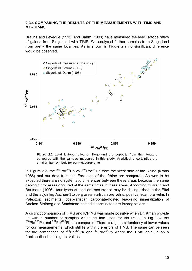
2.3.4 COMPARING THE RESULTS OF THE MEASUREMENTS WITH TIMS AND MC-ICP-MS Brauns and Leveque (1992) and Dahm (1998) have measured the lead isotope ratios of galena from Siegerland with TIMS. We analysed further samples from Siegerland from pretty the same localities. As is shown in Figure 2.2 no significant difference would be observed.

2.075

2.085

2.095

0.844 0.849 0.854 0.859207Pb/206Pb

208 Pb

/206 Pb

Siegerland, measured in this studySiegerland, Brauns (1995)Siegerland, Dahm (1998)

Figure 2.2 Lead isotope ratios of Siegerland ore deposits from the literature compared with the samples measured in this study. Analytical uncertainties are smaller than symbols for our measurements.

In Figure 2.3, the 208Pb/206Pb vs. 207Pb/206Pb from the West side of the Rhine (Krahn 1988) and our data from the East side of the Rhine are compared. As was to be expected there are no systematic differences between these areas because the same geologic processes occurred at the same times in these areas. According to Krahn and Baumann (1996), four types of lead ore occurrence may be distinguished in the Eifel and the adjoining Aachen-Stolberg area: variscan ore veins, post-variscan ore veins in Paleozoic sediments, post-variscan carbonate-hosted lead-zinc mineralization of Aachen-Stolberg and Sandstone-hosted disseminated ore impregnations. A distinct comparison of TIMS and ICP MS was made possible when Dr. Krhan provide us with a number of samples which he had used for his Ph.D. In Fig. 2.4 the 208Pb/206Pb and 207Pb/206Pb are compared. There is a general tendency of lower values for our measurements, which still lie within the errors of TIMS. The same can be seen for the comparison of 208Pb/204Pb and 207Pb/204Pb where the TIMS data lie on a fractionation line to lighter values.

17

Figure 2.3 Lead isotope ratios of German ore deposits in the West (Krahn 1988) and the East and West (measured in this study) Rhenish massif. Analytical uncertainties are not available for Krahn’s data and those for our measurements are smaller than symbols.

85% of the samples show lower 207Pb/206Pb and 208Pb/206Pb ratios as those measured with single collector TIMS by Krahn. The differences can be seen more clearly in 208Pb/204Pb vs. 207Pb/204 diagram (Figure 2.5).

2.075

2.080

2.085

2.090

2.095

2.100

0.844 0.846 0.848 0.850 0.852 0.854 0.856 0.858 0.860207Pb/206Pb

208 Pb

/206 Pb

Hunsrück Variscan Hunsrück Variscan newEifel VariscanEifel Variscan newHunsrück post-Varistic Hunsrück post-Variscan newEifel post-VaristicEifel post-Variscan new

Figure 2.4 208Pb/206Pb vs. 207Pb/206Pb ratios of Hunsrück and Eifel ore deposits measured with TIMS by Krahn (1988) (grey symbols) compared with those measured for the same samples by MC-ICP-MS (colored symbols). Black arrows connect two measurements from the same localities. Analytical uncertainties is not available for Krahn’s data and those for our measurements are smaller than symbols.

2.078

2.083

2.088

2.093

2.098

0.844 0.848 0.852 0.856 0.86207Pb/206Pb

208 Pb

/206 Pb

East Rhenish MassifWest Rhenish Massif measured by KrahnWest Rhenish Massif

18

38.0

38.2

38.4

38.6

15.56 15.58 15.60 15.62 15.64 15.66 15.68 15.70207Pb/204Pb

208 Pb

/204 Pb

Hunsrück VariscanEifel VariscanHunsrück post-VariscanEifel post-VariscanHunsrück Variscan newEifel Variscan newHunsrück post-Variscan newEifel post-Variscan new

Figure 2.5 208Pb/204Pb vs. 207Pb/204Pb ratios of Hunsrück and Eifel ore deposits measured with TIMS by Krahn (1988) (grey symbols) compared with those measured for the same samples with MC-ICP-MS (colored symbols). Black arrows connect two measurements from the same localities. Analytical uncertainty for our measurements is smaller than symbols.

Figure 2.5 shows two tight clusters of the new data, while the data by Krahn show two elongated arrays. The error of TIMS measurements is shown with grey bars the analytical uncertainty for MC-ICP-MS is smaller than the symbols. Some data points coincide within the error, but other differ in a direction that point towards mass fractionation effects. Thermal ionization source in TIMS instruments with the physical evaporation of samples from a heated filament, are subject to mass fractionation effects. These arise because the lighter isotopes of an element are slightly more volatile than heavier isotopes and will therefore be evaporated more rapidly at the beginning of a run. In order to correct for mass fractionation effects, the mass spectrum must be scanned repetitively and a time-dependent interpolation of peak heights carried out. The main advantage of MC-ICP-MS relative to TIMS instruments is the efficient ionization of most elements and the operation of the instrument at steady-state, which allows full control of mass fractionation.

19

2.3.5 COMPARING THE LASER MC-ICP-MS AND SOLUTION MC-ICP-MS RESULTS OF LEAD ISOTOPE ANALYSIS Laser ablation (LA) coupled with ICP-MS has become a popular method for the determination of isotope ratio analysis in solid samples. Some of the numerous advantages of LA-ICP-MS for direct solid sample analysis are:

- Sample preparation is minimum - Contamination from reagents does not exist - Laser can be used to analyze refractory solid samples - Spatial distribution analysis can be conducted with a resolution of less than 10 μm

To compare both methods, eleven galena samples from Siegerland ore deposits were measured both with solution ICP-MS and laser ablation. A sample bracketing method was used to measure the samples with laser ablation. As it can be seen in Figure 2.6, the precision and accuracy of LA-MC-ICP-MS are worse than for solution MC-ICP-MS.

2.075

2.085

2.095

0.844 0.848 0.852 0.856207Pb/206Pb

208 Pb

/206 Pb

Galena LA-MC-ICP-MSGalena Solution MC-ICP-MS

Figure 2.6 The lead isotope analysis by solution compare with those with Laser for galena from Siegerland. Red arrows connect two measurements for the same sample.

As gure 2.6 shows, the 208Pb/206Pb values between two measurements differ systematically and outside their respective errors. The main reasons for this poorer analytical performance are

- The heterogeneous chemical and textural composition

20

- Different sample surface characterization - Vaporization characteristics

The same experiment has been done for lead fragments from Waldgirmes, which are quite pure lead. A very small chip of sample was taken from the objects with a scalpel. The corrosion products were removed mechanically and the samples were cleaned several times in an ultra sonic bath. Then pressed to a flat piece and polished to make a smooth surface. There is again a systematic difference in 208Pb/206Pb ratio (Figure 2.7), which is probably because of big particles. To avoid big particles to go through the system, it is recommended in future work to use a filter. Among the other reasons, uneven surface (despite polishing) could be responsible for the relatively large error.

2.065

2.075

2.085

2.095

0.846 0.85 0.854207Pb/206Pb

208 Pb

/206 Pb

Lead Solution MC-ICP-MSLead LA-MS-ICP-MS

Figure 2.7 The lead isotope analysis by solution compared with those by Laser for lead fragments from the Roman legion in Waldgirmes. Red arrows connect two measurements for the same samples.

2.4 COPPER ISOTOPE ANAYLSIS

2.4.1 SAMPLE SELECTION AND ANALYSIS Dissolved copper ore and bronze samples can be directly analyzed from diluted solution by plasma source mass spectrometry, which avoids any possibility of chromatographic fractionation of copper isotopes. This is important because, without

21

extreme care, ion exchange chromatography may produce significant isotopic effects on copper. Prior to analysis, copper minerals were carefully handpicked under a microscope and visually inspected to ensure purity. Minerals were first dissolved in nitric acid and hydrochloric acid for at least 3 days at 70°C. These solutions were then evaporated to dryness, dissolved again and diluted in 2% nitric acid with 1 ppm Ni to 500ppb Cu.

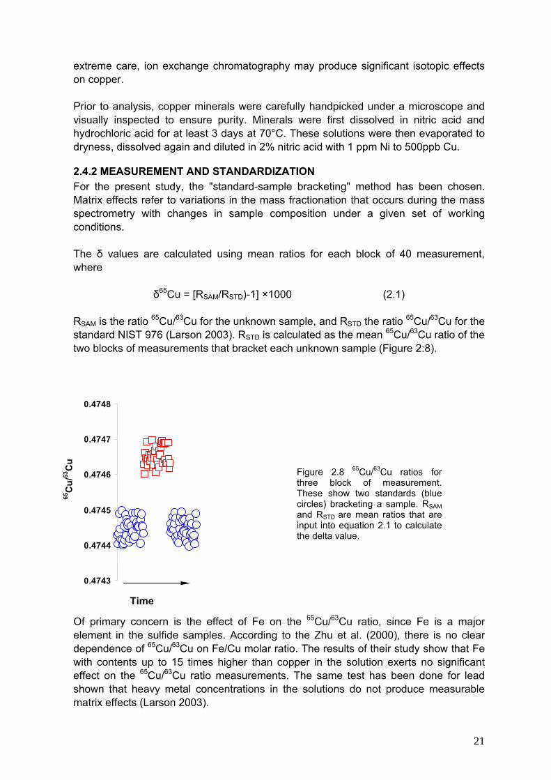
2.4.2 MEASUREMENT AND STANDARDIZATION For the present study, the "standard-sample bracketing" method has been chosen. Matrix effects refer to variations in the mass fractionation that occurs during the mass spectrometry with changes in sample composition under a given set of working conditions. The δ values are calculated using mean ratios for each block of 40 measurement, where

δ65Cu = [RSAM/RSTD)-1] ×1000 (2.1) RSAM is the ratio 65Cu/63Cu for the unknown sample, and RSTD the ratio 65Cu/63Cu for the standard NIST 976 (Larson 2003). RSTD is calculated as the mean 65Cu/63Cu ratio of the two blocks of measurements that bracket each unknown sample (Figure 2:8).

0.4743

0.4744

0.4745

0.4746

0.4747

0.4748

0 20 40 60 80 100 120 140

Of primary concern is the effect of Fe on the 65Cu/63Cu ratio, since Fe is a major element in the sulfide samples. According to the Zhu et al. (2000), there is no clear dependence of 65Cu/63Cu on Fe/Cu molar ratio. The results of their study show that Fe with contents up to 15 times higher than copper in the solution exerts no significant effect on the 65Cu/63Cu ratio measurements. The same test has been done for lead shown that heavy metal concentrations in the solutions do not produce measurable matrix effects (Larson 2003).

Figure 2.8 65Cu/63Cu ratios for three block of measurement. These show two standards (blue circles) bracketing a sample. RSAM and RSTD are mean ratios that are input into equation 2.1 to calculate the delta value.

Time

65C

u/63

Cu

22

To control the possible effect of tin and zinc on isotope fractionation of copper the following test has been done. Different amount of tin and zinc (from single element standard solutions) were added to a 500 ppb Cu standard solution with 1 ppm Ni as internal standard. The results show that these concentrations of tin and zinc have also no effect on the copper isotope ratios (Table 2.1).

Table 2.1 Comparison of copper isotope ratios of copper standard solution with different concentration of Sn, Zn

Concentration (ppb)

Test no. Cu Sn Zn 63Cu/65Cu Standard déviation

1 500 - - 2.24025 4.43E-06 2 500 26 - 2.24032 5.41E-06 3 500 68 - 2.24026 1.07E-05 4 500 31 94 2.24031 6.96E-06 5 500 62 62 2.24037 1.87E-05 6 500 125 - 2.24028 1.86E-05

2.5 ZINC ISOTOPE ANAYLSIS

2.5.1 INTRODUCTION The first attempts to measur the Zn isotope compositions used thermal ionization mass spectrometry (Rosman 1972). Double spike techniques allowed Rosman to obtain TIMS isotopic data with a typical 1-2‰ error, but this study could not identify any terrestrial isotopic variation. The analytical break through came with the advent of multi-collector inductively coupled plasma mass spectrometers equipped with a magnetic mass analyzer. Maréchal et al. (1999) demonstrated that a combination of standard bracketing and normalization with an external element is efficient to correct mass bias and produced data on a variety of ores, rocks and biological materials. Zhu et al. (2000, 2002) used standard bracketing only and collected further data on the isotopic compositions of zinc of different materials, including not only terrestrial and meteoritic rocks and minerals but also enzymes. Very few zinc isotope measurements have been made on ores. Maréchal et al. (1999) analyzed a variety of zinc carbonates (smithsonite) and sulfides (sphalerite) from different localities in Europe. The maximum range of δ66Zn values is from -0.06 to +0.69‰ with little apparent sulfide/carbonate fractionation (smithsonite may be up to 0.3‰ heavier than associated sphalerite). Budd et al. (1999) examined the hypothesis that measurable isotopic fractionation would take place during the evaporation of zinc from liquid brass alloys at elevated temperature. The fractionation of zinc as a result of its evaporation from liquid metal at elevated temperature arises from the slight difference in vapor pressure between its isotopes. This ensures that, in equilibrium, the vapor will be marginally enriched in the lighter isotopes with respect to the liquid. Should the magnitude of fractionation be sufficient to measurably alter the isotopic composition of the residual liquid, Budd suggested the use of zinc isotope ratios to distinguish between the products of the two principal brass-making processes used in

23

antiquity. Although the precision of their quadrupole ICP-MS was still relatively poor, Budd et al. (1999) could assert that for zinc losses by evaporation of more than about 30 wt%, the change in isotopic ratio of the residual liquid alloy would be measurable.

2.5.1 SAMPLE PREPARATION AND ANALYSIS Zinc has five stable isotopes 64Zn, 66Zn, 67Zn, 68Zn and 70Zn with average natural abundances of 48.63, 27.90, 4.1, 18.75 and 0.62% respectively (Rosman and Taylor 1998). With the a exception of a paper by Rosman (1972) who determined the isotopic abundances of zinc isotopes and concluded that there is no noticeable isotopic fractionation in terrestrial samples, the stable isotopes geochemistry of this element remained essentially unexplored. It was not until the advent of inductively coupled plasma mass spectrometry instruments equipped with a magnetic sector and multiple collection that precise measurements became possible. Maréchal et al. (1999) published the first measurements of zinc isotope compositions in a variety of minerals and biological materials. Maréchal et al. (2000) and Pichat et al. (2003) demonstrated the variability of zinc isotopes in ferromanganese nodules, sediment trap material, and marine carbonates. To measure zinc isotope ratios it is necessary to separate zinc from copper, because copper in the matrix causes massive fractionation in zinc isotope ratios (Figure 2.9, own data). In order to separate copper and zinc by column chromatography, both methods introduced by Budd et al. (1999) and Maréchal et al. (1999) were tested. Our measurements showed that none of these methods was able to separate copper and zinc completely. Because of this problem and since the main emphasis of this study was on lead and copper, the study of zinc isotopes eas not continued.

0.6615

0.6620

0.6625

0.6630

0.6635

0 1 2 3 4 5 6

68Zn

/66Zn

0.5 ppm Cu

5 ppm Cu

10 ppm Cu

Figure 2.9 The effect of 0.5, 5 and 10 ppm of Cu on Zn fractionation in a solution of 0.5 ppm Zn

24

CHAPTER 3 ELEMENTAL ANALYSIS

3.1 ELEMENTAL ANALYSIS OF GALENA FROM THE RHEINISCHE SCHIEFERGEBIRGE

3.1.1 INTRODUCTION To determine the major elements in lead sulphides, about 30 galena samples were analyzed from different ore deposits in the Rheinische Schiefergebirge by Electron microprobe analysis. Table 3.1 and 3.2 show the list of samples from the west and east of the Rhine. Since it is very often the case that suitable ores are no longer available from outcrops in the field, most ore samples investigated here were selected from mineral collections of different universities and institutions. Main elements were analyzed by EPMA. Sample preparation and analytical methods are discussed in chapter 2.

Table 3.1 List of ore deposit localities from the West side of the Rhine valley Sample Number Area Location Mine Specification

1 Drohntal Glücksanfang 2 Masterhausen Apollo Second level 3 Gondenau

4 Berglicht in Drohntal Anna

5 Werlau Gute Hoffnung Level of 180 m 6 Werlau Gute Hoffnung Level of 260 m 7

Hunsrück

Bundenbach Friedrichsfeld Test shaft 8 Rescheid Wohlfahrt 9 Mutscheit Klappertshardt

10 Eifel

Mutscheit Klappertshardt 2m above the second level in north

Samples from Institut für Mineralogie und Lagerstättenlehre RWTH-Aachen, by courtesy of Dr. A. Wiechowski. Because these samples did not have an institution number, they were nominated by author.

Table 3.2 List of ore deposit localities from the East side of the Rhine valley Sample no.* Area Location Mine

1972g Biersdorf Füssebergg 99

3349 4086

Salchendorf/ Neunkirchen Pfannenberger Einigkeitg

1aa Müsen Stahlbergc 1172 Eisenzecherzugg 6bo

Eiserfeld Brüderbundd

1003 Eiserfeld (Eisenzecher Zug) Friedbergg 3bo Peterszeched 4113

Burbach Peterszecheg

Mz1 Willroth George Ma1 Niederfischbach Fischbacherwerkb 1757 Obersdorf Prinz Friedrichg 1755 Wilden (Neue Hoffnung) Landskroneg Ma2

Siegerland

Littfeld Victoriab

25

Table 3.2 continued Sample no.* Area Location Mine 60003048001 Littfeld Victoriaa

Be2 Kirchen Fischerbachf 1646

Siegerland Siegen (Pützhorn) Johannesbergg

4064 4066

Steinbach Freudenzecheg

7aa Lahn-Dill

Freital/Dorfhain Aurora Erbstollen Freital/Dorfhainc

Ma3 Biedenkopf/Rachelshausen Grubenfeldern Ritschtahlb Ma4 Boxbachb 5bo

Bad Ems/Nassau Biedenkopf/Wiesenbach

Boxbachd 6aa Lahnstein Friedrichsegenc 4aa Artzbach Mercurc 1730 1654

Holzappelg

3aa

Bad Ems

Holzappelc a: Samples from the Bergbau Museum Bochum, by courtesy of Dr. A. Hauptmann and Dr. M. Ganzelewski b: Samples from the Mineralogisches Museum der Philipps-Universität Marburg, by courtesy of Dr. K. Schürmann c: Samples from the Institut für Mineralogie und Lagerstättenlehre RWTH-Aachen, by courtesy of Dr. A. Wiechowski d: Samples from the Mineralogisches Museum, Rheinische Friedrich-Wilhelms-Universität Bonn, by courtesy of Dr. R. Schumacher e: Samples from the Naturhistorisches Museum Mainz, by courtesy of Dr. H. Lutz and C. Poser f: Samples from the Museum für Naturkunde, Universität zu Berlin, by courtesy of Dr. R.T. Schmitt g: Samples from the Johann Wolfgang Goethe Universität *Because most of the samples did not have an institution number (except for the samples from Bergbau Museum Bochum and those from Johann Wolfgang Goethe Universität) they were named by the author.

3.1.2 RESULTS AND DISCUSSION Tables 3.3 and 3.4 show the result of the EPMA analyses of galena from the localities listed in table 3.1 and 3.2 respectively.

Table 3.3 Elemental analysis of galena from the mines in the West Rhine valley % Sample

number Sb Bi Pb Ag S Co Au

1 bd 0.04± 0.02

87.9± 0.03 bd 11.97±

0.06 0.02± 0.01

0.02± 0.01

2 bd 0.07± 0.02

87.84± 0.14 bd 11.92±

0.05 0.02± 0.01

0.03± 0.02

3 0.03± 0.01

0.05± 0.03

87.85± 0.08 bd 11.97±

0.05 0.03± 0.01 bd

4 bd 0.07± 0.02

87.81± 0.06 bd 12.03±

0.01 0.02± 0.01 bd

5 0.11± 0.01

0.07± 0.03

87.63± 0.12

0.07± 0.02

12.07± 0.07

0.02± 0.01

0.02± 0.01

6 bd 0.06± 0.01

87.41± 0.55 bd 12.07±

0.16 bd bd

7 bd 0.07± 0.01

87.91± 0.04 bd 11.95±

0.03 0.03± 0.01 bd

8 bd 0.07± 0.03

87.95± 0.03 bd 11.91±

0.04 0.02± 0.01 bd

9 0.05± 0.01

0.08± 0.01

87.71± 0.03

0.03± 0.01

12.01± 0.05

0.02± 0.01

0.05± 0.02

10 0.03± 0.01

0.06± 0.03

87.78± 0.09

0.02± 0.01

12.03± 0.02

0.03± 0.01 bd

bd: below detection limit

26

Table 3.4 Elemental analysis of galena from the mines in the East Rhine valley % Sample Name

Sb Bi Pb Ag S Mn

1972 0.12± 0.05

0.04± 0.01

86.92± 0.15 bd 12.83±

0.19 nm

99 0.02± 0.01

0.24± 0.08

86.76± 0.05

0.04± 0.02

12.92± 0.08 nm

3349 bd 0.08± 0.05

86.72± 0.07 bd 13.16±

0.01 nm

4086 0.29± 0.05 bd 85.74±

1.27 bd 12.93± 0.27 nm

1aa bd 0.07± 0.02

87.13± 0.07 bd

12.73± 0.07

0.02± 0.01

1172 0.06± 0.02

0.13± 0.01

86.97± 0.02 bd

12.87± 0.07 nm

6bo bd 0.07± 0.04

87.10± 0.07 bd

12.78± 0.06

0.03± 0.01

1003 bd 0.07± 0.02

87.13± 0.06 bd

12.75± 0.06

0.02± 0.01

3bo 0.09± 0.01

0.06± 0.02

87.02± 0.08

0.02± 0.01

12.77± 0.07

0.02± 0.01

Mz1 0.02± 0.01

0.88± 0.01

85.66± 0.20

0.24± 0.06

13.16± 0.08 bd

Ma1 bd 0.09± 0.03

86.82± 0.32

0.02± 0.01

12.95± 0.05

0.02± 0.01

1757 0.02± 0.01

0.10± 0.03

86.82± 0.12 bd

13.15± 0.08 nm

1755 bd 0.11± 0.01

86.92± 0.07 bd 13.04±

0.08 nm

Ma2 bd 0.07± 0.02

87.08± 0.08

0.02± 0.01

12.76± 0.12

0.02± 0.01

60003048001 bd 0.08± 0.03

86.49± 0.08 bd

13.37± 0.07 bd

Be2 0.16± 0.06

0.06± 0.04

86.72± 0.18

0.14± 0.05

12.89± 0.1 nm

1646 0.08± 0.05

0.04± 0.02

86.87± 0.08 bd

13.08± 0.08 nm

4064 0.10± 0.02

0.04± 0.02

86.85± 0.12

0.09± 0.03

12.90± 0.10 nm

4066 0.02± 0.01

0.04± 0.02

86.89± 0.12 bd 13.04±

0.08 nm

7aa 0.08± 0.05

0.09± 0.03

86.91± 0.21 bd 12.80±

0.10 0.02± 0.01

Ma3 0.10± 0.02 bd 87.06±

0.08 bd 12.76± 0.08 bd

Ma4 0.02± 0.01

0.08± 0.04

87.11± 0.08 bd

12.76± 0.08

0.02± 0.01

5bo bd 0.07± 0.04

87.09± 0.05 bd

12.79± 0.04 bd

6aa bd 0.09± 0.03

87.06± 0.12 bd

12.79± 0.03

0.02± 0.01

4aa 0.11± 0.03

0.08± 0.04

86.82± 0.10

0.08± 0.02

12.87± 0.13

0.02± 0.01

1730 0.05± 0.01

0.09± 0.04

86.82± 0.10 bd

13.17± 0.12 nm

1654 0.05± 0.02

0.07± 0.03

86.97± 0.15

0.02± 0.01

12.85± 0.09

0.02± 0.01

3aa 0.08± 0.04

0.06± 0.03

87.00± 0.06

0.04± 0.02

12.78± 0.05

0.02± 0.01

nm: not measured bd: below detection limit

27

Table 3.3 shows that except for bismuth and cobalt, the concentration of other elements was below detection limit for most of the samples from the western side of the Rhine vally. Zinc, copper, iron, arsenic, nickel and tin were not detected in these samples. Table 3.4 shows the results for galena from lead mines from the East Rhine valley. In these samples tin, iron, gold, nickel, cobalt and arsenic were not detected. The antimony, silver and bismuth content were plotted against lead for both groups of lead sulfide samples from the East and West Rhine mines in Figure 3.1 to 3.3 respectively. In the Southern Rhenish Massif the veins contain antimony and bismuth minerals and silver bearing lead sulfides (Werner and Walter 1995). Table 3.4 shows that the variscan Siegerland vein-type galenas contain lead ores with higher silver in comparison with the post-variscan ore mineralization of the Eifel and Hunsrück areas (Table 3.4). These have also been shown in Fig 3.2 Relative low contents of silver in the samples from western Rhine mines is a typical feature of post-variscan lead occurrences from the western Rhenish Massif (Schaeffer 1984, 1986). The same has been observed for bismuth and antimony content (Figure 3.1 and 3.3), which are higher in Siegerland vein-type mineralization in comparison with the post-variscan ores of the Eifel and Hunsrück area.

85.5 86.0 86.5 87.0 87.50.0

0.1

0.2

0.3

Sb

Pb

Figure 3.1 Sb vs Pb (%) for galena from East and West Rhine ore mines

East Rhine lead ores

West Rhine lead ores

28

85.5 86.0 86.5 87.0 87.50.0

0.2

0.4

0.6

0.8

1.0

Ag

Pb

Figure 3.2 Ag vs Pb (%) for galena from East and West Rhine ore mines

85.5 86.0 86.5 87.0 87.50.0

0.2

0.4

0.6

0.8

Bi

Pb

Figure 3.3 Bi vs Pb (%) for galena from East and West Rhine ore mines

East Rhine lead ores

West Rhine lead ores

East Rhine lead ores

West Rhine lead ores

29

3.2 ELEMENTAL ANALYSIS OF LEAD OBJECTS FROM MAINZ WORKSHOP AND WALDGIRMES

3.2.1 RESULTS

Table 3.5 and 3.6 show the results of elemental analysis of lead objects from the Mainz and the Waldgirmes respectively. Table 3.5 Elemental analysis of lead water pipes from the Mainz

% Sample* name Dating

Bi As Pb Mn Sb Cu

FM 82-018 End of the first century AD

0.05±0.03 bd 99.86±

0.05 0.02±0.01

0.03± 0.02 bd

FM 98-073 First to fourth century AD bd bd 99.94±

0.02 0.02±0.01

0.02± 0.01 bd

FM 01-123 Second century AD bd bd 99.95± 0.03

0.02±0.01

0.02± 0.01 bd

FM 92-073 First to fourth century AD

0.02±0.01 bd 99.92±

0.05 0.02±0.01

0.02± 0.01 bd

FM 84-041 Second century AD bd bd 99.91± 0.03

0.02±0.01 bd bd

FM 89-024 Second to third century AD

0.08±0.03 bd 99.92±

0.07 0.02±0.01

0.02± 0.01 bd

FM 97-142, Fdst.Nr.F87/

F88

Beginning of the fourth century AD bd bd 99.97±

0.05 0.02±0.01 bd bd

FM 97-142, Fdst.Nr.F108

Beginning of the fourth century AD

0.03±0.02 bd 99.95±

0.05 0.02±0.01

0.06± 0.03 bd

FM 97-142, Fdst.Nr.22

Beginning of the fourth century AD

0.03±0.02

0.01±0.01

99.92± 0.06

0.02±0.01 bd bd

FM 97-142, Fdst.Nr.39

Beginning of the fourth century AD

0.02±0.01 bd 99.93±

0.03 bd bd bd

FM 90-064 End of the first and

beginning of the second century AD

bd bd 99.93± 0.18

0.02±0.01

0.03± 0.02

0.09± 0.05

FM 82-061, Fdst.Nr.9/10

End of the first and beginning of the

second century AD

0.04±0.02 bd 99.91±

0.24 0.02±0.01 bd 0.10±

0.05 bd: below detection limit *samples are from Landesamt für Denkmalpflege in Mainz by courtesy of Dr. G. Rupprecht and Dr. J. Dolata.

Table 3.6 Elemental analysis of lead fragments from the Waldgirmes

Sample name Bi Pb Mn Sb Ag Cu

14372 bd 99.94± 0.18

0.02± 0.01 bd bd bd

6057 bd 99.91± 0.07

0.02± 0.01 bd bd bd

14384 bd 99.95± 0.99

0.02± 0.01 bd bd 0.44±

0.09

14597 0.04± 0.02

99.98± 0.02

0.02± 0.01 bd bd bd

14671 bd 99.93± 0.13

0.02± 0.01

0.14± 0.08 bd bd

30

Table 3.6 continued Sample name Bi Pb Mn Sb Ag Cu

19396 0.06± 0.04

99.97± 0.10

0.02± 0.01 bd bd bd

20054 0.03± 0.02

99.97± 0.06

0.02± 0.01

0.11± 0.05 bd bd

20597 bd 99.94± 0.04

0.02± 0.01 bd bd 0.06±

0.03

14679 bd 99.92± 0.25

0.02± 0.01 bd bd bd

bd: below detection limit *samples are from Römisch-Germanische Kommission in Frankfurt by courtesy of Dr. G. Rasbach

3.2.2 DISCUSSION

The lead used to produce the objects from Mainz and Waldgirmes are quite pure. It means that the Roman knew very well how to refine and purify lead ores. The concentration of antimony, iron, gold, zinc, arsenic and silver were lower than detection limit. Although there is good evidence for lead smelting from the earliest stages of metallurgy, comparatively little is known about the details of the processes used. It should be emphasized that the principle objective of most ancient smelting operations appears to have been the recovery of silver from argentiferous lead minerals and not the production of lead metal. Under such circumstances, significant lead losses are unlikely to have been considered disadvantageous. There has been little experimental work on lead smelting under primitive conditions; indeed, the only investigations are those of Smith et al. (1967) and of Hetherington (1977). Neither investigation studied the partitioning of elements between slag and lead metal, both demonstrated the difficulty of obtaining a good yield of lead from impure lead ores and showed that the tapping slags from such primitive smelting contain from 5% to 40% lead. During the ancient smelting processes, gold and silver, which were in lead ores, were scavenged very effectively into the lead metal, while iron, zinc, manganese, silicon, calcium, magnesium and aluminium pass chiefly into the slag. According to the experience acquired up until the 19th century, during cupellation, the litharge absorbs with it the bulk of the tin, arsenic, antimony, zinc, copper and bismuth contained in the argentiferous lead. The silver is then recovered by cupellation in which the lead is heated to about 1000°C and oxidized to litharge by blowing air over or through the molten lead. The litharge is removed by skimming or by absorption in the crucible walls, leaving behind the silver metal. Although the melting point of lead is only 327°C, higher temperatures are required for the reduction of lead oxide and lead smelting is normally carried out at temperature of at least 600-750°C or more. A temperature of 800°C or more is the minimum required for the double decomposition reaction. Under such conditions liquid lead forming at the bottom of the furnace will be subject to considerable superheating and even at relatively low temperature lead volatilisation is quite possible. At higher temperatures (perhaps 1000°C) the lead metal may be protected by a liquid slag, which is itself likely to contain considerable lead.

31

CHAPTER 4 LEAD ISOTOPE ANALYSIS

4.1 LEAD ISOTOPE ANALYSIS OF GERMAN ORES

4.1.1 INTRODUCTION

Natural lead consists of the four isotopes 208Pb, 207Pb, 206Pb and 204Pb. The first three of these isotopes are derived in terrestrial lead partly from the radioactive decay of naturally radioactive isotopes of U and Th. This is the basic reason for the variability of the isotopic composition of natural lead. High precision lead isotope analysis by multi-collector-inductively coupled plasma mass spectrometry has been applied to the investigation of Roman objects from different archaeological sites in Germany to obtain information on the pattern of Roman mining activity and ore processing during the last four decades. Measurements of galena samples from the Siegerland, Eifel and Lahn-Dill area in Germany were made and supplemented with data from the literature to create a data bank of lead isotope ratios of European deposits. It is important to know the geology of the deposit and to have a sampling strategy, which includes all geological formations. Mineral deposits of some geographical regions are complicated and may consist of minerals formed at different times and under different conditions. In such a case, one geographical area can have a large number of very different “fingerprints”, but, since the provenance method is based on direct comparison, the correct interpretation depends on the correct isotope characterization of each single mineralization used for comparison. Only a large number of analyses of ore minerals allow one to characterize separately each small mining region or mine and use statistical methods of discrimination to distinguish between them. Since it is very often the case that suitable ores are no longer available from outcrops in the field, many of the ore samples investigated were selected from the mineral collections of different universities and institutions. Table 4.1 shows a list of studied ore deposits. For the institution numbers and lead isotope ratios, see Tables 1, 2, 5 and 6 from Appendix 1. For preparation and analytical methods, see chapter 2. The isotopic composition of the German mines as the potential ore sources for the Roman artifacts was measured. Table 4.1 List of the German lead and copper mines and their localities

Area Location Mine Biersdorf Füsseberg

Salchendorf/ Neunkirchen Pfannenberger Einigkeit Stahlberg Müsen

Brüche Eisenzecherzug Eiserfeld

Brüderbund

Siegerland

Eiserfeld (Eisenzecher Zug) Friedberg

32

Tabel 4.1 continued Area Location Mine

Burbach Peterszeche Willroth Georg

Niederfischbach Fischbacherwerk Eisern Ameise

Obersdorf Prinz Friedrich Wilden (Neue Hoffnung) Landskrone

Littfeld Victoria Kirchen Fischerbach Silberg Merkur Wissen St. Andreas

Altenseelbach (Große Burg) Lohmannsfeld Fischbacherhütte/Wingendorf Glücksbrunnen

Gosenbach Alte Lurzenbach

Siegerland

Siegen (Pützhorn) Johanesberg Steinbach Freudenzeche Lahn-Dill

Freital/Dorfhain Aurora Erbstollen Freital/Dorfhain Biedenkopf/Rachelshausen Grubenfeldern Ritschtahl

Biedenkopf/Wiesenbach Boxbach Arenberg Mühlenbach Lahnstein Friedrichsegen Artzbach Mercur Braubach Rosenberg

Bad Ems

Holzappel Rescheid Wohlfahrt

Mechernich Bleiberg Mayen Silbersand Bleialf Gute Hoffnung

Eifel

Mutscheit Klappertshardt Altley Barbarasegen

Werlau St. Goar Drohntal Glücksanfang

Masterhausen Apollo Gondenau

Berglicht in Drohntal Anna Werlau Gute Hoffnung

Hunsrück

Bundenbach Friedrichsfeld

4.1.2 RESULTS AND DISCUSSION Results of our measurements were compared with those for the same localities done by TIMS (Brauns and Leveque 1992 and Dahm 1998), see chapter 2. Several hundred accurately determined data points are available in the literature. They belong to many ore sources covering the Mediterranean world (Stos-Gale et al. 1995, 1996), Britain and Island (Rohl 1996), some Eastern European countries (Stos-Gale et al. 1998), Middle Eastern locations (Yener et al. 1991; Hauptmann et al. 1992) and others. Among so many sources, we selected only the historically most probable provenance sites. They are summarized in Figure 4.1 in a 208Pb/206Pb vs. 207Pb/206Pb diagram. In such a diagram, the 207Pb/206Pb value reflects the model age of the ore

33

deposits (Stacey & Kramers 1975) and the 208Pb/206Pb value the U/Th ratio of the fluid medium responsible for the ore formation. The Mediterranean ore deposits range from Cambrian (high 207Pb/206Pb values) to Tertiary (lower 207Pb/206Pb value). More specifically, the Cypriot deposits are young, while the Spanish deposits fall either with the younger Sardic ores or close to the older Cypriot ores (Klein et al. 2004). The lead isotope ratios of German ore deposits measured in this study fall between the 208Pb/206Pb vs. 207Pb/206Pb ratios of Sardinia and southwest Spain and those from southeast Spain and Cyprus, where the lead isotope signatures of France and British ore deposits also appear. German ore deposits have 207Pb/206Pb ratios between 0.845 and 0.860, which corresponds to an age gap between around 330 and 150 mya, the time span between the variscan and the precursor of the Alpine orogeny in Europe, when there were few ore-forming events (Klein et al. 2004).

34

2.05

2.06

2.07

2.08

2.09

2.1

2.11

2.12

2.13

2.14

0.825 0.835 0.845 0.855 0.865 0.875207Pb/206Pb

208 Pb

/206 Pb

German rhenish deposits

Figure 4.1 208Pb/206Pb vs. 207Pb/206Pb ratio plot showing the trend of German lead ores and the distinct differences between them and Mediterranean lead ore sources.

France

Sardinia

England

Cyprus

Tuscany Spain

Aegean

35

4.2 LEAD ISOTOPE ANALYSIS OF LEAD OBJECTS

4.2.1 INTRODUCTION The present work was devised to address the systematic analysis of samples from a range of artefacts and from different archaeological contexts and sites. The sites selected for this study included forts and associated civilian settlements, towns, villas, temples, ritual hoards and workshops. We studied the progress of metallurgy with focusing on lead from different Roman sites in Germania Superior and Gallia Belgica. This begins from early Roman period legion, Dangstetten, which was a military site on the border of Germania and Gaul and active from 15-9 B.C (Fingerlin 1986, 1999). Another studied site is Waldgirmes, a potential center of Romans at the border with the Germans about AD 1-10, which was of course, after a very short blooming time, abounded after the defeat of the Romans at the Battle of the Teutoburger Forest and never had the chance to become a Roman metropolis (Becker 1998, von Freeden and Schnurbein 2002). A little further from the border with the Germans, Romans built the new towns, and began to have new commercial contact with neighbors, rising demand for new tools and of course more material. This culture boomed for four centuries and achieved its highest point around the middle of third century AD. Romans improved their metallurgical methods and used the local and regional metal sources together with importing basic materials from other regions. Mainz (Trier 1989), Martberg (von Freeden and Schnurbein 2002) and Trier (von Freeden and Schnurbein 2002) are three other Roman sites, studied in this project, which are considered as important Roman settlements and centers of metal production during this period. The last series of samples are from the Celtic/Roman settlement of Wallendorf. Over 240 lead samples were measured. The type of artefacts and dating are summarized in table 4.2 and Figure 4.2 shows the localities and references. In archaeological lead isotope analysis, the isotopic abundance ratios of artefacts are compared with those taken from potential ore sources. Over the last twenty years, a large number of such measurements have been made particularly in the eastern Mediterranean (Stos-Gale et al. 1995; Stos-Gale et al. 1996; Gale et al. 1997). Attempts have been made to identify characteristic lead isotope “fields” for particular regions and even for individual mine sites (Gale and Stos-Gale 1992b; Stos-Gale and Gale 1992).

36

Waldgirmes

Martberg

AugustaTreverorum

(Trier)

Dangstetten

Mogontiacum (Mainz)

Figure 4.2 Map showing the Roman sites in Germany and Gaul, sampled in this study (modified after von Freeden and Schnurbein 2002).

Wallendorf

Dünsberg

37

Table 4.2 A list of studied lead objects together with localities and references

Number of studied

artefacts Type of artefact Locality Dating Reference by courtesy of

30 Mix of lead objects Dangstetten 15-9 BC Archäologische Denkmalpflege Freiburg Prof. Dr. G. Fingerlin

20 Fragments Waldgirmes AD 1-10 Römisch-Germanische Kommission,

Frankfurt Dr. G. Rasbach

10 Mix of lead objects Mainz workshop 10-100 AD Archäologie und Geschichte der römischen Provinzen, Frankfurt University

Dr. A. Heising

8 Water pipe 5 Filling clamp

Mainz and its surrounding

100-400 AD Landesamt für Denkmalpflege in Mainz Dr. G. Rupprecht and

Dr. J. Dolata. 19 Amulet 1 Minerva 24 Mix of lead objects 15 Sacrificial offering

Martberg 100-400 AD

1) Akademie der Wissenschaften und der Literatur Mainz

2) Landesamt für Denkmalpflege, Außenstelle Koblenz

1) Dr. D. Wigg-Wolf 2) Dr.C. Nickel and

Dr. M. Thoma

24 Good’s label 9 Coffin 10 Execration plate 30 Mix of lead objects 1 Minerva

Trier 300-400 AD 1) Landesmuseum Trier

2) Bischofliches Museum Trier

1) Dr. Sabine Faust and Dr. L. Schwinden 2) Dr. H. Merten

28 Rouelle and beads Wallendorf Celtic period 1) Akademie der Wissenschaften und der

Literatur Mainz 2) University of Kiel

1) Dr. D. Wigg-Wolf 2) Dr. D. Krausse

5 Slingshot Dünsberg Celtic period

1) Akademie der Wissenschaften und der Literatur Mainz

2) Römisch-Germanische Kommision, Frankfurt

1) Dr. D. Wigg-Wolf 2) Dr. C. Nickel and Dr. K.-F. Rittershofer

38

4.2.2 RESULTS

DANGSTETTEN

The early Roman legion camp Dangstetten lies on a kind of peninsula within the upper Rhine Valley, close to the place in which the highway from central Switzerland crosses the Rhine to the Danube and Neckar valley. The camp of Dangstetten is the oldest Legionary camp in Southern Germany. The Legion camp of Dangstetten on the upper Rhine was occupied by a Roman expeditionary troop during the years 15-9 BC. The coins show that it was given up soon after the year 10 BC. Its end stands in connection with a revision of the Roman conquest politics against Germanic tribes after the death of the Drusus on the Elbe in the year 9 BC. Nothing points to destruction by force. The camp was obviously vacated because of the intended transfer of the troops to another location. Although the Legion was relatively self-supporting, a strong dependence on supply and trade remained. Besides a few republican and Augustan silver coins, there have been found above all bronze coins from the southern French provinces. The excavation in Dangstetten began 1967 and has been supported by the firm Tröndle (Fingerlin 1986, 1999).

a) b)

c) d) Figure 4.3 Lead objects from Dangstetten: a) lead pig, inventory number 449,44; b) metal strap, inventory number DA 437A, 15; c) half a round plate with a quadratic hole in the middle, inventory number DA 375,2 and d) metal strap, inventory number DA 447,8 (Fingerlin 1984)

39

30 samples were taken from lead objects of the excavation in Dangstetten. The main part of these samples is being kept in storage at the Archäologische Denkmalpflege in Freiburg.

2.08

2.09

2.10

0.845 0.850 0.855 0.860207Pb/206Pb

208 Pb

/206 Pb

Post-Variscan ore deposits EifelVariscan ore deposits EifelWorkshop wasteLead objectsLead ingotSouthern Massif CentralLead Solder

Variscan ore deposits of Eifel

Post-Variscan ore deposits of Eifel

Southern Massif Central

Figure 4.4 The lead isotope ratios of the workshop waste, lead objects, lead solders and a lead ingot from Dangstetten compared with Eifel ore deposits.

Except for the artifacts shown in Figure 4.3, the rest of lead objects are considered as workshop rest. They are either small plates and straps form patches or shapeless pieces. As shown in Figure 4.4 lead isotope ratios of most of the lead objects, among them the four lead artifacts from Figure 4.3, fall on the mixing line between variscan and post-variscan ore mineralization of Eifel. Some of the lead fragments show the similar isotopic signature of the post-variscan ore mineralization of Eifel, but lead isotope ratios of six objects recovered outside of the Eifel field point to Massif Central ores as sources (For a list of inventory numbers and lead isotope ratios, see Table 8 in Appendix 1). The analytical uncertainties are smaller than the symbols.

WALDGIRMES

The excavation in Waldgirmes-Lahnau began in 1993 with the support of the DFG and particularly with the encouragement of the Landsamt für Denkmalpflege Hessen and the Römisch-Germanische Kommission.

40

Lahnau-Waldgirmes is located in Hessen about 50 km north of Frankfurt. It lies between the towns Wetzlar and Gießen north of the Lahn River. The Romans founded this place about 2000 years ago and it ranks among the oldest town in Germany. The majority of the present cities in the western and Southern Germany are based on Roman establishments.

Waldgirmes on the right side of the Rhine and outside of the later Limes area, was built at the beginning of the first decade AD. Waldgirmes was a forum establishment, which the Romans built as a typical market and administrative center of a new province. Some of the objects found in Waldgirmes include luxury articles from the time of Augustus imported from Italy. There is a large and unique amount of Germanic ceramics, which occurs always mixed with Roman finds in the waste pits. This is an indication that the Germanic population in the Lahn valley had already begun to trade with Romans (Becker 1998).

Perhaps in later times, this installation would have grown into a large German town, if history had taken a different course. Coins found at the site indicate that the installation was abandoned around AD 9 after an occupation of about a decade. This was the year of "the Battle of Teutoburger Forest", where the Romans had suffered a disastrous defeat in northern Germania. After that, they withdrew completely to the left bank of the Rhine River. The installation near today's Waldgirmes had been burned down and was forgotten over the centuries. Decades later, when the Romans were successful again in conquering land on the right bank of the Rhine River, they apparently had lost all interest in their former base. The much later constructed Limes, that guarded the Roman border in Germania, runs along 15 km southeast of Waldgirmes and does not include this base anymore (von Freeden and Schnurbein 2002). 20 samples were taken from lead fragments found in excavations at Waldgirmes, which are being stored in the Römisch-Germanische Kommission. As lead has a very low melting point (327°C), lead objects were all melted during the big fire in Waldgirmes, so the studied objects are nothing but shapeless pieces or crumpled sheets of lead. Apart from the five lead fragments from Waldgirmes, which lie within the field of post-variscan Eifel lead ore deposits, the rest of the lead objects show a variation in lead isotope ratios, but are still associated with the lead isotope signature of German ore deposits (Figure 4.5). For a list of inventory numbers and lead isotope ratios, see Table 9 in Appendix 1.

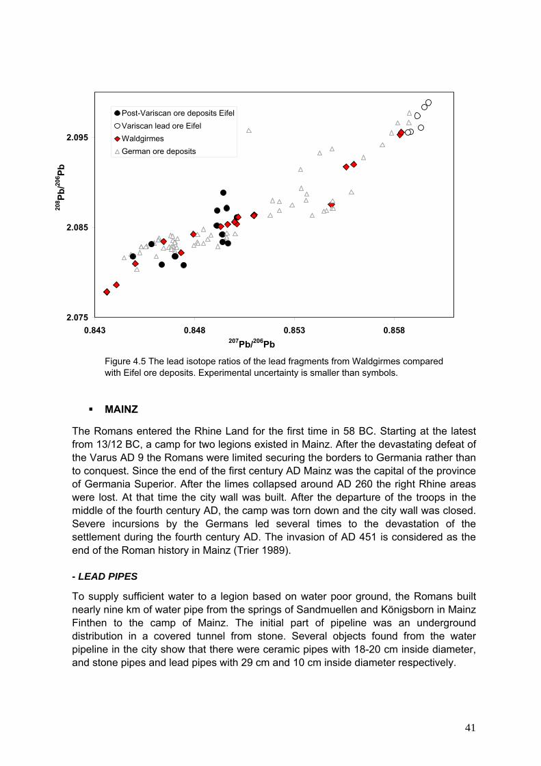
41

2.075

2.085

2.095

0.843 0.848 0.853 0.858207Pb/206Pb

208 Pb

/206 Pb

Post-Variscan ore deposits EifelVariscan lead ore EifelWaldgirmesGerman ore deposits

Figure 4.5 The lead isotope ratios of the lead fragments from Waldgirmes compared with Eifel ore deposits. Experimental uncertainty is smaller than symbols.

MAINZ

The Romans entered the Rhine Land for the first time in 58 BC. Starting at the latest from 13/12 BC, a camp for two legions existed in Mainz. After the devastating defeat of the Varus AD 9 the Romans were limited securing the borders to Germania rather than to conquest. Since the end of the first century AD Mainz was the capital of the province of Germania Superior. After the limes collapsed around AD 260 the right Rhine areas were lost. At that time the city wall was built. After the departure of the troops in the middle of the fourth century AD, the camp was torn down and the city wall was closed. Severe incursions by the Germans led several times to the devastation of the settlement during the fourth century AD. The invasion of AD 451 is considered as the end of the Roman history in Mainz (Trier 1989). - LEAD PIPES

To supply sufficient water to a legion based on water poor ground, the Romans built nearly nine km of water pipe from the springs of Sandmuellen and Königsborn in Mainz Finthen to the camp of Mainz. The initial part of pipeline was an underground distribution in a covered tunnel from stone. Several objects found from the water pipeline in the city show that there were ceramic pipes with 18-20 cm inside diameter, and stone pipes and lead pipes with 29 cm and 10 cm inside diameter respectively.

42

Figure 4.6 Water pipe from Mainz

- LEAD CLAMPS

There are innumerable examples throughout the ancient world where lead was run into the joint of masonry and metal bars as a building substance, or was used as a dowel and for fixing metal clamps and plaques to blocks of stone. The iron clamps, which used to fasten the stones of the walls, were riveted with lead. This method was used extensively during the Roman period.

Figure 4.7 Lead clamp from Mainz Lead isotope ratios of eight water pipes and five lead clamp samples from Mainz together with ten lead objects from the Mainz workshop were analyzed in this study (For the inventory numbers, a list of artefacts and lead isotope ratios, see Tables 10a and 10b Appendix 1). The lead objects from Mainz workshop are most small plates and shapeless pieces. The lead isotope ratios of five water pipes and three clamps together with the lead artifacts from the Mainz workshop are concentrated in a very restricted area of the diagram and fall within the post-variscan Eifel ore deposits field. The other three water pipes and two clamps show a variation in their lead isotope ratios (Figure 4.8). A close up look at the area of post-variscan Eifel ores and most of the lead objects of Mainz in Figure 4.9 shows: 70% of samples fall on the mixing line between the three lead mines of Silberberg, Glückstal and Bleialf whereby the latter one is known as a Roman mine.

43

2.075

2.085

2.095

0.845 0.850 0.855 0.860207Pb/206Pb

208 Pb

/206 Pb

German ore depositsPost-Variscan ore deposits EifelVariscan ore deposits EifelMainz workshopLead clampWater pipe

Variscan ore deposits of Eifel

Post-Variscan ore deposits of Eifel

Figure 4.8 The lead isotope ratios of the lead water pipes and the lead clamps from Mainz and its surrounding area and the lead objects from Mainz workshop compared with those of Eifel ore deposits.

2.080

2.085

2.090

0.847 0.849 0.851 0.853

207Pb/206Pb

208 Pb

/206 Pb

Figure 4.9 a close look at the area of post-variscan Eifel ore mineralization with the lead artifacts from Mainz.

Bleialf

Silberberg

Glückstal

Post-Variscan ore depositsEifelMainz workshopLead clampWater pipe

44

MARTBERG

The Martberg is a plateau rising 180-190 m over the Mosel river valley between Pommern and Karden. On the Plateau of the Martberg lies a former Celtic settlement of the Late Lateen period, which was largely abundant in the middle of the first century BC. The settlement was an important center and contained a workshop, which minted coins. There was also a ritual-religious center with a large temple complex. The site covers an area of 70 hectares and was surrounded by a typical Celtic fortification. The temple and ritual center existed during the Roman period. At that time a new temple construction took place. According to numismatic evidence the Martberg was abounded sometime towards the end of the fourth century AD. Some of the most important lead objects from Martberg, which were investigated in this study, are:

- MINERVA

Figure 4.10 A Statue of the goddess Minerva from the Martberg

She was for the Romans the moon goddess, virgin goddess of art and talent, wisdom and sciences and the guardian goddess of the craftsmen, doctors, teachers and artists. As one of the main goddesses of Rome, she is the goddess of peace and war. Associated with Minerva are the owl and the olive tree. Minerva is similar to the Greek goddess Athena.

45

- AMULETS

Amulets are objects generally kept on the person and are believed to confer some benefit to the wearer. The use of amulets, talismans, and charms is deeply ingrained in many cultures to the present day. Many people use lucky pins and wear religious medals without believing literally in their powers to affect their lives. They help them muster the confidence they need in times of self-doubt. They empower them to dare, to believe in themselves. a- PHALLUS AMULET People wear many types of phallus shaped Amulets on a necklace, or carry one in a charm bag to increase male virility and sexual magnetism. Phallus amulets were commonly used in ancient times by various cultures to avert the evil eye. b- WHEEL AMULETS They are small wheels, made of lead, pewter or bronze, which were used 2000 years ago for various purposes: as toys for children, amulet, votive and decoration. The majority of the round slices with rays found are of Gallic origin (first century BC–second century AD).

Figure 4.11 Wheel Amulet (Rouelle) - Water pump

Figure 4.12 Water pump from the Martberg

46

- Sacrificial offerings

Coins were often used as votive offerings to the Gods. Typical places for offering coins are wells, wellsprings and sacrificial sites. The visitors to holy places sent their offering coins to the treasure administration where they were kept in the treasure house, within the temple. Samples were taken from 15 sacrificial offerings and 46 lead artifacts from the Martberg and the temple. Among them were 14 Phallus amulets, one water pump, one Minerva Statue, four Wheel amulets (Rouelle), several valve caps and casting remains. Lead isotope ratios of these objects together with those from lead ore deposits of Eifel and Southern Pennines in Britain are plotted in Figure 4.13.

2.075

2.085

2.095

0.845 0.85 0.855 0.86207Pb/206Pb

208 Pb

/206 Pb

Post-Variscan ore deposits EifelVariscan ore deposits EifelSacrificial offeringPhallus amuletPumpMinervaSouthern Pennines, BritainCasting remain

Southern PenninesBritain

Post-Variscan ore mineralization of Eifel

Figure 4.13 The lead isotope ratios of the lead objects from the Martberg compared with those from lead ore deposits from the Eifel.

As Figure 4.13 shows, lead isotope ratios of all objects from the Martberg, except the four Rouelle (see below), fall in the fields of German and British ore deposits. A close up to the field of Southern Pennines is shown in Figure 4.14. Most of the phallus amulets fall on the mixing line between the Cromford and Ashby de la Zouch mining region of the Southern Pennines. The four Rouelle show completely different isotopic signatures, which are similar to Tuscan lead ore deposits. The majority of the other lead objects plot in the mixing area between Silberberg, Glückstahl und Bleialf and the other few on a mixing line to the variscan deposits. 208Pb/206Pb vs. 207Pb/206Pb ratios of the four Wheel amulets (Rouelle) together with those from Mediterranean and German lead ores are presented in Figure 4.15. For lead isotope ratios, see Table 11 in Appendix 1.

47

2.077

2.079

2.081

2.083

2.085

0.845 0.847 0.849207Pb/206Pb

208 Pb

/206 Pb

Phallus amuletSouthern Pennines, Britain

Figure 4.14 A close look at the area of Southern Pennines ore

deposits in Britain with the phallus amulets from Martberg

2.05

2.06

2.07

2.08

2.09

2.1

2.11

2.12

2.13

2.14

0.825 0.835 0.845 0.855 0.865 0.875207Pb/206Pb

208 Pb

/206 Pb

German rhenish deposits

Lead objects from Martberg

Rouelle

Sardinia

Spain

Cyprus

Tuscany

Aegean

Rouelle

Figure 4.15 Lead isotope ratios of Rouelle from the Martberg compared with those from Mediterranean and German ore deposits.

Ashby de la Zouch

Cromford

48

TRIER

Trier was built by the Romans around 16 BC. Towards the end of the 3rd century, Trier became the Roman emperor's residence. In the third century it was also already the seat of a bishop. In AD 870 Trier became a part of the east-Frankish Empire and then in AD 925 it joined the German Empire. Trier was a designated colony of the Roman Empire in 16 BC but its origins were much older and there were earlier native settlements. Trier is situated in the Mosel Valley just a few miles from the present day border with Luxembourg and just a short distance from the French border. The Romans first introduced wine to the area and a significant part of the region's economy still depends on wine growing on the high and steep banks of the Mosel River. The first Roman construction in Trier was the bridge, which was built in AD 18. The first bridge was of wood and was replaced in about AD 150 by a stone construction. The foundations of that 1,848-year-old bridge still bears modern traffic on a four-lane street. As protection against the Germanic treibs, from across the Rhine to the east, a wall was built around the city in AD 180, of which the north gate, called the Porta Nigra, still stands completely intact. The greatest glory of Trier came in the late third and the fourth centuries BC when the Roman Empire was divided into four administrative districts and Trier became the capital of the Western Empire. Some of the most important lead objects from Trier, analysed in this study, are: - LEAD COFFINS Lead coffins do not represent an everyday burial rite, but signify some kind of exception from the rule. However, in comparison with some of the extraordinarily rich grave gifts in sarcophagi found in the Rhineland of the third century AD, the lead coffins do not necessarily indicate burial of the very rich. Thus, the social status of the people buried in lead coffins remains unclear. In rural settlements, these may have belonged to the families of villa owners. In addition, the type of grave gifts and the size of some of the coffins suggest that lead coffins were often made for women or children (Gottschalk and Baumann 2001). Samples were taken from nine lead coffins from the third to fourth century AD, among them two coffins from Bischofliches Museum and seven from Landesmuseum Trier. Samples were also taken from three lead plates with relief, which are probably fragments of lead coffins (Merten 1987). Lead isotope ratios of these samples together with those of lead coffins from Cologne (Gottschalk and Baumann 2001), from the same period, are compared with the lead isotope signatures of Eifel and British ore deposits in Figure 4.17.

49

Figure 4.16 Lead coffin from the Landesmuseum Trier

These Roman coffins consist of a thick sheet of lead metal shaped to form a box. The edges were soldered. This box was put inside a stone coffin. Most of them have a thick plate as cover. The inventory number and some specification of some of the lead coffins are as follows (Merten 1987):

a) Plates with relief:

- lead plate from Rockeskyll, district Daun, without inventory number

- lead plate from Peffingen, district Bitburg-Prüm, inventory number 09, 658

- lead plate from Trier, inventory number 17238, (new inventory number 10,682)

b) Lead coffins:

- lead coffin with top cover from Medardstraße (St Matthias), Trier, 1934, Grab 14. Inventory number 35,959g.

- lead coffin in a stone coffin from Thebäerstraße 1, Trier, inventory number 71,53.

- lead coffin with top cover in a stone coffin from St. Matthias, “Grundstücke Gärtner Neis, Aulstraße”, inventory number 20,1.

- lead coffin with top cover for a child from St. Matthias, 1905, Grab 192,

inventory number 04, 366a.

There is no more inventory number available for the other lead coffins.

50

2.075

2.085

2.095

0.845 0.850 0.855 0.860207Pb/206Pb

208 Pb

/206 Pb

Lead coffins from Cologne (Gottschalk 2001)Lead coffin from TrierPost Variscan ore deposits EifelPlate with reliefVariscan ore deposits EifelSouthern Pennines, Britain

Southern PenninesBritain

Lead coffins from Cologne

Post-Variscan ore deposits of Eifel

Figure 4.17 The lead isotope ratios of the lead coffins from Trier compared with those from Cologne and lead ore deposits of the Eifel.

Some of the lead coffins show the similar lead isotope signature of the post-variscan lead ore deposits of Eifel. Two coffins and one plate fall in the area of Southern Pennines mixing line and the other coffins spread definitly between the Eifel and the Southern Pennines field. The coffins from Cologne studied by Gottschalk also indicate the post varistican Eifel and the southern Pennines. - EXECRATION PLATES

Lead is a soft and durable metal. It can be easily worked to a flat plate, scratched with a sharp tool to write texts and rolled in the form of an execration plate. Most execration plates are made of lead with dates covering the fifth to sixth century AD. The lead stripes were rolled after inscription bored with a nail and then they were put into a grave, the sanctum of an underworld godhood, the battlefield, wells, cisterns and rivers. Samples were taken from nine execration plats from the Landesmuseum Trier dated around the third and fourth centuries AD (Önnerfors 1991, Schwinden 1996).

- Inventory number: 1909,929. Execration Plat of Prissia, found in Trier, cellar of amphitheater, from end of second or third century AD.

- Inventory number: 1909,943. Execration Plat of a group of persons, found in

Trier, cellar of amphitheater, from fourth century AD.

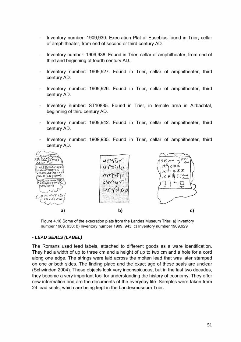
51

- Inventory number: 1909,930. Execration Plat of Eusebius found in Trier, cellar of amphitheater, from end of second or third century AD.

- Inventory number: 1909,938. Found in Trier, cellar of amphitheater, from end of

third and beginning of fourth century AD.

- Inventory number: 1909,927. Found in Trier, cellar of amphitheater, third century AD.

- Inventory number: 1909,926. Found in Trier, cellar of amphitheater, third

century AD.

- Inventory number: ST10885. Found in Trier, in temple area in Altbachtal, beginning of third century AD.

- Inventory number: 1909,942. Found in Trier, cellar of amphitheater, third

century AD.

- Inventory number: 1909,935. Found in Trier, cellar of amphitheater, third century AD.

a) b) c)

Figure 4.18 Some of the execration plats from the Landes Museum Trier: a) Inventory number 1909, 930; b) Inventory number 1909, 943; c) Inventory number 1909,929

- LEAD SEALS (LABEL)

The Romans used lead labels, attached to different goods as a ware identification. They had a width of up to three cm and a height of up to two cm and a hole for a cord along one edge. The strings were laid across the molten lead that was later stamped on one or both sides. The finding place and the exact age of these seals are unclear (Schwinden 2004). These objects look very inconspicuous, but in the last two decades, they become a very important tool for understanding the history of economy. They offer new information and are the documents of the everyday life. Samples were taken from 24 lead seals, which are being kept in the Landesmuseum Trier.

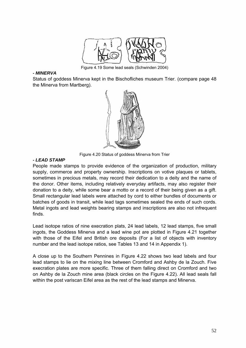
52

Figure 4.19 Some lead seals (Schwinden 2004)

- MINERVA Status of goddess Minerva kept in the Bischofliches museum Trier. (compare page 48 the Minerva from Martberg).

Figure 4.20 Status of goddess Minerva from Trier

- LEAD STAMP People made stamps to provide evidence of the organization of production, military supply, commerce and property ownership. Inscriptions on votive plaques or tablets, sometimes in precious metals, may record their dedication to a deity and the name of the donor. Other items, including relatively everyday artifacts, may also register their donation to a deity, while some bear a motto or a record of their being given as a gift. Small rectangular lead labels were attached by cord to either bundles of documents or batches of goods in transit, while lead tags sometimes sealed the ends of such cords. Metal ingots and lead weights bearing stamps and inscriptions are also not infrequent finds. Lead isotope ratios of nine execration plats, 24 lead labels, 12 lead stamps, five small ingots, the Goddess Minerva and a lead wine pot are plotted in Figure 4.21 together with those of the Eifel and British ore deposits (For a list of objects with inventory number and the lead isotope ratios, see Tables 13 and 14 in Appendix 1). A close up to the Southern Pennines in Figure 4.22 shows two lead labels and four lead stamps to lie on the mixing line between Cromford and Ashby de la Zouch. Five execration plates are more specific. Three of them falling direct on Cromford and two on Ashby de la Zouch mine area (black circles on the Figure 4.22). All lead seals fall within the post variscan Eifel area as the rest of the lead stamps and Minerva.

53

2.075

2.085

2.095

0.845 0.85 0.855 0.86207Pb/206Pb

208 Pb

/206 Pb

Post variscan ore deposits EifelLead labelLead potExecration Plat Lead stampSmall ingotMinervaSouth Pennines, Britain

Southern PenninesBritain

Post-Variscan ore deposits of Eifel

Figure 4.21 The lead isotope ratios of the artifacts from Trier compared with those from lead ore deposits of the Eifel.

2.075

2.08

2.085

2.09

0.845 0.847 0.849

207Pb/206Pb

208 Pb

/206 Pb

Lead potExecration Plat Lead stampSouth Pennines, BritainLead label

Figure 4.22 A close look at the area of Southern Pennines

ore deposits in Britain with the lead artifacts from Trier.

54

WALLENDORF

The archaeological site of Wallendorf, sits on a 41 hectare Plateau. A narrow ridge, which connects the plateau with the north-neighboring hill, was secured in Celtic period by a double fortification. The site was settled from the fifth century BC. Early Celtic buildings and pit houses are distributed over a surface of approximately 10 hectares at the center of the plateau. The settlement lost its importance in the early 1st century BC, but was still occupied through the Roman period. Samples were taken from 28 Rouelle, beads and lead fragments from the Wallendorf. Groups of Rouelle often form chains of up to 11 small wheels, which have been used as coins or sacrificial offerings in temples or sanctuaries during the Celtic and early Roman periods. Lead isotope ratios were measured on these samples and results were plotted together with those from lead ore deposits from the Rhenish Massif in figure 4.24. The Rouelle from the Wallendorf show different signatures as those from Martberg and fall in the same area in the lead isotope diagram as German ores and particularly in the Eifel ore fields. For a list of inventory numbers and lead isotope ratios, see Table 15 in Appendix 1.

Figure 4.23 Celtic Rouelle from the Wallendorf

55

2.075

2.085

2.095

0.845 0.850 0.855 0.860207Pb/206Pb

208 Pb

/206 Pb

German ore depositsWallendorf lead objectsVariscan ore deposits EifelPost-Variscan ore deposits Eifel

Variscan ore deposits of Eifel

Post-Variscan ore deposits of Eifel

Figure 4.24 The lead isotope ratios of the Rouelle, beads and lead fragments from the Wallendorf compared with Eifel ore deposits. Analytical uncertainty is smaller than the symbols

DÜNSBERG

After Caesar’s conquest of Celtic Gaul, the northern border of the Roman realm was along the Rhine River. However, from 12 BC the Romans undertook large-scale campaigns to the Elbe to conquer Germany. The Dünsberg was a Celtic oppidum north of the river Lahn near later Roman Settlement of Waldgirmes and the modern town of Giessen. It prospered in the late second and first centuries BC, but seems to have been already abounded for several years by the time the Roman first arrived in the area about 12 BC. Roman and Celtic weaponry found at the Dünsberg together with historical considerations suggest that a battle took place here around 11 or 10 B.C (Schlott 2001). Lead isotope ratios were measured for five Roman slingshots from the Dünsberg. Results are plotted together with those from the Mediterranean ore deposits in figure 4.25. They seem to be probably a mixture of lead from German and Tuscan ores. Therefore, more samples should be analyzed for a precise interpretation (for lead isotope ratios, see Table 16 in Appendix 1).

56

2.05

2.07

2.09

2.11

2.13

0.825 0.845 0.865207Pb/206Pb

208 Pb

/206 Pb

German rhenish deposits

Dünsberg

Figure 4.25 The lead isotope ratios of the slingshots from the Dünsberg compared with Mediterranean ore deposits. Experimental uncertainty is smaller than symbols.

Sardinia

Cyprus

Tuscany

Spain

Aegean

57

4.2.3 DISCUSSION Lead isotope analysis of early Roman artifacts from Dangstetten, the oldest Roman camp in southern Germany, showed that there are two possible sources for the lead objects, which are the Eifel and the southern Massif Central ore deposits. 22 lead objects among them two lead ingots and four lead objects (see page 38) fall in the area of post-variscan ore mineralization of Eifel or on the mixing line between variscan and post-variscan ore mineralization of the Eifel and were probably made from Eifel lead. The remaining six lead fragments, or workshop wastes, show similar lead isotope signature as the lead ores from southern Massif Central deposits (Figure 4.4). Archaeological evidence in Dangstetten indicates that the camp had a workshop and its own metal production since several lead objects are interpreted as workshop waste. Therefore, the Romans probably brought lead from the Eifel and the Massif Central deposits, melted and used it to make lead objects. Another possibility was to import the lead objects instead of lead ingots from France, like the bronze coins from the excavation in Dangstetten, which were minted in southern provinces of France. However, these objects are shapeless fragments, which are not stamped. Therefore, it is not possible to reach a conclusion. The next chosen early Roman camp is Waldgirmes, which was on the border between the Germans and Romans and was active for a period of ten years. Waldgirmes was a military camp. Although, besides lead fragments, other metal objects have been found in this site, no evidence for metal production has been found. As Figure 4.5 shows, the 207Pb/206Pb ratios of lead objects from Waldgirmes are between 0.843-0.858 and the 208Pb/206Pb ratios are between 2.082-2.095, which fall within the field of ore deposits from the Rhenish Massif. However, because of a large variation in isotopic signature of these objects, it is not possible to discuss a single artifact in terms of its possible provenance from the Rhenish Massif ore deposits (Figure 4.5). It seems that the Romans brought the finished lead objects and tools for daily use from other camps to Waldgirmes and they have never carried ores from local or regional ore deposits to the camp to smelt. On the contrary, Mainz was an important military town throughout the Roman period, probably due to its strategic position at the confluence of the Main and Rhine rivers. It was without doubt the base of a Roman river fleet and a provincial capital. The story of the Romans in Mainz begins in 13 BC. Archaeological finds showed several production phases. Lead isotope ratios were measured for 23 lead objects from Mainz. As Figure 4.8 shows, ten lead objects from the Mainz workshop date back to AD 1-100, all of them fall in the same area as the Eifel deposits. three lead clamps and five water pipes from Mainz and its surrounding show the same isotopic signature as the Eifel deposits. The other objects do not show the same lead isotope ratios as Eifel ores, but they fall still in the area of German ore deposits. Figure 4.9 shows a close up look at the area of post-variscan ore mineralization of Eifel in lead isotope diagram. It seems that the lead objects were produced from the mixture of lead ores from three mines of Bleialf,

58

Silberberg and Glückstal, because the lead isotope ratios fall exactly on the mixing line between these mines. The investigation of 60 lead objects from the first to fourth century AD from the Roman-Celtic camp of the Martberg showed most of the sacrificial offerings, water pumps, the Minerva statue and some of the casting remains to have 207Pb/206Pb ratios between 0.8491 to 0.8502 and fall in the post-variscan Eifel lead ore field (Figure 4.13). The rest of the casting remains are spread along a mixing line between the variscan and post-variscan Eifel ore fields. One sample of sacrificial offering and one casting remain show very similar lead isotope signatures as the Eifel mine known as “Tondorf”. Most of the phallus amulets show completely different isotopic pattern. As Figure 4.14 shows, the lead isotope ratios of these artifacts fall within the field of Southern Pennines in Derbyshire (Britain) and more specifically on the mixing line between Cromford and Ashby de la Zouch mining area. These objects were being worn as amulets or talismans; they were probably produced in Britain and exported to the Martberg for use in the Temple. Lead mining was one of the most important industrial activities of the Romano British population in Derbyshire. The distribution of pigs of Derbyshire lead (Dool and Hughes 1976) indicates the shipment of this material around Britain. A few of lead pigs are dateable, an inscribed example from Cormford Nether Moor bore the name of the Emperor Hadrian (AD 117-138). The four Rouelle (amulets in the form of wheel) show very different lead isotope signatures, they match with lead ore deposits of Tuscany (Figure 4.15). These objects are famous as Celtic amulets. Trier is the oldest city in Germany and was an important Roman camp at the same time as Mainz. A great deal of the lead objects was found in different areas of the city and archaeologists have found evidences of metal production. Lead isotope ratios of 74 samples were measured. Lead isotope ratios of nine lead coffins and three plates with relief are either from Eifel and British deposits. They were also compared with contemporary lead coffins from Cologne Gottschalk and Baumann (2001) (see Figure 4.17). The Eifel ore deposits were without doubt one of the main sources of lead for these objects. Gottschalk and Baumann and Baumann (2001) suggested Wiesloch (near Heidelberg) as a resource of lead for two coffins with 207Pb/206Pb 0.8452 and 0.8456, but the ore deposits at Wiesloch are much younger and show isotopic signatures between 0.8159 and 0.8368. As shown in Figure 4.17, the other source of lead are British ore deposits from the Southern Pennines (Britain). Mixtures of both sources are also possible for some of lead coffins. For three of them a) one of the lead plates with relief (inventory number 10,682) and two lead coffins: b) small coffin from Bischofliches Museum, without inventory number and c) lead coffin from Landesmuseum, inventory number 71,53; British source is more probable. Lead isotope ratios of these objects fall on the mixing line between two Cromford and Ashby de la Zouch ore deposits. The other lead objects from Trier show the same pattern, as both the Eifel and British ore deposits are probably the source of lead (Figure 4.21). Most of the artifacts, which

59

have the same lead isotope ratio as Eifel ores, fall specifically within the mixing line between Silberberg, Bleialf and Glückstal. This case was also seen for the lead artifacts from Mainz (Figure 4.9). Because the Roman troops first settled around 50 BC in Germany, it is not expected that they had own knowledge of mineral resources in the Eifel. Therefore finding Eifel lead ores as a source of the lead artifacts from Dangstetten was quite surprising. One can speculat that the Romans used the resources already known to and mined by the Celtic people during the late Iron Age. About 30 Celtic lead objects from the Wallendorf were analyzed. The results in Figure 4.24 show that most of them fall in the lead isotope diagram in the area of Eifel field with the same alignment, which has been observed for lead objects from Mainz in Figure 4.9. It means that most of the samples fall within the mixing line between three mines of Silberberg, Bleialf and Glückstal. It confirms the above speculation. Analysis of five lead slingshots from Dünsberg, on the other hand, shows no specific pattern in lead isotope diagram. These objects were not precious artifact and were made probably from the useless wares or the remains of metal works. Therefore, they were quite often a mixture of lead from different origins. As the Figure 4.25 shows, the studied slingshots fall probably on the proposed mixing line between German and Tucane lead ores, but more samples should be analyzed for a precise judgment.

4.2.4 CONCLUSION Lead isotope ratios of the studied artifacts were compared with those from German, Mediterranean and part of the British and French ores deposits. Results show that, in spite of rich Mediterranean lead deposits and the trade routes throughout the Roman Empire, the Romans began early on to use regional sources and to establish the local production of lead artifacts in Roman controlled Germany (Fig. 4.26). The Romans successfully explored the Eifel in search of lead. Lead from the Eifel was mined, extracted, sold and used. In the first and second century AD, the Romans used lead from local mining in the Eifel. In third and fourth centuries, both the local mining and imported lead from Great Britain together with the smelting of old lead objects became the main source of lead. This study has also confirmed the above assumption that Roman miners in Germany used the geological knowledge of the Celtic predecessors. Lead isotope ratios of the whole lead artifacts together with those from the German and Mediteranean lead ore deposits were plotted in Figure 4.27.

60

Figure 4.26 Lead resources in the Roman Empire and trade routs (modified after S. W. Meier 1995)

Remote trade routes

Lead mining area

Roman empire borderlins in second century AD

61

2.05

2.06

2.07

2.08

2.09

2.1

2.11

2.12

2.13

2.14

0.825 0.835 0.845 0.855 0.865 0.875207Pb/206Pb

208 Pb

/206 Pb

German rhenish depositsRoman lead artifacts

Figure 4.27 208Pb/206Pb vs. 207Pb/206Pb ratios of lead artifacts compared with German and Mediterranean lead ore deposits

Sardinia

TuscanyFrance

Cyprus Aegean

Britain

62

CHAPTER 5 ELEMENTAL AND ISOTOPIC ANALYSIS OF COPPER ORES AND ALLOYS

5.1 METALLURGY OF COPPER

5.1.1 INTRODUCTION Copper is a common metallic element, reddish in color, readily bent and easily extended, yet tough. Copper is frequently found in native form in nature, but rarely in high enough concentrations to mine economically. Important alloys of copper, known for many centuries, are brass (copper and zinc) and, the most ancient of all, bronze (copper and tin). Copper was first used in antiquity for tools, implements and weapons. From the Chalcolithic period about 4000 to 6000 BC, copper came into common use. Cu, the symbol of copper, comes from the Latin cuprum meaning from the island Cyprus. Initially native copper was chipped into small pieces, which were then hammered. However, when copper was hammered it became brittle and would easily break. The solution to this problem was to anneal the copper. This discovery was probably made when pieces were dropped in campfires and then hammered. By 5000 BC, copper sheet were being made. The first copper smelted artifacts in the form of rings, bracelets and chisels were found in the Nile valley, dating to around 3600 BC By 3000 BC, weapons and tools were widely used, however, only kings and royalty had such tools; it would take another 500 years before they reached the peasants. Malachite, a green friable stone, was the source of copper in the early smelters. Originally, it was thought that the smelting of copper was invented by the chance dropping of malachite into campfires. However, campfire temperatures are normally in the region of 600-650°C, whereas 700-800°C is necessary for the reduction of copper carbonate. It is more probable that ancient potters whose clay firing furnaces could reach temperatures of 1100-1200°C discovered the first copper smelting. If malachite was added to those furnaces, copper nodules would easily be found. Although the first smelted copper was found in the Nile valley, it is thought that this copper was brought to Egypt by the Gerzeans and copper smelting originated in Western Asia between 4000 and 4300 BC.

5.1.2 MINING AND MINERALS

Copper ores can be divided into two types:

1- Oxide ores includeing malachite CuCO3.Cu(OH)2, chrysocolla CuSiO3.2H2O and cuprite Cu2O. Such ores are usually formed by natural oxidation or weathering of sulfide ores in successive stages:

63

Cu2S CuSO4 CuCO3 (5.1)

often with the aid of surface waters. These oxidized ores occur on the top of ore deposit, deeper mining intersecting supergene enriched ores (native copper, tennerite) and finally, the sulfides.

2- Sulfide ores include chalcocite (Cu2S) or chalcopyrite (CuFeS2) and the so-

called gray ore or fahlerz-tetrahedrite (Cu3SbS3, with replacement of some Sb by As).

The majority of copper sulfide ores contain substantial amounts of iron sulfide, i.e. iron pyrite, which would be converted to oxide by weathering and is present to a greater or less extent in the ore body. Certain conditions on the surface can cause the dissolution and removal of the iron, leaving behind a concentrated copper ore. The majority of oxide ores seem to be relatively free of iron, and the iron content of reined copper and copper artifacts has often been made the criterion for deciding whether an oxide or a sulfide ore has been smelted. In some cases, it is the copper that is dissolved from the surface ores, and this can give rise to a zone between the weathered surface ores and the deeper sulfide ores, where a process of secondary enrichment has occurred. In this zone, the primary sulfides are enriched by the deposition of copper and other minerals leached out of the oxidized zone above. This is the “supergene” zone, in which the gray fahlerz ores occur, which due to their high concentration of copper are often indicated as being one of the earliest ores to be smelted. These ores are relatively inconspicuous, but the weathered surface ores with their high iron content (known as gossans or iron caps), left behind by dissolution of the copper bearing minerals, give an indication of what lies below. The gray ores are of course sulfides, and contain appreciable quantities of arsenic, antimony and silver, but unlike the deeper deposits are relatively low in iron, which has remained in the oxidized zone above. Iron, however, is an element that is easily removed from copper via primitive smelting processes. It is much more difficult to reduce iron than copper and therefore it goes readily into the slag. For the same reason, iron would be more readily oxidized, and an oxidizing roast of the ore before smelting will tend to oxidize iron rather than copper, which will assist the iron to find its way into the slag. Iron is therefore not considered as an element, which will give a useful indication of the type of ore used and its provenance; as it is far too dependent on slight changes in smelting technique. Many researchers have attempted to decide weather oxide or sulfide ores have been smelted by looking for traces of sulfur in the product, but copper has a remarkable affinity for sulfur and traces are present in most coppers, and could have come from sulfates present in oxidized copper ores. With the fall of the Roman realm, the mining industry found a provisional end. The fact is that Germania had less rich occurrences in comparison to Britannia or Hispania and

64

it played a subordinated role in the supply of metals like copper. The Romans explored all around the Mediterranean for mineral wealth to support their growing empire. The major supply for copper came from deposit was found in the southwest corner of Spain. The presence of copper and iron on the surface of the Earth in that area, made the nearby river red. This mining district is called Rio Tinto. The deposit originally consisted of a reddish mountain, with iron, silver and gold as well as copper. 3000 years of mining have left a crater where the red mountain once stood. The crater is over 800 feet deep and over three-quarters of a mile wide in which the remnants of Roman tunnels and shafts in the walls can still be seen. Water wheels with bronze axes, which were used to lift water out of the ancient tunnels, can still be found. Rio Tinto is still being mined today. Now the miners are working in open pits, rather than the tunnels of the ancient Romans. Tons of black slag remain from Roman smelting operations. The slag contains small amounts of gold and silver, as well as copper, showing that the Romans were interested in these precious metals. The Romans were fortunate that the oxide ore was closer to the surface, and that there was a great deal of it. During most of the time up until and of the Roman Empire, sufficient copper ore was available to meet the needs of the Mediterranean world's demands. However, by the fall of the Roman Empire the ore from Rio Tinto that could be exploited by Roman technology was exhausted.

5.1.3 COPPER ALLOYS

Tin, zinc and lead were combined with copper in varying proportions to produce the two major copper alloys of later Antiquity, bronze and brass. Unalloyed copper is also prevalent for particular uses, especially for rivets. The exact amount of tin or zinc needed in an alloy to warrant the name “bronze” or “brass” was not always the same and depends on the exact nature of the material under discussion. Modern metallurgists suggest that many of the alloys described here as “brass” are not “true” brasses at all, but “gilding metals” or “commercial bronze”. The ancient metalworker obeyed a different set of criteria in the selection and production of copper alloys, which reflected the fashions, biases and requirements of the time and culture and not only the mechanical properties.

BRONZE

The south-west of Britannia prospered from the increased trade in tin, mined locally in the area, thanks to the Roman invasion. The area had been mining and trading in tin for many years but the arrival of the Romans opened up new trade routes. Most of the tin in the area comes from opencast mines and has long been prized because of its purity.

65

The early tin industry would have been based on alluvial deposits. This is where streams had eroded down through the surface and cut across tin seams. The tin was washed out forming alluvial deposits. Collection of the ore could be carried out via the use of water to enable the heavier tin bearing minerals to be sorted from the other minerals. Originally, the tin would have been manually panned.

The gradual addition of tin to copper produces a series of physical changes in the bronze that makes the resultant alloy more suitable for the functions of the object to be made. When the tin content is increased the alloy becomes harder and harder and the color of the alloy changes; less than 5% tin results in copper-red which, becomes golden-yellow when the tin reaches between 5 and 10%, and when the percentage hits 20% the alloy becomes pale yellow. So long as the content of tin remains under 12%, the alloy assumes the form of a "solid solution" and is hence workable when cold (malleable alloys). When the tin content rises from 12 to 20%, the bronze can be worked only when heated to between 590 and 790 °C. Bronze with only 4 to 11% of tin is extremely fluid and hence is used for fusing statues, etc., (foundry bronze) because it easily fills the mold.

BRASS

Zinc is usually found in nature as sulfide (ZnS) blende or sphalerite, the carbonate (ZnCO3) calamine or smithsonite, and hermimorphite (2ZnO.SiO2.H2O). These ores are found in association with copper and lead ores, in fact sulphidic copper ores almost invariably contain some zinc. It is, however, rare for prehistoric artifacts to contain more than traces of zinc. Zinc melts at 420°C and boils at about 950°C i.e. at a much lower temperature than any other common metal (except lead). In order to reduce it from its ores, it needs to be heated in contact with charcoal at 1000°C. Unfortunately, this is above its boiling point, so that it comes off as a vapor and is quickly converted back to zinc oxide, and therefore lost. The modern process uses zinc sulfide (zinc blende) as an ore, roasts it to zinc oxide, and then smelts it at 1000-1300°C in an almost closed vessel with coke to reduce it to metal vapor. This vapor is quickly condensed to metal at one end of the vessel, which is kept just above the melting point of zinc. The characteristics of zinc are such that its extraction and retention in an alloy require particular, refined processes during production. The production of copper-zinc alloys indicates a high level of working knowledge of materials and material processing on the part of the metal smiths. During the medieval period of Europe, zinc was added to copper-tin alloys as a form of cheap bronze. Alternatively, copper-zinc alloys may have been highly valued due to their golden color, distinct from bronze alloys, and thus their resemblance to objects fashioned from gold. Ultimately, evidence of brass production and the reconstruction of the components and production processes used in the manufacture of zinc-copper alloys indicate something

66

about the methods used and the decisions and choices metal smiths were making to produce the desired finished product. - PRODUCTION OF BRASS IN THE ROMAN PERIOD

By the middle of the 1st century BC, the Romans had started the largest production of brass. This can be dated with reasonable accuracy because coins were amongst the earliest objects to be made of brass (Caley, 1964). Large scale Roman brass works are believed to have been operating in North Gaul near present day Aachen and Stolberg, and excavations have revealed evidence of Roman calamine mining, but no evidence of brass making (Craddock 1978). High zinc copper-base alloys are extremely difficult to make due to the volatility of zinc at temperatures above 906°C, i.e. 177°C below the melting point of copper. Although zinc ores (e.g. sphalerite, ZnS) are often found in association with copper and lead ores and could easily have found their way into a smelt accidentally, the majority of zinc present in the ores would vaporize leaving only a trace (up to 1%wt) in the resulting copper metal. In rare instance, such as under extreme reducing conditions, copper-zinc alloys with up to 8 weight percent zinc could be produced by mixing copper and zinc ores in a furnace (Craddock 1990). It seems that early metalworkers were not aware of the zinc content until much later in history or were not in possession of the technical knowledge to control it. Up until the eighteenth century, brass was made by mixing the ore calamine (ZnCO3) with copper under reducing condition (i.e. charcoal). The calamine was ground and mixed with charcoal and granulated copper. This was heated in a crucible at about 950-1000°C to reduce the calamine to zinc vapor, which was then absorbed by the solid copper granules. The temperature was then raised and the copper-zinc alloy melted. The addition of zinc lowers the melting point of copper from 1083°C for pure copper to 1000°C for a 20% zinc alloy (Ponting and Segel 1999). Prior to the Roman period, the introduction of zinc into copper was always by smelting zinc and copper ores together. In the Roman period the technique of adding zinc as calamine was well understood, and was probably the only method used. It would not be easy to obtain such an accurate control over composition as with tin, which was added by this time in metallic form. All this would suggest that the copper used by the Roman brass workshops was prepared in some way to remove any oxide coating. Where impure copper did slip into the system the result was “gunmetal” with reduced zinc content. Haedecke (1973) confirmed by experiment that the maximum practical amount of zinc that could be absorbed by copper during the cementation process used in Antiquity was 28%. However, such a high content is rarely encountered in Roman brasses. Several models can be suggested as to why this is the case and why the 18-24% range is so prevalent in first-century brasses. The most likely explanation is that this phenomenon is the result of re-melting together with the difficulties in guaranteeing the purity of the copper (especially if recycled). There is a “zinc equivalent” rule. A known amount of lead and/or tin is introduced during cementation resulting in the copper absorbing a set amount of zinc. The presence of a given percentage of lead will reduce zinc absorption by the same amount, whereas tin will reduce the zinc

67

absorption by twice its own concentration. Thus, copper with 2% of tin will absorb 4% less zinc than pure copper. Brass will lose approximately 10% of its zinc content on every re-melt (Caley 1964). Thus, one re-melt of 28% cementation brass will reduce the zinc content to about 25%, another to about 22% and another to about 19%. Consequently, the range of values so frequently encountered can be explained as metal that has been re-melted approximately 2-4 times. Furthermore, the use of impure copper for cementation will also reduce the amount of zinc absorbed (Craddock 1980). However, the actual situation would have been more complex than that, with the likelihood of off cuts and scrap that had been re-melted a variety of times being mixed in the same crucible, but in general, this appears to be the most likely explanation.

LEADED BRONZE

Unlike zinc and tin, lead is not present in copper alloys in solid solution. Lead forms discrete droplets throughout the metal. This makes leaded alloys more likely to crack when hammers and forges, and so sheet and wire almost never have more than 1% lead. However, lead does lower the melting point of copper and produces more fluid molten alloys. This makes it a useful addition to alloys, which are to be used in the manufacture of large or complex casting, such as statues. The technical properties of leaded and unleaded copper alloys were understood and utilized by Roman copper workers. The types of artefacts produced and the methods used in their manufacture changed over time, for example, many early Roman fittings were made from riveted sheet metal while later fittings were cast in moulds. It is not clear to what extent changes in the alloy available forced changes in fabrication techniques or if, on the other hand, changes in typology encouraged changes in alloy composition.

5.2 ELEMENTAL ANALYSIS

5.2.1 INTRODUCTION Analysis of Roman copper alloys has been carried out by a number of researchers in this field (Riederer and Briese 1974; Riederer 1984; Craddock 1975, 1978, 1986a, 1986b; Laurenze and Riederer 1980; Bayley 1981, Bayley 1985; Beck et al. 1985; Caple 1986; Unglick 1991; Stos-Gale 1993; Bollingberg and Lund Hansen 1993; Dungworth 1997). Roman copper alloys have been subjected to scientific analysis for almost two centuries and a large data set now exists. Most research has been aimed at investigating two themes:

- The relationship between alloy composition and the mode of manufacture - Finding the recipes for making ancient alloys.

Variety of different copper alloys was used in the Roman Empire. The traditional tin bronze, which had been in use in the Mediterranean for two millennia, continued in use but with increased variation in the exact level of tin added depending on the nature of the product. In the late first century BC bronze was joined by brass and these two alloys were mixed together to produce mixed alloys containing copper, zinc and tin.

68

An alloy is not a homogeneous material. During the cooling process, in particular lead separates out and solidifies as worm-like inclusions in the metal. When drilling samples for analysis, one might happen to strike into one of these and obtain erroneous results for the lead content of the alloy. The inclusions are extremely small, and distributed quite regularly in the alloy. Therefore, the variation found between several analyses from the same artefact is not always analytical uncertainty. Corrosion can change the chemistry of the surface layer. Tin might migrate to the surface and give too high a value compared to the alloy itself. Sometimes tin can even migrate out of the surface if corrosion is heavy.

5.2.2 RESULTS The Riederer (1984) study of Roman copper alloys showed that the cultural-historically definable groups of alloys were usually made of same alloys with closely limited fluctuation of the composition. He tried to classify Roman alloys into 24 groups of copper/tin/lead/zinc alloys, Table 5.1. Riederer’s classification method was used to categorize the copper alloy samples measured in this study. As the three-angel diagram in Figure 5.1 shows 6 different groups of alloys are definable. Two samples were taken from artifact 40, from belt binder and its pin, which are 40a and 40b respectively. Table 5.1 Roman alloy groups after Riederer Nr. Group Copper Tin Lead Zinc 1 Copper - - - 2 Tin bronze (low tin content) 95-99 1-5 - - 3 Tin bronze (middle tin content) 90-95 5-10 - - 4 Tin bronze (high tin content) <90 >10 - - 5 Lead bronze (middle lead content) 90-99 - 1-10 - 6 Lead bronze (high lead content) 80-90 - 10-20 - 7 Lead bronze (very high lead content) <80 - >20 - 8 Brass (low zinc content) 95-99 - - 1-5 9 Brass (middle zinc content) 90-95 - - 5-10 10 Brass (high zinc content) 80-90 - - 10-30 11 Brass (very high zinc content) 70-80 - - >30 12 Lead-tin-bronze (low lead and tin content) 80-98 1-10 1-10 - 13 Lead-tin-bronze (low lead content) 70-89 10-20 1-10 - 14 Lead-tin-bronze (high lead content) 70-89 1-10 10-20 - 15 Lead-tin-bronze (very high lead content) >79 1-10 >20 - 16 Lead-brass (low zinc content) 80-98 - 1-10 1-10 17 Lead-brass (high zinc content) 70-89 - 1-10 10-30 18 Tin-brass (low tin content) 80-98 1-10 - 1-10 19 Tin-brass (high tin content) 70-98 1-10 - 10-30 20 Lead-tin-brass (low zinc content) 85-97 1-5 1-5 1-5 21 Lead-tin-brass (middle zinc content) 70-85 1-10 1-10 5-10 22 Lead-tin-brass (middle zinc content) 60-80 1-10 10-20 5-10 23 Lead-tin-brass (high zinc content) 60-80 1-10 1-10 10-30 24 Lead-tin-brass (very high zinc content) 60-78 1-10 1-10 >30

69

Table 5.2 The chemical composition of Roman copper alloy artefacts from the Mainz workshop determined by EPMA

Sample Sb As Sn Cu Pb Zn Ag Fe Ni After

Riederer’s Classification

11 0.15+ 0.02

0.02+ 0.01

4.41+ 0.25

94+ 0.47

0.22+ 0.04

b.d. 0.05+ 0.01

0.63+ 0.07

0.03+ 0.01

15 0.15+ 0.04

0.03+ 0.01

2.69+ 1.03

93.99+ 1.09

0.08+ 0.04

b.d. 0.03+ 0.01

0.08+ 0.02

24 0.06+ 0.02

b.d. 1.43+ 0.07

86.79+ 0.51

0.12+ 0.02

8.19+ 0.01

0.07+ 0.01

0.12+ 0.01

0.02+ 0.01

2

18 0.13+ 0.07

0.04+ 0.02

8.15+ 1.84

84.49+ 1.08

0.57+ 0.05 b.d. b.d. 0.02+

0.01 0.03+ 0.01

31 b.d. 0.02+ 0.01

4.38+ 0.13

93.86+ 0.69 b.d. 1.37+

0.05 0.04+ 0.02

0.07+ 0.02

0.02+ 0.01

40b 0.12+ 0.02

0.05+ 0.01

7.77+ 0.67

89.46+ 0.2

0.46+ 0.06

0.3+ 0.05

0.04+ 0.01

0.03+ 0.01

0.03+ 0.01

4

41 0.09+ 0.01

0.04+ 0.01

3.05+ 0.19

80.95+ 0.16

0.24+ 0.09

15.17+ 0.07

0.05+ 0.01

0.17+ 0.03 b.d.

14 0.08+ 0.01

0.03+ 0.01

3.86+ 0.21

80.11+ 0.44

0.38+ 0.14

14.29+ 0.04

0.04+ 0.01

0.22+ 0.02

b.d.

33 0.12+ 0.01

b.d. 1.78+ 0.16

80.63+ 0.10

0.14+ 0.05

16.19+ 0.03

0.11+ 0.02

0.46+ 0.05

0.02+ 0.01

36 0.06+ 0.01

b.d. 0.78+ 0.19

82.16+ 0.37

0.06+ 0.01

15.31+ 0.08

0.08+ 0.01

0.37+ 0.03

b.d.

40a 0.13+ 0.01

0.05+ 0.01

1.62+ 0.16

80.86+ 0.26

0.13+ 0.06

16.33+ 0.13

0.04+ 0.01

0.31+ 0.01

b.d.

44 0.09+ 0.01

0.03+ 0.02

0.03+ 0.01

82.90+ 0.26

0.23+ 0.05

15.92+ 0.18

0.05+ 0.01

0.21+ 0.01

b.d.

27 0.13+ 0.02

0.04+ 0.01

1.89+ 0.042

85.19+ 1.1

0.14+ 0.04

12.11+ 0.08

0.07+ 0.02

0.34+ 0.06

0.06+ 0.02

19

20 b.d. b.d. 0.38+ 0.05

99.37+ 0.12

b.d. b.d. 0.02+ 0.01

b.d. 0.05+ 0.01

21 0.02+ 0.01

b.d. b.d. 99.78+ 0.35

0.06+ 0.03

b.d. b.d. b.d. b.d.

23 b.d. b.d. 0.37+ 0.04

99.30+ 0.24

0.02+ 0.01

b.d. 0.02+ 0.01

b.d. 0.04+ 0.01

16 0.08+ 0.02

0.04+ 0.01

0.27+ 0.03

99.34+ 0.16

0.02+ 0.01

b.d. 0.04+ 0.01

b.d. b.d.

1

29 0.11+ 0.02

0.03+ 0.01

4.55+ 0.21

86.85+ 0.81

0.38+ 0.04

7.34+ 0.09

0.06+ 0.03

0.58+ 0.03

0.05+ 0.01

39 0.07+ 0.02

0.03+ 0.01

3.30+ 0.45

87.75+ 0.64

0.13+ 0.06

6.32+ 0.08

0.50+ 0.22

0.21+ 0.01

0.02+ 0.01

43 0.05+ 0.01

0.02+ 0.01

2.14+ 0.08

84.96+ 0.54

0.34+ 0.05

9.76+ 0.06

0.04+ 0.02

0.67+ 0.05

0.03+ 0.01

12 0.05+ 0.02

0.02+ 0.01

0.99+ 0.52

85.36+ 1.13

0.30+ 0.02

9.7+ 0.04

0.03+ 0.02

1.83+ 0.07

0.05+ 0.01

18

26 0.18+ 0.02

0.03+ 0.01

0.48+ 0.03

79.86+ 0.12

0.09+ 0.01

18.97+ 0.07

0.03+ 0.01

0.25+ 0.02

b.d.

45 b.d. b.d. 0.17+ 0.07

77.92+ 0.61

0.07+ 0.05

21.34+ 0.18

0.02+ 0.01

b.d. b.d.

46 0.03+ 0.01

b.d. 0.19+ 0.05

78.08+ 0.92

0.18+ 0.07

21.32+ 0.17

0.02+ 0.01

0.15+ 0.03

b.d.

10

70

Cu/10 Zn

Pb*10

Figure 5.1 Roman copper alloy objects analysed in this study, classified after the Riederer classification method. On this tri-plot of Cu, Zn and Pb; Cu concentrations have been divided by 10 and Pb concentration have been multiplied by 10 to see the different groups of copper alloy.

5.2.3 DISCUSSION The common additions, used in antiquity for forming an alloy with copper, are tin, lead and zinc. The chemical analysis results presented in table 5.2 and Figure 5.1 show that these elements were combined in different proportions to produce alloys of different properties that were used in the manufacturing of the objects. Examination of the results suggests that the analyzed objects may be divided into six groups based on their Zn, Cu and Pb content. One of the impurities in ‘calamine’ brass is manganese, which, although present in amounts too small to make any noticeable difference to working properties, has been identified as a diagnostic feature of smithsonite brass (Carradice and Cowel 1987). Consequently, the brasses produced from smithsonite will all contain elevated levels of iron and manganese, and in certain instances, lead. Iron, on the other hand, although always present in copper through its common use as a fluxing agent and from certain ores, was an undesirable contaminant and so efforts were made to produce copper virtually free of iron, and subsequent re-melting will reduce this even further. Iron can be used as an indicator of smelting process (Tylecote and Boydell 1978). Roman copper alloys generally has an iron content of below 0.25% (iron content of studied

1

2

4

1819

10

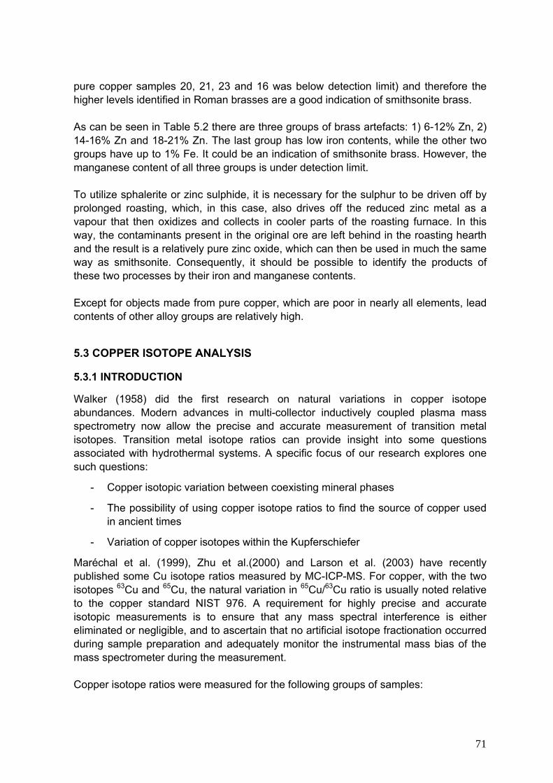
71

pure copper samples 20, 21, 23 and 16 was below detection limit) and therefore the higher levels identified in Roman brasses are a good indication of smithsonite brass. As can be seen in Table 5.2 there are three groups of brass artefacts: 1) 6-12% Zn, 2) 14-16% Zn and 18-21% Zn. The last group has low iron contents, while the other two groups have up to 1% Fe. It could be an indication of smithsonite brass. However, the manganese content of all three groups is under detection limit. To utilize sphalerite or zinc sulphide, it is necessary for the sulphur to be driven off by prolonged roasting, which, in this case, also drives off the reduced zinc metal as a vapour that then oxidizes and collects in cooler parts of the roasting furnace. In this way, the contaminants present in the original ore are left behind in the roasting hearth and the result is a relatively pure zinc oxide, which can then be used in much the same way as smithsonite. Consequently, it should be possible to identify the products of these two processes by their iron and manganese contents. Except for objects made from pure copper, which are poor in nearly all elements, lead contents of other alloy groups are relatively high.

5.3 COPPER ISOTOPE ANALYSIS

5.3.1 INTRODUCTION

Walker (1958) did the first research on natural variations in copper isotope abundances. Modern advances in multi-collector inductively coupled plasma mass spectrometry now allow the precise and accurate measurement of transition metal isotopes. Transition metal isotope ratios can provide insight into some questions associated with hydrothermal systems. A specific focus of our research explores one such questions:

- Copper isotopic variation between coexisting mineral phases

- The possibility of using copper isotope ratios to find the source of copper used in ancient times

- Variation of copper isotopes within the Kupferschiefer

Maréchal et al. (1999), Zhu et al.(2000) and Larson et al. (2003) have recently published some Cu isotope ratios measured by MC-ICP-MS. For copper, with the two isotopes 63Cu and 65Cu, the natural variation in 65Cu/63Cu ratio is usually noted relative to the copper standard NIST 976. A requirement for highly precise and accurate isotopic measurements is to ensure that any mass spectral interference is either eliminated or negligible, and to ascertain that no artificial isotope fractionation occurred during sample preparation and adequately monitor the instrumental mass bias of the mass spectrometer during the measurement. Copper isotope ratios were measured for the following groups of samples:

72

a) Malachite and azurite from the same piece of ore and different localities.

b) Copper sulfide and copper carbonate from the same piece of ore and different localities.

c) Roman copper alloy artifacts from the Mainz workshop.

d) Early Bronze Age copper alloy artifacts from the Landesmuseum Mainz

e) Three profiles of the Kupferschiefer

We report our first results for copper isotope ratio measurements on copper minerals from ore deposits in this study together with early Bronze Age samples and some bronze objects from the Mainz workshop. These data, together with other published copper isotope ratios on ore minerals may be used to evaluate the sources of copper in hydrothermal ore deposits. However, there are many questions that need to be addressed before such data can be fully applied to assessing copper sources in hydrothermal environments. Therefore, the mechanisms, which control copper isotope fractionation, such as redox reactions and equilibrium thermodynamic fractionations among solids or dissolved dynamic aqueous species, and their temperature dependencies, must be known.

5.3.2 RESULTS a) Malachite and azurite from the same piece of ore and different localities

δ65Cu was measured in malachite and azurite in the same specimen of ore to find whether copper isotopes fractionate during the formation of the two copper carbonates. The results are given in Table 5.3 and in Figure 5.2. Figure 5.2 shows that no isotope fractionation occurred during co-precipitation of malachite and azurite. Samples 1, 3 and 4 deviate from the 1:1 equiline. 2σ is the difference between two mesurements of one sample. Table 5.3 Copper isotope ratios of malachite and azurite from coexisting phases

δ65Cu 2σ δ65Cu 2σ Location Sample name

Malachite Azurite

Insel Elba, Rio Marina 3471 0.09 0.10 -0.16 0.06 Afrika, Namibia/ Tsumeb 819 0.71 0.06 0.70 0.06 Afrika, Namibia/ Tsumeb 813 1.78 0.06 1.70 0.06 Afrika, Namibia/ Tsumeb 2615 3.17 0.06 3.26 0.08

Grichenland/ Laurion 1 -0.13 0.06 -0.28 0.06 Spanian/ Villamanin, Prov. Leon 2 -0.44 0.06 -0.37 0.06

USA /Maiam 3 2.57 0.06 2.81 0.06 Maroko 4 3.45 0.06 3.07 0.06

73

-1

0

1

2

3

4

-1 0 1 2 3 4

Azurite Delta 65Cu

Mal

achi

te D

elta

65C

u

813

3

2615

4

1

2

8193435

Figure 5.2 Comparison of δ65Cu of malachite and azurite from coexisting phases from Table 5.3.

-1

0

1

2

3

4

17.8

18.0

18.2

18.4

18.6

18.8

19.0

206Pb/204Pb

δ65C

u

Malachite

Azurite

819

813

26154

3

1

Figure 5.3 Shows the correlation between lead and copper isotope analysis of malachite and azurite minerals from the Table 5.3

74

Lead isotopes are not expected to differ between co-precipitating phases of low temperatures and this is the case for the coexisting malachite and azurite (Figure 5.3). The samples 3, 4 and 1 which fell off the equiline in Figure 5.2, differ also in their lead isotopes. The lead isotope ratios were not measured for sample 3435. Figure 5.3 also shows that δ65Cu of copper carbonate display large difference even within a single locality. Samples 819, 813 and 2615 are from Tsumeb in Namibia and they show a variation of up to 2.5‰ in δ65Cu. These samples have identical lead isotope ratios (for lead isotope ratios see Table 7 in appendix 1). b) Copper sulfide and carbonate from the same piece of ore and different localities

Variation in copper isotope ratios in copper sulfide has also been studied and the results together with those for copper carbonates were plotted against 206Pb/204Pb in Figure 5.4. Table 5.4 shows the localities (for the copper isotope ratios see Tables 1 and 2 in Appendix 2).

17.5

18.0

18.5

19.0

-2.0 -1.0 0.0 1.0 2.0 3.0 4.0

δ65Cu

206 Pb

/204 Pb

MalachiteChalcopyriteAzurite

819

813 2615

3471

1171

Figure 5.4 Shows the correlation between 206Pb/204Pb and the copper isotopes of copper sulfide and copper carbonates. The marked signs belong to coexisting phases.

Table 5.4 name and locality of the studied mines

Sample name Area Locality Mine 60003018001a Niederhövels/Steckenstein Friedrich 60003040001a Hamm Huth 60003046001a

Siegerland Eiserfeld Eisenzecher Zug

1171f Lahn-Dill Westerwald/Haiger Hachelbach 3471 f Tuscany Insel Elba Rio Marina 819 f Tsumeb 813 f Tsumeb

Mal

achi

te

2615 f Namibia

Tsumeb

75

Table 5.2 continued Sample name Area Locality Mine

2.2/2/10 f Gosenbach Schmiedeberg Ma6b Stahlberg Ma5b Brüche 2aac Schwabengrube

2214 f

Müsen

Altenberg 60001439001a Müsen/Gosenbach Alte Lurzenbach

2304 f Betzdorf/Herdorf Wolff

Cha

lcop

yrite

4bod

Siegerland

Littfeld Victoria 5aac

V19/17 f Littfeld Victoria

Mz1e Willroth Georg 1234 f Steinebach königszug 2002 f Gosenbach Stroch 2003 f Biedenkopf/ Breidenbach Boxbach

Ma3b Biedenkopf/Rachelshausen Grubenfeldern Ritschtahl

8aac 60003021001a

Siegerland

Wilgersdorf Neue Hoffnung

33 f Haiger Hachelbach 4123 f Nazenbach Neuer Muth 2303 f Dillenburg/Nanzenbach Hilfe Gottes 1761 f 4063 f

Stangenwaag

862 f 1171 f

Lahn-Dill

Westerwald/Haiger Hachelbach

4Tüg Wiesen Eupen M1991/221LSe 1990/1601LSe

Eifel Werlau Gute Hoffnung

60003007001a 60003026001a

Bad Ems Braubach Rosenberg

Cha

lcop

yrite

3471 f Tuscany Insel Elba Rio Marina 819 f Tsumeb 3440 f Tsumeb 813 f Tsumeb A

zurit

e

2615 f

Namibia

Tsumeb a: Samples from the Bergbau Museum Bochum, by courtesy of Dr. A. Hauptmann and Dr. M. Ganzelewski b: Samples from the Mineralogisches Museum der Philipps-Universität Marburg, by courtesy of Dr. K. Schürmann c: Samples from the Institut für Mineralogie und Lagerstättenlehre RWTH-Aachen, by courtesy of Dr. A. Wiechowski d: Samples from the Mineralogisches Museum, Rheinische Friedrich-Wilhelms-Universität Bonn, by courtesy of Dr. R. Schumacher e: Samples from the Naturhistorisches Museum Mainz, by courtesy of Dr. H. Lutz and C. Poser f: Samples from the Johann Wolfgang Goethe Universität g: Samples from the Institut für Geowissenschaften, Unversität Tübingen, by courtesy of Dr. U. Neumann *Because most of the samples did not have an institution number (except for the samples from Bergbau Museum Bochum and those from Johann Wolfgang Goethe Universität) they were nominated by author.

76

More copper isotope variation has been observed between chalcopyrite and copper carbonates (Figure 5.4). It could be explained on the basis of the preferential precipitation of 65Cu during hydrothermal processes or selective isotopic exchange between the crystallized Cu-sulfides and hydrothermal fluids. In the case of coexisting malachite and chalcopyrite, copper isotope ratios differ significantly (for lead isotope ratios, see Tables 3 and 4 in Appendix 1).

-4 -3 -2 -1 0 1 2 3 4Delta 65Cu/63Cu

ChalcopyriteMalachiteAzurite

Dillenburg, Nassau, Germany

Lauterberg, Harz, Germany

Falkenstein

Dillenburg, Nassau, Germany

Bad Lauternberg, Germany

Rio Marina, Tuscany

Hachelbach, Westerwald, Germany

Figure 5.5 δ65Cu of Chalcopyrite Azurite and malachite from coexisting phases.

The δ65Cu of copper sulfides varies between -1.5 to +0.75‰, while the copper carbonates display much more variations in isotopic composition between -1.0 to +3.5‰. Figure 5.5 shows copper isotope variation between malachite, azurite and chalcopyrite in coexisting phases. In all studied cases, copper carbonates are enriched in the 65Cu isotope relative to copper sulfide. Relatively abundant data exists on the isotope composition of copper ores from both continental deposits and black smokers (Maréchal et al. 1999; Zhu et al. 2000, Larson et al. 2003). The δ65Cu values of most chalcopyrite samples from mafic intrusions cluster tightly between -0.10 and -0.20‰. chalcopyrite, bornite, covellite and atacamite from black smokers define a much broader range between ≈-0.10 and 4.0‰. Larson (2003) also suggest that copper is lighter in bornite by up to 0.4‰ with respect to coexisting chalcopyrite. Maréchal et al. (1998) and Larson (2003) observed that low-temperature deposits, such as chrysocolle, azurite, malachite, cuprite and native copper show a

77

broader range of copper isotopic compositions (from -3.0‰ in some minerals from Ray, Arizona up to +5.6‰ for three concordant minerals from Morenci, Arizona), which strongly suggest that the isotopic variability may be ascribed to the alteration of primary high-temperature deposits. Using this basic concept and our measurement data, we considered another hypothesis that copper carbonate, which is deposited through high temperature hydrothermal processes, dissolves and is re-precipitated under lower temperatures in another place. According to Zhu, under such circumstances copper will be fractionated. Therefore, copper isotope fractionation could be observed in copper artifacts, which were made from the low temperature copper carbonates. This has been tested in two groups of artifacts. Results are presented in the next two sections.

c) Roman copper alloy artifacts from the Mainz workshop. Measurements were made by Gale et al. 1999 to assess whether smelting or fire-refining processes produce changes in copper isotope composition. Table 5.5 presents the results of these copper isotope measurements on the source material and smelting products of a smelting experiment carried out using malachite ore, in the copper metal smelted from this ore, and in copper extracted (by dissolution and ion exchange separation) from the slag produced in this smelting process. The data presented in Table 5.5 show that, in this experiment, there are no statistically significant difference in the 63Cu/65Cu ratios between the starting malachite ore, the copper smelted from it, or the traces of copper remaining in the slag. Based on this experiment there is at present no evidence that smelting changes the isotopic composition of copper in the smelted metal (Gale et al. 1999). Table 5.5 A comparison of copper isotope compositions obtained for the products of smelting and fire refining experiments carried out by J. Merkel. MC-ICP-MS was used for JM1, JM2, JM3, with internal bias corrected in terms of 66Zn/68Zn= 1.512680 for an internal laboratory Zn standard. Low temperature TIMS was used for JM6 and JM7. The copper metal of samples JM6 and JM7 was smelted from an ore sample from a different mine than that involved in JM1, JM2 and JM3 (after Gale et al. 1999).

Copper isotope ratios were measured in 23 copper alloy artifacts from the excavation in Mainz workshop. Results were shown in table 5.6 and Figure 5.6. Twelve samples show δ65Cu between -0.5 to +0-5‰. Only two artifacts 25 and 41 show enrichment in heavy isotopes. A group of 9 samples show δ65Cu between -0.81 to -1.22‰. For lead isotope ratios, see table 17 in appendix 1.

Sample No. Product 63Cu/65Cu Standard déviation

JM1 Malachite ore from Zaire 2.24505 0.00024 JM2 Copper metal smelted from the above ore 2.24513 0.00006 JM3 Copper metal in slag from the above smelt 2.24519 0.00009 JM6 Copper metal; product of one fire refining Step 2.24426 0.00060 JM7 Copper metal, fire refined from JM6 2.24456 0.00092

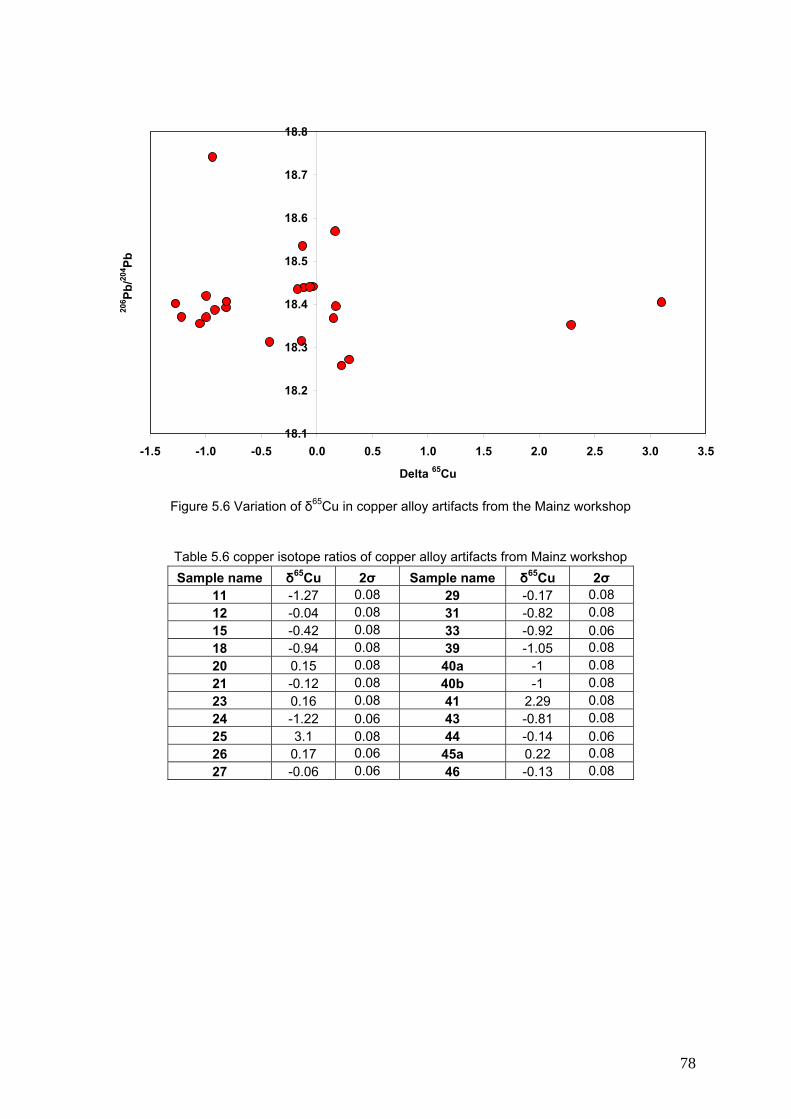
78

18.1

18.2

18.3

18.4

18.5

18.6

18.7

18.8

-1.5 -1.0 -0.5 0.0 0.5 1.0 1.5 2.0 2.5 3.0 3.5

Delta 65Cu

206 Pb

/204 Pb

Figure 5.6 Variation of δ65Cu in copper alloy artifacts from the Mainz workshop

Table 5.6 copper isotope ratios of copper alloy artifacts from Mainz workshop Sample name δ65Cu 2σ Sample name δ65Cu 2σ

11 -1.27 0.08 29 -0.17 0.08 12 -0.04 0.08 31 -0.82 0.08 15 -0.42 0.08 33 -0.92 0.06 18 -0.94 0.08 39 -1.05 0.08 20 0.15 0.08 40a -1 0.08 21 -0.12 0.08 40b -1 0.08 23 0.16 0.08 41 2.29 0.08 24 -1.22 0.06 43 -0.81 0.08 25 3.1 0.08 44 -0.14 0.06 26 0.17 0.06 45a 0.22 0.08 27 -0.06 0.06 46 -0.13 0.08

79

d) Early Bronze Age copper alloy artifacts from the Landesmuseum Mainz Low temperature precipitated copper carbonates were probably removed by the ancient metallurgist in early Bronze Age. Since the copper isotope signature does not change during smelting and making metal objects from ore (Gale et al. 1999), a large isotopic variation, reflecting mass fractionation deposition at low temperature could be seen, for instance, in Bronze Age objects. For this purpose, samples were taken from 10 axes from early Bronze Age from the Landesmuseum in Mainz (Figure 5.7). For sample preparation method, see chapter 2. δ65Cu values were measured with Multi-Collector Inductively Coupled Plasma Mass Spectrometry (MC-ICP-MS) using the sample-standard bracketing technique. Table 5.7 shows the δ65Cu for these objects.

a) b) c)

d) e) f)

Figure 5.7 Some Early Bronze Age axes from the Landesmuseum Mainz, Inventory number: a) 2280, b) 2279, c) 2289, d) 2403, e) F162 and f) F162

No large variation in copper isotope composition was observed. This number of samples is definitely not enough for a systematic study, therefore the measurement of samples from different periods of certain production centers together with copper minerals from large copper deposits like Rio Tinto should be made. Table 5.7 copper isotope ratios of copper alloy artifacts from Landesmuseum Mainz

Sample name δ65Cu 2σ Sample name δ65Cu 2σ 2279 0.01 0.06 2403 -0.04 0.08 2280 0.21 0.08 V2406 0.51 0.06 2289 0.14 0.08 F162 0.28 0.08 2294 0.14 0.08 F163 0.16 0.08

80

5.4 LEAD ISOTOPE ANALYSIS AND PROVENANCING THE COPPER ALLOYS FROM THE MAINZ WORKSHOP

As was explained in the chapter 6, from 24 analyzed artifacts, six different alloy groups were identified, among them three groups of brass, whose lead isotope ratios were plotted together with Mediterranean ore deposits in Figure 5.8. Lead can come from two origins in brass, one is zinc ore, which occur usually with lead and the other is lead from copper ore. The studied samples have over 6% zinc, therefore, the effect of lead isotope signature from zinc ore is more probable. Two of four brass artifacts with 18-21% zinc lie in the area of the Rio Tinto copper ore deposits and others seem to be on the mixing line between two Spanish fields. The other brass artifacts with 6-12% and 14-16% zinc content have 207Pb/208Pb ratios between 0.8454 to 0.8565, the same area as the Zn ore deposits of Aachen-Stolberg and Maubach-Mechernich in Germany. Zinc from this ore deposit was probably used to make brass in the Mainz workshop. As was discussed before in this Chapter, these two groups of brass have relatively high iron contents, which could be an indication of using smithsonite from Aachen-Stollberg ore deposits (for lead isotope ratios, see Table 17 in Appendix 1).

2.05

2.07

2.09

2.11

0.825 0.835 0.845 0.855 0.865208Pb/206Pb

207 Pb

/206 Pb

Aachen-StolbergMaubach-MechernichSn:0-4%, Zn14-16%Sn:1-8%, Zn:6-12%Zn:18-21%

Aeugean

Cyprus

Spain

Spain

Figure 5.8 Lead isotope ratios of brass artifacts from the Mainz workshop compared with German lead-zinc ore deposits and Mediterranean copper deposits.

81

Lead isotope ratios of copper and bronze artifacts were plotted together in Figure 5.9. As it was shown in Table 5.2 in this chapter, the lead contents of these objects are all below 0.8%, therefore lead was probably not added to alloy during the melting process. Thus, the source of lead could be the copper ores, which, were probably provided from both copper deposits of Spain and Cyprus. As Figure 5.9 shows, 207Pb/208Pb ratios of copper and bronze artifacts are between 0.835 to 0.86 and on the mixing line between one of the Spanish ore deposits field and those from Cyprus.

2.05

2.07

2.09

2.11

0.825 0.835 0.845 0.855 0.865207Pb/206Pb

208 Pb

/206 Pb

Sn: 1-5%

Sn:9-11%, Zn:0-1%

CuAeugean

Cyprus

Spain

Spain

Figure 5.9 Lead isotope ratios of copper and bronze artifacts from the Mainz workshop compared with Mediterranean copper deposits.

82

5.5 COPPER AND LEAD ISOTOPES IN KUPFERSCHIEFER

5.5.1 INTRODUCTION The Kupferschiefer is a typical bituminous marl which extends from England through the Netherlands and Germany to Poland. This black shale contains high concentrations of organic material (TOC up to 20%), sulfides (mainly iron sulfides like pyrite) and abnormally high concentrations of zinc, copper, lead and barium. The sediments were deposited 260 million years ago, when the big landmasses of Laurasia and Gondwana collided during the Permian. Before, the Old-Red-Continent was rather dry, with a wide dry basin existing in the middle of Europe . Because of an increase of sea level and subsidence of the landmasses between Greenland and Fenno-scandia, seawater flowed into the large basin from the North. The basin may have been filled with seawater in a relatively short time of only 10 years and the environmental conditions changed from terrestrial to marine. The Zechstein Sea covered middle Europe. The early marine system was relatively rich in nutrients. This probably led to a strong production of biomass and a high accumulation rate of organic material in the sediments. It seems to be undeniable that this large accumulation of organic debris on the seafloor leads to the consumption of oxygen within the water column. The Kupferschiefer was deposited under anoxic (euxinic) conditions in the water column. The ore mineralization is a diagenetic process, which took place millions of years later. The source for the metal is probably the underlying Rotliegend (early Perm) or Carboniferous material. The Kupferschiefer can be regarded as one of the best investigated black shales in the world. Wedepohl (1964) and Marowsky (1969) proposed that the Kupferschiefer is a “prototype of synsedimentary ore deposits” with bacterial sulfate reduction as the key process for H2S formation and base metal precipitation already occurring during the deposition of the sediment. Rentzsch (1974) showed that copper mineralization in Kupferschiefer was controlled by the Rote Fäule which is clearly of post depositional origin. In the Rote Fäule zones, primary framboidal and euhedral pyrites are replaced by hematite and base metals and are almost completely removed. Copper mineralization is generally enriched in front of the Rote Fäule. Both Rentzsch (1974) and Gustafson and Williams (1981) suggest that Cu-Fe sulfides and copper sulfides in front of the Rote Fäule were formed by pyrite replacement. Vaughan et al. (1989) distinguished three stages of Kupferschiefer mineralization. The first stage represents weak mineralization during deposition of the sediment. The second stage is observed in areas where additional metal accumulation occurred during early diagenesis. A third stage of mineralization is observed solely in areas such as the Richelsdorf Hills and the Spessart/Rhön in the Hessian Depression (Germany), and is related to the occurrence of Saxonian tectonism. Evidence for post-depositional metal enrichment processes also come from organic geochemical and stable isotope investigations (Püttmann et al. 1988, 1989, 1993; Bechtel and Püttmann 1991, 1992). These studies showed a significant oxidation of bitumen and Kerogen in Cu-bearing Kupferschiefer sections. The intensity of oxidation tends to decrease with increasing distance from the Rote

83

Fäule zone. The depletion of hydrogen in organic matter of Cu-mineralized Kupferschiefer was interpreted to be a result of thermochemical sulfate reduction being effective at temperatures as low as 130°C (Püttmann et al. 1990). Two profiles were investigated in this study: 6 samples from a profile in the Sangerhausen Basin, which was not directly influenced by the oxidizing brines of the Rote Fäule, and 18 samples from a core from the Oberkatz-Schwelle, where both the Rote Fäule-controlled and structural-controlled mineralization of the Kupferschiefer have been observed.

5.5.2 METAL ACCUMULATION MECHANISM1

Metal accumulation in Kupferschiefer from Oberkatz:

Table 5.8 shows the element concentration and the organic carbon content within the profile of Oberkatz from top to bottom. The distribution of uranium largely parallels the organic carbon content in the upper part of the Oberkatz profile. An exception is seen in the lowermost part, particularly in the Weissliegendes sandstone. Here, the content of organic carbon is low (<0.25%), although the uranium content exceeds 20 ppm. The correlation between organic carbon and uranium in Kupferschiefer can be explained by the accumulation of uranium during Kupferschiefer sedimentation. Organic matter provides a reducing agent which is able to adsorb and precipitate uranium from U(VI)-bearing solutions through reduction (Nakashima et al. 1984, Disnar Sureau 1990, Ten Haven et al. 1988). However, in the Oberkatz profile the maximum of organic matter enrichment is observed higher in the profile in sample O5 whereas the uranium concentration shows its maximum below the Kupferschiefer in the Weisliegendes sandstone (sample O2). Table 5.8 elemental analysis of the Kupferschiefer from Oberkatz (Sun 1996)

Elemental concentration (ppm) Sample No. Cu Pb Zn As Co Ag U Ni V Cr Corg O18 689 4784 39 77 15 3 5.2 112 280 140 1.45 O17 1018 7493 58 79 17 9 5.5 120 420 159 1.00 O16 1316 8696 52 62 16 11 5.3 106 420 139 1.36 O15 1600 6234 32 62 13 7 4.4 84 398 125 1.25 O14 1548 1949 23 52 11 5 3.4 47 252 76 0.56 O13 756 822 33 52 13 3 3.7 37 202 76 1.00 O12 926 883 27 75 15 3 3.9 54 387 132 1.63 O11 1903 938 34 150 31 7 5.9 85 605 173 1.53 O10 3811 597 39 180 45 19 6.5 115 779 215 1.73 O9 4863 205 143 540 44 28 8.4 78 538 132 1.83 O8 9575 164 93 400 81 54 9.8 116 678 153 1.83 O7 9878 86 28 160 74 54 11 96 572 132 2.00 O6 7987 80 27 280 121 59 15 131 520 126 2.15 O5 20499 75 26 340 203 170 21 196 639 151 2.06 O4 33543 51 27 390 198 240 24 148 813 173 1.68 O3 27009 15 393 1400 43 130 25 41 364 90 1.05 O2 5790 63 16 3000 59 30 27 34 32 46 0.26 O1 5598 48 162 3300 177 45 21 32 22 40 0.45

1 This text was largly taken from Sun (1996)

84

The enrichment of uranium from seawater by adsorption and reduction is therefore, only reasonable for the upper part of the profile. In the sandstone below the Kupferschiefer, the enrichment of uranium has to be attributed to other processes. According to Nash et al. (1981), dispersed organic matter acted as an adsorbing-reducing trap for uranium in many sandstone uranium deposits either during sedimentation or after sedimentation. In the Oberkatz profile the accumulation of uranium in the sandstones most likely occurred after deposition. The copper content of the Weisliegendes sandstones amounts to 5790 ppm. According to mineralogical investigations (Schmidt and Friedrich 1988), the characteristic minerals of the structural-controlled mineralization in the Kupferschifer are loellingite (FeAs2) and tennantite (Cu12As4S13). Moving upwards in the profile from the sandstones to the Kupferschiefer unit, the maximum concentration of copper is observed. Here the Cu mineralization does not consist of loellingite and tennantite but is composed of Cu- or Cu/Fe- sulfides. The maximum copper content is 3.35%. The copper minerals consist of bornite (Cu5FeS4) and chalcocite (Cu2S), with a bornite predominating. At the top of the profile, a significant enrichment of Pb up to 0.87% is detected (Sun 1996).

Metal accumulation in Kupferschiefer from Sangerhausen

Table 5.9 shows the elemental concentration and organic carbon content of the profile of Sangerhausen. The determination of facies-dependent parameters along the profile indicates that Kupferschiefer from the Sangerhausen Basin was largely deposited in a marine environment; only at the beginning of Kupferschiefer sedimentation did euxinic conditions prevail. The bottom part of the profile is significantly enriched in trace elements such as Cu, Pb, Zn, As, Co, Ag and U.

Table 5.9 elemental analysis of Kupferschiefer from Sangerhausen (Sun 1996) Elemental concentration (ppm) Sample

No. Cu Pb Zn As Co Ba U Ni V Cr Corg 92762 547 3791 539 23 88 227 -- 129 175 66 1.01 92763 1051 4965 540 46 172 282 5 295 440 40 2.85 92764 6209 1797 77 12 258 238 8 322 605 -- 4.50 92765 21441 423 148 29 442 290 26 431 1010 -- 8.75 92766 103780 1048 676 766 1148 721 475 740 2006 -- 14.34 92767 56236 90 88 97 571 362 32 437 1285 -- 10.27

The copper concentration increases to 10%. Post-depositional oxidation of the organic matter is observed only in the transition zone between the Kupferschiefer and the Zechstein conglomerate indicating the influence of ascending, oxidizing brines. Microscopic analyses show that only iron sulfides form framboidal textures; copper minerals are present along the total profile preferentially in fractures and as patchy structures composed of chalcocite, chalcopyrite and bornite. In the highly mineralized bottom section, copper sulfides are associated with pyrobitumen, sparry calcite and arsenopyrite. A 3-step process of metal accumulation is proposed. During deposition of the sediment, framboidal pyrite and pyrite precursors were precipitated by bacterial SO4

2- reduction (BSR). During diagenesis the pyrite and pyrite precursors were largely replaced by mixed Cu/Fe minerals and by chalcocite (PR). In the section with very high copper contents, reduced sulfur from Fe-sulfides was not sufficient for precipitation of copper and other trace metals from ascending solutions. In this part of the profile,

85

thermochemical SO42- reduction (TSR) occurred after pyrite replacement as indicated

by the presence of the pyrobitumen and sparry calcite (Sun and Püttmann 1997).

5.5.3 SAMPLE PREPARATION AND ANALYSIS Acids and standards were prepared using 18.2 MΩ H2O from a Milli-Q water system. Ultra pure reagents were used during sample preparation and mass spectrometry. NIST-SRM 976 Cu metal was used as the reference copper isotopic standard. Samples were ground to powder using a marble mill. Sulfides were dissolved in concentrated aqua regia and the residue were heated in Suprapur nitric acid 6 N at 120°C for a week to make sure that all sulfides were dissolved. The solutions were separated from the residue by centrifuge and then evaporated to dryness and dissolved again in HBr 0.6 N. The lead and copper were separated by ion exchange column with Dowex AG1 X8 100-200 resin. The residue was dried, melted on an iridium band and fixed in resin. The surface were polished. Then the copper content in the residue was measured with LA-ICP-MS. The concentration of copper in the residue was negligible. For lead isotope analysis: after chromatography lead fractions were evaporated to dryness and dissolved in 2% nitric acid to give final concentrations of 500ppb lead. For mass bias correction, the samples were mixed with a 100ppb natural Tl standard solution (Alpha ICP standard). The natural 205Tl/203Tl ratio of 2.3871 (Dunstan et al. 1980) was used to correct for instrumental mass bias of the Pb isotope ratios. 204Pb, 206Pb, 207Pb and 208Pb are measured simultaneously along with 203Tl and 205Tl. 202Hg was also measured so as to monitor the interference of 204Hg on 204Pb. For copper isotope analysis, the copper fraction was evaporated to dryness and then dissolved in 2% nitric acid with 1 ppm Ni, for mass bias correction, to give a final concentration of 500 ppb Cu. The "standard-sample bracketing" method was chosen in which matrix effect refers to variations in the mass fractionation that occurs during the mass spectrometry with changes in sample composition under a given set of working conditions.

5.5.4 RESULTS Copper and lead isotope ratios were measured for the Sangerhausen and Oberkatz profiles. Results together with U, Pb and Cu concentrations (measured by Sun 1996) and the relative depth are summarized in table 5.10 and 5.11. Copper isotope ratios in Kupferschiefer from Sangerhausen vary from -0.78 to +0.58‰ and from Oberkatz from -0.81 to +0.68. Figure 5.10 to 5.13 show the correlation of U, Pb and Cu concentration with copper and lead isotope ratios in both profiles. Table 5.10 Lead and copper isotope ratios (measured in this study) together with copper, uranium and lead concentration of Kupferschiefer (Sun 1996) from Sangerhausen profile Sample

No. Depth

(m) Cu

(ppm) δ65Cu 2σ Pb U Corg

207Pb/206Pb +2.E-04

208Pb/206Pb +2.E-04

206Pb/204Pb +6.E-03

92762 547 -0.78 0.08 3791 -- 1.01 0.8532 2.0916 18.277 92763 1051 -0.70 0.08 4965 5 2.85 0.8532 2.0917 18.277 92764 6209 -0.15 0.08 1797 8 4.50 0.8527 2.0906 18.289 92765 21441 0.08 0.08 423 26 8.75 0.8476 2.0804 18.403 92766 103780 0.58 0.08 1048 475 14.34 0.8349 2.0553 18.701 92767

56 cm

thickness

56236 0.45 0.08 90 32 10.27 0.8326 2.0464 18.750

86

Table 5.11 Lead and copper isotope ratios (measured in this study) together with the copper, uranium and lead concentrations of the Kupferschiefer (Sun 1996) from the Oberkatz profile Sample

No. Depth

(m) Cu

(ppm) δ65Cu 2σ Pb U Corg

207Pb/206Pb +2.E-04

208Pb/206Pb +2.E-04

206Pb/204Pb +6.E-03

O18 600.00 689 -0.38 0.08 4784 5.2 1.45 0.8437 2.0785 18.530 O17 600.12 1018 -0.34 0.08 7493 5.5 1.21 0.8437 2.0785 18.530 O16 600.18 1316 -0.20 0.08 8696 5.3 1.27 0.8438 2.0785 18.530 O15 600.24 1600 -0.34 0.08 6234 4.4 1.17 0.8438 2.0786 18.530 O14 600.30 1548 -0.01 0.08 1949 3.4 0.77 0.8437 2.0784 18.533 O13 600.38 756 0.68 0.08 822 3.7 0.71 0.8435 2.0781 18.536 O12 600.46 926 0.19 0.08 883 3.9 1.12 0.8435 2.0780 18.538 O11 600.52 1903 -0.71 0.08 938 5.9 1.70 0.8434 2.0779 18.540 O10 600.58 3811 -0.81 0.08 597 6.5 2.56 0.8430 2.0772 18.548 O9 600.64 4863 -0.55 0.08 205 8.4 2.01 0.8413 2.0732 18.588 O8 600.70 9575 -0.51 0.08 164 9.8 3.11 0.8403 2.0714 18.612 O7 600.75 9878 -0.39 0.08 86 11 3.08 0.8355 2.0606 18.724 O6 600.81 7987 -0.11 0.08 80 15 3.78 0.8307 2.0489 18.836 O5 600.88 20499 0.01 0.08 75 21 5.12 0.8247 2.0341 18.982 O4 600.94 33543 0.32 0.08 51 24 4.46 0.8076 1.9923 19.407 O3 601.00 27009 0.40 0.08 15 25 1.74 0.7195 1.7672 21.959 O2 601.10 5790 0.34 0.08 63 27 0.22 0.7990 1.9822 19.623 O1 601.20 5598 0.40 0.08 48 21 0.24 0.8098 2.0038 19.344

Figures 5.10 and 5.11 show the concentration of uranium, lead and copper with copper and lead isotope compositions within the profile of the Oberkatz together with the lithography of the profile. Figure 5.12 and 5.13 show the same plots for the profile of the Sangerhausen.

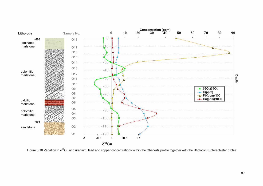
87

Figure 5.10 Variation in δ65Cu and uranium, lead and copper concentrations within the Oberkatz profile together with the lithologic Kupferschiefer profile

-1 -0.5 0 +0.5 +1

O18 O17

O16

O15

O14

O13

O12

O11

O10

O9

O8

O7

O6 O5

O4

O3 O2 O1

Concentration (ppm) Lithology Sample No.

-600laminated marlstone dolomitic marlstone calcitic marlstone dolomitic marlstone -601

sandstone

δ65Cu

Depth

88

Figure 5.11 Variation in 207Pb/206Pb and uranium and lead concentrations within the Oberkatz profile together with the lithologic Kupferschiefer profile

0.86 0.84 0.82 0.80 0.78 0.76 0.74 0.72

O18 O17

O16

O15

O14 O13 O12

O11

O10

O9

O8

O7 O6 O5

O4

O3 O2 O1

Concentration (ppm) Lithology Sample No.

-600laminated marlstone dolomitic marlstone calcitic marlstone dolomitic marlstone

-601

sandstone

207Pb/206Pb

Depth

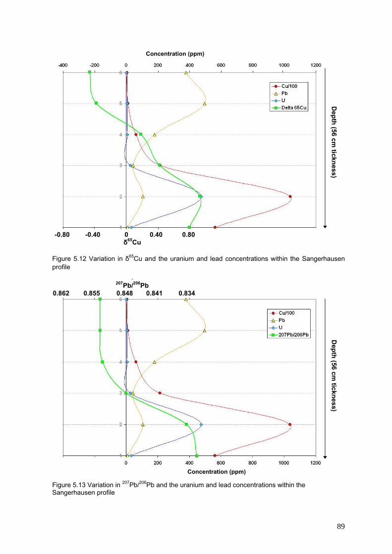
89

Figure 5.12 Variation in δ65Cu and the uranium and lead concentrations within the Sangerhausen profile

Figure 5.13 Variation in 207Pb/206Pb and the uranium and lead concentrations within the Sangerhausen profile

Depth (56 cm

tickness) D

epth (56 cm tickness)

Concentration (ppm)

4

207Pb/206Pb

0.862 0.855 0.848 0.841 0.834

Concentration (ppm)

-0.80 -0.40 0 0.40 0.80 δ65Cu

90

5.5.4 DISSCUSION One of the most intriquing features seen in Figures 5.11 and 5.13 are the highly variable lead isotopes which parallel the concentration of uranium. Figure 5.14 shows the negative correlation of the uranium with 207Pb/206Pb. Sample O3 with 3 ppm uranium falls much lower at about 207Pb/206Pb=0.72. In Figure 5.15, 207Pb/206Pb ratios were plotted against logarithmic sacale of Pb/U ratio for both profiles from Oberkatz and Sangerhausen. This shows the variation in the lead insits decay of uranium. In Figure 5.16 δ65Cu for both profiles were plotted against copper concentration. There is a positive correlation between the copper concentration and the copper isotope ratios in the Kupferschiefer profile from Sangerhausen. The profile of Oberkatz shows the same pattern with a parabolic upper limit in the relation δ65Cu and copper content, but also positive δ65Cu for lower Cu content. It appears that δ65Cu ~ 0.5 of the secondry fluid. In samples O1-O11 with a high accumulation level of copper, the δ65Cu values correlate with copper concentration, this shows that samples with high concentrations of copper are enriched in 65Cu.

0.79

0.80

0.81

0.82

0.83

0.84

0.85

0 5 10 15 20 25 30

U (ppm)

207 Pb

/206 Pb

Figure 5.14 207Pb/206Pb against uranium concentration of the Kupferschiefer profile from Oberkatz

3.4 ppm<U < 6.5 ppm 9000ppm>Pb > 600 ppm

8.4 ppm<U < 27 ppm 200 ppm>Pb > 15 ppm

O3 207Pb/206Pb=0.72

91

0.70

0.74

0.78

0.82

0.86

0 1 10 100 1000 10000Log Pb/U

207 Pb

/206 Pb

OberkatzSangerhausen

Figure 5.15 207Pb/206Pb against the logarithmic scale lead/uranium ratio of the Kupferschiefer profiles from Oberkatz and Sangerhausen

0 5 10-1.0

-0.5

0.0

0.5

1.0

Delta 65Cu

Cu%

O1O2

O3O4

O5

O6

O7

O8O9

O10O11

O12

O13

O14

O15

O16

O17O18

Figure 5.16 Correlation between copper concentrations and copper isotope ratios in the Kupferschiefer profiles from Sangerhausen and Oberkatz

Sangerhausen

Oberkatz

92

Figures 5.10 and 5.11 show the comparison between the variation of δ65Cu and 207Pb/206Pb, respectively, with copper, lead and uranium concentrations within the Kupferschiefer profile from Oberkatz. The Kupferschiefer in the Oberkatz can be divided into to four sections. The bottom of the Kupferschiefer is a dolomitic marlstone, which is succeeded upwards by a calcitic dolomitic marlstone. The middle strata are composed of dolomitic marlstones and the upper strata are represented by laminated dolomitic marlstone. The Liegend rocks are composed of Weissliegendes sandstones. As Figure 5.10 shows, the sandstone at the bottom of the Oberkatz profile has positive δ65Cu values. The laminated marlstone on the top of the profile with only 700-1000 ppm Cu, show negative values, which are probably the δ65Cu of the sedimentation process, before the secondary fluid was introduced. The most variable values from -0.81-+0.68 have been observed in dolomitic marlstone. In Figure 5.11 207Pb/206Pb ratios were plotted against the lead and uranium concentrations. Samples O10-O18 has the highest levels of lead, the isotopic signature of lead shows a constant value, which is independent of the lithology of the base sediment. High concentrations of uranium together with low concentrations of lead in samples O1-O9 result strong variations in lead isotopes between 0.72-0.84 for 207Pb/206Pb in this part of the profile and the samples are arrange in consecutive order. Figures 5.12 and 5.13 show the same comparison for the Kupferschiefer profile from Sangerhausen. Unfortunately, there is no detailed information about the depth and lithology of the Kupferschiefer in this profile. Isotopic data from both the Sangerhasen and Oberkatz profiles were also compared with values from the Lower Rhine Basin profile. In most parts of the basin, the metal content does not exceed values commonly observed in black shales. Such a profile should provide an idea about the isotopic signature of Kupferschiefer sediments before the infiltration of secondry fluids. In the area of the Lower Rhine Basin the Permian Kupferschiefer was deposited in a shallow water environment. Water exchange from this marginal basin with the Zechstein Sea was restricted by Palaeohighs. The Zechstein sea transgressed the folded Carboniferous rocks within the study area of the Lower Rhine Basin. Therefore, Lower Permian sediments are only deposited in very few areas as thin layers and there is a general lack of volcanic sedimentary rocks (Diedel and Püttmann 1988). The geological structure of the Lower Rhine Basin is characterized by a folded and faulted Carboniferous basement and a gently northwards dipping Permian, Mesozoic and Cenozoic sedimentary cover (Vaughan et al. 1989). The Kupferschiefer, a bituminous calcareous or dolomitic shale, represents the first fully marine sediment after a long period of arid to semi-arid conditions. In the area investigated it is separated only by a thin bed of fluviatile sediments from the Carboniferous basement. Maturation of the organic matter was governed only by the geothermal gradient not exceeding 68°C/km during the late Carboniferous (Bechtel and Püttmann 1997).

93

Mineralogical data show that the Carboniferous basement is relatively poor in transition metals as well as in barium. A significant increase of zinc and lead is observed in the bottom part of Kupferschiefer, from basinal Carboniferous formation waters. The lead concentration of Kupferschiefer samples range from 100 to 700 ppm. A concomitant copper enrichment in the Kupferschiefer is not observed. This is not surprising because red beds or metal-bearing volcanics as potential source rocks of copper are missing in this part of the basin (Diedel 1986). The maximum copper concentration observed in the studied samples is only 60 ppm. Such low copper content have to be enriched by chromatographic separation for copper isotope measurement. Copper could be successfully separated from matrix by chromatography, but none of the known chromatographic methods were able to separate copper from barium, which has concentrations of up to 100 times more than copper. Because of strong matrix effect no isotopic measurement could be done for the profile of Lower Rhine Basin. Lead isotopes were measured in the sulfide fraction of Sangerhausen profile (for sample preparation see page 85) and in the whole rock samples. Results together with those from two profiles from the Lower Rhine Basin were plotted in Figure 5.17. Samples with low concentrations of uranium and high concentrations of lead from the top of the profile, show 1:1 correlation of 207Pb/206Pb. Samples from the bottom of the profile with high uranium concentrations show a shift of 207Pb/206Pb to higher ratios in the whole rock. This excess lead produced from uranium decay, may be present in the form of sulfides and trapped in clay minerals in the Sangerhausen profile. For the samples from the Lower Rhine Basin, lead isotope ratios of the Kupferschiefer fraction show the same signature as the Sangerhausen profile, with 207Pb/206Pb between 0.85 and 0.853 .This probably indicates the base original isotopic signature of the Kupferschiefer, without the influence of secondary fluids. Samples from the Zechstein conglomerate on top of the profile seem to contain more radiogenic lead (Figure 5.17). In the profile of Oberkatz, where both Rote Fäule-controlled and structural-controlled mineralization of the Kupferschiefer are observed, the low concentrated uranium fraction has still more radiogenic lead with 207Pb/206Pb of about 0.843.

94

0.825

0.835

0.845

0.855

0.825 0.835 0.845 0.855207Pb/206Pb Whole rock

207 Pb

/206 Pb

Sul

fide

SangerhausenLower Rhine Basin 1Lower Rhine Basin 2

Figure 5.17 Comparison of 207Pb/206Pb measured in whole rock samples and sulfide separates in the Sangerhausen Profile and the Lower Rhine Basin

Bottom of the Profile

Zechstein conglomerate (Top of the profile)

95

REFERENCES Ahrendt H.; Hunziker J.C.; Weber K. (1978). K/Ar-Altersbestimmungen an schwache metamorphen Gesteinen des Rheinischen Schiefergebirges. Z. Dtsch. Geol. Ges. 129: 229-247. Anderle H-J.; Massone H-.J.; Oncken O. and Weber K. (1990). Southern Taunus Mauntains. In: Franke, W.; Weber, K. (eds). Conf. Paleozoic orogens-geology and geophysics, IGCP 233, Field Guide Mid-German Crystalline Rise & Rheinisches Schiefergebirge. Göttingen-Giessen, 125-148. Bachmann H.G. (1969). Eine römische Bleischlacke aus der Nordeifel und ihre metallurgische Zuordnung, in: GDMB 1982, 102-103. Bauer G.; Ebert A.; Hesemann J.; v. Kamp H.; Mueller D.; Pietzner H.; Podufal P.; Scherp A.; Wellmer F.W., with contributions from Arnold O.; Eckhardt H.; Herbst F.; Miederer W. (1979). Monographien der Deutschen Blei-Zink-Erzlagerstätten 6. Die Beli-Zink-Lagerstätten von Ramsbeck und Umgebung. Geol. Jahrb. D33: 1-377. Bayley J. & Butcher S. (1981). Variation in alloy composition of Roman brooches. Reveue d’Archéométrie, supplément: 29-36. Bayley J. (1988). Non-ferrous metalworking: continuity and change. In (E.A.Slater & J.O.Tate, Eds). Science and archaeology, Glasgow 1987. BAR (International) 196. Oxford: British Archaeological Reports. Pp.193-208. Bayley J. (1990). The Production of Brass in Antiquity with Particular Reference to Roman Britain, in: 2000 Years of Zinc and Brass. British Museum Occasional Paper No. 50, London, 7-28. Bechtel A., and Püttmann W. (1991). The origin of the Kupferschiefer-type mineralization in the Richelsdorf Hills, Germany, as deduced from stable isotope and organic geochemical studies. Chem. Geol. 91, 1-18. Bechtel A. and Püttmann W. (1992). Combined isotopic and biomarker investigations of temperature- and facies-dependent variations in the Kupferschiefer of Lower Rhine Basin, northwest Germany. Chem. Geol. 102, 23-40. Bechtel A. and Püttmann W. (1997). Palaeoceanography of the early Zechstein Sea during Kupferschiefer deposition in the Lower Rhine Basin (Germany): a reappraisal from stable isotope and organic geochemical investigation. Palaeogeography, Palaeoclimatology, Palaeoecology 136, 331-358. Beck F., Menu M., Berthoud T. & Hurtel L-P. (1985). Métallurgie des Bronzes. In (J.Horis, Ed.) Researches Gallo-Romaines I. Paris: Laboratoire de Researches de Musées de France, pp.70-139.

96

Becker A. (1998). Der spätaugusteische Stützpunkt Lahnau-Waldgirmes. Vorbericht über die Ausgrabungen 1996-1997, Sonderdruck aus Germaina 76, 1998, 2. Halbband. Römisch-Germanische Kommission des Deuschen Archäologischen Instituts, Frankfurt am Main. Verlag Philipp Zabern, Mainz am Rhein. Belshaw N.S. Freedman P.A. O’Nions R.K., Frank M. and Guo Y. (1998). A new variable dispersion double-focusing plasma mass spectrometer with performance illustrated for Pb isotopes. Int. J. Mass Specttrom. 181, 51-58. Bollingberg H.J. & Lund Hansen U. (1993). Trace element studies by DC ARC/laser-optical emission spectrograph of some bronze artifacts from the Roman import to Scandinavia. Archaeology and Natural Science 1. 24-42. Boulakia J. D. C. (1972). Lead in the Roman World, American Journal of Archaeology, 76, 139-144. Brauns M.; Leveque J. (1992). Bleiisotope in Galeniten aus dem Siegerland-Wied-Distrikt-SPP, Kolloquium der DFG.”Intraformationale Lagerstättenbildung”; Bonn. Budd P., Pollard A.M., Scaife B. (1995). The possible fractionation of lead isotope in ancient metallurgical processes. Archaeometry 37, 1, 143-150. Budd P.; Lythgoe P; McGill R.A.R; Pollard A.M and Scaife B. (1999). Zinc isotope fractionation in liquid brass (Cu-Zn) alloy: potential environmental and archaeological applications. Geoarchaeology: Exploration, Environment, Resources. 165, 147-153. Buntebarth G.; Koppe I.; Teichmueller M. (1982). Paleogeothermics in the Ruhr basin. In: Cermak V.; Haenel R. (Eds). Geothermic and geothermal energy. Schweizerbart, Stuttgart. 44-45. Caley E.R. (1964). Orichalcum and Related Ancient Alloys. New York: American Numismatic Society, No. 151. Caple C. (1986). An Analytical Appraisal of Copper Alloy Pin Production: 400-1600 AD. Ph.D. thesis, University of Bardford. Carradice I. and Cowel M. (1987). The minting of Roman Imperial bronze coins for circulation in the east: Vespasian to Trajan, Numismatic Chronicle, 147, 26-50. Copur M. (2001). Solubility of ZnS concentrate containing pyrite and chalcopyrite in HNO3 solution. Chem. Biochem. Eng. Q. 15(4)181-184. Craddock P.T. (1975). The Composition of Copper Alloys in the Classical World. Ph.D. thesis, University of Landon. Craddock P.T. (1978). The composition of the copper alloys used by the Greek, Etruscan and Roman Civilizations. Journal of Archaeological Science. 5, 1-16.

97

Craddock P.T. (1980). The first brass: Some early claims reconsidered. MASCA Journal, 1.5: 131-133. Craddock P.T. (1986a). Three thousand years of copper alloys: from Bronze Age to the Industrial Revolution. In (P. England & L. Van Selts, Eds) Application of Science in Examination of Works of Art. Boston, MA: Museum of Fine Arts, pp.59.67. Craddock P.T. (1986b). The metallurgy and composition of Etruscan Bronze. Studi Etrusch. 52, 211-271. Craddock P.T.(ed) (1990). 2000 Years of Zinc and Brass. British Museum Occasional Paper No.50, London. Craddock Paul T. (1995). Early metal mining and production. Edinburgh Univ. Press Dahm C. (1998). Der Altenberg-Bergwerk und Siedlung aus dem 13. Jahrhundert im Siegerland. Band 2, Dr. Rudolf Habelt GmbH, Bonn.

Dallmeyer R. D. (1995). Pre-permian geology of Central and Eastern Europe. Springer.

Davies O. (1935). Roman Mines in Europe. Oxford.

Diedel R. (1986). Die Metallogenese des Kupferscheifer in der Niederrheinischen Bucht. Ph.D. Thesis, RWTH Aachen. Diedel R., Püttmann W. (1988). Base metal mineralization and organic carbon maturity in the Kupferschiefer of the Lower Rhine Basin. In: Friedrich, G.H., Herzig, P. (Eds.), Base Metal Sulfide Deposits in Volcanic and Sedimentary Environments. SGA Spec. Publ. 6, 60-73. Disnar J.R. and Sureau J.F. (1990). Organic matter in ore genesis. Org.Geochem. 16, 577-599. Dool J. and Hughes R.G. (1976). Two Roman pigs of lead from Derbyshire. Derbyshire Archaeological Journal, 96, 15-16. Dungworth D. (1997). Roman Copper Alloys: Analysis of Artifacts from Northern Britain. Journal of Archaeological Science, 24, 901-910. Dunstan L.P., Gramlich J.W., Barnes I.L., Purdy W.C., (1980). J. Res. Natl. Bur. Stand., 85, 1, 1-10. Fenchel W.; Gies H., Gleichmann H.D.; Hellmund W.; Hentschel H.; Hey K.E.; Hüttenhain H.; Langenbach U.; Lippert H.J., Lusznat M.; Meyer W.; Pahl A.; Rao M.S.; Reichenbach R.; Stadler G.; Volger H.; Walther H.W. (1985). Sammelwerk Deutsche Eisenerzlagerstätten, I. Eisenerze im Grundgebirge (Varistikum), 1.Die Sideriterzgänge im Siegerland-Wied-Distrikt. Geol. Jahrb. D77: 1-517.

98

Fingerlin G. (1984). Dangstetten: Katalog der Funde I und II. Seiten: 361, 382, 385 und 388. Kommissionverlag, Konrad Theiss Verlag, Stuttgard. Fingerlin G. (1986). Küssaberg-Dangstetten in: Die Römer in Baden-Württemberg. Hrsg: von Philipp Filtzinger. Theiss, Stuttgard. Fingerlin G. (1999). Römische und keltische Reiter im Lager der XIX. Legion von Dangstetten am Hochrhein in: Archäologische Nachrichten aus Baden, Förderkreis Archäologie in Baden e.V. 3-18. Franke W. (1989). Tectonostratigraphic units in the variscan belt of Central Europe. In: Dallmeyer R.D. (Ed) Terranes in the Circum-Atlantic Paleozoic orogens. Geol. Soc. Am. Spec. Pap. 230: 67-90. Gale N.H. and Stos-Gale Z.A. (1992). Evaluating lead isotope data: cooments on E.V.Sayre, K.A.Yener, E.C. Joel and I.L. Barnes, ‘Statistical evaluation of the presently acuumulated lead isotope data from Anatolia and surrounding regions’, …, I, Archaeometry, 34(2), 311-317. Gale N.H., and St os-Gale Z.A., (1992b), Evaluating lead isotope data: comments on E.V. Sayre K.A.Jener, E.C.Jeol and I.L.Barnes. Archaeometry, 34(2), 311-36 Gale N.H., and Stos-Gale Z.A., Maliotis G. and Annetts N. (1997). Lead isotope data from the Isotrace Laboratory, Oxford: Archaeometry data base 4, ores from Cyprus. Archaeometry 39, (1), 237-246. Gale N.H., Woodhead A.P., Stos-Gale Z.A., Walder A., Bowen I., (1999). International Journal of Mass Spectrometry, 184, 1-9. Germann A.; Jochum J.; Friedrich G.; Horsfield B. (1997). The sandstone-hosted lead-zinc deposits of Maubach/Mechernich- A new genetic model based on thermochemical sulphate reduction. Zentralbl. Geol. Paläont, Teil I, 1995, 11/12: 1133-1139. Gottschalk R. and Baumann A. (2001) Material provenance of late Roman lead coffins in the Rhineland, Germany. European Journal of Mineralogy. 13, 197-205. Guénette-Beck B.; Furger A. R (2004). Blei für Augusta Raurica. Jahresberichte aus Augst und Kaiseraugst 25, 245-272. Guerra M. F. (1995). Elemental analysis of coins and glasses. Appl. Radiat. Isot., 46, 583-588. Guerra M. F. Sarthre C. -O., Gondonneau A. and Barrandon J. -N. (1999). Precious metals and provenance enquiries using LA-ICP-MS. Journal of Archaeological Science, 26, 1101-1110.

99

Gussone R. (1964). Untersuchungen und Betrachtungen zur Paragenesis und Genesis der Blei-Zink-Erzlagerstätten im Raume Aachen-Stolberg. PhD Thesis, RWTH Aachen. Gustafson L. B. and Williams N. (1981). Sediment-hosted stratiform deposits of copper, lead and zinc. Econ. Geol. 75th Annivers. 139-178. Haedecke K. (1973). Gleichgewichtsverhältnisse bei der Messingherstellung nach dem Galmeiverfahren. Erzmetall, 26, 229-233. Hannak H. (1964). Ergebnisse der Untersuchungen im Blei-Zink-Erzbezirk des südlichen Rheinischen Schiefergebirges. Erzmetall, 17: 291-298. Hauptmann A; Begemann F.; Heitkemper E.; Pernicka E. And Schmitt-Strecher S. (1992). Early copper preoduced at Feinan, Wadi Araba, Jordan: the composition of ores and copper, Archaeomaterials, 6, 1-33. Hein U.F. (1993). Synmethamorphic variscan siderite mineralization of the Rhenish Massif, Central Europe. Min. Mag. 57: 451-467. Henneke J. (1977). Die bergwirtschaftliche Bedeutung der Blei-Zink-Erzlagerstätte Mechernich. Glückauf-Forschungsh. 38: 9-18. Hetherington R. (1977). Investigation into primitive lead smelting and its products, in: Aspects of Early Metallurgy, W.A. Oddy, ed. (British Museum)London, 27-40. Hesemann J. (1978). Der Blei-Zink-Erzbezirk des Bergischen Landes (Rheinisches Schiefergebirge) als Prototyp einer frühorogenen und palingenen Vererzung. Decheniana. 131: 292-299. Hildebrandt L. (1989). Der mittelalteriche Blei-Zink-Silberebrgbau im nordwestlichen Kraichgau südlich Heidelberg. In: Archäometallurgie der Alten Welt. Der Anschnitt, Beiheft 7, 241-246. Horall K.B.; Hagni R.D.; Kisvarsanyi, G. (1983). Mineralogical, textural and paragenetic studies of selected ore deposits in the South East Missouri Lead-Zinc-Copper District and their genetic implications. In: Kisvarsanyi G.; Grant S.K.; Pratt W.D.; König J.W. (eds) Int. Conf. Mississippi Valley Type Lead-Zinc Deposits, Proc. Vol: 289-316. Jochum J. (2000). Variscan and post-variscan lead-zinc mineralization, Rhenish Massif, Germany: evidence for sulfide precipitation via thermochemical sulfate reduction. Mineral. Deposita, 35, 451-464. Johnson M.C.; Beard B.L.; Albarede F. (2004). Geochemistry of Non-Traditional Stable Isotopes, Reviews in Mineralogy and Geochemistry, Volume 55, MINERALOGICAL SOCIETY OF AMERICA GEOCHEMICAL SOCIETY:

100

Kalcyk H. (1983). Der Silberbergbau von Laureion in Attika, in: Antike Welt 14, 3, 12-29. Klein S.; Lahaye Y.; Brey G.P.; Von Kaenel H.M. (2004). The early Roman imperial ases coinage II: tracing the copper source by analysis of lead and copper isotopes-copper coins of Augustus and Tiberius. Archaeometry 46, 3 (2004) 469-480. Krahn L. (1988). Buntmetall-Vererzung und Blei-isotope im Linkrheinischen Schiefergebirge und in angrezenden Gebieten. PhD Thesis, RWTH Aachen. Mitt. Mineral Lagerstättenkunde. 30: 1-199. Krahn L. And Baumann (1996). Lead isotope systematics of epigenetic lead-zinc mineralization in the western part of the Rheinisches Schiefergebirge, Germany. Miner. Deposita 31: 225-237. Larson P.B., Maher K., Ramos F.C., Chang Z., Gaspar M., Meinert L.D. (2003). Copper isotope ratios in magmatic and hydrothermal ore-forming environments, Chemical Geology, 201, 337-350. Laurenze C & Riederer J. (1980). Metallanalysen römischer Henkel. Berliner Beiträge zur Archäometrie 5, 37-42. Lehmann H.; Pietzner H. (1970). Der Lüderich-Gangzug und das Gangvorkommen Nikolaus-Phönix im Bergischen Land. Fortschr. Geol. Rheinld. Westf. 17: 589-664. Meisl S. (1970). Petrographische Studien im Grenzbereich Diagenese-Metamorphose. Abh. Hess. Landesamtes Bodenforsch. 57: 1-93. L’Hour M. (1987). Un site sous-marin sur la cote de l’Armorique, L’epave antique de Ploumanac’h, in: Revue Archeologique de l’ouest. 4, 113-131. Liou B. (1982). Informations archeologiques: recherches sous-marines, in: Gallia 40, fasc. 1, 437-454. Maréchal C.N., Telouk P., Albarede F. (1999). Precise analysis of copper and Zinc isotopic compositions by plasma-source mass spectrometry. Chemical Geology 156, 252-273. Marowsky G. (1969). Schwefel-, Kohlnstoff- und Sauerstoff-Isotopenuntersuchungen am Kupferschiefer als Beitrag zur genetischen Deutung. Contrib. Miner. Petrol. 22, 290-334. Maus H. (1977). Römischer Bergbau bei Sulzburg (Baden), in: Der Aufschluss 28, 5, 165-176. Meier S. (1995). Blei in der Antike: Bergbau, Verhüttung and Fernhandel. Ph. D thesis. Universität Zürich.

101

Meisl S (1970). Petrographische Studien im Gerenzbereich Diagenese-Metamorphose. Abh Hess Landesamt Bodenforsch 57: 1-93. Merten M. (1987): Drei römische Bleiplatten mit Jagdfries im Rheinischen Landesmuseum Trier. Trierer Zeitschrift. 50, 255-267. Nakashima S., Disnar J.R., Perruchot A. and Trichet J. (1984). Experimental study of mechanisms of fixation and reduction of uranium by sedimentary organic matter under diagenetic or hydrothermal conditions. Geochim. Cosmochim. Acta 48, 2321-2329. Nash J.H., Granger H.C. and Adams S.S. (1981). Geology and concepts of genesis of important types of uranium deposits. Econ. Geol., 75 Annivers. Vol., 63-116. Nriagu J.O. (1983). Lead and Lead Poisoning in Antiquity. John Wiley & Sons. Önnerfors A. (1991). Antike Zaubersprüche. Stuttgart. Petrikovits H.v., (1958). Bergbau und Hüttenwesen in der römischen Rheinzone. Erzmetall, Bd.XI, H.12. 594-600 Ostwald D. & Lieber W. (1957). Blei und Zinkminerale von Nussloch nahe Wiesloch, in: Der Aufschluss 8, 7-8, 156-159. Petrikovits H. (1956). Neue Forschungen zur römerzeitlichen Rheinzone, in: Germania 34, 99-125. Pichat S., Douchet Ch. and Albarede F. (2003). Zinc isotope variations in deep-sea carbonates from the eastern equatorial Pacific over the last 175 ka. Earth and Planetary Science Letters, 210, 167-178. Pollard A.M. & Heron, C. (1996).Arcaeolgical Chemistry. Cambridge. Ponting M. & Segel I. (1998). Inductively coupled plasma-atomic emission spectroscopy analyses of Roman military copper-alloy artifacts from the excavations at Masada, Israel. .Archaeometry 40:109-122. Ponting M.J. (1999). East meets west in past-classical Bet She’an: The archaeometallurgy of cultural change. Journal of Archaeological Science 26: 1311-1321. Preuschen E. (1957). Zur ältesten Geschichte des Mechernicher Bleierzbergbaues, in: der Anschnitt 8, 1, 32-34. Püttmann W., Hagemann H.W., Merz C. And Speczik S. (1988). Influence of organic material on mineralization processes inthe Permian Kupferschiefer Formantion, Poland, Org. Geochem. 13, 357-363.

102

Püttmann W., Merz C. And Speczik S. (1989). The secondary oxidation of organic material and its influence on Kupferschiefer mineralization of Southwest Poland. Appl. Geochem. 4, 151-161. Püttmann W., Hepprnheimer H. And Diedel R. (1990). Accumulation of copper in the Permian Kupferschiefer: A result of post-depositional redox reaction. Org. Geochem. 16, 1145-1156. Püttmann W., Bechtel A., Speczik S and Fermont W.J.J. (1993). Combined application of various geochemical methods on Kupferschiefer of the North-Sudetic Syncline, SW Poland: evidence for post-depositional accumulation of copper and silver. In: Current Research in Geology Applied to Ore Deposits. (eds Fenoll Hack-Ali, Torres-Ruzi and Gervilla), Grananda. Putzger F. W. (1970). Historischer Weltatlas. Velhagen & Klasing. Rentzsch J. (1974). The Kupferschiefer in comparison with the deposits of the Zambian Copperbelt. In: Centenaire de la Société Geologique de Belgique, Gisements Stratiforms et Provinces Cupriféres, (ed P. Bartholomé), pp. 395-418, Liége. Riederer J. & Briese E. (1974). Metallanalysen römischer Gebrauchsgegenstände. Jahrbuch des Römische-Germanischen Zentral Museum Mainz 19, 83-88. Riederer J., (1984). Metallanalysen römischer Bronzen, in : Toreutik und figürliche Bronzen römischer Zeit, Akten der 6. Tagung über antike Bronzen, Berlin 1980, Berlin, 220-225. Rohl B.M. (1996). Lead isotope data from the isotrace laboratory, Oxford: archaeometry data base 2, galena from Britain and Ireland. Archaeometry 38(1), 165-180. Rosman K I R. and Taylor P. D. P. (1998). Isotopic Compositions of Elements 1997. Journal of Physical and Chemical Reference Data (JPCRD), 27(6), 1275- 1287 (1998) Rosman, K.J.R. (1971a). The isotopic and elemental abundance of zinc in terrestrial and meteoritic matter. PhD dissertation, Univ. Western Australia, p.201. Rosman, K.J.R. (1972). A survey of the Isotopic Elemental Abundance of Zinc. Geochim. Cosmochim. Acta. 36, 801-819. Russell W.A., Papanastassiou D.A, Tombrello T.A., (1978). Ca isotope fractionation on the earth and other solar system materials, Geochimica et Cosmochimica Acta, 42, 1075-1090. Schanchner-Korn D. (1960). Bravoitführende Blei-Zinkvererzungen im devon und Buntsandstein der Nordeifel. Neues Jahrb. Mineral Abh. 94: 469-478.

103

Schachner D. (1961). Blei-Zinkerz-Lagerstätten im Buntsandstein der Triasmulde Maubach-Mechernich-Kall. Der Aufschluß (Sonderheft). 10: 43-49. Schaeffer R. (1984). Die postvaristische Mineralisation im nordöstlichen Rheinischen Schiefergebirge. Ph D Thesis, TU Braunschweig. Braunschweiger Geol-Paläont. Diss. 3: 1-206. Schaeffer R. (1986). Geochemische Charakteristik und Genese der jungmesozoisch-tertiären Vererzung im Sauerland (Rheinisches Schiefergebirge). Fortschr. Geol. Rheinld. Westf. 34: 337-381. Schlott Ch. (2001). Dünsberg : Keltenmetropole an der Lahn ; illustrierte Archäologie ; Sonderausstellung im Stadt- und Industriemuseum Wetzlar. Schmidt F.P. and Friedrich G. (1988). Geological setting and genesis of Kupferschiefer mineralization in West Germany. In: Base Metal Sulfide Deposits in Sedimentary and Volcanic Environments. SGA Spec. Publ. 5 (eds G.H. Friedrich and P.M. Herzig). 25-59. Berlin, Heidelberg. Schwinden L. (1996). In: Religio Romana. Wege zu den Göttern im antiken Trier. Hrsg. vom Rheinischen Landesmuseum Trier. Schriftenreihe des Rheinischen Landesmuseums Trier Nr. 12. Schwinden L. (2004). Warenetikett für Spargel, in: Geritzt und Entziffert, Schriftzeugnisse der römischen Informationgesellschaft, von Reuter M., und Scholz M. Limesuseum, Theiss. Siemes H.; Breuer Ch. (1992). Geostatistische Vorratsberechung einer sedimentären Pb-Zn-Lagerstätte. Erzmetall, 45: 48-56. Smith C.S. Wertime T.A. and Pleiner R. (1967). Preliminary reports of the metallurgical project, in Excavations at Tal-i-Iblis, J. Caldwell, ed. (Springfield, Illinois) 318-407. Stacey J.S. and Kramers J.D. (1975). Approximation of terrestrial lead isotope evolution by a two-stage model, Earth and Planetary Science Letters, 26, 207-21. Stos-Gale Z.A., and Gale N.H., (1992). New Light on the Provenance of the Copper Oxhide Ingots Found on Sardinia, in Sardinia in the Mediterranean: a Footprint in the Sea, 317-47. Sheffield Academic Press, Sheffield. Stos-Gale Z.A. (1993). The origin of metals from the Roman Period levels of the site in southern Poland. Journal of European Archaeology 1.2, 101-131. Stos-Gale Z.A., and Gale N.H., Houghton J. and Speakman R. (1995). Lead isotope data from the Isotrace Laboratory, Oxford: Archaeometry data base 1, ores from western Mediterranean. Archaeometry 37, (2), 407-415.

104

Stos-Gale Z.A., and Gale N.H. and Annetts N. (1996). Lead isotope data from the Isotrace Laboratory, Oxford: Archaeometry data base 3, ores from Aegean. Archaeometry 38, (2), 381-390. Stos-Gale Z.A., and Gale N.H. and Annetts N.; Todorov T.; Lilov P.; Raduncheva A. and Panayotov I. (1998). Lead isotope data from the Isotrace Laboratory, Oxford: Archaeometry data base 5, ores from Bulgaria, Archaeometry, 40(1), 217-26. Sun Y. (1996). Geochemical Evidence for Multi-Stage Base Metal Enrichment in Kupferschiefer. PhD Thesis, Shaker Verlag, Aachen. Sun Y. and Püttmann W. (1997). Metal accumulation during and after deposition of the Kupferschiefer from the Sangerhausen Basin, Germany. Applied Geochemistry, 12, 5, 577-592. Ten Haven H.L., Leeuw J.W.De, Schenk P.A. and Klaver G.T. (1988). Geochemistry of Mediteranean sediments. Bromine/organic carbon and uranium/organic carbon ratios as indicators for different sources of input and post-depositional oxidation, respectively. Org. Geochem. 13, 255-261. Todt W., Cliff R.A., Hanse A. and Hofmann A.W. (1996). Evaluation of a 202Pb-205Pb double spike for high precision lead isotope analysis. Geophys. Monogr. 95, 429-437. Trier B. (1989). 2000 Jahre Römer in Westfalen. Landschaftsverband Westfalen-Lippe, Westfälisches Museum für Archäologie. Tylecote R.F. (1962). Metallurgy in Archaeology, London, Arnold. Tylecote R.F. and Boydell P.J. (1978). Experiments on copper smelting, in Chalcolithic copper smelting (Ed. B. Rothenberg), 1-14, Ins. Archaeometallurgical Stud. Monograph ser., 1, London. Tykot R. H. & Young S. M. M. (1996). Archaeological applications of inductively coupled plasma-mass spectrometry. Archaeological Chemistry. 5, 116-130. Unglick H. (1991). Structure, composition, and technology of late Roman copper alloy artifices from the Canadian excavations at Carthage. Archaeomaterials 5, 91-110. Vaughan D. J., Sweeney M., Friedrich G., Diedel R. and Haranczyk C. (1989). The Kupferschiefer: An overview with the appraisal of different type of mieralization. Econ. Geol. 84, 1003-1027. Von Freeden U. and von Schnurbein S. (2002). Spuren der Jahrtausende , Archäologie und Geschichte in Deutschland, Korad Theiss Verlag.

105

Walder, A.J., Platzner, I. and Freeman, P.A. (1993b). isotope ratio measurement of lead, neodymium and neodymium-samarium mixtures, hafnium and hafnium-lutetium mixtures with a double foucusing multiple collector inductively coupled plasma mass spectrometry. J. Anal. Atom. Spectrom. 8, 19-23. Walther H.W.; Dill H.G. (1995). Bodenschätze Mitterleuropas-ein Überblick. In: Walther, R. (ed). Geologie von Mitteleuropa, 6th edn, Schweizerbart, Stuttgart, 410-466. Weber K. (1977). Bau und tektonische Entwicklung des Ostsauerländer Hauptsattels und der variszischen Ramsbecker Blei-Zinkerzlagerstätte. Forschr. Min. 55/2: 48-63. Weber K. (1981). The structural development of the Rheinisches Schiefergebirge. Geol. Mijnbouw. 60: 149-159. Wedepohl K.H. (1964). Untersuchungen am Kupferschiefer in NW-Deutschland; Ein Beitrag zur Deutung der Genese bituminöser Sedimente. Geochim. Cosmochim.Acta., 28, 305-364. Weisgerber G. (1985). Bemerkung zur prähistorischen und antiken Bergbautechnik, in: Silber, Blei und Gold auf Sifons. Der Anschnitt, Beiheft Nr. 3, 113-158. Werner W.; Walther H.W. (1995). Metallogenesis. In: Dallmeyer, R.D.; Franke, W.; Weber, K. (Eds). Pre-Permian Geology of Central and Eastern Europe. Springer, New York. 87-95. Yener K. A.; Sayre E.V.; Joel E.C.; Özbal H.; Barnes I.L. and Brill R.H. (1991). Stable lead isotope studies of Central Taurus ore sources and related artifacts from Eastern Mediterranean chalcolithic and bronze age sites, Journal of Archaeological Science, 18, 541-77. Young S. M. M., Budd P., Haggerty T. and Pollard A. M. (1997). Inductively coupled plasma-mass spectrometry for the analysis of ancient metals. Archaeometry, 39, 379-392. Zhu X.K., O'Nions R.K., Guo Y., Belshaw N.S. and Rickard D. (2000). Determination of natural Cu-isotope variation by plasma-source mass spectrometry: implications for use as geochemical tracers. Chemical Geology 163, 139-149. Zhu K.X., Guo Y., Williams R.J.P., O’Nions R.K., Matthews A., Belshaw N.S., Canters G.W., de Waal E.C., Weser U., Burgess B.K., Salvato B. (2002). Mass fractionation processes of transition metal isotopes. Earth and Planetary Science Letters 200, 47-62.

106

APPENDIX 1 LEAD ISOTOPE RATIOS

Lead isotope ratios ± 2σ Sample Name Mine 207Pb/206Pb

+2.E-04

208Pb/206Pb +2.E-04

206Pb/204Pb +6.E-03

208Pb/204Pb +1.E-02

207Pb/204Pb +1.E-03

1972 Füsseberg 0.8491 2.0829 18.386 38.29 15.612 99 0.8481 2.0833 18.411 38.35 15.616

3349 0.8469 2.0828 18.440 38.40 15.618 4086 0.8542 2.0932 18.272 38.24 15.609

60003037001a 0.8469 2.0835 18.441 38.42 15.617 6000302400 a 0.8479 2.0830 18.413 38.35 15.614 60003030003a 0.8467 2.0828 18.448 38.42 15.621 60003006001a 0.8484 2.0847 18.405 38.37 15.616 60003012001a 0.8469 2.0825 18.441 38.40 15.618 60003005001a 0.8468 2.0828 18.443 38.41 15.618 60003030001a

Pfannenberger Einigkeit

0.8469 2.0840 18.440 38.43 15.617 Aa1d 0.8470 2.0833 18.439 38.41 15.618

60003010001a Stahlberg

0.8522 2.0878 18.319 38.24 15.612 Ma5 c Brüche 0.8581 2.0965 18.186 38.12 15.607 1172 Eisenzecherzug 0.8548 2.0937 18.258 38.22 15.608 Bo6e Brüderbund 0.8471 2.0837 18.435 38.41 15.617 1003 Friedberg 0.8444 2.0816 18.500 38.51 15.623 Bo3e 0.8468 2.0841 18.444 38.44 15.619

60003020001a 0.8469 2.0828 18.438 38.40 15.616 4113

Peterszeche 0.8496 2.0839 18.377 38.29 15.613

60003031001a 0.8496 2.0843 18.364 38.27 15.602 Mz1f 0.8486 2.0837 18.397 38.33 15.613

60003013001a Georg

0.8491 2.0842 18.383 38.31 15.609 Ma1c 0.8536 2.0887 18.278 38.17 15.602 Be1g

Fischbacherwerk 0.8574 2.0942 18.195 38.10 15.600

Table 1 Lead isotope ratios of galena from Siegerland

107

Lead isotope ratios ± 2σ Sample Name Mine 207Pb/206Pb

+2.E-04

208Pb/206Pb +2.E-04

206Pb/204Pb +6.E-03

208Pb/204Pb +1.E-02

207Pb/204Pb +1.E-03

60003036001a Ameise 0.8470 2.0824 18.436 38.39 15.615 1757 Prinz Friedrich 0.8564 2.0927 18.215 38.12 15.601 1755 Landskrone 0.8452 2.0822 18.481 38.48 15.621 Ma2 0.8587 2.0977 18.173 38.12 15.606

60003048001a Victoria

0.8589 2.0977 18.167 38.11 15.604 60003028001a San Fernando 0.8527 2.0850 18.344 38.24 15.643

Be2g Fischerbach 0.8578 2.0955 18.188 38.11 15.603 Tü1b Merkur 0.8517 2.0863 18.319 38.22 15.604

60003011001a St. Andreas 0.8470 2.0833 18.435 38.40 15.615 60003019001a Lohmannsfeld 0.8461 2.0835 18.459 38.46 15.620 60003025001a Glücksbrunnen 0.8471 2.0827 18.437 38.4 15.618 60001439001a Alte Lurzenbach 0.8500 2.0842 18.365 38.27 15.610

1646 Johanesberg 0.8464 2.0826 18.450 38.42 15.617 a: Samples from the Bergbau Museum Bochum b: Samples from the Institut für Geowissenschaften, Universität Tübingen c: Samples from the Mineralogisches Museum der Philipps-Universität Marburg d: Samples from the Institut für Mineralogie und Lagerstättenlehre RWTH-Aachen e: Samples from the Mineralogisches Museum, Rheinische Friedrich-Wilhelms-Universität Bonn f: Samples from the Naturhistorisches Museum Mainz g: Samples from the Museum für Naturkunde, Universität zu Berlin

Table 1 Continued

108

Table 2 Lead isotope ratios of galena from Lahn-Dill Lead isotope ratios ± 2σ

Sample Name Mine 207Pb/206Pb +2.E-04

208Pb/206Pb +2.E-04

206Pb/204Pb +6.E-03

208Pb/204Pb +1.E-02

207Pb/204Pb +1.E-03

4064 0.8484 2.0832 18.402 38.33 15.613 4066

Freudenzeche 0.8549 2.0870 18.243 38.07 15.597

Aa7c Aurora Erbstollen Freital/Dorfhain 0.8462 2.0838 18.460 38.46 15.621

Ma3b Grubenfeldern Ritschtahl 0.8453 2.0828 18.480 38.49 15.622

Ma4b 0.8453 2.0828 18.480 38.49 15.622 Bo5d

Boxbach 0.8455 2.0828 18.473 38.47 15.620

M1990/0089LSe Mühlenbach 0.8536 2.0880 18.279 38.16 15.603 Aa6c Friedrichsegen 0.8448 2.0820 18.492 38.50 15.622 Aa4c Mercur 0.8558 2.0889 18.229 38.08 15.601

60003007001a Rosenberg 0.8528 2.0875 18.299 38.2 15.607 1730 0.8549 2.0879 18.254 38.11 15.605 1654 0.8507 2.0957 18.328 38.41 15.592 Aa3c

Holzappel 0.8546 2.0869 18.257 38.10 15.603

a: Samples from the Bergbau Museum Bochum b: Samples from the Mineralogisches Museum der Philipps-Universität Marburg c: Samples from the Institut für Mineralogie und Lagerstättenlehre RWTH-Aachen d: Samples from the Mineralogisches Museum, Rheinische Friedrich-Wilhelms-Universität Bonn e: Samples from the Naturhistorisches Museum Mainz

109

Lead isotope ratios ± 2σ Sample name Mine 207Pb/206Pb

+2.E-04

208Pb/206Pb +2.E-04

206Pb/204Pb +6.E-03

208Pb/204Pb +1.E-02

207Pb/204Pb +1.E-03

1537 0.8480 2.0828 18.414 38.35 15.616 60003024001a 0.8479 2.0828 18.411 38.34 15.611 60003012001a

Pfannenberger Einigkeit

0.8477 2.0836 18.422 38.38 15.617 36 0.8406 2.0726 18.603 38.55 15.638

Tü2b Mercur

0.8569 2.0930 18.208 38.11 15.603 1174 Brüderbund 0.8558 2.0930 18.430 38.37 15.612 3389 Eupel 0.8489 2.0859 18.385 38.35 15.609 1001 Neue Haardt 0.8402 2.0709 18.575 38.47 15.610

M1989/1197f Füsseberg 0.8586 2.0970 18.170 38.10 15.602 2.2/2/10 Schmiedeberg 0.8476 2.0817 18.43 38.36 15.622

Ma6c 0.8581 2.0963 18.182 38.11 15.602 60001615001a

Stahlberg 0.8527 2.0888 18.294 38.21 15.600

Ma5 c Brüche 0.8581 2.0966 18.187 38.13 15.607 Aa2d Schwabengrube 0.8531 2.0896 18.298 38.23 15.610 2214 Altenberg 0.8586 2.0971 18.174 38.11 15.605

60001439001a Alte Lurzenbach 0.8497 2.0840 18.376 38.29 15.616 2304 Wolff 0.8525 2.0875 18.291 38.18 15.593 Bo4e 0.8551 2.0926 18.246 38.18 15.603 Aa5d 0.8586 2.0973 18.172 38.11 15.603

V19/17 Victoria

0.8587 2.0974 18.173 38.12 15.607 1234 königszug 0.8478 2.0833 18.424 38.38 15.620 2002 Stroch 0.8484 2.0798 18.397 38.26 15.609 2003 Boxbach 0.8423 2.0766 18.539 38.50 15.617

Ma3 c Grubenfeldern Ritschtahl 0.8458 2.0836 18.463 38.47 15.620

Table 3 Lead isotope ratios of Chalcopyrite from Siegerland

110

Table 3 Continued Lead isotope ratios ± 2σ Sample

name Mine 207Pb/206Pb +2.E-04

208Pb/206Pb +2.E-04

206Pb/204Pb +6.E-03

208Pb/204Pb +1.E-02

207Pb/204Pb +1.E-03

Aa8d 0.8522 2.0865 18.314 38.21 15.610 60003021001a

Neue Hoffnung 0.8506 2.0874 18.374 38.35 15.630

a: Samples from the Bergbau Museum Bochum , b: Samples from the Institut für Geowissenschaften, Universität Tübingen, c: Samples from the Mineralogisches Museum der Philipps-Universität Marburg, d: Samples from the Institut für Mineralogie und Lagerstättenlehre RWTH-Aachen, e: Samples from the Mineralogisches Museum, Rheinische Friedrich-Wilhelms-Universität Bonn, f: Samples from the Naturhistorisches Museum Mainz

Lead isotope ratios ± 2σ Sample Name Mine 207Pb/206Pb

+2.E-04

208Pb/206Pb +2.E-04

206Pb/204Pb +6.E-03

208Pb/204Pb +1.E-02

207Pb/204Pb +1.E-03

33 Hachelbach 0.8472 2.0825 18.439 38.40 15.622 4123 Neuer Muth 0.8492 2.0862 18.379 38.34 15.608 2303 Hilfe Gottes 0.8497 2.0865 18.386 38.36 15.621 1761 Stangenwaag 0.8463 2.0819 18.457 38.42 15.622 4063 Stangenwaag 0.8456 2.0809 18.475 38.44 15.623 862 Hachelbach 0.8469 2.0820 18.464 38.44 15.638 1171 Hachelbach 0.8470 2.0823 18.430 38.37 15.612

Table 5 Lead isotope ratios of galena from the Eifel and Hunsrück deposits

Lead isotope ratios ± 2σ No. Location and Mine 207Pb/206Pb

+2.E-04

208Pb/206Pb +2.E-04

206Pb/204Pb +6.E-03

208Pb/204Pb +1.E-02

207Pb/204Pb +1.E-03

1 Drohntal, Glücksanfang 0.8485 2.0824 18.392 38.30 15.606 2 Masterhausen, Apollo, Second level 0.8505 2.0846 18.346 38.24 15.604 3 Berglicht in Drohntal, Gondenau 0.8565 2.0911 18.212 38.08 15.599 4 Anna 0.8485 2.0822 18.389 38.29 15.605 5 Werlau, Gute Hoffnung, Level of 180 m 0.8547 2.0866 18.250 38.08 15.600

Table 4 Lead isotope ratios of Chalcopyrite from Lahn-Dill

111

Table 5 Continued Lead isotope ratios ± 2σ

No. Location and Mine 207Pb/206Pb +2.E-04

208Pb/206Pb +2.E-04

206Pb/204Pb +6.E-03

208Pb/204Pb +1.E-02

207Pb/204Pb +1.E-03

6 Werlau, Gute Hoffnung, Level of 260 m 0.8552 2.0876 18.240 38.08 15.600 7 Bundenbach, Friedrichsfeld, Test shaft 0.8530 2.0858 18.283 38.13 15.597 8 Rescheid, Wohlfahrt 0.8495 2.0828 18.372 38.26 15.609 9 Mutscheit, Klappertshardt 0.8587 2.0952 18.153 38.03 15.589 10 Mutscheit, Klappertshardt, 2m over the

second level in north 0.8588 2.0952 18.152 38.03 15.589

Samples from the Institut für Mineralogie und Lagerstättenlehre RWTH-Aachen Table 6 Lead isotope ratios from the Eifel and Hunsrück area

Lead isotope ratios ± 2σ No. Location and Mine 207Pb/206Pb

+2.E-04

208Pb/206Pb +2.E-04

206Pb/204Pb +6.E-03

208Pb/204Pb +1.E-02

207Pb/204Pb +1.E-03

1 Mühenbach, 350m Sohle, Abbau 2 0.8568 2.0918 18.206 38.08 15.600 2 Rosenberg, 60 m Sohle 0.8571 2.0932 18.205 38.10 15.605 3 Grube Adolph-Helene, 400m Sohle 0.8569 2.0927 18.209 38.10 15.604 4 Grube Adolph-Helene, 8 Sohle Abbau 14 0.8568 2.0923 18.211 38.10 15.604 5 Werlau, 180 m Sohle 0.8548 2.0870 18.254 38.09 15.604 6 Werlau, 310 m Sohle 0.8554 2.0883 18.244 38.10 15.607 7 Apollo bei Mastershausen 0.8555 2.0902 18.209 38.06 15.579 8 Hunolstein 0.8557 2.0894 18.226 38.08 15.596 9 Helene-Therese, Kasel 0.8534 2.0853 18.285 38.13 15.606 10 Minheim 0.8528 2.0869 18.295 38.18 15.604

11 Hürnigskopf, 50m Sohle, Querschlag n. Norden 0.8508 2.0859 18.344 38.26 15.609

12 Klappertshardt, 44m Sohle Hauptg. VAR 0.8588 2.0956 18.157 38.05 15.593 13 Grube Bendisberg/Virneburg 0.8586 2.0955 18.159 38.05 15.593 14 Emmeroth 0.8485 2.0827 18.394 38.31 15.608 15 Grube Aurora bei Weiden 0.8471 2.0796 18.43 38.32 15.612 16 Gollenfels bei Stromberg 0.8461 2.0784 18.466 38.38 15.624

112

Table 6 continued Lead isotope ratios ± 2σ

No. Location and Mine 207Pb/206Pb +2.E-04

208Pb/206Pb +2.E-04

206Pb/204Pb +6.E-03

208Pb/204Pb +1.E-02

207Pb/204Pb +1.E-03

17 Gielert, untertage 0.8458 2.0781 18.457 38.35 15.612 18 Gielert, Steinbruch 0.8496 2.0833 18.373 38.27 15.610 19 Schwalenbach, Gute-Hoffnung 0.8493 2.0833 18.380 38.29 15.612 20 Walporzheim 1 0.8470 2.0817 18.435 38.37 15.616 21 Walporzheim 2 0.8470 2.0818 18.437 38.38 15.616 22 Tondorf 0.8474 2.0808 18.424 38.33 15.613 23 Alberts Grube, Schalenblende 0.8486 2.0840 18.398 38.34 15.613 24 Alberts Grube, 181.3m 0.8487 2.0841 18.394 38.33 15.612 25 Maubacher Bleiberg, Oberes lager 0.8516 2.0877 18.332 38.27 15.612 27 Falck 0.8452 2.0779 18.471 38.38 15.613

Samples from Dr. Ludgar Krahn Frauenhofer IZM, Paderborn Table 7 lead isotope ratios from copper carbonates

Lead isotope ratios ± 2σ

Locality and mine Sample number

207Pb/206Pb+2.E-04

208Pb/206Pb +2.E-04

206Pb/204Pb+6.E-03

208Pb/204Pb+1.E-02

207Pb/204Pb+1.E-03

819 0.8631 2.1095 18.1686 15.6823 38.3272 813 0.8631 2.1097 18.1662 15.6794 38.3252 Afrika Namibia Tsumeb 2615 0.8633 2.1096 18.1637 15.6812 38.3194

Grichenland Laurion 1 0.8327 2.0604 18.8233 15.6742 38.7839 USA Maiami 3 0.8608 2.1229 18.0616 15.5480 38.3434

Malachite

Maroko 4 0.8447 2.0584 18.4459 15.5813 37.9707 819 0.8632 2.1097 18.1672 15.6823 38.3275 813 0.8632 2.1097 18.1691 15.6840 38.3320 Afrika Namibia Tsumeb 2615 0.8631 2.1096 18.1703 15.6832 38.3333

Grichenland Laurion 1 0.8319 2.0594 18.8427 15.6759 38.8053 USA Maiami 3 0.8651 2.1105 17.9994 15.5719 37.9877

Azurite

Maroko 4 0.8443 2.0616 18.4683 15.5944 38.0761

113

Lead isotope ratios ± 2σ Inventory number 207Pb/206Pb

+2.E-04

208Pb/206Pb +2.E-04

206Pb/204Pb +6.E-03

208Pb/204Pb +1.E-02

207Pb/204Pb +1.E-03

DA375,2 2.0877 0.8522 18.303 38.21 15.599 DA447,9 2.0851 0.8495 18.369 38.30 15.606 DA1220,3 2.0845 0.8500 18.355 38.26 15.603 DA545,50 2.0866 0.8511 18.334 38.25 15.605 DA555,7 2.0921 0.8522 18.319 38.32 15.612 DA1171,5 2.1018 0.8564 18.223 38.30 15.608 DA876,23 2.0855 0.8495 18.371 38.31 15.607 DA1337,27 2.0874 0.8521 18.309 38.21 15.601 DA447,8 2.0842 0.8490 18.384 38.31 15.608 DA1038,12 2.0882 0.8526 18.298 38.21 15.602 DA1354,4 2.0900 0.8481 18.431 38.52 15.632 DA788,27 2.0910 0.8513 18.344 38.35 15.618 DA551,26 2.0873 0.8519 18.314 38.22 15.603 DA925,55 2.0854 0.8507 18.342 38.25 15.604 DA1291,8 2.0888 0.8510 18.349 38.33 15.616 DA1039,10 2.0844 0.8499 18.360 38.27 15.605 DA707,8 2.1042 0.8573 18.212 38.32 15.613 DA547,4 2.0908 0.8548 18.247 38.15 15.598 DA454,8 2.0842 0.8490 18.382 38.31 15.607 DA700,33 2.0846 0.8500 18.356 38.26 15.604 DA562,15 2.0843 0.8494 18.370 38.29 15.605 DA1330,4 2.0843 0.8490 18.382 38.31 15.606 DA437A,15 2.0877 0.8524 18.303 38.21 15.601 In the pit 265 2.0972 0.8510 18.362 38.51 15.628 In the pit 544 2.0896 0.8482 18.426 38.50 15.630 In the pit 217 2.0941 0.8492 18.408 38.54 15.632 DA449,45 2.0896 0.854 18.269 38.17 15.602 DA449,44 2.0895 0.8539 18.266 38.16 15.599 Plumb line I (without inventory number)

2.0871 0.8517 18.322 38.24 15.605

Plumb line II (without inventory number)

2.0862 0.8508 18.346 38.27 15.610

Table 8 Lead isotope ratios of lead fragments from Dangstetten

114

Table 9 Lead isotope ratios of lead fragments from Waldgirmes

Lead isotope ratios ± 2σ Artifact Number

207Pb/206Pb +2.E-04

208Pb/206Pb +2.E-04

206Pb/204Pb +6.E-03

208Pb/204Pb +1.E-02

207Pb/204Pb +1.E-03

14372 2.0809 0.8450 18.489 38.47 15.623 14647 2.0786 0.8440 18.510 38.47 15.624 14653 2.0821 0.8473 18.431 38.37 15.617 26894 2.0875 0.8548 18.256 38.11 15.606 6054 2.0853 0.8496 18.375 38.31 15.612 14384 2.0863 0.8509 18.343 38.27 15.609 14597 2.0778 0.8436 18.521 38.48 15.624

14597a 2.0778 0.8436 18.522 38.48 15.625 14671 2.0834 0.8464 18.456 38.45 15.622 19396 2.0953 0.8582 18.172 38.07 15.597 19858 2.0864 0.851 18.344 38.27 15.610 20054 2.0920 0.8559 18.232 38.14 15.606 20597 2.0955 0.8583 18.170 38.07 15.596 22194 2.0842 0.8479 18.418 38.38 15.617 22443 2.0861 0.8501 18.361 38.30 15.610 26896 2.0863 0.8509 18.344 38.27 15.610 26930 2.0853 0.8501 18.364 38.29 15.612 14485 2.0917 0.8555 18.242 38.15 15.608 14679 2.0851 0.8493 18.385 38.33 15.614 19360 2.0855 0.8499 18.368 38.30 15.612

115

Table 10a Lead isotope ratios of water pipes and clamps from Mainz and its surrounding area

Lead isotope ratios ± 2σ

Artifact name Site Dating 207Pb/206Pb +2.E-04

208Pb/206Pb +2.E-04

206Pb/204Pb +6.E-03

208Pb/204Pb +1.E-02

207Pb/204Pb +1.E-03

FM 82-018 Mainz city center, Emmerich-Josef street Breidenbacher street

Beginning of the first Century AD 2.0854 0.8498 18.368 38.30 15.609

FM 01-123

Mainz-Innenstadt, Schillerstraße/ Münsterstraße, Hof Proviantmagazin

Second Century AD 2.0856 0.8499 18.359 38.29 15.604

FM 92-073(1) Windesheim, Ring street 5

First to fourth Century AD 2.0834 0.8481 18.414 38.36 15.619

FM 92-073(2) Windesheim, Ring street 5

First to fourth Century AD 2.0833 0.8481 18.414 38.36 15.618

FM 84-041 Aspisheim, Kirch street 8/ Ecke Wassergasse

Second Century AD 2.0850 0.8495 18.376 38.31 15.611

FM 89-024 Oppenheim, Am vorderen Goldberg

First to second Century AD 2.0893 0.8537 18.288 38.21 15.613

FM 98-073 Mainz city center, Windmühlen street

First to fourth Century AD 2.0850 0.8490 18.399 38.36 15.622

FM 97-142, Bl.101, Fdst. No.F87/F88

Mainz city center, Zitadellenweg, Römisches Bühnentheater

Beginning of the first Century AD 2.0847 0.8491 18.388 38.33 15.614

116

Table 10a continued

Lead isotope ratios ± 2σ Artifact Number

Site Dating 207Pb/206Pb +2.E-04

208Pb/206Pb +2.E-04

206Pb/204Pb +6.E-03

208Pb/204Pb +1.E-02

207Pb/204Pb +1.E-03

FM 97-142, Bl.105, Fdst. No.F108

Mainz city center, Zitadellenweg, Römisches Bühnentheater

Beginning of the fourth Century AD

2.0912 0.8534 18.295 38.26 15.615

FM 97-142, Bl.78, Fdst. No.22

Mainz city center, Zitadellenweg, Römisches Bühnentheater

Beginning of the fourth Century AD

2.0805 0.8468 18.454 38.39 15.627

FM 97-142, Bl.150, Fdst. No.39

Mainz city center, Zitadellenweg, Römisches Bühnentheater

Beginning of the fourth Century AD

2.0857 0.8502 18.360 38.29 15.610

FM 90-064 Bad Kreuznach-Planig, Mainzer street (against No.118)

End of the first and the Beginning of the second Century AD

2.0837 0.8495 18.377 38.29 15.613

FM 82-061, Bl.253, Fdst. No.9/10

Mainz-Weisenau, Wilhelm-Theodor-Römheld street Bettelpfad

End of the first and the Beginning of the second Century AD

2.0849 0.8493 18.383 38.32 15.613

117

Table 10b Lead isotope ratios of lead artifacts from Mainz Workshop

Lead isotope ratios ± 2σ Artifact Number

207Pb/206Pb+2.E-04

208Pb/206Pb +2.E-04

206Pb/204Pb +6.E-03

208Pb/204Pb +1.E-02

207Pb/204Pb +1.E-03

207Pb/206Pb +2.E-04

47 0.85013 2.0854 18.363 38.29 18.363 15.6114 48 0.84966 2.0853 18.367 38.30 18.367 15.6062 49 0.84955 2.0861 18.380 38.34 18.380 15.6155 51 0.84920 2.0847 18.337 38.26 18.337 15.6121 53 0.84951 2.0852 18.388 38.33 18.388 15.6160 54 0.84955 2.0850 18.371 38.30 18.371 15.6063 56 0.85003 2.0856 18.372 38.30 18.372 15.6082 57 0.84978 2.0854 18.364 38.30 18.364 15.6109 58 0.84950 2.0858 18.375 38.32 18.375 15.6154 59 0.84983 2.0852 18.384 38.34 18.384 15.6175 50 0.85136 2.0868 18.370 38.30 18.370 15.6118

118

Table11 Lead isotope ratios of lead objects from the Martberg Lead isotope ratios ± 2σ

Artifact Inventory number

207Pb/206Pb+2.E-04

208Pb/206Pb+2.E-04

206Pb/204Pb+6.E-03

208Pb/204Pb +1.E-02

207Pb/204Pb +1.E-03

02.22/9.18.14.1 2.0852 0.8485 18.408 38.38 15.620 02.22/9.18.54 2.0852 0.8485 18.407 38.38 15.619 99.1/1.9.175 2.0841 0.8486 18.404 38.35 15.618

02.22/9.B.163.1 2.0853 0.8485 18.408 38.38 15.620 02.22/9.18.13 2.0856 0.8495 18.383 38.34 15.616

02.22/9.18.14.1 2.0852 0.8485 18.408 38.38 15.620

band

02.22/9.18.54 2.0852 0.8485 18.407 38.38 15.619 99.1/7.14.49 2.0843 0.8491 18.388 38.32 15.614 99.1/3.11.38 2.0884 0.8529 18.302 38.22 15.612

99.1/3.11.36.1 2.0994 0.8603 18.126 38.05 15.594 99.1/7.15.13.1 2.0851 0.8497 18.374 38.31 15.613 99.1/7.10.143.1 2.0958 0.8584 18.172 38.08 15.600

Plate

99.1/4.21.72.1 2.0920 0.8556 18.241 38.16 15.608 99.1/1.9.42 2.0847 0.8488 18.404 38.36 15.622

99.1/2.11.38 2.0847 0.8496 18.373 38.30 15.610 99.1/3.4.16 2.0865 0.8493 18.398 38.38 15.625

99.1/1.6/A4/1 2.0848 0.8489 18.402 38.36 15.623 99.1/1.6.A4.7 2.0799 0.8463 18.454 38.38 15.618 99.1/1-6/A4/3 2.0843 0.8489 18.392 38.33 15.612 99.1/1-6/A4/6 2.0854 0.8499 18.369 38.30 15.612 3.76/10.26.2.2 2.0859 0.8505 18.353 38.28 15.610

casting remain

2.22/9.18.11.1 2.0852 0.8485 18.409 38.38 15.620 99.1/L3066 2.0813 0.8366 18.735 38.99 15.675

99.1/2.6.32.5 2.0823 0.8374 18.716 38.97 15.674 2.1020 0.8639 18.037 37.91 15.584 2.0955 0.8576 18.164 38.05 15.578 2.0793 0.8375 18.703 38.89 15.664

Rouelle

2.0806 0.8378 18.697 38.9 15.665 1-5-274a 2.0844 0.8490 18.389 38.33 15.613 1-5-274b 2.0843 0.8490 18.390 38.33 15.613 1-6-275a 2.0843 0.8490 18.39 38.33 15.613

Water pump

1-6-275b 2.0844 0.8490 18.390 38.33 15.613 99.1/1.5.334 2.0850 0.8494 18.379 38.32 15.613 99.1/1.5.277 2.0864 0.8493 18.393 38.37 15.623 99.1/1.5.278 2.0851 0.8495 18.379 38.32 15.613

valve cap

99.1/1.5.276 2.085 0.8494 18.378 38.31 15.611 Minerva 99.1/2.12.15.1 2.0848 0.8496 18.371 38.30 15.608

20451 2.0852 0.8500 18.366 38.29 15.612 20452 2.0852 0.8500 18.365 38.29 15.611 20453 2.0805 0.8465 18.448 38.38 15.618 20455 2.0847 0.8490 18.389 38.33 15.614 20458 2.0843 0.8494 18.383 38.31 15.614 20460 2.0856 0.8497 18.373 38.32 15.613 20461 2.0867 0.8510 18.340 38.27 15.608 20462 2.0862 0.8501 18.373 38.33 15.62 20466 2.0867 0.8509 18.347 38.28 15.612

sacrify offering

20470 2.0852 0.8498 18.370 38.30 15.612

119

Table 11 continued

Lead isotope ratios ± 2σ Artifact Inventory

number 207Pb/206Pb

+2.E-04

208Pb/206Pb+2.E-04

206Pb/204Pb+6.E-03

208Pb/204Pb +1.E-02

207Pb/204Pb +1.E-03

20471 2.085 0.8494 18.381 38.32 15.614 20473 2.0845 0.8493 18.385 38.32 15.616 20475 2.0853 0.8498 18.369 38.30 15.611 20479 2.0854 0.8495 18.372 38.31 15.609

sacrify offering

29718 2.0855 0.8497 18.371 38.31 15.610 99.1/L3033/1 2.0849 0.8498 18.366 38.29 15.607 99.1/L1380 2.0823 0.8477 18.424 38.36 15.619 99.1/L48 2.0824 0.8478 18.424 38.36 15.619 10.18.25 2.0834 0.8481 18.418 38.37 15.621

99.1/4.3.14 2.0804 0.8467 18.449 38.38 15.622 10.2.13 2.0853 0.8485 18.410 38.39 15.622

99.1/A12/30 2.0825 0.8478 18.421 38.36 15.619 99.1/A12/31 2.0817 0.8473 18.432 38.37 15.619

99.1/1-6/A4/4 2.0803 0.8467 18.446 38.37 15.620 99.1/2.6.77 2.0786 0.8457 18.477 38.41 15.626

99.1/4/A40/1 2.0851 0.8489 18.401 38.36 15.622 99.1/A7816 2.0809 0.847 18.438 38.37 15.619

99.1/1-6/A3/22 2.0850 0.849 18.371 38.30 15.612

Phallus amulet

99.1/1-6/A3/24 2.0834 0.848 18.408 38.35 15.616 Table 13 Lead isotope ratios of lead objects from the Bischoflisches museum Trier

Lead isotope ratios ± 2σ Artifact Inventory

number 207Pb/206Pb

+2.E-04

208Pb/206Pb +2.E-04

206Pb/204Pb +6.E-03

208Pb/204Pb +1.E-02

207Pb/204Pb +1.E-03

2.0805 0.8468 18.452 38.39 15.626 Big coffin 2.0805 0.8468 18.453 38.39 15.626 2.0848 0.8491 18.390 38.34 15.616 Small

coffin

2.0848 0.8492 18.384 38.32 15.613 Minerva Δ01-130 2.0843 0.8492 18.386 38.32 15.614

∆00-400 2.0869 0.8513 18.332 38.25 15.607 ∆00-247 2.0841 0.8489 18.392 38.33 15.614 ∆00-338 2.082 0.8477 18.421 38.35 15.617 ∆00-253 2.0820 0.8477 18.424 38.35 15.618 ∆00-244 2.0847 0.8494 18.382 38.32 15.614 ∆00-267 2.0818 0.8474 18.425 38.36 15.614

Lead plump

∆00-240 2.0829 0.8495 18.373 38.27 15.609

120

Table 14 Lead isotope ratios of lead labels, small ingots and plumps from the Landesmuseum Trier Lead isotope ratios ± 2σ

Artifact Inventory number

207Pb/206Pb+2.E-04

208Pb/206Pb+2.E-04

206Pb/204Pb+6.E-03

208Pb/204Pb +1.E-02

207Pb/204Pb +1.E-03

EV89-37 2.1354 0.8853 17.556 37.49 15.543 EV89-90 2.0850 0.8500 18.364 38.29 15.610

EV89-103-1 2.0795 0.8462 18.469 38.40 15.629 EV89-103-2 2.0839 0.8485 18.395 38.33 15.610 EV91-64-1 2.0851 0.8501 18.365 38.29 15.612 EV91-64-2 2.0851 0.8489 18.404 38.37 15.624 EV85-67 2.0851 0.8500 18.363 38.29 15.61 EV86-32 2.0838 0.8485 18.410 38.36 15.622 EV87-64 2.0845 0.8498 18.356 38.26 15.601 EV87-116 2.0854 0.8501 18.364 38.29 15.612 EV88-68 2.0853 0.8496 18.377 38.32 15.615 EV88-91 2.0852 0.8499 18.367 38.30 15.611 EV88-118 2.0848 0.8497 18.375 38.31 15.614

EV89-3 2.0851 0.8488 18.408 38.38 15.626 EV85-42 2.0849 0.8496 18.374 38.30 15.612 EV85-41 2.0848 0.8495 18.379 38.31 15.614 EV85-14 2.0842 0.8492 18.390 38.33 15.617 EV84-2 2.0848 0.8489 18.395 38.35 15.616

EV82-85 2.0813 0.8472 18.437 38.37 15.621 EV93-16 2.0848 0.8495 18.376 38.31 15.611 EV93-17 2.0851 0.8497 18.368 38.30 15.607 EV2000 2.0852 0.8502 18.359 38.28 15.611 EV90-2a 2.0851 0.8495 18.376 38.31 15.612

Lead lable

EV91-64-3 2.0864 0.8491 18.404 38.39 15.628 2.0859 0.8501 18.355 38.28 15.604 2.0843 0.8491 18.390 38.33 15.615 2.0845 0.8493 18.384 38.32 15.614 2.0843 0.8491 18.385 38.32 15.612

Small ingot

2.0844 0.8491 18.390 38.33 15.616 2.0846 0.8489 18.404 38.36 15.623 2.0805 0.8455 18.469 38.42 15.616 2.0794 0.8462 18.465 38.39 15.626 2.0920 0.8534 18.315 38.31 15.630

Plump

2.0757 0.8445 18.497 38.39 15.622 35,959g (Coffin) 2.0844 0.8493 18.375 38.30 15.607 35,959g (Cover) 2.0848 0.8494 18.377 38.31 15.610 EV1971,53 2.0792 0.8462 18.459 38.38 15.621 1920,1 (Coffin) 2.0839 0.8489 18.393 38.33 15.615 1920,1 (Cover) 2.0838 0.8489 18.392 38.32 15.614 Coffin 2.0846 0.8491 18.388 38.33 15.614 Cover 2.0846 0.8489 18.396 38.34 15.617 Coffin 2.0832 0.8485 18.4 38.33 15.613 Cover 2.0839 0.8489 18.393 38.33 15.615 Coffin 2.0839 0.8489 18.393 38.33 15.615 Cover 2.0839 0.8489 18.393 38.33 15.615 1904,366 (Coffin) 2.0874 0.8491 18.408 38.42 15.631

Lead coffin

1904,366 (Cover) 2.0855 0.8489 18.405 38.38 15.624

121

Table 14 continued Lead isotope ratios ± 2σ

Artifact Inventory number

207Pb/206Pb+2.E-04

208Pb/206Pb+2.E-04

206Pb/204Pb+6.E-03

208Pb/204Pb +1.E-02

207Pb/204Pb +1.E-03

99.1/L3033/1 2.0849 0.8498 18.366 38.29 15.607 99.1/L1380 2.0823 0.8477 18.428 38.36 15.619 99.1/L48 2.0824 0.8478 18.424 38.36 15.619 10.18.25 2.0834 0.8481 18.418 38.37 15.621

99.1/4.3.14 2.0804 0.8467 18.449 38.38 15.622 10.2.13 2.0853 0.8485 18.410 38.39 15.622

99.1/A12/30 2.0825 0.8478 18.421 38.36 15.619 99.1/A12/31 2.0817 0.8473 18.432 38.37 15.619

99.1/1-6/A4/4 2.0803 0.8467 18.446 38.37 15.620 99.1/2.6.77 2.0786 0.8457 18.477 38.41 15.626

99.1/4/A40/1 2.0851 0.8489 18.401 38.36 15.622 99.1/A7816 2.0809 0.8471 18.438 38.37 15.619

99.1/1-6/A3/22 2.0850 0.8498 18.371 38.30 15.612

Phallus amulet

99.1/1-6/A3/24 2.0834 0.8483 18.408 38.35 15.616 20451 2.0852 0.8500 18.366 38.29 15.612 20452 2.0852 0.8500 18.365 38.29 15.611 20453 2.0805 0.8465 18.448 38.38 15.618 20455 2.0847 0.8490 18.389 38.33 15.614 20458 2.0843 0.8494 18.383 38.31 15.614 20460 2.0856 0.8497 18.373 38.32 15.613 20461 2.0867 0.8510 18.340 38.27 15.608 20462 2.0862 0.8501 18.373 38.33 15.62 20466 2.0867 0.8509 18.347 38.28 15.612 20470 2.0852 0.8498 18.370 38.30 15.612 20471 2.085 0.8494 18.381 38.32 15.614 20473 2.0845 0.8493 18.385 38.32 15.616 20475 2.0853 0.8498 18.369 38.30 15.611 20479 2.0854 0.8495 18.372 38.31 15.609

sacrificial offering

29718 2.0855 0.8497 18.371 38.31 15.610 A 2.0848 0.8491 18.387 38.33 15.613 B 2.0779 0.8456 18.469 38.37 15.618 C 2.0784 0.8458 18.471 38.39 15.623 D 2.0840 0.8485 18.402 38.35 15.615 F 2.0863 0.8492 18.400 38.39 15.626 H 2.0844 0.8490 18.398 38.34 15.621 I 2.0848 0.8491 18.385 38.33 15.613 J 2.0784 0.8456 18.471 38.39 15.619

Execration plate

K 2.0835 0.8484 18.407 38.35 15.618 17238-910,682 2.081 0.8472 18.436 38.36 15.619

1909,658 2.0837 0.8487 18.393 38.32 15.611 Plate with relief

--- 2.0842 0.8489 18.388 38.32 15.611 Lead pot EV2005,3 2.0822 0.8477 18.421 38.35 15.617

EV76,46-22 2.0847 0.8492 18.379 38.31 15.609 Water pipe EV76,46-22 2.0846 0.8495 18.370 38.29 15.606

122

Table 15 Lead isotope ratios of lead objects from Wallendorf Lead isotope ratios ± 2σ Artifact Inventory

number 207Pb/206Pb+2.E-04

208Pb/206Pb+2.E-04

206Pb/204Pb+6.E-03

208Pb/204Pb +1.E-02

207Pb/204Pb +1.E-03

3151 2.1030 0.8625 18.079 38.02 15.593 3152 2.0835 0.8495 18.378 38.29 15.613 3371 2.0853 0.8496 18.374 38.31 15.611 3377 2.0859 0.8503 18.357 38.29 15.610

Lead fragments

3378 2.0852 0.8495 18.376 38.32 15.612 3159 2.0794 0.8458 18.47 38.40 15.623 3167 2.0844 0.8492 18.384 38.32 15.612 3171 2.0864 0.8508 18.347 38.28 15.611

Stray find

6130 2.0852 0.8494 18.383 38.33 15.615 Bead 3175 2.0876 0.8518 18.325 38.25 15.611

Weight 3176 2.0856 0.8502 18.364 38.30 15.613 3379b 2.0844 0.8496 18.375 38.30 15.613 3380 2.0950 0.8579 18.183 38.09 15.600 3384 2.0848 0.8493 18.383 38.32 15.614 3385 2.0831 0.8487 18.397 38.32 15.614 3386 2.0854 0.8496 18.372 38.31 15.610 3387 2.0858 0.8500 18.364 38.30 15.611 3388 2.0850 0.8491 18.401 38.36 15.625 3389 2.0843 0.8487 18.400 38.35 15.617 3390 2.0869 0.8519 18.322 38.23 15.608 3391 2.0950 0.8579 18.181 38.08 15.599 3392 2.0859 0.8504 18.362 38.30 15.616 3393 2.0851 0.8490 18.397 38.36 15.620 3394 2.0856 0.8499 18.361 38.29 15.605 3396 2.0876 0.8492 18.400 38.41 15.627 3397 2.0850 0.8495 18.378 38.31 15.612 3398 2.0815 0.8467 18.457 38.41 15.628

Rouelle

3399 2.0876 0.8492 18.401 38.41 15.627 Table 16 Lead isotope ratios of lead fragments from Dünsberg

Lead isotope ratios ± 2σ Artifact Number

207Pb/206Pb +2.E-04

208Pb/206Pb +2.E-04

206Pb/204Pb +6.E-03

208Pb/204Pb +1.E-02

207Pb/204Pb +1.E-03

10481 2.0922 0.8511 18.360 38.41 15.627 10303 2.0957 0.8583 18.177 38.09 15.602 9990 2.0902 0.8485 18.427 38.51 15.636 9872 2.0958 0.8583 18.177 38.09 15.602 111 2.0892 0.8439 18.551 38.75 15.656

123

Table 17 lead isotope ratios of copper alloy artifacts from Mainz Lead isotope ratios ± 2σ Inventory

number 207Pb/206Pb

+2.E-04

208Pb/206Pb +2.E-04

206Pb/204Pb +6.E-03

208Pb/204Pb +1.E-02

207Pb/204Pb +1.E-03

11 2.0859 0.8490 18.401 38.38 15.623 12 2.0865 0.8477 18.440 38.47 15.633 14 2.0871 0.8502 18.372 38.34 15.620 15 2.0948 0.8540 18.312 38.36 15.639 16 2.0998 0.8581 18.217 38.25 15.633 18 2.0738 0.8361 18.741 38.86 15.669 20 2.0870 0.8503 18.367 38.33 15.618 21 2.0825 0.8468 18.438 38.40 15.615 23 2.0799 0.8431 18.569 38.62 15.656 24 2.0935 0.8520 18.370 38.46 15.653 25 2.0890 0.8500 18.404 38.44 15.645 26 2.0900 0.8505 18.395 38.44 15.646 27 2.0869 0.8477 18.440 38.48 15.632 29 2.0862 0.8478 18.435 38.46 15.631 31 2.0853 0.8490 18.392 38.35 15.615 33 2.0874 0.8495 18.387 38.38 15.620 36 2.0857 0.8492 18.402 38.38 15.627 37 2.0873 0.8507 18.358 38.32 15.618 39 2.0892 0.8510 18.355 38.34 15.621 40a 2.0877 0.8502 18.369 38.35 15.618 40b 2.0880 0.8487 18.419 38.46 15.633 41 2.0888 0.8511 18.352 38.33 15.620 43 2.0861 0.8489 18.406 38.39 15.626 44 2.0936 0.8534 18.314 38.34 15.630 45 2.0964 0.8558 18.272 38.30 15.637 46 2.0853 0.8453 18.535 38.65 15.669

124

APPENDIX 2 COPPER ISOTOPE ANALYSIS Table 1 Copper isotope analysis of copper sulfides and carbonates from Siegerland

Institut number area locality mine δ65Cu 2σ

60003018001a Niederhövels/ Steckenstein Friedrich -0.93 0.08

60003040001a Hamm Huth 1.71 0.08 60003046001a

Siegerland

Eiserfeld Eisenzecher Zug 1.18 0.06 1171f Lahn-Dill Westerwald/Haiger Hachelbach 1.20 0.08 3471f Tuscany Insel Elba Rio Marina 0.34 0.06 819f 0.71 0.06 813f 1.78 0.06

Mal

achi

te

2615f Africa Namibia Tsumeb

3.17 0.06 2.2/2/10f Gosenbach Schmiedeberg 0.06 0.06

Ma6b Stahlberg 0.22 0.06 Ma5b Brüche 0.10 0.08 2aac Schwabengrube 0.49 0.08 2214f

Müsen

Altenberg -0.12 0.06 60001439001a Müsen/Gosenbach Alte Lurzenbach -0.25 0.08

2304f Betzdorf/Herdorf Wolff -0.14 0.06 4bod -0.99 0.06 5aac 0.00 0.06

V19/17f Littfeld Victoria

-0.28 0.08 Mz1e Willroth Georg -0.28 0.06 1234f Steinebach königszug 0.06 0.06 2002f Gosenbach Stroch 0.11 0.06 2003f Biedenkopf/

Breidenbach Boxbach -0.19 0.06

Ma3b Biedenkopf/ Rachelshausen

Grubenfeldern Ritschtahl -0.28 0.06

8aac -0.04 0.06 60003021001a

Siegerland

Wilgersdorf Neue Hoffnung 0.04 0.08

33f Haiger Hachelbach 0.04 0.06 4123f Nazenbach Neuer Muth -1.47 0.06 2303f Dillenburg/

Nanzenbach Hilfe Gottes -0.08 0.06 1761f 0.02 0.08 4063f

Stangenwaag -0.26 0.06

862f -0.07 0.06 1171f

Lahn-Dill

Westerwald/Haiger Hachelbach -0.92 0.06

4Tüg Wiesen Eupen -0.16 0.08 M1991/221Lse -0.10 0.08 1990/1601Lse

Eifel Werlau Gute Hoffnung

0.37 0.06 60003007001a -0.16 0.06 60003026001a

Bad Ems Braubach Rosenberg -0.14 0.06

Cha

lcop

yrite

3471f Tuscany Insel Elba Rio Marina -0.16 0.06 819f 0.70 0.06 3440f 0.53 0.08 813f 1.70 0.06 A

zurit

2615f

Africa Namibia Tsumeb

3.26 0.08 a: Samples from the Bergbau Museum Bochum, by courtesy of Dr. A. Hauptmann and Dr. M. Ganzelewski

125

b: Samples from the Mineralogisches Museum der Philipps-Universität Marburg, by courtesy of Dr. K. Schürmann c: Samples from the Institut für Mineralogie und Lagerstättenlehre RWTH-Aachen, by courtesy of Dr. A. Wiechowski d: Samples from the Mineralogisches Museum, Rheinische Friedrich-Wilhelms-Universität Bonn, by courtesy of Dr. R. Schumacher e: Samples from the Naturhistorisches Museum Mainz, by courtesy of Dr. H. Lutz and C. Poser f: Samples from the Johann Wolfgang Goethe Universität g: Samples from the Institut für Geowissenschaften, Unversität Tübingen, by courtesy of Dr. U. Neumann *Because most of the samples did not have an institution number (except for the samples from Bergbau Museum Bochum and those from Johann Wolfgang Goethe Universität) they were nominated by author. Table 2 Cu isotope composition of Cu minerals from Lahn-Dill

b: Samples from the Institut für Geowissenschaften, Universität Tübingen

Sample Number Locality/ Mine Mineral δ65Cu 2σ

33 Haiger / Hachelbach Chalcopyrite 0.04 0.06 4123 Nazenbach / Neuer Muth Chalcopyrite -1.47 0.06 3Tüb Chalcopyrite -0.11 0.06 2303

Dillenburg/Nanzenbach/ Hilfe Gottes Chalcopyrite -0.08 0.06

1761 Chalcopyrite 0.02 0.06 4063

Stangenwaag Chalcopyrite -0.26 0.06

2289 Chalcopyrite -0.05 0.06 862 Chalcopyrite -0.07 0.06 1171 Malachite 1.20 0.06 1171

Westerwald/Haiger/ Hachelbach

Chalcopyrite -0.92 0.06

126

Kelsterbacher Str. 2B 60528 Frankfurt am Main

Telefon 069/67865830 E-Mail durali@em.uni-frankfurt.de

Soodabeh Durali-Müller

Persönliche Informationen

Nationalität: iranisch geboren am: 18.09.1969 Geburtsort: Tehran/Iran

Ausbildung und berufliche Tätigkeit

2001-2005 Promotion Naturwissenschaft

am Institut für Mineralogie, Johann Wolfgang Goethe Universität, Frankfurt Schwerpunkt: Isotopenanalysen von Kupfer, Blei und Zink an archäologischen Artefakten und Erzmineralen

1995-2001 Wissenschafliche Angestellte

am Forschungszentrum des National Museum in Teheran im Iran. Forschungstätigkeiten: Anwendung von naturwissenschaftlichen Methoden zur Untersuchung von archäologischen und geologischen Proben. Durchführung von verschiedenen Archäometrie-Projekten. Lehre in Materialbestimmung an der Restorationsfakultät des Museums.

1992-1994 Master of Science in organischer Chemie

mit der Jahrgangsbestnote 18.84 (maximal möglich: 20) an der Naturwissenschaftlichen Fakultät der iranischen National-Universität, Teheran. Arbeitsthema: “Synthesis of Oxadiazol and Triazin Heterocycles from Fatty acid Esters”

1988-1992 Bachelor of Science in allgemeiner Chemie

mit der Note 16.37 (maximal möglich: 20) an der Naturwissenschaftlichen Fakultät der iranischen National-Universität, Teheran.

1987 Schulabschluß Gymnasium in Teheran

Berufliche Qualifikationen und Fortbildungen Erfahrung mit analytischen Methoden:

Fourier Transform Infrared spectroscopy (FT-IR), Nuclear Magnetic Resonance (NMR), Mass Spectrometry (MS), X-Ray Diffractometer (XRD), X-Ray Fluorescence (XRF), Particle Induced X-Ray Emission (PIXE), Multi-collector Inductively Coupled Plasma Mass Spectrometry (MC-ICP-MS)

127

Erfahrung in der Reinstraumchemie (Clean Lab): Chromatographie für Blei-, Kupfer-, Zink- und Lithiumisotopenmessungen

Kurs „Synchrotron X-ray and IR methods”, Forschungszentrum Karlsruhe, 2005

Kurs „Laserablation und Plasmainduzierte Massenspektrometrie“, Institut für Mineralogie, Universität Frankfurt, Workshop “On Site Training on Conservation of Earth Heritage and Management”, Organisator: Cultural Heritage Organization of Iran, UNESCO und CRATerre-EAG, Susa, Iran, 2000 Strahlenschutzausbildung bei der iranische Atomenergie-Behörde

Sprachkenntnisse: Englisch: fließend Deutsch: verhandlungssicher Persisch: Muttersprache

EDV: Vertraut mit Windows, MS-Office, Internetanwendung, Photoshop und Adobe Illustrator

Vorträge und wissenschaftliche Publikationen

Vorträge und Kurzfassungen in Konferenzen: Durali S., Brey G.P. und Püttmann W. (2005). Copper and lead isotope ratios of Kupferschiefer in Germany. Berichte der Deutschen Mineral. Ges., Eur. J. Mineral., 17, 1, 31.s Durali S., Lahaye Y., Brey G.P. and Fingerlin G. (2005). The source provenance of Roman lead objects from Germany. 35th International Symposium on Archaeometry. Beijing, China. Seitz H.-M., Brey G.P, Weyer S., Durali S., Ott U. and Münker C. (2005). Lithium isotope compositions of martian and lunar reservoirs. 68th Annual Meteoritical Society Meeting, 5102. Seitz H.-M., Brey G.P, Weyer S., Durali S., Münker C. and Ott U. (2005). Lithium isotope compositions of Moon and Mars reservoirs. Berichte der Deutschen Mineral. Ges., Eur. J. Mineral., 17, 1, 129.s Seitz H.-M., Brey G.P, Weyer S., Durali S., Ott U. and Münker C. (2005). Lithium isotope compositions of martian and lunar reservoirs. Paneth Kolloquium, #028 Durali S., Lahaye Y. and Brey G.P. (2004). Lead isotope ratios as indicators for local production of Roman lead products from Mainz (Germany). 32nd International Geological Congress. Florence, Italy.

128

Seitz H.-M., Brey G.P., Lahaye Y., Durali S. and Weyer S. (2004). Li isotopic signatures of peridotite xenoliths and isotopic fractionation at high temperature between olivine and pyroxenes. GCA Conference Abstracts, Goldschmidt, Copenhagen, A 53. Durali S., Oliaiy P., Shokouhi F., Lamehi M. and Rahighi J. (2001). Evolution of the tile work of Friday mosque in Isfahan (Iran), based on glaze analysis. Proceedings of the first Forbes Symposium “Scientific Research in the Field of Asian Art” at the Freer Gallery of Art. Washington, USA.

Durali, S. (1999) A Study of the Effects of Air Pollution on Stone Relief of Persepolis. Proceeding of first International Conference on Environment Pollution; June 1999. Ardebil, Iran.

Durali, S., Abdolakhan Gorji, M. (1998). An Investigation of the Effects of Air Pollution on the Bronze Objects in Archaeological Museum of Iran, Proceeding of 3rd Annual Symposium on Conservation and Restoration of Historical Artifacts and Architectural Decoration; November 1998. Teheran, Iran.

Durali, S. (1997). A Study of the Building Material of Takhte Soleiman. Proceeding of 1st Annual Symposium on Conservation and Restoration of Historical Artifacts and Architectural Decoration; February 1997. Teheran, Iran.

Durali, S., Salar, P. (1997). A Study of the Building Material of Bridges of Sasanian Period. Proceeding of 2nd Annual Symposium on Conservation and Restoration of Historical Artifacts and Architectural Decoration; November 1997. Teheran, Iran.

Publikationen Seitz H.-M., Brey G.P, Weyer S., Durali S., Ott U. and Münker C. (submitted to EPSL) Lithium isotope compositions of martian and lunar reservoirs. Seitz, H.-M., Brey, G.P., Lahay, Y., Durali, S. and Weyer, S. (2004). Li Isotopic signatures of peridotite xenoliths and isotopic fractionation at high temperature between olivine and pyroxenes. Chemical Geology, 212: 163-177. Shokouhi F., Oliaiy P., Rahighi J., Lamehi M. and Durali S. (2002). Elemental analysis of ancient Iranian luster decoration pottery. International Journal of PIXE, 12, 3 & 4, 253-258.

Durali S., Bahrololoumi F. (2000) Determination of Firing Temperature of Pottery, Brick and Tile. Journal of Crystallography and Mineralogy, No 2, March 2000. Tehran, Iran.