rohit garg - NIT Kurukshetra

Ph.D. THESIS

On

EFFECT OF PROCESS PARAMETERS ON PERFORMANCE

MEASURES OF WIRE ELECTRICAL DISCHARGE MACHINING

By

ROHIT GARG

REGISTRATION NO: 2K-05-NITK Ph.D. 1065M

Submitted to

MECHANICAL ENGINEERING DEPARTMENT

NATIONAL INSTITUTE OF TECHNOLOGY, KURUKSHETRA-136 119,

HARYANA, INDIA

Under the supervision of

Dr. Hari Singh

Associate Professor, Mechanical Engineering Department,

National Institute of Technology, Kurukshetra

MAY, 2010

i

CERTIFICATE

Certified that the thesis entitled “EFFECT OF PROCESS PARAMETERS ON

PERFORMANCE MEASURES OF WIRE ELECTRICAL DISCHARGE

MACHINING” submitted by Mr. Rohit Garg in partial fulfilment of the requirements for

the award of the degree of Doctor of Philosophy in the Mechanical Engineering, is the

candidate‟s own work carried out by him under my supervision and guidance.

The matter presented in this thesis has not been submitted for the award of any

other degree of this or any other University/Institute.

Dr. Hari Singh

Associate Professor

Mechanical Engineering Department

National Institute of Technology

Kurukshetra-139 119

ii

ABSTRACT

Accompanying the development of mechanical industry, the demands for alloy

materials having high hardness, toughness and impact resistance are increasing. Wire

EDM machines are used to cut conductive metals of any hardness or that are difficult or

impossible to cut with traditional methods. The machines also specialize in cutting

complex contours or fragile geometries that would be difficult to be produced using

conventional cutting methods. Machine tool industry has made exponential growth in its

manufacturing capabilities in last decade but still machine tools are not utilized at their

full potential. This limitation is a result of the failure to run the machine tools at their

optimum operating conditions. The problem of arriving at the optimum levels of the

operating parameters has attracted the attention of the researchers and practicing

engineers for a very long time.

The literature survey has revealed that a little research has been conducted to

obtain the optimal levels of machining parameters that yield the best machining quality in

machining of difficult to machine materials like hot die steel H-11. The hot die steel H-11

is extensively used for hot-work forging, extrusion, manufacturing punching tools,

mandrels, mechanical press forging die, plastic mould and die-casting dies, aircraft

landing gears, helicopter rotor blades and shafts, etc. The consistent quality of parts being

machined in wire electrical discharge machining is difficult because the process

parameters can not be controlled effectively. These are the biggest challenges for the

researchers and practicing engineers. Manufacturers try to ascertain control factors to

improve the machining quality based on their operational experiences, manuals or failed

attempts. Keeping in view the applications of material H-11 hot die steel, it has been

selected and has been machined on wire-cut EDM (Elektra Sprintcut 734) of Electronica

Machine Tools Limited.

The objective of the present work was to investigate the effects of the various

WEDM process parameters on the machining quality and to obtain the optimal sets of

process parameters so that the quality of machined parts can be optimized. The working

ranges and levels of the WEDM process parameters are found using one factor at a time

approach. The Taguchi technique has been used to investigate the effects of the WEDM

iii

process parameters and subsequently to predict sets of optimal parameters for optimum

quality characteristics. The response surface methodology (RSM) in conjunction with

second order central composite rotatable design has been used to develop the empirical

models for response characteristics. Desirability functions have been used for

simultaneous optimization of performance measures. Also, the Taguchi technique and

utility function have been used for multi- response optimization. Confirmation

experiments are further conducted to validate the results.

The following levels of process parameters are selected for the present work:

Process Parameters Symbol units Range

(machine units)

Range

(actual units)

Pulse on Time Ton µs 105-126 0.35-1.4 µs

Pulse off time Toff µs 40-63 14 -52 µs

Spark gap set voltage SV V 10-50 10-50 volt

Peak Current IP A 70-230 70-230 ampere

Wire Feed WF m/min 4-12 4 -12 m/min

Wire Tension WT gram 4-12 500-1800 gram

Apart from the parameters mentioned above, the following parameters are kept

constant at a fixed value during the experiments:

1. Work Material : Hot Die Steel, H-11

2. Cutting Tool : Brass wire of diameter 0.25 mm

3. Servo Feed : 2050 unit

4. Flushing Pressure : 1 unit (15 kg/cm2)

5. Peak Voltage : 2 units (110 volt DC)

6. Conductivity of Dielectric : 20 mho

7. Work Piece Height : 24 mm

The entire set of experiments was carried out in a phased manner. The experiments

in each phase were repeated three times. The different phases of experiments and the

techniques used for the experimentation are as follows:

iv

Phase -I

Development of experimental set up providing varying range of input

parameters in WEDM and measuring the various responses on-line and off-

line

Investigation of the working ranges and the levels of the WEDM process

parameters (pilot experiments) affecting the selected quality characteristics,

by using one factor at a time approach

Phase –II

Investigation of the effects of WEDM process parameters on quality

characteristics viz. cutting rate, surface roughness, gap current and

dimensional deviation while machining H-11 hot die steel

Optimization of quality characteristics of machined parts:

Prediction of optimal sets of WEDM process parameters

Prediction of optimal values of quality characteristics

Prediction of confidence interval (95%CI)

Experimental verification of optimized individual quality characteristics

The Taguchi‟s parameter design approach has been used to obtain the above objectives.

Phase –III

Development of mathematical models and response surfaces of cutting rate,

surface roughness, gap current and dimensional deviation using response

surface methodology

The half fractional second order central composite rotatable design has been used

to plan the experiments and the input parameters like pulse on time, pulse off time, spark

gap set voltage, peak current and wire tension are varied to ascertain their effects on the

responses.

Phase –IV

Development of single response optimization model using desirability

function

v

Development of multi objective optimization models using desirability

function

Determination of optimal sets of WEDM process parameters for desired

combinations of quality characteristics

Experimental verification of quality characteristics optimized in different

combinations

Phase –V

Development of multi objective optimization models using Taguchi technique

and utility concept


combined quality characteristics


combinations

Chapter wise breakup of the present thesis is given below:

Chapter 1 deals with the general introduction, advantages, and applications of WEDM

machine tools, statement of the problem, and objectives of the present investigation.

Chapter 2 presents the review of the published literature on machining under different

conditions, optimization of process parameters, multi-objective optimization of

machining parameters used in WEDM process. Also, the identified gaps in the literature

have been discussed.

Chapter 3 deals with the details of the experimental set-up and the equipment used for

measurement of different performance characteristics of the machined parts (cutting rate,

surface roughness, gap current and dimensional deviation) and their evaluation criterion.

An Ishikawa cause-effect diagram has been drawn for this purpose. Also, the levels of the

process parameters based on preliminary investigation are finalized in this chapter.

vi

Chapter 4 deals with details of Taguchi experimental design technique and response

surface methodology. Also, the data analysis procedure has been described in this

chapter.

Chapter 5 presents the description of the process variables and their selection using

Taguchi‟s method for experimentation. The optimal levels of the process parameters for

the selected quality characteristics are identified and their respective confidence intervals

are determined.

Chapter 6 deals with the development of mathematical models and 3-D graphs through

response surface methodology. The regression models for cutting rate, surface roughness,

gap current and dimensional deviation are presented in this chapter.

Chapter 7 deals with the use of desirability function for single response and multi-

response optimization. Responses were simultaneously optimized using this technique

and the optimal levels of process parameters yielding maximum desirability were

determined.

Chapter 8 deals with the development of multi-objective optimization models using

utility function and Taguchi technique. The responses are simultaneously optimized and

the optimal levels of the process parameters are determined.

Chapter 9 contains the summary of the research conducted in this thesis. Also, at the end

of this chapter, some suggestions for future work on the related topics have been

enumerated.

vii

ACKNOWLEDGEMENT

I take the opportunity to express my heart felt adulation and gratitude to my

supervisor, Dr. Hari Singh, Associate Professor, Mechanical Engineering Department,

National Institute of Technology, Kurukshetra for his unreserved guidance, constructive

suggestions, thought provoking discussions and unabashed inspiration in nurturing this

research work. It has been a benediction for me to spend many opportune moments under

the guidance of the perfectionist at the acme of professionalism. The present work is a

testimony to his alacrity, inspiration and ardent personal interest, taken by him during the

course of this thesis work in its present form.

I am grateful to Dr. S.S. Rattan, Professor and Head, Mechanical Engineering

Department, National Institute of Technology, Kurukshetra for providing facilities to

carry out the investigations. Thanks are also due to Dr. K.S. Kasana, Professor and

former Head, Mechanical Engineering Department, National Institute of Technology,

Kurukshetra to facilitate my experimental work.

I am thankful to Dr. Sudhir Kumar, Professor, Department of Mechanical

Engineering, Noida Institute of Engineering and Technology, Greater Noida, for his

timely guidance, support and encouragement during the course of my work.

I wish to thank Sh. C.P. Khatter, former Director, Central Institute of Hand Tools,

Jalandhar for providing valuable suggestions concerning this research work. I am

particularly thankful to Mr. Aman Verma, Central Institute of Hand Tools, Jalandhar for

providing technical assistance during the experimental work.

I would like to thank Mr. Bikramjeet (Branch Manager), Mr. Vipin (Senior

Engineer) and Mr. Maneesh (Service Engineer), Electronica Machine Tools Ltd.,

Ludhiana for extending their help during this work.

The services of the staff of Advanced Manufacturing Technology, Mechanical

Engineering Department, National Institute of Technology, Kurukshetra are

acknowledged with sincere thanks.

It is a pleasure to acknowledge the support and help extended by all my

colleagues Dr. Vinay Kumar Goyal , Dr. Prithvi Raj Arora and Mr. Rahul Goel.

viii

I cannot close these prefatory remarks without expressing my deep sense of

gratitude and reverence to my dear parents for their blessings and endeavour to keep my

moral high throughout the period of my work. The author feels extremely happy to

express his sincere appreciation to his wife Shelly and son Adi for their understanding,

care, support and encouragement.

I want to express my sincere thanks to all those who directly or indirectly helped

me at various stages of this work.

Above all, I express my indebtedness to the “ALMIGHTY” for all His blessing

and kindness.

(ROHIT GARG)

ix

CONTENTS

CERTIFICATE i

ABSTRACT ii

ACKNOWLEDGEMENT vii

CONTENTS ix

LIST OF FIGURES xv

LIST OF TABLES xxii

NOMENCLATURE xxvii

CHAPTER 1: INTRODUCTION AND PROBLEM FORMULATION 1-9

1.1 INTRODUCTION 1

1.2 IMPORTANCE OF WEDM PROCESS IN PRESENT DAY 1

MANUFACTURING

1.3 BASIC PRINCIPLE OF WEDM PROCESS 2

1.4 MECHANISM OF MATERIAL REMOVAL IN WEDM 5

PROCESS

1.5 ADVANTAGES OF WEDM PROCESS 6

1.6 DISADVANTAGES OF WEDM PROCESS 6

1.7 APPLICATIONS OF WEDM PROCESS 6

1.8 STATEMENT OF THE PROBLEM 7

1.9 OBJECTIVES OF THE PRESENT INVESTIGATION 8

1.10 DIFFERENT PHASES OF EXPERIMENTATION 8

CHAPTER 2: LITERATURE SURVEY 10-21

2.1 REVIEW OF LITERATURE 10

2.2 IDENTIFIED GAPS IN THE LITERATURE 21

CHAPTER 3: EXPERIMENTAL SET-UP AND PROCESS PARAMETER 22-42

SELECTION

3.1 MACHINE TOOL 22

3.2 WORK PIECE MATERIAL 23

x

3.3 PREPARATION OF SPECIMENS 24

3.4 MEASUREMENT OF EXPERIMENTAL PARAMETERS 25

3.4.1 Cutting Rate 25

3.4.2 Gap Current 25

3.4.3 Surface Roughness 26

3.4.4 Dimensional Deviation 27

3.5 EXPERIMENTATION 28

3.6 SELECTION OF PROCESS PARAMETERS 29

3. 6 1 Pulse on Time 29

3. 6 2 Pulse off Time 30

3. 6 3 Peak Current 31

3. 6 4 Spark Gap Set Voltage 31

3. 6 5 Wire Feed 31

3. 6 6 Wire Tension 31

3. 6 7 Pulse Peak Voltage 32

3. 6 8 Flushing Pressure 32

3. 6 9 Servo Feed 32

3.7 PILOT EXPERIMENTS 32

3.7.1 Effect of Pulse on Time on Performance Measures 33

3.7.2 Effect of Pulse off Time on Performance Measures 34

3.7.3 Effect of Spark Gap Set Voltage on Performance Measures 36

3.7.4 Effect of Peak Current on Performance Measures 38

3.7.5 Effect of Wire Feed on Performance Measures 39

3.7.6 Effect of Wire Tension on Performance Measures 40

3.8 SELECTION OF RANGE OF PARAMETERS BASED ON PILOT 42

INVESTIGATION

CHAPTER 4: EXPERIMENTAL DESIGN METHODOLOGY 43-70

4.1 TAGUCHI EXPERIMENTAL DESIGN AND ANALYSIS 43

4. 1 1 Taguchi‟s Philosophy 43

xi

4. 1 2 Experimental Design Strategy 44

4. 1 3 Loss Function 46

4.1.3.1 Average loss function for product population 47

4.1.3.2 Other loss functions 47

4. 1 4 Signal to Noise Ratio 47

4. 1 5 Relation between S/N Ratio and Loss Function 51

4. 1 6 Steps in Experimental Design and Analysis 52

4.1.6.1 Selection of orthogonal array (OA) 52

4.1.6.2 Assignment of parameters and interaction to the OA 54

4.1.6.3 Selection of outer array 55

4.1.6.4 Experimentation and data collection 55

4.1.6.5 Data analysis 55

4.1.6.6 Parameters design strategy 56

4.1.6.6.1 Parameter classification and selection of optimal 56

levels

4.1.6.6.2 Prediction of the mean 57

4.1.6.6.3 Determination of confidence intervals 57

4.1.6.6.4 Confirmation experiment 58

4.2 RESPONSE SURFACE METHODOLOGY 59

4.2.1 Central Composite Second Order Rotatable Design 60

4.2.2 Estimation of the Coefficients 62

4.2.3 Analysis of Variance 65

4.2.4 Significance Testing of the Coefficients 65

4.2.5 Adequacy of the Model 67

CHAPTER 5: EXPERIMENTAL RESULTS AND ANALYSIS - TAGUCHI 71-108

DESIGN METHOD

5.1 INTRODUCTION 71

5.2 SELECTION OF ORTHOGONAL ARRAY AND PARAMETER 71

ASSIGNMENT

xii

5.3 EXPERIMENTAL RESULTS 72

5.4 ANALYSIS AND DISCUSSION OF RESULTS 77

5.4.1 Effect on Cutting Rate 77

5.4.1.1 Selection of optimal levels 80

5.4.2 Effect on Surface Roughness 82


5.4.3 Effect on Gap Current 87


5.4.4 Effect on Dimensional Deviation 94


5.5 ESTIMATION OF OPTIMUM RESPONSE CHARATERISTICS 100

5.5.1 Cutting Rate (CR) 101

5.5.2 Surface Roughness (SR) 102

5.5.3 Gap Current (IG) 104

5.5.4 Dimensional Deviation (DD) 106

5.6 CONFIRMATION EXPERIMENT 107

CHAPTER 6: EXPERIMENTAL RESULTS AND ANALYSIS – 109-140

RESPONSE SURFACE METHODOLOGY

6.1 INTRODUCTION 109

6.2 EXPERIMENTAL RESULTS 109

6.3 ANALYSIS AND DISCUSSION OF RESULTS 113

6.3.1 Selection of Adequate Model 113

6.3.2 Effect of Process Variables on Cutting Rate 118

6.3.3 Effect of Process Variables on Surface Roughness 121

6.3.4 Effect of Process Variables on Gap Current 127

6.3.5 Effect of Process Variables on Dimensional Deviation 131

6.4 ANALYSIS OF VARIANCE 135

CHAPTER 7: MULTI CHARACTERISTIC OPTIMIZATION USING 141-201

DESIRABILITY FUNCTION

xiii

7.1 DESIRABILITY FUNCTION 141

7.2 SINGLE RESPONSE OPTIMIZATION USING DESIRABILITY 143

FUNCTION

7.2.1 Optimal Solutions 145

7.3 MULTI RESPONSE OPTIMIZATION USING DESIRABILITY 165

FUNCTION

7.3.1 Model 1: Cutting Rate and Surface Roughness 165

7.3.2 Model 2: Cutting Rate, Surface Roughness and Gap Current 174

7.3.3 Model 3: Cutting Rate, Surface Roughness and Dimensional 183

Deviation

7.3.4 Model 4: Cutting Rate, Surface Roughness, Gap Current and 192

Dimensional Deviation

CHAPTER 8: MULTI CHARACTERISTIC OPTIMIZATION USING 202-247

UTILITY FUNCTION

8.1 MULTI-CHARACTERISTIC OPTIMIZATION MODEL 202

8.1.1 Introduction 202

8.1.2 The Utility Concept 203

8.1.3 Determination of Utility Value 203

8.1.4 The Algorithm 204

8.2 MULTI CHARACTERISTIC OPTIMIZATION OF QUALITY 205

CHARACTERISTICS

8.2.1 Introduction 205

8.2.2 Model 1: Cutting Rate and Surface roughness 206

8.2.3 Model 2: Cutting Rate, Surface Roughness and Gap Current 216

8.2.4 Model 3: Cutting Rate, Surface Roughness, and Dimensional 226

Deviation

8.2.5 Model 4: Cutting Rate, Surface Roughness, Gap Current and 236


xiv

CHAPTER 9: CONCLUSIONS AND SCOPE FOR FURTHER WORK 248-253

9.1 CONCLUSIONS 248

9.2 SUGGESTIONS FOR FUTURE WORK 253

REFERENCES 254-263

LIST OF PUBLICATIONS 264-265

APPENDIX A: CNC PROGRAM FOR CUTTING A PUNCH OF 5 MM FROM 266-284

WORK PIECE ON ELECTRONICA SPRINT CUT WEDM

MACHINE TOOL

APPENDIX B: CONVERSION TABLES FOR PROCESS VARIABLES FROM 268

MACHINE UNITS TO ACTUAL VALUES

APPENDIX C: INNER / OUTER ORTHOGONAL ARRAY AND LINEAR 270

GRAPH

APPENDIX D: UNPOOLED ANOVA TABLES FOR THE RESPONSE 272

CHARACTERISTICS AS PER TAGUCHI METHODS

APPENDIX E: UNPOOLED ANOVA TABLES FOR THE RESPONSE 276

CHARACTERISTICS AS PER RESPONSE SURFACE

METHODOLOGY

APPENDIX F: UNPOOLED ANOVA TABLES OF UTILITY FUNCTIONS FOR 281

VARIOUS MODELS

xv

LIST OF FIGURES

Number Title Page

No.

Fig. 1.1 Schematic Diagram of the Basic Principle of WEDM Process 3

Fig. 1.2 Block Diagram of Wire-EDM 4

Fig. 1.3 Detail of WEDM Cutting Gap 5

Fig. 3.1 Pictorial View of WEDM Machine Tool 23

Fig. 3.2 Plate Material Blank Mounted on WEDM Machine 24

Fig. 3.3a The Specimens Shown Lying Horizontally 25

Fig. 3.3b The Specimens Shown Lying Vertically 25

Fig. 3.4 Set Up for Cutting Rate and Gap Current Measurement 26

Fig. 3.5 Set Up for Surface Roughness Measurement 27

Fig. 3.6 Set Up for Measurement of Dimensional Deviation 28

Fig. 3.7 Ishikawa Cause and Effect Diagram for WEDM Process 29

Fig. 3.8 Process Parameters and Performance Measures of WEDM 30

Fig. 3.9 Series of Electrical Pulses at the Inter Electrode Gap 31

Fig. 3.10. Scatter Plots of Pulse on Time vs. Response characteristics 35

Fig. 3.11 Scatter Plots of Pulse off Time vs. Response characteristics 35

Fig. 3.12 Scatter Plots of Spark Gap Set Voltage vs. Response characteristics 37

Fig. 3.13 Scatter Plots of Peak Current vs. Response characteristics 39

Fig. 3.14 Scatter of Wire feed vs. Response characteristics 40

Fig. 3.15 Scatter Plots of Wire Tension vs. Response characteristics 41

Fig. 4.1 (a) The Taguchi Loss-Function (b) The Traditional Approach 48

Fig. 4.2 (a, b)The Taguchi Loss-Function for LB and HB Characteristics 49

Fig. 4.3 Taguchi Experimental Design and Analysis Flow Diagram 53

Fig. 4.4 Central Composite Rotatable Design in 3X-Variables 61

Fig. 5.1 Effects of Process Parameters on Cutting Rate (Raw Data) 78

Fig. 5.2 Effects of Process Parameters on Cutting Rate (S/N Data) 78

Fig. 5.3 Effects of Process Parameters Interactions on Cutting Rate 79

(Raw Data)

xvi

Fig. 5.4 Effects of Process Parameters Interactions on Cutting Rate 79

(S/N Data)

Fig. 5.5 Residual Plots for Cutting Rate (Raw Data) 81

Fig. 5.6 Residual Plots for Cutting Rate (S/N Data) 81

Fig. 5.7 Effects of Process Parameters on Surface Roughness (Raw Data) 84

Fig. 5.8 Effects of Process Parameters on Surface Roughness (S/N Data) 84

Fig. 5.9 Effects of Process Parameters Interactions on Surface Roughness 85

(Raw Data)

Fig. 5.10 Effects of Process Parameters Interactions on Surface Roughness 85

(S/N Data)

Fig. 5.11 Residual Plots for Surface Roughness (Raw Data) 86

Fig. 5.12 Residual Plots for Surface Roughness (S/N Data) 86

Fig. 5.13 Effects of Process Parameters on Gap Current (Raw Data) 90

Fig. 5.14 Effect of Process Parameters on Gap Current (S/N Data) 90

Fig. 5.15 Effect of Process Parameters Interactions on Gap Current (Raw Data) 91

Fig. 5.16 Effect of Process Parameters Interactions on Gap Current (S/N Data) 91

Fig. 5.17 Residual Plots for Gap Current (Raw Data) 92

Fig. 5.18 Residual Plots for Gap Current (S/N Data) 92

Fig. 5.19 Effect of Process Parameters on Dimensional Deviation (Raw Data) 96

Fig. 5.20 Effect of Process Parameters on Dimensional Deviation (S/N Data) 96

Fig. 5.21 Effect of Process Parameters Interactions on Dimensional 97

Deviation (Raw Data)

Fig. 5.22 Effect of Process Parameters Interactions on Dimensional 97

Deviation (S/N Data)

Fig. 5.23 Residual Plots for Dimensional Deviation (Raw Data) 98

Fig. 5.24 Residual Plots for Dimensional Deviation (S/N Data) 98

Fig. 6.1a Combined Effect of Toff and Ton on Cutting Rate 119

Fig. 6.1b Combined Effect of SV and Ton on Cutting Rate 119

Fig. 6.1c Combined Effect of IP and Ton on Cutting Rate 120

xvii

Fig. 6.1d Combined Effect of WT and Ton on Cutting Rate 120

Fig. 6.2 Normal Plot of Residuals for Cutting Rate 122

Fig. 6.3 Predicted Vs. Actual Plot for Cutting Rate 122

Fig. 6.4a Combined Effect of Toff and Ton on Surface Roughness 124

Fig. 6.4b Combined Effect of SV and Ton on Surface Roughness 124

Fig. 6.4c Combined Effect of IP and Ton on Surface Roughness 125

Fig. 6.4d Combined Effect of WT and Ton on Surface Roughness 125

Fig. 6.5 Normal Plot of Residuals for Surface Roughness 126

Fig. 6.6 Predicted vs. Actual for Surface Roughness 126

Fig. 6.7a Combined Effect of Toff and Ton on Gap Current 128

Fig. 6.7b Combined Effect of SV and Ton on Gap Current 128

Fig. 6.7c Combined Effect of IP and Ton on Gap Current 129

Fig. 6.7d Combined Effect of WT and Ton on Gap Current 129

Fig. 6.8 Normal Plot of Residuals for Gap Current 130

Fig. 6.9 Predicted vs. Actual for Gap Current 130

Fig. 6.10a Combined Effect of Toff and Ton on Dimensional Deviation 132

Fig. 6.10b Combined Effect of SV and Ton on Dimensional Deviation 132

Fig. 6.10c Combined Effect of IP and Ton on Dimensional Deviation 133

Fig. 6.10d Combined Effect of WT and Ton on Dimensional Deviation 133

Fig. 6.11 Normal Plot of Residuals for Dimensional Deviation 134

Fig. 6.12 Predicted vs. Actual for Dimensional Deviation 134

Fig. 7.1 3D Surface Graph of Desirability for Cutting Rate (Toff, Ton) 152

Fig. 7.2 3D Surface Graph of Desirability for Cutting Rate (SV, Ton) 152

Fig. 7.3 3D Surface Graph of Desirability for Cutting Rate (IP, Ton) 153

Fig. 7.4 3D Surface Graph of Desirability for Cutting Rate (WT, Ton) 153

Fig. 7.5 3D Surface Graph of Desirability for Surface Roughness (Toff, Ton) 154

Fig. 7.6 3D Surface Graph of Desirability for Surface Roughness (SV, Ton) 154

Fig. 7.7 3D Surface Graph of Desirability for Surface Roughness (IP, Ton) 155

Fig. 7.8 3D Surface Graph of Desirability for Surface Roughness (WT, Ton) 155

xviii

Fig. 7.9 3D Surface Graph of Desirability for Gap Current (Toff, Ton) 156

Fig. 7.10 3D Surface Graph of Desirability for Gap Current (SV, Ton) 156

Fig. 7.11 3D Surface Graph of Desirability for Gap Current (IP, Ton) 157

Fig. 7.12 3D Surface Graph of Desirability for Gap Current (WT, Ton) 157

Fig. 7.13 3D Surface Graph of Desirability for Dimensional Deviation 158

(Toff, Ton)


(SV, Ton)


(IP, Ton)


(WT, Ton)

Fig. 7.17 Ramp Function Graph of Desirability for Cutting Rate 161

Fig. 7.18 Bar Graph of Desirability for Cutting Rate 161

Fig. 7.19 Ramp Function Graph of Desirability for Surface Roughness 162

Fig. 7.20 Bar Graph of Desirability for Surface Roughness 162

Fig. 7.21 Ramp Function Graph of Desirability for Gap Current 163

Fig. 7.22 Bar Graph of Desirability for Gap Current 163

Fig. 7.23 Ramp Function Graph of Desirability for Dimensional Deviation 164

Fig. 7.24 Bar Graph of Desirability for Dimensional Deviation 164

Fig. 7.25 Ramp Function Graph of Desirability for CR and SR 168

Fig. 7.26 Bar Graph of Desirability for CR and SR 168

Fig. 7.27 3D Surface Graph of Desirability for CR and SR (Toff, Ton) 170

Fig. 7.28 3D Surface Graph of Desirability for CR and SR (SV, Ton) 170

Fig. 7.29 3D Surface Graph of Desirability for CR and SR (IP, Ton) 171

Fig. 7.30 3D Surface Graph of Desirability for CR and SR (WT, Ton) 171

Fig. 7.31 Contour Plot of Desirability for CR and SR (Toff, Ton) 172

Fig. 7.32 Contour Plot of Desirability for CR and SR (SV, Ton) 172

Fig. 7.33 Contour Plot of Desirability for CR and SR (IP, Ton) 173

xix

Fig. 7.34 Contour Plot of Desirability for CR and SR (WT, Ton) 173

Fig. 7.35 Ramp Function Graph of Desirability for CR, SR and IG 177

Fig. 7.36 Bar Graph of Desirability for CR, SR and IG 177

Fig. 7.37 3 D Surface Graph of Desirability for CR, SR and IG (Toff, Ton) 179

Fig. 7.38 3 D Surface Graph of Desirability for CR, SR and IG (SV, Ton) 179

Fig. 7.39 3 D Surface Graph of Desirability for CR, SR and IG (IP, Ton) 180

Fig. 7.40 3 D Surface Graph of Desirability for CR, SR and IG (WT, Ton) 180

Fig. 7.41 Contour Plot of Desirability for CR, SR and IG (Toff, Ton) 181

Fig. 7.42 Contour Plot of Desirability for CR, SR and IG (SV, Ton) 181

Fig. 7.43 Contour Plot of Desirability for CR, SR and IG (IP, Ton) 182

Fig. 7.44 Contour Plot of Desirability for CR, SR and IG (WT, Ton) 182

Fig. 7.45 Ramp Function Graph of Desirability for CR, SR and DD 187

Fig. 7.46 Bar Graph of Desirability for CR, SR and DD 187

Fig. 7.47 3D Surface Graph of Desirability for CR, SR and DD (Toff, Ton) 188

Fig. 7.48 3D Surface Graph of Desirability for CR, SR and DD (SV, Ton) 188

Fig. 7.49 3D Surface Graph of Desirability for CR, SR and DD (IP, Ton) 189

Fig. 7.50 3D Surface Graph of Desirability for CR, SR and DD (WT, Ton) 189

Fig. 7.51 Contour Plot of Desirability for CR, SR and DD (Toff, Ton) 190

Fig. 7.52 Contour Plot of Desirability for CR, SR and DD (SV, Ton) 190

Fig. 7.53 Contour Plot of Desirability for CR, SR and DD (IP, Ton) 191

Fig. 7.54 Contour Plot of Desirability for CR, SR and DD (WT, Ton) 191

Fig. 7.55 Ramp Function Graph of Desirability for CR, SR, IG and DD 196

Fig. 7.56 Bar Graph of Desirability for CR, SR, IG and DD 196

Fig. 7.57 3D Surface Graph of Desirability for CR, SR, IG and DD (Toff, Ton) 198

Fig. 7.58 3D Surface Graph of Desirability for CR, SR, IG and DD (SV, Ton) 198

Fig. 7.59 3D Surface Graph of Desirability for CR, SR, IG and DD (IP, Ton) 199

Fig. 7.60 3D Surface Graph of Desirability for CR, SR, IG and DD (WT, Ton) 199

Fig. 7.61 Contour Plot of Desirability for CR, SR, IG and DD (Toff, Ton) 200

Fig. 7.62 Contour Plot of Desirability for CR, SR, IG and DD (SV, Ton) 200

xx

Fig. 7.63 Contour Plot of Desirability for CR, SR, IG and DD (IP, Ton) 201

Fig. 7.64 Contour Plot of Desirability for CR, SR, IG and DD (WT, Ton) 201

Fig. 8.1 Effects of Process Parameters on Utility Function (UCR, SR) for 210

Raw Data

Fig. 8.2 Effects of Process Parameters on Utility Function (UCR, SR) for 210

S/N Data

Fig. 8.3 Effects of Process Parameters Interactions on Utility Function 211

(UCR, SR) for Raw Data


(UCR, SR) for S/N Data

Fig. 8.5 Residual Plots for Utility Function (UCR, SR) for S/N Data 213

Fig. 8.6 Residual Plots for Utility Function (UCR, SR) for Raw Data 213

Fig. 8.7 Effects of Process Parameters on Utility Function (UCR, SR, IG) 220

for Raw Data

Fig. 8.8 Effects of Process Parameters on Utility Function (UCR, SR, IG) for 220

S/N Data


(UCR, SR, IG) for Raw Data


(UCR, SR, IG) for S/N Data

Fig. 8.11 Residual Plots for Utility Function (UCR, SR, IG) for S/N Data 223

Fig. 8.12 Residual Plots for Utility Function (UCR, SR, IG) for Raw Data 223

Fig. 8.13 Effects of Process Parameters on Utility Function (UCR, SR, DD) for 230

Raw Data

Fig. 8.14 Effects of Process Parameters on Utility Function (UCR, SR, DD) for 230

S/N Data


(UCR, SR, DD) for Raw Data


xxi

(UCR, SR, DD) for S/N Data

Fig. 8.17 Residual Plots for Utility Function (UCR, SR, DD) for S/N Data 233

Fig. 8.18 Residual Plots for Utility Function (UCR, SR, DD) for Raw Data 233

Fig. 8.19

Effects of Process Parameters on Utility Function (UCR, SR, IG, DD)

240

for Raw Data

Fig. 8.20 Effects of Process Parameters on Utility Function (UCR, SR, IG, DD) 240

for S/N Data

Fig. 8.21 Effects of Process Parameters Interactions on (UCR, SR, IG, DD) for 241

Raw Data

Fig. 8.22 Effects of Process Parameters Interactions on (UCR, SR, IG, DD) for 241

S/N Data

Fig. 8.23 Residual Plots for (UCR, SR, IG, DD) for S/N Data 244

Fig. 8.24 Residual Plots for (UCR, SR, IG, DD) for Raw Data 244

Fig. A.1 2D Profile Generated on ELCAM Software for Developing a 266

CNC Program

Fig. C.1 Linear Graph of L27 Orthogonal Array 270

xxii

LIST OF TABLES

Number Title Page

No.

Table 3.1 Chemical Composition of the Material 24

Table 3.2 Performance Measures for Pulse on Time 34

Table 3.3 Performance Measures for Pulse off Time 36

Table 3.4 Performance Measures for Spark Gap Set Voltage 37

Table 3.5 Performance Measures for Peak Current 38

Table 3.6 Performance Measures for Wire Feed 39

Table 3.7 Performance Measures for Wire Tension 41

Table 3.8 Process Parameters, Symbols and their Ranges 42

Table 4.1 Components of Central Composite Second Order Rotatable Design 61

Table 4.2 Analysis of Variance for Central Composite Second Order 66

Rotatable Design

Table 4.3 Central Composite Second Order Rotatable Design Matrix for 68

5 Variables

Table 5.1 Process Parameters and their Levels 71

Table 5.2 Taguchi's L27 Standard Orthogonal Array 73

Table 5.3 Experimental Results of Cutting Rate and Surface Roughness 75

Table 5.4 Experimental Results for Gap Current and Dimensional Deviation 76

Table 5.5 Pooled Analysis of Variance for Cutting Rate (S/N Data) 82

Table 5.6 Pooled Analysis of Variance for Cutting Rate (Raw Data) 82

Table 5.7 Response Table for Cutting Rate (S/N Data) 83

Table 5.8 Response Table for Cutting Rate (Raw Data) 83

Table 5.9 Pooled Analysis of Variance for Surface Roughness (S/N Data) 88

Table 5.10 Pooled Analysis of Variance for Surface Roughness (Raw Data) 88

Table 5.11 Response Table for Surface Roughness (S/N Data) 88

Table 5.12 Response Table for Surface Roughness (Raw Data) 89

Table 5.13 Pooled Analysis of Variance for Gap Current (S/N data) 93

Table 5.14 Pooled Analysis of Variance for Gap Current (Raw Data) 93

xxiii

Table 5.15 Response Table for Gap Current (S/N data) 93

Table 5.16 Response Table for Gap Current (Raw Data) 94

Table 5.17 Pooled Analysis of Variance for Dimensional Deviation (S/N Data) 99

Table 5.18 Pooled Analysis of Variance for Dimensional Deviation (Raw Data) 99

Table 5.19 Response Table for Dimensional Deviation (S/N Data) 99

Table 5.20 Response Table for Dimensional Deviation (Raw Data) 100

Table 5.21 Predicted Optimal Values, Confidence Intervals and Results of 108

Confirmation Experiments

Table 6.1 Process Parameters and their Levels 109

Table 6.2 Coded Values and Real Values of the Variables 110

Table 6.3 Observed Values for Performance Characteristics 111

Table 6.4 Selection of Adequate Model for Cutting Rate 114

Table 6.5 Selection of Adequate Model for Surface Roughness 115

Table 6.6 Selection of Adequate Model for Gap Current 116

Table 6.7 Selection of Adequate Model for Dimensional deviation 117

Table 6.8 Pooled ANOVA- Cutting Rate 136

Table 6.9 Pooled ANOVA- Surface Roughness 137

Table 6.10 Pooled ANOVA- Gap Current 138

Table 6.11 Pooled ANOVA- Dimensional Deviation 139

Table 7.1 Range of Input Parameters and Cutting Rate for Desirability 143

Table 7.2 Range of Input Parameters and Surface Roughness for Desirability 143

Table 7.3 Range of Input Parameters and Gap Current for Desirability 144

Table 7.4 Range of Input Parameters and Dimensional Deviation for Desirability 144

Table 7.5 Set of Optimal Solutions for Desirability (Cutting Rate) 146

Table 7.6 Set of Optimal Solutions for Desirability (Surface Roughness) 147

Table 7.7 Set of Optimal Solutions for Desirability (Gap Current) 149

Table 7.8 Set of Optimal Solutions for Desirability (Dimensional Deviation) 150

Table 7.9 Optimal sets of Process parameters using RSM and Desirability 160

Function

xxiv

Table 7.10 Range of Input Parameters and Responses for Desirability 165

(CR and SR)

Table 7.11 Set of Optimal Solutions for Cutting Rate and Surface Roughness 166

Table 7.12 Point Prediction at Optimal Setting of Responses (CR and SR) 169

Table 7.13 Range of input parameters and responses for desirability 174

(CR, SR and IG)

Table 7.14 Set of Optimal Solutions for Cutting Rate, Surface Roughness 175

and Gap Current

Table 7.15 Point Prediction at Optimal Setting of Responses (CR, SR & IG) 183


(CR, SR and DD)

Table 7.17 Set of Optimal Solutions for Desirability (CR, SR and DD) 185

Table 7.18 Point Prediction at Optimal Setting of Responses (CR,SR & DD) 192


(CR, SR, IG and DD)

Table 7.20 Set of Optimal Solutions for Desirability (CR, SR, IG and DD) 194

Table 7.21 Point Prediction at Optimal Setting of Responses (CR, SR, IG & DD) 197

Table 8.1 Optimal Settings of Process Parameters and Optimal Values of 206

Individual Quality Characteristics

Table 8.2 Utility Data Based on Quality Characteristics 209

(a)Cutting Rate (b) Surface Roughness

Table 8.3 Pooled Analysis of Variance for Utility Function (UCR, SR) 212

for S/N Data

Table 8.4 Pooled Analysis of Variance for Utility Function (UCR, SR) 212

for Raw Data

Table 8.5 Response Table for Utility Function (UCR, SR) (S/N Data) 212

Table 8.6 Response Table for Utility Function (UCR, SR) (Raw Data) 212


(a) Cutting Rate (b) Surface Roughness (c) Gap Current

xxv

Table 8.8 Pooled Analysis of Variance for Utility Function (UCR, SR, IG) 222

for S/N Data

Table 8.9 Pooled Analysis of Variance for Utility Function (UCR, SR, IG) 222

for Raw Data

Table 8.10 Response Table for Utility Function (UCR, SR, IG) for S/N Data 222

Table 8.11 Response Table for Utility Function (UCR, SR, IG) for Raw Data 222


(a) Cutting Rate (b) Surface Roughness (c) Dimensional Deviation

Table 8.13 Pooled Analysis of Variance for Utility Function (UCR, SR, DD) 232

for S/N Data

Table 8.14 Pooled Analysis of Variance for Utility Function (UCR, SR, DD) 232

for Raw Data

Table 8.15 Response Table for Utility Function (UCR, SR, DD) for S/N Data 232

Table 8.16 Response Table for Utility Function (UCR, SR, DD) for Raw Data 232


(a)Cutting Rate (b) Surface Roughness (c) Gap Current

(d) Dimensional Deviation

Table 8.18 Pooled Analysis of Variance for (UCR, SR, IG, DD) for S/N Data 243

Table 8.19 Pooled Analysis of Variance for (UCR, SR, IG, DD) for Raw Data 243

Table 8.20 Response Table for (UCR, SR, IG, DD) for S/N Data 243

Table 8.21 Response Table for (UCR, SR, IG, DD) for Raw Data 243

Table 8.22 Predicted Optimal Values, Confidence Intervals and Results of 247

Confirmation Experiments for Utility Functions

Table B.1 Conversion Table for Pulse on Time from Machine Units to 268

Micro Seconds

Table B.2 Conversion Table for Pulse off Time from Machine Units to 268

Micro Seconds

Table B.3 Conversion Table for Wire Tension from Machine Units to Grams 269

Table C.1 Inner / Outer Orthogonal Array 271

xxvi

Table D.1 Analysis of Variance for Cutting Rate (S/N Data) 272

Table D.2 Analysis of Variance for Cutting Rate (Raw Data) 272

Table D.3 Analysis of Variance for Surface Roughness (S/N Data) 273

Table D.4 Analysis of Variance for Surface Roughness (Raw Data) 273

Table D.5 Analysis of Variance for Gap Current (S/N Data) 274

Table D.6 Analysis of Variance for Gap Current (Raw Data) 274

Table D.7 Analysis of Variance for Dimensional Deviation (S/N Data) 275

Table D.8 Analysis of Variance for Dimensional Deviation (Raw Data) 275

Table E.1 Analysis of Variance for Cutting Rate 276

Table E.2 Analysis of Variance for Surface Roughness 278

Table E.3 Analysis of Variance for Gap Current 279

Table E.4 Analysis of Variance for Dimensional Dimension 280

Table F.1 Analysis of Variance of Utility Function (UCR, SR) for S/N Data 281

Table F.2 Analysis of Variance of Utility Function (UCR, SR) for Raw Data 281

Table F.3 Analysis of Variance of Utility Function (UCR, SR, IG) for S/N Data 282

Table F.4 Analysis of Variance of Utility Function (UCR, SR, IG) for Raw Data 282

Table F.5 Analysis of Variance of Utility Function (UCR, SR, DD) for S/N Data 283

Table F.6 Analysis of Variance of Utility Function (UCR, SR, DD) for Raw Data 283

Table F.7 Analysis of Variance of Utility Function (UCR, SR, IG, DD) for S/N Data 284

Table F.8 Analysis of Variance of Utility Function (UCR, SR, IG, DD) for Raw Data 284

xxvii

NOMENCLATURE

Symbol Description

A Pulse on time

B Pulse off time

C Spark gap set voltage

CCD Central composite design

CF Correction factor

CI Confidence interval

CICE Confidence interval for the confirmation experiments

CIPOP Confidence interval for the population

CR Cutting rate

D Peak current

DF,DOF Degree of freedom

DD Dimensional deviation

EDM Electric Discharge Machining

E Wire feed

EL Expected loss

F Wire Tension

f1 Number of degree of freedom for residual sum of squares

NLf Total degrees of freedom of an OA

Fα (1, fe) The F ratio at a confidence level of (1-α) against DOF, 1 and

error degree of freedom fe.

HB Higher is better

IG Gap current

LN OA designation

L(y) Loss in monetary unit

LB Lower is better

m Target value for quality characteristic

MS Mean Square (Variance)

xxviii

MSD Mean square deviation

n Number of units in a given sample

neff Effective number of replication

N Total number of observations

NB Nominal is best

OA Orthogonal array

OFAT One factor at a time

RMS Root mean square

S/N Signal to Noise

SR Surface Roughness

SS Sum of Square

_

T Overall mean of the response characteristics

Ve Error of the variance

WEDM Wire-electric discharge machining

1

CHAPTER 1

INTRODUCTION AND PROBLEM FORMULATION

1.1 INTRODUCTION

Accompanying the development of mechanical industry, the demands for alloy

materials having high hardness, toughness and impact resistance are increasing.

Nevertheless, such materials are difficult to be machined by traditional machining methods.

Hence, non-traditional machining methods including electrochemical machining, ultrasonic

machining, electrical discharging machine (EDM) etc. are applied to machine such difficult

to machine materials. WEDM process with a thin wire as an electrode transforms electrical

energy to thermal energy for cutting materials. With this process, alloy steel, conductive

ceramics and aerospace materials can be machined irrespective to their hardness and

toughness. Furthermore, WEDM is capable of producing a fine, precise, corrosion and wear

resistant surface.

WEDM is considered as a unique adoption of the conventional EDM process, which

uses an electrode to initialize the sparking process. However, WEDM utilizes a continuously

travelling wire electrode made of thin copper, brass or tungsten of diameter 0.05-0.30 mm,

which is capable of achieving very small corner radii. The wire is kept in tension using a

mechanical tensioning device reducing the tendency of producing inaccurate parts. During

the WEDM process, the material is eroded ahead of the wire and there is no direct contact

between the work piece and the wire, eliminating the mechanical stresses during machining.

1.2 IMPORTANCE OF WEDM PROCESS IN PRESENT DAY MANUFACTURING

Wire electrical discharge machining (WEDM) technology has grown tremendously

since it was first applied more than 30 years ago. In 1974, D.H. Dulebohn applied the optical-

line follower system to automatically control the shape of the components to be machined by

the WEDM process. By 1975, its popularity rapidly increased, as the process and its

capabilities were better understood by the industry. It was only towards the end of the 1970s,

when computer numerical control (CNC) system was initiated into WEDM, which brought

about a major evolution of the machining process (Ho et. al., 2004).

2

Its broad capabilities have allowed it to encompass the production, aerospace and

automotive industries and virtually all areas of conductive material machining. This is

because WEDM provides the best alternative or sometimes the only alternative for

machining conductive, exotic, high strength and temperature resistive materials, conductive

engineering ceramics with the scope of generating intricate shapes and profiles (Kozak et.al.,

2004 and Lok and Lee, 1997).

WEDM has tremendous potential in its applicability in the present day metal cutting

industry for achieving a considerable dimensional accuracy, surface finish and contour

generation features of products or parts. Moreover, the cost of wire contributes only 10% of

operating cost of WEDM process. The difficulties encountered in the die sinking EDM are

avoided by WEDM, because complex design tool is replaced by moving conductive wire and

relative movement of wire guides.

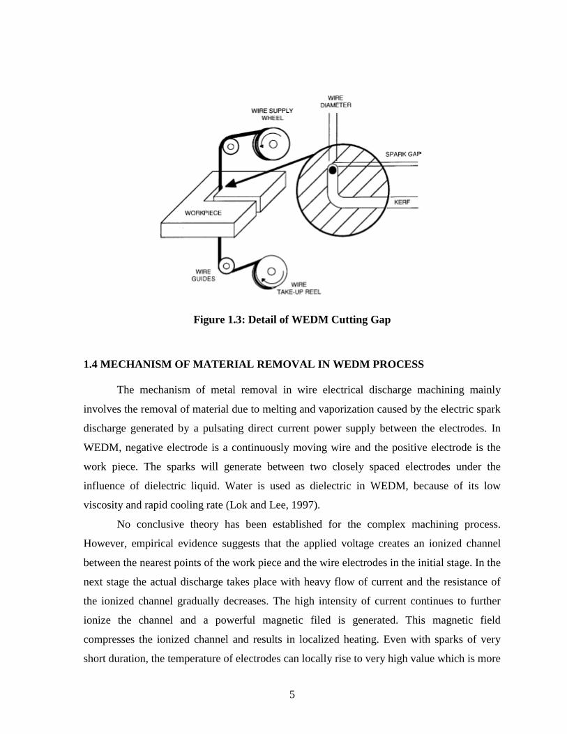
1.3 BASIC PRINCIPLE OF WEDM PROCESS

The WEDM machine tool comprises of a main worktable (X-Y) on which the work

piece is clamped; an auxiliary table (U-V) and wire drive mechanism. The main table moves

along X and Y-axis and it is driven by the D.C servo motors. The travelling wire is

continuously fed from wire feed spool and collected on take up spool which moves though

the work piece and is supported under tension between a pair of wire guides located at the

opposite sides of the work piece. The lower wire guide is stationary where as the upper wire

guide, supported by the U-V table, can be displaced transversely along U and V-axis with

respect to lower wire guide. The upper wire guide can also be positioned vertically along Z-

axis by moving the quill.

A series of electrical pulses generated by the pulse generator unit is applied between

the work piece and the travelling wire electrode, to cause the electro erosion of the work

piece material. As the process proceeds, the X-Y controller displaces the worktable carrying

the work piece transversely along a predetermined path programmed in the controller. While

the machining operation is continuous, the machining zone is continuously flushed with

water passing through the nozzle on both sides of work piece. Since water is used as a

dielectric medium, it is very important that water does not ionize. Therefore, in order to

3

prevent the ionization of water, an ion exchange resin is used in the dielectric distribution

system to maintain the conductivity of water.

In order to produce taper machining, the wire electrode has to be tilted. This is

achieved by displacing the upper wire guide (along U-V axis) with respect to the lower wire

guide. The desired taper angle is achieved by simultaneous control of the movement of X-Y

table and U-V table along their respective predetermined paths stored in the controller. The

path information of X-Y table and U-V table is given to the controller in terms of linear and

circular elements via NC program. Figure 1.1 exhibits the schematic diagram of the basic

principle of WEDM process (Saha et. al., 2004). The complete block diagram of WEDM is

shown in Figure1.2. Figure 1.3 shows the detail of WEDM cutting gap (Tosun et.al., 2004).

Figure 1.1: Schematic Diagram of the Basic Principle of WEDM Process

4

Fig

ure

1.2

: B

lock

Dia

gra

m o

f W

ire-

ED

M

5

Figure 1.3: Detail of WEDM Cutting Gap

1.4 MECHANISM OF MATERIAL REMOVAL IN WEDM PROCESS

The mechanism of metal removal in wire electrical discharge machining mainly

involves the removal of material due to melting and vaporization caused by the electric spark

discharge generated by a pulsating direct current power supply between the electrodes. In

WEDM, negative electrode is a continuously moving wire and the positive electrode is the

work piece. The sparks will generate between two closely spaced electrodes under the

influence of dielectric liquid. Water is used as dielectric in WEDM, because of its low

viscosity and rapid cooling rate (Lok and Lee, 1997).

No conclusive theory has been established for the complex machining process.

However, empirical evidence suggests that the applied voltage creates an ionized channel

between the nearest points of the work piece and the wire electrodes in the initial stage. In the

next stage the actual discharge takes place with heavy flow of current and the resistance of

the ionized channel gradually decreases. The high intensity of current continues to further

ionize the channel and a powerful magnetic filed is generated. This magnetic field

compresses the ionized channel and results in localized heating. Even with sparks of very

short duration, the temperature of electrodes can locally rise to very high value which is more

6

than the melting point of the work material due to transformation of the kinetic energy of

electrons into heat. The high energy density erodes a part of material from both the wire and

work piece by locally melting and vaporizing and thus it is the dominant thermal erosion

process.

1.5 ADVANTAGES OF WEDM PROCESS (Benedict G.F., 1987)

As continuously travelling wire is used as the negative electrode, so electrode

fabrication is not required as in EDM.

There is no direct contact between the work piece and the wire, eliminating the

mechanical stresses during machining.

WEDM process can be applied to all electrically conducting metals and alloys

irrespective of their melting points, hardness, toughness or brittleness.

Users can run their work pieces over night or over the weekend unattended.

1.6 DISADVANTAGES OF WEDM PROCESS (Benedict G.F., 1987)

High capital cost is required for WEDM process.

There is a problem regarding the formation of recast layer.

WEDM process exhibits very slow cutting rate.

It is not applicable to very large work piece.

1.7 APPLICATIONS OF WEDM PROCESS

The present application of WEDM process includes automotive, aerospace, mould,

tool and die making industries. WEDM applications can also be found in the medical,

optical, dental, jewellery industries, and in the automotive and aerospace R & D areas (Ho et.

al., 2004).

The machine‟s ability to operate unattended for hours or even days further increases

the attractiveness of the process. Machining thick sections of material, as thick as 200 mm, in

addition to using computer to accurately scale the size of the part, make this process

especially valuable for the fabrication of dies of various types. The machining of press

stamping dies is simplified because the punch, die, punch plate and stripper, all can be

machined from a common CNC program. Without WEDM, the fabrication process requires

7

many hours of electrodes fabrication for the conventional EDM technique, as well as many

hours of manual grinding and polishing. With WEDM the overall fabrication time is reduced

by 37%, however, the processing time is reduced by 66%. Another popular application for

WEDM is the machining of extrusion dies and dies for powder metal (PM) compaction

(Benedict G.F., 1987).

1.8 STATEMENT OF THE PROBLEM

The present work “Effect of Process Parameters on Performance Measures of Wire

Electrical Discharge Machining” has been undertaken keeping into consideration the

following problems:

It has been long recognized that cutting conditions such as pulse on time, pulse off

time, servo voltage, peak current and other machining parameters should be selected

to optimize the economics of machining operations as assessed by productivity, total

manufacturing cost per component or other suitable criterion.

High cost of numerically controlled machine tools, compared to their conventional

counterparts, has forced us to operate these machines as efficiently as possible in

order to obtain the required payback.

New materials of increasing strengths and capabilities are being developed

continuously and response characteristics are not only dependent on the machining

parameters but also on materials of the work part (Ho et. al., 2004). H-11, hot die

steel is one such material which can be used in applications of extreme loads such as

hot-work forging, extrusion, manufacturing punching tools, mandrels, mechanical

press forging die, plastic mould and die-casting dies, aircraft landing gears, helicopter

rotor blades and shafts, etc. The investigation of optimal machining parameters for H-

11 is thus very essential.

Predicted optimal solutions may not be achieved practically using optimal setting of

machining parameters suggested by any optimization technique. So, all the predicted

optimal solutions should be verified experimentally using suggested combination of

machining parameters.

8

1.9 OBJECTIVES OF THE PRESENT INVESTIGATION

Investigation of the working ranges and levels of the WEDM process parameters

using one factor at a time approach

Experimental determination of the effects of the various process parameters viz pulse

on time, pulse off time, spark gap set voltage, peak current, wire feed and wire

tension on the performance measures like cutting rate, surface roughness, gap current

and dimensional deviation in WEDM process

Optimization of the performance measures using Taguchi method

Modelling of the performance measures using response surface methodology (RSM)

Single response optimization of the process parameters of WEDM process using

RSM and desirability function

Multi-objective optimization of the process parameters of WEDM process using

desirability function in conjunction with RSM

Multi-objective optimization of the process parameters of WEDM process using

Taguchi‟s technique and utility concept

Validation of the results by conducting confirmation experiments

1.10 DIFFERENT PHASES OF EXPERIMENTATION

To accomplish the objectives, present work has been done in five phases

Phase -I

Development of experimental set up providing varying range of input parameters

in WEDM and measuring the various responses on-line and off-line

Investigation of the working ranges and the levels of the WEDM process

parameters (pilot experiments) affecting the selected quality characteristics, by

using one factor at a time approach

Phase –II

Investigation of the effects of WEDM process parameters on quality

characteristics viz. cutting rate, surface roughness, gap current and dimensional

deviation while machining H-11 hot die steel

9

Optimization of quality characteristics of machined parts:

Prediction of optimal sets of WEDM process parameters

Prediction of optimal values of quality characteristics

Prediction of confidence interval (95%CI)

Experimental verification of optimized individual quality characteristics

The Taguchi‟s parameter design approach has been used to obtain the above objectives.

Phase –III

Development of mathematical models and response surfaces of cutting rate,

surface roughness, gap current and dimensional deviation using response surface

methodology

The half fractional second order central composite rotatable design has been used to

plan the experiments and the input parameters like pulse on time, pulse off time, spark gap

set voltage, peak current and wire tension are varied to ascertain their effects on the

responses.

Phase –IV

Development of single response optimization model using Desirability Function

Development of multi objective optimization models using Desirability Function


combinations of quality characteristics


combinations

Phase –V

Development of multi objective optimization models using Taguchi technique and

utility concept


combined quality characteristics

Experimental verification of quality characteristics optimized in different comb

10

CHAPTER 2

LITERATURE SURVEY

2.1 REVIEW OF LITERATURE

WEDM is an essential operation in several manufacturing processes in some

industries, which gives importance to variety, precision and accuracy. Several researchers

have attempted to improve the performance characteristics namely the surface roughness,

cutting speed, dimensional accuracy and material removal rate. But the full potential

utilization of this process is not completely solved because of its complex and stochastic

nature and more number of variables involved in this operation (Spedding and Wang, 1997;

Scott et al., 1991). Scott et. al. (1991) developed mathematical models to predict material

removal rate and surface finish while machining D-2 tool steel at different machining

conditions. It was found that there is no single combination of levels of the different factors

that can be optimal under all circumstances. Tarng et. al. (1995) formulated a neural network

model and simulated annealing algorithm in order to predict and optimize the surface

roughness and cutting velocity of the WEDM process in machining of SUS-304 stainless

steel materials. Spedding and Wang (1997) attempted to model the cutting speed and surface

roughness of EDM process through the response-surface methodology and artificial neural

networks (ANNs). The authors attempted further to optimize the surface roughness, surface

waviness and used the artificial neural networks to predict the process performance. Liao et.

al. (1997) performed an experimental study using SKD11 alloy steel as the workpiece

material and established mathematical models relating the machine performance like MRR,

SR and gap width with various machining parameters and then determined the optimal

parametric settings for WEDM process applying feasible-direction method of non-linear

programming. Spedding and Wang (1997) attempted to optimize the process parametric

combinations by modeling the process using artificial neural networks (ANN) and

characterizing the WEDM machined surface through time series techniques. A feed-forward

back-propagation neural network based on a central composite rotatable experimental design

is developed to model the machining process. Optimal parametric combinations are selected

for the process. The periodic component of the surface texture is identified and an

11

autoregressive AR (3) model is used to describe its stochastic component. Huang et.

al.(1999) investigated experimentally the effect of various machining parameters on the gap

width, SR and the depth of white layer on the machined workpiece (SKD11alloy steel)

surface. They adopted the feasible-direction non-linear programming method for

determination of the optimal process settings. Hsue et. al. (1999) introduced a useful concept

of discharge-angle Cθ and presented a systematic analysis for metal removal rate (MRR) in

corner cutting. Discharge-angle Cθ and MRR dropped drastically to a minimum and then

recovered to the same level of straight-path cutting sluggishly. The amount of the drop at the

corner apex was dependent on the angle of the turning corner. The drastic variation of

sparking frequency in corner cutting could be interpreted as the symptom of the abrupt

change of MRR. The sudden increase of gap-voltage could also be interpreted as the result of

abrupt MRR drop. Murphy and Lin (2000) developed a combined structural-thermal model

using energy balance approach to describe the vibration and stability characteristics of an

EDM wire. High-temperature effects were also included resulting from the energy

discharges. The thermal field was used to determine the induced thermal stresses in the wire.

An equilibrium and eigen value analysis (for small vibrations about the computed

equilibrium) showed that the transport speed influenced the stability of the straight

equilibrium configuration. The wire had an extended residency time in the kerf and the wire

thermally buckled. Yan et. al. (2001) presented a feed forward neural network using a back

propagation learning algorithm for the estimation of the work piece height in WEDM. The

average error of work piece height estimation was 1.6 mm, and the transient response to

change in work piece height was found reasonably satisfactory. The developed hierarchical

adaptive control system enabled the machining stability and the machining speed to be

improved by 15% compared with a commonly used gap voltage control system. Lin et. al.

(2001) proposed a control strategy based on fuzzy logic to improve the machining accuracy.

Multi-variables fuzzy logic controller was designed to determine the reduced percentage of

sparking force. The objective of the total control was to improve the machining accuracy at

corner parts, but still keep the cutting feed rate at fair values. As a result of experiments,

machining errors of corner parts, especially in rough-cutting, could be reduced to less than

50% of those in normal machining, while the machining process time increased not more

than 10% of the normal value. Lin and Lin (2001) reported a new approach for the

12

optimization of the electrical discharge machining (EDM) process with multiple performance

characteristics based on the orthogonal array with the grey relational analysis. Optimal

machining parameters were determined by the grey relational grade obtained from the grey

relational analysis as the performance index. The machining parameters, namely work piece

polarity, pulse on time, duty factor, open discharge voltage, discharge current and dielectric

fluid were optimized with considerations of multiple performance characteristics including

material removal rate, surface roughness, and electrode wear ratio. Liao et. al. (2002) used a

feed-forward neural network with back propagation algorithm to estimate the work piece

height. The developed network could successfully estimate the work piece height. Based on

the on-line estimated work piece height, a rule-based strategy for adaptive parameters setting

was proposed to maintain a stable machining and improve the machining efficiency. Miller et

al. (2003) investigated the effect of spark on-time duration and spark on-time ratio on the

material removal rate (MRR) and surface integrity of four types of advanced material; porous

metal foams, metal bond diamond grinding wheels, sintered Nd-Fe-B magnets and carbon–

carbon bipolar plates. Regression analysis was applied to model the wire EDM MRR.

Scanning electron microscopy (SEM) analysis was used to investigate effect of important

EDM process parameters on surface finish. Machining the metal foams without damaging the

ligaments and the diamond grinding wheel to precise shape was very difficult. Sintered Nd-

Fe-B magnet material was found very brittle and easily chipped by using traditional

machining methods. Carbon–carbon bipolar plate was delicate but could be machined easily

by the EDM. Huang et al. (2003) reported the microstructure analysis for martensitic

stainless steel quenched and then tempered at 600°C. Specimens of the material were

finished with either 4 or 5 cutting passes. Negatively polarized wire electrode (NPWE) was

applied in the first four cutting passes, except the last cutting pass, in which the positively

polarized wire electrode (PPWE) was used. From the results of scanning electron microscopy

(SEM) examination, craters and martensitic grains were registered in the micrograph of the

finished surface machined after the 4th cutting pass. From the results of transmission electron

microscopes TEM-examination, a heat-affected zone (HAZ) of 1.5µm thick was detected in

the surface layer finished with NPWE. Klocke et. al. (2003) tested different electrical

parameters in a series of experiments. The measuring sensor was positioned at the place

where the discharges occurred and was electrically isolated in order to prevent measuring

13

interference. Cutting speed was found to be lower for material containing more number of

electrically non-conductive particles. The idle voltage pulse on-time and the discharge

current had little influence on the crater dimensions. At lower idle voltages the craters

became more elliptical. The discharge forces depended strongly on the electrical parameters

and the machined materials. The forces were linearly proportional to the discharge current

and the idle voltage. Liao and Yu (2003) presented a new concept of specific discharge

energy (SDE), a material property in WEDM. The relative relationship of SDE between

different materials remained fixed as long as the materials were machined under the same

machining conditions. Under steady machining process, the smaller discharge gap resulted in

higher discharge efficiency. The shorter the normal discharge on time, the higher was the

discharge efficiency. Using the characteristics of SDE, determination of parameter settings of

different materials could be greatly simplified. Puri and Bhattacharyya (2003) performed

analysis of wire-tool vibration in order to achieve a high precision and accuracy in WEDM

with the system equation based on the force acting on the wire in a multiple discharge

process. It was clarified from the solution that the wire vibration during machining got

mainly manipulated by the first order mode (n = 1). Also, a high tension without wire rupture

proved always beneficial to reduce the amplitude of wire-tool vibration. Ho and Newman

(2003) reviewed the research work carried out from the inception to the development of die-

sinking EDM within the past decade. It reported on the EDM research relating to improving

performance measures, optimizing the process variables, monitoring and control the sparking

process, simplifying the electrode design and manufacture. A range of EDM applications

were highlighted together with the development of hybrid machining processes. Ebeid et. al.

(2003) designed a knowledge-based system (KBS) to select an optimal setting of process

parameters and diagnose the machining conditions for WEDM. The system allowed a fast

retrieval for information and ease of modification or of appending data. The sample results

for alloy steel 2417 and Al 6061 of the various twelve tested materials were presented in the

form of charts to aid WEDM users for improving the performance of the process. Altpeter

and Perez (2003) carried out a survey on wire modeling and control of WEDM. They found

that the numerous solutions have been proposed in the past for mastering wire slackness but

very little publications deal with issues like vibration damping and amplification of process

randomness. Puri and Bhattacharyya (2003) employed Taguchi methodology involving

14

thirteen control factors with three levels for an orthogonal array L27 (313

) to find out the

main parameters that affect the different machining criteria, such as average cutting speed,

surface roughness values and the geometrical inaccuracy caused due to wire lag. Tosun et. al.

(2003) studied the effect of the cutting parameters on size of erosion craters (diameter and

depth) on wire electrode in WEDM. Brass wire of 0.25 mm diameter and AISI 4140 steel of

0.28 mm thickness were used as tool and work piece materials in the experiments. It was

found that increase in the pulse duration, open circuit voltage and wire speed increases the

crater size, whereas increase in the dielectric flushing pressure decreases the crater size. The

variation of wire crater size with machining parameters was modelled mathematically by

using a power function. The level of importance of the machining parameters on the wire

crater size was determined through analysis of variance (ANOVA). Liao et. al. (2003) used

the modified traditional circuit using low power for ignition for WEDM. With the assistance

of Taguchi quality design, ANOVA and F-test, machining voltage, current-limiting

resistance, type of pulse-generating circuit and capacitance were identified as the significant

parameters affecting the surface roughness in finishing process. It was found that a low

conductivity of dielectric should be incorporated for the discharge spark to take place. After

analyzing the effect of each relevant factor on surface roughness, appropriate values of all

parameters were chosen and a fine surface of roughness Ra = 0.22 µm was achieved. Saha et.

al. (2003) developed a new approach using finite element modeling and optimization

procedures for analyzing the process of wire electro-discharge machining. The results of the

modeling and optimization showed that non uniform heating is the most important variable

affecting the temperature and thermal strains. Tzeng and Chiu (2003) conducted experiments

on castek-03 for medium carbon steel material having excellent wear resistance. The most

important factors affecting the EDM process robustness were pulse on time, applied electric

current in low voltage and sparking current in high voltage. The most important factors

affecting the machining speed were pulse on time and applied electric current in low voltage.

The gain of 13.17 dB was able to decrease the variation range to 21.84%, which improved

process robustness by 4.6 times. Huang and Liao (2003) presented the use of grey relational

and S/N ratio analysis, for determining the optimal parameters setting of WEDM process.

The results showed that the MRR and surface roughness are easily influenced by the table

feed rate and pulse on time. Kuriakose et. al. (2003) carried out experiments with titanium

15

alloy (Ti-6Al-4V) and used a data-mining technique to study the effect of various input

parameters of WEDM process on the cutting speed and SR. They reformulated the WEDM

domain as a classification problem to identify the important decision parameters. In their

approach, however, the optimal process parameters for the multiple responses need to be

decided by the engineers based on judgment. Puri and Bhattacharyya (2003) investigated the

wire lag phenomenon in wire-cut electrical discharge machining process and the trend of

variation of the geometrical inaccuracy caused due to wire lag with various control

parameters. They found that the optimal parametric settings with respect to productivity, SR

and geometrical inaccuracy due to wire lag were different. Lin and Lin (2004) reported the

use of an orthogonal array, grey relational generating, grey relational coefficient, grey-fuzzy

reasoning grade and analysis of variance to study the performance characteristics of the

WEDM machining process. The machining parameters (pulse on time, duty factor and

discharge current) with considerations of multiple responses (electrode wear ratio, material

removal rate and surface roughness) were effective. The grey-fuzzy logic approach helped to

optimize the electrical discharge machining process with multiple process responses. The

process responses such as the electrode wear ratio, material removal rate and surface

roughness in the electrical discharge machining process could be greatly improved. Sarkar et.

al. (2004) performed experimental investigation on single pass cutting of wire electrical

discharge machining of γ-TiAl alloy. The process was successfully modelled using additive

model. Both surface roughness as well as dimensional deviation was independent of the pulse

off time. The process was optimized using constrained optimization and pareto optimization

algorithm. Based on constrained optimization algorithm the WEDM process was optimized

under single constraint as well as multi-constraint condition. By using pareto optimization

algorithm, the 20 pareto optimal solutions were searched out from the set of all 243 outputs.

Ho et. al. (2004) reviewed the vast array of research work carried out from the spin-off from

the EDM process to the development of the WEDM. It reported on the WEDM research

involving the optimization of the process parameters surveying the influence of the various

factors affecting the machining performance and productivity. The paper also highlighted the

adaptive monitoring and control of the process investigating the feasibility of the different

control strategies of obtaining the optimal machining conditions. Tosun et. al. (2004)

investigated the effect and optimization of machining parameters on the kerf (cutting width)

16

and material removal rate (MRR) in wire electrical discharge machining (WEDM)

operations. Based on ANOVA method, the highly effective parameters on both the kerf and

the MRR were found as open circuit voltage and pulse duration, whereas wire speed and

dielectric flushing pressure were less effective factors. The results showed that open circuit

voltage was about three times more important than the pulse duration for controlling the kerf,

whereas open circuit voltage for controlling the MRR was about six times more important

than pulse duration. Yan et. al. (2004) performed experiments on a FANUC W1 CNC wire

electrical discharge machine for cutting both the 10 and 20 vol. % Al2O3 particles reinforced

6061Al alloys-based composite and 6061Al matrix material itself. Results indicated that the

cutting speed (material removal rate), the surface roughness and the width of the slit of

cutting test material significantly depend on volume fraction of reinforcement (Al2O3

particles). Liao and Yu (2004) used specific discharge energy (SDE) concept in WEDM.

Experimental results revealed that the relative relationship of SDE between different

materials is invariant as long as all materials are machined under the same machining

conditions. By means of dimensional analysis of SDE, a quantitative relationship between the

machining parameters and gap width in WEDM was obtained. Under the same machining

conditions, the surface finish improved when there was a greater SDE and vice versa. Manna

and Bhattacharyya (2004) performed experiments using a typical four-axes Electronica

Supercut-734 CNC-wire cut EDM machine on aluminium-reinforced silicon carbide metal

matrix composite Al/SiCMMC. Open gap voltage and pulse on period are the most

significant machining parameters, for controlling the metal removal rate. The open gap

voltage affected the cutting speed significantly. Wire tension and wire feed rate were the

most significant machining parameters, for the surface roughness. Wire tension and spark

gap voltage setting were the most significant for controlling spark gap. Tosun et. al. (2004)

modelled the variation of response variables with the machining parameters in WEDM using

regression analysis method and then applied simulated annealing approach searching for

determination of the machining parameters that can simultaneously optimize all the

performance measures, e.g. kerf and MRR. Ozdemir and Ozek (2005) investigated the

machinability of standard GGG40 nodular cast iron by A300 Fine Sodick Mark XI WEDM

using different parameters. The increase in surface roughness and cutting rate clearly

followed the trend indicated with increasing discharge energy as a result of an increase in

17

current and pulse on time, because the increased discharge energy produced larger and

deeper discharge craters. Three zones were identified in rough regimes of machining for all

samples: decarburized layer, heat affected layer, and bulk metal. Miller et. al. (2005)

investigated effects of spark cycle and pulse on-time on wire EDM micro features. Tests

were conducted on various materials viz. Nd–Fe–B magnetic material, carbon bipolar plate,

and titanium for wire EDM cutting of minimum cross section thickness. A hypothesis was

proposed based on the combined thermal and electrostatic force to cause the fracture of thin-

section during wire EDM. This was supported by findings from SEM micrographs of EDM

surface, subsurface and debris. Sarkar et. al. (2005) developed a feed forward back-

propagation neural network to model WEDM machining process. A feed forward neural

network of type 6-15-3 was adopted to model the process. Twenty-seven such optimal

parametric combinations were identified out of 15625 combinations. The three most

important measures of the process performance parameters –cutting speed, surface roughness

and wire offset were considered. The model was capable of predicting the response

parameters as a function of six different control parameters, i.e. pulse on time, pulse off

time, peak current, wire tension, dielectric flow rate and servo reference voltage. It was

observed that the surface quality decreased as the cutting speed increased and it varies almost

linearly up to a surface roughness value of 2.44 μm and a cutting speed of 2.65 mm/min.

Beyond this value of cutting speed, surface roughness deteriorated drastically. Kuriakose and

Shunmugam (2005) used a multiple regression model to represent relationship between input

and output variables and a multi-objective optimization method based on a non-dominated

sorting genetic algorithm (NSGA) is used to optimize wire-EDM process. The sorting

procedure employs a fitness assignment scheme which prefers non dominated solutions and

uses a sharing strategy which reserves diversity among the solutions. Also, none of the

solutions in the pareto-optimal set was better than any other solution in the set.

Ramakrishnan and Karunamoorthy (2005) described the multi objective optimization of the

WEDM process using parametric design of Taguchi methodology. The effect of various

machining parameters such as pulse on time, wire tension, delay time, wire feed speed, and

ignition current intensity has been studied in machining of heat-treated tool steel. It was

identified that the pulse on time and ignition current intensity has influence more than the

other parameters. Moreover, the multiple performance characteristics such as material

18

removal rate, surface roughness, and wire wear ratio for the WEDM process could be

improved by setting the various process parameters at their optimal levels. Sarkar et. al.

(2005) performed experiments using γ-titanium aluminide alloy as work material and then

formulated mathematical models to predict the cutting speed, surface finish and dimensional

deviation as the function of different control parameters. They determined the optimal

process parameters by applying constrained optimization technique in which one

performance characteristic was optimized considering others as constraints. Kuriakose and

Shunmugam (2005) used titanium alloy (Ti-6Al-4V) as the work material and conducted

experiments based on Taguchi‟s L-18 orthogonal array. Then they employed the non-

dominated sorting genetic algorithm to determine the optimal process parameters that would

optimize the cutting velocity and SR of WEDM process. Chiang and Chang (2006) presented

an approach for the optimization of the WEDM process of Al2O3 particle reinforced material

with two performance characteristics, e.g. SR and MRR, based on the grey relational

analysis. Ramakrishnan and Karunamoorthy (2006) considered three response characteristics,

e.g. MRR, SR and wire wear ratio (WWR) for a WEDM process and determined the optimal

process settings by optimization of multiple response signal-to-noise (MRSN) ratio, which is

the logarithmic transformation of the sum of the weighted normalized quality loss of

individual response variable. Manna and Bhattacharyya (2006) established mathematical

models relating to the machining performance criteria like MRR, SR, spark gap and gap

current using the Gauss elimination method for effective machining of Al/SiC-MMC.

Mahapatra and Patnaik (2006) conducted experiments on ROBOFIL 100 high precision 5

axis CNC WEDM to find the relationship between control factors and responses like MRR,

SF and kerf by means of nonlinear regression analysis. Genetic algorithm was employed to

optimize the wire electrical discharge machining process with multiple objectives. The error

associated with MRR, SF, and kerf were 3.14%, 1.95%, and 3.72%, respectively. The

optimum search of machining parameter values for maximizing MRR and SF and

minimizing kerf was formulated as a multi-objective, multivariable, non-linear optimization

problem. Hargrove and Ding (2006) applied finite element method (FEM) to determine work

piece temperature for different cutting parameters. They investigated the effect of WEDM

parameters such as discharge voltage and pulse on-time on the damaged layer thickness of a

machined work piece using low carbon steel (AISI 4340) as the cutting material. The

19

thickness of the temperature affected layers for different cutting parameters was computed

based on a critical temperature value. Through minimizing the thickness of the temperature

affected layers and satisfying a certain cutting speed, a set of the cutting process parameters

was determined for work piece manufacture. A set of optimum parameters for this machining

process was selected such that the condition of machine cutting speed was 1.2 mm/min, on

time pulse was 8 μs and no load voltage was 4 volt. The analyzed results had a good

agreement with testing results. Han et al (2006) conducted experiments on WEDM EU64 to

machine alloy steel (Cr12) having thickness of 40 mm. It was reported that the surface finish

improved by decreasing pulse duration and discharge current. Mahapatra and Patnaik (2007)

developed relationships between various process parameters and responses like MRR, SR

and kerf by means of non-linear regression analysis and then employed genetic algorithm to

optimize the WEDM process with multiple objectives. Saha et. al. (2007) developed a second

order multi-variable regression model and a feed-forward back-propagation neural network

(BPNN) model to correlate the input process parameters, such as pulse on-time, pulse off

time, peak current and capacitance with the performance measures namely, cutting speed and

surface roughness in wire electro- discharge machining (WEDM) of tungsten carbide-cobalt

(WC-Co) composite material. 4-11-2 neural network architecture provides the best prediction

capability with 3.29% overall mean prediction error, while 6.02% error was revealed by

regression model. Li et. al. (2007) developed a model of WEDM with higher forecast

precision and generalization ability which combined modeling function of fuzzy inference

with the learning ability of artificial neural network and a set of rules were generated directly

from the experimental data. The process relation expressed by the neural-fuzzy inference

model was used directly as the fitness function and was embedded in GA to be optimised,

and then the automatic optimization of the wire electrical discharge machining was realized.

Sarkar et. al. (2007) performed experimental investigation on trim cutting of wire electrical

discharge machining of γ-TiAl alloy. The process was successfully modelled using RSM and

model adequacy checking was also carried out. WEDM process was optimized using Minitab

(statistical software package) which generally makes use of the desirability function

approach. But it was observed that lot of trial and error and manual tuning was required to

obtain the true optimal solution. By using developed computer program based upon pareto

optimization algorithm, the 33 pareto-optimal solutions were searched out from the set of all

20

6561 outputs. It was observed that the developed pareto optimization strategy eliminates the

guess work. It was also seen that the surface quality decreases as the cutting speed increases

and varies almost linearly up to surface roughness value of 1.22 µm and cutting speed of

13.88 mm/min. Beyond this value of cutting speed, surface roughness deteriorates

drastically. Kanlayasiri and Boonmung (2007) investigated influences of wire-EDM

machining variables on surface roughness of newly developed DC 53 die steel of width,

length, and thickness 27, 65 and 13 mm, respectively. The machining variables included

pulse-on time, pulse-off time, pulse-peak current, and wire tension. The variables affecting

the surface roughness were identified using ANOVA technique. Results showed that pulse-

on time and pulse-peak current were significant variables to the surface roughness of wire-

EDMed DC53 die steel. The maximum prediction error of the model was less than 7% and

the average percentage error of prediction was less than 3%. Ramakrishnan and

Karunamoorthy (2008) developed artificial neural network (ANN) models and multi

response optimization technique to predict and select the best cutting parameters of wire

electro-discharge machining (WEDM) process. Inconel 718 was selected as work material to

conduct experiments and brass wire of 0.25mm diameter was used as tool electrode.

Experiments were planned as per Taguchi‟s L-9 orthogonal array. Experiments were

performed under different cutting conditions of pulse on time, delay time, wire feed speed

and ignition current. It was found that the pulse on time, delay time and ignition current had

more influence than wire feed speed on the performance characteristics considered in the

study. An MRR was improved with increase in pulse on time and ignition current. But the

surface quality of the work specimen was affected adversely with increased value of pulse on

time and ignition current. Gauri and Chakraborty (2008) suggested a modified approach of

the principal component analysis (PCA) based procedure for multi-response optimization.

Analysis was done data on experimental data on WEDM processes obtained by the past

researchers i.e. on γ-titanium aluminized alloy with the settings of six controllable factors.

Quality characteristics were material removal rate (MRR) (larger the better type), surface

roughness (SR) (smaller the better type) and wire wear ratio (WWR) (smaller the better

type). Rao and Sarcar (2009) analyzed the effects of process parameters on machining

characteristics for CNC WEDM for brass work pieces of varying thickness. Mathematical

relations were obtained for cutting speed, spark gap and MRR. Pradhan et. al. (2009)

21

optimized micro-EDM process parameters for machining Ti-6Al-4V super alloy. The

influence of machining process parameters such as peak current, pulse-on-time, dielectric

flushing pressure and duty ratio on performance criteria like MRR, TWR, over cut and taper

have been examined. Manna and Kumar (2009) investigated the effects of various cutting

parameters of WEDM on wire crater depth, electrode wear rate and surface roughness using

Taguchi methods based on L-18 mixed orthogonal array.

2.2 IDENTIFIED GAPS IN THE LITERATURE

After a comprehensive study of the existing literature, a number of gaps have been

observed in machining of WEDM.

Most of the researchers have investigated influence of a limited number of

process parameters on the performance measures of WEDMed parts.

Literature review reveals that the researchers have carried out most of the work on

WEDM developments, monitoring and control but very limited work has been

reported on optimization of process variables.

The effect of machining parameters on hot working tool steel (H-11) has not been

fully explored using WEDM with brass wire as electrode.

Multi-response optimization of WEDM process is another thrust area which has

been given less attention in past studies.

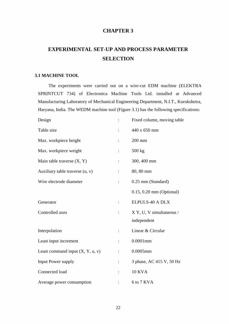
22

CHAPTER 3

EXPERIMENTAL SET-UP AND PROCESS PARAMETER

SELECTION

3.1 MACHINE TOOL

The experiments were carried out on a wire-cut EDM machine (ELEKTRA

SPRINTCUT 734) of Electronica Machine Tools Ltd. installed at Advanced

Manufacturing Laboratory of Mechanical Engineering Department, N.I.T., Kurukshetra,

Haryana, India. The WEDM machine tool (Figure 3.1) has the following specifications:

Design : Fixed column, moving table

Table size : 440 x 650 mm

Max. workpiece height : 200 mm

Max. workpiece weight : 500 kg

Main table traverse (X, Y) : 300, 400 mm

Auxiliary table traverse (u, v) : 80, 80 mm

Wire electrode diameter : 0.25 mm (Standard)

0.15, 0.20 mm (Optional)

Generator : ELPULS-40 A DLX

Controlled axes : X Y, U, V simultaneous /

independent

Interpolation : Linear & Circular

Least input increment : 0.0001mm

Least command input (X, Y, u, v) : 0.0005mm

Input Power supply : 3 phase, AC 415 V, 50 Hz

Connected load : 10 KVA

Average power consumption : 6 to 7 KVA

23

Figure 3.1: Pictorial View of WEDM Machine Tool

3.2 WORK PIECE MATERIAL

The H-11 hot die steel plate of 125mm x 100mm x 24mm size has been used as a

work piece material for the present experiments. H-11 is special hot-worked chromium

tool-steel with good hardness and toughness properties. It is used for extreme load

conditions such as hot-work forging, extrusion etc. It has varied practical applications

such as manufacturing of punching tools, mandrels, mechanical press forging die, plastic

mould and die-casting dies, aircraft landing gears, helicopter rotor blades and shafts. The

working life and dimensional accuracy of H-11 steel dies and tools can be improved with

suitable heat treatment. The H-11 die steel plate blank has been heated to a temperature of

10250C with half an hour soak time followed by quenching in a 500

0C hot salt bath. It is

then tempered in three cycles with maximum temperature of 5500C and 2 hours of soak

time to obtain a final hardness of 55 HRC. The chemical composition of this material as

obtained by EDAX (Electro Dispersive X-ray Spectroscopy) test is given in Table 3.1.

DISPLAY SCREEN

KEYBOARD

POWER ON/OFF

WORK TANK

WIRE FEED SPOOL

WORK HEAD

24

LOWER NOZZLE

UPPER NOZZLE

WORK-PIECE

Table 3.1: Chemical Composition of the Material

Constituent C Si Mn P S Cr Mo V

%

Composition 0.33 0.53 0.27 0.012 0.027 5.30 1.40 0.53

3.3 PREPARATION OF SPECIMENS

The H-11 hot die steel plate of 125mm x 100mm x 24mm size is mounted on the

ELECTRONICA SPRINTCUT WEDM machine tool (Figure 3.1) and specimens of

5mmx5mmx24mm size are cut. The close up view of plate blank used for cutting the

specimens is shown mounted on the WEDM machine (Figure 3.2). A set of cut specimens

is shown in Figures 3.3a and 3.3b.

Figure 3.2: Plate Material Blank Mounted on WEDM Machine

25

Figure 3.3a: The Specimens Shown

Lying Horizontally.

Figure 3.3b: The Specimens Shown

Lying Vertically.

3.4 MEASUREMENT OF EXPERIMENTAL PARAMETERS

The discussions related to the measurement of WEDM experimental parameters e.g.

cutting rate, surface roughness, gap current and dimensional accuracy, are presented in

the following subsections.

3.4.1 Cutting Rate

For WEDM, cutting rate is a desirable characteristic and it should be as high as

possible to give least machine cycle time leading to increased productivity. In the present

study cutting rate is a measure of job cutting which is digitally displayed on the screen of

the machine and is given quantitatively in mm/min (Figure 3.4).

3.4.2 Gap Current

In WEDM machining the specimen is mounted on the machine and during the

process of cutting a small amount of gap is maintained between the job and the electrode

wire. To initiate the cutting a pulse of current is given by the pulse generator and the

current passes through the material being cut which is measured and named as gap

current. The gap current is read on an ammeter, which is an integral part of the machine,

in amperes and is shown in Figure 3.4.

26

3.4.3 Surface Roughness

Roughness is often a good predictor of the performance of a mechanical

component, since irregularities in the surface may form nucleation sites for cracks or

corrosion. Roughness is a measure of the texture of a surface. It is quantified by the

vertical deviations of a real surface from its ideal form. If these deviations are large, the

surface is rough; if small, the surface is smooth. Roughness is typically considered to be

the high frequency, short wavelength component of a measured surface.

Figure 3.4: Set Up for Cutting Rate and Gap Current Measurement

The parameter mostly used for general surface roughness is Ra. It measures average

roughness by comparing all the peaks and valleys to the mean line, and then averaging

them all over the entire cut-off length. Cut-off length is the length that the stylus is

KEYBOARD

ON/OFF SWITCH AMMETER

(GAP CURRENT)

DISPLAY

CUTTING RATE

http://en.wikipedia.org/wiki/Surface

27

dragged across the surface; a longer cut-off length will give a more average value, and a

shorter cut-off length might give a less accurate result over a shorter stretch of surface.

In this work the surface roughness was measured by Mitutoyo surftest SJ-201P

(Figure 3.5). The surftest is a shop–floor type surface-roughness measuring instrument,

which traces the surface of various machine parts and calculates the surface roughness

based on roughness standards, and displays the results in µm. The work piece is attached

to the detector unit of the SJ-201P which traces the minute irregularities of the work piece

surface. The vertical stylus displacement during the trace is processed and digitally

displayed on the liquid crystal display of the SJ-201P. The surf test has a resolution

varying from .01 µm to 0.4 µm depending on the measurement range.

Figure 3.5: Set Up for Surface Roughness Measurement

3.4.4 Dimensional Deviation

The specimen cross-section is measured with the help of a Mitutoyo‟s digital

micrometer having the least count of 0.001 mm and the deviation of the measured

dimension is calculated in percentage using the following expression:

(3.1)

The set up for the measurement of dimensions is shown in Figure 3.6.

WORK PIECE

DISPLAY

WORK TABLE

PARAMETER CONTROL

PROBE / STYLUS

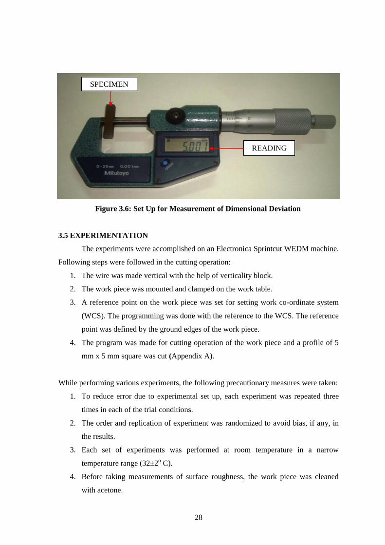
28

Figure 3.6: Set Up for Measurement of Dimensional Deviation

3.5 EXPERIMENTATION

The experiments were accomplished on an Electronica Sprintcut WEDM machine.

Following steps were followed in the cutting operation:

1. The wire was made vertical with the help of verticality block.

2. The work piece was mounted and clamped on the work table.

3. A reference point on the work piece was set for setting work co-ordinate system

(WCS). The programming was done with the reference to the WCS. The reference

point was defined by the ground edges of the work piece.

4. The program was made for cutting operation of the work piece and a profile of 5

mm x 5 mm square was cut (Appendix A).

While performing various experiments, the following precautionary measures were taken:

1. To reduce error due to experimental set up, each experiment was repeated three

times in each of the trial conditions.

2. The order and replication of experiment was randomized to avoid bias, if any, in

the results.

3. Each set of experiments was performed at room temperature in a narrow

temperature range (32±2o C).

4. Before taking measurements of surface roughness, the work piece was cleaned

with acetone.

SPECIMEN

READING

29

3.6 SELECTION OF PROCESS PARAMETERS

In order to identify the process parameters that may affect the machining

characteristics of WEDM machined parts an Ishikawa cause and effect diagram was

constructed and is shown in Figure 3.7.

Figure 3.7: Ishikawa Cause and Effect Diagram for WEDM Process

The input process parameters and output characteristics selected from Ishikawa

cause and effect diagram for the present work are shown in Figure 3.8.

3.6.1 Pulse on Time

The pulse on time is referred as Ton and it represents the duration of time in micro

seconds, µs, for which the current is flowing in each cycle (Figure 3.9). During this time

the voltage, VP, is applied across the electrodes. The Ton setting time range available on

the machine tool is 100-131 which is applied in steps of 1 unit. The equivalent time

setting in micro seconds is given in Table B.1 (Appendix B). The single pulse discharge

energy increases with increasing Ton period, resulting in higher cutting rate. With higher

values of Ton, however, surface roughness tends to be higher. The higher value of

discharge energy may also cause wire breakage.

Dielectric flow rate

(WP)

Wire Tension (WT)

ELECTRODE PARAMETERS

Pulse off Time (Toff)

Servo Feed (SF)

Wire Feed rate (WF)

Conductivity of dielectric (S)

Pulse on Time

(Ton)

Gap Voltage (VP)

Material

Height

WEDM

Performance

Meseaures

(CR, SR, IG, DD)

WORK PIECE

Wire Size

Wire Material

NON ELECTRICAL PARAMETERS

Spark gap set voltage (SV)

ELECTRICAL PARAMETERS

Peak Current (IP)

30

WEDM PROCESS

PROCESS

PARAMETERS

PERFORMANCE

MEASURES

PULSE ON TIME

PULSE OFF TIME

WIRE TENSION

WIRE FEED

PEAK CURRENT

SPARK GAP SET

VOLTAGE

CUTTING RATE

DIMENSIONAL

DEVIATION

GAP CURRENT

SURFACE ROUGHNESS

Figure 3.8: Process Parameters and Performance Measures of WEDM

3.6.2 Pulse off Time

The pulse off time is referred as Toff and it represents the duration of time in

micro seconds, µs, between the two simultaneous sparks (Figure 3.9). The voltage is

absent during this part of the cycle. The Toff setting time range available on the machine

tool is 00 - 63 which is applied in steps of 1 unit. The equivalent time setting in micro

seconds is given in Table B.2 (Appendix B). With a lower value of Toff, there are more

number of discharges in a given time, resulting in increase in the sparking efficiency. As

a result, the cutting rate also increases. Using very low values of Toff period, however,

may cause wire breakage which in turn reduces the cutting efficiency. As and when the

discharge conditions become unstable, one can increase the Toff period. This will allow

lower pulse duty factor and will reduce the average gap current.

31

Figure 3.9: Series of Electrical Pulses at the Inter Electrode Gap

3.6.3 Peak Current

The peak current is represented by IP and it is the maximum value of the current

passing through the electrodes for the given pulse. The IP setting current range available

on the present WEDM machine is 10–230 ampere which is applied in steps of 10 ampere.

Increase in the IP value will increase the pulse discharge energy which in turn can

improve the cutting rate further. For higher value of IP, gap conditions may become

unstable with improper combination of Ton, Toff, SV & SF settings. As and when the

discharge conditions become unstable one must reduce the IP value (Tarng et. al.,

(1994)).

3.6.4 Spark Gap Set Voltage

The spark gap set voltage is a reference voltage for the actual gap between the

work piece and the wire used for cutting. The SV voltage range available on the present

machine is 00 - 99 volt and is applied in steps of 1volt.

3.6.5 Wire Feed

Wire feed is the rate at which the wire-electrode travels along the wire guide path

and is fed continuously for sparking. The wire feed range available on the present WEDM

machine is 1–15 m/min in steps of 1m/min. It is always desirable to set the wire feed to

maximum. This will result in less wire breakage, better machining stability and slightly

more cutting speed.

3.6.6 Wire Tension

Wire tension determines how much the wire is to be stretched between upper and

lower wire guides. This is a gram-equivalent load with which the continuously fed wire is

kept under tension so that it remains straight between the wire guides. More the thickness

32

of job more is the tension required. Improper setting of tension may result in the job

inaccuracies as well as wire breakage. The wire tension range available on the machine is

1-15 units in steps of 1. The gram equivalent load and the machine setting units are

reported in Table B.3 (Appendix B).

3.6.7 Pulse Peak Voltage

Pulse peak voltage setting is for selection of open gap voltage. Increase in the VP

value will increase the pulse discharge energy which in turn can improve the cutting rate.

The pulse peak voltage setting range available on the machine is either 1 or 2 .Normally it

is selected at value 2.

3.6.8 Flushing Pressure

Flushing Pressure is for selection of flushing input pressure of the dielectric. The

flushing pressure range on this machine is either 1 (High) or 0 (low). High input pressure

of water dielectric is necessary for cutting with higher values of pulse power and also

while cutting the work piece of more thickness. Low input pressure is used for thin work

piece and in trim cuts.

3.6.9 Servo Feed

Servo feed setting decides the servo speed; the servo speed, at the set value of SF,

can vary in proportion with the gap voltage (normal feed mode) or can be held constant

while machining (with constant feed mode).

The ranges of process parameters for the experiments were decided on the basis of

literature survey and the pilot experiments conducted using one factor at a time approach

(OFAT). Results of the pilot experiments are given in subsequent sections.

3.7 PILOT EXPERIMENTS

The purpose of the pilot experiments is to study the variations of the WEDM

process parameters on performance measures such as cutting rate, surface roughness, gap

current and dimensional deviation. Also, it is intended to ascertain the range of different

parameters required for the two types of experimental design methodology used in this

work.

The pilot experiments were performed on ELEKTRA SPRINTCUT 734 WEDM

machine (Figure 3.1). Various input parameters varied during the experimentation are

33

pulse on time (Ton), pulse off time (Toff), servo voltage (SV), peak current (IP), wire

feed (WF) and wire tension (WT). The effects of these input parameters are studied on

cutting rate, surface roughness, gap current and dimensional deviation using one factor at

a time approach.

Apart from the parameters mentioned above following parameters were kept

constant at a fixed value during the experiments:

8. Work Material : Hot Die Steel, H-11

9. Cutting Tool : Brass wire of diameter 0.25 mm

10. Servo Feed : 2050 unit

11. Flushing Pressure : 1 unit (15 kg/cm2)

12. Peak Voltage : 2 unit (110 volt DC)

13. Conductivity of Dielectric : 20 mho

14. Work Piece Height : 24 mm

Cutting rate in mm/min and gap current in ampere were directly noted from

machine‟s control panel. Surface roughness measurements in µm were repeated three

times using a Mitutoyo‟s surftest, a portable surface roughness tester and the average

value was considered as surface roughness value for the analysis purpose. The

dimensions of the samples, cut from the material blank, were measured by a Mitutoyo‟s

digital micrometer having a least count of 0.001mm. Dimensional deviation was

calculated in percentage using Equation 3.1 as given below:

3.7.1 Effect of Pulse on Time on Performance Measures

The pulse on time (Ton) is varied from 105 unit to 129 unit in steps of 3 units. The

values of the other parameters are kept constant and their values are given as Toff = 51

unit; IP = 230 ampere; WF = 8 m/min; WT = 8 unit; SV = 20 volt; SF = 2050 unit. The

experimentally observed data for the response characteristics for different values of pulse

on time is given in Table 3.2. Figure 3.10 shows the scatter plots of pulse on time versus

response characteristics. The cutting rate increases with the increase in the pulse on time

in a practically straight line fashion and is shown plotted in Figure 3.10a.The value of

surface roughness though increases with increase in pulse on time but rather with a little

34

wavy pattern and is shown in Figure 3.10b. Whereas the value of the gap current with

pulse on time shows initially a wavy pattern but ends up finally into a straight line pattern

(Figure 3.10.c). The dimensional deviation shows an irregular pattern. It increases first

with pulse on time initially for few machine units of pulse on time and then settles into a

decreasing pattern with increase in pulse on time (Figure 3.10.d). These findings are in

agreement with Tarng et. al. (1994), Hascalyk and Cayda (2004), Hang et.al. (2007),

Kanlayasiri and Boonmung (2007) and Ramakrishnan and Karunamoorthy (2008).

Table 3.2: Performance Measures for Pulse on Time

S. No.

Pulse on

Time

(machine unit)

Cutting

Rate

(mm/min)

Surface

Roughness

(µm)

Gap

Current

(ampere)

Dimensional

Deviation

(%)

1 105 0.34 1.33 0.8 0.0033

2 108 0.65 1.59 1 0.0490

3 111 0.94 2.11 1.8 0.0507

4 114 1.26 2.46 2.2 0.0477

5 117 1.57 2.53 2.92 0.0430

6 120 1.96 2.64 3.8 0.0397

7 123 2.25 3.05 4.6 0.0367

8 126 2.63 3.15 5.5 0.0333

3.7.2 Effect of Pulse off Time on Performance Measures

The pulse off time (Toff) is varied from 63 unit to 39 unit with a decrement of 3

units. The values of the other parameters are kept constant and their values are given as

Ton = 114 unit; IP = 230 ampere; WF = 8 m/min; WT = 8 unit; SV = 20 Volt; SF = 2050

unit. The experimentally observed data for the performance parameters for a given value

of pulse off time is given in Table 3.3. Figure 3.11 shows the scatter plots of pulse off

time versus response characteristics. The cutting rate decreases with the increase in the

pulse off time in a practically straight line fashion and is shown plotted in Figure 3.11a

which is in agreement with the findings of Tarng et. al. (1994), Hascalyk and Caydas

(2004) and Kern (2007). The average value of surface roughness is little higher for pulse

off value from 36 unit to 42 unit and then remains practically constant (Figure 3.11b).

The values of the gap current with pulse off time show a decreasing trend with an

35

129126123120117114111108105102

3.0

2.5

2.0

1.5

1.0

0.5

0.0129126123120117114111108105102

3.5

3.0

2.5

2.0

1.5

1.0

0.5

0.0

129126123120117114111108105102

6

5

4

3

2

1

0129126123120117114111108105102

0.100

0.075

0.050

0.025

0.000

(a) Cutting Rate (b) Surface Roughness

(c) Gap Current (d) Dimensional Deviation

Pulse on Time Pulse on Time

Pulse on Time Pulse on Time

Figure 3.10: Scatter Plots of Pulse on Time vs. Response Characteristics

6663605754514845423936

3.0

2.5

2.0

1.5

1.0

0.5

0.0

6663605754514845423936

3.5

3.0

2.5

2.0

1.5

1.0

0.5

0.0

6663605754514845423936

6

5

4

3

2

1

0

6663605754514845423936

0.100

0.075

0.050

0.025

0.000



Pulse off Time Pulse off Time

Pulse off Time Pulse off Time

Figure 3.11: Scatter Plots of Pulse off Time vs. Response Characteristics

36

increase of pulse off time (Figure 3.11c). The dimensional deviation though shows an

irregular pattern but it remains practically constant with increase in pulse off time (Figure

3.11d). This is in agreement with Scott et. al. (1991), Tarng et. al. (1994), Hascalyk and

Caydas (2004), Manna and Bhattacharyya (2006), Kern (2007) and Ramakrishnan and

Karunamoorthy (2008).

3.7.3 Effect of Spark Gap Set Voltage on Performance Measures

The spark gap set voltage is varied from 5 volt to 80 volt in the increments of 15

volt. The values of the other parameters are kept constant and their values are given as

Ton = 114 unit; Toff = 51 unit; WF = 8 m/min; IP = 230 ampere; WT = 8 unit; SF = 2050

unit. The experimentally observed data for the performance measures for different values

of SV is given in Table 3.4. Figure 3.12 shows the scatter plots of spark gap set voltage

versus response characteristics. The cutting rate, surface roughness, and gap current

decrease linearly with increase in spark gap set voltage (Figures 3.12a-3.12c).The

dimensional deviation also decreases with wavy trend with increase in spark gap set

voltage (Figure 3.12d). This is in agreement with Tarng et. al. (1994).

Table 3.3: Performance Measures for Pulse off Time

S. No.

Pulse off

Time

(machine unit)

Cutting

Rate

(mm/min)

Surface

Roughness

(µm)

Gap

Current

(ampere)

Dimensional

Deviation

(%)

1. 63 0.69 2.33 1.4 0.0447

2. 60 0.78 2.32 1.5 0.0433

3. 57 0.88 2.2 1.8 0.0453

4. 54 1.06 2.36 2 0.0447

5. 51 1.23 2.36 2.2 0.0460

6. 48 1.5 2.31 2.7 0.0497

7. 45 1.87 2.34 3.35 0.0443

8. 42 2.13 2.67 3.75 0.0523

9. 39 2.31 2.554 4.2 0.0480

37

Table 3.4: Performance Measures for Spark Gap Set Voltage

S. No.

Spark Gap

Set Voltage

(volt)

Cutting

Rate

(mm/min)

Surface

Roughness

(µm)

Gap

Current

(ampere)

Dimensional

Deviation

(%)

1. 5 1.49 2.54 2.5 0.0647

2. 20 1.24 2.36 2.2 0.0460

3. 35 1.01 2.16 1.95 0.0423

4. 50 0.75 2 1.55 0.0317

5. 65 0.56 1.89 1.25 0.0263

6. 80 0.36 1.82 1 0.0213

95806550352050

3.0

2.5

2.0

1.5

1.0

0.5

0.095806550352050

3.5

3.0

2.5

2.0

1.5

1.0

0.5

0.0

95806550352050

6

5

4

3

2

1

095806550352050

0.100

0.075

0.050

0.025

0.000



Figure 3.12: Scatter Plots of Spark Gap Set Voltage vs. Response Characteristics

Spark Gap Set Voltage Spark Gap Set Voltage

Spark Gap Set Voltage Spark Gap Set Voltage

38

3.7.4 Effect of Peak Current on Performance Measures

The peak current is varied from 230 ampere to 50 ampere in the decrements of 30

ampere. The values of the other parameters are kept constant and their values are given as

Ton = 114 unit; Toff = 51 unit; WF = 8 m/min; SV = 20 volt; WT = 8 unit; SF = 2050

unit. The experimentally observed data for the performance measures for different values

of peak current is given in Table 3.5.

Figure 3.13 shows the scatter plots of peak current versus response characteristics.

The cutting rate first increases then rate of increase decreases and again increases with

almost same rate with increase in peak current (Figure 3.13a). The surface roughness

value increases first with increase in peak current and thereby levels off with increase in

peak current (Figure 3.13b). These results tally with those of Tarng et. al. (1994). and

Rozenek et. al. (2001). The gap current first increases with peak current and then remains

practically constant with wavy nature with further increase in peak current (Figure 3.13c).

The dimensional deviation has a slightly decreasing trend with wavy nature with increase

in peak current (Figure 3.13d).

Table 3.5: Performance Measures for Peak Current

S. No.

Peak

Current

(ampere)

Cutting

Rate

(mm/min)

Surface

Roughness

(µm)

Gap

Current

(ampere)

Dimensional

Deviation

(%)

1. 230 1.26 2.36 2.2 0.046

2. 200 1.16 2.38 2.15 0.0507

3. 170 1.08 2.46 1.9 0.055

4. 140 1.03 2.51 2 0.054

5. 110 0.95 2.44 1.95 0.0587

6. 80 0.8 2.25 1.8 0.0597

7. 50 0.52 1.59 1.3 0.0563

39

260230200170140110805020

3.0

2.5

2.0

1.5

1.0

0.5

0.0260230200170140110805020

3.5

3.0

2.5

2.0

1.5

1.0

0.5

0.0

260230200170140110805020

6

5

4

3

2

1

0

260230200170140110805020

0.100

0.075

0.050

0.025

0.000



Peak Current Peak Current

Peak Current Peak Current

Figure 3.13: Scatter Plots of Peak Current vs. Response Characteristics

3.7.5 Effect of Wire Feed on Performance Measures

The wire feed is varied from 2 m/min to 12 m/min in the steps of 2m/min.The

values of the other parameters are kept constant and their values are given as Ton = 114

unit; Toff = 51 unit; IP = 230 ampere; SV = 20 volt; WT = 8 unit; SF = 2050 unit.

The experimentally observed data for the performance measures for different

values of wire feed is given in Table 3.6.

Table 3.6: Performance Measures for Wire Feed

S. No.

Wire

Feed

(m/min)

Cutting

Rate

(mm/min)

Surface

Roughness

(µm)

Gap

Current

(ampere)

Dimensional

Deviation

(%)

1. 2 1.25 2.33 2.2 0.0513

2. 4 1.27 2.32 2.2 0.0480

3. 6 1.24 2.41 2.2 0.0483

4. 8 1.26 2.36 2.2 0.0460

5. 10 1.27 2.48 2.2 0.0473

6. 12 1.24 2.31 2.2 0.0493

40

Figure 3.14 shows the scatter plots of wire feed versus response characteristics. The

cutting rate and gap current remain practically constant with the increase in wire feed

(Figure 3.14a, 3.14c). Whereas the surface roughness though remains practically constant

but has a little wavy character (Figure 3.14b). The dimensional deviation first decreases

drastically with wire feed and then increases with the further increase in wire feed (Figure

3.14d). These finding are in agreement with Hascalyk and Cayda (2004), Ramakrishnan

and Karunamoorthy (2008).

14121086420

3.0

2.5

2.0

1.5

1.0

0.5

0.014121086420

3.5

3.0

2.5

2.0

1.5

1.0

0.5

0.0

14121086420

6

5

4

3

2

1

014121086420

0.100

0.075

0.050

0.025

0.000



Wire Feed Wire Feed

Wire Feed Wire Feed

Figure:3.14 Scatter Plots of Wire Feed vs. Response Characteristics

3.7.6 Effect of Wire Tension on Performance Measures

The wire tension is varied from 2 unit to 12 unit in the steps of 2 units. The values

of the other parameters are kept constant and their values are given as Ton = 114 unit;

Toff = 51 unit; IP = 230 ampere; WF = 8 m/min; SV = 20 volt; SF = 2050 unit. The

experimentally observed data for the performance measures for different values of wire

tension is given in Table 3.7. Figure 3.15 shows the scatter plots of wire tension versus

response characteristics. The cutting rate, surface roughness and gap current remain

practically constant with the increase in wire tension (Figure 3.15a-3.15c). These findings

are in agreement with Rajurkar and Wang (1993).

41

Table 3.7: Performance Measures for Wire Tension

S. No.

Wire

Tension

(machine unit)

Cutting

Rate

(mm/min)

Surface

Roughness

(µm)

Gap

Current

(ampere)

Dimensional

Deviation

(%)

1. 2 1.23 2.36 2.2 0.0430

2. 4 1.23 2.36 2.15 0.0403

3. 6 1.23 2.37 2.2 0.0433

4. 8 1.23 2.36 2.2 0.0460

5. 10 1.22 2.38 2.2 0.0483

6. 12 1.24 2.36 2.2 0.0520

14121086420

3.0

2.5

2.0

1.5

1.0

0.5

0.014121086420

3.5

3.0

2.5

2.0

1.5

1.0

0.5

0.0

14121086420

6

5

4

3

2

1

014121086420

0.100

0.075

0.050

0.025

0.000



Wire Tension Wire Tension

Wire Tension Wire Tension

Figure:3.15 Scatter Plots of Wire Tension vs. Response Characteristics

The dimensional deviation increases slightly with increase in wire tension (Figure

3.15d). This is in agreement with Hascalyk and Cayda (2004) and Kanlayasiri and

Boonmung (2007).

42

3.8 SELECTION OF RANGE OF PARAMETERS BASED ON PILOT

INVESTIGATION

The pilot experiments were carried by varying the process parameters e.g. pulse

on time, pulse off time, spark gap set voltage, peak current, wire feed and wire tension to

study their effect on output parameters e.g. cutting rate, surface roughness, gap current,

and dimensional deviation as shown in Figures 3.10 to 3.15. The ranges of these process

parameters are given in Table 3.8. From these ranges of the process parameters, different

levels of process parameters would be selected for Taguchi experimental design and

experimental design methodology using response surface methodology.

Table 3.8: Process Parameters, Symbols and their Ranges

Process Parameters Symbol units Range

(machine units)

Range

(actual units)





Wire Feed WF m/min 4-12 4 -12 m/min

Wire Tension WT gram 4-12 500-1800 gram

43

CHAPTER 4

EXPERIMENTAL DESIGN METHODOLOGY

A scientific approach to plan the experiments is a necessity for efficient conduct

of experiments. By the statistical design of experiments the process of planning the

experiment is carried out, so that appropriate data will be collected and analyzed by

statistical methods resulting in valid and objective conclusions. When the problem

involves data that are subjected to experimental error, statistical methodology is the only

objective approach to analysis. Thus, there are two aspects of an experimental problem:

the design of the experiments and the statistical analysis of the data. These two points are

closely related since the method of analysis depends directly on the design of

experiments employed. The advantages of design of experiments are as follows:

Numbers of trials is significantly reduced.

Important decision variables which control and improve the performance of the

product or the process can be identified.

Optimal setting of the parameters can be found out.

Qualitative estimation of parameters can be made.

Experimental error can be estimated.

Inference regarding the effect of parameters on the characteristics of the process

can be made.

In the present work, the Taguchi‟s method, and the response surface methodology have

been used to plan the experiments and subsequent analysis of the data collected.

4.1 TAGUCHI EXPERIMENTAL DESIGN AND ANALYSIS

4.1.1 Taguchi’s Philosophy

Taguchi‟s comprehensive system of quality engineering is one of the greatest

engineering achievements of the 20th

century. His methods focus on the effective

application of engineering strategies rather than advanced statistical techniques. It

includes both upstream and shop-floor quality engineering. Upstream methods efficiently

44

use small-scale experiments to reduce variability and remain cost-effective, and robust

designs for large-scale production and market place. Shop-floor techniques provide cost-

based, real time methods for monitoring and maintaining quality in production. The

farther upstream a quality method is applied, the greater leverages it produces on the

improvement, and the more it reduces the cost and time. Taguchi‟s philosophy is founded

on the following three very simple and fundamental concepts (Ross, 1988; Roy, 1990):

Quality should be designed into the product and not inspected into it.

Quality is best achieved by minimizing the deviations from the target. The

product or process should be so designed that it is immune to uncontrollable

environmental variables.

The cost of quality should be measured as a function of deviation from the

standard and the losses should be measured system-wide.

Taguchi proposes an “off-line” strategy for quality improvement as an alternative

to an attempt to inspect quality into a product on the production line. He observes that

poor quality cannot be improved by the process of inspection, screening and salvaging.

No amount of inspection can put quality back into the product. Taguchi recommends a

three-stage process: system design, parameter design and tolerance design (Ross, 1988,

Roy, 1990). In the present work Taguchi‟s parameter design approach is used to study the

effect of process parameters on the various responses of the WEDM process.

4.1.2 Experimental Design Strategy

Taguchi recommends orthogonal array (OA) for laying out of experiments. These

OA‟s are generalized Graeco-Latin squares. To design an experiment is to select the most

suitable OA and to assign the parameters and interactions of interest to the appropriate

columns. The use of linear graphs and triangular tables suggested by Taguchi makes the

assignment of parameters simple. The array forces all experimenters to design almost

identical experiments (Roy, 1990).

In the Taguchi method the results of the experiments are analyzed to achieve one

or more of the following objectives (Ross, 1988):

To establish the best or the optimum condition for a product or process

To estimate the contribution of individual parameters and interactions

45

To estimate the response under the optimum condition

The optimum condition is identified by studying the main effects of each of the

parameters. The main effects indicate the general trends of influence of each parameter.

The knowledge of contribution of individual parameters is a key in deciding the nature of

control to be established on a production process. The analysis of variance (ANOVA) is

the statistical treatment most commonly applied to the results of the experiments in

determining the percent contribution of each parameter against a stated level of

confidence. Study of ANOVA table for a given analysis helps to determine which of the

parameters need control (Ross, 1988).

Taguchi suggests (Roy, 1990) two different routes to carry out the complete

analysis. First, the standard approach, where the results of a single run or the average of

repetitive runs are processed through main effect and ANOVA analysis (Raw data

analysis). The second approach which Taguchi strongly recommends for multiple runs is

to use signal- to- noise ratio (S/N) for the same steps in the analysis. The S/N ratio is a

concurrent quality metric linked to the loss function (Barker, 1990). By maximizing the

S/N ratio, the loss associated can be minimized. The S/N ratio determines the most robust

set of operating conditions from variation within the results. The S/N ratio is treated as a

response (transform of raw data) of the experiment. Taguchi recommends (Ross, 1988)

the use of outer OA to force the noise variation into the experiment i.e. the noise is

intentionally introduced into experiment. However, processes are often times subject to

many noise factors that in combination, strongly influence the variation of the response.

For extremely „noisy‟ systems, it is not generally necessary to identify specific noise

factors and to deliberately control them during experimentation. It is sufficient to

generate repetitions at each experimental condition of the controllable parameters and

analyze them using an appropriate S/N ratio (Byrne and Taguchi, 1987).

In the present investigation, the raw data analysis and S/N data analysis have been

performed. The effects of the selected WEDM process parameters on the selected quality

characteristics have been investigated through the plots of the main effects based on raw

data. The optimum condition for each of the quality characteristics has been established

46

through S/N data analysis aided by the raw data analysis. No outer array has been used

and instead, experiments have been repeated three times at each experimental condition.

4.1.3 Loss Function

The heart of Taguchi method is his definition of the nebulous and elusive term

„quality‟ as the characteristic that avoids loss to the society from the time the product is

shipped (Braker, 1986). Loss is measured in terms of monetary units and is related to

quantifiable product characteristic.

Taguchi defines quality loss via his „loss function‟. He unites the financial loss

with the functional specification through a quadratic relationship that comes from a

Taylor series expansion. The quadratic function takes the form of a parabola. Taguchi

defines the loss function as a quantity proportional to the deviation from the nominal

quality characteristic (Roy, 1990). He has found the following quadratic form to be a

useful workable function (Roy, 1990):

L(y) = k (y-m)2

(4.1)

Where,

L = Loss in monetary units

m = value at which the characteristic should be set

y = actual value of the characteristic

k = constant depending on the magnitude of the characteristic and the monetary

unit involved

The loss function represented in Eq. 4.1 is graphically shown in Figure 4.1a. The

characteristics of the loss function are (Roy, 1990):

The farther the product‟s characteristic varies from the target value, the greater is

the loss. The loss must be zero when the quality characteristic of a product meets

its target value.

The loss is a continuous function and not a sudden step as in the case of

traditional (goal post) approach (Figure 4.1b). This consequence of the continuous

loss function illustrates the point that merely making a product within the

specification limits does not necessarily mean that product is of good quality.

47

4.1.3.1 Average loss-function for product population

In a mass production process, the average loss per unit is expressed as (Roy

1990):

2

n

2

2

2

1 myk...mykmyk1

yL n

(4.2)

Where,

y1, y2…yn = Actual value of the characteristic for unit 1, 2,…n respectively

n = Number of units in a given sample

k = Constant depending on the magnitude of the characteristic and the

monetary unit involved

m = Target value at which the characteristic should be set

The Eq. 4.2 can be simplified as:

NBMSDkyL (4.3)

Where,

MSDNB = Mean squared deviation or the average of squares of all deviations

from the target or nominal value

NB = “Nominal is Best”

4.1.3.2 Other loss functions

The loss-function can also be applied to product characteristics other than the

situation where the nominal value is the best value (m).

The loss-function for a „smaller is better‟ type of product characteristic (LB) is

shown in Figure 4.2a. The loss function is identical to the „nominal-is-best‟ type of

situation when m=0, which is the best value for „smaller is better‟ characteristic (no

negative value). The loss function for a „larger-is-better‟ type of product characteristic

(HB) is also shown in Figure 4.2b, where also m=0.

4.1.4 Signal to Noise Ratio

The loss-function discussed above is an effective figure of merit for making

engineering design decisions. However, to establish an appropriate loss-function with its

48

(a) Taguchi Loss Function

(b) Traditional (Goal-Post) Approach

Figure 4.1(a, b): The Taguchi Loss-Function and The Traditional Approach

(Ross, 1988)

NO LOSS

TARGET (m)

LOSS LOSS

LSL USL

AO AO

A0 A0

49

CHARCTERISTIC: LB 2kyL

Loss

(m

onet

ary u

nit

)

Y

CHARACTERISTIC: HB

2

1

ykL

y

Lo

ss (

monet

ary U

nit

)

(a)

(b)

Figure 4.2(a, b): The Taguchi Loss-Function for LB and HB Characteristics

(Barker, 1990)

50

k value to use as a figure of merit is not always cost-effective and easy. Recognizing the

dilemma, Taguchi created a transform function for the loss-function which is named as

signal -to-noise (S/N) ratio (Barker, 1990).

The S/N ratio, as stated earlier, is a concurrent statistic. A concurrent statistic is

able to look at two characteristics of a distribution and roll these characteristics into a

single number or figure of merit. The S/N ratio combines both the parameters (the mean

level of the quality characteristic and variance around this mean) into a single metric

(Barker, 1990).

A high value of S/N implies that signal is much higher than the random effects of

noise factors. Process operation consistent with highest S/N always yields optimum

quality with minimum variation (Barker, 1990).

The S/N ratio consolidates several repetitions (at least two data points are

required) into one value. The equation for calculating S/N ratios for „smaller is better‟

(LB), „larger is better‟ (HB) and „nominal is best‟ (NB) types of characteristics are as

follows (Ross, 1988):

1. Larger the Better:

HB( ) 10 log MSDHBS

N (4.4)

Where,

R

1j

)2j

(1/yR

1MSDHB

2. Smaller the Better:

LBLB

S 10 log MSDN

(4.5)

Where,

R

1j

2

jLB )(yR

1MSD

3. Nominal the Best

NBNB

S 10 log MSDN

(4.6)

51

Where,

R

1j

2

ojNB )y-(yR

1MSD

R = Number of repetitions

The mean squared deviation (MSD) is a statistical quantity that reflects the deviation

from the target value. The expressions for MSD are different for different quality

characteristics. For the „nominal is best‟ characteristic, the standard definition of MSD is

used. For the other two characteristics the definition is slightly modified. For „smaller is

better‟, the unstated target value is zero. For „larger is better‟, the inverse of each large

value becomes a small value and again, the unstated target value is zero. Thus for all

three expressions, the smallest magnitude of MSD is being sought.

4.1.5 Relation between S/N Ratio and Loss Function

Figure 4.2a shows a single sided quadratic loss function with minimum loss at the

zero value of the desired characteristic. As the value of y increases, the loss grows. Since,

loss is to be minimized the target in this situation for y is zero.

The basic loss function (Eq. 4.1) is:

L(y) = k (y-m)2

If m = 0

L(y) = k (y2)

The loss may be generalized by using k=1 and the expected value of loss may be found

by summing all the losses for a population and dividing by the number of samples R

taken from this population. This in turn gives the following expression (Barker, 1990).

EL = Expected loss = (Σy2/R) (4.7)

The above expression is a figure of demerit. The negative of this demerit

expression produces a positive quality function. This is the thought process that goes into

the creation of S/N ratio from the basic quadratic loss function. Taguchi adds the final

touch to this transformed loss-function by taking the log (base 10) of the negative

expected loss and then he multiplies by 10 to put the metric into the decibel terminology

52

(Barker, 1990). The final expression for „smaller-is-better‟ S/N ratio takes the form of

Equation 4.2. The same thought pattern follows in creation of other S/N ratios.

4.1.6 Steps in Experimental Design and Analysis

The Taguchi experimental design and analysis flow diagram is shown in Figure

4.3. The important steps are discussed in the subsequent article.

4.1.6.1 Selection of orthogonal array (OA)

In selecting an appropriate OA, the pre-requisites are (Ross, 1988; Roy, 1990):

Selection of process parameters and/or interactions to be evaluated

Selection of number of levels for the selected parameters

The determination of which parameters to investigate hinges upon the product or

process performance characteristics or responses of interest (Ross, 1988). Several

methods are suggested by Taguchi for determining which parameters to include in an

experiment. These are (Ross, 1988):

a) Brainstorming

b) Flow charting

c) Cause-Effect diagrams

The total Degrees of Freedom (DOF) of an experiment is a direct function of total

number of trials. If the number of levels of a parameter increases, the DOF of the

parameter also increases because the DOF of a parameter is the number of levels minus

one. Thus, increasing the number of levels for a parameter increases the total degrees of

freedom in the experiment which in turn increases the total number of trials. Thus, two

levels for each parameter are recommended to minimize the size of the experiment (Ross,

1988). If curved or higher order polynomial relationship between the parameters under

study and the response is expected, at least three levels for each parameter should be

considered (Barker, 1990). The standard two level and three level arrays (Taguchi and

Wu, 1979) are:

Two level arrays: L4, L8, L12, L16, L32

Three level arrays : L9, L18, L27

53

Selection of Orthogonal Array (OA)

Decide: Number of parameters

Number of levels

Interactions of interest

Degrees of freedom (DOF) required

OA Selection Criterion

Total DOF of OA> DOF required for parameters and

interactions

Assign parameters and interactions to columns of OA

using linear graph and/or Triangular tables

Noise?

Consider noise factors and use

appropriate outer array Decide the number of repetitions

(at least two repetitions)

Run the experiment in random order

Record the responses

Determine the S/N ratio

Conduct ANOVA on raw data Conduct ANOVA on S/N data

Classify the factors

Class I: affect both average and variation

Class II: affect variation only

Class III: affect average only

Class IV: affect nothing

Identify control parameters which

affect mean of the quality

characteristics

Identify control parameters which

affect mean and variation of the

quality characteristics

Select proper levels of Class I and Class II factors to reduce

variation and Class III factors to adjust the mean to the target

and Class IV to the most economic levels

Predict the mean at the selected levels

Determine confidence intervals

Determine optimal range

Conduct confirmation experiments

Draw conclusions

Figure 4.3: Taguchi Experimental Design and Analysis Flow Diagram

54

The number as subscript in the array designation indicates the number of trials in that

array. The total degrees of freedom (DOF) available in an OA are equal to the number of

trials minus one (Ross, 1988):

1NfNL (4.8)

Where,

NLf = Total degrees of freedom of an OA

LN = OA designation

N = Number of trials

When a particular OA is selected for an experiment, the following inequality must be

satisfied (Ross, 1988):

NLf ≥ Total degree of freedom required for parameters and interactions (4.9)

Depending on the number of levels of the parameters and total DOF required for the

experiment, a suitable OA is selected.

4.1.6.2 Assignment of parameters and interaction to the OA

The OA‟s have several columns available for assignment of parameters and some

columns subsequently can estimate the effect of interactions of these parameters. Taguchi

has provided two tools to aid in the assignment of parameters and interactions to arrays

(Ross, 1988; Roy, 1990):

1. Linear graphs

2. Triangular tables

Each OA has a particular set of linear graphs and a triangular table associated

with it. The linear graphs indicate various columns to which parameters may be assigned

and the columns subsequently evaluate the interaction of these parameters. The triangular

tables contain all the possible interactions between parameters (columns). Using the

linear graphs and /or the triangular table of the selected OA, the parameters and

interactions are assigned to the columns of the OA. The linear graph of L27 OA is given in

Figure C.1 (Appendix C).

55

4.1.6.3. Selection of outer array

Taguchi separates factors (parameters) into two main groups: controllable factors

and uncontrollable factors (noise factors). Controllable factors are factors that can easily

be controlled. Noise factors, on the other hand, are nuisance variables that are difficult,

impossible, or expensive to control (Byrne and Taguchi, 1987). The noise factors are

responsible for the performance variation of a process. Taguchi recommends the use of

outer array for the noise factors and inner arrays for controllable factors. If an outer array

is used, the noise variation is forced into the experiment. However, experiments against

the trial conditions of the inner array (the OA used for the controllable factors) may be

repeated and in this case the noise variation is unforced into the experiment (Byrne and

Taguchi, 1987). The outer array, if used, will have same assignment considerations.

However, the outer array should not be complex as the inner array because the outer array

is noise only which is controlled only in the experiment (Ross, 1988). An example of

inner and outer array combination is shown in Table C.1 (Appendix C).

4.1.6.4. Experimentation and data collection

The experiment is performed against each of the trial conditions of the inner

array. Each experiment at a trial condition is repeated simply (if outer array is not used)

or according to the outer array (if used). Randomization should be carried to reduce bias

in the experiment.

The data (raw data) are recorded against each trial condition and S/N ratios of the

repeated data points are calculated and recorded against each trial condition.

4.1.6.5 Data analysis

A number of methods have been suggested by Taguchi for analyzing the data:

observation method, ranking method, column effect method, ANOVA, S/N ANOVA,

plot of average response curves, interaction graphs etc. (Ross, 1988). However, in the

present investigation the following methods have been used:

Plot of average response curves

ANOVA for raw data

56

ANOVA for S/N data

S/N response graphs

Interaction graphs

Residual graphs

The plot of average responses at each level of a parameter indicates the trend.

It is a pictorial representation of the effect of parameter on the response. The

change in the response characteristic with the change in levels of a parameter can

easily be visualized from these curves. Typically, ANOVA for OA‟s are

conducted in the same manner as other structured experiments (Ross, 1988).

The S/N ratio is treated as a response of the experiment, which is a measure of the

variation within a trial when noise factors are present. A standard ANOVA can be

conducted on S/N ratio which will identify the significant parameters (mean and

variation). Interaction graphs are used to select the best combination of interactive

parameters (Peace, 1993). Residual plots are used to check the accurac

4.1.6.6. Parameters design strategy

4.1.6.6.1 Parameter classification and selection of optimal levels

When the ANOVA on the raw data (identifies control parameters which affect

average) and S/N data (identifies control parameters which affect variation) are

completed, the control parameters may be put into four classes (Ross1988):

Class I : Parameters which affect both average and variation

(Significant in both i.e. raw data ANOVA and S/N ANOVA)

Class II : Parameters which affect variation only

(Significant in S/N ANOVA only)

Class III : Parameters which affect average only

(Significant in raw data ANOVA only)

Class IV : Parameters which affect nothing.

(Not significant in both ANOVAs)

The parameters design strategy is to select the proper levels of class I and class II

parameters to reduce variation and class III parameters to adjust the average to the target

57

value. Class IV parameters may be set at the most economical levels since nothing is

affected.

4.1.6.6.2 Prediction of the mean

After determination of the optimum condition, the mean of the response (µ) at the

optimum condition is predicted. The mean is estimated only from the significant

parameters. The ANOVA identifies the significant parameters. Suppose, parameters A

and B are significant and A2B2 (second level of A=A2, second level of B=B2) is the

optimal treatment condition. Then, the mean at the optimal condition (optimal value of

the response characteristic) is estimated as (Ross, 1988):

TBA

TBTATμ

22

22

Where

T = Overall mean of the response

22 B ,A = Average values of response at the second levels of parameters A and B

respectively

It may also so happen that the prescribed combination of parameter levels

(optimal treatment condition) is identical to one of those in the experiment. If this

situation exists, then the most direct way to estimate the mean for that treatment

condition is to average out all the results for the trials which are set at those particular

levels (Ross, 1988).

4.1.6.6.3 Determination of confidence interval

The estimate of the mean (µ) is only a point estimate based on the average of

results obtained from the experiment. Statistically this provides a 50% chance of the true

average being greater than µ. It is therefore customary to represent the values of a

statistical parameter as a range within which it is likely to fall, for a given level of

confidence (Ross, 1988). This range is termed as the confidence interval (CI). In other

words, the confidence interval is a maximum and minimum value between which the true

average should fall at some stated percentage of confidence (Ross, 1988).

58

The following two types of confidence interval are suggested by Taguchi in

regards to the estimated mean of the optimal treatment condition (Ross, 1988).

1. Around the estimated average of a treatment condition predicted from the

experiment. This type of confidence interval is designated as CIPOP

(confidence interval for the population).

2. Around the estimated average of a treatment condition used in a confirmation

experiment to verify predictions. This type of confidence interval is

designated as CICE (confidence interval for a sample group).

The difference between CIPOP and CICE is that CIPOP is for the entire population

i.e., all parts ever made under the specified conditions, and CICE is for only a sample

group made under the specified conditions. Because of the smaller size (in confirmation

experiments) relative to entire population, CICE must slightly be wider. The expressions

for computing the confidence intervals are given below (Ross, 1988; Roy, 1990)

eff

eeαPOP

n

V)f(1,FCI (4.10)

R

1

n

1V)f(1,FCI

eff

eeαCE (4.11)

Where, Fα (1, fe) = The F ratio at a confidence level of (1-α) against DOF 1, and error

degree of freedom fe.

mean theof estimatethein associated DOF Total1

Neff

n

N = Total number of results

R = Sample size for confirmation experiment

In Eq. 4.11, as R approaches infinity, i.e., the entire population, the value 1/R

approaches zero and CICE = CIPOP. As R approaches 1, the CICE becomes wider.

4.1.6.6.4 Confirmation experiment

The confirmation experiment is a final step in verifying the conclusions from the

previous round of experimentation. The optimum conditions are set for the significant

59

parameters (the insignificant parameters are set at economic levels) and a selected

number of tests are run under specified conditions. The average of the confirmation

experiment results is compared with the anticipated average based on the parameters and

levels tested. The confirmation experiment is a crucial step and is highly recommended to

verify the experimental conclusion (Ross, 1988).

4.2 RESPONSE SURFACE METHODOLOGY

Response surface methodology (RSM) is a collection of mathematical and

statistical techniques useful for analyzing problems in which several independent

variables influence a dependent variable or response, and the goal is to optimize this

response (Cochran and Cox, 1962). In many experimental conditions, it is possible to

represent independent factors in quantitative form as given in Equation 4.12. Then these

factors can be thought of as having a functional relationship with response as follows:

1 2 k r Y x ,x ,..........., x e (4.12)

This represents the relation between response Y and x1, x2,… ,xk of k quantitative

factors. The function Φ is called response surface or response function. The residual er

measures the experimental errors (Cochran and Cox, 1962). For a given set of

independent variables, a characteristic surface is responded. When the mathematical form

of Φ is not known, it can be approximated satisfactorily within the experimental region

by a polynomial. Higher the degree of polynomial, better is the correlation but at the

same time costs of experimentation become higher.

For the present work, RSM has been applied for developing the mathematical

models in the form of multiple regression equations for the quality characteristic of

machined parts produced by WEDM process. In applying the response surface

methodology, the dependent variable is viewed as a surface to which a mathematical

model is fitted. For the development of regression equations related to various quality

characteristics of WEDM process, the second order response surface has been assumed

as:

r

2

2ji

jiij

k

1i

2

iii

k

1i

iio exxbxbxbbY

(4.13)

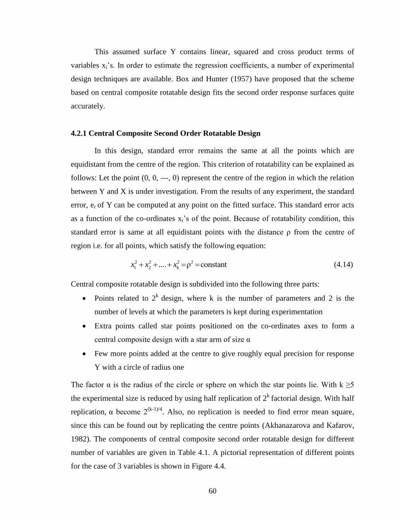
60

This assumed surface Y contains linear, squared and cross product terms of

variables xi‟s. In order to estimate the regression coefficients, a number of experimental

design techniques are available. Box and Hunter (1957) have proposed that the scheme

based on central composite rotatable design fits the second order response surfaces quite

accurately.

4.2.1 Central Composite Second Order Rotatable Design

In this design, standard error remains the same at all the points which are

equidistant from the centre of the region. This criterion of rotatability can be explained as

follows: Let the point (0, 0, ---, 0) represent the centre of the region in which the relation

between Y and X is under investigation. From the results of any experiment, the standard

error, er of Y can be computed at any point on the fitted surface. This standard error acts

as a function of the co-ordinates xi‟s of the point. Because of rotatability condition, this

standard error is same at all equidistant points with the distance ρ from the centre of

region i.e. for all points, which satisfy the following equation:

2 2 2 2

1 2 k.... ρ constantx x x (4.14)

Central composite rotatable design is subdivided into the following three parts:

Points related to 2k

design, where k is the number of parameters and 2 is the

number of levels at which the parameters is kept during experimentation

Extra points called star points positioned on the co-ordinates axes to form a

central composite design with a star arm of size α

Few more points added at the centre to give roughly equal precision for response

Y with a circle of radius one

The factor α is the radius of the circle or sphere on which the star points lie. With k ≥5

the experimental size is reduced by using half replication of 2k

factorial design. With half

replication, α become 2

(k-1)/4. Also, no replication is needed to find error mean square,

since this can be found out by replicating the centre points (Akhanazarova and Kafarov,

1982). The components of central composite second order rotatable design for different

number of variables are given in Table 4.1. A pictorial representation of different points

for the case of 3 variables is shown in Figure 4.4.

61

Table 4.1: Components of Central Composite Second Order Rotatable Design

(Cochran and Cox, 1962)

Variables

(k)

Factorial

Points (2k)

Star Points

(2k)

Center

Points (n)

Total (N) Value of α

3 8 6 6 20 1.682

4 16 8 7 31 2.000

5** 16* 10 6 32 2.000

6 32* 12 9 53 2.378

* Half replication , **This row is used in the present work

Figure 4.4: Central Composite Rotatable Design in 3X-Variables

(Cochran and Cox, 1962)

X3

X1

X2

(0, 0, - 1.682)

(0, 0, 1.682)

(1.682, 0, 0) (-1.682, 0, 0)

(0, 1.682, 0)

(0, -1.682, 0)

(1, -1, -1) (-1, -1, -1)

(-1, -1, 1) (1, -1, 1)

(1, 1, 1)

(1, 1, -1)

(-1, -1, 1)

(-1, 1, -1)

6 Points at center

62

4.2.2 Estimation of the Coefficients

As stated earlier the regression equation representing second order response

surface has been assumed as (Eq. 4.13):

r

2

2ji

jiij

k

1i

2

iii

k

1i

iio exxbxbxbbY

(4.15)

Where, Y is the estimated response, b‟s are the coefficients and xi‟s are the independent

variables.

The method of least squares may be used to estimate the regression coefficients

(Hines and Montgomery, 1990). Let xqi denote the qth

observation of the variable xi and N

the total number of observations. Then the data for N observations in terms of various

variables will appear as shown below:

Y x1 x2… xk x12 x2

2…

xk

2 x1x2… xk-1xk

y1 x11 x12 x1k x112 x12

2 x1k

2 x11x12 x1k-1x1k

y2 x21 x22 x2k x212 x22

2 x2k

2 x21x22 x2k-1x2k

.

.

.

.

yN xN1 xN2 xNk xN12

xN22

xNk2

xN1xN2 xNk-1xNk

In terms of the qth

observation the Equation 4.13 can be written as:

qqkqkkkqqqkkkqqkkqqq exxbxxbxbxbxbxbxbbY 1,12112

22

11122110 ......

(4.16)

Or

63

q

k

2ji

qjqiij

k

1i

2

qiii

k

1i

qiioq exxbxbxbbY

(4.17)

Where,

q = 1, 2… N

The least square function is,

N

q

qeL1

2 (4.18)

Hence from the Equation 4.17

2

1 1 1 2

0

N

q

k

i

k

i

k

ji

qjqiijqiiiqiiq xxbxbxbbYL (4.19)

This function L is to be minimized with respect to b0, b1… This least square estimate of

b0, bi, bii and bij must satisfy the following set of equations:

021 1 1 2

2

0

0

N

q

k

i

k

i

k

Ji

qjqiijqiiiqiiq xxbxbxbbYb

L (4.20)

021 1 1 2

2

0

qi

N

q

k

i

k

i

k

Ji

qjqiijqiiiqiiq

i

xxxbxbxbbYb

L (4.21)

02 2

1 1 1 2

2

0

qi

N

q

k

i

k

i

k

Ji

qjqiijqiiiqiiq

ii

xxxbxbxbbYb

L (4.22)

021 1 1 2

2

0

qjqi

N

q

k

i

k

i

k

Ji

qjqiijqiiiqiiq

ij

xxxxbxbxbbYb

L (4.23)

There are P = k+1 normal equations, one for each unknown regression equation

coefficient. Hence, by solving the above equations the coefficients of the regression

equation can be obtained.

It is simpler to solve the normal equations if they are expressed in matrix form.

The second order response surface in matrix form may be written as:

εβXY (4.24)

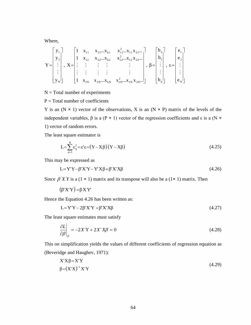
64

Where,

N

2

1

y

y

y

Y

,

...x...xx...xxx1

...x...xx...xxx1

...x...xx...xxx1

X

2N1N

2

1NkN2N1N

2212

2

12k22212

2111

2

11k12111

,

p

1

o

b

b

b

β

,

N

2

1

e

e

e

ε

N = Total number of experiments

P = Total number of coefficients

Y is an (N × 1) vector of the observations, X is an (N × P) matrix of the levels of the

independent variables, β is a (P × 1) vector of the regression coefficients and ε is a (N ×

1) vector of random errors.

The least square estimator is

XβYβXYεε'εL'

N

1q

2

q

(4.25)

This may be expressed as

XβX'β'βXY'YX'β'YY'L (4.26)

Since YX '' is a (1 × 1) matrix and its transpose will also be a (1× 1) matrix. Then

Y'XβYX'β''

Hence the Equation 4.26 has been written as:

XβX'β'YX'β'2YY'L (4.27)

The least square estimates must satisfy

0'2'2

XXYXL

(4.28)

This on simplification yields the values of different coefficients of regression equation as

(Beveridge and Haughev, 1971):

YX'XX'β

YX'βXX'

1

(4.29)

65

4.2.3 Analysis of Variance

For the analysis of variance, the total sum of squares may be divided into four

parts:

The contribution due to the first order terms

The contribution due to the second order terms

A „Lack of fit‟ component which measures the deviations of the response from

the fitted surface

Experimental error which is obtained from the centre points

The general formulae for the sum of squares are given in Table 4.2 (Peng, 1967;

Steel and Torrie, 1986), where, N is the total number of experimental points, n0, Ys, 0Y

represent total number of observations, sth

response value and mean value of response

respectively at the centre points of the experimental region. The design matrix for five

independent variables is shown in Table 4.3.

4.2.4 Significance Testing of the Coefficients

In order to determine the individual coefficients for significance one has to set up

a null hypothesis, which tests the estimated coefficients for difference from its mean

value using the student‟s t-test (Hines, 1990; Steel, 1986). Where design is completely

randomized, it may be shown that the analysis of variance could be used in place of t-test

to compare two treatments. This is due to the reason that the one tailed F-test with 1 and

n degree of freedom (DOF) corresponds to the two tailed t-test with n degree of freedom

i.e. t2

= F for 1 DOF (Steel and Torrie, 1986). Hence, for the significance testing of

individual coefficients F test with 1 and n0 degree of freedom has been used, where n0 is

the total number of observations of the centre point.

66

Table 4.2: Analysis of Variance for Central Composite Second Order Rotatable

Design (Peng, 1967)

S. No. Source Sum of Squares Degree of freedom

1 First order terms

k

q

N

q

qiqi Yxb1 1

K

2 Second order

terms

N

y

yxxb

Yqxbyb

N

q

qk

ji

qjq

N

q

iqij

k

i

N

q

iqii

N

q

qo

2

1

1

1 1

2

1

2

1kk

3 Lack of fit Found by subtraction

2

3

kknN o

4 Experimental

error

on

1s

2

os yy no-1

5 Total

N

y

y

N

q

qN

q

q

2

1

2

1

N-1

The F ratio is given by:

2

e

ii

2

i

oS

cb

n1,F

(4.30)

Where,

'

ib = Regression coefficients

cii = Element of the error matrix 1' )( XX

Se = Standard deviations of experimental error calculated from replicating

observations at zero level as:

67

;yy1n

1S

on

1s

2

os

o

2

e

(4.31)

Where,

0

10

0

1n

s

syn

y

Ys = sth

response value at the centre

This calculated value of F can be compared with theoretical value of F at 95% confidence

level. If for a coefficient the computed value of F is greater than the theoretical value,

then the effect of that term is significant. The insignificant second order terms can be

deleted from the equations and remaining co-efficients can be recalculated.

4.2.5 Adequacy of the Model

Once the co-efficients have been estimated and tested for their significance, the

estimated regression equation is then tested for the adequacy of fit as follows

(Akhanazarova and Kafarov, 1982):

1. Find the residual sum of squares as:

N

1q

2

qq1 yyS (4.32)

Where, yq‟s are the observations at experimental points and qy is the mean of all

observations. N is the total number of observations and k is the total number of

variables. The number of degree of freedom for residual sum of squares will be:

2

321

kkNf

2. From repeated observations at the centre point, the error sum of squares can be

found as

on

1s

2

os2 yyS (4.33)

Where, ys is the sth

response value at center point. oy is the mean of all the

responses at the center point and n0 is the total number of experimental points at the

centre. The degree of freedom for error sum of squares is f2 = n0-1.

68

Table 4.3: Central Composite Second Order Rotatable Design Matrix for 5 Variables (Kumar, 1994)

SN.

Linear terms Square terms Interaction terms

C X1 X2 X3 X4 X5 X1

1

X2

2

X3

3

X4

4

X5

5

X1

2

X1

3

X1

4

X1

5

X2

3

X2

4

X2

5

X3

4

X3

5

X4

5

1 1 -1 -1 -1 -1 1 1 1 1 1 1 1 1 1 -1 1 1 -1 1 -1 -1

2 1 1 -1 -1 -1 -1 1 1 1 1 1 -1 -1 -1 -1 1 1 1 1 1 1

3 1 -1 1 -1 -1 1 1 1 1 1 1 -1 1 1 1 -1 -1 -1 1 1 1

4 1 1 1 -1 -1 -1 1 1 1 1 1 1 -1 -1 1 -1 -1 1 1 -1 -1

5 1 -1 -1 1 -1 1 1 1 1 1 1 1 -1 1 1 -1 1 1 -1 -1 1

6 1 1 -1 1 -1 -1 1 1 1 1 1 -1 1 -1 1 -1 1 -1 -1 1 -1

7 1 -1 1 1 -1 1 1 1 1 1 1 -1 -1 1 -1 1 -1 1 -1 1 -1

8 1 1 1 1 -1 -1 1 1 1 1 1 1 1 -1 -1 1 -1 -1 -1 -1 1

9 1 -1 -1 -1 1 1 1 1 1 1 1 1 1 -1 1 1 -1 1 -1 1 -1

10 1 1 -1 -1 1 -1 1 1 1 1 1 -1 -1 1 1 1 -1 -1 -1 -1 1

11 1 -1 1 -1 1 1 1 1 1 1 1 -1 1 -1 -1 -1 1 1 -1 -1 1

12 1 1 1 -1 1 -1 1 1 1 1 1 1 -1 1 -1 -1 1 -1 -1 1 -1

13 1 -1 -1 1 1 1 1 1 1 1 1 1 -1 -1 -1 -1 -1 -1 1 1 1

14 1 1 -1 1 1 -1 1 1 1 1 1 -1 1 1 -1 -1 -1 1 1 -1 -1

15 1 -1 1 1 1 1 1 1 1 1 1 -1 -1 -1 1 1 1 -1 1 -1 -1

16 1 1 1 1 1 -1 1 1 1 1 1 1 1 1 1 1 1 1 1 1 1

17 1 -2 0 0 0 0 4 0 0 0 0 0 0 0 0 0 0 0 0 0 0

Contd……

69

SN.

Linear terms Square terms Interaction terms

C X1 X2 X3 X4 X5 X1

1

X2

2

X3

3

X4

4

X5

5

X1

2

X1

3

X1

4

X1

5

X2

3

X2

4

X2

5

X3

4

X3

5

X4

5

18 1 2 0 0 0 0 4 0 0 0 0 0 0 0 0 0 0 0 0 0 0

19 1 0 -2 0 0 0 0 4 0 0 0 0 0 0 0 0 0 0 0 0 0

20 1 0 2 0 0 0 0 4 0 0 0 0 0 0 0 0 0 0 0 0 0

21 1 0 0 -2 0 0 0 0 4 0 0 0 0 0 0 0 0 0 0 0 0

22 1 0 0 2 0 0 0 0 4 0 0 0 0 0 0 0 0 0 0 0 0

23 1 0 0 0 -2 0 0 0 0 4 0 0 0 0 0 0 0 0 0 0 0

24 1 0 0 0 2 0 0 0 0 4 0 0 0 0 0 0 0 0 0 0 0

25 1 0 0 0 0 -2 0 0 0 0 4 0 0 0 0 0 0 0 0 0 0

26 1 0 0 0 0 2 0 0 0 0 4 0 0 0 0 0 0 0 0 0 0

27 1 0 0 0 0 0 0 0 0 0 0 0 0 0 0 0 0 0 0 0 0

28 1 0 0 0 0 0 0 0 0 0 0 0 0 0 0 0 0 0 0 0 0

29 1 0 0 0 0 0 0 0 0 0 0 0 0 0 0 0 0 0 0 0 0

30 1 0 0 0 0 0 0 0 0 0 0 0 0 0 0 0 0 0 0 0 0

31 1 0 0 0 0 0 0 0 0 0 0 0 0 0 0 0 0 0 0 0 0

32 1 0 0 0 0 0 0 0 0 0 0 0 0 0 0 0 0 0 0 0 0

X11=X1*X1, X22= X2*X2, X33= X3*X3, X44=X4*X4, X55=X5*X5, X12=X1*X2, X13=X1*X3, X14=X1*X4, X15=X1*X5,

X23=X2*X3, X24=X2*X4, X25=X2*X5, X34=X3*X4, X35=X3*X5, X45=X4*X5

70

3. Find the inadequacy of fit sum of squares

S3 = S1 – S2 (4.34)

For which the number of degree of freedom is

1n

2

2k1kNfff o213

4. Apply F- test to test the adequacy of fit as below

2

2

3

3

fS

fS

F (4.35)

The estimated regression equation fits the data adequately if F<F0.05 (f3, f2) at 95%

confidence level or if F< F0.99 (f3, f2) at 99% confidence level.

71

CHAPTER 5

EXPERIMENTAL RESULTS AND ANALYSIS –

TAGUCHI DESIGN METHOD

5.1 INTRODUCTION

The present chapter gives the application of the Taguchi experimental design

method. The scheme of carrying out experiments was selected and the experiments were

conducted to investigate the effect of process parameters on the output parameters e.g.

cutting rate, surface roughness, gap current and dimensional deviation. The experimental

results are discussed subsequently in the following sections.

5.2 SELECTION OF ORTHOGONAL ARRAY AND PARAMETER

ASSIGNMENT

For the present experimental work the six process parameters each at three levels

have been decided. It is desirable to have three minimum levels of process parameters to

reflect the true behaviour of output parameters of study. The process parameters are

renamed as factors and they are given in the adjacent column. The levels of the individual

process parameters/factors are given in Table 5.1.

Table 5.1: Process Parameters and their Levels

Factors Parameters Levels

L1 L2 L3

A Pulse on Time 106 116 126

B Pulse off Time 40 50 60

C Spark Gap Set Voltage 20 40 60

D Peak Current 70 150 230

E Wire Feed 4 8 12

F Wire Tension 4 8 12

72

As per Taguchi experimental design philosophy a set of three levels assigned to

each process parameter has two degrees of freedom (DOF). This gives a total of 12 DOF

for six process parameters selected in this work. For three process parameters, pulse on

time, pulse off time and spark gap set voltage, taking two parameters at a time we have

three possible interactions (AxB, AxC and BxC) which have been included in the present

study. As a two factor interaction consists of two process parameters and the degree of

freedom of interaction will be equal to the product of DOF of the interacting factors.

Thus each interaction e.g. AxB will have (3-1) x (3-1) = 4 DOF. This gives total DOF of

12 for three interactions AxB, AxC & BxC. Thus we have a total of 24 DOF for the

factors as well as the interactions considered for the present experiments. The nearest

three level orthogonal array available satisfying the criterion of selecting the OA is L27

having 26 DOF (Ross 1988). For each trial in the L27 array, the levels of the process

parameters are indicated in Table 5.2.

5.3 EXPERIMENTAL RESULTS

The WEDM experiments were conducted to study the effect of process

parameters over the output response characteristics with the process parameters and

interactions assigned to columns as given in Table 5.2. The experimental results for

cutting rate and surface roughness are given in Table 5.3 and Table 5.4 reports the same

for gap current and dimensional deviation. 27 experiments were conducted using Taguchi

experimental design methodology and each experiment was simply repeated three times

for obtaining S/N values. In the present study all the designs, plots and analysis have

been carried out using Minitab statistical software.

73

Table 5.2: Taguchi's L27 Standard Orthogonal Array

Colu

mn

No.

1 2 3 4 5 6 7 8 9 10 11 12 13 RESPONSE

(Raw Data) S/N

RATIO

(dB) Trial

No. A B AxB AxB C AxC AxC BxC D E BxC F R1 R2 R3

1 1 1 1 1 1 1 1 1 1 1 1 1 1 Y11 Y12 Y13 S/N(1)

2 1 1 1 1 2 2 2 2 2 2 2 2 2 . . . .

3 1 1 1 1 3 3 3 3 3 3 3 3 3 . . . .

4 1 2 2 2 1 1 1 2 2 2 3 3 3 . . . .

5 1 2 2 2 2 2 2 3 3 3 1 1 1 . . . .

6 1 2 2 2 3 3 3 1 1 1 2 2 2 . . . .

7 1 3 3 3 1 1 1 3 3 3 2 2 2 . . . .

8 1 3 3 3 2 2 2 1 1 1 3 3 3 . . . .

9 1 3 3 3 3 3 3 2 2 2 1 1 1 . . . .

10 2 1 2 3 1 2 3 1 2 3 1 2 3 . . . .

11 2 1 2 3 2 3 1 2 3 1 2 3 1 . . . .

12 2 1 2 3 3 1 2 3 1 2 3 1 2 . . . .

13 2 2 3 1 1 2 3 2 3 1 3 1 2 . . . .

Contd ….

74

Colu

mn

No.

1 2 3 4 5 6 7 8 9 10 11 12 13 RESPONSE

(Raw Data)

S/N

RATIO

(dB)

Trial

No. A B AxB AxB C AxC AxC BxC D E BxC F R1 R2 R3

14 2 2 3 1 2 3 1 3 1 2 1 2 3 . . . .

15 2 2 3 1 3 1 2 1 2 3 2 3 1 . . . .

16 2 3 1 2 1 2 3 3 1 2 2 3 1 . . . .

17 2 3 1 2 2 3 1 1 2 3 3 1 2 . . . .

18 2 3 1 2 3 1 2 2 3 1 1 2 3 . . . .

19 3 1 3 2 1 3 2 1 3 2 1 3 2 . . . .

20 3 1 3 2 2 1 3 2 1 3 2 1 3 . . . .

21 3 1 3 2 3 2 1 3 2 1 3 2 1 . . . .

22 3 2 1 3 1 3 2 2 1 3 3 2 1 . . . .

23 3 2 1 3 2 1 3 3 2 1 1 3 2 . . . .

24 3 2 1 3 3 2 1 1 3 2 2 1 3 . . . .

25 3 3 2 1 1 3 2 3 2 1 2 1 3 . . . .

26 3 3 2 1 2 1 3 1 3 2 3 2 1 . . . .

27. 3 3 2 1 3 2 1 2 1 3 1 3 2 Y271 Y272 Y273 S/N(27)

R1, R2, R3 represent response values for three repetitions of each trial. The 1‟s, 2‟s, and 3‟s represent levels 1, 2, and 3 of the

variables, which appear at the top of the column. Yij are the measured values of the quality characteristic (response).

75

Table 5.3: Experimental Results of Cutting Rate and Surface Roughness

Trial

No.

Cutting Rate (mm/min) S/N

Ratio

Surface Roughness (µm) S/N Ratio

R1 R2 R3 R1 R2 R3

1 0.66 0.68 0.69 -3.39697 1.41 1.35 1.37 -2.778

2 0.72 0.7 0.7 -3.018 1.26 1.26 1.25 -1.98446

3 0.5 0.51 0.5 -5.96402 1.18 1.21 1.13 -1.39186

4 0.47 0.49 0.47 -6.44071 1.31 1.35 1.37 -2.56517

5 0.4 0.41 0.4 -7.88848 1.26 1.25 1.29 -2.05403

6 0.2 0.2 0.2 -13.9794 1.07 1.11 1.12 -0.82953

7 0.32 0.31 0.31 -10.0828 1.39 1.3 1.4 -2.69676

8 0.17 0.16 0.17 -15.5737 1.16 1.24 1.08 -1.30291

9 0.17 0.16 0.17 -15.5737 1.09 1.08 1.06 -0.64221

10 2.44 2.4 2.38 7.626926 2.51 2.63 2.63 -8.26807

11 2.24 2.2 2.18 6.873079 2.38 2.41 2.39 -7.58018

12 0.73 0.75 0.76 -2.54113 1.47 1.43 1.42 -3.16823

13 1.55 1.52 1.57 3.785625 2.54 2.56 2.5 -8.07427

14 0.58 0.57 0.59 -4.73402 1.38 1.35 1.41 -2.79895

15 0.66 0.67 0.65 -3.61112 1.7 1.72 1.73 -4.69395

16 0.46 0.48 0.46 -6.62508 1.66 1.63 1.6 -4.24473

17 0.63 0.63 0.62 -4.06001 1.91 1.8 1.9 -5.43989

18 0.49 0.5 0.51 -6.02408 1.61 1.58 1.73 -4.30365

19 3.3 3.45 3.4 10.58243 3.01 2.9 2.84 -9.30027

20 1.27 1.24 1.26 1.983112 1.86 1.88 1.83 -5.37521

21 2.2 2.15 2.3 6.903836 2.68 2.66 2.65 -8.50861

22 0.91 0.92 0.9 -0.82022 2.11 2.05 2.08 -6.36187

23 1.67 1.64 1.66 4.383961 2.54 2.64 2.68 -8.36822

24 1.54 1.56 1.53 3.768347 2.42 2.46 2.45 -7.75986

25 1.34 1.32 1.35 2.519323 2.85 2.83 2.87 -9.09704

26 1.37 1.34 1.33 2.583145 2.61 2.5 2.63 -8.23452

27 0.28 0.28 0.3 -10.8661 1.31 1.27 1.3 -2.23496

76

Table 5.4: Experimental Results for Gap Current and Dimensional Deviation

Trial

No.

Gap Current (ampere) S/N Ratio


(%) S/N Ratio

R1 R2 R3 R1 R2 R3

1 1.4 1.3 1.4 2.6972277 0.69 0.64 0.68 3.47399146

2 1.2 1.3 1.2 1.8032341 0.454 0.486 0.47 6.55468879

3 1.1 1 1.1 0.5340159 0.5 0.61 0.55 5.11167366

4 1 1 1 0 0.8 0.76 0.78 2.15620482

5 0.8 0.9 0.8 -1.6232219 0.48 0.44 0.46 6.73937366

6 0.6 0.7 0.7 -3.5916553 0.593 0.564 0.605 4.61857927

7 0.8 0.75 0.8 -2.1332095 0.62 0.605 0.632 4.16480443

8 0.6 0.65 0.6 -4.2173658 0.67 0.714 0.694 3.18658645

9 0.6 0.7 0.6 -4.0348496 0.28 0.27 0.31 10.8372156

10 4.4 4.3 4.2 12.66467 0.58 0.6 0.59 4.5821281

11 4 3.9 3.8 11.815579 0.52 0.532 0.56 5.39090135

12 1.6 1.7 1.6 4.2509301 0.28 0.26 0.255 11.5278735

13 2.8 2.7 2.9 8.9320723 0.44 0.4 0.4 7.6649624

14 1.4 1.3 1.4 2.6972277 0.376 0.347 0.363 8.82116924

15 1.3 1.4 1.3 2.4830117 0.372 0.38 0.321 8.9073089

16 1.1 1.2 1.1 1.0654581 0.56 0.523 0.576 5.1385064

17 1.3 1.3 1.2 2.0345425 0.22 0.232 0.243 12.6955959

18 1.1 1.2 1.1 1.0654581 0.02 0.018 0.027 33.1485564

19 6.4 6.5 6.3 16.121479 0.633 0.617 0.654 3.94661189

20 2.6 2.7 2.5 8.2866053 0.38 0.4 0.285 8.90956073

21 4.4 4.6 4.5 13.05996 0.167 0.143 0.189 15.5253704

22 2.3 2.4 2.3 7.354317 0.793 0.756 0.806 2.09944597

23 3.7 3.6 3.7 11.283249 0.553 0.523 0.586 5.12044731

24 3.4 3.4 3.3 10.541414 0.427 0.407 0.453 7.34249289

25 2.9 2.8 2.9 9.1439651 0.44 0.424 0.469 7.03819823

26 3.1 3 3 9.6353014 0.1 0.095 0.134 19.091426

27 1.2 1.2 1.2 1.5836249 0.38 0.4 0.307 8.76530576

77

5.4 ANALYSIS AND DISCUSSION OF RESULTS

The WEDM experiments were conducted by using the parametric approach of the

Taguchi‟s method. The effects of individual WEDM process parameters, on the selected

quality characteristics – cutting rate, surface roughness, gap current and dimensional

deviation, have been discussed in this section. The average value and S/N ratio of the

response characteristics for each variable at different levels were calculated from

experimental data. The main effects of process variables both for raw data and S/N data were

plotted. The response curves (main effects) are used for examining the parametric effects on

the response characteristics. The analysis of variance (ANOVA) of raw data and S/N data is

carried out to identify the significant variables and to quantify their effects on the response

characteristics. The most favourable values (optimal settings) of process variables in terms of

mean response characteristics are established by analyzing the response curves and the

ANOVA tables.

5.4.1 Effect on Cutting Rate

In order to see the effect of process parameters on the cutting rate, experiments were

conducted using L27 OA (Table 5.2). The experimental data is given in Tables 5.3 and

5.4.The average values of cutting rate for each parameter at levels 1, 2 and 3 for raw data and

S/N data are plotted in Figures 5.1 and 5.2 respectively.

Figures 5.1 and 5.2 shows that the cutting rate increases with the increase of pulse on

time and peak current, and decreases with increase in pulse off time and spark gap set

voltage. This is because the discharge energy increases with the pulse on time and peak

current leading to a faster cutting rate. As the pulse off time decreases, the number of

discharges within a given period becomes more which leads to a higher cutting rate. With

increase in spark gap set voltage the average discharge gap gets widened resulting into a

lower cutting rate. The effects of wire feed and wire tension on cutting rate are not very

significant. It is also evident that cutting rate is minimum at first level of pulse on time and

maximum at first level of pulse off time. It is seen from the Figures 5.3 and 5.4 that there is

very weak interaction between the process parameters in affecting the cutting rate since the

responses at different levels of process parameters for a given level of parameter value are

almost parallel.

78

126116106

1.50

1.25

1.00

0.75

0.50

605040 604020

23015070

1.50

1.25

1.00

0.75

0.50

1284 1284

Ton

Me

an

of

Me

an

s

Toff SV

IP WF WT

Main Effects Plot for MeansData Means

Figure 5.1: Effects of Process Parameters on Cutting Rate (Raw Data)

126116106

0

-5

-10

605040 604020

23015070

0

-5

-10

1284 1284

Ton

Me

an

of

SN

ra

tio

s

Toff SV

IP WF WT

Main Effects Plot for SN ratiosData Means

Signal-to-noise: Larger is better

Figure 5.2: Effects of Process Parameters on Cutting Rate (S/N Data)

79

2

1

0

604020

605040

2

1

0

126116106

2

1

0

T on

T off

SV

106

116

126

Ton

40

50

60

Toff

20

40

60

SV

Interaction Plot for MeansData Means

Figure 5.3: Effects of Process Parameters Interactions on Cutting Rate (Raw Data)

0

-8

-16

604020

605040

0

-8

-16

126116106

0

-8

-16

T on

T off

SV

106

116

126

Ton

40

50

60

Toff

20

40

60

SV

Interaction Plot for SN ratiosData Means


Figure 5.4: Effects of Process Parameters Interactions on Cutting Rate (S/N Data)

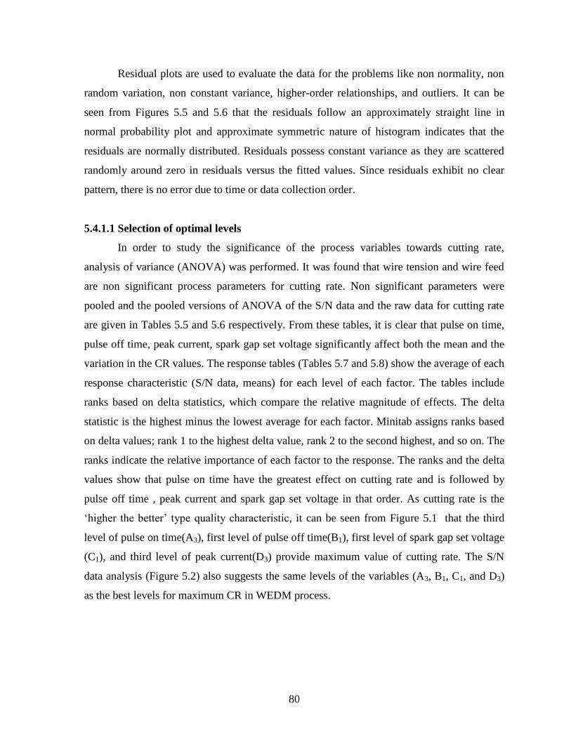
80

Residual plots are used to evaluate the data for the problems like non normality, non

random variation, non constant variance, higher-order relationships, and outliers. It can be

seen from Figures 5.5 and 5.6 that the residuals follow an approximately straight line in

normal probability plot and approximate symmetric nature of histogram indicates that the

residuals are normally distributed. Residuals possess constant variance as they are scattered

randomly around zero in residuals versus the fitted values. Since residuals exhibit no clear

pattern, there is no error due to time or data collection order.

5.4.1.1 Selection of optimal levels

In order to study the significance of the process variables towards cutting rate,

analysis of variance (ANOVA) was performed. It was found that wire tension and wire feed

are non significant process parameters for cutting rate. Non significant parameters were

pooled and the pooled versions of ANOVA of the S/N data and the raw data for cutting rate

are given in Tables 5.5 and 5.6 respectively. From these tables, it is clear that pulse on time,

pulse off time, peak current, spark gap set voltage significantly affect both the mean and the

variation in the CR values. The response tables (Tables 5.7 and 5.8) show the average of each

response characteristic (S/N data, means) for each level of each factor. The tables include

ranks based on delta statistics, which compare the relative magnitude of effects. The delta

statistic is the highest minus the lowest average for each factor. Minitab assigns ranks based

on delta values; rank 1 to the highest delta value, rank 2 to the second highest, and so on. The

ranks indicate the relative importance of each factor to the response. The ranks and the delta

values show that pulse on time have the greatest effect on cutting rate and is followed by

pulse off time , peak current and spark gap set voltage in that order. As cutting rate is the

„higher the better‟ type quality characteristic, it can be seen from Figure 5.1 that the third

level of pulse on time(A3), first level of pulse off time(B1), first level of spark gap set voltage

(C1), and third level of peak current(D3) provide maximum value of cutting rate. The S/N

data analysis (Figure 5.2) also suggests the same levels of the variables (A3, B1, C1, and D3)

as the best levels for maximum CR in WEDM process.

81

0.80.40.0-0.4-0.8

99

90

50

10

1

Residual

Pe

rce

nt

3210

0.5

0.0

-0.5

Fitted Value

Re

sid

ua

l

0.80.60.40.20.0-0.2-0.4

10.0

7.5

5.0

2.5

0.0

Residual

Fre

qu

en

cy

2624222018161412108642

0.5

0.0

-0.5

Observation Order

Re

sid

ua

l

Normal Probability Plot Versus Fits

Histogram Versus Order

Residual Plots for Means

Figure 5.5: Residual Plots for Cutting Rate (Raw Data)

3.01.50.0-1.5-3.0

99

90

50

10

1

Residual

Pe

rce

nt

100-10-20

2

1

0

-1

-2

Fitted Value

Re

sid

ua

l

2.41.20.0-1.2-2.4

4.8

3.6

2.4

1.2

0.0

Residual

Fre

qu

en

cy

2624222018161412108642

2

1

0

-1

-2

Observation Order

Re

sid

ua

l



Residual Plots for SN ratios

Figure 5.6: Residual Plots for Cutting Rate (S/N Data)

82

5.4.2 Effect on Surface Roughness

In order to see the effects of process parameters on the surface roughness,

experiments were conducted using L27 OA (Table 5.2). The experimental data are given in

Table 5.3. The average values of surface roughness for each parameter at levels 1, 2, and 3

for raw data and S/N data are plotted in Figures 5.7 and 5.8.

Table 5.5: Pooled Analysis of Variance for Cutting Rate (S/N Data)

Source DF Seq SS Adj SS Adj MS F P

Ton 2 621.95 621.95 310.977 137.72 0.000

Toff 2 381.20 381.20 190.602 84.41 0.000

SV 2 115.27 115.27 57.637 25.53 0.000

IP 2 187.63 187.63 93.817 41.55 0.000

Residual Error 18 40.64 40.64 2.258

Total 26 1346.71

DF - degrees of freedom, SS - sum of squares, MS - mean squares(Variance), F-ratio of

variance of a source to variance of error, P < 0.05 - determines significance of a factor at

95% confidence level

Table 5.6: Pooled Analysis of Variance for Cutting Rate (Raw Data)


Ton 2 5.990 5.990 2.9948 20.17 0.000

Toff 2 4.603 4.603 2.3015 15.50 0.000

SV 2 1.227 1.227 0.6137 4.13 0.033

IP 2 2.539 2.539 1.2695 8.55 0.002

Residual Error 18 2.672 2.672 0.1485

Total 26 17.031




Table 5.7: Response Table for Cutting Rate (S/N Data)

83

Level Ton Toff SV IP

1 -9.1020 2.1166 -0.3168 -6.2837

2 -1.0344 -2.8373 -2.1612 -1.2522

3 2.3375 -7.0781 -5.3208 -0.2630

Delta 11.4395 9.1947 5.0040 6.0208

Rank 1 2 4 3

Table 5.8: Response Table for Cutting Rate (Raw Data)


1 0.4015 1.5670 1.2796 0.5878

2 1.0822 0.8863 0.9944 1.1393

3 1.5485 0.5789 0.7581 1.3052

Delta 1.1470 0.9881 0.5215 0.7174

Rank 1 2 4 3

It is seen from the Figures 5.7 and 5.8 that surface roughness increases with the

increase of pulse on time, and peak current and decreases with increase in pulse off time,

spark gap set voltage, and wire feed. The discharge energy increases with the pulse on time

and peak current and larger discharge energy produces a larger crater, causing a larger

surface roughness value on the work piece. As the pulse off time decreases, the number of

discharges increases which causes poor surface accuracy. With increase in spark gap set

voltage the average discharge gap gets widened resulting into better surface accuracy due to

stable machining .The effects of wire tension are not very significant. It is noticed from

Figures 5.9 and 5.10 that there is a slight interaction between pulse off time and spark gap set

voltage while there is very weak interaction between all the other process parameters in

affecting the surface roughness since the responses at different levels of process parameters

for a given level of parameter value are almost parallel. Residual plots do not show any

problem in the distribution of the data and model assumptions (Figures 5.11 and 5.12).

84

126116106

2.4

2.1

1.8

1.5

1.2

605040 604020

23015070

2.4

2.1

1.8

1.5

1.2

1284 1284

Ton

Me

an

of

Me

an

s

Toff SV

IP WF WT


Figure 5.7: Effects of Process Parameters on Surface Roughness (Raw Data)

126116106

-2

-4

-6

-8

605040 604020

23015070

-2

-4

-6

-8

1284 1284

Ton

Me

an

of

SN

ra

tio

s

Toff SV

IP WF WT


Signal-to-noise: Smaller is better

Figure 5.8: Effects of Process Parameters on Surface Roughness (S/N Data)

85

2.5

2.0

1.5

604020

605040

2.5

2.0

1.5

126116106

2.5

2.0

1.5

T on

T off

SV

106

116

126

Ton

40

50

60

Toff

20

40

60

SV


Figure 5.9: Effects of Process Parameters Interactions on Surface Roughness

(Raw Data)

0

-4

-8

604020

605040

0

-4

-8

126116106

0

-4

-8

T on

T off

SV

106

116

126

Ton

40

50

60

Toff

20

40

60

SV



Figure 5.10: Effects of Process Parameters Interactions on Surface Roughness

(S/N Data)

86

0.40.20.0-0.2-0.4

99

90

50

10

1

Residual

Pe

rce

nt

3.02.52.01.51.0

0.2

0.0

-0.2

-0.4

Fitted Value

Re

sid

ua

l

0.30.20.10.0-0.1-0.2-0.3

12

9

6

3

0

Residual

Fre

qu

en

cy

2624222018161412108642

0.2

0.0

-0.2

-0.4

Observation Order

Re

sid

ua

l




Figure 5.11: Residual Plots for Surface Roughness (Raw Data)

10-1

99

90

50

10

1

Residual

Pe

rce

nt

0.0-2.5-5.0-7.5-10.0

1.0

0.5

0.0

-0.5

-1.0

Fitted Value

Re

sid

ua

l

1.00.50.0-0.5-1.0

6.0

4.5

3.0

1.5

0.0

Residual

Fre

qu

en

cy

2624222018161412108642

1.0

0.5

0.0

-0.5

-1.0

Observation Order

Re

sid

ua

l




Figure 5.12: Residual Plots for Surface Roughness (S/N Data)

87

5.4.2.1 Selection of Optimal Levels

In order to study the significance of the process variables towards surface roughness,

analysis of variance (ANOVA) was performed. It was found that wire tension is non

significant process parameter for surface roughness. Non significant parameter was pooled

and the pooled versions of ANOVA of the S/N data and the raw data for surface roughness

are given in Tables 5.9 and 5.10 respectively. From these tables, it is observed that pulse on

time, pulse off time, peak current, spark gap set voltage and wire feed significantly affect

both the mean and the variation in the SR values. The response tables (Tables 5.11 and 5.12)

show the average of each response characteristic (S/N data and raw data) for each level of

each factor. The Tables include ranks based on delta statistics, which compare the relative

magnitude of effects. The delta statistic is the highest minus the lowest average for each

factor. Minitab assigns ranks based on delta values; rank 1 to the highest delta value, rank 2

to the second highest, and so on. The ranks indicate the relative importance of each factor to

the response. The ranks and the delta values for various parameters show that pulse on time

has the greatest effect on surface roughness and is followed by peak current, spark gap set

voltage, wire feed and pulse of time in that order. As surface roughness is the „lower the

better‟ type quality characteristic, from Figure 5.7, it can be seen that the first level of pulse

on time (A1), third level of pulse off time (B3), third level of spark gap set voltage (C3), first

level of peak current (D1), and third level of wire feed (E3) result in minimum value of

surface roughness. The S/N ratio analysis (Figure 5.8) also suggests the same levels of the

variables (A1, B3, C3, D1 and E3) as the best levels for minimum SR in WEDM process.

5.4.3 Effect on Gap Current

In order to see the effects of process parameters on the gap current, experiments were

conducted using L27 OA (Table 5.2). The experimental data are given in Table 5.4. The

average values of gap current for each parameter at levels 1, 2 and 3 for raw data and S/N

data are plotted in Figure 5.13 and 5.14. It is seen from the Figures 5.13 and 5.14 that gap

current increases with increase in pulse on time and peak current, decreases with increase in

pulse off time, spark gap set voltage, and wire feed.

88

Table 5.9: Pooled Analysis of Variance for Surface Roughness (S/N Data)


Ton 2 137.905 137.905 68.9527 111.85 0.000

Toff 2 5.737 5.737 2.8683 4.65 0.026

SV 2 21.905 21.905 10.9526 17.77 0.000

IP 2 34.068 34.068 17.0339 27.63 0.000

WF 2 9.614 9.614 4.8072 7.80 0.004

Residual Error 16 9.863 9.863 0.6165

Total 26 219.093




Table 5.10: Pooled Analysis of Variance for Surface Roughness (Raw Data)


Ton 2 5.8365 5.8365 2.91826 81.47 0.000

Toff 2 0.2702 0.2702 0.13510 3.77 0.045

SV 2 0.9546 0.9546 0.47732 13.33 0.000

IP 2 1.7351 1.7351 0.86753 24.22 0.000

WF 2 0.5801 0.5801 0.29005 8.10 0.004

Residual Error 16 0.5731 0.5731 0.03582

Total 26 9.9496




Table 5.11: Response Table for Surface Roughness (S/N Data)

Level Ton Toff SV IP WF

1 -1.805 -5.373 -5.932 -3.233 -5.649

2 -5.397 -4.834 -4.793 -5.508 -4.522

3 -7.249 -4.244 -3.726 -5.711 -4.280

Delta 5.444 1.129 2.206 2.478 1.370

Rank 1 5 3 2 4

89

Table 5.12: Response Table for Surface Roughness (Raw Data)


1 1.235 1.963 2.076 1.480 2.037

2 1.910 1.831 1.820 1.999 1.785

3 2.367 1.718 1.616 2.034 1.690

Delta 1.132 0.245 0.460 0.555 0.347

Rank 1 5 3 2 4

Wire tension is not influencing the gap current significantly. It is observed from

Figures 5.15 and 5.16 that there is a slight interaction between pulse off time and spark gap

set voltage and there is very weak interaction between all the other process parameters in

affecting the gap current since their responses at different levels of process parameters for a

given level of parameter value are almost parallel.

Four residual plots (Figures 5.17 and 5.18) are drawn for estimating the accuracy of

the model. The histogram plot indicates a mild tendency for the non normality; however the

normal probability plots of these residuals do not reveal any abnormality. Residual versus

fitted value and residual versus observation order plot do not indicate any undesirable effect.


In order to study the significance of the process variables towards gap current,

analysis of variance (ANOVA) was performed. It was found that spark gap set voltage, wire

feed, and wire tension are non significant process parameter for gap current. Non significant

parameters were pooled and the pooled versions of ANOVA of the S/N data and the raw data

for gap current are given in Tables 5.13 and 5.14 respectively. From these tables, it is

observed that pulse on time, pulse off time and peak current significantly affect both the

mean and the variation in the gap current values. The response tables (Tables 5.15 and 5.16)

show the average of each response characteristic (S/N data, raw data) for each level of each

factor. The tables include ranks based on delta statistics, which compare the relative

magnitude of effects. The delta statistic is the highest minus the lowest average for each

factor. Minitab assigns ranks based on delta values; rank 1 to the highest delta value, rank 2

to the second highest, and so on.

90

126116106

3.0

2.5

2.0

1.5

1.0

605040 604020

23015070

3.0

2.5

2.0

1.5

1.0

1284 1284

Ton

Me

an

of

Me

an

s

Toff SV

IP WF WT


Figure 5.13: Effects of Process Parameters on Gap Current (Raw Data)

126116106

10.0

7.5

5.0

2.5

0.0

605040 604020

23015070

10.0

7.5

5.0

2.5

0.0

1284 1284

Ton

Me

an

of

SN

ra

tio

s

Toff SV

IP WF WT



Figure 5.14: Effect of Process Parameters on Gap Current (S/N Data)

91

4.5

3.0

1.5

604020

605040

4.5

3.0

1.5

126116106

4.5

3.0

1.5

T on

T off

SV

106

116

126

Ton

40

50

60

Toff

20

40

60

SV


Figure 5.15: Effect of Process Parameters Interactions on Gap Current (Raw Data)

10

5

0

604020

605040

10

5

0

126116106

10

5

0

T on

T off

SV

106

116

126

Ton

40

50

60

Toff

20

40

60

SV



Figure 5.16: Effect of Process Parameters Interactions on Gap Current (S/N Data)

92

210-1-2

99

90

50

10

1

Residual

Pe

rce

nt

4.83.62.41.20.0

2

1

0

-1

Fitted Value

Re

sid

ua

l

1.51.00.50.0-0.5-1.0

8

6

4

2

0

Residual

Fre

qu

en

cy

2624222018161412108642

2

1

0

-1

Observation Order

Re

sid

ua

l




Figure 5.17: Residual Plots for Gap Current (Raw Data)

5.02.50.0-2.5-5.0

99

90

50

10

1

Residual

Pe

rce

nt

151050-5

4

2

0

-2

-4

Fitted Value

Re

sid

ua

l

3210-1-2-3

4.8

3.6

2.4

1.2

0.0

Residual

Fre

qu

en

cy

2624222018161412108642

4

2

0

-2

-4

Observation Order

Re

sid

ua

l




Figure 5.18: Residual Plots for Gap Current (S/N Data)

93

Table 5.13: Pooled Analysis of Variance for Gap Current (S/N Data)


Ton 2 534.67 534.67 267.333 55.98 0.000

Toff 2 182.65 182.65 91.325 19.12 0.000

IP 2 75.98 75.98 37.992 7.96 0.003

Residual Error 20 95.51 95.51 4.775

Total 26 888.81




Table 5.14: Pooled Analysis of Variance for Gap Current (Raw Data)


Ton 2 26.325 26.325 13.1625 22.06 0.000

Toff 2 11.864 11.864 5.9321 9.94 0.001

IP 2 6.542 6.542 3.2711 5.48 0.013

Residual Error 20 11.934 11.934 0.5967

Total 26 56.665


variance of a source to variance of error, P < 0.05 - determines significance of a factor` at


Table 5.15: Response Table for Gap Current (S/N Data)

Level Ton Toff IP

1 -1.174 7.915 2.236

2 5.223 4.231 5.382

3 9.668 1.571 6.099

Delta 10.842 6.343 3.863

Rank 1 2 3

94

Table 5.16: Response Table for Gap Current (Raw Data)

Level Ton Toff IP

1 0.9111 3.0000 1.4352

2 2.0963 1.9296 2.3111

3 3.3296 1.4074 2.5907

Delta 2.4185 1.5926 1.1556

Rank 1 2 3

The ranks indicate the relative importance of each factor to the response. The ranks

and the delta values for various parameters show that pulse on time has the greatest effect on

gap current and is followed by pulse off time and peak current in that order. As gap current is

the „larger the better‟ type quality characteristic, from Figure 5.13, it can be seen that the

third level of pulse on time (A3), first level of pulse off time (B1) and third level of peak

current (D3), provide maximum value of gap current. The S/N data analysis (Figure 5.14)

also suggests the same levels of the variables (A3, B1, and D3) as the best levels for maximum

gap current in WEDM process.

5.4.4 Effect on Dimensional Deviation

In order to see the effects of process parameters on the dimensional deviation,

experiments were conducted using L27 OA (Table 5.2). The experimental data are given in

Table 5.4. The average values of dimensional deviation for each parameter at levels 1, 2, and

3 for raw data and S/N data are plotted in Figures 5.19 and 5.20 respectively.

Figure 5.19 show that dimensional deviation first decreases strongly with increase in

pulse on time and then very slightly increases. As pulse off time increases, the dimensional

deviation first increases and then decreases. With the increase in peak current and spark gap

set voltage, decrement in the value of dimensional deviation is observed. Increasing wire

tension value leads to higher dimensional deviation. The effect of wire feed is not very

clearly seen. The forces acting on the wire electrode are the main causes of the geometrical

inaccuracy of the machined parts. The efficiency and the accuracy of the process are limited

by the process parameters as well. Dimensional deviation value increases if the energy

95

contained in a pulse increases to a large value. That‟s why when pulse on time is very high

the dimensional deviation increases. With increase in wire tension the vibration and

deflection of the wire change resulting into increase of dimensional deviation.

It is clear from the Figures 5.21 and 5.22 that there is moderate interaction between

pulse on time and pulse off time, pulse on time and spark gap set voltage and pulse off time

and spark gap set voltage in affecting the dimensional deviation since the responses at

different levels of these process parameters are non parallel.

Residual plots are drawn to check for data for the non normality, non random

variation, non constant variance, higher-order relationships, and outliers (Figures 5.23 and

5.24). The residual versus fitted value indicates a little tendency for variance of the residuals

to increase as the dimensional deviation value increases.

The problem, however, is not severe enough to have any dramatic impact on the

analysis and conclusions. The normal probability plot, histogram plot, and residual versus

observation order plot of these residuals (Figure 5.23) do not reveal any problem.


In order to study the significance of the process variables towards dimensional

deviation, analysis of variance (ANOVA) was performed. It was found that the peak current,

and wire feed are non significant process parameters for dimensional deviation. Non

significant parameters were pooled and the pooled versions of ANOVA of the S/N data and

the raw data for dimensional deviation are given in Tables 5.17 and 5.18 respectively. From

these tables, it is observed that pulse on time, pulse off time, spark gap set voltage and wire

tension significantly affect both the mean and the variation in the dimensional deviation

values. The response tables (Tables 5.19 and 5.20) show the average of each response

characteristic (S/N data, raw data) for each level of each factor. The tables include ranks

based on delta statistics, which compare the relative magnitude of effects. The delta statistic

is the highest minus the lowest average for each factor. Minitab assigns ranks based on delta

values; rank 1 to the highest delta value, rank 2 to the second highest, and so on. The ranks

indicate the relative importance of each factor to the response. The ranks and the delta values

for various parameters show that spark gap set voltage has the greatest effect on dimensional

deviation and is followed by pulse on time, wire tension and pulse off time in that order. As

dimensional deviation is the „lower the better‟ type quality characteristic, from Figure 5.20,

96

126116106

0.6

0.5

0.4

0.3

605040 604020

23015070

0.6

0.5

0.4

0.3

1284 1284

Ton

Me

an

of

Me

an

s

Toff SV

IP WF WT


Figure 5.19: Effect of Process Parameters on Dimensional Deviation (Raw Data)

126116106

12

10

8

6

4

605040 604020

23015070

12

10

8

6

4

1284 1284

Ton

Me

an

of

SN

ra

tio

s

Toff SV

IP WF WT



Figure 5.20: Effect of Process Parameters on Dimensional Deviation (S/N Data)

97

0.6

0.4

0.2

604020

605040

0.6

0.4

0.2

126116106

0.6

0.4

0.2

T on

T off

SV

106

116

126

Ton

40

50

60

Toff

20

40

60

SV


Figure 5.21: Effect of Process Parameters Interactions on Dimensional Deviation

(Raw Data)

15

10

5

604020

605040

15

10

5

126116106

15

10

5

T on

T off

SV

106

116

126

Ton

40

50

60

Toff

20

40

60

SV



Figure 5.22: Effect of Process Parameters Interactions on Dimensional Deviation

(S/N Data)

98

0.20.10.0-0.1-0.2

99

90

50

10

1

Residual

Pe

rce

nt

1.00.80.60.40.2

0.2

0.1

0.0

-0.1

-0.2

Fitted Value

Re

sid

ua

l

0.200.150.100.050.00-0.05-0.10-0.15

8

6

4

2

0

Residual

Fre

qu

en

cy

2624222018161412108642

0.2

0.1

0.0

-0.1

-0.2

Observation Order

Re

sid

ua

l




Figure 5.23 Residual Plots for Dimensional Deviation (Raw Data)

1050-5-10

99

90

50

10

1

Residual

Pe

rce

nt

24181260

15

10

5

0

-5

Fitted Value

Re

sid

ua

l

12.510.07.55.02.50.0-2.5-5.0

10.0

7.5

5.0

2.5

0.0

Residual

Fre

qu

en

cy

2624222018161412108642

15

10

5

0

-5

Observation Order

Re

sid

ua

l




Figure 5.24 Residual Plots for Dimensional Deviation (S/N Data)

99

Table 5.17: Pooled Analysis of Variance for Dimensional Deviation (S/N Data)


Ton 2 146.9 146.9 73.46 3.55 0.050

Toff 2 156.2 156.2 78.11 3.77 0.043

SV 2 239.4 239.4 119.69 5.78 0.011

WT 2 144.5 144.5 72.27 3.49 0.052

Residual Error 18 372.6 372.6 20.70

Total 26 1059.6




Table 5.18: Pooled Analysis of Variance for Dimensional Deviation (Raw Data)


Ton 2 0.1885 0.1885 0.09423 8.86 0.002

Toff 2 0.1135 0.1135 0.05676 5.33 0.015

SV 2 0.3538 0.3538 0.17688 16.62 0.000

WT 2 0.1449 0.1449 0.07244 6.81 0.006

Residual Error 18 0.1915 0.1915 0.01064

Total 26 0.9922

DF -degrees of freedom, SS - sum of squares, MS - mean squares(Variance), F-ratio of



Table 5.19: Response Table for Dimensional Deviation (S/N Data)

Level Ton Toff SV WT

1 5.205 7.225 4.474 8.470

2 10.875 5.941 8.501 10.956

3 8.649 11.563 11.754 5.303

Delta 5.670 5.622 7.280 5.654

Rank 2 4 1 3

Table 5.20: Response Table for Dimensional Deviation (Raw Data)

100

Level Ton Toff SV WT

1 0.5688 0.4713 0.6099 0.3950

2 0.3702 0.5254 0.4191 0.4123

3 0.4267 0.3690 0.3366 0.5583

Delta 0.1986 0.1564 0.2733 0.1633

Rank 2 4 1 3

it can be seen that the second level of pulse on time (A2), third level of pulse off time (B3),

third level of spark gap set voltage (C3), and first level of wire tension (F1) provide minimum

value of dimensional deviation. The S/N data analysis (Figure 5.21) also suggests the same

levels of the variables (A1, B3, C3, and F1) as the best levels for minimum dimensional

deviation in WEDM process.

5.5 ESTIMATION OF OPTIMUM RESPONSE CHARATERISTICS

In this section, the optimal values of the response charateristics (cutting rate, surface

roughness, gap current, dimensional deviation) along with their respective confidence

intervals have been predicted. The results of confirmation experiments are also presented to

validate the optimal results. The optimal levels of the process parameters for the selected

response charateristics have already been identified and are reported in the previous section.

The optimal value of each response charateristic is predicted considering the effect of the

significant parametes only. The average values of the response charateristics obtained

through the confirmation experiments must lie within the 95% confidence interval, CICE

(equation 4.11, Chapter 4). However, the average values of quality charateristics obtained

from the confirmation experiments may or may not lie with in 95% confidence interval,

CIPOP (calculated for the mean of the population, equation 4.10). The Taguchi approach for

predicting the mean of response charateristics and determination of confidence intervals for

the predicted means has been presented in section 4.1.6.6 (Chapter 4).

101

5.5.1 Cutting Rate (CR)

The optimum value of CR is predicted at the optimal levels of significant variables

which have already been selected as pulse on time (A3), pulse off time(B1), spark gap set

voltage (C1) and peak current(D3) (Table 5.6 and Figure 5.1). The estimated mean of the

response characteristic (CR) can be determined (Kumar, 1993 and Roy, 1990) as

(5.1)

Where,

T = overall mean of cutting rate = (R1+R2+R3)/81 =1.010741 mm/min

Where, R1, R2, and R3 values are taken from the Table 5.3, and the values of 3A , 1B , 1C , and

3D are taken from the Table 5.8.

3A = average value of cutting rate at the third level of pulse on time = 1.5485 mm/min

1B = average value of cutting rate at the first level of pulse off time = 1.5670 mm/min

1C = average value of cutting rate at the first level of spark gap set voltage = 1.2796 mm/min

3D = average value of cutting rate at the third level of peak current = 1.3052 mm/min

Substituting the values of various terms in the above equation,

µCR = 1.5485 + 1.5670 + 1.2796 + 1.3052 – 3 (1.010741) = 2.6681 mm/min

The 95 % confidence intervals of confirmation experiments (CICE) and

population (CIPOP) are calculated by using the Equations 4.10 and 4.11as rewritten below for

ready reference:

R

1

n

1V)f(1,FCI

eff

eeαCE and

eff

eeα

POPn

V)f(1,FCI

Where, Fα (1, fe) = The F ratio at the confidence level of (1-α) against DOF 1 and error


T33113CR DCBA

102

responsemean ofestimatethein associatedDOF1

Neff

n

= 81 / (1+8)

= 9

N = Total number of results = 27 x 3 = 81

R = Sample size for confirmation experiments = 3

Ve = Error variance = 0.1485 (Table 5.6)

fe = error DOF = 18 (Table 5.6)

F0.05 (1, 18) = 4.4139 (Tabulated F value ; Roy, 1990)

So, CICE = ± 0.5397 , and

CIPOP = ± 0.2699

Therefore, the predicted confidence interval for confirmation experiments is:

Mean µCR - CICE < µCR < Mean µCR + CICE

2.1284 < µCR < 3.2078

The 95% confidence interval of the population is:

Mean µCR – CIPOP < µCR < Mean µCR + CIPOP

2.3982 < µCR < 2.938

The optimal values of process variables at their selected levels are as follows:

Third level of pulse on time (A3) : 126 machine unit

First level of pulse off time (B1) : 40 machine unit

First level of spark gap set voltage (C1) : 20 volt

Third level of peak current (D3) : 230 ampere

5.5.2 Surface Roughness (SR)

The optimum value of SR is predicted at the optimal levels of significant variables


voltage (C3), peak current(D1) and wire feed (E3) (Table 5.10 and Figure 5.7). The estimated

mean of the response characteristic (SR) can be determined (Kumar, 1993 and Roy, 1990) as

(5.2)

Where,

T4 31331 EDCBASR

103

T = overall mean of surface roughness= (R1+R2+R3)/81 = 1.8411 µm

Where, R1, R2, and R3 values are taken from the Table 5.3, and the values of 1A , 3B , 3C ,

1D and 3E are taken from the Table 5.12.

1A = average value of surface roughness at the first level of pulse on time =1.235 µm

3B = average value of surface roughness at the third level of pulse off time =1.718 µm

3C = average value of surface roughness at the third level of spark gap set voltage =1.616 µm

1D = average value of surface roughness at the first level of peak current =1.480 µm

3E = average value of surface roughness at the third level of wire feed =1.690 µm


µSR = 1.235 + 1.718 + 1.616 + 1.480 + 1.690 – 4 (1.8375) = 0.3890 µm

The 95 % confidence intervals of confirmation experiments (CICE) and population (CIPOP) are

calculated by using the following Equations 4.10 and 4.11 as reproduce below:

R

1

n

1V)f(1,FCI

eff

eeαCE and

eff

eeα

POPn

V)f(1,FCI




Neff

n

= 81 / (1+10)

= 7.3636





104

F0.05 (1, 16) = 4.4940 (Tabulated F value; Roy, 1990)

So, CICE = ± 0.2748, and

CIPOP = ± 0.1478


Mean µSR - CICE < µSR < Mean µSR + CICE

0.1142 < µSR < 0.6638


Mean µSR – CIPOP < µSR < Mean µSR + CIPOP

0.2412 < µSR < 0.5368


First level of pulse on time (A1) : 106 machine unit

Third level of pulse off time (B3) : 60 machine unit

Third level of spark gap set voltage (C3) : 60 volt

First level of peak current (D1) : 70 ampere

Third level of wire feed (E3) : 12 m/min

5.5.3 Gap Current (IG)

The optimum value of IG is predicted at the optimal levels of significant variables

which have already been selected as pulse on time (A3), pulse off time (B1) and peak current

(D3) (Table 5.14 and Figure 5.13). The estimated mean of the response characteristic (IG)

can be determined (Kumar, 1993 and Roy, 1990) as

(5.3)

Where,

T = overall mean of gap current = (R1+R2+R3)/81 = 2.11234 ampere

Where, R1, R2, and R3 values are taken from the Table 5.4, and the values of, 3A , 1B , and


3A = average value of gap current at the third level of pulse on time = 3.3296 ampere

1B = average value of gap current at the first level of pulse off time = 3.0 ampere

T2313IG DBA

105

3D = average value of gap current at the third level of peak current = 2.5907 ampere


µIG = 3.3296 + 3.0 + 2.5907 – 2 (2.11234) = 4.6956 ampere


calculated by using the Equations 4.10 and 4.11 as reproduced below

R

1

n

1V)f(1,FCI

eff

eeαCE and

and eff

eeα

POPn

V)f(1,FCI




Neff

n

= 81 / (1+6)

= 11.5714

N = Total number of results = 27 x 3 =81





So, CICE = ± 1.0437 and

CIPOP = ± 0.4736


Mean µIG - CICE < µIG < Mean µIG + CICE

3.6519 < µIG < 5.7393


Mean µIG – CIPOP < µIG < Mean µIG + CIPOP

4.222 < µIG < 5.1692


106




5.5.4 Dimensional Deviation (DD)

The optimum value of DD is predicted at the optimal levels of significant variables


voltage (C3) and wire tension (F1) (Table5.18and Figure 5.19). The estimated mean of the

response characteristic (DD) can be determined (Kumar, 1993 and Roy, 1990) as

(5.4)

Where, T = overall mean of dimensional deviation (R1+R2+R3)/81 = 0.1052 %

Where, R1, R2, and R3 values are taken from the Table 5.4, and the values of, 2A , 3B , 3C

and 1F are taken from the Table 5.20.

2A = average value of dimensional deviation at the third level of Ton = 0.3702 %

3B = average value of dimensional deviation at the first level of Toff = 0.3690 %

3C = average value of dimensional deviation at the first level of SV = 0.3366 %

1F = average value of dimensional deviation at the third level of WT = 0.3950 %


µDD = 0.3702 + 0.3690 + 0.3366 + 0.3950 – 3 (0.45522) = 0.10524 %


calculated by using the Equations 4.10 and 4.11 as reproduced below:

R

1

n

1V)f(1,FCI

eff

eeαCE and

eff

eeα

POPn

V)f(1,FCI



T31332DD FCBA

107


Neff

n

= 81 / (1+8)

= 9.0






So, CICE = ± 0.1445 and

CIPOP = ± 0.0722


Mean µDD - CICE < µDD < Mean µDD + CICE

-0.0393 < µDD < 0.2497


Mean µDD – CIPOP < µDD < Mean µDD + CIPOP

0.0330 < µDD < 0.1774


Second level of pulse on time (A2) : 116 machine unit

Third level of pulse off time (B3) : 60 machine unit

Third level of spark gap set voltage (C3) : 60 volt

First level of wire tension (F1) : 04 machine unit

5.6 CONFIRMATION EXPERIMENT

In order to validate the results obtained, three confirmation experiments were

conducted for each of the response characteristics (CR, SR, IG, and DD) at optimal levels of

the process variables. The average values of the characteristics were obtained and compared

with the predicted values. The results are given in Table 5.21. The values of CR, SR, IG and

DD obtained through confirmation experiments are with in the 95% of CICE of respective

108

response characteristic. It is to be pointed out that these optimal values are with in the

specified range of process variables. Any extrapolation should be confirmed through

additional experiments.

Table 5.21: Predicted Optimal Values, Confidence Intervals and Results of Confirmation

Experiments

Performance

Measures/

Responses

Optimal Set

of

Parameters

Predicted

Optimal

Value

Predicted Confidence Intervals

at 95% Confidence Level

Actual Value

(average of

three

confirmation

experiments)

Cutting Rate A3B1C1D3 2.6681

mm/min

CIPOP : 2.3982 < µCR < 2.938

CICE : 2.1284 < µCR < 3.2078 2.85 mm/min

Surface

Roughness A1B3C3D1E3

0.3890

µm

CIPOP : 0.2412 < µSR < 0.5368

CICE : 0.1142 < µSR < 0.6638 0.479 µm

Gap Current A3B1D3 4.6956

ampere

CIPOP : 4.222 < µIG < 5.1692

CICE : 3.6519 < µIG < 5.7393 5.0 ampere

Dimensional

Deviation A2B3C3F1

0.10524

%

CIPOP : -0.0330 < µDD < 0.1774

CICE : -0.0393 < µDD < 0.2497 0.124 %

109

CHAPTER 6

EXPERIMENTAL RESULTS AND ANALYSIS - RESPONSE

SURFACE METHODOLOGY

6.1 INTRODUCTION

The present chapter gives the application of the response surface methodology.

The scheme of carrying out experiments was selected and the experiments were

conducted to investigate the effect of process parameters on the output parameters e.g.

cutting rate, surface roughness, gap current and dimensional deviation. The experimental

results are discussed subsequently in the following sections. The selected process

variables were varied up to five levels and central composite rotatable design was

adopted to design the experiments. Response Surface Methodology was used to develop

second order regression equation relating response characteristics and process variables.

The process variables and their ranges are given in Table 6.1.

Table 6.1: Process Parameters and their Levels

Coded

Factors

Real

Factors Parameters

Levels

(-2) (-1) (0) (+1) (+2)

X1 Ton Pulse on Time 105 110 115 120 125

X2 Toff Pulse off Time 43 48 53 58 63

X3 SV Spark Gap Set Voltage 10 20 30 40 50

X4 IP Peak Current 150 170 190 210 230

X5 WT Wire Tension 4 6 8 10 12

6.2 EXPERIMENTAL RESULTS

The WEDM experiments were conducted, with the process parameter levels set as

given in Table 6.1, to study the effect of process parameters over the output parameters.

Experiments were conducted according to the test conditions specified by the second

order central composite design (Table 6.2). Experimental results are given in Table 6.3

for cutting rate, surface roughness, gap current and dimensional deviation. Altogether 32

experiments were conducted using response surface methodology.

110

Table 6.2: Coded Values and Real Values of the Variables

S.No. X1 (Ton) X2 (Toff) X3 (SV) X4 (IP) X5 (WT)

Coded Real Coded Real Coded Real Coded Real Coded Real

1 -1 110 -1 48 -1 20 -1 170 1 10

2 1 120 -1 48 -1 20 -1 170 -1 6

3 -1 110 1 58 -1 20 -1 170 -1 6

4 1 120 1 58 -1 20 -1 170 1 10

5 -1 110 -1 48 1 40 -1 170 -1 6

6 1 120 -1 48 1 40 -1 170 1 10

7 -1 110 1 58 1 40 -1 170 1 10

8 1 120 1 58 1 40 -1 170 -1 6

9 -1 110 -1 48 -1 20 1 210 -1 6

10 1 120 -1 48 -1 20 1 210 1 10

11 -1 110 1 58 -1 20 1 210 1 10

12 1 120 1 58 -1 20 1 210 -1 6

13 -1 110 -1 48 1 40 1 210 1 10

14 1 120 -1 48 1 40 1 210 -1 6

15 -1 110 1 58 1 40 1 210 -1 6

16 1 120 1 58 1 40 1 210 1 10

17 -2 105 0 53 0 30 0 190 0 8

18 2 125 0 53 0 30 0 190 0 8

19 0 115 -2 43 0 30 0 190 0 8

20 0 115 2 63 0 30 0 190 0 8

21 0 115 0 53 -2 10 0 190 0 8

22 0 115 0 53 2 50 0 190 0 8

23 0 115 0 53 0 30 -2 150 0 8

24 0 115 0 53 0 30 2 230 0 8

25 0 115 0 53 0 30 0 190 -2 4

26 0 115 0 53 0 30 0 190 2 12

27 0 115 0 53 0 30 0 190 0 8

28 0 115 0 53 0 30 0 190 0 8

29 0 115 0 53 0 30 0 190 0 8

30 0 115 0 53 0 30 0 190 0 8

31 0 115 0 53 0 30 0 190 0 8

32 0 115 0 53 0 30 0 190 0 8

X1, X2, X3, X4, X5 represent coded values of various factors

111

Table 6.3: Observed Values for Performance Characteristics

Std.

order

Run

order

Factor

A

Factor

B

Factor

C

Factor

D

Factor

E

Response

1

Response

2

Response

3

Response

4

Pulse on

Time

Pulse

off

Time

Spark

Gap Set

Voltage

Peak

Current

Wire

Tension

Cutting

Rate

(mm/min)

Surface

Roughness

(µm)

Gap

Current

(ampere)

Dimensional

Deviation

(%)

1 24 110 48 20 170 10 0.83 1.62 1.53 0.593

2 32 120 48 20 170 6 1.83 2.65 3.5 0.453

3 4 110 58 20 170 6 0.48 1.68 1.13 0.473

4 6 120 58 20 170 10 1.09 2.35 2.17 0.487

5 26 110 48 40 170 6 0.63 1.48 1.33 0.367

6 15 120 48 40 170 10 1.4 2.29 2.97 0.187

7 9 110 58 40 170 10 0.33 1.7 1 0.327

8 10 120 58 40 170 6 0.78 2.2 1.93 0.127

9 27 110 48 20 210 6 1 1.97 1.89 0.5

10 25 120 48 20 210 10 2.1 2.78 3.97 0.393

11 22 110 58 20 210 10 0.5 1.72 1 0.56

12 19 120 58 20 210 6 1.22 2.55 2.37 0.287

13 29 110 48 40 210 10 0.7 1.7 1.57 0.393

14 20 120 48 40 210 6 1.58 2.35 3.23 0.087

15 16 110 58 40 210 6 0.38 1.37 1 0.32

16 17 120 58 40 210 10 0.89 2.1 2 0.113

Contd…..

112

Std.

order

Run

order

Factor

A

Factor

B

Factor

C

Factor

D

Factor

E

Response

1

Response

2

Response

3

Response

4

Pulse on

Time

Pulse

off

Time

Spark

Gap Set

Voltage

Peak

Current

Wire

Tension

Cutting

Rate

(mm/min)

Surface

Roughness

(µm)

Gap

Current

(ampere)

Dimensional

Deviation

(%)

17 5 105 53 30 190 8 0.31 1.14 0.9 0.533

18 21 125 53 30 190 8 1.72 2.58 3.63 0.267

19 12 115 43 30 190 8 1.7 2.3 3.27 0.36

20 11 115 63 30 190 8 0.57 2 1.3 0.293

21 28 115 53 10 190 8 1.17 2.5 2.1 0.767

22 23 115 53 50 190 8 0.68 1.77 1.57 0.153

23 30 115 53 30 150 8 0.87 2.03 1.9 0.387

24 31 115 53 30 230 8 1 2.11 1.97 0.213

25 7 115 53 30 190 4 0.96 1.97 2 0.247

26 18 115 53 30 190 12 0.95 1.96 2 0.400

27 14 115 53 30 190 8 0.93 1.89 1.93 0.307

28 13 115 53 30 190 8 0.94 2.07 1.93 0.287

29 3 115 53 30 190 8 0.96 2.01 1.9 0.340

30 8 115 53 30 190 8 0.86 1.89 2.03 0.353

31 1 115 53 30 190 8 0.97 1.9 2 0.320

32 2 115 53 30 190 8 0.97 1.98 2 0.307

113

6.3 ANALYSIS AND DISCUSSION OF RESULTS

The experiments were designed and conducted by employing response surface

methodology (RSM). The selection of appropriate model and the development of response

surface models have been carried out by using statistical software, “Design Expert (DX-7)”.

The regression equations for the selected model were obtained for the response

characteristics, viz., cutting rate, surface roughness, gap current and dimensional deviation.

These regression equations were developed using the experimental data (Table 6.3) and were

plotted to investigate the effect of process variables on various response characteristics. The

analysis of variance (ANOVA) was performed to statistically analyze the results.

6.3.1 Selection of Adequate Model

To decide about the adequacy of the model, three different tests viz. sequential model

sum of squares, lack of fit tests and model summary statistics were performed for cutting

rate, surface roughness, gap current and dimensional deviation characteristics of WEDM

process. The Tables 6.4 - 6.7 display three different tests to select an adequate model to fit

various output characteristics. The sequential model sum of squares test in each table shows

how the terms of increasing complexity contribute to the model. It can be observed that for

all the responses, the quadratic model is appropriate. The „lack of fit‟ test compares the

residual error to the pure error from the replicated design points. The results (Tables 6.4- 6.7)

indicate that the quadratic model in all the characteristics does not show significant lack of

fit, hence the adequacy of quadratic model is confirmed. Another test „model summary

statistics‟ given in the following sections further confirms that the quadratic model is the best

to fit as it exhibits low standard deviation, high “R-Squared” values, and a low “PRESS”

(Adeq Precision).

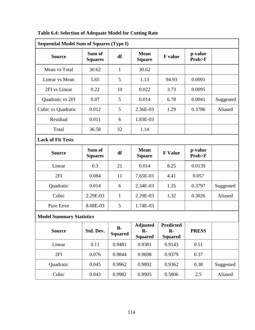
114

Table 6.4: Selection of Adequate Model for Cutting Rate

Sequential Model Sum of Squares (Type I)

Source Sum of

Squares df

Mean

Square F value

p-value

Prob>F

Mean vs Total 30.62 1 30.62

Linear vs Mean 5.65 5 1.13 94.93 0.0001

2FI vs Linear 0.22 10 0.022 3.73 0.0095

Quadratic vs 2FI 0.07 5 0.014 6.78 0.0041 Suggested

Cubic vs Quadratic 0.012 5 2.36E-03 1.29 0.3786 Aliased

Residual 0.011 6 1.83E-03

Total 36.58 32 1.14

Lack of Fit Tests

Source Sum of

Squares df

Mean

Square F Value

p-value

Prob>F

Linear 0.3 21 0.014 8.25 0.0139

2FI 0.084 11 7.65E-03 4.41 0.057

Quadratic 0.014 6 2.34E-03 1.35 0.3797 Suggested

Cubic 2.29E-03 1 2.29E-03 1.32 0.3026 Aliased

Pure Error 8.68E-03 5 1.74E-03

Model Summary Statistics

Source Std. Dev. R-

Squared

Adjusted

R-

Squared

Predicted

R-

Squared

PRESS

Linear 0.11 0.9481 0.9381 0.9143 0.51

2FI 0.076 0.9844 0.9698 0.9379 0.37

Quadratic 0.045 0.9962 0.9892 0.9362 0.38 Suggested

Cubic 0.043 0.9982 0.9905 0.5806 2.5 Aliased

115

Table 6.5: Selection of Adequate Model for Surface Roughness


Source Sum of

Squares df

Mean

Square F value

p-value

Prob>F

Mean vs Total 130.45 1 130.45

Linear vs Mean 4 5 0.8 51.88 0.0001

2FI vs Linear 0.21 10 0.021 1.72 0.1605



Residual 0.031 6 5.14E-03

Total 134.85 32 4.21

Lack of Fit Tests

Source Sum of

Squares df

Mean

Square F Value

p-value

Prob>F

Linear 0.37 21 0.018 3.13 0.1044

2FI 0.16 11 0.015 2.64 0.1467


Cubic 2.51E-03 1 2.51E-03 0.44 0.5356 Aliased

Pure Error 0.028 5 5.67E-03


Source Std. Dev. R-

Squared

Adjusted

R-

Squared

Predicted

R-

Squared

PRESS

Linear 0.12 0.9089 0.8914 0.8556 0.64

2FI 0.11 0.9561 0.915 0.8421 0.69


Cubic 0.072 0.993 0.9638 0.3728 2.76 Aliased

116

Table 6.6: Selection of Adequate Model for Gap Current


Source Sum of

Squares df

Mean

Square F value

p-value

Prob>F

Mean vs Total 132.11 1 132.11

Linear vs Mean 18.25 5 3.65 73.40 0.0001

2FI vs Linear 0.87 10 0.087 3.25 0.0176


Cubic vs Quadratic 0.051 5 0.010 2.44 0.1543 Aliased

Residual 0.025 6 4.182E-003

Total 151.66 32 4.74

Lack of Fit Tests

Source Sum of

Squares df

Mean

Square F Value

p-value

Prob>F

Linear 1.28 21 0.061 22.82 0.0013

2FI 0.41 11 0.038 14.07 0.0045

Quadratic 0.063 6 0.010 3.91 0.0779 Suggested

Cubic 0.012 1 0.012 4.40 0.0901 Aliased

Pure Error 0.013 5 2.670E-003


Source Std. Dev. R-

Squared

Adjusted

R-

Squared

Predicted

R-

Squared

PRESS

Linear 0.22 0.9338 0.9211 0.8903 2.14

2FI 0.16 0.9782 0.9577 0.9199 1.56


Cubic 0.065 0.9987 0.9934 0.3469 12.76 Aliased

117

Table 6.7: Selection of Adequate Model for Dimensional deviation

Sequential Model Sum of Squares [Type I]

Source Sum of

Squares df

Mean

Square F value

p-value

Prob>F

Mean vs Total 3.92 1 3.92

Linear vs Mean 0.59 5 0.12 36.56 < 0.0001

2FI vs Linear 0.025 10 2.535E-003 0.68 0.7247

Quadratic vs 2FI 0.041 5 8.250E-003 5.04 0.0121 Suggested


Residual 4.414E-

003 6 7.356E-004

Total 4.60 32 0.14

Lack of Fit Tests

Source Sum of

Squares df

Mean

Square F Value

p-value

Prob>F

Linear 0.082 21 3.891E-003 6.69 0.0221

2FI 0.056 11 5.123E-003 8.80 0.0132


Cubic 1.504E-

003 1 1.504E-003 2.58 0.1689 Aliased

Pure Error 2.910E-

003 5 5.820E-004


Source Std. Dev. R-

Squared

Adjusted

R-Squared

Predicte

d R-

Squared

PRESS

Linear 0.057 0.8755 0.8515 0.8049 0.13

2FI 0.061 0.9128 0.8310 0.4958 0.34


Cubic 0.027 0.9935 0.9664 -1.4077 1.64 Aliased

118

6.3.2 Effect of Process Variables on Cutting Rate

The regression coefficients of the second order equation (Equation 4.15, Chapter 4)

are obtained by using the experimental data (Table 6.3). The regression equation for the

cutting rate as a function of five input process variables was developed using experimental

data and is given below. The coefficients (insignificant identified from ANOVA) of some

terms of the quadratic equation have been omitted.

Cutting rate = -13.04695+0.10669 * Ton+0.19454 * Toff+0.068183 * SV-0.012100 * Ip-

3.65000E-003 * Ton* Toff -1.02500E-003 *Ton* SV +2.37500E-004 * Ton* Ip+6.75000E-

004 * Toff* SV-2.37500E-004 * Toff* Ip+6.35714E-004 * Ton2+1.83571E-003 * Toff2

(6.1)

The above response surface is plotted to study the effect of process variables on the

cutting rate and is shown in Figures 6.1a-6.1d. From Figure 6.1a the cutting rate is found to

have an increasing trend with the increase of pulse on time and at the same time it decreases

with the increase of pulse off time. This establishes the fact that cutting rate is proportional to

the energy consumed during machining and is dependent not only on the energy contained in

a pulse determining the crater size, but also on the applied energy rate or power. It is

observed from Figure 6.1b that cutting rate decreases with increase in spark gap set voltage.

With increase in spark gap set voltage the average discharge gap gets widened resulting into

a lower cutting rate. It is seen from Figure 6.1c that cutting rate increases with increase in

the peak current values. The higher is the peak current setting, the larger is the discharge

energy. This leads to increase in cutting rate. But, the sensitivity of the peak current setting

on the cutting performance is stronger than that of the pulse on time. While the peak current

setting is too high, wire breakage may occur frequently. It is seen from Figure 6.1d that

cutting rate almost remains constant with increase in the wire tension. Though with increase

in wire tension, the machining stability increases as vibrations get restricted. But its

increment does not influence the cutting rate much.

119

110.00

112.50

115.00

117.50

120.00

48.00

50.50

53.00

55.50

58.00

0.4

0.75

1.1

1.45

1.8

C

uttin

g R

ate

A: Pulse on Time B: Pulse off Time

Figure 6.1a: Combined Effect of Toff and Ton on Cutting Rate

110.00

112.50

115.00

117.50

120.00

20.00

25.00

30.00

35.00

40.00

0.4

0.7

1

1.3

1.6

C

uttin

g R

ate

A: Pulse on Time C: Spark Gap set voltage

Figure 6.1b: Combined Effect of SV and Ton on Cutting Rate

120

110.00

112.50

115.00

117.50

120.00

170.00

180.00

190.00

200.00

210.00

0.54

0.755

0.97

1.185

1.4

C

uttin

g R

ate

A: Pulse on Time D: Peak Current

Figure 6.1c: Combined Effect of IP and Ton on Cutting Rate

110.00

112.50

115.00

117.50

120.00

6

7

8

9

10

0.57

0.7575

0.945

1.1325

1.32

C

utt

ing

Ra

te

A: Pulse on Time E: Wire Tension

Figure 6.1d: Combined Effect of WT and Ton on Cutting Rate.

121

The residual analysis as a primary diagnostic tool is also done. Normal probability

plot of residuals has been drawn (Figure 6.2). All the data points are following the straight

line. Thus the data is normally distributed. It can be seen from Figure 6.3 that all the actual

values are following the predicted values and thus declaring model assumptions are correct.

6.3.3 Effect of Process Variables on Surface Roughness

The regression coefficients of the second order equation (Equation 4.8, Chapter 4) are

obtained by using the experimental data (Table 6.3). The regression equation for the surface

roughness as a function of five input process variables was developed using experimental

data and is given below. The coefficients (insignificant identified from ANOVA) of some

terms of the quadratic equation have been omitted.

Surface roughness = -31.55752 + 0.43482 * Ton + 0.074671 * Toff + 0.086635 * SV +

0.018187 * Ip - 0.072396 * WT - 1.42500E-003 * Ton* Toff - 8.12500E-004 * Ton * SV -

5.93750E-004 * Toff * Ip - 2.71875E-004 * SV* Ip + 2.40625E-003 * SV * WT - 1.13333E-

003 * Ton2 + 1.76667E-003 * Toff2 + 4.04167E-004 * SV2 + 6.04167E-005 * Ip2

(6.2)

The above response surface is plotted to study the effect of process variables on the surface

roughness and is shown in Figures 6.4 (a, b, c, d). It is clear that from Figure 6.4a the surface

roughness has an increasing trend with the increase of pulse on time and at the same time it

decreases with the increase of pulse off time. The surface roughness is most affected by the

amount of discharge energy which increases with increase in pulse on-time. The surface

roughness depends on the size of spark crater. A shallow crater together with a larger

diameter leads to a better workpiece surface roughness. To obtain a flat crater, it is important

to control the electrical discharging energy at a smaller level by setting a small pulse-on time

(Ton). A large discharging energy will cause violent sparks resulting in a deeper erosion

crater on the surface. Accompanying the cooling process after the spilling of molten metal,

residues will remain at the periphery of the crater to form a rough surface. Furthermore,

greater discharge energy will produce a larger crater, causing a larger surface roughness

value on the workpiece. It is observed from Figure 6.4b that surface roughness decreases

with increase in spark gap set voltage. With the higher spark gap set voltage, the discharge

122

Internally Studentized Residuals

No

rm

al

% P

ro

ba

bil

ity

Normal Plot of Residuals

-1.91 -0.92 0.07 1.06 2.05

1

5

10

20

30

50

70

80

90

95

99

Figure 6.2: Normal Plot of Residuals for Cutting Rate

22

Actual

Pre

dic

ted

Predicted vs. Actual

0.26

0.72

1.18

1.64

2.10

0.31 0.76 1.21 1.65 2.10

Figure 6.3: Predicted vs. Actual Plot for Cutting Rate

123

time gets longer. To obtain the longer discharge time, the machining speed needs to be

slowed down. This will lead to a wider average discharge gap. Therefore, the discharge

condition becomes more stable but the number of discharge cycles decreases within a given

period. Owing to this stable machining, surface accuracy becomes better and surface

roughness value decreases. It is seen from Figure 6.4c that surface roughness increases

slightly with increase in the peak current values. The higher is the peak current setting, the

larger is the discharge energy. This leads to increase in surface roughness. It is seen from

Figure 6.4d that surface roughness shows mild tendency to increase with increase in the wire

tension. This can be attributed to minimize the wire bending due to increase wire tension

which leads to a dynamic stable condition of wire.

Normal probability plot has been drawn for residuals in Figure 6.5. Linearity of this

normal plot confirms the normal distribution of the data. It can be seen from Figure 6.6 that

all the actual values are following the predicted values.

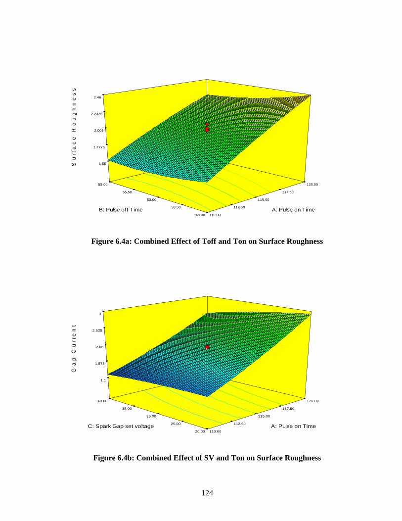
124

110.00

112.50

115.00

117.50

120.00

48.00

50.50

53.00

55.50

58.00

1.55

1.7775

2.005

2.2325

2.46

S

ur

fac

e R

ou

gh

ne

ss


Figure 6.4a: Combined Effect of Toff and Ton on Surface Roughness

110.00

112.50

115.00

117.50

120.00

20.00

25.00

30.00

35.00

40.00

1.1

1.575

2.05

2.525

3

G

ap

Cu

rre

nt


Figure 6.4b: Combined Effect of SV and Ton on Surface Roughness

125

110.00

112.50

115.00

117.50

120.00

170

180

190

200

210

1.54

1.745

1.95

2.155

2.36

S

ur

fac

e R

ou

gh

ne

ss


Figure 6.4c: Combined Effect of IP and Ton on Surface Roughness.

110.00

112.50

115.00

117.50

120.00

6.00

7.00

8.00

9.00

10.00

1.55

1.74

1.93

2.12

2.31

S

ur

fac

e R

ou

gh

ne

ss


Figure 6.4d: Combined Effect of WT and Ton on Surface Roughness

126


No

rm

al

% P

ro

ba

bil

ity


-1.97 -0.98 0.01 0.99 1.98

1

5

10

20

30

50

70

80

90

95

99

Figure 6.5: Normal Plot of Residuals for Surface Roughness

2

Actual

Pre

dic

ted


1.10

1.53

1.95

2.38

2.81

1.14 1.55 1.96 2.37 2.78

Figure 6.6: Predicted vs. Actual for Surface Roughness

127

6.3.4 Effect of Process Variables on Gap Current


obtained by using the experimental data (Table 6.3). The regression equation for the gap

current as a function of five input process variables was developed using experimental data

and is given below. The coefficients (insignificant identified from ANOVA) of some terms

of the quadratic equation have been omitted.

Gap current = - 23.11525 - 0.027826*Ton + 0.56794*Toff + 0.11664*SV + 0.042773*Ip -

7.52500E-003*Ton*Toff - 1.53750E-003*Ton*SV + 1.31250E-003*Toff*SV - 7.43750E-

004*Toff*Ip + 2.67692E-003*Ton2 + 2.87692E-003*Toff2 - 4.05769E-004*SV2 (6.3)

The response surface is plotted to study the effect of process variables on the gap

current and is shown in Figures 6.7a-6.7d. From Figure 6.7a it is seen that the gap current

increases with increase in pulse on time. A probable reason for it may be that with increase in

pulse on time, discharge energy increases causing higher gap current. Further it is seen from

Figure 6.7b that higher the spark gap set voltage, the longer the discharge wait time leading

to a smaller gap current. It is observed from Figure 6.7c that the gap current increases with

increase in the peak current This result has been attributed to the increase in peak current

which leads to the increase in the rate of the heat energy and hence in the rate of melting and

evaporation. Figure 6.7d shows that the wire tension is not influencing the gap current

significantly.

A typical check for normality assumption is made by constructing a normal

probability plot of the residuals. Each residual is plotted against its expected value under

normality. The residual distribution is found normal, as this plot is a straight line (Figure

6.8). It can be seen from Figure 6.9 that the predicted values and the actual values have a

linear graph.

128

110.00

112.50

115.00

117.50

120.00

48.00

50.50

53.00

55.50

58.00

1

1.625

2.25

2.875

3.5

G

ap

Cu

rre

nt


Figure 6.7a: Combined Effect of Toff and Ton on Gap Current

110.00

112.50

115.00

117.50

120.00

20.00

25.00

30.00

35.00

40.00

1.1

1.575

2.05

2.525

3

G

ap

Cu

rre

nt


Figure 6.7b: Combined Effect of SV and Ton on Gap Current

129

110.00

112.50

115.00

117.50

120.00

170

180

190

200

210

1.2

1.65

2.1

2.55

3

G

ap

Cu

rre

nt


Figure 6.7c: Combined Effect of IP and Ton on Gap Current

110.00

112.50

115.00

117.50

120.00

6.00

7.00

8.00

9.00

10.00

1.3

1.675

2.05

2.425

2.8

G

ap

Cu

rre

nt


Figure 6.7d: Combined Effect of WT and Ton on Gap Current

130


No

rm

al

% P

ro

ba

bil

ity


-1.81 -0.87 0.06 0.99 1.93

1

5

10

20

30

50

70

80

90

95

99

Figure 6.8: Normal Plot of Residuals for Gap Current

42

Actual

Pre

dic

ted


0.80

1.59

2.38

3.18

3.97

0.90 1.67 2.44 3.20 3.97

Figure 6.9: Predicted vs. Actual for Gap Current

131

6.3.5 Effect of Process Variables on Dimensional Deviation


obtained by using the experimental data (Table 6.3). The regression equation for the

dimensional deviation as a function of five input process variables was developed using

experimental data and is given below. The coefficients (insignificant identified from

ANOVA) of some terms of the quadratic equation have been omitted.

Dimensional Deviation = + 5.59943 - 0.11868*Ton - 3.44167E-003*Toff + 0.023276*SV +

0.026339*Ip + 0.015521*WT - 4.83750E-004*Ton*SV - 2.41875E-004*Ton*Ip +

7.08929E-004*Ton2 + 3.27232E-004*SV2 (6.4)

The response surface is plotted to study the effect of process variables on the

dimensional deviation and is shown in Figures 6.10a-6.10d. It is seen from Figure 6.10a that

the dimensional deviation decreases with increase in pulse on time. A probable reason for it

may be that with increase in pulse on time, discharge energy increases. During every

individual spark discharge, the wire experiences an impact, which acts in the reverse

direction of the discharge occurrence. Thus, dimensional deviation decreases. It is seen from

Figure 6.10b that dimensional deviation decreases with higher spark gap set voltage. It is

observed from Figure 6.10c that the dimensional deviation increases with increase in the

peak current. The density of spark discharges would also be changed depending on the peak

current. This will have an impact on the precision and accuracy of the work piece. It can be

seen from Figure 6.10d that the dimensional deviation gradually increases with the increase

in the wire tension. This can be attributed to the increase of the wire tension minimizing the

wire bending which leads to a dynamic stable condition of the diameter and the depth of the

crater leading to higher dimensional deviation. Normal probability plot has been drawn for

residuals in Figure 6.11. Normality of residuals was checked using a normal probability plot.

Linearity of this normal plot confirms the normal distribution of the data. Linearity is

observed between predicted values and actual values (Figure 6.12).

132

110.00

112.50

115.00

117.50

120.00

48

50.5

53

55.5

58

0.23

0.28

0.33

0.38

0.43

D

ime

ns

ion

al

De

via

tio

n


Figure 6.10a: Combined Effect of Toff and Ton on Dimensional Deviation

110.00

112.50

115.00

117.50

120.00

20.00

25.00

30.00

35.00

40.00

0.13

0.235

0.34

0.445

0.55

D

ime

ns

ion

al

De

via

tio

n

A: Pulse on Time

C: Spark Gap set voltage

Figure 6.10b: Combined Effect of SV and Ton on Dimensional Deviation

133

110.00

112.50

115.00

117.50

120.00

170.00

180.00

190.00

200.00

210.00

0.19

0.2475

0.305

0.3625

0.42

D

ime

ns

ion

al

De

via

tio

n

A: Pulse on Time

D: Peak Current

Figure 6.10c: Combined Effect of IP and Ton on Dimensional Deviation

110.00

112.50

115.00

117.50

120.00

6.00

7.00

8.00

9.00

10.00

0.21

0.27

0.33

0.39

0.45

D

ime

ns

ion

al

De

via

tio

n


Figure 6.10d: Combined Effect of WT and Ton on Dimensional Deviation

134


No

rm

al

% P

ro

ba

bil

ity


-1.65 -0.49 0.68 1.84 3.01

1

5

10

20

30

50

70

80

90

95

99

Figure 6.11: Normal Plot of Residuals for Dimensional Deviation

2

Actual

Pre

dic

ted


0.06

0.24

0.42

0.59

0.77

0.09 0.26 0.43 0.60 0.77

Figure 6.12: Predicted vs. Actual for Dimensional Deviation

135

6.4 ANALYSIS OF VARIANCE

In order to statistically analyze the results, ANOVA was performed. Process variables

having p-value<0.05 are considered significant terms for the requisite response

characteristics. The insignificant parameters were pooled using backward elimination

method. The pooled version of ANOVA for cutting rate (Table 6.8) indicates that the pulse

on time (A), the pulse off time(B), Spark gap set voltage(C), Peak current(D), the interaction

terms (AB, AC, AD, BC, BD) and the quadratic terms (A2, B2)are significant parameters

affecting cutting rate. For surface roughness the pulse on time(A), the pulse off time(B),

Spark gap set voltage(C), Peak current(D), the interaction terms (AC, BD, CD, CE), and the

quadratic terms (A2, B2, C2) are significant parameters affecting its value (Table 6.9). For

gap current the pulse on time(A), the pulse off time(B), Spark gap set voltage(C), Peak

current(D), the interaction terms (AB, AC, BC, BD), and the quadratic terms (A2, B2, C2)

are significant terms (Table 6.10). For dimensional deviation the pulse on time(A), the pulse

off time(B), Spark gap set voltage(C), Peak current(D), the wire tension (E), the interaction

terms (AC, AD), and the quadratic terms (A2,C2) are significant model terms (Table 6.11).

Some more statistical inferences are also given at the bottom of ANOVA tables (Tables 6.8 -

6.11).

136

Table 6.8: Pooled ANOVA- Cutting Rate

Source Sum of

Squares Df Mean Square F Value

p-value

Prob > F

Model 5.93 11 0.54 354.80 0.0001 Significant

A-Pulse on Time 3.27 1 3.27 2152.95 0.0001

B-Pulse off Time 1.85 1 1.85 1216.51 0.0001

C-Spark Gap set

voltage 0.46 1 0.46 305.96 0.0001

D-Peak Current 0.066 1 0.066 43.54 0.0001

AB 0.13 1 0.13 87.69 0.0001

AC 0.042 1 0.042 27.66 0.0001

AD 9.025E-003 1 9.025E-003 5.94 0.0243

BC 0.018 1 0.018 12.00 0.0025

BD 9.025E-003 1 9.025E-003 5.94 0.0243

A2 7.544E-003 1 7.544E-003 4.97 0.0375

B2 0.063 1 0.063 41.41 0.0001

Residual 0.030 20 1.519E-003

Lack of Fit 0.022 15 1.447E-003 0.83 0.6444 Not

significant

Pure Error 8.683E-003 5 1.737E-003

Cor Total 5.96 31

R-Squared = 0.9949 Adj R-Squared = 0.9921

Pred R-Squared = 0.9853 Adeq Precision =75.356

Statistical inferences:

1. The Model F-value of 354.80 implies the model is significant. There is only a 0.01%

chance that a "Model F-Value" of this much magnitude could occur due to noise.

2. The "Lack of Fit F-value" of 0.83 implies the Lack of Fit is not significant relative to

the pure error. There is a 64.44% chance that a "Lack of Fit F-value" of this order

could occur due to noise. Non-significant lack of fit is good.

3. The "Pred R-Squared" of 0.9853 is in reasonable agreement with the "Adj R-

Squared" of 0.9921."Adeq Precision" measures the signal to noise ratio. This model

can be used to navigate the design space as the ratio (75.356) indicates an adequate

signal.

4. Values of "Prob > F" less than 0.0500 indicate model terms are significant. In this

case A, B, C, D, AB, AC, AD, BC, BD, A2, B

2 are significant model terms.

137

Table 6.9: Pooled ANOVA- Surface Roughness

Source Sum of

Source df

Mean

Square

F

Value

p-value

Prob >

F


A-Pulse on Time 3.31 1 3.31 838.49 0.0001

B-Pulse off Time 0.13 1 0.13 33.09 0.0001

C-Spark Gap set

voltage 0.54 1 0.54 136.12 0.0001

D-Peak Current 0.022 1 0.022 5.63 0.0297

E-Wire Tension 4.167E-006 1 4.167E-006 1.056E-

003 0.9745

AB 0.020 1 0.020 5.15 0.0366

AC 0.026 1 0.026 6.69 0.0192

BD 0.056 1 0.056 14.30 0.0015

CD 0.047 1 0.047 11.99 0.0030

CE 0.037 1 0.037 9.39 0.0070

A2 0.024 1 0.024 6.01 0.0253

B2 0.058 1 0.058 14.61 0.0014

C2 0.048 1 0.048 12.23 0.0028

D2 0.017 1 0.017 4.37 0.0518

Residual 0.067 17 3.945E-003

Lack of Fit 0.039 12 3.228E-003 0.57 0.8033 Not

significant

Pure Error 0.028 5 5.667E-003

Cor Total 4.40 31


Pred R-Squared = 0.9442 Adeq Precision=39.596




2. The "Lack of Fit F-value" of 0.57implies the Lack of Fit is not significant relative to






138

signal.


case A, B, C, D, AB, AC, BD, CD, CE, A2, B

2, C


Table 6.10: Pooled ANOVA- Gap Current

Source Sum of

Source

df Mean

Square

F Value p-value

Prob > F


A-Pulse on Time 12.26 1 12.26 1834.32 0.0001

B-Pulse off Time 5.35 1 5.35 800.59 0.0001

C-Spark Gap set

voltage 0.54 1 0.54 80.38 0.0001

D-Peak Current 0.11 1 0.11 16.17 0.0007

AB 0.57 1 0.57 84.76 0.0001

AC 0.095 1 0.095 14.15 0.0012

BC 0.069 1 0.069 10.31 0.0044

BD 0.089 1 0.089 13.25 0.0016

A2 0.13 1 0.13 19.92 0.0002

B2 0.15 1 0.15 23.01 0.0001

C2 0.049 1 0.049 7.32 0.0136

Residual 0.13 20 6.681E-003

Lack of Fit 0.12 15 8.018E-003 3.00 0.1149 Not

significant

Pure Error 0.013 5 2.670E-003

Cor Total 19.54 31


Pred R-Squared = 0.9780 AdeqPrecision=61.296









139


signal.


case A, B, C, D, AB, AC, BC, BD, A2, B

2, C


Table 6.11: Pooled ANOVA- Dimensional Deviation

Source Sum of

Source

df Mean Square F

Value

p-value

Prob >

F


A-Pulse on Time 0.16 1 0.16 128.18 0.0001

B-Pulse off Time 7.107E-003 1 7.107E-003 5.86 0.0242

C-Spark Gap set

voltage 0.39 1 0.39 320.41 0.0001

D-Peak Current 0.021 1 0.021 17.28 0.0004

E-Wire Tension 0.023 1 0.023 19.08 0.0002

AC 9.361E-003 1 9.361E-003 7.72 0.0109

AD 9.361E-003 1 9.361E-003 7.72 0.0109

A2 9.381E-003 1 9.381E-003 7.74 0.0109

C2 0.032 1 0.032 26.39 0.0001

Residual 0.027 22 1.212E-003

Lack of Fit 0.024 17 1.397E-003 2.40 0.1692 Not

significant

Pure Error 2.910E-003 5 5.820E-004

Cor Total 0.68 31

R-Squared=0.9608 Adj R-Squared = 0.9447

Pred R-Squared = 0.8792 Adeq Precision =32.590









140


signal.


case A, B, C, D, E, AC, AD, A2, C

2 are significant model terms

141

CHAPTER-7

SINGLE AND MULTI RESPONSE OPTIMIZATION USING

DESIRABILITY FUNCTION

7.1 DESIRABILITY FUNCTION

Derringer and Suich (1980) describe a multiple response method called desirability. It

is an attractive method for industry for optimization of multiple quality characteristic

problems. The method makes use of an objective function, D(X), called the desirability

function and transforms an estimated response into a scale free value (di) called desirability.

The desirable ranges are from zero to one (least to most desirable respectively). The factor

settings with maximum total desirability are considered to be the optimal parameter

conditions.

The simultaneous objective function is a geometric mean of all transformed responses:

n

nddddD/1

321 =

nn

i

id

/1

1

(7.1)

Where, n is the number of responses in the measure. If any of the responses or factors falls

outside the desirability range, the overall function becomes zero.

It can be extended to

nwn

n

ww dddD/12

2

1

1 (7.2)

to reflect the possible difference in the importance of different responses, where the weight

iw satisfies 0< iw <1 and 121 nwww .

Desirability is an objective function that ranges from zero outside of the limits to one

at the goal. The numerical optimization finds a point that maximizes the desirability function.

The characteristics of a goal may be altered by adjusting the weight or importance. For

several responses and factors, all goals get combined into one desirability function.

For simultaneous optimization each response must have a low and high value

142

assigned to each goal. The "Goal" field for responses must be one of five choices: "none",

"maximum", "minimum", "target", or "in range". Factors will always be included in the

optimization, at their design range by default, or as a maximum, minimum of target goal. The

meanings of the goal parameters are:

Maximum:

di = 0 if response < low value

0 di 1 as response varies from low to high

di = 1 if response > high value

Minimum:


1 di 0 as response varies from low to high


Target:


0 di 1 as response varies from low to target

1 di 0 as response varies from target to high


Range:


di = 1 as response varies from low to high


The di for "in range" are included in the product of the desirability function "D", but are not

counted in determining "n": D = n

id/1

.

If the goal is none, the response will not be used for the optimization.

Desirability function has been used to determine the optimum parameters for WEDM

parts for optimization of cutting rate, surface roughness, gap current and dimensional

deviation in the present investigation. Second order central composite experimental design

involving five factors ( Pulse on time, pulse off time, spark gap set voltage, peak current and

wire tension) each at five levels has been used to find optimum combination of factors and

levels in WEDM machining of H-11 steel. The single response and multi response

optimizations were achieved through desirability function.

143

7.2 SINGLE RESPONSE OPTIMIZATION USING DESIRABILITY FUNCTION

The constraints for the optimization of individual response characteristics viz. cutting

rate, surface roughness, gap current, and dimensional deviation, are given in Tables 7.1-7.4.

Goals and limits were established for each response individually in order to accurately

determine their impact on individual desirability. A maximum or minimum level is provided

for each response characteristic which has to be optimized.

Table 7.1: Range of Input Parameters and Cutting Rate for Desirability

Process

Parameter Goal

Lower

Limit

Upper

Limit

Lower

Weight

Upper

Weight Importance

Pulse on Time is in range 110 120 1 1 3

Pulse off Time is in range 48 58 1 1 3

Spark Gap set

voltage is in range 20 40 1 1 3

Peak Current is in range 170 210 1 1 3

Wire Tension is in range 6 10 1 1 3

Cutting Rate maximize 0.31 2.1 1 1 3

Table 7.2: Range of Input Parameters and Surface Roughness for Desirability

Process Parameter Goal Lower

Limit

Upper

Limit

Lower

Weight

Upper

Weight Importance



Spark Gap set




Surface Roughness minimize 1.14 2.78 1 1 3

144

Table 7.3: Range of Input Parameters and Gap Current for Desirability


Limit

Upper

Limit

Lower

Weight

Upper

Weight Importance



Spark Gap set




Gap Current maximize 0.9 3.97 1 1 3

Table 7.4: Range of Input Parameters and Dimensional Deviation for Desirability


Limit

Upper

Limit

Lower

Weight

Upper

Weight Importance



Spark Gap set




Dimensional

Deviation minimize 0.087 0.767 1 1 3

Weights are assigned to give added emphasis to upper / lower bounds or to emphasize

a target value. The default value “1”of weight is assigned to a goal to adjust the shape of its

particular desirability function. The default value “3” is selected for importance in order to

give equal importance to all goals.

145

7.2.1 Optimal Solutions

The goal of optimization is to find a good set of conditions that will meet all the

goals. It is not necessary that the value of desirability is always 1.0 as the value is completely

dependent on how closely the lower and upper limits are set relative to the actual optimum

(Aggarwal et. al., 2008). A set of 47 optimal solutions is derived for the specified design

space constraints for individual response characteristic viz. cutting rate, surface roughness,

gap current, and dimensional deviation using Design Expert statistical software. The set of

conditions possessing highest desirability value is selected as optimum condition for the

desired response. Tables 7.5-7.8 report the optimal set of conditions with higher desirability

function required for obtaining desired response characteristic under specified constraints.

Desirability 3D-plots were first drawn keeping input parameters in range and cutting

rate and gap current at maximum. Likewise plots were made for surface roughness, and

dimensional deviation independently keeping their values at minimum level. Figure 7.1

shows a plot of desirability function distribution of cutting rate for H-11 steel according to

pulse on time and pulse off time. It can be visualized that high level of pulse on time and low

value of pulse off time favor high cutting rate. Likewise plots were drawn between spark gap

set voltage and pulse on time. Plots revealed that low value of spark gap set voltage and

higher value of pulse on time favor high cutting rate (Figure 7.2). From Figure 7.3 it can be

seen that the high values of peak current favor high cutting rate. Wire tension has almost

insignificant effect (Figure 7.4). Figures 7.5-7.8 show plots of desirability function

distribution of surface roughness for H-11 steel according to various input process

parameters. Low level of pulse on time, higher value of pulse off time, higher values of spark

gap set voltage and higher peak current favor lower value of surface roughness. Figures 7.9-

7.12 show plots of desirability function distribution of gap current for H-11 steel according to

various input process parameters. High level of pulse on time, low level of pulse off time,

lower values of spark gap set voltage and high values of peak current favor higher value of

gap current. Wire tension does not affect the gap current significantly. Figures 7.13-7.16

show plots of desirability function distribution of dimensional deviation for H-11 steel

according to various input process parameters. High level of pulse on time, low level of pulse

off time, higher values of spark gap set voltage, high values of peak current and lower values

of wire tension favor lower values of dimensional deviation.

146

Table 7.5: Set of Optimal Solutions for Desirability (Cutting Rate)

S.No. Ton Toff SV IP WT CR Desir-

ability

1 120.00 48.00 20.00 210.00 10.00 2.05565 0.975 Selected

2 120.00 48.00 20.09 210.00 6.59 2.05365 0.974

3 120.00 48.00 20.00 209.51 7.42 2.05319 0.974

4 120.00 48.00 20.00 209.51 8.45 2.05317 0.974

5 120.00 48.02 20.04 210.00 6.00 2.0523 0.973

6 119.94 48.00 20.00 210.00 9.95 2.04857 0.971

7 119.93 48.00 20.00 210.00 9.01 2.04804 0.971

8 120.00 48.11 20.00 210.00 7.04 2.04396 0.969

9 119.84 48.00 20.00 210.00 6.17 2.0374 0.965

10 120.00 48.19 20.00 209.99 8.10 2.03565 0.964

11 119.74 48.00 20.00 210.00 6.67 2.02616 0.959

12 119.74 48.00 20.00 210.00 8.41 2.0257 0.958

13 120.00 48.00 20.00 203.16 8.65 2.02126 0.956

14 120.00 48.00 20.01 203.16 6.47 2.02123 0.956

15 120.00 48.00 20.00 201.98 8.49 2.01556 0.953

16 120.00 48.01 21.79 210.00 6.04 2.01409 0.952

17 120.00 48.00 20.43 202.10 10.00 2.0066 0.948

18 120.00 48.40 20.00 206.64 7.39 1.99791 0.943

19 119.99 48.00 20.00 198.51 6.65 1.99659 0.942

20 120.00 48.00 20.00 195.99 7.08 1.98559 0.936

21 120.00 48.00 20.00 194.56 6.48 1.97824 0.932

22 119.54 48.00 21.26 209.99 6.00 1.97555 0.930

23 119.81 48.00 20.01 198.18 6.00 1.97511 0.930

24 120.00 48.76 20.00 209.37 10.00 1.97465 0.930

25 119.99 48.07 23.28 210.00 7.29 1.97346 0.929

26 120.00 48.00 23.80 210.00 6.00 1.97052 0.928

27 120.00 48.00 22.17 202.63 10.00 1.97019 0.927

28 120.00 48.00 20.00 191.93 9.74 1.96523 0.925

29 120.00 48.25 22.88 210.00 7.57 1.96521 0.925

30 119.40 48.33 20.00 210.00 6.86 1.95519 0.919

31 120.00 48.32 20.01 195.01 6.00 1.94869 0.915

Contd…….

147


ability

32 119.45 48.00 20.00 200.30 6.08 1.94654 0.914

33 118.82 48.00 20.00 210.00 6.00 1.92286 0.901

34 120.00 48.00 22.80 194.68 9.04 1.91638 0.897

35 120.00 49.16 22.27 208.87 6.00 1.8836 0.879

36 120.00 48.00 28.01 210.00 7.80 1.87588 0.875

37 120.00 48.00 23.82 188.45 10.00 1.86218 0.867

38 119.91 48.00 20.00 172.05 10.00 1.85627 0.864

39 119.99 48.04 20.00 170.00 9.07 1.85096 0.861

40 120.00 49.17 20.00 188.15 8.15 1.83378 0.851

41 120.00 48.00 30.07 209.59 6.17 1.82794 0.848

42 119.97 49.72 20.00 190.95 6.00 1.79265 0.828

43 117.81 48.00 20.00 191.27 9.99 1.72584 0.791

44 120.00 49.87 26.76 210.00 10.00 1.72546 0.791

45 118.05 48.00 20.00 170.00 10.00 1.65489 0.751

46 120.00 48.00 38.45 210.00 6.29 1.64205 0.744

47 120.00 50.10 36.08 208.96 10.00 1.50357 0.667

Table 7.6: Set of Optimal Solutions for Desirability (Surface Roughness)


ability

1 110.00 58.00 40.00 210.00 6.00 1.38979 0.848 Selected

2 110.00 57.40 40.00 209.71 6.00 1.39217 0.846

3 110.00 58.00 40.00 209.99 6.41 1.39961 0.842

4 110.00 55.82 40.00 210.00 6.14 1.40557 0.838

5 110.00 56.71 40.00 202.50 6.00 1.40588 0.838

6 110.00 56.19 39.98 199.70 6.00 1.41247 0.834

7 110.00 55.60 39.30 210.00 6.00 1.41372 0.833

8 110.09 58.00 39.10 210.00 6.40 1.41665 0.831

9 110.00 54.98 39.96 197.86 6.00 1.42027 0.829

10 110.12 54.55 40.00 210.00 6.00 1.42629 0.825

11 110.52 58.00 39.85 210.00 6.00 1.42828 0.824

12 110.02 53.91 40.00 195.22 6.00 1.4312 0.822

13 110.00 56.04 39.98 209.88 7.32 1.43198 0.822

Contd………

148

S.No. Ton Toff SV IP WT SR Desir-

ability

14 110.42 55.64 40.00 210.00 6.03 1.43562 0.820

15 110.00 57.25 39.71 191.88 6.00 1.43813 0.818

16 110.03 53.85 40.00 188.91 6.00 1.44178 0.816

17 110.00 57.45 36.49 208.48 6.00 1.44295 0.815

18 110.09 55.03 40.00 188.82 6.00 1.44417 0.815

19 110.00 58.00 39.33 210.00 8.26 1.44911 0.812

20 110.00 53.51 40.00 192.12 6.78 1.45511 0.808

21 110.00 58.00 39.84 209.95 8.71 1.45554 0.808

22 110.00 56.90 36.03 210.00 6.28 1.45617 0.807

23 110.00 57.99 39.99 210.00 8.84 1.45755 0.806

24 110.02 57.15 40.00 210.00 8.93 1.46416 0.802

25 110.00 56.66 39.95 183.03 6.00 1.46535 0.802

26 110.00 56.54 40.00 194.36 7.72 1.46595 0.801

27 110.00 51.51 40.00 179.22 6.00 1.46863 0.800

28 110.00 52.48 40.00 191.93 7.13 1.47282 0.797

29 110.00 57.36 40.00 205.88 9.14 1.47315 0.797

30 110.00 57.13 40.00 191.06 7.52 1.47402 0.796

31 110.00 57.32 40.00 209.96 9.53 1.47603 0.795

32 110.00 50.73 39.43 180.02 6.00 1.47675 0.795

33 110.11 56.15 40.00 210.00 8.94 1.4773 0.794

34 110.00 57.99 40.00 209.97 9.79 1.48056 0.792

35 110.00 55.67 34.58 197.78 6.00 1.48188 0.792

36 110.02 53.05 40.00 189.58 8.02 1.49267 0.785

37 110.00 53.28 40.00 183.60 8.32 1.50748 0.776

38 110.00 53.42 40.00 190.21 9.00 1.51139 0.774

39 110.07 54.66 40.00 170.00 6.23 1.51394 0.772

40 110.00 51.56 40.00 180.21 8.25 1.52032 0.768

41 110.00 51.91 36.11 210.00 6.30 1.52766 0.764

42 110.00 55.59 34.12 194.67 9.98 1.52848 0.763

43 110.00 53.19 36.74 192.70 9.85 1.53155 0.761

44 110.00 52.24 29.57 170.00 9.92 1.55074 0.750

45 110.00 52.25 25.21 170.00 10.00 1.56269 0.742

46 110.00 54.17 25.39 171.36 10.00 1.57116 0.737

47 110.02 52.47 32.83 210.00 9.95 1.59648 0.722

149

Table 7.7: Set of Optimal Solutions for Desirability (Gap Current)

S.No. Ton Toff SV IP WT IG Desir-

ability

1 120.00 48.00 20.00 210.00 10.00 3.86478 0.966 Selected

2 120.00 48.01 20.00 210.00 6.04 3.86214 0.965

3 120.00 48.00 20.10 210.00 6.73 3.86209 0.965

4 120.00 48.01 20.20 209.98 8.38 3.85843 0.964

5 120.00 48.00 20.00 208.25 9.77 3.8523 0.962

6 119.92 48.00 20.00 210.00 6.77 3.84655 0.960

7 120.00 48.00 20.00 207.27 9.80 3.84542 0.959

8 120.00 48.00 20.00 205.36 9.15 3.83189 0.955

9 119.90 48.00 20.73 209.97 9.42 3.82788 0.954

10 120.00 48.07 20.00 206.51 6.54 3.82768 0.954

11 119.99 48.00 21.86 209.97 6.00 3.82084 0.951

12 119.78 48.02 20.06 210.00 6.65 3.81141 0.948

13 119.74 48.00 20.00 209.99 9.37 3.80699 0.947

14 120.00 48.00 20.00 201.56 7.87 3.80507 0.946

15 120.00 48.00 22.88 209.41 7.80 3.7965 0.943

16 120.00 48.00 20.00 200.06 7.66 3.79444 0.943

17 120.00 48.01 23.44 210.00 9.97 3.78617 0.940

18 119.99 48.22 20.02 202.68 10.00 3.77024 0.935

19 120.00 48.00 20.00 196.31 7.21 3.76728 0.934

20 119.98 48.00 24.68 210.00 6.00 3.75377 0.930

21 120.00 48.08 20.01 195.43 10.00 3.74703 0.927

22 120.00 48.00 25.23 209.97 9.92 3.74297 0.926

23 120.00 48.00 25.31 209.96 8.16 3.74096 0.925

24 120.00 48.00 20.23 190.95 6.07 3.72519 0.920

25 120.00 48.01 20.05 190.06 8.18 3.72147 0.919

26 119.99 48.00 20.00 189.56 8.43 3.71717 0.918

27 120.00 48.84 20.00 210.00 7.60 3.70817 0.915

28 119.95 48.00 20.00 187.35 9.80 3.69439 0.910

29 120.00 48.00 26.25 203.66 6.00 3.67214 0.903

30 119.85 48.00 20.61 187.86 6.00 3.66174 0.900

31 120.00 48.33 26.24 210.00 6.00 3.65791 0.898

Contd……..

150


ability

32 119.96 48.00 20.00 179.67 7.91 3.64184 0.893

33 120.00 48.00 20.00 170.43 6.74 3.58493 0.875

34 119.73 48.00 20.34 178.55 10.00 3.57619 0.872

35 120.00 48.00 21.38 170.13 8.12 3.55287 0.864

36 120.00 49.72 20.18 209.98 6.01 3.5452 0.862

37 120.00 48.02 24.86 180.88 10.00 3.54273 0.861

38 120.00 48.00 34.11 210.00 8.82 3.48617 0.842

39 120.00 48.00 24.28 170.00 7.87 3.48427 0.842

40 120.00 48.00 28.32 170.00 6.70 3.37838 0.807

41 119.75 48.00 35.98 202.90 10.00 3.32499 0.790

42 120.00 48.00 38.95 210.00 6.04 3.31927 0.788

43 120.00 51.17 20.00 210.00 6.85 3.29496 0.780

44 119.98 49.61 30.76 205.67 10.00 3.28731 0.778

45 120.00 48.19 40.00 170.00 6.52 2.97261 0.675

46 120.00 48.46 40.00 170.00 9.82 2.93731 0.664

47 120.00 51.14 33.36 182.80 10.00 2.87203 0.642

Table 7.8: Set of Optimal Solutions for Desirability (Dimensional Deviation)

S.No. Ton Toff SV IP WT %D Desir-

ability

1 119.68 56.12 39.59 200.83 6.20 0.0718747 1.000

2 119.17 57.00 39.55 205.21 7.32 0.0844189 1.000

3 119.84 49.47 39.31 203.96 6.17 0.0858989 1.000

4 119.98 56.40 36.98 206.98 6.42 0.0782588 1.000

5 119.70 52.69 39.67 208.69 7.19 0.0774591 1.000

6 119.92 54.72 39.98 205.01 6.26 0.0590252 1.000

7 119.76 56.29 39.74 197.48 6.77 0.0862995 1.000

8 119.47 57.65 37.19 207.11 6.85 0.0867775 1.000

9 119.90 54.90 39.65 201.68 6.96 0.0813809 1.000

10 120.00 48.00 40.00 210.00 6.00 0.0632262 1.000 Selected

11 119.98 57.83 39.95 209.77 9.56 0.0859158 1.000

12 119.87 50.12 39.18 204.79 6.45 0.0864382 1.000

13 119.84 57.60 38.99 206.59 7.27 0.0708631 1.000

Contd…….

151


ability

14 118.96 57.86 39.94 209.31 8.17 0.0853462 1.000

15 118.09 57.16 38.96 209.77 6.32 0.0837448 1.000

16 120.00 57.84 39.88 196.81 7.33 0.0865397 1.000

17 119.94 48.17 39.32 207.83 6.63 0.0852636 1.000

18 119.21 56.46 38.30 207.15 6.50 0.0790664 1.000

19 120.00 49.02 39.45 209.97 7.42 0.0867664 1.000

20 120.00 51.14 39.98 209.60 8.06 0.0856057 1.000

21 119.83 53.96 39.07 207.30 7.28 0.0810984 1.000

22 119.89 48.74 39.90 209.90 7.35 0.0847615 1.000

23 119.64 57.93 39.67 203.64 6.62 0.0648702 1.000

24 119.74 51.49 38.56 209.80 7.04 0.0856608 1.000

25 119.89 57.99 39.34 206.06 7.77 0.0746668 1.000

26 119.90 54.30 39.95 197.20 6.02 0.0782201 1.000

27 119.86 51.89 39.88 208.77 7.78 0.084328 1.000

28 119.90 53.40 39.97 209.92 8.51 0.0859122 1.000

29 119.56 56.62 39.65 205.32 6.84 0.0700299 1.000

30 120.00 57.91 40.00 210.00 9.82 0.0884137 0.998

31 117.67 58.00 38.65 210.00 6.29 0.0913407 0.994

32 119.10 48.68 40.00 202.90 6.00 0.0957774 0.987

33 120.00 58.00 40.00 184.76 6.00 0.0966458 0.986

34 119.99 51.33 40.00 209.71 8.91 0.097812 0.984

35 120.00 57.16 40.00 184.35 6.00 0.100595 0.980

36 119.99 49.91 40.00 210.00 8.86 0.101256 0.979

37 119.98 58.00 40.00 203.34 10.00 0.109179 0.967

38 118.26 48.00 38.48 209.99 6.00 0.110435 0.966

39 116.90 58.00 40.00 210.00 7.29 0.113534 0.961

40 120.00 52.70 40.00 191.98 7.54 0.119424 0.952

41 120.00 54.05 34.09 203.06 6.00 0.123223 0.947

42 120.00 49.57 40.00 207.88 9.97 0.125125 0.944

43 118.78 58.00 39.56 180.13 6.00 0.127649 0.940

44 120.00 48.11 39.25 210.00 10.00 0.131539 0.935

45 120.00 58.00 40.00 188.87 9.76 0.143926 0.916

46 120.00 58.00 40.00 178.56 9.07 0.161033 0.891

47 117.25 57.97 40.00 176.75 7.73 0.179674 0.864

152

110.00

112.50

115.00

117.50

120.00

48.00

50.50

53.00

55.50

58.00

0.100

0.320

0.540

0.760

0.980

D

es

ira

bil

ity


Figure 7.1: 3D Surface Graph of Desirability for Cutting Rate (Toff, Ton)

110.00

112.50

115.00

117.50

120.00

20

25

30

35

40

0.240

0.425

0.610

0.795

0.980

D

es

ira

bil

ity


Figure 7.2: 3D Surface Graph of Desirability for Cutting Rate (SV, Ton)

153

110.00

112.50

115.00

117.50

120.00

170.00

180.00

190.00

200.00

210.00

0.310

0.477

0.645

0.813

0.980 D

es

ira

bil

ity


Figure 7.3: 3D Surface Graph of Desirability for Cutting Rate (IP, Ton)

110.00

112.50

115.00

117.50

120.00

6

7

8

9

10

0.370

0.522

0.675

0.828

0.980

D

es

ira

bil

ity


Figure 7.4: 3D Surface Graph of Desirability for Cutting Rate (WT, Ton)

154

110.00

112.50

115.00

117.50

120.00

48.00

50.50

53.00

55.50

58.00

0.280

0.422

0.565

0.708

0.850 D

es

ira

bil

ity

A: Pulse on Time

B: Pulse off Time

Figure 7.5: 3D Surface Graph of Desirability for Surface Roughness (Toff, Ton)

110.00

112.50

115.00

117.50

120.00

20

25

30

35

40

0.130

0.310

0.490

0.670

0.850

D

es

ira

bil

ity

A: Pulse on Time

C: Spark Gap set voltage

Figure 7.6: 3D Surface Graph of Desirability for Surface Roughness (SV, Ton)

155

110.00

112.50

115.00

117.50

120.00

170.00

180.00

190.00

200.00

210.00

0.380

0.498

0.615

0.732

0.850

D

es

ira

bil

ity

A: Pulse on Time

D: Peak Current

Figure 7.7: 3D Surface Graph of Desirability for Surface Roughness (IP, Ton)

110.00

112.50

115.00

117.50

120.00

6

7

8

9

10

0.420

0.527

0.635

0.742

0.850

D

es

ira

bil

ity


Figure 7.8: 3D Surface Graph of Desirability for Surface Roughness (WT, Ton)

156

110.00

112.50

115.00

117.50

120.00

48.00

50.50

53.00

55.50

58.00

0.050

0.280

0.510

0.740

0.970 D

es

ira

bil

ity


Figure 7.9: 3D Surface Graph of Desirability for Gap Current (Toff, Ton)

110.00

112.50

115.00

117.50

120.00

20

25

30

35

40

0.230

0.415

0.600

0.785

0.970

D

es

ira

bil

ity


Figure 7.10: 3D Surface Graph of Desirability for Gap Current (SV, Ton)

157

110.00

112.50

115.00

117.50

120.00

170.00

180.00

190.00

200.00

210.00

0.230

0.415

0.600

0.785

0.970 D

es

ira

bil

ity


Figure 7.11: 3D Surface Graph of Desirability for Gap Current (IP, Ton)

110.00

112.50

115.00

117.50

120.00

6

7

8

9

10

0.320

0.482

0.645

0.807

0.970

D

es

ira

bil

ity


Figure 7.12: 3D Surface Graph of Desirability for Gap Current (WT, Ton)

158

110.00

112.50

115.00

117.50

120.00

48.00

50.50

53.00

55.50

58.00

0.640

0.730

0.820

0.910

1.000 D

es

ira

bil

ity


Figure 7.13: 3D Surface Graph of Desirability for Dimensional Deviation (Toff, Ton)

110.00

112.50

115.00

117.50

120.00

20

25

30

35

40

0.380

0.535

0.690

0.845

1.000

D

es

ira

bil

ity


Figure 7.14: 3D Surface Graph of Desirability for Dimensional Deviation

(SV, Ton)

159

110.00

112.50

115.00

117.50

120.00

170.00

180.00

190.00

200.00

210.00

0.670

0.753

0.835

0.917

1.000 D

es

ira

bil

ity


Figure 7.15: 3D Surface Graph of Desirability for Dimensional Deviation (IP, Ton)

110.00

112.50

115.00

117.50

120.00

6

7

8

9

10

0.580

0.685

0.790

0.895

1.000

D

es

ira

bil

ity


Figure 7.16: 3D Surface Graph of Desirability for Dimensional Deviation (WT, Ton)

160

The ramp function graphs and bar graphs (Figures 7.17-7.24) drawn using Design

Expert solver show the desirability for each factor and each response. The dot on each ramp

reflects the factor setting or response prediction for that response characteristic. The height of

the dot shows how desirable it is. A linear ramp function is created between the low value

and the goal or the high value and the goal as the weight for each parameter was set equal to

one. Bar graphs show the individual/ partial desirability functions (di) of each of the

responses (cutting rate, surface roughness, gap current, dimensional deviation); di varies

from 0 to 1 depending upon the closeness of the response towards target (Aggarwal et. al.,

2009). The bar graph shows how well each variable satisfies the criterion: values close to one

are considered good. Table 7.9 reports the final set of optimum levels of various process

parameters and the predicted values of various response characteristics.

Table 7.9: Optimal Sets of Process Parameters Using RSM and Desirability Function

FACTORS→

RESPONSE↓ Desirability

A

Ton

B

Toff

C

SV

D

IP

E

WT

Predicted

Optimal

Response

CR 0.975 120.00 48.00 20.00 210.00 10.00 2.05565

mm/min

SR 0.848 110.00 58.00 40.00 210.00 6.00 1.38979

µm

IG 0.966 120.00 48.00 20.00 210.00 10.00 3.86478

ampere

DD 1.000 120.00 48.00 40.00 210.00 6.00 0.063226

%

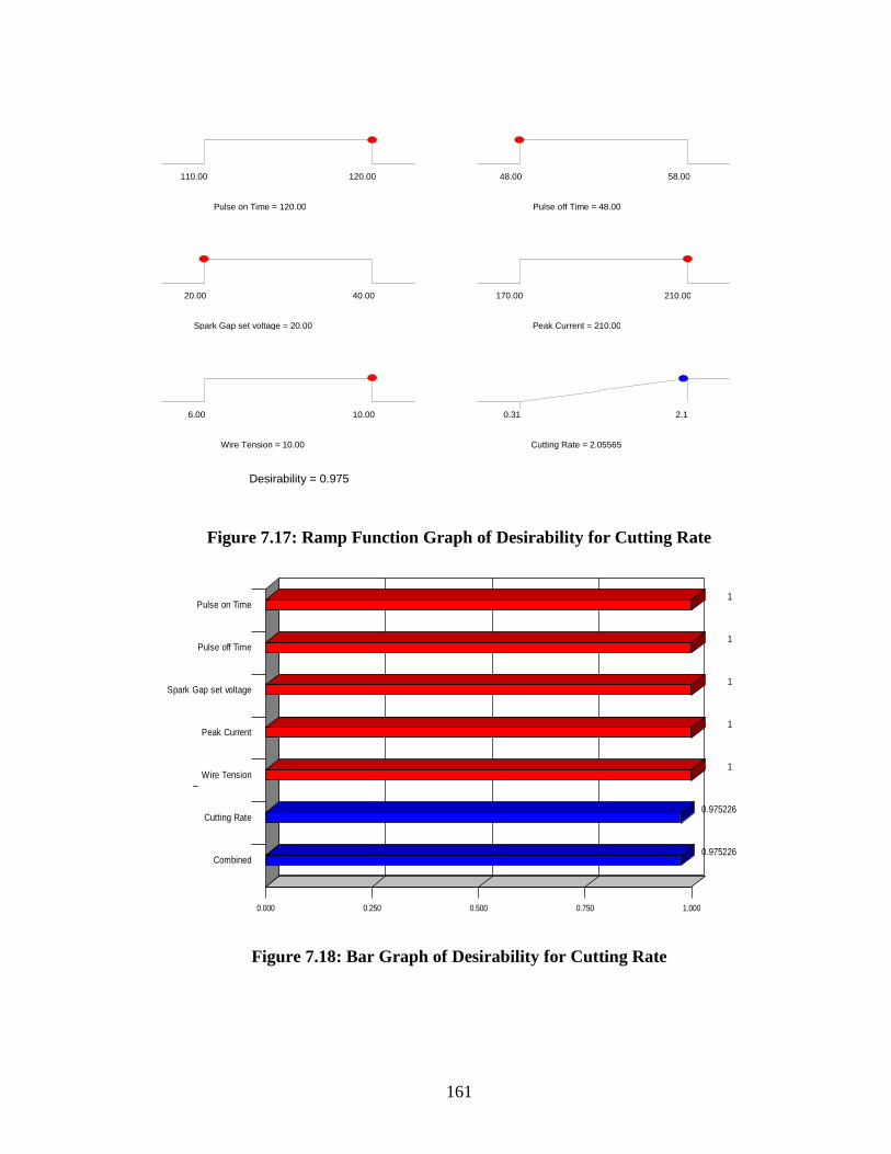
161

Figure 7.17: Ramp Function Graph of Desirability for Cutting Rate

1

1

1

1

1

0.975226

0.975226

Desirability

0.000 0.250 0.500 0.750 1.000

Pulse on Time

Pulse off Time

Spark Gap set voltage

Peak Current

Wire Tension

Cutting Rate

Combined

Figure 7.18: Bar Graph of Desirability for Cutting Rate

Pulse on Time = 120.00

110.00 120.00

Pulse off Time = 48.00

48.00 58.00

Spark Gap set voltage = 20.00

20.00 40.00

Peak Current = 210.00

170.00 210.00

Wire Tension = 10.00

6.00 10.00

Cutting Rate = 2.05565

0.31 2.1

Desirability = 0.975

162

Figure 7.19: Ramp Function Graph of Desirability for Surface Roughness

1

1

1

1

1

0.847688

0.847688

Desirability

0.000 0.250 0.500 0.750 1.000

Pulse on Time

Pulse off Time


Peak Current

Wire Tension

Surface Roughness

Combined

Figure 7.20: Bar Graph of Desirability for Surface Roughness


110.00 120.00


48.00 58.00


20.00 40.00


170.00 210.00

Wire Tension = 6.00

6.00 10.00

Surface Roughness = 1.38979

1.14 2.78


163

Figure 7.21: Ramp Function Graph of Desirability for Gap Current

1

1

1

1

1

0.965725

0.965725

Desirability

0.000 0.250 0.500 0.750 1.000

Pulse on Time

Pulse off Time


Peak Current

Wire Tension

Gap Current

Combined

Figure 7.22: Bar Graph of Desirability for Gap Current


110.00 120.00


48.00 58.00


20.00 40.00


170.00 210.00

Wire Tension = 10.00

6.00 10.00

Gap Current = 3.86478

0.9 3.97


164


110.00 120.00


48.00 58.00


20.00 40.00


170.00 210.00

Wire Tension = 6.20

6.00 10.00

Dimensional Deviation = 0.0718747

0.087 0.767


Figure 7.23: Ramp Function Graph of Desirability for Dimensional Deviation

1

1

1

1

1

1

1

Desirability

0.000 0.250 0.500 0.750 1.000

Pulse on Time

Pulse off Time


Peak Current

Wire Tension


Combined

Figure 7.24: Bar Graph of Desirability for Dimensional Deviation

165

7.3 MULTI RESPONSE OPTIMIZATION USING DESIRABILITY FUNCTION

To overcome the problem of conflicting responses of single response optimization,

multi response optimization was carried out using desirability function in conjunction with

response surface methodology. Various multi-characteristic models have been developed.

Goals and limits were established for each response in order to accurately determine their

impact on overall desirability. A maximum or minimum level is provided for all response

characteristics which are to be optimized. Weights are assigned in order to give added

emphasis to upper or lower bounds or to emphasize a target value. The importance is

assigned to each response relative to the other responses. Importance varies from the least

important (1), to the most important (5).

7.3.1 Model 1: Cutting Rate and Surface Roughness

The ranges and goals of input parameters viz. pulse on time, pulse off time, spark gap set

voltage, peak current, wire tension, and the response characteristics viz. cutting rate and

surface roughness are given in Table 7.10. Cutting rate has been assigned an importance of 5

relative to surface roughness with an importance of 2.

Table 7.10: Range of Input Parameters and Responses for Desirability (CR and SR)


Limit

Upper

Limit

Lower

Weight

Upper

Weight Importance



Spark Gap set






166

The goal of optimization is to find a good set of conditions that will meet all the

goals. It is not necessary that the desirability value is 1.0 as the value is completely

dependent on how closely the lower and upper limits are set relative to the actual optimum. A

set of 47 optimal solutions is derived for the specified design space constraints (Table 7.11)

for cutting rate and surface roughness using Design expert statistical software. The set of


desired responses. Table 7.11 shows the optimal set of condition with higher desirability

function required for obtaining desired response characteristics under specified constraints.

Table 7.11: Set of Optimal Solutions for Cutting Rate and Surface Roughness

S.No. Ton Toff SV IP WT CR SR Desir-

ability

1 120.00 48.00 40.00 210.00 6.00 1.60732 2.31729 0.554 Selected

2 120.00 48.00 39.14 205.35 6.01 1.60311 2.31661 0.552

3 120.00 48.07 39.26 210.00 6.00 1.61761 2.32967 0.552

4 120.00 48.00 39.58 210.00 6.18 1.61672 2.33027 0.552

5 118.25 48.00 21.08 170.01 10.00 1.65378 2.36112 0.552

6 120.00 48.00 38.38 201.93 6.00 1.60327 2.31925 0.552

7 118.18 48.05 20.37 170.00 10.00 1.6572 2.3647 0.551

8 117.87 48.00 20.00 170.00 9.83 1.63697 2.34957 0.551

9 119.82 48.00 39.79 210.00 6.14 1.59519 2.31375 0.551

10 117.79 48.00 21.17 174.14 10.00 1.62365 2.34122 0.550

11 117.38 48.03 20.00 174.49 10.00 1.60418 2.32628 0.549

12 118.28 48.10 22.13 170.00 10.00 1.62617 2.34602 0.549

13 120.00 48.00 35.69 198.42 6.00 1.64603 2.36216 0.549

14 120.00 48.00 40.00 209.43 6.55 1.60449 2.32811 0.549

15 118.19 48.00 22.68 175.63 10.00 1.64006 2.35842 0.549

16 118.37 48.00 22.63 170.00 9.74 1.63286 2.35303 0.549

17 118.89 48.00 24.03 170.12 10.00 1.65603 2.372 0.548

18 118.80 48.00 23.57 170.00 9.71 1.65565 2.37447 0.547

19 119.59 48.00 39.85 210.00 6.63 1.57308 2.30994 0.545

20 120.00 48.00 36.83 201.62 6.86 1.63658 2.3645 0.545

21 119.10 48.00 37.25 210.00 6.00 1.58367 2.32025 0.545

22 117.95 48.35 20.01 170.00 9.73 1.61522 2.35027 0.544

Contd……

167

S.No. Ton Toff SV IP WT CR SR Desir-

ability

23 117.63 48.00 20.87 170.00 9.06 1.59583 2.33414 0.544

24 119.18 48.00 34.85 195.87 6.04 1.57479 2.31578 0.544

25 120.00 48.00 39.04 207.82 7.15 1.61799 2.35335 0.544

26 118.73 48.35 23.07 170.00 10.00 1.62924 2.36251 0.544

27 120.00 48.73 37.45 210.00 6.06 1.59871 2.33865 0.543

28 119.55 48.00 26.93 172.81 10.00 1.67019 2.39538 0.543

29 119.25 48.00 34.00 190.12 6.00 1.57181 2.31629 0.543

30 119.47 48.29 23.06 170.00 10.00 1.70747 2.42124 0.543

31 116.63 48.02 20.00 182.94 10.00 1.56506 2.31233 0.542

32 120.00 48.00 35.81 194.24 7.35 1.62244 2.36277 0.542

33 117.58 48.02 20.02 183.00 9.98 1.66304 2.39338 0.542

34 119.90 48.00 32.19 184.83 7.33 1.64657 2.38639 0.540

35 118.98 48.05 28.67 184.09 10.00 1.62707 2.37204 0.540

36 119.78 48.00 32.13 188.72 7.71 1.65611 2.39498 0.539

37 119.81 48.00 31.35 182.81 7.80 1.64669 2.38964 0.539

38 119.90 48.00 28.96 181.39 9.14 1.70175 2.42843 0.538

39 120.00 48.00 32.73 175.12 6.06 1.59579 2.35149 0.538

40 119.56 48.04 30.42 182.18 7.65 1.63691 2.38395 0.538

41 119.74 48.00 32.21 188.52 8.51 1.64961 2.39427 0.538

42 120.00 48.00 33.12 204.01 6.00 1.73132 2.44795 0.537

43 120.00 48.42 23.19 170.00 10.00 1.74579 2.45635 0.537

44 117.25 48.00 22.27 186.37 8.78 1.60181 2.37061 0.533

45 119.98 48.15 30.73 170.00 6.01 1.60032 2.37143 0.532

46 117.35 48.12 20.01 170.00 7.45 1.57487 2.36154 0.528

47 120.00 49.49 38.59 209.99 8.35 1.50693 2.32306 0.521

The ramp function graph and bar graph (Figures 7.25 and 7.26) drawn using Design

Expert solver show the desirability for cutting rate and surface roughness. The dot on each

ramp reflects the factor setting or response prediction for that response characteristic. The

height of the dot shows how much desirable it is. A linear ramp function is created between

the low value and the goal or the high value and the goal as the weight for each parameter

was set equal to one. Bar graph shows the overall desirability function of the responses

(cutting rate and surface roughness). Desirability varies from 0 to 1 depending upon the

closeness of the response towards target. The bar graph shows how well each variable

satisfies the criterion, values close to one are considered good.

168

Figure 7.25: Ramp Function Graph of Desirability for CR and SR

1

1

1

1

1

0.724761

0.282139

0.553514

Desirability

0.000 0.250 0.500 0.750 1.000

Pulse on Time

Pulse off Time


Peak Current

Wire Tension

Cutting Rate

Surface Roughness

Combined

Figure 7.26: Bar Graph of Desirability for CR and SR


110.00 120.00


48.00 58.00


20.00 40.00


170.00 210.00

Wire Tension = 6.00

6.00 10.00


0.31 2.1


1.14 2.78


169

Desirability 3D-plots were first drawn keeping input parameters in range, cutting rate

at maximum and surface roughness at minimum. Figure 7.27 shows a plot of desirability

function distribution of desired responses for H-11 steel according to pulse on time and pulse

off time. It can be interpreted that overall desirability value is less in the region of low pulse

on time and high level of pulse off time. To show the sensitivity of results to condition,

contour plots for overall desirability for the considered model are shown in Figure 7.31. The

near optimal region was located close to the right hand bottom region of the plot, which had

overall desirability value greater than 0.55 that gradually reduced while moving left and

upwards. Sensitivities are obtained using the shape of the contour lines in Figure 7.31.

Figures 7.28-7.30 show that overall desirability value is higher in the region where there is a

high pulse on time, high spark gap set voltage, and high peak current while the wire tension

does not significantly affect the overall desirability. Contour plots (Figures 7.32-7.34) also

reveal the same fact.

Table 7.12 shows point prediction of optimal responses at optimal setting of

parameters. The 95% CI (confidence interval) is the range in which one can expect the

process average to fall into 95% of the time. The 95% PI (prediction interval) is the range in

which one can expect any individual value to fall into 95% of the time. The prediction

interval will be larger (a wider spread) than the confidence interval since one can expect

more scatter in individual values than in averages. Confirmation experiments were

conducted at optimal levels and the results were found within 95% confidence interval.

Table 7.12: Point Prediction at Optimal Setting of Responses (CR and SR)

Response Prediction 95%

CI low

95%

CI high

95%

PI low

95%

PI high

Actual value

(average of three

confirmation

experiments)

Cutting Rate

(mm/min) 1.60732 1.55 1.67 1.51 1.71 1.62

Surface

Roughness

(µm)

2.31729 2.22 2.42 2.15 2.48 2.34

170

110.00

112.50

115.00

117.50

120.00

48.00

50.50

53.00

55.50

58.00

0.100

0.218

0.335

0.453

0.570 D

es

ira

bil

ity


Figure 7.27: 3D Surface Graph of Desirability for CR and SR (Toff, Ton)

110.00

112.50

115.00

117.50

120.00

20

25

30

35

40

0.000

0.143

0.285

0.428

0.570

D

es

ira

bil

ity


Figure 7.28: 3D Surface Graph of Desirability for CR and SR (SV, Ton)

171

110.00

112.50

115.00

117.50

120.00

170.00

180.00

190.00

200.00

210.00

0.270

0.345

0.420

0.495

0.570 D

es

ira

bil

ity


Figure 7.29: 3D Surface Graph of Desirability for CR and SR (IP, Ton)

110.00

112.50

115.00

117.50

120.00

6

7

8

9

10

0.320

0.383

0.445

0.508

0.570

D

es

ira

bil

ity


Figure 7.30: 3D Surface Graph of Desirability for CR and SR (WT, Ton)

172

110.00 112.50 115.00 117.50 120.00

48.00

50.50

53.00

55.50

58.00

Desirability

A: Pulse on Time

B: P

uls

e o

ff T

ime 0.178

0.253

0.328

0.403

0.478

Prediction 0.554

Figure 7.31: Contour Plot of Desirability for CR and SR (Toff, Ton)

110.00 112.50 115.00 117.50 120.00

20.00

25.00

30.00

35.00

40.00

Desirability

A: Pulse on Time

C: S

pa

rk

G

ap

s

et v

olt

ag

e

0.092

0.185

0.2770.369

0.369

0.461

0.461

Prediction 0.554

Figure 7.32: Contour Plot of Desirability for CR and SR (SV, Ton)

173

110.00 112.50 115.00 117.50 120.00

170.00

180.00

190.00

200.00

210.00

Desirability

A: Pulse on Time

D: P

ea

k C

ur

re

nt

0.322

0.368 0.414 0.4610.507

Prediction 0.554

Figure 7.33: Contour Plot of Desirability for CR and SR (IP, Ton)

110.00 112.50 115.00 117.50 120.00

6.00

7.00

8.00

9.00

10.00

Desirability

A: Pulse on Time

E: W

ire

T

en

sio

n

0.361 0.400 0.438 0.4770.515

Prediction 0.554

Figure 7.34: Contour Plot of Desirability for CR and SR (WT, Ton)

174

7.3.2 Model 2:.Cutting Rate, Surface Roughness and Gap Current

The ranges and goals of input parameters viz. pulse on time, pulse off time, spark gap

set voltage, peak current, wire tension, and the response characteristics viz. cutting rate,

surface roughness, and gap current are given in Table 7.13. Cutting rate has been assigned an

importance of 5 relative to surface roughness and gap current each with an importance of 3.

Table 7.13: Range of Input Parameters and Responses for Desirability (CR, SR and IG)


Limit

Upper

Limit

Lower

Weight

Upper

Weight Importance



Spark Gap set







Table 7.14 reports 47 values of overall desirability and the corresponding responses

under discussion. The set of conditions possessing highest desirability value is selected as

optimum condition for the desired responses.

The ramp function graph drawn using Design Expert solver shows the desirability for

cutting rate, surface roughness and gap current (Figure 7.35). A linear ramp function is

created between the low value and the goal or the high value and the goal as the weight for

each parameter was set equal to one.

175

Table 7.14: Set of Optimal Solutions for Cutting Rate, Surface Roughness and Gap Current

S.No. Ton Toff SV IP WT CR SR IG Desir-

ability

1 120.00 48.00 40.00 210.00 6.00 1.60732 2.31729 3.28061 0.571 Selected

2 120.00 48.02 39.59 208.11 6.00 1.60496 2.31701 3.27868 0.570

3 120.00 48.03 39.34 207.70 6.00 1.60806 2.3203 3.28421 0.570

4 120.00 48.00 38.44 203.50 6.00 1.60967 2.3238 3.29167 0.570

5 119.97 48.00 38.71 210.00 6.00 1.63364 2.34365 3.32279 0.570

6 119.91 48.00 39.97 206.83 6.00 1.58389 2.29968 3.24216 0.569

7 120.00 48.02 40.00 209.97 6.22 1.60509 2.32132 3.27664 0.569

8 120.00 48.00 38.87 205.81 6.23 1.61181 2.32897 3.29281 0.568

9 119.84 48.00 38.07 204.75 6.00 1.60979 2.32671 3.28379 0.568

10 120.00 48.00 37.48 197.40 6.00 1.6009 2.32152 3.2831 0.568

11 120.00 48.00 40.00 203.05 6.19 1.57257 2.29559 3.23145 0.568

12 120.00 48.06 37.20 210.00 6.00 1.66483 2.37682 3.37245 0.566

13 120.00 48.00 35.88 193.65 6.28 1.61787 2.34473 3.31176 0.565

14 120.00 48.00 39.68 209.99 6.76 1.61405 2.34141 3.29173 0.565

15 119.64 48.00 39.97 209.98 6.37 1.57493 2.30459 3.21366 0.564

16 120.00 48.00 39.86 206.00 6.86 1.59047 2.32447 3.25756 0.563

17 120.00 48.01 34.87 192.58 6.65 1.63437 2.36477 3.33673 0.563

18 119.82 48.00 35.42 187.75 6.00 1.58252 2.32028 3.25073 0.563

19 120.00 48.00 37.43 207.51 6.89 1.65241 2.37833 3.35612 0.563

20 120.00 48.00 35.18 194.52 7.18 1.63804 2.37264 3.3417 0.561

21 119.12 48.00 35.83 199.67 6.00 1.56634 2.30587 3.18384 0.560

22 120.00 48.24 34.34 189.05 6.42 1.60802 2.35161 3.29348 0.560

23 119.04 48.00 24.33 170.00 9.91 1.6633 2.38015 3.2773 0.559

Contd……

176

S.No. Ton Toff SV IP WT CR SR IG Desir-

ability

24 119.11 48.00 21.56 170.00 10.00 1.73021 2.42274 3.35428 0.559

25 119.93 48.00 26.14 172.55 10.00 1.72375 2.4323 3.44011 0.559

26 119.91 48.01 26.57 170.96 10.00 1.7033 2.41993 3.41146 0.559

27 120.00 48.00 32.54 183.17 7.09 1.64032 2.38092 3.34658 0.559

28 119.79 48.10 24.76 170.00 10.00 1.71912 2.42791 3.41203 0.558

29 119.41 48.00 24.55 170.36 9.64 1.69678 2.41068 3.35326 0.558

30 119.07 48.14 22.32 170.00 10.00 1.69786 2.40519 3.30957 0.558

31 120.00 48.00 32.49 181.73 7.42 1.63416 2.3795 3.33777 0.557

32 120.00 48.00 31.99 181.64 7.50 1.64505 2.38785 3.3529 0.557

33 120.00 48.06 27.91 175.26 10.00 1.69928 2.42296 3.41774 0.557

34 120.00 48.00 31.40 179.05 7.55 1.64525 2.39013 3.35252 0.556

35 119.55 48.00 31.80 185.19 7.49 1.62475 2.37158 3.2934 0.556

36 120.00 48.00 29.08 176.27 9.04 1.6835 2.41687 3.40126 0.556

37 120.00 48.00 29.59 178.64 9.02 1.68392 2.4174 3.40339 0.556

38 120.00 48.00 29.08 176.37 9.01 1.68393 2.4172 3.40186 0.556

39 120.00 48.00 30.24 179.78 8.49 1.67493 2.41189 3.39236 0.556

40 119.88 48.00 30.32 171.86 6.94 1.6226 2.38037 3.30983 0.553

41 120.00 48.00 31.50 190.30 9.84 1.69937 2.43509 3.42922 0.553

42 119.38 48.00 26.29 170.00 7.67 1.65458 2.40294 3.30234 0.550

43 118.80 48.00 29.63 191.29 6.00 1.62842 2.38464 3.24658 0.549

44 118.63 48.00 25.41 170.01 8.10 1.60087 2.35625 3.16745 0.549

45 118.19 48.00 34.70 210.00 6.00 1.54971 2.31705 3.11274 0.548

46 118.47 48.10 33.38 210.00 6.00 1.59519 2.3644 3.18999 0.546

47 120.00 49.11 26.60 180.37 10.00 1.65916 2.42572 3.32569 0.543

177

Figure 7.35: Ramp Function Graph of Desirability for CR, SR and IG

1

1

1

1

1

0.724761

0.282139

0.775443

0.570763

Desirability

0.000 0.250 0.500 0.750 1.000

Pulse on Time

Pulse off Time


Peak Current

Wire Tension

Cutting Rate

Surface Roughness

Gap Current

Combined

Figure 7.36: Bar Graph of Desirability for CR, SR and IG


110.00 120.00


48.00 58.00


20.00 40.00


170.00 210.00

Wire Tension = 6.00

6.00 10.00


0.31 2.1


1.14 2.78


0.9 3.97


178

Bar graph (Figure 7.36) shows the overall desirability function of the responses in the

considered model. Desirability varies from 0 to 1 depending upon the closeness of the

response towards target. The bar graph shows how well each variable satisfies the criterion:

values close to one are considered good.

Desirability 3D-plots (Figures 7.37-7.40) were drawn keeping input parameters in

range, cutting rate and gap current at maximum and surface roughness at minimum. It can be

interpreted that overall desirability value is less in the region of low pulse on time and high

level of pulse off time. To show the sensitivity of results to condition, contour plots for

overall desirability for the considered model are shown in Figures 7.41-7.44. It is revealed

that overall desirability value is higher in the region where there is a high pulse on time, high

spark gap set voltage, and high peak current while the wire tension does not significantly

affect the overall desirability.

Table 7.15 gives point prediction of optimal responses at optimal setting of

parameters. The 95% CI (confidence interval) is the range in which one can expect the

process average to fall into 95% of the time. The 95% PI (prediction interval) is the range in

which one can expect any individual value to fall into 95% of the time. The prediction

interval will be larger (a wider spread) than the confidence interval since one can expect

more scatter in individual values than in averages. Confirmation experiments were

conducted at optimal levels and the results were found to lie within 95% confidence interval.

179

110.00

112.50

115.00

117.50

120.00

48.00

50.50

53.00

55.50

58.00

0.100

0.220

0.340

0.460

0.580

D

es

ira

bil

ity


Figure 7.37: 3D Surface Graph of Desirability for CR, SR and IG (Toff, Ton)

110.00

112.50

115.00

117.50

120.00

20

25

30

35

40

0.000

0.145

0.290

0.435

0.580

De

sir

ab

ilit

y


Figure 7.38: 3D Surface Graph of Desirability for CR, SR and IG (SV, Ton)

180

110.00

112.50

115.00

117.50

120.00

170.00

180.00

190.00

200.00

210.00

0.250

0.333

0.415

0.497

0.580

D

es

ira

bil

ity


Figure 7.39: 3D Surface Graph of Desirability for CR, SR and IG (IP, Ton)

110.00

112.50

115.00

117.50

120.00

6

7

8

9

10

0.310

0.378

0.445

0.512

0.580

De

sir

ab

ilit

y


Figure 7.40: 3D Surface Graph of Desirability for CR, SR and IG (WT, Ton)

181

110.00 112.50 115.00 117.50 120.00

48.00

50.50

53.00

55.50

58.00

Desirability

A: Pulse on Time

B: P

uls

e o

ff T

ime 0.179

0.257

0.336

0.414

0.492

Prediction 0.571

Figure 7.41: Contour Plot of Desirability for CR, SR and IG (Toff, Ton)

110.00 112.50 115.00 117.50 120.00

20.00

25.00

30.00

35.00

40.00

Desirability

A: Pulse on Time

C: S

pa

rk

G

ap

s

et v

olt

ag

e

0.095

0.190

0.285

0.381

0.381

0.476

Prediction 0.571

Figure 7.42: Contour Plot of Desirability for CR, SR and IG (SV, Ton)

182

110.00 112.50 115.00 117.50 120.00

170.00

180.00

190.00

200.00

210.00

Desirability

A: Pulse on Time

D: P

ea

k C

ur

re

nt

0.307

0.360 0.412 0.465 0.518

Prediction 0.571

Figure 7.43: Contour Plot of Desirability for CR, SR and IG (IP, Ton)

110.00 112.50 115.00 117.50 120.00

6.00

7.00

8.00

9.00

10.00

Desirability

A: Pulse on Time

E: W

ire

T

en

sio

n

0.360 0.402 0.444 0.486 0.529

Prediction 0.571

Figure 7.44: Contour Plot of Desirability for CR, SR and IG (WT, Ton)

183

Table 7.15: Point Prediction at Optimal Setting of Responses (CR, SR & IG)

Response Prediction 95% CI

low

95%

CI high

95% PI

low

95% PI

high

Actual value

(average of

three

confirmation

experiments)

Cutting Rate

(mm/min) 1.60732 1.55 1.67 1.51 1.71 1.62

Surface

Roughness

(µm)

2.31729 2.22 2.42 2.15 2.48 2.34

Gap Current

(ampere) 3.28061 3.17 3.40 3.07 3.49 3.2

7.3.3 Model 3: Cutting Rate, Surface Roughness and Dimensional Deviation

The ranges and goals of input parameters viz. pulse on time, pulse off time, spark gap

set voltage, peak current, wire tension and the response characteristics viz. cutting rate,

surface roughness and dimensional deviation are given in Table 7.16. Cutting rate has been

assigned an importance of 5 relative to surface roughness and dimensional deviation each

with an importance of 3.

Table 7.16: Range of Input Parameters and Responses for Desirability (CR, SR &DD)


Limit

Upper

Limit

Lower

Weight

Upper

Weight Importance



Spark Gap set






Dimensional

Deviation maximize 0.087 0.767 1 1 3

184

Table7.17 shows the values of 47 settings of input parameters that will give high

values of overall desirability and the corresponding values of responses under discussion are

also given. The set of conditions possessing highest desirability value is selected as optimum

condition for the desired responses.

The ramp function graph (Figure 7.45) drawn using Design Expert solver shows the

desirability for cutting rate, surface roughness and dimensional deviation. The dot on each

ramp reflects the factor setting or response prediction for that response characteristic. The

height of the dot shows how much desirable it is. A linear ramp function is created between

the low value and the goal or the high value and the goal as the weight for each parameter

was set equal to one. Bar graph (Figure 7.46) shows the overall desirability function of the

responses. Desirability varies from 0 to 1 depending upon the closeness of the response

towards target. The bar graph shows how well each variable satisfies the criterion: values

near one are considered to be good.


range, cutting rate at maximum, surface roughness and dimensional deviation at minimum.

The contour plots for overall desirability for the considered model are shown in Figures 7.51-

7.54. It is revealed that overall desirability value is higher in the region where there is a high

pulse on time, high spark gap set voltage, high peak current, and low value of wire tension.

185

Table 7.17: Set of Optimal Solutions for Desirability (CR, SR and DD)

S.No Ton Toff SV IP WT CR SR %D Desir-

ability

1 119.61 48.00 39.94 204.04 6.01 1.54322 2.27143 0.0866602 0.613 Selected

2 119.59 48.00 40.00 205.84 6.00 1.54885 2.27533 0.0818034 0.613

3 120.00 48.11 40.00 203.83 6.00 1.56708 2.28871 0.0794445 0.613

4 119.66 48.00 40.00 204.10 6.10 1.54697 2.27593 0.0864677 0.613

5 119.35 48.00 40.00 209.97 6.00 1.54684 2.27631 0.0757819 0.613

6 118.90 48.00 40.00 209.38 6.00 1.50334 2.24554 0.0860455 0.613

7 119.73 48.46 39.99 208.74 6.00 1.53581 2.27272 0.0701991 0.611

8 119.96 48.77 40.00 210.00 6.02 1.53508 2.2767 0.0616824 0.610

9 119.92 48.00 40.00 208.94 6.31 1.59478 2.31553 0.0723683 0.610

10 119.36 48.01 38.73 209.86 6.01 1.57383 2.30306 0.0870017 0.610

11 120.00 48.84 40.00 207.51 6.09 1.52137 2.26879 0.0683787 0.609

12 120.00 48.01 40.00 195.98 6.00 1.53663 2.27016 0.100861 0.609

13 120.00 48.44 40.00 196.84 6.00 1.50355 2.25378 0.097064 0.608

14 119.29 48.65 40.00 207.86 6.45 1.47499 2.24322 0.0870017 0.607

15 118.76 48.09 38.54 210.00 6.01 1.51634 2.26488 0.0995588 0.606

16 120.00 48.00 40.00 193.46 6.06 1.5246 2.26587 0.108532 0.606

17 119.98 48.00 39.97 191.99 6.01 1.51633 2.26118 0.112375 0.604

18 119.78 48.00 40.00 191.46 6.00 1.49537 2.24689 0.116163 0.603

19 119.79 48.00 40.00 207.33 7.12 1.57434 2.31995 0.0916091 0.603

20 120.00 48.99 40.00 196.57 6.18 1.4556 2.2348 0.0986729 0.602

21 120.00 48.00 38.89 190.88 6.00 1.53649 2.27751 0.124593 0.601

22 119.78 48.06 40.00 208.70 7.38 1.57583 2.32872 0.0920244 0.600

23 119.94 48.34 40.00 209.90 7.52 1.57099 2.33215 0.087006 0.599

Contd…..

186

S.No Ton Toff SV IP WT CR SR %D Desir-

ability

24 118.59 48.00 37.89 197.14 6.00 1.46136 2.22027 0.139378 0.597

25 119.67 48.00 38.07 190.37 6.02 1.52276 2.26974 0.138417 0.596

26 120.00 48.62 40.00 189.16 6.05 1.45122 2.23405 0.117897 0.596

27 118.78 48.00 40.00 201.50 7.11 1.45507 2.23546 0.12457 0.595

28 120.00 51.00 40.00 207.53 6.00 1.34301 2.17341 0.0595418 0.594

29 118.21 49.36 40.00 204.83 6.00 1.31096 2.12394 0.10585 0.593

30 119.74 48.00 38.27 186.11 6.05 1.50345 2.2627 0.147198 0.592

31 119.98 48.64 40.00 210.00 8.12 1.54927 2.33496 0.0943187 0.591

32 120.00 48.00 39.94 183.03 6.32 1.4739 2.25669 0.141128 0.589

33 119.92 48.32 40.00 210.00 8.35 1.57185 2.35244 0.10008 0.588

34 120.00 49.77 39.57 191.07 6.41 1.37615 2.21041 0.118092 0.585

35 119.96 48.00 40.00 177.68 6.00 1.44218 2.24253 0.150558 0.583

36 120.00 48.91 38.83 210.00 8.53 1.55251 2.35066 0.109924 0.582

37 120.00 48.91 39.99 210.00 8.93 1.52709 2.34194 0.105645 0.581

38 120.00 48.79 40.00 210.00 8.99 1.5374 2.34905 0.106897 0.580

39 120.00 49.82 40.00 210.00 9.01 1.4497 2.30147 0.103677 0.578

40 118.90 48.00 33.58 192.18 6.00 1.55817 2.3083 0.193068 0.577

41 120.00 50.34 40.00 210.00 9.01 1.40614 2.27814 0.101868 0.576

42 120.00 49.12 33.63 210.00 6.04 1.64645 2.4135 0.127993 0.572

43 118.29 48.00 38.90 175.19 6.00 1.31325 2.14757 0.185245 0.568

44 119.05 48.00 32.54 172.36 6.00 1.49958 2.28366 0.252942 0.555

45 119.99 53.89 37.49 202.51 6.00 1.15895 2.12402 0.0869978 0.555

46 120.00 48.02 36.35 170.00 7.79 1.48739 2.31593 0.234247 0.548

47 118.60 48.14 36.38 184.35 10.00 1.42351 2.26936 0.245486 0.545

187

Figure 7.45: Ramp Function Graph of Desirability for CR, SR and DD

1

1

1

1

1

0.688949

0.310104

1

0.613435

Desirability

0.000 0.250 0.500 0.750 1.000

Pulse on Time

Pulse off Time


Peak Current

Wire Tension

Cutting Rate

Surface Roughness


Combined

Figure 7.46: Bar Graph of Desirability for CR, SR and DD


110.00 120.00


48.00 58.00


20.00 40.00


170.00 210.00

Wire Tension = 6.01

6.00 10.00


0.31 2.1


1.14 2.78


0.087 0.767


188

110.00

112.50

115.00

117.50

120.00

48.00

50.50

53.00

55.50

58.00

0.200

0.305

0.410

0.515

0.620

D

es

ira

bil

ity


Figure 7.47: 3D Surface Graph of Desirability for CR, SR and DD (Toff, Ton)

110.00

112.50

115.00

117.50

120.00

20

25

30

35

40

0.000

0.155

0.310

0.465

0.620

D

es

ira

bil

ity


Figure 7.48: 3D Surface Graph of Desirability for CR, SR and DD (SV, Ton)

189

110.00

112.50

115.00

117.50

120.00

170.00

180.00

190.00

200.00

210.00

0.380

0.440

0.500

0.560

0.620

D

es

ira

bil

ity


Figure 7.49: 3D Surface Graph of Desirability for CR, SR and DD (IP, Ton)

110.00

112.50

115.00

117.50

120.00

6

7

8

9

10

0.390

0.448

0.505

0.563

0.620

D

es

ira

bil

ity


Figure 7.50: 3D Surface Graph of Desirability for CR, SR and DD (WT, Ton)

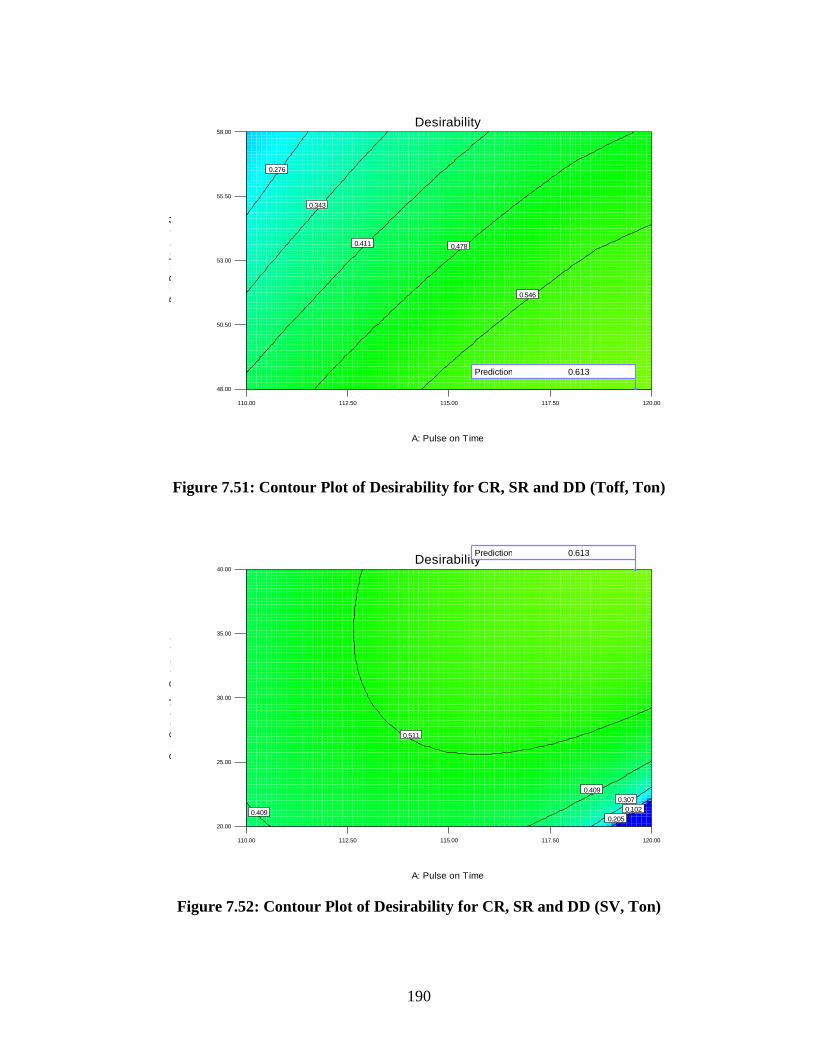
190

110.00 112.50 115.00 117.50 120.00

48.00

50.50

53.00

55.50

58.00

Desirability

A: Pulse on Time

B: P

uls

e o

ff T

ime

0.276

0.343

0.411 0.478

0.546

Prediction 0.613

Figure 7.51: Contour Plot of Desirability for CR, SR and DD (Toff, Ton)

110.00 112.50 115.00 117.50 120.00

20.00

25.00

30.00

35.00

40.00

Desirability

A: Pulse on Time

C: S

pa

rk

G

ap

s

et v

olt

ag

e

0.102

0.205

0.307

0.409

0.409

0.511

Prediction 0.613

Figure 7.52: Contour Plot of Desirability for CR, SR and DD (SV, Ton)

191

110.00 112.50 115.00 117.50 120.00

170.00

180.00

190.00

200.00

210.00

Desirability

A: Pulse on Time

D: P

ea

k C

ur

re

nt

0.420

0.459 0.4970.536 0.575

Prediction 0.613

Figure 7.53: Contour Plot of Desirability for CR, SR and DD (IP, Ton)

110.00 112.50 115.00 117.50 120.00

6.00

7.00

8.00

9.00

10.00

Desirability

A: Pulse on Time

E: W

ire

T

en

sio

n

0.433 0.469 0.505 0.541

0.577

Prediction 0.613

Figure 7.54: Contour Plot of Desirability for CR, SR and DD (WT, Ton)

192

Table 7.18 shows point prediction at optimal setting of responses. The 95% CI

(confidence interval) is the range in which one can expect the process average to fall into

95% of the time. The 95% PI (prediction interval) is the range in which one can expect any

individual value to fall into 95% of the time. The prediction interval will be larger (a wider

spread) than the confidence interval since one can expect more scatter in individual values

than in averages. Confirmation experiments were conducted at optimal levels predicted and

the results were found to be within 95% confidence interval.

Table 7.18: Point Prediction at Optimal Setting of Responses (CR, SR & DD)


CI low

95%

CI high

95%

PI low

95%

PI high

Actual Value

(average of

three

confirmation

experiments)

Cutting Rate

(mm/min) 1.54322 1.49 1.59 1.45 1.64 1.57

Surface

Roughness

(µm)

2.27143 2.18 2.36 2.11 2.43 2.31

Dimensional

Deviation

(%)

0.0866602 0.048 0.13 4.576E-

003

0.17

0.0901

7.3.4 Model 4: Cutting Rate, Surface Roughness, Gap Current and Dimensional

Deviation

The ranges and goals of input parameters viz. pulse on time, pulse off time, spark gap set

voltage, peak current, wire tension and the response characteristics viz. cutting rate, surface

roughness, gap current and dimensional deviation are given in Table 7.19. Cutting rate has

been assigned an importance of 5 relative to surface roughness, gap current and dimensional

deviation each with an importance of 3.

193

Table 7.19: Range of Input Parameters and Responses for Desirability (CR, SR, IG and

DD)


Limit

Upper

Limit

Lower

Weight

Upper

Weight Importance



Spark Gap set







Dimensional

Deviation minimize 0.087 0.767 1 1 3

A set of 47 optimal solutions is derived for the specified design space constraints

(Table 7.20) for the output responses using Design expert statistical software. The set of


desired responses. Table 7.20 shows the optimal set of condition with higher desirability

function required for obtaining desired response characteristics under specified constraints.

The ramp view drawn using Design Expert software shows the desirability for the output

responses (Figure 7.55). The dot on each ramp reflects the factor setting or response

prediction for that response characteristic. The height of the dot shows how much desirable it

is. A linear ramp function is created between the low value and the goal or the high value and

the goal as the weight for each parameter was set equal to one. Bar graph (Figure 7.56)

shows the overall desirability function of the responses. Desirability varies from 0 to 1

depending upon the closeness of the response towards target.

194

Table 7.20: Set of Optimal Solutions for Desirability (CR, SR, IG and DD)

S.

No. Ton Toff SV IP WT CR SR IG %D

Desir-

ability

1 120.00 48.00 40.00 210.00 6.00 1.60732 2.31729 3.28061 0.0632262 0.644 Selected

2 120.00 48.00 38.97 209.97 6.02 1.63007 2.33977 3.31807 0.0728684 0.643

3 120.00 48.00 38.85 207.85 6.17 1.62237 2.33639 3.3078 0.0819406 0.642

4 120.00 48.04 40.00 210.00 6.18 1.60331 2.31928 3.27338 0.0658536 0.642

5 119.96 48.00 39.50 202.18 6.00 1.57616 2.29563 3.237 0.0891519 0.641

6 119.80 48.00 39.99 203.76 6.22 1.5579 2.28638 3.19817 0.0869991 0.639

7 119.99 48.00 39.44 207.00 6.69 1.60421 2.33188 3.27883 0.0869947 0.639

8 120.00 48.00 39.89 205.70 6.65 1.58835 2.31794 3.2544 0.0857945 0.639

9 120.00 48.02 37.41 203.96 6.00 1.63386 2.34688 3.32946 0.103909 0.639

10 119.90 48.00 38.85 209.52 6.65 1.62121 2.34729 3.30007 0.0866512 0.638

11 119.37 48.00 38.81 209.42 6.00 1.57241 2.30062 3.19996 0.0869886 0.638

12 120.00 48.21 39.99 197.98 6.00 1.52939 2.26678 3.16415 0.0949215 0.635

13 119.99 48.00 40.00 195.44 6.00 1.53318 2.26821 3.17476 0.102577 0.635

14 120.00 48.00 39.60 210.00 7.31 1.61627 2.35575 3.29544 0.0870168 0.634

15 120.00 48.33 38.59 199.21 6.00 1.55591 2.29099 3.20466 0.103893 0.634

16 120.00 48.52 38.58 210.00 6.82 1.59238 2.33869 3.24821 0.0870012 0.633

17 120.00 48.00 40.00 193.66 6.00 1.52548 2.26491 3.16473 0.107165 0.633

18 120.00 48.00 40.00 192.56 6.01 1.52011 2.26276 3.15724 0.11017 0.631

19 120.00 49.05 38.92 203.41 6.00 1.50715 2.26595 3.1105 0.0869984 0.630

20 120.00 48.00 36.23 193.47 6.00 1.60926 2.33333 3.29876 0.144734 0.628

21 119.84 48.00 34.92 209.72 6.00 1.70444 2.42338 3.42656 0.118559 0.626

22 120.00 48.00 36.71 198.63 7.39 1.62414 2.36356 3.31846 0.147193 0.622

23 120.00 49.82 38.40 207.49 6.00 1.47227 2.25624 3.03554 0.0783206 0.621

Contd……

195

S.

No. Ton Toff SV IP WT CR SR IG %D

Desir-

ability

24 120.00 48.63 39.93 208.59 8.04 1.5456 2.32998 3.1719 0.0971571 0.621

25 120.00 48.00 39.43 184.88 6.00 1.49455 2.25857 3.12416 0.135724 0.620

26 119.80 48.00 39.44 209.94 8.54 1.60098 2.37375 3.26263 0.111477 0.619

27 120.00 48.29 39.95 209.96 8.62 1.5826 2.36572 3.2359 0.103384 0.618

28 120.00 48.05 40.00 210.00 8.80 1.60291 2.38167 3.27265 0.106582 0.618

29 120.00 48.00 40.00 209.82 8.84 1.60634 2.38427 3.27918 0.107829 0.618

30 120.00 48.00 38.26 182.68 6.00 1.50968 2.27313 3.15101 0.152575 0.617

31 120.00 48.00 37.41 204.28 8.71 1.63678 2.39671 3.33409 0.145164 0.614

32 120.00 48.08 36.07 187.95 7.10 1.57811 2.33307 3.25288 0.178124 0.613

33 120.00 48.34 36.11 199.98 8.58 1.61375 2.38136 3.29436 0.16738 0.609

34 120.00 48.03 40.00 174.36 6.05 1.42697 2.24518 3.02494 0.159646 0.600

35 119.94 48.05 36.70 172.04 6.00 1.48288 2.28076 3.11362 0.197453 0.598

36 120.00 48.84 34.46 199.19 8.91 1.60236 2.38685 3.26507 0.192329 0.598

37 120.00 49.23 39.27 209.94 9.97 1.51488 2.36009 3.11073 0.127284 0.596

38 118.73 48.00 34.13 179.13 6.00 1.46961 2.24841 3.01734 0.219577 0.593

39 120.00 48.00 35.01 182.18 9.51 1.58006 2.36714 3.25995 0.243431 0.588

40 118.75 48.00 34.94 174.94 6.02 1.4345 2.23029 2.96632 0.220424 0.587

41 120.00 48.00 31.83 170.00 6.87 1.59044 2.36131 3.2755 0.276196 0.584

42 120.00 48.00 29.80 170.00 6.17 1.63596 2.39357 3.33615 0.295011 0.580

43 120.00 48.00 30.99 176.29 9.29 1.64074 2.39305 3.34544 0.308947 0.578

44 120.00 48.00 34.70 173.32 9.44 1.54281 2.35397 3.20772 0.269935 0.577

45 120.00 48.00 36.20 176.60 9.96 1.52541 2.35485 3.18021 0.251707 0.577

46 120.00 48.00 39.89 170.23 10.00 1.41087 2.34178 3.00331 0.233065 0.555

47 120.00 52.53 33.05 210.00 10.00 1.37131 2.31588 2.80166 0.185225 0.553

196

Figure 7.55: Ramp Function Graph of Desirability for CR, SR, IG and DD

1

1

1

1

1

0.724761

0.282139

0.775443

1

0.643641

Desirability

0.000 0.250 0.500 0.750 1.000

Pulse on Time

Pulse off Time


Peak Current

Wire Tension

Cutting Rate

Surface Roughness

Gap Current


Combined

Figure 7.56: Bar Graph of Desirability for CR, SR, IG and DD


110.00 120.00


48.00 58.00


20.00 40.00


170.00 210.00

Wire Tension = 6.00

6.00 10.00


0.31 2.1


1.14 2.78


0.9 3.97


0.087 0.767 Desirability = 0.644

197


range, cutting rate and gap current at maximum and surface roughness and dimensional

deviation at minimum. The contour plots for overall desirability for the considered model are

shown in Figures 7.61-7.64. It is revealed that overall desirability value is higher in the

region where there is a high pulse on time, high spark gap set voltage, and high peak current

while the wire tension does not significantly affect the overall desirability.

Table 7.21 shows point prediction at optimal setting of responses. The 95% CI

(confidence interval) is the range in which one can expect the process average to fall into

95% of the time. The 95% PI (prediction interval) is the range in which one can expect any

individual value to fall into 95% of the time. The prediction interval will be larger (a wider

spread) than the confidence interval since one can expect more scatter in individual values

than in averages. Confirmation experiments were conducted at optimum levels and the

results were within 95% confidence interval.

Table 7.21: Point Prediction at Optimal Setting of Responses (CR, SR, IG & DD)


CI low

95%

CI high

95%

PI low

95%

PI high

Actual Value

(average of

three

confirmation

experiments)

Cutting Rate

(mm/min) 1.60732 1.55 1.67 1.51 1.71 1.62

Surface

Roughness

(µm)

2.31729 2.22 2.42 2.15 2.48 2.34

Gap Current

(ampere) 3.28061 3.17 3.40 3.07 3.49 3.2

Dimensional

Deviation

(%)

0.0632262 0.019 0.11 -0.021 0.15

0.0804

198

110.00

112.50

115.00

117.50

120.00

48.00

50.50

53.00

55.50

58.00

0.150

0.275

0.400

0.525

0.650 D

es

ira

bil

ity


Figure 7.57: 3D Surface Graph of Desirability for CR, SR, IG and DD (Toff, Ton)

110.00

112.50

115.00

117.50

120.00

20

25

30

35

40

0.000

0.163

0.325

0.488

0.650

D

es

ira

bil

ity


Figure 7.58: 3D Surface Graph of Desirability for CR, SR, IG and DD (SV, Ton)

199

110.00

112.50

115.00

117.50

120.00

170.00

180.00

190.00

200.00

210.00

0.300

0.388

0.475

0.563

0.650 D

es

ira

bil

ity


Figure 7.59: 3D Surface Graph of Desirability for CR, SR, IG and DD (IP, Ton)

110.00

112.50

115.00

117.50

120.00

6

7

8

9

10

0.350

0.425

0.500

0.575

0.650

D

es

ira

bil

ity


Figure 7.60: 3D Surface Graph of Desirability for CR, SR, IG and DD (WT, Ton)

200

110.00 112.50 115.00 117.50 120.00

48.00

50.50

53.00

55.50

58.00

Desirability

A: Pulse on Time

B: P

uls

e o

ff T

ime 0.234

0.316

0.398

0.480

0.562

Prediction 0.644

Figure 7.61: Contour Plot of Desirability for CR, SR, IG and DD (Toff, Ton)

110.00 112.50 115.00 117.50 120.00

20.00

25.00

30.00

35.00

40.00

Desirability

A: Pulse on Time

C: S

pa

rk

G

ap

s

et v

olt

ag

e

0.107

0.215

0.322

0.429

0.429

0.536

Prediction 0.644

Figure 7.62: Contour Plot of Desirability for CR, SR, IG and DD (SV, Ton)

201

110.00 112.50 115.00 117.50 120.00

170.00

180.00

190.00

200.00

210.00

Desirability

A: Pulse on Time

D: P

ea

k C

ur

re

nt

0.365

0.421 0.477 0.5320.588

Prediction 0.644

Figure 7.63: Contour Plot of Desirability for CR, SR, IG and DD (IP, Ton)

110.00 112.50 115.00 117.50 120.00

6.00

7.00

8.00

9.00

10.00

Desirability

A: Pulse on Time

E: W

ire

T

en

sio

n

0.406 0.454 0.501 0.5490.596

Prediction 0.644

Figure 7.64: Contour Plot of Desirability for CR, SR, IG and DD (WT, Ton)

202

CHAPTER 8

MULTI - CHARACTERISTIC OPTIMIZATION USING UTILITY

FUNCTION

8.1 MULTI-CHARACTERISTIC OPTIMIZATION MODEL

8.1.1 Introduction

The work of Taguchi for determining the optimal settings of controllable factors

(parameters) through off-line experiments focuses on products with a single quality

characteristic. But most of the products have several quality characteristics of interest. A

single setting of process parameters may be optimal for one quality characteristic but the

same setting may yield detrimental results for other quality characteristics. In such cases, a

need arises to obtain an optimal setting of the process parameters so that the product can be

produced with optimum or near optimum quality characteristics. A number of techniques

have been developed for obtaining the multi-characteristic optimization of product quality.

Phadke (1989) presented a case of products with multiple characteristics such as surface

defects and thickness in his example of polysilicon deposition. In order to estimate the loss

caused by quality characteristics, Phadke has assigned a weight from experience to each

quality characteristic. A computer software package developed by Texas Instruments (1990)

offers a convenient environment for the analysis of off-line experiments. However, it

roughly chooses the most important characteristic in the case of multi-characteristic product

and determines the optimal level settings of controllable factors accordingly. Elsayed and

Chen (1993) presented a model using loss function approach to determine the optimal

settings of the process parameters of the production process for products with multiple

characteristics. Tsui (1999) extended the multivariate loss considered by Pignatiello (1993)

to include the smaller and larger the better type characteristics. Under various assumptions,

he developed an appropriate two-step procedure that minimizes the average multivariate

quality loss for products with multiple characteristics. Byrne and Taguchi (1987) presented a

case where the quality characteristics were independently optimized using Taguchi approach

and then the results were compared subjectively to select the best levels in terms of the

quality characteristics of interest. In the present investigation a simplified methodology

203

based on Taguchi‟s approach and utility concept has been developed for determining optimal

settings of the process parameters for multi characteristic product. In fact, the methodology

is an extension of Byrne and Taguchi (1987). The trade off between conflicting quality

characteristics is made objective in the developed model through utility concept. The

fundamentals of the model are discussed in the following articles.

8.1.2 The Utility Concept

A customer evaluates a product on a number of diverse quality characteristics. To be

able to make a rational choice, these evaluations on different characteristics should be

combined to give a composite index. Such a composite index represents the utility of a

product. The overall utility of a product measures the usefulness of that product in the eyes of

the evaluator. The utility of a product on a particular characteristic measures the usefulness

of that particular characteristic of the product. The overall utility of a product is the sum of

utilities of each of the quality characteristics.

Thus if xi is the measure of effectiveness of the attribute (characteristic) i and there

are n attributes evaluating the outcome space, then the joint utility function can be expressed

as (Derek, 1982) :

U(x1, x2, . . . , xn) = f[U1(x1), U2(x2), . . ., Un(xn)] (8.1)

In linear case, the function becomes :

U(x1, x2, . . . , xn) = )x(UW i

n

1i

i

(8.2)

where, Wi, is the weightage assigned to the attribute i and the sum of the weightages for all

attributes is equal to 1.

If the composite measure (the overall utility) is maximized the quality characteristics

considered for evaluation of utility will automatically be optimized (maximized or minimized

whatsoever the case may be).

8.1.3 Determination of Utility Value

A preference scale for each quality characteristic is constructed. To determine the

utility value for a number of quality characteristics later these scales are weighted to obtain a

composite number (overall utility). The weighting is done to satisfy the test of indifference

204

on the various quality characteristics. The preference scale should be a logarithmic one

(Gupta and Murthy 1980). The minimum acceptable quality level for each quality

characteristic is set out at 0 preference number and the best available quality is assigned a

preference number of 9. If a log scale is chosen the preference number (Pi) is given by Eq.

8.3 (Gupta and Murthy, 1980).

/

i

ii

x

xlogAP (8.3)

where xi = any value of quality characteristic or attribute i

x/i = minimum acceptable value of quality characteristic or attribute i

A = a constant

At optimum value (xi*) of attribute i, Pi = 9

So,

/

i

*

i

x

xlog

9A (8.4)

The next step is to assign weights or relative importance to the quality characteristics.

This assignment is subjective and based on experience. Moreover, it depends on the end use

of the product or it may depend on the customer‟s requirements. The weightage should be

assigned such that the following condition is satisfied:

1Wn

1i

i

(8.5)

The overall utility can be calculated as:

n

1i

iij PWU (8.6)

Where j = product index.

8.1.4 The Algorithm

The step by step procedure of the model developed is as follows:

1. Find optimal values of the selected quality characteristics separately using Taguchi

experimental design and analysis.

2. Using these optimal values and bare minimum quality levels for the quality

characteristics from the experimental data construct difference scales (preference

205

scales) for each quality characteristic. Use Eqs. 8.3 & 8.4.

3. Assign weightage, Wi, i = 1, 2, . . . ., n based on experience and end use of the product

such that Eq. 8.5 is satisfied.

4. Find utility values for each product against each trial condition of the experiment

using Eq. 8.6.

5. Use these values as responses of the trial conditions of the experimental plan (OA)

that is earlier used to determine the individual optimal values of the quality

characteristics. If trials are repeated, find the S/N ratios (higher-the-better type). The

Taguchi analysis procedure is given in Chapter 4.

6. Analyze results using procedure as suggested by Taguchi (Roy, 1990).

7. Find the optimal settings of the process parameters for optimum utility (mean and

minimum deviation around the mean (optimum S/N ratio)) based on the analysis in

step 6.

8. Predict the individual characteristic values considering the optimal significant

parameters determined in step 7.

9. Conduct confirmation experiment at the optimal setting and compare the predicted

optimal values of the quality characteristics with the actual ones.

8.2 MULTI CHARACTERISTIC OPTIMIZATION OF QUALITY

CHARACTERISTICS

8.2.1 Introduction

It has been observed in Chapter 5 that the optimal settings of WEDM process

parameters for different quality characteristics viz. cutting rate, surface roughness, gap

current and dimensional deviation of the machined parts, are conflicting in nature. For

example, cutting rate is improved at higher levels of pulse on time whereas the surface finish

deteriorates at higher pulse on time.

The following cases of combined quality characteristics have been considered to

obtain optimal settings of WEDM process parameters and subsequently to predict optimal

values for the selected quality characteristics in combination.

206

8.2.2 Model 1: Cutting rate and Surface roughness

The optimal settings of process parameters and the optimal values of cutting rate and

surface roughness (when they are optimized individually) have already been established

(Chapter 5) by using Taguchi‟s design of experiment. The summary results are reproduced in

Table 8.1.

(i) Preference scale construction

(a) Cutting rate (CR)

x* = optimum value of CR (when optimized individually)

= 2.6681 (Table 8.1)

Table 8.1: Optimal Settings of Process Parameters and Optimal Values of Individual

Quality Characteristics

Quality

Characteristic

(Individual)

Optimal Settings of

Process Parameters

Significant Process

Parameters (at 95%

confidence level)

Predicted Optimal

value of Quality

Characteristics

Cutting Rate A3B1C1D3 A, B, C, D 2.6681 mm/min

Surface Roughness A1B3C3D1E3 A, B, C, D, E 0.3890 µm

Gap Current A3B1D3 A, B, D 4.6956 ampere

Dimensional

Deviation A2B3C3F1 A, B, C, F 0.10524 %

* A – pulse on time; B – pulse off time ; C – Spark Gap Set Voltage ; D – Peak Current ; E

- Wire Feed ; F - Wire Tension

** Subscripts represent levels of the process parameters.

207

x/ = minimum acceptable value of CR

= 0.1 mm/min (assumed)

(All the CR values in Table. 5.3 are in between 0.16 and 3.45 mm/min)

Using these values and the Equations 8.3 & 8.4, the following preference scale for CR has

been constructed:

PCR = 6.310466 log 1.0

ix (8.7)

(b) Surface roughness (SR)

x* = optimum value of SR (when optimized individually)

= 0.3890 µm (Table 8.1)

x/ = maximum acceptable value of SR

= 3.1 µm (assumed)

(All the SR values in Table 5.3 are in between: 1.06 and 3.01 µm)

Using these values and the Eqs. 8.3 and 8.4, the following preference scale for SR

has been found:

PSR = -9.98433 log 1.3

ix (8.8)

(ii) Weightage of quality characteristic

It has been assumed that both the quality characteristics are equally important and

hence equal weightage has been assigned. However, there is no constraint on the weightage

and it can be any value between 0 and 1 subjected to the condition specified in Equation 8.5

(Singh and Kumar, 2006).

WCR = weightage for CR = 0.5

WSR = weightage for SR = 0.5

(iii) Utility value calculation

The utility value of each machined part has been calculated by using the following

relation (Singh et. al., 2006):

U(n, R) = PCR (n, R) x WCR + PSR (n, R) x WSR (8.9)

208

Where,

n = trial number, n = 1, 2, . . ., 27

R = repetition, R = 1, 2, 3

The utility values thus calculated are given in Table 8.2.

(iv) Determination of optimal settings of process parameters

The data (utility values) have been analyzed both for mean response (mean of utility

at each level of each parameter) and signal-to-noise (S/N) ratio. Since utility is a higher-the-

better (HB) type of quality characteristic, (S/N)HB has been used (Chapter 4). The mean

responses and main effects (in terms of utility value) and the S/N ratios are given in Table

8.2. The data from Table 8.2 is plotted in Figures 8.1 and 8.2. It is clear from the Figures 8.1

and 8.2 that third level of pulse on time (A3), first level of pulse off time (B1), first level of

spark gap set voltage (C1) and third level of peak current (D1) would yield best performance

in terms of utility value and S/N ratio within the selected range of parameters. Figures 8.3

and 8.4 reveal that none of the interactions between various process parameters is significant.

The pooled versions of ANOVA for S/N data and raw data (utility) are given in

Tables 8.3 and 8.4 respectively. It is seen that pulse on time (A), pulse off time (B), spark

gap set voltage (C) and peak current (D) significantly affect both mean of utility values and

S/N ratios since all these process parameters are significant in both the ANOVAS. From

Table 8.5 it can be seen that pulse off time is the most significant parameter in affecting

utility function for cutting rate and surface roughness. This is followed by pulse on time,

peak current and spark gap set voltage in that order. Residual plots are used to evaluate the

data for the problems like non normality, non-random variation, non constant variance,

higher-order relationships, and outliers. It can be seen from Figures 8.5 and 8.6 that the

residuals follow an approximately straight line in normal probability plot, and an

approximate symmetric nature of histogram indicates that the residuals are normally

distributed. Residuals possess constant variance as they are scattered randomly around zero

in residuals versus the fitted values. Residuals exhibit no clear pattern in residual versus

order plot, thus there is no error due to time or data collection order.

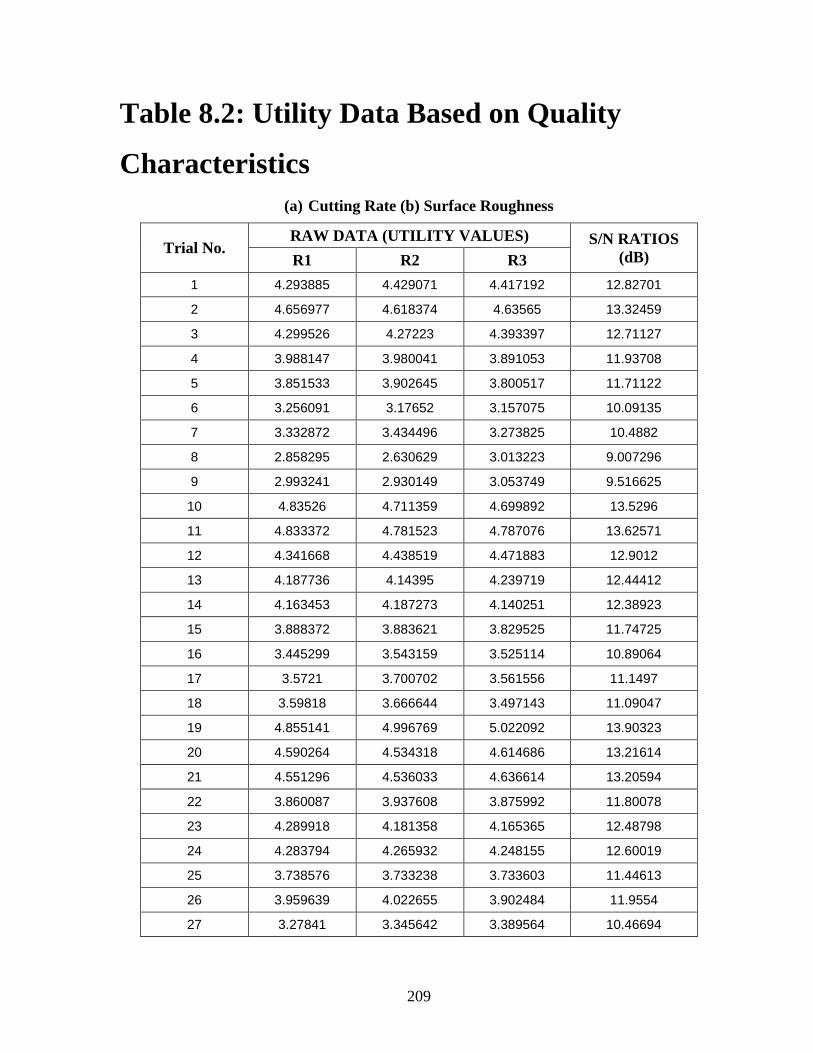
209

Table 8.2: Utility Data Based on Quality

Characteristics


Trial No. RAW DATA (UTILITY VALUES) S/N RATIOS

(dB) R1 R2 R3

1 4.293885 4.429071 4.417192 12.82701

2 4.656977 4.618374 4.63565 13.32459

3 4.299526 4.27223 4.393397 12.71127

4 3.988147 3.980041 3.891053 11.93708

5 3.851533 3.902645 3.800517 11.71122

6 3.256091 3.17652 3.157075 10.09135

7 3.332872 3.434496 3.273825 10.4882

8 2.858295 2.630629 3.013223 9.007296

9 2.993241 2.930149 3.053749 9.516625

10 4.83526 4.711359 4.699892 13.5296

11 4.833372 4.781523 4.787076 13.62571

12 4.341668 4.438519 4.471883 12.9012

13 4.187736 4.14395 4.239719 12.44412

14 4.163453 4.187273 4.140251 12.38923

15 3.888372 3.883621 3.829525 11.74725

16 3.445299 3.543159 3.525114 10.89064

17 3.5721 3.700702 3.561556 11.1497

18 3.59818 3.666644 3.497143 11.09047

19 4.855141 4.996769 5.022092 13.90323

20 4.590264 4.534318 4.614686 13.21614

21 4.551296 4.536033 4.636614 13.20594

22 3.860087 3.937608 3.875992 11.80078

23 4.289918 4.181358 4.165365 12.48798

24 4.283794 4.265932 4.248155 12.60019

25 3.738576 3.733238 3.733603 11.44613

26 3.959639 4.022655 3.902484 11.9554

27 3.27841 3.345642 3.389564 10.46694

210

R1, R2, R3 – Repetitions of experiments against each of the trial conditions

126116106

4.50

4.25

4.00

3.75

3.50

605040 604020

23015070

4.50

4.25

4.00

3.75

3.50

1284 1284

Ton

Me

an

of

Me

an

s

Toff SV

IP WF WT


Figure 8.1: Effects of Process Parameters on Utility Function (UCR, SR) for Raw Data

126116106

13.0

12.5

12.0

11.5

11.0

605040 604020

23015070

13.0

12.5

12.0

11.5

11.0

1284 1284

Ton

Me

an

of

SN

ra

tio

s

Toff SV

IP WF WT



211

Figure 8.2: Effects of Process Parameters on Utility Function (UCR, SR) for S/N Data

4.8

4.0

3.2

604020

605040

4.8

4.0

3.2

126116106

4.8

4.0

3.2

T on

T off

SV

106

116

126

Ton

40

50

60

Toff

20

40

60

SV


Figure 8.3: Effects of Process Parameters Interactions on Utility Function (UCR, SR) for

Raw Data

14

12

10

604020

605040

14

12

10

126116106

14

12

10

T on

T off

SV

106

116

126

Ton

40

50

60

Toff

20

40

60

SV



212

Figure 8.4: Effects of Process Parameters Interactions on Utility Function (UCR, SR) for

S/N Data

Table 8.3: Pooled Analysis of Variance for Utility Function (UCR, SR) for S/N Data


Ton 2 5.846 5.846 2.9231 20.86 0.000

Toff 2 30.001 30.001 15.0005 107.04 0.000

SV 2 1.670 1.670 0.8351 5.96 0.010

IP 2 2.797 2.797 1.3987 9.98 0.001

Residual Error 18 2.522 2.522 0.1401

Total 26 42.837

Table 8.4: Pooled Analysis of Variance for Utility Function (UCR, SR) for Raw Data


Ton 2 1.0306 1.0306 0.51528 27.72 0.000

Toff 2 6.1570 6.1570 3.07852 165.62 0.000

SV 2 0.3328 0.3328 0.16642 8.95 0.002

IP 2 0.5145 0.5145 0.25725 13.84 0.000

Residual Error 18 0.3346 0.3346 0.01859

Total 26 8.3695

Table 8.5: Response Table for Utility Function (UCR, SR) (S/N Data)


1 11.29 13.25 12.14 11.51

2 12.20 11.91 12.10 12.04

3 12.34 10.67 11.59 12.28

Delta 1.05 2.58 0.55 0.77

Rank 2 1 4 3

Table 8.6: Response Table for Utility Function (UCR, SR) (Raw Data)


1 3.724 4.602 4.079 3.812

2 4.099 3.955 4.072 4.037

3 4.168 3.435 3.840 4.143

Delta 0.445 1.167 0.239 0.331

Rank 2 1 4 3

213

0.80.40.0-0.4-0.8

99

90

50

10

1

Residual

Pe

rce

nt

1413121110

0.5

0.0

-0.5

Fitted Value

Re

sid

ua

l

0.60.40.20.0-0.2-0.4-0.6-0.8

8

6

4

2

0

Residual

Fre

qu

en

cy

2624222018161412108642

0.5

0.0

-0.5

Observation Order

Re

sid

ua

l




Figure 8.5: Residual plots for Utility Function (UCR, SR) for S/N Data

0.20.10.0-0.1-0.2

99

90

50

10

1

Residual

Pe

rce

nt

5.04.54.03.53.0

0.2

0.1

0.0

-0.1

-0.2

Fitted Value

Re

sid

ua

l

0.20.10.0-0.1-0.2

8

6

4

2

0

Residual

Fre

qu

en

cy

2624222018161412108642

0.2

0.1

0.0

-0.1

-0.2

Observation Order

Re

sid

ua

l




214

Figure 8.6: Residual plots for Utility Function (UCR, SR) for Raw Data

The optimal settings of process parameters for optimization of cutting rate and

surface roughness for WEDM process ascertained from main effects plots are as given

below:

Parameter Level

Pulse on Time (A) 3 (126 machine unit)

Pulse off Time (B) 1 (40 machine unit)

Spark Gap Set Voltage (C) 1 (20 volt)

Peak Current (D) 3 (230 ampere)

(v) Predicted means (Optimal)

The optimum value of utility (UCR,SR) is predicted at the selected levels of significant

variables as stated above viz. pulse on time (A3), pulse off time(B1), spark gap set voltage

(C1) and peak current(D3). The estimated mean of the response characteristic utility (UCR,SR)

can be determined (Kumar, 1993 and Roy, 1990) as

(8.10)

Where, T = overall mean of utility (UCR,SR) = (R1+R2+R3)/81 = 3.9971



3A = average value of utility (UCR,SR) at the third level of pulse on time = 4.168

1B = average value of utility (UCR,SR) at the first level of pulse off time = 4.602

1C = average value of utility (UCR,SR) at the first level of spark gap set voltage = 4.079

3D = average value of utility (UCR,SR) at the third level of peak current = 4.143


µCR,SR = 4.168 + 4.602 + 4.079 + 4.143 – 3 (3.9971) = 5.0007

The 95 % confidence intervals of confirmation experiments (CICE) and of population (CIPOP)

were calculated by using the Equations 4.10 and 4.11, which are reproduced below for ready

reference:

T33113U SRCR, DCBA

215

R

1

n

1V)f(1,FCI

eff

eeαCE and

eff

eeα

POPn

V)f(1,FCI

Where, Fα (1, fe) = The F ratio at confidence level of (1-α) against DOF 1 and error degree of

freedom fe.


Neff

n

= 81 / (1+8)

= 9.0




fe = Error DOF = 18 (Table 8.4)


So, CICE = ± 0.1909 and

CIPOP = ± 0.0955


Mean µCR,SR - CICE < µCR,SR < µCR,SR + CICE

4.8098 < µCR,SR < 5.1916

The 95% confirmation interval of the predicted mean is:

Mean µCR,SR – CIPOP < µCR,SR < Mean µCR,SR + CIPOP

4.9052 < µCR,SR < 5.0962






216

(vi) Confirmation experiments

Three confirmation experiments have been conducted at the optimum settings of the

process parameters. The following average values have been found for the quality

characteristics considered:

(a) Average cutting rate = 2.85 mm/min

(b) Average surface roughness = 2.65 µm

The utility value of the machined part has been calculated using the following relation:

U= PCR*WCR + PSR*WSR

= 9.1807*0.5 + 0.6801*0.5

= 4.9304

This experimentally obtained utility value is lying within the 95% CICE of the optimal range

of the utility calculated for utility function (UCR, SR).

8.2.3 Model 2: Cutting Rate, Surface Roughness and Gap Current

The optimal settings of process parameters and the optimal values of cutting rate,

surface roughness and gap current (when they are optimized individually) have already been

established (Chapter 5). The summary results are reproduced in Table 8.1.




= 2.6681 (Table 8.1)



(All the CR values in Table. 5.3 are in between 0.16 to 3.45)

Using these values and the Equations. 8.3 & 8.4, the following preference scale for CR has

been constructed:

PCR = 6.310466 log 1.0

ix (8.11)



217

= 0.3890 µm (Table 8.1)


= 3.1 µm (assumed)

(All the SR values in Table 5.3 are in between: 1.06 to 3.01 µm)


has been found:

PSR = -9.98433 log 1.3

ix (8.12)

(c) Gap current (IG)

x* = optimum value of IG (when optimized individually)

= 4.70162 ampere (Table 8.1)

x/ = minimum acceptable value of IG

= 0.5 ampere (assumed)

(All the IG values in Table 5.4 are in between: 0.6 to 6.5 ampere)


has been found:

PIG = 8.89557 log 5.0

ix (8.13)


It has been assumed that the quality characteristics SR and IG are equally important

and hence equal weightage has been assigned to them. However, there is no constraint on the

weightage and it can be any value between 0 to 1 subjected to the condition specified in

Equation 8.5. The weights assigned to the various quality characteristics are:



WIG = weightage for IG = 0.3


The utility value of each machined part has been calculated using the following

relation:

218

U (n, R) = PCR (n, R) x WCR + PSR (n, R) x WSR + PIG (n, R) x WIG (8.14)

Where, n = trial number,

n = 1,2, . . ., 27







responses and main effects (in terms of utility value) and S/N ratios are given in Table 8.7.

The data from Table 8.7 are plotted in Figures 8.7 and 8.8. It is clear from the Figures 8.7 and

8.8 that third level of pulse on time (A3), first level of pulse off time (B1), first level of spark

gap set voltage (C1), third level of peak current (D1) and first level of wire feed (E1) would

yield best performance in terms of utility value and S/N ratio within the selected range of

parameters. Figures 8.9 and 8.10 reveal that none of the interaction between various process

parameters is significant as the responses are almost parallel.


Tables 8.8 and 8.9 respectively. It is seen that pulse on time (A), pulse off time (B), spark

gap set voltage (C), peak current (D) and wire feed (E) significantly affect both mean of

utility values and S/N ratios since all these process parameters are significant in both the

ANOVAS . From Table 8.10 it can be seen that pulse on time is the most significant

parameter in affecting utility function for cutting rate, surface roughness and gap current.

This is followed by pulse off time ,peak current, spark gap set voltage and wire feed in that

order. Four residual plots are drawn to check the data for the non normality, non-random

variation, non constant variance, higher-order relationships, and outliers (Figures 8.11 and

8.12). The residual versus fitted value indicates a little tendency for variance of the residuals

to increase as the desired output response value increases. The problem, however, is not

severe enough to have a dramatic impact on the analysis and conclusions. The normal

probability plot, histogram plot, and residual versus observation order plot of these residuals

do not reveal any problem.

219

Table 8.7: Utility Data Based on Quality Characteristics

(a) Cutting Rate (b) Surface Roughness (c) Gap Current


(dB) R1 R2 R3

1 4.286819 4.290222 4.372986 12.70189

2 4.349862 4.411748 4.329345 12.79617

3 3.934612 3.813198 3.990934 11.84528

4 3.620363 3.626921 3.562107 11.13274

5 3.235577 3.40952 3.204967 10.31677

6 2.354927 2.485843 2.474177 7.733955

7 2.863225 2.840699 2.819096 9.068922

8 2.07171 2.011264 2.164666 6.360047

9 2.152677 2.276866 2.188982 6.865624

10 6.297177 6.191662 6.155216 15.86717

11 6.162143 6.096752 6.067476 15.71856

12 4.497877 4.633658 4.587043 13.20177

13 5.260464 5.186686 5.335838 14.41961

14 4.173148 4.096783 4.163912 12.3488

15 3.957621 4.044782 3.918128 11.98119

16 3.399224 3.570449 3.447113 10.8067

17 3.755108 3.83227 3.651628 11.46702

18 3.508267 3.655728 3.458609 10.97503

19 6.826117 6.941245 6.916217 16.76941

20 5.361487 5.365109 5.328517 14.56972

21 6.098422 6.134483 6.187842 15.76325

22 4.689934 4.788768 4.696449 13.48695

23 5.665235 5.563376 5.588857 14.97201

24 5.54135 5.534169 5.483582 14.83803

25 4.99174 4.943745 4.990793 13.93634

26 5.20774 5.201478 5.127323 14.28401

27 3.263882 3.304221 3.349483 10.38424


220

126116106

5.0

4.5

4.0

3.5

3.0

605040 604020

23015070

5.0

4.5

4.0

3.5

3.0

1284 1284

Ton

Me

an

of

Me

an

s

Toff SV

IP WF WT


Figure 8.7: Effects of Process Parameters on Utility Function (UCR, SR, IG) for Raw Data

126116106

14

13

12

11

10

605040 604020

23015070

14

13

12

11

10

1284 1284

Ton

Me

an

of

SN

ra

tio

s

Toff SV

IP WF WT



Figure 8.8: Effects of Process Parameters on Utility Function (UCR, SR, IG) for S/N Data

221

6

4

2

604020

605040

6

4

2

126116106

6

4

2

T on

T off

SV

106

116

126

Ton

40

50

60

Toff

20

40

60

SV


Figure 8.9: Effects of Process Parameters Interactions on Utility Function (UCR, SR, IG)

for Raw Data

16

12

8

604020

605040

16

12

8

126116106

16

12

8

T on

T off

SV

106

116

126

Ton

40

50

60

Toff

20

40

60

SV



Figure 8.10: Effects of Process Parameters Interactions on Utility Function (UCR, SR, IG)

for S/N Data

222

Table 8.8: Pooled Analysis of Variance for Utility Function (UCR, SR, IG) for S/N Data


Ton 2 94.294 94.294 47.1469 134.23 0.000

Toff 2 68.403 68.403 34.2017 97.38 0.000

SV 2 12.124 12.124 6.0622 17.26 0.000

IP 2 17.140 17.140 8.5700 24.40 0.000

WF 2 1.095 1.095 0.5477 1.56 0.241

Residual Error 16 5.620 5.620 0.3512

Total 26 198.677

Table 8.9: Pooled Analysis of Variance for Utility Function (UCR, SR, IG) for Raw Data


Ton 2 19.8473 19.8473 9.92367 285.60 0.000

Toff 2 15.2570 15.2570 7.62849 219.54 0.000

SV 2 2.5501 2.5501 1.27503 36.69 0.000

IP 2 4.0834 4.0834 2.04168 58.76 0.000

WF 2 0.6199 0.6199 0.30993 8.92 0.002

Residual Error 16 0.5560 0.5560 0.03475

Total 26 42.9136

Table 8.10: Response Table for Utility Function (UCR, SR, IG) for S/N Data


1 9.869 14.359 13.132 11.288 12.509

2 12.976 12.359 12.537 12.754 12.560

3 14.334 10.461 11.510 13.137 12.110

Delta 4.465 3.898 1.622 1.849 0.451

Rank 1 2 4 3 5

Table 8.11: Response Table for Utility Function (UCR, SR, IG) for Raw Data


1 3.228 5.320 4.700 3.823 4.497

2 4.559 4.284 4.430 4.537 4.440

3 5.300 3.483 3.957 4.727 4.150

Delta 2.072 1.836 0.744 0.903 0.346

Rank 1 2 4 3 5

223

1.00.50.0-0.5-1.0

99

90

50

10

1

Residual

Pe

rce

nt

18151296

1.0

0.5

0.0

-0.5

-1.0

Fitted Value

Re

sid

ua

l

1.00.50.0-0.5-1.0

8

6

4

2

0

Residual

Fre

qu

en

cy

2624222018161412108642

1.0

0.5

0.0

-0.5

-1.0

Observation Order

Re

sid

ua

l




Figure 8.11: Residual Plots for Utility Function (UCR, SR, IG) for S/N Data

0.40.20.0-0.2-0.4

99

90

50

10

1

Residual

Pe

rce

nt

642

0.4

0.2

0.0

-0.2

Fitted Value

Re

sid

ua

l

0.40.30.20.10.0-0.1-0.2

10.0

7.5

5.0

2.5

0.0

Residual

Fre

qu

en

cy

2624222018161412108642

0.4

0.2

0.0

-0.2

Observation Order

Re

sid

ua

l




Figure 8.12: Residual Plots for Utility Function (UCR, SR, IG) for Raw Data

224


surface roughness for WEDM process ascertained from main effects plots are given below:

Parameters Level



Spark Gap Set Voltage (C) 1 (20 volt)


Wire Feed (E) 1 (4 m/min)


The optimum value of utility (UCR,SR,IG) is predicted at the selected levels of

significant variables as stated above viz. pulse on time (A3), pulse off time(B1), spark gap set

voltage (C1) peak current(D3) and wire feed(E1). The estimated mean of the response

characteristic utility (UCR,SR,IG) can be determined (Kumar, 1993 and Roy, 1990) as

(8.15)

Where, T = overall mean of utility (UCR,SR,IG) = (R1+R2+R3)/81 = 4.3622



3A = average value of utility (UCR,SR,IG) at the third level of pulse on time = 5.3

1B = average value of utility (UCR,SR,IG) at the first level of pulse off time = 5.32

1C = average value of utility (UCR,SR,IG) at the first level of spark gap set voltage = 4.7

3D = average value of utility (UCR,SR,IG) at the third level of peak current = 4.727

1E = average value of utility (UCR,SR,IG) at the first level of wire feed = 4.497


µCR,SR,IG = 5.3 + 5.32 + 4.7 + 4.727 + 4.497 – 4(4.3622)

= 7.0952

The 95 % confidence intervals of confirmation experiments (CICE) and of population

(CIPOP) were calculated by using the Equations 4.10 and 4.11 are reproduced below:

T413113U IGSR,CR, EDCBA

225

R

1

n

1V)f(1,FCI

eff

eeαCE and

eff

eeα

POPn

V)f(1,FCI




Neff

n

= 81/ (1+10)

= 7.3636






So, CICE = ± 0.7326 and

CIPOP = ± 0.1456


Mean µCR,SR,IG - CICE < µCR,SR,IG < µCR,SR,IG + CICE

6.3626 < µCR,SR,IG < 7.8278


Mean µCR,SR,IG – CIPOP < µCR,SR,IG < Mean µCR,SR,IG + CIPOP

6.9496< µCR,SR,IG < 7.2408






First level of wire feed (E1) : 4 m/min

226







(c) Average gap current = 5.2 ampere

The utility value of the machined part has been calculated using the following

relation:

U= PCR*WCR + PSR*WSR + PIG*WIG

= 9.2659*0.4 + 0.7627*0.3+ 9.0471*0.3

= 3.70636 + 0.2288 + 2.71413

= 6.6493


of the utility calculated for utility function (UCR, SR, IG).

8.2.4 Model 3: Cutting Rate, Surface Roughness, and Dimensional Deviation


surface roughness, and dimensional deviation (when they are optimized individually) have

already been established (Chapter 5). The summary results are reproduced in Table.8.1.




= 2.6681 (Table 8.1)



(All the CR values in Table. 5.3 are in between 0.16 to 3.45)

Using these values and the Equations 8.3 & 8.4, the following preference scale for CR has

been constructed:

227

PCR = 6.310466 log 1.0

ix (8.16)



= 0.3890 µm (Table 8.1)


= 3.1 µm (assumed)

(All the SR values in Table 5.3 are in between 1.06 to 3.01 µm)

Using these values and the Equations 8.3 and 8.4, the following preference scale for

SR has been found:

PSR = -9.98433 log 1.3

ix (8.17)

(c) Dimensional deviation (DD)

x* = optimum value of DD (when optimized individually)

= 0.1052 % (Table 8.1)

x/ = maximum acceptable value of DD

= 0.8 % (assumed)

(All the DD values in Table 5.4 are in between 0.02 to 0.8 %)

Using these values and the Equations 8.3 and 8.4, the following preference scale for

DD has been found:

PDD = -10.2105 log 8.0

ix (8.18)


It has been assumed that the quality characteristics CR, SR and DD are not equally

important and hence unequal weightage has been assigned. However, there is no constraint

on the weightage and it can be any value ranging from 0 to 1 subjected to the condition

specified in Equation 8.5. The weights assigned are:



WDD = weightage for DD = 0.15

228


The utility value of each machined part has been calculated using the following

relation:

U (n, R) = PCR (n, R) x WCR + PSR (n, R) x WSR + PDD (n, R) x WDD (8.19)

Where, n = trial number

n = 1,2, . . ., 27








The data from Table 8.12 are plotted in Figures 8.13 and 8.14. It is clear from the figure that

third level of pulse on time (A3), first level of pulse off time (B1), third level of peak current

(D1) would yield best performance in terms of utility value and S/N ratio within the selected

range of parameters. Figures 8.15 and 8.16 reveal that the interactions between pulse off

time, pulse on time and spark gap set voltage affect moderately the output responses since the

responses are not parallel.


Tables 8.13 and 8.14 respectively. It is seen that pulse on time (A), pulse off time (B), and

peak current (D) significantly affect both mean of utility values and S/N ratios since all these

process parameters are significant in both the ANOVAS. From Table 8.16, it can be seen that

pulse on time is the most significant parameter in affecting utility function for cutting rate,

surface roughness and dimensional deviation. This is followed by pulse off time and peak

current in that order. Four residual plots are drawn for estimating the accuracy of the model

(Figures 8.17 and 8.18).The histogram plot indicates a mild tendency for the non normality;

however the normal probability plot of these residuals does not reveal any particular trouble.

Residual versus fitted value and residual versus observation order plot do not indicate any

undesirable effect.

229

Table 8.12: Utility Data Based on Quality Characteristics

(a) Cutting Rate (b) Surface Roughness (c) Dimensional Deviation


(dB) R1 R2 R3

1 3.879865 4.036803 3.994164 11.97275

2 4.448229 4.364321 4.398681 12.87565

3 3.983917 3.840684 3.986231 11.89922

4 3.427891 3.473466 3.376765 10.69412

5 3.605743 3.709548 3.59834 11.21446

6 2.762994 2.741019 2.680731 8.715543

7 2.980713 3.055088 2.913577 9.488548

8 2.336897 2.110301 2.421937 7.15086

9 3.011698 2.966802 2.986353 9.507946

10 4.911846 4.79577 4.795483 13.68514

11 4.948001 4.889125 4.85514 13.79855

12 4.554657 4.682857 4.724573 13.3534

13 4.455801 4.480512 4.560856 13.06114

14 4.139262 4.202174 4.153452 12.39168

15 4.006937 3.99564 4.057546 12.08403

16 3.2763 3.407764 3.313432 10.45184

17 4.115805 4.170501 4.035708 12.26883

18 5.625719 5.752029 5.371823 14.92704

19 4.991368 5.126161 5.099148 14.10224

20 4.75318 4.670073 4.958378 13.60554

21 5.499975 5.58171 5.494328 14.8465

22 3.615427 3.706246 3.611482 11.23063

23 4.405539 4.359596 4.27773 12.7631

24 4.540849 4.565039 4.473388 13.11415

25 4.081541 4.09626 4.038661 12.19601

26 5.230882 5.300009 4.984022 14.26342

27 3.213321 3.226266 3.461384 10.35607


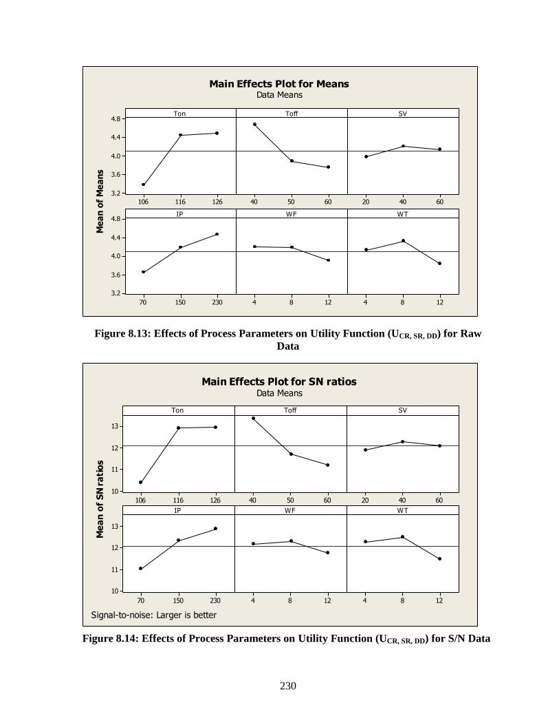
230

126116106

4.8

4.4

4.0

3.6

3.2

605040 604020

23015070

4.8

4.4

4.0

3.6

3.2

1284 1284

Ton

Me

an

of

Me

an

s

Toff SV

IP WF WT


Figure 8.13: Effects of Process Parameters on Utility Function (UCR, SR, DD) for Raw

Data

126116106

13

12

11

10

605040 604020

23015070

13

12

11

10

1284 1284

Ton

Me

an

of

SN

ra

tio

s

Toff SV

IP WF WT



Figure 8.14: Effects of Process Parameters on Utility Function (UCR, SR, DD) for S/N Data

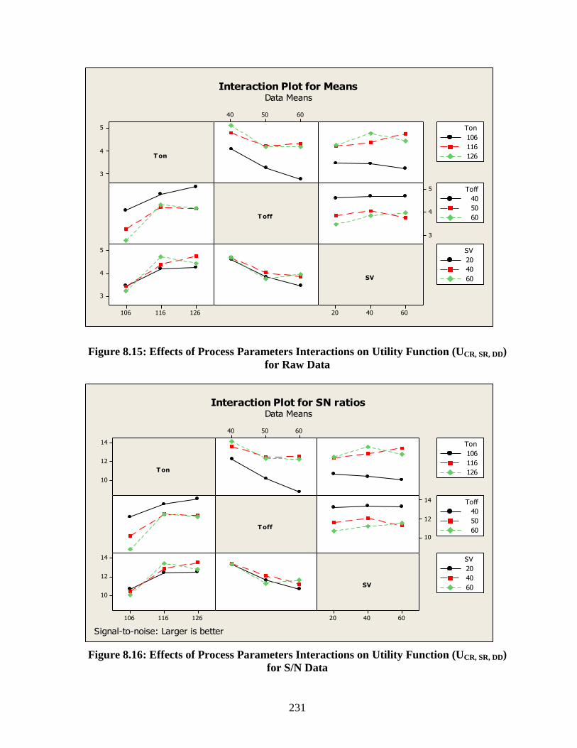
231

5

4

3

604020

605040

5

4

3

126116106

5

4

3

T on

T off

SV

106

116

126

Ton

40

50

60

Toff

20

40

60

SV


Figure 8.15: Effects of Process Parameters Interactions on Utility Function (UCR, SR, DD)

for Raw Data

14

12

10

604020

605040

14

12

10

126116106

14

12

10

T on

T off

SV

106

116

126

Ton

40

50

60

Toff

20

40

60

SV



Figure 8.16: Effects of Process Parameters Interactions on Utility Function (UCR, SR, DD)

for S/N Data

232

Table 8.13: Pooled Analysis of Variance for Utility Function (UCR, SR, DD) for S/N Data


Ton 2 38.28 38.28 19.1420 21.57 0.000

Toff 2 23.12 23.12 11.5589 13.02 0.000

IP 2 16.23 16.23 8.1131 9.14 0.002

Residual Error 20 17.75 17.75 0.8875

Total 26 95.38

Table 8.14: Pooled Analysis of Variance for Utility Function (UCR, SR, DD) for Raw Data


Ton 2 7.281 7.281 3.6404 19.68 0.000

Toff 2 4.441 4.441 2.2205 12.00 0.000

IP 2 3.161 3.161 1.5807 8.55 0.002

Residual Error 20 3.699 3.699 0.1850

Total 26 18.583

Table 8.15: Response Table for Utility Function (UCR, SR, DD) for S/N Data

Level Ton Toff IP

1 10.39 13.35 11.03

2 12.89 11.70 12.32

3 12.94 11.18 12.87

Delta 2.55 2.17 1.85

Rank 1 2 3

Table 8.16: Response Table for Utility Function (UCR, SR, DD) for Raw Data

Level Ton Toff IP

1 3.374 4.676 3.653

2 4.455 3.888 4.192

3 4.495 3.759 4.479

Delta 1.121 0.918 0.826

Rank 1 2 3

233

210-1-2

99

90

50

10

1

Residual

Pe

rce

nt

16141210

2

1

0

-1

Fitted Value

Re

sid

ua

l

2.01.51.00.50.0-0.5-1.0-1.5

8

6

4

2

0

Residual

Fre

qu

en

cy

2624222018161412108642

2

1

0

-1

Observation Order

Re

sid

ua

l




Figure 8.17: Residual Plots for Utility Function (UCR, SR, DD) for S/N Data

1.00.50.0-0.5-1.0

99

90

50

10

1

Residual

Pe

rce

nt

543

1.0

0.5

0.0

-0.5

Fitted Value

Re

sid

ua

l

1.000.750.500.250.00-0.25-0.50

8

6

4

2

0

Residual

Fre

qu

en

cy

2624222018161412108642

1.0

0.5

0.0

-0.5

Observation Order

Re

sid

ua

l




Figure 8.18: Residual Plots for Utility Function (UCR, SR, DD) for Raw Data

234


surface roughness for WEDM process ascertained from main effects plots are given below:

Parameters Level





The optimum value of utility (UCR,SR,DD) is predicted at the selected levels of

significant variables as stated above viz. pulse on time (A3), pulse off time(B1) and peak

current(D3). The estimated mean of the response characteristic utility (UCR,SR,DD) can be

determined (Kumar, 1993 and Roy, 1990) as

(8.20)

Where, T = overall mean of utility (UCR,SR,DD) = (R1+R2+R3)/81 = 4.1078

Where, R1, R2, and R3 values are taken from the Table 8.12, and the values of 3A , 1B and 3D

are taken from the Table 8.16.

3A = average value of utility (UCR,SR,DD) at the third level of pulse on time = 4.495

1B = average value of utility (UCR,SR,DD) at the first level of pulse off time = 4.676

3D = average value of utility (UCR,SR,DD) at the third level of peak current = 4.479


µCR,SR,DD = 4.495 + 4.676 + 4.479 – 2(4.1078)

= 5.4344


(CIPOP) were calculated by using the Equations 4.10 and 4.11 which are reproduced below:

R

1

n

1V)f(1,FCI

eff

eeαCE and

eff

eeα

POPn

V)f(1,FCI

T2313U DDSR,CR, DBA

235

Where, Fα (1, fe) = The F ratio at confidence level of (1-α) against DOF 1 and error degree of

freedom fe.


Neff

n

= 81 / (1+6)

= 11.57






So, CICE = ± 0.5812 and

CIPOP = ± 0.2637


Mean µCR,SR,DD - CICE < µCR,SR,DD < µCR,SR,DD + CICE

4.8532 < µCR,SR,DD < 6.0156


Mean µCR,SR,DD – CIPOP < µCR,SR,DD < Mean µCR,SR,DD + CIPOP

5.1707 < µCR,SR,DD < 5.6981











236

(c) Average dimensional deviation = 0.553 %


U= PCR*WCR + PSR*WSR + PDD*WDD

= 9.3030*0.5 + 0.6313*0.35 + 1.6374*0.15

= 4.6515 + 0.2209 + 0.2456

= 5.118


of the utility calculated for utility function (UCR, SR, DD).

8.2.5 Model 4: Cutting Rate, Surface Roughness, Gap Current and Dimensional

Deviation


surface roughness, gap current and dimensional deviation (when they are optimized

individually) have already been established (Chapter 5). The summary results are reproduced

in Table.8.1.




= 2.6681 (Table 8.1)



(All the CR values in Table 5.3 are in between 0.16 to 3.45)

Using these values and the Eqs. 8.3 and 8.4, the following preference scale for CR has been

constructed:

PCR = 6.310466 log 1.0

ix (8.21)



= 0.3890 µm (Table 8.1)


237

= 3.1 µm (assumed)

(All the SR values in Table 5.3 are in between: 1.06 to 3.01 µm)


has been found:

PSR = -9.98433 log 1.3

ix (8.22)

(c) Gap current (IG)

x* = optimum value of IG (when optimized individually)

= 4.70162 ampere (Table 8.1)

x/ = minimum acceptable value of IG

= 0.5 ampere (assumed)

(All the IG values in Table 5.4 are in between 0.6 to 6.5 ampere)


has been found:

PIG = 8.89557 log 5.0

ix

(d) Dimensional deviation (DD)

x* = optimum value of DD (when optimized individually)

= 0.1052 % (Table 8.1)

x/ = maximum acceptable value of DD

= 0.8 % (assumed)

(All the DD values in Table 5.4 are in between 0.02 to 0.806 %)

Using these values and the Eqs. 8.3 and 8.4, the following preference scale for DD

has been found:

PDD = -10.2105 log 8.0

ix (8.23)


It has been assumed that both the quality characteristics CR and SR are equally

important and hence equal weightage has been assigned. Further the quality characteristics

IG and DD, have been assigned to be equally important and assigned equal weight

However, there is no constraint on the weightage and it can be any value between 0 to 1

238

subjected to the condition specified in Equation 8.5 the weighted assign to the chacterstics

are:



WIG = weightage for IG = 0.2

WDD = weightage for DD = 0.2


The utility value of each machined part has been calculated using the following relation:

U(n, R) = PCR (n, R) x WCR + PSR (n, R) x WSR + PIG (n, R) x WIG+ PDD (n, R) x WDD

(8.24)

Where, n = trial number, n = 1,2, . . ., 27


The utility values thus calculated are given in Table 8.17






The data from Table 8.17 are plotted in Figures 8.19 and 8.20. It is clear from the figure that

third level of pulse on time (A3), first level of pulse off time (B1), third level of peak current

(D1) would yield best performance in terms of utility value and S/N ratio within the selected

range of parameters. Figures 8.21 and 8.22 reveal that the interaction between pulse off time

and spark gap set voltage at second level values affect the output responses significantly

since the responses are not parallel.


Tables 8.18 and 8.19 respectively. It is seen that pulse on time (A), pulse off time (B), and

peak current (D) significantly affect both mean of utility values and S/N ratios since all these

process parameters are significant in both the ANOVAS.

239

8.17: Utility Data Based on Quality Characteristics

(a) Cutting Rate (b) Surface Roughness (c) Gap Current (d) Dimensional Deviation


(dB) R1 R2 R3

1 3.503062 3.593628 3.589994 11.03261

2 3.973051 3.95133 3.929538 11.93455

3 3.605758 3.339383 3.577552 10.88451

4 2.928455 2.969082 2.892652 9.336061

5 3.12711 3.325951 3.134245 10.08097

6 2.359574 2.475903 2.402001 7.644189

7 2.588933 2.621761 2.536503 8.238046

8 2.013122 1.881959 2.074866 5.955194

9 2.867875 2.981379 2.813912 9.203592

10 4.866702 4.744532 4.734376 13.58992

11 4.888773 4.817868 4.755639 13.66065

12 4.434779 4.605455 4.595853 13.14744

13 4.373959 4.404115 4.51679 12.92877

14 3.963226 3.991442 3.98051 11.99404

15 3.750402 3.785941 3.845866 11.58071

16 2.992713 3.179282 3.015619 9.712266

17 4.026483 4.056543 3.870126 12.00165

18 6.039682 6.241432 5.712905 15.54271

19 5.090124 5.210252 5.149648 14.23498

20 4.688234 4.638336 4.92772 13.52748

21 5.802282 5.963296 5.759312 15.32777

22 3.502595 3.624741 3.49809 10.98098

23 4.447359 4.411055 4.321757 12.8541

24 4.6089 4.640035 4.511337 13.22824

25 4.131576 4.134111 4.071985 12.2816

26 5.629738 5.687703 5.310549 14.8624

27 3.303709 3.298557 3.559592 10.58073


240

126116106

4.5

4.0

3.5

3.0

605040 604020

23015070

4.5

4.0

3.5

3.0

1284 1284

Ton

Me

an

of

Me

an

sToff SV

IP WF WT


Figure 8.19: Effects of Process Parameters on Utility Function (UCR, SR, IG, DD) for

Raw Data

126116106

13

12

11

10

9

605040 604020

23015070

13

12

11

10

9

1284 1284

Ton

Me

an

of

SN

ra

tio

s

Toff SV

IP WF WT



Figure 8.20: Effects of Process Parameters on Utility Function (UCR, SR, IG, DD) for

S/N Data

241

5

4

3

604020

605040

5

4

3

126116106

5

4

3

T on

T off

SV

106

116

126

Ton

40

50

60

Toff

20

40

60

SV


Figure 8.21: Effects of Process Parameters Interactions on (UCR, SR, IG, DD) for Raw Data

15

12

9

604020

605040

15

12

9

126116106

15

12

9

T on

T off

SV

106

116

126

Ton

40

50

60

Toff

20

40

60

SV



Figure 8.22: Effects of Process Parameters Interactions on (UCR, SR, IG, DD) for S/N Data

242

From Tables 8.20 and 8.21, it can be seen that pulse on time is the most significant

parameter in affecting utility function for cutting rate, surface roughness, gap current and

dimensional deviation. This is followed by peak current and pulse off time in that order. Four

residual plots are drawn for estimating the accuracy of the model (Figures 8.23 and 8.24).

Residual plots do not show any problem in the distribution of the data and model

assumptions. The optimal settings of process parameters for optimization of cutting rate,

surface roughness, gap current and dimensional deviation for WEDM process ascertained

from main effects plots are given below:

Parameters Level





The optimum value of utility (UCR,SR,IG,DD) is predicted at the selected levels of

significant variables as stated above viz. pulse on time (A3), pulse off time (B1) and peak

current (D3). The estimated mean of the response characteristic utility (UCR, SR, IG, DD) can be

determined (Kumar, 1993 and Roy, 1990) as

(8.25)

Where, T = overall mean of utility (UCR, SR, IG, DD) = (R1+R2+R3)/81 = 3.9898

Where, R1, R2, and R3 values are taken from the Table 8.17, and the values of 3A , 1B , and


3A = average value of utility (UCR, SR, IG, DD) at the third level of pulse on time = 4.590

1B = average value of utility (UCR, SR, IG, DD) at the first level of pulse off time = 4.546

3D = average value of utility (UCR, SR, IG, DD) at the third level of peak current = 4.424


Table 8.18: Pooled Analysis of Variance for (UCR, SR, IG, DD) for S/N Data

T2313U DDIG,SR,CR, DBA

243


Ton 2 75.24 75.24 37.622 29.91 0.000

Toff 2 23.85 23.85 11.924 9.48 0.001

IP 2 21.42 21.42 10.709 8.51 0.002

Residual Error 20 25.16 25.16 1.258

Total 26 145.67

Table 8.19: Pooled Analysis of Variance for (UCR, SR, IG, DD) for Raw Data


Ton 2 13.370 13.370 6.6852 23.33 0.000

Toff 2 4.178 4.178 2.0890 7.29 0.004

IP 2 4.192 4.192 2.0961 7.32 0.004

Residual Error 20 5.730 5.730 0.2865

Total 26 27.471

Table 8.20: Response Table for (UCR, SR, IG, DD) for S/N Data

Level Ton Toff IP

1 9.368 13.038 10.508

2 12.684 11.181 12.012

3 13.098 10.931 12.629

Delta 3.730 2.107 2.121

Rank 1 3 2

Table 8.21: Response Table for (UCR, SR, IG, DD) for Raw Data

Level Ton Toff IP

1 3.002 4.546 3.470

2 4.377 3.696 4.075

3 4.590 3.728 4.424

Delta 1.588 0.850 0.954

Rank 1 3 2

244

3.01.50.0-1.5-3.0

99

90

50

10

1

Residual

Pe

rce

nt

161412108

3

2

1

0

-1

Fitted Value

Re

sid

ua

l

210-1

6.0

4.5

3.0

1.5

0.0

Residual

Fre

qu

en

cy

2624222018161412108642

3

2

1

0

-1

Observation Order

Re

sid

ua

l




Figure 8.23: Residual Plots for (UCR, SR, IG, DD) for S/N Data

10-1

99

90

50

10

1

Residual

Pe

rce

nt

65432

1.5

1.0

0.5

0.0

-0.5

Fitted Value

Re

sid

ua

l

1.51.00.50.0-0.5

8

6

4

2

0

Residual

Fre

qu

en

cy

2624222018161412108642

1.5

1.0

0.5

0.0

-0.5

Observation Order

Re

sid

ua

l




Figure 8.24: Residual Plots for (UCR, SR, IG, DD) for Raw Data

245

µCR, SR, IG, DD = 4.168 + 4.602 + 4.079 + 4.143 – 2 (3.9898) = 5.5804


(CIPOP) were calculated by using the Equations 4.10 and 4.11

R

1

n

1V)f(1,FCI

eff

eeαCE and

eff

eeα

POPn

V)f(1,FCI




Neff

n

= 81 / (1+6)

= 11.57





F0.05 (1, 20) = 4.35 (Tabulated F value; Ross, 1996)

So, CICE = ± 0.7233 and

CIPOP = ± 0.3282


Mean µCR, SR, IG, DD - CICE < µCR, SR, IG, DD < µCR, SR, IG, DD + CICE

4.8571 < µCR, SR, IG, DD < 6.3037


Mean µCR,SR,IG,DD – CIPOP < µCR,SR,IG,DD < Mean µCR,SR,IG,DD + CIPOP

5.2522 < µCR,SR,IG,DD < 5.9086


246










(c) Average gap current = 5.0 ampere

(d) Average dimensional deviation = 0.553 %


U= PCR*WCR + PSR*WSR + PIG*WIG + PDD*WDD

= 9.3030*0.3 + 0.6313*0.3 + 8.89557*0.2 + 1.6374*0.2

= 2.7909+ 0.1894 + 1.7791+ 0.3275

= 5.0869


of the utility calculated for utility function (UCR, SR, IG, DD).

The final results for utility function and confirmation experiments are summarized in

Table 8.22. The values of individual response characteristics are obtained by carrying out

confirmation experiments at the optimal set of levels of process parameters suggested by

utility function analysis and further utility function values are calculated based on the

measured response characteristics. The findings are with in the 95% of CICE of respective

response characteristic model obtained through utility function. It is to be pointed out that

these optimal values are with in the specified range of process variables. Any extrapolation

should be confirmed through additional experiments.

247

Table 8.22: Predicted Optimal Values, Confidence Intervals and Results of

Confirmation Experiments for Utility Functions

Performance

Measures in

terms of Utility

Function

Optimal Set

of

Parameters

Predicted

Optimal

Value

predicted confidence intervals

at 95% confidence level

Actual value

(average of

three

confirmation

experiments)

USR,CR A3B1C1D3 5.0007 CIPOP :4.9052<µCR,SR< 5.0962

CICE :4.8098< µCR,SR < 5.1916 4.9304

USR,CR, IG A3B1C1D3E1 7.0952

CIPOP:6.9496< µCR,SR,IG< 7.2408

CICE :6.3626<µCR,SR,IG< 7.8278 6.6493

USR,CR, DD A3B1D3 5.4344 CIPOP:5.1707<µCR,SR,DD< 5.6981

CICE :4.8532<µCR,SR,DD< 6.0156 5.118

USR,CR, IG,DD A3B1D3 5.5804 CIPOP:5.2522<µCR,SR,IG,DD<5.9086

CICE:4.8571<µCR,SR,IG,DD<6.3037 5.0869

248

CHAPTER 9

CONCLUSIONS AND SCOPE FOR FUTURE WORK

In the earlier chapters, the effects of process variables on response characteristics

(cutting rate, surface roughness, gap current and dimensional deviation) of the wire electric

discharge machining (WEDM) process have been discussed. An optimal set of process

variables that yields the optimum quality features to machined parts produced by WEDM

process has also been obtained. The important conclusions from the present research work are

summarized in this chapter.

9.1 CONCLUSIONS

1. Ranges of Wire EDM process parameters have been established based on review of

literature and by performing the pilot experiments using one factor at a time (OFAT)

approach as under:

Process Parameters Symbol Units Range

(m/c units)

Range

(actual units)





Wire Feed WF m/min 4 -12 4 -12 m/min

Wire Tension WT gram 4 -12 500-1800 gram

2. The effects of the process parameters viz. pulse on time, pulse off time, spark gap set

voltage, peak current, wire tension and wire feed, on response characteristics viz. cutting rate,

surface roughness, gap current and dimensional deviation, were studied.

3. The optimal sets of process parameters were obtained for various performance measures

using Taguchi‟s design of experiment methodology. The summary results of predicted

249

optimal values of the responses and their confidence intervals (both for confirmation

experiment and population) are given as under:

Performance

Measures/

Responses

Optimal Set

of

Parameters

Predicted

Optimal

Value



Actual Value

(Average of

Three

Confirmation

Experiments)

Cutting Rate A3B1C1D3 2.6681

mm/min

CIPOP : 2.3982 < µCR < 2.938

CICE : 2.1284 < µCR < 3.2078

2.85 mm/min

Surface

Roughness A1B3C3D1E3

0.3890

µm

CIPOP : 0.2412 < µSR < 0.5368

CICE : 0.1142 < µSR < 0.6638

0.479 µm

Gap Current A3B1D3 4.6956

ampere

CIPOP : 4.222 < µIG < 5.1692

CICE : 3.6519 < µIG < 5.7393

5.0 ampere

Dimensional

Deviation A2B3C3F1

0.10524

%

CIPOP : -0.0330 < µDD < 0.1774

CICE : -0.0393 < µDD < 0.2497

0.124 %

4. Response surface methodology (RSM) was applied for developing the mathematical

models in the form of multiple regression equations correlating the dependent parameters with

the independent parameters (pulse on time, pulse off time, spark gap set voltage, peak current,

wire tension) in WEDM machining of H-11 steel. Using the model equations, the response

surfaces have been plotted to study the effects of process parameters on the performance

250

characteristics. From the experimental data of RSM, empirical models were developed and

the confirmation experiments were performed, which were found within 95% confidence

interval. The results based on RSM were found similar to that of Taguchi‟s technique and

were more informative and crystal clear. There is better visualization of the responses due to

3-D graphs in RSM, where as there is no such representation of the responses through

Taguchi‟s approach. Moreover, it is possible to obtain regression equations correlating the

dependent response with the independent variables through RSM which is not possible

through Taguchi‟s technique.

Mathematical regression equation obtained for cutting rate is:

Cutting Rate = -13.04695 + 0.10669*Ton + 0.19454*Toff + 0.068183*SV-0.012100 Ip -

3.65000E-003*Ton*Toff - 1.02500E-003*Ton*SV + 2.37500E-004*Ton*Ip + 6.75000E-

004*Toff*SV - 2.37500E-004*Toff*Ip.+ 6.35714E-004*Ton2 + 1.83571E-003*Toff2

Mathematical regression equation obtained for surface roughness is

Surface Roughness = -31.55752 + 0.43482*Ton + 0.074671*Toff + 0.086635*SV +

0.018187*Ip - 0.072396*WT - 1.42500E-003*Ton*Toff - 8.12500E-004*Ton*SV -

5.93750E-004 *Toff*Ip - 2.71875E-004*SV*Ip + 2.40625E-003*SV*WT - 1.13333E-

003*Ton2 + 1.76667E-003*Toff2 + 4.04167E-004*SV2 + 6.04167E-005*Ip2

Mathematical regression equation obtained for gap current is:

Gap Current = -23.11525 - 0.027826*Ton + 0.56794*Toff + 0.11664*SV + 0.042773*Ip -

7.52500E-003*Ton*Toff - 1.53750E-003*Ton*SV + 1.31250E-003*Toff*SV - 7.43750E-

004*Toff*Ip + 2.67692E-003*Ton2 + 2.87692E-003*Toff2 - 4.05769E-004*SV2

Mathematical regression equation obtained for dimensional deviation is:

Dimensional Deviation = + 5.59943-0.11868*Ton - 3.44167E-003*Toff + 0.023276*SV +

0.026339*Ip + 0.015521*WT - 4.83750E-004*Ton*SV - 2.41875E-004*Ton*Ip + 7.08929E-

004*Ton2 + 3.27232E-004*SV2

251

5 Desirability function in combination with response surface methodology has been used for

single response optimization. Optimal sets of process parameters, predicted optimal response

and desirability value for single response optimization are summarized in the table.

FACTORS→

RESPONSE↓

A

Ton

B

Toff

C

SV

D

IP

E

WT

Predicted

Optimal

Response

Desirability

CR 120.00 48.00 20.00 210.00 10.00 2.05565

mm/min 0.975

SR 110.00 58.00 40.00 210.00 6.00 1.38979

µm 0.848

IG 120.00 48.00 20.00 210.00 10.00 3.86478

ampere 0.966

DD 119.68 56.12 39.59 200.83 6.20 0.0718747

% 1.000

6. Concept of desirability in combination with RSM has also been used for simultaneous

optimization of response characteristics of conflicting nature. The optimal sets of process

parameters for multi response optimization with maximum desirability of the selected

performance measures were found as per the assumed models. The optimal values of process

parameters for multi response optimization using RSM and desirability function are reported

in the table.

FACTORS→

RESPONSE↓ Ton Toff SV IP WT Desirability

CR & SR 120.00 48.00 40.00 210.00 6.00 0.554

CR , SR & IG 120.00 48.00 40.00 210.00 6.00 0.571

CR , SR & DD 119.61 48.00 39.94 204.04 6.01 0.613

CR , SR ,IG &

DD 120.00 48.00 40.00 210.00 6.00 0.644

252

7. The Utility concept has been used along with Taguchi technique for multi-response

optimization. In the multi-response problem, various combinations of responses were studied.

The optimal sets of process parameters for multi response optimization using Taguchi‟s

technique and utility concept are reported below:

Performance

Measures in

terms of

Utility

Function

Optimal Set of

Parameters

Predicted

Optimal

Value



Actual Value

(average of

three

confirmation

experiments)

USR,CR A3B1C1D3 5.0007 CIPOP :4.9052<µCR,SR< 5.0962

CICE :4.8098< µCR,SR < 5.1916 4.9304

USR,CR, IG A3B1C1D3E1 7.0952

CIPOP:6.9496< µCR,SR,IG< 7.2408

CICE :6.3626<µCR,SR,IG< 7.8278 6.6493

USR,CR, DD A3B1D3 5.4344 CIPOP:5.1707<µCR,SR,DD< 5.6981

CICE :4.8532<µCR,SR,DD< 6.0156 5.118

USR,CR, IG,DD A3B1D3 5.5804

CIPOP:5.2522<µCR,SR,IG,DD<5.9086

CICE:4.8571<µCR,SR,IG,DD<6.3037

5.0869

253

9.2 SUGGESTIONS FOR FUTURE WORK

Although the WEDM machining has been thoroughly investigated for H-11 Steel

work material, still there is a scope for further investigation. The following suggestions may

prove useful for future work:

1. The effects of machining parameters on recast layer thickness and overcut should be

investigated.

2. Efforts should be made to investigate the effects of WEDM process parameters on

performance measures in a cryogenic cutting environment.

3. The weightages to be assigned to various characteristics in multi response

optimization models should be based upon requirements of industries.

4. The effect of process parameters such as flushing pressure, conductivity of dielectric,

wire diameter, workpiece height etc. may also be investigated.

254

REFERENCES

1. Abbas, N.M., Solomon, D.G., Bahari, M. F. (2007), “A review on current research

trends in electrical discharge machining (EDM)”, International Journal of Machine

Tools & Manufacture, 47, 1214–1228.

2. Abouelatta, O.B. and Madl, J. (2001), “Surface roughness prediction based on

cutting parameters and tool vibrations in turning operations”, Journal of Materials

Processing Technology, 118, 269-277.

3. Adler, Yu. P., Markova, E.V., Granovsky, Yu.V. (1975), “The design of

experiments to find optimal conditions”, Mir Publishers, Moscow.

4. Aggarwal, A., Singh H., Kumar, P. and Singh, M.(2008), “Modeling of machining

parameters and cooling conditions in hard turning of AISI P-20 tool steel using

response surface methodology and desirability graphs”, International Journal of

Machining & Machinability of Materials , 4(1), 95-110.

5. Aggarwal, A., Singh H., Kumar, P. and Singh, M. (2009). “Simultaneous

optimization of conflicting responses for CNC turned parts using desirability

function”, International Journal of Manufacturing Technology and Management,

18, 319-332.

6. Akhanazarova, S. and Kafarov, V. (1982), “Experiment optimization in chemistry

and chemical engineering”, Mir Publishers, Moscow.

7. Altpeter, F. and Roberto, P. (2004), “Relevant topics in wire electrical discharge

machining control”, Journal of Materials Processing Technology, 149, 147–151.

8. Antony, J. (2000), “Multi response optimization in industrial experiments using

Taguchi‟s quality loss function and principal component analysis”, Quality and

Reliability Engineering International, 16, 3-8.

9. Barker, T.B. (1986), “Quality engineering by design: Taguchi‟s Philosophy”,

Quality Progress, December, 33-42.

10. Barker, T.B. (1990), “Engineering quality by design”, Marcel Dekker, Inc., New

York.

11. Benedict, G.F. (1987), “Electrical discharge machining (EDM), non traditional

manufacturing process”, Marcel Dekker, Inc, New York & Basel, 231-232.

255

12. Beveridge, G.S.G. and Haughev, D.P. (1971), “Axial heat transfer in packed beds,

stagnant beds between 20 and 750”, International Journal of Heat Mass Transfer,

14, 1093-1113.

13. Box, G.E.P., and Hunter, J.S. (1957), “Multifactor experimental design”, J. Ann.

Math. Statistics, 28.

14. Byrne, D.M. and Taguchi, S. (1987), “The Taguchi approach to parameter design”,

Quality Progress, 19-26.

15. Chiang, K.T., Chang, F.P. (2006), “Optimization of the WEDM process of particle-

reinforced material with multiple performance characteristics using grey relational

analysis”, Journal of Materials Processing Technology, 180, 96-101.

16. Cochran, G., and Cox, G.M. (1962), “Experimental design”, Asia Publishing

House, New Delhi.

17. Crosby, P.B. (1980), “Quality is free”, McGraw-Hill, New York.

18. Derek, W. Bunn (1982), “Analysis for optimal decisions”, John Wiley and Sons,

New York.

19. Deringer, G. and Suich, R. (1980), “Simultaneous optimization of several response

variables”, Journal of Quality Technology, 12, 214-219.

20. Ebeid, S., Fahmy, R., Habib, S. (2003), “An operating and diagnostic knowledge-

based system for wire EDM”, Springer Berlin/Heidelberg Publisher, 2773, 1611-

3349.

21. Electronica Machine Tools Ltd., “Technology manual for Wire cut Edm-Elektra

Sprintcut 734”, 1-2.

22. Elsayed, E.A. and Chen, A. (1993), “Optimal levels of process parameters for

products with multiple characteristics”, International Journal of Production

Research, 31(5), 1117-1132.

23. Fenggou, C., Dayong, Y. (2004), “The study of high efficiency and intelligent

optimization system in EDM sinking process”, Journal of Materials Processing

Technology, 149, 83–87.

24. Gauri, S.K. and Chakraborty, S. (2009), “Multi-response optimization of wedm

process using principal component analysis”, International Journal of Advanced

Manufacturing Technology, 41, 741-748.

25. Gokler, M. I., Ozanozgu, A. M.(2000), “Experimental investigation of effects of

cutting parameters on surface roughness in the WEDM process”, International

Journal of Machine Tools & Manufacture, 40,1831–1848

256

26. Gu,Y.H. and Hocheng, H. (2001), “Improvement of fatigue life of electrical

discharge machined AISI D2 tool steel by TiN coating”, Material Science

Engineering, 318, 155–162.

27. Guiqin, L., Fanhui, K., Wenle, L., Qingfeng, Y., Minglun, F. (2007), “The neural-

fuzzy modeling and genetic optimization in WEDM”, IEEE International

Conference on Control and Automation.

28. Gupta, V. and Murthy, P.N. (1980), “An introduction to engineering design

method”, Tata McGraw-Hill, New Delhi.

29. Han, F., Jiang, J., Dingwen, Yu. (2007), “Influence of machining parameters on

surface roughness in finish cut of WEDM”, International Journal of Advanced

Manufacturing Technology, 34, 538–546.

30. Hargrove, S. K., Ding, D. (2007), “Determining cutting parameters in wire EDM

based on workpiece surface temperature distribution”, International Journal of

Advanced Manufacturing Technology, 34, 295-299.

31. Hascalyk, A. and Caydas, U. (2004), “Experimental study of wire electrical

discharge machining of AISI D5 tool steel”, Journal of Materials Processing


32. Hewidy, M.S., El-Taweel, T.A, El-Safty.M.F. (2005), “Modeling the machining

parameters of wire electrical discharge machining of Inconel 601 using RSM”,

Journal of Materials Processing Technology, 169, 328–336.

33. Hines, W.W. and Montgomery, D.C. (1990), “Probability and statistics in engg.

and management science”, 3rd

Edition, Wiley Publications.

34. Ho,K.H. and Newman, S.T. (2003), “State of the art in electrical discharge

machining (EDM)”, International Journal of Machine Tools & Manufacture, 43,

1287–1300.

35. Ho, K.H., Newman, S.T., Rahimifard, S., Allen, R.D. (2004), “State of art in wire

electrical discharge machining (WEDM)”, International Journal of Machine Tools

and Manufacture, 44, 1247-1259.

36. Holman, J.P. (1971), “Experimental methods for engineers (second ed.)”, McGraw

Hill Inc., Tokyo.

37. Hsue, W.J., Liao, Y.S., Lu, S.S. (1999), “Fundamental geometry analysis of wire

electrical discharge machining in corner cutting”, International Journal of Machine


257

38. Huang, J.T., Liao, Y.S., Hsue, W.J. (1999), “Determination of finish-cutting

operation number and machining parameter setting in wire electrical discharge

machining”, Journal of Materials Processing Technology, 87, 69–81.

39. Jeelani, S. and Collins, M.R. (1988), “Effect of electric discharge machining on the

fatigue life of Inconel 718”, International. Journal. Fatigue, 10, 121–125.

40. Jin, Y., Kesheng, W., Tao, Y., Minglun, F. (2008), “Reliable multi-objective

optimization of high-speed WEDM process based on Gaussian process regression”,

International Journal of Machine Tools & Manufacture, 48, 47–60.

41. Jose, A. S., Luis N. L., Pez, D. L. and Lamikiz, A. (2004) “A computer-aided

system for the optimization of the accuracy of the wire electro-discharge machining

process”, Int. J. computer integrated manufacturing, 17(5), 413–420.

42. Kanlayasiri, K., Boonmung, S. (2007), “An investigation on effects of wire-EDM

machining parameters on surface roughness of newly developed DC53 die steel”,

Journal of Materials Processing Technology, 187–188, 26–29.

43. Kanlayasiria, K., Boonmung, S. (2007), “Effects of wire-EDM machining variables

on surface roughness of newly developed DC 53 die steel: design of experiments

and regression model”, Journal of Materials Processing Technology, 192-193, 459-

464.

44. Kansal, H.K., Singh, S., Kumar,P. (2005),” Parametric optimization of powder

mixed electrical discharge machining by response surface methodology”, Journal of

Materials Processing Technology,169, 427-436.

45. Kern, R. (2007), “Improving WEDM productivity”, Techtips section, EDM Today,

March/April issues.

46. Kozak, J., Rajurkar, K.P., Chandarana, N. (2004), “Machining of low electrical

conductive materials by wire electrical discharge machining (WEDM) process”,

Journal of Materials Processing Technology, 149, 266-276.

47. Kumar, P. (1993), “Optimization of process variables affecting the quality of Al-

11%Si alloy castings produced by V-process”, Ph.D. Thesis, University of

Roorkee, Roorkee.

48. Kumar, S., Kumar, P., and Shan, H.S. (2005), “Effect of process variables on sand

mold properties in EPC process using response surface methodology”, Indian

Foundry Journal, 51,12, 21-33.

49. Kuriakose. S, Shunmugam, M.S. (2004), “Characteristics of wire-electro discharge

machined Ti6Al4V surface” , Materials Letters, 58, 2231– 2237.

258

50. Kuriakose, S., Shunmugam, M.S. (2005), “Multi-objective optimization of wire-

electro discharge machining process by non-dominated sorting genetic algorithm”,

Journal of Materials Processing Technology, 170,133-141.

51. Lautre, N.K., Manna, A. (2006), “A study on fault diagnosis and maintenance of

CNC-WEDM based on binary relational analysis and expert system”, International

Journal of Advanced Manufacturing Technology, 29, 490–498.

52. Liao,Y.S., Huang, J.T., Chen, Y.H. (2004), “ A study to achieve a fine surface

finish in Wire-EDM” , Journal of Materials Processing Technology, 149,165–171.

53. Liao, Y.S., Huang, J.T., Su, H.C. (1997), “A Study of machining-parameters

Optimization of wire electrical discharge machining”, Journal of Material

Processing Technology, 71 , 487-493

54. Liao, Y.S. and Woo, J.C. (1997) “The effects of machining setting on the behavior

of pulse trains in the WEDM process” Journal of Materials Processing Technology,

71, 434-440.

55. Liao, Y.S. and Yu, Y.P. (2004), “The energy aspect of material property in WEDM

and its application”, Journal of Materials Processing Technology, 149, 77–82.

56. Liao,Y.S., Yub, Y.P. (2004), “Study of specific discharge energy in WEDM and its

application”, International Journal of Machine Tools & Manufacture, 44, 1373–

1380.

57. Lin, C.T., Chung, I.F., Huang, S.Y. (2001), “Improvement of machining accuracy

by fuzzy logic at corner parts for wire-EDM”, Fuzzy Sets and Systems, 122, 499–

511.

58. Lin, H.C.,Lin, K.M., Chen, Y.S., Chu, C.L. (2005) ,“The wire electro-discharge

machining characteristics of Fe–30Mn–6Si and Fe–30Mn–6Si–5Cr shape memory

alloys”, Journal of Materials Processing Technology, 161, 435–439.

59. Lin, J.L., Lin, C.L. (2005), “The use of grey-fuzzy logic for the optimization of the

manufacturing process”, Journal of Materials Processing Technology, 160, 9–14.

60. Lok, Y.K. and Lee, T.C. (1997), “Processing of advanced ceramics using the wire-

cut EDM process”, Journal of Materials Processing Technology, 63 (1-3), 839-843.

61. Lu, S.S., Liao, Y.S., Hsue, W.J. (1999), “Fundamental geometry analysis of wire

electrical discharge machining in corner cutting”, International Journal of Machine


259

62. Magara, T., Yamada, H., Sato, S., Yatomi, T., Kobayashi, K. (1993),

“Improvement of surface quality by non-electrolysis wire-EDM”, Journal of the

Japan Society for Precision Engineering, 59(7), 1157-1162.

63. Mahapatra, S. and Patnaik, A. (2006), “Parametric optimization of wire electrical

discharge machining (wedm) process using Taguchi method”, J. of the Braz. Soc.

of Mech. Sci. & Eng., 28, 422-429.

64. Mahapatra, S. S. and Patnaik, A. (2007), “Optimization of wire electrical discharge

machining (WEDM) process parameters using Taguchi method”, International

Journal of Advanced Manufacturing Technology, 34, 911-925.

65. Manna, A. and Bhattacharyya, B. (2006), “Taguchi and Gauss elimination method:

A dual response approach for parametric optimization of CNC wire cut EDM of

PRAlSiCMMC”, International Journal of Advanced Manufacturing Technology,

28, 67–75.

66. Miller, S. F., Chen, C.K., Shih, A. J., Qu, J. (2005), “Investigation of wire electrical

discharge machining of thin cross-sections and compliant mechanisms”,


67. Miller, S. F., Shih, A. J., Qu, J. (2004). “Investigation of the spark cycle on material

removal rate in wire electrical discharge machining of advanced materials”,


68. Mingqi, L., Minghui, L., Guangyao, X. (2005), “Study on the Variations of Form

and Position of the Wire Electrode in WEDM-HS”, International Journal of

Advanced Manufacturing Technology, 25, 929–934.

69. Murphy, K.D. and Lin, Z. (2000), “The influence of spatially no uniform

temperature fields on the vibration and stability characteristics of EDM wires”,

International Journal of Mechanical Sciences, 42, 1369-1390.

70. Ozdemir, N. and Ozek, C. (2006), “An investigation on machinability of nodular

cast iron by WEDM”, International Journal of Advanced Manufacturing

Technology, 28, 869–872

71. Parmeswara, C.V.S. and Sarcar, M.M.M. (2009), “Evaluation of optimal

parameters for machining brass with wire cut EDM”, Journal of Scientific and

Industrial Research, 68, 32-35.

72. Peace, G.S. (1993), Taguchi Methods: A hands on approach, Addison Wesley, New

York.

260

73. Peng, K.C. (1967), “The design and analysis of scientific experiments”, Addison-

Wesley Publishing Company, London.

74. Phadke, M.S. (1986), “Design optimization case studies”, AT & T Technical

Journal, March-April, 65, 51-84.

75. Phadke, M.S. (1989), Quality engineering using robust design, Prentice-Hall, N.J.,

USA.

76. Pignatiello, J.J. (1993), “Strategies for robust multi-response quality engineering”,

IIE Transactions, 25, 5-25.

77. Poros, D. and Zaborski, S. (2009), “Semi-empirical model of efficiency of wire

electrical Discharge machining of hard-to-machine materials”, Journal of materials

processing technology”, 209, 1247–1253.

78. Puri, A.B. and Bhattacharyya, B. (2003), “An analysis and optimization of the

geometrical inaccuracy due to wire lag phenomenon in WEDM”, International

Journal of Machine Tools & Manufacture, 43, 151–159.

79. Puri, A.B. and Bhattacharyya, B. (2003), “Modeling and analysis of the wire-tool

vibration in wire-cut EDM”, Journal of Materials Processing Technology, 141,

295–301.

80. Puri, A.B and Bhattacharyya, B. (2005), “Modeling and analysis of white layer

depth in a wire-cut EDM process through response surface methodology”,

International Journal of Advanced Manufacturing Technology, 25, 301–307.

81. Qin, G.W., Oikawa, K., Smith, G.D.W., Hao, S.M. (2003), “Wire electric discharge

machining induced titanium hydride in Ti–46Al–2Cr alloy”, Intermetallics, 11,

907–910.

82. Rajurkar, K.P. and Wang, W.M. (1993), “Thermal modeling and on-line

monitoring of wire-EDM”, Journal of Materials Processing Technology, 38, 417-

430.

83. Rakwal,D. and Bamberg, E. (2008), “ Experimental investigation of wire electrical

discharge machining of gallium-doped germanium”, Journal of materials

processing technology,197, 419–427.

84. Ramakrishnan, R. and Karunamoorthy, L. (2006), “Multi response optimization of

wire EDM operations using robust design of experiments”, International Journal of

Advanced Manufacturing Technology, 29, 105–112.

261

85. Ramakrishnan,R. and Karunamoorthy,L. (2008), “Modeling and multi-response

optimization of Inconel 718 on machining of CNC WEDM process”, Journal of

materials processing technology, 2 0 7, 343–349.

86. Ross, P.J. (1988), “Taguchi techniques for quality engineering”, McGraw-Hill

Book Company, New York.

87. Ross, P.J. (1996), “Taguchi techniques for Quality Engineering”, McGraw-Hill

Book Company, New York.

88. Roy, R.K. (1990), “A primer on Taguchi method”, Van Nostrand Reinhold, New

York.

89. Roy, R.K. (2001), “Design of Experiments Using the Taguchi approach” Canada

John Wiley & Sons.

90. Rozenek, M. and Kozak, J. (2001), “Electrical discharge machining characteristics

of metal matrix composites”, Journal of Materials Processing Technology, 109,

367-370.

91. Saha, P., Singha, A., Pal, S.K., Saha, P. (2008), “Soft computing models based

prediction of cutting speed and surface roughness in wire electro-discharge

machining of tungsten carbide cobalt composite”, International Journal of

Advanced Manufacturing Technology, 39.,74-84.

92. Saha, S., Pachon, M., Ghoshal, A., Schulz, M.J. (2004), “Finite element modeling

and optimization to prevent wire breakage in electro-discharge machining”,

Mechanics Research Communications, 31, 451–463.

93. Sarkar, S., Mitra, S., Bhattacharyya, B. (2005), “Parametric analysis and

optimization of wire electrical discharge machining of γ-titanium aluminide alloy”,

Journal of Materials Processing Technology, 159, 286–294.

94. Sarkar, S., Mitra, S., Bhattacharyya, B. (2006), “Parametric optimisation of wire

electrical discharge machining of γ titanium aluminide alloy through an artificial

neural network model”, International Journal of Advanced Manufacturing


95. Sarkar, S. , Sekh, M., Mitra, S., Bhattacharyya, B. (2007), “Modeling and

optimization of wire electrical discharge machining of γ-TiAl in trim cutting

operation”, Journal of Material Processing Technology, 205, 376-387.

96. Scott, D., Boyina, S., Rajurkar, K.P. (1991), “Analysis and optimization of

Parameter Combination in Wire Electrical Discharge Machining”, International

Journal of Production Research, 29, 2189-2207.

262

97. Singh, H. and Kumar, P. (2003), “Quality optimization of turned parts (En24 steel)

by Taguchi method”, Productivity, 44, 43-49.

98. Singh, H. and Kumar, P. (2004), “Tool wear optimization in turning operation by

Taguchi method”, Indian Journal of Engineering and Materials Sciences, 11, 19-24.

99. Singh, H., Kumar P. (2004), “Tool wear optimization in turning operation by

Taguchi method”, Indian Journal of Engineering and Materials Sciences, 2, 25-30.

100. Singh, H. and Kumar, P. (2005), “Optimizing cutting force for turned parts by

Taguchi parameter design approach”, Indian Journal of engineering and Materials

Sciences, 12, 97-103.

101. Singh, H. and Kumar, P. (2006), “Optimizing multi-machining characteristics

through Taguchi‟s approach and utility concept”, Journal of Manufacturing

Technology Management, 17, 36-45.

102. Spedding, T. A., Wang, Z.Q. (1997), “Parametric optimization and surface

characterization of wire electrical discharge machining process”, Precision

Engineering, 20(1), 5-15.

103. Spedding, T. A., Wang, Z.Q. (1997), “Study on modeling of wire EDM process”,

Journal of Materials Processing Technology, 69, 8- 28.

104. Steel, R.G.D. and Torrie, J.H. (1986), “Principles and procedures of statistics – a

biometric approach”, Second Edition, McGraw-Hill International Book Company,

Singapore.

105. Taguchi, G. and Wu, Y. (1979), “Off-line quality control”, Central Japan Quality

Control Association, Nagaya, Japan.

106. Tarng, Y. S., Ma, S. C., Chung, L. K. (1995), “Determination Of optimal cutting

parameters in wire electrical discharge machining”, International Journal of

Machine Tools and Manufacture, 35, 1693-170|.

107. Texas Instruments (1990), Taguchi Analyst, American Supplier Institute, Inc.,

Detroit, MI, USA.

108. Tosun, N. and Cogun, C.(2003), “ An investigation of wire wear in WEDM”,


109. Tosun, N., Cogun, C. and Pihtili, H.(2003), “The effect of cutting parameters on

wire crater sizes in wire EDM”, International Journal of Advanced Manufacturing

Technology,21,857-865.

263

110. Tosun, N., Cogun, C. and Tosun, G. (2004), “A study on kerf and material

removal rate in wire electrical discharge machining based on Taguchi method”,


111. Tsui, K.L. (1999), “Robust design optimization for multiple characteristics

problems”, International. Journal of Production Research, 37(2), 433-445.

112. Tzeng, Y.F. and Chiu, N.H. (2003), “Electrical-discharge machining process using

a Taguchi dynamic experiment”, International Journal of Advanced

Manufacturing Technology, 21, 1005-1014.

113. Tzeng, Y.F. and Chen, F.C. (2007), “Multi-objective optimisation of high-speed

electrical discharge machining process using a Taguchi fuzzy-based approach”,

Materials and Design, 28, 1159–1168.

114. Wansheng, Z. and Zhenlong, W., Shichun, D., Guanxin, C. and Hongyu, W.

(2002), “Ultrasonic and electric discharge machining to deep and small hole on

titanium alloy”, Journal of Materials Processing Technology, 120,101-106.

115. Williams, R. E. and Rajurkar, K. P. (1991), “Study of wire electrical discharge

machined surface characteristics”, Journal of Materials Processing Technology,

28, 127-138.

116. Yan, B. H., Tsai, H. C., Huang, F. Y., Long, L. Chorng. (2005), “Examination of

wire electrical discharge machining of Al2O3p/6061Al composites”, International

Journal of Machine Tools & Manufacture, 45, 251–259.

117. Yan, M.T., Lai,Y.P. (2007), “Surface quality improvement of wire-EDM using a

fine-finish power supply”, International Journal of Machine Tools & Manufacture,

47, 1686–1694.

118. Yan, M.T., Liao, Y.S., Chang, C.C. (2001), “On-line estimation of workpiece

height by using neural networks and hierarchical adaptive control of WEDM”,

International Journal of Advanced Manufacturing Technology, 18, 884–891.

119. Zeid, O.A. (1997), “Study on the effect of electro discharge machining parameters

on the fatigue life of AISI D6 tool steel”, Journal of Material Processing


264

LIST OF PUBLICATIONS

(a) PUBLICATIONS IN JOURNALS

1. Rohit Garg and Hari Singh (2008), “Effects of process parameters on output

characteristics in WEDM, International Journal of Manufacturing Science and

Technology”, Vol.2, No.2, Dec.2008, pp. 103-112

2. Hari Singh and Rohit Garg (2009), “Effects of process parameters on material

removal rate in WEDM, Journal of Achievements in Materials and Manufacturing

Engineering”, Vol. 32, Issue-1, Jan., pp.70-74

3. Hari Singh and Rohit Garg (2010), “Effects of process parameters on gap current

in WEDM, International Journal of Materials Engineering and Technology”, Vol.

3, No. 1, pp 95-106

4. Hari Singh and Rohit Garg (2010), “Effect of process parameters on surface

roughness and dimensional accuracy in wire cut electro discharge machining",

Journal of Machining and Forming Technologies …....Accepted

5. Hari Singh and Rohit Garg (2010), “Optimization of process parameters in wire

cut electro discharge machining using Taguchi‟s DOE approach”, Indian Journal

of Engineering and Material Sciences …..Communicated

6. Rohit Garg and Hari Singh, (2010), “Multi response optimization of machining

parameters in WEDM using RSM and desirabilty function” Journal of Materials

Processing Technology ……Communicated

7. Rohit Garg and Hari Singh, (2010), “Modeling and optimization of surface

roughness in wire cut EDM using desirability function” International Journal of

Manufacturing Research …...Communicated

8. Rohit Garg and Hari Singh (2010), “Multi characteristics optimization in CNC

WEDM using Taguchi method and utility concept” International Journal of

Machine Tools and Manufacture ……Communicated

265

(b) PUBLICATIONS IN CONFERENCES

1. Rohit Garg and Hari Singh (2007) “Advances in the art of wire electrical

discharge machining (WEDM) ”, Proceedings of National conference on Quality

Reliability and Maintainability Aspects in Engineering Systems (QRMAES-07),

Dec.27-28, National Institute of Technology, Hamirpur, pp. 279-286.

2. Rohit Garg and Hari Singh (2008) “Accuracy improvement strategies in wire

electrical discharge machining”, Proceedings of Futuristic Trends in Engineering

& Technology(FTET-08), Jan. 28-29, Jan Nayak Ch. Devi Lal Memorial College

of Engineering, Sirsa, pp.248-251

3. Rohit Garg and Hari Singh (2008) “Comparative studies of non-conventional

machining processes”, Proceedings of National Conference on Emerging Trends

in Engineering & Technology, May 26-27, Deen Bandhu Chotu Ram University

of Science and Technology, Murthal, pp.293-296

4. Rohit Garg, Sudhir Kumar and Hari Singh (2009) “Effects of process parameters

on surface roughness in WEDM, Proceedings of Twenty Fifth National

Convention of Mechanical Engineers”, Nov.6-7, Institution of Engineers, New

Delhi, pp.T.79-T.86

5. Hari Singh and Rohit Garg (2010) “Optimization of process parameters for gap

current in wire electrical discharge machining”, e-Proceedings of International

Conference on Advances in Industrial Engineering Applications (ICAIEA- 2010),

Jan. 6-8, Anna University, Chennai

6. Rohit Garg, Hari Singh and Sudhir Kumar (2011), “Modeling and optimization of

machining parameters in WEDM process using response surface methodology

and desirability function”, ASME International Mechanical Engineering Congress

& Exposition, Denver, Colorado, USA ….communicated

266

APPENDIX A

CNC PROGRAM FOR CUTTING A PUNCH OF 5 MM FROM WORK PIECE ON

ELECTRONICA SPRINT CUT WEDM MACHINE TOOL

(0,0)

(-3,0)

(-8, -2.5)

(-8, 2.5) (-3, 2.5)

(-3, -2.5)

Figure A.1: 2D Profile Generated on ELCAM Software for Developing a CNC Program

267

CNC PROGRAM

G71

G90

G27

G40

G47

G50

G90

G75

D0 = 0.0000

D1 = 0.1600

G26 A0 X0 Y0

; #1.0

G0 X0 Y0 U0 V0

M0

G42 D0; D0 =0

G1 X-3 Y0

G42 D1; D1=0.160

G1 X-3 Y2.5

G1 X-8 Y2.5

G1 X-8 Y-2.5

G1 X-3 Y-2.5

G1 X-3 Y0

G42 D0; D0 = 0

G1 X0 Y0

G40

M00

268

APPENDIX B

CONVERSION TABLES FOR PROCESS VARIABLES FROM MACHINE UNITS

TO ACTUAL VALUES

Table B.1: Conversion Table for Pulse on Time from Machine Units to Micro Seconds

Ton

(machine

unit)

Ton

( µs )

Ton

(machine

unit)

Ton

( µs )

Ton

(machine

unit)

Ton

( µs )

Ton

(machine

unit)

Ton

( µs )

100 0.1 108 0.5 116 0.9 124 1.3

101 0.15 109 0.55 117 0.95 125 1.35

102 0.2 110 0.6 118 1 126 1.4

103 0.25 111 0.65 119 1.05 127 1.45

104 0.3 112 0.7 120 1.1 128 1.5

105 0.35 113 0.75 121 1.15 129 1.55

106 0.4 114 0.8 122 1.2 130 1.6

107 0.45 115 0.85 123 1.25 131 1.65

Table B.2: Conversion Table for Pulse off Time from Machine Units to Micro Seconds

Toff

(machine

unit)

Toff

( µs )

Toff

(machine

unit)

Toff

( µs )

Toff

(machine

unit)

Toff

( µs )

Toff

(machine

unit)

Toff

( µs )

0 2 16 6 32 10 48 22

1 2.25 17 6.25 33 10.5 49 24

2 2.5 18 6.5 34 11 50 26

3 2.75 19 6.75 35 11.5 51 28

4 3 20 7 36 12 52 30

5 3.25 21 7.25 37 12.5 53 32

6 3.5 22 7.5 38 13 54 34

7 3.75 23 7.75 39 13.5 55 36

8 4 24 8 40 14 56 38

9 4.25 25 8.25 41 14.5 57 40

10 4.5 26 8.5 42 15 58 42

11 4.75 27 8.75 43 16 59 44

12 5 28 9 44 17 60 46

13 5.25 29 9.25 45 18 61 48

14 5.5 30 9.5 46 19 62 50

15 5.75 31 9.75 47 20 63 52

269

Table B.3: Conversion Table for Wire Tension from Machine Units to Grams

WT

(machine

unit)

WT

(gram)

WT

(machine

unit)

WT

(gram)

WT

(machine

unit)

WT

(gram)

WT

(machine

unit)

WT

(gram)

0 450 4 500 8 1000 12 1800

1 450 5 600 9 1200 13 2000

2 450 6 700 10 1400 14 2200

3 450 7 850 11 1600 15 2500

270

APPENDIX C

INNER / OUTER ORTHOGONAL ARRAY AND LINEAR GRAPH

C.1 LINEAR GRAPH OF L27 OA

The linear graph of L27 OA is shown in Fig A.1. The dot in the figure represents a

column available for a three level factor which is allocated 2 degrees of freedom (DOF). The

line represents two columns (as indicated) which will evaluate the interaction of the factors

assigned to the respective dots. The two-factor interaction of 3 level factor is having 4 DOF.

So, two columns have to be assigned for each two factor interaction.

11

Figure: C.1 Linear Graph of L27 Orthogonal Array (Peace 1993)

2

5

8

11

1

2

9

10

1 5

3, 4

6, 7

9, 10

12, 13

6, 7

8, 11

3, 13

4, 12

1 9 10 12 13

3,4 6, 7

2 5 8, 11

271

OU

TE

R A

RR

AY

C.2 INNER / OUTER ORTHOGONAL ARRAY

The Table A.1 represents a situation where outer array is used along with the inner

array (a two level OA). The inner array is an L8 OA, having seven columns and eight

experiment runs. The associated outer array is an L4 OA (2 – level OA) where at the most

three noise factors can be assigned for each experimental condition of the inner array. The

experiments are repeated four times with different noise conditions specified in the outer

array. There will be 32 data points (under „Results‟ column) for such a design.

TABLE C.1: INNER / OUTER ORTHOGONAL ARRAY (ROY 1990)

CONTROL FACTORS RESULTS

Column.

Expt.

No.

1

2

3

4

5

6

7

1

2

3

4

1

2

3

4

5

6

7

8

1

1

1

1

2

2

2

2

1

1

2

2

1

1

2

2

1

1

2

2

2

2

1

1

1

2

1

2

1

2

1

2

1

2

1

2

2

1

2

1

1

2

2

1

1

2

2

1

1

2

2

1

2

1

1

2

-

-

-

-

-

-

-

-

-

-

-

-

-

-

-

-

-

-

-

-

-

-

-

-

-

-

-

-

-

-

-

-

Colu

mns

1 2

3

1

1

1

1

2

1

2

2

3

2

1

2

4

2

2

1

Nois

e F

acto

rs

INNER ARRAY

No

272

APPENDIX D

UNPOOLED ANOVA TABLES FOR THE RESPONSE CHARACTERISTICS

AS PER TAGUCHI METHODS

Table D.1: Analysis of Variance for Cutting Rate (S/N Data)


Ton 2 621.95 621.954 310.977 592.03 0.002

Toff 2 381.20 381.204 190.602 362.86 0.003

SV 2 115.27 115.275 57.637 109.73 0.009

IP 2 187.63 187.634 93.817 178.61 0.006

WF 2 20.75 20.751 10.375 19.75 0.048

WT 2 2.46 2.465 1.232 2.35 0.299

Ton*Toff 4 2.24 2.236 0.559 1.06 0.537

Ton*SV 4 2.09 2.087 0.522 0.99 0.558

Toff*SV 4 12.06 12.055 3.014 5.74 0.154

Residual Error 2 1.05 1.051 0.525

Total 26 1346.71


variance of a source to variance of error, P < 0.05 - determines significance of a factor at 95%

confidence level

Table D.2: Analysis of Variance for Cutting Rate (Raw Data)


Ton 2 5.9896 5.98960 2.99480 219.59 0.005

Toff 2 4.6030 4.60303 2.30152 168.75 0.006

SV 2 1.2273 1.22733 0.61366 45.00 0.022

IP 2 2.5390 2.53901 1.26950 93.08 0.011

WF 2 0.5648 0.56482 0.28241 20.71 0.046

WT 2 0.1267 0.12671 0.06336 4.65 0.177

Ton*Toff 4 0.7925 0.79251 0.19813 14.53 0.065

Ton*SV 4 0.3935 0.39346 0.09837 7.21 0.125

Toff*SV 4 0.7676 0.76760 0.19190 14.07 0.067

Residual Error 2 0.0273 0.02728 0.01364

Total 26 17.0314


variance of a source to variance of error, P < 0.05 - determines significance of a factor at 95%

confidence level

273

Table D.3: Analysis of Variance for Surface Roughness (S/N Data)


Ton 2 137.905 137.905 68.9527 255.15 0.004

Toff 2 5.737 5.737 2.8683 10.61 0.086

SV 2 21.905 21.905 10.9526 40.53 0.024

IP 2 34.068 34.068 17.0339 63.03 0.016

WF 2 9.614 9.614 4.8072 17.79 0.053

WT 2 0.474 0.474 0.2370 0.88 0.533

Ton*Toff 4 1.511 1.511 0.3776 1.40 0.458

Ton*SV 4 1.001 1.001 0.2503 0.93 0.578

Toff*SV 4 6.337 6.337 1.5843 5.86 0.151

Residual Error 2 0.540 0.540 0.2702

Total 26 219.093




Table D.4: Analysis of Variance for Surface Roughness (Raw Data)


Ton 2 5.83652 5.83652 2.91826 574.81 0.002

Toff 2 0.27020 0.27020 0.13510 26.61 0.036

SV 2 0.95464 0.95464 0.47732 94.02 0.011

IP 2 1.73507 1.73507 0.86753 170.88 0.006

WF 2 0.58010 0.58010 0.29005 57.13 0.017

WT 2 0.01432 0.01432 0.00716 1.41 0.415

Ton*Toff 4 0.10223 0.10223 0.02556 5.03 0.173

Ton*SV 4 0.12697 0.12697 0.03174 6.25 0.143

Toff*SV 4 0.31942 0.31942 0.07985 15.73 0.061

Residual Error 2 0.01015 0.01015 0.00508

Total 26 9.94964




274

Table D.5: Analysis of Variance for Gap Current (S/N Data)


Ton 2 534.665 534.665 267.333 1826.11 0.001

Toff 2 182.651 182.651 91.325 623.83 0.002

SV 2 49.900 49.900 24.950 170.43 0.006

IP 2 75.985 75.985 37.992 259.52 0.004

WF 2 20.208 20.208 10.104 69.02 0.014

WT 2 0.339 0.339 0.170 1.16 0.463

Ton*Toff 4 8.983 8.983 2.246 15.34 0.062

Ton*SV 4 6.438 6.438 1.610 10.99 0.085

Toff*SV 4 9.348 9.348 2.337 15.96 0.060

Residual Error 2 0.293 0.293 0.146

Total 26 888.810




Table D.6: Analysis of Variance for Gap Current (Raw Data)


Ton 2 26.3250 26.3250 13.1625 265.16 0.004

Toff 2 11.8643 11.8643 5.9321 119.50 0.008

SV 2 3.1242 3.1242 1.5621 31.47 0.031

IP 2 6.5422 6.5422 3.2711 65.90 0.015

WF 2 1.9726 1.9726 0.9863 19.87 0.048

WT 2 0.5026 0.5026 0.2513 5.06 0.165

Ton*Toff 4 2.5540 2.5540 0.6385 12.86 0.073

Ton*SV 4 1.1635 1.1635 0.2909 5.86 0.151

Toff*SV 4 2.5176 2.5176 0.6294 12.68 0.074

Residual Error 2 0.0993 0.0993 0.0496

Total 26 56.6653




275

Table D.7: Analysis of Variance for Dimensional Deviation (S/N Data)


Ton 2 146.92 146.92 73.458 10.19 0.089

Toff 2 156.22 156.22 78.108 10.84 0.084

SV 2 239.39 239.39 119.695 16.61 0.057

IP 2 72.34 72.34 36.169 5.02 0.166

WF 2 30.13 30.13 15.067 2.09 0.324

WT 2 144.53 144.53 72.266 10.03 0.091

Ton*Toff 4 90.42 90.42 22.605 3.14 0.256

Ton*SV 4 98.14 98.14 24.536 3.40 0.240

Toff*SV 4 67.11 67.11 16.777 2.33 0.322

Residual Error 2 14.42 14.42 7.208

Total 26 1059.61




Table D.8: Analysis of Variance for Dimensional Deviation (Raw Data)


Ton 2 0.188455 0.188455 0.094228 35.23 0.028

Toff 2 0.113521 0.113521 0.056760 21.22 0.045

SV 2 0.353768 0.353768 0.176884 66.13 0.015

IP 2 0.048349 0.048349 0.024175 9.04 0.100

WF 2 0.010004 0.010004 0.005002 1.87 0.348

WT 2 0.144883 0.144883 0.072441 27.08 0.036

Ton*Toff 4 0.081380 0.081380 0.020345 7.61 0.120

Ton*SV 4 0.028271 0.028271 0.007068 2.64 0.293

Toff*SV 4 0.018182 0.018182 0.004545 1.70 0.403

Residual Error 2 0.005349 0.005349 0.002675

Total 26 0.992162




276

APPENDIX E

UNPOOLED ANOVA TABLES FOR THE RESPONSE CHARACTERISTICS

AS PER RESPONSE SURFACE METHODOLOGY

Table E.1: Analysis of Variance for Cutting Rate

Source Sum of Squares df Mean

Square F Value

p-value

Prob > F

Model 5.94 20 0.30 143.53 0.0001 significant

A-Pulse on Time 3.27 1 3.27 1581.49 0.0001

B-Pulse off Time 1.85 1 1.85 893.61 0.0001

C-Spark Gap set

voltage 0.46 1 0.46 224.75 0.0001

D-Peak Current 0.066 1 0.066 31.98 0.0001

E-Wire Tension 2.667E-004 1 2.667E-004 0.13 0.7263

AB 0.13 1 0.13 64.42 0.0001

AC 0.042 1 0.042 20.32 0.0009

AD 9.025E-003 1 9.025E-003 4.36 0.0608

AE 2.500E-003 1 2.500E-003 1.21 0.2951

BC 0.018 1 0.018 8.81 0.0128

BD 9.025E-003 1 9.025E-003 4.36 0.0608

BE 1.000E-004 1 1.000E-004 0.048 0.8300

CD 2.025E-003 1 2.025E-003 0.98 0.3437

CE 1.000E-004 1 1.000E-004 0.048 0.8300

DE 4.000E-004 1 4.000E-004 0.19 0.6686

A2 6.600E-003 1 6.600E-003 3.19 0.1016

B2 0.059 1 0.059 28.72 0.0002

C2 1.650E-003 1 1.650E-003 0.80 0.3909

D2 7.333E-004 1 7.333E-004 0.35 0.5636

E2 0.000 1 0.000 0.000 1.0000

Residual 0.023 11 2.068E-003

Lack of Fit 0.014 6 2.344E-003 1.35 0.3797 Not

significant

Pure Error 8.683E-003 5 1.737E-003

Cor Total 5.96 31

R-Squared : 0.9962; Adj R-Squared : 0.9892; Pred R-Squared: 0.9362 ; Adeq Precision : 49.357


1. The Model F-value of 143.53 implies the model is significant. There is only a 0.01% chance

that a "Model F-Value" this large could occur due to noise.

277

2. The "Lack of Fit F-value" of 1.35 implies the Lack of Fit is not significant relative to the

pure error. There is a 37.97% chance that a "Lack of Fit F-value" this large could occur

dueto noise. Non-significant lack of fit is good.

3. The "Pred R-Squared" of 0.9362is in reasonable agreement with the "Adj R-Squared" of

0.9892."Adeq Precision" measures the signal to noise ratio. This model can be used to

navigate the design space as the ratio of 49.357 indicates an adequate signal.

4. Values of "Prob > F" less than 0.0500 indicate model terms are significant. In this case

A,B,C, D, AB, AC, BC, B2 are significant model terms. Insignificant model terms are pooled

using backward elimination method by the software and the pooled ANOVA is discussed in

Chapter 6.

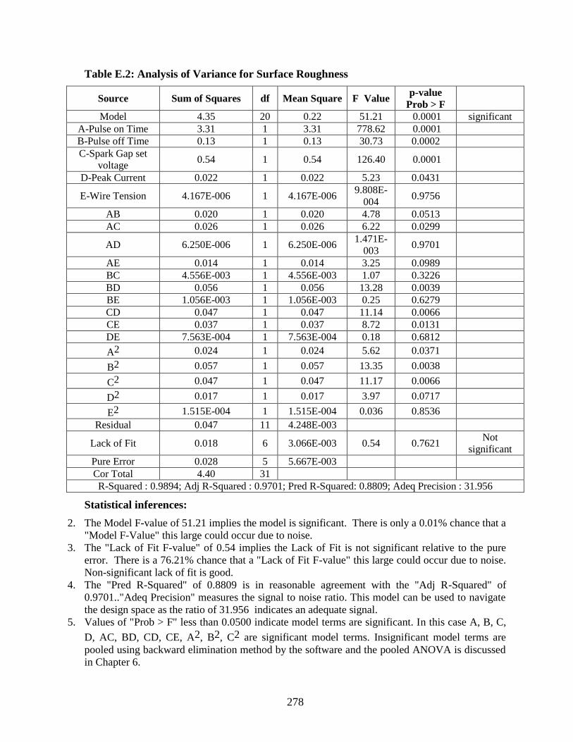
278

Table E.2: Analysis of Variance for Surface Roughness

Source Sum of Squares df Mean Square F Value p-value

Prob > F


A-Pulse on Time 3.31 1 3.31 778.62 0.0001

B-Pulse off Time 0.13 1 0.13 30.73 0.0002

C-Spark Gap set

voltage 0.54 1 0.54 126.40 0.0001

D-Peak Current 0.022 1 0.022 5.23 0.0431

E-Wire Tension 4.167E-006 1 4.167E-006 9.808E-

004 0.9756

AB 0.020 1 0.020 4.78 0.0513

AC 0.026 1 0.026 6.22 0.0299

AD 6.250E-006 1 6.250E-006 1.471E-

003 0.9701

AE 0.014 1 0.014 3.25 0.0989

BC 4.556E-003 1 4.556E-003 1.07 0.3226

BD 0.056 1 0.056 13.28 0.0039

BE 1.056E-003 1 1.056E-003 0.25 0.6279

CD 0.047 1 0.047 11.14 0.0066

CE 0.037 1 0.037 8.72 0.0131

DE 7.563E-004 1 7.563E-004 0.18 0.6812

A2 0.024 1 0.024 5.62 0.0371

B2 0.057 1 0.057 13.35 0.0038

C2 0.047 1 0.047 11.17 0.0066

D2 0.017 1 0.017 3.97 0.0717

E2 1.515E-004 1 1.515E-004 0.036 0.8536

Residual 0.047 11 4.248E-003

Lack of Fit 0.018 6 3.066E-003 0.54 0.7621 Not

significant

Pure Error 0.028 5 5.667E-003

Cor Total 4.40 31

R-Squared : 0.9894; Adj R-Squared : 0.9701; Pred R-Squared: 0.8809; Adeq Precision : 31.956


2. The Model F-value of 51.21 implies the model is significant. There is only a 0.01% chance that a

"Model F-Value" this large could occur due to noise.

3. The "Lack of Fit F-value" of 0.54 implies the Lack of Fit is not significant relative to the pure

error. There is a 76.21% chance that a "Lack of Fit F-value" this large could occur due to noise.

Non-significant lack of fit is good.

4. The "Pred R-Squared" of 0.8809 is in reasonable agreement with the "Adj R-Squared" of

0.9701.."Adeq Precision" measures the signal to noise ratio. This model can be used to navigate

the design space as the ratio of 31.956 indicates an adequate signal.

5. Values of "Prob > F" less than 0.0500 indicate model terms are significant. In this case A, B, C,

D, AC, BD, CD, CE, A2, B2, C2 are significant model terms. Insignificant model terms are

pooled using backward elimination method by the software and the pooled ANOVA is discussed

in Chapter 6.

279

Table E.3: Analysis of Variance for Gap Current


Square

F Value p-value

Prob > F


A-Pulse on Time 12.26 1 12.26 1772.53 0.0001

B-Pulse off Time 5.35 1 5.35 773.61 0.0001

C-Spark Gap set

voltage 0.54 1 0.54 77.67 0.0001

D-Peak Current 0.11 1 0.11 15.62 0.0023

E-Wire Tension 1.204E-003 1 1.204E-003 0.17 0.6845

AB 0.57 1 0.57 81.90 0.0001

AC 0.095 1 0.095 13.68 0.0035

AD 0.018 1 0.018 2.54 0.1394

AE 6.806E-003 1 6.806E-003 0.98 0.3424

BC 0.069 1 0.069 9.97 0.0091

BD 0.089 1 0.089 12.80 0.0043

BE 7.656E-003 1 7.656E-003 1.11 0.3152

CD 6.806E-003 1 6.806E-003 0.98 0.3424

CE 4.556E-003 1 4.556E-003 0.66 0.4341

DE 4.556E-003 1 4.556E-003 0.66 0.4341

A2 0.13 1 0.13 18.24 0.0013

B2 0.15 1 0.15 21.13 0.0008

C2 0.052 1 0.052 7.46 0.0195

D2 8.409E-003 1 8.409E-003 1.22 0.2936

E2 1.364E-005 1 1.364E-005 1.972E-

003 0.9654

Residual 0.076 11 6.914E-003

Lack of Fit 0.063 6 0.010 3.91 0.0779 not significant

Pure Error 0.013 5 2.670E-003

Cor Total 19.54 31



5. The Model F-value of 140.78 implies the model is significant. There is only a 0.01% chance



pure error. There is a 7.79% chance that a "Lack of Fit F-value" this large could occur due to

noise. Non-significant lack of fit is good.

7. The "Pred R-Squared" of 0.9154 is in reasonable agreement with the "Adj R-Squared" of

0.9890."Adeq Precision" measures the signal to noise ratio. This model can be used to

navigate the design space as the ratio 46.630 indicates an adequate signal.

8. Values of "Prob > F" less than 0.0500 indicate model terms are significant. In this case A, B,

C, D, AB, AC, BC, BD, A2, B2, C2 are significant model terms. Insignificant model terms

are pooled using backward elimination method by the software and the pooled ANOVA is

discussed in Chapter 6.

280

Table E.4: Analysis of Variance for Dimensional Dimension


Square

F Value p-value

Prob > F

Model 0.66 20 0.033 20.20 < 0.0001 significant

A-Pulse on Time 0.16 1 0.16 94.89 < 0.0001

B-Pulse off Time 7.107E-003 1 7.107E-003 4.34 0.0613

C-Spark Gap set

voltage

0.39 1 0.39 237.19 < 0.0001

D-Peak Current 0.021 1 0.021 12.79 0.0043

E-Wire Tension 0.023 1 0.023 14.12 0.0032

AB 2.806E-004 1 2.806E-004 0.17 0.6869

AC 9.361E-003 1 9.361E-003 5.72 0.0358

AD 9.361E-003 1 9.361E-003 5.72 0.0358

AE 1.056E-005 1 1.056E-005 6.451E-

003

0.9374

BC 1.406E-005 1 1.406E-005 8.589E-

003

0.9278

BD 5.406E-004 1 5.406E-004 0.33 0.5771

BE 9.151E-004 1 9.151E-004 0.56 0.4704

CD 1.828E-003 1 1.828E-003 1.12 0.3134

CE 2.525E-003 1 2.525E-003 1.54 0.2401

DE 5.176E-004 1 5.176E-004 0.32 0.5852

A2 8.353E-003 1 8.353E-003 5.10 0.0452

B2 6.600E-005 1 6.600E-005 0.040 0.8445

C2 0.030 1 0.030 18.20 0.0013

D 1.936E-003 1 1.936E-003 1.18 0.3001

E2 1.485E-004 1 1.485E-004 0.091 0.7689

Residual 0.018 11 1.637E-003

Lack of Fit 0.015 6 2.517E-003 4.32 0.0648 not significant

Pure Error 2.910E-003 5 5.820E-004

Cor Total 0.68 31



5. The Model F-value of 20.20implies the model is significant. There is only a 0.01% chance



pure error. There is a 6.48% chance that a "Lack of Fit F-value" this large could occur due to

noise. Non-significant lack of fit is good.

7. The "Pred R-Squared" of 0.4067 is not as close to the "Adj R-Squared" of 0.9253 as

expected. This indicate a large block effect or a possible problem with the model. To

overcome this problem, insignificant models are pooled using backward elimination

method."Adeq Precision" measures the signal to noise ratio. This model can be used to

navigate the design space as the ratio 19.195 indicates an adequate signal.

8. Values of "Prob > F" less than 0.0500 indicate model terms are significant. In this case A, C,

D, E, AC, AD, A2, C2 are significant model terms.

281

APPENDIX F

UNPOOLED ANOVA TABLES OF UTILITY FUNCTIONS

FOR VARIOUS MODELS

Table F.1: Analysis of Variance of Utility Function (UCR, SR) for S/N Data


Ton 2 5.8463 5.8463 2.9231 181.87 0.005

Toff 2 30.0011 30.0011 15.0005 933.29 0.001

SV 2 1.6702 1.6702 0.8351 51.96 0.019

IP 2 2.7974 2.7974 1.3987 87.02 0.011

WF 2 0.6403 0.6403 0.3202 19.92 0.048

WT 2 0.0845 0.0845 0.0422 2.63 0.276

Ton*Toff 4 1.1328 1.1328 0.2832 17.62 0.054

Ton*SV 4 0.4828 0.4828 0.1207 7.51 0.121

Toff*SV 4 0.1498 0.1498 0.0375 2.33 0.322

Residual Error 2 0.0321 0.0321 0.0161

Total 26 42.8374




Table F.2: Analysis of Variance of Utility Function (UCR, SR) for Raw Data


Ton 2 5.8463 5.8463 2.9231 181.87 0.005

Toff 2 30.0011 30.0011 15.0005 933.29 0.001

SV 2 1.6702 1.6702 0.8351 51.96 0.019

IP 2 2.7974 2.7974 1.3987 87.02 0.011

WF 2 0.6403 0.6403 0.3202 19.92 0.048

WT 2 0.0845 0.0845 0.0422 2.63 0.276

Ton*Toff 4 1.1328 1.1328 0.2832 17.62 0.054

Ton*SV 4 0.4828 0.4828 0.1207 7.51 0.121

Toff*SV 4 0.1498 0.1498 0.0375 2.33 0.322

Residual Error 2 0.0321 0.0321 0.0161

Total 26 42.8374




282

Table F.3: Analysis of Variance of Utility Function (UCR, SR, IG) for S/N Data


Ton 2 94.294 94.2938 47.1469 1077.63 0.001

Toff 2 68.403 68.4033 34.2017 781.75 0.001

SV 2 12.124 12.1244 6.0622 138.56 0.007

IP 2 17.140 17.1401 8.5700 195.88 0.005

WF 2 1.095 1.0955 0.5477 12.52 0.074

WT 2 0.409 0.4092 0.2046 4.68 0.176

Ton*Toff 4 3.716 3.7161 0.9290 21.23 0.045

Ton*SV 4 1.135 1.1345 0.2836 6.48 0.138

Toff*SV 4 0.272 0.2724 0.0681 1.56 0.427

Residual Error 2 0.088 0.0875 0.0438

Total 26 198.677




Table F.4: Analysis of Variance of Utility Function (UCR, SR, IG) for Raw Data


Ton 2 19.8473 19.8473 9.92367 2191.38 0.000

Toff 2 15.2570 15.2570 7.62849 1684.55 0.001

SV 2 2.5501 2.5501 1.27503 281.56 0.004

IP 2 4.0834 4.0834 2.04168 450.85 0.002

WF 2 0.6199 0.6199 0.30993 68.44 0.014

WT 2 0.0220 0.0220 0.01101 2.43 0.291

Ton*Toff 4 0.1496 0.1496 0.03741 8.26 0.111

Ton*SV 4 0.1464 0.1464 0.03659 8.08 0.113

Toff*SV 4 0.2289 0.2289 0.05723 12.64 0.075

Residual Error 2 0.0091 0.0091 0.00453

Total 26 42.9136




283

Table F.5: Analysis of Variance of Utility Function (UCR, SR, DD) for S/N Data


Ton 2 38.2840 38.2840 19.1420 79.79 0.012

Toff 2 23.1178 23.1178 11.5589 48.18 0.020

SV 2 0.6640 0.6640 0.3320 1.38 0.420

IP 2 16.2262 16.2262 8.1131 33.82 0.029

WF 2 1.4418 1.4418 0.7209 3.00 0.250

WT 2 5.0631 5.0631 2.5316 10.55 0.087

Ton*Toff 4 5.0670 5.0670 1.2667 5.28 0.166

Ton*SV 4 3.4556 3.4556 0.8639 3.60 0.229

Toff*SV 4 1.5779 1.5779 0.3945 1.64 0.412

Residual Error 2 0.4798 0.4798 0.2399

Total 26 95.3773




Table F.6: Analysis of Variance of Utility Function (UCR, SR, DD) for Raw Data


Ton 2 7.2807 7.2807 3.64037 52.66 0.019

Toff 2 4.4410 4.4410 2.22048 32.12 0.030

SV 2 0.2321 0.2321 0.11603 1.68 0.373

IP 2 3.1615 3.1615 1.58075 22.87 0.042

WF 2 0.4902 0.4902 0.24511 3.55 0.220

WT 2 1.0964 1.0964 0.54822 7.93 0.112

Ton*Toff 4 0.7057 0.7057 0.17642 2.55 0.301

Ton*SV 4 0.7149 0.7149 0.17872 2.59 0.298

Toff*SV 4 0.3219 0.3219 0.08047 1.16 0.511

Residual Error 2 0.1383 0.1383 0.06913

Total 26 18.5826




284

Table F.7: Analysis of Variance of Utility Function (UCR, SR, IG, DD) for S/N Data


Ton 2 75.245 75.2450 37.6225 127.03 0.008

Toff 2 23.848 23.8480 11.9240 40.26 0.024

SV 2 1.620 1.6196 0.8098 2.73 0.268

IP 2 21.419 21.4186 10.7093 36.16 0.027

WF 2 2.655 2.6551 1.3276 4.48 0.182

WT 2 7.769 7.7690 3.8845 13.12 0.071

Ton*Toff 4 5.040 5.0402 1.2601 4.25 0.199

Ton*SV 4 3.667 3.6667 0.9167 3.10 0.259

Toff*SV 4 3.815 3.8153 0.9538 3.22 0.251

Residual Error 2 0.592 0.5923 0.2962

Total 26 145.670

Table F.8: Analysis of Variance of Utility Function (UCR, SR, IG, DD) for Raw Data


Ton 2 13.3703 13.3703 6.68517 67.16 0.015

Toff 2 4.1780 4.1780 2.08901 20.99 0.045

SV 2 0.5190 0.5190 0.25952 2.61 0.277

IP 2 4.1922 4.1922 2.09610 21.06 0.045

WF 2 0.9930 0.9930 0.49652 4.99 0.167

WT 2 1.7428 1.7428 0.87140 8.75 0.103

Ton*Toff 4 0.6719 0.6719 0.16798 1.69 0.405

Ton*SV 4 0.8625 0.8625 0.21563 2.17 0.340

Toff*SV 4 0.7417 0.7417 0.18543 1.86 0.378

Residual Error 2 0.1991 0.1991 0.09954

Total 26 27.4707

rohit garg - NIT Kurukshetra

Documents

Transcript of rohit garg - NIT Kurukshetra