Risk- and Value-Based Management for Non-Life

Insurers under Solvency Constraints

Johanna Eckert, Nadine Gatzert

Working Paper

Department of Insurance Economics and Risk Management

Friedrich-Alexander University Erlangen-Nürnberg (FAU)

Version: July 2017

1

RISK- AND VALUE-BASED MANAGEMENT FOR NON-LIFE

INSURERS UNDER SOLVENCY CONSTRAINTS

Johanna Eckert, Nadine Gatzert*

This version: July 11, 2017

ABSTRACT

The aim of this paper is to study optimal risk- and value-based management deci-

sions regarding a non-life insurer’s investment strategy by maximizing shareholder

value based on preference functions, while simultaneously controlling for the ruin

probability. We thereby extend previous work by explicitly accounting for the poli-

cyholders’ willingness to pay depending on their risk sensitivity based on the in-

surer’s reported solvency status, which will be of great relevance under Solvency

II. We further investigate the impact of the risk-free interest rate, (non-linear) de-

pendencies between assets and liabilities, distributional assumptions as well as re-

insurance. One main finding is that the consideration of default-risk-driven premi-

ums is vital for optimal management decisions, since, e.g., the target ruin probabil-

ity implying a higher shareholder value differs for various risk sensitivities of the

policyholders. Furthermore, in the present setting, proportional reinsurance in-

creases shareholder value only for non-risk sensitive policyholders.

Keywords: Non-life insurance; Solvency II; shareholder value optimization; default-risk-

driven premium; copulas

JEL Classification: G22; G28; G31

1. INTRODUCTION

An insurance company’s equity capital can be exposed to large fluctuations, which may po-

tentially result in severe solvency problems. These fluctuations can arise from both the in-

vestment side (due to an increasing volatility in the financial markets) as well as the under-

writing side against the background of a rising frequency and severity of natural catastrophes

in the last decades (Swiss Re, 2016). In this context, risk- and value-based management is

essential for the long-term success of insurance companies, in that investment as well as un-

derwriting decisions should take into account risk and return in order to ensure an efficient

and profitable use of capital and to control for default risk.

* Johanna Eckert and Nadine Gatzert are at the Friedrich-Alexander University Erlangen-Nürnberg (FAU),

Department of Insurance Economics and Risk Management, Lange Gasse 20, 90403 Nürnberg, Germany,

Tel.: +49 911 5302 884, johanna.eckert@fau.de, nadine.gatzert@fau.de.

2

In order to protect the policyholders and the stability of the financial system, Solvency II as

the new European regulatory framework for insurers1 came into force on January 1st, 2016.

Pillar 1 introduces risk-based capital requirements by demanding sufficient equity capital to

fulfill insurance contracts also under adverse events, Pillar 2 specifies qualitative require-

ments such as a governance system and the Own Risk and Solvency Assessment (ORSA), and

Pillar 3 comprises reporting requirements. The insurer thereby has to provide information not

only to the supervisor but also to the public by means of the Solvency and Financial Condi-

tion Report (SFCR), which is intended to provide transparency and enforce market discipline.

Pillar 1’s solvency capital requirements are thereby based on the Value at Risk with a 99.5%

confidence level, implying a one-year ruin probability that does not exceed 0.50%. It can be

derived either by means of a standard model provided by the regulatory authorities or based

on a company-specific internal model that adequately reflects the firm’s risks (e.g., Eling et

al., 2009). An internal model should also be used in Pillar 2 for the firm’s ORSA and should

thus represent an integral part of an insurer’s risk- and value-based management, i.e., to be

applied for corporate risk management and asset allocation decisions, for instance.2

Against this background, the aim of this paper is to study optimal risk- and value-based man-

agement decisions regarding the investment strategy for a non-life insurer, which contribute

to increasing shareholder value in terms of preference functions.3 In particular, by adjusting

the asset allocation to satisfy solvency capital requirements, the approach should be less cost-

ly than raising equity capital or adjusting the liability side (Eling et al., 2009). Toward this

end, we considerably extend the analyses and model frameworks in previous work (e.g., Eling

et al., 2009; Zimmer et al., 2014; Braun et al., 2017) by using a more general model based on

the literature on non-life insurance and ruin theory, thereby focusing on shareholder value

based on preferences while simultaneously controlling for the insurer’s ruin probability. In

particular, we consider the impact of several new key features on risk- and value-based man-

agement regarding the investment strategy, including the policyholders’ willingness to pay

depending on the insurer’s reported solvency status, which despite its great impact has not

1 Furthermore, since many countries have a Solvency II equivalent (e.g., the Swiss Solvency Test or the China

Risk Oriented Solvency System) or at least seek to establish one (Sub-Saharan African countries opt for

regulation systems resembling a simplified form of Solvency II (EY, 2016)), these results are not limited to

the impact of Solvency II but are generally of relevance. 2 The quantitative approaches in Pillar 1 and 2 rely on a market consistent balance sheet of the insurer, which

reflects an insurer’s assets and liabilities and thus the shareholders’ equity capital at a single point in time.

For instance, Allianz Group as one of the most important insurance groups worldwide (and identified as a

global systemically important insurer by regulators) exhibits a total value of assets of approximately 850 bn

Euros and 66 bn Euros equity capital, implying an unweighted capital ratio of 7.8% (Allianz Group annual

report 2015, also for remarks regarding their internal model). 3 Note that for simplicity, we use the expression “shareholder value” or “shareholder preference value”, while

assuming preferences for the evaluation (instead of relative market valuation).

3

been studied to date in this context, the dependencies between assets and liabilities, the impact

of reinsurance contracts as well as the risk-free interest rate.

In previous work, Eling et al. (2009) derive minimum requirements for a non-life insurer’s

capital investment strategy that satisfy solvency restrictions based on different risk measures.

Using “solvency lines”, i.e. isoquants of risk and return combinations of the asset allocation

for a fixed safety level of the insurer, they determine admissible risk and return asset combi-

nations given a certain liability structure, and then compare these to allocation opportunities

actually available at the capital market based on portfolio theory. Similarly, but in a life insur-

ance context, Braun et al. (2017) study optimal asset allocations taking into account re-

strictions from solvency capital requirements, thereby comparing the Solvency II standard

formula with an internal model. In the context of a fixed investment decision and a default-

risk-driven customer demand, Schlütter (2014) further studies an insurer who chooses insur-

ance prices and an allowed solvency level when optimizing shareholder value given risk-

based capital requirements or price regulation. In addition, experimental and empirical re-

search (Wakker et al., 1997; Zimmer et al., 2009; Lorson et al., 2012; Zimmer et al., 2014)

shows that an insurer’s default risk can have a strong influence on customer demand, where

lower safety levels can lead to a considerable reduction of achievable premiums. In this con-

text, Zimmer et al. (2014) develop a risk management model assuming that the insurer’s de-

fault risk is fully known to consumers, and based on this derive the solvency level that max-

imizes shareholder value, which is the case for a ruin probability of zero. These results em-

phasize that an insurer’s safety level should be taken into account in risk- and value-based

management as the reaction of customers to default risk (by way of the premium level) can

considerably impact shareholder value. This will be even more relevant when insurers have to

publicly report their solvency status under Solvency II. In the context of deriving minimum

requirements for the investment strategy, Fischer and Schlütter (2015) further criticize that the

standard model leads to an incentive to avoid diversification between assets and liabilities, as

dependencies are not adequately taken into account in the standard model, which is in line

with the results in Braun et al. (2017).

The ruin probability (as one basis of Solvency II) is also a classical topic of applied mathe-

matics in non-life insurance as introduced by Lundberg (1903) and Cramér (1930), with the

Cramér-Lundberg model being the classical model of risk theory in non-life insurance math-

ematics (Mikosch, 2009). Since then, various extensions have been developed, e.g., regarding

the process of the total claims amount (e.g., the Sparre-Andersen (1957) model generalizes

the total claims process to a renewal model, Albrecher and Teugels (2006) model the depend-

ence between claim size and the inter-claim time) as well as the investment side of the insurer.

Taking into account the possibility of investing in (risky) assets that influence the probability

of ruin goes back to Segerdahl (1942) and Paulsen (1993) (see Paulsen, 2008). Some further

4

recent works in this regard include Paulsen (2008), Klüppelberg and Kostadinova (2008),

Heyde and Wang (2009), Hult and Lindskog (2011), Bankovsky et al. (2011), Hao and Tang

(2012), and Ramsden and Papaioannou (2017). There are also a number of papers focusing on

a discrete-time risk model where the insurer’s surplus is controlled by i.i.d. discrete insurance

and financial risk processes that are independent from each other (e.g., Nyrhinen, 1999; Tang

and Tsitsiashvili, 2003, 2004; Yang and Zhang, 2006; Li and Tang, 2015). Moreover, the in-

surance risk models can be modified to a dual version that are suitable for the any company

(Avanzi et al., 2007) where the ruin probability is also focus of research (e.g., Dimitrova et

al., 2015).

In recent years, the applied math literature also focused on optimal investment and/or reinsur-

ance strategies in the sense of minimizing the ruin probability or optimizing other objective

functions. For example, Schmidli (2001, 2002) and Promislow and Young (2005) minimize

the ruin probability in continuous time, and Schäl (2004), Diasparra and Romera (2009,

2010), Romera and Runggaldier (2012), and Lin et al. (2015) in discrete time. Another popu-

lar and relevant optimization criterion is the maximization of expected utility of the insurer’s

terminal wealth, e.g. in continuous time in general in Liang et al. (2011, 2012), Liang and

Bayraktar (2014), and Huang et al. (2016), and in particular for mean-variance preferences in

Bäuerle (2005), Bai and Zhang (2008), and Bi and Guo (2012). For discrete time, we further

refer to Schäl (2004).

Another strand of the literature relates to the (frequent) assumption of independence between

insurance and financial risk processes, which simplifies analytical solutions but is difficult for

practical applications. Since discrete-time risk models create an efficient possibility to inves-

tigate the interplay of both risks, several papers drop this assumption, using, e.g., an insurance

risk process and/or a financial risk process being a sequence of dependent random variables

while keeping the independence between the two processes (e.g., Chen and Yuen, 2009; Col-

lamore, 2009; Shen et al., 2009; Weng et al., 2009; Zhang et al., 2009; Yi et al., 2011). Alter-

natively, Chen (2011), Yang et al. (2012), Yang and Hashorva (2013), and Yang and Kon-

stantinides (2015) allow for dependences between the insurance and financial risk processes

assuming each process is i.i.d.

The purpose of this paper is to contribute to the existing literature in various relevant ways.

First, in contrast to Braun et al. (2017), we study a non-life insurer instead of a life insurer and

do not use the standard model. Moreover, we extend the analysis in Eling et al. (2009) and

Braun et al. (2017) by focusing on the firm’s shareholder value based on preferences under

risk- and value-based management decisions and by considering the policyholders’ willing-

ness to pay when deriving admissible asset allocations under solvency constraints. The insur-

er’s surplus process is modeled by a discrete time representation of the Sparre-Andersen

5

(1957) model in the presence of risky investments and reinsurance similar to Huang et al.

(2016), Jin et al. (2016), and Yang and Zhang (2006) in order to derive the discrete one-year

ruin probability as used in Solvency II. We thus combine approaches in the economic litera-

ture (e.g., Braun et al., 2017, Eling et al., 2009) and the applied math literature on ruin theory

by generalizing the economic model for the total claims payments using a probabilistic

framework with stochastic frequency and severity and by applying this model to a shareholder

value optimization problem. Moreover, the dependence structure between the insurance and

financial risk processes is modeled similar to Chen (2011) and Yang and Konstantinides

(2015) by means of copulas and we consider the possibility of purchasing reinsurance. We

further extend the economic and applied math literature by explicitly taking into account the

policyholders’ willingness to pay in our model framework when deriving admissible asset

allocations under solvency constraints that are determined by the ruin probability. We thereby

generalize the approach in Lorson et al. (2012) and Zimmer et al. (2014) and model the

achievable premium in the presence of market discipline as a function of the insurer’s safety

level and the policyholders’ risk assessment. In contrast to the mentioned applied math litera-

ture, we study the optimal investment problem regarding the shareholders’ expected utility

while simultaneously controlling for the ruin probability given several influencing factors. In

this setting, we follow Eling et al. (2009) and link the admissible risk-return combinations of

the insurer’s asset portfolio (i.e. those that are allowed under solvency constraints) to alloca-

tion opportunities actually attainable at the capital market using Tobin (1958)’s capital market

line.

In a numerical analysis, we first investigate the impact of a default-risk-driven premium in-

come on the maximum shareholder value for an insurer facing solvency constraints and, sec-

ond, the impact of changing the reported target solvency status on the shareholder value in the

presence of market discipline. One main finding is that the consideration of policyholders’

willingness to pay based on the ruin probability is of great relevance when deriving optimal

risk-return asset allocations under solvency constraints (e.g., the target ruin probability imply-

ing a higher shareholder value differs for various risk sensitivities of the policyholders) and

that reinsurance can considerably impact the results, depending on the level of the policyhold-

ers’ risk sensitivity.

The remainder of this paper is structured as follows. Section 2 presents the model framework

for a non-life insurer, while Section 3 focuses on the derivation of attainable and admissible

risk-return combinations as well as shareholder value maximization. An application of the

developed approach based on several underlying simplified assumptions with sensitivity anal-

yses for various policyholders’ risk sensitivities, proportional reinsurance, risk-free interest

rate, (non-linear) asset-liability dependences, and claims distributions is provided in Sec-

tion 4. The last section summarizes our main findings.

6

2. MODEL FRAMEWORK

2.1 Model foundations

We consider the problem of ruin in a risk model of a non-life insurer. Let , be a

probability space equipped with a family of increasing (over time) σ-fields 0t t

, where t

represents the information available at time t. Since Solvency II requires insurers to derive

solvency capital requirements such that the one-year ruin probability does not exceed a certain

threshold, we consider a discrete-time model for the insurer’s surplus process ,nU n , ac-

cumulated until the end of year 1,n n in the presence of risky investments with return rn

and with claims Sn as well as a constant premium intensity p > 0. The claims are subject to

payments from reinsurance for a reinsurance premium n, implying remaining claims pay-

ments 1,n nf S S (depending on the type of reinsurance), such that

1 1 01 , , , ,n n n n n nU r U p f S S U u n (1)

where u > 0 is the initial equity capital of the insurer. The following assumptions are made:

Assumption 1: Total claims payments Sn are modeled by the discrete-time representation of a

compound renewal process.

Assumption 1 is motivated by the Sparre-Andersen (1957) model (see Andersen, 1957),

which is widely used in risk theory due to its tractability, see, e.g., Li and Garrido (2004), Wu

et al. (2007), Li (2012), and Jin et al. (2016).4

Assumption 2: The financial process generating the return on investment from year n-1 to

year n is defined as a sequence of normally distributed i.i.d. random variables ,nr n with

2,n r rr N .

This distribution assumption is made in order to be consistent with the assumptions of Tobin

(1958)’s capital market line and can be justified by the Euler discretization of the return pro-

cess as used in Hult and Lindskog (2011) and Kabanov and Pergamenshchikov (2016).

Assumption 3: The insurance process and the financial process (more precisely 1n nS S

and rn) form a sequence of i.i.d. random variables, and the dependence structure is given by a

copula C.

4 Regarding risk models used in non-life insurance, we further refer to Mikosch (2009), Asmussen and Al-

brecher (2010), and Beard et al. (2013) for an introduction to risk theory.

7

Typically, the insurance process and the financial process are assumed to be independent from

each other as laid out in the introduction. To drop this assumption, we use the concept of cop-

ulas similar to Chen (2011) and Yang and Konstantinides (2015) as will be laid out in more

detail later.

Assumption 4: For each n, the insurer purchases a proportional (quota-share) reinsurance

contract with retention level 0,1nq , i.e., 1 1,n n n n nf S S q S S with corresponding

reinsurance premium rate n nq .

This reinsurance contract provides coverage over the entire range of claims, which might be

more expensive compared to contracts that reinsure losses above a certain threshold, e.g., an

aggregate excess of loss reinsurance contract (e.g., Gatzert and Kellner, 2014), but is a com-

mon choice in actuarial literature (e.g., Diasparra and Romera, 2010; Liang et al., 2012;

Huang et al., 2016). As a robustness test, we later also consider an aggregate excess of loss

reinsurance contract, whose payment is given by 1min max ,0 ,n n n nS S d l with the

attachment of the company loss dn and layer ln, implying remaining claims payments

1 1 1, min max ,0 ,n n n n n n n nf S S S S S S d l .

In addition, as most insurers issue financial reports once a year due to the one-year perspec-

tive of Solvency II, for instance, we focus on an annual frequency, leading to

1 1 0 1 1 1 01 ,U r U p q q S U u , (2)

with a one-year ruin probability RP that should not exceed 0.50%,

1 0 1 1 1 10 | 1 0 0.50%RP U U u r u p q q S .

2.2 Premium income and policyholders’ risk sensitivity

In ruin theory, the premium income of the surplus process is mostly modeled by a constant

rate p > 0 (Mikosch, 2009). In what follows, we use the expected value principle to determine

the premium rate

11 ,p S

for some positive premium loading , which results in a premium income that on average ex-

ceeds the total claims payments and can thus absorb fluctuations of the claims amount. How-

ever, if the insurer imposes an overly large premium loading, it becomes less competitive

compared to other premiums offered at the market. Thus, we assume a fixed premium loading

that is exogenously given in the sense of a market standard in the insurance industry. In addi-

8

tion, for robustness test purposes we also consider the standard deviation principle, where the

loading is determined by a portion of the standard deviation of the claims payments

1 1 , 0.p S S

Moreover, according to experimental and empirical research (Wakker et al., 1997; Zimmer et

al., 2009; Zimmer et al., 2014), an insurer’s default risk can strongly impact customer de-

mand, with lower safety levels leading to a considerable reduction of the achievable premi-

ums below the actuarially fair premium. Whereas expected utility theory suggests that a small

increase in the ruin probability should only reduce the policyholders’ willingness to pay in a

marginal way, Wakker et al. (1997) observe that the actual willingness to pay decreases

sharply in the context of “probabilistic insurance”, i.e. insurance contracts with a small non-

zero ruin probability. They explain this phenomenon based on Kahneman and Tversky’s

(1979) prospect theory, according to which individuals tend to overweigh small probability

events. Hence, we adapt our model framework in order to take into account the policyholders’

willingness to pay as a reaction to the reported solvency status depending on their risk sensi-

tivity, which is especially relevant under Solvency II’s Pillar 3. In the presence of market dis-

cipline, customers could be influenced by the reported solvency status when comparing it to

other insurers. A potentially induced change of customer demand could thereby incentivize

insurers to achieve a higher solvency status than the required regulatory minimum. To take

this aspect into account, we use and extend the approach in Lorson et al. (2012), who calcu-

late the premium reduction compared to the premium offered by a default-free insurer as a

log-linear function of the reported one-year ruin probability RP, given by

ln 0, ,1 .PR RP a RP b RP (3)

However, since the policyholders’ risk assessment is not known, i.e. how well-informed the

policyholders are and if they can assess the numerical ruin probability correctly, the actual

premium reduction might differ. To take into account the policyholders’ risk sensitivity, we

thus extend this model and not only link the premiums paid in t = 0 to the insurer’s reported

ruin probability RP = , but also to the policyholders’ risk sensitivity represented by a scaling

parameter similar to Gatzert and Kellner (2014). In case of the expected value principle, for

instance, the premium payments in t = 0, P(RP,), are then given by

, max 1 ,0 , 0,1 ,0, P p PR RP PR RP (4)

where RP = represents the reported one-year ruin probability and PR the premium reduction

function in Equation (3). Note that the functional form of the latter is chosen for illustration

purposes and can also be adjusted (e.g. depending on the type of contract). For = 1, we ob-

tain the risk sensitivity modeled in Lorson et al. (2012).

9

We further assume that the reinsurance premium is also calculated according to the expected

value or the standard deviation principle, respectively, resulting in

1 1 11 1req q S or 1 1 1 1 11 1q q S q V S .

3. OPTIMAL ATTAINABLE AND ADMISSIBLE RISK-RETURN COMBINATIONS

To derive optimal risk- and value-based management decisions, we next consider minimum

solvency requirements in a risk-return (asset) context (here: expected return and standard de-

viation of assets that are compatible with the solvency requirements) and link these “admissi-

ble” risk-return combinations of the insurer’s asset portfolio to allocation opportunities actual-

ly “attainable” at the capital market as is done in Eling et al. (2009). In contrast to previous

work, however, we generalize this model by explicitly taking into account the policyholders’

willingness to pay depending on the insurer’s solvency level, dependencies between assets

and liabilities as well as the effect of reinsurance contracts.

3.1 Capital market line: “Attainable” risk-return combinations

To identify the risk-return profiles (r,r) that are actually attainable at the market, we follow

the classical approach of Tobin (1958) and derive the capital market line with the risk-free

interest rate rf and the Sharpe ratio of the market portfolio m:

0

:,

  r fr r

CMLr m

(5)

representing the set of efficient risk–return combinations (r,r given risk-free lending and

borrowing. Note that a derivation of efficient risk-return combinations that takes into account

the insurer’s liabilities can be found in Brito (1977) and Mayers and Smith (1981).

3.2 Solvency lines: “Admissible” risk-return combinations

We next fix the insurer’s desired ruin probability RP at time t = 1 to a prescribed maximum

value denoted “target ruin probability” (note that the risk measure can as well be changed

as is done in Eling et al. (2009), but closed-form solutions may not be derivable). At time

t = 0 the insurer communicates the maximum value to the policyholders, who in turn adapt

their willingness to pay based on this information. Based on the resulting amount of premium

income (Equation (4)), the insurer makes the actual investment decision (i.e., chooses a risk-

return asset combination), which must be compatible with the announced target level to

10

preserve the policyholders’ trust and confidence. Thus, the real ruin probability RP must not

exceed the reported target ruin probability , i.e.

!

1 1 1 11 , 0 .RP r u P q q S (6)

For a given σr, we can solve for μr and obtain the so-called “solvency lines” SolvL.5 Thus, the

solvency lines are (r,r -combinations that satisfy !

RP , which implies that for a given

risk the expected return r needs to be at least as high to ensure that the ruin probability does

not exceed the given target level .

3.3 Maximizing shareholder value given attainable and admissible risk-return combinations

Among the typical firm objectives is the creation of shareholder value through risk- and val-

ue-based decision making regarding assets and liabilities. Toward this end, our model can be

used for deriving the shareholders’ maximum expected utility while maintaining a minimum

(typically regulatory required) solvency level in order to protect the policyholders. Let de-

note the shareholders’ preference function to determine their expected utility dependent on the

(r,r)-combination of the insurer’s asset allocation. In its decisions regarding the investment

portfolio, the insurer can consider the shareholders’ preferences within the limits of attainable

and admissible investment opportunities, leading to the optimization problem

max , : , ,r r r r (7)

with (r,r) element of the feasible set

, : 0, , , ,SolvL CML SolvL CML . (8)

The constraints ensure that only risk-return combinations are taken into consideration that are

attainable at the market (i.e. on or below the CML) and that are admissible according to sol-

vency restrictions (i.e. on or above the SolvL). The optimal (r,r-combination that solves

the optimization problem (7) depends on the actual preference function . Since decisions

based on any utility function can be well approximated by assuming mean-variance prefer-

ences6 (Kroll et al. (1984) and Markowitz (2014) in general, and Bäuerle, 2005; Bai and

5 The notion follows Eling et al. (2009) who derived closed-form solutions for a one-year period model using a

normal power approximation for the difference between assets and liabilities. 6 Full compatibility of mean-variance analysis and expected utility theory is given in case of a normal distribu-

tion or a quadratic utility function. Even if these conditions do not hold, decisions of any utility function can

be well approximated by those based on mean-variance preferences as shown in Kroll et al. (1984) or Mar-

kowitz (2014), where the necessary and sufficient condition for the practical use of mean–variance analysis is

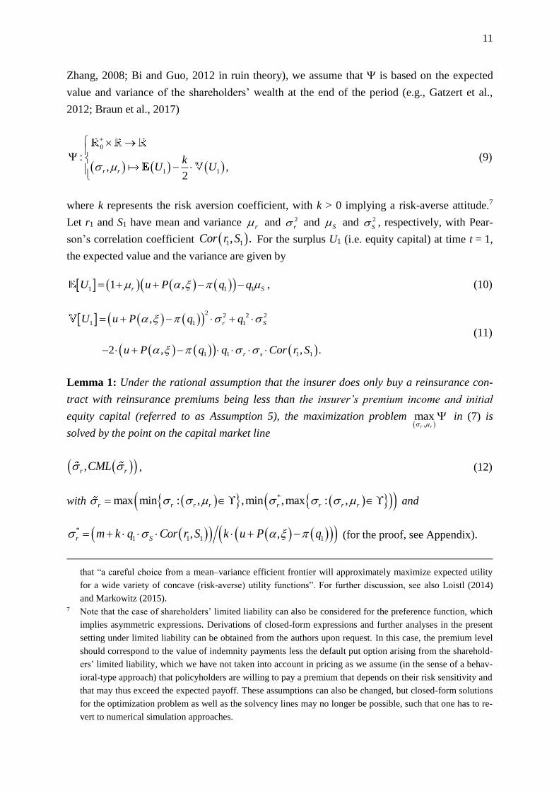
11

Zhang, 2008; Bi and Guo, 2012 in ruin theory), we assume that is based on the expected

value and variance of the shareholders’ wealth at the end of the period (e.g., Gatzert et al.,

2012; Braun et al., 2017)

0

1 1, ,2

:

r r

kU U

(9)

where k represents the risk aversion coefficient, with k > 0 implying a risk-averse attitude.7

Let r1 and S1 have mean and variance r and 2

r and S and 2

S , respectively, with Pear-

son’s correlation coefficient 1 1, .Cor r S For the surplus U1 (i.e. equity capital) at time t = 1,

the expected value and the variance are given by

1 11 1 ,r SU u P q q , (10)

2 2 2 2

1 1

1 11

1

1

,

2 , , .

r S

r s

U u P q q

u P q q Cor r S

(11)

Lemma 1: Under the rational assumption that the insurer does only buy a reinsurance con-

tract with reinsurance premiums being less than the insurer’s premium income and initial

equity capital (referred to as Assumption 5), the maximization problem ,max

r r in (7) is

solved by the point on the capital market line

,r rCML , (12)

with *max min : , ,min ,max : ,r r r r r r r r and

1

*

1 11, ,r S Cor rm k Sq k u P q (for the proof, see Appendix).

that “a careful choice from a mean–variance efficient frontier will approximately maximize expected utility

for a wide variety of concave (risk-averse) utility functions”. For further discussion, see also Loistl (2014)

and Markowitz (2015). 7 Note that the case of shareholders’ limited liability can also be considered for the preference function, which

implies asymmetric expressions. Derivations of closed-form expressions and further analyses in the present

setting under limited liability can be obtained from the authors upon request. In this case, the premium level

should correspond to the value of indemnity payments less the default put option arising from the sharehold-

ers’ limited liability, which we have not taken into account in pricing as we assume (in the sense of a behav-

ioral-type approach) that policyholders are willing to pay a premium that depends on their risk sensitivity and

that may thus exceed the expected payoff. These assumptions can also be changed, but closed-form solutions

for the optimization problem as well as the solvency lines may no longer be possible, such that one has to re-

vert to numerical simulation approaches.

12

Note that at the end of the year, the insurer again faces the same decision problem of an opti-

mal investment strategy and can re-apply the model. Given the new equity capital U1 = u and

the remaining input parameters, which do not necessarily have to be identical to the previous

year values, there might be changes in the feasible set and the solution of the shareholder val-

ue maximization problem. However, as the asset composition is more easily adjusted than the

liability side or raising additional equity capital, solving the optimization problem and making

the necessary adjustments appears doable. More insight in regard to the impact of the initial

equity capital u can be obtained when considering the following: If * *,r rCML ,

shareholder value is maximized by * *,r rCML and the derivative of * *,r rCML

with respect to u (see Appendix) is

* *,1 ,

r r

f

CMLr

u

implying that the maximum shareholder value is linearly increasing in u with slope 1+rf. If

* *,r rCML , the boundary point of the feasible set next to * *,r rCML maximizes

shareholder value. A graphical contour plot analysis of the solvency lines indicates that a

higher initial equity capital u implies a downward shift of the solvency lines and thus the

boundary point comes closer to * *,r rCML , therefore also implying a higher maximum

shareholder value, since ,r rCML is increasing towards * *,r rCML .

The effect of further parameter changes on the feasible set and the resulting maximum share-

holder value can also be assessed by sensitivity analyses as shown in Section 4.

3.4 Special case: The model in a Gaussian environment

We now consider a special case that bridges the gap to the simpler but more tractable model

frameworks in economics that do not differentiate between the number and size of claims, as

is done in, e.g., Eling et al (2009) and Braun et al. (2017), which allows to calculate the sol-

vency lines and the shareholder preference function (Equations (6) and (9)) analytically.

The one-period model of the non-life insurer’s surplus in t =1 is given by Equation (2) taking

into account the policyholders’ willingness to pay, i.e.

1 1 0 1 1 1 01 , ,U r U P q q S U u .

We make use of the central limit theorem to approximate the total claims amount using the

normal distribution for the Sparre-Andersen model with finite variance of the inter-arrival

times and claims sizes (e.g., Embrechts et al., 2013; Mikosch, 2009), i.e.,

13

.

,

approx

S t N S t S t .

The approximation by a normal distribution based on the central limit theorem is quite good

in the center of the distribution, but not as good in case of tail probabilities. Nevertheless, the

Gaussian dynamic allows obtaining first insight due to its simple calculation.

The bivariate distribution function of the asset return r1 and the total claims amount S1 is fully

captured by their marginal distribution functions that are both normally distributed with

2

1 ~ ,r rr N and 2

1 ~ ,app

S SNS and their copula C (Assumption 3). In particular, accord-

ing to Sklar’s Theorem (Sklar, 1959), for any multivariate distribution function F on d

with

univariate margins Fi, a function : 0,1 0,1d

C exists, such that

1 1 ,..., d

d dF x C F x F x x . To model the dependence structure, one can use ellip-

tical copulas such as the Gaussian copula or the t-copula, which only capture elliptical sym-

metry, or Archimedean and Hierarchical Archimedean copulas to obtain asymmetric depend-

encies, for instance (McNeil et al., 2005). In this paper, we first focus on the (elliptical) 2-

dimensional Gaussian copula (before changing this assumption, see next section) given by

Gauss 1 1

1 2 1 2, , ,C u u u u

where stands for the distribution function of the bivariate standard normal distribution

with linear correlation and for a univariate normal distribution function (McNeil et al.,

2005).

Note that in case of normally distributed marginals, 1 1,r S are bivariate normally distributed

and the parameter of the Gaussian copula equals the linear correlation, i.e., 1 1, .Cor r S

Therefore, 1U and 1U and thus the shareholder preference function (Equations

(9)–(11)) can be calculated analytically, and the solvency lines can be derived as follows:

Lemma 2: If 1r and 1S are normally distributed with 2

1 ~ ,r rr N and 2

1 ,S SS N

with a Gaussian copula GaussC with parameter , the solvency line SolvL with target ruin

probability is given by

1

1

11.

,

S

r r

q N USolvL

u P q

(13)

Proof: Given the assumptions above, the resulting surplus (i.e. equity capital) at time t = 1 is

also normally distributed with

14

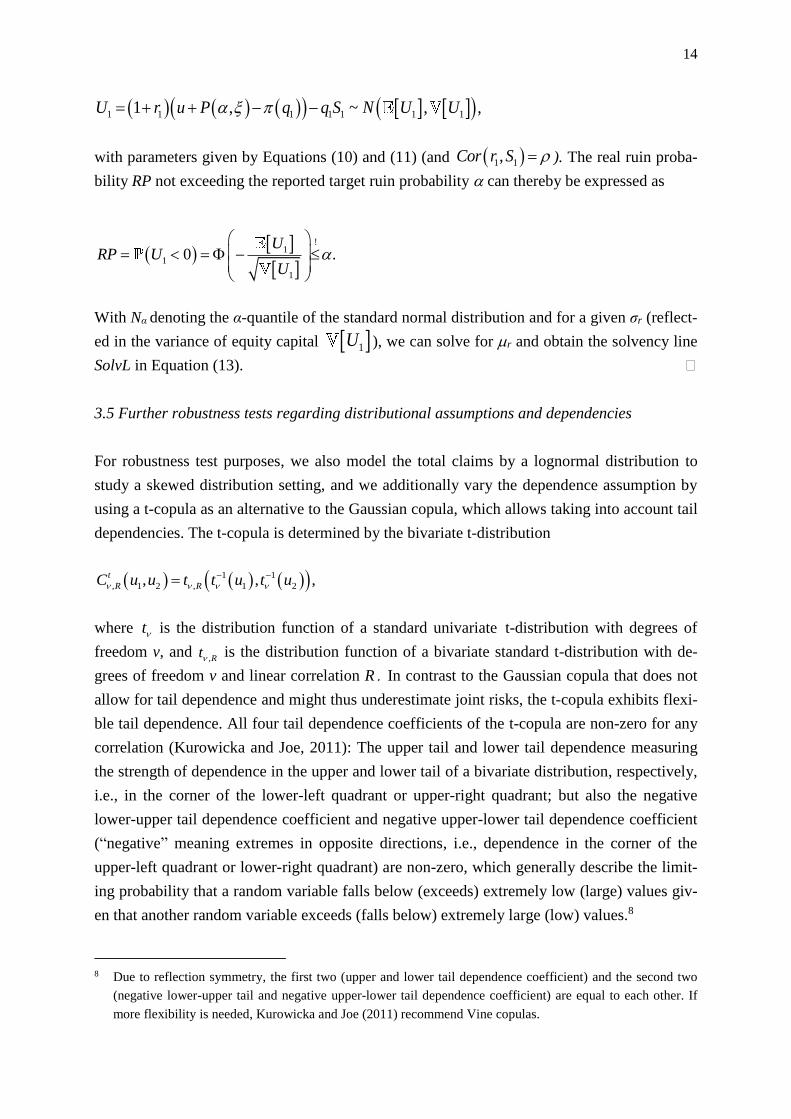
1 1 1 1 11 11 , ,~ ,U r u P Nq q S U U

with parameters given by Equations (10) and (11) (and 1 1,Cor r S ). The real ruin proba-

bility RP not exceeding the reported target ruin probability can thereby be expressed as

1

!

1

1

0 .U

RP UU

With Nα denoting the α-quantile of the standard normal distribution and for a given σr (reflect-

ed in the variance of equity capital 1U ), we can solve for r and obtain the solvency line

SolvL in Equation (13).

3.5 Further robustness tests regarding distributional assumptions and dependencies

For robustness test purposes, we also model the total claims by a lognormal distribution to

study a skewed distribution setting, and we additionally vary the dependence assumption by

using a t-copula as an alternative to the Gaussian copula, which allows taking into account tail

dependencies. The t-copula is determined by the bivariate t-distribution

1 1

, 1 2 , 1 2, , ,t

R RC u u t t u t u

where t is the distribution function of a standard univariate t-distribution with degrees of

freedom v, and ,Rt is the distribution function of a bivariate standard t-distribution with de-

grees of freedom v and linear correlation R In contrast to the Gaussian copula that does not

allow for tail dependence and might thus underestimate joint risks, the t-copula exhibits flexi-

ble tail dependence. All four tail dependence coefficients of the t-copula are non-zero for any

correlation (Kurowicka and Joe, 2011): The upper tail and lower tail dependence measuring

the strength of dependence in the upper and lower tail of a bivariate distribution, respectively,

i.e., in the corner of the lower-left quadrant or upper-right quadrant; but also the negative

lower-upper tail dependence coefficient and negative upper-lower tail dependence coefficient

(“negative” meaning extremes in opposite directions, i.e., dependence in the corner of the

upper-left quadrant or lower-right quadrant) are non-zero, which generally describe the limit-

ing probability that a random variable falls below (exceeds) extremely low (large) values giv-

en that another random variable exceeds (falls below) extremely large (low) values.8

8 Due to reflection symmetry, the first two (upper and lower tail dependence coefficient) and the second two

(negative lower-upper tail and negative upper-lower tail dependence coefficient) are equal to each other. If

more flexibility is needed, Kurowicka and Joe (2011) recommend Vine copulas.

15

To ensure comparability with the Gaussian setting in Section 3.4, we calibrate the lognormal-

ly distributed claims to the same mean S and standard deviation S; for the copulas we fix

Kendall’s tau and calculate the parameters and R using 2 arcsinKendall for the

Gaussian and 2 arcsinKendall R for the t-copula. Since the closed-form solution of the

solvency line in Equation (13) relies on a Gaussian setting, the solvency line (Equation (6))

must be derived numerically in these cases. Moreover, Pearson’s correlation coefficient is not

invariant under non-linear strictly increasing transformations of the margins, so the correla-

tion Cor(r1,S1) in Equation (11) does not equal the parameter of the Gaussian copula in case

of lognormally distributed claims and R of the t-copula, respectively, implying that Cor(r1,S1)

as input of the preference function (Equation (9)) is calculated by Monte Carlo Simulation.

4. NUMERICAL ANALYSES

We now conduct numerical analyses in order to study the impact of various economic param-

eters on an insurer’s optimal risk- and value-based management decisions and to derive re-

spective key drivers. The base case relies on the Gaussian setting in Section 3.4, where the

solvency line, the preference function and the optimal solution (Equations (6), (9), (12) and

(13)) are derived analytically. For the robustness tests in Section 3.5, the solvency lines are

determined by Monte Carlo simulation with 108 sample paths and Brent’s (1973) method as a

root searching algorithm. Cor(r1,S1) as input of the preference function and the optimal

solution (Equations (9) and (12)) is also derived by Monte Carlo simulation with 108 sample

paths. For the simulation of the copulas, we use the “copula” R-package of Hofert et al.

(2017).9

4.1 Input parameters

Input parameters of the base case are summarized in Tables 1 to 3. Table 1 is thereby based

on the parameters of a German non-life insurer estimated in Eling et al. (2009) (except for the

newly introduced parameters asset-claims correlation, premium loadings, retention level of

proportional reinsurance, and risk aversion parameter, which were subject to robustness tests).

The parameters of the premium reduction function PR (in comparison to the default-free pre-

mium p) rely on the estimation by Lorson et al. (2012)10.

9 For Monte Carlo simulation, we used a sufficiently high number of sample paths and ensured that the results

remain stable for different sets of random numbers. Moreover, the analytic solution of shareholder value op-

timization problem (Equation (12)) is also checked by the Differential Evolution algorithm in the “DEoptim”

R-package of Ardia et al. (2016). 10 In Lorson et al. (2012) a default-free insurer corresponds to a ruin probability of 0.01%. Since the estimation

is based on very few data points taken from an empirical study in Zimmer et al. (2009), they also consider an

16

Table 1: Input parameters (base case) Available equity capital at time 0

0U u

175

Expected value of claims S 1,171

Standard deviation of claims S 66

Parameter of Gaussian copula of stochastic return of assets and claims 0

Premium loading for an insurer without default risk 5%

Retention level of proportional reinsurance q1 1

Premium loading for proportional reinsurance re 5%

Policyholders’ risk sensitivity 0, 0.3, 1

Parameters of the premium reduction function a 0.0419

b 0.3855

Maximum value of ruin probability (target ruin probability) 0.50%

Shareholders’ risk aversion coefficient k 0.005

Table 2: Descriptive statistics (annualized) for monthly return time series from January 2004

to November 2015 from the Datastream database Asset class Index Description i i

Money

market

JPM Euro Cash 3 Months (1) Money market in the EMU = rf 2.04% -

Stocks MSCI World ex EMU (2) Worldwide stocks without the EMU 8.11% 47.06%

MSCI EMU ex Germany (3) Stocks from the EMU without Germany 5.92% 61.71%

MSCI Germany (4) Stocks from Germany 8.55% 68.16%

Bonds JPM GBI Global All Mats. (5) Worldwide government bonds 4.58% 28.83%

JPM GBI Europe All Mats. (6) Government bonds from Europe 5.30% 14.46%

JPM GBI Germany All Mats. (7) Government bonds from Germany 4.74% 14.57%

IBOXX Euro Corp. All Mats (8) Corporate bonds from Europe 4.31% 13.71%

Real estate GPR General World (9) Real estate worldwide 9.11% 51.67%

GPR General Europe (10) Real estate in Europe 6.71% 36.53%

GPR General Germany (11) Real estate in Germany 2.60% 9.22%

Furthermore, the capital market line is calibrated based on monthly time series from January

2004 to November 2015 of benchmark indices from the Datastream database that illustrate the

available investment opportunities. Each benchmark measures the total investment returns for

its asset on a Euro basis including coupons and dividends where applicable. As is done in

Eling et al. (2009), we consider 11 indices with different regional focus in the four asset clas-

ses stocks, bonds, real estate, and money market instruments where insurers typically invest

in. The expected return of the JPM Euro Cash 3 Month from January 2004 to November 2015

(2.04%) is thereby used as a proxy for the risk-free rate as is done in Eling et al. (2009), and

since a constant, maturity independent risk-free interest rate does not exist in practice, we

upper and lower bound for the premium reduction to take into account the variability, and we further conduct

sensitivity analyses, using these parameters as a starting point.

17

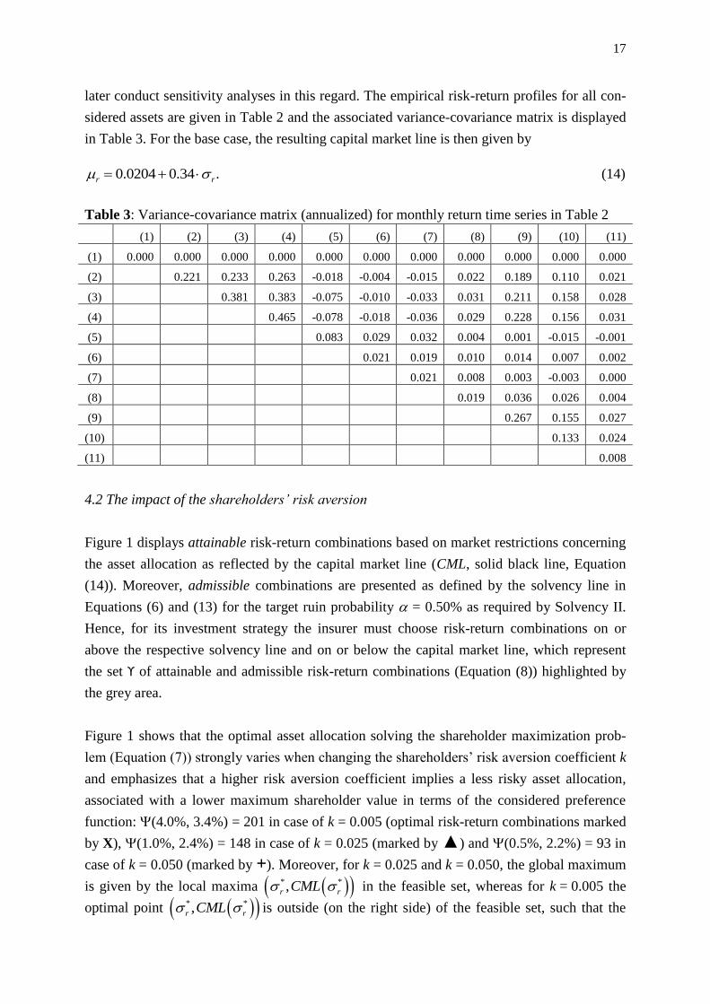
later conduct sensitivity analyses in this regard. The empirical risk-return profiles for all con-

sidered assets are given in Table 2 and the associated variance-covariance matrix is displayed

in Table 3. For the base case, the resulting capital market line is then given by

0.020 .4 0.34r r (14)

Table 3: Variance-covariance matrix (annualized) for monthly return time series in Table 2

(1) (2) (3) (4) (5) (6) (7) (8) (9) (10) (11)

(1) 0.000 0.000 0.000 0.000 0.000 0.000 0.000 0.000 0.000 0.000 0.000

(2) 0.221 0.233 0.263 -0.018 -0.004 -0.015 0.022 0.189 0.110 0.021

(3) 0.381 0.383 -0.075 -0.010 -0.033 0.031 0.211 0.158 0.028

(4) 0.465 -0.078 -0.018 -0.036 0.029 0.228 0.156 0.031

(5) 0.083 0.029 0.032 0.004 0.001 -0.015 -0.001

(6) 0.021 0.019 0.010 0.014 0.007 0.002

(7) 0.021 0.008 0.003 -0.003 0.000

(8) 0.019 0.036 0.026 0.004

(9) 0.267 0.155 0.027

(10) 0.133 0.024

(11) 0.008

4.2 The impact of the shareholders’ risk aversion

Figure 1 displays attainable risk-return combinations based on market restrictions concerning

the asset allocation as reflected by the capital market line (CML, solid black line, Equation

(14)). Moreover, admissible combinations are presented as defined by the solvency line in

Equations (6) and (13) for the target ruin probability = 0.50% as required by Solvency II.

Hence, for its investment strategy the insurer must choose risk-return combinations on or

above the respective solvency line and on or below the capital market line, which represent

the set ϒ of attainable and admissible risk-return combinations (Equation (8)) highlighted by

the grey area.

Figure 1 shows that the optimal asset allocation solving the shareholder maximization prob-

lem (Equation (7)) strongly varies when changing the shareholders’ risk aversion coefficient k

and emphasizes that a higher risk aversion coefficient implies a less risky asset allocation,

associated with a lower maximum shareholder value in terms of the considered preference

function: (4.0%, 3.4%) = 201 in case of k = 0.005 (optimal risk-return combinations marked

by X), (1.0%, 2.4%) = 148 in case of k = 0.025 (marked by ▲) and (0.5%, 2.2%) = 93 in

case of k = 0.050 (marked by +). Moreover, for k = 0.025 and k = 0.050, the global maximum

is given by the local maxima * *,r rCML in the feasible set, whereas for k = 0.005 the

optimal point * *,r rCML is outside (on the right side) of the feasible set, such that the

18

right boundary point (intersection point of capital market line and solvency line) maximizes

shareholder value (Lemma 1).

Figure 1: Attainable (capital market line CML) and admissible (“solvency line”) risk-return

combinations for target ruin probability = 0.50% and medium ( = 0.3) policyholder risk

sensitivity for various shareholder risk aversion coefficients k = 0.005, 0.025, 0.050

4.3 The impact of policyholder risk sensitivity and the insurer’s safety level on admissible

risk-return asset profiles

Figure 2 shows the case where the insurer faces fixed solvency constraints (ruin probability

= 0.50%) and emphasizes the impact of the default-risk-driven premium income on the

maximum shareholder preference value. In particular, the admissible risk-return combinations

(solvency lines) strongly depend on the policyholders’ risk sensitivity. For higher risk sensi-

tivities (going from = 0 to 1 in the considered example), the solvency lines are shifted up-

wards for a given ruin probability, until for = 1 (high risk sensitivity) the solvency line lies

above the CML, such that no possible allocation opportunities remain. The results emphasize

that a more risk sensitive assessment of the solvency status reduces policyholder demand and

hence the achievable premium income, implying that the insurer has considerably less flexi-

bility for its asset allocation to fulfill the solvency requirements. Moreover, the maximum

shareholder value in terms of the considered preference function is given by (4.8%,

3.7%) = 263 in case of no risk sensitivity (marked by X) and (4.0%, 3.4%) = 201 in case of

medium risk sensitivity (marked by ▲). Thus, a higher risk sensitivity implies a less risky

investment and a lower maximum shareholder preference value.

We also observe in Figure 2 that in the case without policyholder risk sensitivity, expected

asset returns may even be negative for low standard deviations, and the insurer would still

satisfy the required safety level due to sufficient equity capital and premium loadings. Further

sensitivity analysis emphasizes that reducing the initial equity capital or lowering the premi-

19

um loading implies an upward shift of the solvency lines, such that negative expected returns

are no longer permitted.

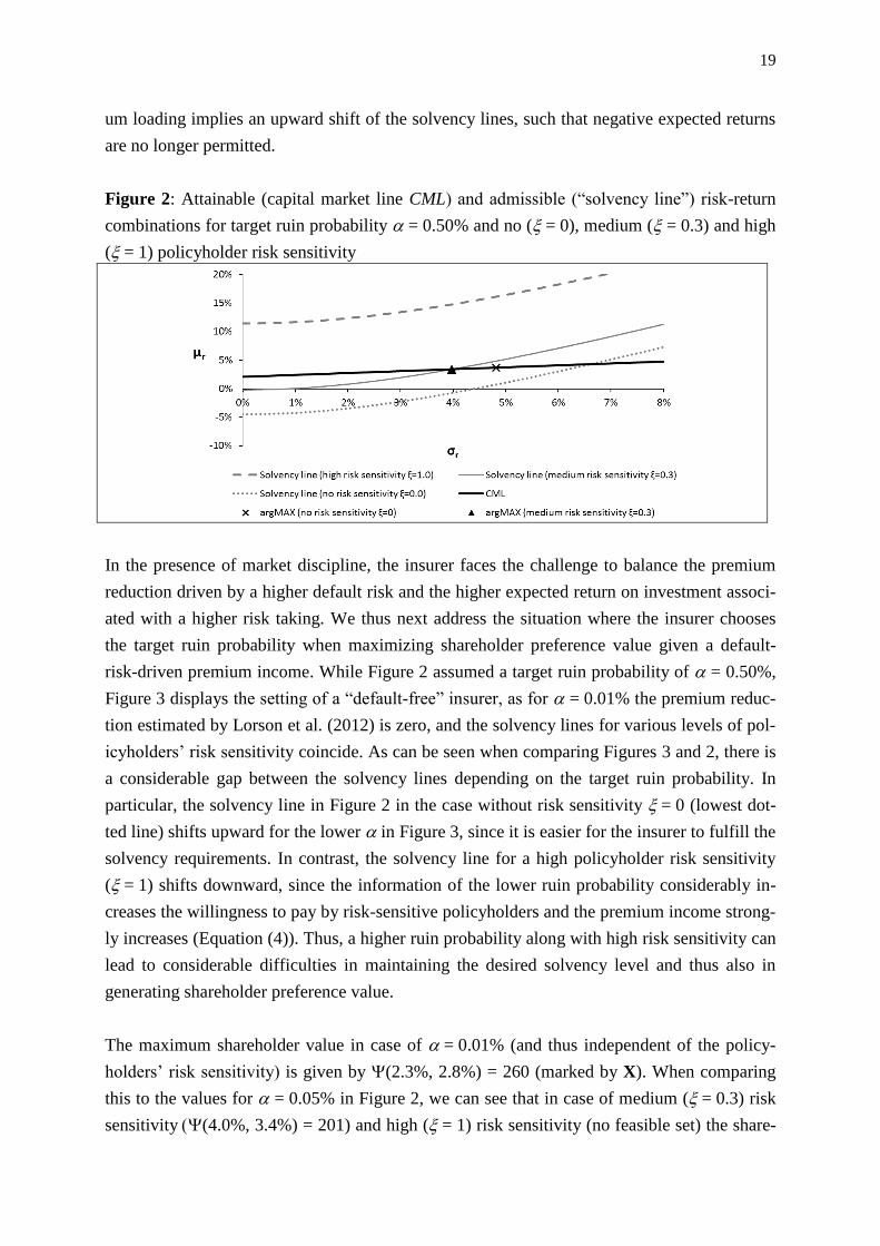
Figure 2: Attainable (capital market line CML) and admissible (“solvency line”) risk-return

combinations for target ruin probability = 0.50% and no ( = 0), medium ( = 0.3) and high

( = 1) policyholder risk sensitivity

In the presence of market discipline, the insurer faces the challenge to balance the premium

reduction driven by a higher default risk and the higher expected return on investment associ-

ated with a higher risk taking. We thus next address the situation where the insurer chooses

the target ruin probability when maximizing shareholder preference value given a default-

risk-driven premium income. While Figure 2 assumed a target ruin probability of = 0.50%,

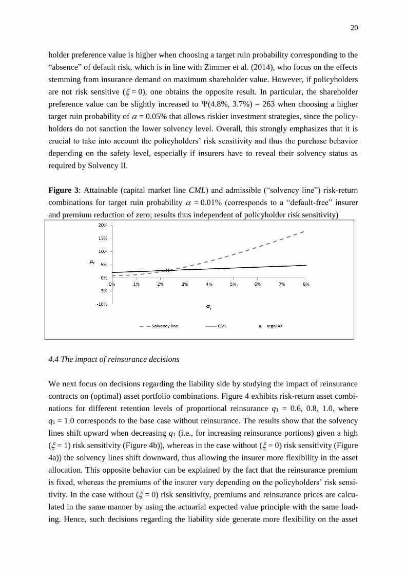
Figure 3 displays the setting of a “default-free” insurer, as for = 0.01% the premium reduc-

tion estimated by Lorson et al. (2012) is zero, and the solvency lines for various levels of pol-

icyholders’ risk sensitivity coincide. As can be seen when comparing Figures 3 and 2, there is

a considerable gap between the solvency lines depending on the target ruin probability. In

particular, the solvency line in Figure 2 in the case without risk sensitivity = 0 (lowest dot-

ted line) shifts upward for the lower in Figure 3, since it is easier for the insurer to fulfill the

solvency requirements. In contrast, the solvency line for a high policyholder risk sensitivity

( = 1) shifts downward, since the information of the lower ruin probability considerably in-

creases the willingness to pay by risk-sensitive policyholders and the premium income strong-

ly increases (Equation (4)). Thus, a higher ruin probability along with high risk sensitivity can

lead to considerable difficulties in maintaining the desired solvency level and thus also in

generating shareholder preference value.

The maximum shareholder value in case of = 0.01% (and thus independent of the policy-

holders’ risk sensitivity) is given by (2.3%, 2.8%) = 260 (marked by X). When comparing

this to the values for = 0.05% in Figure 2, we can see that in case of medium ( = 0.3) risk

sensitivity(4.0%, 3.4%) = 201) and high ( = 1) risk sensitivity (no feasible set) the share-

20

holder preference value is higher when choosing a target ruin probability corresponding to the

“absence” of default risk, which is in line with Zimmer et al. (2014), who focus on the effects

stemming from insurance demand on maximum shareholder value. However, if policyholders

are not risk sensitive ( = 0), one obtains the opposite result. In particular, the shareholder

preference value can be slightly increased to (4.8%, 3.7%) = 263 when choosing a higher

target ruin probability of = 0.05% that allows riskier investment strategies, since the policy-

holders do not sanction the lower solvency level. Overall, this strongly emphasizes that it is

crucial to take into account the policyholders’ risk sensitivity and thus the purchase behavior

depending on the safety level, especially if insurers have to reveal their solvency status as

required by Solvency II.

Figure 3: Attainable (capital market line CML) and admissible (“solvency line”) risk-return

combinations for target ruin probability = 0.01% (corresponds to a “default-free” insurer

and premium reduction of zero; results thus independent of policyholder risk sensitivity)

4.4 The impact of reinsurance decisions

We next focus on decisions regarding the liability side by studying the impact of reinsurance

contracts on (optimal) asset portfolio combinations. Figure 4 exhibits risk-return asset combi-

nations for different retention levels of proportional reinsurance q1 = 0.6, 0.8, 1.0, where

q1 = 1.0 corresponds to the base case without reinsurance. The results show that the solvency

lines shift upward when decreasing q1 (i.e., for increasing reinsurance portions) given a high

( = 1) risk sensitivity (Figure 4b)), whereas in the case without ( = 0) risk sensitivity (Figure

4a)) the solvency lines shift downward, thus allowing the insurer more flexibility in the asset

allocation. This opposite behavior can be explained by the fact that the reinsurance premium

is fixed, whereas the premiums of the insurer vary depending on the policyholders’ risk sensi-

tivity. In the case without ( = 0) risk sensitivity, premiums and reinsurance prices are calcu-

lated in the same manner by using the actuarial expected value principle with the same load-

ing. Hence, such decisions regarding the liability side generate more flexibility on the asset

21

side if policyholders exhibit no (or a low) risk sensitivity. This is generally in line with Dias-

parra and Romera (2010) who study upper bounds for the ruin probability in an insurance

model where the risk process can be controlled by proportional reinsurance. They find i.a.

(also assuming a fixed premium income) that a decreasing retention level leads to decreasing

upper bounds of the ruin probability. However, our results show that considering the policy-

holders’ willingness to pay given a high ( = 1) risk sensitivity, this effect is reversed.

Figure 4: Attainable (CML) and admissible (“solvency lines”) risk-return combinations for

= 0.50% for different retention levels of proportional reinsurance q1 = 0.6, 0.8, 1.0

a) Risk-return asset combinations for no risk sensitivity ( = 0)

b) Risk-return asset combinations for high risk sensitivity ( = 1)

In particular, as for high risk sensitivity there are no admissible and attainable asset allocation

opportunities, shareholder value cannot be created (in terms of the preference function) since

the insurer has to pay the fixed reinsurance premiums from a much lower premium income

caused by the policyholders’ premium reduction (Equation (4)).11 One can further observe

11 Further analyses (available upon request) showed that, as expected, the solvency lines shift upward for an

increasing reinsurance premium loading δre. Therefore, the insurer generally has to take into account that

22

that in the case of no risk sensitivity, the shareholder preference value decreases from

(4.8%, 3.7%) = 263 for q1 = 1.0 (no reinsurance, marked by X) to (7.4%, 4.5%) = 236 in

case of q1 = 0.6 (marked by +). Overall, this again illustrates the strong interaction between

decisions on the asset and liability side and it emphasizes the relevance of taking into account

policyholders’ willingness to pay also in the context of reinsurance contracts, for instance,

given that solvency levels have to be reported.

4.5 The impact of the risk-free interest rate

Since interest rates play an important role for solvency ratios, especially against the back-

ground of currently very low interest rate levels, Figure 5 illustrates risk-return asset combina-

tions for various levels of the risk-free rate. In the base case, we use the expected return of the

JPM Euro Cash 3 Month from January 2004 to November 2015 (2.04%) as a proxy for a con-

stant, maturity independent risk-free interest rate. As pointed out before, since such a risk-free

interest rate does not exist in practice, the calibration only serves as a proxy and we addition-

ally use the JPM Euro Cash 3 Month in November 2015 (0.01%) to illustrate the impact of the

low interest rate level.

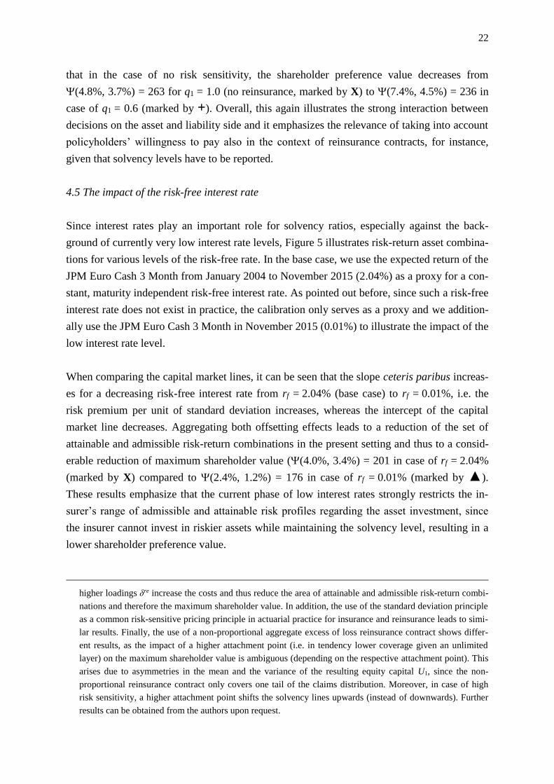
When comparing the capital market lines, it can be seen that the slope ceteris paribus increas-

es for a decreasing risk-free interest rate from rf = 2.04% (base case) to rf = 0.01%, i.e. the

risk premium per unit of standard deviation increases, whereas the intercept of the capital

market line decreases. Aggregating both offsetting effects leads to a reduction of the set of

attainable and admissible risk-return combinations in the present setting and thus to a consid-

erable reduction of maximum shareholder value ((4.0%, 3.4%) = 201 in case of rf = 2.04%

(marked by X) compared to (2.4%, 1.2%) = 176 in case of rf = 0.01% (marked by ▲).

These results emphasize that the current phase of low interest rates strongly restricts the in-

surer’s range of admissible and attainable risk profiles regarding the asset investment, since

the insurer cannot invest in riskier assets while maintaining the solvency level, resulting in a

lower shareholder preference value.

higher loadings δre increase the costs and thus reduce the area of attainable and admissible risk-return combi-

nations and therefore the maximum shareholder value. In addition, the use of the standard deviation principle

as a common risk-sensitive pricing principle in actuarial practice for insurance and reinsurance leads to simi-

lar results. Finally, the use of a non-proportional aggregate excess of loss reinsurance contract shows differ-

ent results, as the impact of a higher attachment point (i.e. in tendency lower coverage given an unlimited

layer) on the maximum shareholder value is ambiguous (depending on the respective attachment point). This

arises due to asymmetries in the mean and the variance of the resulting equity capital U1, since the non-

proportional reinsurance contract only covers one tail of the claims distribution. Moreover, in case of high

risk sensitivity, a higher attachment point shifts the solvency lines upwards (instead of downwards). Further

results can be obtained from the authors upon request.

23

Figure 5: Attainable (capital market line CML) and admissible (“solvency line”) risk-return

combinations for a target ruin probability = 0.50% and given medium ( = 0.3) policyholder

risk sensitivity for different levels of the risk-free interest rate rf = 2.04%:

2.04% 0.34r rCML and rf = 0.01%: 0.01 0.5% 0 r rCML

4.6 The impact of dependencies between assets and liabilities

To investigate the impact of the dependence structure between assets and liabilities on the

requirements for the investment strategy and hence for maximizing shareholder value, we first

compare the solvency lines for different parameters ρ = -0.5, 0.0, 0.5 of the Gaussian copula

(equal to Pearson’s correlation coefficient in the Gaussian setting) and thus different diversifi-

cation levels in Figure 6. In case of a positive ρ, high asset values are positively related to

high liability values and hence the risks are well diversified, resulting in a well-balanced as-

set-liability profile. A negative ρ, in contrast, represents an increasing riskiness of the asset-

liability profile (in terms of the variance of equity capital) due to insufficient diversification,

i.e. low asset values are positively related to high liability values (Fischer and Schlütter,

2015).

Figure 6 shows that the convexity of the solvency line increases for higher ρ, while the inter-

cept remains unchanged. A lower linear dependence between assets and liabilities is thereby

penalized by higher solvency capital requirements and reduces the area of admissible and at-

tainable risk-return combinations. Furthermore, an insufficient diversification in an asset-

liability context in terms of a lower ρ has negative consequences in regard to maximizing

shareholder value, as declines from (7.5%, 4.6%) = 215 in case of ρ = 0.5 (marked by +)

to (1.8%, 2.7%) = 192 in case of ρ = -0.5 (marked by X). It is thus crucial that a risk man-

agement model takes into account the diversification between assets and liabilities to avoid

inadequate incentives for insurers, which is part of the criticism of Fischer and Schlütter

(2015) in their analysis regarding the standard formula of Solvency II.

24

Figure 6: Attainable (CML) and admissible (solvency lines) risk-return combinations for a

target ruin probability = 0.50% and medium ( = 0.3) policyholder risk sensitivity for corre-

lations ρ = -0.5, 0.0, 0.5

To study the impact of non-linear dependence structures, we now drop the Gaussian setting

(i.e. Gaussian copula with Gaussian marginals) and consider a t-copula with the same margin-

al distributions. Figure 7 exhibits results for a Gaussian copula GaussC with parameter ρ = 0.5,

implying a Kendall’s tau = 0.33, and a t-copula ,

t

RC with degrees of freedom = 3 and pa-

rameter R = 0.5 calibrated to the identical Kendall’s tau to ensure comparability.

Figure 7: Attainable (CML) and admissible (solvency lines) risk-return combinations for tar-

get ruin probability = 0.50% and medium ( = 0.3) policyholder risk sensitivity for Gaussi-

an copula and t-copula (Kendall’s tau = 0.33)

As can be seen from Figure 7, even though fixing Kendall’s tau ensures a constant degree of

general dependence between assets and liabilities, the solvency lines differ considerably. For

the t-copula, the solvency line lies above the one of the Gaussian copula, implying stronger

restrictions and less risky asset allocations along with a slightly lower maximum shareholder

value: (5.7%, 4.0%) = 213 in case of the t-copula compared to (7.5%, 4.6%) = 215 in case

25

of the Gaussian copula. While the Gaussian copula exhibits no tail dependence, the t-copula

demands a higher expected return due to (negative lower-upper) tail dependence, i.e. the lim-

iting probability of extremely low asset returns given extremely high claims is non-zero. This

emphasizes that even though many risk models such as the standard formula of Solvency II

focus on linear correlations, one should take into account that non-linear dependencies may

lead to decisively different results and might be more appropriate to model dependences de-

pending on the insurer’s individual risk situation.

4.7 The impact of the claims distribution

Lastly, we also deviate from the purely Gaussian setting by using a lognormal distribution for

the claims that ensures non-negative values and better reflects empirically observed properties

(e.g., right-skewness, heavy tail) than a normal distribution. Figure 8 compares the solvency

line derived based on normally distributed claims with that based on lognormally distributed

claims calibrated to the same mean S and standard deviation S. While both solvency lines

show similar results, the lognormal distribution with heavy tails still implies higher solvency

capital requirements, leading to an almost equal maximum shareholder value but with a dif-

ferent optimal asset allocation: (3.5%, 3.2%) = 200 in case of the lognormal distribution

(marked by X) compared to (4.0%, 3.4%) = 201 for the normal distribution (marked by ▲).

Figure 8: Attainable (capital market line CML) and admissible (“solvency line”) risk-return

combinations for target ruin probability = 0.50% and medium ( = 0.3) policyholder risk

sensitivity for normally and lognormally distributed claims (same mean and standard devia-

tion)

26

5. SUMMARY

In this article, we study risk- and value-based management decisions regarding a non-life in-

surer’s capital investment strategy by deriving minimum capital standards for the insurer’s

asset allocation based on a fixed solvency level, since adjusting the asset side to satisfy sol-

vency capital requirements should generally be easier than short-term adaptions regarding

equity capital or the liability side as pointed out by Eling et al. (2009). In this setting, we fol-

low the latter and link the admissible (i.e. satisfying solvency requirements based on the ruin

probability) risk-return combinations of the insurer’s asset portfolio to actually attainable al-

location opportunities at the capital market using Tobin’s (1958) capital market line. We then

study the optimal investment problem when maximizing shareholder value based on mean-

variance preference functions and simultaneously controlling for the ruin probability in order

to protect the policyholders. We thereby extend previous work in several relevant ways: We

use a more general model and explicitly include the policyholders’ willingness to pay, which

to the best of our knowledge has not been done so far in this context, taking into account the

insurer’s reported target safety level and the policyholders’ risk sensitivity. We further inves-

tigate the impact of reinsurance contracts, the risk-free interest rate, (non-linear) asset-liability

dependencies as well as distributional assumptions, which considerably influence the set of

attainable and admissible risk-return combinations as well as the maximum achievable share-

holder preference value. This is done based on comprehensive analytical and numerical anal-

yses, whereby we formally derive the global maximum of the shareholder preference func-

tion.

Our results show that the consideration of the policyholders’ willingness to pay depending on

their risk sensitivity based on the insurer’s reported solvency status is crucial, since a more

risk-sensitive assessment reduces the premium income and thus the flexibility of investments

on the asset side as well as the resulting maximum shareholder preference value. This is espe-

cially relevant in the future in the presence of market discipline, when insurers have to regu-

larly reveal their solvency status according to Solvency II. Moreover, given a default-risk-

driven premium income, the optimal reported target ruin probability differs for various levels

of policyholders’ risk sensitivity. In case of high and medium risk sensitivity, a target ruin

probability corresponding to the absence of default risk implies a higher shareholder value,

while no policyholder risk sensitivity leads to contrary results. To satisfy the interests of both

shareholders and policyholders, our approach can thus be used for balancing shareholder val-

ue and risk taking. In particular, depending on the policyholders’ risk sensitivity, it is advisa-

ble for firms to closely monitor the reactions of policyholders to safety levels and to possibly

enhance the solvency level in order to generate more flexibility for the investment strategy

and to increase shareholder value.

27

We further observe that the set of attainable and admissible investment opportunities and thus

the maximum shareholder preference value only increases for lower retention levels (i.e.,

higher portions) of proportional reinsurance if policyholders are not risk sensitive. In particu-

lar, this effect is reversed when taking into account the policyholders’ willingness to pay, as

the insurer’s premium income, which must be used to pay the fixed reinsurance premiums

(not subject to risk sensitivity influences), is reduced, implying a reduction of the set of avail-

able risk-return asset combinations. Furthermore, an analysis of the impact of the risk-free

interest rate shows that the current phase of low interest rates strongly restricts the insurer’s

investment opportunities and considerably reduces shareholder preference value. In addition,

we find that lower linear dependencies between assets and liabilities can considerably reduce

the area of attainable and admissible risk-return combinations, emphasizing that diversifica-

tion between assets and the underwriting portfolio can generate more flexibility regarding the

risk profile of the capital investment, which also implies the potential of generating a higher

shareholder value. Moreover, robustness tests emphasize that non-linear (tail) dependencies

and heavy tail claims distributions can lead to even stronger solvency restrictions and lower

maximum shareholder preference value.

Overall, our results strongly emphasize the strong interaction between decisions regarding the

asset and the liability side, and they underline the importance of considering the policyhold-

ers’ demand for insurance products given that solvency levels have to be reported, which

should be taken into account by insurers in the context of their risk- and value-based man-

agement decisions.

REFERENCES

Albrecher, H., Teugels, J. L. (2006): Exponential Behavior in the Presence of Dependence in

Risk Theory. Journal of Applied Probability, 43(1), 257-273.

Andersen, E. S. (1957): On the Collective Theory of Risk in Case of Contagion between

Claims. Bulletin of the Institute of Mathematics and its Applications, 12, 275-279.

Ardia, D., Mullen, K. M., Peterson, B. G., Ulrich, J. (2016): “DEoptim”: Differential Evolu-

tion in “R”. R package version 2.2-4. https://CRAN.R-project.org/package=DEoptim.

Asmussen, S., Albrecher, H. (2010): Ruin Probabilities. World Scientific, Singapore.

Avanzi, B., Gerber, H. U., Shiu, E. S. (2007): Optimal Dividends in the Dual Mod-

el. Insurance: Mathematics and Economics, 41(1), 111-123.

Bai, L., Zhang, H. (2008): Dynamic Mean-variance Problem with Constrained Risk Control

for the Insurers. Mathematical Methods of Operations Research, 68(1), 181-205.

28

Bankovsky, D., Klüppelberg, C., Maller, R. (2011): On the Ruin Probability of the General-

ised Ornstein-Uhlenbeck Process in the Cramér Case. Journal of Applied Probability,

48(A), 15-28.

Bäuerle, N. (2005): Benchmark and Mean-variance Problems for Insurers. Mathematical

Methods of Operations Research, 62(1), 159-165.

Beard, R., Pentikäinen, T., Pesonen, E. (2013): Risk theory: The Stochastic Basis of Insur-

ance. Springer, New York.

Bi, J., Guo, J. (2012): Optimal Mean-variance Problem with Constrained Controls in a Jump-

diffusion Financial Market for an Insurer. Journal of Optimization Theory and Applica-

tions, 157(1), 252-275.

Braun, A., Schmeiser, H., Schreiber, F. (2017): Portfolio Optimization under Solvency II:

Implicit Constraints Imposed by the Market Risk Standard Formula. Journal of Risk and

Insurance, 84(1), 177-207.

Brent, R. (1973): Algorithms for Minimization without Derivatives. Prentice-Hall, Englewood

Cliffs, NJ.

Brito, N. O. (1977): Marketability Restrictions and the Valuation of Capital Assets under Un-

certainty. Journal of Finance, 32(4): 1109-1123.

Chen, Y. (2011): The Finite-time Ruin Probability with Dependent Insurance and Financial

Risks. Journal of Applied Probability, 48(4), 1035-1048.

Chen, Y., Yuen, K. C. (2009): Sums of Pairwise Quasi-asymptotically Independent Random

Variables with Consistent Variation. Stochastic Models, 25(1), 76-89.

Collamore, J. F. (2009): Random Recurrence Equations and Ruin in a Markov-dependent

Stochastic Economic Environment. The Annals of Applied Probability, 19(4), 1404-1458.

Cramér, H. (1930): On the Mathematical Theory of Risk. Skandia Jubilee Volume, Stock-

holm.

Diasparra, M. A., Romera, R. (2009): Bounds for the Ruin Probability of a Discrete-time Risk

Process. Journal of Applied Probability, 46(1), 99-112.

Diasparra, M., Romera, R. (2010): Inequalities for the Ruin Probability in a Controlled Dis-

crete-Time Risk Process. European Journal of Operational Research, 204(3), 496-504.

Dimitrova, D. S., Kaishev, V. K., Zhao, S. (2015): On Finite-time Ruin Probabilities in a

Generalized Dual Risk Model with Dependence. European Journal of Operational Re-

search, 242(1), 134-148.

Eling, M., Gatzert, N., Schmeiser, H. (2009): Minimum Standards for Investment Perfor-

mance: A New Perspective on Non-Life Insurer Solvency. Insurance: Mathematics and

Economics, 45(1), 113-122.

Fischer, K., Schlütter, S. (2015): Optimal Investment Strategies for Insurance Companies

when Capital Requirements are Imposed by a Standard Formula. The Geneva Risk and In-

surance Review, 40(1), 15-40.

29

Gatzert, N., Holzmüller, I., Schmeiser, H. (2012): Creating Customer Value in Participating

Life Insurance. Journal of Risk and Insurance, 79(3), 645-670.

Gatzert, N., Kellner, R. (2014): The Effectiveness of Gap Insurance with Respect to Basis

Risk in a Shareholder Value Maximization Setting. Journal of Risk and Insurance, 81(4),

831-860.

Embrechts, P., Klüppelberg, C., Mikosch, T. (2013): Modelling Extremal Events: For Insur-

ance and Finance. Springer, New York.

EY (2016): Sub-Saharan Africa — the evolution of insurance regulation.

http://www.ey.com/Publication/vwLUAssets/EY-sub-saharan-africa-the-evolution-of-

insurance-regulation/$FILE/EY-sub-saharan-africa-the-evolution-of-insurance-

regulation.pdf.

Hao, X., Tang, Q. (2012): Asymptotic Ruin Probabilities for a bivariate Lévy-driven Risk

Model with Heavy-tailed Claims and Risky investments. Journal of Applied Probability,

49(4), 939-953.

Heyde, C. C., Wang, D. (2009): Finite-time Ruin Probability with an Exponential Lévy Pro-

cess Investment Return and Heavy-tailed Claims. Advances in Applied Probability, 41(1),

206-224.

Hofert, M., Kojadinovic, I., Maechler, M., Yan, J. (2017): “copula”: Multivariate Depend-

ence with Copulas. R package version 0.999-17. https://CRAN.R-

project.org/package=copula.

Huang, Y., Yang, X., Zhou, J. (2016): Optimal Investment and Proportional Reinsurance for a

Jump–diffusion Risk model with Constrained Control Variables. Journal of Computational

and Applied Mathematics, 296, 443-461.

Hult, H., Lindskog, F. (2011): Ruin Probabilities under General Investments and Heavy-tailed

Claims. Finance and Stochastics, 15(2), 243-265.

Jin, C., Li, S., Wu, X. (2016): On the Occupation Times in a Delayed Sparre Andersen Risk

Model with Exponential Claims. Insurance: Mathematics and Economics, 71, 304-316.

Kabanov, Y., Pergamenshchikov, S. (2016): In the Insurance Business Risky Investments are

Dangerous: The Case of Negative Risk Sums. Finance and Stochastics, 20(2), 355-379.

Kahneman, D., Tversky, A. (1979): Prospect Theory: An Analysis of Decision under Risk.

Econometrica, 47(2), 263-292.

Klüppelberg, C. Kostadinova, R. (2008): Integrated Insurance Risk Models with Exponential

Lévy Investment. Insurance: Mathematics and Economics, 42(2), 560–577.

Kroll, Y., Levy, H., Markowitz, H. M. (1984): Mean‐Variance versus Direct Utility Maximi-

zation. Journal of Finance, 39(1), 47-61.

Kurowicka, D., H. Joe (2011). Dependence Modeling: Vine Copula Handbook. World Scien-

tific Publishing, Singapore.

Li, J. (2012): Asymptotics in a Time-Dependent Renewal Risk Model with Stochastic Return.

Journal of Mathematical Analysis and Applications, 387(2), 1009-1023.

30

Li, S., Garrido, J. (2004): On a Class of Renewal Risk Models with a Constant Dividend Bar-

rier. Insurance: Mathematics and Economics, 35(3), 691-701.

Li, J., Tang, Q. (2015): Interplay of Insurance and Financial Risks in a Discrete-time Model

with Strongly Regular Variation. Bernoulli, 21(3), 1800-1823.

Liang, Z., Bayraktar, E. (2014): Optimal Reinsurance and Investment with Unobservable

Claim Size and Intensity. Insurance: Mathematics and Economics, 55, 156-166.

Liang, Z., Yuen, K. C., Guo, J. (2011): Optimal Proportional Reinsurance and Investment in a

Stock Market with Ornstein–Uhlenbeck Process. Insurance: Mathematics and Economics,

49(2), 207-215.

Liang, Z., Yuen, K. C., Cheung, K. C. (2012): Optimal Reinsurance–investment problem in a

Constant Elasticity of Variance Stock market for Jump‐diffusion Risk Model. Applied Sto-

chastic Models in Business and Industry, 28(6), 585-597.

Lin, X., Dongjin, Z., Yanru, Z. (2015): Minimizing Upper Bound of Ruin Probability Under

Discrete Risk Model with Markov Chain Interest Rate. Communications in Statistics-

Theory and Methods, 44(4), 810-822.

Loistl, O. (2015): Does Mean-Variance Portfoliomanagement Deserve Expected Utility's Ap-

proximative Affirmation? European Journal of Operational Research, 247(2), 676-680.

Lorson, J., Schmeiser, H., Wagner, J. (2012): Evaluation of Benefits and Costs of Insurance

Regulation - A Conceptual Model for Solvency II. Journal of Insurance Regulation, 31(1),

125-156.

Lundberg, F. (1903): Approximerad Framställning Afsannollikhetsfunktionen: II. Åter-

försäkring Af Kollektivrisker. Almqvist & Wiksells Boktr., Uppsala.

Markowitz, H. (2014): Mean–Variance Approximations to Expected Utility. European Jour-

nal of Operational Research, 234(2), 346-355.

Markowitz, H. (2015): Reply to Professor Loistl. European Journal of Operational Re-

search, 247(2), 680-681.

Mayers, D., Smith, C. W. (1981): Contractual Provisions, Organizational Structure, and Con-

flict Control in Insurance Markets. Journal of Business, 54(3), 407-434.

McNeil, A. J., Frey, R., Embrechts, P. (2005): Quantitative Risk Management: Concepts,

Techniques and Tools. Princeton University Press, Princeton.

Mikosch, T. (2009): Non-life Insurance Mathematics: An Introduction with the Poisson Pro-

cess. Springer, Berlin.

Nyrhinen, H. (1999): On the Ruin Probabilities in a General Economic Environment. Stochas-

tic Processes and their Applications, 83(2), 319-330.

Paulsen, J. (1993): Risk Theory in a Stochastic Economic Environment. Stochastic processes

and their Applications, 46(2), 327-361.

Paulsen, J. (2008): Ruin Models with Investment Income. Probability Surveys, 5, 416-434.

Promislow, D. S., Young, V. R. (2005): Minimizing the Probability of Ruin when Claims

Follow Brownian Motion with Drift. North American Actuarial Journal, 9(3), 110-128.

31

Ramsden, L., Papaioannou, A. D. (2017): Asymptotic Results for a Markov-modulated Risk

Process with Stochastic investment. Journal of Computational and Applied Mathematics,

313, 38-53.

Romera, R., Runggaldier, W. (2012): Ruin Probabilities in a Finite-horizon Risk Model with

Investment and Reinsurance. Journal of Applied Probability, 49(4), 954-966.

Schäl, M. (2004): On Discrete-time Dynamic Programming in Insurance: Exponential Utility

and Minimizing the Ruin Probability. Scandinavian Actuarial Journal, 2004(3), 189-210.

Schlütter, S. (2014): Capital Requirements or Pricing Constraints? An Economic Analysis of

Measures for Insurance Regulation. The Journal of Risk Finance, 15(5), 533-554.

Schmidli, H. (2001): Optimal Proportional Reinsurance Policies in a Dynamic Setting. Scan-

dinavian Actuarial Journal, 2001(1), 55-68.

Schmidli, H. (2002): On Minimizing the Ruin Probability by Investment and Reinsurance.

Annals of Applied Probability, 12(3), 890-907.

Segerdahl, C. O. (1942): Über einige Risikotheoretische Fragestellungen. Scandinavian Actu-

arial Journal, 1942(1-2), 43-83.

Shen, X. M., Lin, Z. Y., Zhang, Y. (2009): Uniform Estimate for Maximum of Randomly

Weighted Sums with Applications to Ruin Theory. Methodology and Computing in Ap-

plied Probability, 11(4), 669-685.

Sklar, A. (1959): Distribution Functions of n Dimensions and Margins. Publications of the

Institute of Statistics of the University of Paris, 8, 229-231.

Swiss Re (2016): Sigma Nr. 1/2016. Natural Catastrophes and Man-made Disasters in 2015:

Asia Suffers Substantial Losses. http://media.swissre.com/documents/sigma1_2016_

en.pdf.

Tang, Q., Tsitsiashvili, G. (2003): Precise Estimates for the Ruin Probability in Finite Horizon

in a Discrete-time Model with Heavy-tailed Insurance and Financial risks. Stochastic Pro-

cesses and their Applications, 108(2), 299-325.

Tang, Q., Tsitsiashvili, G. (2004): Finite- and Infinite-time Ruin Probabilities in the Presence

of Stochastic Returns on Investments. Advances in Applied Probability, 36(4), 1278-1299.

Tobin, J. (1958): Liquidity Preference as Behavior toward Risk. Review of Economic Studies,

25(2), 65-86.

Wakker, P., Thaler, R., Tversky, A. (1997): Probabilistic Insurance. Journal of Risk and Un-

certainty, 15(1), 7-28.

Weng, C., Zhang, Y., Tan, K. S. (2009): Ruin Probabilities in a Discrete Time Risk Model

with Dependent Risks of Heavy Tail. Scandinavian Actuarial Journal, 3, 205-218.

Wu, R., Lu, Y., Fang, Y. (2007): On the Gerber-Shiu Discounted Penalty Function for the

Ordinary Renewal Risk Model with Constant Interest. North American Actuarial Journal,

11(2), 119-134.

Yang, Y., Hashorva, E. (2013): Extremes and Products of Multivariate AC-Product Risks.

Insurance: Mathematics and Economics, 52(2), 312-319.

32

Yang, Y., Konstantinides, D. G. (2015): Asymptotics for Ruin Probabilities in a Discrete-time

Risk Model with Dependent Financial and Insurance Risks. Scandinavian Actuarial Jour-

nal, 2015(8), 641-659.

Yang, Y., Leipus, R., Šiaulys, J. (2012): Tail Probability of Randomly Weighted Sums of

Subexponential Random Variables under a Dependence Structure. Statistics & Probability

Letters, 82(9), 1727-1736.

Yang, H., Zhang, L. (2006): Ruin Problems for a Discrete Time Risk Model with Random

Interest rate. Mathematical Methods of Operations Research, 63(2), 287-299.

Yi, L., Chen, Y., Su, C. (2011). Approximation of the Tail Probability of Randomly Weighted

Sums of Dependent Random Variables with Dominated Variation. Journal of Mathemati-

cal Analysis and Applications, 376(1), 365-372.

Zhang, Y., Shen, X., Weng, C. (2009): Approximation of the Tail Probability of Randomly

Weighted Sums and Applications. Stochastic processes and their applications, 119(2),

655-675.

Zimmer, A., Schade, C., Gründl, H. (2009): Is Default Risk Acceptable when Purchasing In-

surance? Experimental Evidence for Different Probability Representations, Reasons for

Default, and Framings. Journal of Economic Psychology, 30(1), 11-23.

Zimmer, A., Gründl, H., Schade, C., Glenzer, F. (2014): An Incentive-compatible Experiment

on Probabilistic Insurance and Implications for an Insurer's Solvency Level. Working Pa-

per, Goethe University of Frankfurt.

33

APPENDIX

Proof of Lemma 1: The preference function is strictly increasing in μr under Assumption

5, since it is differentiable and

1

,, 0

r r

r

u P q

.

In addition, since the capital market line CML (Equation (5)) is the upper bound of the feasi-

ble set of risk-return combinations, the following holds for the optimization problem in Equa-

tion (7)

*

max , : , max , : ,

max : : min : , ,max : , ,

r r r r r r r r

r r r r r r r r

CML CML

I CML CML

with

* 0

,  :

,r rr CML

i.e. with r f rr m from Equations (5), (10), and (11), one obtains under Assumption 5

*

1 1

1

2 2 2 2

1 1 1 1 1 1

2

1 ,

, 2 , , ,2

r

S

r S r s

f r

kU U

u P q q

ku P q q u P q q

r

Cor r S

m

*2

1 1

1 1 1 1

, ,

, , ,

r

r

r

s

m u P q k u P q

k u P q q Cor r S

and

2 *2

12, 0

r

r

k u P q

(with k > 0 and Assumption 5).

34

Therefore, *  is strictly concave on 0

with unique global maximum (

*

0r

r

) in

11*

1

1,

,

S

r

Cor rm k q

k u P q

S

.

If *

r I , *max :r r I is solved by *

r . If *

r I , it holds that

* min : ,r r r rCML or * max : ,r r r rCML . In the first case,

* is strictly decreasing on I and *max :r r I is solved by the left boundary point

of I. In the second case, * is strictly increasing on I and *max :r r I is solved by

the right boundary point of I.

Derivative of * *,r rCML with respect to u:

* *

1

1

2

1 12 2

1 1

1 1 1

1

1

1 11

,

1 ,

2

,

, .2

, ,

r r

S

S

S S

S s

f

Cor r Sr m

C

CML

m k qu P q q

k

m k q m k qkq q Cor r S

or r S Co

k

r S

k

r

Hence one obtains:

* *,1 .

r r

f

CMLr

u