Mortality Risk, Insurance, and the Value of Life - National ...

NBER WORKING PAPER SERIES

MORTALITY RISK, INSURANCE, AND THE VALUE OF LIFE

Daniel BauerDarius Lakdawalla

Julian Reif

Working Paper 25055http://www.nber.org/papers/w25055

NATIONAL BUREAU OF ECONOMIC RESEARCH1050 Massachusetts Avenue

Cambridge, MA 02138September 2018, Revised October 2019

We are grateful to Dan Bernhardt, Tatyana Deryugina, Don Fullerton, Sonia Jaffe, Ian McCarthy, Nolan Miller, Alex Muermann, George Pennacchi, Mark Shepard, Dan Silverman, George Zanjani, and participants at the AEA/ARIA meeting, the NBER Insurance Program Meeting, the Risk Theory Society Annual Seminar, Temple University, the University of Chicago Applications Workshop, and the University of Wisconsin-Madison for helpful comments. We are also grateful to Bryan Tysinger for assistance with the Future Elderly Model. Bauer acknowledges financial support from the Society of Actuaries. Lakdawalla acknowledges financial support from the National Institute on Aging (1R01AG062277). Lakdawalla discloses that he is a consultant to Precision Health Economics (PHE) and an investor in its parent company, Precision Medicine Group. PHE provides research and consulting services to firms in the biopharmaceutical, medical device, and health insurance industries, including Otsuka Pharmaceuticals and Novartis Pharmaceuticals. The views expressed herein are those of the authors and do not necessarily reflect the views of the National Bureau of Economic Research.

NBER working papers are circulated for discussion and comment purposes. They have not been peer-reviewed or been subject to the review by the NBER Board of Directors that accompanies official NBER publications.

© 2018 by Daniel Bauer, Darius Lakdawalla, and Julian Reif. All rights reserved. Short sections of text, not to exceed two paragraphs, may be quoted without explicit permission provided that full credit, including © notice, is given to the source.

Mortality Risk, Insurance, and the Value of Life Daniel Bauer, Darius Lakdawalla, and Julian Reif NBER Working Paper No. 25055September 2018, Revised October 2019JEL No. H51,H55,I10

ABSTRACT

We develop a new framework for valuing health and longevity improvements that departs from conventional but unrealistic assumptions of full annuitization and deterministic health. Our framework can value the prevention of mortality and of illness, and it can quantify the effects of retirement policies on the value of life. We apply the framework to life-cycle data and generate new insights absent from the conventional approach. First, treatment is up to five times more valuable than prevention, even when both extend life equally. This asymmetry helps explain low observed investment in preventive care. Second, severe illness can significantly increase the value of statistical life, helping to reconcile theory with empirical findings that consumers value life-extension more in bleaker health states. Third, retirement annuities boost aggregate demand for life-extension. We calculate that Social Security adds $10.6 trillion (11 percent) to the value of post-1940 longevity gains and would add $127 billion to the value of a one percent decline in future mortality.

Daniel BauerUniversity of [email protected]

Darius LakdawallaUniversity of Southern California635 Downey Way, VPD 414-KSchaeffer Center for Health Policy and Economics Los Angeles, CA 90089-7273and [email protected]

Julian ReifDepartment of FinanceUniversity of Illinois at Urbana-Champaign515 E. Gregory StreetChampaign, IL 61820and [email protected]

A data appendix is available at http://www.nber.org/data-appendix/w25055

2

I. INTRODUCTION The economic analysis of risks to life and health has made enormous contributions to both academic

discussions and public policy. Economists have used the standard tools of life-cycle consumption theory

to propose a transparent framework that measures the value of improvements to both health and longevity

(Rosen 1988; Murphy and Topel 2006). Economic concepts such as the value of statistical life play

central roles in discussions surrounding public and private investments in medical care, public safety,

environmental hazards, and countless other arenas.

The standard life-cycle framework employed by the value of life literature assumes full annuitization and

deterministic health risk. While analytically convenient and useful for illustrating some of the underlying

economics, these assumptions are not realistic: it is well known that most people are far from fully

annuitized (Brown et al. 2008), and that health risk depends on one’s health state. Moreover, these

assumptions hamper explanatory power in several ways: the standard framework sheds no light on what

happens to the value of life upon falling ill, cannot meaningfully distinguish between preventive care and

medical treatment, and glosses over policy-relevant relationships between demand for health care and the

structure of annuity markets. These issues are empirically relevant. An array of evidence suggests that

society invests less in prevention than treatment, even when both have the same consequences for health

and longevity (Weisbrod 1991; Dranove 1998; Pryor and Volpp 2018). And, prior research suggests the

value consumers place on improvements in quality of life and longevity varies considerably with health

state (Nord et al. 1995; Shah 2009; Shah, Tsuchiya, and Wailoo 2018).

We develop and apply a framework for valuing health improvements that relaxes the unrealistic

assumptions of full annuitization and deterministic health risk. We establish three main results. First, we

derive the value of statistical illness (VSI), which captures the willingness to pay to avoid sickness and

includes VSL as a special case. We calculate that—holding wealth constant—a sick individual’s initial

willingness to pay for medical treatment is several times greater than a healthy individual’s willingness to

pay for preventive care that improves longevity by the same amount. Second, we derive conditions under

which the value of life can rise following a negative health shock, and we demonstrate that this effect is

economically significant under reasonable parameterizations. For example, we calculate that the value of

statistical life (VSL) for a 70-year-old rises by $600 thousand (25 percent) following the development of

chronic conditions that impair her everyday living. Third, we calculate that the US Social Security

program adds $10.6 trillion (11 percent) to the value of post-1940 longevity gains.

Incomplete annuitization drives all three of these results. A simple example illustrates the intuition.

Imagine a 60-year-old retiree with no bequest motive and a flat optimal consumption profile. If she fully

3

annuitizes her savings, her consumption remains flat at, say, $30,000 annually. Now suppose annuities are

unavailable. In this case, it is well known that the optimal consumption profile shifts forward to earlier

ages (Yaari 1965), in response to the risk of dying with money still left in the bank (see Figure 1).

Because VSL depends greatly on consumption, the life-cycle profile of VSL will also shift forward. Thus,

reductions in annuitization lower VSL at older ages, and increase VSL at younger ages. Conversely,

retirement savings programs such as Social Security that increase annuitization levels will raise VSL at

older ages and lower it at younger ages.

The incorporation of stochastic mortality risk yields our other results. It is optimal for an incompletely

annuitized individual to shift her consumption forward, i.e., to spend down her wealth, following an

adverse shock to life expectancy. Although a negative shock to longevity reduces lifetime utility, the

accompanying reduction in the contemporaneous marginal utility of consumption can be large enough to

increase her VSL. This result contrasts with the conventional (fully annuitized) life-cycle model, where a

reduction in longevity always reduces VSL (Murphy and Topel 2006). Similarly, in our framework a sick

individual’s willingness to pay for treatment can be higher than a healthy individual’s willingness to pay

for preventive care, even when both interventions add the same number of life-years.

The first half of this paper provides a formal framework that yields these insights. We show that optimal

consumption increases following an adverse shock to longevity and derive a sufficient condition under

which VSL also increases. This condition holds under a wide range of typical parameterizations.1 We

focus on mortality shocks, but allow for shocks to quality of life and income as well. We also derive VSI,

a generalization of VSL that can be interpreted as a person’s willingness to pay for a marginal decrease in

the risk of acquiring an illness. VSI allows us to compare the value of prevention to the value of

treatment. We show that prevention and treatment are valued equally only when consumers are fully

annuitized. The value of treatment can exceed the value of prevention when annuity markets are

incomplete. This result sheds new light on why consumers, firms, and health insurers appear reluctant to

invest in prevention, even when there are considerable private life expectancy benefits (Weisbrod 1991;

Dranove 1998; Pryor and Volpp 2018).

1 Intuitively, the condition holds when the loss in lifetime utility is more than offset by a corresponding decrease in

marginal utility. Specifically, an adverse mortality shock increases VSL when demand for current consumption is

sufficiently inelastic, or when the marginal utility of demand is sufficiently linear (as measured by relative

prudence).

4

The second half of the paper applies our model to data. Our first empirical exercise incorporates detailed

real-world data from the Future Elderly Model into a stochastic life-cycle model that allows mortality,

medical spending, and quality of life to vary across 20 different health states. Under typical utility

parameterizations, we calculate that the value of treating lethal conditions like cancer is worth up to 5

times more to individuals than equivalent preventive care that adds the same number of years to life

expectancy. This asymmetry arises because the value of life rises substantially following a health shock.

For instance, VSL rises from $2.4 million to $3.0 million for a 70-year-old who suffers a debilitating

health shock that reduces her life expectancy by nearly 7 years and also worsens her quality of life. This

dynamic relationship between health shocks and VSL generates substantial variability in the aggregate:

Monte Carlo simulations performed on a population of initially healthy 50-year-olds yield an inter-

vigintile (middle 90 percent) VSL range of $1.7 to $2.5 million by age 70.

Our second exercise illustrates the connections between public annuity programs and the aggregate value

of increases in longevity. We calculate that Social Security adds $10.6 trillion (11 percent) to the value of

post-1940 longevity gains, relative to a setting with no annuity markets, by raising the value of life at

older ages. This gain is worth over $30,000 per person to the current population, or more than half the

longevity insurance value of Social Security. Moreover, Social Security increases the aggregate value of

potential future increases in longevity by over 10 percent, so that a 1 percent reduction in population-wide

mortality is $127 billion more valuable than it would have been without the program. Increasing the

generosity of Social Security by 50 percent would add a further $64 billion of value to this mortality

decline. This result also implies that Medicare is more valuable than previously recognized, by revealing

that the value of old-age health insurance increases when coupled with annuity programs like Social

Security. Finally, we show that a strong bequest motive reduces the effect of Social Security on the value

of longevity improvements by 20 percent. This result suggests the effect of annuitization on the value of

life matters more for low-income individuals, who are less likely to have a significant bequest motive.

Our stochastic model helps explain puzzles such as why consumers invest less in prevention than

treatment or why preventive care interventions frequently fail to deliver results (e.g., Jones, Molitor, and

Reif (2019)), although we do not rule out alternative behavioral explanations that may reinforce these

effects, such as inattention or hyperbolic discounting (Lawless, Drichoutis, and Nayga 2013). We caution

that our model does not necessarily imply that underinvestment in preventive care is socially optimal. As

we discuss in the main text, a full accounting of the normative implications requires taking a stance on

unsettled questions regarding the welfare economics of risk (Fleurbaey 2010). For this reason, we employ

a deterministic model when quantifying the effect of public annuity programs on the aggregate value of

life at older ages.

5

Our primary contribution is the development and application of a new and more general life-cycle model

of the value of life. The economic literature on the value of life reaches back to Schelling (1968) and

includes seminal studies by Arthur (1981), Rosen (1988), Murphy and Topel (2006), and Hall and Jones

(2007). A few studies have considered departures from the assumption of full annuitization, but only

under specialized preferences or alternative contexts (Shepard and Zeckhauser 1984; Ehrlich 2000;

Ehrlich and Yin 2005). Córdoba and Ripoll (2016) use Epstein-Zin-Weil preferences to study the

implications of state non-separable utility on the value of life when mortality is deterministic. Our

stochastic framework accommodates general additively separable preferences, allows for incomplete

annuity markets, and to our knowledge is the first to provide a life-cycle analysis of the value of

preventing illness.2 We establish the important result that, under standard assumptions about risk

preferences, consumers value treatment more than prevention even when both extend life equally.

Our model also reconciles the standard life-cycle framework with results from a distinct literature that

uses one-period models to study the value of mortality risk-reduction (Raiffa 1969; Weinstein, Shepard,

and Pliskin 1980; Pratt and Zeckhauser 1996; Hammitt 2000). These static models predict that an increase

in baseline risk must raise the value of statistical life when insurance markets are incomplete, a result

often referred to as the “dead-anyway” effect. In contrast, we show in our more general setting that

mortality shocks in life-cycle models can raise or lower the value of statistical life, depending on risk

attitudes and other utility parameters.

The remainder of this paper is organized as follows. Section II reviews the predictions of the conventional

theory on the value of life and demonstrates how relaxing its assumption of full annuitization alters these

predictions. Section III generalizes the framework further by allowing health and income to be stochastic

and provides a discussion of welfare. Section IV presents empirical analyses that quantify: (1) the value

of preventing different kinds of illness; (2) the effect of health shocks on the value of statistical life; and

(3) the effect of Social Security on the aggregate value of life-extension. Section V concludes.

II. DETERMINISTIC MODEL Consider an individual who faces mortality risk. We are interested in analyzing the value of a marginal

reduction in this risk. Section II.A quantifies this value in the conventional setting where annuity markets

are complete (Rosen 1988; Murphy and Topel 2006). Section II.B then repeats this exercise in a

2 The value of preventing illness has already found application in the empirical literature on mortality risk-reduction

(Cameron and DeShazo 2013; Hummels, Munch, and Xiang 2016).

6

“Robinson Crusoe” economy where the consumer cannot purchase annuities to insure against her

uncertain lifetime (Shepard and Zeckhauser 1984; Johansson 2002). We compare these two polar cases to

illustrate the basic insights of the paper. Finally, Section II.C considers a more realistic situation where

the consumer optimally invests part of her wealth in a constant annuity. We focus on the value of

longevity improvements, but we allow for improvements in quality of life as well.3

Except for certain special cases, it will not be optimal for the consumer to fully annuitize when annuity

markets are incomplete (Davidoff, Brown, and Diamond 2005). Section II.C demonstrates this point in

the context of deterministic health, and Section III.C extends it to a setting that allows for stochastic

health and correlated income shocks (Reichling and Smetters 2015). Section IV uses a numerical model to

probe the sensitivity of our results to different assumptions about consumer preferences, such as the

presence of a bequest motive, which prior studies have argued might also rationalize low observed rates

of annuitization. There continues to be debate over why real-world consumption trajectories and annuity

purchase decisions look the way they do. However, as we show, the implications for life-extension

depend primarily on the consumption trajectory itself, not the reasons that lie beneath.

Like prior studies on the value of life, we focus throughout this paper on the demand for health and

longevity. Quantifying optimal health spending requires additionally modeling the supply of health care

(Hall and Jones 2007). In light of all the variation in health care delivery systems, a wide variety of

plausible approaches can be taken to this modeling problem, which we leave to future research.

II.A. The fully annuitized value of life Let 𝑐𝑐(𝑡𝑡) be consumption at time 𝑡𝑡, 𝑊𝑊0 be baseline wealth, 𝑚𝑚(𝑡𝑡) be exogenous income, 𝜌𝜌 be the rate of

time preference, and 𝑟𝑟 be the rate of interest. Let 𝑊𝑊 be the net present value of wealth and future earnings

at baseline. Finally, define 𝑞𝑞(𝑡𝑡) as health-related quality of life at time 𝑡𝑡. Since it sacrifices little

generality in our application, we take 𝑞𝑞(𝑡𝑡) as exogenous.4 As needed, one can consider any relevant

quality of life profile in concert with a given profile of mortality, and we investigate this issue in our

3 In keeping with the vast majority of prior literature, we abstract from indemnity health insurance and treat non-

fatal health risks as exogenous and uninsurable. Since indemnity health insurance does not exist outside a few

specialized disease areas, and since health care insurance is imperfect, this does not sacrifice substantial generality.

Our empirical exercises in Section IV.B consider scenarios with and without out-of-pocket medical spending.

4 It is straightforward to incorporate endogenous labor supply (Murphy and Topel 2006). In the stochastic model

presented in Section III.C, we allow income and quality of life to depend on the health state.

7

empirical analysis later. The maximum lifespan of a consumer is 𝑇𝑇, and her mortality (hazard) rate at any

point in time is given by 𝜇𝜇(𝑡𝑡), where 0 ≤ 𝑡𝑡 ≤ 𝑇𝑇. The probability that a consumer will be alive at time 𝑡𝑡 is:

𝑆𝑆(𝑡𝑡) = exp �−� 𝜇𝜇(𝑠𝑠)𝑑𝑑𝑠𝑠𝑡𝑡

0�

We assume that annuity markets are complete and actuarially fair. The consumer’s maximization problem

is:

𝑉𝑉(0) = max𝑐𝑐(𝑡𝑡)

� 𝑒𝑒−𝜌𝜌𝑡𝑡𝑆𝑆(𝑡𝑡)𝑢𝑢(𝑐𝑐(𝑡𝑡), 𝑞𝑞(𝑡𝑡))𝑑𝑑𝑡𝑡𝑇𝑇

0

subject to the budget constraint:

� 𝑒𝑒−𝑟𝑟𝑡𝑡𝑆𝑆(𝑡𝑡)𝑐𝑐(𝑡𝑡)𝑑𝑑𝑡𝑡𝑇𝑇

0= 𝑊𝑊 = 𝑊𝑊0 + � 𝑒𝑒−𝑟𝑟𝑡𝑡𝑆𝑆(𝑡𝑡)𝑚𝑚(𝑡𝑡)𝑑𝑑𝑡𝑡

𝑇𝑇

0

The consumer’s utility function, 𝑢𝑢(𝑐𝑐(𝑡𝑡), 𝑞𝑞(𝑡𝑡)), depends on both consumption and health-related quality of

life. We assume throughout this paper that 𝑢𝑢(⋅) is strictly increasing and concave in its first argument, and

twice continuously differentiable. Let 𝑢𝑢𝑐𝑐(⋅) denote the marginal utility of consumption, and assume that

this function diverges to positive infinity as consumption approaches zero, so that optimal consumption is

always positive. Associating the multiplier 𝜃𝜃 with the wealth constraint, optimal consumption is

characterized by the first-order condition:

𝜕𝜕𝑉𝑉(0)𝜕𝜕𝑊𝑊

= 𝜃𝜃 = 𝑒𝑒(𝑟𝑟−𝜌𝜌)𝑡𝑡𝑢𝑢𝑐𝑐(𝑐𝑐(𝑡𝑡), 𝑞𝑞(𝑡𝑡))

To analyze the value of life, let 𝛿𝛿(𝑡𝑡) be a perturbation on the mortality rate with ∫ 𝛿𝛿(𝑡𝑡)𝑑𝑑𝑡𝑡𝑇𝑇0 = 1, and

consider:

𝑆𝑆𝜀𝜀(𝑡𝑡) = exp �−� (𝜇𝜇(𝑠𝑠)− 𝜀𝜀𝛿𝛿(𝑠𝑠))𝑑𝑑𝑠𝑠𝑡𝑡

0� , 𝜀𝜀 > 0

Let 𝑐𝑐𝜀𝜀(𝑡𝑡) represent the equilibrium variation in 𝑐𝑐(𝑡𝑡) caused by this perturbation. As shown in Rosen

(1988), the marginal utility of this life-extension is given by:

𝜕𝜕𝑉𝑉𝜕𝜕𝜀𝜀 �𝜀𝜀=0

=𝜕𝜕𝜕𝜕𝜀𝜀� 𝑒𝑒−𝜌𝜌𝑡𝑡𝑆𝑆𝜀𝜀(𝑡𝑡)𝑢𝑢�𝑐𝑐𝜀𝜀(𝑡𝑡), 𝑞𝑞(𝑡𝑡)�𝑑𝑑𝑡𝑡𝑇𝑇

0�𝜀𝜀=0

= � �𝑒𝑒−𝜌𝜌𝑡𝑡𝑢𝑢(𝑐𝑐(𝑡𝑡), 𝑞𝑞(𝑡𝑡)) + 𝑒𝑒−𝑟𝑟𝑡𝑡𝜃𝜃�𝑚𝑚(𝑡𝑡) − 𝑐𝑐(𝑡𝑡)�� 𝛿𝛿(𝑠𝑠)𝑑𝑑𝑠𝑠𝑡𝑡

0� 𝑆𝑆(𝑡𝑡)𝑑𝑑𝑡𝑡

𝑇𝑇

0

8

The marginal value of life-extension is equal to the marginal rate of substitution between longer life and

wealth:

𝜕𝜕𝑉𝑉/𝜕𝜕𝜀𝜀𝜕𝜕𝑉𝑉/𝜕𝜕𝑊𝑊�

𝜀𝜀=0= � 𝑒𝑒−𝑟𝑟𝑡𝑡𝑆𝑆(𝑡𝑡)�

𝑢𝑢(𝑐𝑐(𝑡𝑡), 𝑞𝑞(𝑡𝑡))𝑢𝑢𝑐𝑐(𝑐𝑐(𝑡𝑡), 𝑞𝑞(𝑡𝑡)) +𝑚𝑚(𝑡𝑡) − 𝑐𝑐(𝑡𝑡)� �� 𝛿𝛿(𝑠𝑠)𝑑𝑑𝑠𝑠

𝑡𝑡

0� 𝑑𝑑𝑡𝑡

𝑇𝑇

0

(1)

The value of a life-year is the value of a one-period change in survival from the perspective of current

time:

𝑣𝑣(𝑡𝑡) =

𝑢𝑢�𝑐𝑐(𝑡𝑡), 𝑞𝑞(𝑡𝑡)�𝑢𝑢𝑐𝑐�𝑐𝑐(𝑡𝑡), 𝑞𝑞(𝑡𝑡)�

+ 𝑚𝑚(𝑡𝑡) − 𝑐𝑐(𝑡𝑡) (2)

The value of a life-year, 𝑣𝑣(𝑡𝑡), is equal to the value of consumption in that year plus net savings, 𝑚𝑚(𝑡𝑡) −

𝑐𝑐(𝑡𝑡), which can be used to finance consumption in other periods.

A canonical choice for 𝛿𝛿(⋅) in equation (1) is the Dirac delta function, so that the mortality rate is

perturbed at 𝑡𝑡 = 0 and remains unaffected otherwise. This then yields an expression that is commonly

called the value of statistical life (VSL):

𝑉𝑉𝑆𝑆𝑉𝑉 = � 𝑒𝑒−𝑟𝑟𝑡𝑡𝑆𝑆(𝑡𝑡)𝑣𝑣(𝑡𝑡)𝑑𝑑𝑡𝑡

𝑇𝑇

0= � 𝑒𝑒−𝑟𝑟𝑡𝑡𝑆𝑆(𝑡𝑡)


𝑑𝑑𝑡𝑡𝑇𝑇

0−𝑊𝑊0

(3)

VSL corresponds to the value that the individual places on a marginal reduction in the risk of death in the

current period. For example, it is the amount that 1,000 people are collectively willing to pay to eliminate

a current risk that is expected to kill one of them. It is equal to the present discounted value of lifetime

utility (the marginal benefit to the annuity pool from saving a life), net of baseline wealth at time zero (the

marginal cost to the annuity pool from saving a life). Here and elsewhere, 𝑊𝑊0 can be interpreted as

baseline wealth or expected net dissaving over the individual’s lifetime. Holding wealth constant, VSL

increases with survival, which implies increasing returns in health improvements (Murphy and Topel

2006). Conversely, this leads to the conventional result that VSL falls when mortality rises.

VSL depends on how substitutable consumption is at different ages, i.e., on how easily an individual can

reallocate consumption over time. Intuitively, if present consumption is a good substitute for future

consumption, then living longer is less valuable. Define the elasticity of intertemporal substitution, 𝜎𝜎, as:

1𝜎𝜎≡ −

𝑢𝑢𝑐𝑐𝑐𝑐𝑐𝑐𝑢𝑢𝑐𝑐

In addition, define the elasticity of quality of life with respect to the marginal utility of consumption as:

𝜂𝜂 ≡𝑢𝑢𝑐𝑐𝑐𝑐𝑞𝑞𝑢𝑢𝑐𝑐

9

When 𝜂𝜂 is positive, the marginal utility of consumption is higher in healthier states, and vice-versa.

Taking logarithms of the first-order condition for consumption and differentiating with respect to time

yields the rate of change for consumption over the life cycle:

�̇�𝑐𝑐𝑐

= 𝜎𝜎(𝑟𝑟 − 𝜌𝜌) + 𝜎𝜎𝜂𝜂�̇�𝑞𝑞𝑞

(4)

A crucial feature of the conventional model is that consumption growth over the life-cycle is independent

of the mortality rate, because the individual is fully insured against longevity risk. This feature in turn

implies that the rate of change in the value of a life-year is also not a function of the mortality rate:

�̇�𝑣𝑣𝑣

= �1𝜎𝜎𝑣𝑣

𝑢𝑢𝑢𝑢𝑐𝑐��̇�𝑐𝑐𝑐

+ �−𝜂𝜂𝑣𝑣

𝑢𝑢𝑢𝑢𝑐𝑐

+𝑞𝑞𝑣𝑣𝑢𝑢𝑐𝑐𝑢𝑢𝑐𝑐��̇�𝑞𝑞𝑞

+�̇�𝑚𝑣𝑣

In sum, we have identified two major features of the theory on the value of life under the conventional

assumptions of full annuitization and deterministic health risk:

• The relative value of a life-year within a lifetime is independent of the mortality rate.

• The value of statistical life falls when mortality rises.

II.B. The uninsured value of life Next, we consider a setting where the consumer lacks access to annuity markets. We employ the classical

Yaari (1965) model of consumption behavior under survival uncertainty.5 Let the state variable 𝑊𝑊(𝑡𝑡)

represent current wealth at time 𝑡𝑡. The consumer’s maximization problem is:

𝑉𝑉(0,𝑊𝑊0) = max𝑐𝑐(𝑡𝑡)


0

subject to:

𝑊𝑊(0) = 𝑊𝑊0,

𝑊𝑊(𝑡𝑡) ≥ 0,𝑊𝑊(𝑇𝑇) = 0, 𝜕𝜕𝑊𝑊(𝑡𝑡)𝜕𝜕𝑡𝑡

= 𝑟𝑟𝑊𝑊(𝑡𝑡) − 𝑐𝑐(𝑡𝑡)

Optimal consumption is again characterized by the first-order condition:

5 We do not allow for income in this model, so that we can focus on interior solutions (Leung 1994). We relax this

assumption in Section II.C.

10

𝜕𝜕𝑉𝑉(0,𝑊𝑊0)𝜕𝜕𝑊𝑊0

= 𝜃𝜃 = 𝑒𝑒(𝑟𝑟−𝜌𝜌)𝑡𝑡𝑆𝑆(𝑡𝑡)𝑢𝑢𝑐𝑐(𝑐𝑐(𝑡𝑡), 𝑞𝑞(𝑡𝑡))

Unlike in the case of perfect markets, the survival function enters the consumer’s first-order condition for

consumption. Instead of setting the discounted marginal utility of consumption equal to the marginal

utility of wealth, the consumer sets the expected discounted marginal utility of consumption at time 𝑡𝑡

equal to the marginal utility of wealth. This shifts consumption to earlier ages, which is rational because

consumption allocated to later time periods will not be enjoyed in the event of an early death.

The expression for the marginal utility of life-extension is:


=𝜕𝜕𝜕𝜕𝜀𝜀� 𝑒𝑒−𝜌𝜌𝑡𝑡𝑆𝑆𝜀𝜀(𝑡𝑡)𝑢𝑢�𝑐𝑐𝜀𝜀(𝑡𝑡), 𝑞𝑞(𝑡𝑡)�𝑑𝑑𝑡𝑡𝑇𝑇

0�𝜀𝜀=0

= � 𝑒𝑒−𝜌𝜌𝑡𝑡 �� 𝛿𝛿(𝑠𝑠)𝑑𝑑𝑠𝑠𝑡𝑡

0� 𝑆𝑆(𝑡𝑡)𝑢𝑢(𝑐𝑐(𝑡𝑡), 𝑞𝑞(𝑡𝑡))𝑑𝑑𝑡𝑡

𝑇𝑇

0+ � 𝑒𝑒−𝜌𝜌𝑡𝑡𝑆𝑆(𝑡𝑡)𝑢𝑢𝑐𝑐(𝑐𝑐(𝑡𝑡), 𝑞𝑞(𝑡𝑡))

𝜕𝜕𝑐𝑐𝜀𝜀(𝑡𝑡)𝜕𝜕𝜀𝜀 �

𝜀𝜀=0𝑑𝑑𝑡𝑡

𝑇𝑇

0


0� 𝑆𝑆(𝑡𝑡)𝑢𝑢(𝑐𝑐(𝑡𝑡), 𝑞𝑞(𝑡𝑡))𝑑𝑑𝑡𝑡

𝑇𝑇

0+ 𝜃𝜃

𝜕𝜕𝜕𝜕𝜀𝜀� 𝑒𝑒−𝑟𝑟𝑡𝑡𝑐𝑐𝜀𝜀(𝑡𝑡)𝑑𝑑𝑡𝑡𝑇𝑇

0


0� 𝑆𝑆(𝑡𝑡)𝑢𝑢(𝑐𝑐(𝑡𝑡), 𝑞𝑞(𝑡𝑡))𝑑𝑑𝑡𝑡,

𝑇𝑇

0

where the last equality follows from the budget constraint.6

Dividing this result by the marginal utility of wealth, 𝜃𝜃, then yields the marginal value of life-extension:

𝜕𝜕𝑉𝑉/𝜕𝜕𝜀𝜀𝜕𝜕𝑉𝑉/𝜕𝜕𝑊𝑊�

𝜀𝜀=0= � 𝑒𝑒−𝜌𝜌𝑡𝑡 �� 𝛿𝛿(𝑠𝑠)𝑑𝑑𝑠𝑠

𝑡𝑡

0� 𝑆𝑆(𝑡𝑡)

𝑢𝑢�𝑐𝑐(𝑡𝑡), 𝑞𝑞(𝑡𝑡)�𝑢𝑢𝑐𝑐�𝑐𝑐(0), 𝑞𝑞(0)�


0

= � 𝑒𝑒−𝑟𝑟𝑡𝑡 �� 𝛿𝛿(𝑠𝑠)𝑑𝑑𝑠𝑠𝑡𝑡

0�𝑢𝑢�𝑐𝑐(𝑡𝑡), 𝑞𝑞(𝑡𝑡)�𝑢𝑢𝑐𝑐�𝑐𝑐(𝑡𝑡), 𝑞𝑞(𝑡𝑡)�


0

In this setting, the value of a life-year from the perspective of current time is:

𝑣𝑣(𝑡𝑡) =


(5)

When the consumer is uninsured, the value of a life-year depends only on the value of consumption.

Recall that the VSL expression in equation (3) also included a term reflecting the marginal cost of saving

a life, equal to baseline wealth. This term is absent in equation (5), because the consumer’s wealth has not

6 The budget constraint 𝑊𝑊(𝑇𝑇) = 0 implies 0 = 𝑊𝑊0 − ∫ 𝑒𝑒−𝑟𝑟𝑡𝑡𝑐𝑐𝜀𝜀(𝑡𝑡)𝑑𝑑𝑡𝑡𝑇𝑇0 , so that differentiation yields zero.

11

been pooled into annuity markets. Therefore, saving a life does not deprive others in an annuity pool of

any consumption.

Choosing again the Dirac delta function for 𝛿𝛿(⋅) yields an expression for VSL that differs from the

complete annuity markets case:

𝑉𝑉𝑆𝑆𝑉𝑉 = � 𝑒𝑒−𝑟𝑟𝑡𝑡𝑣𝑣(𝑡𝑡)𝑑𝑑𝑡𝑡

𝑇𝑇

0= � 𝑒𝑒−𝜌𝜌𝑡𝑡𝑆𝑆(𝑡𝑡)

𝑢𝑢(𝑐𝑐(𝑡𝑡), 𝑞𝑞(𝑡𝑡))𝑢𝑢𝑐𝑐�𝑐𝑐(0), 𝑞𝑞(0)�


0

(6)

The value of statistical life is proportional to (expected) lifetime utility, and inversely proportional to the

marginal utility of consumption. It is well known that removing annuity markets lowers lifetime utility

(Yaari 1965). As we show more formally below, removing these markets also shifts consumption to

earlier ages, thereby lowering the marginal utility of consumption at earlier ages. When consumers shift

consumption forward, near-term life-years rise in value but distant life-years fall in value. Thus, the net

effect of annuity markets on VSL is in general ambiguous. Put differently, exposure to longevity risk does

not necessarily lower VSL. In Section III, we will show that this basic insight extends to exposing a

consumer to a longevity “shock.” We emphasize that in both cases the ambiguity in the relationship

between mortality shocks and VSL depends critically on the absence of complete annuity markets.

Unlike in the complete markets case, the rate of change for consumption over the life-cycle now depends

explicitly on the mortality rate. Taking logarithms of the first-order condition for consumption and

differentiating with respect to time yields:

�̇�𝑐𝑐𝑐

= 𝜎𝜎(𝑟𝑟 − 𝜌𝜌) + 𝜎𝜎𝜂𝜂�̇�𝑞𝑞𝑞− 𝜎𝜎𝜇𝜇(𝑡𝑡)

(7)

Comparing this result to the standard case, given by equation (4), reveals both similarities and differences.

As in the standard, fully annuitized model, the non-annuitized consumption profile described by equation

(7) changes shape when the rate of time preference is above or below the rate of interest and when the

quality of life changes. Unlike in the standard model, the consumption profile here depends explicitly on

the mortality rate, 𝜇𝜇(𝑡𝑡). Higher rates of mortality depress the rate of consumption growth over the life-

cycle. This rate of growth is always higher in the fully annuitized case, in which the last term drops out of

the consumption growth equation (7). Put another way, eliminating annuity markets “pulls consumption

earlier” in the life-cycle.

The rate of change in the value of a life-year is:

�̇�𝑣𝑣𝑣

= �1𝜎𝜎

+𝑐𝑐𝑣𝑣��̇�𝑐𝑐𝑐

+ �𝑞𝑞𝑢𝑢𝑐𝑐𝑢𝑢

− 𝜂𝜂��̇�𝑞𝑞𝑞

(8)

12

Equation (8) shows that the rate of change in the value of a life-year depends on the rate of change in

consumption, �̇�𝑐/𝑐𝑐, and thus on mortality. Holding quality of life constant, it is evident from equation (5)

that increases in the mortality rate—which shift consumption forward—will raise 𝑣𝑣, the current value of a

life-year. Thus, mortality also shifts forward the value of life. All else equal, individuals who face poor

survival prospects will pay more for a marginal (near-term) life-year, but less for a distant life-year, than

healthy peers who face good survival prospects. This differs from the implications of the conventional

model, in which higher mortality reduces the values of life-years but has no impact on their relative

values.

To summarize, we have identified the following two properties of the uninsured model that contrast with

those of the fully annuitized model:

• When mortality rises, near-term life-years rise in value, but distant life-years fall in value.

• The value of statistical life may rise or fall when mortality rises.

II.C. The incompletely annuitized value of life Finally, we consider a more realistic setting that introduces incomplete annuity markets and life-cycle

income, 𝑚𝑚(𝑡𝑡). These features can generate non-interior solutions, as shown in Appendix Figure A1. For

convenience of exposition, we consider a consumer near retirement age who has a one-time opportunity

to purchase a constant annuity, 𝑚𝑚, and focus on the case where there is a single set of non-interior

solutions. For example, this will occur if life-cycle income is constant and the mortality rate profile

satisfies the condition 𝜇𝜇(𝑡𝑡) ≥ 𝑟𝑟 − 𝜌𝜌 + 𝜂𝜂 �̇�𝑐𝑐𝑐. In this case, consumption will decrease with age and

eventually converge to a constant level (e.g., the left panel in Appendix Figure A1). In addition to

matching observed elderly consumption profiles, this case allows us to communicate our results without

having to sequentially consider the multiple corner solutions that may occur when income or mortality

profiles are allowed to vary arbitrarily (e.g., see the right panel in Appendix Figure A1). Our stochastic

model, which we present later, includes these deterministic results as a special case. Thus, we keep our

presentation brief and refer the reader to Section III.C for more formal derivations.

Our model is based on the Leung (1994) model of consumption behavior under survival uncertainty. We

assume the consumer has an option at time zero to purchase a flat lifetime annuity at a level 𝑚𝑚 with a

price markup of 𝜉𝜉 ≥ 0. The consumer cannot finance the purchase of the annuity using future income,

and she cannot purchase or sell annuities after time zero. The consumer’s maximization problem is:

𝑉𝑉(0,𝑊𝑊0) = max𝑐𝑐(𝑡𝑡),𝑚𝑚


0

13

subject to:

𝑊𝑊(0) = 𝑊𝑊0 − (1 + 𝜉𝜉)𝑚𝑚� 𝑒𝑒−𝑟𝑟𝑡𝑡𝑆𝑆(𝑡𝑡)𝑑𝑑𝑡𝑡𝑇𝑇

0,


= 𝑟𝑟𝑊𝑊(𝑡𝑡) + 𝑚𝑚(𝑡𝑡) + 𝑚𝑚 − 𝑐𝑐(𝑡𝑡)

The Hamiltonian for this problem is:

𝐻𝐻(𝑡𝑡) = 𝑒𝑒−𝜌𝜌𝑡𝑡𝑆𝑆(𝑡𝑡)𝑢𝑢�𝑐𝑐(𝑡𝑡), 𝑞𝑞(𝑡𝑡)� + 𝑝𝑝(𝑡𝑡)�𝑟𝑟𝑊𝑊(𝑡𝑡) + 𝑚𝑚(𝑡𝑡) + 𝑚𝑚 − 𝑐𝑐(𝑡𝑡)� + 𝜓𝜓(𝑡𝑡)𝑊𝑊(𝑡𝑡)

where 𝑝𝑝(𝑡𝑡) and 𝜓𝜓(𝑡𝑡) are the costate variables for the law of motion of wealth and the non-negative

wealth constraint, respectively. If the non-negative wealth constraint binds, then the solution to the

consumer’s problem is to set 𝑐𝑐(𝑡𝑡) = 𝑚𝑚(𝑡𝑡) + 𝑚𝑚. Under our maintained assumptions, this will occur during

old ages only. When the wealth constraint does not bind, optimal consumption is characterized by the

first-order condition:

𝜕𝜕𝑉𝑉(0,𝑊𝑊0)𝜕𝜕𝑊𝑊0

= 𝜃𝜃 = 𝑒𝑒(𝑟𝑟−𝜌𝜌)𝑡𝑡𝑆𝑆(𝑡𝑡)𝑢𝑢𝑐𝑐(𝑐𝑐(𝑡𝑡), 𝑞𝑞(𝑡𝑡))

The first-order condition for the optimal flat annuity is:

𝜕𝜕𝑉𝑉(0,𝑊𝑊0)𝜕𝜕𝑚𝑚

=𝜕𝜕𝑉𝑉(0,𝑊𝑊0)𝜕𝜕𝑊𝑊0

(1 + 𝜉𝜉)� 𝑒𝑒−𝑟𝑟𝑡𝑡𝑆𝑆(𝑡𝑡)𝑑𝑑𝑡𝑡𝑇𝑇

0

At the optimum, the marginal benefit of an increase in annuitization is equal to the marginal cost of the

annuity. An increase in the price, 𝜉𝜉, weakly decreases the optimal annuitization level. Because the

consumer may prefer a non-flat consumption profile—for example, because of life-cycle changes in the

quality of life—the optimal level of annuitization may be partial even if the markup 𝜉𝜉 is equal to zero

(Davidoff, Brown, and Diamond 2005). However, full annuitization is optimal when 𝜉𝜉 = 0, 𝑟𝑟 = 𝜌𝜌, and

quality of life and income are constant, so this model nests the full annuitization scenario in some special

cases.

The rest of the analysis proceeds analogously to the uninsured case presented in Section II.B. The

marginal utility of life-extension is:

𝜕𝜕𝑉𝑉𝜕𝜕𝜀𝜀�𝜀𝜀=0


0� 𝑆𝑆(𝑡𝑡)𝑢𝑢�𝑐𝑐(𝑡𝑡), 𝑞𝑞(𝑡𝑡)�𝑑𝑑𝑡𝑡

𝑇𝑇

0− 𝜃𝜃(1 + 𝜉𝜉)𝑚𝑚� 𝑒𝑒−𝑟𝑟𝑡𝑡 �� 𝛿𝛿(𝑠𝑠)𝑑𝑑𝑠𝑠

𝑡𝑡

0� 𝑆𝑆(𝑡𝑡)𝑑𝑑𝑡𝑡

𝑇𝑇

0

(9)

Choosing the Dirac delta function for 𝛿𝛿(⋅) and dividing by the marginal utility of wealth yields:

14

𝑉𝑉𝑆𝑆𝑉𝑉 = � 𝑒𝑒−𝜌𝜌𝑡𝑡𝑆𝑆(𝑡𝑡)

𝑢𝑢(𝑐𝑐(𝑡𝑡), 𝑞𝑞(𝑡𝑡))𝑢𝑢𝑐𝑐�𝑐𝑐(0), 𝑞𝑞(0)�


0− (1 + 𝜉𝜉)𝑚𝑚� 𝑒𝑒−𝑟𝑟𝑡𝑡𝑆𝑆(𝑡𝑡)𝑑𝑑𝑡𝑡

𝑇𝑇

0

(10)

In the special case where the consumer has a flat optimal consumption profile and the markup 𝜉𝜉 = 0, this

VSL expression simplifies to the one given by (3).7 Otherwise, the expression will be equivalent to the

uninsured VSL expression given by (6), net of the marginal cost to the annuity pool of saving a life. In the

latter case, the willingness to pay for longevity will again depend on the life-cycle mortality profile.

To summarize, introducing incomplete annuity markets has the following effects:

• Except for certain special cases, the optimal level of annuitization is partial.

• When annuitization is partial, the qualitative conclusions from the uninsured model in Section

II.B continue to hold. In particular, the value of statistical life may rise or fall when mortality

rises.

Our results imply that public programs that increase annuitization rates, such as Social Security, will

affect society’s willingness to pay for longevity, thereby creating a feedback loop that could dampen or

increase program expenditures.8 In our empirical exercises, we will quantify how the degree of

annuitization influences the value of statistical life.

In the next section, we allow mortality to be stochastic so that we can investigate the effect of disease and

other health shocks on the value of life. Before turning to that analysis, we pause to note that suffering an

adverse shock to longevity is similar to removing access to annuity markets: both expose an individual to

longevity risk. Not surprisingly, we shall see that longevity shocks also shift the value of life-years

forward, with an ambiguous net effect on VSL.

III. STOCHASTIC MODEL The previous section illustrated how relaxing the conventional assumption of full annuitization affects the

relationship between mortality risk and the value of life. The conventional framework is ill-equipped to

study the influence of mortality risk for another reason as well. Just like our deterministic model above, it

treats the mortality rate as a nonrandom parameter, i.e., shifts in the mortality rate are preordained and

7 Wealth at time 𝑡𝑡 = 0, 𝑊𝑊(0), is zero upon full annuitization. This implies 𝑊𝑊0 = (1 + 𝜉𝜉)𝑚𝑚∫ 𝑒𝑒−𝑟𝑟𝑡𝑡𝑆𝑆(𝑡𝑡)𝑑𝑑𝑡𝑡𝑇𝑇0 .

8 Philipson and Becker (1998) make the important, but distinct, point that the moral hazard effects of public annuity

programs also increase an individual’s willingness to pay for longevity gains.

15

fully anticipated. In the real world, however, neither the timing nor the size of shifts in the mortality rate

is known. As a related matter, the conventional framework does not allow for different health states. This

omission precludes a meaningful analysis of the value of preventing health deterioration.

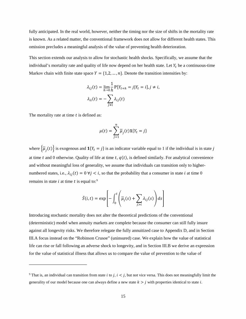
This section extends our analysis to allow for stochastic health shocks. Specifically, we assume that the

individual’s mortality rate and quality of life now depend on her health state. Let 𝑌𝑌𝑡𝑡 be a continuous-time

Markov chain with finite state space 𝑌𝑌 = {1,2, … ,𝑛𝑛}. Denote the transition intensities by:

𝜆𝜆𝑖𝑖𝑖𝑖(𝑡𝑡) = limℎ→0

1ℎℙ[𝑌𝑌𝑡𝑡+ℎ = 𝑗𝑗|𝑌𝑌𝑡𝑡 = 𝑖𝑖], 𝑗𝑗 ≠ 𝑖𝑖,

𝜆𝜆𝑖𝑖𝑖𝑖(𝑡𝑡) = −�𝜆𝜆𝑖𝑖𝑖𝑖(𝑡𝑡)𝑖𝑖≠𝑖𝑖

The mortality rate at time 𝑡𝑡 is defined as:

𝜇𝜇(𝑡𝑡) = �𝜇𝜇𝑖𝑖(𝑡𝑡)𝟏𝟏{𝑌𝑌𝑡𝑡 = 𝑗𝑗}𝑛𝑛

𝑖𝑖=1

where �𝜇𝜇𝑖𝑖(𝑡𝑡)� is exogenous and 𝟏𝟏{𝑌𝑌𝑡𝑡 = 𝑗𝑗} is an indicator variable equal to 1 if the individual is in state 𝑗𝑗

at time 𝑡𝑡 and 0 otherwise. Quality of life at time 𝑡𝑡, 𝑞𝑞(𝑡𝑡), is defined similarly. For analytical convenience

and without meaningful loss of generality, we assume that individuals can transition only to higher-

numbered states, i.e., 𝜆𝜆𝑖𝑖𝑖𝑖(𝑡𝑡) = 0 ∀𝑗𝑗 < 𝑖𝑖, so that the probability that a consumer in state 𝑖𝑖 at time 0

remains in state 𝑖𝑖 at time 𝑡𝑡 is equal to:9

�̃�𝑆(𝑖𝑖, 𝑡𝑡) = exp �−� �𝜇𝜇𝑖𝑖(𝑠𝑠) +�𝜆𝜆𝑖𝑖𝑖𝑖(𝑠𝑠)𝑖𝑖>𝑖𝑖

� 𝑑𝑑𝑠𝑠𝑡𝑡

0�

Introducing stochastic mortality does not alter the theoretical predictions of the conventional

(deterministic) model when annuity markets are complete because the consumer can still fully insure

against all longevity risks. We therefore relegate the fully annuitized case to Appendix D, and in Section

III.A focus instead on the “Robinson Crusoe” (uninsured) case. We explain how the value of statistical

life can rise or fall following an adverse shock to longevity, and in Section III.B we derive an expression

for the value of statistical illness that allows us to compare the value of prevention to the value of

9 That is, an individual can transition from state 𝑖𝑖 to 𝑗𝑗, 𝑖𝑖 < 𝑗𝑗, but not vice versa. This does not meaningfully limit the

generality of our model because one can always define a new state 𝑘𝑘 > 𝑗𝑗 with properties identical to state 𝑖𝑖.

16

treatment. Section III.C incorporates incomplete annuity markets and life-cycle income, and Section III.D

discusses welfare implications.

III.A. The uninsured value of life The consumer’s maximization problem is:

𝑉𝑉(0,𝑊𝑊0,𝑌𝑌0) = max

𝑐𝑐(𝑡𝑡)𝔼𝔼 �� 𝑒𝑒−𝜌𝜌𝑡𝑡𝑆𝑆(𝑡𝑡)𝑢𝑢 �𝑐𝑐(𝑡𝑡), 𝑞𝑞𝑌𝑌𝑡𝑡(𝑡𝑡)�𝑑𝑑𝑡𝑡

𝑇𝑇

0� 𝑌𝑌0,𝑊𝑊0�

(11)

subject to:

𝑊𝑊(0) = 𝑊𝑊0,


= 𝑟𝑟𝑊𝑊(𝑡𝑡) − 𝑐𝑐(𝑡𝑡)

Define the consumer’s objective function at time 𝑡𝑡 as:

𝐽𝐽(𝑡𝑡,𝑊𝑊(𝑡𝑡), 𝑖𝑖) = 𝔼𝔼 �� 𝑒𝑒−𝜌𝜌𝜌𝜌 exp �−� 𝜇𝜇(𝑡𝑡 + 𝑠𝑠)𝑑𝑑𝑠𝑠𝜌𝜌

0�𝑢𝑢�𝑐𝑐(𝑡𝑡 + 𝑢𝑢), 𝑞𝑞𝑌𝑌𝑡𝑡+𝑢𝑢(𝑡𝑡 + 𝑢𝑢)�𝑑𝑑𝑢𝑢

𝑇𝑇−𝑡𝑡

0� 𝑌𝑌𝑡𝑡 = 𝑖𝑖,𝑊𝑊(𝑡𝑡)�

Define the optimal value function as:

𝑉𝑉(𝑡𝑡,𝑊𝑊(𝑡𝑡), 𝑖𝑖) = max𝑐𝑐(𝑠𝑠),𝑠𝑠≥𝑡𝑡

{𝐽𝐽(𝑡𝑡,𝑊𝑊(𝑡𝑡), 𝑖𝑖)}

subject to the wealth dynamics above. Under conventional regularity conditions, if 𝑉𝑉 and its partial

derivatives are continuous, then 𝑉𝑉 satisfies the following Hamilton-Jacobi-Bellman (HJB) system of

equations:

�𝜌𝜌 + 𝜇𝜇𝑖𝑖(𝑡𝑡)� 𝑉𝑉(𝑡𝑡,𝑊𝑊(𝑡𝑡), 𝑖𝑖) = max

𝑐𝑐(𝑡𝑡)�𝑢𝑢�𝑐𝑐(𝑡𝑡), 𝑞𝑞𝑖𝑖(𝑡𝑡)� +

𝜕𝜕𝑉𝑉(𝑡𝑡,𝑊𝑊(𝑡𝑡), 𝑖𝑖)𝜕𝜕𝑊𝑊(𝑡𝑡)

[𝑟𝑟𝑊𝑊(𝑡𝑡) − 𝑐𝑐(𝑡𝑡)] +𝜕𝜕𝑉𝑉(𝑡𝑡,𝑊𝑊(𝑡𝑡), 𝑖𝑖)

𝜕𝜕𝑡𝑡

+ �𝜆𝜆𝑖𝑖𝑖𝑖(𝑡𝑡)[𝑉𝑉(𝑡𝑡,𝑊𝑊(𝑡𝑡), 𝑗𝑗) − 𝑉𝑉(𝑡𝑡,𝑊𝑊(𝑡𝑡), 𝑖𝑖)]𝑖𝑖>𝑖𝑖

� , 𝑖𝑖 = 1, … ,𝑛𝑛

(12)

where 𝑐𝑐(𝑡𝑡) = 𝑐𝑐(𝑡𝑡,𝑊𝑊(𝑡𝑡), 𝑖𝑖) is the (optimal) rate of consumption. In order to apply our value of life

analysis, we exploit recent advances in the systems and control literature. Parpas and Webster (2013)

show that one can reformulate a stochastic finite-horizon optimization problem as a deterministic problem

that takes 𝑉𝑉(𝑡𝑡,𝑊𝑊(𝑡𝑡), 𝑗𝑗), 𝑗𝑗 ≠ 𝑖𝑖, as exogenous. More precisely, we focus on the path of 𝑌𝑌 that begins in

state 𝑖𝑖 and remains in state 𝑖𝑖 until time 𝑇𝑇. We denote optimal consumption and wealth in that path by

17

𝑐𝑐𝑖𝑖(𝑡𝑡) and 𝑊𝑊𝑖𝑖(𝑡𝑡), respectively.10 A key advantage of this method is that it allows us to apply the standard

deterministic Pontryagin maximum principle and derive analytic expressions.

Lemma 1:

Consider the following deterministic optimization problem for 𝑌𝑌0 = 𝑖𝑖 and 𝑊𝑊(0) = 𝑊𝑊0:

𝑉𝑉(0,𝑊𝑊0, 𝑖𝑖) = max

𝑐𝑐𝑖𝑖(𝑡𝑡)�� 𝑒𝑒−𝜌𝜌𝑡𝑡�̃�𝑆(𝑖𝑖, 𝑡𝑡)�𝑢𝑢(𝑐𝑐𝑖𝑖(𝑡𝑡), 𝑞𝑞𝑖𝑖(𝑡𝑡)) + �𝜆𝜆𝑖𝑖𝑖𝑖(𝑡𝑡)𝑉𝑉(𝑡𝑡,𝑊𝑊𝑖𝑖(𝑡𝑡), 𝑗𝑗)

𝑖𝑖>𝑖𝑖

� 𝑑𝑑𝑡𝑡𝑇𝑇

0�

(13)

subject to:

𝑊𝑊𝑖𝑖(0) = 𝑊𝑊0,

𝑊𝑊𝑖𝑖(𝑡𝑡) ≥ 0,𝑊𝑊𝑖𝑖(𝑇𝑇) = 0, 𝜕𝜕𝑊𝑊𝑖𝑖(𝑡𝑡)𝜕𝜕𝑡𝑡

= 𝑟𝑟𝑊𝑊𝑖𝑖(𝑡𝑡) − 𝑐𝑐𝑖𝑖(𝑡𝑡)

where 𝑉𝑉(𝑡𝑡,𝑊𝑊𝑖𝑖(𝑡𝑡), 𝑗𝑗) are taken as exogenous. The optimal value function, 𝑉𝑉(𝑡𝑡,𝑊𝑊𝑖𝑖(𝑡𝑡), 𝑖𝑖), satisfies the HJB

equation given by (12), for all 𝑖𝑖 ∈ {1, … ,𝑛𝑛}.

Proof of Lemma 1: see Appendix A

Because the value function 𝑉𝑉 corresponding to (13) satisfies the HJB equation given by (12), it must also

be equal to the consumer’s optimal value function (see Proposition 3.2.1, Bertsekas (2005)). The present

value Hamiltonian corresponding to (13) is:

𝐻𝐻 �𝑊𝑊𝑖𝑖(𝑡𝑡), 𝑐𝑐𝑖𝑖(𝑡𝑡),𝑝𝑝𝑡𝑡(𝑖𝑖)� = 𝑒𝑒−𝜌𝜌𝑡𝑡�̃�𝑆(𝑖𝑖, 𝑡𝑡)�𝑢𝑢�𝑐𝑐𝑖𝑖(𝑡𝑡), 𝑞𝑞𝑖𝑖(𝑡𝑡)� + �𝜆𝜆𝑖𝑖𝑖𝑖(𝑡𝑡)𝑉𝑉(𝑡𝑡,𝑊𝑊𝑖𝑖(𝑡𝑡), 𝑗𝑗)

𝑖𝑖>𝑖𝑖

�+ 𝑝𝑝𝑡𝑡(𝑖𝑖)[𝑟𝑟𝑊𝑊𝑖𝑖(𝑡𝑡) − 𝑐𝑐𝑖𝑖(𝑡𝑡)]

where 𝑝𝑝𝑡𝑡(𝑖𝑖) is the costate variable for state 𝑖𝑖. The necessary costate equation is:

�̇�𝑝𝑡𝑡

(𝑖𝑖) = −𝜕𝜕𝐻𝐻

𝜕𝜕𝑊𝑊𝑖𝑖(𝑡𝑡)= −𝑝𝑝𝑡𝑡

(𝑖𝑖)𝑟𝑟 − 𝑒𝑒−𝜌𝜌𝑡𝑡�̃�𝑆(𝑖𝑖, 𝑡𝑡)�𝜆𝜆𝑖𝑖𝑖𝑖(𝑡𝑡)𝜕𝜕𝑉𝑉(𝑡𝑡,𝑊𝑊𝑖𝑖(𝑡𝑡), 𝑗𝑗)

𝜕𝜕𝑊𝑊𝑖𝑖(𝑡𝑡)𝑖𝑖>𝑖𝑖

(14)

10 Consumption, 𝑐𝑐(𝑡𝑡), is a stochastic process. We occasionally denote it as 𝑐𝑐(𝑡𝑡,𝑊𝑊(𝑡𝑡),𝑌𝑌𝑡𝑡) to emphasize that it

depends on the states (𝑡𝑡,𝑊𝑊(𝑡𝑡),𝑌𝑌𝑡𝑡). When we reformulate our stochastic problem as a deterministic problem and

focus on a single path 𝑌𝑌𝑡𝑡 = 𝑖𝑖, consumption is no longer stochastic because there is no uncertainty in the development

of health states. We emphasize this point in our notation here by writing consumption as 𝑐𝑐𝑖𝑖(𝑡𝑡), and wealth as 𝑊𝑊𝑖𝑖(𝑡𝑡).

18

The solution to the costate equation can be obtained using the variation of the constant method:

𝑝𝑝𝑡𝑡(𝑖𝑖) = �� 𝑒𝑒(𝑟𝑟−𝜌𝜌)𝑠𝑠�̃�𝑆(𝑖𝑖, 𝑠𝑠)�𝜆𝜆𝑖𝑖𝑖𝑖(𝑠𝑠)

𝜕𝜕𝑉𝑉(𝑠𝑠,𝑊𝑊𝑖𝑖(𝑠𝑠), 𝑗𝑗)𝜕𝜕𝑊𝑊𝑖𝑖(𝑠𝑠)

𝑖𝑖>𝑖𝑖

𝑑𝑑𝑠𝑠𝑇𝑇

𝑡𝑡� 𝑒𝑒−𝑟𝑟𝑡𝑡 + 𝜃𝜃(𝑖𝑖)𝑒𝑒−𝑟𝑟𝑡𝑡

where 𝜃𝜃(𝑖𝑖) > 0 is a constant. The necessary first-order condition for consumption is:

𝑝𝑝𝑡𝑡(𝑖𝑖) = 𝑒𝑒−𝜌𝜌𝑡𝑡�̃�𝑆(𝑖𝑖, 𝑡𝑡)𝑢𝑢𝑐𝑐�𝑐𝑐𝑖𝑖(𝑡𝑡), 𝑞𝑞𝑖𝑖(𝑡𝑡)� (15)

where the marginal utility of wealth at time 𝑡𝑡 = 0 is 𝜕𝜕𝜕𝜕(0,𝑊𝑊0,𝑖𝑖)𝜕𝜕𝑊𝑊0

= 𝑝𝑝0(𝑖𝑖) = 𝑢𝑢𝑐𝑐�𝑐𝑐𝑖𝑖(0),𝑞𝑞𝑖𝑖(0)�. Since the

Hamiltonian is concave in 𝑐𝑐𝑖𝑖(𝑡𝑡) and 𝑊𝑊𝑖𝑖(𝑡𝑡), the necessary conditions for optimality are also sufficient

(Seierstad and Sydsaeter 1977).

To analyze the value of life, we let 𝛿𝛿(𝑡𝑡) be a perturbation on the mortality rate in state 𝑖𝑖 with ∫ 𝛿𝛿(𝑡𝑡)𝑑𝑑𝑡𝑡𝑇𝑇0 =

1 and consider:

�̃�𝑆𝜀𝜀(𝑖𝑖, 𝑡𝑡) = exp �−� �𝜇𝜇𝑖𝑖(𝑠𝑠)− 𝜀𝜀𝛿𝛿(𝑠𝑠)� + �𝜆𝜆𝑖𝑖𝑖𝑖(𝑠𝑠)𝑖𝑖>𝑖𝑖

𝑑𝑑𝑠𝑠𝑡𝑡

0� , where 𝜀𝜀 > 0

We first derive an expression for the effect of this perturbation on expected lifetime utility.

Lemma 2:

The marginal utility of life extension in state 𝑖𝑖 is equal to:


= � �𝑒𝑒−𝜌𝜌𝑡𝑡 �� 𝛿𝛿(𝑠𝑠)𝑑𝑑𝑠𝑠𝑡𝑡

0� �̃�𝑆(𝑖𝑖, 𝑡𝑡)�𝑢𝑢(𝑐𝑐𝑖𝑖(𝑡𝑡), 𝑞𝑞𝑖𝑖(𝑡𝑡)) + �𝜆𝜆𝑖𝑖𝑖𝑖(𝑡𝑡)

𝑖𝑖>𝑖𝑖

𝑉𝑉(𝑡𝑡,𝑊𝑊𝑖𝑖(𝑡𝑡), 𝑗𝑗)��𝑑𝑑𝑡𝑡𝑇𝑇

0


In order to facilitate comparison to the deterministic case, it is useful to derive an expression for the

marginal utility of wealth at time 𝑡𝑡.

Lemma 3:

The expected marginal utility of wealth in state 𝑖𝑖 at time 𝑡𝑡 is equal to:

𝜕𝜕𝑉𝑉(𝑡𝑡,𝑊𝑊𝑖𝑖(𝑡𝑡), 𝑖𝑖)𝜕𝜕𝑊𝑊𝑖𝑖(𝑡𝑡)

= 𝑢𝑢𝑐𝑐�𝑐𝑐𝑖𝑖(𝑡𝑡), 𝑞𝑞𝑖𝑖(𝑡𝑡)�

19

= 𝔼𝔼 �𝑒𝑒(𝑟𝑟−𝜌𝜌)(𝜏𝜏−𝑡𝑡) exp �−� 𝜇𝜇(𝑠𝑠)𝑑𝑑𝑠𝑠𝜏𝜏

𝑡𝑡� 𝑢𝑢𝑐𝑐�𝑐𝑐(𝜏𝜏,𝑊𝑊(𝜏𝜏),𝑌𝑌𝜏𝜏), 𝑞𝑞𝑌𝑌𝜏𝜏(𝜏𝜏)�� 𝑌𝑌𝑡𝑡 = 𝑖𝑖,𝑊𝑊(𝑡𝑡) = 𝑊𝑊𝑖𝑖(𝑡𝑡)� ,∀𝜏𝜏 > 𝑡𝑡


This is the stochastic analogue of the consumer’s first-order condition from Section II.B, and it shows that

the consumer sets the expected discounted marginal utility of consumption at time 𝜏𝜏 > 𝑡𝑡 equal to the

current marginal utility of wealth. Our next result demonstrates that the value of statistical life also takes

the same basic form as in the deterministic case.

Proposition 4:

Set 𝛿𝛿(⋅) in the expression for the marginal utility of life-extension given in Lemma 2 equal to the Dirac

delta function. Dividing the result by the marginal utility of wealth at time 𝑡𝑡 = 0 yields:

𝑉𝑉𝑆𝑆𝑉𝑉(𝑖𝑖) = 𝔼𝔼 �� 𝑒𝑒−𝜌𝜌𝑡𝑡𝑆𝑆(𝑡𝑡)

𝑢𝑢 �𝑐𝑐(𝑡𝑡), 𝑞𝑞𝑌𝑌𝑡𝑡(𝑡𝑡)�

𝑢𝑢𝑐𝑐 �𝑐𝑐(0),𝑞𝑞𝑌𝑌0(0)�𝑑𝑑𝑡𝑡� 𝑌𝑌0 = 𝑖𝑖,𝑊𝑊(0) = 𝑊𝑊0

𝑇𝑇

0� =

𝑉𝑉(0,𝑊𝑊0, 𝑖𝑖)𝑢𝑢𝑐𝑐�𝑐𝑐𝑖𝑖(0), 𝑞𝑞𝑖𝑖(0)�

(16)

Applying Lemma 3 and rearranging yields the following, equivalent expression for VSL in state 𝑖𝑖:

𝑉𝑉𝑆𝑆𝑉𝑉(𝑖𝑖) = � 𝑒𝑒−𝑟𝑟𝑡𝑡𝑣𝑣(𝑖𝑖, 𝑡𝑡)𝑑𝑑𝑡𝑡𝑇𝑇

0

where the value of a life-year, 𝑣𝑣(𝑖𝑖, 𝑡𝑡), is equal to the expected utility of consumption normalized by the

expected marginal utility of consumption:

𝑣𝑣(𝑖𝑖, 𝑡𝑡) =𝔼𝔼 �𝑆𝑆(𝑡𝑡) 𝑢𝑢 �𝑐𝑐(𝑡𝑡),𝑞𝑞𝑌𝑌𝑡𝑡(𝑡𝑡)��𝑌𝑌0 = 𝑖𝑖,𝑊𝑊(0) = 𝑊𝑊0�

𝔼𝔼 �𝑆𝑆(𝑡𝑡) 𝑢𝑢𝑐𝑐 �𝑐𝑐(𝑡𝑡),𝑞𝑞𝑌𝑌𝑡𝑡(𝑡𝑡)��𝑌𝑌0 = 𝑖𝑖,𝑊𝑊(0) = 𝑊𝑊0�

Proof of Proposition 4: see Appendix A

As in the earlier setting with deterministic health (see equation 6), the value of statistical life here is

proportional to expected lifetime utility, and inversely proportional to the marginal utility of consumption.

As we shall show later, an adverse shock to mortality increases current consumption, causing the net

effect on VSL to be ambiguous.

We can derive an expression for the life-cycle profile of consumption from (15), the first-order condition

for consumption. Differentiating with respect to 𝑡𝑡, plugging in the result for the costate equation and its

solution, and rearranging yields:

20

�̇�𝑐𝑖𝑖𝑐𝑐𝑖𝑖

= 𝜎𝜎(𝑟𝑟 − 𝜌𝜌) + 𝜎𝜎𝜂𝜂�̇�𝑞𝑖𝑖𝑞𝑞𝑖𝑖− 𝜎𝜎𝜇𝜇𝑖𝑖(𝑡𝑡) − 𝜎𝜎�𝜆𝜆𝑖𝑖𝑖𝑖(𝑡𝑡) �1 −

𝑢𝑢𝑐𝑐 �𝑐𝑐(𝑡𝑡,𝑊𝑊𝑖𝑖(𝑡𝑡), 𝑗𝑗),𝑞𝑞𝑖𝑖(𝑡𝑡)�

𝑢𝑢𝑐𝑐�𝑐𝑐(𝑡𝑡,𝑊𝑊𝑖𝑖(𝑡𝑡), 𝑖𝑖), 𝑞𝑞𝑖𝑖(𝑡𝑡)��

𝑖𝑖>𝑖𝑖

(17)

As in the deterministic case, the rate of change in consumption is a declining function of the individual’s

current mortality rate, 𝜇𝜇𝑖𝑖(𝑡𝑡): removing annuity markets “pulls consumption earlier” in the life-cycle.

There is also now an additional source of risk, captured by the fourth term in equation (17). This term

represents the possibility that the consumer might transition to a different health state in the future. This

transition would shift life-cycle consumption earlier still if the marginal utility of consumption in those

future states is likely to be low.

Equation (17) describes consumption dynamics conditional on the individual’s health state 𝑖𝑖. It is not

readily apparent from (17) whether modeling health as stochastic causes consumption to shift forward, on

average across all states, relative to modeling health as deterministic. We confirmed in numerical

exercises that modeling health as stochastic has an ambiguous effect on consumption (and VSL), even

when holding quality of life constant across states and time.11

Consumption will jump when an uninsured consumer transitions between health states. The sign of that

jump depends on how the accompanying changes in mortality risk and quality of life jointly affect the

marginal utility of consumption. Because there is no consensus regarding the sign or magnitude of health

state dependence, 𝑢𝑢𝑐𝑐𝑐𝑐(⋅), we hold quality of life constant for the time being and return to this issue in our

empirical analysis.12 Under this assumption, the model predicts that transitioning to a state where current

11 Counterintuitively, modeling health as stochastic has a positive effect on lifetime utility. This positive effect arises

because a stochastic environment allows the consumer to react to health shocks by adjusting consumption. Put

differently, a deterministic model is equivalent to a stochastic model where the consumer must keep consumption

constant across states. Consumers prefer the ability to adjust consumption across states.

12 Viscusi and Evans (1990), Sloan et al. (1998), and Finkelstein, Luttmer, and Notowidigdo (2013) find evidence of

negative state dependence. Lillard and Weiss (1997) and Edwards (2008) find evidence of positive state dependence.

Evans and Viscusi (1991) find no evidence of state dependence. Murphy and Topel (2006) assume negative state

dependence when performing their empirical exercises, while Hall and Jones (2007) assume state independence.

21

and future expected mortality are high will shift consumption forward, and vice versa (see Figure 2). Our

next result proves this formally for a two-state case.13

Proposition 5:

Let there be 𝑛𝑛 = 2 states with identical quality of life profiles, so that 𝑞𝑞1(𝑠𝑠) = 𝑞𝑞2(𝑠𝑠) ∀𝑠𝑠. Assume that the

transition intensities 𝜆𝜆12(𝑠𝑠) are uniformly bounded (finite), and that 𝜇𝜇1(𝑠𝑠) < 𝜇𝜇2(𝑠𝑠) ∀𝑠𝑠, so that state 1 is

“healthy” and state 2 is “sick.” Suppose that the consumer transitions from state 1 to state 2 at time 𝑡𝑡.

Then 𝑐𝑐1(𝑡𝑡,𝑤𝑤, 1) ≤ 𝑐𝑐2(𝑡𝑡,𝑤𝑤, 2),𝑤𝑤 > 0.


It follows immediately from Proposition 5 that the value of near-term life-years will increase, and the

value of distant life-years will decrease, when transitioning from a healthy state with low mortality to a

sick state with higher mortality. Whether VSL rises or falls is ambiguous, however. A rise in mortality

risk lowers lifetime utility, which reduces VSL, but it also reduces the marginal utility of consumption,

which increases VSL. Thus, the net effect depends on the curvature of the utility function relative to the

curvature of the marginal utility function.

We formally demonstrate this tradeoff by again comparing a (persistently) healthy individual to someone

who suffers an adverse shock to life expectancy but is otherwise identical. We know from Proposition 5

that the sick person’s optimal consumption is initially higher. Under what conditions is the sick person’s

VSL also higher? To make headway we must introduce the notion of prudence. The elasticity of

intertemporal substitution, 1/𝜎𝜎, measures utility curvature. Prudence is the analogous measure for the

curvature of marginal utility (Kimball 1990). Define relative prudence as:

𝜋𝜋 ≡ −𝑐𝑐𝑢𝑢𝑐𝑐𝑐𝑐𝑐𝑐(⋅)𝑢𝑢𝑐𝑐𝑐𝑐(⋅)

It will also be convenient to define the elasticity of the flow utility function:

𝜖𝜖 =𝑐𝑐𝑢𝑢𝑐𝑐(⋅)𝑢𝑢(⋅)

13 The proof can be extended to allow for a larger number of states, but the conditions required to sign the jump in

consumption then become a complicated function of the matrix of transition probabilities and state-specific

mortality rates. The two-state case conveys the basic result without a meaningful loss of generality.

22

The utility elasticity, 𝜖𝜖, is positive when utility is positive. Positive utility ensures well-behaved

preferences, and is often enforced by adding a constant to the utility function. (See Section IV.A. for a

related discussion on this point.)

Our next result provides sufficient conditions for VSL to rise following an adverse shock to longevity.

Proposition 6:

Consider a two-state setting with assumptions set out in Proposition 5. Assume further that 𝑟𝑟 ≤ 𝜌𝜌, and

that utility is positive and satisfies the condition:

𝜋𝜋 ≤2𝜎𝜎

+ 𝜖𝜖 (18)

Suppose that the consumer transitions from state 1 to state 2 at time 𝑡𝑡, and that 𝜆𝜆12(𝜏𝜏) = 0 ∀𝜏𝜏 > 𝑡𝑡. Then

𝑉𝑉𝑆𝑆𝑉𝑉(1, 𝑡𝑡) ≤ 𝑉𝑉𝑆𝑆𝑉𝑉(2, 𝑡𝑡).


The assumption 𝑟𝑟 ≤ 𝜌𝜌 is consistent with prior studies on discount and interest rates (Moore and Viscusi

1990).14 VSL will rise following a longevity shock if prudence, 𝜋𝜋, is low relative to the elasticity of

intertemporal substitution, 1/𝜎𝜎. Consumers with inelastic demand (low 𝜎𝜎) prefer to smooth consumption

over time. They therefore have a high willingness to pay for life-extension and are more likely to exhibit a

rise in VSL following an adverse mortality shock. Likewise, consumers with low levels of prudence, 𝜋𝜋,

have near-linear marginal utility that decreases rapidly with consumption. This generates a high

willingness to pay for life-extension following a shock that increases consumption.

The condition (18) specified in Proposition 6 is satisfied by hyperbolic absolute risk aversion (HARA)

utility functions, a class that includes CRRA and quadratic utility, provided that utility is positive.

However, this condition is not innocuous: for example, one can easily find linear combinations of CRRA

and polynomial utility functions where VSL declines following an illness. Prior studies on the value of

life generally assume that 0.5 to 0.8 is a reasonable range for the value of 𝜎𝜎 (Murphy and Topel 2006;

Hall and Jones 2007), and recent empirical studies suggest that 𝜋𝜋 is about 2 (Noussair, Trautmann, and

Van de Kuilen 2013; Christelis et al. forthcoming). Under these parameterizations, condition (18) will

hold whenever utility is positive.

14 The assumption 𝑟𝑟 ≤ 𝜌𝜌 is made for technical convenience: it ensures that the growth rate of consumption is

negative, which facilitates the comparison of VSL across the two states.

23

We emphasize that this result differs from the findings of prior studies that examine the effect of baseline

risk on VSL in a static environment (Weinstein, Shepard, and Pliskin 1980; Pratt and Zeckhauser 1996;

Hammitt 2000). Those studies consider a one-period setting with two states, dead and alive. In this static

setting, if the marginal utility of consumption is lower in the dead state, then an increase in the risk of

death necessarily lowers the expected marginal utility of consumption and thus raises the willingness to

pay for survival (the “dead-anyway” effect).15 Proposition 5 describes how the effect of mortality risk on

marginal utility plays out in a life-cycle model. In this dynamic context, an increase in the risk of death

shifts consumption forward, which does reduce marginal utility. However, unlike in the conventional one-

period setting, the resulting effect on VSL is ambiguous because of an offsetting effect on lifetime utility.

III.B. The value of statistical illness The stochastic model permits us to investigate the value of avoiding transitions to other health states. This

requires only a slight modification to the analysis presented above, and will result in a more general

concept we term the value of statistical illness. With a slight abuse of notation, let state 𝑁𝑁 + 1 correspond

to death, so that 𝑉𝑉(𝑡𝑡,𝑊𝑊(𝑡𝑡),𝑁𝑁 + 1) = 0. Let 𝛿𝛿𝑖𝑖𝑖𝑖(𝑡𝑡), 𝑗𝑗 ≤ 𝑁𝑁, be a perturbation on the transition intensity,

𝜆𝜆𝑖𝑖𝑖𝑖(𝑡𝑡), and let 𝛿𝛿𝑖𝑖,𝑁𝑁+1(𝑡𝑡) be a perturbation on the mortality rate, 𝜇𝜇𝑖𝑖(𝑡𝑡), 𝑖𝑖 ≤ 𝑁𝑁, where ∑ ∫ 𝛿𝛿𝑖𝑖𝑖𝑖(𝑡𝑡)𝑑𝑑𝑡𝑡𝑇𝑇0

𝑁𝑁+1𝑖𝑖=𝑖𝑖+1 =

1, and consider:

�̃�𝑆𝜀𝜀(𝑖𝑖, 𝑡𝑡) = exp �−� �𝜇𝜇𝑖𝑖(𝑠𝑠) − 𝜀𝜀𝛿𝛿𝑖𝑖,𝑁𝑁+1(𝑠𝑠)� + � �𝜆𝜆𝑖𝑖𝑖𝑖(𝑠𝑠) − 𝜀𝜀𝛿𝛿𝑖𝑖𝑖𝑖(𝑠𝑠)�𝑁𝑁

𝑖𝑖=𝑖𝑖+1


0� , where 𝜀𝜀 > 0

Proposition 7:

The marginal utility of preventing an illness or death is given by:

𝜕𝜕𝑉𝑉𝜕𝜕𝜀𝜀�𝜀𝜀=0

= � 𝑒𝑒−𝜌𝜌𝑡𝑡�̃�𝑆(𝑖𝑖, 𝑡𝑡) �� 𝛿𝛿𝑖𝑖𝑖𝑖(𝑠𝑠)𝑖𝑖>𝑖𝑖


0��𝑢𝑢(𝑐𝑐𝑖𝑖(𝑡𝑡),𝑞𝑞𝑖𝑖(𝑡𝑡)) + �𝜆𝜆𝑖𝑖𝑖𝑖(𝑡𝑡)

𝑖𝑖>𝑖𝑖

𝑉𝑉(𝑡𝑡,𝑊𝑊𝑖𝑖(𝑡𝑡), 𝑗𝑗)�−�𝛿𝛿𝑖𝑖𝑖𝑖(𝑡𝑡)𝑖𝑖>𝑖𝑖

𝑉𝑉(𝑡𝑡,𝑊𝑊𝑖𝑖(𝑡𝑡), 𝑗𝑗)� 𝑑𝑑𝑡𝑡𝑇𝑇

0

15 Let expected utility be equal to 𝐸𝐸𝐸𝐸 = 𝑝𝑝𝑢𝑢(0, 𝑐𝑐) + (1 − 𝑝𝑝)𝑢𝑢(1, 𝑐𝑐), where 𝑝𝑝 ∈ (0,1) is the probability of death and

the states {0,1} represent death and life, respectively. The willingness to pay for a marginal reduction in the

probability of dying is given by 𝑉𝑉𝑆𝑆𝑉𝑉 = 𝜌𝜌(1,𝑐𝑐)−𝜌𝜌(0,𝑐𝑐)𝑝𝑝𝜌𝜌𝑐𝑐(0,𝑐𝑐)+(1−𝑝𝑝)𝜌𝜌𝑐𝑐(1,𝑐𝑐)

, which increases with 𝑝𝑝 if 𝑢𝑢𝑐𝑐(1, 𝑐𝑐) > 𝑢𝑢𝑐𝑐(0, 𝑐𝑐). Pratt and

Zeckhauser (1996) also discuss an offsetting “high-payment” effect, which arises when the at-risk individual

increases spending on risk reduction. This reduction in wealth raises her marginal utility and thus lowers VSL.

24


The value of preventing an illness or death is equal to the marginal rate of substitution between the

transition perturbation and wealth:

𝜕𝜕𝑉𝑉/𝜕𝜕𝜀𝜀𝜕𝜕𝑉𝑉/𝜕𝜕𝑊𝑊

�𝜀𝜀=0

= �𝑒𝑒−𝜌𝜌𝑡𝑡�̃�𝑆(𝑖𝑖, 𝑡𝑡)

𝑢𝑢𝑐𝑐�𝑐𝑐𝑖𝑖(0),𝑞𝑞𝑖𝑖(0)�� 𝛿𝛿𝑖𝑖𝑖𝑖(𝑠𝑠)

𝑖𝑖>𝑖𝑖


0��𝑢𝑢(𝑐𝑐𝑖𝑖(𝑡𝑡),𝑞𝑞𝑖𝑖(𝑡𝑡)) + �𝜆𝜆𝑖𝑖𝑖𝑖(𝑡𝑡)

𝑖𝑖>𝑖𝑖

𝑉𝑉(𝑡𝑡,𝑊𝑊𝑖𝑖(𝑡𝑡), 𝑗𝑗)�−�𝛿𝛿𝑖𝑖𝑖𝑖(𝑡𝑡)𝑖𝑖>𝑖𝑖

𝑉𝑉(𝑡𝑡,𝑊𝑊𝑖𝑖(𝑡𝑡), 𝑗𝑗)� 𝑑𝑑𝑡𝑡𝑇𝑇

0

As before, it is helpful to choose the Dirac delta function for 𝛿𝛿(⋅), so that the intensities are perturbed at

𝑡𝑡 = 0 and remain unaffected otherwise. It is also helpful to consider a reduction in the transition

probability for only one alternative state, 𝑗𝑗, so that 𝛿𝛿𝑖𝑖𝑖𝑖(𝑡𝑡) = 0 ∀𝑘𝑘 ≠ 𝑗𝑗. Applying these two conditions then

yields what we term the value of statistical illness, 𝑉𝑉𝑆𝑆𝑉𝑉(𝑖𝑖, 𝑗𝑗):

𝑉𝑉𝑆𝑆𝑉𝑉(𝑖𝑖, 𝑗𝑗) =

𝑉𝑉(0,𝑊𝑊0, 𝑖𝑖) − 𝑉𝑉(0,𝑊𝑊0, 𝑗𝑗)𝑢𝑢𝑐𝑐�𝑐𝑐𝑖𝑖(0), 𝑞𝑞𝑖𝑖(0)�

= 𝑉𝑉𝑆𝑆𝑉𝑉(𝑖𝑖) − 𝑉𝑉𝑆𝑆𝑉𝑉(𝑗𝑗)𝑢𝑢𝑐𝑐 �𝑐𝑐𝑖𝑖(0), 𝑞𝑞𝑖𝑖(0)�

𝑢𝑢𝑐𝑐�𝑐𝑐𝑖𝑖(0),𝑞𝑞𝑖𝑖(0)�

(19)

The interpretation of VSI is analogous to VSL: it is the amount that 1,000 individuals are collectively

willing to pay in order to eliminate a current disease risk that is expected to befall one of them. Note that

if health state 𝑗𝑗 corresponds to death, so that 𝑉𝑉𝑆𝑆𝑉𝑉(𝑗𝑗) = 𝑉𝑉𝑆𝑆𝑉𝑉(𝑁𝑁 + 1) = 0, then 𝑉𝑉𝑆𝑆𝑉𝑉(𝑖𝑖, 𝑗𝑗) = 𝑉𝑉𝑆𝑆𝑉𝑉(𝑖𝑖). Thus,

VSI is a generalization of VSL.

It is instructive to compare VSI for the uninsured consumer, given in (19), to VSI for a fully annuitized

consumer, which we denote as 𝑉𝑉𝑆𝑆𝑉𝑉∗:16

𝑉𝑉𝑆𝑆𝑉𝑉∗(𝑖𝑖, 𝑗𝑗) = 𝑉𝑉𝑆𝑆𝑉𝑉∗(𝑖𝑖) − 𝑉𝑉𝑆𝑆𝑉𝑉∗(𝑗𝑗) (20)

Under full annuitization, the value of a life-year is equal across health states (holding quality of life

constant). As shown by equation (20), this implies that prevention and treatment are equally valuable, as

16 The value of the consumer’s annuity depends on the health state. If she purchases an annuity in state 𝑖𝑖 and then

later transitions to a worse health state 𝑗𝑗, causing her life expectancy to fall, then the value of her annuity will also

fall, an effect not reflected in the notation used in equation (20). See equation (D8) and accompanying discussion in

Appendix D.

25

long as they add the same number of expected life-years.17 In other words, full annuitization justifies the

common cost-effectiveness practice of equating the values of prevention and treatment (Drummond et al.

2015).

In contrast, equation (19) shows that eliminating annuity markets breaks this equivalence between

treatment and prevention. VSI in this case is not equal to the simple difference in VSL between the

healthy and sick states, because VSL in the sick state is valued from the perspective of the sick, who are

likely to have a lower marginal utility of consumption due to their shorter life span. This leads to the

natural hypothesis that whenever VSL rises following an illness, the value of treatments (VSL per life-

year) will be higher than equivalent preventive care consumed prior to the illness (VSI per life-year). It is

simple to prove this for the case where the illness reduces life expectancy by one-half or more (see

Proposition 8 in Appendix A), and our numerical exercises suggest that the hypothesis is true under far

more general conditions. Our empirical exercises find that, under reasonable parameterizations, the value

of treatment is higher than the value of prevention for a number of different diseases.

To summarize, the uninsured stochastic model yields the following implications:

• All else equal, when an individual transitions to a higher mortality state, near-term life-years rise

in value, and distant life-years fall in value.

• The value of statistical life may rise or fall when an individual transitions to a higher mortality

state. If the individual’s demand is sufficiently inelastic, or if the individual is insufficiently

prudent, then VSL will rise.

• Therapies that increase survival by treating sick patients are not generally worth the same as

preventives that add the same amount of life expectancy for healthy patients. If the disease causes

VSL to rise, then we expect treatment to be worth more than equally effective preventive care.

III.C. The incompletely annuitized value of life We now introduce a one-time opportunity to purchase a flat lifetime annuity, and also endow the

consumer with state-dependent life-cycle income, 𝑚𝑚𝑌𝑌𝑡𝑡(𝑡𝑡). Recall that we previously solved the

consumer’s problem for each state 𝑖𝑖 by focusing on the path of 𝑌𝑌 that begins in state 𝑖𝑖 and remains in state

𝑖𝑖 until time 𝑇𝑇 (Parpas and Webster 2013). Incomplete annuity markets and life-cycle income complicate

17 Consistent with our model, Rheinberger, Herrera-Araujo, and Hammitt (2016) point out that prevention can be

more valuable (ex ante) than treatment for a highly lethal, but rare, disease, because a disease-specific mortality

reduction in this case has a much smaller effect on total life-years gained than a reduction in disease incidence.

26

our analysis by introducing the possibility of multiple sets of non-interior solutions within and across

different states. For convenience, we focus here on the case where there is a single set of non-interior

solutions in each state. In particular, we follow Section II.C and consider the case where, conditional on

remaining in the same state, consumption decreases with age and eventually converges to the consumer’s

annuity income (e.g., left panel in Appendix Figure A1). This occurs if, for example, the consumer has a

constant income across and within states, has a mortality rate profile in that state that obeys the condition

𝜇𝜇𝑖𝑖(𝑡𝑡) ≥ 𝑟𝑟 − 𝜌𝜌 + 𝜂𝜂 𝑐𝑐�̇�𝚤𝑐𝑐𝑖𝑖

, and cannot transition to a healthier state.18

Borrowing an approach from Reichling and Smetters (2015), we assume the consumer has an option at

time zero to purchase a flat lifetime annuity that pays out 𝑚𝑚𝑌𝑌0 ≥ 0 in all health states and that has a price

markup of 𝜉𝜉 ≥ 0. The consumer cannot finance the purchase of the annuity using future income, and she

cannot purchase or sell annuities after time zero. The consumer’s maximization problem is:

𝑉𝑉(0,𝑊𝑊0,𝑌𝑌0) = max𝑐𝑐(𝑡𝑡),𝑚𝑚𝑌𝑌0

𝔼𝔼 �� 𝑒𝑒−𝜌𝜌𝑡𝑡𝑆𝑆(𝑡𝑡)𝑢𝑢 �𝑐𝑐(𝑡𝑡), 𝑞𝑞𝑌𝑌𝑡𝑡(𝑡𝑡)� 𝑑𝑑𝑡𝑡𝑇𝑇

0� 𝑌𝑌0,𝑊𝑊0�

subject to:

𝑊𝑊(0) = 𝑊𝑊0 − (1 + 𝜉𝜉)𝑚𝑚𝑌𝑌0 𝔼𝔼 �� 𝑒𝑒−𝑟𝑟𝑡𝑡𝑆𝑆(𝑡𝑡)𝑑𝑑𝑡𝑡𝑇𝑇

0� 𝑌𝑌0 = 𝑖𝑖� ,


= 𝑟𝑟𝑊𝑊(𝑡𝑡) + 𝑚𝑚𝑌𝑌𝑡𝑡(𝑡𝑡) + 𝑚𝑚𝑌𝑌0 − 𝑐𝑐(𝑡𝑡)

The optimal annuity amount is chosen in the consumer’s initial state, 𝑌𝑌0, and its value may change

following a transition to a new health state because a fixed payout is worth more to a person with higher

life expectancy. We emphasize this in our notation below by writing 𝑉𝑉 as a function of the optimally

chosen annuity and remaining wealth. In addition, it is helpful to define the value of a one-dollar annuity

at time 𝑡𝑡 in state 𝑖𝑖 as:

18 More precisely, we are interested in studying the case where 𝑐𝑐�̇�𝑖𝑐𝑐𝑖𝑖≤ 0 ∀𝑖𝑖. From equation (17), this occurs when

𝜇𝜇𝑖𝑖(𝑡𝑡) ≥ 𝑟𝑟 − 𝜌𝜌 + 𝜂𝜂 �̇�𝑐𝑖𝑖𝑐𝑐𝑖𝑖− ∑ 𝜆𝜆𝑖𝑖𝑖𝑖(𝑡𝑡) �1 −

𝜌𝜌𝑐𝑐�𝑐𝑐(𝑡𝑡,𝑊𝑊𝑖𝑖(𝑡𝑡),𝑖𝑖),𝑐𝑐𝑗𝑗(𝑡𝑡)�

𝜌𝜌𝑐𝑐�𝑐𝑐(𝑡𝑡,𝑊𝑊𝑖𝑖(𝑡𝑡),𝑖𝑖),𝑐𝑐𝑖𝑖(𝑡𝑡)��𝑖𝑖>𝑖𝑖 . The fourth term is negative if, for example, quality of

life is constant and the consumer can only transition to states with higher mortality, as in Proposition 5.

27

𝑎𝑎(𝑡𝑡, 𝑖𝑖) = 𝔼𝔼 �� 𝑒𝑒−𝑟𝑟(𝑠𝑠−𝑡𝑡) exp �−� 𝜇𝜇(𝑢𝑢)𝑑𝑑𝑢𝑢𝑠𝑠

𝑡𝑡� 𝑑𝑑𝑠𝑠

𝑇𝑇

t� 𝑌𝑌𝑡𝑡 = 𝑖𝑖�

Proposition 9:

The value of statistical life in state 𝑖𝑖 is equal to:

𝑉𝑉𝑆𝑆𝑉𝑉(𝑖𝑖) =

𝑉𝑉(0,𝑊𝑊𝑖𝑖(0),𝑚𝑚𝑖𝑖, 𝑖𝑖)𝑢𝑢𝑐𝑐�𝑐𝑐𝑖𝑖(0),𝑞𝑞𝑖𝑖(0)�

− (1 + 𝜉𝜉) 𝑚𝑚𝑖𝑖 𝑎𝑎(0, 𝑖𝑖) (21)


As in the deterministic case given by equation (10), the expression for the partially annuitized value of

life here captures elements of both the uninsured and fully insured cases. When annuities are absent

(𝑚𝑚𝑖𝑖 = 0), equation (21) simplifies to the uninsured case given by equation (16). Similarly, full

annuitization is optimal when 𝜉𝜉 = 0, 𝑟𝑟 = 𝜌𝜌, and quality of life and future income are constant, in which

case equation (21) simplifies to the complete markets case given by equation (D7) in Appendix D.19

Finally, the value of statistical illness under partial annuitization again takes an intermediate form.

Corollary 10:

The value of a marginal reduction in the risk of transitioning from state 𝑖𝑖 to state 𝑗𝑗 is equal to:

𝑉𝑉𝑆𝑆𝑉𝑉(𝑖𝑖, 𝑗𝑗) = �𝑉𝑉(0,𝑊𝑊𝑖𝑖(0),𝑚𝑚𝑖𝑖, 𝑖𝑖)𝑢𝑢𝑐𝑐�𝑐𝑐𝑖𝑖(0),𝑞𝑞𝑖𝑖(0)�

− (1 + 𝜉𝜉)𝑎𝑎(0, 𝑖𝑖)𝑚𝑚𝑖𝑖� − �𝑉𝑉(0,𝑊𝑊𝑖𝑖(0),𝑚𝑚𝑖𝑖, 𝑗𝑗)𝑢𝑢𝑐𝑐�𝑐𝑐𝑖𝑖(0),𝑞𝑞𝑖𝑖(0)�

− (1 + 𝜉𝜉)𝑎𝑎(0, 𝑗𝑗)𝑚𝑚𝑖𝑖�

= 𝑉𝑉𝑆𝑆𝑉𝑉(𝑖𝑖) − �𝑉𝑉(0,𝑊𝑊𝑖𝑖(0),𝑚𝑚𝑖𝑖, 𝑗𝑗)𝑢𝑢𝑐𝑐�𝑐𝑐𝑖𝑖(0),𝑞𝑞𝑖𝑖(0)�

− (1 + 𝜉𝜉) 𝑎𝑎(0, 𝑗𝑗) 𝑚𝑚𝑖𝑖�

Proof of Corollary 10: see Appendix A

VSI is again not exactly equal to the difference in VSL between the two health states. One reason why is

because, as in the uninsured case, the utility of state 𝑗𝑗 is valued from the perspective (marginal utility) of

state 𝑖𝑖. A second reason is because the flat annuity was purchased in state 𝑖𝑖, and the size of this annuity

may differ from the optimal flat annuity that would have been purchased in state 𝑗𝑗.

To summarize, combining stochastic health with incomplete annuity markets has the following effects:

19 Remaining wealth at time 𝑡𝑡 = 0, 𝑊𝑊(0), is zero upon full annuitization. This implies 𝑊𝑊0 = (1 + 𝜉𝜉) 𝑚𝑚𝑖𝑖 𝑎𝑎(0, 𝑖𝑖).

28

• As in the deterministic model, the optimal level of annuitization is partial except for certain

special cases.

• The insights from Sections III.A and III.B continue to hold when annuitization is partial. In

particular, the value of statistical life may in general rise or fall following a mortality shock, and

treatment and prevention are not valued equally.20

III.D. Welfare Our stochastic model describes a person’s willingness to pay to extend life and shows how it changes ex

post following a health shock. This model generates several positive predictions. It helps explain why the

value of life-extension varies considerably with a person’s health state and why people value prevention

and treatment differently, even when both generate the same gain in life expectancy. The normative

implications depend on how one resolves several longstanding controversies in the theoretical literature

on welfare economics.

Aggregate social surplus remains the most widely used welfare criterion in applied microeconomics,

including within the literature on life-extension. Murphy and Topel (2006) employ this principle in the

framework of the standard life-cycle VSL model. Garber and Phelps (1997) rely on it to develop the

theory of cost-effectiveness for health interventions. Einav, Finkelstein, and Cullen (2010) use it to study

the welfare effects of health insurance. More generally, industrial organization economists use it, in the

form of deadweight loss, to evaluate the welfare consequences of market power (Martin 2019).

However, the aggregate surplus approach has several shortcomings (Boadway 1974; Blackorby and

Donaldson 1990). Each dollar of consumer or producer surplus is weighted equally, regardless of its

owner, which raises equity concerns. Aggregation can produce intransitive rankings of alternative

allocations. Heterogeneity in marginal utility can break the link between surplus and utility (Martin 2019).

Since part of the ex post variation in VSL following a health shock is driven by changes in marginal

utility, the surplus approach may result in misleading normative implications when applied to our setting.

A social welfare approach, by contrast, aggregates utilities rather than surplus. But debate persists about

how to apply this approach under uncertainty, where the ex ante and ex post perspectives of a consumer

20 Under the conditions outlined in Proposition 5, consumption will always increase following a mortality shock

provided the consumer is not fully annuitized. Whether there is an accompanying rise in VSL will in general depend

on the degree of annuitization in addition to the usual conditions outlined in Proposition 6. We show in Appendix D

that VSL always declines following a mortality shock when the consumer is fully annuitized.

29

might differ (Fleurbaey 2010). In a foundational study, Harsanyi (1955) shows that a social welfare

function satisfying both rationality and the Pareto principle must be a weighted sum of ex ante individual

utilities. However, this utilitarian approach ignores distributional concerns (Diamond 1967). As a result,

one cannot simultaneously satisfy both rationality and the Pareto principle while still pursuing equity.

Theorists have argued for abandoning one or the other of these principles. Diamond (1967) advocates

minimizing ex ante inequality, but this violates rationality. Adler and Sanchirico (2006) advocate

minimizing ex post inequality, but this violates the Pareto principle. In the specific context of VSL, Pratt

and Zeckhauser (1996) advocate maximizing ex ante utility, but this ignores equity concerns in light of

Diamond’s result.

Given the inevitable trade-offs, we do not aim to defend one or another specific welfare perspective.

When quantifying the value of statistical life under uncertainty (Section IV.B), we focus on positive

implications only, e.g., explaining why there is less observed investment in prevention than treatment.

When evaluating the effects of retiree programs on the value of life (Section IV.C), we employ a

deterministic model and pursue an aggregate surplus approach. A deterministic setting avoids the need to

model welfare under uncertainty and allows for a straightforward comparison to prior work (Murphy and

Topel 2006).

As a practical matter, health policymakers and analysts frequently evaluate policy using cost-benefit

analysis (CBA), which equates social welfare with aggregate social surplus (Viscusi 1992). It is therefore

worth briefly mentioning the implications of our stochastic model for CBA, in spite of CBA’s well-

documented shortcomings. CBA is equivalent to a utilitarian approach where all individuals’ utilities are

weighted by the inverse of their marginal utilities of consumption. We showed previously that when

annuity markets are incomplete, the marginal utility of consumption is lower for people with short life

expectancies. Thus, the incomplete annuities framework causes CBA to place more weight on the sick,

which some scholars have advocated (Adler, Hammitt, and Treich 2014).21

21 A special case of CBA, cost-effectiveness analysis, is widely used for studying the optimal allocation of

healthcare resources. The traditional cost-effectiveness framework presumes that the value of a “quality-adjusted

life-year” is independent of health state. Our model suggests that it should instead vary with the health state of the

individuals responsible for financing health care.

30

IV. QUANTITATIVE ANALYSIS This section demonstrates how the value of statistical life depends on an individual’s health history and

illustrates that, under typical consumer preferences, the willingness to pay for treatment exceeds the

willingness to pay for prevention. We also measure the aggregate value of gains to health and longevity

and how that value depends on the level of annuitization.

Our empirical framework, which incorporates survival and health status uncertainty into a life-cycle

model, is related to a number of papers that study the savings behavior of the elderly (Kotlikoff 1988;

Palumbo 1999; De Nardi, French, and Jones 2010). These prior studies allow health to affect wealth

accumulation by including two or three different health states in the model. By contrast, we allow

mortality, medical spending, and quality of life to vary across 20 different health states.

IV.A. Framework We employ the discrete time analogue of our stochastic theoretical model. There are 𝑛𝑛 health states.

Denote the transition probabilities between health states by:

𝑝𝑝𝑖𝑖𝑖𝑖(𝑡𝑡) = ℙ[𝑌𝑌𝑡𝑡+1 = 𝑗𝑗|𝑌𝑌𝑡𝑡 = 𝑖𝑖]

The mortality rate at time 𝑡𝑡, 𝑑𝑑(𝑡𝑡), depends on the individual’s health state:

𝑑𝑑(𝑡𝑡) = �𝑑𝑑𝑖𝑖(𝑡𝑡)𝟏𝟏{𝑌𝑌𝑡𝑡 = 𝑗𝑗}𝑛𝑛

𝑖𝑖=1

where �𝑑𝑑𝑖𝑖(𝑡𝑡)� are given and 𝟏𝟏{𝑌𝑌𝑡𝑡 = 𝑗𝑗} is an indicator equal to 1 if the individual is in state 𝑗𝑗 at time 𝑡𝑡 and

0 otherwise. The probability of surviving from time period 𝑡𝑡 to time period 𝑠𝑠 is denoted as 𝑆𝑆𝑡𝑡(𝑠𝑠), where:

𝑆𝑆𝑡𝑡(𝑡𝑡) = 1,

𝑆𝑆𝑡𝑡(𝑠𝑠) = 𝑆𝑆𝑡𝑡(𝑠𝑠 − 1)�1 − 𝑑𝑑(𝑠𝑠 − 1)�, 𝑠𝑠 > 𝑡𝑡

The survival probability is stochastic because it depends on the individual’s health history. Let 𝑐𝑐(𝑡𝑡) and

𝑊𝑊(𝑡𝑡) denote consumption and wealth in period 𝑡𝑡, respectively. The individual’s health state at time 𝑡𝑡, 𝑌𝑌𝑡𝑡,

determines her quality of life, 𝑞𝑞𝑌𝑌𝑡𝑡(𝑡𝑡). Let 𝜌𝜌 denote the rate of time preference, and 𝑟𝑟 the interest rate.

Assume that in each period the consumer receives exogenous income, 𝑦𝑦(𝑡𝑡), and that the maximum

lifespan of a consumer is 𝑇𝑇 (i.e., 𝑑𝑑(𝑇𝑇) = 1). Our baseline model assumes there is no bequest motive,

although we relax this assumption in later exercises.

The consumer’s maximization problem is:

31

max𝑐𝑐(𝑡𝑡)

𝔼𝔼 ��𝑒𝑒−𝜌𝜌𝑡𝑡𝑆𝑆0(𝑡𝑡)𝑢𝑢 �𝑐𝑐(𝑡𝑡), 𝑞𝑞𝑌𝑌𝑡𝑡(𝑡𝑡)�𝑇𝑇

𝑡𝑡=0

� 𝑌𝑌0,𝑊𝑊0�

subject to:

𝑊𝑊(0) = 𝑊𝑊0,

𝑊𝑊(𝑡𝑡) ≥ 0,

𝑊𝑊(𝑡𝑡 + 1) = �𝑊𝑊(𝑡𝑡) + 𝑦𝑦(𝑡𝑡) − 𝑐𝑐(𝑡𝑡)�𝑒𝑒𝑟𝑟

The individual’s period income is equal to 𝑦𝑦(𝑡𝑡) = (1 − 𝜏𝜏)𝑚𝑚(𝑡𝑡) + 𝑎𝑎(𝑡𝑡), where 𝑎𝑎(𝑡𝑡) is nonwage defined-

benefit income financed by an actuarially fair earnings tax, 𝜏𝜏. We choose the individual’s labor earnings,

𝑚𝑚(𝑡𝑡), to fit data on average life-cycle earnings as estimated by the Current Population Survey and the

Health and Retirement Study (see Appendix B1 for details). Our retirement policy exercises, described in

detail later, consider different levels of generosity for 𝑎𝑎(𝑡𝑡).

Unless stated otherwise, we assume that 𝑟𝑟 = 𝜌𝜌 = 0.03 (Siegel 1992; Moore and Viscusi 1990). Finally,

we follow Murphy and Topel (2006) and assume that utility takes the following CRRA form:

𝑢𝑢(𝑐𝑐, 𝑞𝑞) = 𝑞𝑞𝑢𝑢(𝑐𝑐) = 𝑞𝑞 �

𝑐𝑐1−𝛾𝛾 − 𝑐𝑐1−𝛾𝛾

1 − 𝛾𝛾 � (22)

As discussed in Section III, there is no consensus regarding the sign or magnitude of health state

dependence (𝑢𝑢𝑐𝑐𝑐𝑐(⋅)). Here, we assume a multiplicative relationship where the marginal utility of

consumption is higher when quality of life is high, and vice versa.

Quality of life, 𝑞𝑞, is an index that ranges from 0 to 1, where 𝑞𝑞 = 1 indexes perfect health. We have

normalized the utility of death to zero in (22). A consumer receives positive utility if she consumes an

amount greater than 𝑐𝑐, which represents a subsistence level of consumption. Consuming an amount less

than 𝑐𝑐 generates utility that is worse than death. Although adding a constant to the utility function does

not affect the solution to the consumer’s maximization problem, this constant matters for the value of

life.22 We are unaware of any empirical evidence on the magnitude of 𝑐𝑐, the subsistence level of

consumption in the United States. We assume it is equal to $5,000, which is in line with the

parameterization employed in Murphy and Topel (2006).

22 Rosen (1988) was the first to point out that the level of utility is an important determinant of the value of life. See

also additional discussion on this point in Hall and Jones (2007) and Córdoba and Ripoll (2016).

32

The parameter 𝛾𝛾 is the inverse of the elasticity of intertemporal substitution, an important determinant of

both the value of life and the value of annuitization. We follow Hall and Jones (2007) and set 𝛾𝛾 = 2 in

our main specification.

We employ dynamic programming techniques to solve for the optimal consumption path. The value

function is defined as:

𝑉𝑉(𝑡𝑡,𝑤𝑤, 𝑖𝑖) = max𝑐𝑐(𝑡𝑡)

𝔼𝔼 ��𝑒𝑒−𝜌𝜌(𝑠𝑠−𝑡𝑡)𝑆𝑆𝑡𝑡(𝑠𝑠)𝑢𝑢(𝑐𝑐(𝑠𝑠), 𝑞𝑞𝑖𝑖(𝑠𝑠))𝑇𝑇

𝑠𝑠=𝑡𝑡

� 𝑌𝑌𝑡𝑡 = 𝑖𝑖,𝑊𝑊(𝑡𝑡) = 𝑤𝑤�

We then reformulate the optimization problem as a recursive Bellman equation:

𝑉𝑉(𝑡𝑡,𝑤𝑤, 𝑖𝑖) = max𝑐𝑐(𝑡𝑡)

� 𝑢𝑢�𝑐𝑐(𝑡𝑡)� +1 − 𝑑𝑑𝑖𝑖(𝑡𝑡)

𝑒𝑒𝜌𝜌�𝑝𝑝𝑖𝑖𝑖𝑖(𝑡𝑡)𝑉𝑉(𝑡𝑡 + 1, �𝑤𝑤 + 𝑦𝑦(𝑡𝑡) − 𝑐𝑐(𝑡𝑡)�𝑒𝑒𝑟𝑟, 𝑗𝑗)𝑁𝑁

𝑖𝑖=1

�

After solving for the optimal consumption path, we use the analytical formulas derived in the previous

sections to calculate the value of life. We provide complete details in Appendix C.

There is significant uncertainty among economists regarding the proper values of many of the parameters

in our model. The goal of the subsequent analyses is to illustrate the economic significance of our insights

when applying our model to data using reasonable parameterizations. In some analyses, we investigate the

sensitivity of our results to alternative assumptions regarding the elasticity of intertemporal substitution,

1/𝛾𝛾, and to the presence of a bequest motive. While the value of 𝛾𝛾 matters greatly for the magnitude of

VSL, it does not have any qualitative effect on our findings regarding the relative determinants of VSL.

The remainder of this section reports results from two separate empirical exercises. The first exercise

illustrates the novel implications of our framework by showing that the value of treatment generally

exceeds the value of prevention and that the value of statistical life can increase following a health shock.

The second exercise illustrates the effect of different annuitization schemes on the aggregate value of

improvements in longevity. All code and data underlying these exercises are publicly available online.23

IV.B. The value of life when health is stochastic This section applies our stochastic life-cycle model to real-world data on mortality and quality of life that

vary according to a person’s health state. Later exercises further incorporate medical spending that varies

23 See http://julianreif.com/research/mortality_risk_replication.zip.

33

by health state. We interpret our estimates here as the private value of statistical life, i.e., the individual’s

willingness to pay for life-extension and disease prevention.

The data for this set of exercises are provided by the Future Elderly Model (FEM), a widely published

microsimulation model that employs comprehensive, nationally representative data from a wide array of

sources (see Appendix B2). The model, which has been released into the public domain, produces

estimates of mortality, disease incidence, quality of life, and medical spending at the individual level for

people over the age of 50 with different comorbid conditions. The FEM accounts for six different chronic

conditions (cancer, diabetes, heart disease, hypertension, chronic lung disease, and stroke) and six

different impaired activities of daily living (bathing, eating, dressing, walking, getting into or out of bed,

and using the toilet). The FEM provides us with a well-validated tool that combines information from the

Health and Retirement Study (HRS), the Medical Expenditure Panel Survey (MEPS), the Panel Study of

Income Dynamics, and the National Health Interview Survey. This combination provides a number of

advantages. For instance, while the HRS possesses a uniquely rich set of covariates on health and wealth,

it lacks survey questions that would allow us to calculate quality of life using validated survey

instruments. To solve this problem, the FEM weaves together validated quality of life estimates from the

MEPS and maps them to the HRS using variables common to both databases.

We divide the health space within the FEM into 𝑛𝑛 = 20 states. Each state corresponds to the number (0,

1, 2, 3 or more) of impaired activities of daily living (ADL) and the number (0, 1, 2, 3, 4 or more) of

chronic conditions, for a total of 4 × 5 = 20 health states. Health states are ordered first by number of

ADLs and then by number of chronic diseases, so that state 1 corresponds to 0 ADLs and 0 chronic

conditions, state 2 corresponds to 0 ADLs and 1 chronic condition, and so on. This aggregation provides a

parsimonious way of incorporating information about functional status and several major diseases.24 For

each health state and age, the FEM estimates the probability of dying and the probability of transitioning

to each of the other health states in the next year. As in the theoretical model, individuals can transition

only to higher-numbered states, i.e., 𝑝𝑝𝑖𝑖𝑖𝑖(𝑡𝑡) = 0 ∀𝑗𝑗 < 𝑖𝑖. In other words, all ADLs and chronic conditions

are permanent. The FEM also estimates quality of life for each health state and age, as measured by the

EuroQol five dimensions questionnaire (EQ-5D). These five dimensions are based on five survey

questions that elicit the extent of a respondent’s problems with mobility, self-care, daily activities, pain,

24 While fully interacting all these variables would provide a more granular state space, it would also result in a very

large number of possible states and correspondingly small cell sizes within many of them.

34

and anxiety/depression. These questions are then weighted using stated preference data to compute the

relative importance of each.25 The result is a single quality of life measure, the EQ-5D, typically reported

on a scale from zero to one.

Table 1 presents descriptive statistics for the data provided by the FEM. Initial life expectancy at age 50

ranges from 30.4 years for a healthy individual in state 1 to 8.6 years for an ill individual in state 20.

Quality of life, as measured by the EQ-5D, ranges from 0.54 to 0.88 at age 50. Columns (7) and (8) of

Table 1 report the probability that an individual exits her health state but remains alive, i.e., acquires at

least one new ADL or chronic condition within the following year. Health states are relatively persistent,

with exit rates never exceeding 15 percent. State 20 is an absorbing state with an exit rate of 0 percent.

We set wealth equal to $862,947 and provide all of it to the individual at baseline (age 50). This value is

approximately equal to the net present value of future earnings at age 50 plus savings at that age, as

estimated by the retirement policy model we employ in Section IV.C (see Appendix C3). We also assume

annuity markets are absent. These two simplifications allow us to calculate the effect of stochastic health

shocks on the value of life using an analytical solution to the consumer’s problem (see Appendix C2).26

This analytical solution avoids numerical precision error and speeds up calculations, which is especially

useful when performing the Monte Carlo simulations described below. We consider partial annuitization

scenarios and allow for life-cycle income in the numerical model presented in the next section.

VSL in our baseline scenario for a healthy 50-year old in health state 1 is $5.4 million, which is within the

range estimated by empirical studies of VSL for working-age individuals (see O'Brien 2018 for a recent

review).

IV.B.1 The value of prevention We begin by calculating the value of statistical illness (VSI) for different diseases. Column (4) of Table 2

reports VSI at age 50 from the perspective of a healthy individual. Each value represents the healthy

25 The five dimensions of the EQ-5D are weighted using estimates from Shaw, Johnson, and Coons (2005). The

specific process for estimating the quality of life score is explained in the FEM technical documentation, which can

be found in the supplemental information appendix of Agus et al. (2016). The methods used to measure the quality

of life are consistent with our assumed utility specification, given in (22).

26 It is possible (and available upon request) to incorporate partial annuitization in this setting along the lines

discussed in Section III.C. Further generalization requires numerical optimization, which likely would necessitate

significantly limiting the number of health states included in the model.

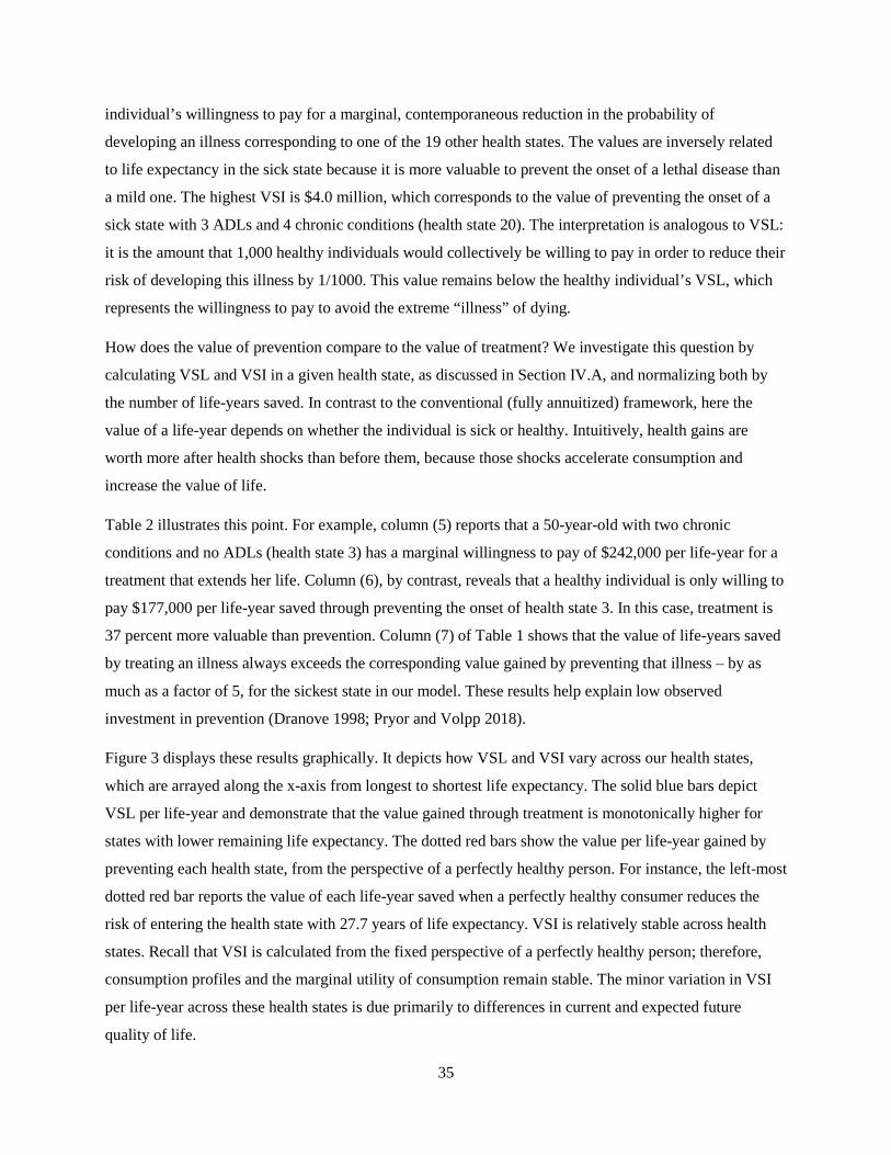
35

individual’s willingness to pay for a marginal, contemporaneous reduction in the probability of

developing an illness corresponding to one of the 19 other health states. The values are inversely related

to life expectancy in the sick state because it is more valuable to prevent the onset of a lethal disease than

a mild one. The highest VSI is $4.0 million, which corresponds to the value of preventing the onset of a

sick state with 3 ADLs and 4 chronic conditions (health state 20). The interpretation is analogous to VSL:

it is the amount that 1,000 healthy individuals would collectively be willing to pay in order to reduce their

risk of developing this illness by 1/1000. This value remains below the healthy individual’s VSL, which

represents the willingness to pay to avoid the extreme “illness” of dying.

How does the value of prevention compare to the value of treatment? We investigate this question by

calculating VSL and VSI in a given health state, as discussed in Section IV.A, and normalizing both by

the number of life-years saved. In contrast to the conventional (fully annuitized) framework, here the

value of a life-year depends on whether the individual is sick or healthy. Intuitively, health gains are

worth more after health shocks than before them, because those shocks accelerate consumption and

increase the value of life.

Table 2 illustrates this point. For example, column (5) reports that a 50-year-old with two chronic

conditions and no ADLs (health state 3) has a marginal willingness to pay of $242,000 per life-year for a

treatment that extends her life. Column (6), by contrast, reveals that a healthy individual is only willing to

pay $177,000 per life-year saved through preventing the onset of health state 3. In this case, treatment is

37 percent more valuable than prevention. Column (7) of Table 1 shows that the value of life-years saved

by treating an illness always exceeds the corresponding value gained by preventing that illness – by as

much as a factor of 5, for the sickest state in our model. These results help explain low observed

investment in prevention (Dranove 1998; Pryor and Volpp 2018).

Figure 3 displays these results graphically. It depicts how VSL and VSI vary across our health states,

which are arrayed along the x-axis from longest to shortest life expectancy. The solid blue bars depict

VSL per life-year and demonstrate that the value gained through treatment is monotonically higher for

states with lower remaining life expectancy. The dotted red bars show the value per life-year gained by

preventing each health state, from the perspective of a perfectly healthy person. For instance, the left-most

dotted red bar reports the value of each life-year saved when a perfectly healthy consumer reduces the

risk of entering the health state with 27.7 years of life expectancy. VSI is relatively stable across health

states. Recall that VSI is calculated from the fixed perspective of a perfectly healthy person; therefore,

consumption profiles and the marginal utility of consumption remain stable. The minor variation in VSI

per life-year across these health states is due primarily to differences in current and expected future

quality of life.

36

While large initially, the gap between the value of treatment and prevention narrows in the years

following an adverse health shock. For example, Figure 4 compares the value of treatment for a consumer

who suffers a health shock at age 70 to an otherwise identical consumer who remains healthy. The value

of treatment exceeds the value of prevention, but only for the first 7 years following the shock. After that

point, the sick patient has spent down much of her wealth, which causes a significant reduction in her

VSL, although we note that most patients will have died before reaching this point. (The FEM estimates

that life expectancy for this sick patient is 8.0 years at age 70.)

IV.B.2 The effect of health shocks on the value of life If an individual never suffers a health shock, then her consumption and VSL will decline smoothly with

age. However, the arrival of a health shock can increase VSL, sometimes substantially. Figure 5 displays

consumption and VSL for an initially healthy individual who develops one ADL (health state 6) at age

60, and then one more ADL plus three chronic conditions (health state 14) at age 70. The first shock

reduces her life expectancy by 3.0 years and her quality of life by 0.06. The second one reduces her life

expectancy by 6.8 years and her quality of life by 0.16. Both shocks increase consumption. The first

shock has a mild effect on the declining trend in VSL, but the second increases VSL at age 70 by 24

percent, from $2.4 million to $3.0 million. This jump is driven by the reduction in life expectancy and

would remain large even if quality of life were held constant.

Individual-level shocks generate substantial variability in VSL in the aggregate. Figure 6 reports results

from a Monte Carlo simulation of 10,000 life-cycle modeling exercises. At age 50, all individuals are

identical and have a VSL of $5.4 million. As they age, some begin to suffer health shocks that, at least

initially, increase their VSL. By age 70, the VSL inter-vigintile range spans $1.7 to $2.5 million. This

dispersion is compressed towards the end of life, when mortality reaches 100 percent.

Next, we incorporate medical spending data from the FEM into our framework. Appendix Figure B3

reports average out-of-pocket medical spending for selected health states, by age. These data are

comprehensive and include all inpatient, outpatient, prescription drug, and long-term care spending that is

not paid for by insurance. Spending is higher in sicker health states, and—consistent with De Nardi,

French, and Jones (2010)—increases greatly at older ages, when long-term care expenses arise. The effect

of sickness on out-of-pocket spending is modest in comparison to long-term care costs, and the overall

gap in spending across states shrinks with age. This shrinkage occurs because out-of-pocket medical

37

expenses are concentrated in the first year of incidence, and their effect on average spending is dampened

in health states which include few newly diagnosed individuals.27

Incorporating these spending data directly into our model would require numerical optimization methods.

Instead, we reformulate these data as wealth shocks, which should yield qualitatively similar results while

still allowing us to calculate an exact solution to the consumer’s problem. This approach has the

additional benefit of yielding insight into health shocks that reduce labor supply, since these would also

ultimately reduce wealth. To implement, we modify the law of motion for wealth so that the individual’s

effective interest rate depends on her health state:

𝑊𝑊(𝑡𝑡 + 1) = �𝑊𝑊(𝑡𝑡) − 𝑐𝑐(𝑡𝑡)�𝑒𝑒𝑟𝑟(𝑡𝑡,𝑌𝑌𝑡𝑡)

where 𝑟𝑟(𝑡𝑡,𝑌𝑌𝑡𝑡) = 0.03 + ln[1 − 𝑠𝑠(𝑡𝑡,𝑌𝑌𝑡𝑡)] and 𝑠𝑠(𝑡𝑡,𝑌𝑌𝑡𝑡) is the share of an individual’s wealth spent on

medical and nursing home care at time 𝑡𝑡 in health state 𝑌𝑌𝑡𝑡.28 Instead of deducting medical costs from

wealth directly, we treat them as modifying the interest rate. While this is unconventional, it achieves our

desired change in the life-cycle consumption profile, while preserving the closed-form solution that

facilitates our empirical analysis. In addition, treating medical costs as a percentage reduction in wealth

sacrifices relatively little generality as compared to an approach that subtracts those costs from wealth.

Figure 7 illustrates that incorporating medical spending reduces VSL slightly but does not otherwise

appreciably alter its life-cycle profile, even in the presence of significant health shocks. This remains true

even if we employ total, rather than out-of-pocket, medical spending. The reason is that the difference in

medical spending between healthy and sick individuals is small relative to the variation in spending by

age (see Appendix Figure B3). A sufficiently large idiosyncratic spending shock will have a significant

impact, however. This effect is illustrated by the dotted black line in Figure 7, which plots VSL for a

hypothetical case where the individual’s wealth falls by 20 percent following the health shock at age 70,

rather than by the much smaller medical spending amount estimated by the FEM. Although VSL still

27 For more details, see the appendix materials in National Academies of Sciences (2015).

28 Specifically, we calculate 𝑠𝑠(𝑡𝑡,𝑌𝑌𝑡𝑡) by dividing out-of-pocket medical spending in health state 𝑌𝑌𝑡𝑡 at time 𝑡𝑡 by 𝑊𝑊(𝑡𝑡),

where 𝑊𝑊(𝑡𝑡) was estimated by our model for a healthy individual in a setting with no medical spending. Our results

are similar if we instead use wealth estimates from the Health and Retirement Study.

38

increases slightly at age 70, the rise is far smaller than in the other two cases. Thus, while accounting for

typical medical spending does not appear to alter our basic results, catastrophic expenditures do matter.

Our last exercise values the longevity gains experienced over the past 15 years. During this period, all-

cause mortality for the US population ages 50 and over has fallen by 18%, with cancer and heart disease

mortality both falling by 21%.29 Panel A of Table 3 values these health gains from the perspective of a

current 50-year-old. In a setting with no out-of-pocket medical spending, the private value of the

reduction in all-cause mortality is worth $56,000 to $240,000, depending on the assumed value of relative

risk version. Including out-of-pocket medical spending, which causes a small fall in consumption, reduces

these values slightly. Panel B shows that these estimates are reduced by about 10 percent if we

incorporate a bequest motive into the model.30 The next section discusses the relationship between

bequest motives and the value of life in more detail.

IV.C. Retirement policy and the aggregate value of life This section explores the link between retirement policy and the value of life. We build up to these results

by calculating how the value of statistical life varies over the life-cycle under alternative annuitization

policies. We then quantify how these alternative policies influence the aggregate value of permanent

reductions in mortality.

We initiate the model at age 20 and assume nobody survives past age 100. We obtain data on age-specific

mortality rates from the Human Mortality Database. These mortality data are not available by health state,

so this model includes only one health state (i.e., mortality is deterministic). We obtain nationally

representative data on quality of life from the MEPS. These data are measured using the EQ-5D and are

described further in Appendix B1. Since everyone is in the same (ex ante) health state, we interpret the

estimates produced by this model as the long-run aggregate value of longevity improvements. (See

Section III.D for additional discussion on this point.)

All our calculations account for the effect of life-extension on societal wealth in the same way, regardless

of the degree of annuitization. A fully annuitized consumer who dies leaves behind wealth that is

29 Source: authors’ calculations using mortality data from the National Vital Statistics.

30 We follow Fischer (1973) and assume the bequest motive takes a CRRA form, which again allows us to calculate

an exact solution to the consumer’s problem. See Appendix C2 for details.

39

distributed to the rest of the annuity pool. To net out this purely financial consequence of annuitization,

all our calculations distribute remaining wealth in this same way, even when annuity markets are

incomplete or absent.31 This facilitates comparison across different annuitization scenarios and makes it

more appropriate to interpret our estimates as the aggregate value of increased longevity.

Unlike in the previous section, the individual receives a flow of income instead of a baseline endowment

of wealth. This feature is important here because it allows us to model the effects of retirement and

annuitization. Moreover, it is computationally simple to incorporate into this model because we only have

to contend with a single health state. Recall that the individual’s period income is equal to 𝑦𝑦(𝑡𝑡) =

(1 − 𝜏𝜏)𝑚𝑚(𝑡𝑡) + 𝑎𝑎(𝑡𝑡), where 𝑎𝑎(𝑡𝑡) is nonwage defined-benefit income financed by an earnings tax, 𝜏𝜏. We

consider three different policy scenarios in the main text. In the first, annuity markets are absent, and the

consumer’s income equals her labor earnings: 𝑦𝑦1(𝑡𝑡) = 𝑚𝑚(𝑡𝑡). Thus, her consumption is limited by current

period income and savings from prior periods. The second scenario introduces an actuarially fair Social

Security program that provides an annuity equal to $16,195 beginning at age 65.32 In this second scenario,

the consumer is partially annuitized, but she still lacks access to private annuity markets and cannot

borrow against her future income. The third scenario increases the size of the Social Security pension by

50 percent. Finally, in the appendix we also present results for the case where the consumer fully

annuitizes at age 20 and enjoys a constant annuity stream, 𝑦𝑦 = 𝑎𝑎, provided by an actuarially fair annuity

market. The income streams in all scenarios are related according to the following equation:

�𝑦𝑦1(𝑡𝑡)𝑆𝑆(𝑡𝑡)

𝑒𝑒𝑟𝑟𝑡𝑡

𝑇𝑇

𝑡𝑡=0

= �𝑦𝑦2(𝑡𝑡)𝑆𝑆(𝑡𝑡)


𝑇𝑇

𝑡𝑡=0

= �𝑦𝑦3(𝑡𝑡)𝑆𝑆(𝑡𝑡)


𝑇𝑇

𝑡𝑡=0

= 𝑦𝑦�𝑆𝑆(𝑡𝑡)𝑒𝑒𝑟𝑟𝑡𝑡

𝑇𝑇

𝑡𝑡=0

Our assumed interest rate of 3 percent and our data on mortality and earnings imply a full annuity value

of 𝑦𝑦 = $37,897.

The life-cycle profiles of consumption for the first two policy scenarios are displayed in Figure 8.

Consumption is constrained by the consumer’s low income in early life. She saves during middle age

31 For example, we set VSL at time 𝑡𝑡 = 0 equal to ∫ 𝑒𝑒−𝜌𝜌𝑡𝑡𝑆𝑆(𝑡𝑡) 𝜌𝜌(𝑐𝑐(𝑡𝑡),𝑐𝑐(𝑡𝑡))𝜌𝜌𝑐𝑐�𝑐𝑐(0),𝑐𝑐(0)�

𝑑𝑑𝑡𝑡𝑇𝑇0 −𝑊𝑊0 when annuity markets are

absent. Unlike equation (6), this VSL formula follows the fully annuitized equation (3) and subtracts wealth, 𝑊𝑊0.

32 This corresponds to the average retirement benefit paid by Social Security to retired workers in 2016

(www.ssa.gov/policy/docs/quickfacts/stat_snapshot/2016-07.pdf).

40

when income is high, and then consumes her savings during retirement until eventually her consumption

equals her pension (if available).33 Consumption for an individual with no annuity is “shifted forward”

relative to an individual with a Social Security pension. This effect is particularly dramatic in the final 10

years of life, when old consumers outlive their wealth. This is not surprising: a primary benefit of an

annuity is its ability to provide income to consumers in their oldest ages.

Appendix Figure A2 shows that this difference in consumption generates a corresponding difference in

the value of a life-year. Individuals place a low value on life-years at very young and very old ages,

because consumption is low. The slight drop at age 65 reflects the effect of retirement on the net savings

component of the value of life.

Figure 9 displays the corresponding value of statistical life (VSL) for these two scenarios. At age 40, VSL

is equal to $6.8 million for an individual with no annuity, and $7.8 million for an individual who will be

eligible for Social Security at age 65. Figure 9 also shows that VSL is greater at older ages for a person

with a Social Security pension than for a person with no annuity. This difference suggests that annuity

programs are complementary with retiree health care programs and other investments in life-extension for

the elderly population.

Next, we calculate the value of historical reductions in mortality for these different annuitization

scenarios, as well as the prospective value of permanent reductions in future mortality for selected

diseases. Let 𝛿𝛿 denote a vector of mortality reductions for different ages. As in Murphy and Topel (2006),

we calculate the total value of a mortality reduction by aggregating over the age distribution of the 2015

US population:

𝐴𝐴𝐴𝐴𝐴𝐴𝑟𝑟𝑒𝑒𝐴𝐴𝑎𝑎𝑡𝑡𝑒𝑒 𝑉𝑉𝑎𝑎𝑉𝑉𝑢𝑢𝑒𝑒 = �𝑉𝑉𝑉𝑉𝐸𝐸(𝑎𝑎, δ)𝑓𝑓(𝑎𝑎)110

𝑎𝑎=0

33 This inverted U-shape for the age profile of consumption has been widely documented across different countries

and goods (Carroll and Summers 1991; Banks, Blundell, and Tanner 1998; Fernandez-Villaverde and Krueger

2007).

41

where 𝑉𝑉𝑉𝑉𝐸𝐸(𝑎𝑎, δ) is based on equation (9), and 𝑓𝑓(𝑎𝑎) is the count of people alive in 2015 at age 𝑎𝑎.34

We report our results in Table 4. Life expectancy at birth increased by over 10 years between 1940 and

2010. Like Murphy and Topel (2006), we find that the aggregate value of these past longevity gains is

substantial: the post-1940 gains are worth about $100 trillion today, and the post-1970 gains are worth

about $50 trillion. Comparing results for different annuitization scenarios informs our understanding of

the interaction between retirement policies and the value of longevity. For example, consider the

introduction of Social Security over the last century. Comparing column (1) to column (2) of Table 4

suggests that Social Security increased the value of post-1940 longevity gains by $10.6 trillion (11.0

percent) and increased the value of post-1970 gains by $5.7 trillion (12.2 percent). One way to interpret

these values is to compare them to the longevity insurance value of Social Security, which is

approximately $17 trillion.35 Thus, the interaction between post-1940 longevity gains and Social Security

is worth half as much as the longevity insurance value of the entire Social Security program itself.

Table 4 also reveals that Social Security has raised the value of a 10 percent cancer mortality reduction by

$394 billion, or 14 percent. Alternatively, Social Security has raised the value of a 10 percent reduction in

all-cause mortality by $1.27 trillion (13 percent). Column (3) reports that increasing the size of Social

Security pensions by 50 percent would add $639 billion more to that value.

A bequest motive encourages individuals to delay consumption, because money saved for consumption in

old age also has the added benefit of increasing bequests in the event of death. The effect of a bequest

motive on consumption and the value of longevity is therefore similar to that of increased annuitization.

Prior work suggests a bequest motive is most relevant to the rich (Hurd and Smith 2002; De Nardi,

French, and Jones 2010). However, for illustrative purposes we repeat our main exercise under the

assumption of a strong bequest motive.36 Those results, illustrated in Figure 10, demonstrate that a

34 Specifically, 𝑉𝑉𝑉𝑉𝐸𝐸(𝑎𝑎, δ) = ∫ 𝑒𝑒−𝜌𝜌(𝑡𝑡−𝑎𝑎) �∫ 𝛿𝛿(𝑠𝑠)𝑑𝑑𝑠𝑠𝑡𝑡𝑎𝑎 � 𝑆𝑆(𝑡𝑡) 𝜌𝜌�𝑐𝑐(𝑡𝑡)�

𝜌𝜌𝑐𝑐�𝑐𝑐(𝑎𝑎)�𝑑𝑑𝑡𝑡100

𝑎𝑎 − 𝜔𝜔(𝑎𝑎). The effect of life-extension on

societal wealth is 𝜔𝜔(𝑎𝑎) = ∫ 𝑒𝑒−𝑟𝑟(𝑡𝑡−𝑎𝑎) �∫ 𝛿𝛿(𝑠𝑠)𝑑𝑑𝑠𝑠𝑡𝑡𝑎𝑎 � 𝑆𝑆(𝑡𝑡)�𝑚𝑚(𝑡𝑡) − 𝑐𝑐(𝑡𝑡)�𝑑𝑑𝑡𝑡100

𝑎𝑎 . We assume 𝑉𝑉𝑉𝑉𝐸𝐸(𝑎𝑎, 𝛿𝛿) = 𝑉𝑉𝑉𝑉𝐸𝐸(20, 𝛿𝛿) for

𝑎𝑎 < 20, and equal to 𝑉𝑉𝑉𝑉𝐸𝐸(100, 𝛿𝛿) for 𝑎𝑎 > 100. Unlike Murphy and Topel (2006), our calculation does not account

for the value that mortality reductions generate for future (unborn) populations.

35 The longevity insurance value is calculated using the methodology of Mitchell et al. (1999) and does not account

for other potential benefits of Social Security such as protection against inflation risk. See Appendix C1 for details.

36 When accounting for a bequest motive in this exercise, we follow Kopczuk and Lupton (2007) and assume the

utility from leaving a bequest is linear in wealth. See Appendix C1 for details.

42

bequest motive lowers the value of statistical life prior to age 65, and increases it at older ages.

Intuitively, bequest motives increase the value of saving at younger ages. Appendix Table A3 further

shows that in this case, the effect of Social Security on the value of post-1940 longevity gains is $8.6

trillion (9.3 percent), which is about 20 percent smaller than in the setting with no bequest motive. This

result suggests that the effect of retirement policy on the value of life matters more for non-wealthy

individuals, who are less likely to have a significant bequest motive.

To summarize, our model predicts that annuitization raises the value of life for the elderly. This increase

in VSL should cause them to spend more on health care and invest more in healthy behaviors, which in

turn should ultimately manifest in increased life expectancy. This dovetails with the point, made by

Philipson and Becker (1998), that the moral hazard effects of retirement programs also increase the

willingness to pay for longevity. Philipson and Becker (1998) analyze data from Virga (1996) and find

that people with more generous annuities live longer than those with less generous annuities. They

interpret this increase in lifespan as the effect of endogenous longevity investments, which are

encouraged among highly annuitized individuals who do not bear the full cost of an increase in their

longevity. In our model, by contrast, annuitization increases the value of life because it protects against

the risk of outliving one’s wealth. Given that these effects reinforce each other, it is not surprising that

increases in the generosity of public pensions in developed countries have been accompanied by large

increases in public spending on retiree health care.

V. CONCLUSION The economic theory surrounding the life-cycle value of life has many important applications. Yet, a

number of limitations have surfaced over time. The traditional model does not distinguish between

prevention and treatment. It also suffers from several anomalies that appear at odds with intuition or

empirical facts, e.g., the apparent preferences of consumers to pay more for life-extension when survival

prospects are bleaker. We overcome these limitations without abandoning the standard life-cycle

framework, simply by relaxing its assumptions about full annuitization and deterministic health.

Our model offers a single unified framework for valuing both treatment and prevention. This framework

provides a more practical tool for policymakers and decision makers, since many health investments

involve preventing the deterioration of health rather than reducing an immediate mortality risk. Our result

that treatment can be more valuable to individuals than equally effective preventive care also provides

one explanation for why it has proven so difficult for policymakers and public health advocates to

encourage investments in the prevention of disease. Kremer and Snyder (2015) show that heterogeneity in

consumer valuations distorts R&D incentives by allowing firms to extract more consumer surplus from

43

treatments than preventives. Our results suggest that differences in private VSL may reinforce this result

and further disadvantage incentives to develop preventives.

We also show that a given gain in longevity can be more valuable to a consumer with a lower life

expectancy. Under conventional parameterizations, we calculate that differences in baseline risk cause a

sick person’s VSL to exceed a healthy person’s VSL by over $1 million at age 50. This inverse

relationship between health and VSL may explain public preferences for giving priority to patients with

severe diseases (Nord et al. 1995; Shah 2009; Shah, Tsuchiya, and Wailoo 2018).

Finally, our framework suggests that expanding public annuity programs boosts the demand for life-

extending technologies. Intuitively, annuities calm consumer fears about outliving their wealth and thus

enable more aggressive investments in life-extension. Viewed differently, our results also show that

market failures in annuities affect the value of statistical life, and thus the socially optimal level of health

care spending. This relationship suggests that researchers and policymakers should pay more attention to

the public finance interactions between pension and health care systems.

Our analysis raises a number of important questions for further research. First, how does the theory

change if we endogenize the demand for health and longevity and introduce incomplete health insurance

markets? In this setting, medical technology that improves quality of life can act as insurance by

compressing the difference in utility between the sick and healthy states (Lakdawalla, Malani, and Reif

2017). Less clear is how demands for the quantity and quality of life interact with financial market

incompleteness of various kinds. Second, what are the most practical strategies for incorporating these

insights into the literature on cost-effectiveness of alternative medical technologies? This literature

typically assumes that quality-adjusted life-years possess a constant value. While flawed, this approach is

simpler to implement than allowing the value to depend on health histories. Future research should focus

on practical strategies for aligning cost-effectiveness analyses with the generalized theory of the value of

life. Finally, what are the implications for the empirical literature on VSL? Empirical analysis of the

economic theory of life-extension has typically proceeded under the assumption that different kinds of

mortality risk are all valued the same way, as long as they imply similar changes in the probability of

dying (Hirth et al. 2000; Mrozek and Taylor 2002; Viscusi and Aldy 2003). Our framework suggests the

need for a more nuanced empirical approach. This missing insight may be one reason for the widely

disparate empirical estimates of the value of statistical life.

44

VI. REFERENCES Adler, Matthew D, James K Hammitt, and Nicolas Treich. 2014. 'The social value of mortality risk reduction:

VSL versus the social welfare function approach', Journal of Health Economics, 35: 82-93. Adler, Matthew D, and Chris William Sanchirico. 2006. 'Inequality and uncertainty: Theory and legal

applications', University of Pennsylvania Law Review, 155: 279. Agus, David B, Étienne Gaudette, Dana P Goldman, and Andrew Messali. 2016. 'The long-term benefits of

increased aspirin use by at-risk Americans aged 50 and older', PLOS ONE, 11: e0166103. Arthur, W Brian. 1981. 'The Economics of Risks to Life', The American Economic Review: 54-64. Banks, James, Richard Blundell, and Sarah Tanner. 1998. 'Is there a retirement-savings puzzle?', American

Economic Review: 769-88. Bertsekas, D.P. 2005. Dynamic Programming and Optimal Control (Athena Scientific). Blackorby, Charles, and David Donaldson. 1990. 'A review article: The case against the use of the sum of

compensating variations in cost-benefit analysis', Canadian Journal of Economics: 471-94. Boadway, Robin W. 1974. 'The welfare foundations of cost-benefit analysis', The Economic Journal, 84: 926-39. Brown, Jeffrey R, Jeffrey R Kling, Sendhil Mullainathan, and Marian V Wrobel. 2008. 'Why Don't People

Insure Late-Life Consumption? A Framing Explanation of the Under-Annuitization Puzzle', The American Economic Review, 98: 304-09.

Cameron, Trudy Ann, and J. R. DeShazo. 2013. 'Demand for health risk reductions', Journal of Environmental Economics and Management, 65: 87-109.

Carroll, Christopher D, and Lawrence H Summers. 1991. 'Consumption growth parallels income growth: Some new evidence.' in, National Saving and Economic Performance (University of Chicago Press).

Chen, Brian K, Hawre Jalal, Hideki Hashimoto, Sze-chuan Suen, Karen Eggleston, Michael Hurley, Lena Schoemaker, and Jay Bhattacharya. 2016. 'Forecasting trends in disability in a super-aging society: adapting the future elderly model to Japan', The Journal of the Economics of Ageing, 8: 42-51.

Christelis, Dimitris, Dimitris Georgarakos, Tullio Jappelli, and Maarten van Rooij. forthcoming. 'Consumption Uncertainty and Precautionary Saving', The Review of Economics and Statistics, 0: 1-45.

Córdoba, Juan Carlos, and Marla Ripoll. 2016. 'Risk aversion and the value of life', The Review of Economic Studies, 84: 1472-509.

Davidoff, Thomas, Jeffrey R Brown, and Peter A Diamond. 2005. 'Annuities and individual welfare', The American Economic Review, 95: 1573-90.

De Nardi, Mariacristina, Eric French, and John B Jones. 2010. 'Why do the elderly save? The role of medical expenses', Journal of Political Economy, 118: 39-75.

Diamond, Peter A. 1967. 'Cardinal welfare, individualistic ethics, and interpersonal comparison of utility: Comment', Journal of Political Economy, 75: 765.

Dranove, David. 1998. 'Is there underinvestment in R & D about prevention?', Journal of Health Economics, 17: 117-27.

Drummond, Michael F, Mark J Sculpher, Karl Claxton, Greg L Stoddart, and George W Torrance. 2015. Methods for the Economic Evaluation of Health Care Programmes (Oxford University Press).

Edwards, Ryan D. 2008. 'Health risk and portfolio choice', Journal of Business & Economic Statistics, 26: 472-85. Ehrlich, Isaac. 2000. 'Uncertain lifetime, life protection, and the value of life saving', Journal of Health Economics,

19: 341-67. Ehrlich, Isaac, and Yong Yin. 2005. 'Explaining diversities in age-specific life expectancies and values of life

saving: a numerical analysis', Journal of Risk and Uncertainty, 31: 129-62. Einav, Liran, Amy Finkelstein, and Mark R Cullen. 2010. 'Estimating welfare in insurance markets using

variation in prices', The Quarterly Journal of Economics, 125: 877-921. Evans, William N, and W Kip Viscusi. 1991. 'Estimation of state-dependent utility functions using survey

data', The Review of Economics and Statistics: 94-104. Fernandez-Villaverde, Jesus, and Dirk Krueger. 2007. 'Consumption over the life cycle: Facts from consumer

expenditure survey data', The Review of Economics and Statistics, 89: 552-65.

45

Finkelstein, Amy, Erzo FP Luttmer, and Matthew J Notowidigdo. 2013. 'What good is wealth without health? The effect of health on the marginal utility of consumption', Journal of the European Economic Association, 11: 221-58.

Fischer, Stanley. 1973. 'A life cycle model of life insurance purchases', International Economic Review: 132-52. Fleurbaey, Marc. 2010. 'Assessing risky social situations', Journal of Political Economy, 118: 649-80. Garber, Alan M, and Charles E Phelps. 1997. 'Economic foundations of cost-effectiveness analysis', Journal of

Health Economics, 16: 1-31. Goldman, Dana P, David Cutler, John W Rowe, Pierre-Carl Michaud, Jeffrey Sullivan, Desi Peneva, and S Jay

Olshansky. 2013. 'Substantial health and economic returns from delayed aging may warrant a new focus for medical research', Health Affairs, 32: 1698-705.

Goldman, Dana P, Pierre-Carl Michaud, Darius Lakdawalla, Yuhui Zheng, Adam Gailey, and Igor Vaynman. 2010. 'The fiscal consequences of trends in population health', National Tax Journal, 63: 307-30.

Goldman, Dana P, and Peter R Orszag. 2014. 'The growing gap in life expectancy: using the Future Elderly Model to estimate implications for Social Security and Medicare', American Economic Review, 104: 230-33.

Goldman, Dana P, Baoping Shang, Jayanta Bhattacharya, Alan M Garber, Michael Hurd, Geoffrey F Joyce, Darius N Lakdawalla, Constantijn Panis, and Paul G Shekelle. 2005. 'Consequences of health trends and medical innovation for the future elderly', Health Affairs, 24: W5.

Goldman, Dana P, Yuhui Zheng, Federico Girosi, Pierre-Carl Michaud, S Jay Olshansky, David Cutler, and John W Rowe. 2009. 'The benefits of risk factor prevention in Americans aged 51 years and older', American Journal of Public Health, 99: 2096.

Gonzalez-Gonzalez, Cesar, Bryan Tysinger, Dana P Goldman, and Rebeca Wong. 2017. 'Projecting diabetes prevalence among Mexicans aged 50 years and older: the Future Elderly Model-Mexico (FEM-Mexico)', BMJ Open, 7: e017330.

Hall, Robert E, and Charles I Jones. 2007. 'The Value of Life and the Rise in Health Spending', The Quarterly Journal of Economics, 122: 39-72.

Hammitt, James K. 2000. 'Valuing Mortality Risk: Theory and Practice', Environmental Science & Technology, 34: 1396-400.

Harsanyi, John C. 1955. 'Cardinal welfare, individualistic ethics, and interpersonal comparisons of utility', Journal of Political Economy, 63: 309-21.

Hirth, Richard A, Michael E Chernew, Edward Miller, A Mark Fendrick, and William G Weissert. 2000. 'Willingness to pay for a quality-adjusted life year in search of a standard', Medical Decision Making, 20: 332-42.

Hummels, David, Jakob Munch, and Chong Xiang. 2016. "No Pain, No Gain: The Effects of Exports on Sickness, Injury, and Effort." In.: National Bureau of Economic Research.

Hurd, Michael, and James P Smith. 2002. "Expected bequests and their distribution." In.: National Bureau of Economic Research.

Johansson, Per-Olov. 2002. 'On the definition and age-dependency of the value of a statistical life', Journal of Risk and Uncertainty, 25: 251-63.

Jones, Damon, David Molitor, and Julian Reif. 2019. 'What Do Workplace Wellness Programs Do? Evidence from the Illinois Workplace Wellness Study', Quarterly Journal of Economics, 134: 1747-91.

Kimball, Miles S. 1990. 'Precautionary Saving in the Small and in the Large', Econometrica: Journal of the Econometric Society: 53-73.

Kopczuk, Wojciech, and Joseph P Lupton. 2007. 'To leave or not to leave: The distribution of bequest motives', The Review of Economic Studies, 74: 207-35.

Kotlikoff, Laurence J. 1988. 'Health expenditures and precautionary savings.' in, What Determines Savings? (MIT Press).

Kremer, Michael, and Christopher M Snyder. 2015. 'Preventives versus treatments', The Quarterly Journal of Economics, 130: 1167-239.

Lakdawalla, Darius, Anup Malani, and Julian Reif. 2017. 'The Insurance Value of Medical Innovation', Journal of Public Economics, 145: 94-102.

46

Lakdawalla, Darius N, Dana P Goldman, Pierre-Carl Michaud, Neeraj Sood, Robert Lempert, Ze Cong, Han de Vries, and Italo Gutierrez. 2008. 'US pharmaceutical policy in a global marketplace', Health Affairs, 28: w138-w50.

Lakdawalla, Darius N, Dana P Goldman, and Baoping Shang. 2005. 'The health and cost consequences of obesity among the future elderly', Health Affairs, 24: W5R30-W5R41.

Lawless, Lydia, Andreas C Drichoutis, and Rodolfo M Nayga. 2013. 'Time preferences and health behaviour: a review', Agricultural and Food Economics, 1: 17.

Leung, Siu Fai. 1994. 'Uncertain Lifetime, the Theory of the Consumer, and the Life Cycle Hypothesis', Econometrica, 62: 1233-39.

Lillard, Lee A, and Yoram Weiss. 1997. 'Uncertain health and survival: Effects on end-of-life consumption', Journal of Business & Economic Statistics, 15: 254-68.

Martin, Stephen. 2019. 'The Kaldor–Hicks Potential Compensation Principle and the Constant Marginal Utility of Income', Review of Industrial Organization: 1-21.

Michaud, Pierre-Carl, Dana Goldman, Darius Lakdawalla, Adam Gailey, and Yuhui Zheng. 2011. 'Differences in health between Americans and Western Europeans: Effects on longevity and public finance', Social Science and Medicine, 73: 254-63.

Michaud, Pierre-Carl, Dana P Goldman, Darius N Lakdawalla, Yuhui Zheng, and Adam H Gailey. 2012. 'The value of medical and pharmaceutical interventions for reducing obesity', Journal of Health Economics, 31: 630-43.

Mitchell, Olivia S, James M Poterba, Mark J Warshawsky, and Jeffrey R Brown. 1999. 'New evidence on the money's worth of individual annuities', American Economic Review, 89: 1299-318.

Moore, Michael J, and W Kip Viscusi. 1990. 'Models for estimating discount rates for long-term health risks using labor market data', Journal of Risk and Uncertainty, 3: 381-401.

Mrozek, Janusz R, and Laura O Taylor. 2002. 'What determines the value of life? a meta‐analysis', Journal of Policy Analysis and Management, 21: 253-70.

Murphy, Kevin M, and Robert H Topel. 2006. 'The Value of Health and Longevity', Journal of Political Economy, 114: 871-904.

National Academies of Sciences, Engineering, and Medicine. 2015. The Growing Gap in Life Expectancy by Income: Implications for Federal Programs and Policy Responses (The National Academies Press: Washington, DC).

Nord, Erik, Jeff Richardson, Andrew Street, Helga Kuhse, and Peter Singer. 1995. 'Maximizing health benefits vs egalitarianism: an Australian survey of health issues', Social Science and Medicine, 41: 1429-37.

Noussair, Charles N, Stefan T Trautmann, and Gijs Van de Kuilen. 2013. 'Higher order risk attitudes, demographics, and financial decisions', Review of Economic Studies, 81: 325-55.

O'Brien, James H. 2018. 'Age, Autos, and the Value of a Statistical Life', Journal of Risk and Uncertainty: 1-29. Palumbo, Michael G. 1999. 'Uncertain medical expenses and precautionary saving near the end of the life

cycle', The Review of Economic Studies, 66: 395-421. Parpas, Panos, and Mort Webster. 2013. 'A stochastic minimum principle and an adaptive pathwise algorithm

for stochastic optimal control', Automatica, 49: 1663-71. Philipson, Tomas J, and Gary S Becker. 1998. 'Old-age longevity and mortality-contingent claims', Journal of

Political Economy, 106: 551-73. Pratt, John W, and Richard J Zeckhauser. 1996. 'Willingness to pay and the distribution of risk and wealth',

Journal of Political Economy, 104: 747-63. Pryor, Katherine, and Kevin Volpp. 2018. 'Deployment of Preventive Interventions — Time for a Paradigm

Shift', New England Journal of Medicine, 378: 1761-63. Raiffa, Howard. 1969. "Preferences for Multi-Attributed Alternatives." In.: RAND Corporation. Reichling, Felix, and Kent Smetters. 2015. 'Optimal Annuitization with Stochastic Mortality and Correlated

Medical Costs', The American Economic Review, 105: 3273-320. Rheinberger, Christoph M, Daniel Herrera-Araujo, and James K Hammitt. 2016. 'The value of disease

prevention vs treatment', Journal of Health Economics, 50: 247-55. Rosen, Sherwin. 1988. 'The value of changes in life expectancy', Journal of Risk and Uncertainty, 1: 285-304. Schelling, Thomas C. 1968. 'The life you save may be your own', Problems in Public Expenditure: 127-62.

47

Seierstad, Atle, and Knut Sydsaeter. 1977. 'Sufficient conditions in optimal control theory', International Economic Review: 367-91.

Shah, Koonal K. 2009. 'Severity of illness and priority setting in healthcare: a review of the literature', Health Policy, 93: 77-84.

Shah, Koonal K, Aki Tsuchiya, and Allan J Wailoo. 2018. 'Valuing health at the end of life: A review of stated preference studies in the social sciences literature', Social Science and Medicine, 204: 39-50.

Shaw, James W, Jeffrey A Johnson, and Stephen Joel Coons. 2005. 'US valuation of the EQ-5D health states: development and testing of the D1 valuation model', Medical Care, 43: 203-20.

Shepard, Donald S, and Richard J Zeckhauser. 1984. 'Survival versus consumption', Management Science, 30: 423-39.

Siegel, Jeremy J. 1992. 'The real rate of interest from 1800–1990: A study of the US and the UK', Journal of Monetary Economics, 29: 227-52.

Sloan, Frank A, W Kip Viscusi, Harrell W Chesson, Christopher J Conover, and Kathryn Whetten-Goldstein. 1998. 'Alternative approaches to valuing intangible health losses: the evidence for multiple sclerosis', Journal of Health Economics, 17: 475-97.

Virga, M. 1996. 'Earn More, Live Longer-Variation in Mortality by Income Level', Pension Section News: 1-7. Viscusi, W Kip. 1992. Fatal tradeoffs: Public and private responsibilities for risk (Oxford University Press). Viscusi, W Kip, and Joseph E Aldy. 2003. 'The value of a statistical life: a critical review of market estimates

throughout the world', Journal of Risk and Uncertainty, 27: 5-76. Viscusi, W Kip, and William N Evans. 1990. 'Utility functions that depend on health status: estimates and

economic implications', The American Economic Review: 353-74. Weinstein, Milton C, Donald S Shepard, and Joseph S Pliskin. 1980. 'The economic value of changing

mortality probabilities: a decision-theoretic approach', The Quarterly Journal of Economics, 94: 373-96. Weisbrod, Burton A. 1991. 'The health care quadrilemma: an essay on technological change, insurance, quality

of care, and cost containment', Journal of Economic Literature: 523-52. Yaari, Menahem E. 1965. 'Uncertain lifetime, life insurance, and the theory of the consumer', The Review of

Economic Studies: 137-50.

48

VII. TABLES AND FIGURES

Table 1. Summary statistics for the Future Elderly Model data

(1) (2) (3) (4) (5) (6) (7) (8) Life expectancy Quality of life Exit probability Health state

ADLs Chronic conditions

Age 50 Age 70 Age 50 Age 70 Age 50 Age 70

1 (healthy) 0 0 30.4 14.0 0.884 0.873 4.2% 12.6% 2 0 1 27.7 12.4 0.850 0.840 3.6% 10.8% 3 0 2 24.1 10.4 0.812 0.804 3.6% 10.2% 4 0 3 20.0 8.4 0.773 0.765 3.9% 10.2% 5 0 4+ 15.6 6.6 0.730 0.720 3.9% 7.9% 6 1 0 26.1 12.0 0.830 0.816 6.3% 14.7% 7 1 1 23.5 10.6 0.795 0.783 5.7% 12.7% 8 1 2 20.0 8.8 0.754 0.745 6.1% 12.2% 9 1 3 16.3 7.1 0.716 0.707 6.4% 11.7% 10 1 4+ 12.7 5.5 0.669 0.662 6.1% 8.6% 11 2 0 23.8 10.8 0.781 0.765 7.3% 14.3% 12 2 1 21.0 9.4 0.746 0.731 7.5% 14.3% 13 2 2 17.6 7.8 0.706 0.693 7.5% 13.8% 14 2 3 14.5 6.3 0.669 0.655 7.5% 13.1% 15 2 4+ 11.0 4.8 0.630 0.610 7.3% 10.6% 16 3+ 0 21.4 8.9 0.700 0.692 3.4% 11.1% 17 3+ 1 18.5 7.9 0.664 0.660 2.8% 8.5% 18 3+ 2 15.2 6.4 0.622 0.622 2.3% 7.1% 19 3+ 3 12.2 5.0 0.584 0.584 1.4% 5.3% 20 3+ 4+ 8.6 3.8 0.536 0.540 0.0% 0.0%

Notes: This table reports selected summary statistics for the Future Elderly Model (FEM) data employed by the stochastic life-cycle modeling exercise presented in Section IV.B. Columns (1) and (2) report the number of impaired activities of daily living (ADL) and the number of chronic conditions, which together define a health state. Column (3)-(6) report life expectancy (in years) and quality of life for an individual in one of these health states. Quality of life is measured using the EQ-5D index, which ranges from 0 (death) to 1 (perfectly healthy). Columns (7) and (8) report the probability that an individual transitions to a different health state in the following year. All ADLs and chronic conditions are permanent, so individuals can transition only to higher-numbered health states. Additional details about the Future Elderly Model are available in Appendix B2.

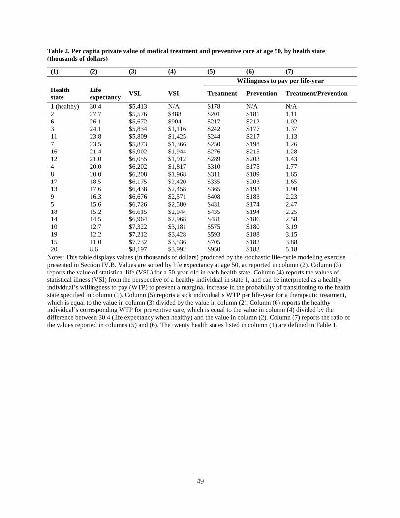
49

Table 2. Per capita private value of medical treatment and preventive care at age 50, by health state (thousands of dollars)

(1) (2) (3) (4) (5) (6) (7) Willingness to pay per life-year Health state

Life expectancy VSL VSI Treatment Prevention Treatment/Prevention

1 (healthy) 30.4 $5,413 N/A $178 N/A N/A 2 27.7 $5,576 $488 $201 $181 1.11 6 26.1 $5,672 $904 $217 $212 1.02 3 24.1 $5,834 $1,116 $242 $177 1.37 11 23.8 $5,809 $1,425 $244 $217 1.13 7 23.5 $5,873 $1,366 $250 $198 1.26 16 21.4 $5,902 $1,944 $276 $215 1.28 12 21.0 $6,055 $1,912 $289 $203 1.43 4 20.0 $6,202 $1,817 $310 $175 1.77 8 20.0 $6,208 $1,968 $311 $189 1.65 17 18.5 $6,175 $2,420 $335 $203 1.65 13 17.6 $6,438 $2,458 $365 $193 1.90 9 16.3 $6,676 $2,571 $408 $183 2.23 5 15.6 $6,726 $2,580 $431 $174 2.47 18 15.2 $6,615 $2,944 $435 $194 2.25 14 14.5 $6,964 $2,968 $481 $186 2.58 10 12.7 $7,322 $3,181 $575 $180 3.19 19 12.2 $7,212 $3,428 $593 $188 3.15 15 11.0 $7,732 $3,536 $705 $182 3.88 20 8.6 $8,197 $3,992 $950 $183 5.18

Notes: This table displays values (in thousands of dollars) produced by the stochastic life-cycle modeling exercise presented in Section IV.B. Values are sorted by life expectancy at age 50, as reported in column (2). Column (3) reports the value of statistical life (VSL) for a 50-year-old in each health state. Column (4) reports the values of statistical illness (VSI) from the perspective of a healthy individual in state 1, and can be interpreted as a healthy individual’s willingness to pay (WTP) to prevent a marginal increase in the probability of transitioning to the health state specified in column (1). Column (5) reports a sick individual’s WTP per life-year for a therapeutic treatment, which is equal to the value in column (3) divided by the value in column (2). Column (6) reports the healthy individual’s corresponding WTP for preventive care, which is equal to the value in column (4) divided by the difference between 30.4 (life expectancy when healthy) and the value in column (2). Column (7) reports the ratio of the values reported in columns (5) and (6). The twenty health states listed in column (1) are defined in Table 1.

50

Table 3. Per capita private value of historical 2001-2015 health gains, at age 50 (thousands of dollars)

Disease

Increase in life expectancy at age 50 (years) (1) (2) (3) (4) (5) (6)

A. No bequest motive All causes 1.43 $56 $117 $240 $49 $101 $205 Cancer 0.39 $12 $28 $59 $10 $23 $49 Heart disease 1.21 $32 $73 $160 $22 $55 $125 B. Bequest motive All causes 1.43 $52 $109 $228 $43 $91 $188 Cancer 0.39 $12 $26 $56 $9 $20 $44 Heart disease 1.21 $29 $68 $150 $19 $47 $109 Relative risk aversion 1.5 2 2.5 1.5 2 2.5 OOP medical spending No No No Yes Yes Yes

Notes: This table reports the value of the reduction in mortality experienced in the United States between 2001 and 2015, from the perspective of a 50-year-old alive in 2015. The cancer and heart disease calculations do not account for competing risks, and thus should be interpreted as holding mortality from all other causes constant. Columns (1)-(3) report results under the assumption that the individual has no out-of-pocket health care or nursing home costs. Columns (4)-(6) report results under the assumption that the health shocks are accompanied by an increase in health care and nursing home costs. The values in Panel A are calculated under the assumption that individuals do not have a bequest motive, while those in Panel B assume the bequest motive specification described in Appendix C2. The table also shows that these values increase with the size of the coefficient of relative risk aversion, which in our utility specification is equal to the inverse of the elasticity of intertemporal substitution.

Table 4. Aggregate value of historical and prospective reductions in mortality (billions of dollars)

(1) (2) (3) No annuity Social Security Social Security + 50% A. Historical reduction 1940-2010 $96,116 $106,695 $111,619 1970-2010 $46,695 $52,414 $55,143 B. 10% reduction, all ages All causes $9,894 $11,150 $11,789 Cancer $2,885 $3,279 $3,477 Diabetes $316 $359 $380 Heart disease $2,060 $2,351 $2,505 Homicide $96 $93 $90 Infectious diseases $139 $159 $170

Notes: These aggregate values were calculated using the 2015 US population by age. Panel A reports the current value of historical reductions in all-cause mortality. Panel B reports the value of a 10 percent prospective reduction in mortality. Column (1) presents estimates under the assumption that individuals have no annuities. Column (2) presents estimates under the assumption that individuals receive typical Social Security benefits that are financed by an earnings tax. Column (3) increases the generosity of Social Security by 50%, financed by an increase in the earnings tax. The net present value of individuals’ wealth at age 20 is the same across all three columns.

51

Figure 1. Illustrative example: annual consumption for fully annuitized and non-annuitized consumers

Notes: This figure illustrates the well-known result that it is optimal for a non-annuitized consumer who is exposed to longevity risk to shift her consumption forward in time, relative to a fully annuitized consumer. For simplicity, this example assumes that the optimal consumption profile of the fully annuitized consumer is flat.

52

Figure 2. Illustrative example: upon falling ill, consumption initially increases

Notes: Both individuals have identical initial wealth at time 𝑡𝑡 = 0. It is optimal for the sick individual (state 2) to consume at a higher rate than the healthy individual (state 1) because she has lower life expectancy. Thus, initial consumption at time 𝑡𝑡 = 0 in the sick state is higher than in the healthy state, i.e., 𝑐𝑐2(0) > 𝑐𝑐1(0). Proposition 6 provides conditions under which VSL at time 𝑡𝑡 = 0 in the sick state is also higher.

53

Figure 3. Treatments for an ill patient are worth more than preventive care for a healthy individual

Notes: The solid blue bars report the value of statistical life (VSL) for an individual in one of 19 different sick states, divided by life expectancy in that state. The dotted red bars report the value of statistical illness (VSI) for a healthy individual (life expectancy: 30.4 years) divided by the reduction in life expectancy she would experience if she fell ill. The data plotted in this figure are also reported in columns (5) and (6) of Table 2.

54

Figure 4. The value of treatment relative to prevention declines with time since illness

Notes: The solid blue bars report the value of statistical life (VSL) divided by life expectancy for an individual who suffers a health shock at age 70 that reduces her life expectancy by 6.8 years and her quality of life by 0.16. (This same health shock is also depicted in Figure 5 at age 70.) The dotted red bars report the value of statistical illness (VSI) for an otherwise identical individual divided by the reduction in life expectancy she would experience if she fell ill with the same disease.

55

Figure 5. Consumption and the value of statistical life can increase when an individual falls ill

Notes: This figure plots an individual’s consumption (left axis) and value of statistical life (right axis), as calculated by a life-cycle modeling exercise where mortality and quality of life are stochastic. The individual is healthy at age 50, but then falls ill twice, once at age 60 and then again at age 70. At age 60, the illness causes permanent difficulties with one routine activity of daily living (ADL). At age 70, she is diagnosed with three chronic conditions and one additional ADL. In our data, this corresponds to transitioning from state 1 to state 6 at age 60, and then from state 6 to state 14 at age 70. Summary statistics for these health states are available in Table 1.

56

Figure 6. The value of statistical life depends on an individual’s health history

Notes: This figure reports the mean, 5th percentile, and 95th percentile of the value of statistical life (VSL) from a Monte Carlo simulation that is repeated 10,000 times. Each simulation begins at age 50 with a consumer in health state 1 (“healthy”). We then generate a health state path {𝑌𝑌51,𝑌𝑌52, … ,𝑌𝑌100} using the transition probabilities estimated by the Future Elderly Model and solve for optimal consumption and VSL using the methods described in Appendix C2. Differences in VSL at older ages are caused by differences in the evolution of people’s health states.

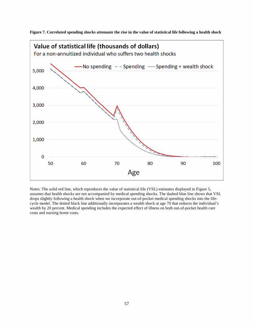
57

Figure 7. Correlated spending shocks attenuate the rise in the value of statistical life following a health shock

Notes: The solid red line, which reproduces the value of statistical life (VSL) estimates displayed in Figure 5, assumes that health shocks are not accompanied by medical spending shocks. The dashed blue line shows that VSL drops slightly following a health shock when we incorporate out-of-pocket medical spending shocks into the life-cycle model. The dotted black line additionally incorporates a wealth shock at age 70 that reduces the individual’s wealth by 20 percent. Medical spending includes the expected effect of illness on both out-of-pocket health care costs and nursing home costs.

58

Figure 8. Life-cycle profiles of consumption and income when mortality is deterministic

Notes: This figure plots consumption results from a life-cycle modeling exercise where mortality is deterministic. “Consumption (no annuity)” displays consumption for a consumer whose income equals her earnings. “Consumption (Social Security)” displays consumption for a consumer receiving typical Social Security benefits that are financed by an earnings tax. The net present value at age 20 of all future income is the same across both scenarios.

59

Figure 9. Life-cycle profile of the value of statistical life when mortality is deterministic

Notes: This figure plots the value of statistical life for the two scenarios displayed in Figure 8. The “No annuity” scenario assumes the consumer’s income equals her labor earnings. The “Social Security” scenario assumes the consumer receives typical Social Security benefits that are financed by an earnings tax. The net present value at age 20 of all future income is identical in both scenarios.

60

Figure 10. Similar to annuitization, a bequest motive shifts the value of statistical life towards older ages

Notes: This figure plots the value of statistical life in a setting with deterministic health and no annuity markets. The “No bequest motive” scenario is identical to the “No annuity” scenario depicted in Figure 9. The bequest motive specification is described at the end of Appendix C1.

Mortality Risk, Insurance, and the Value of Life - National ...

Documents

Transcript of Mortality Risk, Insurance, and the Value of Life - National ...