Ricardo José de Jesus Duarte Estudo Comparativo das Técnicas de ...
118
-
Upload
khangminh22 -
Category
Documents
-
view
0 -
download
0
Transcript of Ricardo José de Jesus Duarte Estudo Comparativo das Técnicas de ...

Universidade de Aveiro Departamento de Engenharia Mecânica2010
Ricardo José deJesus Duarte
Estudo Comparativo das Técnicas de Colmataçãode Perda Óssea na A.T.J.
A comparative study of bone defects repairtechniques in T.K.A.

Universidade de Aveiro Departamento de Engenharia Mecânica2010
Ricardo José deJesus Duarte
Estudo Comparativo das Técnicas de Colmataçãode Perda Óssea na A.T.J.
A comparative study of bone defects repairtechniques in T.K.A.


Universidade de Aveiro Departamento de Engenharia Mecânica2010
Ricardo José deJesus Duarte
Estudo Comparativo das Técnicas de Colmataçãode Perda Óssea na A.T.J.
Comparative study of the techniques to bridgethe bone loss in T.K.A.
Dissertação apresentada à Universidade de Aveiro para cumprimento dos re-quisitos necessários à obtenção do grau de Mestre em Engenharia Mecânica,realizada sob a orientação cientíca de António Manuel Godinho Completo,Professor Auxiliar do Departamento de Engenharia Mecânica da Universi-dade de Aveiro e co-orientada por António Manuel Amaral Monteiro Ramos,Professor Auxiliar Convidado do Departamento de Engenharia Mecânica daUniversidade de Aveiro.
Work submitted to Universidade de Aveiro in order to satisfy the necessaryrequirements for Master's Degree in Mechanical Engineering, performed un-der the scientic orientation of António Manuel Godinho Completo, Assis-tant Professor of Departamento de Engenharia Mecânica da Universidade deAveiro and co-oriented by António Manuel Amaral Monteiro Ramos, InvitedAssistant Professor of Departamento de Engenharia Mecânica da Universi-dade de Aveiro.

o júri / the jury
presidente / president Professor Doutor Rui Pedro Ramos CardosoProfessor Auxiliar do Departamento de Engenharia Mecânica da Universidade de
Aveiro
vogais / examiners committee Professor Doutor Fernando Manuel Pereira FonsecaProfessor Auxiliar da Faculdade de Medicina de Coimbra
Professor Doutor António Manuel Godinho CompletoProfessor Auxiliar do Departamento de Engenharia Mecânica da Universidade de
Aveiro
António Manuel Amaral Monteiro RamosProfessor Auxiliar Convidado do Departamento de Engenharia Mecânica da Uni-
versidade de Aveiro


Aos meus pais e irmã.Adoro-vos


agradecimentos /acknowledgements
A realização deste trabalho não teria sido possível sem a ajuda de diversaspessoas, como tal, aproveito esta oportunidade para agradecer a todas elaso apoio e disponibilidade demonstradas.
Em primeiro lugar, gostaria de agradecer ao meu orientador, o ProfessorDoutor António Completo, por todos os ensinamento, apoio, disponibilidadee paciência demonstrados, sendo ele uma peça chave para a conclusão destetrabalho.
Gostaria também de agradecer ao meu co-Orientador Professor Doutor An-tónio Ramos, pela ajuda na identicação de alguns erros, permitindo assima sua correcção atempadamente.
Um agradecimento especial para todo o pessoal do talho BioBom Talhosde Aveiro pelo fornecimento do material usado para alguns dos testes, bemcomo ao Professor António Bastos e á Professora Gabriela Vincze pela ajudacom o material de medição por vídeo.
Gostaria também de agradecer a todo o pessoal do Laboratório deBiomecânica, em especial á Eng. Joana Silva por toda a ajuda prestadaao longo da execução deste trabalho.
Agradeço à Ana Marques todo o apoio, incentivo, entrega e amizade demon-strados durante a execução deste trabalho, o qual sem a sua ajuda não teriasido possível.
Finalmente, gostaria de agradecer aos meus pais e irmã, por terem sempreuma palavra de incentivo e conforto nas alturas mais complicadas permitindoassim ultrapassar as diculdades e encarar com um maior optimismo situ-ações futuras.
A todos vós o meu mais sincero obrigado!

Palavras-chave Biomecânica, articulação do joelho, cunhas metálicas, enxertos ósseos, hastemetálica, medição experimental de extensões, método dos elementos nitos,revisão da artroplastia total do joelho
Resumo Nesta tese foi objectivo estudar os aspectos biomecânicos das diferentes téc-nicas de colmatação de perda óssea na tibia proximal aquando da revisãoda artroplastia total do joelho. Procurou-se especicamente avaliar comocada uma das diferentes técnicas altera a transferência de carga ao ossode suporte, aferindo assim potenciais riscos de reabsorção óssea ou mesmofalha por fadiga do osso de suporte. Foi também avaliada de uma formacomparativa a estabilidade de cada construção de colmatação do defeitorelativamente à solução sem defeito ósseo. Procurou-se também nesta teseavaliar o efeito da utilização da haste intramedular quando associada àsdiferentes técnicas. Para o efeito numa primeira fase procurou-se realizaruma analise detalhada à articulação do joelho na sua vertente anatómica ebiomecânica com especial enfoque na artroplastia e no processo de revisãodesta. Foi seleccionada a prótese do joelho P.F.C. Sigma como elementopara a realização do estudo comparativo, os elementos protésicos metálicosutilizados nas diferentes construções da substituição óssea foram também domesmo modelo; hemi-cunha, cunha total e bloco. Em complemento foramtambém comparadas mais duas técnicas de colmatação óssea; uma com re-curso apenas ao cimento ósseo e outra com a utilização de um enxerto deosso bovino. Na fase seguinte desenvolveram-se modelos experimentais comrecurso à tibia em material compósito, onde os defeitos ósseos foram gera-dos e as diferentes técnicas de colmatação aplicadas através da realização decirurgias "in-vitro". A m de aferir as alterações de transferência de carga eestabilidade foram colocados extensometros na região anexa ao defeito per-mitindo a avaliação das deformações principais na superfície dos modelos,assim como recorreu-se a utilização de técnicas de vídeo para avaliação daestabilidade do prato tibial nas diferentes técnicas. Estes modelos foramsubmetidos a um severo caso de carga no condilo medial onde se situa odefeito, tendo-se procedido à avaliação e comparação dos resultados das de-formações no osso e estabilidade do prato. Numa fase posterior procedeu-seao desenvolvimento de modelos numéricos de elementos nitos que procu-ram replicar os modelos avaliados experimentalmente. Este modelos foramsubmetidos a dois casos de carga, um idêntico ao aplicado nos modelos ex-perimentais que permitiu a validação destes modelos numéricos e um outrocaso de carga representativo de uma condição de carga mais siológica du-rante o ciclo de marcha. Este modelos numéricos permitiram a avaliação deparâmetros biomecânicos não passíveis de avaliação com recurso aos modelosexperimentais anteriores. Foram assim analisadas as deformações impostasaos osso cortical e esponjoso na vizinhança do defeito e na interface comeste. Estes mesmos modelos foram comparados com os resultados obtidosnos modelos experimentais de forma a avaliar a sua correlação.

Os resultados experimentais e numéricos obtidos permitiram evidenciar boacorrelação entre estes demonstrando que os modelos numéricos são capazesde replicar com delidade o comportamento dos modelos experimentais. Osresultados obtidos em ambos os tipos de modelos evidenciam alterações detransferência de carga e estabilidade entre os diferentes tipos de técnicas. Osmodelos com cunha total e bloco aumentaram em média as deformações nolado medial (lado do defeito) do osso cortical adjacente ao implante quandocomparados com o modelo de colmatação só com cimento ósseo e hemi-cunha. No entanto, os valores de máximos de incremento de deformação noosso cortical no lado medial ocorram para a construção com enxerto ósseobovino. Estes incrementos observados no osso cortical para as construçõesde maior dimensão é oposto ao comportamento observado no osso esponjosona interface com o implante, pois neste caso estas construções originam umaredução das deformações relativamente à solução sem defeito. Assim, temosque as soluções mais invasivas potenciam o risco de dano por fadiga óssea doosso cortical e simultaneamente potencializam o risco de reabsorção óssea noosso esponjoso adjacente. Em termos de estabilidade apenas a construçãocom bloco se revelou signicativamente mais estável que as restantes técni-cas. O efeito adicional de estabilidade das hastes apenas se fez sentir nasconstruções menos invasivas com recurso ao cimento ósseo e hemi-cunha.
2


keywords Biomechanics, bone grafts, experimental strain measurements, nite ele-ment method, knee joint, metal wedges, metal stem, revision of total kneearthroplasty
abstract This thesis objective was to study the biomechanical aspects of the dier-ent repair techniques of bone loss in the proximal tibia, in the revision oftotal knee arthroplasty. We sought to specically evaluate how each of thedierent techniques changes the load transfer to the supporting bone, thusgauging the potential for bone resorption or fatigue failure of the supportingbone. Was also assessed, in a comparative way, the stability of each repairconstruction of the bone defects, relatively to the solutions without bonedefects. We also sought, in this work, to evaluate the eect of the use ofintramedullary stems when associated to dierent techniques. For this pur-pose, as a rst step, we tried to perform a detailed analysis of the knee jointin its anatomical and biomechanical aspects, with special focus on arthro-plasty and its revision process. We selected the knee prosthesis P.F.C. Sigmaas an element for the realization of the comparative study. The prostheticmetal elements used in the dierent bone replacement constructions werealso the same model, hemi-wedge, wedge and block total. As a complementtwo more bone repair techniques were also compared: using only bone ce-ment in contrast with the use of a bovine bone graft. In the following phaseexperimental models were developed using the tibia in composite material,where the bone defects were created and the dierent techniques appliedduring "in vitro" surgeries. In order to assess the changes of load transferand stability in the region annexed to the bone defect were placed gauges,allowing the evaluation of the models main surface deformations, as well asthe use of video techniques for assessing the stability of the tibial plateau inthe dierent techniques. These models were subjected to a severe case ofload on the medial condyle where the defect is located, proceeding to eval-uation and comparison of results of deformation and stability of the boneplate. At a later stage we proceeded to the development of nite elementnumerical models that seek to replicate the models evaluated experimen-tally. The models were subjected to two load cases, one case identical to theone applied in experimental models that allowed the validation of numericalmodels and another load case representing a physiological load conditionduring the walking cycle. The numerical models have allowed the assess-ment of biomechanical parameters, not eligible for evaluation before, usingexperimental models. Thereby the strains imposed on cortical and cancel-lous bone in the vicinity of the defect and in the interface with this havebeen analysed. These same models were compared with results obtained inexperimental models in order to assess their correlation.

The experimental and numerical results obtained allow us to show a goodcorrelation between these numerical models demonstrating that they are ableto faithfully replicate the behaviour of experimental models. The results ob-tained in both types of models show changes in load transfer and stabilitybetween the dierent types of techniques. The models with full wedge andblock, on average, increased the strains on the medial side (the one with de-fect) of the cortical bone adjacent to the implant when compared with thebone and cement graft model and metallic hemi-wedge. However is duringthe construction with bovine bone graft that takes place the maximum incre-ment of strain in cortical bone, on the medial side. These increases observedin the cortical bone for larger buildings is opposite to the behavior observedin the cancellous bone at the implant interface, in which case these construc-tions originate a reduction of deformation on the solution without defect. Sothe more invasive solutions potentiate the risk of fatigue damage in corticalbone and simultaneously increase the risk of bone resorption in the adjacentcancellous bone. In terms of stability only the metallic block implant provedto be signicantly more stable than the other techniques. The additionalstability provided by stems was felt only in less invasive constructions withthe use of bone cement and hemi-wedge.The experimental and numerical results obtained allow us to show a goodcorrelation between these numerical models demonstrating that they are ableto faithfully replicate the behaviour of experimental models. The results ob-tained in both types of models show changes in load transfer and stabilitybetween the dierent types of techniques. The models with full wedge andblock, on average, increased the strains on the medial side (the one with de-fect) of the cortical bone adjacent to the implant when compared with thebone and cement graft model and metallic hemi-wedge. However is duringthe construction with bovine bone graft that takes place the maximum incre-ment of strain in cortical bone, on the medial side. These increases observedin the cortical bone for larger buildings is opposite to the behavior observedin the cancellous bone at the implant interface, in which case these construc-tions originate a reduction of deformation on the solution without defect. Sothe more invasive solutions potentiate the risk of fatigue damage in corticalbone and simultaneously increase the risk of bone resorption in the adjacentcancellous bone. In terms of stability only the metallic block implant provedto be signicantly more stable than the other techniques. The additionalstability provided by stems was felt only in less invasive constructions withthe use of bone cement and hemi-wedge.
2


Contents
1 Introduction 1
2 Revision of Total Knee Arthroplasty 3
2.1 The Knee Joint . . . . . . . . . . . . . . . . . . . . . . . . . . . . . . . . . . . . 3
2.2 Articular surfaces of the knee joint . . . . . . . . . . . . . . . . . . . . . . . . . . 5
2.2.1 Femur . . . . . . . . . . . . . . . . . . . . . . . . . . . . . . . . . . . . . 5
2.2.2 Tibia . . . . . . . . . . . . . . . . . . . . . . . . . . . . . . . . . . . . . . 7
2.2.3 Patella . . . . . . . . . . . . . . . . . . . . . . . . . . . . . . . . . . . . . 8
2.3 Knee Joint Biomechanics . . . . . . . . . . . . . . . . . . . . . . . . . . . . . . . 9
2.4 Anatomic Planes . . . . . . . . . . . . . . . . . . . . . . . . . . . . . . . . . . . . 11
2.5 Ligaments . . . . . . . . . . . . . . . . . . . . . . . . . . . . . . . . . . . . . . . 13
2.6 Minisci . . . . . . . . . . . . . . . . . . . . . . . . . . . . . . . . . . . . . . . . . 16
2.7 Articular Capsule . . . . . . . . . . . . . . . . . . . . . . . . . . . . . . . . . . . . 17
2.8 Varus and Valgus malalignment . . . . . . . . . . . . . . . . . . . . . . . . . . . . 18
2.9 Total Knee Arthroplasty . . . . . . . . . . . . . . . . . . . . . . . . . . . . . . . . 20
2.10 Bone defects on the proximal tibia . . . . . . . . . . . . . . . . . . . . . . . . . . 22
2.10.1 Type 1 defect intact metaphyseal bone . . . . . . . . . . . . . . . . . . . 23
2.10.2 Type 2 defect damaged metaphyseal bone . . . . . . . . . . . . . . . . . 24
2.10.3 Type 3 defect decient metaphyseal bone . . . . . . . . . . . . . . . . . 25
2.11 Materials to repair the bone loss . . . . . . . . . . . . . . . . . . . . . . . . . . . 28
2.11.1 Metal Wedges . . . . . . . . . . . . . . . . . . . . . . . . . . . . . . . . . 29
2.11.2 Stem . . . . . . . . . . . . . . . . . . . . . . . . . . . . . . . . . . . . . . 31
2.11.3 Grafts . . . . . . . . . . . . . . . . . . . . . . . . . . . . . . . . . . . . . 32
2.12 Revision Total Knee Arthroplasty Surgery . . . . . . . . . . . . . . . . . . . . . . 33
3 Experimental tests with dierent bone defect repair techniques 37
3.1 Introduction . . . . . . . . . . . . . . . . . . . . . . . . . . . . . . . . . . . . . . 37
3.2 Materials and Methods . . . . . . . . . . . . . . . . . . . . . . . . . . . . . . . . 38
3.3 Results . . . . . . . . . . . . . . . . . . . . . . . . . . . . . . . . . . . . . . . . . 48
3.4 Discussion . . . . . . . . . . . . . . . . . . . . . . . . . . . . . . . . . . . . . . . 55
4 Computational models with dierent bone defect repair techniques 57
4.1 Introduction . . . . . . . . . . . . . . . . . . . . . . . . . . . . . . . . . . . . . . 57
4.2 Materials and Methods . . . . . . . . . . . . . . . . . . . . . . . . . . . . . . . . 57
4.3 Results . . . . . . . . . . . . . . . . . . . . . . . . . . . . . . . . . . . . . . . . . 68
4.3.1 Mesh convergence results . . . . . . . . . . . . . . . . . . . . . . . . . . . 68
i

4.3.2 Load cases results . . . . . . . . . . . . . . . . . . . . . . . . . . . . . . . 694.3.3 Experimental Models v.s. Numerical Models Results . . . . . . . . . . . . . 83
4.4 Discussion . . . . . . . . . . . . . . . . . . . . . . . . . . . . . . . . . . . . . . . 85
5 Conclusions and Future Works 895.1 Conclusions . . . . . . . . . . . . . . . . . . . . . . . . . . . . . . . . . . . . . . 895.2 Future works . . . . . . . . . . . . . . . . . . . . . . . . . . . . . . . . . . . . . . 90
ii

List of Figures
2.1 Knee joint scheme . . . . . . . . . . . . . . . . . . . . . . . . . . . . . . . . . . . 4
2.2 Femur's scheme . . . . . . . . . . . . . . . . . . . . . . . . . . . . . . . . . . . . 6
2.3 Tibia's scheme . . . . . . . . . . . . . . . . . . . . . . . . . . . . . . . . . . . . . 7
2.4 Patella or Kneecap scheme . . . . . . . . . . . . . . . . . . . . . . . . . . . . . . 8
2.5 Schematic representation of the knee motion . . . . . . . . . . . . . . . . . . . . . 9
2.6 Distance and time dimensions of walking cycle [1] . . . . . . . . . . . . . . . . . . 10
2.7 Knee joint components . . . . . . . . . . . . . . . . . . . . . . . . . . . . . . . . 11
2.8 Anatomic biomechanical planes . . . . . . . . . . . . . . . . . . . . . . . . . . . . 12
2.9 Anterior view of the knee with the representation of the collateral ligaments [2, 3] . 13
2.10 Anterior and posterior view of the knee with the representation of the cruciateligaments [3, 4] . . . . . . . . . . . . . . . . . . . . . . . . . . . . . . . . . . . . 14
2.11 Popliteal ligament of the knee joint . . . . . . . . . . . . . . . . . . . . . . . . . . 15
2.12 Quadriceps Tendon . . . . . . . . . . . . . . . . . . . . . . . . . . . . . . . . . . 15
2.13 Minisci . . . . . . . . . . . . . . . . . . . . . . . . . . . . . . . . . . . . . . . . . 16
2.14 Articular capsule . . . . . . . . . . . . . . . . . . . . . . . . . . . . . . . . . . . . 17
2.15 Varus and Valgus malalignment [5] . . . . . . . . . . . . . . . . . . . . . . . . . . 18
2.16 Osteolysis in the knee arthroplasty . . . . . . . . . . . . . . . . . . . . . . . . . . 21
2.17 Bone Defect Type 1. [6] . . . . . . . . . . . . . . . . . . . . . . . . . . . . . . . . 23
2.18 Bone Defect Type 2a (A). Bone Defects Type 2b (B). [6] . . . . . . . . . . . . . . 24
2.19 Bone Defect Type 3. [6] . . . . . . . . . . . . . . . . . . . . . . . . . . . . . . . . 25
2.20 Bone defects summary [6] . . . . . . . . . . . . . . . . . . . . . . . . . . . . . . . 26
2.21 Revision of total knee arthroplasty . . . . . . . . . . . . . . . . . . . . . . . . . . 27
2.22 Materials used to repair the defects in R.T.K.A. . . . . . . . . . . . . . . . . . . . 28
2.23 Metallic Total Wedge (A); Metallic Block (B); Metallic HemiWedge (C) . . . . . 29
2.24 Some stems used on knee arthroplasty . . . . . . . . . . . . . . . . . . . . . . . . 31
2.25 Cement Graft(A); Bone graft (B) . . . . . . . . . . . . . . . . . . . . . . . . . . . 33
2.26 R.T.K.A. used materials, removal procedure (A); Mini-Lexer Osteotomes (B); Os-cilating Saw (C); Gigli Saw (D) . . . . . . . . . . . . . . . . . . . . . . . . . . . . 34
2.27 Joint space [7] . . . . . . . . . . . . . . . . . . . . . . . . . . . . . . . . . . . . 35
2.28 Assembly of the implant components(A); Set procedure of the tibial components(B)[7]35
3.1 Materials used on the Experimental Tests . . . . . . . . . . . . . . . . . . . . . . 39
3.2 Implants used on the experimental tests: Cemented tibial tray (A); Metallic hemiwedge (B); Cement graft (C); Metallic total wedge (D); Metallic block (E); Bonegraft (F) . . . . . . . . . . . . . . . . . . . . . . . . . . . . . . . . . . . . . . . . 40
3.3 Strain gauge setting . . . . . . . . . . . . . . . . . . . . . . . . . . . . . . . . . . 41
iii
3.4 Strain gauge position . . . . . . . . . . . . . . . . . . . . . . . . . . . . . . . . . 423.5 Videoextensometer materials . . . . . . . . . . . . . . . . . . . . . . . . . . . . . 443.6 Load and constrain components . . . . . . . . . . . . . . . . . . . . . . . . . . . . 453.7 Test machine . . . . . . . . . . . . . . . . . . . . . . . . . . . . . . . . . . . . . . 463.8 Experimental test apparatus . . . . . . . . . . . . . . . . . . . . . . . . . . . . . . 473.9 Maximum Principal Strain ε 1 (a); Minimum Principal Strain ε 2(b) of the
models without stem . . . . . . . . . . . . . . . . . . . . . . . . . . . . . . . . . 503.10 Maximum Principal Strain ε 1 (a); Minimum Principal Strain ε 2(b) of the
models with stem . . . . . . . . . . . . . . . . . . . . . . . . . . . . . . . . . . . 513.11 Displacement comparison between models with and without stem . . . . . . . . . . 54
4.1 Bone structures. Cortical Bone (A); Cancellous Bone (B), Bone section (C) . . . . 584.2 Assembling sequence of the numerical models . . . . . . . . . . . . . . . . . . . . 594.3 Sectioning to represent the model with stem and without stem . . . . . . . . . . . 604.4 Schematic representation of the sections on the tibia (a); Schematic representation
of the dimensions of the prosthesis (b). . . . . . . . . . . . . . . . . . . . . . . . . 614.5 Mesh surfaces on the dierent bone structures. Cortical bone (A); Cancellous bone
(B) and both structures (C) . . . . . . . . . . . . . . . . . . . . . . . . . . . . . . 634.6 Mesh guide lines: cortical bone guide lines(a);cancellous bone guide line (b). . . . . 644.7 Numerical models used . . . . . . . . . . . . . . . . . . . . . . . . . . . . . . . . 654.8 Constrain and applied loads on the models . . . . . . . . . . . . . . . . . . . . . . 654.9 Load cases: Medial load (A); Medial and Lateral load (B). . . . . . . . . . . . . . 664.10 Convergence mesh results, Maximum displacement v.s. Number of elements . . . . 684.11 Principal strain guide lines . . . . . . . . . . . . . . . . . . . . . . . . . . . . . . . 694.12 Medial load cases: Principal strains on the models with and without stem on the
cortical bone: 2mm from the reference . . . . . . . . . . . . . . . . . . . . . . . . 704.13 Medial load cases: Principal strains on the models with and without stem on the
cortical bone: 7mm from the reference . . . . . . . . . . . . . . . . . . . . . . . . 714.14 Medial load cases: Principal strains on the models with and without stem on the
cortical bone: 17mm from the reference . . . . . . . . . . . . . . . . . . . . . . . 724.15 Medial load cases: Principal strains on the models with and without stem on the
cortical bone: frontal plane on the cancellous bone . . . . . . . . . . . . . . . . . . 734.16 Medial/Lateral load cases: Principal strains on the models with and without stem
on the cortical bone: 2mm from the reference . . . . . . . . . . . . . . . . . . . . 774.17 Medial/Lateral load cases: Principal strains on the models with and without stem
on the cortical bone: 7mm from the reference . . . . . . . . . . . . . . . . . . . . 784.18 Medial/Lateral load cases: Principal strains on the models with and without stem
on the cortical bone: 7mm from the reference . . . . . . . . . . . . . . . . . . . . 794.19 Medial/Lateral load cases: Principal strains on the models with and without stem:
frontal plane on the cancellous bone . . . . . . . . . . . . . . . . . . . . . . . . . 804.20 Numeric models validation . . . . . . . . . . . . . . . . . . . . . . . . . . . . . . 834.21 Comparison between numeric and experimental models . . . . . . . . . . . . . . . 84
iv

List of Tables
3.1 Resume table of the components used (n/a - not applicable) . . . . . . . . . . . . 383.2 Position and connection table . . . . . . . . . . . . . . . . . . . . . . . . . . . . . 433.3 Procedure sequence table [8] . . . . . . . . . . . . . . . . . . . . . . . . . . . . . 463.4 Resume experimental table . . . . . . . . . . . . . . . . . . . . . . . . . . . . . . 483.5 Displacement table . . . . . . . . . . . . . . . . . . . . . . . . . . . . . . . . . . 54
4.1 Material properties [9] [10] . . . . . . . . . . . . . . . . . . . . . . . . . . . . . . 674.2 Validation mesh table . . . . . . . . . . . . . . . . . . . . . . . . . . . . . . . . . 68
v


Chapter 1
Introduction
One of the most challenging problems to orthopaedics and the most debatable topic nowadaysis the fact that surgeons don't know what methods and techniques available to correct the bonedefects on the knee joint.
The bone tissue is one of the strongest and most rigid tissues of the human body, as an uniquetissue to support pressures. Next to the cartilage and like cartilaginous tissue, the bone belongsto the connective group tissues hold up, being the major constituent of the skeleton, acting as asustain for soft tissues and protecting the vital organs.
The knee joint is composed by three bones: femur, tibia and knee-cap or patella which is linkedto the muscles that make the extension of the knee acting as a pulley.
Sometimes, and because the knee, is one of the most requested joints of the human body andthe most loaded part during the walk, receiving rotation, extension and compression movements,through the years it can show some wear or injuries, causing to the person discomfort or even somepain during the walk.
Therefore, to provide quality of life to the patients, they are submitted to a surgical interventionnamed Total Knee Arthroplasty.
The main goal of this intervention is the substitution of the cartilage for a prosthesis, providingpain relief and giving back the lost amplitude of movements to patient.
After the rst surgery and through the years, the patients faces some problems which leads toa revision of total knee arthroplasty.
One of the main reasons to perform the revision of total knee arthroplasty, is the bone lossaround the primary implants, questioning its stability and making compulsory a surgical intervention.
The bone loss is linked to osteolysis and stress-shielding eects (Wol's Law).
According to this, when the patient needs a revision of his arthroplasty, the surgeons arecommonly confronted with the need to repair the bone losses with the materials that ensure thepossibility to put a new implant that provides the desired stability. To accomplish properly thistask, the surgeons can use many techniques such as cement, bone graft, metallic wedges or metallicblocks and stems.
Usually, each one of these techniques is directly linked to the dimension of the bone defect.However, the surgeons don't have a specic answer about the best solution for each case.
According to this, the main objectives on this thesis is to assign to the orthopaedic surgeonswhich method/technique is more appropriate to each kind of defects during the revision of totalknee arthroplasty.
1

The rst step was to generate a bibliographic research about the most common defects in thetotal knee arthroplasty and its classication in dimensional and local terms.
At this point was crucial to know the dierent techniques that surgeons can appeal to ensurethe stability of all the components in the revision of the total knee arthroplasty.
In this thesis we analysed the main tibia defects as well as the main components of the kneeprosthesis according to the collected data in the previous point.
An experimental models were developed, which allowed to assess the principal strains andstability on the dierent studied techniques. At the same time, a numerical models, using niteelement methods (F.E.M.),was developed in order to assess the complementary biomechanicalparameters that are impossible to evaluate with experimental models. These numerical modelswere then compared to the same load conditions.
Finally, were compared and analysed the principal strains on the numerical and experimentalmodels, in order to identify the advantages and disadvantages of the several techniques.
2

Chapter 2
Revision of Total Knee Arthroplasty
2.1 The Knee Joint
The knee joint is essentially composed of four adjacent bones: femur, tibia, patella and bula. Asit's function is to provide movement in a rigid network, that is the human skeleton, the biome-chanical system involved is very complex.
This is the largest joint in the human body and structurally the more complex one. As asynovial bicondilar folding joint between the femur condyles and tibia condyles, this articulationcan be divided in three main articulations, tibiofemoral articulation (two joints) and patellofemoralarticulation, [1] therefore this articulation is an important anatomical system in the human skeleton.This joint is constantly dealing with the high developed forces and moments in order to transferstatic and dynamic forces to the leg, allowing simultaneously the skeleton mobility but also itsstability.
A joint should have both stability and mobility but usually one of them is sacriced over theother. The knee joint, however combines the both conditions, allowing the free movement in oneplane, combining at the same time the stability and the mobility of the joint, particularly whenextent.
The stability and mobility provided by this joint are due, in large part, to the interaction ofligaments, muscles, complex movements of planar slip and rotational movements in the articularsurfaces. When the knee joint is totally exed the free rotation of this joint can be seen.
This joint, beyond the great stability particularly when extended, has at the same time a largerange of movements due to the type of the tting joint surfaces that are relatively small. Withthis type of connection, the knee joint is prone to developing various deseases.
3

The great stability presented by this joint may appear incoherent at rst sight because it isbasically the joint of the two biggest bones on its vertically opposite ends, but it's not. The safetyof the knee is then provided by many compensatory mechanisms, such as, an expansion of theweight bearing areas of the femur and the tibia, collateral and intracapsullar ligaments, a capsuleand the aponeurosis (aways or muscular ends of at board, histologically similar to tendons [11]) and tendons reinforcement eects. [12]
Figure 2.1: Knee joint scheme[ http://www.aclsolutions.com]
4

2.2 Articular surfaces of the knee joint
It is then necessary to understand how each constituents of the knee joint interact in order toprovide motion and stability. According to this, the three main bones of the knee joint will besummary described.
2.2.1 Femur
Femur, is the longest and the most voluminous bone of the human body. It is located in thehip, transmitting the weight of the body from the hip bone to the tibia bone, when the person isstanding. [5, 13]
Just as all human body bones, it's size varies in proportion to the person's height. The length
of the femur is usually around1
4of a person's height. This bone consists of a body (diaphysis)
and two ends, superior and inferior end. The upper end of the femur bone consists of the femoralhead, which is joined to the bone shaft by a narrow piece of the bone known as the neck of thefemur, two laps and trochanters (greater tronchanter, lesser tronchanter).
The articular surfaces of femoral condyle are the two areas that bear, on the tibia and patellarsurface joining, the condyles in front.[12]
The medial condyle area may be divided into two parts: the posterior one, parallel to the lateralcondyle and with the same extension; and an anterior extension that goes obliquely and laterally.[12]
The patellar surface is divided by a furrow on the medial side and by a larger and prominentsurface on the lateral side. [12]
The femoral condyles form two convex relief on both planes. The femoral condyles are longeranteroposteriorly than transversely, while the medial condyle is narrower and more prominent thanthe lateral one. The femoral axis diverge in its posterior position, however, the intercondylar incisurecontinues the line of the furrow patellar surface.
In the transverse plane, the femoral convex condyles corresponds more or less to the tibialconcavity condyles, in matters that they t together to form the femorotibial articulation. In thesagittal plane, the curvature radius of the condyle isn't uniform, varying in spiral. The condylespirals of the femur are not simple spires since it has a series of rotation centres that are themselvesinto a spire. [12] In other words, the condyle curvature represents a spiral of a spiral. However,thecondyles did not show the same curvature because their curvature radius are dierent, and sothe internal form of the femoral condyles will reect its geometry as well as the applied eorts.However, this curvature radius decreases in anterior and posterior anks. [12]
In each condyle can be identied the furrow that separates the condyle areas and patellarsurface. [12]
5

The femur is smaller in women than in men due to the lower pelvis and the major obliquity ofthe femur's shaft, therefore allowing more mobility of the femur at the hip's articulation. Howeverthis leads to increased stress on the neck of the femur.
Figure 2.2: Femur's scheme[ http://www.edoctoronline.com/]
6

2.2.2 Tibia
Tibia, the second biggest bone in the human body, is located in the anteromedial part of the leg,almost parallel to the bula. The top surface of the tibia presents a at form, forming the tibialplateau, composed by the medial and lateral condyles and by an intercondylar eminence betweenthe tibial and femural condyles. These joint surfaces of the tibia are covered areas, covered forcartilage in the upper region of each condyle. [5, 12]
The lateral condyle of the tibia internally has a face for the bula's head.The body of the tibia presents a triangular shape, having medial, lateral and posterior faces
which is divided in four faces: medial; lateral; posterior and anterior face or peak composed by abroad and oblique tuberosity that provides distal xation to the patellar ligament.
The most prominent area of the tibial bone is the anterior one, which is thinner at the junctionof its middle and distal thirds.
It should also be noted that the distal end of the tibia is smaller than the proximal, havingfaces for the articulation with the bula and talus. [5]
The Basic parts of the tibia and femur surfaces essentially allows motion in one plane (ex-tion and extension). The axial rotation involves torsion of the femur against the tibia or theopposite, where the intercondylar eminence of the femur acts as a pivot. The pivot consists ofthe intercondylar tubercles forming the lateral edge of medial condyle and lateral condyle of themedial.
Figure 2.3: Tibia's scheme[ http://homepage.mac.com]
7
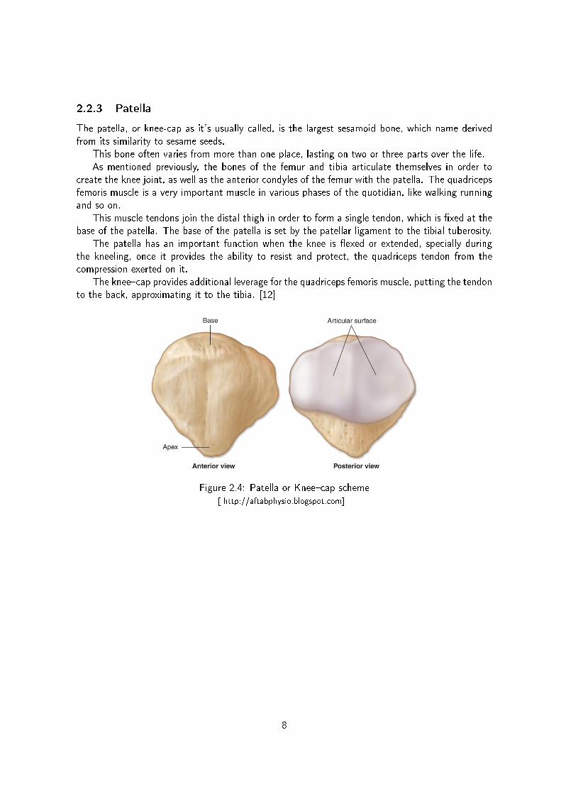
2.2.3 Patella
The patella, or knee-cap as it's usually called, is the largest sesamoid bone, which name derivedfrom its similarity to sesame seeds.
This bone often varies from more than one place, lasting on two or three parts over the life.As mentioned previously, the bones of the femur and tibia articulate themselves in order to
create the knee joint, as well as the anterior condyles of the femur with the patella. The quadricepsfemoris muscle is a very important muscle in various phases of the quotidian, like walking runningand so on.
This muscle tendons join the distal thigh in order to form a single tendon, which is xed at thebase of the patella. The base of the patella is set by the patellar ligament to the tibial tuberosity.
The patella has an important function when the knee is exed or extended, specially duringthe kneeling, once it provides the ability to resist and protect, the quadriceps tendon from thecompression exerted on it.
The kneecap provides additional leverage for the quadriceps femoris muscle, putting the tendonto the back, approximating it to the tibia. [12]
Figure 2.4: Patella or Kneecap scheme[ http://aftabphysio.blogspot.com]
8

2.3 Knee Joint Biomechanics
To improve the articial joints is necessary to understand correctly the biomechanics of this artic-ulation.
The load reduction in this articulation during the daily activities and the implants design thatsupports these loads contributed to approximate the performances of this joint articulation to thenatural one.
Although the knee apparently performs a movement similar to a hinge, this joint actually workswith much more complex movements. The knee joint can be subjected to many types of movementssuch as, exion and extension, medial to lateral, anterior to posterior and axial rotation. Because ofthis, its easy to understand that abnormal or even normal motion causes wear on these structures.
Beyond all the bone structures that makes up this joint, the knee joint is also composed bymenisci and ligaments, surrounded by muscle.
The knee joint has six degrees of freedom, with exion and extension, translation, rotation,varus or adduction (moving closer to the midline) or valgus or abduction (movement of the segmentaway from the midline). [14, 15, 16]
Figure 2.5: Schematic representation of the knee motion[ www.gustavokaempf.com.br]
Nordin et al [1] have measured motion in this joint during the walk. Full or nearly full extensionwas noted at the beginning of the stance phase (0% of cycle), at heel strike, and at the end ofthe stance phase before toe-o (around 60% of cycle) as showed in the gure 2.6 by blue oval.Maximum exion was observed during the middle of the swing phase pointed in gure 7.2 by pinkoval. These measurements are velocity dependent and must be interpreted with caution.
Taking the walking cycle into account, it is possible to describe the movement from full exionto full extension in three phases. In the fully exed condition the posterior parts of the femoralcondyles rest on the corresponding portions of the meniscotibial surfaces, and in this position slight
9

Figure 2.6: Distance and time dimensions of walking cycle [1]
amount of simple rolling movement is allowed. During the passage of the limb from the exed tothe extended position, a gliding movement is superposed on the rolling, so that the axis, which atthe beginning is represented by a line through the inner and outer condyles of the femur, graduallyshifts forward. In this part of the movement, the posterior twothirds of the tibial articular surfacesof the two femoral condyles are involved, and as these have similar curvatures and are parallel oneto another, they move forward equally.
The lateral condyle of the femur is brought almost to rest by the tightening of the anteriorcruciate ligament; it moves, however, slightly forward and medialward, pushing before it the anteriorpart of the lateral meniscus.
The tibial surface on the medial condyle is prolonged further forward than that on the lateral,and this prolongation is directed lateralward.
When, therefore, the movement forward of the condyles is checked by the anterior cruciateligament, continued muscular action causes the medial condyle, dragging with it the meniscus, totravel backward and medialward, thus producing an internal rotation of the thigh on the leg. Whenthe full extension position is reached the lateral part of the groove on the lateral condyle is pressedagainst the anterior part of the corresponding meniscus, while the medial part of the groove restson the articular margin in front of the lateral process of the tibial intercondyloid eminence. Into thegroove on the medial condyle is tted the anterior part of the medial meniscus, while the anteriorcruciate ligament and the articular margin in front of the medial process of the tibial intercondyloideminence are received into the forepart of the intercondyloid fossa of the femur. This third phase,by which all these parts are brought into accurate apposition, is known as the screwing home, orlocking movement of the joint.
10

The human knee joint is a complex articulation, because it is actually composed by a doublearticulation, the tibiofemoral and patellofemoral articulation where large forces and moments areinvolved [1]
Figure 2.7: Knee joint components[ http://sotstenio.blogspot.com(A); www.veloxtness.com.br (B)]
2.4 Anatomic Planes
The motion of the knee takes place simultaneously in three planes, sagittal, frontal and transverseplane.
The movement analysis in any joint requires the kinematic data. Kinematics is the part ofmechanics that deals with the body movements without taking into account the loads and theweight. The analysis of forces and moments acting on the joint, involves both kinetic and kinematicdata.
The kinematics denes the range of motion and describes the motion surface in an articulationon the previously described three planes. The reference point for measurements is dened as thebody's natural position.
11

Figure 2.8: Anatomic biomechanical planes
The movement in the frontal plane is aected by the exion degree of the knee joint, becausewhen the knee is at full extension the movement in the frontal plane is denied. [12]
The angle that makes the dierence between an easy or dicult movement in the frontal planeis at 30º. To angles till 30º, a passive valgus and varus increases while to angles higher than 30º,the motion in frontal plane decreases because of the limiting function of the soft tissues. [17] Thesagittal plane is where the larger movements happens, because when it goes from full extension tofull exion the angle varies between 0º and 140º. [1, 12]
According to this, Laubenthal et al (1972) studied that the values of the range of motion ofthe knee joint in sagittal plane vary according the kind of activities. For example, climbing stairsvaries between 00 and 670, tying a shoe from 00 to 1060 or lifting an object from 00 to 1170.[12] The movements of the knee joint in the transverse plane are inuenced by the position of thesagittal plane. Because of the tibial and the femoral condyle, when the knee is at full extension thejoint rotation is fully restricted since the medial femoral condyle length is greater than the lateralcondyle.
The range of rotation increases as the knee is exed, reaching a maximum at 900 of exion;with the knee in this position, external rotation ranges from 00 to approximately 450 and internalrotation ranges from 00 to approximately 300. Beyond 900 of exion, the range of internal andexternal rotation decreases, primarily because the soft tissues restrict rotation. [1, 12]
The movement in the sagittal plane is highest relatively to the frontal and to the transverseplane and because of that, this plane could be considered to be the main movement plane of theknee. Consequently, and in order to simplify the analysis, and its variables, the biomechanicalvariables can be restricted to one simple plane and to the forces exerted by a group of muscles,allowing this way an easy understanding of the movements and previous prediction of the mainforces and moments in the joint. [5]
Advanced dynamic analysis of the biomechanics of the knee joint include all the soft tissueson the articulation, such as ligaments, meniscus and cartilage, as well as the previous complexstructures.
12

2.5 Ligaments
The knee joint, in order to stabilize and control the movements, is composed by four main ligaments,two collateral and two cruciate ligaments, as well as three secondary ligaments, patellar, obliquepopliteal and arcuate popliteal ligament. The ligaments work better when the load is in the bberdirection. [12, 18, 19]
Subdivided into two classes, according to their location: the medial collateral ligament (MCL)once that is on the medial side. and the Lateral Collateral Ligament (LCL) once it is on the lateralside.
Figure 2.9: Anterior view of the knee with the representation of the collateral ligaments [2, 3]
The Medial Collateral ligament (MCL) joins the medial condyles of the femur and tibia, helpingthe resistance to the valgus stress, tibia rotation, lateral rotation and anterior displacement of thetibia. Its deep surface covers the inferior medial genicular vessels and nerve and the anterior portionof the tendon of the semimembranosus, with which it is connected by a few bbers; it is intimatelyadherent to the medial meniscus. [3, 14, 20]
The Lateral Collateral ligament (LCL) is located at the lateral site of the knee, connecting thelateral condyles of the femur and tibia, improving the resistance forces in varus, rotation of thetibia and rotation of the tibia with posterior displacement. [20]
The cruciate ligaments are located inside the intercondillar space of the joint and they have avery important role in the knee kinematics, having a high structural organization. This ligamentsare rolled up on themselves and on each other in all planes except the horizontal. This ligamentsare subdivided into anterior cruciate ligament (ACL) and in posterior cruciate ligament (PCL),limiting the rotation and causing the sliding of the condyles on the inected tibia.[19]
13

Figure 2.10: Anterior and posterior view of the knee with the representation of the cruciate liga-ments [3, 4]
The anterior cruciate ligament provides the primary constrain to the anterior movement of thetibia under the femur. It resists to medial rotation of the knee, and in complete extension thereis the maximum stress. This ligament is the weakest ligament of the cruciate ligaments once itsblood supply is reduced. The anterior cruciate ligament has its origin in the anterior intercondylararea of the tibia, soon after the medial menisci xation. [14]
The posterior cruciate ligament, is the strongest cruciate ligament, having its origins in theposterior intercondylar area of the tibia, passing over and in front of the medial side of the anteriorcruciate ligament to settle on the anterior side of the lateral face of the medial femoral condyle.This ligament creates primary restriction to the posterior movement of the tibia under the femur; itresists to knee rotation and also helps to prevent hyper extension of the knee joint. This ligamentis also the main factor for stabilization of the femur when the knee is exed. [14]
Pattelar ligament is composed by the tendon of the femoral quadriceps muscle and extendsfrom the patellar apex to the tibial tuberosity. The medial and lateral portions of the tendon ofthe quadriceps pass down on either side of the patella, to be inserted into the upper extremityof the tibia on either side of the tuberosity. The patellar ligament is the anterior ligament of theknee joint. It merges with the patellar medial and lateral retinaculum, since the retinaculum areresponsable for the lateral support of the articular capsule of the knee. [5]
The oblique popliteal ligament is an expansion of the muscle tendon semimebranaceo whichreinforces the knee joint in the posterior face. The origin of this ligament is on the posterior medialcondyle of the tibia and passes upper laterally to settle in the center of the posterior surface of thebrous capsule. [5]
The arcuate popliteal ligament is a ligamentar reinforcement of the posterior brous capsulewhich is positioned in an arc. It begins in the posterior face of the bula's head, passing supero-medially to the tendon of the popliteo muscle and spreading itself under the posterior face of theknee joint. This ligament performs the reinforcement of the brous capsule on the posterior partof the knee. [5, 12, 19]
14

Figure 2.11: Popliteal ligament of the knee joint[ http://wapedia.mobi]
A tendon is a glistening white cord of connective tissue that attaches muscle to bone. It issimilar in structure to a ligament, which connects bone to bone. Tendons play a critical role in themovement of the human body by transmitting the force created by muscles to move bones. In thisway, they allow muscles to control movement from a distance.
Like ropes, tendons are tough, brous and exible. They are not, however, particularly elastic.If they were, much of the muscular force tendons are intended to carry would dissipate before ithad a chance to even reach bones.
Tendons are formed from the same components that make up other kinds of connective tissue,such as cartilage, ligaments and bones. These components are collagen bers, ground substance,and cells, which in the tendon are called brocytes. At the point where a tendon touches bone,the tendon bers gradually pass into the substance of the bone and meld with it. The tendonmicrostructure can be observed in Figure 2.12. [3, 20]
Figure 2.12: Quadriceps Tendon[ http://orthoinfo.aaos.org]
15

2.6 Minisci
One of the brocartilages is the meniscus of the knee. Minisci from the greek word meniskos, thatmeans growing, are present mainly in the joint femorotibial cartilage, between the tibia and femurcondyles.
Minisci can be subdivided in medial and lateral minisci, and are composed by resistents bro-cartilages. [21]
Both, the medial menisci than the lateral, are located above the tibia, with a similar shape ofa half moon. As a cartilage, menisci have a few blood vessels, hindering its regeneration in case ofinjury.
The upper surfaces of the menisci are concave, and are in contact with the condyles of thefemur; their lower surfaces are at and rest upon the head of the tibia; both surfaces are smooth,and invested by synovial membrane.
Each meniscus covers approximately the peripheral two-thirds of the corresponding articularsurface of the tibia.The menisci plays an important role in the articulation of the knee, since itdirectly assists in joint stabilization, deepening the joint surfaces of tibia and femur. The meniscialso helps to absorb the impact, giving a part of the sustention load because of the weight infull extension and a part of exion load. The menisci promote joint lubrication and also limit themovement between the tibia and femur. [22]
Figure 2.13: Minisci[ http://www.msd.com.mx]
16
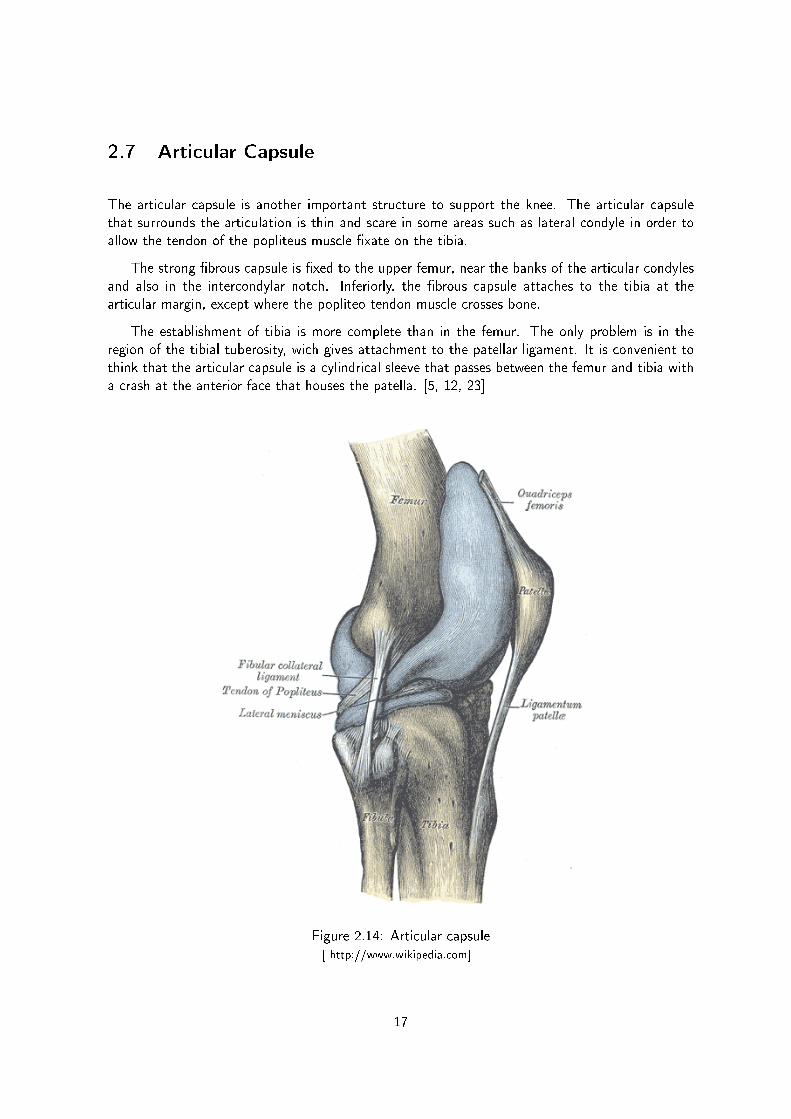
2.7 Articular Capsule
The articular capsule is another important structure to support the knee. The articular capsulethat surrounds the articulation is thin and scare in some areas such as lateral condyle in order toallow the tendon of the popliteus muscle xate on the tibia.
The strong brous capsule is xed to the upper femur, near the banks of the articular condylesand also in the intercondylar notch. Inferiorly, the brous capsule attaches to the tibia at thearticular margin, except where the popliteo tendon muscle crosses bone.
The establishment of tibia is more complete than in the femur. The only problem is in theregion of the tibial tuberosity, wich gives attachment to the patellar ligament. It is convenient tothink that the articular capsule is a cylindrical sleeve that passes between the femur and tibia witha crash at the anterior face that houses the patella. [5, 12, 23]
Figure 2.14: Articular capsule[ http://www.wikipedia.com]
17

2.8 Varus and Valgus malalignment
The knee joint combines the two bigger bones of the human body and because of the forces thatare concentrated on it, in some cases or illness/injury in others, the correct alignment of thesebones isn't achieved.
In normal circumstances, where the knee is correctly aligned, its load-bearing axis is on the linethat runs down the middle of the leg through the hip, knee and ankle. However, there are caseswhere this axis is shifted from the center a few degrees, creating an articulation malalignement.
The joint with angular deformities often has a tense complex capsuloligamentar in the com-partment where the arthrosis is installed and slack in the other side. If the surgery does not correctthis deviation, the overload leads to a progressive slack, instability and the short sustainability ofthe knee joint. [10]
During the revision of total knee arthroplasty, sometimes is found this malalignement is foundbetween the femur and the tibia. To this type of malalignment is given the name of varus or valgusdeformity (varus or valgus knee). This term refers to the direction pointed by the distal segmentof the knee joint points. [5]
Figure 2.15: Varus and Valgus malalignment [5]
This kind of malalignment between tibia and the femur can cause arthrosis, i.e. the cartilagedestruction in the knee joint, causing pain and sickening sense on the patients.
The characterization of these two types of malalignment is mainly based on the side that theangle occurs, as previously mentioned. A lateral angle leg is called as valgus knee (genu valgum),which results in an extra tensile stress being placed on the medial side of the knee and the lateralside of the ankle. Although the valgus can be at least partly compensated for by strengtheningthe quadriceps muscles which stabilize the knee, and strengthening the muscles which support thelateral side of the foot. [24]
On the other hand, when the angle is from the inside of the knee joint, that malalignment iscalled as varus knee. In other words, the varus knee deformity is basically the opposite of valgusknee deformity. The varus deformation will cause greater stress on the medial compartment of theknee. [25]
However, this kind of deformities and malalignment can be corrected as states Russel E. Wind-sor, at Current Concepts in Joint Replacement 2010 Winter Meeting in Orlando, Fla. [26]
18

Since the varus deformity is characterized by joint space narrowing with medial joint erosion,potentially occurring in a normal medial collateral ligament (MCL), Windsor et al.[26] states thatif this deformities occur in small angles (between 10 to 15 degrees), should be corrected using arectangular space of both exion and extension. However, if the angle deformity is bigger than 15degrees, it could require a release to equalize the exion gap.
Regarding to valgus deformity, Windsor [26] says that this is characterized by a contracted ortight lateral ligament (LCL), iliotibial band, popliteus muscle and ligament complex. In this casesthe goal, according to Windsor, is to achieve a deformity between 0 and 5 degrees.
A passively correctable valgus deformity could be handled by restoring the epicondylar axiswithout lateral release. Formal releases are usually necessary, and Windsor reported there is acontroversy regarding which release should be performed rst. [26]
For moderate valgus of 15° to 45°, Windsor starts with the iliotibial bands either step-cut ordistal o of Gerdy's tubercle, then the posterolateral corner of the arcuate ligament, then theLCL. He added that with bigger releases, the popliteus should be preserved to avoid a signicantgaping in the lateral side inection. [26]
Merely as a note, although at the rst sight we could think that this kind of deformities onlyoccur in older people who may have already performed a rst surgical intervention in the kneejoint that is not true. Sometimes, children one or two years after starting to walk have this kind ofmalalignment on their knees. The persistence of these abnormal angles of the knee in late childhoodusually means that there are deformities that may require an intervention. If this intervention doesnot happen, the articular cartilage will be rapidly eroded. [5]
19

2.9 Total Knee Arthroplasty
The Parisian, Jules P'eau (1830-1898), dened an arthroplasty as the creation of an articial jointfor the purpose of restore motion.
As stated above the knee articulation is a joint that depends mainly on two bones, the femurand tibia. Each end is covered by a cartilage that allows movement. When that cartilage isdamaged or degraded the bones contact each other directly, causing an inammatory response andpain to the patient [27].
To solve this problem arose the knee arthroplasty, in order to restore a normal life to thepatients, allowing them to walk without pain. At this chapter we will introduce the rst total kneearthroplasty. This is a surgical procedure where parts of the knee joint are replaced by articialparts, [28] usually metallic and plastic parts, whose main objectives are the elimination of painfullysymptoms, the correction of deformations and stabilization of the knee.
It was back in the nineteenth century that took place the rst attempts to perform a kneearthroplasty, using techniques such as interposition or resections. In 1826 Barton attempted oneof the rst simple resection in a joint but he was unsuccessful because later on he came to suerfrom ankylosis (joint stiness). Only a few years later, in 1861, took place the rst successful kneearthroplasty, using soft tissue interposition, performed by Ferguson at the Medical Times.
At this time, the material used for reconstructing the joints was soft tissue. The problem withusing this kind of material is that it's prone to suer from infections and anchylosis, so there wasa need to search for new materials, such as plastics and metals. With this need, in 1938, came anew age in the knee arthroplasty. In 1951 Borje Walldius invented the rst prototype of a hingedprosthesis in acrylic resin, in Sweden. [5]
So that being said, one can conclude that this intervention, which has been practised for over50 years and initially was not so successful, due to the complexity of the knee joint [29] , nowadays,thanks to the advancements in the knowledge of knee mechanics and technology, [29]is one of themost successfully performed operations, with 95% to 98% good to excellent results reported at 10to 15 years.
Although there are a lot of factors which can cause problems in the knee joint, the mostcommon ones are usually related to the absence or deterioration of the articular cartilage. Amongthe various diseases we can quote the most common ones: osteoarthritis, which can be caused byan old trauma, overexertion or by changes in the knee shape, causing the surfaces of the knee jointto become rough and irregular; and rheumatoid arthritis which is a chronic inammatory disease.[5, 30, 31]
Mestriner et al. [32] show, by a study made with twenty six T.K.A. in arthritic knees, quitesatisfactory results for the treatment of osteoarthritis.
In another study performed by the same authors, with the objective of establishing possibledierences in the behaviour of TKA in twenty six knees with rheumatoid arthritis and twenty sixknees with osteoarthritis, concluded that there were signicant dierences between the two groups,reaching the conclusion that the results were excellent, 92% for rheumatoid arthritis and 80% forosteoarthritis. [32]
This type of surgery has had a very signicant increase in the last years, mostly due to the ageingof the population and also due to good functional results provided by the progressive developmentof both implants and instrumentation used. [31]
Although the results of the rst knee replacement surgery are very satisfactory, there are severalfactors that inuence the durability of the knee prosthesis and the success of total knee arthroplasty
20

and sometimes complications occur, such as joint stiness, instability and infection. The infectionis the most feared complication and it's usually caused by bacteria. [33]
The factors that inuences the durability of prostheses are inherent to the surgical techniquesadopted, the design of materials to correct the defects and also to the material used to make theimplants. Despite all this there are two more complications one has to consider concerning thistype of procedure: osteolysis and stress-shielding.
Osteolysis generally refers to a problem common to articial joint replacement such as totalhip replacements, total knee replacements and total shoulder replacements. This problem is theend result of a biologic process that begins when the number of wear particles generated in thejoint space overwhelms the capsule's capacity to clear them. The residual particles stimulate amacrophage-induced inammatory response that can lead to bone loss and subsequent implantloosening. Although cement particles were once exclusively blamed for osteolysis, it has becomeclear that any particle debris can result in bone resorption. [34]
Figure 2.16: Osteolysis in the knee arthroplasty[ www.medscape.com]
21

By the other hand, stress-shielding refers to the reduction in bone density as a result of theremoval of normal stress from the bone, by an implant. This was explained by Julius Wol, aGerman physiologist, whom in 1892 proposed an explanation to this problem name as Wolf's Law.This law states that bone density changes in response to changes in the functional forces on thebone.
Wol proposed that changes in the form and function of bones are followed by changes in theinternal structure and shape of the bone, in accordance with mathematical laws. Thus, in maturebone, where the general form is established, the bone elements place or displace themselves, andincrease or decrease their mass, in response to the mechanical demands imposed on them. Thistheory is supported by the observation that bones atrophy when they're not mechanically stressedand hypertrophy when they are stressed. [35]
2.10 Bone defects on the proximal tibia
On this chapter the most common defects will be addressed. The identication of bone defects inthe tibia during the revision of knee arthroplasty is important in order to provide a proper evaluation,thus providing a more appropriate intervention. Preoperative radiographs should be used to classifybone defects into categories of comparable diculty.
When carrying out the preparation for revision of total knee arthroplasty, surgeons shouldanticipate the worst possible scenario, being the experience of the surgeon a very important factor,and taking into account all the diculties that this surgery entails.
There have been various attempts over the years to establish a classication of bone defects,both for rst arthroplasty and for the revision arthroplasty.
Dorr et al. [36] in 1989 established a classication, Dorr's classication, considered to be themost straightforward one, in which defects are dened as either central or peripheral and cases areseparated as primary or revision procedures, not being made any attempt to dene the size andlocation of the defect.
Years later, Insall et al. [37] used a similar terminology in primary cases of central and peripheralbone defects. This classication was based on three stages of how the defect should be handled:in the rst stage treatment involves the simple use of cement; the second stage is related with theuse of cement or augmentation plus a stemmed component; and the third stage involves the useof block augmentation and stem extension.
Although several attempts have been made, no bone defect classication has been acceptedby orthopedic surgeons until the classication developed by the Anderson Orthopedic ResearchInstitute (Aori) emerged, which goal is to make an easy system to understand and apply. [38]
This new classication system is based on ve main criteria:
use of the same terminology for both femoral and tibial defects due to the similarities in theboth metaphyseal segments;
the commonly used denitions in most classications of bone defects, as central or peripheral,cortical or cancellous, contained or uncontained were eliminated because of the absence of corticalbone in the metaphyseal segments of the distal femur and proximal tibia;
clear and precise denitions were established to minimize ambiguity when bone defects arecategorized;
was established a minimum number of defects to permit clinical investigators to accumulateenough cases to allow meaningful statistical comparisons;
22

nally, this classication was created to allow retrospective categorization of cases throughintraoperative information and post-operative radiographs. [5, 6]
In the evaluation system Aori defects are classied only when a component has been removed,based on preoperative radiographs for anticipated bone deciency and then the classication iseither conrmed or changed intra-operatively. Sometimes, due to lack of clarity of preoperativemethods, there is the need to classify the bone defects through the post-revision radiographs.
Therefore, and based on previously described, the defects can be classied into three distinctclasses:
2.10.1 Type 1 defect intact metaphyseal bone
Is a bone defects that don't compromise the stability of the component.In this type of defects there is a correctly aligned tibial component signicant implant subsidence
or tibial osteolysis. In T1 defects the metaphyseal area is intact, and though minor defects mightbe expected, they are not enough to put the stability of the joint at risk. Usually, in order to controland correct these defects, it is used either a standard component with a combined polyethyleneand metal thickness of less than 20 mm, or cement grafts. [5, 6]
Figure 2.17: Bone Defect Type 1. [6]
23

2.10.2 Type 2 defect damaged metaphyseal bone
Is the bone defects that don't compromise the stability of the component.The type 2 defect is often caused by component loosening and secondary subsidence of the
tibia, commonly into a varus orientation. This type of defect requires the lling with bone graft,cement or metal wedges. A circumferential radiolucency develops between the cement and boneas the component subsides. The distance between the top of the bula and the component isdiminished. The lateral radiograph is useful in measuring this distance. Osteolysis may presentas cavitary defects beneath the component. This kind of defect can still be subdivided into twoclasses, 2a and 2b: in the type 2a only one of the condyles is aected and in 2b both condyles areaected. [5, 6]
Figure 2.18: Bone Defect Type 2a (A). Bone Defects Type 2b (B). [6]
Type 2a defects is when the bone defects occur either in a femoral condyle or in a tibial plateau.The type 2a defect is usually the result of tibial component loosening and subsiding into varus.
The tibia rarely subsides into a valgus orientation, even in knees with valgus alignment. Onpreoperative radiographs, a widening radiolucency is frequently seen beneath the tibial component.Bone in the opposite tibial plateau is present at a relatively normal joint line level. Type 2a defectscan also occur with aseptic loosening of a unicondylar tibial component.
It is important to avoid converting a type 2a defect into a type 2b defect by resecting the tibialplateau at a more distal level. When a type 2b defect is created iatrogenically, a thicker tibialcomponent is required. [5, 6]
Type 2b defects is when the bone defects occur on both femoral condyle or in the plateau.In its turn, as stated previously, defects of type 2b involve both plateaus, since in this type of
defect a metaphyseal segment of tibia is damaged. The damage may extend to the level of thebular head, but should not include extensive destruction of bone below this level. The surgicalmanagement of a type 2b defect usually includes the use of a long-stemmed tibial component andreconstruction of the tibial plateaus by bone graft, augments, or an extra thick tibial component.In this defect is convenient to use wedgeshaped components when one notes a signicant bone lossin both plateaus, although that bone loss may be larger in one of the sides. A stem can also beused, especially if a structural bone graft has been used. The use of cement, on the other hand,isn't very common in this type of defects. [5, 6]
24
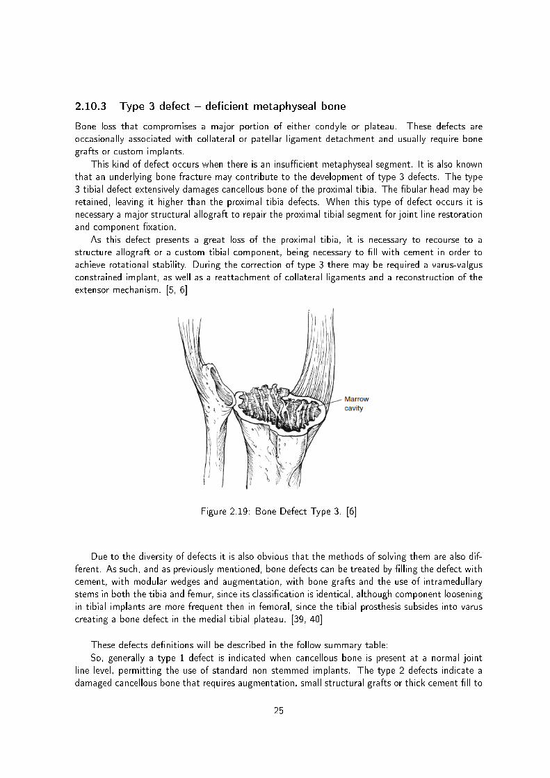
2.10.3 Type 3 defect decient metaphyseal bone
Bone loss that compromises a major portion of either condyle or plateau. These defects areoccasionally associated with collateral or patellar ligament detachment and usually require bonegrafts or custom implants.
This kind of defect occurs when there is an insucient metaphyseal segment. It is also knownthat an underlying bone fracture may contribute to the development of type 3 defects. The type3 tibial defect extensively damages cancellous bone of the proximal tibia. The bular head may beretained, leaving it higher than the proximal tibia defects. When this type of defect occurs it isnecessary a major structural allograft to repair the proximal tibial segment for joint line restorationand component xation.
As this defect presents a great loss of the proximal tibia, it is necessary to recourse to astructure allograft or a custom tibial component, being necessary to ll with cement in order toachieve rotational stability. During the correction of type 3 there may be required a varus-valgusconstrained implant, as well as a reattachment of collateral ligaments and a reconstruction of theextensor mechanism. [5, 6]
Figure 2.19: Bone Defect Type 3. [6]
Due to the diversity of defects it is also obvious that the methods of solving them are also dif-ferent. As such, and as previously mentioned, bone defects can be treated by lling the defect withcement, with modular wedges and augmentation, with bone grafts and the use of intramedullarystems in both the tibia and femur, since its classication is identical, although component looseningin tibial implants are more frequent then in femoral, since the tibial prosthesis subsides into varuscreating a bone defect in the medial tibial plateau. [39, 40]
These defects denitions will be described in the follow summary table:
So, generally a type 1 defect is indicated when cancellous bone is present at a normal jointline level, permitting the use of standard non stemmed implants. The type 2 defects indicate adamaged cancellous bone that requires augmentation, small structural grafts or thick cement ll to
25

Figure 2.20: Bone defects summary [6]
restore joint line level and knee stability. The type 3 defect should be reserved primarily for thosesevere cases in which the damaged metaphyseal segment of bone must be repaired with a salvagehinged implant or with major bone grafts to support the component. [6]
It is noteworthy that in any classication scheme there may be cases where classication isdicult because they are in the borderline, and when that happens the postoperative radiographsand the surgical treatment mode should be evaluated, never forgetting that the target in thetreatment of the defects described is to create a good support surface for the tibial plateau.
Although in the case of revision arthroplasty the grafts are from other donors, which may inthe long term develop complications either because of lack of union of the halogens to the bone(other donor),or due to the graft migration because of the resorption of the graft or because ofinfections. [5, 37, 39]
26

Like any other joint replacement implant, the total knee arthroplasty implant doesn't lastforever and it may fail after ten to fteen years or even sooner. [41] Therefore there is a need formaintenance of the prosthesis. As such, in cases of total knee arthroplasty, the treatment used is arevision of the total knee arthroplasty which, in very general terms, can be dened as an operationto replace in part or to replace the entire previous prosthesis (prosthesis, cement, surrounding tissueand dead bone) that wears out, loosens or develops a problem, before inserting a new prosthesis.
The symptoms indicating the need for an arthroplasty revision are pain and limited mobility.Another way to detect the need for review is through an X-Ray examination, which is recommendedto be made lifelong following the total knee arthroplasty. This failure, and the need of a new surgicalintervention, may result from many causes such as: plastic wear (in this case only the plastic insertis changed); instability (the knee is not stable and may giving way or not feel safe when the patientwalks); loosening (loosening of either femoral, tibial or patella component which can be detectedon regular follow-up X-Ray examinations); infections (usually presents as pain but may present asswelling or an acute fever); fracture; recurrent dislocation; ongoing unrelieved pain; osteolysis. [41]
As stated above, revision surgery is much more complex and technically more dicult than theprimary total knee arthroplasty due to the diculty removing the old prosthesis and also due tothe reduced amount of bone to place the new knee into. [41]
In other words, bone loss is closely related to the revision of total knee arthroplasty, as it isnecessary to make a new incision in an area previously traumatized during the rst surgery. We alsoneed to consider bone loss by osteolysis and the phenomenon of bone resorption as a consequenceof stress-shielding eect, caused by the implant placed in the rst surgery. All this leads to increasedrisk of inammation and diculty removing the prosthesis components. [5]
(a) (b) (c)
Figure 2.21: Revision of total knee arthroplasty[http://juninhobarboza.blogspot.com/ (a); www.zimmer.com (b)]
27

2.11 Materials to repair the bone loss
Sometimes extra bone is required since the revision arthroplasty requires, in many cases, the removalof large bone volume. This problem, of bone loss, can be solved in several ways: bone grafts fromthe bone bank, articial bone substitutes or even the patient's bone [42]; modular wedges thatadd to tibial and femoral components; intramedullary stem; and bone cement extracts in cases ofminor bone loss, to ll the empty spaces. [5]
Figure 2.22: Materials used to repair the defects in R.T.K.A.[ www.rmedinc.com]
This whole procedure is very invasive to the bone, thereby increasing the time of surgery andalso the risks associated with post-operative. The purpose of the replacement bone is to ensurestability of the new components used in the revision.
Typically, the components developed for the primary arthroplasty don't give the necessaryguarantees of stability since, its areas of support are usually substitute materials of primary boneloss. [5]
Thus, in cases of revision of total knee arthroplasty it's essential to use components developedspecically for each case, to ensure joint stability.
28

2.11.1 Metal Wedges
Metal wedges are used in order to give stability to the joint. In revision total knee arthroplasty,durable long-term xation of the tibial components is dependent on component stability withinhost bone [43]
Although this is rarely an issue in primary procedures, in the revision setting component xationposes a signicant challenge due to the loss of metaphyseal bone stock and to the presence of bonedefects.
Therefore, and because this assessment is very important, the management of bone defects ofthe tibia in R.T.K.A. is controversial [44, 45] since there is a wide variety of defects and there'slack of evidence from clinical studies on experimental basis to the surgical decisions.[45]
The defects can be rebuilt/repaired through the use of several techniques such as lling withcement, modular metal augments, structural allografts and compact morsellised bone graft. [46]
Figure 2.23: Metallic Total Wedge (A); Metallic Block (B); Metallic HemiWedge (C)
Modular augments used beneath the tibial tray are usually wedges shaped, which t abovean oblique bone resection, or blocks. Hemiwedges can be used to ll small peripheral defects,whereas full wedges augments can be used to correct axial alignment beneath the tibial tray or tosubstitute for more extensive proximal cortical bone loss [47]
Block augments, often also called as step wedges, are employed when bone loss at cortical rimincludes segmented medial (or lateral) bone and supporting anterior or posterior cortical bone atthe level of the tray-bone resection.[47]
Studies published by Fehring et al [48], indicate that tensile strain within the cement-boneinterface was less with block augments, when compared with other wedges. Although the maximalstrain dierential between step wedges and other wedges was only slight, one should use theaugments that best ll the defects.
However, as the rst clinical reports using metal wedges for tibial bone deciencies were in1989 by Brand et al. [49] there aren't long term results in what refers to modular augments in therevision of total knee arthroplasty.
In that same study, Brand et al.reported that twenty two knees with modular metal wedgeswere used, in which three of the twenty two knees treated were cases of revision of arthroplasty. Ineach case a small cemented stem was used. It was reported that in the past thirty seven months,in six of the operated knees the follow up revealed radiolucent lines beneath the tibial wedges,however no tibial tray was judged to be loose. [47, 49]
Modular augmentation represents an attractive option in re constructive surgery, allowing asurgeon to produce a custom implant, to re establish correct component levels with respect to thejoint line, maintaining or re establishing limb alignment, and to adjust soft tissue balance.
29

Tibial augmentation with modular metal wedges or block is usually applied to defects of 5 to20 mm in depth, particularly when these defects fail to support more than 25 % of the tibial baseplate.
The depth of modular augmentation has to take into account that most commercially availableaugmentations don't taper as the host bone metaphysic does, and that larger tibial augments maylikewise expose a sharp prosthetic edge at the base of the augment and may cause pain. It'simportant to note that the depth of a modular augmentation is additionally limited by the extensormechanism. Resection levels greater than 20 mm below the native joint line place the tibial tubercleand extensor mechanism in jeopardy, especially on the lateral side. [47]
Extensive proximal tibial bone loss over both surfaces of the proximal tibia may be handled withthicker polyethylene inserts. However, as the polyethylene inserts thickness increases, the stress atthe insert locking mechanism also increases, potentially leading to increased micro motion. Thisnegative biomechanical consequence can be oset by elevating the tibial base plate and reducing thethickness of the polyethylene insert required. Full tibial base plate augments or bilateral matchedmedial and lateral augments can be used to raise the tibial tray closer to the native joint line. [47]
However, clinical results in which metal augments are used are excellent in what concerns totheir use related to potential bone loss, and related to fretting and dissociation of the modularcomponents. [50]
This bone loss occurs because the use of modular metal augment does not involve restorationof bone stock, and may actually require further resection of bone to accommodate the component.[45]
30

2.11.2 Stem
With the aim to create an increased consistency of TKA revision, many systems and componentshave been developed. One system often used is modular stem, because it provides additionalxation and ensures a better alignment between the components of the tibia and femur. Thesestems are used especially when there is a lower quality of bone or the existence of bone defects inthe metaphysic area. Its use is also recurrent when metallic wedges or bone excerpts are also used[5]
Figure 2.24: Some stems used on knee arthroplasty[ www.biotech-medical.com; www.djosurgical.com]
There are several types of stems, which dier depending upon the diameter, length, and it'stype of attachment to the bone. In cemented stems the stem xation is ensured by the layer ofcement between stem and bone, whereas in the press-t stems the xation is established throughthe intramedullary canal, being in direct contact with the bone. If the stem is short the contactis made in the metaphysic, on the other hand if the stem is long the contact takes place in thediaphysis. [5]
There is a main dierence between cemented stems and press-t stems. Although cementedstems oer a bigger contact surface between the stem and the bone, due to the cement, it's muchmore dicult to remove them during a revision of total knee arthroplasty, leading to the destructionof the adjacent bone. On the other hand the press-t stem, is very easy to remove and doesn'tdamage the adjacent bone but it is more likely to cause pain in its end. This type of stem leadsto great eort in its end due to its length, causing bone hypertrophy and even bone fractures.[31, 51, 52]
It is worth noting that a study by Jazrawi et al., in a cadaveric tibia, described that long press-tstems provide the same stability as a totally cemented short stem, without noticing an increasedstress-shielding eect in the proximal area of the tibia. [18]
In another study, developed by Akbrektsson et al, was demonstrated that non cemented longstems allow good stability and less sinking [53]
These stems are usually made of titanium alloys due to studies conducted by Barrack et al,demonstrating that 18.8 % of patients who had stems of Cr-Co alloys have been complaining ofpain while this number dropped to 8.1% when titanium stems were used. [31, 54]
31

2.11.3 Grafts
Although modular metal augments are useful for large bone defects, they aren't justied for smalldefects, since it would need a larger and unnecessary removal of bone. As such, in order to remedysmall bone defects (AORI T1), the choice should be to use bone grafts. [39]
The use of bone grafting is an important tool to manage the irregularly sized and shaped bonedefects observed in revision total knees. Impaction bone grafting was originally described in thetreatment of bone loss after total hip arthroplasty . [55, 56]
That technique has been modied to use with revision knees. The bone grafting xationrequires the use of screws or pins or, on the other hand, the graft can be fashioned into a wedgeto t the tibia defect, although one must consider that the intrusion of cement into the host graftinterface must be avoided because it impairs bone union.
Grafts that ll contained defects provide more reliable support for tibial component than thegrafts that ll uncontained defects. The goal is to obtain rm seating of the tibial tray on a rimof viable bone along with rigid press xation of the medullary stem. Bulk and morselized allogenicbone are more commonly used in revision arthroplasty, and are xed using the same techniquesdescribed for autologous grafts. The long-term outcomes for allogenic grafts are not yet available;
A study directed by Paul et al [57] to evaluate the use of bone grafts concludes that theimpaction bone grafting appears to be a valuable tool in the management of patients with severebone loss noted during R.T.K. surgery.
This same study also shows that bone grafts are useful for lling irregular defects or aws ofall sizes, and also has great potential to reconstitute bone and to remodel host bone with largedefects [57]
It is also referred in this study that impaction bone graft in revision of total knee arthroplastyfor patients with substantial bone defects is very positive for the early and midterm outcome. Thereconstructed bone in these irregularly sized and shaped defects appears to be mechanically stablealthough there may be some complications such as[57]:
- non union at the allograft-host bone junction;
- loosening with formation of radiolucent lines or migration of prosthesis;
- infection (may occur in about 12% of patients)
Windsor et al reported that tibial bone grafting is an excellent option because of the reducedcosts, when compared with prosthetic adding wedges. [58]
The use of cement grafts is an option that's only usable for small defects. The cementing ofbone defects is readily available, and its use is less technically demanding than the other procedures.The cement augmentation will work for small circumscribed areas within intact peripheral rim, whenusing methylmethacrylate cement. However it will not support peripheral rim defects. The useof cement should be limited to defects smaller than 10 mm. However it can be used along withscrews, to reinforce the cement, for aws greater than 10 mm.
So, one can conclude that there are several possible techniques to implement in a revision oftotal knee arthroplasty, and as Bourne and Crawford et al. concluded, approximately 70 % of thetotal knee revisions are satisfactory for three and a half years, yet not reaching the clinical resultsand the success rate of primary arthroplasty. [59]
32

We can also conclude that the revision of total knee arthroplasty is essentially similar to therst intervention but the revision however, has to deal with the probable loss of bone incurredduring the removal of the original knee replacement, named as defects. [41]
Figure 2.25: Cement Graft(A); Bone graft (B)[ http://www.innomed.net; http://www.wephysio.co.uk]
2.12 Revision Total Knee Arthroplasty Surgery
The revision of total knee arthroplasty surgery focuses on several stages such as extraction of theimplants from the primary surgery, joint space assessments, alignment of tibia system and theprosthesis assembly and nal tibia preparation.
Before this, it's obvious that a pre-operative analysis and surgical considerations should betaken into account (bone defects analysis and repair techniques and materials ).
The rst step in order to start the surgical procedure is to choose where the incision will bemade. Usually, the surgeons prefer to perform the incision in the exact same place where the rstcut was made.
This incision extends from the proximal margin of the rectus femoris to the distal margin ofthe tibia tubercle, following the medial border of the patella.
The next step is to remove the previous implants. In this step, the surgeons try to keep asmuch bone as possible, using for that a large number of tools and materials such as, osteotomes(used to cut and prepare bone, invented by Bernhard Heine in1830) [60], oscillating saws (used tocut the bone ), Gigli saw (exible wire saw for bone cutting, used specially in amputation surgerieswhere the bone has to be smoothly cut). Although in the majority of surgeries just an osteotom isused.
33

Figure 2.26: R.T.K.A. used materials, removal procedure (A); Mini-Lexer Osteotomes (B); Os-cilating Saw (C); Gigli Saw (D)
[ [7] (A); www.innomed.net (B); http://topfreebiz.com (C); www.shopmedvet.com (D) ]
Before the extraction of the components from the rst surgery, these materials are slackenedin order to facilitate easier the removal of the rst surgery components, preventing fractures andbone waste.
After this, it is essential to ensure the true joint line evaluation and the joint space assessmentswhere the joint space is determined and ensured. The exion / extension gap ratio and thesymmetry of both exion and extension gaps are evaluated with spacer blocks in order to decide ifprosthetic augmentation is needed or not.
After this, the tibial alignment system is dened, which could be extramedullary or intramedullary.The dierences between these two types is because the rst alignments are performed outside
the tibia and the intramedullary ones inside the tibia. These methods are used in order to guaranteethe three types of alignments: rotational alignment, varus/ valgus alignment and exion/extensionalignment.
34

Figure 2.27: Joint space [7]
In order to provide a biggest articular stability, sometimes a stem is used by orthopaedic sur-geons.
According to this, in the surgical procedure, the cancellous bone is drilled, avoiding to damagethe cortical bone.
During the surgical procedure it's essential to ensure the good support of the materials suchas tibial tray, metallic wedges and augmentations, so, the most proximal surface of the tibia isprepared.
Due to the rst surgical intervention, in the revision surgery, and in order to save bone, a cutnot superior than 12mm should be performed in the most prominent condyle is performed.
Afterwards, the step wedge cutting block or hemi wedge cutting block is placed in order toproceed to the sectioning of the tibia, to place the dierent options.
Finally, the components are prepared to be placed on the tibia, however, after its positioning,the surface where the materials will be placed needs to be cleaned, in order to avoid posteriorproblems, like infections.
Figure 2.28: Assembly of the implant components(A); Set procedure of the tibial components(B)[7]
35


Chapter 3
Experimental tests with dierent
bone defect repair techniques
3.1 Introduction
At this chapter, we intended to experimentally analyse and evaluate the inuence of the dierentwedges and grafts, as well as the use of a metallic stem.
This procedures has as main goal ensure how each one of this repair techniques, provide anadditional knee stability in the revision of total knee arthroplasty.
The knee stability provided by each implant is important to assess because, this factor exces-sively inuence the durability of the arthroplasty.
The experimental analysis in in vitro studies is usually performed whether on cadaveric orarticial bone, including composite bones.
At this chapter were made experimental tests with composite bones where the strains weremeasured on the models surfaces on each model conguration.
At the experimental tests, a medial load was applied on the medial condyle of the polyethylenecomponent. The principal strains were measured on the cortical tibia surface in order to assess themaximal and minimal principal strains near the prosthesis.
In order to evaluate the stability provided by each prosthesis technique, displacement betweenthe tibial tray and the tibia bone was also measured.
These results were used to analyse the structural changes on the tibia surface after the revisionof the total knee arthroplasty, specially the stressshielding eect and osteolysis.
37

3.2 Materials and Methods
The tibia used in the experimental tests is a composite bone of the left leg, which is commerciallyavailable from Sawbones Pacic Research Labs, Vashon Island, WA, U.S.A. with a reference 3302.
This composite model is made by short bber glass reinforced with epoxy resin on its externalstructure and polyurethane foam on its internal which, according to Condit et al [61], is an adequatematerial to reproduce the real models.
In our study we used three kind of implants, metallic (metallic wedges), bone (bone grafts)and cement (cement graft) implants.
The tibial tray used on or model was from P.F.C. Sigma Knee System, DePuy International,Inc. Johnson and Johnson Warsaw/Indiana, size 5 - Ti-6Al-4V, 83mm M/L and 55mm A/P, witha 10mm polyethylene component above.
The metallic wedges and block are made by a chromiumcobalt alloy (CrCo) and was providedby DePuy International, Inc. Johnson and Johnson Warsaw/Indiana. Was used three types ofmetallic implants, metallic hemiwedge and metallic total wedge with a inclination of 10º, andmetallic block.
The bone graft used on our experimental model was a bovine bone, provided by BioBom Talhos,AveiroPortugal. The bovine bone was cut and prepared with the same dimension than the metallicblock in order to be applied on the composite model.
The cement used either as cement graft or just as xation cement was provided by DePuyInternational, Ltd. Johnson and Johnson Blackpool, England. Its a bone cement (CMW1) selfcuring radiopaque, composed by polymethyl methacrylate, specially recommended for securing ametal prosthesis to living bone in arthroplasty procedures.
At last, a press-t stem used on the experimental model was provided by DePuy International,Inc. Johnson and Johnson Warsaw/Indiana with ϕ16mmx115mmonTi − 6Al − 4v .
This materials are summarized on the table 3.1.
Table 3.1: Resume table of the components used (n/a - not applicable)Component Materials Dimensions Supplier
Fiber glass andComposit bone epoxy resin with Reference 3302 Sawbones
polyurethane foam
83mm M/LTibial Tray Ti-6Al-4V 55mm A/P DePuy
Size 5
Polyethylene Component Polyethylene Stabilized 10mm component n/a
Metallic Total Wedge Cr-Co Size 5 - 10º DePuy
Metallic HemiWedge Cr-Co Size 5 - 10º DePuy
Metallic Block Cr-Co 16mm x 34mm x 55mm DePuy
Metal Stem Ti-6Al-4V ϕ16mmx115mm DePuy
Bone graft Bovine Bone 16mm x 34mm x 55mm BioBom Talho
Cement PMMA n/a DePuy
38

Some of the experimental test materials are presented in the next gure.
Figure 3.1: Materials used on the Experimental Tests
In our experimental tests were used six experimental models in order to simulate the type 2defects on the tibia. The sequence of use of the implants was: cemented tibial tray without anyimplant; metallic hemiwedge; cement graft model; metallic total wedge; metallic block and nallythe bone graft model. All these models were testes, rst with stem but also without stem.
In order to set the tibial implants on the tibia, a surgery procedure was needed on our compositemodels.
The surgical procedure was performed following the methodology of a normal surgical procedureon a patient. At rst, a cut was made from 2 mm on the most proximal tibia with a conventionalsaw, creating a at and stable surface to place the tibial tray.
Then, a ϕ 16mm hole in the intercondylar region of the tibia was made in order to place theboth tibial tray and metallic stem.
Finally, the dierent sections were made in order to place the dierent implants used in thisstudy.
The rst cut performed was at 5mm with a 10º angle on the medial side of the tibia in orderto place the metallic hemiwedge.
39

When a cement graft was placed, any cut was needed because, we used the previous cut of themetallic hemiwedge and full ll it with cement, placing above this cement layer the tibial tray.
After this, a new cut was needed in order to set the metallic total wedge. According to this acut on the medial side of 15mm from the reference and a 10º degrees was made.
Finally, in order to place the both metallic block and bone graft, a rectangular cut on the medialside of 16mm from the reference was made. Because of this, a small part of the lateral side of thetibia was cemented in order to ll the area removed during the placing of the metallic total wedge.
Before placing the bone graft, a bovine bone was prepared and cut with the same dimensionsof the metallic block.
The referred sections were made by the described specic order, because this way way a betterutilization of the materials was made.
That order was also important to preserve the maximum number of strain gauges as long aspossible, since one of them had to be removed, because of the metallic total wedge dimensions,which turned out to be incompatible with the strain gauge set position.
Between each implant, a thin layer of cement was set in order to guarantee that the implant iscompletely secure to the bone.
We had a special attention on the cement application because the temperature has a spe-cial interference in the cement, since to higher temperatures there is a lower solidication time.According to this, the registered temperature on the experimental room was between 22ºC and24ºC.
The sequence used is represented from the left to right on the gure 3.2.
Figure 3.2: Implants used on the experimental tests: Cemented tibial tray (A); Metallic hemiwedge(B); Cement graft (C); Metallic total wedge (D); Metallic block (E); Bone graft (F)
40

In order to evaluate the use of several implants and the stabilization promoted by each pros-thesis, a several measurements was made in the experimental test models.
On this study we tried to evaluate essentially two types of measurements. The measurements ofthe principal strain on the cortical surface of the tibia and also the measurement of the displacementbetween the tibial tray and the tibia surface.
In other words, to analyse how each model behaved in terms of principal strain, a group of sixstrain gauges were placed on the composite model of the tibia.
The strain gauge is a transducer capable of measuring deformations on the bodies.The principle of operation of the strain gauges is, when the model is shrunken the length of the
lament is also shrunken which decreases its length in diameter, causing a decrease in the lament'selectrical resistance. Therefore by measuring the electric intensity of the conductive lament, wecan obtain a continuous and precise reading of the strain, according to the load increment.
The tri-axial strain gauges contains three laments aligned 45º between it selves, which allows toobtain enough information to completely describe the Cauchy's deformation tensor on the modelssurfaces. This procedure is vital to validate the numerical models. According to this, we havechosen tri-axial strain gauges (KFG-3-120-D17-11L3M2S, Kyowa Electronic Instruments Co, Ltd,Tokyo, Japan) as measurement system.
The positions of the strain gauges were selected with the purpose of measuring the strains onthe anterior, posterior, medial and lateral sides of the tibia models. Was also taken into accountthe increase of the dimensions of the prosthesis in order to keep the strain gauge positions as muchas possible.
In this context, initially 6 strain gauges were placed on the experimental model.After a certain point of the experimental work, one of the strain gauges was sacriced due
to the metallic total wedge interference, since its geometry was incompatible to this strain gaugeposition. According to this, after the metallic total wedge just 5 strain gauges was used.
Figure 3.3: Strain gauge setting
41

Figure 3.4: Strain gauge position
The implementation of the strain gauges at the surface of the models requires a prior surfacepreparation. According to that, the tibial surface was grinded with a dry grind P400 and cleanedwith alcohol. After that, a little portion of glue was applied on the back of the gauges and then thegauge was placed on the tibia by pressing it against the surface of the tibia at the desired location(the pressure made was about one minute to complete the drying). [62]
Note that we have aligned the middle lament of the the strain gauge with the tibia verticalaxis. After that, each strain gauge was identied according to its position on the model, as wellas the lament that follows from them, in order to easily identify it.
Before the connection between strain gauges and the acquisition data software, the internalresistance of the strain gauges was checked, verifying that its internal resistance is 120 Ω asrecommended by the supplier. After this, the connection between equipments was made. Thisprocedure was very cautious, verifying that there are no wire changes or connection errors becauseerror would compromise the results.
All strain gauges were connected to the National Instruments PXI 1050 acquisition data system,which in its turn was connected to a computer where the results were stored and processed by aLab View Signal Express application.
42
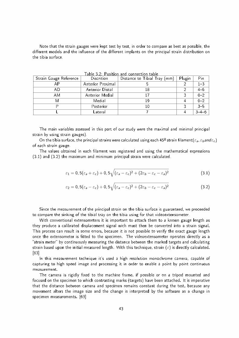
Note that the strain gauges were kept test by test, in order to compare as best as possible, thedierent models and the inuence of the dierent implants on the principal strain distribution onthe tibia surface.
Table 3.2: Position and connection tableStrain Gauge Reference Discrition Distance to Tibial Tray (mm) Plugin Pin
AP Anterior Proximal 5 2 13
AD Anterior Distal 18 2 46
AM Anterior Medial 17 3 02
M Medial 19 4 02
P Posterior 10 3 35
L Lateral 7 4 346
The main variables assessed in this part of our study were the maximal and minimal principalstrain by using strain gauges).
On the tibia surface, the principal strains were calculated using each 45º strain lament(εa, εbandεc)of each strain gauge.
The values obtained in each lament was registered and using the mathematical expressions(3.1) and (3.2) the maximum and minimum principal strain were calculated.
ε1 = 0, 5(εa + εc) + 0, 5√
(εa − εc)2 + (2εb − εc − εa)2 (3.1)
ε2 = 0, 5(εa − εc) + 0, 5√
(εa − εc)2 + (2εb − εc − εa)2 (3.2)
Since the measurement of the principal strain on the tibia surface is guaranteed, we proceededto compare the sinking of the tibial tray on the tibia using for that videoextensometer.
With conventional extensometers it is important to attach them to a known gauge length asthey produce a calibrated displacement signal wich must then be converted into a strain signal.This process can result in some errors, because it is not possible to verify the exact gauge lengthonce the extensometer is tted to the specimen. The videoextensometer operates directly as astrain meter by continuously measuring the distance between the marked targets and calculatingstrain based upon the initial measured length. With this technique, strain (ε) is directly calculated.[63]
In this measurement technique it's used a high resolution monochrome camera, capable ofcapturing to high speed image and processing it in order to enable a point by point continuousmeasurement.
The camera is rigidly xed to the machine frame, if possible or on a tripod mounted andfocused on the specimen to which contrasting marks (targets) have been attached. It is imperativethat the distance between camera and specimen remains constant during the test, because anymovement alters the image size and the change is interpreted by the software as a change inspecimen measurements. [63]
43

Using the buer data it is possible to produce grey scale (contrast) diagrams for every horizontalscan line and for every vertical pixel column. Due to the vast amount of data produced by eachpicture scan, it is imperative that this is eciently processed, in order to achieve an adequatedynamic response thus allowing the videoextensometer to be used with conventional static testingmachines.
The Videoextensometer software uses the frame buer data to automatically detect and followthe targets during testing. The targets produce rapid grey scale contrast transitions along a scanline and this data is dierentiated to produce distinct peaks, which are chosen as the measuringpoints. Reference marks are shown on the monitor, indicating the selected targets, and the operatoris provided with the opportunity to manually select alternatives in the eventuality that softwaremakes an incorrect interpretation.
The target datum point values are selected where the contrast line crosses the mean value ofthe maximum and minimum target grey scale levels. This value is dynamically adapted throughoutthe testing process and compensates if the contrast points fade due to the specimen stretching.
Beyond the evident advantages of the equipment installation, the accuracy level is 0,3 microns,according to the supplier. Since that we are working with a very low range of values, this accuracylevel seemed to be indicated to our study.
The installation of this equipment requires some caution in terms of illumination levels, since thesoftware recognizes the displacements by measuring the contrasts of the strip targets. Obviously,this contrast is much more evident if the workplace has a good illumination level. So this factor isvery important while using a videoextensometer. [64]
Before starting any displacement measurement on each model, a calibration of the equipmentwas made, using a calibrated ruler provided with the equipment, that sets the initial distancebetween targets to the software.
Figure 3.5: Videoextensometer materials
44

We also placed the videoextensometer (Videoextensometer ME46, Messphysik, Materials Test-ing) at 1,5 m of distance from the model in order to measure the displacement between tibial trayand tibia. At this point, was necessary to give special attention to setting the target as well as theequipment calibration between tests in order to ensure that the luminosity dierences that occursin the lab, according to the day time don't inuence the results.
The videoextensometer was connected to a computer with the Videoextensometer NG Version5.25.0 software in order to provide the acquisition data from the experimental tests.
After the models assembled, they were submitted to a severe load case on the medial condyle.
In everyday activity, the tibia bone is exposed to many dierent loads, as extion, rotation andcompression. The compression is the most important one in the knee joint. So, for this study, aperson with 85 kg, with a fully extended knee was considered.
According to the bibliographic research, the load on the knee joint is three times the weight ofthe person. So according to this and as well as in the numerical models, a 1600N load was appliedon the medial condyle of each model. [65, 66]
To apply the desired load was necessary to use an adapter on the side of the applied loadwhich was made with a piece of wood and a metal sphere. On the condyle surface of the tibiaanother adapter was set. A polyethylene component with a support on each concave surface ofthe condyles was xated with epoxy adhesive and prepared to get the metal sphere from the otheradapter.
Was also needed to create some constrains on our model. According to this, in the loadmachine, conception of the Laboratório de Biomecânica do Departamento de Engenharia Mecânicada Universidade de Aveiro, was implemented a mechanical clamping system in its lower base inorder to xate the model, leaving the superior part of the model free to be loaded. We consideredthat the tibia would be recessed at it most distal face, using for that a mechanical clamping systemthat allows the complete xation and recess of the composite tibia, preventing any deviation.
The main goal of this load case was to severe the location of the bone defect, since all thedefects were located on the medial side.
Figure 3.6: Load and constrain components
45
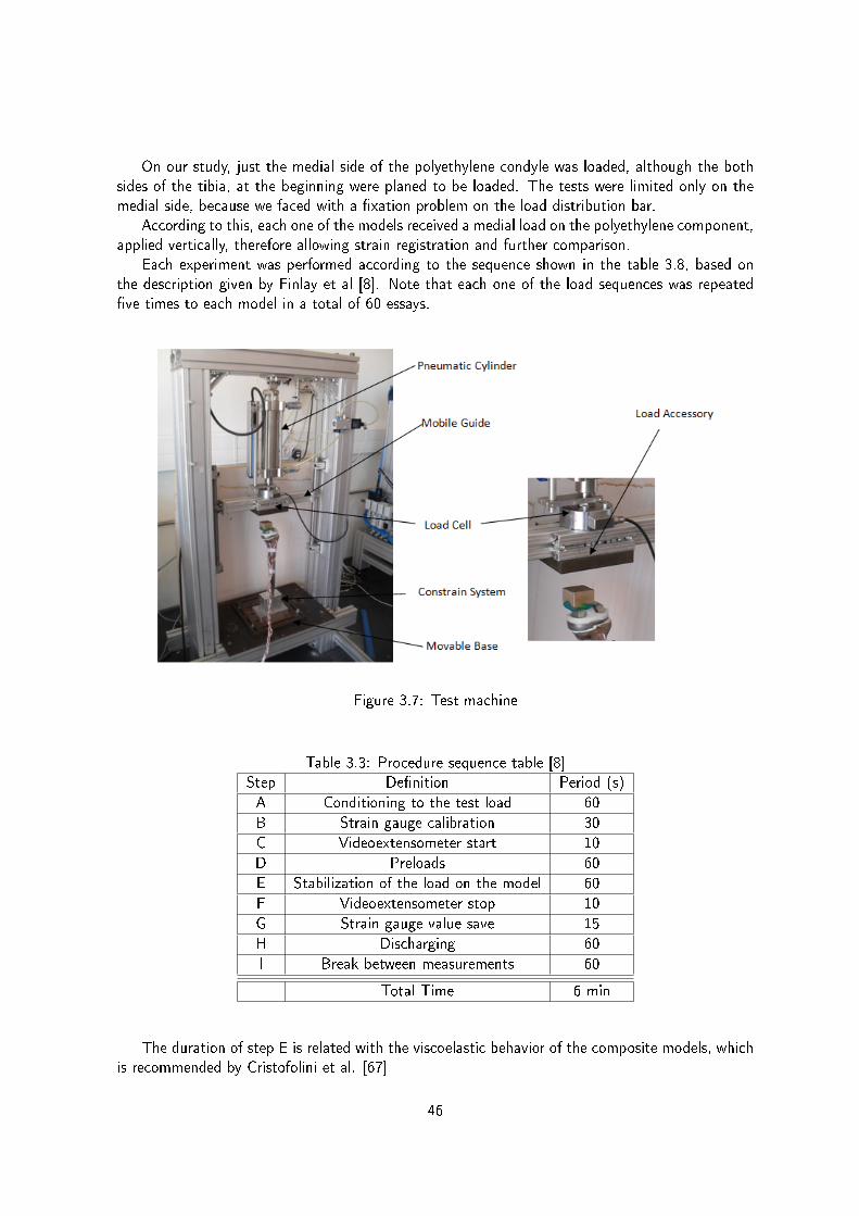
On our study, just the medial side of the polyethylene condyle was loaded, although the bothsides of the tibia, at the beginning were planed to be loaded. The tests were limited only on themedial side, because we faced with a xation problem on the load distribution bar.
According to this, each one of the models received a medial load on the polyethylene component,applied vertically, therefore allowing strain registration and further comparison.
Each experiment was performed according to the sequence shown in the table 3.8, based onthe description given by Finlay et al [8]. Note that each one of the load sequences was repeatedve times to each model in a total of 60 essays.
Figure 3.7: Test machine
Table 3.3: Procedure sequence table [8]Step Denition Period (s)
A Conditioning to the test load 60
B Strain gauge calibration 30
C Videoextensometer start 10
D Preloads 60
E Stabilization of the load on the model 60
F Videoextensometer stop 10
G Strain gauge value save 15
H Discharging 60
I Break between measurements 60
Total Time 6 min
The duration of step E is related with the viscoelastic behavior of the composite models, whichis recommended by Cristofolini et al. [67]
46

All of this components were mounted according to the gure 3.8 in order to save space onthe lab and allowing free movements between controlling computers from the load machine, straingauge acquisition data and videoextesometer acquisition data.
Figure 3.8: Experimental test apparatus
On the experimental results were analysed the mean and the standard deviation for both ε1 andε2 on the dierent models, as well as, the displacement of the tibial tray using a video measuringsystem.
47

3.3 Results
After the experimental tests, the collected data was treated in order to calculate the principalstrains and standard deviations obtained with the strain gauges on each test.
The results from videoextensometer were also treated in order to evaluate the displacementbetween tibia and tibial tray.
This procedure provided essential information about what happened on our twelve experimentalmodels.
The information collected with the strain gauges will allow us to know what happens aroundthe tibia surface, on the previous set positions.
Table 3.4: Resume experimental table
Models Without Stem
Cemented Tibial Tray Hemi Wedge Cement graft Total Wedge Block Bone Graft
Mean σ Mean σ Mean σ Mean σ Mean σ Mean σAP e2 -36 7,34 -179 17,31 -119 8,57 - - - - - -
e1 263 6,48 793 64,82 570 46,43 - - - - - -AD e2 -56 4,49 -47 1,58 -61 2,67 -51 3,51 -86 2,75 -48 4,65
e1 530 13,02 500 6,82 570 2,47 438 10,79 384 4,49 296 15,61AM e2 -197 57,43 -88 4,22 -145 1,69 -104 4,86 -252 4,98 -3 4,31
e1 110 12,21 129 3,98 89 1,74 193 7,54 176 5,67 117 6,84P e2 -313 5,75 -532 5,25 -899 4,91 -410 1,38 -34 17,78 -48 4,96
e1 110 73,45 132 137,67 252 260,1 236 81,53 33 6,07 84 13,75M e2 -551 10,12 -848 15,67 -811 0,97 -873 22,72 -872 33,17 -1204 42,51
e1 -46 2,17 -11 1,03 -34 1,18 2 2,44 187 7,32 334 7,34L e2 12 1,73 -11 4,79 -34 7,06 6 2,08 -28 3,26 36 16,15
e1 21 3,18 31 5,48 56 7,73 81 2,76 38 5,16 121 4,93
Models With Stem
AP e2 -93 24,04 -446 34,04 -173 31,21 - - - - - -e1 282 93,51 570 77,43 478 184,49 - - - - - -
AD e2 -77 2,42 -60 5,65 -50 4,74 -39 5,55 -70 11,73 -54 5,97e1 399 84,01 285 4,29 405 9,5 452 46,39 399 14,86 125 4,17
AM e2 -95 11,19 -88 5,06 -115 4,86 -120 4,2 -173 19,03 5 3e1 113 15,27 125 5,58 113 2,43 257 3,09 222 20,33 172 6,98
P e2 -332 15,45 -431 8,65 -625 11,17 -394 22,77 -19 9,63 -62 12,36e1 116 99,97 90 117,83 185 192,24 197 118,61 15 7,69 95 25,02
M e2 -431 3,14 -640 9,23 -497 3,33 -781 31,64 -787 39,33 -1166 103,71e1 -29 10,58 6 1,61 -13 3,26 -37 17,88 146 13,16 305 4,08
L e2 27 10,24 -23 24,88 0 13,9 15 46,51 6 14,81 53 6,48e1 66 20,87 64 23,37 60 5,31 105 5,09 57 5,35 106 4,77
* Mean = (1x10⁻⁶ m/m)
The mean value of standard deviations, regarding non stemmed models, is about 17µstrain.The cemented tibial tray model shows that the values of standard deviation are higher on the
M position for the ε1.Using a metallic hemiwedge or a cement graft we've obtained higher values of standard devi-
ation of ε1 on the P position. When compared to the standard deviation mean of all models, thesemodels show a dierence of approximately 85%. The metallic total wedge also has higher valuesof standard deviation on the P position, but in this case the dierence is approximately 80%.
On the metallic block model, as well as on the bone graft model, there is nothing to mentionregarding the P position. However the major dierences, relatively to the standard deviation mean,occur on the M position for ε2.
As shown in table 3.4, concerning the other positions in the models without stem, almost allstandard deviation values are lower than 18 µstrain, revealing an insignicant dispersion betweentests.
On the models with stem, the value of the standard deviation mean suers an increase, whencompared to the models without stem. On these models, this value is about 27%.
On the metallic hemiwedge model and on the cement graft model we've observed the highestvalues of ε1 on the P position, as seen before on the same non stemmed models. On these models,
48

the dierence to the standard deviation mean is about 85%. The metallic total wedge model alsoshows higher values of ε1 on the same position, with a 75% dierence to the standard deviationmean.
In what concerns the metallic block model, the highest standard deviation values are seen onε2 of the M position, showing a 30% dierence to the standard deviation mean. However we haveobserved, on the same position of the bone graft model, an increase of the standard deviationvalue, showing a dierence of approximately 73% to the standard deviation mean.
All the other stemmed model positions register standard deviation values inferior to 40 µstrain.Through the observation of table 3.4, when we compare the overall values of standard deviation
between stemmed and non stemmed models, we can state that they are higher in stemmed models.However, when we compare the same values between specic positions in both stemmed and nonstemmed models, we won't nd a signicant dierence.
A graphical description was made in order to compare and analyse a few aspects:- rst, the inuence of the several types of implants in what refers to principal strain
distribution around the tibia surface, on the set positions;- second, the dierence between using or not a metal stem.
49

(a)
(b)
Figure 3.9: Maximum Principal Strain ε 1 (a); Minimum Principal Strain ε 2(b) of the modelswithout stem
50

(a)
(b)
Figure 3.10: Maximum Principal Strain ε 1 (a); Minimum Principal Strain ε 2(b) of the modelswith stem
51

As we can see in the graphical results for the models without stem, the higher values on theAP position occur on the models with a metallic hemi-wedge, either in maximum and minimumprincipal strains. The model with lower values of ε1 and ε2 is the model where a cemented tibialtray was used. The model that shows a bigger dierence, when compared to the cemented tibialtray model, is the one where a metallic hemiwedge was used, showing a dierence of 530 µ strainfor ε1 and 143 µ strain for ε2.
On the AD position, the highest maximum principal strain value is achieved on the cement graftmodel and the lowest ε1 value on the bone graft model. In the same position, the models with theclosest ε1 to the cemented tibial tray model are the cement graft and the metallic hemiwedge,although one is higher and the other is lower, respectively. In this position, the minimum principalstrains do not show any signicant dierences between models. The bone graft model is the onethat presents the greatest dierence to the cemented tibial tray model, showing a decrease of 234µ strain for ε1.
On the AM position the situation is completely dierent, since the range of values is smallerthan on the previous strain gauge positions. On this position the model that shows a higher valueof ε1 is the model with a metallic total wedge, although this value is very similar to the oneobtained from the metal block model The model that shows lower values on this position of ε1 isthe model where a cement graft was used. On this position, the biggest dierence to the cementedtibial tray happens on the model with a total wedge. The dierence between these two models isabout 83µ strain. Regarding the minimum principal strain (ε2), the metallic block model showsthe highest value. The dierence from this model to the cemented tibial tray model is very small,about 55µstrain. Despite that, the cement graft model, whose 2 is lower than the cemented tibialtray value, shows a dierence of only 52µstrain, which makes it the closest one. On the other handthe biggest dierence occurs with the model where a hemiwedge was used, showing a dierenceof 109µ strain.
On the P position the values of ε1 are higher on the cement graft model, but the values ofmetallic total wedge are very near to this one. The lower value is registered on the model withmetallic block. On the cement graft model the ε1 value increases 142µstrain, compared to thecemented tibial tray model, which is the biggest dierence. The graphical representation of theε2 on the same position shows that the cement graft model is the one with the highest value,registering an increase of 586 µstrain when compared to the cemented tibial tray model. Onthis position, the dierence between the model with higher value and the other models is verysignicant. The metallic block model is the model with the smallest ε2 value. The decreaseregistered between this model and the model with cemented tibial tray is about 279 µ strain.
On the M position, the maximum principal strain value is higher on the model with bone graft,with a dierence of 380 µ strain from the cemented tibial tray model. Regarding the minimumprincipal strain, on the same position, we have that the bone graft model is also the one with thehighest value, and that the cemented tibial tray also is the model with the lowest value, having adierence of 653µstrain between them. Next we have all the other models, showing very similarvalues between them, with a dierence of 270µstrain to the cemented tibial tray.
Finally, on the L position, the ε1 has its highest value on the model with bone graft and thelowest on the cemented tibial tray model, with a dierence of 100 µ strains. Regarding the ε2,the model that shows the highest value is the cement graft model, despite all the results are verysimilar.
Now we proceed with the comparison of ε1 and ε2 values between both non stemmed andstemmed models, on the dierent strain gauge positions.
On the AP position the biggest dierence was found on the metallic hemiwedge models.
52

The ε1 values show a decrease of 30% (about 223 µstrain) from the non stemmed model to thestemmed model. However, the ε2 values register an increase of 60% (approximately 267µstrain)from the non stemmed model to the stemmed one.
On the AD position the biggest dierence on ε1 was also found on the metallic hemiwedgemodels, registering a decrease of 215 µstrain, which represents a reduction of 43%, from nonstemmed to stemmed models. Regarding the minimum principal strains, we may observe a decreaseof about 20% in all the models.
The ε1 on the AM position registered the main dierence between non stemmed and stemmedmodels on the metallic total wedge models, which shows an increase of about 63 µ strain, whichrepresents a raise of 24%. On the same position, but concerning the ε2, we can see that the maindierence occurs on the cemented tibial tray models, where a decrease of 79 µstrain, or a 31 %reduction, is registered when we use a stem. We should note that there are no dierences on thehemiwedge models.
On the P position, the ε1 shows a reduction of 67 µstrain on the cement graft model withstem, representing a 27% decrease, when compared with a non stemmed model. Something similaroccurs with the ε2 on the cement graft models, although the dierence in this case is about 274 µstrain, representing a decrease of 30%, which is the biggest dierence between non stemmed andstemmed models.
The maximum principal strains on the M position show that the biggest dierence occurs onthe metallic total wedge models, showing a dierence of 41 µstrain, which represents a decreaseof 22%. The minimum principal strain values on the same position show that the main dierenceoccurs on the cement graft models, registering a decrease of 314 µstrain, representing a reductionof 38% from the non stemmed model to the stemmed one.
Finally, the maximum principal strain values on the L position show that the biggest dierencehappens on the cemented tibial tray model, an increase of 45µstrain that represents a rise of 68%.On this position, the bone graft models are the ones who register a bigger dierence of the ε2values, increasing 32% (about 17µ strain).
53

As mentioned before, the displacement between tibia and tibial tray was also measured, in orderto evaluate the displacement/sinking of the tibial tray on the tibia. This measurement was madein each test.
Due to the applied forces on the medial condyle of the polyethylene component, the tibial traysuered a soft sinking in the tibia, causing a poor positioning of this component in the knee and,consequently a poor stability. In order to assess this phenomenon an experimental measurementwas made.
Figure 3.11: Displacement comparison between models with and without stem
Table 3.5: Displacement table
Model Displacemente (mm) between Stem and without Stem
Cement Tibial Tray with Stem 0,0682 0,0148Cement Tibial Tray without Stem 0,083
Metallic HemiWedge with Stem 0,0386 0,0428Metallic HemiWedge without Stem 0,0814
Cement Graft with Stem 0,0664 0,0206Cement Graft without Stem 0,087
Metallic Total Wedge with Stem 0,0576 0,0004Metallic Total Wedge without Stem 0,058
Metallic Block with Stem 0,0212 0,0040Metallic Block without Stem 0,0252
Bone Graft with Stem 0,0592 0,0008Bone Graft Tray without Stem 0,06
54

The table 3.5 shows the displacement values between tibia and tibial tray on the dierentmodels, with and without stem, in order to complete the graphical information.
In the cemented tibial tray, metallic hemiwedge and cement graft models there is an importantdierence between stemmed and non stemmed models. In opposite to that, in the metallic totalwedge and bone graft models that dierence is very small. The metallic block, although showingsmall displacements between tibial tray and tibia, are also the models that show the major dierenceto the cemented tibial tray with and without stem. The cement graft models are the ones thatpresent higher similarities to the cemented tibial tray model.
3.4 Discussion
Usually in this kind of in vitro experimental tests, in order to evaluate the stability of the arthroplasty,a measurement of the displacements between tibial tray and tibia is made. According to this, inthe previous studies a LVDT (Linear Variable Dierential Transformer) technique is used. Thistechnique requires a xation system on the models, in order to place the LVDT measurementequipment. This said, and because in our study we would have to measure the displacementsbetween the tibial tray and the tibia surface, we would need to create a xation system betweenboth bodies to allow the LVDT connection. This xation system requires two holes in the tibial trayin order to xate the movable supports of the measuring system. [5] According to this, and becausethat technique would need a greater preparatory work, other possibilities were considered, such asthe videoextensometer. Although the videoextensometer wasn't used in any previous biomechanicalstudy, it came as a good alternative since it would only be necessary to set the measurement targetsin each component. With this method we can save both time and materials. This method seemedto be a good alternative to the traditional methods. [63, 64] According to all of this, and sinceit has a desired range of measurement accuracy as well, we chose this method.
On this part of our study an experimental comparison using a composite tibia and dierenttypes of implants was made, as well as the use of a metal stem or not in each implant.
Nowadays, with the development of the composite materials, the substitution of the cadavericbones by composite bones was exponential, since its behaviour is very similar to the real bones andalso because it's easier to obtain and treat.
It's also important to refer that the use of such models in composite materials allows a distri-bution of the strains caused by beading loads, compression and torsion, identical to the real bone.According to Heiner et al [68]the results repeatability between tests on the same model shows thatthe range of results is between 0,5% and 7,8%. This results are superior in the cadaveric modelswhich has a 4,5% of repeatability [61, 67], despite this, a composite bone was used on this study.
The standard deviation values are good on all the positions, showing a small dispersion ofvalues between tests. However, in the P position we've observed high standard deviation values,leading to a greater dispersion on this position. This may be explained by the poor positioning ofthe P strain gauge. According to this we ensure that the repeatability of our tests is good.
In what concerns the models without stem, and according to the obtained results we mayconclude that the implants that cause less changes to the bone, when compared to the cementedtibial tray model, are the cement graft and the metallic hemiwedge. This goes in favour with the
55

work of A.D.Toms et al [45], which states that the use of cement to repair the defects seemed tobe a good choice. On the other hand, the model that more changes causes to the bone is the bonegraft model, because its values are distant to the cemented tibial tray model values.
Regarding the models with stem, we may conclude that the ones that less changes cause tothe bone are the cement graft model and the metallic hemiwedge model. As well as seen inthe models without stem, the bone graft model is the one that shows a major dierence from acemented tibial tray model. However, when we go from non stemmed models to stemmed ones weobserve a general reduction of all principal strain values.
According to the variation of principal strain values some problems may occur. When it suersa big increment, there is a possibility of hypertrophy or fatigue failure. On the other hand, when weobserve a substantial decrease of principal strain values, the bone density also decreases, causingbone resorption, according to Wolf's Law.
Although the metallic hemiwedge model has a strong probability of hypertrophy or fatiguefailure on the AP position, on the other positions, the principal strains present similar values tocemented tibial tray model, which shows that this model is the least harmful to the bone.
According to the obtained results when the displacement between tibia and tibial tray wasmeasured, we may conclude that the implant that more stability ensures when a medial load isapplied, is the model with the metallic block, because its values of displacement are lower than theother models.
We may also see that the use of metal stem does not make sense on the models with bonegraft and metallic total wedge because when we compare the displacement obtained on the thesemodels, with and without stem, the values of displacement are very similar. However, there is asignicant increase of stability on the cemented tibial tray, metallic hemiwedge and cement graft,therefore justifying the reinforcement of stability with a metal stem.
We think that the metal stem is not compulsory on the model with metallic block, despite theincrease of stability that occurs with it. We concluded this because the displacement observed ontibial tray is not much when a stem is used. According to this, and because the stem installationon the tibia requires extra time, materials and bone damage we think that it shouldn't be used.
So, although the use of a metal stem increases stability and the reduction of the principal strainvalues, we think that this instrument is only justied on the models with metallic hemiwedge andcement graft because it is on these models that it has greater inuence.
Regarding the obtained results we may say that, in general, the values were as expected,according to Brooks et al [69] studies.
56

Chapter 4
Computational models with
dierent bone defect repair
techniques
4.1 Introduction
As complement the experimental models, several numeric models were developed. Using niteelement methods (F.E.M.)techniques which allowed an evaluation of other important biomechanicalparameters, that are impossible to be studied on the experimental models because of physicallimitations. Two of this parameters are the principal strains on the cancellous bone under theimplants as well, as on the cortical surface adjacent to the implants. Using the numeric modelswas also possible to assess a physiological load case which was impossible with the experimentalmodels. In this chapter was used geometric modelling and structural calculations through theF.E.M. techniques.
4.2 Materials and Methods
The geometric modelling of the revision tibia and its components is a complicated task, since thebones have a high degree of complexity in its geometry and dimensions.
The modelling of the constituent components of total knee arthroplasty was based on CADmodelling (computer aided design) software, Dassault System CATIA V5 R19. Tibia, polyethylenecomponent and tibial tray geometric models used were the same used by Completo et al [5] obtainedby 3D scanning techniques. The model of the tibia was based on the commercial bones of Sawbone,Pacic Research Labs, Vashon Island, WA. [70].
Note that cortical structure of a real bone has a maximum thickness of 3 mm which changesalong the tibia surface. Because of this thickness changes, the two bone structures are dicultto precisely perform on the composite and consequently on the geometric bone. Because of thisproblem, a constant thickness of 2,5 mm was assigned to the geometric model. [71, 72]
The material properties atrtributed to the bone constituints, cortical and cancellous bone, werethe recommended ones by the supplier of the composite bone used on the experimental tests.
This two bone structures were assembled in order to create a geometric model of the humanbone. [5, 73]
57

The material properties of the tibial tray and the polyethylene component was the same thatof the real components.
These three components, tibia, tibial tray and polyethylene component were the same geometricmodels used by Completo et al [5].
The modelled repair technique components, such as: metallic total wedge, metallic hemiwedgeand metallic block was directly modelled in CATIA V5R19 with the same proprieties of the materialsthat they are made. The bone graft was also directly designed on CATIA V5R19 with the sameproperties of the bone and the cement with the same properties described by Murphy et al [9].
The stem used on our study was also modelled in CATIA V5R19 with the same properties ofthe real stems.
As mentioned before, the nal geometric model of the tibia was obtained by assembling bothparts, cortical and cancellous bone.
The structures assembled were performed following some constrains criteria, in order to makethat the both sides of the bone could be entirely in touch. This assembly was performed by theAssembly Design sub-module from the Mechanical Design module.
The gure 4.1 shows some images of the bone constituents.
Figure 4.1: Bone structures. Cortical Bone (A); Cancellous Bone (B), Bone section (C)
The geometric models obtained for the dierent implanted tibia models were based on thesurgical procedure, using for that the P.F.C.Sigma, P.F.C. Sigma Knee System, DePuy (Johnsonand Johnson Company) documentation.
Based on the available information, several sections were made on the intact tibia models inorder to place the desired implants.
These implants were aligned with the anatomical axis and with the articular motion plane,trying, at the same time, to cover the biggest surface on the proximal tibia.
58

The dierent cuts and implant models was combined using the sequence on the gure 4.2..The wedges used were obtained beyond the previous measurement and design of the real
wedges, attempting to be as much realistic as possible.All the components were reproduced on CATIA V5 R19, using the Part Design sub-module
from the module Mechanical Design.
Figure 4.2: Assembling sequence of the numerical models
Note that the metal stem was used in only half of the models, while in the other half just atibial tray was used. When the stem was not used at the end of the tibial tray, a polyethylenecover was set in its place, in order to minimize the eect of the contact between the cancellousbone and the titanium of the tibial tray.
In this study was used a metal non cemented stem with ϕ16 mm x 115 mm , combined withthe tibial tray. According to this, the models could be divided in two large groups of six modelseach (with and without stem).
59

On the gure 4.3 the dierence between models with and without stem are revealed and it'seasy to understand the dierences between the two types of models.
Figure 4.3: Sectioning to represent the model with stem and without stem
Three dierent types of metal wedges were used, as well as bone grafts and cement to repairthe defects on the revision of total knee arthroplasty.
In the gures 4.5, the dierent sections performed in the tibial bone can be seen as well as themetal and grafts implants.
All these models were obtained through the assembly of each part such as the tibia bone andthe many implant components using the Assembly Design of the Mechanical Design module.
The section that took place in each model were performed in the sub-module Part-Design ofthe Mechanical Design module, using for that tools like Sketch (were the section to cut was drawn)and Pocket (cut tool).
At last, the area in the cancellous bone where the tibial tray takes place was modelled usingthe Remove tool of the sub-module Part Design. To do so, the tibial tray was selected as thecomponent to be removed from the cancellous bone. This procedure was equally adopted with thecement, metallic stem and metallic wedge.
Since the load will be applied on both condyles, medial and lateral, in order to make easier thistask a previous preparation of the surfaces was made. So, a very small thick surface was createdin each condyle, using the Skecth tool of the Design Part submodule to draw the surface and thePad tool to extrude that.
60
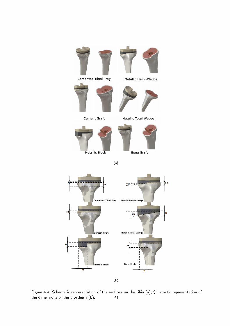
(a)
(b)
Figure 4.4: Schematic representation of the sections on the tibia (a); Schematic representation ofthe dimensions of the prosthesis (b). 61

The nite element method (F.E.M.) is a numeric computational technique originally developedto obtain the stress-strain state in complex problems.
Nowadays this method is widely used in engineering when we intend to simulate the behaviorof real systems.
The nite element models over the years has proven to be capable to providing good resultsaccording to the mechanical properties. This method has also proved to be capable of dealing withthe requirements of biomechanics problems.
An appropriately developed nite element model is a powerful tool to predict the eects of thedierent parameters involved and to provide information dicult to obtain from experiments.
It's important to note that, the reliability of these models strongly depends on an appropri-ate geometrical reconstruction and on accurate mathematical descriptions of the behavior of thebiological parts involved and their interactions with the surrounding environment. [3, 74]
A computational analysis may predict possible stress/strain distribution for dierent geometriesor positions, providing a basis for evaluation of surgical procedures, and aid in medical education.[75]
In this study we used a tibia bone, tibial tray and a polyethylene component, metallic wedgesand block, bone and cement grafts, and at last a metallic stem. This part of our study hasas main goal to investigate the many biomechanical issues around of the tibia model and tibialplateau surface. The use of numerical models was essential once this is very dicult to study withexperimental tests on composite materials.
It is known that the quality of the results is directly linked with the type and size of the niteelements. The convergence mesh analysis is important because when this procedure is not takeninto account, the nal results could show some errors, inuencing the conclusions of the numericanalysis. This errors could be avoided when a right mesh size is chosen.
So, in order to chose the proper nite element mesh size, the rst step was to perform aconvergence study on the cemented tibial tray. According to this, was analysed the maximumdisplacement and Von Misses stress on the model.
This study permitted to chose the proper mesh size used on the comparative models.We may say that a mesh convergence is achieved when the maximum displacement of each
element do not changes signicantly with the increase of the number of elements.In order to evaluate the mesh convergence, one single model was used, the cemented tibial tray
model without stem where a total of 17 meshes with dierent dimensions were generated(8 mm, 7mm, 6 mm, 5,5 mm, 5 mm, 4,5 mm, 4 mm, 3,5 mm, 3 mm, 2,8 mm, 2,6 mm, 2,5 mm, 2,4 mm,2,3 mm, 2,2 mm, 2,1 mm e 2 mm).
We chose to use the tetrahedra elements because, according to Ramos et al [76], the use oftetrahedral linear elements allows closer results to the theoretical ones, although the hexahedralquadractic elements are more stable and less inuenced to the degree of renement of the mesh.
According to this, a comparison between the number of elements and the maximum displace-ment on each element was made for each mesh size in order to evaluate which mesh should beused.
After the proper mesh was obtained on the test model, the mesh was also generated on theother models which will allow a posterior principal strain analysis.
In order to generate the numerical models, a geometric models generated previously was used.On our models was generated tetrahedral nite elements, based on tibia three-dimensional
geometry . Each threedimensional nite element mesh was created on the dierent model surfaceswith triangular elements of 3 nodes.
62

The tibial surface considered extends from the beginning of tibia's anterior crest till its condylesurfaces. We're chosen just this section because the remainder section was not important to ourstudy, since the surface analysed was the proximal surface of the tibia and also, because if all tibiawas considered, the computation time would be largely increased.
The cortical bone meshes were created internally and externally in order to create a closedvolume. In the other hand, on the cancellous bone, an exterior mesh was created, correspondingto its anatomical limit, resulting also in a completely closed mesh surface.
Figure 4.5: Mesh surfaces on the dierent bone structures. Cortical bone (A); Cancellous bone(B) and both structures (C)
In the cortical bone/cancellous bone interface, we assured that all the elements in this interfacewere shared between the two bodies, creating this way a rigid border between them. We also createdseveral lines along the tibia periphery in order to ensure that the created mesh passes along thesame location on the dierent models, providing this way the chance to a subsequent analysisbetween models.
63

According to this, seven guide lines in seven dierent planes were created in the tibial surfaces,at 2 mm, 4 mm, 7 mm, 17 mm, 27 mm, 40 mm and 60 mm distanced from the reference on thetibial planteau. Note that despite this seven planes are available, just three of them were used onour analyses(2 mm, 7 mm and 17 mm), because they have revealed to be the most important inthis study case, since the 2 mm guide line is the closest line to the beginning of the implant andthe 7 mm is on the middle line of the implant. The guide line at 17 mm was considered in orderto evaluate what happens on the bone surface after the implant. The planes are represented onthe gure 4.6.
(a) (b)
Figure 4.6: Mesh guide lines: cortical bone guide lines(a);cancellous bone guide line (b).
As well as on the cortical bone, the cancellous bone was also adjusted in order to provideimportant elements of study. On the reference cut of the tibial plateau, two planes were drawn,one in the sagittal plane and other in the frontal plane, as we can observe on the gure 4.6.
To accomplish this task, the sub-module Wireframe and Surface Design from the MechanicalDesign module was used.
After this, a threedimensional mesh was automatically generated, using for that TetrahedronFiller tool.
To perform the element propagation, was used the standard quality optimization option al-though it requires more computation resources.
After this, there were several issues related to the element geometry which were veried, suchas: jacobian ;skew; warpage; aspect ratio as well as the mesh quality, quality report,where no abnormal parameters were reported.
It was veried, during the threedimensional mesh generation, that the mesh quality clearlydepends on the surface mesh quality previously generated.
64

This mesh generation criteria was the same for all the numerical models of all components usedon the numerical experiments.
A total of twenty four numerical models were created, divided in four groups, stemmed andnon stemmed models, with just medial load and medial/lateral load.
Figure 4.7: Numerical models used
In order to create a similar environment to real bone in our numeric models, a several consid-erations were made.
In this study we considered that the numeric model was completely clamped on its distal surface,right on the anterior crest. In other words, every displacement or rotation was prevented.
Figure 4.8: Constrain and applied loads on the models
65

According to the research previously made, everyday the knee joint, in general, and tibia inparticular, are exposed to many forces and loads, although the compressive load are the ones thatmore inuences cause on the tibial bone.
For this study, we considered a 85 kg person with a full extension knee. The loads were appliedon the condylar surfaces of the tibia.
According to Morrison, the loads in the knee joint are approximately three times bigger thanthe weight of the person. [65]
The applied load on the condyles of the tibial plateau is non equally divided. According toHarrington, the loads are divided in 60 to 70% of the load on the medial condyle and 40 to 30%on the lateral one. [66]
This asymmetrical distribution allows to increase the exion eect on the tibia.
According to this, a person with 85 kg has an applied load of 2,5 kN asymmetrical distributedbetween each condyle, 65% on the medial side and 35% on the lateral. This results in a 1600 Non the medial condyle and 870 N on the lateral one.
So, the applied load was also divided in two classes. The numerical models in which only medialload was applied, the medial condyle received 1600 N, while on the models with medial and lateralloads each condyle receives 1600 N on the medial condyle and 870 N on the lateral condyle.
The loads were applied on the central surface of each condyle of the polyethylene componentas we can see in the gure 4.10. The load spots were kept on each numerical tests.
Figure 4.9: Load cases: Medial load (A); Medial and Lateral load (B).
It was also necessary to apply materials to our models in order to indicate how the dierentcomponents would behave according to the applied load.
The material characteristics of each component used are described in the table 4.1. All themodels were considered homogeneous, isotropic and linear elastic.
The contact conditions on each component of each model were considered as a fastenedsurfaces, except on the bone graft model. On this case, the contact conditions between the screw
66

Table 4.1: Material properties [9] [10]
Component Material Young Modulus (GPa) Poisson's Ratio
Cortical Bone Fiberglass - Epoxy Resin 16 0,3
Cancellous Bone Polyurethane foam 0,104 0,3
Polyethylene Component Polyethylene 0,5 0,3
Tibial Tray Titanium 110 0,3
Cement Polymethyl Methacrylate 2,28 0,3
Bone Grafts Bovine Bone 16 0,3
Wedges Co-Cr 210 0,3
Stem Titanium 110 0,3
used to xate the graft on the tibia, and the both surfaces of the graft and the cancellous bone,was considered as a friction surfaces (contact connection).
The maximum and minimum principal strain values in the cortical bone and cancellous boneof each dierent model were obtained and analysed along the schematic guide lines shown before.
All the analysis were performed on a computer COMPAL FL90 with a Intel® Core 2 DuoCPU a 2,40 GHz processor with 4,00 GB of installed memory (RAM), using the CATIA V5R19Dassault System software
In order to validate the numerical models was used the experimental models described on thelast chapter as well as the numerical ones.
The validations was made, measuring on the numeric models the same positions used onexperimental models. According to this was possible to analyse the dierence between numericand experimental models.
67
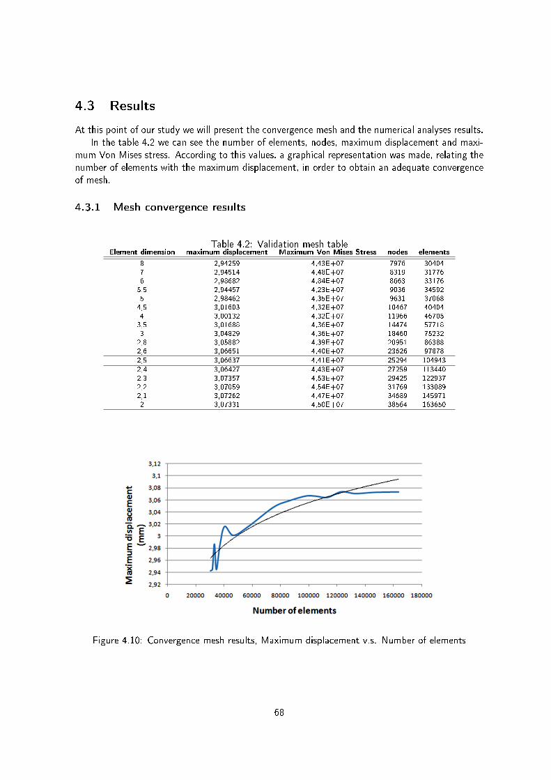
4.3 Results
At this point of our study we will present the convergence mesh and the numerical analyses results.In the table 4.2 we can see the number of elements, nodes, maximum displacement and maxi-
mum Von Mises stress. According to this values, a graphical representation was made, relating thenumber of elements with the maximum displacement, in order to obtain an adequate convergenceof mesh.
4.3.1 Mesh convergence results
Table 4.2: Validation mesh tableElement dimension maximum displacement Maximum Von Mises Stress nodes elements
8 2,94259 4,43E+07 7976 30404
7 2,94514 4,48E+07 8319 31776
6 2,98682 4,84E+07 8663 33176
5,5 2,94457 4,23E+07 9036 34592
5 2,98462 4,35E+07 9631 37068
4,5 3,01603 4,32E+07 10467 40404
4 3,00132 4,32E+07 11966 46705
3,5 3,01688 4,36E+07 14474 57718
3 3,04829 4,36E+07 18460 75232
2,8 3,05882 4,39E+07 20951 86388
2,6 3,06651 4,40E+07 23626 97878
2,5 3,06637 4,41E+07 25294 104943
2,4 3,06427 4,43E+07 27259 113440
2,3 3,07357 4,53E+07 29425 122937
2,2 3,07059 4,54E+07 31769 133089
2,1 3,07262 4,47E+07 34689 145971
2 3,07331 4,50E+07 38564 163650
Figure 4.10: Convergence mesh results, Maximum displacement v.s. Number of elements
68

As mentioned before, a mesh is considered adequately rened when its displacement does notchange signicantly with the increase of the number of elements. The dierence of the 2,5mmmesh size to the previous mesh size, 2,6mm is less than 1% when an increase of 1x10⁷ is observed.
According to this, based on displacement v.s. number of elements graphical results, to concludethat the mesh size of 2,5 mm is the one which satisfy the convergence criteria.
4.3.2 Load cases results
After the mesh is dened, the numerical models were processed in order to evaluate the principalstrains on the surface of the tibia.
The real knee joint receives medial and lateral load (physiologic load), because of this and inorder to assess what happens in this joint, two load cases will be described (just a medial load of1600N and a medial-lateral load 1600N-870N).
The principal strains were analysed on the cortical surface periphery along the 2mm, 7mm and17mm guide lines. As complement and according the objective of this study, the maximal andminimal principal strains were analysed on the cancellous bone on the dierent implants.
Figure 4.11: Principal strain guide lines
A graphical representation of the maximum and minimum principal strain at 2mm, 7mm, 17mmand frontal plane was made in order to simplify the analyses of the numerical models.
69

Figure 4.12: Medial load cases: Principal strains on the models with and without stem on thecortical bone: 2mm from the reference
70

Figure 4.13: Medial load cases: Principal strains on the models with and without stem on thecortical bone: 7mm from the reference
71
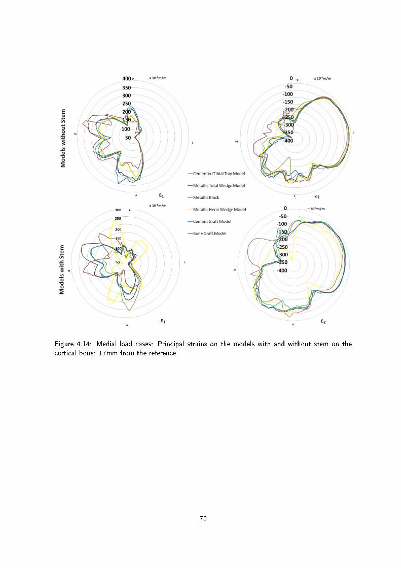
Figure 4.14: Medial load cases: Principal strains on the models with and without stem on thecortical bone: 17mm from the reference
72

Figure 4.15: Medial load cases: Principal strains on the models with and without stem on thecortical bone: frontal plane on the cancellous bone
73

We can see from gure 4.12, that the maximum principal strains at 2mm from the reference aremajority distributed on the medial side (M) of the model. On the lateral side (L) we observe thatthe values of ε1 are signicantly lower when compared with the medial side, showing a dierenceof approximately 350µ strain. On this side all the models have a similar behaviour, where there isno signicant dierence to point. In the anterior side (A) we observe that the ε1 distribution onthis position is similar to the posterior side (P). On this position there is no signicant dierencebetween anterior and posterior sides.
When compared to the model using a stem, we can see that occurs a signicant decrease ofthe ε1 in all positions of almost all models.
Regarding the minimum principal strain at 2mm from the reference we can observe that is inthe medial side that the higher values of ε2 are distributed. Despite a small area is covered, wecan see that in this side the cement graft model is the one that shows higher values. On the otherpositions, anterior (A), posterior (P) and lateral (L), the models show that the distribution of ε2is similar to the model with a cemented tibial tray model.
When we compare the minimum principal strain of the models with and without stem we cansee that a small decrease is observed on the medial (M) side. On the P side, an increase of theε2 is registered on the hemi-wedge, as well as on the A side. On the lateral side is where thebiggest dierence between stemmed and non stemmed models happens, specially on the modelswith hemiwedge. This model shows an increase of 100 µ strain when compared with the modelwithout stem.
The ε1 of the models with a medial load at 7mm from the reference, are mainly distributed onthe M side of the models. On the medial side the cement graft is the model that shows the highestvalues, showing a little dierence to the cemented tibial tray model. On the A side, the modelsshow a distribution of ε1 inferior than on the M side (50µ strain). On this side, the cementedtibial tray is the model that shows higher values when compared with the other models. The modelthat is closer to this one is the bone graft model. On the P side no signicant dierence betweenmodels is observed as well as on the lateral side, where the ε1 distribution is about 200 µ strainand 50µ strain, respectively.
When compared to the models with stem, we may observe that a general decrease of valuesoccur in each position. The main dierence registered happens on the medial side, where a decreaseof 100µ strain occur, which means a reduction of 20% when a stem is used. The stemmed cementgraft models are the ones that are closer to the cemented tibial tray model, when compared to allthe other stemmed models.
Regarding the minimum principal strain, we may observe, on the medial side (M), that thehighest values are distributed on this position, specially on the model with a metallic hemiwedge,which is the most distant model to cemented tibial tray model. On the other hand, lateral side (L)is where the lower values of µ strain are distributed. On this side there is no signicant dierencebetween models. On the P position we can see that all models show a similar distribution, exceptthe metallic-hemi wedge model which shows the lowest and the most distant values to cementedtibial tray model. On the A position we can observe that the metallic block shows the smallest andmost distant values from the cemented tibial tray model, while the metallic hemiwedge shows thehigher ones.
When we compared these models with the models with stem, we observed that the µ strainsuered a decrease, specially on the M and A position about 30%. On the other hand, the metallichemiwedge shows an increase of 50% and is the model where the dierence is higher.
At 17mm from the reference, after the implants, we may observe that the maximum principalstrain distribution on the medial side (M) shows smaller values than the anterior one. On M
74

position we can see that the bone graft model and metallic total wedge are the two models thatare more distant from the cemented tibial tray model, showing higher values. The other modelsshow similar values to cemented tibial tray model on this position. As mention before, the Aposition is where the higher values are present. On this case, the cemented tibial tray is the modelthat shows the highest values whereas the metallic total wedge has the lowest ones. On the Pposition the dierence to the cemented tibial tray is not that much, but also in this position, themetallic total wedge is the one that shows the smaller values of ε1. On the L position, all themodels have almost the same behaviour. On this position any signicant dierence can be shown.
When compared with the stemmed models we can see that ε1 decreases in all, the tibia surface.With stem, the model with a metallic block is the one that shows the biggest dierence to thecemented tibial tray model, showing smaller values than this one, specially on the M position.
About the minimum principal strain we can see that, is on the medial side that the highervalues are present. On this side, we can see that the model with metallic total wedge is the modelthat shows smaller values and where the dierence to the reference model is bigger (1000µ strain),representing a decrease of about 50%. On the anterior position (A), we can see that the generallyvalues of ε2 is 100µ strain and the dierence between models is insignicant, excepts with themetallic block, that shows a 200µ strain, 30% higher values. On the posterior position P, we cansee that that's where the higher values are concentrated, showing values of about 250µ strain. Onthis position, the model where the dierence to the cemented tibial tray model is bigger is the onewith total wedge, showing a dierence of 50µ strain. Finally on the lateral side, (L) the dierencebetween models is not signicant, showing all of them similar values to cemented tibial tray. It'salso on this position that the ε2 has smaller values. When compared with the stemmed models wecan see a signicant decrease of the ε2 on the P position.
On the anterior medial position we can see that increase the ε2 occurs, except in the modelwith metallic total wedge. So, this is the model that shows more dierent values when comparedwith the cemented tibial tray model. The other positions, despite the normal decrease of 30% whencompared with the models without stem, do not show any signicant dierence when comparedwith the cemented tibial tray model. On the medial position M we can see that that the metallichemi-wedge shows smaller values when compared to the cemented tibial tray.
The distribution of the ε1 on the surface of the tibial plateau (bonecement interface) showshigher values on the medial side (medial condyle). The model that less dierences show to thecemented tibial tray model is the cement graft model, showing a dierence of about 72µ strain,about 7% higher values. The model that shows the biggest dierence is the metallic total wedge,since on the medial side this model is the one that shows the lower values of ε1. This dierenceis about 98x10µ strain, around 90% lower values. On the lateral side, the distribution of themaximum principal strain is very similar in all the models, although the model where a metallicblock was used we can observe higher values and a bigger distance to the cemented tibial tray.
When compared with the models with stem we can see that there is a small decrease of themodels maximum principal strain values, except on the bone graft model on the medial side andon the hemiwedge model on the lateral. This changes on this two models represents the biggestdierences to the non stemmed models.
About the minimum principal strain on the tibial plateau surface, we can see that on themedial side of the models without stem, the cemented tibial tray model is the one that highervalues present, specially on the medial side of the surface. On this case, the metallic hemiwedgeis the one that lower values present and also the more distant ones. Where a cement graft wasused, we can see that the ε2 distribution is very similar to the cement tibial tray model. On thelateral side, there's nothing to declare, since the distribution of the ε2 is very similar on all the
75

models.When compared with the models with stem, we can see that the bone graft shows a peak on the
condyler surface, being the model that shows the higher values of ε2. Despite this, the dierencesbetween stemmed and non stemmed models show a signicant decrease of the ε2 distribution in themodels with cement graft, cemented tibial tray, metallic block and total wedge (20%). Although,the metallic hemi-wedge model doesn't show a signicant dierence. On the lateral side, whencompared with the models without stem, we may observe that exists an increase of the ε2 values.
76

Figure 4.16: Medial/Lateral load cases: Principal strains on the models with and without stem onthe cortical bone: 2mm from the reference
77
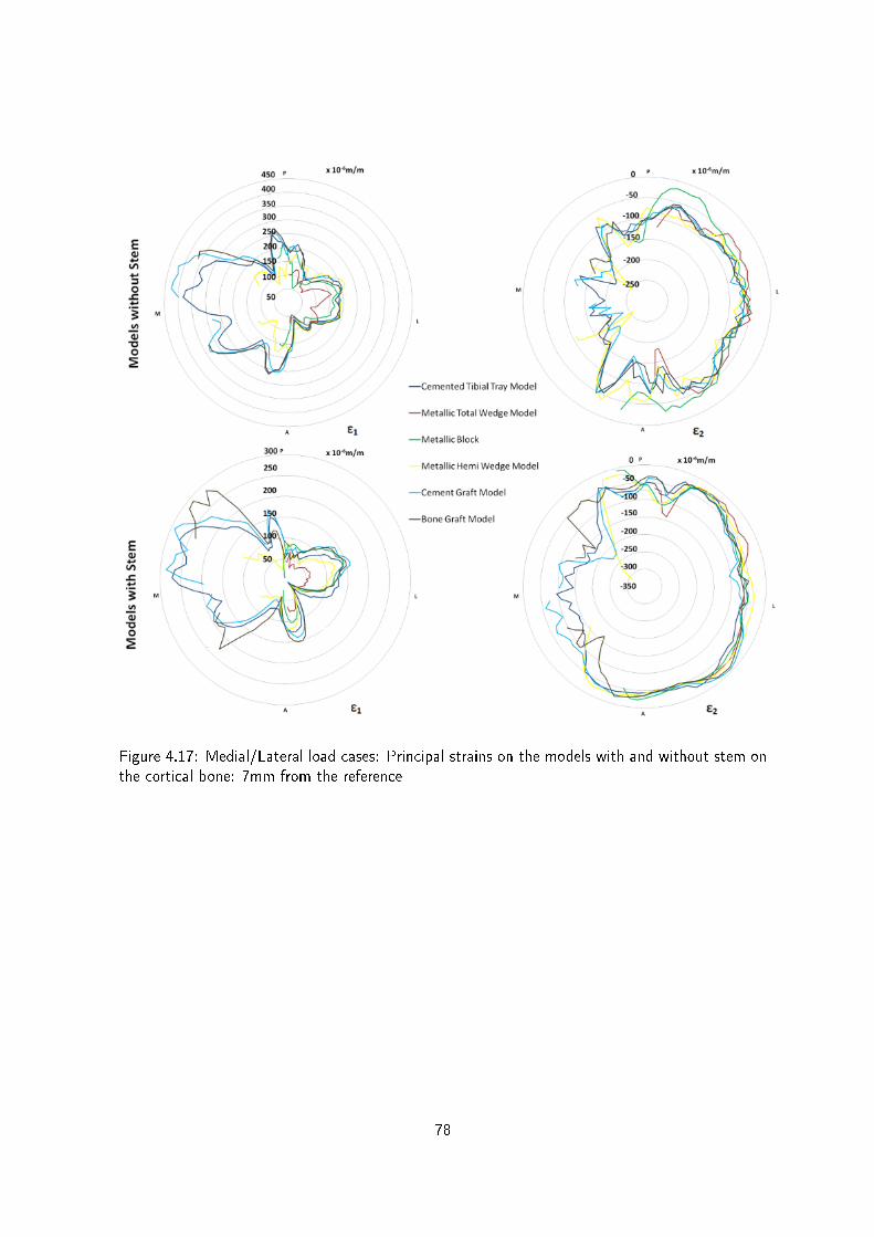
Figure 4.17: Medial/Lateral load cases: Principal strains on the models with and without stem onthe cortical bone: 7mm from the reference
78

Figure 4.18: Medial/Lateral load cases: Principal strains on the models with and without stem onthe cortical bone: 7mm from the reference
79

Figure 4.19: Medial/Lateral load cases: Principal strains on the models with and without stem:frontal plane on the cancellous bone
80

We can see at 2 mm from the reference that the maximum principal strains are distributedmajorly on the medial side of each models. On the anterior position, A, we can see that the ε1are lower, when compared with the other positions. On the other hand, the P and L position showa very similar distribution. The models that show the biggest dierences in the cemented tibialtray are where a metallic hemiwedge was used, specially on the P side. The metallic block is themodel that shows lower values of ε1 on the P side.
Regarding the stemmed models, we can see that the distribution around the tibia surface issimilar between models with and without stem, although the models without stem have highervalues than the models with stem.
On the model where a metallic hemiwedge (without stem) was used we can see that it is on theposterior position that the values of maximum principal strain are higher, registering a considerabledierence to the metallic hemi wedge model with stem (about 200µ strain which represents a 66%lower values).
As well, we can see on the maximum principal strain gures that the model with metallic blockwas the one with lower values of ε1 and the values of the bone graft are the closest ones to thecemented tibial tray model, specially on the lateral side. The values of cement graft show on theposterior medial side a considerable dierence to the model with cemented tibial tray.
The minimum principal strain at 2 mm shows the highest distributions on the medial side of themodels, although the dierence between sides is not so big. On the other hand, the values shownon the lateral side, L, are the lowest on each model and any signicant change is noted betweenmodels. So, we can see that the posterior medial side is where the highest values of ε2 occurs but,on the other hand, the anterior lateral side is where the lowest values of ε2 are distributed.
When we compare the models with and without stem, we can see that the ones without stemshow higher values than the models with stem, about 18% on the medial side, 35% on the lateral,40% on the anterior and 20% on the posterior side. The side where the biggest dierence wasregistered using a stem was on the L side. With a stem, on the P and A position the models getcloser to the cemented tibial tray model.
In general, all the models have similar behaviour around the tibia surface although the modelwith bone graft and metallic block are the ones closer to the cemented tibial tray models.
The maximum principal strain on the models without stem at 7mm from the reference showshigher values on the medial side On this position, we can see that the bone graft model and thecement graft are the ones that more similar values present on the entire surface of the tibia, despitethe other models shows not so dierent values. On the P and A side, the results are similar, and onthese positions we can see that the metallic hemi-wedge is the model which has the most dierentvalues when compared to the cemented tibial tray model. On the L position the situation changes,because, the metallic hemiwedge shows very closer values to the cemented tibial tray model. Onthis position, the metallic total wedge is the one that shows the most distant values.
When compared with to models with stem, we can see that as well as the models with stem,the higher values of ε1 are located on the medial side, although this values are smaller.
The metallic total wedge is the model with the smallest values of maximum principal strain,specially on the models with metal stem.
The bone graft models show, on both groups, that its medial side has the highest values whichare and very similar values to the cemented tibial tray model.
Regarding the minimum principal strain, we can see that the highest values are concentratedon the medial side. On the L side we can see that the dierence between models is not signicant.Near the P side, we can see that the metallic block values show a smaller decrease when comparedwith the other models, but on the P position this decrease is not observed. On the A position we
81

may see that the bone graft model is the one that shows higher dierences when compared to thecemented tibial tray model.
The dierence between models on the medial side is not signicant around the tibia. Despitethis, the values between models with stem and without stem is about 32%, according to themaximum values of each model, on each position. The dierence between medial side and lateralside is about 150 µ strain. That dierence on models with stem is about 100 µ strain.
At 17mm from the reference, after the implants, we may observe that the maximum principalstrain distribution on the medial side (M) shows the highest values, although there is a very smalldierence to the posterior side. On M position we can see that the bone graft model and metallictotal wedge are more distant from the cemented tibial tray model, showing higher values. Theother models show similar values to cemented tibial tray model on this position.
On the A position we can see that all the models have similar behaviour, specially the cementgraft model, that shows a similar distribution than cement tibial tray model. On this position, themetallic block is the model which more distanced to the cemented tibial tray are.
On the P position, the dierence to the cemented tibial tray is not that much. In this position,the metal block is the one that shows the smaller values of ε1 and the metallic hemiwedge, cementgraft and metallic total wedge the closest values. On the L position, all the models have almostthe same behaviour. On this position any signicant dierence can be shown. When comparedwith the stemmed models we can see that the ε1 decrease in all the tibia surface is about 30%generally. With stem, the model with a bone graft is the one that shows the biggest dierence tothe cemented tibial tray model, showing higher values than this one, specially on the M position.The metall block and metallic total wedge are the ones that lower values shows.
Regarding the minimum principal strain we can see that is on the medial side, M, that thehighest values occur, despite the values on the P side not being so distant. We can see on the Mside that the metallic total wedge and metallic block are the ones which present lower and moredistant values to the cemented tibial tray model. The remain models show similar behaviour tothe cemented tibial tray model.
On the L and A positions, the registered values are almost the same and them dierence tothe cemented tibial tray is not signicant.
When compared to the models with stem, although a reduction on the P side is noted of about40%, any other change is noted.
The maximum and minimum principal strain were also analysed on the frontal plane of thetibial plateau, in order to evaluate de tibial tray stability. The maximum principal strain of themodels without stem shows higher values on the medial side, specially the models with cementgraft and cemented tibial tray, which are very closer.
The models with metallic block and metallic total wedge show the smaller values of maximumprincipal strain on both sides, and they are more distant to the cemented tibial tray. The cementgraft is the model with closer results on the medial side present.
On the lateral side, we can see that all the models have a similar behaviour to the cementedtibial tray model.
When compared to models with stem we can see that the values are not so dierent on thelateral side, showing very close values to the non stemmed models.
About the minimum principal strain, on the medial side, we can see that the the cement modelis the one that shows closer values to the cemented tibial tray model. The most distant models tothe reference one are the models with a metallic hemiwedge and metallic block. This dierenceis about 2000 µ strain, which is about 60% dierent. On the lateral side, we can see that only themetallic block and metallic total wedge shows a signicant dierence to the cememtned tibial tray
82

model. This dierence is about 480 µ strain on the metal block and 1200 µ strain on the metallictotal wedge.
The minimum principal strain shows higher values on the medial side of the models either onthe stemmed or non stemmed models.
The dierence on the medial side between models with and without stem is signicant, about20%, except in the bone graft model with stem, which shows similar values to the models withoutstem.
On the lateral side, although the values of the models with stem are lower than the modelswithout stem, the dierence is just about 500 µ strain.
4.3.3 Experimental Models v.s. Numerical Models Results
In this section the results of the validation made on our models will be presented, as well as thedierence between numerical and experimental models.
The numerical models validation will be presented on the gure 5.12.
Figure 4.20: Numeric models validation
We can see that the values of the linear regressions show values of R2 near 1 as well as valuesof the linear regression slopes.
On the next gure will be shown the graphical dierences between numerical and experimentalmodels of the maximum and minimum principal strain obtained.
83

Figure 4.21: Comparison between numeric and experimental models
We see on the gure 4.18 that on the maximum principals strain of the models with stem thedierences between numerical models and experimental models are bigger on the AD position ofthe metallic total wedge and on the AP position of the metallic hemi wedge and cement graft.
The minimum principal strain of the stemmed models shows the biggest dierences on the Mand AP side.
According to the results of the non stemmed models we can see that the only the cement graftshows a considerable dierence between numerical and experimental models on the P position.
At last, we also compared the dierences between minimum principal strain on the modelswithout stem. We see that the main dierences happens on the M and P sides of the bone graftand hemiwedge models.
84

4.4 Discussion
The rst important point to discuss regards to the mesh dimension. The mesh used was 2,5mm since this value was where the values of the maximum displacement v.s.number of elementsstarted to converge, and there was no reason to choose smaller elements than 2,5 mm because theconvergence was achieved, because that would just increase the computation time and wouldn'tmake any signicant improvement on the results obtained.
We will focus our discussion on the medial/lateral load case because this is closer to a physi-ological situation. The medial load case was only important to assess the veracity and feasibilityof the numerical models when compared to the experimental ones. It is important to refer thatthe results of this comparison are very positive, showing similar results to the experimental model,which guaranties a good replication of the numerical models.
So, in order to evaluate the validation of the numerical models, a comparison between numericaland experimental models was made. This comparison demonstrates that the experimental modelsin fact validate the numerical models, as mentioned by Jeremy et al [77].
The validation results are very satisfactory, since the R2 is near 1 and the the regression line isalso near 1. These values mean that the correlation between experimental and numerical modelswas achieved.
A general illustration of this correlation has been shown, and also an individual analysis wasmade in order to assess how each model contributes to this correlation. According to this we sawthat, in general, all the models show satisfactory values of R2 (near 1), except the last two models,bone graft and metallic block model. These models, metallic block and bone graft, show dierentresults because the values of R2 and regression line are distant than 1 (0,91 and 1,2 respectively).We think that this happened because of the problem on the white lament of the posterior straingauge, which was accidentally damaged during the surgical procedure.
According to this, and despising this situation, we may say that the relationship betweenexperimental and numerical models is good, which validates our numerical models.
By other words, we have observed that both the maximum and minimum principal strainsobtained on the numerical models followed the behaviour of the maximum and minimum principalstrain of the experimental models. Since a good replication of the numerical models was guaranteed,their use is allowed to investigate the principal strains in areas where it is impossible to evaluatethrough experimental test.
According to the results obtained with the comparison between numerical and experimentalmodels we may say that the position which shows more dierences in all the comparisons graphsis the AP position. This probably happened because of the strain gauge position on the surface ofthe tibia, which was set in a prominent surface of the experimental model. When comparing to thenumerical model, we should see the principal strain values on the same position. So, because thisstrain gauge was set is a prominent surface, the approximation made by nite element method, onthat same position, could be a bit far from reality.
The minimum principal strain dierences on the M position of the stemmed and non stemmedmodels can only be explained by the use of a screw on bone graft numerical models, in order toxate the bone graft to the tibial bone. On the experimental models we didn't use any screw, andthat may be the explanation for the dierence occurred.
85

According now to the obtained values from the numerical models we may conclude that, ingeneral, the models with medial load show the expected behaviour in all the dierent distances tothe reference.
As expected, the highest values of the compression forces occur on the medial side of themodels, since only a medial load was applied.
The implant that less inuence causes to the bone is the cement graft, as well as the metallichemiwedge, because the principal strains registered on these models are very similar to the ce-mented tibial tray model. Both models show less dierences to the cemented tibial tray model onthe M position. Despite that, we can also see that the other models do not change signicantlyon the lateral side, because only a medial load was applied.
The model that more changes causes to the bone, when compared with the cemented tibialtray, is the bone graft model. On the M position of this model is where the dierences to thecemented tibial tray are higher.
On the L position, the dierence of each model to the cemented tibial tray is insignicant,which is normal since only the medial side has been loaded. According to this, the compressionforces on this side are insignicant, leading to small changes on the models.
On this load case, although the results should be taken into account, the problematic situationmay not occur on the physiologic load situation, where the loads are applied on the both medialand lateral sides.
On the models where we tried to simulate the physiological case, with medial and lateral load,the scenario was dierent, specially, and as expected, on the lateral side.
The cement graft model is the model that, either on the beginning, middle or after the implant,shows similar results to the cemented tibial tray model, although in some positions may occuroccasional bigger dierences. These dierences never exceed 15%. According to this, the riskof hypertrophy or even bone resorption is not signicant. The values are specially closer to thecemented tibial tray on the lateral, posterior and anterior positions, which was expected since thedefect is on the medial side, which is reinforced by the strains distribution on the medial side thatalso shows closer results to the cemented tibial tray, as we can see on the gure 4.18.
We can see, specially after the implant, at 17mm to the reference, that the bone graft is themodel that shows a bigger dierence to the cemented tibial tray, specially on the M position(wherethe defect is). According to this, we may say that when this model is used the chance of fatiguefailure on the medial side increases, since there is an increment of 25% of the maximum principalstrain.
The models with metallic hemiwedge show that in all the dierent distances to the reference,its values are closer to the cemented tibial tray values, specially on the lateral side (L). When thistechnique is used, the increases registered are never higher than 20%.
The metallic total wedge, specially on the side of the defect, may cause fatigue failure to thebone since there is an increase of 25% of the principal strains registered, when compared with thecemented tibial tray model.
The implant that guarantees better results on the tibial plateau of the cancellous bone wasassessed with the measurement of the interface bonecement. According to this, we may see thatthe cement graft is the model that shows better results, since there is only a small dierence tothe cement tibial tray, about 14%. This result could be improved with the use of a metallic stem,decreasing to a 10% dierence.
On the other hand, the models with metallic wedges and bone graft enhance the risk of boneresorption on the cancellous bone, specially on the medial side of the models, because their principal
86

strain values show a reduction, when compared with the cemented tibial tray model. This reductionis about 40% on the bone graft model, and between 65 to 78% on the models with metallic wedgesand block. On the lateral side these problems just occurs on the metallic total wedge, which showsa reduction about 50 % of minimum principal strain when compared to the cemented tibial tray.According to this, the model with metallic total wedge can cause bone resorption on the lateralside.
We can arm, based on the numerical tests, that the metal stem provides a decrease of theprincipal strains on the cortical and cancellous tibia. This results are consistent with Jeremy et al[77] previous studies.
According to these results, we can conclude that the models with cement graft and metallichemiwedge are the ones where the use of a metal stem makes sense. However, when a decreaseof the principal strain is needed the stem is useful.
When an intervention is required, in order to repair any type of the defects mentioned in ourwork, we should use a metallic hemiwedge with a metal stem or a cement graft, because thoseare the models that less interferences cause to the subjacent bone.
87


Chapter 5
Conclusions and Future Works
5.1 Conclusions
The obtained results from the numerical models reected the principal strains behaviour of theexperimental models on the analysed positions. This shows the ability of the numerical models toreplicate the behaviour of the experimental models.
The results obtained from the dierent analysed models allow us to conclude that the loadcases, the technique to repair the defect and the use of stem inuence the levels of strains in thebone, as well as the implant stability.
We also concluded that the metallic total wedge and metal block increases the principal strainsnear the implant, on the medial side of the cortical bone. However, when compared these modelswith the bone graft model, we can see that this one shows the biggest dierence. According tothis increase of principal strains, a tendency of hypertrophy or fatigue failure on this side of thecortical bone when the most invasive techniques are used, may occur.
On the cancellous bone, the cement graft is the model that closer are to the cemented tibialtray model, according to this, we may say that is the less invasive to the bone. On the other hand,the metallic wedges/block models are the ones that a bigger changes cause in the cancellous bone,specially on the medial side(defect side). These models increase the potential of bone resorption,since the principal strains of these models show a relatively decrease when compared with thecemented tibial tray model. The bone graft also shows a signicant dierence to the cementedtibial tray model on the medial side of the cancellous bone which also cause the bone resorption.
According to our study we also concluded that the use of a metal stem guarantees an extrastabilization eect on the models and should be used, specially on the simplest implants, wherecement graft and metallic hemiwedge was used.
The metallic stem is not important on the metallic total wedge model and metallic block modelbecause their principal strain values don't show a signicant variation with the use of a stem, asshown in our tests. This behaviour can be justied by geometry and big dimensions of these kindof implants.
On our study, with the displacement comparison between tibia and tibial tray, we concludedthat the metal block is the more stable model, since the displacement registered on this case wasvery small when compared with the other models
89

5.2 Future works
In order to provide more knowledge about revision of total knee arthroplasty will be presented somesuggestions for future studies in this area attempting to give more answers about the mechanicalbehaviour of the knee joint and especially about osteolysis and stress-shielding.
In order to increment the feasibility of this study, we propose the use of cadaveric bone insimilar tests in order to evaluate the dierences between this resource and the composite material.
Since on this study just a static load case was applied, we think that would be suitable to verifyhow the used techniques on this study behave when exposed to a severe fatigue tests.
We also propose experimental tests with dierent types of stem since, that on this study, justone type of stem was tested. We suggest the use of modular stem, press t, and combined tibialtray with decentered xation stem, with dierent lengths, in order to assess which ones have betterresults. It should be also tested the use of cement in the stem xation.
90

Bibliography
[1] M. Nordin and V. H. Frankel. Basic Biomechanics of the Musculoskeletal System. Williams& Wilkins, 2001.
[2] http://www.nlm.nih.gov, 2008.
[3] Susana Meireles. Strain shieldingindistalfemurafterpatellofemoralarthroplastyunder dierentactivityconditions. Master's thesis, Universidade de Aveiro, 2009.
[4] http://www.upmc.com, 2008.
[5] A. Completo. Estudo numérico e experimental da biomecânica da prótese do joel. Master'sthesis, Universidade de Aveiro, 2006.
[6] Ammeen D. J Engh, G. A. Bone loss with revision total knee arthroplasty defect classicationand alternatives for reconstruction. Instr Course Lect, 48:167175, 1999.
[7] P.F.C: Sigma Knee System. P.F.C: Sigma Knee System. Depuy a Johnson and JohnsonCompany.
[8] Bournet R.B. McLeant J Finlay, J. B. A technique for in vitro measurement of principal strainsin the human tibia. J. Biomechanics, 15:723739, 1982.
[9] Prendergast PJ. Murphy BP. Measurement of non-linear microcrack accumulation rates inpolymethylmethacrylate bone cement under cyclic loading. J Mater Sci, 10:77981, 1999.
[10] Whiteside LA. Selective ligament release in total knee arthroplasty of knee in valgus. ClinOrthop, 17:2327, 2002.
[11] http://en.wikipedia.org.
[12] Ana Rego. Estudo experimental do efeito das hastes femorais na tibia na ratj. Master's thesis,Universidade de Aveiro, 2008.
[13] www.daviddarling.info.
[14] Henry Gray. Anatomy of the human body.
[15] http://www.bartleby.com/.
[16] J. Goldblatt and J. Richmond. Anatomy and biomechanics of the knee. Operative Techniquesin Sports Medicine, 11:172186, 2003.
91

[17] Lubinus H. H. Patella glides bearing total replacement. orthopedics. Journal Bone JointSurgery AM, 2:119127, 1979.
[18] Kummer F. Jazrawi L., Bai B. The eect of stem modularity and mode of xation on tibialcomponent stability in revision total knee arthroplasty. The Journal of Arthroplasty, 16:759767, 2001.
[19] Leila Castro Michelle Ferrandis Priscila Lopes Sandra Santoro Paulo Roberto, Flavio Oliveira.Estudos apresentados no seminário velox de atualização cientíca. In Análise biomecânica doagachamento e as principais lesões relacionadas ao joelho, 2007.
[20] Cheryl Perry. Anatomica, the complete home medical reference. Global Book Publishing,2005.
[21] http://pt.wikipedia.org/wiki/Menisco.
[22] Rik Huiskes Van C. Mow. Basic orthopaedic biomechanics. Lippincott -Raven, New York,1997.
[23] J. Fritz. Articular cartilage defects in the knee basics, therapies and results. Injury Int. J.Care Injured, 39S1:5057, 2008.
[24] www.answers.com.
[25] Carol Eustice. What is varus or valgus knee deformity? About.com Guide, 2008.
[26] Windsor RE. Correction of deformity: When the implant itself is not enough. In CurrentConcepts in Joint Replacement, 2010.
[27] Adam Sertaoggi, 5 2008.
[28] Gregory M Martin. Total knee replacement.
[29] Simon H Palmer. Total knee arthroplasty. Medscape Reference, .:., May,2011 2011.
[30] P Dieppe. Osteoarthritis: time to shift the paradigm. British Medical Journal, 7192-7200:318, 1999.
[31] Ines Marques Martins Silva. Estudo experimental das tensões no osso na revisão da artroplastiatotal do joelho com haste press-t. Master's thesis, Universidade de Aveiro, 2008.
[32] Filho J. Mestriner, L. Artroplastia total do joelho em osteoartrose. Revista Brasil Ortop., .:.,1993.
[33] Pécora J. Infecção nas artroplastias do joelho. Revist@ do Joelho, .:., 2006.
[34] Ivan Oransky. The eects of osteolysis and aseptic loosening. Medscape Orthopaedics, .:.,2001.
[35] Oxford Dictionary of Sports Science & Medicine.
[36] Dorr L. Bone grafts for bone loss with total knee replacement. Orthop Clin North Am, .:.,1989.
92

[37] Rand J. Bone deciency in total knee arthroplasty. use of metal wedge augmentation. ClinOrthop, 271:6371, 1991.
[38] Rorabeck C Engh G. A classication of bone defects in revision knee arthroplasty. Baltimore:Williams & Wilkins, 6:63120, 1997.
[39] Lotke PA. Elia EA. Results of revision total knee arthroplasty associated with signicant boneloss. Clin Orthop, 392:213220, 1991.
[40] Rand JA Pagnano MW, Trousdale RT. Tibial wedge augmentation for bone deciency intotal knee arthroplasty. a follow-up study. Clin Orthop Relat Res, 321:151155, 1995.
[41] Healthbase Online Inc, 2011.
[42] Shalby Hospitals. Total knee replacement (tkr).
[43] Santavicca EA Insall JN Bartel DL, Burstein AH. Performance of the tibial component intotal knee replacement. J Bone Joint Surgery Am, 76:769777, 1982.
[44] Toms AD. Whittaker JP, Dharmarajan R. The management of bone loss in revision total kneereplacement. J Bone Joint Surg [Br], -:, 2008.
[45] D. McClelland L. Chua R. Spencer-Jones J.-H. Kuiper A. D. Toms, R. L. Barker. Repair ofdefects and containment in revision total knee replacement. The Robert Jones & Agnes HuntOrthopaedic Hospital, Oswestry, England, -:, 2008.
[46] Puri N. Lotke PA, Carolan GF. Impaction grafting for bone defects in revision total kneearthroplasty. Clin Orthop, 406:145151, 2006.
[47] Richard David Scott James V.Bono. Revision Total Knee Arthroplasty. Springer, 2005.
[48] Humble RS et al. Fehring TK, PeindlRD. Modular tibial augmentations in total knee arthro-plasty. Clin. Orthop., 17:207327, 1996.
[49] Ewald FC Brand MG, Daley RJ. Tibial tray augmentation with modular metal wedges fortibial bone stock deciency. Clin Orthop Relat Res, 248:7179, 1989.
[50] Guerin J Bourne RB Rorabeck CH. Patel JV, Masonis JL. The fate of augments to treattype-2 bone defects in revision knee arthroplasty. J Bone Joint Surg Br., 9:86195, 2004.
[51] Burt M. Sawhney J Barrack R., Rorabeck C. Pain at the end of the stem after revision totalknee arthroplasty. Clin. Orthop., 19:119124, 1999.
[52] Kloepper R. Mohr R. Peters C., Erickson J. Revision total knee arthroplasty with modularcomponents inserted with metaphyseal cement and stems without cement. The Journal ofArthroplasty, 9:320, 2005.
[53] Freeman M. Albrektsson B., Carlsson L. The eect of a stem on the tibial component of kneearthroplasty: roentgen stereophotogrammetric study of uncemented tibial components in thefreeman-samuelson knee arthroplasty. J Bone Joint Surg Br, 35:33, 1990.
[54] Burt M. Hopkins S. Barrack R., Stanley T. The eect of stem design on end-of-stem pain inrevision total knee arthroplasty. The Journal of Arthroplasty, 19:119124, 2004.
93

[55] Buma P. Sloof TJ, Schimmel J. Cemented xation with bone grafts. Orthop Clin North Am,.:., 1993.
[56] Ling RSM Gie GA, Linder L. Impacted cancellous allograft and cement for revision total hiparthroplasty. J Bone Joint Surg Br, 39:133296, 1993.
[57] Gregory F. Carolan MD Paul A. Lotke, MD and BS Neil Puri. Technique for impaction bonegrafting of large bone defects in rtka. The journal of arthroplasty, 21:., 2006.
[58] Haas SB Becker-Fluegel MW Windsor RE. Scuderi GR, Insall JN. autogeneic bone graftingof tibial defects in primary total knee arthroplasty. Clin Orthop Relat Res, 24:6065, 1994.
[59] Crawford H. Bourne R. Principles of revision total knee arthroplasty. Orthop Clin North Am,29:331337, 2003.
[60] Wikipedia.
[61] S. J. Kreuzer S. Condit MA, Ilario. From 50th annual meeting of the orthopedic researchsociety; march 7-10, san francisco, ca. In Mechanical validation of a foam tibial model forevaluating xation of revision tibial components., 2004.
[62] Gautier E. Cordey, J. Strain gauges used in the mechanical testing of bones, part ii: in vitroand in vivo technique, injury. Int. J. care Injured, 30:1420, 1999.
[63] MESSPHYSIK. MESSPHYSIK - Materials Testing Version 5.25.0. MESSPHYSIK - MaterialsTesting, 5.25.0 edition.
[64] http://www.instron.com.br.
[65] J. B Morrison. The mechanics of the knee joint in relation to normal walking. JBiomech, 3:5161, 1970.
[66] I. J. Harrington. A bioengineering analysis of force actions at the knee in normal and patho-logical gait. Biomed Eng, 11:167172, 1976.
[67] Viceconti M. Cristofolini, L. Mechanical validation of whole bone composite tibia models.Journal of Biomechanics, 33:279288, 2000.
[68] Brown T. D Heiner, A. D. Structural properties of a new design of composite replicate femursand tíbias. Journal Biomechanics, 34:773781, 2001.
[69] Walker P.S. Scott R. D Brooks, P. J. Tibial component xation in decient tibial bone stock.Clin Orthop, 184:302308, 1984.
[70] www.sawbones.com.
[71] Professor online, 2010.
[72] Mediped.
[73] Joana Miguel da Silva Leal Pereira. Caracterização numérica e experimental do cotovelonativo e protésico. Master's thesis, Universidade de Aveiro, 2010.
94

[74] E. Pena. A three-dimensional nite element analysis of the combined behavior of ligamentsand menisci in the healthy human knee joint. Journal of Biomechanics, 39:16861701, 2006.
[75] J. W. ] Fernandez and P. J. Hunter. An anatomically based patient-specic nite elementmodel of patella articulation: towards a diagnostic tool. Biomech Model, 4:2038, 2005.
[76] J.A. Simões A. Ramos. Tetrahedral versus hexahedral nite elements in numerical modellingof the proximal femur. Medical Engineering and Physics, 28:916924, 2006.
[77] Nicole Davis Timothy M. Wright PhD Russell Windsor MD Jeremy J. Rawlinson PhD, RobertF. Closkey Jr MD. Stemmed Implants Improve Stability in Augmented Constrained CondylarKnees. The Association of Bone and Joint Surgeons, 2008.
95


![Duarte revisitado portada [imprenta] - Banco Central de la ...](https://static.fdokumen.com/doc/165x107/631bf509c2fddc481907c5d4/duarte-revisitado-portada-imprenta-banco-central-de-la-.jpg)