Retrieval of Gas Pollutants Vertical Profile in the Boundary Layer by Means of Multiple-Axis DOAS
7
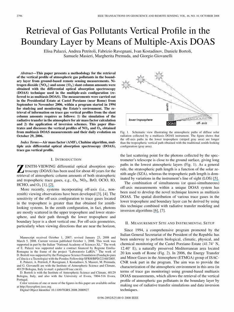
2796 IEEE TRANSACTIONS ON GEOSCIENCE AND REMOTE SENSING, VOL. 46, NO. 10, OCTOBER 2008 Retrieval of Gas Pollutants Vertical Profile in the Boundary Layer by Means of Multiple-Axis DOAS Elisa Palazzi, Andrea Petritoli, Fabrizio Ravegnani, Ivan Kostadinov, Daniele Bortoli, Samuele Masieri, Margherita Premuda, and Giorgio Giovanelli Abstract—This paper presents a methodology for the retrieval of the vertical profile of atmospheric gas pollutants in the bound- ary layer from ground-based remote sensing measurements. Ni- trogen dioxide (NO 2 ) and ozone (O 3 ) slant column amounts were obtained with the differential optical absorption spectroscopy (DOAS) technique used in the multiple-axis configuration (re- ferred to as multiaxis DOAS). The measurements were carried out in the Presidential Estate at Castel Porziano (near Rome) from September to November 2006, within a program started in 1994 for studying and monitoring the Estate’s environment. The re- trieval of information on trace gas vertical profiles from the slant column amounts requires as follows: 1) the simulation of the radiative transfer in the atmosphere for air mass factor calculation and 2) the application of inversion schemes. This paper illus- trates and discusses the vertical profiles of NO 2 and O 3 obtained from multiaxis DOAS measurements and their daily evolution on October 29, 2006. Index Terms—Air mass factor (AMF), Chahine algorithm, mul- tiple axis differential optical absorption spectroscopy (DOAS), trace gas vertical profile. I. I NTRODUCTION Z ENITH-VIEWING differential optical absorption spec- troscopy (DOAS) has been used for about 40 years for the retrieval of atmospheric column amounts of both stratospheric and tropospheric trace gases, e.g., O 3 , NO 2 , BrO, OClO, IO, HCHO, and O 4 [1], [2]. More recently, systems incorporating off-axis (i.e., non- zenith) viewing observations have been developed [3], [4]. The sensitivity of the off-axis configuration to trace gases located in the troposphere is greater than that obtained for zenith- looking systems. In the zenith configuration, in fact, photons are mostly scattered in the upper troposphere and lower strato- sphere, and their path through the lower troposphere and boundary layer is a short vertical one. For off-axis geometries, particularly when viewing directions that are near the horizon, Manuscript received October 1, 2007; revised January 23, 2008 and March 5, 2008. Current version published October 1, 2008. This work was supported in part by the Italian “National Academy of Sciences XL.” The work of E. Palazzi was supported under a contract financed by Regione Emilia- Romagna in the frame of the project “Laboratorio LaRIA.” The work of D. Bortoli was supported by the Portuguese Science Foundation (Fundação para a Ciência e a Tecnologia) with the Postdoc Fellowship SFRH/BPD/22160/2005. E. Palazzi, A. Petritoli, F. Ravegnani, I. Kostadinov, S. Masieri, M. Premuda, and G. Giovanelli are with the Institute of Atmospheric Science and Climate, 40129 Bologna, Italy (e-mail: [email protected]). D. Bortoli is with the Institute of Atmospheric Science and Climate, 40129 Bologna, Italy, and also with the University of Evora, 7004-516 Evora, Portugal. Color versions of one or more of the figures in this paper are available online at http://ieeexplore.ieee.org. Digital Object Identifier 10.1109/TGRS.2008.2000927 Fig. 1. Schematic view illustrating the atmospheric paths of diffuse solar radiation collected by a multiaxis DOAS instrument. The figure shows that the off-axis paths in the lower troposphere (striped gray area) are longer than the tropospheric vertical path obtained with the traditional zenith-looking configuration (gray area). the last scattering point for the photons collected by the spec- trometer’s telescope is close to the ground surface, giving long paths in the lowest atmospheric layers (Fig. 1). As a general rule, the stratospheric path length is a function of the solar ze- nith angle (SZA), whereas the tropospheric path length is dom- inated by variations in the instrument’s line of sight (LOS) [5]. The combination of simultaneous (or quasi-simultaneous) off-axis measurements within a unique DOAS system has been used to develop the novel technique known as multiaxis DOAS. The spatial distribution of various trace gases in the lower troposphere and boundary layer can be derived by using this technique combined with radiative transfer modeling and inversion algorithms [6], [7]. II. MEASUREMENT SITE AND I NSTRUMENTAL SETUP Since 1994, a comprehensive program promoted by the Italian General Secretariat of the President of the Republic has been underway to perform biological, climatic, physical, and chemical monitoring of the Castel Porziano Estate (41.74 ◦ N, 12.40 ◦ E), a naturally preserved Mediterranean area located 20 km south of Rome (Fig. 2). In 2006, the Energy Transfer and Minor Gases in the Atmosphere (ETMGA) group of ISAC- CNR took part in the program. The aim was to provide the characterization of the atmospheric environment in this area (in terms of trace gas monitoring) using ground-based multiaxis DOAS measurements, which allows the retrieval of the vertical profile of atmospheric gas pollutants in the boundary layer by making use of radiative transfer simulations and data inversion techniques. 0196-2892/$25.00 © 2008 IEEE
-
Upload
independent -
Category
Documents
-
view
6 -
download
0
Transcript of Retrieval of Gas Pollutants Vertical Profile in the Boundary Layer by Means of Multiple-Axis DOAS
2796 IEEE TRANSACTIONS ON GEOSCIENCE AND REMOTE SENSING, VOL. 46, NO. 10, OCTOBER 2008
Retrieval of Gas Pollutants Vertical Profile in theBoundary Layer by Means of Multiple-Axis DOAS
Elisa Palazzi, Andrea Petritoli, Fabrizio Ravegnani, Ivan Kostadinov, Daniele Bortoli,Samuele Masieri, Margherita Premuda, and Giorgio Giovanelli
Abstract—This paper presents a methodology for the retrievalof the vertical profile of atmospheric gas pollutants in the bound-ary layer from ground-based remote sensing measurements. Ni-trogen dioxide (NO2) and ozone (O3) slant column amounts wereobtained with the differential optical absorption spectroscopy(DOAS) technique used in the multiple-axis configuration (re-ferred to as multiaxis DOAS). The measurements were carried outin the Presidential Estate at Castel Porziano (near Rome) fromSeptember to November 2006, within a program started in 1994for studying and monitoring the Estate’s environment. The re-trieval of information on trace gas vertical profiles from the slantcolumn amounts requires as follows: 1) the simulation of theradiative transfer in the atmosphere for air mass factor calculationand 2) the application of inversion schemes. This paper illus-trates and discusses the vertical profiles of NO2 and O3 obtainedfrom multiaxis DOAS measurements and their daily evolution onOctober 29, 2006.
Index Terms—Air mass factor (AMF), Chahine algorithm, mul-tiple axis differential optical absorption spectroscopy (DOAS),trace gas vertical profile.
I. INTRODUCTION
Z ENITH-VIEWING differential optical absorption spec-troscopy (DOAS) has been used for about 40 years for the
retrieval of atmospheric column amounts of both stratosphericand tropospheric trace gases, e.g., O3, NO2, BrO, OClO, IO,HCHO, and O4 [1], [2].
More recently, systems incorporating off-axis (i.e., non-zenith) viewing observations have been developed [3], [4]. Thesensitivity of the off-axis configuration to trace gases locatedin the troposphere is greater than that obtained for zenith-looking systems. In the zenith configuration, in fact, photonsare mostly scattered in the upper troposphere and lower strato-sphere, and their path through the lower troposphere andboundary layer is a short vertical one. For off-axis geometries,particularly when viewing directions that are near the horizon,
Manuscript received October 1, 2007; revised January 23, 2008 andMarch 5, 2008. Current version published October 1, 2008. This work wassupported in part by the Italian “National Academy of Sciences XL.” The workof E. Palazzi was supported under a contract financed by Regione Emilia-Romagna in the frame of the project “Laboratorio LaRIA.” The work ofD. Bortoli was supported by the Portuguese Science Foundation (Fundação paraa Ciência e a Tecnologia) with the Postdoc Fellowship SFRH/BPD/22160/2005.
E. Palazzi, A. Petritoli, F. Ravegnani, I. Kostadinov, S. Masieri, M. Premuda,and G. Giovanelli are with the Institute of Atmospheric Science and Climate,40129 Bologna, Italy (e-mail: [email protected]).
D. Bortoli is with the Institute of Atmospheric Science and Climate, 40129Bologna, Italy, and also with the University of Evora, 7004-516 Evora,Portugal.
Color versions of one or more of the figures in this paper are available onlineat http://ieeexplore.ieee.org.
Digital Object Identifier 10.1109/TGRS.2008.2000927
Fig. 1. Schematic view illustrating the atmospheric paths of diffuse solarradiation collected by a multiaxis DOAS instrument. The figure shows thatthe off-axis paths in the lower troposphere (striped gray area) are longerthan the tropospheric vertical path obtained with the traditional zenith-lookingconfiguration (gray area).
the last scattering point for the photons collected by the spec-trometer’s telescope is close to the ground surface, giving longpaths in the lowest atmospheric layers (Fig. 1). As a generalrule, the stratospheric path length is a function of the solar ze-nith angle (SZA), whereas the tropospheric path length is dom-inated by variations in the instrument’s line of sight (LOS) [5].
The combination of simultaneous (or quasi-simultaneous)off-axis measurements within a unique DOAS system hasbeen used to develop the novel technique known as multiaxisDOAS. The spatial distribution of various trace gases in thelower troposphere and boundary layer can be derived by usingthis technique combined with radiative transfer modeling andinversion algorithms [6], [7].
II. MEASUREMENT SITE AND INSTRUMENTAL SETUP
Since 1994, a comprehensive program promoted by theItalian General Secretariat of the President of the Republic hasbeen underway to perform biological, climatic, physical, andchemical monitoring of the Castel Porziano Estate (41.74◦ N,12.40◦ E), a naturally preserved Mediterranean area located20 km south of Rome (Fig. 2). In 2006, the Energy Transferand Minor Gases in the Atmosphere (ETMGA) group of ISAC-CNR took part in the program. The aim was to provide thecharacterization of the atmospheric environment in this area (interms of trace gas monitoring) using ground-based multiaxisDOAS measurements, which allows the retrieval of the verticalprofile of atmospheric gas pollutants in the boundary layer bymaking use of radiative transfer simulations and data inversiontechniques.
0196-2892/$25.00 © 2008 IEEE
PALAZZI et al.: RETRIEVAL OF GAS POLLUTANTS VERTICAL PROFILE IN THE BOUNDARY LAYER 2797
Fig. 2. Map of the area showing the Castel Porziano Estate (black outlinedarea) located about 20 km south of the city of Rome on the Tyrrhenian coast.The black square inside the area indicates the measurement site.
The entire instrumental setup used to perform multiaxisDOAS measurements was installed at Castel Porziano insidea van and operated during almost all the campaign fromSeptember to November 2006. It consists of a UV/visiblespectrometer called TROPOGAS (TROPOspheric GASCOD,where GASCOD means gas analyzer spectrometer correlat-ing optical differences) [8] that is able to operate in the285–950-nm range. The spectrometer features a custom-builtmonochromator based on a Jobin-Yvon holographic spheri-cal grating with N = 1200 grooves/mm, blaze maximized at320 nm, a focal length of 300 mm, and an entrance slit of0.1 mm × 8 mm. The linear dispersion and resolution are about2.4 nm/mm and 0.7 nm at 350 nm, respectively. A steppermotor connected to the grating permits the view of the 285–950-nm spectral range in 50–60-nm single intervals. The sensoris a 2-D (1100 × 330 pixels) back-illuminated SITe charge-coupled device (CCD). In order to reduce the dark current,the measured signal is binned into a matrix of 1092 columnsand 11 rows (in the SITe-manufactured CCD sensor, the darkcurrent per pixel is reduced by a factor of nrow × 0.013, wherenrow is the number of added rows). A Peltier cooling systemmaintains the detector at a constant operating temperature of−30.0 ◦C ± 0.1 ◦C. A small integrating sphere with a diameterof 60 mm, equipped with Hg and Quartz-Iodine tungsten lamps,is incorporated into the system for spectral calibrations aswell as for checking the CCD performance and the overallinstrumental spectral characteristics. A small telescope withboth azimuthal and zenithal movements transmits the radiationcollected at a given LOS to the spectrometer by means of anoptical fiber. Fig. 3 shows some pictures of various componentsof the instrumental setup.
III. METHODOLOGY
To derive the desired trace gas profile from the slant col-umn density (SCD) measured at different LOS, the physicalrelation between the two quantities needs to be established.Within this work, radiative transfer was simulated by the
Fig. 3. (Left) Picture of the van interior, with the spectrometer, PC, and tele-scope mounted on the tripod. (Middle) Picture of the TROPOGAS spectrometerand PC for row data acquisition and preliminary plotting. (Right) Picture ofthe small telescope designed for multiaxis measurements. It is connected tothe spectrometer by optical fiber and is powered by a stepper motor for bothzenithal and azimuthal movements.
spherical Monte Carlo (MC) radiative transfer model (RTM)PROMSAR (PROcessing of Multi-Scattered AtmosphericRadiation) [9] in order to compute the air mass factor (AMF) forthe target trace gases (see Section III-A). AMFs relate the tracegas concentrations at the different layers of the atmosphereto the measured SCDs and are useful for converting SCDsinto vertical column densities (VCDs, the vertically integratedconcentration). Subsequently, inversion schemes based on theiterative Chahine algorithm were used to retrieve the verticalprofile of the trace gas under consideration, employing thematrix of computed AMFs as the kernel in the inversion process(see Section III-B).
A. AMF Computation by PROMSAR RTM
For the interpretation of remote sensing measurements, a fun-damental output is a measure for their sensitivity to atmospherictrace gases. Generally, the sensitivity is expressed as the so-called AMF, which is defined by the ratio of the measured SCDand the VCD
AMF = SCD/VCD. (1)
The accuracy the AMF values depends on the length of thelight path through the atmosphere and on the vertical distri-bution of absorbing trace gases. The length of the light pathis, in turn, dependent on the Sun’s position (expressed in theSZA), the telescope LOS, the aerosol profile in the atmosphere,radiation wavelength, and other quantities. The AMF can beprecalculated for a variety of such quantities and for differentatmospheric scenarios, and be applied to the SCDs to find theVCDs. For this paper, the spherical RTM PROMSAR, basedon MC, was used to simulate the radiative transfer in theatmosphere under various conditions, calculating the mean pathof radiation (i.e., photons) in the atmospheric layers and, hence,computing the AMF of the trace gases under interest.
1) Description of the PROMSAR Model: In the PROMSARRTM, each starting photon is released from the detector (thefield of view set to values < 0.1) in the LOS direction and isfollowed in a direction which is opposite to that where it wouldphysically propagate (backward MC scheme). Each originalphoton is assigned a statistical weight (i.e., the source intensity)equal to one unless differently specified. Once photons aregenerated at the “fictitious” source, their path in the atmosphereis traced. The technique utilizes a computer to generate randomnumbers that correspond to the direction and length of eachstep in the random walk. First, random numbers uniformly
2798 IEEE TRANSACTIONS ON GEOSCIENCE AND REMOTE SENSING, VOL. 46, NO. 10, OCTOBER 2008
distributed in the interval [0, 1] are obtained from an algorithmfor generating pseudorandom numbers. Such random numbersare then transformed, so that they are distributed according toprobability density functions derived from the basic scatteringand absorption properties of the medium. The random pathlength between two successive scattering events (hereinafterreferred to as free optical path, FOP) is deduced from theBeer–Lambert law, i.e., the FOP is sampled from an exponentialdistribution. To avoid the photons escaping the atmospherewithout interactions with its components, a collision can beforced to occur (forced collision technique) by sampling theFOP from a truncated exponential distribution [10]. At eachcollision point, the statistical weight of the photon is adjustedaccording to the survival probability ω = b/(a + b), where aand b are the absorption coefficient and the scattering coeffi-cient, respectively. When the path of the photon intersects theground surface, the photon weight is decreased by the surfacealbedo. Random numbers also decide the type of scatteringevent, molecular or aerosol type, by comparing the ratio of themolecular scattering coefficient to the sum of the molecular andaerosol coefficients of the layer at which the scattering altitudebelongs. If the random number is less than that ratio, molecularscattering occurs; otherwise, the event is considered to be anaerosol scattering event. The new direction of the photon aftercollision is determined by sampling a polar scattering anglefrom the Rayleigh phase function, if the event is a molecularevent, or from the Mie phase function, if it is an aerosol event.The azimuthal angle is selected at random from a uniformdistribution because, from physical considerations, there is anequal probability that a photon will be scattered in a givenazimuthal direction. At this point, a new path length beforecollision is generated. The process continues until the photonhas undergone a fixed number of collisions or has had its weightdecreased to a preassigned threshold value. Many simulationsare then performed (called histories), and the desired result istaken as an average over the number of photon histories. Inmany practical applications, one can predict the statistical error(variance) in this average result, allowing an estimate of thenumber of histories required to achieve a given variance. In thisregard, to accomplish the MC simulation of radiative transfer,batches of preassigned number of photon histories, each onerepresentative of a single valuable numerical experiment, areprocessed. Aside from being more appropriate for the variancecalculation, this procedure allows a high number of historiesto be run without significant precision loss when collecting thesimulation results (105 photon histories can be run by process-ing, for instance, 100 batches, each one of 1000 histories). Itshould be borne in mind that, although the variance is a functionof the number of histories, some variance reducing techniques,such as the aforementioned forced collision, can effectively beused to reduce the computational time and keep the statisticaloscillations relatively small.
Two kinds of input data are required to be run by thePROMSAR code for simulating a given radiative transfer sce-nario. The first is related to the features of the MC calculationto be carried out, i.e., batch strategy, receiver and source de-scription, type of variance reducing technique, etc. The secondis related to the physical data needed for the history tracking,i.e., absorption and scattering coefficients, phase functions, and
refraction indexes. With regard to the second kind of input data,a library of physical data for the environment in question is as-sumed to have been made previously available. This library dataset characterizes each kind of atmosphere in terms of its compo-nents (both aerosol particles and molecules) and their physicalproperties, i.e., the vertical spatial distribution of the interactioncoefficients, phase functions, and the refraction indexes. Thus,the MODerate resolution TRANsmittance (MODTRAN) code[11], with its carefully chosen atmospheric models and accuratephysical description of possible events, can be convenientlylinked to the PROMSAR code. In addition, MODTRAN canalso be assumed as the reference for checking the correct acqui-sition and treatment of library data, for instance, by comparingcorresponding transmittances. Such data are acquired by thecode, and appropriately processed, through a subroutine calledPRELIB, allowing the swift availability of optical depths andprobability distributions during the MC simulation.
Simulated SCDs of a given trace gas can be obtained by thePROMSAR RTM once the photon paths are computed layer bylayer, together with the trace gas absorption along these paths.The AMFs (and weighting functions) are then computed fromthe SCDs.
The so-called box-AMFs for different atmospheric heightlayers can also be computed instead of standard AMFs. Thebox-AMFs characterize the ratio of the partial SCD to thepartial VCD of an atmospheric layer with a given trace gasconcentration (box vertical profile). They therefore describethe sensitivity of the measurements as a function of alti-tude. It is interesting to note that, for optically thin absorbers(optical depth � 1), the box-AMFs are identical to the so-called weighting functions [12], [13]. Weighting functions playan important role in the retrieval of atmospheric constituentsfrom spectroscopic measurements, as they provide a linearrelationship between differential changes in the atmospheric pa-rameters, and the resulting change in the measured atmosphericquantity. For optical thin absorbers, box-AMFs can also beapproximated by the intensity weighted geometrical path lengthextension with respect to the vertical thickness of the selectedlayer, averaged over all the contributing light paths. The greatadvantage of calculating box-AMFs is that they can serve asa universal database to calculate appropriate (total) AMFs forarbitrary species with different height profiles. Total AMFs caneasily be calculated (2) from the box-AMFs, and the respectivetrace gas profile as the sum of the box-AMFs over the whole at-mosphere weighted by the respective partial trace gas VCD [14]
AMF =
(TOA∑
0
AMFi · VCDi
) / (TOA∑
0
VCDi
). (2)
In (2), AMFi and VCDi refer to the box-AMF and the partialVCD for layer i; within the layer, the trace gas concentration isassumed to be constant. The sum is carried out over all layersi, from the surface to the top of atmosphere (TOA).
In June 2005, the PROMSAR model participated in anextended comparison exercise of nine RTMs from eightinternational research groups for the UV and visible spec-tral range. The comparison focused on the multiaxis DOASmethod and on the systematic investigation of the sensitivityof this technique under various viewing geometries and aerosol

PALAZZI et al.: RETRIEVAL OF GAS POLLUTANTS VERTICAL PROFILE IN THE BOUNDARY LAYER 2799
conditions. Accurate modeling of box-AMFs and radiances wasperformed, obtaining a good overall agreement (differences<10%) for the various RTMs [14].
B. Inversion Algorithm
A nonlinear iterative inversion method based on the weightedChahine algorithm [15] was used to retrieve nitrogen dioxideand ozone concentration profiles in the boundary layer from aset of slant columns measured at different LOS.
Given reasonable first guess profiles of the trace gases understudy, this method minimizes the difference between measuredand simulated slant column values in determining the optimumsolution profile. During each iteration, the profile shape ischanged to allow the calculation to fit the observation. TheChahine method was first used by McKenzie et al. [16], whoalso demonstrated its ability to detect tropospheric pollution.The ETMGA group has experience with the use of the Chahineinversion scheme for the retrieval of NO2 vertical profiles inthe upper troposphere lower stratosphere (UTLS) region, asillustrated in [17].
The theoretical and formal approach to error calculation ininversion techniques has been studied in detail by Rodgers[12]. Given the true profile of the trace gas in the atmospherex, the a priori profile used for the inversion xp, the vectorof measurements y, the forward model F , and the inversemodel R, the total error of the profile retrieval is the differencebetween the retrieved and the true profile (xr − x). It can beexpressed as
xr − x = (A − In)(x − xp) + GyKb(b − bg)
+ GyΔF + Gyε. (3)
In (3), A is the matrix of averaging kernels, which definethe sensitivity of the retrieved profile to changes in the realatmospheric profile. The vertical resolution of the profile re-trieval is determined from the averaging kernels. Gy is thematrix of contribution functions representing the sensitivity ofthe retrieved profile to the changes in the slant columns, and isintroduced to characterize the retrieved profile more precisely.In is the n-dimensional unit matrix, and ΔF is the error foundwhen the real atmosphere is approximated by the forwardmodel. The forward model accounts for the radiative transferin the atmosphere and instruments effects, and in this paper,the RTM PROMSAR was used. ε is the vector of measurementerror, b is the vector with parameters (other than the trace gasunder consideration) influencing the measurement, and bg isthe best estimate of these forward model parameters. Kb is thesensitivity of the forward model to the b parameters.
IV. RESULTS AND DISCUSSION
NO2 and ozone concentrations in the lower troposphere aredriven by a series of factors, such as the presence of sourcesand sinks, the chemical transformations, and the transport. Allthese factors lead to a strong variability of such species both inspace and time. For nonurban sites, typical values of NO2 andozone in the boundary layer range from 1 to 20 ppb and from20 to 100 ppb, respectively [18], [19].
Fig. 4. (Top) NO2 and (bottom) O3 concentration profiles and troposphericcolumn amounts deduced from a set of DOAS measurements taken at four LOSand azimuthal direction of 115◦ at Castel Porziano on October 29, 2006.
In this paper, a first guess exponential profile for NO2
and a homogeneous box profile for O3 were chosen in orderto retrieve the vertical profile of the trace gases from theirmultiaxis slant column measurements. The measurements wereperformed at 12 LOS (zenith, 20◦, 40◦, 60◦, 70◦, 75◦, 80◦,84◦, 87◦, 88◦, 89◦, and 90◦ with respect to the zenith) andwith azimuthal direction of 115◦ (southeast direction). The436–464-nm and 487–510-nm spectral ranges for NO2 andO3, respectively, were used. Although ozone shows a strongerabsorption in the UV than in the visible, the 487–510-nminterval was chosen because the ozone absorption cross sectionin the visible is less temperature-dependent, and the intensity ofavailable radiation at ground is stronger in the visible than in theUV, allowing a better signal-to-noise ratio, a short integrationtime, and, therefore, a better time resolution.
Fig. 4 shows the retrieved concentration profiles of NO2 andO3, obtained from a set of measurements taken at four LOSs(84◦, 87◦, 88◦, and 89◦) on October 29, 2006, which was afine meteorological day. The profiles, which are a continuousfunction in the real atmosphere, have to be sampled discretelywhen retrieved by the inversion algorithm. In this case, four
2800 IEEE TRANSACTIONS ON GEOSCIENCE AND REMOTE SENSING, VOL. 46, NO. 10, OCTOBER 2008
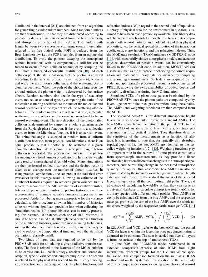
altitude levels were chosen for sampling, corresponding to 50,350, 650, and 1150 m. The first level was set to 50 m fortwo main reasons. First, this altitude was deduced from simplegeometric considerations based on the greatest off-axis angleused (89◦) and the PROMSAR-estimated length of the path(∼3 km) the photon covers when collected at this LOS. Second,this choice prevents light reflected by the ground or obstaclesfrom entering the field of view of the instrument. The other lev-els correspond to the heights for which averaging kernels showthe highest retrieval sensitivity. In spite of the four samplinglevels, analysis of the averaging kernels showed that, at most,three pieces of information were achievable employing thechosen set of four LOSs. Essentially, no information, other thanthat contained in the first guess profile, was found to come fromthe upper level (1150 m). Concerning the other levels, the errorcalculated according to (3) was found to be of about 40% forthe levels corresponding to 50 and 350 m, and higher than 40%for the level corresponding to 650 m. In Fig. 4, the troposphericcolumn amounts of NO2 and O3 are also shown, calculated byintegrating the concentration values from the lower to the upperlevel of retrieval. It can be seen that the tropospheric columnsreach maximum values on the order of 6 · 1015 molecules/cm2
for nitrogen dioxide and 1.5 · 1017 molecules/cm2 for ozone.It can also be observed that the columns of the gases understudy are anticorrelated, which is indicative of their daily pho-tochemical cycle. Focusing on nitrogen dioxide, for example,Fig. 4 shows that its highest concentration values are not atthe lowest altitude level. This is also evident in Fig. 5, wherethe diurnal variation of NO2 concentrations is shown as afunction of the retrieval altitude heights, 50, 350, and 650 m.Here, the highest NO2 values (10–12 local time) correspondto the medium level (350 m), although the exponential NO2
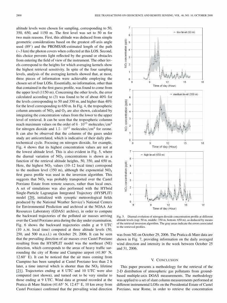
first guess profile was used in the inversion algorithm. Thissuggests that NO2 was probably transported over the CastelPorziano Estate from remote sources, rather than local ones.A set of simulations was also performed with the HYbridSingle-Particle Lagrangian Integrated Trajectory (HYSPLIT)model [20], initialized with synoptic meteorological fieldsproduced by the National Weather Service’s National Centersfor Environmental Prediction and archived at the NOAA AirResources Laboratory (GDAS1 archive), in order to computethe backward trajectories of the polluted air masses arrivingover the Castel Porziano area during the day under examination.Fig. 6 shows the backward trajectories endin g at 9 UTC(10 A.M. local time) computed at three altitude levels (50,250, and 500 m.a.s.l.) on October 29, 2006. It can be seenthat the prevailing direction of air masses over Castel Porzianoresulting from the HYSPLIT model was the northeast (NE)direction, which corresponds to the areas of heavy traffic sur-rounding the city of Rome and Ciampino airport (41.80◦ N,12.60◦ E). It can be noticed that the air mass coming fromCiampino has been sampled at Castel Porziano less than 2 hlater, a time interval which is shorter than the NO2 lifetime[21]. Trajectories ending at 8 UTC and 10 UTC were alsocomputed (not shown), and turned out to be very similar tothose ending at 9 UTC. Wind data at ground recorded at thePratica di Mare Station (41.65◦ N, 12.47◦ E, 10 km away fromCastel Porziano) confirmed that the prevailing wind direction
Fig. 5. Diurnal evolution of nitrogen dioxide concentration profile at differentaltitude levels (top: 50 m, middle: 350 m, bottom: 650 m), as deduced by meansof the retrieval inversion algorithm. The gray areas indicate the errors associatedto the retrieved profiles.
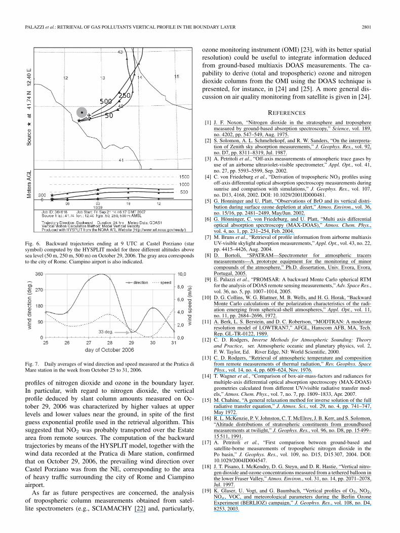
was from NE on October 29, 2006. The Pratica di Mare data areshown in Fig. 7, providing information on the daily averagedwind direction and intensity in the week between October 25and 31, 2006.
V. CONCLUSION
This paper presents a methodology for the retrieval of the2-D distribution of atmospheric gas pollutants from ground-based multiple-axis DOAS measurements. The methodologywas applied to a set of slant column measurements performed atdifferent instrumental LOSs on the Presidential Estate of CastelPorziano, near Rome, in order to retrieve the concentration
PALAZZI et al.: RETRIEVAL OF GAS POLLUTANTS VERTICAL PROFILE IN THE BOUNDARY LAYER 2801
Fig. 6. Backward trajectories ending at 9 UTC at Castel Porziano (starsymbol) computed by the HYSPLIT model for three different altitudes abovesea level (50 m, 250 m, 500 m) on October 29, 2006. The gray area correspondsto the city of Rome. Ciampino airport is also indicated.
Fig. 7. Daily averages of wind direction and speed measured at the Pratica diMare station in the week from October 25 to 31, 2006.
profiles of nitrogen dioxide and ozone in the boundary layer.In particular, with regard to nitrogen dioxide, the verticalprofile deduced by slant column amounts measured on Oc-tober 29, 2006 was characterized by higher values at upperlevels and lower values near the ground, in spite of the firstguess exponential profile used in the retrieval algorithm. Thissuggested that NO2 was probably transported over the Estatearea from remote sources. The computation of the backwardtrajectories by means of the HYSPLIT model, together with thewind data recorded at the Pratica di Mare station, confirmedthat on October 29, 2006, the prevailing wind direction overCastel Porziano was from the NE, corresponding to the areaof heavy traffic surrounding the city of Rome and Ciampinoairport.
As far as future perspectives are concerned, the analysisof tropospheric column measurements obtained from satel-lite spectrometers (e.g., SCIAMACHY [22] and, particularly,
ozone monitoring instrument (OMI) [23], with its better spatialresolution) could be useful to integrate information deducedfrom ground-based multiaxis DOAS measurements. The ca-pability to derive (total and tropospheric) ozone and nitrogendioxide columns from the OMI using the DOAS technique ispresented, for instance, in [24] and [25]. A more general dis-cussion on air quality monitoring from satellite is given in [24].
REFERENCES
[1] J. F. Noxon, “Nitrogen dioxide in the stratosphere and tropospheremeasured by ground-based absorption spectroscopy,” Science, vol. 189,no. 4202, pp. 547–549, Aug. 1975.
[2] S. Solomon, A. L. Schmeltekopf, and R. W. Sanders, “On the interpreta-tion of Zenith sky absorption measurements,” J. Geophys. Res., vol. 92,no. D7, pp. 8311–8319, Jul. 1987.
[3] A. Petritoli et al., “Off-axis measurements of atmospheric trace gases byuse of an airborne ultraviolet-visible spectrometer,” Appl. Opt., vol. 41,no. 27, pp. 5593–5599, Sep. 2002.
[4] C. von Friedeburg et al., “Derivation of tropospheric NO3 profiles usingoff-axis differential optical absorption spectroscopy measurements duringsunrise and comparison with simulations,” J. Geophys. Res., vol. 107,no. D13, 4168, 2002. DOI: 10.1029/2001JD000481.
[5] G. Honninger and U. Platt, “Observations of BrO and its vertical distri-bution during surface ozone depletion at alert,” Atmos. Environ., vol. 36,no. 15/16, pp. 2481–2489, May/Jun. 2002.
[6] G. Hönninger, C. von Friedeburg, and U. Platt, “Multi axis differentialoptical absorption spectroscopy (MAX-DOAS),” Atmos. Chem. Phys.,vol. 4, no. 1, pp. 231–254, Feb. 2004.
[7] M. Bruns et al., “Retrieval of profile information from airborne multiaxisUV-visible skylight absorption measurements,” Appl. Opt., vol. 43, no. 22,pp. 4415–4426, Aug. 2004.
[8] D. Bortoli, “SPATRAM—Spectrometer for atmospheric tracersmeasurements—A prototype equipment for the monitoring of minorcompounds of the atmosphere,” Ph.D. dissertation, Univ. Evora, Evora,Portugal, 2005.
[9] E. Palazzi et al., “PROMSAR: A backward Monte Carlo spherical RTMfor the analysis of DOAS remote sensing measurements,” Adv. Space Res.,vol. 36, no. 5, pp. 1007–1014, 2005.
[10] D. G. Collins, W. G. Blattner, M. B. Wells, and H. G. Horak, “BackwardMonte Carlo calculations of the polarization characteristics of the radi-ation emerging from spherical-shell atmospheres,” Appl. Opt., vol. 11,no. 11, pp. 2684–2696, 1972.
[11] A. Berk, L. S. Berstein, and D. C. Robertson, “MODTRAN: A moderateresolution model of LOWTRAN7,” AFGL, Hanscom AFB, MA, Tech.Rep. GL-TR-0122, 1989.
[12] C. D. Rodgers, Inverse Methods for Atmospheric Sounding: Theoryand Practice, ser. Atmospheric oceanic and planetary physics, vol. 2,F. W. Taylor, Ed. River Edge, NJ: World Scientific, 2000.
[13] C. D. Rodgers, “Retrieval of atmospheric temperature and compositionfrom remote measurements of thermal radiation,” Rev. Geophys. SpacePhys., vol. 14, no. 4, pp. 609–624, Nov. 1976.
[14] T. Wagner et al., “Comparison of box-air-mass-factors and radiances formultiple-axis differential optical absorption spectroscopy (MAX-DOAS)geometries calculated from different UV/visible radiative transfer mod-els,” Atmos. Chem. Phys., vol. 7, no. 7, pp. 1809–1833, Apr. 2007.
[15] M. Chahine, “A general relaxation method for inverse solution of the fullradiative transfer equation,” J. Atmos. Sci., vol. 29, no. 4, pp. 741–747,May 1972.
[16] R. L. McKenzie, P. V. Johnston, C. T. McElroy, J. B. Kerr, and S. Solomon,“Altitude distributions of stratospheric constituents from groundbasedmeasurements at twilight,” J. Geophys. Res., vol. 96, no. D8, pp. 15 499–15 511, 1991.
[17] A. Petritoli et al., “First comparison between ground-based andsatellite-borne measurements of tropospheric nitrogen dioxide in thePo basin,” J. Geophys. Res., vol. 109, no. D15, D15 307, 2004. DOI:10.1029/2004JD004547.
[18] J. T. Pisano, I. McKendry, D. G. Steyn, and D. R. Hastie, “Vertical nitro-gen dioxide and ozone concentrations measured from a tethered balloon inthe lower Fraser Valley,” Atmos. Environ., vol. 31, no. 14, pp. 2071–2078,Jul. 1997.
[19] K. Glaser, U. Vogt, and G. Baumbach, “Vertical profiles of O3, NO2,NOx, VOC, and meteorological parameters during the Berlin OzoneExperiment (BERLIOZ) campaign,” J. Geophys. Res., vol. 108, no. D4,8253, 2003.
2802 IEEE TRANSACTIONS ON GEOSCIENCE AND REMOTE SENSING, VOL. 46, NO. 10, OCTOBER 2008
[20] R. R. Draxler and G. D. Hess, “An overview of the hysplit_4 modelingsystem for trajectories, dispersion, and deposition,” Aust. Meteorol. Mag.,vol. 47, pp. 295–308, 1998.
[21] P. V. Hobbs, Introduction to Atmospheric Chemistry. Cambridge, U.K.:Cambridge Univ. Press, 2000, p. 262.
[22] J. P. Burrows, E. Hölzle, A. P. H. Goede, H. Visser, andW. Fricke, “SCIAMACHY-scanning imaging absorption spectrometer foratmospheric chartography,” Acta Astronaut., vol. 35, no. 7, pp. 445–451,1995.
[23] M. R. Dobber et al., “Ozone monitoring instrument calibration,” IEEETrans. Geosci. Remote Sens., vol. 44, no. 5, pp. 1209–1238, May 2006.
[24] E. J. Bucsela, “Algorithm for NO2 vertical column retrieval from theozone monitoring instrument,” IEEE Trans. Geosci. Remote Sens., vol. 44,no. 5, pp. 1245–1258, May 2006.
[25] P. F. Levelt, “The ozone monitoring instrument,” IEEE Trans. Geosci.Remote Sens., vol. 44, no. 5, pp. 1093–1101, May 2006.
[26] C. P. Loughner, “A method to determine the spatial resolution requiredto observe air quality from space,” IEEE Trans. Geosci. Remote Sens.,vol. 45, no. 5, pp. 1308–1314, May 2007.
Elisa Palazzi received the Laurea degree in physicsin 2003 and the Ph.D. degree in atmospheric sci-ences, with specialization in “physical modeling forthe environmental protection” in 2008, both from theUniversity of Bologna, Bologna, Italy.
She is currently a Postdoctoral Fellow withthe Institute of Atmospheric Science and Climate,Bologna, working on the validation of chemi-cal circulation models and the analysis of uppertroposphere-lower stratosphere data. She has alsoworked on the development of Monte Carlo radiative
transfer models for the interpretation of DOAS remote sensing measurements.She is the author or coauthor of five refereed publications and has contributedto several international conferences.
Andrea Petritoli received the Ph.D. degree in at-mospheric sciences from the University of Bologna,Bologna, Italy, in 2004.
He is currently a Postdoctoral Fellow with theInstitute of Atmospheric Science and Climate,Bologna, working on atmospheric observations andmodeling issues. In particular, he has remarkableexperience on the use of DOAS techniques for mea-suring trace gas constituents in the lower and middleatmosphere and on the use and development of radia-tive transfer models for treating remote sensing data
by means of inversion techniques. He has also been involved, as a PrincipalInvestigator, in several European Union and national research projects. He isthe author of more than ten peer-reviewed articles.
Fabrizio Ravegnani received the Laurea degree inphysics from the University of Bologna, Bologna,Italy.
Since 1995, he has been a Researcher withthe Institute of Atmospheric Science and Climate,Bologna, having more than 15 years of experienceworking on atmospheric science. He was involved inseveral projects funded by the Italian Space Agency(ASI) and the National Antarctic Research Program(PNRA), and was the Principal Investigator in sev-eral EC-funded projects. His expertise is mainly on
the development and application of complex instrumentation for in situ, ground-based, and airborne monitoring of atmospheric composition.
Ivan Kostadinov received the B.S. and M.S. degreesin physics, with specialization in meteorology andatmospheric physics, from Sofia University, Sofia,Bulgaria.
He is currently with the Institute of AtmosphericScience and Climate, Bologna, Italy. He has workedon the analysis of satellite data concerning UV-VIS emissions of the upper atmosphere. Since 1995,he has been working on the application of differ-ential optical absorption spectroscopy (DOAS), thedevelopment of UV-VIS equipment for long-path
and zenith-sky DOAS measurements; laboratory tests, optical alignment, andcalibration and validation of spectrometers; the influence of polarization andring effect on the DOAS measurement accuracy; spectra calibration usingFraunhofer lines; and satellite remote sensing data validation.
Daniele Bortoli received the B.S. and M.S. degreesfrom the University of Bologna, Bologna, Italy, andthe Ph.D. degree in atmospheric physics from theUniversity of Evora, Evora, Portugal.
He is currently a Researcher with the Univer-sity of Evora, and collaborates with the Instituteof Atmospheric Science and Climate, Bologna. Hecurrently works on optical instrumentation for themonitoring of atmospheric compounds by the ap-plication of the DOAS methodology to the mea-sured spectral data. His research interests include
stratospheric ozone depletion at high latitudes and mid-latitude monitoring ofatmospheric compounds.
Samuele Masieri received the Laurea degree inphysics from the University of Bologna, Bologna,Italy, in 2005. His thesis was entitled “Utilizzo diun sistema remote sensing DOAS per il controllo diprocessi fotochimici in area urbana.”
He is currently with the Institute of AtmosphericScience and Climate, Bologna, working on the useof the DOAS technique, particularly on data analysisand instrumental development tasks.
Margherita Premuda received the Laurea degree inphysics from the University of Bologna, Bologna,Italy, in 1994 and the Ph.D. degree in nuclear engi-neering from the University of Bologna, in 2002. Herthesis was entitled “Modellistica fisica e matematicadel trasporto radiativo nell’atmosfera e simulazioneMonte Carlo.”
She is currently with the Institute of AtmosphericScience and Climate, working on the use of theDOAS technique, particularly on data analysis tasks.
Giorgio Giovanelli received the Laurea degree inphysics in 1965 from the University of Bologna,Bologna, Italy.
He is currently a Senior Researcher with the Insti-tute of Atmospheric Sciences and Climate (ISAC),National Research Council (CNR), Bologna, Italy,where he directs the Technical Structure: Ground-based Experimental Stations and Large-Scale facil-ities and coordinates the research group on radiativetransfer and trace gases in the atmosphere. He hasmore than 30 years of experience in the development
of remote sensing systems and in the data analysis for the study of chemicalprocesses and trace gas transport in the atmosphere.