Electronic copy available at: http://ssrn.com/abstract=1004568Electronic copy available at: http://ssrn.com/abstract=1004568

1

Resilience of Microfinance Institutions to National Macroeconomic Events: An Econometric Analysis of MFI Asset Quality1

Adrian Gonzalez,

Research Analyst, Microfinance Information Exchange, Inc. (MIX)2 July-2007

MIX Discussion Paper No. 1.

The goal of MIX Discussion Paper Series is to disseminate the findings of work in progress to encourage the exchange of ideas about microfinance issues, and further exploit the wealth of data in MIX’s database. It presents findings of empirical analysis, highlights research questions and areas for further exploration. In order to get these findings out quickly, we will publish papers even if the presentation is less than fully polished. The findings, interpretations, and conclusions expressed in this paper are entirely those of the authors, and they do not represent necessarily the view of MIX or its board of Directors.

Abstract

After controlling for MFI and country characteristics, we find no evidence suggesting a strong (in magnitude) and statistically significant relationship between changes in GNI per capita (GROWTH) and four indicators of MFI portfolio risk: quality at Risk over 30 Days (PAR-30), Portfolio at Risk over 90 Days (PAR-90), Loan loss Rate (LLR), and Write-off Ratio (WOR). We test the robustness of the models with different specifications that confirm the general result and test for different impact from growth rates according to average loan sizes disbursed by MFIs. These tests suggest that microfinance portfolios have high resilience to economic shocks. Specifically, we found only a significant relationship between growth and PAR-30. We also control for other explanatory variables like size, age, average loan size, and productivity.

1 For a summary and non-technical discussion of this paper see Gonzalez, Adrian (2007). 2 I want to thank Blaine Stephens, Peter Wall, all MIX analysts, and Jonathan Conning for valuables comments that improve the quality of the paper. All errors remain mine.

Electronic copy available at: http://ssrn.com/abstract=1004568Electronic copy available at: http://ssrn.com/abstract=1004568

2

Resilience of Microfinance Institutions to National Macroeconomic Events: An Econometric Analysis of MFI asset quality3

Adrian Gonzalez,

Research Analyst, Microfinance Information Exchange, Inc. (MIX)4 July 2007

MIX Discussion Paper No. 1.

Introduction Microfinance is growing and is becoming a major component of most financial systems in developing countries. The number of borrowers of the MFIs in this sample have been growing on average 17% per year in the period 1999-2005, with growth rates over 20% in the last two years. Loan Portfolios in dollars have been growing on average 28% in the same period, with rates over 35% in the last two years. In addition, many of these MFIs mobilize savings and are regulated by local superintendencies or central banks. As microfinance booms, local regulators get concerned about the impact of systemic shocks on MFIs performance, especially on their loan portfolios. Funders and all types of investors also worry about losing their investments as economic conditions worsen in many countries. Conventional wisdom and case studies5 have long pointed to the resilience of microfinance to macroeconomic shocks. To date, however, global studies analyzing these dynamics with panel data among large numbers of MFIs and countries have yet to appear6. In an attempt to fill this gap, we analyze MIX’s global MFI data set in search of quantitative evidence of impact of macroeconomic shocks and other variables on the quality of microfinance loan portfolios7. Using panel regression we control for those observable variables that may have an impact on the quality of the portfolio, such as the size of an institution8, lending methodology, years of experience as a microcredit provider, its clients’ average loan balance, key factors in its cost structure, staff

3 For a summary and non-technical discussion of this paper see Gonzalez, Adrian (2007). 4 I want to thank Blaine Stephens, Peter Wall and MIX analyst for valuables comments that improve the quality of the paper. All errors remain mine. 5 McGuire, Paul B. (1998), Reille, Xavier and Dominique Gallmann (2000), Gonzalez, Adrian and Claudio Gonzalez-Vega (2003), Benoit-Calderón, Thierry (2006) 6 Walter, Ingo and Nicolas Krauss (2006), using MIX Market data, analyzed correlations for various indicators of MFI performance and both domestic and international markets. Their sample size is smaller than ours and they do not consider others explanatory variables in the analysis. However, they compare correlations for MFIs and commercial banks for most performance variables in their analysis. Also, Ahlin, Christian, and Jocelyn Lin (2006), used a subsample of MIX Market data to evaluate the impact of macroeconomic events over MFIs performance. 7 We want to emphasis that the following analysis is not static pool analysis where data is analyzed at the loan level. In our sample, all data is aggregated at the MFI level. For an example of static pool analysis on microfinance, see Ayton, Rupert and Stephanie L. Sarver (2007). 8 We present results using Gross Loan Portfolio (GLP) as a proxy for size; however, results using borrowers instead of GLP were almost identical to the ones presented here.

3

productivity and salaries, and lending methodology. In the country context, we look at inflation, commercial lending interest rate, and financial depth. The following analysis shows that after controlling for MFI and country characteristics, we find no evidence suggesting a strong (in magnitude) and statistically significant relationship between changes in GNI per capita (GROWTH) and four indicators of MFI portfolio quality: Portfolio at Risk over 30 Days (PAR-30), Portfolio at Risk over 90 Days (PAR-90), Loan loss Rate (LLR), and Write-off Ratio (WOR). We test the robustness of the models with different specifications that confirm the general results and test for different impacts from growth rates according to average loan size disbursed by MFIs. These tests suggest that microfinance portfolios have high resilience to economic shocks. This paper is organized in four more sections. A general description of the sample and the discussion of many self-selection issues are discussed in section two. The econometric estimation and discussion of the expected results are discussed in section three. The main results of the paper are presented in section four, and conclusions are presented at the end. Sample Description The sample consists on 639 MFIs in 88 countries reporting data to the Microfinance Information Exchange, Inc. (MIX), mainly in the period 1999-2005, with eight MFIs reporting as early as 1996. These MFIs represent 36 million borrowers with 13.7 billion USD in loan portfolio in 2005. There are self-selection issues that need to be discussed in order to understand the policy implications of the paper. All MFIs in the sample have the ability to produce a minimum set of financial indicators, and the willingness to share private data with MIX (and very often with the world through their published profiles available at www.mixmarket.org). These two characteristics are not common to all MFIs in the world. The ability to disclose data is mostly related to the availability (at the MFI level) of adequate information systems, also used to monitor daily MFI operations, like disbursement and collection of loans. MFIs that do not have the ability to report data to MIX, most likely do not have the best tools to monitor the quality of their portfolios. Also, since most MFIs in the sample have provided audited financial statements to be published with their public profiles, ability has to do as well with the capacity of providing all data necessary to satisfy the minimum requirements of auditing firms. But the willingness to share detailed financial information with MIX analysts and the world is driven by the potential exposure to investors and donors looking for investment opportunities among MFIs. To be good investment opportunities, most MFIs reporting to MIX run their operations very efficiently and pay close attention, among other variables, to the portfolio quality and profitability of their operations. Therefore, we expect that the MFIs in the sample are a random sample of the best MFIs in the world in terms of portfolio quality (among other variables), but definitely not a random sample of all MFIs.

4

Given the distinctive characteristics of MFIs in the sample, the high quality of their loan portfolios should not come as a surprise. As shown in Table 1, average PAR-30 is just five percent, and the average value for any of the other three indicators of portfolio quality is below three percent. In fact the average values are very close to the 75th percentile, meaning that only 25 percent of the observations in the sample have a PAR-30 higher than six percent, or any of the other three indicators over three percent. Looking at the results from a different angle, median PAR-30 is just three percent, and the median for the other variables is one percent. The high quality of most portfolios in the sample proves that for many MFIs in developing countries collection of small loans from informal microenterprenuers is not an issue. Empirical Approach We test the robustness of the results by estimating various econometric specifications for four different dependent variables: PAR-30, PAR-90, WOR and LLR. The specific definition and source of all explanatory variables is presented in Appendix 1. It is important to highlight that only WOR and LLR are measures of default, while both PARs are measures of risk of default. But given the high incentive that MFIs clients have to repay their loans and the effectiveness of MFIs collecting them, most late loans will be paid at some point. For example, the average PAR-30 in the sample is five percent, but average LLR and WOR are three percent (Table 1).9 Also, it is expected that PARs will be affected by very recent economic events, like this year’s growth, while this year’s WOR and LLR may be affected by last year’s growth, given the lag between arrears and MFIs writing off defaulted loans from their portfolios. Therefore, we try different econometric specifications using GROWTH and LAG GROWTH for arrears (PAR-30 and PAR-90) and defaults (LLR and WOR) respectively. In order to control for differences between lending methodologies, we include a set of dummy variables identifying Individual Lenders, Solidarity Groups, Village Banks and those MFIs with both Individual and Solidarity (IS) loans from Individual Lenders. The results from these tests are very important from a policy perspective, because if they confirm the conventional wisdom that some lending methodologies are riskier than others, then microfinance supporters concerned about portfolio quality can identify the least risky lending methodologies. In order to test whether smaller loans are riskier than larger loans, we control for relative loan sizes as percentage of GNI per capita (LS/GNI). Also we divide MFIs into three groups according to their relative loan size, and test whether the relationship between GROWTH (and its LAG) and portfolio risk changes by tercile. Knowing if the resilience of MFIs varies by average loan size will help determine which loans are less resilient to local macroeconomic conditions. While actual client screening and portfolio monitoring cannot be measured, PRODUCTIVITY is included as a proxy for both. For example, a low borrower to staff

9 The following discussion of the econometric results will present more evidence supporting this argument.

5

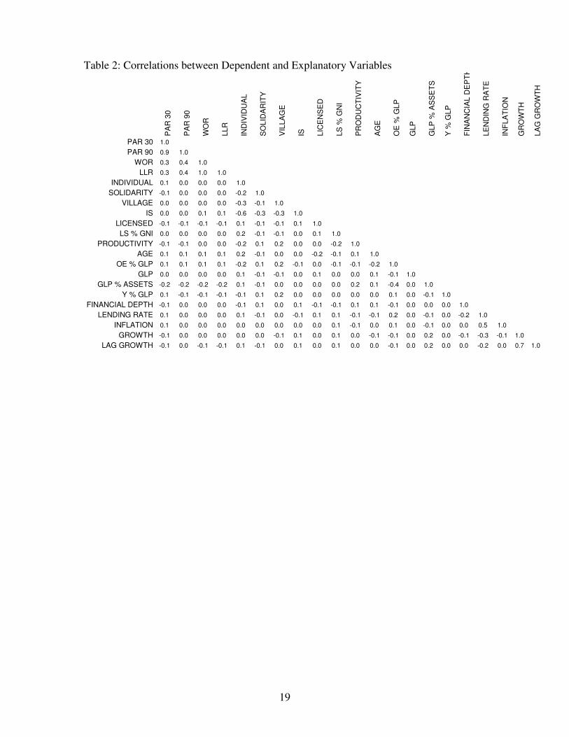
ratio would suggest more time spent screening and monitoring borrowers than higher ratio. We include AGE of the MFIs in order to control for differences in experienced lending and collection practices. Operating expense ratio (OE/GLP) captures differences between cost structures. Also, as higher interest rates on loans may increase risk of default, we use nominal yields10 to control for higher risk typically associated with higher interest rates (adverse selection). Finally, various macroeconomic variables such as changes in price levels and depth of the financial system are analyzed to account for differences between countries. Results In Tables 3-4, we present all the different specifications tried under Fixed Effects (FE) for each of the four risk variables under analysis. When looking at these results, it is important to remember the high correlation between PAR-30 and PAR-90 (86 percent, Table 2) and between WOR and LLR (99 percent). As a result, regression results for arrears (PAR-30 and PAR-90) are similar as are those for measures of defaults (LLR and WOR). We test for Random Effects (RE) using the Hausman Specification Test in every model and reject the RE hypothesis on most of them. In particular, we reject the RE hypothesis for all specifications for PAR-30 and PAR-9011. For LLR, we could not reject the RE hypothesis in specification 1, and for WOR we could not reject the RE hypothesis for specifications 2 and 3. The regression coefficients for LLR and WOR under RE are presented in Table 5. More important, there are not visible differences between the coefficients for GROWTH or LAG even when the RE hypothesis was not rejected. However, the results for the impact of different lending methodologies vary between the RE and the FE results. This is discussed later in the paper. Overall, we found that the coefficients for GROWTH (and its square) are significant only for PAR-30 and that their coefficients are very similar regardless of the sample used for the estimation (only MBB MFIs, specifications 1-2-3 versus MBB plus MIX Market MFIs, or specifications 1’-2’-3’). Surprisingly, for none of the other three dependent variables did we find any significant relationship with GROWTH or LAG GROWTH (and their squares). In Figure 1 we show that the predicted relationship between GROWTH and PAR-30 is not very strong. For example, a drop in GROWTH from 9 percent (average in the sample, indicated in the graph with dotted line) to -10 percent (below 10th percentile) will produce an average increase in PAR-30 of only two percentage points. The result is very

10 Just before publication we ran all regressions using real yield instead of nominal yield and obtained almost identical results to the ones presented here. 11 Chi2 results and Prob>Chi2 are presented at the bottom of each table with Fixed Effect results (3-4-6-7), for H0: difference in coefficients is not systematic.

6

consistent over samples for the specification where MFIs are not divided by loan size (1 and 1’). Figure 1: Predicted Effects for GROWTH

PAR-30 versus GROWTH

0

2

4

6

8

10

-10 -5 0 5 10 15 20 25 30

Percentage Change in GNI per capita

PA

R-3

0

PAR-30 (1)

PAR-30 (1')

Interestingly, these predictions also suggest that PAR-30 will reach its minimum level somewhere between 15-17 percent of GROWTH (depending on the specification used), and once local economies grow faster than this range it would not be surprising to observe small increases in PAR-30. This is consistent with MFIs taking more risks when economic conditions are favorable for their operations. However, the regression results suggest no relationship with PAR-90, LLR and WOR. Our interpretation of these results is that when economic conditions become less favorable for MFIs, they experience a small deterioration in short term repayment (increases in PAR-30), but also succeed in collecting most of their loans, so that in the end, we do not observe any statistically significant relationship between either LLR or WOR and GROWTH. In the same way, when economic conditions are more favorable for MFIs they are willing to increase the risk of their portfolios, and do so without deteriorating the overall quality of their portfolios as measure by LLR and WOR. It is important to highlight that these results do not imply that very low or negative growth is not harmful for MFIs. It is expected that as PAR-30 increases when GROWTH goes down, MFIs need to allocate more of their resources to monitor and collect delinquent loans in order to guarantee their repayment. Most likely, this will result in an increase in costs that needs to be compensated with lower profits or higher interest rates. Also, it is expected that more prudent MFIs will adjust their growth targets if they perceive that PARs are going up, and negative economic conditions will persist for a longer periods in order to control the quality of their portfolios.

7

Figure 2: Predicted Effects for GROWTH by Target Market

PAR-30 versus GROWTH by Terciles

0

2

4

6

8

10

-10 -5 0 5 10 15 20 25 30

Percentage Change in GNI per capita

PA

R-3

0

3rd Tercile

2nd Tercile

1st Tercile

Breaking MFIs into three groups according to relative loan sizes (LS/GNI), and estimating three different coefficients for GROWTH did not change the general result regarding GROWTH and portfolio quality that is that only PAR-30 exhibits statistically significant relationships with GROWTH, but not PAR-90, LLR and WOR. However, as shown in Figure 2, this analysis also suggests that compared to their average level12, PAR-30 of MFIs disbursing smaller loans (1st Tercile) will improve more with higher growth than the predicted improvements in PAR-30 for MFIs in the 2nd and 3rd Terciles. Also compared to their average levels, MFIs in the 2nd Tercile will experienced the worst deterioration in PAR-30 with lower growth compared to the deteriorations predicted for the 1st and 3rd Terciles. The fact that MFIs in the 1st Tercile do not exhibit the worst deterioration in PAR-30 when economic conditions weaken is a surprising results given the common association between loan size and income level of the borrowers, and suggests that poorer borrowers are not the ones that suffer more when growth is low or negative. One alternative explanation, that we cannot test here, is that for poorer borrower repaying their loan is so important, that they will not repay late, even when overall economic conditions are bad. However, given that we could not find any significant relationship with any other dependent variable when breaking MFIs into terciles by relative loan size also suggests that independent of the loan size (and income level of the borrowers), MFIs manage to keep repayment rates high when growth is low or negative. Ahlin and Lin (2006) did not find any significant result between portfolio quality (WOR and PAR-30) and growth in their fixed effect results, and they report significant effects between these variables for their between results and pooled results. Based on our results we know that fixed effects results are better than random effect ones, and ignoring them may result in biased results, but such tests are not available in Ahlin and Lin (2006).

12 5% PAR-30 and 7% GROWTH for 1st Tercile, 5% and 9% for 2nd Tercile, and 6% and 11% for 3rd Tercile.

8

A frequent source of debate between microfinance practitioners is whether solidarity groups are less risky than individual loans13. Some theoretical models support this position, arguing that repayment is higher because groups provide incentives for peers to screen, monitor and enforce each other’s loans, especially when one member of the group has suffered a shock. While this holds for idiosyncratic shocks, systemic shocks like the ones under analysis here would be expected to induce more generalized defaults among group members. In our model, we control for differences in lending methodologies with dummy variables for Solidarity Groups (SOLIDARITY), Village Banks (VILLAGE), and both Individual-Solidarity Groups (IS)14. Compared to Individual Lenders, our results show that Village Banks have a PAR-30 over three percentage points higher, and a PAR-90 two percentage points higher. Also compared to Individual Lenders, these results show that Solidarity Groups have a PAR-90 over one percentage point higher, and that ISs have a PAR-30 over one percentage point higher15. The evidence on the relationship between lending methodologies and both LLR and WOR is not that robust (Table 4). In all estimations under FE none of the coefficients associated with lending methodologies was statistically significant, and their absolute value was less than half a percentage point. However, we could not reject RE for two specifications of LLR (2-3) and one of WOR (3). Overall, this suggests that FE is the best estimation for all dependent variables with the exception of LLR, and that there is no statistically significant relationship between lending methodology and PAR-30, PAR-90 and WOR. However, in two of the specifications for LLR where we did not reject FE (2-3) we found evidence that compared to Individual Lenders, Solidarity Groups have a LLR 1.3-1.4 percentage points lower and Village Banks have a LLR 1.6 percentage points lower.16 PAR-30 is the only dependent variable for which it is possible to estimate regressions using both MIX Market and MBB data. The coefficients for ONLYMM suggests that MFIs that report only to MIX Market have an average PAR-30 over 1.2-1.5 percentage points higher than those MFIs that report only to MBB or to both databases. Also, combining both samples we found that Licensed MFIs have a PAR-30 five percentage points higher than other MFIs17, but no significant difference regarding the other dependent variables. Regarding size, we found that larger MFIs, both in terms of larger loan sizes and larger loan portfolios are not riskier than smaller MFIs. In particular, we did not find any significant relationship between loans size and any of the four measures of portfolio

13 For example, see the discussion on the topic in Development Finance discussion group between July-August 2006. 14 The omitted variable is INDIVIDUAL. 15 In addition, this results show that regarding PARs, ISs and Solidarity Groups are very similar. 16 Gine, Xavier and Dean Karlan (2006) found no difference in repayment between members of groups that were randomly assigned to individual loans in a control experiment. Additional references and discussion can be found in chapter 4 of Armendáriz de Aghion, Beatriz and Jonathan Morduch (2005). 17 We did not control for type of MFIs for the other three dependent variables at the present time.

9

quality under analysis. For GLP (Figure 3), we found only one significant relationship with PAR-30 in all three specifications that use only MBB data. However, running similar regressions with the combined sample did not result in significant results for GLP. Figure 3: Predicted Effect for GLP

PAR-30 versus GLP

0

2

4

6

8

10

0 10 20 30 40 50 60 70 80 90 100

Millions $

PA

R-3

0

We found that on average older MFIs tend to have lower PARs and higher LLR and WOR (See Figure 4). These results are not inconsistent with each other once you consider that we have a sample with many young MFIs (25 percent are five years old or less) that do not accumulate write-offs during their first years of operations, especially when compared to their growing loan portfolios. As MFIs get older we will expect higher LLR and WOR, but less PARs as lending methodologies and collection practices improve, as illustrated by the declining spread between predicted PAR-30 and PAR-90. Figure 4: Predicted Effect for AGE

PAR-30, PAR-90, LLR and WOR versus AGE

-2

0

2

4

6

8

10

0 5 10 15 20

Years since Establishement

Per

cent

age

of G

LP

PAR-30 PAR-90

WOR LLR

10

In Figure 4, we draw each predicted curved at its sample average. According to these predictions, a 20 year old MFI will have an average LLR and WOR one percentage point higher, a PAR-30 over one percentage point lower, and a PAR-90 less than one percentage point lower than a ten year old MFI. However, given than less than 10 percent of the sample is over 20 years old, it is likely that these results will be adjusted as the sample ages. We found that more productive MFIs have lower PAR-30 and did not find any significant effect on the other three dependent variables. This means that with the right lending and collection practices it is possible to improve productivity without sacrificing portfolio quality. However, as shown in Figure 5, we found that the relationship between productivity and PAR-30 change direction once productivity reaches somewhere between 340-400 borrowers per staff depending on the specification used. After this point increases in productivity may increase PAR because the ability of staff to screen and monitor borrowers get compromised. Figure 5: Predicted Effect for PRODUCTIVITY

PAR-30 versus PRODUCTIVITY

0

2

4

6

8

10

0 100 200 300 400 500 600Borrowers per Staff

PA

R-3

0

PAR-30 (1)

PAR-30 (3)

The coefficients for OE/GLP show a positive relationship with WOR and a negative relationship with PAR-30, meaning that more efficient MFIs tend to have lower WOR and higher PAR-30 (Figure 6). Remember that we did not find any significant relationship with relative loan size of any of these variables and that PRODUCTIVITY was significant only for PAR-30. Therefore, our interpretation of this apparently inconsistent results is that efficiency gains come from MFIs using lending methodologies that care less about short term repayment problems (so that PAR-30 increases), but that guarantee the ultimate repayment of most loans at collection.

11

Figure 6: Predicted Effect for OE/GLP

PAR-30 and WOR versus OE/GLP

0

2

4

6

8

10

101520253035404550556065OE/GLP

Per

cen

tag

e o

f G

LP

PAR-30

WOR

We also control for the percentage of assets that MFIs allocate as loan portfolio. Young MFIs and fast growing MFIs tend to have higher reserves (idle assets) to finance their future growth than mature MFIs or MFIs with limited access to external resources. In Figure 7, we plot the predicted relationship between both PARs and GLP/ASSETS. The average GLP/ASSETS is 72 percent and the extremes of the horizontal scale correspond to the 10th and 90th percentiles. Figure 7: Predicted Effect for GLP/ASSETS

PAR-30 and PAR-90 versus GLP/ASSETS

0

2

4

6

8

10

45 50 55 60 65 70 75 80 85 90

GLP/ASSETS

PA

R

PAR-30

PAR-90

According to this prediction, PARs increase as MFIs improve the share of their assets allocated to GLP. However, we did not find any significant relationship for LLR and WOR. This means that MFIs onto the right of the average are those that are willing to let PARs run a little bit higher without sacrificing overall portfolio quality. For these MFIs

12

the efficiency gains from maximizing the percentage of assets as GLP compensate the extra effort necessary to guarantee the repayment of their loans, even when PARs go up. Finally, we did not find any statistically significant relationship between YIELD and any proxy of arrears (LLR and WOR). We only found one significant relationship between PAR-30 and YIELD using the combined sample. However the magnitude of the coefficient is almost zero and the sign is not what we would have expected (Figure 8). This result may be surprising to many because it suggest that overall the MFIs in the sample succeed in mitigating any adverse selection effect from charging higher interest rates. In a similar analysis, Cull et. al. (2006), found a significant relationship between PAR-30 and real yields only for Individual MFIs and with a cross section of 124 MFIs. Figure 8: Predicted Effect for YIELD.

PAR-30 versus YIELD/GLP

0

2

4

6

8

10

0 20 40 60 80 100 120YIELD/GLP

PA

R-3

0

Testing for commitment to sustainability In an attempt to measure the commitment to sustainability of an MFI’s management, we included a dummy variable (SUSTAINABLE) set to 1 for all MFIs that had positive returns the previous year, and 0 otherwise (Tables 6-8). We found that previously sustainable MFIs have a PAR-30 almost 1 percentage point higher. However, we also found that these MFIs have a WOR and LLR 0.6 percentage points lower than other MFIs. For all other explanatory variables, the general result is that less of them are significant. This result confirms that unobservable MFI characteristics play an important role on the overall performance of MFIs. We also test whether the duration of a crisis has any impact on portfolio quality. For that, we run a full analysis replacing GROWTH with the cumulative growth of the last two and three years (or LAG with the cumulative LAG of the previous two and three years). For all specifications and dependent variables, we did not find any improvement in

13

goodness of fit, changes in the significance of the coefficients, or relevant differences in the magnitude of significant coefficients.18 Conclusions Microloans resilient to macroeconomic changes Our estimates show no relationship between changes in GNI per capita and asset quality. Specifically, regression results show no statistically significant relationship between GROWTH (and its lag) and PAR-90, LLR and WOR. In all specifications for these dependent variables, the coefficients associated with GROWTH (or its lag) were not statistically significant, even when estimating different impacts according to relative loan size. In short, economic crises showed up in increased delinquency, but not in eventual default. Assets were stressed, but not unrecoverable. Overall, this analysis shows that there are many unobserved variables that are important for explaining variability of portfolio risk. This result is not surprising. Industry analysts have long argued that the most important factors determining the risk in an MFI’s portfolio are related to their management and human resources, quality of MIS, governance, credit policies, mission and commitment to sustainability. Similarly, other factors such as poor market infrastructure (e.g. lack of roads or remoteness) or other factors affecting the client population (e.g. long term poor health conditions due poor sanitary conditions or widespread chronic illness like HIV/AIDS) may impact repayment. These are all very important factors but ones for which no consistent, reliable data exist on a significant scale. With the exception of commitment to sustainability, none of these are specifically incorporated into the current analysis. What have we learned? Data available for modeling the risk of MFI portfolios are limited. Despite the breadth of data available through MIX data sets, the explanatory power of existing variables is limited. The data themselves also pose challenges. Little variability in portfolio risk and loss exists among MFIs reporting to MIX. On one end, an MFI never improves risk or loss beyond zero percent. On the other end, MFIs that report data to MIX are more transparent, have basic reporting systems to capture and report on key financial and operational statistics, and are hence more likely to use and act upon the information to prevent crises, including repayment crises, within their institutions. As a result, where there exists a notional maximum risk or loss of 100 percent, reported results lie mostly in a tight range between zero and six percent. The analysis still holds important lessons for investors looking to bundle and sell securities backed by microloan portfolios or buy the microloan portfolios themselves. Evidence to date would indicate that the quality of such assets stands up to economic downturns. Our model finds nothing significant to suggest otherwise. However, given the importance of other factors such as management and governance, business processes, and product design and the likelihood that they influence portfolio risk, this analysis suggests that the quality of the originator of those loans matters even more than the downturns in the economic environment in which the microborrowers operate. Even

18 Please contact the author if you are interested in the regressions coefficients for any of these analyses.

14

when buying microloan portfolios, choosing the right partner MFI is still the best guarantee of success. Finally, this analysis does not suggest that systemic macroeconomic shocks are not harmful at all for MFIs. Additional research needs to be done to understand the impact of economic downturns on growth, cost and profitability of MFIs. Also, future research should consider better estimation techniques that allow for heteroskedasticty in the data, among other potential problems.

15

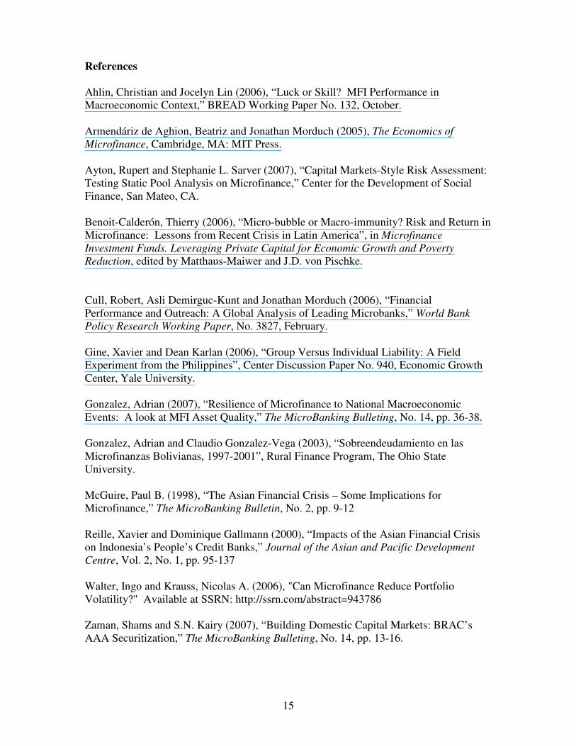
References Ahlin, Christian and Jocelyn Lin (2006), “Luck or Skill? MFI Performance in Macroeconomic Context,” BREAD Working Paper No. 132, October. Armendáriz de Aghion, Beatriz and Jonathan Morduch (2005), The Economics of Microfinance, Cambridge, MA: MIT Press. Ayton, Rupert and Stephanie L. Sarver (2007), “Capital Markets-Style Risk Assessment: Testing Static Pool Analysis on Microfinance,” Center for the Development of Social Finance, San Mateo, CA. Benoit-Calderón, Thierry (2006), “Micro-bubble or Macro-immunity? Risk and Return in Microfinance: Lessons from Recent Crisis in Latin America”, in Microfinance Investment Funds. Leveraging Private Capital for Economic Growth and Poverty Reduction, edited by Matthaus-Maiwer and J.D. von Pischke. Cull, Robert, Asli Demirguc-Kunt and Jonathan Morduch (2006), “Financial Performance and Outreach: A Global Analysis of Leading Microbanks,” World Bank Policy Research Working Paper, No. 3827, February. Gine, Xavier and Dean Karlan (2006), “Group Versus Individual Liability: A Field Experiment from the Philippines”, Center Discussion Paper No. 940, Economic Growth Center, Yale University. Gonzalez, Adrian (2007), “Resilience of Microfinance to National Macroeconomic Events: A look at MFI Asset Quality,” The MicroBanking Bulleting, No. 14, pp. 36-38. Gonzalez, Adrian and Claudio Gonzalez-Vega (2003), “Sobreendeudamiento en las Microfinanzas Bolivianas, 1997-2001”, Rural Finance Program, The Ohio State University. McGuire, Paul B. (1998), “The Asian Financial Crisis – Some Implications for Microfinance,” The MicroBanking Bulletin, No. 2, pp. 9-12 Reille, Xavier and Dominique Gallmann (2000), “Impacts of the Asian Financial Crisis on Indonesia’s People’s Credit Banks,” Journal of the Asian and Pacific Development Centre, Vol. 2, No. 1, pp. 95-137 Walter, Ingo and Krauss, Nicolas A. (2006), "Can Microfinance Reduce Portfolio Volatility?" Available at SSRN: http://ssrn.com/abstract=943786 Zaman, Shams and S.N. Kairy (2007), “Building Domestic Capital Markets: BRAC’s AAA Securitization,” The MicroBanking Bulleting, No. 14, pp. 13-16.

16

Appendix 1: Dependent and Explanatory variables Not all explanatory and dependent variables are available for the full sample as some are only reported to the MicroBanking Bulletin. Descriptive statistics for all Dependent and Explanatory variables are presented in Table 1 and correlation coefficients in Table 2. Dependent variables Out of the four dependent variables, only PAR-90 and LLR are not available to MFIs reporting only to MIX Market. In addition, given that many MFIs reporting only to MIX Market do not have an standard policy about write-offs –some of them never write-off defaulted loans--, for this dependent variable we will analyze only MFIs with adjusted data, where MIX analyst have standardized write-offs for all MFIs in sample following standards policies. � PAR-30 : Outstanding balance, loans overdue >30 Days / Gross Loan Portfolio � PAR-90: Outstanding balance, loans overdue >90 Days / Gross Loan Portfolio � WOR: Value of loans written-off / Average Gross Loan Portfolio � LLR: Write-offs, net of recoveries/ Average Gross Loan Portfolio Explanatory variables Not available in MIX Market � INDIVIDUAL: 1 if lending methodology is individual, 0 otherwise. This is the

omitted variable. � SOLIDARITY GROUPS: 1 if lending methodology is solidarity groups, 0 otherwise � VILLAGE BANKS: 1 if lending methodology is village banks, 0 otherwise � IS: 1 if lending methodology is both individual and solidarity groups, 0 otherwise Available in both MIX Market and MBB � LICENSED: 1 if charter is Bank or Non Bank Financial Institution (NBFI), 0

otherwise � ONLYMM: 1 if observation is from MIX Market only, 0 otherwise � LS/GNI per capita: Average loan size per borrower / GNI per capita � SUSTAINABLE: 1 if ROA>=0 in previous year, 0 otherwise � AGE: LOG19 of Number of years since establishment � PRODUCTIVITY: Average number of borrowers per staff � GLP: Gross Loan Portfolio in million dollars, proxy of size � OE/GLP: Operating Expense / Average GLP � GLP/ASSETS: GLP / Assets � YIELD/GLP: Yield / GLP Macroeconomic variables from World Development Indicators, various years � LENDING RATE: Bank rate that usually meets the short and medium term financing

needs of the private sector. � FINANCIAL DEPTH: Liquid liabilities (M3) / GDP. � INFLATION: Changes in consumer prices. � GROWTH: Growth rate of GNI per capita. � LAG GROWTH: 1 period Lag of GROWTH

19 Natural Logarithm computed with ln() using Stata.

17

� GROWTH1: GROWTH if LS/GNI in first tercile, 0 otherwise � GROWTH2: GROWTH if LS/GNI in second tercile, 0 otherwise � GROWTH3: GROWTH if LS/GNI in third tercile, 0 otherwise � LAG GROWTH1: LAG GROWTH if LS/GNI in first tercile, 0 otherwise � LAG GROWTH2: LAG GROWTH if LS/GNI in second tercile, 0 otherwise � LAG GROWTH3: LAG GROWTH if LS/GNI in third tercile, 0 otherwise � EAP, EECA, LAC, MENA, S ASIA and SS AFRICA, regional dummies for East

Asia and Pacific, Eastern Europe and Central Asia, Latin America, South Asia, and Sub-Saharan Africa respectively. SS Africa is the omitted dummy variable.

18

Table 1: Means and Percentiles of Dependent and Explanatory Variables

Percentiles Sample Mean P10 P20 P25 P40 P45 P50 P55 P60 P75 P80 P90 PAR-30 2439 5.2 0 1 1 2 2 3 3 4 6 7 13 PAR-90 1431 2.3 0 0 0 1 1 1 1 2 3 3 6 WOR 1432 3.0 0 0 0 1 1 1 1 2 3 4 7 LLR 1432 2.7 0 0 0 0 1 1 1 1 3 3 6 INDIVIDUAL 1432 0.3 0 0 0 0 0 0 0 0 1 1 1 SOLIDARITY 1432 0.1 0 0 0 0 0 0 0 0 0 0 1 VILLAGE BANKS 1432 0.1 0 0 0 0 0 0 0 0 0 0 1 IS 2440 0.3 0 0 0 0 0 0 0 0 0 1 1 LICENSED 2440 0.4 0 0 0 0 0 0 0 0 1 1 1 LS/GNI PER CAPITA 2440 74.3 8 14 16 25 30 36 42 49 78 94 157 SUSTAINABLE 1572 0.6 0 0 0 1 1 1 1 1 1 1 1 PRODUCTIVITY 2394 132.7 36 59 68 93 101 111 122 131 169 188 237 AGE 2437 9.7 3 4 5 6 7 8 8 9 13 14 19 OE/GLP 2429 35.2 10 13 15 19 21 23 26 28 40 46 65 GLP 2440 15.9 0 1 1 1 2 2 3 4 7 10 25 GLP/ASSETS 2440 71.9 46 58 62 71 73 75 77 80 85 87 92 YIELD/GLP 2434 56.6 18 22 23 29 30 33 35 38 48 52 65 FINANCIAL DEPTH 2373 40.3 20 24 26 32 33 36 40 41 50 54 64 LENDING RATE 2034 17.9 9 11 11 14 14 15 16 17 20 23 29 INFLATION 2431 8.2 2 2 3 4 5 6 6 7 9 10 13 GROWTH 2440 9.2 -4 0 3 7 8 9 10 11 15 17 23 LAG GROWTH 2440 6.5 -6 -2 0 3 4 5 6 8 13 15 20 GROWTH_1 781 7.6 -4 2 3 6 7 8 9 10 13 14 18 GROWTH_2 764 10.1 -4 3 4 8 9 10 11 13 15 18 23 GROWTH_3 763 11.4 -3 3 4 9 10 11 13 14 18 20 27 LAG GROWTH_1 748 5.9 -6 -3 0 5 5 5 6 9 11 13 19 LAG GROWTH_2 742 7.5 -6 -2 2 5 6 7 8 9 14 17 22 LAG GROWTH_3 742 8.1 -7 -3 -1 4 5 7 9 10 17 18 23

19

Table 2: Correlations between Dependent and Explanatory Variables

PA

R 3

0

PA

R 9

0

WO

R

LLR

IND

IVID

UA

L

SO

LID

AR

ITY

VIL

LAG

E

IS LIC

EN

SE

D

LS %

GN

I

PR

OD

UC

TIV

ITY

AG

E

OE

% G

LP

GLP

GLP

% A

SS

ETS

Y %

GLP

FIN

AN

CIA

L D

EP

TH

LEN

DIN

G R

ATE

INFL

ATI

ON

GR

OW

TH

LAG

GR

OW

TH

PAR 30 1.0

PAR 90 0.9 1.0

WOR 0.3 0.4 1.0

LLR 0.3 0.4 1.0 1.0

INDIVIDUAL 0.1 0.0 0.0 0.0 1.0

SOLIDARITY -0.1 0.0 0.0 0.0 -0.2 1.0

VILLAGE 0.0 0.0 0.0 0.0 -0.3 -0.1 1.0

IS 0.0 0.0 0.1 0.1 -0.6 -0.3 -0.3 1.0

LICENSED -0.1 -0.1 -0.1 -0.1 0.1 -0.1 -0.1 0.1 1.0

LS % GNI 0.0 0.0 0.0 0.0 0.2 -0.1 -0.1 0.0 0.1 1.0

PRODUCTIVITY -0.1 -0.1 0.0 0.0 -0.2 0.1 0.2 0.0 0.0 -0.2 1.0

AGE 0.1 0.1 0.1 0.1 0.2 -0.1 0.0 0.0 -0.2 -0.1 0.1 1.0

OE % GLP 0.1 0.1 0.1 0.1 -0.2 0.1 0.2 -0.1 0.0 -0.1 -0.1 -0.2 1.0

GLP 0.0 0.0 0.0 0.0 0.1 -0.1 -0.1 0.0 0.1 0.0 0.0 0.1 -0.1 1.0

GLP % ASSETS -0.2 -0.2 -0.2 -0.2 0.1 -0.1 0.0 0.0 0.0 0.0 0.2 0.1 -0.4 0.0 1.0

Y % GLP 0.1 -0.1 -0.1 -0.1 -0.1 0.1 0.2 0.0 0.0 0.0 0.0 0.0 0.1 0.0 -0.1 1.0

FINANCIAL DEPTH -0.1 0.0 0.0 0.0 -0.1 0.1 0.0 0.1 -0.1 -0.1 0.1 0.1 -0.1 0.0 0.0 0.0 1.0

LENDING RATE 0.1 0.0 0.0 0.0 0.1 -0.1 0.0 -0.1 0.1 0.1 -0.1 -0.1 0.2 0.0 -0.1 0.0 -0.2 1.0

INFLATION 0.1 0.0 0.0 0.0 0.0 0.0 0.0 0.0 0.0 0.1 -0.1 0.0 0.1 0.0 -0.1 0.0 0.0 0.5 1.0

GROWTH -0.1 0.0 0.0 0.0 0.0 0.0 -0.1 0.1 0.0 0.1 0.0 -0.1 -0.1 0.0 0.2 0.0 -0.1 -0.3 -0.1 1.0

LAG GROWTH -0.1 0.0 -0.1 -0.1 0.1 -0.1 0.0 0.1 0.0 0.1 0.0 0.0 -0.1 0.0 0.2 0.0 0.0 -0.2 0.0 0.7 1.0

20

Table 3: Dependent Variables: PAR-30 and PAR-90. Fixed Effects Dependent Variable PAR-30 PAR-90 Specification 1 2 3 1' 2' 3' 1 2 3 GROWTH -0.095 -0.102 -0.030 [0.00]*** [0.00]*** [0.14] GROWTH_S 0.003 0.003 0.001 [0.01]** [0.00]*** [0.23] L0Growth_1 -0.100 -0.062 -0.093 -0.075 -0.058 -0.035 [0.08]* [0.09]* [0.03]** [0.05]** [0.15] [0.18] L0Growth_1_S 0.003 0.000 0.002 0.000 0.002 0.000 [0.35] [.] [0.38] [.] [0.45] [.] L0Growth_2 -0.142 -0.059 -0.152 -0.068 -0.028 -0.004 [0.00]*** [0.02]** [0.00]*** [0.03]** [0.33] [0.83] L0Growth_2_S 0.004 0.000 0.004 0.000 0.001 0.000 [0.01]*** [.] [0.02]** [.] [0.27] [.] L0Growth_3 -0.026 -0.013 -0.086 -0.006 -0.007 -0.009 [0.57] [0.62] [0.05]* [0.83] [0.82] [0.64] L0Growth_3_S 0.001 0.000 0.004 0.000 0.000 0.000 [0.68] [.] [0.01]** [.] [0.99] [.] Solidarity Groups 1.208 1.230 1.243 1.240 1.230 1.246 [0.19] [0.19] [0.18] [0.06]* [0.07]* [0.06]* Village Banks 3.066 3.065 3.012 2.332 2.275 2.275 [0.00]*** [0.01]*** [0.01]*** [0.00]*** [0.00]*** [0.00]*** IS 1.204 1.184 1.190 0.770 0.751 0.759 [0.08]* [0.09]* [0.09]* [0.12] [0.13] [0.13] ONLYMIX 1.172 1.118 1.233 [0.02]** [0.02]** [0.01]** Licensed 5.225 5.088 4.833 [0.01]** [0.01]** [0.02]** LS_G 0.003 0.000 -0.004 -0.010 -0.011 -0.012 -0.011 -0.011 -0.012 [0.82] [0.97] [0.77] [0.31] [0.24] [0.23] [0.27] [0.30] [0.25] LS_G_S 0.000 0.000 0.000 0.000 0.000 0.000 0.000 0.000 0.000 [0.51] [0.40] [0.28] [0.37] [0.29] [0.33] [0.02]** [0.02]** [0.02]** GLP_M 0.019 0.020 0.018 0.007 0.009 0.005 0.005 0.005 0.004 [0.01]*** [0.00]*** [0.01]** [0.48] [0.40] [0.60] [0.34] [0.35] [0.42] GLP_M_S 0.000 0.000 0.000 0.000 0.000 0.000 0.000 0.000 0.000 [0.07]* [0.06]* [0.08]* [0.84] [0.77] [0.95] [0.66] [0.68] [0.74] Age -2.052 -2.163 -2.019 -0.664 -0.543 -0.447 -0.882 -0.921 -0.880 [0.00]*** [0.00]*** [0.01]*** [0.36] [0.46] [0.54] [0.09]* [0.08]* [0.09]* Productivity -0.019 -0.020 -0.022 -0.009 -0.009 -0.008 -0.008 -0.008 -0.008 [0.04]** [0.03]** [0.02]** [0.24] [0.26] [0.31] [0.25] [0.26] [0.23] Productivity^2 0.00003 0.00003 0.00003 0.000 0.000 0.000 0.000 0.000 0.000 [0.09]* [0.07]* [0.05]* [0.58] [0.56] [0.66] [0.33] [0.33] [0.29] OE_GLP -0.057 -0.059 -0.071 -0.042 -0.042 -0.040 -0.026 -0.027 -0.030 [0.03]** [0.03]** [0.01]*** [0.00]*** [0.00]*** [0.00]*** [0.17] [0.16] [0.11] OE_GLP_S 0.000 0.000 0.000 0.000 0.000 0.000 0.000 0.000 0.000 [0.49] [0.48] [0.24] [0.01]*** [0.01]*** [0.01]** [0.82] [0.79] [0.64] GLP/ASSETS -0.177 -0.179 -0.190 -0.372 -0.373 -0.375 -0.211 -0.214 -0.217 [0.01]** [0.01]** [0.01]*** [0.00]*** [0.00]*** [0.00]*** [0.00]*** [0.00]*** [0.00]*** GLP/ASSETS^2 0.001 0.002 0.002 0.003 0.003 0.003 0.002 0.002 0.002 [0.00]*** [0.00]*** [0.00]*** [0.00]*** [0.00]*** [0.00]*** [0.00]*** [0.00]*** [0.00]*** Y_GLP 0.036 0.041 0.042 -0.003 -0.003 -0.003 0.022 0.023 0.024 [0.47] [0.41] [0.40] [0.03]** [0.03]** [0.04]** [0.54] [0.51] [0.50] Y_GLP_2 0.000 0.000 0.000 0.0000001 0.0000001 0.0000001 0.000 0.000 0.000 [0.49] [0.54] [0.51] [0.00]*** [0.00]*** [0.00]*** [0.58] [0.59] [0.57] FD 0.061 0.063 0.057 0.031 0.031 0.029 0.019 0.021 0.020 [0.04]** [0.04]** [0.06]* [0.39] [0.40] [0.43] [0.36] [0.33] [0.35] LENDING RATE 0.015 0.009 0.012 0.021 0.030 0.035 0.006 0.004 0.006 [0.60] [0.76] [0.68] [0.35] [0.22] [0.11] [0.76] [0.83] [0.78] inflation 0.011 0.014 0.023 -0.008 -0.009 -0.009 0.003 0.005 0.007 [0.68] [0.60] [0.39] [0.34] [0.30] [0.30] [0.89] [0.81] [0.72] Constant 10.100 10.530 11.440 15.540 15.370 15.220 8.552 8.578 8.806 [0.00]*** [0.00]*** [0.00]*** [0.00]*** [0.00]*** [0.00]*** [0.00]*** [0.00]*** [0.00]*** Observations 1183 1183 1183 1959 1959 1959 1183 1183 1183 Number of id 434 434 434 639 639 639 434 434 434 R2_O 0% 0% 0% 0% 0% 0% 1% 1% 1% R2_W 10% 11% 10% 8% 9% 8% 9% 9% 9% R2_B 1% 1% 1% 1% 0% 0% 4% 4% 3% Chi2 50.71 54.11 44.26 48.27 52 35.13 41.44 43.89 33.82 Prob>Chi2 0% 0% 0% 0% 0% 0% 0% 0% 0%

p values in brackets. * significant at 10%; ** significant at 5%; *** significant at 1%. H0: difference in coefficients not systematic

21

Table 4: Dependent Variables: LLR and WOR. Fixed Effects Dependent Variable LLR WOR Specification 1 2 3 1 2 3 LAGGROWTH -0.023 -0.021 [0.20] [0.25] LAGGROWTH_S 0.001 0.001 [0.41] [0.42] LAGGROWTH_1 -0.031 0.000 -0.027 0.003 [0.40] [1.00] [0.49] [0.92] LAGGROWTH_1_S 0.003 0.000 0.003 0.000 [0.21] [.] [0.25] [.] LAGGROWTH_2 -0.027 -0.017 -0.024 -0.012 [0.26] [0.36] [0.33] [0.53] LAGGROWTH_2_S 0.001 0.000 0.001 0.000 [0.48] [.] [0.43] [.] LAGGROWTH_3 -0.006 -0.019 -0.005 -0.024 [0.86] [0.39] [0.90] [0.30] LAGGROWTH_3_S -0.001 0.000 -0.001 0.000 [0.70] [.] [0.57] [.] SOLIDARITY -0.503 -0.506 -0.465 -0.411 -0.409 -0.380 [0.50] [0.50] [0.53] [0.59] [0.60] [0.62] VILLAGE BANKS -0.574 -0.591 -0.511 -0.761 -0.767 -0.698 [0.50] [0.50] [0.55] [0.39] [0.39] [0.44] IS 0.455 0.448 0.480 0.426 0.425 0.453 [0.41] [0.42] [0.38] [0.45] [0.46] [0.43] LS/GNI -0.001 -0.002 -0.002 0.001 0.000 0.000 [0.91] [0.85] [0.84] [0.96] [0.99] [0.99] LS/GNI_S 0.000 0.000 0.000 0.000 0.000 0.000 [0.68] [0.71] [0.72] [0.57] [0.58] [0.59] GLP_M 0.003 0.003 0.003 0.002 0.003 0.002 [0.63] [0.58] [0.62] [0.68] [0.63] [0.69] GLP_M_S 0.000 0.000 0.000 0.000 0.000 0.000 [0.59] [0.56] [0.55] [0.62] [0.59] [0.58] AGE 1.605 1.586 1.638 2.065 2.048 2.106 [0.00]*** [0.00]*** [0.00]*** [0.00]*** [0.00]*** [0.00]*** PRODUCTIVITY -0.001 -0.002 -0.001 -0.001 -0.002 -0.002 [0.90] [0.82] [0.85] [0.87] [0.82] [0.84] PRODUCTIVITY_S 0.000 0.000 0.000 0.000 0.000 0.000 [0.89] [0.95] [0.93] [0.90] [0.94] [0.93] OE/GLP 0.027 0.028 0.028 0.044 0.046 0.046 [0.20] [0.18] [0.18] [0.04]** [0.04]** [0.04]** OE/GLP_S 0.000 0.000 0.000 0.000 0.000 0.000 [0.31] [0.29] [0.29] [0.12] [0.11] [0.10] GLP/ASSETS 0.050 0.053 0.052 0.079 0.083 0.081 [0.37] [0.34] [0.35] [0.17] [0.15] [0.16] GLP/ASSETS_S -0.001 -0.001 -0.001 -0.001 -0.001 -0.001 [0.06]* [0.06]* [0.06]* [0.02]** [0.02]** [0.02]** YIELD/GLP -0.039 -0.041 -0.042 -0.028 -0.031 -0.032 [0.33] [0.31] [0.29] [0.50] [0.45] [0.43] YIELD/GLP_2 0.000 0.000 0.000 0.000 0.000 0.000 [0.32] [0.31] [0.30] [0.50] [0.48] [0.46] FD -0.016 -0.016 -0.012 -0.016 -0.016 -0.012 [0.51] [0.51] [0.61] [0.52] [0.52] [0.61] LENDING RATE 0.008 0.005 0.008 0.001 -0.003 0.001 [0.74] [0.84] [0.74] [0.97] [0.91] [0.96] INFLATION -0.005 -0.002 -0.002 0.001 0.005 0.004 [0.80] [0.93] [0.94] [0.98] [0.83] [0.85] Constant 0.469 0.539 0.296 -1.688 -1.669 -1.896 [0.87] [0.85] [0.92] [0.56] [0.57] [0.52] Observations 1184 1184 1184 1184 1184 1184 Number of id 434 434 434 434 434 434 R2_O 4% 4% 5% 5% 5% 5% R2_W 6% 7% 6% 8% 8% 8% R2_B 6% 6% 6% 7% 7% 7% Chi2 22.24 25.67 19.21 25.13 27.93 21.50 Prob>Chi2 10% 14% 26% 5% 8% 16%

p values in brackets. * significant at 10%; ** significant at 5%; *** significant at 1%. H0: difference in coefficients not systematic

22

Table 5: Dependent Variables: LLR and WOR. Random Effects Dependent Variable LLR WOR Specification 1 2 3 1 2 3 LAGGROWTH -0.018 -0.017 [0.27] [0.31] LAGGROWTH_S 0.000 0.000 [0.98] [0.99] LAGGROWTH_1 -0.013 -0.006 -0.008 -0.001 [0.69] [0.79] [0.83] [0.96] LAGGROWTH_1_S 0.001 0.001 [0.77] [0.80] LAGGROWTH_2 -0.022 -0.019 -0.021 -0.017 [0.32] [0.24] [0.35] [0.32] LAGGROWTH_2_S 0.000 0.000 [0.88] [0.79] LAGGROWTH_3 -0.013 -0.024 -0.012 -0.029 [0.70] [0.21] [0.74] [0.14] LAGGROWTH_3_S -0.001 -0.001 [0.68] [0.54] SOLIDARITY -1.329 -1.349 -1.346 -1.226 -1.254 -1.256 [0.02]** [0.02]** [0.02]** [0.04]** [0.03]** [0.03]** VILLAGE BANKS -1.616 -1.640 -1.624 -1.763 -1.791 -1.776 [0.01]*** [0.01]*** [0.01]*** [0.00]*** [0.00]*** [0.00]*** IS 0.104 0.090 0.098 0.170 0.152 0.161 [0.79] [0.82] [0.80] [0.67] [0.70] [0.69] LS/GNI -0.009 -0.008 -0.009 -0.009 -0.007 -0.007 [0.23] [0.30] [0.29] [0.28] [0.41] [0.39] LS/GNI_S 0.000 0.000 0.000 0.000 0.000 0.000 [0.71] [0.80] [0.79] [0.68] [0.83] [0.81] GLP_M -0.001 -0.001 -0.001 0.000 0.000 0.000 [0.83] [0.85] [0.84] [0.99] [0.98] [1.00] GLP_M_S 0.000 0.000 0.000 0.000 0.000 0.000 [1.00] [0.99] [0.99] [0.85] [0.84] [0.83] AGE 0.978 0.974 0.985 1.195 1.189 1.204 [0.00]*** [0.00]*** [0.00]*** [0.00]*** [0.00]*** [0.00]*** PRODUCTIVITY -0.004 -0.004 -0.004 -0.004 -0.004 -0.004 [0.34] [0.34] [0.34] [0.33] [0.34] [0.34] PRODUCTIVITY_S 0.000 0.000 0.000 0.000 0.000 0.000 [0.49] [0.48] [0.48] [0.46] [0.47] [0.47] OE/GLP 0.041 0.041 0.041 0.052 0.053 0.053 [0.01]** [0.01]** [0.01]** [0.00]*** [0.00]*** [0.00]*** OE/GLP_S 0.000 0.000 0.000 0.000 0.000 0.000 [0.04]** [0.04]** [0.04]** [0.01]** [0.01]** [0.01]** GLP/ASSETS 0.030 0.031 0.031 0.044 0.045 0.045 [0.53] [0.52] [0.52] [0.37] [0.36] [0.36] GLP/ASSETS_S -0.001 -0.001 -0.001 -0.001 -0.001 -0.001 [0.10] [0.10] [0.10]* [0.06]* [0.06]* [0.06]* YIELD/GLP -0.031 -0.032 -0.033 -0.037 -0.038 -0.039 [0.13] [0.12] [0.12] [0.09]* [0.08]* [0.07]* YIELD/GLP_2 0.000 0.000 0.000 0.000 0.000 0.000 [0.35] [0.36] [0.34] [0.24] [0.23] [0.22] FD 0.015 0.015 0.015 0.015 0.015 0.015 [0.21] [0.21] [0.21] [0.20] [0.20] [0.20] LENDING RATE -0.015 -0.016 -0.014 -0.019 -0.021 -0.018 [0.36] [0.34] [0.38] [0.26] [0.24] [0.28] INFLATION -0.002 -0.001 -0.002 0.002 0.003 0.001 [0.93] [0.97] [0.92] [0.93] [0.87] [0.95] R_EAP -0.534 -0.546 -0.537 -0.508 -0.521 -0.504 [0.55] [0.54] [0.54] [0.58] [0.57] [0.58] R_EECA -0.605 -0.552 -0.558 -0.197 -0.109 -0.125 [0.49] [0.53] [0.53] [0.83] [0.90] [0.89] R_LAC -0.319 -0.341 -0.334 0.005 -0.018 -0.011 [0.69] [0.67] [0.67] [0.99] [0.98] [0.99] R_MENA -2.752 -2.753 -2.731 -2.627 -2.628 -2.595 [0.07]* [0.07]* [0.07]* [0.09]* [0.10]* [0.10]* R_SASIA 0.031 -0.089 -0.063 0.179 0.021 0.055 [0.98] [0.93] [0.95] [0.87] [0.98] [0.96] Constant 2.821 2.812 2.771 1.834 1.793 1.742 [0.20] [0.20] [0.21] [0.42] [0.43] [0.44] R2_O 9% 9% 9% 9% 9% 9% R2_W 5% 5% 5% 7% 7% 7% R2_B 12% 12% 12% 12% 12% 12%

p values in brackets. * significant at 10%; ** significant at 5%; *** significant at 1%

23

Table 6: Dependent Variables: PAR-30 and PAR-90. Fixed Effects PAR-30 PAR-90 Specification 1 2 3 1' 2' 3' 1 2 3 SUSTAINABLE -0.091 -0.078 -0.116 0.833 0.846 0.860 -0.015 -0.003 -0.034 [0.80] [0.83] [0.75] [0.08]* [0.07]* [0.07]* [0.95] [0.99] [0.89] GROWTH -0.044 -0.110 -0.027 [0.18] [0.01]** [0.23] GROWTH_S 0.002 0.006 0.001 [0.08]* [0.00]*** [0.18] GROWTH_1 -0.097 -0.039 -0.057 -0.025 -0.071 -0.028 [0.08]* [0.28] [0.37] [0.58] [0.07]* [0.26] GROWTH_1_S 0.004 0.000 0.002 0.000 0.003 0.000 [0.15] [.] [0.54] [.] [0.14] [.] GROWTH_2 -0.128 -0.040 -0.253 -0.064 -0.034 -0.009 [0.01]*** [0.15] [0.00]*** [0.09]* [0.29] [0.63] GROWTH_2_S 0.004 0.000 0.010 0.000 0.001 0.000 [0.01]** [.] [0.00]*** [.] [0.31] [.] GROWTH_3 0.110 0.063 -0.021 0.100 0.022 0.016 [0.04]** [0.03]** [0.77] [0.01]*** [0.55] [0.41] GROWTH_3_S -0.002 0.000 0.006 0.000 0.000 0.000 [0.29] [.] [0.04]** [.] [0.85] [.] SOLIDARITY 0.500 0.186 0.162 0.873 0.735 0.745 [0.61] [0.85] [0.87] [0.19] [0.28] [0.27] VILLAGE BANKS 1.815 1.610 1.451 0.982 0.852 0.811 [0.08]* [0.13] [0.17] [0.17] [0.24] [0.26] IS 1.430 1.337 1.337 0.879 0.829 0.846 [0.03]** [0.04]** [0.04]** [0.06]* [0.07]* [0.07]* ONLYMM 1.227 1.242 1.331 [0.04]** [0.03]** [0.02]** Licensed 8.828 8.538 7.777 [0.00]*** [0.00]*** [0.00]*** LS/GNI -0.002 -0.011 -0.013 -0.007 -0.012 -0.012 -0.016 -0.018 -0.018 [0.88] [0.51] [0.44] [0.61] [0.35] [0.36] [0.16] [0.12] [0.10] LS/GNI_S 0.000 0.000 0.000 0.000 0.000 0.000 0.000 0.000 0.000 [0.41] [0.24] [0.19] [0.94] [0.75] [0.83] [0.09]* [0.07]* [0.05]* GLP_M 0.017 0.017 0.015 0.005 0.008 0.002 0.007 0.007 0.006 [0.02]** [0.02]** [0.04]** [0.66] [0.47] [0.85] [0.16] [0.18] [0.21] GLP_M_S 0.000 0.000 0.000 0.000 0.000 0.000 0.000 0.000 0.000 [0.08]* [0.07]* [0.10] [0.84] [0.65] [0.99] [0.25] [0.27] [0.32] AGE -3.222 -3.459 -3.430 -1.080 -0.661 -0.786 -0.990 -1.032 -1.085 [0.00]*** [0.00]*** [0.00]*** [0.31] [0.54] [0.46] [0.09]* [0.08]* [0.06]* PRODUCTIVITY -0.014 -0.016 -0.017 -0.031 -0.032 -0.033 -0.008 -0.008 -0.009 [0.17] [0.12] [0.09]* [0.02]** [0.01]** [0.01]*** [0.26] [0.24] [0.21] PRODUCTIVITY_S 0.000 0.000 0.000 0.000 0.000 0.000 0.000 0.000 0.000 [0.18] [0.12] [0.09]* [0.07]* [0.05]* [0.04]** [0.34] [0.31] [0.26] OE/GLP -0.021 -0.032 -0.044 -0.042 -0.048 -0.054 -0.016 -0.018 -0.024 [0.54] [0.34] [0.20] [0.10]* [0.05]* [0.03]** [0.49] [0.45] [0.30] OE/GLP_S 0.000 0.000 0.000 0.000 0.000 0.000 0.000 0.000 0.000 [0.10]* [0.19] [0.26] [0.80] [0.65] [0.51] [0.79] [0.90] [0.98] GLP/ASSETS 0.095 0.086 0.088 -0.128 -0.132 -0.156 0.055 0.053 0.049 [0.29] [0.33] [0.32] [0.19] [0.18] [0.11] [0.37] [0.39] [0.42] GLP/ASSETS_S -0.001 -0.001 -0.001 0.001 0.001 0.001 0.000 0.000 0.000 [0.32] [0.40] [0.37] [0.17] [0.16] [0.11] [0.42] [0.46] [0.48] YIELD/GLP 0.023 0.036 0.031 -0.003 0.003 0.003 0.033 0.036 0.036 [0.65] [0.48] [0.54] [0.83] [0.84] [0.84] [0.35] [0.31] [0.31] YIELD/GLP_2 0.000 0.000 0.000 0.000 0.000 0.000 0.000 0.000 0.000 [0.60] [0.75] [0.62] [0.79] [0.88] [0.88] [0.88] [0.84] [0.90] FD 0.060 0.055 0.053 0.025 0.012 0.015 0.021 0.017 0.020 [0.06]* [0.09]* [0.10]* [0.56] [0.79] [0.73] [0.35] [0.44] [0.38] LENDING RATE 0.001 -0.018 -0.008 0.016 0.027 0.035 0.008 0.002 0.005 [0.97] [0.58] [0.81] [0.69] [0.51] [0.36] [0.73] [0.91] [0.83] INFLATION 0.027 0.042 0.035 0.002 0.029 0.031 0.010 0.015 0.013 [0.32] [0.13] [0.20] [0.96] [0.34] [0.29] [0.60] [0.43] [0.49] Constant 4.177 5.837 6.398 9.652 9.354 10.960 0.960 1.320 1.765 [0.33] [0.17] [0.13] [0.03]** [0.04]** [0.01]** [0.74] [0.65] [0.54] Observations 887 887 887 1303 1303 1303 887 887 887 Number of id 340 340 340 477 477 477 340 340 340 R2_O 0% 0% 0% 0% 0% 0% 1% 1% 1% R2_W 11% 14% 13% 9% 11% 9% 5% 6% 5% R2_B 1% 1% 1% 1% 0% 0% 3% 3% 2% Chi2 58.02 62.75 52.52 35.50 49.03 37.00 43.61 39.16 45.17 Prob>Chi2 0% 0% 0% 0% 0% 0% 0% 0% 0%

24

Table 7: Dependent Variables: LLR and WOR. Fixed Effects LLR WOR Specification 1 2 3 1 2 3 SUSTAINABLE -0.566 -0.551 -0.573 -0.612 -0.592 -0.618 [0.08]* [0.09]* [0.07]* [0.06]* [0.07]* [0.06]* LAGGROWTH -0.022 -0.022 [0.34] [0.35] LAGGROWTH_S 0.001 0.001 [0.29] [0.33] LAGGROWTH_1 -0.065 -0.011 -0.074 -0.015 [0.16] [0.73] [0.12] [0.64] LAGGROWTH_1_S 0.004 0.000 0.004 0.000 [0.10] [.] [0.09]* [.] LAGGROWTH_2 0.000 0.003 0.004 0.006 [0.99] [0.90] [0.91] [0.80] LAGGROWTH_2_S 0.000 0.000 0.000 0.000 [0.78] [.] [0.82] [.] LAGGROWTH_3 -0.018 -0.014 -0.015 -0.018 [0.65] [0.58] [0.72] [0.49] LAGGROWTH_3_S 0.000 0.000 0.000 0.000 [0.84] [.] [0.98] [.] SOLIDARITY -0.644 -0.727 -0.598 -0.549 -0.637 -0.511 [0.45] [0.40] [0.48] [0.53] [0.47] [0.56] VILLAGE BANKS 0.121 -0.004 0.130 0.061 -0.086 0.056 [0.89] [1.00] [0.89] [0.95] [0.93] [0.95] IS 0.716 0.658 0.732 0.612 0.545 0.624 [0.22] [0.26] [0.21] [0.30] [0.36] [0.30] LS/GNI -0.002 -0.002 -0.003 0.003 0.003 0.002 [0.90] [0.92] [0.82] [0.86] [0.83] [0.91] LS/GNI_S 0.000 0.000 0.000 0.000 0.000 0.000 [0.49] [0.49] [0.43] [0.72] [0.73] [0.67] GLP_M 0.007 0.007 0.007 0.007 0.007 0.007 [0.26] [0.28] [0.28] [0.28] [0.30] [0.29] GLP_M_S 0.000 0.000 0.000 0.000 0.000 0.000 [0.30] [0.31] [0.31] [0.33] [0.33] [0.33] AGE 0.819 0.880 0.861 1.388 1.459 1.441 [0.26] [0.23] [0.24] [0.06]* [0.05]* [0.05]* PRODUCTIVITY -0.002 -0.001 -0.002 -0.003 -0.002 -0.002 [0.85] [0.88] [0.85] [0.78] [0.84] [0.81] PRODUCTIVITY_S 0.000 0.000 0.000 0.000 0.000 0.000 [0.78] [0.83] [0.78] [0.75] [0.82] [0.76] OE/GLP 0.010 0.014 0.010 0.028 0.032 0.028 [0.72] [0.64] [0.75] [0.35] [0.30] [0.37] OE/GLP_S 0.000 0.000 0.000 0.000 0.000 0.000 [0.81] [0.89] [0.81] [0.88] [0.79] [0.86] GLP/ASSETS -0.111 -0.115 -0.112 -0.129 -0.135 -0.132 [0.16] [0.14] [0.15] [0.11] [0.09]* [0.10]* GLP/ASSETS_S 0.001 0.001 0.001 0.001 0.001 0.001 [0.27] [0.25] [0.27] [0.20] [0.17] [0.19] YIELD/GLP -0.013 -0.018 -0.017 0.003 -0.003 -0.002 [0.77] [0.69] [0.70] [0.95] [0.94] [0.97] YIELD/GLP_2 0.000 0.000 0.000 0.000 0.000 0.000 [0.61] [0.53] [0.52] [0.81] [0.70] [0.71] FD 0.001 0.001 0.007 -0.001 0.000 0.006 [0.98] [0.97] [0.80] [0.98] [1.00] [0.84] LENDING RATE 0.008 0.010 0.007 -0.003 0.000 -0.002 [0.79] [0.73] [0.80] [0.92] [1.00] [0.94] INFLATION -0.001 0.002 0.004 0.007 0.012 0.011 [0.97] [0.94] [0.87] [0.79] [0.66] [0.65] Constant 4.798 4.730 4.688 3.813 3.746 3.675 [0.19] [0.20] [0.21] [0.31] [0.32] [0.33] Observations 887 887 887 887 887 887 Number of id 340 340 340 340 340 340 R2_O 3% 3% 4% 4% 3% 4% R2_W 5% 5% 5% 6% 6% 6% R2_B 4% 4% 6% 4% 4% 6% Chi2 23.380 25.920 15.770 25.360 29.290 18.360 Prob>Chi2 10% 17% 54% 6% 8% 37%

25

Table 8: Dependent Variables: PAR-30 and PAR-90. Random Effects Specification 1 2 3 1 2 3 SUSTAINABLE -1.021 -1.016 -1.012 -1.051 -1.042 -1.040 [0.00]*** [0.00]*** [0.00]*** [0.00]*** [0.00]*** [0.00]*** LAGGROWTH -0.004 -0.004 [0.83] [0.85] LAGGROWTH_S 0.000 -0.001 [0.65] [0.57] LAGGROWTH_1 -0.032 -0.016 -0.030 -0.015 [0.44] [0.53] [0.47] [0.56] LAGGROWTH_1_S 0.001 0.001 [0.65] [0.69] LAGGROWTH_2 0.011 -0.005 0.008 -0.006 [0.73] [0.78] [0.80] [0.78] LAGGROWTH_2_S -0.001 -0.001 [0.50] [0.55] LAGGROWTH_3 -0.002 -0.015 0.002 -0.019 [0.94] [0.48] [0.96] [0.37] LAGGROWTH_3_S -0.001 -0.001 [0.65] [0.46] SOLIDARITY -1.561 -1.586 -1.547 -1.376 -1.400 -1.368 [0.01]** [0.01]** [0.01]** [0.03]** [0.03]** [0.04]** VILLAGE BANKS -1.394 -1.428 -1.372 -1.393 -1.426 -1.371 [0.02]** [0.02]** [0.03]** [0.03]** [0.03]** [0.03]** IS 0.396 0.386 0.403 0.483 0.472 0.488 [0.33] [0.34] [0.32] [0.25] [0.26] [0.24] LS/GNI -0.015 -0.014 -0.014 -0.014 -0.013 -0.013 [0.11] [0.13] [0.14] [0.13] [0.17] [0.20] LS/GNI_S 0.000 0.000 0.000 0.000 0.000 0.000 [0.15] [0.16] [0.18] [0.12] [0.15] [0.16] GLP_M -0.001 0.000 0.000 0.000 0.000 0.000 [0.87] [0.90] [0.88] [0.93] [0.90] [0.92] GLP_M_S 0.000 0.000 0.000 0.000 0.000 0.000 [0.95] [1.00] [0.96] [0.88] [0.83] [0.86] AGE 0.802 0.798 0.804 1.060 1.054 1.066 [0.02]** [0.02]** [0.02]** [0.00]*** [0.00]*** [0.00]*** PRODUCTIVITY -0.004 -0.004 -0.004 -0.005 -0.004 -0.004 [0.38] [0.40] [0.42] [0.35] [0.38] [0.39] PRODUCTIVITY_S 0.000 0.000 0.000 0.000 0.000 0.000 [0.66] [0.69] [0.71] [0.63] [0.68] [0.69] OE/GLP 0.003 0.005 0.005 0.015 0.017 0.017 [0.89] [0.84] [0.84] [0.54] [0.49] [0.48] OE/GLP_S 0.000 0.000 0.000 0.000 0.000 0.000 [0.73] [0.79] [0.77] [0.92] [0.99] [0.98] GLP/ASSETS -0.094 -0.096 -0.094 -0.106 -0.109 -0.106 [0.13] [0.13] [0.13] [0.10] [0.09]* [0.10] GLP/ASSETS_S 0.000 0.000 0.000 0.001 0.001 0.001 [0.31] [0.30] [0.31] [0.23] [0.22] [0.23] YIELD/GLP -0.045 -0.048 -0.045 -0.046 -0.050 -0.047 [0.19] [0.17] [0.19] [0.19] [0.16] [0.19] YIELD/GLP_2 0.000 0.000 0.000 0.000 0.000 0.000 [0.18] [0.15] [0.17] [0.19] [0.16] [0.19] FD 0.015 0.015 0.014 0.015 0.016 0.015 [0.21] [0.19] [0.22] [0.22] [0.20] [0.23] LENDING RATE -0.020 -0.019 -0.018 -0.030 -0.029 -0.027 [0.32] [0.35] [0.37] [0.16] [0.17] [0.20] INFLATION 0.011 0.013 0.008 0.017 0.020 0.013 [0.60] [0.57] [0.69] [0.45] [0.39] [0.54] R_EAP -0.555 -0.514 -0.472 -0.425 -0.381 -0.324 [0.53] [0.57] [0.60] [0.65] [0.68] [0.73] R_EECA -0.908 -0.907 -0.970 -0.332 -0.317 -0.399 [0.29] [0.29] [0.26] [0.71] [0.72] [0.66] R_LAC -0.191 -0.187 -0.150 0.195 0.199 0.241 [0.81] [0.81] [0.85] [0.81] [0.81] [0.77] R_MENA -2.587 -2.617 -2.488 -2.349 -2.370 -2.215 [0.09]* [0.09]* [0.11] [0.14] [0.14] [0.17] R_SASIA 0.556 0.598 0.659 0.792 0.822 0.907 [0.61] [0.59] [0.55] [0.49] [0.47] [0.43] Constant 8.108 8.120 7.934 7.725 7.735 7.474 [0.00]*** [0.00]*** [0.00]*** [0.01]*** [0.01]*** [0.01]*** R2_O 11% 11% 11% 11% 11% 11% R2_W 4% 4% 4% 4% 5% 4% R2_B 17% 17% 17% 17% 17% 16%