RESERVE BANK OF INDIA - occasional papers
231
occasional papers RESERVE BANK OF INDIA ISSN 0972 - 7493 Vol. 22 - Nos. 1, 2 and 3 SUMMER, MONSOON and WINTER 2001 The Relationship Between Risk and Capital: Evidence from Indian Public Sector Banks The Effectiveness of Intervention in India: An Empirical Assessment International Business Cycles Beyond G-7: The Case of India Sustainability of Services-Led Growth: An Input Output Analysis of the Indian Economy Public Sector Spending and Economic Growth In India Exchange Rate Dynamics: An Indian Perspective Special Notes Book Reviews Abhiman Das and Saibal Ghosh Sitikantha Pattanaik and Satyananda Sahoo O. P. Mall Sanjay K. Hansda Jeevan Kumar Khundrakpam N.K.Unnikrishnan and P.R.Ravi Mohan 1 21 53 73 119 141 l l l l l l RESERVE BANK OF INDIA RESERVE BANK OF INDIA OCCASIONAL PAPERS VOL. 22 2001
-
Upload
khangminh22 -
Category
Documents
-
view
0 -
download
0
Transcript of RESERVE BANK OF INDIA - occasional papers

occasional papers
RESERVE BANK OF INDIA
ISSN 0972 - 7493
Vol. 22 - Nos. 1, 2 and 3 SUMMER, MONSOON and WINTER 2001
The Relationship Between Risk and Capital:
Evidence from Indian Public Sector Banks
The Effectiveness of Intervention in India: An Empirical Assessment
International Business Cycles Beyond G-7: The Case of India
Sustainability of Services-Led Growth:
An Input Output Analysis of the Indian Economy
Public Sector Spending and Economic Growth In India
Exchange Rate Dynamics: An Indian Perspective
Special Notes
Book Reviews
Abhiman Das and Saibal Ghosh
Sitikantha Pattanaik and Satyananda Sahoo
O. P. Mall
Sanjay K. Hansda
Jeevan Kumar Khundrakpam
N.K.Unnikrishnan and P.R.Ravi Mohan
1
21
53
73
119
141
�
�
�
�
�
�
RESERVE BANK OF INDIA
RE
SE
RV
EB
AN
KO
FIN
DIA
OC
CA
SIO
NA
LP
AP
ER
SV
OL
.2
22
00
1

EDITORIAL COMMITTEE
Chairman : Narendra Jadhav
Members : Balwant SinghMichael Debabrata Patra
Associate Editors : Rajiv RanjanSanjay K. HansdaSunando Roy
The objective of the Reserve Bank of India Occasional Papers is to publishhigh quality research produced by the staff of the Reserve Bank of Indiaon a broad array of issues of interest to a large audience including academicsand policy makers. The papers selected for publications are subject to intensereview by internal and external referees. The views expressed in the articles,notes and reviews published in this journal are those of the authors anddo not necessarily reflect the views of the Editorial Committee or of theReserve Bank of India. Moreover, the responsibility for the accuracy ofstatements contained in the contributions rests with the author(s).
There is no objection to the material published herein being reproduced,provided an acknowledgement of the source is made.
Subscription rates for 2001 are :
Inland : Rs. 80 (inclusive of postage)
Foreign : US $ 45 (inclusive of registered air mail charges)
There is no special rate for any category of subscribers. Subscriptions andorders, accompanied by cheques/drafts drawn on Mumbai in favour of ReserveBank of India, should be sent to:
The Director,DRRP (Sales Section),Department of Economic Analysis and Policy,Reserve Bank of India,Amar Building (Ground Floor),Post Box No. 1036,Mumbai-400 001 (India).
All other correspondence may be addressed to the Chairman, EditorialCommittee, Reserve Bank of India Occasional Papers, Department ofEconomic Analysis and Policy, Reserve Bank of India, Post Box No.1036,Mumbai 400 001; E-mail: [email protected]

R E S E RV E B A N K O F I N D I A
OCCASIONAL PAPERS
RESERVE BANK OF INDIA


RESERVE BANK OF INDIA
OCCASIONALPAPERSVOL. 22 NOS. 1, 2 and 3 SUMMER, MONSOON and WINTER 2001
PageArticles
The Relationship Between Risk and Abhiman Das and .......................... 1Capital: Evidence from Indian Public Saibal GhoshSector Banks
The Effectiveness of Intervention in Sitikantha Pattanaik and .............. 21India: An Empirical Assessment Satyananda Sahoo
International Business Cycles Beyond O. P. Mall ...................................... 53G-7: The Case of India
Sustainability of Services-Led Sanjay K. Hansda ........................ 73Growth: An Input-OutputAnalysis of the Indian Economy
Public Sector Spending and Jeevan Kumar Khundrakpam .... 119Economic Growth In India
Exchange Rate Dynamics: An Indian N.K.Unnikrishnan and ............... 141Perspective P.R.Ravi Mohan
Special Notes
Who Needs the IMF as an Sitikantha Pattanaik ................... 153International Lender of Last Resort?
Agricultural Marketing in India: R.K. Jain .................................... 177Problems and Prospects
Book Reviews
Asian Economic Recovery: Policy Sanjay K. Hansda ...................... 205Options for Growth and Stability
India’s Fiscal Matters Rajmal ....................................... 211
Money and Monetary Regimes: Y.Kalyanraman ..........................217Struggle For Monetary Supremacy

Published by Narendra Jadhav for the Reserve Bank of India and printed by him atWork Center Offset Printers (I) Pvt. Ltd.,A-2/32, Shah & Nahar Indl. Estate, S. J. Marg,Lower Parel, Mumbai-400 013.

The Relationship Between Risk andCapital: Evidence from Indian
Public Sector Banks
Abhiman Das and Saibal Ghosh*
The study investigates the relationship between changes in risk and capital in thepublic sector banking system in India, using both the seemingly unrelated regression(SUR) and the two stage least square (2SLS) method of estimation. Empirical findingsestablish a negative and significant impact of size on capital, indicating that large banksincreased their ratio of capital to risk weighted assets less than other banks. Regulatorypressure is also found to have a negative and significant impact on the ratio of capitalto risk weighted assets. Ceteris paribus, adequately capitalised banks decrease theircapital ratio more prominently than other banks.
JEL Classification: G21, G28
Key Words: Capital, Risk, Regulatory pressure
Introduction
The decade of the seventies witnessed a significant decline inthe capital ratios of many banks, especially in the G-10 countries.In an attempt to reverse this decline, the bank regulators issuedexplicit capital standards for banks (and bank holding companies,as in the United States) in December 1981. These standards requiredbanks to hold a fixed percentage of their total assets as capital.Although these minimum regulatory capital standards have beencredited for increasing bank capital levels1 , the 1980s witnessed asignificant number of bank failures. As observed by Lindgren etal. (1996), since 1980, over 130 countries, comprising almost three-fourths of IMF’s member countries have experienced significantbanking problems.
The widespread criticism about declining capital standards ofbanks and the consequent bank failures led the Basel Committee
Reserve Bank of India Occasional PapersVol.22, Nos.1, 2 and 3, Summer, Monsoon and Winter, 2001
* The authors are, respectively, Assistant Adviser in Department of Statistical Analysisand Computer Services and Research Officer in Department of Economic Analysis andPolicy. The views expressed in the paper are the authors’ personal views and not of theinstitution to which they belong. The authors would like to thank an anonymous refereefor the insightful observations on an earlier draft of the paper. Any remaining errors are,however, entirely the authors’ own.

2 RESERVE BANK OF INDIA OCCASIONAL PAPERS
on Banking Supervision (BCBS) to announce the adoption of risk-based capital standards in 1989. The primary purpose of thesestandards was to make capital requirements of banks responsive tothe risk in the asset portfolio of banks. Although capital ratios atcommercial banks have increased since the risk-based standardstook effect, the question arose as to what degree these increasesare a response to risk-based capital. Furthermore, although theadoption of risk-based standards have focused attention on capitallevels and bank lending, insufficient attention was given as to howthe adoption of the risk-based standards may impact bank-portfoliorisk levels.2
Most of the work in this area examines the impact of risk-based standards on capital and risk during a particular period (Shrievesand Dahl, 1992; Jacques and Nigro, 1997). In contrast to thesestudies, the present paper employs a seemingly unrelated regression(SUR) approach to examine the inter-relationships among bankcapital, portfolio risk and the risk-based capital standards over theperiod 1995-96 to 2000-01. By using SUR technique, the modelnot only explicitly recognises the endogeneity of changes in capitaland risk, but also takes cognisance of the fact that the errors in theequation might be contemporaneously correlated and as such, ispreferable to the single equation Ordinary Least Squares (OLS)approach, which assume either capital or risk as exogenous to thebank or assume no correlation in the error structure. In order totest the robustness of the results, the model also employs the two-stage least squares (2SLS) technique. The advantage of the 2SLStechnique lies in the fact that it recognises the simultaneity ofbanks’ adjustment in capital and risk and to obtain asymptoticallyefficient estimates.
The remainder of the paper is organised as follows. The followingsection examines the available literature in this regard. Section IIdescribes the institutional structure of the Indian banking system.The subsequent two sections discuss the risk-based standards andtheir limitations. The framework of the model is outlined in sectionV. The estimation procedure and a discussion of the results arecontained in section VI. Finally, the concluding remarks are gatheredin section VII.

3
Section I
Review of Literature
Recent papers have attempted to provide some evidence as towhether banks change the composition of their assets when theyface a binding capital constraint, substituting away from high risk-weighted assets. Using data on 1,800 Federal Deposit InsuranceCorporation (FDIC) insured banks in the period 1983-87, Shrievesand Dahl (1992) found that banks with capital to assets ratio lessthan 7 per cent applied by the US authorities at that time increasedtheir ratio on an average by 140 basis points per annum more thanother banks. Subsequently, Aggarwal and Jacques (1998) repeatedthe analysis of Shrieves and Dahl, using cross-sectional US bankdata for 1991, 1992 and 1993. They were particularly interested inthe impact of bank behaviour of the 1991 Federal Deposit InsuranceCorporation Improvement Act (FDICIA) legislation and the promptcorrective action provisions laid down. These provisions obligedsupervisors to take specific actions when a bank’s capital ratiosfell below certain trigger levels. They found that banks in theundercapitalised categories increase their capital target ratios morequickly than other banks with higher initial capital.3 Using a three-stage least squares (3SLS) framework, Jacques and Nigro (1997)analysed the relation between bank capital, portfolio risk and therisk-based standards. Their results suggested that the median bankreduced its portfolio risk by 3.49 percentage points over the period1990 to 1991 as a result of the regulatory pressure brought aboutby the risk-based standards.
Most of the above studies pertain to the banking industry inthe US. Two exceptions in this context are Ediz et al. (1998) andRime (2001). The former study employed quarterly data on 94 USbanks over the period 1989:Q1 to 1995:Q4, while the latter studyused annual data on 154 Swiss banks between 1989 and 1995. Thetwo papers adopted broadly similar specifications. In particular,both introduced among the independent variables dummies for capitalpressure, which equals unity when a bank’s capital ratio falls intoa zone starting above the regulatory minimum. The gap betweenthe starting point of the zone and the regulatory minimum variesacross banks and is taken to be proportional to the time-series
THE RELATIONSHIP BETWEEN RISK AND CAPITAL

4 RESERVE BANK OF INDIA OCCASIONAL PAPERS
standard deviation of the bank’s own capital ratio. Both papersfound regulation to be effective in the sense that the dummy variablein their setup had statistically and economically significant coefficients.In the case of Ediz et al. (1998), the ratio of capital to risk-adjusted assets increased by 44 basis points per quarter more forbanks in the regulatory pressure zone compared to adequatelycapitalised banks. In the study by Rime (2001), the impact ofregulation (i.e., of a dummy for the capital ratio less than onestandard deviation above the regulatory minimum) was statisticallysignificant at the one per cent level, although the magnitude wasvery small.
Section II
Institutional Structure of the Indian Banking System
The scheduled commercial banking system comprises of theforeign banks operating in India, in addition to Indian banks in thepublic and the private sectors and the Regional Rural Banks. Thetwo rounds of nationalisation-first in 1969 of 14 major privatesector banks with deposit liability of Rs. 0.50 billion or more, andthereafter in 1980, of 6 major private sector banks with depositsnot less than Rs.2 billion4 - led to the creation of Public SectorBanks (PSBs) with nearly 92 per cent of assets as at end-March1991. While there were several private sector and foreign banksfunctioning at that time, there activities were highly restricted throughbranch licensing and entry regulation norms.
All commercial banks, whether public, private or foreign, areregulated by the central bank, the Reserve Bank of India (RBI). Aprocess of liberalisation of the financial sector was initiated in1992, which aimed at creating a more diversified, profitable, efficientand resilient banking system, based on the recommendations ofthe Narasimham Committee on Financial Sector Reforms (1991).The underlying philosophy was to make the banking system moreresponsive to changes in the market environment and to that end,engendered a shift in the role of the RBI from micro-managementof bank’s operations to macro governance.

5
The reforms sought to improve bank profitability by loweringpre-emptions (through reductions in the cash reserve and statutoryliquidity ratios)5 and to strengthen the banking system throughinstitution of 8 per cent capital adequacy norms, in addition toincome recognition, asset classification and provisioning requirementsin line with international best practices. Competition was soughtto be promoted through entry of new banks in the private sectorand more liberal entry of foreign banks. While regulations relatingto interest rate policy, prudential norms and reserve requirementshave been applied uniformly across bank groups, priority sectorcredit requirements are quite varied for different categories of banks.Illustratively, while the public sector and private sector banks arerequired to allocate 40 per cent of their credit to priority sectors(comprising, agriculture, small-scale industry, transport operators,small business, etc.), the same for foreign banks stands at 32 percent. These amounts, for both the public/private and the foreignbanks are inclusive of several sub-targets, the former comprisinga sub-target of 18 per cent for agriculture, while the latter consistsof a sub-target of 10 per cent for exports6 and 10 per cent forsmall-scale industries.
Until 1991-92, all PSBs were fully owned by the Government.7
After the reforms process was initiated, these banks were allowedto access the capital market to raise up to 49 per cent of theirequity. Till 2000-01, as many as 12 PSBs accessed to capital marketand raised an amount aggregating Rs.64 billion.
Evidence of competitive pressures on the Indian banking industryis evidenced from the decline in the five-bank asset concentrationratio8 from 0.51 in 1991-92 to 0.44 in 1995-96 and thereafter to0.41 in 2000-01 and by the increasing number of private and foreignbanks (Table 1)9 .
THE RELATIONSHIP BETWEEN RISK AND CAPITAL

6 RESERVE BANK OF INDIA OCCASIONAL PAPERS
Table 1: Summary of the Banking Industry: 1990-91 to 2000-01
Year / 1990-91 1995-96 2000-01
Bank Group Pub. Pvt. Forgn. Pub. Pvt. Forgn. Pub. Pvt. Forgn.
No. of Banks 28 25 23 27 35 29 27 32 41
Total Deposits 2087.3 94.3 84.5 3908.2 361.7 306.1 8593.8 1349.2 591.9(Rs. billion)
Total credit 1305.7 49.5 50.6 2075.4 219.3 225.0 4146.3 672.1 429.9(Rs.billion)
Credit-deposit 0.63 0.52 0.60 0.53 0.61 0.75 0.48 0.50 0.73ratio
Share of
Total Deposits 92.1 4.2 3.7 85.4 7.9 6.7 81.6 12.8 5.6
Total Credit 92.9 3.5 3.6 82.4 8.7 8.9 79.0 12.8 8.2
Total Income 240.4 10.4 15.3 536.7 71.8 74.99 1034.9 163.9 119.8(Rs. billion)
Net Profit 4.7 0.4 1.5 -3.3 15.9 7.4 43.2 12.3 10.2(Rs. billion)
Pub. Public-sector Banks; Pvt. Private Sector Banks; Forgn: Foreign Banks
The performance of PSBs has become more responsive tochanges in the marketplace, with growing emphasis on profitabilityas an indicator of performance as opposed to non-commercialconsiderations in the pre-reform era. Illustratively, there was adistinct improvement in the net profit of PSBs (from 4.6 billion in1992-93 to Rs.43.2 billion in 2000-01). Reflecting the efficiencyof the intermediation process, there has been a decline in the spreadas attested by the ratio of net interest income to total assets from3.20 per cent in 1990-91 to 2.84 per cent in 2000-01.
Section III
Risk-Based Standards: The Indian Experience
Capital adequacy has traditionally been regarded as a sign ofstrength of the financial system in India. In terms of Section 17 ofthe Banking Regulation Act, 1949, every banking company incorporatedin India is required to create a reserve fund and has recently beenadvised to transfer a sum equivalent to not less than 25 per centof its disclosed profits to the reserve fund every year.

7
A capital to risk-weighted assets system was introduced forbanks in India since April 1992, in conformity with internationalstandards, under which banks were required to achieve 8 per centcapital to risk weighted-assets ratio. Indian banks with branchesabroad were given time till March 31, 1994 (subsequently extendedto March 31, 1995) to achieve the norm of 8 per cent CRAR; thecapital was to comprise of tier I plus tier II capital, of which tierII should not exceed 100 per cent of tier I. Accordingly, the patternof assigning risk weights and credit conversion factors were alsodelineated, broadly in line with those in the original Accord.10
Although the switchover to stringent prudential regime didaffect the banking system in the initial years, the system exhibitedadequate resilience to record substantial improvements in financialstrength through higher CRAR over the period. Data for publicsector banks reveal that as on March 1996, while only 19 bankssatisfied the CRAR of 8 per cent and above (the overall capitaladequacy of PSBs was 8.72 per cent), the number increased to 26in 1999. As at end-March 2001, as many as 25 out of the 27 publicsector banks complied with the minimum CRAR of 9 per cent,with the overall capital adequacy of PSBs having increased to 11.20per cent.
Section IV
Limitations of Risk-Based Capital Standards
Under an ideal risk-based capital system, any increase in thebank’s portfolio risk would be accompanied by an increase in capitalto act as a buffer against possible losses arising from the additionalrisks. This implies that the risk-based capital standards shouldexplicitly link changes in required bank capital with changes inearnings exposure risk. However, conceptual weaknesses in therisk-based standards may undermine the relationship between changesin portfolio risk and changes in required capital. One reason forthis is that the current risk-based capital standards account primarilyfor credit risk. Thus, a capital deficient bank can, at the margin,improve its risk-based capital ratio by substituting low credit riskassets, such as Government bonds, for shorter term and relativelyinterest-sensitive assets, such as commercial loans. Furthermore,
THE RELATIONSHIP BETWEEN RISK AND CAPITAL

8 RESERVE BANK OF INDIA OCCASIONAL PAPERS
other types of risks, such as interest rate risks, credit concentrationrisks, are not explicitly recognised by the risk-based standards.Last, but not the least, the risk-based capital standards overlookpotential interactions between individual assets. Portfolio theorysuggests that the relevant risk of an asset depends not only on itsown variability, but also its covariance with other assets in theportfolio. The risk-based standards unfortunately fail to incorporatethe latter11 .
Section V
Model Specification
The preceding sections suggest that a relationship exists betweenbank capital and portfolio risk, and that the risk-based capitalstandards may have an impact on both capital and risk. To examinethese issues, the simultaneous equations model developed by Shrievesand Dahl (1992) has been modified to incorporate the risk-basedcapital standards. In that framework, observed changes in bankcapital and risk level are decomposed into two components: adiscretionary adjustment and a change caused by factors exogenousto the bank such that:
tjtjd
tj EC A PC A P,,,
+∆=∆ (1)
tjtjd
tj UR IS KR IS K,,,
+∆=∆ (2)
where �CAP and �RISK are observed changes in capital ratiosand risk levels for bank j in period t, �dCAP and �dRISK representdiscretionary adjustments in capital ratios and risk levels and Eand U are exogenously determined random shocks. In any period,banks may not be able to adjust their desired capital and risklevels instantaneously. Therefore, the discretionary changes in capitaland risk is modeled using the partial adjustment framework, suchthat,
)(1,,
*
, −−=∆
tjtjtj
d C A PC A PC A P α (3)
)(1,,
*
, −−=∆
tjtjtj
d R IS KR IS KR IS K β (4)

9
where CAP*j,t
and RISK*j,t,
are the target capital and risk levels,respectively and � and � are parameters. In the partial adjustmentframework, the discretionary changes in capital and risk are proportionalto the difference between the target level and the level existing inperiod (t-1). Substituting equations (3) and (4) into equations (1)and (2), the changes in capital and risk can be written as:
tjtjtjtj EC A PC A PC A P
,1,,*
,)( +−=∆
−α (5)
tjtjtjtj UR IS KR IS KR IS K
,1,,*
,)( +−=∆
−β (6)
V.1 Definitions of Capital and Risk
We use the following definition of capital: the ratio of capitalto risk weighted assets. This is slightly different from Shrievesand Dahl (1992) who also employ the ratio of capital to totalassets as a measure of capital. In contrast, Rime (2001) employsboth definitions of capital.
The measurement of risk, on the other hand, is subject todebate. In line with the standard work in this area (Shrieves andDahl, 1992; Jacques and Nigro, 1997), we employ the ratio ofrisk-weighted assets to total assets (RWA) as a measure of risk.The rationale for using this measure is that portfolio risk is primarilydetermined by the allocation of asset across different risk categories.Although the use of RWA as a measure of risk has the advantageof reflecting the banks’ decisions on risk taking with timeliness,it, however, pre-supposes that the risk-weights correctly reflectthe economic risk of the different asset categories, which mightnot be necessarily valid in practice.
V.2 Variables Affecting Changes in Bank Capital and Risk
Equations (5) and (6) predict that observed changes in capitaland risk in period t are a function of the target capital and risklevels, lagged capital and risk levels and exogenous factors. Thetarget levels of capital and risk are unobservable and assumed todepend on a set of observable variables. It is to these variablesthat we turn next.
THE RELATIONSHIP BETWEEN RISK AND CAPITAL

10 RESERVE BANK OF INDIA OCCASIONAL PAPERS
V.2.1 Size
Size may influence target capital and risk levels due to itsrelationship with risk diversification, investment opportunities andaccess to equity capital. The natural logarithm of total assets (LNSIZE)is included in the capital and risk equations to capture size effects.
V.2.2 Current Profits
Current profits may have a positive impact on banks’ capitalif financial institutions prefer to increase capital through retainedearnings than through equity issues, as the latter may convey negativeinformation to the market about the bank’s charter value in thepresence of asymmetric information. This runs contrary to Jacquesand Nigro (1997), who employ the income in the previous periodas a proxy for profitability in the current period. However, unliketheir study, we employ the Return on Assets (RoA) in the capitalequation as a proxy for profitability.
V.2.3 Non-Performing Loans
In the Indian context, studies on non-performing loans (NPLs)suggests that it has a sizeable overhang component arising frominfirmities in the existing processes of debt recovery, inadequatelegal provisions on foreclosure and bankruptcy and difficulties inthe execution of court decrees. Banks also face external constraintssuch as the dominance of traditional industries in credit portfolios,industrial sickness and labour problems. It has also been observedthat several internal factors (diversion of funds for expansion/modernisation/diversification, inefficient management, strained labourrelations and inappropriate technology) as well as external factors(recession, input/power shortage, price escalation) contribute tohigh NPLs. The level of NPLs tends to weigh down the bank’soverall profitability and to that extent, increases the bank’s loanloss provisioning. This, in turn, affects the ratio of risk-weightedassets (RWA) to total assets, as it leads to a decrease in the nominalamount of the RWA. Keeping this in view, change in non-performingassets (�NON) has been included in both the equations.12

11
V.2.4 Regulatory Pressure
The buffer theory predicts that a bank approaching the regulatoryminimum capital ratio may have an incentive to boost capital andreduce risk in order to avoid the regulatory costs triggered by abreach of the capital requirements. However, poorly capitalisedbanks may also be tempted to take more risks in the hope thathigher expected return will help them to increase their capital. Weexpect regulatory pressure to have a substantial impact on Indianpublic sector banks behaviour, given the strict supervisory andprudential norms followed by the central bank.
Regulatory pressure can be evaluated in several ways. Shrievesand Dahl (1992) adopt a probabilistic approach wherein the regulatorypressure variable (REG) is unity if the bank’s capital is at leastequal to the regulatory minimum and zero, otherwise. Ediz et al.(1998), on the other hand, adopt a relatively refined approach thatreflects the impact of the capital ratio’s volatility on the probabilityof failing to meet the legal requirements. Aggarwal and Jacques(1998), in contrast, measure regulatory pressure using Prompt CorrectiveAction (PCA) classification between adequately capitalised andundercapitalised categories.
We follow the approach of Shrieves and Dahl (1992) in ouranalysis. Accordingly, we construct a binary variable (REG), whichreflects the degree of regulatory pressure. The variable is unity forbanks with total capital ratios below 8 per cent, and zero, otherwise13 .Additionally, since regulatory pressure may also affect the speedof adjustment of capital levels, therefore an interaction term definedas the product of the regulatory pressure variable and the capitallevel is included in the capital equation.
Combining our analysis, the target capital ratio (CAP*) is influencedby a number of explanatory variables including: the natural logarithmof the size of the bank (LNSIZE), bank-wise return on assets (RoA),as a proxy for profitability (Rime, 2001), regulatory influence (REG),changes in non-performing assets (�NON
j,t) and changes in risk
(�RISKj,t
). In a similar fashion, the target risk ratio (RISK*) isinfluenced by the natural logarithm of bank size (LNSIZE), regulatorypressure variable (REG), changes in capital (�CAP
j,t), the composite
THE RELATIONSHIP BETWEEN RISK AND CAPITAL

12 RESERVE BANK OF INDIA OCCASIONAL PAPERS
risk index in the earlier period (RISKj,t-1
) and changes in non-performing assets (�NON
j,t).
Substituting linear functions of the natural logarithm of banksize (LNSIZE), regulatory influence (REG), return on asset (RoA)and the change in risk (capital) for the target capital (risk) levelyields the model to be estimated, given by equations (7) and (8):
tjtjtjtjtjtj
tjtjtjotj
C A PR E GC A PR E GR o A
R IS KN O NL N S IZ EC A P
,1,,71,6,5,4
,3,2,1,
µλλλλ
λλλλ
+×++++
∆+∆++=∆
−−(7)
tjtjtj
tjtjtjotj
N O NR IS K
C A PR E GL N S IZ ER IS K
,,51,4
,3,2,1,
ψθθ
θθθθ
+∆+−
∆+++=∆
−(8)
where � and � are disturbance terms, assumed to be contemporaneouslycorrelated.
Simultaneous estimation of these equations is carried out bythe SUR process. Under the null hypothesis that changes in riskand capital do not influence each other, the coefficients �
2, �
3 and
�3 will not be significantly different from zero. As mentioned earlier,
in order to check the robustness of the results, we also estimatethe model using the two-stage least squares (2SLS) procedure.
Empirical relationships of (7) and (8) requires measures ofboth bank capital and portfolio risk. Data on capital adequacy forthe period under study has been culled out from the Report onTrend and Progress of Banking in India. Bank-wise data on assetitems has been culled from the Statistical Tables Relating to Banksin India. The asset category is multiplied by the correspondingrisk weight to arrive at the risk-weighted measure.

13
Section VI
Empirical Estimation and Results
The study examined 27 public sector banks (PSBs) for the period1995-96 to 2000-01, which accounted for about 80-85 per cent of thetotal assets of the Indian banking system. Changes in capital and risk aremeasured on a yearly basis, which represents the highest periodicity forwhich data is systematically available. Table 2 shows bank characteristics,including changes in risk, capital and non-performing assets for banks.For instance, as on March 31, 1996, the average level of capital of thePSBs was 7.573 per cent with corresponding risk-weighted asset ratioof 42.681 per cent. Over the period, the average level of capital haswitnessed a rise with the aforesaid ratio being 10.53 per cent in 2001and the risk-weighted asset ratio recording an increase to 44.44 per cent.Likewise, the average level of non-performing assets of PSBs haswitnessed a steady decline from 18.12 per cent as at end-March 1996 to12.73 per cent, as at end-March 2001.
Table 2: Means of Variables, by year (End-March)
Year 1996 1997 1998 1999 2000 2001
CAP 7.573 9.214 11.129 10.349 10.565 10.533
NON 18.118 18.529 17.046 16.349 14.196 12.734
RISK 42.681 42.815 42.446 44.499 44.911 44.436
�CAP 0.137 1.642 1.915 -0.780 0.216 -0.032
�NON -0.966 0.410 -1.482 -0.697 -2.152 -1.462
�RISK -0.425 0.133 -0.369 2.053 0.411 -0.475
LNSIZE 9.420 9.523 9.676 9.842 9.998 10.133
RoA -0.429 0.467 0.711 0.434 0.543 0.495
Table 3 presents the simple correlation among all non-categoricalvariables, including relevant first differences. Correlations are basedon the pooled sample (six observations on 27 banks). As suggestedin the table, cross-sectional positive correlation (0.144) betweenlevels of CAP and RISK is indicated in table 2, whereas the correlationin first differences is negative (-0.160). This underscores the importanceof specifying the dynamics of bank behaviour relative to risk andcapital in terms of first differences, rather than levels.
THE RELATIONSHIP BETWEEN RISK AND CAPITAL

14 RESERVE BANK OF INDIA OCCASIONAL PAPERS
Table 3: Correlations Among the Variables
Variable NONt-1
RISKt-1
�CAPt
�NONt
�RISKt
LNSIZE
CAPt-1
-0.646 0.144 -0.347 0.119 0.172 0.101
NONt-1
-0.413 0.042 -0.249 -0.057 -0.024
RISKt-1
-0.047 0.253 -0.289 0.276
�CAPt
-0.249 -0.160 -0.127
�NONt
-0.138 -0.088
�RISKt
0.109
The results for SUR estimation for the entire sample are givenin Table 4 (panels A and B). All the variables which were includedfor their potential impact on target capital and risk levels werestatistically significant in one of the two equations. Bank size(LNSIZE) had a negative impact on target capital levels, indicatinga relatively lower increase in the ratio of capital to risk-weightedassets for large banks vis-à-vis smaller ones. For banks overall,size was negatively related to the composite risk index. This resultmight reflect differences in the markets served by larger vis-à-vissmaller banks, which in turn affect their product mix, such thatbanks have a smaller fraction of assets in categories with lowerrisk weights (such as loans and advances). The parameter estimateon the lagged capital ratio was quite high, thereby implying fairlyrapid adjustment of capital ratios to the bank’s desired levels. Thereturn on asset (RoA) variable was positive and statistically significant;the result was to be expected, because in equilibrium, riskier banksshould have a higher expected income (and thereby profits), andto the extent that higher returns are realised, they would tend tohave larger changes in capital14 . Finally, the results of Table 4suggest that changes in capital and risk are negatively related. Theresults are not surprising because an undercapitalised banks canmeet the risk-based requirement by raising capital, reducing portfoliorisk, or both, while a bank with a ratio above the risk-based minimummay decrease capital or increase risk.

15
Table 4: SUR Estimates of the Two-Equation Model
Panel A: Dependent Variable =�CAPt
Variable Parameter Estimate t-StatisticIntercept 9.262* 4.34
LNSIZE -0.251 -1.14
REG -7.169* -7.44
CAPt-1
-0.668* -9.79
CAPt-1
*REG 0.209* 2.28
�NONt
-0.041 -0.61
�RISKt
-0.263* -5.64
RoA 1.576* 6.78
Number of Banks 27No. of observations 162Adjusted R-square 0.53
* significant at 1%
In Table 4, potential effects of having total capital below thelevel deemed adequate by regulators (i.e., 8 per cent upto March1999 and 9 per cent, effective April 2000) are accounted for as anintercept effect (REG) in each of the two equation estimated.Additionally, the interactive term (CAP
t-1 x REG) in the capital
equation allows the rate of adjustment of the capital level to varyaccording to the regulatory classification.
Table 4: SUR Estimates of the Two-Equation Model
Panel B: Dependent Variable =∆∆∆∆∆RISKt
Variable Parameter Estimate t-Statistic
Intercept 2.220 0.65
LNSIZE 0.619*** 1.72
REG -4.077* -3.86
RISKt-1
-0.176* -4.27
∆CAPt
-0.377* -4.53
∆NONt
-0.115 -1.06
Number of Banks 27No. of observations 162Adjusted R-square 0.59
* significant at 1%; *** significant at 10%
THE RELATIONSHIP BETWEEN RISK AND CAPITAL

16 RESERVE BANK OF INDIA OCCASIONAL PAPERS
The coefficient on REG in panel A equals –7.169, which indicatesa negative impact on target capital level; the same is also borneout by the negative sign on the REG coefficient in panel B. Additionally,the coefficient on the interaction term in panel A is positive, andsignificant at conventional levels. This might be a pointer to thefact that regulatory pressure induces banks to increase their speedof adjustment of target capital levels.
In order to test the robustness of the results, we also estimatethe same model by two-stage least squares (2SLS). The results ofthe analysis are materially similar in both the capital and riskequations (Table 5: panels A and B). Specifically, in the capitalequation, the magnitudes of the coefficients are roughly of thesame order as in the case of the SUR estimates. Illustratively, inthe capital equation, current earning (RoA) has a significant andpositive impact on capital, indicating that profitable banks canmore easily improve their capitalisation through retained earnings.LNSIZE has a negative and significant impact on capital, suggestingthat large banks increased their ratio of capital to risk-weightedassets less than other banks. Regulatory pressure has a negativeand significant impact on the ratio of capital to risk-weighted assets.Ceteris paribus, adequately capitalised banks decrease their capitalratio more prominently than other banks.
In the risk equation likewise, the regulatory pressure variablehas a significant impact on banks’ risk, indicating that banksapproaching the minimum capital requirements decreased the shareof risk-weighted assets in their portfolio. LNSIZE has a positiveimpact on risk, reflecting big banks disengagement from relativelyrisk-free assets towards relatively riskier asset categories. In bothTables (5A and 5B), there seems to be a significant negative relationshipbetween changes in capital and changes in risk, confirming thefact that increases in capital ratios are accompanied by decreasesin the ratio of risk-weighted assets to total assets.

17
Table 5: 2SLS Estimates of the Two-Equation Model
Panel A: Dependent Variable =�CAPt
Variable Parameter Estimate t-Statistic
Intercept 10.235* 4.54
LNSIZE -0.321 -1.40
REG -6.999* -7.06
CAPt-1
-0.701* -9.76
CAPt-1
*REG 0.213* 2.24
�NONt
0.001 0.01
�RISKt
-0.059 -0.46
RoA 1.600* 6.53
Number of Banks 27
No. of observations 162
Adjusted R-square 0.594
* significant at 1%
Table 4: 2SLS Estimates of the Two-Equation Model
Panel B: Dependent Variable =�RISKt
Variable Parameter Estimate t-Statistic
Intercept 0.322 0.09
LNSIZE 0.862** 2.33
REG -3.024* -2.71
RISKt-1
-0.189* -4.50
�CAPt
-0.092 -0.78
�NONt
-0.024 -0.21
Number of Banks 27
No. of observations 162
Adjusted R-square 0.14
* significant at 1%; ** significant at 5%
THE RELATIONSHIP BETWEEN RISK AND CAPITAL

18 RESERVE BANK OF INDIA OCCASIONAL PAPERS
Section VII
Concluding Remarks
The study utilises several periods of cross-section data oncommercial banks in a simultaneous equation framework to estimatethe effect of changes in risk on changes in capital, and changes incapital upon changes in risk. The sample encompasses 27 publicsector banks operating in India over the period 1995-96 through2000-01. Important regularities in the data are interpreted in thelight of the existing studies on bank behaviour.
Empirical findings establish a negative and significant impactof size on capital, indicating that large banks increased their ratioof capital to risk weighted assets less than other banks. Regulatorypressure is also found to have a negative and significant impact onthe ratio of capital to risk-weighted assets. Ceteris paribus, adequatelycapitalised banks decrease their capital ratio more prominentlythan other banks.
The results establish that risk exposure and capital levels aresimultaneously related, and that the majority of banks mitigate theeffects of increases in capital by decreasing asset risk posture, andvice versa. The results, however, do not necessarily imply thatlevels of bank capital are adequate from a public policy perspective.
Notes1 Evidence presented by Jackson et al. (1999) from the FitchIBCA database as well asthe Basel Committee shows that the industry average capital ratio of banks increasedfrom 9.3 per cent in 1988 to 11.2 per cent in 1996.
2 The New Consultative Paper, put forth by the Basel Committee in June 1999 attemptsto address the several shortcomings associated with the old Accord. The Accord restson three pillars of minimum capital requirements, supervisory review of capital adequacyand market discipline. Under the first pillar, the Committee has proposed to build on theextant minimum capital requirements’ by announcing explicit risk weighting structurefor different activities and explicit risk weights for other categories of risks such asmarket risks and operational risks (Basel Committee on Banking Supervision, June1999).
3 Their estimates suggest that under-capitalised banks raise their capital ratios by 200and 800 basis points per annum (depending on the year and the capital ratio in question)more than do well-capitalised banks. All these estimates are significant at the 5 per centlevel.

19
4 The number has since been reduced to 19, with the merger of two public sector banksin 1993.
5 As at end-December 2001, the cash reserve ratio was 5.5 per cent (statutory minimumof 3 per cent) and the statutory liquidity ratio was 25 per cent (the legal minimum). Thecorresponding figures as at end-March 1994 were 14.0 per cent and 34.25 per cent,respectively.
6 The number has since been revised upwards to 12 per cent in 1996.
7 The State Bank of India (SBI) was fully owned by the RBI and the 7 associates ofSBI were fully owned by SBI itself.
8 Defined as assets of top 5 public sector banks to total assets of the 27 public sectorbanks.
9 The five largest banks (in terms of asset) till 2000-01 were in the state domain.
10 In line with the specificities of the Indian situation, the risk weights on several on-and off-balance sheet items were adjusted to reflect market realities.
11 Nachane et al., 2001.
12 The passage of the Securitisation Bill in the Parliament in 2002 is expected to providenecessary impetus to bankers to ensure sustained recovery.
13 The figure is 9 per cent for the years 1999-2000 and 2000-01, since banks had tocomply with a minimum CRAR of 9 per cent, effective March 31, 2000.
14 It is of significance to note that Indian public sector banks recorded much lowergrowth in provisioning as compared to the private banks. As a result, during the periodunder study, public sector banks were able to increase profit and thus capital by notmanaging the prospective risk via provisioning. The relationship between RoA and
change in capital should thus be treated accordingly.
References
Aggarwal, R and K.Jacques (1998), A Simultaneous Equations Estimation ofthe Impact of Prompt Corrective Action on Bank Capital and Risk, in FinancialServices at the Crossroads: Capital Regulation in the 21 st Century, FederalReserve Bank of New York, Conference Volume.
Ediz, S., I.Michael and W.Perraudin (1998), ‘Bank Capital Dynamics and RegulatoryPolicy’, in Financial Services at the Crossroads: Capital Regulation in the 21st Century, Federal Reserve Bank of New York, Conference Volume.
Jackson, P. C.Furfine, H.Groeneveld, D.Hancock, D.Jones, W.Perraudin, L.Radeckiand M.Yoneyama (1999), Capital Requirements and Bank Behaviour: The Impactof the Basle Accord, Basle Committee on Banking Supervision, WP 1, Basel:Switzerland.
Jacques, K and Nigro, P (1997), ‘Risk-based Capital, Portfolio Risk and BankCapital: A Simultaneous Equations Approach’, Journal of Economics and Business,49, 533-548.
THE RELATIONSHIP BETWEEN RISK AND CAPITAL

20 RESERVE BANK OF INDIA OCCASIONAL PAPERS
Lindgren, C.J., G.Garcia and M.Saal (1996), Bank Soundness and MacroeconomicPolicy, IMF: Washington.
Nachane, D.M., Aditya Narain, Saibal Ghosh and S.Sahoo (2001), ‘RegulatingMarket Risks in Banks: A Comparison of Alternative Regulatory Regimes’,ICRA Bulletin: Money and Finance, August.
Nachane, D.M. and Saibal Ghosh (2001), ‘Risk-based Standards, Portfolio Riskand Bank Capital: An Econometric Study’, Economic and Political Weekly,March.
Reserve Bank of India, Statistical Tables Relating to Banks in India (variousyears).
Reserve Bank of India, Report on Trend and Progress of Banking in India(various years).
Rime, B (2001), ‘Capital Requirements and Bank Behaviour: Empirical Evidencefor Switzerland’, Journal of Banking and Finance, 25, 789-805.
Shrieves, R and D.Dahl (1992), ‘The Relationship between Risk and Capital inCommercial Banks’, Journal of Banking and Finance, 16, 439-457.

21
The Effectiveness of Intervention in India:An Empirical Assessment
Sitikantha Pattanaik and Satyananda Sahoo*
The empirical assessment conducted in this paper suggests that intervention operationsof the Reserve Bank have been effective in containing exchange rate volatility of theRupee, even though the degree of influence does not appear to be very strong. Estimatedresults also indicate that intervention operations may not be very effective in influencingthe exchange rate levels. India’s stated exchange rate policy fully recognises theseaspects and as a result, intervention operations are not used either for driving the exchangerate to any particular level or for keeping the exchange rate contained within any pre-decided range of volatility. Such an intervention strategy reflects the commitment to amarket determined exchange rate regime where the Central Bank normally does notinterfere with the market dynamics as long as the range of factors that influence thelevel and volatility of the exchange rate do not give rise to disorderly conditions in the
market.
JEL Classification: C2, C3, F31
Key words: Intervention effectiveness, Volatility, Exchange rate
Introduction
The objective of this paper is to assess empirically the effectivenessof intervention operations in the foreign exchange market inIndia by drawing on the methodologies commonly applied in theempirical literature on the subject. In undertaking such a study,the unavoidable challenge that one encounters is the inability toconstruct the right counterfactuals, i.e., what could have happenedto the exchange rate, both in terms of its level and volatility, in theabsence of intervention. The second major difficulty arises frominterpreting the objective of countering disorderly market conditions,“a goal that eludes a simple, precise or even impartial definition”(Humpage, 1996). Some even question the rationale behindinterventions in an efficient market condition on the ground thatfundamental changes are better anticipated and priced by the market,and unless a Central Bank retains some information superiority
* Sitikantha Pattanaik is Assistant Adviser and Satyananda Sahoo is Research Officer in theDepartment of Economic Analysis and Policy of the Bank. They are grateful to the anonymousreferees for their useful suggestions. The views expressed in the paper are those of the authorsand not of the institution to which they belong.
Reserve Bank of India Occasional PapersVol.22, Nos.1, 2 and 3, Summer, Monsoon and Winter, 2001

22 RESERVE BANK OF INDIA OCCASIONAL PAPERS
that allows it to interpret fundamentals differently from the market,it must explain transparently why it intervenes to enhance theeffectiveness. The very fact that most Central Banks operatingwith managed flexible regimes have shifted their stated exchangerate goal from “ensuring exchange rate consistent with thefundamentals” to “ensuring orderly conditions in the market” alsolends credence to this argument. Another charge that is generallylevelled against empirical studies on the effectiveness of interventionis that they fail to recognise the presence of a dynamic gamebetween the Central Bank and the market players, that requiresclose and constant monitoring of the activities of market players- rather than fundamentals - for conducting intervention. Accordingto Neely (1997), more than 90 per cent of the dealers use someform of technical analysis (involving identification of trends andreversal of trends, local maxima and minima, etc. through chartingor mechanical trading rules such as the “filter rule”, “tradingrange break rule” or “moving average” and “oscillators” class rules)and over short horizons, technical analysis clearly predominatesfundamental analysis. No empirical analysis, therefore, can trulyassess the effectiveness of any Central Bank intervention. Recognisingthese limitations, this paper only presents an assessment of theeffectiveness of intervention operations in India by using the standardtechniques employed in the empirical literature on the subject.
India’s exchange rate regime since March 1993 can becharacterised as “managed floating with no fixed target” (Jalan,2000). Using measures of Exchange Market Pressure (EMP) andIndex of Intervention Activity (IIA), Patra and Pattanaik (1998)had viewed the exchange rate of the Indian Rupee to be largelymanaged, though market determined. In a managed flexible regime,particularly when the barriers to cross-border trade and financeare less pervasive and are expected to be liberalised further as apart of the overall reform process, the usual instruments of policyfor ensuring orderly market conditions could comprise: (i) directforeign exchange market interventions, (ii) monetary interventions,generally taking the form of high interest rates, and (iii) use ofadministrative measures, including capital controls as “last resort”.Pattanaik and Mitra (2001) studied the effectiveness of monetaryinterventions in relieving the pressure on the exchange rate of the

23
rupee during major episodes of disorderly corrections of the exchangerate in the post-March 1993 period and concluded that the interestrate defence of the exchange rate was effective in India.
In this paper, the emphasis is laid entirely on examining theeffectiveness of interventions, even though it is difficult to disentanglethe effect of direct intervention on the exchange rate from those ofthe monetary and other administrative measures, particularly whenall three are used during occasional phases of significant pressureson the exchange rate. With this broad objective, Section I presentsa brief account of the important features of the present day exchangerate regime in India. Important considerations that often determinethe effectiveness of intervention are encapsulated in Section II. Inview of the large volume of empirical literature that exists on thesubject of effectiveness of intervention and given the fact that theexperience with regard to the efficacy of and the force behinddirect foreign exchange market interventions in “effectively leaningagainst the wind” has been quite mixed, a detailed review of theempirical literature has been avoided by presenting only importantfindings of these studies in Annexure I. Section III sets out themethodologies commonly applied in the empirical literature to studythe effectiveness of intervention. Applying some of thesemethodologies, Section IV offers an assessment of the effectivenessof the intervention operations in stabilising the exchange rate ofthe Indian rupee. Concluding observations are set out in Section V.
Section I
Features of the Indian Exchange Rate Regime
Since March 1993, India has been operating with a managedflexible regime, where the management objective is not to achieveany explicit or implicit target for the exchange rate but to containvolatility by ensuring orderly market conditions. The regime couldbe interpreted as “more flexible” during normal market conditionswith the accent shifting to “management” when the market turnsdisorderly. While in case of the former, intervention could be viewedas “passive”, in case of the latter, intervention is “active”. In otherwords, the objective behind passive intervention could be to “avoid
THE EFFECTIVENESS OF INTERVENTION IN INDIA

24 RESERVE BANK OF INDIA OCCASIONAL PAPERS
a nominal appreciation” whereas in case of active intervention,the objective is to “avoid disruptive market corrections”. Furthermore,during phases of active intervention, a combination of “leaningwith the wind” and “leaning against the wind” may be applied,depending on the perceptions about the extent of accumulatedmisalignment at the beginning of any episode of exchange marketpressure. The policy of leaning with the wind may apply when thecorrection for the perceived misalignment is ensured by the marketforces in an orderly manner. On the other hand, when the marketcorrection turns disorderly – as reflected in heightened volatility– or when the market gets driven primarily by destabilising speculation,pursuing a policy of leaning against the wind becomes inevitable.Though interpretation of misalignment by the market and the authoritiesat times could vary, both the market and the authorities seem tohave referred to the real effective exchange rate (REER) in identifyingmisalignment over the medium to long-run (Pattanaik, 1999). Accordingto Jalan (2000), “…From a competitive point of view and also inthe medium-term perspective, it is the REER which should bemonitored….in the short-run, there is no option but to monitor thenominal rate.” One unique feature of the Indian regime is thatdespite attracting net capital inflows of about US $ 89 billionduring 1992-2001, and the resultant reserve accretion by about US$ 54 billion (excluding valuation effects) after meeting the financinggap in the current account of about US $ 35 billion, the nominalexchange rate depreciated from Rs. 24.47 per US dollar at thebeginning of 1992 to Rs. 48.74 by March 2002. The misalignmentarising on account of the positive inflation differential was thuslargely corrected by nominal depreciation, despite significant surplusconditions in the market which, left to market forces, could haveensured a large nominal appreciation and the associated significantreal misalignment. Nominal appreciation, if allowed, could have,of course, triggered its own corrective mechanism, but that wouldhave represented a different regime altogether whose advantagesand disadvantages may be difficult to compare with the presentregime due to the typical problem involved in constructingcounterfactuals involving exchange rates.
Passive intervention operations in India, thus, not only preventedlarge accumulation of misalignment but also enabled significant

25
build up of foreign exchange reserves. In emerging market economies,irrespective of their exchange rate regimes, maintaining a comfortablereserve level has generally emerged as an integral element of thepolicy for external management in the recent years. The monetarymanagement problems associated with such capital inflows inducedreserve build up often create additional complications while operatingwith a managed flexible regime (Pattanaik, 1997). Even when theobjectives assigned to monetary policy, exchange rate policy, andofficial reserve policy could be different, the direct implicationsof one for the other suggest the need for a coordinated approach.The exchange rate regime, thus, has implications for the monetaryregime.
Unlike passive intervention, active intervention operations haveenabled the authorities to absorb the shock to the foreign exchangemarket arising from temporary supply demand mismatches, particularlythe leads and lags, and also helped in containing destabilisingspeculation which often fuels and feeds on volatility. The co-movementof active intervention and the exchange rate of the rupee – particularlyof the turning points and local peaks – is depicted in Chart 1. Theimpact of any supply demand mismatch in the underlying market- as proxied by the difference between merchant purchase andsales turnover - on the exchange rate is shown in Chart 2. Therelationship between speculative positions and disorderly exchangemarket conditions is graphically presented in Chart 3. Inter-bankto merchant turnover ratio is used as a proxy for speculative positionbecause, given the over-night position limits and absence of anylimits on intra-day positions, speculative inter-bank intra-day positions(or day trading) can raise the inter-bank turnover in relation tothe underlying merchant turnover. Whether nominal exchange ratebehaviour during episodes of significant exchange market pressuresreflects corrections for accumulated real appreciation in the previousperiod can be inferred from Chart 4. The extent of monthly realappreciation depicted in Chart 4 relates to the deviation of the36-country trade based REER from the level prevailing in March1993 (following the approach used in the Annual Report of theReserve Bank of India for 1996-97).
THE EFFECTIVENESS OF INTERVENTION IN INDIA

26 RESERVE BANK OF INDIA OCCASIONAL PAPERS
In assessing the appropriateness of an exchange rate regimein the context of the well known impossible trinity, it is oftenargued that the first best policy option could be one where countrieswith independent monetary policy and open capital account embracea flexible exchange rate system. For the developing countries, however,pursuance of the first best approach generally involves two unavoidablecosts: First, in the face of surges in capital flows flexible regimeswould give rise to nominal appreciations; riding over the positiveinflation differentials the real appreciation could be substantial,eroding thereby the country’s external competitiveness. Externalsector sustainability of a developing economy is highly dependenton the export performance and hence, an exchange rate policy thatcould threaten the external viability may not be in the interest ofsuch economies. Second, due to lack of market efficiency andthinness of markets, flexible regime may entail unduly large volatility.In such markets agents fail to distinguish between “news” and“noise” and do not price information efficiently. Due to marketthinness, some dominant players could even move the market one

27THE EFFECTIVENESS OF INTERVENTION IN INDIA
way. With no restrictions on capital transactions, speculators couldpotentially take positions in excess of a country’s foreign exchangereserves and thereby influence the market at their whim.
The general policy preference, therefore, has been in favourof the second best approaches. Retention of capital controls duringthe phase of gradual transition to the first best represents onevariant of the second best approach. Countries like India whichpursue this variant of the second best approach, emphasise orderlyliberalisation of capital transactions and regulation of capital flowsconsistent with the financing needs and absorptive capacities ofthe economy for reducing vulnerability to exchange rate crises.According to this approach, judicious controls are akin to damswhich “do not stop, but only temper the flow of water from the topof a mountain… without the dams there are floods that bring withthem death and property destruction. By contrast, with the dam,not only is the death and destruction reduced, but the water itselfcan be channelled into more constructive uses” (Stiglitz, 1999).
Section II
Factors Influencing the Effectiveness of Interventions
In the theoretical literature on the subject of interventioneffectiveness, one comes across a host of arguments explainingwhy intervention in general turns ineffective. The simplest ofsuch arguments are that: (i) If exchange rate is primarily decidedby the demand and supply positions in the foreign exchange market,only a large volume of intervention relative to the turnover in theforeign exchange market can make an intervention successful. But,the amount used by the Central Banks to intervene generally representsonly a small proportion of both daily market turnovers and demand-supply mismatch; (ii) If the exchange rate is interpreted as therelative price (value) of national money (at least in the medium tolong-run – as per the monetary approach to exchange rate), non-sterilised interventions can always change the supply of money inrelation to demand in one country and thereby influence the exchangerate. But again, the change in the stock of money resulting fromintervention may not be very significant. Moreover, intervention

28 RESERVE BANK OF INDIA OCCASIONAL PAPERS
operations in general are sterilised – to ensure that interventionoperations remain money supply neutral - and hence, the non-sterilised channel of intervention is not very important empirically;and (iii) If the exchange rate is viewed as the relative price offinancial assets denominated in different national currencies (i.e.,the asset market approach to exchange rate determination), sterilisedinterventions could affect the exchange rate by altering the supplyof domestic bonds vis-a-vis bonds denominated in foreign exchange.In relation to the large stock of publicly traded domestic andforeign bonds, the change in the demand-supply position causedby sterilised intervention operations may, however, be very marginal.
An assessment of intervention effectiveness, thus, involvesclear identification of the transmission channels. From the standpoint of a Central Bank, both sterilised and non-sterilised interventionchannels are important because while the former has implicationsfor the interest rate scenario, the latter can influence the monetarybase and hence, the aggregate money stock. Non-sterilised andsterilised interventions essentially rely on the monetary channeland the portfolio balance channel, respectively. Non-sterilisedintervention purchases (sales) give rise to higher (lower) moneystock, which in turn lead to exchange rate depreciation (appreciation)as per the monetary approach to exchange rate. As per this approach,any money stock mismatch resulting from non-sterilised interventionsmay get reflected in change in the exchange rate, both under flex-price and sticky-price conditions. The argument against the use ofnon-sterlised intervention is that it is akin to open market operations(with the only difference that foreign, rather than domestic assetsare exchanged). In essence, therefore, it is more like a monetarypolicy instrument rather than an instrument for attaining the exchangerate objective. Moreover, non-sterlised intervention generally operatesas a constraint to independent conduct of monetary policy whereassterilisation helps in regaining monetary policy independence. Notmany Central Banks may even tolerate large variability in short-term money market rates resulting from non-sterilised intervention,particularly in view of the fact that short-term interest rate is beingincreasingly relied upon by them as the primary operating instrumentof monetary policy.

29
Sterilised interventions, which are money supply neutral, donot influence the exchange rate through monetary disequilibrium.Instead, by altering the relative supply of domestic and foreignbonds, such interventions engineer a portfolio reallocation in themarket in response to the divergence of the rates of return ondomestic and foreign assets. The assumption of perfect assetsubstitutability that underlies the monetary approach has to berelaxed in the portfolio balance channel for sterilised interventionto work. If assets are assumed to be perfect substitutes, agentswould not be concerned about the relative supplies of assets sincetheir primary concern will be only the total size of the portfolio.Agents will be insensitive to transactions involving exchange offoreign bonds for domestic bonds resulting from sterilised interventionoperations undertaken by a Central Bank. In turn, if assets areassumed to be imperfect substitutes, agents would continuouslyreallocate their portfolios among domestic and foreign bonds basedon expected return changes resulting form intervention inducedchanges in relative supplies of domestic bonds. Under sterilisedintervention, the crucial variable that one has to examine is theexcess return or risk premium that domestic bonds must offer inorder to induce the agents to willingly hold the altered (higher/lower volume of) domestic bonds. The risk premium (RP) can beapproximated by (RP = r – r* - ee), where r and r* representnominal returns on domestic and foreign bonds, respectively andee is the expected change (appreciation/depreciation) of the exchangerate. Condition of uncovered interest rate parity (UIP) would suggestthat a currency fetching higher (lower) interest rate must necessarilydepreciate (appreciate) to equalise return on assets denominated indifferent currencies. Presence of risk premium, however, maycomplicate the empirical assessment of UIP. Empirical tests of theexistence/absence of risk premium actually examine a joint (null)hypothesis of “no risk premium” and “foreign exchange marketefficiency”. Rejection of the null, therefore, does not explain whetherthe foreign exchange market is inefficient or whether there is evidenceof the presence of risk premium. Acceptance of the joint null, inany case, cannot validate the presence of portfolio balance channel.Given the difficulty in inferring results from the joint hypothesis,how could one explain the portfolio balance channel? One optioncould be to explore alternative effects of sterilisation by rewriting
THE EFFECTIVENESS OF INTERVENTION IN INDIA

30 RESERVE BANK OF INDIA OCCASIONAL PAPERS
the risk premium (RP) equation as:
RP= r – r* - [(Ee- E)/E]
where ee = [(Ee- E)/E], E and Ee represent levels of spot and expectedexchange rates (domestic currency units per unit of foreign currency),respectively.
Any increase in the supply of domestic bonds resulting fromsterilised intervention purchases would increase the risk premium;i.e., only by offering higher return agents can be induced to willinglyhold the higher supply of domestic bonds. In practice, this increasein risk premium would get reflected either in: (i) an increase inr, or (ii) a decline in r*, or (iii) a decline in Ee , or (iv) an increasein E, or (v) a combination of all four. r* is least likely to beaffected by sterilised intervention operations undertaken by anyemerging market economy. Regarding the effect on r, there couldbe two views. One view is that sterilised interventions do not alterthe monetary base and, therefore, r should remain unaffected. Anotherview, which relies on the values of offset coefficients to explainhow sterilisation does not solve the monetary management problemarising from surges in capital flows, suggests that only by offeringhigher interest rates a Central Bank can sell more domestic bondsin exchange of the foreign exchange purchased by them to mop upthe capital flows induced surplus in the foreign exchange market.If interest rates remain unchanged and expected exchange ratelevel also remains unchanged, the only possible outcome resultingfrom sterilised purchase (sale) of foreign exchange could be depreciation(appreciation) of the domestic currency. One may argue that duringsurges in capital flows the objective behind sterilised interventionwould be to prevent a nominal appreciation, rather than to ensurea depreciation following the portfolio balance channel. It is difficultto offer any valid counter argument because of the problem ofempirical testing of the joint hypothesis already mentioned aboveas also the lack of success in establishing strong empirical relationshipbetween time varying risk premia and the relative changes in assetsupplies brought about by sterilised interventions.
In view of the growing recognition that “direct” effects ofintervention on exchange rates are either statistically insignificant

31
or quantitatively unimportant, greater emphasis has been laid on“indirect” channels, which operate by altering market expectationsand triggering forced position shifts. In terms of this approach: (i)intervention can be used as a signaling device – i.e., to signal aCentral Banks monetary policy intentions. To establish the credibilityof signals, interventions should be followed up by monetary policyactions; (ii) Intervention can also be used to signal authority’sperceptions about a fundamentals justified “fair/right” value of thecurrency and thereby contribute to anchor market expectations.For this channel to be successful, the Central Bank must haveestablished a track record of superior assessment of fundamentalsthrough its regular publications and other channels of communicationwith the market participants. Information superiority resulting fromnon-transparent dissemination of information could also enablethe Central Bank to view the fundamentals differently from themarket; and (iii) When noise-traders drive the rate far beyond the“fair” value and accumulate large overbought/oversold positions,intervention could be used as a “surprise”, forcing the traders tounwind their positions. In the context of the effectiveness of thesignaling channel, there is a vast literature on “secret” versus “reported”interventions and the related issues of information superiority andtime consistent behavior of the Central Banks. A comprehensivereview of such studies has been avoided in this paper. Only someimportant findings of empirical studies are reported in Annexure-I.
Despite the presence of known arguments against the effectivenessof intervention, it continues to be a major instrument for achievingthe exchange rate objective, even though the magnitude and frequencyof interventions vary widely across countries. In the post BrettonWoods period, even the IMF recognised the role of interventionwhen it adopted the “Principles for the Guidance of Member’sExchange Rate Policy” on April 29, 1977 with the followingprovisions:i) A member shall avoid manipulating exchange rates or the
international monetary system in order to prevent effectivebalance of payments adjustment or to gain an unfair competitiveadvantage over other members.
ii) A member should intervene in the exchange market if necessaryto counter disorderly conditions which may be characterised
THE EFFECTIVENESS OF INTERVENTION IN INDIA

32 RESERVE BANK OF INDIA OCCASIONAL PAPERS
inter alia by disruptive short-term movements in the exchangevalue of its currency.
iii) Members should take into account in their intervention policiesthe interests of other members, including those of the countriesin whose currencies they intervene.
An exact interpretation of “disorderly condition”, however, isalmost non-existent in the literature. Rosenberg (1996) noted thatthe interpretations could vary depending on the stated objectivesbehind intervention, such as:i) Simple smoothing operations to limit potentially erratic short-
run fluctuations in exchange rates;ii) Operations to counter excessive speculation or market overreaction
to changes in economic fundamentals;iii) Trend-breaking operations to put an end to a persistent uptrend
or downtrend in a currency’s value;iv) Operations to counter excessive risk aversion;v) Exchange rate targeting operations designed to rigidly peg a
currency’s value to some specific level or range;vi) Resistance to exchange rate movements that exceed some threshold
rate of change;vii) Intervention only to prevent large and persistent misalignments
of exchange rates that might harm long-term internationalcompetitiveness; and
viii)Trend-indicating operations to help push a currency’s value ina desired direction.
The stated objectives, thus, leave considerable scope for ambiguity.Some ambiguity, however, may be necessary because the sourcesof exchange rate volatility / misalignment could be too many andthe importance of each could vary over time. According to Rosenberg(1996), the disorderly conditions may arise because: (i) the marketmay not be using all available information efficiently, (ii) themarket may be using a defective model to predict the future pathof the exchange rates, (iii) although the market may be using thecorrect model, its perceptions about the future may be seriouslyflawed, (iv) the market may be placing undue emphasis on extraneous

33
information that is not quantitatively important in terms of themedium or long-term trend in exchange rates, or (v) the marketmay be subject to persistent mood swings, constantly shifting fromexcessive optimism to excessive pessimism. The ambiguity in thestated objective behind intervention, therefore, in a sense recognisesthe uncertainty about the alternative sources of exchange rate volatilityand also helps Central Banks in retaining some element of discretionso that similar market developments need not be followed up withsimilar reactions. There may, however, be a trade-off betweenambiguity and scope for time inconsistent behaviour by the CentralBanks. Constructive ambiguity, which is a common feature of theintervention strategies of most Central Banks, essentially reflectsa realisation of the great uncertainty against which an interventionoperation has to be conducted, and in the absence of informationsuperiority, it largely indicates the intention of a Central Bankrather than its ability to attain the stated objective.
Section III
Methodologies for Empirical Tests
In the empirical literature on the effectiveness of intervention,a number of alternative methodologies have been applied, all ofwhich cannot be tested for India due to non-availability of dailydata on intervention. In India, intervention data are available on amonthly basis and, therefore, only such methodologies that can beapplied to monthly data are emphasised here. Other methodologiesthat cannot be applied have only been mentioned to highlight thefuture scope for empirical research in this area.
One of the early attempts to examine the effectiveness ofintervention relied on profitability criterion. Friedman (1953) notedthat “there should be a simple criterion of success – whether theagency makes or loses money”. Edison (1993) proposed the test ofprofitability as:
t � i Π
t = Σ Intv
i (e
t – e
i) + e
t (r
t* - r
t) Σ Intv
i� � (1)
i=1 � i=1
THE EFFECTIVENESS OF INTERVENTION IN INDIA

34 RESERVE BANK OF INDIA OCCASIONAL PAPERS
where profit (Πt ) is a function of the intervention purchase (or
sale) of US dollars at ei in relation to the end period exchange rate
et
and the interest rate differentials (i.e., the difference in the rateof return on rupee and dollar deposits). According to this methodology,positive Π
t would indicate success of intervention operations. Bank
of England also recognised the role of profit when its QuarterlyBulletin for December 1980 reported that “ … intervention hasbeen largely confined to smoothing out fluctuations in the rate –for example, selling sterling when it is strong in demand, with theaim of buying it back at a profit quite soon, perhaps even the sameday”.
The most commonly applied tests, however, use simple regressionsin which either levels of exchange rates or their volatility areexplained by levels of interventions. As per Almekinder’s (1994)regression test:
et – e
t-1 = a
0 + a
1 Interventions
(t to t-1) + a
2 (e
t-1 – e
t-2) + u
t (2)
where the coefficient a1 should be positive for interventions to be
effective and a2 should be positive if there is a “following the
trend” pattern in the exchange rate.
The above OLS regression assumes that the direction of causalityruns only from intervention to exchange rate even though in realityintervention may have to be undertaken in response to observedbehaviour of the exchange rate. Recognising the simultaneity problem,Almekinders and Eijffinger (1994) suggested the followingsimultaneous equation systems:
et – e
t-1 = a
0 + a
1 Interventions
(t to t-1) + a
2 (e
t-1 – e
t-2) + u
t (3)
Interventions (t to t-1)
= b0 + b
1 (e
t – e
t-1 ) + b
2 (e
t-1 – e
t-2) + ∈
t (4)
where a1
should be positive and b1
should be negative.
In the system of equations, the second one is a typical CentralBank reaction function and, therefore, variables representing deviationsof actual exchange rate from any explicit/implicit exchange rate

35
targets can also be included in the regression equation. Severalother factors (X
t) influencing both intervention and exchange
rate could also be used as additional explanatory variables in theabove equations. Following Black (1980), Argy (1982) and Kenerayand MacDonald (1986), the reaction function could be estimatedas :
Intervention t = �
0 + �
1 (% change in exchange rate)
(t-1 to t) +
�2 Intervention
(t-1) + �
3 (deviation of current exchange
rate from PPP or FEER, the latter two representingtargets, if any) + �
4 (actual volatility in excess of
tolerable volatility) + u1t
(5)
where α0 > 0 implies a policy of reserve build up through intervention
purchases.
As opposed to the tests relying on exchange rate levels, somestudies also examine the impact of intervention on volatility. Asper the test suggested by Bonser-Neal (1996):
Exchange rate volatility = β0 + β
1 Interventions +
β2 (macro-economic indicators)+ u
2t (6)
where the macro-economic indicators could include deviation ofREER from PPP, deviation of actual money growth from target,volatility in equity markets, industrial production and exportperformance, as well as lagged exchange rate volatility to capturethe feedback effects. An intervention coefficient β
1 that is negative
and statistically significant suggests that intervention helped inreducing volatility and, therefore, must be stabilising. The simultaneityargument mentioned in case of tests using exchange rate levelsalso apply in this case.
Besides the above alternative approaches, one also comes acrossother methodologies like the Fausten’s (1995) test of co-integrationamong the exchange rate, the targeted level of exchange rate (ifany, say in relation to REER or FEER based misalignment), andthe control variable at the disposal of the authorities (i.e., interestrate and/or intervention purchases/sales).
THE EFFECTIVENESS OF INTERVENTION IN INDIA

36 RESERVE BANK OF INDIA OCCASIONAL PAPERS
This paper applies the above methodologies to assess theeffectiveness of intervention operations in India. Other methodologieswhich can be tested using daily (or even higher frequency) interventiondata include: Engle’s ARCH and Bollerslev’s GARCH models toforecast volatility - both in sample and out of sample - so as toassess whether interventions can be effected in a forward lookingmanner, Bonser-Neal and Tanner (1996) type GARCH estimatesof conditional volatility using implied volatility from currency optionmarkets as proxy for ex-ante volatility, and Galati and Melick(1999) type Logit / Probit models. Due to non-availability of data,this paper does not attempt to apply these techniques for assessingthe intervention effectiveness in India.
Section IV
An Empirical Assessment of InterventionEffectiveness in India
In India, monthly data on intervention operations in the spotmarket are available from June 1995. In applying the Friedman’stest of profitability to assess the effectiveness of intervention,however, one must recognise that in the absence of information ontransaction-wise details of intervention purchases and sales it isalmost impossible to arrive at the true profit/loss figure associatedwith a Central Bank’s intervention operation. We, therefore, followthe approach adopted by Pilbeam (1991) to approximate the profitfigure (Π
t ) as per the following equation by separately estimating
the exchange rate related profit/loss and the interest rate relatedprofit/loss.
t � i
Πt = Σ Intv
i (e
t – e
i) + e
t (r
t* - r
t ) Σ Intv
i� (7)
i=1 � i=1
Here the assumption is that, if the Central Bank can purchaseforeign currency at an appreciated rate and sell at a depreciatedrate, it can make profits (i.e., the principle of buy low and sellhigh). While acquiring foreign currencies through intervention purchase,however, a Central Bank may have to also compare the returns on

37
domestic and foreign assets. If the domestic interest rate scenariocan fetch a higher return on domestic assets than foreign assets,by accumulating reserves through intervention purchases it mayincur some interest rate related loss, with the magnitude of lossdepending on the extent of interest rate differential prevailing atany point of time. The steps to calculate the respective gains/losses are set out below:
i) Convert the monthly US dollar intervention purchases/sales atthe monthly average exchange rate into rupees.
ii) Convert the cumulative US dollar intervention at the end periodexchange rate into rupees.
iii) Calculate the exchange rate related gain/ loss at any point oftime as the difference between (b) and (a).
iv) For arriving at the interest rate related gains/losses, first estimatethe monthly average cumulative intervention balances for everymonth. A simple approximation could be the average cumulativebalance of two consecutive months.
v) Apply the interest rate differential (annual interest rates convertedinto monthly rates) to the monthly cumulative balance.
vi) Convert the cumulative interest gain/loss expressed in US dollarsover months by the end of a particular period at the end periodexchange rate into rupees.
vii) Combine the exchange related gains/losses and the interestrate related gains/losses to arrive at the total profit/loss figureassociated with intervention.
In adopting this approach, as suggested by Edison (1993) andPilbeam (1991), one cannot avoid the following unrealistic assumptions:(i) all interventions are made in US dollar, (ii) interventions arespread out evenly throughout the month, (iii) profits and losses onintra-month trading are ignored, (iv) all interest rate gains/lossesare converted at the end of the period into rupees, and (v) netcumulative intervention can be closed at the end of any period atthe end-period exchange rate without altering the exchange rate.These unrealistic assumptions suggest that any attempt to estimatethe intervention related profits would only be fraught with errors.
THE EFFECTIVENESS OF INTERVENTION IN INDIA

38 RESERVE BANK OF INDIA OCCASIONAL PAPERS
However, such estimates can provide some broad indication overa period of time, if not at any particular point of time, about theprofitability pattern. Keeping this in view, the estimated gains/loses associated with interventions operations in India over a spanof more than seven years are presented in Table 1.
Table 1: The Profitability of Intervention Operations in India
Cumulative Exchange rate Interest rate Total cumulativeInterventions related cumulative related** Profits (+)/loss(-)
Year [In US dollar profits(+)/loss(-) cumulative [In RupeesMillion]* [In Rupees Million] Profits(+)/loss(-) Million]
[In RupeesMillion]
1996-97 7,447 4,251.1 - 4,287.4 -36.3
1997-98 11,316 44,453.3 - 28,987.2 15,466.1
1998-99 13,158 76,199.1 - 55,333.1 20,866.0
1999-2000 16,407 92,382.2 - 91,026.8 1,355.3
2000-01 18,763.68 1,36,951.8 - 143,673.6 -6,721.0
2001-02 25,826.70 1,81,245.6 - 178,711.7 2,533.9
2002-03 26,629.95 1,83,127.5 - 185,093.3 -1,965.8(April-June)
*Cumulative since June 1995.
** Interest rate on 91 day Treasury Bill (TB) in India minus 3 month LIBOR.
As could be seen from Table 1, it is difficult to make anassessment about intervention effectiveness from the estimated end-year profit positions since in different years contrasting positionsare obtained for India. As noted by Pilbeam (1991), authoritiesmay make profit when net interventions are close to zero and asthe levels of net interventions increase, profitability may declineand over time they may even incur net losses. However, whencumulative interventions are large, they need not reflect only theexchange rate objective, as reserve accumulation policy may attimes be guided by a host of factors, including of course the exchangerate objective. In such cases, despite the known opportunity costsof holding high reserves and the associated net loss, reserveaccumulation policy may continue in the interest of other objectivesto be achieved through a high reserve policy. Furthermore, recognising

39
the problem of possible large errors that may be associated withestimates of intervention profitability, we turn to other methodologiesthat are more commonly used in empirical literature.
Applying ordinary least square(OLS) regressions of the typesuggested by Almekinder (1994) and Bonser-Neal (1996), we obtainthe following results for India.
i) DEPR = 0.28 – 0.0002 INTV (5.25)* (-3.97)*
R2 = 0.15 , DW = 1.92
ii) DEPR = 0.12 – 0.0003 INTV +0.02 MISALIGNMENT (0.09) (-4.19)* (1.41)
R2 = 0.16 , DW = 1.95
iii) DEPR = 0.36 – 0.0002 INTV – 0.02 INTGAP (5.24)* (-4.15)* (-1.79)***
R2 = 0.17 , DW = 1.93
iv) VOLA = 0.17 – 0.0005 INTV (8.67)* (-4.22)*
R2 = 0.17 , DW = 1.49
v) VOLA = 0.12 – 0.0008 INTV + 0.01 INTGAP (4.48)* (-3.78)* (2.68)**
R2 = 0.27, DW = 1.96
*,**,*** significant at 1, 5 and 10 per cent, respectively.
In the above equations, DEPR refers to monthly change in theexchange rate (i.e., difference between two consecutive end-monthRupee/US dollar rate) and VOLA represents volatility of dailyexchange rate during a month (i.e., standard deviations of dailyrates). INTV is the net monthly intervention. To capture the possibleimpact of certain fundamental variables on the exchange rate (bothin terms of level and volatility), we use INTGAP (i.e., the differencebetween 91 day Indian tresury bill and 3 month LIBOR) andMISALIGNMENT (i.e., deviation of the REER from its March1993 level, as explained in Section-I).
THE EFFECTIVENESS OF INTERVENTION IN INDIA

40 RESERVE BANK OF INDIA OCCASIONAL PAPERS
First three estimated equations suggest that the interventioncoefficients are wrongly signed, implying that intervention operationsmay not be effective in influencing the exchange rate levels or theextent of change in the exchange rate during a month. The last twoequations, however, suggest that intervention operations can beeffective in lowering exchange rate volatility. The interventioncoefficients in the volatility equations are correctly signed andstatistically significant. Thus, given the Reserve Bank’s exchangerate objective of ensuring orderly conditions in the market (i.e., tocontain volatility and not to achieve any particular level of exchangerate), intervention in India can be viewed as an effective instrument.
All the estimated equations suggest that certain fundamentalslike interest rate gaps and degree of misalignment could have someinfluence on both degree of change in exchange rate as well asvolatility. Exchange rate may depreciate more when the misalignmentis higher (exhibiting thereby a positive relationship). Similarly,higher interest rate gap would create expectations of a depreciationof domestic exchange rate as per the condition of uncovered interestrate parity (explaining a positive relationship of both volatilityand change in exchange rate with interest rate differential). Whilethe respective fundamental variables are correctly signed, in someof the equations they do not turn out to be statistically significant.Since the objective of this paper is to assess the effectiveness ofintervention, we do not attempt to study the relevance of fundamentalsin great detail.
Recognising the problem of simultaneity highlighted byAlmekinders and Eijffinger (1994), we estimated the volatility equationagain in a simultaneous framework along with an intervention reactionfunction of the Central Bank. This framework is more realistic inthe sense that volatility not only responds to intervention operationsbut it also triggers intervention action by the Central Banks. Theresults of Two-Stage Least Square (TSLS) regressions presentedbelow suggest that volatility often triggers intervention actionsbut such interventions may not always be effective in reducingvolatility.

41
INTV = 529.3 – 2859.6 VOLA + 17.9 MISALIGNMENT(1.56) (-2.16)** (0.91)
R2
= 0.12, DW = 1.83
VOLA = 0.14 – 0.0001 INTV + 0.25 VOLA(-1)(1.82)*** (-0.67) (1.23)
R2
= 0.22, DW = 2.02
**,*** significant at 5 and 10 per cent, respectively.
In the Central Bank reaction function, the volatility coefficientis of the expected sign and is also statistically significant. In otherwords, when volatility increases (i.e., + VOLA), intervention saleswill increase (i.e., – INTV). Hence, the negative relationship isobtained. In the volatility equation, the intervention coefficient isof expected sign, though not statistically significant. Hence, estimatesgenerated in the simultaneous framework do not corroborate thefindings of simple OLS.
Following the approach suggested by Fausten (1995), an alternativeto the results obtained through OLS and TSLS could be conductedby exploring the possible existence of a co-integration betweenexchange rate levels/volatility and interventions. ADF test statisticsreported in Table 2 indicate that all the three relevant variables,i.e., DEPR, VOLA and INTV are of the same order of integration.Johansen trace statistics reported in Table-3 indicate the presenceof one co-integrating relationship between VOLA and INTV andtwo such relationships between DEPR and INTV. The estimatedequations as set out below validate the OLS results, implying thatintervention operations in India have been effective in containingvolatility, if not the exchange rate levels/extent of change in exchangerate during any month.
VOLA = 0.32 – 0.0005 INTV
DEPR = 0.28 – 0.0003 INTV
DEPR = 5.96 – 0.017 INTV
THE EFFECTIVENESS OF INTERVENTION IN INDIA

42 RESERVE BANK OF INDIA OCCASIONAL PAPERS
Table 2: Stationarity Test Statistics (June 1995 to June 2002)
ADF Test Statistics
INTV -4.18*
VOLA -2.59***
DEPR -5.08*
*,*** imply significance at 1 and 10 per cent levels, respectively, for 4 lags.
Table 3 : Johansen Trace Statistics
Between VOLA and INTV
Likelihood 5 Percent 1 Percent HypothesisedEigenvalue Ratio Critical Value Critical Value No. of CE(s)
0.214288 28.39483 19.96 24.60 None **
0.107537 9.101611 9.24 12.97 At most 1
Between DEPR and INTV
Likelihood 5 Percent 1 Percent HypothesisedEigenvalue Ratio Critical Value Critical Value No. of CE(s)
0.303370 46.00819 19.96 24.60 None **
0.192330 17.08809 9.24 12.97 At most 1 **
The Co-integrating vector with a constant and four lags.
It may be noted that almost all the estimated equations forIndia exhibit better fit in relation to similar other empirical studiesconducted elsewhere. In the OLS and TSLS specifications, lowvalues of the R
2
in fact turn out to be higher than what one finds
in other similar empirical studies. Most importantly, a positiveconstant term in the reaction function equation corroborates thecontinuous reserve accretion feature that has characterised theintervention operations in India.

43
SectionV
Concluding Observations
The empirical assessment conducted in this paper suggeststhat intervention has been quite effective in India as an instrumentto achieve the stated exchange rate objective of ensuring an orderlyexchange market. There is little evidence in the empirical testsconducted for India that can validate any possibility of interventioninfluencing the exchange rate levels on a sustained basis. Exchangerate volatility, as measured by the standard deviations of dailyexchange rates over months, however, responds to interventionoperations in the expected direction, even though the magnitudeof the impact appears to be not very strong. The findings of thispaper indicate that in the present day managed float regime ofIndia, intervention can serve as a potent instrument of exchangerate management only at the margin, that too only for managingthe magnitude of volatility and not to remove volatility completely.In fact, India’s stated exchange rate objective already recognisesthis aspect, as it neither aims at driving the exchange rate to anyparticular level nor tries to keep the exchange rate containedwithin any pre-decided range of volatility. Due to the generalisedsurplus conditions prevailing in the market, passive interventionpurchases have dominated the intervention operations in India.Active intervention has been resorted to only during occasionalphases of strong exchange market pressures. It is possible, therefore,that the effectiveness of active intervention in lowering volatilitymay be much less in relation to passive intervention operationsconducted during normal conditions. But that need not be viewedas the inability to contain volatility since, first of all, in a marketdetermined regime the exchange rate must necessarily exhibit somevolatility, reflecting the market clearing process. Most importantly,if at every sign of greater volatility the Central Bank reacts withaggressive interventions, the expected market correction for anymisalignment may never materialise. Any empirical assessment ofthe effectiveness of intervention, therefore, cannot account for theentire range of factors, whether stated or unstated, that may beguiding the actual intervention strategy of a Central Bank. Empiricalexercises can at best provide only some broad indications aboutthe effectiveness of intervention in a country.
THE EFFECTIVENESS OF INTERVENTION IN INDIA

44 RESERVE BANK OF INDIA OCCASIONAL PAPERS
Empirical literature reviewed in this paper covering the exchangerates of advanced countries over different time horizons generallysuggest that interventions have not been very effective in the past,either in having any lasting impact on the exchange rate or inlowering the exchange rate volatility. Similar empirical studies onemerging markets are, however, very rare. Given that the type ofexchange rate regime pursued by a country, the depth and sophisticationof the foreign exchange market, and the regulatory controls on thetype and volume of foreign exchange transactions can significantlycondition the impact of intervention, it may not be appropriate toassess the performance of intervention in an emerging market keepingin view the empirical findings obtained mostly for advanced countries.The findings of this paper for India suggest that intervention cancontain volatility. If the Central Bank decides to loose reservesover the intervention cycle, it can even affect the exchange ratelevels. Interventions are, however, carried out only to smooth outtemporary mismatches as reflected in the fact that reserve lossesincurred during disorderly market conditions are recouped duringnormal conditions. Such an intervention strategy essentially establishesthe commitment of the Central Bank to a market determined regime,where it does not interfere with the market dynamics as long asthe market forces continue to determine the course of the exchangerate in an orderly manner.
References
Adams, Donald and Dale Henderson (1983), “Definition and Measurement ofExchange Market Intervention”, Staff Studies 126, Board of Governors of theFederal Reserve System, Washington DC.
Almekinders, G.J. (1995), Foreign Exchange Intervention: Theory and Evidence,Elgar Publication.
Almekinders, G.J. and S.C.W. Eijffinger (1994), “The Ineffectiveness of CentralBank Intervention”, Center for Economic Research Discussion Paper No. 94101,December.
Andrew, Robert and John Broadbent (1994), “Reserve Bank Operations in theForeign Exchange Market: Effectiveness and Profitability”, Research DiscussionPaper No.9406, Reserve Bank of Australia, November.
Argy, V. (1982), “ Exchange Rate Management in Theory and Practice”, PrincetonStudies in International Finance, No.50.

45
Baillie, R.T. and William P. Osterberg (1997), “ Why Do Central Banks Intervene?”,Journal of International Money and Finance, Vol.16, No.6.
Blundell-Wignall, A and P.R. Masson (1985), “Exchange Rate Dynamics andIntervention Rules”, IMF Staff Papers, March.
Bonser-Neal, Catherine (1996), “ Does Central Bank Intervention Stabilise ForeignExchange Rates?”, Federal Reserve Bank of Kansas City Economic Review,First Quarter.
Bonser-Neal, Catherine and Glenn Tanner (1996), “Central Bank Interventionand the Volatility of Foreign Exchange Rates: Evidence from the Options Market”,Journal of International Money and Finance.
Boothe, Paul, Kevin Clinton, Agathe Cote, and David Longworth (1985),“International Asset Substitutability: Theory and Evidence for Canada”, Ottawa,Bank of Canada.
Bossaerts, P. and Hillion P. (1991), “ Market Microstructure Effects of GovernmentIntervention in the Foreign Exchange Market”, Review of Financial Studies, 4,513-541.
Corrado, C. and Taylor D. (1986), “The Cost of a Central Bank LeaningAgainst A Random Walk, “Journal of International Money and Finance, 5,303-314.
Cuddington, J.T. (1991), “Comparing the Intensity of Exchange Market Interventionwith Frenkel and Aizeman’s index of Managed Float”, Journal of InternationalEconomics, 31, 383-386.
Danker, Deborah J, Richard A. Haas, dale W. Henderson, Steven A. Symanskyand Ralph W. Tryon (1987), “Small Empirical Models of Exchange MarketIntervention: Applications to Germany, Japan and Canada”, Journal of PolicyModeling, 9, Spring.
Dominguez, Kathryn (1993), “Does Central Bank Intervention Increase the Volatilityof Foreign Exchange Rates?”, NBER Working Paper No. 4532, November.
Dominguez, K. and Frankel, J.A. (1993), “Does Foreign Exchange InterventionWork?”, American Economic Review, 83, 1356-1369.
Dooley, Michael P.(1982), “An Analysis of Exchange Market Intervention ofIndustrial and Developing Countries”, IMF Staff Papers, June.
Dooley, Michael P, Donal J. Mathieson and Liliana Rojas-Suarez (1997), “CapitalMobility and Exchange Market Intervention in Developing Countries”, NBERWorking Paper No. 6247, October.
Eaton, Jonathan and Stephen J Turnovsky (1984), “ The Forward ExchangeMarket, Speculation and Exchange Market Intervention”, NBER Working PaperNo.1138, November.
THE EFFECTIVENESS OF INTERVENTION IN INDIA

46 RESERVE BANK OF INDIA OCCASIONAL PAPERS
Edison, Hali J. (1993), “The Effectiveness of Central Bank Intervention: ASurvey of the Literature After 1982”, Princeton Special Papers in InternationalEconomics No. 18, July.
Fausten, D. K. (1995), “ The Effectiveness of Exchange Rate Intervention inPost-float Australia”, Economica Internationale, November.
Feldstein, M. (1986), “ New Evidence on the Effects of Exchange Rate Intervention”,NBER Working Paper No. 2052.
Frenkel, M., C. Pierdzioch and G. Stadtman (2001), “The Foreign ExchangeMarket Interventions of the European Central Bank”, BNL Quarterly Review,No.218, 249-287.
Friedman, Milton (1953), “ The Case for Flexible Exchange Rates”, in Essaysin Positive Economics, Chicago.
Galati, Gabriele and William Melick (1999), “ Perceived Central Bank Interventionand Market Expectations: An Empirical Study of the Yen/Dollar Exchange Rate,1993-96”, BIS Working Papers, No.77, October.
Ghosh, A. (1992), “Is it signalling ? Exchange Intervention and Dollar DMRate”, Journal of International Economics, 32, 201-220.
Goodhart, C.A.E. and T. Hesse (1993), “Central Bank Foreign Exchange InterventionAssessed in Continuous Time”, Journal of International Money and Finance,Vol.12, No.4, August, 368-89.
Hsieh, D.A. (1989a), “The Statistical Properties of Daily Exchange Rates”,Journal of International Economics, 24, 129-145.
Hsieh, D.A. (1989b), “Modeling Heteroscedasticity in Daily Foreign ExchangeRates”, Journal of Business and Economic Statistics, 7, 307-317.
Huang, Juann (1995), “Intervention Strategies and Exchange Rate Volatility: ANoise Trading Perspective”, Federal Reserve Bank of New York Working PaperNo. 9515, June.
Humpage, Owen F. (1989), “US Intervention: Assessing the Probability of Success”,Federal Reserve Bank of Cleveland Working Paper No. 9608, Sept.
Jalan, Bimal (2000), “Development and Management of Foreign Exchange Markets:A Central Banking Perspective”, Inaugural Remarks at the 21st Asia pacific Congressheld in New Delhi on December 1.
Jorion, Philippe (1995), “Predicting Volatility in the Foreign Exchange Market”,Journal of Finance, June, 50, 507-528.
Kaminsky, Graciela and Karen Lewis (1993), “Does Foreign Exchange InterventionSignal Future Monetary Policy ?”, NBER Working Paper No. 4298.

47
Karunaratne, N.D. (1995), “ The Effectiveness of Intervention in Post-floatAustralia”, Economica Internationale.
Kearney, Colm and Ronald MacDonald(1986), “ Intervention and Sterilizationunder Floating Exchange Rates: The UK 1973-1983”, European Economic Review,30, April.
Kim, S. J. and J. Sheen (2002), “The Determinants of Foreign Exchange Interventionof Central Banks: Evidence from Australia”, Journal of International Moneyand Finance, vol.18, No.5.
Klein, Michael and Karen Lewis (1991), “Learning About Intervention TargetZones”, NBER Working Paper No. 3674.
Klein, M.W. (1993), “The Accuracy of Reports of Foreign Exchange Intervention”,Journal of International Money and Finance, 12, 644-653.
Leahy, M.P. (1995), “ The Profitability of US Intervention in the Foreign ExchangeMarket”, Journal of International Money and Finance, Vol.14, No.6, Dec.
Lewis, K.K. (1995), “Are Foreign Exchange Intervention and Monetary PolicyRelated and Does it Really Matter?”, Journal of Business, 68, 185-214.
Loopesko, Bonnie (1984), “Relationships Among Exchange Rates, Interventionand Interest Rates: An Empirical Investigation”, Journal of International Moneyand Finance.
Neely, Christopher and Paul Weller (1997), “Technical Analysis and CentralBank Intervention”, Federal Reserve Bank of St. Louis, January 23.
Obstfeld, Maurice (1988), “The Effectiveness of Foreign Exchange Intervention:Recent Experience”, NBER Discussion Paper No. 2796.
” (1983), “ Exchange Rates, Inflation, and the Sterilization Problem: Germany1975-1981”, European Economic Review, 21, March.
Pattanaik, Sitikantha (1999), “ REER: The Leading Indicator”, Reserve Bank ofIndia Occasional Papers, Vol.20, No.2, Monsoon.
” (1997), “ Target and Instruments for the External Sector with an OpenCapital Account”, Economic and Political Weekly, Vol. XXXII, No. 40, October4.
Pattanaik, Sitikantha and A.K. Mitra (2001), “ Interest Rate Defence of ExchangeRate: Tale of the Indian Rupee”, Economic and Political Weekly, Vol. XXXVI,Nos. 46 and 47, Nov.24.
Patra, M.D. and Sitikantha Pattanaik (1998), “ Exchange Rate Management inIndia: An Empirical Evaluation”, Reserve Bank of India Occasional Papers,Vol.19, No.3, Sept.
THE EFFECTIVENESS OF INTERVENTION IN INDIA

48 RESERVE BANK OF INDIA OCCASIONAL PAPERS
Pilbeam, Keith (1991), Exchange Rate Management: Theory and Evidence,MacMillan.
Rogoff, Kenneth (1984),” On the Effects of Sterilised Intervention: An analysisof Weekly Data”, Journal of Monetary Economics, 14, Sept.
Rose, Andrew K. (1996), “ Explaining Exchange Rate Volatility: An EmpiricalAnalysis of the Holy Trinity of Monetary Independence, Fixed Exchange Rates,and Capital Mobility”, Journal of International Money and Finance, Vol.15,No.6.
Rosenberg, Michael R. (1996), “Central Bank Intervention and Determinationof Exchange Rates”, in Currency Forecasting, Irwin Professional Publishing,London.
Sarno, Lucio and M. P. Taylor (2001), “Official Intervention in the ForeignExchange Market: Is It Effective and, If So, How Does It Work?”, Journal ofEconomic Literature, Vol.39, 839-868.
Spencer, P. (1985), “ Official Intervention in the Foreign Exchange Market”,Journal of Political Economy, Vol.93, 1019-1024.
Stiglitz, Joseph E. (1999), “ Lessons from East Asia”, Journal of Policy Modeling,21(3).
Taylor, D. (1982), “Official Intervention in the Foreign Exchange Market”,Journal of Political Economy, 90, 356-368.
Turnovsky, Stephen J. (1985), “Exchange Market Intervention under AlternativeForms of Exogenous Disturbances”, NBER Working Paper No. 1289, April.

49
Empirical Findings
Intervention operations of the Reserve Bank ofAustralia (RBA) during 1983 to 1997 were guided byfive major considerations, viz. trend corrections inexchange rate, volatility smoothing, US-Australiaovernight interest rate differentials, profitability andforeign currency reserve inventory. Intervention relatedprofits of RBA were normally close to zero from 1983to 1988 and in the subsequent years major losses weresustained upto 1997.
Using the very short intervention record of the EuropeanCentral Bank, the study concluded that interventionswere not effective. While intervention had some effecton the level of the exchange rate in the intra-dailyexchange rate data, those effects were only minor andgot reversed on the trading day following theintervention.
By reviewing the existing literature, the study concludedthat studies of the 1990s are largely supportive ofintervention effectiveness whereas those of the 1980slargely rejected the hypothesis that intervention couldbe effective.
The paper examined how market expectations affectedthe likelihood of Central Bank intervention and, in turn,how intervention affected market expectations. Itconcluded that the Bank of Japan and the Fed respondedquite differently. Most importantly, interventionsincreased market uncertainty regarding futuremovement of spot rates.
In a market micro-structure framework, the results ofthis study showed that in some circumstances sterilizedintervention may represent an instrument to influenceexchange rate.
Using daily intervention data from July 6, 1986 toMarch 1, 1990 for the G-3, the paper studied theintervention effectiveness in the US$/DM and US$/Yenspot markets and concluded that interventions may tendto increase volatility rather than calming disorderlyconditions.
Authors (Year)
Kim, S. J. and J. Sheen(2002)
Frenkel, M. C. Pierdziochand G. Stadtman (2001)
Sarno, Lucio and M. P.Taylor (2001)
Galati, G. and WilliamsMelick (1999)
Annexure-I
Effectiveness of Central Bank Intervention:Empirical Evidence from Select Studies
Paolo Vitale (1997)
Baillie, R. and W.P.Weferberg (1997)

50 RESERVE BANK OF INDIA OCCASIONAL PAPERS
Using daily intervention data for the G-3 over 1985 to1991 the study concluded that interventions typicallyhad little effect on exchange rate volatility and in somecases interventions even increased volatility.
This study contradicted the Juttner and Tonkin (1992)findings that Reserve Bank of Australia’s interventionswere futile and ineffective and out-rightly damagingto Australia’s macro-economic performance. It alsocontradicted the RBA claims that its sterilisedinterventions were mainly for “leaning against thewind” since there were instances of sporadic heavydoses of intervention since mid-80s aimed at achievinga variety of stabilisation goals.
US interventions reduced both yen/dollar and DM/dollar exchange rate volatilities during 1985-86, butincreased them during 1987-89. These results makesense in a noise trading framework where theeffectiveness of sterilised intervention may dependcritically on the shrewdness of intervention strategies.
Using daily data from February 23, 1987 to October31, 1989, they found that interventions conducted bythe Bundesbank and the Federal Reserve were notsuccessful at systematically reversing unwantedmovements in the respective exchange rates. [Theycontradicted the findings of Dominguez and Frankel(1993)].
This study identified 19 episodes of coordinatedintervention and found that all episodes were successfulin temporarily reversing the trend movement in the USdollar.
Sterilised intervention, whether coordinated or not, hasno lasting effect on exchange rates.
According to this study, whether any intervention isstabilising or not cannot be directly observed since thebehaviour of the exchange rate in its absence isunknown. Using Friedman’s “profit tests”, it showedthat RBA profited from its intervention operations,indicating that interventions were stabilising.
Using GARCH models on $/DM and $/yen daily dataover the period 1985 to 1991, the study concluded thatpublicly known interventions generally decreased
Bonser-Neal (1996)
Authors (Year) Empirical Findings
Karunaratne, N.D. (1995)
Huang, Juann (1995)
Almekinders andEijffinger (1994)
Catte, Galli andRebecchini (1994)
Weber (1994)
Andrew and Broadbent(1994)
Dominguez, K.M. (1993)

51THE EFFECTIVENESS OF INTERVENTION IN INDIA
volatility. Secret intervention operations by both theFed and the Bundesbank increased exchange ratevolatility.
Using daily data they showed that even sterilisedinterventions can influence the exchange rates,particularly when known to the markets.
The study supported the view that sterilised interventionoperating through the portfolio channel is statisticallysignificant but quantitatively unimportant. To materiallyinfluence the exchange rate, substantial intervention isrequired so as to operate through the portfolio balancechannel.
They found that neither the Federal Reserve nor theBundesbank had used intervention as a signal of futurepolicy changes. Intervention did not consistentlyprecede policy changes, and a large number of policychanges were not preceded by intervention in the post-Plaza period.
Interventions by the Bank of England, which weremostly sterilised, had no significant exchange rateeffects. The authorities made profits when netintervention was close to zero. They generally lostmoney, when net cumulative interventions turned outto be large.
Coordinated intervention is generally statisticallysignificant and of the correct sign and is reported to bequantitatively more important than non-coordinatedintervention.
The study concluded that: (1) systematic interventionhad no apparent impact on exchange rates, (2)intervention can have a short-term effect if it providesnew information to the market, and (3) distinctionbetween coordinated and non-coordinated interventionis not important.
Sterilised intervention, in itself, played an un-importantrole in promoting exchange rate realignment. Thesignaling channel worked occasionally due to thereadiness of the authorities to adjust monetary policypromptly to counteract unwelcome exchange marketpressures.
Authors (Year) Empirical Findings
Dominguez and Frankel(1993)
Ghosh A. (1992)
Klein and Lewis (1991)
Pilbeam, Keith (1991)
Dominguez, K. M. (1989)
Humpage (1989)
Obstfeld Maurice (1988)

52 RESERVE BANK OF INDIA OCCASIONAL PAPERS
None of the alternative models could confirm thatsterilised intervention can be effective.
They concluded that sterilised intervention does appearto have a substantial (quantitatively important) effecton the exchange rate.
The study examined whether a relationship existedbetween intervention and weekly money surprises.During periods when the Fed’s anti-inflation credibilitywas high, there was evidence that money supplysurprises were positively correlated with intervention.When credibility was high, intervention had asignificant positive impact on the exchange rate.
Estimates of portfolio balance equations indicated thatsterilised intervention had a statistically significant butquantitatively unimportant effect. When the purposeof intervention is to limit exchange rate overshooting,evidence provides little justification for such actions.
Examining the effectiveness of sterilised interventionby Bank of Canada, the study showed that movementsin estimated risk premiums were not related to assetstocks. Thus, intervention could only be effective if itcan influence expectations.
Estimated impact of relative asset supplies on exchangerates was found to be insignificant and of the wrongsign.
In at least one sub-sample period, sterilised interventionwas found to be effective through the portfolio balancechannel for 5 of the 6 exchange rates examined.However, when all sub-sample periods were examined,one-half of the cases did not support the existence of aportfolio balance channel. Evidence suggested thatcoordinated intervention may have a significantlygreater impact on exchange rates than non-coordinatedintervention.
Simulation experiments suggested that theBundesbank’s ability to influence the DM/U.S.$exchange rate using sterilised intervention was verylimited.
Authors (Year) Empirical Findings
Danker et al. (1987)
Kearney & MacDonald(1986)Kearney &MacDonald (1986)
Dominguez (1986)
Blundell-Wignall &Masson (1985)
Boothe et al. (1985)
Rogoff (1984)
Loopesko (1984)
Obstfeld (1983)

53
International Business Cycles BeyondG-7: The Case of India
O.P.Mall*
This paper examines the co-movements of business cycle in India, Germany, Japan,UK and USA during 1950-2000. In view of the largely closed nature of Indian economyand the dominant role of the public sector during the early period, it is interesting thatthe Indian business cycles have some correspondence with the business cycles in UKand also with the USA especially in the post-1980 period. The roles of foreign trade,foreign capital investment, oil-price shocks and other global shocks as the possiblesource of common linkage are also studied. It is shown that the oil price shock is thedominant global shock linking the economies under consideration.
JEL Classification: E32, F41
Key words: International Business Cycles, Macroeconomic fluctuations, Investment Cycles, Oil Shocks
Introduction
With the increasing interaction among national economies,there is more synchronisation in the level of economic activitiesof nations. This is more visible in the developed industrial economieswhere there are strong linkages in production of goods and servicesand also in financial flows. As developing countries become moreintegrated with the world economy, macroeconomic fluctuations inthese countries have become increasingly affected by external influences,including business cycles in advanced countries. This has stimulatedincreased attention to the study of the linkages between the cyclicalfluctuations in the developed and the developing countries.
This paper attempts to investigate the relationship betweenthe cyclical movements in India and the major developed industrialcountries during 1950-2000. During this period, India has been amixed economy with roles for both the public sector and the privatesector in the production process. In the post-1980 period, investment
* The author is Director in the Monetary Policy Department, and is grateful toProf. Harmen Lehment, Institüt Für Weltwirtschaft, Germany for his usefulcomments. The views expressed here are personal views of the author.
Reserve Bank of India Occasional PapersVol.22, Nos.1, 2 and 3, Summer, Monsoon and Winter, 2001

54 RESERVE BANK OF INDIA OCCASIONAL PAPERS
in private sector has picked up and the role of public sector hasgradually declined (Annexure I). The economy was growing at anaverage rate of 3.4 per cent in the 1970s and picked up during thesubsequent period. The trend growth was over 5 per cent in 1980sand around 6 per cent in 1990s. The share of external trade inGDP also increased over the 1980s and 1990s.
It was considered appropriate to study the relationship withthe individual major trading partner countries rather than studyingthem vis-à-vis an artificially aggregated economy. This has beendone to avoid the problems in aggregating economies with differentstructures that often do not behave similarly and many importantcountry-specific features get cancelled out in the process of aggregation.The relationship between the Indian business cycles and the businesscycles in USA, UK, Germany and Japan have been investigated asthese are the major trading partners of India and are also the majorcountries with investments in India.
The remainder of the paper is organised in six sections. SectionI briefly reviews the major studies in this area. Section II discussesthe possible channels of the transmission of business cycles to theIndian economy. Section III presents the methodology and the datasources. Section IV presents the stylised facts relating to the relationshipbetween the cyclical fluctuations in the selected economies andalso discusses the impact of capital inflows. Section V analysesthe impact of common shocks through a structural VAR model.Concluding remarks are given in Section VI.
Section I
Review of the Previous Studies
Backus and Kehoe (1992) examined the international evidenceon the historical properties of business cycles in respect of majorindustrial countries. Zimmermann (1995) studied the business cyclebehaviour of trade related aggregates and prices in 19 industrialisedcountries and compared those facts with the computational experimentsof international real business cycle models. A’Hearn and Woitek(2001) studied the historical properties of business cycle for US,

55
Russia, Canada, Australia and major European countries for 1866-1913 and found a fairly long cycle with a periodicity of 7-10 yearsin all countries. They also found some evidence of a less regularand less powerful short cycle of 3-5 years duration. Canova andDellas (1993) developed a stochastic general equilibrium model ofthe world economy to analyse the contribution of trade interdependenceto propagation of international business cycles. Baxter (1995) developeda general equilibrium model of two countries producing a singleconsumption-investment good with frictionless trade and analysedits business cycle implications. It also discusses the volatility ofcurrent account and effects of shocks to government spending.Kouparitsas (1996) developed a quantitative general equilibriummodel of North-South trade and argued that fluctuations in Northernaggregate output account for about 70 per cent of the variation inSouthern hemisphere.
Using a Bayesian dynamic latent factor model for estimatingcommon components in main macroeconomic aggregates, Kose etal (2000) investigated the common dynamic properties of businesscycle fluctuations across countries, regions and the world. Theirresults showed that the world factor is an important source ofvolatility and the region-specific factors play only a minor role inexplaining fluctuations in economic activity. Kwark (1999) foundthat the country-specific shocks to the US are important in explainingdomestic and foreign (non-US G-7 countries) output fluctuationsalthough foreign output fluctuations are partly explained by globalshocks.
Canova and Marrinan (1998) studied the generation andtransmission of international cycles in a multi-country model withproduction and consumption interdependencies. They found that acommon component in the shocks best accounts for the empiricallyobserved output dynamics and also provided evidence that country-specific shocks to the US induce comovements in the output cyclesin Germany and Japan. Prasad (1999) found that nominal shockshave been an important determinant of the forecast error variancefor fluctuations in the trade balance of G-7 countries in the post-Bretton Woods period. Canova and de Nicolo (2000) found thatdemand shocks are the dominant source of fluctuations in output,
INTERNATIONAL BUSINESS CYCLES BEYOND G-7

56 RESERVE BANK OF INDIA OCCASIONAL PAPERS
inflation and term structure of interest rates in six of the G-7countries and, within the class of demand disturbances, the importanceof nominal shocks declined after 1982. Glick and Rogoff (1995)developed an analytically tractable empirical model of investmentand the current account and found that the distinction betweenglobal and country-specific shocks turns out to be quite importantfor explaining current account behaviour of G-7 countries.
Lumsdaine and Prasad (1997) used time-varying weights forconstructing the common component in international economicfluctuations. They found evidence for a world business cycle andalso for a distinct European common component. They also foundsystematic differences in international business cycle relationshipsbetween the Bretton Woods and post-Bretton Woods periods. Assumingthe industrial production in G-7 countries to be driven by twoexogenous disturbances, Gross (2001a) found that the theoreticalpredictions of an open-economy model with common exogenousshocks are largely consistent with the stylised facts of the internationalbusiness cycle and that country-specific and global shock appearto be equal candidates for explaining output fluctuations at businesscycle frequencies across major industrialised countries. Gross (2001b)found that idiosyncratic supply shocks potentially induce changesin the current account and foreign output that vary in direction andmagnitude across G-7 countries.
The relationship in business cycle fluctuations across countriesalso depends on the origin and magnitude of the disturbances.Economic growth of the outward-looking developing countries withcapital mobility is likely to be significantly influenced by thedevelopments in major industrial countries with which they haveclose trade and investment links. On the other hand, the growthpattern of inward-looking developing countries with restrictionson international capital movements is less likely to be affected byinternational business cycles. The literature on international businesscycle has generally dealt with the co-movements in marcoeconomicfluctuations in the United States and major West-European countrieswith some studies also covering Canada, Australia and Japan. Therehas been no attempt to relate it with the similar phenomenon inother developing countries individually. The recent studies relating

57
the various groups of countries (Kouparitsas 1996, Kose et al 2000,IMF 2001) suffer from problems of aggregation due to huge differenceswithin the economic structures and regimes in countries of the“South” and non-conformity between business cycles within the“North”. A study of this phenomenon in the case of a major developingeconomy like India and selected major developed countries wouldhelp to examine the extent of impact of international capital inflowsand trade and the effect of common shocks like the changes in oilprices over different phases of international business cycle.
Section II
Channels of International Business Cycle Transmission
The major possible channels of synchronisation of cycles betweenthe developed and the developing countries are common shocks,trade channel of transmission and financial market channel oftransmission. Events with global impact like the oil-price shocksin the 1970s can be classified as common shocks. The depth oftrade interdependence decides the strength of trade-related spilloverout of disturbances in one or more countries. The integration ofinternational financial markets and also the other international capitalflows provide another strong linkage for international businesscycle movements.
The OECD countries account for a major share of Indian trade(Appendix II). The oil-exporting countries are the other majortrading partner block where the balance of trade is against Indiaon account of high oil import bill. USA, UK, Germany and Japanare the four major trading partners of India. After the Europeanunification, Belgium has become an important trading partner andis an intermediate origin/destination (largely because it has somemajor ports of Europe) for trading goods with other Europeancountries, especially Germany, as the ultimate destination.
Current account deficit has been generally lower than the tradedeficit in India (largely on account of high net invisibles receipts)(Chart 1). The share of both exports and imports in GDP weredeclining during the first two decades largely on account of the
INTERNATIONAL BUSINESS CYCLES BEYOND G-7
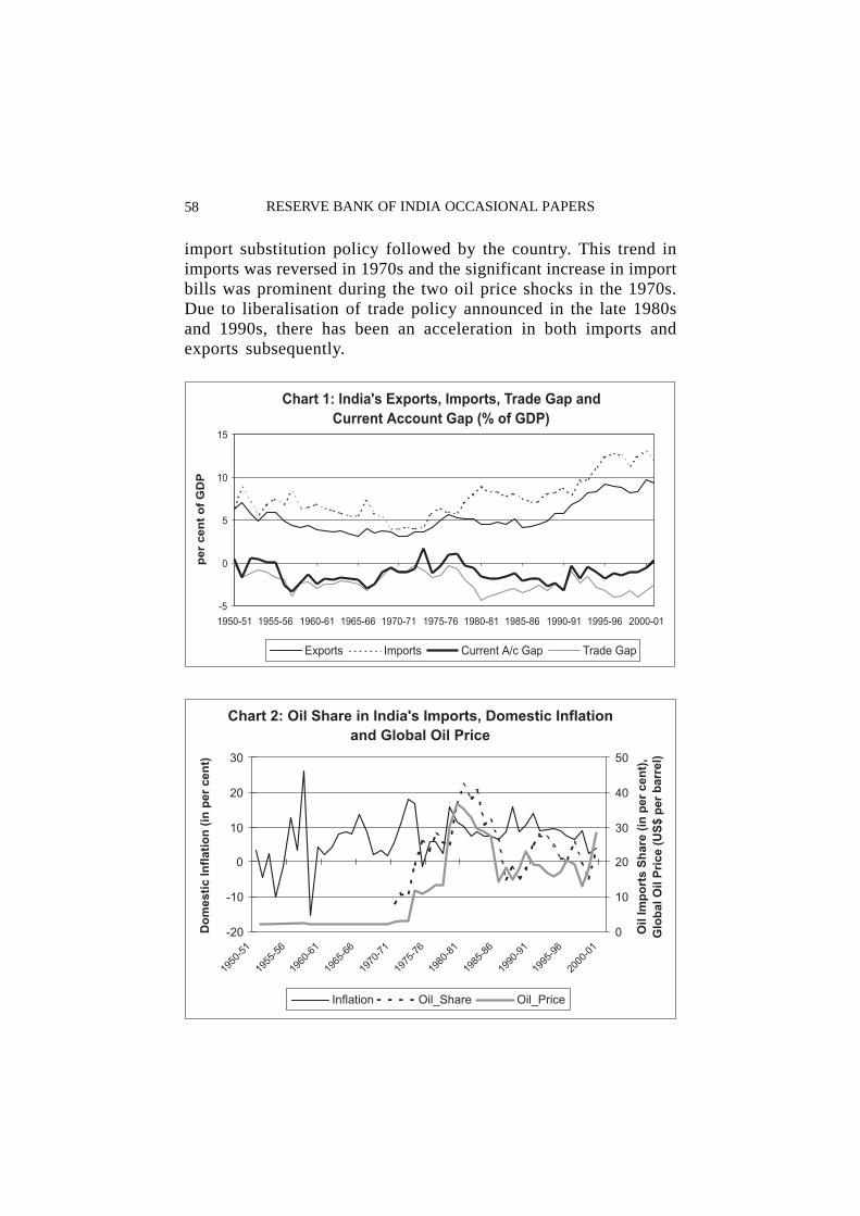
58 RESERVE BANK OF INDIA OCCASIONAL PAPERS
import substitution policy followed by the country. This trend inimports was reversed in 1970s and the significant increase in importbills was prominent during the two oil price shocks in the 1970s.Due to liberalisation of trade policy announced in the late 1980sand 1990s, there has been an acceleration in both imports andexports subsequently.

59
The international oil prices have a major influence on theworld economy since the 1970s. The increases in global oil pricesresulted in substantially inflated oil import bill for India and werealso followed by high domestic inflation (Chart 2). With juxtapositionon Chart 1, it can be seen that other imports were reduced withincreasing oil-imports bill during the periods of oil price shocks.As oil shocks were the most prominent common shocks during thereference period for the economies under consideration, thisphenomenon is examined in detail later in this paper.
Section III
Methodology and Data Sources
The official quarterly estimates of national income and relatedaggregates for India are available only since April-June quarter of1995 and therefore, annual estimates for 1950-2000 are used forthis analysis. Data in respect of India are taken from the officialsources like the publications of the Central Statistical Organisationand the Reserve Bank of India. The estimates for other countriesare taken from the International Financial Statistics (IFS) databaseof the International Monetary Fund (IMF). In view of the GermanUnification in 1989, consistent long-term time series on certainmajor macroeconomic variables are not available and, therefore,the relationship has been explored only for the pre-unificationperiod in respect of Germany. In the case of India, cyclical fluctuationin the non-agricultural GDP is taken as output cycle instead oftotal GDP as agricultural output in India is largely weather dependentand interaction of market forces has lesser role to play in determiningits level. Also the cyclical component of non-agricultural output ismore strongly related to cyclical components of other macro variableslike private consumption, investment, manufacturing sector output,value added from domestic trade, construction activity, private corporatesector output and sales (Mall 1999).
The cyclical components of annual economic time series areestimated by using the band-pass filter proposed by Baxter andKing (1999) which uses the frequency domain approach and allowsthe users to choose the band of cyclical component. For estimating
INTERNATIONAL BUSINESS CYCLES BEYOND G-7

60 RESERVE BANK OF INDIA OCCASIONAL PAPERS
the cyclical components, log transformation of the annual serieshas been taken and the band-pass filter is used to isolate the componentof time series lying within a band of frequencies between two toeight years.
Section IV
International Business Cycles and India –The Correspondence
Among the four developed industrial countries, the businesscycle movements are varied from strong (UK & USA, Germany &USA and Germany & UK) to weak (Japan & UK and Japan &USA) (Table 1 and Chart 3). There has been a change in thepattern of relationship over time, for example, the Germany/USArelationship has become stronger over time (post-1960 correlationof 0.56 increased to 0.83 in the post-1970 period) whereas theJapan/USA relationship has been moving in opposite direction (post-1970 correlation was 0.40 which changed to -0.06 in the post-1980 and further to -0.72 in the post-1990). The Germany/Japan
Note: Curves have been shifted up for illustrative purposes.

61
relationship became more significant in the post-1970 period. Thepositive impact of the 1970s (the major oil-shock period) on therelationship is obvious.
INTERNATIONAL BUSINESS CYCLES BEYOND G-7
Table 1: Correlation of the Output Cycles forSelected Countries (1950-2000)
Country / Period USA UK Japan Germany
All Period 0.09 0.35 0.20 0.08
Post-60 0.13 0.30 0.18 0.08
Post-70 0.22 0.27 -0.03 -0.18
Post-80 0.35 0.65 0.01 0.08
Post-90 0.37 0.71 -0.23 N.A.
All Period 0.56 0.46 0.25
Post-60 0.56 0.49 0.25
Post-70 0.83 0.64 0.77
Post-80 0.86 -0.13 0.45
Post-90 N.A. N.A. N.A.
All Period 0.09 0.31
Post-60 0.07 0.27
Post-70 0.40 0.39
Post-80 -0.06 -0.04
Post-90 -0.72 -0.29
All Period 0.56
Post-60 0.62
Post-70 0.72
Post-80 0.47
Post-90 0.64
Wit
h I
nd
iaW
ith
Ger
man
yW
ith
Jap
anW
ith
UK
N.A. – Not Available

62 RESERVE BANK OF INDIA OCCASIONAL PAPERS
The nature of relationship of output cycles in India with theoutput cycles in the other four countries is very interesting. Thereis a positive relationship between the Indian and the UK outputcycles and it has strengthened over time. Due to historical reasons,India has strong trade relationship with the UK. The co-movementbetween output cycles of India and the USA is also increasingespecially during the 1980s and the 1990s. There is no significantrelationship of the Indian output cycles with those in Germanyand Japan. The amplitude of cycles are good measure of severityof the downturn / recovery and a cycle with higher amplitude islikely to result in more impact on the trading partners. High cyclicalamplitude signifies high impact of cyclical fluctuations in the economy.The amplitude of cycles (measured by standard deviation of thecyclical components) is highest for Japan (0.0203) followed byUSA (0.0145), Germany (0.0134), UK (0.0132) and India (0.0124).This implies that cyclical fluctuations have more profound influenceon the Japanese economy than the remaining countries.
Investment and private consumption in the selected countriesare taken as other major variables for analysing the internationalbusiness cycle relationship. It is interesting to note that there is astrong relationship between the private consumption cycles andthe investment cycles in respect of the USA and the UK and alsobetween the USA and Germany (Table 2). However, the samecannot be said for Japan. The co-movements of the cyclical componentsof investments for Germany and Japan are significant in the post-1970 period as in the case of their output co-movement during thesame period but the same cannot be said for their private consumptionrelationship. In the case of India, the relationship with all thecountries for the whole period is found negative for both privateconsumption and investment but turned positive for the post-1980period. The private consumption behaviour is greatly influencedby the volatility in agricultural output. During the pre-1980 period,investment behaviour in the Indian economy was largely driven bygovernment policies and was not necessarily driven by marketforces. The public sector industries had a major share in totalinvestment in the pre-1980 period and their share has been decliningin the subsequent period. The opening up of the economy aroundmid-1980s witnessed more syncronised movements in these variableswith other countries especially with the USA and the UK.

63INTERNATIONAL BUSINESS CYCLES BEYOND G-7
Table 2: Cross-country Correlation of Cyclical Componentsof Consumption and Investment in Selected Countries
Country / Period USA UK Japan Germany
Private Consumption Expenditure
India Post-1950 -0.11 -0.10 -0.07 -0.34Post-1970 -0.14 -0.13 -0.32 -0.28Post-1980 0.32 0.52 0.13 0.15
Germany Post-1950 0.45 -0.15 -0.03Post-1970 0.48 -0.04 0.44Post-1980 0.14 -0.58 -0.24
Japan Post-1950 0.05 0.34Post-1970 0.26 0.34Post-1980 -0.17 0.09
UK Post-1950 0.42Post-1970 0.66Post-1980 0.64
Gross Fixed Capital Formation
India Post-1950 0.01 0.04 0.01 0.02Post-1970 -0.20 -0.13 -0.32 -0.19Post-1980 0.22 0.27 0.14 -0.04
Germany Post-1950 0.33 0.06 0.20Post-1970 0.52 0.14 0.55Post-1980 0.62 -0.08 0.22
Japan Post-1950 0.01 0.32Post-1970 0.29 0.38Post-1980 -0.17 0.20
UK Post-1950 0.38Post-1970 0.44Post-1980 0.48

64 RESERVE BANK OF INDIA OCCASIONAL PAPERS
Foreign Investment
The negative correlation between investment cycles in Indiaand those in other countries for the post-1980 period is significant.On an average, over 92 per cent of investment in India is met withdomestic savings (Appendix I). However, external investment hadan important role (except in the 1970s when it went down drasticallyand was negative for three years). Chart 4 presents the share offoreign investment (as per cent of GDP) and the output cycles.These movements had low correlation in the total period (correlationcoefficient = 0.10). However, a closer look shows that there is asignificant difference in the relationship between the pre-1980 andthe post-1980 – the pre-1980 relationship was negative (correlationcoefficient = -0.28) which turned positive in the post-1980 (correlationcoefficient = 0.41). The direction of causality between output cyclesand foreign investment cannot be studied from these two variablesas there are other factors like the state of the foreign economies,government policies, investment lags, etc., that influence the relationshipbut the growing association between foreign investment and outputcycles is extremely important. This result is consistent with theoverall output, consumption and investment cycle relationship duringthe post-1980s when there was stronger co-movement with theUSA and the UK – the two major investing countries in India.

65
Section V
The Role of Common Shocks – A Theoretical Model
In this section, we study the the impact of common globalshocks (including the oil-shocks) and country-specific shocks inpropagating similar macroeconomic fluctuations across the selectedcountries. For this purpose, a structural VectorAutoregression (VAR)model using quarterly data for the period 1960:Q1 to 2000:Q4 isused. For this analysis, the Index of Industrial Production (IIP)has been used as output variable for all the countries. Two quarterlyVAR models are used to analyse -
(i) the impact of global shocks and country-specific shocks onoutput fluctuations; and
(ii) the impact of oil price shocks, other global shocks and country-specific shocks on output fluctuations.
To discriminate between country-specific and global shocks,it is assumed that impacts of global shock produce identical percentageoutput changes across countries and their limiting impulse responsesin the level of output are also assumed identical across countries.
The output series (i.e., seasonally adjusted quarterly IIP) arefound to be I(1). In view of its large size and strong trade relationshipwith the major economies across the globe, USA is taken as thereference country and the output differential with respect to theUSA is defined as
Yi = �log(IIPi) - �log(IIPUS) (1)
where i denotes the other four countries. The assumption that Y =[Yi, �log(IIPi)] be a bivariate covariance stationary vector processfor any i would imply that the elements of Y can be expressed asa linear combination of past and present structural shocks, i.e.,
Yt = A(L) �
t(2)
where � = [�h , �g]T is a vector of serially uncorrelated structuraldisturbances with zero mean and unit variance, h and g representingthe home and global supply shocks, and A(L) is a 2×2 matrix ofpolynomial lags. The reduced form moving average representation
INTERNATIONAL BUSINESS CYCLES BEYOND G-7

66 RESERVE BANK OF INDIA OCCASIONAL PAPERS
of Y is
Yt = C(L) e
t(3)
where e = [e1 , e
2 ] is a non-structural residual vector with zero
mean and variance-covariance matrix Σ, and C(L) = A(L) × S-1 isa 2×2 matrix of polynomial lags to be estimated and S is a 2×2matrix to be identified. The elements of e are linear combinationsof the structural shocks by
et = S × �
t(4)
which implies (with nomalisation E(�t �
tT) = I) that Σ = S × ST.
This imposes three non-linear restrictions on the S matrix by theestimates of �. To recover the original VAR structure (by identifyingthe S matrix) by just-identification, we assume additional restrictionfrom economic theory that global supply shock does not havelong-run impact on the differential of the output level across countries.The VAR is estimated for the lag order 3 as residuals do notcontain significant autocorrelations beyond the third lag.
A similar structure is used for the second VAR analysis thatincludes three shocks and Y is now defined as Y = [Yi, � log(IIPi),� log(Price
oil) ]. To just-identify the model, the additional restriction
that oil price is solely driven by oil price shocks (i.e., country-specific and global shocks have zero coefficient for the oil priceequation) is imposed.
The correlation between the country-specific shocks and theglobal shocks before and after the oil price adjustment indicatesthat the the country-specific shocks are generally unrelated acrossthe countries both before and after oil price adjustments (Table 3).In the case of India, the correlation with all other countries is lessthan 0.1 for country-specific shocks. In the case of Japan, thecorrelation with the UK or India is negligible and negative but itis marginally high with Germany. In Section IV too, the relationshipin cyclical components of both output and investment in Germanyand Japan were found to be high. Similar is the case with UK-Germany relationship. On the other hand, the global shocks havebeen more strongly related than the country-specific shocks acrossthe countries both before and after oil price adjustments. Therehas been no major change in the pattern of correlations if oil price

67
shocks are explicitly accounted for. This result is consistent withthe findings of Gross (2001a). Additional calculations show thatthe impacts of oil shocks are near-perfectly correlated across countries(the correlation coefficient ranges between 0.991 to 0.996). Thisimplies that oil shocks are the dominant source of business cyclecomovements in the selected countries.
Table 3: Cross sectional Covariance of Identified Shocks: Global and Country-Specific Shocks Before/After controlling for Oil Prices
Country UK Japan Germany UK Japan Germany
Before Oil price Adjustment After Oil price Adjustment
Country-Specific Shocks
India -0.004 -0.052 0.073 -0.007 -0.093 0.060
Germany 0.284 0.226 0.267 0.225
Japan -0.034 -0.008
Global Shocks
India 0.403 0.441 0.481 0.477 0.433 0.455
Germany 0.422 0.409 0.445 0.402
Japan 0.185 0.243
Section VI
Concluding Observations
The global economy is becoming increasingly integrated underthe influence of a variety of factors like increasing trade in goods,greater technological spillover and increasing factor mobility especially,international capital flows. Over the years, this has resulted ininternational business cycle linkages in the developed industrialcountries in Europe and they often have phases of synchronisedrelationship with the US business cycles. However, its relationshipwith other parts of the world is not yet strong. The Japanese businesscycle is one such example. In view of the non-synchrony andchanging structures, international business cycle analysis usingartificially aggregated economy is prone to cancelling out manyinteresting and relevant country-specific factors.
INTERNATIONAL BUSINESS CYCLES BEYOND G-7

68 RESERVE BANK OF INDIA OCCASIONAL PAPERS
The analysis in this paper shows that the Indian output cycleshave positive relationship with the UK output cycles and also withthe USA output cycles especially during the post-1980s, thoughthe latter relationship is weaker than the former. Also, the relationshipbetween Indian investment or private consumption cycles and therespective cycles in other selected countries turned positive in thepost-1980 period. This can largely be attributed to the closed natureof Indian economy and the institutional set-up in the earlier years.This relationship has undergone changes in the light of the decliningpublic sector investment and also due to the opening up of theeconomy which has led to increased factor movements with othereconomies.
The synchronised output cycles can largely be related to theinternational oil price shocks for all the countries. Though non-oilglobal shocks were important in transmission of international businesscycles, the oil price factor which cannot be considered endogenousto the economies analysed here, has been the dominant factor drivingthe international business cycle relationship through global shocksfor major part of the period.
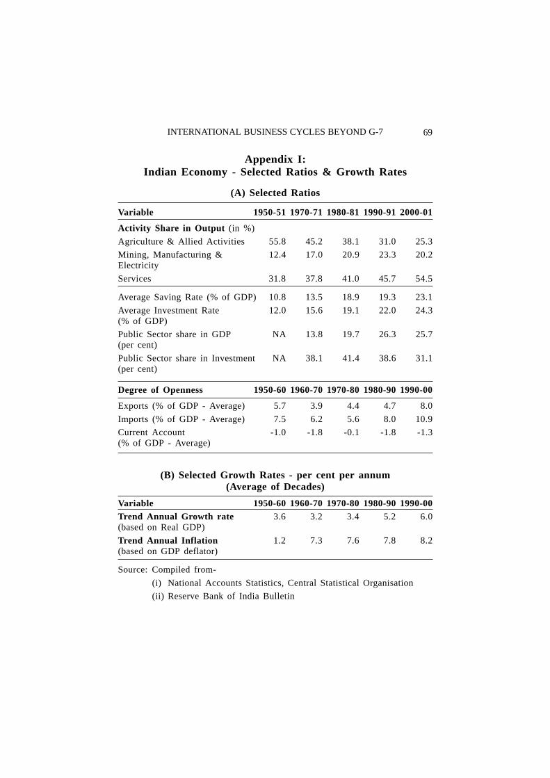
69
Appendix I:Indian Economy - Selected Ratios & Growth Rates
(A) Selected Ratios
Variable 1950-51 1970-71 1980-81 1990-91 2000-01
Activity Share in Output (in %)
Agriculture & Allied Activities 55.8 45.2 38.1 31.0 25.3
Mining, Manufacturing & 12.4 17.0 20.9 23.3 20.2Electricity
Services 31.8 37.8 41.0 45.7 54.5
Average Saving Rate (% of GDP) 10.8 13.5 18.9 19.3 23.1
Average Investment Rate 12.0 15.6 19.1 22.0 24.3(% of GDP)
Public Sector share in GDP NA 13.8 19.7 26.3 25.7(per cent)
Public Sector share in Investment NA 38.1 41.4 38.6 31.1(per cent)
Degree of Openness 1950-60 1960-70 1970-80 1980-90 1990-00
Exports (% of GDP - Average) 5.7 3.9 4.4 4.7 8.0
Imports (% of GDP - Average) 7.5 6.2 5.6 8.0 10.9
Current Account -1.0 -1.8 -0.1 -1.8 -1.3(% of GDP - Average)
(B) Selected Growth Rates - per cent per annum(Average of Decades)
Variable 1950-60 1960-70 1970-80 1980-90 1990-00Trend Annual Growth rate 3.6 3.2 3.4 5.2 6.0(based on Real GDP)
Trend Annual Inflation 1.2 7.3 7.6 7.8 8.2(based on GDP deflator)
Source: Compiled from-
(i) National Accounts Statistics, Central Statistical Organisation
(ii) Reserve Bank of India Bulletin
INTERNATIONAL BUSINESS CYCLES BEYOND G-7

70 RESERVE BANK OF INDIA OCCASIONAL PAPERS
Appendix II:Share of Selected Countries in India’s Foreign Trade
(per cent)
Year\ Belgi- Germa- UK USA Japan Saudi Singa- Hong- USSRCountry um ny Arabia pore kong
1950-51 Exports 1.6 1.8 23.3 19.2 1.7 0.4 4.7 1.7 0.2
Imports 1.4 1.6 20.8 18.3 1.6 0.1 2.5 0.4 0.0
1960-61 Exports 0.8 3.1 26.8 16.0 5.5 0.5 1.1 0.5 4.5
Imports 1.4 10.9 19.4 29.2 5.4 1.3 0.9 0.1 1.4
1970-71 Exports 1.3 2.1 11.1 13.5 13.3 0.9 1.3 1.2 13.7
Imports 0.7 6.6 7.8 27.7 5.1 1.5 0.1 0.0 6.5
1980-81 Exports 2.2 5.7 5.9 11.1 8.9 2.5 1.7 2.2 18.3
Imports 2.4 5.5 5.8 12.1 6.0 4.3 3.4 0.3 8.1
1990-91 Exports 3.9 7.8 6.5 14.7 9.3 1.3 2.1 3.3 16.1
Imports 6.3 8.0 6.7 12.1 7.5 6.7 3.3 0.7 5.9
1999-00 Exports 3.7 4.8 6.0 22.7 4.5 2.0 1.8 6.8 2.9
Imports 7.4 4.0 5.8 7.7 5.0 4.8 3.2 1.7 1.7
Source: Compiled from
(i) Handbook of Statistics on Indian Economy, Reserve Bank of India
(ii) India Database: The Economy (H.L.Chandok and The Policy Group, 1989)

71
References
A’Hearn, Brian and Ulrich Woitek (2001): More International Evidence on theHistorical Properties of Business Cycles, Journal of Monetary Economics, Vol47, pp 321-46.
Backus, D.K. and P.J.Kehoe (1992): International Evidence on the HistoricalProperties of Business Cycles, American Economic Review, Vol. 82, pp 864-88.
Baxter, Marianne (1995): International Trade and Business Cycles, in Grossman,Gene M. and Kenneth Rogoff: Handbook of International Economics (Vol.3),Elsevier Science Publishers B.V.
Baxter, Marianne and Robert G. King (1999): Measuring Business Cycles:Approximate Band-Pass Filters for Economic Time Series, Review of Economicsand Statistics, pp 575-93.
Baxter, Marianne and Michael A.Kouparitsas (2000): What can Account forFluctuations in the Terms of Trade, Federal Reserve Bank of Chicago WorkingPaper.
Canova, Fabio and Harris Dellas (1993): Trade Interdependence and the InternationalBusiness Cycle, Journal of International Economics, Vol 34, pp 23-47.
Canova, Fabio and Jane Marrinan (1998): Sources and Propagation of InternationalOutput Cycles: Common shocks or Transmission? Journal of International Economics,Vol. 46, 133-66.
Canova, Fabio and Gianni de Nicolo (2000): On the Sources of Business Cyclesin the G-7, Working Paper.
Central Statistical Organisation, India: National Accounts Statistics (variousissues)
Chandok, H.L (1989): India Database: The Economy, The Policy Group, NewDelhi
Dellas, Harris, (1986): A Real Model of the World Business Cycle, Journal ofInternational Money and Finance, Vol. 5, pp 381-94.
Fisher, Eric O’N (1995): Growth, Trade and International Transfers, Journal ofInternational Economics, Vol.39, 143-58.
Glick, Reuven and Kenneth Rogoff (1995): Global Versus Country SpecificProductivity Shocks and the Current Account, Journal of Monetary Economics,159-192
Gross, Daniel (2001a): Country-Specific and Global Shocks in the BusinessCycle, Working Paper No.2001/11, Center for Financial Studies, Frankfurt amMain.
INTERNATIONAL BUSINESS CYCLES BEYOND G-7

72 RESERVE BANK OF INDIA OCCASIONAL PAPERS
Gross, Daniel (2001b): Trade Flows and the International Business Cycle, WorkingPaper No.2001/12, Center for Financial Studies, Frankfurt am Main.
Helliwell, John F. and Tim Padmore (1985): Empirical Studies of MacroeconomicInterdependence in Jones, R.W. and P.B.Kenen: Handbook of International Economics(Vol.2), Elsevier Science Publishers B.V.
International Monetary Fund (2001): International Linkages: Three Perspectives(Chapter III), World Economic Outlook, October
Kehoe, Patrick J. (2000): International Business Cycles with Endogenous IncompleteMarkets, NBER Working Paper No. 7870.
Kenen, Peter B. (1985): Macroeconomic Theory and Policy: How the ClosedEconomy was Opened? in Jones, R.W. and P.B.Kenen: Handbook of InternationalEconomics (Vol.2), Elsevier Science Publishers B.V.
Kouparitsas, Michael A. (1996): North-South Business Cycles, Working Paper,Federal Bank of Chicago
Kouparitsas, Michael A. (2000): Evidence of the North-South Business Cycles,Economic Perspectives, Federal Reserve Bank of Chicago
Kwark, Noh-Sun (1999): Sources of International Business Fluctuations: Country-specific Shocks or Worldwide Shocks? Journal of International Economics,Vol 48, pp 367-85.
Kose, M.Ayhan, Christopher Otrok and Charles H.Whiteman (2000): InternationalBusniess Cycles: World, Region and Country-Specific Factors, Paper presentedat the Growth and Business Cycle Conference in Manchester.
Lumsdaine, Robin L. and Eswar S. Prasad (1997): Identifying the CommonComponent in International Economic Fluctuations, NBER Working Paper No.5984
Mall. O.P. (1999): Composite Index of Leading Indicators for Business Cyclesin India, Reserve Bank of India Occasional Papers, Vol.20, No.3,Winter
Obstfeld, Maurice and Kenneth Rogoff (1995): The Intertemporal Approach tothe Current Account, in Grossman, Gene M. and Kenneth Rogoff: Handbook ofInternational Economics (Vol.3), Elsevier Science Publishers B.V.
Prasad, Eswar S. (1999): International Trade and the Business Cycle, WorkingPaper, International Monetary Fund, April.
Reserve Bank of India (2001): Handbook of Statistics on Indian Economy
Zimmermann, Christian (1995): International Trade over the Business Cycle:Stylised Facts and Remaining Puzzles, Working Paper, Research Center onEmployment and Economic Fluctuations, Universite du Quebec a Montreal.

73
Sustainability of Services-Led Growth:An Input Output Analysis of the
Indian Economy
Sanjay K. Hansda*
The sustainability of services as also of services-led growth of the Indian economyhas been addressed in terms of the inter-sectoral linkages as emanating from the input-output transactions tables for 1993-94 both at the disaggregated level of 115 activitiesand the aggregated level of 10 constructed national accounts categories. At the disaggregatedlevel, the Indian economy is found to be predominantly services-intensive with 55 percent activities direct services-intensive and industry the most services-intensive sector.In the process, industrial activities turn out to be the major pace setter for services-growth. On the other hand, services stand out to have the largest inducing effect on theeconomy as per the Rasmussen measure of both backward and forward linkages. Thebackward and forward coefficients of variation indices, however, show that the inducingimpulses from services might have worked mainly through the channel of forward linkage.However, since the forward linkage is inherently less effective than the backward linkage,the inducing impact of services on the rest of the economy could be limited. Nevertheless,as per the index of vertical integration, the services sector is found to have the largestexpansionary potential (multiplying effect) on the rest of the economy. Therefore, theservices-led growth augurs well for the Indian economy for sustaining the overall GDPgrowth. However, since the multiplier value remains less than one for all the activitiesincluding services, the expansionary potential of a services-led growth may not be overemphasised unless accompanied by growth impulses from other sources.
JEL Classification: O14
Key words: Services, Input-Output Analysis
Introduction
The services sector has been the mainstay of the Indian growthprocess in the 1990s. While the share of services has been rulinghigh ever since independence, it has received a major fillip onlyin the 1990s. Indeed, contribution of the services sector to theoverall GDP growth peaked an all time high of 65.1 per cent inthe 1990s up from 43.6 per cent in the 1980s. As a result, theservices share in GDP went up by a spectacular 7.9 per cent in a
Reserve Bank of India Occasional PapersVol.22, Nos.1, 2 and 3, Summer, Monsoon and Winter, 2001
*Shri Sanjay K. Hansda is Assistant Adviser in the Department of Economic Analysisand Policy of the Reserve Bank of India. The author wishes to thank Dr. KaushikBhattacharya for helpful suggestions. However, the usual disclaimer applies. The viewsexpressed are those of the author and not of the institution to which he belongs.

74 RESERVE BANK OF INDIA OCCASIONAL PAPERS
single decade of the 1990s touching the mark of 48.5 per cent in2000-01 while the sector took about four decades to improve itsshare by 12.6 per cent to 40.6 per cent in 1990-91 from 28.0 percent in 1950-51. The ascendancy of services has had a stabilisingeffect on the growth process itself. To quote from the ReserveBank’s Report on Currency and Finance, 2000-01, ‘‘…it is theservices sector which has kept the GDP growth around 6.0 percent in the 1990s when industry and agriculture sectors did notperform relatively well’’ (p. iii – 44). Thus, ‘‘the services sectorhas been the most dynamic sector of the Indian economy, especiallyover the last ten years’’ (National Statistical Commission, 2001,art 7.1.2).1
Another notable feature of the 1990s is the emergence ofinformation technology (IT) related services. On this count, Indiahas come to be increasingly recognised as a post-industrial societyand as a knowledge-based economy. Such optimism is possiblyrouted to the recent spurt in software exports and the perceivedpotential of trade in services such as IT, communications andentertainment. Indeed, in conjunction to the domestic economy,services, hitherto considered non-tradable, have provided a significantsource of comfort to the country’s balance of payments in the1990s. The Reserve Bank’s Report on Currency and Finance, 2000-01 has explicitly recognised this development: ‘‘As against a deficitof US $ 0.2 billion in 1990-91 that partly exacerbated the externalpayments imbalances during that year, the net invisible surplushas grown over time to around US $ 12-13 billion in the recentperiod, imparting resilience and sustainability to current accountdeficits and overall balance of payments during the 1990s’’ (p.vi -6).
The preponderance of services in the Indian economy, however,runs counter to the conventional wisdom on development at leaston two counts (Madheswaran and Dharmadhikary, 2000). The well-known sequence of structural transformation from an agrarian economyto a predominantly service economy en route an industrial economyas noticed in the developed world has not been witnessed in India.While the share of agriculture in GDP has registered a seculardecline from 57.7 per cent in 1950-51 to 24.2 per cent in 2000-01,the void has not been filled in by industry even though it has

75
improved its share to 27.3 per cent in 2000-01 from 14.8 per centin 1950-51. On the other hand, services sector has come to occupythe position of a prime mover in the Indian economy with its shareat 48.5 per cent in 2000-01 as against 28.0 per cent in 1950-51.The observed dominance of services ahead of industry with thedecline of agriculture has, however, given rise to apprehension asto whether the sequence of the growth process would be reversedin the future particularly when industry is yet to achieve adequategrowth. Such apprehension seems to have gained a ground in theabsence of preponderance of services in the country’s employment.In 1999-00, services have accounted for around 23.5 per cent oftotal employment in the country. On the other hand, agriculturestill continues to account for a major share of employment despiteits secular decline in terms of share in GDP. In the developedworld, however, rise and dominance of a sector in GDP has beenaccompanied by its simultaneous ascendancy in employment. Theobserved counter-factuals in terms of sequence of growth andemployment as also the apparent imbalance between the two havebeen an added concern in the Indian growth process.
The spectacular performance of the services sector in the 1990shas once again raked up the issue of its plausibility and sustainability(Acharya, 2002b). The issue has attracted an added attention inview of the fact that a part of the services growth is reckoned tobe ‘spurious’ as reflecting the revaluation of contribution frompublic administration and defence in line with the Fifth PayCommission’s recommendations. The impact of such wage hikeon GDP has found place even in official documents including theEconomic Survey, 1998-99: ‘‘…fully one percentage point of growthof 5.0 per cent in GDP for 1997-98 is attributed to the 20 per centincrease in real value added in the ‘public administration and defence’sub-sector arising chiefly from pay increases to government servants’’(p.1). Subsequent sobering of the growth performance of the economyseems to have extended credence to such concerns.
Indeed, the high growth momentum of the 1990s seems tohave petered out in the new millennium with the growth fatiguefinally catching up the services sector. The GDP growth crashedto an abysmal 4.0 per cent in 2000-01, the lowest since 1992-93,
SUSTAINABILITY OF SERVICES-LED GROWTH

76 RESERVE BANK OF INDIA OCCASIONAL PAPERS
under the weight of the services growth touching the rock bottomof 4.8 per cent, a level witnessed only in the crisis year of 1991-92. Although a modicum of recovery set in during 2001-02 bothfor the services sector and the GDP, the sudden deceleration of theservices sector has brought the question of its sustainability at thecentre-stage.
Even in the financial press, the question being hotly debatedhas been: how long can the services growth remain immune to thehappenings in agriculture and industry? For example, S. S. AnklesariaIyer (2002a; 2002b) in a series of articles in The Economic Timeshas welcomed the rapid growth of services in the 1990s. In hisview, ‘as the industry-less growth is here to stay, our ability tocompensate for industrial failure with services success is a strength,not a weakness’. On the other hand, Acharya (2002a; 2002c) hasbeen sceptical of the idea of services-led growth. In his words,‘…India’s services sector can’t enjoy fast and sustained growth. Itcan, but only in tandem with a fast growing industrial sector…Servicescannot, by themselves, assure rapid and sustained growth of theIndian economy.’
As the Indian economy is currently passing through a phaseof industrial slowdown coupled with a cyclical downturn in agriculture,a perceptive view on the services growth assumes prescriptiveimportance in steering the economy on to the path of recovery. Itis against this backdrop, the present study sets out its focus on thesustainability of services growth as also of the overall services-ledgrowth process. Specifically, the study is built around the followingquests: what is the services intensity of the various sectors of theeconomy? How strong are the backward and forward linkages ofservices with the rest of the sectors? Are the strong backward andforward linkages of services, if any, an outcome of large transactionswith a few sectors or an outcome of broad-based transactions withmany sectors? What is the expansionary potential of services onnon-services in terms of the multiplying effect on the rest of theeconomy? Which services have the largest multiplier effect on theeconomy?
The rest of the study is organised as follows. Section I presentsa select survey of literature on the role of services in the growth

77
process with special reference to India. Section II offers a snapshotof the observed relationship between the services and the majormacro aggregates including income, consumption, capital and exportin the Indian economy. Section III discusses the methodologicalbackground and data sources. Section IV presents the empiricalfindings coupled with their possible interpretations. Section V concludesthe study.
Section I
Services Sector and Economic Growth:A Select Survey of Literature
The role of services in the development process is marked bya long controversy. In fact, the debate dates back to Adam Smithwho was of the view that services ‘perish in the very instant oftheir performance and seldom leave any trace or value behindthem’. As such, services have drawn for themselves a tag ofunproductive activity from the classical economists. Until recently,services used to be treated accordingly by the erstwhile socialistor centrally planned economies and classified as ‘non-materialproduction’ as against the productive ‘material production’ in theirnational accounts statistics.
While services have long come out of such categorisation, thedebate seems to have shifted its focus to the level of productivity.While Fisher (1935) and Clark (1940) attributed the preponderanceof services in the developed world to its level of income, theyrecognised the low productivity in services as a factor behind thefaster employment growth in services than in industry. Fuchs (1965)also came to a similar conclusion for the US economy in the1960s. Such productivity differentials formed the basis of the well-known ‘cost disease’ hypothesis of services propounded by Baumol(1967). Higher productivity in industry was visualised to raisewages even in services more than the productivity growth, leadingto a chronic tendency for costs and prices of services to increaserelative to goods. In view of the post-1973 productivity slowdownin the US, increasing tertiarisation of the US economy has been acause for concern (Triplett & Bosworth, 2000).
SUSTAINABILITY OF SERVICES-LED GROWTH

78 RESERVE BANK OF INDIA OCCASIONAL PAPERS
The reported low productivity in services has however beenquestioned, among others, by Griliches (1992). The low level ofservices productivity is advocated to be a fall-out of mis-measurementof services output. Besides, factors like technological change,deregulation and increased competition are set to raise productivityat least in select services (Maclean, 1996). Even Baumol et al(1985) have recognised the case of ‘progressive’ services withsubstantial productivity gains. Besides, the ‘asymptotically stagnant’services initially register productivity gains followed by standardisationand stagnation in productivity. Nevertheless, there is now increasingrecognition that the very act of service even involves externalitiesfor user or the user’s goods in terms of gain in productivity or itspotential (Hill, 1977). In fact, such over-bearing feature of servicesmakes the estimation exercise daunting and more so for the newlyarrived activity of information technology (IT)-related services asthe national statistical systems are largely designed to capturedevelopments only in the goods sector. This has led to a situationof low measured productivity despite increased use of computersand IT, which is otherwise expected to boost the productivity growth.This incongruity is popularly known as the Solow productivityparadox. While several attempts have been made to explain theparadox, the exact role of distortions in official statistics thereinremains controversial (Diewert, et al, 1999).
Yet another popular scepticism perceives services as innovationlaggards and primarily consumers of innovation in manufacturing(Miles, 1993). However, increasingly such a view has come to bequestioned in recent period. In contrast to a manufacturing innovationin terms of new or improved product/process, innovation in servicesoften relates to how, where and when a service is delivered (Howells,2000). Productivity-enhancing investment in ICT (i.e., informationand communication technology), regulatory reform and growingtradability of services are among the major factors contributing toinnovations in services (Pilat, 2000a).
A logical corollary to the concerns of productivity and innovationhas been the view that high growth, be that of services or theservice-oriented economies, is not sustainable. The decline inmanufacturing and the corresponding shift to services is widely

79
held to be unsupportable in the long run since services dependcritically on manufacturing for their existence. Such well-entrenchednotion of parasitic and dependent services has recently come underincreasing scrutiny (Bryson and Daniels, 1998). Rather than servicesfollowing and supporting manufacturing, manufacturing is seen asflowing to those countries and areas where the services infrastructureis efficient and well developed (OECD, 2000). Besides, the increasingresembling of services with commodities has enabled the formerto emerge as the major driving force in economic growth. Thus,the conclusion that service economies are naturally sluggish seemsto be premature (US Department of Commerce, 1996).
Be that as it may, the growing role of services in nationaleconomies is clear and unequivocal particularly for the developedworld, which could better be labelled as post-industrial society(Bell, 1967). A variety of explanations are put forward in theliterature to explain such an orientation. To begin with, the buildingblock of the Fisher-Clark hypothesis of increasing tertiarisationwith increased income has been a variant of the Engel’s Law thatthe income elasticity of demand for services is greater than that ofdemand for goods. While early empirical works have found supportto such hypothesis, recent studies such as Falvey and Gemmell(1996) have tended to reject the income-elastic demand for servicesoverall but confirm a wide range of income elasticity estimates(above and below unity) across different types of services. Indeed,in contrast to a post-industrial society, Gershuny (1978) has evenadvocated a self-service economy, wherein self-service activitieswith the help of consumer durables are visualised to replace thepurchased consumer services. The increased use of consumer durablesis expected to enhance the demand for intermediate services suchas servicing and repair of household equipments. The Gershunyeffect is found to operate in a number of developed and developingeconomies including Brazil (Flores, 1995). The thesis has alsobeen questioned both on theoretical and empirical grounds. Forexample, Silver (1987) has argued that increasing woman participationin workforce reduces the time available for self-service within thehousehold. On the other hand, emergence of a broad-based prosperousmiddle class coupled with an ageing population is found to boostthe demand for consumer services in the Asia (Wirtz, 2001).
SUSTAINABILITY OF SERVICES-LED GROWTH

80 RESERVE BANK OF INDIA OCCASIONAL PAPERS
The process towards increasing specialisation and verticaldisintegration has entailed focusing on core competencies combinedwith outsourcing of peripheral activities (Stigler, 1956). Theexternalisation of non-core activities, formerly carried out in-houseand counted as industrial output, is believed to be the engine ofservices growth and, by the same token, decline of industry. Suchcontracting out renders the firm’s cost structure flexible necessitatedby a shorter product cycle and changing taste pattern. However,externalisation is found to have only marginally influenced thegrowth of small business service firms of the UK (Bryson, et al,1993). Yet another accounting explanation of the services growthcan be traced to the work of Browne (1986). With the increasingmonetisation of the economy, a major chunk of household activitiesis outsourced from the market. The measured growth of nationalincome is, therefore, biased upward since such shifts in productiondo not result in a corresponding increase in total output of thecombined household and market sectors.
With the increasing complexities of modern industrialorganisations, manufacturing activities have become more and moreservice intensive both upstream (e.g., design and R & D) anddownstream (e.g., marketing and advertising) (Pilat, 2000b).Competitive advantage of a firm now depends more on providingspecialised services like financing and after-sales facilities thanon production, which has increasingly become routinised. On theother hand, new in-house services have come up to extend aninterface with the outside provider of services on externalisationof the latter (UNCTAD, 1989, p. 145). All these are arguablyreflected in increased demand for intermediate services. In thecase of Canada, however, intermediate services have not registeredsubstantial increase (Economic Council of Canada, 1991).
The ascendancy of services in the developed world has oftenbeen accompanied by deindustrialisation as in the case of the UK.Kaldor (1966) was of the view that a mature economy could continueto benefit from economies of scale ‘not through a fast growth inmanufacturing industry as a whole, but through greater internationalspecialism … or in other words by increasing the degree ofinterdependence of British industry with the industries of other

81
countries’ (p. 122). Thus, management and service functions maybe located in one country while manufacturing activities in another.Such a process has possibly worked out in rapid industrialisationof the developing world and de-industrialisation of the developedworld.
In the Indian context, the increasing share of services in GDPhas been a source of controversy ever since independence. Rao(1954) discounted it as an indicator of development in the contextof a developing country. Nevertheless, the dominance of serviceswas traced back to factors such as the increasing role of governmentin economic planning and execution, the historical role of urbanmiddle class in wholesale trade and distribution, and the demonstrationeffect of high income countries (Panchamukhi, et al, 1986). Thesustainability of a service-led growth was once again questionedby Shah (1987) and Mitra (1988). Bhattacharya and Mitra (1989;1990) also felt that the service-led growth could have seriousimplications for inflation, income distribution and balance of paymentssince income (employment) might have grown faster than employment(income) in the organised (un-organised) services. Besides, ‘…incomefrom service sector is growing much in excess of the demandgenerated for the services by the commodity sector’ (p. 2449).However, in view of the similar pattern of growth both in netmaterial product and NDP during 1950-51 to 1983-84, Datta (1989)refuted the view of overgrowth of the services sector. Given thelimited role of services in employment generation and absorption,policy intervention was advocated in some circles (Mazumdar, 1995,and Arunachalam and Kumar, 2002). Bhowmik (2000) highlightedthe fact that about 50 per cent industries in the Indian economywere direct and direct plus indirect services intensive in 1991-92.Besides, services appeared to be the most growth-inducing andgenerated a higher value added in other industries than in theirown.
SUSTAINABILITY OF SERVICES-LED GROWTH

82 RESERVE BANK OF INDIA OCCASIONAL PAPERS
Section II
Services Sector in the Indian Growth Process:A Few Stylized Facts
The preponderance of services over industry is not a recentphenomenon for the Indian economy but has been in place sincethe beginning of 1950s (Table 1). Such predominance of servicesover industry could be an outcome of the de-industrialisation processpursued in British India (Bagchi, 1982). While the decline of theprimary sector, i.e., largely agriculture, is in keeping with theconventional wisdom on development, the preponderance of servicesahead of industry stands out as a departure from the past. Nonetheless,the Indian experience is not a standalone case. A number of developingcountries such as Zambia, Chad, Sudan, Kenya and Pakistan havealso undergone a similar phase in their development process.
Table 1: Agriculture, Industry and Services: Shares in GDP
(Per cent)
Year Agriculture Industry Services
1 2 3 4
1950-51 57.2 14.8 28.0
1960-61 54.7 16.6 28.7
1970-71 48.1 19.9 32.1
1980-81 41.8 21.6 36.6
1990-91 34.9 24.5 40.6
2000-01 24.2 27.3 48.5
2001-02 24.3 26.7 49.0
Source: Central Statistical Organisation.
Moreover, the decline in growth of GDP has in general notbeen accompanied by a reduction in share of services (Table 2).This observation runs counter to the established theories but is inkeeping with the growth experience of the developed world(Chandrasekhar and Ghosh, 2000). The visible hand of the governmentas reflected in planning and production in the economy as a wholecould have contributed to such a development (Mazumdar, 1995).

83
Table 2: Services and GDP: Growth and Share
(Per cent)
Year Services GDP ServicesGrowth Growth Share
1 2 3 4
1951-52 2.7 2.3 28.1
1960-61 5.9 7.1 28.7
1970-71 4.9 5.0 32.1
1980-81 4.5 7.2 36.6
1990-91 5.3 5.6 40.6
2000-01 4.8 4.0 48.5
2001-02 6.5 5.4 49.0
Source: Central Statistical Organisation.
The services sector entered the decade of 1990s with a growthof 5.3 per cent, even lower than the GDP growth of 5.6 per centin 1990-91 (Table 3). In the following year of the balance ofpayments crisis when both agriculture and industry encountered anegative growth, services posted a positive growth of 4.8 per cent,ensuring an overall GDP growth of 1.3 per cent. During the boomphase of 7 per cent plus GDP growth, i.e., from 1994-95 to 1996-97, the growth in services as well ruled over 7 per cent. In thesubsequent years till 2001-02, the services growth remained higherthan those of the other sectors barring 2000-01 when it crashed toa mere 4.8 per cent primarily gravitated by the negative growth innon-bank financial companies. Overall, the services sector posteda growth of 7.6 per cent in 1990s up from 6.6 per cent in 1980s.
As per the Economic Survey, 2000-01, liberalisation of theeconomy in the 1990s and encouragement of private investment inindustry and infrastructure have induced sustained high growth inservices sector. A rapid increase in expenditure on public administrationand defence, social services, and rural extension services also hasan impact on the growth of services sector. Besides, IT softwareand services has emerged as one of the fastest growing segmentsof the economy with a compound annual growth of over 50 percent during 1990s (Rastogi, 2002).
SUSTAINABILITY OF SERVICES-LED GROWTH

84 RESERVE BANK OF INDIA OCCASIONAL PAPERS
Table 3: Sectoral and Overall GDP Growth Since 1990-91
(Per cent)
Year Agriculture Industry Services GDP
1 2 3 4 5
1990-91 4.1 7.7 5.3 5.6
1991-92 -0.02 -0.6 4.8 1.3
1992-93 5.8 4.0 5.4 5.1
1993-94 4.1 5.2 7.7 5.9
1994-95 5.0 10.2 7.1 7.3
1995-96 -0.9 11.6 10.5 7.3
1996-97 9.6 7.1 7.2 7.8
1997-98 -2.4 4.3 9.8 4.8
1998-99 6.2 3.4 8.3 6.5
1999-00 1.3 5.3 9.5 6.1
2000-01 -0.2 6.3 4.8 4.0
2001-02 5.7 3.3 6.5 5.4
Memo Item
1990-00 3.3 5.8 7.6 5.8
1980-90 4.4 6.8 6.6 5.8
Source: Central Statistical Organisation.
In commensurate with the value added, services share in privatefinal consumption expenditure has witnessed a steady increase from10.2 per cent in 1950-51 to 29.0 per cent in 2000-01 (Hansda,2002). The share of services export as a per cent of merchandiseexport has also improved from 13.8 per cent in 1950-51 to 45.1per cent in 2001-02. On the other hand, the share of services in netfixed capital stock has declined from as high as 68.4 per cent in1950-51 to 45.3 per cent in 1999-00. Similar trend is observed inits share of gross capital formation (i.e., investment), which hasdecreased from 57.7 per cent in 1950-51 to 39.6 per cent in 1999-2000. The absorption of labour in services has also not been thatencouraging.

85
While the various sources of growth vent out conflicting signalfor services, the sector has come to occupy the dominant positionin the Indian economy by the end of 1990s. Probably greater inter-sectoral linkages as reflected in the growing intermediate use ofservices as against their final use have been the major contributorto the services growth (Table 4). The intermediate use of servicesoutput has grown from 31.2 per cent in 1968-69 to 38.5 per centin 1993-94 when its final use has declined from 68.8 per cent to61.5 per cent over the same period. The increased intermediateuse of services output has taken place in the production of bothcommodities and services. It is towards such exploration of inter-sectoral linkages, the following section discusses the methodologyof the present study.
Table 4: Percentage Distribution of Services Output
Item Year Commo- Services Intermediate Final Totaldities Use Use Output
1 2 3 4 5 6 7
Services 1968-69 21.8 9.4 31.2 68.8 100.0
1973-74 21.2 9.4 30.6 69.4 100.0
1978-79 23.4 15.5 38.9 61.1 100.0
1983-84 24.4 13.1 37.5 62.5 100.0
1989-90 27.8 12.8 40.6 59.4 100.0
1993-94 26.8 11.7 38.5 61.5 100.0
Source: Input-Output Transactions Table 1993-94, CSO (2000).
Section III
Data Base and Methodology
Given the line of inquiry as set out ab initio, the empiricalquest has been pursued in an input-output framework. For thepurpose, CSO’s latest Input-Output Transactions Table (IOTT),which pertains to the year 1993-94, has been utilised. As per theIOTT, 1993-94, the economy is disaggregated into 115 activities,of which 22 activities are in agriculture, 80 in industry and 13 in
SUSTAINABILITY OF SERVICES-LED GROWTH

86 RESERVE BANK OF INDIA OCCASIONAL PAPERS
services. The analysis is carried out both at the level of 115 activitiesand at the aggregated level. For the later, 115 activities are clubbedinto 10 broad categories in line with the sectorisation of nationalaccounts statistics.
The basic input-output relation can be presented in the followingmatrix notation: X = AX + F (1)
where X = (x1, …, x
N)/ is the vector of gross output; A = (a
ij) is
the matrix of technical input-output coefficients and F = (f1, …,
fN)/ is the vector of final demand. Equation (1) states that gross
output, X, is the sum of intermediate demand, AX, and final demand,F. From equation (1), it follows that
X = (I – A)–1 F (2)
if (I – A), known as the Leontief matrix, is non-singular and whereI is the identity matrix. The matrix (I – A)–1 is known as theLeontief inverse matrix, which represents the direct and indirectrequirements of gross output in each line of activity to support oneunit of final demand in each line of activity.
As a first approximation of the inter-sectoral linkages, sectoralintensity of an activity is often employed in the literature (e.g.,Proops, 1988). While such intensity could be defined in a varietyof ways, the popular ones run in terms of output or final demand.Specifically,
GX = Sectoral intensity in relation to output (3)
G*F = Sectoral intensity in relation to final demand (4)
G* = G (I – A)–1 (5)
where G is the vector of direct input requirements from a sector(i.e., agriculture, industry or services) to produce one unit of grossoutput by an activity and G* is the vector of direct and indirectinput requirements from a sector to produce one unit of output forfinal demand.
The widely used measures of inter-sectoral dependence arethe backward, forward and total linkage indices a la Rasmussen

87
(1956). Backward linkage of a sector measures the inducement toproduction in other sectors, which is absorbed as an input to theformer. On the other hand, forward linkage of a sector measuresthe extent to which the sector provides inputs for utilisation byother sectors. The sectors having large total linkage is called thekey sectors for the purpose of investment allocation with a viewto ensuring a faster industrialisation.
The sum of elements in the ith row of the total requirementmatrix (I – A)–1 is normally taken to be the measure of forwardlinkage. Such measure of forward linkage assumes a uniform increasein demand by one unit for all the sectors, which is however unlikelyto materialise in practice. Weighting the total requirement matrixby the share in final demand is claimed to avoid the problem(Claus, 2002). Accordingly, each element of (I – A)–1, say b
ij , is
weighted to generate bij
w, the typical element of the final demandweighted Leontief inverse where b
ijw = b
ij f
i/ �
i=1 f
i
The sum of elements in the ith row of the final demand weightedLeontief inverse, i.e., b
i.w =�
j=1 b
ijw , which is nothing but the forward
linkage, shows the increase in output of the ith sector used asinputs for producing an additional unit of final demand output,given each sector’s share in total final demand. The inter-industrycomparison of forward linkages can be made by constructing anindex of the forward linkage as follows:
Ui.
w = (1/N)bi.
w / (1/N2)��i=1
bi.
w (6)
The numerator of equation (6) measures the average stimulus toother sectors, according to each sector’s share in total demand,resulting from a unit increase in final demand for output of the ith
sector. The denominator measures the average stimulus to the entireeconomy resulting from a unit increase in final demand for outputof all sectors.
Similarly, an index of the backward linkage is derived thefollowing way:
U.j
w = (1/N)b.j
w / (1/N2) �j=1
b.j
w (7)
N
N
N
N
SUSTAINABILITY OF SERVICES-LED GROWTH

88 RESERVE BANK OF INDIA OCCASIONAL PAPERS
where sum of the elements in the jth column, i.e., b.j
w = �i=1
bij
w
stands for the input requirements for a unit increase in the finaldemand for output of the jth sector given each sector’s share intotal final demand. Those sectors having each of the indices ofbackward and forward linkages greater than unity are consideredthe key sectors of the economy. Alternatively, sectors having thesum of indices of backward and forward linkages, i.e., the totallinkage equal to or exceeding the value of 2 may be treated as thekey sectors (Anjaneyulu and Prakash, 1994).
The above indices of backward and forward linkages beingthe averages are sensitive to extreme values. A sector, which buys(sells) large amounts only from (to) a few sectors, may end uphaving a high backward (forward) linkage index. In order to accountfor such dispersion in intermediate (final) demand, the linkageindices are supplemented by the following coefficient of variationindices (Rasmussen, 1956):
Vi.
w = [(1/N) �j=1
N {bij
w - (1/N) bi.w}2]1/2 / (1/N) b
i.w (8)
V.j
w = [(1/N) �i=1
N {bij
w - (1/N) b.jw}2]1/2 / (1/N) b
.jw (9)
The numerators in (8) and (9) are the standard deviations and thedenominators the averages. The coefficient of variation index, V
i.w
(V.j
w) measures the relative evenness with which the ith (jth) industrysells (purchases) to (from) other sectors. A relatively large valueof V
i.w (V
.jw) means that the ith sector sells (purchases) output (inputs)
to (from) only a few industries in the economy. Obviously, the keysectors with low coefficient of variation index score a point inpriority over the sectors with high coefficient of variation index.
The Rasmussen measures of inter-sectoral linkages have beencriticised in the literature on a number of grounds. The backwardand forward linkages are even shown to be mutually inconsistent,among others, by Cella (1984). Against such a backdrop, Heimler(1991) has put forward an alternative index of vertical integration,which measures the multiplying effect of each activity on the grossoutput of the rest of the economy.
N
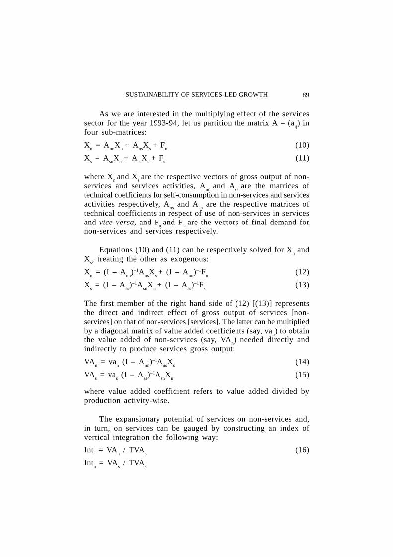
89
As we are interested in the multiplying effect of the servicessector for the year 1993-94, let us partition the matrix A = (a
ij) in
four sub-matrices:
Xn = A
nnX
n + A
nsX
s + F
n(10)
Xs = A
snX
n + A
ssX
s + F
s(11)
where Xn and X
s are the respective vectors of gross output of non-
services and services activities, Ann
and Ass
are the matrices oftechnical coefficients for self-consumption in non-services and servicesactivities respectively, A
ns and A
sn are the respective matrices of
technical coefficients in respect of use of non-services in servicesand vice versa, and F
n and F
s are the vectors of final demand for
non-services and services respectively.
Equations (10) and (11) can be respectively solved for Xn and
Xs, treating the other as exogenous:
Xn = (I – A
nn)–1A
nsX
s + (I – A
nn)–1F
n(12)
Xs = (I – A
ss)–1A
snX
n + (I – A
ss)–1F
s(13)
The first member of the right hand side of (12) [(13)] representsthe direct and indirect effect of gross output of services [non-services] on that of non-services [services]. The latter can be multipliedby a diagonal matrix of value added coefficients (say, va
n) to obtain
the value added of non-services (say, VAn) needed directly and
indirectly to produce services gross output:
VAn = va
n (I – A
nn)–1A
nsX
s(14)
VAs = va
s (I – A
ss)–1A
snX
n(15)
where value added coefficient refers to value added divided byproduction activity-wise.
The expansionary potential of services on non-services and,in turn, on services can be gauged by constructing an index ofvertical integration the following way:
Ints = VA
n / TVA
s(16)
Intn = VA
s / TVA
s
SUSTAINABILITY OF SERVICES-LED GROWTH

90 RESERVE BANK OF INDIA OCCASIONAL PAPERS
where TVAs stands for total value added of services. The index Int
measures the indirect effect of services on non-services and, inturn, on services, providing a dimension free measure of the multiplierof each on the value added of the rest of the economy. The activityfor which Int is the highest can be ranked as the key sector of theeconomy in terms of its ability to generate value added in otheractivities.
Section IV
Empirical Findings
Sectoral Intensity
The sectoral intensity of activities provides a ready-reckonerof the inter-sectoral linkages between agriculture, industry andservices. While the details on sectoral intensity for all the 115activities are presented in Appendix Table 1, Table 5 reports thesummary observations. As per the direct measure of intensity (G),34 out of 115 activities or 30 per cent activities have had theagricultural intensity above the average of 7 per cent of grossoutput. The sector of agriculture itself has turned out to be themost agriculture-intensive sector with 68 per cent of agriculturalactivities having the agriculture intensity above the average asagainst 23 per cent and 8 per cent of industrial and services activitiesrespectively. Only one out of 13 services activities, viz., hotelsand restaurants has the agricultural intensity above the average.This implies that services activities hardly draw their inputs fromagriculture while such linkage is relatively strong between industryand agriculture. In terms of variation in intensities, range in agriculturalintensity has been higher than that of services intensity but lessthan that of industrial intensity. The picture has remained more orless the same in terms of the direct and indirect measure of intensity(G*).

91
Table 5: Distribution of Activities with Above AverageSectoral Intensity
(No. of Activities)
Item Agriculture Industry ServicesIntensive Intensive Intensive
G G* G G* G G*
1 2 3 4 5 6 7
1. Agricultural 15 15 0 0 1 1Activity (68) (68) (0) (0) (5) (5)
2. Industrial 18 22 57 55 56 59Activity (23) (28) (71) (69) (70) (74)
3. Services 1 1 3 3 6 2Activity (8) (8) (23) (23) (46) (15)
4. Total 34 38 60 58 63 62(1+2+3) (30) (33) (52) (50) (55) (54)
Memo Items#
Average 7 12 29 59 15 30Intensity
Minimum to 0 to 0 to 0 to -14 to 0 to 0 toMaximum 74 88 76 154 41 68Intensity Range
Figures in bracket are percentage share in the respective sectoral total of activities.G: Direct intensity; G*: Direct plus indirect intensity; #: As percent to grossoutput.
In terms of the direct measure of intensity (G), 60 out of 115activities or 52 per cent activities have reported higher than theaverage industrial intensity of 29 per cent of gross output. Notably,not a single agricultural activity has the above average industrialintensity. The industrial sector with 57 out of 80 industrial activitiesor 71 per cent of its activities has been the most industry intensivewhen only 3 services activities out of 13, viz., medical and health,railway transport services, and other transport services, have theabove average industry intensity. In other words, neither agriculturalnor services activities seem to be much dependent on industry forinput. However, the industrial intensity of the economy stands outto be of high order with 50 per cent of the total number of activitiesdisplaying the above average industrial intensity even in terms of
SUSTAINABILITY OF SERVICES-LED GROWTH

92 RESERVE BANK OF INDIA OCCASIONAL PAPERS
the direct and indirect measure of intensity (G*). The extent ofvariation in industrial intensity has been the most, possibly reflectingwide variation in technology at the activity level. Besides, theindustrial intensity has turned out even negative for the activity ofrubber production while the same has been more than 100 per centfor 17 industrial activities in terms of the direct and indirect measureof intensity (G*).
With 63 out of 115 activities or 55 per cent activities havingthe above average services intensity, the predominance of servicesintensive activities is clear in the economy. Interestingly, unlikeagriculture and industry, services sector per se is not the mostservices intensive sector. It is the industrial sector, which has turnedout to be relatively services intensive in its 56 out of 80 industrialactivities (i.e., 70 per cent industrial activities). On the other hand,6 out of 13 services activities, i.e., 46 per cent services activitieshave had the services intensity above the average of 15 per centof gross output. Only one agricultural activity, viz., animal services(agricultural) has the above average services intensity. As per thedirect and indirect measure of services intensity (G*), the numberof industrial activities with the above average services intensityhas gone up to 59 (i.e., 74 per cent of industrial activities) whilethat of services activities has declined to 2 with the overall numberof activities down to 62 from 63. The average services intensityhas also doubled to 30 per cent of gross output while the upperlimit of variation in services intensity has increased to 68 per centof gross output for ships and boats from 41 per cent for officecomputing machines. Three industrial activities, viz., office computingmachines, ships and boats, and coal tar products stand out themost services intensive in terms of both direct, and direct andindirect measures of services intensity. On the other hand, publicadministration and ownership of dwellings have the lowest servicesintensity under both the definitions of services intensity. The averagelevel of services intensity has been higher than that of agriculturalintensity but stands lower than that of industrial intensity. Therange of variation in services intensity turns out to be the lowestamong all types of sectoral intensity. On the whole, the majorityof activities and more so of the industrial activities turn out to berelatively services-intensive in the Indian economy.

93
At the aggregate level of 10 categories, three categories, viz.,allied activities, agriculture and manufacturing, in terms of directmeasure, and four categories, viz., the former three and construction,in terms of direct and indirect measure of intensity, have turnedout to be relatively agriculture-intensive (Table 6). None of theaggregate categories of services are agriculture-intensive. Similarlyfor the industrial intensity, three industrial categories, viz., electricity,gas & water supply; manufacturing and construction, and one servicescategory, viz., transport, storage and communication have had theindustrial intensity above the average both in terms of direct, anddirect and indirect measures of industrial intensity. Both the agriculturalcategories - agriculture and allied activities – are found to be notindustry-intensive. On the other hand, industry has turned out tobe more services-intensive than services. Three industrial categoriesout of four, viz., manufacturing, construction, and electricity, gasand water supply, and two services categories out of four, viz.,transport, storage & communication, and trade, hotels & restaurantsare found to be services-intensive in terms of direct measure ofintensity. In terms of direct and indirect measure however, onlyone services category - transport, storage & communication – hasthe services intensity above the average. No agricultural categoryhas been services-intensive. Thus, in keeping with the activity-wise trend, services and industry are found, at the aggregate level,more inter-dependent than services and agricultural sectors.Nonetheless, dominance of the services sector is clear even at theaggregate level.
Backward and Forward Linkages
As per the Rasmussen index of backward linkage accountingfor both direct and indirect linkages, 46 out of the total of 115activities (i.e., 40 per cent) – seven out of 22 agricultural activities(i.e., 32 per cent), 31 out of 80 industrial activities (i.e., 39 percent) and eight out of 13 services activities (i.e., 62 per cent) –have had relatively large index value (Appendix Table 2). Clearly,the services activities have the largest inducing effect on the restin terms of backward linkage. Activity-wise, construction fromindustry, trade and other transport services from services, and animalservices (agricultural) and other crops from agriculture have hadlarge backward index value in that order. The index value of backward
SUSTAINABILITY OF SERVICES-LED GROWTH

94 RESERVE BANK OF INDIA OCCASIONAL PAPERS
linkage has varied between –0.23 for crude petroleum & naturalgas and 4.59 for construction.
Similarly, in terms of the index of forward linkage, 15 out ofthe total of 115 activities (i.e., 13 per cent) – 5 out of 22 agriculturalactivities (i.e., 23 per cent), 3 out of 80 industrial activities (i.e.,4 per cent) and 7 out of 13 services activities (i.e., 54 per cent) –have reported high forward linkage index. Once again, the servicesactivities are endowed with relatively large forward linkage. Activity-wise, forward linkage effects of trade and other transport servicesfrom services, other crops from agriculture, construction from industryand other services from services have been relatively high in thatorder. The index value of forward linkage has varied between-2.43 for crude petroleum & natural gas and 37.95 for trade.
Even in terms of the total of backward and forward linkageindices, a larger proportion of activities in services (69 per cent)than in industry (8 per cent) or agriculture (27 per cent) stand outto be the key sectors of the economy with the total index valuehigher than two. The top five activities in terms of the total indexvalue are trade and other transport services from services, constructionfrom industry, other crops from agriculture, and other servicesfrom services. Clearly, the first four activities are the ones havinghigh backward as well as forward linkage. In total, 21 out of 115activities (i.e., 18 per cent) can be termed as the key sectors of theeconomy with the total index value greater than two.
At the aggregate level, manufacturing, construction, agriculture,personal, social & other services; and transport, storage &communication are the key sectors in terms of the backward linkage(Table 7). On the other hand, only manufacturing and agricultureare the key sectors of the economy in terms of the forward linkage.Clearly, the high linkage of services at the activity level seems tohave been overshadowed by aggregation.

95Table 6: Sectoral Intensity – Aggregate Categories
Sector Ga Rank G*a Rank Gi Rank G*i Rank Gs Rank G*s Rank
1 2 3 4 5 6 7 8 9 10 11 12 13
Agriculture 0.131 2 0.172 3 0.092 7 0.211 8 0.057 10 0.122 8
Allied activities 0.179 1 0.220 1 0.039 10 0.127 9 0.068 8 0.121 9
Mining & quarrying 0.000 9 0.028 9 0.190 5 0.358 5 0.070 7 0.152 7
Manufacturing 0.091 3 0.179 2 0.420 2 0.811 1 0.185 2 0.385 1
Construction 0.024 5 0.095 4 0.362 3 0.706 3 0.202 1 0.381 2
Electricity, gas & 0.004 8 0.038 8 0.453 1 0.800 2 0.166 4 0.330 3water supply
Transport, storage 0.023 6 0.074 5 0.282 4 0.560 4 0.175 3 0.317 4& communication
Trade, hotels & 0.034 4 0.060 6 0.091 8 0.214 7 0.160 5 0.227 5restaurants
Financing, insurance 0.000 10 0.006 10 0.044 9 0.089 10 0.061 9 0.087 10& real estate
Personal, social & 0.016 7 0.048 7 0.152 6 0.301 6 0.090 6 0.167 6other services
Average Intensity 0.050 0.092 0.212 0.418 0.123 0.229
G: Direct sectoral intensity; G*: Direct and indirect sectoral intensity; a: agriculture; i: industry; s: services.
SUSTA
INA
BIL
ITY
OF SE
RV
ICE
S-LE
D G
RO
WT
H

96 RESERVE BANK OF INDIA OCCASIONAL PAPERS
Table 7: Backward & Forward Linkage Indices –Aggregate Categories
Sector B. Index Rank F. Index Rank1 2 3 4 5
1 Agriculture 1.26 3 1.54 2
2 Allied activities 0.81 7 0.53 7
3 Mining & quarrying 0.26 10 -0.18 10
4 Manufacturing 2.24 1 4.32 1
5 Construction 1.46 2 0.67 5
6 Electricity, gas & water 0.48 8 0.07 9supply
7 Transport, storage & 1.03 5 0.64 6communication
8 Trade, hotels & restaurants 0.90 6 0.98 3
9 Financing, insurance & 0.45 9 0.50 8real estate
10 Personal, social & other services 1.11 4 0.92 4
Average Index 1 1
B: Backward Linkage; F: Forward Linkage.
Dispersal of Backward and Forward Linkages
In order to take into account the variation in the index oflinkage, both the backward and forward coefficient of variationindices have been calculated (Appendix Table 3). A relatively largevalue of such indices implies that a sector purchases (sells) inputsonly from (to) a few sectors in the economy. As per the backwardcoefficient of variation index, 5 out of 13 services activities (i.e.,38 per cent), 45 out of 80 industrial activities (i.e., 56 per cent)and 12 out of 22 agricultural activities (i.e., 55 per cent) havetheir index value below the average of 5.50 per cent. The lowproportion of services activities with low backward coefficient ofvariation in contrast to the high proportion of services activitieswith high backward linkage implies that the strong backward linkageof the majority of services owes to the large inter-sectoral purchasesfrom only a few sectors rather than widespread purchases frommany different activities. Notably, all the five top performers interms of the backward linkage index have as well a high backwardcoefficient of variation index.

97
However, in terms of the forward coefficient of variation index,seven out of 13 services activities (i.e., 54 per cent) as against 27out of 80 industrial activities (i.e, 34 per cent) and eight out of 22agricultural activities (i.e., 36 per cent) have the index value belowthe average of 6.91 per cent. Thus, high proportion of servicesactivities with high forward linkage is also accompanied by highproportion of services activities with low forward coefficient ofvariation. In other words, the strong forward linkage of the majorityof services owes to the widespread sale to many different activities.Interestingly, the five top performers in terms of the forward linkagehave also a low forward coefficient of variation. Thus, the inducingimpulses from the services sector appear to have worked mainlythrough the channel of forward linkage with the rest of the economy.
At the aggregate level, mining & quarrying, manufacturing;transport, storage & communication; agriculture; trade, hotels &restaurants, and personal, social & other services have low backwardcoefficient of variation (Table 8). Therefore, the sectors identifiedwith high backward linkage seem to be purchasing inputs from awide spectrum of sectors as reflected in the low backward coefficientof variation. Construction turns out to be the only exception. Themajority of services sectors have a low backward coefficient ofvariation at the aggregate level in contrast to the trend obtained atthe activity level. On the other hand, transport, storage &communication; electricity, gas & water supply; construction, alliedactivities, trade, hotels & restaurants; personal, social & otherservices have low forward coefficient of variation index. In otherwords, the sectors with high forward linkage are found to havehigh forward coefficient of variation index, i.e., selling inputs toonly a few sectors. Thus, the trend at the aggregate level differsfrom the activity level both in terms of linkage index and coefficientof variation index.
SUSTAINABILITY OF SERVICES-LED GROWTH

98 RESERVE BANK OF INDIA OCCASIONAL PAPERS
Table 8: Backward & Forward Coefficient of VariationIndices: Aggregate Categories
Sector Vi.
w Rank V.j
w Rank
1 2 3 4 5
1 Agriculture 1.85 4 2.35 8
2 Allied activities 3.13 8 1.68 4
3 Mining & quarrying -4.71 1 3.47 10
4 Manufacturing 1.09 2 2.53 9
5 Construction 2.64 7 1.59 3
6 Electricity, gas & water supply 10.42 10 1.57 2
7 Transport, storage & communication 1.76 3 1.55 1
8 Trade, hotels & restaurants 1.88 5 1.93 5
9 Financing, insurance & real estate 3.40 9 2.34 7
10 Personal, social & other services 2.32 6 1.99 6
Average Index 2.38 2.10
Vi.
w and V.j
w are respectively the forward and the backward coefficient of variationindices.
Vertical Integration
In order to provide a dimension-free measure of the multiplierof each sector on the value added of the rest of the economy, theindex of vertical integration has been calculated activity-wise (AppendixTable 3). 14 out of the 115 activities having the index value higherthan the average are reported in Table 9. Out of the 14 activities,7 activities belong to services, followed by 6 from industry and 1from agriculture. The top 3 activities in terms of the index valueturn out to be trade, banking and other transport services, all belongingto the services sector. Indeed, out of the total of 13 services activities,as many as 7 have large multiplier effect on the rest of the economy.On the other hand, out of the total of 80 industrial activities, only6 provide a strong stimulus on the rest of the economy whereasonly one activity out of the total of 22 agricultural activities, viz.,other crops, does so. Clearly, services sector stands out to be moregrowth inducing than industry or agriculture. However, the multipliervalue remains less than one for all the 115 activities, implying thatthe value added indirectly induced is less than the direct valueadded by each. Further, the activities – animal services (agricultural)

99
from agriculture, mica from industry, and ownership of dwellingsand public administration from services – appear to have no inducingeffect on the rest of the economy. Only one activity – plasticproducts from industry – indicates a possible negative impact.Notably, the top five performers in terms of the total of backwardand forward linkages, viz., trade, other transport services and otherservices from the services sector, construction from industry, andother crops from agriculture are also found to have relatively highstimulus for the rest of the economy in terms of the index ofvertical integration.
Table 9: Activities with Index of Vertical IntegrationAbove the Average
Activity Index Sector Rank
1 2 3 4
Trade 0.118427 Services 1
Banking 0.053505 Services 2
Other transport services 0.046273 Services 3
Crude petroleum, natural gas 0.026344 Industry 4
Other services 0.023001 Services 5
Electricity 0.018460 Industry 6
Railway transport services 0.016679 Services 7
Other crops 0.014095 Agriculture 8
Communication 0.011990 Services 9
Insurance 0.011414 Services 10
Construction 0.010982 Industry 11
Coal & lignite 0.008537 Industry 12
Miscellaneous manufacturing 0.007211 Industry 13
Drugs & medicines 0.004917 Industry 14
Average Index 0.003878
At the aggregate level of 10 categories, three categories fromservices, viz., trade, hotels & restaurants; transport, storage &communication; and financing, insurance & real estate, and onecategory from industry, viz., manufacturing have the index value
SUSTAINABILITY OF SERVICES-LED GROWTH

100 RESERVE BANK OF INDIA OCCASIONAL PAPERS
above the average, indicating a clear dominance of services interms of the multiplying effect on the rest of the economy vis-à-vis industry or agriculture (Table 10). In contrast to the position atthe activity level, the stimulus of construction on the rest of theeconomy turns out the smallest at the aggregate level. Interestingly,manufacturing has been the single common category in terms ofthe backward/forward linkages as well as the index of verticalintegration.
Table 10: Index of Vertical Integration –Aggregate Categories
Sector Index Rank
1 2 3
1 Agriculture 0.034825 5
2 Allied activities 0.012048 9
3 Mining & quarrying 0.023378 7
4 Manufacturing 0.062276 4
5 Construction 0.010932 10
6 Electricity, gas & water supply 0.020909 8
7 Transport, storage & communication 0.073804 2
8 Trade, hotels & restaurants 0.113444 1
9 Financing, insurance & real estate 0.063660 3
10 Personal, social & other services 0.032675 6
Average Index 0.044795

101
Section V
Concluding Observations
The growth of services as also the services-led growth of theIndian economy has been addressed in the study from the angle ofsustainability. For the purpose, the study has primarily focusedupon the inter-sectoral linkages as emanating from the input-outputtransactions tables for 1993-94 both at the aggregated level of 10constructed national accounts categories and the most disaggregatedlevel of 115 activities. While the aggregative analysis presents avariation from the disaggregated one, the Indian economy is foundto be predominantly services-intensive at the disaggregated levelwith 55 per cent (54 per cent) activities direct (direct and indirect)services-intensive. The average services intensity stands doubledto 30 per cent of gross output with the switchover to direct andindirect services-intensity from direct services-intensity. The rangeof variation in services-intensity turns out the lowest among thethree types of sectoral intensity defined in the study. While servicesand agriculture do not seem to share much inter-dependence, industryis observed to be the most services-intensive with 70 per cent (74per cent) of its activities being direct (direct and indirect) services-intensive. While 46 per cent (15 per cent) of services activitiesstand out services-intensive, 23 per cent (23 per cent) of servicesactivities report industry-intensive. Thus, while the industrial activitiesseem to be predominantly permeated with the services content, bythe same token, they turn out to be the major pace setter for services-growth. In other words, sustained services-growth requires a growingindustry too.
The inter-sectoral linkages are explored further in terms ofthe popular Rasmussen indices of backward and forward linkagesas also their variation. Once again, 62 per cent (54 per cent) ofservices activities as against 39 per cent (4 per cent) of industrialactivities and 32 per cent (23 per cent) of agricultural activitiesreport strong inducing effect on the economy in terms of the backward(forward) linkage. The top 5 key sectors in terms of the total ofbackward and forward linkage indices turn out to be trade, othertransport services and other services, construction and other crops.The strong backward linkage of services is found to be attributable
SUSTAINABILITY OF SERVICES-LED GROWTH

102 RESERVE BANK OF INDIA OCCASIONAL PAPERS
to the large inter-sectoral purchases from only a few sectors. Incontrast, the strong forward linkage of services is accompanied bywidespread sales to many different activities. Thus, the inducingimpulses from services might have worked mainly through thechannel of forward linkage. However, since the forward linkage isinherently less effective than the backward linkage, the inducingimpact of services on the rest of the economy could be limited.
Finally, the expansionary potential of services on non-servicesand services, in turn, has been examined by computing the indexof vertical integration, which provides a dimension-free measureof the multiplier of each activity on the value added of the rest ofthe economy. Seven, six and one respectively out of 13 services,80 industrial and 22 agricultural activities are found to have thelargest expansionary potential. The top three activities in terms ofthe index value turn out to be trade, banking and other transportservices, all belonging to the services sector. Further, the top fiveperformers in terms of the total of backward and forward linkagesare also found to have a relatively high index value of verticalintegration. Clearly, the services sector stands out more growthinducing than industry or agriculture. Therefore, for sustaining theoverall growth process, the services-led growth augurs well forthe Indian economy in so far as the growth impulses originate inservices vis-à-vis industry or agriculture. However, since the valueadded indirectly induced on the rest of the economy falls short ofthe direct value added by each activity including from services,the expansionary potential of services-led growth may not be over-emphasised unless accompanied by growth impulses from othersources.
Notes:1Contrary to the popular view, Nagaraj (2000) however holds that ‘‘since the secondarysector growth rate has modestly slowed, the tertiary sector has become the fastestgrowing sector in the 1990s – but not because its growth rate has improved in thatdecade, statistically significantly’’ (p 2833).

103
References
Acharya, S. (2002a), ‘Growth Prospects Dim’, The Economic Times, January 3.
– (2002b), ‘Macroeconomic Management in the Nineties’, Economic and PoliticalWeekly, 37 (16), April 20, 1515-1538.
– (2002c), ‘Services Not the Real Saviour’, The Economic Times, September 9.
Aiyar, S. S. Anklesaria (2002a), ‘Stuck in the 5-6 Per Cent Groove’, The EconomicTimes, August 7.
– (2002b), ‘Is Industryless Growth Here to Stay?’, The Economic Times, August21.
Anjaneyulu, D. and Prakash, Ajay (1994), ‘Inter-Temporal Comparison of Inter-Industrial Linkages in the Indian Economy (1968-69 to 1983-84)’, ReserveBank of India Occasional Papers, 15 (1), March, 1-30.
Arunachalam, R. and Kumar, K. N. (2002), ‘Dynamics of Services Sector inIndia: An Overview’, 1-12, in Gandhi, P. J. and Ganesan, P. (ed.) (2002),Services Sector in the Indian Economy, Deep and Deep Publications PrivateLtd., New Delhi.
Bagchi, A. K. (1982), The Political Economy of Underdevelopment, Cambridge.
Baumol, W. J. (1967), ‘Macroeconomics of Unbalanced Growth: the Anatomyof an Urban Crisis’, American Economic Review, 57, 415-426, June.
Baumol, W. J., Blackman, S. A. B., and Wolff, E. N. (1985), ‘UnbalancedGrowth Revisited: Asymptotic Stagnancy and the New Evidence’, AmericanEconomic Review, 75, September.
Bell, D. (1967), ‘Notes on the Post-Industrial Society (I)’, Public Interest, 6,Winter, 24-35.
Bhattacharya, B. B. and Mitra, A. (1989), ‘Industry-Agriculture Growth Rates:Widening Disparity: An Explanation’, Economic and Political Weekly, August26.
– (1990), ‘Excess Growth of Tertiary Sector in Indian Economy: Issues andImplications’, Economic and Political Weekly, November 3, 2445-2450.
Bhowmik, R. (2000), ‘Role of Services Sector in Indian Economy: An Input-Output Approach’, Artha Vijnana, XLII (2), June, 158-169.
Browne, L. E. (1986), ‘Taking in Each Other’s Laundry – The Service Economy’,The New England Economic Review, July/August.
Bryson, J. R. and Daniels, P. W. (1998), ‘Introduction: Understanding the Riseand Role of Service Activities and Employment in the Global Economy: An
SUSTAINABILITY OF SERVICES-LED GROWTH

104 RESERVE BANK OF INDIA OCCASIONAL PAPERS
Introduction to the Academic Literature’, in Bryson, J. R. and Daniels, P. W.(edited) (1998), Service Industries in the Global Economy, vol. I, Edward ElgarPublishing Ltd: Cheltenham, UK.
Bryson, J. R., Keeble, D., and Wood, P. (1993), ‘The Creation, Location andGrowth of Small Business Service Firms in the United Kingdom’, Service IndustriesJournal, 13 (2), 118-131.
Cella, G. (1984), ‘The Input-Output Measurement of Inter-industry Linkages’,Oxford Bulletin of Economics and Statistics, 46, February, 73-84.
Central Statistical Organisation (2000), Input-Output Transactions Table 1993-94, Ministry of Statistics and Programme Implementation, Government of India,New Delhi.
Chandrasekhar, C. P. and J. Ghosh (2000), ‘Services Sector Growth: What doesit mean?’, Hindu Business Line.
Clark, C. (1940), The Conditions of Economic Progress, London: Macmillan.
Claus, Iris (2002), ‘Inter Industry Linkages in New Zealand’, Working Paper02/09, June, New Zealand Treasury.
Datta, M. (1989), ‘Tertiary Sector and Net Material Product: Indian Economy,1950-51 to 1983-84’, Economic and Political Weekly, September 23.
Diewert, E. W., Nakamura, A. and Sharpe, A. (ed.) (1999), ‘Special Issue onService Sector Productivity and the Productivity Paradox’, Canadian Journalof Economics, 32 (2), April.
Economic Council of Canada (1991), Employment in the Service Sector, Ministryof Supply and Services, Ottawa, Canada.
Falvey, R. and Gemmell, N. (1996), ‘Are Services Income-Elastic? Some NewEvidence’, Review of Income and Wealth, 42 (3), September.
Fisher, A. G. B. (1935), The Clash of Progress and Security, London: Macmillan.
Flores, R. G. Jr. (1995), ‘Three Hypotheses on the Brazilian Service Sector’,Review of Income and Wealth, 41 (2), June.
Fuchs, V. R. (1965), ‘The Growing Importance of the Service Industries’, Journalof Business, 38, 344-373.
Gershuny, J. (1978), After Industrial Society: The Emerging Self-Service Economy?,London: Macmillan.
Griliches, Z. (ed.) (1992), Output Measurement in the Service Sectors, NationalBureau of Economic Research, Studies in Income and Wealth, Vol. 56, Universityof Chicago Press, Chicago.

105
Hansda, Sanjay K. (2002), ‘Services Sector in the Indian Economy: A StatusReport’, RBI Staff Studies, S. S. (DEAP): 1/2002, September, Mumbai.
Heimler, A. (1991), ‘Linkages and Vertical Integration in the Chinese Economy’,The Review of Economics and Statistics, 73, May, 261-267.
Hill, T. P. (1977), ‘On Goods and Services’, Review of Income and Wealth, 23(4), 315-338, December.
Howells, J. (2000), ‘The Nature of Innovation in Services’, Report Presented tothe OECD/Australia Workshop on Innovation and Productivity in Services, 31October – 3 November, Sydney, Australia.
Kaldor, N. (1966), Causes for the Slow Rate of Growth of the United Kingdom,Cambridge: Cambridge University Press.
Maclean, D. (1996), ‘Productivity Growth in the Commercial Service Sector’,Bank of Canada Review, autumn.
Madheswaran, S. and Dharmadhikary, A. (2000), ‘Income and EmploymentGrowth in Service Sector in India’, The Indian Journal of Labour Economics,43 (4), 835-864.
Mazumdar, Krishna (1995), ‘Disproportional Growth of Service Sector in India:1960-1990’, The Indian Economic Journal, 43 (2), October-December.
Miles, I. (1993), ‘Services in the New Industrial Economy’, Futures, 25, 653-672.
Mitra, Ashok (1988), ‘Disproportionality and the Services Sector: A Note’,Social Scientist, April, 3-8.
Nagaraj, R. (2000), ‘Indian Economy since 1980: Virtuous Growth or Polarisation?’,Economic and Political Weekly, August 5, 2831-2838.
OECD (2000), A Report on Business & Industry Policy Forum, Paris.
Panchamukhi, V. R., Nambiar, R. G. and Mehta, R. (1986), ‘Structural Changeand Economic Growth in Developing Countries’, VIII Work Economic Congressof International Economic Association, December.
Pilat, D. (2000a), ‘Innovation and Productivity in Services: State of the Art’,Paper Prepared for the OECD/Australia Workshop on Innovation and Productivityin Services, 31 October – 3 November, Sydney, Australia.
– (2000b), ‘No Longer Services As Usual’, OECD Observer, November 23.
Proops, J. L. R. (1988), ‘Energy Intensities, Input-Output Analysis and EconomicDevelopment’, in Ciaschini, M. (edited), Input-Output Analysis, London: Chapmanand Hall Ltd.
Rao, V. K. R. V. (1954), ‘Changes in India’s National Income – A Static Economyin Progress’, Capital, December 16.
SUSTAINABILITY OF SERVICES-LED GROWTH

106 RESERVE BANK OF INDIA OCCASIONAL PAPERS
Rasmussen, P. N. (1956), Studies in Intersectoral Relations, Amsterdam, NorthHolland.
Rastogi, R. (2002),‘Indian Information Technology Sector – An Overview’,paper presented at a Seminar on Preparation of an Index of Services Production,January 3-4, Organised at Pune by Union Ministry of Finance, Indian Associationfor Research in National Income & Wealth and National Institute of BankManagement.
Shah, M. (1987), ‘India’s Dream: A Five Per Cent Rate of Growth’, in Brahmananda,P. R. and Panchamukhi, V. R. (edited), The Development Process of the IndianEconomy, Bombay: Himalaya Publishing House.
Silver, H. (1987), ‘Only So Many Hours a Day: Time Constraints, Labor Pools,and Demand for Consumer Services’, The Service Industries Journal, 7 (4), 26-45.
Stigler, G. J. (1956), Trends in Employment in the Service Industries, NationalBureau of Economic Research, Princeton University Press, Princeton.
Triplett, J. and Bosworth, B. (2000), ‘Productivity in the Services Sector’, TheBrookings Institution, Washington DC, US.
UNCTAD (1989), Services in the World Economy, Trade and DevelopmentReport.
US Department of Commerce (1996), Service Industries and Economic Performance,Economics and Statistics Administration, Office of Policy Development, March.
Wirtz, J. (2001), ‘Growth of the Service Sector in Asia’, Singapore ManagementReview.

107
Appendix Table 1: Sectoral Intensity -Sector and Activity-wise
Activity Ga Rank G*a Rank Gi Rank G*i Rank Gs Rank G*s Rank
1 2 3 4 5 6 7 8 9 10 11 12 13
Agriculture
1 Paddy 19.8 14 28.3 12 11.3 80 31.9 79 7.8 86 18.3 80
2 Wheat 15.3 19 21.3 18 17.4 73 43.8 67 7.2 88 19.1 77
3 Jowar 11.9 25 20.8 19 6.6 93 19.1 92 6.4 89 14.0 90
4 Bajra 11.8 26 20.1 21 8.1 91 21.8 87 6.3 90 14.1 89
5 Maize 12.3 24 19.9 23 8.9 88 23.4 85 6.1 92 14.2 88
6 Gram 11.7 27 16.3 30 5.1 103 13.7 100 3.7 106 8.4 104
7 Pulses 22.4 11 33.6 9 10.5 83 29.5 82 8.0 83 19.0 78
8 Sugarcane 6.7 35 8.6 43 5.4 102 12.9 101 3.6 109 7.3 109
9 Groundnut 16.8 17 25.5 15 8.4 90 24.1 84 6.2 91 14.9 87
10 Jute 8.9 31 13.6 32 1.8 112 6.6 111 3.4 110 6.9 111
11 Cotton 7.7 34 11.9 37 9.1 87 22.3 86 4.6 100 11.0 96
12 Tea 5.8 38 7.4 44 1.7 113 5.2 113 2.8 111 4.9 113
13 Coffee 14.6 20 18.9 24 4.1 108 12.5 102 5.4 96 10.3 98
14 Rubber 0.0 105 0.4 113 6.2 96 14.0 99 2.0 113 5.1 112
15 Coconut 5.4 39 6.9 45 4.9 106 12.4 103 3.8 105 7.4 108
16 Tobacco 4.0 42 6.5 47 6.2 98 14.7 96 3.6 108 7.9 107
17 Other crops 9.5 30 14.1 31 6.6 94 17.7 94 4.3 102 10.1 99
18 Milk & milk 14.0 21 17.5 27 2.4 111 7.5 110 5.3 97 8.8 101products
19 Animal services 73.7 1 88.2 1 4.6 107 26.1 83 21.4 17 35.6 53(agricultural)
20 Other livestock 21.4 13 27.0 13 3.3 109 11.1 105 7.3 87 12.5 94products
21 Forestry & logging 0.5 61 1.0 105 5.0 105 11.1 106 4.2 103 7.2 110
22 Fishing 2.0 48 3.3 64 9.4 86 19.0 93 3.9 104 9.4 100
Industry
23 Coal & lignite 0.0 104 2.1 84 26.0 65 50.8 64 9.4 80 20.8 76
24 Crude petroleum, 0.0 103 0.7 110 10.1 85 20.3 91 3.7 107 8.5 102natural gas
25 Iron ore 0.0 102 1.9 88 20.5 67 41.4 69 8.0 82 16.6 84
26 Manganese ore 0.0 108 0.9 106 5.1 104 10.8 107 5.5 95 8.3 105
27 Bauxite 0.0 110 0.9 107 6.2 95 17.4 95 10.1 79 15.3 85
28 Copper ore 0.0 111 1.9 87 20.2 68 40.7 70 7.8 85 16.6 83
29 Other metallic 0.0 112 1.7 94 18.6 70 36.3 73 4.9 99 12.8 92minerals
30 Lime stone 0.0 113 1.8 91 18.0 71 35.1 75 5.7 94 13.3 91
SUSTAINABILITY OF SERVICES-LED GROWTH

108 RESERVE BANK OF INDIA OCCASIONAL PAPERS
31 Mica 0.0 114 5.6 50 28.9 60 58.1 59 13.3 69 25.3 71
32 Other non-metallic 0.0 99 1.4 101 7.2 92 14.7 97 4.5 101 8.2 106minerals
33 Sugar 53.4 3 59.2 5 6.2 97 21.7 88 18.2 39 28.3 66
34 Khandsari, boora 52.0 4 61.1 3 11.0 81 31.0 81 16.5 51 28.6 65
35 Hydrogenated oil 40.2 6 58.1 6 29.4 59 62.3 55 18.5 35 37.5 47(vanaspati)
36 Edible oils other 57.0 2 73.2 2 10.8 82 34.8 76 11.4 76 25.7 70than vanaspati
37 Tea & coffee 29.5 8 36.6 8 12.0 79 36.2 74 33.9 4 50.6 7processing
38 Miscellaneous 45.7 5 60.5 4 15.6 76 38.5 72 17.8 43 32.8 59food products
39 Beverages 9.7 29 17.2 29 28.1 61 55.0 63 19.5 28 34.8 57
40 Tobacco products 18.9 15 23.1 17 16.9 74 42.6 68 22.7 11 36.7 48
41 Khadi, cotton 1.8 50 10.3 40 33.4 52 60.0 58 12.0 74 29.6 63textiles (handlooms)
42 Cotton textiles 25.4 9 32.8 10 21.4 66 55.8 62 27.6 7 46.6 12
43 Woolen textiles 8.1 33 18.0 26 40.6 43 78.2 44 22.2 13 45.0 15
44 Silk textiles 12.3 23 20.1 22 27.2 62 57.2 60 18.9 33 35.9 51
45 Art silk, synthetic 3.3 44 9.5 42 48.2 20 100.1 17 20.3 23 45.7 14fiber textiles
46 Jute, hemp, mesta 18.2 16 24.0 16 17.5 72 47.8 66 32.3 5 49.5 8textiles
47 Carpet weaving 5.1 40 12.2 35 31.0 56 62.0 56 19.3 30 37.7 46
48 Readymade 1.3 54 11.8 38 45.7 33 85.9 38 18.5 36 43.6 20garments
49 Miscellaneous 4.8 41 13.3 34 40.3 45 78.9 43 21.5 16 44.4 16textile products
50 Furniture & 15.5 18 18.8 25 20.1 69 39.1 71 12.2 72 22.3 75fixtures-wooden
51 Wood & wood 23.2 10 26.1 14 14.8 77 31.7 80 13.3 68 22.9 74products
52 Paper, paper 6.5 36 12.1 36 46.7 27 94.0 32 20.5 21 43.9 18prods. & newsprint
53 Printing & 0.2 66 5.0 55 40.7 42 83.9 40 15.8 58 36.5 49publishing
54 Leather footwear 6.0 37 13.5 33 34.3 51 64.6 53 22.4 12 41.7 28
55 Leather & leather 10.5 28 20.1 20 38.5 47 77.7 46 23.3 10 47.4 11products
56 Rubber products 8.3 32 10.3 39 43.2 38 -14.3 115 21.4 19 12.1 95
57 Plastic products 0.3 62 4.1 60 50.0 15 100.7 16 10.4 78 30.7 61
58 Petroleum products 0.1 68 1.5 100 75.6 1 96.6 26 8.9 81 18.6 79
59 Coal tar products 0.1 71 3.2 65 53.9 8 95.3 29 39.6 3 60.6 3
1 2 3 4 5 6 7 8 9 10 11 12 13

109SUSTAINABILITY OF SERVICES-LED GROWTH
1 2 3 4 5 6 7 8 9 10 11 12 13
60 Inorganic heavy 1.6 53 4.6 58 43.0 39 83.9 41 19.0 32 38.3 41chemicals
61 Organic heavy 1.7 51 5.6 51 48.6 19 94.9 31 16.7 49 37.8 42chemicals
62 Fertilizers 0.2 65 4.5 59 60.0 4 108.4 10 18.0 40 40.1 33
63 Pesticides 0.0 76 5.5 52 59.0 5 122.4 4 15.7 59 42.7 24
64 Paints, varnishes 0.6 59 5.0 54 48.8 18 96.4 27 16.6 50 38.5 40& lacquers
65 Drugs & medicines 1.7 52 6.4 48 44.4 37 89.4 35 20.5 20 43.0 22
66 Soaps, cosmetics 3.0 45 9.9 41 50.2 14 99.5 18 16.1 55 39.5 37& glycerin
67 Synthetic fibers, 1.1 56 5.1 53 49.6 16 97.4 22 14.3 66 35.1 55resin
68 Other chemicals 22.0 12 31.0 11 36.7 49 76.1 47 19.0 31 39.6 36
69 Structural clay 1.1 55 3.2 66 40.6 44 68.6 50 21.4 18 35.8 52products
70 Cement 0.1 74 2.4 73 46.7 26 84.2 39 24.4 8 42.7 23
71 Other non-metallic 0.3 63 2.3 77 40.0 46 72.6 49 20.1 25 35.4 54mineral prods.
72 Iron, steel & ferro 0.0 83 1.6 96 53.7 9 113.1 6 21.5 15 49.1 9alloys
73 Iron and steel 0.1 75 1.9 89 60.9 3 129.0 3 16.8 48 47.5 10casting & forging
74 Iron & steel 0.0 84 1.8 93 62.1 2 136.6 2 17.8 42 50.7 6foundries
75 Non-ferrous basic 0.0 85 2.2 81 56.6 7 113.9 5 14.3 65 37.8 43metals
76 Hand tools, 0.1 73 1.9 86 42.6 40 92.7 34 17.5 45 39.5 39hardware
77 Miscellaneous 0.1 70 1.9 90 51.6 11 112.3 7 16.4 52 42.2 27metal products
78 Tractors and agri. 0.0 80 2.2 82 51.0 13 109.6 9 16.2 53 41.2 30implements
79 Industrial 0.0 77 2.3 80 51.5 12 111.5 8 17.3 47 42.7 25machinery (F&T)
80 Industrial 0.0 79 2.7 70 45.1 35 103.0 14 28.7 6 56.1 4machinery (others)
81 Machine tools 0.0 82 2.0 85 47.2 23 102.6 15 15.6 60 39.8 35
82 Office computing 0.0 81 3.0 68 32.1 54 67.6 52 41.1 1 61.0 2machines
83 Other non-electrical 0.0 86 1.8 92 44.7 36 96.8 24 17.6 44 40.5 32machinery
84 Electrical industrial 0.0 89 2.3 75 46.2 28 103.1 13 19.6 26 43.8 19machinery
85 Electrical wires & 0.0 97 3.9 62 58.0 6 154.2 1 12.6 71 53.6 5cables
86 Batteries 0.1 69 3.1 67 52.1 10 106.9 11 14.2 67 36.4 50

110 RESERVE BANK OF INDIA OCCASIONAL PAPERS
87 Electrical appliances 0.0 78 2.3 78 45.3 34 96.7 25 18.2 37 40.0 34
88 Communication 0.0 87 2.3 76 45.7 31 96.2 28 15.9 56 37.7 44equipments
89 Other electrical 0.1 72 2.9 69 45.7 32 97.9 21 19.6 27 42.4 26machinery
90 Electronic equip- 0.0 98 2.5 72 49.1 17 104.1 12 17.9 41 41.6 29ments (incl. TV)
91 Ships & boats 0.0 93 3.8 63 32.7 53 83.3 42 41.0 2 67.6 1
92 Rail equipments 0.0 95 1.6 97 45.7 29 95.1 30 7.8 84 27.6 68
93 Motor vehicles 0.0 91 2.4 74 46.9 25 97.3 23 20.3 22 43.6 21
94 Motor cycles & 0.0 94 2.1 83 47.8 22 98.3 19 18.2 38 40.8 31scooters
95 Bicycles, cycle- 0.0 88 2.3 79 48.0 21 98.3 20 21.8 14 46.5 13rickshaw
96 Other transport 0.6 60 2.6 71 45.7 30 92.8 33 10.8 77 30.1 62equipments
97 Watches & clocks 0.0 92 1.7 95 36.7 48 77.7 45 23.8 9 44.3 17
98 Miscellaneous 1.8 49 4.9 57 42.3 41 86.8 36 14.6 63 33.9 58manufacturing
99 Construction 2.4 47 4.9 56 36.2 50 75.6 48 20.2 24 39.5 38
100 Electricity 0.1 67 1.6 98 47.0 24 86.6 37 17.4 46 35.0 56
101 Gas 13.5 22 17.4 28 1.1 114 6.2 112 12.1 73 16.6 82
102 Water supply 0.0 90 1.2 104 26.8 64 48.6 65 2.6 112 12.7 93
Services
103 Railway transport 0.0 96 1.2 103 30.3 57 62.6 54 14.7 62 28.3 67services
104 Other transport 3.0 46 5.7 49 30.0 58 61.1 57 19.4 29 32.5 60services
105 Storage & 0.0 107 0.8 109 15.9 75 33.6 77 15.9 57 24.8 72warehousing
106 Communication 0.0 109 0.5 111 10.2 84 20.7 90 6.0 93 10.9 97
107 Trade 0.2 64 1.6 99 8.4 89 21.1 89 16.2 54 23.1 73
108 Hotels & restaurants 30.8 7 43.1 7 14.5 78 32.4 78 14.3 64 26.8 69
109 Banking 0.0 106 0.5 112 3.0 110 7.8 109 11.8 75 15.0 86
110 Insurance 0.0 100 0.9 108 5.5 100 14.1 98 13.2 70 17.9 81
111 Ownership of 0.0 101 0.3 114 5.5 99 9.7 108 0.0 114 2.2 114dwellings
112 Education and 0.7 58 1.4 102 5.5 101 12.2 104 5.0 98 8.5 103research
113 Medical & health 1.1 57 4.0 61 31.6 55 67.9 51 18.9 34 37.7 45
114 Other services 3.7 43 6.7 46 27.2 63 56.4 61 15.0 61 29.2 64
115 Public 0.0 115 0.0 115 0.0 115 0.0 114 0.0 115 0.0 115administration
Average Sectoral 7.4 – 11.6 – 28.8 – 59.4 – 14.6 – 29.6 –Intensity
1 2 3 4 5 6 7 8 9 10 11 12 13

111
Appendix Table 2: Backward, Forward & Total Linkages –Activity-wise Indices
Activity Backward Rank Forward Rank Total OverallIndex Index Index Rank
1 2 3 4 5 6 7
Agriculture
1 Paddy 2.42 6 2.41 7 4.83 6
2 Wheat 1.47 19 1.18 14 2.65 15
3 Jowar 0.63 81 0.14 53 0.76 76
4 Bajra 0.54 88 0.06 70 0.60 89
5 Maize 0.57 86 0.11 57 0.68 82
6 Gram 0.40 97 0.16 47 0.56 90
7 Pulses 1.01 44 0.34 34 1.36 41
8 Sugarcane 0.52 91 0.64 24 1.15 47
9 Groundnut 0.53 89 0.13 55 0.67 84
10 Jute 0.25 107 0.01 87 0.26 107
11 Cotton 0.36 100 0.05 71 0.41 101
12 Tea 0.17 111 0.01 88 0.19 111
13 Coffee 0.46 93 0.03 81 0.49 94
14 Rubber 0.10 113 0.00 104 0.10 113
15 Coconut 0.33 102 0.14 49 0.47 97
16 Tobacco 0.22 108 0.00 93 0.22 110
17 Other crops 2.53 5 11.26 3 13.79 4
18 Milk & milk products 2.03 9 2.03 8 4.07 7
19 Animal services 2.60 4 0.00 102 2.60 16(agricultural)
20 Other livestock 1.50 18 1.74 11 3.24 12products
21 Forestry & logging 0.50 92 0.57 26 1.07 54
22 Fishing 0.58 85 0.41 28 1.00 60
Industry
23 Coal & lignite 0.44 94 0.03 77 0.48 95
24 Crude petroleum, -0.23 115 -2.43 115 -2.66 115natural gas
25 Iron ore 0.36 99 0.02 84 0.38 103
26 Manganese ore 0.13 112 0.00 96 0.13 112
27 Bauxite 0.25 106 0.00 98 0.25 108
28 Copper ore 0.34 101 0.00 94 0.34 104
29 Other metallic minerals 0.32 103 0.00 100 0.32 105
30 Lime stone 0.41 96 0.01 91 0.42 100
31 Mica 0.55 87 0.00 101 0.55 92
SUSTAINABILITY OF SERVICES-LED GROWTH

112 RESERVE BANK OF INDIA OCCASIONAL PAPERS
1 2 3 4 5 6 7
32 Other non-metallic -0.12 114 -0.68 114 -0.81 114minerals
33 Sugar 1.19 32 0.39 30 1.58 30
34 Khandsari, boora 1.39 23 0.04 74 1.43 37
35 Hydrogenated oil 1.80 12 0.07 63 1.87 24(vanaspati)
36 Edible oils other 1.32 26 0.39 29 1.71 28than vanaspati
37 Tea & coffee 1.34 25 0.22 43 1.55 32processing
38 Miscellaneous 2.38 7 0.96 17 3.34 11food products
39 Beverages 1.04 41 0.15 48 1.19 46
40 Tobacco products 1.07 39 0.32 36 1.38 40
41 Khadi, cotton 0.97 50 0.14 51 1.11 52textiles (handlooms)
42 Cotton textiles 1.78 13 1.68 13 3.46 9
43 Woolen textiles 1.19 31 0.06 69 1.25 44
44 Silk textiles 0.98 47 0.03 80 1.02 56
45 Art silk, synthetic 1.55 16 0.74 21 2.28 20fiber textiles
46 Jute, hemp, mesta 1.12 36 0.01 89 1.13 50textiles
47 Carpet weaving 0.95 53 0.03 83 0.97 63
48 Readymade garments 1.53 17 0.32 35 1.85 26
49 Miscellaneous 1.23 28 0.19 45 1.42 38textile products
50 Furniture & 0.61 84 0.06 65 0.68 83fixtures-wooden
51 Wood & wood products 0.62 82 0.06 67 0.68 81
52 Paper, paper prods. 1.02 43 -0.02 105 1.00 57& newsprint
53 Printing & publishing 0.98 49 0.23 42 1.21 45
54 Leather footwear 1.16 33 0.14 52 1.29 43
55 Leather & leather 1.40 21 0.13 54 1.54 33products
56 Rubber products 0.28 105 0.23 41 0.51 93
57 Plastic products 0.87 63 0.05 72 0.91 67
58 Petroleum products 0.19 110 0.21 44 0.40 102
59 Coal tar products 0.94 55 -0.11 109 0.83 74
60 Inorganic heavy 0.74 75 -0.14 110 0.61 88chemicals

113
1 2 3 4 5 6 761 Organic heavy chemicals 0.73 76 -0.25 112 0.47 96
62 Fertilizers 0.75 74 -0.20 111 0.55 91
63 Pesticides 0.98 48 0.01 92 0.99 61
64 Paints, varnishes 0.88 61 0.04 73 0.92 66& lacquers
65 Drugs & medicines 1.20 30 0.36 32 1.56 31
66 Soaps, cosmetics 1.24 27 0.28 38 1.53 34& glycerin
67 Synthetic fibers, resin 0.75 73 -0.05 107 0.70 80
68 Other chemicals 1.47 20 0.29 37 1.75 27
69 Structural clay products 0.66 79 0.00 97 0.66 85
70 Cement 0.83 67 0.01 86 0.84 72
71 Other non-metallic 0.85 66 0.28 39 1.13 49mineral prods.
72 Iron, steel & ferro alloys 1.01 45 0.48 27 1.49 35
73 Iron and steel 0.89 58 0.01 90 0.91 68casting & forging
74 Iron & steel foundries 0.93 56 -0.08 108 0.85 71
75 Non-ferrous basic 0.70 78 -0.27 113 0.43 99metals
76 Hand tools, hardware 0.79 71 0.07 64 0.86 70
77 Miscellaneous 1.11 37 0.77 19 1.88 22metal products
78 Tractors and agri. 0.96 51 0.13 56 1.09 53implements
79 Industrial 0.91 57 0.07 62 0.99 62machinery (F&T)
80 Industrial 1.00 46 0.07 61 1.07 55machinery (others)
81 Machine tools 0.82 68 0.06 66 0.88 69
82 Office computing 0.76 72 0.00 95 0.76 77machines
83 Other non-electrical 1.15 34 0.73 22 1.88 23 machinery
84 Electrical industrial 1.03 42 0.37 31 1.40 39machinery
85 Electrical wires & cables 1.40 22 0.08 60 1.48 36
86 Batteries 0.80 70 0.03 78 0.84 73
87 Electrical appliances 0.87 62 0.10 59 0.97 64
88 Communication 0.86 65 0.14 50 1.00 58equipments
SUSTAINABILITY OF SERVICES-LED GROWTH

114 RESERVE BANK OF INDIA OCCASIONAL PAPERS
1 2 3 4 5 6 7
89 Other electrical 0.81 69 -0.02 106 0.78 75machinery
90 Electronic equipments 1.06 40 0.26 40 1.32 42(incl. TV)
91 Ships & boats 1.12 35 0.03 79 1.15 48
92 Rail equipments 0.61 83 0.02 85 0.63 87
93 Motor vehicles 1.22 29 0.63 25 1.86 25
94 Motor cycles & 0.95 52 0.17 46 1.12 51scooters
95 Bicycles, cycle-rickshaw 0.89 59 0.10 58 1.00 59
96 Other transport 0.64 80 0.00 103 0.64 86equipments
97 Watches & clocks 0.71 77 0.04 75 0.75 78
98 Miscellaneous 1.10 38 0.98 16 2.08 21manufacturing
99 Construction 4.59 1 10.31 4 14.91 3
100 Electricity 0.86 64 1.86 10 2.72 14
101 Gas 0.42 95 0.04 76 0.45 98
102 Water supply 0.89 60 0.06 68 0.95 65
Services
103 Railway transport 0.94 54 0.76 20 1.71 29services
104 Other transport services 2.62 3 18.01 2 20.63 2
105 Storage & warehousing 0.29 104 0.00 99 0.29 106
106 Communication 0.40 98 0.34 33 0.75 79
107 Trade 3.55 2 37.95 1 41.50 1
108 Hotels & restaurants 1.80 11 0.73 23 2.53 18
109 Banking 0.52 90 2.45 6 2.98 13
110 Insurance 0.20 109 0.03 82 0.23 109
111 Ownership of dwellings 2.13 8 1.87 9 4.00 8
112 Education and research 1.39 24 1.17 15 2.55 17
113 Medical & health 1.56 15 0.80 18 2.36 19
114 Other services 1.82 10 6.19 5 8.01 5
115 Public administration 1.73 14 1.73 12 3.45 10

115
Appendix Table 3: Indices of Backward & Forward Coefficient ofVariation and Index of Vertical Integration - Activity-wise
Activity IBCV Rank IFCV Rank IVI Rank
1 2 3 4 5 6 7
Agriculture
1 Paddy 8.52 106 8.48 57 0.002962 21
2 Wheat 7.24 99 8.73 63 0.001613 30
3 Jowar 4.67 10 10.52 103 0.000027 105
4 Bajra 4.72 12 10.51 102 0.000028 103
5 Maize 4.57 8 10.38 98 0.000058 98
6 Gram 4.91 23 9.26 71 0.001462 32
7 Pulses 4.76 16 10.02 85 0.000575 51
8 Sugarcane 6.96 95 6.32 38 0.000813 45
9 Groundnut 4.83 20 6.61 41 0.000948 43
10 Jute 4.91 24 8.55 59 0.000211 74
11 Cotton 4.75 15 6.14 37 0.002102 25
12 Tea 4.74 13 8.54 58 0.000333 63
13 Coffee 4.43 6 10.36 96 0.000030 101
14 Rubber 6.95 94 -9.15 2 0.000891 44
15 Coconut 5.33 52 10.14 88 0.000096 90
16 Tobacco 5.17 44 9.58 76 0.000165 77
17 Other crops 9.53 111 2.79 21 0.014095 8
18 Milk & milk products 8.12 104 8.10 49 0.003336 17
19 Animal services 7.21 98 5.77 34 0.000000 113(agricultural)
20 Other livestock 6.16 83 4.80 28 0.003135 20products
21 Forestry & logging 6.55 91 5.57 32 0.002909 22
22 Fishing 7.25 100 10.00 84 0.000429 59
Industry
23 Coal & lignite 4.74 14 2.57 20 0.008537 12
24 Crude petroleum, -22.17 2 -2.53 13 0.026344 4natural gas
25 Iron ore 4.97 31 9.37 74 0.000237 72
26 Manganese ore 4.84 21 10.32 93 0.000068 96
27 Bauxite 4.98 33 10.43 99 0.000038 100
28 Copper ore 4.93 28 10.16 89 0.000082 93
29 Other metallic minerals 4.67 11 8.68 62 0.000402 60
30 Lime stone 4.95 30 9.89 82 0.000117 85
31 Mica 5.54 64 10.68 112 0.000000 111
SUSTAINABILITY OF SERVICES-LED GROWTH

116 RESERVE BANK OF INDIA OCCASIONAL PAPERS
32 Other non-metallic -28.16 1 -4.94 8 0.003196 19minerals
33 Sugar 5.45 61 9.72 78 0.000149 79
34 Khandsari, boora 5.64 71 10.05 87 0.000029 102
35 Hydrogenated oil 5.79 74 10.61 108 0.000016 109(vanaspati)
36 Edible oils other than 4.93 29 8.37 56 0.000242 71vanaspati
37 Tea & coffee processing 5.75 73 10.35 95 0.000284 66
38 Miscellaneous food 4.76 17 9.38 75 0.000329 64products
39 Beverages 4.59 9 10.49 101 0.000163 78
40 Tobacco products 4.79 18 10.65 109 0.000027 104
41 Khadi, cotton textiles 4.97 32 9.26 72 0.000105 87(handlooms)
42 Cotton textiles 5.56 67 4.82 29 0.001136 39
43 Woolen textiles 4.79 19 9.07 68 0.000112 86
44 Silk textiles 4.91 25 10.17 90 0.000077 95
45 Art silk, synthetic 5.28 49 7.56 46 0.000595 50fiber textiles
46 Jute, hemp, mesta 6.08 81 8.26 53 0.000270 67textiles
47 Carpet weaving 5.12 42 10.66 111 0.000003 110
48 Readymade garments 4.85 22 10.44 100 0.000079 94
49 Miscellaneous textile 4.98 34 7.39 44 0.000488 57products
50 Furniture & fixtures- 5.04 37 9.87 81 0.000671 46wooden
51 Wood & wood products 5.02 36 5.70 33 0.002137 24
52 Paper, paper prods. & 5.82 75 -4.68 9 0.002614 23newsprint
53 Printing & publishing 5.13 43 8.67 61 0.001888 29
54 Leather footwear 5.61 70 10.59 106 0.000027 106
55 Leather & leather 6.17 84 9.03 67 0.000174 75products
56 Rubber products 11.87 114 6.42 39 0.002096 26
57 Plastic products 5.19 45 62.02 115 -0.001281 115
58 Petroleum products 24.39 115 3.08 23 0.003640 16
59 Coal tar products 6.91 93 -6.30 5 0.000099 88
60 Inorganic heavy 6.69 92 -4.31 11 0.001162 38chemicals
1 2 3 4 5 6 7

117
1 2 3 4 5 6 7
61 Organic heavy 7.09 97 -4.38 10 0.001387 34chemicals
62 Fertilizers 7.81 103 -5.10 7 0.000498 55
63 Pesticides 6.18 85 8.20 51 0.000123 83
64 Paints, varnishes & 6.2 87 6.50 40 0.000551 53lacquers
65 Drugs & medicines 5.4 57 7.66 47 0.004917 14
66 Soaps, cosmetics & 5.11 40 9.81 79 0.000084 92glycerin
67 Synthetic fibers, resin 6.33 88 -5.35 6 0.001171 37
68 Other chemicals 5.37 56 3.04 22 0.001496 31
69 Structural clay products 6.52 90 9.71 77 0.000302 65
70 Cement 6.07 80 8.78 64 0.000490 56
71 Other non-metallic 5.36 54 8.17 50 0.000391 61mineral prods.
72 Iron, steel & ferro 5.85 76 2.32 19 0.003663 15alloys
73 Iron and steel casting 5.88 77 5.99 36 0.000368 62& forging
74 Iron & steel foundries 6.33 89 -6.34 4 0.000574 52
75 Non-ferrous basic metals 7.08 96 -3.42 12 0.001927 28
76 Hand tools, hardware 5.55 66 6.74 42 0.001269 35
77 Miscellaneous metal 5.25 47 4.60 27 0.001262 36products
78 Tractors and agri. 4.99 35 10.04 86 0.000054 99Implements
79 Industrial machinery 5.56 68 9.21 69 0.000137 82(F&T)
80 Industrial machinery 4.91 26 8.20 52 0.000256 68(others)
81 Machine tools 5.31 51 9.31 73 0.000223 73
82 Office computing 5.05 39 10.56 105 0.000022 107machines
83 Other non-electrical 5.36 55 5.95 35 0.001060 42machinery
84 Electrical industrial 5.11 41 7.20 43 0.000479 58machinery
85 Electrical wires & cables 5.57 69 8.27 54 0.000524 54
86 Batteries 6.19 86 10.36 97 0.000149 80
87 Electrical appliances 5.42 60 8.91 65 0.000251 70
88 Communication 5.41 58 9.02 66 0.000660 48equipments
SUSTAINABILITY OF SERVICES-LED GROWTH

118 RESERVE BANK OF INDIA OCCASIONAL PAPERS
1 2 3 4 5 6 7
89 Other electrical 5.95 78 -7.75 3 0.000255 69machinery
90 Electronic 5.34 53 9.83 80 0.000094 91equipments (incl. TV)
91 Ships & boats 5.45 62 10.25 91 0.000067 97
92 Rail equipments 6.08 82 7.42 45 0.003270 18
93 Motor vehicles 5.21 46 7.86 48 0.002010 27
94 Motor cycles & scooters 5.27 48 10.31 92 0.000121 84
95 Bicycles, cycle- 5.7 72 10.34 94 0.000145 81rickshaw
96 Other transport 5.97 79 -10.06 1 0.000612 49equipments
97 Watches & clocks 5.04 38 10.66 110 0.000018 108
98 Miscellaneous 5.41 59 4.53 26 0.007211 13manufacturing
99 Construction 8.89 108 3.94 25 0.010982 11
100 Electricity 5.54 65 1.47 16 0.018460 6
101 Gas 4.31 4 10.60 107 0.000173 76
102 Water supply 7.33 101 9.24 70 0.001435 33
Services
103 Railway transport 4.92 27 3.22 24 0.016679 7services
104 Other transport services 8.58 107 1.29 15 0.046273 3
105 Storage & warehousing 4.42 5 9.96 83 0.000667 47
106 Communication 5.28 50 4.90 30 0.011990 9
107 Trade 9.83 112 0.98 14 0.118427 1
108 Hotels & restaurants 4.43 7 8.27 55 0.001113 40
109 Banking 8.19 105 1.77 17 0.053505 2
110 Insurance 4.04 3 5.00 31 0.011414 10
111 Ownership of dwellings 9.45 110 10.68 114 0.000000 112
112 Education and research 8.92 109 10.55 104 0.000098 89
113 Medical & health 5.53 63 8.59 60 0.001060 41
114 Other services 7.34 102 2.21 18 0.023001 5
115 Public administration 10.68 113 10.68 113 0.000000 114
Average Index 5.50 6.91 0.003878
IBCV: Index of Backward Coefficient of Variation; IFCV: Index of Forward Coefficientof Variation; and IVI: Index of Vertical Integration.

119
* Shri Jeevan Kumar Khundrakpam is Assistant Adviser in the Department of Economic Analysisand Policy. The views expressed are those of the author and not of the institution to which hebelongs. He would like to thank an anonymous referee for invaluable suggestions, which helpedin clarifying doubts at many places. The usual disclaimer applies.
Reserve Bank of India Occasional PapersVol.22, Nos.1, 2 and 3, Summer, Monsoon and Winter, 2001
Public Sector Spending andEconomic Growth in India
Jeevan Kumar Khundrakpam*
The paper analyses the dynamic interaction between the public sector expenditureand national income in India for the period 1960-61 to 1996-97. It finds a stable long-run relationship between public sector expenditure and national income in India, withthe causality running strictly from the former to the latter. The study also indicates thatlong-run positive impact of public sector expenditure on national income would turnadverse if the growth of the former is excessive. In the short-run, however, there is atrade-off between growth in public sector expenditure and income. Thus, though nationalincome growth in India seems to be investment or demand led, there is the need formaintaining a proper balance between public sector expenditure and investment foreconomic growth.
JEL Classification: C220, E620, H500
Key words: Public Expenditure, National Income, Economic Growth
Introduction
In the economic literature, there are two propositions on therelationship between public sector expenditure and national income.Wagner’s ‘law of increasing state activity’, owing to German politicaleconomist Adolph Wagner (1835-1917), hypothesises that as theeconomic activity grows, there is a tendency for the governmentactivities to increase. Keynesian macroeconomic models, on theother hand, treat government spending as an exogenous policyinstrument that cause changes in aggregate real output.
During the post World War II period, with governments in theWestern economies seeking to control the economy, there was arise in the share of public sector in the national income. Thisspawned interest in the long-term trends in public expendituresand the causes of its growth in the 1960s, and increasing attentionwas paid in testifying Wagner’s law. On the other hand, the reverseKeynesian pattern of public sector expenditure facilitating economic

120 RESERVE BANK OF INDIA OCCASIONAL PAPERS
growth has been somewhat underplayed. In the latter, it is importantto note that while a moderate rise in public sector expenditureleads to growth in national income, its excessive growth could bedetrimental to economic growth due to its crowding out effect.
The present study empirically tests whether the causality betweenpublic sector expenditure and national income in India runs interms of Wagner’s hypothesis or in the Keynesian fashion. This istested on six alternative models, which have their own interpretationsand implications. A comparative analysis between them help indrawing a number of inferences. Thus, besides the test for applicabilityof the two hypotheses in the Indian context, the paper also attemptsto draw various inferences on the dynamic interaction betweenpublic sector expenditure and national income. In addition, a thirdvariable, namely total investment, is considered for explaining growthin national income in each of the six models.
The remaining part of the paper has the following sections.Section I is a brief review of the empirical tests on the relationshipbetween government spending and national income in the literaturein order to draw an analytical framework of the paper. An overviewof the data and the method of estimation are briefly explained insection II. The formal investigation and the empirical results arepresented in section III. Section IV contains the concluding remarks.
Section I
A Brief Review of Empirical Estimatesfor Analytical Framework
Most of the empirical estimates on the relationship betweenpublic sector expenditure and national income in the literaturehave been done with a view to offer exposition of Wagner’s law.Initially, the investigations into the relationship were on analysingthe time pattern of covariance between some measure of governmentsector growth and the rate of economic growth (Peacock and Wiseman(1961), Musgrave (1969), Gupta (1967) and Pryor (1968)). Towardsthe end of the 1970s till the mid-1990s, with the advent of causalityanalysis, the focus shifted to discerning the patterns of causal

121
links between public expenditure and economic growth. Some ofthese studies are Mann (1980), Murthy (1993), Ram (1986, 1987),Abizadeh and Gray (1985), Singh and Sahni (1984), Murthy(1993), Ganti and Kolluri (1979), Vatter and Walker (1986), Kyzyzaniak(1974), Pluta (1979) and Gyles (1991).
Peacock and Scott (2000), however, point out that the lawdoes not necessarily imply causation between the two macroeconomicvariables since Wagner implied only regularities or empiricallyobserved uniformity in the pattern of growth of government expenditureand the national income. They opine that these latter articles seemto be more concerned vying with one another in the sophisticationof testing procedures rather than their purport to offer expositionof the ‘law’. Furthermore, even if rising share of public sectorexpenditure in national income is validated during a given period,the process cannot continue forever since there should be a limitto this share.
As the law itself is open to various interpretations, there is noprecise, but six broad categories of models defining the relationship.In all the six, some variant of the measure of national incomeexplains alternate measures of public sector expenditure. The causation,however, could be in the reverse directions in each of these sixmodels, which are:
LTE = f (LY) (I)
LCE = f (LY) (II)
LTE = f (LYN) (III)
LTEY = f (LYN) (IV)
LTEN = f (LYN) (V)
LTEY = f (LY) (VI)
where LTE is the logarithm of real total government expenditure,LCE is the logarithm of real government consumption expenditure,LY is the logarithm of real gross domestic product, LYN is thelogarithm of the per capita gross domestic product, LTEY is thelogarithm of the ratio of real total government expenditure to realgross domestic product and LTEN is the logarithm of the per capita
PUBLIC SECTOR SPENDING AND ECONOMIC GROWTH IN INDIA

122 RESERVE BANK OF INDIA OCCASIONAL PAPERS
real total government expenditure. In models (I) to (VI), f’ isexpected to be > 0.
Total public sector expenditure as a function of national incomein model I above was adopted by Peacock-Wiseman (1961) andMusgrave (1969) to testify the law. In Pryor (1968), Wagner’slaw holds when consumption component of public sector expenditureincrease with the rise in national income (model II). Gofman (1968)and Mann (1980) define the law as increase in total public sectorexpenditure due to rise in per capita national income (model III).Musgrave (1969), Murthy (1993) and Ram (1987) tested the lawin terms of model IV, by which, growth in per capita nationalincome leads to rise in the share of total public sector expenditurein national income. In Gupta (1967), model V, i.e., per capita totalpublic sector expenditure rising with per capita national income,was tested for validity of the law. Mann (1980) also consideredrise in the share of total public sector expenditure in the nationalincome as a result of growth in national income (model VI), asvalidating the law.
The above studies and many others adopting either one ormore of the six models have been both cross-country and country-specific covering different time periods. The results, however, havebeen mixed. Ram (1986) for 63 countries covering the period 1950to 1980 find limited support to public sector expenditure risingwith growth in national income. On the other hand, Abizadeh andGray (1985) for 55 countries covering a shorter period (1963 to1979) find general support to rise in the share of public sector innational income in the case of wealthier countries but not for thepoorest countries.
Country specific studies include Gupta (1967), Singh and Sahni(1984) and Ram (1986) for Canada, Mann (1980) and Murthy(1993) for Mexico, Ganti and Kolluri (1979) and Vatter and Walker(1986) for the United States, Kyzyzaniak (1974) for Turkey, Pluta(1979) for Taiwan, and Gyles (1991) for the United Kingdom.Majority of these studies provide support to rising share of publicsector expenditure with the growth of national income. Peacockand Wiseman (1961), Musgrave (1969, 1988), Michas (1975), Mann

123
(1980), Ram (1987) and Courakis et al (1993) have also providedsupport to the evidence. Hondroyiannis and Papapetrou (1995)using Johansen’s cointegration analysis find no evidence of anylong-run relationship between public sector expenditure and nationalincome in Mexico.
The major drawbacks in the above studies are that the empiricaltests in many of them are carried out without testing the propertiesof time series data for stationarity thereby lending suspicion topossible cases of spurious regression. Secondly, they are mostlybivariate models whose estimates may be biased. It is also importantto note that a positive relation in any one of the models does notnecessarily imply a similar positive relation in the other. For example,when growth in national income leads to increase in total publicsector expenditure, it does not necessarily imply that the share ofpublic sector expenditure in national income would also rise i.e.,when there is a positive relationship in model I, the relationshipin model VI need not necessarily be positive. In fact, the causationin model VI can be negative such that, as the national incomegrows, the share of public sector expenditure in national incomedeclines. Thus, the validity of the law for a country during givena period of time would depend upon the type of model tested.
Further, in the above studies, the reverse directions of causationare hardly emphasised. In the case of reverse causation, the simultaneousestimation of the six models and interpretation of the results canhelp in drawing number of inferences. For instances, they allowcomparison of the differential impact of rise in public sectorconsumption expenditure and total expenditure (including investment)on national income. Similarly, a comparison between the impactof absolute increase and relative increase in public sector expenditureon growth of national income can be made in the sense that whileincrease in public sector expenditure per se may lead to growth innational income, a more than proportionate increase may have anadverse impact. In other words, even though public sector expenditureleads to growth in national income, excessive growth by way ofrise in its share in national income can dampen income growth bycrowding out private investment.
PUBLIC SECTOR SPENDING AND ECONOMIC GROWTH IN INDIA

124 RESERVE BANK OF INDIA OCCASIONAL PAPERS
Besides public sector expenditure, inclusion of other importantmacroeconomic variables determining national income in the modelalso assumes crucial importance, otherwise the estimated relationshipsmay be biased. Both monetary and debt policies have been foundto influence the pattern of causality between growth of publicexpenditure and growth of national income (see for examples, Ahsan,Kwan and Sahni (1992) for USA and Jha and Seth (1995) forIndia.
In the Indian context there are two studies which deal withthe exposition of the Wagner law. Upender (1995) for the period1970-71 to 1991-92 finds the elasticity of public sector expenditureto national income to be more than one. In other words, the shareof public sector expenditure in national income rose during 1970-71 to 1991-92. The shortcoming of this study is that it is a bivariatemodel and the estimation is made through simple OLS regressionwithout verifying the nature of the time series data i.e., whetherthey are stationary or not. Therefore, it does not resolve the problemof spurious regression and biased estimate.
The second study, by Jha and Seth (1995), employed Granger’stesting procedure for the period 1951 to 1989 by transforming thedata series to stationary time series using Box-Jenkins method.Both bivariate and trivariate models using monetary policy instruments,with M
1 as the variable, are tried out. The findings are as follows:
in the bivariate case, causality runs from real gross domestic productto real government expenditure and in per capita terms, causallink runs from per capita real government expenditure to per capitareal gross domestic product; in trivariate models with money supplygrowth included, the pattern of causality alters from the bivariatemodels and money supply growth and per capita governmentexpenditure have positive effects on output growth.
In the present study, the direction of long-run relationship inthe Indian context for each of the six models is first ascertainedi.e., whether Wagner’s law holds or Keynesian hypothesis predominates.The appropriate long-run relationships and short-run dynamics inan error correction framework are then estimated in order to drawinferences, alternatively with and without total investment as thethird variable for each of the models.

125
Section II
Estimation Method and Data
The standard approach to investigate both the long-run relationshipand short-run dynamics between economic variables is the cointegrationanalysis and its error correction model (ECM) representation. Inthis approach, the well known Engle-Granger (1987) and Johansen(1991) procedures require the data series to be integrated of thesame order1 . For variables integrated of different order, an alternativeprocedure in cointegration analysis is that of autoregressive distributedlag (ARDL) procedure advanced by Pesaran and Shin (1995, 1996).In this procedure, the dependent and the explanatory variableswith different degrees of integration can enter the regression withdifferent lags. It involves two stages of estimation. In the firststage, the existence of long-run relation between the variables isinvestigated by computing the F-statistic for testing the significanceof the lagged levels of the variables in the error correction formof the ARDL model. The second step is to estimate the coefficientof long-run relation and the short-run dynamics for drawing inferences.The estimation procedure2 is given below . For three variables,the error correction version of ARDL model of the following typeis considered in the first stage.
p q r∆Y
t = a
0
+ ∑ b
i ∆Y
t-i + ∑ c
i ∆X
t-i + ∑ d
i ∆Z
t-i
i=1 i =1 i=1
+ δ1 Y
t-1 + δ
2 X
t-1 + δ
3 Z
t-1 + u
t (1)
where X, Y and Z are the three variables, p, q and r are the orderof lags for the three variables, respectively and a
0 is the fixed
effect3 .
The stability tests or the tests for existence of long-run relationshipinvolve testing the null of non-existence of the long-run relationship,
H0
: δi = δ
2 = δ
3 = 0 i.e., all the coefficients of lagged levels of
the variables in (1) are equal to zero, against H1
: δi ≠ 0, δ
2 ≠ 0,
δ3 ≠ 0. This is done by estimating the F-statistic for joint significance
of δI, δ
2 and δ
3.
PUBLIC SECTOR SPENDING AND ECONOMIC GROWTH IN INDIA

126 RESERVE BANK OF INDIA OCCASIONAL PAPERS
Rejection of the null implies that the coefficient of the laggedlevels of the variables are jointly different from zero and thereexist long-run relationship between the variables. Since in thiscase, Y is the explained variable, X and Z are the long-run forcingvariables i.e., the change in long-run value of Y would be explainedby movements in the values of X and Z, and if there is any long-run causality between Y, X and Z, it would run from X and Z toY. However, the reverse directions of long-run relationship andcausation can also exist. This can be checked by computing the F-statistics following the same procedure for each of the variable asthe dependent variable. If the null is rejected only for one particularvariable then it is inferred that the long-run relationship betweenthe variables is unidirectional and the causality, if any, would runfrom the other variables to this dependent variable. Similarly, rejectionof the null for two variables and three variables would imply bi-directional and tri-directional long-run relationship between thevariables with possible bi-directional and tri-directional long-runcausality, respectively4 .
The second stage involves estimating the long-run coefficientsby selecting the optimum lag for each of the variable based onvarious model selection criterions, such as, Akaike InformationCriterion (AIC) and Schwarz Bayesian Criterion (SBC), and thenestimating the error correction model for the selected lags of thevariables. The representative error correction model would be ofthe following type:
p q r
∆Yt = ∝
0
+ ∑ b*
i ∆Y
t-i + ∑ c*
i ∆X
t-i + ∑ d*
i ∆Z
t-i
i=1 i =0 i=0
+ ϕ [Yt - φ
1 X
t - φ
2 Z
t ]
t-1 + u
t(2)
In (2), [Yt - φ
1 X
t - φ
2 Z
t]
t-I is the error correction term obtained
from the estimated long-run relationship [Yt = φ
1 X
t + φ
2 Z
t, + ε
t]
and φ1
and φ2 are the long-run coefficients of the two explanatory
variables. ϕ is the coefficient of the error correction term whichmeasures the speed of adjustment toward the long-run equilibriumfollowing disturbances, and when statistically significant with right

127
sign, it shows long-run causality of Y by X and Z. The short-rundynamics are represented by the coefficients of first differences ofthe variables viz., b*
i ,
c*
i and d*
i5
.
The time series is the annual data for the period 1960-61 to1996-97 at 1980-81 prices culled out from the National AccountsStatistics, Central Statistical Organisation6 . The Government isrepresented by the entire public sector as defined in the system ofnational accounts (SNA). Government transfers are excluded fromthe total expenditures of public sector though researchers debateover the inclusion/exclusion of transfer payments in defininggovernment expenditure7. Thus, total expenditure consists ofconsumption expenditure of government administration and investmentof public sector.
All the variables are in real terms and have been converted tologarithm form. The total investment in the economy (LCF) isincluded as the third variable. The rationale for using investmentis that lack of it is often the constraining factor on growth in adeveloping economy. Secondly, public sector expenditure wouldinteract with the overall investment in the economy as it can eitherpreempt if it is excessive or complement private sector investment8 .Thus, level of investment in the economy would be an importantlong-run forcing variable on income growth.
Section III
Empirical Results
To preempt the appropriate choice of technique of cointegrationanalysis, the variables are first tested for the order of integration.To ensure robustness of the result, the DF, ADF and PP tests wereperformed, both with and without trend.
It is seen from the results presented in Table1 that, except forLTE, LCF and LTEN, different tests show contradictory resultsreflecting different degrees of integration. There are also contradictionsin the test results obtained with trend and without trend. Thus, no
PUBLIC SECTOR SPENDING AND ECONOMIC GROWTH IN INDIA

128 RESERVE BANK OF INDIA OCCASIONAL PAPERS
robust results are obtained on the degree of integration of the dataseries9 . Consequently, the ARDL procedure of cointegration analysisas explained above has been adopted.
Table 1: Unit-Root Tests for Selected Variable(1960-61 to 1996-97)
DF Test ADF Test Phillips-Perron Test
Variable Levels First Levels First Levels FirstDifferences Differences Differences
I. With a constant and no trend
LTE -0.44 -6.26* -0.41 -5.91* -2.09 -6.30*
LCE -0.34 -4.19* -0.40 -4.10* -1.94 -5.58*
LY 2.02 -8.24* 4.42* -4.52* 4.46* -8.3*
LTEY -2.11 -7.08* -1.77 -5.63* -4.24* -8.52*
LTEN -0.60 -6.31* -0.44 -5.94* -2.37 -6.33*
LYN 1.33 -8.1* 4.09* -4.38* 3.12* -8.14*
LCF 0.64 -7.42* 1.35 -4.69* 0.72 -10.83*
II. With a constant and trend
LTE -2.77 -6.15* -2.64 -5.80* -3.24 -6.67*
LCE -1.66 -4.12* -2.33 -4.01* -3.66* -6.29*
LY -1.92 -9.18* -0.08 -4.97* -1.52 -10.2*
LTEY -1.74 -7.12* -1.02 -5.83* -1.83 -12.1*
LTEN -2.94 -6.21* -2.81 -5.86* -3.50 -6.66*
LYN -2.32 -9.20* -0.04 -4.94* -1.45 -10.3*
LCF -2.92 -7.82* -1.84 -4.80* -3.41 -11.18*
* Indicates rejection of the null hypothesis of unit root at the 95% confidence level. DFand ADF tests were performed using maximum lag length of 4, and from this maximum,the appropriate lag length for each of the variable was chosen based on SBC.
Bivariate Model
The stability test, or the test for existence of long-run relationship,is conducted for all the six models mentioned in section II. TheARDL of order 4 with an intercept and no trend were estimatedfor the purpose10 .

129
Table 2: Test for Long-Run Relationship in Bivariate Models(1960-61 to 1996-97)
Formulations F-Statistics F-Statistics
I. LTE and LY LTE on LY = 0.34 LY on LTE = 7.61*
II. LCE and LY LCE on LY = 1.16 LY on LCE = 7.84*
III. LTE and LYN LTE on LYN = 0.99 LYN on LTE = 8.53*
IV. LTEY and LYN LTEY on LYN = 4.33 LYN on LTEY = 8.50*
V. LTEN and LYN LTEN on LYN = 0.61 LYN on LTEN = 8.50*
VI. LTEY and LY LTEY on LY = 3.76 LY on LTEY = 8.86*
* denotes rejection of null at 99% confidence level based on the critical value boundscomputed by Pesaran et al (1996).
The results are presented in Table-2. It can be seen that the F-statistics are significant at 99% confidence level when variousforms of public sector expenditure form the long-run forcing variableson the national income (column 3). For the reverse long-runrelationships (column 2), none of the F-statistics are significant atthe 95% confidence level. Thus, it follows that if there exist anystable long-run relationship between public sector expenditure andnational income in India, it is the former that has long-run influenceson the latter or its per capita, and not the reverse. In other words,there is no evidence for validity of Wagner’s law in the Indiancontext. Rather, the relationship between public sector expenditureand national income in India works in the Keynesian fashion.
The second stage estimate ascertains the exact nature of thelong-run influence of public sector expenditure on national incomeand the associated short-run dynamics in the error correction framework.The long-run coefficients are estimated based on the SBC andAIC model selection criterion11 . As can be seen from Table 3,SBC despite selecting lower order of ARDL model estimates relativelymuch lower value of standard errors, and thus the models selectedby this criterion were preferred.
PUBLIC SECTOR SPENDING AND ECONOMIC GROWTH IN INDIA

130 RESERVE BANK OF INDIA OCCASIONAL PAPERS
Table 3: Estimates of Long-Run Coefficients for Bivariate Models(1960-61 to 1996-97)
Formulations Schwarz Bayesian Criterion Akaike Information Criterion
I. LY on LTE ARDL(1,4) LTE = 1.01 (0.232)* ARDL(1,4) LTE = 1.01 (0.232)*C = 2.28 (1.82) C = 2.28 (1.82)
II. LY on LCE ARDL(1,0) LCE = 1.02 (0.39)** ARDL(3,0) LCE = 1.77 (3.49)C = 2.53 (3.0) C = -2.92 (25.6)
III. LYN on LTE ARDL(2,0) LTE = 1.14 (1.73) ARDL(4,4) LTE = -2.14 (13.2)C = -5.64 (16.1) C = 24.35 (120.5)
IV. LYN on LTEY ARDL(1,1) LTEY = -0.52 (.209)** ARDL (4,3)LTEY = -0.77 (0.42)C = 3.91 (0.36)* C = 3.42 (0.78)*T = 0.028 (0.0026)* T = 0.038 (0.012)**
V. LYN on LTEN ARDL(4,4) LTEN = -3.96 (24.3) ARDL(4,4) LTEN= -3.96 (24.3)C = 16.96 (74.25) C = 16.96 (74.25)
VI. LY on LTEY ARDL(1,0) LTEY = -0.65 (0.19)* ARDL(1,0) LTEY = -0.65(0.19)*C = 9.79 (0.32)* C = 9.79 (0.32)*T = 0.050 (0.002)* T = 0.050 (0.002)*
Figures in the parentheses are the standard errors. * and ** denote significanceat 1% and 5%, respectively. ‘C’ stands for constant term and T stands for trend.
The estimates of the long-run coefficients in the models showthat public sector expenditure, either the total (LTE) or onlyconsumption component (LCE) has positive effect on the nationalincome or its per capita (models (I) to (III)). Of these three, thecoefficients are significant in models (I) and (II) only, and in boththe cases, the values are close to one12 . On the other hand, whenpublic sector expenditure is in per capita term or scaled by thenational income (models (IV) to (VI)), the sign of the coefficientsare negative. The negative coefficient, however, is not statisticallysignificant in (V). These negative coefficients in (IV) and (VI),combined with positive coefficients in (I) and (II), would implythat there is a limit to the positive impact of public sector expenditureon national income. In other words, while public sector expenditureper se has a positive impact on income growth, excessive growththat leads to rise in its share to national income would have anegative impact on national income.

131
Table 4: Estimated Error Correction Models for Bivariate Models(1960-61 to 1996-97)
Formulations Estimated Equations and Diagnostic Tests
I. LY←LTE ∆LY = 0.19 + 0.076∆LTE – 0.29∆LTE(-1)
+ 0.09∆LTE (-2)
- 0.27∆LTE(-3)
-0.08E(-1)
(0.62) (0.84) (-3.2)* (1.1) (-3.3)* (-1.01)
R-bar square = 0.35; F (5,27) = 4.65 (0.003) DW = 2.19
II. LY←LCE ∆LY = 0.19 + 0.077∆LCE - 0.075E
(-1)
(0.41) (0.99) (-0.74)
R-bar square = 0.055; F (2,30) = 1.93 (0.163) DW = 2.35
III. LYN←LTE ∆LYN = -0.26 + 0.053∆LTE - 0.463∆LYN(-1)
- 0.047E(-1)
(-1.34) (1.22) (-2.71)** (- 0.44)
R-bar square = 0.22; F (3,29) = 4.05 (0.016) DW = 2.15
IV. LYN←LTEY ∆LYN = 1.38 + 0.01 Trend – 0.369∆LTEY
- 0.354E
(-1)
(2.59)** (2.91)* (-4.42)* (-2.71)**
R-bar square = 0.44; F (3,29) = 9.82 (0.00) DW = 2.29
V. LYN←LTEN ∆LYN = -0.33 + 0.11∆LTEN – 0.22∆LTEN(-1)
+ 0.24∆LTEN (-2)
- 0.21∆LTEN(-3)
(-1.0) (1.1) (-1.91)*** (2.55)** (-2.22)**
– 0.55∆LYN(-1)
- 0.41∆LYN (-2)
- 0.53∆LYN(-3)
+ 0.02E(-1)
(-2.72)** (-2.03)*** (-3.03)* (0.19)R-bar square = 0.49; F (8,24) = 4.90 (0.001) DW = 2.26
VI. LY←LTEY ∆LY = 3.44 + 0.018Trend – 0.23∆LTEY - 0.35E
(-1)
(3.03)* (3.60)* (-3.57)* (-3.21)*
R-bar square = 0.35; F (3,29) = 6.77 (0.001) DW = 1.97
Figures in the parentheses are the t-values. * , ** and *** denote significance at 1%,5% and 10%, respectively. The terms E in the estimates are the error correction terms.
The error correction models in Table 4, however, show thatthe coefficients of the error correction term defining the speed ofadjustment toward the long-run equilibrium between the variablesare significant and are of the right sign in models (IV) and (VI)only. In other words, long-run causality in the bivariate modelsare discerned only when total public sector expenditure is scaledto national income, and the nature of the causality is such that risein the share of public sector expenditure in national income leadsto decline in the growth of national income and its per capitaincome. However, there are short-run interactions among the variablesin almost all the models.
The results in Table 3 and Table 4 may be summarised asfollows: Growth of public sector expenditure, either the total orthe consumption component, is indicated to have a positive long-run relationship with national income. However, the estimated
PUBLIC SECTOR SPENDING AND ECONOMIC GROWTH IN INDIA

132 RESERVE BANK OF INDIA OCCASIONAL PAPERS
relationships are not in equilibrium and do not show any long-runcausality i.e., there is lack of adjustment and the long-run relationshipcannot persist. In contrast, rise in the share of total public sectorexpenditure in national income causes decline in both the nationalincome and its per capita, and are indicated to be stable relationshipswith any deviations from these equilibriums following shocks beingcorrected by about 35.0 percent within a year.
In the short-run, there are strong indications that public expenditure,whether absolute or scaled to national income or in per capita, hasa negative impact on national income. When there are scarcities ofinvestment fund in the economy at the margin, increase in publicsector expenditure would crowd out private investment and adverselyimpact income growth. Wherever relevant, the lag effects of percapita income is negative, indicating inherent built-in stability inthe growth of per capita income i.e., decline in the post-boom andvice versa.
The lack of long-run causality in most of the bivariate modelsabove may follow due to omission of relevant variable. Further,introducing such variable may alter the results and the inferencesdrawn.
Trivariate Case
The corresponding trivariate models are estimated by includingtotal investment as the third variable. The tests for long-run relationshipbetween the three variables are presented in Table 5. The F-statisticsare statistically significant, either at the 99% or at the 95% confidencelevel, only for national income or its per capita as the dependentvariable and public sector expenditure (either absolute or relative)and investment as the long-run forcing variables (column 4). Reverserelationships (in column 2 and 3) are not statistically significantfor any of the models.

133
Table 5: Test for Long-Run Relationship in Trivariate Models(1960-61 to 1996-97)
Formulations F-Statistics F-Statistics F-Statistics
I. LTE , LY & LCF LTE on LY, LCF = 0.2 LCF on LY, LTE = 2.94 LY on LTE, LCF = 6.52*
II. LCE , LY & LCF LCE on LY, LCF = 1.17 LCF on LY, LCE = 2.05 LY on LCE, LCF = 4.72**
III. LTE , LYN & LCF LTE on LYN, LCF = 06 LCF on LYN, LTE = 1.51 LYN on LTE,LCF = 5.77**
IV. LTEY, LYN & LCF LTEY on LYN, LCF = 3.9 LCF on LYN, LTEY = 1.25 LYN on LTEY,LCF= 5.60**
V. LTEN, LYN & LCF LTEN on LYN, LCF =0.86 LCF on LYN, LTEN = 1.25 LYN on LTEN,LCF= 5.60**
VI. LTEY, LY & LCF LTEY on LY, LCF = 2.75 LCF on LY, LTEY = 2.9 LY on LTEY,LCF = 8.61*
*denotes rejection of null at 99% confidence level and ** at 95% confidence level basedon the critical value bounds computed by Pesaran et al (1996).
The long-run coefficients, therefore, need to be estimated onlyfor income as the dependent variable13 . The results presented inTable 6 show that, whether by SBC or AIC criterion, the coefficientsof investment (LCF) are significant at 1% significance level, andare also positive in all the models. As in the bivariate models, thecoefficients of public sector expenditure are not significant in(III) and (V), and in the rest, they are significant and are also ofthe same sign as in bivariate case. However, the absolute valuesof the coefficients are much lower than those estimated underbivariate models, particularly (I) and (II). The models selected bySBC, except in (II), have been selected for the error correction models,as the standard error for similar or larger coefficients are lower.
Table 6: Estimates of Long-Run Coefficients for Trivariate Models(1960-61 to 1996-97)
Formulations Schwarz Bayesian Criterion Akaike Information Criterion
I. LY on LTE, LCF ARDL(1,4,0) LTE = 0.29 (0.14)** ARDL(1,4,0) LTE = 0.29 (0.14)**,LCF = 0.60 (0.15)*, C=2.8(.38)* LCF = 0.60 (0.15)* , C=2.8(.38)*
II. LY on LCE, LCF ARDL(1,0,0) LCE = 0.28 (0.15)** ARDL(1,4,0) LCE = 0.31 (0.12)*LCF = 0.60 (0.17)*, C=2.97(.50)* LCF = 0.54 (0.14)*, C= 3.32(0.4)*
III. LYN on LTE, LCF ARDL(1,0,0) LTE = -0.12 (0.12) ARDL(4,4,0) LTE = -0.06 (0.27)LCF = 0.59 (0.13)*, C=0.37(0.32) LCF = 0.75 (0.43)*, C=-1.6(2.6)
IV. LYN on LTEY, LCF ARDL(1,1,0) LTEY = -0.22 (0.12)** ARDL(4,4,0) LTEY = -0.13(0.22)LCF = 0.49 (0.03)*, C=-0.13(0.44) LCF = 0.56 (0.1)*, C=0.65(1.1)
V. LYN on LTEN, LCF ARDL(1,1,0) LTEN = -0.16 (0.17) ARDL(4,4,0) LTEN= 0.02 (0.42)LCF = 0.57 (0.11)*, C=0.02(0.5) LCF = 0.68 (0.37)*, C=-1.6(2.9)
VI. LY on LTEY, LCF ARDL(1,0,0) LTEY = -0.41 (0.13)* ARDL(1,0,1)LTEY = -0.53 (0.2)*LCF = 0.30 (0.12)*, C=7.4(1.0)* LCF = 0.13 (0.21)*, C=8.8(1.7)*T = 0.033 (0.006)* T = 0.042 (0.012)*
Figures in the parentheses are the standard errors. * and ** denote significance at 1%and 10%, respectively. ‘C’ stands for constant term and T stands for trend.
PUBLIC SECTOR SPENDING AND ECONOMIC GROWTH IN INDIA

134 RESERVE BANK OF INDIA OCCASIONAL PAPERS
The findings on long-run coefficients may be summarised asfollows: Public sector expenditure, total (LTE) or the consumptioncomponent (LCE), have long-run positive impact on national incomeas in the bivariate models. The magnitude of the positive impact(about 0.29), however, is much lower than indicated in the bivariatecase (about 1.0) due to total investment in the economy explainingmore for economic growth than public sector expenditure14. As inbivariate models, rise in the share of public sector expenditure innational income (LTEY) leads to decline in both the national income(LY) and its per capita (LYN). Irrespective of the specification,investment in the long-run positively impact income growth. Thus,the inclusion of investment as the third variable neither changesthe directions of causation nor seriously alters the significancelevel of the explanatory variables as obtained in bivariate models,albeit the absolute value of the coefficients of public sector expenditureare dampened markedly.
Table 7: Estimated Error Correction Models forTrivariate Models (1960-61 to 1996-97)
Formulations Estimated Equations and Diagnostic Tests
I. LY←LTE, ∆LY = 0.84 + 0.044∆LTE – 0.28∆LTE(-1)
+ 0.042∆LTE (-2)
- 0.27∆LTE(-3)
+ 0.18∆LCF -0.3 E(-1)
LCF (2.27)* (0.54) (-3.5)* (0.54) (-3.7)* (2.61)* (-2.75)*R-bar square = 0.47; F (6,26) = 5.88 (0.001) DW = 2.23
II. LY←LCE, ∆LY = 1.35 + 0.022∆LCE – 0.041∆LTCE(-1)
+ 0.053∆LCE (-2)
- 0.32∆LCE(-3)
+ 0.22∆LCF - 0.3 E(-)
LCF (2.48)* (0.16) (-0.34) (0.47) (-3.0)* (2.94)* (-2.95)*R-bar square = 0.33; F (6,26) = 3.78 (0.001) DW = 2.01
III. LYN←LTE, ∆LYN = 0.18 - 0.055∆LTE + 0.28 ∆LCF - 0.474E
(-1)
LCF
(0.94) (-0.99) (3.40)* (-3.39)*
R-bar square = 0.30; F (3,29) = 5.63 (0.004) DW = 2.37
IV. LYN←LTEY, ∆LYN = -0.064 - 0.32∆LTEY + 0.239 ∆LCF - 0.487E
(-1)
LCF (-0.30) (-4.33)* (4.23)* (-3.99)*
R-bar square = 0.56; F (3,29) = 14.75 (0.00) DW = 2.18
V. LYN←LTEN,∆LYN = 0.007 - 0.08∆LTEN + 0.27∆LCF
- 0.48E
(-1)
LCF
(0.03) (-1.0) (3.58)* (-3.39)*R-bar square = 0.30; F (3,29) = 5.64 (0.004) DW = 2.33
VI.LY←LTEY, ∆LY = 3.65 + 0.016Trend – 0.204∆LTEY + 0.148 ∆LCF - 0.49E
(-1)
LCF
(3.39)* (3.45)* (-3.36)* (2.12)* (-4.0)*
R-bar square = 0.42; F (4,28) = 6.82 (0.001) DW = 1.80
Figures in the parentheses are the t-values. * denotes significance at 5%. The terms E in theestimates are the error correction terms.

135
The estimated error correction models, however, differ significantlyfrom that of the corresponding bivariate models. Table 7 showsthat all the ECM equations without exception now pass the diagnostictests and the equations are also much more precisely estimatedthan the corresponding bivariate models. The coefficients of theECM terms are also significant at least at the 5% significancelevel in all the equations. The signs are also correct implying thatthe long-run causalities flow from public sector expenditure tonational income, either positively or negatively, depending uponthe degree of its growth. Interestingly, the speed of adjustmenttowards equilibrium defined by the coefficients of the ECM termsare also of equivalent magnitudes for similar specification of publicexpenditure. Thus, for public sector expenditure when not scaled(LTE and LCE), the speed of adjustment is about 30.0 percentwithin a year (models (I) and (II)). When scaled by population ornational income (models (III) to (VI)), the speed of adjustment isuniformly about 48 to 49 percent within a year. Where the bivariatemodels show unstable equilibrium, the corresponding trivariatemodels now show a stable long-run equilibrium. For models (IV)and (VI) whose bivariate models also show stable equilibrium, thespeeds of adjustment are higher in the trivariate models.
With regard to short-run dynamics, irrespective of the modelformulation, growth in investment leads to rise in national incomeand its per capita. On the other hand, increase in public sectorexpenditure, irrespective of its specification, has net negative impacton income growth, as the coefficients which are statistically significanthave negative signs on balance. Interestingly, the magnitudes ofthe impact are similar between comparable bivariate and trivariatemodels ((I), (IV) and (VI)).
Section IV
Concluding Remarks
The paper attempts to analyse the dynamic interaction betweenthe public sector expenditure and national income in India duringthe period 1960-61 to 1996-97 for both bivariate models andtrivariate models, with total investment included as the third variable
PUBLIC SECTOR SPENDING AND ECONOMIC GROWTH IN INDIA

136 RESERVE BANK OF INDIA OCCASIONAL PAPERS
in the latter. It finds the existence of a stable long-run relationshipbetween public sector expenditure and national income in Indiaand the causality strictly running from the former to the latter.This is in contrast to Jha and Seth (1995) who found the causalityin the reverse direction15 . Public sector expenditure has a long-runpositive impact on national income, but the same increase in publicsector expenditure does not lead to increase in per capita income.This again is in contrast to the positive effect found in Jha andSeth (1995). On the other hand, if public sector expenditure growthis more than national income growth, that is, the share of publicsector expenditure in national income rises, then it reduces thegrowth in both the national income and also its per capita. Thisindicates that excessive growth of public sector expenditure has along-run detrimental effect on growth, which would follow as aresult of higher public sector expenditure leading to excessivedraft on private sector savings and investment.
In the short-run, the impact of growth in public sector expenditureon income growth is unambiguously negative. In a resource scarceeconomy, when there are competitions for funds at the margin,rise in public sector expenditure may preempt fund for the privatesector such that overall investment and growth in the economy isdampened in the short-run irrespective of whether there is crowdingin or crowding out effect in the long-run. For investment, whetherit is the long or the short-run, its increase leads to growth inincome.
National income growth in India, thus, seems to be investmentor demand led. Though public sector expenditure has a positiveimpact on national income, it is detrimental to income growthwhen excessive, as private sector investment would be crowdedout. Thus, there is the need for maintaining a proper balance betweenpublic sector expenditure and investment for economic growth inIndia.
Notes :1 There are at least three methods viz., Dicky Fuller (DF), Augmented Dickey Fuller (ADF) andPhillips-Perron (PP) tests for testing the order of integration of the data series.
137
2 For detailed derivation of the testing and estimation procedure, refer to Pesaran and Shin(1995, 1996). The following is based on Pesaran and Pesaran (1997).
3 In this error correction version employed for the first stage, the current values of the explanatoryvariables ∆X and ∆Z are not considered as it is not known a priori whether X and Z are the long-run forcing variables for the explained variable Y. Once the existence of the long-run relationshipis established by the stability tests, they are included in the second stage estimating the long-runcoefficients and the error correction model (Pesaran and Pesaran, (1997)).
4 Unlike the Engle-Granger and Johansen procedure which estimates error correction models foreach of the variables involved in the cointegration analysis, in this procedure, the number oferror correction models required to be estimated depends upon the number of long-runrelationships determined by the stability tests.
5 It may be noted that the lag lengths p, q and r in (1) and (2) are not the same. They have beenretained only for notational convenience. In (1) they are the maximum order of lag length assignedto the variables for conducting the stability tests. In (2) the lag orders are the appropriate lagsselected for each of the variables from the maximum lags based on the selection criterion adoptedfor the estimation of long-run coefficients. It may also be noted that, as explained in footnote(4), the instantaneous values of the explanatory variables are included in this error correctionframework.
6 This is the old national income series, but has been preferred as the new series covering theperiod up to 2000-01 reflects some inconsistency among various tables. Information on publicsector investment at constant prices for the period prior to 1960-61 is not available.
7 Ram (1986, 1987) argues that transfer payments should be excluded to make total governmentspending definition truly compatible with Wagner’s ideas. On the other hand, Bird (1970),Musgrave and Musgrave (1988) favour its inclusion in government spending.
8 Objection may be raised that public sector investment is a part of both total investment andtotal public sector expenditure, which are two separate variables in the models. However, it istrue that national income also includes part of public sector expenditure, which is public sectorinvestment, though they are the two variables tested for relationship in the literature.
9 For the ratio variables LTEY, LTEN and LYN, it is indicated that the correct model specificationfor unit root tests should be without including a time trend while for variables which are notratios i.e., LTE, LCE and LY, the tests should be with the inclusion of a trend. Even then thealternative tests contradict each other for some of the variables. For examples, LCE is non-stationary by Phillips-Perron test with trend while LYN and LTEY are non-stationary by thesame test without trend. Thus, at least one of the variable appears to be non-stationary in each ofthe six models.
10 There is no set criterion for selecting ARDL of order 4, which is the maximum order of lags,in the stability tests. This order was chosen as it gave the best F-statistics on the stability test andthe coefficients for higher lags were found to be statistically insignificant. The number of datapoints was also kept in view while selecting the order.
11 The F-statistics obtained from variable deletion tests suggest inclusion of a trend componentfor models (IV) and (VI), while in the rest, inclusion of trend are rejected. Therefore, the long-run coefficients for models (IV) and (VI) were estimated with a deterministic trend.
12 That the impact of public consumption expenditure and total public expenditure has the similarimpact on national income may indicate the unimportance of distinction in public sector
PUBLIC SECTOR SPENDING AND ECONOMIC GROWTH IN INDIA

138 RESERVE BANK OF INDIA OCCASIONAL PAPERS
expenditure and/or the problem of biased estimate due to omission of variables determiningnational income.
13 F-tests indicate that a trend should be included in the case of model (VI).
14 The impacts of total expenditure and consumption components of expenditure on nationalincome are similar as in the bivariate models. The crowding in/out effect of public investmenton private investment, and therefore, on national income depends upon the sector in whichpublic investments are made. Public consumption expenditure also has a positive impact onprivate consumption expenditure (see for example, Report on Currency and Finance, 2000-01,RBI). Interestingly, in the estimation of national income in India, hike in wages and salaries ofpublic sector employees, which is part of public sector current expenditure, is reflected in thegrowth of national income as public sector’s contribution to national income is calculated on thecost of public services provided.
15 The definition and the source of information on real public sector expenditure and also thetime period in this referred study differ from the present study. It may be noted that NationalAccounts Statistics by Central Statistical Organisation (CSO) in India, the present source ofinformation, has not published data on real public sector investment for the period prior to1960-61, though the referred study covers the period 1950-51 to 1960-61.
References:
Abizadeh, S., and J. Gray, (1985), “Wagner’s Law: A Pooled Time-Series,Cross-Section Comparison”, National Tax Journal, Vol.38, No.2, pp. 209-18.
Courakis, A.S., F. Moura-Roque and G. Tridimas (1993), “Public ExpenditureGrowth in Greece and Portugal: Wagner’s Law and Beyond”, Applied Economics,Vol.25, No.1, pp. 125-34.
Ganti, S., and B.R. Kolluri, (1979), “Wagner’s Law of Public Expenditures:Some Efficient Results for the United States”, Public Finance/Finances Publiques,Vol.34, No. 2, pp. 225-33.
Goffman, I.J., (1968), “On the Empirical Testing of Wagner’s Law: A TechnicalNote”, Public Finance/Finances Publiques, Vol.23, No. 3, pp. 359-64.
Government of India, National Accounts Statistics, Central Statistical Organization,Various Issues.
Gupta, S.P., (1967), “Public Expenditure and Economic Growth: A Time-SeriesAnalysis”, Public Finance/Finances Publiques, Vol. 22, No.4, pp. 423-61.
Gyles, A.F., (1991), “A Time-Domain Transfer Function Model of Wagner’sLaw: The Case of the United Kingdom Economy”, Applied Economics, Vol. 23,No. 2, pp. 327-30.
Henrekson, M., (1993), “Wagner’s Law-A Spurious Relationship?”, Public Finance/Finances Publiques, Vol. 48, No.2, pp. 406-15.
Hondroyiannis, G., and Papapetrou, E., (1995), “An Examination of Wagner’sLaw for Greece: A Cointegration Analysis”, Public Finance/Finances Publiques,Vol. 50 (1), pp. 67-79.

139
Jha, R. and Seth, S., (1995), “Causal Relation Between Public Expenditure andNational Income Growth in India”, Indian Journal of Applied Economics, Vol.4, pp. 11-25.
Kyzyzaniak, M., (1974), “The Case of Turkey: Government Expenditures, theRevenue Constraint and Wagner’s Law, Growth and Change, Vol.5, No.2, pp.13-19.
Mann, A.J., (1980), “Wagner’s Law: An Econometric Test for Mexico, 1925-1976”, National Tax Journal, Vol.33, No.2, pp. 189-201.
Michas, N.A., (1975), “Wagner’s Law of Public Expenditures: What is theAppropriate Measurement for a Valid Test”, Public Finance/Finances Publiques,Vol. 30, No. 1, pp. 77-84.
Murthy, V.N.R., (1993), “Further Evidence of Wagner’s Law for Mexico: AnApplication of Cointegration Analysis”, Public Finance/Finances Publiques,Vol. 48, No.1, pp. 92-96.
Musgrave, R.A., (1969), Fiscal Systems (New Haven London: Yale UniversityPress).
Musgrave, R.A., and B. Musgrave (1988), Public Finance in Theory and Practice,5th ed. (New York:McGrow-Hill Book Company).
Peacock, A. and A. Scott, (2000), “The Curious Attraction of Wagner’s Law”,Public Choice, Vol. 102, Nos. 1-2, pp. 1-17.
Peacock, A.T., and J. Wiseman, (1961), The Growth of Public Expenditure inthe United Kingdom (Princeton: Princeton University Press).
Pesaran, M.H. and Pesaran, B., (1997), “Working Microfit 4.0”, Oxford UniversityPress.
Pesaran, M.H. and Shin, Y., (1995), “ An Autoregressive Distributed Lag ModellingApproach to Cointegration Analysis”, DAE Working Paper No. 9514, Departmentof Applied Economics, University of Cambridge.
Pesaran, M.H. and Shin, Y., (1996), “ Cointegration and Speed of Convergenceto Equilibrium”, Journal of Econometrics, Vol. 71, pp. 117-43.
Pluta, J.E., (1979), “Wagner’s Law, Public Sector Patterns, and Growth of PublicEnterprises in Taiwan”, Public Finance/Finances Publiques, Vol.7, No.1, pp.25-46.
Pryor, F.L., (1968), Public Expenditures in Communist and Capitalist Nations(London: George Allen and Unwin).
Ram, R., (1986), “Causality Between Income and Government Expenditure: ABroad International Perspective”, Public Finance/Finances Publiques, Vol. 31,No.3, pp. 393-413.
Ram, R., (1987), “Wagner’s Hypothesis in Time Series and Cross SectionPerspectives: Evidence From Real Data for 115 Countries”, Review of EconomicsStatistics, Vol. 69, No. 2, pp. 359-93.
PUBLIC SECTOR SPENDING AND ECONOMIC GROWTH IN INDIA

140 RESERVE BANK OF INDIA OCCASIONAL PAPERS
Reserve Bank of India, (2002), Report on Currency and Finance, 2000-01.
Singh, B. and Sahni, B.S., (1984), “Causality Between Public Expenditures andNational Income”, Review of Economic and Statistics, Vol. 66, No.4, pp. 630-44.
Upender, M., (1995), “The Income Elasticity of Public Expenditure in India:An Empirical Investigation”, Prajnan, Vol. XXIV, No. 2., pp. 111-123.
Vatter, H.G., and J.F. Walker, (1986), “Real Public Sector Employment Growth,Wagner’s Law, and Economic Growth in the United States”, Public Finance/Finances Publiques, Vol. 41, No. 1, pp. 116-36.
Wagner, R.E., and W.E. Weber, (1977), “Wagner’s Law, Fiscal Institutions, andthe Growth of Government”, National Tax Journal, Vol. 30, No. 1, pp. 59-68.

141
* The authors are Assistant General Manager and General Manager in the Departmentof External Investments and Operations. Dr.T.C.Nair and Mr.P.Krishnamurthy made valuablesuggestions on an earlier version of the paper. The views expressed are those of theauthors and not of the institution to which they belong.
Reserve Bank of India Occasional PapersVol.22, Nos.1, 2 and 3, Summer, Monsoon and Winter, 2001
Exchange Rate Dynamics:An Indian Perspective
N.K.Unnikrishnan and P.R.Ravi Mohan*
Based on monthly data from January 1996 to March 2002 on exchange rate, netpurchase by the Reserve Bank of India, data on open market operations in the debtmarket and Nominal Effective Exchange Rate (NEER), the paper develops a GeneralisedAutoregressive Conditional Heteroskedastic (GARCH) model for USD/INR exchangerate. Major conclusions of the paper are the following: (i) central bank interventionreduces volatility in the market; (ii) open market operations in the debt market in thecase of sterilised intervention reduces volatility in exchange rate and (iii) NEER playsa dominant role on return and volatility. Besides, results indicate that USD/INR exchangerate and NEER are cointegrated.
JEL classification: E58; F31
Key words: Central Bank Intervention; Cointegration; GARCH; Nominal Effective Exchange
Rate; Open Market Operations.
Introduction
Wide ranging literature is available on the effectiveness ofcentral bank intervention in the foreign exchange market. Most ofthe central banks use sterilised intervention as part of their foreignexchange market operations. The dispute on the effectiveness ofsterilised interventions is unresolved ever since the so-called Jurgensenreport (Jurgensen, 1983). Even though empirical literature findsweak evidence in this regard, central banks continue to use thisinstrument as a major policy tool.
Another related issue on which there is no clear cut solutionis the effect of intervention on volatility in foreign exchange market.Fatum and Hutchison (1999), Doroodian and Caporale (2001), amongothers, used GARCH framework to analyse the problem and foundthat interventions enhanced volatility in some of the markets. However,using an event study methodology commonly used in finance, Fatum

142 RESERVE BANK OF INDIA OCCASIONAL PAPERS
(1999) concluded that sterilised intervention is indeed effective.Humpage (1996) studied DEM/USD rates using binary choice modelson daily data and found that intervention is systematically associatedwith exchange rate movements. In a series of papers, Dominguezand Frankel emphasised the signaling effect of intervention thatwould work on expectation of institutional investors. Ito (2002)studied the effectiveness of central bank operations in the USD/JPY market; he made interesting observation to the effect thatintervention strategy adopted by Dr.Sakakibara, when he was DirectorGeneral of International Finance Bureau, Bank of Japan, wasdistinctively different and highly successful.
In a related study, Bofinger and Wollmershaeuser (2001) foundthat many countries classified by International Monetary Fund (IMF)as “independent float” are actually “managed float”; the majordifference between independent and managed float is the activeintervention by the central bank. In other words, pure float orindependent float remains a theoretical proposition with activeintervention being done by central banks without such interventionbeing in the public domain.
As Bofinger and Wollmershaeuser (2001) pointed out, literatureon intervention is mainly on a few developed countries and thusit would be difficult to generalise these results to developing countriessuch as India. One of the major difficulties in studying the problemfor other countries is lack of data on central bank interventionoperations. Bhattacharya and Weller (1997) developed a theoreticalmodel to study behavioural pattern of central banks and foundsupporting evidence in ‘hiding one’s hand’ while concluding thatsecrecy about the scale of an intervention operation is always desirable.However, this hampers progress in further research in the field asthe data requirements can be satisfied only in the case of some ofthe developed countries.
Against the above background, based on monthly data fromJanuary 1996 to March 2002 on exchange rate of the Indian rupee(INR), net purchase by the Reserve Bank of India, data on openmarket operations in the debt market and Nominal Effective ExchangeRate (NEER), this paper develops a Generalised Autoregressive

143
Conditional Heteroskedastic (GARCH) model for USD/INR exchangerate. Analysis of data is undertaken in Section I, followed by themodel results in Section II. The paper concludes with majorobservations.
Section I
Analysing the Data
In India, the Reserve Bank of India (RBI) has been regularlypublishing its total market purchase and sale on a monthly basis;this is inclusive of forward and swap market operations on valuedate basis. The paper first reviews the monthly published datafrom January 1996 to March 2002 and then develops a GARCHmodel for log return on USD/INR rate. This of course is not enoughto study the impact of RBI interventions in the market and theshort-term effect essentially gets smoothed out while using theaggregate monthly data. Nevertheless, it enables us to give a panoramicview of its policies adopted in the USD/INR market at the macrolevel. In addition to intervention data, we also use Nominal EffectiveExchange Rate (NEER) as independent variable in the model; detailsare given in Section II.
Plotting the movement of USD/INR exchange rate from April1993 to March 2002, it is clear that ever since the Indian rupeebecame ‘fully float’, there were longer stable periods as coupledwith occasional periods for greater exchange rate volatility (Chart1). Being a developing market, the Reserve Bank of India necessarilyhas to intervene in the market to relieve the pressure either fromexcessive appreciation or from volatile depreciation of its currency.The major objectives of exchange rate management by the ReserveBank of India inter alia include containing undue volatility in theforeign exchange markets and meeting temporary demand-supplymismatches due to lump sum demand or lag effect.
EXCHANGE RATE DYNAMICS: AN INDIAN PERSPECTIVE

144 RESERVE BANK OF INDIA OCCASIONAL PAPERS
In order to study whether RBI adopts a ‘leaning-against-the-wind’ policy at least at the macro level or not, we plot log returnin percentage (i.e., ��ln (INR(t))*100, where INR(t) is the price ofone USD in Indian Rupee and � is the difference operator) and theReserve Bank of India intervention in USD million in Chart 2.This plot indicates an interesting pattern: most of the time, wheneverreturn moves downward, net purchase moves upwards and viceversa and the correlation between the two is -0.28, which is statisticallysignificant. This justifies the common perception that, at least atthe macro policy making level, the central bank adopts a ‘leaning-

145
against-the-wind’ policy. This can be explained further: wheneverINR is depreciating the Reserve Bank of India provides USD tothe market and whenever INR is appreciating the Reserve Bank ofIndia absorbs USD from the market, resulting in negative relationshipbetween the two variables. We may explain this negative relationshipfurther from the stated policy objective of the Reserve Bank ofIndia: “... the prime objective of the Reserve Bank is to managevolatility with no fixed target for the exchange rate which is determinedby market forces” (RBI Annual Report, 2001-02, page 10). Fromthe stated objective, we may infer that the Reserve Bank of Indiastand is against volatility and not necessarily against any particulartrend in the market. This means that when INR is depreciatingagainst USD, it will continue to depreciate but the objective isonly to temper the rate at which it is depreciating. Similarly, whenINR is appreciating the Reserve Bank of India may try to temperthe speed of appreciation. In both the cases, the relationship betweenthe two variables is negative. One hypothetical example in an INRappreciating scenario may help in understanding this better. Supposethat the rate opens at Rs.48.57 against USD and assume that it isthe closing rate of the previous day also. The rate moves to Rs.48.50per USD at some occasion during the day and at this time pointthe Reserve Bank of India purchases USD from the market and therate moves to Rs.48.53 per USD, due to reduced supply of the USdollar in the market. Thus, if the time of intervention is known,the relationship between net purchase and return before and afterintervention will be positive. However, suppose that the rate closesat Rs.48.53 per USD so that compared to the previous day close,return is negative and still net purchase is positive, yielding anegative relationship. In such a scenario, the Reserve Bank of Indiais not against a particular trend in the market but only againstvolatility and negative relationship is natural. A similar argumentmay be given in a depreciating scenario too. Thus, we may reach thefollowing conclusions, depending on data availability:
i) If the time of intervention is known, the Central Bank interventionmay be termed successful if the relationship between the returnbefore intervention and after intervention and net purchaseduring the intervention period is positive. Based on this,Almekinders and Eijffinger (1994) have argued that within a
EXCHANGE RATE DYNAMICS: AN INDIAN PERSPECTIVE

146 RESERVE BANK OF INDIA OCCASIONAL PAPERS
GARCH model setup, coefficient of the intervention variableshould be positive in the mean equation and negative in thevariance equation.
ii) However, when the time of intervention is largely unknown,but total intervention amount is known, then the relationshipbetween the two is likely to be negative. This is especiallytrue for currencies with uni-directional movements like INRand also when data are available only on monthly basis.
These issues are further explored in Section II.
Based on the curve for net purchase of USD from Chart 2, afew more observations on the nature of interventions could bemade. During January 1996 – March 2002, maximum monthly netpurchase occurred in November 2000 at USD 3.69 billion whilethe minimum net purchase occurred in June 1998 amounting toUSD -1.63 billion. Average monthly net purchase during the periodwas USD 0.35 billion with a standard deviation of 0.87. While netmonthly purchase of more than USD 0.9 billion occurred 20 percent of the times during the period, that below USD -0.9 billionoccurred only during 5.33 per cent.
Another important aspect of the Reserve Bank’s market operationis with regard to the sterilisation operation and its effect on exchangerate. The Reserve Bank has been publishing data on open marketoperations (OMOs) in the money market on a monthly basis. Inorder to control impact of foreign exchange interventions on moneymarkets, it may be possible that the liquidity added or depleted isabsorbed back or pumped into the market by the Reserve Bank.One way of getting a picture on the combined operation is to lookat incremental Foreign Currency Assets (FCA) during a monthand the corresponding OMO figures. Chart 3 plots these two variables.It is interesting to note the co-movements of these variables. Duringthe whole period, the correlation between them is 0.37 and, duringJanuary 1998 to May 2001, the correlation is 0.46, indicating thatduring the periods of high increase in FCA, OMO was also high.Even though it is not possible to separate out the effects of OMOdue to ‘liquidity operations’ and ‘sterilisation operations’, thereseems to be an overall relationship between the increase in FCAand the OMO.

147
The monthly data published by the Reserve Bank on its foreignexchange market interventions have some limitations. The publisheddata are purchase, sale during the month and outstanding net forwardsales and purchases at the end of the month. The purchase andsale are inclusive of swaps and forwards, which do not influencethe spot market directly but influence it through expectations. Strictlyspeaking, only spot, forward and swap interventions with cashflows within the month are to be considered for the analysis. However,given the published data, it is neither possible to obtain spot interventiondata nor possible to make crude adjustments. For instance, forwardsmaturing in a specific month may be high but the overall netposition may be much lower. Thus, analysis given here is subjectto these limitations.
Section II
Model Specifications and Results
The objective of the present section is to explore the relationshipamong major variables in the context of exchange rate managementusing a GARCH model, especially with respect to the effectivenessof intervention activities of central banks. GARCH models havebeen used in such situations by Almekinders and Eijffinger (1994),Fatum and Hutchison (1999), Doroodian and Caporale (2001), Ito
EXCHANGE RATE DYNAMICS: AN INDIAN PERSPECTIVE

148 RESERVE BANK OF INDIA OCCASIONAL PAPERS
(2002), among others. Independent variables considered here areNominal Effective Exchange Rate (NEER), Real Effective ExchangeRate (REER), Net Purchases (NetP) and Open Market Operations(OMOs) by the central bank. Dependent variable in the GARCHset up is log return on exchange rate of Indian Rupee (INR); to beprecise, let INR(t) denote price of one US Dollar in INR, then logreturn is defined as �ln(INR(t)). Both ln(INR) and ln(NEER) haveunit roots, as reported in Table 1 below based on weighted symmetric(WS) and Dicky-Fuller (DF) unit root tests. Thus modeling basedon differenced log series for these two variables are justified.
Table 1: Unit root tests for NEER and USD/INR exchange rate
Test ln(NEER) ln(USD)Test Statistic P-Value Test Statistic P-Value
WS Test -1.8194 0.7599 -1.8432 0.7467
DF Test -1.5821 0.7994 -2.6338 0.2646
Relationship among the variables can be broadly specified in thefollowing regression model:
�ln(INR(t))=f(�ln(NEER(t),ln(REER(t)),OMO(t),h(t))+ �(t)
where �(t) is distributed as Normal(0, h(t)) and h(t) is the volatilityparameter; h(t) is modeled in a GARCH framework as
h(t)=g(lags of �(t)2, �ln(NEER(t)), ln(REER(t)),OMO(t)).
Preliminary model with all variables included both in mean and invariance equations is given by
ln(INR(t)) = -0.35+ 0.01 NetP(t) – 0.00 OMO(t) -0.50 �ln(NEER(t)) (-1.68) (1.38) (-0.27) (-2.27)
+0.23 ln(REER(t)) +0.80 h(t)0.5+�(t) (1.12) (-2.22)

149
h(t) = 0.25+ 0.99 �(t-1)2 - 0.02 NetP(t) - 0.03 OMO(t) - 0.24 �ln(NEER(t)) (3.08) (17.26) (-2.32) (-3.04) (1.69) - 0.23 ln(REER(t)) (-1.85)
R2=0.39; D.W. =2.14.
Clearly, the model requires modification by dropping insignificantvariables from both the equations. After deleting least significant variableone at a time, we arrived at the following model:
ln(INR(t)) = -0.29 + 0.01 NetP(t) – 0.27 �ln(NEER(t)) +0.79 h(t)0.5+�(t) (-1.39) (1.19) (-7.42) (2.16)
h(t) = 0.24+ 1.00 �(t-1)2 - 0.02 NetP(t) - 0.03 OMO(t) - 0.24 �ln(NEER(t)) (3.20) (26.36) (-2.25) (-3.67) (1.79)
- 0.24 ln(REER(t)) (-2.04)
R2=0.38; D.W. =2.01.
Major observations from this equation are the following:
1. NetP is not significant in the mean equation, even though it hascorrect sign in the sense of Almekinders and Eijffinger (1994).
2. NEER has significant impact on the mean equation.
3. All major variables that we are considering have significant impacton the volatility of returns. Particularly, NetP, REER and OMOshave significant impact on volatility equation.
If we drop the insignificant NetP from the mean equation, evenREER in the volatility equation becomes insignificant and the modifiedmodel is as follows:
ln(INR(t)) = -0.07 – 0.24 �ln(NEER(t)) +0.56 h(t)0.5+�(t) (-3.07) (-3.50) (2.67)
h(t) = 0.27+ 0.74 �(t-1)2 - 0.02 NetP(t) - 0.01 OMO(t) (7.09) (16.58) (-6.76) (-1.79)
R2=0.36; D.W. =2.02.
EXCHANGE RATE DYNAMICS: AN INDIAN PERSPECTIVE

150 RESERVE BANK OF INDIA OCCASIONAL PAPERS
Based on this final model, we may observe the following:
1. REER does not appear at all.
2. Both NetP and OMOs have significant influence on the behaviourof volatility in the market.
3. Also NEER plays a significant role in mean equation, indicating itsinfluence on expectations.
The negative coefficients of NetP and OMO have important policyimplications. The pronounced policy of the central bank in exchangerate management is that its main objective is volatility containment andorderly market conditions. The final equation captures this effectively:Net purchases by the central bank reduce volatility in the market, whichis in alignment with the pronounced policy. Besides, even the sterilisationoperations assist in containment of volatility. Thus it may be said thatthe central bank is successful in its policy objective.
Since the final model indicates that NEER and not REER playsmajor role in exchange rate dynamics of Indian Rupee, it is desirable tosee whether the relationship between NEER and exchange rate is true inlong term perspective too. In order to study long term relationshipbetween exchange rate and NEER we tested for cointegration of thesevariables after log transformation. Engle-Granger cointegration teststatistic value was -3.41 with P-value 0.12, indicating that these twovariables are cointegrated. Thus, these variables move in tandem in thelong run, which further reinforces the general perception on the role ofNEER in the exchange rate.
Section III
Concluding Remarks
The paper explores effectiveness of the central bank intervention onUSD/INR exchange rate. It was found that the central bank adopts a policyof ‘leaning-against-the-wind’ at macro level, as reflected in negativecorrelation between exchange rate return and net dollar purchases by thecentral bank; it is further reinforced through the GARCH models.However, it cannot be interpreted as a policy against appreciation or

151
depreciation of the domestic currency; instead, it reflects a stand againstvolatility in the market. In fact, the GARCH model effectively capturesthe central bank policy of volatility containment, indicating that RBI issuccessful in achieving the objectives of intervention policies. It was alsofound that log-differenced NEER has significant effect on return; besides,movement of NEER is indicative of the direction of USD/INR exchangerate in the sense of long term relationship captured through cointegration.
References
Almekinders, G.J. and Eijffinger, C.W.S. (1994), The Ineffectiveness Of Central BankIntervention. Center for Economic Research, No.94101.
Bhattacharya, U. and Weller, P. (1997), The Advantage to Hiding One’s Hand:Speculation and Central Bank Intervention in the Foreign Exchange Market, Journalof Monetary Economics, Vol. 39, 251-277.
Bofinger, Peter and Wollmersshaeuer, Timo (2000), Managed Floating: Understandingthe New International Monetary Order, Working Paper No. 3064, Center for EconomicPolicy Research.
Doroodian, K. and Caporale, T. (2001), Central Bank Intervention and ForeignExchange Volatility, International Advances in Economic Research, Vol. 7, No. 4, pp.385-392, November 2001.
Fatum, R. (1999), On the Effectiveness Of Sterilised Foreign Exchange Intervention,SCCIE Working Paper No.99-2.
Fatum, R. and Hutchison, M.M. (1999), Is Intervention a Signal Of Future MonetaryPolicy? Evidence from the Federal Funds Futures Market, Journal of Money, Creditand Banking, 31:1.
Humage, O.F. (1996), U.S. Intervention: Assessing the Probability Of Success, FederalReserve Bank of Cleveland Working Paper No. 9608.
Ito, Takatoshi (2002), Is Foreign Exchange Intervention Effective? The JapaneseExperience in the 1990s, NBER working paper 8914.
Jurgensen, P. (1983), Report of the Working Group on Exchange Market Intervention,Washington, Treasury Department.
Reserve Bank of India, Annual Report, 2001-02.
Reserve Bank of India Bulletin, Various issues.
EXCHANGE RATE DYNAMICS: AN INDIAN PERSPECTIVE

152 RESERVE BANK OF INDIA OCCASIONAL PAPERS
153
Special Notes
Who Needs the IMF as an InternationalLender of Last Resort?
Sitikantha Pattanaik*
In the context of the growing international perception that the International MonetaryFund (IMF) cannot and should not function as an International Lender of Last Resort(ILOLR), this note presents a perspective on why the emerging market economies needthe IMF as an ILOLR. It argues that the risk of financial instability and associated lossof output and employment is a more serious concern than the risk of moral hazard, andthat an effective and credible ILOLR can make the current process of globalisation lesspainful and disorderly. It highlights that a transparent and financially empowered IMFcan enhance the effectiveness of national Lender of Last Resort (LOLRs) in dealingwith twin crises. It also emphasises the point that international initiatives on crisisprevention/resolution undertaken as part of the work programme on new internationalfinancial architecture should not be viewed as a substitute for ILOLR. The ILOLRwould continue to be relevant, irrespective of the degree of progress that can be achievedon these initiatives.
JEL Classification: F330; F020
Key words: ILOLR, Liquidity, Solvency, Moral hazard.
Introduction
The conclusion of the Twelfth General Review of Quotas inJanuary 2003 with a decision against any increase in the generalresources of the IMF clearly weakened the capacity of the IMF tofunction as an International Lender of Last Resort (ILOLR). Thedecision, however, helped in formally validating the argument thathas been gaining ground since the Mexican crisis of December1994 that the IMF cannot and should not function as an ILOLR.According to this view, the Bagehot (1873) principle would requirethat like a domestic LOLR, the ILOLR should be in a position tolend freely, at a penal rate, and on good collaterals. Other thanpossibly using a penal rate on its lending, IMF cannot meet theother requirements. Hence, IMF cannot be an ILOLR (Schwartz,1999). Also, the IMF should not perform the role of an ILOLR
* Sitikantha Pattanaik is Assistant Adviser in the Department of Economic Analysis and Policyof the Bank. The views expressed in the paper are those of the author and not of the institutionto which he belongs.
Reserve Bank of India Occasional PapersVol.22, Nos.1, 2 and 3, Summer, Monsoon and Winter, 2001

154 RESERVE BANK OF INDIA OCCASIONAL PAPERS
because that would accentuate the moral hazard problem and therebyencourage more imprudent lending and borrowing and ultimatelygive rise to financial crises (Calomiris, 1998). Some even arguethat any increase in the general resources of the Fund may bemade, if necessary, only after the present work on constructivePrivate Sector Involvement (PSI)/Sovereign Debt RestructuringMechanism (SDRM) achieves the envisioned objective, since anearly increase in general resources could in fact raise the moral-hazard problem and weaken the response of both creditors anddebtors to such initiatives.
The argument that the IMF cannot and should not be the ILOLRessentially reflects the position of advanced countries who in factdo not require an ILOLR, because their domestic LOLRs can fillthe vacuum due to their ability to create international liquidity.Central Banks of emerging market economies, however, cannotcreate international liquidity and they generally find it the mostdifficult to arrange international liquidity from any source amidsta crisis. In the absence of a credible ILOLR, they often try tostrengthen the capacity of their domestic LOLRs by pursuing apolicy of maintaining high foreign exchange reserves. Such a self-insurance centric domestic financial architecture not only comesat the expense of less flexible exchange rates, but also entailsseveral other costs which could have been avoided to some extentwith an ILOLR. The moral hazard argument has been convenientlyused to stall appropriate financial empowerment of the IMF, despitethe fact that IMF liabilities have rarely been defaulted by emergingmarkets and that countries actually approach the IMF only as alast – not first – resort due to the fear of intrusive conditionalitypackage that accompanies Fund assistance. The growing impact ofcontagion on the prospects of emerging markets and the generalunpredictability of the timing and intensity of any crisis suggestthat liquidity needs of a country at times could change dramatically,and could be large as well. In this context, a role for an ILOLRis justified on the ground that it may be more appropriate to supportthe country where crisis strikes first with quick provision of adequateinternational liquidity, instead of allowing the contagion to showits full strength and then assist a number of countries with largerliquidity.

155
The objective of this paper is to present an emerging marketperspective on the need for an ILOLR. For developing the rationalebehind an ILOLR, one needs to examine first the relevance of allthe arguments that support the view that the IMF cannot and shouldnot take up the role of an ILOLR. Accordingly, Section I sets outthe basic functions of any domestic LOLR and evaluates theextent to which IMF can perform those functions at the internationallevel. Section II encapsulates all the arguments on moral hazardand presents a comparative assessment of the costs, with orwithout ILOLR. Section III presents the arguments as to how theIMF can, and why it should function as the ILOLR. Section IVoffers a few concluding observations.
Section I
The Difference Between LOLR and ILOLR
Since the origination of the idea in the 19th Century by Thornton(1802) and Bagehot (1873), the architecture of an ideal LOLR hasbeen extensively debated, even though the essential elements ofany LOLR continue to be more or less the same even today. Accordingto Saxton (1999):
(i) The LOLR has a macroeconomic rather than microeconomicresponsibility. Only when the failure of an insolvent individualinstitution threatens the stability of both the financial systemand the value of money that the LOLR should make availableadequate liquidity. Unsound institutions should be allowed tofail, unless they have important spillover effects.
(ii) The fractional reserve system of banking and the governmentmonopoly over issuance of legal tender suggest that while theformer creates a need for LOLR the latter provides the meansfor satisfying the need.
(iii) The LOLR function, which is a short-run stabilisation role,should not conflict with the medium- to long-term goal of aCentral Bank, particularly price stability.
WHO NEEDS THE IMF AS AN ILOLR

156 RESERVE BANK OF INDIA OCCASIONAL PAPERS
(iv) An important function of any LOLR being to avert panic, itshould be transparent. To minimise the moral hazard problem,however, it must make the point loud and clear that liquiditywill not be provided to insolvent banks directly, but only tothe market or at best to the solvent and sound banks directlywho can offer appropriate collateral while receiving the liquiditysupport at a penal rate. Transparent assurance to “lend freelyto the market at a penal rate on good collateral” ensures thatlending remains short-term and that borrowers exhaust all otherprivate sources of fund and approach the LOLR genuinely asa last resort.
In practice, most of the above essential elements are difficultto realise. The most important challenge that any LOLR encountersis to distinguish between solvent and insolvent banks. As underscoredby Freixas et al (1999), “a central bank may not always be ableto make this distinction, particularly in the short time-scale inwhich a lending decision may have to be made”. The argumentthat the LOLR should lend only to the market through open marketoperations also presumes that the markets must be efficient, sothat all solvent banks can get enough liquidity from the inter-bankmarket. Insolvent banks, in turn, would automatically be eliminatedfrom the system. In reality, the inter-bank market suffers frominformation problem and it cannot differentiate the banks on thebasis of their solvency in any way better than a national regulator/supervisor, even when information disclosure and transparency normsare in place. Coordination problem could also prevent access toliquidity for some solvent banks amidst a run on the bank. In viewof the moral hazard problem associated with a policy of transparency,LOLRs often maintain “constructive ambiguity” under which theliquidity support is determined on an ad-hoc and ex-post basis. Asemphasised by Niskanen (2002), “central banks are, in the finalanalysis, faced with a time inconsistency problem. Even if an LOLRfacility were beneficial ex-post, i.e. after a liquidity shortage hasoccurred, expectations of support from such a facility may weakenthe bank’s incentives ex-ante in a way that makes the occurrenceof a liquidity shock even more probable”. This justifies a policyof constructive ambiguity. Rochet and Vives (2002), however, suggestthat transparency can be better than constructive ambiguity, provided

157
the LOLR policies could be based on the principles that guide the“private lines of credit” of commercial banks. In such a case,LOLR would assume a contractual character which need no longerprovide liquidity support “free of charge, without limits, and atthe complete discretion of the central bank”. The LOLR functionthen should be guided by: (i) payment of commitment fees ex anteby the banks, (ii) explicit limits on the access to liquidity support,and (iii) compliance with preconditions (say, proper risk managementand prudential regulation). In this context, it is interesting to notethe findings of a study by Herrala (2001) which compares thesocial desirability of three alternative governance structures ofLOLR: a public lender of last resort, a mutual clearing house thatformulates policy by voting, and a profit maximising private LOLRscheme. Voluntary/private schemes succeed as long as all recipientsof liquidity repay loans with interest, so that the LOLR does notsuffer losses. When the LOLR suffers losses, good quality bankswould tend to stay away and only weaker banks would join thescheme. Hence, LOLR in the public sector may remain as the onlyviable option.
In the context of the debate on transparency versus constructiveambiguity, Guttentag and Herring (1983) differentiate between threedifferent forms of commitment that the LOLR can do in advance:(i) it explicitly states what it is able and prepared to do and whatit is not prepared to do, (ii) it promises less than what it is ableand prepared to do, and (iii) it promises more than what it is ableand prepared to do. The last one is a clear prescription for disaster,and should always be avoided. Between the first two, even thoughthe Bagehot prescription would favour the first option, the moreappropriate policy of any LOLR could be based on the secondoption. Constructive ambiguity that represents the second option,however, could provide some unavoidable advantage to large bankswho may be too big to fail.
Irrespective of these above operational challenges, every nationaleconomy operates with a LOLR, and as highlighted by Guttentagand Herring (1983), real life experience suggests that “ central tothe LOLR function is a willingness to accept a risk unacceptableto other lenders…Because of capital market imperfections, the LOLR
WHO NEEDS THE IMF AS AN ILOLR

158 RESERVE BANK OF INDIA OCCASIONAL PAPERS
function requires direct credit extensions to individual banks. …Thesocial costs associated with bank failures during a financial crisisare larger than private costs.” To avoid the social costs, a LOLRcould willingly assume risks that the private market would refuseto bear. Hence, “banking crises are preventable by an LOLR atrelatively small social cost”. Economic historians, such as Kindleberger(1989) and Bordo (1990) also found that the development ofLOLR has helped in reducing the frequency and severity of nationalbanking crises.
Unlike any national LOLR, the IMF cannot lend freely, constrainedby the lack of ability to issue international liquidity. Decisionslike the one taken under the Twelfth General Review of Quotascan further constrain its capacity to lend freely. It also cannot lendquickly, due to the requirement of Board approval and acceptanceof conditionality by the national authorities. It is more difficult forthe Fund than any national LOLR to differentiate solvency crisisfrom liquidity crisis. Most importantly, it can at best lend againstconditionality, but not against good collaterals, since a country inthe midst of a crisis may not possess internationally acceptablecollaterals at its disposal. It can lend at penal rates, as it has doneagainst purchases under the Supplemental Reserve Facility (SRF),but SRF is neither backed by any additional Fund resources (henceit competes with conventional Fund facilities for limited resourcesat the disposal of the Fund) nor is it subject to the usual accesslimits (enlarging thereby the scope for discretion, which couldpotentially be used to favour a few preferred Fund members). Thelack of any progress on the Contingent Credit Lines (CCL) alsoclearly shows that penal rates and intrusive pre-qualifying normsmay not be acceptable to a vast majority of Fund members, evenwhen CCL could have the typical features of an ILOLR. All theseelements which constrain the IMF’s ability to function as an ILOLRare examined in greater detail in Section III in the context of theanalysis justifying an ILOLR role for the IMF.

159
Section II
Greater Evil - Moral Hazard orGlobal Financial Instability?
Balancing the moral hazard risk against the meltdown risk isthe key challenge for an ILOLR. The international perception,which is essentially a pro-market view advanced and propagatedby the first world, seems to have overemphasised the risk ofmoral hazard. Litschig (2001) went to the extent of arguing thatmoral hazard was the key determinant of financial crises in emergingmarkets in the 1990s. Expectation of an official bailout inducedovertly risky behaviour by creditors. Since the Mexican bailout“creditors have learned that there is an implicit IMF guarantee oncapital flows to large emerging markets and that a risk premiumcan be collected without incurring the risk”. As a result of theMexican bailout, international investors could collect a risk premiumof about 6 per cent without assuming any risk, because the bailoutessentially equated the 12 per cent Mexican sovereign debt withthe 6 per cent US Treasury securities. According to Calomiris(1998), an ardent supporter of the moral hazard argument, “if therisk taking bankers know that future gains from taking on risk willbe private, but losses will be borne by taxpayers, that amounts toa government subsidy for risk, which thereby encourages excessiverisk taking (the so called moral hazard problem)”. Based on thesearguments, IMF bailouts, as the experience of Mexico and Indonesiawould suggest, lead to emergence of the wealthy and the politicallyinfluential risk-takers as winners and the taxpayers as biggest losers.Furthermore, recent IMF bailouts, instead of preventing panic, actuallyfacilitated transfer of wealth from taxpayers to insolvent financialinstitutions and international creditors. He recommends, therefore,that policy makers should realise how counterproductive IMF bailoutscould be and why IMF’s resources should not be expanded forfinancing bailouts.
More than an ILOLR, therefore, what the global financialarchitecture requires is stronger and more effective crisis preventionmeasures. As stressed by Kaufman (1999), “the need is not for alender of last resort, the need is for improved supervision andregulation over the major risk-takers and the major markets….no
WHO NEEDS THE IMF AS AN ILOLR

160 RESERVE BANK OF INDIA OCCASIONAL PAPERS
matter what happens in the emerging countries, the result willnever be a systemic risk (to the global system)”. Tietmeyer (1999)also echoed a similar perception by viewing that neither everyfinancial crisis can have systemic implications nor is systemic riska given quantity. Rather it is an endogenous variable, which isinfluenced by the structure of financial markets, supervisory frameworkat the national and international levels, and the decisions of thenational political and monetary authorities. The emphasis, therefore,should be on avoidance of systemic risk rather than an ILOLR.
Calomiris (1998), like Kaufman (1999) also viewed that “irrationalfinancial contagion” is not the real concern because history andtheory of banking panics suggest that panics have always beenrational phenomena. “Thus, concerns of irrational contagion spreadingfrom one country to another without any fundamental explanatorylink connecting the countries are unwarranted. Such concerns shouldnot be used to justify financial bailouts.” Contagion, however,has been a major source of financial crises in countries havingsound fundamentals in the past decade. As underscored by Mishkin(2000), “ a successful speculative attack on one emerging marketcountry does lead to speculative attacks on other emerging marketcountries, which can lead to collapses of additional currencies….AnILOLR has the ability to stop contagion by providing internationalreserves to emerging market countries threatened by speculativeattacks so that they can keep their currencies from plummeting.”The formation of the G-20 after the Asian crises is a clear demonstrationof the international recognition of the importance of contagion,particularly if it originates in one of the systemically importantcountries. Besides the concern of contagion and the large outputand employment costs associated with banking and currency crisesthat justify the need for an ILOLR, the following arguments alsoprovide considerable support to the relevance of an ILOLR for theemerging market economies.
i) Sovereign Debt Restructuring Mechanism (SDRM) andconstructive Private Sector Involvement (PSI) can preventunsustainable sovereign debt induced crises; but crises arisingfrom over-lending and over-investment can not be preventedby such initiatives.

161
ii) Those who target IMF bailouts as the source of moral hazardgenerally assume that all instances of past IMF financial packageswere dealing with sovereign insolvency, rather than illiquidity.
iii) IMF always gets back the crisis time finance it provides to itsmembers. Outstanding arrears at any point of time have beennegligible, and with a view to safeguard Fund resources,even the impact of such arrears is completely offset by theburden sharing arrangement that shifts the burden to the Fundmembers.
iv) As rightly emphasised by Litschig (2001), “the governmentsof Mexico, Thailand, Korea, Indonesia or Brazil were merelyilliquid, rather than insolvent, as witnessed by their success inavoiding default on private claims and their early repaymentof the IMF financing that was made available”.
v) Most importantly, the ILOLR has to lend to sovereign governments,not to the banks/private creditors directly. Unlike the creditormoral hazard, there is hardly any sovereign moral hazard (unlessit is made out to be so through biased arguments). Moreover,to determine as to whether a sovereign is insolvent or merelyilliquid is an art rather than a science. Hence, in the absenceof sovereign moral hazard, the ILOLR should provide internationalliquidity without being motivated by the concern of creditormoral hazard. Absence of ILOLR would not necessarily makedomestic LOLRs to stop doing what they have been doing.
vi) International initiatives on crisis prevention are no substitutefor an ILOLR. Progress on PSI/SDRM, effective Fundsurveillance, promotion of transparency and compliance withinternational standards and codes, etc. could reduce the needfor an elaborate ILOLR, but cannot deliver what an ILOLRcan. No emerging market needs an ILOLR as a substitute forreform. They, however, feel that despite pursuing soundmacroeconomic policies and having strong financial systems,they can still encounter situations of liquidity crises.
vii) Ramifications of a default on Fund liability are too costly;that itself is the best collateral against which the Fund shouldlend freely.
WHO NEEDS THE IMF AS AN ILOLR

162 RESERVE BANK OF INDIA OCCASIONAL PAPERS
viii)To sustain and deepen the process of globalisation (whichalmost all the supporters of the moral hazard argument want),national financial and corporate entities have to necessarilyincrease their exposures to different international currencies.In the international context, national financial institutions haveto not only ensure appropriate maturity transformation butalso prudent transformation of currency exposures. Liquidityproblem arising from asset-liability mismatch in terms of bothmaturity and currency exposure can be addressed only to alimited degree by national central banks, depending on theexchange rate regime and the size of the foreign exchangereserves in relation to the aggregate exposure. An ILOLR,thus, is a global safety-net that is essential to deal with thechallenges of growing globalisation.
The above assessment clearly suggests that the need for avoidingglobal financial crises is a much more serious concern than therisk of moral hazard. The objective of the debate on the newglobal financial architecture, therefore, should be to strengthen thecrisis prevention framework and to undertake measures that couldcontain the scope for moral hazard. Such initiatives, however, shouldnot undermine the importance of an ILOLR. As noted by Frankel(1999), “moral hazard is not to refrain from ameliorating the effectsof a given crash …moral hazard cannot be the fundamental (sourceof) market failure”. Little and Olivei (1999) echoed a similar concernthat “the absence of a reliable ILOLR may have increased thevolatility of investor sentiment, aggravating herd behaviour”. Awell functioning international capital market cannot do the job ofan ILOLR. As the pattern of private capital flows to emergingmarkets in the last decade reveals, there has been high degree ofconcentration of such flows in few emerging markets and whenany of these countries needs such capital the most it may actuallyexperience a rush for exit by the private creditors. A large numberof countries do not get adequate foreign private capital when theyneed, but face the pangs of contagion once it starts. As noted byGoodhart and Huang (2000), “when there is an international inter-bank market, the total amount of necessary liquidity to meet pureliquidity shocks to be provided by an ILOLR is smaller than thatwhen there is no international inter-bank market”. The risk of

163
contagion, however, increases when the international inter-bankmarket exists and grows in importance over time. An ILOLR,therefore, is required to deal with the uncertainty arising from thefailure of international inter-bank market.
Section III
Empowering the IMF as an ILOLR.
Lack of adequate resources has been a major factor that severelyconstrains the IMF to assume the role of an ILOLR. Further financialempowerment of the Fund, however, was deliberately stalled inthe Twelfth General Review of Quotas. Sufficient financialempowerment of the Fund is crucial for enhancing its capacityto undertake credible crisis prevention and resolution measures. Itneeds to be noted that crises in the capital account have completelychanged the dynamics of demand for Fund resources. A smallnumber of large arrangements can take the Fund to exhaustionlimit. Past recent arrangements in Mexico, Thailand, Korea, Russia,Brazil, Argentina and Turkey suggest that individual arrangementswere much in excess of what any quota linked financing wouldhave warranted. For Korea and Turkey the arrangements were 1939per cent and 1560 per cent of their respective quotas. Further,more than 70 per cent of the agreed resources under these highaccess arrangements were made available within one year. As severalcountries like Mexico, Brazil, Korea and Russia effected repurchasesahead of schedule, that relieved the pressure on Fund’s resourceposition to a great extent. But there are cases like Argentina thatrequested for an extension of repurchase and Turkey that financedits SRF obligations by using stand-by resources. It may be notedthat if the above seven countries alone (with an aggregated actualquota of about 17.4 billion SDRs) get into a crisis simultaneouslyand require ten times their respective quotas under the high accessarrangements, the Fund would not be able to meet the demand,even after tapping the entire amount available under General Agreementto Borrow and New Arrangement to Borrow (GAB and NAB). Ifthese countries together request for extension of repurchase, theFund’s revolving financing mechanism itself may completely
WHO NEEDS THE IMF AS AN ILOLR

164 RESERVE BANK OF INDIA OCCASIONAL PAPERS
breakdown. There is a high degree of discretion and flexibility indealing with arrangements under exceptional access facilities likethe SRF and there has been evidence of high degree of creditconcentration in few countries in the 1990s, which may also threatenthe financial position of the Fund given the mandated need tosafeguard its resources. It was just a coincidence that 88 per centof the arrangements entered into after 1995 were within the normalaccess limits of stand-by and EFF. If the number of exceptionalarrangements increases in future and if the CCL is also activatedafter suitably streamlining the scheme, Fund’s present level ofresources may appear grossly inadequate.
The costs associated with any shortfall in Fund resources todeal with future crises are also asymmetric as far as the creditorsand debtors are concerned. The creditors, who may like to delayany early augmentation in Fund resources, have little to looseeven when they agree to an augmentation because they earn aremuneration at market related rate and make available their resourcesonly when needed by the Fund, depending on the Financial TransactionPlan (FTP) for any quarter. The potential costs for the debtorsstemming from inadequate Fund resources, however, could besubstantial, particularly in a globalised system where channels ofcontagion are stronger and more disruptive.
The argument that an early augmentation of fund resourcesmay raise the moral hazard problem and disrupt the ongoing workon PSI/SDRM is not entirely correct. Only a financially strongerand more credible IMF can broker deals between debtors and privatecreditors; the incentive to enter into any IMF brokered deal willbe higher for both private creditors and debtors when the size ofFund financing under an arrangement would be expected to behigher. The debtors can be better disciplined and the private sectorcan be more effectively bailed-in to share the burden of adjustmentduring the stabilisation programmes only when the Fund will havethe resources and the willingness to extend financial assistance tocountries depending on their need during a crisis. Again, on theground of containing moral hazard, stiffer conditionality shouldnot be attached to higher access facilities like the SRF. Rather thecatalytic role of the Fund be strengthened so that Fund’s resources

165
can be better safeguarded by creating the fear among the debtorsthat unless the repurchase schedules of the IMF are met, the accessto private capital could be significantly constrained. PSI and SDRMcan help in strengthening the international architecture for crisisprevention and resolution. But they cannot be viewed as substitutesof what an ILOLR is expected to do.
It may be correct that Fund’s resources proved sufficient todeal with the series of emerging market crises in the 1990s. Butin the absence of the 45 per cent augmentation through the EleventhReview, one is not sure whether the condition would have beenthe same. Fund resources aim at dealing with uncertainty and akey fundamental fact of the globalisation process in the recentyears has been greater uncertainty.
Other than the argument based on possible disruption of theSDRM/PSI initiative, several other arguments have also been offeredto stall any augmentation of the Fund’s quota-based general resources.One view would suggest that the future demand for Fund resourcesis difficult to quantify in view of the uneven behaviour of thekey determinants of the quotas (i.e. the variables used in alternativequota formulas) in the recent period, as also the heightened uncertaintyabout the timing and the nature of future crises. Another view mayemphasise that financial globalisation has led to increasing relianceon private capital. Hence, mechanisms that could ensure greaterparticipation of the private creditors in crisis prevention/resolutionmay be more credible and effective than a mere augmentation ofFund resources. The Fund could contribute to strengthen theeffectiveness of such mechanisms by adapting its surveillance policiesmore appropriately, ensuring improved vulnerability assessment,greater transparency, compliance with international standards andcodes, and rigorous external assessment of the strength and resilienceof national financial systems. It may be correct that the Fund’scurrent liquidity position has generally been viewed as adequateby historical standards. But, as noted by Fisher (1999), “ if theIMF were today the same size relative to the output of its memberStates as it was in 1945, it would be more than three times larger…If the quota formula applied in 1945 were used to calculateactual quota today, the Fund would be five times its size; and if
WHO NEEDS THE IMF AS AN ILOLR

166 RESERVE BANK OF INDIA OCCASIONAL PAPERS
the size of the Fund had been maintained relative to the volumeof world trade, it would be more than nine times larger – that is,the size of the Fund would be over 2.5 trillion dollars ( as againstcurrent total quota size of SDR 212.7 billion, or about US $ 290billion).” The Fund size may have to be even larger if one takesinto consideration the demand for Fund resources arising fromcapital account crises, since private capital flows were not thatvery important in 1945 as they are today. One also has to keep inperspective that even though newer facilities like SRF and CCLhave been introduced/contemplated, they compete with the conventionalfacilities (like stand-by and EFF) for the general resources of theFund. Any new facility, however, must be additionally funded –whether through augmentation of the general resources, or throughcreation of separate Funds as has been done in the case of PovertyReduction and Growth Facility (PRGF).
If the IMF has to function as an ILOLR, the polar alternativeswould indicate that it should be in a position to either “issue anindefinite amount of its own currency that could be widely acceptableat the global level” or “it must have a pool of reserve currencieswhich is large enough to deal with international liquidity crises”.In case of the latter, the key issue is how large should be the pooland what factors should decide the size of the pool. An importantconsideration in this respect is the distinction that is often madebetween “lending in last resort as an input to monetary policy”and “lending in last resort as an input to banking policy” (Jeanneand Wyplosz, 2001). In case of the former, monetary and financialstability of the system becomes the overriding objective. Hence,ensuring availability of liquidity to the system as a whole, not justto any specific institution, is what a national LOLR intends toachieve. Through open market operations, liquidity is injected tothe system. Institutions that are solvent, get liquidity from themarket and not from the LOLR. Insolvent institutions, however,are allowed to perish. This helps in addressing the moral hazardproblem ( i.e. the problem of insolvency being wrongly interpretedas illiquidity by the LOLR). In the global context, for an ILOLRto inject liquidity into financial systems of the affected countries,whether directly or through national central banks who would beconducting the Open Market Operations (OMOs), it must be in a

167
position to issue its own liquidity. This suggests that only theFederal Reserve (Fed) in the USA can operate as the ILOLR.
This option would not meet the requirements of all emergingmarkets for a number of reasons. If the Fed injects enough liquiditythrough the global financial market, many countries may not getthe desired amount of international liquidity due to the reasonsstated earlier, particularly the observed lopsided pattern of capitalflows and the manner in which the inter-bank market for globalliquidity functions. Most importantly, if the Fed functions as theILOLR, it is discriminatory treatment that will become the rule.Unlike Mexico, not many countries could get US $ 12 billion fromthe Exchange Stabilisation Fund. Nor can they hope to get thetype of support that was extended to Korea - an OECD country(Korea received a total package of US $ 57 billion – of which US$ 21 billion that came from the IMF represented 1939 per cent ofKorea’s quota, another US $ 14 billion was provided by the WorldBank and the ADB, and the G-7 agreed to arrange a second lineof defence of about US $ 22 billion). Thus, it is the bilateralrelationship with the US rather than the genuine liquidity needsof solvent countries that would guide the functioning of the Fed-run ILOLR.
Due to the inability of the inter-bank market to discriminatesolvent from the insolvent, the Fed has to operate through thenational central banks, who in turn would inject the dollars madeavailable by the Fed into the system (not to specific institutions)against high quality collaterals (like domestic currency denominatedbonds and securities). As the objective would be to deal with aliquidity crisis, over time, the swap could be reversed (i.e. bondsand securities could be sold and dollars acquired when normalcyrestores in the system) and the ILOLR be paid back. Under thisarrangement, effectively the ability of a central bank to operateas a LOLR would be enhanced through liquidity support fromanother central bank, most importantly in foreign exchange. Thekey dilemma as per this variant of ILOLR is that why should theFed take up this responsibility: (i) unless its own economic linkageswith a country are strong enough to cause systemic concerns forits own financial system, and (ii) when IMF arrangements in any
WHO NEEDS THE IMF AS AN ILOLR

168 RESERVE BANK OF INDIA OCCASIONAL PAPERS
case bailout the creditors from developed countries at the expenseof tax payers of the countries who use conditional Fund resources.The official position of the US has been that as against its 17.7per cent share in IMF quota, its share in the usable resources ofthe Fund is as high as 26 per cent, and its share in GAB credit lineis also about 25 per cent. The US has also made available theseresources to the Fund at more favourable rates than the cost ofmoney to the Government (i.e. US Treasury rates), involving asubsidy of hundreds of millions of US dollar per year. IMFremunerations also do not adequately reflect the increased riskinessof IMF lending (Frenze and Keleher, 1999). The essence of thisofficial position is that the US already contributes substantially tothe IMF. It would assume additional responsibility, it appears, onlyif that can help in serving its national interest. There are ampleevidences of that as well. When Mexico was extended US $ 12billion from the Exchange Stabilisation Fund at a penal rate, theTreasury got back the entire amount over a short time span fetchingan interest income of about US $ 500 million. When the IMF bailsout a country in crisis, it is the private creditors of advancedcountries whose imprudent lending behaviour is rewarded andtheir profit prospects are protected. Crisis also opens up the windowto acquire banks and corporates of the crisis affected countries atdepressed prices. An ILOLR role for the IMF has been discardedby the advanced countries on the ground that the ILOLR, withcapacity to create international liquidity, can give rise to a situationof excess liquidity. It has been a fact, however, that the reservecurrency countries often pursue easy monetary policy stance keepingin view the national growth concerns; but such easy national policieshave also given rise to excess international liquidity. The Asiancrisis was a manifestation of such excess liquidity created by theadvanced countries, which were redirected by private creditors tothe East Asian countries in search of higher return. Excess liquidityargument has, thus, been conveniently used to stall an ILOLR rolefor the IMF, though the global financial system has already experiencedsituations of excess liquidity even without an ILOLR.
In case of lending in last resort as an input to banking policy,on the other hand, failing banks/institutions are extended liquiditysupport directly. Every country maintains some variant of domestic

169
banking safety nets and an ILOLR has to only supplement thenational efforts. Hence, the resource requirement of the ILOLRneed not be large, possibly should be just sufficient to meet theliquidity gaps in the domestic banking sector (liquidity gap definedas the difference between the banking sector’s short-term foreignexchange liabilities and their liquid foreign exchange assets). Underthis arrangement, the ILOLR could finance the discount windowof the domestic central bank or directly offer limited guaranteeson foreign exchange liabilities of domestic banks. Solvent bankscould get dollars from the central bank under the discount windowagainst good collaterals. To enhance the effectiveness of thisarrangement one has to address the agency cost problem (giventhat the domestic LOLR has to operate as an agent on behalf ofthe ILOLR -the principal- under this arrangement). As per the fearof agency problem, national LOLRs can bail-out insolvent domesticbanks when the ILOLR finances the operation. Over a period oftime, the ILOLR has to be paid back by the domestic LOLR. Butto safeguard the interest of few insolvent domestic bankers whootherwise should have been allowed to perish, the authorities maytransfer the burden to domestic taxpayers while repaying to theILOLR. To deal with such possible imprudent behaviour of nationalauthorities, the ILOLR may have to possess the maximum possibleinformation about each and every bank/financial institution (implyingassociated intrusion into regulatory and supervisory frameworksof national governments).
One needs to recognise in this regard the fact that the ILOLRhas to necessarily deal with the sovereign government, and theIMF has already strengthened its tools of surveillance to identifythe country specific vulnerabilities. Along with regular Article-IVbilateral surveillance, Financial Sector Assessment Programmes(FSAPs) and preparation of Reports on Observance of Standardsand Codes (ROSCs) should provide enough information about themember countries, and it should not aim at obtaining informationon each bank/financial institution while providing liquidity support.Macro level information should be sufficient for the ILOLR tolend to the domestic LOLR, who in turn could monitor individualbanks and decide whether to bailout the solvent/insolvent banks.Decision to bailout an insolvent bank at the expense of tax payers
WHO NEEDS THE IMF AS AN ILOLR

170 RESERVE BANK OF INDIA OCCASIONAL PAPERS
is a decision that is internal to every national economy, and evenin the absence of an ILOLR, such decisions would continue to betaken, though ideally should be avoided. While functioning as anILOLR, thus, only the relationship between the ILOLR and theLOLR should be important and as long as a country maintainsclean track record of honouring all Fund obligations on time, theILOLR should not be guided by the consideration agency problem.
In practice, the world has seen ILOLR interventions of bothvariants in the past. In the aftermath of the December 1994 Mexicancrisis, US $ 12 billion was made available in January 1995 toMexico by the US from its Exchange Stabilisation Fund (whichwas initially created with the objective of stabilising the externalvalue of the US dollar, not Mexican peso). Effectively, the Fedassumed the role of an ILOLR. In other cases, IMF has providedconditional resources to national authorities to deal with twin crises.When its resources proved insufficient, additional resources weremobilised under the General Agreement to Borrow (GAB) and theNew Arrangement to Borrow (NAB). Under the GAB, IMF arrangedSDR 6.3 billion for Russia in July 1998 and again in December1998 it arranged SDR 9.1 billion under the NAB for Brazil.
For the IMF to take over the second variant of ILOLR function,sufficient augmentation of its general resources appear critical.Even though the aggregate quota of all members amount to aboutSDR 212 billion, usable resources at the disposal of the Fund atany point of time are about 30 to 40 per cent less since a large partof the quota based resources are not usable. NAB and GAB cansupplement the Fund resources to a maximum of SDR 34 billion.The IMF has the option of assuming the ILOLR function of thefirst variant also, as under Article XVIII it can allocate SDRs “tomeet the long-term global need, as and when it arises, to supplementexisting reserve assets”. India has also raised this issue on severaloccasions that IMF could issue SDRs to itself to augment its resourcesat the time of need and relinquish the additional liquidity so createdas and when the member countries effect the repurchases (Jalan,1999). The complex issues involved in implementing this suggestionare: (i) 85 per cent majority support, (ii) de-linking allocation ofSDRs from quotas and linking the disbursement to a country’s

171
liquidity needs, and (iii) the overall international acceptability ofSDR when larger volumes of SDRs are created (so far the cumulativeallocation amounts to only SDR 21.4 billion, even though the initialobjective was to enhance the role of SDR as the principal reservecurrency). If this arrangement can be implemented, IMF can effectivelycreate unlimited liquidity and support the national initiatives inbridging any liquidity shortfall.
There is also a perception that lending by the IMF againstgood collateral may not be feasible (excluding exceptional cases,like the option to use future oil revenue of oil exporting countriesas good collateral). IMF has to, therefore, lend against policy,implying thereby the fact that an ILOLR can only function effectivelyif greater policy intrusion becomes acceptable to the members. Asmentioned earlier, IMF has already expanded the scope and coverageof its regular surveillance of members and the spectre of conditionalityalready haunts the members which have accepted IMF programmesin the last decade or so (Pattanaik and Misra, 2002). ILOLR lendingagainst policy, therefore, is already in vogue. As mentioned earlier,the ILOLR need not seek institution/bank-wise information to ensurethat only solvent institutions get the liquidity support from theILOLR, since that will be the role and purview of national LOLRs.
Section IV
Concluding Observations
The role played by the IMF in dealing with the series ofemerging market crises in the last decade has led to a near polarisationof international perceptions on the need for an ILOLR. While theadvanced countries feel that the IMF is too generous and that itcreates moral hazard through its generous lending which is detrimentalto the smooth functioning of the international financial markets,the emerging market economies generally feel that the IMF providestoo little too late, and that it is too severe on crisis countries thatoften gives rise to economic recession. Reflecting the concern ofthe advanced countries, financial empowerment of the IMF hasbeen deliberately stalled. At least, such a decision has been postponed
WHO NEEDS THE IMF AS AN ILOLR

172 RESERVE BANK OF INDIA OCCASIONAL PAPERS
till the progress on SDRM/PSI becomes clearly visible. The argumentsuggests that a stronger crisis prevention architecture would reducethe need for an ILOLR. The experience of the emerging markets,in turn, suggests that inter-bank markets do not allocate internationalliquidity as per the liquidity needs of countries, and that contagionand uncertain behaviour of private markets that often give rise torush for exit entail large costs for the countries that participate inthe process of globalisation. An ILOLR can make the globalisationprocess smoother and less painful, even if that gives rise to theproblem of moral hazard. Despite the risk of moral hazard, everycountry has its own national LOLR. In the international context,the ILOLR has to necessarily operate through the national LOLRswhile providing the liquidity support, and it should be up to thenational LOLRs to address the liquidity problems of national financialinstitutions. Unlike the constructive ambiguity that characterisesnational LOLRs, the policies of the ILOLR, however, should betransparent so as to avoid the scope for misuse arising from unfairdiscrimination of countries.
Initiatives that can strengthen the global crisis prevention andresolution architecture, such as SDRM/PSI, stronger Fund surveillance,private Contingent Credit Lines, declaration of Fund approvedstandstills, market friendly measures such as transparency andcompliance with international standards and codes, and even appropriateexchange rate regimes and domestic safety nets should not beviewed as a substitute of an ILOLR; instead, the ILOLR shouldcontinue to have a role irrespective of the degree of progress onthese initiatives. The IMF has already assumed the role of anILOLR, and at times it has lent even to countries which are clearlyidentified as insolvent due to their unsustainable debt, such as theHIPC/PRGF countries. Lending under the SRF is not constrainedby any access limit and such financing is also provided more quicklyand at a penal rate. IMF lends against policy and conditionalityserves the role of collateral. Irrespective of a country’s performanceunder conditionality, IMF obligations are always paid back and, inthat sense, the implications of a default on Fund liability representthe best form of collateral against which the IMF can lend freely.Its capacity to lend freely, however, is constrained by its limitedresources. A few systemically important emerging markets can

173
take the IMF to the point of exhaustion if they together approachthe Fund for assistance. The present policy of highlighting thecurrent comfortable liquidity ratio as the indicator of adequateavailability of resources with the Fund clearly disregards the potentialfor sudden spurt in demand that may arise in the eventuality ofsustained and simultaneous crises in several systemically importantemerging market economies.
References:
Bagehot, W. (1873), “ Lombard Street – A Description of the Money Market”,John Wiley and Sons, Inc. (New Edition in 1999).
Bordo, M.D. (1990), “ The Lender of Last Resort: Alternative Views and HistoricalExperience”, Federal Reserve Bank of Richmond Economic Review, Jan./Feb.
Calomiris, Charles W. (1998), “ The IMF’s Imprudent Role as Lender of LastResort”, The Cato Journal, Vol.17, No.3.
Fischer, Stanley (1999), “On the Need for an International Lender of LastResort” Speech delivered at the Joint Luncheon of the American EconomicAssociation and the American Finance Association, New York, January 03.
Frankel, Jeffrey A. (1999), “ International Lender of Last Resort”, paper presentedat the conference on Rethinking the International Monetary System, FederalReserve Bank of Boston, June 7-9.
Frenze, Christopher and Robert Keleher (1999), Statement before the InternationalFinancial Advisory Commission, September 09.
Frexias, Xavier, Curzio Gianini, Glenn Hoggarth and Farouka Soussa (1999),“ Lender of Last Resort: A Review of the Literature”, Bank of England FinancialStability Review, November.
Giannini, Curzio (1999), “ Enemy of None but a Common Friend of All”,Princeton Essays in International Finance, No. 214, June.
Goodfriend, M. and J.M. Lacker (1999), “ Limited Commitment and CentralBank Lending”, Federal Reserve Bank of Richmond Working Paper.
Goodhart, Charles A.E. and Haizhou Huang (2000), “ A simple Model of anInternational Lender of Last Resort”, IMF Working Paper WP/00/75, April.
Guttentag, J. and R. Herring (1983), “ The Lender of Last Resort Function inan International Context”, Princeton Essays in International Finance, No. 151,May.
WHO NEEDS THE IMF AS AN ILOLR

174 RESERVE BANK OF INDIA OCCASIONAL PAPERS
Herrala, Risto (2001), “ An Assessment of Alternative Lender of Last ResortSchemes”, Bank of Finland Discussion Papers, No.1
Humphrey, Thomas (1975), “ The Classical Concept of the Lender of LastResort”, Federal Reserve Bank of Richmond Economic Review, Vol. 61.
Jalan, Bimal (1999), “ Interim Committee Statement”, IMF, April 27.
Kindleberger, C. (1989), “ Manias, Panics, and Crashes: A History of FinancialCrises”, Basic Books, New York.
Litschig, Stephen (2001), “ Blueprint for an International Lender of Last Resort:An Assessment”, Graduate Institute of International Studies, November 27.
Mann, Catherine L.(1998), “ An International Lender of Last Resort and theInternational Financial Markets”, Institute for International Economics, April.
Mishkin, Frederic S. (2000), “ The International Lender of Last Resort: Whatare the Issues?”, paper presented at the Keil conference on the “World’s NewFinancial Landscape: Challenges for Economic Policy”, June 19-20.
Niskanen, Mikko (2002), “ Lender of Last Resort and the Moral Hazard Problem”,Bank of Finland Discussion Papers, No. 17.
Pattanaik, Sitikantha and Sangita Misra (2002), “ The Spectre of IMF Conditionality:Some Streamlining Options”, The Indian Economic Journal, Vol.50, No.1.
Rochet, Jean-Charles and Xavier Vives (2002), “ Coordination Failures and theLender of Last Resort: Was Bagehot Right After All?”, FMG Discussion PaperDP0408, Financial Markets Group.
Rogoff, Kenneth (1999), “ International Institutions for Reducing Global FinancialInstability”, Journal of Economic Perspectives, Vol. 13.
Sachs, Jeffrey D. (1999), “ The International Lender of Last Resort: What arethe Alternatives?”, paper presented at the Conference on Rethinking the InternationalMonetary System, Federal Reserve Bank of Boston, June 7-9.
Saxton, Jim (1999), “ An International Lender of Last Resort, the IMF, and theFederal Reserve”, Joint Economic Committee Study.
Schwartz, A.J. (1997), “ From Obscurity to Notoriety: A Biography of theExchange Stabilization Fund”, Journal of Money, Credit and Banking, No.29,May.
Schwartz, A.J. (1999), “ Is There a Need for an International Lender of LastResort?”, NBER, Shadow Open Market Committee, March.
Thornton, H (1802), “ An Enquiry into the Nature and Effects of the PaperCredit of Great Britain”.

175
Tietmeyer, Hans (1999), “ Systemic Risk and Lender of Last Resort Facilities”,Speech delivered at the Center for Financial Studies, June 11.
Wyplosz, C. and O. Jeanne (2001), “ The International Lender of Last Resort:How Large is Large Enough?”, NBER Working Paper No. 8381, July.
WHO NEEDS THE IMF AS AN ILOLR

176 RESERVE BANK OF INDIA OCCASIONAL PAPERS

177
* R.K. Jain is Director in the Department of Economic Analysis and Policy of the Bank.The views expressed in this study are his own and he alone is responsible for errors andomissions, if any.
Reserve Bank of India Occasional PapersVol.22, Nos.1, 2 and 3, Summer, Monsoon and Winter, 2001
Agricultural Marketing in India:Problems and Prospects
R.K. Jain*
Since the existing agricultural marketing system in India was developed in thecontext of a planned economy, a fresh approach to marketing is necessary in the liberalisedand globalised atmosphere. The National Agriculture Policy also envisages the need fora new demand driven set up catering to domestic as well as export markets. The promotionof an efficient marketing system is, therefore, necessary for expediting agriculturalgrowth in India. In this context, this study attempts to analyse the state of presentmarketing system, examine alternative marketing options and suggest ways to developa vibrant agricultural marketing system in India to meet the emerging situation.
JEL Classification: Q 130
Key words: Agricultural Markets and Marketing; Cooperatives; Agribusiness
Introduction
Agriculture has a vital place in the economic development ofthe country as it contributes about 22 per cent of the gross domesticproduct (GDP) and employs about 65 per cent of the workforce.In any design of economic development, the development of agriculturehas to be an integral part. Marketing is as critical to better performanceof agriculture as farming itself. Although a considerable progresshas been achieved in technological improvements in agricultureby the use of irrigation facilities, high-yielding variety seeds, chemicalfertilisers and plant protection measures, the rate of growth infarming has not attained the expected levels. This has been largelyattributed to the fact that not enough attention has been paid tomarketing facilities and services. Therefore, marketing reforms oughtto be an integral part of the national policy for agricultural development.In this context, this study attempts to analyse the current state ofexisting agricultural marketing system and its efficiency, examinealternative marketing options and their suitability, and suggest waysand means to promote an effective, efficient and integrated agriculturalmarketing system in India.

178 RESERVE BANK OF INDIA OCCASIONAL PAPERS
The study has been organised into four sections. Section Ipresents an overview of agricultural marketing in India, while SectionII analyses the current state of agricultural marketing system. SectionIII highlights emerging strategies including alternative marketingoptions and Section IV contains the concluding observations.
Section I
Overview of Agricultural Marketing in India
Agricultural marketing, essentially being a sub-set of the overallmarketing system, refers to all the activities, agencies and policiesinvolved in the procurement of farm inputs by the farmers and themovement of agricultural produce from the farms to the consumers/manufacturers/ exporters. An efficient marketing system minimisescosts and maximises benefits to all the sections of the society. Itought to provide remunerative prices to the farmer, food of therequired quality at reasonable prices to the consumers and adequatemargins to the middlemen so that they remain in the trade.
In India, the importance of an efficient marketing system asa vital link between the farmer and the consumer was recognisedway back in 1928 by the Royal Commission on Agriculture (Acharya,1996). Since then, a good deal of progress has been made in organisingagricultural marketing by adoption of various administrative andlegislative measures from time to time. The establishment of theDirectorate of Marketing and Inspection in 1935, the enactment ofthe Act for grading and marking of agricultural produce in 1937,the conduct of commodity market surveys and the establishmentof regulated markets in the States under the Agricultural ProduceMarketing Regulations Acts are some of the measures which weretaken up before independence to improve the marketing situation.
After independence, three major sets of inter-dependent policiesand programmes were pursued for the development of agriculturalmarketing in India. These were: the creation of infrastructure (bothphysical and institutional), the implementation of price stabilisationpolicy and the approach to foreign trade in agricultural products.Intervention through creation of infrastructure facilitates the

179
performance of various marketing functions. For example, theWarehousing Corporations Act, 1962 and the National Grid ofRural Godowns Scheme of 1979 enabled the Central and StateWarehousing Corporations to construct warehouses for storage ofagricultural crops. The Cold Storage Order, 1980 helped in expandingcold storage facility for preserving perishable agricultural commoditiessuch as fruits and vegetables. Similarly, Forward Contracts (Regulation)Act, 1952; Prevention of Food Adulteration Act, 1954; EssentialCommodities Act, 1955; Export (Quality Control & Inspection)Act, 1963; Standards of Weights and Measures Act, 1976; ConsumerProtection Act, 1986; and Bureau of Indian Standards Act, 1986were enacted and a number of apex institutions and organisationssuch as Central Warehousing Corporation (CWC), Food Corporationof India (FCI), Agricultural Price Commission (later on renamedas Commission for Agricultural Costs and Prices), National Co-operative Development Corporation (NCDC), National Co-operativeMarketing Federation (NAFED), State Trading Corporation (STC),Agricultural and Processed Foods Export Development Authority(APEDA), Marine Products Export Development Authority (MPEDA),National Dairy Development Board (NDDB), National HorticultureBoard (NHB), Spices Board, National Institute of AgriculturalMarketing (NIAM), etc. were set up for facilitating various marketingfunctions. In pursuance of the price stabilisation policy, the Stateintervenes directly in the market through various State agenciesfor the purpose of procurement and distribution. In respect of 22items, the Government announces the minimum support prices (MSP)at which the State agencies would make purchases (GOI, 2003).The Commission for Agricultural Costs and Prices (CACP), theFCI, States’ Civil Supply Departments and fair price shops play apivotal role in implementing the Government’s price stabilisationpolicy.
As for the State’s policy towards foreign trade in agricultureis concerned, two phases are visible. Till recently, as a componentof inward looking strategy, agricultural policies were largely drivenby the objective of achieving self-sufficiency in production andstabilisation of domestic prices. More recently, the emphasis hasshifted on generation of surplus for exports in order to increaseagricultural exports (GOI, 1995). The objective of the shift in
AGRICULTURAL MARKETING IN INDIA

180 RESERVE BANK OF INDIA OCCASIONAL PAPERS
policy stance is to increase farm income, reduce unemployment,earn foreign exchange and in general, to set the agricultural sectoron a higher growth trajectory.
At present, the structure of Indian agricultural marketing systemconsists of: the Agricultural Co-operative Marketing Societies, theRegulated Markets, the Public Trading and the Futures Trading.Besides, there is private trading, which takes place out of thesesegments. The agricultural co-operative marketing societies generallyundertake marketing of agricultural produce on behalf of the membersas also supply of agricultural inputs to them. Moreover, co-operativeshave diversified their activities into other areas such as constructingwarehouses, providing credit facilities, processing of agro-products,etc. The agricultural co-operative marketing is generally featuredby a four-tiered structure: the primary marketing societies are atthe base level, district/regional federations at the district level,State marketing federations at the State level and National Federationat the apex level. The National Agricultural Co-operative MarketingFederation (NAFED) is the apex co-operative marketing organisation.The regulated markets have been organised in most of the Statesto facilitate trading in an orderly manner in specified commoditiesat specified places at the least margin. For this purpose, comprehensiverules have been framed and market committees have been set upto enforce discipline among the participants under the respectiveState Agricultural Produce Marketing Regulations Acts. The objectiveof State trading is stabilisation of prices at levels that are regardedas remunerative to producers and reasonable to consumers. Underthe present practice, the Government purchases specified commoditiesat notified procurement prices directly from producers and distributesthe purchased items among consumers through a network of fairprice shops at notified issue prices.
Futures trading has also been allowed to protect the marketparticipants from the risk arising out of adverse price fluctuations.There is a three-tier regulatory structure for conduct of futurestrading. At the base level, there are recognised/ registered commodityassociations/ exchanges. At the middle level, there is Forward MarketsCommission (FMC), which regulates the functioning of commodityexchanges and approves their constitution and bye-laws. The

181
Department of Consumer Affairs, Ministry of Consumer Affairs,Food and Public Distribution, Government of India is at the toplevel, which oversees the overall functioning of the forward andfutures markets.
Section II
Current State of Agricultural Marketing System in India
To analyse the current state of agricultural marketing systemin India, it is essential to examine the trends in agricultural productionand marketed surplus, progress made by various marketing networksin handling the marketed surplus and the efforts made in improvingtheir efficiency and increasing infrastructural facilities therein.
Agricultural Production and Marketed Surplus
In order to assess the adequacy of agricultural marketinginfrastructure in the country, it is imperative to estimate the marketedsurplus. Generally, there is a positive correlation between productionand marketed surplus. In the past 30 years, while the productionof foodgrains and non-foodgrains has approximately doubled, theproduction of vegetables, fruits, flowers and spices has risen evenfaster in response to the changing consumption pattern of the population.According to an estimate, the production of potatoes has multipliedby 12 times over the past three decades (Mohan, 2002). The marketedsurplus has also gone up in tandem or even faster with the rise inproduction of foodgrains, non-foodgrains, vegetables, fruits, flowersand spices. For example, the procurement of rice and wheat by thepublic procurement agencies has increased by 5 times over thepast 30 years. Marketed surplus indeed is a function of manyfactors - type of crop, nature of farming and size of holding. Themarketed surplus is almost hundred per cent in respect of commercialcrops such as cotton, jute, cashewnuts and black pepper. On theother hand, marketed surplus was as low as 18.2 per cent in respectof ragi (GOI, 1995a). This necessarily implies that the estimate ofmarketed surplus would have to be commodity-specific.
Projections of marketed surplus of various farm products forthe year 2006-07 have been made on the basis of the estimates of
AGRICULTURAL MARKETING IN INDIA

182 RESERVE BANK OF INDIA OCCASIONAL PAPERS
marketed surplus - output ratio for the year 1999-2000 in order toexamine the adequacy of marketing infrastructure for the future.The marketed surplus of all cereals taken together would rise from89.90 million tonnes in 1999-2000 to 102.74 million tonnes in2006-07. As regards pulses, the marketed surplus is expected torise from 9.77 million tonnes in 1999-2000 to 15.20 million tonnesin 2006-07 ( Kumar and Mathur, 1996 and GOI, 2001a). Similarly,the marketed surplus of non-foodgrains, fruits, vegetables, flowersand spices is also likely to go up substantially in 2006-07 from theproduction level in 1999-2000. The export and import of agriculturalcommodities are also expected to rise significantly as per the presentindications. Thus the marketed surplus, which the marketing systemwould be required to handle in 2006-07, would be about 15-20 percent larger as compared to the levels prevailing in 1999-2000. Theexisting marketing infrastructure is barely adequate to meet thepresent marketing requirements. Larger and better-equipped marketinginfrastructure would therefore be required for handling larger quantumof market surplus in 2006-07.
Marketing Networks
In India, the formal marketing networks consist of agriculturalco-operative marketing societies, regulated markets, State tradingand futures trading as discussed earlier. The produce marketedthrough agricultural co-operative marketing societies accounts forabout 8 to 10 per cent of the marketed surplus. The importantcommodities marketed by these societies are foodgrains, sugarcane,cotton, oilseeds, fruits, vegetables and plantation crops. The progressof co-operative marketing societies has varied from State to Stateand within each State from commodity to commodity. Maharashtra,Uttar Pradesh, Gujarat, Punjab, Haryana, Karnataka and Tamil Nadutogether account for more than 80 per cent of the total agriculturalproduce marketed through co-operatives in the country. In Punjab,Maharashtra, Uttar Pradesh, Andhra Pradesh and Tamil Nadu, 75per cent of the foodgrains are marketed by co-operative societies.In Maharashtra and Uttar Pradesh, 75 per cent of sugarcane, inMaharashtra and Gujarat, 75 per cent of cotton, and in Karnataka84 per cent of plantation crops are marketed through the co-operativesocieties (Rangarajan, 1997).

183
The progress of co-operative marketing societies has been farfrom satisfactory in most of the States in the country becausefarmer members do not patronise these societies for the sale oftheir produce. Instead they use the services of commission agentsin the regulated markets for various reasons such as easy accessto commission agents, facility of advance loan, hassle free transactionsand personalised services rendered by commission agents. Stateintervention through its nominated officials (Secretaries) andpoliticisation of these societies had also been responsible for theirfailure.
Though the establishment of regulated markets was startedduring 1930s, the programme got momentum only after independence.The number of regulated markets has risen from 236 in April 1951to 7,161 in March 2001. Nearly 98 per cent of the wholesalemarkets are now functioning under this scheme. The country alsohas 27,294 rural periodical markets as on March 2001, about 15per cent of which function under the ambit of regulated markets(GOI, 2001a). The progress of regulated markets is not uniform inall the States. There is appreciable growth in the number of regulatedmarkets in the States of Andhra Pradesh, Bihar, Gujarat, Haryana,Karnataka, Madhya Pradesh, Maharashtra, Orissa, Punjab, Rajasthan,Tamilnadu, Uttar Pradesh and West Bengal. The growth of regulatedmarkets is moderate in the States of Assam, Goa, Himachal Pradeshand Tripura. Market regulation has not been enforced in eightStates (Arunachal Pradesh, Jammu and Kashmir, Kerala, Manipur,Meghalaya, Mizoram, Nagaland and Sikkim). The average areaserved by a regulated market varies from State to State. It variesfrom 1200 sq. km. in Orissa to 76 sq. km. in Punjab (GOI, 2003).The number of commodities under regulation also varies from Stateto State, but they include almost all the important commoditiessuch as foodgrains, oilseeds, fibre crops, commercial crops, fruitsand vegetables. There are also variations across States in thedevelopment of infrastructural facilities as well as market feescharged in the regulated markets.
The number of regulated markets and the infrastructural facilitiestherein are by and large inadequate to meet the current marketingrequirements. While regulated markets have helped in mitigating
AGRICULTURAL MARKETING IN INDIA

184 RESERVE BANK OF INDIA OCCASIONAL PAPERS
the market handicaps of the producers/sellers at the wholesale level,the rural periodic markets in general and the tribal markets inparticular remained out of its developmental ambit. Thus, the institutionof regulated market has achieved a limited success. The restrictivelegal provisions did not augur well with competitive market structure.Funds meant for providing and maintaining marketing facilitieshave been siphoned off in many States from the Agricultural MarketingBoard to the public ledger account. Consequently, the modernisation/development of infrastructural facilities conducive to operationalefficiency of the markets suffered heavily.
The price stablisation policy of the Government can be describedas a well-conceived package, if we take the objectives, the instrumentsand terms of reference of the price-recommending expert body,i.e., CACP into consideration. The price components bear uponproduction (minimum support price), securing surpluses (procurementprices) and distribution or meeting the needs of consumers (issueprices). The procurement agencies, the fair price shops, bufferstock operations and imports, when necessary, back the implementationof the price stabilisation policy. Thus seen as a whole, these seemto be a well-set design of the price stabilisation policy. However,as for the achievement in terms of price stabilisation is concerned,the success has not been as expected. The short-term prices havebeen fluctuating because of random impact on supply. Generally,these are at the lowest at the time of harvest and the highestbefore the next crop is harvested. In case of rice, jowar, bajra andgroundnut, a major proportion (55 to 74 per cent) is sold withinsix months of the harvest. Quite a substantial part of this consistsof distress sale. In the case of certain crops like wheat, there is,however, moderation of fluctuations, partly because the producersbeing rich have holding power and access to credit/ storage facilitiesand partly because of the operations of the procurement agencies(Rangarajan, 1997). The increases in the minimum support priceof wheat and rice have been pronounced, which led to increasingcultivation of wheat and rice and in turn contributed to the rise inthe procurement of foodgrains. Annual procurement of rice andwheat had averaged 21.9 million tonnes during 1991-97 (GOI,2002a). This has increased in every successive year since thenfrom 25.4 million tonnes in 1997-98 to 35 million tonnes in

185
2000-01 and further to 42 million tonnes in 2001-02. The increasingprocurement, coupled with declining off-take, had raised the levelof food stocks to 65 million tonnes in 2001-02 as against thebuffer stock norms of 16-24 million tonnes (GOI, 2003). The costof operations of the procurement agencies has therefore gone upsubstantially and the open-ended procurement by these agencieshas become unsustainable.
Till 1991, futures trading was permitted in only 6 commodities.The process of reform was set in motion with the setting up ofKabra Committee, which submitted its report in 1994. Since then,several measures have been initiated in a phased manner to promotefutures markets in the country. But the pace of reforms has so farbeen slow and cautious. At present, futures trading is permitted in42 commodities under the auspices of 19 commodity exchanges.In addition, 10 commodity exchanges have been granted in-principleapproval. Further, two commodity exchanges viz. Online CommodityExchange of India Ltd. (OCEIL), Ahmedabad and National Boardof Trade (NBOT) have been identified as exchanges having “NationalStatus”, implying that these exchanges would be automaticallypermitted to conduct futures trading in all approved commodities,subject to clearance of bye-laws and contract specifications by theFMC. While OCEIL has been given final approval in this regard,NBOT has been accorded in-principal approval for setting up anation-wide commodity exchange (GOI, 2003).
In general, the commodity exchanges are deficient in severalaspects such as infrastructure, logistic, organisational structure,management, linkages with spot markets and financial markets,reliability and an efficient market information system. Of late, thenumber of active members and the volume of trade in most of thecommodity exchanges had been shrinking. Setting up of screen-based online trading, warehouse receipt system, guarantee fund,electronic clearinghouse and settlement system, etc. has not foundfavour with most of the commodity exchanges so far. The resourcecrunch has, no doubt, been the major constraint facing most of theexchanges in undertaking these reforms. In a nutshell, the commodityfutures markets in India continue to be underdeveloped and separatedfrom spot markets.
AGRICULTURAL MARKETING IN INDIA

186 RESERVE BANK OF INDIA OCCASIONAL PAPERS
Infrastructural Facilities
With the rise in agricultural production and marketed surplus,impressive growth was recorded in the development of infrastructuralfacilities for marketing as well. The transport sector had expandedfast. The road length, in particular modern surface roads, had increasedat a fast rate. Similarly, the total covered storage capacity of theFood Corporation of India, Central Warehousing Corporation andthe State Warehousing Corporations rose from 3.6 lakh tonnes in1960-61 to 26.4 million tonnes in 2001. In addition, the storagecapacity of around 25.3 million tonnes is available with public,private and co-operative sectors (GOI, 2001a). However, in thebackground of over 200 million tonnes of foodgrains production,the available storage capacity is quite inadequate. The cold storagecapacity has multiplied by many times from 359 cold storage unitswith 3.1 lakh tonnes capacity in 1960 to 4,199 units with 153.85lakh tonnes capacity by end-March 2001, but it is also inadequateto meet the present requirements. It is sufficient only for about 10per cent of the total production of fruits, vegetables and otherperishable commodities (GOI, 2001a). Grading and marking ofagricultural products also went up substantially. During the year2000-01, 163 agricultural commodities were graded and markedunder AGMARK for export purposes. There are 23 laboratoriesand 43 offices spread across the country to keep check on thequality of certified products (GOI, 2002b). Processing, packaging,extension services, research and dissemination of market informationhave also registered impressive growth over the past few years.However, the infrastructural facilities developed so far are notadequate to meet the present marketing requirements. About halfof the villages in the country are still not connected to the marketplace by all weather roads. The rail transport suffers from shortagesof wagon capacity and congestion on trunk routes. The presentstorage capacity for foodgrains, non-foodgrains, fruits and vegetablesis inadequate, resulting in lot of wastages every year. Processingof agricultural products especially perishable commodities formsonly a small percentage of the total production. In case of fruitsand vegetables, only one per cent of the production is processedin India as against 83 per cent, 78 per cent and 70 per cent of thetotal production in countries like Malaysia, Philippines and Brazil,respectively (Rangarajan, 1997).

187
Marketing Efficiency
Marketing efficiency is essentially the degree of marketperformance. Broadly, one may look at efficiency of a marketstructure as to whether it fulfills the objectives assigned to it atminimum possible cost or maximises the fulfillment of objectiveswith a given level of resources. Thus the objectives assigned tothe system are of critical importance in assessing the marketingefficiency. An ideal agricultural marketing system should ensureremunerative prices to the producers, uninterrupted supply of goodsat cheaper prices to the consumers and the accumulation of surplusfor further development (Subbarao, 1996). An efficient market should,therefore, ensure ‘operational efficiency’ as well as ‘distributiveefficiency’. Operational efficiency ensures the availability of theproduct at all places at the same price subject to adjustment fortransport costs, storage costs and quality differences. Distributiveefficiency is obtained when all the producers get the same pricesubject to the quality of the produce and all the buyers pay thesame price subject, again, to the quality of the product.
Measurement of market efficiency at the national level is extremelydifficult due to a variety of factors. To be meaningful, the concepthas to be, in fact, crop-specific and location-specific. The availableevidence suggests that the degree of efficiency of the Indian foodgrainmarkets vary from location to location within the country. In respectof perishables, oilseeds and pulses, no tangible benefit had accruedto both producers and consumers. In general, the unit marketingcosts of these items have remained stable and, at any rate, havenot shown any tendency to decline. On the contrary, according tocertain studies in some locations, the share of the intermediarieshad risen (Swarup, et. al., 1985; Tilekar, 1980; Desai, 1985; Sinha,and Prasad, 1985; Prasad, et.al., 1985). In certain instances, theproducers’ share was lower at regulated markets as compared withthat in unregulated markets (Subbarao, 1986; Ajjan, 1986). Therecould be several reasons to account for this phenomenon: i) Theactive participation of State agencies in the procurement was foundto be often not timely and usually limited; ii) The farmers wereunder compulsion to sell the products quickly in the open marketswhere monopolistic conditions were often found to be strong; andiii) The prevalence of high levy charges in regulated markets had
AGRICULTURAL MARKETING IN INDIA

188 RESERVE BANK OF INDIA OCCASIONAL PAPERS
also contributed to the sale of products by farmers at lower prices.According to another estimate, the farm-gate prices for vegetablesand fruits range between 20-30 per cent of the eventual retailprices in India. In developed countries, such as the USA, the UKand Japan, the farm-gate prices for such products range between40-55 per cent of retail prices (Mohan, 2002). This is because ofvarious restrictions that currently inhibit farmers from selling theirproducts freely. The consequence of the existing controls is proliferationof intermediaries between the farmer and the consumer, which inturn, results in higher transportation, storage and distribution costsof agricultural products.
To ensure uninterrupted supply of goods at reasonable pricesto consumers, there should be stability in prices. Stability in priceswould require that variations in prices between seasons and regionsare minimal. As for inter-seasonal variations in prices, a Foodand Agricultural Organisation (FAO) Study showed that, during1968 to 1985, the differences in the prices that prevailed duringthe peak harvesting seasons and the lean months were very highin respect of both wheat and rice. The differences were so highthat they could not be explained by carrying costs. However,when a range was taken by using mean prices during the peak andlean seasons, the percentage variation was found to be less thanthat warranted by the carrying costs. This variation tended todecline after 1974-75 due probably to the creation of buffer stockby the Food Corporation of India. With regard to the inter-regionalprice dispersion, it was found to decline for both wheat and riceafter 1974-75, but the trend was characterised by large year-to-year fluctuations (Bhalla, 1996). In the recent past, the publicprocurement agencies procured about 15-20 per cent of total productionof wheat and 12-15 per cent of rice under their open-ended procurementpolicy. These buffer stock operations had the desired impact onthe stability of prices of rice and wheat.
To ensure marketing efficiency, it is necessary that the cost ofmarketing should be minimal. Studies on the cost of marketingreveal that there is a large variation in the cost per unit. Thefactors which affect marketing costs are: perishability of the product,extent of loss in storage and transportation, volume of the product

189
handled, regularity in the supply of the produce, extent of packaging,extent of adoption of grading, necessity of demand creation, bulkinessof the product, need for retailing, extent of price and demand risk,marketing facilities extended by the dealer to the consumers suchas free home delivery, credit facility, etc. The cost of marketing ofagricultural commodities is generally higher than that of manufacturedproducts because of widely dispersed farms and small output perfarm, bulkiness of agricultural products, difficulty in grading, irregularsupply, greater need for storage and processing, long chain ofmiddlemen, higher risk of price fluctuation, etc.
The marketing cost of foodgrains in India is lower than indeveloped countries. It is mainly because of two reasons: i) foodgrainsare sold in a relatively unprocessed form in India, while in developedcountries, consumers want them mostly in processed form; ii) humanlabour (a component of marketing cost) is relatively cheap in Indiathan in the developed countries. However, over time, there hasbeen an increase in the marketing cost in India too. Some of thefactors which have been responsible for this increase are: shiftfrom subsistence to commercialised farming, technological advancesin preservation and storage, change in the form of consumer demand,multiplicity of taxes, poor infrastructure which increases costs andputs barriers to entry and competition, etc.
The most comprehensive study of the FCI’s operations and itscosts was made by Bureau of Industrial Costs and Prices (BICP)in 1991. More recently, in 2001, the Administrative Staff Collegeof India (ASCI) has carried out a study on costs of acquisition anddistribution of the FCI. BICP study found that FCI costs of procurementand distribution had increased more than the overall price leveland much more than the purchase price of grains during 1980s.However, it also found that most of the excess cost increase wasbecause of factors beyond FCI control, particularly statutory leviesat the procurement stage and railway freight rates. Nonetheless,BICP identified several important areas in which controllable costswere excessive and could have been reduced. These were openingof procurement centers and staffing of these, excessive railwaymovement compared to purchase and final distribution, and storagepractices which caused avoidable costs and storage losses. ASCI
AGRICULTURAL MARKETING IN INDIA

190 RESERVE BANK OF INDIA OCCASIONAL PAPERS
reports that though FCI’s economic cost of wheat has declined aspercentage of minimum support price during 1990s and this hasremained roughly constant for rice, it is a failure of sorts that FCIhas not reduced costs further given improved communication andtransport and also that FCI’s economic cost in 2000 was higherthan market prices. ASCI has also identified areas for cost reduction,but almost all of these involve items beyond FCI control and requirechange in Government policy. The Committee on Long-Term GrainPolicy has evaluated the BICP and ASCI conclusions in conjunctionwith other estimates of FCI’s cost relative to the private trade.There are some studies which show somewhat lower costs (5 to 20per cent) of private trade than FCI in primary trade. This appearsto be mainly on account of lower labour costs in private trade vis-à-vis FCI. However, a few studies available show higher storagelosses in the private trade, which also incurs higher distributioncosts, i.e., transport costs and higher trading margins at variouslevels (GOI, 2002a). In a nutshell, there is scope to reduce thecost of operations of FCI by transferring some of its functions toother Central/ State agencies or the private sector in which it isless efficient than these agencies. For example, storage cost offoodgrains is lesser in case of Central Warehousing Corporationand State Warehousing Corporations than FCI.
Thus the strategies followed so far have undoubtedly helpedin achieving self-sufficiency in foodgrains, increasing the productionof oilseeds and other cash crops, reducing intra-year price fluctuations,stabilising returns to the farmers, improving market efficiency insome crops and building up a broad-based institutional infrastructurefor marketing of agricultural produce. Notwithstanding thesequantitative and qualitative improvements, several weaknesses inthe agricultural marketing system, as discussed above, still persist.The restrictions on trading, storage, processing, pricing and movementof agricultural commodities still continue to hamper directly orindirectly the orderly growth of agricultural marketing in India.The end result is the imperfections in the marketing system,unmanageable State trading operations, seasonal variations in pricesand stagnation in agricultural growth rates.

191
Section III
Emerging Strategies
The economic reforms that are currently underway in Indiaencompass the agricultural marketing system as well. The essenceof these measures is to improve the efficiency and productivity ofall institutions whose working is far from satisfactory. Againstthis background, it is necessary to see the lacunae that have arisenin the agricultural marketing system and initiate measures to correctthe same. As the production technology and the post harvest technologychange, there has to be a consequential change in the marketingtechnology as well. There cannot be a hiatus between the two.The agricultural production base is getting diversified and the processof commercialisation of agriculture will gather further momentumin the coming years. Apart from the production of foodgrains andcommercial crops, horticulture and floriculture are emerging asimportant components. Production of fruits, vegetables and flowerswill assume increasing importance in the production system. Incase of fruits and vegetables because of their perishable nature,there will be a considerable loss unless the marketing technologyis suitably modified. While in case of cereal, pulses and sugarcane,the loss by storage is estimated between 5-20 per cent, in the caseof fruits and vegetables, it is estimated between 25-30 per cent(Rangarajan, 1997). Apart from the pricing policy, which has severalmacro economic implications, the evolving strategy for agriculturalmarketing must emphasise the following:
Integration of Domestic Markets with International Markets
The domestic markets, particularly for foodgrains, should bethe whole country. This calls for dismantling of restrictions onpricing, trading, distribution and movement of agricultural productswithin the country. A review of all laws which regulate participationin market such as registration/licensing, laws affecting market place,laws relating to access to credit and capital, dispute resolutionmechanism, etc. also needs to be undertaken in order to makethem conducive for free play of market forces.The Government ofIndia has already reviewed the operation of the Essential CommoditiesAct, 1955, while the restrictive orders inhibiting storage, selling
AGRICULTURAL MARKETING IN INDIA

192 RESERVE BANK OF INDIA OCCASIONAL PAPERS
and movement of food and agricultural products are currently underreview. To carry this process forward, the States should also initiateappropriate measures to remove all restrictions on agricultural marketingon similar lines. Further, India, being a signatory to the WorldTrade Organisation (WTO) Agreement, should do away with physicalbarriers, both for imports and exports, on various agriculturalcommodities. Simultaneously, it should reduce tariff barriers withina time frame. These steps could facilitate the integration of domesticmarkets with international markets in due course.
Strengthening Co-operative Marketing Societies
The progress made by co-operative marketing societies so far,though noteworthy, is not wholly satisfactory. Co-operatives haveyet to cover a substantial part of the total agricultural produce. Itis, therefore, essential that these co-operatives develop at a fasterspeed and along right lines. Marketing societies need to be moreclosely intertwined with other societies dealing with farming inputs,credit, etc. The best way to do so is to establish multipurposesocieties to look after all the aspects of agricultural marketing.These societies, apart from organising the sale of agricultural produce,should undertake construction of their own storage capacity, providefor their own transport, arrange for the processing of produce,grade their goods, organise exports, etc. This will reduce theirdependence on other sources and provide a total view of marketingservices to the members.
Strengthening Regulated Market Structure
The management of regulated markets is entrusted to agriculturalproduce marketing committees (APMC) on which different interestsare represented. There is an urgent need to make these marketcommittees viable and managerially competent in keeping withliberalised trade atmosphere. The market committees should beheaded either by professionals or the existing Secretaries shouldbe trained in professional management of markets. The functionsof market committees and marketing boards may also have to beremodeled accordingly. Further, the present number of regulatedmarkets is not enough to meet the growing requirements of thecountry. It has been estimated that the country needs 12,000 to

193
14,000 additional market yards. Further, development of infrastructurewithin spot markets and other places is a huge task involving anestimated investment of Rs. 6,026 crore (GOI, 2001a). Since theStates are not in position to mobilise resources of this order, theprivate sector investment backed up with suitable package of incentivesneeds to be encouraged. However, the public sector should continueplaying its role in providing infrastructure in remote and difficultareas and overall market regulation.
There is also an urgent need to develop rural periodic marketsin a phased manner with necessary infrastructural amenities tohave a strong grass-root level link in the marketing chain. Theinvestment requirement for developing these market places is estimatedat Rs. 2,146 crore (GOI, 2001a). There is also a need for developingspecialised markets for fruits and vegetables, flowers, cattle, etc.It has been assessed that there are at least 241 such places in thecountry where fruits and vegetables markets could be developed.The investment requirement for these markets is around Rs. 970crore (GOI, 2001a). Besides, there is an urgent need to turn thesemarkets into growth centers of farming community.
Re-framing Price Stabilisation Policy
With a view to provide remunerative price to the farmer, foodat affordable price to the consumer and sustained growth of marketablesurplus, all undesirable restrictions on agricultural trade has to beremoved. Public procurement, storage and distribution of foodgrainsneed to be managed efficiently and on commercial lines. Oncecommodity futures markets become fully operational, the role andinvolvement of public procurement agencies should be minimised.
The current situation of open-ended procurement by FoodCorporation of India at a high price and disposal at a heavilysubsidised price is not sustainable. In this regard, the “Report onLong Term Grain Policy, 2002” recommends that India must continueto plan for cereals self-sufficiency. This is of strategic necessitysince India accounts for 15 per cent of total world consumption ofcereals and since world production and trade is highly distorted bypolicies of rich countries. These countries are subsidising grainproduction heavily at present, but may push up prices if they acquiremonopoly in world trade. However, it is necessary to supplement
AGRICULTURAL MARKETING IN INDIA

194 RESERVE BANK OF INDIA OCCASIONAL PAPERS
the MSP policy with other measures to make it sustainable, e.g.,market-based insurance against price and income fluctuation anda system of negotiable warehouse receipts. Then there is considerablescope to improve FCI’s performance to lower its costs of operationsand most importantly to raise the quality of grains it supplies.
Further, the export and import policies for agricultural commoditiesneed to be clear-cut and should remain stable over a sufficientlylong period of time. Barring exceptional cases such as coping withemergencies, it is advisable to move towards a system whereinexports and imports of agricultural produce are freely allowed andany well-defined interest to be safeguarded is achieved by an appropriateimport or export duty. These measures could go a long way instabilising prices of agricultural produce.
Developing Efficient Commodity Futures Markets
Since the Government’s acceptance of the recommendationsof the Kabra Committee, 1994, efforts have been made to allowfutures trading in more commodities, set up more commodityexchanges, improve the regulatory and supervisory systems, moderniseclearinghouse operations, upgrade training facilities and establishan enabling legal framework to develop vibrant commodity futuresmarket in India. But, the pace of reforms has been very cautiousand slow. Much more concerted efforts need to be made to accomplishthe task fully. Removal of a number of deficiencies that still persistis a formidable challenge before the Government, the FMC andthe commodity exchanges. In this context, the removal of priceand distribution controls, development of competitive cash markets,provision of an enabling legal framework, demutualisation andrestructuring of the existing commodity exchanges, setting up ofmulti-commodity exchanges and strengthening the FMC should beaccorded priority.
Promoting Direct Marketing
Promotion of direct marketing as one of the alternative marketingstructures is beneficial for the farmers as well as the buyers as itenables the former to meet the specific requirements of the latter.Direct marketing enables farmers and buyers to economise on

195
transportation costs, handling charges, market fees, etc., to improveprice realisation considerably. In direct marketing, the market willoperate outside the purview of Agricultural Produce MarketingAct and will be owned by professional agencies, such as wholesalers,trade associations, farmers associations, companies, etc. in the privatesector or through Self-Help Groups (SHGs), informal groups, co-operatives, Non-Government Organisations (NGOs), etc., as non-profit organisations free from Government intervention. As a firststep in this direction, the State Governments should amend theAgricultural Produce Marketing Acts to enable farmers to sell directlyto potential processors. As a second step, a common code of conductand modalities with regard to ownership, operation and need-basedinfrastructure will have to be prepared and circulated to spread theconcept of direct marketing. As a third step, the Government shouldsupport these organisations with schemes such as providing back-ended incentives for refrigerated and general transport, constructinggodowns and cold storages, setting up grading and packaging houses,etc.
Improving Transport Infrastructure
The traditional rural transport system should be improved byencouraging use of pneumatic tyre in place of wooden and ironwheels and springs in the axle of the cart as also by the developmentof good all weather roads linking the villages to the markets. Theinvestment requirement for this purpose has been estimated at Rs.74,000 crore (GOI, 2001a). In this context, it may be noted thatthe Pradhan Mantri Gram Sadak Yojana (PMGSY) initiated to provideconnectivity through all weather roads to all the villages is makingsome headway. A further allocation of Rs. 2,500 crore has beenmade for the year 2002-03 over and above Rs. 5,000 crore providedso far (GOI, 2002). To supplement the Centre’s efforts, the StateGovernments, the local bodies and NGOs should also come forwardto expedite the process. Improvement in the availability of railwaywagons and decongestion at trunk routes is the other area of crucialimportance. The Railway Ministry should take necessary and urgentsteps in this direction. “Own your wagon” scheme need to bereviewed and modified to popularise it among the users. Developmentof coastal shipping and inland waterways is another area where lotof initiative and investment is called for.
AGRICULTURAL MARKETING IN INDIA

196 RESERVE BANK OF INDIA OCCASIONAL PAPERS
Improving Storage facility
With the increase in marketed surplus, the need for increasedstorage facilities will also rise. The requirement of an additionalstorage capacity to be built during the next decade is estimated atabout 20 million tonnes for which an additional investment requirementis estimated at Rs. 5,400 crore (GOI, 2001a). The private sectorneeds to be encouraged to enter the warehousing and storage in abig way by extending proper incentives to it. The experiment ofthe creation of decentralised rural godowns also needs to be pursuedmore vigorously. Village Panchayats, co-operatives, SHGs, farmersorganisations, NGOs, etc., should also be encouraged to undertakewarehousing activity under the scheme. In case of perishablecommodities like fruits, vegetables and flowers, the complete coldchain comprising pre-cooling, grading, packaging, cold storageand refrigerated vans become necessary. Any break at any pointmay result in heavy loss to the producers. In the next 10 years,15,000 cold storage units would need an investment of the orderof Rs. 27,000 crore (GOI, 2001a). Again, the investment has tocome from the private sector with the back up of a package ofincentives. In 2000-01, the Government announced a Credit LinkedSubsidy Scheme for construction of cold storages. Sanction hasalready been accorded for creation of 21 lakh tonnes capacityunder this scheme. The Union Budget, 2002-03 proposed to allocateRs. 70 crore of subsidy for 2002-03. The country also requiresreefer containers/ vans for transport of perishable items for domesticand export purposes. At present, their availability in the countryis negligible as compared to their requirement. At least, 3,000such vehicles costing Rs. 600 crore will be required in the nextdecade (GOI, 2001a). Simultaneously, the use of various preservationand temperature management technologies for perishables likeirradiation, nitrogen-fill packaging, vacuum packaging, shrimp wrappingand others also need to be encouraged.
Providing Processing, Packaging and Grading Facilities
Considering the rising demand for value added and processedproducts, there is a need to enhance tshe capacity of the agro-processing sector. Though the Government of India have formulatedseveral schemes of assistance, there is need to popularise these

197
schemes by creating awareness about the beneficial effects of theseschemes. Conscious efforts in the direction of creating infrastructuresuch as setting up of food laboratories for testing, training centersfor skill upgradation, consultancy services for guidance, etc., willaugment the value addition and export potential. At present, valueaddition is estimated at only seven per cent and processing onlytwo per cent of total production. Within next 10 years, there is aneed to increase value addition to 35 per cent and processing toat least 10 per cent. Accordingly, the investment potential in valueaddition and food processing has been estimated at Rs. 1,50,000crore (GOI, 2001a).
Proper cleaning, grading and packaging of primary productswill need greater attention not only in the physical markets, butalso in the villages from where produce is brought to the marketfor sale. Besides, there is need to educate the farmers for propergrading and packaging before they bring the produce to the market.In the changed context, new technologies of packing like tetrapacks, ascetic packing, retortable pouches, etc. need to be introduced.
With a view to taking advantage of the liberalised internationalenvironment, there is need to encourage export of high value non-traditional products grown in various parts of the country. TheMinistry of Commerce has launched a scheme of creating Export-Oriented Agri-Zones (EOAZ). While private entrepreneurs shouldmake investment in the processing units, the Government shouldinvest in common facilities such as roads, electricity, communication,warehousing, testing laboratories, quality certification, etc. Aninvestment of Rs. 200 crore by the public sector and Rs. 400 croreby the private sector for 50 such EOAZs has been estimated (GOI,2001a). In this context, it may be mentioned that EOAZs are presentlybeing promoted in different States and 15 such Zones have beenapproved so far (GOI, 2002).
Making Available Credit for Marketing
Provision of credit by the organised financial system to supportagricultural marketing has to grow further, though even now, thecredit made available by the banking system for the public tradingagencies such as Food Corporation of India, Jute Corporation of
AGRICULTURAL MARKETING IN INDIA
198 RESERVE BANK OF INDIA OCCASIONAL PAPERS
India, Cotton Corporation of India, etc. is considerable. The totalfood credit outstanding as on March 28, 2003 was of the order ofRs. 49,398 crore (RBI, 2003). Banks also disburse advances up toRs. one lakh against pledge/ hypothecation of agricultural producefor a period not exceeding six months to those farmers who haveavailed crop loans for raising their produce. As compared to this,the credit facility available to private traders and processors forstorage of agricultural commodities has remained limited. As therole of the private sector in agricultural marketing is envisaged toincrease in the liberalised environment, there is a need to streamlinethe procedures and systems for collaterals. In this context, certifiedwarehouses and a system of negotiable warehouse receipts couldlead to improved credit delivery, better loan recovery and conveniencein asset management. The institutionalisation of the warehousereceipt system through the commodity exchanges can yield thebest results, in particular, through a national system of electronicwarehouse receipts. Moreover, all the credit flows to agriculturalmarketing should be reckoned as priority sector lending, includingbanks’ financing to wholesalers/ traders in agricultural commoditiesand inputs in order to provide further incentives to the bankingsystem to lend to this segment.
Improving Market Information System
In India, both official and non-official agencies collect marketinformation. Among non-official agencies, dealers in inputs andtrade associations are prominent ones, but their role is limited.The main official agencies collecting market information are theState Marketing Department, the State Agricultural Marketing Boards,the Food Department and the Directorate of Economics and Statisticsof the State and Central Governments. Weekly data on marketarrivals, sales, prices, etc. are collected regularly from a largenumber of reporting agencies. Data on retail prices are also collectedby the Government agencies. Besides, daily prices of importantagricultural commodities are broadcasted from all regional stationsof All-India Radio and displayed on ‘Agmarknet’ portal on theofficial web-site of the Government of India. The ‘Agmarknet’ or‘Agricultural Marketing Information Network’ portal has been setup by the Directorate of Marketing and Inspection (DMI) by providingcomputer connectivity to important markets in the country. Newspapers

199
also publish commodity prices in major markets. Thus there havebeen considerable improvements in collection of market informationduring the past few decades. But, the collected information has nomeaning until it is comprehensible and up to date. There should bea standardised system of quoting the prices of different varietiesof a commodity per unit, so that the prices may be compared overtime and space. The prices announced on All India Radio and TVChannels should be in the local language and should cover morelocal markets of the area rather than secondary and terminal marketslocated far from the area. A correct and intelligent interpretationof market information should be made along with the marketinformation. Further, the use of information technology in agri-marketing needs to be encouraged in order to generate and hostuseful portals, websites, databases, information packages, etc., genericas well as customise for both spot and futures markets.
Promoting Agricultural Marketing Research
There is an urgent need to set up linkages amongst the agriculturalresearch institutions. Regional and other Centres of Indian Councilof Agricultural Research (ICAR) and State agricultural universitiesshould be given a mandate for applied research in agriculturalmarketing. Marketing organisations also need to be encouraged toset apart a certain percentage of their profits/ turnover for marketingresearch. The probable areas for research and training could beagri-business management, post-harvest management, grading,standardisation, quality assurance, export promotion and informationtechnology. The National Institute of Agricultural Marketing (NIAM)should be further strengthened to undertake applied and operationalresearch in agricultural marketing, impart training to marketfunctionaries and provide consultancy services to the public aswell as private organisations engaged in agricultural marketing. Itshould also co-ordinate and promote regional institutions engagedin agricultural marketing research and training.
Further, conferences, seminars, and workshops should be conductedfrom time to time on current and relevant issues to facilitate exchangeof views among various market functionaries. Researchers shouldalso be enthused and assisted to undertake research on issues oftopical interest to agricultural marketing.
AGRICULTURAL MARKETING IN INDIA

200 RESERVE BANK OF INDIA OCCASIONAL PAPERS
Section IV
Conclusion
The agricultural marketing system stands today at a criticalstage of its evolution. It needs to meet the growing requirementsof farmers, consumers, industry and exports as also of agriculture,which is becoming input-intensive and getting diversified. At thesame time, the requirements of the small farmers and poorer sectionshave also to be met. The National Agriculture Policy, 2000 haspostulated an increase in agricultural production of the order of 4per cent per annum during the Tenth Plan. The scope for exportsof agricultural commodities will also expand in the changing worldtrade environment. If the country is to take full benefit of theexpanding domestic and external markets, agricultural marketingmust receive adequate emphasis. The long chain of marketingfrom the producing centres to the ultimate consumers needsimprovement at every stage. Efficient marketing can ensure betterincome for the producers and improved satisfaction to the consumers.In order to improve the efficiency of the marketing system: i) theGovernment needs to examine all existing laws, regulations, rules,policies and programmes with a view to remove all legal provisionsinhibiting free play of market forces in agricultural commodities;ii) the operations of co-operative marketing societies have to belinked with credit, processing and other farming societies eitherthrough promoting multi-purpose co-operative societies or throughproper co-ordination among the activities of different societies;iii) the regulated markets need to be professionally managed, theirnumber to be appropriately increased and all modern marketingfacilities to be provided in the market yards; iv) futures marketsin as many commodities as economically feasible and sociallydesirable have to be made fully functional and the spot markets tobe linked with them to get price signals and manage market andprice risks; v) direct marketing has to be encouraged as an alternativestructure of marketing as it will benefit the farmers as well as theconsumers; and vi) the role of the State in agricultural marketinghas to be confined to the promotion and regulation of market networksaiming at improving their efficiency.
201
Further, the development of market infrastructure like all weatherlink roads, warehouses, godowns, cold storage units, refrigeratedvans, grading units, processing and packaging facilities, testinglaboratories and market information system is another importantarea where lot of work has to be done. To improve upon the prevailingsituation, it is therefore necessary to take action on three mainlines: i) more investments for further additions to the infrastructuralfacilities; ii) proper maintenance and upgradation of the existingfacilities through repair, replacements and technological modernisation;and iii) fuller and more efficient use of the existing facilities. Theoverall investment requirements for strengthening agricultural marketinginfrastructure have been estimated at Rs. 2,68,742 crore for thenext decade (GOI, 2001a). The Central and State Governmentsalone would not be able to mobilise resources of this order. Mostof these investments would, therefore, need to come from the privatesector. However, complementary investment by the Centre and theStates, subsidising a few activities to enable private sector initiativesto attain viability and an active stance by the Central Governmentin taking some important initiatives for creating a conducive andfavourable environment would be required. Simultaneously, adequateinstitutional credit flow to agricultural marketing, particularly tothe private sector, has to be ensured from the banking sector. Moreover,the development of peoples’ participatory institutions has to beencouraged for the management and sustainable growth of marketinfrastructure. In effect, we need to make all concerted efforts toput in place an efficient agricultural marketing system, which cancater to the needs of all segments of society and also contribute inraising sufficient marketable surplus for faster economic developmentof the country.
References
Acharya, S.S. (1996), Marketing Environment for Farm Products: EmergingIssues and Challenges, in Vistas in Agricultural Marketing (1987-1996). Vol. I,Indian Society of Agricultural Marketing, Jaipur.
Ajjan, N. (1986), Regulated Markets in Tamilnadu: A Malady - Remedy Analysis,Agricultural Situation in India, September.
Bhalla, G.S. (1996), Some Issues in Agricultural Marketing in India, in Vistasin Agricultural Marketing (1987-1996), Vol. I, Indian Society of AgriculturalMarketing, Jaipur.
AGRICULTURAL MARKETING IN INDIA

202 RESERVE BANK OF INDIA OCCASIONAL PAPERS
Desai, G. (1985), Rapporteur’s Report, Indian Journal of Agricultural Economics,XL (3) (July - September).
Government of India (1994), Report of the Committee on Forward Markets”,Ministry of Civil Supplies, Consumer Affairs and Public Distribution, NewDelhi.
Government of India (1995), Report of the Task Force on Terms of TradeBetween Agricultural and Non-Agricultural Sectors, New Delhi.
Government of India (1995a), Economic Survey, 1995-96, Ministry of Finance.
Government of India (1997), Economic Survey, 1997-98, Ministry of Finance.
Government of India (2000), National Agriculture Policy, Ministry of Agriculture,July.
Government of India (2001), Economic Survey, 2001-02, Ministry of Finance.
Government of India (2001a), Report of the Expert Committee on Strengtheningand Developing of Agricultural Marketing, Ministry of Agriculture, Departmentof Agriculture and Co-operation, New Delhi.
Government of India (2002), Union Budget, 2002-03, Ministry of Finance.
Government of India (2002a), Report on Long-Term Grain Policy, Ministry ofConsumer Affairs, Food and Public Distribution, New Delhi.
Government of India (2002b), Annual Report, 2001-02, Department of Agriculture& Co-operation, Ministry of Agriculture.
Government of India (2003), The Official Website, http://agmarknet.nic.in.
Jain, R.K. (2000), Commodity Futures Markets in India - Challenges Ahead,Economic Developments in India - Continuing Series: Vol. 22, Raj Kapila &Uma Kapila, ed., Academic Foundation, New Delhi.
Jalan, Bimal (1997), India’s Economic Policy, Penguin Books, New Delhi.
Kumar, P. and Mathur, V.C. (1996), Agriculture in Future: Demand – SupplyPerspective for the Ninth Five Year Plan, Economic and Political Weekly, September28.
Mishra, G.P. (1993), On the Question of Forced Commercialisation in Agriculture,quoted in Prasad, J. and Prasad, A. (Eds.): Indian Agricultural Marketing, MittalPublications, New Delhi.
Mohan, Rakesh (2002), A Decade After 1991: New Challenges Facing theIndian Economy, Reserve Bank of India Bulletin, November.
Prasad, A., et.al (1985), Net Price Spread of Paddy/Rice in Regulated andUnregulated Markets, Indian Journal of Agricultural Economics, XL (3).

203
Prasad, J. (1989), Marketable Surplus and Market Performance, Mittal Publications,New Delhi.
Patnaik, U. (1975), Contribution to Output and Marketable Surplus of AgriculturalProducts by Cultivating Groups in India, 1960-61, Economic and Political Weekly,Vol.X.No.52, December.
Pavaskar, Madhoo (1994), Commodity Futures - Myths & Realities, The EconomicTimes, March 5, 12 and 19.
Rangarajan, C. (1997), Presidential Address at the XIth National Conference onAgricultural Marketing at Chennai on September 17.
Rao, C H Hanumantha (2003), Reform Agenda for Agriculture, Economic andPolitical Weekly, Februaray 15.
Sinha, S.P. and Prasad, J. (1985), Farmer’s Share in Consumer’s Rupee inMuzaffarpur, U.P., Indian Journal of Agricultural Economics, XL (3).
Reserve Bank of India (2003), Weekly Statistical Supplement to RBI Bulletin,April, 12.
Subbarao, K. (1986), Agricultural Marketing in Indian Agricultural Developmentsince Independence, Indian Society of Agricultural Economics, Bombay.
Subbarao, K. (1996), An Analysis of Agricultural Marketing Systems, in Vistasin Agricultural Marketing (1987-1996), Vol. I, Indian Society of AgriculturalMarketing, Jaipur.
Swarup, R. et.al. (1985), Price Spread and Marketing Margins for HimachalApples, Indian Journal of Agricultural Economics, XL (3).
Tilkar, S.N. (1980), A Study of Marketing Problems of Farmers in RatnagiriDistrict, quoted in Subba Rao, K. (1996).
AGRICULTURAL MARKETING IN INDIA

204 RESERVE BANK OF INDIA OCCASIONAL PAPERS

205
Asian Economic Recovery: Policy Options for Growth and StabilityEdited by Tan Kong Yam, The Institute of Policy Studies, SingaporeUniversity Press and World Scientific, Singapore, 2002, pages300.
Very few economic events other than the Great Depression of1929 have generated such worldwide interest as the East Asianfinancial crisis of 1997-99. Not only its sudden emergence in thelands of fiscal rectitude and export competitiveness but also theirremarkable recovery in a short span of time have given rise toheated debates on a host of diagnostic issues, opening new horizonand dimension in open economy macroeconomics. The crisis hasalso left the ardent proponents of free trade defensive and evenintrospective. For instance, Jagdish Bhagwati has noted in his recentwritings that while mutual gains from free trade in goods andservices are obvious, they are not so in the case of free capitalmovements. To the least, the crisis has rendered the causal relationbetween free capital flow and economic development tenuous. Setagainst such backdrop, the volume under review, which is a selectionof 10 Conference papers presented in June 1999 at the Institute ofPolicy Studies, Singapore, delineates the lessons and policy optionsfor the post-crisis East Asia in pursuit of growth and stability.
In projecting the scenarios for post-crisis East Asia, Tan KongYam identified the improper pricing of the exchange rate risk asthe key distortion that led to excessive short-term foreign borrowingand lending which lay at the core of the financial crisis. The post-crisis South East Asia, Yam visualises, could be one burdened bythe ballooning foreign and domestic debt, and dominated by theresurgent China and Latin America particularly when Japan, caughtin a muddle since long, could no longer be expected to act as alocomotive for the South East Asia. Alternatively, the South EastAsia could come out reformed and resurgent. In such a scenario,there could be intense competition for scarce capital to deliver
Book Reviews
Reserve Bank of India Occasional PapersVol.22, Nos.1, 2 and 3, Summer, Monsoon and Winter, 2001

206 RESERVE BANK OF INDIA OCCASIONAL PAPERS
goods and services to the people by both the democratic andauthoritarian regimes in the region. The structural reforms undertakenin sequel would avoid much of the excesses of over-borrowingand over-investment, ensuring a robust recovery of the East Asiancountries. In a similar vein, Manu Bhaskaran presented an optimisticscenario for the post-crisis East Asia on the basis of its continuingreform and restructuring even though the pace of such reformswas admittedly slow in some countries characterised by ‘cronycapitalism’. In his comments, William Overholt disagreed that theexogenous banking crisis was an important trigger. Indeed, theThai economy and the property markets were headed into a crunchtwo years before the financial crisis with the asset market bubblesin Japan and the withdrawal of capital from the Asian Markets byJapanese banks. Besides, the competition between China and SouthEast Asia was not viewed to be a zero sum game. As a matter offact, the East Asian economies displayed remarkable resilience,staging a robust recovery in less than 18 months on the strengthof their fundamentals anchored in high domestic saving, exportcompetitiveness and fiscal prudence. This essentially underlinesthe importance of strong macro-fundamentals (i.e., solvency) evenin rendering the liquidity problem short-lived.
In search for a viable exchange rate regime for the East Asia,John Williamson felt that most exchange rate crises including theEast Asian one were attributable to the failure to maintain a competitiveexchange rate. He felt that a regime of floating exchange rate (freeor managed), which was likely to be pursued by the East Asiancountries might not be consistent with the objective of restoringhigh growth. Instead, a crawling band would be suitable to avoidany over-valuation of the domestic currency in the wake of capitalinflows. Besides, the East Asian countries should go for peggingto a common basket that reflects their average trade pattern insteadof a single currency peg. This would help in maintaining the relativecompetitiveness position within the East Asian countries and outside,especially in the face of swing in US dollar-yen rate. In theircomments, both Donald Brash and Sven Arndt advocated for aclean float as against a pegged exchange rate regime. This wouldavoid or survive not only speculative attack but would make the

207
domestic banks hedge the currency risk of foreign borrowing unlikein the pegged exchange rate regime. Besides, the proposed regimeof a crawling band or pegging to a common basket demands highdiscipline on the part of an individual country or countries peggedto a common basket, which is unlikely to be met with. As a matterof fact, the East Asian economies have subsequently switched overto a floating exchange rate system without much hitch. However,in emerging economies like India where the foreign exchange marketis yet to attain its depth or maturity, clean float with its attendantfluctuation and exchange rate risk may adversely affect the exportoriented or import intensive industries. Possibly a managed floatmight work better if guided by avoidance of over- (or under-)valuation of the currency and supplemented by market-based restrictionon short-term capital flow and central bank intervention withoutany specific exchange rate target. It is in this context, India’ssuccess in exchange rate management stands out.
The East Asian crisis has brought the issue of corporate governanceto the fore, so much so that the crisis is often taken to be routedin the culture and practices of business and society aptly labelledas ‘crony capitalism’. Here, a change of mindset has been advocatedby Mario Antonio Lopez at least in the case of the Philippines.What is required is a clearly defined legal and administrative framework,openness and transparency, integrity and accountability as well asa lean and well-paid bureaucracy. Echoing the concerns of Lopez,Richard Wong in his comments underlined the relevance of a market-oriented corporate governance based on maximising shareholdervalue in an increasingly globalised world. Wong, however, notedthe importance of small and medium sized, family-owned firms inthe Asian economic growth and the role of family in resolving theprincipal-agent problems. In his comments, Dong-Sung Cho notedthat corporate governance norms vary from country to country,e.g., focusing on shareholders in the US, various stakeholders inthe Europe, employees in Japan, and major shareholders in Korea.In the aftermath of the East Asian crisis, while the American modelis widely advocated, learning by doing approach could be a betterguide in resolving the key issues. Indeed, the corporate US itselfhas been caught unaware in a series of accounting scandals in therecent past.
ASIAN ECONOMIC RECOVERY

208 RESERVE BANK OF INDIA OCCASIONAL PAPERS
The most controversial issue in the wake of the East Asiancrisis has been the role of the IMF in resolution of the crisis. Asmany as four papers of the volume under review are devoted to acritical assessment of the IMF sponsored programmes in Indonesia,Korea, Thailand and Malaysia. Mari Pangestu and Hadi Soesastroin their paper on Indonesia held the IMF and/or the Indonesiangovernment responsible for the banking panic and closures in theabsence of preventive steps such as temporary full deposit insurance.In their opinion, the IMF underestimated the risks and effects ofstructural reforms on vested interests around the President Suharto.The resultant ambivalence and mixed signals brought the confidenceto its nadir. In the case of Thailand, Chalongphob Sussangkarnnoted, the IMF prescription of swift upgradation of the prudentialstandards intensified the vicious cycle of recession, non-performingloan, liquidity crunch and further recession. The full guaranteeextended to depositors and creditors as part of confidence-buildingmeasures, however, absolved the foreign creditors of much of theattendant risk. On the whole, Thai experience underlines the needfor some global norm on management of short-term capital flows.In the context of Malaysia, Mohd. Haflah Piei felt that the IMFconditionalities, which demand structural reforms including furthercapital account liberalisation at the height of a financial crisis,were largely inappropriate. Indeed, the Malaysian recovery camewith loosening of the IMF sponsored fiscal and monetary austeritycoupled with imposition of capital controls.
On the other hand, the Korean experience of crisis managementturned out to be relatively smooth with establishment of the legalinstitutions spearheading reforms in banks, corporate sector andlabour market. However, the real dilemma, Chungsoo Kim observedin his paper, lies in actual implementation and practices particularlywhen the extent of government intervention has considerably increasedin the economy in course of crisis management. While presentingthe IMF’s views, Donald Donovan clarified the rationale for structuralreforms since the crisis was routed largely in structural factors.The fiscal and monetary programmes were often reviewed, leadingto their subsequent easing. Donovan, however, accepted that bankclosures in Indonesia could have been thought out more carefully.On the whole, as per Donovan, the single most important lessonof the East Asian crisis is that participants in the global capital

209
market need to be properly forewarned. While the limitations ofthe IMF’s routine reliance on conventional wisdom in tackling theEast Asian crisis were too obvious particularly for countries knownfor fiscal rectitude, the challenge lies in devising alternative crisismanagement formulation. Here, however, the picture is not all thatunequivocal when pursuit of divergent crisis management policieshas produced broadly uniform results – resurgence of the EastAsian countries. The turnaround of Malaysia definitely goes againstthose, who argued that the imposition of capital controls wouldresult in unmitigated disaster. On the other hand, the resurgence ofKorea and Thailand does not lend support to those who advocatedthat the tight monetary and fiscal policies accompanying the currencyfloat would do long-term damage to these countries. In the absenceof a consensus, the real world policy making, unfortunately, continuesto be a terrain incognito dogged by confusion and dilemma.
As part of the regional policy options for the East Asia, MasayukiKichikawa chalked out an agenda for action during the transitionto growth and stability. Regulation of short-term capital flow wasadvocated particularly in times of financial instability. Besides,partial linkage of the Asian currencies to Yen was prescribed tocontain the adverse implications of large swings in Yen-dollar rateas the Asian countries in general imported parts and capital goodsfrom Japan and exported final goods to the US. In his comments,Augustine Tan recommended for developing a long-term bond marketto reduce dependence on short-term capital inflow. Similarly, ManuelMontes traced the origin of the crisis to abundance of internationalliquidity that swamped the domestic financial systems and createddilemmas for exchange rate management. As part of regional co-operation, joint exchange rate management, regional fund for emergencyliquidity, and internationalisation of Yen and Singapore dollar weresuggested. Indeed, the case for concerted action in the area offiscal, monetary and exchange rate policies can hardly be emphasisedfor the East Asian countries having strong financial and trade linkages.Not surprisingly, the initial attempts to stabilise the currency marketby pushing interest rate high coupled with fiscal tightening actedas a dampener in an otherwise closely inter-twined region.
In the concluding paper, Antonio Borges focused on the G-3exchange rates and international monetary system coupled with
ASIAN ECONOMIC RECOVERY

210 RESERVE BANK OF INDIA OCCASIONAL PAPERS
their implications for the East Asia. In the context of the mountingUS trade and current account deficits, Borges visualised a weakeningUS dollar and volatile G-3 exchange rates between US dollar, Yenand Euro. He felt that like the European Union, Asia would not bebereft of currency volatility and speculative attack since it washardly an optimum single currency area. In their comments, KhorHoe Ee and Edward Robinson observed that the appreciation ofYen during 1986-95 worked as a positive external shock for theAsian economies with FDI flows from Japan. The shift in Japaneseproduction base led to an economic boom in the region.
While the volume has flagged out a number of issues forresolution, it has hardly thrown light on the needed future globalfinancial architecture or issues pertaining to central bank maintenanceof foreign exchange reserves. Both these issues have generatedlots of interest and assumed considerable importance in recentpublic policy debates. While the need for an international lenderof last resort has long been felt, among others, by Lord Keynes,to tide over a temporary liquidity crisis or its snowballing into asystemic crisis, the possibility of such an establishment appears tobe remote in the foreseeable future. Meanwhile resources at thedisposal of the existing institutions like the IMF need to be enhancedin order to reduce their dependence on the major sponsors (G7countries) in times of crisis. The potency of foreign exchangereserves in defending a country’s currency has been demonstratedby the contrasting experiences of China, Hong Kong and Taiwan,on the one hand and that of the crisis afflicted East Asian countries,on the other. It is in this context, India’s record accumulation offoreign exchange reserves to the tune of over US $ 78 billionsignals a creditable cushion against external shocks. The crisis hasonce again highlighted the virtues of transparency and reliabilityof information disseminated by economic agents including the centralbank. Such shortcomings notwithstanding, the volume has turnedout to be an important contribution to the understanding of originand ramifications of the currency crises.
Sanjay K. Hansda*
* Shri Sanjay K. Hansda is Assistant Adviser in the Department of Economic Analysisand Policy of the Bank.

211
India’s Fiscal Matters by Parthasarathi Shome, Oxford UniversityPress, New Delhi, 2002, pages 260, Price Rs. 495
The fiscal situation across a wide spectrum of countries posesformidable challenges in public policy making. The way the authorhas handled these challenges marks his wide experience in thisarea. The author relies on his analysis of cross-country experienceto identify the issues and address them in the Indian context. Thebook highlights that the prevailing issues and emerging challengesfor the fiscal policy in India demand a medium-term fiscal strategy.An efficient and implementable system of taxes, a rational andaffordable level of expenditure, role of public and private sectorsin economic activities, and an appropriate level of decentralisationshould be the essential elements of the medium-term fiscal strategy.The appropriate fiscal strategy would help to move an economylike India towards a higher growth path without high inflation orinter-generational transfers of the burden of public debt.
The book under review attempts to provide inputs in developinga comprehensive medium-term fiscal strategy for India. With theobjective of charting out the strategy, it reviews the fiscal performanceof the Indian economy during the 1990s when liberalisation of theeconomy essentially began. While some initial improvement infiscal health, particularly for the Centre took place, size of thegross fiscal deficit especially from 1997-98 has become difficultto contain both at the Centre as well as State level. The significantgrowth in expenditure was not matched by similar growth in revenues.Revenue expenditure like interest payments, pensions, wages andsalaries triggered the growth in expenditure. On the other hand,capital expenditure registered a marked decline, having adverseimplications for the growth process of the economy. Overall, worseningof the combined fiscal position of Centre and State Governmentshas resulted in voluminous debt and debt service obligations.
Book Reviews
Reserve Bank of India Occasional PapersVol.22, Nos.1, 2 and 3, Summer, Monsoon and Winter, 2001
212 RESERVE BANK OF INDIA OCCASIONAL PAPERS
The book tries to ascertain the optimal degree of fiscaldecentralisation for India in the light of international experience.The theoretical developments on fiscal decentralisation underlineits usefulness in optimal utilisation of resources through enhancedlocal participation in decision making. However, the opposing viewspoint towards lack of efficiency and equity whereby decentralisationcould lead to problems in macro-economic management. Issueslike corruption and fiscal transparency and their association withfiscal decentralisation are also discussed at length. The internationalexperiences, particularly of Argentina and Brazil reveal that broadbased revenue productive taxes such as income and consumptiontaxes are usually subject to revenue sharing. As revenue sharefrom shared taxes has tended to increase for lower level of governments,federal governments have devised non-sharable taxes that are ofteninefficient such as tax on financial transactions that appears tohave become increasingly popular in Latin America. Besides, therehas been hardly any specific rule on distribution of tax revenue,and changes have usually favoured lower level government sharesmainly in support of further decentralisation. While rules have tobe clear and simple with a minimum of objectives, experienceshows that even that is not sufficient if different tiers of governmentcannot be persuaded to carry out their responsibility adequately.In this connection, only cooperative not competitive federalismwill ultimately achieve the desired results in terms of efficienteconomic growth, fiscal consolidation and equitable vertical andhorizontal distribution.
The book provides a comprehensive historical perspective onIndian fiscal arrangements at the local level from the early 20th
century right up to the 73rd and 74th amendments to the Constitution,empowering the local governments. It is felt that there is a needto give more taxing power/tax bases, in view of the want fordevelopment of social and economic infrastructure at the lowertiers of governments. Further, these governments should make effortstowards setting their tax structure broad-based and efficient in taxcollections with user charges and emphasis on productive expenditure.The empirical tests for India cited in the book conclude thatdecentralisation of expenditure is supportive of higher growth andlower fiscal deficit. It is indicated that decentralised expenditure

213
responsibilities can improve growth and fiscal performance so longas resource availability is ensured at lower level of government.
The book assesses various measures initiated for improvementin revenue performance during the 1990s, particularly with referenceto the Central taxes: reduction in individual and corporate incometax rate, scaling back of custom duties, and rationalisation of excisetax structure. The focus of the on-going tax reform remained onsimplification and rationalisation of both direct and indirect taxes.However, the measures have not been accompanied, by and large,by expansions in the tax base. The existing tax incentives in incometaxes, exemptions in indirect taxes and omission of a feasible expansionof the tax base through taxation of consumption of services havecontinued. The various exemptions have also affected the qualityof tax administration and revenue performance. For a couple ofdecades, services sector has grown rapidly and now represent morethan half of the GDP. In view of its increasing role in GDP, thetaxation of service sector assumes importance. It is imperative tointroduce comprehensive taxation of services at the Central leveland the selected services should also be seriously considered forappropriate assignment for taxation to the States and local bodies.On taxation of services, India can draw important lessons fromBrazil, which was one of the first country to introduce a comprehensiveValue added tax (VAT) on both goods and services in the mid-1960s.
In order to enhance the revenue performance, tax reforms havealso assumed importance at State level. States have made variousefforts to enhance their revenues over the last decade. The taxationpolicy of many States has been gradually rationalised to make thetax structure simpler, transparent and easy for compliance, and torender support to both trade and industry. It was recognised thatcompetitive sales tax reductions by States aimed at attractinginvestments had led to revenue losses without commensurate gains.It is in this context, the book has discussed at length the applicabilityof VAT in India. The VAT has become popular across the world.More than 100 countries have introduced VAT though most ofthem have introduced at the level of Central government as hasbeen the case with India. The introduction of VAT at the Central
INDIA’S FISCAL MATTERS

214 RESERVE BANK OF INDIA OCCASIONAL PAPERS
level is not as much challenging as at the State level. Brazil andCanada have introduced VAT even at the State level, while Argentinaand India are in the process of doing the same. In India, preparationsfor a State level VAT have been going on since the early 1990s.Some States have already made efforts to introduce VAT, coveringa few items. Recently, with a view to harmonising the inter-statetaxes and ultimately switching over to State level VAT, Stateshave introduced uniform floor rates for different groups of taxablecommodities during 2000. Currently, preparations are underwayfor introduction of VAT at the State level as envisaged in theUnion Budget, 2003-04. Once introduced, it is expected to increaserevenue buoyancy, as the coverage expands to value addition at allstages of production and distribution chain. The issues and challengesahead in introducing the VAT also assume importance. First, giventhe floor rates agreed to by the States, it would be difficult todesign a VAT that is single rated or even double rated, by anyparticular State. Thus, there is a need to come to an agreementregarding new floor rates in case any particular State introduces aVAT before others. Secondly, when States introduce a comprehensiveVAT, the treatment of inter-state trade under such a VAT has to beresolved and revenue compensation to losing States needs to beconsidered.
Overall, in view of the sluggish growth in revenue, a broadtax base needs to be developed. Having a broad tax base enableslower average tax rate for generating the same tax revenue. Emphasisshould be given to minimise the exemptions from the VAT, deductionsfrom the individual income tax and other incentives given to boostsome economic activities like exports. Further, there is a need tomaintain a close link between tax policy formulation and taxadministration practices. The strategies focusing on rationalisationof tax rates, better tax compliance, improved efficiency in taxadministration and review of tax exemptions/incentives would behelpful in improving the revenue performance.
The book has emphasized the importance of fiscal transparencyand suggested that proper economic management should be basedon a clear fiscal framework, which needs to be developed. In thecase of India, though the Five Year Plans do provide a broad

215
framework for conduct of fiscal policy, the medium-term macro-economic forecasts are rarely used for fiscal policy planning andbudgeting. Countries such as Argentina and Brazil have drawn upguidelines for fiscal responsibility in line with the IMF guidelines.
It may be concluded that the book is very timely and pertinentto Indian fiscal affairs. The issues of tax administration, expansionof tax base through more services in tax net, introduction oftransparency in fiscal matters and channelisation of expenditurealong productive lines are well recognised. Several measures havealready been initiated in India during 1990s covering most of theseareas. Further, the book provides very useful insights on the optimallevel of fiscal decentralisation for India. The discussion on VAT isvery relevant and will provide valuable inputs to the policy makersin India to facilitate the smooth implementation of VAT at Statelevel. However, issues like rigidities in bringing expenditure to alower level or in channelising it towards productive lines apartfrom sustainability of public debt, which continue to pose problemsfor the on-going process of fiscal consolidation could have beenaddressed adequately. Nevertheless, the book remains an importantcontribution to India’s fiscal matters.
Rajmal*
* Shri Rajmal is Research Officer in the Department of Economic Analysis and Policyof the Reserve Bank of India, Central Office, Mumbai.
INDIA’S FISCAL MATTERS

216 RESERVE BANK OF INDIA OCCASIONAL PAPERS

217
Money and Monetary Regimes: Struggle for Monetary Supremacyby George Macesich, Pracger Publishers, CT, U.S.A 2002, ppXIV +167,US $ 62.
The title of the book evokes considerable academic curiosityand even excitement in the mind of an aspiring reader, especiallyif he takes the “Struggle for Monetary Supremacy” at face value.“Struggle for Monetary Supremacy” is generally perceived as acontest among various national currencies for a pre-eminent rolein international transactions. However, the present book confinesitself to the role of money and the performance of monetary regimeswithin a national economy.
Ever since the abolition of private banks to issue notes, powerand authority in monetary matters are shared between the FinanceMinistry and the Central bank. The interlinkage between politicalpower structures and policy introduces an element of discretion inmonetary policy. The exercise of such a discretion, according tothe author, affects the conduct of monetary policy. The efficacy ofmonetary policy can be substantially enhanced through impositionof constraints on the use of discretionary authority in monetaryaffairs by bureaucracy and political elites. The author providesinteresting historical accounts of the rules versus discretion debateby looking at the actions of the Federal Government in USA todeprive the Second Bank of United States (a defacto Quasi Centralbank at that time) of its right to hold Federal deposits and of itsFederal Charter during 1830s. Two instances of an internationalperspective are presented in detail. These relate to imposition of‘indemnity payment’ by Germany on France after Franco-Germanwar of 1871, and imposition of ‘reparation payment’ by the allieson Germany after the end of the First World War.
The author exhibits a lurking predilection for the gold standardmonetary regime at the global level, scarcely falling short of overtespousal of its return. This emerges both from his uncharitable
Book Reviews
Reserve Bank of India Occasional PapersVol.22, Nos.1, 2 and 3, Summer, Monsoon and Winter, 2001

218 RESERVE BANK OF INDIA OCCASIONAL PAPERS
treatment of the ‘fiat monetary regime’ through much of the book,and from his categorical attribution of virtues of relative stabilityto gold standard era with respect to both real growth in grossnational product (GNP) and absolute price level. The statisticalfigures that he adduces to support his contention of greater stabilityin real GNP growth are far from sufficient to conclusively vindicatethat contention (besides being confined to only two countries, theU.K. and the USA). More importantly, the author overlooks thefact that long-run GNP growth rate has been faster in most countries,including the U.K. and the USA, under the fiat monetary regime,than under the earlier gold standard regime - a higher rate ofsecular growth would make greater degree of sub-period deviationsmore inevitable as well as more acceptable. Even the protractedeconomic travails and tribulations of the inter-war period as adirect result of growing shortage of gold at the global level areunconvincingly dismissed by the author as being due to “unfortunatecoincidence”.
The argument presented in the book strongly supports the viewthat much greater discipline at the policy level, and much greaterorder at the operational level prevailed under the gold standardmonetary regime, and disparages the fiat monetary regime incomparison therewith, at various points in the book. The collapseof the gold standard, the onset of the Great Depression of 1930sand the advent of Keynesianism have been discussed by lookingat the Keynesian economic model. According to the author, theKeynesian Policy prescriptions introduced elements of discretionin monetary policy and the exponential growth of the bureaucraticset-up in modern democracies. The treatment of Keynes is inadequate,and based on a supply side view of Keynes’ Liquidity PreferenceTheory : “The monetary crises (of the 1930s) was indeed due toan inadequacy in the supply of base money, consisting of gold,…….. This is certainly consistent with what keynes was to calla rise in liquidity preference. In effect, there was not enough basemoney for the banking system to be able to come to the reserve”(P 50). Thus the author ignores the behaviourial assumptions embeddedin Keynesian economics, that, liquidity preference is essentially apsychological phenomenon, which is subject to temporal fluctuationin the face of changing subjective views about future interest rate,

219
and at its extreme, renders inadequate a money supply which wouldbe otherwise adequate - even substantial increase in money supplyat the initiative of the monetary authority gets absorbed by hordesof economic agents, whose preference for cash vis-à-vis any otherasset becomes absolute.
The discussions on determination of price level in a Keynesianframework is clearly inadequate. The author argues that in theKeynesian model, the absolute price level is determined entirelyoutside the mechanics of the economic system, with the result,changes in aggregate demand register themselves entirely in outputchange, and not at all in price level (P 92, also P 62). While it istrue that Keynes did highlight certain degree of downward rigidityin the price level, deriving from corresponding rigidity in moneywages due to trade union resistance, he saw no such rigidity in theupward movement of the price level. For, while it is integral to theKeynes analytical model that during the upswing of an economyfrom under employment equilibrium (one of the salient features ofthe model), every monetary increase does not lead to correspondingincrease in commodity prices, the absolute price level is far fromunaffected by conditions and movements of the relevant macroeconomic variables. Indeed, chapter 21 (entitled “The Theory ofPrice Level”) of The General Theory, which is devoted to a rigoroustreatment of the price behavior in the course of an economy’sapproach to full employment, delineates intermittent bouts ofinflationary pressures (due particularly to shortage of specific inputsand diminishing returns) at what are known as “semi-critical points”before full employment is finally reached. And what is more, afterattaining the level of full-employment, at which point true inflationis supposed to set in, every increase in the quantity of money isexpressly shown to be accompanied by corresponding increase inthe general price level.
The salient theme of the book is the debate over discretionversus rules in the formulation and conduct of monetary policy.The author consistently evinces unconcealed penchant and supportfor rule-based monetary policy, as against a discretionary one. Thepresent popularity of rule-based monetary regimes is linked to thefailure of discretionary monetray regimes to abate inflationary pressures
MONEY AND MONETARY REGIMES

220 RESERVE BANK OF INDIA OCCASIONAL PAPERS
of 1960s and 1970s in large number of countries. He portrays aregime of discretionary monetary policy as not only inherentlyexpansionary in its stance, but also inexorably inflationary in itsoutcome. However, a reader well familiar with monetary and bankinghistory would be quick to point out that even during pre-Keynesianera, monetary authority did resort to discretion in ample measurefor monetary management, whenever economic exigencies so warranted.The author himself reports instances of monetary expansion in thepre-Keynesian periods in overt disregard of clearly laid down rulesfor monetary policy. Efforts by monetary authorities in severalcountries of the world to economise on the gold coinage duringgold standard in order to increase the ratio of money stock to theexisting gold stock (to which the author makes specific referenceon Page 7) is an eloquent testimony to the fact that monetaryauthorities faced an inevitable need for discretion even in the pre-Keynesian era. One of the main grounds on which the author isdistrustful of discretion in monetary policy is the near impossibilityof making correct choices, while implementing such a policy. Therule-oriented monetary policy that he has in mind throughout thebook is what Milton Friedman advocates in terms of a pre-determinedstable annual rate of growth in money supply. Even if the particularrate of growth which is statutorily laid down, happens to be correctand appropriate at the time when such a growth rate is scientificallydecided upon, how can that rate be similarly correct and appropriatefor all subsequent periods in the face of changes in economicconjunctures and configurations?
With regard to money and monetary policy, the author displaysexcessive and even exclusive focus on the price level effects (realor putative), and altogether disregards effects on the real sector.He approvingly cites the 19th century dominant view, which wasagainst using monetary expansion even for raising the level ofaggregate output and employment. This standpoint, aside from itsintrinsic plausibility on empirical plane appears irreconcilable withhis dismissal of the very possibility of monetary authority influencingreal values of economic variables, including output and employment,and categorically affirms that the impact of monetary changes isconfined only to nominal values of these variables. Moreover, theauthor grants a dubious role for monetary policy, when he speaks
221
of monetary disorder adversely affecting real magnitudes; that isto say, in positive direction, money affects only nominal values,but in negative direction, it affects real values - a standpoint thathas everything in it to severely circumscribe the perceived role ofmonetary policy, and to engender diffidence in the minds of monetaryauthorities. He generally endorses policy prescription of economistlike Milton Friedman for a statutorily fixed rate of annual growthin money supply as a sure means of reducing fluctuation in prices,real output and employment. However, readers with more realisticview of economic variables and tendencies cannot help questioningthe practical value of such a policy-prescription, in so far as fluctuationin the real sector like effective demand, technology, labour efficiency/attitude, and even weather (which has a crucial bearing on agriculturaloutput) would inevitably tend to entail fluctuation in prices, outputand employment, especially in prices - it is disparity between moneyand real output that causes price fluctuation.
The book has an intellectually stimulating chapter on fiscalpolicy dealing with some new concepts. First is the concept of‘Fiscal Policy Multiplier’, which denotes ratio of change in realGross National Product to policy induced fiscal changes. The secondis the concept of ‘Formula Flexibility’, which denotes counter-cyclical fiscal measures through legislative changes in tax rates/exemptions, in contrast with ‘built-in flexibility’, by which counter-cyclical fiscal changes are brought about automatically by the verycyclical movements in the economy. The chapter advocates legislativelystipulated balanced budget, which has its counterpart in the ideaof ‘Fiscal Responsibility Act’ in this country. In the United States,as early as 1982, under the Republican Administration of PresidentReagan (known for strong conservative persuasions on monetaryand fiscal matters) a proposed constitutional amendment for alegislatively mandated balanced budget was rejected by the Congress.What this implies is that it is easy for people to speak or writeglibly about balanced budget, fiscal responsibility, but those in thehelm of fiscal affairs become conscious of the stark fact that sucha limitation on the executive may create more problems than itsolves in terms of day-to-day economic management. In fact theauthor himself alludes to the attempts in the United States to cutfederal spending in the 1980s, under the relentless campaign of
MONEY AND MONETARY REGIMES

222 RESERVE BANK OF INDIA OCCASIONAL PAPERS
the advocates of constitutionally mandated fiscal balance. Yet theseattempts only led to further increase in the federal deficits becauseof the deep recession that ensued in consequence of such cuts inspending - recession meant decline in fiscal receipts due to loweraggregate income, and rise in expenditures due in particular toincome transfers to the unemployed.
The book has a chapter on ‘Inflations and Monetary Regime’.The author portrays the post World War II period as particularlyinflationary, which he attributes to hyper sensitivity of policy makersto any degree of unemployment. The author also discusses theinfluence of trade unions and oligopolies on inflationary trends.He holds monetary increase as necessary pre-conditions for thesuccessful exercise of market power by trade unions and oligopolies,a contention, whose empirical validity is conspicuously called inquestion by stagflationary experiences in different countries at variousperiods. He also glosses over the distinction between demand-pulland cost-push varieties of inflation on the plea that Keynesiansand monetarists, respectively, regard types of inflation as empiricallyand conceptually indistinguishable.
The chapter on monetary policy brings out the dichotomy between‘adaptive’ expectation and ‘rational’ expectation. Adaptive expectationis based on forecasting movements of economic variables on thebasis of their behavior in the recent past - veritable extrapolation,so to say. Rational expectation, on the other hand, takes into accountthe past behavior of not only the variable being forecast, but alsoof other variables which interact with that variable, besides anyother information under the possession of economic agents aboutpossible future course of economic variables in general. The authormakes the economically crucial point that the econometric modelsbased on adaptive expectations (which dominantly influenced model-buildings until mid-1970s) mislead policy makers into regardinginflation as integral to the national economic structure. The operationalimplication of such models was that monetary and/or fiscal policy,to have any durable dent on the inflationary process, would needto be restrictive for a very long time, since the lower inflation ratewould have to pass through the parameters of adaptive expectationprocess in order to alter the momentum of inflationary course in

223
a significant manner. Consequently, policy makers were erroneouslyadvised by the users of such models into believing that haltinginflation would impose unacceptable costs on society in terms ofunemployment and output losses, a belief which, as the authorpoints out, had imparted an inflationary bias to macroeconomicpolicies in most industrialised countries. At the same time theauthor is not much sanguine about the alternative models based onthe rival ‘rational’ expectations hypothesis. After underscoring certainpossible scenarios, citing Robert Lucas, the author urges economiststo reconsider the entire way in which econometric models areformulated.
In retrospect, the book is readable for the engrossing debateamong major schools of economic thought : between Monetaristsand Keynesians, between those who regard money as the ultimateprovenance of price movements, and those who emphasise a hostof non-monetary factors in this regard; between those who exaggeratethe importance and feasibility of a stable price level, and lookupon any inflation as an unmixed evil, and those who accept theinevitability of price instability in the course of economic progress,and even believe in utility of inflation within moderate limits inthis regard; and between those who advocate rule-based monetaryand fiscal policy as a panacea for problems of economic instability,and those who would like monetary and fiscal authorities to havesufficient latitude to counter instability from non-monetary factors.
Y. Kalyanraman1
MONEY AND MONETARY REGIMES
1 Dr. Y.Kalyanraman is Assistant Adviser in the Department of Economic Analysis andPolicy of the Bank.

STATEMENT ABOUT OWNERSHIP AND OTHER PARTICULARS OF THERESERVE BANK OF INDIA OCCASIONAL PAPERS
FORM : IV(Rule No.8)
1. Place of Publication : Reserve Bank of India,Shahid Bhagat Singh Road, Fort, Mumbai 400 001
2. Periodicity of its Publication : Three Issues in a year
3. Printer’s Name : Narendra Jadhav
Nationality : Indian
Address : 304, Shalaka, Maharshi Karve Road, NearCooperage Telephone Exchange, Mumbai 400 021
4. Publisher’s Name : Narendra Jadhav
Nationality : Indian
Address : 304, Shalaka, Maharshi Karve Road, NearCooperage Telephone Exchange, Mumbai 400 021
5. Chairman, Editorial Committee : Narendra Jadhav
Members, Editorial Committee : Balwant Singh
Michael Debabrata Patra
Nationality : Indian
Address : 1. Narendra Jadhav,304, Shalaka, Maharshi Karve Road,Near Cooperage Telephone Exchange,Mumbai 400 021.
2. Balwant Singh,S-4/429, Reserve Bank Officers’ Quarters,Gokuldham, Goregaon (East),Mumbai – 400 063.
3. Michael Debabrata Patra121, Vasant Vihar, Reserve Bank Officers’Quarters, 85, Napean Sea Road,Mumbai - 400 006.
6. Names and address of : Reserve Bank of India Occasional Papers isindividuals who own the owned by the Reserve Bank of India, Shahidnewspaper and partners or Bhagat Singh Road, Fort, Mumbai 400 001shareholders holding morethan one per cent of thetotal capital
I, Narendra Jadhav hereby declare that the particulars given above are true to the best ofmy knowledge and belief.
Date: May 27, 2003 (NARENDRA JADHAV)Signature of the Publisher

Regd. No. “R.N. 37535/80”