Research Articletgis_1234 811..832

Remote Sensing of Turbidity andPhosphate in Creeks and Coast ofMumbai: An Effect of Organic Matter

Deepty Ranjan SatapathyEnvironment and SustainabilityDivisionInstitute of Minerals and MaterialsTechnology

Ritesh VijayEnvironmental System Design andModeling DivisionNational EnvironmentalEngineering Research Institute

Swapnil R. KambleEnvironmental System Design andModeling DivisionNational EnvironmentalEngineering Research Institute

Rajiv A. SohonyEnvironmental System Design andModeling DivisionNational EnvironmentalEngineering Research Institute

AbstractGeospatial approaches to monitoring and mapping water quality over a wide rangeof temporal and spatial scales have the potential to save field and laboratory efforts.The present study depicts the estimation of water quality parameters, namely tur-bidity and phosphate, through regression analysis using the reflectance derived fromremote sensing data on the west coast of Mumbai, India. The predetermined coastalwater samples were collected using the global positioning system (GPS) and weremeasured concurrently with satellite imagery acquisition. To study the influence ofwastewater, the linear correlations were established between water quality param-eters and reflectance of visible bands for either set of imagery for the study area,which was divided into three zones: creek water, shore-line water and coastal water.Turbidity and phosphate have the correlation coefficients in the range 0.75–0.94 and0.78–0.98, respectively, for the study area. Negative correlation was observed forcreek water owing to high organic content caused by the discharges of domesticwastewater from treatment facilities and non-point sources. Based on the leastsquare method, equations are formulated to estimate turbidity and phosphate, to

Address for Correspondence: Deepty Ranjan Satapathy, E & S Division, IMMT, Bhubaneswar – 13,India. E-mail: drsatapathy@immt.res.in; drsatapathy@gmail.com

Transactions in GIS, 2010, 14(6): 811–832

© 2010 Blackwell Publishing Ltddoi: 10.1111/j.1467-9671.2010.01234.x

map the spatial variation on the GIS platform from simulated points. The applica-bility of satellite imagery for water quality pattern on the coast is verified for efficientplanning and management.

1 Introduction

Protection and maintenance of water quality is a primary objective for any regulatoryagency and organization. The quality of water, and thus its suitability for recreation andother activities, is affected by the type and the quantity of various suspended anddissolved substances, including sediments. Increase of turbidity and phosphate is symp-tomatic of eutrophic conditions (Shafique et al. 2001) and serves as a carrier and storageagent for nitrogen, phosphorous and organic compounds that can be indicators ofpollution (Jensen 2000). The water quality parameters that can be estimated with opticalremote sensing methods include phytoplankton (chlorophyll), turbidity, water tempera-ture, suspended inorganic material, e.g. sand, dust and clay, colored dissolved organicmatter, etc. (Allee and Johnson 1999, Forster et al. 1993, Fraser 1998, Kondratyev et al.1998, Parada and Canton 1998, Pattiaratchi et al. 1994, Rimmer et al. 1987, Tassan1998). Some of the substances found in water contribute to the way in which opticalradiation interacts with water bodies through scattering and absorption of electromag-netic radiation (EMR). Since these optically significant substances change the color ofwater, remote sensing instruments using spectral bands in the optical region of thespectrum can detect the changes and estimate the amount of optically significant sub-stances. Remote sensing satellites measure the amount of solar radiation at variouswavelengths reflected by surface water (Ekercin 2007). Remote sensing techniques havethe potential to overcome the limitation of traditional methods of water quality studiesby providing an alternative means of studying and monitoring water quality over a widerange of both temporal and spatial scales. Water turbidity is widely accepted as arepresentative parameter for the littoral dynamic study investigated by diverse authorsfrom digital images at different spatial (scale) and spectral resolutions, e.g. ATM(Pattiaratchi et al. 1986), SPOT HVR (Lathrop and Lillesand 1989), Landsat TM(Pattiaratchi et al. 1994).

Water quality assessment of ocean and inland waters using satellite data has beencarried out since the first remote sensing satellite Landsat MSS was operational(Thiemann and Kaufmann 2000). Today, there are many satellites with high resolutionfor use in water quality monitoring studies. Among these satellites, IKONOS, despite therestrictive spectral range of its multispectral imagery (up to 800 nm), is suitable for waterquality mapping because of its high spatial resolution (Li and Li 2004, Ritchie et al.1990). Most of the previous studies focused on the discovery of the relationship betweenremote sensing data and in-situ measurements. Moreover, integrating a geographicinformation system (GIS) into the system, rather than using traditional numerical tech-niques, aids the study of spatial variation of monitoring data results. Water quality withinsurface water bodies can exhibit significant spatial variability and the estimation andcharacterization of these patterns will help in planning and management.

The primary aim of the study was to estimate turbidity and phosphorus using remotesensing data in order to produce thematic maps complementing experimental informa-tion and to interpret the spatial distribution of water quality parameters. Based on in situmeasurements and reflectance data from satellite imagery during the same period,

812 D R Satapathy, R Vijay, S R Kamble and R A Sohony

© 2010 Blackwell Publishing LtdTransactions in GIS, 2010, 14(6)

correlation coefficients for the abovementioned water quality parameters were calcu-lated. Two different numerical approaches were used, namely traditional multiple regres-sion and geostatistical techniques. Finally, thematic maps resulting from theseapplications were integrated into a GIS, together with other information, with the goalof achieving more efficient planning in water quality management.

2 Study Area

Maharashtra, one of the coastal states located on the west coast of India, is endowedwith a coastline of 720 km. Mumbai is one of the densely populated metropolitan citieslocated on the west coast, 26 km along its western edge. The coastline is indented withlarge and small creeks. These creeks or coastal waterways are tide dominant, andtherefore naturally turbid because of the strong tidal currents, which mobilize thesuspended particles. The study covers an area from longitude 72°42′45″ to 72°50′00″and latitude 19°06′47″ to 19°14′52″ including Malad creek, Manori creek, seashore andcoast (see Figure 1). The study area is divided into three zones, coast, creek and seashore,because the interference of organic matter through wastewater varies the relationshipbetween turbidity and phosphate with satellite derived reflectance.

3 Methodology

Broadly, the methodology consisted of the following steps:

1. conversion of satellite image digital number values to unit-less surface reflectance toeliminate the effects of high local variability on remote sensing observation values;

2. atmospheric and geometric correction of the satellite image;3. regression analysis between the pixel (5 ¥ 5 pixel configuration array) reflectance

values and the water quality parameters;4. estimating water quality through simulation;5. mapping turbidity and phosphate from the satellite image.

3.1 Estimation of Water Quality Parameters: Field Data

3.1.1 Sampling

The sampling was performed by a boat at the predetermined sampling location fixed withthe help of a Trimble Juno global positioning system unit and synoptic coverage ofsatellite imagery and its variance in digital number (DN) values. The position of eachsampling location was constrained by differential global positioning system. In all, 32sampling locations were fixed to cover the entire study area divided into three differentstudy zones (see Figure 1). Sampling locations S1-S16 are categorized as coast, S17–S21,S23 as seashore and S22, S24, S25, and S26–32 as creek.

3.1.2 Chemical analysis

The turbidity of sea water samples is determined in the laboratory with the help of aturbidity meter by measuring the scattering of light from the water sample. The intensity

Remote Sensing of Turbidity and Phosphate in Creeks and Coast of Mumbai 813

© 2010 Blackwell Publishing LtdTransactions in GIS, 2010, 14(6)

70°0

'0"E

70°0

'0"E

80°0

'0"E

80°0

'0"E

90°0

'0"E

90°0

'0"E

10°0'0"N

10°0'0"N

20°0'0"N

20°0'0"N

30°0'0"N

30°0'0"N

«0

560

1,1

20 Km

73°0

'0"E

73°0

'0"E

74°0

'0"E

74°0

'0"E

18°0'0"N

18°0'0"N

19°0'0"N

19°0'0"N

20°0'0"N

20°0'0"N

«0

3060 K

m

Figu

re1

Stu

dy

area

dep

icti

ng

the

sam

plin

glo

cati

on

sas

mea

sure

dfo

rtu

rbid

ity

and

ph

osp

hat

eal

on

gth

ew

est

coas

to

fM

um

bai

,In

dia

814 D R Satapathy, R Vijay, S R Kamble and R A Sohony

© 2010 Blackwell Publishing LtdTransactions in GIS, 2010, 14(6)

of light scattered at 90 degrees as the beam of light passes through a water sample.Turbidity measured in NTU (Nephelometric Turbidity Units) was estimated per thestandard method APHA (2002). Similarly, phosphate in sea water samples is determinedby molybdate reactive orthophosphate with the calorimetric stannous chloride estima-tion method. The intensity of the blue coloured complex is measured using a spectro-photometer, which is directly proportional to the concentration of phosphate present inthe sample in mg/L.

3.2 Image Analysis

The satellite imageries used for this case study consisted of: (1) IKONOS (SpaceImaging) 1-m color product, IKONOS Geo-processing level, which was created bypan-sharpening multispectral (red: 0.632–0.698 mm, green: 0.506–0.595 mm, blue:0.445–0.516 mm) imagery at a spatial resolution of 4 m using panchromatic imageryat a spatial resolution of 1 m; (2) Landsat 7 ETM+ consisting of visible and infraredbands at a spatial resolution of 30 m. The scenes used in this study were collectedcoincident with the water survey for quality parameters. The image is cloud-free overthe water and no wind lines are visible on the water surface.

The digital number values in the satellite image bands were converted to surfacereflectance values as described below. This conversion is necessary for studies regardingreflectance of water surfaces because the raw digital numbers of a Landsat 7 ETM+/IKONOS image are not only dependent on the reflectance characteristics of the specificscene, but also contain noise and digital number value offsets that are a result of theviewing geometry of the satellite, the angle of the sun’s incoming radiation, atmosphericdepth due to viewing angle and the design characteristics of the sensor. Conversion of thedata to radiance removes the voltage bias and gains from the satellite sensor usingequations (1) and (3). The radiance values are then further converted to satellite reflec-tance according to equations (2) and (4). This conversion accounts for the varying sunangle due to differences in latitude, season, and time of day, and the variation in thedistance between the Earth and Sun.

3.2.1 Image standardization

Image standardization is the process of normalizing image pixel values for differencesin sun illumination geometry, atmospheric effects and instrument calibration. In thefield of remote sensing the most commonly used measure of radiant energy is radiance(L). Radiance is defined as the amount of radiant energy per unit time per unit solidangle (i.e. towards a certain direction) per unit of projected area of the source. Spectralradiance is the radiance per unit wavelength interval at a given wavelength (unit W m-2

sr-1 mm-1).

(i) DN-to-Reflectance Conversion: Landsat ETM+

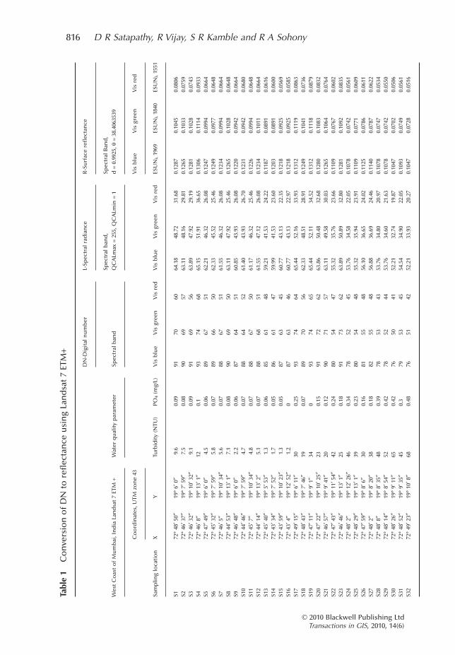
The conversion of DN values to radiance has been carried out using the followingequation (1) using different characteristics of the imagery (see Table 1).

LL L

Q QDN Q LMax Min

Cal CalCal Minλ = −

−⎛⎝⎜

⎞⎠⎟

× −( ) +max min

min (1)

Remote Sensing of Turbidity and Phosphate in Creeks and Coast of Mumbai 815

© 2010 Blackwell Publishing LtdTransactions in GIS, 2010, 14(6)

Tabl

e1

Co

nve

rsio

no

fD

Nto

refl

ecta

nce

usi

ng

Lan

dsa

t7

ETM

+

Wes

tC

oas

to

fM

um

bai

,In

dia

Lan

dsa

t7

ETM

+W

ater

qu

alit

yp

aram

eter

DN

-Dig

ital

nu

mb

erL-

Spec

tral

rad

ian

ceR

-Su

rfac

ere

flec

tan

ce

Spec

tral

ban

d

Spec

tral

ban

d,

QC

ALm

ax=

255,

QC

ALm

in=

1

Spec

tral

Ban

d,

d=

0.99

25,q

=38

.406

3539

Sam

plin

glo

cati

on

Co

ord

inat

es,U

TMzo

ne

43

Turb

idit

y(N

TU)

PO4

(mg/

L)V

isb

lue

Vis

gree

nV

isre

dV

isb

lue

Vis

gree

nV

isre

d

Vis

blu

eV

isgr

een

Vis

red

XY

ESU

Nl

1969

ESU

Nl

1840

ESU

Nl

1551

S172

°48

′50″

19°

6′0″

9.6

0.09

9170

6064

.18

48.7

231

.68

0.12

870.

1045

0.08

06S2

72°

46′3

7″19

°7′

59″

7.5

0.08

9069

5763

.11

48.1

629

.81

0.12

650.

1033

0.07

59S3

72°

46′3

2″19

°10

′32″

9.1

0.09

9169

5663

.89

47.9

229

.19

0.12

810.

1028

0.07

43S4

72°

46′8

″19

°13

′1″

120.

193

7468

65.1

551

.91

36.6

50.

1306

0.11

140.

0933

S572

°47

′49″

19°

6′0″

4.5

0.06

8967

5162

.21

46.3

226

.08

0.12

470.

0994

0.06

64S6

72°

45′3

2″19

°7′

59″

5.8

0.07

8966

5062

.33

45.5

225

.46

0.12

490.

0977

0.06

48S7

72°

46′5

″19

°10

′34″

5.6

0.07

8867

5161

.55

46.3

226

.08

0.12

340.

0994

0.06

64S8

72°

44′5

3″19

°13

′1″

7.1

0.08

9069

5063

.11

47.9

225

.46

0.12

650.

1028

0.06

48S9

72°

46′4

8″19

°6′

0″2.

20.

0687

6451

60.8

543

.93

26.0

80.

1220

0.09

420.

0664

S10

72°

44′4

6″19

°7′

59″

4.7

0.07

8864

5261

.40

43.9

326

.70

0.12

310.

0942

0.06

80S1

172

°45

′7″

19°

10′3

4″4.

80.

0788

6750

61.1

746

.32

25.4

60.

1226

0.09

940.

0648

S12

72°

44′1

4″19

°13

′2″

5.1

0.07

8868

5161

.55

47.1

226

.08

0.12

340.

1011

0.06

64S1

372

°45

′40″

19°

5′53

″1.

30.

0685

6148

59.2

141

.53

24.2

20.

1187

0.08

910.

0616

S14

72°

43′3

4″19

°7′

52″

1.7

0.05

8661

4759

.99

41.5

323

.60

0.12

030.

0891

0.06

00S1

572

°43

′59″

19°

10′2

3″1.

30.

0587

6345

60.7

743

.13

22.3

50.

1218

0.09

250.

0569

S16

72°

43′4

″19

°12

′52″

1.2

087

6346

60.7

743

.13

22.9

70.

1218

0.09

250.

0585

S17

72°

49′1

5″19

°6′

11″

300.

2593

7464

65.4

452

.16

33.9

30.

1312

0.11

190.

0863

S18

72°

48′4

3″19

°7′

46″

190.

0789

7056

62.3

348

.51

28.9

10.

1249

0.10

410.

0736

S19

72°

47′1

1″19

°9′

1″34

093

7465

65.4

452

.11

34.5

20.

1312

0.11

180.

0879

S20

72°

47′2

2″19

°10

′25″

230.

1591

7262

63.8

650

.48

32.6

80.

1280

0.10

830.

0832

S21

72°

46′5

7″19

°9′

41″

200.

1290

7157

63.1

149

.58

30.0

30.

1265

0.10

640.

0764

S22

72°

47′4

3″19

°11

′54″

420.

2480

5447

55.3

235

.76

23.6

60.

1109

0.07

670.

0602

S23

72°

46′4

6 ″19

°13

′1″

250.

1891

7362

63.8

950

.89

32.8

00.

1281

0.10

920.

0835

S24

72°

48′2

″19

°12

′26″

460.

3478

5245

53.7

634

.58

22.0

50.

1078

0.07

420.

0561

S25

72°

48′2

9″19

°13

′1″

390.

2380

5448

55.3

235

.94

23.9

10.

1109

0.07

710.

0609

S26

72°

47′5

9″19

°8′

6″30

0.16

8155

4856

.10

36.6

524

.02

0.11

250.

0786

0.06

11S2

772

°48

′2″

19°

8′20

″38

0.18

8255

4856

.88

36.6

924

.46

0.11

400.

0787

0.06

22S2

872

°48

′8″

19°

8′35

″48

0.39

7853

4353

.76

34.8

020

.97

0.10

780.

0747

0.05

34S2

972

°48

′14″

19°

8′54

″52

0.42

7852

4453

.76

34.6

021

.63

0.10

780.

0742

0.05

50S3

072

°48

′26″

19°

9′11

″65

0.42

7650

4152

.21

32.7

419

.87

0.10

470.

0702

0.05

06S3

172

°48

′52″

19°

9′35

″45

0.3

7953

4554

.54

34.9

022

.05

0.10

930.

0749

0.05

61S3

272

°49

′23″

19°

10′8

″68

0.48

7651

4252

.21

33.9

320

.27

0.10

470.

0728

0.05

16

816 D R Satapathy, R Vijay, S R Kamble and R A Sohony

© 2010 Blackwell Publishing LtdTransactions in GIS, 2010, 14(6)

where Ll is the radiance for spectral band 1 at the sensor’s aperture (W/m2/mm/sr), DNl

is the Digital Number of each pixel in the image, LMAX and LMIN are the calibrationconstants, and QCALMAX and QCALMIN are the highest and the lowest points of the range ofrescaled radiance in DN.

(ii) Spectral Reflectance Calculation, Landsat ETM+

The reflectance for band l is computed by the following equation (Markham and Barker1986, NASA 2002):

ρ πθλ

λ

λ= × ×

×L d

ESUN

2

cos(2)

where Ll is the spectral radiance, which is the outgoing radiation energy of the bandobserved at the top of atmosphere by the satellite, d is the Earth-Sun distance inastronomical units, ESUNl is the mean solar exo-atmospheric irradiances for the band l,and Cosq is the cosine of the solar incident angle. Supposing a horizontal land surface isflat, the cosine of solar incident angle (cosq) can be calculated from the Sun Elevation cos(90-SunElevation). The Zenith angle for the image is 38.40° (obtained from the headerfile of the imagery).

(iii) DN-to-Reflectance Conversion: IKONOS Data

The pixel value in the 11-bit IKONOS DNs in different bands are transformed to spectralradiance value (W sr-1 cm-2) using different characteristic features of the sensor (seeTable 2) using equation (3) (Space Imaging Eurasia 2006):

L DN CalCoef Bandwidthλ λ λ λ= ∗( ) ∗( )104 (3)

where Ll is the radiance for spectral band 1 at the sensor’s aperture (W/m2/mm/sr), DNl

is the digital value for spectral band 1, CalCoefl is the radiometric calibration coefficient[DN/(mW/cm2-sr)], Bandwidthl is the bandwidth of spectral band 1 (nm).

The three IKONOS bands were converted to at-satellite reflectance (albedo) r

ρ πθλ

λ

λ= × ×

×L d

ESUN

2

cos(4)

where r is the at-sensor reflectance, Ll is the radiance for spectral band 1 at the sensor’saperture (W/m2/mm/sr), ESUNl is the band dependent mean solar exoatmospheric irra-diance and d is the Earth-sun distance, in astronomical units, and qs is solar zenith angleand was found to be 27.29 (Fleming 2003).

4 Correlation of in situ Water Quality Parameter with Reflectance

An attempt was made to establish the relationship between the average reflectance valuesof 5 ¥ 5 pixels with measured concentration of turbidity and phosphate in three visiblebands of satellite imagery (Ekercin 2007). The spectral signature of the waterbodyindicates that it has reflectance only in visible red and green bands but absorbance in thenear-infrared band. The regression model was calibrated by in situ samples. Differentlinear regression models are formulated for different study zones using different satellite

Remote Sensing of Turbidity and Phosphate in Creeks and Coast of Mumbai 817

© 2010 Blackwell Publishing LtdTransactions in GIS, 2010, 14(6)

Tabl

e2

Co

nve

rsio

no

fD

Nto

refl

ecta

nce

usi

ng

IKO

NO

S

Wes

tC

oas

to

fM

um

bai

,In

dia

IKO

NO

SW

ater

qu

alit

yp

aram

eter

DN

-Dig

ital

nu

mb

erL-

Spec

tral

rad

ian

ceR

-Su

rfac

ere

flec

tan

ce

Spec

tral

ban

dSp

ectr

alb

and

Spec

tral

ban

d,d

=0.

9925

,q=

27.2

959

Sam

plin

glo

cati

on

Co

ord

inat

es,U

TMzo

ne

43

Turb

idit

y(N

TU)

PO4

(mg/

L)V

isb

lue

Vis

gree

nV

isre

d

Vis

blu

eV

isgr

een

Vis

red

Vis

blu

eV

isgr

een

Vis

red

XY

Cal

ib.C

oef

f.

ESU

Nl

1930

.9ES

UN

l18

54.8

ESU

Nl

1556

.5

728

727

949

Ban

dW

idth

(nm

)

71.3

88.6

65.8

S172

°48

′50″

19°

6′0″

9.6

0.09

664

482

276

127.

9274

.78

44.1

80.

2306

0.14

030.

0988

S272

°46

′37″

19°

7′59

″7.

50.

0865

347

327

112

5.90

73.5

043

.43

0.22

690.

1379

0.09

71S3

72°

46′3

2″19

°10

′32″

9.1

0.09

659

479

293

127.

0274

.41

46.9

90.

2290

0.13

960.

1051

S472

°46

′8″

19°

13′1

″12

0.1

676

539

352

130.

1883

.67

56.3

50.

2347

0.15

700.

1260

S572

°47

′49″

19°

6′0″

4.5

0.06

629

419

217

121.

1764

.97

34.8

20.

2184

0.12

190.

0779

S672

°45

′32″

19°

7′59

″5.

80.

0764

946

124

512

5.00

71.5

139

.31

0.22

530.

1342

0.08

79S7

72°

46′5

″19

°10

′34″

5.6

0.07

638

457

255

122.

9770

.96

40.8

10.

2217

0.13

320.

0913

S872

°44

′53″

19°

13′1

″7.

10.

0865

146

226

012

5.45

71.6

941

.56

0.22

610.

1345

0.09

29S9

72°

46′4

8″19

°6′

0″2.

20.

0662

841

921

512

0.99

64.9

734

.45

0.21

810.

1219

0.07

70S1

072

°44

′46″

19°

7′59

″4.

70.

0762

942

824

412

1.17

66.4

339

.13

0.21

840.

1247

0.08

75S1

172

°45

′7″

19°

10′3

4″4.

80.

0763

144

123

712

1.62

68.4

238

.00

0.21

920.

1284

0.08

50S1

272

°44

′14″

19°

13′2

″5.

10.

0763

845

524

412

2.97

70.6

039

.13

0.22

170.

1325

0.08

75S1

372

°45

′40″

19°

5′53

″1.

30.

0662

340

719

212

0.04

63.1

630

.70

0.21

640.

1185

0.06

87S1

472

°43

′34″

19°

7′52

″1.

70.

0562

741

221

412

0.72

63.8

934

.26

0.21

760.

1199

0.07

66S1

572

°43

′59″

19°

10′2

3″1.

30.

0560

937

120

011

7.34

57.5

332

.01

0.21

150.

1080

0.07

16S1

672

°43

′4″

19°

12′5

2″1.

20

586

357

150

112.

8455

.36

23.9

60.

2034

0.10

390.

0536

818 D R Satapathy, R Vijay, S R Kamble and R A Sohony

© 2010 Blackwell Publishing LtdTransactions in GIS, 2010, 14(6)

Tabl

e2

Co

nti

nu

ed

Wes

tC

oas

to

fM

um

bai

,In

dia

IKO

NO

SW

ater

qu

alit

yp

aram

eter

DN

-Dig

ital

nu

mb

erL-

Spec

tral

rad

ian

ceR

-Su

rfac

ere

flec

tan

ce

Spec

tral

ban

dSp

ectr

alb

and

Spec

tral

ban

d,d

=0.

9925

,q=

27.2

959

Sam

plin

glo

cati

on

Co

ord

inat

es,U

TMzo

ne

43

Turb

idit

y(N

TU)

PO4

(mg/

L)V

isb

lue

Vis

gree

nV

isre

d

Vis

blu

eV

isgr

een

Vis

red

Vis

blu

eV

isgr

een

Vis

red

XY

Cal

ib.C

oef

f.

ESU

Nl

1930

.9ES

UN

l18

54.8

ESU

Nl

1556

.5

728

727

949

Ban

dW

idth

(nm

)

71.3

88.6

65.8

S17

72°

49′1

5″19

°6′

11″

300.

2564

748

634

812

4.55

75.5

055

.79

0.22

450.

1417

0.12

48S1

872

°48

′43″

19°

7′46

″19

0.07

635

451

270

122.

2970

.06

43.2

50.

2204

0.13

150.

0967

S19

72°

47′1

1″19

°9′

1″34

064

949

237

112

5.00

76.4

159

.35

0.22

530.

1434

0.13

27S2

072

°47

′22″

19°

10′2

5″23

0.15

639

475

333

123.

2073

.70

53.3

60.

2221

0.13

830.

1193

S21

72°

46′5

7″19

°9′

41″

200.

1263

746

430

212

2.74

72.0

548

.30

0.22

130.

1352

0.10

80S2

272

°47

′43″

19°

11′5

4″42

0.24

617

437

334

118.

9267

.88

53.5

40.

2144

0.12

740.

1197

S23

72°

46′4

6″19

°13

′1″

250.

1864

648

033

912

4.38

74.5

954

.29

0.22

420.

1400

0.12

14S2

472

°48

′2″

19°

12′2

6″46

0.34

611

413

305

117.

7964

.07

48.8

60.

2123

0.12

020.

1093

S25

72°

48′2

9″19

°13

′1″

390.

2362

546

536

412

0.49

72.2

358

.22

0.21

720.

1356

0.13

02S2

672

°47

′59″

19°

8′6″

300.

1666

350

939

012

7.70

78.9

562

.53

0.23

020.

1482

0.13

98S2

772

°48

′2″

19°

8′20

″38

0.18

631

484

336

121.

6275

.14

53.7

30.

2192

0.14

100.

1202

S28

72°

48′8

″19

°8′

35″

480.

3960

741

230

411

6.89

63.8

948

.68

0.21

070.

1199

0.10

88S2

972

°48

′14″

19°

8′54

″52

0.42

587

401

257

113.

0662

.25

41.1

90.

2038

0.11

680.

0921

S30

72°

48′2

6″19

°9′

11″

650.

4257

939

926

111

1.48

61.8

941

.75

0.20

100.

1161

0.09

34S3

172

°48

′52″

19°

9′35

″45

0.3

614

434

312

118.

2467

.33

49.9

90.

2131

0.12

640.

1118

S32

72°

49′2

3″19

°10

′8″

680.

4853

933

827

810

3.83

52.4

544

.56

0.18

720.

0984

0.09

96

Remote Sensing of Turbidity and Phosphate in Creeks and Coast of Mumbai 819

© 2010 Blackwell Publishing LtdTransactions in GIS, 2010, 14(6)

imagery for turbidity and phosphate. Spatial variation of water quality parameters areplotted as contours using the spline interpolation method on the GIS platform based onin-situ values of turbidity and phosphate.

5 Retrieval of Water Quality Parameters using Remote Data

The linear least squares fitting technique is the simplest and most commonly applied formof linear regression and provides a solution to the problem of finding the best fittingstraight line through a set of points. Regression equations were developed for twodifferent datasets (Bilge et al. 2003). A mathematical procedure was utilized for findingthe best-fitting curve to a given set of points by minimizing the sum of the squares of theoffsets (the residuals) of the points from the curve. The sum of the squares of the offsetsis used instead of the offset absolute values because this allows the residuals to be treatedas a continuous differentiable quantity (Farebrother 1999). The correlation coefficientand the standard error are calculated as in linear regression. Based on the least squaremethod, constants are derived using Solver in MS Excel to be best fitted to N data points.Finally, equations are formulated as illustrated below in order to estimate the selectedwater quality parameter.

Y A A X A A X= + ∗ + ∗ + ∗0 1 1 2 2 3 3χ (5)

Equations derived for Y, Turbidity (NTU)/ Phosphate (mg/L) through regression analysis,for x, the pixel reflectance in the vis blue, green and red bands using satellite imagery andA0, A1, A2 and A3 are derived constants. The turbidity and phosphate water qualityparameters are estimated at numerous locations other than the in situ sampling locationsfrom reflectance of satellite imagery falling under three different study zones using theequations derived based on the least square method (see Table 3). These simulated valuesare plotted as contours and compared with the in-situ contours.

6 Results

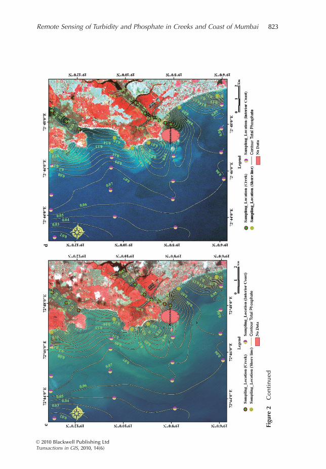
The turbidity and phosphate in creek water and seashore are high as compared to coastalwater based on in situ measurements, due to wastewater discharges emanating from theanthropogenic activities of a densely populated city like Mumbai as visualized fromsatellite imagery. Spatial variability of in situ water quality parameters is depicted fromthe contours superimposed upon the satellite imagery (see Figures 2a–d).

Before finding any relationship between one of the water quality parameters andreflectance in the satellite imagery, an attempt was made to establish a relationship ofreflectance among various bands. It was found that there is a strong relationship betweenvis-blue and green bands of either set of imagery, which is conducive for the study ofwater quality in both the bands (see Table 4).

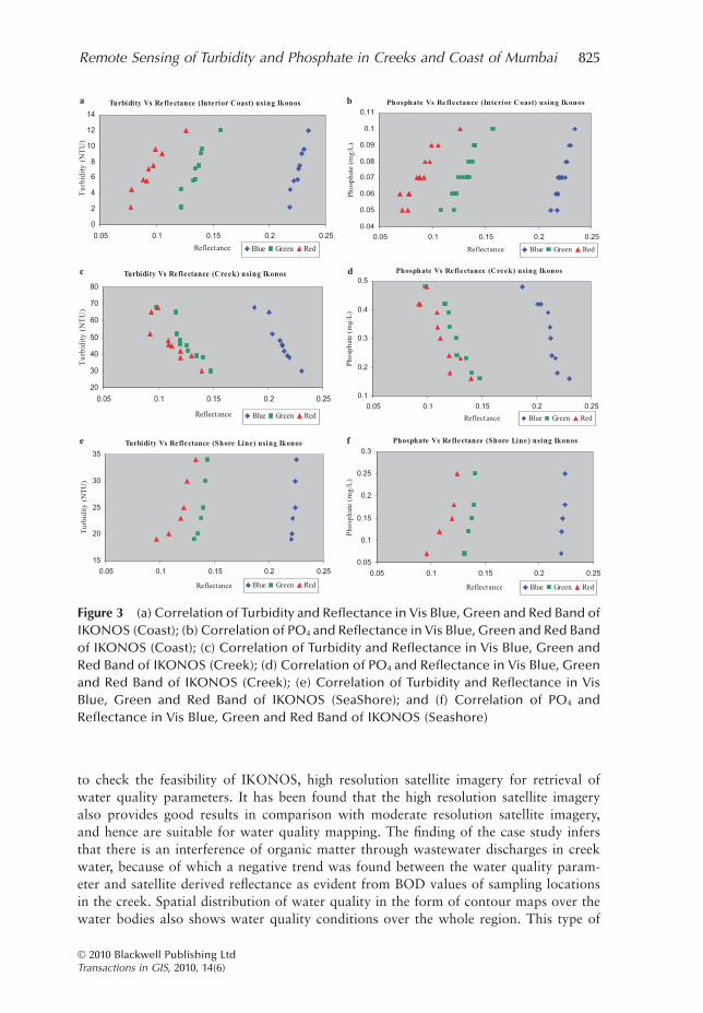
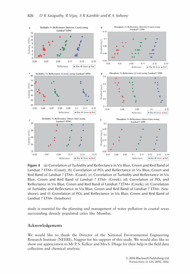
Goward et al. (2003) found radiometric differences between the two sensors butwhen the Ikonos sensor is aggregated to 30 m spatial resolution, the difference isminimized. However, correlations of turbidity and phosphate with reflectance wereexplored in different visible bands, namely vis-blue, green and red of IKONOS (seeFigures 3a–f) and Landsat 7 ETM+ (see Figures 4a–f) in order to formulate equations toderive water quality parameters.

820 D R Satapathy, R Vijay, S R Kamble and R A Sohony

© 2010 Blackwell Publishing LtdTransactions in GIS, 2010, 14(6)

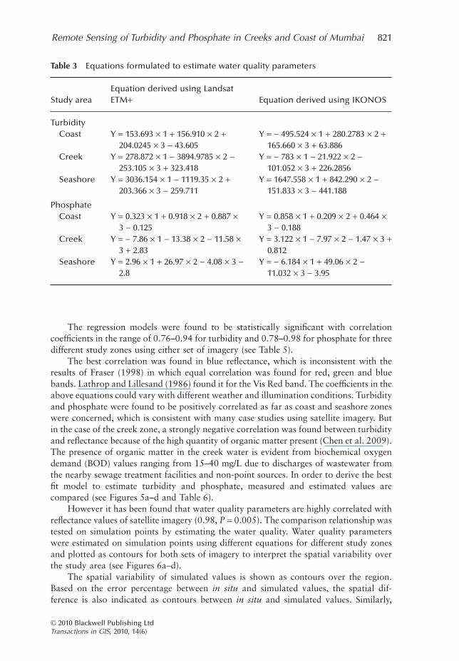
The regression models were found to be statistically significant with correlationcoefficients in the range of 0.76–0.94 for turbidity and 0.78–0.98 for phosphate for threedifferent study zones using either set of imagery (see Table 5).

The best correlation was found in blue reflectance, which is inconsistent with theresults of Fraser (1998) in which equal correlation was found for red, green and bluebands. Lathrop and Lillesand (1986) found it for the Vis Red band. The coefficients in theabove equations could vary with different weather and illumination conditions. Turbidityand phosphate were found to be positively correlated as far as coast and seashore zoneswere concerned, which is consistent with many case studies using satellite imagery. Butin the case of the creek zone, a strongly negative correlation was found between turbidityand reflectance because of the high quantity of organic matter present (Chen et al. 2009).The presence of organic matter in the creek water is evident from biochemical oxygendemand (BOD) values ranging from 15–40 mg/L due to discharges of wastewater fromthe nearby sewage treatment facilities and non-point sources. In order to derive the bestfit model to estimate turbidity and phosphate, measured and estimated values arecompared (see Figures 5a–d and Table 6).

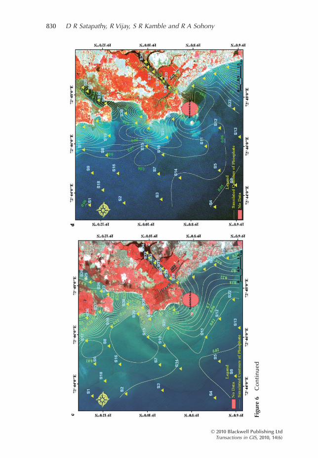
However it has been found that water quality parameters are highly correlated withreflectance values of satellite imagery (0.98, P = 0.005). The comparison relationship wastested on simulation points by estimating the water quality. Water quality parameterswere estimated on simulation points using different equations for different study zonesand plotted as contours for both sets of imagery to interpret the spatial variability overthe study area (see Figures 6a–d).

The spatial variability of simulated values is shown as contours over the region.Based on the error percentage between in situ and simulated values, the spatial dif-ference is also indicated as contours between in situ and simulated values. Similarly,

Table 3 Equations formulated to estimate water quality parameters

Study areaEquation derived using LandsatETM+ Equation derived using IKONOS

TurbidityCoast Y = 153.693 ¥ 1 + 156.910 ¥ 2 +

204.0245 ¥ 3 - 43.605Y = - 495.524 ¥ 1 + 280.2783 ¥ 2 +

165.660 ¥ 3 + 63.886Creek Y = 278.872 ¥ 1 - 3894.9785 ¥ 2 -

253.105 ¥ 3 + 323.418Y = - 783 ¥ 1 - 21.922 ¥ 2 -

101.052 ¥ 3 + 226.2856Seashore Y = 3036.154 ¥ 1 - 1119.35 ¥ 2 +

203.366 ¥ 3 - 259.711Y = 1647.558 ¥ 1 + 842.290 ¥ 2 -

151.833 ¥ 3 - 441.188

PhosphateCoast Y = 0.323 ¥ 1 + 0.918 ¥ 2 + 0.887 ¥

3 - 0.125Y = 0.858 ¥ 1 + 0.209 ¥ 2 + 0.464 ¥

3 - 0.188Creek Y = - 7.86 ¥ 1 - 13.38 ¥ 2 - 11.58 ¥

3 + 2.83Y = 3.122 ¥ 1 - 7.97 ¥ 2 - 1.47 ¥ 3 +

0.812Seashore Y = 2.96 ¥ 1 + 26.97 ¥ 2 - 4.08 ¥ 3 -

2.8Y = - 6.184 ¥ 1 + 49.06 ¥ 2 -

11.032 ¥ 3 - 3.95

Remote Sensing of Turbidity and Phosphate in Creeks and Coast of Mumbai 821

© 2010 Blackwell Publishing LtdTransactions in GIS, 2010, 14(6)

Figu

re2

(a)C

on

tou

rso

ftu

rbid

ity

(in

situ

)su

per

imp

ose

do

ver

Iko

no

sim

ager

y;(b

)Co

nto

urs

oft

urb

idit

y(i

nsi

tu)s

up

erim

po

sed

ove

rLa

nd

sat

7ET

M+

imag

ery;

(c)

Co

nto

urs

of

ph

osp

hat

e(i

nsi

tu)

sup

erim

po

sed

ove

rIK

ON

OS

imag

ery;

and

(d)

Co

nto

urs

of

ph

osp

hat

e(i

nsi

tu)

sup

erim

po

sed

ove

rLa

nd

sat

ETM

+im

ager

y

822 D R Satapathy, R Vijay, S R Kamble and R A Sohony

© 2010 Blackwell Publishing LtdTransactions in GIS, 2010, 14(6)

Figu

re2

Co

nti

nu

ed

Remote Sensing of Turbidity and Phosphate in Creeks and Coast of Mumbai 823

© 2010 Blackwell Publishing LtdTransactions in GIS, 2010, 14(6)

the difference in spatial extent of the simulated values between Landsat ETM+ andIKONOS vary due to reflectance estimated based on the empirical relationship.

It is also important to evaluate the effect of pixel size on water quality assessment.There are many possible sources of errors for estimation of the water quality param-eters as far as this study is concerned. The spatial resolution of the LandsatETM+ data may result in an overestimation of water quality parameters comparedwith IKONOS. Even though the 30 m resolution is low in comparison to theIKONOS, 1 m with a coverage of 30 ¥ 30 m represents the same value. In reality,however, within the small coverage of 1 ¥ 1 m the water quality parameter is nothomogeneous. Another source of error is geometric error carried with the satelliteimagery. Hence, care has been taken while performing geometric correction of theimagery to study the sampling locations coherently, with the help of DGPS. Selectionof sampling sites may have been insufficient, resulting in a high spatial variability ofthe water quality parameter. This presents another source of error in estimating waterquality using satellite data. Sources of error in measuring water quality using remotesensing data will be there for 1 m2 (IKONOS sensor) as well as more for 900 m2

(Landsat ETM+). Bearing in mind that the studied parameters, turbidity and phos-phate, dilute over a large spatial extent of sea region, a 5 ¥ 5 pixel array is consideredfor the study.

7 Conclusions

In the present study, an attempt has been made to establish the relationship betweenwater quality parameters, such as turbidity and phosphate, with high and moderateresolution satellite imageries such as IKONOS and Landsat 7 ETM+ in a specific studyarea on the west coast of Mumbai, India. The applicability of satellite imagery to thiskind of study show strong evidence of turbidity and phosphate, as discussed above.Multiple regression results give significantly consistent information with very highdetermination coefficients for both of the water quality parameters. In the creek zone,strong negative correlation was found reflecting high turbidity and low reflectance dueto the presence of a large quantity of organic matter. Another aspect of the study was

Table 4 Correlation matrix of reflectance between differ-ent bands of Landsat ETM+ and IKONOS imageries

Blue Green Red

Landsat ETM+Blue 1Green 0.966 1Red 0.723 0.772 1

IKONOSBlue 1Green 0.795 1Red 0.126 0.465 1

824 D R Satapathy, R Vijay, S R Kamble and R A Sohony

© 2010 Blackwell Publishing LtdTransactions in GIS, 2010, 14(6)

to check the feasibility of IKONOS, high resolution satellite imagery for retrieval ofwater quality parameters. It has been found that the high resolution satellite imageryalso provides good results in comparison with moderate resolution satellite imagery,and hence are suitable for water quality mapping. The finding of the case study infersthat there is an interference of organic matter through wastewater discharges in creekwater, because of which a negative trend was found between the water quality param-eter and satellite derived reflectance as evident from BOD values of sampling locationsin the creek. Spatial distribution of water quality in the form of contour maps over thewater bodies also shows water quality conditions over the whole region. This type of

Turbidity Vs Reflectance (Interior Coast) using Ikonos

0

2

4

6

8

10

12

14

0.05 0.1 0.15 0.2 0.25

Reflectance

Tu

rbid

ity (

NT

U)

Blue Green Red

Turbidity Vs Reflectance (Creek) using Ikonos

20

30

40

50

60

70

80

0.05 0.1 0.15 0.2 0.25

Reflectance

Tur

bid

ity (

NT

U)

Blue Green Red

Turbidity Vs Reflectance (Shore Line) using Ikonos

15

20

25

30

35

0.05 0.1 0.15 0.2 0.25

Reflectance

Tu

rbid

ity

(NT

U)

Blue Green Red

Phosphate Vs Reflectance (Interior Coast) using Ikonos

0.04

0.05

0.06

0.07

0.08

0.09

0.1

0.11

0.05 0.1 0.15 0.2 0.25

Reflectance

Pho

sph

ate

(mg

/L)

Blue Green Red

Phosphate Vs Reflectance (Shore Line) using Ikonos

0.05

0.1

0.15

0.2

0.25

0.3

0.05 0.1 0.15 0.2 0.25

Reflectance

Pho

spha

te (

mg/

L)

Blue Green Red

Phosphate Vs Reflectance (Creek) using Ikonos

0.1

0.2

0.3

0.4

0.5

0.05 0.1 0.15 0.2 0.25

Reflectance

Pho

spha

te (

mg

/L)

Blue Green Red

a b

c d

e f

Figure 3 (a) Correlation of Turbidity and Reflectance in Vis Blue, Green and Red Band ofIKONOS (Coast); (b) Correlation of PO4 and Reflectance in Vis Blue, Green and Red Bandof IKONOS (Coast); (c) Correlation of Turbidity and Reflectance in Vis Blue, Green andRed Band of IKONOS (Creek); (d) Correlation of PO4 and Reflectance in Vis Blue, Greenand Red Band of IKONOS (Creek); (e) Correlation of Turbidity and Reflectance in VisBlue, Green and Red Band of IKONOS (SeaShore); and (f) Correlation of PO4 andReflectance in Vis Blue, Green and Red Band of IKONOS (Seashore)

Remote Sensing of Turbidity and Phosphate in Creeks and Coast of Mumbai 825

© 2010 Blackwell Publishing LtdTransactions in GIS, 2010, 14(6)

study is essential for the planning and management of water pollution in coastal areassurrounding densely populated cities like Mumbai.

Acknowledgements

We would like to thank the Director of the National Environmental EngineeringResearch Institute (NEERI), Nagpur for his support of this study. We would also like toshow our appreciation to Mr P. S. Kelkar and Mrs S. Dhage for their help in the field datacollection and chemical analysis.

Turbidity Vs Reflectance (Interior Coast) using Landsat7 ETM+

0

2

4

6

8

10

12

14

0.05 0.07 0.09 0.11 0.13 0.15

Reflectance

Tur

bidi

ty (

NT

U)

Blue Green Red

Turbidity Vs Reflectance (Creek) using Landsat7 ETM+

20

30

40

50

60

70

80

0.05 0.06 0.07 0.08 0.09 0.1 0.11 0.12

Reflectance

Tur

bidi

ty (

NT

U)

Blue Green Red

Turbidity Vs Reflectance (Shore line) usingLandsat7 ETM+

15

20

25

30

35

0.05 0.07 0.09 0.11 0.13 0.15

Reflectance

Tu

rbid

ity (

NT

U)

Blue Green Red

Phosphate Vs Reflectance (Interior Coast) using Landsat7+ ETM

0.04

0.06

0.08

0.1

0.12

0.05 0.07 0.09 0.11 0.13 0.15

Reflectance

Pho

spha

te (

mg/

L)

Blue Green Red

Phosphate Vs Reflectance (Shore Line) usingLandsat7+ ETM

0.05

0.1

0.15

0.2

0.25

0.3

0.07 0.08 0.09 0.1 0.11 0.12 0.13 0.14

Reflectance

Phos

phat

e (m

g/L

)

Blue Green Red

Phosphate Vs Reflectance (Creek) using Landsat7+ ETM

0.1

0.2

0.3

0.4

0.5

0.04 0.06 0.08 0.1 0.12

Reflectance

Phos

phat

e (m

g/L

)

Blue Green Red

a b

c d

e f

Figure 4 (a) Correlation of Turbidity and Reflectance in Vis Blue, Green and Red Band ofLandsat 7 ETM+ (Coast); (b) Correlation of PO4 and Reflectance in Vis Blue, Green andRed Band of Landsat 7 ETM+ (Coast); (c) Correlation of Turbidity and Reflectance in VisBlue, Green and Red Band of Landsat 7 ETM+ (Creek); (d) Correlation of PO4 andReflectance in Vis Blue, Green and Red Band of Landsat 7 ETM+ (Creek); (e) Correlationof Turbidity and Reflectance in Vis Blue, Green and Red Band of Landsat 7 ETM+ (Sea-shore); and (f) Correlation of PO4 and Reflectance in Vis Blue, Green and Red Band ofLandsat 7 ETM+ (Seashore)

826 D R Satapathy, R Vijay, S R Kamble and R A Sohony

© 2010 Blackwell Publishing LtdTransactions in GIS, 2010, 14(6)

Measured Vs. Estimated (Landsat ETM+)

y = 0.9719x + 0.1376R2 = 0.9812

0

10

20

30

40

50

60

70

0 20 40 60 80

Measured Turbidity (NTU)

Est

imat

ed T

urb

idity

(N

TU

)

Measured Vs Estimated (IKO NO S)

y = 0.9886x - 0.1869R2 = 0.9894

0

10

20

30

40

50

60

70

80

0 20 40 60 80Measured Turbidity (NTU)

Est

imat

ed T

urbid

ity

(NT

U)

Measured Vs. Estimated using Landsat ETM+

y = 0.9613x + 0.004R2 = 0.9742

0

0.1

0.2

0.3

0.4

0.5

0.6

0 0.1 0.2 0.3 0.4 0.5 0.6Measured Phosphate (mg/L)

Est

imat

ed P

hosp

hate

(m

g/L

)

Measured Vs. Estimated using IKO NO S

y = 0.9458x + 0.0063R2 = 0.9839

0

0.1

0.2

0.3

0.4

0.5

0 0.1 0.2 0.3 0.4 0.5 0.6Measured Phosphate (mg/L)

Est

imat

ed P

hosp

hate

mg/

L)

a b

c d

Figure 5 (a) Correlation of Measured and Estimated Turbidity using Landsat 7 ETM+; (b)Correlation of Measured and Estimated Turbidity using IKONOS; (c) Correlation ofMeasured and Estimated Phosphate using Landsat 7 ETM+; and (d) Correlation of Mea-sured and Estimated Phosphate using IKONOS

Table 5 Correlation of in situ data and satellite derived reflectance through regressionanalysis

Category ofwaterbody

No. ofobservation Satellite/sensor

Spectralband

Turbidity Phosphate

Multiple R R Square Multiple R R Square

Coast 16 Landsat ETM+ B 0.956 0.913 0.904 0.817G 0.943 0.890 0.897 0.804R 0.901 0.812 0.886 0.785

Creek 10 Landsat ETM+ B 0.925 0.855 0.950 0.903G 0.913 0.833 0.895 0.801R 0.906 0.821 0.947 0.897

Seashore 6 Landsat ETM+ B 0.958 0.918 0.987 0.975G 0.939 0.882 0.994 0.988R 0.915 0.838 0.935 0.874

Coast 16 IKONOS B 0.970 0.940 0.947 0.896G 0.945 0.893 0.940 0.883R 0.943 0.890 0.937 0.878

Creek 10 IKONOS B 0.964 0.930 0.917 0.840G 0.926 0.857 0.954 0.910R 0.870 0.757 0.904 0.817

Sea Shore 6 IKONOS B 0.940 0.884 0.939 0.881G 0.928 0.861 0.959 0.920R 0.912 0.831 0.919 0.845

Min = 0.757Max = 0.94

Min = 0.78Max = 0.98

Remote Sensing of Turbidity and Phosphate in Creeks and Coast of Mumbai 827

© 2010 Blackwell Publishing LtdTransactions in GIS, 2010, 14(6)

Tabl

e6

Stan

dar

der

ror

of

the

esti

mat

e

Sam

plin

g

loca

tio

n

Turb

idit

yPh

osp

hat

e

Insi

tum

easu

rem

ent

(NTU

)

Lan

dsa

tET

M+

IKO

NO

S

Insi

tum

easu

rem

ent

(mg/

L)

Lan

dsa

tET

M+

IKO

NO

S

Esti

mat

ed%

of

Erro

rEs

tim

ated

%o

fEr

ror

Esti

mat

ed%

Erro

rEs

tim

ated

%Er

ror

S19.

69.

015

6.09

15.

316

44.6

240.

090.

088

2.09

20.

085

5.92

6S2

7.5

7.52

8-0

.379

6.18

117

.586

0.08

0.08

2-2

.572

0.08

0-0

.321

S39.

17.

364

19.0

726.

970

23.4

050.

090.

081

10.3

490.

086

4.39

6S4

1212

.971

-8.0

9312

.490

-4.0

810.

10.

106

-6.4

720.

104

-4.2

62S5

4.5

4.69

6-4

.360

2.72

939

.357

0.06

0.06

9-1

5.51

20.

061

-1.1

02S6

5.8

4.14

128

.598

4.41

023

.967

0.07

0.06

65.

194

0.07

4-5

.439

S75.

64.

493

19.7

676.

489

-15.

874

0.07

0.06

91.

620

0.07

2-2

.875

S87.

15.

188

26.9

314.

935

30.4

890.

080.

072

10.3

210.

077

3.86

8S9

2.2

3.47

2-5

7.82

32.

749

-24.

957

0.06

0.06

4-5

.904

0.06

00.

004

S10

4.7

3.96

215

.699

5.08

8-8

.249

0.07

0.06

56.

701

0.06

66.

146

S11

4.8

4.05

415

.547

5.31

9-1

0.81

80.

070.

067

3.98

60.

066

5.69

7S1

25.

14.

762

6.62

95.

674

-11.

252

0.07

0.07

0-0

.694

0.07

0-0

.175

S13

1.3

1.19

28.

338

1.25

43.

504

0.06

0.05

311

.041

0.05

410

.108

S14

1.7

1.10

934

.779

2.35

0-3

8.26

30.

050.

052

-4.9

860.

059

-17.

910

S15

1.3

1.24

14.

546

1.19

58.

091

0.05

0.05

3-6

.891

0.04

92.

186

S16

1.2

1.56

4-3

0.30

61.

091

9.11

5S1

730

30.9

25-3

.084

29.1

182.

942

0.25

0.24

71.

394

0.23

65.

616

S18

1918

.135

4.55

218

.062

4.93

80.

070.

069

1.50

80.

069

0.98

7S1

934

31.3

507.

795

30.6

629.

817

S20

2324

.688

-7.3

3923

.061

-0.2

630.

150.

153

-2.0

830.

145

3.25

6S2

120

20.8

86-4

.428

20.8

39-4

.194

0.12

0.12

4-3

.190

0.12

3-2

.823

S22

4240

.346

3.93

943

.492

-3.5

520.

240.

235

2.19

60.

290

-20.

905

S23

2523

.910

4.36

227

.688

-10.

750

0.18

0.17

62.

468

0.19

1-6

.253

S24

4650

.333

-9.4

2046

.296

-0.6

440.

340.

340

-0.1

140.

356

-4.7

70S2

539

38.6

570.

880

40.0

29-2

.639

0.23

0.22

23.

455

0.21

94.

991

S26

3033

.117

-10.

390

28.6

044.

653

0.16

0.18

6-1

6.49

70.

145

9.68

6S2

738

32.8

7813

.479

39.3

35-3

.513

0.18

0.16

011

.211

0.19

6-8

.997

S28

4849

.204

-2.5

0847

.618

0.79

60.

390.

366

6.14

70.

354

9.10

9S2

952

50.4

742.

935

54.7

83-5

.353

0.42

0.35

216

.111

0.38

29.

056

S30

6566

.232

-1.8

9556

.897

12.4

660.

420.

482

-14.

779

0.37

710

.316

S31

4548

.119

-6.9

3245

.272

-0.6

050.

30.

319

-6.3

270.

306

-2.0

67S3

268

56.0

2117

.617

67.4

630.

790

0.48

0.43

69.

187

0.46

53.

022

SD=

17.2

16SD

=17

.01

SD=

8.08

SD=

7.54

828 D R Satapathy, R Vijay, S R Kamble and R A Sohony

© 2010 Blackwell Publishing LtdTransactions in GIS, 2010, 14(6)

Figu

re6

(a)

Co

nto

urs

of

Turb

idit

y(s

imu

late

d)

sup

erim

po

sed

ove

rIk

on

os

imag

ery;

(b)

Co

nto

urs

of

Turb

idit

y(s

imu

late

d)

sup

erim

po

sed

ove

rLa

nd

sat

7ET

M+

imag

ery;

(c)

Co

nto

urs

of

Pho

sph

ate

(sim

ula

ted

)su

per

imp

ose

do

ver

Iko

no

sim

ager

y;an

d(d

)C

on

tou

rso

fPh

osp

hat

e(s

imu

late

d)

sup

erim

po

sed

ove

rLa

nd

sat

7ET

M+

imag

ery

Remote Sensing of Turbidity and Phosphate in Creeks and Coast of Mumbai 829

© 2010 Blackwell Publishing LtdTransactions in GIS, 2010, 14(6)

Figu

re6

Co

nti

nu

ed

830 D R Satapathy, R Vijay, S R Kamble and R A Sohony

© 2010 Blackwell Publishing LtdTransactions in GIS, 2010, 14(6)

References

Allee R J and Johnson J E 1999 Use of satellite imagery to estimate surface chlorophyll a and Secchidisc depth of Bull Shoals Reservoir, Arkansas, USA. International Journal of Remote Sensing20: 1057–72

APHA 2002 Standard Methods for the Examination of Water and Wastewater. Washington, DC,American Public Health Association, American Water Works Association, and Water Envi-ronment Federation

Bilge F, Yazici B, Dogeroglu T, and Ayday C 2003 Statistical evaluation of remotely sensed data forwater quality monitoring. International Journal of Remote Sensing 24: 5317–26

Chen A S, Fang C L, Zhang B L, and Huange W 2009 Remote sensing of turbidity in seawaterintrusion reaches of Pearl River Estuary: A case study in Modaomen water way, China.Estuarine, Coastal and Shelf Science 82: 119–27

Ekercin S 2007 Water quality retrievals from high resolution Ikonos multispectral imagery: A casestudy in Istanbul, Turkey. International Journal of Environmental Pollution 183: 239–51

Farebrother R W 1999 Fitting Linear Relationships: A History of the Calculus of Observations.New York, Springer-Verlag

Fleming D 2003 Ikonos DN value conversion to planetary reflectance. WWW document, http://www.geog.umd.edu/cress/papers/guide_dn2pr.pdf

Forster B C, Xingwei I S, and Baide X 1993 Remote sensing of water quality parameters usingLandsat TM. International Journal of Remote Sensing 14: 2759–71

Fraser R N 1998 Multispectral remote sensing of turbidity among Nebraska Sand Hill lakes.International Journal of Remote Sensing 23: 15–35

Goward S N, Davis P E, Fleming D, Miller L, and Townshend J R 2003 Empirical comparison ofLandsat 7 and IKONOS multispectral measurements for selected Earth Observation System(EOS) validation sites. Remote Sensing of Environment 88: 80–99

Jensen J R 2000 Remote Sensing of the Environment. Englewood Cliffs, NJ, Prentice-HallKondratyev K Y, Pozdnyakov D V, and Pettersson L H 1998 Water quality remote sensing in the

visible spectrum. International Journal of Remote Sensing 19: 957–79Lathrop R G Jr and Lillesand T M 1986 Use of Thematic Mapper data to assess water quality in

Green Bay and central Lake Michigan. Photogrammetric Engineering and Remote Sensing 52:671–80

Lathrop R G and Lillesand T M 1989 Monitoring water quality and river plume transport in GreenBay, Lake Michigan, with SPOT-1 imagery. Photogrammetric Engineering and RemoteSensing 55: 349–54

Li R and Li J 2004 Satellite remote sensing technology for lake water clarity monitoring: Anoverview. Environmental Informatics Archives 2: 893–901

Markham B and Barker J 1986 Landsat MSS and TM Post-Calibration Dynamic Ranges, Exoat-mospheric Reflectances and At-Satellite Temperatures. Lanham, MD, EOSAT Landsat Tech-nical Note

NASA 2002 Landsat 7 science user data handbook. Chap.11 2002 WWW document, http://landsathandbook.gsfc.nasa.gov/handbook/handbook_htmls/chapter11/chapter11.html

Parada M and Canton M 1998 Sea surface temperature variability in Alboran Sea from satellitedata. International Journal of Remote Sensing 19: 2439–50

Pattiaratchi C B, Hammond T M, and Collins M B 1986 Mapping of tidal currents in the vicinityof an offshore sandbank, using remotely sensed imagery. International Journal of RemoteSensing 7: 1015–29

Pattiaratchi C B, Lavery P, Wyllie A, and Hick P 1994 Estimates of water-quality in coastal watersusing multi-date Landsat Thematic Mapper data. International Journal of Remote Sensing 15:1571–84

Rimmer J C, Collins M B, and Pattiaratchi C B 1987 Mapping of water-quality in coastal watersusing Airborne Thematic Mapper data. International Journal of Remote Sensing 8: 85–100

Ritchie C J, Cooper C M, and Schiebe F R 1990 The relationship of MSS and TM digital data withsuspended sediment, chlorophyll and temperature in Moon Lake, Mississippi. Remote Sensingof Environment 33: 137–48

Remote Sensing of Turbidity and Phosphate in Creeks and Coast of Mumbai 831

© 2010 Blackwell Publishing LtdTransactions in GIS, 2010, 14(6)

Shafique N A, Autrey B C, Fulk F, and Cormier S M 2001 Hyperspectral narrow wavebandsselection for optimizing water quality monitoring on the Great Miami River, Ohio. Journal ofSpatial Hydrology 1: 1–22

Space Imaging Eurasia 2006 IKONOS relative spectral response and radiometric CalCoefficients.WWW documents, http://www.spaceimaging.com/products/ikonos/spectral.htm

Tassan S 1998 A procedure to determine the particulate content of shallow water from ThematicMapper data. International Journal of Remote Sensing 19: 557–62

Thiemann S and Kaufmann H 2000 Determination of chlorophyll content and trophic state of lakesusing field spectrometer IRS-1C satellite data in the Mecklenburg Lake District, Germany.Remote Sensing of Environment 73: 227–35

832 D R Satapathy, R Vijay, S R Kamble and R A Sohony

© 2010 Blackwell Publishing LtdTransactions in GIS, 2010, 14(6)