Remote origins of interannual variability in the Indonesian Throughflow region from data and a...

Remote origins of interannual variability in the Indonesian

Throughflow region from data and a global Parallel Ocean Program

simulation

Julie L. McClean1 and Detelina P. Ivanova1

Department of Oceanography, Naval Postgraduate School, Monterey, California, USA

Janet SprintallScripps Institution of Oceanography, University of California, San Diego, La Jolla, California, USA

Received 10 May 2004; revised 31 May 2005; accepted 6 July 2005; published 14 October 2005.

[1] The mean and interannual variability of the thermal structure of the World OceanCirculation Experiment (WOCE) repeat IX1-expendable bathythermograph (XBT)transect between Java and Western Australia were compared statistically for the years1987–1997 with concurrent, co-located output from a global eddy-permittingconfiguration of the Parallel Ocean Program (POP) model forced with realistic surfacefluxes. Dominant variability at long timescales for both model and data in the southern IX1region was associated with Pacific El Nino–Southern Oscillation (ENSO) events; atthe northern end it was due to remote equatorial Indian Ocean forcing and Indian OceanDipole Mode events. In the Indo-Pacific domain the model reproduced the structure andmagnitude of observed low-frequency variability. Event analyses following the warmENSO phase showed low-frequency off-equatorial Rossby waves interacting with theNorth Pacific western maritime boundary to reflect onto the equator and excite a coastallytrapped response that propagated through the Indonesian seas and along the northwestcoast of Australia. In turn, the signal progressively propagated away from this coast as freebaroclinic Rossby waves to 90�E. Cross-spectral analyses confirmed that on interannualtimescales, both off-equatorial and equatorial signals remotely forced in the Pacificwere largely responsible for the strong observed and modeled variability at the southernend of IX1.

Citation: McClean, J. L., D. P. Ivanova, and J. Sprintall (2005), Remote origins of interannual variability in the Indonesian

Throughflow region from data and a global Parallel Ocean Program simulation, J. Geophys. Res., 110, C10013,

doi:10.1029/2004JC002477.

1. Introduction

[2] The Indonesian Seas form an oceanic conduit ofmomentum, heat, and freshwater between the Pacific andIndian oceans that significantly impacts the thermohalinebalance of both basins [Bryden and Imawaki, 2001; Wijffelset al., 2001]. Much effort has been expended to understandboth the magnitude and variability of these fluxes (see Lukaset al. [1996], Godfrey [1996], and Gordon [2001] forreviews). Remote forcing from both the Pacific and Indianocean basins, as well as the regional monsoon forcing,complicates the property flux estimates within the Indone-sian seas, causing variability over a range of timescales.[3] A particularly significant data set that has contributed

to our understanding of the Indonesian Throughflow (ITF)variability is the expendable bathythermograph (XBT)

measurements collected along the IX1 transect betweenJava and northwest Australia since 1983 [Meyers et al.,1995; Meyers, 1996] (the latter hereinafter referred to asM96). M96 state that this data set is representative of theITF on long timescales; hence it has provided a means ofmonitoring interannual variability of the Throughflow. Anempirical orthogonal function (EOF) analysis of this datarevealed the dominant variability to be associated with ElNino-Southern Oscillation (ENSO). Second mode variabil-ity was associated with a modulation of the annual cycleoff Java, due to reversals in the South Java Current[Quadfasel and Cresswell, 1992; Sprintall et al., 1999].Correlations between the amplitude time series of the firstjoint EOF mode and the zonal wind stress in the Pacificand Indian oceans revealed a maximum correlation in thewestern central Pacific, with secondary maximums occur-ring over the equatorial Indian and eastern Pacific oceans.Drawing on the findings of Clarke and Liu [1994], M96attributed these results to a remote Pacific signal comprisedof energy from equatorial Rossby waves passing the NewGuinea–Australia landmass and equatorial Kelvin waves

JOURNAL OF GEOPHYSICAL RESEARCH, VOL. 110, C10013, doi:10.1029/2004JC002477, 2005

1Now at Scripps Institution of Oceanography, University of California,San Diego, La Jolla, California, USA.

Copyright 2005 by the American Geophysical Union.0148-0227/05/2004JC002477

C10013 1 of 18

reflected from the Indonesia/Borneo/Asia boundary thatwas transmitted along the northwest (NW) coast of Aus-tralia, and Indian Ocean equatorial Kelvin waves propa-gating along the eastern Indian Ocean boundary.[4] In a very recent paper, Wijffels and Meyers [2004]

used lagged partial regression analyses to relate the inter-annual temperature and sea level variability in the Indonesiaseas and the southern Indian Ocean to remote winds alongthe equator of the Indian and Pacific oceans. Much of theresponse was explained by these equatorial winds thatproduced free equatorial Kelvin and Rossby waves whosesignals reached the study region. Equatorial Pacific Rossbywaves excited coastally trapped waves off the western tip ofNew Guinea that propagated poleward along the Arafura/Australian shelf break. As well, Pacific energy radiatedwestward into the southeast Indian Ocean via the BandaSea. Equatorial Indian Ocean Kelvin waves penetrated asfar as the Savu Sea, the western Banda Sea, and MakassarStrait. As in M96, their findings further substantiate those ofClarke and Liu [1994], who first identified this region asone where two oceanic waveguides intersect.[5] Long period, off-equatorial baroclinic Rossby waves

have recently been documented in the Pacific basin byWhite et al. [2003]. Biennial (2.2- and 2.8-year), interannual(3.5-, 5.4-, and 7-year), and decadal (11-year) Rossby wavespropagate westward across the Pacific basin to reach thewestern boundary at approximately 7�N, 12�N, and 18�N,respectively. The waves form in response to off-equatorialcyclonic wind stress curl anomalies, induced by westerlysurface wind anomalies produced in the wake of warm seasurface temperature (SST) anomalies that propagate slowlyeastward along the equator. On reaching the western mar-itime boundary of the Pacific, these waves excite coastally-trapped Munk-Kelvin waves, identified by Godfrey [1975]and further explained by McCreary [1983], that propagatesouthwards to reflect back onto the equator as equatorialKelvin waves [Pazan et al., 1986; White et al., 1989]. Whiteet al. [2003] report the reflected signals as slow equatorialcoupled waves, producing a delayed negative feedback tothe warm SST anomalies located in the central Pacific. Thisprocess represents a modification of the delayed actionoscillation El Nino model [Philander, 1990] such that inaddition to the equatorial Rossby waves that reflect asequatorial Kelvin waves, feedback is provided by off-equatorial biennial, interannual, and decadal Rossby waves.White et al. [2003] used the NCEP/NCAR reanalysis andthe Scripps Institution of Oceanography (SIO) upper oceantemperature reanalysis data sets to identify the Pacificwaves. In this paper we use a global ocean general circu-lation model (OGCM), whose grid spacing and realistictopography resolve the waveguide through the IndonesianSeas, to determine if these off-equatorial low-frequencysignals, once reflected back onto the equator, excite coast-ally trapped signals that propagate through the IndonesianSeas and along the northwest coast of Australia. White et al.[2003] did not consider this pathway in their analyses. M96and Wijffels and Meyers [2004] only considered the equa-torial Pacific Rossby waves that generate coastally trappedwaves with pathways through the Indonesian seas.[6] The transmission of coastally trapped signals through

the Indonesian passages has been documented using numer-ical models of varying complexity. Wajsowicz [1996]

performed a suite of sensitivity runs using a 1� � 1� OGCMcontaining simplified, idealized or realistic, complex repre-sentations of the Indonesian archipelago within the large-scale Pacific-Indian domain. She identified coastal Kelvinwaves on the west Australian coast emerging from theidealized Indonesian archipelago. These coastally trappedwaves resulted when off-equatorial Rossby waves generatedby negative wind stress curl in the North Pacific reached thewestern boundary of the Pacific and were partially scatteredinto the archipelago and partially reflected into the equatorialwaveguide. Potemra [1999], using a 1-1/2 layer reducedgravity model forced with monthly climatological winds,reported that annual winds just north of the equator in theeastern Pacific produced annual Rossby waves by Ekmanpumping. These off-equatorial waves interacted with thewestern boundary of the Pacific to form coastal Kelvinwaves that propagated through the Indonesian Seas. Schilleret al. [2000] found that both the IX1 data and output from acoarse resolution OGCM forced with interannual fluxesrevealed a shallower (deeper) thermocline associated withthe arrival of El Nino (La Nina) signals along the westAustralian coast at the southern end of the section. Theyattributed the upwelling (downwelling) to the passage ofKelvin waves originating from the tip of Irian-Jaya. Using a0.5� grid model driven by ERS satellite winds, Masumoto[2002] found two dominant modes in the model surfacedynamic height on interannual timescales, corresponding toENSO Pacific forcing and eastern Indian Ocean forcing, thatconfirm the observations of M96 and Wijffels and Meyers[2004]. However, in agreement with Yamagata et al. [1996],Masumoto [2002] suggested that variations in the modelThroughflow transport have highest correlation with thesecond mode’s Indian Ocean variability.[7] In this paper, we perform some of the same analyses

as in M96, but include more recently collected data and usethe 1987–1997 period, when sampling along the IX1-XBTtransect was increased to be near fortnightly. The variabilityat the location of the IX1 transect is analyzed using a globaleddy-permitting (1/3�, 32 vertical levels) configuration ofthe Parallel Ocean Program (POP) model forced with dailyEuropean Center for Medium Range Forecasts (ECMWF)wind stresses, heat and freshwater fluxes for 1979–1997.The decade-long time series of XBT data provides us with ameans of evaluating the ability of the model to reproduceinterannual variability in the Subtropical Indian Ocean(STIO). We then use the model to explore forcing mecha-nisms that are not possible from data alone. Particularly, weprovide support for our hypothesis that some of the coast-ally trapped wave signals that propagate through the Indo-nesian Seas and along the NW Australian shelf are excitedby equatorial Kelvin waves resulting from Kelvin-Munkwave reflection that in turn were excited by off-equatorialbaroclinic Rossby waves on reaching the western boundaryof the North Pacific Ocean. This wave process at interan-nual timescales is in addition to the equatorial Pacific signalthat radiates through the ITF and into the STIO as discussedby Clarke and Liu [1994], M96, and Wijffels and Meyers[2004]. The model will also be used to understand theimpact of remotely forced signals from the Indian andPacific Oceans on the eastern STIO. The propagation ofvariability from the eastern boundary into the Indian Oceancould substantially impact the coupled ocean-atmosphere

C10013 MCCLEAN ET AL.: TITLE IX1 AND POP VARIABILITY IN THE ITF

2 of 18

C10013

system [Morrow and Birol, 1998] and affect SST vari-ability in the STIO [Behera et al., 2000; Murtugudde etal., 2000; Xie et al., 2002]. In the study presented here,we will use a combination of statistical and eventanalyses, using both model and data, to examine the roleof remotely forced interannual variability within theSTIO. It is anticipated that coupled climate models willbe run using eddy-permitting ocean models in the nearfuture. Before this occurs however, we need to under-stand the representation of low-frequency variability instand-alone ocean models at this resolution to simulatemodes of variability such as those on interannual time-scales, in the tropics and elsewhere.[8] The paper is organized in the following manner:

details of the in situ data are provided in section 2 whilethe model is described in section 3. Results of the compar-ative analyses of the observed and modeled thermal struc-ture in the waters between Java and Australia are found insection 4, while section 5 contains a discussion of the natureof the remote signals influencing this region in the model.Conclusions are found in section 6.

2. Data

[9] A repeat XBT-line between Fremantle, Western Aus-tralia, and Sunda Strait, at the western end of Java (Figure 1),was designated IX1 in 1983 as part of the Tropical Ocean-Global Atmosphere (TOGA) XBT network, and continuedduring the World Ocean Circulation Experiment (WOCE).

The sampling frequency was increased from 6 sections peryear in 1983–1986, to >18 sections per year after 1987, with�100 km spacing between profiles. In this paper, we use thetemperature data only from 1987 through 1997, to takeadvantage of the higher sampling frequency and thus min-imize the need for interpolation due to missing data. Thedensity of the XBT sampling can be found in Figure 2 ofM96; it shows thorough coverage for 1987–1994 between7.5�S and 24�S.[10] To study the Throughflow variability, the 288 avail-

able IX1 temperature sections between 1987–1997 wereinterpolated in time and space. The XBT profile data werefirst averaged into 10-m vertical bins between 5 and 750 mdepth. Monthly means were then calculated. Next, averageswere constructed for overlapping bi-months, i.e., January–February, February–March, etc. These fields were thenaveraged into 1�-latitude bins along the IX1-XBT trackbetween 8�S and 24�S. Finally, optimal interpolation wasused to fill in missing values. Dynamic height relative to400 db was calculated from the temperature observationsand a temperature-salinity relationship derived from the rawobserver data compiled by Levitus et al. [1994a, 1994b]supplemented by more recent WOCE hydrographic data inthe region [Sprintall et al., 2002].

3. Global Ocean Model

[11] The ocean model used in this study is the LosAlamos National Laboratory (LANL) Parallel Ocean Pro-

Figure 1. Bathymetry of the Indonesian Seas, the western tropical Pacific, and the southeastern IndianOcean from Smith and Sandwell [1997] topography interpolated onto the 1/3�, 32-level global POP grid.The thick black line between Java and Australia identifies the repeat XBT line known as WOCE IX1. The1000-m isobath is contoured in black.


3 of 18

C10013

gram (POP) [Dukowicz and Smith, 1994]. It is a three-dimensional, z-level primitive equation ocean generalcirculation model. The domain is fully global and isconfigured on a displaced pole grid whereby the North Poleis rotated into Hudson Bay to avoid a polar singularity. Thegrid is eddy-permitting: it has an average resolution of 1/3�latitude and longitude with increased latitudinal resolutionnear the equator of about 1/4�, and 32 levels. It wasconfigured to have exactly double the horizontal resolutionof the 2/3� global POP used in the Parallel Climate Model(PCM) [Washington et al., 2000], a global coupled air/ocean/ice/land system used for centennial climate simula-tions. It is anticipated that the 1/3� POP or some verysimilarly configured eddy-permitting global POP model willbe used in the next-generation higher resolution coupledclimate system. A blended global bathymetry was created

from the work of Smith and Sandwell [1997], with ETOPO5used in the Antarctic and Arctic. All important sills andchannels were checked and modified to encourage correctflow. Figure 1 shows the model bathymetry of the region tobe discussed in this paper: the Indonesian Seas and theeastern Indian and western Pacific oceans. The modelresolves all the major straits in the Indonesian Seas suchas the Makassar, Halmahera, Lombok, Ombai, and SundaStraits, and Timor Passage. Torres Strait between Australiaand New Guinea has been restricted to mimic the very smallamount of flow that enters the Arafura Sea directly from theSouth Pacific.[12] The model was initialized from the annual Levitus et

al. [1994a, 1994b] climatology of potential temperature (q)and salinity (S), and was spun up for 30 years. During thespin-up it was forced with a daily climatology of momen-

Figure 2. Mean temperature (�C) of (a) the IX1-XBT data; (b) co-located POP model output; and(c) the difference field (�C) between the data and model for 1987–1997.


4 of 18

C10013

tum, heat, and freshwater fluxes formed from 1979–1993ECMWF daily reanalysis (ERA15) fields. River dischargewas included in the daily freshwater fluxes. Daily riverrunoff values were obtained from annual data [Perry et al.,1996] by dividing the discharge by the number of days in ayear, and then distributing over several ocean grid pointsadjacent to the location of the river mouths. To ensure aglobal balance of the resulting freshwater and heat fluxes onan annual basis, any globally integrated imbalance for aparticular year was equally distributed over that year andover the tropics (20�S to 20�N). This spatial distributionwas necessary because of cloud parameterization limitationsthat would likely significantly impact the tropical regions.Jakob [1999] identified cloud cover deficiencies in thetropics and subtropics by comparing monthly values fromthe International Satellite Cloud Climatology Project(ISCCP) with the ERA15 fields. To limit model drift, upperlevel (top 25 m) properties were restored to Levitus et al.[1994a, 1994b] monthly climatological q and S with atimescale of 6 months.[13] Biharmonic diffusion operators with spatially varying

viscosities and diffusivities are used in POP to performthe horizontal mixing of momentum and tracers. Themomentum and tracer coefficients were �0.4 � 1017 cm4/sand �0.5 � 1016 cm4/s, respectively. They were scaled by(GCA/GCAmin)

2 where GCA is either the tracer or velocitygrid cell area. This choice was made so that mixing wouldbe reduced at progressively higher latitudes. The resultingviscosities and diffusivities are consistent with those used inother eddy-permitting basin-scale numerical studies [Boningand Budich, 1992]. The model time step was 27 min.The Large et al. [1994] mixed layer K-Profile Parameteri-zation (KPP) was turned on at the end of the fifth year of thespin-up.[14] Following the 30-year spin-up, the model was forced

with the daily surfaces fluxes formed from the ECMWFreanalysis fields for 1979–1993 and from the ECMWFoperational products for 1994–1997. During the 1979–1997 run, 3-day averages of sea surface height, three-dimensional meridional and zonal velocity, q, and S werearchived. In order to compare the model output with the IX1data for 1987–1997, it was necessary to place the modelfields on a spatially and temporally co-located grid with thedata. Bilinear interpolation was used to extract profiles ofsimulated q and S at the station locations from the 3-daymodel averages that most closely matched the collectiondates of the IX1 profiles. The model profiles were theninterpolated into the vertical 10-m data grid by means of acubic spline. The model q and S were binned horizontallyand averaged temporally to the same space and time grid asundertaken for the XBT temperature data. Finally, dynamicheight relative to 400 db was calculated using the modeltemperature and salinity.

4. Results

[15] How well does the POP ocean model reproduce theobserved interannual variability in the Indonesian Through-flow region? The frequency and decade-long time series ofrepeated sampling of the IX1 line allows us to evaluate themodel’s ability to reproduce the thermal structure on thesetimescales. However, it is constructive to first examine the

mean temperature fields from the observations (Figure 2a)and the model (Figure 2b), and to understand their differ-ences (Figure 2c). As expected, the observed mean IX1temperature (Figure 2a) is largely consistent with the earlierstudy of Meyers et al. [1995]. Against the Java coast,temperature gradients above the thermocline are relativelyweak, supporting the idea that the isopycnal signature of theSouth Java Current (SJC) is dominated by salinity [Wijffelset al., 2002]. Below the thermocline however, at �400 mdepth, the dipping of the isotherms reflects the eastwardflowing South Java Undercurrent [Sprintall et al., 2002].Over most of the IX1 transect the thermocline slopesupwards from Australia to Java, indicative of the SouthEquatorial Current (SEC) and the Indonesian Throughflowwaters. Farther south at �20�S, eastward shear near thesurface indicates the Eastern Gyral Current (EGC): anextension of the southern Indian Ocean subtropical gyreinto the region between Australia and Indonesia. Qualita-tively, the model (Figure 2b) does a good job in capturingthe salient features of the mean observed temperaturesection. The eastward shear in the South Java Undercurrentis evident, and for the most part the model thermocline alsoslopes upward toward Java thus successfully capturing theSEC and Throughflow features. South of 16�S, the modelhas stronger eastward shear between 50 and 200 m, result-ing in cooler water relative to the observed (Figure 2c). Inthe surface layer, model temperature is warmer than theobserved. This may be due to a number of causes: inaccu-racies in the surface forcing, the use of surface restoring toLevitus et al. [1994a, 1994b] monthly climatology, the lackof tidal mixing in the model, the misrepresentation ofisopycnal mixing processes that occurs in z-level models,or a surface flow bias advecting too much warm surfacewater into the region. Ffield and Gordon [1996] attributedhigh SST variability at monthly periodicities to tidal mixingin the vicinity of the middle of the IX1 line; lower SSTsresult when colder deeper water mixes with that at thesurface. This artificially warm surface water may also beresponsible for the intensification and trapping of thewestward flow in the subsurface south of 17�S.[16] Following the same approach as M96, we calculated

observed and simulated anomaly fields of dynamic heightrelative to 400 db, SST, and depth of the 20� isotherm(D20) (Figure 3). The anomalies were obtained for both thedata and the model by removing the means shown inFigures 2a and 2b, removing the annual and semi-annualcycles by least squares fitting, detrending, and low-passfiltering at 5 months. The interannual signals depicted inthe data and model D20, SST, and dynamic height anomalyfields represent a combination of forcing from both theIndian and Pacific oceans. At the southern end of the IX1transect, the 1987–1997 data show that the 20�C isotherm(Figure 3a) was shallower, SST was cooler (Figure 3b), anddynamic height lower (Figure 3c) during 1991–1995 whenthe Southern Oscillation Index (SOI) was negative for anextended period. Cooler SSTs and shallow D20 also oc-curred during the 1986–1987 El Nino event. WarmerSSTs, deeper D20 and elevated dynamic height are evidentfollowing the onset of the subsequent 1988–1989 La Nina,and again during 1996 when the SOI was positive. Fol-lowing this event, D20 started to shoal after the Pacificentered the 1997–1998 El Nino. North of 12�S, the


5 of 18

C10013

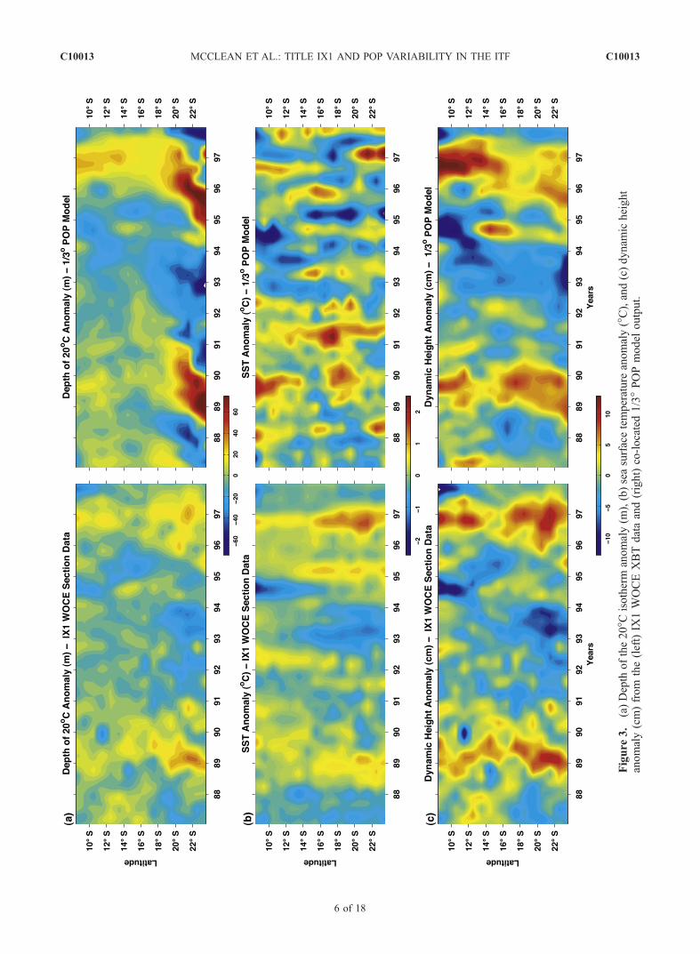
Figure

3.

(a)Depth

ofthe20�C

isotherm

anomaly(m

),(b)seasurfacetemperature

anomaly(�C),and(c)dynam

icheight

anomaly(cm)from

the(left)IX

1WOCEXBTdataand(right)co-located1/3�POPmodel

output.


6 of 18

C10013

extreme Indian Ocean Dipole (IOD) mode events of 1994and 1997 are readily identifiable by the cold SST anoma-lies (Figure 3b) and the lower dynamic height (Figure 3c).In the years prior to these dipole events, warm SSTanomalies are observed at the northern end of the section.Saji et al. [1999] have previously documented these eventsand the biennial tendency in SST for this region. For theperiod of overlap (1987–1994) as well as the more recentdata, our results are in close agreement with M96: Inter-annual variability in thermocline depth and SST are great-est at the southern end of the IX1 transect and nearly inphase with the Pacific El Nino and La Nina signals, whileinterannual variability in SST anomalies is large at thenorthern end of the transect, and closely related to theIndian Ocean dipole mode events.

[17] Good agreement between the model and data interms of the spatial and temporal distribution of the anoma-lies are found in the dynamic height and D20 anomaly fields(Figures 3a and 3c). The sequence of simulated dynamicheight and D20 anomaly events related to El Nino and LaNina track closely with the observed events, however themagnitude of the model anomalies are larger than observedand the duration of the simulated events are too long,particularly for the La Nina event of 1988–1989. Themodel SST shows the best agreement with data at thesection’s northern end (Figure 3b).[18] Before discussing the influence of the remote ENSO

Pacific signal in the STIO, we first examine the veracity ofthe model ENSO signal itself. We chose to compare themodel NINO3 index (monthly SST anomalies averaged

Figure 4. (a) Time series of NINO3 (SSTA for 90�W–150�W, 5�N–5�S) from the model and data[Reynolds and Smith, 1994]. Time series of dynamic height anomalies (cm) from (b) southern and(c) northern IX1 calculated from the IX1 XBT data (solid line) and the POP model (solid line with dots).The dashed line is the equatorial Southern Oscillation Index (EQSOI [Kistler et al., 2001]), and the dash-dotted line is the Indian Ocean Dipole Mode Index (DMI [Saji et al., 1999]).


7 of 18

C10013

over 90�W–150�W, 5�S – 5�N) with that from data[Reynolds and Smith, 1994]. Very good agreement is seen(Figure 4a) from 1989–1998, except for 1994 through early1995 when the model is too cold. In 1987 and 1988 themodel index is in phase with the data, but underestimates themagnitude of the observed SSTA. This discrepancy is likelydue to the adjustments made to the ECMWF reanalysisforcing fields to achieve a global balance on an annual basis;adjustments were larger in the 1980s relative to the veryminor ones made in the 1990s. In all, the agreement is good(correlation between the two time series is 80%) giving usconfidence to use the model to study interannual relatedvariability in the Throughflow region.[19] To better demonstrate the close phase agreement

between Pacific El Nino and La Nina signals and thevariability at the southern end of the IX1 transect, observedand modeled time series of the dynamic height anomalieswere constructed by spatially averaging over the four mostsoutherly bins (23.5�S–20.5�S). Dynamic height is used asit represents the variability over the upper water column.These time series are seen in Figure 4b together with the

equatorial SOI (EQSOI). The EQSOI was developed at theNational Center for Environmental Prediction and is basedon sea level pressures over Indonesia and the easternequatorial Pacific [Kistler et al., 2001]. We use this indexrather than the standard SOI, as we are interested inrelating the remote equatorial and Northern Hemisphereoff-equatorial ENSO signals that propagate through theIndonesian Seas to the variability at the southern end ofIX1. The seasonal cycle has been removed from theEQSOI and a 5-month running mean has been applied toremove high-frequency fluctuations. All time series arenormalized by their respective space-time standard devia-tions. Both time series are well correlated with the EQSOI:0.58 for the observed time series, and 0.63 for the modeltime series. The correlation between the data and the modeltime series is 0.80. All relationships are significant at the95% level. We note an unrealistically long La Nina ismaintained by the model in 1989: both the EQSOI and thedata time series start to decrease after peaking in early1989, while the model values stay elevated until the end ofthe year. This is likely due to inaccuracies in the Pacific

Figure 5. Variance preserving spectra (cm2) of dynamic height anomaly from (a, c) XBT data and(b, d) the POP model at the southern (Figures 5a and 5b) and northern (Figures 5c and 5d) ends of theIX1 transect.


8 of 18

C10013

surface forcing that resulted in an overly warm Pacificanomaly during the 1988 La Nina (Figure 4a).[20] Time series of the observed and modeled dynamic

height anomaly from the northern end of the IX1 transect(8.5�S–9.5�S) are plotted along with the EQSOI and theDipole Mode Index (DMI [Saji et al., 1999]) in Figure 4c.The seasonal cycle was removed from the DMI and it waslow-pass filtered at 5 months. Clearly the data and modeltime series are visually inversely correlated with the DMI;both extreme dipole mode events in 1994 and 1997 areseen in the observed and modeled time series. Correlationvalues between the DMI and the data, and the DMI andthe model, are �0.8 and �0.76, respectively. The correla-tion between the model and data is 0.84. All correlationsare significant at the 95% level. Additionally, the observedand modeled time series are significantly correlated withthe SOI index: values of 0.60 and 0.54 are obtained,respectively.[21] To identify the dominant narrow-band periodicities,

we calculated variance-preserving spectra of the data andmodel dynamic height anomaly time series from thenorthern and southern ends of the IX1 transect. Sinceour focus is on long-period signals, peaks with periodici-ties less than 1.8 years although present in the spectra arenot discussed. The southern IX1 data and model spectra(Figures 5a and 5b) both display peaks at 2.7 and5.5 years, with the magnitude of the 5.5-year signalbeing 4.7 (3.6) times larger than the observed (modeled)signal at 2.7 years. In addition, the modeled 5.5-year

signal is 1.7 times larger than the equivalent observedvalue. We refer to the 2.7 year signal as quasi-biennial(QB) and the 5.5 year as quasi-pentadal (QP). Clearly, themodel is overestimating the strength of the 2.7 and 5.5-yearsignals, however in keeping with the observations, it doesdemonstrate that at the southern end of IX1, the QPvariability is stronger than the QB signal. The spectra ofthe observed and modeled time series from northern IX1(Figures 5c and 5d) display peaks at 3.7 years; the modelpeak (230 cm2) is just slightly larger than that of the data(215 cm2). Using variance-preserving spectra of averagedwind anomalies along the pathways of the equatorial andcoastal waveguides from the Pacific and Indian oceans,Wijffels and Meyers [2004, Figure 11] found Pacific windswere dominated by ENSO (5–6 years) while the IndianOcean winds displayed energy at around 3.3–3.7 years.Clearly, as shown in Figure 5, these Pacific and IndianOcean remote signals are also contributing to the upperocean response at the southern and northern ends of IX1,respectively.[22] To further understand the nature of the remote

signals impacting IX1 the zonal component of wind stressand the wind stress curl over the tropics and subtropics inthe Indian and Pacific Oceans were correlated with thetimes series of dynamic height anomalies from the south-ern and northern ends of the IX1 transect. Both the modeland the data time series were correlated with the ECMWFwinds that were used to force the model. The seasonalcycle was removed from the winds, which were then low-

Figure 6. Correlations of dynamic height anomaly (cm) at the southern end of IX1 calculated from (top)IX1 data and (bottom) the POP model and zonal wind stress anomaly (dynes cm�2) over the tropical andmidlatitudes of the Pacific and Indian oceans.


9 of 18

C10013

pass filtered at 13 months, and interpolated to a 2� � 2�grid. The IX1 model and data time series were also low-pass filtered at 13 months (capturing variability overinterannual timescales). Figure 6, top and bottom plots,show the correlation between the zonal wind stress and thesouthern IX1 data and the model time series, respectively.Maximum negative correlations (>�0.70) for both timeseries were found with the equatorial winds over thewestern and central Pacific Ocean. The correlations wererepeated using timescales greater than 3 years (QP), andcorrelation values increased to over �0.80, explainingabout 70% of the variance. Maximum correlations betweenthe northern IX1 time series and the zonal winds (notshown) occurred over the equatorial Indian Ocean; valuesgreater than 0.8 were found on the equator between 80�E–90�E for both the model and the data. These findingsindicate that remote signals generated along the equator inthe Pacific and Indian oceans propagate along the equato-rial and coastal waveguides into the IX1 region, consistentwith the findings of Clarke and Liu [1994], M96, andWijffels and Meyers [2004]. Correlations between thesouthern IX1 time series for both data and model andwind stress curl (low-pass filtered at 13 months) indicatethat another remote oceanic signal is impacting this sectionof the transect (Figure 7). Maximum negative correlations(>�0.8) are seen between �5�N and 10�N in the westernand central Pacific for both the model and the data. Therelationship between variability at the southern end of IX1and this remote off-equatorial signal in the Pacific will be

discussed in the next section in the light of the observa-tional findings of White et al. [2003].

5. Discussion

[23] White et al. [2003] documented long period, off-equatorial baroclinic Rossby waves in the Pacific basin withQB (2.2- and 2.8-year) and QP (3.5-, 5.4-, and 7-year)periodicities that propagate westward across the Pacificbasin to arrive at the western boundary at approximately7�N and 12�N, respectively. They argue that these off-equatorial signals reach the western boundary of the Pacificand reflect as slow eastward propagating equatorial coupledwaves. M96 and Wijffels and Meyers [2004] attributed theremote Pacific signal in their IX1 results to interannual freeequatorial Rossby waves and reflected equatorial Kelvinwaves whose energy radiates through the Indonesian Seas,as predicted by Clarke and Liu [1994]. M96 and Wijffelsand Meyers [2004] did not discuss the impact of the off-equatorial waves from the Pacific on the ITF region. Inaddition, the White et al. [2003], M96 and Wijffels andMeyers [2004] studies identified the waves using observa-tional data sets. Here we investigate using the model, whoseresolution and realistic topography resolve the waveguidethrough the Indonesian Seas, whether the remote signalfound at the southern IX1 transect in Figure 7, can also betraced back to Pacific off-equatorial low-frequency Rossbywaves. These waves would excite Kelvin-Munk waves atthe western boundary of the Pacific, which in turn, would

Figure 7. Correlations of dynamic height anomaly (cm) at the southern end of IX1 calculated from (top)IX1 data and (bottom) the POP model and wind stress curl anomaly (dynes cm�3) over the tropical andmidlatitudes of the Pacific and Indian oceans.


10 of 18

C10013

propagate equatorward to reflect as equatorial Kelvinwaves, exciting a coastally trapped wave response thatwould propagate through the Indonesian Seas and alongthe northwest coast of Australia. This signal could thenprogressively propagate into the STIO as Rossby waves. Weaddress the importance of both off-equatorial and equatoriallong waves to the composition of the remote Pacific signal,and evaluate the penetration of this remote Pacific signalinto the interior of the STIO.[24] To understand the importance of the low-frequency

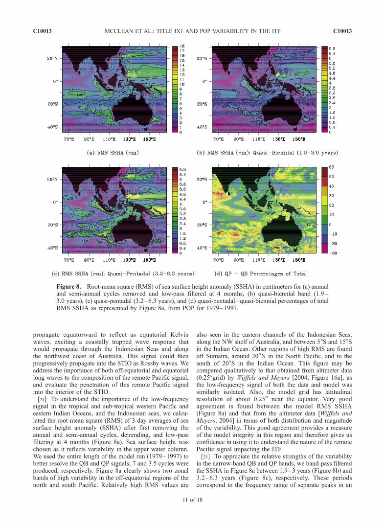
signal in the tropical and sub-tropical western Pacific andeastern Indian Oceans, and the Indonesian seas, we calcu-lated the root-mean square (RMS) of 3-day averages of seasurface height anomaly (SSHA) after first removing theannual and semi-annual cycles, detrending, and low-passfiltering at 4 months (Figure 8a). Sea surface height waschosen as it reflects variability in the upper water column.We used the entire length of the model run (1979–1997) tobetter resolve the QB and QP signals; 7 and 3.5 cycles wereproduced, respectively. Figure 8a clearly shows two zonalbands of high variability in the off-equatorial regions of thenorth and south Pacific. Relatively high RMS values are

also seen in the eastern channels of the Indonesian Seas,along the NW shelf of Australia, and between 5�S and 15�Sin the Indian Ocean. Other regions of high RMS are foundoff Sumatra, around 20�N in the North Pacific, and to thesouth of 20�S in the Indian Ocean. This figure may becompared qualitatively to that obtained from altimeter data(0.25�grid) by Wijffels and Meyers [2004, Figure 16a], asthe low-frequency signal of both the data and model wassimilarly isolated. Also, the model grid has latitudinalresolution of about 0.25� near the equator. Very goodagreement is found between the model RMS SSHA(Figure 8a) and that from the altimeter data [Wijffels andMeyers, 2004] in terms of both distribution and magnitudeof the variability. This good agreement provides a measureof the model integrity in this region and therefore gives usconfidence in using it to understand the nature of the remotePacific signal impacting the ITF.[25] To appreciate the relative strengths of the variability

in the narrow-band QB and QP bands, we band-pass filteredthe SSHA in Figure 8a between 1.9–3 years (Figure 8b) and3.2–6.3 years (Figure 8c), respectively. These periodscorrespond to the frequency range of separate peaks in an

Figure 8. Root-mean square (RMS) of sea surface height anomaly (SSHA) in centimeters for (a) annualand semi-annual cycles removed and low-pass filtered at 4 months, (b) quasi-biennial band (1.9–3.0 years), (c) quasi-pentadal (3.2–6.3 years), and (d) quasi-pentadal–quasi-biennial percentages of totalRMS SSHA as represented by Figure 8a, from POP for 1979–1997.


11 of 18

C10013

Figure

9.

Tim

esequence

ofmapsofSSHA

(cm)fortheperiod16October

1987through27Decem

ber

1987.SSHAwas

low-passfiltered

at13monthsfollowingtheremoval

oftheannual

andsemi-annual

cycles.


12 of 18

C10013

area-averaged (90�E–�170�E, 20�S–20�N) variance-pre-serving spectrum of demeaned SSH (not shown). In bothcases, the highest variability associated with each period isseen in the off-equatorial regions of the Pacific Ocean, theeastern channels of the Indonesian Seas, along the NWshelf of Australia, off Sumatra, and between 70�E and90�E in the STIO. The percent of the total variabilityexplained by each band was calculated and the QBpercentage was then subtracted from the QP variability(Figure 8d). In the regions where the highest variabilitywas observed in Figures 8b and 8c, the QP band is roughly10–25% more energetic than the QB band. This agreeswith the stronger QP signal compared to the QB signal inthe variance-preserving spectra of the southern IX1 shownin Figure 5. As a result in the following event analyses wewill not attempt to separate out the QB and QP signals,rather we will consider their combined effects as an overall‘‘interannual’’ signal.[26] To help distinguish between the off-equatorial and

the equatorial pathways, and to understand the changes inthe space-time structure of these low-frequency signalspassing through the Indonesian Seas from the North Pacific,we show two time series of snapshots of SSHA: onedepicting the passage of equatorial Rossby waves and theother the evolution of the off-equatorial signal. Thesesnapshots were derived from an animation of the full timeseries (1979–1997). Annual and semi-annual cycles werefirst removed from the demeaned SSH by least squaresfitting; it was then detrended and low-pass filtered at13 months (to include all QB and QP frequencies).[27] Figure 9 shows the low-frequency signal during the

1987 El Nino for the period 16 October 1987 through 27December 1987. The equatorial Rossby wave can be easilyrecognized by the band of negative SSHA spanning theequator with its maximum amplitude occurring at about 5�in both hemispheres. Negative anomalies are seen through-out the Indonesian Seas and along the NW shelf ofAustralia. By 27 December 1987, the wave has diminishedin magnitude. We move forward to 8 April 1988 (Figure 10)and now see negative SSHA on the equator associated withKelvin wave activity (from the reflected equatorial Rossbywave), while positive SSHA signals are increasing inmagnitude in the off-equatorial regions. Focusing on thenorthern hemisphere, we see a combination of processesunderway. A band of intensifying positive SSHA (8 April1988 to 14 May 1998 and onward) is seen between thenorthern tip of Halmahera Island extending northwestwardto about 170�E, 8�N. A Hovmueller (time versus longitude)diagram (not shown) depicts westward propagating wavesentering this region from the east between 6�N and 9�N;however, to the west of 150�E the signal is also due to localwind stress curl anomalies (see Figure 7). Concurrently,intensifying positive SSHA is found along the Irian Jayashelf, in the Arafura/Australian waveguide, and along theNW Australian shelf. Near 10�N–12�N a positive SSHAsignal is seen at 160�E on 8 April 1988. It can be seen atprogressively more westward locations at subsequent dates,until by 19 June 1988, a continuous band of positive SSHAis found across 10�N–12�N. A Hovmueller plot along thislatitude band (not shown) indeed confirmed this to be awestward propagating wave. Increasingly positive SSHA isalso seen spreading westward in the Banda Sea. Subsequent

SSHA snapshots show the signal to further intensify overthe entire region and to progress eastward along the equator,indicative of reflection at the western boundary. Along theNW Australian shelf, the signal is seen to propagate off-shore. In the southern hemisphere, positive SSHA is seenbetween 5�S and 8�S east of New Guinea (Figure 10).Tracking the signal in the time sequence ending 19 June1988, it is seen to intensify at this location, however only avery weak positive SSHA signal is seen closer to the equatorto the north of New Guinea. The local coastal waveguidehere intersects the equator to the east of the northern tip ofIrian Jaya which itself extends north of the equator. Itappears from the animation (later time, not shown) that thisweak off-equatorial signal on reaching the equator reflects tothe east of Irian Jaya and is therefore unlikely to impact theIndonesian Seas.[28] This scenario described by Figure 10 is in agreement

with White et al. [2003]: Low-frequency westward propa-gating baroclinic Rossby waves are found in the off-equatorial western Pacific following the warm phase ofENSO. White et al. [2003] were able to track the incidentpaths of these low-frequency off-equatorial Rossby waves atthe northwestern Pacific boundary and their emergencealong the equatorial Pacific as coupled waves. They didnot, however, track these signals through the ITF. Wecontend that upon reflecting onto the equator, the resultingcoupled waves excite a coastally trapped response in theIndonesian Seas that propagates along the NW shelf ofAustralia. To further understand the relationship betweenthe remote Pacific signals and the STIO where the QPvariability appears to be strongest (Figure 8c), we use cross-spectral analyses (coherence-squared and phase calcula-tions) of 3-daily SSHA (demeaned only) between thesouthern end of the IX1 line (110�E, 22�S) and each gridpoint of the model domain in the STIO and the westerntropical Pacific. The autospectral density functions, theco-spectrum and the quadrature spectrum calculated as partof the coherence-squared/phase calculation were averagedover three adjacent frequency bands to produce 6 degrees offreedom. The demeaned SSH were pre-whitened using afinite difference filter prior to calculating the spectra. Onlythe QP frequency bands are selected and discussed here asthe QB signals have already been shown to be of lesserimportance particularly off western Australia (Figure 5).The coherence-squared between SSHA at 110�E, 22�S(identified by a star) and the SSHA at other grid points inthe domain for the QP frequencies are seen in the top panelof Figure 11a. Regions where the coherence-squared isbelow the 90% significance level (0.69) are shaded gray.The 95% significance level is 0.78. The middle panels showthe equivalent phase, with its associated error in the bottompanels, between each pair in the time series.[29] Statistically significant coherence-squared values

are seen in the tropical North Pacific between 150�E andthe maritime western boundary as far north as 15�N(Figure 11a). The highest values (>0.9) in this region areseen off the equator (7�N–8�N). Significant values arefound in the Halmahera, Seram, and Banda Seas, in OmbaiStrait, and along and offshore of the NWAustralian shelf tothe south of Timor Strait (see Figure 1 for locations). Thenegative phases in the Indonesian Seas and in the westernPacific associated with these coherence-squared values


13 of 18

C10013

Figure

10.

Tim

esequence

ofmapsofSSHA(cm)fortheperiod8April1988through19June1988.TheSSHAwas

low-

passfiltered

at13monthsfollowingtheremoval

oftheannual

andsemi-annual

cycles.


14 of 18

C10013

Figure

11.

Cross-spectrum

ofSSHA

atquasi-pentadal

frequencies

betweeneach

gridpointofthemodel

domainin

the

southerntropical

IndianOcean

andthewestern

tropical

Pacific

and(a)thesouthernendoftheIX

1line(110�E

,22�S)and

(b)Tim

orStrait(125�E

,12�S);theselocationsareidentified

bystars.(top)Coherence-squared

values

(areas

shaded

grayare

below

the90%

significance

level)AND

(middle)phases

with(bottom)theirassociated

error.


15 of 18

C10013

indicate that the SSHA at the southern end of the IX1 linelags the SSHA at these locations. Positive phases in thewestern Pacific to the north of 8�N are consistent with thearrival of the Rossby waves at 10�N–12�N after the lowerlatitude signals in the western Pacific have started topenetrate and impact the STIO, as seen in Figure 10. Thepositive phases to the north and to the west of 110�E, 22�Sindicate that the signal that radiates offshore of Australia islagging that at the southern end of IX1. The phase error isup to ±20�where the coherence-squared values are >0.9.[30] These analyses strongly suggest that for QP perio-

dicities the southern IX1 line is affected by signalsoriginating in both the equatorial and off-equatorial north-western tropical Pacific. Coastally trapped responses aregenerated by either equatorial Rossby or reflected Kelvinwaves resulting from the Munk-Kelvin waves or theequatorial Rossby waves. The signals propagate south-wards through the Halmahera Sea into the Seram Sea andthen southwestward around the Banda Sea to pass throughOmbai Strait. A visual correlation of the 1000-m isobath inthe Indonesian Seas (Figure 1) and the pathway of thecoherent signal around the Banda Sea and southwestwardalong the NW Australian shelf shows that the signal ispropagating along the continental shelf. The signal finallyradiates offshore as a Rossby wave into the STIO.A statistically significant signal does not exist west of90�E, in agreement with earlier observational findings byMasumoto and Meyers [1998]. Using OGCM output andXBT data, they found that interannual variations of theD20 in this region were largely due to the wind stress curlintegrated along the Rossby wave pathways. However, intheir models, both Murtugudde et al. [2000] and Xie et al.[2002] suggested that during El Nino periods, there issignificant SST variability in the western STIO that can belinked to these Rossby waves generated in the easternSTIO.[31] The results shown in Figure 11a can be contrasted

with those obtained by calculating cross-spectra of SSHAbetween a location in Timor Strait (125�E, 12�S, againidentified by a star) and the rest of the domain for QPfrequencies (Figure 11b). Statistically significant coherenceis again seen in the western tropical Pacific, however valuesare slightly lower to the north of 8�N than in Figure 11a.Patches of high coherence-squared values (>0.95) are seenclose to the equator from 140�E to Halmahera in thenorthern hemisphere and north of Irian-Jaya in the southernhemisphere, in the Seram, Banda, and Arafura Seas, and onthe NW Australian shelf to about 17�S. Westward propa-gating wave crests are found along the Pacific equator inthe associated phase diagram (middle panel); here the phaseis progressively less negative as the western boundaryis approached. In the Indonesian Seas and on the NWAustralian shelf the phase is unchanged. Clearly, the TimorStrait SSHA is most strongly correlated with the equatorialPacific signal.[32] It has been demonstrated from all these model

analyses that the STIO is impacted by both remotePacific equatorial and off-equatorial Rossby waves. UsingXBT data, Wijffels and Meyers [2004] clearly foundequatorial Pacific winds to be driving the interannualtemperature and sea level response as represented by freeequatorial Pacific Rossby waves. The signal radiated

through the Banda Sea into the STIO as well as enteringthe coastal waveguide at the western tip of New Guineaand propagating poleward through Timor Strait and alongthe Arafura/Australian shelf break as coastally trappedwaves. In turn, these trapped waves excited free westwardpropagating Rossby waves that could be detected severalhundreds of kilometers offshore at 22�S. The model, asshown in Figure 11, reproduced all these wave processes.As well, the model delineates an off-equatorial NorthPacific signal that enters the coastal waveguide andpropagates southward through the Halmahera Sea intothe Seram Sea and then southwestward around the BandaSea to pass through Ombai Strait. These off-equatorialwaves form in response to off-equatorial cyclonic windstress curl anomalies (Figure 7), induced by westerlysurface wind anomalies produced in the wake of warmSST anomalies that propagate slowly eastward along theequator [White et al., 2003]. Interestingly, the low-fre-quency lagged regressions of Wijffels and Meyers [2004,Figure 17a] also revealed a strong response in off-equatorial western Pacific sea level anomaly to Pacificeasterly equatorial wind anomalies. This suggests that theoff-equatorial signal passing through the ITF and reachingthe STIO, as demonstrated by the model, also occurs inreality. Wijffels and Meyers [2004] did not look for oridentify this pathway in their observational study.[33] Clearly, the remotely forced long waves interacting

with the complex topography of the Indonesian Through-flow produce varied responses in different parts of theSTIO. For completeness, we also computed cross-spectraof SSHA at QP frequencies between points in the northernand middle part of the IX1-XBT line and the rest of thedomain to help identify other possible remote influences(figures not shown). For locations at the northern end of theIX1-XBT line, a significant coherent, in-phase signal inSSHA was evident off the coast of Sumatra and Java,extending through the Lombok Strait into Makassar Strait:the coherence drops off to the north of the Dewakang sill at2�S in Makassar Strait. This signal is likely due to interan-nual Kelvin waves forced remotely by equatorial interan-nual zonal winds in the Indian Ocean as discussed byClarke and Liu [1994] and Wijffels and Meyers [2004].For locations in the middle of the IX1-XBT transect (15�S–19�S), significant coherence is only found offshore of theNWAustralian shelf in the STIO. Here the negative phasesto the east and positive phases to the west of the IX1 lineindicate the signal is due to Rossby waves propagatingaway from the west Australian coast.

6. Conclusions

[34] The mean and interannual variability of the thermalstructure of the repeat XBT line known as IX1 werecompared statistically for the years 1987–1997 with con-current, co-located output from a global eddy-permittingconfiguration of the POP model forced with realistic surfacefluxes. Both data and the model showed that the QP signalwas strongest at the southern end of the IX1 line where itexhibited variability nearly in phase with ENSO in thePacific. The dominant low-frequency variability (3.7 years)at the northern end of IX1 was attributed to remote forcingfrom the equatorial Indian Ocean. Correlations between the


16 of 18

C10013

observed and model time series and the winds in both thetropical and subtropical Indian and Pacific oceans furtherconfirmed this result.[35] The model demonstrated integrity in its representa-

tion of low-frequency variability as demonstrated by com-parisons with data analyses presented in this study, and withresults from previous observational studies. In particular,the data/model comparisons of dynamic height variability atthe southern and northern ends of IX1 and the comparisonof RMS SSHA from altimetry [from Wijffels and Meyers,2004] and the model in the Indo-Pacific domain showedstrong agreement. Model discrepancies such as the remotePacific signal being too strong and lasting for too long in themodel STIO are likely due to shortcomings in the surfaceforcing over the Pacific, particularly the annual adjustmentover the tropics to balance the global heat balance. The SSTdiscrepancy in the STIO may also be due to inaccuracies inthe surface forcing and other factors such as the lack of tidalmixing in the model.[36] White et al. [2003] stated that low-frequency Rossby

waves form in response to off-equatorial cyclonic windstress curl anomalies induced by westerly surface windanomalies produced in the wake of warm SST anomaliesthat propagate slowly eastward along the equator. In ourstudy, we found that off-equatorial Rossby waves, on reach-ing the western maritime boundary of the North Pacific,excited a coastally trapped response (Munk-Kelvin waves)that propagated equatorward and reflected onto the equator.In turn, this equatorial signal excited a coastally trappedresponse off Irian Jaya that propagated through the Indone-sian Seas and along the northwest coast of Australia whereit progressively radiated off as Rossby waves into the STIO.Cross-spectral analyses confirmed that on QP scales, thefree westward propagating Rossby waves in the STIOexcited by coastally trapped waves along the NW shelf,resulted from both equatorial and off-equatorial low-frequency signals remotely forced in the Pacific Ocean.Comparative cross-spectral analyses, suggested that TimorStrait is more strongly affected by the equatorial signal thanthe off-equatorial signal, while the southern IX1 responds toboth.[37] The northern end of the IX1 XBT transect

responded to interannual Kelvin waves forced remotelyby equatorial interannual zonal winds in the Indian Oceanas discussed by Clarke and Liu [1994], while the middleof the transect only experienced the passage of Rossbywaves propagating away from the west Australian coast.In the POP model used here, these Rossby waves donot penetrate farther westward than 90�E as found byMasumoto and Meyers [1998]. These results further attestto the integrity of the simulation and hence the reliabilityof the model findings that have not been identified fromdata. Clearly, the resolution and realistic topography ofthe model has allowed us to resolve the waveguidethrough the Indonesian Seas and understand the variedresponses on low-frequency timescales in the STIO toremotely forced long waves.[38] A study of the energy transmission and the transport

variability associated with the passage of these coastallytrapped waves through the Indonesian Seas and along theNWAustralian shelf would further quantify the importanceof these signals to the STIO. However, these calculations

would be better performed with a higher resolution modelthat will more accurately depict the complex bathymetry ofthe region. A suitable candidate is the 0.1�, 40-level globalPOP simulation [Maltrud and McClean, 2005]; some2 decades of a spin-up integration have recently beencompleted and a post spin-up simulation is now underway.

[39] Acknowledgments. The Department of Energy (CCPP program)and the National Science Foundation (OCE-0221781 (J. M.) and OCE-0220382 (J. S.)) sponsored this work. The Alaska Region SupercomputingCenter (ARSC) provided computer time. We thank Susan Wijffels and GaryMeyers (CSIRO, Australia) for the IX1-XBT data. We thank Tony Craig(NCAR) and Wieslaw Maslowksi (NPS) for collaborating with the authorsto set up and test the global POP simulation. Mathew Maltrud (LANL)provided the global model grid. Robin Tokmakian (NPS) collaborated withthe authors in the processing of the ECMWF reanalysis fluxes. PeterBraccio performed some of the post-processing of the model output. Weobtained the Indian Ocean Dipole Mode Index from Kevin Vranes (http://www.ldeo.columbia.edu/~kvranes/research/DMI). The NINO3 data wasobtained from the IRI/LDEO Climate data library (http://ingrid.ldeo.columbia.edu). We thank Jim Potemra and Ted Durland (U. Hawaii) forcomments on an earlier draft. The reviewers and editors are thanked fortheir helpful comments.

ReferencesBehera, S. K., P. S. Salvekar, and T. Yamagata (2000), Simulation ofInterannual SST variability in the tropical Indian Ocean, J. Clim., 13,3487–3499.

Boning, C. W., and R. G. Budich (1992), Eddy dynamics in a primitiveequation model: Sensitivity to horizontal resolution and friction, J. Phys.Oceanogr., 22, 361–381.

Bryden, H. L., and S. Imawaki (2001), Ocean transport of heat, in OceanCirculation and Climate, edited by G. Siedler, J. Church, and J. Gould,pp. 445–474, Elsevier, New York.

Clarke, A. J., and X. Liu (1994), Interannual sea level in the northern andeastern Indian Ocean, J. Phys. Oceanogr., 24, 1224–1235.

Dukowicz, J. K., and R. D. Smith (1994), Implicit free-surface methodfor Bryan-Cox-Semtner ocean model, J. Geophys. Res., 99, 7991–8014.

Ffield, A., and A. Gordon (1996), Tidal mixing signatures in the IndonesianSeas, J. Phys. Oceanogr., 26, 1924–1937.

Godfrey, J. S. (1975), On ocean spindown: I. A linear experiment, J. Phys.Oceanogr., 5, 399–409.

Godfrey, J. S. (1996), The effect of the Indonesian Throughflow on oceancirculation and heat exchange with the atmosphere: A review, J. Geophys.Res., 101, 12,217–12,237.

Gordon, A. L. (2001), Interocean exchange, in Ocean Circulation andClimate, edited by G. Siedler, J. Church, and J. Gould, chap. 4.7,pp. 303–314, Elsevier, New York.

Jakob, C. (1999), Cloud cover in the ECMWF Reanalysis, J. Clim., 12,947–959.

Kistler, R., et al. (2001), The NCEP–NCAR 50-year reanalysis: Monthlymeans CD–ROM and documentation, Bull. Am. Meteorol. Soc., 82,247–268.

Large, W. G., J. C. McWilliams, and S. C. Doney (1994), Oceanic verticalmixing: A review and a model with a nonlocal boundary layer parame-terization, Rev. Geophys., 32, 363–403.

Levitus, S., R. Burgett, and T. P. Boyer (1994a), World Ocean Atlas 1994,vol. 3, Salinity, NOAA Atlas NESDIS 3, Natl. Oceanic and Atmos. Ad-min., Silver Spring, Md.

Levitus, S., R. Burgett, and T. P. Boyer (1994b), World Ocean Atlas 1994,vol. 4, Temperature, NOAA Atlas NESDIS 4, Natl. Oceanic and Atmos.Admin., Silver Spring, Md.

Lukas, R., T. Yamagata, and J. P. McCreary (1996), Pacific low-latitudewestern boundary currents and the Indonesian Throughflow, J. Geophys.Res., 101, 12,209–12,216.

Maltrud, M. E., and J. L. McClean (2005), An eddy resolving global 1/10�ocean simulation, Ocean Modell., 8, 31–54.

Masumoto, Y. (2002), Effects of interannual variability in the easternIndian Ocean on the Indonesian Throughflow, J. Oceanogr., 58,175–182.

Masumoto, Y., and G. Meyers (1998), Forced Rossby waves in the southerntropical Indian Ocean, J. Geophys. Res., 103, 27,589–27,602.

McCreary, J. P. (1983), A model of tropical ocean-atmosphere interaction,Mon. Weather Rev., 111, 370–387.

Meyers, G. (1996), Variation of Indonesian Throughflow and the El Nino–Southern Oscillation, J. Geophys. Res., 101, 12,255–12,263.


17 of 18

C10013

Meyers, G., R. J. Bailey, and A. P. Worby (1995), Geostrophic transport ofIndonesian Throughflow, Deep Sea Res., Part I, 42, 1163–1174.

Morrow, R., and F. Birol (1998), Variability in the southeast Indian Oceanfrom altimetry: Forcing mechanisms for the Leeuwin Current, J. Geo-phys. Res., 103, 18,529–18,544.

Murtugudde, R., J. P. McCreary, and A. J. Busalacchi (2000), Oceanicprocesses associated with anomalous events in the Indian Ocean withrelevance to 1997–1998, J. Geophys. Res., 105, 3295–3306.

Pazan, S. E., W. B. White, M. Inoue, and J. J. O’Brien (1986), Off-equa-torial influence upon Pacific equatorial dynamic height variability duringthe 1982–1983 El Nino–Southern Oscillation event, J. Geophys. Res.,91, 8437–8450.

Perry, G. D., P. B. Duffy, and N. L. Miller (1996), An extended data set ofriver discharges for validation of the general circulation models, J. Geo-phys. Res., 101, 21,339–21,349.

Philander, S. G. (1990), El Nino, La Nina and the Southern Oscillation, 293pp., Elsevier, New York.

Potemra, J. T. (1999), Seasonal variations of upper ocean transport from thePacific to the Indian Ocean via Indonesian Straits, J. Phys. Oceanogr., 29,2930–2944.

Quadfasel, D., and G. Cresswell (1992), A note on the seasonal variabilityof the South Java Current, J. Geophys. Res., 97, 3685–3688.

Reynolds, R. W., and T. M. Smith (1994), Improved global sea surfacetemperature analyses, J. Clim., 7, 929–948.

Saji, N. H., B. N. Goswami, P. N. Vinayachandran, and T. Yamagata(1999), A dipole mode in the tropical Indian Ocean, Nature, 401,360–363.

Schiller, A., J. S. Godfrey, P. C. McIntosh, G. Meyers, and R. Fiedler(2000), Interannual dynamics and thermodynamics of the Indo-PacificOceans, J. Phys. Oceanogr., 30, 987–1011.

Smith, W. H. F., and D. T. Sandwell (1997), Global seafloor topographyfrom satellite altimetry and ship depth soundings, Science, 277, 1957–1962.

Sprintall, J., J. Chong, F. Syamsudin, W. Morawitz, S. Hautala, N. Bray,and S. Wijffels (1999), Dynamics of the South Java Current in the Indo-Australian basin, Geophys. Res. Lett., 26, 2493–2496.

Sprintall, J., S. Wijffels, T. Chereskin, and N. Bray (2002), The JADEand WOCE I10/IR6 Throughflow sections in the southeast Indian

Ocean: Part 2. Velocity and transports, Deep Sea Res., Part II, 49,1363–1390.

Wajsowicz, R. C. (1996), The response of the Indo-Pacific Throughflow tointerannual variations in the Pacific wind stress: Part II. Realistic geometryand ECMWF wind stress anomalies for 1985–89, J. Phys. Oceanogr.,26, 2589–2610.

Washington, W. M., et al. (2000), Parallel climate model (PCM) control andtransient simulations, Clim. Dyn., 16, 755–774.

White, W. B., Y. He, and S. E. Pazan (1989), Off-equatorial westwardpropagating Rossby waves in the tropical Pacific during the 1982–1983and 1986–87 ENSO events, J. Phys. Oceanogr., 19, 1397–1406.

White, W. B., Y. M. Tourre, M. Barlow, and M. Dettinger (2003), A delayedaction oscillator shared by biennial, interannual, and decadal signals inthe Pacific Basin, J. Geophys. Res., 108(C3), 3070, doi:10.1029/2002JC001490.

Wijffels, S., and G. Meyers (2004), An intersection of oceanic waveguides:Variability in the Indonesian Throughflow region, J. Phys. Oceanogr., 34,1232–1253.

Wijffels, S., J. Toole, and R. Davis (2001), Revisiting the South Pacificsubtropical circulation: A synthesis of World Ocean Circulation Ex-periment observations along 32�S, J. Geophys. Res., 106, 19,481–19,514.

Wijffels, S., J. Sprintall, M. Fieux, and N. Bray (2002), The JADE andWOCE I10/IR6 Throughflow sections in the southeast Indian Ocean:Part 1: Water mass distribution and variability, Deep Sea Res., Part II,49, 1411–1422.

Yamagata, T., K. Mizuno, and Y. Masumoto (1996), Seasonal variations inthe equatorial Indian Ocean and their impact on the Lombok Through-flow, J. Geophys. Res., 101, 12,465–12,473.

Xie, S.-P., H. Annamalai, F. A. Schott, and J. P. McCreary (2002), Structureand mechanisms of South Indian Ocean climate variability, J. Clim., 15,864–878.

��D. P. Ivanova, J. L. McClean, and J. Sprintall, Scripps Institution of

Oceanography, University of California, San Diego, La Jolla, CA 92093-0230, USA. ([email protected])


18 of 18

C10013

Remote origins of interannual variability in the Indonesian Throughflow region from data and a...

Documents

Transcript of Remote origins of interannual variability in the Indonesian Throughflow region from data and a...