Remote condition monitoring of structural integrity of rails and ...

REMOTE CONDITION MONITORING OF STRUCTURAL

INTEGRITY OF RAILS AND CROSSINGS USING

ACOUSTIC EMISSION TECHNIQUE

by

Shengrun Shi

A thesis submitted to the University of Birmingham for the degree of

DOCTOR OF PHILOSOPHY

School of Metallurgy and Materials

College of Engineering and Physical Sciences

University of Birmingham

October 2018

University of Birmingham Research Archive

e-theses repository This unpublished thesis/dissertation is copyright of the author and/or third parties. The intellectual property rights of the author or third parties in respect of this work are as defined by The Copyright Designs and Patents Act 1988 or as modified by any successor legislation. Any use made of information contained in this thesis/dissertation must be in accordance with that legislation and must be properly acknowledged. Further distribution or reproduction in any format is prohibited without the permission of the copyright holder.

SYNOPSIS

Today, rail networks worldwide are becoming increasingly busy. Rolling stock operates

at faster speed and deals with heavier load than before. The operating conditions can cause

wear and fatigue damage under cyclic loading and generate different types of rail defects,

such as shelling crack, rail-end-bolt hole crack, split head and head check defects.

At present, depending on the severity of damage, a defective rail or crossing can still

remain in service with or without repairs being performed or replaced within a

standardized time-schedule ranging from immediately to up to 1 week after applying

Emergency Speed Restriction (ESR). Therefore, inspection and assessment of the growth

of these defects in service is critical in making maintenance decisions and ensuring the

smooth operation of the rail network. Various non-destructive testing (NDT) techniques

have been used for structural integrity evaluation in rail sector. Acoustic emission (AE)

technique is a passive NDT technique and its application in rail sector is still very limited.

In this research, the possibility of using AE technique to monitor structural integrity of

rails and crossings in real time has been investigated. AE technique has been used to

monitor the damage evolution process of three different types of sample including:R260

grade rail steel samples (precracked and without precracking), Hadfield steel samples

(precracked and without precracking), and a reference carbon steel sample during low

and high frequency bending fatigue crack growth tests. A commercial AE system

manufactured by Physical Acoustics Corporation (PAC) and a customised AE system

developed by researchers at the University of Birmingham and Krestos Limited, UK have

been used for data collection.

AE parameters including amplitude, energy, risetime, duration, count and average signal

level (ASL) have been used to correlate crack length with AE hits for the commercial

system. For all R260 rail steel samples, the occurrence of brittle cleavage fracture at

certain crack lengths has been shown in the fractographs and the resulting sudden increase

in crack length has been successfully detected by AE. The waveform based analysis has

been carried out on the data captured by the customized system. Various signal processing

algorithms including FFT (Fast Fourier Transform), moving RMS, moving crest factor,

moving kurtosis, moving skewness are employed for the in-depth analysis of the acquired

raw AE waveforms captured during the fatigue tests. All the algorithms show the

capability to reflect the severity of damage accurately. However, the results obtained by

various algorithms should be interpreted based on the principal of each algorithm. In

addition, SK has been employed to analyse the signals. Although SK values can reveal

the damage progression, the frequency ranges at which SK attain the peak values vary

considerably at different stages. This is due to the influence of noise caused by crack faces

rubbing during crack opening and closing. Field trials have been carried out on two

different crossings on the west coast mainline. Template-based cross-correlation analysis

has been employed to analyse the data captured from the instrumented crossing and

proved to be effective in evaluating the health state of the monitored crossings. Overall,

this research has shown that AE can be used as a tool to effectively evaluate the structural

integrity of rails and Hadfield steel crossings online.

Acknowledgements

First and foremost, I would like to thank my deceased father , Guibo Shi, who passed

away on August 26th ,2017, and my mother, Pengqing Gao for their continuous support

they have given to me throughout my study and their numerous sacrifices for the family.

I could not have done it without them. Many thanks to my brother Shengwei and my sister

Lishuang for their support.

I would like to express my heartfelt thanks to my supervisor Dr Mayorkinos Papaelias for

providing me the great opportunity to carry out the research under his supervision and for

his dedicated guidance, encouragement, continuous support through the course of the

research. It was my great privilege and honour to work with him.

I would like to thank Prof Clive Roberts and Dr Sakdirat Kaewuruen for their support

during the research. My sincere thanks also go to my industrial supervisor, Dr Slim Soua

from TWI Ltd, for providing me the opportunity of performing the research in an

industrial environment and for his kind support during the study. I also gratefully

acknowledge the scholarship provided from the National Structural Integrity Research

Centre (NSIRC).

I would also like to show gratitude to Mr Patrick Vallely from Network Rail for providing

the opportunities for performing the field trials at Cropredy. My sincere thanks also go to

Dr Arash Amini, Dr Zheng Huang, Dr Jinlong Du, Dr Zhiyuan Han,Dr Jun Zhou ,Dr

Nikolaos Angelopoulos Mr Zipeng Liu for their assistance and support in the research.

Last but not the least, my warm thanks to Dr Timothy Doel and Mr David Price for their

valuable assistance during fatigue testing.

Publications

Journal Papers

Shi, S., Han, Z., Liu, Z., Vallely, P., Soua, S., Kaewunruen, S & Papaelias, M. (2017).

“Quantitative monitoring of brittle fatigue crack growth in railway steel using acoustic

emission”, Proceedings of the Institution of Mechanical Engineers, Part F: Journal of Rail

and Rapid Transit. Available at https://doi.org/10.1177/0954409717711292

Conference Papers and Presentations

Shi,S., Soua, S., Kaewunruen, S & Papaelias, M “Online structural integrity monitoring

of railway infrastructure using acoustic emission”NSIRC conference,Cambridge, 27-28

June 2016

Shi,S., Huang Z., Kaewunruen,S, Vallely,P., Soua,S & Papaelias,M."Remote Condition

Monitoring of Structural integrity of Rails and Crossings" First World Congress on

Condition Monitoring-WCCM 2017,London, 13-16 June,2017

Valley,P., Papaelias,M., Huang,Z., Shi,S., Kaewunruen,S & Davis,J “Development of

novel acoustic emission techniques for monitoring the structural health of cast manganese

crossings”,Stephenson Conference 2017,London, 25-27 April 2017 (Won Prize for Best

paper)

Shi,S.“Acoustic emission monitoring of flaws in rails and cast manganese crossings”

Researcher Links Workshop in RCM for Railway,Istanbul,Turkey, 22-24 March 2016

https://doi.org/10.1177/0954409717711292

Shi, S., Papaelias ,M., Kaewunruen, S., Roberts, C & Soua, S., “Acoustic emission

monitoring of flaws in rails and cast manganese crossings”,Next Generation Rail

Conference 2016,Derby

TABLE OF CONTENTS

: INTRODUCTION ......................................................................... 2

: MANUFACTURING PROCESSS AND MECHANICAL

PROPERTIES OF RAIL AND CAST MANGANESE STEEL GRADES ............. 6

2.1 Rail steel ................................................................................................... 6

2.2 Cast manganese steels ......................................................................... 10

: FUNDAMENTALS OF FATIGUE AND FRACTURE OF RAILS

AND CAST MANGANESE CROSSINGS ......................................................... 14

3.1 Introduction ............................................................................................ 14

3.2 Fatigue .................................................................................................... 14

3.3 Ductile and brittle fracture .................................................................... 25

3.4 Types of loads and stresses in rails and crossings ........................... 27

3.4.1 Bending stresses ............................................................................... 30

3.4.2 Shear stresses .................................................................................. 31

3.4.3 Contact stresses ................................................................................ 32

3.4.4 Thermal stresses ............................................................................... 32

3.4.5 Residual stresses .............................................................................. 33

3.4.6 Dynamic and other effects ................................................................. 33

: STRUCTURAL DEFECTS IN RAILS AND CROSSINGS ......... 38

4.1 Introduction ............................................................................................ 38

4.2 Ratcheting behaviour ............................................................................ 39

4.3 Corrugation ............................................................................................ 40

4.4 Rolling contact fatigue .......................................................................... 41

4.4.1 Head checking ................................................................................... 41

4.4.2 Shelling .............................................................................................. 44

4.4.3 Tongue lipping ................................................................................... 46

4.5 Other types of defects ........................................................................... 46

4.5.1 Vertical split defects........................................................................... 46

4.5.2 Horizontal split defects ...................................................................... 47

4.6 Rail inspection techniques ................................................................... 47

4.6.1 Magnetic flux leakage ........................................................................ 48

4.6.2 Ultrasonic testing ............................................................................... 49

4.6.3 Visual inspection ............................................................................... 51

4.6.4 Ultrasonic phase arrays ..................................................................... 51

4.6.5 Long range ultrasonic testing or guided waves ................................. 52

4.6.6 Electromagnetic acoustic transducers ............................................... 52

4.6.7 Alternating current field measurement ............................................... 53

4.6.8 Probe vehicle ..................................................................................... 54

4.7 Damage tolerance concept and maintenance in railway .................... 55

: REMOTE CONDITION MONITORING WITH ACOUSTIC

EMISSION AND DATA ANALYSIS .................................................................. 58

5.1 Introduction ............................................................................................ 58

5.2 AE waveforms and measurement parametrisation ............................. 60

5.3 AE propagation mode and attenuation ................................................ 65

5.4 The Kaiser effect .................................................................................... 66

5.5 Crack propagation monitoring using AE ............................................. 68

5.6 Analysis of AE signals .......................................................................... 74

5.6.1 Root mean square ............................................................................. 74

5.6.2 Fourier transform ............................................................................... 75

5.6.3 Crest factor ........................................................................................ 77

5.6.4 Power spectral density ...................................................................... 78

5.6.5 Kurtosis and skewness ...................................................................... 79

5.6.6 Spectral kurtosis ................................................................................ 81

: EXPERIMENTAL METHODOLOGY ......................................... 84

6.1 Metallography ........................................................................................ 84

6.2 AE measurement ................................................................................... 87

6.3 Fatigue testing ....................................................................................... 93

6.4 Field trials ............................................................................................... 96

: RESULTS AND DISCUSSION ................................................ 101

7.1 Low frequency fatigue tests ............................................................... 101

7.1.1 Introduction ...................................................................................... 101

7.1.2 Analysis of AE signals captured from commercial system ............... 103

7.1.3 Analysis of AE signals captured from customized system ............... 145

7.2 High frequency fatigue tests............................................................... 176

7.2.1 Introduction ...................................................................................... 176

7.2.2 Analysis of AE signals captured from commercial system ............... 177

7.2.3 Analysis of AE signals captured with the customized system .......... 213

7.3 Field tests ............................................................................................. 219

: CONCLUSIONS AND FUTURE WORK ................................. 232

8.1 Conclusions ......................................................................................... 232

8.2 Future work .......................................................................................... 234

REFERENCES ............................................................................................... 236

LIST OF FIGURES

Figure 1-1: Gross Network Rail Expenditure 2015-2016 [5] ........................................... 3

Figure 2-1: The Fe-C phase diagram [7]. .......................................................................... 7

Figure 3-1: The different modes of crack surface displacement [25] ............................. 15

Figure 3-2: Illustration of stress state at a point ahead of the crack tip [25] ................... 16

Figure 3-3: Typical S-N curve for a single mean stress value for a material exhibiting endurance limit [24]. ................................................................................................ 18

Figure 3-4: Dislocation glide during loading process and the corresponding PSB formation [27] .......................................................................................................... 19

Figure 3-5: The three different phases of a surface-initiated (Rolling Contact Fatigue or RCF) crack [39]. ...................................................................................................... 24

Figure 3-6: Brittle and ductile fracture of steel at low temperature (80K) and high temperature (300K) respectively [43]. ..................................................................... 26

Figure 3-7: Schematic of typical rail cross section [44] ................................................. 27

Figure 3-8: Degrees of freedom for wheelset [46]. ......................................................... 29

Figure 3-9: A wheel rolling on continuously welded rail and the longitudinal stress state on the rail [49].......................................................................................................... 30

Figure 3-10: Shear loading of a vertical crack during the passage of a wheel [17]. ....... 31

Figure 3-11: General switch & crossing unit [55]. ......................................................... 35

Figure 4-1: Aerial view of the eight derailed coaches in the Hatfield rail crash in 2000 [58]. .......................................................................................................................... 39

Figure 4-2: Material responses due to different stress levels and nature [59]. ............... 40

Figure 4-3: Heavy GCC present on the rail head surface [45] . ...................................... 42

Figure 4-4: Different stages of Crack propagation in the railhead [67] .......................... 43

Figure 4-5: The life cycle of a crack in the railhead [68]................................................ 44

Figure 4-6: Correlation between the shear stress and depth below the contact surface [69] ................................................................................................................................. 45

Figure 4-7: Schematic of the principle of MFL application on rails monitoring [76] .... 48

Figure 4-8: Masking effect of a larger crack caused by a shallow crack in front [79] ... 50

Figure 4-9: Schematic diagram showing the use of EMATS for measurement and detection of transverse cracks [83] .......................................................................... 53

Figure 4-10: Principle of ACFM technique [84] ............................................................ 54

Figure 5-1: The principle of AE testing [91] .................................................................. 59

Figure 5-2: Typical burst-type (left) and continuous waveforms (right). ....................... 60

Figure 5-3: The major parameters measured in a typical burst AE waveform [37]. ...... 61

Figure 5-4:llustration of improper sampling [96]. .......................................................... 64

Figure 5-5: The Kaiser and Felicity effects [104] ........................................................... 68

Figure 5-6: Two current waveforms with the same RMS value yet different crest factors [124] ......................................................................................................................... 78

Figure 5-7: Illustration of leptokurtic and platykurtic distribution [127] ...................... 79

Figure 6-1: the microstructure of a) Hadfield steel b) R260 steel................................... 85

Figure 6-2: AE sensor calibration curves for a) Wideband sensor b) R50α sensor [139, 140] .......................................................................................................................... 90

Figure 6-3: Hsu-Nielsen source [143] ............................................................................. 93

Figure 6-4:a) schematic diagram to show the dimensions of the samples used for fatigue tests [144] b) example of the dimension of one R260 rail steel sample cut off the rail ................................................................................................................................. 94

Figure 6-5: Experimental setup for the fatigue crack growth tests ................................. 96

Figure 6-6: photographs show a) AE measurement equipment b) indicative rolling stock c)instrumented crossing location d) sensor location for field trial near Wembley station. ...................................................................................................................... 99

Figure 7-1 : Photograph showing a close-up of failed R260 rail steel sample ............. 102

Figure 7-2：AE signal amplitude in dB versus number of fatigue cycles with crack growth in mm for R260 rail steel a) sample 1, b) sample 2, c) sample 3, d) sample 4, and Hadfield steel e) sample 1, f ) sample 2, g) sample 3, h) sample 4................. 109

Figure 7-3: AE signal count versus number of fatigue cycles with crack growth in mm for R260 rail steel a) sample 1, b) sample 2, c) sample 3, d) sample 4, and Hadfield steel e) sample 1, f ) sample 2, g) sample 3, h) sample 4. .............................................. 114

Figure 7-4: Count rate and crack growth rate with ΔK for all a) rail steel and b) Hadfield steel samples in logarithmic scale. ......................................................................... 116

Figure 7-5: AE signal duration in μs versus number of fatigue cycles with crack growth in mm for rail steel a) sample 1 b) sample 2 c) sample 3 d) sample 4 and Hadfield steel e)sample 1 f ) sample 2 g) sample 3 h) sample 4 .......................................... 121

Figure 7-6 : Correlation between amplitude and duration for a) R260 rail steel samples b) Hadfield steel samples ........................................................................................... 122

Figure 7-7: Duration rate and crack growth rate with ΔK for all a) rail steel and b) Hadfield steel samples in logarithmic scale .......................................................................... 123

Figure 7-8:AE signal energy with number of fatigue cycles with crack growth in mm for rail steel a) sample 1, b) sample ,2 c) sample 3, d) sample 4, and Hadfield steel e) sample 1, f ) sample 2, g) sample 3, h) sample 4. .................................................. 129

Figure 7-9:Plot showing the Energy rate and crack growth rate with ΔK for all a) rail steel and b) Hadfield steel samples in logarithmic scale................................................ 130

Figure 7-10: AE signal risetime with number of fatigue cycles with crack growth in mm for rail steel a) sample 1, b) sample ,2 c) sample 3, d) sample 4, and Hadfield steel e) sample 1, f ) sample 2, g) sample 3, h) sample 4. .............................................. 135

Figure 7-11: AE ASL with number of fatigue cycles with crack growth in mm for rail steel a) sample 1, b) sample ,2 c) sample 3, d) sample 4, and Hadfield steel e) sample 1, f ) sample 2, g) sample 3, h) sample 4. .............................................................. 140

Figure 7-12: AE signal amplitude in dB versus number of fatigue cycles with crack growth in mm for the additional sample cut from used rail section. ..................... 141

Figure 7-13: Comparison between cumulative energy and crack length with cycle number ............................................................................................................................... 142

Figure 7-14: Fracture surface of R260 steel sample showing clear evidence of cleavage fracture ................................................................................................................... 142

Figure 7-15: Original energy rate, filtered energy rate and crack growth rate versus time for Hadfield sample 1. ........................................................................................... 144

Figure 7-16 : Trend of a) RMS b) peak-peak value c)crest factor d)kurtosis e) skewness during the test......................................................................................................... 148

Figure 7-17: The raw AE signal for the reference sample within a 5-sec acquisition window................................................................................................................... 149

Figure 7-18: a)Raw AE data and b)zoomed-in section for the R260 rail steel sample at an earlier stage during 5-sec acquisition window ................................................. 150

Figure 7-19: a)Raw AE data and b)zoomed-in section for the 260 rail steel sample at a later stage during 5-sec acquisition window. ........................................................ 151

Figure 7-20: Template 1 related to crack growth .......................................................... 152

Figure 7-21: Template 2 related to crack growth .......................................................... 153

Figure 7-22: Template 3 related to crack closure.......................................................... 153

Figure 7-23 :Normalized FFT comparison between a) two raw waveforms containing crack growth related peaks b) raw waveform containing crack growth related peak and raw waveform containing crack closure related peak ..................................... 155

Figure 7-24: Raw AE data for the Hadfield steel sample during 5-sec acquisition at early stage. ...................................................................................................................... 156

Figure 7-25: Raw AE data for the Hadfield steel sample during 5-sec acquisition at stage 2 (middle stage). .................................................................................................... 157

Figure 7-26: Raw AE dataset for the Hadfield steel sample at late stage (near final failure) during 5-sec window. ............................................................................................. 158

Figure 7-27: AE Data for the reference sample with no crack growth happening for a) moving RMS b) moving crest factor c) moving kurtosis d) moving skewness ..... 161

Figure 7-28: Comparison between AE data for a) moving RMS b) moving crest factor c) moving kurtosis d) moving skewness at the earlier and later stage of the fatigue test for the R260 rail steel sample .......................................................................... 163

Figure 7-29 : Comparison between AE data for a) moving RMS b) moving crest factor c) moving kurtosis d) moving skewness at the early and middle stage of the fatigue test for the Hadfield steel sample ........................................................................... 165

Figure 7-30:Comparison between AE data for a) moving RMS b) moving crest factor c) moving kurtosis d) moving skewness at the middle and late stage of the fatigue test for Hadfield steel sample 1 .................................................................................... 167

Figure 7-31 : SK versus normalized frequency for the reference sample ..................... 169

Figure 7-32: SK versus normalized frequency for the R260 rail steel sample at the a) earlier stage b) later stage ...................................................................................... 170

Figure 7-33: Spectral kurtosis versus normalized frequency for the Hadfield steel sample at the a) early stage b)middle stage c) late stage .................................................... 171

Figure 7-34: Kurtogram for the previous AE signal. .................................................... 172

Figure 7-35: Filtered waveform for the Hadfield sample at the a) early stage b) middle stage c) late stage ................................................................................................... 175

Figure 7-36: Crack growth rate with time Hadfield steel sample in a) three point and b) four point bending fatigue test. .............................................................................. 178

Figure 7-37: AE signal amplitude in dB versus time with crack growth in mm for Hadfield steel sample in a) three point and b) four point bending fatigue tests. ... 180

Figure 7-38: AE signal count versus time with crack growth in mm for Hadfield steel sample in a) three point and b) four point bending fatigue tests............................ 182

Figure 7-39: AE signal energy versus number of fatigue cycles with crack growth in mm for Hadfield steel sample in a) three point and b) four point bending fatigue tests. ............................................................................................................................... 184

Figure 7-40: AE signal energy versus number of fatigue cycles with crack growth in mm for Hadfield steel sample in a) three point and b) four point bending fatigue tests. ............................................................................................................................... 186

Figure 7-41: Micrographs showing the crack path after a fatigue crack test (from sample 4) showing a mixture of both transgranular and intergranular cracking................ 187

Figure 7-42: Comparison between crack growth rate and a) count rate b) duration rate c) energy rate for two pre-cracked Hadfield sample during high frequency bending fatigue test. ............................................................................................................. 190

Figure 7-43: Energy frequency distribution for AE events AE events recorded during the test on the dummy sample. .................................................................................... 191

Figure 7-44: Crack length with time for a) Sample 1 b) Sample 2 ............................... 192

Figure 7-45: Correlation between amplitude and crack length for a) sample 1 b) sample 2 ............................................................................................................................... 195

Figure 7-46: Energy versus time for a) sample 1 b) sample 2 ...................................... 197

Figure 7-47: count versus time for 1) sample 1 2) sample 2 ......................................... 199

Figure 7-48: Duration with time for a) sample 1 b) sample 2 ....................................... 201

Figure 7-49: Comparison between cumulative energy and crack growth rate for sample 2 ............................................................................................................................... 202

Figure 7-50: Comparison between crack growth rates and a) count rates b) energy rates for sample 1 and 2 during the bending fatigue tests .............................................. 203

Figure 7-51: a)amplitude b) count c)cumulative energy d)cumulative count versus time for 260 rail steel sample 1 ...................................................................................... 208

Figure 7-52: a) amplitude b) energy c) cumulative energy d) cumulative count versus time for 260 rail steel sample 2 ...................................................................................... 212

Figure 7-53: Fracture surface of three point bending sample ....................................... 213

Figure 7-54: Variation of overall a)RMS b)peak-peak value c)crest factor d)kurtosis e)skewness with measurement No. ........................................................................ 216

Figure 7-55: Comparison between data captured at early and late stage for a)moving RMS b)moving crest factor c)moving kurtosis d)moving skewness .............................. 219

Figure 7-56: Template related to crack growth at the early stage ................................. 221

Figure 7-57: Raw AE signal from passenger train passing over the Wembley crossing. ............................................................................................................................... 222

Figure 7-58: Cross-correlation result using the early stage crack growth template. ..... 223

Figure 7-59: Cross-correlation result using the middle stage crack growth template .. 223

Figure 7-60: Raw AE signal captured during the passing of a freight train. ................ 224

Figure 7-61: Correlation result using the early stage crack growth template. .............. 225

Figure 7-62: Cross-correlation result using the middle stage crack growth template. . 225

Figure 7-63: AE data captured during the passing of one of the Chiltern passenger trains ............................................................................................................................... 226


Figure 7-65: Cross-correlation result based on the middle stage crack growth template ............................................................................................................................... 228

Figure 7-66: AE data captured during the passing of a heavy freight train .................. 229


Figure 7-68: Cross-correlation result using the middle stage crack growth template. . 230

LIST OF TABLES

Table 2-1: Chemical composition of R260 steel grade (in wt. %) .................................... 9

Table 2-2: Material properties of R260 rail steel grade .................................................... 9

Table 2-3: Chemical composition of Hadfield steel grade (in wt. %) ............................ 11

Table 6-1: Summary of the Charpy impact tests carried out at -20℃ ............................ 86

Table 7-1: Fitting parameters of crack growth rate and AE constants for R260 rail steel samples................................................................................................................... 131

Table 7-2: Fitting parameters of crack growth rate and AE constants for Hadfield steel samples................................................................................................................... 131

Table 7-3: the modified Swansong II filter [152] ......................................................... 144

Table 7-4: Optimum Bandwidth and centre frequency for AE signal from manganese sample at different stages. ...................................................................................... 173

LIST OF ABBREVIATIONS

ΔK Stress intensity factor range

AE Acoustic emission

ASL Average Signal Level

ACFM Alternating Current Field Measurement Inspection Technique

BCC Body-centred Cubic

CT Compact Tension

CWT Continuous Wavelet Transform

DFT Discrete Fourier Transform

DWT Discrete Wavelet Transform

DCPD Direct Current Potential Drop

ESR Emergency speed restriction

EMATS Electromagnetic acoustic transducers

EPFM Elastoplastic Fracture Mechanics

FT Fourier Transform

FCC Face-centred Cubic

FCG Fatigue Crack Growth

FFT Fast Fourier Transform

FIR Finite Impulse Response

GCC Gauge Corner Cracking

HDT Hit Definition Time

HLT Hit lockout time

IIR Infinite Impulse Filter

IMC Infrastructure Maintenance Contractors

KIc Plane-strain Fracture Toughness

LEFM Linear Elastic Fracture Mechanics

MFL Magnetic Flux Leakage

MIT Magnetic Induction Testing

MARSE Mean Area under the Rectified Signal Envelope

NDT Non-Destructive testing

PDT Peak Definition Time

PLB Pencil Lead Break

PSB Persistent Slip Bands

PSD Power Spectral Density

PICC Plasticity-induced Crack Closure

RCF Rolling Contact Fatigue

RCM Remote Condition Monitoring

RMS Root Mean Square

SK Spectral Kurtosis

SCF Stress Concentration Factor

SFE Stack Fault Energy

SFT Stress Free Temperature

SIF Stress Intensity Facor

SHM Structural Health Monitoring

STFT Short-time Fourier Transform

TWIP Twinning-induced Plasticity

UT Ultrasonic Testing

1

Chapter 1:

Introduction

2

: INTRODUCTION

In-service rails and Hadfield crossings may develop structural defects due to the stresses

and environmental conditions they are subjected to. The railway networks have been

accommodating high traffic densities during the past decade. Currently, depending on the

severity of damage, a defective rail or crossing can remain in service with or without

repairs being carried out or replaced within a standardised time-schedule ranging from

immediately to up to 1 week after an Emergency Speed Restriction (ESR) has been

imposed. For certain defects, the application of fish plates or clamps may be necessary to

ensure that at least theoretically the defect is not growing further during passage of the

trains even though the ESR has been imposed.

During emergency repairs, normal operation of the railway line affected can be seriously

disrupted resulting in delays and unnecessary costs. Outsourcing the majority of

maintenance activities to Infrastructure Maintenance Contractors (IMCs) has contributed

greatly to the reduction of cost for maintaining the railway during Control Period 3 (CP3)

and Control Period 4 (CP4) for Network Rail. The total maintenance cost in 2015-2016

for Network Rail is £1.3bn，which accounts for 18% of total Network Rail expenditure

as shown in Figure 1-1.

Railway infrastructure managers including Network Rail have been gradually shifting

their maintenance strategy from conventional reactive modes to condition-based and

predictive approaches [1]. The importance of Remote Condition Monitoring (RCM) in

terms of reducing maintenance costs has been gradually realized since CP4 in part through

the deployment of intelligent infrastructure has been carried out for some assets. During

CP5，focus has been given to the deployment of intelligent infrastructure to other assets

3

to further reduce maintenance cost. In order for predictive and prognostic modes to be

applied efficiently and reliably in the railway context, accurate identification of the type

of defect and evaluation of its severity are necessary. Accurate prediction of the remaining

life time of in-service rails and Hadfield crossing would enable better allocation of

available resources and improved scheduling of repairs overall leading to minimal

disruption and reduced cost of maintenance. Moreover, techniques which could confirm

the status of the in-service components being monitored, i.e. whether a defect is

propagating or not could allow higher ESRs to be applied instead or the requirement of

an ESR to be imposed removed all together [2-4].

Figure 1-1: Gross Network Rail Expenditure 2015-2016 [5]

4

AE testing is a dynamic condition monitoring technique which is extensively used for

online Structural Health Monitoring (SHM) and evaluation of critical structural

components. AE has the potential of being employed as an efficient tool in the real-time

monitoring of the structural integrity of rails and crossings. However, an inherent

limitation associated with AE is that it is very sensitive to unwanted external noises and

it is highly essential that some specific analysis be employed to discriminate the signals

correlated with defects from the noises or at least weaken the influence of the noises on

the useful signals, especially when the AE inspection is performed in noisy environments.

In this project, the applicability of using AE to monitor structural integrity of rails and

crossings online has been investigated. A commercial AE system manufactured by

Physical Acoustics Corporation (PAC) and a customised AE system developed by

researchers at the University of Birmingham and Krestos Limited, UK have been used

for data collection.AE data captured during fatigue crack growth tests performed on

different rail and Hadfield steel samples have been based on different AE signal related

parameters and signal processing algorithms such as Fast Fourier Transform (FFT) and

Spectral Kurtosis (SK). The aim of the analysis was apart from identifying the crack

growth events to quantify the severity of damage in the specimens at least in a semi-

quantitative way. One of the key objectives of the project was to evaluate appropriate

filtering algorithms in order to minimise the influence of unwanted noise on the AE

signals and increase the accuracy of the results acquired. Field tests have also been carried

out to evaluate the effect of rolling stock noise on the AE measurements. The main results

from this research are shown in the following chapters along with the methodology used.

The main conclusions and recommendations for future work are shown in final chapter.

5

Chapter 2:

Manufacturing Processes and Mechanical

Properties of Rail and Cast Manganese

Steel Grades

6

: MANUFACTURING PROCESSS AND MECHANICAL PROPERTIES OF RAIL AND CAST MANGANESE

STEEL GRADES

2.1 Rail steel

The manufacturing process of modern rail steel bloom comprises three key stages. It

includes the molten pig iron production, the continuously casting process and the cutting

into blooms. The final microstructure of different rail steel grades is dependent on the

chemical composition and cooling profile. The vast majority of rail steels have a

predominantly pearlitic microstructure with little ferrite present. The iron-carbon (Fe-C)

phase diagram can be used as reference for the quick estimation of the microstructure of

steels dependent on the amount of carbon present at different temperatures and

equilibrium as shown in Figure 2-1. At higher temperatures, austenite is the only phase in

the microstructure present. Austenite has a face-centred cubic (FCC) crystal structure,

allowing a higher solubility of carbon. As the steel cools down the crystallographic

structure changes to body-centred cubic (BCC) due to the gradual phase transformation

of austenite to ferrite and pearlite, or cementite and pearlite depending on the carbon

content. The BCC crystal structure allows lower solubility of carbon than FCC. The

insoluble carbon results in the formation of cementite (Fe3C) and ferrite (Fe) lamellae or

pearlite as this phase is otherwise known [6].

7

Figure 2-1: The Fe-C phase diagram [7].

Modern pearlitic steel grades such as the R220 and R260 grade are the most widely used

in rail manufacturing. Pearlitic steel grades have low production cost and relatively high

resistance to wear thanks to the higher level of hardness they exhibit. Older rail steels due

to their lower hardness used to wear at a much higher level in comparison with modern

rail steel grades and hence surface defects due to rolling contact fatigue effects were quite

rare.The carbon content in pearlitic rail steels is normally between 0.5 wt. % to 0.8 wt. %

with small amounts of Mn and Si added during the steel-making process to increase

hardness and improve toughness. If the carbon content exceeds the eutectoid point, some

extra brittle cementite will form. Hence, carbon content needs to be kept below the

eutectoid composition. Cracking of the harder cementite lamellae results in more energy

being released and hence higher levels of AE activity arises in comparison with the softer

ferrite grains during damage evolution.

8

The mechanical properties of pearlitic rail steels, especially the yield strength and

hardness, are largely influenced by the interlamellar spacing. Normally, the yield strength

and hardness are inversely related to the interlamellar spacing which is similar to the

relationship between yield strength and grain size for steels with austenite or ferritic

structures. Finer interlamellar spacing can be obtained by increasing the cooling rate, but

the rate should be smaller than the upper limit for the martensitic transformation [8, 9].

Bainitic steel grades are promising materials to be used for improving the fatigue crack

growth resistance of rails. Bainite is composed of ferrite and insoluble cementite resulting

from higher cooling rates during the steelmaking process. Depending on the processing

procedure and composition, the microstructure of bainitic steels can vary greatly. Bainitic

steel grades normally contain 0.15-0.45 in wt. % C, 0.15-0.2 in wt. % Si, 0.3-2.0 in wt. %

Mn, 0.5-3.0 in wt. % Cr and other alloying elements. Bainitic steels can be classified into

two types, the upper bainite and lower bainite. Upper bainite contains lath-shaped ferrites

with the carbides distributed in between the laths. In lower bainite the carbides are

distributed within the laths. Excellent mechanical properties can be acquired if no

carbides come out of the solution through the addition of appropriate alloying elements

such as B. Oxidising elements are needed to prevent B from being oxidized, thus keeping

it an effective alloying element. Tests have been carried out to compare the mechanical

properties between carbide-free bainitic steel and premium pearlitic steel. It has been seen

that carbide-free bainitic steels are exhibit better resistance to RCF in comparison with

pearlitic rail steels [6, 10].

The R260 rail steel grade has become the most commonly used steel grade for rail

manufacturing around the world. It has a predominantly pearlitic microstructure with very

small amounts (>1%) of ferrite present along the pearlite grain boundary. The chemical

9

composition and material properties for the R260 steel grade are shown in Table

2-1&Table 2-2 respectively [11].

Table 2-1: Chemical composition of R260 steel grade (in wt. %)

C Si Mn P S Cr V Al N

0.60-

0.82

0.13-

0.60

0.65-

1.25

<0.030 0.008-

0.030

<0.15 <0.030 <0.004 <0.008

Table 2-2: Material properties of R260 rail steel grade

Minimum UTS(ultimate

tensile strength)/MPa

Minimum elongation / % Hardness / BHN

880 10 220-260

Apart from the mechanical properties shown in Table 2-2, other parameters of interest

such as fatigue crack growth rate, fatigue strength, fracture toughness and the level of

residual stresses should also meet the requirements required by the relevant rail

manufacturing industrial standards which need to be upheld at all times[12] .

El-shabasy and Lewandowski investigated the effect of changes in R-ratio on the fatigue

crack growth behaviour of a fully eutectoid pearlitic steel. Fatigue crack growth (FCG)

tests were carried out on separate three-point bending samples with different R-ratios,

0.1, 0.4 and 0.7 respectively at room temperature. They found that as the R-ratio

increases, the threshold value ΔKth decrease and the magnitude of the slope in the Paris-

10

Erdogan regime increases. Furthermore, the percentage of static fracture, i.e. cleavage

fracture in the fracture surface increases with the R-ratio for the same ΔK value.

Maya-Johnson et al. in their study evaluated the influence of interlamellar spacing on

FCG characteristics for two different types of pearlitic rail steels, R260 and 370CrHT.

The interlamellar spacing of pearlite in R370CrHT steel is smaller than that in R260. It

was found that 370CrHT shows slower crack growth rate than R260 in the Paris-Erdogan

regime. They argued that most of the energy needed for the crack to grow is consumed

for the same increment in crack length for 370CrHT when compared with the R260 grade.

The smaller interlamellar spacing means more interfaces between ferrite and cementite

exist within the same volume. It was also found that for ΔK values smaller than

11MPa·m1/2 no crack initiation occurs whilst the fracture toughness ranges at

approximately 35MPa·m1/2 [13] .

2.2 Cast manganese steels

For switches and crossings due to the high dynamic impact loads they are subjected to,

steel grades which show superior impact resistance and fracture toughness to standard

ones need to be used. The preferred material in this case is the cast manganese steel grades

or Hadfield steel. The content of Mn in this type of steel is much higher than normal

pearlitic rail steel. Mn is an austenite stabiliser, thus facilitating the formation of an FCC

austenitic microstructure which has much higher toughness and impact resistance than

conventional rail pearlitic steel grades. Hadfield steel has a low stack fault energy (SFE).

The composition of the Hadfield used in this research is as shown in Table 2-3

11

Table 2-3: Chemical composition of Hadfield steel grade (in wt. %)

C Si Mn P S

1.2 0.15 11-14 0.02 0.02

Hadfield steel becomes much harder with time after it is put into use due to work

hardening [6]. The exceptional strain hardening property of Hadfield steel is closely

related to its low SFE and high concentration of carbon atoms in interstitial solid solution.

Low SFE makes it more difficult for cross-slip to happen but favours the twinning

formation in Hadfield steel.

The nominal composition for Hadfield steel grades is 1-1.4% carbon and 10-14% Mn

with a Mn/C ratio of roughly 10:1. Manganese increase the ductility of the steel

contributing to the resistance to abrasive action from train wheels. It is the excellent

combination of these properties that makes Hadfield steel widely used in many

engineering applications, especially in rail crossings. As-cast Hadfield steels normally

have carbides, it is common that solution treatment and water quenching are applied in

order to generate a fully austenitic microstructure before they are put into use [14, 15].

To enhance the wear and deformation resistance of Hadfield steel at the early stage of its

service life, pre-hardening treatment should be performed on the surface. Explosive

hardening is considered the best pre-hardening method for Hadfield steel [16].

Kang et al. investigated the cyclic deformation and fatigue behaviours of Hadfield steel

under laboratory conditions. They did strain-controlled low cycle and stress-controlled

high cycle fatigue tests. Severe plastic deformation occurred near the fracture surface

12

during the high cycle fatigue. The fracture surface was characterised by quasi-cleavage.

They found that the main reason for work hardening in cast manganese steel is the

interaction between dislocations and carbon atoms in the C-Mn clusters [17].

Niendorf et al. studied the crack growth behaviour of a high-manganese TWIP (Twinning

Induced Plasticity) steel. They used miniature CT specimens with stress ratios R=0.1 and

R=0.5 during testing. The surface in the crack wakes became rougher once the crack

growth enters into the unstable stage. The same could be observed if stepwise ΔK increase

was applied during the stable stage [18]. The effect of different grain sizes on fatigue

strength of high-Mn TWIP steels has been reported by Hamada et al. They used

thermodynamic modelling to calculate the SFE and they proved that the SFE values of

the investigated steels are within the range that twinning formation during plastic

deformation is facilitated. Although most cracks initiate from grain boundaries, they

mostly grew transgranularly during the process [19].

The repeated contact stresses between the train wheels and crossing nose can harden the

surface layers of the nose to a certain depth. However, when the increase in the hardness

cannot offset the wear resulting in different defect to form. Fatigue cracks normally

initiate where the shear stress is maximum. After the initiation, the crack will grow

internally following arc paths and then grow parallel to the running surface at a larger

depth [20, 21]. The susceptibility of rails and cast manganese crossings to crack initiation

and propagation is determined not only by external loading, but also their fatigue resistant

properties. The fundamentals of fatigue and fracture of rails and cast manganese crossings

are shown in the following chapter. Various types of loads and stresses in rails and

crossing have also been introduced.

13

Chapter 3:

Fundamentals of Fatigue and Fracture of Rails and Cast Manganese Crossings

14

: FUNDAMENTALS OF FATIGUE AND FRACTURE OF RAILS AND CAST MANGANESE CROSSINGS

3.1 Introduction

Rails and cast manganese crossings are exposed to harsh operational and environmental

conditions which with time can result in the structural degradation of these valuable

railway infrastructure assets. Therefore, it is imperative that the condition of the structural

integrity of both rails and cast manganese crossings is known in order to make effective

and cost-efficient maintenance decision leading to higher safety and reliability levels as

well as minimal disruption to normal railway operations. In heavily used railway

networks any delays or disruption are highly undesirable as they result in higher

operational costs, loss of valuable time for the rail network users and hence further costs

to the national and international economy and a growing resistance to use rail transport

more in comparison with road transport. In the present chapter, the effects of fatigue and

environmental-based degradation are discussed together with fracture.

3.2 Fatigue

Fatigue refers to the repetitive loading process leading to gradual structural deterioration

and eventually final failure that a material undergoes when it is subjected to external

stresses (normally below the yield strength of the material) varying with time [22, 23].

The earliest research on fatigue can dated as early as the beginning of 1800 and

interestingly has been partly related to the railway industry [24]. To characterise the

fatigue resistance of any material, the stress intensity threshold value (Kth) above which

fatigue crack can initiate and subsequently propagate along with Fatigue Crack Growth

(FCG) rates need to be evaluated. When a cracked metallic structure is loaded，three

possible types of crack tip displacement based on the relative movements of the opposing

15

crack surfaces can be observed. These include mode I, mode II and mode III, as shown

in Figure 3-1 and relate to the types of stresses to which the structure has been exposed

to. Mode I relates to the movement of the surfaces in the opposite directions. Fatigue

cracks in metals grow mostly in mode I as long as the elastic conditions are strictly met.

In Mode II, the opposing crack surfaces move over each other in the direction that is

perpendicular to the crack tip. In Mode III, the two surfaces move relative to each other

in the direction that is parallel to the crack tip [22].

Figure 3-1: The different modes of crack surface displacement [25]

16

In order to characterise the stress and displacement fields (Figure 3-2) in the vicinity of

the fatigue crack, the stress intensity factor K（mode I） is employed as shown in

Equation 3-1.

Figure 3-2: Illustration of stress state at a point ahead of the crack tip [25]

K = lim𝑟→0

𝜎𝑦√2𝜋𝑟 (3-1)

Where r is the distance to the crack tip, σy is the stress perpendicular to the crack tip, √2

is the commonly used numerical constant，although different values can also be found,

leading to different K values.

For the other two modes，the equations have the same form as the above one，but the

shear stress should be used instead. It is also noteworthy to point out the difference

between the stress intensity factor (SIF) and stress concentration factor (SCF). Stress

17

concentration will arise if the cross-sectional area of the structure show abrupt changes,

such as a notch for example. A notch is a common typical stress raiser and small cracks

tend to initiate from it under sufficient loads. However, it should be noted that

discontinuities in the material or inclusions can also act as stress concentrators, so it is

not only a macroscopic geometrical related factor. SCF is used to characterize the

intensity of stress concentration which is determined by the shape and size of the notch

that exists in the structure，whereas SIF is inherent property of the material and needs to

be calculated experimentally for different geometry and loading conditions [26]. For a

through crack of width 2a in an infinite plate subjected to uniform tension σ, the SIF is :

K = σ√ 𝜋𝑎 (3-2)

The fatigue resistance of any material including rail and cast manganese steel grades is

dependent on the stress amplitude and mean stress. There are four major phases that

dominate the fatigue process, including cyclic hardening or softening, t, microcrack

formation, macrocrack or dominant crack formation and dominant macrocrack growth.

The percentage of each phase in the total fatigue process is determined by the stress

amplitude and mean stress as shown in Figure 3-3 [24]. The number of cycles is

represented by Ni,j where the first subscript i (i=1,2,3,4) represents the phase and second

j(j=f,1,2,3) the stress amplitude. The occurrence of cyclic hardening or softening is

dependent on the magnitude of the cyclic stress amplitude. If cyclic stress amplitude is

below the yield strength, then cyclic hardening will not happen.

18

Figure 3-3: Typical S-N curve for a single mean stress value for a material exhibiting

endurance limit [24].

The fatigue degradation process normally comprises three different stages. In the first

stage, the crack initiates. This occurs when the stress intensity factor range, ΔK, reaches

the threshold value, Kth. Subsequently initiated micro-cracks will grow at a fairly slow

rate. Microscopically, the crack initiation is caused by the movement of slip bands or

dislocations within the material. Persistent slip bands (PSB) can be formed due to the

extrusion and intrusion over a few loading-unloading cycles. A microcrack can then

nucleate at PSB or the edge of extrusion bands as shown in Figure 3-4. It is expected that

the slip activity should be detectable using the acoustic emission technique.

19

Figure 3-4: Dislocation glide during loading process and the corresponding PSB formation [27]

The fracture of inclusions or non-metallic phases can also cause the formation of

microcrack. The crack propagates in the same direction as the slip bands, which is usually

orientated at 45° with respect to the stress axis [28].It is noteworthy to point out that

depending on the stress amplitude and mean stress, cyclic hardening or softening may

also happen before. In the second stage, the crack growth rate satisfies the Paris-Erdogan

law, in which the crack growth rate exhibits a logarithmic linear relationship with ΔK,

which is quantified using Equation 3-3 below:

da/dn=CΔKm (3-3)

where da/dn represent the crack rate, C and m are material-related constants which are

determined experimentally.

During the second stage cracks grow perpendicularly to the applied stress. The crack

proceeds through a repetitive blunting followed by sharpening process, resulting in the

formation of the so-called ‘striations’ on the fractured surface commonly observed using

typical scanning electron microscopy[28]. Beach marks, which are caused by the change

of the stress state during the fatigue process can be observed visually on the fracture

20

surface of the specimens. Beach marks may contain thousands of striations. They can also

be caused by the differences in the degree of oxidation for different parts of the specimen

produced by factors like temperature, pH, etc. In reality, the crack growth rate depends

on numerous factors apart from ΔK like environment, loading frequency, etc.

It should be noted that the above equation only applies when the Linear Elastic Fracture

Mechanics theory holds true. It can result in an underestimation of the crack growth rate

when Kmax approach the KIc of the material or overestimation when Kmax is close to long

crack threshold below which the crack does not grow or grow at an extremely small rate

that cannot be detected under laboratory conditions [29]. It has been reported that short

cracks, which are of similar size to grains in the microstructure, can even grow below the

long crack stress intensity range threshold and the crack growth rate decrease

continuously until the threshold is reached. More generally, short cracks should be taken

into consideration in the following scenarios

(1) When the crack is similar to the local plastic zone in terms of the size.

(2) When the crack size is similar to the grain size of the material.

(3) When the crack is short physically, e.g., crack length ≤0.5-1mm.

For cracks initiating from the notch root, crack propagation is controlled by the notch tip

plasticity in the early growth stage. When the crack grows inside the notch plastic zone,

the shear plastic strain ahead of the crack tip is the combination of plastic deformation

caused by notch plasticity and crack tip singularity. As the crack grows in the plastic zone,

the contribution to the shear plastic deformation from notch plasticity decreases, whereas

the contribution from crack tip increases. However, the decrease of the influence from

notch tip plasticity is faster than the increase of influence of crack tip plasticity, hence,

21

the crack growth rate will decrease gradually after the crack initiation. Once the crack

grows away from the notch plastic zone, crack arrest can even happen if the crack tip

plasticity is not large enough, as crack tip plasticity is the only driving force in this case.

Moreover, when the crack size is small, the influence of the microstructure of the

materials cannot be neglected.

Another factor that needs to be taken into consideration when applying the Paris-Erdogan

empirical law in order to characterise the crack propagation is the possibility of the

occurrence of crack closure during the cyclic loading process. This process is known as

Elber’s rule. There are four major types of crack closure mechanisms, including

plasticity-induced crack closure, roughness-induced crack closure, oxide-induced crack

closure and phase transformation-induced crack closure. If crack closure occurs

throughout the loading cycle then the crack will be arrested. This is a microstructural

related effect which is applicable only to short cracks.

Plasticity-induced crack closure (PICC) is caused when there is residual compressive

stress left behind on the fatigue crack wake. Crack closure can occur even when the

external stress is tensile during the unloading process [30]. Roughness-induced crack

closure can occur due to the zig-zag type crack growth path. This kind of crack closure is

more commonly found near the threshold around which crack growth path is

crystallographic and tortuous. Oxide-induced crack closure occurs due to the fretting

action of the crack faces in air or operational atmosphere .Transformation-induced crack

closure is caused by the increase in the material’s volume due to phase transform ahead

of the crack tip. It is similar to PICC in the sense that residual compressive stress was

induced as a result of the dilation of the transformed area and the crack can be closed

prematurely during the unloading process [31]. The factors influencing phase

22

transformation include strain rate, temperature, phase meta-stability, etc. It has been

reported that strain-induced martensite transformation can decrease the crack growth rate

in the initial to middle stages of crack propagation for metastable austenite stainless steel

grades [32, 33].

Finally, at the third and last stage of crack growth, the crack becomes unstable growing

at a very high rate which is followed by final brittle fracture. At this stage, the crack

growth rate can reach 10-3 mm/cycle or above, depending on the material type. There are

two basic fatigue crack growth modes; tensile mode and shear mode [28].

Actually, cracks tend to be subjected to mixed mode loadings rather than a single load

type, in which case, both Ki and Kii should be taken into consideration when fully

characterising the crack growth properties of a certain material. Kim, J.-K. and C.-S. Kim

investigated the influence of mixed mode loading on the crack growth behaviour of rail

steel using laboratory-based experiments. They employed comparative stress intensity

factor ranges ΔKv combining both Ki and Kii to characterise the stress condition that the

specimen was subjected to under varying stress ratio and loading angle. They found that

the crack growth rate was smaller for mix-mode loading when ΔKv is in the low range.

This was more obvious when the stress ratio became smaller. The lower crack growth

rate may be caused by the asperity interlock mechanism brought about by Kii, which does

not exist in single Ki mode [34].

Conventional FCG is governed by the LEFM theory in which all the material is

approximately elastic and is caused by the mutual competition of two mechanisms,

intrinsic and extrinsic. Intrinsic mechanisms involve processes such as micro-cracking

or creation of voids, whereas extrinsic mechanisms include crack deflection or crack

23

faces in contact through bridging, wedging, sliding or a combination of all [35]. Intrinsic

mechanisms are dependent on mechanical properties of the material. However, it is worth

noting that plastic deformation can be induced ahead of the crack tip during the FCG

process. The size of the plastic zone is determined by the combined effect of the yield

stress and Kmax during the loading process. The LEFM theory can only hold if the plastic

zone size is small enough in comparison to the size of crack. Once the plastic zone is large

enough compared with the crack length, the Elastoplastic Fracture Mechanics (EPFM)

should be used instead [36].

For a rail surface initiated crack, which will be described in detail later, both LEFM and

EPFM theory need to be utilized during the crack evolution process. The surface-initiated

crack goes through three different phases as shown in Figure 3-5. For crack growth in

Phase (i), LEFM theory is valid and the crack initiates from the shear stress. After crack

growth pass through Phase (i) into Phase (ii) [37], EPFM should be employed since the

crack tip plastic zone is very large if compared to the crack length. Finally, the crack

propagates deeper, being less influenced by the cyclic shear loading (Phase (iii)), hence

LEFM is valid again. The crack growth is mainly driven by shear or tensile stress [38].

24

Figure 3-5: The three different phases of a surface-initiated (Rolling Contact Fatigue or

RCF) crack [39].

There are four major factors that can influence the fatigue life of a steel structure. These

include loading type and amplitude, microstructure, mechanical properties and

environmental conditions [40].

When the external stress applied is higher than the yield strength, the material is subjected

to plastic deformation. The ability of the material to bear plastic deformation is defined

as ductility. It can be characterized quantitatively in the following equation:

%ε = (

𝑙𝑓 − 𝑙0

𝑙0) ∗ 100 (3-4)

where lf and lo are the final and original lengths respectively.

25

Strain, ε, has a value lower than 5% in typical brittle materials. At room temperature,

most steel grades show a considerable degree of ductility [41].To improve the resistance

to ratcheting damage, it is fairly preferable that a steel grade with higher ductility should

be used for rail manufacturing. Normally, the ductility decreases with increasing carbon

content in rail steels due to the formation of cementite as discussed earlier. However,

cementite and the formation of a predominantly pearlitic microstructure can improve the

resistance of rails to wear thanks to the higher hardness achieved [42]. However,

increased hardness may result in fatigue surface cracks (such as RCF) to initiate and

subsequently propagate with time.

3.3 Ductile and brittle fracture

There are two possible fracture modes for metals, ductile and brittle. Examples of both

fracture modes macroscopically are shown in Figure 3-6. In most situations, the ductile

fracture mode is preferred to brittle mode due to the fact that a crack can be found before

final failure occurs if appropriate inspection is carried out. The ductile fracture is

accompanied by extensive plastic deformation ahead of the crack tip with the crack

growing relatively slowly. This apart from allowing enough time for inspection, it also

permits repair or replacement actions to be completed before final failure occurs

unexpectedly which would be the case in brittle fracture.

26

Figure 3-6: Brittle and ductile fracture of steel at low temperature (80K) and high

temperature (300K) respectively [43].

Brittle fracture normally happens in an unnoticed way, giving very little if any indication

before the sudden final catastrophic failure occurs. The crack grows very quickly with

little plastic deformation being produced. Far more strain energy is required to facilitate

the ductile fracture in comparison with brittle fracture. To characterize the materials

resistance to brittle fracture, an important expression relating stress with facture

toughness has been proposed as shown in Equation 3-5 below

𝐾𝑐 = 𝑌𝜎𝑐√𝜋𝑎 (3-5)

where KC is defined as fracture toughness, Y is a parameter related to specimen size and

geometry as well as loading configuration, σC is the critical stress and α, is the crack

length. Based on equation 3-5, the likelihood of brittle fracture increases with crack length

for the same loading mode. The KC value decreases with the thickness of the specimen

for the same material. When the thickness reaches a critical value after which the KC

becomes constant, plane strain conditions start to occur. Kc under plane strain conditions

27

is commonly known as plane strain fracture toughness (KIC) and it is more preferable than

Kc in damage tolerant design and fatigue life prediction [23].

3.4 Types of loads and stresses in rails and crossings

The rail network infrastructure is subject to continuously increasing axle loads, higher

rolling stock speeds and larger traffic density. A typical railway track consists of two

major structures, the superstructure and substructure. Superstructures comprise the rails,

rail pads, sleepers and fastening systems, whereas substructures comprise the ballast, sub-

ballast and subgrade.

Rails and crossings are central to the whole railway track structure and they transfer the

impact and vibrations caused by the moving rolling stock to the underlying sleepers. A

schematic showing the cross section of a typical rail is shown in Figure 3-7

Figure 3-7: Schematic of typical rail cross section [44]

28

There are several major types of forces applied by the wheels on rails and crossings

including, vertical, lateral and creep forces. Vertical loads are applied directly by the

wheel tread on the rail head during normal operation. Vertical loads contain three

components, including static, dynamic and impact loads. The static component is directly

related to the weight of rolling stock sustained by each wheel, which should be constant

over a relatively long period of time for a certain rail line. In curved track, the nominal

wheel load applied on the high and low rails can be quite different, influenced by various

factors such as train speed, superelevation, rail and wheel geometry, etc. The dynamic

and impact component is induced by increases in speed, surface roughness, corrugation,

height and gauge dimensional changes, and irregularities on rails such as joints or

transitional regions from normal rails to crossings. The lateral component normally refers

to the load exerted by the wheel flange on high rails during curving，although high lateral

loads can also be generated due to the dynamic behaviour of wheelset and rolling stock,

especially hunting. Creep forces are generated in a localised area due to wheel rolling on

the rail. The longitudinal creep force is caused by the traction applied by the rolling stock

on the rails, whereas the lateral creep force is due to the lateral oscillation of wheelset on

the rails [45]. The wheel-rail interface contact problem is considerably complex. If the

rail is considered as a rigid structure, then there will be two degrees of freedom for the

wheelset, namely the lateral displacement, y, and the yaw angle α as shown in Figure 3-8.

29

Figure 3-8: Degrees of freedom for wheelset [46].

Under ideal conditions, the magnitude of contact force between rails and wheels should

be equal to that of static loading when both rails and wheels are free from any

abnormalities and they are in perfect contact with each other. However, realistically,

quasi-static loading is more often used when taking into account the influence of track

support, curvature, superelevation, surface roughness, etc. Moreover, the deteriorating

wheel and rail profiles can induce high frequency dynamic loading during a short period

of time [47]. Rails and cast manganese steel crossings found in-service are subjected to

five major types of stresses, including bending, shear, contact, thermal and residual

stresses. The longitudinal stress state is shown as in Figure 3-9 [48, 49].

30

Figure 3-9: A wheel rolling on continuously welded rail and the longitudinal stress

state on the rail [49].

3.4.1 Bending stresses

Bending stresses are caused by the vertical and horizontal component of the wheel load.

These take the form of compressive stress in the rail head and tensile stress in the rail

foot. The wheel lateral load can also cause the rail head to move laterally relative to rail

foot, thus producing vertical tensile stress in the web plane. If off-centre vertical loading

occurs, torsion of rail will take place. When evaluating the level of bending stress, the

dynamic effects should be taken into account. The sleeper quality and wet beds

influencing track stiffness may also have an important effect on the actual bending stress

amplitude, although when calculating bending stress, it is normally assumed that the track

rests on a continuous structure with constant modulus for simplicity. The irregularities on

31

the rail surface like dips, joints and on the wheel tread surface such as flats and out of

roundness may also influence the bending stress amplitude.

3.4.2 Shear stresses

Shear stresses are mainly caused by surface imperfections and the vehicle acceleration

and deceleration. Shear stresses are responsible for failures in the boltholes which are

used for joining rail sections which are not continuously welded. Nowadays, more

continuously welded rails are used to reduce the occurrence of bolthole failures, however,

plates similar to fishplates are still in use today. Mode II and III loading of the vertical

crack in the rails are triggered due to the shear stress generated by the passage of the

wheel, as shown in Figure 3-10.

Figure 3-10: Shear loading of a vertical crack during the passage of a wheel [17].

32

3.4.3 Contact stresses

Stresses arising from the rail-wheel contact interactions are very high. Contact stresses

can be predicted based on Hertzian analysis. Hertz assume that the contact area between

two non-conforming bodies are elliptical in shape and the pressure distribution is of semi-

ellipsoid shape. The formula for calculating the pressure at certain point is as follows,

p = 𝑝0 (1 −

𝑥2

𝑎2−

𝑦2

𝑏2) (3-6)

Here, p0 is the maximum pressure at the origin of the coordinate (center of the ellipse), a

and b is the length of major and minor semi-axis, respectively, x and y determine the

location of the contact point. In the above equation, the values of p0, a, b are determined

by the geometry of contact bodies near the contact area and external normal compressive

force.

For the Hertz theory to be valid, at least two conditions discussed below should be met.

1) The contact between the elastic bodies should be frictionless.

2) The size of the contact area should be much smaller than the radii of the curvature

of the two elastic bodies.

The contact stresses are mainly determined from the wheel load and the forces in the

plane near the wheel-rail interface [46, 50].

3.4.4 Thermal stresses

Thermal stresses occur predominantly as a result of the expansion or compression of

continuously welded rails when the environmental temperature is lower or higher than

the design Stress Free Temperature (SFT). The rail-sleeper system can buckle under

33

external compression increasing the derailment risk if the thermal stresses arising by high

temperatures exceed the tolerance allowed or welds can break when the temperature drops

far below the SFT. The movement of rolling stock as well as braking can be a contributor

of thermal stresses at local and have a temporary effect. However, in cases where high

ambient environmental temperatures prevail the extra heat generated by the wheels of

rolling stock due to friction can be sufficient to cause the rail to buckle, likely resulting

in derailment of the train itself. For this reason Emergency Speed Restrictions (ESRs) can

be applicable.

To decrease the likelihood of buckling, rails are continuously welded using specially

designed procedures to make sure they are in tension for most of time. When the

temperature is high, compressive thermal stresses are produced to restrict the longitudinal

expansion, whereas if the temperature is low, especially in winter, tensile thermal stresses

are generated to avert rail shrinkage.

3.4.5 Residual stresses

Residual stresses are primarily produced during the manufacturing process, particularly

the heat treatment and straightening processes. For head-hardened rails, longitudinal

tensile residual stresses can be found on top of the rail head and foot, whereas in rail web,

compressive longitudinal stresses tend to be dominant [45, 51]. As the bending stresses

in the rail foot are tensile also, the combination of both bending and residual stresses

expose the rail foot under higher risk of crack propagation [52].

3.4.6 Dynamic and other effects

Rails also sustain loads generated from acceleration, traction and braking of the train

moving at a certain speed. During cornering, the lateral load allowing the train to follow

34

the curved route as well as the load distribution from low rail to high rail also needs to be

taken into consideration. Force analysis becomes more complicated if dynamic loads are

considered. Due to the irregularities on the rail and wheel surfaces, rail stresses can be

increased greatly. The dynamic effect is more obvious in high speed conditions, which

can lead to unexpectedly higher crack growth rates to occur. The dynamic loads can be

obtained by multiplying the static load by a magnification factor, K, as shown in Equation

3-7 [49]:

𝐹𝑑𝑦𝑛𝑎𝑚𝑖𝑐 = 𝐾𝐹𝑠𝑡𝑎𝑡𝑖𝑐 (3-7)

The duration of the dynamic load is very short, for example, 2-10 ms. The most common

source of the dynamic load is from the wheel-rail interface interactions caused by wheel

shelling and wheel flat. It is generally believed that the magnitude of dynamic load is

determined by the severity of the discontinuity, the axle load and the unsprung mass of

the train[47, 53]. For switches and crossings, the inherent structural differences from plain

track make it susceptible to both high static and dynamic load. The curves in switches

and crossings have smaller radius in comparison with that for plain track. Thus higher

lateral guiding forces are needed. Moreover, high vehicle jerk happens during the short

transition from straight to curved section. Cant is rarely applied in the transition curve of

switches and crossings, hence requiring more lateral force compared with plain

track[54].A general switch & crossing unit can be found in Figure 3-11.

35

Figure 3-11: General switch & crossing unit [55].

High impact loads can be induced when the wheel transfer from stock rail to switch rail

and from the wing rail to the crossing nose. Ideally, the contact force should not increase

much during the transition. However, the actual force value shows a high deviation

mainly due to the irregularities on the rail and wheel surfaces. More specifically, factors

influencing the value of the impact load include the wheel speed, axle load and profile of

the wheels and crossings. The wing rail deviates outwards before the frog entry, as does

the contact point on the outer wheel with the rolling radius decreased. Hence, the vertical

force for the rail before the crossing nose keeps decreasing until the wheel contacts the

crossing nose, whereas the lateral force shows a reversal before and after the transition.

Normally, the wheel passes the wing rail in a downward trend.

It is noteworthy to point out that if the nose is higher than the wing rail，then the induced

impact load will be even larger. Hence, wear, plastic deformation or even crack growth

can take place in both the wheels and crossings. It has been reported that defects in

switches and crossings account for the largest percentage of all major faults found on the

railway network [56, 57]. Defects in rails and crossings, if not detected in time, can pose

36

a significant threat to the safety and efficiency of the network. Therefore, inspection and

assessment of the growth of these defects in service is critical in making maintenance

decisions and ensuring the smooth operation of the rail network. Various NDT techniques

have been used for structural integrity evaluation in rail sector. The different types of

structural defects in rails and crossings and commonly used NDT techniques are

presented in Chapter 4.

37

Chapter 4:

Structural Defects in Rails and Crossings

38

: STRUCTURAL DEFECTS IN RAILS AND CROSSINGS

4.1 Introduction

Traditionally, there are three major types of defects found on the railway network,

including manufacturing-related defects, improper usage-related defects and fatigue-

related defects. Manufacturing-related defects refer to the damage type caused by

hydrogen accumulation in the steel. For example during the steel-making process is not

controlled properly, some hydrogen atoms or other inclusions such as manganese

sulphides (MnS) can be left in the steel. Hydrogen atoms can combine to form molecular

hydrogen, thus increasing the internal pressure within the microstructure vicinity causing

crack initiation. Similarly Mn can react with S to form soft MnS inclusions from where

RCF cracks and other defects can initiate and subsequently propagate. Improper usage-

related defects refer to those caused by inappropriate operational activities, such as wheel-

burns, accidental impacts, etc. Over the last 30 years, due to the improvement in

manufacturing quality, defects related to steel quality are rarely found. Rail defects

occurring due to fatigue, and the possibility of failures resulting from RCF defects in

particular have been increasing in recent years due to the more wear resistant steel grades.

The derailment at Hatfield, UK (2000) is an example of the possible consequences that

uncontrolled RCF damage can have on the railway network if it is not addressed in time

[48]. Figure 4-1 shows the aerial view of the eight derailed coaches after the catastrophic

train derailment at Hatfield.

39

Figure 4-1: Aerial view of the eight derailed coaches in the Hatfield rail crash in 2000

[58].

4.2 Ratcheting behaviour

The rail surface deformation during wheel-rail contact is mainly determined by the level

and nature of the rolling contact stress, as shown in Figure 4-2. If the stress level is low,

the surface material behaves elastically with no accumulated deformation. Plastic

deformation will start to occur only after a certain load level is exceeded.

The surface layer will accumulate deformation plastically as a result of the repeated

friction loading that the rails are subjected to. Residual stress can be induced along with

the occurrence of plastic deformation. At some point, the further plastic deformation will

be prevented from the residual stress and the surface material will respond elastically

again. This type of material behaviour is termed as elastic shakedown. If the load level

exceeds the elastic shakedown limit value, the plastic shakedown theory will apply. If the

plastic shakedown limit load is exceeded, the residual stress will not be big enough to

40

suppress further deformation and plastic strain will continue to accumulate. Figure 4-2

also shows the material responses due to different stress levels. Once the critical strain

value is reached, cracking will initiate. The critical strain is much higher than that during

tensile test due to the contribution of compressive loading. This sort of strain

accumulation with each cycle is commonly known as ratcheting behaviour.

Figure 4-2: Material responses due to different stress levels and nature [59].

If the friction co-efficient is fairly small, it is very likely that the fatigue crack will initiate

underneath the rail surface. Subsurface fatigue cracks mostly happen in the high rails of

curves in some heavy haul lines. It has been reported that cracks can initiate 3mm to

15mm below the surface, resulting from the locally high tensile stress. Unlike surface

initiated cracks, these cracks are more influenced by such factors like material

microstructural defects (such as inclusions), residual stresses, thermal cooling and global

bending[49].

4.3 Corrugation

Grassie [60, 61] made a thorough review of the characteristics, causes and treatments of

rail corrugation. Corrugation refers to quasi-sinusoidal surface irregularities on either

wheel or rail. If the corrugation wave length is smaller than one meter then it can be

41

normally observed by naked eye. It can add extra impact loads to the nominal wheel load

and also reduce passenger comfort. Moreover, it can facilitate the RCF on high speed line

and cause ‘Belgrospi’ type defects to form, although itself is not fatigue-related defect

[62].

Based on the fixed waveform length and damage mechanisms, corrugations can be

classified into six major types，namely ‘heavy haul’ and ‘light rail’ corrugation, ‘pinned-

pinned resonance’ and ‘rutting’ corrugation, other P2 resonance corrugation and track

form-specific corrugation. The detailed damage mechanism and corresponding

treatments for each type can be found in Grassie’s comprehensive review study [60]

4.4 Rolling contact fatigue

Normally, there are three different modes of RCF in the UK. The probability of RCF

occurring is closely related with curve radius. Normally, the higher radius the curve is,

the more possible the occurrence of RCF will be. In curves, the outer rail is more

susceptible to wear and RCF, which is caused by:

(1) The smaller contact zone, which is equivalent to a pound coin sized area

(2) The dynamic load producing the centripetal acceleration and the axle oscillation when

the train rounds the curve [63]

4.4.1 Head checking

In the British railway system, the most common type of RCF is head checking, which is

also known as gauge corner cracking or GCC if it occurs at the gauge corner, as shown

in Figure 4-3. Head checks and GCC initiate from the rail surface as small and fine cracks.

Shelling defects initiate due to the fact that the shear stress exceeds the maximum

allowable values for the rail. After the initiation, they grow at a shallow angle into the rail

42

before turning into a steeper angle at around 3 to 5mm deep. Normally, this type of defect

can be found on highly canted curves with the curve radius and cant deficiency

determining its location on the rail head [64, 65].

Figure 4-3: Heavy GCC present on the rail head surface [45] .

The angle at which the head checking cracks grow into the rail head is closely related to

rail fracture. If the angle is approximate 15°, it is highly possible that multiple fractures

could happen, leading to train derailment [66]. Four distinct regions can be identified

during crack propagation process as shown in Figure 4-4. In Region A，the crack initiates

on the surface and starts to grow. In regions B and C, the crack keeps growing under a

certain angle until it reaches a depth of 3-5mm. As the crack grows its growth rate

increases due to the continuously increasing stress ahead of the crack tip. However, once

the crack length reaches a critical value, the rate starts to drop, as the influence of localised

stress field caused by the rail-wheel contact has been greatly weakened due to the

increasing distance between the crack tip and the stress field. In Region D, they continue

to propagate branching vertically or horizontally and the crack growth rate increases

43

again. The crack growth rate is mainly controlled by the contact stress and global bending,

both of which can greatly enhance the crack growth rate.

Figure 4-4: Different stages of Crack propagation in the railhead [67]

The actual crack length is determined not only by crack growth rate but also the wear rate,

as shown in Figure 4-5. When the wear rate is very high (Level 1), the crack initiation

can be prevented. The crack propagation can be retarded if the wear rate is at Level 2,

since the wear rate exceeds crack growth rate once the crack reaches a length. If the wear

rate is fairly small (Level 3), then the crack length is not restricted by wear rate at all.

44

Figure 4-5: The life cycle of a crack in the railhead [68]

4.4.2 Shelling

This is one type of internal defects induced by the high shear stress, which is influenced

by a combination of factors like wheel load, rail crown radius and traction force. They

initiate at around 2-8mm below the rail surface and then grow longitudinally for some

distance before either spalling out or turning into transverse defects. The difference

between shelling and head checking in terms of crack initiation location is mainly because

of the influence of the ratio of tangential force to normal force the maximum shear stress

occurs, as shown in Figure 4-6.

Clearly, as the ratio increases, the maximum shear stress increases and the location for

maximum stress is shifted closer the rail surface, thus facilitating the formation of surface

cracks. Another factor explaining the different growth characteristics for shelling crack

compared with head checking cracks is work hardening property of the rail materials. The

45

work hardened layer can be up to 8-10mm in depth and it can prohibit the shallow head

checking cracks from growing into the rail head, whereas for shelling cracks, they may

grow through the worked hardened zone and with the effect of other types of forces like

bending develop into transverse defects [45].

Figure 4-6: Correlation between the shear stress and depth below the contact surface [69]

4.3.3 Squats

Squats are another type of RCF damage. They occur in straight tracks or large curves and

originate from the sheared surface layers of the rail head. Squats are characterised by

darkening of the rail surface as well as an increase in the running band. They are normally

shown as two lobes of similar size on the rail surface. Squats can cause initiation of

transverse cracking underneath. They can be of two types: squats on the rail crown and

those occurring at the gauge corner. They are accompanied by two cracks, one in the

46

direction of travelling and the other in the opposite direction [45, 70, 71]. The root cause

for initiation and growth mechanism is still not fully understood up to now.

4.4.3 Tongue lipping

Tongue lipping, which is named for the extrusion of thin layers of material from the rail

head, can result in the crack initiation under the extruded steel and the following

propagation in nearly horizontal plane. The crack may deviate from the horizontal plane

and if it grows towards the rail surface, it will finally break loose a piece of rail surface

material, however, if the crack deviates towards the rail foot, it may cause complete rail

failure [45].

4.5 Other types of defects

4.5.1 Vertical split defects

Vertical split head defects initiate near the central line of the rail head and as the name

indicates, they can result in the separation of the rail head into two parts if not detected

and controlled properly in time. They can initiate from the longitudinal seams,

segregation, inclusion generated during the manufacturing process. The type of defects

are more commonly found for rails produced from ingots rather than the current

continuous casting.

Although some visual characteristics on the rail surface can be observed for very large

defects, the detection of small to medium size defects have to be performed with the aid

of non-destructive testing techniques. After the initiation, they can grow both

longitudinally and vertically and it is not uncommon for one end to extend towards gauge

side and the other end to extend towards field side.

47

4.5.2 Horizontal split defects

Similar to vertical split head defects in terms of source type，they can initiate from

internal segregation, longitudinal seams and manufacturing-related inclusions. After the

initiation, the defects develop longitudinally and horizontally in the rail head. Again, for

small and medium-sized defects, there are no visual characteristics. Impact loads may be

one of the factors responsible for the initiation and development of these defects. During

the crack growth process, stress conditions may involve both shear and tensile stresses,

as the white etching layer which indicate the rubbing between crack faces can be found.

The turnout or crossing is an important system used to divert train from one route to

another in the railway network. It consists of different parts including the rails, rail pad,

fastener, screw spikes, sleepers (concrete, timber, etc.), ballast and formation. A high

percentage of track renewals happen in switches and crossings. The degradation of

switches and crossings under service is detrimental to passengers’ ride quality, hence it

is crucial that effective and efficient maintenance strategy be employed for turnout

systems. The types of degradation in switches and crossings include RCF defect, wear,

impact damage, etc [28, 72].

4.6 Rail inspection techniques

Traditionally, rail inspection was carried out manually and qualified personnel walking

along the railway network to check visually if there are any existing defects that could

pose threat to the integrity of the rail track, hence requiring a huge amount of labour which

is also cost inefficient. Moreover, the accuracy and consistency of the inspection could

not be ascertained as it is highly subjective and dependent to the skills and attention of

the individual as well as physical condition, including vision condition. To reduce the

48

amount of time and labour spent on rail track inspection，various techniques and related

equipment have been employed.

4.6.1 Magnetic flux leakage

Currently, magnetic flux leakage (MFL) and ultrasonic testing (UT) are two commonly

employed techniques in rail inspection. One inherent limitation of MFL is its insensitivity

to the defects far from the surface. Moreover，the orientation of the defects can affect

their detectability. More specifically, the size of the magnetic flux leakage field decreases

with the angle between the cracks and magnetic flux. If the orientation of the cracks is

parallel to the induced flux, then they cannot be detected. If the orientation is vertical to

the flux, the size of leakage field attains a maximum and smaller defects can be detected

[73]. Rails become part of the magnetic circuit through a high ampere current that is

input into the rails through a brush making contact with the rail head. The route that the

current passes through will be distorted if a defect gets in the way and the resulting

disturbance of magnetic field can be detected by an array of sensors [74, 75].

Figure 4-7: Schematic of the principle of MFL application on rails monitoring [76]

49

For MFL inspection on rails， sensing coils are placed a constant distance above the rails

as shown in Figure 4-7. MFL is normally used as a complement to conventional ultrasonic

testing to detect near-surface defects in a Sperry models. To get accurate results, the speed

cannot be above 35km/h [76].

4.6.2 Ultrasonic testing

In ultrasonic testing, ultrasonic beams are input and transmitted through the rails at

various angles. The ultrasonic waves are reflected back when they encounter defects in

the rail structure. Based on the arrival time and amplitude, the location and severity of the

defects can be determined together with its orientation. However, due to geometrical

reasons, it is difficult to detect head checking cracks with this method and to determine

the crack tip, which makes it impossible to calculate the crack length and give a reliable

evaluation of the severity of damage present in the rails. Moreover, it is difficult to detect

the defects in the rail foot using the ultrasonic technique as part of this rail region is

obscured [77]. UT can be carried out manually by qualified personnel during the line

closure period using special trolleys. The UT system can also be installed in hi-rail

vehicles or test trains. The typical test trains are Sperry trains of models UTU1 and UTU2

and the maximum speed they can attain is 65km/h. The speed of deployment and

resolution achieved by automated UT systems can be influenced by the way that the

transducers are deployed, sled or wheel carriers. Sled carriers enable a shorter distance

between the ultrasonic probes and the rail surface [78]. The inspection results of test trains

and hi-rail vehicles need to be further confirmed by portable inspection units deployed

manually [76]. However, some deeper cracks cannot be detected if the ultrasonic beams

are reflected by the shallow cracks as shown in Figure 4-8 and this is one major

disadvantage for ultrasonic inspection of rails.

50

Figure 4-8: Masking effect of a larger crack caused by a shallow crack in front [79]

The false detection of defects with ultrasonic means can occur if the threshold and time

window are not set properly. Then the corresponding manual inspection will cause further

delays to the railway network operation restoration until it is completed.

It is also noteworthy that UT is very sensitive to the environment. Under very cold

weather，intervening interface forms due to the ice on the rails influencing the accuracy

of detection. Leaf mould on the rails can also greatly undermine the sensitivity of the

probe, which is a long-existing problem on UK railway lines.

4.5.3 Eddy current testing

Eddy current testing (ECT) is used as a complement to conventional UT testing especially

for the detection of gauge corner cracks. It is one of the NDT techniques that employ the

theory of electromagnetic induction. When an alternating current is input to a coil of

conductive wire, a corresponding alternating magnetic field is generated. The eddy

current can be induced once the wire is moved close enough to the rail surface and flow

in opposite direction in close loops based on Lenz’s Law. Once a crack exists, the eddy

current will be disturbed and the resultant impedance change in the coil can then be

51

measured. Based on the level of impedance change the crack length can be correlated and

analysed.

4.6.3 Visual inspection

Visual inspection should be carried out twice a year using photographs and video images

and then the information is filled in the form for future reference [80]. It can be either

portable or installed on the train. Extra attention should be paid to irregular track geometry

like switches, rail weld zones, expansion joints and other irregular areas. Visual

inspection can be easily influenced by the weather conditions prevailing at the time of the

inspection. Lubrication and soiled rails can also adversely affect the quality of the visual

inspection. The speed of the train needs to set properly to enable sufficient resolution.

4.6.4 Ultrasonic phase arrays

Ultrasonic phase array inspection is a type of ultrasonic testing method involving multiple

sensing piezoelectric elements. Instead of conventional ultrasonic monocrystal or twin

probes, ultrasonic phased arrays contain multiple elements in a single probe. The

generated beam can be steered, swept and scanned by varying accordingly the excitation

times of the elements resulting in different interference patterns. More specifically, the

ultrasonic wave generated by each element can act constructively or destructively,

resulting in the increase or decrease of the wave energy introduced in the rail. Compared

with conventional ultrasonics, it has two advantages. Firstly, different inspections from

the same location can be performed, hence enabling the accurate detection of cracks of

different angles. Secondly, internal structure of the inspected object can be obtained [81].

However, ultrasonic phased arrays can only be used at slow speeds and need to be

deployed manually.

52

4.6.5 Long range ultrasonic testing or guided waves

Long range ultrasonic testing or guided waves are a modified technique based on

conventional UT which is better suited for the detection of transverse defects in the rail

head. It employs much lower ultrasonic frequency range than conventional ultrasonic

testing. In the low frequency range employed, the guided wave can easily penetrate

alumino-thermic welds which can scatter the ultrasonic waves for conventional UT.

However, the challenge for this technique is the data interpretation when the waves of

different modes traveling at different velocities overlap [82].

4.6.6 Electromagnetic acoustic transducers

Electromagnetic acoustic transducers or EMATs based systems have the capability of

generating and receiving ultrasonic waves without contact between the transducers and

the rail surface (Figure 4-9). Its principle is based on the generation of ultrasonic

oscillations arising from eddy current interactions with the microstructure of the material

due to magnetostrictive and Lorenz force effects near the surface of the rail head. Both

surface and bulk waves can be generated to assist the evaluation of the whole rail section.

The intensity of the magnetic field will decrease rapidly with the increasing distance

between the coil and the surface. The real challenge for EMAT is the low signal to noise

ratio and the effective and accurate control of the probe’s lift-off. EMATs are very

sensitive to variations in the lift-off for both the generator and receiver part of the sensor.

As a result of that, frequency domain rather than time domain should be looked into for

the analysis, as the frequency content will hardly change over a standoff change of few

millimetres.

53

Figure 4-9: Schematic diagram showing the use of EMATS for measurement and

detection of transverse cracks [83]

4.6.7 Alternating current field measurement

Alternating current field measurement (ACFM）was originally developed as a substitute

to Magnetic Particle Inspection (MPI) for use in the oil industry. Its principle is based on

the induction of a uniform alternating current within the thin layer at the surface of any

conductor. If there is crack in the layer, the current will be redistributed around the ends

and down the surface of the crack, causing the disturbance of the corresponding magnetic

field associated with the current. The advantages of this technique over conventional ones,

like UT, is its capability to capture the information regarding the depth as well as the

length of the crack.

54

Figure 4-10: Principle of ACFM technique [84]

4.6.8 Probe vehicle

Kojima proposed the concept of probe vehicle which can detect track faults using a

portable on-board sensing system. The system consists of accelerometers, microphones,

an analogue input terminal, GPS receiver, a rate gyroscope. The accelerometers and

microphones are used to measure track irregularities and corrugation，respectively. The

system has successfully detected irregularities and corrugation on the commercial line in

Japan using spectral peak calculation. The GPS receiver can locate the area where the

track faults were found. Another system named RAIDARSS-3 has been installed on the

in-service trains to check the car-body acceleration and longitudinal levels for Tokaido

55

Shinkansen. The repeatability of the measurements was confirmed and even minor

changes in track irregularity could be detected. The information regarding the ability of

both systems to detect the existence and growth of RCF crack has not been reported yet

[85].

4.7 Damage tolerance concept and maintenance in railway

There are five approaches in assessing damage tolerance. First of all, the size and shape

of existing cracks and other types of defects should be assessed correctly. The NDT

techniques can be used to determine the size of the crack. The accuracy of the

measurement depends on the used NDT techniques, the skills of the operators, etc. The

crack shape can be determined based on the NDT results as well as past experience from

experiments and failure analysis. After the determination of crack size and shape, the

relationship between crack growth rate and effective stress intensity factor which takes

into account factors such as variable load amplitude and mixed loading then needs to be

obtained. For railway applications, the dominant mechanism for crack growth is fatigue,

although sometimes corrosion-related damage evolution also needs to be accounted for.

This is however more relevant to tunnels where moisture can accumulate for long periods

of times under the rail foot. An inspection plan can then be made after the critical size of

the crack is determined. It has to be ensured that the inspection interval is smaller than

the remaining service lifetime of the damaged rail or crossing. However, if it can be

proven that the crack does not grow between inspection intervals, then the number of

inspections within a certain period of time can be potentially reduced [51].

As unplanned maintenance activities can cause severe disruption to the normal operation

of the network with huge financial losses being incurred, the condition-based

maintenance is becoming increasingly important for the realisation of more efficient and

56

high standard railway service. The concept of intelligent infrastructure has been put

forward by Network Rail to enable the conversion from reactive to preventative

maintenance for railway infrastructure. In Schöbel and Maly’s work, interconnections

between different faulty states have been established and the need for active monitoring

of railway components using automated device has been clearly pointed out [86, 87].

SHM or RCM has been regarded as a promising way to enable more intelligent and

efficient surveillance and management. It can minimise the disruption to normal operation

of the railway network and provide continuous rather than intermittent monitoring of the

infrastructure. Informed decision on the maintenance strategy employed can be made

automatically based on the interpretation of the collected data in synthesis with historical

data using appropriate algorithms. In the long run, the implication of SHM on safety and

cost aspect of railway sector is immense. The above NDT techniques have their own

advantages and disadvantages and a system integrated with different techniques seems a

better solution to the infrastructure maintenance and management in the railway industry

as mentioned in [77]. AE technique is another passive NDT technique and its application

in rail sector is still very limited. The principles of AE technique and its application are

presented in the following chapter. Some common algorithms for AE signal processing

are also introduced.

57

Chapter 5:

Remote Condition Monitoring with

Acoustic Emission and Data Analysis

58

: REMOTE CONDITION MONITORING WITH ACOUSTIC EMISSION AND DATA ANALYSIS

5.1 Introduction

AE testing is gaining more popularity as a versatile means for SHM. The fundamental

principles of the AE technique are visualised in Figure 5-1. The technique is based on the

detection of elastic stress waves emitted during damage evolution while a structure is

loaded structure. The elastic stress waves are detected by piezoelectric sensors mounted

on the surface of the structure and converted into electric signal which can subsequently

be digitised by an appropriate data acquisition card capable of high sampling rates.

One of the key advantages of AE over other NDT techniques is that it is passive in nature.

Hence, it depends on capturing the energy released from the structure as damage evolves.

The passive nature of AE increases its sensitivity to even extremely small defects that are

growing (or otherwise are active) and hence infinitesimal small damage growth events

are possible to be detected. However, it also makes quantification of damage far more

difficult. Thus, although AE provides more flexibility when compared with other

techniques, it is not under normal operation considered to be quantitative in its standard

approach at least. Moreover, based on its principles, it can only work on dynamic

processes such as crack growth and provide some indication regarding the severity of

damage inside the structure. However, if the load exerted on the structure is not big

enough to trigger AE activities, defects are not active and therefore, cannot be detected.

The piezoelectric sensors can be classified into two categories; resonant and wideband.

Resonant sensors have the highest sensitivity at certain frequencies which is known as

the sensor’s resonant frequency, whereas wideband sensors show a stable response in

wide frequency spectrum. The piezoelectric sensors will generate oscillating voltage at

59

the same frequency as the excitation causing them to vibrate like a bell[88] . Due to the

lower cost and good sensitivity to signals from the preferred frequency range, resonant

sensors are more commonly used in the field since they tend to cope better when dealing

with filtering out unwanted noise sources. The selection of piezoelectric sensors is mainly

based on their frequency response. The calibration curve of the sensors can be verified by

inputting sinusoidal excitation. It is crucial that the sensors are coupled effectively with

the surface of the monitored structure. Therefore, it is necessary to prepare the structure’s

surface in order to make sure it is smooth and clean before mounting the AE sensors.

Wave direction and the type of medium can also influence the sensor’s response [89].

Normally, before the signals are transmitted to an AE instrument for further analysis, they

need to be amplified using appropriate amplification. This is achieved with the use of pre-

amplifiers and amplifiers [90].

Figure 5-1: The principle of AE testing [91]

60

AE sources range from natural phenomena such as earthquakes to micro-crack initiation

and subsequent propagation, dislocation slip and aggregation, impact, or phase

transformation in metallic materials. In composite materials, AE signals can be generated

from fibre breakage, delamination, debonding, etc. AE has also been reported to be

applied in monitoring structures made of wood, concrete and polymer materials [92].

5.2 AE waveforms and measurement parametrisation

Normally，AE signals can be classified into two types of waveforms; continuous and

burst-type as shown in Figure 5-2.

Figure 5-2: Typical burst-type (left) and continuous waveforms (right).

The type of AE waveforms captured during the test is mostly dependent on the source

mechanism. In general, burst waveforms are related to damage degradation, such as crack

growth, whereas continuous signals are more likely generated from unwanted noises,

such as mechanical noise from the environment. In the case of crack growth in metallic

materials, the signal intensity is determined by the crack growth rate. When the crack

growth rate is below a certain limit，the burst signals related to crack propagation may

be hidden within the noise signal level. This highlights the necessity to employ some

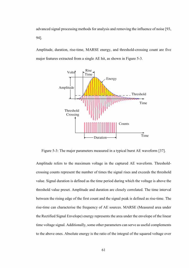
61

advanced signal processing methods for analysis and removing the influence of noise [93,

94].

Amplitude, duration, rise-time, MARSE energy, and threshold-crossing count are five

major features extracted from a single AE hit, as shown in Figure 5-3.

Figure 5-3: The major parameters measured in a typical burst AE waveform [37].

Amplitude refers to the maximum voltage in the captured AE waveform. Threshold-

crossing counts represent the number of times the signal rises and exceeds the threshold

value. Signal duration is defined as the time period during which the voltage is above the

threshold value preset. Amplitude and duration are closely correlated. The time interval

between the rising edge of the first count and the signal peak is defined as rise-time. The

rise-time can characterise the frequency of AE sources. MARSE (Measured area under

the Rectified Signal Envelope) energy represents the area under the envelope of the linear

time voltage signal. Additionally, some other parameters can serve as useful complements

to the above ones. Absolute energy is the ratio of the integral of the squared voltage over

62

the duration of one single AE hit to the reference resistance (1KSignal strength refers to

the measured area of the rectified signal and it is related to the MARSE energy). ASL

(average signal level) refers to the ratio of the integration of the absolute value of the

amplitude of a rectified signal to its duration. Average frequency (counts/duration),

initiation frequency and reverberation frequency are used to characterise the frequency of

different parts of the single AE hit. As its name suggests, the average frequency can reflect

the average frequency over the entire duration of an AE hit. Initiation frequency is the

average frequency during the period between the first threshold crossing and the signal

peak. Hence it can also be interpreted as the rise-time frequency. Reverberation frequency

is essentially represented as the average frequency during the period between the signal

peak and last threshold crossing and thus can be regarded as the ring down frequency.

The formulae to calculate the above frequencies are shown in Equation 5-1 through

Equation 5-3 [95]. Extra features can also be obtained by operation on two or more of the

above features, including division, multiplication. Trend of cumulative sum of certain

features like energy, count, etc. can give an indication of the condition

Average frequency =Counts

Duration (5-1)

Initiation frequency =𝐶𝑜𝑢𝑛𝑡𝑠 𝑡𝑜 𝑝𝑒𝑎𝑘

𝑅𝑖𝑠𝑒𝑡𝑖𝑚𝑒 (5-2)

Reveberation frequency =(𝐶𝑜𝑢𝑛𝑡𝑠−𝐶𝑜𝑢𝑛𝑡𝑠 𝑡𝑜 𝑝𝑒𝑎𝑘)

(𝐷𝑢𝑟𝑎𝑡𝑖𝑜𝑛−𝑅𝑖𝑠𝑒𝑡𝑖𝑚𝑒) (5-3)

It is very important to filter out any unwanted noises as much as possible during the data

acquisition process. For a hit-based AE system, which will be described later, it is

necessary to set an appropriate threshold prior to the tests. Any hits with amplitude lying

lower than the threshold will be discarded. To determine a hit, three key parameters are

employed which are set by the user, including the hit definition time (HDT), hit lockout

63

time (HLT) and peak definition time (PDT). HDT represents the maximum time between

the first and last threshold crossing and it can prevent the merging of two different hits

into one single hit. HLT specifies the time period during which the system is locked out

after a hit has been captured and before a new hit can be detected. If the HLT value is set

to be too low, then the reflections from the initially captured AE hit can also be logged.

If the HLT value is set to be too high, then the system may miss some important signals.

The PDT enables the correct determination of the signal peak and should be set as low as

possible, however, if it is set too low, true peaks may be not identified [89]. Another

important AE acquisition parameter is the sampling rate. If the sampling rate is set too

low as shown in Figure 5-4, the true frequency contained in the original data cannot be

revealed, which is known as aliasing as described in the Shannon theorem. The

continuous signals can be properly sampled only when the sampling rate is higher than

half of the maximum frequency contained in the original signal.

64

Figure 5-4:llustration of improper sampling [96].

There are two major methods to record and analyse AE signals. These are based on

parameter-based or signal-based AE approaches. For the parameter-based AE method, a

set of parameters rather than the original waveform is stored by the system. Post

processing and analysis are based on the recorded parameters. The major merit of

parameter-based technique is that it can save space and have higher data storing speed.

However, sometimes it can be misleading to use only some parameters for characterising

the actual signals. It is not easy to discriminate useful signals from noise and the

parameters are highly dependent on various factors such as geometry of the structure,

attenuation, etc. Statistical analysis focusing on the reduction of the influence of possible

noise sources have therefore to be utilised for post-processing. In comparison with

parameter-based approaches, the signal-based approaches enable more comprehensive

and reliable analysis but generate a vast larger amount of data which may or may not be

manageable. The signal-to- noise ratio can be visually evaluated from the captured

65

waveform. Moreover, the ratio can be significantly enhanced if some specific filtering

algorithms are applied, which can be of great help to assess the severity of damage in the

monitored structures accurately using AE. The limitation of the signal-based approaches

is that they require much more computational and storage capacity for the AE system due

to the larger amount of data generated and requiring processing and storage. The system

can crash or run out of space if its specification cannot meet the requirements. A solution

to this is to apply some triggering algorithms or take the measurement at a periodic

interval depending on the type of application [97].

Certain types of filters need to be used to reduce the effect of background noise on AE

signals, namely, low-pass, high-pass and band-pass filter. Traditionally, the way to apply

these filters are through the use of analogue filters. Nowadays, digital filters are becoming

increasingly popular due to the advantages they have. Digital filters are programmable

and more precise. Moreover, they are free from the influence of temperature,

manufacturing quality, etc. Finite impulse response and infinite impulse response filters

are the most commonly used types of digital filters. As the names indicate, FIR filter has

a finite response duration to the input signal，whereas that for IRF filter is infinite

because the feedback added by the filter itself. Essentially, digital filtering is a type of

calculation based on convolution technique and the number of source signal samples

determines the order of the filter [98].

5.3 AE propagation mode and attenuation

AE signals can propagate in four major wave types, including longitudinal, shear, surface

and Lamb or plate waves. If the source is internal to the structures and the sensors are

close enough to it, then both longitudinal and shear waves can be detected. However,

66

when there is some distance between the sources and sensors, the surface and plate waves

play a dominant role, as they are attenuated less than the other modes. It should be also

noted that the wave detected by the sensors are often the results of the overlap of different

modes and sources including the echoes and reverberation produced within the structures

[94]. The energy released by AE sources can be transmitted to the sensors by different

types of waves propagating through the solid depending on the shape of the medium and

the source-sensor distance. When P or longitudinal waves strike the surface at the second

critical angle, Rayleigh (Surface) waves can be generated. The attenuation loss of

Rayleigh waves is less, which can be very helpful if the waves have to propagate long

distances to reach the sensors. In plate-like structures, Lamb or plate waves dominate.

There are two main differences between Lamb waves and bulk waves. Firstly, Lamb

waves can travel in different types of modes, among which asymmetrical mode and

symmetrical mode are the most common ones. Secondly, Lamb wave tends to be

dispersive. The velocity is highly influenced by the frequencies and the thickness of the

medium. The limitation of the Lamb waves and Rayleigh waves is that it is very difficult

to derive the original form at the source based on the captured waves. Hence, the source

depth cannot be determined accurately [94, 99]. For wave propagation in rails, there is a

shift of frequency to lower components and this feature has been employed to detect break

or partial break in the rail as reported in [100].

5.4 The Kaiser effect

The severity of damage can sometimes be inferred based on the AE response from the

structure under different loading patterns. Normally, for a previously loaded structure,

during re-loading process AE signals will be emitted only when the load level exceeds

the previous maximum load level. This type of phenomenon was first investigated by

67

Joseph Kaiser and is known as the Kaiser effect to honour his contribution to this field of

science and engineering [101, 102]. The Kaiser effect can be explained based on the AE-

load curve displayed in Figure 5-5. Initially, as the load increases from A to B, the amount

of cumulative emission accumulates. During CB segment, no signals are generated, in

that the load level is lower than the level at point B. When the load at point B is exceeded,

the AE activity resumes and increases as the load rises again. It is noteworthy to indicate

that once the load is high enough (Point F), AE activities can be induced even the load is

lower than the previous maximum load (Point D). This phenomenon is termed as Felicity

effect. Felicity effect can be characterised by the Felicity ratio, which is defined as the

ratio of the load at which AE activities reappear to the previous maximum load. The

Felicity ratio can be regarded as a descriptive factor related to the extent to which the

Kaiser effect has been violated. The higher the Felicity ratio deviates from unity, the more

severe the damage in the monitored structure is [103].

68

.

Figure 5-5: The Kaiser and Felicity effects [104]

5.5 Crack propagation monitoring using AE

Sinclair, A. et al performed AE analysis during fatigue crack growth in three steels with

an ACEMAN system. The direct relationship between the event count (N) and the created

crack area (A) was established as follows:

𝑁 = 𝛾𝐴 (5-4)

where γ is a constant determined by material properties and test conditions. The equation

signifies that it is not the crack growth rate that determines the event count generated per

unit crack length. However, the crack growth rate or ΔK can influence the amplitude

spectra of the emissions. When ΔK increases to a greater value, a high energy emission

mechanism can be activated.

Felicity effect effect

Kaiser effect

69

Then they evaluated the possibility of three potential source mechanisms underlying AE

generation during fatigue crack growth. The expansion of the plastic zone ahead of the

crack tip was ruled out as the dominant source mechanism based on the measurements

and calculations. A combination of micro-fracture processes ahead of the crack tip and

crack closure unsticking are regarded as the main sources for AE generation, of which

micro-fracture happens near the maximum load and unsticking normally happens in the

earlier stage of the loading cycle [105].

Due to its sensitivity, the AE measurement can reveal the sub-stages of stable crack

growth process during which FCG rate satisfies the Paris-Erdogan law (Equation 3-3) that

can be hidden using conventional linear elastic fracture mechanics as reported in [106].It

has been reported that the AE activity deteriorates during stage IIb of the crack growth

test on austenitic stainless steel samples as a result of the reduced crack tip plastic zone

size under plane stress condition. Cumulative count and crack growth rates were plotted

against the stress intensity factor range on a log-log scale. A clear transition from IIa to

IIb can be identified in the cumulative count plot whilst the crack growth rate plot showed

a consistent trend. The relationship between the count rate and ΔK on a logarithmic scale

should be expected to show similar trend as that for cumulative count and ΔK .However ,

due to the sensitivity of AE to microstructure features, for other types of steel, like

pearlite steel, this trend may not be found [107].

The crack growth in pressure vessel steels has been monitored using both AE and direct

current potential drop techniques. The displacement ahead the crack tip was also recorded.

Three different types of compact tension (CT) samples in terms of the locations where

fatigue pre-crack were induced, namely, base material, weld material and heat affected

zone (HAZ) were used during tests for both 304L stainless and P265GH steels. The

70

microstructure of P265GH steel consists of ferrite and pearlite, whereas that of 304

stainless steel consists of austenite. AE sources during different stages of damage

evolution have been identified and the ability of different AE signatures to separate each

source mechanism was evaluated. More specifically, the maximum amplitude increases

as the damage develops from plastic deformation stage to stable crack growth stage. It

has also been shown that the value of maximum amplitude depends on not only the zone

of propagation but also the type of steel. Counts are an identifier of plastic deformation,

as the maximum count during plastic deformation is much smaller than that during other

stages of damage evolution [108].

Roberts, T. and M. Talebzadeh used AE to monitor the fatigue crack growth in steel,

welded steel CT and T-section girder test specimens. The AE signals generated from

crack extension were separated from those from other sources by using the source location

software in the system. The AE count rates during the top 100%, 10% and 5% of the load

range were plotted as a function of ΔK on a log-log scale. It showed that the count rate

for 10% and 5% of the whole load range had better correlations with the crack growth

rate than 100% of the load range and increased regularly with the cycle number. The

relationship between AE count rate and ΔK can be approximated as log-linear, which is

similar to the Paris-Erdogan equation. Hence theoretically it is possible to predict the

remaining life of a structure solely based on AE measurement [109].

Yu, J., et al., developed a model to correlate the absolute energy rate to the crack growth

rate during the fatigue test on CT steel specimen. They tried to remove the false emissions

completely through a combination of different methods. The waveforms generated from

friction and pencil lead break (PLB) were used as reference to filter out false emissions.

Then they employed a modified Swansong filter to further eliminate the friction signals

71

[110]. The principle behind Swansong II filter is that the duration of AE hits induced by

fatigue crack growth should be directly proportional to their amplitudes. For a hit caused

by friction or rubbing, the duration can be much higher than it should be if it is genuine

emission.

Aggelis et al. used different parameters in AE waveforms to characterise the change in

crack growth mode in aluminium specimens. When the crack growth changed from

tensile mode to shear mode, the duration and rise-time of AE events exhibited an increase.

Also the same happened to the the average frequency, but in a less obvious way. The

change is attributed to the shift from longitudinal wave to shear wave in term of the

dominant wave propagation type in the specimens, which is caused by the change in the

crack growth mode [111].

Bassim et al. investigated the capability of AE to detect the onset of fatigue crack growth

in four rail steels. Aside from AE acquisition, they also measured ΔK during four-point

bending fatigue tests. The results demonstrated that AE could detect crack growth as

small as 0.009 mm reliably and the fatigue stress intensity factor threshold was obtained

based on the AE measurement. Furthermore, they found that fatigue crack mostly initiated

near or in the inclusions in the rail steel samples using both optical and scanning electron

microscope [112].

The earliest investigation on the potential of AE to detect rail track defects can date back

to the research carried out by Kristoffer Bruzelius and D. Mba. They employed a test-rig

to simulate the contact between wheel and track. They compared the AE original signals

generated from the contacts between the rail wheel and track wheel with defects seeded

on the track wheel and no seeded defects. Due to the natural wear between the contact

72

surfaces, it was impossible to discriminate the signals from the defect and those from the

wear process. However, the number of AE bursts increase with time during a certain

length of time window, consistent with the observation that the wear for both the wheel

surface and track surface intensified with time. The observation of AE background

activity (mostly from wear) during the test have been shown to be highly dependent on

the load exerted on the track. It is noteworthy to mention that the material used during the

test was carbon steel which is not typical of the rail head in actual conditions. Moreover,

the rail head needs to go through a hardening process before being put into use, so the

wearing problem may not as severe as shown in their research [113].

Kostryzhev, et al. employed AE to detect the signals released during the three point

fatigue bending tests on pre-cracked and non-precracked R260 rail steel samples. They

found that in a noisy environment, hit waveform and power spectrum are better choices

to determine the onset of fatigue crack growth. Moreover, the peak frequencies for

different fracture modes in the power spectrum are different. For fully pearlitic steels, the

peak frequencies related to ductile fracture were observed to be smaller than 50 kHz,

whereas those for brittle fracture were above 200 kHz [114].

Korenska, M., et al. used AE sensors to record the signals induced by the train passage.

They compared the results from the loaded rail and those with the other unloaded rail

using count rate versus time curve and frequency spectral diagram. When the train passed

over the monitored section of the rail, the AE count increased continuously, in comparison

to the isolated increase for that recorded by the sensors mounted on the unloaded rail.

They used a high pass filter to remove a part of noise from the results. Moreover, they

found the amplitudes in the frequency spectrum for the unloaded rail are smaller than

those from the run-over (loaded) rail. From their experiments, it can be seen that not only

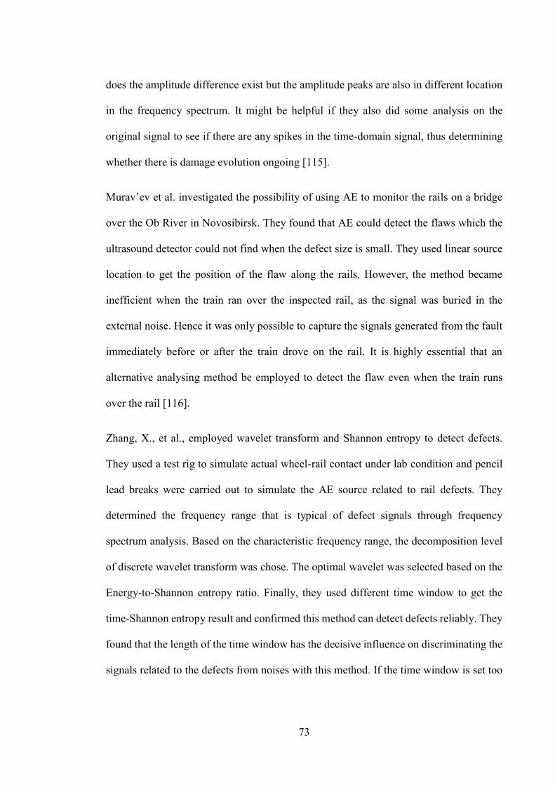
73

does the amplitude difference exist but the amplitude peaks are also in different location

in the frequency spectrum. It might be helpful if they also did some analysis on the

original signal to see if there are any spikes in the time-domain signal, thus determining

whether there is damage evolution ongoing [115].

Murav’ev et al. investigated the possibility of using AE to monitor the rails on a bridge

over the Ob River in Novosibirsk. They found that AE could detect the flaws which the

ultrasound detector could not find when the defect size is small. They used linear source

location to get the position of the flaw along the rails. However, the method became

inefficient when the train ran over the inspected rail, as the signal was buried in the

external noise. Hence it was only possible to capture the signals generated from the fault

immediately before or after the train drove on the rail. It is highly essential that an

alternative analysing method be employed to detect the flaw even when the train runs

over the rail [116].

Zhang, X., et al., employed wavelet transform and Shannon entropy to detect defects.

They used a test rig to simulate actual wheel-rail contact under lab condition and pencil

lead breaks were carried out to simulate the AE source related to rail defects. They

determined the frequency range that is typical of defect signals through frequency

spectrum analysis. Based on the characteristic frequency range, the decomposition level

of discrete wavelet transform was chose. The optimal wavelet was selected based on the

Energy-to-Shannon entropy ratio. Finally, they used different time window to get the

time-Shannon entropy result and confirmed this method can detect defects reliably. They

found that the length of the time window has the decisive influence on discriminating the

signals related to the defects from noises with this method. If the time window is set too

74

small, it will be extremely difficult to suppress the noise signals, however, if the window

is set too big, the time resolution of the signals will be greatly lowered [117].

5.6 Analysis of AE signals

Convolution is one of the most important theoretical basis for digital signal processing

and is the operation between two functions (x and g) as shown below:

(𝑥 ∗ 𝑔)(𝑡) ≝ ∫ 𝑥(𝜏)𝑔(𝑡 − 𝜏)𝑑𝜏

−∞

+∞

(5-5)

Although t is used in the equation, it need not represent the time domain. But in that

context, the convolution formula can be described as a weighted average of the function

x (τ) at the moment t where the weighting is given by g (–τ) simply shifted by amount t.

In linear system, convolution can be employed to show the relationship between the

impulse signal, the input signal and the output signal. It shows both how each sample in

the input signal contributes to the formation of the corresponding output signal and how

each sample in the output signal gets the contribution from the input signal.

5.6.1 Root mean square

Root mean square (RMS) is closely related to the energy of the signal. Given a set of n

samples {x1, x2, ⋯ , xn}, the RMS XRMS is :

𝑋𝑅𝑀𝑆 = √

1

𝑛(𝑥1

2 + 𝑥22 + ⋯ + 𝑥𝑛

2) (5-6)

A more efficient way to characterise RMS is to divide the signal into overlapping

segments and calculate the RMS in each segment. Balance should be made between

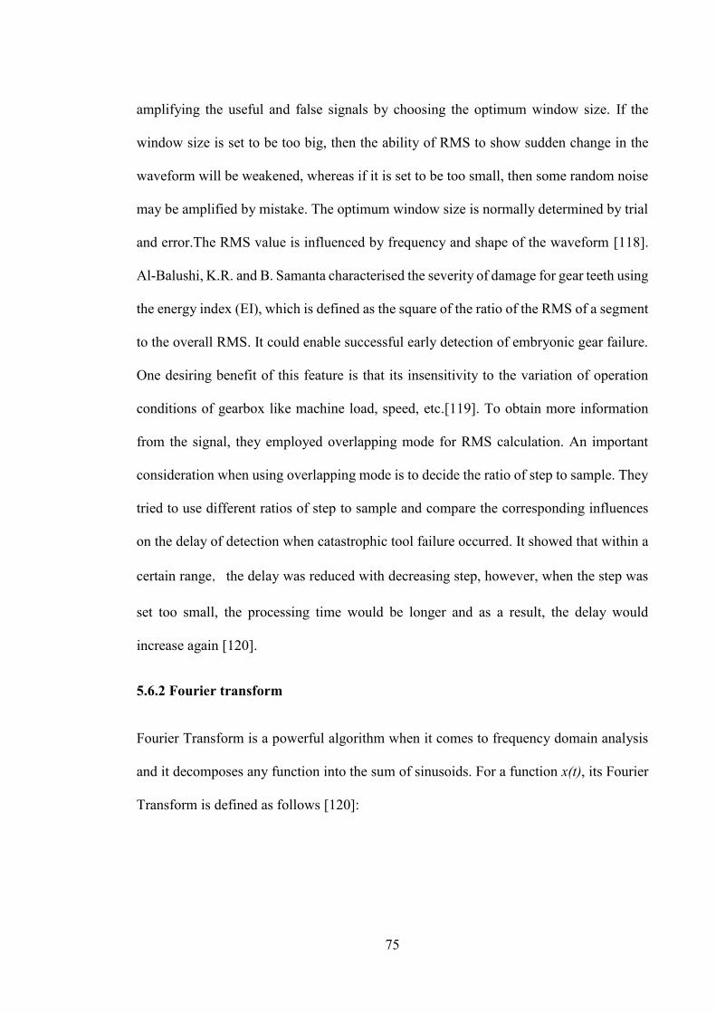
75

amplifying the useful and false signals by choosing the optimum window size. If the

window size is set to be too big, then the ability of RMS to show sudden change in the

waveform will be weakened, whereas if it is set to be too small, then some random noise

may be amplified by mistake. The optimum window size is normally determined by trial

and error.The RMS value is influenced by frequency and shape of the waveform [118].

Al-Balushi, K.R. and B. Samanta characterised the severity of damage for gear teeth using

the energy index (EI), which is defined as the square of the ratio of the RMS of a segment

to the overall RMS. It could enable successful early detection of embryonic gear failure.

One desiring benefit of this feature is that its insensitivity to the variation of operation

conditions of gearbox like machine load, speed, etc.[119]. To obtain more information

from the signal, they employed overlapping mode for RMS calculation. An important

consideration when using overlapping mode is to decide the ratio of step to sample. They

tried to use different ratios of step to sample and compare the corresponding influences

on the delay of detection when catastrophic tool failure occurred. It showed that within a

certain range，the delay was reduced with decreasing step, however, when the step was

set too small, the processing time would be longer and as a result, the delay would

increase again [120].

5.6.2 Fourier transform

Fourier Transform is a powerful algorithm when it comes to frequency domain analysis

and it decomposes any function into the sum of sinusoids. For a function x(t), its Fourier

Transform is defined as follows [120]:

76

𝑆(𝜔) = ∫ 𝑥(𝑡)exp (−𝑖𝜔𝑡

+∞

−∞

)𝑑𝑡 (5-7)

Actually, only a finite number of samples are employed to compute a discrete set of

frequency range, commonly known as Discrete Fourier transform (DFT).The output

frequencies are integer multiples of the fundamental frequency that is determined by the

sampling interval. Actually, DFT is the only type of Fourier Transform that a digital

computer is capable of performing. FFT is a fast algorithm to implement the DFT via a

computer. When performing FFT, the number of samples used in time domain ideally

should be a power of two [96]. One inherent limitation of FFT is that the variation of

frequency distribution with time cannot be obtained, as the time t in the exponential basis

exp(-iwt) cover the whole duration of the analysed signal [121]. If time frequency

information is also preferred，Short Time Fourier Transform or Wavelet Transform

should be used instead [122].However, in this case, uncertainty principles apply as shown

below:

∆𝑡∆𝑤 = 1/2 (5-8)

Another problem that can be commonly encountered when using the Fast Fourier

transform is spectral leakage. It is caused by the signal which is not time limited and

hence frequency spectrum can be smeared out. Harmonics caused by periodic loading

conditions can also be found in DFT, but their amplitudes are normally very small and

sometimes can even be neglected during analysis.

77

Short time Fourier transform is proposed initially to overcome the drawback of no time-

dependence information for FT. A window function is employed to multiply the original

signal and FT is then calculated in each chunk of samples determined by the window

function. The simplest window is the rectangular window and it replaces all but N values

in a data sequence with 0. The mathematical formulae for STFT are as follows:

𝑋(𝜏, 𝜔) ≜ ∫ 𝑥(𝑡)𝑤(𝑡 − 𝜏)𝑒−𝑗𝜔𝑡𝑑𝑡

+∞

−∞

(5-9)

Where w(t) is the window function, commonly a Hann window or Gaussian window

centered around zero, and x(t) is the signal to be transformed.

5.6.3 Crest factor

Crest factor is defined as the ratio of the peak amplitude to the RMS of the signal as

shown in Equation 5-10.

Crest factor =

𝑃𝑒𝑎𝑘 𝑎𝑚𝑝𝑙𝑖𝑡𝑢𝑑𝑒

𝑅𝑀𝑆 (5-10)

It can serve to identify abnormal spikes related to damage evolution in the signals and

normally high crest factor values indicate damage developing in the structure. As shown

in Figure 5-6，although the two current waveform has the same RMS value，their crest

factor values are obviously quite different, due to the differences in peak currents and this

is exactly what crest factor is capable to detect. However, one inherent limitation of crest

factor is its sensitivity to loading noise, as the increase in load will inevitably cause the

increase of RMS. If the increase in RMS is higher than that for the damage-related peak,

78

then a decrease in the Crest Factor value will be anticipated as reported in the previous

study [123].

Figure 5-6: Two current waveforms with the same RMS value yet different crest factors [124]

5.6.4 Power spectral density

Power spectral density (PSD) is a powerful tool to characterize the energy of the signal

at each frequency. The definition of PSD for x(t) is as shown in the following equation

[125].

𝑆𝑥(𝑓) = ∫ 𝐺𝑥(𝜏)𝑒𝑖2𝜋𝑓𝜏𝑑𝜏

+∞

−∞

(5-11)

Where Gx (τ) is the autocorrelation function of x(t).

Welch’s method, named after Peter D. Welch, is now commonly employed to estimate

the PSD. It has simpler computation and requires less storage space, thus making it more

79

easily implemented by the computers. The major steps consist of dividing the signal into

different sections with overlap, taking modified periodogram for each section and

calculating the average power spectral density [126].

5.6.5 Kurtosis and skewness

Kurtosis is defined as the ratio of the fourth central moment to the fourth power of

standard deviation.

𝛽2 =

𝑚4

𝑚22 =

1𝑛 ∑ (𝑥𝑖 − �̅� )4𝑛

1

(1𝑛

∑ (𝑥𝑖−�̅�)2𝑛1 )2

(5-12)

When using kurtosis, it is important to bear in mind that it reflects the combination of

peakedness and tailedness. The kurtosis value for normal distribution is 3 and depending

whether kurtosis is above 3 or not, the distribution can be described as either leptokurtic

or platykurtic as shown in Figure 5-7Figure 5-7. The leptokurtic distribution has

higher peaks and heavier tails, whereas platykurtic distribution has more flatten peaks and

lighter tails, in comparison to normal distribution [127].

Figure 5-7: Illustration of leptokurtic and platykurtic distribution [127]

80

Skewness is a useful parameter to characterize the asymmetry of a set of random values

relative to their mean value. The traditional formula to calculate skewness is as follows,

𝑆 =

𝑚3

𝑚23/2

=

1𝑛 ∑ (𝑥𝑖 − �̅� )3𝑛

1

[1𝑛 ∑ (𝑥𝑖 − �̅� )2𝑛

1 ]3/2

(5-13)

This is the so-called Fisher-Pearson coefficient of skewness and is used for the calculation

in the following analysis here.

Skewness and kurtosis have been employed to characterise the distribution moments of

RMS signal recorded during cutting and tool wearing experiments. It has been shown that

both parameters could effectively detect the condition change of contact between chip

and tool rake face. For catastrophic tool failure (CTF), it has been reported in previous

research that RMS is not sensitive enough to detect it when it happens, whereas skewness

and kurtosis can fit for the purpose. They assumed AERMS signal obeyed Beta distribution

and calculated the mean and deviation of the AERMS signal. Skewness and kurtosis were

then calculated based on the distribution parameters[128] [129].

In addition, it has been reported that higher order statistics including kurtosis could be

used to identify the arrival time of AE signals. The even statistic moments can show a

change even when the real signal is of similar intensity to background noise [129]. It

should be noted that the number of samples used to reveal the distribution characteristics

based on the above parameters should be guaranteed.

81

5.6.6 Spectral kurtosis

Spectral Kurtosis (SK) is a useful tool to characterise the transients and their location in

the frequency domain. It was first introduced by Dwyer as the normalised fourth moment

of real part of short time fourier transformation [130]. Later, C. Otonnello and S. Pagnan

modified the original definition and they defined SK as the fourth order moment of the

magnitude of STFT. Moreover, they found SK can be used to restore transient signals

corrupted by external stationary noises [131, 132].

Antonio provided a formalization of SK for conditionally non-stationary (CNS) process

and employed short time Fourier transform to develop an SK estimator. Equation 5-14

was proposed for calculating the SK:

𝐾𝑌(𝑓) =

𝑆4𝑌(𝑓)

𝑆2𝑌2 − 2

(5-14)

And 𝑆𝑛𝑌(𝑓) ≜< |𝑌𝑤(𝑡, 𝑓)|𝑛 > (5-15)

𝑌𝑤(𝑡, 𝑓) ≜ ∑ 𝑋(𝑛) ∗ 𝑊(𝑛 − 𝑡)𝑒−𝑗2𝜋𝑛𝑓

∞

−∞ (5-16)

Where Yw(t,f ) is estimated using STFT and X(n) is the selected part of the signal X(t)

using and W(n) is the window function which is zero-valued outside the chosen interval.

The principal of the algorithm is that through the calculation of the time average of

spectral moments at a certain frequency, transients if any that occur at a certain frequency

will contribute to a higher average of the moment. The most important parameter in

designing a SK estimator is the window size. If the window size is set too big, the SK

value will decrease very quickly after a certain limit is exceeded, whereas if it is set too

small, some bias will be induced. He introduced the concept of Kurtogram which is a map

82

showing the STFT-based SK values as a function of centre frequency and window size.

The centre frequency and window size corresponding to the maximum SK values are used

as the optimal parameters to design a band-pass filter. The optimal band-pass filter

determined by the method has two major characteristics. Firstly, the maximum SK can be

determined by the centre frequency. Secondly, the window size is obtained by striking a

balance between the signal-to-noise ratio and the impulse-like nature of the filtered

signals [133].

Eftekharnejad et al. employed an SK-based technique to analyse the signals generated

from the naturally degraded rolling bearings. They designed the band pass filter based on

the centre frequency and window size (bandwidth) at which the spectral kurtosis reached

the peak. They found that the Crest Factor value for the filtered signal showed an obvious

increase in comparison with the original signal, suggesting that SK based filter can

effectively demonstrate spikes among the noises [134, 135]. Sawalhi and Randall

investigated the optimum window size for SK during their research. They found that if

the window size is too small，the frequency resolution will be decreased greatly, whereas

if it is too big, the SK values will be reduced compared with those obtained from a normal

window size [136].

83

Chapter 6:

Experimental Methodology

84

: EXPERIMENTAL METHODOLOGY

Experiments were carried out on R260 grade rail steel samples cut off from rails obtained

with the help of Network Rail. Cast manganese steel samples were cut off using plasma

cutting from a 10 mm thick plate procured from West York Steel. Some reference testing

was carried out on a carbon steel sample. Various tests were carried out including

metallographic evaluation, Charpy testing and fatigue testing in conjunction with the use

of acoustic emission monitoring. This chapter describes the experimental configuration

and parameters employed.

6.1 Metallography

Samples of Size 10*10*10 were cut off and mounted on Bakelite. The samples were

ground to 1200 grit and then mirror polished to 1µm before using 2% nital to etch the

surface of the samples for microscopy. Microscopy was performed using a Karl Zeiss

optical microscope. Metallographic analysis of the R260 samples revealed a

predominantly pearlitic microstructure as expected (Figure 6-1). Some pro-eutectoid

ferrite (~1%) was observed in the pearlite colony grain boundaries. The microstructure of

the cast manganese steel was found to consist of an austenitic microstructure with

equiaxed grains as shown in Figure 6-1. The size of the austenite grains was found to be

in the range of ~20μm. Some carbide inclusions could also be observed.

85

a)

b)

Figure 6-1: the microstructure of a) Hadfield steel b) R260 steel

Five Charpy V-notch Hadfield steel specimens were prepared and tested. The specimens

had standard dimensions of 10 x 10 x 55 mm (height x width x length) containing a

86

standard notch of depth 2.5 mm and 0.25 mm notch radius. A Charpy impact machine

was used with a 298 J capability. Tests were conducted at -20°C (samples were chilled in

a bath of ethanol and liquid nitrogen, the ratio is adjusted to meet the temperature

requirements). The results of the tests are given in table. The Charpy test results for R260

steel specimens with the same size at the same temperature were reported in [137] and

the average absorbed energy for R260 steel is 6 Joule. It can be inferred that Hadfield

steel is more ductile than R260 steel even at room temperature, as austenite steel does not

show fracture change behaviour with temperature.

Table 6-1: Summary of the Charpy impact tests carried out at -20℃

Temperature/℃ Impact Energy /Joule

-19 45

-19 46

-20 39

-20 42

-22 44

87

6.2 AE measurement

A customised AE system developed by the researchers from the University of

Birmingham and Krestos Limited and the commercial AE system procured from Physical

Acoustic Corporation (PAC) were employed to capture the AE signals generated during

the tests.

For the commercial system, the data was captured using the PAC AEwin v2 software

package. The sampling rate in all cases was set at 2MS/s. The detailed information

regarding the type of sensors, filters will be introduced separately. The threshold during

the data acquisition with commercial system was set as 40dB in most cases apart from

the one for test on non-precracked R260 steel samples 5 which had been extracted from

the used rail section. The PDT, HDT and HLT were set at 300µs, 800 µs and 800µs,

respectively. For sample 5, due to the noisier testing configuration arising from the more

rapid cyclic loading (10 Hz), the filtering range employed was set slightly higher at 200–

1000 kHz.

The operation of the customised acoustic emission system is slightly different to that of

the PAC system. The PAC acoustic emission system monitors acoustic emission activity

and then deletes the complete waveform keeping only the data related to the definition of

an acoustic emission hit as defined by the user, whereas the customized system can

capture the original waveform during the test. The duration and frequency of the AE data

acquisition were set before the measurement. The customised AE system uses Agilent

2531A 2 MSamples/s data acquisition cards with decoupling box whilst the logging and

signal processing software is written in Matlab. The data acquisition card also support

multi channels mode if lower sampling rate is used. It is connected to the computer via a

Universal Serial Bus cable. The amplifiers and pre-amplifiers were purchased from PAC.

88

All the connections were done with BNC cables. The integrated analysis package and

data logger developed by UoB using Matlab is as shown in figure. Due to the large amount

of data generated the recording cannot be maintained indefinitely since the system will

crash due to the high sampling rate (at least 1 MS/s) or the hard disk will run out of free

space.

There are two types of sensors, namely single-ended sensor and differential sensor.

Differential sensors have better immunity to electromagnetic interference and ground

loop currents. For most applications, the single-ended sensors are preferred due to their

low cost and acceptable low amplitude noise [138].

The sensitivity of AE sensor, S, which is dependent on the frequency of input sinusoidal

motion, is characterized by the ratio of output voltage amplitude to input motion

amplitude. The units for input motion amplitude can be displacement, velocity (m/s) or

pressure (µBar).

AE sensor calibration curves are used to show how sensor sensitivity change with

frequency. The X axis is the frequency of the input sinusoidal motion and Y axis is the

sensitivity labelled in decibels relative to a reference value at the corresponding frequency

as shown in equation below.

dB = 20log (𝑆 𝑆𝑓⁄ ) (6-1)

S is the sensitivity of AE sensor in V/µBar or V/ (m/s) and Sf is the corresponding

reference value 1V/µBar or 1V/ (m/s). During this project, two types of AE sensors have

been used, namely wideband differential sensor and R50a sensor. Wideband sensor has a

good frequency response over the range of 100-900 kHz. It is ideally suitable for high

89

bandwidth of frequency analysis for source mechanisms identification and noise

elimination. It can provide good reproduction of original source wave motion[139]. Low

cost general purpose sensor can then be selected based on the frequency information

obtained from wideband sensors. R50a is a narrow band resonant sensor with high

sensitivity and an operating frequency range of 150-700 kHz [140].

The calibration curves for Wideband sensor and R50α sensor are shown in Figure 6-2

a)

90

b)

Figure 6-2: AE sensor calibration curves for a) Wideband sensor b) R50α sensor [139,

140]

The good acoustic contact of AE sensors with the surface of the monitored structure is of

utmost importance .The couplant should be used to remove roughness effects as well the

presence of air pockets between the contact surfaces as the acoustic impedance of air is

much lower than that of the sensor wear plate and steel. The couplants available include,

1) Liquid. The advantages of liquid couplants such as water are that they are

straightforward to apply and can drive away the air between the sensor and

material surface easily. However, due to low viscosity, they are not suitable for

vertical mounting and long-period usage, as this can result in dripping and drying

up of the couplant layers.

91

2) Gel. Gel couplants have higher viscosity and acoustic impedance than liquid

counterparts, thus making them more suitable for rough surfaces. Vertical

mounting is acceptable for gel couplants, as They are less likely to drip than liquid

couplants.The common used gel couplants include:Vaseline, glycerine, ultrasonic

gel, etc. Clamping fixtures are needed when using both gel and liquid couplants.

The gel couplants around the edge of AE sensors can dry up after a few hours,

making them not suitable for long-period application.

3) Grease. Grease has much higher viscosity than both liquid and gel couplants.

Hence it is well suited for rough surfaces. If applied properly, it can provide better

stability compared with liquid and gel couplants. However, it is difficult to clean

the surface afterwards, especially for silicon based greases.

4) Adhesive. Adhesive couplants such as Araldite and superglue are preferred if AE

sensors needs to be kept in place for a relatively long period of time and optimum

coupling stability is needed. Two types of adhesive couplants are commonly used

for AE, namely silicon rubber compound and rigid bond. In case of occurrence of

surface vibration or movement, Rubber compound can offers excellent

stability.For rigid bond, it can offer the best transmission of both longitudinal and

shear displacement if mounted properly [141].

Apart from the above mentioned couplants, other types of couplants are also available to

meet specific requirements such as when high temperature applications are involved. For

the common couplants used for AE application, please refer to the table in [141]. The

couplants used for this project are Vaseline and Araldite® .Before mounting the sensor, it

is crucial that the material surface is as smooth and flat as possible to maximize the effect

of couplant,as air trapped in the layers under the surface won’t be driven away by the

92

couplants [142]. Sensor mounting fixtures like magnetic holders or adhesive tapes should

be used for non-adhesive couplants to keep the sensors’ position and applied force

constant. The coupling layer between the sensor and material surface should be as thin

as possible and one common practice to achieve that, which has been employed in this

project, is to apply a small amount of couplant in the middle of sensor surface and push

the sensor down against the material surface with a consistent force to let the couplant

extend in a circle until no more couplants emerge from the edge of the sensor surface.

The preamplifier is used to increase the strength of the input signal and decrease the

influence of electromagnetic noise generated along the cables during the signal

transmission between the sensor and the instrument. Moreover, it can convert a high

impedance signal into a low impedance signal which is suitable for long cable

transmission. Preamplifiers can be either integrated with AE sensor or serve as a separated

unit. The advantage of preamplifiers integrated with AE sensor is the compact design and

the improved signal-to -noise ratio thanks to the minimal signal loss between the sensor

and preamplifier. Sensors without integral preamplifier are lighter and smaller and

preferred when the space for sensor deployment is limited. The PAC preamplifier used in

this study provides a 20/40/60 dB switch selectable gain and it is powered via the output

signal BNC cable. It can be connected to both single-ended and differential sensor. The

PAC pre-amplifier also incorporates filters to decrease the interference of low frequency

mechanical noise.

Before the test, it is very important to use a pencil lead break，also referred to as Hsu-

Nielsen source, as an artificial acoustic source to check the acoustic coupling quality

93

between the sensor and the surface of the test-piece by pressing the pencil lead firmly

against the surface of the structure until the lead breaks as shown in Figure 6-3 .

Figure 6-3: Hsu-Nielsen source [143]

6.3 Fatigue testing

Bending fatigue crack growth tests were carried out on three different specimens: R260

grade rail steel notched samples, cast manganese steel notched samples, and one carbon

steel sample with no notch used as reference. The fatigue loading conditions under which

tests were carried out included various loading frequencies ranging from 1Hz and up to

~100 Hz. The bending fatigue configuration employed in the tests is partially

representative of the loading conditions that the rails and crossings are subjected to. The

specimen used for fatigue testing can be seen in the schematic of Figure 6-4.

94

a)

b)

Figure 6-4:a) schematic diagram to show the dimensions of the samples used for fatigue

tests [144] b) example of the dimension of one R260 rail steel sample cut off the rail

95

Before the low frequency fatigue testing was performed, all samples except the reference

carbon steel sample were pre-cracked using an Amsler 20KN Vibrophore electro-

mechanical high frequency fatigue machine. The pre-cracking length was monitored by

observation of the microscopy replicas of the notch tip field. If the stress at the notch tip

is higher than the yield strength, a plastic zone will form ahead of the notch and upon

unloading, the compressive residual stress will remain in the plastic zone. The residual

stress relaxation may occur in the following crack growth test, which can be captured by

AE [145-148]. A DARTEC 50kN servo-hydraulic universal test machine was used for

the low frequency fatigue testing. The loading frequency was set at 1Hz and 10Hz for one

rail steel sample in each case.

For the high frequency tests, Notched samples with and without pre-crack made were

tested on An Amsler 20KN Vibrophore electro-mechanical high frequency fatigue

machines. A carbon steel reference sample with no notch or pre-crack was also tested for

comparison purpose. For samples with no pre-crack, it was expected that the AE activity

during stage I, II, and III of crack growth could all be recorded. The loading ratio was set

to R = 0.1 for all samples. Sinusoidal loading pattern was used during the tests.

The crack length was monitored using the Direct Current Potential Drop (DCPD)

technique for all tested samples. DCPD is based on the principle that the resistance of the

material will increase with decreasing size of cross section resulting from a fatigue crack

growing. Base on Ohm’s Law, the output voltage (V) across the cracked test piece will

increase under constant input current. The crack length α can be obtained by comparing

the actual voltage reading with a reference voltage measured from another area of the test

piece which is not affected by crack growth behaviour and using appropriate calibration

96

curves. The output voltage is normally in the range of 0.1 to 50 mv for common current

(from 5 to 50A), sample configuration and materials.

Constant current is input through two clips into the specimen. Two voltage probes across

the notch will then measure the voltage. The crack length increase can be reflected by the

pen traces on the chart recorder. The crack growth rate was calculated based on the secant

method as described in the British standard [144].Figure 6-5 shows the general laboratory

setup employed in this study.

Figure 6-5: Experimental setup for the fatigue crack growth tests

6.4 Field trials

Field trials were carried out on two different crossings on the west coast mainline. The

crossings are 2561A points (near Wembley Stadium - direction to Birmingham) and on

Chiltern rail line (near Hatton Railway Station - direction to Birmingham), which are both

97

used by passenger and freight trains. The large impact load which can be induced when

the rolling stock move from wing rail to crossing nose makes the crossing nose the most

likely area for crack to initiate and propagate, hence AE sensors were attached to both

sides of crossing nose during the field trials.

The Wembley crossing was proved to healthy using visual inspection, whereas for Hatton

crossings, surface damages (cracking and lipping) are obvious. The maximum allowable

train speed for both crossings is 100 MPH. The sensors was attached to the crossings

using araldite, as it can provide long term adhesion as well as good electrical insulation

required. Araldite is two-component epoxy adhesive which is easy to handle and can

enable the installation of sensors within a few minutes. Moreover, it can enable good

transmissibility of stress waves caused by growing defect due to the external loading. The

analysis of field data is based on correlation analysis. The customized AE system was

temporarily installed on-site to monitor the crossings with no trigger system used. The

system was triggered manually once the rolling stock approached the instrumented area.

The Photographs in Figure 6-6 show the measurement setup at Wembley crossing.

98

a)

b

99

c)

d)

Figure 6-6: photographs show a) AE measurement equipment b) indicative rolling stock

c)instrumented crossing location d) sensor location for field trial near Wembley station.

100

Chapter 7:

Results and Discussion

101

: RESULTS AND DISCUSSION

7.1 Low frequency fatigue tests

7.1.1 Introduction

The R260 rail steel samples numbered 1 to 4 with size 120mm*20mm*10mm and notch

depth 8mm were pre-cracked to an initial length of 9.5mm,10.0mm,10.8mm and 9.5mm,

respectively. The maximum load for samples 1 through 4 was set at 3.5kN. Another R260

rail steel sample, numbered as 5, was extracted from the web of a used rail section

removed from the UK rail network. This sample had the same geometrical dimensions as

the other four rail samples but the notch depth was kept to only 2mm with a 30 angle. It

was also pre-cracked using the Vibophore fatigue machine to an initial crack length of 3

mm. The maximum load in this case was set at 9kN. All the above five samples were

monitored using the PAC AE system during the bending fatigue tests. A second set of

R260 rail steel samples with notch depth 8mm and angle 60° was also tested to evaluate

the complete waveform using an R50a sensor connected to the customised AE system.

The maximum load was also set at 3.5kN. Figure 7-1 shows a R260 rail steel sample after

the final failure occurs.

102

Figure 7-1 : Photograph showing a close-up of failed R260 rail steel sample

Hadfield steel samples numbered 1 to 4 with the same configuration as R260 rail steel

sample 1 through 4 were pre-cracked to initial crack lengths 10.3mm,10.2mm, 10.9mm

and 10.4mm.The maximum load was set at 3 kN.

Two PAC pico wideband AE piezoelectric transducers with a bandwidth range between

150 and 750 kHz were used to monitor the AE activity during fatigue testing of the R260

rail steel samples 1 through 4. The pico AE sensors were coupled to the surface of the

sample using vaseline and held in place with duct tape. A band pass signal filter with a

range of 100-1000 kHz was employed to reduce the effect of mechanical noise during the

testing. For sample 5 and 6, R50a resonant AE sensors procured from PAC were used

instead.

103

For the Hadfield steel samples, two PAC R50a sensors with an operating frequency range

of 100-700 kHz were employed. One sensor was connected to the commercial PAC AE

system and the other was connected to the customized system during testing. A 100 kHz

high-pass filter was used to filter out loading-related noise in this case. The sampling rate

for the customized system was set at 1 MSample/s.

The threshold during the data acquisition with commercial AE system was set as 40 dB

in all cases apart from the one for test on R260 steel sample 5 which had been extracted

from the used rail section. The PDT, HDT and HLT were set at 300 µs, 800 µs and 800

µs, respectively. For sample 5, due to the noisier testing configuration arising from the

more rapid cyclic loading (10 Hz), the filtering range employed was set slightly higher at

200–1000 kHz. Also the amplitude threshold was set at 55 dB. The sampling rate in all

cases was set at 2 MSample/s.

7.1.2 Analysis of AE signals captured from commercial system

Figure 7-11 shows the correlation of different AE parameters with crack length during

low frequency bending fatigue tests on both the R260 rail steel and Hadfield steel

samples. As it can be seen, both the average amplitude and duration increase with fatigue

cycles, signifying the deteriorating structural integrity of the samples with increasing

crack depth. It should be noted that the AE activity reduces after the initial relatively

intense activity. This is attributed to the fact that the crack growth at the initial stages of

the test is not stable and this is reflected in the increased AE activity recorded. The

instability may be partly because of the influence of notch tip plasticity. However, as the

test progresses the crack growth rate becomes more stable, resulting in reduced AE

activity until the crack growth rate increases sufficiently again to give rise to higher

energy AE signals. The initial instability due to the very small increments of crack growth

104

occurring cannot be detect by the DCPD instrument as exceeds its measuring sensitivity.

It is also interesting that before the final failure of the specimens, all the four Hadfield

samples show a substantial increase in AE activity, signifying the imminent failure.

The performance of each parameter in terms of their ability to describe the severity of

damage is evaluated as follows.

Figure 7-2 shows the correlation of amplitude with crack length during low frequency

three-point bending fatigue tests on both R260 rail steel and Hadfield steel samples. The

threshold set was set at 40 dB for both types of samples. The amplitude for most of AE

signals captured for ferritic, ferritopearlitic, martensitic and bainitic steel samples under

the same loading condition is smaller than 70 dB as reported in [149]. For the R260 steel

samples tested, the captured AE signals with amplitude above 70 dB occur even during

stable crack propagation and this is attributed to brittle cleavage fracture causing high

energy AE signals to be emitted [150]. The distributions of the highest amplitude AE

signals captured during the tests carried out on R260 and Hadfield steel samples are

different. For the Hadfield steel samples, most of the AE signals with high amplitude

(>60dB) occur during the final stage of damage evolution. This is attributed to the gradual

work hardening of the Hadfield samples resulting into a gradually evolving more brittle

fracture as the material is work-hardened further. For the R260 steel samples the

distribution of high amplitude AE events are more scattered throughout the tests. This is

related to a constant pattern of brittle cleavage fracture during crack evolution as reported

in [150].The highest amplitude during the tests for all Hadfield samples is smaller than

that for R260 steel due to plasticity at the crack tip causing lower levels of AE energy to

be emitted.

105

As mentioned before, the microstructure of Hadfield steel is austenitic. Hence, Hadfield

steel has a FCC crystal structure. FCC crystal lattices have a large number of slip systems

for dislocations to be able to move. Moreover, the Fe atoms are more closely packed in

FCC structure, making the cleavage fracture less likely to happen during the crack

evolution process in comparison to R260 steel. That partially explains why high

amplitude or energy AE signals did not occur during the stable crack propagation process

for the Hadfield steel samples but activity picked up during the latter stages due to the

increasing hardness of the material due to work-hardening. At the later stage of the tests

for Hadfield sample, the highest amplitude values show a close to exponential increase

until final failure occurs. For the R260 steel samples, all of them exhibited a sudden jump

in crack growth at a certain stage before final failure. This is attributed to larger areas in

the samples fractured surface exhibiting cleavage and thus giving rise to higher AE energy

to be emitted at these particular instances. This is shown in Figure 7-2(a) to Figure 7-2(d)

indicating an increase in AE activity successfully being captured during sudden increases

in crack growth rate as indicated by the arrows. The reason behind cleavage fracture of

larger areas is likely related to inclusion present in the path of the growing crack resulting

in a larger area to fracture before the crack slows down. Another possibility could be

related to the presence of favourable residual stresses resulting in high stresses locally

and hence a larger area to fracture.

106

a)

b)

107

c)

d)

108

e)

f)

109

g)

h)

Figure 7-2：AE signal amplitude in dB versus number of fatigue cycles with crack

growth in mm for R260 rail steel a) sample 1, b) sample 2, c) sample 3, d) sample 4,

and Hadfield steel e) sample 1, f ) sample 2, g) sample 3, h) sample 4.

Figure 7-3 shows the correlation between count and crack length for all the samples. For

110

the R260 steel samples, the temporary increase in crack growth rate is consistent with the

amplitude and the counts recorded in the AE signals captured. Moreover, the amplitude

of all captured AE events with count value above 250 is higher than 70 dB. For the

Hadfield samples, at the later stage of stable crack growth, indications of imminent failure

can be clearly observed due to the higher AE activity recorded. Both hit number and hit

counts clearly increase in comparison with the initial stages of damage evolution in the

samples being tested. Some events with obviously higher count values than others and

highlighted in red can also be observed. These AE events can be used as an indicator and

hence alarm for the impending final failure. Some of these AE events cannot be discerned

clearly just by evaluating amplitude-crack length plots. This is due to the fact that other

events with similar high amplitude level can also occur at other stages of damage

evolution.

111

a)

b)

112

c)

d)

113

e)

f)

114

g)

h)

Figure 7-3: AE signal count versus number of fatigue cycles with crack growth in mm

for R260 rail steel a) sample 1, b) sample 2, c) sample 3, d) sample 4, and Hadfield

steel e) sample 1, f ) sample 2, g) sample 3, h) sample 4.

115

Figure 7-4 shows the correlation of the calculated AE count rate with crack growth rate

and ΔK for the R260 and Hadfield steel samples in logarithmic scale. The count rate is

defined as the ratio of the sum of counts of all AE hits to the time interval during which

these AE hits are captured. For the R260 steel samples, the count rate shows a similar

trend to the crack growth rate for every sample, although the variation between different

samples is higher than that for crack growth rate. For the Hadfield steel samples, the

correlation between count rate and crack growth rate is poor when ΔK is below

30MPam1/2 as indicated by the blue dashed line and the better correlation can be seen

when ΔK is above 30MPam1/2 .This is very likely due to the plasticity effect at earlier

stages and the evolution to cleavage fracture as the material gets harder due to work

hardening during fatigue loading (bending). Obviously more AE energy will be released

when the crack propagates through a more brittle area as more elastic energy will be

released and subsequently captured by the AE sensors mounted on the samples. This does

not occur in the R260 rail samples which behave more consistently in terms of their

hardness throughout the tests with little work hardening occurring in comparison with the

Hadfield samples. It should be noted that the count rate was calculated using the same

method as for the crack growth rate so there is direct relationship with the Paris-Erdogan

law.

116

a)

b)

Figure 7-4: Count rate and crack growth rate with ΔK for all a) rail steel and b) Hadfield

steel samples in logarithmic scale.

117

Figure 7-5 shows the correlation between duration and crack length for all the samples.

The AE events with the highest duration occur during the final stage of the fatigue crack

growth tests. For Hadfield steel samples, most of AE events recorded during stable crack

propagation have duration below 2000 s, whereas for R260 steel samples, intermittent

occurrence of AE events with duration above 2000 s can be seen. For R260 steel samples,

the amplitudes of all signals with duration above 2000 s are above 60 dB during stable

crack propagation as shown in Figure 7-6(a).The only few AE hits with duration above

2000 s and amplitude smaller than 60 dB are those which occur during the final stage of

crack growth and prior to final failure. The AE signal duration (above 2000 s) exhibits

a quasi-linear relationship with amplitude for R260 steel. However, for Hadfield steel

samples, the distribution of amplitude versus duration is more scattered as shown in

Figure 7-6(b). This is attributed to the fact that Hadfield steel is more ductile than R260

steel at the initial stages at least of the test, progressively becoming harder as work

hardening effects increase. Figure 7-7 shows the correlation between the duration rate and

crack growth rate with ∆K in logarithmic scale. The duration rate exhibits similar trends

with the crack growth rate for all the samples.

118

a)

b)

119

c)

d)

120

e)

f)

121

g)

h)

Figure 7-5: AE signal duration in μs versus number of fatigue cycles with crack

growth in mm for rail steel a) sample 1 b) sample 2 c) sample 3 d) sample 4 and

Hadfield steel e)sample 1 f ) sample 2 g) sample 3 h) sample 4

122

a)

b)

Figure 7-6 : Correlation between amplitude and duration for a) R260 rail steel samples

b) Hadfield steel samples

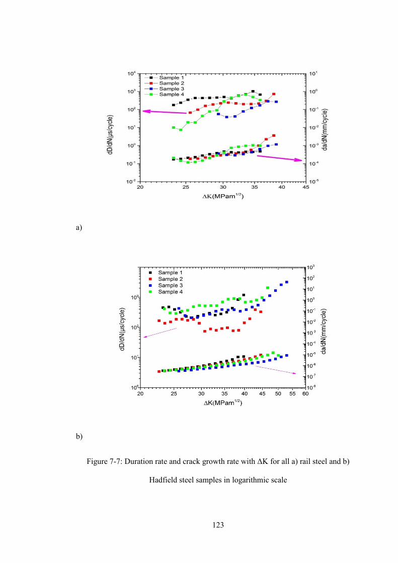
123

a)

b)

Figure 7-7: Duration rate and crack growth rate with ΔK for all a) rail steel and b)

Hadfield steel samples in logarithmic scale

124

Figure 7-8 shows the plots for energy with crack length and time for each of the samples

tested. AE hits with high energy above 2000 (10µVolt-sec/count) were captured for rail

steel samples during damage evolution. The high energy hits are also those exhibiting

high amplitude (99 dB) which were shown previously. For the Hadfield steel samples,

the energy values are shown in logarithmic scale for better resolution. The AE hits with

the highest energy values occurs at the final stage. This is in line with the behaviour of

this material as it gets gradually harder and hence more brittle with work hardening taking

place. The number of AE hits with energy above 10 (10µVolt-sec/count) exhibits an

obvious increase at a point before final failure. The AE hits with obviously higher energy

can be observed in the plot indicating that the final failure is imminent. The energy rates

were calculated and then the variation of the energy rate with time was compared with

that of crack growth rate. The energy rate was calculated in the same way as crack growth

rate. Hence, the relationship between energy rate and ΔK can be described as follows

[31, 110],

dE

dN= B ΔK𝑝 (7-1)

or

log (

dE

dN) = logB + 𝑝logΔK (7-2)

The plots in Figure 7-9 show the crack growth rate with energy rate and ΔK in logarithmic

scale for every sample. As it can be seen, the energy rate for Hadfield steel samples show

a “trough-like” (decreasing and then increasing) trend. Generally, the energy rate for both

types of materials does reflect the crack growth rate trend. However, Hadfield steel shows

a more stable trend in comparison with that for R260 steel especially at the end of stage

125

II or the Paris-Erdogan regime. The fitting values for all the parameters are summarised

in Table 7-1 and Table 7-2. For the R260 steel samples, the intermittent occurrence of

cleavage fracture corresponds precisely to the high energy AE hits, which has been shown

in [151].

It has been reported that Hadfield steel and other high Mn manganese steel show a ductile

crack growth behaviour [17, 18]. However, as work hardening progresses, ductility will

be noticeably reduced resulting in more cleavage to occur. More specifically, the Hadfield

steel samples exhibit a quasi-cleavage fracture which is the dominant fracture mode

during high cycle fatigue (HCF). This fracture mode is in agreement with the relatively

low energy rate in comparison with that observed for pearlitic rail steel samples. The

lower crack growth rate is consistent with plasticity occurring ahead of the crack tip and

work hardening [17].

126

a)

b)

127

c)

d)

128

e)

f)

129

g)

h)

Figure 7-8:AE signal energy with number of fatigue cycles with crack growth in mm for

rail steel a) sample 1, b) sample ,2 c) sample 3, d) sample 4, and Hadfield steel e)

sample 1, f ) sample 2, g) sample 3, h) sample 4.

130

a)

b)

Figure 7-9:Plot showing the Energy rate and crack growth rate with ΔK for all a) rail

steel and b) Hadfield steel samples in logarithmic scale

131

Table 7-1: Fitting parameters of crack growth rate and AE constants for R260 rail steel

samples

m C p B

1 4.88 2E-11 5.45 7E-8

2 2.56 6E-8 4.29 8E-6

3 6.65 5E-14 7.23 3E-10

4 5.83 1E-12 12.1 2E-18

Table 7-2: Fitting parameters of crack growth rate and AE constants for Hadfield steel

samples

M C p B

1 5.79 5E-12 0.94 8E-02

2 4.80 8E-11 0.69 8E-02

3 3.67 2E-09 2.36 4E-04

4 4.58 1E-10 1.27 5E-02

Figure 7-10 shows the plots for risetime with crack length and time for each of the

samples tested. For the R260 rail steel samples only a few AE events with a rise time

above 1000 µs occur before the final stage prior to failure. However, nearer to final failure,

a higher number of AE events with higher rise time are captured. However, most of high

amplitude (>=70 dB) AE events related to brittle cleavage fracture tend to have rise time

smaller than 200 µs., Therefore, it is difficult to detect brittle crack growth based on this

parameter. However, the number of hits with high rise time for Hadfield steel samples is

obviously higher indicating the different behaviour in crack propagation in this material

132

in comparison with pearlitic rail steel. This is actually in agreement with the behaviour

expected due to plasticity in front of the crack tip.

a)

b)

133

c)

d)

134

e)

f)

10

10.5

11

11.5

12

12.5

13

13.5

14

0.00E+00

1.00E+03

2.00E+03

3.00E+03

4.00E+03

5.00E+03

6.00E+03

7.00E+03

8.00E+03

0 1000 2000 3000 4000 5000

Cra

ck le

ngt

h(m

m)

Ris

eti

me

(µs

)

Fatigue cycles

Risetime

Crack length

135

g)

h)

Figure 7-10: AE signal risetime with number of fatigue cycles with crack growth in mm

for rail steel a) sample 1, b) sample ,2 c) sample 3, d) sample 4, and Hadfield steel e)

sample 1, f ) sample 2, g) sample 3, h) sample 4.

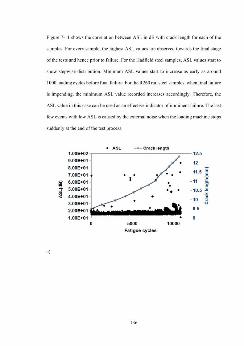
136

Figure 7-11 shows the correlation between ASL in dB with crack length for each of the

samples. For every sample, the highest ASL values are observed towards the final stage

of the tests and hence prior to failure. For the Hadfield steel samples, ASL values start to

show stepwise distribution. Minimum ASL values start to increase as early as around

1000 loading cycles before final failure. For the R260 rail steel samples, when final failure

is impending, the minimum ASL value recorded increases accordingly. Therefore, the

ASL value in this case can be used as an effective indicator of imminent failure. The last

few events with low ASL is caused by the external noise when the loading machine stops

suddenly at the end of the test process.

a)

137

b)

c)

138

d)

e)

139

f)

g)

140

h)

Figure 7-11: AE ASL with number of fatigue cycles with crack growth in mm for rail

steel a) sample 1, b) sample ,2 c) sample 3, d) sample 4, and Hadfield steel e) sample 1,

f ) sample 2, g) sample 3, h) sample 4.

One additional R260 steel sample cut from the used rail section was tested in three-point

bending fatigue mode with an ESH servo-hydraulic universal testing machine. This

sample had the same geometrical dimensions as the other four R260 rail steel samples,

but the notch depth was kept to only 2mm with 30 angle. It was also pre-cracked using a

Vibrophore to an initial crack length of 3 mm. The maximum load in this case was set at

9kN. The loading ratio and frequency was set at 0.1 and 10 Hz, respectively. The AE

measurement threshold in this case was set to 55 dB. The sample was pre-cracked to 1

mm before the test. Figure 7-12 shows the correlation between the AE signal amplitude

and measured crack length. A sudden increase in crack growth at the later stage of the

test is associated with a sudden increase in the cumulative energy together with higher

141

amplitude AE signals. Points a, b and c in Figure 7-13 indicate the points where a sudden

increase in the cumulative AE energy takes place. SEM observation of the fractured

surface of the sample was subsequently carried out using a JEOL 6060. The captured

SEM micrographs show evidence of cleavage fracture at the regions where sudden

increment of cumulative energy occurs and are in good agreement with the AE data.

Figure 7-12: AE signal amplitude in dB versus number of fatigue cycles with crack

growth in mm for the additional sample cut from used rail section.

142

Figure 7-13: Comparison between cumulative energy and crack length with cycle

number

Figure 7-14: Fracture surface of R260 steel sample showing clear evidence of cleavage

fracture

143

The ‘false’ emissions caused by hydraulic flow, friction noise, etc, can distort the genuine

trend of energy rate versus time. To evaluate and impair the influence of noises generated

during the test, a modified Swansong II Filters were employed to remove those ‘false

‘emission based on the characteristics of waveforms from PLB and actual tests on the

reference sample. The basic principal behind the Swansong II Filters is that the generally

duration of the hits generated from crack growth should increase with their amplitude.

Table 7-3 shows the modified Swansong II Filters employed in the current results for the

Hadfield steel sample in terms of duration and amplitude. Figure 7-15 shows the original

energy rate, filtered energy rate and crack growth rate versus time for Hadfield sample 1.

It can be seen that the energy rate trend after the filter being applied is quite similar to the

original one and it has proved that the influence of The energy rates are generally

consistent with that of crack growth rate, apart from the higher values in the initial stage.

They still exist even after the filtering, suggesting that they may be caused by the extra

contribution of residual stress relaxation in the plastic zone ahead of the notch tip induced

in the fatigue pre-cracking process. The higher energy rates in the initial stages were also

found for the other Hadfield samples.

144

Table 7-3: the modified Swansong II filter [152]

Duration/μs Amplitude/dB

>1000 <53

>2000 <55

>3000 <58

>4000 <60

>5000 <63

>7000 <70

>8000 <80

Figure 7-15: Original energy rate, filtered energy rate and crack growth rate versus time

for Hadfield sample 1.

145

7.1.3 Analysis of AE signals captured from customized system

Figure 7-16 shows the trend of peak-peak amplitude, overall RMS, kurtosis, skewness,

crest factor with measurement /time for one Hadfield steel sample during three-point

bending fatigue testing under low frequency condition. A ten-second long AE

measurement was taken every 5 minutes and then as the tested progressed every 1 minute

at a sampling rate of 1 MSamples/s using the customised AE system. The RMS shows a

clear upward trend with some fluctuations also observed especially in the early stage.

However, it is not sufficient to accurately assess the severity of the damage, as it cannot

reflect the other features of the captured data. Therefore, it is crucial to take into account

the trend of different parameters to make AE signal evaluation effective. The trend of the

other parameters has higher fluctuation in the early and middle stage with sudden increase

or decrease occurring at the twentieth measurement (around 2000 cycles before final

failure of the sample). The trend of peak-peak, kurtosis, crest factor in the late stage is

generally consistent with that for RMS, whereas skewness exhibit decreasing trends.

However, the highlighted sudden change in different parameters, which could be used as

alarm for the final failure, is not reflected by the RMS results. The initial fluctuation of

the parameters may be attributed to the influence of bulk (notch) plasticity on crack

growth. The highest values for all the parameters are observed at the late stage of the test.

146

a)

b)

147

c)

d)

148

e)

Figure 7-16 : Trend of a) RMS b) peak-peak value c)crest factor d)kurtosis e) skewness

during the test

Figure 7-17 shows the raw AE signal for the reference carbon steel sample captured using

the customised AE system during a 10 sec period. The sinusoidal loading pattern can be

obviously reflected by the waveforms. During the loading stage the signal gradually

increases and drops back to background noise level during the unloading stage. This

increase is associated with the bending moments and the hydraulic pump controlling the

load cell. As it can be seen, there are no obvious peaks related to crack growth events.

The captured signals are purely caused by the cyclic loading and can be considered as

periodic deterministic signals, which are non-stationary in nature. The only few small

peaks represent random noise during the acquisition. The maximum amplitude is far less

than the saturation voltage of 10 V. Few peaks are related to the noise generated from the

servo-hydraulic mechanism. The peak-peak value is around ±0.11V.

149

Figure 7-17: The raw AE signal for the reference sample within a 5-sec acquisition

window.

Figure 7-18 shows the raw AE signal from the one of the second set of R260 rail steel

samples recorded using the customised AE system at the early stage of the fatigue test.

Clear peaks related to crack growth event can be seen. The maximum amplitude of these

peaks related to crack growth reaches ~0.5 V.

Figure 7-19 shows the raw data for the same sample at a later stage where the crack

growth rate has increased further. The amplitude of the peak related to crack growth is

higher in comparison with the previous signal. However, multiple peaks attributed to

crack faces closing and rubbing against each other can also be observed. The amplitude

is even higher than that related to crack growth, which can be misleading. Crack closure

and surfaces rubbing at later stage also cause the crack growth occur closer to peak value

150

of the loading cycle than the earlier stage as shown by the red arrows in zoomed-in

sections.

a)

b)

Figure 7-18: a)Raw AE data and b)zoomed-in section for the R260 rail steel sample

at an earlier stage during 5-sec acquisition window

151

a)

b)

Figure 7-19: a)Raw AE data and b)zoomed-in section for the 260 rail steel sample at a

later stage during 5-sec acquisition window.

Around 0.02 Sec

152

Figure 7-20 through Figure 7-22 show three templates selected from the waveform in

Figure 7-19(a). Templates selected from the raw data which contains the crack growth

related peak and crack closure related peak are both of burst type and in this case clearly

it is impossible to differentiate these two types of signals just based on time domain

analysis. The templates size is 5000 points.

Figure 7-20: Template 1 related to crack growth

153

Figure 7-21: Template 2 related to crack growth

Figure 7-22: Template 3 related to crack closure

154

FFT analysis has been proven to be a valid tool for determining the source mechanisms

of the captured AE signals. Analysis based on normalized FFT comparison between

different windows containing these peaks was carried out in this case as shown in Figure

7-23. The FFT results are normalized, so the influence of signal intensity on the

comparison is eliminated. As it can be seen, for crack faces closing and rubbing related

peaks, the dominant frequency has a lower value as expected for mechanical noise

related signals. However, the power spectrum for the two waveforms containing crack

growth related peaks show similar dominant frequency at a higher value.

Figure 7-24 shows the original signal at the initial stage from one Hadfield steel sample

(sample 1 in the analysis of data captured by the commercial system). Once again，the

peaks signifying crack growth events can be clearly identified. Peak attributed to crack

faces rubbing can also be observed, however, its intensity is smaller than that of crack

growth related ones.

155

a)

b)

Figure 7-23 :Normalized FFT comparison between a) two raw waveforms containing

crack growth related peaks b) raw waveform containing crack growth related peak and

raw waveform containing crack closure related peak

156

Figure 7-24: Raw AE data for the Hadfield steel sample during 5-sec acquisition at early

stage.

Figure 7-25 shows the original signal from the same sample at the middle stage. Some

more obvious spikes can be found and the peak amplitude is around 0.9 V, suggesting the

crack grew at an accelerating rate. More peaks related to crack facets rubbing can be

observed, however their intensity is still smaller than that of crack growth relate ones.

157

Figure 7-25: Raw AE data for the Hadfield steel sample during 5-sec acquisition at stage

2 (middle stage).

Figure 7-26 shows the signal captured at a stage which is very close to the final failure of

the same sample. The peak amplitude reached the saturation value of the system (10 V)

and the ratio of signal to noise is very high, suggesting that the final sample fracture is

imminent. It is worth mentioning that during the final stage, the static mode is also

complementary to striation growth mode and this can cause the crack to grow extremely

quick, releasing high energy during a short time period.

158

Figure 7-26: Raw AE dataset for the Hadfield steel sample at late stage (near final

failure) during 5-sec window.

Figure 7-27 through Figure 7-29 show signal analysis for the reference sample and both

types of steel samples for the raw data shown above in an overlapping mode during

fatigue tests. The window size is 1000 with overlapping set as 500. The selection of

window size is based on the characteristics of AE hits captured using the commercial

system. For the reference sample, clearly no obvious peak related to crack growth can be

found in the moving RMS analysis. Moving crest factor and skewness analysis is

consistent with moving RMS，whereas moving kurtosis shows a big peak at around 3.2

sec, which might be caused by random noise during the loading process. For R260 rail

steel sample, moving RMS analysis successfully reveals the accelerated crack growth

during the test. Both moving crest factor and kurtosis analysis do not show the consistent

159

results. This might be caused by the smaller time difference between crack growth related

peak and external loading related peak at later stage due to the effect of crack surfaces

rubbing and crack closure as shown in Figure 7-18 and

Figure 7-19 , which can weaken the influence of higher crack growth related peak on the

result of crest factor and kurtosis. For skewness analysis, AE data at both stages show

fairly symmetric distributions (skewness between 0.5 and -0.5) [153]. For Hadfield steel

samples, moving RMS at different stages can clearly reflect the integrity is deteriorating

for the sample. Moving kurtosis, crest factor in this case show consistent result as RMS.

More significant differences can be observed between different stages by comparing the

kurtosis values. It is also noteworthy that the amplitude does not necessarily attain the

maximum in the window corresponding to the maximum kurtosis value, which is

reasonable given the fact that kurtosis characterizes the distribution shape. In comparison

to the middle stage, the values of moving crest factor peaks at the final stage increase

sharply, although the maximum value does not show the same amount of increase as that

for moving kurtosis. Moderately skewed distributions (skewness between −1 and −½ or

between +½ and +1) and highly skewed distributions (skewness less than −1 or greater

than +1) as defined in[153] are observed for middle and late stage ,respectively.

160

a)

b)

161

c)

d)

Figure 7-27: AE Data for the reference sample with no crack growth happening for a)

moving RMS b) moving crest factor c) moving kurtosis d) moving skewness

162

a)

b)

163

c)

d)

Figure 7-28: Comparison between AE data for a) moving RMS b) moving crest factor

c) moving kurtosis d) moving skewness at the earlier and later stage of the fatigue test

for the R260 rail steel sample

164

a)

b)

165

c)

d)

Figure 7-29 : Comparison between AE data for a) moving RMS b) moving crest factor

c) moving kurtosis d) moving skewness at the early and middle stage of the fatigue test

for the Hadfield steel sample

166

a)

b)

167

c)

d)

Figure 7-30:Comparison between AE data for a) moving RMS b) moving crest factor

c) moving kurtosis d) moving skewness at the middle and late stage of the fatigue test

for Hadfield steel sample 1

168

In order to better characterise the signal, SK analysis was also carried out. SK is also the

fundamental basis for designing an optimum band-pass filter as described later. The

window span used for short time fourier transform is 100 s. Figure 7-31 shows SK

analysis for the raw data captured during the test on the reference sample. The unit

frequency in this case is the sampling frequency 1MSamples/S. The SK value throughout

most of the frequency range is very small (<1). Figure 7-32(a) shows the SK plots for

the raw data captured at the earlier stage of fatigue test on R260 steel sample. It is clearly

seen that the peaks have shifted towards higher frequencies and maximum peak value has

increased considerably. For the data captured at later stage, the maximum SK value

increases. However, due to the influence of crack surfaces rubbing and crack closure, the

SK values vary heavily with frequencies.

It can be seen the peak value of SK increases from the early stage to the late stage for the

chosen results for the cast manganese steel sample 1, suggesting the potential of using SK

to monitor the damage degradation. For the R260 steel sample, the trend is similar.

Further, when comparing the SK result for the R260 steel sample at later stage with that

for cast manganese steel sample 1 at the middle stage, it can be seen that the peak value

of the latter is much higher. This is further confirmed by the higher crack growth rate of

Hadfield steel sample 1 in comparison with the R260 steel sample. However, the peak-

peak value in the raw data for R260 steel sample at the later stage is higher. This has

proven the better accuracy of detecting the damage evolution for SK than amplitude.

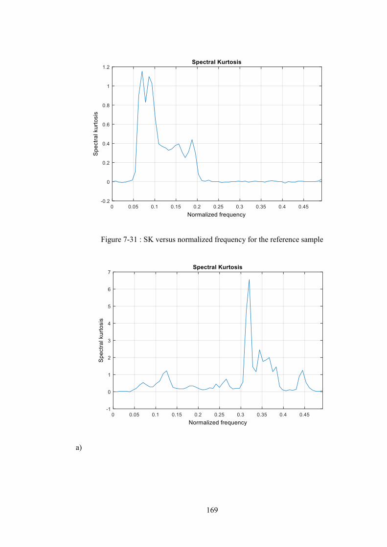
169

Figure 7-31 : SK versus normalized frequency for the reference sample

a)

170

b)

Figure 7-32: SK versus normalized frequency for the R260 rail steel sample at the a)

earlier stage b) later stage

a)

171

b)

c)

Figure 7-33: Spectral kurtosis versus normalized frequency for the Hadfield steel sample

at the a) early stage b)middle stage c) late stage

172

Once the noise reaches a higher level, especially in field condition, the defect signal can

be masked. In this case certain filters can be used to remove or at least suppress the

influence of the noise. Even though the noise level was not very high under the current

laboratory testing condition, it is still worth to investigate the filtering effect.

Hence, the band-pass filter was designed based on the window size and centre frequency

at which the SK attained the maximum. However, the window size in the above can not

necessarily guarantee the SK was the maximum among all the possible choices. In this

case, the Kurtogram developed by Antoni was employed to obtain the maximum SK and

the corresponding window size Nw and center frequency [154]. The Kurtogram for the

original dataset at the early stage for Hadfield steel sample 1 is as shown in Figure 7-34.

Figure 7-34: Kurtogram for the previous AE signal.

173

The Centre frequency and window size at which the maximum kurtosis can be obtained

at all the stages for Hadfield steel sample 1 are shown in Table 7-4.

Table 7-4: Optimum Bandwidth and centre frequency for AE signal from manganese

sample at different stages.

Centre Frequency /Hz Log2(Nw) Maximum kurtosis

Early stage 297526 8.5 24.4

Middle stage 476562 5 394.2

Late stage 10416 4.5 20049

Bandpass filter was designed based on the centre frequency and the window size Nw as

shown in the above table and the filtered waveforms for the Hadfield samples at the three

stages are shown in Figure 7-35.

174

a)

b)

175

c)

Figure 7-35: Filtered waveform for the Hadfield sample at the a) early stage b) middle

stage c) late stage

As it can be seen the signal to noise ratio shows an obvious increase for every filtered

waveform compared with their corresponding original waveform. It cannot be ignored

that the original signal to noise ratio is still acceptable under this laboratory testing

condition. However, in the actual field condition, the noise level can increase

dramatically, and SK-based filter may contribute to the identification of spikes related to

defect evolution in the rails based on the current result.

176

7.2 High frequency fatigue tests

7.2.1 Introduction

Three and four point bending fatigue tests are carried out on four pre-cracked Hadfield

steel samples numbered 1 through 4. They were also pre-cracked using the Vibrophore

fatigue machine to an initial crack length of 9- 11 mm. Sample 1 and 2 were tested under

3 point bending condition, whereas sample 3 and 4 were tested under 4 point bending

condition . The maximum load in this case was set at 3.75kN.Both R50a sensors were

connected to the commercial PAC system. The thresholds for all the four samples were

set to 40dB

To further investigate the capability of AE to detect crack initiation and propagation ,

three point bending fatigue crack growth tests have been carried out on Hadfield steel

centre-notched samples of rectangular cross-section with dimension 120mm

(L)×20mm(W)×10mm(H) and notch depth 9mm. The samples have not been pre-cracked

in this case. Reference test have also been performed on a dummy sample with no notch

or pre-cracking. Same as low frequency tests mentioned previously, one R50a sensor was

connected to the commercial PAC AE system and the other one was connected to the

customized system during testing.

Two 260 rail steel samples numbered 1 and 2 were tested with the frequency set at around

88Hz. The notch depth in this case was 2mm for both samples and no pre-cracking was

made, so the signal features for all fatigue crack propagation process could be analysed.

The peak loads used during the tests were set at 9kN, 9.2kN respectively. The analog

filter 200 KHz-1MHz in the PAC system was applied for both samples before further

processing. The thresholds for sample 1 and 2 were set to 71dB and 74 dB, respectively.

177

The reasons why thresholds were set at the above values are twofold. The first one is to

reduce the influence of loading-related noise on post-processing and the second one is to

reduce the amount of data that needs to be stored in the computer for ease of operation

and post-processing.

7.2.2 Analysis of AE signals captured from commercial system

Figure 7-36 shows the change of crack growth rate with time and Figure 7-37 through

Figure 7-40 show the correlation of amplitude, count, duration, energy with crack length

for the samples in three and four point-bending fatigue test respectively. Zoomed-in

sections of the correlation plots have also been shown in Figure 7-37 through Figure 7-40

as indicated by the blue arrows. Time (second) instead of cycles was plotted on the

abscissa as the machine could not keep loading frequency constant at the later stage of

the tests. For three point bending sample, the crack growth starts to pick up speed from

around 100s (indicated by the red arrow) and at the same period AE activities starts to

show steady increase until final failure. At around 60s, a cluster of relatively high

amplitude AE hits which are similar to those captured during final stage in terms of

intensity. However, their count, energy and duration values are clearly smaller than those

captured during the final stage. For four point bending sample, the crack growth starts to

pick up speed at around 200s (indicated by the red arrow), at which point significant

amount of AE hits with amplitude above 60dB occurs which might be related to a mixed

intergranular and transgranular failure mode as shown from the micrographs in Figure

7-41 and for all the parameters, a region with nearly no AE hits can be observed. After

that, the crack growth rate keep increasing and the values of different parameters (count,

duration and energy) except for amplitude show a clear upward trend. The crack growth

rate reaches a plateau before final failure at around 310s (circled in red), at which point

178

all the parameters show a sudden drop. However, the high amplitude (equal or above

70dB) AE hits captured at the same time also indicates impending collapse of the sample.

a)

b)

Figure 7-36: Crack growth rate with time Hadfield steel sample in a) three point and b)

four point bending fatigue test.

179

a)

180

b)

Figure 7-37: AE signal amplitude in dB versus time with crack growth in mm for

Hadfield steel sample in a) three point and b) four point bending fatigue tests.

181

a)

182

b)

Figure 7-38: AE signal count versus time with crack growth in mm for Hadfield steel

sample in a) three point and b) four point bending fatigue tests.

183

a)

184

b)

Figure 7-39: AE signal energy versus number of fatigue cycles with crack growth in

mm for Hadfield steel sample in a) three point and b) four point bending fatigue tests.

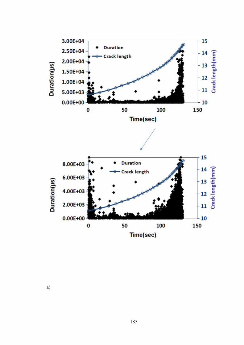
185

a)

186

b)

Figure 7-40: AE signal energy versus number of fatigue cycles with crack growth in

mm for Hadfield steel sample in a) three point and b) four point bending fatigue tests.

187

Figure 7-41: Micrographs showing the crack path after a fatigue crack test (from sample

4) showing a mixture of both transgranular and intergranular cracking

188

Figure 7-42 shows the correlation between dC/dN, dD/dN,dE/dN and da/dN for all the

four samples . Sample 1 and 2 were subjected to three point bending load, whereas Sample

3 and 4 were subjected to four point bending load. For the three point bending fatigue

tests, it has been shown that both count rate and energy rate start to show upward trend

beyond a certain value of ΔK. The initial drop was attributed to the influence of the

residual stress generated in the pre-cracking process and it proves that AE is very sensitive

to the loading history of the structure. It can be found that the crack growth rates under

three-point bending are higher than those under four point bending for the same ΔK.

Generally, count rate, energy rate and duration rate show similar trend for all the samples.

For the samples under three point bending tests, however, energy rate exhibits a higher

increase close to the end of stable crack growth indicating final failure is imminent, which

is not reflected by neither count rate nor duration rate. Therefore, the energy rate is better

indicator for later stage of stable crack propagation than count rate and duration rate for

three point bending fatigue tests. Although energy rates for four point bending test are

higher than those for three point bending tests for most of the ΔK range, the slopes of

linear regression fit equations are lower than those for three point bending tests. It proves

the energy rates values may be more sensitive to the loading configuration, whereas the

slope of energy rate is more closely related to the magnitude of crack growth rate.

189

a)

b)

190

c)

Figure 7-42: Comparison between crack growth rate and a) count rate b) duration rate c)

energy rate for two pre-cracked Hadfield sample during high frequency bending fatigue

test.

Figure 7-43 through Figure 7-50 show the results for Hadfield steel centre-notched

samples and the dummy sample with no notch or pre-cracking. Figure 7-43 shows the

energy frequency distribution for AE events recorded during the test on the dummy

sample. As no crack initiation and growth activity is expected, all the events can thus be

attributed to external noises generated by friction, impact, machine running, etc. It is

obvious that energy values of the noises are mainly distributed in the range 0-2(µVolt-

sec/count). Hence AE events with energy in the range 0-2(µVolt-sec/count) could be

removed for Hadfield steel samples during the post-processing.

191

Figure 7-43: Energy frequency distribution for AE events AE events recorded during

the test on the dummy sample.

Another parameter that can be used for signal filtering is risetime. Under current

experiment condition, AE events with rise time above 1ms are most likely caused by

external noise.AE events with energy in the range (0-2) (µVolt-sec/count) or risetime

above 1ms are removed during the analysis.

Figure 7-44 shows the evolution of crack length with time for two Hadfield samples

numbered 1 and 2, respectively. The peak load for sample 1 was initially set as 3kN and

after around 0.5h.The value was increased to 3.3kN to reduce the amount of time for crack

initiation and the AE results shown here are captured after the load increase. For sample

2, throughout the test, the peak load was set as 3.3kN with the loading frequency of around

70Hz.For both samples, the macro cracks initiate at around 960s and 800s respectively.

192

a)

b)

Figure 7-44: Crack length with time for a) Sample 1 b) Sample 2

193

Figure 7-45 through Figure 7-48 show the AE activity captured during the tests. Zoomed

in views of AE activities around the time of crack initiation have also been shown in each

figure as indicated by the blue arrows. It can be seen that the intensity of AE activity

drop as indicated by the red arrows after crack initiation and this may be attributed to

the decreasing crack growth rate typical of microstructurally small crack[29]. When

crack length grows 1mm from the notch, it is assumed that the crack growth enter into

stage II. As it can be seen, the intensity of AE activity increases with increasing crack

length during the second stage of the fatigue test. However, it is noteworthy that even at

stage I, which covers a large percentage of the fatigue life time, high intensity AE signals

have also been generated. This can be partly attributed to the movement of slip bands and

micro-crack formation.

194

a)

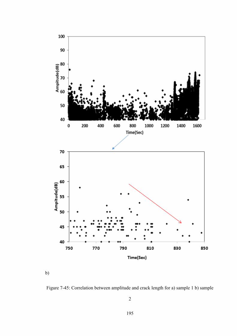
195

b)

Figure 7-45: Correlation between amplitude and crack length for a) sample 1 b) sample

2

196

a)

197

b)

Figure 7-46: Energy versus time for a) sample 1 b) sample 2

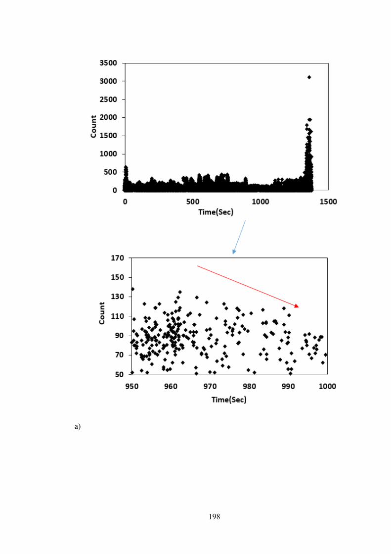
198

a)

199

b)

Figure 7-47: count versus time for 1) sample 1 2) sample 2

200

a)

201

b)

Figure 7-48: Duration with time for a) sample 1 b) sample 2

202

Figure 7-49 shows the plots of cumulative energy and crack growth rate versus time for

sample 2. It is obvious that most of the test time is spent on stage 1,which is consistent

with the classification of fatigue life regime in [24].The slope of cumulative energy versus

time curve is relatively small, compared with that for stage II. However, at the end of

stage I, the slope starts to increase gradually. Once the crack growth enters into stage II,

the cumulative energy shows an exponential increase. However, it shows a slow-down in

the slope at the transition between stage II and III.

Figure 7-49: Comparison between cumulative energy and crack growth rate for sample 2

Figure 7-50 shows the correlation of count rate, energy rate with crack growth rate for

both samples. Both samples show a “trough-like” trend (‘decrease-increase alternation )

and the initial drop of count rate and energy rate for sample 1 may be caused by the

release of residual stress induced during the previous loading with a smaller peak load.

It is noteworthy that for sample 2, count rate and energy rate show different trend in the

203

ΔK range of around 25-30MPam1/2 .Count rate show consistent increase whereas energy

rate show a decrease trend.

a)

b)

Figure 7-50: Comparison between crack growth rates and a) count rates b) energy rates

for sample 1 and 2 during the bending fatigue tests

204

Figure 7-51 and Figure 7-52 show AE activity captured during the tests on 260 rail steel

sample 1 and sample 2, respectively. For sample 1, according to DCPD measurement, the

macrocrack initiate at around 68000s and strong AE activity can be observed. The AE

intensity increases when the peak load increases from 9 to 9.2kN. After macrocrack

initiation, the AE activity decreases and this is more obvious for sample 2. Higher loading

force (9.2kN) contributed to more obvious drop of AE activity and this is because the

stress intensity factors increase as the loading forces go up, strengthen the AE sources of

cyclic plasticity and crack extension. Therefore, higher loading forces make the AE

indications visually easier. When the crack initiate, both amplitude and count of the

captured events tend to be of similar magnitude, whereas they are more scattered in terms

of the distribution of the magnitude at the final stage. Both cumulative energy and count

plots can show the occurrence of crack initiation and final failure. The crack nucleation

generates high intensity AE signals resulting in the sharp increase of the slope of

cumulative plots. Cumulative count in this case proves to be a better indicator for crack

initiation than cumulative energy .The large increase of cumulative energy and count

before the final failure is attributed to cleavage fracture as shown in Figure. At the top

part of crack, the roughness morphology indicates the cyclic fatigue propagation which

has low AE output. The cleavage fracture at the bottom part of crack indicates the brittle

fracture which is very high AE releasing.

205

a)

206

b)

207

c)

208

d)

Figure 7-51: a)amplitude b) count c)cumulative energy d)cumulative count versus time

for 260 rail steel sample 1

209

a)

210

b)

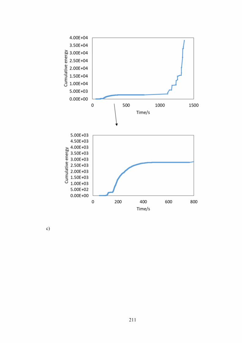
211

c)

212

Figure 7-52: a) amplitude b) energy c) cumulative energy d) cumulative count versus

time for 260 rail steel sample 2

213

Figure 7-53: Fracture surface of three point bending sample

7.2.3 Analysis of AE signals captured with the customized system

Figure 7-54 shows the variation of different parameters with measurement time for one

non-precracked Hadfield sample during the high frequency test. The RMS values

successfully show the degradation process of the tested sample .The RMS shows obvious

increase trend after initial decrease following the crack initiation captured by the DCPD

technique, although some fluctuation in the results can also be observed. Peak-peak

values at two different levels can be found before and after crack initiation, respectively.

The peak-peak values do not show increase trend as that shown by RMS. It is obvious

that crest factor and kurtosis values before and after crack initiation in this case do not

214

show big difference, however they can also capture the big value jump(indicated by the

red arrows) that has been reflected by RMS and peak-peak analysis. Skewness shows a

downward trend after crack initiation, however the big deviations can still be observed.

a)

215

b)

c)

216

d)

e)

Figure 7-54: Variation of overall a)RMS b)peak-peak value c)crest factor d)kurtosis

e)skewness with measurement No.

217

Figure 7-55 shows the signal differences between early stage and later stage of the

Hadfield sample during the high frequency test. The moving RMS, crest factor and

kurtosis values of the signal at the late stage show obvious increase compared with those

of the signal at the early stage, whereas most moving skewness values show a decrease

the signal at the late stage.

a)

218

b)

c)

219

d)

Figure 7-55: Comparison between data captured at early and late stage for a)moving RMS

b)moving crest factor c)moving kurtosis d)moving skewness

The application of AE to monitor the integrity of rails and crossings in the field can be

complicated by two main factors. Firstly, the external noise level in the field can be much

higher than that during the laboratory trials. Secondly, some types of crack grow under

mixed mode loading condition. However, as the bending fatigue configuration employed

during the laboratory trials is partially representative of the loading conditions that the

rails and crossings are subjected to, the feasibility of applying AE to monitor the integrity

of rails and crossings has been justified.

7.3 Field tests

Frequency and power distribution analysis can be effective on AE signals. Such

conclusion is also suitable for wayside crossing monitoring mainly because crack growth

220

and plastic deformation would generate unique spectral information and are not correlated

with other AE sources.

Therefore, the power spectrum estimation (PSE) is used as the feature to perform

correlation processing. By calculating the similarity between the PSE of both template

and the acquired AE data, we are able to determine whether such a signal is generated by

crack growth or plastic deformation.

The signals attributed to crack evolution from the laboratory tests have been used as

templates for correlation analysis, as the loading conditions during the laboratory tests

are partially representative of the loading conditions of crossings in the field. The

principle is that if signals captured from the instrumented crossing have similar features

to the templates, it is highly possible that damage evolution occurs in the crossings.

Frequency and power distribution can be used as the feature for correlation processing.

The severity of damage in the crossings have been evaluated based on the correlation

between the signals and the templates. Low frequency components of the signals have

been filtered out before correlation analysis to weaken the influence of false AE sources.

One template related to crack growth has been selected from the raw data captured from

laboratory tests on Hadfield steel samples as shown in Figure 7-56.

221

Figure 7-56: Template related to crack growth at the early stage

As mentioned earlier, the Wembley crossing was confirmed to be healthy using visual

inspection, so no indication of damage evolution is anticipated from the correlation

analysis. Figure 7-57 shows the raw AE signal captured from one of the AE sensors while

a passenger train passed over the crossing. The only few high peaks might be caused by

the sliding of the wheels.

222

Figure 7-57: Raw AE signal from passenger train passing over the Wembley crossing.

Figure 7-58 shows the cross-correlation result using the template related to crack growth

at the early stage. No obvious indication of damage evolution can be observed in the result.

The correlation between the raw signal and the template related to crack growth at the

middle stage further confirms that there is no damage evolution happening in Wembley

crossing.

223

Figure 7-58: Cross-correlation result using the early stage crack growth template.

Figure 7-59: Cross-correlation result using the middle stage crack growth template

224

Figure 7-60 shows signals captured during the passing of a freight train. The high peaks

in the signal are mainly generated by engine noise causing sliding of locomotive wheels.

Apart from the engine noise induced peaks, no other visible peaks can be observed during

the passing of the rest of train, which indicates no crack growth occurs in the crossing.

Figure 7-60: Raw AE signal captured during the passing of a freight train.

Figure 7-61 shows the correlation result using the early stage damage template. No

obvious peaks indicative of crack growth can be found in the plot.

225

Figure 7-61: Correlation result using the early stage crack growth template.

Figure 7-62 shows cross-correlation result based on the moderate stage damage template.

Similarly, no obvious peaks indicative of crack growth can be found in the plot.

Figure 7-62: Cross-correlation result using the middle stage crack growth template.

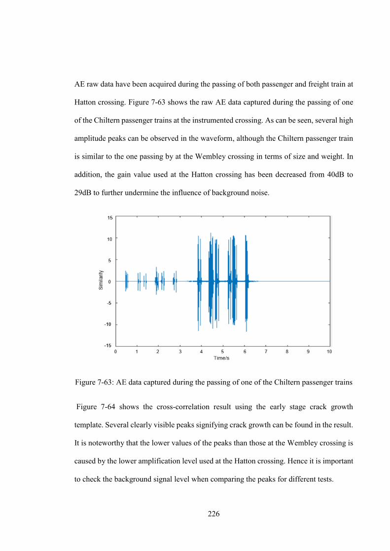
226

AE raw data have been acquired during the passing of both passenger and freight train at

Hatton crossing. Figure 7-63 shows the raw AE data captured during the passing of one

of the Chiltern passenger trains at the instrumented crossing. As can be seen, several high

amplitude peaks can be observed in the waveform, although the Chiltern passenger train

is similar to the one passing by at the Wembley crossing in terms of size and weight. In

addition, the gain value used at the Hatton crossing has been decreased from 40dB to

29dB to further undermine the influence of background noise.

Figure 7-63: AE data captured during the passing of one of the Chiltern passenger trains

Figure 7-64 shows the cross-correlation result using the early stage crack growth

template. Several clearly visible peaks signifying crack growth can be found in the result.

It is noteworthy that the lower values of the peaks than those at the Wembley crossing is

caused by the lower amplification level used at the Hatton crossing. Hence it is important

to check the background signal level when comparing the peaks for different tests.

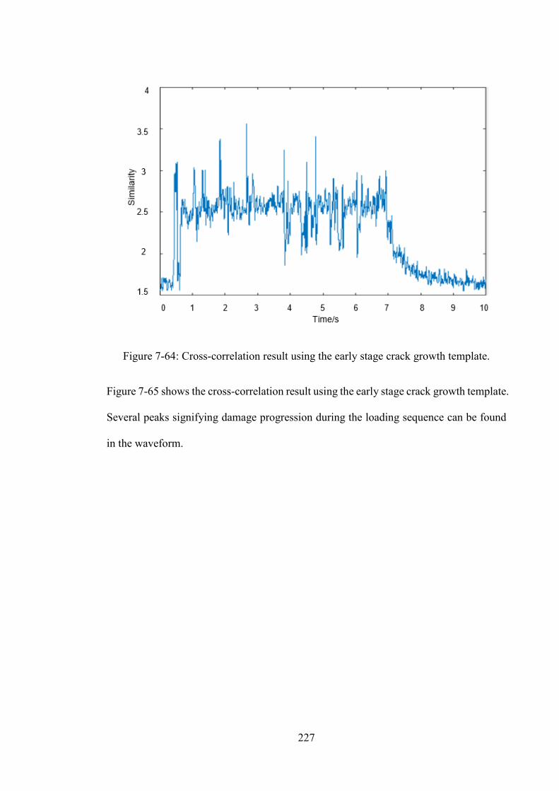
227


Figure 7-65 shows the cross-correlation result using the early stage crack growth template.

Several peaks signifying damage progression during the loading sequence can be found

in the waveform.

228

Figure 7-65: Cross-correlation result based on the middle stage crack growth template

Figure 7-66 shows the raw AE data captured during the passing of a heavy freight train

at the instrumented crossing. The small peaks in the waveform are caused by periodical

loading of the wheels on the crossing and the few high peaks might be due to heavier

weight of one of the wagons

229

Figure 7-66: AE data captured during the passing of a heavy freight train

Figure 7-67 shows the cross-correlation result using the early stage crack growth template.

Peaks indicative of crack growth nearly appear in every loading cycle.


230

Figure 7-68 shows the cross-correlation result using the middle stage crack growth

template. It is noteworthy that at the 5 sec a very high peak is clearly evident indicating

the crack grows more rapidly at that point.

Figure 7-68: Cross-correlation result using the middle stage crack growth template.

231

Chapter 8:

Conclusions and Future Work

232

: CONCLUSIONS AND FUTURE WORK

8.1 Conclusions

This research has investigated the possibility of using acoustic emission technique to

monitor the structural integrity of rails and crossings in real time. Low and high frequency

bending fatigue crack growth tests have been carried out on the three different types of

specimens: R260 grade rail steel samples(precracked and non-precracked), Hadfield steel

samples(precracked and non-precracked), and carbon steel sample with AE being used to

monitor the damage evolution process. The configuration of the bending tests is partially

representative of the actual loading experienced by the rails and crossings.

For laboratory tests, both a customised system developed by University of Birmingham

and a commercial AE system procured from Physical Acoustics Corporation were used

to monitor the bending fatigue tests. For the commercial system, parameters including

amplitude, energy, risetime, duration, count and ASL were used to correlate crack length

with AE hits. For R260 steel, high amplitude (>70dB) AE hits occur even during stable

crack propagation and this is attributed to brittle cleavage fracture. Sudden increase of

crack length at certain stage before final failure can be successfully detected by AE. The

fractograph and AE energy results show brittle cleavage fracture occur certain crack

length for all R260 steel specimens. The AE cumulative energy was clearly correlated to

microstructural features related to brittle cleavage fracture. Hence it has confirmed that

brittle fracture can be quantitatively described using AE.For Hadfield steel, nearly all

high amplitude(>70dB) hits occur at the final stage of crack growth and the stair-like

amplitude distribution can be observed before final failure. The correlation between AE

parameter rate (count, duration, energy) and crack growth rate, is performed for the whole

load range. The parameter rate generally shows similar trend to crack growth rate for both

233

types of steel. However, the previous loading history like precracking can influence the

correlation.

The waveform based analysis has been carried out on the data captured with the

customized system developed by University of Birmingham. Crack growth related peaks

can be clearly observed in the raw AE waveforms captured by the customized system

during the low frequency bending fatigue tests on both R260 and Hadfield steel samples.

The intensity of crack growth related peaks increases from early stage to final stage. Peaks

due to crack surface rubbing can also be found in some of the waveforms. Fourier

transform has been proved to be capable of differentiate crack growth related peaks from

those due to crack surfaces rubbing. The trend of various parameters with time for the AE

waveforms captured during the bending fatigue test on Hadfield steel sample was

obtained. The RMS shows a clear upward trend with some fluctuations also observed

especially in the early stage. The trend of peak-peak, kurtosis, crest factor in the late stage

is generally consistent with that for RMS, whereas skewness shows decreasing trend for

low frequency fatigue tests.

The possibility of using algorithms like moving RMS, crest factor, kurtosis and skewness

to characterize the severity of damage have also been investigated. All the algorithms

show the capability to reflect the severity of damage accurately. However, the results

obtained by various algorithms should be interpreted based on the principal of each

algorithm. In addition, SK has been employed to analyse the signals. Although SK values

can reveal the damage progression, the frequency ranges at which SK attain the peak

values vary considerably at different stages. This is due to the influence of noise caused

by crack faces rubbing during crack opening and closing. In addition, the feasibility of

applying various filters to weaken the influence of noise has been explored. The influence

234

of applying Swansong II filters in this case is very limited. The bandpass filter designed

based on bandwidth and centre frequency derived from Kurtogram analysis has proved

to be effective in undermining the influence of external noise.

Finally, initial field trials have been carried out on two different crossings on the west

coast mainline. Template-based cross correlation analysis, which is capable of

differentiating the AE source mechanisms, like crack growth, impact etc., has been

employed to analyse the data captured from the instrumented crossing. It has shown that

cross correlation analysis is effective in evaluating the health state of the monitored

crossings. Overall, this research has shown that AE can be used as a tool to effectively

evaluate the structural integrity of rails and Hadfield steel crossings online.

8.2 Future work

Further work could be done from the following aspects to improve the accuracy of

evaluation of the damage of rails and crossings with AE.

The fatigue crack growth tests carried out in the current research are of mode I, however

in actual railway line, some types of crack grow under mixed mode loading condition.

Hence it would be beneficial that AE monitoring of fatigue crack growth tests on both

types of steel samples under Mix-mode (mode I and mode II) loading could be performed

to obtain the signal features. The relationship between different AE parameters including

amplitude, energy, risetime, count ,duration etc. during the fatigue tests could be

investigated in more depth to see its change with damage progression. More signal

processing techniques should be investigated in terms of their capability to reveal the

severity of damage accurately.

235

The possibility of using the average duration of AE events captured using the commercial

system to determine optimal window size for time series analysis should also be

investigated.

236

REFERENCES

1. Network Rail's Strategic Business Plan-Maintenance activity and expenditure,

Document ref. SBPT222, Version 0.14. 01/2013.

2. Turner, C., et al., A review of key planning and scheduling in the rail industry in

Europe and UK. Proceedings of the Institution of Mechanical Engineers, Part F:

Journal of Rail and Rapid Transit, 2015: p. 0954409714565654.

3. Yılmazer, P., A. Amini, and M. Papaelias, The structural health condition

monitoring of rail steel using acoustic emission techniques. 2012.

4. Dadashi, N., et al. A framework of data processing for decision making in railway

intelligent infrastructure. in Cognitive Methods in Situation Awareness and

Decision Support (CogSIMA), 2011 IEEE First International Multi-Disciplinary

Conference on. 2011. IEEE.

5. Office of Rail and Road, UK Rail Industry Financial Information 2015-16.

02/2017.

6. Garnham, J.E. and C.L. Davis, 5 - Rail materials, in Wheel–Rail Interface

Handbook, R. Lewis and U. Olofsson, Editors. 2009, Woodhead Publishing. p.

125-171.

7. Herring, D.H. Principles of Gas Nitriding: The Nitriding Process (Part 1). [online]

2011; Available from: http://www.industrialheating.com/articles/89998-

principles-of-gas-nitriding-the-nitriding-process-part-1?v=preview.

8. Maya-Johnson, S., A. Ramirez, and A. Toro, Fatigue crack growth rate of two

pearlitic rail steels. Engineering Fracture Mechanics, 2015. 138: p. 63-72.

9. Wu, K. and H. Bhadeshia, Extremely fine pearlite by continuous cooling

http://www.industrialheating.com/articles/89998-principles-of-gas-nitriding-the-nitriding-process-part-1?v=preview

http://www.industrialheating.com/articles/89998-principles-of-gas-nitriding-the-nitriding-process-part-1?v=preview

237

transformation. Scripta Materialia, 2012. 67(1): p. 53-56.

10. Aglan, H., et al., Mechanical and fracture behavior of bainitic rail steel. Journal

of materials processing technology, 2004. 151(1): p. 268-274.

11. Rae, BS EN 13674-1:2011 - Railway applications. Track. Rail. Vignole railway

rails 46 kg/m and above. Bahnanwendungen. Oberbau. Schienen. Vignolschienen

ab 46 kg/m.

12. EN, T., 13674-1): Railway applications–track–rail–part 1: Vignole railway rails

46 kg/m and above. 2011, Brussels.

13. El-Shabasy, A.B. and J.J. Lewandowski, Effects of load ratio, R, and test

temperature on fatigue crack growth of fully pearlitic eutectoid steel (fatigue

crack growth of pearlitic steel). International journal of fatigue, 2004. 26(3): p.

305-309.

14. Srivastava, A.K. and K. Das, Microstructural characterization of Hadfield

austenitic manganese steel. Journal of Materials Science, 2008. 43(16): p. 5654-

5658.

15. Ham, Y.-S., et al., Critical cooling rate on carbide precipitation during quenching

of austenitic manganese steel. China Foundry, 2010. 2: p. 016.

16. Zhang, F., et al., Explosion hardening of Hadfield steel crossing. Materials

Science and Technology, 2010. 26(2): p. 223-229.

17. Kang, J., et al., Cyclic deformation and fatigue behaviors of Hadfield manganese

steel. Materials Science and Engineering: A, 2014. 591: p. 59-68.

18. Niendorf, T., et al., Fatigue crack growth—microstructure relationships in a high-

manganese austenitic TWIP steel. Materials Science and Engineering: A, 2010.

527(9): p. 2412-2417.

238

19. Hamada, A., L. Karjalainen, and J. Puustinen, Fatigue behavior of high-Mn TWIP

steels. Materials Science and Engineering: A, 2009. 517(1): p. 68-77.

20. Harzallah, R., et al., Rolling contact fatigue of Hadfield steel X120Mn12. Wear,

2010. 269(9): p. 647-654.

21. Mahlami, C. and X. Pan, An Overview on high manganese steel casting. 2014.

22. Pook, L., Why Metal Fatigue Matters. 2007: Springer.

23. Callister, W.D. and D.G. Rethwisch, Materials science and engineering: an

introduction. Vol. 7. 2007: Wiley New York.

24. Milella, P.P., Fatigue and corrosion in metals. 2012: Springer Science & Business

Media.

25. Frost, N.E., K.J. Marsh, and L.P. Pook, Metal fatigue. 1974: Courier Corporation.

26. eFunda. Stress Intensity Factor and Crack Tip Stresses. [online] 2018 [cited 2018

04/01]; Available from:

http://www.efunda.com/formulae/solid_mechanics/fracture_mechanics/fm_lefm

_K.cfm.

27. Noels, L. Fracture Mechanics Online Class. unknown; Available from:

http://www.ltas-cm3.ulg.ac.be/FractureMechanics/print.php?p=overview_P5.

28. ASM International. Fatigue in Elements of Metallurgy and Engineering Alloys.

[online] 2008; Available from:

http://www.asminternational.org/documents/10192/1849770/05224G_Chapter14

.pdf.

29. Suresh, S. and R. Ritchie, Propagation of short fatigue cracks. International

Metals Reviews, 1984. 29(1): p. 445-475.

30. Milne, I., R.O. Ritchie, and B.L. Karihaloo, Comprehensive structural integrity:

http://www.efunda.com/formulae/solid_mechanics/fracture_mechanics/fm_lefm_K.cfm

http://www.efunda.com/formulae/solid_mechanics/fracture_mechanics/fm_lefm_K.cfm

http://www.ltas-cm3.ulg.ac.be/FractureMechanics/print.php?p=overview_P5

http://www.asminternational.org/documents/10192/1849770/05224G_Chapter14.pdf

http://www.asminternational.org/documents/10192/1849770/05224G_Chapter14.pdf

239

cyclic loading and fatigue. Vol. 4. 2003: Elsevier.

31. Suresh, S., Fatigue of materials. 1998, Cambridge university press.

32. Pineau, A. and R. Pelloux, Influence of strain-induced martensitic

transformations on fatigue crack growth rates in stainless steels. Metallurgical

Transactions, 1974. 5(5): p. 1103-1112.

33. Hornbogen, E., Martensitic transformation at a propagating crack. Acta

Metallurgica, 1978. 26(1): p. 147-152.

34. Kim, J.-K. and C.-S. Kim, Fatigue crack growth behavior of rail steel under mode

I and mixed mode loadings. Materials Science and Engineering: A, 2002. 338(1):

p. 191-201.

35. Ritchie, R.O., Mechanisms of fatigue-crack propagation in ductile and brittle

solids. International Journal of Fracture, 1999. 100(1): p. 55-83.

36. totalmateria. Linear Elastic Fracture Mechanics : Part One. [Online] 2010;

Available from:

http://www.totalmateria.com/page.aspx?ID=CheckArticle&site=kts&NM=295.

37. Huang, M., et al., Using acoustic emission in fatigue and fracture materials

research. JOM, 1998. 50(11): p. 1-14.

38. Ringsberg, J.W. and A. Bergkvist, On propagation of short rolling contact fatigue

cracks. Fatigue & Fracture of Engineering Materials & Structures, 2003. 26(10):

p. 969-983.

39. Ringsberg, J.W., Life prediction of rolling contact fatigue crack initiation.

International Journal of fatigue, 2001. 23(7): p. 575-586.

40. Sinclair, G. and R. Pieri, On obtaining fatigue crack growth parameters from the

literature. International journal of fatigue, 1990. 12(1): p. 57-62.

http://www.totalmateria.com/page.aspx?ID=CheckArticle&site=kts&NM=295

240

41. Hearn, E., Mechanics of Materials, Vol. 2-The Mechanics of Elastic and Plastic

Deformation of Solids and Structural Materials. 1997, Butterworth-Heinemann.

42. Onal, O., et al., Investigation of rolling contact crack initiation in bainitic and

pearlitic rail steels. Fatigue & Fracture of Engineering Materials & Structures,

2012. 35(11): p. 985-997.

43. UMIST. Failure of Materials [online ] Unknown [cited 2014 05/07]; Available

from: http://pwatlas.mt.umist.ac.uk/internetmicroscope/micrographs/failure.html.

44. Care, R., et al., Why rails crack: Gauge corner cracking on the British network-

Analysis. Arup Journal, 2006. 41(1): p. 16.

45. ARTC. Rail Defects Handbook

Some Rail Defects, their Characteristics,

Causes and Control. [Online] 2006; Available from:

http://extranet.artc.com.au/docs/eng/track-civil/guidelines/rail/RC2400.pdf.

46. Ayasse, J.-B. and H. Chollet, Wheel-rail contact. Handbook of railway vehicle

dynamics, 2006: p. 86-120.

47. Remennikov, A.M. and S. Kaewunruen, A review of loading conditions for

railway track structures due to train and track vertical interaction. Structural

control and Health monitoring, 2008. 15(2): p. 207-234.

48. Cannon, D., et al., Rail defects: an overview. Fatigue & Fracture of Engineering

Materials & Structures, 2003. 26(10): p. 865-886.

49. Zerbst, U., et al., Introduction to the damage tolerance behaviour of railway rails–

a review. Engineering fracture mechanics, 2009. 76(17): p. 2563-2601.

50. Yan, W. and F. Fischer, Applicability of the Hertz contact theory to rail-wheel

contact problems. Archive of Applied Mechanics, 2000. 70(4): p. 255-268.

http://pwatlas.mt.umist.ac.uk/internetmicroscope/micrographs/failure.html

http://extranet.artc.com.au/docs/eng/track-civil/guidelines/rail/RC2400.pdf

241

51. Zerbst, U., K. Mädler, and H. Hintze, Fracture mechanics in railway

applications––an overview. Engineering Fracture Mechanics, 2005. 72(2): p. 163-

194.

52. Schleinzer, G. and F. Fischer, Residual stress formation during the roller

straightening of railway rails. International Journal of Mechanical Sciences, 2001.

43(10): p. 2281-2295.

53. SMITH, R., Fatigue and the railways: an overview. Fatigue in Railway

Infrastructure, 2009: p. 1.

54. Zwanenburg, W.-J., Modelling degradation processes of switches & crossings for

maintenance & renewal planning on the Swiss railway network. 2009.

55. Cornish, A., Life-time monitoring of in service switches and crossings through

field experimentation. 2014.

56. Andersson, C. and T. Dahlberg, Wheel/rail impacts at a railway turnout crossing.

Proceedings of the Institution of Mechanical Engineers, Part F: Journal of Rail

and Rapid Transit, 1998. 212(2): p. 123-134.

57. Pålsson, B.A. and J.C. Nielsen, Wheel–rail interaction and damage in switches

and crossings. Vehicle System Dynamics, 2012. 50(1): p. 43-58.

58. Board, H.I., Train Derailment at Hatfield: A Final Report by the Independent

Investigation Board,July 2006. 2006: London.

59. Ringsberg, J., Rolling contact fatigue of railway rails with emphasis on crack

initiation. 2000: Chalmers University of Technology.

60. Grassie, S. and J. Kalousek, Rail corrugation: characteristics, causes and

treatments. Proceedings of the Institution of Mechanical Engineers, Part F:

Journal of Rail and Rapid Transit, 1993. 207(1): p. 57-68.

242

61. Grassie, S., Rail corrugation: characteristics, causes, and treatments.



62. Popović Z, P.L., Lazarević L, Rail defects due to rolling contact fatigue. Rail

defects due to rolling contact fatigue, 2011. 54(2): p. 17-29.

63. Vidaud, M. and W.-J. Zwanenburg. Current situation on rolling contact fatigue–a

rail wear phenomenon. in 9th Swiss Transport Research Conference. 2009.

64. Grassie, S.L., Rolling contact fatigue on the British railway system: treatment.

Wear, 2005. 258(7): p. 1310-1318.

65. Fletcher, D., F. Franklin, and A. Kapoor, Rail surface fatigue and wear. Wheel-

Rail Interface Handbook, 2009: p. 280.

66. Popović, Z., et al., Rail defects head checking on the Serbian Railways. Tehnički

vjesnik, 2014. 21(1): p. 147-153.

67. Plu, J., et al., Application of fracture mechanics methods to rail design and

maintenance. Engineering Fracture Mechanics, 2009. 76(17): p. 2602-2611.

68. Ringsberg, J.W., Shear mode growth of short surface-breaking RCF cracks. Wear,

2005. 258(7): p. 955-963.

69. Marich, S., Marich Consulting Services - Module 1: Wheel rail dynamics in Wheel

Rail Interface Forum. 2014: Brisbane.

70. Grassie, S., Squats and squat-type defects in rails: the understanding to date.



71. Lewis, R. and U. OLOfssOn, Basic tribology of the wheel–rail contact. Wheel-

Rail Interface Handbook, 2009: p. 34.

243

72. Kaewunruen, S., Monitoring structural deterioration of railway turnout systems

via dynamic wheel/rail interaction. Case Studies in Nondestructive Testing and

Evaluation, 2014. 1: p. 19-24.

73. Lovejoy, M., Magnetic particle inspection: a practical guide. 2012: Springer

Science & Business Media.

74. Falkenach, G.J., D. Kooger, and R. Meister, Improvement in Magnetic Techniques

for Rail Inspection. 1981.

75. Clark, R., Rail flaw detection: overview and needs for future developments. NDT

& E International, 2004. 37(2): p. 111-118.

76. University of Birmingham, D4.4.1- Rail Inspection Technologies. 2007:

Birmingham.

77. Krull, R., et al. Eddy-current Detection of Head Checks on the Gauge Corners of

Rails: Recent Results. in PROCEEDINGS OF THE INTERNATIONAL

CONFERENCE AND EXHIBITION RAILWAY ENGINEERING 2003, HELD

LONDON, UK, 30 APRIL-1 MAY 2003-CDROM. 2003.

78. Papaelias, M., An integrated strategy for efficient non-destructive evaluation of

rails in Fault Detection: Classification, Techniques and Role in Industrial Systems,

U. Fausto Pedro García Márquez and Mayorkinos Papaelias (Birmingham

University, Editor. 2013.

79. Zumpano, G. and M. Meo, A new damage detection technique based on wave

propagation for rails. International journal of solids and structures, 2006. 43(5):

p. 1023-1046.

80. Popović, Z., et al., Rail inspection of RCF defects. Metalurgija, 2013. 52(4): p.

537-540.

244

81. Drinkwater, B.W. and P.D. Wilcox, Ultrasonic arrays for non-destructive

evaluation: A review. Ndt & E International, 2006. 39(7): p. 525-541.

82. Wilcox, P., et al. Long range inspection of rail using guided waves. in AIP

Conference Proceedings. 2003. AIP.

83. University of Warwick Rail Inspection. [online] 2010 [cited 2018 04/01];

Available from:

https://warwick.ac.uk/fac/sci/physics/research/ultra/research/rail_inspection/.

84. Topp, D., Recent developments and applications of the acfm inspection method

and ASCM stress measurement method. NON DESTRUCTIVE TESTING

AUSTRALIA, 2005. 42(5): p. 143.

85. Tsunashima, H., et al., Condition monitoring of railway track using in-service

vehicle, in Reliability and safety in railway. 2012, InTech.

86. Schöbel, A. and T. Maly, Operational fault states in railways. European transport

research review, 2012. 4(2): p. 107-113.

87. Zhang, T., J. Andrews, and R. Wang, Optimal scheduling of track maintenance on

a railway network. Quality and Reliability Engineering International, 2013. 29(2):

p. 285-297.

88. Vrije Universiteit Brussel. acoustic emission testing [online ] Unknown; Available

from:

http://mech.vub.ac.be/teaching/info/Damage_testing_prevention_and_detection_

in_aeronautics/PDF/acoustic-emission.pdf.

89. Unnþórsson, R., Hit Detection and Determination in AE Bursts. 2013: INTECH

Open Access Publisher.

90. Mistras Group Inc. Acoustic Emission Technology. [Online] 2014 11/06/2015];

https://warwick.ac.uk/fac/sci/physics/research/ultra/research/rail_inspection/

http://mech.vub.ac.be/teaching/info/Damage_testing_prevention_and_detection_in_aeronautics/PDF/acoustic-emission.pdf

http://mech.vub.ac.be/teaching/info/Damage_testing_prevention_and_detection_in_aeronautics/PDF/acoustic-emission.pdf

245

Available from:

http://www.mistrasgroup.com/products/technologies/acousticemission.aspx.

91. Physical Acoustics Corporation. Acoustic Emission Technology. [online] 2010;

Available from:

http://www.pacndt.com/index.aspx?go=technologies&focus=acoustic%20emissi

on.htm.

92. NDT Resource Centre. Introduction to Acoustic Emission Testing. 2014; Available

from: https://www.nde-

ed.org/EducationResources/CommunityCollege/Other%20Methods/AE/AE_Intr

o.htm.

93. Vallen, H., AE testing fundamentals, equipment, applications. Journal of

Nondestructive Testing(Germany), 2002. 7(9): p. 1-30.

94. Scruby, C., An introduction to acoustic emission. Journal of Physics E: Scientific

Instruments, 1987. 20(8): p. 946.

95. Beck, P., Quantitative damage assessment of concrete structures using Acoustic

Emission. 2004, Cardiff University.

96. Smith, S.W., The scientist and engineer's guide to digital signal processing. 1997.

97. Christian U. Grosse, L.M.L., Signal-Based AE Analysis, in Acoustic Emission

Testing, C.U. Grosse, Ohtsu, Masayasu Editor. 2008, Springer-Verlag Berlin

Heidelberg.

98. Grosse, C.U., et al., Signal conditioning in acoustic emission analysis using

wavelets. NDT. net, 2002. 7(9): p. 1-9.

99. Kaphle, M., et al., Identification of acoustic emission wave modes for accurate

source location in plate‐like structures. Structural control and health monitoring,

http://www.mistrasgroup.com/products/technologies/acousticemission.aspx

http://www.pacndt.com/index.aspx?go=technologies&focus=acoustic%20emission.htm

http://www.pacndt.com/index.aspx?go=technologies&focus=acoustic%20emission.htm

https://www.nde-ed.org/EducationResources/CommunityCollege/Other%20Methods/AE/AE_Intro.htm



246

2012. 19(2): p. 187-198.

100. Rose, J.L., M.J. Avioli Jr, and Y. Cho. Elastic wave analysis for broken rail

detection. in Quantitative Nondestructive Evaluation. 2002. AIP Publishing.

101. Kaiser, J., An investigation into the occurrence of noises in tensile tests, or a study

of acoustic phenomena in tensile tests. Technische Hochschule, 1950.

102. Tensi, H.M. The Kaiser-effect and its scientific background. in 26th European

conference on acoustic emission testing. 2004.

103. Waller, J., et al. Use of acoustic emission to monitor progressive damage

accumulation in Kevlar® 49 composites. in Aip Conference Proceedings. 2010.

104. NDT Resource Center. Theory-AE Sources. [Online] Unknown; Available from:

https://www.nde-

ed.org/EducationResources/CommunityCollege/Other%20Methods/AE/AE_The

ory-Sources.htm.

105. Sinclair, A., D. Connors, and C. Formby, Acoustic emission analysis during

fatigue crack growth in steel. Materials Science and Engineering, 1977. 28(2): p.

263-273.

106. Moorthy, V., T. Jayakumar, and B. Raj, Influence of micro structure on acoustic

emission behavior during stage 2 fatigue crack growth in solution annealed,

thermally aged and weld specimens of AISI type 316 stainless steel. Materials

Science and Engineering: A, 1996. 212(2): p. 273-280.

107. Raj, B., et al. Acoustic Emission Technique for Characterizing Deformation and

Fatigue Crack Growth in Austenitic Stainless Steels. in AIP Conference

Proceedings. 2003. AIP.

108. Ennaceur, C., et al., Monitoring crack growth in pressure vessel steels by the

https://www.nde-ed.org/EducationResources/CommunityCollege/Other%20Methods/AE/AE_Theory-Sources.htm



247

acoustic emission technique and the method of potential difference. International

Journal of Pressure Vessels and Piping, 2006. 83(3): p. 197-204.

109. Roberts, T. and M. Talebzadeh, Acoustic emission monitoring of fatigue crack

propagation. Journal of Constructional Steel Research, 2003. 59(6): p. 695-712.

110. Yu, J., et al., Prediction of fatigue crack growth in steel bridge components using

acoustic emission. Journal of Constructional Steel Research, 2011. 67(8): p. 1254-

1260.

111. Aggelis, D.G., E.Z. Kordatos, and T.E. Matikas, Monitoring of metal fatigue

damage using acoustic emission and thermography. Journal of Acoustic Emission,

2011. 29: p. 113-122.

112. Bassim, M., S.S. Lawrence, and C. Liu, Detection of the onset of fatigue crack

growth in rail steels using acoustic emission. Engineering Fracture Mechanics,

1994. 47(2): p. 207-214.

113. Bruzelius, K. and D. Mba, An initial investigation on the potential applicability

of Acoustic Emission to rail track fault detection. NDT & E International, 2004.

37(7): p. 507-516.

114. Kostryzhev, A., C. Davis, and C. Roberts, Detection of crack growth in rail steel

using acoustic emission. Ironmaking & Steelmaking, 2013. 40(2): p. 98-102.

115. KORENSKA, M., et al., Experimental Study of the Potential Usage of Acoustic

Emission to Railway Track Faults Detection.

116. Murav’ev, V., M. Murav’ev, and T. Murav’ev, The possibilities of acoustic

emission testing of rails during exploitation. Russian Journal of Nondestructive

Testing, 2008. 44(1): p. 33-40.

117. Zhang, J., et al., Defect detection and location in switch rails by acoustic emission

248

and Lamb wave analysis: A feasibility study. Applied Acoustics, 2016. 105: p. 67-

74.

118. Johnson, K., Acoustic and auditory phonetics. Phonetica, 2004. 61(1): p. 56-58.

119. Al-Balushi, K. and B. Samanta, Gear fault diagnosis using energy-based features

of acoustic emission signals. Proceedings of the Institution of Mechanical

Engineers, Part I: Journal of Systems and Control Engineering, 2002. 216(3): p.

249-263.

120. Jemielniak, K. and O. Otman, Tool failure detection based on analysis of acoustic

emission signals. Journal of Materials Processing Technology, 1998. 76(1): p.

192-197.

121. Suzuki, H., et al., Wavelet transform of acoustic emission signals. Journal of

Acoustic Emission, 1996. 14: p. 69-84.

122. Polikar, R., The wavelet tutorial. 1996.

123. Tan, C.K. and D. Mba, Limitation of acoustic emission for identifying seeded

defects in gearboxes. Journal of Nondestructive Evaluation, 2005. 24(1): p. 11-28.

124. Ametek. Definition : Crest Factor. [online] Unknown [cited 2018 06/01];

Available from:

http://www.programmablepower.com/support/FAQs/DF_Crest_Factor.pdf.

125. Stoica, P. and R.L. Moses, Spectral analysis of signals. 2005: Pearson/Prentice

Hall Upper Saddle River, NJ.

126. Welch, P.D., The use of fast Fourier transform for the estimation of power spectra:

A method based on time averaging over short, modified periodograms. IEEE

Transactions on audio and electroacoustics, 1967. 15(2): p. 70-73.

127. DeCarlo, L.T., On the meaning and use of kurtosis. Psychological methods, 1997.

http://www.programmablepower.com/support/FAQs/DF_Crest_Factor.pdf

249

2(3): p. 292.

128. Kannatey-Asibu, E. and D. Dornfeld, A study of tool wear using statistical

analysis of metal-cutting acoustic emission. Wear, 1982. 76(2): p. 247-261.

129. Lokajíček, T. and K. Klima, A first arrival identification system of acoustic

emission (AE) signals by means of a high-order statistics approach. Measurement

Science and Technology, 2006. 17(9): p. 2461.

130. Dwyer, R.F. Detection of non-Gaussian signals by frequency domain kurtosis

estimation. in Acoustics, Speech, and Signal Processing, IEEE International

Conference on ICASSP'83. 1983. IEEE.

131. Ottonello, C. and S. Pagnan, Modified frequency domain kurtosis for signal

processing. Electronics Letters, 1994. 30(14): p. 1117-1118.

132. Pagnan, S., C. Ottonello, and G. Tacconi. Filtering of randomly occurring signals

by kurtosis in the frequency domain. in Pattern Recognition, 1994. Vol. 3-

Conference C: Signal Processing, Proceedings of the 12th IAPR International

Conference on. 1994. IEEE.

133. Antoni, J., The spectral kurtosis: a useful tool for characterising non-stationary

signals. Mechanical Systems and Signal Processing, 2006. 20(2): p. 282-307.

134. Shinde, S., et al., WAVELET BASED DENOISIONG OF ACOUSTIC SIGNAL.

135. Eftekharnejad, B., et al., The application of spectral kurtosis on acoustic emission

and vibrations from a defective bearing. Mechanical Systems and Signal

Processing, 2011. 25(1): p. 266-284.

136. Sawalhi, N. and R.B. Randall. The application of spectral kurtosis to bearing

diagnostics. in Proceedings of ACOUSTICS. 2004.

137. TABATABAEI, A.M. FRACTURE AND FATIGUE CRACK GROWTH

250

CHARACTERIZATION OF CONVENTIONAL AND HEAD HARDENED

RAILWAY RAIL STEELS [online ] 2014; Available from:

http://etd.lib.metu.edu.tr/upload/12616888/index.pdf.

138. Vallen. Acoustic Emission Preamplifiers Specification. [online ] 2017; Available

from: http://www.vallen.de/fileadmin/user_upload/Pre.pdf.

139. Mistras Group Inc. Product Data Sheet: WD Sensor. [online] 2011; Available

from:

http://www.physicalacoustics.com/content/literature/sensors/Model_WD.pdf.

140. Mistras Group Inc. Product Data Sheet: R50α Sensor. [online ] 2011; Available

from:

http://www.physicalacoustics.com/content/literature/sensors/Model_R50a.pdf.

141. National Physical Laboratory. Guide on Acoustic Emission Sensor Couplants.

[online] 2012 [cited 2017 23/10]; Available from:

http://www.npl.co.uk/ultrasound-and-underwater-

acoustics/ultrasonics/research/guide-on-acoustic-emission-sensor-couplants.

142. ASTM E650, Standard Guide for Mounting Piezoelectric Acoustic Emission

Sensors. 2017: ASTM International, West Conshohocken, PA.

143. Grosse, C. Acoustic Emission (AE) Hsu-Nielsen source. [online] 2002 [cited 2018

05/10]; Available from: https://www.ndt.net/ndtaz/content.php?id=474.

144. British Standards Institution, Method for the determination

of the rate of fatigue crack

growth in metallic materials -Part 1: Fatigue crack growth rates of

above 1028 m per cycle. 1998.

145. McEvily, A.J. and J. Kasivitamnuay, Metal failures: mechanisms, analysis,

http://etd.lib.metu.edu.tr/upload/12616888/index.pdf

http://www.vallen.de/fileadmin/user_upload/Pre.pdf

http://www.physicalacoustics.com/content/literature/sensors/Model_WD.pdf

http://www.physicalacoustics.com/content/literature/sensors/Model_R50a.pdf

http://www.npl.co.uk/ultrasound-and-underwater-acoustics/ultrasonics/research/guide-on-acoustic-emission-sensor-couplants

http://www.npl.co.uk/ultrasound-and-underwater-acoustics/ultrasonics/research/guide-on-acoustic-emission-sensor-couplants

https://www.ndt.net/ndtaz/content.php?id=474

251

prevention. 2013: John Wiley & Sons.

146. Pluvinage, G., Notch effects in fatigue and fracture. 2001: Springer.

147. Barile, C., et al., Acoustic Emission Analysis of Aluminum Specimen Subjected to

Laser Annealing, in Residual Stress, Thermomechanics & Infrared Imaging,

Hybrid Techniques and Inverse Problems, Volume 8. 2014, Springer. p. 309-315.

148. Evans, A., Residual stress measurement using acoustic emission. Journal of the

American Ceramic Society, 1975. 58(5‐6): p. 239-243.

149. Shi, S., Evaluating the structural integrity of high strength low alloy steels

considered for shipbuilding using acoustic emission. 2015, University of

Birmingham.

150. Han, Z., et al., Acoustic emission monitoring of brittle fatigue crack growth in

railway steel, in Advances in Acoustic Emission Technology. 2017, Springer. p.

371-382.

151. Shi, S., et al., Quantitative monitoring of brittle fatigue crack growth in railway

steel using acoustic emission. Proceedings of the Institution of Mechanical

Engineers, Part F: Journal of Rail and Rapid Transit, 2017: p. 0954409717711292.

152. Fowler, T., et al., The MONPAC system. Journal of acoustic emission, 1989. 8(3):

p. 1-8.

153. Bulmer, M.G., Principles of statistics. 1979: Courier Corporation.

154. Antoni, J. and R. Randall, The spectral kurtosis: application to the vibratory

surveillance and diagnostics of rotating machines. Mechanical Systems and

Signal Processing, 2006. 20(2): p. 308-331.

Remote condition monitoring of structural integrity of rails and ...

Documents

Transcript of Remote condition monitoring of structural integrity of rails and ...