Discrete Applied Mathematics 155 (2007) 2612–2624www.elsevier.com/locate/dam

Distance distributions for graphs modeling computer networks

Bruce Elenbogena, John Frederick Finkb

aDepartment of Computer and Information Science, University of Michigan-Dearborn, Dearborn, MI 48128-1491, USAbDepartment of Mathematics and Statistics, University of Michigan-Dearborn, Dearborn, MI 48128-1491, USA

Received 2 April 2004; received in revised form 24 May 2007; accepted 2 July 2007Available online 25 September 2007

Abstract

The Wiener polynomial of a graph G is a generating function for the distance distribution dd(G) = (D1, D2, . . . , Dt ), whereDi is the number of unordered pairs of distinct vertices at distance i from one another and t is the diameter of G. We use theWiener polynomial and several related generating functions to obtain generating functions for distance distributions of unweightedand weighted graphs that model certain large classes of computer networks. These provide a straightforward means of computingdistance and timing statistics when designing new networks or enlarging existing networks.© 2007 Elsevier B.V. All rights reserved.

MSC: primary 05C12; secondary 05A15; 68M10; 68R10; 90B12

Keywords: Wiener index; Wiener polynomial; Distance; Distance distribution; Computer network

1. Introduction

Distance is an important concept in applications of graph theory to computer science, chemistry, and a variety ofother fields. Indeed, the literature on the concept is so rich that Buckley and Harary [2] have an entire book dedicated toit. In this paper we explore generating functions for the distance distributions of graphs representing computer networks,although the methods and results may be translated to any setting requiring distance analysis in a network.

If a graph is being used to model a computer network, the distance (or weighted distance) between vertices rep-resents the time required for the corresponding processors to communicate with each other. This concept is usefulwhen estimating timing statistics associated with distributed computing. The statistics generated assume a uniformdistribution of message length and frequency, but the results obtained can be useful even when these conditions areonly approximately satisfied.

In Sections 2 and 3 of this article, we model several useful classes of computer networks with unweighted graphs andshow how to use polynomials to both generate the distance distributions and compute corresponding distance/timingstatistics; these network classes arise naturally in distributed computing settings. In Section 4, we introduce and discussgenerating functions for weighted distance distributions in weighted graph models of computer networks; these havethe form

∑�∈� a�q

� where the exponents in the set � need not be integers. In both situations, we show how to generate

E-mail address: jffink@umich.edu (J.F. Fink).

0166-218X/$ - see front matter © 2007 Elsevier B.V. All rights reserved.doi:10.1016/j.dam.2007.07.020

B. Elenbogen, J.F. Fink / Discrete Applied Mathematics 155 (2007) 2612–2624 2613

the appropriate generating functions for classes of networks with varying degrees of subnetwork homogeneity. Wealso show how to “update” the distance distribution generating functions when a new subnetwork is to be added to anexisting network. Section 5 contains concluding remarks. The remainder of this introductory section is devoted to adiscussion of the history, definitions and observations relevant to our work.

The use of polynomials to generate distance distributions for graphs was first suggested in Hosoya’s paper [6]on various counting polynomials in chemistry. Sagan, Yeh and Zhang independently introduced similar polynomialsin [8] and explored them in some detail. The inspiration for both papers was work done by Wiener [10] regardingthermodynamic properties of saturated hydrocarbon molecules.

We begin with an introduction and discussion of some terminology and notation, and refer the reader to [2,3] forterminology not defined herein. All graphs considered in this work are undirected and finite. For an arbitrary pair ofvertices u and v in a connected graph G, the distance from u to v is the length of a shortest path (i.e., a geodesic)from u to v. We use d(u, v) to denote the distance from u to v. For a connected graph G, Wiener [10] defined theparameter W(G) = ∑

{u,v}⊆V (G) d(u, v), since called the Wiener index of G; Wiener, who was using graphs to modelvarious hydrocarbon molecules, used this parameter as a measure of “molecular compactness” and a predictor of boilingpoints in different saturated paraffins. More recent results concerning the Wiener index can be found in [1,4,7,9,11].In [8], Sagan, Yeh and Zhang, defined the Wiener polynomial of a connected graph G, in terms of a parameter q,to be

W(G; q) =∑

{u,v}⊆V (G)

qd(u,v),

where the sum is over all unordered pairs {u, v} of distinct vertices in G. This is a slight variation of the Wienerpolynomial introduced previously by Hosoya [6], and studied by Dobrynin [5]; Hosoya’s version includes the constantterm |V (G)|, which counts the number of “pairs of vertices at distance 0 from each other.” Sagan et al. [8] pointed outthat W(G) = W ′(G; 1), where W ′(G; 1) is the derivative of W(G; q) with respect to q, evaluated at q = 1. Recallingthat the distance distribution of a connected graph G of diameter t is the sequence dd(G) = (D1, D2, . . . , Dt ), whereDi is the number of pairs of vertices at distance i from one another, we see that the Wiener polynomial of [10] is thegenerating function for dd(G). Taking a suggestion of Andreas Blass, Sagan et al. [8] found it useful to introduce theordered Wiener polynomial

W(G; q) =∑

(u,v)∈V (G)×V (G)

qd(u,v),

where, in contrast to the ordinary Wiener polynomial, the sum is over all ordered pairs (u, v) of not necessarily distinctvertices; the constant term in this polynomial is |V (G)|, the sum of all terms of the form qd(u,u). This polynomial isa generating function for what might be called an ordered distance frequency distribution; i.e., the coefficient of qk

in W(G; q) is the number the ordered pairs of vertices at distance k from each other. The Wiener polynomial and theordered Wiener polynomial are related by the equation

W(G; q) = 2W(G; q) + |V (G)|, (1)

which allows one to compute either of the two polynomials if the other is known. For a variety of classes of graphs,Sagan et al. [8] computed these polynomials.

We will frequently use another variant on the Wiener polynomial that was briefly mentioned in [8]: if u is a vertexof a connected graph G, the Wiener polynomial of G relative to u is

Wu(G; q) =∑

v∈V (G)

qd(u,v).

We will refer to such a polynomial as a relative Wiener polynomial. Since the sum defining a relative Wiener polynomialincludes one term with v = u, the constant term for every relative Wiener polynomial is 1. Recalling that the distancedegree sequence of a vertex u is the sequence dds(u) = (d0(u), d1(u), . . . , de(u)(u)), where di(u) is the number ofvertices at distance i from u, and e(u) (the eccentricity of u) is the maximum distance from u to any other vertexin G, we see that Wu(G; q) is the generating function for dds(u). Distance degree sequences, and therefore, relative

2614 B. Elenbogen, J.F. Fink / Discrete Applied Mathematics 155 (2007) 2612–2624

Wiener polynomials, can be easily found for specific graphs by employing breadth-first searches of the graphs. If wevary u over all vertices of G, we obtain the following relationship which is useful in determining the ordered Wienerpolynomial, and thus the Wiener polynomial, of a specified graph.

W(G; q) =∑

u∈V (G)

Wu(G; q).

If G is a distance degree regular graph (i.e., if all vertices have the same distance degree sequence), and r is any vertexof G, then this last equation reduces to

W(G; q) = |V (G)| · Wr(G; q).

For example, if Qn is the n-cube, then W(Qn; q) = 2n∑n

k=0

(nk

)qk = 2n(1 + q)n.

Since the polynomials defined above are generating functions, we can use standard elementary probabilityarguments to obtain several facts about distance statistics for connected graphs. In the following, we useW ′(G; 1), W ′′(G; 1), W

′(G; 1), W ′′(G; 1), W ′

u(G; 1), and W ′′u (G; 1) to represent the first and second derivatives of

W, W , and Wu with respect to q, evaluated with q = 1. Recall that W ′(G; 1) = ∑{u,v}⊆V (G)d(u, v)(=W(G)), and

observe that W ′′(G; 1) = ∑{u,v}⊆V (G)(d(u, v))2 − ∑

{u,v}⊆V (G)d(u, v); similar expressions exist for W ′(G; 1) and

W ′′(G; 1). Using these observations and the standard definitions of mean and variance, we obtain thefollowing:

Fact 1. Let G be a connected graph having p vertices, and assume that the probability of selecting any unordered pairof distinct vertices in G is 1/

(p2

). Then:

(i) the mean distance between pairs of distinct vertices in G is

� = W ′(G; 1)(p

2

) = W ′(G; 1)

p(p − 1)and

(ii) the variance of the distance distribution of G is

�2 = W ′′(G; 1)(p

2

) + � − �2 = W ′′(G; 1)

p(p − 1)+ � − �2.

Fact 2. Let u be a vertex of a connected graph G having p vertices, and assume that 1/(p − 1) is the probability ofselecting any vertex of G other than u. Then:

(i) the mean distance from u to any other vertex of G is

�u = W ′u(G; 1)

p − 1and

(ii) the variance of the distribution of distances from u to distinct vertices of G is

�2u = W ′′

u (G; 1)

p − 1+ �u − �2

u.

2. Homogeneous articulated networks

By an articulated network, we mean a computer network consisting of a so-called backbone network and a collectionof peripheral networks we call perinets. Each perinet has a designated gateway processor and either it shares its gatewayprocessor (and no other processor) with the backbone network or it shares no processor with the backbone network but

B. Elenbogen, J.F. Fink / Discrete Applied Mathematics 155 (2007) 2612–2624 2615

G

H1

x1 = r1 x2 = r2 xp = rp

H2 Hp

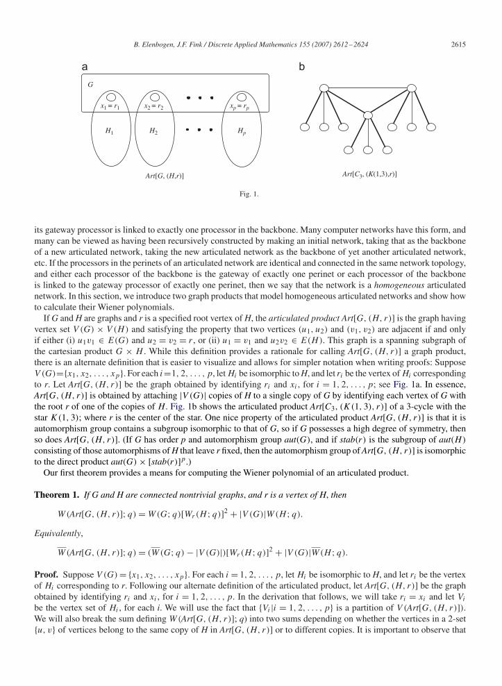
Art[G, (H,r)] Art[C3, (K(1,3),r)]

Fig. 1.

its gateway processor is linked to exactly one processor in the backbone. Many computer networks have this form, andmany can be viewed as having been recursively constructed by making an initial network, taking that as the backboneof a new articulated network, taking the new articulated network as the backbone of yet another articulated network,etc. If the processors in the perinets of an articulated network are identical and connected in the same network topology,and either each processor of the backbone is the gateway of exactly one perinet or each processor of the backboneis linked to the gateway processor of exactly one perinet, then we say that the network is a homogeneous articulatednetwork. In this section, we introduce two graph products that model homogeneous articulated networks and show howto calculate their Wiener polynomials.

If G and H are graphs and r is a specified root vertex of H, the articulated product Art[G, (H, r)] is the graph havingvertex set V (G) × V (H) and satisfying the property that two vertices (u1, u2) and (v1, v2) are adjacent if and onlyif either (i) u1v1 ∈ E(G) and u2 = v2 = r , or (ii) u1 = v1 and u2v2 ∈ E(H). This graph is a spanning subgraph ofthe cartesian product G × H . While this definition provides a rationale for calling Art[G, (H, r)] a graph product,there is an alternate definition that is easier to visualize and allows for simpler notation when writing proofs: SupposeV (G)={x1, x2, . . . , xp}. For each i=1, 2, . . . , p, let Hi be isomorphic to H, and let ri be the vertex of Hi correspondingto r. Let Art[G, (H, r)] be the graph obtained by identifying ri and xi , for i = 1, 2, . . . , p; see Fig. 1a. In essence,Art[G, (H, r)] is obtained by attaching |V (G)| copies of H to a single copy of G by identifying each vertex of G withthe root r of one of the copies of H. Fig. 1b shows the articulated product Art[C3, (K(1, 3), r)] of a 3-cycle with thestar K(1, 3); where r is the center of the star. One nice property of the articulated product Art[G, (H, r)] is that it isautomorphism group contains a subgroup isomorphic to that of G, so if G possesses a high degree of symmetry, thenso does Art[G, (H, r)]. (If G has order p and automorphism group aut(G), and if stab(r) is the subgroup of aut(H)

consisting of those automorphisms of H that leave r fixed, then the automorphism group of Art[G, (H, r)] is isomorphicto the direct product aut(G) × [stab(r)]p.)

Our first theorem provides a means for computing the Wiener polynomial of an articulated product.

Theorem 1. If G and H are connected nontrivial graphs, and r is a vertex of H, then

W(Art[G, (H, r)]; q) = W(G; q)[Wr(H ; q)]2 + |V (G)|W(H ; q).

Equivalently,

W(Art[G, (H, r)]; q) = (W(G; q) − |V (G)|)[Wr(H ; q)]2 + |V (G)|W(H ; q).

Proof. Suppose V (G) = {x1, x2, . . . , xp}. For each i = 1, 2, . . . , p, let Hi be isomorphic to H, and let ri be the vertexof Hi corresponding to r. Following our alternate definition of the articulated product, let Art[G, (H, r)] be the graphobtained by identifying ri and xi , for i = 1, 2, . . . , p. In the derivation that follows, we will take ri = xi and let Vi

be the vertex set of Hi , for each i. We will use the fact that {Vi |i = 1, 2, . . . , p} is a partition of V (Art[G, (H, r)]).We will also break the sum defining W(Art[G, (H, r)]; q) into two sums depending on whether the vertices in a 2-set{u, v} of vertices belong to the same copy of H in Art[G, (H, r)] or to different copies. It is important to observe that

2616 B. Elenbogen, J.F. Fink / Discrete Applied Mathematics 155 (2007) 2612–2624

r

r*

H rrr

G

H HH

H* (r) Susp[G, (H,r)] = Art[G, (H*(r),r*)]

Fig. 2.

if u ∈ Vi and v ∈ Vj , with i �= j , then each u.v geodesic in Art[G, (H, r)] consists of a u.ri geodesic in Hi , followedby an xi.xj geodesic in G, followed by an rj .v geodesic in Hj . Furthermore, we note that W(Hi; q) = W(H ; q) andWri (Hi; q) = Wr(H ; q), for each i. With these observations, we see that

W(Art[G, (H, r)]; q) =∑

{u,v}⊆V (Art[G,(H,r)])qd(u,v)

=p∑

i=1

∑{u,v}⊆Vi

qd(u,v) +∑

1� i<j �p

∑u∈Vi

∑v∈Vj

qd(u,v)

=p∑

i=1

W(Hi; q) +∑

1� i<j �p

∑u∈Vi

∑v∈Vj

qd(u,ri )+d(xi ,xj )+d(rj ,v)

= pW(H ; q) +∑

1� i<j �p

qd(xi ,xj )∑u∈Vi

qd(u,ri )∑v∈Vj

qd(rj ,v)

= pW(H ; q) + W(G; q)[Wr(H ; q)]2,

as claimed. Using this result and identity (1) given in the introduction, we obtain the equation W(Art[G, (H, r)]; q) =(W(G; q) − |V (G)|)[Wr(H ; q)]2 + |V (G)| · W(H ; q). �

We now consider a restricted class of articulated products. Let H be a graph and let r be a specified vertex of H.Let H ∗(r) denote the graph obtained by adding a single vertex r∗ to H together with an edge joining r∗ to r; seeFig. 2a. We define the suspended product Susp[G, (H, r)] to be the articulated product Art[G, (H ∗(r), r∗)]; seeFig. 2b. The suspended product corresponds to a network having a backbone modeled by the graph G, and |V (G)|identical perinets each modeled by the graph H and having a gateway processor corresponding to the vertex r. Eachprocessor of the backbone network is connected by a single link to the gateway processor of exactly one perinet andeach perinet’s gateway processor is linked to exactly one processor in the backbone network. To find the ordered Wienerpolynomial of Susp[G, (H, r)](=Art[G, (H ∗(r), r∗)]), we may find the ordered Wiener polynomial of the graph H ∗(r)and the Wiener polynomial of H ∗(r) relative to the vertex r∗ and apply Theorem 1.

Lemma 1. If r is a specified vertex of a connected graph H, and if r∗ and H ∗(r) are as defined in the precedingparagraph, then

(i) Wr∗(H ∗(r); q) = 1 + qWr(H ; q), and(ii) W(H ∗(r); q) = W(H ; q) + qWr(H ; q), or equivalently, W(H ∗(r); q) = W(H ; q) + 2qWr(H ; q) + 1.

B. Elenbogen, J.F. Fink / Discrete Applied Mathematics 155 (2007) 2612–2624 2617

Proof. We first establish Eq. (i). For each vertex v different from r∗, an r∗.v geodesic consists of the path of lengthone from r∗ to r followed by an r.v geodesic in H, so d(r∗, v) = 1 + d(r, v). Thus,

Wr∗(H ∗(r); q) =∑

v∈V (H ∗(r))qd(r∗,v)

= qd(r∗,r∗) +∑

v∈V (H)

qd(r∗,v)

= 1 +∑

v∈V (H)

q1+d(r,v)

= 1 + q∑

v∈V (H)

qd(r,v)

= 1 + qWr(H ; q).

The key idea in the following derivation of the first statement of (ii) is that the set of 2-element subsets of V (H ∗(r))can be partitioned into those 2-sets containing r∗ and those that do not contain r∗. We also use the statement (i)established above:

W(H ∗(r); q) =∑

{u,v}⊆V (H ∗(r))qd(u,v)

=∑

{u,v}⊆V (H)

qd(u,v) +∑

v∈V (H)

qd(r∗,v)

= W(H ; q) + [Wr∗(H ∗(r); q) − qd(r∗,r∗)]= W(H ; q) + qWr(H ; q).

This proves the first equation of (ii). By applying Eq. (1) from the introduction to this equation, one may deriveW(H ∗(r); q) = W(H ; q) + 2qWr(H ; q) + 1 in a straightforward manner. �

Using Theorem 1, Lemma 1, and the fact that Susp[G, (H, r)] = Art[G, (H ∗(r), r∗)], we get the following result.

Theorem 2. If G is a connected graph and r is a specified vertex of a connected graph H, then

W(Susp[G, (H, r)]; q) = W(G; q)(1 + qWr(H ; q))2 + |V (G)|(W(H ; q) + qWr(H ; q)),

and

W(Susp[G, (H, r)]; q) = W(G; q)(1 + qWr(H ; q))2 + |V (G)|(W(H ; q) − q2(Wr(H ; q))2).

To illustrate the utility of these theorems, we will compute the mean distances between vertices in some examplesof suspended products formed using several graphs often encountered as models of local area computer networks.Wiener polynomials of the graphs used to form these suspended products are given in the following lemma whichwe state without proof. Some parts of this lemma are results that are either stated in [8] or follow immediatelyfrom results in [8]; the remaining statements are not difficult to verify. In Lemma 2 and Corollary 1, we use Pn,Qn and K1,n to represent, respectively, the path with n vertices, the n-dimensional hypercube, and the star with nleaves; Pm × Pn (denoted by some authors as Pm�Pn) is the cartesian product of the paths Pm and Pn and willbe referred to as the m × n grid. Also, in statement 1 of Lemma 2, we use the standard q-analog of n which is[n] = 1 + q + · · · + qn−1.

2618 B. Elenbogen, J.F. Fink / Discrete Applied Mathematics 155 (2007) 2612–2624

Lemma 2. For positive integers m and n:

1. W(Pn; q) = (q/(1 − q))(n − [n]), W(Pn; q) = n + (2q/(1 − q))(n − [n]), and if r is an end-vertex of Pn, thenWr(Pn; q) = [n];

2. W(Pm × Pn; q) = W(Pm; q)W(Pn; q);3. W(Qn; q)=2n−1((1+q)n −1), W(Qn; q)=2n(1+q)n, and if r is any vertex of Qn, then Wr(Qn; q)= (1+q)n;4. W(K1,n; q) = nq + (n(n − 1)/2)q2 and, if r is the center of the star K1,n, then Wr(K1,n; q) = 1 + nq.

Using Theorems 1, 2, Fact 1, Lemma 2, and basic features of the Mathematica software package in a straightforwardway, we obtained the Wiener polynomials and the mean distances between vertices for several representative examplesof suspended products that model homogeneous articulated networks. The means are given in the following corollary.

Corollary 1. In each of the following statements, � represents the mean distance between pairs of distinct vertices inthe specified graph:

(a) For the graph Susp[Pm, (Qn, r)], where r is any specified vertex of Qn,

� = −2(1 + 21+n + 7 ∗ 4n) + 2(1 + 2n)2 ∗ m2 − 3n4n + 6m(2n + 4n)(2 + n)

6(1 + 2n)(−1 + m + m ∗ 2n).

(b) For Susp[Pm, (Pn, r)], where r is an end-vertex of Pn,

� = −1 − 2n − 2n2 + m2(1 + n) + 3mn(1 + n)

3(−1 + m + mn).

(c) For Susp[Pm, (K1,n, r)], where r is the center of K1,n,

� = −10 − 22n − 7n2 + m2(2 + n)2 + 6m(2 + 5n + 2n2)

3(2 + n)(−1 + m(2 + n)).

(d) For Susp[Pm × Pn, (Ps, r)], where r is an end-vertex of Ps ,

� = −n + s + ns + 2s2 − m2n(1 + s) − m(1 + s)(−1 + n2 + 3ns)

3(−1 + mn(1 + s)).

(e) For Susp[Pm × Pn, (Qs, r)], where r is an arbitrary specified vertex of Qs ,

� = −2(1+2s)2n+2(1+2s)2m2n−3 · 4s(4+s)+2(1+2s)m(−1−2s+(1+2s)n2+3 · 2sn(2+s))

6(1+2s)(−1+(1+2s)mn).

(f) For Susp[Pm × Pn, (K1,n, r)], where r is the center of K1,n,

� = −n(2 + s)2 + m2n(2 + s)2 − 6(1 + 3s + s2) + m(2 + s)(−2 − s + n2(2 + s) + 6n(1 + 2s))

3(2 + s)(−1 + mn(2 + s)).

(g) For Susp[Qm, (Qn, r)], where r is an arbitrary specified vertex of Qn,

� = 2m(1 + 2n)2m + 2(2(−1 + 2m+n + 2m+2n) + (−6 + 2m+n + 2m+2n)n − 2n2

2(1 + 2n)(−1 + 2m + 2m+n).

3. Nonhomogeneous articulated networks

As mentioned earlier, networks modeled by articulated products or suspended products are termed homogeneousarticulated networks. In these networks the perinets are mutually identical, and either each processor of the backboneis the gateway processor of exactly one perinet or each processor of the backbone is linked to the gateway processor of

B. Elenbogen, J.F. Fink / Discrete Applied Mathematics 155 (2007) 2612–2624 2619

exactly one perinet. In practice, of course, not all articulated networks are homogeneous. An articulated network neednot have a perinet dedicated to each processor in the backbone network and/or different perinets might have differenttopologies. In this section, we consider these nonhomogeneous articulated networks.

Let G and H be connected graphs, and let r be a specified vertex of H. Furthermore, let X = {x1, x2, . . . , xn} be anonempty subset of V (G), let H1, H2, . . . , Hn be graphs isomorphic to H, and, for each i = 1, 2, . . . , n, let ri be avertex of Hi that corresponds to r. We define Paste[(G, X), (H, r)] to be the graph obtained by identifying xi with ri(as a single vertex) for each i =1, 2, . . . , n. Also, we define Link[(G, X), (H, r)] to be the graph obtained by joining xi

to ri with an edge for each i = 1, 2, . . . , n. These graphs are subgraphs of Art[G, (H, r)] and Susp[G, (H, r)], respec-tively, and Art[G, (H, r)] = Paste[(G, V (G)), (H, r)], while Susp[G, (H, r)] = Link[(G, V (G)), (H, r)]. Defining r∗and H ∗(r) as in the paragraph preceding Lemma 1, we note that Link[(G, X), (H, r)] = Paste[(G, X), (H ∗(r), r∗)].To help find the distance distribution for these graphs, we define the Wiener polynomial of G restrictedto X as

W(G|X; q) =∑

{u,v}⊆X

qd(u,v),

and the Wiener polynomial of G relative to X as

WX(G; q) =∑x∈X

Wx(G; q).

In the Wiener polynomial of G restricted to X, the constant term is 0 and the coefficient of q is the number of edges inthe subgraph of G induced by X; the exponents d(u,v) are distances in G. The constant term of the Wiener polynomialof G relative to X is |X|.

Theorem 3. Let G and H be connected graphs, let X = {x1, x2, . . . , xn} be a nonempty subset of V (G), and let r be aspecified vertex of H. Then

W(Paste[(G, X), (H, r)]) = W(G; q) + WX(G; q)[Wr(H ; q) − 1]+ W(G|X; q)[Wr(H ; q) − 1]2 + n[W(H ; q) − Wr(H ; q) + 1]

and

W(Link[(G, X), (H, r)]; q) = W(G; q) + qWX(G; q)Wr(H ; q) + q2W(G|X; q)[Wr(H ; q)]2 + nW(H ; q).

Proof. We first obtain the Wiener polynomial of Paste[(G, X), (H, r)]. In the following derivation, we use severalfacts. The first is that for each pair of distinct vertices in Paste[(G, X), (H, r)], exactly one of the following is true: (i)both vertices belong to G; (ii) exactly one vertex of the pair is in G; (iii) for some distinct indices i and j, one vertexis in Hi , the other is in Hj , and neither is in G; (iv) for some index i, both vertices are in Hi and neither is in G.Using this fact, the sum that defines W(Paste[(G, X), (H, r)]; q) will be broken into four sums. In order to transformthese four sums into more meaningful expressions, we will use the facts that for each i = 1, 2, . . . , n, we have xi = ri ,W(Hi; q) = W(H ; q) and Wri (Hi; q) = Wr(H ; q). We now proceed with the derivation.

W(Paste[(G, X), (H, r)]; q) =∑

{u,v}⊆V (Paste[(G,X),(H,r)])qd(u,v)

=∑

{u,v}⊆V (G)

qd(u,v) +n∑

i=1

∑u∈V (G)

∑v∈V (Hi )

v �=ri

qd(u,v)

+∑

1� i<j �n

∑u∈V (Hi )

u �=ri

∑v∈V (Hj )

v �=rj

qd(u,v) +n∑

i=1

∑{u,v}⊆V (Hi)\{ri }

qd(u,v)

2620 B. Elenbogen, J.F. Fink / Discrete Applied Mathematics 155 (2007) 2612–2624

= W(G; q) +n∑

i=1

∑u∈V (G)

∑v∈V (Hi )

v �=ri

qd(u,xi )+d(ri ,v)

+∑

1� i<j �n

∑u∈V (Hi )

u�=ri

∑v∈V (Hj )

v �=rj

qd(u,ri )+d(xi ,xj )+d(rj ,v)

+n∑

i=1

[W(Hi; q) − Wri (Hi; q) + 1]

= W(G; q) +n∑

i=1

∑u∈V (G)

qd(u,xi )∑

v∈V (Hi )

v �=ri

qd(ri ,v)

+∑

1� i<j �n

qd(xi ,xj )∑

u∈V (Hi )

u�=ri

qd(u,ri )∑

v∈V (Hj )

v �=rj

qd(rj ,v)

+ n[W(H ; q) − Wr(H ; q) + 1]

= W(G; q) +n∑

i=1

∑u∈V (G)

qd(xi ,u)[Wri (Hi; q) − 1]

+∑

1� i<j �n

qd(xi ,xj )[Wri (Hi; q) − 1][Wrj (Hj ; q) − 1]

+ n[W(H ; q) − Wr(H ; q) + 1]

= W(G; q) +⎡⎣ n∑

i=1

∑u∈V (G)

qd(xi ,u)

⎤⎦ [Wr(H ; q) − 1]

+ W(G|X; q)(Wr(H ; q) − 1)2 + n[W(H ; q) − Wr(H ; q) + 1]= W(G; q) + WX(G; q)(Wr(H ; q) − 1)

+ W(G|X; q)(Wr(H ; q) − 1)2 + n[W(H ; q) − Wr(H ; q) + 1].

To prove the identity involving the Wiener polynomial W(Link[(G, X), (H, r)]; q), we recall that Paste[(G, X),

(H ∗(r), r∗)] = Link[(G, X), (H, r)], use the identity just proved to compute W(Paste[(G, X), (H ∗(r), r∗)]; q), andapply Lemma 1 to eliminate references to Wr∗(H ∗(r); q) and W(H ∗(r); q). �

If X=V (G), then WX(G; q)=W(G; q)=2W(G; q)+|V (G)| and W(G|X; q)=W(G; q). Using these observationswe can obtain Theorems 1 and 2 as corollaries of Theorem 3. At the other extreme for the size of X, we see that if Xcontains only one vertex, say x, then WX(G; q) = Wx(G; q) and W(G|X; q) = 0, and we get the following corollary.

Corollary 2. Let G and H be connected graphs, let x be a vertex of G, and let r be a specified vertex of H.

(i) If F is the graph obtained from G and H by identifying the vertices x and r as a single vertex (i.e., ifF = Paste[(G, {x}), (H, r)], then

W(F ; q) = W(G; q) − Wx(G; q) + Wx(G; q)Wr(H ; q) + W(H ; q) − Wr(H ; q) + 1.

B. Elenbogen, J.F. Fink / Discrete Applied Mathematics 155 (2007) 2612–2624 2621

(ii) If J is the graph obtained from G and H by adding a single edge from x to r, (i.e., if J = Link[(G, {x}), (H, r)],then

W(J ; q) = W(G; q) + qWx(G; q)Wr(H ; q) + W(H ; q).

The preceding corollary can be used repeatedly to find the distance distributions of arbitrary articulated networksthat are constructed by linking one perinet at a time to an existing articulated network. In effect, this allows one toboth preview and update the distance distribution generating functions when a new perinet is to be added to an existingnetwork. More generally, if a network can be constructed by a finite sequence of Paste and Link operations, thenTheorem 3 and/or Corollary 2 can be used repeatedly to find the Wiener polynomial of the network.

4. Generalizing the Wiener polynomials to weighted graphs

In mathematical modeling, graphs with positive edge weights are often useful. For example, if a graph G models acomputer network, the weight on an edge may represent the time required to send a message of unit length along thatedge. Similarly, the sum of the weights on the edges of a path represents the time required to send a unit length messagealong the path. It seems natural then to generalize the polynomials discussed in previous sections to the weighted graphsetting. Further support for such a generalization is given by the fact that a Wiener index for weighted graphs has beenstudied in [7,4,9,11] in relation to chemical graph theory.

For weighted graphs, we define the weight of a path to be the sum of the weights on the path’s edges. A path ofminimum weight from a vertex u to a vertex v (lying in a common component of the graph) will be called a u.vweight-geodesic; its weight is termed the weighted distance from u to v and denoted by wd(u, v). We will find itconvenient to reserve the notation d(u, v) for the usual unweighted distance from u to v in the underlying unweightedgraph. If a connected graph is uniformly weighted with each edge having weight c, then, for each pair (u, v) of vertices,a u.v path is a u.v geodesic if and only if it is a u.v weight-geodesic; furthermore, wd(u, v) = c · d(u, v).

By analogy with the varieties of Wiener polynomials discussed earlier, we define five generating functions fordistance distributions in weighted graphs. The (unordered) weighted Wiener function of a connected weighted graphG is

wW(G; q) =∑{u,v}

qwd(u,v),

where the sum is over all unordered pairs {u, v} of distinct vertices in G. The ordered weighted Wiener function is

wW(G; q) =∑(u,v)

qwd(u,v),

where the sum is over all ordered pairs (u, v) of not necessarily distinct vertices. If u is a vertex of G the weightedWiener function of G relative to u is

wWu(G; q) =∑

v∈V (G)

qwd(u,v).

For each nonempty subset X of V (G), we define the weighted Wiener function of G restricted to X as

wW(G|X; q) =∑

{u,v}⊆X

qwd(u,v),

and the weighted Wiener function of G relative to X as

wWX(G; q) =∑x∈X

wWx(G; q).

The first three of these five functions are generating functions for weighted distance distributions, ordered weighteddistance distributions, and weighted distance degree sequences, respectively; e.g., the coefficient of qk in wW(G; q) isthe number of ordered pairs of vertices at distance k from each other. These distance frequency functions are polynomials

2622 B. Elenbogen, J.F. Fink / Discrete Applied Mathematics 155 (2007) 2612–2624

if and only if the edge weights in G are integers. They equal the corresponding Wiener polynomials if and only if alledge weights are 1. In a manner analogous to the Wiener polynomials, the weighted distance frequency function andthe ordered weighted distance frequency function are related by the equation

wW(G; q) = 2wW(G; q) + |V (G)|.Furthermore,

wW(G; q) =∑

u∈V (G)

wWu(G; q).

Relative weighted distance frequency functions can be easily found for specific graphs by employing Dijkstra’s algo-rithm. Also, in a manner similar to the methods used to obtain Facts 1 and 2, we can use standard elementary probabilityarguments to obtain the following facts about weighted distance statistics for connected weighted graphs; these are theweighted analogues to Facts 1 and 2 that were stated earlier.

Fact 3. Let G be a connected weighted graph having p vertices, and assume that the probability of selecting anyunordered pair of distinct vertices in G is 1/

(p2

). Then

(i) the mean weighted distance between pairs of distinct vertices in G is

� = wW ′(G; 1)(p

2

) = wW ′(G; 1)

p(p − 1)and

(ii) the variance of the weighted distance distribution of G is

�2 = wW ′′(G; 1)(p

2

) + � − �2 = wW ′′(G; 1)

p(p − 1)+ � − �2.

Fact 4. Let u be a vertex of a connected weighted graph G having p vertices, and assume that 1/(p − 1) is theprobability of selecting any vertex of G other than u. Then

(i) the mean weighted distance from u to any other vertex of G is

�u = wW ′u(G; 1)

p − 1and

(ii) the variance of the set of weighted distances from u to distinct vertices of G is

�2u = wW ′′

u(G; 1)

p − 1+ �u − �2

u.

As one would expect, many of the theorems, corollaries and lemmas of the preceding sections have analogues forweighted graphs. For each such result, the proof of the analogue is very similar to the proof of the correspondingstatement for unweighted graphs, so we omit the proofs. For example, by making minor changes in the proof ofTheorem 1 to account for weighted distances, we can obtain the following result that is analogous to Theorem 1.

Theorem 4. If G and H are connected weighted graphs, and r is a vertex of H, then

wW(Art[G, (H, r)]; q) = wW(G; q)[wWr(H ; q)]2 + |V (G)|wW(H ; q).

Equivalently,

wW(Art[G, (H, r)]; q) = (wW(G; q) − |V (G)|)[wWr(H ; q)]2 + |V (G)| · wW(H ; q).

B. Elenbogen, J.F. Fink / Discrete Applied Mathematics 155 (2007) 2612–2624 2623

Formulations of the weighted distance frequency functions for suspended products Susp[G, (H, r)] depends on theweight assigned to the edge joining r∗ to r in H ∗(r). The following lemma is analogous to Lemma 1.

Lemma 3. Suppose that r is a specified vertex of a connected weighted graph H, and r∗ and H ∗(r) are as given inthe definition of the suspended product Susp[G, (H, r)], for some connected graph G. Furthermore, suppose that theedge from r∗ to r has been given the weight �. Then

(i) wWr∗(H ∗(r); q) = 1 + q�wWr(H ; q), and(ii) wW(H ∗(r); q)=wW(H ; q)+q�wWr(H ; q), or equivalently,wW(H ∗(r); q)=wW(H ; q)+2q�wWr(H ; q)+1.

By direct application of Theorem 4, Lemma 3 and the definition of a suspended product, we obtain the followinganalogue to Theorem 2.

Theorem 5. Let G be a connected weighted graph and r be a specified vertex of a connected weighted graph H. Letr∗ and H ∗(r) be as given in the definition of the suspended product Susp[G, (H, r)], and suppose that the edge fromr∗ to r has been given the weight �. Then

wW(Susp[G, (H, r)]; q) = wW(G; q)(1 + q�wWr(H ; q))2 + |V (G)|(wW(H ; q) + q�wWr(H ; q))

and

wW(Susp[G, (H, r)]; q) = (wW(G; q) − |V (G)|)(1 + q�wWr(H ; q))2

+ |V (G)|(wW(H ; q) + 2q�wWr(H ; q) + 1).

Minor adjustments to the proof of Theorem 3 yield that theorem’s weighted distance analogue, which follows.

Theorem 6. Let G and H be connected weighted graphs, let X = {x1, x2, . . . , xn} be a nonempty subset of V (G), andlet r be a specified vertex of H. Then

wW(Paste[(G, X), (H, r)]) = wW(G; q) + wWX(G; q)[wWr(H ; q) − 1]+ wW(G|X; q)[wWr(H ; q) − 1]2 + n[wW(H ; q) − wWr(H ; q) + 1].

Furthermore, if for each i = 1, 2, . . . , n, the edge joining xi to ri , as given in the definition of Link[(G, X), (H, r)],has weight �, then

W(Link[(G, X), (H, r)]; q) = wW(G; q) + q�wWX(G; q)wWr(H ; q)

+ q2�wW(G|X; q)[wWr(H ; q)]2 + nwW(H ; q).

As a corollary to this theorem, we have an analogue to Corollary 2. Its proof follows immediately from the pre-vious theorem and the observations that if X contains only one vertex, say x, then wWX(G; q) = wWx(G; q) andwW(G|X; q) = 0.

Corollary 3. Let G and H be connected weighted graphs, let x be a vertex of G, and let r be a specified vertex of H.

(i) If F is the weighted graph obtained from G and H by identifying the vertices x and r as a single vertex (i.e., ifF = Paste[(G, {x}), (H, r)], then

wW(F ; q) = wW(G; q) − wWx(G; q) + wWx(G; q)wWr(H ; q) + wW(H ; q) − wWr(H ; q) + 1.

(ii) If J is the graph obtained from G and H by adding a single edge of weight �, from x to r, (i.e., if J = Link[(G, {x}),(H, r)], then

wW(J ; q) = wW(G; q) + q�wWx(G; q)wWr(H ; q) + wW(H ; q).

2624 B. Elenbogen, J.F. Fink / Discrete Applied Mathematics 155 (2007) 2612–2624

Finally, we remark that if each edge of a weighted graph G has the same weight, say c, then the five functions discussedin this section can be expressed in terms of the corresponding polynomials for unweighted graphs. Specifically, wehave the following:

Remark. If each edge of a connected weighted graph G has the same weight, say c, then

1. wW(G; q) = W(G; qc),2. wW(G; q) = W(G; qc),3. wWr(G; q) = Wr(G; qc), for each vertex r of G,4. wW(G|X; q) = W(G|X; qc), for each subset X of V (G), and5. wWX(G; q) = WX(G; qc), for each subset X of V (G).

Consequently, a weighted Wiener function (and variants) of a uniformly weighted graph can be easily computed ifthe corresponding (unweighted) polynomial is known; e.g., if each edge of the n-dimensional hypercube has weight c,then, wW(Qn; q)=W(Qn; qc)= 2n(1 +qc)n. Furthermore, each of Theorems 4, 5 and 6 can be modified to a slightlysimpler form in the cases when one or both of the connected weighted graphs G and H are uniformly weighted. As anillustration, we state the following corollary to Theorem 5.

Corollary 4. Let G be a connected weighted graph and r be a specified vertex of a connected weighted graph H.Furthermore, suppose that every edge of G has weight � and every edge of H has weight �. Let r∗ and H ∗(r) be asgiven in the definition of the suspended product Susp[G, (H, r)], and suppose that the edge from r∗ to r has weight �.Then

wW(Susp[G, (H, r)]; q) = W(G; q�)(1 + q�Wr(H ; q�))2 + |V (G)|(W(H ; q�) + q�Wr(H ; q�))

5. Conclusion

In this paper we have presented a relatively simple and useful way, via generating functions, to find and store distancedistributions for graphs modeling the very large class of computer networks we call articulated networks. By assigningappropriate weights to the edges of the graph modeling an articulated network and using these generating functionmethods with a symbolic computation engine, one can quickly generate data and statistics related to the communicationtime between distinct processors during distributed computing. In this manner, the generating function approach canbe used as a design and analysis tool for large articulated networks. These methods are especially simple when thearticulated networks are homogeneous and/or when the backbone and the perinets are modeled by distance transitivegraphs with uniformly weighted edges. The authors are currently preparing a paper in which properties of the Wienerfunctions are exploited to analyze existing networks and design new networks. We will also present new results ofspecial interest to computer scientists.

References

[1] Discrete Math. 80 (1997). (Special issue on the Wiener index.)[2] F. Buckley, F. Harary, Distance in Graphs, Addison-Wesley, Redwood, CA, 1990.[3] G. Chartrand, L. Lesniak, Graphs & Digraphs, second ed., Wadsworth & Brooks/Cole, Monterey, CA, 1986.[4] V. Chepoi, S. Klavzar, Distances in benzenoid systems: further developments, Discrete Math. 192 (1998) 27–39.[5] A.A. Dobrynin, Construction of graphs with a palindromic Wiener polynomial, Vychislitel’nye Sistemy No. 151, Teor. Grafov i ee Prilozhen.

118 (1994) (1995) 37–54.[6] H. Hosoya, On some counting polynomials in chemistry. Applications of graphs in chemistry and physics, Discrete Appl. Math. 19 (1–3) (1988)

239–257.[7] S. Klavzar, I. Gutman, Wiener number of vertex-weighted graphs and a chemical application, Discrete Appl. Math. 80 (1997) 73–81.[8] B.E. Sagan, Y.-N. Yeh, P. Zhang, The wiener polynomial of a graph, Internat. J. Quantum Chem. 60 (1996) 959–969.[9] P. Senn, The computation of the distance matrix and the Wiener index for graphs of arbitrary complexity with weighted vertices and edges,

Comput. Chem. 12 (1988) 219–227.[10] H. Wiener, Structural determination of paraffin boiling points, J. Amer. Chem. Soc. 69 (1947) 17–20.[11] B. Zmazek, J. Zerovnik, Computing the weighted Wiener and Szeged number on weighted cactus graphs in linear time, Croat. Chem. Acta 76

(2003) 137–143.