arX

iv:a

stro

-ph/

9809

257v

1 2

1 Se

p 19

98

Relativistic and Newtonian core-shell models: analytical and numerical results

Werner M. Vieira and Patricio S. Letelier

Departamento de Matematica Aplicada, Instituto de Matematica, Estatıstica e Computacao Cientıfica,

Universidade Estadual de Campinas, CP 6065,

13081-970 Campinas, SP, Brazil

ABSTRACT

We make a detailed analysis of the exact relativistic core-shell models recently proposed

to describe a black hole or neutron star surrounded by an axially symmetric, hollow halo of

matter, and in a seminal sense also galaxies since there are massive shell-like structures – as

for example rings and shells – surrounding many of them and also evidences for many galactic

nuclei hiding black holes. We discuss the unicity of the models in relation to their analyticity

at the black hole horizon and to the full elimination of axial (conical) singularities. We also

consider Newtonian and linearized core-shell models, on their own to account for dust shells

and rings around galaxies and supernova and star remnants around their centers, and also as

limiting cases of the corresponding relativistic models to gain physical insight.

Secondly, these models are generic enough to numerically study the role played by the

presence/lack of discrete reflection symmetries about planes, i. e. the presence/lack of equatorial

planes, in the chaotic behavior of the orbits. This is to be contrasted with the almost universal

acceptance of reflection symmetries as default assumptions in galactic modeling. We also

compare the related effects if we change a true central black hole by a Newtonian central mass.

Our main numerical findings are:

1- The breakdown of the reflection symmetry about the equatorial plane in both Newtonian

and relativistic core-shell models does i) enhance in a significant way the chaoticity of orbits

in reflection symmetric oblate shell models and ii) inhibit significantly also the occurrence of

chaos in reflection symmetric prolate shell models. In particular, in the prolate case the lack of

the reflection symmetry provides the phase space with a robust family of regular orbits that is

otherwise not found at higher energies.

2- The relative extents of the chaotic regions in the relativistic cases (i. e. with a true central

black hole) are significantly larger than in the corresponding Newtonian ones (which have just a

−1/r central potential).

Subject headings: black holes — galaxies: structure — galaxies: rings, shells — circumstellar

matter: rings, shells — dark matter: hollow halos — stars: stellar dynamics

1. Introduction

We make a more detailed study, both analytical and numerical, of some exact relativistic solutions

we recently proposed to describe static, axially symmetric massive core-shell systems (Vieira and Letelier

1996a, 1997, hereafter VL1 and VL2, respectively). We add in this way to the efforts of modeling many

situations of interest in astrophysics involving massive shell-like structures around centers, as for example

– 2 –

black holes or neutron stars surrounded by massive shell and ring remnants. A nice illustration of this

possibility is offered by the famous Supernova 1987A plus its physical rings, see e. g. Panagia et al. (1996),

Meyer (1997) and Chevalier (1997). At least in a seminal sense, the model could also describe galaxies

since there are many of them exhibiting massive rings (Sackett and Sparke 1990, Arnaboldi et al. 1993,

Reshetnikov and Sotnikova 1997) and shells (Malin and Carter 1983, Quinn 1984, Dupraz and Combes

1987, Barnes and Hernquist 1992), while many others possibly have galactic nuclei hiding black holes (see

Kormendy and Richstone 1995 for a review).

Specifically, we implement here a monopolar core (a black hole in the relativistic case) plus an exterior

shell of dipoles, quadrupoles and octopoles. Obviously, these multipoles are shell-like Legendre expansions

i. e. their corresponding terms increase with the distance in the intermediate vacuum between the core and

the shell. Beyond its own applicability, the model also points to the possibility of a realistic description of

any axially symmetric relativistic core-shell configuration whose approximation as a static system should

be valid at some useful time scale, via a systematic multipolar Legendre expansion. In fact, a further step

in this program was lastly started in Letelier and Vieira (1997) by giving stationarity (rotation) to the

relativistic case of a monopolar core plus a purely dipolar shell. This is an important improvement since

real celestial objects do rotate. The present analysis will be extended to rotating core-shell models in a

forthcoming contribution.

Additionally, we consider the Newtonian counterpart of the relativistic model above, which was only

sketched in the previous works, and show that they could describe core-shell systems “per se” interesting in

astronomy. So, we can have massive circumstellar dust shells around certain types of stars as byproducts of

their death, see e. g. Barlow et al. (1994) for an example of (irregular) circumstelar shells around luminous

blue variables and a review by Groenewegen et al. (1998) about dust shells around carbon Mira variables.

Another potential application for core-shell models is to the more speculative possibility of hollow galactic

halos of dark matter made of neutrinos recently considered by Ralston and Smith (1991), Madsen (1991)

and Barnes (1993). Moreover, we will see that the study of the relativistic core-shell model in parallel to its

Newtonian counterpart is useful also to clarify the physical content of the former one.

After Poincare (1957) and the KAM theory (after Kolmogorov 1954, Arnol’d 1963a, 1963b and Moser

1967) it became well established that non-integrability and hence chaos is a general rather than exceptional

manifestation in the context of dynamical systems (modeling or not physical situations) (see Berry 1977).

Given this ubiquitous fact, an important issue in astronomical modeling is to study in which extent in phase

space chaoticity rises in models that are relevant to describe real systems and what are its consequences.

For example, Binney (1982a) discusses the difficulties of constructing stationary self-consistent models

when a significant fraction of orbits are irregular since they may not obey neither Vlasov’s nor Jean’s

equations. Then, it is remarkable that a wide class of fully integrable potentials, the so called Stackel

potentials (Lynden-Bell 1962, de Zeeuw 1985 and de Zeeuw et al. 1986), are feasible starting points to

describe, by themselves or by adding perturbations, real disc, elliptical or even triaxial galaxies. For more

realistic tridimensional models there are evidences for rounder and smoother mass distributions generating

only relatively small fractions of chaotic orbits (Schwarzschild 1979, Binney and Tremaine 1987 and Evans

et al. 1997), while flattening and/or sharpening of the mass distributions, for example through increasing

triaxiality and/or putting cusps and central masses to mimic black holes, tends to increase the chaoticity

and force us to take it into account (Gerhard and Binney 1985, Schwarzschild 1993, Merrit and Fridman

1996, Norman et al. 1996, Merrit 1997 and Valluri and Merrit 1998). On the other hand, the emergence of

chaos in two-dimensional models has more loose correlations with morphological aspects, see for example

Binney and Spergel (1982), Richstone (1982), Binney (1982b), Gerhard (1985) and Sridhar and Touma

– 3 –

(1997).

We address in this work also a numerical study about the chaoticity of orbits trapped in the bound

gravitational zones between the core and the external massive shell. Beyond its own applicability as

seen above, we take advantage of models that are generic within the class of axially symmetric core-shell

distributions and moreover offer exact relativistic and Newtonian counterparts to be compared, in order

to achieve some understanding about chaoticity related to two aspects: firstly, to the role of reflection

symmetries shared by almost all models in astronomy and astrophysics, and secondly to the consequences

of treating exact central black holes as just Newtonian central masses.

In the first part of this article (section 2) we present analytical results concerning some properties

like unicity and analyticity of the relativistic solutions themselves, in connection with both the linearized

core-shell solutions and the corresponding Newtonian models taken as limiting cases.

In section 2.1 we enlarge the relativistic solution presented in VL1 for a monopolar core plus a shell of

quadrupoles and octopoles in order to include a dipolar shell component. This complete solution was only

outlined in VL2. In this later reference it was emphasized that the case of a core plus purely dipolar shell is

physically non-trivial already in the Newtonian gravity, moreover, it was shown that the Newtonian dipolar

case is integrable, in contrast with its chaotic relativistic counterpart, which allowed us to characterize

the chaotic behavior in this case as an intrinsic general relativistic effect. Here, we take advantage of

this striking difference of the dipolar case in order to reinforce the numerical conclusions presented in

section 3 concerning the non-trivial dynamical role played by the presence/absence of the discrete reflection

symmetry about the equatorial plane on the chaoticity of the orbits.

In section 2.2 we proceed to a full elimination of axial (conical) singularities (hereafter CSs) from the

relativistic model, which was only partially accomplished in VL1. In fact, CSs are not globally removable

from neither static nor stationary many-body relativistic solutions since they are self-consistently demanded

by Einstein’s equations to strut the otherwise unstable configuration against its own gravity (see Robertson

and Noonan 1968 and Letelier and Oliveira 1998 for a recent review). So, in the present case the most we

can do is really move all them outside the shell, thus obtaining a true vacuum in the intermediate space

between the core and the shell. We also discuss in this section the conditions for the Kruskal-type analyticity

of the solutions at the horizon of the central black hole and use both aspects to find the conditions under

which the unicity of the models is assured.

In section 2.3 we present the linearization of the relativistic model in the multipole strengths via the so

called Regge-Wheeler (RW) formalism. In particular, we see that our model exemplifies the fact that CSs

survive to the linearization process, their presence in the intermediate vacuum being in fact an obstruction

to the application of the RW formalism. This does reinforce the interpretation of CSs as a kind of singular

matter distribution necessary to the dynamical consistency of static and stationary relativistic models.

However being intrinsecally relativistic manifestations, an adiabatic treatment of CSs in the Newtonian

limit allows for estimates concerning the emission rate of gravitational waves by two coalescing rotating

black holes (Araujo et al. 1998).

In section 2.4 we discuss Newtonian core-shell models, on their own as well as limiting cases of the

corresponding relativistic ones. We put the Henon-Heiles-like structure of the relativistic models in the

appropriate astronomical context and stress the physical content of the various terms present in them, in

particular we see that the apparently naive constant relativistic solution does in fact hide a relativistic

homoeoid (see Chandrasekhar 1987 for Newtonian homoeoids).

– 4 –

The numerical part of this article is presented in section 3 and deals with a study of the chaoticity of

orbits trapped in the intermediate vacuum between the core and the shell. Specifically, we shall explore

in this section the fact that, due to its generality, axially symmetric core-shell expansions are particularly

suitable to study the dynamical role played by a discrete symmetry of the model — namely the reflection

symmetry about an equatorial plane, on the chaoticity of orbits. The reflection symmetry is present in the

model if and only if the shell is of even-type, i. e. iff 22n-poles, n = 0, 1, 2, 3, ..., occur in the shell expansion,

and it is broken if we add any odd, 22n+1-poles to the expansion. The hypothesis of reflection symmetry

is a widely spread assumption in astronomical modeling and its twofold justification lies firstly in that too

many real celestial objects to be modeled, for example stars themselves, star clusters and galaxies seem

in fact very symmetric with respect to a middle plane. Another reason for this symmetry assumption is

that the resulting model gets strongly simplified in both analytical and numerical aspects. Of course, we

do not expect the reflection symmetry be realized in nature exactly, so it is relevant to search for possible

detectable dynamical effects arising from deviations of that symmetry.

A strong additional motivation for this numerical study is to compare from the point of view of the

chaotic behavior what happens when the presence of true central black holes are simplified by reducing

them to Newtonian central masses. This is a commom practice in current modeling, as for example in

Gerhard and Binney (1985), Sridhar and Touma (1997) and Valluri and Merrit (1998).

Surprisingly enough, the numerical findings show marked effects on the chaoticity of the orbits in the

intermediate vacuum between the core and the shell linked to the presence/lack of the reflection symmetry

in the relativistic as well as Newtonian models. We also find strong quantitative differences in the chaoticity

manifested in both relativistic and Newtonian cases.

Finally, we present the conclusions with some discussion and prospects in section 4.

2. Analytical results: exact, linearized and Newtonian core-shell models

2.1. The exact model

We deal here with static, axially symmetric models, for which the Weyl coordinates (t, ρ, z, φ) are the

starting point:

ds2 = e2νdt2 − e2γ−2ν[dz2 + dρ2] − e−2νρ2dφ2, (1)

where ν and γ are functions of ρ and z only. Except where units are explicitly required (particularly in

section 2.4), we use non-dimensional variables: s ↔ s/L (idem for ρ and z), and t ↔ ct/L where c is the

light velocity in vacuum and L is some convenient unit of length. Einstein’s equations in absence of matter

(vacuum) reduce in this case to the usual Laplace equation for ν

ν,ρρ +1

ρν,ρ + ν,zz = 0, (2)

and the quadrature

dγ = ρ[(ν,ρ)2 − (ν,z)

2] dρ + 2ρν,ρν,z dz (3)

for γ.

Before proceeding, we mention that the Weyl coordinates should be considered somewhat deceiving if

we insist in naively transferring their image contents about mass configurations to the Newtonian common

sense. For example, the spherical shape of the horizon of a black hole is compressed into a bar in Weyl’s

– 5 –

coordinates, the interior portion of the black hole space-time being wholly discarded from the portrait.

Apart from the well known fact that the relativistic context is not cast in a straight relation with the

Newtonian one in strong regimes, they are mathematically sound as will be clear later when we will compare

both versions of the core-shell models.

We pass to the prolate spheroidal coordinates (t, u, v, φ), which have a direct link with the “spherical”

ones (t, R, θ, φ) (R ↔ R/L) we will use later,

u = R − 1 =1

2[√

ρ2 + (z + 1)2 +√

ρ2 + (z − 1)2], u ≥ 1,

v = cosθ =1

2[√

ρ2 + (z + 1)2 −√

ρ2 + (z − 1)2], −1 ≤ v ≤ 1, (4)

or, in terms of ρ, z,

ρ =√

(u2 − 1)(1 − v2) =√

R(R − 2)sinθ, R ≥ 2,

z = uv = (R − 1)cosθ. (5)

Eqs. (2) and (3) are written in terms of u, v as

[(u2 − 1)ν,u],u + [(1 − v2)ν,v],v = 0, (6)

γ,u =1 − v2

u2 − v2[u(u2 − 1)(ν,u)2 − u(1 − v2)(ν,v)2 − 2v(u2 − 1)ν,uν,v],

γ,v =u2 − 1

u2 − v2[v(u2 − 1)(ν,u)2 − v(1 − v2)(ν,v)2 + 2u(1 − v2)ν,uν,v]. (7)

In the prolate spheroidal coordinates u, v, Laplace equation (6) can be separated and solved in terms

of standard Legendre polynomials Qℓ, Pℓ (see for example Moon and Spencer 1988, and, for relativistic

applications, Reina and Treves 1976):

ν(u, v) =∞∑

0

[aℓQℓ(u) + bℓPℓ(u)][cℓQℓ(v) + dℓPℓ(v)]. (8)

The particular solution picked out from the general one above is determined by the matter distribution

whose model is wanted. We are interested here in monopolar core plus shell-type models, so we are guided

by the Newtonian case (to be detailed in section 2.4) to the specific solution of the form (up to third order)

2ν = 2ν0 − 2κQ0(u) + 2DP1(u)P1(v) + (4/3)QP2(u)P2(v) + (4/5)OP3(u)P3(v). (9)

ν0 is an integration constant and Q0 describes the monopolar core, which either reduces to a black hole if

we put κ = 1 and identify 2L with the Schwarzschild radius of the core (in which case (t, R, θ, φ) above

are Schwarzschild’s coordinates), or can be switched off by simply putting κ = 0. The remaining terms

correspond to the multipoles originated from the exterior shell of matter: dipole D, quadrupole Q and

octopole O (note the opposite sign convention for dipoles in this definition with respect to that appearing

in VL2). The nontrivial character of shell dipoles in both Newtonian and general relativistic theories of

gravity has been anticipated in VL2 while shells made of quadrupoles plus octopoles were considered in

VL1. If non-monopolar cores should be considered, we should add to (9) terms of the form Qℓ(u)Pℓ(v),

ℓ ≥ 1.

– 6 –

Much more sophisticated multipolar relativistic treatments for core, shell and core-shell models are

considered by Thorne (1980), Zhang (1986) and Suen (1986a, 1986b), respectively, in terms of higher order

systematic expansions of the metric in de Donder coordinates. Our approach is more modest at this stage

and inspired only on the zeroth order, Newtonian limit of the full relativistic situation.

The odd multipoles of v in (9) (D and O in the present case) break the reflection symmetry about the

plane z = 0, and we shall show in section 2.2 that we need of both D and O being simultaneously either

present or absent if we want to rule out conical singularities of the intermediate vacuum between the core

and the shell. We rewrite (9) as

2ν = κ log(u−1u+1 ) + P (u, v),

P = 2ν0 + 2Duv + 13Q(3u2 − 1)(3v2 − 1) + 1

5Ouv(5u2 − 3)(5v2 − 3).(10)

After integrating (7) we obtain the corresponding solution for γ:

2γ = κ2 log( u2−1u2−v2 ) + Q(u, v),

Q = 2γ0 + γD + γQ + γO + γDQ + γDO + γQO,

γD = 4κDv −D2[u2(1 − v2) + v2],

γQ = −4κQu(1− v2)

+ (1/2)Q2[u4(1 − v2)(1 − 9v2) − 2u2(1 − v2)(1 − 5v2) − v2(2 − v2)],

γO = −(2/5)κOv[5(3u2 − 1)(1 − v2) − 4]

+ (3/100)O2[−25u6(1 − v2)(5v2 + 2v − 1)(5v2 − 2v − 1)

+ 15u4(1 − v2)(65v4 − 40v2 + 3) − 3u2(1 − v2)(25v2 − 3)(5v2 − 3)

− v2(25v4 − 45v2 + 27)],

γDQ = −4DQuv(u2 − 1)(1 − v2),

γDO = (3/10)DO[u2(5u2 − 6)(1 − v2)(1 − 5v2) + v2(5v2 − 6)],

γQO = −(6/5)QOuv(u2 − 1)(1 − v2)[(5u2 − 1)(3v2 − 1) + 2(1 − v2)].

(11)

This is the complete solution, which was outlined in VL2. The additional integration constant γ0 will be

fixed in the next section in connection with the elimination of conical singularities from the intermediate

vacuum, while the integration constant ν0 will prove to be necessary in assuring analyticity to the full

core-shell solution at the horizon in the absence of conical singularities. The terms proportional to κ in γD,

γQ and γO represent nonlinear interactions between the black hole and the external shell.

2.2. Unicity and smoothness requirements

We shall be interested in two classes of singularities of the Weyl spacetime. The first one are the

strong singularities that are located in the points wherein the scalar polynomial invariants of the curvature

tensor blow up. For a static axially symmetric spacetime solution to the vacuum field equations we have

only two non-vanishing invariants. They are (Carminati and McLenaghan 1991) w1 ≡ 18CabcdC

abcd and

w2 ≡ − 116Ccd

abCefcd Cab

ef where Cabcd is the Weyl trace-free tensor, which for vacuum solutions coincides with

– 7 –

the Riemann curvature tensor. After some algebraic manipulations, they reduce to

w1 = 2κ2[3σ(ν2,z + ρ2ν2

,ρν2,z − ν,ρ/ρ − ρν,ρσ) + ν2

,ρ(1 + 2ργ,ρ + 3ρν,ρ)

+ ρ2(ν6,z + ν6

,ρ) + ν,ρz(6ν,ρν,z + ν,ρz − 2(ν,zγ,ρ + ν,ργ,z))

+ ν,ρρ(3γ,ρ(1 − 2ρν,ρ)/ρ − ν,zz + 2ν,zγ,z)],

w2 = 3κ3ρ−2(ν,ρ/ρ − σ)[σ(3ρ3ν2,ρν

2,z + ρ(1 − 3ρν,ρ)σ + 2ν,ρ)

− ν2,z(γ,ρ + 3ν,ρ(1 − 2ρν,ρ)) + ρ3(ν6

,z + ν6,ρ)

+ rν,ρz(2ν,z(3ν,ρ(1 − ρν,ρ) + ρν2,z) + νρz)

+ ν,ρρ(3γ,ρ(1 − 2ρν,ρ) + 4r2ν3,ρ − ρν,zz)]

(12)

where σ ≡ ν2,z +ν2

,r an κ ≡ exp 2 (ν − γ). In the present case, these scalars are singular on the position of the

attraction center and will be also singular in some directions of the spatial infinity (the specific directions

will depend on the signs of D, Q, etc.), in other words they are singular in the position of the sources of the

gravitational field.

There is another class of singularities that do not show up in a simple way in the curvature, the so

called conical singularities (CSs) (Sokolov and Starobinskii 1977). These singularities are in some sense

like the distributions related to a low dimensional Newtonian potential, e.g., for an infinite massive wire

the potential is φ = 2λ ln ρ, we have that the Laplace equation, the analog to the curvature, gives us

∇2φ = 0 for ρ 6= 0 while for ρ = 0 we need to use some global property, for example Gauss theorem,

to get ∇2φ = 4πλδ(ρ). To be more precise, let us consider a conical surface, z = αρ, embedded in

the usual Euclidean three dimensional space ds2 = dρ2 + ρ2dϕ2 + dz2, so that we have on the cone

ds2 = (1 + α2)dρ2 + ρ2dϕ2 = dρ2 + β2ρ2dϕ2 with ρ =√

1 + α2ρ and β2 = 1/(1 + α2). Note that the

coordinate range of ρ as well as ϕ are the usual ones. The ratio between the arc of the circumference and

its radius is 2βπ in this case. If we compute the Riemann tensor for this last metric we find that Rρϕρϕ = 0

for ρ 6= 0. By using the Gauss-Bonnet theorem in this case, we can pick up the curvature singularity as

being of the form Rρϕρϕ ∝ δ(ρ).

It is well known that CSs arise when we consider Weyl’s solutions near the symmetry axis (Robertson

and Noonan 1968 and Letelier and Oliveira 1998a). They are interpreted as a geometric consequence of the

presence of some kind of “strut”, necessary to consistently prevent any static non-spherically symmetric

model from collapsing due to self-gravity. In this sense, the uniqueness of the core-type, one-body solution

for the (static) spherically symmetric Einstein’s equations (namely, the Schwarzschild one) should relate

to the fact that it is impossible to attach struts in a perfectly round metric. For the Weyl solutions, we

can always consider a small disk centered in the symmetry axis (t = t0, z = z0, ρ = ǫ, 0 ≤ ϕ < 2π) and

impose that the ratio between the circumference and its radius equals 2π. This is the condition to eliminate

CSs from the intermediate vacuum (then attaching them to the infinity), which amounts to impose on the

function γ the well known conditions of elementary flatness

2γ |ρ=0,|z|>1≡ 2γ |u=|z|,v=±1= 0. (13)

These two conditions fix the constant γ0 and impose an additional constraint on the odd shell multipoles

(D and O here) in the presence of the black hole:

2γ0 −D2 − 1

2Q2 − 21

100O2 − 3

10DO = 0, (14)

κ[D +2

5O] = 0. (15)

– 8 –

The condition (14) fixing γ0 is necessary in all cases to rule out the conical singularities. From (15) we

see that the former is also a sufficient condition in two cases: i) the shell of dust is left alone by switching

off the core (κ = 0), and ii) in the presence of the black hole (κ = 1), the shell is made only of even-type

multipoles (Q here). We also see that it is possible to eliminate conical singularities for a single or pure

shell component only if it is of the even type. Then, it follows that the core-shell dipole solution presented

in VL1, as well as those with O 6= 0 presented in VL2, all have conical singularities since they do satisfy

(14) but not (15) . If we include the necessary condition (14) in (11), we have the following for γ:

2γ = κ2 log( u2−1u2−v2 ) + Q(u, v),

Q = γD + γQ + γO + γDQ + γDO + γQO,

γD = 4κDv −D2(u2 − 1)(1 − v2),

γQ = −4κQu(1 − v2) − (1/2)Q2(u2 − 1)(1 − v2)[u2(9v2 − 1) + 1 − v2],

γO = −(2/5)κOv[5(3u2 − 1)(1 − v2) − 4]

− (3/100)O2(u2 − 1)(1 − v2)[(25u4 − 20u2 + 1)(25v4 − 14v2 + 1)

+ 30u2v2(5v2 − 1) + 6(1 − v2)],

γDQ = −4DQuv(u2 − 1)(1 − v2),

γDO = (3/10)DO(u2 − 1)(5u2 − 1)(1 − v2)(1 − 5v2),

γQO = −(6/5)QOuv(u2 − 1)(1 − v2)[(5u2 − 1)(3v2 − 1) + 2(1 − v2)].

(16)

Here, it is explicitly seen that only the first terms in γD and γO, respectively, do not vanish identically

at v = ±1. They cancel one another at those points only if we use the additional condition (15) in the

equation above, which amounts to put there either κ = 0 or D+ (2/5)O = 0 plus κ = 1. In the later case, γ

lastly becomes

2γ = log( u2−1u2−v2 ) + Q(u, v),

Q = γQ + γDO + γQDO,

γQ = −4Qu(1 − v2) − (1/2)Q2(u2 − 1)(1 − v2)[u2(9v2 − 1) + 1 − v2],

γDO = −2Ov(3u2 − 1)(1 − v2) − (1/4)O2(u2 − 1)(1 − v2)×(75u4v4 − 42u4v2 − 42u2v4 + 18u2v2 + 3u4 + 3v4 + 1),

γQDO = −2QOuv(u2 − 1)(1 − v2)(3u2 − 1)(3v2 − 1),

(17)

remembering that now D is present only through O.

It remains an arbitrariness in the full solution, namely the constant ν0. To show that it plays a

non-trivial role in assuring analyticity to the solution at the black hole horizon, we start by writing the

solution in the Schwarzschild coordinates (t, R, θ, φ):

ds2 = (1 − 2

R)eP dt2 − eQ−P [(1 − 2

R)−1dR2 + R2dθ2] − e−P R2sin2θdφ2, (18)

with P = P (u = R − 1, v = cosθ) and Q = Q(u = R − 1, v = cosθ) given respectively by (10) and (11)

with κ = 1. At first sight we should expect that the singularity of this metric at the horizon remains only

a coordinate defect since all metric functions here do differ from the corresponding Schwarzschild ones by

well–behaved exponentials. To see what really happens there, we go to Kruskal coordinates (V, U, θ, φ),

defined as(R − 2)eR/2 = U2 − V 2,

t = 2 log(U+VU−V ),

(19)

in order to eliminate the usual horizon divergence coming from the factor (1 − 2/R)−1. The new, Kruskal

components g′µν(x′) are obtained from the old, Schwarzschild ones gαβ(x) via

g′µν(x′) =∂xα

∂x′µ

∂xβ

∂x′νgαβ(x). (20)

– 9 –

The line element (18) reads in Kruskal’s coordinates as

ds2 = F 2[−(1 − H · U2)dU2 + (1 + H · V 2)dV 2]

− eQ−P R2dθ2 − e−P R2sin2θdφ2,(21)

where R (and hence u = R− 1) is implicitly, analytically given in terms of U, V by the first relation in (19),

v = cosθ, and F 2 and H are defined by

F 2 ≡ 16R e−R/2eP ,

H ≡ (1 − eQ−2P )(U2 − V 2)−1.(22)

An inspection of (21) and (22) clearly shows that this metric is analytic at the horizon (u = R − 1 = 1

or U = ±V ) if and only if H is analytic there. If we define u = R − 1 = 1 + ǫ, from which follows

that U2 − V 2 = ǫ e(1+ǫ/2), this amounts just to impose the finiteness of limǫ→0 H . In fact, we see that

Q− 2P = C0 + f(cosθ)ǫ + O(ǫ2), with C0 a constant depending only upon ν0, γ0, D, Q and O, and f being

a function only of cosθ, so that the limit

limǫ→0

H = limǫ→0

{e−(1+ǫ/2)[(1 − eC0)

ǫ− eC0f(cosθ) + O(ǫ)]} (23)

is finite (and equals to −e−1f(cosθ)) if and only if the condition C0 = 0 holds identically. This additional

constraint on ν0 and γ0 reads

−2(2ν0 + 43Q) + [2γ0 −D2 − 1

2Q2 − 21100O2 − 3

10DO] = 0, (24)

which fixes ν0. We see that the analyticity at the horizon and the non-existence of conical singularities are

independent conditions, however if the necessary condition for the absence of conical singularities (14) also

holds, (24) reduces to the following first order relation

2ν0 +4

3Q = 0. (25)

In any case both conditions taken jointly make the solution to be unique.

It is worth to emphasize that assuring analyticity to the metric at the horizon has nothing to do with

removing neither strong nor conical singularities from curvature invariants, since the vacuum between

the core and the shell are free from strong singularities while the conical ones are removable from there

through conditions (14) and (15) above. Secondly, however Kruskal coordinates are historically linked to

the question of geodesic completness, this issue is not necessary to our purposes. In fact, we use here the

analyticity of the Kruskal coordinates near the horizon of the central black hole only to assure that the

shell is a truly controllable perturbation of the black hole in that region if expanded at any truncation

order in the shell parameters, in the same sense considered by Vishveshwara (1970) for linear perturbations.

Relations (24) and (25) show that analyticity near the horizon is a nontrivial property of the relativistic

shells, having to be forced into the solution to assure its analytic behavior there.

2.3. The linearized model: conical singularities and the Regge-Wheeler formalism

We consider now the linearization of the solution with respect to the shell parameters, i. e. , we

consider the shell as a small perturbation (e. g. formed by dust) of the central black hole geometry. Due to

the spherical symmetry of the Schwarzschild background, it is assumed that any linear perturbation could

– 10 –

be expanded in spherical harmonics, an approach due firstly to Regge and Wheeler (1957) to study the

stability of black holes under small perturbations. We shall see that this is not true if conical singularities

are present, in spite of the perturbation we are dealing with being a perfectly linear one.

We firstly summarize the Regge-Wheeler approach. The metric is expanded as gµν = gSµν +ǫhµν +O(ǫ2),

where gSµν is the Schwarzschild metric, ǫ is some small parameter and hµν is the general first order

perturbation of the metric. We put gµν in the Einstein vacuum equations ℜµν = 0, where ℜµν is the

Ricci tensor, and obtain ℜµν = 0 + ǫRµν + O(ǫ2) = 0, which leads to the well known Regge-Wheeler

(RW) differential equations ǫRµν = 0 for the perturbation ǫhµν . Before trying to solve these equations, it

is possible to expand ǫhµν in tensor spherical harmonics in the Schwarzschild coordinates (t, R, θ, φ) (see

Mathews (1962), Zerilli (1970) and Thorne(1980)). ǫhµν falls in one of the two following general classes of

perturbations, depending on its parity under rotations about the origin performed on the 2-dimensional

manifold t =const., R =const. : one class (the even-type one) has parity (−1)ℓ and its general (symmetric)

form is

ǫhµν =

(1 − 2/R)Hℓm0 Hℓm

1 hℓm0 ∂θ hℓm

0 ∂φ

Hℓm1 (1 − 2/R)−1Hℓm

2 hℓm1 ∂θ hℓm

1 ∂φ

hℓm0 ∂θ hℓm

1 ∂θ R2(Kℓm + Gℓm∂1) R2Gℓm∂2

hℓm0 ∂φ hℓm

1 ∂φ R2Gℓm∂2 R2sin2θ(Kℓm + Gℓm∂3)

Yℓm, (26)

where Yℓm(θ, φ) is the standard ℓ, m-mode spherical harmonic, Hℓmi (t, R), hℓm

i (t, R), Kℓm(t, R) and

Gℓm(t, R) are the corresponding functions of the non-angular coordinates and we define the partial

differential operators ∂1 = ∂θθ, ∂2 = ∂θφ − (cosθ/sinθ)∂φ, and ∂3 = (1/sin2θ)∂φφ + (cosθ/sinθ)∂θ.

The odd class has parity (−1)ℓ+1 and its general (symmetric) form is

ǫhµν =

0 0 −f ℓm0 (1/sinθ)∂φ f ℓm

0 sinθ∂θ

0 0 −f ℓm1 (1/sinθ)∂φ f ℓm

1 sinθ∂θ

−f ℓm0 (1/sinθ)∂φ −f ℓm

1 (1/sinθ)∂φ f ℓm2 ∂4 (1/2)f ℓm

2 ∂5

f ℓm0 sinθ∂θ f ℓm

1 sinθ∂θ (1/2)f ℓm2 ∂5 −f ℓm

2 sin2θ∂4

Yℓm, (27)

where f ℓmi = f ℓm

i (t, R) and ∂4 = (1/sinθ)∂θφ − (cosθ/sin2θ)∂φ, and ∂5 = (1/sinθ)∂φφ + cosθ∂θ − sinθ∂θθ.

The superposition of perturbations are valid in the linearized theory, so in the matrices above we can

assume the Einstein summation convention in the indices ℓ, m (truncated at the convenience) for the case of

a more general multi-mode perturbation. We can simplify these matrices further by exploring the freedom

to make arbitrary, first order in ǫ, coordinate transformations around (t, R, θ, φ). In particular, the matrices

achieve its most simple or canonical forms in the so called Regge-Wheeler infinitesimal gauge (Regge and

Wheeler 1957). Nonetheless, we do not need to go to that gauge here.

If we linearize (18) in the shell strengths we obtain for the perturbation ǫhµν

ǫhµν =

(1 − 2R )P 0 0

0 (1 − 2R )−1(−Q + P ) 0 0

0 0 R2(−Q + P ) 0

0 0 0 R2sin2θP

, (28)

with P and Q given respectively by (10) and (11) after dropping the second order terms in the shell

strengths appearing in those equations (remember that u = R − 1 and v = cosθ).

– 11 –

The linear perturbation (28) is a compulsory solution of the linearized equations ǫRµν = 0, since it

is the first order term of the expansion of an exact solution of the full equations. Having in mind the

axial symmetry of our static diagonal perturbation, an inspection of it shows that it is a superposition

of even-type modes only. Then, it should be fitted by the matrix (26) with the terms ℓ = 0, 1, 2, 3 and

m = 0 retained. We find that this fitting is impossible in general. In fact, the linearized solution (28) is a

Regge-Wheeler perturbation only if it satisfy the following additional constraints (here κ = 1):

γ0 = 0, D +2

5O = 0. (29)

On the other hand, the RW formalism lies on a sound mathematical basis, namely the multipole

expansion theory (for a review with emphasis in general relativity, see Thorne 1980), so the reason for

this drawback must have a physical origin. In fact, as it is shown in Sokolov and Starobinskii (1977),

to conical singularities there correspond a curvature (and hence a Ricci) tensor proportional to a Dirac

delta term centered at the symmetry axis. From Einstein’s equations, this means that there correspond to

them a certain energy-momentum tensor with this same structure (it does not matter here how exotic they

should be) and hence we does not have a true vacuum between the core and the shell, as it is supposed

from the starting in the RW formalism. By comparing (29) with the conditions (14) plus (15) with κ = 1

for Schwarzschild’s metric, we see that the former amounts to rule out the conical singularities from the

linear approximation. In other words, conical singularities survive to the linearization and their presence

is an obstruction to the application of the RW formalism. So, what is some surprising in all this is that

conical singularities strutting the model against its own gravity persist after the linearization, contrary to

the loosely accepted idea that they should lie in the very non-linear realm of general relativity.

2.4. The Newtonian limit of the relativistic models

We now consider the Newtonian limit of the model (18) in the Schwarzschild coordinates (t, R, θ, φ).

We assume that there exist a region D in the vacuum between the core’s horizon and the shell where the

conditions of weak gravitational field and slow motion of test particles occur. Then, Eintein’s equations

reduce in D to Laplace’s equation for the Newtonian potential Φ, which relates to the metric gµν only

through the temporal component as gtt = 1 + (2/c2)Φ. The remaining components of the metric are

irrelevant to this approximation.

Now, we consistently assume that D is far away from the horizon, where the Schwarzschild coordinates

approximate to the usual time plus the Euclidean spherical ones (we maintain the notation (t, R, θ, φ) in

the later approximation). Next, we pass to cylindrical coordinates (t, r, z, φ) via z = Rcosθ, r = Rsinθ and

expand the component gtt of (18) to the first order in ν0, D, Q and O, to obtain after some manipulation:

gtt = 1 + (2/c2)Φ ≡ 1 + 2ν0 − 2R − 4ν0

R + 2Dz[1 − 2R ][1 − 1

R ]

+ Q(2z2 − r2)[1 − 2R ][(1 − 1

R )2 − 13R2 ]

+ O(2z3 − 3zr2)[1 − 2R ][1 − 1

R ][1 − 2R + 2

5R2 ].

(30)

The equation above was presented in VL1 (without the dipole) in a rather obscure (yet correct) form

for the sake of obtaining the Newtonian limit. By assumption, the non-dimensional constants satisfy

|ν0,D,Q,O| ≪ 1; moreover, R satisfies R ≫ 2 in the region D, so that each square bracket appearing in

(30) reduces to unity in this approximation. The only place where R itself survives is in the term 2/R of

(30), just that due to the monopolar core with mass M . The final step is to rewrite the surviving terms

– 12 –

with the unit of length L = GM/c2 appearing explicitly (remember that until now R stood for R/L, etc.).

The result for Φ is

Φ = c2ν0 −GM

R+

Dc2

Lz +

Qc2

2L2(2z2 − r2) +

Oc2

2L3(2z3 − 3zr2). (31)

For comparison, let us briefly recall ab initio the proper Newtonian formulation: let the coordinate origin

stay at the center of mass of the monopolar core (with mass M), z be the symmetry axis of the core–shell

system and DN be the region between the smallest and the largest spheres centered at the origin that isolate

the inner vacuum from the core and the shell. We have to solve Laplace’s equation in DN for the axially

symmetric Newtonian potential. By using the standard Legendre expansion, we arrive at the following

gravitational potential ΦN felt by test particles evolving in DN :

ΦN = −GM

R− G[I0 + I1z +

1

2I2(2z2 − r2) +

1

2I3(2z3 − 3zr2) + · · ·], (32)

where R2 = r2 + z2 = x2 + y2 + z2, and x, y, z are the usual Cartesian coordinates. I0, I1, I2, I3 are

respectively the constant, dipole, quadrupole and octopole shell strengths given by the following volume

integrals over the shell with mass distribution ρ(R, θ) (Pn standing for the Legendre polynomial of order n):

In =∫ ∫ ∫

shell

ρ(R, θ)Pn(cosθ)

Rn+1dV. (33)

Obviously, the regions D and DN above must have a non-empty intersection if the Newtonian approximation

to the full relativistic case is valid, so we assume this and compare both expressions (31) and (32) for the

potential in D ∩ DN , thus obtaining

|ν0 = − mM × L I0

m | ≪ 1,

|D = − mM × L2 I1

m | ≪ 1,

|Q = − mM × L3 I2

m | ≪ 1,

|O = − mM × L4 I3

m | ≪ 1,

(34)

where m is the mass of the shell.

The question is: for which Newtonian shells are these constraints on the constants In attainable? To

exemplify, let the shell be an homogeneous ring of mass m, radius a, and centered on the z-axis at z = b,

whose density in cylindrical coordinates is ρ = m2πaδ(r − a)δ(z − b). The integrals In in this case are

I0/m = (a2 + b2)−1/2 = a−1(1 + b2/a2)−1/2,

I1/m = b(a2 + b2)−3/2 = ba−3(1 + b2/a2)−3/2,

I2/m = 12 (2b2 − a2)(a2 + b2)−5/2 = − 1

2a−3(1 − 2b2/a2)(1 + b2/a2)−5/2,

I3/m = 12 (2b3 − 3a2b)(a2 + b2)−7/2 = − 1

2ba−5(3 − 2b2/a2)(1 + b2/a2)−7/2.

(35)

In the limit a → 0 the ring reduces to a particle with mass m placed at z = b, while if b → 0 it reduces

to a ring placed at the equatorial plane with vanishing odd multipoles. In the case of m/M ≤ 1, and

given the characteristic core lenght L = GM/c2 (a relativistic parameter we know, but that can be crudely

anticipated already in the Newtonian frame by assuming light can be trapped by gravity like ordinary

matter), we see that all constraints in (34) are satisfied for, say, a ≫ |b|, L (for the limiting case of a point

particle at z = b, we let a → 0 and this condition become |b| ≫ L). Although intuitively expected, this

example enlightens and realizes the criteria to overlap both theories, that is to say, to assure the validity

of the assumption D ∩ DN 6= ∅, and should be compared to the treatment made for example in Perry and

Bohun (1992) for Weyl’s solutions with usual, decreasing core-type multipoles.

– 13 –

We discuss now the physical role played by the constant ν0 in the model. Obviously, ν = ν0, γ = γ0

in (1) is a solution of eqs. (2) and (3) for any values of the constants ν0, γ0. By the preceding discussion,

its Newtonian limit leads to the constant potential ΦN = c2ν0 = −GI0. What is the physical meaning of

a constant Newtonian potential? It does describe either trivially the empty space or rather the interior of

a very special class of matter distributions, the so called homoeoids (see Chandrasekhar 1987 and Binney

and Tremaine 1987). The value of the constant potential inside an homoeoid is not arbitrary, having its

value fixed by continuity requirements of the potential through the mass distribution of the homoeoid.

Homoeoids are thus gravitationally undetectable from inside. This shows that the constant solution above

is a struted, relativistic version of a Newtonian homoeoid. If in addition we remove the conical singularity

from inside the relativistic homoeoid by letting γ0 = 0 (remember that conical singularities are not globally

removable in static relativistic shell solutions since they are indispensable to strut the shell against its own

gravity, so γ0 = 0 really moves them outside the shell), we see that a simple rescaling of the time and the

radial coordinate reduces the metric inside the homoeoid to that of Minkowski. On the other hand, the

condition (24) with D = Q = O = 0 shows that if we add a black hole inside an homoeoid then the metric

does not extend analytically through the black hole horizon unless we maintain the “strut” in place with

strength γ0 = 2ν0. This is a non-intuitive aspect of the (relativistic) composition of a black hole with the

rather simple homoeoidal shell.

An easy point that is worth to emphasize concerning the interpretation of multipolar expansions of

core and shell types is the following: core multipoles measure deviations from sphericity of central mass

distributions, while shell multipoles measure how much shells deviate from homoeoids, the later being a

rather large class of distributions in which homogeneous spherical shells are very particular members.

We close this section with a brief discussion about the Henon-Heiles structure of the present Newtonian

limit. It was already pointed out in VL1 that the potential of the shell alone pertains to the Henon-Heiles

family of potentials, yet it does not suffice from its own to confine orbits in the intermediate vacuum (see

the opposite signs of r and z in the quadrupole term of (31)). Though in practice we need to consider the

full potential of a given galactic model viz. its effective potential Φeff . The hamiltonian H of a test particle

with mass µ is given in this case by

H = 12µ(p2

r + p2z) + µΦeff ,

Φeff = 12 ( ℓ

µr )2 + ΦN ,(36)

where ℓ is the conserved angular momentum of the particle associated to the axial symmetry of the galaxy

(Binney and Tremaine 1987). It is also usual to assume that galaxies have further a reflection symmetry

about an equatorial plane, in which case the motion restricted to that plane is integrable, in particular

having a central stable circular orbit at some fixed radius, say, r = r0. To study a nonplanar stelar orbit as a

small deviation from the planar one, we perform a series expansion of Φeff in the variables ((r − r0, z), thus

approximating the full motion by a bi-dimensional harmonic oscillator perturbed by higher order terms.

This is the very astronomical origin (after truncating the series and idealizing the numeric coefficients) of

the cubic Henon-Heiles polynomial, now a paradigm of non-integrable potential. Some history about this

potential in astronomy can be traced, for example, from Contopoulos (1960), Barbanis (1962), van de Hulst

(1962), Ollongren (1962) and Henon and Heiles (1964).

By adding the other terms to the terms originated from the shell expansion to form Φeff , we are able

to confine test motions in the intermediate vacuum around the central stable orbit. If the galaxy does not

have reflection symmetry around a middle plane (I1, I3 6= 0 in the Newtonian case and D,O 6= 0 in the

relativistic one), planar central stable orbits are not possible, there remaining only stable orbits of distorted,

– 14 –

nonplanar type. We will return in section 3 to the discussion of the implications for orbit regularity of the

largely assumed hypothesis of reflection symmetry about middle plones in galaxy modeling.

3. Numerical results: reflection symmetry and chaotic motion in relativistic and Newtonian

core-shell models

We study the chaoticity of orbits in the intermediate vacuum of Newtonian static axially symmetric

core-shell models and then compare them to the geodesics of the corresponding relativistic cases. It is

amazing that this class of models has relativistic and Newtonian counterparts to be compared, there existing

moreover sound observational motivations for both.

Specifically, we analyse in both cases the role played by a discrete symmetry, namely the reflection

symmetry around the equatorial plane, in regularizing orbits against chaoticity. The hypothesis of reflection

symmetry is a widely spread assumption in astronomical modeling and its twofold justification lies firstly

in that too many real objects to be modeled seem in fact nearly symmetric with respect to a plane. On

the other hand, the models are simplified in both analytical and numerical aspects by that assumption.

Of course, we do not expect that symmetry be realized in nature exactly so it is relevant to search for

possible orbital effects of its breaking. It is important to realize that all cases treated here preserve the

axial symmetry — the next continuous symmetry after the missing spherical one, which allows us to isolate

the dynamical effects of only breaking or preserving the reflection symmetry itself.

Another advantage of the present study is that it is model independent (of course within the class of

models we are dealing with) as we are focusing on general multipolar shell expansions instead on specific

mass distributions.

All is made non-dimensional again in this section by formally taking ΦN ↔ ΦN/c2, R ↔ R/L, etc.,

H ↔ H/(µc2), pz ↔ pz/(µc), etc., and ℓ ↔ ℓ/(µcL) in equations (31 –32) plus (36), such that the Newtonian

system we consider comes from the hamiltonian (R2 = r2 + z2)

H = 12 (p2

r + p2z) + 1

2ℓ2

r2 − 1R

+ Dz + 12Q(2z2 − r2) + 1

2O(2z3 − 3zr2).(37)

On the other hand, the geodesic system comes from the lagrangean L ↔ L/(µc) given by

L =1

2gαβ xαxβ , (38)

where the metric tensor gαβ and the coordinates x0 = t, x1 = ρ, x2 = z, x3 = φ are obtained from the

non-dimensional invariant interval (1), and the dot stands for the derivative d/ds. The proper definition

of time-like geodesics out of the metric interval furnishes the first constant of motion L = 1/2. The

Euler-Lagrange formulation of the geodesic equations is

d

ds

∂L∂xµ

− ∂L∂xµ

= 0, (39)

from which the two additional constants of motion associated to the static nature and axiality of the

relativistic system are read out, namely the relativistic energy h and angular momentum l defined by

h ≡ ∂L∂t

= gttt,

l ≡ ∂L∂φ

= gφφφ.(40)

– 15 –

The remaining two equations in (39) describe the dynamics for the variables ρ, z. We note that these ρ, z

are Weyl’s coordinates. From (5) we see that whenever the Schwarzschild coordinate R satisfies R ≫ 2

it approximates the usual radial spherical one (denoted here by the same letter R) and the Weyl ρ, z

approximate the usual cylindrical ones r, z. We remember also that in the Newtonian limit dt/ds ≈ 1/√

gtt

(low velocities), gtt ≈ 1 + 2ΦN/c2, so the relativistic energy h and the Newtonian energy E ↔ µΦN/(µc2)

of an orbiting particle with mass µ are related through h ≈ 1 + E, and the corresponding angular momenta

through l ≈ ℓ. We put ν0 = 0 and κ = 1 in this section. We impose the conditions (14) and (15) for the

absence of conical singularities on all running relativistic situations presented bellow, except of course for

the purely dipolar shell. All Newtonian as well as relativistic Poincare sections (surfaces of section) shown

here are made at the plane z = 0 (with the appropriate coordinate interpretation in each case).

In Fig. 1 we present typical effective Newtonian potential wells for the bounded orbits we are considering

(U stands for Φeff and the positive parts of the potential surfaces surrounding the wells are cut). Figs. 1(a)

and (c) show cases of oblate and prolate potentials, respectively, both possessing reflection symmetry about

the equatorial plane given by z = 0. Oblate cases (a) have positive quadrupole strengths (Q > 0) while

prolate cases (c) have Q < 0 (respectively I2 < 0 and I2 > 0, see eqs. (31) and (32) and, for the specific

case of a ring, eq. (35)). The presence of the reflection symmetry implies the vanishing of all odd shell

multipoles (D, O and I1, I3 here). We see that the oblate case has only one unstable equilibrium point (in

the equatorial plane) while the prolate case has two of them (symmetrically placed outside the equatorial

plane), which is easy to understand in terms of the exterior oblate/prolate shell mass distributions. Figs.

1 (b) and (d) show the typical deformation of the previous oblate and prolate cases, respectively, when we

break the symmetry of reflection about z = 0 by introducing non-vanishing odd shell multipoles (D, O).

On the other hand, the relativistic regime is felt in the situation we are concerned with mainly through

the existence of one more unstable equatorial equilibrium point in addition to those already present in the

Newtonian potential. This intrinsically relativistic additional unstable point is associated to the presence

of the black hole at the center and marks the point above which the orbits fall into the black hole. In the

remaining, the relativistic potentials are qualitatively similar to those displayed in Fig. 1 for the Newtonian

case.

We have made a wider exploration of the shell parameters, energy and angular momentum than shown

here, with the same conclusions in large. The parameter values we actually chose to show are a compromise

between the need to make consistent comparisons and the sharpening of the effects we found.

The case of a purely dipolar shell has been anticipated in VL2, where we stressed that the monopolar

core plus shell dipole is non-trivial already in the Newtonian context. Moreover, we show that the

Newtonian case is integrable whereas the relativistic one is chaotic, which justifies the characterization of

chaos in the purely dipolar case as an intrinsic general relativistic effect. Here, we explore the fact that

the Newtonian dipolar shell breaks the reflection symmetry of the model without breaking the integrability

of the motion itself. Thus core-shell models provide us with two very distinct integrable situations from

the point of view of the reflection symmetry: core plus dipolar shells (D-cases), which do not have that

symmetry, and purely monopolar cores (Kleperian cases) which do have it. A typical Poincare section of an

integrable D-case is shown in Fig. 2(a).

Firstly, we perturb both integrable configurations above with a reflection symmetry preserving, oblate

quadrupolar term (Q > 0). Surfaces of section for core plus oblate quadrupolar shells (oblate Q-cases) are

shown in Figs. 2(b,c,f) while sections for core plus oblate dipolar-quadrupolar shells (oblate DQ-cases) are

shown in Figs. 2(d,e). These figures show that the breaking of the integrability of the D-cases (without

– 16 –

reflection symmetry) by a quadrupole is much stronger than that of the Keplerian case (with reflection

symmetry) by the same quadrupole. Moreover: Fig. 2(c) shows that chaoticity in the oblate Q-cases is

in fact present only in a residual, “microscopic” level, Fig. 2(f) illustrates the robustness of the strong

regularity of the oblate Q-cases against the varying of the quadrupole strength, while Fig. 2(e) shows that

the strong chaoticity in the DQ-cases is very dependent on the energy, in contrast with the robustness of

the almost regularity of the oblate Q-cases also with the energy.

Fig. 3 shows the effects of introducing a reflection symmetry breaking, octopolar perturbation on the

two integrable configurations (D-cases and Keplerian cases), and also on the almost regular oblate Q-cases.

Figs. 3(a) and (f) show the effects of a purely octopolar shell on the Keplerian case (O-case) at two different

octopole strengths. We see that these effects are very much stronger in comparison with the almost-regular

oblate Q-cases. Figs. 3(b-e) show the effects of the various combinations of shell multipoles and confirm

the dominance of the chaotic effects associated to the odd multipoles over those related to the purely

oblate Q-cases. In particular, the enhancement of chaoticity associated to the breakdown of the reflection

symmetry is reinforced by the oblate QO-cases presented in Fig. 3(c) in comparison with the oblate Q-cases,

and Figs. 3(d) and (e) confirm the strong dependence with the energy of the chaoticity associated to the

lack of reflection symmetry.

Fig. 4 shows surfaces of section for prolate quadrupolar cases (Q < 0). Figs. 4(a-c) show the very much

higher chaoticity of the prolate Q-cases in comparison to the previous quasi-regular oblate Q-cases. This is

to be expected in view of the prolate Q-cases having two unstable equilibrium points (and hence suffering

the simultaneous influence of the two corresponding instability regions) instead of only one occurring in the

oblate Q-cases. These figures also show that the central primary stable orbit, deeply inside the accessible

region, is strikingly the first one to bifurcate and drive the chaotic behavior with the rising of the energy.

The strong dependence with the energy of the whole set of bifurcations is also a distinctive aspect of

these figures. In Fig. 4(d) we show the effect of applying the perturbing prolate quadrupolar term on the

integrable, reflection symmetry missing D-cases (prolate DQ-cases). We find that the absence of mirror

symmetry in the prolate DQ-cases causes the opposite to that occurring in the oblate DQ-cases, namely

the missing mirror symmetry does greatly enhance the orbit regularity in the prolate cases. Fig. 4(e)

does confirm that the breakdown of mirror symmetry associated to the addition of an octopolar term to

the prolate Q-cases (prolate QO-cases) strongly reduces the chaotic manifestation of the prolate Q-cases

themselves. In particular, Figs. 4(d-f) show evidences that the lack of symmetry introduces a robust family

of regular asymmetric orbits around a stable primary one in the bounded region. This regularizing effect

due to the lack of mirror symmetry in the prolate DQO-cases is easily understandable in terms of the

progressive lack of influence of one among the two unstable equilibrium points of the potential on the

bounded region accessible to the particle if odd shell multipoles are put in scene (cf. Figs. 1(c) and (d)).

We present in Fig. 5 the findings for the corresponding relativistic core-shell models. We choose for

these figures the same non-dimensional multipole shell strengths and angular momenta of the corresponding

Newtonian figures and, except for the purely dipolar shell, we always eliminate the conical singularities (or

“struts”) from the intermediate vacuum by fixing γ0 and D in terms of Q and O through the conditions

(14) and (15). Also, we always put ν0 = 0 here. The relativistic energy h is chosen in each case to be close

that given by the approximate relation h ≈ 1 + E where E is the Newtonian energy.

Fig. 5(a) shows a typical surface of section for a black hole plus purely dipolar shells (RD-cases),

its strong chaoticity having to be compared with both the almost regularity of the oblate relativistic

quadrupolar case (RQ-case) shown in Fig. 5(b) (its very small chaotic zones are visible if we zoom the

cross-type regions between the islands) and the corresponding integrable Newtonian D-case shown in Fig.

– 17 –

2(a). [In particular, the smallness of the chaotic zones of the oblate RQ-case shown in VL1 occasioned the

misleading statement made by us therein of these cases not exhibiting chaos, which was promptly corrected

in Vieira and Letelier 1996b.]

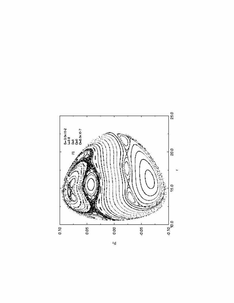
In fact, Fig. 5(b) does not represent the full chaotic behavior possible to oblate RQ-cases. As we saw

above about the relativistic counterparts of the Newtonian potentials, the relativistic oblate cases have one

more unstable scape point (in fact, an infall point into the black hole) inermost at the equator in addition

to that one provided in both cases by the oblate shell itself. Hence, if we vary the energy and the angular

momentum so that both unstable regions are equally accessible by the bound nearly equatorial geodesics, it

is possible to enhance strongly the chaotic behavior of Fig. 5(b) to encompass even a significant portion of

the more external region of the surface of section (that associated to the nearly equatorial orbits). We will

see more about this enhancement for the relativistic cases below in Fig. 5(e).

Fig. 5(c) shows a surface of section for relativistic dipolar-octopolar cases (RDO-cases). Remember

that both odd components are simultaneously needed in view of the off-strut constraint (15). Fig. 5(d)

is the same for full oblate RDQO-cases. Figs. 5(a-d) show that the chaotic zones are greatly enlarged

whenever odd shell multipoles are present, in contrast with the almost-regular oblate RQ-case shown.

Figs. 5(e) shows a surface of section for relativistic prolate cases (prolate RQ-cases). It is to be

compared to the corresponding prolate Newtonian one (see Fig. 4(b)), in particular we note the evident

fingerprints of the bifurcation series starting from the originally stable central primary orbit already present

in the prolate Q-cases. We also see that the prolate RQ-cases share with the prolate Q-cases the same

relatively wild chaotic behavior as compared to the respective oblate (R)Q-cases.

Like in the Fig. 5(b), the dynamics would be more chaotic in Fig. 5(e) if the angular momentum and

the energy (unaltered here for the sake of full comparison) were ajusted to allow all the three unstable

points of the relativistic potential (instead only the two ones related to the prolate character of the shell, see

Fig. 1 and the comments therein about the additional black hole unstable point) have stronger combined

influence on the motion. So, the remaining differences between the relativistic figure 5(e) and the Newtonian

one 4(b) are due to the following : the central region (in the surface of section) is the only one able to

become chaotic in the Newtonian case since its orbits are just those (non-planar ones) that can reach the

unstable regions near the two unstable scape points symmetrically placed outside the equatorial plane,

while the more external (in the surface of section) quasi-equatorial orbits are regular since they are far

from those two points and under the strong influence of the equatorial stable orbit in the boundary of the

surface of section. When we change the Newtonian central mass by a true black hole then a third unstable

scape point (in fact a rolling down point into the black hole) is placed innermost in the equatorial plane.

Associated to it there is one more unstable region which can be reached, this time by the quasi-equatorial

orbits. The specific combination of parameters of Fig. 5(e) is such that the central, non-planar orbits can

feel only moderately the influence of the two scape points linked to the presence of the prolate shell, while

the quasi-equatorial orbits are feeling strongly the nearby influence of the unstable point associated to the

black hole. As we said above, other combinations of parameters will allow a much stronger spread and

eventually the overlaping of both types of chaotic regions.

Finally, Fig. 5(f) shows the restoration of a robust set of regular asymmetric orbits around a primary

stable one when we break the reflection symmetry around the equatorial plane by switching on the odd

multipoles onto the prolate RQ-cases, much the same as occured in the prolate Newtonian Q-cases.

– 18 –

4. Discussion

In the first part of this article we presented an unifying discussion concerning with the properties

and, more important, the physical content of some relativistic, static, axially symmetric core-shell models

on their own as well as in connection with the corresponding linearized and Newtonian models taken as

limiting cases. The analytical and observational motivations for these relativistic and Newtonian models

were also shown. This was acomplished in a reasonably self-contained manner in the introduction and

section 2 and needs no additional comments.

In the second, numerical part of this work we explored the fact that the models i) are generic within

the class they pertain and ii) have exact relativistic and Newtonian counterparts to be compared, to study

the chaoticity of bound orbits in the vacuum between the core and the shell.

Specificaly, we firstly tested the relevance of the presence/absence of the reflection symmetry around

the equatorial plane for the chaotic behavior of the orbits. We find consistent evidences for a non-trivial

role played by the reflection symmetry on the chaoticity of the dynamics in both the relativistic and

Newtonian cases. We summarize these findings as follows: the breakdown of the reflection symmetry about

the equatorial plane in both Newtonian and relativistic core-shell models does i) enhance in a significant

way the chaoticity of orbits in reflection symmetric oblate shell models and ii) inhibit significantly also the

occurrence of chaos in reflection symmetric prolate shell models. In particular, the lack of the reflection

symmetry provides the phase space in the prolate case with a robust family of regular orbits around a

stable periodic orbit that is otherwise missing at higher energies.

The other point we addressed about the chaotic behavior of orbits was for the consequences of

substituting true central black holes by Newtonian central masses. We find that the relative extents of

the chaotic regions in the relativistic cases are significantly larger than in the corresponding Newtonian

ones. Although not surprising in thesis, the strong differences between both regimes are in order in view

of the procedure found in the literature of simulating the presence of a black hole at the core of a galaxy

with a naive −1/r Newtonian term (see for example Gerhard and Binney 1985, Sridhar and Touma 1997

and Valluri and Merrit 1998). This approximation is certainly valid far from the black hole but not in its

proximity as is the case here.

These findings stress i) the non-trivial role of the reflection simmetry in both relativistic and Newtonian

regimes, in contrast with its universal acceptance in astronomical modeling, ii) the strong qualitative

and quantitative differences between relativistic and Newtonian regimes, in particular when dealing with

orbits in the vicinity of black holes, and iii) the intrincate interplay between both aspects when they are

simultaneously present.

The true dynamical aspect related to the role of reflection symmetries on the regularity of the orbits

refers of course to the parity of the constants of motion (the famous third one in the present axially

symmetric case) with respect to the coordinates, as well as their power to regularize orbits in phase space.

Translated to these terms, the findings above are saying that the additional constant of motion in question

is by far more powerful whenever i) it is an even function of the coordinates for oblate cases, or ii) it is

an odd function of the coordinates for prolate cases. Since the issue of finding global or even approximate

constants of motion given the dynamics is hard if not feasible in most cases, the former procedure of simply

checking the presence/absence of reflection symmetries is of much more practical interest.

Additional study is needed to see if and how our findings are extendible to more realistic configurations,

with and without black holes/central masses. The obvious improvement is to fill the intermediate vacuum

– 19 –

with some reasonable mass distribution. While this is far from obvious in general relativity, it is easy to

do in the Newtonian context. For example, we are considering just superpose our shell multipoles to some

relevant potentials of celestial mechanics such as Plummer-Kuzmin, Ferrers and others and even triaxial

potentials. They have one or more planes of symmetry, with or without axial symmetry, and so we can

perturb them with shell terms to verify similar effects to those we found.

Here we considered only tube orbits (lz 6= 0) since we are interested in the effects of the existence

of planes of symmetry on tridimensional motion (somewhat similar effects to the found here are seen in

Gerhard 1985 for the restricted case of planar motions with respect to the existence of one or more lines

of symmetry). The model improvements above will allow us to study the effects of breaking the reflection

symmetry also on tridimensional box orbits.

Meantime, the fully relativistic program is in progress. We have recently succeeded in giving rotation

to a black hole (i. e. in converting it into a Kerr black hole) plus a dipolar shell term (Letelier and Vieira

1997). There are increasing evidences for the existence of black holes, particularly inside active galactic

nuclei (Kormendy and Richstone 1995), which motivate us to consider also rotating core-shell models in the

same lines followed here.

The authors thank FAPESP and CNPq for financial support, and Jorge E. Horvath and Andre L. B.

Ribeiro for discussions.

REFERENCES

Araujo, M. E., Letelier, P. S., and Oliveira, S. R., 1998, Class. Quantum Grav., in press.

Arnaboldi, M., Capaccioli, M., Cappellaro, E., Held, E. V., and Sparke, L., 1993, A&A, 267, 21.

Arnol’d, V. I., 1963a, Russ. Math. Surv., 18, 9.

Arnol’d, V. I., 1963b, Russ. Math. Surv., 18, 85.

Barbanis, B., 1962, Zeit. Astrophys., 56, 56.

Barlow, M. J., Drew, J. E., Meaburn, J., and Massey, R. M., 1994, MNRAS, 268, L29.

Barnes, J. E., 1993, ApJ, 419, L17.

Barnes, J. E., and Hernquist, L., 1992, ARA&A, 30, 705.

Berry, M. V., 1978, Am. Inst. Phys. Conf. Proc., 46, 16.

Binney, J., 1982a, MNRAS, 201, 15.

Binney, J., 1982b, MNRAS, 201, 1.

Binney, J., and Spergel, D., 1982, ApJ, 252, 308.

Binney, J., and Tremaine, S., 1987, Galactic Dynamics (Princeton: Princeton Univ. Press).

Carminati, J., and McLenaghan, R. G., 1991, J. Math. Phys., 32, 3135.

Chandrasekhar, S., 1987, Ellipsoidal Figures of Equilibrium (New York: Dover).

Chevalier, R. A., 1997, Science, 276, 1374.

Contopoulos, G., 1960, Zeit. Astrophys., 49, 273.

de Zeeuw, T., 1985, MNRAS, 216, 273.

– 20 –

de Zeeuw, T., Peletier, R., and Franx, M., 1986, MNRAS, 221, 1001.

Dupraz, C., and Combes, F., 1987, A&A, 185, L1.

Evans, N. W., Hafner, R. M., and de Zeeuw, 1997, MNRAS, 286, 315.

Gerhard, O. E., 1985, A&A, 151, 279.

Gerhard, O. E., and Binney, J., 1985, MNRAS, 216, 467.

Groenewegen, M. A. T., Whitelock, P. A., Smith, C. H., and Kerschbaum, F., 1998, MNRAS, 293, 18.

Henon, M., and Heiles, C., 1964, AJ, 69, 73.

Kolmogorov, A. N., 1954, Dokl. Akad. Nauk. SSSR, 98, 527.

Kormendy, J., and Richstone, D., 1995, ARA&A, 33, 581.

Madsen, J., 1991, ApJ, 367, 507.

Moon, P., and Spencer, D. E., 1988, Field Theory Handbook (Berlin: Springer-Verlag).

Letelier, P. S., and Vieira, W. M., 1997, Phys. Rev. D, 56, 8095.

Letelier, P. S., and Oliveira, S. R., 1998, Class. Quantum Grav., 15, 421.

Lynden-Bell, 1962, MNRAS, 124, 95.

Malin, D. F., and Carter, D., 1983, ApJ, 274, 534.

Mathews, J., 1962, J. Soc. Indust. Appl. Math., 10, 768.

Merrit, D., and Fridman, T., 1996, ApJ, 460, 136.

Merrit, D., 1997, ApJ, 486, 102.

Meyer, F., 1997, MNRAS, 285, L11.

Moser, J., 1967, Math. Ann., 169, 136.

Norman, C. A., Sellwood, J. A., and Hasan, Hashima, 1996, ApJ, 462, 114.

Ollongren, A., 1962, Bull. Astron. Inst. Netherlands, 16, 241.

Panagia, N., Scuderi, S., Gilmozzi, R., Challis, P. M., Garnavich, P. M., and Kirshner, R. P., 1996, ApJ,

459, L17.

Perry, G. P., and Bohun, C. S., 1992, Phys. Rev. D, 46, 1866.

Poincare, H., 1957, Les Methodes Nouvelles de la Mecanique Celeste (New York: Dover), vols.1-3.

Quinn, P. J., 1984, ApJ, 279, 596.

Ralston, J. P., and Smith, L. L., 1991, ApJ, 367, 54.

Regge, T., and Wheeler, J. A., 1957, Phys. Rev., 108, 1063.

Reina, C., and Treves, A., 1976, Gen. Rel. Grav., 7, 817.

Reshetnikov, V., and Sotnikova, N., 1997, A&A, 325, 933.

Richstone, D. O., 1982, ApJ, 252, 496.

Robertson, H., and Noonan, T., 1968, Relativity and Cosmology (London: Saunders).

Sackett, P. D., and Sparke, L. S., 1990, ApJ, 361, 408.

Schwarzschild, M., 1979, ApJ, 232, 236.

Schwarzschild, M., 1993, ApJ, 409, 563.

– 21 –

Sokolov, D. D., and Starobinskii, A. A., 1977, Sov. Phys. Dokl., 22, 312.

Sridhar, S., and Touma, J., 1997, MNRAS, 287, L1.

Suen, Wai-Mo, 1986a, Phys. Rev. D, 34, 3617.

Suen, Wai-Mo, 1986b, Phys. Rev. D, 34, 3633.

Thorne, K. S., 1980, Rev. Mod. Phys., 52, 299.

Valluri, M., and Merrit, D., 1998, ApJ, to appear.

van de Hulst, H. C., 1962, Bull. Astron. Inst. Netherlands, 16, 235.

Vieira, W. M., and Letelier, P. S., 1996a, Phys. Rev. Lett., 76, 1409 (VL1).

Vieira, W. M., and Letelier, P. S., 1996b, Los Alamos Data Bank (gr-qc/9608030).

Vieira, W. M., and Letelier, P. S., 1997, Phys. Lett. A, 228, 22 (VL2).

Vishveshwara, C. V., 1970, Phys. Rev. D, 1, 2870.

Zerilli, F. J., 1970, Phys. Rev. D, 2, 2141.

Zhang, X.-H., 1986, Phys. Rev. D, 34, 991.

This preprint was prepared with the AAS LATEX macros v4.0.

– 22 –

Fig. 1.— Typical effective Newtonian potential wells we are dealing with. U stands for Φeff and the positive

parts of the full potential surfaces are cut. (a) shows an even (D = O = 0) oblate (Q > 0) shell and (b)

shows its perturbation due to the presence of the odd shell multipoles D and/or O. On the other hand, (c)

shows an even prolate (Q < 0) shell and (d) shows its perturbation due to the presence of the odd shell

multipoles. Note that (a) and (c) have a plane of symmetry, which is broken by the odd multipoles in (b)

and (d).

Fig. 2.— This figure exhibits, for the parameter values shown, surfaces of section at the plane z = 0 of

integrable Newtonian configurations (D-cases and Keplerian cases) perturbed by oblate shell quadrupoles

only. Note that quadrupolar perturbations do preserve the mirror symmetry. In all figures L accounts for

the non-dimensional angular momentum ℓ. (a) shows a typical section of the integrable D-case. This case

does not have a plane of symmetry, in contrast with the also integrable spherically symmetric Keplerian case.

(b), (c) and (f) show the perturbed Keplerian cases (oblate Q-cases), while (d,e) show perturbed D-cases

(DQ-cases). Note that orbit regularity is strongly broken (preserved) in the absence (presence) of mirror

symmetry, this conclusion being robust against multipole strength variations.

Fig. 3.— In this figure we add octopolar components (O 6= 0) to the shell, which necessarily does break

the mirror symmetry. In (a) and (f) we see the strong chaotic effect of perturbing Keplerian cases with

octopoles (O-cases) (compare with the almost-regularity of Figs. 1(b,c,f)). In (b) we see the strong chaotic

effect of octopoles on integrable D-cases (DO-cases), which is fully expected as mirror symmetry is already

absent from the starting. In (c) we break the reflection symmetry of the almost-regular oblate Q-case with

octopoles (QO-cases) and in (d,e) we present the full DQO-case for two slightly different energies, which

confirms the strong dependence of the chaoticity with the energy when the mirror symmetry is broken, in

contrast with the robustness of the almost-regular, mirror symmetric cases against energy variations.

Fig. 4.— We show in this figure prolate Q-cases. In (a-c) we illustrates the well known fact that (mirror

symmetric) prolate Q-cases are strongly chaotic on their own and that their chaoticity is highly energy

dependent. We note in particular that the orbit bifurcations toward the chaotic behavior unusually start

from the central primary stable orbit itself rather than from the boundary. In (d-f) we break the mirror

symmetry of the prolate Q-cases with different combinations of odd multipoles. This does cause a strong

regularizing effect on the orbits, in particular by restoring, of course in a distorted fashion, the whole family of

regular orbits around a primary stable orbit. Moreover, this restoration is robust against multipole strength

as well as energy variations.

Fig. 5.— We present some surfaces of section at the plane z = 0 for the corresponding fully relativistic

core-shell configurations. In this figure, the coordinates r, z stand for the Weyl ones ρ, z (see text for more

details). In addition, in (a) we set ν0 = γ0 = 0 (in the purely dipolar case conical singularities (CSs) are

unavoidable), while in (b-f) we set ν0 = 0 and, in order to eliminate CSs, γ0 and D are given in terms of Q and

O according to the conditions (14) and (15). The relativistic case confirm the role of the presence/absence of

the reflection symmetry on the chaoticity of the orbits already detected in the preceding Newtonian figures.