Scale-dependent relationships between tree speciesrichness and ecosystem function in forestsRyan A. Chisholm1*, Helene C. Muller-Landau1, Kassim Abdul Rahman2, Daniel P.Bebber3, Yue Bin4, Stephanie A. Bohlman5, Norman A. Bourg6, Joshua Brinks7, SarayudhBunyavejchewin8, Nathalie Butt9,10, Honglin Cao4, Min Cao11, Dairon C�ardenas12, Li-WanChang13, Jyh-Min Chiang14, George Chuyong15, Richard Condit1, Handanakere S.Dattaraja16, Stuart Davies17, Alvaro Duque18, Christine Fletcher2, Nimal Gunatilleke19,Savitri Gunatilleke19, Zhanqing Hao20, Rhett D. Harrison21,22, Robert Howe23, Chang-FuHsieh24, Stephen P. Hubbell1,25, Akira Itoh26, David Kenfack17, Somboon Kiratiprayoon27,Andrew J. Larson28, Juyu Lian4, Dunmei Lin29,30, Haifeng Liu29,31, James A. Lutz32, KepingMa29, Yadvinder Malhi9, Sean McMahon7, William McShea6, Madhava Meegaskumbura19,Salim Mohd. Razman2, Michael D. Morecroft33, Christopher J. Nytch34, AlexandreOliveira35, Geoffrey G. Parker7, Sandeep Pulla16, Ruwan Punchi-Manage36, Hugo Romero-Saltos37, Weiguo Sang29,31, Jon Schurman38, Sheng-Hsin Su13, Raman Sukumar16, I-FangSun39, Hebbalalu S. Suresh16, Sylvester Tan17, Duncan Thomas40, Sean Thomas38, JillThompson34,41, Renato Valencia37, Amy Wolf23, Sandra Yap42, Wanhui Ye4, ZuoqiangYuan20 and Jess K. Zimmerman34

1Smithsonian Tropical Research Institute, PO Box 0843-03092, Balboa, Ancón, Republic of Panamá; 2ForestResearch Institute Malaysia, Kepong 52109, Selangor Darul Ehsan, Malaysia; 3Earthwatch Institute, 256 BanburyRoad, Oxford OX2 7DE, UK; 4Key Laboratory of Plant Resources Conservation and Sustainable Utilization, SouthChina Botanical Garden, Chinese Academy of Sciences, Guangzhou 510650, China; 5School of Forest Resourcesand Conservation, University of Florida, Gainesville, FL 32611, USA; 6Conservation Ecology Center, SmithsonianConservation Biology Institute, National Zoological Park, Front Royal, VA 22630, USA; 7Smithsonian EnvironmentalResearch Center, 647 Contees Wharf Road, Edgewater, MD 21037-0028, USA; 8Research Office, Department ofNational Parks, Wildlife and Plant Conservation Bangkok 10900, Thailand; 9Environmental Change Institute, School ofGeography and the Environment, Oxford University, Oxford OX1 3QY, UK; 10ARC Centre of Excellence forEnvironmental Decisions, University of Queensland, St. Lucia 4072, Australia; 11Key Laboratory of Tropical ForestEcology, Xishuangbanna Tropical Botanical Garden, Chinese Academy of Sciences, 88 Xuefu Road, Kunming650223, China; 12Instituto Amazónico de Investigaciones Científicas Sinchi, Calle 20 # 5-44, Bogotá D.C., Colombia;13Taiwan Forestry Research Institute, Taipei 10066, Taiwan; 14Department of Life Science, Tunghai University, POBox 851, Taichung City 40704, Taiwan; 15Department of Plant and Animal Sciences, University of Buea, PO Box 93,Buea, SWP, Cameroon; 16Centre for Ecological Sciences, Indian Institute of Science, Bangalore 560012, India;17Department of Botany, MRC-166, Smithsonian Institution, PO Box 37012, Washington, DC 20013-7012, USA;18Universidad Nacional de Colombia, Calle 59A # 63-20, Medellín, Colombia; 19Department of Botany, Faculty ofScience, University of Peradeniya, Peradeniya 20400, Sri Lanka; 20State Key Laboratory of Forest and Soil Ecology,Institute of Applied Ecology, Chinese Academy of Sciences, Shenyang 110164, China; 21Kunming Institute of Botany,Chinese Academy of Sciences, Kunming 650201, China; 22World Agroforestry Institute, East Asia Office, Kunming650201, China; 23Department of Natural and Applied Sciences, University of Wisconsin-Green Bay, Green Bay, WI54311, USA; 24Institute of Ecology and Evolutionary Biology, National Taiwan University, Taipei 10617, Taiwan;25Department of Ecology and Evolutionary Biology, University of California, Los Angeles, CA 90095, USA; 26GraduateSchool of Science, Osaka City University, Osaka 558-8585, Japan; 27Faculty of Science and Technology, ThammasatUniversity (Rangsit), Klongluang, Patumtani 12121, Thailand; 28Department of Forest Management, The University ofMontana, 32 Campus Drive, Missoula, MT 59812, USA; 29State Key Laboratory of Vegetation and EnvironmentalChange Institute of Botany, Chinese Academy of Sciences, Beijing 100093, China; 30Graduate University of ChineseAcademy of Sciences, Beijing 100049, China; 31College of Life and Environmental Science, Minzu University ofChina, Beijing 100081, China; 32Wildland Resources Department, Utah State University, 5230 Old Main Hill, Logan,UT 84322-5230; 33Natural England, 15 Andover Road, Winchester, Hampshire SO23 7BT, UK; 34Institute for TropicalEcosystem Studies, University of Puerto Rico, PO Box 70377, San Juan, PR 00936-8377, USA; 35Departamento deEcologia- IB Universidade de São Paulo, São Paulo-SP 04582-050, Brazil; 36Department of Ecosystem Modeling,University of Göttingen, B€usgenweg 4, G€ottingen 37077, Germany; 37Escuela de Ciencias Biológicas, Pontificia

© 2013 The Authors. Journal of Ecology © 2013 British Ecological Society

Journal of Ecology doi: 10.1111/1365-2745.12132

Universidad Católica del Ecuador, Av. 12 de Octubre 1076, Quito, Ecuador; 38University of Toronto, 33 WillcockStreet, Toronto, ON M5S 3B3, Canada; 39Department of Natural Resources and Environmental Studies, NationalDong Hwa University, Hualien 97401, Taiwan; 40Department of Botany and Plant Pathology, Oregon State University,Corvallis, OR 97331, USA; 41Centre for Ecology & Hydrology, Bush Estate, Penicuik, Midlothian, EH26 0QB, UK; and42Institute of Biology, University of the Philippines Diliman, 1101, Quezon City, NCR, Philippines

Summary

1. The relationship between species richness and ecosystem function, as measured by productivity or biomass,is of long-standing theoretical and practical interest in ecology. This is especially true for forests, which repre-sent a majority of global biomass, productivity and biodiversity.2. Here, we conduct an analysis of relationships between tree species richness, biomass and productivity in 25forest plots of area 8–50 ha from across the world. The data were collected using standardized protocols, obvi-ating the need to correct for methodological differences that plague many studies on this topic.3. We found that at very small spatial grains (0.04 ha) species richness was generally positively related to pro-ductivity and biomass within plots, with a doubling of species richness corresponding to an average 48%increase in productivity and 53% increase in biomass. At larger spatial grains (0.25 ha, 1 ha), results weremixed, with negative relationships becoming more common. The results were qualitatively similar but muchweaker when we controlled for stem density: at the 0.04 ha spatial grain, a doubling of species richness corre-sponded to a 5% increase in productivity and 7% increase in biomass. Productivity and biomass were them-selves almost always positively related at all spatial grains.4. Synthesis. This is the first cross-site study of the effect of tree species richness on forest biomass and productiv-ity that systematically varies spatial grain within a controlled methodology. The scale-dependent results are consis-tent with theoretical models in which sampling effects and niche complementarity dominate at small scales, whileenvironmental gradients drive patterns at large scales. Our study shows that the relationship of tree species richnesswith biomass and productivity changes qualitatively when moving from scales typical of forest surveys (0.04 ha) toslightly larger scales (0.25 and 1 ha). This needs to be recognized in forest conservation policy and management.

Key-words: biodiversity, biomass, complementarity, determinants of plant community diversityand structure, productivity, sampling effects, species diversity, trees

Introduction

Research into the relationship between species richness andecosystem function is motivated by both a basic interest inunderstanding ecological communities (Pianka 1966; Odum1969; Tilman et al. 1997) and a practical need to conserveand manage ecosystem services (Schwartz et al. 2000; Sri-vastava & Vellend 2005). Ecosystem functions are classifiedas stocks, fluxes or stabilizing functions (Pacala & Kinzig2002; Srivastava & Vellend 2005). Woody productivity (aflux) and biomass carbon storage (a stock) are two key eco-system functions in forests (Pacala & Kinzig 2002). Forestcarbon storage is of particular concern because globally for-ests hold more carbon than the atmosphere (Pan et al. 2011),and management of these carbon stores is an important toolfor mitigating global climate change. In total, forests accountfor approximately 60% of terrestrial productivity and 85% ofbiomass (Randolph et al. 2005) and tropical forests aloneaccount for more than 50% of terrestrial species diversity(Wilson 1988).

Many studies of species richness and ecosystem functionhave focused on productivity (Tilman et al. 1997; Loreauet al. 2001). Theory predicts positive effects of species rich-ness on productivity through niche complementarity, facilita-tion and sampling effects (Abrams 1995; Tilman 1999;Fridley 2001; Loreau et al. 2001; Flombaum & Sala 2008).Niche complementarity occurs because niches, such as differ-ences in resource-use or enemy-defence strategies, lead toincreases in a species’ performance as local abundance ofconspecifics decreases and thus to better overall community-level performance, that is, higher productivity, when there aremore species and fewer individuals per species (Janzen 1970;Connell 1971; Comita et al. 2010; Mangan et al. 2010).Facilitation occurs when species enhance one another’s per-formances (Hooper 1998). Sampling effects arise because spe-cies richness varies randomly across quadrats, and quadratswith high species richness are more likely, by chance, to con-tain particular high-yield species. These sampling effects arealso referred to as selection effects (Turnbull et al. 2012),because they assume that the high-yield species contributedisproportionately in mixtures.The predicted positive relationships between richness and

productivity are broadly supported by small-scale empirical*Correspondence author. E-mail: ryan.chis@gmail.com

© 2013 The Authors. Journal of Ecology © 2013 British Ecological Society, Journal of Ecology

2 R. A. Chisholm et al.

studies that manipulate species richness in herbaceous com-munities (Tilman et al. 1997; Hooper 1998; Symstad et al.1998; Loreau et al. 2001), but observational studies haveproduced mixed results. Early observational studies pointedto a hump-shaped relationship in which species richnesspeaks at intermediate productivity and declines towardsextreme high or low productivity (Grime 1979; Loreau et al.2001; Mittelbach et al. 2001; Rahbek 2005; Mittelbach2010). But subsequent studies have cast doubt on the gener-ality of the hump-shaped relationship, with positive, negative,flat and even U-shaped relationships being observed (Mittel-bach 2010; Whittaker 2010). Theoretical explanations forhump-shaped productivity–richness patterns (Abrams 1995;Rosenzweig & Abramsky 1998; Aarssen 2001) generallyassume that productivity acts as a proxy for environmentalconditions and that environmental conditions drive speciesrichness. One proposed mechanism for declines in speciesrichness at high productivity is that in high-resource environ-ments, there is less environmental heterogeneity and hencefewer niches (Rosenzweig & Abramsky 1998). Alternatively,the ‘species pool’ hypothesis explains the overall unimodalpattern by postulating that fewer species are adapted toextreme low- or high-productivity environments, because of amid-domain effect (Aarssen 2004) or because low- and high-productivity areas have been less common over geologicaltime (Schamp, Aarssen & Lee 2003). Although the hump-shaped productivity–richness pattern has a long history oftheoretical and empirical support, its general applicabilityremains a matter of debate (Whittaker 2010; Adler et al.2011; Fridley et al. 2012).The predictions for relationships between richness and pro-

ductivity outlined above lead directly to similar predictionsfor richness–biomass relationships, insofar as higher forestproductivity is associated with higher standing biomass. Inannual herbaceous communities, above-ground biomass isessentially synonymous with productivity, and the two termsare often used interchangeably. In forests, however, produc-tivity and biomass are distinct (Rosenzweig & Abramsky1998): although at local scales higher productivity enablesfaster biomass accumulation over forest succession and highereventual old-growth biomass (Bonan et al. 2003), productiv-ity and biomass and are not significantly associated at globalscales (Keeling & Phillips 2007). Therefore, biomass and pro-ductivity should be treated separately in analyses of speciesrichness and ecosystem function in forests.Relatively few studies on the relationship of species rich-

ness to biomass and productivity have been conducted in for-ests. Those that do have generally been limited to smallspatial grains (i.e. small size of the sampling unit or quadrat;typically < 0.1 ha) and local to regional spatial extents (Vil�aet al. 2007; Ruiz-Jaen & Potvin 2010; Paquette & Messier2011) and generally have found positive relationships. Rich-ness–productivity relationships in forests have also beenincorporated in meta-analyses that include other ecosystemtypes (e.g. Mittelbach et al. 2001), but methodological differ-ences between individual studies that comprise the meta-anal-yses have confounded attempts to draw general conclusions

(Whittaker 2010): different studies use different spatialextents, spatial grains, census methodologies and measures ofproductivity (including rainfall, biomass and other surrogatevariables) and focus on different taxonomic groups (includingboth plants and animals).For this study, we utilized a global data set of large-scale

forest plots to investigate how the relationship of tree speciesrichness to forest biomass and productivity varies across arange of spatial grains within sites and to test whether theobserved patterns are general across sites. Our approach ofusing a standardized global data set allowed us to overcomethe limitations of many previous cross-site studies (usuallymeta-analyses) that address the topic of species richness, pro-ductivity and biomass. We predicted that richness and func-tion (the latter measured by productivity and biomass) wouldbe positively related at most sites and that productivity wouldbe strongly positively related to biomass at all sites. We alsopredicted that successional processes associated with treefallgaps (Schnitzer & Carson 2001) might lead to negative rela-tionships at small spatial grains at some sites, because areasthat have recently been in gaps typically have many smallstems, high species richness and low biomass, while areaswith mature trees have fewer, larger stems, lower speciesrichness and higher biomass (Condit et al. 1996; Aarssen,Laird & Piter 2003).

Materials and methods

SITE SELECTION

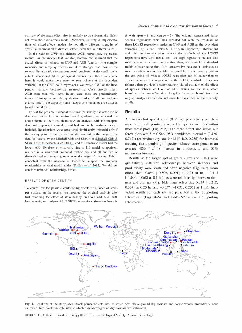
We compared relationships between tree species richness, annualabove-ground coarse woody dry productivity (CWP) and above-ground dry woody biomass (AGB) across 25 forest plots in the globalnetwork coordinated by the Center for Tropical Forest Science/Smith-sonian Institution Global Earth Observatories (CTFS/SIGEO) (http://www.sigeo.si.edu/). The plots spanned temperate and tropical regionsacross five continents (Table 1; Fig. 1). Twelve of the plots werecensused two or more times (at intervals of 4–10 year; Table 1), inwhich case we used two consecutive censuses for CWP estimates(see below) and the first of these censuses for AGB and richness esti-mates. For single-census plots, we analysed only AGB and richness.The forest plots have similar spatial extents (8–50 ha; Table 1) andcensuses of individual stems at each site followed the standard CTFS/SIGEO protocols (Condit 1998).

DATA COLLECTION

The data for each plot were trimmed, if necessary, to fit within a rect-angular region with edges that were even multiples of 100 m(Table 1). This guaranteed that the plot could be evenly divided into1 ha quadrats and that the same total area could be used for analysesat all spatial grains. Sections of the plot outside the rectangular regionwere discarded. We then subdivided the plot into nonoverlappingquadrats at three spatial grains: 20 9 20 m (0.04 ha), 50 9 50 m(0.25 ha) and 100 9 100 m (1 ha).

Species richness for each quadrat at each spatial grain was calcu-lated by summing the number of tree species with at least 1 stem ≥10 cm DBH in the quadrat. We used species richness rather than

© 2013 The Authors. Journal of Ecology © 2013 British Ecological Society, Journal of Ecology

Species richness and ecosystem function in forests 3

some other measure of diversity (e.g. Shannon’s index) because rich-ness is easily interpreted and most relevant to theoretical richness–function mechanisms (e.g. niche complementarity and samplingeffects). We included only trees ≥ 10 cm DBH because trees of thissize contribute the vast majority of CWP and AGB. (For CWP,trees ≥ 10 cm DBH constitute 91.3 � 3.8% (mean � standard devia-tion) of the CWP of all trees ≥ 1 cm DBH at the 12 sites at whichCWP was calculated, all of which had data on stems ≥ 1 cm DBH.For AGB, trees ≥ 10 cm DBH constitute 96.3 � 2.9% of the AGBof all trees ≥ 1 cm DBH at the 19 sites for which data on stems≥1 cm DBH were available.)

The AGB of each individual stem (including all stems ≥10 cmDBH on multistemmed individuals) was estimated from DBH andallometric regressions. At some sites, we were able to use site-specificor species-specific allometric regressions; at other sites, we used gen-eric allometric equations (Chave et al. 2005; Table S1, in SupportingInformation). Total AGB for each quadrat at each spatial grain wascalculated by summing AGB for all stems in a quadrat. Althougherrors associated with allometric equations can be large (Chave et al.2004), they should in general lead to fairly consistent under- or over-estimates of AGB within sites, meaning that the resulting within-siterelationships between richness and AGB should be robust.

The CWP for each quadrat was calculated as the sum of AGBgrowth for surviving stems and AGB of new stems divided by thelength of the census interval in years. In six of the plots, individualstems on multistemmed trees had not been tagged and recorded con-sistently, so we could estimate change in AGB only at the tree level.For these plots, CWP was therefore underestimated (because the datado not reveal cases in which a stem on a multistemmed tree died andwas replaced by a different stem during the census interval). In allplots, negative CWP estimates for stems or trees that apparentlyshrunk were replaced with zero CWP, because individual tree CWP,by definition, cannot be negative.

STAT IST ICAL ANALYS IS

All variables were log-transformed prior to analysis. Statisticalanalyses were performed in the software R version 2.15.0 (http://www.r-project.org/). At each site and for each spatial grain, we usedgeneralized least-squares models with a maximum likelihood fittingmethod (nlme package in R) to fit richness–CWP (independent–dependent variable), richness–AGB and CWP–AGB relationshipsamong quadrats. We used generalized least-squares models becausewe needed to account for spatial autocorrelation among quadrats, andgeneralized least-squares is a reliable method for doing so (Bealeet al. 2010). We used a maximum likelihood method rather than arestricted maximum likelihood method because we wanted to comparethe separate models with Akaike Information Criterion (AIC) andbecause we did not need to estimate variance components (Zuur et al.2009). We fitted linear models with and without spherical autocorrela-tion structure, and for each combination of site, scale and variables,we selected the model with the lowest AIC (Tables S2 and S3 inSupporting Information). Effect size was measured as the slope of arelationship on log-log axes, so that if y = Axb, then b is the effectsize, and an effect size of zero indicates no effect of the variable x onthe variable y. The mean effect size across sites for each relationshipwas calculated as a variance-weighted mean of the site effects, andconfidence intervals on the mean effect size were estimated by boot-strapping over sites.

Our method of fitting individual site models with generalized least-squares is exactly equivalent to fitting a single mixed-effects modelfor all of the data with ‘site’ as a fixed effect. A different approachwould be to treat ‘site’ as a random effect: this would minimize theoverall error in the mean effect size but would lead to biased siteeffects because of shrinkage (individual site observations are pulledtowards the mean). We did not fit such a random-effects modelbecause we wanted unbiased site effects and because the resulting

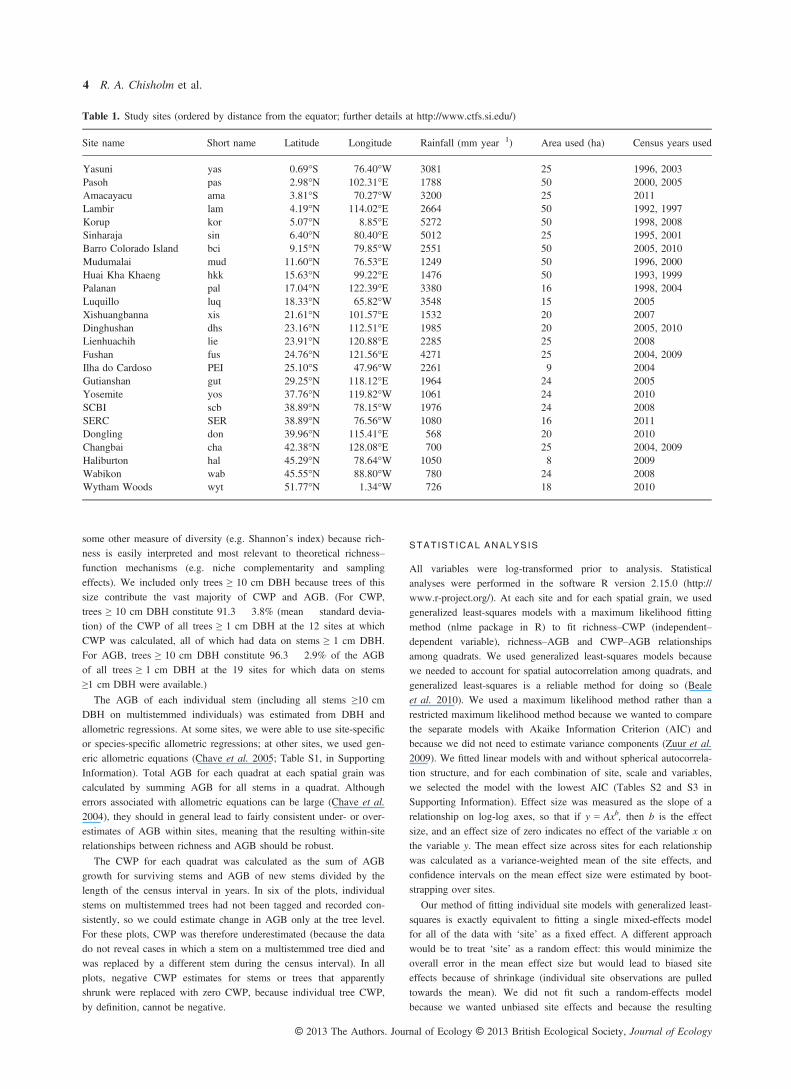
Table 1. Study sites (ordered by distance from the equator; further details at http://www.ctfs.si.edu/)

Site name Short name Latitude Longitude Rainfall (mm year�1) Area used (ha) Census years used

Yasuni yas 0.69°S 76.40°W 3081 25 1996, 2003Pasoh pas 2.98°N 102.31°E 1788 50 2000, 2005Amacayacu ama 3.81°S 70.27°W 3200 25 2011Lambir lam 4.19°N 114.02°E 2664 50 1992, 1997Korup kor 5.07°N 8.85°E 5272 50 1998, 2008Sinharaja sin 6.40°N 80.40°E 5012 25 1995, 2001Barro Colorado Island bci 9.15°N 79.85°W 2551 50 2005, 2010Mudumalai mud 11.60°N 76.53°E 1249 50 1996, 2000Huai Kha Khaeng hkk 15.63°N 99.22°E 1476 50 1993, 1999Palanan pal 17.04°N 122.39°E 3380 16 1998, 2004Luquillo luq 18.33°N 65.82°W 3548 15 2005Xishuangbanna xis 21.61°N 101.57°E 1532 20 2007Dinghushan dhs 23.16°N 112.51°E 1985 20 2005, 2010Lienhuachih lie 23.91°N 120.88°E 2285 25 2008Fushan fus 24.76°N 121.56°E 4271 25 2004, 2009Ilha do Cardoso PEI 25.10°S 47.96°W 2261 9 2004Gutianshan gut 29.25°N 118.12°E 1964 24 2005Yosemite yos 37.76°N 119.82°W 1061 24 2010SCBI scb 38.89°N 78.15°W 1976 24 2008SERC SER 38.89°N 76.56°W 1080 16 2011Dongling don 39.96°N 115.41°E 568 20 2010Changbai cha 42.38°N 128.08°E 700 25 2004, 2009Haliburton hal 45.29°N 78.64°W 1050 8 2009Wabikon wab 45.55°N 88.80°W 780 24 2008Wytham Woods wyt 51.77°N 1.34°W 726 18 2010

© 2013 The Authors. Journal of Ecology © 2013 British Ecological Society, Journal of Ecology

4 R. A. Chisholm et al.

estimate of the mean effect size is unlikely to be substantially differ-ent from the fixed-effects model. Moreover, existing R implementa-tions of mixed-effects models do not allow different strengths ofspatial autocorrelation at different effect levels (i.e. at different sites).

In the richness–CWP and richness–AGB regressions, we treatedrichness as the independent variable, because we assumed that thecausal effects of richness on CWP and AGB (due to niche comple-mentarity and sampling effects) would be stronger than those in thereverse direction (due to environmental gradients) at the small spatialextents considered (at larger spatial extents than those consideredhere, it would make more sense to treat richness as the dependentvariable). In the CWP–AGB regressions, we treated CWP as the inde-pendent variable, because we assumed that CWP directly affectsAGB more than vice versa. In any case, these are predominantlyissues of interpretation: the qualitative results of all our analyseschange little if the dependent and independent variables are switched(results not shown).

To test for possible unimodal relationships usually characteristic ofdata sets across broader environmental gradients, we repeated theabove richness–CWP and richness–AGB analyses with the indepen-dent and dependent variables switched and with quadratic modelsincluded. Relationships were considered significantly unimodal only ifthe turning point of the quadratic model was within the range of thedata [as judged by the Mitchell-Olds and Shaw test (Mitchell-Olds &Shaw 1987; Mittelbach et al. 2001)], and the quadratic model had thelowest AIC. By these criteria, only nine of 111 model comparisonsresulted in a significant unimodal relationship, and all but two ofthese showed an increasing trend over the range of the data. This isconsistent with the absence of theoretical support for unimodalrelationships at local spatial scales (Fridley et al. 2012). We did notconsider unimodal relationships further.

EFFECTS OF STEM DENSITY

To control for the possible confounding effects of number of stemsper quadrat on the results, we repeated the original analysis afterfirst removing the effect of stem density on CWP and AGB withlocally weighted polynomial (LOESS) regressions (function loess in

R with span = 1 and degree = 2). The original generalized least-squares regressions were then repeated but with the residuals ofthese LOESS regressions replacing CWP and AGB as the dependentvariables (Fig. 3 and Tables S3.1–S3.6 in Supporting Information)and with no intercept term because the residuals of the LOESSregressions have zero mean. This two-stage regression method wasused because it is more conservative than, for example, a standardmultiple linear regression. It is conservative because it attributes asmuch variation in CWP or AGB as possible to stem density (withinthe constraints of what a LOESS regression can fit) rather than tospecies richness. The regression of the LOESS residuals on speciesrichness then provides a conservatively biased estimate of the effectof species richness on CWP or AGB, which we use as a lowerbound on the true effect size alongside the upper bound from theoriginal analysis (which did not consider the effects of stem densityat all).

Results

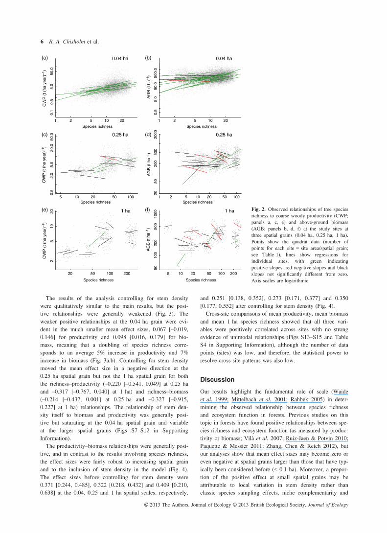
At the smallest spatial grain (0.04 ha), productivity and bio-mass were both positively related to species richness withinmost forest plots (Fig. 2a,b). The mean effect size across ourforest plots was b = 0.566 (95% confidence interval = [0.426,0.717]) for productivity and 0.613 [0.480, 0.755] for biomass,meaning that a doubling of species richness corresponds to anaverage 48% (=2b–1) increase in productivity and 53%increase in biomass.Results at the larger spatial grains (0.25 and 1 ha) were

qualitatively different: relationships between richness andproductivity were weak and often negative (Fig. 2c,e; meaneffect size –0.096 [–0.309, 0.091] at 0.25 ha and –0.415[–1.090, 0.068] at 0.1 ha), as were relationships between rich-ness and biomass (Fig. 2d,f; mean effect size 0.059 [–0.218,0.337] at 0.25 ha and –0.357 [–1.031, 0.255] at 1 ha). Indi-vidual results for each site are presented in the SupportingInformation (Figs S1–S6 and Tables S2.1–S2.6 in SupportingInformation).

Yosemite

Pasoh

Huai Kha KhaengXishuangbanna

Lambir

Palanan

Yasuni

FushanLienhuachih

Changbai

Korup

DinghushanGutianshan

SinharajaMudumalaiBCI

DonglingSERCSCBI

Ilha do Cardoso

Wytham WoodsWabikon

Luquillo

Haliburton

Amacayacu

Fig. 1. Locations of the study sites. Black points indicate sites at which both above-ground dry biomass and coarse woody productivity wereestimated. Red points indicate sites at which only above-ground dry biomass was estimated.

© 2013 The Authors. Journal of Ecology © 2013 British Ecological Society, Journal of Ecology

Species richness and ecosystem function in forests 5

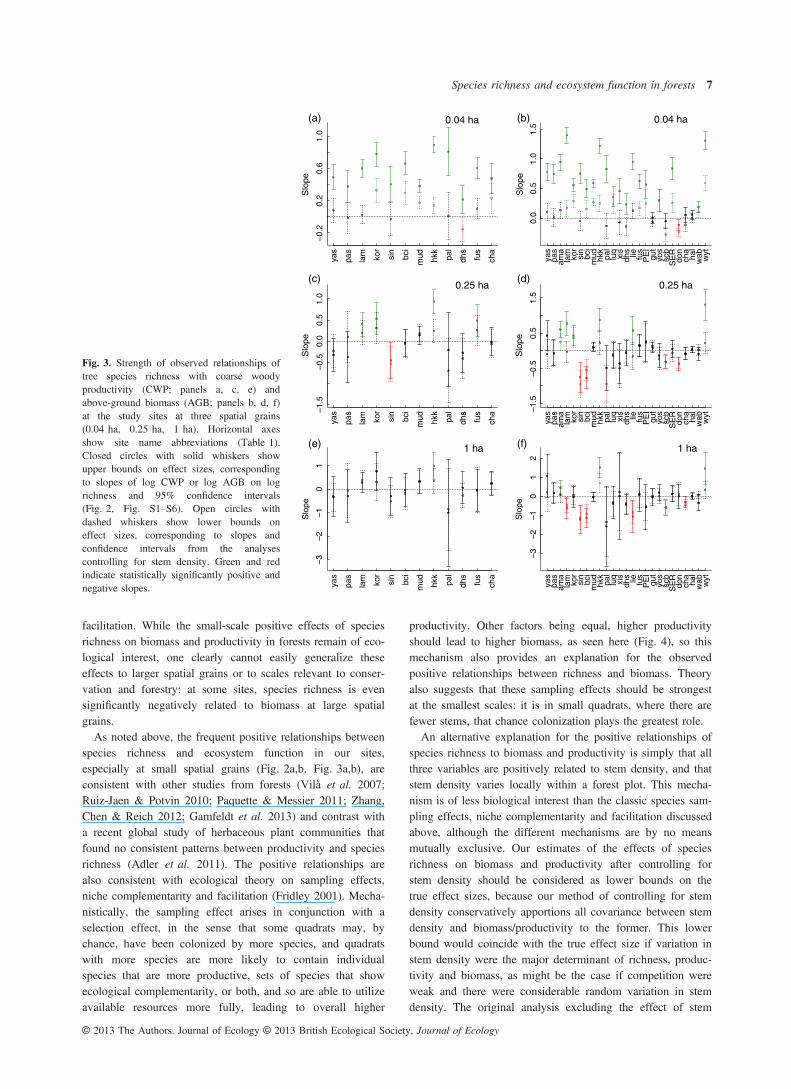
The results of the analysis controlling for stem densitywere qualitatively similar to the main results, but the posi-tive relationships were generally weakened (Fig. 3). Theweaker positive relationships at the 0.04 ha grain were evi-dent in the much smaller mean effect sizes, 0.067 [–0.019,0.146] for productivity and 0.098 [0.016, 0.179] for bio-mass, meaning that a doubling of species richness corre-sponds to an average 5% increase in productivity and 7%increase in biomass (Fig. 3a,b). Controlling for stem densitymoved the mean effect size in a negative direction at the0.25 ha spatial grain but not the 1 ha spatial grain for boththe richness–productivity (–0.220 [–0.541, 0.049] at 0.25 haand –0.317 [–0.767, 0.040] at 1 ha) and richness–biomass(–0.214 [–0.437, 0.001] at 0.25 ha and –0.327 [–0.915,0.227] at 1 ha) relationships. The relationship of stem den-sity itself to biomass and productivity was generally posi-tive but saturating at the 0.04 ha spatial grain and variableat the larger spatial grains (Figs S7–S12 in SupportingInformation).The productivity–biomass relationships were generally posi-

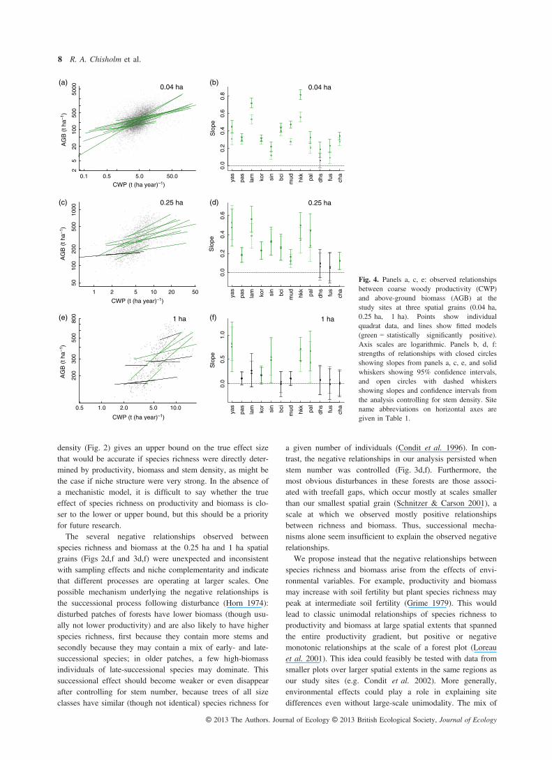
tive, and in contrast to the results involving species richness,the effect sizes were fairly robust to increasing spatial grainand to the inclusion of stem density in the model (Fig. 4).The effect sizes before controlling for stem density were0.371 [0.244, 0.485], 0.322 [0.218, 0.432] and 0.409 [0.210,0.638] at the 0.04, 0.25 and 1 ha spatial scales, respectively,

and 0.251 [0.138, 0.352], 0.273 [0.171, 0.377] and 0.350[0.177, 0.552] after controlling for stem density (Fig. 4).Cross-site comparisons of mean productivity, mean biomass

and mean 1 ha species richness showed that all three vari-ables were positively correlated across sites with no strongevidence of unimodal relationships (Figs S13–S15 and TableS4 in Supporting Information), although the number of datapoints (sites) was low, and therefore, the statistical power toresolve cross-site patterns was also low.

Discussion

Our results highlight the fundamental role of scale (Waideet al. 1999; Mittelbach et al. 2001; Rahbek 2005) in deter-mining the observed relationship between species richnessand ecosystem function in forests. Previous studies on thistopic in forests have found positive relationships between spe-cies richness and ecosystem function (as measured by produc-tivity or biomass; Vil�a et al. 2007; Ruiz-Jaen & Potvin 2010;Paquette & Messier 2011; Zhang, Chen & Reich 2012), butour analyses show that mean effect sizes may become zero oreven negative at spatial grains larger than those that have typ-ically been considered before (< 0.1 ha). Moreover, a propor-tion of the positive effect at small spatial grains may beattributable to local variation in stem density rather thanclassic species sampling effects, niche complementarity and

Species richness

CW

P (

t (ha

yea

r)–1

)

0.04 ha

1 2 5 10 20

0.1

0.5

5.0

50.0

Species richness

AG

B (

t ha–1

)

0.04 ha

1 2 5 10 20

0.5

5.0

50.0

500.

0

Species richness

0.25 ha

5 10 20 50 100

0.5

2.0

5.0

20.0

50.0

Species richness

0.25 ha

1 2 5 10 20 50 100

2050

200

500

2000

Species richness

1 ha

20 50 100 200

25

1020

Species richness

1 ha

5 10 20 50 100 200

5010

020

050

010

00

CW

P (

t (ha

yea

r)–1

)C

WP

(t (

ha y

ear)

–1)

AG

B (

t ha–1

)A

GB

(t h

a–1)

(a) (b)

(c) (d)

(e) (f) Fig. 2. Observed relationships of tree speciesrichness to coarse woody productivity (CWP;panels a, c, e) and above-ground biomass(AGB; panels b, d, f) at the study sites atthree spatial grains (0.04 ha, 0.25 ha, 1 ha).Points show the quadrat data (number ofpoints for each site = site area/spatial grain;see Table 1), lines show regressions forindividual sites, with green indicatingpositive slopes, red negative slopes and blackslopes not significantly different from zero.Axis scales are logarithmic.

© 2013 The Authors. Journal of Ecology © 2013 British Ecological Society, Journal of Ecology

6 R. A. Chisholm et al.

facilitation. While the small-scale positive effects of speciesrichness on biomass and productivity in forests remain of eco-logical interest, one clearly cannot easily generalize theseeffects to larger spatial grains or to scales relevant to conser-vation and forestry: at some sites, species richness is evensignificantly negatively related to biomass at large spatialgrains.As noted above, the frequent positive relationships between

species richness and ecosystem function in our sites,especially at small spatial grains (Fig. 2a,b, Fig. 3a,b), areconsistent with other studies from forests (Vil�a et al. 2007;Ruiz-Jaen & Potvin 2010; Paquette & Messier 2011; Zhang,Chen & Reich 2012; Gamfeldt et al. 2013) and contrast witha recent global study of herbaceous plant communities thatfound no consistent patterns between productivity and speciesrichness (Adler et al. 2011). The positive relationships arealso consistent with ecological theory on sampling effects,niche complementarity and facilitation (Fridley 2001). Mecha-nistically, the sampling effect arises in conjunction with aselection effect, in the sense that some quadrats may, bychance, have been colonized by more species, and quadratswith more species are more likely to contain individualspecies that are more productive, sets of species that showecological complementarity, or both, and so are able to utilizeavailable resources more fully, leading to overall higher

productivity. Other factors being equal, higher productivityshould lead to higher biomass, as seen here (Fig. 4), so thismechanism also provides an explanation for the observedpositive relationships between richness and biomass. Theoryalso suggests that these sampling effects should be strongestat the smallest scales: it is in small quadrats, where there arefewer stems, that chance colonization plays the greatest role.An alternative explanation for the positive relationships of

species richness to biomass and productivity is simply that allthree variables are positively related to stem density, and thatstem density varies locally within a forest plot. This mecha-nism is of less biological interest than the classic species sam-pling effects, niche complementarity and facilitation discussedabove, although the different mechanisms are by no meansmutually exclusive. Our estimates of the effects of speciesrichness on biomass and productivity after controlling forstem density should be considered as lower bounds on thetrue effect sizes, because our method of controlling for stemdensity conservatively apportions all covariance between stemdensity and biomass/productivity to the former. This lowerbound would coincide with the true effect size if variation instem density were the major determinant of richness, produc-tivity and biomass, as might be the case if competition wereweak and there were considerable random variation in stemdensity. The original analysis excluding the effect of stem

–0.2

–0.5

–0.5

0.2

0.6

1.0

Slo

pe

yas

pas

lam kor

sin

bci

mud hk

k

pal

dhs

fus

cha

0.04 ha 0.04 ha

0.0

0.5

1.0

1.5

Slo

pe

yas

pas

ama

lam kor

sin

bci

mud hk

kpa

llu

qxi

sdh

s lie fus

PE

Igu

tyo

ssc

bS

ER

don

cha

hal

wab wyt

0.0

0.5

1.0

Slo

pe

yas

pas

lam kor

sin

bci

mud hk

k

pal

dhs

fus

cha

0.5

1.5

Slo

pe

yas

pas

ama

lam kor

sin

bci

mud hk

kpa

llu

qxi

sdh

s lie fus

PE

Igu

tyo

ssc

bS

ER

don

cha

hal

wab wyt

0.25 ha 0.25 ha

01

Slo

pe

yas

pas

lam kor

sin

bci

mud hk

k

pal

dhs

fus

cha

1 ha

01

2

Slo

pe

yas

pas

ama

lam kor

sin

bci

mud hk

kpa

llu

qxi

sdh

s lie fus

PE

Igu

tyo

ssc

bS

ER

don

cha

hal

wab wyt

1 ha

–1.5

–1.5

–1–2

–3

–1–2

–3

(a) (b)

(c) (d)

(e) (f)

Fig. 3. Strength of observed relationships oftree species richness with coarse woodyproductivity (CWP; panels a, c, e) andabove-ground biomass (AGB; panels b, d, f)at the study sites at three spatial grains(0.04 ha, 0.25 ha, 1 ha). Horizontal axesshow site name abbreviations (Table 1).Closed circles with solid whiskers showupper bounds on effect sizes, correspondingto slopes of log CWP or log AGB on logrichness and 95% confidence intervals(Fig. 2, Fig. S1–S6). Open circles withdashed whiskers show lower bounds oneffect sizes, corresponding to slopes andconfidence intervals from the analysescontrolling for stem density. Green and redindicate statistically significantly positive andnegative slopes.

© 2013 The Authors. Journal of Ecology © 2013 British Ecological Society, Journal of Ecology

Species richness and ecosystem function in forests 7

density (Fig. 2) gives an upper bound on the true effect sizethat would be accurate if species richness were directly deter-mined by productivity, biomass and stem density, as might bethe case if niche structure were very strong. In the absence ofa mechanistic model, it is difficult to say whether the trueeffect of species richness on productivity and biomass is clo-ser to the lower or upper bound, but this should be a priorityfor future research.The several negative relationships observed between

species richness and biomass at the 0.25 ha and 1 ha spatialgrains (Figs 2d,f and 3d,f) were unexpected and inconsistentwith sampling effects and niche complementarity and indicatethat different processes are operating at larger scales. Onepossible mechanism underlying the negative relationships isthe successional process following disturbance (Horn 1974):disturbed patches of forests have lower biomass (though usu-ally not lower productivity) and are also likely to have higherspecies richness, first because they contain more stems andsecondly because they may contain a mix of early- and late-successional species; in older patches, a few high-biomassindividuals of late-successional species may dominate. Thissuccessional effect should become weaker or even disappearafter controlling for stem number, because trees of all sizeclasses have similar (though not identical) species richness for

a given number of individuals (Condit et al. 1996). In con-trast, the negative relationships in our analysis persisted whenstem number was controlled (Fig. 3d,f). Furthermore, themost obvious disturbances in these forests are those associ-ated with treefall gaps, which occur mostly at scales smallerthan our smallest spatial grain (Schnitzer & Carson 2001), ascale at which we observed mostly positive relationshipsbetween richness and biomass. Thus, successional mecha-nisms alone seem insufficient to explain the observed negativerelationships.We propose instead that the negative relationships between

species richness and biomass arise from the effects of envi-ronmental variables. For example, productivity and biomassmay increase with soil fertility but plant species richness maypeak at intermediate soil fertility (Grime 1979). This wouldlead to classic unimodal relationships of species richness toproductivity and biomass at large spatial extents that spannedthe entire productivity gradient, but positive or negativemonotonic relationships at the scale of a forest plot (Loreauet al. 2001). This idea could feasibly be tested with data fromsmaller plots over larger spatial extents in the same regions asour study sites (e.g. Condit et al. 2002). More generally,environmental effects could play a role in explaining sitedifferences even without large-scale unimodality. The mix of

CWP (t (ha year)–1)

AG

B (

t ha–1

)

0.04 ha

0.1 0.5 5.0 50.0

25

2010

050

050

00

0.0

0.2

0.4

0.6

0.8

Slo

pe

yas

pas

lam kor

sin

bci

mud hk

k

pal

dhs

fus

cha

0.04 ha

0.25 ha

1 2 5 10 20 50

5010

020

050

010

00

0.0

0.2

0.4

0.6

Slo

pe

yas

pas

lam kor

sin

bci

mud hk

k

pal

dhs

fus

cha

0.25 ha

1 ha

0.5 1.0 2.0 5.0 10.0

200

300

500

800

0.0

0.5

1.0

Slo

pe

yas

pas

lam kor

sin

bci

mud hk

k

pal

dhs

fus

cha

1 ha

AG

B (

t ha–1

)A

GB

(t h

a–1)

CWP (t (ha year)–1)

CWP (t (ha year)–1)

(a) (b)

(c) (d)

(e) (f)

Fig. 4. Panels a, c, e: observed relationshipsbetween coarse woody productivity (CWP)and above-ground biomass (AGB) at thestudy sites at three spatial grains (0.04 ha,0.25 ha, 1 ha). Points show individualquadrat data, and lines show fitted models(green = statistically significantly positive).Axis scales are logarithmic. Panels b, d, f:strengths of relationships with closed circlesshowing slopes from panels a, c, e, and solidwhiskers showing 95% confidence intervals,and open circles with dashed whiskersshowing slopes and confidence intervals fromthe analysis controlling for stem density. Sitename abbreviations on horizontal axes aregiven in Table 1.

© 2013 The Authors. Journal of Ecology © 2013 British Ecological Society, Journal of Ecology

8 R. A. Chisholm et al.

negative and positive relationships could be attributable tovariation in the species pool between regions (e.g. owing todifferent regional abundances of rich and poor soils) andhence variation in the relationship between species richnessand environmental variables (Schamp, Aarssen & Lee 2003;Rahbek 2005).Previous studies on the species richness–productivity rela-

tionship have used various surrogates for productivity, includ-ing biomass (Whittaker 2010). Our results provide a clearempirical demonstration of why this may not always be valid:although biomass and productivity are generally positivelycorrelated within our sites (Fig. 4), their relationships to spe-cies richness may differ. For example, at the largest spatialgrain, a few sites showed significantly negative relationshipsbetween species richness and biomass (Fig. 3f), but no rela-tionship between species richness and productivity (Fig. 3e).In forests, at least, biomass and productivity should be treatedas separate ecosystem functions.In view of our results showing scale-dependent relation-

ships of species richness to productivity and biomass, we rec-ommend that models be developed to integrate large-scaleenvironmental information with small-scale sampling effects,niche complementarity and stem density effects. The develop-ment of such models should be informed by empirical investi-gations into the pattern and scale of environmental factorsthat drive local variation in richness, productivity and biomassin forests. Ultimately, such research should reproduce rela-tionships between richness, productivity and biomass in for-ests across a range of spatial scales, thus demonstrating amore general understanding of these relationships andproviding practical guidance for forestry and conservationendeavours.

Acknowledgements

This work was generated using data from the Center for Tropical Forest Sci-ence/Smithsonian Institution Global Earth Observatory network (http://www.sigeo.si.edu/). The synthesis was made possible through the financial support ofthe US National Science Foundation (DEB-1046113), the National Natural Sci-ence Foundation of China (31011120470), the Smithsonian Institution GlobalEarth Observatories and the HSBC Climate Partnership. Individual plot datacollection and analysis were supported by the US National Science Foundation(BSR-9015961, DEB-0516066, BSR-8811902, DEB-9411973, DEB-008538,DEB-0218039, and DEB-0620910), the National Natural Science Foundation ofChina (31061160188), the Chinese Academy of Sciences (KZCX2-YW-430),the National Science & Technology Pillar Program of China (2008BAC39B02),the ‘111 Program’ from the Bureau of China Foreign Expert and Ministry ofEducation (No. 2008-B08044), the Council of Agriculture of Taiwan (93AS-2.4.2-FI-G1(2) and 94AS-11.1.2-FI-G1(1)), the National Science Council ofTaiwan (NSC92-3114-B002-009, NSC98-2313-B-029-001-MY3 and NSC98-2321-B-029-002), the Forestry Bureau of Taiwan (92-00-2-06 and No. TFBM-960226), the Taiwan Forestry Research Institute (97 AS- 7.1.1.F1-G1), theMellon Foundation, the International Institute of Tropical Forestry of the USDAForest Service, the University of Puerto Rico, Yosemite National Park, the 1923Fund, the Dirección de Investigaciones Universidad Nacional de Colombia(Convocatoria 2010-2012), the Centre for Ecology and Hydrology, the GermanAcademic Exchange Services (DAAD), Ministry of Environment & Forests(Government of India), the Tamilnadu Forest Department, Sarawak ForestDepartment, Sarawak Forestry Corporation, Global Environment Research Fundof the Ministry of the Environment Japan (D-0901), Japan Society for the Pro-motion of Science (#20405011), the Pontifical Catholic University of Ecuador,the government of Ecuador (Donaciones del Impuesto a la Renta), the Smithso-nian Tropical Research Institute and the University of Aarhus of Denmark. We

thank the hundreds of people who contributed to the collection and organiza-tion of the data from the plots, including Gordon Campbell, Gary Fewless,Maria Uriarte and Linfang Wu. We thank Stephen Pacala, Roman Carrasco andColin Beale for discussions. None of the authors has any conflict of interest.

References

Aarssen, L.W. (2001) On correlations and causations between productivity andspecies richness in vegetation: predictions from habitat attributes. Basic andApplied Ecology, 2, 105–114.

Aarssen, L.W. (2004) Interpreting co-variation in species richness and produc-tivity in terrestrial vegetation: making sense of causations and correlations atmultiple scales. Folia Geobotanica, 39, 385–403.

Aarssen, L.W., Laird, R.A. & Pither, J. (2003) Is the productivity of vegetationplots higher or lower when there are more species? Variable predictions frominteraction of the ‘sampling effect’ and ‘competitive dominance effect’ onthe habitat templet. Oikos, 102, 427–432.

Abrams, P.A. (1995) Monotonic or unimodal diversity-productivity gradients:what does competition theory predict? Ecology, 76, 2019–2027.

Adler, P.B., Seabloom, E.W., Borer, E.T., Hillebrand, H., Hautier, Y., Hector,A. et al. (2011) Productivity is a poor predictor of plant species richness.Science, 333, 1750–1753.

Beale, C.M., Lennon, J.J., Yearsley, J.M., Brewer, M.J. & Elston, D.A. (2010)Regression analysis of spatial data. Ecology Letters, 13, 246–264.

Bonan, G.B., Levis, S., Sitch, S., Vertenstein, M. & Oleson, K.W. (2003) Adynamic global vegetation model for use with climate models: concepts anddescription of simulated vegetation dynamics. Global Change Biology, 9,1543–1566.

Chave, J., Condit, R., Aguilar, S., Hernandez, A., Lao, S. & Perez, R. (2004)Error propagation and scaling for tropical forest biomass estimates. Philo-sophical Transactions of the Royal Society of London Series B-BiologicalSciences, 359, 409–420.

Chave, J., Andalo, C., Brown, S., Cairns, M.A., Chambers, J.Q., Eamus, D.et al. (2005) Tree allometry and improved estimation of carbon stocks andbalance in tropical forests. Oecologia, 145, 87–99.

Comita, L.S., Muller-Landau, H.C., Aguilar, S. & Hubbell, S.P. (2010) Asym-metric density dependence shapes species abundances in a tropical treecommunity. Science, 329, 330–332.

Condit, R. (1998) Tropical Forest Census Plots. Springer-Verlag and R. G.Landes Company, Berlin, Germany, and Georgetown, Texas.

Condit, R., Hubbell, S.P., Lafrankie, J.V., Sukumar, R., Manokaran, N., Foster,R.B. & Ashton, P.S. (1996) Species-area and species-individual relationshipsfor tropical trees: a comparison of three 50-ha plots. Journal of Ecology, 84,549–562.

Condit, R., Pitman, N., Leigh, E.G., Chave, J., Terborgh, J., Foster, R.B. et al.(2002) Beta-diversity in tropical forest trees. Science, 295, 666–669.

Connell, J.H. (1971) On the role of natural enemies in preventing competitiveexclusion in some marine animals and in rain forest trees. Dynamics ofPopulations (eds P.J. den Boer & G.R. Gradwell). pp. 298–312. Centre forAgricultural Publishing and Documentation, Wageningen, the Netherlands.

Flombaum, P. & Sala, O.E. (2008) Higher effect of plant species diversity onproductivity in natural than artificial ecosystems. Proceedings of the NationalAcademy of Sciences of the United States of America, 105, 6087–6090.

Fridley, J.D. (2001) The influence of species diversity on ecosystem productiv-ity: how, where, and why? Oikos, 93, 514–526.

Fridley, J.D., Grime, J.P., Huston, M.A., Pierce, S., Smart, S.M., Thompson,K. et al. (2012) Comment on “Productivity Is a Poor Predictor of PlantSpecies Richness”. Science, 335, 1441.

Gamfeldt, L., Snall, T., Bagchi, R., Jonsson, M., Gustafsson, L., Kjellander, P.et al. (2013) Higher levels of multiple ecosystem services are found inforests with more tree species. Nature Communications, 4, 1340.

Grime, J.P. (1979) Plant Strategies and Vegetation Processes. John Wiley &Sons, New York, NY, USA.

Hooper, D.U. (1998) The role of complementarity and competition in ecosys-tem responses to variation in plant diversity. Ecology, 79, 704–719.

Horn, H.S. (1974) The ecology of secondary succession. Annual Review ofEcology and Systematics, 5, 25–37.

Janzen, D.H. (1970) Herbivores and the number of tree species in tropicalforests. The American Naturalist, 104, 501–528.

Keeling, H.C. & Phillips, O.L. (2007) The global relationship between forestproductivity and biomass. Global Ecology and Biogeography, 16, 618–631.

Loreau, M., Naeem, S., Inchausti, P., Bengtsson, J., Grime, J.P., Hector, A.,Hooper, D.U., Huston, M.A., Raffaelli, D., Schmid, B., Tilman, D. &Wardle, D.A. (2001) Ecology – biodiversity and ecosystem functioning:current knowledge and future challenges. Science, 294, 804–808.

© 2013 The Authors. Journal of Ecology © 2013 British Ecological Society, Journal of Ecology

Species richness and ecosystem function in forests 9

Mangan, S.A., Schnitzer, S.A., Herre, E.A., Mack, K.M.L., Valencia, M.C.,Sanchez, E.I. & Bever, J.D. (2010) Negative plant-soil feedback predictstree-species relative abundance in a tropical forest. Nature, 466, 752–755.

Mitchell-Olds, T. & Shaw, R.G. (1987) Regression analysis of natural selection:statistical inference and biological interpretation. Evolution, 41, 1149–1161.

Mittelbach, G.G. (2010) Understanding species richness-productivity relation-ships: the importance of meta-analyses. Ecology, 91, 2540–2544.

Mittelbach, G.G., Steiner, C.F., Scheiner, S.M., Gross, K.L., Reynolds, H.L.,Waide, R.B., Willig, M.R., Dodson, S.I. & Gough, L. (2001) What is theobserved relationship between species richness and productivity? Ecology,82, 2381–2396.

Odum, E.P. (1969) The strategy of ecosystem development. Science, 164,262–270.

Pacala, S. & Kinzig, A.P. (2002) Introduction to theory and the common eco-system model. Functional Consequences of Biodiversity: Empirical Progressand Theoretical Extensions (eds A.P. Kinzig, S.W. Pacala & D. Tilman), pp.169–174. Princeton University Press, Princeton, NJ, USA.

Pan, Y., Birdsey, R.A., Fang, J., Houghton, R., Kauppi, P.E., Kurz, W.A. et al.(2011) A large and persistent carbon sink in the world’s forests. Science,333, 988–993.

Paquette, A. & Messier, C. (2011) The effect of biodiversity on tree productiv-ity: from temperate to boreal forests. Global Ecology and Biogeography, 20,170–180.

Pianka, E.R. (1966) Latitudinal gradients in species diversity – a review ofconcepts. American Naturalist, 100, 33–46.

Rahbek, C. (2005) The role of spatial scale and the perception of large-scalespecies-richness patterns. Ecology Letters, 8, 224–239.

Randolph, J.C., Green, G.M., Belmont, J., Burcsu, T. & Welch, D. (2005) For-est ecosystems and the human dimension. Seeing the Forest and the Trees:Human-Environment Interactions in Forest Ecosystems (eds E.F. Moran &E. Ostrom), pp. 105–125. MIT Press, Cambridge, MA, USA.

Rosenzweig, M.L. & Abramsky, Z. (1998) How are diversity and productivityrelated? Species Diversity in Ecological Communities: Historical andGeographical Perspectives (eds R.E. Ricklefs & D. Schluter), pp. 39–51.University of Chicago Press, Chicago, IL, USA.

Ruiz-Jaen, M.C. & Potvin, C. (2010) Tree diversity explains variation in eco-system function in a Neotropical forest in Panama. Biotropica, 42, 638–646.

Schamp, B.S., Aarssen, L.W. & Lee, H. (2003) Local plant species richnessincreases with regional habitat commonness across a gradient of forestproductivity. Folia Geobotanica, 38, 273–280.

Schnitzer, S.A. & Carson, W.P. (2001) Treefall gaps and the maintenance ofspecies diversity in a tropical forest. Ecology, 82, 913–919.

Schwartz, M.W., Brigham, C.A., Hoeksema, J.D., Lyons, K.G., Mills, M.H. &van Mantgem, P.J. (2000) Linking biodiversity to ecosystem function: impli-cations for conservation ecology. Oecologia, 122, 297–305.

Srivastava, D.S. & Vellend, M. (2005) Biodiversity-ecosystem functionresearch: is it relevant to conservation? Annual Review of Ecology Evolutionand Systematics, 36, 267–294.

Symstad, A.J., Tilman, D., Willson, J. & Knops, J.M.H. (1998) Species lossand ecosystem functioning: effects of species identity and community com-position. Oikos, 81, 389–397.

Tilman, D. (1999) The ecological consequences of changes in biodiversity: asearch for general principles. Ecology, 80, 1455–1474.

Tilman, D., Knops, J., Wedin, D., Reich, P., Ritchie, M. & Siemann, E. (1997)The influence of functional diversity and composition on ecosystem pro-cesses. Science, 277, 1300–1302.

Turnbull, L.A., Levine, J.M., Loreau, M. & Hector, A. (2012) Coexistence,niches and biodiversity effects on ecosystem functioning. Ecology Letters,16, 116–127.

Vil�a, M., Vayreda, J., Comas, L., Josep Ibá~nez, J., Mata, T. & Obón, B. (2007)Species richness and wood production: a positive association in Mediterra-nean forests. Ecology Letters, 10, 241–250.

Waide, R.B., Willig, M.R., Steiner, C.F., Mittelbach, G., Gough, L., Dodson,S.I., Juday, G.P. & Parmenter, R. (1999) The relationship between productiv-ity and species richness. Annual Review of Ecology and Systematics, 30,257–300.

Whittaker, R.J. (2010) Meta-analyses and mega-mistakes: calling time on meta-analysis of the species richness-productivity relationship. Ecology, 91, 2522–2533.

Wilson, E.O. (1988) The current state of biological diversity. Biodiversity (edsE.O. Wilson & F.M. Peter), pp. 1–18. National Academy Press, Washington,DC, USA.

Zhang, Y., Chen, H.Y.H. & Reich, P.B. (2012) Forest productivity increaseswith evenness, species richness and trait variation: a global meta-analysis.Journal of Ecology, 100, 742–749.

Zuur, A.F., Ieno, E.N., Valker, N.J., Saveliev, A.A. & Smith, G.M. (2009)Mixed Effects Models and Extensions in Ecology With R. Springer,New York, NY, USA.

Received 6 January 2013; accepted 10 June 2013Handling Editor: David Coomes

Supporting Information

Additional Supporting Information may be found in the onlineversion of this article:

Figure S1. Observed relationships between species richness andcoarse woody productivity (CWP) at the study sites at the 0.04 haspatial scale (as for Fig. 2a but with each site on a separate panel).

Figure S2. Observed relationships between species richness andcoarse woody productivity (CWP) at the study sites at the 0.25 haspatial scale (as for Fig. 2c but with each site on a separate panel).

Figure S3. Observed relationships between species richness andcoarse woody productivity (CWP) at the study sites at the 1.0 ha spa-tial scale (as for Fig. 2e but with each site on a separate panel).

Figure S4. Observed relationships between species richness andaboveground biomass (AGB) at the study sites at the 0.04 ha spatialscale (as for Fig. 2b but with each site on a separate panel).

Figure S5. Observed relationships between species richness andaboveground biomass (AGB) at the study sites at the 0.25 ha spatialscale (as for Fig. 2d but with each site on a separate panel).

Figure S6. Observed relationships between species richness andaboveground biomass (AGB) at the study sites at the 1.0 ha spatialscale (as for Fig. 2f but with each site on a separate panel).

Figure S7. LOESS regressions of coarse woody productivity (CWP)versus stem density at the 0.04 ha spatial scale.

Figure S8. LOESS regressions of coarse woody productivity (CWP)versus stem density at the 0.25 ha spatial scale.

Figure S9. LOESS regressions of coarse woody productivity (CWP)versus stem density at the 1.0 ha spatial scale.

Figure S10. LOESS regressions of aboveground biomass (AGB) ver-sus stem density at the 0.04 ha spatial scale.

Figure S11. LOESS regressions of aboveground biomass (AGB) ver-sus stem density at the 0.25 ha spatial scale.

Figure S12. LOESS regressions of aboveground biomass (AGB) ver-sus stem density at the 1.0 ha spatial scale.

Figure S13. Cross-site relationship of productivity to 1 ha speciesrichness.

Figure S14. Cross-site relationship of biomass to 1 ha species rich-ness.

Figure S15. Cross-site relationship of biomass to productivity.

© 2013 The Authors. Journal of Ecology © 2013 British Ecological Society, Journal of Ecology

10 R. A. Chisholm et al.

Table S1 Methods used to estimate productivity and biomass at eachsite.

Table S2 Numerical output from the fits of the generalized least-squares models of productivity and biomass on species richness.

Table S3 Numerical output from the fits of the generalized least-squares models of productivity and biomass on species richness in theanalysis controlling for stem density.

Table S4. Summary data for species richness, biomass and productiv-ity of 1 ha quadrats at each site.

© 2013 The Authors. Journal of Ecology © 2013 British Ecological Society, Journal of Ecology

Species richness and ecosystem function in forests 11