Web Book of Regional Science Regional Research Institute

2020

Regional Impact Models Regional Impact Models

William A. Schaffer

Follow this and additional works at: https://researchrepository.wvu.edu/rri-web-book

The Web Book of Regional Science

Sponsored by

Regional Impact Models

Second Edition

By

William A. Schaffer

Published: 1999

Updated: March 2020

Series Editors: Scott Loveridge Randall Jackson

Professor, Extension Specialist Director, Regional Research Institute

Michigan State University West Virginia University

Emeritus Professor of Economics

Georgia Institute of Technology

<This page blank>

The Web Book of Regional Science is offered as a service to the regional research community in an effort to make a wide range of reference and instructional materials freely available online. Roughly three dozen books and monographs have been published as Web Books of Regional Science. These texts covering diverse subjects such as regional networks, land use, migration, and regional specialization, include descriptions of many of the basic concepts, analytical tools, and policy issues important to regional science. The Web Book was launched in 1999 by Scott Loveridge, who was then the director of the Regional Research Institute at West Virginia University. The director of the Institute, currently Randall Jackson, serves as the Series editor. When citing this book, please include the following: Schaffer, William A. Regional Impact Models. Web Book of Regional Science. Regional Research Institute, West Virginia University. Edited by Scott Loveridge, 1999: Randall Jackson, 2020.

<This page blank>

PREFACEThis survey of regional input-output models and their use in impact analysis has evolved from over twentyyears of experience in constructing regional economic models and in teaching about them. My objectives areto present this family of models in an easily understood format, to show that the models we use in economicsare well-structured, and to provide a basis for understanding applications of these models in impact analysis.I have tried to present the models in such a way that understanding the logic and algebra of the simplesteconomic-base model leads to an understanding of the only slightly more complex regional and interregionalinput-output models in common use today. The advanced models become matrix-algebra extensions of thesimple models.

I have greatly benefited from the guidance of Professor Kong Chu over the years. He first introduced thesemodels to me in 1967 and has helped with interpretations and tedious explanations of mathematical pointsuntil only recently; now he teaches me about life and philosophy. I am in debt to a number of Georgia Techstudents as well. While they have been assistants and students in title, they have been my best teachers aswell. To name a few: Richard Dolce was my first programmer; Malcolm Sutter spent three years with meprogramming models in Hawaii and for Georgia; Clay Hamby maintained Sutter’s programs and helped withseveral impact studies; Larry Davidson, now Professor of Economics at Indiana, has remained a colleaguefor over 25 years; Ross Herbert spent two summers in Nova Scotia thrashing out a completely new system;Steve Stokes had the pleasure of reconstructing both the Hawaii and Nova Scotia models; and John McLeodcontinues to improve my computing skills and graphics and managed data collection and organization in arecent study of amateur sports in Indianapolis with Davidson. In addition, John converted this documentto its HTML format. Thanks to all of these, to a set of astute but anonymous reviewers, and to ScottLoveridge, the Regional Research Institute, and West Virginia University for making this experiment inelectronic publication possible.

I would appreciate your reporting of all errors of communication and expression in this document.

William A. SchafferJune 1999

i

<This page blank>

Contents1 PLACE AND SPACE 1

The place of space in economics . . . . . . . . . . . . . . . . . . . . . . . . . . . . . . . . . . . . . . 1Neglect of space in economic thought . . . . . . . . . . . . . . . . . . . . . . . . . . . . . . . . . . . 1

The Anglo-Saxon tradition: an emphasis on time . . . . . . . . . . . . . . . . . . . . . . . . . 1The quest for a "wonderland of no spatial dimension" . . . . . . . . . . . . . . . . . . . . . . 2Noneconomic factors of location . . . . . . . . . . . . . . . . . . . . . . . . . . . . . . . . . . . 2The marginal analysis . . . . . . . . . . . . . . . . . . . . . . . . . . . . . . . . . . . . . . . . 3The importance of national issues . . . . . . . . . . . . . . . . . . . . . . . . . . . . . . . . . . 3Data deficiencies . . . . . . . . . . . . . . . . . . . . . . . . . . . . . . . . . . . . . . . . . . . 3

The importance of space in economic life . . . . . . . . . . . . . . . . . . . . . . . . . . . . . . . . . 3What is regional economics? . . . . . . . . . . . . . . . . . . . . . . . . . . . . . . . . . . . . . . . . 4

2 WHAT IS A REGION? 6Homogeneous regions . . . . . . . . . . . . . . . . . . . . . . . . . . . . . . . . . . . . . . . . . . . . 6Nodal regions . . . . . . . . . . . . . . . . . . . . . . . . . . . . . . . . . . . . . . . . . . . . . . . . 6

Metropolitan Statistical Areas before 2003 . . . . . . . . . . . . . . . . . . . . . . . . . . . . . 6Core-Based Statistical Areas after 2003 . . . . . . . . . . . . . . . . . . . . . . . . . . . . . . 7

An economic-base approach . . . . . . . . . . . . . . . . . . . . . . . . . . . . . . . . . . . . . . . . 7Other classifications . . . . . . . . . . . . . . . . . . . . . . . . . . . . . . . . . . . . . . . . . . . . 8

Physical regions . . . . . . . . . . . . . . . . . . . . . . . . . . . . . . . . . . . . . . . . . . . . 8Political regions . . . . . . . . . . . . . . . . . . . . . . . . . . . . . . . . . . . . . . . . . . . . 8Territories . . . . . . . . . . . . . . . . . . . . . . . . . . . . . . . . . . . . . . . . . . . . . . . 8Regions of convenience . . . . . . . . . . . . . . . . . . . . . . . . . . . . . . . . . . . . . . . . 8Data regions . . . . . . . . . . . . . . . . . . . . . . . . . . . . . . . . . . . . . . . . . . . . . 9

Appendix 1: Metropolitan Area Concepts before 2000 (from U.S. Statistical Abstract, 1994) . . . . 9Appendix 2: Defining Metropolitan and Micropolitan Statistical Areas . . . . . . . . . . . . . . . . 11

3 REGIONAL MODELS OF INCOME DETERMINATION:SIMPLE ECONOMIC-BASE THEORY 13Economic-base concepts . . . . . . . . . . . . . . . . . . . . . . . . . . . . . . . . . . . . . . . . . . 13

Antecedents . . . . . . . . . . . . . . . . . . . . . . . . . . . . . . . . . . . . . . . . . . . . . . 13Modern origins . . . . . . . . . . . . . . . . . . . . . . . . . . . . . . . . . . . . . . . . . . . . 14

The structure of macroeconomic models . . . . . . . . . . . . . . . . . . . . . . . . . . . . . . . . . 14The "strawman" export-base model . . . . . . . . . . . . . . . . . . . . . . . . . . . . . . . . . . . . 16The typical economic-base model . . . . . . . . . . . . . . . . . . . . . . . . . . . . . . . . . . . . . 17Techniques for calculating multiplier values . . . . . . . . . . . . . . . . . . . . . . . . . . . . . . . 18

Comparison of planner’s relationship and the economist’s model . . . . . . . . . . . . . . . . . 18The survey method . . . . . . . . . . . . . . . . . . . . . . . . . . . . . . . . . . . . . . . . . . 19The ad hoc assumption approach . . . . . . . . . . . . . . . . . . . . . . . . . . . . . . . . . . 19Location quotients . . . . . . . . . . . . . . . . . . . . . . . . . . . . . . . . . . . . . . . . . . 19Minimum requirements . . . . . . . . . . . . . . . . . . . . . . . . . . . . . . . . . . . . . . . . 21"Differential" multipliers: a multiple-regression analysis . . . . . . . . . . . . . . . . . . . . . 21

Critique: advantages, disadvantages, praise, criticism . . . . . . . . . . . . . . . . . . . . . . . . . . 22Appendix A: Review of Economic-Base Literature . . . . . . . . . . . . . . . . . . . . . . . . . . . 23Appendix B: An Economic-Base Model of Atlanta . . . . . . . . . . . . . . . . . . . . . . . . . . . 39Note A: Techniques for Data Analysis . . . . . . . . . . . . . . . . . . . . . . . . . . . . . . . . . . 43

Introduction . . . . . . . . . . . . . . . . . . . . . . . . . . . . . . . . . . . . . . . . . . . . . . 43Location quotients . . . . . . . . . . . . . . . . . . . . . . . . . . . . . . . . . . . . . . . . . . 43Shift-share analysis . . . . . . . . . . . . . . . . . . . . . . . . . . . . . . . . . . . . . . . . . . 43Thoughts on writing an area profile . . . . . . . . . . . . . . . . . . . . . . . . . . . . . . . . . 45Elements to include in a location quotient analysis . . . . . . . . . . . . . . . . . . . . . . . . 46

4 INPUT-OUTPUT TABLES AND REGIONAL INCOME ACCOUNTS 48

i

Introduction . . . . . . . . . . . . . . . . . . . . . . . . . . . . . . . . . . . . . . . . . . . . . . . . . 48The regional transactionstable . . . . . . . . . . . . . . . . . . . . . . . . . . . . . . . . . . . . . . 48Income and product accounts . . . . . . . . . . . . . . . . . . . . . . . . . . . . . . . . . . . . . . . 50Summary . . . . . . . . . . . . . . . . . . . . . . . . . . . . . . . . . . . . . . . . . . . . . . . . . . 52Appendix 1: DVD data sources: the Regional Economic Information System . . . . . . . . . . . . 52Appendix 2: Measures of regional welfare: Personal Income . . . . . . . . . . . . . . . . . . . . . . 53

The problem with GSP estimates . . . . . . . . . . . . . . . . . . . . . . . . . . . . . . . . . . 53The widespread use of personal income estimates . . . . . . . . . . . . . . . . . . . . . . . . . 53

5 THE LOGIC OF INPUT-OUTPUT MODELS 54Introduction . . . . . . . . . . . . . . . . . . . . . . . . . . . . . . . . . . . . . . . . . . . . . . . . . 54The rationale for a model: analysis vs. description . . . . . . . . . . . . . . . . . . . . . . . . . . . 54Preparing the transactions table: closing with respect to households . . . . . . . . . . . . . . . . . 54The economic model . . . . . . . . . . . . . . . . . . . . . . . . . . . . . . . . . . . . . . . . . . . . 55

Identities: the transactions table . . . . . . . . . . . . . . . . . . . . . . . . . . . . . . . . . . 55Technical conditions: the direct-requirements table . . . . . . . . . . . . . . . . . . . . . . . . 56Equilibrium condition: supply equals demand . . . . . . . . . . . . . . . . . . . . . . . . . . . 57Solution to the system: the total- requirements table . . . . . . . . . . . . . . . . . . . . . . . 57

Economic change in input-output models . . . . . . . . . . . . . . . . . . . . . . . . . . . . . . . . 60Causes vs. consequences of change . . . . . . . . . . . . . . . . . . . . . . . . . . . . . . . . . 60Structural change . . . . . . . . . . . . . . . . . . . . . . . . . . . . . . . . . . . . . . . . . . . 60Changes in final demand . . . . . . . . . . . . . . . . . . . . . . . . . . . . . . . . . . . . . . . 61

6 REGIONAL INPUT-OUTPUT MULTIPLIERS 63Introduction . . . . . . . . . . . . . . . . . . . . . . . . . . . . . . . . . . . . . . . . . . . . . . . . . 63The multiplier concept . . . . . . . . . . . . . . . . . . . . . . . . . . . . . . . . . . . . . . . . . . . 63

An intuitive explanation . . . . . . . . . . . . . . . . . . . . . . . . . . . . . . . . . . . . . . . 63The iterative approach . . . . . . . . . . . . . . . . . . . . . . . . . . . . . . . . . . . . . . . . 64

Multiplier transformations . . . . . . . . . . . . . . . . . . . . . . . . . . . . . . . . . . . . . . . . . 66Output multipliers . . . . . . . . . . . . . . . . . . . . . . . . . . . . . . . . . . . . . . . . . . 67Employment multipliers . . . . . . . . . . . . . . . . . . . . . . . . . . . . . . . . . . . . . . . 68Income multipliers . . . . . . . . . . . . . . . . . . . . . . . . . . . . . . . . . . . . . . . . . . 68Government-income multipliers . . . . . . . . . . . . . . . . . . . . . . . . . . . . . . . . . . . 69

Appendix 1 Multiplier concepts, names, and interpretations . . . . . . . . . . . . . . . . . . . . . . 69Introduction . . . . . . . . . . . . . . . . . . . . . . . . . . . . . . . . . . . . . . . . . . . . . . 69Income multipliers . . . . . . . . . . . . . . . . . . . . . . . . . . . . . . . . . . . . . . . . . . 70Employment multipliers . . . . . . . . . . . . . . . . . . . . . . . . . . . . . . . . . . . . . . . 72Output multipliers . . . . . . . . . . . . . . . . . . . . . . . . . . . . . . . . . . . . . . . . . . 73Observations and summary . . . . . . . . . . . . . . . . . . . . . . . . . . . . . . . . . . . . . 73Further extensions . . . . . . . . . . . . . . . . . . . . . . . . . . . . . . . . . . . . . . . . . . 74

7 INTERREGIONAL MODELS 75Interregional economic-base models . . . . . . . . . . . . . . . . . . . . . . . . . . . . . . . . . . . . 75

Review of one-region models . . . . . . . . . . . . . . . . . . . . . . . . . . . . . . . . . . . . . 75Two-region model with interregional trade . . . . . . . . . . . . . . . . . . . . . . . . . . . . . 76

Extensions and further study . . . . . . . . . . . . . . . . . . . . . . . . . . . . . . . . . . . . . . . 77Interregional interindustry models . . . . . . . . . . . . . . . . . . . . . . . . . . . . . . . . . . 77Economic-ecologic models . . . . . . . . . . . . . . . . . . . . . . . . . . . . . . . . . . . . . . 78

8 COMMODITY-BY-INDUSTRY ECONOMIC ACCOUNTS:THE NOVA SCOTIA INPUT-OUTPUT TABLES 79Introduction . . . . . . . . . . . . . . . . . . . . . . . . . . . . . . . . . . . . . . . . . . . . . . . . . 79A schematic social-accounting framework . . . . . . . . . . . . . . . . . . . . . . . . . . . . . . . . 79

Commodity accounts . . . . . . . . . . . . . . . . . . . . . . . . . . . . . . . . . . . . . . . . . 79Industry accounts . . . . . . . . . . . . . . . . . . . . . . . . . . . . . . . . . . . . . . . . . . . 79

ii

Final accounts . . . . . . . . . . . . . . . . . . . . . . . . . . . . . . . . . . . . . . . . . . . . 80Aggregated input-output tables . . . . . . . . . . . . . . . . . . . . . . . . . . . . . . . . . . . . . . 84

The commodity flows table . . . . . . . . . . . . . . . . . . . . . . . . . . . . . . . . . . . . . . 84The commodity origins table . . . . . . . . . . . . . . . . . . . . . . . . . . . . . . . . . . . . . 84

9 COMMODITY-BY-INDUSTRY INTERINDUSTRY MODELS:THE LOGIC OF THE NOVA SCOTIA INPUT-OUTPUT MODEL 87Introduction . . . . . . . . . . . . . . . . . . . . . . . . . . . . . . . . . . . . . . . . . . . . . . . . . 87The data . . . . . . . . . . . . . . . . . . . . . . . . . . . . . . . . . . . . . . . . . . . . . . . . . . 87Technical conditions . . . . . . . . . . . . . . . . . . . . . . . . . . . . . . . . . . . . . . . . . . . . 87

The constant-imports assumption . . . . . . . . . . . . . . . . . . . . . . . . . . . . . . . . . . 87The constant market-share assumption . . . . . . . . . . . . . . . . . . . . . . . . . . . . . . . 89The constant-technology assumption . . . . . . . . . . . . . . . . . . . . . . . . . . . . . . . . 91Equilibrium condition: supply equals demand . . . . . . . . . . . . . . . . . . . . . . . . . . . 92Solution: the total-requirements table . . . . . . . . . . . . . . . . . . . . . . . . . . . . . . . . 92

Economic change in commodity- by-industry models . . . . . . . . . . . . . . . . . . . . . . . . . . 93Appendix 1 The mathematics of the United States input-output model . . . . . . . . . . . . . . . . 97

10 BUILDING INTERINDUSTRY MODELS 99The basic model . . . . . . . . . . . . . . . . . . . . . . . . . . . . . . . . . . . . . . . . . . . . . . 99Estimating techniques . . . . . . . . . . . . . . . . . . . . . . . . . . . . . . . . . . . . . . . . . . . 99

Survey-only techniques . . . . . . . . . . . . . . . . . . . . . . . . . . . . . . . . . . . . . . . . 100The supply-demand pool procedure . . . . . . . . . . . . . . . . . . . . . . . . . . . . . . . . . 100Export-survey method . . . . . . . . . . . . . . . . . . . . . . . . . . . . . . . . . . . . . . . . 101Selected-values method . . . . . . . . . . . . . . . . . . . . . . . . . . . . . . . . . . . . . . . . 101Known-trade method . . . . . . . . . . . . . . . . . . . . . . . . . . . . . . . . . . . . . . . . . 101

11 REGIONAL GROWTH MODELS 102Export-base theory of regional growth . . . . . . . . . . . . . . . . . . . . . . . . . . . . . . . . . . 102

The enduring theme of mercantilism . . . . . . . . . . . . . . . . . . . . . . . . . . . . . . . . 102The shortcomings of a static model . . . . . . . . . . . . . . . . . . . . . . . . . . . . . . . . . 102Exports and long-run growth . . . . . . . . . . . . . . . . . . . . . . . . . . . . . . . . . . . . . 102

The Harrod-Domar model of regional growth . . . . . . . . . . . . . . . . . . . . . . . . . . . . . . 104

REFERENCES 107

iii

1 PLACE AND SPACEThe place of space in economicsEconomic activity is dispersed around the globe. And this dispersion is uneven and discontinuous. Resourcesand population are spread unevenly around the world. Production and consumption concentrate in centers ofdifferent sizes and structures. Some activities are concentrated and others are distributed.

But, even though these observations are easily made, mainstream economic theory has still neglected space.Almost every author of a general text in regional economics has decried this neglect: Isard (1956), Bos (1965),and Richardson (1969) among others. (Richardson did it best, and our discussion in the next section followshis.) Why should we complain?

Neglect of space in economic thoughtThe catalogue of complaints against economists contains at least six items: an emphasis on time, the classicalbias, a belief in noneconomic factors of location, reliance on marginal analysis, a preoccupation with nationalissues, and data deficiencies. Let’s look at each of these.

The Anglo-Saxon tradition: an emphasis on time

Walter Isard begins his catalogue of complaints with a quote from Alfred Marshall:

The difficulties of the problem depends chiefly on variations in the area of space, and the period oftime over which the market in the question extends; the influence of time being more fundamentalthan that of space.

Decrying this statement by Marshall, Isard continues to say:

Thus spoke Marshall, in line with Anglo- Saxon tradition, and in the half century to followAnglo-Saxon economists were to harken to his cry (Isard 1956, p. 24)

This emphasis on time could be for a number of reasons. One is analytic: Time can be treated rigorously. Itis regular and one-dimensional, while space is three-dimensional and possibly irregular. Another reason couldbe that space was then regarded by English economists as trivial and manageable with traditional theories.Or it could be that economists then simply explained the world as they saw it, a world concentrated in verysmall areas.

A counterpoint to this complaint can be found in the following quotation from Peter J. Ling (1990)

David Harvey has recently reminded us of Marx’s observation that under capitalism, ’even spatialdistance reduces itself to time: the important thing is not the market’s distance in space, but thespeed ... with which it can be reached’ [T]he automobile served a dual need within capitalism:first, by breaking down spatial barriers to exchange it expanded the scope of the market; andsecondly, by increasing the speed of travel, it increased what Marx termed the ’annihilation ofspace by time’. This phrase does not mean that the spatial aspect becomes irrelevant, instead, itimplies a process by which space is organised to meet the time-discipline of capitalism.1

A related note comes from a book on wars in North America by the British author John Keegan (1996). It isworth quoting from a recent review:

Now, when "American exceptionalism" has become unfashionable here, he draws on a lifetime ofobservations to insist that American culture is in fact distinctive, and that one reason lies in thevast land we occupy. "a people who live in space, not time," for whom space consumes time (inairports, at car-rental returns, on interstate highways) and is measured by units of time (placesare "an hour" or "a day" away), become different from others," particularly Europeans, whosewilderness disappeared 4,000 years ago.

1Quotation from David Harvey, The Urbanization of Capital, 1985, p. 37.

1

...

The book concludes with a detailed portrait of the Wright brothers. They were "excellent practicalengineers," Ohio bicycle manufacturers who managed to solve the problem of flight, which hadpuzzled men for centuries — just the kind of can-do Americans Mr. Keegan admires. Theirachievement, too, was "quintessentially American": "America needed the aeroplane and theaeroplane was made for America" in that it had the "potentiality to defeat distance, the enemy ofAmerican collective action." Ardent Christians, the Wright brothers hoped the airplane would, bybringing people together, end warfare. But "human ingenuity all too swiftly serves the devil."2

Thus, time is the enemy as well.

The quest for a "wonderland of no spatial dimension"

Isard also complained in 1956 that modern general equilibrium theory ignores space, and that major theoristshave assumed that all factors, producers, consumers, etc. are concentrated at a point. This complaint hadless validity in the late 1950’s and the 1960’s, for many more spatial models had been developed by thenshowing how space could be inserted into the general equilibrium model (Takayama and Judge 1971).

It is no big deal to be left out of formulations of general equilibrium theory. But a more important complaintis in the classical assumption that perfect competition makes space irrelevant! If you assume pure competition,that is, if you assume price and wage flexibility and factor mobility, you wipe out all regional differencesin prices, wages, etc. (except those due to transportation costs). But a spatial world is characterized byimperfections, and it is a world in which perfect competition doesn’t necessarily apply. Distance yieldsmonopolistic protection, as the existence of general stores in small towns may attest. And a strong resistanceto movement of resources and population exists. The almost annual investigation of North-South wagedifferentials is a clear indication of this resistance.

This puzzle has been addressed at length by Paul Krugman, a professor at MIT. Krugman has wondered whyspatial issues have been so long ignored by mainstream economists. He contends that economies of scale andoligopolistic behavior, both critical topics in the economics of location, pose almost insurmountable barriersto the development of sound theory.

And so how did the mainstream cope with spatial issues? By ignoring them. Never mind that theimportance of location confronts us continually in daily life Like geologists who could not reallylook at where mountain ranges are located because they knew they had no model of mountainformation, economists avoided looking at the spatial aspect of economies because they knew theyhad no way to model that aspect. (Krugman 1995, pp.36-7)

I recommend Krugman’s writings for insight into both spatial economics and mainstream economics. He is afrequent contributor to the national press.

Noneconomic factors of location

General economists have frequently tended to assume that noneconomic factors determine location: naturalresources determine locations, and people choose where to live, work, play, and produce for noneconomicreasons. Such assumptions mean that other disciplines such as geography, sociology, demography, and regionalscience are welcomed to the study of location factors, and that such study can be safely ignored by themainstream in economics.

But this is no excuse for economists to ignore location theory. And it is pleasant to note that economists havebegun to consider location factors in economic studies. This may be pleasing, but it is also unfortunate, forthe stimulus for these studies has been rising transportation costs and a realization that location is important.

2From Pauline Maier, "Continent of Conquest," New York Times Book Reviews, July 14, 1996, a review of John Keegan,Fields of Battle: The Wars for North America, New York: Alfred A. Knopf, 1996.

2

The marginal analysis

Economists have long relied on the marginal analysis in microeconomic theory. This is a difficult theory toovercome.

The Latin preface of Marshall’s Principles of Economics (Marshall 1890) was "Natura Non Facit Saltum,"which translates as "Nature does not leap." With this start, Marshall subordinated discrete change and mademarginal analysis the basic tool of almost all economists.

Richardson notes that marginalism frequently does not apply in studies of location and space. This complainthowever may depend on the size of the margin. The movement of manufacturing plants is discontinuous andclearly the infinitesimal calculus does not apply, but a discrete calculus might. Price relationships in spatiallyseparated markets are best expressed as inequalities. Transportation networks developed along limited routes,clearly distorting the smooth surface along which a calculus might depend, and settlements of space acrossthe world are highly irregular.

The importance of national issues

Since the great depression and the rise of macroeconomic analysis at the hands of John Maynard Keynes andhis followers, it has been difficult for economists to gain national fame by discussing any but national issues.

Fiscal policy and monetary policy examine manipulation to achieve full employment or national economicstability and are topics more likely to attract national attention than would analysis of issues of purelyregional concern. Other topics of (almost faddish) concern, such as inequities in income distribution or povertyor debt management are likely to attract the attention of the media, and are thus more likely to producefame and fortune for an economist on the cocktail circuit than are insignificant purely regional concerns.

Data deficiencies

A final, and legitimate, reason for ignoring regional questions is the data deficiencies which have so frequentlyhindered regional investigations. But this is less of a problem now than it used to be.

For example, before the 1960’s regional employment patterns were simply not available in any level of detail.Now, the Bureau of Economic Analysis reports employment in industry detail as well as personal income forall counties in the nation, with little more than two year’s delay. Changes in wage patterns and consumercost of living indices are similarly well documented now and are reasonably timely, thanks to the Bureau ofLabor Statistics, a couple of decades of procedure development, and modern electronic data processing.

The importance of space in economic lifeAfter this long, and somewhat depressing, listing of excuses for economists in their neglect of space, it mightbe worthwhile to consider why space might be important in economic life.

One very important reason to consider space is that we fight wars for it -- territorial issues are frequently themost important bases for conflict. In The Territorial Imperative, Robert Ardrey (Ardrey 1966) starts hisinquiry into the animal origins of property and nations by defining a "territory . . . {as] . . . an area of space,whether of water or earth or air, which an animal or group of animals defends as an exclusive preserve." Heproceeds to review both creature behavior and human life in terms of the drive for space.

“Lebensraum," or "living room," is the concept around which German wars have been fought. And while it ispopular to credit more noble issues with the beginning of the War between the States it might be plausible tocredit more crass economic issues for conflict between the industrial and commercial north and the agrariansouth. The settlement of the new world and the fights between the English and French and Portuguese andSpanish are clear indications of the economic importance of space.

Another reason to concern ourselves with spatial questions is the rising cost of energy. Declining energy costand declining transportation costs have lulled us into thinking that space has been conquered. But the energycrisis made us nervous, and we can now realize the tenuous grounds on which our society rests.

3

Another issue which makes space important is simply population growth. By the year 2050, world populationis expected to double. Despite our philosophical inclination towards free enterprise, such growth may forceus to plan the spatial configuration of our society. Should we centralize or decentralize our population?Should we continue to consume space and potentially valuable agricultural land in our short-run pursuit ofsuburban happiness, or should we take a long-run view and preserve our options for agricultural use of land?Should we develop new towns or expand old ones? Where should new activity be located? How are locationsinterdependent? With pollution and externalities a real concern, which industries should be permitted orencouraged in what places? These are all questions which make space a regional concern.

A final reason gets down to man himself. Expressing a geographer’s point of view, Michael Elliot Hurstcontends that man can only define his actions in spatial terms and that space can only be defined in terms ofmans’ behavior. "An individual is not distinct from his place; he is that place." (Hurst 1972, p.23)

What is regional economics?As ’regional science’ evolved as a broad academic discipline encompassing the space-related aspects ofeconomics, geography, city planning, political science, sociology and other fields of study, the definition ofregional economics was an early topic of discussion. The best approach appeared in 1964 from the hand of athen-young economics professor, Vinod Dubey (1964). These comments rely heavily on his.

The definition of economics itself has followed the path blazed by Sir Lionel Robbins (1932). Robbins arguedthat economics is defined less by its subject matter, "the ordinary business of life" (which was one of AlfredMarshall’s favorite definitions), but by its point of view. The definition which evolved from Robbins is thateconomics is the study of the allocation of scarce resources among alternative uses or competing ends.

Dubey’s first cut, then, was to define regional economics as the study of the problems of regions from theeconomic point of view. He makes it clear that a list of economic problems is not adequate, suffering fromtoo many defects: (1) a list is never complete, (2) a list may fail to bring out its distinguishing characteristic,and (3) a list definition is classificatory and not analytic. By appending "the economic point of view" hebrings out the need to consider problems regarding the allocation of resources.

Another alternative is to consider regional economics to be "the economics of spatial separation." Thisapproach suffers from two weaknesses. One is that it emphasizes location problems, and is thus too narrow.The other is that "spatial separation is a necessary but not sufficient condition for the existence of problemsstudied in regional economics." In a world of uniformly and evenly distributed production and consumptionwith no indivisibilities, each of us could be self-sufficient and isolated. Regional economics would not exist atall.

A final alternative is that the field may be considered to be "the economics of regional resource immobility."Resource immobility, however, is not a sufficient condition. It must be jointly applied with an unevendistribution of resources over space.

Dubey concludes that:

The ultimate justification for regional economics derives from three fundamental and ubiquitousfacts about human existence. First, human activity and its concomitants occupy space. Resources,markets, and products are not located at mythical points having no length and breath. Thereis spatial separation. Secondly, resources and their production and consumption are not evenlydistributed over space. Not only do real differentials exist, but they also vary over time. Unevendistribution of resources is not merely a matter of resource immobility. In a plane in which initiallyresources and activities are spread evenly, in which resources are completely mobile, but in whichindivisibilities (i.e., increasing returns) exist, production would concentrate at certain points.The initial areal uniformity would be replaced by areal differentiation . . . . . . . . . The existenceof regional resource immobility inhibits the erosion of areal differences, but it is conceptuallydistinct. Thirdly, the ends of human activity are many, the resources to attain them scarce andcapable of alternative uses. In ...[other] words, there exists the economic problem of allocationand augmentation of scarce resources. All of these fundamental conditions must exist together for

4

regional economics to develop. Spatial separation or resource immobility by themselves are notenough ... .

Spatial separation, uneven distribution of resources, lack of perfect mobility, and the necessityto economise should all be included in a complete definition of regional economics. Regionaleconomics is, therefore, the study from the viewpoint of economics, of the differentiation andinterrelationship of areas in a universe of unevenly and imperfectly mobile resources. (Dubey1964, pp. 27-8)

This review focuses on regional macroeconomics. Like national macroeconomics, it can be attacked as ignoringthe question of resource allocation in that it tends in large part to ignore the impact of prices. The modelsused in regional impact analysis treat the populations and features of regions as homogeneous, concentratingon relations to other regions and outside forces.

5

2 WHAT IS A REGION?What is a "region?" The simplest definition, and possibly the most attractive definition for the theoreticaleconomist, is that a region is “... that area within which there is perfect mobility of factors" (this is theview held by Bertrand Ohlin in his book Interregional and International Trade, as paraphrased by Isard(1956)). Another attractive definition is stated by Harvey Perloff, an early stalwart in regional science. Perloffdefined a region as an “... area of distinctive group consciousness . . . .” (Conference on Research in Incomeand Wealth 1957) This definition would be the basis on which a “folk region” such as the "South" would bedefined. But, while attractive in a theoretical or conceptual sense, these definitions are inadequate bases fordelineating regions in the real world.

For the statistical delineation of regions, two principles are commonly used. One is the principle of homogeneitywhile the other is the principle of functional integration.

Homogeneous regionsA homogeneous region is defined on the basis of some uniform characteristic or characteristics, which mightbe economic or social or geographic or political or some combination thereof. Statistically, a nation would bedivided into a set of homogeneous regions by some procedure which minimized the variation within the regionwhile maximizing variations between these economic units. Analysis of variance might be used in defining aset of regions on the basis of some single characteristic, while analysis of covariance or factor analysis mightbe used for defining homogeneous regions on the basis of sets of characteristics.

Typically, homogeneous regions would be specialized and interdependent one with the other. External tradewould be very important for each region. In fact, with an increase in trade, the homogeneity of producingregions would become stronger as they used their factors of production to comparative advantage.

Examples of homogeneous regions include: the corn belt in the Midwest, the cotton belt of the old South,the coal- producing regions of Appalachia and Pennsylvania, the iron-producing regions such as the GreatLakes or the Ruhr Valley in Germany, the Black Forest in Southern Germany, the Rocky Mountain range.Sometimes homogeneous regions are defined in terms of per capita income levels. Examples of these areAppalachia, the Coastal Plains region, the Great Lakes development region, the Ozark mountain region.

Regional macroeconomics is essentially based on a system of homogeneous regions. The nation is viewedas a set of spatially separated points. Analysis under these conditions thus excludes consideration of localtransportation and congestion issues and focuses on long-distance relationships.

Data is compiled by the Bureau of the Census frequently on the basis of the homogeneity principle. Itsessentially homogeneous areas include, for example, census tracts, urbanized areas, and census geographicregions and divisions.

Nodal regionsThe principle of functional integration is the basis for defining nodal regions, which are sometimes called“polarized” regions or “core” regions. In general, functional integration means a high degree of diversificationor intraregional interdependence. This is in contrast to the interregional interdependence characteristic ofhomogeneous regions. A nodal region, as the name would indicate, is usually based on a nucleus in an area ofinfluence.

The nodal region is based on a number of characteristics ignored in the definition of a homogeneous region.Some of these are the functional inter- relations between units in a society, population distribution, the factsof agglomeration, interactions of heterogeneous units, and the existence of hierarchies of activities.

Metropolitan Statistical Areas before 2003

The most common example of a nodal region is the Metropolitan Statistical Area (MSA). An MSA alwaysincludes a central city of some specified population, the county in which it is located and possibly, contiguouscounties when they meet criteria of the metropolitan character and integration. An MSA is defined on the

6

basis of three criteria. One is the size of the central city, generally 50,000 in population. The second is itsmetropolitan character, defined in terms of its nonagricultural labor force, its urban population, its increasein total population or its population density. And the third is integration, defined in terms of commutingpatterns. The definition as it stands is summarized in Appendix 1.

Core-Based Statistical Areas after 2003

The system for defining statistical areas at the Bureau of the Census was substantially revised in 2000. Itsimplementation now seems complete, with earlier delays associated with streamed release of Census 2000data.

Core-Based Statistical Areas (CBSAs) are defined around urban clusters of 10,000 population or more.Metropolitan Statistical Areas (MSAs) are based on urbanized areas of 50,000 population or more. Microp-olitan Statistical Areas (mSAs) are based on urban clusters of at least 10,000 but not more than 50,000population. Both include the surrounding county and may include other counties based on commutingpatterns as determined by journey-to-work statistics (currently from Census 2000).

A summary of these standards is attached as Appendix 2 along with maps showing Georgia areas.

An economic-base approachIn Chapter 3, the concepts underlying economic-base models are pursued in more detail. Here it is interestingto note the relationships between these concepts and the definition of regions, in particular city- regions. Allof this has its origins in the writings of Werner Sombart between 1902 and 1927 (Krumme 1968).3

The following material is based on an article by the Polish economic geographer Kazimierz Dziewonski (1967),who attempts to retreat from the current trend of using economic-base analysis in studying already-definedcity-regions to the defining of regions with the concept itself.

Werner Sombart was looking for a definition of "city" ("town" is the more appropriate English term) as aneconomic phenomenon. He defined it as a "territorial human community" firmly related to its economic base:

To exist, it must import from the outside world food as well as other goods, specifically rawmaterials. Its economic base lies, therefore, in its inhabitants and in those elements of theiractivities which enable it to pay for its imports. ... The urban economic base was, to him[Sombart], the most characteristic feature of urban change and development throughout the ages(Dziewonski 1967, p. 139)

Dziewonski proceeds from this beginning to define a region as "a subspace of socio-economic time-space."

A subspace is characterized in turn by some of its elements and relations being a part of the largerset —a space—and by other associated elements, and relations or additional relations betweenthe first elements forming together a separate, although obviously smaller, set. ... [T]o define asubspace we have to define how it is integrated into a larger set—a space—and how it forms itsown separate community. In mathematical terms, we may say that a subspace is ’closed’ as tocertain elements and relations and is ’open’ as to others.

Turning to the economic region and to its economic base, this last concept enables us to answer towhat extent the economy of an area is open or participates in the larger economy of the nation orof the world. But to indicate the open elements and relations is not enough: the parallel closureof the regional economy must be defined, for otherwise there is no subspace, no economic region.Moreover, the closure cannot be accidental. If we take any part of the earth occupied by men, wewill probably find it closed as to some socio-economic activities and open as to others. But this isnot sufficient to make this area an economic region. To call it a region, the elements and relations

3Günter Krumme provides an interesting study of the development of ideas and the effect of academic carelessness on properattribution of credit. Much of what appears in the "economic-base concepts" appendix to the following chapter had its origins inSombart although credited to Frederick Nussbaum, who had based his book on Sombart’s works with the publisher’s permissionbut without proper citation.

7

closed within have to be significant for the given community, and the closure must have somefeatures of stability and permanence. By definition, too, the open part should not be accidentaleither in structure or in time. (Dziewonski 1967)

Other classificationsPhysical regions

Regions are frequently defined on the basis of geography or natural resources. The Tennessee Valley, theCoastal Plains, Appalachia, the Ozarks, and the Mississippi Valley are just a few of the physical featuresaround which development regions have been organized. But the difficulties with such definitions are wellrecognized:

According to one dictionary, a region is "a major indefinite division of inanimate creation." Thesewords imply that there are regions which exist without any effort of man and that there are nodefinite natural limits to them. When one begins to define the limits of such regions, however,one must select which natural phenomena are to be considered and ignore the others. Hence,a geographer, Derwent Whittelsy, could write: "A region is not an object self-determined ornature given. It is an intellectual concept ... created by the selection of certain features that areconsidered to be relevant."4 (Thompson 1972)

Political regions

Regions organized for purposes of governance or administrative convenience suffer from the same problemsas geographic ones when we attempt to use them as "economic regions" (maybe that is why they are calledpolitical regions!). State boundaries have little relationship to economic activities. In fact, with rivers oftenused as boundaries, the communities that grew because of the rivers frequently interact more with theirout-of-state cousins than with other state communities. (E.g. the Augusta metropolitan area on the SavannahRiver in Georgia has always included the adjoining Aiken County in South Carolina, and Chattanooga hasa close affinity to Walker County in Georgia (which occasionally threatens to secede from Georgia whentornado emergency aid comes from their Tennessee neighbors and is denied by Georgia!)

Congressional districts are frequently gerrymandered to meet pressing political needs, making them poorcandidates for lasting regions.

Counties have a better chance to stand the test, although changes in transportation and the urbanization ofthe economy have shifted the focus of (at least in Georgia) relatively small counties from their county seats,which functioned as central places in more agrarian times, to the central counties in metropolitan areas.

Territories

A relative of the political classification deserving brief mention is the concept of "territory," as in "LouisianaTerritory" or "Northwest Territory." A territory is defined arbitrarily, often with no particular feature savepossession determining its boundaries. Perhaps the anthropological definition used by Ardrey (1966) is goodenough: a "territory . . . [is] . . . an area of space, whether of water or earth or air, which an animal or groupof animals defends as an exclusive preserve." For us, of course, the animal is homo sapiens.

Regions of convenience

Other regions may be specified as a matter of administrative convenience. The Federal government has manyoverlapping regional divisions: thus, the regions of the Environmental Protection Agency are not the same asthe districts of the Corps of Engineers, and Federal Reserve Districts differ from almost all other definitions.

4Quoted from Whittelsy, Derwent. “The Regional Concept and the Regional Method.” In American Geography -- Inventoryand Prospect, eds. Preston F. James and Clarence F. Jones. Syracuse: University of Syracuse Press, 1954, p.30

8

Business firms define sales regions to minimize costs of travel or to maximize sales. Their regions mustobviously differ in size according to the firm’s sales volume, the intensity of personal contact required to closesales, the density of population, etc.

Data regions

A special region of convenience commonly used by academics and consultants is the data region. Earlyrecognition of this was in the very first volume of the Papers of the Regional Science Association by JosephL. Fisher then Associate Director of Resources for the Future and shortly before he became a member ofCongress: "Here the region is selected simply because it is the only geographic area about which relevant dataare available or can easily be made available. Thus, economists, as well as others, frequently are forced to usestates or groups of states as their regions simply because the relevant data of income payments, employment,and other aspects are not to be had on any other basis." (Fisher 1955, p. W-7)

Appendix 1: Metropolitan Area Concepts before 2000 (from U.S. StatisticalAbstract, 1994)The following paragraphs reproduce the condensed description of metropolitan area concepts reported inthe U.S. Statistical Abstract , 1994 (U.S. Bureau of the Census 1993). For the official standards, see thegeographic concepts and codes presented in the State and Metropolitan Area Data Book 1997-98, AppendixB; for area definitions, see Appendix C (U. S. Bureau of the Census 1998).

Although replaced by new standards published in 2000, they are included here since much of the literaturestill refers to these concepts.

Statistics for metropolitan areas (MA’s) shown in the Statistical Abstract represent areas designatedby the U.S. Office of Management and Budget (OMB) as metropolitan statistical areas (MSA’s),consolidated metropolitan statistical areas (CMSA’s), and primary metropolitan statistical areas(PMSA’s).

The general concept of an MA is that of a core area containing a large population nucleus, togetherwith adjacent communities having a high degree of economic and social integration with thatcore. Currently defined MA’s are based on application of 1990 standards (which appeared in theFederal Register on March 30, 1990) to 1990 decennial census data. These MA definitions wereannounced by OMB effective June 30,1993.

... As of the June 1993 OMB announcement, there were 250 MSA’S. and 18 CMSA’s comprising73 PMSA’s in the United States. (in addition, there were 3 MSA’s, 1 CMSA, and 3 PMSA’sin Puerto Rico; MA’s in Puerto Rico do not appear in these tables.) ... New England countymetropolitan areas (NECMA’s) [are] the county-based alternative metropolitan areas for the city-and town- based MSA’s and CMSA’s of the six New England States.

Standard definitions of metropolitan areas were first issued in 1949 by the then Bureau of theBudget (predecessor of OMB), under the designation "standard metropolitan area’ (SMA). Theterm was changed to "standard metropolitan statistical area" (SMSA) in 1959, and to "metropolitanstatistical area" (MSA) in 1983. The current collective term "metropolitan area" (MA) becameeffective in 1990. OMB has been responsible for the official metropolitan areas since they werefirst defined, except for the period 1977 to 1981, when they were the responsibility of the Office ofFederal Statistical Policy and Standards, Department of Commerce.

The standards for defining metropolitan areas were modified in 1958, 1971, 1975, 1980, and 1990.

Defining MSA’S, CMSA’S, and PMSA’S. The current standards provide that each MSAmust include at least: (a) One city with 50,000 or more inhabitants, or (b) A Census Bureau-defined urbanized area (Of at least 50,000 inhabitants) and a total metropolitan population of atleast 100,000 (75,000 in New England).

9

Under the standards the county (or counties) that contains the largest city becomes the centralcounty (counties), along with any adjacent counties that have at least 50 percent of their populationin the urbanized area surrounding the largest city. Additional "outlying counties" are includedin the MSA if they meet specified requirements of commuting to the central counties and otherselected requirements of metropolitan character (such as population density and percent urban).In New England, the MSA’s are defined in terms of cities and towns rather than counties.

An area that meets these requirements for recognition as an MSA and also has a populationof one million or more may be recognized as a CMSA if: 1) separate- component areas can beidentified within the entire area by meeting statistical criteria specified in the standards, and 2)local opinion indicates there is support for the component areas. If recognized, the componentareas are designated PMSA’s and the entire area becomes a CMSA. (PMSA’s, like the CMSA’sthat contain them, are composed of individual or groups of counties outside New England, andcities and towns within New England.) If no PMSA’s are recognized, the entire area is designatedas an MSA.

The largest city in each MSA/CMSA is designated a "central city," and additional cities qualify ifspecified requirements are met concerning population size and commuting patterns. The title ofeach MSA consists of the names of up to three of its central cities and the name of each Stateinto which the MSA extends. However, a central city with less than one-third the population ofthe area’s largest city is not included in an MSA title unless local opinion desires its inclusion.Titles of PMSA’s also typically are based on central city names but in certain cases consist ofcounty names. Generally, titles of CMSA’s are based on the names of their component PMSA’s.

A 1990 census list, CPH-L-145, showing 1990 and 1980 populations for current MA’s andtheir component counties or New England subcounty areas is available through the StatisticalInformation Office, Population Division, (301) 763-5002. A 1990 census Supplementary Report,1990 CPH-S-1-1, Metropolitan Areas as Defined by the Office of Management and Budget, June30, 1993, contains extensive population and housing statistics and is available from the U.S.Government Printing Office GPO) (stock number 003-024-08739-3). Also available from the GPOis the Census Bureaus wall map for the 1993 MA’s (stock number 003-024-08740-5).

Defining NECMA’S. The OMB defines NECMA’s as a county-based alternative for the city-and town-based New England MSA’s and CMSA’S. The NECMA for an MSA or CMSA includes:1) the county containing the first-named city in that MSA/CMSA title (this county may includethe first-named cities of other MSA’s/CMSA’s as well), and 2) each additional county having atleast half its population in the MSA’s/CMSA’s whose first- named cities are in the previouslyidentified county. NECMA’s are not identified for individual PMSA’S. There are twelve NECMA’S,including one for the Boston- Worcester-Lawrence CMSA and one for the portion of the NewYork-Northern New Jersey-Long Island CMSA in Connecticut.

Central cities of a NECMA are those cities in the NECMA that qualify as central cites of an MSAor a CMSA. NECMA titles derive from names of central cites of MSA’s/CMSA’s.

Changes In MA definitions over time. Changes in the definitions of MA’s since the 1950census have consisted chiefly of (1) the recognition of new areas as they reached the minimumrequired city or area population; and (2) the addition of counties or New England cities and townsto existing areas as new census data showed them to qualify. Also, former separate MA’s havebeen merged with other areas, and occasionally territory has been transferred from one MA toanother or from an MA to nonmetropolitan territory. The large majority of changes have takenplace on the basis of decennial census data, although the MA standards specify the bases forIntercensal updates.

Because of these changes in definition, users must be cautious in comparing MA data fromdifferent dates. For some purposes, comparisons of data for MA’s as defined at given dates maybe appropriate. To facilitate constant-area comparisons, data for earlier dates have been revisedin tables where possible to reflect the MA boundaries of the more recent data.

10

Appendix 2: Defining Metropolitan and Micropolitan Statistical AreasThe following is copied from the website of the Bureau of Business and Economic Research at the Universityof Alabama and amended as appropriate. Similar condensations appear at other sites. The location (as of2010) of the original documentation of the standards appears in the last paragraph of the statement.

OMB’s Standards for Defining Metropolitan and Micropolitan Statistical AreasSummary of the Notice in the Federal Register, December 27, 2000

The new standards replace and supersede the 1990 standards for defining Metropolitan Areas.These new standards will not affect the availability of federal data for states, counties, countysubdivisions, and municipalities. The new standards apply only to defining metropolitan, andnow micropolitan, areas.

The new standards will consider statistical rules only when defining Metropolitan and MicropolitanStatistical Areas. Local opinion carries no weight, except in one instance detailed below.

Census 2000 data will be published using the old definitions. For the near term, theCensus Bureau will tabulate and publish data from Census 2000 for all Metropolitan Areas inexistence at the time of the census (that is, those areas defined as of April 1, 2000). OMB plansto announce new definitions of metropolitan and micropolitan areas based on the new standardsand Census 2000 data in 2003. Federal agencies should begin to use the new area definitions totabulate and publish statistics when the definitions are announced.

The new standards are not an urban-rural classification. The Metropolitan and Microp-olitan Statistical Area Standards do not equate to an urban-rural classification. All countiesincluded in Metropolitan and Micropolitan Statistical Areas and many other counties contain bothurban and rural territory and populations. OMB recognizes that formal definitions of settlementtypes such as inner city, inner suburb, outer suburb, exurb, and rural are useful to researchers,analysts, and other users of federal data. However, such settlement types are not considered forthe statistical areas in this classification.

Core Based Statistical Areas (CBSAs). Metropolitan and Micropolitan Statistical Areaswill be called collectively Core Based Statistical Areas (CBSAs). Metropolitan Statistical Areaswill be based on urbanized areas of 50,000 or more population and Micropolitan Statistical Areaswill be based on urban clusters of at least 10,000 but less than 50,000 population. The location ofthese cores will be the basis for identifying the central counties of CBSAs. The use of urbanizedareas as cores for Metropolitan Statistical Areas is consistent with current practice. Urbanclusters, used to identify the Micropolitan Statistical Areas, will be identified by the CensusBureau following Census 2000 and will be conceptually similar to urbanized areas.

Counties will be the geographic building blocks. Counties will be the geographic buildingblocks for defining CBSAs throughout the United States and Puerto Rico. (Cities and towns willbe the geographical building blocks for defining New England City and Town Areas (NECTAs).)Using counties as the building blocks continues the current practice.

Commuting patterns will determine how many counties are part of the CBSA. Journeyto work, or commuting, will be the basis for grouping counties together to form CBSAs. A countyqualifies as a CBSA county if (a) at least 25 percent of the employed residents of the county workin the CBSA’s central county or counties, or (b) at least 25 percent of the jobs in the potentialoutlying county are accounted for by workers who reside in the CBSA’s central county or counties.Measures of settlement structure, such as population density, will not qualify outlying countiesfor inclusion in CBSAs.

Some contiguous CBSAs will be merged to form a single CBSA. Contiguous CBSAswill be merged to form a single CBSA when the central county or counties of one area qualify asoutlying to the central county of another.

OMB will use the same minimum commuting threshold—25 percent—as is used to qualify outlying

11

counties. Patterns of population distribution and commuting sometimes are complex and, as aresult, close social and economic ties, as measured by commuting, exist between some contiguousCBSAs. Strong ties between the central counties of two contiguous CBSAs, similar to the tiesbetween an outlying county and a central county, should be recognized by merging the two areasto form a single CBSA.

Some contiguous CBSAs can be combined. When ties between contiguous CBSAs are lessintense than those captured by mergers, but still significant, those CBSAs can be combined.Combinations of CBSAs can occur with an employment interchange measure of at least 15 percent,but less than 25 percent, only if local opinion in both areas is in favor. Because a combinationrepresents a relationship of moderate strength between two CBSAs, the combining areas willretain their identities as separate CBSAs within the combination.

Principal Cities will be used to title areas. The new rules ensure that at least one incorpo-rated place of 10,000 or more population is recognized as a Principal City. The new rules also allowa fuller identification of places that represent the more important social and economic centerswithin a Metropolitan or Micropolitan Statistical Area. Under the previous recommendations,there were instances in which an incorporated place of at least 10,000 population accounted for alarger amount of employment than the most populous place, but lacked sufficient population toqualify as a Principal City. With the new emphasis on commuting patterns and place-of-workdestinations, the new guidelines will recognize approximately 100 additional Principal Citiesnationwide. There are four specific criteria for determining which places will be designated asPrincipal Cities. These criteria are found in Section 5 of the new standards.

Metropolitan Divisions can contain the names of up to three Principal Cities, in order of descendingpopulation size.

Local opinion. There is only one instance where local opinion plays any part in these standards,and that will be in the designation of and naming of Combined CBSAs. Where employmentinterchange measures at least 15 percent and less than 25 percent, the measured ties may beperceived as minimal by residents of the two areas. In these situations, local opinion is useful indetermining whether to combine the two areas, and if so, what to name the combined area.

Current metropolitan areas will not be "grandfathered" in the implementation of thenew standards. "Grandfathering" refers to the continued designation of an area even though itdoes not meet the standards currently in effect. To maintain the integrity of the classification,OMB will objectively apply the new standards rather than continuing to recognize areas that donot meet the standards. The current status of a county as being within or outside a MetropolitanArea will play no role in the application of the new standards.

New CBSAs will be defined and existing CBSAs will be redefined between censuses.The first areas to be designated using the new standards will be announced in 2003. In the years2004 through 2007, OMB will designate new CBSAs if they meet certain qualifications, spelledout in the guidelines. It should be possible to use the Census Bureau’s American CommunitySurvey in 2008 to update the definition of all existing CBSAs at that time.

For More Information

The "Standards for Defining Metropolitan and Micropolitan Statistical Areas Notice" appearsin the Wednesday, December 27, 2000, Federal Register. Internet users can access the noticeonline by going to the Census Bureau’s web page at http://www.census.gov. There a plethora ofdefinitions and specifications are available as are state and national maps at some detail.

Source: https://cber.culverhouse.ua.edu/

12

3 REGIONAL MODELS OF INCOME DETERMINATION:SIMPLE ECONOMIC-BASE THEORYEconomic-base conceptsEconomic-base concepts originated with the need to predict the effects of new economic activity on cities andregions. Say a new plant is located in our city. It directly employs a certain number of people. In a marketeconomy these employees depend on others to provide food, housing, clothing, education, protection andother requirements of the good life. The question which city planners and economists need to answer, then,is "what are the indirect effects of this new activity on employment and income in the community?" Withthese estimates in hand, we can work toward planning the social infrastructure needed to support all of thesepeople.

Economic-base models focus on the demand side of the economy. They ignore the supply side, or theproductive nature of investment, and are thus short- run in approach. In their modern form, they are in thetradition of Keynesian macroeconomics. In an introductory economics course, we might start with a simplemodel of a closed economy, usually with some unemployment. In regional economics we deal with an openeconomy with a highly elastic supply of labor.

It is appropriate to start this chapter first with a look at the place of economic- base theory in the history ofeconomic will then look at methods of estimating the values of multipliers.

Antecedents

We commonly divide economies into two often opposing parts. In action, it’s us against them; in primitivelife, it is hunters and gatherers; in analysis, it will be primary and secondary, productive and nonproductive,basic and nonbasic, export and support, fillers and builders, productive and sterile workers, necessary andsurplus labor, etc. The following notes trace obvious antecedents.1

Mercantilistic thought is a prime example. During the period in which the mercantilists were dominant,normally considered to be from 1500 to 1776, the nation-states of Europe were consolidating their power andgaining strength to resist or conquer others. The writers who documented the times emphasized a philosophynot unlike that of a modern merchant or chamber of commerce.

The mercantilists stressed accumulating a supply of gold with which to pursue the nation’s political andmilitary objectives. The economic base of a nation included the sectors which created a favorable balanceof trade. Goods were produced for export despite the needs of a poor population, export of unprocessedmaterials was prohibited, shipping in local bottoms was forced whenever possible, and colonies were exploitedas a source of raw materials.

Thomas Mun, a merchant in the Italian and Near Eastern trade and a director of the East India Company,was probably the most famous of these writers. His exposition of mercantilist doctrine in England’s Treasureby Foreign Trade, written in 1630, explained how ". . . to enrich the kingdom and to encrease our Treasure."He emphasized a surplus of exports as the key:

Although a Kingdom may be enriched by gifts received, or by purchase taken from some otherNations, yet these are things uncertain and of small consideration when they happen. The ordinarymeans therefore to encrease our wealth and treasure is by Forraign Trade, wherein wee must everobserve this rule; to sell more to strangers yearly than wee consume of theirs in value.(from Oser1963 p.14)

The Physiocrats, led by François Quesnay and briefly prominent in France in the second half of the 18thcentury prior to the French Revolution, responded to the excesses of the mercantilists with several pointsimportant to later thought. They considered society subject to the laws of nature and opposed governmentalinterference beyond protection of life, property, and freedom of contract. They opposed all feudal, mercantilist,

1This section is based on (Oser 1963) and (Kang and Palmer 1958). Oser’s The Evolution of Economic Thought is one ofthe best short histories of economic thought in print.

13

and government restrictions. "Laissez faire, laissez passer," the theme phrase for the free enterprise system, isfrom the Physiocrats. They opposed luxury goods as interfering with the accumulation of capital.

But, for our purposes, they were precursors of economic-base thought in two ways. First, they were importantin their treatment of the sources of value. To the Physiocrats, only agriculture was productive. The soilyielded all value; manufacturing, trade, and the professions were sterile, simply passing value on to consumers.This classification of productive and sterile activities is similar to the basic and service classification ineconomic-base discussions.

And second, the Physiocrats visualized money flowing through the economic system in much the same way asblood flows through the living body. Quesnay’s tableau economique was a predecessor of the circular-flowdiagrams popularized in Keynesian macroeconomics.

Adam Smith, writing in 1776, and heavily influenced by these French authors, took a less extreme butnevertheless strong position. He emphasized production of material or tangible goods and considered serviceand government as unproductive.

Karl Marx, in das Kapital, also divided the economy into two parts. To Marx, necessary labor was the sourceof wealth and was paid for with a wage barely sufficient to maintain its provider. Surplus labor was alsoprovided by workers but its value was appropriated by the capitalists in the form of surplus value. Workershad to produce not only what they consumed but also a surplus for the capitalist. Menial servants, landlords,the Church, and commercial activities were unproductive – they added nothing to total value.

Others of the nineteenth century were more generous. Jean Baptiste Say in his Treatise on Political Economy(1803) popularized Adam Smith in France. Say’s famous Law of Markets, paraphrased as "supply creates itsown demand," required that all work be productive, that all compensated activity creates utility.

Nevertheless, we can see a strong line of thought dividing economic activities into two parts, and we can seeeconomic-base concepts as fitting into a centuries-old pattern.

Modern origins

Modern literature on the economic base has been voluminous, but plagued occasionally by scholastic sloppinessin appropriate citations.

It seems that Werner Sombart, a German (historical) economist writing in the early part of this century,should receive major credit for modern concepts.2

Sombart was responsible for the distinction between "town fillers" and "town builders," ("Städtegründer" and“Städtefüller") which appeared in Frederick Nussbaum’s A History of the Economic Institutions of ModernEurope (with full permission). But in a series of articles in the early 1950’s, Richard B. Andrews quotedextensively from Nussbaum without mentioning the fact that Nussbaum had based his book on Sombart’swork. Andrew’s work was widely circulated and became the standard reference.

The structure of macroeconomic modelsIt is convenient to begin with a review of the basic elements of model building. We can start with the simplestof all macroeconomic models, the Keynesian model of a closed economy. This model is presented algebraicallyin Illustration 3.1 and follows the standard format we will use in all of our models: we outline definitions,behavioral or technical assumptions, equilibrium conditions, and finally the solution. Since this is a processwe will follow with each new model considered, it may be worthwhile to review the nature of these modelelements.

A definition is a statement of fact. By definition, it is always true. In mathematics, the proper term isidentity. One of the more important identities in macroeconomics is the national income identity: realizednational income (actual expenditures) is the sum of realized consumption and realized investment. In the

2I rely on Gunter Krumme for this statement (Krumme 1968). Professor Krumme points out that, according to Marc deSmidt, Sombart himself traces the concept back to a 1659 manuscript by the Dutch mercantilst Pieter de la Court. Wang andHofe(2008) also refer to de la Court’s contributions.”

14

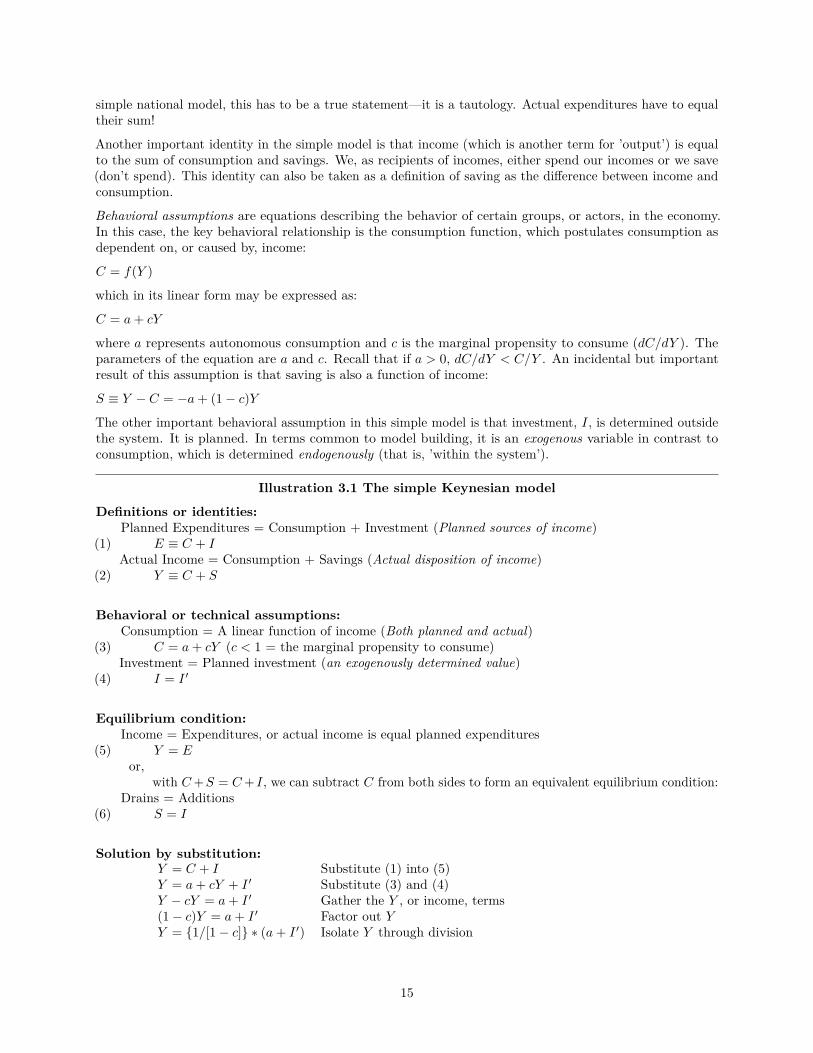
simple national model, this has to be a true statement—it is a tautology. Actual expenditures have to equaltheir sum!

Another important identity in the simple model is that income (which is another term for ’output’) is equalto the sum of consumption and savings. We, as recipients of incomes, either spend our incomes or we save(don’t spend). This identity can also be taken as a definition of saving as the difference between income andconsumption.

Behavioral assumptions are equations describing the behavior of certain groups, or actors, in the economy.In this case, the key behavioral relationship is the consumption function, which postulates consumption asdependent on, or caused by, income:

C = f(Y )

which in its linear form may be expressed as:

C = a+ cY

where a represents autonomous consumption and c is the marginal propensity to consume (dC/dY ). Theparameters of the equation are a and c. Recall that if a > 0, dC/dY < C/Y . An incidental but importantresult of this assumption is that saving is also a function of income:

S ≡ Y − C = −a+ (1− c)Y

The other important behavioral assumption in this simple model is that investment, I, is determined outsidethe system. It is planned. In terms common to model building, it is an exogenous variable in contrast toconsumption, which is determined endogenously (that is, ’within the system’).

Illustration 3.1 The simple Keynesian model

Definitions or identities:Planned Expenditures = Consumption + Investment (Planned sources of income)

(1) E ≡ C + IActual Income = Consumption + Savings (Actual disposition of income)

(2) Y ≡ C + S

Behavioral or technical assumptions:Consumption = A linear function of income (Both planned and actual)

(3) C = a+ cY (c < 1 = the marginal propensity to consume)Investment = Planned investment (an exogenously determined value)

(4) I = I ′

Equilibrium condition:Income = Expenditures, or actual income is equal planned expenditures

(5) Y = Eor,

with C+S = C+ I, we can subtract C from both sides to form an equivalent equilibrium condition:Drains = Additions

(6) S = I

Solution by substitution:Y = C + I Substitute (1) into (5)Y = a+ cY + I ′ Substitute (3) and (4)Y − cY = a+ I ′ Gather the Y , or income, terms(1− c)Y = a+ I ′ Factor out YY = {1/[1− c]} ∗ (a+ I ′) Isolate Y through division

15

The simple Keynesian investment multiplier is:dY/dI = 1/[1− c]

(An example of a technical assumption in economics is the production function. A production functiondescribes the relations between inputs and outputs. A familiar example is Q = F (K,L), commonly used todescribe how capital and labor are combined to produce output.)

Equilibrium is a condition in which the expectations (plans) of decision- makers (actors) in the system aremet. In this simple model, the equilibrium condition is that income equals planned expenditures, or, what isthe same thing, that saving (which sets the limits on actual investment) equals planned investment.

The point is that planned investment and saving do not have to be equal (even though, in the end, actualsaving has to equal actual investment—this is a fundamental principle of accounting). When they are equal,then all parties are satisfied. When they are not, forces are at play which will take income to a lower orhigher level, bringing saving into equality with planned investment.3

Good introductions to the art of model-building can be found in several readily available books (e.g. Bowersand Baird 1971; Kogiku 1968; Neal and Shone 1976). The simple Keynesian model is outlined in almost alltexts on the principles of economics. A good reference is (Case and Fair 1994).

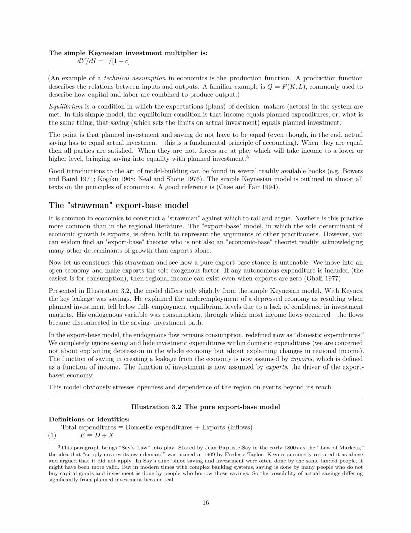
The "strawman" export-base modelIt is common in economics to construct a "strawman" against which to rail and argue. Nowhere is this practicemore common than in the regional literature. The "export-base" model, in which the sole determinant ofeconomic growth is exports, is often built to represent the arguments of other practitioners. However, youcan seldom find an "export-base" theorist who is not also an "economic-base" theorist readily acknowledgingmany other determinants of growth than exports alone.

Now let us construct this strawman and see how a pure export-base stance is untenable. We move into anopen economy and make exports the sole exogenous factor. If any autonomous expenditure is included (theeasiest is for consumption), then regional income can exist even when exports are zero (Ghali 1977).

Presented in Illustration 3.2, the model differs only slightly from the simple Keynesian model. With Keynes,the key leakage was savings. He explained the underemployment of a depressed economy as resulting whenplanned investment fell below full- employment equilibrium levels due to a lack of confidence in investmentmarkets. His endogenous variable was consumption, through which most income flows occurred—the flowsbecame disconnected in the saving- investment path.

In the export-base model, the endogenous flow remains consumption, redefined now as “domestic expenditures.”We completely ignore saving and hide investment expenditures within domestic expenditures (we are concernednot about explaining depression in the whole economy but about explaining changes in regional income).The function of saving in creating a leakage from the economy is now assumed by imports, which is definedas a function of income. The function of investment is now assumed by exports, the driver of the export-based economy.

This model obviously stresses openness and dependence of the region on events beyond its reach.

Illustration 3.2 The pure export-base model

Definitions or identities:Total expenditures ≡ Domestic expenditures + Exports (inflows)

(1) E ≡ D +X

3This paragraph brings “Say’s Law” into play. Stated by Jean Baptiste Say in the early 1800s as the “Law of Markets,”the idea that “supply creates its own demand” was named in 1909 by Frederic Taylor. Keynes succinctly restated it as aboveand argued that it did not apply. In Say’s time, since saving and investment were often done by the same landed people, itmight have been more valid. But in modern times with complex banking systems, saving is done by many people who do notbuy capital goods and investment is done by people who borrow those savings. So the possibility of actual savings differingsignificantly from planned investment became real.

16

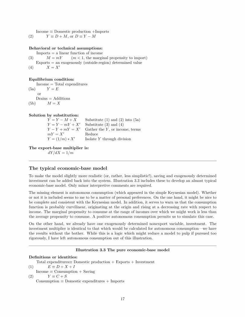
Income ≡ Domestic production +Imports(2) Y ≡ D +M , or D ≡ Y −M

Behavioral or technical assumptions:Imports = a linear function of income

(3) M = mY (m < 1, the marginal propensity to import)Exports = an exogenously (outside-region) determined value

(4) X = X ′

Equilibrium condition:Income = Total expenditures

(5a) Y = EorDrains = Additions

(5b) M = X

Solution by substitution:Y = Y −M +X Substitute (1) and (2) into (5a)Y = Y −mY +X ′ Substitute (3) and (4)Y − Y +mY = X ′ Gather the Y , or income, termsmY = X ′ ReduceY = (1/m) ∗X ′ Isolate Y through division

The export-base multiplier is:dY/dX = 1/m

The typical economic-base modelTo make the model slightly more realistic (or, rather, less simplistic!), saving and exogenously determinedinvestment can be added back into the system. Illustration 3.3 includes these to develop an almost typicaleconomic-base model. Only minor interpretive comments are required.

The missing element is autonomous consumption (which appeared in the simple Keynesian model). Whetheror not it is included seems to me to be a matter of personal preferences. On the one hand, it might be nice tobe complete and consistent with the Keynesian model. In addition, it serves to warn us that the consumptionfunction is probably curvilinear, originating at the origin and rising at a decreasing rate with respect toincome. The marginal propensity to consume at the range of incomes over which we might work is less thanthe average propensity to consume. A positive autonomous consumption permits us to simulate this case.

On the other hand, we already have one exogenously determined nonexport variable, investment. Theinvestment multiplier is identical to that which would be calculated for autonomous consumption—we havethe results without the bother. While this is a logic which might reduce a model to pulp if pursued toorigorously, I have left autonomous consumption out of this illustration.

Illustration 3.3 The pure economic-base model

Definitions or identities:Total expenditures≡ Domestic production + Exports + Investment

(1) E ≡ D +X + IIncome ≡ Consumption + Saving

(2) Y ≡ C + SConsumption ≡ Domestic expenditures + Imports

17

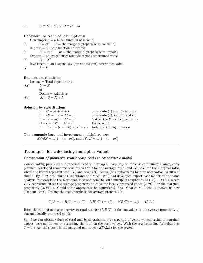
(3) C ≡ D +M , or D ≡ C −M

Behavioral or technical assumptions:Consumption = a linear function of income

(4) C = cY (c = the marginal propensity to consume)Imports = a linear function of income

(5) M = mY (m = the marginal propensity to import)Exports = an exogenously (outside-region) determined value

(6) X = X ′

Investment = an exogenously (outside-system) determined value(7) I = I ′

Equilibrium condition:Income = Total expenditures

(8a) Y = EorDrains = Additions

(8b) M + S = X + I

Solution by substitution:Y = C −M +X + I Substitute (1) and (3) into (8a)Y = cY −mY +X ′ + I ′ Substitute (4), (5), (6) and (7)Y − cY +mY = X ′ + I ′ Gather the Y , or income, terms(1− c+m)Y = X ′ + I ′ Factor out YY = {1/[1− (c−m)]} ∗ (X ′ + I ′) Isolate Y through division

The economic-base and investment multipliers are:dY/dX = 1/[1− (c−m)], and dY/dI = 1/[1− (c−m)]

Techniques for calculating multiplier valuesComparison of planner’s relationship and the economist’s model

Concentrating purely on the practical need to develop an easy way to forecast community change, earlyplanners developed economic-base ratios (T/B for the average ratio, and ∆T/∆B for the marginal ratio,where the letters represent total (T ) and basic (B) income (or employment) by pure observation as rules ofthumb. By 1952, economists (Hildebrand and Mace 1950) had developed export-base models in the sameanalytic framework as the Keynesian macroeconomists, with multipliers expressed as (1/(1− PCL), wherePCL represents either the average propensity to consume locally produced goods (APCL) or the marginalpropensity (MPCL). Could these approaches be equivalent? Yes. Charles M. Tiebout showed us how(Tiebout 1962). Tracing the metamorphosis for average propensities,

T/B = 1/(B/T ) = 1/((T −NB)/T )) = 1/(1−NB/T ) = 1/(1−APCL)

Here, the ratio of nonbasic activity to total activity (NB/T ) is the equivalent of the average propensity toconsume locally produced goods.

So, if we can obtain values of total and basic variables over a period of years, we can estimate marginalexport- base multipliers by regressing the total on the basic values. With the regression line formulated asT = a+ bB, the slope b is the marginal multiplier (∆T/∆B) for the region.

18

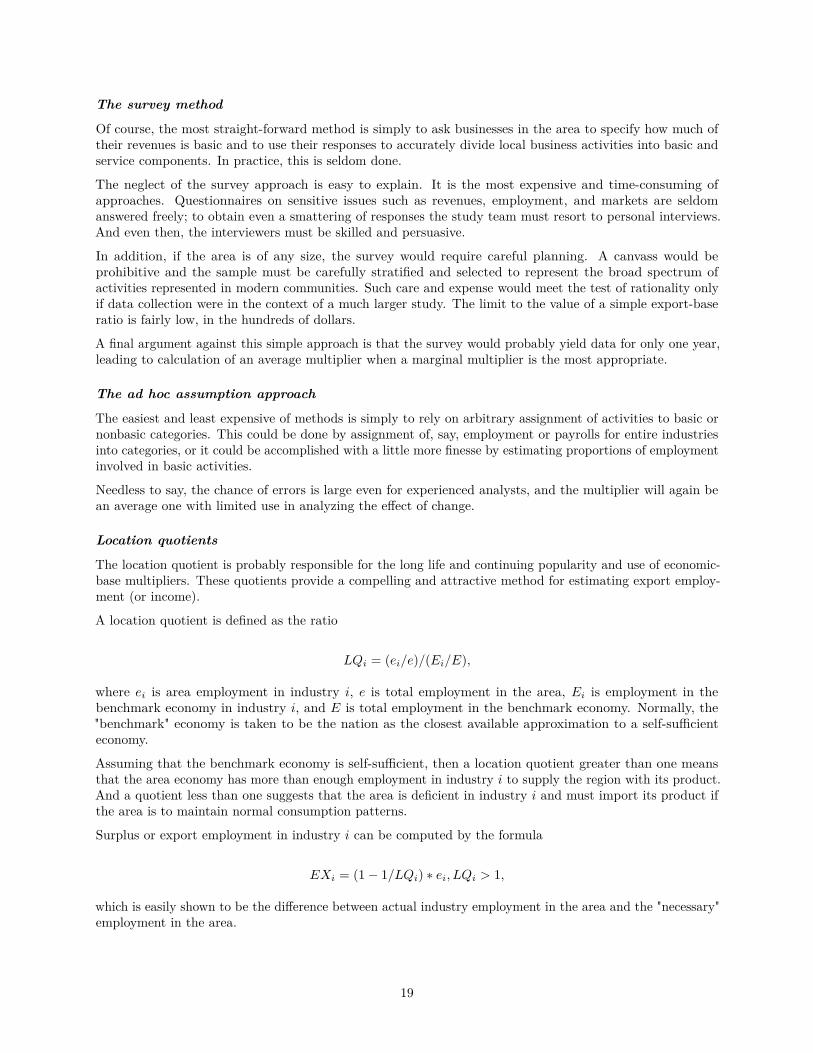
The survey method

Of course, the most straight-forward method is simply to ask businesses in the area to specify how much oftheir revenues is basic and to use their responses to accurately divide local business activities into basic andservice components. In practice, this is seldom done.

The neglect of the survey approach is easy to explain. It is the most expensive and time-consuming ofapproaches. Questionnaires on sensitive issues such as revenues, employment, and markets are seldomanswered freely; to obtain even a smattering of responses the study team must resort to personal interviews.And even then, the interviewers must be skilled and persuasive.

In addition, if the area is of any size, the survey would require careful planning. A canvass would beprohibitive and the sample must be carefully stratified and selected to represent the broad spectrum ofactivities represented in modern communities. Such care and expense would meet the test of rationality onlyif data collection were in the context of a much larger study. The limit to the value of a simple export-baseratio is fairly low, in the hundreds of dollars.

A final argument against this simple approach is that the survey would probably yield data for only one year,leading to calculation of an average multiplier when a marginal multiplier is the most appropriate.

The ad hoc assumption approach

The easiest and least expensive of methods is simply to rely on arbitrary assignment of activities to basic ornonbasic categories. This could be done by assignment of, say, employment or payrolls for entire industriesinto categories, or it could be accomplished with a little more finesse by estimating proportions of employmentinvolved in basic activities.

Needless to say, the chance of errors is large even for experienced analysts, and the multiplier will again bean average one with limited use in analyzing the effect of change.

Location quotients

The location quotient is probably responsible for the long life and continuing popularity and use of economic-base multipliers. These quotients provide a compelling and attractive method for estimating export employ-ment (or income).

A location quotient is defined as the ratio

LQi = (ei/e)/(Ei/E),

where ei is area employment in industry i, e is total employment in the area, Ei is employment in thebenchmark economy in industry i, and E is total employment in the benchmark economy. Normally, the"benchmark" economy is taken to be the nation as the closest available approximation to a self-sufficienteconomy.

Assuming that the benchmark economy is self-sufficient, then a location quotient greater than one meansthat the area economy has more than enough employment in industry i to supply the region with its product.And a quotient less than one suggests that the area is deficient in industry i and must import its product ifthe area is to maintain normal consumption patterns.

Surplus or export employment in industry i can be computed by the formula

EXi = (1− 1/LQi) ∗ ei, LQi > 1,

which is easily shown to be the difference between actual industry employment in the area and the "necessary"employment in the area.

19

In fact, then, excess employment can be computed without reference to location quotients through thisreduction of the formula:

EXi = ei − (Ei/E) ∗ e

It is convenient to retain the initial formula as a reminder of the logic, and to compute location quotients asreminders of the strengths of exporting industries.

Now it is easy to estimate export employment for each industry in the area and to sum these estimatesto yield a value for export employment for the area in some particular year. With this number and totalemployment, an average multiplier for the area can be computed. With a set of these values over 10-20 years,the more acceptable marginal multiplier can be estimated by simple regression.

While it is common to use employment as the primary basis for these calculations, other measures such aswages and salaries are just as appropriate. Indeed, wage data is more accessible electronically, especially onCD-ROM. County Business Patterns, a standard source of employment and payroll data, is available foryears since 1986, two years per disk. In considerable detail, this is the best data for recent years, but skillwith mainframe computers, tapes, and programming is required to gain access for earlier years. The RegionalEconomic Information System (REIS), updated on CD-ROM annually by the U.S. Department of Commercewith a two-year lag, includes a relatively aggregated 16-category employment series for the years 1969-2000as well as a more detailed earnings series for every county in the nation (categories are based on the oldStandard Industrial Classification (SIC) system). This data makes earnings-based location quotients a snap,especially if historic estimates are desired. The REIS files can be accessed at https://apps.bea.gov/regional/.

From 2001 on, the industry categories are based on the new North American Industry Classification System(NAICS), with 23 categories of employment and even more categories for earnings. This shift in industrydefinitions means that categorical data is not available in time series. Everything starts anew in 2001.

Location quotients have been in use by regional analysts for over 50 years now, and have been commented on atlength. We should look at the assumptions involved in their use as well as the advantages and disadvantages.

The literature records at least three specific assumptions: (1) that local and benchmark consumption patternsare the same, (2) that labor productivity is a constant across regions, and (3) that all local demands are metby local production whenever possible.

The first assumption is not serious: not only can we not discern differences in consumption patterns withoutextraordinary expense but we can suspect that differences in production patterns are more important.Purchases of intermediate goods by producers differ for regions depending on industry mix. (It turns outthat we can account for industry mix with input-output models, so this difference has been accounted for bythe march of time.).

The constant-labor-productivity assumption is difficulty to avoid. Its impact can be ameliorated slightlythrough using earnings data, which can be assumed to reflect regional productivity variation throughdifferences in wage rates. (This assumption could in turn be attacked if wages vary more by area cost ofliving than by productivity.)

The assumption that local demands are met first by local production is the more tenuous of the three. It isobviously not true, as any visit to a grocery or clothing store will attest. But it is common, and a betteralternative is hard to come by.

In addition to the disadvantages accruing from these assumptions, another major fault is that the method isdependent on the degree of aggregation of the data, making comparisons among various studies of little value.To illustrate the problem, consider the food and kindred products industry in Atlanta. The location quotientcomputed for this broad industry should be less than one, and if excess employment were computed based onthis classification, none would be credited to the food industry. But if the classification were more detailed,the soft-drink industry would show a large number of excess employees, since the headquarters of Coca-Colais in the city.

20

The overpowering advantages of using location quotients are that the method is inexpensive and the exercise ofcomputing excess employment may give the analyst an opportunity to gain insights of interest in themselves.

Minimum requirements

In the 1960’s, when available computing technology favored frequent use of economic-base models, one of thealternatives to the use of location quotients was the minimum- requirements approach (Ullman and Dacey1960). This variation involved a slight revision of the location-quotient formula to

EXi = ei − (Ei/E)min ∗ e,

where(Ei/E)min is the minimum employment proportion for industry i in cities of size similar to the subjectcity. You can readily see that we have substituted a varying benchmark employment proportion for a constantone:

LQi = (ei/e)/(Ei/E)min.

While still appearing in various forms in the literature, the method suffers from two major criticisms. One isthat, if enough cities are included in the selected set, all regions will be exporting and none may be importing.The other is similar in that, if we use data defined in a fine level of detail (which should be an improvement,as it was in location- quotient estimates), we may reduce local needs to near zero and make almost allproduction for export (Pratt 1968).

At any rate, the method is not commonly used now. The location- quotient method remains the virtuallysole survivor as a simple means of identifying export industries.

"Differential" multipliers: a multiple-regression analysis

Another approach which has been used in estimating economic-base multipliers is to fit a multiple-regressionequation to regional data. The first of these studies arose in a study of the impact of military bases onPortsmouth, New Hampshire in 1968 by Weiss and Gooding (Weiss and Gooding 1968).

Simple economic-base models ignore the possibility that different industries may have different impacts ontheir communities. The regression technique eliminates this simplifying assumption. Weiss and Gooding setup an equation

S = Q+ b1X1 + b2X2 + b3X3,

where S represents service employment, Q is a constant, and the X terms are, in order, private exportemployment, civilian employment at the Portsmouth Naval Shipyard, and employment at Pease Air ForceBase.

With data fitted from 1955-64, their results were

S = −12905 + .78(.31)

X1 + .55(.23)

X2 + .35(.14)

X3

The multipliers are 1 + bi for each sector.

Weiss and Gooding used a mixture of assumption and location quotient methods in allocating exportemployment and assumed that the export sectors were independent and that workers in the export sectorsdemanded similar services.

This variation on economic-base modeling has not fallen into widespread use for several reasons: its flexibility(in number of exogenous sectors) and the statistical significance of coefficients are limited by the numberof observations available; determining the export content of industry employment remains a demanding

21

chore; and with the rise of desktop computing, input-output models are better sources of industry-specificmultipliers and are similar in cost.

Critique: advantages, disadvantages, praise, criticismEconomic-base models suffer from old age: they have been built by so many analysts with varying levels ofquality and they have been criticized so often that little remains except the concept.

The indictment would include the following phrases:

Short run

Nonspatial

Simple adaptations of national models

Data is normally available for administrative units (counties) which may be poorly defined as economicregions.

Ignores capacity constraints

Assumes perfect elasticity of supply for inputs

Pits the area against the rest of the world, showing no interdependence between regions

Multiplier varies with size of region. (As a region grows it diversifies, importing less and so increasinglocal consumption and the multiplier (Sirkin 1959)). Also, larger regions tend to influence neighborsmore and so to enjoy larger feedback effects (Richardson 1972)

An employment multiplier is often used to discuss income changes. (But this assumes that employmentand per capita income are perfectly correlated -- in a simple economy with perfectly elastic supplies oflabor this might be the case although, of course, the world is not simple.)

Assumes that exports are the sole determinant of economic growth. (It is not reasonable for us totake the rap for this.) Any rational person can see that the determinants of growth are many -- thesimple model just emphasizes one determinant. Perhaps the fault lies in early attempts to formulatemultipliers and the ease with which the simple multipliers could be constructed. (Ghali 1977; Sirkin1959))

Direction of dependence may be questionable: which comes first, export growth or a strong servicesector, or interdependence? Should we be concerned with preconditions for export growth (setting upan attractive service sector) in this simple model? Are we planning growth or explaining the true basis?

Although castigated for decades, the economic-base model has survived as a very succinct expression of thepower of demand in regional income determination. The most current, and perhaps the clearest and mostcomplete, statement of its status is found in a recent review by Andrew J. Krikelas (1992), reprinted belowwith permission from the Atlanta Federal Reserve Bank..

22

Appendix A: Review of Economic-Base LiteratureThe following article appeared in the Economic Review, Federal Reserve Bank of Atlanta, July/August 1992,pp. 16-29 , and represents the latest in reviews and critiques of economic-base literature.

Why Regions Grow: A Review of Research On the Economic- Base ModelAndrew C. Krikelas

The author is an economist in the regional section of the Atlanta Fed’s research department.

Regional economic models are used in a variety of decision-making contexts. Governmentofficials use them to prepare annual budgets. Businesses rely on them for producing short-runmarket demand forecasts and for analyzing longer-term growth strategies. Urban planners andtransportation officials use them to develop long-range plans for urban and regional development.Finally, state and local policymakers turn to them to get new ideas for programs and policies topromote long-run regional growth.

Although it would be convenient if a single model had been developed to serve all these purposessimultaneously, no such model is ever likely to exist. Instead, regional models tend to be highlyspecialized in terms of the issues that they are able to address and the time horizons over whichtheir analytical results are most reliable. For example, a short-run forecasting model might servethe needs of state or local government officials engaged in the annual budgeting process, butit would contribute little information relevant to long-run local economic development issuesconfronting planners and policymakers. Only rarely is a regional model able to perform well inmore than one of these distinct decision-making contexts.1

The rapid pace of urban growth during this century, along with the challenge it has presented forplanners trying to anticipate and influence this growth, has ensured a healthy demand for regionaleconomic models, particularly since 1945. Unfortunately, models supplied have been inadequate.

At the beginning of the postwar period, the economic base model was probably the only suchinstrument generally available for regional economic analysis. This model focuses on regionalexport activity as the primary determinant of local-area growth; it is one of the oldest and mostdurable theories of regional growth, with origins extending at least as far back as the early 1900s.However, economic base theory received the greatest amount of attention from scholars in regionalscience between 1950 and 1985. Despite the model’s acceptance over such a long period, when thenoted regional scientist Harry W. Richardson, writing for a special twenty-fifth anniversary issueof the Journal of Regional Science, reflected upon the more than forty years of research conductedwithin this paradigm, he concluded that "the findings on economic base models are conclusive.The spate of recent research has done nothing to increase confidence in them The literaturewould need to be much more convincing than it has been hitherto for a disinterested observerto resist the conclusion that economic base models should be buried, and without prospects forresurrection" (1985, 646).

Like Richardson, others over the years have expressed concern with the narrow focus of economicbase theory on exports—just one portion of the demand side of the regional growth equation—tothe exclusion of important supply-side factors and constraints. Many have suggested that economicbase theory, its analytical and methodological techniques, and the public policies that it promotesshould be abandoned in favor of other, more comprehensive theories of regional growth anddevelopment.

Nevertheless, economic base research continues. Most notably, James P. Lesage and J. DavidReed (1989) and Lesage (1990) have provided empirical evidence in support of the economic basehypothesis as both a short-run and long-run theory of regional growth. These authors suggestthat their models could be used both for short-term forecasting of regional employment, income,

1Structural econometric models are often used for purposes of both forecasting and policy analysis. However, the greatexpense required to specify and maintain such models has generally led economists either to develop less complex models thatfocus narrowly on a small set of policy issues or to develop theoretical time-series models that perform well for purposes ofshort-run economic forecasting.

Economic Review, FRB Atlanta 23 Jul/Aug 1992

and product and for longer- range regional economic planning and policy analysis. If these claimswere valid, then the economic base model, rather than being of little value, would be one of thefew regional models that might be useful in each of these very different but crucially importantdecision-making contexts.

Because regional economic models play such an important role in planning and policy discussions,it is important to have a clear understanding of their strengths and weaknesses. Limitations ofthe economic base model in particular, because it tends to be widely used, should be recognized.Recent research has provided evidence suggesting substantial improvement in traditionally staticeconomic base model specifications through the adoption of techniques routinely employed in themacroeconomics time-series literature. However, this author’s research suggests that these studiesmay have overstated the usefulness of these new economic base model specifications (Andrew C.Krikelas 1991).

The purpose of this article, therefore, is twofold. First, a concise analytical history of the old andextensive economic base literature generated by a variety of professional and academic disciplinesis provided in order to place recent research in perspective. The discussion then turns to thecentral question addressed in Krikelas (1991): Can techniques borrowed from statistical time-seriesliterature successfully breathe new life into the traditional economic base model?

Definition of the Economic Base Concept

As originally formulated, the economic base model focused on regional export activity as theprimary source of local- area growth. According to this theory total economic activity, ET isassumed to be dichotomous, with a distinction being made between basic economic activity, EB

(activities devoted to the production of goods and services ultimately sold to consumers outsidethe region), and nonbasic economic activity, ENB , which includes activities involved in producinggoods and services consumed locally:

ET = EB + ENB (1)

This division of regional economic activity into these two distinct sectors is the central concept ofthe model.2 A serious empirical concern is immediately raised by this approach, however, becauseappropriate export data are available at any subnational level only at high cost and with long lags.Various alternative measures have been proposed and analyzed in the literature over the years,but none has been found entirely adequate. Data problems, therefore, have always complicatedeconomic base research.

While the central concept of the economic base model is the duality of regional economic activity, itsfundamental behavioral assumption is that nonbasic economic activity depends on basic economicactivity. In this perspective, external demand for a region’s exportable goods and services injectsincome into the regional economy, in turn augmenting local demand for nonexportable goodsand services. The model assumes that the income injected into the regional economy and theaccompanying potential for developing locally oriented, nonbasic industries are in proportion tothe size of a region’s export base. Static and demand-oriented, the model ignores factors thataffect the supply of a region’s output and other changes, such as the introduction of new products,that affect demands.

ENB = f(EB) = α+ β ∗ EB . (2)

Equations (1) and (2) can then be combined into the reduced-form expression in equation (3),2Besides the terms basic and nonbasic, a number of others have been proposed to distinguish between the two types of

economic activity: town builders/town fillers, exchange production/own production, primary/ancillary, export/local, as well asothers. Andrews (1953b) directly addresses the issue of the profligate and confusing terminology of the economic base paradigm.

Economic Review, FRB Atlanta 24 Jul/Aug 1992

which indicates that total economic activity is primarily a function of basic activity:

ET = α+ (1 + β) ∗ EB (3)

The expression (1+β) is commonly referred to as the economic base multiplier, and the parameter,β, is called the economic base ratio.

When applied to analyzing regional growth, the economic base model suggests that the growthprocess will be led by industries that export goods and services beyond regional boundaries. Iteven offers a prediction, captured in the multiplier, of the total regional impact likely to resultfrom a change in basic economic activity generated outside the region. Understanding the futurepath of a regional economy, the model implies, requires simply concentrating on the prospects forthe base industries. These few important industries are often dubbed "engines of regional growth."

This simple model captures the essence of economic base theory. Although the model has beenenhanced over the years to include additional variables as well as to capture more explicitlythe dynamic nature of the regional growth process, most changes have been made within thescope of this simple demand-oriented specification. In general, economic base models have notevolved to acknowledge the potential impact of many important variables that may affect regionalgrowth—interregional capital flows; labor migration patterns; changes in products, tastes, andproduction processes; demographic shifts; and changes in state and local tax laws, to name afew. Because these issues are generally too important to ignore, many regional scientists haveconcluded that economic base theory lacks the complexity to provide a useful framework foranalyzing many regional economic issues and policies. The following review of the developmentand testing of the model will summarize where the debate on this topic stands at this point.

History of the Economic Base Literature

Five fairly distinct chronological periods characterize the history of the economic base literature:(1) the origin of the concept, 1916-21; (2) early development, 1921-50; (3) the first round of seriousdebate, 1950-60; (4) the second round of debate, 1960-85; and (5) a third and perhaps final roundof debate begun in 1985 and continuing today. Decades of research within the economic baseparadigm have created a body of conventional wisdom concerning the uses and limitations of themodel, both in theory and in practice. Nonetheless, as yet another round of discussion has begun,it seems that few lessons of the past have been learned and that a brief summary of the history ofthis literature might be useful.

Origin of the Economic Base Concept.

The essential duality of regional economic activity that is central to the simple model expressed inthe equations above was first articulated in 1916 by the German sociologist Werner Sombart, whowrote of "actual city founders," identified as the "active, originative, or primary city formers"—thosewhose positions of authority, wealth, or occupation allowed them to draw income from outsidethe city—and the "passive or derived or secondary city founders," whose livelihood depended onthe city formers (Gunter Krumme 1968, 114).3

In 1921 M. Arrousseau made a similar observation in commenting on the relationship betweenwhat he distinguished as a town’s primary and secondary occupations: "The primary occupationsare those directly concerned with the functions of the town. The secondary occupations are thoseconcerned with the maintenance of the well-being of the people engaged in those of primarynature" (John W. Alexander 1954, 246).4 Also in 1921, landscape architect Frederick Law Olmsted

3Krumme was translating Werner Sombart’s Der Moderne Kapitalismus, Erster Band: Die Vorkapitalistische Wirtschaft,2nd rev. ed. (Munich: Duncker and Humblot, 1916). Sombart identified the city formers as "a king who collects taxes; a landlordwho receives rent payments; a merchant who profits from trade with outsiders; a craftsman, a manufacturer, who sells industrialproducts to the outside; an author, whose writings are being bought outside the gates; a physician, who has clients in thecountryside; a student, who is supported by his parents in another place, etc. These are the people who live and let live."

4Alexander was citing M. Arrousseau, "The Distribution of Population: A Constructive Problem," Geographical Review 11(1921).

Economic Review, FRB Atlanta 25 Jul/Aug 1992

distinguished between what he called primary and ancillary economic activity in an urban area(Alexander 1954, 246.)5

Thus, although Sombart was apparently the first to observe formally the seeming duality of urbanand regional economic activity, the remarks of his contemporaries Arrousseau and Olmsted makeit abundantly clear that the concept was ripe for expression. By the early 1920s, therefore, theeconomic base concept had generally surfaced as a potential theory for explaining the regionalgrowth process.

Early Development of the Theory.

Following establishment of the theory, the next logical step should have been the empirical testingof the validity of the model’s central hypothesis. However, this step was almost universally ignoredand the model adopted as useful as the rapid growth of cities early in the century pressured stateand local officials to improve the way in which they developed plans for urban expansion and theprovision of public infrastructure and government services. The economic base model provided amuch-desired framework for developing such plans, and studies designed to identify and measurebasic industries— economic base studies—quickly became primary tools employed in acquiringinformation for long-range planning.

After identifying a region’s export base, economic base studies calculate a local- area economicbase ratio,β. Once calculated, the economic base ratio can be used with forecasts of the futuregrowth of the region’s export base industries to predict the region’s overall growth. The study’sfocus on the smaller number of industries identified as regional export industries helps streamlinethe process of forecasting total regional economic activity. In addition, by identifying thoseindustries considered most important to the regional growth process, an economic base studyprovides information that adds insight to discussions of regional industrial policies and programs.

Sombart’s analysis of the Berlin economy, published in 1927, was the first economic base studyconducted during this period. Sombart, complaining that "nobody makes the effort to sit downwith a pencil and figure out with the help of occupational statistics how much there actually is ofa city-forming industry in a city such as Berlin," developed an empirical approach for dividing anurban economy into its dual parts (Krumme 1968,116).6

Lacking detailed information on regional export activity, Sombart relied upon industry employmentdata collected in Berlin in 1907 to estimate the basic and nonbasic sectors of the city’s economy.Relying mainly upon his personal judgment, Sombart estimated that approximately 262,000 ofBerlin’s total work force of 543,000 were employed in export base industries (Krumme 1968, 113).These calculations placed Berlin’s nonbasic/basic ratio, β, at 1.07, an approximately one-to-onerelationship. Although Sombart did not use this information to forecast Berlin’s growth, hecould have done so. Making a more limited forecast of the prospects for those industries he hadidentified as being part of the city’s export base and multiplying that total by the city’s economicbase multiplier (1 + β) of 2.07 (assuming that the city’s base ratio had remained relatively stablein the intervening twenty years since the census was conducted) would have provided a forecast ofthe change in total economic activity expected in Berlin as a result of some externally generatedchange in demand for its export product.

5Alexander cites a letter dated February 21, 1921, to John M. Glenn, a member of the New York Regional PlanningCommittee in which Olmsted wrote, "The multiplicity of their productive occupations may be roughly divided into those whichcan be considered primary, such as carrying on the marine shipping business of the port and manufacturing goods for generaluse (i.e., not confined to use within the community itself), and those occupations which may be called ancillary, such as aredevoted directly or indirectly to the service and convenience of the people engaged in the primary occupations."

6According to Krumme’s translation, Sombart wrote, "It is necessary to find out for each trade how much of it is engaged inwork for local consumption and how much in work for exports out of the city. This figure then is the city-forming ratio for theindividual trade. Naturally, the ratio can be found accurately only with the assistance of an extensive enquete (survey). However,one could gain at least an approximate impression of the shares of the export industries in the total gainful employment by acareful investigation of the results of the occupational census" (1968, 116). The empirical study cited by Krumme was publishedfor the first time in the second revised edition of Sombart’s Der Moderne Kapitalismus, Drifter Band: Das Wirtschaftsleben imZeitalterr des Hochkapitalismus, in 1927. Krumme, however, was quoting from the third printing of this edition, published inBerlin in 1955.

Economic Review, FRB Atlanta 26 Jul/Aug 1992

The reliance on secondary data sources for Sombart’s study of Berlin’s economic base is typicalof most such research. As pointed out earlier, even today the appropriate regional export datarequired to conduct an adequate economic base study are available only at relatively high cost. Thecomprehensive economic analysis of the city of Oskaloosa, Iowa, published in Fortune magazinein 1938 illustrates this point ("Oskaloosa. . ." 1938).

Although published in a popular magazine, this study represents an important contribution toresearch on the economic base theory. The magazine staff conducted a complete census of thetown’s 3,000 families in order to determine the origin and destination of income flows withinthe city. They also conducted a census of the town’s businesses, including an accounting ofthe destination of their output and the source and value of the most important inputs into thelocal-area production process.

The results of the study indicated that in 1937 Oskaloosa was a net exporter of goods and servicesto the rest of the world and that manufactured goods and professional services were the town’sleading export industries. The study’s findings are interesting because they were based upon acensus that provides a relatively accurate portrayal of Oskaloosa’s export activity during the yearstudied. Even by present standards this study represents one of the most thorough economicanalyses of a small community ever published.

The great effort required to collect these data, however, explains why a survey- or census-oriented approach to economic base identification generally has been abandoned for the nonsurveyidentification techniques made popular by Homer Hoyt in the late 1930s. Working with theFederal Housing Administration during the mid-1930s, Hoyt developed and employed an economicbase methodology for producing forecasts of local housing market demand. His techniques becameknown to a wide audience with the original publication of his textbook, Principles of UrbanReal Estate (coauthored with Arthur M. Weimer in 1939), which Richard B. Andrews called thefirst "complete statement of the theory of the economic base." In commenting on the impact ofthis work, Andrews continued, "This statement included much material that was new outsideof technical reports. For example, it introduced in formal fashion the idea of a mathematicalrelation between basic employment and service employment Hoyt considered the economic baseidea to be a tool that might be employed in analyzing the economic background of cities with theobjective of forecasting the future of the entire city" (1953a, 163).

In this text Weimer and Hoyt distinguished between "urban growth" and "urban service" industries,suggesting that a region’s potential for growth depended primarily upon the prospects for theregion’s urban growth industries. They provided a six-step procedure for identifying such industries.Using relatively accessible income and employment data, the authors developed a methodologythat represented a combination of what has become known as the assignment technique and thelocation-quotient technique of economic base identification. The assignment technique is essentiallyidentical to Sombart’s methodology, in which personal judgment is used to assign industries withina particular regional economy to basic and nonbasic sectors. The location- quotient technique, onthe other hand, relies upon regional economic data to make such distinctions.

Location-quotient methodology compares a region’s concentration of economic activity in aparticular industry with that of a benchmark economy, usually the entire country in which theregion is located. If the regional concentration, measured in terms of the industry’s share of totalregional employment or income, exceeds the benchmark economy’s concentration in that industry,the surplus level of employment or income is assumed to measure regional export activity. Forexample, if an industry accounts for 6 percent of regional employment but only 2 percent ofnational employment, two- thirds of that industry’s employment would be called basic. (If theregional activity in an industry is less than that at the national level, the industry is categorizedas nonbasic.) Making this identification requires only industry employment or income data forthe region and a similar set of data for an appropriate benchmark economy.

Although Weimer and Hoyt were not the first to propose using the location quotient and assignmenttechniques as nonsurvey methodologies for dividing regional economic activity into its basic and

Economic Review, FRB Atlanta 27 Jul/Aug 1992

nonbasic components, dissemination of the techniques through their textbook introduced theseshortcuts to a wide audience. With these methodologies available it became feasible for localdevelopment officials to adopt the economic base paradigm for purposes of analyzing specificurban and regional economies. During the latter half of the 1940s, once these techniques hadbecome more widely known, a much larger number of cities and states began to use the economicbase model in urban and regional planning and economic analysis.7

Theoretical Debate.

By 1950 economic base theory and its methodological techniques had become established asthe primary tools of regional planning. The theory itself had been accepted, uncritically, as anexplanation of local- area growth and economic development. Between 1950 and 1960, however,discussion at the theoretical and methodological level turned directly to the question of the validityof the economic base hypothesis itself. Unfortunately, only a handful of empirical tests werereported during this entire decade.

The earliest and most cogent critique of economic base theory was presented by George Hildebrandand Arthur Mace (1950) in their analysis of the Los Angeles metropolitan area. This importantcontribution identified the theoretical model upon which the economic base paradigm was foundedand performed an empirical test that provided evidence supporting the validity of the economicbase hypothesis, at least for short-run forecasting.

Hildebrand and Mace’s most significant contribution was their explicit formulation of economicbase theory as a testable behavioral hypothesis. Their results, which demonstrated a statisticallysignificant short-run relationship between basic and nonbasic employment in Los Angeles, repre-sented the first empirical confirmation of the economic base hypothesis. Furthermore, the authorsformulated their tests within the context of an explicitly Keynesian national income model andthen outlined the inherent limitations of such a model.

Consider the familiar Keynesian relationship:

Y = C + I +G+ (X −M) (4)

where total regional income, Y , is divided into a number of distinct sectors, including consumption,C; investment, I; government expenditures, G; and exports minus imports, X − M . Thereduced-form expression of this model would include some smaller set of exogenous variables,only one of which would be regional exports. (Other exogenous variables would include theautonomous components of consumption, investment, government expenditures, and imports;marginal propensities to consume locally, to invest locally, and to import; and local and federaltax policies.) It is this set of exogenous factors that would determine, theoretically, a region’stotal income level, Y .

The economic base model focuses on one particular aspect of this relationship, regional exportactivity, X(EB) in equation [1] above), and can be considered a special case of the more generalKeynesian model in equation (4). Given this interpretation, it becomes clear that for exportsto be considered the only exogenous determinant of regional growth, all other relevant factors,related to both demand and supply, must remain fairly constant or be functions of export activity.Although this might be a tenable assumption in the short run, it probably is an extremely poorone in the long run. Hildebrand and Mace made this observation explicit and suggested that themodel was most appropriate for anticipating regional economic trends over a short time horizon.

7The following list identifies a few of the communities that performed economic base studies during the 1940s, the individualsor institutions that performed these analyses, and the base ratios (,B) calculated, respectively: New York, The Regional PlanAssociation Inc., 2.1; Detroit, Detroit City Plan Commission, 1.1; Cincinnati, Victor Roterus and the staff of Cincinnati CityPlanning Commission, 1.7; Washington, D.C., National Capitol Park and Planning, 1.1; Brockton, Massachusetts, Homer Hoyt,0.8; the state of New Jersey, Homer Hoyt, 1. 1; and Albuquerque, New Mexico, Federal Reserve Bank of Kansas City, 0.9. Thisinformation was originally compiled by Edward Ullman and published in the third edition of Weimer and Hoyt’s text in 1954and was reprinted in Pfouts (1960, 30).

Economic Review, FRB Atlanta 28 Jul/Aug 1992

In addition, they listed some of the other variables that they thought should be taken into accountin developing a more comprehensive model of regional economic activity: population levels andinterregional migration patterns, regional capital investment levels and annual flows, state andlocal tax policies, and changes in the cost of transportation to reach external markets. Despitethese reservations, Hildebrand and Mace offered a fairly encouraging assessment of the prospectsfor this type of research, based on the availability of additional census data and further empiricalanalysis across a ten- year span. 8

Unfortunately, the lessons contained in Hildebrand and Mace’s study were not widely disseminated.Hildebrand and Mace were among the first economists to contribute to the economic base literature.Their article was published in a journal not normally read by geographers and urban planners,who, before 1950, had played a dominant role in the research conducted within the economicbase paradigm. Therefore, rather than playing the role of a seminal article to a further body ofempirical research, the Hildebrand and Mace article remained relatively unknown. The debate ofthe 1950s brought many of their important insights to the attention of geographers and urbanplanners, but it took nearly a decade for all of these contributions to be uncovered.

Most of the 1950s’ debate on economic base theory was conducted in the geography and planningliteratures. The origin of this debate can be traced to a series of nine articles published byAndrews between 1953 and 1956 (see reference list). These articles provided a careful expositionof economic base theory and the methodologies that had been developed to analyze urban andregional economic activity. The author’s stated purpose was to explore and evaluate the entireconcept. "We have operated far too long on a set of ideas which appear valid but which, despitesubstantial conceptual omissions and difficulties of application, seem to be accepted all tooblithely," he wrote, calling for "more fundamental thinking on and questioning of the reality andutility of base theory as presently conceived" (1953a, 167).

While Andrews was somewhat critical in his assessment of the economic base paradigm, he clearlywas a proponent of its inherent validity and usefulness. Instead of suggesting the abandonment ofthe model as a tool for urban and regional economic analysis, he identified ways in which it couldbe improved to serve such purposes better. His recommendation included better efforts at basicindustry identification and measurement, improvements in the collection of regional data, andmodifications in the way in which economic base concepts were used. Given Andrews’s criticismof the state of the economic base research prior to 1950, it is surprising to note he did not addressone of the most fundamental shortcomings of this research: the lack of empirical verification ofthe underlying hypothesis. Krikelas (1991) identified only five empirical tests of the economicbase hypothesis conducted during the 1950s. Three of those studies, including that of Hildebrandand Mace, supported the validity of the economic base hypothesis, at least in the short run, andtwo provided evidence against it. A decade of research, therefore, provided insufficient empiricalevidence for determining the validity of the model’s central hypothesis.

When applied to analyzing regional growth, the economic base model suggests that thegrowth process will be led by industries that export goods and services beyond regionalboundaries.

Instead, most of the debate of the 1950s centered on questions related to theory and practicerather than testing. Hans Blumenfeld (1955) was critical of the economic base model’s narrowfocus on export activity as the primary source of regional growth. While he agreed that thismodel might do well to explain economic growth in small or highly specialized economies, he

8Hildebrand and Mace wrote, "The forthcoming Census of 1950 will permit further advances in this research. Recalculationof location quotients and comparisons with 1940 will indicate changes in external markets and locational concentrations duringthe war decade, particularly in communities undergoing large gains or losses in population. With monthly statistics of insuredemployment, a current record of employment in non- localized industries can be maintained. Improved multiplier analysis, withcurrent local labor force statistics, should then permit more precise depiction of local unemployment problems, and attainmentof more adequate policies at the o r-all and community levels" (1950, 249).

Economic Review, FRB Atlanta 29 Jul/Aug 1992

argued that it was inadequate to explain the growth of complex urban economies. Blumenfeldwas also critical of the policy implications of the model; these focused almost exclusively onsupporting existing export industries at the expense of other reasonable alternatives, such asfostering the establishment and development of industries that would compete with importedgoods and services.

Charles M. Tiebout (1956a, 1956b) and Douglass C. North (1955, 1956) engaged in a short butlively debate over the short-run versus long-run applicability of the economic base model. Tiebout,explicitly recognizing the Keynesian roots of the economic base model, supported Hildebrandand Mace’s (1950) contention that the economic base model was most appropriate for short-runeconomic analysis. He also argued that the economic base model minimized the importantcontribution that nonbasic economic activity made to local area growth and development. Hewrote that, although export activity was important, "in terms of causation, the nature of theresidentiary industries will be a key factor in any possible development. Without the ability todevelop residentiary activities, the cost of development of export activities will be prohibitive"(1956a, 164).

North, however, objected to the characterization of the economic base model as an adaptation ofthe demand- oriented Keynesian model. Instead, he argued that the most important determinantof a region’s long-run growth potential was its ability to attract capital and labor into the regionfrom outside. Such supply-enhancing flows in turn would respond quite favorably to profitopportunities offered by regions engaged in high levels of export activity. North observed thathistorically "it was frequently the opportunities in manufacturing for the United States marketwhich led to immigration of labor and capital into a region. The important point is that thepull of economic opportunity as a result of a comparative advantage in producing goods andservices in demand in existing markets was the principal factor in the differential rates of growthof regions" (1956, 166).

Many regional scientists have concluded that economic base theory lacks the complexityto provide a useful framework for analyzing many regional economic issues and policies.

The economic base model proposed by North explicitly recognized the important role of supplyfactors in determining the nature and growth potential of a region’s export base. In practice,however, most economic base models of this and subsequent periods have maintained a fairlystrict demand orientation. This demand-oriented model is also the one to which Tiebout raisedso many objections. As a result, although Tiebout and North found themselves on different sidesconcerning the validity of the model as a long-run theory of regional growth, both ultimatelyagreed that supply factors needed to be added to the model in order to make it relevant forlong-run regional economic analysis.

One additional advance in the theoretical literature of this period that called into question theadequacy of economic base modeling techniques was the development of regional input-outputmodels. Before 1950 the economic base model represented the primary tool available to regionalplanners for analyzing the impacts of anticipated changes in regional economic activity. During thefirst half of the 1950s, however, input-output modeling techniques first developed by Wassily W.Leontief (1951) were adapted for purposes of regional economic analysis.9 While a regional input-output model could distinguish between the differential regional impacts that might be associatedwith, for example, the construction of a specialty steel manufacturer versus a mail-order catalogfacility—two very different kinds of basic economic activity—the simple two-sector economic basemodel could not make such a distinction. Given this limitation, many urban planners beganto advocate input-output techniques as more appropriate for forecasting anticipated changes in

9Perhaps the most often-cited contribution to the early regional input-output literature was an article coauthored by Isardand Kuenne (I 95 3).

Economic Review, FRB Atlanta 30 Jul/Aug 1992

regional economic activity.

The debate of the 1950s also focused on several important methodological issues. Papers by JohnM. Mattila and Wilbur R. Thompson (1955) and Charles L. Leven (1956) considered the adequacyof the location-quotient technique’s ability to identify a region’s economic base industries. Whilesuggesting certain improvements to the traditional formulation of the location quotient, Mattilaand Thompson concluded that "if used with care, the index of surplus workers in both its absoluteand relative form should prove to be a highly useful tool in regional economic base studies"(1955, 227).10 Leven, on the other hand, arrived at the opposite conclusion, stating that "theshortcomings of this technique render it useless as a quantitative measure of basic activity in anarea" (1956, 256).

The issue of the appropriate measure to be used for calculating location quotients was alsodiscussed. Because employment data were more readily available than wage or income data, mosteconomic base studies of this period used employment in identifying regional export activity.This measure, however, has some serious drawbacks. In addition to placing equal weight uponpart-time and full-time employment and failing to adjust adequately for productivity and wagedifferences between workers employed in different industries, employment data do not provideany measure of the impact that transfer payments and other sources of unearned income, such asinterest payments, rents, and profits, have upon a regional economy.

Recognizing the serious weaknesses associated with the use of employment data for purposesof identifying a region’s economic base, Andrews (1954a), Leven (1956) and Tiebout (1956c)all suggested the adoption of alternative measures of regional economic activity. Andrews andTiebout advocated the use of income received by residents of the region, and Leven argued fora value-added measure. Income and value-added data, however, generally are not available forregional economies, especially at the substate level, except with long lags.

By the beginning of the 1960s professionals engaged in urban and regional economic analysishad divided into three distinct camps concerning the conduct of research within the economicbase paradigm: those who still considered the economic base model to be a reasonable frameworkfor urban and regional economic analysis; those who questioned its validity but sought moreempirical evidence before abandoning the paradigm; and those who rejected the validity of thehypothesis, instead turning to the investigation of other methods of regional economic analysis,including regional input-output models. Whereas the debate of the 1950s was conducted primarilyat the theoretical level, the quarter-century between 1960 and 1985 was filled with empiricalexaminations of a wide range of theoretical and methodological questions related to the economicbase model.

Empirical Debate.

Between 1960 and 1985 a large number of articles and several books were published on theeconomic base model.11 Yet while the question of the empirical relevance of the economic basehypothesis was arguably the most important issue facing the profession on the heels of thedebate of the 1950s, only a quarter of these contributions actually addressed it. To provide someperspective on the extensive literature of this period, Krikelas (1991) developed a taxonomy. Thesix categories listed represent distinct facets of the economic base literature of this period: (1)identification of export base activity, (2) calibration studies, (3) extensions of the base model, (4)case studies, (5) theoretical works, and (6) tests of the economic base hypothesis.

A thorough discussion of the contributions that fall into each of these categories is beyond thescope of this article. However, a summary of the major developments in each category should yieldinsights. It should be noted that the majority of the research published during this period—thatis, categories (l)-(4)—assumed, at least implicitly, the validity of the economic base hypothesis.

10The index of surplus workers is simply a measure of the number of workers in excess of that which would be required if theregion’s employment profile matched the national average.

11Krikelas (1991) identified eighty-four contributions to the literature during this period.

Economic Review, FRB Atlanta 31 Jul/Aug 1992

Identification of Export Base Activity. The most contentious issue facing researchers using theeconomic base model is the identification of regional export activity. Much attention has beenpaid to the development of nonsurvey techniques, and during this period seventeen studies weredevoted to creating new or improving old methodologies. Edward L. Ullman and Michael F.Dacey (1960) and Vijay K. Mathur and Harvey S. Rosen (1974) introduced two completely newnonsurvey methods for identifying regional export activity, and several other researchers suggestedrefinements for improving both the location-quotient and assignment methods of economic baseidentification. Andrew M. Isserman (1980) offers an excellent survey of the developments of thisperiod, including a critique of each methodology.

Calibration Studies. Calibration studies are research designed to test the adequacy of competingnonsurvey identification techniques. Researchers either compare nonsurvey estimates of regionalexports with benchmark survey or census data on regional exports or simply compare resultsof several nonsurvey techniques. Another seventeen studies conducted between 1960 and 1985can be classified as calibration studies, and Isserman provides an excellent summary of suchresearch, concluding that although efforts to develop and refine the nonsurvey methods had beensubstantial, "the situation is lamentable" (1980, 179-79).

Extensions of the Base Model. During this period at least two important extensions were madeto the simple economic base model. In the first, additional variables other than basic economicactivity were added to the original specification in order to investigate their effects on the regionalgrowth process. Stanislaw Czamanski’s (1965) study represents the first of several in which ademographic variable—population—was explicitly included in the model specification. Paul E.Polzin (1977), on the other hand, developed a model designed to capture the effects of local-arealabor supply conditions on regional economic activity, and Ron E. Shaffer (1983) and ShahinShahidsaless, William Gillis, and Shaffer (1983) included variables designed to measure thecontribution of both demographic and geographic factors. Given the fact that these authorsgenerally found the additional variables to be very important determinants of regional growth, itis somewhat surprising that relatively few studies focused on this issue.

A second innovation, which gained a much broader acceptance in the literature, was the disaggre-gation of basic activity into more than one sector—manufacturing, construction, services, andgovernment, for example.

This work was stimulated by the challenge posed by regional input-output models and their cleardemonstration that changes in regional activity in different export industries were likely to havevery different effects upon a regional economy. Steven J. Weiss and Edwin C. Gooding (1968)provide the first example of a multisectoral economic base model, and their work was repeatedand extended in many subsequent studies. However, while the literature of this period reportedthe results of numerous multisectoral economic base models, the maximum number of sectorsfor which multipliers can be estimated has always been limited by the length of available dataseries, usually to ten sectors or fewer. As a result, no economic base model has ever been able toreproduce the level of industry disaggregation available in most regional input-output models.

Case Studies. In most instances the main purpose of these base studies was the calculation ofmultisectoral economic base multipliers intended to demonstrate the significant impact of thesectors under consideration. Early studies had focused mainly on the role of manufacturing inthe regional growth process. Many of these later works were instead devoted to showing theimportant contribution that the trade and service sectors could also play in regional growth.12

Theoretical Works. Several contributions during this period were devoted exclusively to advancingthe theoretical foundations of the economic base paradigm. Edwin F. Terry (1965) explicitly

12Some of the sectoral multiplier studies conducted and the region or project for which they were calculated, include thefollowing, respectively: retail trade multipliers calculated by Friedly (1965) for Redondo Beach, California; trade and servicesector multipliers calculated by Terry (1965) for St. Louis, Missouri; defense industry multipliers calculated by Billings (1970) forthe state of Arizona and by Erickson (1977) for the Badger Ammunition Plant, near Baraboo, Wisconsin; rural area multiplierscalculated by Garrison (1972) for five nonmetropolitan counties in Kansas; and university sector multipliers calculated by Wilson(1977) for Tulsa, Oklahoma.

Economic Review, FRB Atlanta 32 Jul/Aug 1992

derived the linkage between the economic base model and the Keynesian model. John Mutti (1981),on the other hand, demonstrated the close relationship between economic base and internationaltrade models. And finally, Wolfgang Mayer and Saul Pleeter (1975) and F.J.B. Stillwell andB.D. Boatwright (1971) developed economic base theoretic models that demonstrated that thelocation-quotient and minimum- requirements methods of export industry identification could bederived from, and were consistent with, economic base theory. While these and other contributionsprovided a formal statement of the theoretical underpinnings of the economic base model and itsmethodological techniques, they did not provide empirical evidence in support of the theory’scentral hypothesis.

Tests of the Economic Base Hypothesis. In considering the empirical results of studies publishedduring this period, it is important to distinguish between dynamic and static tests of the economicbase hypothesis. Although the economic base paradigm generally has been used, implicitly, toanalyze dynamic regional economic events, most specifications of the model, like that in equations(l)-(4), have been explicitly static in nature. This point was made clear first by Charles E.Ferguson (1960). Subsequently, one of the major contributions of this period was the more explicitconsideration of the dynamic properties of the economic base model. Researchers began usingtime-series modeling and other econometric techniques to analyze the short-run versus long-runapplicability of the economic base model as well as to develop practical regional forecastingmodels.

The majority of these studies, however, were still predicated upon explicitly static model specifi-cations. Even some of the studies that ostensibly attempted to capture the dynamic propertiesof the economic base model failed to do so adequately.13 Given that the utility of an economicbase study depends upon its use for analyzing dynamic economic events, it is unfortunate—andsurprising—that relatively few of these empirical studies were specified in such a way as to explorethis issue.

In reviewing the literature of this period, Krikelas (1991) examined twenty-three studies thatreported the results of tests of the economic base hypothesis. Eleven were static tests; twelve,dynamic. Of these, six static tests and seven dynamic tests provided results consistent with theeconomic base hypothesis. Many of the dynamic tests of the hypothesis were further designed toexplore the issue of the short-run versus long-run validity of the economic base hypothesis. Onlyfour studies—Harold T. Moody and Frank W. Puffer (1970), Curtis Braschler (1972), Braschlerand John A. Kuehn (1975), and James E. McNulty (I977)— provided any ostensible evidence insupport of economic base theory as a long-run theory of regional growth.

As Shelby D. Gerking and Isserman (1981) have pointed out, however, the model specificationsadopted in three of these four studies actually tested only the contemporaneous relationshipbetween basic and nonbasic economic activity rather than the long-run relationship purportedlytested by the authors. They further concluded that Moody and Puffer’s (1970) results, whichwere based upon an appropriately specified dynamic model, were more likely to be attributableto the authors’ choice of bifurcation methodology than to the existence of a long-run economicrelationship between basic and nonbasic employment. Thus, while a narrow majority of the testresults reported during this twenty-five-year period provided evidence in support of the validity ofthe economic base hypothesis, at least in the short run, very little empirical evidence suggestedthat the model could also perform well in the long run.

By 1985 the most definite and positive comment the literature could support about an economicbase model was that it would perform best in providing relatively short-term forecasts of totalregional economic activity. More than fifty years of research had failed to provide any substantialevidence in support of the model as a long-run theory of regional growth—a serious limitationin light of the fact that policymakers are generally more interested in long-run growth issues.It should be clear that the economic base model, because it fails to account for some of the

13See Gerking and Isserman’s (1981) discussion of the results of Braschler (1972), Braschler and Kuehn (1975), and McNulty(1977).

Economic Review, FRB Atlanta 33 Jul/Aug 1992

fundamental determinants of the regional growth process, should not be adopted for long-rangeplanning and policy analysis. These are the results that led to Richardson’s call (cited earlier) forburying economic base models "without prospects for resurrection" (1985, 646).

Third Period of Debate.

Despite Richardson’s impassioned warning, research continues to be performed within the frame-work of the economic base paradigm. Recently, a resurgence in such research has been fueled by arecognition that some sophisticated econometric techniques used in analysis of macroeconomicstime series may be applied to the economic base model. In particular, it has been demonstratedthat the essential features of the economic base model can be captured within the context of abivariate vector autoregression (VAR) linking basic and nonbasic economic activity.14 Once speci-fied, such a VAR can be subjected to the time-series econometric tests and analytical proceduresthat have been developed over the years. Granger causality tests can be formulated in order totest the validity of the economic base hypothesis. Impulse-response functions (the response ofa variable to an unanticipated increase in other variables) can be derived and given a naturalinterpretation as dynamic base multipliers. Forecasting competitions can be held in order toassess how well competing models improve the accuracy of a given forecast. Finally, co-integrationtests can be performed in order to assess whether there might be a long-run relationship betweenbasic and nonbasic economic activity.

Using such techniques, Lesage and Reed (1989) and Lesage (1990) found empirical evidencein support of the economic base hypothesis. Lesage and Reed reported Granger causality testresults that were generally consistent with the economic base hypothesis, at least in the shortrun. Proceeding further, the authors used their VAR model specifications to derive impulse-response functions describing the dynamic relationships between basic and nonbasic employmentin eight metropolitan statistical areas (MSAs) in Ohio. The reasonable nature of the multiplierscalculated from this experiment led the authors to conclude that this methodology offered promisefor regional economic forecasting and policy analysis purposes. When Lesage (1990) reported theresults of co-integration tests that demonstrated a long-run economic relationship between basicand nonbasic employment in several of these MSAs, the combined results of this research effortseemed to provide evidence that such empirical work was both justified and could prove fruitful.

A third period of debate on the economic base model centers on the question of whethernew techniques borrowed from macroeconomics time-series literature can revive thetraditional economic base model.

The results of Lesage and Reed’s (1989) and Lesage’s (1990) studies are already being cited inthe literature. David S. Kraybill and Jeffrey Dorfman (I992), for example, used these authors’methodology to estimate a three-sector model for the state of Georgia. These and other recentcontributions represent examples of what has become a third period of debate on the economicbase model, centered on the question of whether new techniques borrowed from macroeconomicstime-series literature can revive the traditional economic base model.

Replicating and expanding this research, this author conducted extensive time- series econometrictests of the economic base hypothesis on models specified for the state of Wisconsin (Krikelas1991). The results of this research, based upon a large number of two-sector and multisectormodel specifications, suggest that these new techniques do not provide the convincing evidenceto support revival of the economic base model for purposes of long-term forecasting or planningcontext.

14A VAR model consists of an equation for each variable in which the equations are estimated by regressing each of thevariables against lagged values of all the variables. By not imposing any particular theoretical connection among the variables,the VAR will capture any correlations that exist in the data. In this sense, VARs are distinct from traditional structural models,which typically include a large number of variables that are theoretically linked.

Economic Review, FRB Atlanta 34 Jul/Aug 1992

First and foremost, the fundamental problems associated with deriving adequate estimates ofregional export activity remain unresolved. Although Lesage and Reed (1989) claimed thattheir dynamic location-quotient technique "provides a more accurate decomposition of localarea employment" (1989, 616), this claim seems to be overstated. Krikelas (1991) confirms theresults reported by Isserman (1980) and several others who have found that the location-quotienttechnique tends to underestimate the level of regional export activity and, consequently, lend anupward bias to export base multiplier estimates.

Second, in order to assess the stability of multiplier estimates derived from a bivariate VAR,Krikelas (1991 calculated impulse response functions for models that were based upon datagenerated from a variety of alternative sample separation techniques. The results of this experimentshow that small changes in the way in which a given data set is divided into its basic and nonbasiccomponents can lead to large changes in multiplier estimates. These results call into questionthe usefulness of the dynamic multipliers derived from a bivariate economic base VAR for evenshort-run regional impact analysis.

Finally, Krikelas (1991) explored the possibility of deriving multipliers from multisectoral VARspecifications and found similar difficulties. As the number of sectors included in a VAR isexpanded, establishing identifying restrictions required in order to derive multiplier estimatesbecomes so arbitrary as to call into question the credibility of the multipliers derived from suchspecifications. As a result, any policy implications that might be implicit in a finding of significantdifferences between sectoral multiplier estimates would also be questionable.

More fundamentally, however, Krikelas concludes that the new techniques employed in Lesageand Reed and similar research do nothing to broaden the economic base paradigm’s focus on thedemand side of the regional growth equation. Past research has clearly indicated that economicbase models that fail to account for important supply-side factors and constraints do not perform aswell as models that try to incorporate such relationships. Labor migration patterns, interregionalcapital flows, and state and local tax policies all have important effects upon regional economicgrowth and development and need to be incorporated into regional economic model specificationsfor the model to have value for anything other than short-term forecasting. Although it is possibleto expand the bivariate economic base VAR to include some of these important supply-sidevariables, this author has concluded that such research would be largely in vain because otherproblems would remain (see Krikelas 1991). The recent attempt to breathe new life into theeconomic base model seems to have failed to resuscitate the patient.

Conclusion

Given the fact that several authors have begun to report empirical results in support of thevalidity of the economic base hypothesis, a third round of debate on the model seems alreadyunder way in the literature. An examination of some of the claims made by the proponents ofthese new dynamic economic base models, however, indicates that they are apparently unawareof the scope of the literature preceding their efforts.15 This brief analytical history should besufficient to convince users that the economic base model has severe limitations, especially foreconomic planning and policy analysis, and to help make this next and perhaps final round ofdebate a relatively short-lived one.

ReferencesAlexander, John W.,. "The Basic-Nonbasic Concept of Urban Economic Functions." EconomicGeography 30 (1954): 246-6 1.

Andrews, Richard B., "Mechanics of the Urban Economic Base: Historical Development of theBase Concept." Land Economics 29 (1953a): 161-67.

15Lesage, for example, reported on one of the few empirical tests recorded in the history of the literature that supportsthe economic base hypothesis as a long-run theory of regional growth and wrote that "this finding would not be particularlysurprising to most regional economists" (1990, 309). His is one of several comments published recently that have pointed towardthe need for presentation of a comprehensive history of the extensive body of literature that exists.

Economic Review, FRB Atlanta 35 Jul/Aug 1992

. "The Problem of Terminology." Land Economics 29 (1953b): 263-68.

. "A Classification of Base Types." Land Economics 29 (1953c):343-49.

. "The Problem of Base Measurement." Land Economics 30 (1954a): 52-60.

. "General Problems of Base Identification." Land Economics 30 (1954b): 164-72.

. "Special Problems of Base Identification." Land Economics 30 (1954c): 260-69.

. "The Problem of Base Area Delimitation." Land Economics 30 (1954d): 309-19.

. "The Concept of The Base Ratios." Land Economics 31 (1955): 47-53.

. "The Base Concept and the Planning Process." Land Economics 32 (1956): 69-84.

Billings, R. Bruce, "Regional Defense Impact-A Case Study Comparison of Measurement Tech-niques." Journal of Regional Science 10 (1970): 199-216.

Blumenfeld, Hans, "The Economic Base of the Metropolis." Journal of the American Institute ofPlanners 21 (1955): 114-32.

Braschler, Curtis,. "A Comparison of Least-Squares Estimates of Regional Employment Multiplierswith Other Methods." Journal of Regional Science 12 (1972): 457-68.

., and John A. Kuehn. "Industry Sectors and the Export Base Determination of Non-metropolitan Employment Change in Four Midwestern States." Review of Regional Studies 3(1975): 82-89.

Czamanski, Stanislaw, "A Method of Forecasting Metropolitan Growth by Means of DistributedLags Analysis." Journal of Regional Science 6 (1965): 35-49.

Erickson, Rodney A., "Sub-Regional Impact Multipliers: Income Spread Effects from a MajorDefense Installation." Economic Geography 53 (1977): 283-94.

Ferguson, Charles E., "Statics, Dynamics, and the Economic Base." In Techniques of UrbanEconomic Analysis, edited by Ralph W. Pfouts, 325-39. West Trenton, N.J.: Chandler and DavisPublishing Company, 1960.

Friedly, Philip., "A Note on the Retail Trade Multiplier and Residential Mobility." Journal ofRegional Science 6 (1965): 57-63.

Garrison, Charles B., "The Impact of New Industry: An Application of the Economic BaseMultiplier to Small Rural Areas." Land Economics 48 (1972): 329-37.

Gerking, Shelby D., and Andrew M. Isserman, "Bifurcation and the Time Pattern of Impacts inthe Economic Base Model." Journal of Regional Science 21 (1981): 451-67.

Hildebrand, George, and Arthur Mace, "The Employment Multiplier in an Expanding IndustrialMarket: Los Angeles County, 1940-47." Review of Economics and Statistics 32 (1950): 241-49.

Isard, Walter, and Robert Kuenne, "The Impact of Steel upon the Greater New York-PhiladelphiaIndustrial Region." Review of Economics and Statistics 35 (1953): 289-30 1.

Isserman, Andrew M., "Estimating Export Activity in a Regional Economy: A Theoretical andEmpirical Analysis of Alternative Methods." International Regional Science Review 5 (1980):155-84.

Kraybill, David S., and Jeffrey Dorfman,. "A Dynamic Intersectoral Model of Regional EconomicGrowth." Journal of Regional Science 32 (1992): 1-17.

Krikelas, Andrew C., "Industry Structure and Regional Growth: A Vector Autoregression Fore-casting Model of the Wisconsin Regional Economy." Ph.D. diss., University of Wisconsin-Madison,1991.

Economic Review, FRB Atlanta 36 Jul/Aug 1992

Krumme, Gunter,. "Werner Sombart and the Economic Base Concept." Land Economics 48(1968): 112- 16.

Leontief, Wassily W. The Structure, of the American Economy. New York: Oxford UniversityPress, 195 1.

Lesage, James P. "Forecasting Metropolitan Employment Using an Export-Base Error-CorrectionModel." Journal of Regional Science 30 (1990): 307-23.

., and J. David Reed. "The Dynamic Relationship between Export, Local, and Total AreaEmployment." Regional Science and Urban Economics 19 (1989): 615-36.

Leven, Charles L. "Measuring the Economic Base." Papers and Proceedings of the Regional ScienceAssociation 2 (1956): 250-58.

Mathur, Vijay K., and Harvey S. Rosen. "Regional Employment Multiplier: A New Approach."Land Economics 50 (1974): 93-96.

Mattila, John M., and Wilbur R. Thompson. "The Measurement of the Economic Base of theMetropolitan Area." Land Economics 31 (1955): 215-28.

Mayer, Wolfgang, and Saul Pleeter. "A Theoretical Justification for the Use of Location Quotients."Regional Science and Urban Economics 5 (1975): 343-55.

McNulty, James E. "A Test of the Time Dimension in Economic Base Analysis." Land Economics53 (1977): 359-68.

Moody, Harold T., and Frank W. Puffer. "The Empirical Verification of the Urban Base Multiplier:Traditional and Adjustment Process Models." Land Economics 46 (1970): 91-98.

Mutti, John. "Regional Analysis from the Standpoint of International Trade: Is It a UsefulPerspective?" International Regional Science Review 6 (1981): 95-120.

North, Douglass C. "Location Theory and Regional Economic Growth." Journal of PoliticalEconomy 63 (1955): 243-58.

. "A Reply." Journal of Political Economy 64 (1956): 165-68.

"Oskaloosa vs. The United States." Fortune, April 1938, 58ff. Pfouts, Ralph W., ed. Techniques ofUrban Economic Analysis. West Trenton, N.J.: Chandler and Davis Publishing Company, 1960.

Polzin, Paul E. "Urban Labor Markets: A Two-Sector Approach." Growth and Change 8 (1977):11-15.

Richardson, Harry W. "Input-Output and Economic Base Multipliers: Looking Backward andForward." Journal of Regional Science 25, no. 4 (1985): 607-61.

Shaffer, Ron E. "A Test of the Differences in Export Base Multipliers in Expanding and ContractingEconomies." Regional Science Perspectives 13 (1983): 61-74.

Shahidsaless, Shahin, William Gillis, and Ron Shaffer. "Community Characteristics and Employ-ment Multipliers in Nonmetropolitan Counties, 1950-70." Land Economics 59 (1983): 84-93.

Stillwell, F.J.B., and B.D. Boatwright. "A Method of Estimating Interregional Trade Flows."Regional and Urban Economics 1 (1971): 77-87.

Terry, Edwin F. "Linear Estimators of the Export Employment Multiplier." Journal of RegionalScience 6 (1965): 17-34.

Tiebout, Charles M. "Exports and Regional Economic Growth." Journal of Political Economy 64(1956a): 160-64.

. "Rejoinder." Journal of Political Economy 64 (1956b): 169.

. "The Urban Economic Base Reconsidered." Land Economics 32 (1956c): 95-99.

Economic Review, FRB Atlanta 37 Jul/Aug 1992

Ullman, Edward L., and Michael F. Dacey. "The Minimum Requirements Approach to the UrbanEconomic Base." Papers and Proceedings of the Regional Science Association 6 (1960): 175-94.

Weimer, Arthur M., and Homer Hoyt. Principles of Real Estate. Rev. ed. New York: RolandPress Company, 1948.

Weiss, Steven J., and Edwin C. Gooding. "Estimation of Differential Employment Multipliers ina Small Regional Economy." Land Economics 44 (1968): 235-44.

Wilson, J. Holton. "Impact Analysis and Multiplier Specification." Growth and Change 8 (1977):42-4.

Economic Review, FRB Atlanta 38 Jul/Aug 1992

Appendix B: An Economic-Base Model of AtlantaThe following article is an example of a simple economic-base multiplier, probably the last computed forAtlanta. With modern data sources and computing equipment, such models are seldom seen; but just a fewdecades ago they were quite common. Their virtue is the ease with which they are understood.

AN ECONOMIC-BASE MODEL OF ATLANTA,1961-1970

LAWRENCE S. DAVIDSON and WILLIAM A. SCHAFFER

Atlanta Economic Review, vol. 23, no. 4, July-August 1973, 52-4.

THIS ARTICLE OUTLINES the concept of an economic-base multiplier and develops a roughestimate of such a multiplier for Atlanta. In the interest of simplicity, we choose to ignore manypoints concerning economic-base models, which are already well documented in economic literature.1 Instead, we discuss the principles involved and show how our estimates were derived from ageneral computing model applicable in other metropolitan areas.

The multiplier is useful in discussing the general importance of new economic activity in theregion. For instance, a multiplier of the type developed here has been used in pointing out theeconomic impact of the Braves and the Falcons on Atlanta. 2 It is important to note severalcautions before proceeding. First, the economic model is highly aggregated and should be usedonly in forming general conclusions; it is not "industry specific" and cannot be used for policydecisions which require choices between alternative actions. Economic-base multipliers have beenreplaced in recent years by more sophisticated and useful input-output studies so that their usecan be justified "only when crude, hurried research is required."3 While the Georgia EconomicModel, a large input-output model of the state, is in use by state planners,4 the simple modeloutlined here is all that is available for Atlanta.

Second, the estimating technique is one of a number of equally rough alternatives. Other techniquesmay yield different values for Atlanta’s multiplier. But the technique which we use is as good asany requiring so little data, and its results are adequate to bridge the gap until a more detailedand realistic model of Atlanta can be developed.

Economic-base theory, a commonly held explanation of urban growth, states that export activityis crucial to the economic growth of a region. Some times called export-base theory, it divides aregion’s economy into two sectors, the export (or basic) sector and the local (or support) sector.The former holds the promise of economic growth, while the latter, often called the service sector,primarily serves the needs of the basic sector. Change in employment in the service sector is afunction of change in employment in the export sector. Hence, growth of employment in a regioncan be expressed as a simple function of growth of employment in export-base industries.

Exporters such as automobile and aircraft manufacturers, hotels, restaurants, service stations,department stores, and recreation centers obtain income from customers outside the region. Thisexport income then enters the local economy in the form of wages and salaries, purchases ofmaterials, dividends, and so on, and becomes income to other local citizens. Since a local economyis usually dependent on its neighbors for at least some of its goods and services, a portion of this

1For a discussion of the conceptual basis, application, limitations , and criticisms of the economic-base multipliers, seeCharles M. Tiebout, The Community Economic Base Study (Washington, Committee for Economic Development, 1962); Walterlsard, Methods of Regional Analysis: An Introduction to Regional Science (New York, John Wiley and Sons, Inc . , 1960), chap.6; and Harry W. Richardson,Elements of Regional Economics (New York, Praeger Publishers, 1969), chap. 10.

2See William A. Schaffer, George D. Houser, and Robert A. Weinberg, The Economic Impact of the Braves on Atlanta: 1966(Atlanta, The Industrial Management Center, Georgia Institute of Technology. 1967); and William A. Schaffer and Lawrence S.Davidson, The Economic Impact of the Falcons on Atlanta: 1972 (Atlanta, The Atlanta Falcons, 1973).

3Isard, op. cit., p. 221.4This study is reviewed in William A. Schaffer, Eugene A. Laurent, and Ernest M. Sutter, Jr., "The Georgia Economic

Model-A Nontechnical Lesson in Input-Output Analysis ." Atlanta Economic Review. March-April 1973, p. 34; it is reported infull in William A. Schaffer, Eugene A. Laurent, and Ernest M. Sutter, Jr., Using the Georgia Economic Model (Atlanta, Collegeof Industrial Management, Georgia Institute of Technology, 1972).

ATLANTA ECONOMIC REVIEW 39 Jul/Aug 1973

new circulating income leaks out of the local economy when goods, supplies, and services arepurchased from outsiders. With each subsequent round of expenditures, local incomes increase ina continuing but diminishing chain. The impact of the original export sale persists over time andtends to decrease with each successive round of expenditures as leakages continue. This seriesof income and employment changes which follows the initial injection of money is known as the"multiplier effect ." This term covers both direct and indirect effects of new economic activity.

The multiplier may also be expressed in terms of employment, as we will do. Each basicemployee, who brings money into the region, requires a certain number of workers who provide theservices needed to support his efforts. As new economic activity requires new basic employment,employment in the service sector is also stimulated, leading to an increase in total employmentwhich is greater than the initial change. The ratio of change in total employment to change inbasic employment is the economic-base multiplier.

Let us examine the main features of Atlanta’s economic base, using "location quotients" to identifythe industries which are strong exporters in Atlanta. A location quotient is a ratio comparingemployment by an industry in a region as a percentage of total regional employment to employmentby this industry in a benchmark economy as a percentage of total employment. The benchmarkis normally taken to be the rest of the nation or state, with a degree of self-sufficiency normallyimputed to this economy. Let us take the retail trade industry as an example. In Atlanta, 16.6 % of employment is in retail trade, but in Georgia, only 14.1 % is employed in retail trade .The location quotient, obtained by division, is 1.18, which means that Atlanta has 18% moreretail trade employees than would be expected accorqing to national standards. Since Atlanta isa well-known regional shopping center, we can reasonably assume that these extra employees areselling to persons who live outside the metropolitan area; that is, they are exporting their servicesto other areas. With 101,100 retail trade employees in Atlanta, 85,760 are required to serve localneeds, while 15,340, or 18% of local required employment, are involved in export sales.

Exhibit I shows employment and location quotients for industries in Atlanta in 1970. Atlanta’sstrengths are evident, and here its economic "base" lies primarily in the so-called "non basic"industries. Atlanta’s rapid growth requires a larger than normal construction industry, and thesize of her employment pool has permitted automobile and aircraft manufacturers to flourish .Transportation and communications, as seen in both public utilities and printing, are importantfunctions of the city, as are finance, insurance, real estate, and the other service industries. Buther greatest strength is in trade, especially wholesale trade, where 45,000 workers in excess ofnormal requirements for a region of Atlanta’s size are employed. And while Atlanta has morethan her share of federal government employees, Georgia’s capital city, strangely, has less than herquota of state and local government employees, due primarily to the spread of highway-relatedemployees across the rest of the state.

ATLANTA ECONOMIC REVIEW 40 Jul/Aug 1973

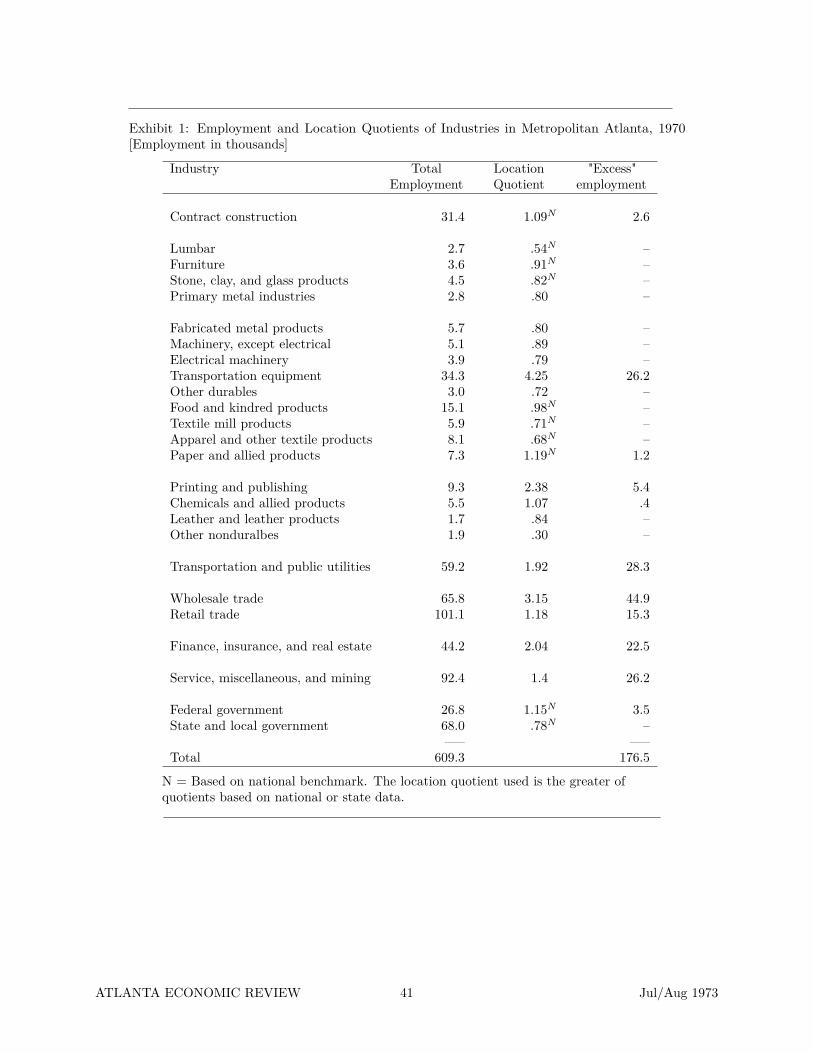
Exhibit 1: Employment and Location Quotients of Industries in Metropolitan Atlanta, 1970[Employment in thousands]

Industry TotalEmployment

LocationQuotient

"Excess"employment

Contract construction 31.4 1.09N 2.6

Lumbar 2.7 .54N –Furniture 3.6 .91N –Stone, clay, and glass products 4.5 .82N –Primary metal industries 2.8 .80 –

Fabricated metal products 5.7 .80 –Machinery, except electrical 5.1 .89 –Electrical machinery 3.9 .79 –Transportation equipment 34.3 4.25 26.2Other durables 3.0 .72 –Food and kindred products 15.1 .98N –Textile mill products 5.9 .71N –Apparel and other textile products 8.1 .68N –Paper and allied products 7.3 1.19N 1.2

Printing and publishing 9.3 2.38 5.4Chemicals and allied products 5.5 1.07 .4Leather and leather products 1.7 .84 –Other nonduralbes 1.9 .30 –

Transportation and public utilities 59.2 1.92 28.3

Wholesale trade 65.8 3.15 44.9Retail trade 101.1 1.18 15.3

Finance, insurance, and real estate 44.2 2.04 22.5

Service, miscellaneous, and mining 92.4 1.4 26.2

Federal government 26.8 1.15N 3.5State and local government 68.0 .78N –

—– —–Total 609.3 176.5

N = Based on national benchmark. The location quotient used is the greater ofquotients based on national or state data.

ATLANTA ECONOMIC REVIEW 41 Jul/Aug 1973

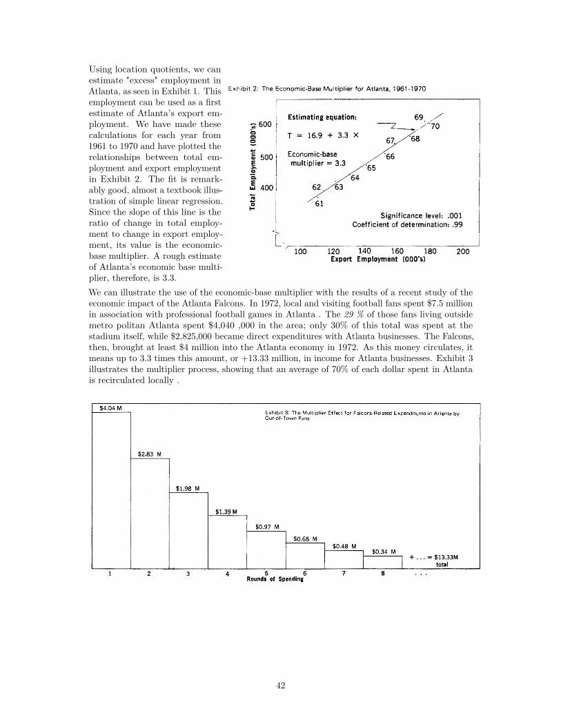
Using location quotients, we canestimate "excess" employment inAtlanta, as seen in Exhibit 1. Thisemployment can be used as a firstestimate of Atlanta’s export em-ployment. We have made thesecalculations for each year from1961 to 1970 and have plotted therelationships between total em-ployment and export employmentin Exhibit 2. The fit is remark-ably good, almost a textbook illus-tration of simple linear regression.Since the slope of this line is theratio of change in total employ-ment to change in export employ-ment, its value is the economic-base multiplier. A rough estimateof Atlanta’s economic base multi-plier, therefore, is 3.3.We can illustrate the use of the economic-base multiplier with the results of a recent study of theeconomic impact of the Atlanta Falcons. In 1972, local and visiting football fans spent $7.5 millionin association with professional football games in Atlanta . The 29 % of those fans living outsidemetro politan Atlanta spent $4,040 ,000 in the area; only 30% of this total was spent at thestadium itself, while $2,825,000 became direct expenditures with Atlanta businesses. The Falcons,then, brought at least $4 million into the Atlanta economy in 1972. As this money circulates, itmeans up to 3.3 times this amount, or +13.33 million, in income for Atlanta businesses. Exhibit 3illustrates the multiplier process, showing that an average of 70% of each dollar spent in Atlantais recirculated locally .

42

Note A: Techniques for Data AnalysisIntroduction

Now, with a few explanatory models under our belts, let us take a look at a couple of techniques for examiningdata. The term “analysis” comes from the Greek term for “a breaking up.” I like to think of it as a “layingout” of essential features for the better understanding of some phenomenon or thing. The process of analysiscan involve a simple re- ordering of elements or it can involve a complex statistical tool or maybe even amodel.

Sometimes, the simple approach is the best and can yield insights with great benefits at small costs. Here, Iwould like to re-visit our old friend the location quotient and consider a new technique, shift-share analysis.Both of these tools have their critics in academic circles, but both can be used to suggest strengths andweaknesses in an economy and both can point toward actions for developing a community.

Location quotients

A location quotient is commonly defined as the ratio

LQi = (ei/e)/(Ei/E), (a-1)

where ei is area employment in industry i, e is total employment in the area, Ei is employment in thebenchmark economy in industry i, and E is total employment in the benchmark economy. Normally, the"benchmark" economy is taken to be the nation as the closest available approximation to a self-sufficienteconomy.

As pointed out in our discussion of economic-base models, it is easily converted for use in estimating exportemployment. We simply assume that a location quotient greater than one means that an industry producesmore than expected in a self-sufficient economy and thus would be an export industry. On this assumptionand location quotients for a local economy, we built an estimate of the economic base multiplier for aneconomy.

But all of these computations for detailed industries can lead to questions as well as answers. The analystcould proceed to ask why the local economy varies from the benchmark economy. What resources are presentor absent? What opportunities for import substitution are unexploited? What is the apparent comparativeadvantage signaled by a large location quotient? Could it be an impediment or an enhancement for futuregrowth?

Obviously, this means that location quotients are suggestive in nature -- they point toward further analysis,and they force us to proceed next to understand production processes and to explore comparative advantageand ways to change the local economy and promote growth.

The popularity of location quotients has lead to a large number of variations. As Avrom Bendavid-Val pointsout in his excellent practitioner’s book, the list of derived measures includes “... coefficient of localization,coefficient of specialization, index of diversification, coefficient of redistribution, coefficient of geographicassociation, coefficient of participation, index of occupational discrimination, coefficient of deviation, frictionratio, and more. All of these amount to little more than imaginative applications of the basic location quotienttechnique, computing a ratio of ratios, in response to particular analytic needs.” (Bendavid-Val 1983)

Advantages and disadvantages of using location quotients are discussed earlier in Chapter 3 along with sourcesof data.

Shift-share analysis

Sometimes, it may be helpful to increase your general knowledge of change in the area in which you areconducting a regional impact analysis. For this task, “shift-share analysis” may be appropriate. It is the most

43

common technique for breaking economic change in areas into components is called “shift- share analysis.”1

Although originating in the 1940’s, the technique was introduced to frequent use in 1960 by a team ofeconomists undertaking a massive study of regions and economic growth (Perloff et al. 1960). Since then,it has been extended, used, criticized and revived numerous times. As a projection technique, it has beenabandoned by all (including the U.S. Department of Commerce, a staunch supporter in the 1960’s) but themost faithful. As an expository technique, it has enjoyed continued life. Economists have criticized it asmerely a definitional manipulation of data containing no explanation of phenomena (that is, it is simply away to organize data) -- the explanation of change has to come from further investigation.

But its major fault is that its interpretation relies heavily on the level of aggregation of the data used.Nevertheless, it is a great and inexpensive way to start a review of the industrial structure of an area.

Now, to see how this tool works, let us try various ways to estimate regional employment in year 2 forindustry i (R2i), given knowledge of growth in national employment in industry i (N2i/N1i ), growth intotal national employment (N2./N1.), and even knowledge of actual employment in industry i in the region(R2i/R1i). How could we proceed?

There are four alternative estimating techniques consistent with shift-share analysis. First, we could assumethat employment in industry i is the same in period 2 as it is in period 1 :

R2i = R1i (a-2)

Here, we simply have neither knowledge nor hope for growth.

Second, we could assume that the local employment in industry i grows at the same rate as does the nationaleconomy:

R2i = R1i ∗N2./N1. (a-3)

This, of course, is also a naîve assumption. In effect, we have assumed that both the industry and theeconomy have grown at the same rate, that local elements have each retained a constant share of nationalgrowth (hence the term).

Third, we could assume that the local employment in industry i grows at the same rate as does the employmentin industry i in the national economy:

R2i = R1i ∗N2i/N1i (a-4)

This is a little better. We can reasonably assume that local industries are subject to the same demandpressures felt by their competitors at the national level.

Fourth, we could assume that the local employment in industry i grows at the same rate as actually occurs(if we somehow could know this!):

R2i = R1i ∗R2i/R1i (a-5)

Now, what if we try subtraction to make equations a-3 through a-5 into expressions of net change so thatthey can be added? We can do this by subtracting the right side of the preceding equation from each andnaming the results.

1A clear statement of this technique is contained in an essay by Charles F. Floyd included as an appendix to (Schaffer 1976).My comments rely on Professor Floyd’s work as well as appendix B in (Jackson et al. 1981)

44

The change in employment due to national growth alone, assuming the region gets its share, we call thenational growth effect (NGi):

NGi = R1i ∗N2./N1 −R1i

NGi = R1i(N2./N1 − 1) (a-6)

The other two changes represent shifts away from the national trend. The first is called the industry-mixeffect (IMi) and shows the additional change due to the growth characteristics of industry i:

IMi = R1i ∗N2i/N1i −R1i ∗N2./N1.

IMi = R1i(N2i/N1i −N2./N1.) (a-7)

The last change is called the regional- shift effect (RSi) and shows the additional change due to the specificcharacteristics of the region itself:

RSi = R1i ∗R2i/R1i −R1i ∗N2i/N1i

RSi = R1i(R2i/R1i −N2i/N1i) (a-8)

Total change for each industry can be summarized as:

TCi = NGi + IMi +RSi (a-9)

These elements can then be summed to yield:

TC =∑

i

TCi =∑

i

(R2i −R1i) (a-10)

Demonstration that all of these equations fit together to form this identity is left as an exercise.

We should note that the terminology used here, while it seems the most common, is not unique. Thetechnique has been used and reinterpreted frequently, leading to renaming of effects. “Effects” are sometimes“components.” The “industry-mix effect” has been the “structural component,” the “proportional shift,” andthe “industry-composition effect;” and the “regional-share effect” has been called the “differential shift” andthe “competitive effect.” (Floyd 1976)

Thoughts on writing an area profile

An area profile might be defined as an economic description which may lead to action or insight. Profilesmay have many purposes. They may be intended to inform potential investors, to attract visitors, to informcitizens about the structure of their community, etc. The challenge for an analyst is to break free of theexclamatory hype associated with promotional literature. You should organize data to proclaim advantagesand accomplishments, to identify problems and opportunities, or to suggest future policy, as appropriate. Thefollowing words and phrases are random points derived from a general reading of published and unpublishedprofiles; I suggest a scanning of collections of brochures, of Federal Reserve Economic Reviews, of the WorldWide Web, etc. for further guidance:

What is the region? Describe it absolutely and relative to other places.

How is the region defined? If it is a political region, what is its economic component. If it is a statisticalregion, are there any unusual features?

45

Geography and significant landscape features, advantages, and limitations.

Demography: population, age and ethnic composition if significant, education, etc.

Employment -- Have recent changes been due to dramatic changes for particular industries, or havethey occurred across the board?

Governments -- fragmented, consolidated, etc.

Subregions -- definitions and boundaries, uneven growth or population distribution?

Economic base, before, now, expected. Location quotient analysis. How similar to the nation or state?Should it change? Where is the market for its exports? Where should major imports originate? Arethese other markets stable or volatile (that is, is the region subject to an interregional business cycle)?

Will the economic base help or hinder in the future?

What are the prospects for improving the industry mix to get higher personal incomes, less pollution,whatever?

Which industries lead the region’s performance? Do they contribute to cycles or to stability?

What is the reason for the region’s existence? Why do people live there?

What will happen in the next two, three years -- expected new industries or activities, departures,significant events?

Development policies stated by authorities and in practice.

Problems

Trends in various indicators and performance relative to nation or other regions.

Why should the region be optimistic or pessimistic about its future? (Remember that you are anobjective analyst, not a promoter.)

Elements to include in a location quotient analysis

A location-quotient analysis should be carefully planned to take advantage of modern spreadsheets such asMicrosoft’s Excel. The challenge is to lay out the system so that you can sort and resort on the basis of thevalues of location quotients and on calculated surplus employment and back into industry order as needed.

You should pay careful attention to presentation of data in tabular format:

Does the table title clearly identify the region under study, the year, and the data?

Are the columns clearly identified in the caption?

Does the stub identify all rows and are sections specified and set apart?

Are columns wide enough for data?

Are decimals set consistently and at the appropriate level for discussion?

In other words, does the presentation meet the standards of good scholarship and sound workmanship?

Have you presented only data that is relevant, excluding items that are inconsequential?

The written part of the analysis is also important. Here are some points to consider:

At a very basic level, do you define “location quotients” and how they are used?

Do you show awareness of your data source, the level at which you work, and problems which may beassociated with your data?

Did you experiment with several sources (e.g. both the Regional Economic Information System andCounty Business Patterns) to see if they yield similar results?

46

Did you use both quotients and estimated excess employment?

Did you set up the tables and your statements such that the reader could easily check your results andeven make their own conclusions?

Did you speculate on apparently questionable results?

Did you explore changes over time? (Since REIS data is since 1969 and the CBP data is availablein yearly chunks on CD-ROM since 1986, we might expect an alert and energetic analyst to look atvariation over time either to show trends or to identify data problems.)

47

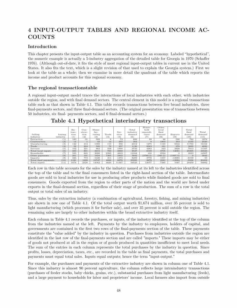
4 INPUT-OUTPUT TABLES AND REGIONAL INCOME AC-COUNTSIntroductionThis chapter presents the input-output table as an accounting system for an economy. Labeled “hypothetical”,the numeric example is actually a 5-industry aggregation of the detailed table for Georgia in 1970 (Schaffer1976). (Although out-of-date, it fits the style of most regional input-output tables in current use in the UnitedStates. It also fits the text, which is a slight revision of that used to explain the Georgia system.) First welook at the table as a whole; then we examine in more detail the quadrant of the table which reports theincome and product accounts for this regional economy.

The regional transactionstableA regional input-output model traces the interactions of local industries with each other, with industriesoutside the region, and with final demand sectors. The central element in this model is a regional transactionstable such as that shown in Table 4.1. This table records transactions between five broad industries, threefinal-payments sectors, and three final-demand sectors. (The original presentation was of transactions between50 industries, six final- payments sectors, and 6 final-demand sectors.)

Table 4.1 Hypothetical interindustry transactionsHouse- Other

Ex- Con- Manu- Total hold local Totaltrac- struc- fac- Ser- industry expendi- final final Total

Selling buying tion tion turing Trade vices demand tures demand Exports demand demandindustry industry (1) (2) (3) (4) (5) (6) (7) (8) (9) (10) (11)Extraction (1) 183 31 599 6 73 892 99 88 596 782 1674Construction (2) 14 1 43 14 293 364 0 1803 353 2155 2520Manufacturing (3) 142 414 1390 110 356 2412 1275 1130 9344 11750 14162Trade (4) 52 224 520 72 257 1126 2563 161 970 3695 4820Services (5) 102 221 862 558 1990 3733 4262 523 2828 7613 11347Total local inputs (6) 493 891 3415 760 2969 8527 8199 3705 14091 25995 34523Households (7) 595 665 3696 2385 4603 11944 100 2524 0 2623 14567Other payments (8) 261 191 1624 1365 2402 5842 (3789.2) (943.2) (1097.5) 0 5842Imports (9) 325 773 5428 311 1372 8209 3778 1057 -12994 -8159 50Total final payments (10) 1181 1629 10747 4060 8378 25995 3878 3581 -12994 -5536 20459Total inputs (11) 1674 2520 14162 4820 11347 34523 12077 7285 1097 20459 54982

Each row in this table accounts for the sales by the industry named at its left to the industries identified acrossthe top of the table and to the final consumers listed in the right-hand section of the table. Intermediategoods are sold to local industries for use in producing other products while finished goods are sold to finalconsumers. Goods exported from the region to other parts of the nation and the world are listed underexports in the final-demand section, regardless of their stage of production. The sum of a row is the totaloutput or total sales of an industry.

Thus, sales by the extraction industry (a combination of agricultural, forestry, fishing, and mining industries)are shown in row one of Table 4.1. Of the total output worth $1,674 million, over 35 percent is sold tolight manufacturing (which processes it for further sale), and over 35 percent is sold outside the region. Theremaining sales are largely to other industries within the broad extractive industry itself.

Each column in Table 4.1 records the purchases, or inputs, of the industry identified at the top of the columnfrom the industries named at the left. Payments by the industry to employees, holders of capital, andgovernments are contained in the first two rows of the final-payments section of the table. These paymentsconstitute the "value added" by the industry in question. Purchases from industries outside the region areidentified in the last row of the final-payments section and are called "imports." These imports may be eitherof goods not produced at all in the region or of goods produced in quantities insufficient to meet local needs.The sum of the entries in each column represents the total purchases by the industry in question. Sinceprofits, losses, depreciation, taxes, etc., are recorded in the table as final payments, the total purchases andpayments must equal total sales. Inputs equal outputs; hence the term "input-output."

For example, the purchases and payments of the extractive industry are shown in column one of Table 4.1.Since this industry is almost 90 percent agriculture, the column reflects large intraindustry transactions(purchases of feeder stocks, baby chicks, grains, etc.), substantial purchases from light manufacturing (feeds),and a large payment to households for labor and proprietors’ income. Local farmers also import from outside

48

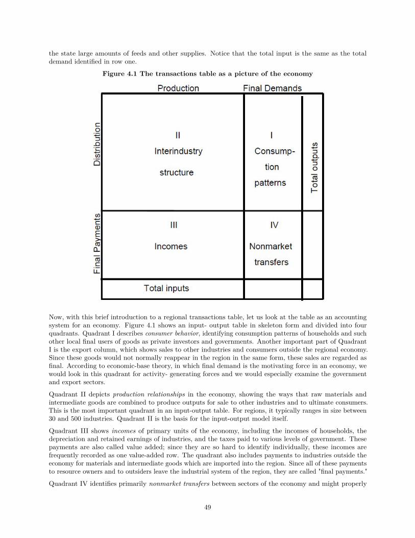
the state large amounts of feeds and other supplies. Notice that the total input is the same as the totaldemand identified in row one.

Figure 4.1 The transactions table as a picture of the economy

Now, with this brief introduction to a regional transactions table, let us look at the table as an accountingsystem for an economy. Figure 4.1 shows an input- output table in skeleton form and divided into fourquadrants. Quadrant I describes consumer behavior, identifying consumption patterns of households and suchother local final users of goods as private investors and governments. Another important part of QuadrantI is the export column, which shows sales to other industries and consumers outside the regional economy.Since these goods would not normally reappear in the region in the same form, these sales are regarded asfinal. According to economic-base theory, in which final demand is the motivating force in an economy, wewould look in this quadrant for activity- generating forces and we would especially examine the governmentand export sectors.

Quadrant II depicts production relationships in the economy, showing the ways that raw materials andintermediate goods are combined to produce outputs for sale to other industries and to ultimate consumers.This is the most important quadrant in an input-output table. For regions, it typically ranges in size between30 and 500 industries. Quadrant II is the basis for the input-output model itself.

Quadrant III shows incomes of primary units of the economy, including the incomes of households, thedepreciation and retained earnings of industries, and the taxes paid to various levels of government. Thesepayments are also called value added; since they are so hard to identify individually, these incomes arefrequently recorded as one value-added row. The quadrant also includes payments to industries outside theeconomy for materials and intermediate goods which are imported into the region. Since all of these paymentsto resource owners and to outsiders leave the industrial system of the region, they are called "final payments."

Quadrant IV identifies primarily nonmarket transfers between sectors of the economy and might properly

49

be labeled the "social transfers" quadrant. Here we see gifts, savings, and taxes of households; we see thesurpluses and deficits of governments and their payments to households and intergovernmental transfers. Thequadrant also typically includes purchases by final-demand sectors from industries outside the region.

Now, to make a major point about the hazards of aggregation, let’s look at the table as originally presented, asa picture of the Georgia economy in 1970. Out of a total output of over $34 billion, Georgia’s manufacturingoutput in 1970 was valued at over $14 billion and its service output at over $11 billion, indicating thatGeorgia’s economy was dominated by the manufacturing and service industries. Even so, Georgia was not amajor manufacturing or service economy by national standards, as can be seen in the following comparison ofthe industrial origins of value added in Georgia and the United States (Schaffer 1976)

Percent of value addedSector Georgia U.S.Agriculture, mining 4.2 5.2Construction 4.4 5.6Manufacturing 26.0 28.9Transportation, utilities 7.7 8.1Trade 18.3 14.6Services 25.6 26.9Government 13.7 10.7

Georgia had larger contributions to value added from trade and government than did the nation, andsmaller contributions from the extractive industries, construction, manufacturing, utilities, and services. Thisdeviation from the national pattern is an expression of the region’s modest stage of development and itscentral position in the Southeast.

But this observation also shows that the "importance" of an industry is completely dependent on thedefinitions and aggregation patterns employed in constructing a table. By enlarging the table and alteringsector definitions, we could change the apparent importance of industries. For example, by combining theagricultural industries with the food- processing industry (normally in manufacturing) we could make the"agriculture-based" industry larger than any of the components of the "trade" or "service" industries. In fact,in the 29- industry version (not shown here) of the Georgia table, the five largest industries in terms of outputare: 1) trade, 2) finance, insurance and real estate, 3) services, 4) textile mill products, and 5) transportationequipment.

A second interesting item in Table 4.1 is the gross product of Georgia. Analogous in concept to the grossnational product, gross regional product (GRP) can be defined as total production without duplication, or asthe economic product of all factors of production residing in the region. It can also be seen as the total finalpayments (adjusted for imports) in the region, 20.459 billion dollars. Alternatively, it is also the total finaldemand by ultimate consumers of the region’s products (net of imports).

In summary, an input-output table traces the paths by which incomes flow through the economy. Quadrant Iis where the spending cycle begins and is where finished goods go to satisfy the needs of final consumers.Quadrant III is where the production cycle starts, with households and other resource owners, includinggovernments, receiving payments for their contributions to the production process. Quadrant II tracesproduction relationships, describing the technology of production in the economy. It outlines the marketsector of the economy. Quadrant IV identifies nonmarket flows of money, showing purchases of labor inputsby governments, taxes paid by households, surpluses and deficits of governments, and transfers betweengovernments and other governments and people.

Income and product accountsThe input-output table embodies not only measures of gross regional product but also a summary set ofsocial, or income and product, accounts for the region. Like the input-output table itself, these accounts arepart of a double-entry accounting system for the economy. In the same way that a businessman uses hisaccounts to develop a consolidated income statement for his firm, the economist uses income and product

50

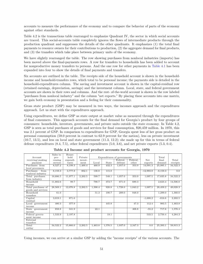
accounts to measure the performance of the economy and to compare the behavior of parts of the economyagainst other standards.

Table 4.2 is the transactions table rearranged to emphasize Quadrant IV, the sector in which social accountsare traced. This social-accounts table completely ignores the flows of intermediate products through theproduction quadrant and suppresses the details of the other quadrants. It emphasizes (1) the total finalpayments to resource owners for their contributions to production, (2) the aggregate demand for final products,and (3) the transfers which take place between primary units of the economy.

We have slightly rearranged the table. The row showing purchases from nonlocal industries (imports) hasbeen moved above the final-payments rows. A row for transfers to households has been added to accountfor nonproductive money transfers to persons. And the one row for other payments in Table 4.1 has beenexpanded into four to show the details of final payments and transfers.

Six accounts are outlined in the table. The receipts side of the household account is shown in the household-income and household-transfers rows, which total to be personal income; the payments side is detailed in thehousehold-expenditures column. The saving and investment account is shown in the capital-residual row(retained earnings, depreciation, savings) and the investment column. Local, state, and federal governmentaccounts are shown in their rows and columns. And the rest- of-the-world account is shown in the row labeled"purchases from nonlocal industry" and the column "net exports." By placing these accounts into one matrix,we gain both economy in presentation and a feeling for their commonality.

Gross state product (GSP) may be measured in two ways, the incomes approach and the expendituresapproach. Let us start with the expenditures approach.

Using expenditures, we define GSP as state output at market value as measured through the expendituresof final consumers. This approach accounts for the final demand for Georgia’s product by four groups ofconsumers: households, investors, governments, and private units outside the state economy. In Table 4.2,GSP is seen as total purchases of goods and services for final consumption, $20,459 million. In 1970, thiswas 2.1 percent of GNP. In comparison to expenditures for GNP, Georgia spent less of her gross product onpersonal consumption (59.0 percent in contrast to 62.9 percent for the nation), less on private investment(10.7, 13.5), and less on local and state government (11.3, 12.2); she made up for this in terms of federaldefense expenditures (8.4, 7.5), other federal expenditures (5.0, 3.6), and net private exports (5.3, 0.4).

Table 4.2 Income and product accounts for Georgia, 1970Sales to House-

Account pro- hold Private Expenditures of governments Totalreceiving\making cessing expendi- invest- Federal, Federal, Net final Total

payment sectors tures ment Local State defense other exports demand receiptsPurchases fromlocal processors

8,527.2 8,199.3 1,400.4 460.9 432.3 1,057.0 353.9 14,091.3 25,995.1 34,522.3

Purchases fromnonlocal industry

8,159.3 3,777.8 802.1 138.8 115.8 -12,993.8 -8,159.3 0.0

Total purchasesfrom industry

16,686.5 11,977.1 2,202.5 599.7 548.1 1,057.0 353.9 1,097.5 17,835.8 34,522.3

Householdincome

11,882.6 99.7 790.7 372.7 671.0 689.3 2,623.4 14,506.0

Total purchases ofgoods and services

28,569.1 12,076.8 2,202.5 1,390.4 920.8 1,728.0 1,043.2 1,097.5 20,459.2 49,028.3

Householdtransfers

61.0 51.3 190.7 209.0 848.0 1,299.0 1,360.0

Capitalresidual

3,019.1 871.6 -1,688.2 -816.6 2,202.5

Local governmentincome

480.3 377.9 445.9 47.3 112.4 983.5 1,463.8

State governmentincome

858.8 341.9 22.1 408.8 -55.2 717.6 1,576.4

Federal govern-ment income

1,533.9 2,197.8 19.1 533.5 2,750.4 4,284.3

ExternaltransfersTotaloutlay

34,522.2 15,866.0 2,202.5 1,463.8 1,576.5 1,937.0 2,347.3 0.0 25,393.1 59,915.3

Using incomes, we can arrive at a similar GSP by adding the "income receipts" of the various accounts. The

51

major receipt is earned household or personal income, which consists of wages and salaries, other labor income,proprietors’ income, and property incomes. Including business transfer payments (primarily bad debts) andsocial security contributions, this amounts to $14,567 million, or 71.2 percent of GSP; the correspondingnational figure is 75.2 percent. The "capital residual," or gross business saving, of processors is $3,019 millionand comprises 14.8 percent of GSP, which corresponds to 9.4 percent in the nation. The capital-residual rowof Table 4.2 includes two transfers worth noting: one is personal savings; the other is a negative entry of$1,688 million in the exports column. This "export" accounts for the surpluses and deficits of the variousgovernments and the outside world. Much of it represents flows of retained earnings and capital consumptionallowances to the nonresident owners of branch plants in Georgia.

The third receipt to be added to GSP is local government income from the processing sector. At $480million, this figure accounted for 2.3 percent of GSP. The next largest income of local governments in Georgiawas a set of intergovernmental transfers from the state government (much of which is offset by a similartransfer from the federal government to the state). The deficits of local governments are shown as an "export"(primarily bonds) worth $112.4 million.

The fourth receipt to be counted as part of GSP is state government income from the processing sector of$859 million. Combined state and local revenues from industrial sources are 6.5 percent of GSP, comparedto 8.5 percent on the national level. Note that the state had a surplus in 1970 of $55 million, entered as anegative value in the exports column.

The final receipt to be included in GSP is federal government income from the processing sectors. Totaling$1,534 million, this income was 7.5 percent of GSP, compared with 6.9 percent on the national level. Noticethat the federal government still spent $534 million more in Georgia than it received in taxes, accounted forlargely through defense expenditures.

In sum, total receipts and payments by each of the six final sectors in the economy were $25,393 million.This figure is $4,934 million in excess of GSP. Where quadrant II shows intermediate transactions in theprocessing sector, the transfers quadrant records duplicative transactions in the social or political sector.

SummaryA state input-output table accounts for flows of monies through the state, showing details regarding consumerbehavior, the technology of production, incomes, and social transfers. The transfers quadrant of a table canbe slightly modified to show the details presented in the more traditional income and product accounts.

The social accounts are useful in two ways. One is in comparisons between economies; a brief contrast ofthe Georgia and U.S. economies has been sketched here and Georgia has been found to be strong in tradeand government and slightly below the national pattern in manufacturing and services. The other way is incomparisons over time. But to show performance over time, social accounts and input-output tables must beconstructed on a regular basis by state agencies.

Appendix 1: DVD data sources: the Regional Economic Information SystemOne of the best sources of regional data is the Regional Economic Information System (REIS), produced bythe Regional Economic Measurement Division of the Bureau of Economic Analysis.

Many Web sites have information from REIS available for downloading, but the most common source for theheavy user is the DVD disk. Published annually in May, it contains data for states, regions, and counties from1969 forward, with a two-year lag. (Thus, the May 2009 disk contains data from 1969 to 2007.) Now, the datacontained in the disk and much more are also available free of charge from https://apps.bea.gov/regional/.(Note that this web page is hard to find when starting from bea.gov – this may signal the demise of thisproduct due to budget constraints.)

For counties, the disk provides data on personal income and its sources, employment (in broad industrycategories), an economic profile, transfer payments, and agricultural output. In addition it contains data onthe journey to work between counties in 1970, 1980, 1990, and 2000, as well as annual estimates of grosscommuter incomes.

52

More detailed data on journey to work and place of work as developed in the 2000 Census can be found athttps://www.census.gov/topics/employment/commuting.html.

Appendix 2: Measures of regional welfare: Personal IncomeThe problem with GSP estimates

Gross state product accounts have been established for a number of states and using a variety of methods. InHawaii, with a long history of independence, accounts have been constructed along exactly the same linesas a nation (in fact, some of the people involved in these accounts were close associates of members of theaccounts team in the U.S. Bureau of the Census.

In most other states, however, the method has been a short-cut method known as the Kendricks-Jaycoxmethod and involves estimates based on ratios.

Estimates of Gross State Product have been assembled from all sources available to the Regional EconomicMeasurement Division. These are available for selected years on the Regional Economic Information System.One nice thing about this central source is that the accounts for the 50 states are consistent with the accountsfor the nation as a whole. For details and availability, see http://www.bea.gov/regional/index.htm

The following statement shows the formal difference between "Gross Regional Product" (GRP) and "GrossDomestic Regional Product," (GDRP) which parallels the difference between GNP and GDP. This equationshows development of GRP as GDRP adjusted for net factor payments (including profits).

GROSS DOMESTIC REGIONAL PRODUCT

LESS INTEREST AND DIVIDENDS TO NONRESIDENTS

PLUS INTEREST AND DIVIDENDS FROM REST OF WORLD

LESS WAGES EARNED BY IN-COMMUTERS

PLUS WAGES EARNED BY OUT-COMMUTERS

EQUALS GROSS REGIONAL PRODUCT

GROSS REGIONAL PRODUCT is the total value of goods and services produced by factors of productionowned by residents of the region; GROSS DOMESTIC REGIONAL PRODUCT is the total value of productionin the region.

In the United States, GNP is greater than GDP -- we own more abroad than others do here. In Hawaii, GRPis less that GDRP -- natives own less abroad than others own in Hawaii. In other states, the question has notbeen answered.

The point of this is that, since people always confuse lengthy titles, we just go ahead and confuse things tobegin with and rename gross domestic state product as gross state product!

GSP = GDSP

The widespread use of personal income estimates

The problems associated with estimating flows of capital income from one area to another are severe. We justcan’t develop accurate statistics on ownership of large multi-state and multi- national corporations and thuson the flows of dividends and interest across state boundaries.

As a result of this handicap, we normally consider personal income as a better measure of individual welfare.Considerable data on journey to work and commuting across county boundaries over the last three decennialcensuses has permitted the Regional Economic Measurement Division to estimate adjustments for residency,which solves part of the GRP/GDRP problem.

53

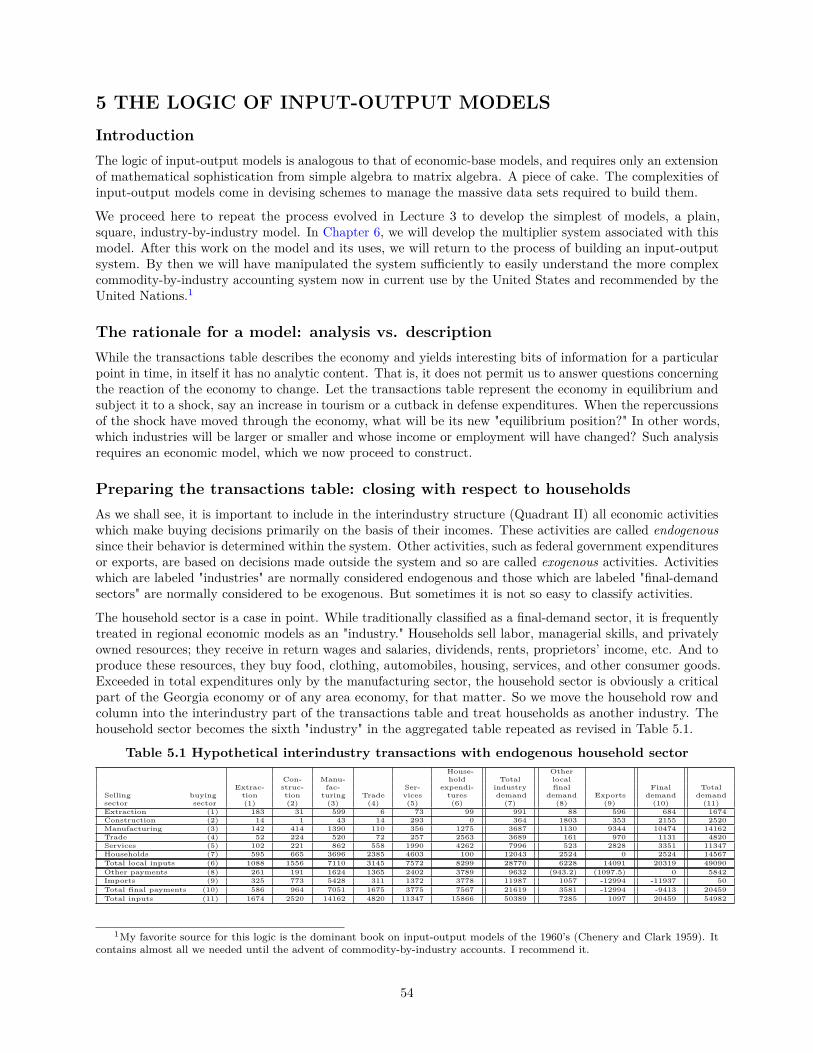
5 THE LOGIC OF INPUT-OUTPUT MODELSIntroductionThe logic of input-output models is analogous to that of economic-base models, and requires only an extensionof mathematical sophistication from simple algebra to matrix algebra. A piece of cake. The complexities ofinput-output models come in devising schemes to manage the massive data sets required to build them.

We proceed here to repeat the process evolved in Lecture 3 to develop the simplest of models, a plain,square, industry-by-industry model. In Chapter 6, we will develop the multiplier system associated with thismodel. After this work on the model and its uses, we will return to the process of building an input-outputsystem. By then we will have manipulated the system sufficiently to easily understand the more complexcommodity-by-industry accounting system now in current use by the United States and recommended by theUnited Nations.1

The rationale for a model: analysis vs. descriptionWhile the transactions table describes the economy and yields interesting bits of information for a particularpoint in time, in itself it has no analytic content. That is, it does not permit us to answer questions concerningthe reaction of the economy to change. Let the transactions table represent the economy in equilibrium andsubject it to a shock, say an increase in tourism or a cutback in defense expenditures. When the repercussionsof the shock have moved through the economy, what will be its new "equilibrium position?" In other words,which industries will be larger or smaller and whose income or employment will have changed? Such analysisrequires an economic model, which we now proceed to construct.

Preparing the transactions table: closing with respect to householdsAs we shall see, it is important to include in the interindustry structure (Quadrant II) all economic activitieswhich make buying decisions primarily on the basis of their incomes. These activities are called endogenoussince their behavior is determined within the system. Other activities, such as federal government expendituresor exports, are based on decisions made outside the system and so are called exogenous activities. Activitieswhich are labeled "industries" are normally considered endogenous and those which are labeled "final-demandsectors" are normally considered to be exogenous. But sometimes it is not so easy to classify activities.

The household sector is a case in point. While traditionally classified as a final-demand sector, it is frequentlytreated in regional economic models as an "industry." Households sell labor, managerial skills, and privatelyowned resources; they receive in return wages and salaries, dividends, rents, proprietors’ income, etc. And toproduce these resources, they buy food, clothing, automobiles, housing, services, and other consumer goods.Exceeded in total expenditures only by the manufacturing sector, the household sector is obviously a criticalpart of the Georgia economy or of any area economy, for that matter. So we move the household row andcolumn into the interindustry part of the transactions table and treat households as another industry. Thehousehold sector becomes the sixth "industry" in the aggregated table repeated as revised in Table 5.1.

Table 5.1 Hypothetical interindustry transactions with endogenous household sectorHouse- Other

Con- Manu- hold Total localExtrac- struc- fac- Ser- expendi- industry final Final Total

Selling buying tion tion turing Trade vices tures demand demand Exports demand demandsector sector (1) (2) (3) (4) (5) (6) (7) (8) (9) (10) (11)Extraction (1) 183 31 599 6 73 99 991 88 596 684 1674Construction (2) 14 1 43 14 293 0 364 1803 353 2155 2520Manufacturing (3) 142 414 1390 110 356 1275 3687 1130 9344 10474 14162Trade (4) 52 224 520 72 257 2563 3689 161 970 1131 4820Services (5) 102 221 862 558 1990 4262 7996 523 2828 3351 11347Households (7) 595 665 3696 2385 4603 100 12043 2524 0 2524 14567Total local inputs (6) 1088 1556 7110 3145 7572 8299 28770 6228 14091 20319 49090Other payments (8) 261 191 1624 1365 2402 3789 9632 (943.2) (1097.5) 0 5842Imports (9) 325 773 5428 311 1372 3778 11987 1057 -12994 -11937 50Total final payments (10) 586 964 7051 1675 3775 7567 21619 3581 -12994 -9413 20459Total inputs (11) 1674 2520 14162 4820 11347 15866 50389 7285 1097 20459 54982

1My favorite source for this logic is the dominant book on input-output models of the 1960’s (Chenery and Clark 1959). Itcontains almost all we needed until the advent of commodity-by-industry accounts. I recommend it.

54

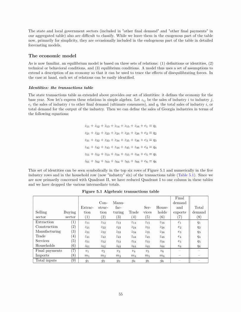
The state and local government sectors (included in "other final demand" and "other final payments" inour aggregated table) also are difficult to classify. While we leave them in the exogenous part of the tablenow, primarily for simplicity, they are occasionally included in the endogenous part of the table in detailedforecasting models.

The economic modelAs is now familiar, an equilibrium model is based on three sets of relations: (1) definitions or identities, (2)technical or behavioral conditions, and (3) equilibrium conditions. A model thus uses a set of assumptions toextend a description of an economy so that it can be used to trace the effects of disequilibrating forces. Inthe case at hand, each set of relations can be easily identified.

Identities: the transactions table

The state transactions table as extended above provides our set of identities: it defines the economy for thebase year. Now let’s express these relations in simple algebra. Let zij be the sales of industry i to industry j,ei the sales of industry i to other final demand (ultimate consumers), and qi the total sales of industry i, ortotal demand for the output of the industry. Then we can define the sales of Georgia industries in terms ofthe following equations:

z11 + z12 + z13 + z14 + z15 + z16 + e1 ≡ q1

z21 + z22 + z23 + z24 + z25 + z26 + e2 ≡ q2

z31 + z32 + z33 + z34 + z35 + z36 + e3 ≡ q3

z41 + z42 + z43 + z44 + z45 + z46 + e4 ≡ q4

z51 + z52 + z53 + z54 + z55 + z56 + e5 ≡ q5

z61 + z62 + z63 + z64 + z65 + z66 + e6 ≡ q6

This set of identities can be seen symbolically in the top six rows of Figure 5.1 and numerically in the fiveindustry rows and in the household row (now "industry" six) of the transactions table (Table 5.1). Since weare now primarily concerned with Quadrant II, we have reduced Quadrant I to one column in these tablesand we have dropped the various intermediate totals.

Figure 5.1 Algebraic transactions tableFinal

Con- Manu- demandExtrac- struc- fac- Ser- House- and Total

Selling Buying tion tion turing Trade vices holds exports demandsector sector (1) (2) (3) (4) (5) (6) (7) (8)Extraction (1) z11 z12 z13 z14 z15 z16 e1 q1Construction (2) z21 z22 z23 z24 z55 z26 e2 q2Manufacturing (3) z31 z32 z33 z34 z35 z36 e3 q3Trade (4) z41 z42 z43 z44 z45 z46 e4 q4Services (5) z51 z52 z53 z54 z55 z56 e5 q5Households (6) z61 z62 z63 z64 z65 z66 e6 q6Final payments (7) v1 v2 v3 v4 v5 v6 – –Imports (8) m1 m2 m3 m4 m5 m6 – –Total inputs (9) g1 g2 g3 g4 g5 g6 – –

55

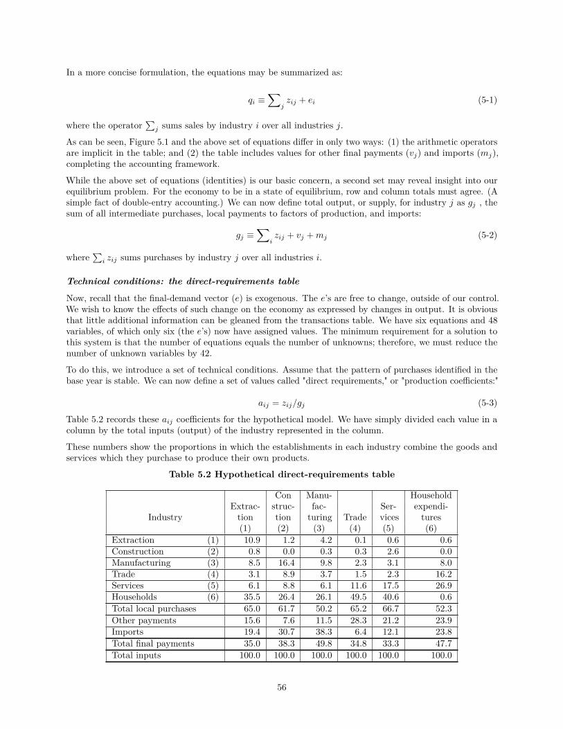
In a more concise formulation, the equations may be summarized as:

qi ≡∑

jzij + ei (5-1)

where the operator∑

j sums sales by industry i over all industries j.

As can be seen, Figure 5.1 and the above set of equations differ in only two ways: (1) the arithmetic operatorsare implicit in the table; and (2) the table includes values for other final payments (vj) and imports (mj),completing the accounting framework.

While the above set of equations (identities) is our basic concern, a second set may reveal insight into ourequilibrium problem. For the economy to be in a state of equilibrium, row and column totals must agree. (Asimple fact of double-entry accounting.) We can now define total output, or supply, for industry j as gj , thesum of all intermediate purchases, local payments to factors of production, and imports:

gj ≡∑

izij + vj +mj (5-2)

where∑

i zij sums purchases by industry j over all industries i.

Technical conditions: the direct-requirements table

Now, recall that the final-demand vector (e) is exogenous. The e’s are free to change, outside of our control.We wish to know the effects of such change on the economy as expressed by changes in output. It is obviousthat little additional information can be gleaned from the transactions table. We have six equations and 48variables, of which only six (the e’s) now have assigned values. The minimum requirement for a solution tothis system is that the number of equations equals the number of unknowns; therefore, we must reduce thenumber of unknown variables by 42.

To do this, we introduce a set of technical conditions. Assume that the pattern of purchases identified in thebase year is stable. We can now define a set of values called "direct requirements," or "production coefficients:"

aij = zij/gj (5-3)

Table 5.2 records these aij coefficients for the hypothetical model. We have simply divided each value in acolumn by the total inputs (output) of the industry represented in the column.

These numbers show the proportions in which the establishments in each industry combine the goods andservices which they purchase to produce their own products.

Table 5.2 Hypothetical direct-requirements table

Con Manu- HouseholdExtrac- struc- fac- Ser- expendi-

Industry tion tion turing Trade vices tures(1) (2) (3) (4) (5) (6)

Extraction (1) 10.9 1.2 4.2 0.1 0.6 0.6Construction (2) 0.8 0.0 0.3 0.3 2.6 0.0Manufacturing (3) 8.5 16.4 9.8 2.3 3.1 8.0Trade (4) 3.1 8.9 3.7 1.5 2.3 16.2Services (5) 6.1 8.8 6.1 11.6 17.5 26.9Households (6) 35.5 26.4 26.1 49.5 40.6 0.6Total local purchases 65.0 61.7 50.2 65.2 66.7 52.3Other payments 15.6 7.6 11.5 28.3 21.2 23.9Imports 19.4 30.7 38.3 6.4 12.1 23.8Total final payments 35.0 38.3 49.8 34.8 33.3 47.7Total inputs 100.0 100.0 100.0 100.0 100.0 100.0

56

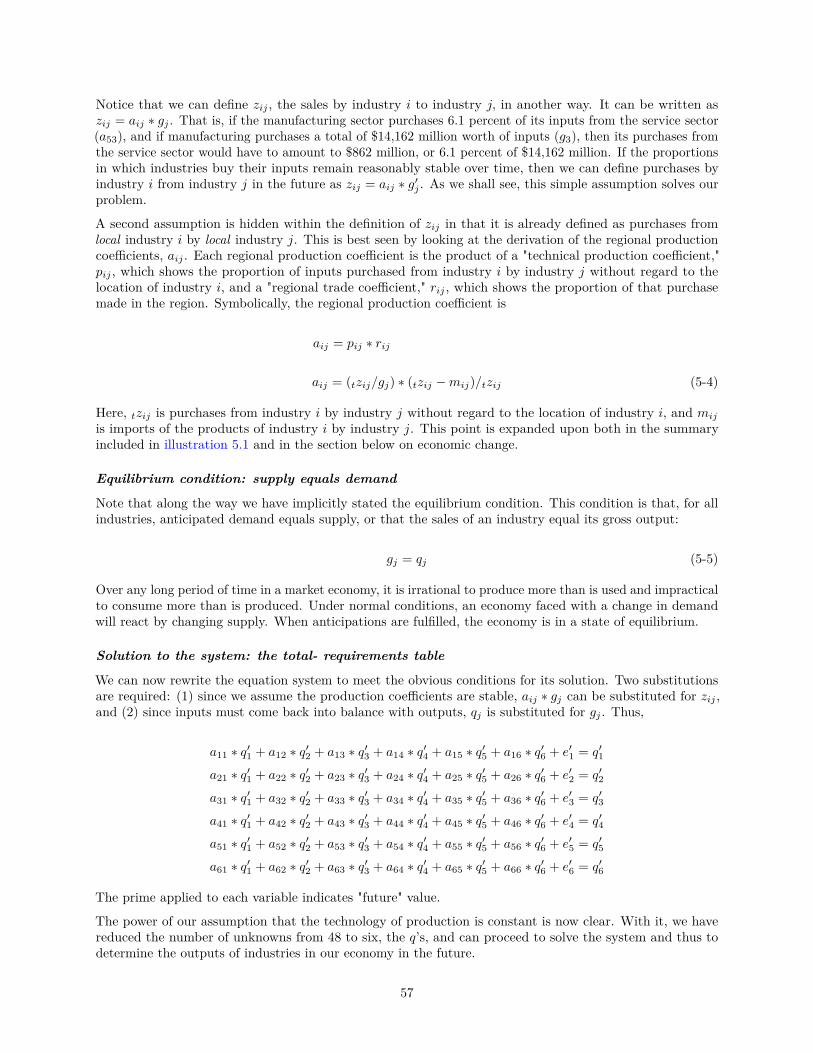
Notice that we can define zij , the sales by industry i to industry j, in another way. It can be written aszij = aij ∗ gj . That is, if the manufacturing sector purchases 6.1 percent of its inputs from the service sector(a53), and if manufacturing purchases a total of $14,162 million worth of inputs (g3), then its purchases fromthe service sector would have to amount to $862 million, or 6.1 percent of $14,162 million. If the proportionsin which industries buy their inputs remain reasonably stable over time, then we can define purchases byindustry i from industry j in the future as zij = aij ∗ g′j . As we shall see, this simple assumption solves ourproblem.

A second assumption is hidden within the definition of zij in that it is already defined as purchases fromlocal industry i by local industry j. This is best seen by looking at the derivation of the regional productioncoefficients, aij . Each regional production coefficient is the product of a "technical production coefficient,"pij , which shows the proportion of inputs purchased from industry i by industry j without regard to thelocation of industry i, and a "regional trade coefficient," rij , which shows the proportion of that purchasemade in the region. Symbolically, the regional production coefficient is

aij = pij ∗ rij

aij = (tzij/gj) ∗ (tzij −mij)/tzij (5-4)

Here, tzij is purchases from industry i by industry j without regard to the location of industry i, and mij

is imports of the products of industry i by industry j. This point is expanded upon both in the summaryincluded in illustration 5.1 and in the section below on economic change.

Equilibrium condition: supply equals demand

Note that along the way we have implicitly stated the equilibrium condition. This condition is that, for allindustries, anticipated demand equals supply, or that the sales of an industry equal its gross output:

gj = qj (5-5)

Over any long period of time in a market economy, it is irrational to produce more than is used and impracticalto consume more than is produced. Under normal conditions, an economy faced with a change in demandwill react by changing supply. When anticipations are fulfilled, the economy is in a state of equilibrium.

Solution to the system: the total- requirements table

We can now rewrite the equation system to meet the obvious conditions for its solution. Two substitutionsare required: (1) since we assume the production coefficients are stable, aij ∗ gj can be substituted for zij ,and (2) since inputs must come back into balance with outputs, qj is substituted for gj . Thus,

a11 ∗ q′1 + a12 ∗ q′2 + a13 ∗ q′3 + a14 ∗ q′4 + a15 ∗ q′5 + a16 ∗ q′6 + e′1 = q′1

a21 ∗ q′1 + a22 ∗ q′2 + a23 ∗ q′3 + a24 ∗ q′4 + a25 ∗ q′5 + a26 ∗ q′6 + e′2 = q′2

a31 ∗ q′1 + a32 ∗ q′2 + a33 ∗ q′3 + a34 ∗ q′4 + a35 ∗ q′5 + a36 ∗ q′6 + e′3 = q′3

a41 ∗ q′1 + a42 ∗ q′2 + a43 ∗ q′3 + a44 ∗ q′4 + a45 ∗ q′5 + a46 ∗ q′6 + e′4 = q′4

a51 ∗ q′1 + a52 ∗ q′2 + a53 ∗ q′3 + a54 ∗ q′4 + a55 ∗ q′5 + a56 ∗ q′6 + e′5 = q′5

a61 ∗ q′1 + a62 ∗ q′2 + a63 ∗ q′3 + a64 ∗ q′4 + a65 ∗ q′5 + a66 ∗ q′6 + e′6 = q′6

The prime applied to each variable indicates "future" value.

The power of our assumption that the technology of production is constant is now clear. With it, we havereduced the number of unknowns from 48 to six, the q’s, and can proceed to solve the system and thus todetermine the outputs of industries in our economy in the future.

57

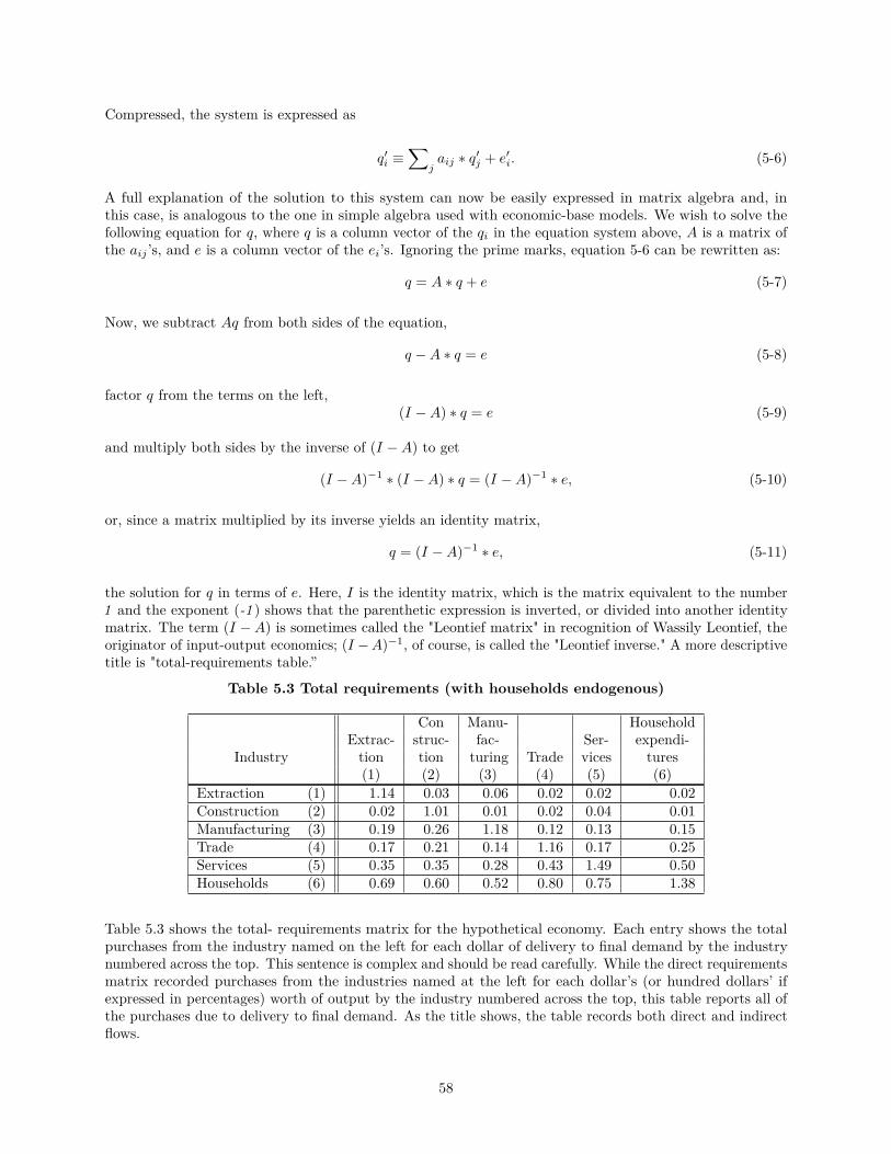
Compressed, the system is expressed as

q′i ≡∑

jaij ∗ q′j + e′i. (5-6)

A full explanation of the solution to this system can now be easily expressed in matrix algebra and, inthis case, is analogous to the one in simple algebra used with economic-base models. We wish to solve thefollowing equation for q, where q is a column vector of the qi in the equation system above, A is a matrix ofthe aij ’s, and e is a column vector of the ei’s. Ignoring the prime marks, equation 5-6 can be rewritten as:

q = A ∗ q + e (5-7)

Now, we subtract Aq from both sides of the equation,

q −A ∗ q = e (5-8)

factor q from the terms on the left,(I −A) ∗ q = e (5-9)

and multiply both sides by the inverse of (I −A) to get

(I −A)−1 ∗ (I −A) ∗ q = (I −A)−1 ∗ e, (5-10)

or, since a matrix multiplied by its inverse yields an identity matrix,

q = (I −A)−1 ∗ e, (5-11)

the solution for q in terms of e. Here, I is the identity matrix, which is the matrix equivalent to the number1 and the exponent (-1 ) shows that the parenthetic expression is inverted, or divided into another identitymatrix. The term (I −A) is sometimes called the "Leontief matrix" in recognition of Wassily Leontief, theoriginator of input-output economics; (I −A)−1, of course, is called the "Leontief inverse." A more descriptivetitle is "total-requirements table.”

Table 5.3 Total requirements (with households endogenous)

Con Manu- HouseholdExtrac- struc- fac- Ser- expendi-

Industry tion tion turing Trade vices tures(1) (2) (3) (4) (5) (6)

Extraction (1) 1.14 0.03 0.06 0.02 0.02 0.02Construction (2) 0.02 1.01 0.01 0.02 0.04 0.01Manufacturing (3) 0.19 0.26 1.18 0.12 0.13 0.15Trade (4) 0.17 0.21 0.14 1.16 0.17 0.25Services (5) 0.35 0.35 0.28 0.43 1.49 0.50Households (6) 0.69 0.60 0.52 0.80 0.75 1.38

Table 5.3 shows the total- requirements matrix for the hypothetical economy. Each entry shows the totalpurchases from the industry named on the left for each dollar of delivery to final demand by the industrynumbered across the top. This sentence is complex and should be read carefully. While the direct requirementsmatrix recorded purchases from the industries named at the left for each dollar’s (or hundred dollars’ ifexpressed in percentages) worth of output by the industry numbered across the top, this table reports all ofthe purchases due to delivery to final demand. As the title shows, the table records both direct and indirectflows.

58

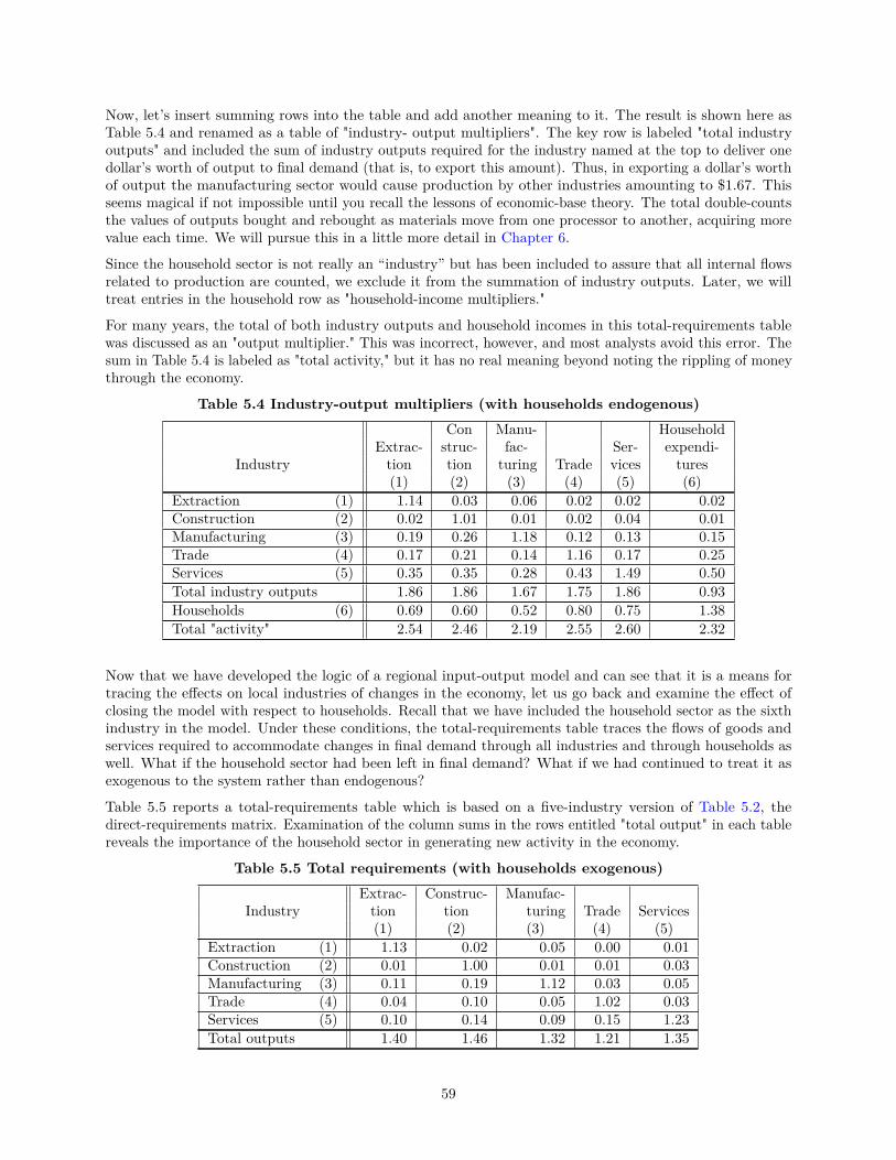
Now, let’s insert summing rows into the table and add another meaning to it. The result is shown here asTable 5.4 and renamed as a table of "industry- output multipliers". The key row is labeled "total industryoutputs" and included the sum of industry outputs required for the industry named at the top to deliver onedollar’s worth of output to final demand (that is, to export this amount). Thus, in exporting a dollar’s worthof output the manufacturing sector would cause production by other industries amounting to $1.67. Thisseems magical if not impossible until you recall the lessons of economic-base theory. The total double-countsthe values of outputs bought and rebought as materials move from one processor to another, acquiring morevalue each time. We will pursue this in a little more detail in Chapter 6.

Since the household sector is not really an “industry” but has been included to assure that all internal flowsrelated to production are counted, we exclude it from the summation of industry outputs. Later, we willtreat entries in the household row as "household-income multipliers."

For many years, the total of both industry outputs and household incomes in this total-requirements tablewas discussed as an "output multiplier." This was incorrect, however, and most analysts avoid this error. Thesum in Table 5.4 is labeled as "total activity," but it has no real meaning beyond noting the rippling of moneythrough the economy.

Table 5.4 Industry-output multipliers (with households endogenous)Con Manu- Household

Extrac- struc- fac- Ser- expendi-Industry tion tion turing Trade vices tures

(1) (2) (3) (4) (5) (6)Extraction (1) 1.14 0.03 0.06 0.02 0.02 0.02Construction (2) 0.02 1.01 0.01 0.02 0.04 0.01Manufacturing (3) 0.19 0.26 1.18 0.12 0.13 0.15Trade (4) 0.17 0.21 0.14 1.16 0.17 0.25Services (5) 0.35 0.35 0.28 0.43 1.49 0.50Total industry outputs 1.86 1.86 1.67 1.75 1.86 0.93Households (6) 0.69 0.60 0.52 0.80 0.75 1.38Total "activity" 2.54 2.46 2.19 2.55 2.60 2.32

Now that we have developed the logic of a regional input-output model and can see that it is a means fortracing the effects on local industries of changes in the economy, let us go back and examine the effect ofclosing the model with respect to households. Recall that we have included the household sector as the sixthindustry in the model. Under these conditions, the total-requirements table traces the flows of goods andservices required to accommodate changes in final demand through all industries and through households aswell. What if the household sector had been left in final demand? What if we had continued to treat it asexogenous to the system rather than endogenous?

Table 5.5 reports a total-requirements table which is based on a five-industry version of Table 5.2, thedirect-requirements matrix. Examination of the column sums in the rows entitled "total output" in each tablereveals the importance of the household sector in generating new activity in the economy.

Table 5.5 Total requirements (with households exogenous)Extrac- Construc- Manufac-

Industry tion tion turing Trade Services(1) (2) (3) (4) (5)

Extraction (1) 1.13 0.02 0.05 0.00 0.01Construction (2) 0.01 1.00 0.01 0.01 0.03Manufacturing (3) 0.11 0.19 1.12 0.03 0.05Trade (4) 0.04 0.10 0.05 1.02 0.03Services (5) 0.10 0.14 0.09 0.15 1.23Total outputs 1.40 1.46 1.32 1.21 1.35

59

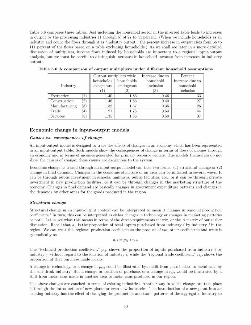
Table 5.6 compares these tables. Just including the household sector in the inverted table leads to increasesin output by the processing industries (1 through 5) of 27 to 44 percent. (When we include households as anindustry and count the flows through it as “industry output,” the percent increase in output rises from 66 to111 percent of the flows based on a table excluding households.) As we shall see later in a more detaileddiscussion of multipliers, income flows induced by households are important to a regional input-outputanalysis, but we must be careful to distinguish increases in household incomes from increases in industryoutputs.

Table 5.6 A comparison of output multipliers under different household assumptionsOutput mutipliers with: Increase due to Percenthouseholds households household increase due to

Industry exogenous endogeous inclusion household(1) (2) (3) inclusion

Extraction (1) 1.40 1.86 0.46 33Construction (2) 1.46 1.86 0.40 27Manufacturing (3) 1.32 1.67 0.35 26Trade (4) 1.21 1.75 0.54 44Services (5) 1.35 1.86 0.50 37

Economic change in input-output modelsCauses vs. consequences of change

An input-output model is designed to trace the effects of changes in an economy which has been representedin an input-output table. Such models show the consequences of change in terms of flows of monies throughan economy and in terms of incomes generated for primary resource owners. The models themselves do notshow the causes of change; these causes are exogenous to the system.

Economic change as traced through an input-output model can take two forms: (1) structural change or (2)change in final demand. Changes in the economic structure of an area can be initiated in several ways. Itcan be through public investment in schools, highways, public facilities, etc., or it can be through privateinvestment in new production facilities, or it can be through changes in the marketing structure of theeconomy. Changes in final demand are basically changes in government expenditure patterns and changes inthe demands by other areas for the goods produced in the region.

Structural change

Structural change in an input-output context can be interpreted to mean it changes in regional productioncoefficients." In turn, this can be interpreted as either changes in technology or changes in marketing patternsor both. Let us see what this means in terms of the direct-requirements matrix, or the A matrix of our earlierdiscussion. Recall that aij is the proportion of total inputs purchased from industry i by industry j in theregion. We can treat this regional production coefficient as the product of two other coefficients and write itsymbolically as

aij = pij ∗ rij .

The "technical production coefficient," pij , shows the proportion of inputs purchased from industry i byindustry j without regard to the location of industry i, while the "regional trade coefficient," rij , shows theproportion of that purchase made locally.

A change in technology, or a change in pij , could be illustrated by a shift from glass bottles to metal cans bythe soft-drink industry. But a change in location of purchase, or a change in rij , would be illustrated by ashift from metal cans made in another area to metal cans produced in our region.

The above changes are couched in terms of existing industries. Another way in which change can take placeis through the introduction of new plants or even new industries. The introduction of a new plant into anexisting industry has the effect of changing the production and trade patterns of the aggregated industry to

60

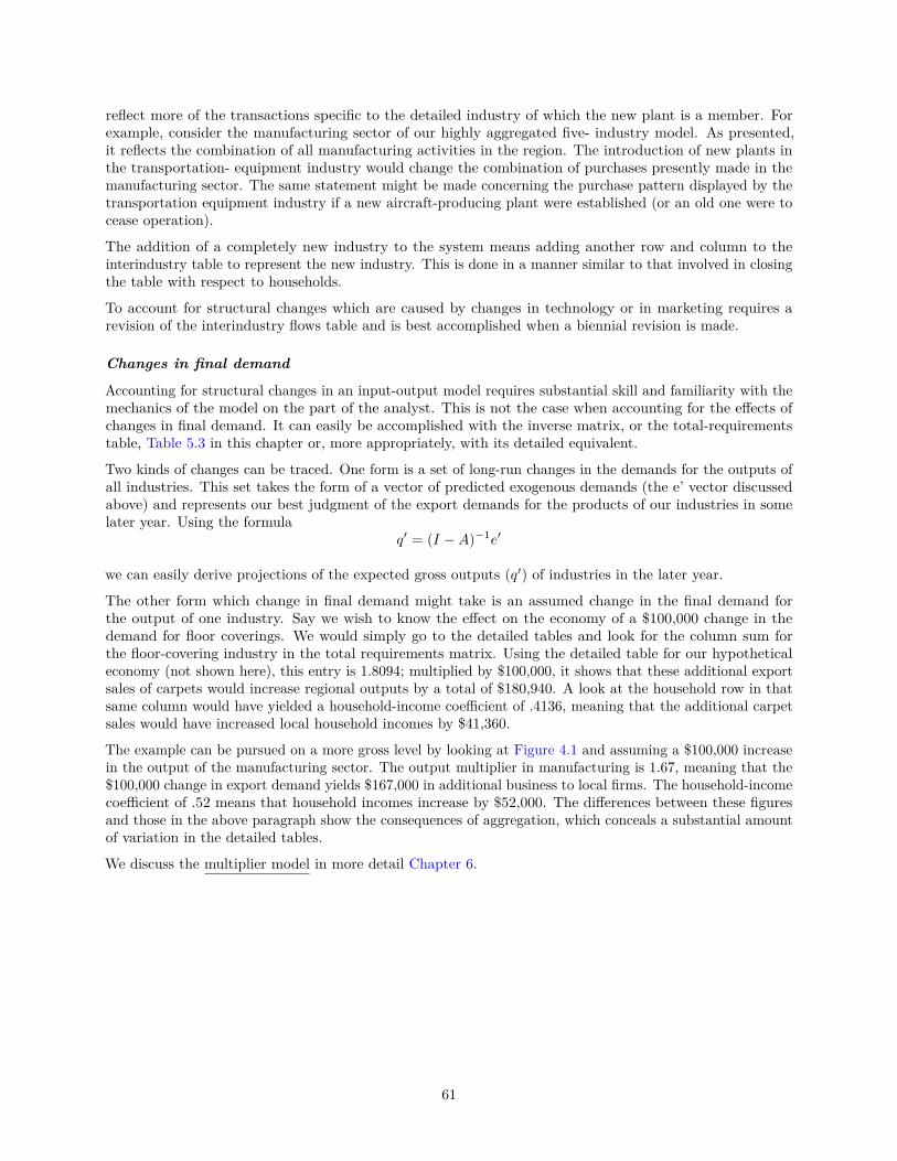
reflect more of the transactions specific to the detailed industry of which the new plant is a member. Forexample, consider the manufacturing sector of our highly aggregated five- industry model. As presented,it reflects the combination of all manufacturing activities in the region. The introduction of new plants inthe transportation- equipment industry would change the combination of purchases presently made in themanufacturing sector. The same statement might be made concerning the purchase pattern displayed by thetransportation equipment industry if a new aircraft-producing plant were established (or an old one were tocease operation).

The addition of a completely new industry to the system means adding another row and column to theinterindustry table to represent the new industry. This is done in a manner similar to that involved in closingthe table with respect to households.

To account for structural changes which are caused by changes in technology or in marketing requires arevision of the interindustry flows table and is best accomplished when a biennial revision is made.

Changes in final demand

Accounting for structural changes in an input-output model requires substantial skill and familiarity with themechanics of the model on the part of the analyst. This is not the case when accounting for the effects ofchanges in final demand. It can easily be accomplished with the inverse matrix, or the total-requirementstable, Table 5.3 in this chapter or, more appropriately, with its detailed equivalent.

Two kinds of changes can be traced. One form is a set of long-run changes in the demands for the outputs ofall industries. This set takes the form of a vector of predicted exogenous demands (the e’ vector discussedabove) and represents our best judgment of the export demands for the products of our industries in somelater year. Using the formula

q′ = (I −A)−1e′

we can easily derive projections of the expected gross outputs (q′) of industries in the later year.

The other form which change in final demand might take is an assumed change in the final demand forthe output of one industry. Say we wish to know the effect on the economy of a $100,000 change in thedemand for floor coverings. We would simply go to the detailed tables and look for the column sum forthe floor-covering industry in the total requirements matrix. Using the detailed table for our hypotheticaleconomy (not shown here), this entry is 1.8094; multiplied by $100,000, it shows that these additional exportsales of carpets would increase regional outputs by a total of $180,940. A look at the household row in thatsame column would have yielded a household-income coefficient of .4136, meaning that the additional carpetsales would have increased local household incomes by $41,360.

The example can be pursued on a more gross level by looking at Figure 4.1 and assuming a $100,000 increasein the output of the manufacturing sector. The output multiplier in manufacturing is 1.67, meaning that the$100,000 change in export demand yields $167,000 in additional business to local firms. The household-incomecoefficient of .52 means that household incomes increase by $52,000. The differences between these figuresand those in the above paragraph show the consequences of aggregation, which conceals a substantial amountof variation in the detailed tables.

We discuss the multiplier model in more detail Chapter 6.

61

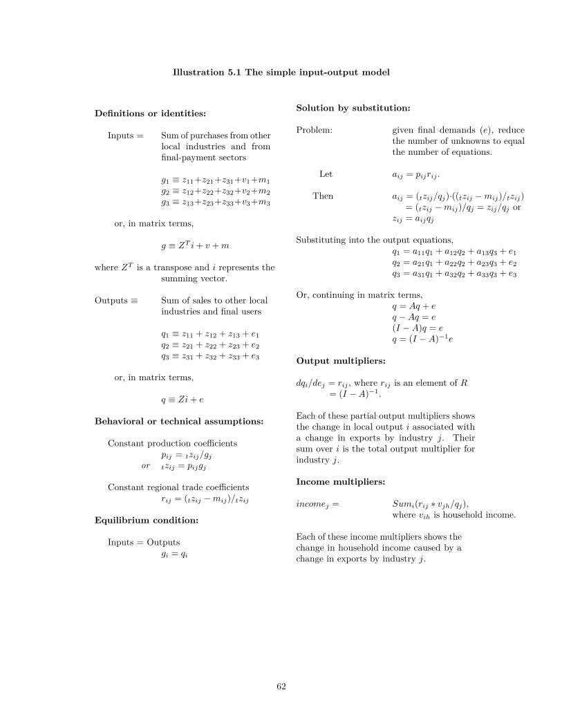
Illustration 5.1 The simple input-output model

Definitions or identities:

Inputs = Sum of purchases from otherlocal industries and fromfinal-payment sectors

g1 ≡ z11+z21+z31+v1+m1g2 ≡ z12+z22+z32+v2+m2g3 ≡ z13+z23+z33+v3+m3

or, in matrix terms,

g ≡ ZT i+ v +m

where ZT is a transpose and i represents thesumming vector.

Outputs ≡ Sum of sales to other localindustries and final users

q1 ≡ z11 + z12 + z13 + e1q2 ≡ z21 + z22 + z23 + e2q3 ≡ z31 + z32 + z33 + e3

or, in matrix terms,

q ≡ Zi+ e

Behavioral or technical assumptions:

Constant production coefficientspij = tzij/gj

or tzij = pijgj

Constant regional trade coefficientsrij = (tzij −mij)/tzij

Equilibrium condition:

Inputs = Outputsgi = qi

Solution by substitution:

Problem: given final demands (e), reducethe number of unknowns to equalthe number of equations.

Let aij = pijrij .

Then aij = (tzij/qj)·((tzij −mij)/tzij)= (tzij −mij)/qj = zij/qj or

zij = aijqj

Substituting into the output equations,q1 = a11q1 + a12q2 + a13q3 + e1q2 = a21q1 + a22q2 + a23q3 + e2q3 = a31q1 + a32q2 + a33q3 + e3

Or, continuing in matrix terms,q = Aq + eq −Aq = e(I −A)q = eq = (I −A)−1e

Output multipliers:

dqi/dej = rij , where rij is an element of R= (I −A)−1.

Each of these partial output multipliers showsthe change in local output i associated witha change in exports by industry j. Theirsum over i is the total output multiplier forindustry j.

Income multipliers:

incomej = Sumi(rij ∗ vjh/qj),where vih is household income.

Each of these income multipliers shows thechange in household income caused by achange in exports by industry j.

62

6 REGIONAL INPUT-OUTPUT MULTIPLIERSIntroductionAs noted in Chapter 5, a regional input-output model can be used to provide a set of economic multiplierswith which to trace the effects of changes in demand on economic activity in the region. After explaining moregraphically the multiplier concept, this chapter formulates employment, household-income, and government-income multipliers and presents examples.

The multiplier conceptInput-output models are most commonly used to trace individual changes in final demand through theeconomy over short periods of time. In this function, they are called impact models, or multiplier models. Letus now look more closely at these models. First, we take an intuitive approach to understanding the meaningof the total- requirements table, illustrating the multiplier effect with a two-dimensional chart. Then we solvethe model using the formula for the sum of an infinite series and present the results in three dimensions.

An intuitive explanation

A total-requirements table for the aggregated six-industry model was presented in Table 5.3 for the previouschapter. This table shows the direct, indirect, and induced changes in industry outputs required to deliverunits to final demand. A table of this type is the basic element used in estimating multipliers.

Table 6.1 Hypothetical direct-requirements table

Extrac- Construc- Manufac- HouseholdIndustry tion tion turing Trade Services expenditures

(1) (2) (3) (4) (5) (6)Extraction (1) 10.9 1.2 4.2 0.1 0.6 0.6Construction (2) 0.8 0.0 0.3 0.3 2.6 0.0Manufacturing (3) 8.5 16.4 9.8 2.3 3.1 8.0Trade (4) 3.1 8.9 3.7 1.5 2.3 16.2Services (5) 6.1 8.8 6.1 11.6 17.5 26.9Households (6) 35.5 26.4 26.1 49.5 40.6 0.6

To better understand the meaning of a total-requirements table and the multipliers derived from it, let usgo back and trace the flow of outputs induced by a $100 purchase from the manufacturing sector throughthe direct- requirements table (repeated as Table 6.1). The result of this step-by-step tracing is illustratedin Figure 6.1 and reported in Table 6.2. First, $100 enters the state economy through manufacturing. (Myconvention is to label this initial round as “round zero” -- this is the “insertion” before the rounds of circulationbegin. It is also consistent with the exponents in the solution based on the sum of an infinite series.) Toproduce output worth $100, firms in manufacturing purchase inputs from other industries in the economy.According to column 3 in the direct- requirements table, $4.20 goes to agriculture and mining, $0.30 goes toconstruction, an additional $9.80 goes to other firms in manufacturing, $3.70 goes to trade, $6.10 goes toservices, and $26.10 is paid to households in wages and salaries (This is round one.). Capacity permitting,each of these industries must expand its output to accommodate this additional production load.

63

Figure 6.1 The activity effect of $100 sale to final demand by the manufacturing sector

Thus, in producing additional output valued at $4.20, firms in agriculture and mining buy output worth $0.46(10.9% of $4.20) from others in this sector, $0.03 (0.8% of $4.20) from construction, $0.36 (8.5% of $4.20) frommanufacturing, and so on, for a total of $2.72. At the same time, each of the other industries is purchasingthe additional inputs required to produce the output requested of them. The results are summarized inFigure 6.1 as the second round of purchases. Other purchases follow in succeeding rounds, each smaller asmoney flows out of the interindustry sector into the hands of the owners of primary inputs (excluding labor),into government coffers, and for the purchase of imported materials.

This chain of purchases continues for all industries until the economy is again in equilibrium. The initial $100purchase from manufacturing has led to money flows throughout the regional economy valued at $219, asshown in Table 5.4 in the previous chapter... Notice that if the value of additional output is summed throughround six, most of the effect of the initial purchase has already been realized: as seen in Table 6.2, $214 hasbeen spent at this point. The total-requirements table just counts the rounds of spending to infinity andadds them up. The total appears in Table 5.4 in the previous chapter as the column sum for manufacturing,and is labeled "total activity." The column itself has elements which show the output impact of the initialexpenditure on each industry in the system.

Now, before we go on to explore mathematically this alternative approach to solution by inversion, let usreduce the "activity effect" to a "multiplier effect" focusing on industries. This reduction is accomplishedsimply by excluding the household row in the table of rounds of spending. Now we count only the effectson industries. This leads to Figure 6.2. The striking thing about the contrast of these two effects is theimportance of the household in a regional economy. (The same relative pattern occurs in all regional modelswhich I have encountered.)

The iterative approach

This intuitive explanation may be expressed in a more concise mathematical form as a “solution by iterations.”This process uses the sum of an infinite series to approximate the solution to the economic model. In matrixalgebra, the process is:

T = IX +AX +A2X +A3X + ...+AnX

Here, T is the solution, a column vector of changes in each industry’s outputs caused by the changesrepresented in the column vector X. A is the direct- requirements matrix. n is the number of rounds required

64

to produce results approximating those obtained when n approaches infinity. (For this and most other cases,n = 6 is high enough to capture over 97 percent of the flows; eight rounds capture over 99 percent.)

Table 6.2 The multiplier effect of $100 in manufacturing output tracedin rounds of spending through the hypothetical economy

—–Round of spending—–Industry (0) (1) (2) (3) (4) (5) (6) Total

Extraction (1) 0.00 4.23 1.09 0.40 0.20 0.11 0.07 6.09Construction (2) 0.00 0.30 0.23 0.28 0.14 0.09 0.05 1.06Manufacturing (3) 100.00 9.82 3.74 1.60 1.05 0.57 0.35 117.13Trade (4) 0.00 3.67 4.93 1.87 1.48 0.73 0.48 13.16Services (5) 0.00 6.09 9.39 4.84 3.29 1.79 1.11 26.51Total industry outputs 100.00 24.11 19.38 8.98 6.15 3.30 2.06 163.98Households (6) 0.00 26.10 8.60 7.72 3.57 2.47 1.32 49.77Total "activity" 100.00 50.21 27.97 16.71 9.72 5.77 3.38 213.76

Figure 6.2 The multiplier effect of $100 sale to final demand by themanufacturing sector

The multiplier-effects, or "rounds-of- spending," table (Table 6.2) lays out the results of applying this equationto the problem of tracing direct expenditures. In this table, the total column is T . Round 0 is IX, the initialexpenditures to be traced (I is the identity matrix, which is operationally equivalent to the number 1 inordinary algebra). Round 1 is AX, the result of multiplying the matrix A by the vector X. It answers thequestion: what are the outputs required of each supplier to produce the goods and services purchased inthe initial change under study? Round 2 is A2X, which is the same as AAX, or A(AX); it is the result ofmultiplying the matrix A by Round 1 (or AX). It answers for Round 2 the same question as was applied toRound 1: what are the outputs required of each supplier to produce the goods and services purchased inRound 1 of this chain of events? Round 3 is A3X, which is the same as A(A2X); and the story repeats, roundafter round. Each of columns 1 through 6 in the multiplier-effects table represents a term in the continuingbut diminishing chain of expenditures on the right side of the equation.

65

Figure 6.3 The ripple effect of a $100 export of manufacturing output

The tracing of these rounds in Table 6.2 can also be presented in three dimensions with a spreadsheetprogram (I used Excel.). Figure 6.3 shows once again the multiplier effects (now it might be proper to jointhe newspapers in discussing the "ripple effect") of a $100 export sale of manufacturing goods by our economy.Notice the large flow through households, especially in round 1, and note how quickly circulation falls off.This economy is pretty leaky!

This process has several advantages to recommend it over the inversion solution. The analyst builds a directimpact vector (Round 0) through survey or assumption and then sets the iterative process in motion on adesktop computer. He can see clearly the paths taken by indirect rounds of spending and can perform a checkboth on his direct impact vector and on the input-output model itself. Further, he has the material availableto make a graphic presentation of his results which is easily understood by a reader.

Before the advent of microcomputers, the typical input-output study included lengthy sets of inverse matricesand multiplier tables in which the analyst looked up multipliers which applied to his problem. These numberswere then applied blindly and with faith.

Multiplier transformationsNow let us go back to the solution of the input-output model by inversion as presented in the previouschapter. This has the advantage of permitting us to generalize and produce the various kinds of multiplierspossible in an input-output system.

66

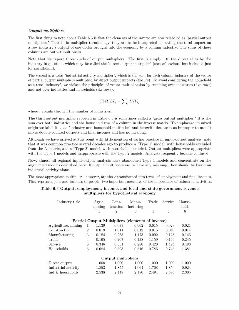
Output multipliers

The first thing to note about Table 6.3 is that the elements of the inverse are now relabeled as "partial outputmultipliers." That is, in multiplier terminology, they are to be interpreted as stating the total impact ona row industry’s output of one dollar brought into the economy by a column industry. The sums of thesecolumns are output multipliers.

Note that we report three kinds of output multipliers. The first is simply 1.0, the direct sales by theindustry in question, which may be called the "direct output multiplier" (sort of obvious, but included justfor parallelism).

The second is a total "industrial activity multiplier", which is the sum for each column industry of the vectorof partial output multipliers multiplied by direct output impacts (the 1’s). To avoid considering the householdas a true "industry", we violate the principles of vector multiplication by summing over industries (five rows)and not over industries and households (six rows).

QMULTj =∑

iINVij

where i counts through the number of industries.

The third output multiplier reported in Table 6.3 is sometimes called a "gross output multiplier." It is thesum over both industries and the household row of a column in the inverse matrix. To emphasize its mixedorigin we label it as an "industry and household multiplier" and herewith declare it as improper to use. Itmixes double-counted outputs and final incomes and has no meaning.

Although we have arrived at this point with little mention of earlier practice in input-output analysis, notethat it was common practice several decades ago to produce a "Type 1" model, with households excludedfrom the A matrix, and a “Type 2" model, with households included. Output multipliers were appropriatewith the Type 1 models and inappropriate with the Type 2 models. Analysts frequently became confused.

Now, almost all regional input-output analysts have abandoned Type 1 models and concentrate on theaugmented models described here. If output multipliers are to have any meaning, they should be based onindustrial activity alone.

The more appropriate multipliers, however, are those transformed into terms of employment and final incomes.They represent jobs and incomes to people, two important measures of the importance of industrial activities.

Table 6.3 Output, employment, income, and local and state government revenuemultipliers for hypothetical economy

Industry title Agric, Cons- Manu- Trade Service House-mining truction facturing holds

1 2 3 4 5 6

Partial Output Multipliers (elements of inverse)Agriculture, mining 1 1.139 0.033 0.062 0.015 0.023 0.021Construction 2 0.019 1.011 0.012 0.015 0.040 0.014Manufacturing 3 0.184 0.253 1.173 0.092 0.128 0.146Trade 4 0.165 0.207 0.138 1.159 0.166 0.245Service 5 0.346 0.351 0.280 0.428 1.494 0.498Households 6 0.684 0.593 0.516 0.785 0.745 1.381

Output multipliersDirect output 1.000 1.000 1.000 1.000 1.000 1.000Industrial activity 1.853 1.855 1.664 1.708 1.850 0.924Ind & households 2.538 2.448 2.180 2.494 2.595 2.305

67

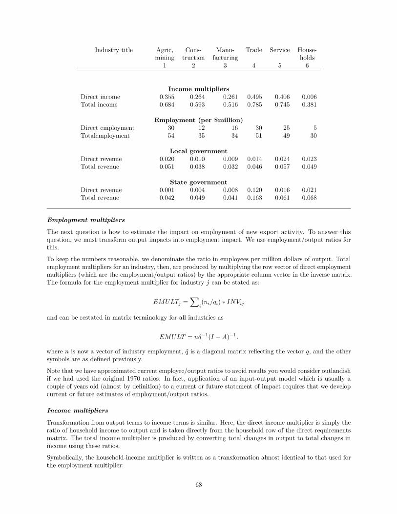
Industry title Agric, Cons- Manu- Trade Service House-mining truction facturing holds

1 2 3 4 5 6

Income multipliersDirect income 0.355 0.264 0.261 0.495 0.406 0.006Total income 0.684 0.593 0.516 0.785 0.745 0.381

Employment (per $million)Direct employment 30 12 16 30 25 5Totalemployment 54 35 34 51 49 30

Local governmentDirect revenue 0.020 0.010 0.009 0.014 0.024 0.023Total revenue 0.051 0.038 0.032 0.046 0.057 0.049

State governmentDirect revenue 0.001 0.004 0.008 0.120 0.016 0.021Total revenue 0.042 0.049 0.041 0.163 0.061 0.068

Employment multipliers

The next question is how to estimate the impact on employment of new export activity. To answer thisquestion, we must transform output impacts into employment impact. We use employment/output ratios forthis.

To keep the numbers reasonable, we denominate the ratio in employees per million dollars of output. Totalemployment multipliers for an industry, then, are produced by multiplying the row vector of direct employmentmultipliers (which are the employment/output ratios) by the appropriate column vector in the inverse matrix.The formula for the employment multiplier for industry j can be stated as:

EMULTj =∑

i(ni/qi) ∗ INVij

and can be restated in matrix terminology for all industries as

EMULT = nq−1(I −A)−1.

where n is now a vector of industry employment, q is a diagonal matrix reflecting the vector q, and the othersymbols are as defined previously.

Note that we have approximated current employee/output ratios to avoid results you would consider outlandishif we had used the original 1970 ratios. In fact, application of an input-output model which is usually acouple of years old (almost by definition) to a current or future statement of impact requires that we developcurrent or future estimates of employment/output ratios.

Income multipliers

Transformation from output terms to income terms is similar. Here, the direct income multiplier is simply theratio of household income to output and is taken directly from the household row of the direct requirementsmatrix. The total income multiplier is produced by converting total changes in output to total changes inincome using these ratios.

Symbolically, the household-income multiplier is written as a transformation almost identical to that used forthe employment multiplier:

68

HMULTj =∑

i(hi/qi) ∗ INVij

Here, hi represents the household income of industry i.

Income multipliers are most useful compared to output multipliers. Output multipliers are "gross" in thatthey double-count transactions. One of the problems with economic-base multipliers was this double-counting,which led naive audiences to believe that we could magically get more stuff out of an economy than we put in,and it led sophisticated audiences into disbelief in the analyst’s results. Income multipliers report the moneythat drops into the hands of owners of resources as income. In this case, the owners happen to be workers.

Government-income multipliers

The same process can be applied to government incomes, simply by substituting "local-government revenue"or "state-government revenue" for "household income" in the transformation formula. The resulting multipliersare relatively low because the revenue/output ratios are low.

Government-income multipliers suffer in interpretation because, while we generally consider governments asowners of resources and so treat them as we do households, they are in fact organized as businesses, and wehope they produce outputs in response to their incomes. This anomaly means that they should be interpretedas yielding excess revenue in some short-run period (in which excess capacity exists in streets, protection,utilities, etc.), but, in the long run, the piper must be paid and new capacity must be financed. Interpretationdepends on your time horizon.

Appendix 1 Multiplier concepts, names, and interpretationsIntroduction

This appendix examines the development of input-output multiplier concepts and the evolution of theirnames. It is included to show the evolution of the concepts over the last several decades. I will restrict thisstatement to regional input-output models mostly in North America and to multipliers commonly used inimpact analysis, pointing out some preferred alternatives.1

It is traditional to start such an exposition with salutes both to R. F. Kahn, who introduced the employmentmultiplier to describe the effect upon unemployment of a net increase in home investment (Kahn 1931), andto John Maynard Keynes, who elaborated on and expanded the concept as an income multiplier in supportof his arguments on national income and employment (Keynes 1936). These are familiar beginnings foreconomics students.

While the concept of economic-base analysis had been at play in geography and planning for a couple ofdecades, the economic-base multiplier did not seriously enter the literature in economics until 1950, withestimation of an employment multiplier for Los Angeles County by George H. Hildebrand and ArthurMace, Jr. (Hildebrand and Mace do credit M. C. Daly, writing in the Economic Journal in 1940 for theirapproach.(Hildebrand and Mace 1950)) From this start, economic- base multipliers thrived in regionaleconomics. Theodore Lane provides an excellent review of economic-base industry into its last great decade(Lane 1966).

The early literature on input-output analysis contained relatively few references to multipliers, although theinverse or interdependence matrix was well known and used with national tables. Essentially, it was leftto regional economists to develop input-output multipliers. The serious literature on regional input-outputmultipliers starts with Frederick T. Moore in a now- classic article on "Regional Economic Reaction Paths" in1955 (Moore 1955). And this is where I begin.

1This appendix is based on a paper presented at the North American meetings of the Regional Science Association in 1990.

69

Income multipliersOrigins of Types I and II income multipliers

Reporting on models of California and Utah developed in association with James W. Petersen, Moore defines"... the ’simple’ income multiplier as the ratio of the direct-plus-indirect income effects to the direct alone"(Moore and Petersen 1955). His formula is well- known:

Mk =

∑j

ahjdjk

ahk(1)

where Mk is the simple income multiplier for industry k, ahj is the household income coefficient for industryj, and djk is the element in the inverse showing direct and indirect purchases from industry j associated witha unit exogenous sale by industry k.

Moore explains his caution in using the term "simple" with a note that the Utah study reports multipliersbased on an inverse derived from a coefficient matrix closed with respect to households (but he fails to use anadjective in describing these other multipliers). In addition, he discusses "... one more type of relationship:the effects upon investment induced by the changes in income and consumption. These effects he calls"accelerator coefficients," and he calculates them with a modification of the numerator of his simple incomemultiplier:

Rk =∑

j

bjdjk (2)

Rk is the accelerator coefficient, and bj is the capital-output ratio for industry j. This coefficient hasapparently disappeared from the literature, probably due to data deficiencies.

Moore and Petersen report an interindustry model of Utah which remains a monument to scholarship. Theygo beyond Leontief’s earlier- described "balanced regional model" (Leontief 1953) to develop a transactionstable with pure regional transactions, albeit transactions estimated with what Schaffer and Chu later (1969)called the "supply-demand pool" technique, or the commodity-balance approach.

They proceed with development of three sets of income multipliers. Interestingly, especially given the problemswe have faced over the years in terminology, they give these multipliers no specific names. The first incomemultiplier was the one named earlier by Moore as the "simple income multiplier." Its numerator was "incomereactions to changes in demand," or the direct and indirect income effects of a unit change in final demand.The second was derived from "income reactions including induced via homogeneous consumption functions," orthe direct, indirect, and induced income effects of change. The third multiplier was based on "income reactionsincluding induced via nonhomogeneous consumption functions. This third multiplier was computed usingthe marginal coefficients in consumption functions estimated from national data for only three aggregationsof the seven-industry model used to illustrate the study. Moore and Petersen felt that the induced effect isoverstated by the homogeneous consumption functions implied by the closure of the model with respect tohouseholds.

Werner Z. Hirsch, in his model of St. Louis, moved beyond Moore and Petersen in three ways: he builtthe model from company records, he prepared a detailed exports matrix, and he treated the household andlocal government sectors as endogenous parts of the economy (Hirsch 1959). But he remained consistent inhis treatment of income multipliers, although he developed only two sets and gave them parenthetic names.Moore’s simple income multiplier became "multiplier (Model I)" and his second multiplier became "multiplier(Model II)."

At this point, little attention had been paid to input-output multipliers in the literature. In his Methods ofRegional Analysis, Walter Isard, pays scant attention to them, seven pages out of over 700, devoted almostexclusively to the income and employment multipliers of the Utah study (Isard 1960). Hollis B. Chenery andPaul G. Clark, in their Interindustry Economics, long the comprehensive reference in the field, cite the term

70

"multiplier" only twice in their index (Chenery and Clark 1959). Chenery and Clark do build inverses forModel I and Model II tables, as did Hirsch, with the Model II tables including households as endogenous.

But in 1965, William H. Miernyk devoted 14 pages of over 150 to multiplier analysis, and 8 of these to incomemultipliers. Simple, clear, and easily understood, Miernyk’s Elements of Input-Output Analysis (Miernyk1965) became a virtual bible to budding regional input-output analysts. Interest in regional input-outputstudies was intensifying in the sixties, and with this interest came a need to present in study reports some ofthe tools which might help others in using models produced at substantial expense and effort.

Miernyk based his table illustrating "income interactions" on a similar table from Hirsch. But he changedcolumn headings describing multipliers for models I and II to be "Type I multiplier" and "Type II multiplier."To my knowledge, this is the beginning of the line for these names, which are still in use today. My suspicionsare confirmed by P. Smith and W. I. Morrison, who calculated income multipliers "... using methods developedby Hirsch and discussed further by Miernyk, ... described (after Miernyk) as type 1 and type 2 incomemultipliers" (Smith and Morrison 1974, p. 57).Type III multipliers

Moore and Petersen as well as Hirsch developed crude consumption functions for sets of industries in anattempt to reduce the impact of average propensities to consume (as expressed in a household coefficientscolumn) on the induced income effect included in their type II multipliers. But the resulting third set ofmultipliers was unnamed. Miernyk obliged in his Boulder study by labeling these multipliers as "type IIImultipliers." Miernyk calculated consumption functions in Boulder and applied estimated marginal propensitiesto consume instead of household coefficients in computing income multipliers. As he expected, the resultingtype III multipliers were lower than type II multipliers by slightly more than 10 percent. (Miernyk et al.1967)

A second definition of type III multipliers is in use in Canada in the Atlantic Provinces and Nova Scotia(See Jordan and Polenske 1988 for a clear summary.). Following the lead of Kari Levitt and a team atStatistics Canada, I used three levels of closure to develop output, income, and employment multipliersfor the 1974, 1979, and 1984 Nova Scotia input- output models (DPA Group Inc. and Schaffer 1989).Model I is the traditional open model, yielding direct and indirect effects; model II is closed with respectto households, yielding direct, indirect, and induced effects; model III is closed with respect to local andprovincial government sectors as well, yielding direct, indirect, and extended effects. We devised the term"extended effects" to include effects induced both by households and by local and provincial governments.

This treatment of type III multipliers as reflective of greater closure seems a better use of the numberingsystem.Household-income multipliers

Income multipliers are the most troublesome of multipliers. When we documented the Hawaii input-outputmodel for 1967 the problems became obvious (Schaffer et al. 1972). Because it was by then traditional toshow income and output multipliers, we did so, designating them as "simple" and "total," feeling these termsmore descriptive than "type I" and "type II." (The "simple" came from the income multiplier in Moore andPetersen; the "total" came from their employment multiplier.) But we could not recall any instance in whichthe Department of Planning and Economic Development or any other agency had been asked to show thetotal effect on household incomes of a specified direct income change due to exogenous forces on an industry.People asked about the impact of new plant investment (a problem for which no convenient multipliers havebeen constructed) and about the impact of export sales, but none would ask about the effect of a payrollincrease. So we added an "income coefficient," showing the total income effect associated with a unit changein export sales. The format of the table was Hirsch’s (1959, p.366), with a total column added.

In documenting the 1970 Georgia input-output model, (Schaffer 1976), the traditional definition became "...awkward and inconsistent with the approach taken in most interpretations. Therefore, we ... defined the’household- income multiplier’ for industry j to be the addition to household incomes in the economy due toa one-unit increase in final demand for the output of industry j." The footnote explaining this move is a clearsummary of the twisted path described thus far:

71

The notion of an income multiplier as first introduced to the regional literature by Moore andPetersen (1955) was used to describe additional household income attributable to unit change inhousehold income in the industry in question. This definition is far removed from the exogenouschanges which precipitate additional income changes, and it forces its user to unnecessary troublein determining, e.g., the importance of an industry to its community. We have therefore switchedAlthough a similar concept appeared in Moore and Petersen, our point is that the label is confusing.We first saw this concept discussed as ’income coefficients’ in the Mississippi study by Cardenand Whittington (1964) and used the term to distinguish our multiplier from the one seen in theliterature as late as 1973. (p. 67)

Davis (1968, p. 33) makes the importance of this distinction clear. Two old-style income multipliersmay have exactly the same values but may differ substantially in terms of income change per unitchange in final demand. He suggests that an emphasis on absolute changes ... rather than onrelative changes, as in Moore and Petersen, be made to avoid the confusion. The caution wasalso expressed by Miernyk (1967, p. 101) in his Boulder study, which reported old-style incomemultipliers.

But despite these problems, the old- style income multipliers live on. Two not-too-distant uses are in theDelaware model produced by Sharon Brucker and Steve Hastings (1984) and in the 1984 Nova Scotia Study,where the term ’income-generated multiplier’ substitutes for the above-recommended ’household- incomemultiplier’ and ’income multipliers’ are defined in the original way.Other income multipliers

It became obvious early that other multipliers reflecting the total impact of changes in final demand onincomes could be generated.

The documentation of the 1963 Washington input-output (Bourque and others 1967) reports only onemultiplier, the regional income multiplier, which includes the change in total state income per $100,000change in final demand. The 1972 Washington study (Bourque and Conway 1977), in one of the clearestexpositions of multiplier development yet written, defines type I and type II value added multipliers, alongwith labor-income multipliers, and jobs multipliers. In each case, the multiplier is calculated as "... a simpletransformation of the output multipliers given in the inverse matrix ... ." Thus:

Mk =∑

i

vkjbij

∑vkjbij (3)

where Mk is the income multiplier for the kth factor income, vki is the input coefficient for the kth factor inindustry i, and bij is the inverse coefficient.

This view of the multiplier as an operator with which to transform changes in industry output into impactson incomes of factors of production was well expressed by Hays B. Gamble and David L. Raphael (1966).In a survey- based model of Clinton County, Pennsylvania, they develop "residual income multipliers" byinverting a coefficient matrix including vectors for the nonprofit sector, three local government sectors, andfour household sectors. Then by summing elements in these rows of the interdependency matrix (inverse) foreach industry, they produced household multipliers, local government multipliers, and nonprofit multipliers.

In both the Nova Scotia studies and the Georgia model, I produce government-income multipliers. for localgovernments and for provincial or state governments.

In all these cases, the multipliers can be unambiguously interpreted as changes in incomes per change inexogenous demand. It is only the income multiplier associated with households that is ambiguous.

Employment multipliers

Employment multipliers were developed by Moore and Petersen at the same time as and analogous to theirincome multipliers. They estimated a set of aggregated employment-production relationships and used thecoefficients showing change in employment per change in output as the a’s in equation (1), transforming the

72

multiplier from dollar terms into employment terms. Their multipliers relate total employment change todirect employment change.

Both Hirsch and Miernyk repeat this definition. In his Boulder study, Miernyk built "type III" employmentmultipliers as well, with a complete set of employment functions. Later, in his West Virginia Study,Miernyk apparently used simple employment- output ratios to effect the transformation from output terms toemployment terms.

The first employment multipliers produced in the Washington series were for 1972. Bourque and Conwayunwaveringly maintain their devotion to defining multipliers denominated with final demand changes,producing type I and type II versions to reflect levels of closure.

In Georgia, I also denominated my simple and total employment multipliers with final demand changes. InNova Scotia, we produced both output-based employment multipliers and employment-based employmentmultipliers for models with three levels of closure, parallel to our other multipliers. This was largely becauseof a feeling that, in inflationary times, the shelf life of output-based employment multipliers was much lowerthan that of employment-based ones.

Output multipliers

Output multipliers are an obvious starting point for multiplier analyses. They are simply the column sums ofthe industry part of an inverse matrix. These columns are the essential ingredients in the other multipliercalculations. Yet, output multipliers were neither mentioned nor alluded to by either Moore and Petersen orHirsch or Miernyk.

Floyd Harmston in his 1962 Wyoming study used a “business and industry multiplier” which was a typeI output multiplier under another name (Harmston 1962). I used output multipliers in both Georgia andNova Scotia studies. But, after a little note from Rod Jensen, Australia’a leading authority on input-outputanalysis, commenting on an early draft, I made explicit a warning that output multipliers should be usedonly as general indicators of industrial activity. While they represent the essence of interindustry models, theflows of intermediate transactions are not our basic interests in summary multipliers. Effects on income andemployment are our primary concerns. Nevertheless, these by- products of useful multiplier production arecommon statements in many studies.

In explaining why they did not produce aggregate output multipliers for the 1972 Washington model, Bourqueand Conway express this caution beautifully:

... we have not specified aggregate output multipliers. Although the output multipliers givenby the elements of the inverse matrix are at the root of the multipliers ...[calculated] ... , it isnot very meaningful to sum these elements into aggregate output multipliers for each industryIn other words, given the concepts that lie behind each output measure, it does not make muchsense, economically speaking, to combine, say, the shipments of pulp mills with the margins of theinsurance industry into an aggregate transactions measure. Furthermore, users of the Washingtontables in the past have sometimes employed aggregate output multipliers inappropriately, in atleast one case confusing them with income multipliers. For these reasons, we have chosen not topresent aggregate output multipliers. (Bourque and Conway 1977, p. 48)

Observations and summary

These comments are consistent with conventions used in a recent comprehensive compendium on input- outputanalysis by Ronald E. Miller and Peter G. Blair (1985). Multipliers have admittedly become a larger questionthan for earlier writers. Miller and Blair devote over ten percent of their book to regional, interregional,multiregional, and interrelation multipliers. (Only five percent is devoted to basic regional multipliers.)

They resolve my concern regarding the denominating of income and employment multipliers by relegatingthe terms "type I" and "type II" exclusively to multipliers with denominators in the same terms as thenumerators. They then use "simple" to identify multipliers based on pure industry transactions tables and"total" for multipliers based on tables closed with respect to households. “Income” multipliers show changes

73

in income per unit change in final demand and “employment” multipliers are expressed per unit change infinal demand as well.

These statements and the explanations accompanying them are helpful indeed. But, an appropriate conclusionof this review is that analytic purposes determine the terminology to use. The problem which we mightperceive comes from overall study reports which suggest through terminology the impacts which might beexamined through regional input-output models. When particular questions are pursued, explanations shouldeliminate the ambiguities in impact interpretations.

Further extensions

The point of view taken above can be described as that of an old-line traditionalist. More multipliers continueto evolve and recirculate. I should mention two of them.

One is income-distribution multipliers. to my knowledge, efforts to develop income-distribution multipliersstarted with Roland Artle in his studies of the Stockholm economy (Artle 1965) and in his efforts in the earlysixties to estimate such multipliers while working with a research team in Hawaii. While he conceptualizeda system with the household row divided into several income classes and with the household expenditurecolumn similarly divided, the effort failed due to complex data problems.

An effort which has yielded more fruit is that of Kenichi Miyazawa documented in several articles in thesixties and seventies and in his book (Miyazawa 1976). His “intersectoral income multipliers” have been usedon numerous occasions in the last two decades. Since such studies are beyond the realm of normal economicimpact analyses, we do not treat them further.

The second multiplier system that has been resurrected is the “SAM-based multiplier.” Social AccountingMatrices (SAMs) evolved to a high level in the sixties in several streams of literature. One is the work ofRichard A. Stone (leading to his Nobel Laureate in Economics) and extended at great detail in the UnitedNations social accounting literature. Another is the work at Statistics Canada as exemplified in the mostexhaustive theoretical and empirical analysis of social accounts by Kari Levitt for the Atlantic Provinces(Levitt 1975a; 1975b). A third outstanding example of social accounting was executed by the late Jerald R.Barnard at the University of Iowa (Barnard 1967).

Each of these streams resulted in interindustry tables augmented by social accounts documenting incomesin various sectors of the economy (detailed income and product accounts of which the aggregated regionalaccounting table in Chapter 3 is a simple example) and yielding multipliers for the various sectors.

A more recent example of SAM multiplier models is the one in current use by IMPLAN, the modeling systemdeveloped by MIG, Inc. (Minnesota IMPLAN Group Inc. 1997)

A final comment is simply a caution. The proliferation of multipliers over the years and the complexity ofextensions to input-output analysis can lead to substantial confusion among even knowledgeable analysts.Any multiplier analysis intended for a broad audience (or even an important decision-making audience) shouldbe reduced to the simplest possible terms but should be sufficiently documented to permit some evaluation ofits conclusions.

74

7 INTERREGIONAL MODELSNow we can easily combine the economic-base and interindustry concepts to yield a quick feeling for multi-regional models. While we stop with this introduction, extensions to include transactions between industriesin different regions are immediately obvious. In fact, a considerable literature has developed on interregionalinterindustry models and efforts have even been made to relate such models to “other worlds” such as theenvironment delineating the interactions of the human economy with the highly interactive elements of ourland, sea, and air “economies.”

Interregional economic-base modelsIn the following summary models, I have left implicit the definitions and identities which we labored overbefore. The common glossary is as follows:

Y: incomeE: income-related expendituresEi: income-related expenditures in region iEij : income-related expenditures in region i by residents of region jA autonomous expenditurese: marginal propensity to spend, dE(Y )/dY = eX: exportsM: importsm: marginal propensity to import, dM(Y )/dY = m

i: subscript for region (A subscript of 0 is for “autonomous value.” )

Review of one-region models

The one-region models are the Keynesian and economic-base models. Their distinguishing characteristic isthat the value of income is determined by some autonomous activity out there. It may be investor behavior,as in the Keynesian model, or it may be purchases by consumers outside the region, as in the economic-basemodel.Closed economy, no external trade

Assumptions:E = E(Y ) = eYA = A0

Equilibrium condition:Y = E +A

Solution:Y = eY +A0Y = [1/(1 − e)]A0

Multiplier:dY/dA = 1/(1 − e)

Open economy, with trade leakage

Assumptions:E1 = E1(Y1) = e1Y1X1 = X0M1 = M1(Y1) = m1Y1A1 = A0

75

Equilibrium condition:Y1 = E1 +A1 +X1 −M1

Solution:Y1 = e1Y1 +A0 +X0 −m1Y1Y1 = (A0 +X0) ∗ 1/(1 − (e1 −m1))

Multiplier: dY1/dX0 = dY1/dA0 = 1/(1 − (e1 −m1))

Two-region model with interregional tradeWhat has been missing all along has been interaction between regions. Obviously this takes place in the real world;otherwise, there would be no regions. Exports by one region have to be imports into another economy.

Partial solution, two-region interregional model

The system can more easily be presented by laying out the system in the same form as above but stoppingbefore the algebra requires the theory of determinants, which has either been forgotten or ignored by most ofus. We will limit the statement to region one alone in this section.

Assumptions:E1 = E1(Y1) = e1Y1X1 = M2 = M2(Y2) = m2Y2M1 = M1(Y1) = m1Y 1A1 = A0

Equilibrium condition:Y1 = E1 +X1 −M1 +A1

Solution:Y1 = e1Y1 −m1Y1 +m2Y2 +A0dY1 = e1dY1 −m1dY1 +m2(dY2/dY1)dY1 + dA0dY1 = e1dY1 −m1dY1 +m2(dY2/dY1)dY1(dM1/dX2) + dA0dY1 = e1dY1 −m1dY1 +m2m1(dY2/dX2)dY1 + dA0

But this line of attack becomes unnecessarily complicated. We can’t easily reduce the interactive term withoutknowing the multiplier for the other region (dY2/dX2)!

Multiplier:dY1/dA0 = 1/(1− (e1 −m1 +m2m1(dY2/dX2))dY1/dA0 = 1/(1− (e1 −m1+ interregional effect))

Let us take a more familiar tack. (This approach originated with Alan Metzler (Metzler 1950); HarryRichardson provides the restatement on which the above is based (Richardson 1969)Matrix solution, two-region interregional model

This model can be more systematically expressed with the matrix algebra developed for input-output analysis. Matrixalgebra permits us to immediately extend our logic from two regions as above to n regions without producing pageafter page of cumbersome calculations. Nevertheless, we will work with a two-region system for simplicity of discussion.We proceed as follows:

Assumptions:

As above, but now for both regions 1 and 2.

Ei = Ei(Yi) = eiYi

Xi = Mj = Mj(Yj) = mjYj

Equilibrium conditions:E1 +X1 −M1 +A1 = Y1E2 +X2 −M2 +A2 = Y2

Rewrite to align purchases from the two regions:

76

E1 −M1 +X1 +A1 = Y1X2 + E2 −M2 +A2 = Y2

Now, observing the following definitions, we can rewrite the equation system preparatory to matrix manipulation:

E11 = E1 −M1 = e1Y1 −m1Y1 = e11Y1E12 = M2 = M2(Y2) = m2Y2 = e12Y2E21 = X2 = M1(Y1) = m1Y1 = e21Y1E22 = E2 −M2 = e2Y2 −m2Y2 = e22Y2

Note that the e’s now show double subscripts showing purchases from region i by region j. So the system becomes

E11 + E12 +A1 = Y1E21 + E22 +A2 = Y2

or

e11Y1 + e12Y2 +A1 = Y1e21Y1 + e22Y2 +A2 = Y2

which translates into matrices as[e11 e12e21 e22

][Y2Y2

]+[A1A2

]=[Y1Y2

]or

eY +A = Y

where e is the matrix of eij . This solves exactly as would an input-output system:

Y − eY = A(I − e)Y = A(I − e)−1(I − e)Y = (I − e)−1AY = (I − e)−1A

Now, to give the elements of this inverse a designation, set

R = (I − e)−1 =[R11 R12R21 R22

]rewrite the solution asY1 = R11A1 +R12A2Y2 = R21A1 +R22A2

The interregional multipliers are thusdYi/dAj = Rij

for each ith row and jth column.

Now, it is a simple matter to expand the system to treat n regions. The process is identical to that used in thetwo-region system but with larger matrices!

Extensions and further studyInterregional interindustry modelsThe obvious extension is to expand the cell entries to become interindustry transactions matrices. Thus the E12entries would become klEij , showing purchases from industry k in region i by industry l in region j; where i = j, theregional transactions matrix for region i is inserted, and where i is not equal j, a matrix of imports is inserted.

The most commonly used multi-regional interindustry model of the United States was assembled by ProfessorKaren Polenske at MIT. Her model includes transactions generally for 50 industries in each of 44 states or sets ofstates.(Polenske 1980)

77

Economic-ecologic modelsEconomic-ecologic models append matrices depicting interaction between sectors in the natural environment andbetween those sectors and the industrial ones. The concept is similar to interregional interindustry analysis butimplementation becomes a harrowing experience. The dominant example of this was a complex model of theMassachusetts Bay area. (Isard et al. 1972)

Both of these extensions are discussed in detail in the comprehensive input-output reference by Ronald Miller andPeter Blair. (Miller and Blair 1985)

78

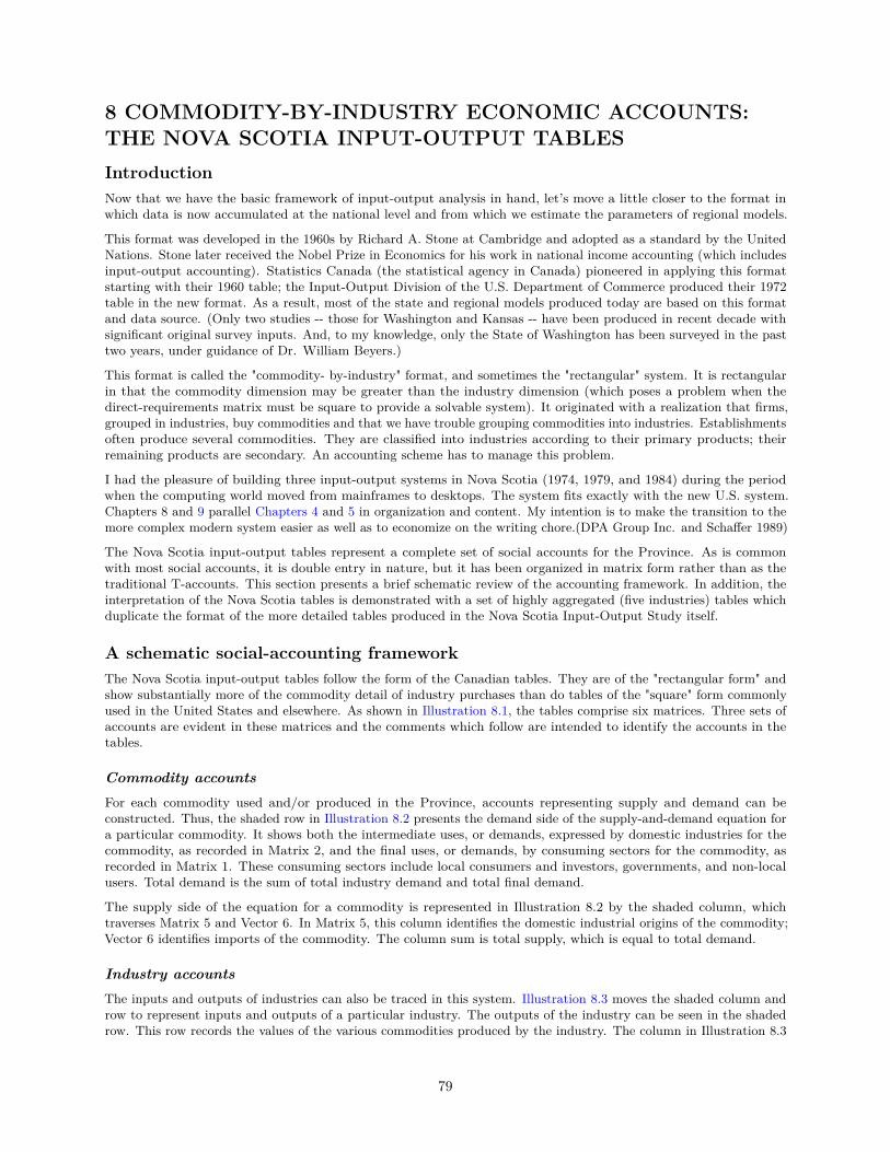
8 COMMODITY-BY-INDUSTRY ECONOMIC ACCOUNTS:THE NOVA SCOTIA INPUT-OUTPUT TABLESIntroductionNow that we have the basic framework of input-output analysis in hand, let’s move a little closer to the format inwhich data is now accumulated at the national level and from which we estimate the parameters of regional models.

This format was developed in the 1960s by Richard A. Stone at Cambridge and adopted as a standard by the UnitedNations. Stone later received the Nobel Prize in Economics for his work in national income accounting (which includesinput-output accounting). Statistics Canada (the statistical agency in Canada) pioneered in applying this formatstarting with their 1960 table; the Input-Output Division of the U.S. Department of Commerce produced their 1972table in the new format. As a result, most of the state and regional models produced today are based on this formatand data source. (Only two studies -- those for Washington and Kansas -- have been produced in recent decade withsignificant original survey inputs. And, to my knowledge, only the State of Washington has been surveyed in the pasttwo years, under guidance of Dr. William Beyers.)

This format is called the "commodity- by-industry" format, and sometimes the "rectangular" system. It is rectangularin that the commodity dimension may be greater than the industry dimension (which poses a problem when thedirect-requirements matrix must be square to provide a solvable system). It originated with a realization that firms,grouped in industries, buy commodities and that we have trouble grouping commodities into industries. Establishmentsoften produce several commodities. They are classified into industries according to their primary products; theirremaining products are secondary. An accounting scheme has to manage this problem.

I had the pleasure of building three input-output systems in Nova Scotia (1974, 1979, and 1984) during the periodwhen the computing world moved from mainframes to desktops. The system fits exactly with the new U.S. system.Chapters 8 and 9 parallel Chapters 4 and 5 in organization and content. My intention is to make the transition to themore complex modern system easier as well as to economize on the writing chore.(DPA Group Inc. and Schaffer 1989)

The Nova Scotia input-output tables represent a complete set of social accounts for the Province. As is commonwith most social accounts, it is double entry in nature, but it has been organized in matrix form rather than as thetraditional T-accounts. This section presents a brief schematic review of the accounting framework. In addition, theinterpretation of the Nova Scotia tables is demonstrated with a set of highly aggregated (five industries) tables whichduplicate the format of the more detailed tables produced in the Nova Scotia Input-Output Study itself.

A schematic social-accounting frameworkThe Nova Scotia input-output tables follow the form of the Canadian tables. They are of the "rectangular form" andshow substantially more of the commodity detail of industry purchases than do tables of the "square" form commonlyused in the United States and elsewhere. As shown in Illustration 8.1, the tables comprise six matrices. Three sets ofaccounts are evident in these matrices and the comments which follow are intended to identify the accounts in thetables.

Commodity accountsFor each commodity used and/or produced in the Province, accounts representing supply and demand can beconstructed. Thus, the shaded row in Illustration 8.2 presents the demand side of the supply-and-demand equation fora particular commodity. It shows both the intermediate uses, or demands, expressed by domestic industries for thecommodity, as recorded in Matrix 2, and the final uses, or demands, by consuming sectors for the commodity, asrecorded in Matrix 1. These consuming sectors include local consumers and investors, governments, and non-localusers. Total demand is the sum of total industry demand and total final demand.

The supply side of the equation for a commodity is represented in Illustration 8.2 by the shaded column, whichtraverses Matrix 5 and Vector 6. In Matrix 5, this column identifies the domestic industrial origins of the commodity;Vector 6 identifies imports of the commodity. The column sum is total supply, which is equal to total demand.

Industry accountsThe inputs and outputs of industries can also be traced in this system. Illustration 8.3 moves the shaded column androw to represent inputs and outputs of a particular industry. The outputs of the industry can be seen in the shadedrow. This row records the values of the various commodities produced by the industry. The column in Illustration 8.3

79

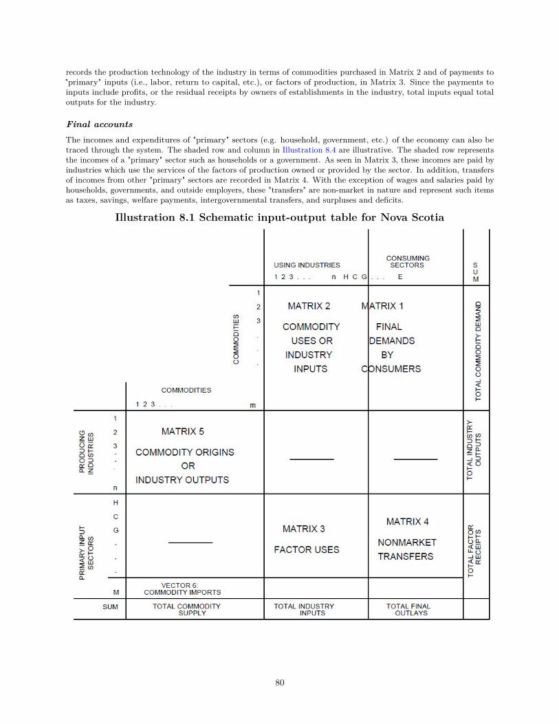
records the production technology of the industry in terms of commodities purchased in Matrix 2 and of payments to"primary" inputs (i.e., labor, return to capital, etc.), or factors of production, in Matrix 3. Since the payments toinputs include profits, or the residual receipts by owners of establishments in the industry, total inputs equal totaloutputs for the industry.

Final accountsThe incomes and expenditures of "primary" sectors (e.g. household, government, etc.) of the economy can also betraced through the system. The shaded row and column in Illustration 8.4 are illustrative. The shaded row representsthe incomes of a "primary" sector such as households or a government. As seen in Matrix 3, these incomes are paid byindustries which use the services of the factors of production owned or provided by the sector. In addition, transfersof incomes from other "primary" sectors are recorded in Matrix 4. With the exception of wages and salaries paid byhouseholds, governments, and outside employers, these "transfers" are non-market in nature and represent such itemsas taxes, savings, welfare payments, intergovernmental transfers, and surpluses and deficits.

Illustration 8.1 Schematic input-output table for Nova Scotia

80

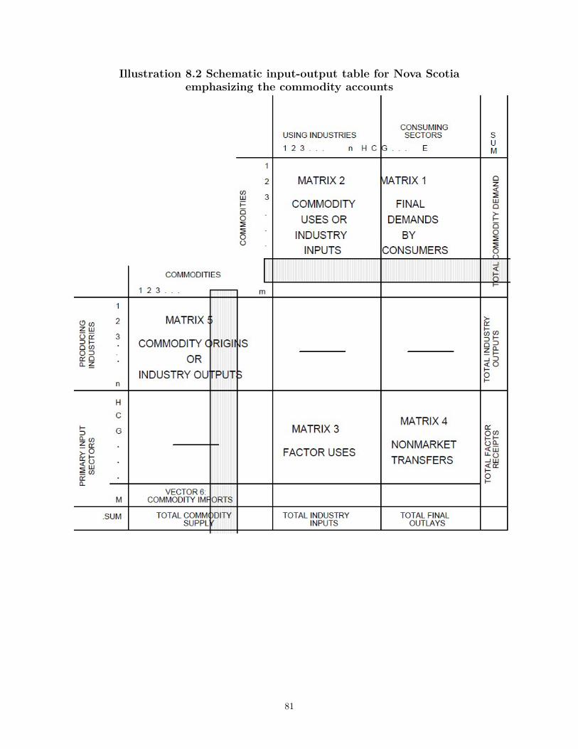
Illustration 8.2 Schematic input-output table for Nova Scotiaemphasizing the commodity accounts

81

Illustration 8.3 Schematic input-output table for Nova Scotiaemphasizing the industry accounts

82

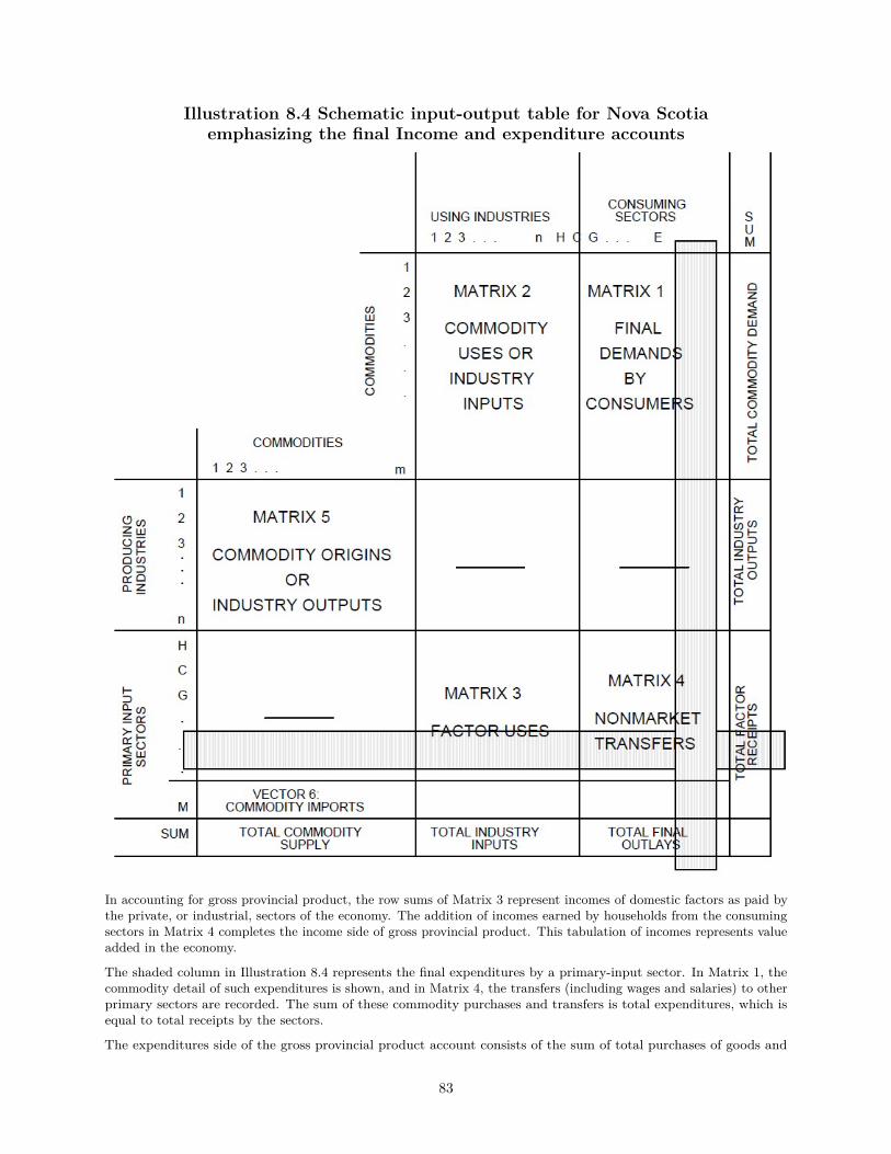
Illustration 8.4 Schematic input-output table for Nova Scotiaemphasizing the final Income and expenditure accounts

In accounting for gross provincial product, the row sums of Matrix 3 represent incomes of domestic factors as paid bythe private, or industrial, sectors of the economy. The addition of incomes earned by households from the consumingsectors in Matrix 4 completes the income side of gross provincial product. This tabulation of incomes represents valueadded in the economy.

The shaded column in Illustration 8.4 represents the final expenditures by a primary-input sector. In Matrix 1, thecommodity detail of such expenditures is shown, and in Matrix 4, the transfers (including wages and salaries) to otherprimary sectors are recorded. The sum of these commodity purchases and transfers is total expenditures, which isequal to total receipts by the sectors.

The expenditures side of the gross provincial product account consists of the sum of total purchases of goods and

83

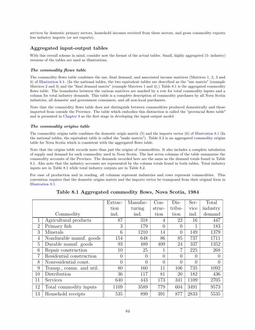
services by domestic primary sectors, household incomes received from these sectors, and gross commodity exportsless industry imports (or net exports).

Aggregated input-output tablesWith this overall scheme in mind, consider now the format of the actual tables. Small, highly aggregated (5- industry)versions of the tables are used as illustrations.

The commodity flows tableThe commodity flows table combines the use, final demand, and associated income matrices (Matrices 1, 2, 3 and4) of Illustration 8.1. (In the national tables, the two equivalent tables are described as the "use matrix" (exampleMatrices 2 and 3) and the "final demand matrix" (example Matrices 1 and 4).) Table 8.1 is the aggregated commodityflows table. The boundaries between the various matrices are marked by a row for total commodity inputs and acolumn for total industry demands. This table is a complete description of commodity purchases by all Nova Scotiaindustries, all domestic and government consumers, and all non-local purchasers.

Note that the commodity flows table does not distinguish between commodities produced domestically and thoseimported from outside the Province. The table which embodies this distinction is called the "provincial flows table"and is presented in Chapter 9 as the first stage in developing the input-output model.

The commodity origins tableThe commodity origins table combines the domestic origin matrix (5) and the imports vector (6) of Illustration 8.1 (Inthe national tables, the equivalent table is called the "make matrix"). Table 8.2 is an aggregated commodity originstable for Nova Scotia which is consistent with the aggregated flows table.

Note that the origins table records more than just the origins of commodities. It also includes a complete tabulationof supply and demand for each commodity used in Nova Scotia. The last seven columns of the table summarize thecommodity accounts of the Province. The demands recorded here are the same as the demand totals found in Table8.1. Also note that the industry accounts are represented by the column totals found in both tables. Total industryinputs are in Table 8.1 while total industry outputs are in Table 8.2.

For ease of production and in reading, all columns represent industries and rows represent commodities. Thisconvention requires that the domestic origins matrix and the imports vector be transposed from their original form inIllustration 8.1.

Table 8.1 Aggregated commodity flows, Nova Scotia, 1984

Extrac- Manufac- Con- Dis- Ser- Totaltion turing struc- tribu- vice industry

Commodity ind. ind. tion tion ind. demand1 Agricultural products 87 318 4 22 16 4472 Primary fish 3 179 0 0 1 1833 Minerals 6 1210 14 0 149 13794 Nondurable manuf. goods 154 648 86 85 737 17115 Durable manuf. goods 93 489 409 24 337 13526 Repair construction 10 25 1 7 225 2687 Residential construction 0 0 0 0 0 08 Nonresidential const. 0 0 0 0 0 09 Transp., comm. and util. 80 160 11 106 735 109210 Distribution 36 117 81 20 182 43611 Services 640 443 173 341 1109 270512 Total commodity inputs 1109 3589 779 604 3491 957313 Household receipts 535 899 391 877 2833 5535

84

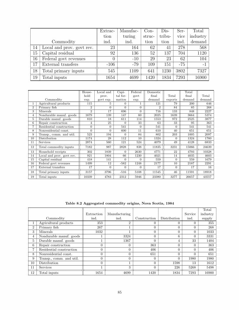
Extrac- Manufac- Con- Dis- Ser- Totaltion turing struc- tribu- vice industry

Commodity ind. ind. tion tion ind. demand14 Local and prov. govt rev. 23 164 62 41 278 56815 Capital residual 92 136 52 137 704 112016 Federal govt revenues 0 -10 29 23 62 10417 External transfers -106 -79 109 151 -75 -118 Total primary inputs 545 1109 641 1230 3802 732719 Total inputs 1654 4699 1420 1834 7293 16900

House- Local and Capi- Federal Domestic Totalhold prov. tal for- govt final Total final Total

Commodity exp. govt exp. mation exp. demand exports demand demand1 Agricultural products 115 5 0 1 121 79 200 6462 Primary fish 2 0 0 0 2 84 85 2683 Minerals 2 17 696 0 716 133 848 22274 Nondurable manuf. goods 1679 139 147 60 2025 1639 3664 53745 Durable manuf. goods 810 18 611 114 1553 972 2525 38776 Repair construction 4 25 0 33 63 33 95 3637 Residential construction 0 0 541 0 541 0 541 5418 Nonresidential const. 0 0 600 11 610 40 651 6519 Transp., comm. and util. 523 194 0 84 802 203 1005 209710 Distribution 1174 28 112 10 1324 0 1324 176011 Services 2874 560 121 524 4079 49 4128 683312 Total commodity inputs 7182 987 2828 838 11835 3231 15066 2463913 Household receipts 302 1839 0 2630 4771 22 4793 1032814 Local and prov. govt rev. 921 1804 66 1230 4021 14 4035 460315 Capital residual 418 141 0 0 559 0 559 167916 Federal govt revenues 1499 12 -582 1248 2177 10 2187 229117 External transfers 17 0 0 0 17 0 17 1618 Total primary inputs 3157 3796 -516 5108 11545 46 11591 1891819 Total inputs 10339 4783 2312 5946 23380 3277 26657 43557

Table 8.2 Aggregated commodity origins, Nova Scotia, 1984

TotalExtraction Manufacturing Service industry

Commodity ind. ind. Construction Distribution ind. supply1 Agricultural products 353 2 0 0 0 3552 Primary fish 267 1 0 0 0 2683 Minerals 1032 1 0 0 0 10334 Nondurable manuf. goods 1 3324 0 6 0 33315 Durable manuf. goods 1 1367 0 4 33 14046 Repair construction 0 0 363 0 0 3637 Residential construction 0 0 406 0 0 4068 Nonresidential const. 0 0 651 0 0 6519 Transp., comm. and util. 0 0 0 0 1980 1980

10 Distribution 0 1 0 1598 13 161211 Services 1 3 0 226 5268 549812 Total inputs 1654 4699 1420 1834 7293 16900

85

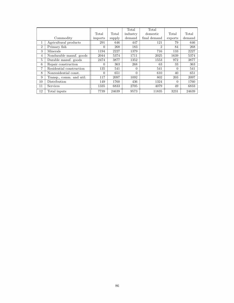
Total TotalTotal Total industry domestic Total Total

Commodity imports supply demand final demand exports demand1 Agricultural products 291 646 447 121 79 6462 Primary fish 0 268 183 2 84 2683 Minerals 1194 2227 1379 716 133 22274 Nondurable manuf. goods 2044 5374 1711 2025 1639 53745 Durable manuf. goods 2474 3877 1352 1553 972 38776 Repair construction 0 363 268 63 33 3637 Residential construction 135 541 0 541 0 5418 Nonresidential const. 0 651 0 610 40 6519 Transp., comm. and util. 117 2097 1092 802 203 2097

10 Distribution 149 1760 436 1324 0 176011 Services 1335 6833 2705 4079 49 683312 Total inputs 7739 24639 9573 11835 3231 24639

86

9 COMMODITY-BY-INDUSTRY INTERINDUSTRY MODELS:THE LOGIC OF THE NOVA SCOTIA INPUT-OUTPUTMODELIntroductionThis section develops an economic model from the accounting tables for Nova Scotia. The process parallels thatused in the traditional regional format presented in Chapter 5. It differs in that we now shift from a world in whichregional economists collect their own data into one requiring vast teams of statisticians. As seen in Chapter 8, muchnew information and detail is now available. We need more assumptions to reduce it to a manageable format.

As the literature associated with the Canadian and Atlantic Provinces input- output studies suggests, and asdemonstrated in the appendix to this chapter describing the mathematics of the U.S. system, the model could bephrased in terms of commodities. The procedures are similar, however, and the reader is referred to the earlierliterature for further details. Here we do a simple sketch.

Essentially, we manipulate the new system of accounts until the number of variables in a set of simultaneous equationsdescribing the economy equals the number of equations. The system differs slightly from the traditional squareregional matrices in that now we have not only more commodities (and so more equations) than industries but alsotwo equation systems to face! We must devise some way to redress this imbalance.

While the commodity-by-industry format traditional to the Canadian and Nova Scotia input-output systems opens upa variety of possibilities for forming this model, the approach employed here develops a solution to the model in termsof industries rather than commodities. This means that, while the economy is described initially in terms of setsof equations representing the tables of commodity-by-industry flows and origins, we must convert them to regionalflows (through application of the constant-imports assumption) and then reduce the equations to a solvable formin industry-by-industry dimensions on the basis of the fixed market-share assumption. Finally, using the constant-technology assumption, we can solve the system conventionally.

The dataWe start with two sets of tables defining the economy: The commodity flows table and the commodity origins table.Both are described in Chapter 8.

Technical conditionsNow say that final demands have been estimated for some future date and that we wish to identify the effect of thisdemand on the Province. What are the gross outputs of industries in Nova Scotia at that time? It is obvious thatthe system of flow equations is not prepared for solution: in the flows table, there are 11 equations, one for eachcommodity, and 82 variables of which only 11, the final demands, have preassigned values. Neither is the system oforigins, or make equations, which consists of 5 equations and 66 unknowns.

The minimum requirement for solution of this system is that the number of equations equals the number of unknowns.One task, therefore, is to reduce the number of unknowns. Further, the system is expressed in terms of both commodityoutputs and industry inputs, while our stated goal is to determine the effect of final-demand changes on industries.So a second task is to express the system in terms of industry variables alone. This conversion will both reduce thenumber of equations and, more importantly, permit us to establish a familiar equilibrium condition. The third andfinal task before solution is that of reducing the flows matrix from a statement of production technology to one ofregional trade. We proceed in reverse order.

The constant-imports assumptionNone of the recent regional input- output studies in this format have included survey-based or cell-specific importdetails. As a result, regional (or provincial, in this case) trade flows must be estimated by assumption. We knowimports for each commodity in the system (Table 8.2) and we know total industry domestic final demands. And thatis all, so the best way to estimate regional trade is to assume that each industry purchases imported commodities inconstant proportions:

µk = mk/(∑

jukj + ek) (9-1)

87

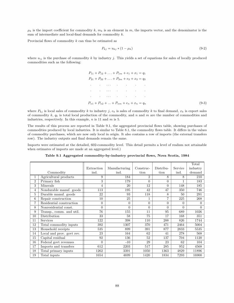
µk is the import coefficient for commodity k, mk is an element in m, the imports vector, and the denominator is thesum of intermediate and local-final demands for commodity k.

Provincial flows of commodity k can thus be estimated as

Pkj = ukj ∗ (1 − µk) (9-2)

where uij is the purchase of commodity k by industry j. This yields a set of equations for sales of locally producedcommodities such as the following:

P11 + P12 + . . .+ P1m + e1 + x1 = q1

P21 + P22 + . . .+ P2m + e2 + x2 = q2

. . . . . . . . .

. . . . . . . . .

. . . . . . . . .

Pn1 + Pn2 + ...+ Pnm + en + xn = qn (9-3)

where Pkj is local sales of commodity k to industry j, ek is sales of commodity k to final demand, xk is export salesof commodity k, qk is total local production of the commodity, and n and m are the number of commodities andindustries, respectively. In this example, n is 11 and m is 5.

The results of this process are reported in Table 9.1, the aggregated provincial flows table, showing purchases ofcommodities produced by local industries. It is similar to Table 8.1, the commodity flows table. It differs in the valuesof commodity purchases, which are now only local in origin. It also contains a row of imports (the external transfersrow). The industry outputs and final demands remain the same.

Imports were estimated at the detailed, 602-commodity level. This detail permits a level of realism not attainablewhen estimates of imports are made at an aggregated level.)

Table 9.1 Aggregated commodity-by-industry provincial flows, Nova Scotia, 1984

TotalExtraction Manufacturing Construc- Distribu- Service industry

Commodity ind. ind. tion tion ind. demand1 Agricultural products 9 184 2 8 8 2102 Primary fish 3 179 0 0 1 1833 Minerals 4 20 12 0 148 1854 Nondurable manuf. goods 113 195 42 47 350 7465 Durable manuf. goods 22 93 118 8 50 2916 Repair construction 10 25 1 7 225 2687 Residential construction 0 0 0 0 0 08 Nonresidential const. 0 0 0 0 0 09 Transp., comm. and util. 76 155 11 95 689 1026

10 Distribution 33 58 75 17 168 35111 Services 122 398 110 288 826 174412 Total commodity inputs 392 1307 370 471 2464 500413 Household receipts 535 899 391 877 2833 553514 Local and prov. govt rev. 23 164 62 41 278 56815 Capital residual 92 136 52 137 704 112016 Federal govt revenues 0 -10 29 23 62 10417 Imports and transfers 612 2203 517 285 952 456818 Total primary inputs 1262 3391 1050 1363 4829 1189619 Total inputs 1654 4699 1420 1834 7293 16900

88

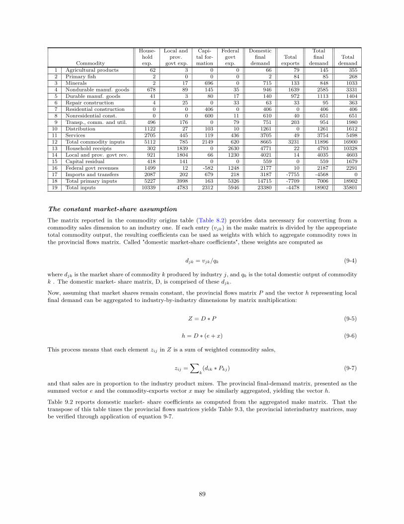
House- Local and Capi- Federal Domestic Totalhold prov. tal for- govt final Total final Total

Commodity exp. govt exp. mation exp. demand exports demand demand1 Agricultural products 62 3 0 0 66 79 145 3552 Primary fish 2 0 0 0 2 84 85 2683 Minerals 2 17 696 0 715 133 848 10334 Nondurable manuf. goods 678 89 145 35 946 1639 2585 33315 Durable manuf. goods 41 3 80 17 140 972 1113 14046 Repair construction 4 25 0 33 63 33 95 3637 Residential construction 0 0 406 0 406 0 406 4068 Nonresidential const. 0 0 600 11 610 40 651 6519 Transp., comm. and util. 496 176 0 79 751 203 954 198010 Distribution 1122 27 103 10 1261 0 1261 161211 Services 2705 445 119 436 3705 49 3754 549812 Total commodity inputs 5112 785 2149 620 8665 3231 11896 1690013 Household receipts 302 1839 0 2630 4771 22 4793 1032814 Local and prov. govt rev. 921 1804 66 1230 4021 14 4035 460315 Capital residual 418 141 0 0 559 0 559 167916 Federal govt revenues 1499 12 -582 1248 2177 10 2187 229117 Imports and transfers 2087 202 679 218 3187 -7755 -4568 018 Total primary inputs 5227 3998 163 5326 14715 -7709 7006 1890219 Total inputs 10339 4783 2312 5946 23380 -4478 18902 35801

The constant market-share assumptionThe matrix reported in the commodity origins table (Table 8.2) provides data necessary for converting from acommodity sales dimension to an industry one. If each entry (vjk) in the make matrix is divided by the appropriatetotal commodity output, the resulting coefficients can be used as weights with which to aggregate commodity rows inthe provincial flows matrix. Called "domestic market-share coefficients", these weights are computed as

djk = vjk/qk (9-4)

where djk is the market share of commodity k produced by industry j, and qk is the total domestic output of commodityk . The domestic market- share matrix, D, is comprised of these djk.

Now, assuming that market shares remain constant, the provincial flows matrix P and the vector h representing localfinal demand can be aggregated to industry-by-industry dimensions by matrix multiplication:

Z = D ∗ P (9-5)

h = D ∗ (e+ x) (9-6)

This process means that each element zij in Z is a sum of weighted commodity sales,

zij =∑

k(dik ∗ Pkj) (9-7)

and that sales are in proportion to the industry product mixes. The provincial final-demand matrix, presented as thesummed vector e and the commodity-exports vector x may be similarly aggregated, yielding the vector h.

Table 9.2 reports domestic market- share coefficients as computed from the aggregated make matrix. That thetranspose of this table times the provincial flows matrices yields Table 9.3, the provincial interindustry matrices, maybe verified through application of equation 9-7.

89

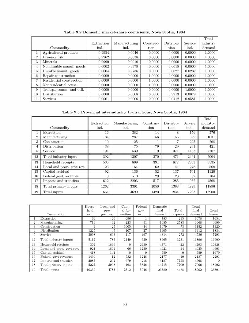
Table 9.2 Domestic market-share coefficients, Nova Scotia, 1984

TotalExtraction Manufacturing Construc- Distribu- Service industry

Commodity ind. ind. tion tion ind. demand1 Agricultural products 0.9954 0.0046 0.0000 0.0000 0.0000 1.00002 Primary fish 0.9962 0.0038 0.0000 0.0000 0.0000 1.00003 Minerals 0.9990 0.0010 0.0000 0.0000 0.0000 1.00004 Nondurable manuf. goods 0.0002 0.9979 0.0000 0.0018 0.0000 1.00005 Durable manuf. goods 0.0004 0.9736 0.0000 0.0027 0.0232 1.00006 Repair construction 0.0000 0.0000 1.0000 0.0000 0.0000 1.00007 Residential construction 0.0000 0.0000 1.0000 0.0000 0.0000 1.00008 Nonresidential const. 0.0000 0.0000 1.0000 0.0000 0.0000 1.00009 Transp., comm. and util. 0.0000 0.0000 0.0000 0.0000 1.0000 1.0000

10 Distribution 0.0000 0.0008 0.0000 0.9913 0.0079 1.000011 Services 0.0001 0.0006 0.0000 0.0412 0.9581 1.0000

Table 9.3 Provincial interindustry transactions, Nova Scotia, 1984

TotalExtraction Manufacturing Construc- Distribu- Service industry

Commodity ind. ind. tion tion ind. demand1 Extraction 16 382 14 8 156 5762 Manufacturing 134 287 156 55 399 10313 Construction 10 25 1 7 225 2684 Distribution 38 75 79 29 201 4215 Service 194 539 119 371 1483 2707

12 Total industry inputs 392 1307 370 471 2464 500413 Household receipts 535 899 391 877 2833 553514 Local and prov. govt rev. 23 164 62 41 278 56815 Capital residual 92 136 52 137 704 112016 Federal govt revenues 0 -10 29 23 62 10417 Imports and transfers 612 2203 517 285 952 456818 Total primary inputs 1262 3391 1050 1363 4829 1189619 Total inputs 1654 4699 1420 1834 7293 16900

House- Local and Capi- Federal Domestic Totalhold prov. tal for- govt final Total final Total

Commodity exp. govt exp. mation exp. demand exports demand demand1 Extraction 66 20 696 1 783 295 1078 16542 Manufacturing 719 92 223 51 1085 2583 3668 46993 Construction 4 25 1005 44 1079 73 1152 14204 Distribution 1225 45 107 27 1405 8 1412 18345 Service 3098 603 117 497 4314 272 4586 729312 Total industry inputs 5112 785 2149 620 8665 3231 11896 1690013 Household receipts 302 1839 0 2630 4771 22 4793 1032814 Local and prov. govt rev. 921 1804 66 1230 4021 14 4035 460315 Capital residual 418 141 0 0 559 0 559 167916 Federal govt revenues 1499 12 -582 1248 2177 10 2187 229117 Imports and transfers 2087 202 679 218 3187 -7755 -4568 018 Total primary inputs 5227 3998 163 5326 14715 -7709 7006 1890219 Total inputs 10339 4783 2312 5946 23380 -4478 18902 35801

90

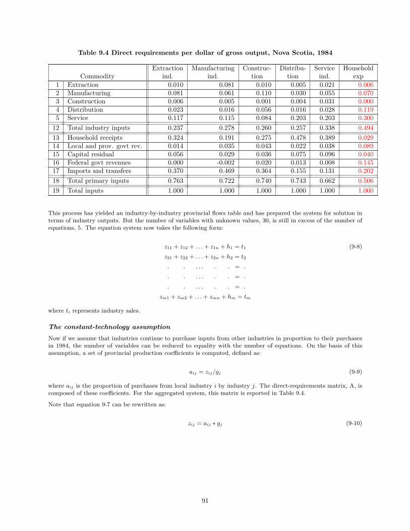
Table 9.4 Direct requirements per dollar of gross output, Nova Scotia, 1984

Extraction Manufacturing Construc- Distribu- Service HouseholdCommodity ind. ind. tion tion ind. exp

1 Extraction 0.010 0.081 0.010 0.005 0.021 0.0062 Manufacturing 0.081 0.061 0.110 0.030 0.055 0.0703 Construction 0.006 0.005 0.001 0.004 0.031 0.0004 Distribution 0.023 0.016 0.056 0.016 0.028 0.1195 Service 0.117 0.115 0.084 0.203 0.203 0.30012 Total industry inputs 0.237 0.278 0.260 0.257 0.338 0.49413 Household receipts 0.324 0.191 0.275 0.478 0.389 0.02914 Local and prov. govt rev. 0.014 0.035 0.043 0.022 0.038 0.08915 Capital residual 0.056 0.029 0.036 0.075 0.096 0.04016 Federal govt revenues 0.000 -0.002 0.020 0.013 0.008 0.14517 Imports and transfers 0.370 0.469 0.364 0.155 0.131 0.20218 Total primary inputs 0.763 0.722 0.740 0.743 0.662 0.50619 Total inputs 1.000 1.000 1.000 1.000 1.000 1.000

This process has yielded an industry-by-industry provincial flows table and has prepared the system for solution interms of industry outputs. But the number of variables with unknown values, 30, is still in excess of the number ofequations, 5. The equation system now takes the following form:

z11 + z12 + . . .+ z1n + h1 = t1 (9-8)z21 + z22 + . . .+ z2n + h2 = t2

. . . . . . . = .

. . . . . . . = .

. . . . . . . = .

zm1 + zm2 + . . .+ zmn + hm = tm

where ti represents industry sales.

The constant-technology assumptionNow if we assume that industries continue to purchase inputs from other industries in proportion to their purchasesin 1984, the number of variables can be reduced to equality with the number of equations. On the basis of thisassumption, a set of provincial production coefficients is computed, defined as:

aij = zij/gj (9-9)

where aij is the proportion of purchases from local industry i by industry j. The direct-requirements matrix, A, iscomposed of these coefficients. For the aggregated system, this matrix is reported in Table 9.4.

Note that equation 9-7 can be rewritten as:

zij = aij ∗ gj (9-10)

91

If the aij remain reasonably stable over time, aij ∗ gj can be substituted for zij in the equation system 9-8 with theneeded result:

a11 ∗ g1 + a12 ∗ g2 + . . .+ a1m ∗ gm + h1 = t1

a21 ∗ g1 + a22 ∗ g2 + . . .+ a2m ∗ gm + h2 = t2

. . . . . . . .

. . . . . . . .

. . . . . . . .

am1 ∗ g1 + am2 ∗ g2 + . . .+ amm ∗ gm + hm = tm (9-11)

The system is now reduced to a set of 5 simultaneous equations in 10 unknowns and can easily be reduced to solvabledimensions by imposing the traditional equilibrium condition.

Equilibrium condition: supply equals demandEquilibrium occurs when anticipated supply equals demand, or when the gross outputs of an industry equal its sales.So the condition is that

gj = tj (9-12)

(The condition could also be stated in terms of commodity outputs and demands.)

Solution: the total-requirements tableThe response of an economy in moving to another equilibrium position when faced with a change in demand canbe seen in the solution to the set of simultaneous equations (9-11). In terms of matrix algebra, this system may berewritten as:

A ∗ g′ + h′ = g′ (9-13)

where A is the matrix of provincial production coefficients (aij) and g′ is a column vector of gross industry outputs.h′ is a column vector of final demands for industry outputs (from equation 9-6)

The solution is analogous to that of common algebra in its formulation. Grouping the g′ terms yields:

g′ −A ∗ g′ = h′ (9-14)

while factoring produces:

(I −A) ∗ g′ = h′ (9-15)

Multiplying both sides of this equation by the inverse of (I −A) produces a solution in terms of X ′:

(I −A)−1 ∗ (I −A) ∗ g′ = (I −A)−1 ∗ h′′

or

g′ = (I −A)−1 ∗ h′ (9-16)

The inverse, (I −A)−1, is called a "total- requirements table" and shows the direct and indirect effects of a change infinal demand. Table 9.5 reports such a table for the aggregated system closed with respect to households . Table 9.6converts these numbers to “multipliers,” properly recognizing the status of households as recipient of flows of finalincomes.

Now, we are at the same stage as completed in Chapter 5, and can revert to its descriptive elements. Only a fewcomments remain on economic change in the new system.

92

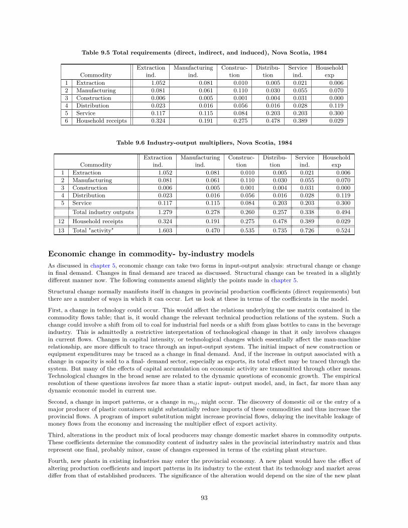
Table 9.5 Total requirements (direct, indirect, and induced), Nova Scotia, 1984

Extraction Manufacturing Construc- Distribu- Service HouseholdCommodity ind. ind. tion tion ind. exp

1 Extraction 1.052 0.081 0.010 0.005 0.021 0.0062 Manufacturing 0.081 0.061 0.110 0.030 0.055 0.0703 Construction 0.006 0.005 0.001 0.004 0.031 0.0004 Distribution 0.023 0.016 0.056 0.016 0.028 0.1195 Service 0.117 0.115 0.084 0.203 0.203 0.3006 Household receipts 0.324 0.191 0.275 0.478 0.389 0.029

Table 9.6 Industry-output multipliers, Nova Scotia, 1984

Extraction Manufacturing Construc- Distribu- Service HouseholdCommodity ind. ind. tion tion ind. exp

1 Extraction 1.052 0.081 0.010 0.005 0.021 0.0062 Manufacturing 0.081 0.061 0.110 0.030 0.055 0.0703 Construction 0.006 0.005 0.001 0.004 0.031 0.0004 Distribution 0.023 0.016 0.056 0.016 0.028 0.1195 Service 0.117 0.115 0.084 0.203 0.203 0.300

Total industry outputs 1.279 0.278 0.260 0.257 0.338 0.49412 Household receipts 0.324 0.191 0.275 0.478 0.389 0.02913 Total "activity" 1.603 0.470 0.535 0.735 0.726 0.524

Economic change in commodity- by-industry modelsAs discussed in chapter 5, economic change can take two forms in input-output analysis: structural change or changein final demand. Changes in final demand are traced as discussed. Structural change can be treated in a slightlydifferent manner now. The following comments amend slightly the points made in chapter 5.

Structural change normally manifests itself in changes in provincial production coefficients (direct requirements) butthere are a number of ways in which it can occur. Let us look at these in terms of the coefficients in the model.

First, a change in technology could occur. This would affect the relations underlying the use matrix contained in thecommodity flows table; that is, it would change the relevant technical production relations of the system. Such achange could involve a shift from oil to coal for industrial fuel needs or a shift from glass bottles to cans in the beverageindustry. This is admittedly a restrictive interpretation of technological change in that it only involves changesin current flows. Changes in capital intensity, or technological changes which essentially affect the man-machinerelationship, are more difficult to trace through an input-output system. The initial impact of new construction orequipment expenditures may be traced as a change in final demand. And, if the increase in output associated with achange in capacity is sold to a final- demand sector, especially as exports, its total effect may be traced through thesystem. But many of the effects of capital accumulation on economic activity are transmitted through other means.Technological changes in the broad sense are related to the dynamic questions of economic growth. The empiricalresolution of these questions involves far more than a static input- output model, and, in fact, far more than anydynamic economic model in current use.

Second, a change in import patterns, or a change in mij , might occur. The discovery of domestic oil or the entry of amajor producer of plastic containers might substantially reduce imports of these commodities and thus increase theprovincial flows. A program of import substitution might increase provincial flows, delaying the inevitable leakage ofmoney flows from the economy and increasing the multiplier effect of export activity.

Third, alterations in the product mix of local producers may change domestic market shares in commodity outputs.These coefficients determine the commodity content of industry sales in the provincial interindustry matrix and thusrepresent one final, probably minor, cause of changes expressed in terms of the existing plant structure.

Fourth, new plants in existing industries may enter the provincial economy. A new plant would have the effect ofaltering production coefficients and import patterns in its industry to the extent that its technology and market areasdiffer from that of established producers. The significance of the alteration would depend on the size of the new plant

93

relative to the rest of the industry. But only in exceptional cases should the impact of the structural change be moreimportant than the impact of its sales pattern.

Fifth, a completely new industry might appear in the province. This should normally be considered part of thenew-plant alternative discussed above.

In summary, structural change in input-output models is primarily a matter of changes in technical productioncoefficients, in domestic market-share coefficients, or in import coefficients.

94

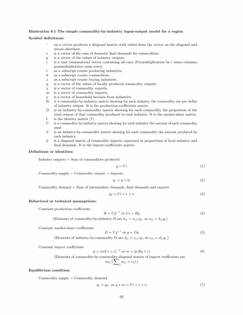
Illustration 9.1 The simple commodity-by-industry input-output model for a region

Symbol definitions:

ˆ on a vector produces a diagonal matrix with values from the vector on the diagonal andzeroes elsewhere.

e is a vector of the sum of domestic final demands for commodities.g is a vector of the values of industry outputs.i is a unit (summation) vector containing all ones (Premultiplication by i sums columns;

postmultiplication sums rows).i as a subscript counts producing industries.k as a subscript counts commodities.j as a subscript counts buying industries.q is a vector of the values of locally produced commodity outputs.x is a vector of commodity exports.m is a vector of commodity imports.y is a vector of household incomes from industriesB is a commodity-by-industry matrix showing for each industry the commodity use per dollar

of industry output. It is the production-coefficients matrix.D is an industry-by-commodity matrix showing for each commodity the proportion of the

total output of that commodity produced in each industry. It is the market-share matrix.I is the identity matrix (1)U is a commodity-by-industry matrix showing for each industry the amount of each commodity

used.V is an industry-by-commodity matrix showing for each commodity the amount produced by

each industry.µ is a diagonal matrix of commodity imports expressed as proportions of local industry and

final demands. It is the import-coefficients matrix.

Definitions or identities:

Industry outputs = Sum of commodities produced

g = V i (1)

Commodity supply = Commodity output + imports

qs = q +m (2)

Commodity demand = Sum of intermediate demands, final demands and exports

qd = Ui+ e+ x (3)

Behavioral or technical assumptions:

Constant production coefficientsB = Ug−1 or Ui = Bg (4)

(Elements of commodity-by-industry B are bij = uij/gj , so uij = bijgj)

Constant market-share coefficientsD = V q−1 or g = Dq (5)

(Elements of industry-by-commodity D are dji = vji/qi, so vji = dijqi.)

Constant import coefficientsµ = m(Ui+ e)−1 or m = µ(Bg + e) (6)

(Elements of commodity-by-commodity diagonal matrix of import coefficients aremk/(

∑jukj + ek).)

Equilibrium condition:

Commodity supply = Commodity demand

qs = qd, or q +m = Ui+ e+ x (7)

95

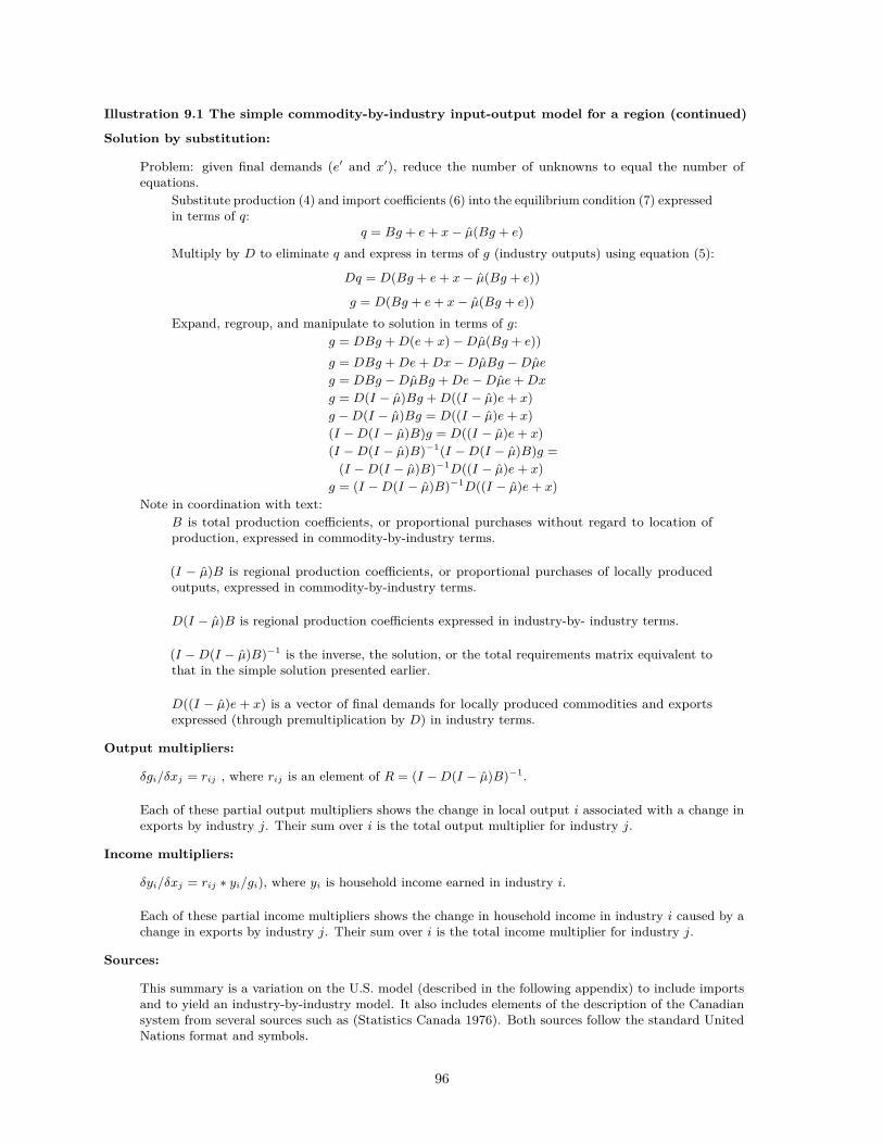
Illustration 9.1 The simple commodity-by-industry input-output model for a region (continued)

Solution by substitution:

Problem: given final demands (e′ and x′), reduce the number of unknowns to equal the number ofequations.

Substitute production (4) and import coefficients (6) into the equilibrium condition (7) expressedin terms of q:

q = Bg + e+ x− µ(Bg + e)Multiply by D to eliminate q and express in terms of g (industry outputs) using equation (5):

Dq = D(Bg + e+ x− µ(Bg + e))

g = D(Bg + e+ x− µ(Bg + e))Expand, regroup, and manipulate to solution in terms of g:

g = DBg +D(e+ x) −Dµ(Bg + e))g = DBg +De+Dx−DµBg −Dµe

g = DBg −DµBg +De−Dµe+Dx

g = D(I − µ)Bg +D((I − µ)e+ x)g −D(I − µ)Bg = D((I − µ)e+ x)(I −D(I − µ)B)g = D((I − µ)e+ x)(I −D(I − µ)B)−1(I −D(I − µ)B)g =

(I −D(I − µ)B)−1D((I − µ)e+ x)g = (I −D(I − µ)B)−1D((I − µ)e+ x)

Note in coordination with text:B is total production coefficients, or proportional purchases without regard to location ofproduction, expressed in commodity-by-industry terms.

(I − µ)B is regional production coefficients, or proportional purchases of locally producedoutputs, expressed in commodity-by-industry terms.

D(I − µ)B is regional production coefficients expressed in industry-by- industry terms.

(I −D(I − µ)B)−1 is the inverse, the solution, or the total requirements matrix equivalent tothat in the simple solution presented earlier.

D((I − µ)e+ x) is a vector of final demands for locally produced commodities and exportsexpressed (through premultiplication by D) in industry terms.

Output multipliers:

δgi/δxj = rij , where rij is an element of R = (I −D(I − µ)B)−1.

Each of these partial output multipliers shows the change in local output i associated with a change inexports by industry j. Their sum over i is the total output multiplier for industry j.

Income multipliers:

δyi/δxj = rij ∗ yi/gi), where yi is household income earned in industry i.

Each of these partial income multipliers shows the change in household income in industry i caused by achange in exports by industry j. Their sum over i is the total income multiplier for industry j.

Sources:

This summary is a variation on the U.S. model (described in the following appendix) to include importsand to yield an industry-by-industry model. It also includes elements of the description of the Canadiansystem from several sources such as (Statistics Canada 1976). Both sources follow the standard UnitedNations format and symbols.

96

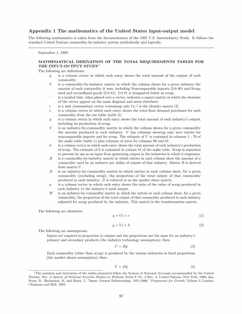
Appendix 1 The mathematics of the United States input-output modelThe following mathematics is taken from the documentation of the 1987 U.S. Interindustry Study. It follows thestandard United Nations commodity-by-industry system symbolically and logically.

September 1, 1993

MATHEMATICAL DERIVATION OF THE TOTAL REQUIREMENTS TABLES FORTHE INPUT-OUTPUT STUDY1

The following are definitions:q is a column vector in which each entry shows the total amount of the output of each

commodity.U is a commodity-by-industry matrix in which the column shows for a given industry the

amount of each commodity it uses, including Noncomparable imports (I-0 80) and Scrap,used and secondhand goods (I-0 81). I-0 81 is designated below as scrap.

ˆ is a symbol that, when placed over a vector, indicates a square matrix in which the elementsof the vector appear on the main diagonal and zeros elsewhere.

i is a unit (summation) vector containing only l’s; i is the identity matrix (I).e is a column vector in which each entry shows the total final demand purchases for each

commodity from the use table (table 2).g is a column vector in which each entry shows the total amount of each industry’s output,

including its production of scrap.V is an industry-by-commodity matrix in which the column shows for a given commodity

the amount produced in each industry. V has columns showing only zero entries fornoncomparable imports and for scrap. The estimate of V is contained in columns 1 - 79 ofthe make table (table 1) plus columns of zeros for columns 80 and 81.

h is a column vector in which each entry shows the total amount of each industry’s productionof scrap. The estimate of h is contained in column 81 of the make table. Scrap is separatedto prevent its use as an input from generating output in the industries in which it originates.

B is a commodity-by-industry matrix in which entries in each column show the amount of acommodity used by an industry per dollar of output of that industry. Matrix B is derivedfrom matrix U .

D is an industry-by-commodity matrix in which entries in each column show, for a givencommodity (excluding scrap), the proportion of the total output of that commodityproduced in each industry. D is referred to as the market share matrix.

p is a column vector in which each entry shows the ratio of the value of scrap produced ineach industry to the industry’s total output.

W is an industry-by-commodity matrix in which the entries in each column show, for a givencommodity, the proportion of the total output of that commodity produced in each industryadjusted for scrap produced by the industry. This matrix is the transformation matrix.

The following are identities:q = Ui+ e (1)

g = V i+ h (2)The following are assumptions:

Inputs are required in proportion to output and the proportions are the same for an industry’sprimary and secondary products (the industry technology assumption); then:

U = Bg (3)

Each commodity (other than scrap) is produced by the various industries in fixed proportions(the market shares assumption); then:

V = Dq (4)1The notation and derivation of the tables presented follow the System of National Accounts recommended by the United

Nations. See: A System of National Accounts Studies in Methods, Series F No. 2 Rev. 3, United Nations, New York, 1968; also,Stone, R., Bacharach, M. and Bates, J., "Input- Output Relationships, 1951-1966," Programme for Growth, Volume 3, London,Chapman and Hall, 1963.

97

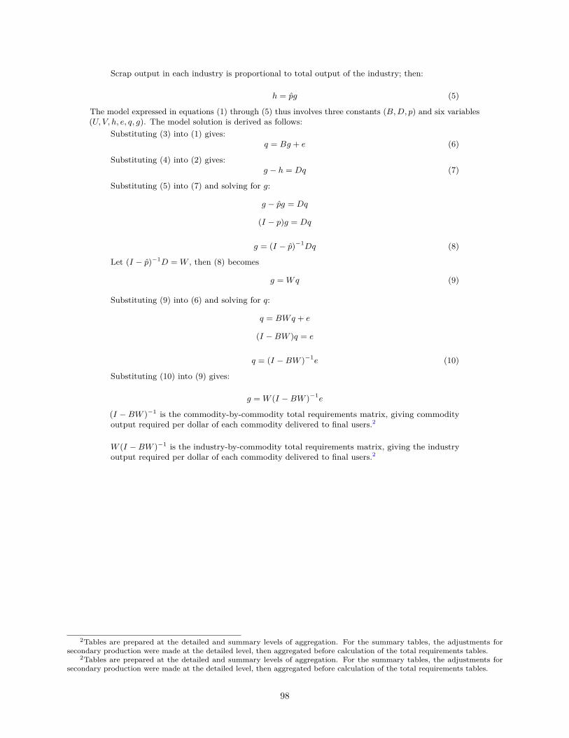
Scrap output in each industry is proportional to total output of the industry; then:

h = pg (5)

The model expressed in equations (1) through (5) thus involves three constants (B,D, p) and six variables(U, V, h, e, q, g). The model solution is derived as follows:

Substituting (3) into (1) gives:q = Bg + e (6)

Substituting (4) into (2) gives:g − h = Dq (7)

Substituting (5) into (7) and solving for g:

g − pg = Dq

(I − p)g = Dq

g = (I − p)−1Dq (8)

Let (I − p)−1D = W , then (8) becomes

g = Wq (9)

Substituting (9) into (6) and solving for q:

q = BWq + e

(I −BW )q = e

q = (I −BW )−1e (10)

Substituting (10) into (9) gives:

g = W (I −BW )−1e

(I − BW )−1 is the commodity-by-commodity total requirements matrix, giving commodityoutput required per dollar of each commodity delivered to final users.2

W (I −BW )−1 is the industry-by-commodity total requirements matrix, giving the industryoutput required per dollar of each commodity delivered to final users.2

2Tables are prepared at the detailed and summary levels of aggregation. For the summary tables, the adjustments forsecondary production were made at the detailed level, then aggregated before calculation of the total requirements tables.

2Tables are prepared at the detailed and summary levels of aggregation. For the summary tables, the adjustments forsecondary production were made at the detailed level, then aggregated before calculation of the total requirements tables.

98

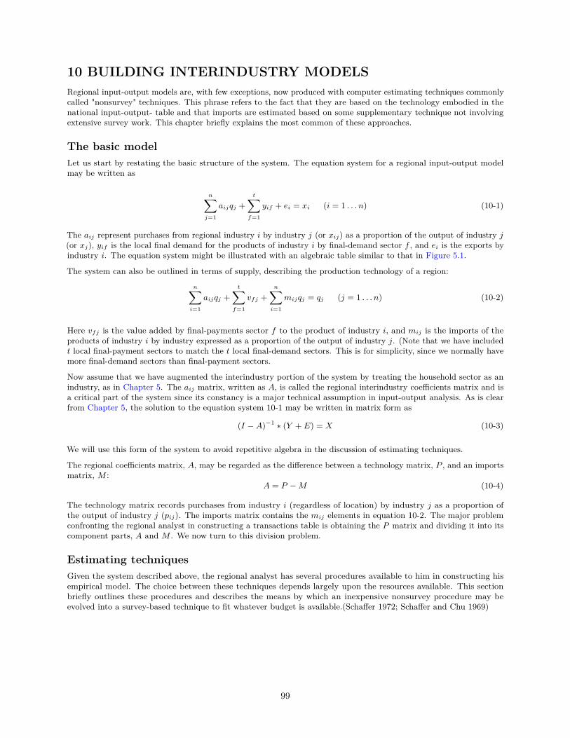
10 BUILDING INTERINDUSTRY MODELSRegional input-output models are, with few exceptions, now produced with computer estimating techniques commonlycalled "nonsurvey" techniques. This phrase refers to the fact that they are based on the technology embodied in thenational input-output- table and that imports are estimated based on some supplementary technique not involvingextensive survey work. This chapter briefly explains the most common of these approaches.

The basic modelLet us start by restating the basic structure of the system. The equation system for a regional input-output modelmay be written as

n∑j=1

aijqj +t∑

f=1

yif + ei = xi (i = 1 . . . n) (10-1)

The aij represent purchases from regional industry i by industry j (or xij) as a proportion of the output of industry j(or xj), yif is the local final demand for the products of industry i by final-demand sector f , and ei is the exports byindustry i. The equation system might be illustrated with an algebraic table similar to that in Figure 5.1.

The system can also be outlined in terms of supply, describing the production technology of a region:

n∑i=1

aijqj +t∑

f=1

vfj +n∑

i=1

mijqj = qj (j = 1 . . . n) (10-2)

Here vfj is the value added by final-payments sector f to the product of industry i, and mij is the imports of theproducts of industry i by industry expressed as a proportion of the output of industry j. (Note that we have includedt local final-payment sectors to match the t local final-demand sectors. This is for simplicity, since we normally havemore final-demand sectors than final-payment sectors.

Now assume that we have augmented the interindustry portion of the system by treating the household sector as anindustry, as in Chapter 5. The aij matrix, written as A, is called the regional interindustry coefficients matrix and isa critical part of the system since its constancy is a major technical assumption in input-output analysis. As is clearfrom Chapter 5, the solution to the equation system 10-1 may be written in matrix form as

(I −A)−1 ∗ (Y + E) = X (10-3)

We will use this form of the system to avoid repetitive algebra in the discussion of estimating techniques.

The regional coefficients matrix, A, may be regarded as the difference between a technology matrix, P , and an importsmatrix, M :

A = P −M (10-4)

The technology matrix records purchases from industry i (regardless of location) by industry j as a proportion ofthe output of industry j (pij). The imports matrix contains the mij elements in equation 10-2. The major problemconfronting the regional analyst in constructing a transactions table is obtaining the P matrix and dividing it into itscomponent parts, A and M . We now turn to this division problem.

Estimating techniquesGiven the system described above, the regional analyst has several procedures available to him in constructing hisempirical model. The choice between these techniques depends largely upon the resources available. This sectionbriefly outlines these procedures and describes the means by which an inexpensive nonsurvey procedure may beevolved into a survey-based technique to fit whatever budget is available.(Schaffer 1972; Schaffer and Chu 1969)

99

Survey-only techniquesProperly, an input-output model is based on a full survey of industries and final consumers which documents bothsales and purchases. Each respondent is asked to designate sales to regional industries (xij) and to final users inside(yif ) and outside (ei) the region. The respondents are also asked to designate their purchases from regional industries(aijqj), their purchases from industries outside the region (mijxj), and their final payments (vfj) to primary resourceowners in the form of wages and salaries, profits, depreciation allowances, taxes, etc. These purchases and finalpayments outline the production technology of each industry in a usable format, already separated into a regionalflows matrix and an imports matrix.

In acquiring data on both purchases and sales, the analyst has assembled the information required to produce apotentially reliable table. But the table is also very expensive and its construction is very time consuming. Noticewhat happens if you don’t have a complete census of firms and perfect reporting in each case. In this perfect case, therow estimates of xij will be identical to the column estimates. Now notice what happens if you have sampled only afew firms: the row estimates and the column estimates now vary widely. Sampling problems and reporting errorsare substantial and the analyst is forced to achieve balance by tediously assaying the reliability of responses and byjuggling numbers until totals finally match.

A basic alternative to this full-survey approach is the “rows-only” method. First used by Hansen and Tiebout, thismethod assumes

... that firms know the destination of their outputs far better than the origin of their inputs, especiallywhere regional breakdowns are required. In other words, in terms of input- output flows, information forthe "rows" is easier to obtain than information for the "columns.” The reason for this is that the bundleof inputs is usually so varied and complex that their origins are difficult even for firms involved to trackdown accurately. However, the same firms are especially concerned with where and to whom they selltheir output. (Hansen and Tiebout 1963)

This approach permits the analyst to avoid a complex data reconciliation. It produces only one entry per cell in thetransactions table; the full-survey method forces the analyst to check his work by producing two estimates of cellvalues.

A second alternative to the full-survey approach is what is called the “columns- only” method. This approach assumesthat business firms know their sources of supply better than they do the locations of their customers. Harmston andLund argue that this approach takes advantage of the detailed knowledge of expenditures required by businessmen forcontrol and tax purposes (Harmston and Lund 1967). Producing data in the same simple form as that of the rows-only method, the columns-only approach seems well-suited for use in small regions characterized by a relatively largenumber of locally-owned firms.

The supply-demand pool procedureA nonsurvey technique commonly used in the United States, the supply-demand pool technique relies on the nationalinput-output table as a reasonable estimate of the production- technology matrix, or P matrix, of a region andproceeds to estimate regional flows and imports using the concept of regional commodity balances (Isard 1953). Thismethod is sometimes called the Moore-Petersen technique since it was first applied to a study of Utah by Moore andPetersen (Moore and Petersen 1955).

The only additional data assumed to be available are gross outputs for the n regional industries, qj , and the grosspurchases of t final-demand sectors. Now, to avoid more complex addition, let us assume that the P matrix includesboth industries and final-demand sectors, so A is of dimension n ∗ (n+ 1). Value added is three rows in the nationaltable and has been excluded from P .

Let di be the row sum of total demands for the products of industry i, computed from A as follows:

di =n+t∑j=1

pijxj (10-5)

Here, of course, the pij have been computed from the national input-output table and we have simply reduced nationalflows to regional size.

A commodity-balance ratio comparing regional production or supply (qi) with regional demand can be computed as

bi = qi/di (10-6)

100

and the P matrix can be divided into its A and M components through a simple set of rules. If bi is greater than orequal to one, then all inputs can be supplied by local producers and we can set aij = pij , mij = 0, and ei = qi − di. Ifbi is less than one, inputs must be imported, so aij = bipij , mij = pij − aij and ei = 0.

This pool procedure allocates local production, when adequate, to meet local needs; when the local output is inadequate,it allocates to each purchasing industry i a share of regional output qi based on the needs of the purchasing industryitself (pijqj) relative to total needs for output i(di).

Export-survey methodOne of the major characteristics of a regional input-output model is its openness. Exports and imports are substantial,if not dominant, parts of the typical regional transactions table. Since simulated exports are so greatly at variance withthe survey-based exports in the above comparison, it seems reasonable to believe that correction of this discrepancycould lead to a much better estimate of regional transactions.

If we can afford neither of the more powerful alternatives to a full survey as discussed above, then an export surveycombined with a supply-demand pool procedure may be an adequate substitute. This approach requires that wesimply canvass firms in the region, asking for three bits of information: their industry classification, value of sales forthe year, and the proportion of their sales going to out-of-region purchasers. The first two answers permit the analystto classify replies and to properly weight export proportions in constructing the transactions table.

The procedure, then, involves setting exports of each industry i at the survey-estimated value and simulating theremainder of the table. For the balance ratio used above, we simply substitute a ratio which excludes exports fromthe supply available for local use:

bei = qi − ei

di(10-7)

This approach satisfies export requirements first and then allocates the remainder of local production to satisfyinglocal needs in proportion to requirements. If be

i is greater than one, the technology matrix may have to be adjusted,but this proves to be a minor problem.

Selected-values methodNow, if more trade information than just export estimates can be assembled, the method can be extended to permit asetting of selected values in the transactions table. We simply set observed values xig, xih, ..., xik and estimate theremaining regional flows using an adjusted balance ratio:

bsi = qi − ei − xig − xih − . . .− xik

di − xig − xih . . .− xik(10-8)

Known-trade methodThe development of the commodity- origins table in the new commodity-by-industry format suggested a slight variationon this system. What if we know some imports as well as some exports? This makes the formula into

bki = qi −mi − ei

di(10-9)

Here the numerator contains supply available for local use (local supply is equal to local demand less imports andlocal supply less exports is the amount available for local use) while the denominator is simply local demands. Thismethod would be used if a local survey provided technical coefficients and estimates of imports and exports, as wasthe case in our Nova Scotia study (DPA Group Inc. and Schaffer 1989).

This method is tricky when both imports and exports are "known" for the same commodity. The supply-demandequation has to balance, and this surely means that one of the known values has to be adjusted. Tricky, but that’sstatistics.

101

11 REGIONAL GROWTH MODELSExport-base theory of regional growthThe enduring theme of mercantilismExporting as a source of growth is almost overbearing: we can observe it so easily, and it permeates the literature onlocal growth. It is appropriate to start by recalling our first model to the stage.

The shortcomings of a static modelThe usual economic-base study (and certainly the usual economic-base model) makes no distinction between short-runand long-run considerations. Multiplier analyses derived from economic-base models focus on short-run changes indemand. But determinants of growth, a long-run phenomenon, must include supply-based issues as well. Natural andhuman resources as well as available technology ultimately underlie a region’s ability to grow. (Lane, 1966, 342)

Exports and long-run growthThe relationship between exports and long-run growth can be shown with a set of production-possibilities curvestaken from the typical presentation in principles of economics (based on Lane, 1966, 345-7). Consider a simplelocal economy. With a vertical axis representing service goods and a horizontal axis representing export goods,draw a curve concave to the origin in the positive quadrant at some arbitrary position. This curve representsthe full-employment output combinations of service and export goods available at this particular time, givenresources and technology. Assume we are at point X, representing production of two units of service goods to oneof export goods. (This position is determined by tangency with a budget line representing total income, givenprices of local and export goods. Actually, it may be much more complicated than this, since export income isspent on imported goods and the prices of these goods must be taken into consideration. But this is another exer-cise.) What happens when we increase production of export goods? How is economic growth illustrated in this diagram?

102

Economic growth requires two sets of factors, permissive and implemental. The permissive factors are the resourcesavailable to the economy: natural resources, human resources, technology, capital, etc. They determine the position ofthe curve at any particular time. The curve ab is based on a given set of permissive factors; the curve cd is based onanother and larger set. (They are concave to the origin because of the law of diminishing returns and the imperfectadaptability of resources.) Implemental factors are those which cause change to happen, which cause a shift from abto cd.

The primary implemental factor in export-base theory is export demand. Any increase in aggregate demand, whetherlocal investment or exports, may move the economy from an unemployed state (W ) to a fully employed state (sayX) Any further increase in export demand (with no increase in resources) will cause a shift along the production-possibilities curve (along ab). The cost of this increase is a decrease in production of service goods as resources areshifted from one sector to the other.

The increase in factor prices (e.g. wages) now stimulates in-migration (or even commuting). Since a region has nooverpowering economic boundaries, the resources available are now increased and growth occurs: the production-possibilities curve now shifts out to a new and higher level, to point Z.

As an aside, note that the export-base multiplier describes this path. The marginal multiplier value is one plus theslope of the path from one equilibrium point to another; the average multiplier is one plus the slope of a line from theorigin to the particular equilibrium point (T/B = (B + S)/B = 1 + S/B). If the tradeoff ratio between local andexport goods remains constant and the shift in the frontier is neutral (parallel to the previous frontier, reflecting noeconomies of scale in producing one good or the other), the expansion path should be a straight line and the multipliershould thus be constant. If the export goods cost more to produce (in terms of service goods) or show diseconomiesof scale with expansion, then the expansion path would tend to rise at a diminishing rate and the multiplier woulddecline.

(This could be much more complex. What we really might compare is the tradeoff in consumption between local goodsand imported goods, given prices. Then we would need to look at tradeoffs in production between local goods andexport goods. Where we settle is reflected by the eventual diminution of our comparative advantage in producing theexport goods relative to imported goods.)

We will come back to this important issue of factor mobility and substitutability when we look at the neoclassicalmodel.

An interesting approach to the economic base and regional growth was taken in the early literature by Charles Leven(Leven, 1964).

The fundamental assumption underlying the economic base idea is simple and uncomplicated. Specifically,base theory assumes that the only reason for concentrating economic activities in a central location is thehigher income made available to the inhabitants of the locality or region via increased returns to factorsof production as a consequence of economies of scale. For many industries the achievement of such a scale,however, requires production far in excess of that demanded by the local market. This leads to regionalspecialization, and the institutional factor necessary to permit the exploitation of such scale economies istrade among regions.

Nonbasic industries are those whose economies of scale are exhausted within the region. Basic industries are thosewhich require demand from outside markets to realize economies of scale.

Leven points out several shortcomings of the export-base approach to regional growth. One critical flaw is that itfocuses on growth in output alone. With the assumption that basic and nonbasic activities grow in constant proportion,per capita income would not rise through export growth alone, even though incomes may differ in the two sectors.Growth in per capita income requires a change in productivity under these conditions. In fact, Leven builds a case forchange in productivity or technology as the real basis for growth with the following simple example:

Suppose three persons are living on a remote island. Suppose that two are barbers and one a masseur,and that they provide each other with personal services, otherwise living on wild nuts and berries.Under such conditions increased productivity in their primary occupations would lead to increased realincome. This greater productivity initially might take the form of increased leisure for all of them.But it also might result in a sufficient increase in the price of entertainment (i.e., in the number ofhaircuts required for one entertainment), the price of massages (in terms of haircuts) remaining thesame, to induce one of the barbers to forsake his shears for a fiddle. Or, in the absence of a lack ofmusical ability on the part of any of the aboriginal inhabitants, they might bid up the price of musical

103

entertainment sufficiently high to persuade a musician to immigrate to their island. Quite clearly growthin per capita income could proceed indefinitely without external trade limited only by the productivityof the inhabitants of the island and the possible gains from the division of labor. Accompanyinggrowth in the island’s population could also increase indefinitely without external trade, limited onlyby the foregoing limitations and by a continued differential of per capita real income of the islandersover levels someplace else, including full allowance for detractions to real income stemming from congestion.

But there is something else that is also likely to happen to the island’s economy. Specifically, opportunitiesfor the division of labor are not likely to be fully realized within the island alone. Comparative advantagesin production most probably would arise and trade with other regions would occur. Moreover, so longas the possibility of gains from trade are not exhausted, the absolute volume of trade would increasealong with the increase in the island’s total population. Basically, then, in this example the driving forcebehind economic growth is rising productivity. This is hardly a very startling statement. Such increasedproductivity could stem from increases in the stock of physical capital, but also from increases in the stockof human capital, from discovering resources, from invention, or from a change in tastes. The increases inthe volume of trade is simply an expected consequence of market adjustments to higher productivity. Itis generated mainly by the proliferation rather than intensification of human wants as real income rises,and by secular changes in technology which tend to increase the technological possibilities for exploitingthe division of labor.

After building his arguments regarding these two explanations of regional growth, he posits three hypotheses. Thefirst two explain differential rates of regional growth in terms consistent with economic base theory: the "market"hypothesis and the "ignorance" hypothesis. The third hypothesis based on the productivity theory of growth may becalled the "capital deficiency" hypothesis.

The "market" hypothesis says that "an area’s growth rate depends upon the export demand for goods and services inwhich the area has a delivered cost advantage." This hypothesis leads to development policies focusing on productpromotion and resource discovery. But Leven does not think these would be extremely effective. Product promotion isnot necessarily place-specific, and one tends to look for specific resources wherever they may be most likely, not justfor "more ’things’ in Pennsylvania." He also contends that

The search for technological advance, similarly, is related to processes rather than places. Thus thereis reason to be skeptical about what could be accomplished by focusing the search for resources andtechnology on "places" rather than on input needs or production processes.

The "ignorance" hypothesis" assumes

...that lagging growth in a particular region mainly is a consequence of potential new firms or firms inother areas being unaware of the profit opportunities in the region. The resultant implied policy is thetraditional regional promotion approach -- in its crudest form simply fatuous pronouncements aboutparks, churches, and playgrounds, the superior caliber of its workers, or its friendly attitude towardsbusiness; and more rationally, in terms of assembled information on wage rates, power costs, water quality,and other information on input costs and quality and transportation facilities and rates.

Again, he is less than sanguine on the usefulness of promotion policies.

Leven prefers policies which stem from the "capital deficiency" hypothesis. This hypothesis assumes "that the majorproblem is plant obsolescence, the low quality of the labor force or deficiencies in social overhead capital." To stimulateregional development we must divert resources toward internal capital improvements, toward building the socialinfrastructure. Leven feels that this policy would have broader effectiveness than export-base policies. Unfortunately,it involves much greater risk and financial commitment.

The Harrod-Domar model of regional growthIllustration 11.1 outlines the evolution of an export-base model of regional growth based on the "Harrod-Domar"model.

104

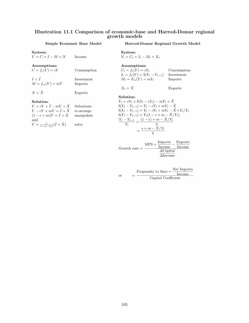
Illustration 11.1 Comparison of economic-base and Harrod-Domar regionalgrowth models

Simple Economic Base Model

System:Y = C + I −M +X Income

Assumptions:C = fc(Y ) = cY Consumption

I = I InvestmentM = fm(Y ) = mY Imports

X = X Exports

Solution:Y = cY + I −mY + X SubstituteY − cY +mY = I + X re-arrange(1 − c+m)Y = I + X manipulateandY = 1

1−(c−m) (I + X) solve

Harrod-Domar Regional Growth Model

System:Yt = Ct + It −Mt +Xt

Assumptions:Ct = fc(Y ) = cYt ConsumptionIt = fI(Y ) = b(Yt − Yt−1) InvestmentMt = Fm(Y ) = mYt Imports

Xt = X Exports

Solution:Yt = cYt + b(Yt − cYt) −mYt + Xb(Yt − Yt−1) = Yt − cYt +mYt − Xb(Yt − Yt−1) = Yt − cYt +mYt − X ∗ Yt/Yt

b(Yt − Yt−1) = Yt(1 − c+m− X/Yt)Yt − Yt−1

Yt= (1 − c) +m− X/Yt

b

= s+m− X/Yt

b

Growth rate =MPS + Imports

Income − ExportsIncome

∆Capital∆Income

or =Propensity to Save + Net Imports

IncomeCapital Coefficient

105

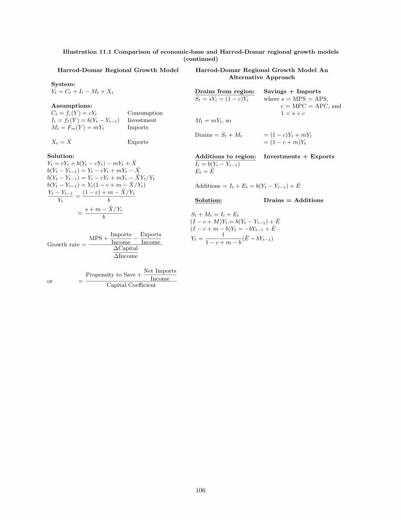
Illustration 11.1 Comparison of economic-base and Harrod-Domar regional growth models(continued)

Harrod-Domar Regional Growth Model

System:Yt = Ct + It −Mt +Xt

Assumptions:Ct = fc(Y ) = cYt ConsumptionIt = fI(Y ) = b(Yt − Yt−1) InvestmentMt = Fm(Y ) = mYt Imports

Xt = X Exports

Solution:Yt = cYt + b(Yt − cYt) −mYt + Xb(Yt − Yt−1) = Yt − cYt +mYt − Xb(Yt − Yt−1) = Yt − cYt +mYt − XYt/Yt

b(Yt − Yt−1) = Yt(1 − c+m− X/Yt)Yt − Yt−1

Yt= (1 − c) +m− X/Yt

b

= s+m− X/Yt

b

Growth rate =MPS + Imports

Income − ExportsIncome

∆Capital∆Income

or =Propensity to Save + Net Imports

IncomeCapital Coefficient

Harrod-Domar Regional Growth Model AnAlternative Approach

Drains from region: Savings + ImportsSt = sYt = (1 − c)Yt where s = MPS = APS,

c = MPC = APC, and1 = s+ c

Mt = mYt, so

Drains = St +Mt = (1 − c)Yt +mYt

= (1 − c+m)Yt

Additions to region: Investments + ExportsIt = b(Yt − Yt−1)Et = E

Additions = It + Et = b(Yt − Yt−1) + E

Solution: Drains = Additions

St +Mt = It + Et

(I − c+M)Yt = b(Yt − Yt−1) + E(I − c+m− b)Yt = −bYt−1 + E

Yt = 11 − c+m− b

(E − bYt−1)

106

REFERENCESArtle, R. (1965). The Structure of the Stockholm Economy (American Edition), Cornell University Press, Ithaca.

Barnard, J. R. (1967). Design and Use of Social Accounting Systems in State Development Planning, The Universityof Iowa, Bureau of Business and Economic Research, Iowa City.

Bourque, P. J., and Conway, R. S., Jr. (1977). The 1972 Washington Input-Output Study, University of Washington,Graduate School of Business Administration, Seattle.

Bourque, P. J., and others. (1967). The Washington Economy and Input-Output Study, University of Washington,Graduate School of Business Administration, Seattle.

Bowers, D. A., and Baird, R. N. (1971). Elementary Mathematical Macroeconomics, Printice-Hall, Inc., EnglewoodCliffs.

Brucker, S. M., and Hastings, S. E. (1984). An Interindustry Analysis of Delaware’s Economy, University of Delaware,Agricultural Experiment Station, Bulletin 452, Newark.

Carden, J. G. D., and Whittington, F. G. J. (1964). Studies in the Economic Structure of the State of Mississippi,Mississippi Industrial and Technological Research Commission, Jackson.

Case, K. E., and Fair, R. C. (1994). Principles of Economics, Prentice-Hall, Inc., Englewood Cliffs.

Chenery, H. B., and Clark, P. G. (1959). Interindustry Economics, John Wiley and Sons, New York.

DPA Group Inc., and Schaffer, W. (1989). The Nova Scotia Input-Output System, 1984, The DPA Group, Inc.,Halifax.

Gamble, H. B., and Raphael, D. L. (1966). A Microregional Analysis of Clinton County, Pennsylvania, Volume II,The Pennsylvania State University, University Park.

Ghali, M. (1977). “Tourism and regional growth: An empirical study of the alternative growth paths for Hawaii.”Studies in applied regional science, Martinus Nijhoff Social Sciences Division, Leiden.

Harmston, F. K. (1962). A Study of the Resources, People, and Economy of Carbon County, Wyoming, 1962, WyomingNatural Resource Board, Cheyenne.

Hildebrand, G. H., and Mace, A., Jr. (1950). “The Employment Multiplier in an Expanding Industrial Market: LosAngeles County, 1940-47.” Review of Economics and Statistics, XXXII, 241-249.

Hirsch, W. Z. (1959). “Interindustry Relations of a Metropolitan Area.” Review of Economics and Statistics, 41,360-369.

Isard, W., Choguill, C. L., Kissin, J., Seyfarth, R. H., and Tatlock, R. (1972). Ecologic-Economic Analysis for RegionalDevelopment, The Free Press, New York.

Isard, W. e. a. (1960). Methods of Regional Analysis: an Introduction to Regional Science, The M.I.T. Press,Cambridge, Massachusetts.

Jordan, P. G., and Polenske, K. R. (1988). “Multiplier Impacts of Fishing Activities in New England Nova Scotia.”Input-Output Analysis: Current Developments, M. Ciaschini, ed., Chapman Hall, London, 326-366.

Kahn, R. F. (1931). “The Relation of Home Investment to Unemployment.” Economic Journal, XLI, 173-198.

Keynes, J. M. (1936). The General Theory of Employment, Interest, Money, MacMillan, London.

Kogiku, K. C. (1968). An Introduction to Macroeconomic Models, McGraw-Hill Book Company, New York.

Krikelas, A. C. (1992). “Why Regions Grow: A Review of Research On the Economic Base Model.” Economic Reviewof the Federal Reserve Bank of Atlanta, 16-29.

Lane, T. (1966). “The Urban Base Multiplier: An Evaluation of the State of the Art.” Land Economics, 42, 339-347.

Leontief, W. (1953). “Interregional Theory.” Studies in the Structure of the American Economy, W. L. a. others, ed.,New York.

Levitt, K. (1975a). Input-Output Study of the Atlantic Provinces, 1965. Vol. I: Structural Analysis Data Sources,Statistics Canada, Input-Output Division, Ottawa.

107

Levitt, K. (1975b). Input-Output Study of the Atlantic Provinces, 1965. Vol. I: Social Accounting Matrix Models,Statistics Canada, Input-Output Division, Ottawa.

Metzler, L. A. (1950). “A Multiple-Region Theory of Income and trade.” Econometrica, 18, 329- 354.

Miernyk, W. H. (1965). The Elements of Input-Output Analysis, Random House, New York.

Miernyk, W. H., Bonner, E. R., Chapman, J. H., Jr., and Shellhammer, K. (1967). Impact of the Space Program on aLocal Economy, West Virginia University Library, Morgantown.

Miller, R. E., and Blair, P. D. (1985). Input-Output Analysis: Foundations and Extensions, Prentice-Hall, Inc.,Englewood Cliffs, NJ.

Minnesota IMPLAN Group Inc. (1997). IMPLAN Professional, MIG, Inc., Stillwater, MN.

Miyazawa, K. (1976). Input-Output Analysis and the Structure of Income Distribution, Springer- Verlag, Berlin.

Moore, F. T. (1955). “Regional Economic Reaction Paths.” American Economic Review, 45, 133- 148.

Moore, F. T., and Petersen, J. W. (1955). “Regional Analysis: An Interindustry Model of Utah.” Review of Economicsand Statistics, 37, 368-383.

Neal, F., and Shone, R. (1976). Economic Model Building, Macmillan Press Ltd, London.

Oser, J. (1963). The Evolution of Economic Thought, Harcourt, Brace and World, Inc., New York.

Polenske, K. R. (1980). The U. S. Multiregional Input-Output Accounts and Model, D.C. Heath and Company,Lexington, Massachusetts.

Pratt, R. T. (1968). “An Appraisal of the Minimum Requirements Technique.” Economic Geography, XLIV, 117-124.

Richardson, H. W. (1969). Regional Economics, Praeger Publishers, Inc., New York.

Richardson, H. W. (1972). Input-Output and Regional Economics, Weidenfeld and Nicolson.

Schaffer, W. A. (1976). On the use of input-output models for regional planning, Martinus Nijhoff, Leiden.

Schaffer, W. A., and Chu, K. (1969). “Nonsurvey Techniques for Constructing Regional Interindustry Models.”Regional Science Association Papers, 23, 83-101.

Schaffer, W. A., Joun, R. Y., and others. (1972). Interindustry Study of the Hawaiian Economy, Department ofPlanning and Economic Development, State of Hawaii, Honolulu.

Sirkin, G. (1959). “The Theory of the Regional Economic Base.” Review of Economics and Statistics, 59, 426-429.

Smith, P., and Morrison, W. I. (1974). Simulating the Urban Economy, Pion Limited, London.

Tiebout, C. M. (1962). The Community Economic Base Study, Committee for Economic Development, New York.

Ullman, E. L., and Dacey, M. F. (1960). “The Minimum Requirements Approach to the Urban Economic Base.”Regional Science Association Papers, 6, 175-194.

Wang, X. and Hofe, R. (2008). Research methods in urban and regional planning. Springer Science & Business Media.

Weiss, S. J., and Gooding, E. C. (1968). “Estimation of Differential Employment Multipliers in a Small RegionalEconomy.” Land Economics, XLIV, 235-244.

108