CCIIFF CCeennttrroo ddee IInnvveessttiiggaacciióónn eenn FFiinnaannzzaass

ESCUELA DE NEGOCIOS

Universidad Torcuato Di Tella

Documento de Trabajo 13/2002

Reforming Capital Requirements in Emerging Countries

Andrew Powell

Universidad Torcuato Di Tella

Verónica Balzarotti BCRA

Christian Castro

UPF

Miñones 2177, C1428ATG Buenos Aires • Tel: 4784.0080 interno 181 y 4787.9394 • Web site: www.utdt.edu/departamentos/empresarial/cif/cif.htm

Reforming Capital Requirements in Emerging Countries:

Calibrating Basel II using Historical Argentine Credit Bureau Data and CreditRisk+

Verónica Balzarotti, Christian Castro and Andrew Powell1

November 2002

Preliminary draft, comments welcome Paper prepared for World Bank project on Credit Risk Measurement and Capital Regulations in Emerging Economies. To be presented at the joint World Bank - Financial Stability Institute Workshop on November 21s1t 2002, Basel, Switzerland. Please send comments to third author: apowell@utdt.edu

1 First author Central Bank of Argentina, second author Pompeau Fabrá, Barcelona, third author Universidad Torcuato Di Tella, Buenos Aires. This paper represents strictly the views of the authors and not necessarily the views of the Central Bank of Argentina, the World Bank or any other institution. We are grateful to the World Bank for support. We thank Giovanni Majnoni, Margaret Miller and all participants of the preliminary September meeting of the World Bank project on Credit Risk Measurement and Capital Regulation in Washington for helpful comments. All mistakes remain our own.

2

Introduction The 1988 Basel Accord (Basel I) has been widely recognized as a significant advance in establishing an internationally recognized language to analyze and compare capital across different jurisdictions (summarized in the concept of assets at risk) and in attempting to establish a level playing field for international bank competition2. Indeed, Basel I was so successful as a financial standard that is has been explicitly adopted in more than 100 countries and, in many jurisdictions, applied not only to 'internationally active banks' but rather, to all banks3. At the same time, Basel I has come under increasing criticism, especially for the very broad definitions of asset classes and corresponding risk weights that lie behind the measurement of 'assets at risk' coupled with the lack of any portfolio dimension. As banks' own models of credit risk measurement have become more sophisticated, this has driven a wedge between the concepts of 'regulatory' and 'economic' capital. The regulatory response to this growing wedge has been the set of new proposals embodied in Basel II that attempts to bring regulatory capital closer to the banks' own measurement of economic capital. Basel II retains the focus on "internationally active banks" and yet in the majority of the 100 or so countries that have actually implemented Basel I, the action is elsewhere. In the majority of these countries, the universe of rated claims is highly restricted, limiting the relevance of the standardized approach. On the other hand, the IRB approaches as they stand appear complex for an emerging economy regulator to consider implementing. And yet at the same time, many emerging countries have developed interesting policies with respect to information systems on credit risk. Indeed, perhaps given the history of severe banking crises sparked by problems of related lending, some have gone much further in collecting finer information on financial system claims than their G10 counterparts. These public credit registries (PCR's) are typically now used to set and monitor countries' provisioning rules and to monitor related lending. One view gaining ground is that provisioning should cover expected losses whereas capital should cover unexpected losses, and while there may not as yet be full consensus on that, it is clearly within the spirit of Basel II that the sum of provisions and capital should cover the sum of expected and unexpected loss. If PCR's are then helpful to set and monitor 2 See Perraudin et al - Basel document. 3 See Caprio, Majnoni etc.

3

provisions it is a small step to consider that they may also be useful to set and monitor capital. This paper then attempts to show how a PCR, in this case from Argentina, can help to set capital and provisioning rules. In order to so this, we employ an econometric credit scoring model on the PCR data - an ordered probit - and we use a recently developed "off the shelf" credit risk portfolio model - CreditRisk+. Section 2 provides a review of the development in credit risk measurement, with emerging countries in mind, to motivate this modeling choice. We then provide a description of the Argentine PCR (section 3) and discuss some of the issues in applying CreditRisk+ to Argentine data (section 4). We then turn our attention to Basel II and show how the PCR and the credit-scoring model can be used to simulate the effect of the Basel II IRB approach as currently proposed. We compare our IRB simulation with our CreditRisk+ estimates of provisioning and capital requirements (section 5). We discuss how the IRB approach might be recalibrated to "fit" the local data (section 6). In section 7 we then discuss the regulatory choices faced by an emerging country regulator given the Basel II proposals and section 8 concludes. Naturally, given this study covers historical data and not current Argentine data it is of interest as an exploration into the methodology of the use of PCR data to calibrate the IRB approach using an off the shelf portfolio model of credit risk rather than how to set capital requirements in Argentina today. Moreover as the case study is a country hopefully emerging from a financial crisis, some words of caution are particularly in order regarding the use of VAR type models to analyze the total risks of banking systems. The focus here is credit risk. We do not take into account the risk inherent in large public sector bond holdings of banks as the Government neared default, nor the risk of devaluation and its effect on credit risk nor the risk of “asymmetric pesification” and subsequent compensation with Government bonds. These risks are “outside the model” which only serves to underline the view that the sorts of models used here should be thought of as just one element in estimating total bank risk and other techniques should be used to complement the estimates found by employing these technical models. Section 2: Evolution of Credit Risk Models and Tools In this section, we present a brief review of some of the developments in credit risk measurement and then discuss how these might be relevant in the

4

context of an emerging economy given the type of data frequently available. In particular emerging countries are frequently characterized by (i) a lack of rated and a lack of stock-market quoted claims (ii) some but frequently under-developed private credit bureau services and (iii) the existence of public credit registries covering a large number of claims but with limited information on loan instruments and debtors. In the review in this section we then consider the costs and benefits of each methodology in light of these characteristics. In the US in March 1991, a major innovation towards the more technical and accurate measurement of credit risk was the launch by KMV of the Credit Monitor. This model essentially tracked default probabilities for companies with trading equities and was subsequently further enhanced by the 1993 launch of Portfolio Manager by the same company that was the first commercially available credit risk portfolio model. While the KMV style methodology may be of substantial interest to the larger (quoted) corporate equities in more sophisticated emerging economies, given the use of the volatility of the quoted stock as an important input to the model, the characteristics of typical emerging country bank portfolios is likely to render this kind of approach to be of limited applicability in thinking about regulatory capital in emerging economies more generally. It should also be noted that over the period 1992-1997 there was a substantial development in market-traded instruments that contain pertinent information regarding companies' default risks. The OTC credit derivative markets started to grow substantially and reached some $4-5bn of notional value trades by 19934. However, while a relatively liquid market in credit derivatives for some emerging market sovereigns developed, again the number of emerging market corporates with liquid credit derivatives is very thin on the ground and once again restricted to the larger corporates in the more sophisticated emerging economies. A second significant development in commercially available credit risk modeling was the 1997 launch of CreditMetrics by JP Morgan, subsequently developed by JP Morgan affiliate RiskMetrics. CreditMetrics is known as a marked-to-market credit-risk model and essentially links a set of ratings to bond prices and uses a matrix of transition probabilities on those ratings to calculate the probability distribution of future bond prices and hence a description of credit risk. Credit risk is then the risk of financial loss due to an

4 Reference

5

increase in spread (fall in bond price) as a result of a "downgrade" in rating. This implies that to make the model operative a reasonably good idea of the credit yield curve is required plus reasonable estimates of the transition probabilities and correlations. While there are several tricks that can be applied to lessen the actual number of data estimates required, the data requirements to make CreditMetrics operative are formidable5. In the context of an emerging economy with, in general, a lack of liquid corporate bond markets (at any maturity), while the credit yield curve can be estimated using the sovereign yield curve, and guesswork guided by common sense, it will remain at best something of a guess. Moreover, without a large number of rated claims, at first sight the model may not appear very applicable to an emerging economy context. However, the ratings in CreditMetrics can be thought of not as external ratings but, say, the internal ratings of a Superintendency and the traded bonds then become loans. This then implies the need to link the internal ratings system of the Superintendency with the credit yield curve and also requires a reasonable history of those internal ratings (with consistent rules over time) to estimate the transition probabilities6. In 1997, Credit Suisse Financial Products (CSFP - an affiliate of Credit Suisse First Boston, CSFB) launched a rival to CreditMetrics known as CreditRisk+. In contrast to CreditMetrics, which is normally available on commercial terms through RiskMetrics, CreditRisk+ is "available" for free and appears to be used by CSFB more as a marketing tool for other business than an independent commercial activity7. CreditRisk+ differs in concept to CreditMetrics as it is not a marked-to-market model but normally referred to as an "actuarial model" where the actuarial "event" modeled is a default - sometimes defined more widely as a "credit risk event". Unlike CreditMetrics that then considers financial losses due to an increase in credit risk (a downgrade) before default, CreditRisk+ only considers the credit risk inherent in default or the defined credit risk event8.

5 In general these tricks refer to 'standard values' where estimates are sometimes not available and regulatory rules on the matrix of transition probabilities to ensure stationarity. 6 Creditmetrics was programmed to work on the Argentine Central Bank database but see Catena (2001) on the difficulties of the use of this model and on the interpretation of the results. 7 Available is placed in commas as while the codes are available on the world wide web, it requires a certain level of user-skill and a considerable investment in time to become familiar with the model and the codes to program it to a particular application. 8 Of course a downgrade in itself is a credit risk event so the difference is really in that Creditmetrics uses a marked to market methodology to calibrate financial loss given a downgrade (and the model normally includes the possibility of several downgrades) whereas Creditrisk+ incorporates only one credit risk event

6

CreditRisk+ is then somewhat simpler than CreditMetrics across several dimensions although the cost of this simpler approach is that the output may be more restrictive. In general the model is more appropriate for the estimation of risk than for pricing - although of course from the risk estimation, some information on pricing can be gleaned. One of the most significant advantages of CreditRisk+ is that there is an analytical solution to the model that makes computation much simpler. Moreover, the data requirements are certainly less arduous than CreditMetrics and arguably more suitable to the context of estimating appropriate capital and provisioning in the context of an emerging country, however, that does not mean that the data requirements are straightforward! A critical variable in the model is the loan default rate which is stochastic and assumed to have a gamma distribution. The general model has several sectors such that each sector has an independent distribution of default rates but where within each sector loan default rates are perfectly correlated. The model is set-up such that if the user wishes, loans can be related to a small number of orthogonal (fundamental) factors that drive credit risk. In effect each loan can be sub-divided into those factors (sectors) with the percentage of each loan in each sector given by the sensitivity of the loan to each fundamental risk-driver (factor). The multi-sector version can then be quite complex and CSFP reports that under most circumstances a one sector model provides good first order approximations to two and three sector versions. In the context of an emerging economy, it is likely that 'systemic' risk is high such that a one sector model, which is also the most conservative approach, provides an even better approximation than perhaps within the context of a larger G10 economy. In what follows, we consider the one sector version of CreditRisk+. The critical data input required is then the mean default rate for each loan and the variance of that default rate. The covariances between loans are then determined by the distributional assumptions. The default rate is typically estimated using an econometric model and a sample of actual defaults (or credit events) and information on the loan instrument and the borrower as explanatory variables. The variance of the default risk is a critical variable and unfortunately one that is quite difficult to estimate. Several rules of

(default) and employs assumptions about the loss given default when default occurs. Increasingly, however, the similarity of the two models has been stressed in the literature rather than the differences – see especially Gordy (1998) and Crouchy and Robert (1999).

7

thumb are available for how to fix this variable (normally expressed as a percentage of the mean default rate) and estimates are available from published studies in the US and elsewhere. In the context of an emerging economy with a reasonable time-period of data on internal ratings or "credit risk" events an estimate of the variance of the default rate can also be obtained from a calculated transition probability matrix9. A second vital dimension of required data is the loss given the default (or credit event). To a large extent the loss given the event depends on the precise definition of the event. If the event is really default, then losses for creditors, even with guarantees, are likely to be a very high proportion of the claim whereas if the event is defined as say the loan entering into a Superintendency's worst internal rating, frequently labeled "non-recoverable", then despite the name, some recovery is normally expected. The loss given the event will depend largely on the proportion of the loan guarantees and the quality of the guarantee which in turn will depend on the legal environment of the country. As in Basel II, the estimation of this recovery rate (the opposite of the loss), is a further critical input for establishing the credit risk being taken. Considering the data available in a typical emerging economy with only a small universe of quoted stocks and a small number of traded corporate debt instruments, but with some information on default (or credit risk event) patterns, it appears that an actuarial style model may be more appropriate than either the KMV financial-option or the CreditMetrics marked to market approach considering current commercially available models. However, as noted, even the application of an actuarial based model such as CreditRisk+, is not without its problems. In what follows we review the data available to the Argentine regulators and discuss how the various methodological problems were confronted with the application of Creditrisk+. Section 3: A brief description of the Argentine Public Credit Information For the analyses to follow, we used data from the “Central de Deudores” database, which is managed by the Central Bank of Argentina. The database contains monthly information on all debtors with a total debt larger than $50. The data we used spanned 1988 to 2000, and include around 6 million debtors per month. 9 An advantage of a credit registry with a standardised sysrtem of credit ratings is the better estimation of transition probabilities and hence of this crucial parameter.

8

For each debtor, the information included the balance of the debt, the value of the collateral or guarantee and the bank’s rating of the debt according to the standardized rating procedures. The rating is a number between 1 and 510 that represents the history of the debt and an evaluation of the debtor’s ability to pay in the future. The five ratings have the definitions as given in Table 1.

Table 1: Definitions of the Central Bank of Argentina’s ratings Rating Definition 1 Normal 2 Potential Risk 3 With Problems 4 High Insolvency Risk 5 Irrecoverable Financial institutions calculated the rating differently for commercial and consumer loans. For commercial loans the rating depended on a cash flow analysis, and for consumer loans the rating depended on the history of payment. Loans that are greater than $200,000 were automatically treated as commercial loans, whereas loans that are less than $200,000 were treated as consumer loans. Financial institutions could choose to treat loans under $200,000 to corporations as either consumer or commercial loans. As discussed above, to apply Creditrisk+ requires a definition of “default” of the “credit risk event”. We will define a loan entering into Situation 5 as having defaulted. Thus the probability of default is equal to the probability of ending in situation 511. Section 4: Methodological Issues applying CreditRisk+ to Argentine Data A number of steps are required to apply Creditrisk+ to any particular application. Here we consider 6 steps and discuss the different decisions that can be taken and the pros and cons of each.

10 A new rating “6” was subsequently added and include the non-performing loans of liquidated banks. We treat loans in Situation 6 as if they were in Situation 5. These loans constitute only a very small percentage of the loans in Situations 5 and 6 and the difference for our purposes is not particularly important. 11 For a more detailed description see Balzarotti, Falkenheim and Powell (forthcoming, World bank Economic Review).

9

1. Choose an appropriate time horizon to consider “default”.

The time horizon is a fundamental choice and refers most fundamentally to the time horizon that regulators have in mind when they set capital requirements discussed in detail in the Basel documents. In other words, the time horizon to be used in the modeling exercise should be the same as the time horizon regulators have in mind, which is perhaps the time required for the owners of a bank to reconstitute capital in the case of a deficiency. Basel II has advocated the use of essentially one-year default probabilities and that is the typical standard used. This implies that capital and provisions will be set according to some Value at Risk style formula considering a one-year time horizon. Naturally if a longer time horizon is chosen it is likely that default probabilities and required capital will rise.

2. Choose the number of sectors and allocate the loans to the different

sectors

Creditrisk+ is set up to consider different fundamental risk drivers, factors or sectors with individual loans being sensitive in different proportions to each. As discussed above, given the importance of systemic risk, we believe that a reasonable starting point for emerging economies is a one-sector model. This is in fact the most conservative assumption as it implies that mean default probabilities are all perfectly correlated12. In other words this assumption will in general result in higher required capital levels. An alternative would be to say define 2 sectors. One possibility would be to define two orthogonal factors to represent internal and external events (roughly corresponding to traded and non-traded sectors). Percentages of each loan could then be assigned to each factor. We stress that these factors would have to be orthogonal i.e.: the risk driver in the “traded” sector that is independent of the local or “non traded” risk driver. Whether this would result in very different required capital requirements for loans in each sector would of course be an empirical matter. And overall this would tend to result in a lower capital cushion. It would of course also complicate considerably the data requirements and the calculations.

12 We stress that this does not mean that all loans will default at the same time. Default probabilities are stochastic variables with standard deviations with assumed gamma distributions. In fact the inputted mean and standard deviation of default probabilities determines the correlation structure.

10

3. For each loan obtain the exposure and the loss given default.

In the case of Argentina loan exposures are available from the “Central de Deudores”. Basel II discusses in some detail assumptions regarding exposure at default and this is a reasonably complex issue especially for credit lines or other forms of contingent commitments. The “Central de Deudores” uses actual loans outstanding plus loan commitments and we simply follow those definitions in the analysis to follow. An alternative would be to make assumptions regarding the use of contingent lines but this would require reasonably precise detail on the type of credit which typically a public credit registry does not have. The value added of including such data in a standard PCR is an interesting point worth discussing further. The loss given default is a critical parameter of any analysis of credit risk. In the case of emerging countries, recovery rates on loans tend to be very low indeed although also there are few good studies aimed at estimating such variables13. Typically, if the loan is unsecured recovery rates are close to zero. If they have collateral a percentage of the value of the collateral well below 100% (net of legal and administration costs), is likely to be recovered. The loss given default also depends on the definition of default. In the analysis below, we assume that recovery rates are 50% of the guarantees14. Overall we believe this is a reasonable assumption perhaps erring somewhat on the conservative side. In Creditrisk+ it turns out that required capital is a linear function of this parameter. Hence if say a 75% figure is preferred the results can simply be multiplied by the (75/50)*(% guarantee) to obtain the new implied requirement.

4. Estimate the mean probability of default

Default probabilities can be obtained by a variety of approaches in the spectrum of subjective to objective measures. Basel II argues in favor of more objective measures essentially founded in econometric scoring type models. Increasingly, for new clients, banks are moving towards more objective scoring techniques often based on a scorecard of particularly important variables with weights determined by an underlying econometric scoring modeling exercise. For existing clients banks tend to have of

13 An exception is a detailed World Bank sponsored study on Argentine mortgages. See Pena (1997). 14 This assumption is consistent with Argentina’s system of minimum loan allowances, which requires half as much previsions for fully collateralized loans as it does for loans without collateral.

11

course much more powerful information including the detailed use of clients’ accounts. This underlines the significant trade-offs involved in the use of internal models and a more centralized system as discussed further in section 6. Here, we employ a credit-scoring model based on the information available in the Central de Deudores. This has significant advantages in that information across the banking system can be used in the estimation and that the regulator can check more easily banks’ own default probability estimations. It has the disadvantage that more subtle information available to the bank on its own clients is not incorporated in the model. In a forthcoming paper in this project we discuss how the quality of these models vary depending on the precise information available. One very important variable is typically the borrower’s history. This turns out to be very significant. This underlines the importance of maintaining positive as well as negative data otherwise this variable may not be available or may lose its power. In the case of the Argentine database there is very little information available regarding the borrower but more information regarding the type of loan. More recently, more information was collected on borrowers (5 fields for consumers and 13 for commercial credit). However, the quality of this information has been somewhat questionable. Again, this speaks to some of the tradeoffs involved in the design of PCR’s for different purposes. A database of 6+ million entries per month is a cumbersome beast and adding even 2 or 3 new fields implies a significant increase in the data to be managed and obviously makes checking the quality of the information difficult to say the least. It should be noted however that the credit scoring model that we estimate below appears to work reasonably well despite the very small number of fields used to estimate the default probabilities. The model is included in Appendix 1. 5. Estimating the standard deviation of the probability of default In applying CreditRisk+, it turns out that the standard deviation of the default rates is a crucial parameter of the model. There are at least three possibilities for estimating these standard deviations:

12

a. The credit scoring model that estimates the default probabilities also generates a number of statistics that might be used to estimate average default rates and the distribution of their sample estimates]. However, this is a little complicated as the model estimates a credit score and it is not entirely obvious how the standard deviation of the “equation” of a score then translates into the standard deviation of a default probability. However, one natural possibility is to use the standard deviation of the constant in the regression. In the appendix this can be seen as about 50%. The drawback of this approach however is that the standard deviation estimated is essentially one of cross-section rather than over time as we employ only one year of data. It is not obvious that this is the right standard deviation applicable to CreditRisk+. However, if more data had been available over time, this would certainly be one possibility. b. A transition probability matrix can also be used to estimate the standard deviation of the transition probabilities and as we have used entering into the Situation 5 as our definition of default, the standard deviation of the relevant transition probability is indeed analogous to the standard deviation of the default rate that we need. The estimation of such standard deviations is explained in Nichols and Perraudin (19xx). On the Argentine data this gives something of the order of 27%. c. International estimates of default probability standard deviations are also available. However, such estimates typically come from US, and other G7 bond data and hence apply to rated corporates – in general the wrong sample from the standpoint of an emerging economy regulator. This literature contains estimates ranging from below 50% to over 100%. d. The CreditRisk+ Technical Manual contains advice for the user on how to fix this parameter and it is recommended as fixed as a linear function of the default probabilities estimated.

Given the fundamental importance of this variable for what follows, it is of course crucial to conduct some kind of sensitivity analysis of the results with respect to different assumptions. In what follows, we employ assumptions of the default probabilities spanning what we believe as reasonable to conservative estimates for this variable for Argentina. As can be seen below, the results are indeed sensitive to this assumption.

13

6. Use the CreditRisk+ algorithm to calculate the loss distribution. The CreditRisk+ technical documents available on the internet provide the relevant algorithms to estimate the loss distribution for any portfolio given the other data as described above. This requires some programming skill and the code can be written in Visual Basic or another preferred language. The size of the portfolio, and secondly the skill of the programmer, will to a large extent determine the size and the speed of the hardware necessary to run the model in a reasonable time period. Again a significant advantage of CreditRisk+ is the relative ease of computation against some of its competitors. However, although it does not require Monte Carlo simulations to obtain the loss distributions, the recursive nature of the algorithm can eat up computer time fairly rapidly. The Argentine database is fairly large with some 6+ million entries. On a Pentium II desktop the program tended to need four hours or so to run. Below we then summarize the main assumptions used to make CreditRisk+ operational on the Argentine data:

1. The loan data are obtained from the Central de Deudores. 2. The exposure is amount of debt outstanding plus loan commitments. 3. Default is defined as Category 5 of the Central de Duedores. 4. Recovery given default = 50% of any collateral. 5. The default Probability is the probability of entering category 5 in a one

year period, estimated using an ordered Probit ‘scoring’ model 6. The loss distribution is estimated using the CreditRisk+ algorithm with

one sector

Figure 1 here: CR+ Estimated Capital Requirements 5 Top Private Banks In Figure 1, we illustrate the results of this kind of estimation using Argentine data by graphing the probability loss distribution curves of the top 5 private banks (aggregated) in the Argentine system for different values of the volatility of the default probability (we use 0.3 and 0.5 times the default probability as we think that this is a reasonable range). Also Table 2 compares the CR+ estimated requirements (using a 99.9% percentile confidence limit) with the actual requirements and the actual levels of capital – the date of this analysis is September 200015. Table 2 here: Comparing CR+ and Actual Requirements and Capital

15 These figures are taken from Balzarotti, Falkenheim and Powell (forthcoming).

14

The results are interesting for a number of reasons. First, the graph shows the sensitivity of the CR+ estimated requirements to the volatility parameter. Identifying provisions with expected loss and capital with unanticipated loss, the graph also makes clear that increasing the volatility of default affects much more the unanticipated loss subject to some percentile value (we take 99.9%) than the expected loss. Comparing the values of the results of the CR+ estimation with the actual requirements it can be noted that with the volatility parameter set at 30% of the default probabilities the aggregate charge (capital and provisions) in Argentina appeared adequate but that with this parameter at 50% the requirements were deficient. The Table also gives actual capital and provisioning levels that were significantly higher than the requirements. Of course this analysis is based on a rather short history of debtor behavior and cannot possibly capture subsequent events in Argentina that included Government default and a maxi devaluation with “asymmetric pessification”. This experience illustrates that the usual caveats associated with the use of VAR models are very important to bear in mind especially ion the context of countries subject to large, hopefully low probability, events. Section 5: Simulating Basel II IRB on Argentine Data16 In this section we use the same credit-scoring model to simulate banks’ internal ratings and hence simulate an IRB Basel II approach using the Argentine data. Our purpose is to then be able to compare the results of CreditRisk+ and the simulated IRB approach using the same estimates from the scoring model to be able to consider the Basel II calibration of the IRB approach for a country such as Argentina. Again there are a number of steps required to implement the IRB approach as expounded in the BASEL documents. We divide the portfolio of banks into corporate (loans > $200,000) and retail (loans < $200,000). For the corporate portfolio we employ the following steps:

1. Loan data from Central de Deudores 2. Exposure at Default (EAD) =amount of debt outstanding 3. Recovery Rate=50% of any guarantees and Loss Given Default

(LGD) for each loan is then 100% -50%*Guarantees. 4. Probability of default from Scoring Model

16 Here we consider only the Basel II IRB Foundation approach. The advanced IRB approach which allows banks to also estimate loss given default and other parameters is not considered.

15

5. We calculate the correlation coefficient, R, using the formula provided.

6. We use the Basel II, October 2002 curve, from “Quantitative Impact Study 3. technical Guidance”, Foundational IRB Approach.

7. We use a maturity of 2 years for corporate loans (this is our estimate of the average maturity of corporate lending in Argentina at the time) and we employ the maturity adjustment formula as indicated.

8. We calculate the Capital Requirement, K, as a function of the correlation coefficient, R, the probability of default, PD and the Loss Given Default (LGD) using the formula provided.

9. We calculate the “IRB assets at risk” as K*12.5*EAD. 10. Calculation of the total capital charge as 8% of the "IRB assets at

risk". For the retail portfolio, we use the approach suggested in “other retail loans” and the relevant formulae as the information in the credit bureau did not at that time specify well the types of loans (mortgages versus other loans). Section 6: Analysis of the results and re-calibrating the IRB. In this section we discuss the results and compare the required capital and provisions following CreditRisk+, and the required capital and provisions following the simulation of the Basel II IRB approach. We conduct this analysis for the 18 largest private Argentine banks using historical (2000) data. Again we consider different values of the volatility parameter in CR+ to compare the CR+ results with the IRB simulations. Figure 2 illustrates the simulated IRB requirements against the CR+ calculated requirements for the 18 largest private banks in the Argentine system using this historical data. Each point in this graph represents a bank and each point then represents a comparison of the required capital and provisioning (expected and unexpected loss) estimated using the two different techniques (IRB and CR+). The X axis always refers to the simulated IRB requirements and the two sets of points refer to CR+ estimates for volatility assumptions of 20% and 50% of the default probabilities. We explain below why we choose these particular values.

Figure 2 here IRB versus CR+ (20% and 50%)

16

The graph illustrates how the CR+ estimated requirements shift up with higher default rate volatility assumptions. We choose 20% of the default rate for one value of the CR+ volatility parameter as can be seen from the graph it turns out that the new IRB curve appears a close fit to the CR+ estimates given a volatility assumption of 20% of the default probabilities. This is confirmed by a regression across these 18 banks of the CR+ estimates (with 20% volatility) against the IRB "assets at risk" (with the constant set to zero), which yields a coefficient not significantly different from 8% - the IRB requirement as a percentage of the "IRB assets at risk". The regression results are reported in the appendix 2. It should also be noted that the R-squared of the regression is extremely high - we note however that there are problems of interpretation of an R squared when there is no constant in the regression. However, as we have discussed above, estimates of the volatility parameter in CR+ normally yield higher estimates than 20%. As illustration we consider a volatility estimate of 50% of the default probability and the comparison of the CR+ estimates against the IRB simulated requirements is also graphed in Figure 1. As can be noted this implies quite different estimates to the current IRB calibration, and these differences appear to be larger - at least in peso terms - as the size of the requirement increases. It would appear that if CR+ with a volatility of 50% is considered as the "truth", then at least for this historical Argentine data the October IRB curve is too flat. In theory, given the non-linearities involved in modeling credit risk, this results probably calls for a whole re-calibration of the entire IRB curve to 'fit' more closely the higher default probabilities and higher volatility of default probabilities found in emerging economies. As most emerging economies have implemented Basel I with higher requirements than the standard 8%, it should not be too much of surprise that estimated requirements using CR+ give higher values than the current G10 calibrated IRB curve. In the case of Argentina the minimum requirement under Basel I was 11.5%. In Figure 3 we simply adjust the IRB requirements using 11.5% and not 8% and apply this higher figure to the October 2002 IRB curve "assets at risk" and compare this to the CR+ estimates with the 50% volatility parameter17. This is clearly an improvement but it turns out a better 'fit' can be achieved.

17 In fact the 11.5% for Argentina only really gave a base level for minimum capital requirements. Various add-on features, including a factor that increased “assets at risk” relative to the Basel definition that depended on the interest rate charged on each loan (using that rate as a signal of risk), pushed minimum capital requirements to 13-14% of assets at risk using Basel I criteria.

17

Figure 3: IRB with 11.5% vs CR+ with Volatility Parameter set at 50% Indeed, one methodology is to run a regression between the IRB simulated assets at risk and the CR+ estimated requirements with the 50% volatility parameter. The coefficient of that regression then yields the 'best fit' capital requirement percentage to employ to fit the IRB requirements to the CR+ calculated requirements for this group of banks. The result was a capital requirement of 14.1%. The result of this regression is reported in appendix 3 and Figure 4 illustrates the results.

Figure 4: IRB 14.5% vs CR+ with Volatility Parameter, 50% We should note however from the regression results that there is some evidence that the 'fit' is not so good than in the case with the IRB using 8% and the CR+ volatility parameter set at 14.5%. This would be a natural finding if for example, the IRB curve had been calibrated with the equivalent of a CR+ 20% volatility assumption. In summary we have found that the current calibration of the IRB curve fits the Argentine data extremely well assuming that the 'truth' is represented by the CreditRisk+ model with the volatility parameter set to 20%. However, estimates for this parameter on Argentine data have revealed estimates in the 30-50% range. If we take the 50% figure then the current calibration of the IRB curve appears inadequate. One rough method that might be used in practice is then to use a regression analysis to find a liner transformation of the IRB "assets at risk" essentially replacing the 8% requirement with a new and higher requirement. In the case of the historical Argentine data the best fit was found with a requirement of 14.5% of the "IRB assets at risk". However, this technique comes at some cost as the underlying is non-linear. Further analysis is required to consider how important this cost is in practice. Section 7: Regulatory choices for emerging countries under Basel II According to Basel Committee’s proposals, supervisors in emerging economies will have a choice either to implement the standardized approach to set capital requirements or to allow their regulated banks to employ one of the two internal ratings based approaches. Bearing in mind the difficulties posed by the implementation of an IRB approach in an emerging economy, which are reviewed below, it is quite

18

likely that most local authorities will simply choose to implement the standardized approach. In this case, much of the effort of the BCBS in revising the 1988 Accord may have little relevance given the very small number of rated corporations in emerging countries18. Furthermore, rated corporates are typically those with lower risk and greater information available and therefore improving the link between capital and risk in this sector would mean very limited progress on the measurement and management of the risk stemming from the universe of bank obligors. Under Basel II, emerging country regulators then face a difficult choice. They may implement the standardized approach in which case little will change or attempt to implement the complex IRB even in its simpler foundational form. Many are also likely to shy away from the IRB as currently envisaged as it appears to give a high degree of autonomy to regulated institutions to employ their own rating scales and their own methodologies to convert the internal ratings into regulatory capital charges. At the same time many emerging countries, in contrast to some G10 counterparts19, have well-developed or developing public credit registries that are already being used to set and monitor provisioning20. As illustrated in this paper these databases are extremely useful tools to assess adequate both capital and provisioning levels 21. We argue that this situation could be improved by focusing more closely on the transition process toward and IRB approach and possibly devising some “structured” transition process. This “transition” approach would consist of an adaptation of certain definitions and parameters of the IRB approach to better reflect the real risks in an emerging market and to apply all or a broad number of financial institutions in the economy. This approach would attempt to combine some of the advantages of the IRB approach (a better link between economic and regulatory capital) but it is more standardized than the

18 In Argentina the "central de Deudores" had some 80,000 corporates of which less than some 150 had a rating. 19 Exceptions are France and Italy. 20 We note that in many emerging countries (Argentina being an exception), capital requirements are set by law and in contrast top the Basel core principals regulators do not have the flexibility to change capital charges without going to congress. However, this is typically not the case for provisioning. Hence in countries where capital is set at say 9% of Basel I assets at risk, regulators may be able to use provisioning to gain flexibility in adjusting total requirements (capital plus provisions to asset risks). These public credit registries are then very important tools in this process. 21 After all as illustrated in Figure 1, whatever the breakdown between provisions and capital the sum of the two should cover both anticipated and unanticipated losses.

19

current IRB proposals from the BCBS and, importantly, it draws on existing policies in emerging economies. As will be discussed further below, the main advantages of this alternative would be (i) to adapt the methodology to turn it into a more accurate instrument to measure risks in an emerging economy environment; (ii) to make it possible for an IRB type methodology to be implemented, even at the expense of some loss of individuality and (iii) to facilitate control and validation.

Adaptation of definitions and parameters A primary drawback of the application of the BCBS’s, IRB proposal in emerging countries is that it is calibrated on G10 and not on emerging country data. Portfolio models that are used to calibrate the methodology imply that, for sufficiently large and fine-grained portfolios, loss rates should be driven by the sensitivity to systemic economic factors of borrowers’ ability to repay and by the frequency and severity of systemic events. Apart from the level of some variables, such as sensitivity and loss rates, which are reviewed later, as a practical matter, the conventional VaR models embed estimates of the likelihood and severity of systemic events. In other words, a choice of a portfolio loss distribution percentile –one of the key prudential parameters- may be interpreted as one minus the estimated bank failure rate in an economic downturn of the specified –or implied- severity, if banks hold capital equal to the estimated loss at that percentile. The most important systemic events are economic recessions and these in emerging economies, needless to say, differ in severity and frequency and sometimes also in nature as compared to the systemic events embedded in the models and the parameters deriving from them. Other basic definitions embedded in the models may also differ in emerging economies. For example, loan maturities are likely to be shorter and loss given default assumptions may have to be adapted. Moreover, credit risk cannot be so easily diversified away in emerging markets as in developed economies, even in slightly distressed markets, banks could have little ability to manage their loss exposures or to raise additional capital. In the same fashion, the actual average level of asset return correlation between loans in an emerging economy is likely to be different from that of the sample used to calibrate the model.

20

The use of centralized rating systems The probability of default is determined by banks in both the foundation and the advanced alternatives of the IRB approach and could be considered as well in transition process toward the IRB approach. However, in emerging economies there may be advantages if banks rate borrowers according to a rating system (scale and criteria), not only principles, determined by the regulator. The rating would then be used to calculate a capital requirement. To a significant extent this approach might mirror and build on existing policies in some countries. Such policies, properly adapted, could also be applied to set minimum capital requirements.

Coverage (historical window) and applicability of the data As established by the BCBS, the minimum requirements of the IRB demand the historical period for the data employed to be 5 years and that this should be very much seen as a minimum. Emerging economies are unlikely to have this data ready by the time of Basel II implementation. Again this may call for a more structured transition period towards Basel II. Besides that consideration, it is clear that a centralized set of data in many cases will solve coverage problems, as long as (i) the criteria and definitions have been kept invariant during the relevant period22 and (ii) the environment remains mostly unchanged. However, the regulator could address this loss if parameters were customized for individual banks or groups of banks. Anyway, it may be argued that the loss in applicability is more than compensated by the fact that a better treatment of risk could be applied to a much broader group of banks. For example, in the research experience of the Central Bank of Argentina, it has become clear that even the largest banks may not have experienced sufficient number of defaults and losses from some asset classes to produce reasonably accurate parameter estimates. Furthermore, only few banks have not been involved in institutional transformations such as mergers and acquisitions in some emerging economies in the last decade and this trend is likely to remain

22 We note that in periods of stress there is often a pressure to relax definitions on for example non-performing loans. It is in our view important for the integrity of the data series that these definitions remain constant although whether the provisions as a function of that data should be relaxed is another issue. There has been much discussion regarding whether provisions should be made anti-cyclical.

21

the same in the near future. In these cases, applicability of historical data to forecast potential losses is hampered. Needless to say, parameters and methodologies calibrated in a G10 headquarters would not necessarily be appropriate for a subsidiary of an international bank in an emerging country. As we have attempted to illustrate, the data gathered in credit registries may be used to compensate for the lack of market risk data in emerging countries. Data from publicly traded corporate bonds is highly limited and reflects, as has already been said, some of the cases with the lowest risk, in only a few sectors of the economy. Therefore, mark-to-market values are generally not available for the exposures to which credit risk modeling is applied.

Validation The third main advantage of a more standardized IRB approach refers to validation. The process of ensuring that a model is implemented in an appropriate way in the background of the BCBS proposal involves serious difficulties related to testing heterogeneous bank models. This may pose demands for supervisory capabilities that may be difficult to meet by emerging market authorities. In contrast, in order to supervise a standard IRB approach, supervisors, especially while conducting on site inspections, only need to address internal controls and procedures surrounding the rating process, and focus on issues in which they usually have ample experience and skills. A specialized group within the supervision or regulation agencies, might test the model with the degree of rigor that would make authorities comfortable. Furthermore, the model can be tested examining the accuracy of predictions in a cross-sectional sense. However, this kind of validation should be done with caution since there is a strong positive correlation between the, credit standing of different obligors deriving from the strong cyclical element in credit risk. Therefore the time series dimension of validation cannot be completely replaced by cross-sectional analysis.

Provisioning rules Having reviewed the need to adapt parameters and definitions so as to make them suitable for local conditions, there is still another issue to be handled,

22

namely that of provisions and expected losses. The BCBS’s proposals make explicit that required capital is calibrated such that it covers both the expected and unexpected loss stemming from a loan. On the one hand, the proposals are understandable given the lack of international agreement on provisioning rules, the fact that general provisions can count as capital and the desire of the BCBS to err on the side of being conservative. On the other hand, in the case of many Latin American countries, for example, supervisors have much more freedom to set provisioning requirements than capital requirements that are frequently fixed under law. This has been one of the drivers for an increase in the relative importance of provisions in the region relative to capital. Moreover, in some countries, provisions are specifically thought of as covering expected losses. As the level of provisions in these countries exceeds 8%, then there is likely to be some problematic double counting. While the BCBS has already published some material that addresses this issue, further consideration is required for the treatment of capital and provisions23. Section 8: Conclusions In this paper we have attempted to show how a public credit registry (PCR) can be an extremely valuable resource for a bank regulator to set and monitor both regulations for provisions and capital. In this application we have taken the case of Argentina, that had a comprehensive PCR, and we used that PCR information to (a) estimate a credit scoring model, (b) calculate provisioning and capital requirements for banks given a leading credit risk portfolio model - CreditRisk+ (c) simulate a Basel II, IRB approach and (d) consider how that Basel II, IRB approach might need to be re-calibrated. In turn the analysis provokes some questions regarding the Basel II proposals especially for emerging economies. The focus of Basel II has been on internationally active banks and therefore it is perhaps not too surprising that the proposals may not fit well the situation of many emerging country regulators. Our feeling is that for many emerging countries, that will wish to adhere to the international standard, the relevance of the standardized approach may be limited due to the lack of rated claims and yet the IRB approach as written may a) be too complex b) give too much autonomy to

23 Working Paper on the IRB Treatment of Expected Losses and Future Margin Income, July 2001.

23

regulated institutions and c) may not be calibrated correctly given the risk-profile of emerging economy claims. At the same time, many emerging economies have developed PCR's which we have attempted to show could be a valuable resource in attempting to set and monitor provisions and capital. We feel that further consideration should be given to the transition process toward a IRB approach and in particular to the possibility of defining some “structured” transition process. Within that transition, the local regulator might determine more variables centrally than under the full IRB and the centralized rating scale of a PCR might be employed whereby banks provide their own ratings - but where the regulator determines how those ratings feed into default probabilities. We believe that allowing a structured transition to the IRB along these lines might provide a useful way for Basel II to become highly relevant to emerging country regulators and allow regulatory capital to more closely reflect economic capital in regions where rated claims are highly limited but where a full IRB approach looks still very many years away.

24

References Basel Committee on Bank Supervision, “The New Basel Capital Accord” , Consultative Document, Bank for International Settlements, January 2001. Basel Committee on Bank Supervision, “Quantitative Impact Study 3. Technical Guidance”, Bank for International Settlements, October 2002. Carey M., Hrycay M., 2001. “Parameterizing credit risk models with rating data”. Journal of Banking and Finance 25, 197-270. Credit Suisse Financial Products, CreditRisk+: A Credit Risk Management Framework, London: Credit Suisse Financial Products, 1997. Crouhy, Michel and Mark, Robert, “A comparative analysis of current credit risk models.” Financial Stability Review, June 1999, 110-112

Crouhy M., Galai D., Mark R., 2001. “Prototype risk rating system”. Journal of Banking and Finance 25, 47-95.

Falkenheim, M., “Using a portfolio-based model to estimate the Credit Risk of Argentine Financial Institutions”, BCRA, mimeo, 2000.

Falkenheim, M. and A. Powell, “The use of credit bureau information for the estimation of credit risk: the case of Argentina”, BCRA, mimeo, 2000. Gordy, Michael B., “A Comparative Anatomy of Credit Risk Models,” Journal of Banking and Finance, January 2000, 24 (1-2), 119–149. Treacy W.F., Carey M., 1998. “Credit risk rating at large US banks”. Federal Reserve Bulletin 84, November.

Saunders, A. Credit Risk Measurement. John Wiley & Sons Inc. New York, 1999. To be completed

25

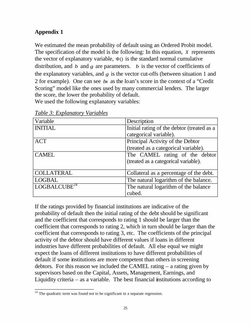
Appendix 1 We estimated the mean probability of default using an Ordered Probit model. The specification of the model is the following: In this equation, X represents the vector of explanatory variable, ()Φ is the standard normal cumulative distribution, and β and γ are parameters. β is the vector of coefficients of the explanatory variables, and γ is the vector cut-offs (between situation 1 and 2 for example). One can see xβ as the loan’s score in the context of a “Credit Scoring” model like the ones used by many commercial lenders. The larger the score, the lower the probability of default. We used the following explanatory variables:

Table 3: Explanatory Variables

Variable Description INITIAL Initial rating of the debtor (treated as a

categorical variable). ACT Principal Activity of the Debtor

(treated as a categorical variable). CAMEL The CAMEL rating of the debtor

(treated as a categorical variable).

COLLATERAL Collateral as a percentage of the debt. LOGBAL The natural logarithm of the balance. LOGBALCUBE24 The natural logarithm of the balance

cubed. If the ratings provided by financial institutions are indicative of the probability of default then the initial rating of the debt should be significant and the coefficient that corresponds to rating 1 should be larger than the coefficient that corresponds to rating 2, which in turn should be larger than the coefficient that corresponds to rating 3, etc. The coefficients of the principal activity of the debtor should have different values if loans in different industries have different probabilities of default. All else equal we might expect the loans of different institutions to have different probabilities of default if some institutions are more competent than others in screening debtors. For this reason we included the CAMEL rating – a rating given by supervisors based on the Capital, Assets, Management, Earnings, and Liquidity criteria – as a variable. The best financial institutions according to

24 The quadratic term was found not to be significant in a separate regression.

26

this criteria receive a rating of 1 and the worst a 5. Like with the initial rating of the debtor we would expect that the coefficient corresponding to rating 1 should be higher than the coefficient corresponding to rating 2 etc. We include the collateral of the loan as a measure of the willingness to pay of debtors. They are likely to be more careful about paying if they stand to lose their collateral in the case of a default. We suspected that the loan’s balance might have a complex relationship with its probability of default. One the one hand, the recent recession has generated financial problems for Argentina’s small and medium sized enterprises. Thus we expect that a high probability of default be associated with intermediate levels of debt. However, we know that financial institutions screen large exposures more carefully than the screen small exposures. This suggests that low probabilities of default would be associated with the largest debts. Thus, the relation between loan balance and the probability of default is probably non-linear. For this reason, we estimated various specifications of the loan balance and in the end decided to use the specification with the natural log of the balance and its cube. While our data allow us to estimate the mean probability of default fairly well we do not have a long enough stretch of data to properly estimate the standard deviation.25 Instead of estimating the standard deviation of the default probability, we assumed that it was a fixed percentage of the mean of the distribution, as suggested by CreditRisk+’s technical document.26 A simulation experiment suggested that the standard deviation is typically 27% of the mean. We will estimate the model using that and other percentages to test the sensitivity of the model to this assumption.

25 In a previous attempt, we estimated the standard deviation using a resampling technique. This method was found to have drawbacks. In particular it depended on the Markov assumption – that’s a loan’s rating in the next period is a function only of the rating in the current period. This not valid in the context of our data and thus the results of the previous estimation were biased 26 See CDSF (1997) page 44.

27

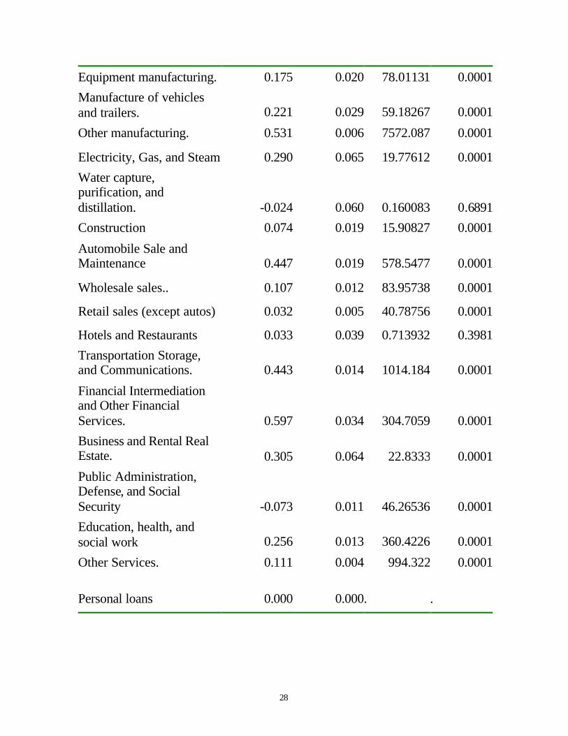
Parameters The following are the parameters of the ordered probit:

Coefficient Standard

Error t Probability

Intercept -3.5928623 0.055309 4219.76 0.0001

Initial Rating

1 5.6537 0.047544 9999.90 0.0001

2 4.2612 0.047645 7999.04 0.0001

3 3.6617 0.047781 5873.11 0.0001

4 3.0149 0.047779 3981.87 0.0001

5 2.1466 0.047461 2045.78 0.0001

Principal Activity

Agricultural Cultivation and Services 0.244 0.004 3421.861 0.0001

Animal rearing and related services (except veterinary services) 0.209 0.005 1747.033 0.0001

Hunting and Capture of Live Animals 0.029 0.061 0.219933 0.6391

Fishing and Related Services. 0.013 0.072 0.034379 0.8529

Mining and Exploration 0.120 0.051 5.555528 0.0184

Foods and Beverages. 0.039 0.017 5.103405 0.0239

Manufacture of textiles, furs, and leathers 0.046 0.018 6.749645 0.0094

Manufacture of substances and chemical products 0.392 0.028 194.598 0.0001

28

Equipment manufacturing. 0.175 0.020 78.01131 0.0001

Manufacture of vehicles and trailers. 0.221 0.029 59.18267 0.0001

Other manufacturing. 0.531 0.006 7572.087 0.0001

Electricity, Gas, and Steam 0.290 0.065 19.77612 0.0001

Water capture, purification, and distillation. -0.024 0.060 0.160083 0.6891

Construction 0.074 0.019 15.90827 0.0001

Automobile Sale and Maintenance 0.447 0.019 578.5477 0.0001

Wholesale sales.. 0.107 0.012 83.95738 0.0001

Retail sales (except autos) 0.032 0.005 40.78756 0.0001

Hotels and Restaurants 0.033 0.039 0.713932 0.3981

Transportation Storage, and Communications. 0.443 0.014 1014.184 0.0001

Financial Intermediation and Other Financial Services. 0.597 0.034 304.7059 0.0001

Business and Rental Real Estate. 0.305 0.064 22.8333 0.0001

Public Administration, Defense, and Social Security -0.073 0.011 46.26536 0.0001

Education, health, and social work 0.256 0.013 360.4226 0.0001

Other Services. 0.111 0.004 994.322 0.0001

Personal loans 0.000 0.000. .

29

CAMEL Coefficient Standard

Error t Probability

1 -0.6384963 0.028 505.7021 0.0001

2 -1.0022493 0.028 1252.844 0.0001

3 -0.9053715 0.028 1020.934 0.0001

4 -1.1689842 0.029 1678.648 0.0001

5 0 0.000. .

Coeficiente Standard

Error t Probability

LOGBAL -0.018 0.000885 430.165 0.0001

LOGBALCUBE 1.365E-04 0.000037 13.30655 0.0003

COLLATERAL 0.072 0.003739 371.1363 0.0001

2γ 0.315 0.00079

3γ 0.510 0.001037

4γ 0.937 0.00157

5γ 4.443 0.009453

Remembering that larger coefficients represent lower default probabilities, we can see significant differences between different activities. “Financial Intermediation and Other Financial Services.”, for example, has a much larger coefficient than “Water capture, purification, and distillation.” The CAMEL rating is also significant but not always in the way that we would expect. Financial institutions with a CAMEL equal to 1 seem to have less risky loans than CAMEL 2, 3, y 4. However the coefficient of CAMEL 5 is the highest of all, even though 5 represents the worst classification. This is probably because only one bank had a CAMEL equal to 5 in the moment of estimation. Also we did not expect the coefficient of CAMEL 2 to be lower than that of CAMEL 3. Probably in the future it will be best to estimate the model with

30

three groups defined by the CAMEL rating: CAMEL = 1, CAMEL = 2 or 3, and CAMEL = 4 or 5. The parameters LOGBAL and LOGBALCUBE show that the balance has a non-monotonic relationship with credit risk with a maximum somewhere around $808,000. COLLATERAL, as expected, has a positive and significant coefficient, which suggests that loans with collateral are less likely to default.

Universidad Torcuato Di Tella, Business School Working Papers

Working Papers 2003

Nº16 "Business Cycle and Macroeconomic Policy Coordination in MERCOSUR" Martín Gonzalez Rozada (UTDT) y José Fanelli (CEDES).

Nº15 "The Fiscal Spending Gap and the Procyclicality of Public Expenditure" Eduardo Levy Yeyati (UTDT) y Sebastián Galiani (UDESA).

Nº14 "Financial Dollarization and Debt Deflation under a Currency Board" Eduardo Levy Yeyati (UTDT), Ernesto Schargrodsky (UTDT) y Sebastián Galiani (UDESA).

Nº13 "¿ Po qué crecen menos los regímenes de tipo de cambio fijo? El efecto de los Sudden Stops", Federico Stuzenegger (UTDT).

Nº12 Concentration and Foreign Penetration in Latin American Banking Sec ors: Impact on Competition and Risk", Eduardo Levy Yeyati (UTDT) y Alejandro Micco (IADB).

Nº11 Default`s in the 1990`s: What have we learned?", Federico Sturzenegger (UTDT) y Punan Chuham (WB).

r

" t

"

"

"

r

"

Nº10 "Un año de medición del Indice de Demanda Laboral: situación actual y perspectivas , Victoria Lamdany (UTDT) y Luciana Monteverde (UTDT)

Nº09 "Liquidity Protection versus Moral Hazard: The Role of the IMF", Andrew Powell (UTDT) y Leandro Arozamena (UTDT)

Nº08 "Financial Dedollarization: A Carrot and Stick Approach", Eduardo Levy Yeyati (UTDT)

Nº07 "The Price of Inconvertible Deposits: The Stock Market Boom during the Argentine crisis", Eduardo Levy Yeyati (UTDT), Sergio Schmukler (WB) y Neeltje van Horen (WB)

Nº06 "Aftermaths of Current Account Crisis: Export Growth or Import Contraction?", Federico Sturzenegger (UTDT), Pablo Guidotti (UTDT) y Agustín Villar (BIS)

Nº05 Regional Integration and the Location of FDI", Eduardo Levy Yeyati (UTDT), Christian Daude (UM ) y Ernesto Stein (BID)

Nº04 "A new test for the success of inflation targeting", Andrew Powell (UTDT), Martin Gonzalez Rozada (UTDT) y Verónica Cohen Sabbán (BCRA)

Nº03 "Living and Dying with Ha d Pegs: The Rise and Fall of Argentina´s Currency Board", Eduardo Levy Yeyati (UTDT), Augusto de la Torre (WB) y Sergio Schmukler (WB)

Nº02 "The Cyclical Nature of FDI flows , Eduardo Levy Yeyati (UTDT), Ugo Panizza (BID) y Ernesto Stein (BID)

Nº01 "Endogenous Deposit Dollarization", Eduardo Levy Yeyati (UTDT) y Christian Broda (FRBNY)

Working Papers 2002 Nº15 "The FTAA and the Location of FDI", Eduardo Levy Yeyati (UTDT), Christian Daude (UM ) y Ernesto Stein ( BID)

Nº14 "Macroeconomic Coordination and Moneta y Unions in a N-country World: Do all Roads Lead to Rome?" Federico Sturzenegger (UTDT) y Andrew Powell (UTDT)

Nº13 Reforming Capital Requirements in Emerging Countries" Andrew Powell (UTDT), Verónica Balzarotti (BCRA) y Christian Castro (UPF)

Nº12 "Toolkit for the Analysis of Debt Problems , Federico Sturzenegger (UTDT)

Nº11 "On the Endogeneity of Exchange Rate Regimes", Eduardo Levy Yeyati (UTDT), Federico Sturzenegger (UTDT) e Iliana Reggio (UCLA)

Nº10 "Defaults in the 90´s: Factbook and Preliminary Lessons", Federico Sturzenegger (UTDT)

Nº09 "Countries with international payments´ difficulties: what can the IMF do?" Andrew Powell (UTDT)

Nº08 "The Argentina Crisis: Bad Luck, Bad Management, Bad Politics, Bad Advice", Andrew Powell (UTDT)

Nº07 "Capital Inflows and Capital Outflows: Measurement, Determinants, Consequences", Andrew Powell (UTDT), Dilip Ratha (WB) y Sanket Mohapatra (CU)

Nº06 "Banking on Foreigners: The Behaviour of International Bank Lending to Latin America, 1985-2000", Andrew Powell (UTDT), María Soledad Martinez Peria (WB) y Ivanna Vladkova ( IMF)

Nº05 "Classifying Exchange Rate Regimes: Deeds vs. Words" Eduardo Levy Yeyati (UTDT) y Federico Sturzenegger (UTDT)

r

"

"

rNº04"The Effect of Product Market Competition on Capital Structu e: Empirical Evidence from the Newspaper Industry", Ernesto Schargrodsky (UTDT)

Nº03 "Financial globalization: Unequal blessings", Augusto de la Torre (World Bank), Eduardo Levy Yeyati (Universidad Torcuato Di Tella) y Sergio

L. Schmukler (World Bank) Nº02 "Inference and estimation in small sample dynamic panel data models", Sebastian Galiani (UdeSA) y Martin Gonzalez-Rozada (UTDT) Nº01 "Why have poverty and income inequality increased so much? Argentina 1991-2002",

Martín González-Rozada, (UTDT) y Alicia Menendez, (Princeton University).