Reference Handbook - Share ITS

Reference Handbook9.4 Version for Computer-Based TestingFEThis document may be printed from the NCEES Web site

for your personal use, but it may not be copied, reproduced,

distributed electronically or in print, or posted online

without the express written permission of NCEES.

Contact [email protected] for more information.

Copyright ©2013 by NCEES®. All rights reserved.

All NCEES material is copyrighted under the laws of the United States. No part of this publication may be reproduced, stored in a retrieval system, or transmitted in any form or by any means without the prior written permission of NCEES. Requests for permissions should be addressed in writing to [email protected].

PO Box 1686Clemson, SC 29633800-250-3196www.ncees.org

ISBN 978-1-932613-67-4

Printed in the United States of AmericaFourth printing June 2016Edition 9.4

PREFACE

About the HandbookThe Fundamentals of Engineering (FE) exam is computer-based, and the FE Reference Handbook is the only resource material you may use during the exam. Reviewing it before exam day will help you become familiar with the charts, formulas, tables, and other reference information provided. You won't be allowed to bring your personal copy of the Handbook into the exam room. Instead, the computer-based exam will include a PDF version of the Handbook for your use. No printed copies of the Handbook will be allowed in the exam room.

The PDF version of the FE Reference Handbook that you use on exam day will be very similar to the printed version. Pages not needed to solve exam questions—such as the cover, introductory material, index, and exam specifications—will not be included in the PDF version. In addition, NCEES will periodically revise and update the Handbook, and each FE exam will be administered using the updated version.

The FE Reference Handbook does not contain all the information required to answer every question on the exam. Basic theories, conversions, formulas, and definitions examinees are expected to know have not been included. Special material required for the solution of a particular exam question will be included in the question itself.

Updates on exam content and proceduresNCEES.org is our home on the web. Visit us there for updates on everything exam-related, including specifications, exam-day policies, scoring, and practice tests. A PDF version of the FE Reference Handbook similar to the one you will use on exam day is also available there.

ErrataTo report errata in this book, send your correction using our chat feature on NCEES.org. We will also post errata on the website. Examinees are not penalized for any errors in the Handbook that affect an exam question.

CONTENTS

Units ................................................................................................................... 1

Conversion Factors ............................................................................................. 2

Ethics .................................................................................................................. 3

Safety .................................................................................................................. 6

Mathematics ..................................................................................................... 22

Engineering Probability and Statistics ............................................................. 37

Chemistry ......................................................................................................... 54

Materials Science/Structure of Matter ............................................................. 60

Statics ............................................................................................................... 67

Dynamics .......................................................................................................... 72

Mechanics of Materials .................................................................................... 80

Thermodynamics .............................................................................................. 87

Fluid mechanics ............................................................................................. 103

Heat Transfer ...................................................................................................117

Instrumentation, Measurement, and Controls ................................................ 124

Engineering Economics ................................................................................. 131

Chemical Engineering .................................................................................... 138

Civil Engineering ........................................................................................... 146

Environmental Engineering ........................................................................... 179

Electrical and Computer Engineering ............................................................ 200

Industrial and Systems Engineering ............................................................... 228

Mechanical Engineering ................................................................................. 237

Index ............................................................................................................... 251

Appendix: FE Exam Specifications ...............................................................257

1 UNITS

UNITSThe FE exam and this handbook use both the metric system of units and the U.S. Customary System (USCS). In the USCS system of units, both force and mass are called pounds. Therefore, one must distinguish the pound-force (lbf) from the pound-mass (lbm).

The pound-force is that force which accelerates one pound-mass at 32.174 ft/sec2. Thus, 1 lbf = 32.174 lbm-ft/sec2. The expression 32.174 lbm-ft/(lbf-sec2) is designated as gc and is used to resolve expressions involving both mass and force expressed as pounds. For instance, in writing Newton's second law, the equation would be written as F = ma/gc, where F is in lbf, m in lbm, and a is in ft/sec2.

Similar expressions exist for other quantities. Kinetic Energy, KE = mv2/2gc, with KE in (ft-lbf); Potential Energy, PE = mgh/gc, with PE in (ft-lbf); Fluid Pressure, p = ρgh/gc, with p in (lbf/ft2); Specific Weight, SW = ρg/gc, in (lbf/ft3); Shear Stress, τ = (µ/gc)(dv/dy), with shear stress in (lbf/ft2). In all these examples, gc should be regarded as a force unit conversion factor. It is frequently not written explicitly in engineering equations. However, its use is required to produce a consistent set of units.

Note that the force unit conversion factor gc [lbm-ft/(lbf-sec2)] should not be confused with the local acceleration of gravity g, which has different units (m/s2 or ft/sec2) and may be either its standard value (9.807 m/s2 or 32.174 ft/sec2) or some other local value.

If the problem is presented in USCS units, it may be necessary to use the constant gc in the equation to have a consistent set of units.

METRIC PREFIXES Multiple Prefix Symbol

COMMONLY USED EQUIVALENTS

1 gallon of water weighs 8.34 lbf 1 cubic foot of water weighs 62.4 lbf 1 cubic inch of mercury weighs 0.491 lbf The mass of 1 cubic meter of water is 1,000 kilograms

10–18

10–15

10–12

10–9

10–6

10–3

10–2

10–1

101

102

103

106

109

1012

1015

1018

attofemtopiconano

micromillicentidecidekahectokilo

megagigaterapetaexa

afpn

mcddahkMGTPE

ºF = 1.8 (ºC) + 32 ºC = (ºF – 32)/1.8 ºR = ºF + 459.69 K = ºC + 273.15

µ

TEMPERATURE CONVERSIONS

1 mg/L is 8.34 lbf/Mgal

IDEAL GAS CONSTANTSThe universal gas constant, designated as R in the table below, relates pressure, volume, temperature, and number of moles of an ideal gas. When that universal constant, R , is divided by the molecular weight of the gas, the result, often designated as R, has units of energy per degree per unit mass [kJ/(kg·K) or ft-lbf/(lbm-ºR)] and becomes characteristic of the particular gas. Some disciplines, notably chemical engineering, often use the symbol R to refer to the universal gas constant R .

FUNDAMENTAL CONSTANTSQuantity Symbol Value Unitselectron charge e 1.6022 × 10−19 C (coulombs)Faraday constant F 96,485 coulombs/(mol)gas constant metric R 8,314 J/(kmol·K)gas constant metric R 8.314 kPa·m3/(kmol·K)gas constant USCS R 1,545 ft-lbf/(lb mole-ºR) R 0.08206 L-atm/(mole-K)gravitation−Newtonian constant G 6.673 × 10–11 m3/(kg·s2)gravitation−Newtonian constant G 6.673 × 10–11 N·m2/kg2gravity acceleration (standard) metric g 9.807 m/s2gravity acceleration (standard) USCS g 32.174 ft/sec2molar volume (ideal gas), T = 273.15K, p = 101.3 kPa Vm 22,414 L/kmolspeed of light in vacuum c 299,792,000 m/sStefan-Boltzmann constant σ 5.67 × 10–8 W/(m2·K4)

2 CONVERSION FACTORS

CONVERSION FACTORS

Multiply By To Obtain Multiply By To Obtain

joule (J) 9.478 × 10–4 BtuJ 0.7376 ft-lbfJ 1 newton·m (N·m)J/s 1 watt (W)

kilogram (kg) 2.205 pound (lbm)kgf 9.8066 newton (N)kilometer (km) 3,281 feet (ft)km/hr 0.621 mphkilopascal (kPa) 0.145 lbf/in2 (psi)kilowatt (kW) 1.341 horsepower (hp)kW 3,413 Btu/hrkW 737.6 (ft-lbf )/seckW-hour (kWh) 3,413 BtukWh 1.341 hp-hrkWh 3.6 × 106 joule (J)kip (K) 1,000 lbfK 4,448 newton (N)

liter (L) 61.02 in3

L 0.264 gal (U.S. Liq)L 10–3 m3

L/second (L/s) 2.119 ft3/min (cfm)L/s 15.85 gal (U.S.)/min (gpm)

meter (m) 3.281 feet (ft)m 1.094 yardm/second (m/s) 196.8 feet/min (ft/min)mile (statute) 5,280 feet (ft)mile (statute) 1.609 kilometer (km)mile/hour (mph) 88.0 ft/min (fpm)mph 1.609 km/hmm of Hg 1.316 × 10–3 atmmm of H2O 9.678 × 10–5 atm

newton (N) 0.225 lbf newton (N) 1 kg·m/s2

N·m 0.7376 ft-lbfN·m 1 joule (J)

pascal (Pa) 9.869 × 10–6 atmosphere (atm)Pa 1 newton/m2 (N/m2)Pa·sec (Pa·s) 10 poise (P)pound (lbm, avdp) 0.454 kilogram (kg)lbf 4.448 Nlbf-ft 1.356 N·mlbf/in2 (psi) 0.068 atmpsi 2.307 ft of H2Opsi 2.036 in. of Hgpsi 6,895 Pa

radian 180/π degree

stokes 1 × 10–4 m2/s

therm 1 × 105 Btuton (metric) 1,000 kilogram (kg) ton (short) 2,000 pound (lb)

watt (W) 3.413 Btu/hrW 1.341 × 10–3 horsepower (hp)W 1 joule/s (J/s)weber/m2 (Wb/m2) 10,000 gauss

acre 43,560 square feet (ft2)ampere-hr (A-hr) 3,600 coulomb (C)ångström (Å) 1 × 10–10 meter (m)atmosphere (atm) 76.0 cm, mercury (Hg)atm, std 29.92 in., mercury (Hg)atm, std 14.70 lbf/in2 abs (psia)atm, std 33.90 ft, wateratm, std 1.013 × 105 pascal (Pa)

bar 1 × 105 Pabar 0.987 atmbarrels–oil 42 gallons–oilBtu 1,055 joule (J)Btu 2.928 × 10–4 kilowatt-hr (kWh)Btu 778 ft-lbfBtu/hr 3.930 × 10–4 horsepower (hp)Btu/hr 0.293 watt (W)Btu/hr 0.216 ft-lbf/sec

calorie (g-cal) 3.968 × 10–3 Btucal 1.560 × 10–6 hp-hrcal 4.186 joule (J)cal/sec 4.184 watt (W)centimeter (cm) 3.281 × 10–2 foot (ft)cm 0.394 inch (in)centipoise (cP) 0.001 pascal·sec (Pa·s)centipoise (cP) 1 g/(m·s)centipoise (cP) 2.419 lbm/hr-ftcentistoke (cSt) 1 × 10–6 m2/sec (m2/s)cubic feet/second (cfs) 0.646317 million gallons/day (MGD)cubic foot (ft3) 7.481 galloncubic meters (m3) 1,000 literselectronvolt (eV) 1.602 × 10–19 joule (J)

foot (ft) 30.48 cmft 0.3048 meter (m)ft-pound (ft-lbf) 1.285 × 10–3 Btuft-lbf 3.766 × 10–7 kilowatt-hr (kWh)ft-lbf 0.324 calorie (g-cal)ft-lbf 1.356 joule (J)

ft-lbf/sec 1.818 × 10–3 horsepower (hp) gallon (U.S. Liq) 3.785 liter (L)gallon (U.S. Liq) 0.134 ft3

gallons of water 8.3453 pounds of watergamma (γ, Γ) 1 × 10–9 tesla (T)gauss 1 × 10–4 Tgram (g) 2.205 × 10–3 pound (lbm)

hectare 1 × 104 square meters (m2)hectare 2.47104 acreshorsepower (hp) 42.4 Btu/minhp 745.7 watt (W)hp 33,000 (ft-lbf)/minhp 550 (ft-lbf)/sechp-hr 2,545 Btuhp-hr 1.98 × 106 ft-lbfhp-hr 2.68 × 106 joule (J)hp-hr 0.746 kWh

inch (in.) 2.540 centimeter (cm)in. of Hg 0.0334 atmin. of Hg 13.60 in. of H2Oin. of H2O 0.0361 lbf/in2 (psi)in. of H2O 0.002458 atm

22 MATHEMATICS

MATHEMATICS

DISCRETE MATH

Symbolsx ∈X x is a member of X , φ The empty (or null) setS ⊆ T S is a subset of TS ⊂ T S is a proper subset of T(a,b) Ordered pairP(s) Power set of S(a

1, a

2, ..., a

n) n-tuple

A × B Cartesian product of A and BA ∪ B Union of A and BA ∩ B Intersection of A and B∀ x Universal qualification for all x; for any x; for each x∃ y Uniqueness qualification there exists yA binary relation from A to B is a subset of A × B.

Matrix of RelationIf A = a

1, a

2, ..., a

m and B = b

1, b

2, ..., b

n are finite sets

containing m and n elements, respectively, then a relation R from A to B can be represented by the m × n matrix M

R < [m

ij], which is defined by:

mij = 1 if (a

i, b

j) ∈ R

0 if (ai, b

j) ∉ R

Directed Graphs, or Digraphs, of RelationA directed graph, or digraph, consists of a set V of vertices (or nodes) together with a set E of ordered pairs of elements of V called edges (or arcs). For edge (a, b), the vertex a is called the initial vertex and vertex b is called the terminal vertex. An edge of form (a, a) is called a loop.

Finite State MachineA finite state machine consists of a finite set of states S

i = s

0, s

1, ..., s

n and a finite set of inputs I; and a transition

function f that assigns to each state and input pair a new state.

A state (or truth) table can be used to represent the finite state machine.

Input

StateS0S1S2S3

i0S0S2S3S0

i1S1S2S3S3

i2S2S3S3S3

i3S3S3S3S3

Another way to represent a finite state machine is to use a state diagram, which is a directed graph with labeled edges.

S0

S2

S3S1

i2i2, i3

i0, i1, i2, i3i0, i1

i1 i3i0

i1, i2, i3

The characteristic of how a function maps one set (X) to another set (Y) may be described in terms of being either injective, surjective, or bijective.

An injective (one-to-one) relationship exists if, and only if, ∀ x

1, x

2 ∈ X, if f (x

1) = f (x

2), then x

1 = x

2

A surjective (onto) relationship exists when ∀ y ∈ Y, ∃ x ∈ X such that f(x) = y

A bijective relationship is both injective (one-to-one) and surjective (onto).

STRAIGHT LINEThe general form of the equation is

Ax + By + C = 0The standard form of the equation is

y = mx + b,which is also known as the slope-intercept form.

The point-slope form is y – y1 = m(x – x1)

Given two points: slope, m = (y2 – y1)/(x2 – x1)

The angle between lines with slopes m1 and m2 is

α = arctan [(m2 – m1)/(1 + m2·m1)]Two lines are perpendicular if m1 = –1/m2

The distance between two points is

d y y x x2 12

2 12

= - + -_ ^i hQUADRATIC EQUATION

ax2 + bx + c = 0

ab b ac

24Rootsx

2!=- -

=

QUADRIC SURFACE (SPHERE)The standard form of the equation is

(x – h)2 + (y – k)2

+ (z – m)2 = r2

with center at (h, k, m).

In a three-dimensional space, the distance between two points is

d x x y y z z2 12

2 12

2 12

= - + - + -^ _ ^h i h

23 MATHEMATICS

LOGARITHMSThe logarithm of x to the Base b is defined by

logb (x) = c, where bc = x

Special definitions for b = e or b = 10 are:ln x, Base = e

log x, Base = 10To change from one Base to another:

logb x = (loga x)/(loga b)e.g., ln x = (log10 x)/(log10 e) = 2.302585 (log10 x)

Identities logb b

n = n

log xc = c log x; xc

= antilog (c log x)

log xy = log x + log y

logb b = 1; log 1 = 0 log x/y = log x – log y

ALGEBRA OF COMPLEX NUMBERSComplex numbers may be designated in rectangular form or polar form. In rectangular form, a complex number is written in terms of its real and imaginary components.

z = a + jb, where

a = the real component,

b = the imaginary component, and

j = 1- (some disciplines use i 1= - )

In polar form z = c ∠ θ wherec = ,a b2 2+

θ = tan–1 (b/a),

a = c cos θ, and

b = c sin θ.

Complex numbers can be added and subtracted in rectangular form. If

z1 = a1 + jb1 = c1 (cos θ1 + jsin θ1)

= c1 ∠ θ1 and

z2 = a2 + jb2 = c2 (cos θ2 + jsin θ2)

= c2 ∠ θ2, then

z1 + z2 = (a1 + a2) + j (b1 + b2) and

z1 – z2 = (a1 – a2) + j (b1 – b2)

While complex numbers can be multiplied or divided in rectangular form, it is more convenient to perform these operations in polar form.

z1 × z2 = (c1 × c2) ∠ (θ1 + θ2)

z1/z2 = (c1 /c2) ∠ (θ1 – θ2)

The complex conjugate of a complex number z1 = (a1 + jb1) is defined as z1* = (a1 – jb1). The product of a complex number and its complex conjugate is z1z1* = a1

2 + b1

2.

Polar Coordinate Systemx = r cos θ; y = r sin θ; θ = arctan (y/x)

r x jy x y2 2= + = +x + jy = r (cos θ + j sin θ) = rejθ

[r1(cos θ1 + j sin θ1)][r2(cos θ2 + j sin θ2)] =

r1r2[cos (θ1 + θ2) + j sin (θ1 + θ2)]

(x + jy)n = [r (cos θ + j sin θ)]n

= rn(cos nθ + j sin nθ)

cos sin

cos sincos sin

r j

r jrr

j2 2 2

1 1 1

2

11 2 1 2

i i

i ii i i i

+

+= − + −`

` _ _jj i i9 C

Euler's Identityejθ = cos θ + j sin θe−jθ = cos θ – j sin θ

,cos sine ej

e e2 2

j j j j

i i= + = -i i i i- -

RootsIf k is any positive integer, any complex number (other than zero) has k distinct roots. The k roots of r (cos θ + j sin θ) can be found by substituting successively n = 0, 1, 2, ..., (k – 1) in the formula

cos sinw r k n k j k n k360 360k c ci i= + + +c cm m< F

TRIGONOMETRYTrigonometric functions are defined using a right triangle.sin θ = y/r, cos θ = x/r

tan θ = y/x, cot θ = x/y

csc θ = r/y, sec θ = r/x

Law of Sines

sin sin sinAa

Bb

Cc= =

Law of Cosinesa2

= b2 + c2

– 2bc cos A

b2 = a2

+ c2 – 2ac cos B

c2 = a2

+ b2 – 2ab cos C

Brink, R.W., A First Year of College Mathematics, D. Appleton-Century Co., Inc., Englewood Cliffs, NJ, 1937.

y

x

r

θ

θ

24 MATHEMATICS

Identitiescos θ = sin (θ + π/2) = −sin (θ − π/2)

sin θ = cos (θ − π/2) = −cos (θ + π/2)

csc θ = 1/sin θsec θ = 1/cos θtan θ = sin θ/cos θcot θ = 1/tan θsin2θ + cos2θ = 1

tan2θ + 1 = sec2θcot2θ + 1 = csc2θsin (α + β) = sin α cos β + cos α sin βcos (α + β) = cos α cos β – sin α sin βsin 2α = 2 sin α cos αcos 2α = cos2α – sin2α = 1 – 2 sin2α = 2 cos2α – 1

tan 2α = (2 tan α)/(1 – tan2α)

cot 2α = (cot2α – 1)/(2 cot α)

tan (α + β) = (tan α + tan β)/(1 – tan α tan β)

cot (α + β) = (cot α cot β – 1)/(cot α + cot β)

sin (α – β) = sin α cos β – cos α sin βcos (α – β) = cos α cos β + sin α sin βtan (α – β) = (tan α – tan β)/(1 + tan α tan β)

cot (α – β) = (cot α cot β + 1)/(cot β – cot α)

sin (α/2) = /cos1 2! - a^ hcos (α/2) = /cos1 2! + a^ htan (α/2) = /cos cos1 1! - +a a^ ^h hcot (α/2) = /cos cos1 1! + -a a^ ^h hsin α sin β = (1/2)[cos (α – β) – cos (α + β)]

cos α cos β = (1/2)[cos (α – β) + cos (α + β)]

sin α cos β = (1/2)[sin (α + β) + sin (α – β)]

sin α + sin β = 2 sin [(1/2)(α + β)] cos [(1/2)(α – β)]

sin α – sin β = 2 cos [(1/2)(α + β)] sin [(1/2)(α – β)]

cos α + cos β = 2 cos [(1/2)(α + β)] cos [(1/2)(α – β)]cos α – cos β = – 2 sin [(1/2)(α + β)] sin [(1/2)(α – β)]

MENSURATION OF AREAS AND VOLUMES

NomenclatureA = total surface areaP = perimeterV = volume

Parabola

Ellipse

a

b

A = πab

(h, k)x'

y'

2 /2

1 1/2 1/2 1/4

1/2 1/4 3/6 1/2 1/4 3/6 5/8

1/2 1/4 3/6 5/8 7/10

,

/

P a b

P a b

a b a b

where

2 2

2 2 2 4

2 6 2 8

2 10

approx

#

# # # # #

# # # # f

r

r

m m

m m

m

m

= +

= +

+ +

+ +

+ +

= − +_

_

_

_

^^

^ ^^

i

i

i

hi

hh

hh

R

T

SSSSS

V

X

WWWWW

Gieck, K., and R. Gieck, Engineering Formulas, 6th ed., Gieck Publishing, 1967.

25 MATHEMATICS

Circular Segment♦

/

/ /

sin

arccos

A r

s r r d r

2

2

2= -

= = -

z z

z

^^

hh

87

BA$ .

Circular Sector♦

/ /

/

A r sr

s r

2 22= =

=

z

z

Sphere♦

/V r d

A r d

4 3

4

3 3

2 2

= =

= =

r r

r r

/6

Parallelogram

cos

cos

sin

P a b

d a b ab

d a b ab

d d a b

A ah ab

2

2

2

2

12 2

22 2

12

22 2 2

= +

= +

= + +

+ = +

= =

z

z

z

-

^^^

_^

hhh

ih

If a = b, the parallelogram is a rhombus.

A

s

d

r

Regular Polygon (n equal sides)♦

/

/

/

tan

n

nn

nP ns

s r

A nsr

2

2 1 2

2 2

2

=

= - = -

=

=

=

z r

i r r

z

^ b

^^

h l

hh

;

8

E

B

Prismoid♦

/V h A A A6 41 2= + +^ ^h h

Right Circular Cone♦

/

: :

V r hA

r r r h

A A x h

3sidearea basearea

x b

2

2 2

2 2

=

= +

= + +

=

r

r

_

`

i

j

♦ Gieck, K., and R. Gieck, Engineering Formulas, 6th ed., Gieck Publishing, 1967.

26 MATHEMATICS

Case 1. Parabola e = 1:•

(y – k)2 = 2p(x – h); Center at (h, k)is the standard form of the equation. When h = k = 0,Focus: (p/2, 0); Directrix: x = –p/2

Case 2. Ellipse e < 1:

a

b

A = πab

(h, k)x'

y'

( ) ( ); Center at ( , )

ax h

by k

h k12

2

2

2-+-

=

is the standard form of the equation. When h = k = 0,

Eccentricity: / /e b a c a1 2 2= - =_ i;b a e1 2= -

Focus: (± ae, 0); Directrix: x = ± a/e

♦ Gieck, K., and R. Gieck, Engineering Formulas, 6th ed., Gieck Publishing, 1967.• Brink, R.W., A First Year of College Mathematics, D. Appleton-Century Co., Inc., 1937.

Right Circular Cylinder♦

V r h d h

A r h r4

2side area end areas

22

= =

= + = +

r r

r ^ h

Paraboloid of Revolution

V d h8

2

= r

CONIC SECTIONS

e = eccentricity = cos θ/(cos φ)[Note: X ′ and Y ′, in the following cases, are translated axes.]

27 MATHEMATICS

Case 3. Hyperbola e > 1:•

ax h

b

y k12

2

2

2- -

-=

^ _h i; Center at (h, k)

is the standard form of the equation. When h = k = 0,

Eccentricity: / /e b a c a1 2 2= + =_ i;b a e 12= -

Focus: (± ae, 0); Directrix: x = ± a/e.

Case 4. Circle e = 0: (x – h)2

+ (y – k)2 = r2; Center at (h, k) is the standard

form of the equation with radius

r x h y k2 2

= - + -^ _h i•

k

h

Length of the tangent line from a point on a circle to a point (x′,y′):

t2 = (x′ – h)2 + (y′ – k)2 – r2

•

• Brink, R.W., A First Year of College Mathematics, D. Appleton-Century Co., Inc., 1937.

Conic Section EquationThe general form of the conic section equation is

Ax2 + Bxy + Cy2

+ Dx + Ey + F = 0where not both A and C are zero.

If B2 – 4AC < 0, an ellipse is defined.

If B2 – 4AC > 0, a hyperbola is defined.

If B2 – 4AC = 0, the conic is a parabola.

If A = C and B = 0, a circle is defined.If A = B = C = 0, a straight line is defined.

x2 + y2

+ 2ax + 2by + c = 0is the normal form of the conic section equation, if that conic section has a principal axis parallel to a coordinate axis.h = –a; k = –b

r a b c2 2= + -

If a2 + b2 – c is positive, a circle, center (–a, –b).

If a2 + b2

– c equals zero, a point at (–a, –b).

If a2 + b2

– c is negative, locus is imaginary.

DIFFERENTIAL CALCULUS

The DerivativeFor any function y = f (x),the derivative = Dx y = dy/dx = y′

/

/

f x

y y x

f x x f x x

y

limit

limit

the slope of the curve ( ) .

x

x

0

0

=

= + -

=

D D

D D

"

"

D

D

l

l

_ ^

^ ^ ^i h

h h h87

BA$ .

Test for a Maximumy = f (x) is a maximum forx = a, if f ′(a) = 0 and f ″(a) < 0.

Test for a Minimumy = f (x) is a minimum forx = a, if f ′(a) = 0 and f ″(a) > 0.

Test for a Point of Inflectiony = f (x) has a point of inflection at x = a,if f ″(a) = 0, andif f ″(x) changes sign as x increases throughx = a.

The Partial DerivativeIn a function of two independent variables x and y, a derivative with respect to one of the variables may be found if the other variable is assumed to remain constant. If y is kept fixed, the function

z = f (x, y)

becomes a function of the single variable x, and its derivative (if it exists) can be found. This derivative is called the partial derivative of z with respect to x. The partial derivative with respect to x is denoted as follows:

,xz

xf x y

22

22

=_ i

28 MATHEMATICS

INTEGRAL CALCULUSThe definite integral is defined as:

f x x f x dxlimitn i

n

i i a

b

1=D

" 3 =_ ^i h! #

Also, ∆xi →0 for all i.

A table of derivatives and integrals is available in the Derivatives and Indefinite Integrals section. The integral equations can be used along with the following methods of integration:A. Integration by Parts (integral equation #6),B. Integration by Substitution, andC. Separation of Rational Fractions into Partial Fractions.

♦ Wade, Thomas L., Calculus, Ginn & Company/Simon & Schuster Publishers, 1953.

The Curvature of Any Curve♦

=

The curvature K of a curve at P is the limit of its average curvature for the arc PQ as Q approaches P. This is also expressed as: the curvature of a curve at a given point is the rate-of-change of its inclination with respect to its arc length.

Ks ds

dlimits 0

= =a aDD

"D

Curvature in Rectangular Coordinates

Ky

y

12 3 2=

+ l

m

_ i9 CWhen it may be easier to differentiate the function withrespect to y rather than x, the notation x′ will be used for thederivative.

/x dx dy

Kx

x

12 3 2

=

=

+

-

l

l

m

^ h8 BThe Radius of CurvatureThe radius of curvature R at any point on a curve is defined as the absolute value of the reciprocal of the curvature K at that point.

RK

K

Ry

yy

1 0

10

2 3 2

!

!

=

=+

m

lm

^

_ _

h

i i9 C

L'Hospital's Rule (L'Hôpital's Rule)If the fractional function f(x)/g(x) assumes one of the indeterminate forms 0/0 or ∞/∞ (where α is finite or infinite), then

/f x g xlimitx " a

^ ^h h

is equal to the first of the expressions

, ,g xf x

g xf x

g xf x

limit limit limitx x x" " "a a al

l

m

m

n

n^^

^^

^^

hh

hh

hh

which is not indeterminate, provided such first indicatedlimit exists.

29 MATHEMATICS

DERIVATIVES AND INDEFINITE INTEGRALSIn these formulas, u, v, and w represent functions of x. Also, a, c, and n represent constants. All arguments of the trigonometric functions are in radians. A constant of integration should be added to the integrals. To avoid terminology difficulty, the following definitions are followed: arcsin u = sin–1

u, (sin u)–1 = 1/sin u.

1. dc/dx = 0

2. dx/dx = 1

3. d(cu)/dx = c du/dx

4. d(u + v – w)/dx = du/dx + dv/dx – dw/dx

5. d(uv)/dx = u dv/dx + v du/dx

6. d(uvw)/dx = uv dw/dx + uw dv/dx + vw du/dx

7. / / /dx

d u vv

v du dx udv dx2= -^ h

8. d(un)/dx = nun–1 du/dx

9. d[f (u)]/dx = d[f (u)]/du du/dx

10. du/dx = 1/(dx/du)

11. log

logdx

d ue u dx

du1aa=

_ _i i

12. dx

d uu dx

du1 1n=

^ h

13. dx

d a a adxdu1n

uu=

_ ^i h

14. d(eu)/dx = eu du/dx

15. d(uv)/dx = vuv–1 du/dx + (ln u) uv

dv/dx

16. d(sin u)/dx = cos u du/dx

17. d(cos u)/dx = –sin u du/dx

18. d(tan u)/dx = sec2u du/dx

19. d(cot u)/dx = –csc2u du/dx

20. d(sec u)/dx = sec u tan u du/dx

21. d(csc u)/dx = –csc u cot u du/dx

22. / /sin sindx

d uu dx

du u1

1 2 21

21# #=

-- r r

--_ _i i

23. cos cosdx

d u

u dxdu u

11 0

1

21# #=-

-r

--_ _i i

24. / < < /tan tandx

d uu dx

du u1

1 2 21

21=

+- r r

--_ _i i

25. < <cot cotdx

d uu dx

du u1

1 01

21=-

+r

--_ _i i

26.

27.

< < / < /

sec

sec sec

dxd u

u u dxdu

u u

11

0 2 2

1

2

1 1#

=-

- -r r r

-

- -

_

_ _

i

i i

< / < /

csc

csc csc

dxd u

u u dxdu

u u

11

0 2 2

1

2

1 1# #

=--

- -r r r

-

- -

_

_ _

i

i i

1. # d f (x) = f (x)

2. # dx = x

3. # a f(x) dx = a # f(x) dx

4. # [u(x) ± v(x)] dx = # u(x) dx ± # v(x) dx

5. x dx mx m1 1m

m 1!=

+-

+ ^ h#

6. # u(x) dv(x) = u(x) v(x) – # v (x) du(x)

7. ax b

dxa ax b1 1n

+= +#

8. x

dx x2=#

9. a dx aa

1nx

x

=#

10. # sin x dx = – cos x

11. # cos x dx = sin x

12. sin sinxdx x x2 4

22 = -#

13. cos sinxdx x x2 4

22 = +#

14. # x sin x dx = sin x – x cos x

15. # x cos x dx = cos x + x sin x

16. # sin x cos x dx = (sin2x)/2

17.

18. # tan x dx = –lncos x= ln sec x19. # cot x dx = –ln csc x = ln sin x20. # tan2x dx = tan x – x

21. # cot2x dx = –cot x – x

22. # eax dx = (1/a) eax

23. # xeax dx = (eax/a2)(ax – 1)

24. # ln x dx = x [ln (x) – 1] (x > 0)

25. tana x

dxa a

x a1 02 21 !

+= - ^ h#

26. , > , >tanax c

dxac

x ca a c1 0 02

1

+= - b ^l h#

27a.

27b.

27c. ,ax bx c

dxax b

b ac2

2 4 022

+ +=-

+- =_ i#

sin cos cos cosax bx dxa ba b x

a ba b x a b

2 22 2!=-

-- -

++

^^

^^ _h

hhh i#

>

tanax bx c

dxac b ac b

ax b

ac b

42

42

4 0

2 21

2

2

+ +=

- -

+

-

-

_ i

#

>

ax bx cdx

b ac ax b b ac

ax b b ac

b ac

41 1

2 4

2 4

4 0

n2 2 2

2

2

+ +=

- + + -

+ - -

-_ i

#

30 MATHEMATICS

Properties of Series

;

/

c nc c

cx c x

x y z x y z

x n n 2

constanti

n

ii

n

ii

n

i i ii

n

ii

n

ii

n

ii

n

x

n

1

1 1

1 1 1 1

1

2

= =

=

+ - = + -

= +

=

= =

= = = =

=

_

_

i

i

!

! !

! ! ! !

!

Power Series

a x ai ii

0 -3= ^ h!

1. A power series, which is convergent in the interval –R < x < R, defines a function of x that is continuous for all values of x within the interval and is said to represent the function in that interval.

2. A power series may be differentiated term by term within its interval of convergence. The resulting series has the same interval of convergence as the original series (except possibly at the end points of the series).

3. A power series may be integrated term by term provided the limits of integration are within the interval of convergence of the series.

4. Two power series may be added, subtracted, or multiplied, and the resulting series in each case is convergent, at least, in the interval common to the two series.

5. Using the process of long division (as for polynomials), two power series may be divided one by the other within their common interval of convergence.

Taylor's Series

! !

... ! ...

f x f af a

x af a

x a

nf a

x a

1 2n

n

2= + - + -

+ + - +

l m^ ^ ^ ^ ^ ^

^ ^^

h h h h h h

h hh

is called Taylor's series, and the function f (x) is said to be expanded about the point a in a Taylor's series.

If a = 0, the Taylor's series equation becomes a Maclaurin's series.

DIFFERENTIAL EQUATIONS

A common class of ordinary linear differential equations is

bdx

d y xb

dxdy x

b y x f xn n

n

1 0f+ + + =^ ^ ^ ^h h h h

where bn, … , bi, … , b1, b0 are constants.

When the equation is a homogeneous differential equation, f(x) = 0, the solution is

y x Ce C e Ce C ehr x r x

ir x

nr x

1 2i n1 2 f f= + + + + +^ h

where rn is the nth distinct root of the characteristicpolynomial P(x) with

P(r) = bnrn + bn–1r

n–1 + … + b1r + b0

CENTROIDS AND MOMENTS OF INERTIAThe location of the centroid of an area, bounded by the axes and the function y = f(x), can be found by integration.

x AxdA

y AydA

A f x dx

dA f x dx g y dy

c

c

=

=

=

= =

^^ _hh i

#

#

#

The firstmomentofareawith respect to the y-axis and the x-axis, respectively, are:

My = ∫x dA = xc A

Mx = ∫y dA = yc A

The moment of inertia (second moment of area) with respect to the y-axis and the x-axis, respectively, are:

Iy = ∫x2 dA

Ix = ∫y2 dA

The moment of inertia taken with respect to an axis passing through the area's centroid is the centroidal moment of inertia. The parallel axis theorem for the moment of inertia with respect to another axis parallel with and located d units from the centroidal axis is expressed by

Iparallel axis = Ic + Ad2

In a plane, J =∫r 2dA = Ix + Iy

PROGRESSIONS AND SERIES

Arithmetic ProgressionTo determine whether a given finite sequence of numbers isan arithmetic progression, subtract each number from thefollowing number. If the differences are equal, the series isarithmetic.1. The first term is a.2. The common difference is d.3. The number of terms is n.4. The last or nth term is l.5. The sum of n terms is S. l = a + (n – 1)d S = n(a + l)/2 = n [2a + (n – 1) d]/2

Geometric ProgressionTo determine whether a given finite sequence is a geometricprogression (G.P.), divide each number after the first by thepreceding number. If the quotients are equal, the series isgeometric:1. The first term is a.2. The common ratio is r.3. The number of terms is n.4. The last or nth term is l.5. The sum of n terms is S. l = arn−1

S = a (1 – rn)/(1 – r); r ≠1 S = (a – rl)/(1 – r); r ≠1

limit Sn= a/(1 − r); r < 1 n→∞

A G.P. converges if |r| < 1 and it diverges if |r| > 1.

31 MATHEMATICS

If the root r1 = r2, then C2er2

x is replaced with C2xer1x.

Higher orders of multiplicity imply higher powers of x. The complete solution for the differential equation is

y(x) = yh(x) + yp(x),

where yp(x) is any particular solution with f(x) present. If f(x) has ern x

terms, then resonance is manifested. Furthermore, specific f(x) forms result in specific yp(x) forms, some of which are:

f(x) yp(x)A B

Aeαx Beαx, α ≠rn

A1 sin ωx + A2 cos ωx B1 sin ωx + B2 cos ωx

If the independent variable is time t, then transient dynamic solutions are implied.

First-Order Linear Homogeneous Differential Equations with Constant Coefficients y′+ ay = 0, where a is a real constant: Solution, y = Ce–at

where C = a constant that satisfies the initial conditions.

First-Order Linear Nonhomogeneous Differential Equations

<>dt

dyy Kx t x t

A tB t

y KA

00

0

+ = =

=

x ^ ^

^

h h

h

) 3

τ is the time constantK is the gainThe solution is

expy t KA KB KA t

tKB y

KB KA

1

1

or

n

= + - - -

=--

x

x

^ ] bch g lm

< F

Second-Order Linear Homogeneous Differential Equations with Constant CoefficientsAn equation of the form

y″+ ay′+ by = 0can be solved by the method of undetermined coefficients where a solution of the form y = Cerx

is sought. Substitution of this solution gives

(r2 + ar + b) Cerx

= 0and since Cerx

cannot be zero, the characteristic equation must vanish or

r2 + ar + b = 0

The roots of the characteristic equation are

r a a b2

4,1 2

2!=- -

and can be real and distinct for a2 > 4b, real and equal for

a2 = 4b, and complex for a2

< 4b.

If a2 > 4b, the solution is of the form (overdamped)

y = C1er1x + C2e

r2 x

If a2 = 4b, the solution is of the form (critically damped)

y = (C1+ C2x)er1x

If a2 < 4b, the solution is of the form (underdamped)

y = eαx (C1 cos βx + C2 sin βx), where

α= – a/2

b a2

4 2

=-b

FOURIER TRANSFORMThe Fourier transform pair, one form of which is

/

F f t e dt

f t F e d1 2

j t

j t

=

=

~

r ~ ~

3

3

3

3

-

-

-

~

~

^ ^^ ^ ^h hh h h7 A

#

#

can be used to characterize a broad class of signal models in terms of their frequency or spectral content. Some useful transform pairs are:

f(t) F(ω)

td^ h 1

u(t) /j1+rd ~ ~^ h

u t u t r t2 2 rect+ - - =x x

xb bl l /

/sin2

2x~x~x^ h

ej to~ 2 o-rd ~ ~_ i

Some mathematical liberties are required to obtain the second and fourth form. Other Fourier transforms are derivable from the Laplace transform by replacing s with jω provided

, <

<

f t t

f t dt

0 0

03

=3

^^hh#

FOURIER SERIESEvery periodic function f(t) which has the period T = 2π/ω0

and has certain continuity conditions can be represented by a series plus a constant

cos sinf t a a n t b n tn nn

0 0 01

= + +~ ~3

=

^ _ _h i i8 B!

The above holds if f(t) has a continuous derivative f ′(t) for all t. It should be noted that the various sinusoids present in the series are orthogonal on the interval 0 to T and as a result the coefficients are given by

, ,

, ,

cos

sin

a T f t dt

a T f t n t dt n

b T f t n t dt n

1

2 1 2

2 1 2

T

nT

nT

0

0

0

f

f

~

~

=

= =

= =

0

0

0

_ ^_ ^ __ ^ _

i hi h ii h i

#

#

#

The constants an and bn are the Fouriercoefficientsof f(t) for the interval 0 to T and the corresponding series is called the Fourier series of f(t) over the same interval.

32 MATHEMATICS

Given:f3(t) = a train of impulses with weights A

t2TTT 0 3T

then

cos

t A t nT

t A T A T n t

t A T e

2

n

n

jn t

n

3

3 01

30

f

f

f

= -

= +

=

d

~

3

3

3

3

3

=-

=

=-

~

^ ^

^ _ _ _

^ _

h h

h i i i

h i

!

!

!

The Fourier Transform and its Inverse

X f x t e dt

x t X f e df

j ft

j ft

2

2

=

=

3

3

3

3

-

+ -

-

+

r

r

_ ^^ _i hh i

#

#

We say that x(t) and X(f) form a Fourier transform pair:x(t) ↔ X(f)

The integrals have the same value when evaluated over any interval of length T.

If a Fourier series representing a periodic function is truncated after term n = N the mean square value FN

2 of the truncated series is given by Parseval's relation. This relation says that the mean-square value is the sum of the mean-square values of the Fourier components, or

F a b1 2N n nn

N2

02 2 2

1a= + +

=_ `i j!

and the RMS value is then defined to be the square root of this quantity or FN.

Three useful and common Fourier series forms are definedin terms of the following graphs (with ω0 = 2π/T).Given:

t

T

f (t)1

V0

V0

2

T

2

T

0

then

cost V n n t1 4n

n

11

1 2

0 0

n odd

f = - r ~3

=

-

^ ] _ _^

^

h g i ih

h

!

Given:

f (t)2

t

22 TTT 0

V0

thensin

cos

sin

t TV

TV

n T

n Tn t

t TV

n T

n Te

2n

n

jn t

20 0

10

20 0

f

f

= +

=

x x

rx

rx~

x

rx

rx

3

3

3

=

=-

~

^ __ _

^ __

h ii i

h ii

!

!

33 MATHEMATICS

Fourier Transform Pairs

x(t) X(f)

1 ( )fδ

( )tδ 1

)(tu1 1

( )2 2

fj f

δ +π

( / )tΠ τ τ sinc (τ f )

sinc( )Bt1

( / )f BB

Π

( / )tΛ τ

( )ate u t− 1 02

aa j f

>+ π

)(tute at−2

1 0( 2 )

aa j f

>+ π

tae−2 2

2 0(2 )

aa

a f>

+ π

2)(ate−2( / )f ae

a− ππ

0cos(2 )f tπ + θ0 0

1[ ( ) ( )]

2j je f f e f fθ − θδ − + δ +

0sin(2 )f tπ + θ 0 01

[ ( ) ( )]2

j je f f e f fj

θ − θδ − − δ +

( )n

sn

t nT=+∞

=−∞δ −∑ 1

( ) k

s s ssk

f f kf fT

=+∞

=−∞δ − =∑

τ sinc2 (τ f )

Fourier Transform Theorems

Linearity ( ) ( )ax t by t+ ( ) ( )aX f bY f+

Scale change ( )x at1 f

Xa a

Time reversal ( )x t− ( )X f−

Duality ( )X t ( )x f−

Time shift 0( )x t t− 02( ) j ftX f e− π

Frequency shift 02( ) j f tx t e π0( )X f f−

Modulation 0( )cos 2x t f tπ

0

0

1( )

2

1( )

2

X f f

X f f

−

+ +

Multiplication ( ) ( )x t y t ( ) ( )X f Y f

Convolution ( )x(t) y t ( ) ( )X f Y f

Differentiationn

n

dt

txd )(( 2 ) ( )nj f X fπ

Integration ( )t

–x λ d

∞λ∫

1( )

2

1(0) ( )

2

X fj πf

X f+ δ

( )

*

*

where:

P =

K =

,,

,,

sin

otherwise

otherwise

t tt

t t

t t t

1 21

0

1 10

sinc

#

#

rr

=

-

_ _

_

_

i i

i

i

*

(

34 MATHEMATICS

LAPLACE TRANSFORMSThe unilateral Laplace transform pair

f

where

F s t e dt

f t j F s e dt

s j21

st

j st

rv ~

=

=

= +

3

3v

-

+

-0

j3v-

^ ^^ ^h hh h#

#

represents a powerful tool for the transient and frequency response of linear time invariant systems. Some useful Laplace transform pairs are:

)s(F )t(f

δ(t), Impulse at t = 0 1

u(t), Step at t = 0 1/s

t[u(t)], Ramp at t = 0 1/s2

e–α t 1/(s + α )

te–α t 1 /(s + α )2

e–α t sin βt β/[(s + α )2 + β2]

e–α t cos βt (s + α )/[(s + α )2 + β2]

( )n

n

dt

tfd ( ) ( )td

fdssFs

m

mn

m

mnn 01

0

1∑−−

=

−−

( )∫ ττt df0 (1/s)F(s)

( )∫ ττ−∞ d)τ(htx0 H(s)X(s)

f (t – τ) u(t – τ) e–τ sF(s)

( )tft ∞→limit ( )ssF

s 0limit

→

( )tft 0

limit→

( )ssFs ∞→limit

The last two transforms represent the Final Value Theorem (F.V.T.) and Initial Value Theorem (I.V.T.), respectively. It is assumed that the limits exist.

MATRICESA matrix is an ordered rectangular array of numbers with m rows and n columns. The element aij refers to row i and column j.

Multiplication of Two Matrices

column matrix

column matrix

-

-

row,2

row,2

-

-

AACE

BDF

A is a3

BHJ

IK

B is a2

3,2

2,2

=

=

R

T

SSSS

=

V

X

WWWW

G

In order for multiplication to be possible, the number of columns in A must equal the number of rows in B.

Multiplying matrix B by matrix A occurs as follows:

CACE

BDF

HJ

IK

CA H B JC H D JE H F J

A I B KC I D KE I F K

:

: :

: :

: :

: :

: :

: :

=

=+++

+++

___

___

iii

iii

R

T

SSSSR

T

SSSS

=V

X

WWWW

V

X

WWWW

G

Matrix multiplication is not commutative.

AdditionAD

BE

CF

GJ

HK

IL

A GD J

B HE K

C IF L

+ =++

++

++

= = >G G H

Identity MatrixThe matrix I = (aij) is a square n × n matrix with 1's on the diagonal and 0's everywhere else.

Matrix TransposeRows become columns. Columns become rows.

AAD

BE

CF

AABC

DEF

T= =

R

T

SSSS

=V

X

WWWW

G

Inverse [ ]–1 The inverse B of a square n × n matrix A is

whereB AAA

,adj1

= =- ^ h

adj(A) = adjoint of A (obtained by replacing AT elements with their cofactors) and A = determinant of A.

[A][A]–1 = [A]–1[A] = [I] where I is the identity matrix.

35 MATHEMATICS

The dot product is a scalar product and represents the projection of B onto A times A . It is given by

A•B = axbx + ayby + azbz

cosA B B A:= =i

The cross product is a vector product of magnitude B A sin θ which is perpendicular to the plane containing

A and B. The product is

A B

i j k

B Aab

ab

ab

x

x

y

y

z

z

# #= =-

The sense of A × B is determined by the right-hand rule.

A × B = A B n sin θ, where

n = unit vector perpendicular to the plane of A and B.

Gradient, Divergence, and Curl

i j k

V i j k i j k

V i j k i j k

x y z

x y z V V V

x y z V V V

1 2 3

1 2 3

: :

# #

d22

22

22

d22

22

22

d22

22

22

= + +

= + + + +

= + + + +

z zc

c _

c _

m

m i

m i

The Laplacian of a scalar function φ is

x y z2

2

2

2

2

2

2

d2

2

2

2

2

2= + +z

z z z

IdentitiesA • B = B • A; A • (B + C) = A • B + A • CA • A = |A|2

i • i = j • j = k • k = 1

i • j = j • k = k • i = 0

If A • B = 0, then either A = 0, B = 0, or A is perpendicular to B.

A × B = –B × AA × (B + C) = (A × B) + (A × C)

(B + C) × A = (B × A) + (C × A)

i × i = j × j = k × k = 0i × j = k = –j × i; j × k = i = –k × jk × i = j = –i × kIf A × B = 0, then either A = 0, B = 0, or A is parallel to B.

A

A A A

0

0

2

2

: :

#

: #

# # :

d d d d d

d d

d d

d d d d d

= =

=

=

= -

z z z

z

^ ]

^^ ]

h g

hh g

DETERMINANTSA determinant of order n consists of n2 numbers, called the elements of the determinant, arranged in n rows and n columns and enclosed by two vertical lines.

In any determinant, the minor of a given element is the determinant that remains after all of the elements are struck out that lie in the same row and in the same column as the given element. Consider an element which lies in the jth column and the ith row. The cofactor of this element is the value of the minor of the element (if i + j is even), and it is the negative of the value of the minor of the element (if i + j is odd).

If n is greater than 1, the value of a determinant of order n is the sum of the n products formed by multiplying each element of some specified row (or column) by its cofactor. This sum is called the expansion of the determinant [according to the elements of the specified row (or column)]. For a second-order determinant:aabb

ab a b1 2

1 21 2 2 1= -

For a third-order determinant:a

b

c

a

b

c

a

b

c

ab c a b c a b c a b c a b c ab c1

1

1

2

2

2

3

3

3

1 2 3 2 3 1 3 1 2 3 2 1 2 1 3 1 3 2= + + - - -

VECTORS

A = axi + ayj + azk

Addition and subtraction:

A + B = (ax + bx)i + (ay + by)j + (az + bz)kA – B = (ax – bx)i + (ay – by)j + (az – bz)k

36 MATHEMATICS

DIFFERENCE EQUATIONSAny system whose input v(t) and output y(t) are defined only at the equally spaced intervals

'f t y t ty y

1

1

i i

i i= = −−

+

+^ hcan be described by a difference equation.

First-Order Linear Difference Equation

'

t t t

y y y t1

1

i i

i i

D

D

= −= +

+

+ _ iNUMERICAL METHODS

Newton's Method for Root ExtractionGiven a function f(x) which has a simple root of f(x) = 0 at x = a an important computational task would be to find that root. If f(x) has a continuous first derivative then the (j +1)st estimate of the root is

a a

dxdf xf x

x a

j j

j

1 = -

=

+

^^hh

The initial estimate of the root a0 must be near enough to the actual root to cause the algorithm to converge to the root.

Newton's Method of MinimizationGiven a scalar value function

h(x) = h(x1, x2, …, xn)find a vector x*∈Rn such that

h(x*) ≤ h(x) for all xNewton's algorithm is

,x x

x x x xxh

xh

xh

xh

xh

xh

xh

xh

x xh

x xh

x xh

xh

x xh

x xh

x xh

xh

where

and

k k

k k

n

n

n

n n n

1 2

2

1

1

2

2

2

12

2

1 2

2

1

2

1 2

2

22

2

2

2

1

2

2

2

2

2

22

22

22

22

22

g

g

22

22

22

2 22 g g

2 22

2 22

22 g g

2 22

g g g g g

g g g g g

2 22

2 22 g g

22

= -

= =

=

=

+

-J

L

KKKK

N

P

OOOO

R

T

SSSSSSSSSSS

R

T

SSSSSSSSSSSS

V

X

WWWWWWWWWWW

V

X

WWWWWWWWWWWWW

Numerical IntegrationThree of the more common numerical integration algorithms used to evaluate the integral

f x dxa

b ^ h#

are:Euler's or Forward Rectangular Rule

f x dx x f a k xa

b

k

n

0

1. +D D

=

-^ ^h h!#

Trapezoidal Rulefor n = 1

f x dx xf a f b

2a

b.

+D^ ^ ^h h h< F#

for n > 1

f x dx x f a f a k x f b2 2a

b

k

n

1

1. + + +D D

=

-^ ^ ^ ^h h h h< F!#

Simpson's Rule/Parabolic Rule (n must be an even integer)for n = 2

f x dx b a f a f a b f b6 4 2a

b. - + + +^ b ^ b ^h l h l h; E#

for n ≥ 4

3

2

4

f x dx x

f a f a k x

f a k x f b

2, 4, 6,

2

1, 3, 5,

1a

bk

n

k

n

.D

D

D

+ +

+ + +

f

f

=

−

=

−^

^

_

_

^h

h

i

i

h

R

T

SSSSSSSSSSSSSSS

V

X

WWWWWWWWWWWWWWW

/

/

#

with ∆x = (b – a)/nn = number of intervals between data points

Numerical Solution of Ordinary Differential Equations

Euler's ApproximationGiven a differential equation

dx/dt = f (x, t) with x(0) = xo

At some general time k∆t

x[(k + 1)∆t] ≅ x(k∆t) + ∆tf [x(k∆t), k∆t]

which can be used with starting condition xo to solve recursively for x(∆t), x(2∆t), …, x(n∆t).

The method can be extended to nth order differential equations by recasting them as n first-order equations.In particular, when dx/dt = f (x)

x[(k + 1)∆t] ≅ x(k∆t) + ∆tf [x(k∆t)]

which can be expressed as the recursive equation

xk + 1 = xk + ∆t (dxk/dt)

xk + 1 = x + ∆t [f(x(k), t(k))]

37 ENGINEERING PROBABILITY AND STATISTICS

DISPERSION, MEAN, MEDIAN, AND MODE VALUESIf X1, X2, … , Xn represent the values of a random sample of n items or observations, the arithmetic mean of these items or observations, denoted X , is defined as

.

X n X X X n X

X n

1 1

for sufficiently large valuesof

n ii

n

1 21

"

f= + + + =

n

=_ _ _i i i !

The weighted arithmetic mean is

,X ww X

wherew i

i i= !!

Xi = the value of the ith observation, andwi = the weight applied to Xi.

The variance of the population is the arithmetic mean of the squared deviations from the population mean. If µ is the arithmetic mean of a discrete population of size N, the population variance is defined by

/

/

N X X X

N X

1

1

N

ii

N

21

22

2 2

2

1

f= - + - + + -

= -

v n n n

n=

^ ^ ^ _

^ _

h h h i

h i

9 C

!

Standard deviation formulas are

1/

...

A B

N X

n

n

population2

sum 12

22 2

series

mean

product2

b2 2

a2

i

n

v n

v v v v

v v

vv

v v v

= −

= + + +=

=

= +

^ _h j/

The sample variance is

1/ 1s n X X2 2

1i

i

n= − −

=_ `i j8 B /

The sample standard deviation is

/s n X X1 1 ii

n 2

1= - -

=

^ `h j7 A !

The sample coefficient of variation = /CV s X=

The sample geometric mean = X X X Xnn 1 2 3f

The sample root-mean-square value = /n X1 i2^ h!

When the discrete data are rearranged in increasing order and n

is odd, the median is the value of the n2

1th

+b l item

When n is even, the median is the average of the

and .n n2 2 1 items

th th

+b bl lThe mode of a set of data is the value that occurs withgreatest frequency.The sample range R is the largest sample value minus the smallest sample value.

PERMUTATIONS AND COMBINATIONSA permutation is a particular sequence of a given set of objects. A combination is the set itself without reference to order.1. The number of different permutations of n distinct

objects taken r at a time is

,!

!P n rn r

n=-

^ ^h h

nPr is an alternative notation for P(n,r)

2. The number of different combinations of n distinct objects taken r at a time is

, !,

! !!C n r r

P n r

r n rn= =-

^ ^^h h

h7 A

nCr and nre o are alternative notations for C(n,r)

3. The number of different permutations of n objects taken n at a time, given that ni are of type i, where i = 1, 2, …, k and ∑ni = n, is

; , , , ! ! !!P n n n n n n n

nk

k1 2

1 2f

f=_ i

SETS

De Morgan's Law

A B A B

A B A B

, +

+ ,

=

=

Associative Law

A B C A B C

A B C A B C

, , , ,

+ + + +

=

=

^ ]^ ]

h gh g

Distributive Law

A B C A B A C

A B C A B A C

, + , + ,

+ , + , +

=

=

^ ] ^^ ] ^

h g hh g h

LAWS OF PROBABILITY

Property 1. General Character of ProbabilityThe probability P(E) of an event E is a real number in the range of 0 to 1. The probability of an impossible event is 0 and that of an event certain to occur is 1.

Property 2. Law of Total ProbabilityP(A + B) = P(A) + P(B) – P(A, B), where

P(A + B) = the probability that either A or B occur alone or that both occur together

P(A) = the probability that A occurs

P(B) = the probability that B occurs

P(A, B) = the probability that both A and B occur simultaneously

ENGINEERING PROBABILITY AND STATISTICS


Property 3. Law of Compound or Joint ProbabilityIf neither P(A) nor P(B) is zero,

P(A, B) = P(A)P(B | A) = P(B)P(A | B), whereP(B | A) = the probability that B occurs given the fact that A

has occurred

P(A | B) = the probability that A occurs given the fact that B has occurred

If either P(A) or P(B) is zero, then P(A, B) = 0.

Bayes' Theorem

A

P B AP A B P B

P B P A B

P A

A

P B B

B

where is the probability ofevent within the

population of

is the probability of event within the

population of

j

j

i ii

nj j

j

j j

1

=

=

__ _

_ _

_

_

ii i

i i

i

i

!

PROBABILITY FUNCTIONS, DISTRIBUTIONS, AND EXPECTED VALUESA random variable X has a probability associated with each of its possible values. The probability is termed a discrete probability if X can assume only discrete values, or

X = x1, x2, x3, …, xn

The discrete probability of any single event, X = xi, occurring is defined as P(xi) while the probability mass function of the random variable X is defined by f (x

k) = P(X = x

k), k = 1, 2, ..., n

Probability Density FunctionIf X is continuous, the probability density function, f, is defined such that

P a X b f x dxa

b

# # =^ ^h h#

Cumulative Distribution FunctionsThe cumulative distribution function, F, of a discrete random variable X that has a probability distribution described by P(xi) is defined as

, , , ,F x P x P X x m n1 2m kk

m

m1

f#= = ==

_ _ _i i i!

If X is continuous, the cumulative distribution function, F, is defined by

F x f t dtx

=3-

^ ^h h#

which implies that F(a) is the probability that X ≤ a.

Expected ValuesLet X be a discrete random variable having a probabilitymass function

f (xk), k = 1, 2,..., n

The expected value of X is defined as

E X x f xkk

n

k1

= =n=

_ i6 @ !

The variance of X is defined as

V X x f xkk

n

k2 2

1= = -v n

=_ _i i6 @ !

Let X be a continuous random variable having a density function f(X) and let Y = g(X) be some general function.The expected value of Y is:

E Y E g X g x f x dx= =3

3

-

] ^ ^g h h6 7@ A #

The mean or expected value of the random variable X is now defined as

E X xf x dx= =n3

3

-

^ h6 @ #

while the variance is given by

V X E X x f x dx2 2 2= = - = -v n n

3

3

-

^ ^ ^h h h6 9@ C #

The standard deviation is given by

V X=v 6 @

The coefficient of variation is defined as σ/μ.

Combinations of Random VariablesY = a1 X1 + a2 X2 + …+ an Xn

The expected value of Y is:E Y a E X a E X a E Xy n n1 1 2 2 f= = + + +n ] ^ ^ _g h h i

If the random variables are statistically independent, then the variance of Y is:

V Y a V X a V X a V X

a a a

y n n

n n

212

1 22

22

12

12

22

22 2 2

f

f

= = + + +

= + + +

v

v v v

] ^ ^ _g h h i

Also, the standard deviation of Y is:

y y2=v v

When Y = f(X1, X2,.., Xn) and Xi are independent, the standard deviation of Y is expressed as:

y = ...Xf

Xf

Xf

1

2

2

2 2

X Xn

X1 2 n22

22

22

v v v+ + +v d d dn n n


Binomial DistributionP(x) is the probability that x successes will occur in n trials.If p = probability of success and q = probability of failure =1 – p, then

,! !

! ,P x C n x p qx n x

n p qnx n x x n x= =

-- -^ ^ ^h h h

wherex = 0, 1, 2, …, n

C(n, x) = the number of combinations

n, p = parameters

The variance is given by the form:σ2 = npq

Normal Distribution (Gaussian Distribution)This is a unimodal distribution, the mode being x = µ, with two points of inflection (each located at a distance σ to either side of the mode). The averages of n observations tend to become normally distributed as n increases. The variate x is said to be normally distributed if its density function f (x) is given by an expression of the form

, wheref x e2

1 x21

2

=v r

--vn^ ch m

µ = the population meanσ = the standard deviation of the population

x3 3# #-

When µ = 0 and σ2 = σ = 1, the distribution is called a

standardized or unit normal distribution. Then

, where .f x e x21 /x 22

3 3# #= -r-^ h

It is noted that Z x=-vn follows a standardized normal

distribution function.

A unit normal distribution table is included at the end of this section. In the table, the following notations are utilized:F(x) = the area under the curve from –∞ to xR(x) = the area under the curve from x to ∞W(x) = the area under the curve between –x and xF(-x) = 1 - F(x)

The Central Limit TheoremLet X1, X2, ..., Xn be a sequence of independent and identically distributed random variables each having mean µ and variance σ2. Then for large n, the Central Limit Theorem asserts that the sum

Y = X1 + X2 + ... Xn is approximately normal.

y =n n

and the standard deviation

ny =vv

t-DistributionStudent's t-distribution has the probability density function given by:

2

21

1f tv v

v

vt2 2

1v

rC

C=

+

++−

^cachmk

m

where

v = number of degrees of freedom

n = sample size

v = n - 1

Γ = gamma function

/ts nx n

=-r

-∞ ≤ t ≤ ∞A table later in this section gives the values of tα, v for values of α and v. Note that, in view of the symmetry of the t-distribution, t1-α,v = –tα,v

The function for α follows:

f t dtt ,va =

3

a^ h#

χ2 - DistributionIf Z1, Z2, ..., Zn are independent unit normal randomvariables, then

Z Z Zn2

12

22 2f= + + +|

is said to have a chi-square distribution with n degrees of freedom.

A table at the end of this section gives values of , n2|a for

selected values of α and n.

Gamma Function, >n t e dt n 0n t1

0=C3 - -^ h #

PROPAGATION OF ERRORMeasurement Error

x = xtrue

+ xbias

+ xre, where

x = measured value for dimensionx

true = true value for dimension

xbias

= bias or systematic error in measuring dimensionx

re = random error in measuring dimension

N x N x x1 1true biasi

i

n

ii

n

1 1n = = +

= =c c _m m i/ / , where

µ = population or arithmetic meanN = number of observations of measured values for population

N x1population re i

2v v nR= = -_c i m , where

σ = standard deviation of uncertainty


Linear Combinationsccx xv v= , where

c = constant

...c c...c x c x n x12

12 2 2

1 1 nn nv v v= ++ , where

n = number of observations of measured values for sample

Measurement Uncertainties

, ,... , ,...

xu

xu

xu

u x x x f x x x

u x xn

x

n n

1

22

2

22

22

1 2 1 2

n1 222

22

f 22

v v v v= + + +

=_c

_c c

im m

im

where f(x

1, x

2, ... x

n) = the functional relationship between the desired

state u and the measured or available states xi

σxi = standard deviation of the state x

i

σu = computed standard deviation of u with multiple states x

i

When the state variable x1 is to be transformed to u = f(x

1) the

following relation holds:

dxdu

u x1 1

.v v

LINEAR REGRESSION AND GOODNESS OF FITLeast Squares

, where

1/

1/

1/

1/

y a bx

b S /S

a y bx

S xy n x y

S x n x

y n y

x n x

1 1 1

2

1 1

2

1

1

xy xx

xy ii

n

i ii

n

ii

n

xx ii

n

ii

n

ii

n

ii

n

= +

=

= -

= -

= -

=

=

= = =

= =

=

=

t t t

t

t t

^

^

e

e

^

^

e

e e

h

h

o

o

h

h

o

o o/ / /

/ /

/

/

wheren = sample sizeS

xx = sum of squares of x

Syy

= sum of squares of yS

xy = sum of x-y products

Residual e y y y a bxi i i i− −= = +t t t_ iStandard Error of Estimate S2

e` j:

, where

/

SS n

S S SMSE

S y n y

2

1

exx

xx yy xy

yy ii

n

ii

n

22

2

1 1

2

=-

-=

= -= =

^

^ d

h

h n! !

Confidence Interval for Intercept (â):

1a t n Sx MSE/2, 2

2

nxx

! +−at d n

Confidence Interval for Slope (b):

b t SMSE

/ ,nxx

2 2! a -t

Sample Correlation Coefficient (R) and Coefficient of Determination (R2):

RS S

S

R S SS

xx yy

xy

xx yy

xy22

=

=

HYPOTHESIS TESTING

Let a "dot" subscript indicate summation over the subscript. Thus:

andy y y y1

••11

i i jj

n

ijj

n

i

a

• = == ==/ //

♦ One-Way Analysis of Variance (ANOVA)Given independent random samples of size ni from k populations, then:

y y

n y y y y

SS SS SS

2

11

1

2 2

11

ijj

n

i

k

ii

k

i ij ii

n

i

k

••

• •• •

total treatments error

i

i

-

= - + -

= +

==

= ==

`

_ `

j

i j

//

/ //

If N = total number observations

, thenn

SS y Ny

SS ny

Ny

SS SS SS

1

2

112

1

ii

k

ijj

n

i

k

i

i

i

k

2

2

total••

treatments• ••

error total treatments

i

=

= −

= −

= −

=

==

=

/

//

/

♦Randomized Complete Block DesignFor k treatments and b blocks

k

1

1

y y b y y y y

y y y y

SS SS SS SS

SS y kby

SS b y bky

SS k y bky

SS SS SS SS

2

11

2

1

2

1

2

11

2

11

2

1

blocks2

1

ijj

b

i

k

ii

k

jj

b

ij j ij

b

i

k

ijj

b

i

k

ii

k

jj

b

2

2

2

•• • •• • ••

• • ••

total treatments blocks error

total••

treatments •••

•••

error total treatments blocks

- = - + -

+ - - +

= + +

= -

= -

= -

= - -

== = =

==

==

=

=

`

`

_ `j i

j

j// / /

//

//

/

/

♦ From Montgomery, Douglas C., and George C. Runger, Applied Statistics and Probability for Engineers, 4th ed., Wiley, 2007.


Two-factor Factorial DesignsFor a levels of Factor A, b levels of Factor B, and n repetitions per cell:

yy y bn y an y y

n y y y y y y

SS SS SS SS SS

SS y abny

SS bny

abny

SS any

abny

SS ny

abny

SS SS

SS SS SS SS SS

1 1 1

2 2

1j

2

1

2

11 1 1 1

2

AB error

1 1 1

2

1

1

1 1

i

a

j

b

k

n

ijk ii

a

j

b

ij i jj

b

i

a

i

a

j

b

k

n

ijk ij

i

a

j

b

k

n

ijk

i

a

j

b j

i

a

j

b ij

2

2 2

2 2

2 2

••• •• ••• • • •••

• •• • • ••• •

total A B

total•••

A•• •••

B• • •••

AB• •••

A B

error T A B AB

/ / /

/ / /

/ / /

/

/

/ /

- = - + -

+ - - + + -

= + + +

= -

= -

= -

= - - -

= - - -

= = = = =

== = = =

= = =

=

=

= =

`

`

_ `

`

j

j

i j

j

/ /

//

From Montgomery, Douglas C., and George C. Runger, Applied Statistics and Probability for Engineers, 4th ed., Wiley, 2007.

One-Way ANOVA Table

Source of Variation Mean Square F

Between Treatments MSE

MST

Error

1−=

k

SSMST treatments

kN

SSMSE error

−=

Total

Degrees of Freedom

k – 1

N – k

N – 1

Sum of Squares

SStreatments

SSerror

SStotal

Randomized Complete Block ANOVA Table

F

MSE

MST

MSE

MSB

Mean Square

1−=

k

SSMST treatments

1−=

n

SSMSB blocks

))(n(k

SSMSE error

11 −−=

Sum of Squares

SStreatments

blocks

SSerror

SStotal

SS

Degrees of Freedom

k – 1

n – 1

N – 1

))(n(k 11 −−

Source of Variation

Between Treatments

Between Blocks

Total

Error


Two-Way Factorial ANOVA Table

F

MSE

MSA

MSE

MSB

Mean Square

1−=

a

SSMSA A

1−=

b

SSMSB B

))(b(a

SSMSAB AB

11 −−=

Sum of Squares

SSA

B

SSAB

SSerror

SS

Degrees of Freedom

a – 1

b – 1

ab(n – 1)

))(b(a 11 −−

Source of Variation

A Treatments

B Treatments

Error

AB Interaction

SStotalabn – 1Total

=SS

MSE E

ab(n – 1)

MSE

MSAB

Consider an unknown parameter θ of a statistical distribution. Let the null hypothesis beH0: µ = µ0

and let the alternative hypothesis beH1: µ ≠ µ0

Rejecting H0 when it is true is known as a type I error, while accepting H0 when it is wrong is known as a type II error.Furthermore, the probabilities of type I and type II errors are usually represented by the symbols α and β, respectively:

α = probability (type I error)

β = probability (type II error)The probability of a type I error is known as the level of significance of the test.

Table A. Tests on Means of Normal Distribution—Variance Known

noitcejeR rof airetirC citsitatS tseT sisehtopyH

H0: µ = µ0

H1: µ ≠ µ0|Z0| > Zα /2

H0: µ = µ0

H1: µ < µ0

0X

n

− µ≡

σ0Z Z0 < –Zα

H0: µ = µ0

H1: µ > µ0Z0 > Zα

H0: µ1 – µ2 = γH1: µ1 – µ2 ≠ γ |Z0| > Zα /2

H0: µ1 – µ2 = γH1: µ1 – µ2 < γ

1 2

2 21 2

1 2

X X

n n

− − γ≡

σ σ+

0ZZ0 <– Zα

H0: µ1 – µ2 = γH1: µ1 – µ2 > γ Z0 > Zα


Table B. Tests on Means of Normal Distribution—Variance Unknown


H0: µ = µ0

H1: µ ≠ µ0|t0| > tα /2, n – 1

H0: µ = µ0

H1: µ < µ0

0Xs n− µ

=0t t0 < –t α , n – 1

H0: µ = µ0

H1: µ > µ0t0 > tα , n – 1

H0: µ1 – µ2 = γH1: µ1 – µ2 ≠ γ

1 2

1 2

1 2

1 1

2

p

X X

sn n

v n n

− − γ=

+

= + −

0t

|t0| > tα /2, v

H0: µ1 – µ2 = γH1: µ1 – µ2 < γ

1 2

2 21 2

1 2

X X

s s

n n

− − γ=

+

0tt0 < – tα , v

H0: µ1 – µ2 = γH1: µ1 – µ2 > γ ( ) ( )

2

2

2 21 2

1 222 2

1 1 2 2

1 21 1

n n

s n s n

n n

+

ν =

+− −

t0 > tα , v

In Table B, sp2 = [(n1 – 1)s1

2 + (n2 – 1)s22]/v

( )

Variancesequal

Variancesunequal

s s

Table C. Tests on Variances of Normal Distribution with Unknown Mean


H0: σ2 = σ02

H1: σ2 ≠ σ02

121

12 or

−α−

−α

<

>

n,

n,

220

220

χχχχ

H0: σ2 = σ02

H1: σ2 < σ02

( )20

21

σ−

=χ sn20

20χ < 2χ 1– α, n − 1

H0: σ2 = σ02

H1: σ2 > σ02

20χ > 2χ α , n

H0: σ12 = σ2

2

H1: σ12 ≠ σ2

2 22

21

s

s=0F

1121

112

21

21

−−α−−−α

<>

n,n,

n,n,FFFF

0

0

H0: σ12 = σ2

2

H1: σ12 < σ2

221

22

s

s=0F 11 12 −−α> n,n,FF0

H0: σ12 = σ2

2

H1: σ12 > σ2

2 22

21

s

s=0F 11 21 −−α> n,n,FF0

1−


Assume that the values of α and β are given. The sample size can be obtained from the following relationships. In (A) and (B), µ1 is the value assumed to be the true mean.

A : ; :

/ /

H H

nZ

nZ

0 0 1 0

0/2

0/2

!n n n n

bv

n n

v

n nU U

=

=−

+ −−

−a a

^

f f

h

p p

An approximate result is

nZ Z

1 02

/22 2

-n n

v

−

+a b`_

jj

B : ; :

/

H H

nZ

nZ Z

>0 0 1 0

0

1 02

2 2

n n n n

bv

n n

n n

v

U

=

=−

+

=−

+

a

a b__

f

^

jj

p

h

CONFIDENCE INTERVALS, SAMPLE DISTRIBUTIONS AND SAMPLE SIZE

Confidence Interval for the Mean µ of a Normal Distribution

(A)Standarddeviation is known

(B)Standarddeviation is not known

where correspondsto 1degreesof freedom.

X Zn

X Zn

X tns X t

ns

t n

/2 /2

/2 /2

/2

# #

# #

vv

nv

v

n

− +

− +

−

a a

a a

a

Confidence Interval for the Difference Between Two Means µ1 and µ2(A) Standard deviations σ1 and σ2 known

X X Z n n X X Z n n1 2 /21

12

2

22

1 2 1 2 /21

12

2

22

# #v v

n nv v− − + − − + +a a

(B) Standard deviations σ1 and σ2 are not known

2

1 1 1 1

2

1 1 1 1

where correspondsto 2 degreesof freedom.

X X t n nn n s n s

X X t n nn n n s n s

t n n

n1 2 /2

1 2

1 21 1

22 2

2

1 2 1 2 /21 2

1 21 1

22 2

2

/2 1 2

# #n n− − + −

+ − + −− − + + −

+ − + −

+ −

a a

a

c _ _ c _ _m i i m i i9 9C C

Confidence Intervals for the Variance σ2 of a Normal Distribution

xn s

xn s1 1

/ , / ,n n2 12

22

1 2 12

2# #- -v

- - -a a

^ ^h h

Sample Size

zn

Xn x

z 22

vn

n

v=

−= −

a= G


TEST STATISTICSThe following definitions apply.

Z

n

X

t

ns

X

varo

varo

vn

n

=-

=-

where

Zvar is the standard normal Z score

tvar is the sample distribution test statistic

σ is known standard deviation

µo is population mean

X is hypothesized mean or sample mean

n is sample size

s is computed sample standard deviation

The Z score is applicable when the standard deviation(s) is known. The test statistic is applicable when the standard deviation(s) is computed at time of sampling.

Zα corresponds to the appropriate probability under the normal probability curve for a given Zvar.

tα, n-1 corresponds to the appropriate probability under the t distribution with n -1 degrees of freedom for a given tvar.

Values of Zα/2Confidence

IntervalZα/2

80% 1.2816

90% 1.6449

95% 1.9600

96% 2.053798% 2.3263

99% 2.5758


Unit Normal Distribution

x f(x) F(x) R(x) 2R(x) W(x)

0.00.10.20.30.4

0.50.60.70.80.9

1.01.11.21.31.4

1.51.61.71.81.9

2.02.12.22.32.4

2.52.62.72.82.93.0

Fractiles1.28161.64491.96002.05372.32632.5758

0.39890.39700.39100.38140.3683

0.35210.33320.31230.28970.2661

0.24200.21790.19420.17140.1497

0.12950.11090.09400.07900.0656

0.05400.04400.03550.02830.0224

0.01750.01360.01040.00790.00600.0044

0.17550.10310.05840.04840.02670.0145

0.50000.53980.57930.61790.6554

0.69150.72570.75800.78810.8159

0.84130.86430.88490.90320.9192

0.93320.94520.95540.96410.9713

0.97720.98210.98610.98930.9918

0.99380.99530.99650.99740.99810.9987

0.90000.95000.97500.98000.99000.9950

0.50000.46020.42070.38210.3446

0.30850.27430.24200.21190.1841

0.15870.13570.11510.09680.0808

0.06680.05480.04460.03590.0287

0.02280.01790.01390.01070.0082

0.00620.00470.00350.00260.00190.0013

0.10000.05000.02500.02000.01000.0050

1.00000.92030.84150.76420.6892

0.61710.54850.48390.42370.3681

0.31730.27130.23010.19360.1615

0.13360.10960.08910.07190.0574

0.04550.03570.02780.02140.0164

0.01240.00930.00690.00510.00370.0027

0.20000.10000.05000.04000.02000.0100

0.00000.07970.15850.23580.3108

0.38290.45150.51610.57630.6319

0.68270.72870.76990.80640.8385

0.86640.89040.91090.92810.9426

0.95450.96430.97220.97860.9836

0.98760.99070.99310.99490.99630.9973

0.80000.90000.95000.96000.98000.9900

x x x x−xx−x

f


Student's t-Distribution

α,v

α

tVALUES OF tα,v

v

123456789

1011121314151617181920212223242526272829

∞30

0.10

3.0781.8861.6381.5331.4761.4401.4151.3971.3831.3721.3631.3561.3501.3451.3411.3371.3331.3301.3281.3251.3231.3211.3191.3181.3161.3151.3141.3131.311

1.2821.310

0.05

6.3142.9202.3532.1322.0151.9431.8951.8601.8331.8121.7961.7821.7711.7611.7531.7461.7401.7341.7291.7251.7211.7171.7141.7111.7081.7061.7031.7011.699

1.6451.697

0.025

12.7064.3033.1822.7762.5712.4472.3652.3062.2622.2282.2012.1792.1602.1452.1312.1202.1102.1012.0932.0862.0802.0742.0692.0642.0602.0562.0522.0482.045

1.9602.042

0.01

31.8216.9654.5413.7473.3653.1432.9982.8962.8212.7642.7182.6812.6502.6242.6022.5832.5672.5522.5392.5282.5182.5082.5002.4922.4852.4792.4732.4672.462

2.3262.457

v

123456789

1011121314151617181920212223242526272829

∞30

0.15

1.9631.3861.3501.1901.1561.1341.1191.1081.1001.0931.0881.0831.0791.0761.0741.0711.0691.0671.0661.0641.0631.0611.0601.0591.0581.0581.0571.0561.055

1.0361.055

0.20

1.3761.0610.9780.9410.9200.9060.8960.8890.8830.8790.8760.8730.8700.8680.8660.8650.8630.8620.8610.8600.8590.8580.8580.8570.8560.8560.8550.8550.854

0.8420.854

0.25

1.0000.8160.7650.7410.7270.7180.7110.7060.7030.7000.6970.6950.6940.6920.6910.6900.6890.6880.6880.6870.6860.6860.6850.6850.6840.6840.6840.6830.683

0.6740.683

0.005

63.6579.9255.8414.6044.0323.7073.4993.3553.2503.1693.1063.0553.0122.9772.9472.9212.8982.8782.8612.8452.8312.8192.8072.7972.7872.7792.7712.7632.756

2.5762.750

α


CRITICAL VALUES OF THE F DISTRIBUTION – TABLE

For a particular combination of numerator and denominator degrees of freedom, entry represents the critical values of F corresponding to a specified upper tail area (α).

Numerator df1Denominatordf2 1 2 3 4 5 6 7 8 9 10 12 15 20 24 30 40 60 120

123456789

1011121314151617181920212223242526272829304060

120

161.418.5110.137.716.615.995.595.325.124.964.844.754.674.604.544.494.454.414.384.354.324.304.284.264.244.234.214.204.184.174.084.003.923.84

199.519.00

9.556.945.795.144.744.464.264.103.983.893.813.743.683.633.593.553.523.493.473.443.423.403.393.373.353.343.333.323.233.153.073.00

215.719.169.286.595.414.764.354.073.863.713.593.493.413.343.293.243.203.163.133.103.073.053.033.012.992.982.962.952.932.922.842.762.682.60

224.619.25

9.126.395.194.534.123.843.633.483.363.263.183.113.063.012.962.932.902.872.842.822.802.782.762.742.732.712.702.692.612.532.452.37

230.219.309.016.265.054.393.973.693.483.333.203.113.032.962.902.852.812.772.742.712.682.662.642.622.602.592.572.562.552.532.452.372.292.21

234.019.33

8.946.164.954.283.873.583.373.223.093.002.922.852.792.742.702.662.632.602.572.552.532.512.492.472.462.452.432.422.342.252.172.10

236.819.358.896.094.884.213.793.503.293.143.012.912.832.762.712.662.612.582.542.512.492.462.442.422.402.392.372.362.352.332.252.172.092.01

238.919.378.856.044.824.153.733.443.233.072.952.852.772.702.642.592.552.512.482.452.422.402.372.362.342.322.312.292.282.272.182.102.021.94

240.519.38

8.816.004.774.103.683.393.183.022.902.802.712.652.592.542.492.462.422.392.372.342.322.302.282.272.252.242.222.212.122.041.961.88

241.919.408.795.964.744.063.643.353.142.982.852.752.672.602.542.492.452.412.382.352.322.302.272.252.242.222.202.192.182.162.081.991.911.83

243.919.41

8.745.914.684.003.573.283.072.912.792.692.602.532.482.422.382.342.312.282.252.232.202.182.162.152.132.122.102.092.001.921.831.75

245.919.438.705.864.623.943.513.223.012.852.722.622.532.462.402.352.312.272.232.202.182.152.132.112.092.072.062.042.032.011.921.841.751.67

248.019.458.665.804.563.873.443.152.942.772.652.542.462.392.332.282.232.192.162.122.102.072.052.032.011.991.971.961.941.931.841.751.661.57

249.119.45

8.645.774.533.843.413.122.902.742.612.512.422.352.292.242.192.152.112.082.052.032.011.981.961.951.931.911.901.891.791.701.611.52

250.119.468.625.754.503.813.383.082.862.702.572.472.382.312.252.192.152.112.072.042.011.981.961.941.921.901.881.871.851.841.741.651.551.46

251.119.47

8.595.724.463.773.343.042.832.662.532.432.342.272.202.152.102.062.031.991.961.941.911.891.871.851.841.821.811.791.691.591.501.39

252.219.488.575.694.433.743.303.012.792.622.492.382.302.222.162.112.062.021.981.951.921.891.861.841.821.801.791.771.751.741.641.531.431.32

253.319.498.555.664.403.703.272.972.752.582.452.342.252.182.112.062.011.971.931.901.871.841.811.791.771.751.731.711.701.681.581.471.351.22

254.319.50

8.535.634.363.673.232.932.712.542.402.302.212.132.072.011.961.921.881.841.811.781.761.731.711.691.671.651.641.621.511.391.251.00

∞

∞

F(α, df1, df2) F

α = 0.05

0


CRITICAL VALUES OF X2 DISTRIBUTION

f (X 2)

0X

2

X2

α

α,n

Degrees of Freedom .995 .990 .975 .950 .900 .100 .050 .025 .010 X2

.005

1 2 3 4

5 6 7 8 9 10 11 12 13 14 15 16 17 18 19 20 21 22 23 24 25 26 27 28 29 30 40 50 60 70 80 90 100

0.0000393 0.0100251 0.0717212 0.206990 0.411740 0.675727 0.989265 1.344419 1.734926 2.15585 2.60321 3.07382 3.56503 4.07468 4.60094 5.14224 5.69724 6.26481 6.84398 7.43386 8.03366 8.64272 9.26042 9.88623 10.5197 11.1603 11.8076 12.4613 13.1211 13.7867 20.7065 27.9907 35.5346 43.2752 51.1720 59.1963 67.3276

0.0001571 0.0201007 0.114832 0.297110 0.554300 0.872085 1.239043 1.646482 2.087912 2.55821 3.05347 3.57056 4.10691 4.66043 5.22935 5.81221 6.40776 7.01491 7.63273 8.26040 8.89720 9.54249 10.19567 10.8564 11.5240 12.1981 12.8786 13.5648 14.2565 14.9535 22.1643 29.7067 37.4848 45.4418 53.5400 61.7541 70.0648

0.00098210.05063560.2157950.4844190.8312111.2373471.689872.179732.700393.246973.815754.403795.008745.628726.262146.907667.564188.230758.906559.59083

10.2829310.982311.688512.401113.119713.843914.573315.307916.047116.790824.433132.357440.481748.757657.153265.646674.2219

0.0039321 0.102587 0.351846 0.710721 1.145476 1.63539 2.16735 2.73264 3.32511 3.94030 4.57481 5.22603 5.89186 6.57063 7.26094 7.96164 8.67176 9.39046 10.1170 10.8508 11.5913 12.3380 13.0905 13.8484 14.6114 15.3791 16.1513 16.9279 17.7083 18.4926 26.5093 34.7642 43.1879 51.7393 60.3915 69.1260 77.9295

0.0157908 0.210720 0.584375 1.063623 1.61031 2.20413 2.83311 3.48954 4.16816 4.86518 5.57779 6.30380 7.04150 7.78953 8.54675 9.31223 10.0852 10.8649 11.6509 12.4426 13.2396 14.0415 14.8479 15.6587 16.4734 17.2919 18.1138 18.9392 19.7677 20.5992 29.0505 37.6886 46.4589 55.3290 64.2778 73.2912 82.3581

2.70554 4.60517 6.25139 7.77944 9.23635 10.6446 12.0170 13.3616 14.6837 15.9871 17.2750 18.5494 19.8119 21.0642 22.3072 23.5418 24.7690 25.9894 27.2036 28.4120 29.6151 30.8133 32.0069 33.1963 34.3816 35.5631 36.7412 37.9159 39.0875 40.2560 51.8050 63.1671 74.3970 85.5271 96.5782 107.565 118.498

3.84146 5.99147 7.81473 9.48773 11.0705 12.5916 14.0671 15.5073 16.9190 18.3070 19.6751 21.0261 22.3621 23.6848 24.9958 26.2962 27.5871 28.8693 30.1435 31.4104 32.6705 33.9244 35.1725 36.4151 37.6525 38.8852 40.1133 41.3372 42.5569 43.7729 55.7585 67.5048 79.0819 90.5312 101.879 113.145 124.342

5.02389 7.37776 9.34840 11.1433 12.8325 14.4494 16.0128 17.5346 19.0228 20.4831 21.9200 23.3367 24.7356 26.1190 27.4884 28.8454 30.1910 31.5264 32.8523 34.1696 35.4789 36.7807 38.0757 39.3641 40.6465 41.9232 43.1944 44.4607 45.7222 46.9792 59.3417 71.4202 83.2976 95.0231 106.629 118.136 129.561

6.63490 9.21034 11.3449 13.2767 15.0863 16.8119 18.4753 20.0902 21.6660 23.2093 24.7250 26.2170 27.6883 29.1413 30.5779 31.9999 33.4087 34.8053 36.1908 37.5662 38.9321 40.2894 41.6384 42.9798 44.3141 45.6417 46.9630 48.2782 49.5879 50.8922 63.6907 76.1539 88.3794 100.425 112.329 124.116 135.807

7.87944 10.5966 12.8381 14.8602 16.7496 18.5476 20.2777 21.9550 23.5893 25.1882 26.7569 28.2995 29.8194 31.3193 32.8013 34.2672 35.7185 37.1564 38.5822 39.9968 41.4010 42.7956 44.1813 45.5585 46.9278 48.2899 49.6449 50.9933 52.3356 53.6720 66.7659 79.4900 91.9517 104.215 116.321 128.299 140.169

X2

X2

X2

X2

X2

X2

X2X

2X

2

Source: Thompson, C. M., "Tables of the Percentage Points of the X2–Distribution," Biometrika, ©1941, 32, 188-189. Reproduced by permission of Oxford University Press.


Cumulative Binomial Probabilities P(X ≤ x)

n

12

3

4

5

6

7

8

9

x

001012012301234012345012345601234567012345678

0.1

0.90000.81000.99000.72900.97200.99900.65610.94770.99630.99990.59050.91850.99140.99951.00000.53140.88570.98420.99870.99991.00000.47830.85030.97430.99730.99981.00001.00000.43050.81310.96190.99500.99961.00001.00001.00000.38740.77480.94700.99170.99910.99991.00001.00001.0000

0.2

0.80000.64000.96000.51200.89600.99200.40960.81920.97280.99840.32770.73730.94210.99330.99970.26210.65540.90110.98300.99840.99990.20970.57670.85200.96670.99530.99961.00000.16780.50330.79690.94370.98960.99880.99991.00000.13420.43620.73820.91440.98040.99690.99971.00001.0000

0.3

0.70000.49000.91000.34300.78400.97300.24010.65170.91630.99190.16810.52820.83690.96920.99760.11760.42020.74430.92950.98910.99930.08240.32940.64710.87400.97120.99620.99980.05760.25530.55180.80590.94200.98870.99870.99990.04040.19600.46280.72970.90120.97470.99570.99961.0000

0.4

0.60000.36000.84000.21600.64800.93600.12960.47520.82080.97440.07780.33700.68260.91300.98980.04670.23330.54430.82080.95900.99590.02800.15860.41990.71020.90370.98120.99840.01680.10640.31540.59410.82630.95020.99150.99930.01010.07050.23180.48260.73340.90060.97500.99620.9997

0.5

0.50000.25000.75000.12500.50000.87500.06250.31250.68750.93750.03130.18750.50000.81250.96880.01560.10940.34380.65630.89060.98440.00780.06250.22660.50000.77340.93750.99220.00390.03520.14450.36330.63670.85550.96480.99610.00200.01950.08980.25390.50000.74610.91020.98050.9980

0.6

0.40000.16000.64000.06400.35200.78400.02560.17920.52480.87040.01020.08700.31740.66300.92220.00410.04100.17920.45570.76670.95330.00160.01880.09630.28980.58010.84140.97200.00070.00850.04980.17370.40590.68460.89360.98320.00030.00380.02500.09940.26660.51740.76820.92950.9899

0.7

0.30000.09000.51000.02700.21600.65700.00810.08370.34830.75990.00240.03080.16310.47180.83190.00070.01090.07050.25570.57980.88240.00020.00380.02880.12600.35290.67060.91760.00010.00130.01130.05800.19410.44820.74470.94240.00000.00040.00430.02530.09880.27030.53720.80400.9596

0.8

0.20000.04000.36000.00800.10400.48800.00160.02720.18080.59040.00030.00670.05790.26270.67230.00010.00160.01700.09890.34460.73790.00000.00040.00470.03330.14800.42330.79030.00000.00010.00120.01040.05630.20310.49670.83220.00000.00000.00030.00310.01960.08560.26180.56380.8658

0.9

0.10000.01000.19000.00100.02800.27100.00010.00370.05230.34390.00000.00050.00860.08150.40950.00000.00010.00130.01590.11430.46860.00000.00000.00020.00270.02570.14970.52170.00000.00000.00000.00040.00500.03810.18690.56950.00000.00000.00000.00010.00090.00830.05300.22520.6126

0.95

0.05000.00250.09750.00010.00730.14260.00000.00050.01400.18550.00000.00000.00120.02260.22620.00000.00000.00010.00220.03280.26490.00000.00000.00000.00020.00380.04440.30170.00000.00000.00000.00000.00040.00580.05720.33660.00000.00000.00000.00000.00000.00060.00840.07120.3698

0.99

0.01000.00010.01990.00000.00030.02970.00000.00000.00060.03940.00000.00000.00000.00100.04900.00000.00000.00000.00000.00150.05850.00000.00000.00000.00000.00000.00200.06790.00000.00000.00000.00000.00000.00010.00270.07730.00000.00000.00000.00000.00000.00000.00010.00340.0865

P

Montgomery, Douglas C., and George C. Runger, Applied Statistics and Probability for Engineers, 4th ed. Reproduced by permission of John Wiley & Sons, 2007.


Cumulative Binomial Probabilities P(X ≤ x) (continued)

n

10

15

20

x

01234567890123456789

10111213140123456789

10111213141516171819

0.1

0.34870.73610.92980.98720.99840.99991.00001.00001.00001.00000.20590.54900.81590.94440.98730.99780.99971.00001.00001.00001.00001.00001.00001.00001.00000.12160.39170.67690.86700.95680.98870.99760.99960.99991.00001.00001.00001.00001.00001.00001.00001.00001.00001.00001.0000

0.2

0.10740.37580.67780.87910.96720.99360.99910.99991.00001.00000.03520.16710.39800.64820.83580.93890.98190.99580.99920.99991.00001.00001.00001.00001.00000.01150.06920.20610.41140.62960.80420.91330.96790.99000.99740.99940.99991.00001.00001.00001.00001.00001.00001.00001.0000

0.3

0.02820.14930.38280.64960.84970.95270.98940.99840.99991.00000.00470.03530.12680.29690.51550.72160.86890.95000.98480.99630.99930.99991.00001.00001.00000.00080.00760.03550.10710.23750.41640.60800.77230.88670.95200.98290.99490.99870.99971.00001.00001.00001.00001.00001.0000

0.4

0.00600.04640.16730.38230.63310.83380.94520.98770.99830.99990.00050.00520.02710.09050.21730.40320.60980.78690.90500.96620.99070.99810.99971.00001.00000.00000.00050.00360.01600.05100.12560.25000.41590.59560.75530.87250.94350.97900.99350.99840.99971.00001.00001.00001.0000

0.5

0.00100.01070.05470.17190.37700.62300.82810.94530.98930.99900.00000.00050.00370.01760.05920.15090.30360.50000.69640.84910.94080.98240.99630.99951.00000.00000.00000.00020.00130.00590.02070.05770.13160.25170.41190.58810.74830.86840.94230.97930.99410.99870.99981.00001.0000

0.6

0.00010.00170.01230.05480.16620.36690.61770.83270.95360.99400.00000.00000.00030.00190.00930.03380.09500.21310.39020.59680.78270.90950.97290.99480.99950.00000.00000.00000.00000.00030.00160.00650.02100.05650.12750.24470.40440.58410.75000.87440.94900.98400.99640.99951.0000

0.7

0.00000.00010.00160.01060.04730.15030.35040.61720.85070.97180.00000.00000.00000.00010.00070.00370.01520.05000.13110.27840.48450.70310.87320.96470.99530.00000.00000.00000.00000.00000.00000.00030.00130.00510.01710.04800.11330.22770.39200.58360.76250.89290.96450.99240.9992

0.8

0.00000.00000.00010.00090.00640.03280.12090.32220.62420.89260.00000.00000.00000.00000.00000.00010.00080.00420.01810.06110.16420.35180.60200.83290.96480.00000.00000.00000.00000.00000.00000.00000.00000.00010.00060.00260.01000.03210.08670.19580.37040.58860.79390.93080.9885

0.9

0.00000.00000.00000.00000.00010.00160.01280.07020.26390.65130.00000.00000.00000.00000.00000.00000.00000.00000.00030.00220.01270.05560.18410.45100.79410.00000.00000.00000.00000.00000.00000.00000.00000.00000.00000.00000.00010.00040.00240.01130.04320.13300.32310.60830.8784

0.95

0.00000.00000.00000.00000.00000.00010.00100.01150.08610.40130.00000.00000.00000.00000.00000.00000.00000.00000.00000.00010.00060.00550.03620.17100.53670.00000.00000.00000.00000.00000.00000.00000.00000.00000.00000.00000.00000.00000.00000.00030.00260.01590.07550.26420.6415

0.99

0.00000.00000.00000.00000.00000.00000.00000.00010.00430.09560.00000.00000.00000.00000.00000.00000.00000.00000.00000.00000.00000.00000.00040.00960.13990.00000.00000.00000.00000.00000.00000.00000.00000.00000.00000.00000.00000.00000.00000.00000.00000.00000.00100.01690.1821

P

Montgomery, Douglas C., and George C. Runger, Applied Statistics and Probability for Engineers, 4th ed. Reproduced by permission of John Wiley & Sons, 2007.


STATISTICAL QUALITY CONTROL

Average and Range Charts

n A2 D3 D4

23456789

10

1.8801.0230.7290.5770.4830.4190.3730.3370.308

00000

0.0760.1360.1840.223

3.2682.5742.2822.1142.0041.9241.8641.8161.777

Xi = an individual observation

n = the sample size of a group

k = the number of groups

R = (range) the difference between the largest and smallest observations in a sample of size n.

X nX X X

Xk

X X X

Rk

R R R

n

k

k

1 2

1 2

1 2

f

f

f

=+ + +

= + + +

=+ + +

The R Chart formulas are:

CL R

UCL D R

LCL D R

R

R

R

4

3

=

=

=

The X Chart formulas are:

CL X

UCL X A R

LCL X A R

X

X

X

2

2

=

= +

= -

Standard Deviation Charts

n23456789

10

A3

2.6591.9541.6281.4271.2871.1821.0991.0320.975

B3

0000

0.0300.1190.1850.2390.284

B4

3.2672.5682.2662.0891.9701.8821.8151.7611.716

UCL X A S

CL X

LCL X A S

UCL B S

CL S

LCL B S

X

X

X

S

S

S

3

3

4

3

= +

=

=

=

=

=

-

ApproximationsThe following table and equations may be used to generate initial approximations of the items indicated.

n23456789

10

c4

0.79790.88620.92130.94000.95150.95940.96500.96930.9727

d2

1.1281.6932.0592.3262.5342.7042.8472.9703.078

d3

0.8530.8880.8800.8640.8480.8330.8200.8080.797

,

R d

S c

d

c1 where

R

S

2

4

3

42

=

=

=

= -

v

v

v v

v v

t

t

t

t

vt = an estimate of σσR = an estimate of the standard deviation of the ranges of the samples

σS = an estimate of the standard deviation of the standard deviations of the samples

Tests for Out of Control1. A single point falls outside the (three sigma) control limits.2. Two out of three successive points fall on the same side of

and more than two sigma units from the center line.3. Four out of five successive points fall on the same side of

and more than one sigma unit from the center line.4. Eight successive points fall on the same side of the center

line.


Probability and Density Functions: Means and Variances

Variance

np(1 – p)

( ) ( )( )12 −

−−NN

nNnrNr

λ

(1 –p)/p2

r (1 – p)/p2

npi (1 – pi)

(b – a)2/12

αβ 2

β2

α+αΓ−

α+αΓβ α 11 22

σ2

18

222 bmamabmba −−−++

Mean

np

λ

1/p

r/p

npi

(a + b)/2

αβ

β

( )[ ]α+αΓβ α 11

µ

3

mba ++

N

nr

)( )([ ]

Equation

( )!!

!

xnx

nxn

−=

( ) ( ) xnx ppxn

p,n;xb − −= 1

( ) −−

=

nN

xnrN

xr

N,r,n;xh

( )!x

e;xf

x λ−λ=λ

g(x; p) = p (1 – p)x–1

( ) ( )yr ppr

ryp,r;yf −−

−+= 1

11

( ) kxk

x

kk pp

x,,x

nx,xf …

…… 1

11

1 !!

!=

f(x) = 1/(b – a)

( )( )

001

>β>ααΓβ

= α

β−−α,;

exxf

x

( ) β−

β= xexf

1

( ) β−−α α

βα

= xexxf 1

( )2

2

1

2

1 σµ−−

πσ=

x

exf

( )( )

( )( )( )

( )( )≤<

−−−

≤≤−−

−

=

bxmmbab

xb

mxaamab

ax

xf

if2

if2

)(

)(

)( )()(

)(

)(

,

Variable

BinomialCoefficient

Binomial

HyperGeometric

Poisson

Geometric

NegativeBinomial

Multinomial

Uniform

Gamma

Exponential

Weibull

Normal

Triangular

Nur Laila Hamidah

Rectangle

Nur Laila Hamidah

Rectangle

Nur Laila Hamidah

Rectangle

Nur Laila Hamidah

Rectangle

Nur Laila Hamidah

Rectangle

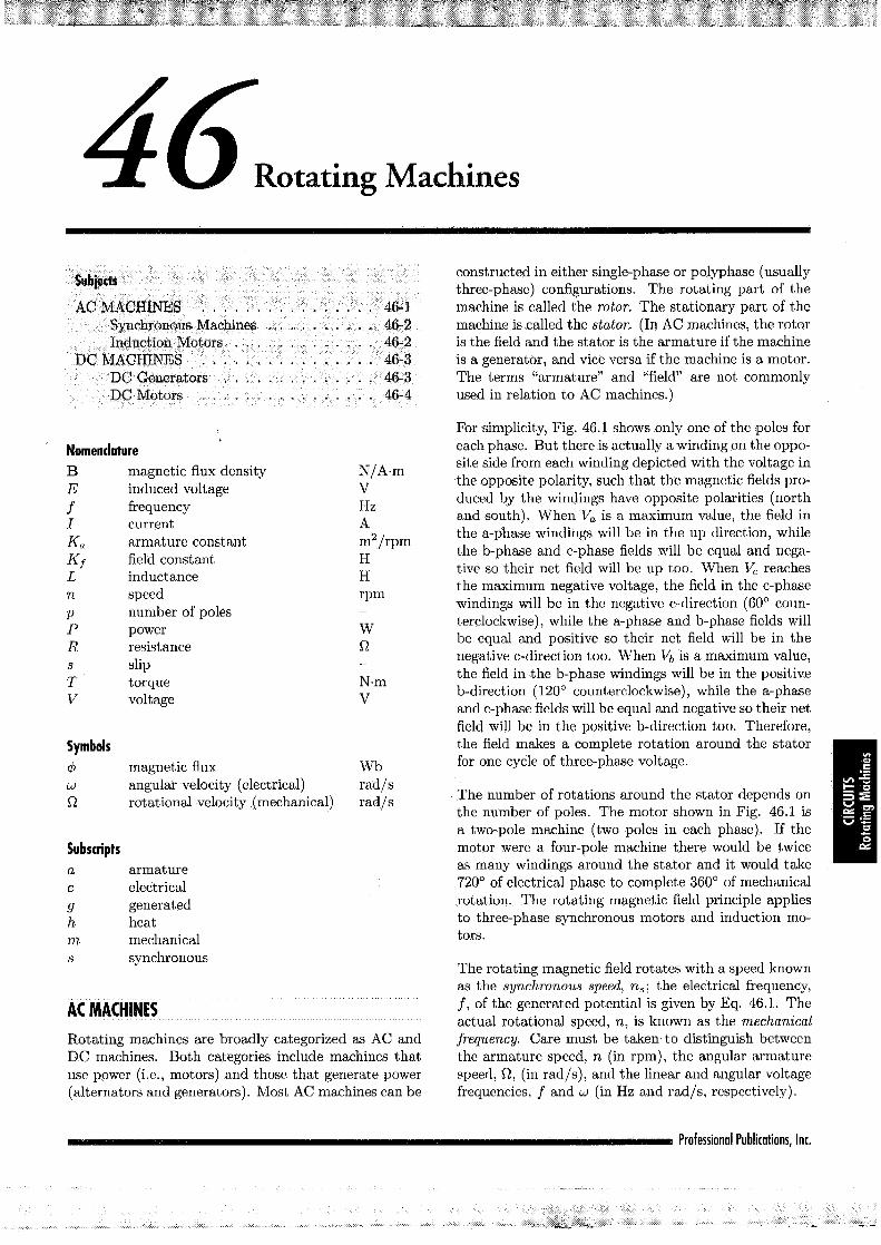
Nur Laila Hamidah

Rectangle

Nur Laila Hamidah

Rectangle

54 CHEMISTRY

CHEMISTRY

DEFINITIONS

Avogadro's Number – The number of elementary particles in a mol of a substance.

1 mol = 1 gram mole

1 mol = 6.02 × 1023 particles

Mol – The amount of a substance that contains as many particles as 12 grams of 12C (carbon 12).

Molarity of Solutions – The number of gram moles of a substance dissolved in a liter of solution.

Molality of Solutions – The number of gram moles of a substance per 1,000 grams of solvent.

Normality of Solutions – The product of the molarity of a solution and the number of valence changes taking place in a reaction.

Molar Volume of an Ideal Gas [at 0°C (32°F) and 1 atm (14.7 psia)]; 22.4 L/(g mole) [359 ft3/(lb mole)].

Mole Fraction of a Substance – The ratio of the number of moles of a substance to the total moles present in a mixture of substances.

Equilibrium Constant of a Chemical Reaction

aA bB cC dD

KA B

C Deq

d

E+ +

= a b

c6666@@@@

Le Chatelier's Principle for Chemical Equilibrium – When a stress (such as a change in concentration, pressure, or temperature) is applied to a system in equilibrium, the equilibrium shifts in such a way that tends to relieve the stress.

Heats of Reaction, Solution, Formation, and Combustion – Chemical processes generally involve the absorption or evolution of heat. In an endothermic process, heat is absorbed (enthalpy change is positive). In an exothermic process, heat is evolved (enthalpy change is negative).

Solubility Product of a slightly soluble substance AB:

AmBn → mAn+ + nBm–

Solubility Product Constant = KSP = [A+]m [B–]n

Faraday's Law – One gram equivalent weight of matter is chemically altered at each electrode for 96,485 coulombs, or 1 Faraday, of electricity passed through the electrolyte.

Faraday's Equation

m FQ

zM= c am k, where

m = mass (grams) of substance liberated at electrodeQ = total electric charge passed through electrolyte (coulomb or ampere•second)F = 96,485 coulombs/molM = molar mass of the substance (g/mol)z = valence number

A catalyst is a substance that alters the rate of a chemical reaction. The catalyst does not affect the position of equilibrium of a reversible reaction.

The atomic number is the number of protons in the atomic nucleus.

Boiling Point Elevation – The presence of a nonvolatile solute in a solvent raises the boiling point of the resulting solution.

Freezing Point Depression – The presence of a solute lowers the freezing point of the resulting solution.

ACIDS, BASES, and pH (aqueous solutions)

HpH log 1 , where10=

+f p7 A[H+] = molar concentration of hydrogen ion, in gram moles per liter. Acids have pH < 7. Bases have pH > 7.

log

For water 10

denotesmolarity

HA A H

KA H

pK K

H OH

HA

14

a

a a

–

–

– –

* +

=

=−

=

+

+

+

_ i777

767

AA

A

A

@A

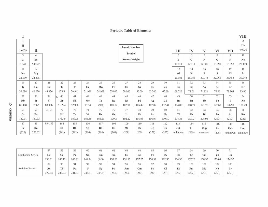
55 CHEMISTRY

Periodic Table of Elements

1

H1.0079

He

4.0026

3

Li

6.941

4

Be

9.0122

B

10.811

6

C

12.011

7

N

14.007

8

O

15.999

9

F

18.998

10

Ne

20.179

11

Na

22.990

12

Mg

24.305

Al

26.981

14

Si

28.086

15

P

30.974

16

S

32.066

17

Cl

35.453

18

Ar

39.948

19

K

39.098

20

Ca

40.078

21

Sc

44.956

22

Ti

47.88

23

V

50.941

24

Cr

51.996

25

Mn

54.938

26

Fe

55.847

27

Co

58.933

28

Ni

58.69

29

Cu

63.546

30

Zn

65.39

31

Ga

69.723

32

Ge

72.61

33

As

74.921

34

Se

78.96

35

Br

79.904

36

Kr

83.80

37

Rb

85.468

38

Sr

87.62

39

Y

88.906

40

Zr

91.224

41

Nb

92.906

42

Mo

95.94

43

Tc

(98)

44

Ru

101.07

45

Rh

102.91

46

Pd

106.42

47

Ag

107.87

48

Cd

112.41

49

In

114.82

50

Sn

118.71

51

Sb

121.75

52

Te

127.60

53

I

126.90

54

Xe

131.29

55

Cs

132.91

56

Ba

137.33

57–71 72

Hf

178.49

73

Ta

180.95

74

W

183.85

75

Re

186.21

76

Os

190.2

77

Ir

192.22

78

Pt

195.08

79

Au

196.97

80

Hg

200.59

81

Tl

204.38

82

Pb

207.2

83

Bi

208.98

84

Po

(209)

85

At

(210)

86

Rn

(222)

87

Fr

(223)

88

Ra

226.02

89–103 104

Rf

(261)

105

Db

(262)

2

5

Atomic Number

Symbol

Atomic Weight

I

II

VIII

VIIVIVIVIII

13

106

Sg

(266)

107

Bh

(264)

108

Hs

(269)

109

Mt

(268)

110

Ds

(269)

111

Rg

(272)

112

Cn

(277)

113

Uut

unknown

114

Fl

(289)

115

Uup

unknown

116

Lv

(298)

117

Uus

unknown

118

Uuo

unknown

Ac

Lanthanide Series

58

Ce

140.12

59

Pr

140.91

60

Nd

144.24

61

Pm

(145)

62

Sm

150.36

63

Eu

151.96

64

Gd

157.25

65

Tb

158.92

66

Dy

162.50

67

Ho

164.93

68

Er

167.26

69

Tm

168.93

70

Yb

173.04

71

Lu

174.97

Actinide Series Th

232.04

91

Pa

231.04

92

U

238.03

93

Np

237.05

94

Pu

(244)

95

Am

(243)

96

Cm

(247)

97

Bk

(247)

98

Cf

(251)

99

Es

(252)

100

Fm

(257)

101

Md

(258)

102

No

(259)

103

Lr

(260)

57

La

138.91

9089

Ac

227.03

56 CHEMISTRY

SELECTED RULES OF NOMENCLATURE IN ORGANIC CHEMISTRY

AlcoholsThree systems of nomenclature are in general use. In the first, the alkyl group attached to the hydroxyl group is named and the separate word alcohol is added. In the second system, the higher alcohols are considered as derivatives of the first mem-ber of the series, which is called carbinol. The third method is the modified Geneva system in which (1) the longest carbon chain containing the hydroxyl group determines the surname, (2) the ending e of the corresponding saturated hydrocarbon is replaced by ol, (3) the carbon chain is numbered from the end that gives the hydroxyl group the smaller number, and (4) the side chains are named and their positions indicated by the proper number. Alcohols in general are divided into three classes. In primary alcohols the hydroxyl group is united to a primary carbon atom, that is, a carbon atom united directly to only one other carbon atom. Secondary alcohols have the hydroxyl group united to a secondary carbon atom, that is, one united to two other carbon atoms. Tertiary alcohols have the hydroxyl group united to a tertiary carbon atom, that is, one united to three other carbon atoms.

EthersEthers are generally designated by naming the alkyl groups and adding the word ether. The group RO is known as an alk-oxyl group. Ethers may also be named as alkoxy derivatives of hydrocarbons.

Carboxylic AcidsThe name of each linear carboxylic acid is unique to the number of carbon atoms it contains. 1: (one carbon atom) Formic. 2: Acetic. 3: Propionic. 4: Butyric. 5: Valeric. 6: Caproic. 7: Enanthic. 8: Caprylic. 9: Pelargonic. 10: Capric.

AldehydesThe common names of aldehydes are derived from the acids that would be formed on oxidation, that is, the acids having the same number of carbon atoms. In general the ic acid is dropped and aldehyde added.

KetonesThe common names of ketones are derived from the acid which on pyrolysis would yield the ketone. A second method, especially useful for naming mixed ketones, simply names the alkyl groups and adds the word ketone. The name is written as three separate words.

Unsaturated Acyclic HydrocarbonsThe simplest compounds in this class of hydrocarbon chemicals are olefins or alkenes with a single carbon-carbon double bond, having the general formula of CnH2n. The simplest example in this category is ethylene, C2H4.

Dienes are acyclic hydrocarbons with two carbon-carbon double bonds, having the general formula of CnH2n–2; butadiene (C4H6) is an example of such.

Similarly, trienes have three carbon-carbon double bonds with the general formula of CnH2n–4; hexatriene (C6H8) is such an example.

The simplest alkynes have a single carbon-carbon triple bond with the general formula of CnH2n–2. This series of compounds begins with acetylene, or C2H2.

57 CHEMISTRY

Important Families of Organic Compounds

FAMILY

Alkane Alkene Alkyne Arene Haloalkane Alcohol Ether Amine Aldehyde Ketone CarboxylicAcid

Ester

SpecificExample CH3CH3 H2C = CH2 HC ≡ CH CH3CH2Cl CH3CH2OH CH3OCH3 CH3NH2

IUPACName Ethane

Ethene

or

Ethylene

Ethyne

or

Acetylene

Benzene Chloroethane Ethanol Methoxy-methane

Methan-amine

Ethanal Acetone Ethanoic

AcidMethyl

ethanoate

CommonName

Ethane Ethylene Acetylene Benzene Ethyl

chlorideEthyl alcohol

Dimethylether

Methyl-amine

Acetal-dehyde

Dimethylketone

Acetic Acid Methylacetate

GeneralFormula RH

RCH = CH2

RCH = CHR

R2C = CHR

R2C = CR2

RC ≡ CH

RC ≡ CR ArH RX ROH ROR

RNH2

R2NH

R3N

FunctionalGroup

C–H

and

C–C

bonds

– C ≡ C –Aromatic

Ring

C = C

O

CH3CH

O

CH3COH

O

CH3COCH3

O

RCH

O

RCOH

O

RCOR

C X C OH C O C C N

O

C H

O

C OH C O C

O

O

CH3CCH3

O

R1CR2

O

C

58 CHEMISTRY

Common Names and Molecular Formulas of Some Industrial(Inorganic and Organic) Chemicals

Common Name Chemical Name MolecularFormula

Muriatic acid Hydrochloric acid HCl Cumene Isopropyl benzene C6H5CH(CH3)2

Styrene Vinyl benzene C6H5CH=CH2

— Hypochlorite ion OCl–1

— Chlorite ion ClO2–1

— Chlorate ion ClO3–1

— Perchlorate ion ClO4–1

Gypsum Calcium sulfate CaSO4

Limestone Calcium carbonate CaCO3

Dolomite Magnesium carbonate MgCO3

Bauxite Aluminum oxide Al2O3

Anatase Titanium dioxide TiO2

Rutile Titanium dioxide TiO2

— Vinyl chloride CH2=CHCl— Ethylene oxide C2H4O

Pyrite Ferrous sulfide FeS Epsom salt Magnesium sulfate MgSO4

Hydroquinone p-Dihydroxy benzene C6H4(OH)2

Soda ash Sodium carbonate Na2CO3

Salt Sodium chloride NaCl Potash Potassium carbonate K2CO3

Baking soda Sodium bicarbonate NaHCO3

Lye Sodium hydroxide NaOH Caustic soda Sodium hydroxide NaOH

— Vinyl alcohol CH2=CHOHCarbolic acid Phenol C6H5OHAniline Aminobenzene C6H5NH2

— Urea (NH2)2COToluene Methyl benzene C6H5CH3

Xylene Dimethyl benzene C6H4(CH3)2

— Silane SiH4

— Ozone O3

Neopentane 2,2-Dimethylpropane CH3C(CH3)2CH3

Magnetite Ferrous/ferric oxide Fe3O4

Quicksilver Mercury Hg Heavy water Deuterium oxide (H2)2O

— Borane BH3

Eyewash Boric acid (solution) H3BO3

— Deuterium H2

— Tritium H3

Laughing gas Nitrous oxide N2O— Phosgene COCl2

Wolfram Tungsten W — Permanganate ion MnO4

–1

— Dichromate ion Cr2O7–2

— Hydronium ion H3O+1

Brine Sodium chloride (solution)

NaCl

Battery acid Sulfuric acid H2SO4

59 CHEMISTRY

ELECTROCHEMISTRY

Cathode – The electrode at which reduction occurs.

Anode – The electrode at which oxidation occurs.

Oxidation – The loss of electrons.

Reduction – The gaining of electrons.

Cation – Positive ion

Anion – Negative ion

Standard Oxidation Potentials for Corrosion Reactions*

Corrosion Reaction Potential, Eo, Volts

vs. Normal Hydrogen Electrode

Au → Au3+ + 3e

2H2O → O2 + 4H+ + 4e

Pt → Pt2+ + 2e

Pd → Pd2+ + 2e

Ag → Ag+ + e

2Hg → Hg22+ + 2e

Fe2+ → Fe3+ + e

4(OH)– → O2 + 2H2O + 4e

Cu → Cu2+ + 2e

Sn2+ → Sn4+ + 2e

H2 → 2H+ + 2e

Pb → Pb2+ + 2e

Sn → Sn2+ + 2e

Ni → Ni2+ + 2e

Co → Co2+ + 2e

Cd → Cd2+ + 2e

Fe → Fe2+ + 2e

Cr → Cr3+ + 3e

Zn → Zn2+ + 2e

Al → Al3+ + 3e

Mg → Mg2+ + 2e

Na → Na+ + e

K → K+ + e

–1.498

–1.229

–1.200

–0.987

–0.799

–0.788

–0.771

–0.401

–0.337

–0.150

0.000

+0.126

+0.136

+0.250

+0.277

+0.403

+0.440

+0.744

+0.763

+1.662

+2.363

+2.714

+2.925

* Measured at 25oC. Reactions are written as anode half-cells. Arrows are reversed for cathode half-cells.

Flinn, Richard A., and Paul K. Trojan, Engineering Materials and Their Applications, 4th ed., Houghton Mifflin Company, 1990.

NOTE: In some chemistry texts, the reactions and the signs of the values (in this table) are reversed; for example, the half-cell potential of zinc is given as –0.763 volt for the reaction Zn2+ + 2e → Zn. When the potential Eo is positive, the reaction proceeds spontaneously as written.

–

–

–

–

–

–

–

–

–

–

–

–

–

–

–

–

–

–

–

–

–

–

–

–

60 MATERIALS SCIENCE/STRUCTURE OF MATTER

MATERIALS SCIENCE/STRUCTURE OF MATTER

ATOMIC BONDING

Primary BondsIonic (e.g., salts, metal oxides)

Covalent (e.g., within polymer molecules)

Metallic (e.g., metals)

CORROSIONA table listing the standard electromotive potentials of metals is shown on the previous page.

For corrosion to occur, there must be an anode and a cathode in electrical contact in the presence of an electrolyte.

Anode Reaction (Oxidation) of a Typical Metal, MMo

→ Mn+ + ne–

Possible Cathode Reactions (Reduction)½ O2 + 2 e–

+ H2O → 2 OH–

½ O2 + 2 e– + 2 H3O

+ → 3 H2O

2 e– + 2 H3O

+ → 2 H2O + H2

When dissimilar metals are in contact, the more electropositive one becomes the anode in a corrosion cell. Different regions of carbon steel can also result in a corrosion reaction: e.g., cold-worked regions are anodic to noncold-worked; different oxygen concentrations can cause oxygen-deficient regions to become cathodic to oxygen-rich regions; grain boundary regions are anodic to bulk grain; in multiphase alloys, various phases may not have the same galvanic potential.

DIFFUSION

Diffusion Coefficient D = Do e−Q/(RT), where

D = diffusion coefficientDo = proportionality constant

Q = activation energy

R = gas constant [8.314 J/(mol•K)]

T = absolute temperature

THERMAL AND MECHANICAL PROCESSINGCold working (plastically deforming) a metal increases strength and lowers ductility.

Raising temperature causes (1) recovery (stress relief), (2) recrystallization, and (3) grain growth. Hot working allows these processes to occur simultaneously with deformation.

Quenching is rapid cooling from elevated temperature, preventing the formation of equilibrium phases.

In steels, quenching austenite [FCC (γ) iron] can result in martensite instead of equilibrium phases—ferrite [BCC (α) iron] and cementite (iron carbide).

PROPERTIES OF MATERIALS

ElectricalCapacitance: The charge-carrying capacity of an insulating material

Charge held by a capacitor

q = CVq = chargeC = capacitanceV = voltage

Capacitance of a parallel plate capacitor

C dAf=

C = capacitanceε = permittivity of materialA = cross-sectional area of the platesd = distance between the platesε is also expressed as the product of the dielectric constant (κ) and the permittivity of free space (ε

0 = 8.85 × 10−12 F/m)

Resistivity: The material property that determines the resistance of a resistor

Resistivity of a material within a resistor

LRA=t

ρ = resistivity of the materialR = resistance of the resistorA = cross-sectional area of the resistorL = length of the resistor

Conductivity is the reciprocal of the resistivity

Photoelectric effect−electrons are emitted from matter (metals and nonmetallic solids, liquids or gases) as a consequence of their absorption of energy from electromagnetic radiation of very short wavelength and high frequency.

Piezoelectric effect−the electromechanical and the electrical state in crystalline materials.

MechanicalStrain is defined as change in length per unit length; for pure tension the following apply:

Engineering strain

LL0

D=f

ε = engineering strain∆L = change in lengthL

0 = initial length

True strain

LdL

T =f

εT

= true straindL = differential change in lengthL = initial lengthε

T = ln(1 + ε)


AluminumAntimonyArsenicBariumBerylliumBismuthCadmiumCaesiumCalciumCeriumChromiumCobaltCopperGalliumGoldIndiumIridiumIronLeadLithiumMagnesiumManganeseMercuryMolybendumNickelNiobiumOsmiumPalladiumPlatinumPotassiumRhodiumRubidiumRutheniumSilverSodiumStrontiumTantalumThalliumThoriumTinTitaniumTungstenUraniumVanadiumZincZirconium

AlSbAsBaBeBiCdCsCaCeCrCoCuGaAuInIrFePbLiMgMnHgMoNiNbOsPdPtKRhRbRuAgNaSrTaTlThSnTiWUVZnZr

26.98121.7574.92137.339.012208.98112.41132.9140.08140.12

5258.9363.5469.72196.97114.82192.2255.85207.26.9424.3154.94200.5995.9458.6992.91190.2106.4195.0839.09102.9185.47101.07107.8722.98987.62180.95204.38232.04118.6947.88183.85238.0350.9465.3891.22

AtomicWeight

2,6986,6925,7763,5941,8469,8038,6471,9001,5306,7117,1948,8008,9335,90519,2817,29022,5507,87311,343

5331,7387,47313,54710,2228,9078,57822,58011,99521,450

86212,4201,53312,36010,500

9662,58316,67011,87111,7257,2854,50819,25419,0506,0907,1356,507

Densityρ (kg/m3)

Water = 1000

660630

subl. 613710

1,28527132129840800

1,8601,4941,084

301,064156

2,4471,540327180650

1,250−39

2,6201,4552,4253,0301,5541,772

631,96338.82,31096197.8770

3,000304

1,700232

1,6703,3871,1351,920419

1,850

MeltingPoint (°C)

895.9209.3347.5284.7

2,051.5125.6234.5217.7636.4188.4406.5431.2389.4330.7129.8238.6138.2456.4129.8

4,576.21,046.7502.4142.3272.1439.6267.9129.8230.3134

753.6242.8330.7255.4234.5

1,235.1−

150.7138.2117.2230.3527.5142.8117.2481.5393.5284.7

Specific Heat [J/(kg˙K)]

2.53926362.81076.818.83.27.312.75.61.5513.62.05

84.78.919.28.553.9413894.1

56.215.28.110

9.816.14.3117.11.474.220

12.310

14.711.5394.928

18.25.540

ElectricalResistivity(10−8 Ω˙m)

at 0°C(273.2 K)

23625.5

−−

2188.29736−11

96.510540341

31984

14783.53686

1578

7.81399453887272

10415158117428142−5710546822

177273111723

Heat Conductivityλ[W/(m˙K)]

at 0°C(273.2 K)

1,2201,166

subl. 1,1351,3102,34551960984

1,5441,4723,3802,7211,983

861,947312

4,4362,804620356

1,2022,282−38

4,7482,6514,3975,4862,8293,221145

3,565102

4,1901,760208

1,4185,432579

3,092449

3,0386,1282,0753,488786

3,362

MeltingPoint (°F)

Metal Symbol

Properties of Metals


The elastic modulus (also called modulus, modulus of elasticity, Young's modulus) describes the relationship between engineering stress and engineering strain during elastic loading. Hooke's Law applies in such a case.

σ = Eε where E is the elastic modulus.

Key mechanical properties obtained from a tensile test curve: • Elastic modulus

• Ductility (also called percent elongation): Permanent engineering strain after failure

• Ultimate tensile strength (also called tensile strength): Maximum engineering stress

• Yield strength: Engineering stress at which permanent deformation is first observed, calculated by 0.2% offset method.

Other mechanical properties:

• Creep: Time-dependent deformation under load. Usually measured by strain rate. For steady-state creep this is:

dtd A en RT

Qfv= -

A = pre-exponential constant

n = stress sensitivityQ = activation energy for creepR = ideal gas law constantT = absolute temperature

• Fatigue: Time-dependent failure under cyclic load. Fatigue life is the number of cycles to failure. The endurance limit is the stress below which fatigue failure is unlikely.

• Fracture toughness: The combination of applied stress and the crack length in a brittle material. It is the stress intensity when the material will fail.

K Y aIC v r=

KIC

= fracture toughness

σ = applied engineering stressa = crack lengthY = geometrical factor

a 2a

EXTERIOR CRACK (Y = 1.1) INTERIOR CRACK (Y = 1)

The critical value of stress intensity at which catastrophiccrack propagation occurs, KIc, is a material property.

♦ W.R. Runyan and S.B. Watelski, in Handbook of Materials and Processes for Electronics, C.A. Harper, ed., McGraw-Hill, 1970.

♦Some Extrinsic, Elemental Semiconductors

BAIGaPAsSbAlGaInAsSb

Periodic tablegroup of dopant

III AIII AIII AV AV AV AIII AIII AIII AV AV A

Maximum solid solubilityof dopant (atoms/m3)

600 × 1024

20 × 1024

40 × 1024

1,000 × 1024

2,000 × 1024

70 × 1024

400 × 1024

500 × 1024

4 × 1024

80 × 1024

10 × 1024

Si

Ge

Element Dopant

♦Impurity Energy Levels for Extrinsic Semiconductors

Eg − Ed(eV)0.0440.0490.0390.069

−−−−−

0.0120.0130.096

−−−−−

0.0050.003

−−

Si

Ge

GaAs

Semiconductor

PAsSbBiBAlGaInTl

PAsSbBAlGaInTl

SeTeZnCd

DopantEa

(eV)

−−−−

0.0450.0570.0650.1600.260

−−−

0.0100.0100.0100.0110.01

−−

0.0240.021

Stress is defined as force per unit area; for pure tension the following apply:

Engineering stress

AF0

v =

σ = engineering stress

F = applied force

A0 = initial cross-sectional area

True stress

AF

Tv =

σT = true stress

F = applied force

A = actual cross-sectional area


Representative Values of Fracture ToughnessMaterial KIc (MPa•m1/2 ) KIc (ksi•in1/2 )A1 2014-T651 24.2 22 A1 2024-T3 44 40 52100 Steel 14.3 13 4340 Steel 46 42 Alumina 4.5 4.1 Silicon Carbide 3.5 3.2

RELATIONSHIP BETWEEN HARDNESS AND TENSILE STRENGTHFor plain carbon steels, there is a general relationship between Brinell hardness and tensile strength as follows:

TS psi 500 BHN

TS MPa 3.5 BHN

-

-

_^ih

ASTM GRAIN SIZE

.,

S P

N

N N

2

2

0 0645Actual Area mmwhere

.

V L

n0 0645

1

2

mm

actual

2

=

=

=

-

_

_^

i

ih

SV = grain-boundary surface per unit volumePL = number of points of intersection per unit length between the line and the boundariesN = number of grains observed in a area of 0.0645 mm2

n = grain size (nearest integer > 1)

COMPOSITE MATERIALS

f

C fc

Ef

E fE

f

1

c i i

c i i

i

ic i i

c i i

# #

t t

v v

R

R

R R

R

==

=

−

= G

ρc = density of composite

Cc = heat capacity of composite per unit volume

Ec = Young's modulus of composite

fi = volume fraction of individual material

ci = heat capacity of individual material per unit volume

Ei = Young's modulus of individual material

σc = strength parallel to fiber directionAlso, for axially oriented, long, fiber-reinforced composites, the strains of the two components are equal.

(∆L/L)1 = (∆L/L)2

∆L = change in length of the composite

L = original length of the composite

Hardness: Resistance to penetration. Measured by denting a material under known load and measuring the size of the dent.

Hardenability: The "ease" with which hardness can be obtained.

JOMINY HARDENABILITY CURVES FOR SIX STEELS

(#2) and (#8) indicate grain size

in.

Van Vlack, L., Elements of Materials Science & Engineering, Addison-Wesley, 1989.


The following two graphs show cooling curves for four different positions in the bar.C = CenterM-R = Halfway between center and surface

3/4-R = 75% of the distance between the center and the surface

S = Surface

These positions are shown in the following figure.

C M-R3/4-R S

♦

COOLING RATES FOR BARS QUENCHED IN AGITATED WATER

♦

COOLING RATES FOR BARS QUENCHED IN AGITATED OIL

Impact TestThe Charpy Impact Test is used to find energy required tofracture and to identify ductile to brittle transition.

Impact tests determine the amount of energy required to cause failure in standardized test samples. The tests are repeated over a range of temperatures to determine the ductile to brittle transition temperature.

♦ Van Vlack, L., Elements of Materials Science & Engineering, Addison-Wesley, 1989.


Concrete♦

8,0006,000

4,000

2,000

1,000

W/C BY WEIGHT

0.40 0.60 0.80 1.00

RECOMMENDEDPERCENT ENTRAINED AIR

NO ADDED AIR AV

ERAG

E 28

-DAY

COM

PRES

SIVE

STRE

NGTH

, PSI

Concrete strength decreases with increases in water-cementratio for concrete with and without entrained air.

Water-cement (W/C) ratio is the primary factor affecting the strength of concrete. The figure above shows how W/C expressed as a ratio of weight of water and cement by weight of concrete mix affects the compressive strength of both air-entrained and non-air-entrained concrete.•

6,000

4,000

3,000

2,000

5,000

1,000

COMP

RESS

IVE

STRE

NGTH

, PSI

AGE, DAYS081098241730

STORED CONTINUOUSLY IN LABORATORY AIR

IN AIR AFTER 28 DAYS

IN AIR AFTER 14 DAYS

IN AIR AFTER 3 DAYS

CONTINUOUSLY MOIST CURED

Concrete compressive strength varies with moist-curing conditions. Mixes tested had a water-cement ratio of 0.50, a slump of 3.5 in., cement content of 556 lb/yd3, sand content of 36%, and air content of 4%.

IN AIR AFTER 7 DAYS

Water content affects workability. However, an increase in water without a corresponding increase in cement reduces the concrete strength. Superplasticizers are the most typical way to increase workability. Air entrainment is used to improve durability.

Amorphous MaterialsAmorphous materials such as glass are non-crystalline solids. Thermoplastic polymers are either semicrystalline or amorphous.

Below the glass transition temperature (Tg) the amorphous

material will be a brittle solid.

TEMPERATURE

VOLU

ME

Tg Tm

GLASS

LIQUID

CRYSTAL

The volume temperature curve as shown above is often used to show the difference between amorphous and crystalline solids.

PolymersPolymers are classified as thermoplastics that can be melted and reformed. Thermosets cannot be melted and reformed.

Tg Tm

LOG

E or

LOG

σ

TEMPERATURE

The above curve shows the temperature dependent strength (σ) or modulus (E) for a thermoplastic polymer.

Polymer AdditivesChemicals and compounds are added to polymers to improve properties for commercial use. These substances, such as plasticizers, improve formability during processing, while others increase strength or durability.

Examples of common additives are:Plasticizers: vegetable oils, low molecular weight polymers or monomers

Fillers: talc, chopped glass fibersFlame retardants: halogenated paraffins, zinc borate, chlorinated phosphates

Ultraviolet or visible light resistance: carbon black

Oxidation resistance: phenols, aldehydes

Thermal PropertiesThe thermal expansion coefficient is the ratio of engineering strain to the change in temperature.

T=a fD

α = thermal expansion coefficientε = engineering strain∆T = change in temperature

Specific heat (also called heat capacity) is the amount of heat required to raise the temperature of something or an amount of something by 1 degree.

At constant pressure the amount of heat (Q) required to increase the temperature of something by ∆T is C

p∆T, where

Cp is the constant pressure heat capacity.

At constant volume the amount of heat (Q) required to increase the temperature of something by ∆T is C

v∆T, where

Cv is the constant volume heat capacity.

An object can have a heat capacity that would be expressed as energy/degree.

The heat capacity of a material can be reported as energy/degree per unit mass or per unit volume.

♦ Concrete Manual, 8th ed., U.S. Bureau of Reclamation, 1975.• Merritt, Frederick S., Standard Handbook for Civil Engineers, 3rd ed., McGraw-Hill, 1983.


BINARY PHASE DIAGRAMSAllows determination of (1) what phases are present at equilibrium at any temperature and average composition, (2) the compositions of those phases, and (3) the fractions of those phases.

Eutectic reaction (liquid → two solid phases)

Eutectoid reaction (solid → two solid phases)

Peritectic reaction (liquid + solid → solid)

Peritectoid reaction (two solid phases → solid)

Lever RuleThe following phase diagram and equations illustrate how the weight of each phase in a two-phase system can be determined:

COMPOSITION, WT% 0% B 100% A

100% B 0% A

BA

L

β + Lα + L

α + β

βα

xα xβx

TEMP

ERAT

URE,

°C

TEMP

ERAT

URE,

°F

(In diagram, L = liquid.) If x = the average composition at temperature T, then

x xx

x xx x

%

%

100

100

xwt

wt

#

#

=

=

a

b

--

--b a

b

b a

a

Iron-Iron Carbide Phase Diagram♦

♦ Van Vlack, L., Elements of Materials Science & Engineering, Addison-Wesley, Boston, 1989.

67 STATICS

FORCEA force is a vector quantity. It is defined when its (1) magnitude, (2) point of application, and (3) direction are known.The vector form of a force is

F = Fx i + Fy j

RESULTANT (TWO DIMENSIONS)The resultant, F, of n forces with components Fx,i and Fy,ihas the magnitude of

F F F, ,x ii

n

y ii

n

1

2

1

2 1 2

= += =d dn n> H! !

The resultant direction with respect to the x-axis is

arctan F F, ,y ii

n

x ii

n

1 1=i

= =e o! !

RESOLUTION OF A FORCEFx = F cos θx; Fy = F cos θy; Fz = F cos θz

cos θx = Fx /F; cos θy = Fy /F; cos θz = Fz /F

Separating a force into components when the geometry of force is known and R x y z2 2 2= + +

Fx = (x/R)F; Fy = (y/R)F; Fz = (z/R)F

MOMENTS (COUPLES)A system of two forces that are equal in magnitude, opposite in direction, and parallel to each other is called a couple. A moment M is defined as the cross product of the radius vector r and the force F from a point to the line of action of the force.

M = r × F; Mx = yFz – zFy, My = zFx – xFz, and Mz = xFy – yFx.

SYSTEMS OF FORCESF = Σ Fn

M = Σ (rn × Fn)

Equilibrium RequirementsΣ Fn = 0

Σ Mn = 0

STATICS

CENTROIDS OF MASSES, AREAS, LENGTHS, AND VOLUMESThe following formulas are for discrete masses, areas, lengths, and volumes:

rc = Σ mnrn /Σ mn, wheremn = the mass of each particle making up the system,rn = the radius vector to each particle from a selected reference point, andrc = the radius vector to the centroid of the total mass from the selected reference point.The moment of area (Ma) is defined as

May = Σ xnan

Max = Σ ynan

The centroid of area is defined asxac = May /A = Σ xn an/A

yac = Max /A = Σ yn an/Awhere A = Σ an

MOMENT OF INERTIAThe moment of inertia, or the second moment of area, is defined as

Iy = ∫x2 dA

Ix = ∫y2 dA

The polar moment of inertia J of an area about a point is equal to the sum of the moments of inertia of the area about any two perpendicular axes in the area and passing through the same point.

Iz = J = Iy + Ix = ∫(x2 + y2) dA

= rp2A, where

rp = the radius of gyration (as defined on the next page)

68 STATICS

Moment of Inertia Parallel Axis TheoremThe moment of inertia of an area about any axis is defined as the moment of inertia of the area about a parallel centroidal axis plus a term equal to the area multiplied by the square of the perpendicular distance d from the centroidal axis to the axis in question.

, where

I I d A

I I d A

2

2

x x y

y y x

c

c

= +

= +

l

l

dx, dy = distance between the two axes in question,Ixc

, Iyc = the moment of inertia about the centroidal axis, and

,I Ix yl l = the moment of inertia about the new axis.

dA

Cdx

dy

0

y

x

y '

x '

Hibbeler, R.C., Engineering Mechanics: Statics and Dynamics, 10 ed., Pearson Prentice Hall, 2004.

Radius of GyrationThe radius of gyration rp, rx, ry is the distance from a reference axis at which all of the area can be considered to be concentrated to produce the moment of inertia.

; ;r I A r I A r J Ax x y y p= = =

Product of InertiaThe product of inertia (Ixy, etc.) is defined as:

Ixy = ∫xydA, with respect to the xy-coordinate system,

The parallel-axis theorem also applies:I'xy = Ixc

yc + dxdy A for the xy-coordinate system, etc.

wheredx = x-axis distance between the two axes in question, anddy = y-axis distance between the two axes in question.

FRICTIONThe largest frictional force is called the limiting friction.Any further increase in applied forces will cause motion.

F ≤ µsN, where

F = friction force,

µs = coefficient of static friction, and

N = normal force between surfaces in contact.

SCREW THREADFor a screw-jack, square thread,

M = Pr tan (α ± φ), where+ is for screw tightening,– is for screw loosening,M = external moment applied to axis of screw,P = load on jack applied along and on the line of the axis,r = the mean thread radius,α = the pitch angle of the thread, andµ = tan φ = the appropriate coefficient of friction.

BELT FRICTIONF1 = F2 eµθ, where

F1 = force being applied in the direction of impending motion,

F2 = force applied to resist impending motion,

µ = coefficient of static friction, andθ = the total angle of contact between the surfaces expressed in radians.

STATICALLY DETERMINATE TRUSS

Plane Truss: Method of JointsThe method consists of solving for the forces in the members by writing the two equilibrium equations for each joint of the truss.

Σ F = 0 and Σ F = 0, whereF = horizontal forces and member components andF = vertical forces and member components.

Plane Truss: Method of SectionsThe method consists of drawing a free-body diagram of a portion of the truss in such a way that the unknown truss member force is exposed as an external force.

CONCURRENT FORCESA concurrent-force system is one in which the lines of action of the applied forces all meet at one point. A two-force body in static equilibrium has two applied forces that are equal in magnitude, opposite in direction, and collinear.

69 STATICS

A = bh/2

xc = 2b/3

yc = h/3

/363hbIcy =

/363bhIcx =

Ix = bh3/12

Iy = b3h/42

6

18

18

22

22

22

22

br

hr

br

hr

y

x

y

x

c

c

=

=

=

=

84

723622

22

hbAbhI

hbAbhI

xy

yx cc

==

==

A = bh/2

xc = b/3

yc = h/3

/363hbIcy =

/363bhIcx =

Ix = bh3/12

Iy = b3h/126

6

18

18

22

22

22

22

br

hr

br

hr

y

x

y

x

c

c

=

=

=

=

2412

723622

22

hbAbhI

hbAbhI

xy

yx cc

==

−=−=

A = bh/2

xc = (a + b)/3

yc = h/3 ( )[ ] 1222 aabbbhI y ++=

123bhI x =

( )[ ] 3622 aabbbhIyc+−=

363bhIxc=

( )

( ) 6

6

18

18

222

22

222

22

aabbr

hr

aabbr

hr

y

x

y

x

c

c

++=

=

+−=

= ( )[ ]( )[ ]( )[ ]( )[ ] 242

122

722

362

2

2

babh

baAhI

babh

baAhI

xy

yx cc

+=

+=

−=

−=

A = bh

xc = b/2

yc = h/2

( )[ ] 1222 hbbhJ +=

33hbI y =

33bhI x =

123hbI yc=

123hbI xc=

( ) 12

3

3

12

12

222

22

22

22

22

hbr

br

hr

br

hr

p

y

x

y

x

c

c

+=

=

=

=

=44

022hbAbhI

I

xy

yx cc

==

=

( )( )( )ba

bahy

bahA

c ++=

+=

32

2

( )1233 bah

I x+=

( )( )36

4 223

ba

babahI xc +

++= ( )( )

( )( )ba

bahr

ba

babahr

x

xc

++=

+++=

6318

4

22

2222

A = ab sin θxc = (b + a cos θ)/2yc = (a sin θ)/2

( ) 6cossin22 θθ− ba

( )[ ] 3cossin 2θ+θ= ababI y

( ) 3sin33 θ= baI x

( )[ ] 12cossin 222 θ+θ= ababI yc

( ) 12sin33 θ= baI xc ( )( )( )( )

( ) 6cos3cos

3sin

12cos12sin

22

22

2222

22

θ−θ+=

θ=

θ+=θ=

ab

abr

ar

abr

ar

y

x

y

x

c

c

( ) 1223 θθ= cossinbaIcc yx

Housner, George W., and Donald E. Hudson, Applied Mechanics Dynamics, D. Van Nostrand Company, Inc., Princeton, NJ, 1959. Table reprinted by permission of G.W. Housner & D.E. Hudson.

hC

b x

y

y

h

xb

C

y

h

xb

a

C

Ch

xb

y

a

h

xb

y

C

y

Ca

xb

Figure Area & Centroid Area Moment of Inertia (Radius of Gyration)2 Product of Inertia

70 STATICS

A = πa2

xc = a

yc = a 2454

4

4

4

aJ

aII

aII

yx

yx cc

π=π==π==

2

45

4

22

222

222

ar

arr

arr

p

yx

yx cc

=

==

==

2

0AaI

I

xy

yx cc

==

A = π (a2 – b2)xc = a

yc = a

( )

( ) 244

54

44

422

4

44

baJ

bba

aII

baII

yx

yx cc

−π=

π−π−π==

−π== ( )( )

( ) 2

45

4

222

2222

2222

bar

barr

barr

p

yx

yx cc

+=

+==

+==

( )222

2

0

baa

AaI

I

xy

yx cc

−π==

=

A = πa2/2xc = a

yc = 4a/(3π)

( )

858872

649

4

4

4

24

aI

aI

aI

aI

y

x

y

x

c

c

π=π=π=

π−π=

( )

45

4

436

649

22

22

22

2

222

ar

ar

ar

ar

y

x

y

x

c

c

=

=

=π

−π=

320

4aI

I

xy

yx cc

==

0

sin3

2

2

=θ

θ=

θ=

c

c

y

ax

aAIx = a4(θ – sinθ cos θ)/4Iy = a4(θ + sinθ cos θ)/4

( )

( )θ

θθ+θ=

θθθ−θ=

cossin4

cossin42

2

22

ar

ar

y

x

00

==

xy

yx

I

Icc

0cossin

sin3

2

22sin

3

2

=θθ−θ

θ=

θ−θ=

c

c

y

ax

aA

θθ−θθθ+=

θθ−θθθ−=

cossincossin21

4

cossin33cossin21

432

32

AaI

AaI

y

x

θθ−θθθ+=

θθ−θθθ−=

cossincossin21

4

cossin33cossin21

432

2

322

ar

ar

y

x

00

==

xy

yx

I

Icc


y

Ca

x

x

b

y

Ca

Cy

2a x

ya

Cx

a

Cx

y [ ][ ][ ]

[ ] [ ]


71 STATICS

A = 4ab/3

xc = 3a/5

yc = 074

17516

154

3

3

3

baI

baI

abII

y

y

xx

c

c

=

=

==

73

17512

5

22

22

222

ar

ar

brr

y

y

xx

c

c

=

=

==

0

0

=

=

xy

yx

I

Icc

A = 2ab/3

xc = 3a/5

yc = 3b/8

Ix = 2ab3/15

Iy = 2ba3/7 73

5

22

22

ar

br

y

x

=

=

Ixy = Aab/4 = a2b2

( )

12

1

2

2

1

1

+

+=

+

+=

+=

n

nhy

bn

nx

nbhA

c

c ( )

3

133

3

3

+=

+=

n

hbI

n

bhI

y

x

( )( )

22

22

3

1

133

1

bn

nr

n

nhr

y

x

+

+=

+

+=

( )h

n

ny

bn

nx

bhn

nA

c

c

22

1

12

1

1

+

+=

+

+=

+=

( )hb

n

nI

bhn

nI

y

x

3

3

13

33

+=

+= ( )

22

22

13

1

13

1

bn

nr

hn

nr

y

x

+

+=

+

+=


y

xb

b

C

a

y

x

b

a

C

h

x

C

b

yy = (h/b n)xn

y y = (h/b 1/n)x1/n

h

xb

C


72 DYNAMICS

DYNAMICS

Unit vectors er and eθ are, respectively, collinear with and normal to the position vector r. Thus:

2 , where

radialposition coordinate

angle from the axis to

/ , etc., / , etc.

r

r

r r

r r r r

r

r r

x

dr dt d r dt

r e

v e e

a e e

2 2

r

r

r2

i

i i i

i

== +

= − + +=== =

i

i

o o

p o p o o

o p

_ _i i

♦ Particle Rectilinear Motion

=v

Variable a

a dtdv

dtds

a ds vdv

=

=

a a

a

=ttan

21

2

Cons

v v s s

v v a t

0

0 0

0 0 02

202

0 0

= +

= + −

s s v t a t= + +

_ j

♦ Particle Curvilinear Motion

v z a z= =v y a y= =

x,y,z Coordinates

v x a xx x

y y

z z

= =o po po p

,

2

r, z Coordinates

v r a r r

v r a r r

v z a z

2r r

z z

i

i

i i i

= = −= = += =i i

o p o

o p o o

o p

n, t, b Coordinates

v = s•

at = v = • dv

dt

an =v2

ρ ρ =1 + (dy/dx)2

3/2[ [d

2ydx2

dvds

= v

♦ Relative Motionr

A = r

B + r

A/B v

A = v

B + v

A/B a

A = a

B + a

A/B

Translating Axes x-yThe equations that relate the absolute and relative position, velocity, and acceleration vectors of two particles A and B, in plane motion, and separated at a constant distance, may be written as

Y

O X

rA

rB

rA/B

x

A

y

B

rA

= rB

+ rA/B

vA

= vB + × r

A/B = v

B +v

A/B

aA

= aB + × r

A/B + × ( × r

A/B) = a

B + a

A/B

♦ Adapted from Hibbeler, R.C., Engineering Mechanics, 10th ed., Prentice Hall, 2003.

COMMON NOMENCLATUREt = times = position coordinate, measured along a curve

from an originv = velocitya = accelerationa

n = normal acceleration

at = tangential acceleration

θ = angular position coordinateω = angular velocityα = angular accelerationΩ = angular velocity of x,y,z reference axis measured from

the X,Y,Z reference

X:

= angular acceleration of x,y,z reference axis measured from the X,Y,Z reference

rA/B

= relative position of "A" with respect to "B"v

A/B = relative velocity of "A" with respect to "B"

aA/B

= relative acceleration of "A" with respect to "B"

PARTICLE KINEMATICSKinematics is the study of motion without consideration of the mass of, or the forces acting on, a system. For particle motion, let r(t) be the position vector of the particle in an inertial reference frame. The velocity and acceleration of the particle are defined, respectively, as

v = dr/dt

a = dv/dt, wherev = the instantaneous velocitya = the instantaneous accelerationt = time

Cartesian Coordinates

, where

, etc.

,etc.

r i j k

v i j k

a i j k

x y z

x y z

x y z

x dx/dt v

x d x/dt a2x

x2

= + += + += + += =

= =

o o o

p p p

o

p

Radial and Transverse Components for Planar Motion

r

y

x

er

eθ

θ

PATH

73 DYNAMICS

where ω and α are the absolute angular velocity and absolute angular acceleration of the relative position vector rA/B of constant length, respectively.

Rotating Axis

Y

X

xy

A

rA/B

rBB

rA

rA = rB + rA/B

vA = vB + X × rA/B + (vA/B)xyz

aA = aB + Xo × rA/B + X × (X × rA/B) + 2X × (vA/B)xyz + (aA/B)xyz

where X and Xo are, respectively, the total angular velocity and acceleration of the relative position vector rA/B.

Plane Circular MotionA special case of radial and transverse components is for constant radius rotation about the origin, or plane circular motion.

rer

s

x

eθ

θ

y

Here the vector quantities are defined asr

r , where

the radius of thecircle

the angle from the axis to

r e

v e

a e e

rx

r

r

r

2

r

r

~

~ a

i

==

= − +==

i

i_ i

The values of the angular velocity and acceleration,respectively, are defined as

~ i

a ~ i

=

= =

o

o p

Arc length, transverse velocity, and transverse acceleration, respectively, are

s r

v r

a r

i

~

a

=

=

=i

i

The radial acceleration is given by

(towardsthe center of thecircle)a rr2~=-

Normal and Tangential Components

r

et

en

PATHx

y

Unit vectors et and en are, respectively, tangent and normal to the path with en pointing to the center of curvature. Thus

/ , where

instantaneous radius ofcurvature

v t

a t v

v e

a e e2

t

t t nt

t

=

= +=

^^ `hh j

Constant AccelerationThe equations for the velocity and displacement when acceleration is a constant are given as

a(t) = a0v(t) = a0 (t – t0) + v0s(t) = a0 (t – t0)

2/2 + v0 (t – t0) + s0, wheres = displacement at time t, along the line of travels0 = displacement at time t0v = velocity along the direction of travelv0 = velocity at time t0a0 = constant accelerationt = timet0 = some initial time

For a free-falling body, a0 = g (downward towards earth).An additional equation for velocity as a function of position may be written as

v v a s s2202

0 0= + -_ i

For constant angular acceleration, the equations for angular velocity and displacement are

/ , where

t

t t t

t t t t t2

0

0 0 0

0 02

0 0 0

=

= - +

= - + - +

a a

~ a ~

i a ~ i

^^ _^ _ _

hh ih i i

θ = angular displacementθ0 = angular displacement at time t0

ω = angular velocityω0 = angular velocity at time t0

α0 = constant angular acceleration

t = time

t0 = some initial time

74 DYNAMICS

An additional equation for angular velocity as a function of angular position may be written as

2202

0 0= + -~ ~ a i i_ iProjectile Motion

x

y

v0

θ

The equations for common projectile motion may be obtained from the constant acceleration equations as

ax = 0

vx = v0 cos(θ)

x = v0 cos(θ)t + x0

ay = –g

vy = –gt + v0 sin(θ)

y = –gt2/2 + v0 sin(θ)t + y0

Non-constant AccelerationWhen non-constant acceleration, a(t), is considered, the equations for the velocity and displacement may be obtained from

v t a d v

s t v d s

t

t

t

t

t

t

00

00

x x

x x

= +

= +

^ ^

^ ^

h h

h h

#

#

For variable angular acceleration

t d

t d

t

t

t

t

t

t

00

00

= +

= +

~ a x x ~

i ~ x x i

^ ^

^ ^

h h

h h

#

#

where τ is the variable of integration

CONCEPT OF WEIGHTW = mg, whereW = weight, N (lbf)m = mass, kg (lbf-sec2/ft)

g = local acceleration of gravity, m/s2 (ft/sec2)

PARTICLE KINETICSNewton's second law for a particle is

ΣF = d(mv)/dt, where

ΣF = the sum of the applied forces acting on the particlem = the mass of the particlev = the velocity of the particle

For constant mass,ΣF = m dv/dt = ma

One-Dimensional Motion of a Particle (Constant Mass)When motion exists only in a single dimension then, without loss of generality, it may be assumed to be in the x direction, and

ax = Fx /m, where

Fx = the resultant of the applied forces, which in general can depend on t, x, and vx.

If Fx only depends on t, then

a t F t /m

v t a d v

x t v d xt

x x

x xt

t

xt

xt

t0

0

00

x x

x x

=

= +

= +^

^^ ^

^

^

h

hh h

h

h#

#

where τ is the variable of integrationIf the force is constant (i.e., independent of time,displacement, and velocity) then

/

/2

a F m

v a t t v

x a t t v t t x

0

0 0

x x

x x xt

x xt t2

0

0 0

=

= − +

= − + − +__

_jj

jNormal and Tangential Kinetics for Planar ProblemsWhen working with normal and tangential directions, the scalar equations may be written as

/

/

F ma mdv dt

F ma m v

andt t t

n n t2

= =

= = t

R

R ` j

PRINCIPLE OF WORK AND ENERGYIf Ti and Vi are, respectively, the kinetic and potential energy of a particle at state i, then for conservative systems (no energy dissipation or gain), the law of conservation of energy is

T2 + V2 = T1 + V1

If nonconservative forces are present, then the work done by these forces must be accounted for. Hence

T2 + V2 = T1 + V1 + U1→2 , where

U1→2 = the work done by the nonconservative forces in moving between state 1 and state 2. Care must be exercised during computations to correctly compute the algebraic sign of the work term. If the forces serve to increase the energy of the system, U1→2 is positive. If the forces, such as friction, serve to dissipate energy, U1→2 is negative.

75 DYNAMICS

♦ Kinetic Energy

Particle T = mv

Rigid Body

T = mv + IPlane Motion c c

1

2

1

2

1

2

2

2 2ω(( )

subscript c represents the center of mass♦ Potential EnergyV

= V

g + V

e , where V

g = Wy

, V

e = 1/2 ks2

The work done by an external agent in the presence of a conservative field is termed the change in potential energy.Potential Energy in Gravity Field

Vg = mgh, where

h = the elevation above some specified datum.

Elastic Potential EnergyFor a linear elastic spring with modulus, stiffness, or spring constant, k, the force in the spring is

Fs = k s, where

s = the change in length of the spring from the undeformed length of the spring.

In changing the deformation in the spring from position s1 to s2, the change in the potential energy stored in the spring is

/2V V k s s12 22

12- = -` j

♦ WorkWork U is defined as

U = ∫F • dr

Variable force U = F dsF ∫ cos θ

Constant force U = F sF c cos θ ∆

Weeight U = W yW − ∆

Couple moment UU = M M

Spring s22 s1

2−

1

2U = s k− 1

2k

♦ Power and Efficiency

P = dU

dt = =

P

P =

U

UF v out

in

out

in

ε•

IMPULSE AND MOMENTUM

LinearAssuming constant mass, the equation of motion of a particle may be written as

mdv/dt = Fmdv = Fdt


For a system of particles, by integrating and summing over the number of particles, this may be expanded to

Fv vm m dti i t i i t it

t

2 11

2

= +R R R^ ^h h #

The term on the left side of the equation is the linear momentum of a system of particles at time t2. The first term on the right side of the equation is the linear momentum of a system of particles at time t1. The second term on the right side of the equation is the impulse of the force F from time t1 to t2. It should be noted that the above equation is a vector equation. Component scalar equations may be obtained by considering the momentum and force in a set of orthogonal directions.

Angular Momentum or Moment of MomentumThe angular momentum or the moment of momentum about point 0 for a particle is defined as

,H r v

H

m

I

or0

0 0

#=

= ~

Taking the time derivative of the above, the equation of motion may be written as

d I /dtH M , where0 0 0~= =o _ i

M0 is the moment applied to the particle. Now by integrating

and summing over a system of any number of particles, this may be expanded to

H H M dt0 0 0i t i t it

t

2 11

2

Σ Σ Σ= +_ _i i #

The term on the left side of the equation is the angular momentum of a system of particles at time t2. The first term on the right side of the equation is the angular momentum of a system of particles at time t1. The second term on the right side of the equation is the angular impulse of the moment M

0

from time t1 to t2.

ImpactDuring an impact, momentum is conserved while energy may or may not be conserved. For direct central impact with no external forces

,v v v vm m m m where1 1 2 2 1 1 2 2+ = +l l

m1, m2 = the masses of the two bodiesv1, v2 = the velocities of the bodies just before impact

,v v1 2l l = the velocities of the bodies just after impact

76 DYNAMICS

For impacts, the relative velocity expression is

,ev v

v vwhere

n n

n n

1 2

2 1=

-

-l l

^ ^^ ^h hh h

e = coefficient of restitution(vi)n = the velocity normal to the plane of impact just before

impactvi nl_ i = the velocity normal to the plane of impact just after

impact

The value of e is such that0 ≤ e ≤ 1, with limiting valuese = 1, perfectly elastic (energy conserved)e = 0, perfectly plastic (no rebound)

Knowing the value of e, the velocities after the impact are given as

v m mm v e m em v

v m mm v e em m v

1

1

nn n

nn n

11 2

2 2 1 2 1

21 2

1 1 1 2 2

= ++ + -

= ++ - -

l

l

^ ^ ^ ^ ^

^ ^ ^ ^ ^h h h h h

h h h h h

FrictionThe Laws of Friction are

1. The total friction force F that can be developed is independent of the magnitude of the area of contact.

2. The total friction force F that can be developed is proportional to the normal force N.

3. For low velocities of sliding, the total frictional force that can be developed is practically independent of the sliding velocity, although experiments show that the force F necessary to initiate slip is greater than that necessary to maintain the motion.

The formula expressing the Laws of Friction isF ≤ µN, where

µ = the coefficient of friction.In general

F < µs N, no slip occurring

F = µs N, at the point of impending slipF = µk N, when slip is occurring

Here,µs = the coefficient of static friction

µk = the coefficient of kinetic friction

PLANE MOTION OF A RIGID BODY

Kinematics of a Rigid BodyRigid Body RotationFor rigid body rotation θ

ω = dθ/dt

α = dω/dt

αdθ = ωdω

Instantaneous Center of Rotation (Instant Centers)An instantaneous center of rotation (instant center) is a point, common to two bodies, at which each has the same velocity (magnitude and direction) at a given instant. It is also a point in space about which a body rotates, instantaneously.

O2

2

A

3

4

B

I12

I23

I34

I14 ∞

1 GROUND

θ2

The figure shows a fourbar slider-crank. Link 2 (the crank) rotates about the fixed center, O2. Link 3 couples the crank to the slider (link 4), which slides against ground (link 1). Using the definition of an instant center (IC), we see that the pins at O2, A, and B are ICs that are designated I12, I23, and I34. The easily observable IC is I14, which is located at infinity with its direction perpendicular to the interface between links 1 and 4 (the direction of sliding). To locate the remaining two ICs (for a fourbar) we must make use of Kennedy's rule.

Kennedy's Rule: When three bodies move relative to one another they have three instantaneous centers, all of which lie on the same straight line.

To apply this rule to the slider-crank mechanism, consider links 1, 2, and 3 whose ICs are I12, I23, and I13, all of which lie on a straight line. Consider also links 1, 3, and 4 whose ICs are I13, I34, and I14, all of which lie on a straight line. Extending the line through I12 and I23 and the line through I34

and I14 to their intersection locates I13, which is common to the two groups of links that were considered.

I14 ∞

I14 ∞

I24

I12

I34

I13

I23

1 GROUND

2 3

4

Similarly, if body groups 1, 2, 4 and 2, 3, 4 are considered, a line drawn through known ICs I12 and I14 to the intersection of a line drawn through known ICs I23 and I34 locates I24.

The number of ICs, c, for a given mechanism is related to the number of links, n, by

c n n2

1= -^ h

77 DYNAMICS

Kinetics of a Rigid BodyIn general, Newton's second law for a rigid body, with constant mass and mass moment of inertia, in plane motion may be written in vector form as

, where

F a

M

M a

m

I

I mc c

p c pc c

c

#

a

a t

ΣΣΣ

=

=

= +

F are forces and ac is the acceleration of the body's mass center both in the plane of motion, Mc are moments and α is the angular acceleration both about an axis normal to the plane of motion, Ic is the mass moment of inertia about the normal axis through the mass center, and ρpc is a vector from point p to point c.

♦ Mass Moment of Inertia I r dm= ∫ 2

Parallel-Axis Theorem I = Ic + md

2

Radius of Gyration mIrm =

♦ Equations of Motion

Rigid Body = m

Plane Motion

x xΣF ac

ΣMc = I

cα or ΣM

P = Σ(M

k)

P

= my yΣF ac

Subscript c indicates center of mass

Mass Moment of InertiaThe definitions for the mass moments of inertia are

I y z dm

I x z dm

I x y dm

2 2

2 2

2 2

x

y

z

= +

= +

= +`

`_

jij#

#

#

A table listing moment of inertia formulas for some standard shapes is at the end of this section.Parallel-Axis TheoremThe mass moments of inertia may be calculated about any axis through the application of the above definitions. However, once the moments of inertia have been determined about an axis passing through a body's mass center, it may be transformed to another parallel axis. The transformation equation is

Inew = Ic + md2, where

Inew = the mass moment of inertia about any specified axis Ic = the mass moment of inertia about an axis that is parallel

to the above specified axis but passes through the body's mass center

m = the mass of the bodyd = the normal distance from the body's mass center to the

above-specified axis

Mass Radius of GyrationThe mass radius of gyration is defined as

r I mm =

Without loss of generality, the body may be assumed to be in the x-y plane. The scalar equations of motion may then be written as

,

F a

F a

M

m

m

I where

x xc

y yc

zc zc

=

=

= a

R

R

R

zc indicates the z axis passing through the body's mass center, axc and ayc are the acceleration of the body's mass center in the x and y directions, respectively, and α is the angular acceleration of the body about the z axis.

Rotation about an Arbitrary Fixed Axis♦ Rigid Body Motion About a Fixed Axis

=

Variable

dd

dd

d d

t

t

α

α °

°θ

° ° α θ

=

=

=ttan

21

2

Cons 0

0 0

0 0 02

202

0 0

α α

° ° α

θ θ ω α

° ° α θ θ-

t t= + +

t= +

= + _ i

For rotation about some arbitrary fixed axis q

M Iq q= aR

If the applied moment acting about the fixed axis is constant then integrating with respect to time, from t = 0 yields

α = Mq /Iq

ω = ω0 + α tθ = θ0 + ω0 t + α t2/2

where ω0 and θ0 are the values of angular velocity and angular displacement at time t = 0 , respectively.The change in kinetic energy is the work done in accelerating the rigid body from ω0 to ω

/ /I I M d2 2q q q2

02

0

= +~ ~ ii

i

#

Kinetic EnergyIn general the kinetic energy for a rigid body may be written as

/ /T mv I2 2c2 2= + ~

For motion in the xy plane this reduces to

/ /T m v v I2 2cx cy c z2 2 2= + + ~` j

For motion about an instant center,T = IICω2/2


78 DYNAMICS

♦ Principle of Angular Impulse and Momentum

Rigid Body

(Plane Motion)

(Hc)

1 + Σ∫Mc

dt = (Hc)

2

where Hc = I

cω

(H0)

1 + Σ∫M0

dt = (H0)

2

where H0 = I

0ω

Subscript c indicates center of mass

♦ Conservation of Angular MomentumΣ(syst. H)

1 = Σ(syst. H)

2

Free VibrationThe figure illustrates a single degree-of-freedom system.

δstm

k

x

Position of Undeformed Length of Spring

Position of Static Equilibrium

The equation of motion may be expressed as

mx mg k x st= - + dp _ i

where m is mass of the system, k is the spring constant of the system, δst is the static deflection of the system, and x is the displacement of the system from static equilibrium.

From statics it may be shown thatmg = kδst

thus the equation of motion may be written as,

/

mx kx

x k m x

0

0

or+ =

+ =

p

p ^ h

The solution of this differential equation isx(t) = C1 cos(ωnt) + C2 sin(ωnt)

where ωn = k m is the undamped natural circular frequency and C1 and C2 are constants of integration whose values are determined from the initial conditions.If the initial conditions are denoted as x(0) = x0 and

,x v0 then0=o ^ h

/cos sinx t x t v tn n n0 0= +~ ~ ~^ _ _ _h i i i


It may also be shown that the undamped natural frequency may be expressed in terms of the static deflection of the system as

/gn st=~ d

The undamped natural period of vibration may now be written as

/

mk g2 2 2

n n

st

x r ~r

d

r= = =

Torsional Vibration

kt

I

θFor torsional free vibrations it may be shown that the differential equation of motion is

,k I 0 wheret+ =i ip _ iθ = the angular displacement of the systemkt = the torsional stiffness of the massless rodI = the mass moment of inertia of the end massThe solution may now be written in terms of the initial conditions 0 0and as0 0= =i i i io o^ ^h h

/cos sint t tn n n0 0= +i i ~ i ~ ~o^ _ _ _h i i iwhere the undamped natural circular frequency is given by

/k In t=~

The torsional stiffness of a solid round rod with associated polar moment-of-inertia J, length L, and shear modulus of elasticity G is given by

kt = GJ/LThus the undamped circular natural frequency for a system with a solid round supporting rod may be written as

/GJ ILn =~

Similar to the linear vibration problem, the undamped natural period may be written as

/

Ik

ILGJ

2 2 2n n

tx r ~

r r= = =

79 DYNAMICS

L x

y

z c

x

y

z

Rc

x

y

z

h

c

R

y

h

cR1

R2

x

x

y

R c

Figure Mass & Centroid Mass Moment of Inertia (Radius of Gyration)2 Product of Inertia

M = ρLAxc = L/2 yc = 0 zc = 0 A = cross-sectional area of

rodρ = mass/vol.

3

12

0

2

2

MLII

MLII

II

zy

zy

xx

cc

c

==

==

==

3

12

0

222

222

22

Lrr

Lrr

rr

zy

zy

xx

cc

c

==

==

==

0etc.

0etc.

=

=

,I

,I

xy

yx cc

M = 2πRρAxc = R = mean radius yc = R = mean radius zc = 0 A = cross-sectional area of

ringρ = mass/vol.

2

2

2

2

3

23

2

MRI

MRII

MRI

MRII

z

yx

z

yx

c

cc

=

==

=

==

22

222

222

222

3

23

2

Rr

Rrr

Rr

Rrr

z

yx

yx

c

cc

=

==

=

==

0

0etc.2

==

=

=

yzxz

zz

yx

II

MRI

,I

cc

cc

M = πR2ρhxc = 0 yc = h/2 zc = 0 ρ = mass/vol.

( )

( ) 1243

2

123

22

2

22

hRMII

MRII

hRMII

zx

yy

zx

c

cc

+==

==

+== ( )

( ) 1243

2

123

2222

222

2222

hRrr

Rrr

hRrr

zx

yy

zx

c

cc

+==

==

+==

0etc.

0etc.

=

=

,I

,I

xy

yx cc

( )

vol.mass0

20

22

21

=ρ===

ρ−π=

c

c

c

zhy

xhRRM ( )

( )( ) 12433

21233

222

21

22

21

222

21

hRRM

II

RRMII

hRRM

II

zx

yy

zx

c

cc

++=

=

+==

++=

= ( )( )

( ) 12433

2

1233

222

21

22

22

21

22

222

21

22

hRR

rr

RRrr

hRRrr

zx

yy

zx

c

cc

++=

=

+==

++==

0etc.

0etc.

=

=

,I

,I

xy

yx cc

M = ρπ 334

R

xc = 0 yc = 0 zc = 0 ρ = mass/vol.

52

52

52

2

2

2

MRII

MRII

MRII

zz

yy

xx

c

c

c

==

==

==

52

52

52

222

222

222

Rrr

Rrr

Rrr

zz

yy

xx

c

c

c

==

==

==0etc. =,I

cc yx


z

z

87 THERMODYNAMICS

THERMODYNAMICS

PROPERTIES OF SINGLE-COMPONENT SYSTEMS

Nomenclature1. Intensive properties are independent of mass.

2. Extensive properties are proportional to mass.

3. Specificpropertiesarelowercase(extensive/mass).

State Functions (properties)Absolute Pressure, P (lbf/in2

orPa)Absolute Temperature, T (°RorK)Volume, V (ft3 or m3)SpecificVolume,v V m= (ft3/lbm or m3/kg)Internal Energy, U (BtuorkJ)SpecificInternalEnergy, u U m= (Btu/lbmorkJ/kg)Enthalpy, H (BtuorkJ)SpecificEnthalpy, h = u + Pv = H/m (Btu/lbmorkJ/kg)Entropy, S (Btu/°RorkJ/K)SpecificEntropy,s = S/m [Btu/(lbm-°R)orkJ/(kg•K)]Gibbs Free Energy, g = h – Ts (Btu/lbmorkJ/kg)Helmholtz Free Energy, a = u – Ts (Btu/lbmorkJ/kg)Forasingle-phasepurecomponent,specificationofanytwointensive,independentpropertiesissufficienttofixalltherest.Heat Capacity at Constant Pressure,

c Th

pP2

2= c m [Btu/(lbm-°R)orkJ/(kg•K)]

Heat Capacity at Constant Volume,

c Tu

vv2

2= b l [Btu/(lbm-°R)orkJ/(kg•K)]

The steam tables in this section provide T, P, v, u, h, and sdataforsaturatedandsuperheatedwater.

A P-h diagram for refrigerant HFC-134a providing T, P, v, h, and s data in a graphical format is included in this section.

Thermal and physical property tables for selected gases, liquids, and solids are included in this section.

Properties for Two-Phase (vapor-liquid) SystemsQuality x (forliquid-vaporsystemsatsaturation)isdefinedasthe mass fraction of the vapor phase:

x = mg /(mg + mf), wheremg = mass of vapor

mf = mass of liquid

Specific volume of a two-phase system canbewritten:v = xvg +(1–x)vf or v = vf + xvfg,wherevf =specificvolumeofsaturatedliquidvg =specificvolumeofsaturatedvaporvfg =specificvolumechangeuponvaporization = vg – vf

Similar expressions exist for u, h, and s:

u = xug +(1–x)uf or u = uf + xufg

h = xhg +(1–x)hf or h = hf + xhfg

s = xsg +(1–x)sf or s = sf + xsfg

PVT BEHAVIOR

Ideal GasFor an ideal gas, Pv = RT or PV = mRT, and

P1v1/T1 = P2v2/T2,whereP = pressure

v =specificvolumem = mass of gas

R = gas constant


V = volume

R is specific to each gas but can be found from

,Rmol. wt

R whereii

= ^ hR = the universal gas constant

= 1,545ft-lbf/(lbmol-°R)=8,314J/(kmol•K) = 8.314kPa•m3/(kmol•K)=0.08206L•atm/(mole•K)

For ideal gases, cp – cv = R

Ideal gas behavior is characterized by: • no intermolecular interactions • molecules occupy zero volume

Thepropertiesofanidealgasreflectthoseofasinglemolecule and are attributable entirely to the structure of the molecule and the system T.

For ideal gases:

Ph

vu0 0

T T22

22= =b bl l

For cold air standard, heat capacities are assumed to be constant at their room temperature values. In that case, the followingaretrue:

∆u = cv∆T; ∆h = cp ∆T

∆s = cp ln(T2 /T1)–R ln(P2 /P1)∆s = cv ln(T2 /T1)+R ln(v2 /v1)

Also, for constant entropy processes:

;

,

PP

vv

TT

PP

TT

vv

k c cwhere

kk

k

k

p v

1

2

2

1

1

2

1

2

1

1

2

2

11

= =

= =

-

-

d d

d

n n

n

88 THERMODYNAMICS

Ideal Gas Mixturesi = 1, 2, …, n constituents. Each constituent is an ideal gas.Mole Fraction:

xi = Ni /N; N = Σ Ni; Σ xi = 1

whereNi = number of moles of component i

N = total moles in the mixture

Mass Fraction: yi = mi /m; m = Σ mi; Σ yi = 1

Molecular Weight: M = m/N = Σ xiMi

To convert mole fractions xi to mass fractions yi:

yx M

x Mi

i i

i i=R_ i

To convert mass fractions to mole fractions:

xy M

y Mi

i i

i i=R_ i

Partial Pressures: P VmRT

ii i= and P = Σ Pi

Partial Volumes: V Pm RT

ii i= and V = Σ Vi

whereP, V, T = the pressure, volume, and temperature of the mixture and R

i = R /Mi

Combiningtheabovegeneratesthefollowingadditionalexpressions for mole fraction.

xi = Pi /P = Vi /V

Other Properties:c

p = Σ(yi cpi

)c

v = Σ(yi cvi

)u = Σ (yiui);h = Σ (yihi);s = Σ (yisi)ui and hi are evaluated at Tsi is evaluated at T and Pi

Real GasMostgasesexhibitidealgasbehaviorwhenthesystempressureislessthan3atmsincethedistancebetweenmolecules is large enough to produce negligible molecular interactions. The behavior of a real gas deviates from that of an ideal gas at higher pressures due to molecular interactions.

For a real gas, Pv = ZRTwhereZ = compressibility factor.

Z = 1 for an ideal gas; Z ≠ 1 for a real gas

Equations of State (EOS)EOS are used to quantify PvT behaviorIdeal Gas EOS(applicableonlytoidealgases)

P vRT= a k

Generalized Compressibility EOS(applicabletoallsystemsasgases,liquids,and/orsolids)

P vRT Z= a k

Virial EOS(applicableonlytogases)

1 ... where , , ...P vRT

vB

vC B C2= + + +a dk n

arevirialcoefficientsobtainedfromPvT measurements or statistical mechanics.

Cubic EOS(theoreticallymotivatedwithintenttopredictgasandliquidthermodynamicproperties)

P v bRT

v cb v c b

a T

1 2

= − −+ +___ii

iwherea(T),b, and c1 and c2arespeciesspecific.An example of a cubic EOS is the Van der Waals equation withconstantsbasedonthecriticalpoint:

P va v b RT2+ − =` _j i

wherea = 6427 , 8P

R Tb P

RT2 2

c

c

c

c=c em o

wherePc and T

c are the pressure and temperature at the critical

point, respectively, and v isthemolarspecificvolume.

EOS are used to predict:• P, v, or Twhentwoofthethreearespecified• other thermodynamic properties based on analytic manipulation of the EOS

• mixture properties using appropriate mixing rules to create a pseudo-component that mimics the mixture properties

The Theorem of Corresponding States asserts that all normalfluidshavethesamevalueofZ at the same reduced temperature Tr and pressure Pr.

T TT P P

Pr

cr

c= =

whereTc and Pc are the critical temperature and pressure, respectively, expressed in absolute units. This is captured in the Generalized Compressibility Factor chart.

FIRST LAW OF THERMODYNAMICSThe First Law of Thermodynamics is a statement of conservation of energy in a thermodynamic system. The net energy crossing the system boundary is equal to the change in energy inside the system.

Heat Q (q = Q/m) is energy transferred due to temperature differenceandisconsideredpositiveifitisinwardoraddedtothe system.

Work W(w = W/m) is considered positive if it is outward orwork done by the system.

89 THERMODYNAMICS

Closed Thermodynamic SystemNo mass crosses system boundary

Q – W = ∆U + ∆KE + ∆PE

where∆U = change in internal energy ∆KE = change in kinetic energy ∆PE = change in potential energy

Energy can cross the boundary only in the form of heat or work.Workcanbeboundarywork,wb,orotherworkforms(electricalwork,etc.)

Reversible boundary work is given by wb = ∫P dv.

SpecialCasesofClosedSystems(withnochangeinkineticorpotentialenergy)ConstantSystemPressureprocess(Charles' Law): wb = P∆v (idealgas)T/v = constant

Constant Volume process: wb =0 (idealgas)T/P = constant

Isentropicprocess(idealgas): Pvk

= constant w =(P2v2 – P1v1)/(1–k) = R(T2 – T1)/(1–k)ConstantTemperatureprocess(Boyle's Law): (idealgas)Pv = constant

wb = RTln(v2 /v1)=RTln(P1/P2)

Polytropicprocess(idealgas): Pvn

= constant w =(P2v2 – P1v1)/(1–n),n ≠ 1

Open Thermodynamic SystemMass crosses the system boundary.Thereisflowwork(Pv)donebymassenteringthesystem.Thereversibleflowworkisgivenby:

wrev = – ∫v dP + ∆KE + ∆PE

FirstLawapplieswhetherornotprocessesarereversible.OpenSystemFirstLaw(energybalance)

/ /

/ ,

m h V gZ m h V gZ

Q W d mu dt

2 2

where

i i i i e e e e

in net s s

2 2+ + - + +

+ - =

R Ro o

o o _ i8 8B B

Wneto = rateofnetorshaftwork

mo =massflowrate(subscriptsi and e refer to inlet and exit statesofsystem)

g = acceleration of gravity

Z = elevation

V = velocity

ms =massoffluidwithinthesystemus = specificinternalenergyofsystemQino = rateofheattransfer(neglectingkineticandpotential

energyofthesystem)

SpecialCasesofOpenSystems(withnochangeinkineticorpotentialenergy)Constant Volume process: wrev = – v (P2 – P1)Constant System Pressure process: wrev =0Constant Temperature process: (idealgas)Pv = constant

wrev = RT ln(v2 /v1)=RT ln(P1 /P2)Isentropicprocess(idealgas): Pvk

= constant wrev = k (P2v2 – P1v1)/(1–k) = kR (T2 – T1)/(1–k)

wk

k RT PP

11

/

rev

k k

11

21

=-

--

d^n

h> H

Polytropicprocess(idealgas): Pvn = constant wrev = n (P2v2 – P1v1)/(1–n)Steady-Flow SystemsThesystemdoesnotchangestatewithtime.Thisassumptionis valid for steady operation of turbines, pumps, compressors, throttling valves, nozzles, and heat exchangers, including boilers and condensers.

/2 /2 0m h V gZ m h V gZ Q W

m m

and

where

2 2i i e e e e in out

i

i i

e

R R

R R

+ + − + + + − =

=

o o o o

o o

` `j j

mo =massflowrate(subscriptsi and e refer to inlet and exit statesofsystem)

g = acceleration of gravity

Z = elevation

V = velocity

Qino = the net rate of heat transfer into the system

Wouto =thenetrateofworkoutofthesystem

90 THERMODYNAMICS

SpecialCasesofSteady-FlowEnergyEquationNozzles, Diffusers: Velocitytermsaresignificant.Noelevationchange,noheattransfer,andnowork.Singlemassstream.

/ /h V h V2 2i i e e2 2+ = +

IsentropicEfficiency(nozzle)= ,h h

V V2

wherei es

e i2 2

-

-

_ ihes = enthalpy at isentropic exit state.

Turbines, Pumps, Compressors: Often considered adiabatic (noheattransfer).Velocitytermsusuallycanbeignored.Therearesignificantworktermsandasinglemassstream.

hi = he + w

IsentropicEfficiency(turbine)=h hh hi es

i e

--

IsentropicEfficiency(compressor,pump)=h hh h

e i

es i

--

For pump only, hes - h

i = v

i(P

e - P

i)

Throttling Valves and Throttling Processes: Nowork,noheattransfer, and single-mass stream. Velocity terms are often insignificant.

hi = he

Boilers,Condensers,Evaporators,OneSideinaHeatExchanger: Heattransfertermsaresignificant.Forasingle-massstream,thefollowingapplies:

hi + q = he

HeatExchangers:Noheatlosstothesurroundingsorwork.Twoseparateflowratesm1o and m2o :

m h h m h hi e e i1 1 1 2 2 2- = -o o_ _i i

Mixers,Separators,OpenorClosedFeedwaterHeaters:mh m h

m m

andi i e e

i e

=

=

R R

R R

o o

o o

BASIC CYCLESHeat engines take in heat QH at a high temperature TH, produceanetamountofworkW, and reject heat QL atalowtemperature TL.Theefficiencyη of a heat engine is given by:

η = W/QH = (QH – QL)/QH

ThemostefficientenginepossibleistheCarnot Cycle. Its efficiencyisgivenby:

ηc = (TH – TL)/TH, whereTH and TL =absolutetemperatures(KelvinorRankine).Thefollowingheat-enginecyclesareplottedonP-v and T-s diagrams in this section:

Carnot, Otto, Rankine

Refrigeration cycles are the reverse of heat-engine cycles. Heatismovedfromlowtohightemperaturerequiringwork,W. Cycles can be used either for refrigeration or as heat pumps.

Coefficient of Performance (COP)isdefinedas:COP = QH /W for heat pumps, and asCOP = QL/W for refrigerators and air conditioners.

Upper limit of COP is based on reversed Carnot Cycle:COPc = TH /(TH – TL)forheatpumpsandCOPc = TL /(TH – TL)forrefrigeration.

1tonrefrigeration=12,000Btu/hr=3,516WThefollowingrefrigerationcyclesareplottedonT-s diagrams in this section:reversedrankine,two-stagerefrigeration,airrefrigeration

PSYCHROMETRICSPropertiesofanair-watervapormixtureatafixedpressurearegiven in graphical form on a psychrometric chart as provided in this section. When the system pressure is 1 atm, an ideal-gas mixture is assumed.

Thedefinitionsthatfollowusesubscripta for dry air and v forwatervapor.P=pressureoftheair-watermixture,normally1atmT=dry-bulbtemp(air/watermixturetemperature)Pa = partial pressure of dry airPv =partialpressureofwatervapor

P = Pa + Pv

Specific Humidity (absolutehumidity,humidityratio)ω:ω= mv /ma, where

mv =massofwatervaporma = mass of dry air

ω =0.622Pv /Pa =0.622Pv /(P – Pv)

Relative Humidity (rh)φ:φ = Pv /Pg

, wherePg =saturationpressureofwateratT.

Enthalpy h: h = ha + ωhv

Dew-Point Temperature Tdp:Tdp = Tsat at Pg = Pv

Wet-bulb temperature Twb is the temperature indicated by a thermometercoveredbyawicksaturatedwithliquidwaterandincontactwithmovingair.

Humid Volume: Volume of moist air/mass of dry air.

91 THERMODYNAMICS

SECOND LAW OF THERMODYNAMICSThermal Energy Reservoirs

∆Sreservoir = Q/Treservoir,whereQ ismeasuredwithrespecttothereservoir.

Kelvin-Planck Statement of Second LawNoheatenginecanoperateinacyclewhiletransferringheatwithasingleheatreservoir.

COROLLARY to Kelvin-Planck: No heat engine can have a higherefficiencythanaCarnotCycleoperatingbetweenthesame reservoirs.

Clausius' Statement of Second LawNorefrigerationorheatpumpcyclecanoperatewithoutanetworkinput.

COROLLARY: No refrigerator or heat pump can have a higher COP than a Carnot Cycle refrigerator or heat pump.

Entropy1

1

ds T q

s s T q2 12

rev

rev

d

d

=

− =1

__i

i#

Inequality of Clausius

1 0

1

T q

T q s s2 12

rev #

#

d

d −1

__ii#

#

Isothermal, Reversible Process∆s = s2 – s1 = q/T

Isentropic Process∆s = 0; ds = 0

A reversible adiabatic process is isentropic.

Adiabatic Processδq = 0; ∆s ≥ 0

Increase of Entropy Principle

/

s s s

s m s m s q T

0

0total system surroundings

total out out in in external external

$

$

D D D

D R R R

= +

= - -o o o o_ iTemperature-Entropy(T-s)Diagram

∫= 21 sdTqrev

s

1

2

AREA = HEAT

T

EntropyChangeforSolidsandLiquidsds = c (dT/T)

s2 – s1 = ∫c (dT/T) = cmeanln (T2 /T1),wherec equals the heat capacity of the solid or liquid.

Exergy (Availability)Exergy(alsoknownasavailability)isthemaximumpossibleworkthatcanbeobtainedfromacycleofaheatengine.Themaximumpossibleworkisobtainedinareversibleprocess.Closed-System Exergy (Availability)(nochemicalreactions)

φ=(u - uL) - TL(s - sL)+pL (v - vL)

wherethesubscriptL designates environmental conditions and φ is availability function.

wmax

= wrev = φi - φ

2

Open-System Exergy (Availability)

Ψ=(h - hL) - TL (s - sL)+V 2/2+gZ

whereV is velocity, g is acceleration of gravity, Z is elevation and Ψ is availability function.

wmax

= wrev = Ψi - Ψ

2

Gibbs Free Energy, ∆GEnergy released or absorbed in a reaction occurring reversibly at constant pressure and temperature.

Helmholtz Free Energy, ∆AEnergy released or absorbed in a reaction occurring reversibly at constant volume and temperature.

Irreversibility, II = wrev - wactual = TL ∆stotal

HEATS OF REACTIONForachemicalreactiontheassociatedenergycanbedefinedin terms of heats of formation of the individual species H fD % at the standard state

H H Hr i f i i f iproducts reactantsy yD R D R D= −% % %` a aj k k

υi=stoichiometriccoefficientforspecies"i"

The standard state is 25°C and 1 bar.

Theheatofformationisdefinedastheenthalpychangeassociatedwiththeformationofacompoundfromits atomic species as they normally occur in nature [i.e., O2(g),H2(g),C(solid),etc.]Theheatofreactionvarieswiththetemperatureasfollows:

H T H Trefr r pT

refD D= +% % cD dT

T^ _h i #

whereTrefissomereferencetemperature(typically25°C or 298K),and:

c c c, ,products reactants

p i p i i p iy yD = -/ /

and cp,i is the molar heat capacity of component i.

The heat of reaction for a combustion process using oxygen is alsoknownastheheatofcombustion.Theprincipalproductsare CO2(g) and H2O(l).

92 THERMODYNAMICS

Combustion ProcessesFirst,thecombustionequationshouldbewrittenandbalanced.For example, for the stoichiometric combustion of methane in oxygen:

CH4 + 2 O2 → CO2 + 2 H2O

Combustion in AirForeachmoleofoxygen,therewillbe3.76molesofnitrogen.For stoichiometric combustion of methane in air:

CH4 + 2 O2 +2(3.76)N2 → CO2 + 2 H2O+7.52N2

Combustion in Excess AirThe excess oxygen appears as oxygen on the right side of the combustion equation.

Incomplete CombustionSomecarbonisburnedtocreatecarbonmonoxide(CO).

Molar Air-Fuel Ratio, / ..

No of moles of fuelNo of moles of airA F =

Air-Fuel Ratio, A/F = / MM

A FMassof fuelMassof air

fuel

air= _ di n

Stoichiometric (theoretical)air-fuelratioistheair-fuelratiocalculated from the stoichiometric combustion equation.

Percent Theoretical Air = A F

A F100

stoichiometric

actual #__ii

Percent Excess Air = A F

A F A F100

stoichiometric

actual stoichiometric #-

__ _

ii i

VAPOR-LIQUID EQUILIBRIUM (VLE)

Henry's Law at Constant TemperatureAt equilibrium, the partial pressure of a gas is proportional toitsconcentrationinaliquid.Henry'sLawisvalidforlowconcentrations; i.e., x ≈ 0.

Pi = Pyi = hxi, whereh = Henry'sLawconstantPi = partialpressureofagasincontactwithaliquidxi = mol fraction of the gas in the liquid

yi = mol fraction of the gas in the vapor

P = total pressure

Raoult's Law for Vapor-Liquid EquilibriumValid for concentrations near 1; i.e., xi ≈1atlowpressure(idealgasbehavior)

Pi = xi Pi*,where

Pi = partial pressure of component i

xi = mol fraction of component i in the liquid

Pi* = vapor pressure of pure component i at the temperature

of the mixture

Rigorous Vapor-Liquid EquilibriumFor a multicomponent mixture at equilibrium

,f f whereiV

iL=t t

fiVt = fugacity of component i in the vapor phase

fiLt = fugacity of component i in the liquid phase

Fugacities of component i in a mixture are commonly calculatedinthefollowingways:

For a liquid ,f x f whereiL

i i iL= ct

xi = mole fraction of component i

γi =activitycoefficientofcomponentifi

L = fugacity of pure liquid component i

For a vapor ,f y P whereiV

i i= Ut t

yi = mole fraction of component i in the vapor

iUt =fugacitycoefficientofcomponenti in the vapor

P = system pressure

Theactivitycoefficientγi is a correction for liquid phase non-ideality. Many models have been proposed for γi such as theVanLaarmodel:

,

A A xA x

A A xA x

1

1

ln

ln where

1 1221 2

12 12

2 2112 1

21 22

= +

= +

c

c

-

-

d

d

n

n

γ1 = activitycoefficientofcomponent1inatwo-component system

γ2 = activitycoefficientofcomponent2inatwo-component system

A12, A21 =constants,typicallyfittedfromexperimentaldataThe pure component fugacity is calculated as:

,expf P v P P RT whereiL

i i iL

isat sat sat= -U ` ]j g% /

isatU =fugacitycoefficientofpuresaturatedi

Pisat

= saturation pressure of pure i

vLi =specificvolumeofpureliquidi

R =IdealGasLawConstantT = absolute temperature

Often at system pressures close to atmospheric:

f PiL

isat,

Thefugacitycoefficient iUt for component i in the vapor is

calculatedfromanequationofstate(e.g.,Virial).Sometimes it is approximated by a pure component value from a correlation. Often at pressures close to atmospheric,

1i =Ut .Thefugacitycoefficientisacorrectionforvapor

phase non-ideality.

93 THERMODYNAMICS

For sparingly soluble gases the liquid phase is sometimes represented as:

f xkiL

i i=t

whereki isaconstantsetbyexperiment(Henry'sconstant).Sometimes other concentration units are used besides mole fractionwithacorrespondingchangeinki.

PHASE RELATIONSClapeyron Equation for phase transitions:

,dTdP

Tvh

vs

wheresat fg

fg

fg

fg= =b l

hfg = enthalpy change for phase transitions

vfg = volume change

sfg = entropy change


(dP/dT)sat =slopeofphasetransition(e.g.,vapor-liquid)saturation line

Clausius-Clapeyron Equation Thisequationresultsifitisassumedthat(1)thevolumechange(vfg)canbereplacedwiththevaporvolume(vg), (2)thelattercanbereplacedwith RP T from the ideal gas law,and(3)hfgisindependentofthetemperature(T).

R

ln PP h

TTT T

1

2

1 2

2 1e

fg:=

−e o

Gibbs Phase Rule (non-reacting systems) P+F=C+2,whereP = number of phases making up a systemF = degrees of freedomC = number of components in a system

CHEMICAL REACTION EQUILIBRIA

DefinitionsConversion –molesreacted/molesfedExtent – For each species in a reaction, the mole balance may bewritten: molesi,out = molesi,in + viξ where ξ is the extent in moles and vi isthestoichiometriccoefficientof the ith species,thesignofwhichisnegativeforreactantsand positive for products.

Limiting reactant –Reactantthatwouldbeconsumedfirstif the reaction proceeded to completion. Other reactants are excess reactants.

Selectivity –Molesofdesiredproductformed/molesofundesired product formed.

Yield –Molesofdesiredproductformed/molesthatwouldhavebeenformediftherewerenosidereactionsandthelimiting reactant had reacted completely.

Chemical Reaction EquilibriumFor the reaction

,

aA bB cC dD

G RT K

Ka a

a aa

ln

where

a

a

Aa

Bb

Cc

Dd

ii

vi

@

c

+ +

=-

= =

D

Pt t

t tt

` `` ` _j jj j i

âi = activity of component i = f

f ci

it

if c = fugacity of pure i in its standard state at the equilibrium reaction temperature, T

vi =stoichiometriccoefficientofcomponenti

∆G° = standard Gibbs energy change of reaction

Ka = chemical equilibrium constant

For mixtures of ideal gases:

if c = unit pressure, often 1 bar

fit = yi P = piwherepi = partial pressure of component i.

Then K Kp p

p pP

y y

y ya p

Aa

Bb

Cc

Dd

c d a b

Aa

Bb

Cc

Dd

= = = + - -

` `` `

` `` `

j jj j

j jj j

For solids âi = 1

For liquids âi = xi γi

The effect of temperature on the equilibrium constant is

lndT

d KRT

H2c= D

where∆H° = standard enthalpy change of reaction.

94 THERMODYNAMICS

STEAM TABLES Saturated Water - Temperature Table

Specific Volume m3/kg

Internal Energy kJ/kg

EnthalpykJ/kg

Entropy kJ/(kg·K)Temp.

oCT

Sat.Press.kPa

psat

Sat.liquid

vf

Sat.vapor

vg

Sat.liquid

uf

Evap.

ufg

Sat.vapor

ug

Sat.liquid

hf

Evap.

hfg

Sat.vapor

hg

Sat.liquid

sf

Evap.

sfg

Sat.vapor

sg

0.015

101520253035404550556065707580859095

0.61130.87211.22761.70512.3393.1694.2465.6287.3849.593

12.349 15.758 19.940 25.03 31.1938.58 47.39 57.83 70.14 84.55

0.001 000 0.001 000 0.001 000 0.001 001 0.001 0020.001 003 0.001 004 0.001 006 0.001 008 0.001 0100.001 012 0.001 015 0.001 017 0.001 020 0.001 0230.001 026 0.001 029 0.001 033 0.001 036 0.001 040

206.14147.12106.3877.93 57.7943.36 32.89 25.22 19.52 15.2612.03

9.5687.6716.1975.0424.1313.4072.8282.3611.982

0.0020.97 42.00 62.99 83.95

104.88125.78146.67167.56188.44209.32230.21251.11272.02292.95313.90334.86355.84376.85397.88

2375.32361.32347.22333.12319.02304.92290.82276.72262.62248.42234.22219.92205.52191.12176.62162.02147.42132.62117.72102.7

2375.32382.32389.22396.12402.92409.82416.62423.42430.12436.82443.52450.12456.62463.12569.62475.92482.22488.42494.52500.6

0.0120.98 42.01 62.99 83.96

104.89125.79146.68167.57188.45209.33230.23251.13272.06292.98313.93334.91355.90376.92397.96

2501.32489.62477.72465.92454.12442.32430.52418.62406.72394.82382.72370.72358.52346.22333.82321.42308.82296.02283.22270.2

2501.42510.62519.82528.92538.12547.22556.32565.32574.32583.22592.12600.92609.62618.32626.82635.32643.72651.92660.12668.1

0.00000.07610.15100.22450.29660.36740.43690.50530.57250.63870.70380.76790.83120.89350.95491.01551.07531.13431.19251.2500

9.15628.94968.74988.55698.37068.19058.01647.84787.68457.52617.37257.22347.07846.93756.80046.66696.53696.41026.28666.1659

9.15629.02578.90088.78148.66728.55808.45338.35318.25708.16488.07637.99137.90967.83107.75537.68247.61227.54457.47917.4159

MPa100105110115120125130135140145150155160165170175180185190195200205210215220225230235240245250255260265270275280285290295300305310315320330340350360370374.14

0.101 35 0.120 82 0.143 27 0.169 06 0.198 530.23210.27010.31300.36130.41540.47580.54310.61780.70050.79170.89201.00211.12271.25441.39781.55381.72301.90622.1042.3182.5482.7953.0603.3443.6483.9734.3194.6885.0815.4995.9426.4126.9097.4367.9938.5819.2029.856

10.547 11.27412.845 14.586 16.513 18.651 21.0322.09

0.001 044 0.001 048 0.001 052 0.001 056 0.001 0600.001 065 0.001 070 0.001 075 0.001 080 0.001 0850.001 091 0.001 096 0.001 102 0.001 108 0.001 1140.001 121 0.001 127 0.001 134 0.001 141 0.001 1490.001 157 0.001 164 0.001 173 0.001 181 0.001 1900.001 199 0.001 209 0.001 219 0.001 229 0.001 2400.001 251 0.001 263 0.001 276 0.001 289 0.001 3020.001 317 0.001 332 0.001 348 0.001 366 0.001 3840.001 404 0.001 425 0.001 447 0.001 472 0.001 4990.001 561 0.001 638 0.001 740 0.001 893 0.002 2130.003 155

1.67291.41941.21021.03660.89190.77060.66850.58220.50890.44630.39280.34680.30710.27270.24280.21680.194 05 0.174 09 0.156 54 0.141 050.127 36 0.115 21 0.104 41 0.094 79 0.086 190.078 49 0.071 58 0.065 37 0.059 76 0.054 710.050 13 0.045 98 0.042 21 0.038 77 0.035 640.032 79 0.030 17 0.027 77 0.025 57 0.023 540.021 67 0.019 948 0.018 350 0.016 867 0.015 4880.012 996 0.010 797 0.008 813 0.006 945 0.004 9250.003 155

418.94440.02461.14482.30503.50524.74546.02567.35588.74610.18631.68653.24674.87696.56718.33740.17762.09784.10806.19828.37850.65873.04895.53918.14940.87963.73986.74

1009.891033.211056.711080.391104.281128.391152.741177.361202.251227.461253.001278.921305.21332.01359.31387.11415.51444.61505.31570.31641.91725.21844.02029.6

2087.62072.32057.02041.42025.82009.91993.91977.71961.31944.71927.91910.81893.51876.01858.11840.01821.61802.91783.81764.41744.71724.51703.91682.91661.51639.61617.21594.21570.81546.71522.01596.71470.61443.91416.31387.91358.71328.41297.11264.71231.01195.91159.41121.11080.9993.7894.3776.6626.3384.5

0

2506.52512.42518.12523.72529.32534.62539.92545.02550.02554.92559.52564.12568.42572.52576.52580.22583.72587.02590.02592.82595.32597.52599.52601.12602.42603.32603.92604.12604.02603.42602.42600.92599.02596.62593.72590.22586.12581.42576.02569.92563.02555.22546.42536.62525.52498.92464.62418.42351.52228.52029.6

419.04440.15461.30482.48503.71524.99546.31567.69589.13610.63632.20653.84675.55697.34719.21741.17763.22785.37807.62829.98852.45875.04897.76920.62943.62966.78990.12

1013.621037.321061.231085.361109.731134.371159.281184.511210.071235.991262.311289.071316.31344.01372.41401.31431.01461.51525.31594.21670.61760.51890.52099.3

2257.02243.72230.22216.52202.62188.52174.22159.62144.72129.62114.32098.62082.62066.22049.52032.42015.01997.11978.81960.01940.71921.01900.71879.91858.51836.51813.81790.51766.51741.71716.21689.81662.51634.41605.21574.91543.61511.01477.11441.81404.91366.41326.01283.51238.61140.61027.9893.4720.3441.6

0

2676.12683.82691.52699.02706.32713.52720.52727.32733.92740.32746.52752.42758.12763.52768.72773.62778.22782.42786.42790.02793.22796.02798.52800.52802.12803.32804.02804.22803.82803.02801.52799.52796.92793.62789.72785.02779.62773.32766.22758.12749.02738.72727.32714.52700.12665.92622.02563.92481.02332.12099.3

1.30691.36301.41851.47341.52761.58131.63441.68701.73911.79071.84181.89251.94271.99252.04192.09092.13962.18792.23592.28352.33092.37802.42482.47142.51782.56392.60992.65582.70152.74722.79272.83832.88382.92942.97513.02083.06683.11303.15943.20623.25343.30103.34933.39823.44803.55073.65943.77773.91474.11064.4298

6.04805.93285.82025.71005.60205.49625.39255.29075.19085.09264.99604.90104.80754.71534.62444.53474.44614.35864.27204.18634.10144.01723.93373.85073.76833.68633.60473.52333.44223.36123.28023.19923.11813.03682.95512.87302.79032.70702.62272.53752.45112.36332.27372.18212.08821.89091.67631.43351.13790.68650

7.35497.29587.23877.18337.12967.07757.02696.97776.92996.88336.83796.79356.75026.70786.66636.62566.58576.54656.50796.46986.43236.39526.35856.32216.28616.25036.21466.17916.14376.10836.07306.03756.00195.96625.93015.89385.85715.81995.78215.74375.70455.66435.62305.58045.53625.44175.33575.21125.05264.79714.4298

95 THERMODYNAMICS

Superheated Water Tables v

m3/kgu

kJ/kgh

kJ/kgs

kJ/(kg⋅K)v

m3/kgu

kJ/kgh

kJ/kgs

kJ/(kg⋅K)T

Temp.oC p = 0.01 MPa (45.81oC) p = 0.05 MPa (81.33oC)

Sat.50

100150200250300400500600700800900

1000110012001300

14.67414.86917.19619.51221.82524.13626.44531.06335.67940.29544.91149.52654.14158.75763.37267.98772.602

2437.92443.92515.52587.92661.32736.02812.12968.93132.33302.53479.63663.83855.04053.04257.54467.94683.7

2584.72592.62687.52783.02879.52977.33076.53279.63489.13705.43928.74159.04396.44640.64891.25147.85409.7

8.15028.17498.44798.68828.90389.10029.28139.60779.8978

10.160810.402810.628110.839611.039311.228711.409111.5811

3.240

3.4183.8894.3564.8205.2846.2097.1348.0578.9819.904

10.82811.75112.67413.59714.521

2483.9

2511.62585.62659.92735.02811.32968.53132.03302.23479.43663.63854.94052.94257.44467.84683.6

2645.9

2682.52780.12877.72976.03075.53278.93488.73705.13928.54158.94396.34640.54891.15147.75409.6

7.5939

7.69477.94018.15808.35568.53738.86429.15469.41789.65999.8852

10.096710.296410.485910.666210.8382

p = 0.10 MPa (99.63oC) p = 0.20 MPa (120.23oC)Sat.100150200250300400500600700800900

1000110012001300

1.69401.69581.93642.1722.4062.6393.1033.5654.0284.4904.9525.4145.8756.3376.7997.260

2506.12506.72582.82658.12733.72810.42967.93131.63301.93479.23663.53854.84052.84257.34467.74683.5

2675.52676.22776.42875.32974.33074.33278.23488.13704.43928.24158.64396.14640.34891.05147.65409.5

7.35947.36147.61347.83438.03338.21588.54358.83429.09769.33989.56529.77679.9764

10.165910.346310.5183

0.8857

0.95961.08031.19881.31621.54931.78142.0132.2442.4752.7052.9373.1683.3993.630

2529.5

2576.92654.42731.22808.62966.73130.83301.43478.83663.13854.54052.54257.04467.54683.2

2706.7

2768.82870.52971.03071.83276.63487.13704.03927.64158.24395.84640.04890.75147.55409.3

7.1272

7.27957.50667.70867.89268.22188.51338.77709.01949.24499.45669.65639.8458

10.026210.1982


1000110012001300

0.46250.47080.53420.59510.6548

0.77260.88931.00551.12151.23721.35291.46851.58401.69961.8151

2553.62564.52646.82726.12804.8

2964.43129.23300.23477.93662.43853.94052.04256.54467.04682.8

2738.62752.82860.52964.23066.8

3273.43484.93702.43926.54157.34395.14639.44890.25146.85408.8

6.89596.92997.17067.37897.5662

7.89858.19138.45588.69878.92449.13629.33609.52569.70609.8780

0.3157

0.35200.39380.43440.47420.51370.59200.66970.74720.82450.90170.97881.05591.13301.2101

2567.4

2638.92720.92801.02881.22962.13127.63299.13477.03661.83853.44051.54256.14466.54682.3

2756.8

2850.12957.23061.63165.73270.33482.83700.93925.34156.54394.44638.84889.65146.35408.3

6.7600

6.96657.18167.37247.54647.70798.00218.26748.51078.73678.94869.14859.33819.51859.6906


1000110012001300

0.24040.26080.29310.32410.35440.38430.44330.50180.56010.61810.67610.73400.79190.84970.9076

2576.82630.62715.52797.22878.22959.73126.03297.93476.23661.13852.84051.04255.64466.14681.8

2769.12839.32950.03056.53161.73267.13480.63699.43924.24155.64393.74638.24889.15145.95407.9

6.66286.81587.03847.23287.40897.57167.86738.13338.37708.60338.81539.01539.20509.38559.5575

0.194 44 0.20600.23270.25790.28250.30660.35410.40110.44780.49430.54070.58710.63350.67980.7261

2583.62621.92709.92793.22875.22957.33124.43296.83475.33660.43852.24050.54255.14465.64681.3

2778.12827.92942.63051.23157.73263.93478.53697.93923.14154.74392.94637.64888.65145.45407.4

6.58656.69406.92477.12297.30117.46517.76228.02908.27318.49968.71188.91199.10179.28229.4543

0.7137 2884.6 3170.1 7.7324

96 THERMODYNAMICS

P-h D

iagram for R

efrigerant HF

C-134a

(metric units)

0.65

0.70

0.75

0.80

0.85

0.90

0.95

1.00

1.05

1.10

1.15

0.1 0.2 0.3QU

ALITY

= 0.4 0.5 0.6 0.7 0.8 0.9

1.20

1.25

1.30

1.35

1.40

1.45

1.50

1.60

1.55

1.65

1.70

1.75

1.80

1.85

1.90

1.95

2.00

2.10

2.05

2.15

2.20

2.25

2.30

2.35

2.45

2.50

2.55

60 70 80 90 10050

-20 -10 0 10 20 30 40 50 60 70 80 90 01

011

012

013

014

015

0 210

200 220

TEMP

ERAT

URE

=°C

230

240

160 170

180

190

0.000

70

0.000

80

0.000

90

0.001

0

0.00110.0012

0.00130.0014

0.00150.0016

0.00200.0030

0.0060

0.00800.010

0.0150.020

0.030

0.040

0.060

0.0800.10

0.150.20

0.300.40

0.600.801.0

1.52.0

volume = 0.0040 ???

403020°C

20100

TEMP

ERAT

URE

=90

7060

5040

30

20

10

-10

-20

-30

-40

-50

-60

TEMPERATURE = 0 °C

SUVAHFC-134a

Pressure-EnthalpyDiagram

100 150 200 250 300 350 400 450 500 550 600 650 700200.

100.80.60.

40.

20.

10.8.6.

4.

2.

1.0.80.6

0.4

0.2

100

20.

10.8.6.

4.

2.

1.0.80.6

0.4

0.2

0.1

Pres

sure

(MPa

)

0.65

0.70

0.75

0.80

0.85

0.90

0.95

1.00

1.05

1.10

1.15

0.1 0.2 0.3QU

ALITY

= 0.4 0.5 0.6 0.7 0.8 0.9

1.20

1.25

1.30

1.35

1.40

1.45

1.50

1.60

1.55

1.65

1.70

1.75

1.80

1.85

1.90

1.95

2.00

2.10

2.05

2.15

2.20

2.25

2.30

2.35

2.45

2.50

2.55

60 70 80 90 10050

-20 -10 0 10 20 30 40 50 60 70 80 90 10

011

012

013

0 140

150 21

020

0

220

TEMP

ERAT

URE

=

Pres

sure

(bar

)

Enthalpy (kJ/kg)

°C23

024

0

160

170 180

190

0.000

70

0.000

80

0.000

90

0.001

0

0.00110.0012

0.00130.0014

0.00160.0018

0.00200.0030

0.0060

0.00800.010

0.0150.020

0.030

0.040

0.060

0.0800.10

0.150.20

0.300.40

0.600.801.0

1.52.0

403020100

TEMP

ERAT

URE

=

0.080.06

0.04

0.02

0.01 150 200 250 300 350

90

7060

5040

30

20

10

-10

-20

-30

-40

-50

-60

TEMPERATURE = 0 °C

400 450 500 550 600 650 7000.1

(SI Units)

volume = 0.0040 m3/kg

satur

ated v

apor

satur

ated l

iquid

−20°

C

9080

??? e

tropts

fd= 2.

40 ??

?

entro

py =

2.40 k

J(kg• K

)

−50

−40

−30

−10

−60

Data provided by D

uPont Refrigerants, a division of E

.I. duPont de Nem

ours and Co., Inc.

0s.po

97 THERMODYNAMICS

Thermal and Physical Property Tables(at room temperature)

GASES

cp cvSubstance Mol

wt kJ/(kg·K) Btu/(lbm-°R) kJ/(kg·K) Btu/(lbm-°R)k

Gases

AirArgonButaneCarbon dioxide Carbon monoxide

EthaneHeliumHydrogenMethaneNeon

NitrogenOctane vapor OxygenPropaneSteam

2940584428

3042

1620

28114

324418

1.000.5201.720.8461.04

1.775.19

14.32.251.03

1.041.710.9181.681.87

0.2400.1250.4150.2030.249

0.4271.253.430.5320.246

0.2480.4090.2190.4070.445

0.7180.3121.570.6570.744

1.493.12

10.21.740.618

0.7431.640.6581.491.41

0.1710.07560.3810.1580.178

0.3610.7532.440.4030.148

0.1770.3920.1570.3620.335

1.401.671.091.291.40

1.181.671.401.301.67

1.401.041.401.121.33

0.28700.20810.14300.18890.2968

0.27652.07694.12400.51820.4119

0.29680.07290.25980.18850.4615

R

kJ/(kg·K)

SELECTED LIQUIDS AND SOLIDS

cp Density

Substance

kJ/(kg·K) Btu/(lbm-°R) kg/m3 lbm/ft3

Liquids

AmmoniaMercuryWater

4.80 0.139 4.18

1.146 0.033 1.000

60213,560

997

3884762.4

Solids

Aluminum

Copper

Ice (0°C; 32°F)

Iron

Lead

0.900

0.386

2.11

0.450

0.128

0.215

0.092

0.502

0.107

0.030

2,700

8,900

917

7,840

11,310

170

555

57.2

490

705

98 THERMODYNAMICS

GENERALIZED COMPRESSIBILITY FACTORS(ze=0.27)

5.003.0

0

2.00

0.50 0.6

00.7

00.8

00.9

01.0

0

10.00

15.00

0.75

0.80

0.80

0.85

0.85

0.900.9

0

0.90

0.95

0.95

0.50

1.00

1.00

1.021.04

1.061.09

1.15

1.20

1.20

1.25

1.30

1.30

1.351.40

1.50

1.50

1.601.70

1.902.00

2.00 5.0015.00Tr

3.00

1.10

1.10

SATURATED LIQUID

SATURATED GAS

0.1 0.2 0.3 0.4 0.5 1.0 2.0Reduced Pressure, Pr

Comp

ress

ibility

Fac

tor, z

3.0 4.0 5.0 10 20 30

1.5

1.4

1.3

1.2

1.1

1.0

0.9

0.8

0.7

0.6

0.5

0.4

0.3

0.2

0.1

0

Generalized Compressibility Factors(ze=0.27)

5.003.0

0

2.00

0.50 0.6

00.7

00.8

00.9

01.0

0

10.00

15.00

0.75

0.80

0.80

0.85

0.85

0.900.9

0

0.90

0.95

0.95

0.50

1.00

1.00

1.021.04

1.061.08

1.15

1.20

1.20

1.25

1.30

1.30

1.351.40

1.50

1.50

1.601.70

1.802.00

2.00 5.0015.00Tr

3.00

1.10

1.10

Saturated Liquid

Saturated Gas

de Nevers, Noel, Physical and Chemical Equilibrium for Chemical Engineers,2nded.,Wiley,2012.

99 THERMODYNAMICS

COMMON THERMODYNAMIC CYCLES

Carnot Cycle Reversed Carnot

Otto Cycle (Gasoline Engine)

η = 1 – r1 – k

r = v1/v2

Rankine Cycle Refrigeration

( ) ( )3 4 2 1

3 2

h h h h

h h

− − −η =

−

p2 = p3

12

32HP

12

41ref hh

hhCOPhhhhCOP

−−

=−−=

p2 = p3

q = 0

q

q

w

w

q

q

T

c

100 THERMODYNAMICS

REFRIGERATION AND HVAC

CyclesRefrigeration and HVACTwo-StageCycle

out

in, 1

in, 2

in

1

5

s

8

4

7

3

6

2T

Thefollowingequationsarevalidifthemassflowsarethesame in each stage.

COPW W

Qh h h h

h h

COPW W

Qh h h h

h h

, ,

, ,

1 2 2 1 6 5

5 8

1 2 2 1 6 5

2 3

refin in

in

HPin in

out

=+

=- + -

-

=+

=- + -

-

o o

o

o o

o

Air Refrigeration Cycle

out

in

in

1

4

3

2

s

T

P = cQout

Qin

P = c

COPh h h h

h href

2 1 3 4

1 4=- - -

-

^ _h i

COPh h h h

h hHP

2 1 3 4

2 3=- - -

-

^ _h i

101 THERMODYNAMICS

ASH

RA

E P

sychrometric C

hart No. 1

(metric units)

©2013A

SHRAEPsychrom

etricChartN

o.1

∆∆

∞

∞∞

102 THERMODYNAMICS

ASH

RA

E P

sychrometric C

hart No. 1

(English units)

©2013A

SHRAEPsychrom

etricChartN

o.1

∆∆

∞∞

∞

103 FLUID MECHANICS

FLUID MECHANICS

DEFINITIONS

Density, Specific Volume, Specific Weight, and Specific GravityThe definitions of density, specific weight, and specific gravity follow:

m V

W V

g m V g

limit

limi t

limi t

V

V

V

0

0

0:

=

=

= =

t

c

c t

D D

D D

D D

"

"

"

D

D

D

also SG = γ/γw = ρ/ρw , wheret = density (also called mass density)

∆m = mass of infinitesimal volume∆V = volume of infinitesimal object consideredγ = specific weight = ρg∆W = weight of an infinitesimal volumeSG = specific gravity

wt = density of water at standard conditions = 1,000 kg/m3

(62.4 lbm/ft3)

γw = specific weight of water at standard conditions = 9,810 N/m3 (62.4 lbf/ft3) = 9,810 kg/(m2•s2)

Stress, Pressure, and ViscosityStress is defined as

/ ,F A1 limit whereA 0

=x D D"D

] g

1x] g = surface stress vector at point 1∆F = force acting on infinitesimal area ∆A

∆A = infinitesimal area at point 1 τn = – P

τt = µ(dv/dy) (one-dimensional; i.e., y), whereτn and τt = normal and tangential stress components at

point 1, respectivelyP = pressure at point 1µ = absolute dynamic viscosity of the fluid N•s/m2

[lbm/(ft-sec)]dv = differential velocitydy = differential distance, normal to boundaryv = velocity at boundary conditiony = normal distance, measured from boundaryv = kinematic viscosity; m2/s (ft2/sec) where v = µ/ρ

For a thin Newtonian fluid film and a linear velocity profile, v(y) = vy/δ; dv/dy = v/δ, wherev = velocity of plate on filmδ = thickness of fluid filmFor a power law (non-Newtonian) fluid τt = K (dv/dy)n, whereK = consistency indexn = power law index n < 1 ≡ pseudo plastic n > 1 ≡ dilatant

Surface Tension and CapillaritySurface tension σ is the force per unit contact length

σ = F/L, whereσ = surface tension, force/lengthF = surface force at the interfaceL = length of interfaceThe capillary rise h is approximated by

h = (4σ cos β)/(γd), whereh = height of the liquid in the vertical tubeσ = surface tensionβ = angle made by the liquid with the wetted tube wallγ = specific weight of the liquidd = the diameter of the capillary tube

CHARACTERISTICS OF A STATIC LIQUID

The Pressure Field in a Static Liquid♦

The difference in pressure between two different points isP2 – P1 = –γ (z2 – z1) = –γh = –ρgh

Absolute pressure = atmospheric pressure + gage pressure reading

Absolute pressure = atmospheric pressure – vacuum gage pressure reading

♦ Bober, W., and R.A. Kenyon, Fluid Mechanics, Wiley, 1980. Diagrams reprinted by permission of William Bober and Richard A. Kenyon.

104 FLUID MECHANICS

Manometers♦

For a simple manometer,P0 = P2 + γ2h2 – γ1h1 = P2 + g (ρ2 h2– ρ1 h1)

If h1 = h2 = hP0 = P2 + (γ2 – γ1)h = P2 + (ρ2 – ρ1)gh

Note that the difference between the two densities is used.P = pressureγ = specific weight of fluidh = heightg = acceleration of gravityρ = fluid densityAnother device that works on the same principle as the manometer is the simple barometer.

Patm = PA = Pv + γh = PB + γh = PB + ρgh♦

Pv = vapor pressure of the barometer fluidForces on Submerged Surfaces and the Center of Pressure•

xdA

CENTROID (C)CENTER OF PRESSURE (CP)

y

PLANAR VIEW FROM ABOVE(x-y PLANE)

FuP dF

y

dA

PatmzLIQUID

Patm

SIDE VIEW(y-z PLANE)

h θ

SUBMERGED PLANE SURFACE

h = y sin θ θyh

yC

yCP

y

The pressure on a point at a vertical distance h below the surface is:

P = Patm + ρgh, for h ≥ 0♦ Bober, W., and R.A. Kenyon, Fluid Mechanics, Wiley, 1980. Diagrams reprinted by

permission of William Bober and Richard A. Kenyon.• Elger, Donald F., et al, Engineering Fluid Mechanics, 10th ed., 2012. Reproduced with

permission of John Wiley & Sons, Inc.

P

P

P

Patm

P = pressurePatm = atmospheric pressurePC = pressure at the centroid of areaPCP = pressure at center of pressureyC = slant distance from liquid surface to the centroid of area yC = hC/sinθhC = vertical distance from liquid surface to centroid of areayCP = slant distance from liquid surface to center of pressurehCP = vertical distance from liquid surface to center of pressureθ = angle between liquid surface and edge of submerged surfaceIxC = moment of inertia about the centroidal x-axisIf atmospheric pressure acts above the liquid surface and on the non-wetted side of the submerged surface:

yCP = yC + IxC/yCAyCP = yC + ρgsin θ IxC/PCAWetted side: FR = (Patm+ ρgyC sinθ)APatm acting both sides: FRnet

= (ρgyC sinθ)A

Archimedes Principle and Buoyancy1. The buoyant force exerted on a submerged or floating

body is equal to the weight of the fluid displaced by the body.

2. A floating body displaces a weight of fluid equal to its own weight; i.e., a floating body is in equilibrium.

The center of buoyancy is located at the centroid of the displaced fluid volume.

In the case of a body lying at the interface of two immiscible fluids, the buoyant force equals the sum of the weights of the fluids displaced by the body.

PRINCIPLES OF ONE-DIMENSIONAL FLUID FLOWThe Continuity Equation So long as the flow Q is continuous, the continuity equation, as applied to one-dimensional flows, states that the flow passing two points (1 and 2) in a stream is equal at each point, A1v1 = A2v2.

Q = Avmo = ρQ = ρAv, where

Q = volumetric flow ratemo = mass flow rateA = cross-sectional area of flowv = average flow velocityρ = the fluid densityFor steady, one-dimensional flow, mo is a constant. If, in addition, the density is constant, then Q is constant.

105 FLUID MECHANICS

The Energy EquationThe energy equation for steady incompressible flow with no shaft device is

2 2

2 2

z g z g h

g z g g z g h

v vor

v v

11

12

22

22

11

12

22

22

f

f

P P

P P

c c

t t

+ + = + + +

+ + = + + +

hf = the head loss, considered a friction effect, and all remaining terms are defined above.

If the cross-sectional area and the elevation of the pipe are the same at both sections (1 and 2), then z1 = z2 and v1 = v2.

The pressure drop P1 – P2 is given by the following:P1 – P2 = γ hf = ρghf

The Field EquationThe field equation is derived when the energy equation is applied to one-dimensional flows. Assuming no friction losses and that no pump or turbine exists between sections 1 and 2 in the system,

or

, where

g z g z

g g

2 2

2 2

v v2 22

21 1

2

1

2 22

21 1

2

1

P P

Pz

Pz

v v

+ + = + +

+ + = + +

c c

t t

P1, P2 = pressure at sections 1 and 2v1, v2 = average velocity of the fluid at the sectionsz1, z2 = the vertical distance from a datum to the sections

(the potential energy)γ = the specific weight of the fluid (ρg)

g = the acceleration of gravityρ = fluid density

Hydraulic Gradient (Grade Line)Hydraulic grade line is the line connecting the sum of pressure and elevation heads at different points in conveyance systems.If a row of piezometers were placed at intervals along the pipe, the grade line would join the water levels in the piezometer water columns.Energy Line (Bernoulli Equation)The Bernoulli equation states that the sum of the pressure, velocity, and elevation heads is constant. The energy line is this sum or the "total head line" above a horizontal datum. The difference between the hydraulic grade line and the energy line is the v2/2g term.

FLUID FLOW CHARACTERIZATIONReynolds Number

/ /

,

Re D D

K nn

D

43 1 8

v v

Re v wherenn

n n

1

2

= =

=+

t n y

t

-

-

l

b ^

^

l h

h

ρ = the mass densityD = the diameter of the pipe, dimension of the fluid streamline, or characteristic lengthµ = the dynamic viscosityy = the kinematic viscosityRe = the Reynolds number (Newtonian fluid)Re′ = the Reynolds number (Power law fluid)K and n are defined in the Stress, Pressure, and Viscosity section.

The critical Reynolds number (Re)c is defined to be the minimum Reynolds number at which a flow will turn turbulent.

Flow through a pipe is generally characterized as laminar for Re < 2,100 and fully turbulent for Re > 10,000, and transitional flow for 2,100 < Re < 10,000.The velocity distribution for laminar flow in circular tubes or between planes is

1 ,r Rrv v wheremax

2

= −^ ch m= G

r = the distance (m) from the centerlineR = the radius (m) of the tube or half the distance between

the parallel planesv = the local velocity (m/s) at rvmax = the velocity (m/s) at the centerline of the ductvmax = 1.18v, for fully turbulent flow vmax = 2v, for circular tubes in laminar flow andvmax = 1.5v, for parallel planes in laminar flow, wherev = the average velocity (m/s) in the duct

The shear stress distribution is

,Rr where

w=x

x

τ and τw are the shear stresses at radii r and R respectively.

106 FLUID MECHANICS

CONSEQUENCES OF FLUID FLOW Head Loss Due to FlowThe Darcy-Weisbach equation is

,h f DL

g2v wheref

2=

f = f(Re, ε/D), the Moody, Darcy, or Stanton friction factor

D = diameter of the pipeL = length over which the pressure drop occursε = roughness factor for the pipe, and other symbols

are defined as beforeAn alternative formulation employed by chemical engineers is

Fanning

Fanning D gL

DgL

ff

2

4

v v

Fanningfriction factor,

f

22

h ff

42

= =

Fanning=

` j

A chart that gives f versus Re for various values of ε/D, known as a Moody, Darcy, or Stanton diagram, is available in this section.

Minor Losses in Pipe Fittings, Contractions, and ExpansionsHead losses also occur as the fluid flows through pipe fittings (i.e., elbows, valves, couplings, etc.) and sudden pipe contractions and expansions.

2 2

2 2 ,

2 , and 2 1

Pz g

Pz g h h

gP

z g gP

z g h h

h C g g

v v

v vwhere

v v velocity head

11

12

22

22

,

11

12

22

22

,

,

2 2

f f

f f

f

fitting

fitting

fitting

c c

t t

+ + = + + + +

+ + = + + + +

= =

Specific fittings have characteristic values of C, which will be provided in the problem statement. A generally accepted nominal value for head loss in well-streamlined gradual contractions is

hf, fitting = 0.04 v2/ 2g

The head loss at either an entrance or exit of a pipe from or to a reservoir is also given by the hf, fitting equation. Values for C for various cases are shown as follows.

Bober, W., and R.A. Kenyon, Fluid Mechanics, Wiley, 1980. Diagrams reprinted by permission of William Bober and Richard A. Kenyon.

Pressure Drop for Laminar FlowThe equation for Q in terms of the pressure drop ∆Pf is the Hagen-Poiseuille equation. This relation is valid only for flow in the laminar region.

8 128Q LR P

LD P4 4

f f

nr

nrD D

= =

Flow in Noncircular ConduitsAnalysis of flow in conduits having a noncircular cross section uses the hydraulic radius RH, or the hydraulic diameter DH, as follows:

RD4wetted perimeter

cross sectional areaH

H= =-

Drag ForceThe drag force FD on objects immersed in a large body of flowing fluid or objects moving through a stagnant fluid is

,FC A

2v

whereDD

2

=t

CD = the drag coefficient,v = the velocity (m/s) of the flowing fluid or moving

object, andA = the projected area (m2) of blunt objects such as

spheres, ellipsoids, disks, and plates, cylinders, ellipses, and air foils with axes perpendicular to the flow.

ρ = fluid densityFor flat plates placed parallel with the flow:CD = 1.33/Re0.5

(104 < Re < 5 × 105)

CD = 0.031/Re1/7 (106 < Re < 109)

The characteristic length in the Reynolds Number (Re) is the length of the plate parallel with the flow. For blunt objects, the characteristic length is the largest linear dimension (diameter of cylinder, sphere, disk, etc.) that is perpendicular to the flow.

CHARACTERISTICS OF SELECTED FLOW CONFIGURATIONS

Open-Channel Flow and/or Pipe Flow of WaterManning's Equation

v = (K/n)RH

2/3S1/2, wherev = velocity (m/s, ft/sec)K = 1.0 for SI units, 1.486 for USCS unitsn = roughness coefficientRH = hydraulic radius (m, ft)S = slope of energy grade line (m/m, ft/ft)Hazen-Williams Equation

v = k1CR0.63H S0.54, where

k1 = 0.849 for SI units, 1.318 for USCS unitsC = roughness coefficient, as tabulated in the Civil

Engineering section. Other symbols are defined as before.

107 FLUID MECHANICS

Flow Through a Packed BedA porous, fixed bed of solid particles can be characterized byL = length of particle bed (m)Dp = average particle diameter (m)Φs = sphericity of particles, dimensionless (0–1)ε = porosity or void fraction of the particle bed,

dimensionless (0–1)The Ergun equation can be used to estimate pressure loss through a packed bed under laminar and turbulent flow conditions.

150 1 1.75 1LP

Dv

2 2 3

2

3

2

s p

o

s p

o

D

vn f

f

t fDU

=−

+−

fU

_ _i i

∆P = pressure loss across packed bed (Pa)vo = superficial (flow through empty vessel) fluid velocity (m/s)

ρ = fluid density (kg/m3)

µ = fluid viscosity [kg/(m•s)]

Submerged Orifice operating under steady-flow conditions:•

Q A C C A g h h

CA g h h

2

2

v c2 2 1 2

1 2

v= = -

= -

^^

hh

in which the product of Cc and Cv is defined as the coefficient of discharge of the orifice.v2 = velocity of fluid exiting orifice

Orifice Discharging Freely into Atmosphere•

Q CA gh20=

in which h is measured from the liquid surface to the centroid of the orifice opening.Q = volumetric flowA0 = cross-sectional area of flowg = acceleration of gravityh = height of fluid above orificeMultipath Pipeline Problems•

For pipes in parallel, the head loss is the same in each pipe.

/ / /

h f D g f D g

D D D

2 2

4 4 4

v v

v v v

L AA

A AB

B

B B

A A B B

2 2

2 2 2

L L= =

= +r r r_ ` `i j j

The total flow rate Q is the sum of the flow rates in the parallel pipes.

THE IMPULSE-MOMENTUM PRINCIPLEThe resultant force in a given direction acting on the fluid equals the rate of change of momentum of the fluid.

ΣF = ΣQ2ρ2v2 – ΣQ1ρ1v1, where

ΣF = the resultant of all external forces acting on the control volume

ΣQ1ρ1v1 = the rate of momentum of the fluid flow entering the control volume in the same direction of the force

ΣQ2ρ2v2 = the rate of momentum of the fluid flow leaving the control volume in the same direction of the force

• Vennard, J.K., Elementary Fluid Mechanics, 6th ed., J.K. Vennard, 1954.

0

Atm

L

L

vv v

P

P

108 FLUID MECHANICS

Pipe Bends, Enlargements, and ContractionsThe force exerted by a flowing fluid on a bend, enlargement, or contraction in a pipeline may be computed using the impulse-momentum principle.•

P1A1 – P2A2cos α – Fx = Qρ (v2cos α – v1)

Fy – W – P2A2sin α = Qρ (v2sin α – 0), whereF = the force exerted by the bend on the fluid (the force

exerted by the fluid on the bend is equal in magnitude and opposite in sign), Fx and Fy are the x-component and y-component of the force F F F2 2

x y= + and

tan .FF1

x

yi = − d n

P = the internal pressure in the pipe lineA = the cross-sectional area of the pipe lineW = the weight of the fluidv = the velocity of the fluid flowα = the angle the pipe bend makes with the horizontalρ = the density of the fluidQ = the quantity of fluid flow

Jet Propulsion•

F = Qρ(v2 – 0)F = 2γhA2, where

F = the propulsive forceγ = the specific weight of the fluidh = the height of the fluid above the outletA2 = the area of the nozzle tipQ = A2 gh2

v2 = gh2

Deflectors and BladesFixed Blade•

– Fx = Qρ(v2cos α – v1)Fy = Qρ(v2sin α – 0)

v

vv

v

v vP

P

v

v

v

v

vv v v

v

Moving Blade•

– Fx = Qρ(v2x – v1x)

= – Qρ(v1 – v)(1 – cos α)

Fy = Qρ(v2y – v1y)

= + Qρ(v1 – v) sin α, where

v = the velocity of the blade.

Impulse Turbine•

,

/

,

/ /

cos

cos

W Q

W

W Q

W Q Q g

1

4 1

180

2 2

v v v where

power of the turbine.

v

When

v v

max

max

1

12

12

12

c

= - -

=

= -

=

= =

t a

t a

a

t c

o

o

o

o

^ ^

` ^

` `

h h

j h

j j

COMPRESSIBLE FLOWMach NumberThe local speed of sound in an ideal gas is given by:

c = kRT , wherec ≡ local speed of sound

k ≡ ratio of specific heats = cc

v

p

R ≡ specific gas constant = -R /(molecular weight)T ≡ absolute temperature

This shows that the acoustic velocity in an ideal gas depends only on its temperature. The Mach number (Ma) is the ratio of the fluid velocity to the speed of sound.

Ma ≡ cV

V ≡ mean fluid velocity


v v

v

v vv

vv v vv

v vv v

α

⋅W

⋅W

v

v v vv

v v v v

v

109 FLUID MECHANICS

Isentropic Flow RelationshipsIn an ideal gas for an isentropic process, the following relationships exist between static properties at any two points in the flow.

PP

TT k

k k

1

2

1

2 1

1

2= = tt-d d^n nh

The stagnation temperature, T0, at a point in the flow is related to the static temperature as follows:

T T cV

2 p0

2

:= +

Energy relation between two points:

hV

hV

2 2112

222

+ = +

The relationship between the static and stagnation properties (T0, P0, and ρ0) at any point in the flow can be expressed as a function of the Mach number as follows:

TT k

PP

TT k

TT k

1 21

1 21

1 21

Ma

Ma

Ma

kk

kk

k k

0 2

0 0 1 2 1

0 0 11

2 11

:

:

:

= +

= = +

= = +tt

-

-

-

- -

- -

c b

c b

^ ^

^ ^

m l

m l

h h

h h

Compressible flows are often accelerated or decelerated through a nozzle or diffuser. For subsonic flows, the velocity decreases as the flow cross-sectional area increases and vice versa. For supersonic flows, the velocity increases as the flow cross-sectional area increases and decreases as the flow cross-sectional area decreases. The point at which the Mach number is sonic is called the throat and its area is represented by the variable, A*. The following area ratio holds for any Mach number.

AA

k

k1

21 1

1 21 1

Ma

Ma*

kk

2 2 11

=+

+ --

+

^^ ^

^

hh h

hR

T

SSSS

V

X

WWWW

whereA ≡ area [length2]A*

≡ area at the sonic point (Ma = 1.0)

Normal Shock RelationshipsA normal shock wave is a physical mechanism that slows a flow from supersonic to subsonic. It occurs over an infinitesimal distance. The flow upstream of a normal shock wave is always supersonic and the flow downstream is always subsonic as depicted in the figure.

Ma > 1 Ma < 1

1 2

NORMAL SHOCK

The following equations relate downstream flow conditions to upstream flow conditions for a normal shock wave.

k k

k

TT

kk

k k

PP

kk k

VV

k

k

T T

2 11 2

2 11

2 1

11 2 1

1 21

MaMa

Ma

MaMa

Ma

Ma

MaMa

212

12

1

212

212

12

1

212

1

2

2

1

12

12

01 02

=- -

- +

= + -+

- -

=+

- -

= =- +

+

=

tt

^^

^^

^

^

^^

hh

hh

h

h

hh

8

8

B

B

FLUID FLOW MACHINERYCentrifugal Pump Characteristics

PUMP PERFORMANCE CURVES(CONSTANT N, D, ρ)

H

P

NPSHR

FLOW RATE, Q

η

HEAD

, H

EFFI

CIEN

CY, η

POW

ER, P

NET

POSI

TIVE

SUCT

ION

HEAD

REQU

IRED

, NPS

H R

Net Positive Suction Head Available (NPSHA)

NPSH H H h H gP

gv

gP

2inlet inlet vapor

A pa s L vp

2

t t= + - - = + -/

where,H

pa = the atmospheric pressure head on the surface of the liquid in the sump (ft or m)Hs = static suction head of liquid. This is height of the surface of the liquid above the centerline of the pump impeller (ft or m) Σh

L = total friction losses in the suction line (ft or m)

Hvp = the vapor pressure head of the liquid at the operating temperature (ft or m)v = fluid velocity at pump inletPvapor = fluid vapor pressure at pump inletρ = fluid densityg = acceleration due to gravity

W gHQ

WgHQ

W W

H

0 1

0 1

Fluid power

Pump brake power

Purchasedpower

pump efficiency to

motor efficiency to

head increaseprovided by pump

fluid

pump

purchased

pump

motor

motor

=

=

=

=

=

=

t

ht

h

h

h

o

o

o o

^

^^

h

hh

110 FLUID MECHANICS

Pump Power Equation/ / ,W Q h Q gh wheret tc h t h= =o

Q = volumetric flow (m3/s or cfs)h = head (m or ft) the fluid has to be liftedη

t = total efficiency pump motor#h h_ i

Wo = power (kg•m2/sec3 or ft-lbf/sec)

Fan Characteristics

CONSTANT N, D, ρ

p

POWER

∆

FLOW RATE, Q

Typical Backward Curved Fans

,WPQ

wheref

= hDo

Wo = fan power∆P = pressure riseηf = fan efficiency

CompressorsCompressors consume power to add energy to the working fluid. This energy addition results in an increase in fluid pressure (head).

INLET

EXIT

COMPRESSOR Win

For an adiabatic compressor with ∆PE = 0 and negligible ∆KE:

W m h hcomp e i=- -o o _ iFor an ideal gas with constant specific heats:

W mc T Tcomp p e i=- -o o _ iPer unit mass:

w c T Tcomp p e i=- -_ i

Compressor Isentropic Efficiency

,ww

T TT T

whereCa

s

e i

es i= =--

h

wa ≡ actual compressor work per unit massws ≡ isentropic compressor work per unit massTes ≡ isentropic exit temperature

For a compressor where ∆KE is included:

2

2

W m h hV V

m c T TV V

comp

2 2

2 2

e ie i

p e ie i

=− − +−

=− − +−

o o

o

d

d _ j

n

nAdiabatic Compression

W m Pkk P

P1

1i c

i

i

ek1 1

comp=-

-t h

-

o o^ dh n> H

Wcompo = fluid or gas power (W)

Pi = inlet or suction pressure (N/m2)

Pe = exit or discharge pressure (N/m2)

k = ratio of specific heats = cp/cv

ρi = inlet gas density (kg/m3)

ηc = isentropic compressor efficiency

Isothermal Compression

( )W mlnMRT

PP

c

i

i

ecomp= ho o

Wcompo , Pi, Pe, and ηc as defined for adiabatic compression

R = universal gas constantTi = inlet temperature of gas (K)M = molecular weight of gas (kg/kmol)♦ Blowers

P CneWRT

PP

1.

w1

1

20 283

= -d n= GC = 29.7 (constant for SI unit conversion) = 550 ft-lb/(sec-hp) (U.S. Customary Units)PW = power requirement (hp)W = weight of flow of air (lb/sec)R = engineering gas constant for air = 53.3 ft-lb/(lb air-°R)T

1 = absolute inlet temperature (°R)

P1 = absolute inlet pressure (lbf/in2)

P2 = absolute outlet pressure (lbf/in2)

n = (k - 1)/k = 0.283 for aire = efficiency (usually 0.70 < e < 0.90)

♦ Metcalf and Eddy, Wastewater Engineering: Treatment, Disposal, and Reuse, 3rd ed., McGraw-Hill, 1991.

111 FLUID MECHANICS

TurbinesTurbines produce power by extracting energy from a working fluid. The energy loss shows up as a decrease in fluid pressure (head).

INLET

EXIT

TURBINE Wout•

For an adiabatic turbine with ∆PE = 0 and negligible ∆KE:W m h hi eturb = -o o _ i

For an ideal gas with constant specific heats:W mc T Tp i eturb = -o o _ i

Per unit mass:w c T Tp i eturb = -_ i

Turbine Isentropic Efficiency

ww

T TT T

Ts

a

i es

i e= =--

h

For a turbine where ∆KE is included:

W m h hV V

m c T TV V

2

2

e ie i

p e ie i

2 2

2 2

turb = - +-

= - +-

o o

o

d

_d

n

i n

Performance of ComponentsFans, Pumps, and CompressorsScaling Laws; Affinity Laws

NDQ

NDQ

NDm

NDm

N DH

N DH

N DP

N DP

N DW

N DW

32

31

32

31

2 22

2 21

2 22

2 21

3 52

3 51

=

=

=

=

=

t t

t t

t t

o o

o o

d d

d d

d d

d d

e e

n n

n n

n n

n n

o o

whereQ = volumetric flow ratemo = mass flow rateH = headP = pressure riseWo = powerρ = fluid densityN = rotational speedD = impeller diameter

Subscripts 1 and 2 refer to different but similar machines or to different operating conditions of the same machine.

FLUID FLOW MEASUREMENTThe Pitot Tube – From the stagnation pressure equation for an incompressible fluid,

/ ,P P g P P2 2v wheres s0 0t c= - = -_ _ _i i iv = the velocity of the fluidP0 = the stagnation pressurePs = the static pressure of the fluid at the elevation where

the measurement is taken•

For a compressible fluid, use the above incompressible fluid equation if the Mach number ≤ 0.3.Venturi Meters

1 /2 ,Q

A A

C Ag

Pz

Pz where

2 12

2 11

22

vc c=

−+ − −

_d

in

Q = volumetric flow rateCv = the coefficient of velocityA = cross-sectional area of flowP = pressureγ = ρgz1 = elevation of venturi entrancez2 = elevation of venturi throat

The above equation is for incompressible fluids.

•


V2g

2

Ps

pV, s Po

A1 A2

112 FLUID MECHANICS

OrificesThe cross-sectional area at the vena contracta A2 is characterized by a coefficient of contraction Cc and given by Cc A.

•

2Q CA gP

zP

z01

12

2c c= + − −d n

where C, the coefficient of the meter (orifice coefficient), is given by

CC A A

C C

1 c

c

20 1

2v=

- _ i♦

For incompressible flow through a horizontal orifice meter installation

2Q CA0 1 2P Pt= −_ i

DIMENSIONAL HOMOGENEITYDimensional AnalysisA dimensionally homogeneous equation has the same dimensions on the left and right sides of the equation. Dimensional analysis involves the development of equations that relate dimensionless groups of variables to describe physical phemona.Buckingham Pi Theorem: The number of independent dimensionless groups that may be employed to describe a phenomenon known to involve n variables is equal to the number (n – rr ), where rr is the number of basic dimensions (e.g., M, L, T) needed to express the variables dimensionally.

0

SimilitudeIn order to use a model to simulate the conditions of the prototype, the model must be geometrically, kinematically, and dynamically similar to the prototype system.To obtain dynamic similarity between two flow pictures, all independent force ratios that can be written must be the same in both the model and the prototype. Thus, dynamic similarity between two flow pictures (when all possible forces are acting) is expressed in the five simultaneous equations below.

[ ] [ ]

[ ] [ ]

[ ] [ ]

[ ] [ ]mp

mpmT

I

pT

I

mp

mvpvmE

I

pE

I

mp

mpmG

I

pG

I

mp

mpmV

I

pV

I

mpmP

I

pP

I

lvlvF

F

F

F

E

vE

vF

F

F

F

g

vg

vF

F

F

F

vlvl

F

F

F

F

P

vP

vF

F

F

F

WeWe

CaCa

FrFr

ReRe

22

22

22

22

==σ

ρ=

σρ

==

==ρ

=ρ

==

=====

==µρ

=µρ

==

ρ=

ρ==

ll

[ ] [ ] [ ] [ ][ ] [ ] [ ] [ ][ ] [ ] [ ] [ ][ ] [ ] [ ] [ ][ ] [ ] [ ] [ ]

where the subscripts p and m stand for prototype and model respectively, andFI = inertia forceFP = pressure forceFV = viscous forceFG = gravity forceFE = elastic forceFT = surface tension forceRe = Reynolds numberWe = Weber numberCa = Cauchy numberFr = Froude numberl = characteristic lengthv = velocityρ = densityσ = surface tensionEv = bulk modulusµ = dynamic viscosityP = pressureg = acceleration of gravity

• Vennard, J.K., Elementary Fluid Mechanics, 6th ed., J.K. Vennard, 1954.♦ Bober, W., and R.A. Kenyon, Fluid Mechanics, Wiley, 1980. Diagrams reprinted by

permission of William Bober and Richard A. Kenyon.

113 FLUID MECHANICS

AERODYNAMICSAirfoil TheoryThe lift force on an airfoil, FL, is given by

FC A

2v

LL P

2

=t

CL = the lift coefficientρ = fluid densityv = velocity (m/s) of the undisturbed fluid andAP = the projected area of the airfoil as seen from above (plan area). This same area is used in defining the drag coefficient for

an airfoil.

The lift coefficient, CL, can be approximated by the equationCL = 2πk1sin(α + β), which is valid for small values of α and βk1 = a constant of proportionalityα = angle of attack (angle between chord of airfoil and direction of flow)β = negative of angle of attack for zero lift

The drag coefficient, CD, may be approximated by

C C ARC

D DL2

= + r3

CD∞ = infinite span drag coefficientThe aspect ratio, AR, is defined

AR Ab

c

A

p

p2

2= =

b = span lengthAp = plan areac = chord lengthThe aerodynamic moment, M, is given by

MC A c

2vM p

2

=t

where the moment is taken about the front quarter point of the airfoil.CM = moment coefficientρ = fluid densityv = velocity

CHORD

αV

AERODYNAMIC MOMENT CENTER

CAMBER LINE

c4

c

114 FLUID MECHANICS

Properties of Waterf (SI Metric Units)

Temperature (°C)

Specific Weighta

γ (kN/m3)

Densitya

ρ(kg/m3)

Absolute DynamicViscositya

µ(Pa•s)

KinematicViscositya

υ(m2/s)

Vapor Pressuree

Pv(kPa)

05

1015202530405060708090

100

9.8059.8079.8049.7989.7899.7779.7649.7309.6899.6429.5899.5309.4669.399

999.81000.0999.7999.1998.2997.0995.7992.2988.0983.2977.8971.8965.3958.4

0.0017810.0015180.0013070.0011390.0010020.0008900.0007980.0006530.0005470.0004660.0004040.0003540.0003150.000282

0.0000017850.0000015180.0000013060.0000011390.0000010030.0000008930.0000008000.0000006580.0000005530.0000004740.0000004130.0000003640.0000003260.000000294

0.610.871.231.702.343.174.247.38

12.3319.9231.1647.3470.10

101.33

, 6th ed., 1982. Reproduced with permission of John Wiley & Sons.

aFrom "Hydraulic Models,"ASCE Manual of Engineering Practice, No. 25, ASCE, 1942. eFrom J.H. Keenan and F.G. Keyes, Thermodynamic Properties of Steam, John Wiley & Sons, 1936. fCompiled from many sources including those indicated: Handbook of Chemistry and Physics, 54th ed., The CRC Press, 1973, and Handbook of Tables for Applied Engineering Science, The Chemical Rubber Co., 1970. Vennard, J.K. and Robert L. Street, Elementary Fluid Mechanics

Properties of Water (English Units)

62.4262.4362.4162.3762.3062.2262.1162.0061.8661.7161.5561.3861.2061.0060.8060.5860.3660.1259.83

1.9401.9401.9401.9381.9361.9341.9311.9271.9231.9181.9131.9081.9021.8961.8901.8831.8761.8681.860

3.7463.2292.7352.3592.0501.7991.5951.4241.2841.1681.0690.9810.9050.8380.7800.7260.6780.6370.593

1.9311.6641.4101.2171.0590.9300.8260.7390.6670.6090.5580.5140.4760.4420.4130.3850.3620.3410.319

0.090.120.180.260.360.510.700.951.241.692.222.893.724.745.997.519.3411.5214.70

32405060708090100110120130140150160170180190200212

Temperature(°F)

Specific Weightγ

(lbf/ft3)

Mass Densityρ

(lbf-sec2/ft4)

Absolute Dynamic Viscosity

µ(× 10−5 lbf-sec/ft2)

Kinematic Viscosity

υ(× 10−5 ft2/sec)

Vapor PressurePv

(psi)

115 FLUID MECHANICS

Moody (Stanton) D

iagram

VALUE OF VD FOR WATER AT 60°F (V IN FPS, D IN INCHES)

FRICTION FACTOR f

REYNOLDS NUMBER Re = VDν—

FLOW IN CLOSED CONDUITS

RELATIVE ROUGHNESSε D

.05

.04

.03

.02

.015

.010

.008

.006

.004

.002

.0010

.0008

.0006

.0004

.0002

.00010

.00006

.00004

104864286428642 103

8642 104 8642 105 8642 106 8642 10886

.00002

CRITICAL Re

COMPLETE TURBULENCE, ROUGH PIPES

LAMINARFLOWf=64/Re

.00002.00001

SMOOTH PIPES

SMOOTH PIPES

32 10786 103

10286420.80.60.40.20.1

.08

.07

.06

.05

CRITICAL Re

COMPLETE TURBULENCE, ROUGH PIPES

LAMINARFLOW

CRITICALZONE

LAMINARFLOWf=64/Re

.04

.03

.02

.01

1 10

—

ε IN FTGLASS, DRAWN BRASS, COPPER, LEAD SMOOTHCOMMERCIAL STEEL, WROUGHT IRON 0.0001–0.0003ASPHALTED CAST IRON 0.0002–0.0006GALVANIZED IRON 0.0002–0.0008CAST IRON 0.0006–0.003CONCRETE 0.001–0.01RIVETED STEEL 0.003–0.03CORRUGATED METAL PIPE 0.1–0.2LARGE TUNNEL, CONCRETE OR STEEL LINED 0.002–0.004BLASTED ROCK TUNNEL 1.0–2.0

TRANSITION ZONETRANSITION ZONE

Chow, Ven Te, H

andbook of Applied Hydrology, M

cGraw

-Hill, 1964.

116 FLUID MECHANICS

REYNOLDS NUMBER Re = Dvρ

µ

DR

AG

CO

EFF

ICIE

NT

CD

=

2FD

ρv2 A

100,000

10,000

1,000

100

10

1.0

0.1

0.0001 0.001 0.01 0.1 1.0 10 100 1,000 10,000 100,000 1,000,000

CYLINDERS

DISKS

SPHERES

Note: Intermediate divisions are 2, 4, 6, and 8

Drag Coefficient for Spheres, Disks, and Cylinders

CD = 24Re

, Re < 10

117 HEAT TRANSFER

HEAT TRANSFER

There are three modes of heat transfer: conduction, convection, and radiation.

BASIC HEAT TRANSFER RATE EQUATIONS

ConductionFourier's Law of Conduction

, whereQ kAdxdT=-o

Qo = rate of heat transfer (W)k = the thermal conductivity [W/(m•K)]A = the surface area perpendicular to direction of heat transfer (m2)

ConvectionNewton's Law of Cooling

, whereQ hA T Tw= - 3o _ i

h =theconvectionheattransfercoefficientofthefluid [W/(m2•K)]A = the convection surface area (m2)Tw = the wall surface temperature (K)T∞=thebulkfluidtemperature(K)

RadiationThe radiation emitted by a body is given by

,Q AT where4= fvo

ε = the emissivity of the bodyσ = the Stefan-Boltzmann constant = 5.67 × 10-8 W/(m2•K4) A = the body surface area (m2)T = the absolute temperature (K)

CONDUCTION

Conduction Through a Plane Wall

T1

Q

T2

k

L

, whereQ LkA T T2 1

=- -o ^ h

A =wallsurfaceareanormaltoheatflow(m2)L = wall thickness (m)T1 = temperature of one surface of the wall (K)T2 = temperature of the other surface of the wall (K)

Conduction Through a Cylindrical Wall

T1Q

T2

r2

r1

k

Cylinder (Length = L)

lnQ

rr

kL T T2

1

2

1 2=

-ro

d^

nh

Critical Insulation Radius

rh

kcr

insulation=3

Thermal Resistance (R)

Q RT

total= Do

Resistances in series are added: ,R R wheretotal = R

Plane Wall Conduction Resistance (K/W): ,RkAL= where

L = wall thickness

Cylindrical Wall Conduction Resistance (K/W): ,ln

RkLrr

21

2

=r

d n

whereL = cylinder length

Convection Resistance (K/W) : RhA1=

Composite Plane Wall

LB

T1T 2h2

Q

T2

T3

LA

kBkAFluid 2

∞T 1h1

Fluid 1

∞

Lk A k A A

LA

BA

A B

T 2

h1 h2

QT3T2T1 ∞T 1∞

1 1

To evaluate surface or intermediate temperatures:

Q RT T

RT T

A B

1 2 2 3=-

=-o

h∞

r insulationkinsulation

118 HEAT TRANSFER

Transient Conduction Using the Lumped Capacitance Model

The lumped capacitance model is valid if

,kAhV 1Biot number, Bi where

s%=

h =theconvectionheattransfercoefficientofthefluid [W/(m2•K)]V = the volume of the body (m3)k = thermal conductivity of the body [W/(m•K)]As = the surface area of the body (m2)

As

Body

ρ, V, c , T P

T h,

Fluid

∞

Constant Fluid TemperatureIf the temperature may be considered uniform within the body at any time, the heat transfer rate at the body surface is given by

,Q hA T T V cdtdT wheres P= - =- t3

o ^ ^ bh h l

T = the body temperature (K)T∞ =thefluidtemperature(K)ρ = the density of the body (kg/m3)cP = the heat capacity of the body [J/(kg•K)]t = time (s)

The temperature variation of the body with time is

,T T T T e whereit- = -3 3

- b_ i

VchA

P

s=b t

and

s

1where

time constant

=

=

b x

x ^ hThe total heat transferred (Qtotal) up to time t is

,Q Vc T T wheretotal P i= -t _ iTi = initial body temperature (K)

Fins Forastraightfinwithuniformcrosssection (assuming negligible heat transfer from tip),

,tanhQ hPkA T T mL wherec b c= - 3o _ _i i

h =theconvectionheattransfercoefficientofthefluid [W/(m2•K)]P =perimeterofexposedfincrosssection(m)k =finthermalconductivity[W/(m•K)]Ac =fincross-sectionalarea(m

2)Tb =temperatureatbaseoffin(K)T∞ =fluidtemperature(K)

mkAhP

c=

Lc = L PAc+ ,correctedlengthoffin(m)

Rectangular Fin

L w

w

= 2w + 2tP

= t

Tb

Ac

T , h∞

t

Pin Fin

L

D

2

= πP D

4πD

=

Tb

Ac

T , h∞

CONVECTION

TermsD = diameter (m)

h =averageconvectionheattransfercoefficientofthefluid [W/(m2•K)]

L = length (m)

Nu = average Nusselt number

Pr = Prandtl number = k

cPn

um =meanvelocityoffluid(m/s)u∞ =freestreamvelocityoffluid(m/s)µ =dynamicviscosityoffluid[kg/(s•m)]

ρ =densityoffluid(kg/m3)

External FlowInallcases,evaluatefluidpropertiesataveragetemperaturebetweenthatofthebodyandthatoftheflowingfluid.Flat Plate of Length L in Parallel Flow

. <

. >

Re

Re Pr Re

Re Pr Re

u L

NukhL

NukhL

0 6640 10

0 0366 10.

L

L L L

L L L

1 2 1 3 5

0 8 1 3 5

=

= =

= =

nt 3

_

_

i

i

119 HEAT TRANSFER

Cylinder of Diameter D in Cross Flow

,

Re

Re Pr

u D

Nuk

hD C where

D

D Dn 1 3

=

= =

nt 3

ReD C n

1 – 4 0.989 0.330

4 – 40 0.911 0.385

40 – 4,000 0.683 0.466

4,000 – 40,000 0.193 0.618

40,000 – 250,000 0.0266 0.805

Flow Over a Sphere of Diameter, D

. . ,

< < , ; . < <

Re Pr

Re Pr

Nuk

hD 2 0 0 60

1 70 000 0 6 400

D D

D

1 2 1 3= = +

^ hInternal Flow

Reu D

Dm= nt

Laminar Flow in Circular TubesForlaminarflow(ReD < 2300), fully developed conditions

NuD = 4.36 (uniformheatflux)NuD = 3.66 (constant surface temperature)

Forlaminarflow(ReD < 2300), combined entry length with constant surface temperature

1.86Re Pr

,Nu

DL where

1 3 0.14

DD

s

bnn= f dp n

L = length of tube (m)

D = tube diameter (m)

µb=dynamicviscosityoffluid[kg/(s•m)] at bulktemperatureoffluid,Tb

µs =dynamicviscosityoffluid[kg/(s•m)] at inside surface temperature of the tube, Ts

Turbulent Flow in Circular TubesForturbulentflow(ReD > 104, Pr > 0.7) for either uniform surfacetemperatureoruniformheatfluxcondition,Sieder-Tate equation offers good approximation:

. Re PrNu 0 023 ..

D Ds

b0 8 1 30 14

= nnd n

Noncircular DuctsIn place of the diameter, D, use the equivalent (hydraulic) diameter (DH)definedas

D wettedperimeter4 crosssectional area

H# -

=

Circular Annulus (Do > Di)In place of the diameter, D, use the equivalent (hydraulic) diameter (DH)definedas

D D DH o i= -

Liquid Metals (0.003 < Pr < 0.05)

. . Re PrNu 6 3 0 0167 . .D D

0 85 093= + (uniformheatflux)

. . Re PrNu 7 0 0 025 . .D D

0 8 0 8= + (constant wall temperature)

BoilingEvaporation occurring at a solid-liquid interface when Tsolid > Tsat, liquid

q" = h(Ts – Tsat) = hΔTe,whereΔTe = excess temperature

Pool Boiling – Liquid is quiescent; motion near solid surface is due to free convection and mixing induced by bubble growth and detachment.

Forced Convection Boiling – Fluid motion is induced by external means in addition to free convection and bubble-induced mixing.

Sub-Cooled Boiling – Temperature of liquid is below saturation temperature; bubbles forming at surface may condense in the liquid.

Saturated Boiling – Liquid temperature slightly exceeds the saturation temperature; bubbles forming at the surface are propelled through liquid by buoyancy forces.

♦

FREECONVECTION NUCLEATE TRANSITION FILM

JETS ANDCOLUMNS

ISOLATEDBUBBLES

LEIDENFROST POINT, q"min

∆Te = Ts − Tsat (°C)

∆Te, D∆Te, C∆Te, B∆Te, A

ONBA

B

P

C CRITICAL HEAT FLUX, q"max

D

q"max

q"min

5 10 30 120 1,0001103

104

107

106

105

q"s (

W/m

2 )

BOILING REGIMES

Typical boiling curve for water at one atmosphere: surface heat fluxq"s as a function of excess temperature, ∆Te = Ts – Tsat

Free Convection Boiling–Insufficientvaporisincontactwiththe liquid phase to cause boiling at the saturation temperature.

Nucleate Boiling – Isolated bubbles form at nucleation sites and separate from surface; vapor escapes as jets or columns.

♦ Incropera, Frank P. and David P. DeWitt, Fundamentals of Heat and Mass Transfer, 3rd ed., Wiley, 1990. Reproduced with permission of John Wiley & Sons, Inc.

120 HEAT TRANSFER

♦For nucleate boiling a widely used correlation was proposed in 1952 by Rohsenow:

Prq hg

C hc T T

nucleate

1/2sat

3

l fgl v

sf fg ln

pl sn v

t t=

− −o

_ _i i< >F H

qnucleateo =nucleateboilingheatflux,W/m2

µl = viscosity of the liquid, kg/(m•s)

hfg = enthalpy of vaporization, J/kg

g = gravitational acceleration, m/s2

ρl = density of the liquid, kg/m3

ρv = density of the vapor, kg/m3

σ = surface tension of liquid-vapor interface, N/m

cpl =specificheatoftheliquid,J/(kg•°C)

Ts = surface temperature of the heater,°C

Tsat =saturationtemperatureofthefluid,°C

Csf = experimental constant that depends on surface-fluid

combination

Prl = Prandtl number of the liquid

n =experimentalconstantthatdependsonthefluid

♦Peak Heat FluxThemaximum(orcritical)heatflux(CHF)innucleatepoolboiling:

q C h gmax2 1/4

cr fg v l vv t t t= −o _ i8 BC

cr is a constant whose value depends on the heater geometry,

but generally is about 0.15.

TheCHFisindependentofthefluid-heating surface combination, as well as the viscosity, thermal conductivity, andspecificheatoftheliquid.

TheCHFincreaseswithpressureuptoaboutone-thirdofthecritical pressure, and then starts to decrease and becomes zero at the critical pressure.

TheCHFisproportionaltohfg, and large maximum heat

fluxescanbeobtainedusingfluidswithalargeenthalpyofvaporization, such as water.

♦Values of the coefficient Ccr for maximum heat flux (dimensionless parameter L* = L[g(ρl − ρv)/σ]1/2

Heater Geometry

Large horizontal flat heaterSmall horizontal flat heater1

Large horizontal cyclinderSmall horizontal cyclinderLarge sphereSmall sphere

0.14918.9 K10.120.12 L*−0.25

0.110.227 L*−0.5

Width or diameterWidth or diameterRadiusRadiusRadiusRadius

L* > 279 < L* < 20L* > 1.20.15 < L* < 1.2L* > 4.260.15 < L* < 4.26

CcrCharac. Dimension

of Heater, L Range of L*

1K1 = σ/[g(ρl − ρv)Aheater]

♦Minimum Heat FluxMinimumheatflux,whichoccursattheLeidenfrostpoint,isofpractical interest since it represents the lower limit for the heat fluxinthefilmboilingregime.Zuber derived the following expression for the minimum heat fluxforalargehorizontalplate

0.09q hg

min 2

1/4

vl v

l vfgtt t

v t t=

+

-o _

_ii> H

The relation above can be in error by 50% or more.

Transition Boiling – Rapid bubble formation results in vapor filmonsurfaceandoscillationbetweenfilmandnucleateboiling.

Film Boiling – Surface completely covered by vapor blanket; includessignificantradiationthroughvaporfilm.♦Film BoilingTheheatfluxforfilmboilingonahorizontalcylinderorsphereof diameter D is given by

D

0.4

0.62 for horizontal cylinders

0.67 for spheres

q CT T

gk h c T TT T

C

film filmv sat

3sat

1/4

sat

film

s

v v l v fg pv ssn

t t t=

−

− + −−

=

o_

__

_i

ii

i> 8 BH

* 4

Film Condensation of a Pure VaporOn a Vertical Surface

. ,Nuk

hLk T T

gh L0 943 where

.

sat

Ll l l s

l fg2 3 0 25

n

t= =

-_ i> H

ρl =densityofliquidphaseoffluid(kg/m3)

g = gravitational acceleration (9.81 m/s2)

hfg = latent heat of vaporization [J/kg]

L = length of surface [m]

µl =dynamicviscosityofliquidphaseoffluid[kg/(s•m)]

kl =thermalconductivityofliquidphaseoffluid[W/(m•K)]

Tsat =saturationtemperatureoffluid[K]Ts = temperature of vertical surface [K]

Note: Evaluate all liquid properties at the average temperature between the saturated temperature, Tsat, and the surface temperature, Ts.

OutsideHorizontalTubes

0.729 ,Nu kh D

k T T

gh Dwhere

sat

2 3 0.25

D

l l s

l fg

n

t= =

−` j> H

D = tube outside diameter (m)Note: Evaluate all liquid properties at the average temperature between the saturated temperature, Tsat, and the surface temperature, Ts.

♦ Cengel, Yunus A., and Afshin J. Ghajar, Heat and Mass Transfer,4thed.,McGraw-Hill,2011.

121 HEAT TRANSFER

Natural (Free) ConvectionVertical Flat Plate in Large Body of Stationary FluidEquationalsocanapplytoverticalcylinderofsufficientlylargediameterinlargebodyofstationaryfluid.

,h C Lk Ra whereL

n=r b l

L = the length of the plate (cylinder) in the vertical direction

RaL = Rayleigh Number = Prv

g T T Ls2

3-b 3_ i

Ts = surface temperature (K)

T∞ =fluidtemperature(K)β =coefficientofthermalexpansion(1/K)

(For an ideal gas: T T2

s=

+b

3 with T in absolute temperature)

υ = kinematic viscosity (m2/s)

Range of RaL C n

104 – 109 0.59 1/4

109 – 1013 0.10 1/3

LongHorizontalCylinderinLargeBodyofStationaryFluid

,h C Dk Ra whereD

n= b l

Prv

g T T DRaD

s2

3

=-b 3_ i

RaD C n

10–3 – 102 1.02 0.148

102 – 104 0.850 0.188

104 – 107 0.480 0.250

107 – 1012 0.125 0.333

Heat ExchangersThe rate of heat transfer in a heat exchanger is

,Q UAF T wherelm= Do

A = any convenient reference area (m2)F = correction factor for log mean temperature difference for more complex heat exchangers (shell and tube arrangements with several tube or shell passes orcross-flowexchangerswithmixedandunmixed flow);otherwiseF = 1.U =overallheattransfercoefficientbasedonareaAand the log mean temperature difference [W/(m2•K)]∆Tlm = log mean temperature difference (K)

OverallHeatTransferCoefficientforConcentricTubeandShell-and-TubeHeatExchangers

,ln

UA hA AR

kLDD

AR

h A1 1

21 where

i i i

fi i

o

o

fo

o o= + + + +

r

d n

Ai = inside area of tubes (m2)

Ao = outside area of tubes (m2)

Di = inside diameter of tubes (m)

Do = outside diameter of tubes (m)

hi =convectionheattransfercoefficientforinsideoftubes [W/(m2•K)]

ho =convectionheattransfercoefficientforoutsideoftubes [W/(m2•K)]

k = thermal conductivity of tube material [W/(m•K)]

Rfi = fouling factor for inside of tube [(m2•K)/W]

Rfo = fouling factor for outside of tube [(m2•K)/W]

Log Mean Temperature Difference (LMTD)

For counterflow in tubular heat exchangers

lnT

T TT T

T T T Tlm

Hi Co

Ho Ci

Ho Ci Hi Co=

--

- - -D

d_ _

ni i

For parallel flow in tubular heat exchangers

,ln

T

T TT T

T T T Twherelm

Hi Ci

Ho Co

Ho Co Hi Ci=

--

- - -D

d_ _

ni i

∆Tlm = log mean temperature difference (K)

THi =inlettemperatureofthehotfluid(K)THo =outlettemperatureofthehotfluid(K)TCi =inlettemperatureofthecoldfluid(K)TCo =outlettemperatureofthecoldfluid(K)

HeatExchangerEffectiveness,ε

QQ

maximumpossible heat transfer rateactual heat transfer rate

max= =f o

o

C T T

C T T

C T T

C T Tor

min minHi Ci

H Hi Ho

Hi Ci

C Co Ci=

-

-=

-

-f f_

___

ii

ii

whereC = mc heat capacity rate (W/K)P =o

Cmin = smaller of CC or CH

122 HEAT TRANSFER

Number of Transfer Units (NTU)

NTU CUA

min=

Effectiveness-NTU Relations

C CC

heat capacity ratiomax

minr = =

For parallel flow concentric tube heat exchanger

exp

ln

CNTU C

NTU CC

11 1

11 1

r

r

r

r

=+

- - +

=-+

- +

f

f

^

^

h

h

8

8

B

B

For counterflow concentric tube heat exchanger

<

<

exp

exp

ln

C NTU C

NTU CC

NTUNTU C

NTU C C C

NTU C

1 1

1 11

1 1

11

11 1

1 1

r r

rr

r

r rr

r

=- - -

- - -

=+

=

=- -

-

=-

=

f

f

ff

ff

^^ ^

^c ^

^

hh h

hm h

h

88

BB

RADIATIONTypes of BodiesAny BodyFor any body, α+ρ+τ=1 , where

α = absorptivity (ratio of energy absorbed to incident energy)

ρ=reflectivity(ratioofenergyreflectedtoincidentenergy)τ = transmissivity (ratio of energy transmitted to incident energy)

Opaque BodyFor an opaque body: α+ρ=1

Gray BodyA gray body is one for which

α=ε, (0 < α < 1; 0 < ε < 1), where

ε = the emissivity of the body

For a gray body: ε+ρ=1

Real bodies are frequently approximated as gray bodies.

Black bodyAblackbodyisdefinedasonethatabsorbsallenergyincidentupon it. It also emits radiation at the maximum rate for a body of a particular size at a particular temperature. For such a body

α=ε=1Shape Factor (View Factor, Configuration Factor) RelationsReciprocity Relations

AiFij = AjFji, where

Ai = surface area (m2) of surface iFij =shapefactor(viewfactor,configurationfactor);fraction of the radiation leaving surface i that is intercepted by surface j;0≤Fij≤1

Summation Rule for N Surfaces

F 1ijj

N

1=

=!

Net Energy Exchange by Radiation between Two BodiesBody Small Compared to its Surroundings

,Q A T T where12 14

24= -fvo ` j

Q12o = the net heat transfer rate from the body (W)

ε = the emissivity of the body

σ = the Stefan-Boltzmann constant

[σ = 5.67 × 10-8 W/(m2•K4)]

A = the body surface area (m2)

T1 = the absolute temperature (K) of the body surface

T2 = the absolute temperature (K) of the surroundings

123 HEAT TRANSFER

Net Energy Exchange by Radiation between Two Black BodiesThe net energy exchange by radiation between two black bodies that see each other is given by

Q AF T T12 1 12 14

24= -vo ` j

Net Energy Exchange by Radiation between Two Diffuse-Gray Surfaces that Form an Enclosure

Generalized Cases

A2 ε2T2

12

, ,

A2 ε2T2, ,

A1 ε1T1, ,

A1 ε1T1, ,

Q 12Q

Q

A AF A

T T1 1 112

1 1

1

1 12 2 2

2

14

24

=-

+ +-

-

ff

ff

vo` j

One-Dimensional Geometry with Thin Low-Emissivity ShieldInserted between Two Parallel Plates

A2ε2

T2, ,

A3 T3,

ε3, 1ε3, 2

A1

ε1

T1, ,

12Q Radiation Shield

Q

A AF A A AF A

T T1 1 1 1 1 1

,

,

,

,12

1 1

1

1 13 3 1 3

3 1

3 2 3

3 2

3 32 2 2

2

14

24

=-+ +

-+-

+ +-

-

ff

ff

ff

ff

vo` j

Reradiating SurfaceReradiating Surfaces are considered to be insulated or adiabatic Q 0R =o_ i.

AR εRTR, ,

A2 ε2T2, ,

A1 ε1T1, ,12Q

Q

AAF AF A F

A

T T1

1 1

1 1

R R

12

1 1

1

1 121 1 2 2

12 2

2

14

24

=-

+

+ +

+-

-

ff

ff

v

-

o

c c

`

m m

j

= G

124 INSTRUMENTATION, MEASUREMENT, AND CONTROLS

INSTRUMENTATION, MEASUREMENT, AND CONTROLS

MEASUREMENT

DefinitionsTransducer – a device used to convert a physical parameter such as temperature, pressure, flow, light intensity, etc. into an electrical signal (also called a sensor).Transducer Sensitivity – the ratio of change in electrical signal magnitude to the change in magnitude of the physical parameter being measured.Resistance Temperature Detector (RTD) – a device used to relate change in resistance to change in temperature. Typically made from platinum, the controlling equation for an RTD is given by:

,R R T T1 whereT 0 0a= + -_ i8 BRT = resistance of the RTD at temperature T (in °C)

R0 = resistance of the RTD at the reference temperature T0 (usually 0°C)α = temperature coefficient of the RTDThe following graph shows tolerance values as a function of temperature for 100-Ω RTDs.

±2.5

±2.0

±1.5

±0.5

0

±1.0

−200 −100 0 100 700600500400300200 850800

±5.0

±4.5

±4.0

±3.5

±3.0

±2.5

±2.0

±1.5

±1.0

±0.50

Temperature (°C)

Toler

ance

Valu

es (Ω

)

Class B

(°C)

Class B (Ω)

Class A (°C)

Class A (Ω)

Toler

ance

Valu

es (°

C)

From Tempco Manufactured Products, as posted on www.tempco.com, July 2013.

Thermocouple (TC) – a device used to relate change in voltage to change in temperature. A thermocouple consists of two dissimilar conductors in contact, which produce a voltage when heated.

70

60

1,000

10

20

30

40

50

0 0 500 2,0001,500 3,0002,500 4,0003,500 4,500 5,000Temperature (°F)

EMF

Outpu

t (mV

)

Ref. J

uncti

on at

32°F

Chrom

el vs

. Con

stanta

nIro

n vs.

Cons

tantan

Copp

er vs.

Cons

tantan

Chromel v

s. Alum

el

Tungsten 5% Rhenium vs. Tungsten 26% Rhenium

Tungsten vs. Tungsten 26% Rhenium

Platinum vs. Platinum 13% Rhodium

Platinum vs. Platinum 10% Rhodium

From Convectronics Inc., as posted on www.convectronics.com, July 2013.

OUTER JACKET + LEAD

− LEAD

Typical Thermocouple (TC) CableFrom Convectronics Inc., as posted on www.convectronics.com, July 2013.

Alloy Combination and Color

+ Lead − Lead

ANSICode Thermocouple

LeadsExtension

Cable

MaximumThermocouple

Temperature RangeEnvironment

J

IRONFe

(magnetic)White

CONSTANTANCOPPER-NICKEL

Cu-NiRed

Brown Black−346 to 2,193°F−210 to 1,200°C

Reducing, Vacuum, Inert.Limited use in Oxidizing at

High Temperatures.Not Recommended for Low

Temperatures

KNICKELCHROMIUM

Ni-CrYellow

NICKEL-ALUMINUMNi-Al

(magnetic)Red

Brown Yellow−454 to 2,501°F−270 to 1,372°C

Clean Oxidizing and Inert.Limited Use in Vacuum or

Reducing.

TCOPPER

CuBlue


Cu-NiRed

Brown Blue−454 to 752°F−270 to 400°C

Mild Oxidizing, ReducingVacuum or Inert. Good where

moisture is present.

ENICKELCHROMIUM

Ni-CrPurple


Cu-NiRed

Brown Purple−454 to 1,832°F−270 to 1,000°C

Oxidizing or Inert. LimitedUse in Vacuum or Reducing.

Outer Jacket Color

From Omega Engineering, as posted on www.omega.com, July 2013.


Strain Gage – a device whose electrical resistance varies in proportion to the amount of strain in the device.Gage Factor (GF) – the ratio of fractional change in electrical resistance to the fractional change in length (strain):

,GFL LR R R R

where= = fDD D

R = nominal resistance of the strain gage at nominal length LΔR = change in resistance due the change in length ΔL

ε = normal strain sensed by the gageThe gage factor for metallic strain gages is typically around 2.

1

1

21

3

1

43

2

1

2

1

3

1 2

4

13 1

1

3 4

21

Gage Setup BridgeType

SensitivitymV/V

@ 100 µεDetailsStrain

1/4

1/2

1/2

Full

1/4

1/2

Full

1/2

Full

0.5

0.65

2.0

1.0

0.5

1.3

1.0

2.0

1.0

Good: Simplest to implement, but must use a dummy gage if compensating for temperature. Also responds to bendingstrain.

Better: Temperature compensated, butit is sensitive to bending strain.

Better: Rejects bending strain, but nottemperature. Must use dummy gagesif compensating for temperature

Best: More sensitive and compensatesfor both temperature and bendingstrain.

Good: Simplest to implement, but mustuse a dummy gage if compensating fortemperature. Responds equally to axialstrain.

Better: Rejects axial strain and is temperature compensated.

Best: Rejects axial strain and is temperature compensated. Most sensitive to bending strain.

Good: Gages must be mounted at 45 degrees from centerline.

Best: Most sensitive full-bridge version of previous setup. Rejects both axial and bending strains.

Axial

Bend

ingTo

rsion

al an

dSh

ear

From National Instruments Corporation, as posted on www.ni.com, July 2013.


A simple piezoelectric transducer generates a voltage that is proportional to the change in its ceramic's volume, or will change volume proportional to the applied voltage. Dimensional changes are usually very small and can be predominantly in one dimension.

♦ Pressure Sensors – can alternatively be called pressure transducers, pressure transmitters, pressure senders, pressure indicators, piezometers, and manometers. ♦

Pressure RelativeMeasurement Types Comparison

Absolute Relative to 0 Pa, the pressure in a vacuum

Gage Relative to local atmospheric pressure

Vacuum Relative to either absolute vacuum (0 Pa) or local atmospheric pressure

Differential Relative to another pressurized container

Sealed Relative to sea level pressure

• pH Sensor – a typical pH meter consists of a special measuring probe connected to an electronic meter that measures and displays the pH reading.

Eel = E0 - S(pH

a - pH

i)

Eel = electrode potential

E0 = zero potential

S = slope (mV per pH unit)pH

a = pH value of the measured solution

pHi = pH value of the internal buffer

♦ From National Instruments Corporation, as posted on www.ni.com, July 2013.• From Alliance Technical Sales, Inc., as posted on www.alliancets.com, July 2013.

Wheatstone Bridge – an electrical circuit used to measure changes in resistance.

R1

R2

R3

R4

+

VIN

−

+− V0

WHEATSTONE BRIDGE

If RR

RR

2

1

4

3= then V0 = 0 V and the bridge is said to be balanced.

If R1 = R2 = R3 = R and R4 = R + ∆R, where ,R R then%D

.V RR V4 IN0 :.D

Piezoelectric Transducers – often comprised of a special ceramic that converts the electrical energy to mechanical energy, or electrical voltage to mechanical force, and vice versa. When an electric field is applied to the material, it will change dimension. Conversely, when a mechanical force is applied to the material, an electric field is produced. Piezoelectric transducers can have multiple layers and many different geometries.

Sensor Type Principle Materials Analyte

Semiconducting oxide sensor

Conductivityimpedance

SnO2, TiO2, ZnO2, WO3,polymers

O2, H2, CO, SOx, NOx, combustible hydrocarbons, alcohol, H2S, NH3

Electrochemical sensor(liquid electrolyte)

Amperiometric composite Pt, Au catalyst H2, O2, O3, CO, H2S, SO2, NOx, NH3, glucose,hydrazine

Ion-selective electrode (ISE) Potentiometric glass, LaF3, CaF2 pH, K+, Na+, Cl−, Ca2, Mg2+, F−, Ag+

Solid electrode sensor AmperiometricPotentiometric

YSZ, H+-conductorYSZ, β-alumina, Nasicon,Nafion

O2, H2, CO, combustible hydrocarbons, O2, H2, CO2, CO, NOx, SOx, H2S, Cl2H2O, combustible hydrocarbons

Piezoelectric sensor Mechanical w/polymer film

quartz combustible hydrocarbons, VOCs

Pyroelectric sensor Calorimetric Pyroelectric + film Vapors

Colorimetricfluorescence

optical fiber/indicator dye Acids, bases, combustible hydrocarbons, biologicalsOptical sensors

Catalytic combustion sensor Calorimetric Pt/Al2O3, Pt-wire H2, CO, combustible hydrocarbons

Examples of Common Chemical Sensors

Reprinted with permission from Journal of The Electrochemical Society, 150 (2), ©2003, The Electrochemical Society.


CONTROL SYSTEMSThe linear time-invariant transfer function model represented by the block diagram

X(s)G(s)

Y(s)

INPUT OUTPUT

can be expressed as the ratio of two polynomials in the form

X sY s G s

D sN s K

s p

s z

nn

N

mm

M

1

1= = =-

-

=

=

^^ ^ ^

^_

_hh h h

hi

i

%

%

where the M zeros, zm, and the N poles, pn, are the roots of the numerator polynomial, N(s), and the denominator polynomial, D(s), respectively.One classical negative feedback control system model block diagram is

R(s)

H(s)

−

+ G1(s)

L(s)

+

+G2(s)

Y(s)

where G1(s) is a controller or compensator, G2(s) represents a plant model, and H(s) represents the measurement dynamics. Y(s) represents the controlled variable, R(s) represents the reference input, and L(s) represents a disturbance. Y(s) is related to R(s) and L(s) by

Y sG s G s H sG s G s

R sG s G s H s

G sL s

1 11 2

1 2

1 2

2=+

++

^ ^ ^ ^^ ^ ^ ^ ^ ^

^ ^h h h hh h h h h h

h h

G1(s) G2(s) H(s) is the open-loop transfer function. The closed-loop characteristic equation is

1 + G1(s) G2(s) H(s) = 0

System performance studies normally include

1. Steady-state analysis using constant inputs based on the Final Value Theorem. If all poles of a G(s) function have negative real parts, then

dc gain = lim G ss 0"

^ h

Note that G(s) could refer to either an open-loop or a closed-loop transfer function.

For the unity feedback control system model

+

–

R(s) E(s)G(s)

Y(s)

SAMPLINGWhen a continuous-time or analog signal is sampled using a discrete-time method, certain basic concepts should be considered. The sampling rate or frequency is given by

ft

1s = D

Nyquist's (Shannon's) sampling theorem states that in order to accurately reconstruct the analog signal from the discrete sample points, the sample rate must be larger than twice the highest frequency contained in the measured signal. Denoting this frequency, which is called the Nyquist frequency, as fN, the sampling theorem requires that

fs > 2fNWhen the above condition is not met, the higher frequencies in the measured signal will not be accurately represented and will appear as lower frequencies in the sampled data. These are known as alias frequencies.Analog-to-Digital ConversionWhen converting an analog signal to digital form, the resolution of the conversion is an important factor. For a measured analog signal over the nominal range [VL,VH], where VL is the low end of the voltage range and VH is the nominal high end of the voltage range, the voltage resolution is given by

V V2V n

H L=-

f

where n is the number of conversion bits of the A/D converter with typical values of 4, 8, 10, 12, or 16. This number is a key design parameter. After converting an analog signal, the A/D converter produces an integer number of n bits. Call this number N. Note that the range of N is [0 , 2n

– 1]. When calculating the discrete voltage, V, using the reading, N, from the A/D converter the following equation is used.

V N VV L= +f

Note that with this strategy, the highest measurable voltage is one voltage resolution less than , .V VorH H V- f

Signal ConditioningSignal conditioning of the measured analog signal is often required to prevent alias frequencies from being measured, and to reduce measurement errors.

MEASUREMENT UNCERTAINTYSuppose that a calculated result R depends on measurements whose values are x1 ± w1, x2 ± w2, x3 ± w3, etc., where R = f(x1, x2, x3, ... xn), xi is the measured value, and wi is the uncertainty in that value. The uncertainty in R, wR, can be estimated using the Kline-McClintock equation:

w w xf

w xf

w xf

R nn

11

2

22

2 2

22

22

g22

= + + +d d dn n n


with the open-loop transfer function defined by

G ssK

s

s

1

1

TB

nn

N

mm

M

1

1#=+

+

~

~

=

=^__

hii

%

%

The following steady-state error analysis table can be constructed where T denotes the type of system, i.e., type 0, type 1, etc.

Input Type T = 0 T = 1 T = 2

Ramp ∞

Acceleration ∞ ∞

Steady-State Error ess

0

0 0 Unit Step 1/(KB + 1)

1/KB

1/KB

2. Frequency response evaluations to determine dynamic performance and stability. For example, relative stability can be quantified in terms of

a. Gain margin (GM), which is the additional gain required to produce instability in the unity gain feedback control system. If at ω = ω180,

∠G(jω180) = –180°; then

GM = –20log10 G j 180~_` i j

b. Phase margin (PM), which is the additional phase required to produce instability. Thus,

PM = 180° + ∠G(jω0dB)

where ω0dB is the ω that satisfies .G j 1=~_ i3. Transient responses are obtained by using Laplace

transforms or computer solutions with numerical integration.

Common Compensator/Controller forms are

PID Controller G s K T s T s1 1C

ID= + +^ ch m

Lag or Lead Compensator G s K sTsT

11

C2

1=++^ dh n depending on

the ratio of T1/T2.

Routh TestFor the characteristic equation

ansn + an–1s

n–1 + an–2s

n–2 +…+ a0 = 0

the coefficients are arranged into the first two rows of an array. Additional rows are computed. The array and coefficient computations are defined by:

an an–2 an–4 … … … an–1 an–3 an–5 … … … b1 b2 b3 … … … c1 c2 c3 … … …

where

b aa a a a

c ba b a b

b aa a a a

c ba b a b

b aa a a a

c bb a a b

11

1 2 31

1

3 1 1 2

21

1 4 52

1

5 1 1 3

1

1 2 2 1

1

1 2 1 1 1

n

n n n n n n

n

n n n n n n

in

n n i n n i

in i n i

=−

=−

=−

=−

=−

=−

−

−

−

− − − −

−

− − − − −

−

− − −

− − − +

The necessary and sufficient conditions for all the roots of the equation to have negative real parts is that all the elements in the first column be of the same sign and nonzero.

First-Order Control System ModelsThe transfer function model for a first-order system is

,R sY s

sK

1 where=+x^

^hh

K = steady-state gainτ = time constant

The step response of a first-order system to a step input of magnitude M is

y t y e KM e1t t0= + -- -x x^ _h i

In the chemical process industry, y0 is typically taken to be zero, and y(t) is referred to as a deviation variable.

For systems with time delay (dead time or transport lag) θ, the transfer function is

R sY s

sKe

1

s

=+x

- i

^^hh

The step response for t ≥ θ to a step of magnitude M is

,y t y e KM e u t1 where/ /t t0= + - - i- - - -i x i x^ _ ^^ ^h i hh h9 C

u(t) is the unit step function.


Second-Order Control System ModelsOne standard second-order control system model is

,R sY s

s s

K

2where

n n

n2 2

2

=+ +g~ ~

~^^hh

K = steady-state gainζ = the damping ratioωn = the undamped natural (ζ = 0) frequency

ωd = ωn 1 2- g , the damped natural frequency

ωr = ωn 1 2 2- g , the damped resonant frequency

If the damping ratio ζ is less than unity, the system is said to be underdamped; if ζ is equal to unity, it is said to be critically damped; and if ζ is greater than unity, the system is said to be overdamped.For a unit step input to a normalized underdamped second-order control system, the time required to reach a peak value tp

and the value of that peak Mp are given by

t

M e

1

1

p n

p

2

1 2

= -

= +

r ~ g

- -rg g

` j

The percent overshoot (% OS) of the response is given by

% e100OS 1 2

= - -rg g

For an underdamped second-order system, the logarithmic decrement is

m xx1 1

1

2nk m

k2

= =-

dg

rg+

d n

where xk and xk + m are the amplitudes of oscillation at cycles k and k + m, respectively. The period of oscillation τ is related to ωd by

ωd τ = 2π

The time required for the output of a second-order system to settle to within 2% of its final value (2% settling time) is defined to be

T 4s

n=g~

An alternative form commonly employed in the chemical process industry is

,R sY s

s sK2 1

where2 2=+ +x gx^

^hh

K = steady-state gainζ = the damping ratioτ = the inverse natural frequency

Root LocusThe root locus is the locus of points in the complex s-plane satisfying

Ks p s p s p

s z s z s zm n1 0

n

m

1 2

1 2

f

f#+

- - -

- - -=_ _ _

^ ^ _i i ih h i

as K is varied. The pi and zj are the open-loop poles and zeros, respectively. When K is increased from zero, the locus has the following properties.1. Locus branches exist on the real axis to the left of an odd

number of open-loop poles and/or zeros.2. The locus originates at the open-loop poles p1, …, pn and

terminates at the zeros z1, …, zm. If m < n then (n – m) branches terminate at infinity at asymptote angles

, , , ,n mk k2 1 180 0 1 2 3! ! !

cf= -

+=a

^ h

with the real axis.3. The intersection of the real axis with the asymptotes is

called the asymptote centroid and is given by

Re Re

n m

p zA

i ii

m

i

n

11= -

-v ==

_ _i i!!

4. If the locus crosses the imaginary (ω) axis, the values of K and ω are given by letting s = jω in the defining equation.

State-Variable Control System ModelsOne common state-variable model for dynamic systems has the form

xo (t) = Ax(t) + Bu(t) (state equation)y(t) = Cx(t) + Du(t) (output equation)

wherex(t) = N by 1 state vector (N state variables)

u(t) = R by 1 input vector (R inputs)

y(t) = M by 1 output vector (M outputs)

A = system matrix

B = input distribution matrix

C = output matrix

D = feed-through matrix


The orders of the matrices are defined via variable definitions.State-variable models are used to handle multiple inputs and multiple outputs. Furthermore, state-variable models can be formulated for open-loop system components or the complete closed-loop system.The Laplace transform of the time-invariant state equation is

sX(s) – x(0) = AX(s) + BU(s)

from whichX(s) = Φ(s) x(0) + Φ(s) BU(s)

where the Laplace transform of the state transition matrix isΦ(s) = [sI – A]–1.

The state-transition matrixΦ(t) = L–1Φ(s)

(also defined as eAt) can be used to write

x(t) = Φ(t) x(0) + t

0# Φ (t – τ) Bu(τ) dτ

The output can be obtained with the output equation; e.g., the Laplace transform output is

Y(s) = CΦ(s) B + DU(s) + CΦ(s) x(0)The latter term represents the output(s) due to initial conditions, whereas the former term represents the output(s) due to the U(s) inputs and gives rise to transfer function definitions.

Nur Laila Hamidah

Rectangle

Nur Laila Hamidah

Rectangle

Nur Laila Hamidah

Rectangle

131 ENGINEERING ECONOMICS

ENGINEERING ECONOMICS

Factor Name Converts Symbol FormulaSingle Payment Compound Amount

to F given P (F/P, i%, n) (1 + i)n

Single Payment Present Worth

to P given F (P/F, i%, n) (1 + i) –n

Uniform Series Sinking Fund

to A given F (A/F, i%, n) ( ) 11 −+ ni

i

Capital Recovery to A given P (A/P, i%, n)( )

( ) 11

1

−+

+n

n

i

ii

Uniform Series Compound Amount

to F given A (F/A, i%, n)( )

i

i n 11 −+

Uniform Series Present Worth

to P given A (P/A, i%, n)( )

( )n

n

ii

i

+

−+

1

11

Uniform GradientPresent Worth

to P given G (P/G, i%, n)( )

( ) ( )nn

n

ii

n

ii

i

+−

+

−+

11

112

Uniform Gradient † Future Worth

to F given G (F/G, i%, n)( )

i

n

i

i n

−−+2

11

Uniform GradientUniform Series

to A given G (A/G, i%, n) ( ) 11

1

−+−

ni

n

i

NOMENCLATURE AND DEFINITIONSA Uniform amount per interest periodB BenefitBV Book valueC Costd Inflation adjusted interest rate per interest periodDj Depreciation in year jF Future worth, value, or amountf General inflation rate per interest periodG Uniform gradient amount per interest periodi Interest rate per interest periodie Annual effective interest ratem Number of compounding periods per yearn Number of compounding periods; or the expected life

of an assetP Present worth, value, or amountr Nominal annual interest rateSn Expected salvage value in year n

Subscriptsj at time jn at time n† F/G = (F/A – n)/i = (F/A) × (A/G)

RiskRisk is the chance of an outcome other than what is planned to occur or expected in the analysis

NON-ANNUAL COMPOUNDING

i mr1 1e

m

= + -b l

BREAK-EVEN ANALYSISBy altering the value of any one of the variables in a situation, holding all of the other values constant, it is possible to find a value for that variable that makes the two alternatives equally economical This value is the break-even pointBreak-even analysis is used to describe the percentage of capacity of operation for a manufacturing plant at which income will just cover expenses.The payback period is the period of time required for the profit or other benefits of an investment to equal the cost of the investment


INFLATIONTo account for inflation, the dollars are deflated by the general inflation rate per interest period f, and then they are shifted over the time scale using the interest rate per interest period i Use an inflation adjusted interest rate per interest period d for computing present worth values PThe formula for d is d = i + f + (i × f)

DEPRECIATION

Straight Line

D nC S

jn=

-

Modified Accelerated Cost Recovery System (MACRS)Dj = (factor) C

A table of MACRS factors is provided below

BOOK VALUEBV = initial cost – Σ Dj

TAXATIONIncome taxes are paid at a specific rate on taxable income. Taxable income is total income less depreciation and ordinary expenses Expenses do not include capital items, which should be depreciated

CAPITALIZED COSTSCapitalized costs are present worth values using an assumed perpetual period of time

Capitalized Costs = P iA=

BONDSBond value equals the present worth of the payments the purchaser (or holder of the bond) receives during the life of the bond at some interest rate iBond yield equals the computed interest rate of the bond value when compared with the bond cost

RATE-OF-RETURNThe minimum acceptable rate-of-return (MARR) is that interest rate that one is willing to accept, or the rate one desires to earn on investments The rate-of-return on an investment is the interest rate that makes the benefits and costs equal

BENEFIT-COST ANALYSISIn a benefit-cost analysis, the benefits B of a project should exceed the estimated costs C

B – C ≥ 0, or B/C ≥ 1

MACRS FACTORS

Recovery Period (Years)

3 5 7 10Year

Recovery Rate (Percent)

1

2

3

4

5

6

7

8

9

10

11

33.33

44.45

14.81

7.41

20.00

32.00

19.20

11.52

11.52

5.76

14.29

24.49

17.49

12.49

8.93

8.92

8.93

4.46

10.00

18.00

14.40

11.52

9.22

7.37

6.55

6.55

6.56

6.55

3.28


n P/F P/A P/G F/P F/A A/P A/F A/G 1 2 3 4 5 6 7 8 9

10 11 12 13 14

15 16 17 18 19

20 21 22 23 24

25 30 40 50 60 100

0.9950 0.9901 0.9851 0.9802

0.9754 0.9705 0.9657 0.9609 0.9561

0.9513 0.9466 0.9419 0.9372 0.9326

0.9279 0.9233 0.9187 0.9141 0.9096

0.9051 0.9006 0.8961 0.8916 0.8872

0.8828 0.8610 0.8191 0.7793 0.7414

0.6073

0.9950 1.9851 2.9702 3.9505 4.9259 5.8964 6.8621 7.8230 8.7791 9.7304 10.6770 11.6189 12.5562 13.4887

14.4166 15.3399 16.2586 17.1728 18.0824

18.9874 19.8880 20.7841 21.6757 22.5629

23.4456 27.7941 36.1722 44.1428 51.7256

78.5426

0.0000 0.9901 2.9604 5.9011 9.8026 14.6552 20.4493 27.1755 34.8244 43.3865 52.8526 63.2136 74.4602 86.5835 99.5743 113.4238 128.1231 143.6634 160.0360

177.2322 195.2434 214.0611 233.6768 254.0820

275.2686 392.6324 681.3347 1,035.6966 1,448.6458 3,562.7934

1.0050 1.0100 1.0151 1.0202

1.0253 1.0304 1.0355 1.0407 1.0459

1.0511 1.0564 1.0617 1.0670 1.0723

1.0777 1.0831 1.0885 1.0939 1.0994

1.1049 1.1104 1.1160 1.1216 1.1272

1.1328 1.1614 1.2208 1.2832 1.3489

1.6467

1.0000 2.0050 3.0150 4.0301 5.0503 6.0755 7.1059 8.1414 9.1821

10.2280 11.2792 12.3356 13.3972 14.4642

15.5365 16.6142 17.6973 18.7858 19.8797

20.9791 22.0840 23.1944 24.3104 25.4320

26.5591 32.2800 44.1588 56.6452 69.7700 129.3337

1.0050 0.5038 0.3367 0.2531

0.2030 0.1696 0.1457 0.1278 0.1139

0.1028 0.0937 0.0861 0.0796 0.0741

0.0694 0.0652 0.0615 0.0582 0.0553

0.0527 0.0503 0.0481 0.0461 0.0443

0.0427 0.0360 0.0276 0.0227 0.0193

0.0127

1.0000 0.4988 0.3317 0.2481

0.1980 0.1646 0.1407 0.1228 0.1089

0.0978 0.0887 0.0811 0.0746 0.0691

0.0644 0.0602 0.0565 0.0532 0.0503

0.0477 0.0453 0.0431 0.0411 0.0393

0.0377 0.0310 0.0226 0.0177 0.0143

0.0077

0.0000 0.4988 0.9967 1.4938 1.9900 2.4855 2.9801 3.4738 3.9668 4.4589 4.9501 5.4406 5.9302 6.4190 6.9069 7.3940 7.8803 8.3658 8.8504 9.3342 9.8172 10.2993 10.7806 11.2611

11.7407 14.1265 18.8359 23.4624 28.0064

45.3613

Factor Table - i = 1.00%n P/F P/A P/G F/P F/A A/P A/F A/G

1 2 3 4 5 6 7 8 9

10 11 12 13 14

15 16 17 18 19

20 21 22 23 24

25 30 40 50 60 100

0.9901 0.9803 0.9706 0.9610

0.9515 0.9420 0.9327 0.9235 0.9143

0.9053 0.8963 0.8874 0.8787 0.8700

0.8613 0.8528 0.8444 0.8360 0.8277

0.8195 0.8114 0.8034 0.7954 0.7876

0.7798 0.7419 0.6717 0.6080 0.5504

0.3697

0.9901 1.9704 2.9410 3.9020 4.8534 5.7955 6.7282 7.6517 8.5650 9.4713 10.3676 11.2551 12.1337 13.0037

13.8651 14.7179 15.5623 16.3983 17.2260

18.0456 18.8570 19.6604 20.4558 21.2434

22.0232 25.8077 32.8347 39.1961 44.9550

63.0289

0.0000 0.9803 2.9215 5.8044 9.6103 14.3205 19.9168 26.3812 33.6959 41.8435 50.8067 60.5687 71.1126 82.4221 94.4810 107.2734 120.7834 134.9957 149.8950

165.4664 181.6950 198.5663 216.0660 234.1800

252.8945 355.0021 596.8561 879.4176 1,192.8061 2,605.7758

1.0100 1.0201 1.0303 1.0406

1.0510 1.0615 1.0721 1.0829 1.0937

1.1046 1.1157 1.1268 1.1381 1.1495

1.1610 1.1726 1.1843 1.1961 1.2081

1.2202 1.2324 1.2447 1.2572 1.2697

1.2824 1.3478 1.4889 1.6446 1.8167

2.7048

1.0000 2.0100 3.0301 4.0604 5.1010 6.1520 7.2135 8.2857 9.3685

10.4622 11.5668 12.6825 13.8093 14.9474

16.0969 17.2579 18.4304 19.6147 20.8109

22.0190 23.2392 24.4716 25.7163 26.9735

28.2432 34.7849 48.8864 64.4632 81.6697 170.4814

1.0100 0.5075 0.3400 0.2563

0.2060 0.1725 0.1486 0.1307 0.1167

0.1056 0.0965 0.0888 0.0824 0.0769

0.0721 0.0679 0.0643 0.0610 0.0581

0.0554 0.0530 0.0509 0.0489 0.0471

0.0454 0.0387 0.0305 0.0255 0.0222

0.0159

1.0000 0.4975 0.3300 0.2463

0.1960 0.1625 0.1386 0.1207 0.1067

0.0956 0.0865 0.0788 0.0724 0.0669

0.0621 0.0579 0.0543 0.0510 0.0481

0.0454 0.0430 0.0409 0.0389 0.0371

0.0354 0.0277 0.0205 0.0155 0.0122

0.0059

0.0000 0.4975 0.9934 1.4876 1.9801 2.4710 2.9602 3.4478 3.9337 4.4179 4.9005 5.3815 5.8607 6.3384 6.8143 7.2886 7.7613 8.2323 8.7017 9.1694 9.6354 10.0998 10.5626 11.0237

11.4831 13.7557 18.1776 22.4363 26.5333

41.3426

Interest Rate TablesFactor Table - i = 0.50%



10 11 12 13 14

15 16 17 18 19

20 21 22 23 24

25 30 40 50 60 100

0.9852 0.9707 0.9563 0.9422

0.9283 0.9145 0.9010 0.8877 0.8746

0.8617 0.8489 0.8364 0.8240 0.8118

0.7999 0.7880 0.7764 0.7649 0.7536

0.7425 0.7315 0.7207 0.7100 0.6995

0.6892 0.6398 0.5513 0.4750 0.4093

0.2256

0.9852 1.9559 2.9122 3.8544 4.7826 5.6972 6.5982 7.4859 8.3605 9.2222 10.0711 10.9075 11.7315 12.5434

13.3432 14.1313 14.9076 15.6726 16.4262

17.1686 17.9001 18.6208 19.3309 20.0304

20.7196 24.0158 29.9158 34.9997 39.3803

51.6247

0.0000 0.9707 2.8833 5.7098 9.4229 13.9956 19.4018 26.6157 32.6125 40.3675 48.8568 58.0571 67.9454 78.4994 89.6974 101.5178 113.9400 126.9435 140.5084

154.6154 169.2453 184.3798 200.0006 216.0901

232.6310 321.5310 524.3568 749.9636 988.1674 1,937.4506

1.0150 1.0302 1.0457 1.0614

1.0773 1.0934 1.1098 1.1265 1.1434

1.1605 1.1779 1.1956 1.2136 1.2318

1.2502 1.2690 1.2880 1.3073 1.3270

1.3469 1.3671 1.3876 1.4084 1.4295

1.4509 1.5631 1.8140 2.1052 2.4432

4.4320

1.0000 2.0150 3.0452 4.0909 5.1523 6.2296 7.3230 8.4328 9.5593

10.7027 11.8633 13.0412 14.2368 15.4504

16.6821 17.9324 19.2014 20.4894 21.7967

23.1237 24.4705 25.8376 27.2251 28.6335

30.0630 37.5387 54.2679 73.6828 96.2147 228.8030

1.0150 0.5113 0.3434 0.2594

0.2091 0.1755 0.1516 0.1336 0.1196

0.1084 0.0993 0.0917 0.0852 0.0797

0.0749 0.0708 0.0671 0.0638 0.0609

0.0582 0.0559 0.0537 0.0517 0.0499

0.0483 0.0416 0.0334 0.0286 0.0254

0.0194

1.0000 0.4963 0.3284 0.2444

0.1941 0.1605 0.1366 0.1186 0.1046

0.0934 0.0843 0.0767 0.0702 0.0647

0.0599 0.0558 0.0521 0.0488 0.0459

0.0432 0.0409 0.0387 0.0367 0.0349

0.0333 0.0266 0.0184 0.0136 0.0104

0.0044

0.0000 0.4963 0.9901 1.4814 1.9702 2.4566 2.9405 3.4219 3.9008 4.3772 4.8512 5.3227 5.7917 6.2582 6.7223 7.1839 7.6431 8.0997 8.5539 9.0057 9.4550 9.9018 10.3462 10.7881

11.2276 13.3883 17.5277 21.4277 25.0930

37.5295


1 2 3 4 5 6 7 8 9

10 11 12 13 14

15 16 17 18 19

20 21 22 23 24

25 30 40 50 60 100

0.9804 0.9612 0.9423 0.9238

0.9057 0.8880 0.8706 0.8535 0.8368

0.8203 0.8043 0.7885 0.7730 0.7579

0.7430 0.7284 0.7142 0.7002 0.6864

0.6730 0.6598 0.6468 0.6342 0.6217

0.6095 0.5521 0.4529 0.3715 0.3048

0.1380

0.9804 1.9416 2.8839 3.8077 4.7135 5.6014 6.4720 7.3255 8.1622 8.9826 9.7868 10.5753 11.3484 12.1062

12.8493 13.5777 14.2919 14.9920 15.6785

16.3514 17.0112 17.6580 18.2922 18.9139

19.5235 22.3965 27.3555 31.4236 34.7609

43.0984

0.0000 0.9612 2.8458 5.6173 9.2403 13.6801 18.9035 24.8779 31.5720 38.9551 46.9977 55.6712 64.9475 74.7999 85.2021 96.1288 107.5554 119.4581 131.8139

144.6003 157.7959 171.3795 185.3309 199.6305

214.2592 291.7164 461.9931 642.3606 823.6975 1,464.7527

1.0200 1.0404 1.0612 1.0824

1.1041 1.1262 1.1487 1.1717 1.1951

1.2190 1.2434 1.2682 1.2936 1.3195

1.3459 1.3728 1.4002 1.4282 1.4568

1.4859 1.5157 1.5460 1.5769 1.6084

1.6406 1.8114 2.2080 2.6916 3.2810

7.2446

1.0000 2.0200 3.0604 4.1216 5.2040 6.3081 7.4343 8.5830 9.7546 10.9497 12.1687 13.4121 14.6803 15.9739 17.2934 18.6393 20.0121 21.4123 22.8406 24.2974 25.7833 27.2990 28.8450 30.4219 32.0303 40.5681 60.4020 84.5794 114.0515

312.2323

1.0200 0.5150 0.3468 0.2626

0.2122 0.1785 0.1545 0.1365 0.1225

0.1113 0.1022 0.0946 0.0881 0.0826

0.0778 0.0737 0.0700 0.0667 0.0638

0.0612 0.0588 0.0566 0.0547 0.0529

0.0512 0.0446 0.0366 0.0318 0.0288

0.0232

1.0000 0.4950 0.3268 0.2426

0.1922 0.1585 0.1345 0.1165 0.1025

0.0913 0.0822 0.0746 0.0681 0.0626

0.0578 0.0537 0.0500 0.0467 0.0438

0.0412 0.0388 0.0366 0.0347 0.0329

0.0312 0.0246 0.0166 0.0118 0.0088

0.0032

0.0000 0.4950 0.9868 1.4752 1.9604 2.4423 2.9208 3.3961 3.8681 4.3367 4.8021 5.2642 5.7231 6.1786 6.6309 7.0799 7.5256 7.9681 8.4073 8.8433 9.2760 9.7055 10.1317 10.5547

10.9745 13.0251 16.8885 20.4420 23.6961

33.9863




10 11 12 13 14

15 16 17 18 19

20 21 22 23 24

25 30 40 50 60 100

0.9615 0.9246 0.8890 0.8548

0.8219 0.7903 0.7599 0.7307 0.7026

0.6756 0.6496 0.6246 0.6006 0.5775

0.5553 0.5339 0.5134 0.4936 0.4746

0.4564 0.4388 0.4220 0.4057 0.3901

0.3751 0.3083 0.2083 0.1407 0.0951

0.0198

0.9615 1.8861 2.7751 3.6299 4.4518 5.2421 6.0021 6.7327 7.4353 8.1109 8.7605 9.3851 9.9856 10.5631

11.1184 11.6523 12.1657 12.6593 13.1339

13.5903 14.0292 14.4511 14.8568 15.2470

15.6221 17.2920 19.7928 21.4822 22.6235

24.5050

0.0000 0.9246 2.7025 5.2670 8.5547 12.5062 17.0657 22.1806 27.8013 33.8814 40.3772 47.2477 54.4546 61.9618 69.7355 77.7441 85.9581 94.3498 102.8933

111.5647 120.3414 129.2024 138.1284 147.1012

156.1040 201.0618 286.5303 361.1638 422.9966

563.1249

1.0400 1.0816 1.1249 1.1699 1.2167 1.2653 1.3159 1.3686 1.4233 1.4802 1.5395 1.6010 1.6651 1.7317 1.8009 1.8730 1.9479 2.0258 2.1068 2.1911 2.2788 2.3699 2.4647 2.5633 2.6658 3.2434 4.8010 7.1067 10.5196

50.5049

1.0000 2.0400 3.1216 4.2465 5.4163 6.6330 7.8983 9.2142 10.5828 12.0061 13.4864 15.0258 16.6268 18.2919 20.0236 21.8245 23.6975 25.6454 27.6712 29.7781 31.9692 34.2480 36.6179 39.0826 41.6459 56.0849 95.0255 152.6671 237.9907

1,237.6237

1.0400 0.5302 0.3603 0.2755

0.2246 0.1908 0.1666 0.1485 0.1345

0.1233 0.1141 0.1066 0.1001 0.0947

0.0899 0.0858 0.0822 0.0790 0.0761

0.0736 0.0713 0.0692 0.0673 0.0656

0.0640 0.0578 0.0505 0.0466 0.0442

0.0408

1.0000 0.4902 0.3203 0.2355

0.1846 0.1508 0.1266 0.1085 0.0945

0.0833 0.0741 0.0666 0.0601 0.0547

0.0499 0.0458 0.0422 0.0390 0.0361

0.0336 0.0313 0.0292 0.0273 0.0256

0.0240 0.0178 0.0105 0.0066 0.0042

0.0008

0.0000 0.4902 0.9739 1.4510 1.9216 2.3857 2.8433 3.2944 3.7391 4.1773 4.6090 5.0343 5.4533 5.8659 6.2721 6.6720 7.0656 7.4530 7.8342 8.2091 8.5779 8.9407 9.2973 9.6479 9.9925 11.6274 14.4765 16.8122 18.6972

22.9800


1 2 3 4 5 6 7 8 9

10 11 12 13 14

15 16 17 18 19

20 21 22 23 24

25 30 40 50 60 100

0.9434 0.8900 0.8396 0.7921

0.7473 0.7050 0.6651 0.6274 0.5919

0.5584 0.5268 0.4970 0.4688 0.4423

0.4173 0.3936 0.3714 0.3505 0.3305

0.3118 0.2942 0.2775 0.2618 0.2470

0.2330 0.1741 0.0972 0.0543 0.0303

0.0029

0.9434 1.8334 2.6730 3.4651 4.2124 4.9173 5.5824 6.2098 6.8017 7.3601 7.8869 8.3838 8.8527 9.2950 9.7122 10.1059 10.4773 10.8276 11.1581

11.4699 11.7641 12.0416 12.3034 12.5504

12.7834 13.7648 15.0463 15.7619 16.1614

16.6175

0.0000 0.8900 2.5692 4.9455 7.9345 11.4594 15.4497 19.8416 24.5768 29.6023 34.8702 40.3369 45.9629 51.7128 57.5546 63.4592 69.4011 75.3569 81.3062 87.2304 93.1136 98.9412 104.7007 110.3812

115.9732 142.3588 185.9568 217.4574 239.0428

272.0471

1.0600 1.1236 1.1910 1.2625 1.3382 1.4185 1.5036 1.5938 1.6895 1.7908 1.8983 2.0122 2.1329 2.2609 2.3966 2.5404 2.6928 2.8543 3.0256 3.2071 3.3996 3.6035 3.8197 4.0489 4.2919 5.7435 10.2857 18.4202 32.9877

339.3021

1.0000 2.0600 3.1836 4.3746 5.6371 6.9753 8.3938 9.8975 11.4913 13.1808 14.9716 16.8699 18.8821 21.0151 23.2760 25.6725 28.2129 30.9057 33.7600 36.7856 39.9927 43.3923 46.9958 50.8156 54.8645 79.0582 154.7620 290.3359 533.1282

5,638.3681

1.0600 0.5454 0.3741 0.2886

0.2374 0.2034 0.1791 0.1610 0.1470

0.1359 0.1268 0.1193 0.1130 0.1076

0.1030 0.0990 0.0954 0.0924 0.0896

0.0872 0.0850 0.0830 0.0813 0.0797

0.0782 0.0726 0.0665 0.0634 0.0619

0.0602

1.0000 0.4854 0.3141 0.2286

0.1774 0.1434 0.1191 0.1010 0.0870

0.0759 0.0668 0.0593 0.0530 0.0476

0.0430 0.0390 0.0354 0.0324 0.0296

0.0272 0.0250 0.0230 0.0213 0.0197

0.0182 0.0126 0.0065 0.0034 0.0019

0.0002

0.0000 0.4854 0.9612 1.4272 1.8836 2.3304 2.7676 3.1952 3.6133 4.0220 4.4213 4.8113 5.1920 5.5635 5.9260 6.2794 6.6240 6.9597 7.2867 7.6051 7.9151 8.2166 8.5099 8.7951 9.0722 10.3422 12.3590 13.7964 14.7909

16.3711




10 11 12 13 14

15 16 17 18 19

20 21 22 23 24

25 30 40 50 60 100

0.9259 0.8573 0.7938 0.7350

0.6806 0.6302 0.5835 0.5403 0.5002

0.4632 0.4289 0.3971 0.3677 0.3405

0.3152 0.2919 0.2703 0.2502 0.2317

0.2145 0.1987 0.1839 0.1703 0.1577

0.1460 0.0994 0.0460 0.0213 0.0099

0.0005

0.9259 1.7833 2.5771 3.3121 3.9927 4.6229 5.2064 5.7466 6.2469 6.7101 7.1390 7.5361 7.9038 8.2442 8.5595 8.8514 9.1216 9.3719 9.6036 9.8181 10.0168 10.2007 10.3711 10.5288

10.6748 11.2578 11.9246 12.2335 12.3766

12.4943

0.0000 0.8573 2.4450 4.6501 7.3724 10.5233 14.0242 17.8061 21.8081 25.9768 30.2657 34.6339 39.0463 43.4723 47.8857 52.2640 56.5883 60.8426 65.0134 69.0898 73.0629 76.9257 80.6726 84.2997 87.8041 103.4558 126.0422 139.5928 147.3000

155.6107

1.0800 1.1664 1.2597 1.3605 1.4693 1.5869 1.7138 1.8509 1.9990 2.1589 2.3316 2.5182 2.7196 2.9372 3.1722 3.4259 3.7000 3.9960 4.3157 4.6610 5.0338 5.4365 5.8715 6.3412 6.8485 10.0627 21.7245 46.9016 101.2571

2,199.7613

1.0000 2.0800 3.2464 4.5061 5.8666 7.3359 8.9228 10.6366 12.4876 14.4866 16.6455 18.9771 21.4953 24.2149 27.1521 30.3243 33.7502 37.4502 41.4463 45.7620 50.4229 55.4568 60.8933 66.7648 73.1059 113.2832 259.0565 573.7702 1,253.2133

27,484.5157

1.0800 0.5608 0.3880 0.3019

0.2505 0.2163 0.1921 0.1740 0.1601

0.1490 0.1401 0.1327 0.1265 0.1213

0.1168 0.1130 0.1096 0.1067 0.1041

0.1019 0.0998 0.0980 0.0964 0.0950

0.0937 0.0888 0.0839 0.0817 0.0808

0.0800

1.0000 0.4808 0.3080 0.2219

0.1705 0.1363 0.1121 0.0940 0.0801

0.0690 0.0601 0.0527 0.0465 0.0413

0.0368 0.0330 0.0296 0.0267 0.0241

0.0219 0.0198 0.0180 0.0164 0.0150

0.0137 0.0088 0.0039 0.0017 0.0008

0.0000 0.4808 0.9487 1.4040

1.8465 2.2763 2.6937 3.0985 3.4910

3.8713 4.2395 4.5957 4.9402 5.2731

5.5945 5.9046 6.2037 6.4920 6.7697

7.0369 7.2940 7.5412 7.7786 8.0066

8.2254 9.1897 10.5699 11.4107 11.9015 12.4545


1 2 3 4 5 6 7 8 9

10 11 12 13 14

15 16 17 18 19

20 21 22 23 24

25 30 40 50 60 100

0.9091 0.8264 0.7513 0.6830

0.6209 0.5645 0.5132 0.4665 0.4241

0.3855 0.3505 0.3186 0.2897 0.2633

0.2394 0.2176 0.1978 0.1799 0.1635

0.1486 0.1351 0.1228 0.1117 0.1015

0.0923 0.0573 0.0221 0.0085 0.0033

0.0001

0.9091 1.7355 2.4869 3.1699

3.7908 4.3553 4.8684 5.3349 5.7590

6.1446 6.4951 6.8137 7.1034 7.3667

7.6061 7.8237 8.0216 8.2014 8.3649

8.5136 8.6487 8.7715 8.8832 8.9847

9.0770 9.4269 9.7791 9.9148 9.9672

9.9993

0.0000 0.8264 2.3291 4.3781 6.8618 9.6842 12.7631 16.0287 19.4215

22.8913 26.3962 29.9012 33.3772 36.8005

40.1520 43.4164 46.5819 49.6395 52.5827

55.4069 58.1095 60.6893 63.1462 65.4813

67.6964 77.0766 88.9525 94.8889 97.7010

99.9202

1.1000 1.2100 1.3310 1.4641 1.6105 1.7716 1.9487 2.1436 2.3579 2.5937 2.8531 3.1384 3.4523 3.7975 4.1772 4.5950 5.0545 5.5599 6.1159 6.7275 7.4002 8.1403 8.9543 9.8497 10.8347 17.4494 45.2593 117.3909 304.4816

13,780.6123

1.0000 2.1000 3.3100 4.6410 6.1051 7.7156 9.4872 11.4359 13.5735 15.9374 18.5312 21.3843 24.5227 27.9750 31.7725 35.9497 40.5447 45.5992 51.1591 57.2750 64.0025 71.4027 79.5430 88.4973 98.3471 164.4940 442.5926 1,163.9085 3,034.8164

137,796.1234

1.1000 0.5762 0.4021 0.3155

0.2638 0.2296 0.2054 0.1874 0.1736

0.1627 0.1540 0.1468 0.1408 0.1357

0.1315 0.1278 0.1247 0.1219 0.1195

0.1175 0.1156 0.1140 0.1126 0.1113

0.1102 0.1061 0.1023 0.1009 0.1003

0.1000

1.0000 0.4762 0.3021 0.2155

0.1638 0.1296 0.1054 0.0874 0.0736

0.0627 0.0540 0.0468 0.0408 0.0357

0.0315 0.0278 0.0247 0.0219 0.0195

0.0175 0.0156 0.0140 0.0126 0.0113

0.0102 0.0061 0.0023 0.0009 0.0003

0.0000 0.4762 0.9366 1.3812

1.8101 2.2236 2.6216 3.0045 3.3724

3.7255 4.0641 4.3884 4.6988 4.9955

5.2789 5.5493 5.8071 6.0526 6.2861

6.5081 6.7189 6.9189 7.1085 7.2881

7.4580 8.1762 9.0962 9.5704 9.8023

9.9927




10 11 12 13 14

15 16 17 18 19

20 21 22 23 24

25 30 40 50 60 100

0.8929 0.7972 0.7118 0.6355

0.5674 0.5066 0.4523 0.4039 0.3606

0.3220 0.2875 0.2567 0.2292 0.2046

0.1827 0.1631 0.1456 0.1300 0.1161

0.1037 0.0926 0.0826 0.0738 0.0659

0.0588 0.0334 0.0107 0.0035 0.0011

0.8929 1.6901 2.4018 3.0373

3.6048 4.1114 4.5638 4.9676 5.3282

5.6502 5.9377 6.1944 6.4235 6.6282

6.8109 6.9740 7.1196 7.2497 7.3658

7.4694 7.5620 7.6446 7.7184 7.7843

7.8431 8.0552 8.2438 8.3045 8.3240

8.3332

0.0000 0.7972 2.2208 4.1273 6.3970 8.9302 11.6443 14.4714 17.3563

20.2541 23.1288 25.9523 28.7024 31.3624

33.9202 36.3670 38.6973 40.9080 42.9979

44.9676 46.8188 48.5543 50.1776 51.6929

53.1046 58.7821 65.1159 67.7624 68.8100

69.4336

1.1200 1.2544 1.4049 1.5735 1.7623 1.9738 2.2107 2.4760 2.7731 3.1058 3.4785 3.8960 4.3635 4.8871 5.4736 6.1304 6.8660 7.6900 8.6128 9.6463 10.8038 12.1003 13.5523 15.1786 17.0001 29.9599 93.0510 289.0022 897.5969

83,522.2657

1.0000 2.1200 3.3744 4.7793 6.3528 8.1152 10.0890 12.2997 14.7757 17.5487 20.6546 24.1331 28.0291 32.3926 37.2797 42.7533 48.8837 55.7497 63.4397 72.0524 81.6987 92.5026 104.6029 118.1552 133.3339 241.3327 767.0914 2,400.0182 7,471.6411

696,010.5477

1.1200 0.5917 0.4163 0.3292

0.2774 0.2432 0.2191 0.2013 0.1877

0.1770 0.1684 0.1614 0.1557 0.1509

0.1468 0.1434 0.1405 0.1379 0.1358

0.1339 0.1322 0.1308 0.1296 0.1285

0.1275 0.1241 0.1213 0.1204 0.1201

0.1200

1.0000 0.4717 0.2963 0.2092

0.1574 0.1232 0.0991 0.0813 0.0677

0.0570 0.0484 0.0414 0.0357 0.0309

0.0268 0.0234 0.0205 0.0179 0.0158

0.0139 0.0122 0.0108 0.0096 0.0085

0.0075 0.0041 0.0013 0.0004 0.0001

0.0000 0.4717 0.9246 1.3589

1.7746 2.1720 2.5515 2.9131 3.2574

3.5847 3.8953 4.1897 4.4683 4.7317

4.9803 5.2147 5.4353 5.6427 5.8375

6.0202 6.1913 6.3514 6.5010 6.6406

6.7708 7.2974 7.8988 8.1597 8.2664

8.3321


1 2 3 4 5 6 7 8 9

10 11 12 13 14

15 16 17 18 19

20 21 22 23 24

25 30 40 50 60 100

0.8475 0.7182 0.6086 0.5158

0.4371 0.3704 0.3139 0.2660 0.2255

0.1911 0.1619 0.1372 0.1163 0.0985

0.0835 0.0708 0.0600 0.0508 0.0431

0.0365 0.0309 0.0262 0.0222 0.0188

0.0159 0.0070 0.0013 0.0003 0.0001

0.8475 1.5656 2.1743 2.6901

3.1272 3.4976 3.8115 4.0776 4.3030

4.4941 4.6560 4.7932 4.9095 5.0081

5.0916 5.1624 5.2223 5.2732 5.3162

5.3527 5.3837 5.4099 5.4321 5.4509

5.4669 5.5168 5.5482 5.5541 5.5553

5.5556

0.0000 0.7182 1.9354 3.4828 5.2312 7.0834 8.9670 10.8292 12.6329

14.3525 15.9716 17.4811 18.8765 20.1576

21.3269 22.3885 23.3482 24.2123 24.9877

25.6813 26.3000 26.8506 27.3394 27.7725

28.1555 29.4864 30.5269 30.7856 30.8465

30.8642

1.1800 1.3924 1.6430 1.9388 2.2878 2.6996 3.1855 3.7589 4.4355 5.2338 6.1759 7.2876 8.5994 10.1472 11.9737 14.1290 16.6722 19.6731 23.2144 27.3930 32.3238 38.1421 45.0076 53.1090 62.6686 143.3706 750.3783 3,927.3569 20,555.1400 15,424,131.91

1.0000 2.1800 3.5724 5.2154 7.1542 9.4423 12.1415 15.3270 19.0859 23.5213 28.7551 34.9311 42.2187 50.8180 60.9653 72.9390 87.0680 103.7403 123.4135 146.6280 174.0210 206.3448 244.4868 289.4944 342.6035 790.9480 4,163.2130 21,813.0937 114,189.6665 85,689,616.17

1.1800 0.6387 0.4599 0.3717

0.3198 0.2859 0.2624 0.2452 0.2324

0.2225 0.2148 0.2086 0.2037 0.1997

0.1964 0.1937 0.1915 0.1896 0.1881

0.1868 0.1857 0.1848 0.1841 0.1835

0.1829 0.1813 0.1802 0.1800 0.1800

0.1800

1.0000 0.4587 0.2799 0.1917

0.1398 0.1059 0.0824 0.0652 0.0524

0.0425 0.0348 0.0286 0.0237 0.0197

0.0164 0.0137 0.0115 0.0096 0.0081

0.0068 0.0057 0.0048 0.0041 0.0035

0.0029 0.0013 0.0002

0.0000 0.4587 0.8902 1.2947

1.6728 2.0252 2.3526 2.6558 2.9358

3.1936 3.4303 3.6470 3.8449 4.0250

4.1887 4.3369 4.4708 4.5916 4.7003

4.7978 4.8851 4.9632 5.0329 5.0950

5.1502 5.3448 5.5022 5.5428 5.5526

5.5555


251 INDEX

INDE

X

INDEX

Symbols2n factorial design and experiments 230χ2 - distribution 39

Aabsorption (packed columns) 142ac circuits 202acids, bases, and pH 54ac machines 205ac power 203activated carbon adsorption 193aerobic digestion 192aerodynamics 113airfoil theory 113air pollution 179air stripping 193alcohols 56aldehydes 56algebra of complex numbers 23algorithm efficiency 224algorithms 225amorphous materials 65amplitude modulation 209anaerobic digestion 192analog filter circuits 210analog-to-digital conversion 127angle modulation 209angular momentum or moment of momentum 75anion 59anode 59anode reaction (oxidation) of a typical metal, M 60ANOVA table 41, 42approximations 52aqueous solutions 54area formulas 176arithmetic progression 30associative law 37ASTM grain size 63atmospheric dispersion modeling 179atomic bonding 60atomic number 54average and range charts 52average value 202Avogadro's number 54

Bbaghouse 184balanced three-phase systems 204basic cycles 90basic freeway segment highway capacity 170basic heat transfer rate equations 117batch reactor, constant volume 138batch reactor, variable volume 139Bayes' theorem 38beams 82, 157beams--flexure 155

beams--shear 155beam stiffness and moment carryover 152bearings 238belt friction 68benefit-cost analysis 132binary number system 218binary phase diagrams 66binomial distribution 39biomechanics of the human body 20biotower 192boiling 119boiling point elevation 54bonds 132book value 132break-even analysis 131break-through time for leachate to penetrate a clay liner 188brittle materials 242

Ccapacitors and inductors 201capacitors and inductors in parallel and series 202capitalized costs 132carboxylic acids 56carcinogens 14Cartesian coordinates 72catalyst 54cathode 59cation 59centroids and moments of inertia 30centroids of masses, areas, lenghts, and volumes 67chemical reaction engineering 138chemical reaction equilibrium 93circular pipe head loss equation 168circular sector 25circular segment 25Clapeyron equation 93clarifier 194Clausius' statement of second law 91closed-system exergy (availability) 91closed thermodynamic system 89codes of ethics 3columns 83, 157combustion processes 92common mode rejection ratio 212common thermodynamic cycles 99communication theory and concepts 207complex power 203composite materials 63composite sections 83computer networking 219computer systems 223concentrations of vaporized liquids 18concept of weight 74concrete 65concurrent forces 68conduction 117

252 INDEX

INDEX

conduction through a cylindrical wall 117conduction through a plane wall 117confidence interval for intercept 40confidence interval for slope 40confidence intervals, sample distributions and sample size 44confined space safety 12conic section equation 27conic sections 26conservation of angular momentum 78constant acceleration 73construction 177control systems 127convection 117, 118, 140conversion 93conversion factors 2convolution 206corrosion 60cost estimation 144CPM precedence relationships 177critical path method 232cumulative distribution functions 38current 200cycles 100cycles and processes 246cyclone 183cylindrical pressure vessel 80

DDarcy's law 165data structures 225dc machines 205decibels and Bode plots 208deflection of beams 83delays in computer networks 221De Morgan's law 37De Morgan's theorems 218depreciation 132derivatives and indefinite integrals 29design column strength, tied columns 155design of reinforced concrete components (ACI 318-11) 154design of steel components (ANSI/AISC 360-10) 157determinants 35deviations for shafts 242difference equations 36, 206differential amplifier 213differential calculus 27differential equations 30diffusion 60, 140diffusion coefficient 60digital signal processing 206dimensional homogeneity 112directed graphs, or digraphs, of relation 22discrete math 22disinfection 197dispersion, mean, median, and mode values 37distillation 141distributive law 37dose-response curves 13double-sideband modulation 209

dual linear program 228ductile materials 243Dupuit's formula 165dynamics of mechanisms 239

Eearned-value analysis 178earthwork formulas 176effective half-life 189effective or rms values 202effect of overburden pressure 188elastic stain energy 83electochemistry 59electrical safety 13electrical units 200electromagnetic dynamic fields 205electrostatic fields 200electrostatic precipitator efficiency 184electrostatics 200ellipse 24endian-ness 224endurance limit for steels 243endurance limit modifying factors 243engineering economics definitions 131engineering strain 80entropy 91equations of state (EOS) 88equilibrium constant of a chemical reaction 54equilibrium requirements 67ergonomics 19ergonomics--hearing 235error coding 221essential prime implicant 219ethers 56ethics 3Euler's approximation 36Euler's identity 23exergy (availability) 91expected values 38exponentially weighted moving average 230external flow 118

Ffacility planning 231facultative pond 192Faraday's law 54fate and transport 185film condensation of a pure vapor 120filtration equations 195finite queue 229finite state machine 22fins 118fire hydrant discharging to atmosphere 168fire sprinkler discharge 168first law of thermodynamics 88first-order linear difference equation 36, 206first-order linear homogeneous differential equations with

constant coefficients 31first-order linear nonhomogeneous differential equations 31

253 INDEX

INDE

X

flammability 11flat bars or angles, bolted or welded 158flip-flops 219flow chart definition 227flow nets 146flow reactors, steady state 139force 67forecasting 178, 230formula for calculating rated capacity at 20 psi from fire

hydrant 168Fourier series 31Fourier transform 31Fourier transform and its inverse 207Fourier transform pairs 33Fourier transform theorems 33frame deflection by unit load method 152free vibration 78freezing point depression 54frequency modulation 209frequency response and impulse response 207friction 68, 76fundamental constants 1fundamental relationships 229

Ggage factor (GF) 125gamma function 39gas flux 188geometric progression 30geotechnical 146Gibbs free energy 91Gibbs phase rule 93Globally Harmonized System (GHS) of Classification 7granular storage and process safety 12gravity model 172Greenshields model 172

Hhalf-life 189hazard assessments 7hazard communication standard (HCS) 10Hazardous Waste Compatibility Chart 15Hazen-Williams equation 168heat exchangers 121heats of reaction 91heats of reaction, solution, formation, and combustion 54Helmholtz free energy 91highway pavement design 173hollow, thin-walled shafts 82Hooke's law 81horizontal curve formulas 175horizontal stress profiles and forces 149HVAC 245hydraulic jump 167hydrology/water resources 165hypothesis testing 40

Iideal gas constants 1ideal gas mixtures 88ideal-impulse sampling 209impact test 64impulse and momentum 75incidence variable values 21incineration 184indices 178induced voltage 200inflation 132integral calculus 28intellectual property 5interaction effects 230interest rate tables 133intermediate- and long-length columns 242internal flow 119international tolerance grades 242inventory models 231inverse transform method 230iron-iron carbide phase diagram 66irreversibility 91iterative 226

Jjob safety analysis 6job sequencing 232joining methods 239

KKelvin-Planck statement of second law 91ketones 56key equations 227kiln formula 184kinematics, dynamics, and vibrations 244kinematics of a rigid body 76kinematics of mechanisms 244kinetic energy 75kinetics of a rigid body 77Kirchhoff's laws 201Kline-McClintock equation 127

Llandfill 188Laplace transforms 34lateral-torsional buckling 157law of compound or joint probability 38laws of probability 37learning curves 231least squares 40Le Chatelier's principle for chemical equilibrium 54Le Chatelier's Rule 12lever rule 66L'Hospital's Rule 28lime-soda softening equations 195limiting reactant 93

254 INDEX

INDEX

limits and fits 241limits for main reinforcements 155linear combinations 40linear programming 228linear regression and goodness of fit 40line balancing 232live load reduction 153load combinations using strength design (LRFD, USD) 153local area network 221logarithms 23logic operations and Boolean algebra 218logit models 172lossless transmission lines 205

Mmagnetic fields 200Manning's equation 167manufacturability 241mass calculations 185mass moment of inertia 77mass transfer 140material handling 232material properties 84matrices 34matrix of relation 22maximum power-transfer theorem 203maxterm 219measurement error 39measurement uncertainties and probability 40measurement uncertainty 127mechanical design and analysis 237member fixed-end moments (magnitudes) 152memory/storage types 223mensuration of areas and volumes 24microbial kinetics 185minimum heat flux 120minterm 219Model Rules 3modified accelerated cost recovery system (MACRS) 132Mohr's Circle--Stress, 2D 81molality of solutions 54molarity of solutions 54molar volume of an ideal gas 54mole fraction of a substance 54moment of inertia 67moment of inertia parallel axis theorem 68moments (couples) 67momentum depth diagram 167moving average 230moving concentrated load sets 152multicore 224multiple server model 229

Nnatural (free) convection 121net energy exchange by radiation between two bodies 122network optimization 228network topologies 222Newton's second law for a particle 74

NIOSH formula 19noise pollution 21non-annual compounding 131noncarcinogens 14non-constant acceleration 74normal and tangential components 73normal and tangential kinetics for planar problems 74normal distribution (Gaussian distribution) 39normality of solutions 54NRCS (SCS) rainfall-runoff 165number systems and codes 218numerical methods 36

Oobject oriented 225one-dimensional motion of a particle (constant mass) 74one-way analysis of variance (ANOVA) 40open-channel flow 167open-system exergy (availability) 91open thermodynamic system 89operational amplifiers 212oxidation 59

Pparabola 24paraboloid of revolution 26parallelogram 25parallel resonance 203Parseval's theorem 208particle curvilinear motion 72particle kinematics 72particle kinetics 74particle rectilinear motion 72partition coefficients 186peak heat flux 120peak hour factor (PHF) 169people requirements 231percent elongation 80percent reduction in area (RA) 80periodic table of elements 55permissible noise exposure 21permutations and combinations 37pert 233phase relations 93phasor transforms of sinusoids 202pH sensor 126pictograms, GHS 8, 9, 10piezoelectric transducers 126pipeline type 223plane circular motion 73plane frame 153plane motion of a rigid body 76plane truss 153plane truss: method of joints 68plane truss: method of sections 68plant location 232pointers 224polar coordinate system 23polymer additives 65

255 INDEX

INDE

X

polymers 65population modeling 188population projection equations 188possible cathode reactions (reduction) 60potential energy 75power absorbed by a resistive element 201power and efficiency 75power screws 238power series 30power transmission 238pressure sensors 126primary bonds 60prime implicant 219principal stresses 81principle of angular impulse and momentum 78principle of work and energy 74prismoid 25probability density function 38probability functions, distributions, and expected values 38process capability 228product of inertia 68progressions and series 30projectile motion 74propagation of error 39properties for two-phase (vapor-liquid) systems 87properties of materials 60properties of series 30properties of single-component systems 87protocol definitions 221psychrometric chart 101, 102psychrometrics 90pulse-amplitude modulation--natural sampling 210pulse-code modulation 210PVT behavior 87

Qquadratic equation 22quadric surface (sphere) 22queueing models 228

Rradial and transverse components for planar motion 72radiation 117, 122, 189radius of gyration 68randomized complete block design 40random variate generation 230Raoult's law for vapor-liquid equilibrium 92rapid mix and flocculator design 196rate-of-return 132rate of transfer as a function of gradients at the wall 143rational formula 165RC and RL transients 203real gas 88reduction 59reference dose 14refrigerant diagram 96refrigeration and HVAC 100regular polygon 25relationship between hardness and tensile strength 63

relative motion 72reliability 231representative values of fracture toughness 63residual 40resistance factors 154resistance temperature detector (RTD) 124resistivity 201resistors in series and parallel 201resolution of a force 67resonance 203resultant (two dimensions) 67reverse osmosis 196right circular cone 25right circular cylinder 26rigorous vapor-liquid equilibrium 92risk 131risk assessment/toxicology 13roots 23Rules of Professional Conduct 3

Ssafety 6safety data sheet (SDS) 10sample correlation coefficient and coefficient of determination 40sampled messages 209sample size 44sampling 127sampling and monitoring 189screw thread 68second law of thermodynamics 91second-order linear difference equation 206second-order linear homogeneous differential equations with

constant coefficients 31selected properties of air 179selected rules of nomenclature in organic chemistry 56selectivity 93series resonance 203servomotors and generators 205sets 37settling equations 195Shannon channel capacity formula 222shape factor (view factor, configuration factor) relations 122shear 157shearing force and bending moment sign conventions 82shear stress-strain 80short columns 155sight distance 169signal conditioning 127signal words 11similitude 112simulation 230sine-cosine relations and trigonometric identities 202single server models 229single-sideband modulation 209singly-reinforced beams 155Soderberg theory 243software development 224software process flows 226

256 INDEX

INDEX

software syntax guidelines 226soil classification 150soil landfill cover water balance 188solid-state electronics and devices 212solubility product 54source equivalents 201specific energy diagram 167sphere 25springs 237sprinkler K factors 168stability, determinacy, and classification of structures 153standard deviation charts 52standard error of estimate 40standard time determination 231state functions (properties) 87statically determinate truss 68static loading failure theories 242statistical quality control 52steady-flow systems 89steam tables 94stopping sight distance 169straight line 22strain gage 125stress and strain 81stresses in beams 82stress-strain curve for mild steel 80structural analysis 152structural design 153sum of squares of random error 231superpave 174sweep-through concentration change in a vessel 18switching function terminology 219systems of forces 67

Ttaxation 132Taylor's series 30Taylor tool life formula 233t-distribution 39tension members 158tests for out of control 52test statistics 45Theim equation 165thermal and mechanical processing 60thermal and physical property tables 97thermal deformations 80thermal properties 65thermal resistance (R) 117thermocouple (TC) 124threading 224threshold limit value (TLV) 14torsion 82torsional vibration 78traffic flow relationships 172traffic safety equations 172transducer 124transformers 205

transient conduction using the lumped capacitance model 118

transmission algorithms 221transportation 169transport phenomena--monentum, heat, and mass

transfer analogy 143trigonometry 23trosional strain 82truss deflection by unit load method 152turns ratio 205two-port parameters 204types of bodies 122

Uultimate bearing capacity 149ultrafiltration 197UML definition 227uniaxial loading and deformation 80uniaxial stress-strain 80unified design provisions 154units in FE exam 1

Vvapor-liquid equilibrium (VLE) 92variable loading failure theories 243variances 178vectors 35vehicle signal change interval 169vertical curve formulas 176vertical stress profiles 149vertical stress profiles with surcharge 149V-model 226voltage 200

Wwastewater treatment and technologies 191water treatment technologies 193weir formulas 167well drawdown 165Wheatstone bridge 126work 75work sampling formulas 233

XYyield 93yielding 157

Zz-transforms 206

257 FE EXAM SPECIFICATIONS

APPENDIXFE EXAM SPECIFICATIONS

Chemical 258

Civil 261

Electrical and Computer 265

Environmental 268

Industrial and Systems 271

Mechanical 274

Other Disciplines 278

258 FE EXAM SPECIFICATIONS1

Fundamentals of Engineering (FE)CHEMICAL CBT Exam Specifications

Effective Beginning with the January 2014 Examinations

• The FE exam is a computer-based test (CBT). It is closed book with an electronic reference.

• Examinees have 6 hours to complete the exam, which contains 110 multiple-choice questions. The 6-hour time also includes a tutorial and an optional scheduled break.

• The FE exam uses both the International System of Units (SI) and the US Customary System (USCS).

Knowledge Number of Questions

1. Mathematics 8–12A. Analytic geometryB. Roots of equationsC. Calculus D. Differential equations

2. Probability and Statistics 4–6A. Probability distributions (e.g., discrete, continuous, normal, binomial)B. Expected value (weighted average) in decision makingC. Hypothesis testingD. Measures of central tendencies and dispersions (e.g., mean, mode,

standard deviation)E. Estimation for a single mean (e.g., point, confidence intervals)F. Regression and curve fitting

3. Engineering Sciences 4–6A. Applications of vector analysis (e.g., statics)B. Basic dynamics (e.g., friction, force, mass, acceleration, momentum)C. Work, energy, and power (as applied to particles or rigid bodies)D. Electricity and current and voltage laws (e.g., charge, energy, current,

voltage, power, Kirchhoff, Ohm)

4. Computational Tools 4–6A. Numerical methods and concepts (e.g., convergence, tolerance)B. Spreadsheets for chemical engineering calculationsC. Simulators

5. Materials Science 4–6A. Chemical, electrical, mechanical, and physical properties (e.g., effect of

temperature, pressure, stress, strain)B. Material types and compatibilities (e.g., engineered materials, ferrous and

nonferrous metals)C. Corrosion mechanisms and control


6. Chemistry 8–12A. Inorganic chemistry (e.g., molarity, normality, molality, acids, bases,

redox reactions, valence, solubility product, pH, pK, electrochemistry, periodic table)

B. Organic chemistry (e.g., nomenclature, structure, qualitative and quantitative analyses, balanced equations, reactions, synthesis, basic biochemistry)

7. Fluid Mechanics/Dynamics 8–12A. Fluid propertiesB. Dimensionless numbers (e.g., Reynolds number)C. Mechanical energy balance (e.g., pipes, valves, fittings, pressure

losses across packed beds, pipe networks)D. Bernoulli equation (hydrostatic pressure, velocity head)E. Laminar and turbulent flowF. Flow measurement (e.g., orifices, Venturi meters)G. Pumps, turbines, and compressorsH. Compressible flow and non-Newtonian fluids

8. Thermodynamics 8–12A. Thermodynamic properties (e.g. specific volume, internal energy,

enthalpy, entropy, free energy)B. Properties data and phase diagrams (e.g. steam tables, psychrometric

charts, T-s, P-h, x-y, T-x-y)C. Thermodynamic laws (e.g., 1st law, 2nd law)D. Thermodynamic processes (e.g., isothermal, adiabatic, isentropic)E. Cyclic processes and efficiency (e.g., power, refrigeration, heat pump)F. Phase equilibrium (e.g., fugacity, activity coefficient)G. Chemical equilibriumH. Heats of reaction and mixing

9. Material/Energy Balances 8–12A. Mass balance (steady and unsteady state)B. Energy balance (steady and unsteady state)C. Recycle/bypass processesD. Reactive systems (e.g., combustion)

10. Heat Transfer 8–12A. Conductive heat transferB. Convective heat transfer (natural and forced)C. Radiation heat transferD. Heat transfer coefficients (e.g., overall, local, fouling)E. Heat transfer equipment, operation, and design (e.g., double pipe,

shell and tube, fouling, number of transfer units, log-mean temperature difference, flow configuration)

11. Mass Transfer and Separation 8–12A. Molecular diffusion (e.g., steady and unsteady state, physical property

estimation)B. Convective mass transfer (e.g., mass transfer coefficient, eddy diffusion)C. Separation systems (e.g., distillation, absorption, extraction, membrane

processes)


D. Equilibrium stage methods (e.g., graphical methods, McCabe-Thiele, efficiency)

E. Continuous contact methods (e.g., number of transfer units, height equivalent to a theoretical plate, height of transfer unit, number of theoretical plates)

F. Humidification and drying

12. Chemical Reaction Engineering 8–12A. Reaction rates and orderB. Rate constant (e.g., Arrhenius function)C. Conversion, yield, and selectivityD. Type of reactions (e.g., series, parallel, forward, reverse, homogeneous,

heterogeneous, catalysis, biocatalysis)E. Reactor types (e.g., batch, semibatch, continuous stirred tank, plug flow,

gas phase, liquid phase)

13. Process Design and Economics 8–12A. Process flow diagrams and piping and instrumentation diagramsB. Equipment selection (e.g., sizing and scale-up)C. Cost estimationD. Comparison of economic alternatives (e.g., net present value, discounted

cash flow, rate of return, expected value and risk)E. Process design and optimization (e.g., sustainability, efficiency, green

engineering, inherently safer design, evaluation of specifications)

14. Process Control 5–8A. Dynamics (e.g., time constants and 2nd order, underdamped, and

transfer functions)B. Control strategies (e.g., feedback, feed-forward, cascade, ratio, and PID)C. Control loop design and hardware (e.g., matching measured and

manipulated variables, sensors, control valves, and conceptual process control)

15. Safety, Health, and Environment 5–8A. Hazardous properties of materials (e.g., corrosivity, flammability, toxicity,

reactivity, handling and storage), including MSDSB. Industrial hygiene (e.g., noise, PPE, ergonomics)C. Process safety and hazard analysis [e.g., layer of protection analysis,

hazard and operability studies (HazOps), fault-tree analysis or event tree]D. Overpressure and underpressure protection (e.g., relief, redundant control,

intrinsically safe)E. Waste minimization, waste treatment, and regulation (e.g., air, water,

solids, RCRA, CWA, EPA, OSHA)

16. Ethics and Professional Practice 2–3A. Codes of ethics (professional and technical societies)B. Agreements and contractsC. Ethical and legal considerationsD. Professional liabilityE. Public protection issues (e.g., licensing boards)


Fundamentals of Engineering (FE)CIVIL CBT Exam Specifications






1. Mathematics 7–11A. Analytic geometryB. CalculusC. Roots of equationsD. Vector analysis

2. Probability and Statistics 4–6A. Measures of central tendencies and dispersions (e.g., mean, mode,

standard deviation)B. Estimation for a single mean (e.g., point, confidence intervals)C. Regression and curve fittingD. Expected value (weighted average) in decision making

3. Computational Tools 4–6A. Spreadsheet computationsB. Structured programming (e.g., if-then, loops, macros)

4. Ethics and Professional Practice 4–6A. Codes of ethics (professional and technical societies)B. Professional liabilityC. LicensureD. Sustainability and sustainable designE. Professional skills (e.g., public policy, management, and business)F. Contracts and contract law

5. Engineering Economics 4–6A. Discounted cash flow (e.g., equivalence, PW, equivalent annual worth,

FW, rate of return)B. Cost (e.g., incremental, average, sunk, estimating)C. Analyses (e.g., breakeven, benefit-cost, life cycle)D. Uncertainty (e.g., expected value and risk)

6. Statics 7–11A. Resultants of force systemsB. Equivalent force systemsC. Equilibrium of rigid bodiesD. Frames and trusses


E. Centroid of areaF. Area moments of inertiaG. Static friction

7. Dynamics 4–6A. Kinematics (e.g., particles and rigid bodies)B. Mass moments of inertiaC. Force acceleration (e.g., particles and rigid bodies)D. Impulse momentum (e.g., particles and rigid bodies)E. Work, energy, and power (e.g., particles and rigid bodies)

8. Mechanics of Materials 7–11A. Shear and moment diagramsB. Stresses and strains (e.g., axial, torsion, bending, shear, thermal)C. Deformations (e.g., axial, torsion, bending, thermal)D. Combined stressesE. Principal stressesF. Mohr's circleG. Column analysis (e.g., buckling, boundary conditions)H. Composite sectionsI. Elastic and plastic deformationsJ. Stress-strain diagrams

9. Materials 4–6A. Mix design (e.g., concrete and asphalt)B. Test methods and specifications (e.g., steel, concrete, aggregates,

asphalt, wood)C. Physical and mechanical properties of concrete, ferrous and nonferrous

metals, masonry, wood, engineered materials (e.g., FRP, laminated lumber, wood/plastic composites), and asphalt

10. Fluid Mechanics 4–6A. Flow measurementB. Fluid propertiesC. Fluid staticsD. Energy, impulse, and momentum equations

11. Hydraulics and Hydrologic Systems 8–12A. Basic hydrology (e.g., infiltration, rainfall, runoff, detention, flood flows,

watersheds)B. Basic hydraulics (e.g., Manning equation, Bernoulli theorem, open-channel

flow, pipe flow)C. Pumping systems (water and wastewater)D. Water distribution systemsE. Reservoirs (e.g., dams, routing, spillways)F. Groundwater (e.g., flow, wells, drawdown)G. Storm sewer collection systems

12. Structural Analysis 6–9A. Analysis of forces in statically determinant beams, trusses, and framesB. Deflection of statically determinant beams, trusses, and framesC. Structural determinacy and stability analysis of beams, trusses, and frames


D. Loads and load paths (e.g., dead, live, lateral, influence lines and moving loads, tributary areas)

E. Elementary statically indeterminate structures

13. Structural Design 6–9A. Design of steel components (e.g., codes and design philosophies,

beams, columns, beam-columns, tension members, connections)B. Design of reinforced concrete components (e.g., codes and design

philosophies, beams, slabs, columns, walls, footings)

14. Geotechnical Engineering 9–14A. GeologyB. Index properties and soil classificationsC. Phase relations (air-water-solid)D. Laboratory and field testsE. Effective stress (buoyancy)F. Stability of retaining walls (e.g., active pressure/passive pressure)G. Shear strengthH. Bearing capacity (cohesive and noncohesive)I. Foundation types (e.g., spread footings, deep foundations, wall

footings, mats)J. Consolidation and differential settlementK. Seepage/flow netsL. Slope stability (e.g., fills, embankments, cuts, dams)M. Soil stabilization (e.g., chemical additives, geosynthetics)N. Drainage systemsO. Erosion control

15. Transportation Engineering 8–12A. Geometric design of streets and highwaysB. Geometric design of intersectionsC. Pavement system design (e.g., thickness, subgrade, drainage, rehabilitation)D. Traffic safetyE. Traffic capacityF. Traffic flow theoryG. Traffic control devicesH. Transportation planning (e.g., travel forecast modeling)

16. Environmental Engineering 6–9A. Water quality (ground and surface)B. Basic tests (e.g., water, wastewater, air)C. Environmental regulationsD. Water supply and treatmentE. Wastewater collection and treatment


17. Construction 4–6A. Construction documentsB. Procurement methods (e.g., competitive bid, qualifications-based)C. Project delivery methods (e.g., design-bid-build, design build, construction

management, multiple prime)D. Construction operations and methods (e.g., lifting, rigging, dewatering

and pumping, equipment production, productivity analysis and improvement, temporary erosion control)

E. Project scheduling (e.g., CPM, allocation of resources)F. Project management (e.g., owner/contractor/client relations)G. Construction safetyH. Construction estimating

18. Surveying 4–6A. Angles, distances, and trigonometryB. Area computationsC. Earthwork and volume computationsD. ClosureE. Coordinate systems (e.g., state plane, latitude/longitude)F. Leveling (e.g., differential, elevations, percent grades)


Fundamentals of Engineering (FE)ELECTRICAL AND COMPUTER CBT Exam Specifications


The FE exam is a computer-based test (CBT). It is closed book with an electronic reference.

Examinees have 6 hours to complete the exam, which contains 110 multiple-choice questions. The 6-hour time also includes a tutorial and an optional scheduled break.

The FE exam uses both the International System of Units (SI) and the US Customary System (USCS).


1. Mathematics 11–17 A. Algebra and trigonometry B. Complex numbers C. Discrete mathematics D. Analytic geometry E. Calculus F. Differential equations G. Linear algebra H. Vector analysis

2. Probability and Statistics 4–6 A. Measures of central tendencies and dispersions (e.g., mean, mode,

standard deviation) B. Probability distributions (e.g., discrete, continuous, normal, binomial) C. Expected value (weighted average) in decision making D. Estimation for a single mean (e.g., point, confidence intervals,

conditional probability)

3. Ethics and Professional Practice 3–5 A. Codes of ethics (professional and technical societies) B. NCEES Model Law and Model Rules C. Intellectual property (e.g., copyright, trade secrets, patents)

4. Engineering Economics 3–5 A. Time value of money (e.g., present value, future value, annuities) B. Cost estimation C. Risk identification D. Analysis (e.g., cost-benefit, trade-off, breakeven)

5. Properties of Electrical Materials 4–6 A. Chemical (e.g., corrosion, ions, diffusion) B. Electrical (e.g., conductivity, resistivity, permittivity, magnetic

permeability) C. Mechanical (e.g., piezoelectric, strength) D. Thermal (e.g., conductivity, expansion)


2

6. Engineering Sciences 6–9A. Work, energy, power, heatB. Charge, energy, current, voltage, powerC. Forces (e.g., between charges, on conductors)D. Work done in moving a charge in an electric field (relationship between

voltage and work)E. CapacitanceF. Inductance

7. Circuit Analysis (DC and AC Steady State) 10–15A. KCL, KVLB. Series/parallel equivalent circuitsC. Thevenin and Norton theoremsD. Node and loop analysisE. Waveform analysis (e.g., RMS, average, frequency, phase, wavelength)F. PhasorsG. Impedance

8. Linear Systems 5–8A. Frequency/transient responseB. ResonanceC. Laplace transformsD. Transfer functionsE. 2-port theory

9. Signal Processing 5–8A. Convolution (continuous and discrete)B. Difference equationsC. Z-transformsD. Sampling (e.g., aliasing, Nyquist theorem)E. Analog filtersF. Digital filters

10. Electronics 7–11A. Solid-state fundamentals (e.g., tunneling, diffusion/drift current,

energy bands, doping bands, p-n theory)B. Discrete devices (diodes, transistors, BJT, CMOS) and models and

their performanceC. Bias circuitsD. Amplifiers (e.g., single-stage/common emitter, differential)E. Operational amplifiers (ideal, non-ideal)F. Instrumentation (e.g., measurements, data acquisition, transducers)G. Power electronics

11. Power 8–12A. Single phase and three phaseB. Transmission and distributionC. Voltage regulationD. TransformersE. Motors and generatorsF. Power factor (pf)


3

12. Electromagnetics 5–8A. Maxwell equationsB. Electrostatics/magnetostatics (e.g., measurement of spatial relationships,

vector analysis)C. Wave propagationD. Transmission lines (high frequency)E. Electromagnetic compatibility

13. Control Systems 6–9A. Block diagrams (feed-forward, feedback)B. Bode plotsC. Closed-loop and open-loop responseD. Controller performance (gain, PID), steady-state errorsE. Root locusF. StabilityG. State variables

14. Communications 5–8A. Basic modulation/demodulation concepts (e.g., AM, FM, PCM)B. Fourier transforms/Fourier seriesC. Multiplexing (e.g., time division, frequency division)D. Digital communications

15. Computer Networks 3–5A. Routing and switchingB. Network topologies/frameworks/modelsC. Local area networks

16. Digital Systems 7–11A. Number systemsB. Boolean logicC. Logic gates and circuitsD. Logic minimization (e.g., SOP, POS, Karnaugh maps)E. Flip-flops and countersF. Programmable logic devices and gate arraysG. State machine designH. Data path/controller designI. Timing (diagrams, asynchronous inputs, races, hazards)

17. Computer Systems 4–6A. Architecture (e.g., pipelining, cache memory)B. MicroprocessorsC. Memory technology and systemsD. Interfacing

18. Software Development 4–6A. AlgorithmsB. Data structuresC. Software design methods (structured, object-oriented)D. Software implementation (e.g., procedural, scripting languages)E. Software testing


Fundamentals of Engineering (FE)ENVIRONMENTAL CBT Exam Specifications






1. Mathematics 4–6A. Analytic geometryB. Numerical methodsC. Roots of equationsD. CalculusE. Differential equations

2. Probability and Statistics 3–5A. Measures of central tendencies and dispersions (e.g., mean, mode,

standard deviation)B. Probability distributions (e.g., discrete, continuous, normal, binomial)C. Estimation (point, confidence intervals) for a single meanD. Regression and curve fittingE. Expected value (weighted average) in decision makingF. Hypothesis testing

3. Ethics and Professional Practice 5–8A. Codes of ethics (professional and technical societies)B. Agreements and contractsC. Ethical and legal considerationsD. Professional liabilityE. Public protection issues (e.g., licensing boards)F. Regulations (e.g., water, wastewater, air, solid/hazardous waste,

groundwater/soils)

4. Engineering Economics 4–6A. Discounted cash flow (e.g., life cycle, equivalence, PW, equivalent

annual worth, FW, rate of return)B. Cost (e.g., incremental, average, sunk, estimating)C. Analyses (e.g., breakeven, benefit-cost)D. Uncertainty (expected value and risk)

5. Materials Science 3–5A. Properties (e.g., chemical, electrical, mechanical, physical)B. Corrosion mechanisms and controlsC. Material selection and compatibility


2

6. Environmental Science and Chemistry 11–17A. Reactions (e.g., equilibrium, acid base, oxidation-reduction,

precipitation)B. StoichiometryC. Kinetics (chemical, microbiological)D. Organic chemistry (e.g., nomenclature, functional group reactions)E. Ecology (e.g., Streeter-Phelps, fluviology, limnology, eutrophication)F. Multimedia equilibrium partitioning (e.g., Henry’s law, octonal

partitioning coefficient)

7. Risk Assessment 5–8A. Dose-response toxicity (carcinogen, noncarcinogen)B. Exposure routes

8. Fluid Mechanics 9–14A. Fluid staticsB. Closed conduits (e.g., Darcy-Weisbach, Hazen-Williams, Moody) C. Open channel (Manning)D. Pumps (e.g., power, operating point, parallel and series)E. Flow measurement (e.g., weirs, orifices, flowmeters)F. Blowers (e.g., power, operating point, parallel, and series)

9. Thermodynamics 3–5A. Thermodynamic laws (e.g., 1st law, 2nd law)B. Energy, heat, and workC. Ideal gasesD. Mixture of nonreacting gasesE. Heat transfer

10. Water Resources 10–15A. Demand calculationsB. Population estimationsC. Runoff calculations (e.g., land use, land cover, time of concentration,

duration, intensity, frequency)D. Reservoir sizingE. Routing (e.g., channel, reservoir)F. Water quality and modeling (e.g., erosion, channel stability,

stormwater quality management)

11. Water and Wastewater 14–21A. Water and wastewater characteristicsB. Mass and energy balancesC. Conventional water treatment processes (e.g., clarification, disinfection,

filtration, flocculation, softening, rapid mix)D. Conventional wastewater treatment processes (e.g., activated sludge, decentralized

wastewater systems, fixed-film system, disinfection, flow equalization, headworks, lagoons)

E. Alternative treatment process (e.g., conservation and reuse, membranes, nutrient removal, ion exchange, activated carbon, air stripping)

F. Sludge treatment and handling (e.g., land application, sludge digestion, sludge dewatering)


3

12. Air Quality 10–15A. Chemical principles (e.g., ideal gas, mole fractions, stoichiometry,

Henry’s law) B. Mass balancesC. Emissions (factors, rates)D. Atmospheric sciences (e.g., stability classes, dispersion modeling, lapse rates)E. Gas handling and treatment technologies (e.g., hoods, ducts, coolers,

biofiltration, scrubbers, adsorbers, incineration)F. Particle handling and treatment technologies (e.g., baghouses, cyclones,

electrostatic precipitators, settling velocity)

13. Solid and Hazardous Waste 10–15A. CompostingB. Mass balancesC. CompatibilityD. Landfilling (e.g., siting, design, leachate, material and energy recovery)E. Site characterization and remediationF. Hazardous waste treatment (e.g., physical, chemical, thermal)G. Radioactive waste treatment and disposal

14. Groundwater and Soils 9–14A. Basic hydrogeology (e.g., aquifers, permeability, water table, hydraulic

conductivity, saturation, soil characteristics)B. Drawdown (e.g., Jacob, Theis, Thiem)C. Groundwater flow (e.g., Darcy’s law, specific capacity, velocity, gradient)D. Soil and groundwater remediation


Fundamentals of Engineering (FE)INDUSTRIAL AND SYSTEMS CBT Exam Specifications






1. Mathematics 6–9 A. Analytic geometry B. Calculus C. Matrix operations D. Vector analysis E. Linear algebra

2. Engineering Sciences 5–8 A. Work, energy, and power B. Material properties and selection C. Charge, energy, current, voltage, and power

3. Ethics and Professional Practice 5–8 A. Codes of ethics and licensure B. Agreements and contracts C. Professional, ethical, and legal responsibility D. Public protection and regulatory issues

4. Engineering Economics 10–15 A. Discounted cash flows (PW, EAC, FW, IRR, amortization) B. Types and breakdown of costs (e.g., fixed, variable, direct and indirect labor) C. Cost analyses (e.g., benefit-cost, breakeven, minimum cost, overhead) D. Accounting (financial statements and overhead cost allocation) E. Cost estimation F. Depreciation and taxes G. Capital budgeting

5. Probability and Statistics 10–15 A. Combinatorics (e.g., combinations, permutations) B. Probability distributions (e.g., normal, binomial, empirical) C. Conditional probabilities D. Sampling distributions, sample sizes, and statistics (e.g., central tendency,

dispersion)E. Estimation (e.g., point, confidence intervals) F. Hypothesis testing G. Regression (linear, multiple)


2

H. System reliability (e.g., single components, parallel and series systems)I. Design of experiments (e.g., ANOVA, factorial designs)

6. Modeling and Computations 8–12A. Algorithm and logic development (e.g., flow charts, pseudocode)B. Databases (e.g., types, information content, relational)C. Decision theory (e.g., uncertainty, risk, utility, decision trees)D. Optimization modeling (e.g., decision variables, objective functions, and

constraints)E. Linear programming (e.g., formulation, primal, dual, graphical solutions)F. Mathematical programming (e.g., network, integer, dynamic, transportation,

assignment)G. Stochastic models (e.g., queuing, Markov, reliability)H. Simulation

7. Industrial Management 8–12A. Principles (e.g., planning, organizing, motivational theory)B. Tools of management (e.g., MBO, reengineering, organizational structure)C. Project management (e.g., scheduling, PERT, CPM)D. Productivity measures

8. Manufacturing, Production, and Service Systems 8–12A. Manufacturing processesB. Manufacturing systems (e.g., cellular, group technology, flexible)C. Process design (e.g., resources, equipment selection, line balancing)D. Inventory analysis (e.g., EOQ, safety stock)E. ForecastingF. Scheduling (e.g., sequencing, cycle time, material control)G. Aggregate planningH. Production planning (e.g., JIT, MRP, ERP)I. Lean enterprisesJ. Automation concepts (e.g., robotics, CIM)K. Sustainable manufacturing (e.g., energy efficiency, waste reduction)L. Value engineering

9. Facilities and Logistics 8–12A. Flow measurements and analysis (e.g., from/to charts, flow planning)B. Layouts (e.g., types, distance metrics, planning, evaluation)C. Location analysis (e.g., single- and multiple-facility location, warehouses)D. Process capacity analysis (e.g., number of machines and people, trade-offs)E. Material handling capacity analysisF. Supply chain management and design

10. Human Factors, Ergonomics, and Safety 8–12A. Hazard identification and risk assessmentB. Environmental stress assessment (e.g., noise, vibrations, heat)C. Industrial hygieneD. Design for usability (e.g., tasks, tools, displays, controls, user interfaces)E. AnthropometryF. BiomechanicsG. Cumulative trauma disorders (e.g., low back injuries, carpal tunnel syndrome)


3

H. Systems safetyI. Cognitive engineering (e.g., information processing, situation awareness,

human error, mental models)

11. Work Design 8–12A. Methods analysis (e.g., charting, workstation design, motion economy)B. Time study (e.g., time standards, allowances)C. Predetermined time standard systems (e.g., MOST, MTM)D. Work samplingE. Learning curves

12. Quality 8–12A. Six sigmaB. Management and planning tools (e.g., fishbone, Pareto, QFD, TQM)C. Control chartsD. Process capability and specificationsE. Sampling plansF. Design of experiments for quality improvementG. Reliability engineering

13. Systems Engineering 8–12A. Requirements analysisB. System designC. Human systems integrationD. Functional analysis and allocationE. Configuration managementF. Risk managementG. Verification and assuranceH. System life-cycle engineering


Fundamentals of Engineering (FE)MECHANICAL CBT Exam Specifications






1. Mathematics 6–9A. Analytic geometryB. CalculusC. Linear algebraD. Vector analysisE. Differential equationsF. Numerical methods

2. Probability and Statistics 4–6A. Probability distributionsB. Regression and curve fitting

3. Computational Tools 3–5A. SpreadsheetsB. Flow charts

4. Ethics and Professional Practice 3–5A. Codes of ethicsB. Agreements and contractsC. Ethical and legal considerationsD. Professional liabilityE. Public health, safety, and welfare

5. Engineering Economics 3–5A. Time value of moneyB. Cost, including incremental, average, sunk, and estimatingC. Economic analysesD. Depreciation

6. Electricity and Magnetism 3–5A. Charge, current, voltage, power, and energyB. Current and voltage laws (Kirchhoff, Ohm)C. Equivalent circuits (series, parallel)D. AC circuitsE. Motors and generators


7. Statics 8–12A. Resultants of force systemsB. Concurrent force systemsC. Equilibrium of rigid bodiesD. Frames and trussesE. CentroidsF. Moments of inertiaG. Static friction

8. Dynamics, Kinematics, and Vibrations 9–14A. Kinematics of particlesB. Kinetic frictionC. Newton’s second law for particlesD. Work-energy of particlesE. Impulse-momentum of particlesF. Kinematics of rigid bodiesG. Kinematics of mechanismsH. Newton’s second law for rigid bodiesI. Work-energy of rigid bodiesJ. Impulse-momentum of rigid bodiesK. Free and forced vibrations

9. Mechanics of Materials 8–12A. Shear and moment diagramsB. Stress types (axial, bending, torsion, shear)C. Stress transformationsD. Mohr’s circleE. Stress and strain caused by axial loadsF. Stress and strain caused by bending loadsG. Stress and strain caused by torsionH. Stress and strain caused by shearI. Combined loadingJ. DeformationsK. Columns

10. Material Properties and Processing 8–12A. Properties, including chemical, electrical, mechanical, physical,

and thermalB. Stress-strain diagramsC. Engineered materialsD. Ferrous metalsE. Nonferrous metalsF. Manufacturing processesG. Phase diagramsH. Phase transformation, equilibrium, and heat treatingI. Materials selectionJ. Surface conditionsK. Corrosion mechanisms and controlL. Thermal failure


M. Ductile or brittle behaviorN. FatigueO. Crack propagation

11. Fluid Mechanics 9–14A. Fluid propertiesB. Fluid staticsC. Energy, impulse, and momentumD. Internal flowE. External flowF. Incompressible flowG. Compressible flowH. Power and efficiencyI. Performance curvesJ. Scaling laws for fans, pumps, and compressors

12. Thermodynamics 13–20A. Properties of ideal gases and pure substancesB. Energy transfersC. Laws of thermodynamicsD. ProcessesE. Performance of componentsF. Power cycles, thermal efficiency, and enhancementsG. Refrigeration and heat pump cycles and coefficients of performanceH. Nonreacting mixtures of gasesI. PsychrometricsJ. Heating, ventilating, and air-conditioning (HVAC) processesK. Combustion and combustion products

13. Heat Transfer 9–14A. ConductionB. ConvectionC. RadiationD. Thermal resistanceE. Transient processesF. Heat exchangersG. Boiling and condensation

14. Measurements, Instrumentation, and Controls 5–8A. SensorsB. Block diagramsC. System responseD. Measurement uncertainty

15. Mechanical Design and Analysis 9–14A. Stress analysis of machine elementsB. Failure theories and analysisC. Deformation and stiffnessD. SpringsE. Pressure vesselsF. BeamsG. Piping


H. BearingsI. Power screwsJ. Power transmissionK. Joining methodsL. ManufacturabilityM. Quality and reliabilityN. Hydraulic componentsO. Pneumatic componentsP. Electromechanical components


Fundamentals of Engineering (FE)OTHER DISCIPLINES CBT Exam Specifications






1. Mathematics and Advanced Engineering Mathematics 12–18 A. Analytic geometry and trigonometry B. Calculus C. Differential equations (e.g., homogeneous, nonhomogeneous, Laplace

transforms) D. Numerical methods (e.g., algebraic equations, roots of equations,

approximations, precision limits) E. Linear algebra (e.g., matrix operations)

2. Probability and Statistics 6–9 A. Measures of central tendencies and dispersions (e.g., mean, mode,

variance, standard deviation) B. Probability distributions (e.g., discrete, continuous, normal, binomial) C. Estimation (e.g., point, confidence intervals) D. Expected value (weighted average) in decision making E. Sample distributions and sizes F. Goodness of fit (e.g., correlation coefficient, least squares)

3. Chemistry 7–11 A. Periodic table (e.g., nomenclature, metals and nonmetals, atomic

structure of matter) B. Oxidation and reduction C. Acids and bases D. Equations (e.g., stoichiometry, equilibrium) E. Gas laws (e.g., Boyle’s and Charles’ Laws, molar volume)

4. Instrumentation and Data Acquisition 4–6 A. Sensors (e.g., temperature, pressure, motion, pH, chemical constituents) B. Data acquisition (e.g., logging, sampling rate, sampling range, filtering,

amplification, signal interface) C. Data processing (e.g., flow charts, loops, branches)

5. Ethics and Professional Practice 3–5 A. Codes of ethics B. NCEES Model Law and Model RulesC. Public protection issues (e.g., licensing boards)


6. Safety, Health, and Environment 4–6A. Industrial hygiene (e.g., carcinogens, toxicology, MSDS, lower

exposure limits)B. Basic safety equipment (e.g., pressure relief valves, emergency

shut-offs, fire prevention and control, personal protective equipment)C. Gas detection and monitoring (e.g., O2, CO, CO2, CH4, H2S, Radon)D. Electrical safety

7. Engineering Economics 7–11A. Time value of money (e.g., present worth, annual worth, future worth,

rate of return)B. Cost (e.g., incremental, average, sunk, estimating)C. Economic analyses (e.g., breakeven, benefit-cost, optimal economic life)D. Uncertainty (e.g., expected value and risk)E. Project selection (e.g., comparison of unequal life projects,

lease/buy/make, depreciation, discounted cash flow)

8. Statics 8–12A. Resultants of force systems and vector analysisB. Concurrent force systemsC. Force couple systemsD. Equilibrium of rigid bodiesE. Frames and trussesF. Area properties (e.g., centroids, moments of inertia, radius of gyration)G. Static friction

9. Dynamics 7–11A. KinematicsB. Linear motion (e.g., force, mass, acceleration)C. Angular motion (e.g., torque, inertia, acceleration)D. Mass moment of inertiaE. Impulse and momentum (linear and angular)F. Work, energy, and powerG. Dynamic frictionH. Vibrations

10. Strength of Materials 8–12A. Stress types (e.g., normal, shear, bending, torsion)B. Combined stressesC. Stress and strain caused by axial loads, bending loads, torsion, or shearD. Shear and moment diagramsE. Analysis of beams, trusses, frames, and columnsF. Deflection and deformations (e.g., axial, bending, torsion)G. Elastic and plastic deformationH. Failure theory and analysis (e.g., static/dynamic, creep, fatigue,

fracture, buckling)


11. Materials Science 6–9A. Physical, mechanical, chemical, and electrical properties of ferrous

metalsB. Physical, mechanical, chemical, and electrical properties of nonferrous

metalsC. Physical, mechanical, chemical, and electrical properties of engineered

materials (e.g., polymers, concrete, composites)D. Corrosion mechanisms and control

12. Fluid Mechanics and Dynamics of Liquids 8–12A. Fluid properties (e.g., Newtonian, non-Newtonian)B. Dimensionless numbers (e.g., Reynolds number, Froude number)C. Laminar and turbulent flowD. Fluid staticsE. Energy, impulse, and momentum equations (e.g., Bernoulli equation)F. Pipe flow and friction losses (e.g., pipes, valves, fittings, Darcy-Weisbach

equation, Hazen-Williams equation)G. Open-channel flow (e.g., Manning equation, drag)H. Fluid transport systems (e.g., series and parallel operations)I. Flow measurementJ. Turbomachinery (e.g., pumps, turbines)

13. Fluid Mechanics and Dynamics of Gases 4–6A. Fluid properties (e.g., ideal and non-ideal gases)B. Dimensionless numbers (e.g., Reynolds number, Mach number)C. Laminar and turbulent flowD. Fluid staticsE. Energy, impulse, and momentum equationsF. Duct and pipe flow and friction lossesG. Fluid transport systems (e.g., series and parallel operations)H. Flow measurementI. Turbomachinery (e.g., fans, compressors, turbines)

14. Electricity, Power, and Magnetism 7–11A. Electrical fundamentals (e.g., charge, current, voltage, resistance,

power, energy)B. Current and voltage laws (Kirchhoff, Ohm)C. DC circuitsD. Equivalent circuits (series, parallel, Norton’s theorem, Thevenin’s theorem)E. Capacitance and inductanceF. AC circuits (e.g., real and imaginary components, complex numbers,

power factor, reactance and impedance)G. Measuring devices (e.g., voltmeter, ammeter, wattmeter)


15. Heat, Mass, and Energy Transfer 9–14A. Energy, heat, and work B. Thermodynamic laws (e.g., 1st law, 2nd law)C. Thermodynamic equilibriumD. Thermodynamic properties (e.g., entropy, enthalpy, heat capacity)E. Thermodynamic processes (e.g., isothermal, adiabatic, reversible,

irreversible)F. Mixtures of nonreactive gasesG. Heat transfer (e.g., conduction, convection, and radiation)H. Mass and energy balancesI. Property and phase diagrams (e.g., T-s, P-h)J. Phase equilibrium and phase changeK. Combustion and combustion products (e.g., CO, CO2, NOX, ash,

particulates)L. Psychrometrics (e.g., relative humidity, wet-bulb)

Reference Handbook - Share ITS

Documents

Transcript of Reference Handbook - Share ITS