Redalyc.Robust analysis of the central tendency, simple and ...

International Journal of Psychological

Research

ISSN: 2011-2084

[email protected]

Universidad de San Buenaventura

Colombia

Courvoisier, Delphine S.; Renaud, Olivier

Robust analysis of the central tendency, simple and multiple regression and ANOVA: A step by step

tutorial.

International Journal of Psychological Research, vol. 3, núm. 1, 2010, pp. 78-87

Universidad de San Buenaventura

Medellín, Colombia

Available in: http://www.redalyc.org/articulo.oa?id=299023509005

How to cite

Complete issue

More information about this article

Journal's homepage in redalyc.org

Scientific Information System

Network of Scientific Journals from Latin America, the Caribbean, Spain and Portugal

Non-profit academic project, developed under the open access initiative

http://www.redalyc.org/revista.oa?id=2990

http://www.redalyc.org/articulo.oa?id=299023509005

http://www.redalyc.org/comocitar.oa?id=299023509005

http://www.redalyc.org/fasciculo.oa?id=2990&numero=23509

http://www.redalyc.org/articulo.oa?id=299023509005

http://www.redalyc.org/revista.oa?id=2990

http://www.redalyc.org

International Journal of Psychological Research, 2010. Vol. 3. No. 1. ISSN impresa (printed) 2011-2084 ISSN electrónica (electronic) 2011-2079

Courvoisier, D.S., Renaud, O., (2010). Robust analysis of the central tendency, simple and multiple regression and ANOVA: A step by step tutorial. International Journal of Psychological Research, 3 (1), 78-87.

78 International Journal of Psychological Research

Robust analysis of the central tendency, simple and multiple regression and ANOVA: A step by step tutorial.

Análisis robusto de la tendencia central, regresión simple y múltiple, y ANOVA: un tutorial paso

a paso.

Delphine S. Courvoisier and Olivier Renaud University of Geneva

ABSTRACT

After much exertion and care to run an experiment in social science, the analysis of data should not be ruined by an improper analysis. Often, classical methods, like the mean, the usual simple and multiple linear regressions, and the ANOVA require normality and absence of outliers, which rarely occurs in data coming from experiments. To palliate to this problem, researchers often use some ad-hoc methods like the detection and deletion of outliers. In this tutorial, we will show the shortcomings of such an approach. In particular, we will show that outliers can sometimes be very difficult to detect and that the full inferential procedure is somewhat distorted by such a procedure. A more appropriate and modern approach is to use a robust procedure that provides estimation, inference and testing that are not influenced by outlying observations but describes correctly the structure for the bulk of the data. It can also give diagnostic of the distance of any point or subject relative to the central tendency. Robust procedures can also be viewed as methods to check the appropriateness of the classical methods. To provide a step-by-step tutorial, we present descriptive analyses that allow researchers to make an initial check on the conditions of application of the data. Next, we compare classical and robust alternatives to ANOVA and regression and discuss their advantages and disadvantages. Finally, we present indices and plots that are based on the residuals of the analysis and can be used to determine if the conditions of applications of the analyses are respected. Examples on data from psychological research illustrate each of these points and for each analysis and plot, R code is provided to allow the readers to apply the techniques presented throughout the article.

Key words: robust methods; ANOVA; regression; diagnostic; outliers

RESUMEN

A menudo, métodos clásicos como la media, la regresión simple y múltiple, y el análisis de varianza (ANOVA), requieren que los datos se distribuyan normalmente y estén exentos de valores extremos, lo que en práctica es inusual. Los investigadores típicamente usan métodos como la detección y eliminación de valores extremos como una medida para que los datos se ajusten a los requerimientos de los métodos clásicos. En este artículo se muestran las desventajas tal práctica. En particular, se muestra que los valores extremos algunas veces pueden ser difíciles de detectar afectando así la interpretación de los resultados. Se propone entonces un método más apropiado y moderno que se basta en procedimientos robustos en donde los valores extremos no afectan los datos permitiendo una interpretación más adecuada de los mismos. Se presenta un tutorial paso a paso de un análisis descriptivo que le permita a los investigadores hacer una revisión inicial del método más apropiado para analizar los datos. Luego, se compara el ANOVA y la regresión tradicional con su versión robusta para discutir sus ventajas y desventajas. Finalmente, se presentan diagramas de los residuales de los análisis y que pueden usarse para determinar si las condiciones de aplicación de los análisis son apropiadas. Se usan ejemplos tomados de la investigación en psicología para ilustrar los argumentos acá expuestos, y se presenta un código en lenguaje R para que el lector use las técnicas acá presentadas.

Palabras clave: métodos robustos, ANOVA, regresión, diagnostico, valores extremos.

Article received/Artículo recibido: December 15, 2009/Diciembre 15, 2009, Article accepted/ Artículo aceptado: March 15, 2009/Marzo 15/2009 Dirección correspondencia/Mail Address: Delphine S. Courvoisier, Division of Clinical Epidemiology, HUG, University of Geneva, Switzerland Email: [email protected] Olivier Renaud, Methodology and Data Analysis, Dept. of Psychology, FPSE, University of Geneva, Switzerland INTERNATIONAL JOURNAL OF PSYCHOLOGICAL RESEARCH esta incluida en PSERINFO, CENTRO DE INFORMACION PSICOLOGICA DE COLOMBIA, OPEN JOURNAL SYSTEM, BIBLIOTECA VIRTUAL DE PSICOLOGIA (ULAPSY-BIREME), DIALNET y GOOGLE SCHOLARS. Algunos de sus articulos aparecen en SOCIAL SCIENCE RESEARCH NETWORK y está en proceso de inclusion en diversas fuentes y bases de datos internacionales. INTERNATIONAL JOURNAL OF PSYCHOLOGICAL RESEARCH is included in PSERINFO, CENTRO DE INFORMACIÓN PSICOLÓGICA DE COLOMBIA, OPEN JOURNAL SYSTEM, BIBLIOTECA VIRTUAL DE PSICOLOGIA (ULAPSY-BIREME ), DIALNET and GOOGLE SCHOLARS. Some of its articles are in SOCIAL SCIENCE RESEARCH NETWORK, and it is in the process of inclusion in a variety of sources and international databases.



International Journal of Psychological Research 79

INTRODUCTION Null hypothesis testing is used in 97% of

psychological articles (Cumming et al., 2007). Thus, it is particularly important that such a widely used tool be applied correctly in order to obtain correct parameter estimates and p-values. Often, classical methods, like the mean, the usual simple and multiple linear regressions, and the ANOVA require normality and absence of outliers, which rarely occurs in data coming from experiments (Micceri, 1989). Some analyses require additional assumptions (e.g., heteroscedasticity for ANOVA). When these conditions of applications are not respected, parameter estimates, confidence intervals, and p-values are not reliable.

Many researchers use ad hoc methods to

“normalize" variables by either transforming them (e.g., logarithmic transformation) or by deleting outlying observations (e.g., deleting observations more than two standard deviations from the mean). However, there are several problems with these methods. The main problem with transformation is that the scale of the variables becomes harder to interpret. Moreover, it is difficult to be sure that the transformation chosen really restored normality. Finally, transformation may not reduce the number of outliers (Wilcox & Keselman, 2005) and thus solve only part of the problem. There are also several problems with outliers deletion. The first is that outliers are difficult to detect. The most common procedure consider as outliers all observations that are more than two SD from the mean (Ratcliff, 1993). However, the mean and the standard deviation used to determine outliers are themselves influenced by outliers, thus yielding inappropriate estimates of central tendency and dispersion (Wilcox & Keselman, 2005; Rousseeuw & Leroy, 1987). Furthermore, by simply removing observations, the standard errors based on the remaining observations are underestimated, thus providing incorrect p-values (Wilcox, 2001). Additionnally, while it has been shown that this method leads to low overestimation of the population's mean, such overestimation is dependent of sample size (Perea, 1999). Finally, expecially in the context of multiple regression, removing outliers variable by variable does not prevent from so called multivariate outliers that cannot be spotted by any simple method, but that can have a huge influence on the estimation and all p-values.

Whereas transformation or deletion of some or all

observations changes the data themselves, robust procedures change the estimation of the indices of interest (e.g., central tendency, regression coefficient). Robust procedures are able to provide correct estimation of parameters and p-values and thus maintain the type I error rate at its nominal level, while keeping almost the same power, even when the conditions of applications of the

classical test are not respected (see Wilcox, 2003 for a more detailed definition). By comparison with classical procedures, robust procedures have several advantages. First, they provide a more correct estimation of the parameters of interest. Second, they allow an a posteriori detection of outliers. With this a posteriori detection, it is possible to check if classical analyses would have led to the correct values. The only disadvantage of robust procedures is that, when the conditions of application were in fact respected, they are slightly less powerful than classical procedures (Heritier, Cantoni, Copt, & Victoria-Feser, 2009).

Robust procedures are often described by two

characteristics. The first characteristic is relative efficiency. Efficiency is maximum when the estimator has the lowest possible variance. Relative efficiency compares two estimators by computing the ratio of their efficiency in a given condition (for example, see below for indications on the relative efficiency of biweight regression compared to OLS when the errors are Gaussian).

The second characteristic of robust procedures is

breakdown point. Breakdown point is a global measure of the resistance of an estimator. It corresponds to the smallest percentage of outliers that the estimator can tolerate before producing an arbitrary result (Huber, 2004).

One of the reasons why robust procedures are not

used more often is that detailed presentations of how to run these analyses are rare. In this tutorial, we will present three step by step robust analyses: central tendency and dispersion measures, regression, and ANOVA.

ROBUST PROCEDURES: ALTERNATIVE TO SOME

CLASSICAL INDICES AND ANALYSES Each analysis will follow the same presentation

and present real data examples. First, we will present the conditions of applications

of the analysis and the consequences when these conditions are not respected. Second, before any analysis, a graphical exploration of the data is always useful. Specifically, it allows researchers to make a first check on the structure of the data (e.g., normality, presence of outliers, presence of groups). For multivariate data, it also allows to check if the data are correlated. Thus, in this second step, we will explain how to check these conditions with plots and/or tests.

Third, we will present several robust alternatives

to the classical tests and discuss their relative merits and disadvantages.




Central tendency and dispersion measures Conditions of applications of the classical

measures. The most well-known measure of central tendency is the mean. The mean provides a correct estimation of the central tendency only if the variable is normally distributed and without outliers. If the variable is skewed and/or has outliers, the mean will be excessively influenced by the extreme observations. Similarly, the most well-known measure of dispersion is the standard deviation. This measure is also highly influenced by non-normality and outliers.

Check of conditions of applications. Normality and

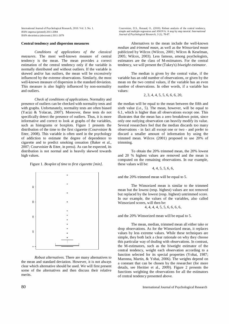
presence of outliers can be checked with normality tests and with graphs. Unfortunately, normality tests are often biased (Yacizi & Yolacan, 2007). Moreover, these tests do not specifically detect the presence of outliers. Thus, it is more informative and correct to look at graphs of the variables, such as histograms or boxplots. Figure 1 presents the distribution of the time to the first cigarette (Courvoisier & Etter, 2008). This variable is often used in the psychology of addiction to estimate the degree of dependence to cigarette and to predict smoking cessation (Baker et al., 2007; Courvoisier & Etter, in press). As can be expected, its distribution is not normal and is heavily skewed towards high values.

Figure 1. Boxplot of time to first cigarette [min].

Robust alternatives. There are many alternatives to

the mean and standard deviation. However, it is not always clear which alternative should be used. We will first present some of the alternatives and then discuss their relative merits.

Alternatives to the mean include the well-known median and trimmed mean, as well as the Winsorized mean publicized by Wilcox (Wilcox, 2001; Wilcox & Keselman, 2005; Wilcox, 2003). Less famous, among psychologists, estimators are the class of M-estimators. For the central tendency, we will present the (Tukey's) biweight estimator.

The median is given by the central value, if the

variable has an odd number of observations, or given by the mean on the two central values, if the variable has an even number of observations. In other words, if a variable has values:

2, 3, 4, 4, 5, 5, 6, 6, 6, 20, the median will be equal to the mean between the fifth and sixth value (i.e., 5). The mean, however, will be equal to 6.1, which is higher than all observations except one. This illustrates that the mean has a zero breakdown point, since only one outlying observation can heavily modify its value. Several researchers feel that the median discards too many observations - in fact all except one or two - and prefer to discard a smaller amount of information by using the trimmed mean. Wilcox (2001) proposed to use 20% of trimming.

To obtain the 20% trimmed mean, the 20% lowest

and 20 % highest values are removed and the mean is computed on the remaining observations. In our example, these values will be:

4, 4, 5, 5, 6, 6, and the 20% trimmed mean will be equal to 5.

The Winsorized mean is similar to the trimmed

mean but the lowest (resp. highest) values are not removed but replaced by the lowest (resp. highest) untrimmed score. In our example, the values of the variables, also called Winsorized scores, will then be:

4, 4, 4, 4, 5, 5, 6, 6, 6, 6,

and the 20% Winsorized mean will be equal to 5. The mean, median, trimmed mean all either take or

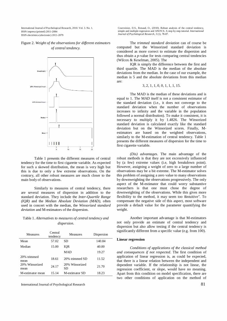
drop observations. As for the Winsorized mean, it replaces values by less extreme values. While these techniques are simple, they both lack a clear rationale on why they choose this particular way of dealing with observations. In contrast, the M-estimators, such as the biweight estimator of the central tendency, weight each observation according to a function selected for its special properties (Yohai, 1987; Maronna, Martin, & Yohai, 2006). The weights depend on a constant that can be chosen by the researcher (for more details, see Heritier et al., 2009). Figure 2 presents the functions weighting the observations for all the estimators of central tendency presented above.




Figure 2. Weight of the observations for different estimators of central tendency.

Table 1 presents the different measures of central

tendency for the time to first cigarette variable. As expected for such a skewed distribution, the mean is very high but this is due to only a few extreme observations. On the contrary, all other robust measures are much closer to the main body of observations.

Similarly to measures of central tendency, there

are several measures of dispersion in addition to the standard deviation. They include the Inter-Quartile Range (IQR) and the Median Absolute Deviation (MAD), often used in concert with the median, the Winsorized standard deviation and M-estimators of the dispersion.

Table 1. Alternatives to measures of central tendency and

dispersion.

Measures Central tendency Measures Dispersion

Mean 57.02 SD 140.84 Median 15.00 IQR 40.00 MAD 19.27 20% trimmed mean 18.61 20% trimmed SD 11.52

20% Winsorized mean 24.17 20% Winsorized

SD 21.70

M-estimator mean 15.14 M-estimator SD 18.23

The trimmed standard deviation can of course be computed but the Winsorized standard deviation is considered as more correct to estimate the dispersion and thus obtain a p-value for tests comparing central tendencies (Wilcox & Keselman, 2005). The

IQR is simply the difference between the first and third quartile. The MAD is the median of the absolute deviations from the median. In the case of our example, the median is 5 and the absolute deviations from this median are:

3, 2, 1, 1, 0, 0, 1, 1, 1, 15. The MAD is the median of these deviations and is

equal to 1. The MAD itself is not a consistent estimator of the standard deviation (i.e., it does not converge to the standard deviation when the number of observations increases to infinity and the variable in the population followed a normal distribution). To make it consistent, it is necessary to multiply it by 1.4826. The Winsorized standard deviation is calculated exactly like the standard deviation but on the Winsorized scores. Finally, M-estimators are based on the weighted observations, similarly to the M-estimation of central tendency. Table 1 presents the different measures of dispersion for the time to first cigarette variable.

(Dis) advantages. The main advantage of the

robust methods is that they are not excessively influenced by (a few) extreme values (i.e, high breakdown point). However, assigning a weight of zero to a large number of observations may be a bit extreme. The M-estimator solves this problem of assigning a zero value to many observations by downweighting the observations progressively. The only aspect of the M-estimator that could worry substantive researchers is that one must chose the degree of downweighting of the observations. While this gives more flexibility to the method, it may seem too “intuitive". To compensate the negative side of this aspect, most software provide a default value for the parameter quantifying the weight.

Another important advantage is that M-estimators

not only provide an estimate of central tendency and dispersion but also allow testing if the central tendency is significantly different from a specific value (e.g. from 100).

Linear regression

Conditions of applications of the classical method

and consequences if not respected. The first condition of application of linear regression is, as could be expected, that there is a linear relation between the independent and dependent variable. If the relationship is not linear, the regression coefficient, or slope, would have no meaning. Apart from this condition on model specification, there are two other conditions of application on the method of




estimation. They can best be understood as conditions on the residuals (i.e., the distance between the predicted and observed value of the dependent variable). The observations are not exactly equal to the values predicted by the model. One condition is that the observations should be normally distributed around their predicted values (i.e., should be above and below the regression line). This implies that the data should not have univariate and multivariate outliers. Note that an observation can have leverage (i.e., be an outlier on an independent variable) and not be influential (i.e., have a high impact on the estimation of the regression parameters). The level of influence of any outlier is determined by both its leverage and its discrepancy between its value as predicted by the regression and its real, observed value. Finally, for each value of the independent variable, the observations should have approximately the same variance (homoscedasticity). While heteroscedasticity only influences the standard errors, thereby modifying the p-values, non-normality and outliers may bias the regression coefficient itself as well as the standard errors.

Note that there are no direct condition on either the

independent or the dependent variables (such as normality of the variables), only conditions based on their relationship: linearity and specifications on the residuals.

Check of conditions of applications. How to check

univariate normality and presence of outliers has already been discussed in the previous section. Thus, while it is still useful to look at each variable separately, we will only present how to detect influential outliers in the context of the regression analysis. There are three main ways to check the conditions of applications, the first is to examine the initial data, the second is to check the residuals (i.e., the distance between the predicted and observed value of the dependent variable), the third is to examine the impact of each observation on the parameter estimation.

The initial data can best be examined by a scatter

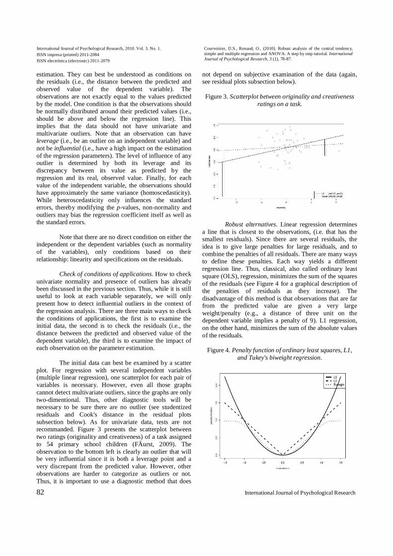
plot. For regression with several independent variables (multiple linear regression), one scatterplot for each pair of variables is necessary. However, even all those graphs cannot detect multivariate outliers, since the graphs are only two-dimentional. Thus, other diagnostic tools will be necessary to be sure there are no outlier (see studentized residuals and Cook's distance in the residual plots subsection below). As for univariate data, tests are not recommanded. Figure 3 presents the scatterplot between two ratings (originality and creativeness) of a task assigned to 54 primary school children (FÄurst, 2009). The observation to the bottom left is clearly an outlier that will be very influential since it is both a leverage point and a very discrepant from the predicted value. However, other observations are harder to categorize as outliers or not. Thus, it is important to use a diagnostic method that does

not depend on subjective examination of the data (again, see residual plots subsection below).

Figure 3. Scatterplot between originality and creativeness

ratings on a task.

Robust alternatives. Linear regression determines

a line that is closest to the observations, (i.e. that has the smallest residuals). Since there are several residuals, the idea is to give large penalties for large residuals, and to combine the penalties of all residuals. There are many ways to define these penalties. Each way yields a different regression line. Thus, classical, also called ordinary least square (OLS), regression, minimizes the sum of the squares of the residuals (see Figure 4 for a graphical description of the penalties of residuals as they increase). The disadvantage of this method is that observations that are far from the predicted value are given a very large weight/penalty (e.g., a distance of three unit on the dependent variable implies a penalty of 9). L1 regression, on the other hand, minimizes the sum of the absolute values of the residuals.

Figure 4. Penalty function of ordinary least squares, L1,

and Tukey's biweight regression.




As can be seen from Figure 4, in L1 regression,

large residuals yield less penalty, and thus have less influence than in OLS regression. However, the influence of observations still increase quickly as the observation gets farther from its predicted value. The M-estimation regression based on Tukey's biweight provides a specific function to penalize the influence of observations that are too far from their predicted values. While the biweight function is more complicated than the OLS and L1 functions, it is also more thought about. In effect, observations are progressively penalized as they get farther from their predicted values up to a threshold. At that threshold, all observations have a given penalty, and thus have a limited effect on the estimation of the regression's coefficients.

As illustrated by the creativity example on Figure

3, coefficients and p-values can be very different when estimated with classical and robust regression. Indeed, the line selected by OLS is very influenced by the observation to the bottom left and the whole regression line is steeper because of this observation, thus yielding a significant regression coefficient. On the other hand, the line selected by biweight regression is not much influenced by this extreme observation and its regression coefficient is almost equal to zero and is not significant. In this example, robust regression protects the analyst from believing that originality has an influence on creativeness (type I error). However, in other cases, the opposite will happen and robust regression may protect the analyst from believing that there is no relationship between two variables when in fact there is one.

Residual plots. There are many ways of checking

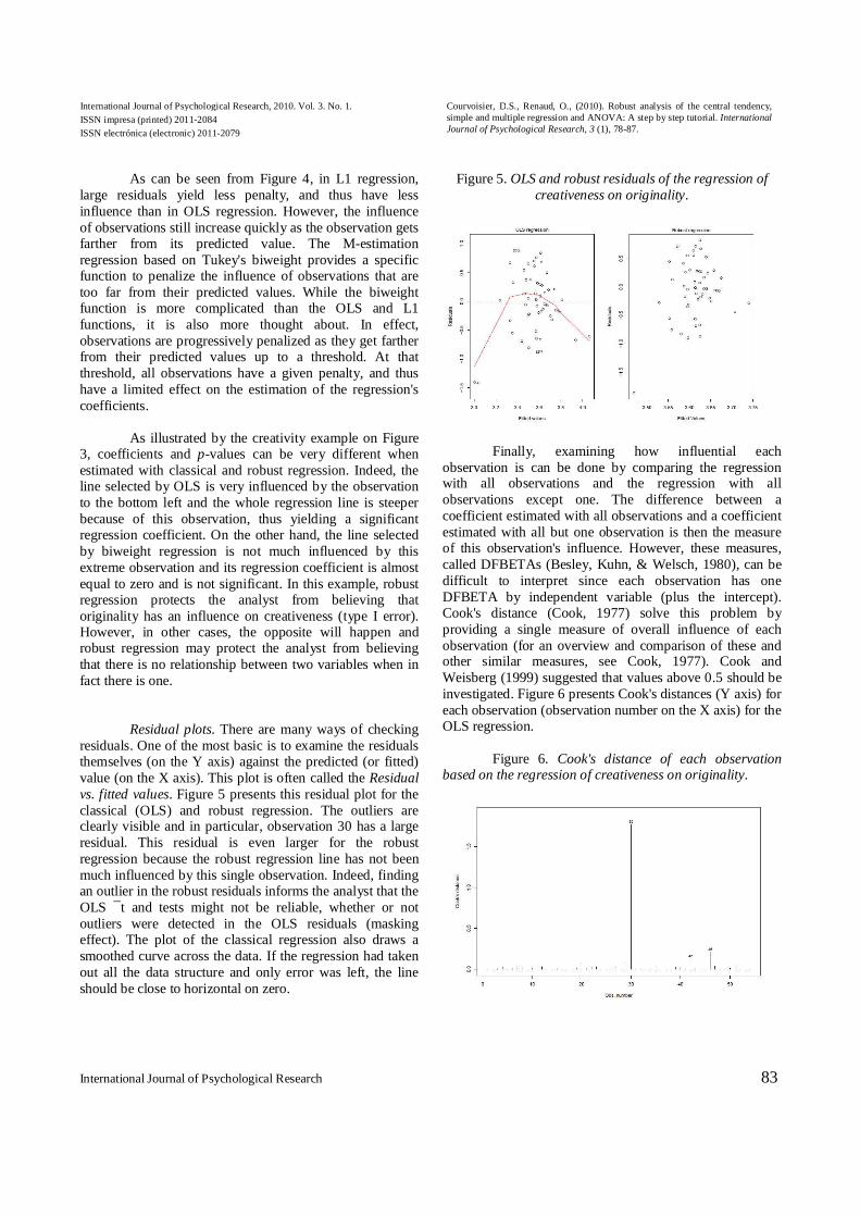
residuals. One of the most basic is to examine the residuals themselves (on the Y axis) against the predicted (or fitted) value (on the X axis). This plot is often called the Residual vs. fitted values. Figure 5 presents this residual plot for the classical (OLS) and robust regression. The outliers are clearly visible and in particular, observation 30 has a large residual. This residual is even larger for the robust regression because the robust regression line has not been much influenced by this single observation. Indeed, finding an outlier in the robust residuals informs the analyst that the OLS ¯t and tests might not be reliable, whether or not outliers were detected in the OLS residuals (masking effect). The plot of the classical regression also draws a smoothed curve across the data. If the regression had taken out all the data structure and only error was left, the line should be close to horizontal on zero.

Figure 5. OLS and robust residuals of the regression of

creativeness on originality.

Finally, examining how influential each observation is can be done by comparing the regression with all observations and the regression with all observations except one. The difference between a coefficient estimated with all observations and a coefficient estimated with all but one observation is then the measure of this observation's influence. However, these measures, called DFBETAs (Besley, Kuhn, & Welsch, 1980), can be difficult to interpret since each observation has one DFBETA by independent variable (plus the intercept). Cook's distance (Cook, 1977) solve this problem by providing a single measure of overall influence of each observation (for an overview and comparison of these and other similar measures, see Cook, 1977). Cook and Weisberg (1999) suggested that values above 0.5 should be investigated. Figure 6 presents Cook's distances (Y axis) for each observation (observation number on the X axis) for the OLS regression.

Figure 6. Cook's distance of each observation

based on the regression of creativeness on originality.




Again, observation 30 has a Cook's distance far above the recommended threshold, which indicates that it has a large influence on the position of the regression line. Note that robust regression does not yield a Cook's distance plot because, by definition, outliers cannot have a large impact on the estimation.

Multiple linear regression examines the effect of

several independent variables on the dependent variable. Exactly the same estimation (OLS, L1 and biweight) and residuals plots are available, so we do not provide an example here. However, the nature of multiple linear regression makes it much harder to diagnose potential problems. Thus, it is even more necessary to use robust regression to ensure that the analysis' results are not influenced by complex (multivariate) outlying observations.

(Dis) advantages. The only disadvantage of robust

regression is that, under fully Gaussian residuals, it is less powerful than OLS regression (Maronna et al., 2006).

However this loss of power is controled (default

settings ensure a 95% relative efficiency) and it is the price to pay for the protection from outliers. This slight loss in efficiency is to be expected since OLS was specifically designed for normally distributed residuals.

ANOVA Conditions of applications and consequences if not

respected. ANOVA with no repeated measures and regression are similar. Indeed, it is possible to code the independent, categorical, variables in such a way that analyzing the data with a linear regression or an ANOVA yields the same estimations and p-values. Thus, the conditions of applications are exactly similar: homoscedasticity, normality of the dependent variable for each experimental condition (each combination of level of the independent variables) and absence of outliers.

Check of conditions of applications. Univariate

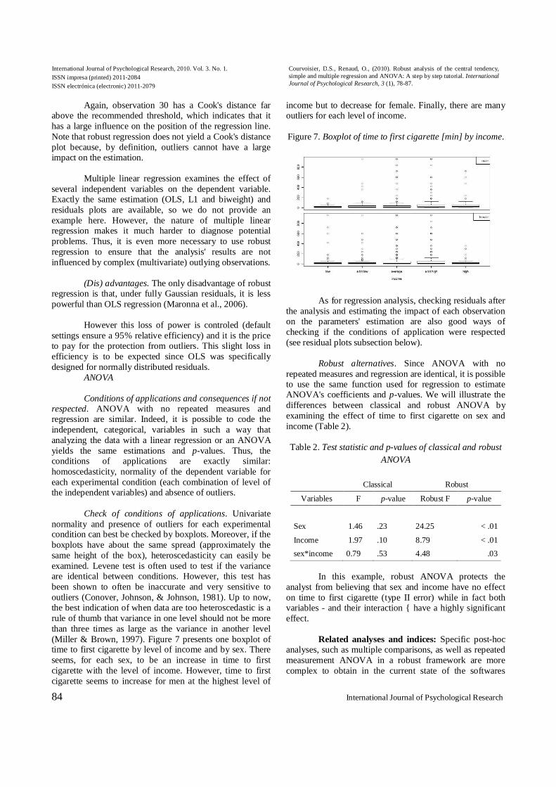
normality and presence of outliers for each experimental condition can best be checked by boxplots. Moreover, if the boxplots have about the same spread (approximately the same height of the box), heteroscedasticity can easily be examined. Levene test is often used to test if the variance are identical between conditions. However, this test has been shown to often be inaccurate and very sensitive to outliers (Conover, Johnson, & Johnson, 1981). Up to now, the best indication of when data are too heteroscedastic is a rule of thumb that variance in one level should not be more than three times as large as the variance in another level (Miller & Brown, 1997). Figure 7 presents one boxplot of time to first cigarette by level of income and by sex. There seems, for each sex, to be an increase in time to first cigarette with the level of income. However, time to first cigarette seems to increase for men at the highest level of

income but to decrease for female. Finally, there are many outliers for each level of income. Figure 7. Boxplot of time to first cigarette [min] by income.

As for regression analysis, checking residuals after

the analysis and estimating the impact of each observation on the parameters' estimation are also good ways of checking if the conditions of application were respected (see residual plots subsection below).

Robust alternatives. Since ANOVA with no

repeated measures and regression are identical, it is possible to use the same function used for regression to estimate ANOVA's coefficients and p-values. We will illustrate the differences between classical and robust ANOVA by examining the effect of time to first cigarette on sex and income (Table 2).

Table 2. Test statistic and p-values of classical and robust

ANOVA Classical Robust

Variables F p-value Robust F p-value

Sex 1.46 .23 24.25 < .01

Income 1.97 .10 8.79 < .01 sex*income 0.79 .53 4.48 .03

In this example, robust ANOVA protects the

analyst from believing that sex and income have no effect on time to first cigarette (type II error) while in fact both variables - and their interaction { have a highly significant effect.

Related analyses and indices: Specific post-hoc

analyses, such as multiple comparisons, as well as repeated measurement ANOVA in a robust framework are more complex to obtain in the current state of the softwares




procedures. This topic goes beyond the scope of this tutorial and will not be presented here.

Furthermore, effect sizes, also known as R

squared, should also be determined by a robust estimates. However, the robust R squared based on Tukey's biweight may not be appropriate (Renaud & Victoria-Feser, 2009). A reliable version of this index is now under development (Renaud & Victoria-Feser, 2009).

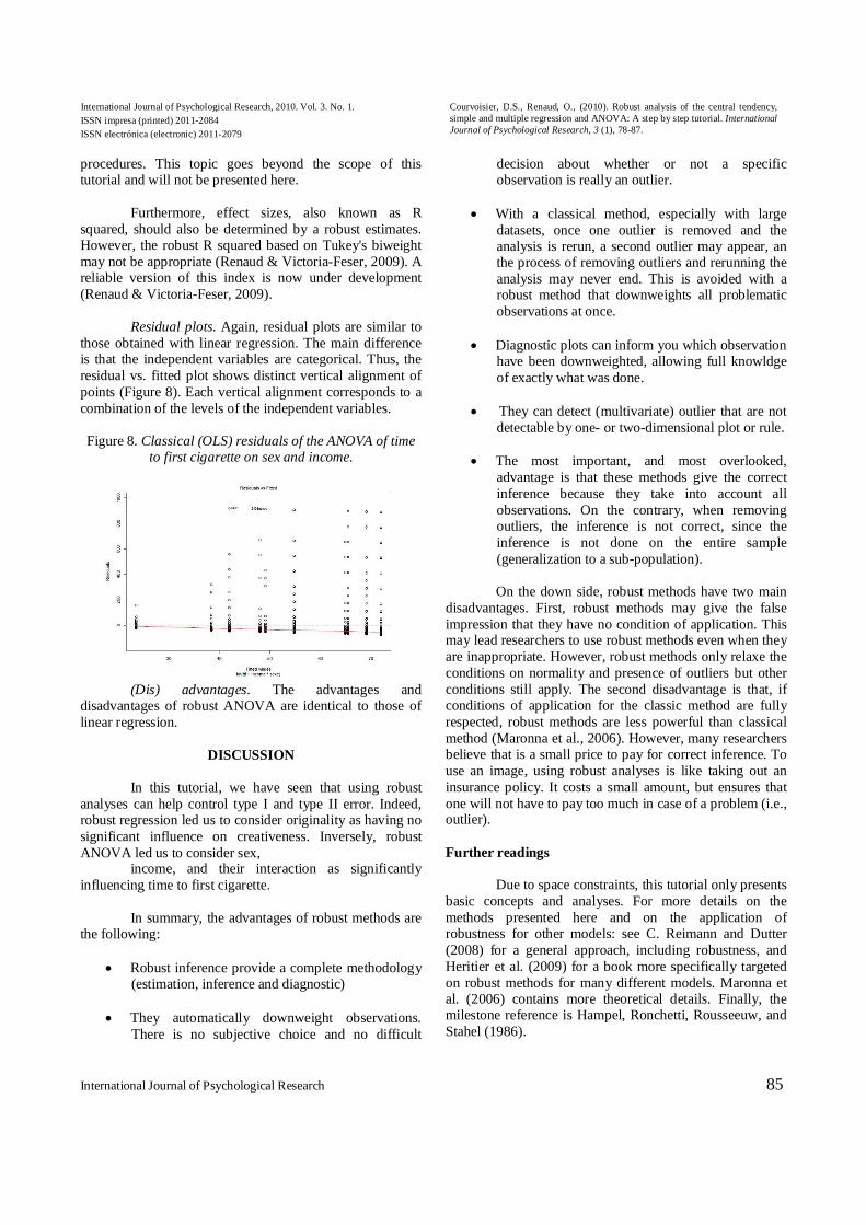
Residual plots. Again, residual plots are similar to

those obtained with linear regression. The main difference is that the independent variables are categorical. Thus, the residual vs. fitted plot shows distinct vertical alignment of points (Figure 8). Each vertical alignment corresponds to a combination of the levels of the independent variables.

Figure 8. Classical (OLS) residuals of the ANOVA of time

to first cigarette on sex and income.

(Dis) advantages. The advantages and

disadvantages of robust ANOVA are identical to those of linear regression.

DISCUSSION

In this tutorial, we have seen that using robust

analyses can help control type I and type II error. Indeed, robust regression led us to consider originality as having no significant influence on creativeness. Inversely, robust ANOVA led us to consider sex,

income, and their interaction as significantly influencing time to first cigarette.

In summary, the advantages of robust methods are

the following:

• Robust inference provide a complete methodology (estimation, inference and diagnostic)

• They automatically downweight observations. There is no subjective choice and no difficult

decision about whether or not a specific observation is really an outlier.

• With a classical method, especially with large

datasets, once one outlier is removed and the analysis is rerun, a second outlier may appear, an the process of removing outliers and rerunning the analysis may never end. This is avoided with a robust method that downweights all problematic observations at once.

• Diagnostic plots can inform you which observation have been downweighted, allowing full knowldge of exactly what was done.

• They can detect (multivariate) outlier that are not

detectable by one- or two-dimensional plot or rule.

• The most important, and most overlooked, advantage is that these methods give the correct inference because they take into account all observations. On the contrary, when removing outliers, the inference is not correct, since the inference is not done on the entire sample (generalization to a sub-population). On the down side, robust methods have two main

disadvantages. First, robust methods may give the false impression that they have no condition of application. This may lead researchers to use robust methods even when they are inappropriate. However, robust methods only relaxe the conditions on normality and presence of outliers but other conditions still apply. The second disadvantage is that, if conditions of application for the classic method are fully respected, robust methods are less powerful than classical method (Maronna et al., 2006). However, many researchers believe that is a small price to pay for correct inference. To use an image, using robust analyses is like taking out an insurance policy. It costs a small amount, but ensures that one will not have to pay too much in case of a problem (i.e., outlier).

Further readings

Due to space constraints, this tutorial only presents

basic concepts and analyses. For more details on the methods presented here and on the application of robustness for other models: see C. Reimann and Dutter (2008) for a general approach, including robustness, and Heritier et al. (2009) for a book more specifically targeted on robust methods for many different models. Maronna et al. (2006) contains more theoretical details. Finally, the milestone reference is Hampel, Ronchetti, Rousseeuw, and Stahel (1986).




Softwares for Robust Analysis The instructions (code) to obtain the results and

graphs in the R software are available on the website of the journal. R is probably the software that contains the largest number of robust methods. Indeed, many more models that presented in this article are available, see http://stat.ethz.ch/CRAN/web/views/Robust.html.

Concerning other statistical softwares, they include

more and more robust methods. Here is the present situation to the best of our knowledge.

Concerning SAS, PROC ROBUSTREG allows to

fit a robust regression. There are also three additional procedures linked to robust methods, namely lts, lms and mve, see http://support.sas.com/rnd/app/da/iml/robustreg.html. Three procedures for robust regression are available in stata: rreg, qreg and MM_REGRESS. In PASW (formerly SPSS), there is no build-in robust procedures, but there are two kinds of plug-in that allow to run within PASW some scripts in the R language. The first is a commercial add-on called ZumaStat, see http://www.zumastat.com/robust_statistics.htm that implements specific robust procedures in a user-friendly environment. The second is a general R plug-in provided by PASW itself (you must register on their website to download it) that allows running any R script within a PASW script, with additional special commands. Finally, Statistica also allows running scripts in the R language and therefore allows for the same capabilities.

REFERENCES

Baker, T. B., Piper, M. E., McCarthy, D. E., Bolt, D. M.,

Smith, S. S., Kim, S. Y., et al. (2007). Time to first cigarette in the morning as an index of ability to quit smoking:

Implications for nicotine dependence. Nicotine and Tobacco Research, 9 , S555-S570. Besley, D. A., Kuhn, E., & Welsch, R. E. (1980). Regression diagnostics. New York: Wiley.

Conover, W. J., Johnson, M. E., & Johnson, M. M. (1981). A comparative study of tests for homogeneity of variances, with applications to the outer continental shelf bidding data. Technometrics, 23 (4), 351-361.

Cook, R. D. (1977). Detection of influential observations in linear regression. Technometrics, 19 , 15-18.

Cook, R. D., & Weisberg, S. (1999). Applied regression including computing and graphics. New York: Wiley.

Courvoisier, D. S., & Etter, J. (2008). Using item response theory to study the convergent and discriminant validity of three questionnaires measuring cigarette dependence. Psychology of Addictive Behavior, 22 , 391-401.

Courvoisier, D. S., & Etter, J. (in press). Comparing the predictive validity of five cigarette dependence questionnaires. Drug and Alcohol Dependence.

C. Reimann, R. G., P. Filzmoser, & Dutter, R. (2008). Statistical data analysis explained: Applied environmental statistics with r. Chichester: Wiley.

Cumming, G., Fidler, F., Leonard, M., Kalinowske, P., Christiansen, A., & Kleinig, A. (2007). Statistical reform in psychology: Is anything changing? Psychological Science, 18 , 230-232.

Fürst, G. (2009). Originalité, caractére approprié et créativité des idées chez les enfants de 8-11 ans. in press.

Hampel, F., Ronchetti, E., Rousseeuw, P., & Stahel, W. (1986). Robust statistics: the approach based on influence functions. New York: Wiley.

Heritier, S., Cantoni, E., Copt, S., & Victoria-Feser, M.-P. (2009). Robust methods in biostatistics. New York: Wiley. (in press)

Huber, P. J. (2004). Robust statistics. Hoboken, NJ: Wiley. Maronna, R. A., Martin, R. D., & Yohai, V. J. (2006).

Robust statistics: Theory and methods. Chichester, West Sussex, UK: Wiley.

Micceri, T. (1989). The unicorn, the normal curve, and other improbable creatures. Psychological Bulletin, 105 , 156-166.

Miller, R. G., & Brown, B. W. (1997). Beyond ANOVA: Basics of applied statistics. New York: Chapman & Hall Ltd.

Perea, M. (1999). Tiempos de reacción y psicología cognitiva: Dos procedimientos para evitar el sesgo debido al tamaño muestral. Psicologica, 20 , 13-21.

Ratcliff, R. (1993). Methods for dealing with reaction time outliers. Psychological Bulletin, 114 , 510-532.

Renaud, O., & Victoria-Feser, M.-P. (2009). A robust coefficient of determination for regression. submitted.

Rousseeuw, P. J., & Leroy, A. M. (1987). Robust regression and outlier detection. New York: Wiley.

Wilcox, R. R. (2001). Fundamentals of modern statistical methods: Substantially improving power and accuracy. New York: Springer.

Wilcox, R. R. (2003). Introduction to robust estimation and hypothesis testing (2nd ed.). San Diego, CA: Academic Press.




Wilcox, R. R., & Keselman, H. J. (2005). Modern robust data analysis method: Measures of central tendency. Psychological Methods, 8, 254-274.

Yacizi, B., & Yolacan, S. (2007). A comparison of various tests of normality. Journal of Statistical Computation and Simulation, 77 , 175-183.

Yohai, V. J. (1987). High breakdown point and high efficiency robust estimates for regression. The Annals of Statistics, 15 , 642{656.

Redalyc.Robust analysis of the central tendency, simple and ...

Documents

Transcript of Redalyc.Robust analysis of the central tendency, simple and ...