HAL Id: tel-02446413https://tel.archives-ouvertes.fr/tel-02446413

Submitted on 20 Jan 2020

HAL is a multi-disciplinary open accessarchive for the deposit and dissemination of sci-entific research documents, whether they are pub-lished or not. The documents may come fromteaching and research institutions in France orabroad, or from public or private research centers.

L’archive ouverte pluridisciplinaire HAL, estdestinée au dépôt et à la diffusion de documentsscientifiques de niveau recherche, publiés ou non,émanant des établissements d’enseignement et derecherche français ou étrangers, des laboratoirespublics ou privés.

Reconstruction of marine mammals’ historicaldistribution and abundance : setting a baseline to

understand the past, inform the present and plan thefuture

Sophie Monsarrat

To cite this version:Sophie Monsarrat. Reconstruction of marine mammals’ historical distribution and abundance : settinga baseline to understand the past, inform the present and plan the future. Biodiversity and Ecology.Université Montpellier, 2015. English. �NNT : 2015MONTS277�. �tel-02446413�

Délivré par l’UNIVERSITE DE MONTPELLIER

Préparée au sein de l’école doctorale SIBAGHE

Et de l’unité de recherche CEFE, CNRS UMR 5175

Spécialité : Ecologie, Evolution, Ressources Génétiques,

Paléontologie

Présentée par Sophie MONSARRAT

Soutenance le Jeudi 07 Mai devant le jury composé de

*

Reconstruction de la distribution et de l’abondance

historiques des mammifères marins :

Etablir un niveau de référence pour comprendre le

passé, renseigner le présent et planifier l’avenir

Mme Ana RODRIGUES, Chargée de recherche, CEFE-CNRS,

Montpellier Mr Francesco BONADONNA, Directeur de recherche, CEFE-

CNRS, Montpellier

Mr Vincent RIDOUX, Professeur, Institut du Littoral et de

l’Environnement, La Rochelle

Mr Pat HALPIN, Professeur, Science Center Nicholas School of

the Environnement, Durham

Mr Alex AGUILAR, Professeur, Facultat de Biologia Universitat

de Barcelona, Barcelona

Mr Oliver GIMENEZ, Directeur de recherche, CEFE-CNRS,

Montpellier

Co-Directrice

de Thèse Co-Directeur

de Thèse

Rapporteur

Rapporteur

Examinateur

Examinateur

1

UNIVERSITE DE MONTPELLIER

THESE

Pour obtenir le grade de

DOCTEUR DE L’UNIVERSITE DE MONTPELLIER

Discipline : Biologie de l’Evolution et Ecologie

Spécialité : Ecologie, Evolution, Ressources Génétiques, Paléontologie

Ecole doctorale : Systèmes Intégrés en Biologie, Agronomie, Géosciences, Hydrosciences,

Environnement (SIBAGHE)

Par

Sophie MONSARRAT

Reconstruction de la distribution et de l’abondance historiques des mammifères marins :

Etablir un niveau de référence pour comprendre le passé, renseigner le présent et planifier l’avenir

Reconstruction of marine mammal’s historical distribution and abundance:

Setting a baseline to understand the past, inform the present and plan the future

Co-Directrice: Dr. Ana RODRIGUES (CEFE-CNRS, Montpellier)

Co-Directeur: Dr. Francesco BONADONNA (CEFE-CNRS, Montpellier)

Soutenance: Jeudi 7 Mai 2015

Membres du jury

Ana RODRIGUES, Chargée de recherche, CEFE-CNRS, Montpellier Co-Directrice de Thèse Francesco BONADONNA, Directeur de recherche, CEFE-CNRS, Montpellier Co-Directeur de Thèse Vincent RIDOUX, Professeur, Institut du Littoral et de l’Environnement, La Rochelle Rapporteur Pat HALPIN, Professeur, Science Center Nicholas School of the Environnement, Durham Rapporteur Alex AGUILAR, Professeur, Facultat de Biologia Universitat de Barcelona, Barcelona Examinateur Oliver GIMENEZ, Directeur de recherche, CEFE-CNRS, Montpellier Examinateur

Laboratoire d’accueil :

Centre d’Ecologie Fonctionnelle et Evolutive, 1919 Route de Mende, 34090 Montpellier, France

2

3

REMERCIEMENTS

Cette thèse est le fruit de plusieurs années d’interactions scientifiques et personnelles intenses avec

mes encadrants, mes collaborateurs, mes collègues devenus amis et l’ensemble des personnes qui

ont fait partie de mon quotidien pendant cette période importante de ma vie. Leur influence a pris

une immense part dans ma construction, et c’est avec plaisir que je pose aujourd’hui par écrit ma

reconnaissance envers chacun d’entre eux.

Je dois ma présence dans le monde scientifique à mes encadrants de stages de recherche en M1 et

M2, qui ont su stimuler ma curiosité pour la compréhension des processus écologiques tout en

m’inculquant la rigueur de la méthode scientifique. Je remercie en particulier Christian Kerbiriou et

Olivier Duriez pour m’avoir encadré lors de stages passionnants au cours desquels ils m’ont transmis

leur passion et dirigé doucement vers la réalisation d’une thèse. Merci également à Simon

Benhamou pour son soutien méthodologique grâce auquel le terme « rigueur » aura pris tout son

sens. Je garde encore aujourd’hui la trace de vos enseignements et vous suis extrêmement

reconnaissante de m’avoir donné goût à la recherche quand mes questionnements auraient pu

m’amener à suivre une toute autre voie.

Ma construction scientifique a fait un bond en avant lorsque ma directrice de thèse, Ana Rodrigues,

m’a offert de réaliser une thèse au sein du très ambitieux projet MORSE. Le sujet absolument

passionnant ainsi que l’encadrement hors pair d’Ana ont fait de ces 3 années une période

incroyablement enrichissante. Je ne te remercierai jamais assez, Ana, de m’avoir donnée ta confiance

pour mener à bien ce projet, d’avoir été autant présente et à l’écoute lorsque j’en avais besoin, et de

m’avoir ouvert au monde de la recherche de cette manière. On dit souvent que l’encadrement est

plus important encore que le sujet pour garantir la réussite d’une thèse, et je me sais, grâce à toi,

extrêmement privilégiée à ces deux niveaux. Tes enseignements tant d’un point de vue scientifique

qu’humain resteront gravés dans ma mémoire. MERCI.

La force de ce projet est d’avoir pu bénéficier d’un remarquable réseau de collaborateurs au contact

desquels j’ai beaucoup appris. La présence d’Anne Charpentier dans le projet MORSE a garanti des

échanges fructueux et passionnés sur le thème des baleines mortes, dont je me souviendrai toujours

avec joie (longue vie à la hache-charrue !). L’incroyable « World Whaling History dataset » utilisé

dans plusieurs chapitres de cette thèse a été entièrement mis à disposition dans le cadre d’une

collaboration des plus passionnantes avec Randall Reeves et Tim Smith, que je remercie du fond du

cœur pour la confiance qu’ils nous ont faite. Connaissant mal les méthodes d’analyses utilisées dans

cette thèse il y a encore 3 ans, j’ai eu la chance de bénéficier du soutien méthodologique de David

Kaplan, Christine Meynard et Maria Grazia Pennino, que je remercie pour leur patience et leur

4

gentillesse. L’opportunité m’ayant été donnée de participer à plusieurs workshop du projet PELAGIC

à la Fondation pour la Recherche et la Biodiversité à Aix-en Provence, je profite de cet espace pour

remercier les membres de ce groupe, avec lesquels j’ai pu avoir des échanges très instructifs. Je

remercie enfin Christel Vidaller, Laureline Chabran et Laura Pinillos qui ont effectué leur stage dans le

cadre du projet MORSE et ont participé à l’effort de collecte de données historiques présentées dans

le deuxième chapitre de ce manuscrit.

Ce travail s’est déroulé dans un cadre de travail très privilégié d’un point de vue logistique, grâce au

professionnalisme de l’équipe administrative du CEFE qui a toujours su faciliter mes démarches. Je

les en remercie, ainsi que l’Agence Nationale de la Recherche pour le soutien financier de ma thèse.

Je souhaite également remercier les membres du jury, qui m’ont fait l’honneur d’accepter de juger

mon travail et m’ont octroyée le grade de Docteur au terme d’une soutenance riche en échanges. Je

suis extrêmement reconnaissante de leur intérêt et du temps qu’ils ont dédié à l’évaluation de ma

thèse.

Je tiens enfin à remercier de manière plus personnelle les nombreuses personnes qui font mon

entourage, sans qui cette thèse n’aurait pas aboutie, et à qui je dois tant…

« Au moindre coup de Trafalgar, C'est l'amitié qui prenait l'quart

C'est elle qui leur montrait le nord, Leur montrait le nord.

Et quand ils étaient en détresse, Qu'leur bras lançaient des S.O.S.,

On aurait dit les sémaphores, Les copains d'abord. »

George Brassens

Des paroles qui ont pris tout leur sens à Montpellier, où j’ai vécu à la fois les moments les plus

difficiles, intenses et joyeux de ma vie, partagés avec des personnes incroyables. Merci à vous, amis

et collègues, de Montpellier et d’ailleurs pour avoir fait de ces trois ans une expérience humaine

inoubliable.

Finalement, je remercie du plus profond de mon cœur mes parents et ma sœur pour avoir toujours

cru en moi et avoir été à mes côtés et Alex, pour son amour et son soutien infaillible.

MERCI A TOUS

5

6

7

TITRE :

Reconstruction de la distribution et de l’abondance historiques des mammifères marins :

Etablir un niveau de référence pour comprendre le passé, renseigner le présent et planifier

l’avenir

Mots-clés :

Abondance, Baleine franche de l’Atlantique Nord, Distribution, Etat de référence, Eubalaena

glacialis, Mammifères marins, Modèles de distribution d’espèces.

RESUME COURT :

La mise en place d’objectifs de conservation adéquats repose sur la définition d’états de référence

appropriés pour la distribution et l’abondance des espèces. Cependant, l’étendue des impacts

cumulés de l’homme sur les écosystèmes est aujourd’hui largement sous-estimée. Dans ce projet, je

m’intéresse aux opportunités qu’offre l’utilisation de données historiques combinées à différentes

méthodes analytiques pour définir ces états de référence ainsi qu’aux défis posés par ce type

d’approche. Des données de présence ont été recueillies pour sept espèces de cétacés et trois

espèces de pinnipèdes à partir de sources archéologiques, historiques et industrielles, révélant des

réductions dans la distribution et l’abondance des espèces depuis la préhistoire à nos jours. Des

modèles de distribution d’espèces ont été développés pour cinq espèces de cétacés, combinant des

données de chasse baleinière du 19ème siècle à des variables environnementales afin d’estimer la

distribution historique des espèces avant qu’elles n’aient été chassées. J’ai obtenu pour la baleine

franche de l’Atlantique Nord (Eubalena glacialis) une estimation détaillée de sa distribution et de son

abondance avant qu’elle ne soit exploitée, en extrapolant des connaissances sur la distribution et

l’abondance d’une espèce congénérique, la baleine franche du Pacifique Nord (E. japonica). Ces

résultats suggèrent que la baleine franche de l’Atlantique Nord occupe une portion réduite de sa

distribution historique, et que son abondance actuelle ne représente qu’une infime portion (<5%) de

son abondance passée. Plus généralement, ces résultats soulignent l’importance de considérer des

données historiques pour comprendre le niveau d’impact par l’homme sur les espèces, évaluer leur

niveau de déplétion et renseigner leur potentiel de rétablissement dans l’avenir.

Laboratoire d’accueil :

Centre d’Ecologie Fonctionnelle et Evolutive, 1919 Route de Mende, 34293 Montpellier 5

8

TITLE:

Reconstruction of marine mammal’s historical distribution and abundance: setting a baseline

to understand the past, inform the present and plan the future

Keywords:

Abundance, Baseline, Eubalaena glacialis, Distribution, Marine mammals, North Atlantic

right whale, Species distribution models

BRIEF ABSTRACT:

Relevant baselines on the historical distribution and abundance of species are needed to support

appropriate conservation targets for depleted species, but the full scale of cumulative human

impacts on ecosystems is highly underestimated. In this project, I investigated the challenges and

opportunities of combining historical data with analytical methods to improve these historical

baselines. Occurrence data from archaeological, historical and industrial sources were reviewed for

seven cetacean and three pinniped species, revealing range contractions and population depletions

from prehistorical times to today. For five whale species, I used species distribution modelling to

combine 19th Century whaling records with environmental data, to estimate pre-whaling

distributions. For the highly depleted North Atlantic right whale, (Eubalaena glacialis), I obtained a

detailed estimate of pre-whaling distribution and abundance by inferring from the historical

distribution and abundance of its congeneric North Pacific right whale (E. japonica). These results

suggest that the North Atlantic right whale occupies a small fraction of its historical range and that its

current population represents <5% of its historical abundance, with implications for the

management, monitoring and conservation targets of this species. More generally, these results

emphasize the utility of considering historical data to understand the extent to which species have

been impacted by humans, assess their current level of depletion, and inform the options available

for their future recovery.

Research Institute:

Centre d’Ecologie Fonctionnelle et Evolutive, 1919 Route de Mende, 34293 Montpellier 5

9

TABLE OF CONTENTS

I. INTRODUCTION...................................................................................................................................... 19

SHIFTING BASELINES AND THE RISE OF “HISTORICAL ECOLOGY” ....................................................................................... 19

The shifting baseline syndrome .................................................................................................................... 19

Implications for conservation ....................................................................................................................... 20

Applied historical ecology ............................................................................................................................. 21

MARINE HISTORICAL ECOLOGY AND THE OVEREXPLOITATION OF MARINE RESOURCES ........................................................... 22

Marine historical ecology ............................................................................................................................. 22

Consequences of the overexploitation of marine resources ......................................................................... 23

OPPORTUNITIES FOR SETTING APPROPRIATE POPULATION BASELINES ................................................................................ 24

Historical occurrence data ............................................................................................................................ 25

Methodological opportunities for setting baselines from historical data .................................................... 28

FOCUS ON MARINE MAMMALS ................................................................................................................................. 29

A brief history of marine mammal exploitation ........................................................................................... 29

Marine mammals as an interesting case study ............................................................................................ 33

OBJECTIVES .......................................................................................................................................................... 34

STRUCTURE .......................................................................................................................................................... 35

II. USING SPECIES’ HISTORICAL OCCURRENCE DATA TO INVESTIGATE RANGE CONTRACTIONS: A REVIEW

FOR TEN MARINE MAMMAL SPECIES AND POSSIBLE APPLICATIONS .............................................................. 39

ABSTRACT ............................................................................................................................................................ 39

INTRODUCTION ..................................................................................................................................................... 40

STRATEGY FOR REVIEWING HISTORICAL DATA ............................................................................................................... 42

SPECIES REVIEWS ................................................................................................................................................... 44

Walrus (Odobenus rosmarus) ....................................................................................................................... 44

Caribbean monk seal (Monachus tropicalis) ................................................................................................ 47

Mediterranean monk seal (Monachus monachus) ....................................................................................... 47

Bowhead whale (Balaena mysticetus) .......................................................................................................... 48

North Atlantic right whale (Eubaleana glacialis) .......................................................................................... 49

North Pacific right whale (Eubalaena japonica) ........................................................................................... 50

Southern right whale (Eubalaena australis) ................................................................................................. 51

Gray whale (Eschrichtius robustus) .............................................................................................................. 54

Humpback whale (Megaptera noveaengliae) .............................................................................................. 57

Sperm whale (Physeter macrocephalus) ...................................................................................................... 57

CHALLENGES AND OPPORTUNITIES IN HISTORICAL OCCURRENCE DATA ............................................................................... 58

Archaeological remains ................................................................................................................................ 58

Historical accounts ....................................................................................................................................... 59

10

Industry statistics .......................................................................................................................................... 60

APPLICATIONS OF SPECIES’ HISTORICAL OCCURRENCE DATA ............................................................................................ 61

Improving understanding of the ecology of depleted species ...................................................................... 61

Mapping the historical envelope of species’ occurrence .............................................................................. 62

Mapping the sequence of historical depletion of a species .......................................................................... 64

Modeling a species’ historical distribution based on its environmental preferences ................................... 65

DISCUSSION AND CONCLUSION ................................................................................................................................. 69

III. COMBINING HISTORICAL DATA AND SPECIES DISTRIBUTION MODELS TO FILL INFORMATION GAPS FOR

SPECIES WITH VARIOUS LEVELS OF DEPLETION .............................................................................................. 75

ABSTRACT ............................................................................................................................................................ 75

INTRODUCTION ..................................................................................................................................................... 77

Three species, three histories of exploitation ............................................................................................... 78

Challenges and Opportunities ...................................................................................................................... 88

MATERIAL AND METHODS ....................................................................................................................................... 89

Nineteenth century whaling data ................................................................................................................. 89

Environmental data ...................................................................................................................................... 90

Species distribution models .......................................................................................................................... 92

RESULTS AND DISCUSSION ....................................................................................................................................... 94

Limitations and caveats ................................................................................................................................ 94

Humpback whale (Megaptera novaeangliae) .............................................................................................. 96

Bowhead whale (Balaena mysticetus) ........................................................................................................ 100

Gray whale (Eschrichtius robustus) ............................................................................................................ 103

Interest of the modeling approach ............................................................................................................. 107

CONCLUSION ...................................................................................................................................................... 110

APPENDIX .......................................................................................................................................................... 111

Appendix S1. Model selection, performance and validation ...................................................................... 111

Appendix S2. Fitted functions of the species-environment relationships produced by the BRT ................. 111

IV. HISTORICAL SUMMER DISTRIBUTION OF THE ENDANGERED NORTH ATLANTIC RIGHT WHALE

(EUBALAENA GLACIALIS): A HYPOTHESIS BASED ON ENVIRONMENTAL PREFERENCES OF A CONGENERIC

SPECIES 117

ABSTRACT .......................................................................................................................................................... 117

INTRODUCTION ................................................................................................................................................... 118

MATERIAL AND METHODS ..................................................................................................................................... 119

Historical records of North Pacific right whales ......................................................................................... 119

Environmental data .................................................................................................................................... 120

Species distribution modeling ..................................................................................................................... 120

Historical records of North Atlantic right whales ....................................................................................... 121

11

RESULTS............................................................................................................................................................. 122

Historical records of North Pacific right whales ......................................................................................... 122

Species distribution model .......................................................................................................................... 122

Model predictions ....................................................................................................................................... 122

Historical records of North Atlantic right whales ....................................................................................... 123

DISCUSSION ........................................................................................................................................................ 126

Assumptions and caveats ........................................................................................................................... 126

Comparison between the model predictions and species records in the North Atlantic ............................ 128

CONCLUSIONS ..................................................................................................................................................... 130

APPENDICES ....................................................................................................................................................... 133

Appendix S1: Historical records of North Pacific right whales .................................................................... 133

Appendix S2: Environmental data .............................................................................................................. 134

Appendix S3: Fitted functions ..................................................................................................................... 135

Appendix S4: Complementary Analyses ..................................................................................................... 137

Appendix S5: Historical distribution records of the North Atlantic Right Whale ........................................ 140

Appendix S6: Extended discussion .............................................................................................................. 149

V. HOW MANY RIGHT WHALES WERE THERE IN THE NORTH ATLANTIC BEFORE COMMERCIAL WHALING?

AN ESTIMATE BASED ON NORTH PACIFIC WHALING RECORDS..................................................................... 159

ABSTRACT .......................................................................................................................................................... 159

INTRODUCTION ................................................................................................................................................... 160

METHODS AND RESULTS ....................................................................................................................................... 163

Data on the distribution of catches of North Pacific right whales .............................................................. 163

Environmental predictors ........................................................................................................................... 164

Abundance modeling in the North Pacific .................................................................................................. 165

Model validation......................................................................................................................................... 167

Estimates of total population size in the North Pacific ............................................................................... 168

Estimates of total population size in the North Atlantic ............................................................................. 169

DISCUSSION ........................................................................................................................................................ 171

Uncertainties and assumptions .................................................................................................................. 171

Agreement between predictions, the historical record and genetic analyses ............................................ 173

Implications for the present and future of the North Atlantic right whale ................................................. 175

CONCLUSION ...................................................................................................................................................... 176

APPENDICES ....................................................................................................................................................... 177

VI. DISCUSSION ..................................................................................................................................... 181

RECONSTRUCTING THE PAST: FROM DESCRIPTION TO PREDICTION .................................................................................. 182

Interpretation of historical anecdotes ........................................................................................................ 182

Estimates of historical catches ................................................................................................................... 184

12

Maps of historical occurrence .................................................................................................................... 185

Envelopes of historical occurrence ............................................................................................................. 189

Predictive models of historical distribution ................................................................................................ 190

Predictive models of historical abundance ................................................................................................. 197

LESSONS LEARNED FROM THE ANALYSIS OF HISTORICAL DATA ........................................................................................ 198

Understanding species’ habitat preferences and how they have been affected by humans ..................... 198

Understanding past distributions and anthropogenic range contractions................................................. 198

Understanding past abundances and human-caused population depletions ............................................ 200

BIODIVERSITY CONSERVATION IN A CHANGING WORLD ................................................................................................ 201

How to define the historical baseline? ....................................................................................................... 201

Is the historical baseline an achievable/desirable target for conservation? .............................................. 203

REFERENCES ................................................................................................................................................. 209

13

LIST OF FIGURES

FIGURE I-1. ILLUSTRATION OF THE SHIFTING BASELINE SYNDROME AND THE CHANGE IN LIVING MEMORY FROM OLD TO YOUNG

FISHERMEN IN THE GULF OF CALIFORNIA. ............................................................................................................... 19

FIGURE I-2. SCHEMATIC REPRESENTATION OF ECOLOGICAL DATA AVAILABILITY AND POSSIBLE SOURCES, OVER THE LAST 10,000 YEARS.

...................................................................................................................................................................... 25

FIGURE I-3. TWO PAGES FROM AN AMERICAN WHALING LOGBOOK, FROM THE SHIP ABIGAIL OF NEW BEDFORD, BENJAMIN CLARK,

MASTER. .......................................................................................................................................................... 28

FIGURE I-4. SITE OF BANGU-DAE, CARVED PLATES (A, B, C, D, E) OF THE MAIN WALL (ULSAN, SOUTH KOREA; 6,000-1,000 YEARS

BP). ............................................................................................................................................................... 30

FIGURE I-5. POSSIBLE WHALING SCENES (DETAILS FROM BANGU-DAE PETROGLYPHS, ULSAN, SOUTH KOREA; 6,000-1,000 YEARS BP).

...................................................................................................................................................................... 30

FIGURE I-6. OLAUS MAGNUS’ WALRUS, 1555, HISTORIA DE GENTIBUS SEPTENTRIONALIBUS .................................................. 31

FIGURE I-7. TOTAL NUMBER OF WHALES KILLED IN INDUSTRIAL WHALING, 1900-99. .............................................................. 32

FIGURE II-1. CURRENT RANGE AND HISTORICAL OCCURRENCE DATA COLLECTED FOR THE WALRUS (ODOBENUS ROSMARUS). .......... 45

FIGURE II-2. CURRENT RANGE AND HISTORICAL OCCURRENCE DATA FOR TWO SPECIES OF MONK SEAL: THE CARIBBEAN MONK SEAL

(MONACHUS TROPICALIS, IN GREEN) AND THE MEDITERRANEAN MONK SEAL (MONACHUS MONACHUS, IN ORANGE). ........... 48

FIGURE II-3. CURRENT RANGE AND 19TH CENTURY WHALING RECORDS FOR THE BOWHEAD WHALE (BALAENA MYSTICETUS). ......... 49

FIGURE II-4. CURRENT SUMMER RANGE AND HISTORICAL OCCURRENCE DATA COLLECTED FOR THE NORTH ATLANTIC RIGHT WHALE

(BALAENA MYSTICETUS). ..................................................................................................................................... 50

FIGURE II-5. CURRENT RANGE AND 19TH CENTURY WHALING RECORDS FOR THE NORTH PACIFIC RIGHT WHALE (EUBALAENA

JAPONICA). ....................................................................................................................................................... 51

FIGURE II-6. CURRENT RANGE AND HISTORICAL DATA COLLECTED FOR THE SOUTHERN RIGHT WHALE (EUBALAENA AUSTRALIS). ....... 52

FIGURE II-7. CURRENT RANGE AND HISTORICAL DATA COLLECTED FOR THE GRAY WHALE (ESCHRICHTIUS ROBUSTUS)...................... 55

FIGURE II-8. 19TH CENTURY WHALING RECORDS FOR THE HUMPBACK WHALE (MEGAPTERA NOVAEANGLIAE). ............................. 57

FIGURE II-9. 19TH CENTURY WHALING RECORDS FOR THE SPERM WHALE (PHYSETER MACROCEPHALUS). .................................... 58

FIGURE II-10. HISTORICAL ENVELOPE OF OCCURRENCE FOR THE NORTH ATLANTIC RIGHT WHALE (EUBALAENA GLACIALIS). ............. 63

FIGURE II-11. HISTORICAL ENVELOPE OF OCCURRENCE FOR THE CARIBBEAN MONK SEAL (MONACHUS TROPICALIS). ...................... 64

FIGURE II-12. SEQUENCE OF DEPLETION OF THE BREEDING DISTRIBUTION OF THE MEDITERRANEAN MONK SEAL (MONACHUS

MONACHUS) OVER THE LAST CENTURY. .................................................................................................................. 65

FIGURE II-13. DIAGRAM SHOWING THE STEPS IN STATISTICAL SPECIES DISTRIBUTION MODELING AND PREDICTIVE MAPPING. ........... 68

FIGURE III-1. HISTORICAL WHALING DATA AND MODEL PREDICTIONS FOR THE GLOBAL WINTER DISTRIBUTION OF THE HUMPBACK

WHALE. ........................................................................................................................................................... 98

FIGURE III-2. HISTORICAL WHALING DATA AND MODEL PREDICTIONS FOR THE SUMMER DISTRIBUTION OF BOWHEAD WHALE. ....... 102

FIGURE III-3. HISTORICAL WHALING DATA AND MODEL PREDICTIONS FOR THE SUMMER DISTRIBUTION OF GRAY WHALE. .............. 105

FIGURE III-4. FITTED FUNCTIONS SHOWING THE SPECIES-ENVIRONMENT RELATIONSHIPS PRODUCED BY THE BRT. ....................... 112

FIGURE IV-1. HISTORICAL DATA AND MODEL PREDICTIONS IN THE NORTH PACIFIC. ............................................................... 124

FIGURE IV-2. MODEL PREDICTIONS AND HISTORICAL DATA IN THE NORTH ATLANTIC. ............................................................ 125

14

FIGURE IV-3. FITTED FUNCTIONS SHOWING THE SPECIES-ENVIRONMENT RELATIONSHIPS PRODUCED BY THE BRT........................ 136

FIGURE IV-4. ENVIRONMENTAL SUITABILITY FOR RIGHT WHALES IN SUMMER PREDICTED BY THE GAM. .................................... 139

FIGURE IV-5. HISTORICAL (PRE-1950) RECORDS OF NORTH ATLANTIC RIGHT WHALE (EUBALAENA GLACIALIS) IN THE SUMMER

MONTHS (JUNE TO SEPTEMBER). ........................................................................................................................ 147

FIGURE IV-6. RECENT (POST-1950) RECORDS OF NORTH ATLANTIC RIGHT WHALE (EUBALAENA GLACIALIS) IN THE SUMMER MONTHS

(JUNE TO SEPTEMBER), OUTSIDE ITS MAIN KNOWN SUMMER GROUNDS. .................................................................... 148

FIGURE IV-7. HISTORICAL (PRE-1950) AND RECENT (POST 1950) RECORDS OF NORTH ATLANTIC RIGHT WHALE (EUBALAENA

GLACIALIS) IN THE SUMMER MONTHS, ACCORDING TO DATE. .................................................................................... 151

FIGURE V-1. HISTORICAL CATCHES OF NORTH PACIFIC RIGHT WHALES, AND MODEL PREDICTIONS OF ABUNDANCE IN THE NORTH

PACIFIC. ........................................................................................................................................................ 167

FIGURE V-2. MODEL PREDICTIONS OF RIGHT WHALE ABUNDANCE IN THE NORTH ATLANTIC AND ABSOLUTE STANDARD ERROR OF THE

PREDICTION. ................................................................................................................................................... 170

FIGURE V-3. SMOOTH FUNCTIONS FOR THE FOUR SELECTED PREDICTORS. ........................................................................... 177

15

LIST OF TABLES & BOXES

TABLE II-1. MARINE MAMMAL SPECIES REVIEWED IN THIS CHAPTER, WITH THEIR CURRENT IUCN RED LIST STATUS, AND A SHORT

SUMMARY ON THE HISTORY OF THEIR EXPLOITATION. ................................................................................................ 43

TABLE II-2. NUMBER OF HISTORICAL RECORDS COLLECTED FOR THE TEN SPECIES CONSIDERED, AND NUMBER OF REFERENCES FROM

WHICH THEY WERE EXTRACTED. ............................................................................................................................ 44

TABLE II-3. HISTORICAL RECORDS COLLECTED FOR THE WALRUS (ODOBENUS ROSMARUS). ....................................................... 46

TABLE II-4. HISTORICAL RECORDS COLLECTED FOR THE SOUTHERN RIGHT WHALE (EUBALAENA AUSTRALIS). ................................. 52

TABLE II-5. HISTORICAL RECORDS OF THE GRAY WHALE (ESCHRICHTIUS ROBUSTUS) IN THE NORTH ATLANTIC. .............................. 56

TABLE III-1. TABLE OF IDENTIFIED CURRENT WINTER GROUNDS FOR THE HUMPBACK WHALE. .................................................... 79

TABLE III-2. NUMBER OF PRESENCES (DAYS WHEN THE SPECIES WAS SEEN OR CAUGHT) AND ABSENCES (DAYS WHEN THE SPECIES WAS

NOT SEEN NOR CAUGHT) IN THE HISTORICAL WHALING DATASET. ................................................................................. 90

TABLE III-3. ENVIRONMENTAL PREDICTORS USED IN THE SPECIES DISTRIBUTION MODELS. ......................................................... 91

TABLE III-4. SELECTED VARIABLES, PERFORMANCE AND VALIDATION PARAMETERS OF THE SPECIES DISTRIBUTION MODELS. ........... 111

TABLE IV-1. ENVIRONMENTAL PREDICTORS USED IN THE SPECIES DISTRIBUTION MODELS. ....................................................... 135

TABLE IV-2. HISTORICAL (PRE 1950) RECORDS OF NORTH ATLANTIC RIGHT WHALE (EUBALAENA GLACIALIS) IN THE SUMMER MONTHS

(JUNE TO SEPTEMBER). .................................................................................................................................... 140

TABLE IV-3. RECENT (POST 1950) RECORDS OF NORTH ATLANTIC RIGHT WHALE (EUBALAENA GLACIALIS) IN THE SUMMER MONTHS

(JUNE TO SEPTEMBER). .................................................................................................................................... 145

TABLE IV-4. COMPARISON BETWEEN THE MODEL PREDICTIONS AND SPECIES RECORDS IN THE NORTH ATLANTIC ......................... 152

TABLE V-1. ENVIRONMENTAL PREDICTORS USED IN THE ANALYSIS. ..................................................................................... 164

TABLE V-2. ESTIMATES OF THE TOTAL PRE-EXPLOITATION POPULATION OF NORTH ATLANTIC RIGHT WHALES. ............................ 171

TABLE V-3. COMPARISON OF THE EXPLICATIVE AND PREDICTIVE PERFORMANCE OF NEGATIVE BINOMIAL AND POISSON GAMS. ..... 177

BOX III-1. SUMMARY OF THE HISTORY OF EXPLOITATION AND CURRENT CONSERVATION STATUS OF THE THREE WHALE SPECIES

CONSIDERED. .................................................................................................................................................... 87

BOX III-2. SUMMARY OF THE MODELS PREDICTIONS AND RELEVANCE OF THE MODELING APPROACH FOR THE THREE WHALE SPECIES

CONSIDERED. .................................................................................................................................................. 109

BOX VI-1. ABOUT THE NORTH ATLANTIC RIGHT WHALE: HISTORICAL ANECDOTES ................................................................. 182

BOX VI-2. ABOUT THE NORTH ATLANTIC RIGHT WHALE: ESTIMATES OF HISTORICAL CATCHES ................................................. 184

BOX VI-3. ABOUT THE NORTH ATLANTIC RIGHT WHALE: MAPS OF HISTORICAL RECORDS ....................................................... 187

BOX VI-4. ABOUT THE NORTH ATLANTIC RIGHT WHALE: ENVELOPE OF HISTORICAL OCCURRENCE ........................................... 189

BOX VI-5. ABOUT THE NORTH ATLANTIC RIGHT WHALE: PREDICTION OF HABITAT SUITABILITY ................................................ 196

BOX VI-6. ABOUT THE NORTH ATLANTIC RIGHT WHALE: PREDICTION OF HISTORICAL ABUNDANCE ........................................... 197

BOX VI-7. ABOUT THE NORTH ATLANTIC RIGHT WHALE: HISTORICAL KNOWLEDGE OF THE SPECIES’ ECOLOGY ............................ 198

BOX VI-8. ABOUT THE NORTH ATLANTIC RIGHT WHALE: UNDERSTANDING PAST DISTRIBUTION .............................................. 199

BOX VI-9. ABOUT THE NORTH ATLANTIC RIGHT WHALE: UNDERSTANDING PAST ABUNDANCE ................................................ 200

BOX VI-10. ABOUT THE NORTH ATLANTIC RIGHT WHALE: CONSERVATION IN A CHANGING WORLD .......................................... 206

16

Chapter I

17

CHAPTER I

INTRODUCTION

Chapter I

18

Chapter I

19

Figure I-1. Illustration of the shifting baseline syndrome and the change in living memory from old to young fishermen in the Gulf of California. (From Lotze and McClenachan 2013, based on Saenz-Arroyo et

al. 2005. By Anne Randall, Pier Thiret and Juan Jesus Lucero

2005. cobi.org.mx)

I. Introduction

Shifting baselines and the rise of “Historical ecology”

The shifting baseline syndrome

In their diaries, early travellers from

the 16th to the 19th century

described the Gulf of California as a

place in which whales were

‘innumerable,’ turtles were ‘covering

the sea’, large fish were so abundant

that they could be taken by hand and

pearl oyster reefs were large and

widespread (Sáenz-Arroyo et al.,

2006). These animals are still present

in the Gulf of California today, but

their numbers are far from being in

accordance with such descriptions of

richness and abundance. But it is not

only animal abundances that are

changing: human perceptions of those

abundances are changing too. In a

recent study, Sáenz-Arroyo and

colleagues (2006) found that although

today’s fishermen in this area are

aware that fisheries have had a

detrimental effect on marine animal

populations, their perception of how

the ecosystem looked in the past is

rapidly shifting. Indeed, they found that over only three generations, the memory of which species

have been depleted from the area has been partially lost, with few young fishers aware that large

species used to be common(Figure I-1). Their study illustrates how the reference of what is

considered as the ‘natural’ state of an ecosystem can shift rapidly over consecutive human

generations.

Chapter I

20

If species ultimately disappear from an area, they can be forgotten altogether, and quickly: Turvey

and colleagues (2010) found over 70% of young fishermen (<40 years-old) interviewed in the middle-

lower Yangtze basin (China) had never even heard of the Yangtze paddlefish (Psephurus gladius) or of

the Yangtze river dolphin (Lipotes vexillifer), compared to <5% of their old peers (> 70 years-old).

These two large species were still regularly seen and/or caught in the mid-20th century, but are now

possibly extinct.

It is only recently that the practical implications of such collective amnesia – what Daniel Pauly called

“the shifting baseline syndrome” (Pauly, 1995) – have started to be realised (e.g. Evans et al., 1982 in

Kahn et al., 2009; Kahn & Friedman, 1995; Pauly, 1995). Indeed, Pauly noted such shifts taking place

among fisheries scientists, possibly because each generation accepts as a baseline the abundance

and species composition that occurred at the beginning of their career. The resulting “gradual

accommodation of the creeping disappearance of resource species” leads to an underestimate of

past changes and progressively less ambitious management strategies and recovery targets (Pauly,

1995)

A number of recent studies have attempted to quantify the “shifting baseline syndrome”, for

example by correlating the results of extensive interviews of local communities with records of

effective loss of biodiversity (Sáenz-Arroyo et al., 2005; Ainsworth et al., 2008; Papworth et al., 2009;

Turvey et al., 2010). Papworth and colleagues (Papworth et al., 2009) distinguish two types of shifting

baselines: 1) general amnesia (“individuals setting their perceptions from their own experience, and

failing to pass their experience on to future generations”) and 2) personal amnesia (“individuals

updating their own perception of normality; so that even those who experienced different previous

conditions believe that current conditions are the same as past conditions”). Ultimately, the

“syndrome” is a socio-psychological phenomenon, and its direct study is beyond the scope of this

work. Here, I will focus on the biological changes underlying it, and their consequences in terms of

our shifting expectations for the conservation and management of biodiversity. I focus on the species

level, and therefore will use the term “baseline” to define the reference condition to which to

compare the current status of populations in terms of distribution or abundance.

Implications for conservation

Conservation science is particularly vulnerable to the shifting baseline syndrome because of its

reliance on recent trends, over years or generations (Frankham & Brook, 2004). Indeed, studies of

population decline are often made over a short period of time: Bonebrake et al. (2010) found that

only 15% of 265 “long-term” studies of animal population declines used data older than 100 years.

Many of the datasets used in biodiversity assessments use temporal records that are less than 50

Chapter I

21

years (Willis et al., 2005), as do most quantitative biodiversity indicators (Butchart et al., 2010). Yet,

human impacts on ecosystems have started millennia ago (Steadman, 2006; Estes et al., 2007;

Roberts, 2007; Dulvy et al., 2009).

The absence of older baselines results in an underestimate of losses, particularly those that occurred

before scientific surveys existed. This in turns affects management decisions, leading to an

underestimation of the potential for recovery of species and unambitious conservation targets,

which attempt to simply stop current declines rather than aiming for the richer state that occurred in

the past. As Balmford (1999) put it, this “endlessly downgrading our conservation expectations may

leave us fighting for remnant scraps of biodiversity, which, even if protected from direct human

impacts, may be ecologically or evolutionarily moribund. We may do far better to keep our

expectations relatively ambitious.”

Applied historical ecology

The recognition that conservationists and resource managers need appropriate ecological baselines

led to a growing integration of tools and knowledge from Historical Sciences with Conservation

Biology. The term “historical ecology” dates back to the 1950s (Nicholls, 1956), but the concept

developed more recently, with the identification of a need to consider a “base datum” to understand

and manage ecosystems (Swetnam et al., 1999). Rick and Lockwood (2013) defined this new

discipline as “the use of historic and prehistoric data (e.g., paleobiological, archeological, historical)

to understand ancient and modern ecosystems, often with the goal of providing context for

contemporary conservation”. Historical Ecology aims is to understand human-environment

interactions in the past and in the present (Szabó & Hédl, 2011) and to understand natural variation

before and after human arrival (Dietl & Flessa, 2011). It is by definition multidisciplinary (Bonebrake

et al., 2010), its aim of contributing to the management of species being encapsulated by the term

“applied historical ecology”.

Even though tools and data from the palaeobiology, archaeology and history have many applications

to determining the historical state of ecosystems and to inform conservation decisions, they are still

quite rare in conservation journals (Lyman, 1996, 2006; Dietl & Flessa, 2011), and conservationists

are thus not aware of the existence of such data. Furthermore, zooarchaeologists, not realizing the

potential that their data have for biodiversity conservation efforts (Willis et al., 2005), often do not

identify fossils to the species level. When they do, they often use as reference to their identifications

the species currently found in the area. This may lead to a vicious cycle where species are not known

by ecologists to have previously been found in an area, and not identified in archaeological records

because they are not listed by ecologists. Better communication between archaeologists, historians

Chapter I

22

and ecologists is still needed to promote multi-disciplinary approaches, essential to integrating an

historical perspective in our understanding of population declines (Bonebrake et al., 2010) and to

raise awareness of the great potential historical ecology holds in conservation.

Marine historical ecology and the overexploitation of marine resources

“It is often thought that the impact of human activity on sea life is a modern phenomenon, a product

of the last half century of pollution and industrial-scale fishing. […]In many places the oceans were

transformed long before scientists first began writing papers on marine ecology, or people of today’s

generation first dipped their toes in the sea”.

Callum Roberts, “The Unnatural History of the Sea” (2007)

Marine historical ecology

The oceans represent 99 percent of the habitable space for life on earth, and provide many nations

with a large proportion of their dietary intake in protein. As such, humans have always turned to the

oceans for exploiting its resources (Erlandson et al., 2008). Perhaps because the condition of ocean

ecosystems is difficultly observable to human, the seas have long been perceived as inexhaustible

sources of food, unspoiled by human activities. This is illustrated by this quote from Thomas Huxley’s

opening speech at the London fisheries exhibition, in 1883: “I believe, then, that the cod fishery, the

herring fishery, the pilchard fishery, the mackerel fishery, and probably all the great sea fisheries, are

inexhaustible; that is to say, that nothing we do seriously affects the number of the fish. And any

attempt to regulate these fisheries seems consequently, from the nature of the case, to be useless.”

Huxley seriously underestimated human’s ability to exploit ocean resources, as evidenced by the

later collapse of these fisheries (Roughgarden & Smith, 1996; Jackson et al., 2001). He also

underestimated the impact humans had already caused to some of those fisheries at the time of his

speech. For example, a recent archaeological study revealed how the origin of the cod consumed in

London between the 9th and the 16th Centuries progressively shifted from local sources in the

southern North Sea, to the northeast Atlantic, to the Baltic, to Newfoundland (Orton et al., 2014),

likely indicative of a progressive depletion in each of these regions. Present day scientists often also

underestimate the impact of centuries, or even millennia, of exploitation on marine populations

(Jackson, 1997). In the absence of long-term historical perspective, observations fail to address

declines predating modern ecological studies.

Chapter I

23

Marine historical ecology developed in response to this concern, starting in the late 1990’s with the

gathering of ecologists, historians, archaeologists and paleontologists to discuss “long-term

ecological records of marine environments, populations and communities”. This resulted in a

foundational paper for the discipline in 2001 in Science: “Historical overfishing and the recent

collapse of coastal ecosystems” (Jackson et al., 2001). At about the same time, the History of Marine

Animal Populations (HMAP) project was founded under the Census of Marine Life program, to assess

and explain the history of diversity, distribution, and abundance of marine life, in a collaborative

effort by some 100 researchers around the globe, from various disciplines (Holm, 2002; Holm et al.,

2010).

From these efforts emerged a number of studies from the archaeology (Rick & Erlandson, 2008a),

history (Shaffer et al., 1998; Holm, 2002; Tingley & Beissinger, 2009; Schwerdtner Máñez et al., 2014)

and marine ecology disciplines (Lotze & Worm, 2009; Lotze et al., 2010). These studies used a variety

of tools to estimate the historical population size (genetic analyses, Roman & Palumbi, 2003; Alter et

al., 2007; sum of historical catches, Scarff, 2001; Reeves & Smith, 2002; Smith & Reeves, 2010;

population modeling, Rosenberg et al., 2005) and reconstruct the historical distribution of species

(mapping historical occurrence, Kittinger et al., 2013; comparing site occupancy over time, Tingley &

Beissinger, 2009; modeling species distribution; Newbold, 2010).

Additionally, huge amount of data were collected and made freely available. For instance, the HMAP

database (www.hull.ac.uk/hmap/, University of Hull, 2012) contains ca. 350,000 records of historical

marine resource occurrence, of which ca. 80% are available through OBIS (Ocean Biogeographic

Information System, Grassle, 2000) (Holm et al., 2010).

Consequences of the overexploitation of marine resources

Studies in marine historical ecology revealed that overexploitation preceded any other

anthropogenic disturbance to marine ecosystems and represents the most important alteration in

the oceans over the past millennium. Jackson and colleagues classified the history of marine

resources exploitation into three stages: 1) aboriginal use, the subsistence exploitation of near-shore,

coastal ecosystems by human cultures with relatively simple technologies; 2) colonial use, the

systematic exploitation and depletion of coastal and shelf seas by foreign mercantile powers

incorporating distant resources into a developing market economy; and 3) global use, a more intense

and geographically pervasive exploitation of coastal, shelf, and oceanic fisheries integrated into

global patterns of resource consumption, with more frequent exhaustion and substitution of

fisheries (Jackson et al., 2001). The timing of major impacts is often associated with European

colonization and exploitation (Jackson et al., 2001), but aboriginal harvesting also had deleterious

Chapter I

24

impacts on marine life (e.g. Simenstad et al., 1978; Porcasi et al., 2000; Jones et al., 2002). The

combined magnitude of loss in terms of biomass and abundance of large animals is enormous.

Furthermore, at the ecosystem level, overfishing induces changes in the food web and community

structure, and the extinction of entire trophic levels increase the vulnerability of ecosystem to

disturbance (Jackson et al., 2001). The decline of large whales has for instance likely altered the

structure and function of ocean ecosystems (Roman et al., 2014).

At least 20 human-caused extinctions of marine species have taken place since ca. 1500 AD, including

four species of marine mammals that got extirpated by overexploitation: Steller’s sea cow

Hydrodamalis gigas (last seen in 1768; Anderson, 1995), the sea mink Neovison macrodon (last seen

in 1860; Carlton et al., 1999), the Japanese sea lion Zalophus japonicas (not seen since the 1950’s;

Carlton et al., 1999) and the Caribbean monk seal Monachus tropicalis (last seen in 1952;

McClenachan & Cooper, 2008) (Dulvy et al., 2009). To these four species can be added the Yangtze

River dolphin or baiji (Lipotes vexillifer), likely to have become extinct due to by-catch in local

fisheries in the late 20th century (Turvey et al., 2007).

Overexploitation has also been responsible for the extirpation of many species across part of their

range (Dulvy et al., 2003) or their reduction in abundance to such extent that they can no longer fulfil

their role in the ecosystem (Lotze et al., 2006). In this PhD, I focused mainly on these cases of local

extirpation (leading to range contractions) and population depletion (reduction in abundance)

caused by overexploitation.

Opportunities for setting appropriate population baselines

Conventional ecological data, even from “long-term” studies rarely go deeper than the last 20-50

years (Bonebrake et al., 2010) and are thus inappropriate to measuring ancient human impacts on

natural ecosystems (Figure I-2). A different approach to gathering data than what ecologists are used

to is required, using tools and data from a variety of disciplines to integrate data from archaeological,

historical and industrial sources. Even though this comes at a cost – the loss of rigor that can be

obtained when using single ecological sampling protocols and techniques – it allows a substantial

expansion of the temporal extent surveyed (Sáenz-Arroyo et al., 2006; Lotze & Worm, 2009; Rick &

Lockwood, 2013) (Figure I-2).

Chapter I

25

Figure I-2. Schematic representation of ecological data availability and possible sources, over the last 10,000 years. Conventional ecological data only cover the last 20-50 years but the timeline of information can be expanded

using data from different disciplines. (Adapted from Lotze & McClenachan, 2013)

Historical occurrence data

We define historical occurrence data as any information that provides evidence for the past presence

or absence of a species, in a particular place and time, including anecdotal and observational data

(Tingley & Beissinger, 2009). In this project, “historical” refers to a broad period from the beginning

of the Holocene period (ca. 10,000 BP) to the early 20th century. Even though human utilization of

marine ecosystems started even before that in some regions (Estes et al., 2007; Roberts, 2007; Rick &

Erlandson, 2008b). I chose to focus on the Holocene period to reduce the confounding effect of

major climate change associated with the end of the last ice age. Three types of historical occurrence

data can be retrieved across this time period:

1) Archaeological records

Animal remains (e.g., shells, bones and teeth) can be found in in archaeological contexts, such as

those associated with former human settlements. Archaeological remains can reflect the presence of

species in coastal areas, the use people made of them (subsistence, ritual, architectural,

ornaments…) and the timeline of their utilization (Rick & Erlandson, 2008b). They may also reveal

information on the size, age and relative abundance of the animals used. The species can be

identified from comparisons with reference collections or through genetic analyses. Information on

the period at which remains were deposited can be obtained from other information in the same

context (e.g. dated coins) or through radiocarbon dating, though the uncertainty around this dating is

often very high. Somewhat counterintuitively, though, the larger a marine species is, the less likely it

Chapter I

26

is that it will be found in the archaeological record. Indeed, small species of fish and molluscs were

typically brought inland for processing, their bones and shells then accumulating in large quantities in

layered garbage piles (or middens), sometimes over several hundreds or thousands of years. In

contrast, for large species such as whales, seals and tuna, processing was typically done on the

beach, with the abandoned bones then dispersed and broken by the action of the waves (Smith &

Kinahan, 1984). Their relative rarity in the archaeological record has contributed to an underestimate

of ancient exploitation of marine mammals.

2) Historical accounts

Many studies considering historical records to document species decline use museum data or

specimens, available in Natural History Collections (NHC) (Shaffer et al., 1998; Graham et al., 2004).

With the development of Geographic Information System (GIS), databases and the internet,

enormous amounts of biodiversity information have been made available through online biodiversity

facilities. Five to ten percent of all natural history collections are included in online catalogues, of

which 20-40% are integrated in centralized databases that allow queries over all participating

institutions simultaneously (see Graham et al., 2004 for a review). The interest of these collections

for current conservation concerns has been recognized, and a number of ecological studies now

integrate them to inform conservation purposes (Shaffer et al., 1998; Graham et al., 2004; Tingley &

Beissinger, 2009; Newbold, 2010, 2010; Ward, 2012).

Much less standardised is historical occurrence data derived from written accounts earlier than 1800

AD. These include reports by early naturalists or travellers, written information on catches and trade,

legal documents regulating the exploitation of wildlife resources, and anecdotal references to species

that can be found in old documents kept in libraries and archives.

Unfortunately, these types of historical data are often overlooked because they are scarce, scattered

and difficult to localize and access. Written historical sources can also be difficult to interpret, being

often written in dead or old languages (e.g. Latin, Greek, old English), and sometimes associated to

social, economic and legal phenomena that are difficult to understand without good knowledge of

the historical context. Such anecdotal information is also difficult to reconcile with other data types,

as they are not standardized to the same format. This makes it difficult to integrate them in

ecological and conservation biology studies. Collaborations with historians to locate, interpret and

turn these data into relevant information for ecological studies is thus advisable (Szabó & Hédl,

2011). Retrieving and using these data is important in a conservation context, as they can provide

valuable insights into species’ former distribution, abundance, behavior, habitat, and uses humans

Chapter I

27

made of them, all of which are particularly useful to understanding past changes and reconstructing

historical baselines for depleted species.

3) Industry statistics

When considering the marine environment, the earliest forms of standardized historical written

sources come from industrial catch statistics, such as records of arrivals to ports and logbooks kept

on-board fishing and whaling vessels. These sources are generally associated to industrial operations

and the monitoring of commercial fisheries, being particularly informative of trends over the second

half of the twentieth century (Myers & Worm, 2003). For marine mammals, whose commercial

exploitation lasted centuries, valuable information can be found going back to the 1500s, but

information quantity and quality improves considerably with time. For example, 17th century records

of Basque whaling ships arriving to major French commercial ports occasionally include information

on number of whales taken, oil obtained, and general area where whaling took place (Du Pasquier

2000); 18th century Dutch ship owners and investors keep detailed records of total whales caught and

total oil production per ship, and the general whaling area (De Jong, 1983); and 19th century

American whaling ships kept detailed logbooks of each trip, including the coordinates, species and

date of each whale caught (Figure I-3, Maury, 1852).

Fortunately, substantial numbers of these American logbooks have been preserved in public and

private collections (Sherman, 1986) and these have received considerable attention. The first large-

scale collections of data from these logbooks was performed by Matthew Fontaine Maury of the US

Navy in the 1850’s (Maury, 1852) and then by Charles Haskins Townsend and his assistant Arthur C.

Watson in the 1920’s in New York (Townsend, 1935). Recently, the Census of Marine Life (CoML)

World Whaling History project digitized Maury and Townsend’s original data sheets and extracted

data from additional logbooks (Smith et al., 2012). The three combined datasets represent roughly

10% of the American whaling voyages between 1780 and 1920, providing tremendous amount of

spatially-explicit information on the daily occurrences of whales sighting and catches for six species

of whales (the sperm whale (Physeter macrocephalus), the bowhead whale (Balaena mysticetus), the

humpback whale (Megaptera novaeangliae), the gray whale (Eschrichtius robustus), the southern

right whale (Eubalaena australis), the North Atlantic right whale (Eubalaena glacialis), and the North

Pacific right whale (Eubalaena japonica)), as well as information on the days were none of these 6

species were observed.

Chapter I

28

Figure I-3. Two pages from an American whaling logbook, from the ship Abigail of New Bedford, Benjamin Clark, master. The logbook was written in a

voyage from November 1831 to

June 1835 to the North and South

Atlantic and South Pacific Oceans.

(From Holm et al., 2010, courtesy of

New Bedford Whaling Museum)

Methodological opportunities for setting baselines from historical data

An obstacle to integrating historical occurrence data in conservation biology remains their increasing

scarcity as we go back in time and the differences in spatial and temporal resolution and extent when

compared to modern ecological data. However, by extending the timeline considered, they can help

to establish more appropriate baselines, to document historical changes and to inform desirable

future conditions (Rick & Lockwood, 2013). This makes it worthwhile to collect these data and find

ways to include them in contemporary analyses. In this PhD, a literature-based review of historical

occurrence records was performed for several species of marine mammals, to identify the challenges

and opportunities that these type of data offer for reconstructing historical baselines.

Lotze and Worm (2009) and Lotze and McClenachan (2013) provide a view of the different possible

approaches to combine or compare data to reconstruct the past. These include: temporal

comparisons (contrasting two periods for the same region), time-series analyses (of abundance or

distribution, to indicate trends and fluctuations over time), hindcasting (to backcalculate population

abundance using population models calibrated with present abundance, historical catch data and

life-history traits), and “space-for-time” comparisons (i.e. the use of surveys from unexploited

regions to provide insights into the former status of species in exploited regions where other

conditions are similar (e.g. Sandin et al., 2008)).

In this PhD, I investigate a set of analytical methods to reconstruct the historical distribution and

abundance of species from spatially-explicit historical occurrence data. This includes mapping the

historical occurrences of the species, mapping the historical envelope of occurrence, and relating

Chapter I

29

environmental conditions with historical records to predict its distribution using species distribution

modeling (SDM). Each approach will be further developed and discussed in the next chapters.

Focus on marine mammals

Though the broad questions addressed in this PhD are relevant to all wildlife species, I will consider

them through the lens of marine mammals. There are approximately 125 marine mammal species

worldwide, categorized in several groups: cetaceans (whales, dolphins and porpoises), sirenians

(dugongs and manatees) and carnivores (pinnipeds, sea otters and polar bears). My main focus in the

core of this PhD is on cetaceans, though the case of three species of pinnipeds (the Walrus Odobenus

rosmarus, the Caribbean monk seal Monachus tropicalis and the Mediterranean monk seal

Monachus monachus) are addressed in Chapter 2.

A brief history of marine mammal exploitation

Easily accessible coastal species of marine mammals were particularly vulnerable to human

exploitation and have been for millennia the target of aboriginal subsistence for the meat, oil, bones

and fur they provide. Pinnipeds, that need to come to land for reproduction, were targeted

particularly early (e.g. Giles-Pacheco et al., 2008). But some whale species coming close to shore for

part of their life-cycles were also accessible. It is not clear when exactly whaling has started, but one

of the earliest testimony of what appears to be active hunting is the representation of whaling

scenes in petroglyphs dated from 6,000-1,000 years Before Present (BP) in Bangu-dae, Ulsan, South

Korea (Lee & Robineau, 2004) (Figure I-4). These carvings represent cetaceans (identified as

Balaenidae, Balaenopteridae and sperm whales) apparently hunted from boats with nets, harpoons

and floats (Figure I-5). This suggests that the Neolithic populations living along the coast of Korea

were actively hunting whales, and with relatively simple technologies.

Chapter I

30

Figure I-4. Site of Bangu-dae, carved plates (A, B, C, D, E) of the main wall (Ulsan, South Korea; 6,000-1,000 years BP).

Scale: 1m (adapted from Lee & Robineau, 2004).

Figure I-5. Possible whaling scenes (details from Bangu-dae petroglyphs, Ulsan, South Korea; 6,000-1,000 years BP).

1. boat, cetacean harpooned and a possible float. 2. Boat with a crew of five men, sort of float? and a large whale seen from above. 3. U shaped net and profile of a large whale blowing. Scale: 20cm. (adapted from Lee & Robineau, 2004)

Commercial hunting for marine mammals started in the middle ages in the North Atlantic. The first

commercial sealing operation we have records of targeted walruses in the North Atlantic. The species

had a high economic value then: its tusks were traded all over Europe and its hides were used to

make ropes for boats. In a report to King Alfred of Wessex around 890 AD, the Scandinavian traveller

Ohthere reports catching 60 walruses in the Norwegian coast. Olaus Magnus, a Swedish Catholic

churchman and scholar (1490-1557) represented a walrus hunting scene in his “Historia de gentibus

septentrionalibus” (“History of the northern people”), basing his description on a 13th century

accounts of walrus hunting in the northern European Ocean (Magnus, 1555) (Figure I-6).

1 2 3

Chapter I

31

Figure I-6. Olaus Magnus’ Walrus, 1555, Historia de Gentibus Septentrionalibus

http://biodiversitylibrary.org/page/41862934

Large scale exploitation of seals, sea lions and fur seals for their meat, oil and the fur of some species

started in Newfoundland in the 16th century. In the early 18th century, it grew as a massive global

industry that lasted almost two centuries, targeting in particular pinniped colonies in the South Seas

(Busch, 1985). The scale of commercial sealing has declined considerably since the 1960’s, though it

is still conducted today, at a much smaller scale, by five nations: Canada, Greenland, Namibia,

Norway and Russia.

The North Atlantic right whale was the first whale species to be commercially exploited by the

Basques in the French and Spanish Basque country in the 11th century (Aguilar, 1986). The species

was a relatively easy target, as it came close to shore to breed in the winter, swam slowly and floated

when dead (and so it could be dragged to shore once killed). Other species, such as the gray whale

Eschrichtius robustus and the sperm whale Physeter macrocephalus may have been secondary

targets of this commercial operation. This early whaling was conducted from shore with boats

pursuing the animal once spotted, using harpoons attached to lines to catch the whale. As right

whales the coasts of the Bay of Biscay, the Basques moved to the other side of the North Atlantic, in

Newfoundland and Labrador, in the 16th century. There, Basque whalers started to hunt the

bowhead whale Balaena mysticetus which yielded even more oil than right whales (Ross, 1979;

McLeod et al., 2008). This exploitation lasted half a century before overhunting led to the

disappearance of whaling activities in this area around 1630. In 1610, the English Muscovy Company,

based on Basque expertise, discovered bowhead grounds around Spitsbergen, where several

European nations fought for dominion of the whaling shore stations in Spitsbergen and Jan Mayen

(De Jong, 1983). As whalers developed new methods to process whales in the sea - using furnaces to

try out whale blubber on board - they were released from the obligation to return on land often,

paving the way to the pelagic whaling industry.

Chapter I

32

In the American colonies of New England, 17th century coastal whalers also caught right whales and

possibly gray whales. In 1712, a boat that was blown offshore Nantucket managed to secure a sperm

whale, highly valuable for the quality of its oil. This event marked the beginning of a pelagic whaling

industry that would over the course of the following two centuries expand to all the world’s oceans

(except Antarctica), targeting mostly sperm, right, bowhead, gray and humpback whales. Whales had

great value at that time in the economy of North America, with oil used for lighting, as industrial

lubricant and for producing soap and the baleens used to make umbrellas and women corsets. As

populations progressively became depleted, whalers went further afield to keep up with the demand

for oil and baleens. The sequence of exploitation developed from the coast of New England, the Gulf

of Mexico, the Caribbean Sea, the Azores the Cape Verde Islands, the west coast of Africa and Brazil

and into the Indian Ocean and the Pacific. Multiple-year voyages allowed whalers to reach every

corner of the globe, and the whaling industry to continue to prosper as whalers constantly switched

from depleted to new whaling grounds where whales had not yet been slaughtered (Smith et al.,

2012).

In the 1860s, steam-powered whale catchers and the exploding harpoon gun were developed by the

Norwegian, allowing for the first time the exploitation of the large and fast rorquals. This modern

whaling era started off the Norwegian coasts before expanding to all the world’s oceans. The

Antarctic, so far unexploited, became the main whaling grounds in the 1900’s. Over the next

decades, and with increasing efficiency thanks to improving technologies, the whaling industry

extirpated the remaining whale populations one by one, bringing many species to the brink of

commercial extinction. With an estimate of minimum 2.9 millions whales killed in a century, the

modern whaling period is considered as the largest cull of any animal in human history in terms of

total biomass (Rocha et al., 2014) (Figure I-7).

Figure I-7. Total number of whales killed in industrial whaling, 1900-99. (Source: Cressey, 2015 ; Adapted from Rocha et al., 2014)

Chapter I

33

The International Whaling Commission (IWC) was established in 1949 to regulate whaling quotas to

allow the long-term sustainability of the whaling industry. However, the IWC has been unable to

regulate whaling and avoid overexploitation, the member nations failing to come to a consensus on

the status of whale stocks. It was only in 1982, when the commercial extinction of most stocks was

undeniable, that the IWC members agreed to suspend all commercial whaling activities, with a

moratorium that took effect in 1986. This ban on commercial whaling is still effective today, apart

from exceptions authorized by the IWC under special scientific permits (but see Clapham et al., 2003)

and for aboriginal subsistence whaling (Reeves, 2002).

Marine mammals as an interesting case study

Several characteristics make marine mammals an interesting case study to learn about the

consequences of the shifting baseline syndrome on our perception of the status of species, and the

resulting decisions for the conservation of these species.

The serial depletion of whales started in the middle ages in Europe and persisted until the late 20th

century. The cumulative impact of almost a millennia of exploitation had dramatic consequences for

whale populations, leading several species to the brink of extinction. Despite the ban on commercial

whaling since the 1980’s, several species or populations remain very depleted and at high risk of

extinction, such as the Endangered North Pacific right whale Eubalaena japonica (Reilly et al., 2008e),

North Atlantic right whale Eubaleana glacialis (Reilly et al., 2012) and the blue whale Balaenoptera

musculus (Reilly et al., 2008). Others have recovered to levels were they are no longer considered at

risk of extinction, such as the southern right whale Eubalaena australis (Reilly et al., 2008c) and the

humpback whale Megaptera novaeangliae (Reilly et al., 2008b), even if they are still far from having

recovered to pre-exploitation levels.

Appropriate management decisions for these species, notably by the IWC, rely on the assessment of

population status, which is based on a comparison with historical population level and distribution.

But given the long history of exploitation of marine mammals, it is challenging to set an appropriate

historical baseline for these species. The shifting baseline syndrome is likely to affect our perception

of the initial state of their populations, resulting in an underestimation of the overall level of past

human impacts. Studying the challenges and opportunities in using historical data to reconstruct

these baselines is thus an important step towards informing the conservation of these species. This

approach is notably facilitated by the possibility to build on existing interdisciplinary efforts that have

already gathered historical occurrence data for marine mammals (e.g. Smith et al., 2012).

In our long history of interaction, the relationship between marine mammals and humans has varied

from a fascinated respect (e.g. monk seals in antiquity myths; Johnson & Lavigne, 1999b, an irrational

Chapter I

34

fear (e.g. whales in medieval times; Szabo, 2005, 2008), and pragmatic exploitation (e.g. medieval

Basque whaling; Aguilar, 1986), with high variation across cultures and epochs. In the past half-

century, the public attitude towards marine mammals has evolved, with a growing interest for the

welfare and the conservation of these animals, to the current state where marine mammals are

much more often considered as emblematic and charismatic species, in need of protection, than as

consumptive resources (especially true in nonwhaling countries; Hamazaki & Tanno, 2001). Marine

mammals are therefore a particularly interesting group to serve as a flagship species for

communicating about the shifting baseline syndrome to both academic and public audiences. I hope

that this project might stimulate an interest in gathering knowledge on the history of exploitation,

the causes of depletion, and the recovery trends for other taxa and ecosystems where species have

also been historically depleted.

Studying marine mammals is thus interesting in its own to inform current conservation and

management decisions for these species that have been heavily depleted by whaling. The work

presented in this PhD is partly intended to inform management for these particular species. But in a

larger perspective, lessons can be learned from this case study to address mode fundamental

questions about the conservation of depleted species in a shifting baseline context.

Objectives

There are two main objectives to this project:

1) To improve understanding of the historical distribution and abundance of marine mammals

in order to contribute to their conservation.

More specifically, I review and synthesize information on the historical distribution of a set

of selected species (walrus Odobenus rosmarus, Caribbean monk seal Monachus tropicalis,

Mediterranean monk seal Monachus monachus, bowhead whale Balaena mysticetus, North

Atlantic right whale Eubalaena glacialis, North Pacific right whale Eubalaena japonica,

southern right whale Eubalaena australis, gray whale Eschrichtius robustus, humpback

whale Megaptera novaeangliae and sperm whale Physeter macrocephalus). I also develop

approaches for combining historical data with environmental data to fill gaps in knowledge

and apply it to a set of species (the humpback, bowhead and gray whales). Finally, I propose

a hypothesis for the past distribution and abundance of one particularly depleted species,

the North Atlantic right whale, using the best available data to reconstruct a pre-exploitation

baseline and inform this species’ conservation.

Chapter I

35

2) To extract lessons about the challenges and opportunities of using historical data to set

appropriate historical baselines and inform conservation, that are applicable to marine

mammals and to other taxa and systems.

Structure

The chapters follow a logic of increasing level of complexity in data analysis. In Chapter 2, I present

the results of a literature-based review of historical data for ten marine mammal species. I use these

results to illustrate the diversity of data types available, their limitations, and how they can be used

to improve our understanding of species’ ecology and historical distribution. In Chapter 3, I combine

19th century American whaling records with environmental data to model the species-environment

relationships for three depleted whale species (the humpback whale Megaptera novaeangliae, the

bowead whale Balaena mysticetus and the gray whale Eschrichtius robustus), in order to fill gaps in

their historical distribution record. I discuss implications for the management of the three considered

species, and the interest of using such modeling approach, according to the level of depletion of the

species, and the knowledge we have of their pre-exploitation distribution. Chapters 4 and 5 focus on

the case of the North Atlantic right whale (Eubalaena glacialis), which came close to extinction after

centuries of overexploitation and is one of the world’s most threatened whale species. Setting an

appropriate baseline for this species is made difficult by the scarcity of records over its very long

whaling history. I take advantage of the well-documented pre-exploitation distribution of a

congeneric species, the North Pacific right whale (E. japonica), and use species distribution modelling

to generate a spatially-explicit statistical prediction of the environmental suitability (chapter 4) and

of the carrying capacity (chapter 5) of the North Atlantic for right whales, as an attempt to

reconstitute the pre-whaling baseline for E. glacialis. In Chapter 6, I discuss the overall approach

undertaken in this PhD, by discussing the possible ways of reconstructing the past based on historical

data, from descriptive to predictive approaches, emphasizing the lessons learned from the analyses

of historical data for the ecology, range contraction and depletion of species. I conclude with a

discussion on the definition and use of historical baselines to inform biodiversity conservation in a

changing world.

Chapter I

36

Chapter II

37

CHAPTER II

USING SPECIES’ HISTORICAL OCCURRENCE DATA TO

INVESTIGATE RANGE CONTRACTIONS: A REVIEW FOR TEN

MARINE MAMMAL SPECIES AND POSSIBLE APPLICATIONS

Chapter II

38

Chapter II

39

II. Using species’ historical occurrence data to investigate

range contractions: a review for ten marine mammal species

and possible applications

Abstract

Assessing the decline of a species in space is necessary based on a comparison between its current

and past distribution, which requires setting a historical baseline to which to refer. In this context,

historical occurrence data are useful to bring context and reconstruct the pre-exploitation range of a

species. Archaeological data, historical anecdotes and industry statistics can be used in this purpose.

Yet, because such data are scarce, scattered and often difficult to identify and access, the task may

prove difficult, and is seldom undertaken. Here, I present the results of a compilation of historical

occurrence data for a set of marine mammal species which have been depleted following a long

history of human exploitation. Data were collected from the ecological, archaeological,

zooarchaeological, and historical literatures and spatially-explicit records of past occurrence were

mapped to be compared with the current range of the species. I discuss the challenges and

opportunities inherent to each type of data and detail possible applications, to illustrate how

gradually more complex utilization is possible, depending on the amount of information contained in

the data. This review highlights the interest of historical occurrence data to reveal evidences of range

contractions, and to challenge our perception of the ecology of these species. Despite the difficulty in

collecting scattered historical data from a variety of sources, and the errors and biases inherent to

this type of data, I argue that there is an important need to pursue this reviewing effort, especially

for species with a long history of exploitation, in order to add historical context into current

conservation concerns.

Chapter II

40

Introduction

Historical records of species’ past occurrence represent an opportunity to contribute to a better

understanding of biodiversity trends over long period of times (Shaffer et al., 1998; Graham et al.,

2004; Tingley & Beissinger, 2009; Kittinger et al., 2013). Species historical occurrence data can come

from a variety of sources, including archaeological remains (Kirch, 2005), natural history collections

(Shaffer et al., 1998) and catch statistics (e.g. Smith et al., 2012). Less attention has been given to

historical anecdotes (in this case defined as written accounts of a species past occurrence and/or

abundance provided by an observer, independently of any scientific or commercial purpose), though

they can prove as useful to understand and overcome the shifting baseline syndrome (Pauly, 1995).

Marine mammals have been the target of human exploitation for millennia, leading to the depletion

of many populations before formal collection of scientific data began. Even today, there are species

whose distribution is still poorly known (e.g. such as some deep-diving beaked whales, that even

today are only known through stranded specimens; MacLeod et al., 2006), but knowledge on species’

distributions is even worse when we go back in time. To properly assess marine mammals’ declines,

the consideration of historical records is thus crucial.

The main difficulty for researchers to obtain historical records of species’ occurrence is the

accessibility of source material, as discussed in Reeves et al (2007). To be useful, a document must

meet several conditions. First, it has to have been written by someone in the past, which is likely the

main filter, as most events were never recorded in written format, particularly for the oldest ones.

Then, it needs to have survived through time in a readable format. There are many reasons why this

second condition may not be met, including loss, damage or illegibility of the document, which is why

the available historical sources represent only a fraction of the written material that has been

originally recorded. Finally, these sources have to be accessible to researchers, meaning that they

need to be identified, located and obtained. Even accessible sources are sometimes difficult to find

and obtaining them requires a great deal of personal, technical and financial resources. For some

sources that are originally produced for a different purpose than recording species’ occurrence (e.g.

personal journals, navigator logbooks…), finding those that are likely to be relevant for a particular

species is particularly challenging. A language issue also arises for nontranslated foreign references.

In my case, I was able to access (myself or with help of MORSE collaborators) references in French,

English, Spanish, Portuguese and Italian, but other references remained out of reach (e.g. references

written in Greek, Latin, German, and all the Asian languages). Sometimes, I had to rely on second-

hand interpretations of texts written in foreign languages, as the original source was no accessible to

Chapter II

41

me (e.g. Lindquist’ interpretation of Icelandic, Danish and Swedish sources from 1000 AD to 1792;

Lindquist, 2000).

If the above conditions are met and the desired reference is identified and located, there is still a

challenge for accessing its content. Interlibrary loans are adapted in some cases where one would

like to obtain a particularly promising reference, but are time consuming and not free of cost. Thanks

to increasing technology, digitization of books now represents an incredible opportunity to gain

access to thousands of references at a limited cost. Indexation enables the search for a particular

reference from a search engine, while character recognition makes it possible to search for particular

words within the text, reducing the time needed to process a reference. For instance, one can search

online for the word “walrus” in a 1885 book, written by the explorer A.E. Nordenskiöld on his voyage

in the Arctic, and identify in which pages the species is mentioned, among the book’s 330 pages

(digitized book made available by The Internet Archive/Million Book Project; www.ulib.org,

www.archive.org/details/universallibrary). This achievement facilitates a lot the search for historical

written accounts. However, there will always be inaccessible or untraceable references, precluding

any hope of making an exhaustive review of historical sources.

As part of the MORSE project, historical occurrence data have been collected by members of the

project and myself, for several species of marine mammals throughout the globe. This review

focused on historical records of species’ past occurrence outside their current ranges, over the past

10,000 years. We focused on a subset of species for which we had reasons to believe a contraction in

their distribution may have taken place due to a known or suspected history of past exploitation by

Humans and for which records of occurrence were likely to be accessible to us (e.g. groups difficult to

identify to the species level, like dolphins, were excluded). Species that approach human-occupied

coastlines during at least part of their life cycle (e.g. seals, coastal whales) were particularly

promising, as these are most likely to have a long history of anthropogenic impact and to appear in

archaeological records. The well-documented industrial whaling period enabled us to consider some

large species of whales as particularly promising (sperm whale Physeter macrocephalus, the three

species of right whales Eubalaena sp., bowhead whale Balaena mysticetus, humpback whale

Megaptera novaeangliae, gray whale Eschrichtius robustus). The sheer number of possible data

sources as well as their dispersed nature rendered it impossible to do a fully comprehensive review

for every considered species within the timeframe of this PhD. However, some interesting results

have nonetheless emerged on the challenges and opportunities of collecting historical data, which I

present and discuss in this chapter.

First, I aim to illustrate the diversity of data types available for understanding species’ historical

distributions, and the challenges to obtaining and compiling those data. I’ll present results from a

Chapter II

42

reviewing effort for a set of ten marine mammal species, mapping those records that have explicit

locations. Then, I’ll emphasize how compilations of historical distribution data can be used to

improve understanding of species’ original ecology and distribution, and of the impacts of human

activities, using examples extracted from this set of ten species.

Strategy for reviewing historical data

In order to improve our efficiency in finding historical records of occurrence in the literature, we

settled on a strategy for reviewing them. First, we looked for existing reviews or compilations of

historical/pre-historical data for a particular species. This entailed searching specifically for

references on the species in question, through scientific papers and academic reports. Then, we

searched for records associated with particular areas, focusing on areas outside the species’ current

EOO either at the edge of the range or in areas which represent “gaps” in the current distribution.

Indeed, if range contractions did occur for these species, such areas are the most likely regions for

those contractions to have taken place. Finally, records of historical occurrence encountered

opportunistically during the review process (e.g., records for walrus found when reviewing the

history of bowhead whaling) were also included in the dataset. I entered the records into a database

capturing information on the species, the location, the time, record details and the reference in

which it was found.

We focused on records within the past 10,000 years (beginning of the Holocene period) to reduce

the confounding effects of climate change during the last ice age and so to focus primarily on the

impact of human exploitation on marine mammal’s range shift. We looked for historical and pre-

historical records of species occurrence from three types of sources: 1) archaeological and

zooarchaeological remains (from 10,000 years before present to today); 2) historical anecdotes,

particularly from marine travel records (over the last few hundred years); and 3) statistics from the

whaling and sealing industries (from the late 18th to the early 20th century).

While the combined effort of members of the MORSE project enabled the collection of historical

records for more than twenty species, I chose to present the results for a selection of species, for

which we have collected more than 30 records of past occurrence, which concerns ten marine

mammal species, in six families. I list these species in Table II-1, providing a short summary on the

history of their exploitation and current IUCN Red List status.

Chapter II

43

Table II-1. Marine mammal species reviewed in this chapter, with their current IUCN Red List status, and a short summary on the history of their exploitation. Red List status: DD=Data Deficient; LC=Least Concern; VU=Vulnerable; EN=Endangered; CR=Critically

Endangered; EX=Extinct.

Species Family Summary of the history of exploitation Red List

Status

Walrus

Odobenus rosmarus Odobenidae

Exploited by indigenous people in the Artic for millennia. Populations were severely

depleted by commercial hunting from the 18th

to the mid-20th

centuries. Walrus’

hunting for subsistence by natives of the Arctic continues today.

DD

Mediterranean monk

seal

Monachus monachus

Phocidae

Has suffered from a long story of interaction with humans throughout the

Mediterranean basin including subsistence hunting, commercial harvest and

persecution. Once inhabiting open sandy beaches, now restricted to cave habitat in a

very small portion of its historical range. It is the most endangered pinniped species in

the world and one of the most endangered mammals.

CR

Caribbean monk seal

Monachus tropicalis Phocidae

Reported in Columbus 1494 trip to the Caribbean, it was intensively exploited

afterwards for its skin and oil. Has not been seen since 1952, and is therefore

considered extinct.

EX

Bowhead whale

Balaena mysticetus Balaenidae

Subsistence exploitation ongoing for millennia and still happening today. Commercial

hunting in the North Atlantic started in the 16th

century and continued until the early

1900s. In the North Pacific, commercial exploitation occurred from the mid-1840s to

the early 20th

century. The Okhotsk sea and Spitsbergen stocks remain severely

depleted.

LC

Southern right whale

Eubalaena australis Balaenidae

Extensively hunted from the early 17th

to the 19th

centuries by American and European

whalers, and then by other nationalities during the modern whaling era. The species

seems to have partially recovered and the population trend is increasing.

LC

North Atlantic right

whale

Eubalaena glacialis

Balaenidae

Commercially exploited for over a thousand years, first by the Basques and then by

other European nations and by Americans as one of the most desired targets of the

17th

-19th

century whaling industry. Became close to biological extinction and now

survives as a small population off the eastern coast of North America.

EN

North Pacific right

whale

Eubalaena japonica

Balaenidae

The bulk of commercial exploitation happened in the mid-19th

century, as American

pelagic whalers nearly extirpated it in the 1840s. Populations remain severely depleted;

the eastern population in particular is in danger of extinction, with only a few tens

individuals remaining in the Bering Sea.

EN

Gray whale

Eschrichtius robustus Eschrichtiidae

In the North Pacific, was commercially exploited from the mid 19th

to early 20th

century.

It seems to have recovered in the eastern part of its range, while the western

subpopulation remains severely depleted.

Was extirpated from the North Atlantic (with last records in the early 1700s) for

undefined reasons, though human exploitation is suspected to be at least partially

responsible for it.

LC

Humpback whale

Megaptera

novaeangliae

Balaenopteridae

Were a secondary seasonal target of American shore-based and ship-based open-boat

whalers in the late 18th century and much of the 19th century, and a target of the

modern whaling industry until the mid 20th

century. The species seems to have

recovered throughout its range, except for the Arabian Sea, western North Pacific and

Oceania subpopulations.

LC

Sperm whale

Physeter macrocephalus Physeteridae

Sperm whaling was a major global industry that lasted from the early 18th

to the mid-

20th

centuries, inducing a global decline in sperm whale populations. There is still

considerable uncertainty on whether the species is recovering from depletion since the

end of modern whaling, but encouraging observations are made for some populations

that appear relatively healthy (e.g. in the North Atlantic).

VU

Chapter II

44

The number of records collected for each species and the number of references from which they

were extracted are summarized in Table II-2. Records were mapped in Google Earth (v. 7.1.2.2041).

Maps showing the historical occurrence data and the species’ extent of occurrence were then

produced in ArcGis 10.0. Maps for the walrus, the southern right whale and the gray whale are

associated to a table containing details on the historical records collected.

Table II-2. Number of historical records collected for the ten species considered, and number of references from which they were extracted. WWH: World Whaling History dataset; BP: Before Present

Species Dataset Nb of records

(nb of references)

Walrus Odobenus rosmarus This review 32 (11)

Mediterranean monk seal Monachus monachus This review 124 (31)

Caribbean monk seal Monachus tropicalis Adam & Garcia, 2003 118 (1)

Bowhead whale Balaena mysticetus WWH 819

North Atlantic right whale Eubalaena glacialis This review 175 (40)

North Pacific right whale Eubalaena japonica WWH 6,414

Southern right whale Eubalaena australis This review 34 (12)

WWH 8,070

Gray whale Eschrichtius robustus This review 14 (7)

WWH 340

Humpback whale Megaptera novaeangliae WWH 1,453

Sperm whale Physeter macrocephalus WWH 14,597

Species reviews

Below is a presentation of the results, species per species, with a short description of the collected

data. Extended discussion on the implications for each species is not provided here, as it is further

developed later in the manuscript, in the literature or in forthcoming scientific papers.

Walrus (Odobenus rosmarus)

We found 32 historical occurrence records for the walrus from 3,930 years BP to 1880 AD, including

21 outside the current extent of occurrence of the species (Table II-3), mostly found through

opportunistic sampling of historical sources. There is a bias towards records in the North Atlantic,

with literature from northern Europe and America being more accessible than one from Asia.

The current range of the species is illustrated by its extent of occurrence (EOO), as provided by the

IUCN Red List for Threatened Species. The EOO, as mapped by the IUCN Red List, is a visual

representation of a species’ distribution, determined by using known occurrences of the species,

knowledge of its habitat preferences, remaining suitable habitat, environmental limits, and other

Chapter II

45

expert knowledge of the species and its range. It gives a broad idea of the current distribution of

each species, but tends to overestimate species’ ranges (including areas where the species may not

be present) (Rondinini et al., 2006).

Many historical records were found south of the species’ current range that cannot be attributed to

vagrancy, as testified by descriptions of “abundant” group of walruses in “herds” or “banks”. Many

records are associated with active exploitation of the species and sometimes refer to “previous

abundance” or “rarity”, suggesting depletion of the populations.

Figure II-1. Current range and historical occurrence data collected for the Walrus (Odobenus rosmarus). The light orange polygons represent the species’ extent of occurrence (EOO) provided by the IUCN Red List for

Threatened Species. Orange dots correspond to historical records, obtained by reviewing the literature for

historical occurrences of walruses. Numbers on the map refer to the Map Id column in

Table II-3. Map is in North Pole Azimuthal Equidistant projection, centered on the North Pole and the

Greenwich meridian.

Chapter II

46

Table II-3. Historical records collected for the walrus (Odobenus rosmarus).

Map ID Details References

1 Walruses caught in Finmark (c. 1698) (Lilienskiold 1968 in Lindquist, 1994)

2 Bear Island: from very abundant (1606) to gone (by 1880) (Nordenskild, 1881, p.117)

3 Mouth of the White Sea: walruses still captured yearly (c. 1876) (Nordenskild, 1881, p.41)

4 Hinloopen St, Spitzbergen: from abundant (1861) to gone (1872-3) (Nordenskild, 1881, p.122)

5 Novaya Zemlya: Ongoing hunting grounds but becoming scarce (c. 1880) (Nordenskild, 1881, p.12)

6 Muffin island, walrus banks (c 1880) (Nordenskild, 1881, p.118)

7 Coast of Yalmal, walrus bank (c 1880) (Nordenskild, 1881, p.118)

8 Walruses killed at Vaygats Island, 1556 (Nordenskild, 1881, p.124)

9 Herds of walrus North of Preobraschenie Island (1878) (Nordenskild, 1881, p.353)

10 Hunting in Spitzbergen: started in the late 1700s; declined by 1860-1870 (Nordenskild, 1881, p.224)

11 Past Cape Chelagskoj, one walrus seen (1878) evidence of indigenous hunting (Nordenskild, 1881, p.329)

12 Walrus North of the Behring's straits, rare in 1878 but abundant in 1778 (Nordenskild, 1881, p.336)

13 East of Kolyutschin Bay, the native Chukches hunted walrus (1878) (Nordenskild, 1881, p.464)

14 Northern Scandinavia: walrus hunting (Ohthere's travel, c 890 AD) (Nordenskild, 1881, p.40-41)

15 East coast of Kamschatka: walrus bank discovered in 1648 (Nordenskild, 1881, p.18)

16 Walrus remains in a Micmac Indian refuse heap, Richibucto, New Brunswick (undated) (Manville & Favour, 1960, p.499)

17 Walrus at Shippegan Island (1761) (Manville & Favour, 1960, p.499)

18 Two hundred walrus at the Orange Islands, N Novaya Zemlya (1594) (Allen, 1880, p.38)

19 Very abundant and heavily hunted in the isle of Ramea in 1534-1591 (Allen, 1880, p.66)

20 30-40 in the Bird Islands, off Cape Breton (ca. 1590) (Allen, 1880, p.66)

21 Abundant and heavily exploited in the Magdalen Islands (1755), only bones by 1880 (Allen, 1880, p.67)

22 Past abundance (testified by bones) near Cape Sable (ca. 1867) (Allen, 1880, p.68)

23 Previously abundant (many bones) at Bay Chaleur (1869) (Allen, 1880, p.68)

24 Present in the 17th-18th centuries, maybe later, at Sable Island (Allen, 1880, p.68)

25 Walrus bones Settlement Period (ca. 870-930) in downtown Reykjavik (Amorosi et al., 1997)

26 Subfossil jaw and canine, Salling peninsula, Denmark (ca. 3930 BP) (Møhl, 1974)

27 Walrus in the Orkneys (ca. 1500) (Boece, 1821, p.li)

28 Several walrus in Brion island (25 June 1534) (Cartier et al., 1865, p.35)

29 Walrus in the St Lawrence River (1535) (Stephens, 1890, p.74)

30 Walrus bones, Iceland (Alþingisreitur, Reykjavik), between 871-1226 and 1226-1500 AD (Buckley et al., 2014)

31 Many walruses at Lofoten and Vesteralen (1591) (Lindquist, 1994, p.206-207)

32 Oreafi district, Iceland: a walrus came ashore and people ate from it (1606) (Lindquist, 1994)

Chapter II

47

Caribbean monk seal (Monachus tropicalis)

Historical occurrence data for the Caribbean monk seal were extracted from a review by Adam and

Garcia (2003) where localities of the species past occurrence were derived from historical,

archaeological, paleontological and place names data. The full table including details on each record

and references was not reproduced here, but it can be found in this review (Adam & Garcia, 2003,

p.311:317). The data indicate that this species inhabited isolated islands and reefs throughout the

Greater and Lesser Antilles, in the southern Caribbean Sea along the northern coast of central and

South America, in the Gulf of Mexico and as far north as the coast Georgia in southeastern America

(Figure II-2).

Mediterranean monk seal (Monachus monachus)

An extensive review has been performed for the Mediterranean monk seal as part of an internship by

Christel Vidaller, supervised by Ana Rodrigues and myself, which aimed at mapping the historical

breeding distribution of the species. A paper is being written based on this review (Vidaller et al., In

Prep), which includes detailed information about the reviewing methods, the criteria for identifying

monk seal reproduction areas, the complete list of records and associated references, and a

discussion of the results. The location of historical records indicates that the species used to breed

throughout the Mediterranean basin, in the eastern Black Sea, in the coasts of Senegal, Mauritania

and Western Sahara, and in the Cape Verde, Canary and Madeira archipelago (Figure II-2). Gaps

around the Lybian and Egyptian coasts are mostly attributed to the inability to find historical sources

rather than to the species’ absence in these areas.

Chapter II

48

Figure II-2. Current range and historical occurrence data for two species of monk seal: the Caribbean monk seal (Monachus tropicalis, in green) and the Mediterranean monk seal (Monachus monachus, in orange). Green dots are historical occurrences of the Caribbean monk seal, mapped after the review by Adam and

Garcia (2003). Orange dots correspond to historical records of historical and current breeding colonies for the

Mediterranean monk seal, obtained by reviewing the literature (Vidaller et al., In Prep). The orange polygons

represent the extent of occurrence (EOO) for the Mediterranean monk seal, provided by the IUCN Red List for

Threatened Species. Map is in Eckert IV projection (centered on Greenwich meridian).

Bowhead whale (Balaena mysticetus)

The historical data presented for this species deserve a particular attention, as the vast majority of

historical records presented in this chapter come from a similar source. These data were retrieved

from a database built as part of a project focusing on the 19th century American offshore whaling

period. This decade long project, named the World Whaling History project, began in 2001 as part of

the History of Marine Animal Populations (HMAP) project, which is in turn part of the Census of

Marine Life (CoML). The World Whaling History database was compiled from information on whale

catches and sightings, extracted from a representative subset of logbooks of known American

offshore whaling voyages for the period 1780-1920. A single trip usually lasted multiple years and

could span multiple oceans: the Arctic, the Atlantic, the Pacific and the Indian Ocean. The whalers

focused specifically on seven species of whales, which are thus the most represented in the

database: the sperm whale (Physeter macrocephalus), the three species of right whale (Eubalaena

sp.), the bowhead whale (Balaena mysticetus), the humpback whale (Megaptera novaeangliae) and

the gray whale (Eschrichtius robustus) (Smith et al., 2012). Records were extracted and compiled by

Lt. Commander Matthew Fontaine Maury in the 1840s, by Charles Haskins Townsend and his

assistant Arthur C. Watson in the 1920s, and by the Census of Marine Life (CoML) World Whaling

Chapter II

49

History project between 2001 and 2010, as described in Smith et al. (2012). In the Maury and CoML

datasets, each daily record includes date (year, month and day), vessel location (latitude and

longitude), information on species presence (days where at least one individual was seen or caught)

and absence (days when the species was neither sighted nor caught). Townsend’s data differ from

the two other sources in that they only report presences, i.e., records of locations and dates for

whale catches. Access to this database was provided by Tim D. Smith and Randall R. Reeves.

Historical occurrence data for the bowhead whale extracted from a sample of these American

whaling logbooks provide information both on the species presence (days when the species was

sighted or caught; in red) and absence (days when this species was neither seen nor caught, in blue)

(Figure II-3). Encounters with the species took place mostly in summer between 1845 and 1891 in

the northern Okhotsk Sea, northern Bering Sea and Chuckchi Sea. Historical whaling records are well

included within the current extent of occurrence of the species.

Figure II-3. Current range and 19th century whaling records for the Bowhead whale (Balaena mysticetus). The orange line represent the species’ extent of occurrence (EOO) provided by the IUCN Red List for

Threatened Species. Orange dots correspond to the species presence (days where bowhead whales were seen

or caught) and blue dots to absence records (days where no bowhead whales were reported in the examined

logbooks), obtained from a sample of 19th century American whaling logbooks. Map is in Bonne projection

(standard parallel: 30°N , central meridian: 170°W).

North Atlantic right whale (Eubaleana glacialis)

Historical occurrence data of the North Atlantic right whale correspond to records of the species in

summer (June to September), generally associated with whaling activities and spanning a period of

nearly 400 years (Figure II-4). The EOO provided by the IUCN Red List includes areas where the

species is suspected to be locally extinct or occur only as a vagrant (e.g. northeast Atlantic). This

Chapter II

50

representation was not very useful to discuss range contraction for the species, and in this case, I

refined the EOO by identifying the species’ current summer range using information from the

literature and current sightings (NOAA-NEFSC, 2013).

Extensive information on these data and discussion on the implications for the species can be found

in Chapter 4 (see in particular Appendix S5).

Figure II-4. Current summer range and historical occurrence data collected for the North Atlantic right whale (Balaena mysticetus). The area shaded in red corresponds to the main feeding grounds for the current population (Bay of Fundy;

Browns Bank; Great South Channel; Massachusetts Bay; Gulf of Maine; Jeffreys Ledge; Georges Bank; Grand

Manan Bank) concentrating 98.6% of June to September recorded sightings (sum of number of individuals in

NOAA 2013). The coastal areas southwards to Florida and northwards to the Scotian Shelf and Gulf of Saint

Lawrence have 1.3% of the sightings together. All data are presented on a 1°x1° grid in Bonne projection

(standard parallel: 30°N, central meridian: 20°W).

North Pacific right whale (Eubalaena japonica)

Sightings and catches of North Pacific right whales in the WWH dataset occurred between 1822 and

1904, with the bulk of exploitation in the 1840’s. Whaling records indicate that NPRW were

historically concentrated in the summer in five main areas: the Gulf of Alaska, the southeastern

Bering Sea, east of Kamchatka and the Kuriles, the Sea of Okhotsk and the Sea of Japan (Figure II-5).

Records in the Gulf of Alaska, southeast of Kamchatka and in the Sea of Japan are not included in the

current EOO of the species, indicating that the species used to occupy a much broader range than it

does today.

Chapter II

51

Figure II-5. Current range and 19th century whaling records for the North Pacific right whale (Eubalaena japonica). The red line represent the species’ extent of occurrence (EOO) provided by the IUCN Red List for Threatened

Species. Red dots correspond to the species presence (days where right whales were seen or caught) and blue

dots to absence records (days where no right whales were reported in the examined logbooks), obtained from

a sample of 19th

century American whaling logbooks. Map is in Bonne projection (standard parallel: 30°N;

central meridian: 170°W).

Southern right whale (Eubalaena australis)

For this species, I compiled 19th century American whaling data (species presence recorded from

1792 to 1912) with historical occurrence records (Figure II-6). Records labeled 1-14 correspond to

summer records while records numbered 15-34 are winter records of identified or suspected calving

grounds, often associated with bay whaling (Table II-4). Some of these records are located further

north than the current EOO of the species, suggesting a possible range contraction.

Chapter II

52

Figure II-6. Current range and historical data collected for the southern right whale (Eubalaena australis). The red line represent the species’ extent of occurrence (EOO) provided by the IUCN Red List for Threatened

Species. Red dots correspond to the species presence (days where right whales were seen or caught) and blue

dots to absence records (days where no right whales were reported in the examined logbooks), obtained from

a sample of 19th

century American whaling logbooks (Smith et al., 2012). Historical records of the species

occurrence were also collected from the literature and mapped as black dots with a red circle. Numbers on the

map refer to the Map ID column in Table II-4. Map is projected in UPS South, centered on the South Pole.

Table II-4. Historical records collected for the southern right whale (Eubalaena australis).

Map ID Details References

1 Whales [right and sperm] in Laurie Harbour, New Zealand (Nov 1840) (Ross, 1847, p.140)

2 Abundant whales in the Antarctic coast/South Shetlands (1842) (Ross, 1847, p.327, 332)

3 S of Bouvet island, right whales, fin whales in deep water sea ice

(December 1822)

(Morrell, 1832, p.59)

4 Abundant whales [mainly right; also sperm and humpbacks], south of

New Zealand, Dec 1840

(Ross, 1847)

5 Right whale near Antarctica 16 Feb (Charcot & Joubin, 1913, p.10)

6 Sightings data collected by Japanese research vessels during the years

1965/66-1981/82

(Ohsumi & Kasamatsu, 1986)

7 Sightings data collected by Japanese research vessels during the years

1965/66-1981/82

(Ohsumi & Kasamatsu, 1986)

8 Sightings data collected by Japanese research vessels during the years (Ohsumi & Kasamatsu, 1986)

Chapter II

53

Map ID Details References

1965/66-1981/82

9 Sightings data collected by Japanese research vessels during the years

1965/66-1981/82

(Ohsumi & Kasamatsu, 1986)

10 Sightings data collected by Japanese research vessels during the years

1965/66-1981/82

(Ohsumi & Kasamatsu, 1986)

11 Sightings data collected by Japanese research vessels during the years

1965/66-1981/82

(Ohsumi & Kasamatsu, 1986)

12 Sightings data collected by Japanese research vessels during the years

1965/66-1981/82

(Ohsumi & Kasamatsu, 1986)

13 Sightings data collected by Japanese research vessels during the years

1965/66-1981/82

(Ohsumi & Kasamatsu, 1986)

14 Sightings data collected by Japanese research vessels during the years

1965/66-1981/82

(Ohsumi & Kasamatsu, 1986)

15 Hunting in breeding bays, Vasse and Burbury, Australia (1856) (Whitecar, 1860)

16 Breeding in the Cape of Good Hope, (ca. 1843) (Hamilton, 1843)

17 Shore-based whaling in Frenchman’s bay, Australia (1857) (Whitecar, 1860)

18 Brazilian bay whaling: area baleeira do Reconcavo Baiano -17th to 19th

century

(Ellis, 1969)

19 Brazilian bay whaling - 17th to 19th century (Ellis, 1969)

20 Whaling in Delagoa Bay (Maputo Bay), Mozambique - 17th-19th century (Banks & et al., 2011)

21 Great numbers of right whales in Coquimbo harbour (ca. 1800) (Delano, 1817, p.299)

22 Plenty of right-whales in Santa Maria (ca. 1800) (Delano, 1817, p.316)

23 St Antonio Harbour, right whales cows and calves from September to

December

(Morrell, 1832, p.41)

24 Golfo Nuevo, several cow righ-whales of large size and perfectly tame

(25 Sept 1822)

(Morrell, 1832, p.41)

25 St Maria Island, Right whales in the calving season (1823) (Morrell, 1832, p.105)

26 Right whales in the calving season, Peninsula de Taytao (Morrell, 1832, p.157)

27 African bay whaling - 19th century (Morrell, 1832, p.319; Lacroix,

1997)

28 Calving bays and migration around New Zealand (Lacroix, 1997)

29 Cow and calf, Guaitecas Island Chile, 3 April 1838 (Margain & Pasquier, 2006,

p.136)

30 Isla Santa Maria (Arauco) – bay frequented by whales, with several

whaling boats in May 1838

(Margain & Pasquier, 2006,

p.143)

31 Isla Quiriquina (Talcauano) – bay frequented by whales (from the 25

May 1838)

(Margain & Pasquier, 2006,

p.150)

32 Baia de San Vicente (Talcauano) – bay frequented by whales & whalers

end of May - June 1838

(Margain & Pasquier, 2006,

p.150)

33 Calving area in Coquimbo, Chile, sometime pre 1866 (Eschricht et al., 1866, p.10)

34 Golfo S Jorge suitable for whaling in the calving season (Morrell, 1832, p.43)

Chapter II

54

Gray whale (Eschrichtius robustus)

Gray whale presence records in the North Pacific correspond to sightings and catches by American

whalers between 1845 and 1885. They indicate that the species used to be found in the coasts of

Baja California, in northern Bering and Chukchi seas and in northern Okhotsk Sea. These records are

well within the current EOO of the species.

The species was already extirpated from the North Atlantic at the time when American pelagic

whalers started their industry. The species presence in this ocean is only attested by subfossil

remains in Europe and the eastern coast of the United States (Table II-5) and a few literature

accounts that were too imprecise to map: In the western North Atlantic, Dudley wrote a letter about

whales off the coasts of New England and described a “scrag whale” whose back is “scragged with

half Dozen Knobs or Knuckles”, “nearest the right whale in Figure and for Quantity of Oil; his Bone is

white, but won’t split” (Dudley, 1725). This description fits the gray whale characteristics and testifies

of the species’ presence along the coast of New England at that time. The gray whale was also found

in Iceland, according to 12th to 18th century texts referring to “Sandaeta”, “Sandlaegja”,

“Hrannlaegja” (respectively translated as sand-eater, sand-lier, and reef-lier, in accordance with the

species’ behavior; Lindquist, 2000) and drawings representing the species (Gudmundsson, 1640).

Gudmundsson’s 17th century description of the species corresponds well to both the morphology and

behavior of the species: “Sandlaegja. Well edible. It has white baleen plates which project from the

upper jaw, instead of teeth, as in other balleen whales [...]. It is very tenacious of life and is able to lie

on sand as a seal [does] for a whole day. But in sand it never fails. - Sandlaegia, reaches 30 ells, has

baleen and is well edible”.

In 1611, Thomas Edge was commissioned to exploit whales in Spitsbergen for the Muscovy Company.

In a previously prepared list (of Basque origin) indicating the species of economic interest they could

find was the Otta Sotta, which corresponds to the gray whale: “The fourth sort of Whale is called Otta

Sotta, and is of the same colour of the Trumpa [sperm whale], having finnes [i.e, baleen] in his mouth

all white, but not above half a yard long, being ticker than the Trumpa but not so long: he yeelds the

best Oyle, but not above 30 hogsheads” (Mead & Mitchell, 1984).

The species was also part of the list of the whales known at Nantucket prior to 1670, as the “Scragg

whale” (Macy, 1835).

Chapter II

55

Figure II-7. Current range and historical data collected for the gray whale (Eschrichtius robustus). The purple line represent the species’ extent of occurrence (EOO) provided by the IUCN Red List for Threatened

Species. Pink dots in the North Atlantic correspond to the historical records of occurrence for the species

collected in the literature. Numbers on the map refer to the Map ID column in Table II-4. Map is in North Pole

Lambert Azimuthal Equal Area projection (central meridian: Greenwich).

Chapter II

56

Table II-5. Historical records of the gray whale (Eschrichtius robustus) in the North Atlantic. Map

ID

Record details References

1 Partial skeleton of a single individual, excavated in 1829 at Pentuan, Cornwall, England; 1,329 ±

195 yrs BP

(Flower, 1872;

Bryant, 1995)

2 Remains found on the coast of the Gulf of Botnia at Gräsö, Roslagen, Sweden; 4,395 ± 155 yrs BP (Lilljeborg, 1861;

Bryant, 1995)

3 Remains found in 1861 and 1865 at Babbacombe Bay, England, dated by Bryant 1995; 340 ± 260

yrs BP

(Gray, 1864, 1866;

Bryant, 1995)

4 Two museum specimens described by van Deinse and Jung at Ijmuiden on the North Sea coast of

the Netherlands: one collected in 1879, dated 8,330 ± 85 yrs BP by Bryant 1995 and the other one

found in 1916, dated 1,400 yrs BP by van Deinse and Jung 1937;

(van Deinse &

Junge, 1937; Mead

& Mitchell, 1984;

Bryant, 1995)

5 Partial skeleton found at Wieringermeer-polder, Netherlands, in 1935, first described by van

Deinse and Jung in 1937 and dated by Bryant, 1995; 4,195 ± 45 yrs BP

(van Deinse &

Junge, 1937; Mead

& Mitchell, 1984;

Bryant, 1995)

6 Jaw bone collected in Toms River, New Jersey, USA; 455 ± 90 yrs BP (Mead & Mitchell,

1984)

7 Partial skeleton of a large adult found in 1959 at Myrtle Beach, South Carolina, USA; 865 ± 165 yrs

BP

(Mead & Mitchell,

1984)

8 Partial skull of a juvenile found near the mouth of Chesapeake Bay, Virginia, USA in 1969; 10,140 ±

125 yrs BP

(Mead & Mitchell,

1984)

9 Left mandibule of a juvenile found near Nags Head, North Carolina, USA in the 1970's; 865 ± 50

yrs BP

(Mead & Mitchell,

1984)

10 Two specimens: a fragment of a right squamosal of a young gray whale found on the beach at

Corolla, North Carolina, USA in 1976, dated 2415 ± 90 yrs BP; and an adult cranium found in 1977,

undated;

(Mead & Mitchell,

1984)

11 Left mandibule of a juvenile found on the beach at Southampton, Long Island, New York, USA in

1977; 275 ± 35 yrs BP

(Mead & Mitchell,

1984)

12 A fragment of the squamosal of an adult found on the beach at Rehobeth, Delaware, USA in 1978; (Mead & Mitchell,

1984)

13 Cranium of a juvenile found on the beach at Cape Lookout, North Carolina, USA, in 1979; (Mead & Mitchell,

1984)

14 Cranium found on Jupiter Island, Florida; 1,190 ± 245 yrs BP (Mead & Mitchell,

1984)

Chapter II

57

Humpback whale (Megaptera noveaengliae)

Humpback whales were a secondary target of American pelagic whalers, hunted throughout their

range, in winter on their calving grounds in tropical and subtropical waters (e.g. Baja California, coast

of northwest South America, coast of Angola, Cape Verde, Lesser Antilles), in summer in their feeding

grounds (e.g. northwest North Pacific, Bering sea), and along the species’ migration routes (e.g. mid

North Atlantic, Gulf of Alaska, southern coasts of Chile and Argentina) (Figure II-8). Hunting for

humpbacks occurred during almost the entire commercial whaling period, with encounters reported

from 1792 to 1902.

Figure II-8. 19th century whaling records for the humpback whale (Megaptera novaeangliae). Green dots correspond to the species presence (days where humpback whales were seen or caught) and blue

dots to absence records (days where no humpback whales were reported in the examined logbooks), obtained

from a sample of 19th

century American whaling logbooks (Smith et al., 2012). Map is in Eckert IV projection

(standard parallel: 0°N; central meridian: 110°W).

Sperm whale (Physeter macrocephalus)

Sperm whales were the main target of the American pelagic whaling industry. Whaling data show

that this species was hunted throughout its range (Figure II-9), in bands along the equator in the

Pacific, between 20°N-40°N in the North Hemisphere, along South America, Western Australia,

Oceania and eastern Africa. Hunting occurred year-round, during the entire period of commercial

whaling (encounters reported from 1776 to 1921).

Chapter II

58

Figure II-9. 19th century whaling records for the sperm whale (Physeter macrocephalus). Blue dots correspond to the species presence (days where sperm whales were seen or caught) and blue dots to

absence records (days where no sperm whales were reported in the examined logbooks), obtained from a

sample of 19th

century American whaling logbooks (Smith et al., 2012). Map is in Eckert IV projection (standard

parallel: 0°N; central meridian: 110°W).

Challenges and opportunities in historical occurrence data

Archaeological remains

Remains of whales in archaeological sites are scarce. This is notably due to the “invisible whale”

phenomena, where whale remains are often absent from settlements because the size of most

whale bones limits their transport beyond the beach where the whale was stranded of killed (Smith

& Kinahan, 1984). The meat and blubber were directly processed on the beach, leaving little or no

organic evidence to document the use of whale resources.

When archaeological remains are found, they are not always identified to the species level, as a

result of technical difficulties regarding the identification of morphological and physical

characteristics, or of a lack of interest from the archaeologist relative to its area of interest. In this

case, genetic analyses or collagen fingerprinting identification (Buckley et al., 2014) may be adapted,

but have an additional cost.

Bone remains and specimens may have been moved, such that their location is not necessarily

representative of the place where the species used to live. When the study considers a large spatial

scale, localized displacements have little consequences, but large-scale trade of resources from

Chapter II

59

marine mammals (e.g. Walrus ivory trade in the Atlantic; Pierce, 2009) can bring substantial

uncertainty to the interpretation of zooarchaeological remains and museum specimens.

However, despite these limitations, archaeological records represent a unique opportunity to extend

the timeline studied beyond the recent past, and offer a viewpoint on the condition of the ecosystem

long before written accounts started to exist.

Historical accounts

The quality and quantity of historical anecdotes decline as we go backward in time. There is a bias

towards recent historical records, as old written references are more likely to have disappeared or to

be inaccessible. Identification of the species is plagued by taxonomic uncertainty, with marine

mammal classification becoming fuzzier as we go back in times (Romero, 2012a) and descriptions

being sometimes imprecise (e.g. no distinction between pinniped species, often referred to as

“seals”). Background information is often useful to discriminate between species: a behavioral

description, the time of the year when the species was reported, the use that human had of it, etc.

can be as many clues of the species identity and should not be overlooked.

Geographic position can be imprecise as well, with references to very broad areas (e.g. “off the coast

of Iceland”), and imprecise coordinates (as methods for accurately measuring longitude at sea have

only been available since the late-18th Century).

Historical accounts are also biased taxonomically, spatially and temporally. Species that are coastal

for at least part of their life cycle are more likely to come into contact with human, and thus to be

present in historical references. Historical sampling is also spatially biased towards coastal areas,

developed countries and less remote regions (Newbold, 2010).

Nonetheless, these limitations should not prevent researchers and practitioners to use this type of

historical data, as they provide much valuable information on the past state of species and

ecosystems that would go unnoticed otherwise.

For example, below is an historical account from a 330-page book describing the voyage the Swedish

ship Vega to the Northeast Passage (the sea route between Europe and Asia through the Arctic

Ocean), under the leadership of Adolf Erik Nordenskiöld, a Finnish arctic explorer. This quote

illustrates the great amount of information that historical anecdotes can provide:

“During Stephen Bennet’s third voyage to Bear Island in 1606, 700 to 800 walruses were killed there

in six hours, and in 1608 nearly 1,000 in seven hours. […] A Norwegian skipper was still able during a

wintering in 1842-1825 to kill 677 walruses. But when Tobiesen wintered here in 1865-66 he killed

only a single walrus, and on the two occasions of my landing there I did not see one. Formerly the

Chapter II

60

hunters almost every year, during late autumn when the drift-ice had disappeared found “walrus on

land”, i.e. herds of several hundred walruses which had crept up on some low, even, sandy beach, to

pass days and weeks there in an almost motionless state. During this period of rest most of them

appear to be sunk in deep sleep, yet not all, for- according to the concurrent statements of all the

walrus-hunters with whom I have conversed on this subject – they keep a watch to warn their

comrades when danger is near. If necessary precautions are observed, i.e. if the hunters approach the

beach where the animals are assembled when the wind blows from the land, and kill with the lance

those that lie nearest the water, the rest are slaughtered without difficulty, being prevented by the

carcasses of their dead comrades from reaching the sea. Now such an opportunity for the hunter

happens exceedingly seldom; there are famous headlands on which in former times the walrus was

found by hundreds, in whose neighborhood now not a single one is to be seen. ”

Adolf Erik Nordenskiöld, The Voyage of the Vega Round Asia and Europe. Vol. I., 1881

This short extract contains valuable information about the historical occurrence of the species in

Bear Island (outside walrus’ current extent of occurrence), its abundances (well above 1,000), about

the timeline of its depletion (from 677 in “a wintering in 1842-1825” to apparently extirpated by the

late 1860’s), about its behavior (“in an almost motionless state”, “most of them appear to be sunk in

deep sleep”, “keep a catch to warn their comrades”), its habitat (“low, even, sandy beach”), and the

method of hunting (“the hunters […] kill with the lance those that lie nearest the water, the rest are

slaughtered without difficulty, being prevented by the carcasses of their dead comrades from

reaching the sea”). It is unlikely that conservation biologists and managers interested in the

conservation of the walrus ever come across such record by chance, which is a shame given the

amount of information included in it that can inform current concerns for the conservation of the

species. The aim of applied historical ecology is thus to make such information available to

practitioners.

Industry statistics

The dataset extracted from American whaling logbooks is by far the one that provides the best

information on the occurrence of species, with global coverage and spatially-explicit data on both

species’ presence and absence, at a daily resolution. It requires a huge amount of effort to be

collected, as only an estimated 10% of the total logbooks were digitized by the 10-year long World

Whaling History project. This dataset is not without limitations, some of which are further developed

in Chapter 4. Notably, it focuses on a limited set of species exploited by American whalers, and is

only informative of the situation in the 19th century. Earlier human impacts (e.g. gray whales and

right whales in the North Atlantic) are thus not covered by this dataset.

Chapter II

61

Applications of species’ historical occurrence data

Improving understanding of the ecology of depleted species

In his chapter on the walrus in the Encyclopedia of Marine Mammals, Kastelein describes the species’

ecology in these terms: “The walrus is found in the Arctic, where its distribution is limited by the

availability of shallow water foraging grounds and thickness of ice” (Kastelein, 2009). And indeed, it is

a well-accepted fact that walruses are associated with sea ice for most of their lives (Fay, 1982;

Moore & Huntington, 2008). Hence, the presence of a single walrus in the Orkneys in March 2013,

way further south than the species’ range, raised much attention and was interpreted as the

wandering of a lost individual. When reviewing the presence of the species in this area, one might

find that its presence was mentioned in Scotland in the 19th century (Boece, 1821; Southwell, 1881).

However, this is not sufficient evidence that the species was regularly found in this area, where the

habitat is very different from the ice-covered regions currently used by the species. Only a larger-

scale perspective on the species former distribution may bring further context to the possibility that

it may have once inhabited terrestrial habitat further south of its current distribution.

Here, we present records of the species occurrence outside of its current range and spanning several

millennia, including in Iceland, Scotland, the Netherlands, the Gulf of St Lawrence and the eastern

coast of Canada south of 50°N. In the North Pacific, a single record was found, referring to a walrus

bank discovered in 1648 along the eastern coast of Kamchatka, south of its current distribution.

Many of these records are not associated with vagrancy, as testified by the use of words describing

abundance of the species (“abundant”, “herds”, “banks”) or references to hunting traditions.

The accumulation of historical records south of the current distribution of the species raises

interesting questions: Did the walrus once inhabited these ice-free areas? Did we lose memory of its

presence here? Would the walrus be able to recolonize this habitat now that the threat of hunting is

gone?

Historical records seem to support the hypothesis that historical populations of walruses were able

to live in these areas. In 2010, an « extra-limital » walrus found in the Faroe islands originated from

the Svalbard population and returned back to it, suggesting not a lost individual but one exploring

(Born et al., 2014).

Potential effect of climate change (e.g. colder climate, little ice age period) could explain to some

extent a range shift for this species, but the historical data span a broad period of time and

reconstruction of past extent of the ice sheet during the Holocene don’t support the idea that ice

was covering areas this far south in the North Atlantic (Dyke & Prest, 1987).

Chapter II

62

Moreover, observations of walrus in Norway have been increasing (despite general climatic

warming), consistent with a recolonization of an ancient range (Gjertz et al., 1993).

References to the heavy exploitation and depletion of hunting grounds support the hypothesis of a

range contraction due to overexploitation of the populations. Two processes might explain the

depletion of the southernmost populations: On one hand, walruses inhabiting ice free areas may

have been more exposed and more impacted by human exploitation than those inhabiting the ice

sheet. On the other hand, walruses may have found shelter from human pressure by moving north

and using only the most remote areas of their distribution. If the walrus exhibit some level of

philopatry (Sonsthagen et al., 2012), the loss of lineages associated with ice-free areas could have

resulted in the loss of this behavior in the population. Genetic and morphological data indicate that

the walruses of the Gulf of St Lawrence were a distinct group. Range contraction in this area may

thus be associated with loss of diversity (and possibly of a phenotype more adapted to southern

latitudes) (McLeod et al., 2014). In the end, this review of historical data brings context to our

knowledge of the ecology of the species and questions current concerns about the resilience of

walrus populations to climate change (Moore & Huntington, 2008).

Mapping the historical envelope of species’ occurrence

The simplest spatial representation of the historical distribution of a species is an envelope which

encompasses all the known occurrences of the species.

Here, I present two examples of such historical envelopes of occurrence, for the summer range of the

North Atlantic right whale (which was already heavily depleted by the 19th century and for which we

have little information on its historical range), and for the Caribbean monk seal (which got extinct by

the mid-20th century). For both species, I draw an envelope around the historical occurrence data

mapped in Figure II-2 and Figure II-4, using a smoothed convex hull polygon (with a detail level of 5%

for a closer fit of the data) (Figure II-10, Figure II-11). For the North Atlantic right whale, I also

considered information on the current distribution of the species, by including the southeastern

coast of the US in the envelope.

The resulting envelopes of occurrence give simplistic views of the historical range of the species, but

are nonetheless informative of the level of depletion when compared to the current range of the

species (overall extirpation for the Caribbean monk seal, restriction to the eastern coast of North

America for the North Atlantic right whale in summer). This gives an idea of regions from which the

species has become extinct. If multiple species are considered within the same area, it is useful to

quantify and map the level of human impact. Mapping the extinct part of species’ ranges is useful for

understanding the composition of past communities in these regions, and is a useful context to

Chapter II

63

zooarchaeologists who try to identify specimens from a pool of candidate species, which is needed to

counteract the shifting baseline syndrome.

This approach is very sensitive to any cases of vagrancy, which will artificially exaggerate the

historical range of the species, and a great care must be taken to identify reliable records justifying

an inclusion in the range: for example the accumulation of records (even imprecise) from the same

area, and reliable descriptions of a former population. While every known sighting are supposed to

be included in this envelope, every part of the envelope was not necessarily used by the species, as a

result of habitat unsuitability, environmental limits, interaction with other species, etc. The IUCN Red

List extent of occurrence (EOO) is likely to better take these factors into account, and in that sense is

a more elaborate version of the envelope of occurrence proposed here. Nonetheless, in the absence

of better information on the historical distribution of a species (e.g. species depleted early in time

with little information on their pre-exploitation distribution, or extinct species), this envelope can be

relevant as a first step towards a better understanding of its historical status. It can be used to assess

the species’ decline in terms of range contraction. It also adds some contexts for recent cases of

vagrancy in areas outside of the species current range, to know whether the area is possibly within

the historical range of the species or not.

Figure II-10. Historical envelope of occurrence for the North Atlantic right whale (Eubalaena glacialis). The envelope encompasses historical occurrence data and the current range of the species, as mapped in

Figure II-4.

Chapter II

64

Figure II-11. Historical envelope of occurrence for the Caribbean monk seal (Monachus tropicalis). The envelope encompasses all historical occurrence data, as mapped in Figure II-2.

Mapping the sequence of historical depletion of a species

If the spatial and temporal coverage of the collected data is informative enough, one can map the

sequence of depletion of a species over time. This in turn informs the rate of range contraction in

response to human impacts and enables to identify areas where the species was recently extirpated.

As an illustration, I present here preliminary results from Vidaller et al. (In Prep) based on

information on the geographical locations of breeding records of the Mediterranean monk seal

through time, in all areas from where it was historically recorded. We divided the study area into 55

regions, for which we summarized all breeding records collected (Figure II-2) in order to obtain an

overview of the historical timeline of breeding and (if appropriate) of extirpation for 5 time periods:

pre 1900, 1901-1950, 1951-1980, 1981-2000, and 2001-Today. For each period, we classified the

species according to its status (breeding, possibly breeding, extirpated or possibly extirpated) in the

region. Regions were mapped in ArcGIS 10.0 and 5 maps were created. Each map corresponds to a

time period, where regions are coded according to the species’ status (Figure II-12). From this

representation, it is clear that extirpation of the monk seal occurred at different time throughout its

range, at a particularly high level between the 1980’s and 2000. Further interpretation of these maps

and an extended discussion on the implications for the monk seal will be the subject of a different

paper (Vidaller et al., In prep).

Chapter II

65

Figure II-12. Sequence of depletion of the breeding distribution of the Mediterranean monk seal (Monachus monachus) over the last century. Regions of interest are represented as a buffer zone of 20km off the shore line, color coded according to the

species’ status. Br: Breeding, PBr: Possibly breeding, Ex: Extirpated, PEx; Possibly extirpated.

Modeling a species’ historical distribution based on its environmental preferences

If the quality and quantity of historical occurrence data collected allows it, one can consider using

species distribution models to propose hypotheses for the historical distribution of species.

Species distribution models relate field observations (presence, presence-absence or abundance) to

environmental predictors through a statistically or theoretically derived response, to model the

correlation between a species presence and its habitat and to produce a geographic description of

the potential distribution of the species (Guisan & Zimmermann, 2000). The conceptual framework of

SDMs relate to the concept of species niche, defined by Hutchinson as the combination of

environmental characteristics in which a population can survive and reproduce (that can be

represented in the n-dimensional space as a hypervolume; Hutchinson, 1957). Hutchinson

Chapter II

66

distinguished the fundamental niche (“the requirements of a species to maintain a positive

population growth rate, disregarding biotic interactions”; Pearman et al., 2008) from the realized

niche (“the portion of the fundamental niche in which a species has positive population growth rates,

given the constraining effects of biological interactions, such as competition”; Pearman et al., 2008).

Most studies identify the outcome of SDMs as the realized niche of the species (Austin, 2002; Guisan

& Thuiller, 2005), as they are based on occurrence data that are already constrained by biological

interactions. When this realized niche is mapped into the geographical space, it represents the

potential distribution of the species, or habitat suitability (Araújo & Guisan, 2006; Soberón, 2007).

The application of the niche concept in static SDMs involves strong assumptions on the quasi-

equilibrium of the species with its environment (Guisan & Zimmermann, 2000; Austin, 2002) and the

conservatism of niche over space and time (in an extrapolative context) (Pearman et al., 2008).

The environmental factors that affect species’ distributions can be distinguished between proximal

(causal, e.g. food resources) and distal (proxy, e.g. temperature, altitude) components, based on

whether they have a direct or indirect action on the species occurrence (Austin, 2002). Distal

variables are often more accessible and easier to compute in SDMs, but decrease the applicability of

the model to other temporal or spatial conditions. However, as it is very difficult to provide GIS

coverage for proximal variables, their use in SDMs is impractical (Austin, 2002).

The following elements are required for building species distribution models (Figure II-13; Austin,

2002; Franklin, 2009):

- A conceptual model of the environmental factors controlling species distribution, in order to

select the appropriate environmental variables to include in the model and define the appropriate

scale at which to perform the analysis.

The environmental predictors should be optimally chosen to reflect the limiting factors controlling

species’ eco-physiology and the resources they use, as well as the disturbances affecting the

environmental system (Guisan & Thuiller, 2005).

- Spatially-explicit data on species occurrence (presence/absence or abundance of the species),

either collected by random or stratified field sampling, or through opportunistic observations (e.g.

Graham et al., 2004).

- Maps of environmental variables supposed to control species distribution, in the form of digital

spatial maps, generally derived from remote sensing or from spatial models of environmental

processes.

- A statistical model linking species occurrence to the environmental predictors (see Guisan &

Zimmermann, 2000 for a review of modeling approaches). The model can be statistical,

Chapter II

67

descriptive, logical or rule-based (Burgman et al., 2005). Only statistical SDMs have been

developed in this study.

- Data and criteria to evaluate the model and validate the predictions, using either an independent

validation dataset or by performing internal cross-validation between a calibration and a

validation dataset, representing subsamples of the overall dataset available.

SDMs are particularly useful in a predictive framework, to fill spatial and temporal gaps in knowledge

of the species distribution. They can thus have direct applications for reconstructing the historical

distribution or abundance of depleted species from fragmentary historical occurrence data.

The minimum number of occurrence data needed to perform this analysis is subject to debate, but

studies have emphasized the possibility to build species distribution models from very few (10-20)

occurrences (Pearson et al., 2006; Papeş & Gaubert, 2007). Limitations of habitat models based on

historical records include: errors and biases in the historical records (taxonomic, temporal, spatial

and environmental) (Graham et al., 2007; Loiselle et al., 2007; Hortal et al., 2008; Lobo et al., 2010;

Newbold, 2010), difficulty to choose the rationale for defining pseudo-absences when using

presence-only data (Lobo et al., 2010), potential effect of climate change (Zurell et al., 2009) and

niche conservatism over space and time (Wiens & Graham, 2005; Hirzel & Le Lay, 2008). Despite

these limitations, SDMs are the main predictive tool in ecology (Dawson et al., 2011), and in a shifting

baseline context, they represent a great opportunity to fill temporal and spatial gaps in our

knowledge of the historical distribution of a species (Raxworthy et al., 2003; Newbold, 2010).

Within the species presented in this chapter, the best candidates for being used in habitat models

are the whale species for which data on the 19th century American whaling period were collected.

The dataset associated with this phase of whaling is remarkably rich in its temporal and spatial

coverage of the species distribution. Moreover, the fact that it contains both species’ presences and

absences is an advantage for building models with a good statistical power (Brotons et al., 2004).

Promising presence-only datasets were also collected in this effort, and could be used in a habitat

modeling approach. The Mediterranean monk seal, for example, is a species with high conservation

concerns for which the data presented here represent, to our knowledge, the most comprehensive

collection of historical locations of the breeding distribution. It is an interesting case study to develop

presence-only habitat models to predict the historical distribution of colonies, prior to extirpation,

with interesting implications for the management of this species.

Chapter II

68

Figure II-13. Diagram showing the steps in statistical species distribution modeling and predictive mapping. Biological and ecological theory frames the problem and identifies the characteristics of the species and

environmental data required. Species occurrence data are linked with maps of environmental predictors to

extract the value of environmental variables at each location of the species. A statistical model is calibrated

that describes the relationship between species occurrence and environmental data. The species-environment

response functions are applied to environmental maps to produce a map of predicted environmental

suitability. (Adapted from Franklin, 2009).

Chapter II

69

Discussion and Conclusion

As species declines can only be assessed through a comparison with an historical baseline, historical

data are essential to inform a species’ status. Evaluating the level of range contraction thus requires

historical occurrence data that can inform us on where the species used to be extant and how it got

depleted from these areas. For many species, we only have a general idea of what used to be their

distribution, based on scattered data from regional case studies, expert knowledge or gray literature.

Adam and Garcia’s review of the Caribbean monk seal (Adam & Garcia, 2003) past distribution is a

good example of a review that brings together comprehensive information on the historical

occurrence of a species, though in this case it will not benefit the species’ management, as it is

already extinct. But such studies are unfortunately rare, leaving practitioners and conservationists

with a tedious task if they want to gather information on the history of a particular species. Putting

together all the information at a basin-wide scale is thus useful in its own to contextualize the history

of exploitation of a species and inform its conservation. Records that are associated to human

exploitation are also informative of the use that human had of this species, and eventually of the

circumstances of its extirpation. The environmental distribution of historical occurrence data might

also inform the ecology of the species, by challenging our beliefs on what is its “natural” habitat, with

interesting perspectives for the study of future impacts of global changes. Besides purely descriptive

approaches, other applications can be made of these historical occurrence data, including using them

to map a species’ historical envelope of occurrence, its sequence of depletion, or building habitat

models to predict its historical distribution based on its environmental preferences.

The collection of historical records presented in this chapter is very incomplete. However, it

represents to our knowledge the most comprehensive collection of historical data for several species

of marine mammals and is therefore a useful contribution to a reviewing process that should to be

pursued. It highlights important range contractions for some species (e.g. for the Mediterranean

monk seal, North Pacific right whale, North Atlantic right whale, gray whale), informs on the original

distribution of an extinct species (the Caribbean monk seal), raises questions about the ecology of a

species (the walrus), etc. Next steps for this set of species would be to complete the review of

historical occurrence data using a multidisciplinary approach, focusing on areas where the sampling

for historical resources was too low. Resulting datasets need to be consolidated and flaws in the data

identified. Once these steps completed, more advanced analyses could be performed. In particular,

using habitat models to predict the historical distribution of these species is a promising perspective,

which I develop in the next chapters. First, I use habitat models to fill distributional gaps in the

distribution of species with various levels of depletions (Chapter 3), then I provide hypotheses for the

distribution of a depleted species based on environmental preferences of a congeneric species

Chapter II

70

(chapter 4), and finally, I estimate the distribution of abundance and the overall pre-exploitation

population size of a depleted species, based on the number of catches (chapter 5).

Overall, I recommend researchers and practitioners who are interested in the conservation of a

depleted species to take historical occurrence data into account to better understand the historical

distribution of the species. Analytical approaches can be considered, but always acknowledging for

the limits inherent to each type of data. Care must be taken to identify the spatial, temporal and

taxonomic errors and biases associated to these data, as they have strong consequences for the

analyses that can be performed. A multidisciplinary approach combining knowledge and tools of the

ecology, history and archaeology disciplines is recommended to overcome some difficulties related

to the acquisition and processing of the data.

Chapter II

71

Chapter II

72

Chapter III

73

CHAPTER III

COMBINING HISTORICAL DATA AND SPECIES DISTRIBUTION

MODELS TO FILL INFORMATION GAPS FOR SPECIES WITH

VARIOUS LEVELS OF DEPLETION

Chapter III

74

Chapter III

75

III. Combining historical data and species distribution

models to fill information gaps for species with various

levels of depletion

Abstract

Exploitation of ocean resources has led to various levels of depletion for marine species, ranging

from reduction in abundance to species extinctions. Currently protected but having been exploited

for millennia, and with little information on their pre-exploitation distribution, marine mammals are

an interesting case study to investigate our ability to respond to conservation challenges for species

with various spatial levels of depletion. Since the end of whaling, some species of whales have

substantially recovered throughout most of their range (e.g. the humpback whale Megaptera

novaeangliae), while others remain heavily depleted in large subsets of their distribution (e.g. the

bowhead whale Balaena mysticetus, for which the originally most abundant Spitsbergen population

currently hosts just a few tens individuals). There are also extreme cases of populations extirpated

from an entire ocean basin, the species being otherwise severely depleted in part of its residual

distribution (e.g the gray whale Eschrichtius robustus, extinct in the North Atlantic and Critically

Endangered in the western part of its North Pacific range). Estimating the historical distribution of

these species is key for guiding current management effort and informing potential conservation

options for the future. Historical whaling data can be informative of the species past occurrence but

are often not representative of the full historical range of the species. However, provided that there

is enough information contained in these historical data, distributional gaps can be filled using

species distribution models, which can provide predictions of suitable habitat based on the species

environmental preferences. The aim of this chapter is to present an innovative use of historical

whaling data to inform the conservation of species with various levels of depletion, through the use

of recent habitat modeling methods. In practice, I combined historical data of 19th century American

whaling catches with a set of environmental variables to build species distribution models for three

species with different history of exploitation and facing incremental levels of depletion: the

humpback, the bowhead and the gray whales. For each species, model predictions were

geographically extrapolated to provide values of habitat suitability at a global scale and compared

with our knowledge of the current range of the species. I discuss implications for the management of

the three considered species, highlighting promising areas for monitoring and providing hypotheses

on the location of yet unidentified stocks. More generally, I emphasize that models’ predictions are

Chapter III

76

more informative for species that are depleted in part of their range and for which we have at least

an approximate knowledge of where they used to be found. The absence of qualitative information

on the occurrence of species in areas where they are depleted today prevents any validation of the

model, limiting our faith in the spatial prediction. In contrast, for species that have spatially

recovered throughout their range, validation of the prediction is possible, but the benefit of the

approach is limited, since there are no spatial gaps to be filled.

Chapter III

77

Introduction

Successive decades of exploitation have resulted in the depletion of many marine mammal species,

and of cetaceans in particular. Despite the ban on commercial whaling by the International Whaling

Commission (IWC) in 1986, many populations of whales remain depleted (Magera et al., 2013).

Conservation status and management measures for these species can be informed by a better

knowledge of their historical distribution, which sheds light on the impact of past hunting on whale

populations and on their potential for recovery in space. Information on the spatial distribution of

these species’ populations is key to their management, as illustrated by the unit chosen by the IWC,

which is based on spatially defined “stocks”. This use of a spatial unit of management asks for a

thorough understanding of the spatial distribution of these populations, which has been the subject

of much research in recent decades. However, information on the current range occupied by these

species does not give the full picture of their potential for recovery, especially for populations that

have been depleted through range contractions early in history and for which we have little data on

their past occurrence. In other words, by overlooking the pre-exploitation distribution of these

species, we limit our options for their management today and in the future. According to the level of

depletion of species, the potential value of historical data for understanding their historical

distribution is likely to vary.

In a previous chapter, I presented how historical occurrence data can be used to highlight the

impacts of human exploitation on marine mammal distribution. Here, I present how more advanced

analyses, namely habitat models based on the environmental preferences of species, can bring

further information on their pre-exploitation distribution and can in turn inform management

measures.

In this chapter, I will focus on three case studies: the humpback whale (Megaptera novaengliae), the

bowhead whale (Balaena mysticetus) and the gray whale (Eschrichtius robustus). These three species

have been vulnerable to human exploitation for subsistence since prehistory, being coastal for at

least part of their life cycle and slow swimmers (Reeves & Smith, 2006). They were later exploited to

near depletion in commercial operations that extended through their entire ranges, with some

populations driven to near or complete extirpation. After decades of protection, the populations of

these species remain depleted at different levels, from some thought to have recovered to pre-

exploitation levels, to others that show no sign of recovery since the end of industrial whaling and

are threatened of extinction. Our level of knowledge of their historical distribution is also varying,

from a virtual loss of memory regarding the historical distribution of gray whales in the North

Chapter III

78

Atlantic, to a rather comprehensive view of the distribution of the humpback whale, today and in the

past.

Three species, three histories of exploitation

Humpback whale (Megaptera novaeangliae)

The humpback whale is one of the best known whale species. It is cosmopolitan and migrates

between low-latitude coastal breeding grounds and high latitude feeding grounds (Clapham, 2009),

with the exception of one resident subpopulation in the Arabian Sea, where whales remain in

tropical waters year-round (Mikhalev, 1997). Humpbacks feed in summer, on euphausiids and small

schooling fish, engulfing their prey with their large mouth, and spend the winter in tropical and

subtropical waters, in calving bays close to shore, islands or reefs (Clapham, 2009). The locations of

current known breeding grounds were reviewed, listed in Table III-1 and mapped in Figure III-1.B. In

the North Pacific, the migration occurs broadly from four breeding grounds in Japan/Philippines,

Hawaii, Mexico and Central America to feeding areas in the Bering Sea, western Gulf of Alaska and

western North Pacific. In the North Atlantic, humpback whale feeding grounds are located in the

northeastern coast of North America, Greenland, Iceland and Norway. North Atlantic humpback

whales breed in the West Indies in winter (Whitehead & Moore, 1982), but some individuals are

known to use an alternative breeding ground in Cape Verde (Wenzel et al., 2009) where the species

was historically caught (Smith & Reeves, 2003). Based on sightings of feeding individuals that were

never identified in known breeding grounds, the existence of a third breeding ground in the North

Atlantic has been proposed, but its locality remains unknown (International Whaling Commission,

2002). In the southern hemisphere, the International Whaling Commission recognizes seven breeding

stocks, labeled A to G (Figure III-1, Table III-1), from which individuals migrate to summer feeding

grounds in circumpolar waters around the Antarctic (Calambokidis et al., 2001; Clapham, 2009;

Fleming & Jackson, 2011).

Chapter III

79

Table III-1. Table of identified current winter grounds for the humpback whale. The Map ID column refers to the names indicated in Figure III-1.B.

Map ID Details Reference

A IWC breeding stock A (International Whaling Commission, 2011a)

B1 IWC breeding stock B1: from Guinea to 18°S (International Whaling Commission, 2012)

B2 IWC breeding stock B2: from 18°S to west South

Africa. (Most likely representing a migration

corridor or a feeding ground)

(International Whaling Commission, 2012)

C IWC breeding stock C: Mozambique, Madagascar

and the islands of the Mozambique channel

(International Whaling Commission, 2011a)

D IWC breeding stock D: northwestern Australia (International Whaling Commission, 2011a)

E1 IWC breeding stock E1: northeastern Australia (International Whaling Commission, 2011a)

E2 IWC breeding stock E2: New Caledonia (International Whaling Commission, 2011a)

E3 IWC breeding stock E3: Tonga (International Whaling Commission, 2011a)

F IWC breeding stock F: Cook Islands and French

Polynesia

(International Whaling Commission, 2011a)

X IWC breeding stock X: Gulf of Oman and Arabian

Sea coasts of Oman

(International Whaling Commission, 2011a;

Minton et al., 2011)

HI Hawaii (Calambokidis et al., 2008)

MX Mainland Mexico (Calambokidis et al., 2008)

Phil Philippines (Acebes et al., 2007)

Okin Okinawa (Ryukyu Islands) (Calambokidis et al., 2008)

Ogas Ogasawara (Bonin Islands) (Calambokidis et al., 2008)

Rev Revillagigedos Islands (Calambokidis et al., 2008)

Baja Baja California (Calambokidis et al., 2008)

CAm Sightings from Guatemala to Panama (Rasmussen et al., 2012)

CV Cape Verde currently supports a small

population of humpback whales in summer. It

was also an important 19th century whaling

ground.

(Reeves et al., 2002a; Wenzel et al., 2009)

WI Whaling for humpback whales occurred in the

Lesser Antilles in the 19th century. Today,the

West Indies are the major breeding/calving

grounds for humpback whales in the North

Atlantic, with a small aboriginal hunt remaining

in Bequia (0-6 animals/year)

(Reeves et al., 2001; Fleming & Jackson,

2011)

Chapter III

80

The cosmopolitan distribution of humpbacks and their coastal behavior made them an easy target

for human exploitation from prehistoric times (e.g. by native tribes in northwestern America,

Huelsbeck, 1988; by the Inuit and Yupik in the Bering-Chuckchi Sea area, Whitridge, 1999) to the

present day. In the past four centuries, humpbacks have greatly suffered from the cumulative impact

of multiple whaling operations throughout the world. Their cosmopolitan distribution makes it

difficult to exhaustively list all the whaling operations that have targeted humpbacks in a systematic

or opportunistic manner. In the North Atlantic however, successive operations have been thoroughly

documented, identifying not less than 27 fisheries and subfisheries that have targeted humpbacks as

a main or secondary target (Reeves & Smith, 2002; Smith & Reeves, 2010). These have been

regrouped in three categories, differentiated by the level of mechanization of the whaling technique

(i.e. sail power vessels and hand-thrown non-explosive harpoons vs engine-powered vessels and gun-

launched, explosive harpoons) and by whether the operations were land-based (shore) or pelagic

(offshore whaling):

1) Nonmechanized shore whaling. It occurred off Greenland, Canada, northeastern United States,

Bermuda, West Indies and the Cape Verde Islands, beginning in the 17th century with a peak in the

19th before declining to very low levels in the 20th century. It accounts for nearly 30% of the

estimated total catches of humpbacks in the North Atlantic. Today, only one of these fisheries

remains, in St Vincent and the Grenadines (West Indies).

2) Nonmechanized offshore whaling. It includes the American (“Yankee”) whaling industry targeting

humpbacks in a number of breeding areas including the West Indies and Cape Verde (in a worldwide

operation that spread throughout the world’s oceans in the late 18th century and much of the 19th

century, targeting primarily sperm, right and bowhead whales, the humpbacks being only a

secondary target, Smith et al., 2012). A Canadian offshore fishery has also been implemented along

the southern shore of the Gulf of St Lawrence throughout most of the 19th century. Overall,

nonmechanised offshore whaling is estimated to be responsible for nearly 35% of the total landing of

humpbacks in the North Atlantic.

3) Mechanized whaling. It began with the development of modern whaling techniques in Norway in

the late 19th century and continued throughout most of the 20th century. Humpbacks were among

the principal target species of this industry that spanned all the world’s oceans, and in the North

Atlantic ranged from Spitsbergen in the north to Grenada, southeastern Caribbean Sea, in the south

(Reeves & Smith, 2002; Smith & Reeves, 2010). An estimated one third of the humpbacks landed in

the North Atlantic were the result of mechanized whaling.

Chapter III

81

These three types of fisheries were not limited to the North Atlantic, and exploitation of humpback

whales occurred extensively in the North Pacific and the southern hemisphere too, in particular

during the American ship-based coastal whaling in the late 18th and the 19th centuries, and during the

modern whaling era from the late 19th to the 20th century. In the southern hemisphere alone, more

than 200,000 humpbacks were caught by modern whaling (Findlay, 2001).

Whaling for humpbacks was prohibited by the International Whaling Commission in 1955 in the

North Atlantic, 1963 in the Southern Hemisphere and 1966 in the North Pacific, but illegal Soviet

whaling occurred in the Southern Hemisphere until the early 1970’s. Today, small subsistence

hunting is conducted under restriction of the IWC in St Vincent and the Grenadines, Lesser Antilles,

and in a few other unregulated locations (Reeves, 2002).

Despite considerable depletion by commercial whaling, humpback whale populations have recovered

at various levels throughout the species range. This recovery is low in some areas (e.g. in the Cape

Verde breeding ground which used to be an important whaling ground and now hosts only a few tens

individuals), but overall, the species’ range was apparently not significantly reduced by human

exploitation, explaining why we qualify this species as having a low level of depletion. The species is

qualified as Least Concerned by the IUCN Red List (Reilly et al., 2008b), on the criteria that its range is

not restricted, that its global population totals more than 60,000 individuals and that it has recovered

beyond the threshold (50% of the 1940 level) that would qualify the species as Vulnerable. Some

populations however still face a risk of extinction. The Arabian Sea and Oceanic populations, for

example, are both very small and isolated, and listed as Endangered.

Bowhead whale (Balaena mysticetus)

The bowhead whale (Balaena mysticetus) lives in Arctic and sub-Arctic waters, and is closely

associated with the ice cap, undertaking seasonal migrations as the ice sheet expands southward in

winter and retreats northward in summer (Moore & Reeves, 1993; Rugh & Shelden, 2009). The

bowhead feeds on zooplankton, mainly copepods and euphausiids (Lowry, 1993; Lowry et al., 2004),

skimming for its prey at the surface or feeding in the water column. In spring and summer, it is

associated with areas whose features promote high concentration of zooplankton (Laidre et al.,

2007; Citta John et al., 2014).

The International Whaling Commission recognizes five stocks for this species: 1) the Bering-Chukchi-

Beaufort Seas stock (also called the “Bering Sea” or “Western Arctic” stock), where individuals winter

in the western and central Bering Sea and then migrate to feeding grounds in the eastern Beaufort

Sea via the Chukchi Sea; 2) the Okhotsk Sea stock, ranging from Russia to Kamchatka Peninsula, north

of ca. 54°N; 3) the Hudson Bay-Foxe Basin stock, with populations found in the northwestern part of

Chapter III

82

Hudson Bay, southeastern part of Foxe Basin and in Hudson Strait ; 4) the Davis Strait-Baffin Bay

stock, where the species aggregates in Baffin Bay in summer and migrates south to the southern

Labrador Sea in winter, with historical evidences suggesting that the species was present in the Strait

of Belle Isle and the Gulf of St Lawrence, further south than its current distribution, in the 16th-17th

centuries (Cumbaa, 1986; McLeod et al., 2008); 5) the Svalbard-Barents Sea stock (“Spitsbergen”

stock), ranging from the waters east of Greenland to the northwest of the central Eurasian Arctic,

and limited in the south by the northern coast of Iceland and the coasts of North Cape in northern

Norway.

Bowheads are slow swimmers, float after death and come close to shore, making them an easy

target for hunters. The species has been exploited for at least the last 2.000 years for subsistence by

indigenous whalers at various time periods and locations throughout the species range, from

Okhotsk Sea to the Aleutians and Alaska and from eastern Canada to northern Europe, but there is

no evidence that the mortality associated with such whaling has threatened any bowhead population

(Stoker & Krupnik, 1993). In the commercial whaling period that started in the mid-16th century,

bowheads were hunted for their oil and baleen bones, and less so for their meat, which was usually

cast adrift by the whalers. Oil tried out from the whales’ blubber was used as fuel for oil lamps, in the

manufacture of soap, paint and varnish, in the processing of fabrics and as lubricant in the industry.

The first commercial exploitation of bowheads started by 1540 in the northwestern North Atlantic,

along the southern coast of Labrador and Strait of Belle Isle (Ross, 1993; McLeod et al., 2008). It was

initiated by Basques whalers, who already had a long experience of North Atlantic right whaling in

European coasts. This industry lasted for about half a century, during which whalers exploited

bowheads from shore-based whaling stations. After 1590, overhunting lead to the gradual

diminution of whaling in this area, and by 1630, there was no more whaling industry in the Strait of

Belle Isle.

The Spitsbergen stock was discovered and first exploited by the English Muscovy Company in 1610,

based on Basque expertise (Muscovy Company, 1905). Bowheads were hunted from shore-based

stations in Spitsbergen and Jan Mayen. Other whaling European nations joined the hunt, but the

Dutch soon dominated the industry. Dutch, British and Danish companies controlled the industry for

the next twenty years, until they lost their influence and the hunt for bowhead was opened to all

nations. Numerous shore-based stations then developed in Spitsbergen, but by 1670, they had

closed down following the disappearance of bowheads near the coasts. Whalers had by then

developed methods that allowed them to expand into pelagic whaling, whereby the whales were

flensed on board and the blubber brought back ashore for boiling. Released from the constraint of

processing whales ashore, whalers expended their activity to the open sea, looking for bowheads

Chapter III

83

along the ice edge off eastern Greenland. To keep up with the Dutch supremacy, the Basques

introduced a new method to process the blubber at sea, with on-board furnaces (De Jong, 1983). By

the end of the 17th century, catches had become uncertain in the Greenland Sea, and whalers turned

to new whaling grounds in Davis Strait and Baffin Bay, west of Greenland. Whaling activities in this

region included both pelagic hunting by European vessels and local shore-based whaling stations in

western Greenland operated by the Danes. The Dutch dominated the 18th century Davis Strait

whaling and the British the 19th, with the participation at various times of whaling vessels from

Germany, Denmark, France, Spain and the United States. Starting in 1860, American whalers from

New England exploited the bowhead stock off the northern coast of Hudson Bay for half a century,

though at a much smaller scale than that of the Spitsbergen and Davis Strait fisheries, with less than

1,000 whales captured in Hudson Bay out of the ca. 120,000 bowheads estimated to have been

caught in the North Atlantic over the previous two and a half century of whaling (Ross, 1979, 1993;

De Jong, 1983; Sanger, 2005).

Commercial bowhead whaling in the North Pacific developed later than in the North Atlantic, starting

in the mid-1840’s when American whalers discovered the yet unexploited populations of Okhotsk

and Bering Seas (Bockstoce & Burns, 1993). The fishery endured for seven decades, largely

dominated by American (Yankee) whalers from New England and Long Island. Whalers left their

home ports in the autumn, going round Cape Horn to reach the Arctic in the summer, where they

could chase bowheads in ice-free waters of the Bering, Chuckchi and Beaufort Seas, harvesting

occasionally the Okhotsk Sea population in the meantime. The intensity of exploitation quickly

reduced the population of bowheads in the Arctic, and the whalers completely turned to the Okhotsk

Sea stock in the mid-1850, decimating the population in just three years. Returning to the Arctic in

1858, they continued the exploitation of bowhead for the next half-century, compensating the low

encounter rate due to depletion of the stocks with increased technology enabling them to access the

most remote northern feeding grounds, and with the settlement of shore whaling stations for the

exploitation of bowheads migrating along the shore in spring (Bockstoce & Burns, 1993).

In the 1910’s, the scarcity of bowhead whales and the substitution of whale oil and baleen by other

products reduced the economic value of bowhead exploitation, putting an end to their commercial

whaling. The last individual taken at sea was caught in 1921. The species has been officially protected

since the inception of the International Whaling Commission in 1946, with only limited aboriginal

subsistence whaling permitted from the Bering-Chuckchi-Beaufort Seas stock. Despite substantial

recovery, notably from the Bering-Chuckchi-Beaufort Seas stock and to a lesser extent from the

Hudson Bay-Foxe Basin and Baffin Bay-Davis Strait stocks, the current population size of bowhead is

only a fraction of its pre-exploitation level (Woodby & Botkin, 1993), and it remains heavily depleted

Chapter III

84

in part of its range, in particular in The Okhotsk Sea and Svalbard-Barents Sea subpopulations. These

subpopulations remain very small, and are respectively classified as Endangered and Critically

Endangered by the IUCN Red List of Threatened Species (Goldsworthy & Gales, 2008).

Gray whale (Eschrichtius robustus)

Gray whales are currently only found in the North Pacific. The eastern population has the longest

known migration of any mammals, traveling between feeding areas in the Bering, Chukchi and

Beaufort Seas, to winter breeding grounds on the west coast of Baja California (Mexico), with some

individuals summering and feeding along the North American coast from Vancouver Island to central

California(Moore & Ljungblad, 1984; Jones & Swartz, 2009). The western population has known

feeding grounds off northeastern Sakhalin Island and is seen in summer off Kamchatka and the

northern coast of Okhotsk Sea. Locations of winter breeding grounds are suspected to be along the

coast of southern China, but remain unknown (Weller et al., 2002). Using a variety of foraging

techniques, it has a generalist diet, primarily composed of benthic amphipods and pelagic

zooplankton (Nerini, 1984).

The gray whale used to be found in the North Atlantic, as revealed by subfossil remains from Europe,

Iceland and North America and several literature accounts (see Chapter 2). Lindquist (2000)

advanced the hypothesis that the North Atlantic gray whale was hunted by coastal inhabitants in

three regions: around the North Sea and the English Channel from prehistoric times to High Middle

Ages; in Iceland by Icelandic peasant fishermen from 900AD to ca. 1730; in New England by European

settlers, and possibly by native Indians from the mid 17th to ca. 1730. The Basques may have also

hunted the gray whale occasionally in the latter half of the 16th century and in the early 17th century,

though the locations remain imprecise. The species has apparently been extirpated from the North

Atlantic in the early 17th century, possibly as a consequence of human hunting. A very surprising

sighting of a gray whale in the Mediterranean Sea in 2010 raised hypotheses about a possible

passage between northern Pacific and northern Atlantic, possibly as a result of the opening of the

northern passage with global warming and the melting of the ice cap (Scheinin et al., 2011).

The slow swimming, coastal behavior of gray whales and the meat, oil, bones and baleens they

provide made gray whales attractive for human exploitation since prehistoric times. In the eastern

North Pacific, native Indians groups from the Aleutian Islands to Washington state actively hunted

gray whales using poisoned-lance whaling and harpoon whaling with line and floats (O’Leary, 1984).

In northeast Asia, aboriginal whaling was traced back as early as the first centuries AD in several

locations from the Chukotka peninsula, Kamchatka and the northern sea of Okhotsk with a variety of

techniques including harpoon whaling from skin boats with line and floats, and bay whaling on young

Chapter III

85

whales and calves with harpoon, poisoned-lance and nets (Krupnik, 1984). In most areas, aboriginal

whaling almost disappeared following contact with American whalers in the second half of the 19th

century, except in the Chukotka peninsula, where it was very active up to the 1960s. Today, the

International Whaling Commission allows limited subsistence whaling on the eastern whale

subpopulation for the nutritive and cultural needs of the native populations of the Chukotka

Peninsula, with a quota set at 620 whales for five years, with a maximum of 140 whales per year

(Reeves, 2002). The impact of early aboriginal whaling on the populations of gray whale remains

unclear, especially in the absence of reliable quantitative information (O’Leary, 1984), but if

abundance of whales has possibly been reduced in some way, the species’ range has probably

remained broadly the same.

Shore whaling was practiced from the mid-1850s to the early 1900s from 17 shore-based stations

located all along the coast of California and Baja California, and operated by Portuguese immigrants

from the Azores and Cape Verde. This activity took place from December to April when whales

cruised up and down the coast in their migration between their southern calving bays and northern

feeding grounds (Scammon, 1874; Starks, 1923; Sayers, 1984). Reeves and Smith (2010) estimated a

total removal of 3,150 gray whales in the period 1854-1899 by California shore whaling.

In parallel, ship-based whaling developed, as American whalers from Long Island and New England

found their way in the Pacific, sequentially discovering stocks of sperm, right and bowhead whales

while exploring the northernmost grounds. Though not the whaler’s primary target, gray whales

were hunted both in winter on their breeding grounds along the coasts of California and Baja

California (“lagoon whaling”), on their migration routes along the western coast of North America

(“coastal” or “alongshore” whaling) and in their summer feeding grounds in Okhotsk Sea and the

Arctic Ocean (Henderson, 1984; Reeves et al., 2010). This commercial activity began in 1846, with a

bonanza period from 1854 to 1865 before its decline by the mid 1870’s in the south and the mid

1880’s in the Arctic (Henderson, 1984). Estimates of total removal of gray whales from this ship-

based whaling industry, including struck but lost whales and non-American vessels’ catches, range

between 6,124 and 8,021 (Reeves et al., 2010), making it a particularly deleterious operation for gray

whale populations.

The next whaling operation targeting gray whales in the North Pacific was the modern commercial

pelagic whaling in the 20th century, different from the previous operations in that it is “conducted by

one or more vessels that catch the whales and process them on board, or deliver the carcass to a

floating processing plant”, with “techniques and implements centered on the use of explosives and

engines, involving deck-mounted cannons, explosive grenades, direct fastening to the whale, and

diesel, gas or steam-powered boats and ships” (Mitchell & Reeves, 1980). Four main whaling nations

Chapter III

86

were involved in this operation: The United States, Japan, Norway and the Soviet Union. The western

population in particular was greatly impacted by modern commercial whaling off Korea and Japan. By

the early 1930’s, it has likely been depleted to commercial extinction (Weller et al., 2002).

The International Whaling Commission banned commercial whaling for gray whales in 1946. From

this date, the only gray whales caught were for aboriginal subsistence whaling in the Bering and

Chukchi seas (ongoing) and catches under special scientific permits (about 320 individuals in the

1960’s), as well as 138 whales caught during the illegal soviet whaling period in the 1960’s. The

western population now survives at a highly depleted state, being close to extinction and listed as

Critically Endangered by the IUCN Red List. The eastern population in contrast is thought to have

recovered at near carrying-capacity and is considered not threatened (but see Alter et al., 2007).

Overall, the level of depletion of this species is very high, considering its total extirpation from the

North Atlantic basin, and the occupation of only a reduced portion of its historical range in the

western North Pacific, while our knowledge of its historical distribution in the North Atlantic is quasi-

inexistent.

Chapter III

87

Box III-1. Summary of the history of exploitation and current conservation status of the three whale species considered. On the right are the gradients of depletion (extent to which the species still occupies its original range or not)

and of our knowledge of its historical distribution. The level of depletion is different from the IUCN Red List

status, which describes the species’ risk of extinction based on a set of criteria including population size and

trends, geographic range, etc. LC: Least Concern, EN: Endangered, CR: Critically Endangered, EX: Extinct.

Humpback whale Megaptera novaengliae In addition to being exploited by natives throughout their range since antiquity, humpback whales have been a secondary seasonal target of American shore-based and ship-based open-boat whalers the late 18th

century and much of the 19th century. They were also a target of the modern whaling industry until the mid-20

th century and the IWC ban for commercial whaling.

These successive centuries of exploitation have led humpbacks to a severe decline, with a global population of only a few thousand animals in the 1960s. The species has strongly recovered since, with an estimated world population of over 60,000 animals. However, concern remains for some small populations that don’t show signs of recovery (Arabian Sea, western North Pacific and Oceania populations). References: (Mitchell & Reeves, 1983); (Clapham, 2009); (Reeves & Smith, 2002); (Reeves & Smith, 2006); (Reilly et al., 2008b)

IUCN Red List

Status

Subpopulations : Oceania

Arabian Sea

Bowhead whale Balaena mysticetus The Basques first hunted the bowhead whale in the North Atlantic in the 16

th-17

th century around

Newfoundland and Labrador, later joined by other European nations around Svalbard, Davis Strait and Baffin Bay from the 1720s to the early 1900s.

In the North Pacific, the Bering Sea bowhead population started to be sought in 1848, just a decade before the whalers turned to the Okhotsk Sea population around 1855. Bowheads were then pursued to the least accessible corners of the Arctic until the market collapsed in the early 20

th century.

All populations were severely depleted by that time and while significant recovery has been noted for some stocks, the Svalbard-Barents and Okhotsk Sea stocks show no evidence of recovery. References: (Burns et al., 1993); (Goldsworthy & Gales, 2008)

IUCN Red List Status

Subpopulations : Bering-Chukchi-

Beaufort Sea

Okhotsk Sea

Svalbard-Barents Sea

Gray whale Eschrichtius robustus The gray whale was once found in the North Atlantic, as revealed by the recent finding of subfossil remains in Europe, supported by historical accounts of living gray whales from Iceland and New England. This population was

extinct by the early 1700s, possibly as a result of human exploitation, though the exact causes of its extirpation remain unclear. In the North Pacific, gray whales have been hunted by natives on both the eastern and the western side. The succession of shore whaling in California from the mid 1850s to the early 1900s, pelagic whaling in the 19

th century and modern commercial

whaling in the 20th

century resulted in the severe depletion of both the western and eastern Pacific stock. Since the end of commercial whaling, only the eastern North Pacific subpopulation has shown signs of recovery, while the western stock remains at only a small fraction of its past population level. References: (Jones et al., 1984); (Bryant, 1995); (Reilly et al., 2008c)

IUCN Red List

Status

Subpopulations : Western Pacific

North Atlantic

+

L

evel

of

dep

leti

on

-

-

Kn

ow

led

ge o

f th

e h

isto

rica

l dis

trib

uti

on

+

CR

EX

LC

EN

EN

LC

LC

CR

LC

EN

Chapter III

88

Challenges and Opportunities

Knowledge of these species’ historical distribution is uneven and fragmented. As we go back in time,

records of occurrence are both less abundant and less precise, as a result of whale taxonomy

becoming progressively fuzzier (Cuvier, 1836), spatial localization becoming less accurate (e.g.,

longitude only began to be accurately recorded in ships at the end of the 18th Century), and written

testimonies getting lost throughout history. Hence, the challenge is even greater for species that

have been depleted early. For example, information on the distribution of the extinct population of

gray whales in the North Atlantic is virtually inexistent, with only some literature accounts and a few

fossil remains as witnesses of its past occurrence. The distribution of the Spitsbergen population of

bowhead whale, already depleted by the late 17th century, suffers from the same uncertainty, as

historical records covering the main period of its exploitation are very scarce (De Jong, 1983). The

World Whaling History dataset provides a coverage of the presence and absence of these three

species of whales in the whaling grounds and voyage routes used by American open-boat pelagic

whalers , in the late 18th and 19th century. It represents an exceptional spatial and temporal coverage

of the species distribution at this period (for a more detailed description of this dataset, see Chapter

2 and Smith et al., 2012). Just looking at the spatial distribution of sightings and catches provides vast

amount of information about the distribution of gray, bowhead and humpback whales before they

got depleted by commercial exploitation. However, spatial gaps remain, as some populations were

already depleted by the 18th century and 19th century American whalers naturally missed these

previously exhausted grounds (e.g. in the North Atlantic). As a result, despite its very high quality,

this dataset only covers part of the original range of these species.

Correlative species distribution models (SDMs) represents a unique opportunity to bridge the gap in

our knowledge of the distribution of species with heterogeneous history of exploitation. SDMs can be

generated from relatively simple distributional data combined with readily available environmental

information to produce a geographic description of the potential distribution of a species (Guisan &

Zimmermann, 2000; Guisan & Thuiller, 2005; Elith & Leathwick, 2009a). Given their wide

applicability, they have been described as the main predictive tool in ecology (Dawson et al., 2011;

Bellard et al., 2012). SDMs can be extrapolated across space (e.g., for predicting the potential

distributions of invasive species; Peterson & Vieglais, 2001; Ficetola et al., 2007) and across time

(e.g., for predicting range shifts under future climate scenarios; Araújo et al., 2005; Thuiller et al.,

2005; Garcia et al., 2012), sometimes on the basis of historical exploitation data (Torres et al., 2013).

Here, I will predict the potential global distribution of gray, bowhead and humpback whales from

SDMs combining 18th-19th century whaling records with a set of environmental predictors. I will

investigate the inputs of the models’ predictions for our knowledge of these species’ historical

Chapter III

89

distribution and I will build on these three case studies to investigate how species distribution

models can be informative for species suffering various levels of depletion.

Material and Methods

Nineteenth century whaling data

I used historical whaling data extracted from a sample of logbooks of American whaling voyages

(corresponding to the open-boat nonmechanized pelagic whaling operation), from the late 18th

century to the end of the 19th century. The data were collected by Lt. Commander Matthew Fontaine

Maury in the 1840s, Charles Haskins and his assistant Arthur C. Watson Townsend in the 1920s and

the Census of Marine Life project between 2001 and 2010, as described in Smith et al. (2012). Each

day's data included year, month and day, vessel location (latitude and longitude) and a separate

record for each species of whale encountered, with number of whales struck and numbers processed

on board (if any) as well as information on the days when none was reported (more information on

this dataset in Appendix S1 of chapter 4). Data were gridded on a 1°x1° grid in which cells containing

at least one positive occurrence were defined as ‘presence’ and the others as ‘absence’. Cells with

fewer than three observations were discarded to reduce the number of false absences (see Appendix

S4 in chapter 4).

For humpback whale, I focused on data from December to March in the North hemisphere and June

to September in the South hemisphere, between 40° and 40°S, to characterize its environmental

preferences in winter, when it is on its calving and breeding grounds (Table III-2; Figure 1-A). Indeed,

Humpbacks were mainly observed by American whalers in tropical waters in winter and spring, in

their breeding grounds (Smith et al., 2012). The whalemen rarely ventured south of 50°S and rarely

visited the northeastern North Atlantic (Smith et al., 2012), and humpback whales’ summer feeding

grounds are thus underrepresented in the WWH dataset.

For bowhead and gray whales, I subsampled the dataset to consider the summer period (June to

September), north of 45°N, when the individuals are on their feeding grounds (Table III-2; Figure III-

2.A and Figure III-3.B). The habitat modeling of gray whales preferences in their calving bays would

require a different, finer-scale, approach. As for bowheads, they were mainly accessible in their icy

environment during spring and summer (Smith et al., 2012).

Chapter III

90

Table III-2. Number of presences (days when the species was seen or caught) and absences (days when the species was not seen nor caught) in the historical whaling dataset.

Species Season Period with sightings Presence Absence Prevalence

Humpback whale Winter 1792-1902 221 5825 3.7%

Bowhead whale Summer 1845-1891 95 873 9.8%

Gray whale Summer 1857-1885 50 918 5.2%

Environmental data

I considered environmental variables that are expected to explain well the preferences of gray

whales and bowhead whales on their feeding areas. I considered both oceanographic and

topographic variables, known to be correlated to the presence of whales : sea surface temperature

SST, mixed layer depth MLD, depth DEPTH, distance to land LANDDIST and slope SLOPE (Hamazaki,

2002; Kaschner et al., 2006; Forney et al., 2012; Mannocci et al., 2013). Bowhead and gray whales

are both zooplankton feeders: in their summer grounds, bowheads feed mainly on copepods and

euphausiids (Lowry et al., 2004; Pomerleau et al., 2011), while gray whales main prey in their

northern feeding grounds are benthic amphipods (Nerini, 1984). Primary productivity is known to be

correlated with zooplankton biomass (Norberg & DeAngelis, 1997) and would have been an

interesting variable to include in the model. However, satellite-derived primary productivity

estimates in the Arctic were unsatisfying regarding the spatial coverage of areas of interest (partial

coverage of the areas north of 70°N).

I chose the appropriate environmental datasets according to several criteria: those with a global

coverage, across the largest period of time possible (in order to reduce the effect of inter-annual

variability and leave only the long-term seasonal signal in the data), and which had fine spatial

resolution (at least 1 degree resolution) (Table III-3).

MLD and SST were both extracted from NODS_WOA94 long-term monthly mean climatology

provided by the NOAA/OAR/ESRL PSD, Boulder, Colorado, USA, from their web site at

http://www.esrl.noaa.gov/psd/. MLD was computed from climatological monthly mean profiles of

potential temperature and potential density based on a density change from the ocean surface of

0.125 (sigma units) (Monterey & Levitus, 1997). NODS_WOA94 SST field calculation is described in

Levitus & Boyer (1994). Although not contemporaneous with the whaling data used in the analyses,

these two datasets provided a long-term climatology (averaged across the period 1900-1992), which

I assume to be representative of the environmental conditions in the 20th century, with the benefit of

Chapter III

91

mitigating the effect of climate change by retaining only the strong seasonal signals in the data

(Gregr, 2011).

Although humpback whales do not feed in their breeding grounds, they are nonetheless expected to

respond to some of the same variables mentioned above, and others may be useful surrogates for

relevant variables that cannot be directly measured. For consistence, I performed the model

selection for the humpback whale with the same set of environmental predictors as for the other

species.

SST and MLD were averaged over the summer months (June to September in the North hemisphere

and December to March in the South hemisphere) for modeling the bowhead and gray whales’

distribution (SSTsummer MLDsummer). In contrast, I averaged SST and MLD over the winter period for the

humpback whale model (SSTwinter and MLDwinter).

Depth was derived from the NOAA-NGDC ETOPO1 Global Relief Model (Amante & Eakins, 2009), a 1

arc-minute global relief model of Earth's surface that integrates land topography and ocean

bathymetry. The slope was then calculated from the depth with the slope function of the ‘SDMTools’

package (VanDerWal et al., 2014) in R 3.0.2. Distance to land at a 0.5°x0.5° resolution was retrieved

from the AquaMaps dataset (Kaschner et al., 2008).

Environmental data were gridded at a 1° x 1° resolution, using the ‘raster’ package (Hijmans, 2014) in

R 3.0.2 (R Development Core Team, 2013).

Table III-3. Environmental predictors used in the species distribution models. The summer season corresponds to the averaged conditions from June to September in the North hemisphere

and from December to March in the South hemisphere (and inversely for the winter season).

Variable Season Acronym Period

Averaged

Derived from Reference

Sea Surface Temperature (°C) Winter SSTwinter

1900-1992 NODC WOA94 Levitus & Boyer, 1994 Summer SSTsummer

Mixed Layer Depth (m) Winter MLDwinter

1900-1992 NODC WOA94 Monterey & Levitus, 1997 Summer MLDsummer

Depth (m) - DEPTH - NOAA-NGDC

ETOPO1 Amante & Eakins, 2009

Distance to Land (km) - LANDDIST - AquaMaps Kaschner et al., 2008

Slope - SLOPE - derivative of

DEPTH -

Chapter III

92

Species distribution models

I generated Boosted Regression Trees (BRTs) to model the relationship between the species

presence-absence data and the associated environmental predictors. BRTs are based on classification

trees, avoiding assumptions regarding variable distributions and optimizing model predictions

through iterative bootstrapping. They are able to fit complex nonlinear relationships between

predictors and the response variable (Elith et al., 2008), and have been shown to perform among the

best when evaluating presence-absence classification rates (Elith et al., 2006). Number of trees for

each model were optimized using the ‘dismo’ (Hijmans et al., 2013) packages in R. Models were built

with an interaction depth of 2 and shrinkage of 0.01 using a Bernoulli distribution. Variable selection

was performed by removing predictors that contributed to less than 5% to the model.

Predictions of environmental suitability from the BRT were projected onto a 1°x1° grid, by assigning a

probability value to each cell based on its environmental values and the models’ fitted functions. The

variable contribution to the model was given by its relative influence in percentage, measured by the

number of time it was selected for tree splitting (Elith et al., 2008). To avoid extrapolating the

predictions outside the range of the environmental conditions encountered in the dataset used to

build the model, I only calculated the predicted suitability in cells for which the environmental values

were contained in the 99% quantile interval represented by the original dataset.

The quality of predictions for the BRT was assessed through an internal 5-fold cross validation in

which the relationship between occurrence data and the environmental variables was modeled using

a training dataset (a random selection of 75% of the whaling data) and the quality of predictions was

then assessed using a validation dataset (the remainder 25% of the whaling data), as advised by

Fielding & Bell (1997). I repeated this calibration-validation procedure 5 times, and averaged the

resulting measures of model performance. During the model validation process, a confusion matrix

is generated, which records the number of true positive, false positive, false negative and true

negative cases predicted by the model. Sensitivity and specificity are then derived respectively as the

proportion of observed presences/absences that are accurately predicted as such. The threshold

used to transform the predicted environmental suitability into a binary presence/absence response

was defined by the value that maximizes the sum of specificity and sensitivity (Jiménez-Valverde &

Lobo, 2007). The True Skill Statistics (TSS), calculated as (specificity + sensitivity – 1) and introduced

by Allouche et al. in 2006, is a simple and intuitive measure to assess the performance of species

distribution models. TSS ranges from -1 to +1, where +1 indicates perfect agreement and values of

zero or less indicate a performance no better than random. An alternative method to assess model

accuracy is the Receiver Operating Characteristic (ROC) curve (Fielding & Bell, 1997), which is

obtained by plotting sensitivity against the corresponding proportion of false positives (equal to 1 −

Chapter III

93

specificity) for a range of threshold probabilities. From this curve, one can calculate the Area Under

the ROC curve (AUC), which is a threshold-independent measure to assess the discrimination

capacity of a model, or in other words, its ability to correctly distinguish between occupied and

unoccupied sites (Pearce & Ferrier, 2000). Values of AUC from 0.5 to 0.7 depict a model with poor

discrimination ability, whereas values above 0.9 indicate very good discrimination ability. Model

validation was performed using the ‘PresenceAbsence’ package (Freeman & Moisen, 2008) in R 3.0.2.

I used ArcGIS 10.0 to create the maps of predicted distribution. I applied a min-max stretch to the

predicted environmental suitability, the minimum value being the threshold defining the species

potential presence envelope. Fitted functions, providing information on the effect of each predictor

on the response variable are given in Appendix S of this chapter.

Information about the current distribution of the three species was collected and mapped to be

compared with the model’s prediction of habitat suitability. The bowhead and gray whales current

distributions were retrieved from the IUCN Red List website, which provides maps of the extent of

occurrence (EOO) of all marine mammal species (IUCN, 2011). These EOO correspond to a general

polygon including all the known areas of presence of the species, excluding cases of vagrancy.

Because this approach doesn’t discriminate well areas where the species may not be present, the

species’ ranges tend to be overestimated. It also considers the distribution of the species throughout

the year, meaning that calving/breeding areas and migratory routes for the bowhead and gray

whales are also represented in the EOO. Despite these limitations, EOO were mapped to bring

context in the discussion and for comparison with the model predictions. The humpback whale being

cosmopolitan, the EOO provided by the IUCN Red List for this species, is not informative for this

analysis. The literature was reviewed to assemble our current knowledge of the winter distribution of

the species, as a basis for identifying and mapping the current known breeding grounds for

humpback whales at a global scale. Given the broad interest of scientists and managers for

humpback whales, a large number of studies have been published that investigate their distribution. I

considered recent reports reviewing the species status at a large spatial scale, which represent the

most comprehensive collection of information on our current knowledge of the species

(Calambokidis et al., 2008; Fleming & Jackson, 2011; International Whaling Commission, 2011b).

Chapter III

94

Results and discussion

Limitations and caveats

This modeling exercise is not without limitations, and potential caveats in the data and the models

need to be discussed before the results can be interpreted1.

First, despite the high quality of the whaling data in terms of spatial coverage and the amount of

presence/absence records they contain, the dataset contains a number of biases which could affect

the habitat model. A number of false absences might be included: visited cells where whales were

present but not recorded. False absences are more expected in regions with low sampling effort, and

effort is spatially very biased in the whaling dataset. However, sampling effort in this case was highly

driven by presence, as whalers actively searched for and then spent most of their time in areas

known to be good whaling grounds (e.g. for sperm whales, across the western Pacific at 30°N; for

bowhead whales, north of 60°N in the North Pacific; for right whales, ca. 40° and 60°N in the North

Pacific). Regions of low effort are therefore likely to reflect true absences outside of whaling grounds,

especially for the bowhead whale, as one of the main target of the industry, for which whalers were

willing to make huge efforts to find them. Gray and humpback whales were generally taken in a

more opportunistic way and, in some grounds where whalers were focused on other species, it is

more likely that the dataset includes false absences for these two species.

In addition, low effort may also correspond to areas where whaling conditions were less favorable,

for example for geographic (e.g., regions further from whaling ports), climatic (e.g., areas of harsher

winds and heavier sea states) or political reasons (e.g., zones of high conflict or outright exclusion).

Furthermore, the data extracted by Maury and CoML likely included days when some whalers were

not maintaining watch for whales or when sightings were not being recorded because of operational

factors (e.g., when whales were being processed on board, or when the vessel was in transit between

whaling grounds). Another possible source of false absences is a temporal bias in the spatial records.

Indeed, although I have treated all data as corresponding to a uniform summer/winter season, there

was variation across months in the distribution of both whales and whalers and whales could have

been missed in some areas if the whalers where not visiting these areas at the right season.

1 Note: Most of the limitations mentioned in this paragraph are common to chapter 4, which is based on a

similar modeling approach. I refer the reader to the discussion section and appendices of the 4th

chapter for

additional discussion on these issues.

Chapter III

95

In contrast, false presences can also appear, resulting from location errors (e.g., incorrect

coordinates) or identification errors (wrong species). I tried to reduce the number of false absences

by considering only cells with at least three days of effort (hence reducing the chance of

misidentifying a cell as an absence because of low sampling effort). The occurrence of false

presences is probably limited by the ability of whalers to correctly identify the three species of

whales considered. However, the fact that the bowhead whale was initially confounded with the

closely related right whale Eubalaena japonica in logbooks, may have brought confusion in the

identification of the two species in the overlapping part of their ranges.

I selected data corresponding to a particular season, assuming that the resulting dataset would

correspond to a particular behavior (i.e. feeding in summer for the bowhead and the gray whales,

breeding in winter for the humpback whale). However, all individuals from a population are not

necessarily engaged in the same behavior at the same time, even within a particular season, and the

selected data might capture migrating individuals, or, in the case of humpback whales, non-breeding

individuals that are not aggregated in the usual calving grounds for the species. As these behaviors

could not be differentiated in the whaling data, model predictions should rather be considered as

informative of the environmental suitability for the species in summer/winter in general, including

for marginal habitat where the species might not be strictly engaged in feeding/breeding.

The modeling approach relies on the geographic extrapolation of the relationship found between

whale presence and their environment in an area, making the assumption that whales react in the

same manner to their environment in geographically distinct areas. To limit the uncertainty

associated with predictions made under new scenarios (Zurell et al., 2009), I limited the predictions

to the environmental envelope sampled by whalers in the whaling dataset, ensuring that

environmental conditions in areas where we predict high environmental suitability are represented

in the dataset used to calibrate the model. However, other differences between areas might exist

(e.g. interactions between environmental conditions, prey availability, species competition…), that I

was unable to account for.

In addition to geographical extrapolation, the predictions were also extrapolated in time, with

whaling data from the 18th-19th century associated with environmental conditions of the 20th century.

Climatic variations, both long-term (e.g., warming since the end of the Little Ice Age; Mann et al.,

2008) and short term (e.g., El Niño Southern Oscillation, Nicholls, 2008 ; Pacific Decadal Oscillation,

Mantua & Hare, 2002) might be responsible for shifts in the species distribution, in ways I was unable

to account for. A strong assumption is being made, that the use of a long-term climatology (MLD and

SST averages over the period 1900-1992) mitigates these effects by keeping only the long-term,

persistent seasonal signal in the data (Gregr, 2011).

Chapter III

96

For comparison purposes, I used the same environmental variables to build the species distribution

models for the three species. However, to be applicable in a management context, such approach

would benefit from a more dedicated review of the species environmental preferences, in order to

select the most appropriate predictors for each species.

With these limitations in mind, I discuss the results from the species distribution models for the three

species, emphasizing agreement and discrepancies between the predictions and our knowledge of

the species distributions.

Humpback whale (Megaptera novaeangliae)

In winter, American whalers concentrated their efforts around the main whaling grounds for the

most desirable species(e.g. for sperm whales around 0°N in the Pacific, for southern right whales

around 40°S in the South Atlantic) and along the corridors between whaling grounds and the main

ports (Figure III-1.A). Humpback whales were hunted throughout the vast majority of their known

winter calving grounds, with exceptions in some areas where the whalers did not go (e.g.

northeastern coast of Australia, Arabian Sea, Philippines). As humpbacks were only a secondary

target of American open-boat whalers at a time when they were chasing several other whale species

throughout the world’s oceans, the prevalence of humpback in the whaling datasets is very low

(3.7% of presences), which may reduce the model predictive performance (Barbet-Massin et al.,

2012). Nonetheless, these absence data are useful to discriminate the non-suitable habitat for

humpback in winter (e.g. pelagic habitat in the mid-ocean, cold waters).

Thirteen areas have been identified as current breeding/calving grounds for humpback whales

(Figure III-1B, Table III-1). Seven of them are in the southern hemisphere, labeled A to G according to

the IWC nomenclature (International Whaling Commission, 2011b), with some of them subdivided

according to different history of exploitation and population genetics (e.g. stocks B1 and B2 on the

west coast of Africa; International Whaling Commission, 2012). In the north hemisphere, three main

breeding areas are currently identified in the North Pacific (the Hawaiian Islands, the eastern North

Pacific and the western North Pacific; Acebes et al., 2007; Calambokidis et al., 2008; Rasmussen et

al., 2012), and two in the North Atlantic (Wenzel et al., 2009; Fleming & Jackson, 2011). In addition, a

resident population of humpbacks was identified in the Arabian Sea (breeding stock X; International

Whaling Commission, 2011b; Minton et al., 2011).

The response functions provided by the BRT relating humpback whale occurrences and the selected

environmental variables indicate a preference in winter for coastal, relatively warm (15°C-25°C)

waters with a low depth of the mixed layer (Figure III-4.A in Appendix S2). The model predicts as

suitable the known winter grounds for the species, but also a much larger area including most coastal

Chapter III

97

areas of mid tropical and tropical waters throughout the globe. There are two not mutually exclusive

hypotheses to explain this pattern: 1) The model may be overestimating the breeding distribution of

the species, as a result of the presence of occurrence data from non-breeding individuals in the

whaling dataset, or because of missing environmental covariates to discriminate the conditions that

make a suitable breeding ground . The coasts of southern South America or the coasts of eastern and

western Australia, for example, are known migratory routes (International Whaling Commission,

2011a), suggesting that the model captures migratory habitat. 2) The known current breeding

grounds may not represent all the historical and potential current grounds for the species. For

example, repeated sightings in areas outside the main breeding grounds (e.g. in the Galapagos,

Castro & Merlen, 2009, in the Gulf of Mexico, Jefferson & Schiro, 1997, off the coast of US mid-

Atlantic states, Barco et al., 2002) raise a doubt on the existence of other grounds suitable for the

species in winter.

Chapter III

98

Figure III-1. Historical whaling data and model predictions for the global winter distribution of the humpback whale. A) Historical distribution of humpback whales in winter (December to March in the North Hemisphere, June to

September in the South Hemisphere), based on whaling records from the late 18th

and 19th

century, between

40°S and 40°N. Data include both presence (in red, where humpback whales were seen or caught) and absence

records (blue, cells visited by whalers but where no humpback whales were reported in the examined

logbooks); white cells were visited less than three times and were not included in the dataset used to train the

model. B) Predicted environmental suitability from a species distribution model fitted to the historical records.

Shades of red indicate progressively higher suitability as predicted by the BRT models (above the p=0.030

threshold); blue cells correspond to areas where the species is predicted as absent; white cells are areas for

which no reliable predictions can be made. Black contours indicate current known breeding grounds for the

species in winter (see text for details).

Chapter III

99

The model prediction for this species provides limited information, for two main reasons. 1) the

global distribution of whaling data makes the model predictions very broad, which is coherent with

our knowledge of the cosmopolitan distribution of the species but which is little informative for the

management of the species at the stock level. A more spatially restricted analysis considering a

particular stock of this species would certainly be more useful for management purposes at a

medium or local scale. 2) The fact that the species is occupying most of its former range and has a

well-known current distribution leaves little room for a model based on historical data to bring new

information. Species distribution models built with current data would also be interesting to

investigate the potentially suitable areas for the species today.

Nonetheless, some interesting information can be extracted from this modeling approach. First, it

confirms what is known about the species preference in terms of habitat and its capacity to live in a

wide variety of regions throughout the world. Then, it adds context to some hypotheses that were

proposed for additional unknown breeding grounds for the species. An example of that is the

hypothesis raised by Smith & Pike (2009), of a third breeding ground in the North Atlantic, in addition

to the two well-known Cape Verde and West Indies grounds. This idea was based on early 20th

century catches of females bearing nearly full-term fetuses off Finnmark, Norway (Ingerbrigtsen,

1929), suggesting the existence of an additional breeding grounds in the North Atlantic, given the

difficulty for these whales to cover the very long distance to the closest known breeding grounds of

Cape Verde (ca. 7 000 km). In addition, acoustic recordings of singing humpbacks in winter off the

British Isles (Charif et al., 2001) and in the southern Norwegian sea (International Whaling

Commission, 2002) bring further evidences of a wintering activity north of 50°N. Our model does not

contradict this hypothesis, as suitable wintering habitat is predicted north of the current known

breeding grounds, around the Canary Islands and the Azores, along the coast of Portugal and in the

Mediterranean and Celtic seas. The model prediction also suggests that there is no suitable winter

habitat for humpbacks in the central North Atlantic. In this particular case, the model prediction

could prove useful, as there is yet little information to support Smith and Pike’s hypothesis and to

guide monitoring in the wide North Atlantic region. However, to bring further depth to the debate,

this would deserve a North Atlantic-centered prediction, based on the relationship between breeding

individuals and their environment in winter.

Other potential suitable regions are highlighted by the model prediction, and while I cannot rule out

the possibility of the model inability to accurately predict the species winter habitat, some areas may

deserve further investigation: In the Mediterranean Sea, occurrences of humpback whales are rare,

but have increased recently. Only two sightings have been reported until 1989, but occurrence have

apparently increased in recent times, with 9 new occurrences between 1990 and 2004 (Frantzis et

Chapter III

100

al., 2004). The emptiness of the Mediterranean basin in terms of cetacean species is puzzling, and

while this remains speculative, the hypothesis that millennia of human activities may have led to the

depletion of whale species in the Mediterranean basin is worth giving attention. Humpbacks could

have effectively used the Mediterranean waters as wintering grounds before being depleted by

human exploitation. In this case, the reappearance of individuals in the Mediterranean could be the

result of a recolonization event, now that hunting pressure on the species has disappeared, rather

than vagrancy. Humpback whales show a strong maternally directed fidelity for breeding sites (e.g. in

the West Indies breeding grounds, Clapham & Mayo, 1987; Palsbøll et al., 1995) and it is possible

that recolonization historical breeding grounds takes time because of the extinction by whaling

exploitation of maternal lineages that showed fidelity to a particular site.

Two populations of humpbacks are endangered today, in the Arabian Sea and Oceania. In the

Arabian Sea, which hosts a resident population of humpback whales, the model predicts highly

suitable winter habitat in the Gulf of Oman and the Persian Gulf, suggesting that monitoring in this

area would be interesting to increase our knowledge of the distribution of this endangered

population. In Oceania, the model predictions suggest that the current winter grounds for the

species are only a subset of the potential areas that the species could use in winter.

Bowhead whale (Balaena mysticetus)

In their summer journeys to the North Pacific, American open-boat whalers encountered bowhead

whales at high latitudes, in the Northern Bering Sea, the Chukchi Sea and the Sea of Okhotsk (Figure

III-2.A), in agreement our knowledge of the concentration of whales in these areas in summer

(Bockstoce & Burns, 1993).

The selected BRT model explains 53.4% of the deviance and has good predictive power, with an AUC

value of 0.93 and a TSS value of 0.74 (Table III-4 of Appendix S1). Fitted functions for the selected

variables indicate that the species presence is mainly associated with shallow and cold waters (Figure

III-4.B of Appendix S2). While the distribution of bowhead whales is generally driven by the

boundaries of the ice cap (Moore & Reeves, 1993), I was unable to retrieve this variable for the 19th

century. While this may be affecting the model prediction in the northernmost latitudes, the

consideration of sea surface temperature in the model is likely to mitigate this limitation, as SST

should be strongly correlated with the proximity of ice in high latitudes.

In the North Pacific, the model predicts the current summer feeding grounds in the eastern Beaufort

Sea and to some extent the migration corridor through the Chukchi and northern Bering Sea.

Predictions of suitable summer habitat in the eastern Bering Sea are not supported by current or

historical summer occurrences of the species. This could be due to model limitations, but also raises

Chapter III

101

the possibility that this area is part of the potential distribution of the species in summer but is

unused, due to environmental constraints or competition with right whales that are also feeding in

the south eastern Bering Sea in summer (Shelden et al., 2005). in the Okhotsk Sea, the model is well

supported by the southern boundary of the species’ extent of occurrence, and by historical catches

of this species that occurred in the northern Okhotsk Sea (Bockstoce & Burns, 1993).

When extrapolated to the North Atlantic, the model predicts suitable areas that are well within the

IUCN extent of occurrence proposed for this species (Baffin Bay, Davis Strait, Hudson Bay, Svalbard

and Barents Seas). This suggests the relevance of the modeling approach, confirming what is known

of the species historical distribution based on historical catches of the species before it got depleted

in these areas (Ross, 1993). However, there are some discrepancies between the model prediction

and the extent of occurrence of the species, which need further discussion.

In general, the prediction tends to predict suitable summer habitat further south than expected from

the extent of occurrence of the species (e.g. in the coasts of Labrador, Gulf of St Lawrence,

northeastern coast of the US, Baltic Sea), which is even more dubious as the EOO also encompasses

the distribution of the species in winter, when individuals are on their southern breeding grounds.

Several non-mutually exclusive hypotheses, including model limitations due to missing covariates,

climatic variations, etc. can be proposed to explain this result, but in some area, whaling history can

shed light on this apparent inconsistency. The predictions along the coast of Canada and the Gulf of

St Lawrence are reminiscent of historical records of Basque shore whalers hunting this species in the

Strait of Belle-Isle and the Gulf of St Lawrence in the 16th and 17th centuries (Cumbaa, 1986; McLeod

et al., 2008). The fact that bowhead whaling in this area likely occurred in winter rather than summer

could suggest the model inability to discriminate unsuitable summer feeding grounds in lower

latitudes. However, records from the late 18th century suggests that whales, probably bowheads,

could still be caught in the ice-fields along the coast of Labrador as late as July (Reeves & Mitchell,

1986a), suggesting that the model predictions in this area are not irrelevant. Moreover, just as

suggested for the prediction in the northeast Bering Sea, the possible competition with right whales

on these summer feeding grounds might explain the absence of bowheads in these areas, even if

they were potentially suitable for the species, and misidentifications between both species,

especially in the early commercial whaling period might bring confusion in the interpretation of

whaling records.

Chapter III

102

Figure III-2. Historical whaling data and model predictions for the summer distribution of bowhead whale. A) Historical distribution of bowhead whales in summer (June to September), based on whaling records from

the late 18th

and 19th

century, north of 45°N. Data include both presence (in orange, where bowhead whales

were seen or caught) and absence records (blue, cells visited by whalers but where no bowheads were

reported in the examined logbooks); white cells were visited less than three times and were not included in the

dataset used to train the model. B) Predicted environmental suitability from a species distribution model fitted

to the historical records. Shades of orange indicate progressively higher suitability as predicted by the BRT

models (above the p=0.080 threshold); blue cells correspond to areas where the species is predicted as absent;

white cells are areas for which no reliable predictions can be made. The IUCN Red List extent of occurrence,

represented with a black contour line, shows the location of the 5 stocks recognized by the International

Whaling Commission: 1.Bering-Chuckchi-Beaufort Sea; 2.Okhotsk sea; 3. Davis Strait-Baffin Bay; 4. Hudson Bay-

Foxe Basin; 5. Svalbard-Barents Sea.

Chapter III

103

Hudson Bay is predicted as highly suitable for the species in summer. And while this is not

contradicted by the species’ extent of occurrence, current sightings and historical catches in the

Hudson Bay-Foxe Basin are actually restricted to northwestern Hudson bay (Moore & Reeves, 1993;

Reeves & Cosens, 2003), and there are no historical or recent evidences of the species being present

in the south of the Bay in summer (Reeves et al., 1983). Here, the model exaggeration could be

explained by the shallowness of Hudson Bay (mean depth = 125m) which drives the prediction

towards high suitability, as the DEPTH variable contributes to more than 50% to the model prediction

(Table III-4). This artifact is not necessarily representative of the true suitability of Hudson Bay, as the

conditions in this area are mainly conditioned by wind and current-driven mechanisms that could not

be included in the model (Prinsenberg, 1986).

The predictions between Greenland and Spitsbergen, north of Iceland are well supported by the

IUCN EOO for the species and by whaling catches in this area (Ross, 1993). The prediction extends

further east, with suitable habitat predicted in the Kara Sea and Laptev Sea. While these areas are

usually not considered as part of the bowhead range, evidences of the species presence, at least

occasional (Moore & Reeves, 1993), suggests the existence of “either an eastern stock of bowheads

in the Barents and Kara Seas or a part of the Spitsbergen stock which spent at least part of some

years in these waters” (Reeves, 1980). The model predictions brings further support to this

hypothesis, indicating that the habitat in this area is suitable for the species in summer, at least in

regard to the environmental variables considered. Considering that the Spitsbergen stock of

bowheads is listed as Critically Endangered by the IUCN Red List, this suggests that more attention

should be given to the Kara Sea, which may represent suitable habitat for the species, and turn out as

a key area for management and monitoring of this stock.

Overall, the model predictions are well supported by current and historical records of the species

occurrence and, though possible model limitations should be kept in mind, raise the hypothesis that

bowheads’ suitable habitat extends further south along the coast of Canada and northeastern US and

further east in the waters off northern Russia. In terms of management, the model predictions raise

interesting hypothesis that could inform future monitoring for depleted populations in the North

Atlantic.

Gray whale (Eschrichtius robustus)

The whaling data indicate that gray whales in the North Pacific aggregated in summer in the northern

Okhotsk and Bering seas and southern Chukchi Sea, with no gray whale sighted south of 50°N,

despite extensive sampling effort throughout the study area (Figure III-3.A).

Chapter III

104

Fitted functions provided by the BRT indicate a correlation between gray whale presence in summer

and shallow, cold and coastal waters, with a mixed layer depth < 15m (Figure III-4.C in Appendix S2).

Predictions in the North Pacific are consistent with our knowledge of the species current summer

distribution, with identified feeding grounds in the northern Bering and southern Chuckchi seas for

the eastern population (Braham, 1984) and off northeastern Sakhalin Island for the western

population (Weller et al., 2002). The whaling data and the model prediction suggest areas of high

suitability in the northern Okhotsk Sea, which is little supported by the current distribution of the

species’ in summer (Weller et al., 2002). Nineteenth century European and American whalers

captured a large number of gray whales in these waters from the 1840s to perhaps the beginning of

the 20th century (Henderson, 1984), suggesting that this area was an important historical feeding

ground, which got heavily depleted by whaling. Predictions of suitable habitat in mid-latitude coastal

areas are coherent with the fact that eastern gray whales occasionally feed along the North American

Pacific coast during the summer (Braham, 1984; Nerini, 1984; Calambokidis et al., 2002).

Chapter III

105

Figure III-3. Historical whaling data and model predictions for the summer distribution of gray whale. A) Historical distribution of gray whales in summer (June to September), based on whaling records from the

late 18th

and 19th

century, north of 45°N. Data include both presence (in pink, where gray whales were seen or

caught) and absence records (blue, cells visited by whalers but where no gray were reported in the examined

logbooks); white cells were visited less than three times and were not included in the dataset used to train the

model. B) Predicted environmental suitability from a species distribution model fitted to the historical records.

Shades of pink indicate progressively higher suitability as predicted by the BRT models (above the p=0.11

threshold); blue cells correspond to areas where the species is predicted as absent; white cells are areas for

which no reliable predictions can be made. Purple dots in the North Atlantic represent historical records of the

gray whale, as presented in the chapter 2. The IUCN Red List extent of occurrence is represented with a black

contour line.

In the North Atlantic, the model’s prediction provides a first hypothesis for the suitable habitat for

the species in summer, which cannot currently be validated by historical occurrences for this species

given their scarcity. Interestingly, this prediction is visually extremely similar to the results of a

habitat model for the months of July to September based on observational data available from

sightings along the eastern Pacific coast of North America and two environmental variables,

bathymetry and sea surface temperature (unpublished; result maps available in National Institute of

Chapter III

106

Invasive Species Science, 2015). The predicted summer distribution of gray whales encompasses the

location of only one subfossil remain in Europe, found on the coast of the Gulf of Botnia at Gräsö,

Sweden. Other records for this species are located around 50°N in the eastern side and below 40°N

on the western side of the North Atlantic, suggesting that they are more likely to correspond to the

winter period, when whales migrate to their breeding grounds. Fossils are most likely to be found in

these areas where the species would have come very close to shore, rather than in its summer

distribution when gray whales have a slightly more pelagic behavior, even if they stay quite coastal

throughout the year. Northernmost locations (Davis Strait, Hudson Bay, Greenland, north of Norway,

Spitsbergen) are also the place where we are less likely to find fossils because of reduced sampling

effort in these areas with a low density of people. Literature accounts of the presence of gray whales

in Iceland (Lindquist, 2000b) and New England (Dudley’s scrag whale) support the model prediction

(Mead & Mitchell, 1984). Lindquist (2000) provides hypotheses for the distribution of North Atlantic

gray whales, with a western population breeding along the coasts of North Carolina and Florida, an

eastern population breeding between southern Portugal and Northwest Africa, both of them

converging to summer feeding grounds around Iceland. The model suggests that gray whales may

have used feeding grounds further north than Iceland, in Hudson Bay, Greenland, Spitsbergen and

the Kara Sea. It is possible that the model is not capturing all the conditions constraining gray whales

distribution in the northernmost latitudes. However, given known affinity of gray whales for arctic

waters in the North Pacific, there is no reason to believe that the North Atlantic population would

have avoided this habitat. Lindquist (2000) mentions a personal comment by Dr Krupnik in 1996

claiming that he had never come upon any reference to the presence of gray whales in the Barent

and Kara Seas (Lindquist, 2000b). In the light of new information presented here about the potential

suitable habitat for this species in the North Atlantic, additional effort could be spent to look for

archaeological evidence of the species’ presence in these northernmost latitudes.

In addition, it would be interesting to model the winter distribution of gray whales, to test the

hypothesis that this species was accessible to hunters from coasts on both sides of the Atlantic.

Information on the environmental conditions encountered by gray whales on their Californian calving

grounds would be the most suited for building this model. However, these correspond to only two

calving lagoons, and the locations of breeding grounds for the western Pacific population remain

unknown, limiting the geographical and environmental coverage of the data used to calibrate the

model.

The singular event of a gray whale sighting in the Atlantic in 2010 raised the possibility of the

existence of a passage between the northern Pacific and the northern Atlantic (Scheinin et al., 2011).

Further analyses of the potential for dispersal of the species between the Pacific and the North

Chapter III

107

Atlantic, based on ancient DNA analyses, radiocarbon dating and predictive habitat modeling,

suggest that an expansion of the species beyond its currently realized range is possible (Alter et al.,

2015). If this reveals true and an event of recolonization of the North Atlantic through the Arctic

Ocean is made possible, such modeling exercise would prove extremely useful to identify potential

suitable grounds and understand the potential for recovery of this species in its former North Atlantic

range.

Interest of the modeling approach

As the shifting baseline phenomenon is limiting our perception of the human impacts on species’

distribution and the options we have for their recovery in the future, habitat models are an

interesting tool to inform and challenge our perception of the distribution that the species used to

have before human exploitation. The applications of this approach for management purposes, as

highlighted in this chapter, range from guiding future research in the history of exploitation of the

species (e.g. for the extinct population of gray whale in the North Atlantic), identifying suitable that

the species could recolonize (mostly for the bowhead whale today or for the gray whale too if

individuals from the North Pacific manage to reach the North Atlantic through the northern passage;

Scheinin et al., 2011), or informing current management monitoring for depleted populations (e.g.

for the Spitsbergen population of bowhead whale).

However, the interest of its habitat modeling approach varies according to the level of depletion of

species, and the knowledge we have of their pre-exploitation distribution.

The prediction tends to be more informative for species that got depleted in a substantial part of

their original range before the commercial exploitation period in the 18th-19th century, as spatial

extrapolation of the prediction can fill the distributional gaps in areas where the species is depleted.

This situation is illustrated by the bowhead and gray whales, which were severely exploited in the

North Atlantic before the 18th century, and remain severely depleted today, with the gray whale

having even been extirpated from the North Atlantic. For these species, the model’s prediction brings

valuable hypotheses for their pre-exploitation distribution. In contrast, the recovery of the humpback

whale throughout its range makes it a poorer candidate for this modeling approach, as the current

and historical distributions are comparable. Nonetheless, even for this species, the model’s

prediction provides interesting hypotheses for the location of unknown breeding grounds in the

North Atlantic (Smith & Pike, 2009).

The level of knowledge that we have of these species’ historical distribution determines also the

interest of using habitat models to reconstruct their pre-exploitation distribution. Indeed, while

predictions for the humpback whale can be easily validated - or invalidated – by our knowledge of

Chapter III

108

the species current and historical distribution, the validity of the model’s prediction for the gray

whale cannot be told, as there is virtually no historical occurrence data to support the predicted

distribution. In between, the general knowledge that we have of the bowhead’s history of

exploitation is useful to validate the model prediction in areas where it was hunted.

As a result, the interest of the modeling approach for these three species varies according to a trade-

off between their level of depletion and the knowledge we have of their historical and current

distribution, as emphasized in Box III-2.

This discussion is based on just three species, which differ in other ways than their level of threat

(e.g. range size, abundance, migration behavior, diet) and the lessons learned from this exercise in

terms of management implications should not be generalized to other cases without many

precautions. Each of these three species would deserve a more thorough effort to review their

environmental preferences in order select the most appropriate covariates and provide a more

comprehensive description of their potential suitable habitat, and a dedicated search for historical

records of occurrence to validate the model predictions. For the gray whale, which was extirpated

from the North Atlantic before formal scientific records were collected, the task of finding more

evidences of its historical distribution will reveal very difficult. For the bowhead in contrast, a

thorough review of historical accounts of occurrence of the species, in particular those associated

with its exploitation, would be worth performing to validate the model prediction.

Chapter III

109

Box III-2. Summary of the models predictions and relevance of the modeling approach for the three whale species considered.

Summary of findings Relevance of the modeling approach

Humpback whale

Megaptera

novaeangliae

The model predicts suitable winter

habitat off most coastal waters

between 40°N and 40°S, describing

all the potential distribution of the

species in winter rather than just

its breeding/calving grounds.

LOW

The low level of depletion of the species and

the fact that we have good knowledge of its

historical distribution gives limited value to a

modeling approach based on historical whaling

data.

However, some insights were provided about

the location of a hypothetical breeding ground

in the North Atlantic, suggested by Smith &

Pike (2009).

Bowhead whale

Balaena mysticetus

The model prediction extends

further than what is known of the

current distribution of the species,

especially in the North Atlantic,

where suitable habitat for the

species is predicted further south

along the coasts of Canada and

northern US and further east, in

the Kara and Laptev Seas.

HIGH (North Atlantic)

The model prediction highlights our possibly

biased perception of the historical distribution

of the species, and provides insights for current

management and monitoring of the depleted

populations.

Gray whale

Eschrichtius robustus

The predicted habitat in the North

Pacific is supported by the current

distribution of the species. In the

North Atlantic, the model provides

the first reconstruction of the

species summer distribution before

it got extinct: the suitable habitat is

located in a coastal band along the

shore of northern US and Canada,

Greenland, Iceland, the Baltic Sea,

Norway, Spitsbergen and Kara Sea.

MEDIUM (North Atlantic)

Given the level of depletion of the species, and

the possibility of a recolonization of the North

Atlantic through the northern passage, there is

a strong interest of using habitat modeling

predict suitable habitat for the species.

However, predictions cannot be validated with

historical occurrence data of the species, which

are virtually inexistent.

+

Lev

el o

f d

eple

tio

n

-

-

Kn

ow

led

ge o

f th

e h

isto

rica

l dis

trib

uti

on

+

Chapter III

110

Conclusion

The spatial distribution of whaling records is informative by itself to investigate the historical

distribution of depleted species (Smith et al., 2012). But using these historical data in a habitat

modeling context adds another level of information, by extrapolating the prediction of suitable

habitat in areas that were not sampled by the whalers and/or where the species is not present today.

However, the interest of this approach varies according to the level of depletion of the species

considered and to our knowledge of its historical distribution.

On one hand, the interest of using a modeling approach to “fill the gaps” in the distribution is higher

for depleted species, for which extrapolation is necessary, than for species that are supposedly

extant throughout their historical range. On the other hand, a minimum level of knowledge of the

species historical range is necessary to validate the model’s prediction, at least qualitatively, to

ensure that the prediction is relevant.

In response to this trade-off between level of depletion and level of knowledge, I argue that this

habitat modeling approach is most relevant for species that were depleted in part of their range, and

for which we have at least qualitative information of where it used to be found, in order to validate

the model’s prediction.

In order to make the best of habitat modeling approaches to inform the management of depleted

species, an effort should be made to collect historical occurrence data and information on the

historical exploitation of species to be able to validate the models’ predictions.

In the next chapters, I present such an analysis for a species that meets the two conditions of high

spatial depletion and availability of information regarding its history of exploitation: the North

Atlantic right whale Eubalaena glacialis.

Chapter III

111

Appendix

Appendix S1. Model selection, performance and validation

Table III-4. Selected variables, performance and validation parameters of the species distribution models. Area Under the Receiver Operating Characteristic Curve; TSS = True Skill Statistics; Threshold = value used to

transform the predicted probability of presence into a binary presence/absence response (defined as the value

which accurately predicts as “presence” 95% of the presences contained in the training dataset)

Species Variables

(% contribution)

Number of

trees

Deviance

explained

AUC TSS Threshold

Humpback whale LANDDIST (33.8) 1950 33.1% 0.81 0.48 0.030

MLDwinter (27.7)

SLOPE (16.5)

SSTwinter (13.3)

DEPTH (8.7)

Bowhead whale DEPTH (54.9) 550 53.4% 0.93 0.78 0.080

SSTsummer (25.7)

MLDsummer (13.3)

SLOPE (6.1)

Gray whale DEPTH (29.7) 950 69.5% 0.96 0.86 0.11

MLDsummer (27.9)

SSTsummer (23.6)

LANDDIST (12.0)

SLOPE (6.8)

Appendix S2. Fitted functions of the species-environment relationships produced by the BRT

Fitted functions, although not perfect representations of species-environment relationships, show

the effect of each predictor on the response variable and provide valuable information on the

characteristics of the habitat preferred by species. The relative influence of each variable, indicated

as a percentage in Figure III-4, is measured by the number of times this variable is selected for tree

splitting (Elith et al., 2008). The distribution of data across the variable gradient indicated on the x-

axis, in deciles, gives an indication of our confidence in the shape of the response curve along the

environmental gradient. This information is particularly important to assess the quality of predictions

in the context of model extrapolation across ocean basins.

Chapter III

112

Figure III-4. Fitted functions showing the species-environment relationships produced by the BRT. A) Humpback whale B) Bowhead whale C) Gray

whale. The relative influence of each variable is

presented as a percentage in parentheses. Rug plots

on the x-axis show data distribution across each

variable, in deciles. SST = sea surface temperature,

NPP = net primary productivity, MLD = mixed layer

depth, DEPTH = mean depth, LANDDIST = distance to

land.

Chapter III

113

Chapter III

114

Chapter IV

115

CHAPTER IV

HISTORICAL SUMMER DISTRIBUTION OF THE ENDANGERED

NORTH ATLANTIC RIGHT WHALE (EUBALAENA GLACIALIS): A

HYPOTHESIS BASED ON ENVIRONMENTAL PREFERENCES OF

A CONGENERIC SPECIES

Chapter IV

116

Chapter IV

117

IV. Historical summer distribution of the endangered North

Atlantic right whale (Eubalaena glacialis): a hypothesis

based on environmental preferences of a congeneric species

Adapted from:

Sophie Monsarrat, M. Grazia Pennino, Tim D. Smith, Randall R. Reeves, Christine N. Meynard, David M. Kaplan,

Ana S.L. Rodrigues. (2015) Historical summer distribution of the endangered North Atlantic right whale

(Eubalaena glacialis): a hypothesis based on environmental preferences of a congeneric species. Diversity and

Distributions. DOI: 10.1111/ddi.12314

Abstract

The North Atlantic right whale (Eubalaena glacialis) is one of the world’s most threatened whale

species. It was previously widespread in the North Atlantic, but after centuries of hunting only

survives as a small population (c. 500 individuals) off eastern North America. Because its exploitation

began before formal records started, information about its historical distribution is fragmentary. We

aim to obtain a plausible reconstitution of the historical distribution of North Atlantic right whales

(Eubalaena glacialis) in their summer feeding grounds. We linked historical records of North Pacific

right whales (E. japonica; obtained from 19th century American whaling voyage logbooks) with

oceanographic data to generate a species distribution model. Assuming that the two species have

similar environmental preferences, the model was projected into the North Atlantic to generate

probabilities of presence for North Atlantic right whales. The reliability of these predictions was

assessed by comparing the model results with historical and recent records in the North Atlantic. Our

model predicts that the North Atlantic right whale’s summer range have occupied a wide continuous

band from the eastern coast of North America to the North Cape in Norway, mostly offshore. This is

well supported by historical and recent records, although not by the current main summer grounds in

the Bay of Fundy, Gulf of Maine, and Scotian Shelf. These results highlight possibilities for additional

research both on the history of exploitation and on the current summer distribution of this species.

In particular, better survey coverage of historical whaling grounds could help inform conservation

efforts for this endangered species. More generally, this study illustrates the challenges and

opportunities in using historical data to understand the original distribution of highly depleted

species.

Chapter IV

118

Introduction

The North Atlantic right whale (NARW, Eubalaena glacialis) is a migratory species that feeds during

the summer at high latitudes, and migrates in the winter to calve in more temperate coastal waters

(Kenney et al., 2001). It is thought to have occurred previously as at least two populations (eastern

and western Atlantic), although genetic analyses suggest they were not genetically differentiated

(Rosenbaum et al., 2000b). Its commercial exploitation spanned over a thousand years, first by the

Basques (Aguilar, 1986), then by the Dutch, English, Americans and other nationalities, as one of the

most desirable targets of the 17th - 19th centuries whaling industry (Reeves et al., 2007). By 1750

NARWs were considered commercially extinct (Allen, 1908), but as the few remaining individuals

continued to be opportunistically taken by whalers, the species became close to biological extinction

before it was given full legal protection in 1935 (Reeves et al., 2007). Today, it is classified as

Endangered by the International Union for Conservation of Nature’s Red List of Threatened Species

(Reilly et al., 2012). There are currently around 500 right whales in the western North Atlantic (Pettis,

2013). In the eastern Atlantic, they are considered functionally extinct, with only a few records in the

past 50 years (Reilly et al., 2012).

Understanding the historical pre-whaling distribution of NARWs can shed light not only on the impact

of past hunting, but also on the potential for recovery now that the main historical threat has been

eliminated. However, given the ancient history of exploitation, data on this species’ historical

distribution are very fragmented, with ancient observations plagued by taxonomic and spatial

uncertainty. As we go back in time, it becomes more difficult to identify records to species, as a

combination of less detail and fuzzier whale taxonomy (Romero, 2012b). Older records also often

have little geographic precision, particularly those corresponding to summer occurrences. Indeed,

whereas right whale exploitation in the winter mainly targeted females and calves in calving bays or

along their coastal migration routes, summer whaling was not necessarily coastal. With methods for

accurately measuring longitude at sea only available from the late-18th Century, earlier offshore

records are scarce. Even today, a bias remains towards coastal occurrences, with the bulk of

monitoring effort on the eastern North American coast (Winn et al., 1986; Pettis, 2013; Whitt et al.,

2013).

As seen in the previous chapter, correlative Species Distribution Models (SDMs) are a useful tool to

compensate for the limited knowledge we have of the historical distribution of a species (Chapter 3).

In a conservation context, they can help identify priority areas for additional sampling of rare species

(e.g. Engler et al., 2004; Guisan et al., 2006), or support conservation planning efforts (Rondinini et

al., 2006). SDMs have even been used specifically to guide management decisions affecting

Chapter IV

119

threatened whale populations (e.g. Keller et al., 2012; Mannocci et al., 2013; Bombosch et al., 2014;

Gowan & Ortega-Ortiz, 2014), sometimes on the basis of historical exploitation data (Torres et al.,

2013). SDMs have been extrapolated across species (e.g., to identify areas likely to harbor still

undescribed species; Raxworthy et al., 2003). The North Pacific right whale (NPRW, Eubalaena

japonica), was also nearly driven to extinction by whaling, but the history of its exploitation is quite

different. Despite some ancient whaling (Omura, 1986; Huelsbeck, 1988; Lee & Robineau, 2004), the

bulk of its exploitation occurred in relatively recent times, mainly in the mid-19th century (Josephson

et al., 2008). Whaling took place across the entire summer range, as American pelagic whalers

explored the entire North Pacific. This particular episode of the history of whaling is well documented

in the logbooks of American whaling ships (Smith et al., 2012), which thus provide a unique snapshot

of the summer distribution of this species prior to its severe depletion.

These two species of right whales have a similar feeding behavior, being both slow cruisers and

specialist copepods filter feeders (Kenney, 2002), sharing the same body morphology in adaptation

to this particular diet (Woodward et al., 2006). In fact, for lack of evidence of significant differences,

they were long considered a single species (Rice, 1998), and only recently distinguished through

genetic analyses (Rosenbaum et al., 2000a; Sasaki et al., 2005). Phylogenetically related species often

share the same ecological traits that affect how their distributions relate to environmental conditions

(Wiens et al., 2010). Historical occurrence data for the NARW are too deficient to generate a basin-

wide SDM. But if these two species share similar environmental preferences, data from the well-

documented historical summer distribution of the NPRW can inform the little-known historical

feeding grounds of the North Atlantic species.

Here, we predict the potential summer distribution of NARWs from a SDM incorporating

environmental data and whaling records of NPRWs, assuming that the two species select the same

type of environments. We then investigate how informative such predictions are by discussing

whether they are supported by historical records in the North Atlantic.

Material and Methods

Historical records of North Pacific right whales

Distribution records of NPRWs were obtained from 19th and early 20th century logbooks kept aboard

American offshore whaling ships (Maury, 1852; Townsend, 1935; Smith et al., 2012). Logbooks

provide information on the date, location and species of whales seen or caught, as well as

information on the days when none were reported. We examined records of NPRW presence and

Chapter IV

120

absence in summer (June to September) north of 20°N, obtained from a sample of these logbooks

(Smith et al., 2012). The dataset included c. 46,000 point records, including c. 4,400 presences,

between 1819 and 1904 (91% of presence records from 1840 to 1850). Point records were gridded at

a 1° x 1° resolution, excluding grid cells with fewer than three observations to minimize the effect of

false absences (Appendix S4). We tallied the number of observations of right whales and the number

of observations where no right whales were reported. The sampling effort was 2176 grid cells, of

which 611 were presences. See Appendix S1 for details.

Environmental data

During the summer months, right whales are actively engaged in feeding, and their distribution is

believed to be mostly driven by the distribution of their prey, mainly copepods (Nemoto, 1970;

Murison & Gaskin, 1989; Mayo & Marx, 1990). No dataset is currently available on the distribution of

copepods at a global scale, but other oceanographic and topographic variables correlated to their

distribution can be used (Rutherford et al., 1999; Friedlaender et al., 2006; Gregr & Coyle, 2009).

We considered three climate variables – Sea Surface Temperature SST (Norberg & DeAngelis, 1997;

Rutherford et al., 1999; Gregr & Coyle, 2009), Mixed Layer Depth MLD (Baumgartner & Mate, 2003)

and Net Primary Productivity NPP (Norberg & DeAngelis, 1997) – and three bathymetric variables –

depth DEPTH, slope SLOPE and distance to land LANDDIST (Hamazaki, 2002; Kaschner et al., 2006;

Gregr, 2011; Torres et al., 2013). They were selected for being known to be correlated with the

presence of right whales and/or copepods in summer (see Appendix S2). SST, MLD and NPP were

averaged over the summer months (June to September) to capture the environmental conditions

encountered during the main feeding period of NPRWs (Clapham et al., 2004a). A long-term

climatology was obtained by averaging SST and MLD over almost the entire 20th century (1900-1992)

and for NPP, which relies on more recent satellite data, over the period 1998-2007. Environmental

data were aggregated at a 1°x1° resolution, using the ‘raster’ package (Hijmans, 2014) in R 3.0.2 (R

Development Core Team, 2013) to match the occurrence data.

Species distribution modeling

We used Boosted Regression Trees (BRT, Elith et al., 2008) to combine environmental data with

NPRW historical records to generate predictions of the environmental suitability for right whales in

the North Atlantic. We performed a formal training of BRT models using the ‘caret’ package in R

(Kuhn, 2008). The ‘train’ function uses resampling to evaluate the effect of model tuning parameters

on performance, and chooses the "optimal" model across different parameters. The caret package

showed an important increase in accuracy from interaction depth 1 to 2, but small benefit above 2,

and we opted for keeping the models simpler and easier to interpret. The model was built with the

Chapter IV

121

following parameters: 5650 trees, interaction depth of 2 and shrinkage of 0.01, using a Bernoulli

distribution. Fitted functions and relative influence of each variable, measured by the number of

times this variable is selected for tree splitting (Elith et al., 2008), are presented in Appendix S3.

Predictions of environmental suitability from the BRT were mapped on a 1°x1° grid in the North

Pacific and the North Atlantic, by assigning a probability value to each cell based on its environmental

values and the model’s fitted functions. Before predicting into new areas, we eliminated cells with

environmental values outside the range used to calibrate the models. The envelope of predicted

presence was defined by applying a threshold which maximizes the sum of sensitivity and specificity

(defined respectively as the proportion of accurately predicted absences/presences) (Jiménez-

Valverde & Lobo, 2007). Statistics on classification rates were then calculated to check on the

predictive ability of the model within the calibration area by performing a 5-fold cross validation with

a training and test dataset (a random selection of respectively 75% and 25% of the whaling data). The

area under the receiver operator curve (AUC) (Pearce & Ferrier, 2000) and the True Skill Statistics

(TSS) (Allouche et al., 2006) were used to evaluate the model in this context (Appendix S3).

I refer the reader to the Method section in Chapter 3 for more details on the calibration and

validation process for the BRT, which are similar in both analyses.

To test the extent to which the modeling assumptions affect the results, we also generated a SDM

using a Generalized Additive Models (GAMs; Hastie & Tibshirani, 1986). Results are similar to those

of the BRT model (see Appendix S4), and are not further discussed.

Historical records of North Atlantic right whales

We reviewed the literature for confirmed or likely records of NARWs up to 1950, known or strongly

suspected to have occurred between June and September. We concentrated on secondary sources

reviewing the history of whaling by the main people known to have exploited right whales in the

North Atlantic (Spanish and French Basques, Norse, Americans, English and Dutch), complemented

by selected primary sources. We focused on records for which there was high confidence in species

identification and high spatial precision (close or within 1°), but we have also included records with

some taxonomic ambiguity (in particular, risk of confusion with bowhead whales Balaena mysticetus)

as well as some records for which location was less precise. For further context, we also mapped

recent records (post-1950) outside the main areas where the species is currently found. Data were

entered into a database capturing each record’s location, time, spatial/taxonomic uncertainty and

sources.

Chapter IV

122

The resulting dataset is not of sufficient quality for a quantitative validation of the model’s

predictions in the North Atlantic. It was therefore used in a qualitative validation, contextualized by

broader information on the history of whaling across the North Atlantic.

Results

Historical records of North Pacific right whales

Records of NPRW presence or absence were widely distributed across space, with a bias in sampling

effort towards exploited whaling grounds and corridors connecting whaling grounds and main ports

(e.g. Hawaii) (Figure IV-1.A). As shown by previous authors (Maury, 1852; Clapham et al., 2004a;

Gregr, 2011; Smith et al., 2012) whaling records indicate that NPRW were historically concentrated in

the summer in five main areas: the Gulf of Alaska, the southeastern Bering sea, east of Kamchatka

and the Kuriles, the Sea of Okhotsk and the Sea of Japan (Figure IV-1.B).

Species distribution model

The BRT fitted the data very well, explaining 67.2% of the deviance. An AUC value of 0.93 illustrates

its good discrimination ability, i.e., the ability to correctly distinguish between occupied and

unoccupied sites. The True Skill Statistics value (TSS) of 0.74 indicates a good agreement between the

predicted and observed values. The BRT prediction was mostly driven by SST, NPP and MLD

(respectively 43.1%, 23.4% and 13.5% of relative influence). The fitted functions indicated that the

suitable feeding habitat for the NPRW was characterized by a surface temperature comprised

between 5°C and 15°C, net primary productivity above 500 mg C/m²/day and mixed layer depth

<20m (Figure IV-3). DEPTH and LANDDIST contributed respectively to 10.9% and 9.0% of the model.

SLOPE contributed to less than 5% to the model and was removed from the analysis.

Model predictions

In the North Pacific (Figure IV-1.C), the model predicts high environmental suitability in a wide band

across the northern extent of the basin, including all the whaling grounds but extending somewhat

into a few other areas such as coastal Oregon and Washington States (USA) and the Yellow Sea.

In the North Atlantic, high environmental suitability is predicted in a wide continuous band extending

from the eastern coast of North America (north of Virginia) to northern Norway (Figure IV-2.B). A few

small pockets of high suitability were predicted around the Iberian Peninsula and in the northern

Mediterranean Sea.

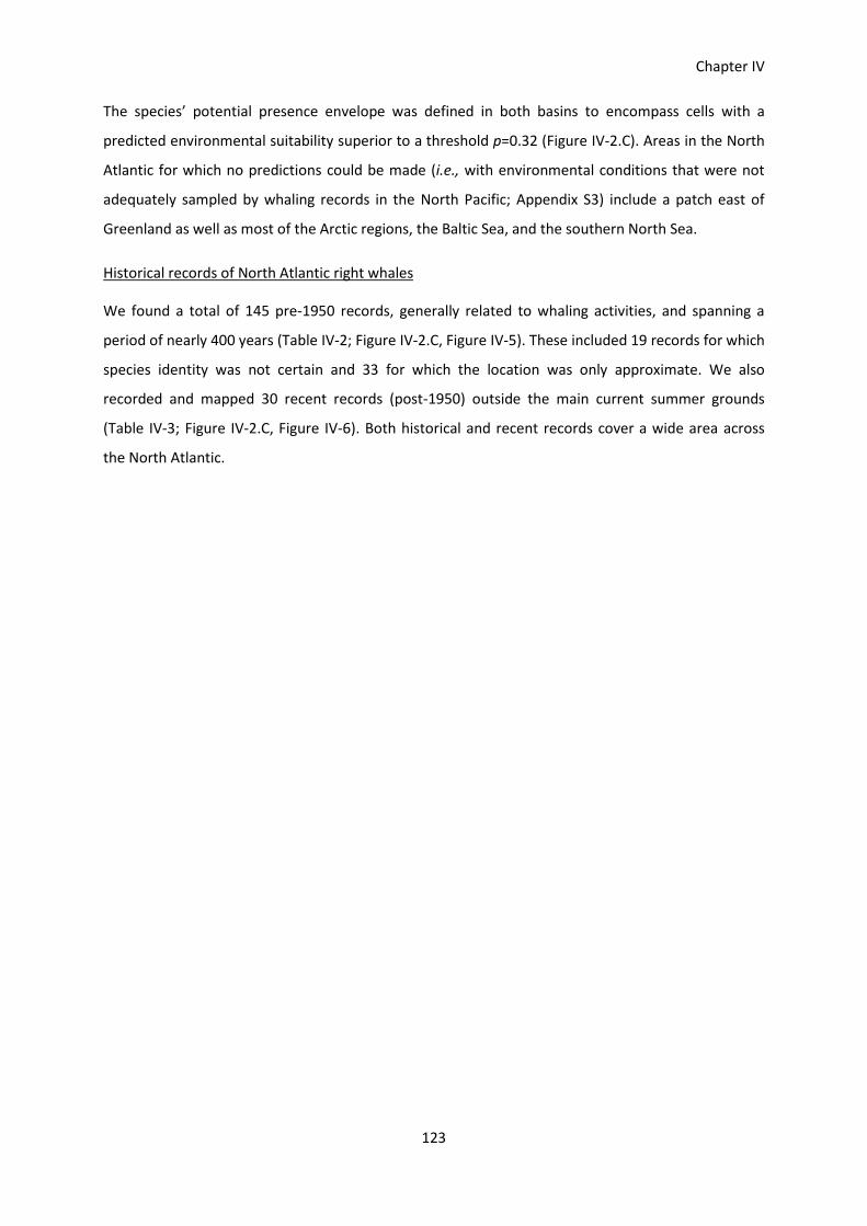
Chapter IV

123

The species’ potential presence envelope was defined in both basins to encompass cells with a

predicted environmental suitability superior to a threshold p=0.32 (Figure IV-2.C). Areas in the North

Atlantic for which no predictions could be made (i.e., with environmental conditions that were not

adequately sampled by whaling records in the North Pacific; Appendix S3) include a patch east of

Greenland as well as most of the Arctic regions, the Baltic Sea, and the southern North Sea.

Historical records of North Atlantic right whales

We found a total of 145 pre-1950 records, generally related to whaling activities, and spanning a

period of nearly 400 years (Table IV-2; Figure IV-2.C, Figure IV-5). These included 19 records for which

species identity was not certain and 33 for which the location was only approximate. We also

recorded and mapped 30 recent records (post-1950) outside the main current summer grounds

(Table IV-3; Figure IV-2.C, Figure IV-6). Both historical and recent records cover a wide area across

the North Atlantic.

Chapter IV

124

Figure IV-1. Historical data and model predictions in the North Pacific. A) Sampling effort (measured as number of days when whalers were present in each cell according to 19th

Century American whaling records) and geographic locations mentioned in the text. Effort was concentrated in

the main whaling grounds for: sperm whales, around 30° N; bowhead whales near the Bering Strait; and North

Pacific right whales in the Gulf of Alaska, east of Kamchatka, in the Sea of Okhotsk and in the Sea of Japan. B)

Historical distribution of North Pacific right whales in the summer months (June to September), based on the

whaling records. Data include both presence (red, where right whales were seen or caught) and absence

records (blue, cells visited by whalers, but where no right whales were reported in the examined logbooks);

white cells were not visited. C) Predicted environmental suitability from a species distribution model fitted to

the historical records. Shades of red indicate progressively higher suitability as predicted by the BRT models

(above the p=0.32 threshold); blue cells correspond to areas where the species is predicted as absent; white

cells are areas for which no reliable predictions can be made. All data are presented on a 1°x1° grid in Bonne

projection (standard parallel: 30°N; central meridian: 170°W).

Chapter IV

125

Figure IV-2. Model predictions and historical data in the North Atlantic. A) Map of the North Atlantic indicating place names mentioned in the text. B) Predicted historical distribution

of the North Atlantic right whale in the summer months (June to September) based on a species distribution

model (BRT) fitted to whaling records for the North Pacific right whale and extrapolated geographically into the

Atlantic. Shades of red indicate progressively higher environmental suitability as predicted by the model (above

the p=0.32 threshold); blue cells correspond to areas where the species is predicted as absent; white cells are

areas for which no reliable predictions can be made. C) Historical records, obtained by reviewing the literature

for confirmed or likely records from June to September. The area shaded in pink corresponds to the envelope

of predicted presence as mapped in B (presented to facilitate comparisons with B). Symbols correspond to: 142

historical (pre-1950) records from 1583 to 1935, distinguishing those for which there is higher (red symbols) or

lower (open symbols) confidence in the species’ identity and those for which there is higher (circles) or lower

(triangles) precision in location. In addition, the map includes 26 recent (post-1950) records outside the main

summer grounds (black crosses). See figures and tables in Appendix S5 for details on each record. All data are

presented on a 1°x1° grid in Bonne projection (standard parallel: 30°N, central meridian: 20°W).

Chapter IV

126

Discussion

We found good – but not perfect – agreement between the model’s predictions (Figure IV-2.B) and

the spatial extent of the historical records of the NARW (Figure IV-2.C). Both suggest that this

species’ historical feeding grounds extended across the North Atlantic, in a wide band from eastern

North America to northern Norway, over the Grand Banks of Newfoundland, south and east of

Greenland’s Cape Farewell, south of Iceland, north of the British Isles and in the Norwegian Sea. This

distribution pattern was mainly driven by cold temperatures, high productivity and low mixed layer

depth.

Before discussing in more detail the extent to which the historical records support the model’s

predictions, we discuss key assumptions and caveats of our study that must be taken into

consideration (also see Appendix S6).

Assumptions and caveats

Species distribution models represent the realized distribution of a species at a given time and place

(Peterson et al., 2011), not differentiating among the factors limiting species distribution (such as

prey availability, presence of competitors, or dispersal limitations). This calls for caution when

interpreting the results of models transferred across species and across temporal or geographical

scenarios (Randin et al., 2006; Sinclair et al., 2010).

The model we have generated is only informative of the historical distribution of the NARW if this

species’ environmental requirements are similar to those of the NPRW. Given this strong assumption,

the model’s predictions must be interpreted as a hypothesis for – rather than as a reconstruction of –

the historical distribution of the NARW. As previously discussed, the species’ similarities in ecology

and morphology justify that we explore this hypothesis. The main drivers of our prediction (SST, NPP

and MLD) are consistent with those found in previous studies on the distribution of right whales

(Baumgartner & Mate, 2003; Gregr, 2011; Torres et al., 2013), reinforcing our assumption that right

whales’ distributions are generally driven by the same mechanisms.

The North Pacific whaling records are an exceptional dataset for developing a SDM. They can

nonetheless include a number of false absences and false presences, as a result of biases (in sampling

effort across space and time) and errors (in location and in species’ identifications). We attempted to

reduce these by analyzing only cells with a reasonable sampling effort, and by reducing sources of

confusion with bowheads (Appendix S1). Nonetheless, we were unable to correct for the poor

representation of shallow-depth data in the NPRW records (given that they correspond to offshore

Chapter IV

127

whaling operations), and its potential effects on the model’s discriminative power in shallow-depth

areas.

Our analysis is based on a geographic extrapolation from one ocean basin (the North Pacific) to

another one (the North Atlantic). To reduce potential errors resulting from this extrapolation, we

restricted predictions to the environmental envelope sampled by whalers in the Pacific Ocean. This

ensures that areas where we predict high environmental suitability are represented in the dataset

used to calibrate the model, reducing one of the main sources of uncertainty under predictions of

new scenarios (Zurell et al., 2009). We were however unable to control for other potential

differences between basins (e.g., in prey availability, in the interactions between oceanographic

conditions) which might limit the transferability of the statistical correlation found in one ocean basin

into the other one (Randin et al., 2006). Process-based models combining behavioral and

environmental factors could lead to a better understanding of the underlying processes driving right

whales distribution (Palacios et al., 2013) but would require extensive physiological and behavioral

information that are difficult to gather for these rare species.

By fitting the model using occurrence data mainly from the mid-19th century (1840-1850) and

environmental data from the 20th century (MLD and SST 1900-1992; NPP 1998-2007), we necessarily

assumed that the environmental spatial structure of the data has remained unchanged. Climatic

variation, both longer-term directional changes (e.g., warming since the end of the Little Ice Age;

Mann et al., 2008) and shorter-term cycles (e.g., El Niño Southern Oscillation, Nicholls, 2008 ; Pacific

Decadal Oscillation, Mantua & Hare, 2002), is known to affect the distribution of marine species (e.g.,

Evans & Bjørge, 2013), and may therefore affect the results of our analyses. However, the use of

occurrence data collected throughout the 19th century and of environmental data obtained by

averaging long-term climatologies is likely to mitigate these effects, by retaining the strong,

persistent, seasonal signals in the data (Gregr, 2011). Furthermore, in a previous study facing a

similar challenge, Gregr (2011) found that a review of climatic reconstructions did not reveal major

differences in the North Pacific climate between the mid-19th and the 20th centuries.

The NARW historical records we compiled constitute the most comprehensive dataset currently

available on the historical summer occurrence of this species. Yet, they are strongly biased spatially

(towards coastal areas, where whales were more accessible) and temporally (towards a recent

period when records became more detailed, despite the species being rarer). They are also plagued

by geographic imprecision (location is only approximate for 23% of records) and by taxonomic

uncertainty (for 13% of records). These limitations preclude the use of these data in a quantitative

validation of the model’s predictions. Instead, we discuss qualitatively, region-by-region, the extent

Chapter IV

128

to which the historical (Table IV-2) and recent (Table IV-3) records either support or contradict the

model’s predictions (Figure IV-2.C, Figure IV-5, Figure IV-6), keeping in mind the strengths and

limitations of both the data and the model.

We place this discussion within the broader background of the history of whaling in each region,

which provides additional records at the regional scale (too imprecise to map) and insights on

whaling effort that contextualize the records in each region. Moving from west to east across the

Atlantic (see Figure IV-2 for the locations mentioned in the text), we discuss in particular the few

instances where the model and records disagree.

Comparison between the model predictions and species records in the North Atlantic

The model predicts an area of suitable habitat for NARWs off the eastern coast of the United States

south of Cape Cod, supported by a few historical records from coastal whaling operations, as well as

by recent records (NOAA-NEFSC, 2013).

North of Cape Cod, the model predicts suitable areas over the continental slope, but absence in the

shelf areas (Gulf of Maine, Nova Scotia; no predictions for the Bay of Fundy). The records show little

evidence of historical presence of right whales in summer along this coast (Reeves et al., 1999,

2002b), and therefore present no major contradiction to the model predictions. However, both the

model predictions and the historical records disagree with today’s known distribution of NARWs, as

this shelf area appears to be the main region where right whales currently concentrate in the

summer (NOAA-NEFSC, 2013; Wikgren et al., 2014). This discrepancy likely results from the model’s

poor capacity to discriminate habitat in shallow waters (having been calibrated mainly with deep

waters data; Figure IV-1). But the scarcity of historical records also raises the possibility that this

region might not have been as important historically this species, at least in relative terms, as it is

today.

The model predicts a broad suitable area over and around the Grand Banks of Newfoundland, well

supported by 18th century American whaling records (e.g., specifically referring to right whaling “east

of the Grand Banks”; Reeves & Mitchell, 1986, and an earlier map of an ‘abandoned’ right whale

ground in this general area ; Clark 1880).

Historical and recent records also support the predictions of suitable habitat around the coast of

Newfoundland and into the Gulf of Saint Lawrence. This region was well-known to 16th and 17th

centuries Basque whalers (Ciriquiain-Gaiztarro, 1961; Du Pasquier, 2000), but studies of the history

of Basque whaling have focused on the northern Gulf of Saint Lawrence and Strait of Belle Isle

(Barkham, 1974), with recent genetic studies indicating that bowheads were the focus (McLeod et

Chapter IV

129

al., 2008). But a 1538 report explicitly mentions whaling in southeast Newfoundland (Haie, 1889),

suggesting Basques exploited a wider area. Furthermore, historical references to separate summer

and early winter whaling seasons suggest that both right whales and bowheads were targeted (but

see McLeod et al. 2008).

A few historical records off northern Labrador are not supported by the model’s predictions.

However, species identity is uncertain for these records, which may plausibly correspond to

bowheads, as this falls within the historical summer distribution of this species (Reeves et al., 1983).

These records are therefore not a main challenge to the model’s predictions.

A large area of high suitability is predicted south and southeast of Greenland, and south of Iceland.

This includes the area known as the Cape Farewell Ground, where the historical presence of right

whales is well supported by 19th century American whaling records (Reeves & Mitchell, 1986a;

Reeves et al., 2007). Basque whalers might have also caught right whales in this region during the

17th-18th centuries (Du Pasquier, 2000). Furthermore, it is one of the few regions outside the eastern

North American coast where NARWs have been recorded recently (Brown et al., 2007; Mellinger et

al., 2011).

Predictions of presence off the southern coast of Iceland are supported by historical records,

including by additional whaling records too imprecise to map (“about 50 miles to the west of that

island”, “to the south-east of Iceland”; Collett, 1909; Du Pasquier, 2000). Several historical records off

northwestern Iceland seem to contradict the model’s predicted absence (Lindquist, 1994; Edvardsson

& Rafnsson, 2006) but are in fact located within coastal cells where the model makes no predictions.

The Faroe Islands are well within the model’s predicted area of historical presence, whereas the

Shetlands are at the edge. Historical records indicate that right whales were taken off both

archipelagos (Jonsgård, 1977).

Model predictions are contradicted by a concentration of historical records off the Hebrides and

Ireland, a region predicted as unsuitable. This may again reflect the model’s limited predictive

capacity in shallow depth regions. However, these records correspond to a specific whaling period,

whose well-documented details (Haldane, 1905, 1907; Collett, 1909; Thompson, 1918) suggest an

exceptional rather than regular presence of NARWs. Indeed, despite ongoing whaling effort (for fin

and sei whales, Balaenoptera physalus and B. borealis) no right whales were reported off the British

Isles between 1889 and 1904. In contrast, 63 were captured between 1905 and 1914, with “several

hundred” seen in 1908 (Collett, 1909). This is reminiscent of concentrations occasionally observed in

other pelagic fisheries, associated with exceptional oceanic conditions (e.g., exceptional catches of

Chapter IV

130

yellowfin tuna off the Seychelles in 2004–2005; Fonteneau et al., 2008). If an oceanic anomaly is the

explanation for these records, they would in any case be impossible to predict with a model based on

a long-term averaged climatology.

The model predicts suitable habitat in the Norwegian Sea and around the North Cape. This is

supported by a few coastal whaling records, reflecting a 17th-18th century right whaling ground (see

Smith et al., 2006 for a review). Du Pasquier (2000) collected >200 records of Basque whaling trips to

“Norway” that we could not map but which could have plausibly corresponded to whaling in this

area. There are also two recent records for this region.

Outside the main band of predicted suitability, the model predicts a few patches of suitable habitat

around the Iberian Peninsula and in the northern Mediterranean Sea. Of these, only in the Gulf of

Biscay we found an historical summer record, but in an area where whaling historically took place in

the winter (Aguilar, 1986; Azpiazu, 2000; Barkham, 2000a). These areas are known to have high

concentrations of zooplankton that support feeding populations of whales (e.g. of fin whales

Balaenoptera physalus in the northwestern Mediterranean Sea; Notarbartolo-Di-Sciara et al., 2003),

but given the lack of support for the predicted presence of NARWs we cannot rule out the possibility

that the model overestimates the historical distribution of the foraging grounds for this species.

Conversely, there are a few records outside the area predicted by the model. A historical record off

Jan Mayen (of low species certainty) and a recent record in the Baltic (where the model makes no

predictions) are not major challenges to the model. But a historical record north of the Azores and

two recent records to the northwest of the Iberian Peninsula contradict the model’s predicted

absence. These are reminiscent of a few isolated records in the central North Pacific (between 20°-

40°N, also outside the area predicted by the model; Figure IV-1.A), where their rarity despite high

whaling effort (for sperm whales) suggests that theycorrespond to migrating individuals rather than

regular feeding grounds.

Conclusions

The generally high agreement between the model predictions and the historical records suggests

that the model based on NPRW whaling data is informative of the historical summer distribution of

NARWs. If so, this distribution extended across the North Atlantic in a wide continuous band from

eastern North America to northern Norway, including substantial areas of offshore habitat outside

known records.

Chapter IV

131

Nonetheless, there are discrepancies between the model’s predictions and the historical data that

point to potential limitations. In particular, failure to predict both the current summer grounds off

North America and the historical whaling grounds off the British Isles suggest lack of predictive

power in shallow-depth, shelf regions. Additionally, predictions in areas for which we have no

evidence that they were historical NARW foraging grounds (e.g., in the Mediterranean) suggest

further limitations in the model. The model’s predictions should therefore be mainly seen as a

hypothesis for the summer offshore distribution of the NARW.

Our results pave the way for additional avenues of research and monitoring with potential

implications for the conservation of the endangered NARW. Indeed, the model predictions raise

hypotheses that should be further explored in two ways. Firstly, exploration of the surviving historical

record in the light of these results can help to clarify the history of the exploitation of this species. In

particular, the model’s results suggest that more attention is warranted to whaling records in and

around Newfoundland, and in offshore grounds around the Grand Banks, south of

Greenland/Iceland, and in the Norwegian Sea. A better understanding of pre-whaling distribution can

inform future conservation perspectives for this species, even if these areas are currently

unoccupied. Secondly, the model highlights regions potentially used by today’s populations. Indeed,

nearly all recent records outside the main known summer grounds fall within the area predicted as

suitable by the model, suggesting that these records correspond to purposeful visits to suitable

feeding areas rather than vagrancy or extra limit straying. With many individuals not accounted for

every year in the intensive surveys at the main grounds (Hamilton et al., 2007), identification of other

regularly used areas is key to guiding strategic conservation efforts. Passive acoustic methods such as

those used by Mellinger et al. (2011) may be a cost-effective option for sampling such areas.

More broadly, our analysis illustrates the challenges and opportunities of combining historical and

environmental data to improve understanding of the original distribution of highly depleted species.

Because the quality of the historical record generally declines strongly as we go back in time,

relatively recent population declines are much better documented that century- or millennia-old

declines, which are often underestimated or even forgotten (Pauly, 1995). Nonetheless, the spatial

heterogeneity of historical human impacts creates opportunities for using information from the more

recently impacted, better-known regions to fill gaps in knowledge elsewhere, using species

distribution models to extrapolate between the two. The challenges are particularly significant for

species that have suffered ancient impacts across their entire range. For some of these, extrapolation

from ecologically-similar phylogenetically-related species can be used to generate hypothesis that

add depth to the fragmentary historical record. As understanding of the ecological and evolutionary

Chapter IV

132

processes that drive species’ spatial distribution improves, the informative value of these

extrapolations across space and taxa will increase, making historical data even more useful.

Appendices

Appendix S1 Historical records of North Pacific right whales

Appendix S2 Environmental data

Appendix S3 Species Distribution Models

Appendix S4 Complementary analyses

Appendix S5 Historical records of North Atlantic Right Whale

Appendix S6 Extended discussion

Chapter IV

133

Appendices

Appendix S1: Historical records of North Pacific right whales

We analyzed records of North Pacific right whale (NPRW) species presence (seen or caught) and

absence from daily data obtained from a sample of logbooks kept aboard 19th and early 20th century

American whaling voyages. For the purposes of the present analysis, we selected whaling voyages

which occurred in the North Pacific Ocean (north of 10°N latitude and longitude between 100°E and

100°W). Most voyages entering the North Pacific did so early in a calendar year and remained there

throughout that year, or occasionally for two and rarely three years. To account for this operational

pattern, we divided the voyage data according to calendar year to define data segments that we

referred to as voyage-years.

We defined temporally continuous segments of the data for each voyage within the North Pacific,

and further divided each of those segments in which logbook entries were available on a near daily

and continuous basis. Subsegments were formed when the vessels were in port or otherwise not

whaling, or when there were temporal or spatial gaps in the reported data. Extended temporal gaps

occurred for two reasons. First, the keeper of the logbook may not have made entries for a time

period or pages may have been removed or otherwise lost from the logbook itself. Second, the data

extractor may have failed to include some observations that were recorded in the logbook, either in

error (e.g. pages stuck together) or by intention in certain circumstances. The latter occurred

occasionally in Maury's data, for example when vessels entered bays or other enclosed areas for

extended periods of whaling. We have identified this pattern in the North Pacific (e.g., Sea of

Okhotsk, Anadyrskiy Gulf). Not recording data in such circumstances was likely part of the data

collection protocol used by Maury's data extractors because his interest appears to have been

primarily in open water rather than coastal oceanic patterns. Extended spatial gaps were frequently

associated with temporal gaps, but also occurred from time to time as a result of errors in logbook

recording (e.g. transposition of digits), errors in data extraction (e.g. transposition of digits or failing

to adjust hemisphere designation as the vessel crossed the International Date Line or the Equator).

We examined maps of voyage tracklines and corrected obvious errors by comparing to original

logbooks where available (see Smith et al., 2012). However, some unexplained spatial gaps without a

temporal gap remained, and we defined subsegments to reflect those situations. This voyage

segmenting procedure occasionally left subsegments with only one logbook entry, and the data for

such subsegments were omitted.

The sightings and catches were usually identified (or reliably identifiable from the context) to species,

and those that were not were omitted. Maury's data were being extracted from logbooks at a time

Chapter IV

134

when right and bowhead whales were not always distinguished in the North Pacific. We noticed that

Maury's data included no observations of bowhead whales in areas where both species are known to

have occurred (Townsend, 1935; Bockstoce et al., 2010), and discarded Maury's data in those regions

(north of 54°N in the Okhotsk Sea and north of 56°N in the Okhotsk Sea).

The American whaling data included information on the distribution of another species of right

whale: the southern right whale (Eubalaena australis), present across the Southern Ocean. We did

not include those data in construction of the species distribution model for two reasons. First, only

part of the distribution of this species is covered by the whaling data. Indeed, although coverage is

quite complete up to about latitude 60°S, it is practically absent further south, maybe because rough

seas rendered whale processing too difficult (e.g., as Lacroix, 1997 mentions for the Falklands).

Accordingly, other historical sources mention right whales at higher latitudes, and up to the Antarctic

shelf (Morrell, 1832; Ross, 1847; Charcot & Joubin, 1913; Ohsumi & Kasamatsu, 1986). Second,

bowhead whales (Balaena mysticetus) are present at high latitudes in the northern but not in the

southern hemisphere. This species may compete directly with right whales for food, as it also feeds

on copepods (Lowry et al., 2004), and its presence may thus affect the distribution of the North

Pacific and North Atlantic species, but not of the Southern right whale. We therefore considered that

a species distribution model obtained solely from data on the North Pacific right whale was more

relevant to make predictions on the distribution of the North Atlantic species than a model including

both the North Pacific and the southern right whales. Accordingly, we found in exploratory analyses

that including whaling data from the Southern Hemisphere did not improve the models’ predictive

power.

Appendix S2: Environmental data

Sea surface temperature (SST) has a strong correlation with the distribution and abundance of

zooplankton (Norberg & DeAngelis, 1997; Rutherford et al., 1999; Gregr & Coyle, 2009) and has been

found to be a good predictor of right whale distribution in previous analyses (Murison and Gaskin

1989; Gregr 2011). Previous authors found that Mixed Layer Depth (MLD) is strongly correlated (r=

0.865, p<0.0001) with the diving depth of North Atlantic right whales (NARW; Baumgartner & Mate,

2003).

Net primary productivity (NPP) was included given that is known to be positively correlated with

zooplankton biomass (Norberg & DeAngelis, 1997). We retrieved 1080x2160 global grids of NPP,

calculated as a function of chlorophyll, available light, and photosynthetic efficiency using the

Vertically Generalized Production Model (VGPM) algorithm (Behrenfeld & Falkowski, 1997) for the

entire SeaWiFS 1998-2007 chlorophyll record, on the Ocean Productivity web site

Chapter IV

135

(http://www.science.oregonstate.edu/ocean.productivity/index.php). We then averaged NPP over

the summer months (June to September) to compute the seasonal climatology.

Ocean bathymetric features have frequently been used as predictors of right whale distribution

(Hamazaki, 2002; Kaschner et al., 2006; Gregr, 2011; Torres et al., 2013). We integrated depth

(DEPTH), slope (SLOPE) and distance to land (LANDDIST) in the model.

Table IV-1. Environmental predictors used in the species distribution models.

Variable Acronym Derived from Period

Averaged

Reference

Net Primary Productivity

(mg C/m²/day)

NPP Ocean

Productivity

web site

1998-2007 Behrenfeld & Falkowski, 1997

Sea Surface Temperature (°C) SST NODC WOA94 1900-1992 Levitus & Boyer, 1994

Mixed Layer Depth (m) MLD NODC WOA94 1900-1992 Monterey & Levitus, 1997

Depth (m) DEPTH NOAA-NGDC

ETOPO1

- Amante & Eakins, 2009

Distance to Land (km) LANDDIST AquaMaps - Kaschner et al., 2008

Slope SLOPE Depth - -

Appendix S3: Fitted functions

While the purpose of this study is not to provide a quantitative description of the feeding habitat of

NPRW (see an in-depth discussion of this topic in Gregr & Coyle, 2009 and Gregr, 2011), we discuss

the species-environment relationships for the NPRW in summer, as a basis for understanding the

underlying processes driving the predicted distribution of right whales in our model.

Relative importance and fitted functions for the predictors used in the BRT are comparable to

previous studies on the ecology or distribution of right whales in summer. The importance of sea

surface temperature and the selection of areas with low sea surface temperature (5°C-15°C) are

consistent with previous studies of right whale distribution, both in the North Pacific and in the

Southern Oceans (Gregr, 2011; Torres et al., 2013). Our results indicate that the model is also

strongly driven by NPP, with the presence of right whales being correlated to a primary productivity

superior to 500 mg C/m²/day. Accordingly, even if not directly comparable, chlorophyll a

concentration also appears as an important predictor of right whale distribution in previous studies

(Torres et al., 2013). The scarcity of occurrence data associated with high values of productivity call

for caution when interpreting the shape of the response curve above 1000 mg C/m²/day. The

importance of MLD in our models and the finding that NPRW presences are associated with low MLD

is coherent with a previous study on NARW foraging ecology, which identified a correlation between

the depth of the mixed layer (MLD) and the diving depth of feeding right whales (Baumgartner &

Chapter IV

136

Mate, 2003). Depth has a non-negligible influence in our model. The North Pacific whaling dataset

however is biased towards offshore waters, as can be seen from the distribution of data along the

depth gradient (Figure IV-3) and the extrapolation of the model in shallow areas should be

considered with care. The bulk of North Pacific right whale presences was associated with habitat

distant from 0 to 800 km away of the coastline, though some presences occurred further offshore (<

1200 km away from the coast).

Figure IV-3. Fitted functions showing the species-environment relationships produced by the BRT. The relative influence of each variable is presented as a percentage in parentheses. Rug plots on the x-axis

show data distribution across each variable, in deciles. SST = sea surface temperature, NPP = net primary

productivity, MLD = mixed layer depth, DEPTH = mean depth, LANDDIST = distance to land.

Chapter IV

137

Appendix S4: Complementary Analyses

Sensitivity to the inclusion of records with low sampling effort

The sampling effort was not uniform across the entire North Pacific (Figure IV-1.A). American whalers

directed their effort towards areas where the density of whales (not only right whales, but also

sperm, bowhead, gray, and humpback whales) was expected to be relatively high. Corridors of

navigation between ports and the main whaling grounds were also oversampled compared to other

areas in the North Pacific. Although these differences in effort give us information on the real

distribution of whales (as in fisheries today, 19th century whalers had prior knowledge of which areas

whales were more easily found, and targeted these preferentially; Townsend, 1935), they can induce

flaws in the structure of the model as not all absences are equally informative (e.g., an absence in a

cell visited only once is more likely to be a false absence, where the species was actually present but

not detected, than a cell visited multiple times). An analysis was conducted to assess the differences

in predicted environmental suitability for models built with the overall dataset, or with cells that

were visited at least two or three times by a whaling ship. The results show very minor differences in

the predicted distribution of right whales. The similarity between the different predictions was

always greater than 85% in the North Atlantic and greater than 90% in the North Pacific when making

pairwise similarity comparison between the different prediction maps. However, the models’

explanatory and predictive power increased when selecting only the cells with more than two days of

effort in the dataset used to build the model, indicating that the strategy of discarding cells with very

low effort was justified.

Sensitivity to the exclusion of medium-latitude data

The whaling dataset contains a large patch of records around 30°N, characterized by an intense

survey effort (for sperm whales) coupled with a virtual absence of NPRW sightings. In a previous

modelling analysis, Gregr (2011) chose to include only data north of 40°N, which cover the vast

majority of the presence records for the NPRW. To test the leverage that medium-latitude data have

in the model, we built a BRT on North Pacific whaling data north of 40°N (“>40°N model”) and

compared its predictions with those of the main model (“>20°N model”) presented in this analysis.

We found that these medium-latitude data had a significant effect on the model’s predictions in the

North Atlantic. Indeed, although predictions in high latitudes remained unchanged, the >40°N model

predicted a wider area of suitable habitat in mid-latitudes regions (e.g. a patch on the coast of

California, a band from the gulf of Biscay and Portugal to the Azores). Given that there is no support

for these predictions (from either historical or recent data), this suggests that the >40°N model is less

capable of discriminating habitat preferences in mid-latitudes latitudes, having apparently a higher

Chapter IV

138

likelihood of commission errors (false positives). These errors should be avoided in a conservation

context, where potentially suitable areas need to be identified to guide strategic conservation efforts

(Loiselle et al., 2003; Rondinini et al., 2006).

The inclusion of data from the North Pacific between 20°N and 40°N seems therefore to provide

valuable information to the model - leading to a better discrimination of areas of low suitability –

justifying their inclusion in the analysis.

Sensitivity to modelling assumptions (BRT vs GAM)

To assess whether our results are sensitive to the type of statistical model used, we performed a

second analysis on the same dataset using a Generalized Additive Models (GAM; Hastie & Tibshirani,

1986). GAMs are often used for their ability to deal with non-linear and non-monotonic relationships

between the response variable and the explanatory variables (Hastie & Tibshirani, 1986; Wood,

2006). This type of model has been shown to perform well for modelling species distribution (Guisan

et al., 2002) and particularly in the case of species with complex distribution patterns, i.e. where

occurrences do not respond to environmental variables according to a predefined ‘shape’ (Segurado

& Araujo, 2004). Variable selection was performed on a forward-stepwise selection based on

optimizing Akaike Information Criterion (AIC), Un-Biased Risk Estimator (UBRE), and deviance

explained. The method used to assess the quality of predictions was the same as for the BRT (see

Appendix S3). Over dispersion in the residuals was assessed by calculating the value of the dispersion

parameter φ described by Zuur et al. (2009). A value of φ=1.12 indicated no over dispersion in the

residuals.

The selected GAM included the six environmental predictors (SST, NPP, MLD, DEPTH, SLOPE and

LANDDIST) and two additional interactions (SST*MLD, SST*DEPTH). As the BRT, the GAM was mainly

driven by SST, NPP and MLD, with a preference for cold and productive waters with a mixed layer

depth inferior to 20m. The performance of the GAM was very satisfactory (deviance explained = 51.3,

AUC=0.92, TSS=0.71), though lower than the BRT (deviance explained= 67.2%, AUC= 0.93, TSS=0.74),

which justified our decision to base the discussion on the results of the BRT.

There was a very high agreement between the predictions of the GAM and BRT models both in the

North Pacific and North Atlantic (Figure IV-1.C, Figure IV-2.B, Figure IV-4), indicating that the areas

predicted as being suitable summer habitats are not dependant of the type of modelling technique

used.

Chapter IV

139

Figure IV-4. Environmental suitability for right whales in summer predicted by the GAM. (A) In the North Pacific and (B) in the North Atlantic. Shades of red indicate progressively higher suitability as

predicted by the model (above the p=0.32 threshold); blue colour corresponds to areas where the species is

predicted as absent. White colour indicates areas outside the environmental envelope, where no prediction

was made. All data are presented on a 1°x1° grid in the Bonne projection.

Chapter IV

140

Appendix S5: Historical distribution records of the North Atlantic Right Whale

Table IV-2. Historical (pre 1950) records of North Atlantic right whale (Eubalaena glacialis) in the summer months (June to September).

“Map ID” corresponds to the number on Figure IV-5. : species reliable, location reliable; : species reliable,

location uncertain; : species uncertain, location reliable; : species uncertain, location uncertain.

Map ID

Date Record details References

Eastern United States, Bay of Fundy, Nova Scotia 1

July 1699 "12-13" whales Reeves & Mitchell,

1986a (Table 1) 2

August 1733

"A whale was taken in the Bay of Fundy by a Captain Hussey, and brought into Boston in August." According to Reeves et al. (1999), this was "probably a right whale"

page 169 in Starbuck, 1878 (also mentioned in Reeves et al., 1999)

3 ca. 1 September

1838

"A Right Whale, about 40 feet long, was found dead off Newburyport, Mass., about September 1st, and towed ashore at Salisbury Point. It was estimated that it would make about forty barrels of oil (Newburyport Herald).

This is unusually early in the fall for this species to appear on our coasts." Allen, 1916 (p. 135)

4

31 July 1839

"40 ft, 40 bbls" Reeves & Mitchell,

1986a (Table 1) 5 1 June

1841 "Whale seen in Gardiners Bay"

Reeves & Mitchell, 1986a (Table 1)

6 28 July 1841

2 killed Reeves & Mitchell,

1986a (Table 1) 7 ca. 1 June

1860 1, found floating

Reeves & Mitchell, 1986a (Table 1)

8 18 June 1866

1 seen Reeves & Mitchell,

1986a (Table 1) 9

June 1872 2 killed Reeves & Mitchell,

1986a (Table 1) 10

ca. 1 June 1888

"Right Whale encountered off Cape Cod about the first of June, 1888, whose calf was first harpooned and killed, while the cow, refusing to leave her offspring, circled around and around until she succumbed after

nine bomb-lances had been shot at her (Nantucket Journal, vol. 10, no. 36, June 7, 1888)."

Allen, 1916 (p. 131); also Reeves et al.,

1999 11 August

1896 1 struck and lost

Reeves & Mitchell, 1986a (Table 1)

12 22 July 1913

"A large whale chased by several boats" Reeves & Mitchell,

1986a (Table 1) 13 9 August

1918 One taken, one struck and lost. "Young whale 'exceptionally fat' expected to produce 25-30 bbls. Only 30 gals

of oil recovered, none sold". "Last whale landed by the Long Island shore whalers." Reeves & Mitchell,

1986a (Table 1) 14 Summer

1919 "A right whale came ashore dead in Sheepscot Bay in summer 1919"

Reeves et al., 1999 (p. 7, citing Norton, 1930)

15 late June 1926

"60 ft. female and 25 ft. calf sighted", "not chased" Reeves & Mitchell,

1986a (Table 1)

Grand Banks, Newfoundland and Gulf of Saint Lawrence

16 Summer 1583

A report of Gilbert’s 1583 trip to Newfoundland includes in the list of the commodities of the country “abundance of whales, for which also is a very great trade in the bays of Placentia and the Grand Bay, where is

made train oils of the whale”. The trip was in the summer but it is not clear if he saw the "train oils" being made.

Haie, 1889

17 11 August 1760

"killed a right Whale & she sunk". "ca. 12-14 leagues [36-42 nmi] E of the Great Bank". Original source: whaler logbook (Enterprise, USA; main activity Sperm whaling).

Reeves & Mitchell, 1986a (Table 1)

18 30-31 August 1754

30 August "saw a Noble Right Whale close" but escaped; 31 August "chased 3 but could not strike". Original source: whaler logbook (Phebe, USA; main activity Sperm whaling).

Reeves & Mitchell, 1986a (Table 1)

19 13 Sept 1765

"saw two & chased, secured one". Original source: whaler logbook (Diamond, USA; main activity Sperm whaling).

Reeves & Mitchell, 1986a (Table 1)

20 5 August 1763

"saw one and chased but could not strike". Original source: whaler logbook (Dolphin, USA; main activity Sperm whaling).

Reeves & Mitchell, 1986a (Table 1)

21 7 August 1763

"saw a Right Whale and chased but could not strike".Original source: whaler logbook (Dolphin, USA; main activity Sperm whaling).

Reeves & Mitchell, 1986a (Table 1)

22 23 July 1754

23 July 1754, "saw several right whales", one struck and lost. Position corresponds to 19 July. Had seen "Icy Islands" on the 20 July. Original source: whaler logbook (Phebe, USA; main activity Sperm whaling).

Reeves & Mitchell, 1986a (Table 1)

Chapter IV

141

Map ID

Date Record details References

23 1850

"The last Right Whale killed in New-foundland was taken near Gaultois, on the south coast, in 1850." The author uses the term "right whale" to refer to bowheads too. No season is given, so presumed summer.

Millais, 1907

24 "mid-August 1937"

"A right whale killed in Placentia Bay in mid-August 1937 was the fist of its kind taken at the Rose-au-Rue whaling station during more than 19 years of operation" Photos included.

Mitchell et al., 1986

25 Sept 1937

"capture" "1,130cm female"; "The files of the Division of Mammals, USNM, have a photograph of a 37 ft (1,130) female rigth whale that was taken by the catcher boat Morelos 14 miles southeast of Cape Race,

Newfoundland"

Mead, 1986 (Appendix 2)

26 Ca. 1595-1610

Genetic analyses of bones found in a marine excavation associated with a sunken galeon in Red Bay (Basque whaling). A single bone of right whale found (among many of bowheads).

McLeod et al., 2008

Labrador Sea

27 15 August 1587

From the record of John Davis' third voyage: “The 17 we met a ship at sea, and as farre as we could judge it was a Biskaine: we thought she went a fishing for whales; for in 52 degrees or thereabout we saw very many.”

The 15 of August they left the coast of Newfoundland/Labrador at about 52 degrees latitude (about the entrance to Belle Isle) and headed eastwards, so presumed that whales were seen east of Belle Isle. "

Janes, 1906

28 10 July 1806

1 killed, young, 20 ft (est.). "Possibly a right whale (Eubalaena)?" Reeves et al., 1983

(Table 1)

29 25-28 July 1768

Context: On the 27 May they say "some whales run" among thick ice (Bowheads?) but then no more whales were reported until the 25 of July. After that, whales frequently reported until the 20 August, between ca. 60°

and 51°N off the coast of Labrador (Right Whales?), including: 25 July "Saw a Rite Whale bound to Nward, gave her chase 6 hours Could Not Strike Her" (24 July: 60.06°N); 26 July "Sar Rite Whales Very Plenty Could

Not Strike them."; 28 July "Saw Whales plenty" at 60°N (29 July - 61°48'N, "Within 20 Leagues of Land"). Original source: whaler logbook (Reliance, USA; main activity right [bowhead?] whaling).

Reeves & Mitchell, 1986a (Table 1)

30

9 August 1768

Context: On the 27 May they say "some whales run" among thick ice (Bowheads?) but then no more whales were reported until the 25 of July. After that, whales frequently reported until the 20 August, between ca. 60°

and 51°N off the coast of Labrador (Right Whales?), including: 9 August "Saw a Rite Whale gave her Chase Could Nots Strike her", "Saw Rite Whales [bowheads?] Plenty" (latitude 10 August 58°N). Original source:

whaler logbook (Reliance, USA; main activity right [bowhead?] whaling).

Reeves & Mitchell, 1986a (Table 1)

31 12-13

August 1768

Context: On the 27 May they say "some whales run" among thick ice (Bowheads?) but then no more whales were reported until the 25 of July. After that, whales frequently reported until the 20 August, between ca. 60°

and 51°N off the coast of Labrador (Right Whales?) including: 12 August "Lots Whalle"; spoke Capt Goodspeede who "told Us WHales Was plenty on the Coste" (53°18N); 13 August "Saw Whales [balaenids?] Struck one Lost her Lost one Iron", "Saw whales gave them Chase Could Not Strike". Original source: whaler

logbook (Reliance, USA; main activity right [bowhead?] whaling).

Reeves & Mitchell, 1986a (Table 1)

32 14 August

1768

Context: On the 27 May they say "some whales run" among thick ice (Bowheads?) but then no more whales were reported until the 25 of July. After that, whales frequently reported until the 20 August, between ca. 60°

and 51°N off the coast of Labrador (Right Whales?) including: 14 August "Saw whales plenty" (54°06N). . Original source: whaler logbook (Reliance, USA; main activity right [bowhead?] whaling).

Reeves & Mitchell, 1986a (Table 1)

33 19-21

August 1768

Context: On the 27 May they say "some whales run" among thick ice (Bowheads?) but then no more whales were reported until the 25 of July. After that, whales frequently reported until the 20 August, between ca. 60°

and 51°N off the coast of Labrador (Right Whales?) including: 19 August "Saw whales" (51°05N); 20 August "Kild one Whale [...] sunken" (51°16N); 21 August "Cutting the head", "Wents to trying"; 22 August "Rafts of

blubber"; 23 August "Stowed away our oyl". Original source: whaler logbook (Reliance, USA; main activity right [bowhead?] whaling).

Reeves & Mitchell, 1986a (Table 1)

34

1887

"They [right whales, Eubalaena] are taken during the summer months off the southern end of Greenland and to a limited extent in the lower part of Davis Strait, near Resolution Island". Clark distinguished right whales

from bowheads (whose distribution is described separately) but given the high latitude of this record it is nonetheless assumed to be taxonomically uncertain.

Clark, 1887 (p. 15)

Southeast Greenland and the Cape Farewell grounds 35

June 1858

"found these whales [the proper Black whale] first on 11 June at 60°30'N, 35° W", "coming from the Eastwards, where they must have been some time in April & May" and then followed them "bound west a

little southerly true course down off Cape Farewell". Two were taken at 61°30'N, 34-36° W in June. Source: letter from Captain C. Chapel (Violet), to Cpt. Wiliam Jackson (16 Oct 1859).

Reeves & Mitchell, 1986a (p. 225)

36 1866

"Right whale ground": Lat 60.00 N to 62.00N; Long. 33.00W to 35.00W. Original source: a note in the abstract of the schooner Petrel (USA)

Reeves & Mitchell, 1986a (p. 226)

37

5 July 1868 1 saved, 1 struck and lost; cow and calf killed 5 July [1868]; cow sunk, calf produced 26bbls. Original source:

whaler logbook (Ansel Gibbs, USA)

Schevill & Moore, 1983 (Table 1 and Fig 1); Reeves & Mitchell,

1986a

Chapter IV

142

Map ID

Date Record details References

38 5 June 1872

Some seen. Original source: whaler logbook (Ansel Gibbs, USA) Reeves et al., 2007

(Table 2.2) 39 10 June

1872 1 killed. Original source: whaler logbook (Ansel Gibbs, USA)

Reeves et al., 2007 (Table 2.2)

40 12 June 1872

Some seen. Original source: whaler logbook (Ansel Gibbs, USA) Reeves et al., 2007

(Table 2.2) 41 25-28 June

1866 Day 1: 2 seen; day 2: two seen; day 3: 1 killed and sank; day 4: 1 killed (coordinates taken on the 25th June).

Original source: whaler logbook (Pacific, USA). Reeves et al., 2007

(Table 2.2) 42

4 July 1866 1 killed and sank. Original source: whaler logbook (Pacific, USA). Reeves et al., 2007

(Table 2.2) 43

9 July 1866 1 seen. Original source: whaler logbook (Pacific, USA). Reeves et al., 2007

(Table 2.2)

44 17 June

1877

Right whale cow & calf; calf killed and tried (estimated 20 bbls), cow struck and lost (estimated 100 bbl). Original source: ship logbook (Daniel Webster, New Bedford). Likely correspond to the 2 individuals recorded

by Schevill & Moore for June 1878.

Schevill & Moore, 1983; Reeves &

Mitchell, 1986a (Table 2); Reeves et al., 2007

(p. 39) 45 27 July

1878 Some seen. Original source: whaler logbook (Adeline Gibbs, USA).

Reeves et al., 2007 (Table 2.2)

46 11 June

1878

Encountered Right whales 11 June 1878, one captured. "Although only one whale was captured, Ferguson believed the vessel was 'into the middle of quite a school of whales, for they could be heard spouting in

different directions all around us any time during the night". Original source: whaler logbook (Abbie, Bradford).

Reeves & Mitchell, 1986a

47 13-15 June 1878

Whales seen by the Shooner Astoria (1878), reported in the abstract of the A.J. Ross. Reeves & Mitchell,

1986a (p. 226) 48 July 30-Aug

3 1878 Whales seen. Original source: whaler logbook (Astoria, USA).

Reeves & Mitchell, 1986a

49 4-8 Aug 1878

Whales seen, by the Shooner Astoria (1878). Reeves & Michell (1986) assume they are right whales. Reeves & Mitchell,

1986a

50 July-August 1886

"sailed 24 June for 'Hudson bay' [...]. By 17 July, however, the Palmetto was at 61°14'N, 36°12'W, i.e. on the Cape Farewell Ground. Right whales were first sighted 20 July, and by 9 August the crew had taken their fifth whale alongside". 15+ whales (5 saved, 2 struck and 8+ sighted). Original source: whaler logbook (Palmetto,

USA).

Schevill & Moore, 1983 (Table 1); Reeves & Mitchell, 1986a (p.

227) 51 23 June

1891 1 right whale seen. Original source: whaler logbook (Petrel, USA).

Reeves et al., 2007 (Table 2.2)

52 13 July 1891

1 seen. Original source: whaler logbook (Petrel, USA). Reeves et al., 2007

(Table 2.2) 53 23-25 July

1891 Day 1: 3 seen, 1 killed (sank); day 2: 2 seen; day three: 1 killed. Original source: whaler logbook (Petrel, USA).

Reeves et al., 2007 (Table 2.2)

54 22 July 1891

1 killed. Original source: whaler logbook (Petrel, but reporting catches by the Mermeid) Reeves et al., 2007

(Table 2.2)

Iceland

55 1610 – 1650

"Archaeological escavations at Strákatangi strongly suggest that the site is a foreign whaling station from the 17th century, with many similarities with whaling stations from the 17th century in the North Atlantic region,

especially Red Bay in Labrador. It is impossible to say from the archaeological material which nationality occupied the station but local tales suggest that the whalers at Strákatanga were Basques that came from the Basque regions in North Spain and South France. [...] These remains suggest that foreign whalers built stations

on land and used them during the whaling season. The artifacts give us a relative date for the occupation of the site, which indicate a occupation in the period 1610 – 1650. No animal bones were recovered during the excavation and sieving of cultural deposits with a 5 mm sieve did neither produce animal nor fish bones." (in Edvardsson & Rafnsson 2006). However, Magnús Rafnsson personal comm (email 18/11/2013): "A couple of

skulls were found around the ruins and DNA research said they were from right whales."

Edvardsson & Rafnsson, 2006

56

1613

The first whaling ship arrived in Strandir in 1613, causing fear among the inhabitants who were not used to seeing ocean-going vessels. The local pastor arrived on the scene and pointed the Spaniards to a suitable

harbor in Steingrímsfjörður, near his abode, all with the consent of the sheriff, Ari Magnússon. The Basques caught 17 whales.

Edvardsson & Rafnsson, 2006 (citing

Jón Guðmundsson)

57 1614-1615

1614: According to Jón Guðmundsson, four ships were whaling in Reykjarfjörður close to where he lived. 1615: That same summer Jón tells of sixteen ships by Strandir, most of which sailed east to Russia but four

ships spent the summer whaling from Reykjafjörður in Strandir.

Edvardsson & Rafnsson, 2006 (citing

Jón Guðmundsson)

Chapter IV

143

Map ID

Date Record details References

58 1752

"J. Eiriksson (1768: 253f) mentions French "sléttbakur" whaling in Ísafjarðardjup in 1752; furthermore: 'it is also probable that his whale fish breeds inside the fiords of Ísafjarðarsysla and Barðastandasysla, and … raises

there its young during the summer, in … May, June and July, and leaves them late in the month of August, when then some of these abandoned ones occasionally fall prey to the inhabitants.' Eiriksson could be

referring to the, mainly, humpback calf whaling in Arnarfjörður."

Lindquist, 1994 (p. 201; citing J. Eiriksson

1768)

59 between

1770-1780 "even American vessels, as late as between 1770 and 1780, occasionally caught Nordkapers in Brede Fiord and

Faxe Bay, in Iceland."

Eschricht & Reinhardt, 1866 (citing

Pontoppidan 1785) 60

1802 "Another good slettboku-hvlalur (i.e. black right whale) came ashore at Naust near Hofson" Lindquist, 1994 (p.

849)

61 April to August, ca.

1873

"Iceland Grounds. Right Whales. April to August Lat 63 to 67 Long 11 to 16 W." Souce: cryptic anotation in an anonymous compilation of American whaling abstracts, not dated but in the same page with memoranda

concerning cruises in 1867 and in 1872-73.

Reeves & Mitchell, 1986a

Norwegian and Barents Seas

62 2-25 July

1667

Hamburg vessel left the Svalbard (Spitzbergen) bowhead whaling ground durimg midsummer to hunt right whales off northern Norway between 2-25 July, in "bay whaling" centred in Lopphavet, the Loppa Sea. Of the

Finnmark coast in July, this ship encountered "many" right whales, as well as Dutch, French, Flemish and German whaleships (about 20 of which used the Loppa Sea as a roadstead). Original source: journal kept by

Christian Bullen (coxswain aboard an unidentified Hamburg whaleship).

Smith et al., 2006 and Reeves & Smith, 2006 (citing Barthelmess,

2003)

63 pre 1884

Bones identified as the N Atlantic Right Whale, presumed to corresponded to Dutch whaling in the previous centuries.

Guldberg, 1884

64 pre 1884

Bones identified as the N Atlantic Right Whale + old try pots (in an area called the Dutchman Hill), presumed to correspond to Dutch whaling in the previous centuries.

Guldberg, 1884

65 1935

"A Biscayan whale was last observed at the coasts of the Kola Peninsula in summer 1935; it was found dead in the surface of the sea and towed to Murmansk (local newspapers erroneously described it as "Greenland

whale")" Tomilin, 1967 (p. 55)

Faroes and Shetlands 66 summer

1892 "One specimen captured off the Faroe Islands"; by Norwegian whalers. Collett, 1909

67 7 July 1898

Collet (1909) refers to "One specimen taken near the Faroe Islands (a female accompanied by a young one)"; by Norwegian whalers, in the summer. Possibly the same 2 individuals in the IWC database taken on the 7th

July 189 by Norwegian whalers (station/factory: Strømnæs, Faroe).

Collett, 1909; IWC, 2013

68 summer

1903

Collet (1909) refers to "One specimen taken off the Faroe Islands"; by Norwegian whalers. Possibly the same individual mentioned in t IWC database as taken in the Faroe Islands by Norway (station/factory: Lopra. A/S

Suderø) in 1903.

Collett, 1909; IWC, 2013

69 summer 1907

"Two specimens were also taken off the Faroe Islands"; by Norwegian whalers. Collett, 1909

70 14 August

1671

"In our home-voyage to Hamburg I saw an example of this enmity of a North-caper whale and a sword-fish, near to Hitland ; they fought and struck at one another so vehemently that the water flew about like dust,

sometimes one, sometimes the other was uppermost". Original source: Friderich Martens' report of a 1671 whaling voyage.

White, 1855 (p. 115)

71 1903 (presumably summer)

"The only other specimen I have heard of was got in 1903 by a Faroe whaler 50 miles off Shetland" Haldane, 1907 (p. 13)

72 Summer 1905-1914

One of 66 points mapped by Thompson (1918); whales taken off the Hebrides and off the Shetlands between 1908 and 1914, in the summer (June to August)

Thompson, 1918 (Fig. 1)

73 Summer 1905-1914

One of 66 points mapped by Thompson (1918); whales taken off the Hebrides and off the Shetlands between 1908 and 1914, in the summer (June to August)

Thompson, 1918 (Fig. 1)

74 Summer 1905-1914

One of 66 points mapped by Thompson (1918); whales taken off the Hebrides and off the Shetlands between 1908 and 1914, in the summer (June to August)

Thompson, 1918 (Fig. 1)

75 Summer 1905-1914

One of 66 points mapped by Thompson (1918); whales taken off the Hebrides and off the Shetlands between 1908 and 1914, in the summer (June to August)

Thompson, 1918 (Fig. 1)

76 Summer 1905-1914

One of 66 points mapped by Thompson (1918); whales taken off the Hebrides and off the Shetlands between 1908 and 1914, in the summer (June to August)

Thompson, 1918 (Fig. 1)

77 Summer 1905-1914

One of 66 points mapped by Thompson (1918); whales taken off the Hebrides and off the Shetlands between 1908 and 1914, in the summer (June to August)

Thompson, 1918 (Fig. 1)

78 Summer 1905-1914

One of 66 points mapped by Thompson (1918); whales taken off the Hebrides and off the Shetlands between 1908 and 1914, in the summer (June to August)

Thompson, 1918 (Fig. 1)

British Isles (Hebrides, Ireland)

Chapter IV

144

Map ID

Date Record details References

79 Summer 1905

"One was wounded off St. Kilda, but escaped" Collett, 1909

80 Summer 1906

"six killed, and more seen [...] off the Hebrides, between the 13th June and the 4th August", by Norwegian whalers.

Collett, 1909

81 to 139

Summer 1905-1914

59 points mapped by Thompson (1918) as whales taken off the Hebrides between 1908 and 1914 (of 66: 3 in May; 43 in June; 19 in July; 1 in August). In 1908 "the schools this year consisted of several hundred", and "the plankton-bearing currents probably flowed nearer land than in 1907, for the whales might be met with quite

in the shallow water between islands and rocks. Their stay this year was of only three week's duration" (Collett 1909). Taken by Norwegian whalers (coastal whaling from bases in the Hebrides).

Collett, 1909; Thompson, 1918 (Fig. 1); Reid et al., 2003;

IWC 2013

140

8-13 June 1908

"Five specimens […] captured off Inishkea, Ireland, between June 8th and June 13th (among them one female and a young one)"; "They were all separate, and no schools were observed" (Collett 1909). By the Arranmore Whaling Company, on the island of S. Inishkea; under Norwegian management (Lillie 1910). The same record

(5 individuals, in "Ireland N", by the UK, station/factory: Iniskea Is, Arranmore Whal. Co) is in the IWC database (2013).

Collett, 1909; Lillie, 1910; IWC, 2013

141 "first fortnight of June" 1909

Five taken by the Arranmore Whaling Company (shore whaling, Norwegian management); "within a radius of 70 miles north, south and west of Innishkea" (Lillie 1919). The same record (5 individuals, in "Ireland N", by

the UK, station/factory: Iniskea Is, Arranmore Whal. Co) is in the IWC database (2013). Lillie, 1910; IWC, 2013

142 summer

1910

9 taken: five by the Arranmore Whaling Company (S. Inishkea island), four by the Blacksod Whaling company (Mullet peninsula St Mayo); shore whaling, companies run by Norvegians (Lillie 1910). Likely to include the 4+4 individuals, in "Ireland N", taken by the UK (4 by station/factory Iniskea Is, Arranmore WhCo and 4 by

station/factory Ardelly Pt, Belmullet. BlacksodWhC) in the IWC database (2013).

Lillie, 1910; IWC, 2013

Mid-Atlantic 143

2 July 1876 "boats where lowered, without success, for 'a Right Whale' at 49°25'N 22°22'W, squarely on the Commodore

Morris Ground". Original source: "a journal kept by the captain's wife (whaler Ohio, USA). Reeves & Mitchell,

1986a (p. 231)

Jan Mayen 144

1618 “whales both Greenland and right, were very plentiful round Jan Mayen when [King] James granted the fishing

to Hull [i.e., 1618]”. However, Lubbock provides no support to this statement (no references, no further information).

Lubbock, 1978 (p. 71)

Spain

145 25 July 1850

"It was at one time supposed that the Balaena biscayensis had become quite extinct; but this is certainly not the case. Whales are seen on the Cantabrian coast at intervals of about ten years. [...] On the 25th of July

1850, early in the morning, a whale appeared off Guetaria. Boats quickly pursued it; but the harpooner missed his aim, and the whale went off, heading N.W." The record is clearly described as Righ Whale, but assumed of

low certainty given the unusual season.

Markham & Flower, 1881 (p. 975)

Chapter IV

145

Table IV-3. Recent (post 1950) records of North Atlantic right whale (Eubalaena glacialis) in the summer months (June to September).

“Map ID” corresponds to the number on Figure IV-6. : species reliable, location reliable; : species reliable,

location uncertain; : species uncertain, location reliable.

Map ID

Date Region Record details References

1

September 1951

Grand Banks, Newfoundland and

Gulf of Saint Lawrence

From the NOAA "Interactive North Atlantic Right Whale Sightings Map" (Reliability: Definite; ID: 46); in Mitchell et al. 1986 (citing Sergeant 1966): "taken 'in error' from a

Newfoundland shore station in 1951"

Mitchell et al., 1986; NOAA NEFSC, 2013

2

July 1959

Grand Banks, Newfoundland and

Gulf of Saint Lawrence

"An animal 'probably from this species' was seen in Dildo Arm, Trinity Bay, in July 1959"

Mitchell et al., 1986 (citing Sergeant 1966)

3

18 June 1964

British Isles (Hebrides, Ireland)

From the NOAA "Interactive North Atlantic Right Whale Sightings Map" (reliability = Definite; ID: 4269)

Jacobsen et al., 2004 (Table 1; citing Maul & Sergeant, 1977); NOAA

NEFSC, 2013

4

8 June 1974

Grand Banks, Newfoundland and

Gulf of Saint Lawrence

From the NOAA "Interactive North Atlantic Right Whale Sightings Map" (reliability = Probable; ID: 464)

NOAA NEFSC, 2013

5

September 1977

Off Spain Sighting offshore N Spain. From the NOAA "Interactive North Atlantic Right Whale

Sightings Map" (reliability = Definite; ID: 612)

NOAA NEFSC, 2013; Jacobsen et al., 2004

(Table 1; citing Aguilar 1981)

6

10-21 July 1978

Grand Banks, Newfoundland and

Gulf of Saint Lawrence

"Reported frequent feeding activity". Also in the NOAA "Interactive North Atlantic Right Whale Sightings Map" (Reliability: Definite; ID: 638)

Lien et al., 1989; NOAA NEFSC, 2013

7

2 August 1979

Southeast Greenland and the Cape

Farewell grounds

Observation of 'in all probability two bowhead whales' by Norwegian whalers, but given the historical absence of bowheads from the W coast of Greenland, particularly

in the summer, Reeves & Mitchell (1986b) consider it likely to correspond to right whales.

Reeves & Mitchell, 1986a (citing Jonsgard

1981)

8

25 August 1979

Grand Banks, Newfoundland and

Gulf of Saint Lawrence

From the NOAA "Interactive North Atlantic Right Whale Sightings Map" (Reliability: Definite; ID: 801)

Lien et al., 1989; NOAA NEFSC, 2013

9

31 August 1981

Grand Banks, Newfoundland and

Gulf of Saint Lawrence

Female alone, matched to an individual seen off the US coast. Bonavista Bay; Newman's Cove.

Knowlton et al., 1992; Mitchell et al., 1986, citing Beamish 1981.

10

26-28 July 1984

Grand Banks, Newfoundland and

Gulf of Saint Lawrence

"was entrapped in a codtrap and resisted all attempts by humans to come near it. [...] Eventually the animal towed the codtrap and all its supporting grapnels out to

sea". From the NOAA "Interactive North Atlantic Right Whale Sightings Map" (Reliability: Definite; ID: 2140)

Lien et al., 1989; NOAA NEFSC, 2013

11

4 July 1987 Mid-Atlantic

From the the NOAA "Interactive North Atlantic Right Whale Sightings Map" (reliability = Definite; ID: 4268).

NOAA NEFSC, 2013

12

5 July 1989

Southeast Greenland and the Cape

Farewell grounds

From the NOAA "Interactive North Atlantic Right Whale Sightings Map" (reliability = Definite; ID: 4269). Matched to an individual seen 15 June 1989 in the Nova Scotial

Shelf.

Knowlton et al., 1992; NOAA NEFSC, 2013

13

5 August 1989

Mid-Atlantic Mother + Calf. From the NOAA "Interactive North Atlantic Right Whale Sightings

Map"; (reliability = Definite; ID: 5531). Both matched to individuals also seen off the US coast.

Knowlton et al., 1992; NOAA NEFSC, 2013

14

6 September

1990

Grand Banks, Newfoundland and

Gulf of Saint Lawrence

Female alone, matched to an individual seen off the US coast. Knowlton et al., 1992

15

21 July 1995

Southeast Greenland and the Cape

Farewell grounds

From the NOAA "Interactive North Atlantic Right Whale Sightings Map" (reliability = Definite; ID: 9421). Also mentioned by Hamilton et al. 2007 (individual Eg # 1412,

also seen in the Gulf of Maine as well as in 2003 west of Iceland)

NOAA NEFSC, 2013; Hamilton et al., 2007

Chapter IV

146

Map ID

Date Region Record details References

16

18 August 1999

Grand Banks, Newfoundland and

Gulf of Saint Lawrence

From the the NOAA "Interactive North Atlantic Right Whale Sightings Map" (Reliability: Unknown; ID: 17738)

NOAA NEFSC, 2013

17

17 September

to 22 October

1999

Norwegian and Barents Seas

Observed from 17 September to 22 October. Sightings were confined to a rather small area in a sound between the mainland and a small island, Skorpa. It was

matched to a Right Whale individual previously seen off Cape Cod, Massachusetts (41"54'N, 68'30'W) on 23 May, 1999. Also: from the NOAA "Interactive North

Atlantic Right Whale Sightings Map" (reliability = Definite; ID: 18227).

Jacobsen et al., 2004; NOAA NEFSC, 2013

18

28 July 2000

Faroes and Shetlands From the NOAA "Interactive North Atlantic Right Whale Sightings Map" (reliability =

Probable; ID: 19607). NOAA NEFSC, 2013

19

August-Sept 2001

Norwegian and Barents Seas

"From August to September 2001 there was a right whale observation claimed to have been made in Oslo fjord, Southern Norway. The whale was observed at short distance, 50-100m, moving northwards east of Tofteholmene (59° 31'N, 10° 34'E).

The next day the presumed same animal was seen in the same area moving southwards. The observation was made by a fisherman with 6 yr experience onboard a whale catcher in the Antartic and he insisted that this was a right whale. However,

the incident was not photo documented"

Jacobsen et al., 2004

20

22-23 June 2003

Iceland

From the NOAA "Interactive North Atlantic Right Whale Sightings Map": 2 sightings in consecutive days of a group of 2 individuals, coordinates are the first day

(reliability = Definite; ID: 26004 and 26005). Also mentioned by Hamilton et al. 2007 (individual Eg # 1412, also seen in the Gulf of Maine as well as in 1995 in the Farewell

Grounds)

NOAA NEFSC, 2013; Hamilton et al., 2007

21

14 July 2003

Southeast Greenland and the Cape

Farewell grounds

From the NOAA "Interactive North Atlantic Right Whale Sightings Map" (reliability = Definite; ID: 26078).

NOAA NEFSC, 2013

22

31 July 2005

Grand Banks, Newfoundland and

Gulf of Saint Lawrence

From the NOAA "Interactive North Atlantic Right Whale Sightings Map" (Reliability: Definite; ID: 29280).

NOAA NEFSC, 2013

23

28 September

2006

Grand Banks, Newfoundland and

Gulf of Saint Lawrence

From the NOAA "Interactive North Atlantic Right Whale Sightings Map" (Reliability: Definite; ID: 31979).

NOAA NEFSC, 2013

24

4 July 2007 Mid-Atlantic

From the NOAA "Interactive North Atlantic Right Whale Sightings Map" (Reliability: Unknown; ID: 33604).

NOAA NEFSC, 2013

25

August to Nov 2007

Southeast Greenland and the Cape

Farewell grounds

Sound recordings from passive acoustic moorings - August to November 2007 (63 calls on 22 days, mainly in August and September)

Mellinger et al., 2011

26

August to Nov 2007

Southeast Greenland and the Cape

Farewell grounds

Sound recordings from passive acoustic moorings - August to November 2007 (931 calls on 22 days, nearly all in August)

Mellinger et al., 2011

27

July to Dec 2007 + 8 July 2008

Southeast Greenland and the Cape

Farewell grounds

Sound recordings from passive acoustic moorings - July to December 2007 (979 calls on 21 days; nearly all in July and August); Calls were

also detected the next season on 8 July 2008 Mellinger et al., 2011

28

Sept 2007

Southeast Greenland and the Cape

Farewell grounds

Sound recordings from passive acoustic moorings - September 2007 (42 calls on 3 days)

Mellinger et al., 2011

29

August 2007

Southeast Greenland and the Cape

Farewell grounds Sound recordings from passive acoustic moorings - August 2007 (1 call on 1 day) Mellinger et al., 2011

30

9 September

2010

Grand Banks, Newfoundland and

Gulf of Saint Lawrence

From the NOAA "Interactive North Atlantic Right Whale Sightings Map" (Reliability: Unknown; ID: 40576).

NOAA NEFSC, 2013

Chapter IV

147

Figure IV-5. Historical (pre-1950) records of North Atlantic right whale (Eubalaena glacialis) in the summer months (June to September). A) in the North Atlantic; B) Eastern United States; C) Grand Banks and Newfoundland; D) Southeast Greenland

and the Cape Farewell Ground; E) Iceland; F) Faroes and Shetlands, distinguishing those for which there is

higher (red symbols) or lower (open symbols) confidence in the species’ identity and those for which there is

higher (circles) or lower (triangles) precision in location. All data are presented on a 1°x1° grid in Bonne

projection (standard parallel: 30°N, central meridian: 20°W). See Table IV-2 for a list of records.

Chapter IV

148

Figure IV-6. Recent (post-1950) records of North Atlantic right whale (Eubalaena glacialis) in the summer months (June to September), outside its main known summer grounds. A) In the North Atlantic; B) Newfoundland; C) Southeast Greenland and Western Iceland, distinguishing those

for which there is higher (red symbols) or lower (open symbols) confidence in the species’ identity and those

for which there is higher (circles) or lower (triangles) precision in location. The area shaded in red corresponds

to the main feeding grounds for the current population (Bay of Fundy; Browns Bank; Great South Channel;

Massachusetts Bay; Gulf of Maine; Jeffreys Ledge ; Georges Bank; Grand Manan Bank) concentrating 98.6%

of June to September recorded sightings (sum of number of individuals in NOAA 2013). The coastal area

southwards to Florida (in pink) has 0.4% of the sightings, while the Scotian Shelf and Gulf of Saint Lawrence to

the north (in orange) have 0.9% of the sightings. All data are presented on a 1°x1° grid in Bonne projection

(standard parallel: 30°N, central meridian: 20°W). See Table IV-3 for a list of records.

Chapter IV

149

Appendix S6: Extended discussion

North Pacific whaling records and model predictions

North Pacific whaling records are impressive in their spatial coverage and sample sizes, far exceeding

even today’s standards of cetacean sightings surveys (Kaschner et al., 2012). Furthermore, as a result

of whalers’ search for new grounds, these records are likely to cover very well the geographic

summer range of the species, including both areas where it was present and wide areas where it was

not. It is therefore not surprising that the statistical models obtained from these data perform

extremely well in predicting the occurrence of NPRWs. Nonetheless, these data and the models built

from them have some intrinsic limitations that can lead to mismatches between the empirical

observations and the model predictions.

This modelling exercise assumes that the whaling records come from a set of individuals with similar

environmental preferences. However, in a previous study, Gregr (2011) found that separate

environmental correlate models for right whales in the eastern and western North Pacific fitted the

data better than a common model. This may reflect differences between separate populations, or

differences in the spatial biases in the eastern and western data.

Although these data are impressive in their coverage, they are likely to include a number of false

absences: visited cells where whales were present but were not recorded due to low sampling effort

or temporal bias in the spatial records. For example, the United States coast north of San Francisco

was visited by whalers in the late summer (August and September; see monthly maps in figures 10-

13 of Smith et al., 2012 and video in Schmidt, 2012). If right whales were present along the US coast

earlier in the summer, they would have been missed by these whalers.

There was also temporal variation across years. During the main period of NPRW exploitation,

whalers moved broadly from east to west, exploiting new areas as whaling grounds were successively

exhausted (Schmidt, 2012). If whales moved between these areas, the population using a given

ground might have been depleted by whaling elsewhere before whalers reached and discovered that

ground.

The whaling data may also include a number of false presences. In high latitudes there is a

particularly high risk of confusion with bowhead whales, and although we have attempted to reduce

this source of error (see Appendix S1), some incorrect assignments might remain, biasing the

predicted distribution of right whales.

In summary, the species distribution model fit well the whaling data for the NPRW, but its spatial

prediction may be affected by model limitations (a failure to capture all nuances of the

Chapter IV

150

environmental conditions favoured by right whales), by data limitations (false absences, false

presences, temporal and spatial biases), and by a combination of both.

Historical records in the North Atlantic

Historical records of NARWs in the summer are extremely biased temporally: two from the 16th

Century; 8 from the 17th; 14 from the 18th; 40 from 19th; and 81 from the 20th Century. They mainly

correspond to recent observations despite the fact that the species became progressively scarcer

(Reeves et al., 2007) and was already considered commercially extinct by the 1750s (Allen, 1908).

The historical records we collected therefore represent the final observations and captures of a

nearly extinct species, unlikely to be perfectly representative of the species’ original range. Indeed,

given that the history of its exploitation has a strong spatial pattern, with particular whaling grounds

successively exploited and exhausted (Reeves et al., 2007), this temporal bias comes inevitably

associated with a strong spatial bias. In addition, there is more pervasive spatial bias towards coastal

regions, where whales were more accessible and where records can be more easily mapped (i.e.

more likely to associated with a landmark). Indeed, offshore whaling records with accurate location

information are very scarce: the most consistent and reliable source of offshore historical records is

19th century American whaling logbooks (Smith et al., 2012), but by 1800 NARWs rare (Reeves et al.,

2007).

Even though we concentrated on records for which there was a reasonable degree of geographic

certainty, for 33 of the historical records (and one of the recent), only an approximate location is

known that could not be mapped with reasonable certainty to a 1° cell. These include, for example,

general locations referring to a landmark (e.g. “off the Faroes”), records at sea where only general

coordinates were given (e.g. a “right whale ground” between 60-62°N and 33-35°W), records where

precise coordinates existed but for a different date (e.g. whaler was at 49.19°N - 48.50°W on the 19

July 1754, and saw whales on the 23 July), and records where there was a precise latitude but only

approximate longitude (e.g. 47°63'N "just E of the Grand Bank"; examples from Collet 1909 and

Reeves & Mitchell, 1986; and seeTable IV-2). Others correspond to precise coastal locations, but

refer to dead whales that could have drifted from elsewhere (e.g. "a right whale came ashore dead in

Sheepscot Bay in summer 1919"; Reeves et al., 1999).

Also, despite our effort to focus on records with a high level of taxonomic certainty, for 19 of our

records (and six of the recent) the species is suspected but not confirmed as right whale. In

particular, some of these could plausibly correspond to bowhead whales (e.g. whales seen and taken

by the American whaler Reliance off the coast of Labrador between the 25 July and the 21 August

Chapter IV

151

1768; Reeves & Mitchell, 1986) given that the two species were often not clearly differentiated in

such early records.

Potential effects of climate variation

Most of the data on the distribution of the NPRW used to calibrate the models comes from a very

narrow temporal window mainly in the mid-19th century (91% of presence records from 1840 to

1850). The environmental data, on the other hand, correspond to 20th century conditions (MLD and

SST 1900-1992; NPP 1998-2007). The historical and recent records for NARW, in turn, span 400 years

(1699 to 2010). Oceanic bathymetry variables are constant within the time scale of our analyses, but

other environmental variables are not. In addition to the point of discussion provided in the

discussion section in the main text, we present a map of NARW historical records color coded

according to the date they correspond to (Figure IV-7). Our dataset of NARW records does not show

a general tendency for a polewards shift over time (Figure IV-7), as could perhaps have been

expected from a general temperature warming over this period (Mann et al., 2008), but the effects of

climate change on the distribution of whales might in any case be more complex than that because

of non-linear effects of climate on sea conditions (e.g. Moffa-Sánchez et al. 2014). Exploring these

effects is beyond the scope of this paper.

Figure IV-7. Historical (pre-1950) and recent (post 1950) records of North Atlantic right whale (Eubalaena glacialis) in the summer months, according to date. Only recent records outside the main current summer grounds are presented. Records are color coded in

relation to 1845, the peak of right whale exploitation in the North Pacific. The map is presented on a Bonne

projection (standard parallel: 30°N, central meridian: 20°W).

Table IV-4. Comparison between the model predictions and species records in the North Atlantic Region-by-region overview of the levels of agreement between the model’s predictions for the summer distribution of the North Atlantic right whale and locations of

known summer records for this species.

Region Model prediction Historical data Recent data Agreement Discussion

USA coast from

Delaware to

Cape Cod

Coastal presence A few coastal

whaling records

A few coastal

observations

Good A few historical and recent records confirm the model’s

prediction of right whale presence in the summer, even if the

relative rarity of these records (compared to much higher

numbers of spring and winter records, both historical and

recent) shows that the species is rare in this season.

Gulf of Maine,

Bay of Fundy,

Scotian Shelf

Absence near the

coast (no

predictions for

the Bay of Fundy),

presence in an

offshore band

The few records do

not suggest a regular

summer presence in

the coastal areas

The bulk of today’s

summer observations

are this coastal area.

Poor The model’s predictions of absence in the coastal area are not

contradicted by the historical data (that provides no evidence of

a regular summer presence). However, they are strongly

contradicted by recent data, as this is the species’ most

important current summer ground. May reflect the model’s lack

of predictive ability in shallow-depth regions.

Over and

around the

Grand Banks of

Newfoundland

Presence Well supported by

whaling records

A few observations Very good The model’s prediction of presence is well supported by a few

precise historical records as well as by a 1880 map of an

abandoned whaling ground.

Coastal

Newfoundland

and Gulf of St.

Lawrence

Presence Well supported by

whaling records

A few observations

around coastal

Newfoundland, an

increasing number of

records in the Gulf of St

Lawrence

Very good The model’s prediction of presence is supported by historical as

well as recent records. The region was well known to 16th and

17th centuries Basque whalers, with historical records referring

to two whaling seasons, the summer one potentially

corresponding to right whales as predicted by the model.

Northern coast

of Labrador

Absence A few whaling

records, but of

uncertain species

(potentially

bowheads)

No observations Medium The few historical records are not a major challenge to the

model’s prediction of absence given that they may all plausibly

correspond to bowhead whales.

Southeast

Greenland and

Cape Farewell

Ground

Presence A concentration of

whaling records

Severall recent records Very good A relative concentration of historical combined with several

recent records support very well the model’s prediction for

presence.

Iceland Presence on the

southern coast,

absence on the

northern coast

Historical records on

both the southern

and the

northwestern coasts

One recent record just

west of Iceland

Good Predicted presence on the southern coast well supported by

historical data. Absence on the north-eastern coast seems

contradicted by historical records, but they are within coastal

cells where the model makes no predictions.

Faroes and

Shetlands

Presence around

the Faroes;

Shetlands at the

edge of predicted

area

Historical records in

both archipelagos

One unconfirmed

observation just north

of the Shetlands

Good Historical records mostly in cells of predicted presence, or at the

edge of those.

British Isles

(Hebrides,

Ireland)

Absence An exceptional

concentration of

historical catches

One observation south

of Ireland

Bad The model’s prediction of absence is strongly contradicted by a

concentration of historical whaling records and by a recent

record. This may reflect the model’s lack of predictive ability in

shallow-depth regions, and/or its inability to predict temporally

exceptional oceanic conditions.

Norwegian and Presence A few precise coastal Two observations Very good The model’s prediction of presence is well supported for the

Barents Seas

(including the

North Cape and

Kola Peninsula)

whaling records in

the North Cape,

known as a coastal

whaling ground).

Possible region of

destination for

Basque pelagic

whaling trips.

coastal North Cape region, which was also the location of a well-

known historical whaling ground. The predicted presence in

offshore areas in the Norwegian Sea is compatible with many

records of Basque pelagic whaling trips to “Norway”. Also, it is

worth nothing that the Dutch name of the species is Noordkaper.

Jan Mayen Absence A single historical

record, but not a

particularly reliable

one

No observations Medium The single record is not a major challenge to the model’s

prediction of absence. Indeed, it comes from a single sentence in

a secondary source (Lubbock 1978 claimed “whales both

Greenland and right, were very plentiful round Jan Mayen [in

1618]”) where it was provided unsupported. Jan Mayen was a

base for Dutch bowhead whaling, and we found no other

references to the presence of right whales in there.

Baltic Sea No prediction No historical records A single recent record No model

prediction

The Baltic Sea is outside the area where the model makes

predictions.

Iberian

Peninsula (Bay

of Biscay,

Portugal) and

Mediterranean

Sea

Presence in five

small coastal

patches: in the

Bay of Biscay, off

central Portugal

and in the

northern

Mediterranean

A single historical

summer coastal

record in the Bay of

Biscay

No observations Poor

An historical summer record brings some support to the model’s

prediction of a suitable coastal patch in the Bay of Biscay (but

the area was known as a winter whaling ground, so this record is

considered exceptional rather than representative). An

archaeological record in Portugal is of unknown season. No

support to the predictions of summer presence in the

Mediterranean (the few records for this region are in the

winter).

Offshore

central North

Atlantic

Absence One offshore record

northeast of the

Azores

Two offshore records (>

100 km to the NW of

the Iberian Peninsula)

Medium These records are in offshore areas where the model predicts

absence. They are however not seen as a major challenge to the

model’s predictions given that similarly isolated records are also

found in the central North Pacific outside the area predicted by

the model, corresponding to rare presences in a region where

there are many more records of whale absence. In that sense,

the scarcity of records in the central North Atlantic is supported

by the model’s prediction of absence in this area.

Chapter V

157

CHAPTER V

HOW MANY RIGHT WHALES WERE THERE IN THE NORTH

ATLANTIC BEFORE COMMERCIAL WHALING? AN ESTIMATE

BASED ON NORTH PACIFIC WHALING RECORDS

Chapter V

158

Chapter V

159

V. How many right whales were there in the North

Atlantic before commercial whaling? An estimate based on

North Pacific whaling records

Sophie Monsarrat, M. Grazia Pennino, Tim D. Smith, Randall R. Reeves, Christine N. Meynard, David

M. Kaplan, Ana S.L. Rodrigues. (To be submitted)

Abstract

The North Atlantic right whale (NARW, Eubalaena glacialis) is one of the world’s most threatened

whale species. Previously widespread, it came close to extinction after centuries of overexploitation,

and currently persists as a population of only ca. 500 individuals in the western North Atlantic.

Setting appropriate conservation targets for this species requires an understanding of its historical

population size, as a baseline for measuring level of depletion and progress towards recovery.

However, this is made difficult by the scarcity of records over its very long whaling history. Here, we

propose a new estimate of the pre-exploitation population size of NARW based on a calculation of

the carrying capacity of the North Atlantic for right whales. To obtain this estimate, we took

advantage of a spatially explicit dataset on historical catches of North Pacific right whales (NPRW,

Eubalaena japonica) to model the relationship between right whale density and the environment.

Assuming that these two congeneric species select the same type of environmental conditions, we

projected this model into the North Atlantic, to obtain a spatially explicit prediction for the summer

distribution of relative abundance for the NARW. By scaling this with estimates of the pre-whaling

NPRW population, we obtained high and low estimates of between 9,091 and 21,328 individuals for

the overall abundance of NARW prior to exploitation. These results support previous estimates based

on the historical record indicating that the NARW is still very far from recovery, but they are difficult

to reconcile with recent genetic analyses. Our results also predict that there were two main areas of

high summer density in the North Atlantic: north of the Grand Banks of Newfoundland and in the

Norwegian Sea. We recommend these as priorities for future summer survey effort, with potential

relevance to the conservation of this endangered species.

Chapter V

160

Introduction

Species conservation often involves setting population targets for the desirable overall number of

individuals to be conserved, as baselines for measuring level of depletion, and as benchmarks for

assessing progress towards recovery (Sanderson, 2006). Historical baselines are often considered for

these purposes (Sanderson, 2006; McClenachan et al., 2012), but they are subject to human

perceptions of what constitutes the “natural” state of populations prior to human impacts. This can

be strongly biased for species that have been impacted over a long period of time (the "shifting

baseline syndrome"; Pauly, 1995; Jackson, 2001; Kittinger et al., 2013).

Whales have been exploited for centuries as key economic resources across the world (Reeves &

Smith, 2006), leading to reductions in population abundance (Woodby & Botkin, 1993; Roman &

Palumbi, 2003), range contractions (Bockstoce & Botkin, 1983; Reeves et al., 2007) and even

extirpations across entire oceans (Mead & Mitchell, 1984). The North Atlantic right whale (NARW,

Eubalaena glacialis) was the first whale species exploited at an industrial scale, in what Reeves et al.

(2007) described as “one of the most extensive, prolonged, and thorough campaigns of wildlife

exploitation in all of human history”. The history of its exploitation extended for nearly a millennium,

resulting in its near-extinction. Today, it persists as a small population of c. 500 individuals in the

western North Atlantic, being listed as Endangered by the International Union for Conservation of

Nature’s Red List of Threatened Species (Reilly et al., 2012).

Given the long history of its exploitation, there is considerable uncertainty regarding the original

population size for the NARW. Several attempts have nonetheless been made to estimate it, focusing

on the better-recorded western population. Aguilar (1986) estimated that from 1530 to 1610 Basque

whalers took 25,000 to 40,000 whales from the coasts of Newfoundland and Labrador, including

unknown proportions of right and bowhead whales (Balaena mysticetus). From the osteological

identification of whale bones at a 16th Century Basque whaling station, Cumbaa (1986) concluded

that roughly equivalent numbers of the two species were taken, leading Gaskin (1991) to estimate

total catches of 12,000 to 15,000 right whales. Consistent with this, the population size in the

northwestern North Atlantic was assumed to correspond to about 10,000 individuals, a figure

adopted as a baseline for discussions of carrying capacity and extent of recovery (Reeves et al. 2007).

However, the 50/50 ratio of bowheads to right whales in Basque catches was subsequently

invalidated by DNA analyses, which revealed a single right whale among many bowheads (Rastogi et

al., 2004a; McLeod et al., 2008). This led McLeod et al. (2008) to conclude that bowheads were the

Chapter V

161

principal target of Basque whalers in this region, and to question whether the impact of Basque

whaling on right whales was actually substantial.

Further south, along the eastern coast of today’s United States, a coastal right whaling industry

focused on the winter calving grounds and spring northwards migration (Reeves & Mitchell, 1986c;

Reeves et al., 1999, 2007), reaching its peak in the early 1700s (Reeves et al., 2007). Eighteenth

century American pelagic whalers also captured right whales near the Grand Banks of Newfoundland

(Reeves & Mitchell, 1986a). Building from a review of records of captures and of exports of baleen

from American colonies, Reeves et al. (2007; see also Reeves et al. 1999) estimated that a minimum

of 5,500 animals were killed between 1634 and 1951 (mainly pre-1750), consistent with a total

population of “at least a few thousand whales present in the mid-1600s” in the western North

Atlantic.

In the eastern North Atlantic, cows and calves in their wintering grounds were the main target of

Basque whalers in the Gulf of Biscay, from the 11th to the 17th century (Aguilar, 1986; Azpiazu, 2000;

Barkham, 2000b; Du Pasquier, 2000). Aguilar (1986) estimated that fewer than one hundred were

taken per year. Right whales may have also been a target of Medieval coastal whaling further north

in the English Channel (Musset, 1964) and further south off Portugal (Brito, 2011; Teixeira et al.,

2014). 17th century Basque whalers captured right whales in the summer months off Iceland

(Edvardsson & Rafnsson, 2006) and Norway (Du Pasquier, 2000). A right whaling ground off the

North Cape in northern Norway was exploited by 17th-18th century Danish, Norwegian, Dutch and

Basque whalers (Smith et al., 2006). Arctic whalers focusing on bowheads (mainly Dutch, but also

British, German and Basque) may have occasionally taken right whales (De Jong, 1983; Reeves et al.,

2007).

Even though the species was already very scarce by the mid-1800s, a few hundred were

subsequently taken throughout the North Atlantic before they became legally protected in 1935

(Reeves et al., 2007). Today’s population concentrates in the western North Atlantic, with only a few

records in the eastern North Atlantic in the past 50 years (Reilly et al., 2012).

Besides what can be learned from whaling records, information on past populations can be obtained

from genetic analyses. Today’s NARW population has levels of genetic variation that are significantly

lower than those of the southern right whale, E. australis, consistent with the fact that the latter,

although also strongly affected by whaling, has survived in substantially larger numbers (Waldick et

al., 2002). However, bottleneck analyses of living NARWs (Waldick et al., 2002) as well as of late-19th

and early-20th centuries specimens suggest no substantial loss of genetic diversity in the past two

Chapter V

162

centuries (Rosenbaum et al., 2000a). More puzzlingly, the analysis of a 16th century bone from

Labrador suggests genetic characteristics have not changed substantially since then (Rastogi et al.,

2004a; Frasier et al., 2007; McLeod et al., 2010). This was an unexpected result, as NARWs are

believed to have been depleted as a result of whaling over the past four centuries. Waldick et al.

(2002) proposed that today’s low genetic variation may have resulted from a slow but continual

erosion of alleles over eight centuries of whaling, but to reconcile this with the genetic analyses

would imply that the most important declines took place before the 16th century, not apparently

compatible with the history of whaling in the western North Atlantic.

Here we attempt to inform discussions on the original population of the NARW by approaching the

subject from a very different perspective: we estimate the ecological carrying capacity of the North

Atlantic for right whales, based on whaling records for a congeneric species, the North Pacific right

whale (NPRW, E. japonica). These two species of right whales are phylogenetically close (Rosenbaum

et al., 2000a; Sasaki et al., 2005) and as specialist copepod filter feeders they have similar

morphology (Woodward et al., 2006) and feeding behavior (Kenney, 2002). Another copepod

specialist, the bowhead whale (Lowry et al., 2004), potentially affected the northern limit of both

right whale species’ ranges. Assuming that the similarities translate into comparable environmental

preferences, the pre-whaling population of the North Pacific right whale, and the distribution of its

abundance across space, can be used to estimate the right whale carrying capacity of the North

Atlantic.

Like the NARW, the NPRW was extensively depleted, but its decline is more recent and better

documented than that of the NARW. Indeed, the bulk of its exploitation was undertaken by 19th

century American offshore whalers, whose exploits were recorded in their ship logbooks. A recent

project (Smith et al., 2012), building from and expanding on previous efforts (Maury, 1852;

Townsend, 1935), compiled data from a representative sample of these logbooks, mapping the

locations of right whale catches across the entire North Pacific. With the bulk of NPRW whaling

having taken place in a single decade (1840 to 1849; Josephson et al., 2008), catch records for this

period provide extraordinarily detailed insights on the overall population size and distribution.

Here we combine information on historical catches of North Pacific right whales with environmental

data to create a spatially explicit prediction of the relative abundance of right whales, from which we

derive an estimate of the pre-whaling population size of North Atlantic right whales.

Chapter V

163

Methods and Results

The first step in our analysis consisted on compiling counts of right whales catches in the North

Pacific from a set of 19th century American whaling logbooks. We then calibrated a statistical model

describing variations of abundance over environmental gradients. This model was used to predict

relative abundances in the North Atlantic, within the envelope of predicted presence obtained in a

previous analysis (Chapter 4). Because these predictions relate to catches over a 10-year window in

the North Pacific during which right whales were almost completely extirpated, we calibrated the

predicted relative abundance with the total number of catches in the North Pacific, to obtain an

estimate of the total abundance in the North Atlantic, which we consider as representative of the

carrying capacity of the North Atlantic for right whales.

Data on the distribution of catches of North Pacific right whales

Spanning the world’s oceans, often in multi-year trips to target mainly right and sperm whales

(Reeves & Smith, 2006), 19th century American whalers successively exploited one North Pacific

ground after the other. This resulted in a sequence of discovery-exploitation-depletion of local

‘grounds’ in a very short period of time (Josephson et al., 2008; Smith et al., 2012). Logbooks from

these voyages contained information on the date, location and number of right whales struck as well

as the days when no encounters or catches of right whale were reported. We obtained historical

catch records of right whales in the North Pacific from a sample of these logbooks, extracted and

compiled by Maury in the 1840s and by the Census of Marine Life (CoML) World Whaling History

project in recent years (Appendix S1 in Chapter 4; Smith et al., 2012).

We considered as “catches” all the whales struck, rather than just those secured and processed on

board, as a better approximation of the total mortality (given that struck whales often subsequently

died from their wounds; Scarff, 2001). We focused on summer records (June to September), believed

to be the main feeding period of North Pacific right whales (Clapham et al., 2004b), because the

North Pacific was well explored by American whalers in this season (Smith et al. 2012), and hence

summer catches should give a fairly reliable overview of the spatial distribution of the NPRW

population. We focused on catches during the 1840-1849 period because this corresponds to the

bulk of NPRW exploitation (80% of the catches; Scarff, 2001), and this period is short enough in

relation to the life cycle of right whales (NARW’s reach sexual maturity at about nine years; Kraus et

al., 2001) to allow us to assume that recruitment during this period had little effect on overall

catches.

Chapter V

164

We mapped on a 1°x1° grid the number of catches per cell, noting as zero those where whalers were

present but no right whales were caught. We considered only cells north of 20°N, with a sampling

effort of at least three days (in order to reduce the risk of false absences – visited cells where whales

were present but not recorded), within the envelope of predicted presence of right whales in

summer (Chapter 4). The bulk of catches was located primarily in the Gulf of Alaska, east of

Kamchatka and along the Kuril Islands, and less importantly in the Sea of Japan and Sea of Okhotsk

(Figure V-1.A).

We considered for analytical purposes that this map approximates the density of NPRWs across the

Pacific pre-whaling. We did not correct for sampling effort (number of visits per cell) because fishing

effort is often driven by abundance, with fishermen focusing on those areas known to be suitable to

the target species (“preferential sampling”; Diggle et al., 2010). We also assumed that whales did not

change their distribution substantially during the analyzed period (e.g., by moving away from the

exploited areas, or because of environmental variation), which we believe is a reasonable

assumption given the short duration of the period.

Environmental predictors

We selected as predictors environmental variables known to be correlated with the distribution of

right whales and/or their main prey in summer. They consisted of three climatic variables (averaged

over June to September) – Sea Surface Temperature, SST (Norberg & DeAngelis, 1997; Rutherford et

al., 1999; Gregr & Coyle, 2009), Mixed Layer Depth, MLD (Baumgartner & Mate, 2003) and Net

Primary Productivity, NPP (Norberg & DeAngelis, 1997) – and three bathymetric features – depth,

DEPTH, slope, SLOPE and distance to land, LANDDIST (Hamazaki, 2002; Kaschner et al., 2006; Gregr,

2011; Torres et al., 2013). Environmental datasets were selected such that they cover both the North

Pacific and the North Atlantic basins, across the largest period of time possible, and with a spatial

resolution of at least 1 degree of latitude/longitude (Table V-1).

Table V-1. Environmental predictors used in the analysis.

Acronym Variable Derived from Period

averaged

Reference

SST Sea Surface Temperature

(°C)

NODC WOA94 1900-1992 Levitus & Boyer, 1994

MLD Mixed Layer Depth (m) NODC WOA94 1900-1992 Monterey & Levitus, 1997

DEPTH Depth (m) NOAA-NGDC

ETOPO1

- Amante & Eakins, 2009

LANDDIST Distance to Land (km) AquaMaps - Kaschner et al., 2008

Chapter V

165

Abundance modeling in the North Pacific

We predicted the relative abundance of NPRWs by modeling the relationships between catch

statistics for the period 1840-1849 and the associated environmental conditions. Species abundance

is generally modeled with a Poisson distribution, which is appropriate to the nonnegative, discrete

nature of count data (Cameron et al., 1998). However, this distribution relies on some assumptions

that may be invalidated by overdispersion caused by the high proportion of zeros in the count data

(i.e., ‘zero-inflation’) often found in field surveys for rare species (Welsh et al., 1996). This in turn

affects the computation of the model, potentially resulting in erroneous conclusions about the

explanatory power of the predictors included in the model and incorrect predictions (Welsh et al.,

1996; Ridout et al., 1998; Tu, 2006). To address this problem, zero-inflated count data can be

modeled by a two-step mixture-model: first modeling a binary presence/absence response with a

logistic regression; then modeling the count data (e.g. with a Poisson regression) to obtain

predictions of abundance, conditional on the species presence (Welsh et al., 1996; Barry & Welsh,

2002). Modeling presence and abundance separately allows the selection of different environmental

and geographical covariates, acknowledging that spatial patterns of occurrence and of abundance

can be driven by different factors (Ridout et al., 1998). By modeling the count data with a distribution

not truncated at zero, mixture-models implicitly allow the prediction of unoccupied suitable sites,

acknowledging the existence of stochastic processes driving the abundance of species (Potts & Elith,

2006).

The subset of whaling data on which we focused included a high proportion of zeros (>85%),

reflecting the wide coverage of whaling effort in the North Pacific both inside and outside the right

whale whaling grounds (e.g. covering sperm whale grounds across 30°N and bowhead grounds north

of 60°N; Smith et al. 2012). To model right whale abundance from these zero-inflated count data, we

have drawn from the mixture-model approach by separately modeling NPRW presence and

abundance. The envelope of predicted presence in the summer months was obtained from a

previous study (Chapter 4) that used Boosted Regression Trees (BRT, Elith et al., 2008) to combine

environmental data with NPRW presence/absence records to generate predictions of the probability

of occurrence. By applying a threshold to this probability of occurrence (Jiménez-Valverde & Lobo,

2007) we obtained the predicted distribution range of the species. 638 cells were included in this

envelope, of which 304 contained at least one record of NPRW, for a total of 1030 catches. We then

modeled the count data within this envelope using a Generalized Additive Model (GAM; Hastie &

Tibshirani, 1986).

Chapter V

166

GAMs are regression-like models that use smoothing splines to relate the response and the

explanatory variables, allowing non-linear relationships (Hastie & Tibshirani, 1986). These are often

used to model the relationships between species and their environment (Guisan et al., 2002) and

provide great flexibility in modeling complex ecological relationships with no predefined shape (Barry

& Welsh, 2002). Standard Poisson often fails to fit overdispersed data, commonly associated with

ecological counting datasets (Barry & Welsh, 2002). Negative Binomial regression has shown good

ability to deal with extra-Poisson variation (Lawless, 1987; Ver Hoef & Boveng, 2007). We tested

residual overdispersion for both Poisson and Negative Binomial distributions, by comparing the value

of the dispersion parameter described by Zuur et al. (2009). The predictive power of the Poisson

model was slightly higher but only the Negative Binomial accounted efficiently for overdispersion in

the residuals (Table V-3 of Supplementary Information) so we have fitted our model with this

distribution. We allowed for four degrees of freedom for each spline to avoid overfitting and selected

the default thin plate regression splines as the smoothing function (Wood, 2003). GAM was

implemented using the mgcv package (Wood, 2011) in R (R Development Core Team, 2013) where

the dispersion parameter θ of the Negative Binomial is determined internally in model fitting.

We selected the variables and interaction terms to include in the GAM through a stepwise forward

approach, based on optimizing the Akaike Information Criterion (AIC) and deviance explained. This

resulted in the selection of four out of the six environmental variables in Table V-1 (SST, MLD, DEPTH

and LANDDIST), plus one interaction (SST*DEPTH) as predictors of NPRW abundance.

Predictions of the spatial distribution of the relative abundance of right whales from this GAM were

projected into a 1°x1° grid in the envelope of predicted presence, by assigning a number of

individuals to each cell based on local environmental values and the model’s fitted functions (Fig.

1B). The absolute values of standard error estimates were also calculated for each predicted cell and

mapped, as measures of the uncertainty in the spatial predictions of the model. The selected GAM

explained 31.9% of the deviance with an R-squared of 0.30. Smooth functions for each of the

selected covariates are provided in Figure V-3 of Supplementary Information. They indicate that the

abundance of NPRW in the summer is associated with low sea surface temperature (less than 10°C),

at a distance from the coast comprised between ca. 200 and 600 kilometers. NPRW density is

negatively correlated with the mean depth and the depth of the mixed layer.

Chapter V

167

Figure V-1. Historical catches of North Pacific right whales, and model predictions of abundance in the North Pacific. A) Data used to calibrate the species distribution model. The number of right whales caught in the summer

months (June to September) are represented, based on 1840-1849 American whaling records. Grey areas

represent cells within the envelope of predicted presence of NARW (Chapter 4), which had no data from the

subset of data used to model abundance. B) Predicted abundance from a GAM fitted to the historical catch

data, within the envelope of predicted presence; white cells are outside of this envelope. Values correspond to

relative abundances (Rel., based on the sample of whaling data analysed) as well as low and high bounds of

absolute abundance per cell (after calibration with total mortality data across the North Pacific). All data are

presented on a 1°x1° grid in Bonne projection (standard parallel: 30°N; central meridian: 170°W).

Model validation

Two approaches were used to assess the predictive accuracy of the selected model: we first

compared the predicted and observed values per cell using the full dataset, then performed a 50-fold

cross validation using a random half of the dataset to build the model and the remaining data to test

the prediction (Fielding & Bell, 1997).

For both of these approaches, three statistics were calculated: Pearson’s correlation coefficient r,

Root Mean Square Error RMSE and the average error AVEerror. Pearson’s correlation coefficient, r,

measures the linear dependence between predicted and observed values. It can vary from -1 to 1,

Chapter V

168

with 1 representing a perfect positive correlation between the two datasets. RMSE represents the

standard error of the differences between predicted values and observed values and AVEerror the

mean error between observed and predicted values. The closer these two statistics are to zero, the

better the prediction (see Potts & Elith, 2006 for further explanation on these different statistics).

We obtained reasonably high values for the Pearson correlation coefficient (r=0.56 in the validation

with the original dataset; r=0.46 in the 50-fold cross validation with half of the dataset), and low

values of RMSE and AVEerror (RMSE= 2.25 and AVEerror=0.033 in the validation with the original

dataset; RMSE= 2.55 and AVEerror=-0.014 in the cross validation with half of the dataset), indicating a

good performance of the model in the North Pacific.

Estimates of total population size in the North Pacific

We assume, conservatively, that the total NPRW mortality between 1840 and 1849 is equivalent to

the total pre-whaling population size. To account for the uncertainties that may affect this estimate,

we considered a low bound based on the most pessimistic values for a number of parameters, and a

high bound based on the most optimistic values.

We considered three sources of uncertainty (Table V-2). First, in the calculation of the total catches

of right whales in the North Pacific, Best (1987) obtained two estimates for the 1840-1849 period: a

lower estimate (of 10,976 individuals) based on oil and whalebone yields imported into the United

States, corrected by estimated proportions of different species of whale; and a higher estimate

(11,306 individuals) based on catches per voyage stratified by voyage type. Second, total catches

account for just a fraction of total mortality, given that a non-negligible number of individuals are

killed but not processed, including those that escape after being harpooned but die later from the

injuries and those that sink or otherwise not secured after being killed. Scarff (2001; his Table 1)

reviewed the literature for struck-but-lost factors for pelagic right whaling, as well as proposing new

values based on his own calculations. We retained the lowest and the highest values among these

(respectively, 1.2 and 2.43 whales killed for each processed). Third, although right whaling in the

North Pacific was mainly by American whalers, there was a non-negligible contribution by other

whaling nations. Based on a preliminary review of historical sources, Scarff (2001) concluded that

“non-American registered ships may have constituted as much as 15-20% of the whaleships on the

northern right whale grounds”. We used 10% and 20% as low and high bounds. From these

parameters, we reached a low estimate of 14,635 and a high estimate of 34,342 right whales killed in

the North Pacific between 1840 and 1849 (Table V-2).

Chapter V

169

Estimates of total population size in the North Atlantic

Summing (across all cells where the species was predicted as present) the predicted values of counts

of right whales in the North Pacific results in a total of 1227 individuals. This represents just a fraction

of the number of catches made during the overall whaling effort (Smith et al. 2012). Hence, the ratio

between the estimate of overall mortality and 1227 quantifies the relationship between the total

population size and the relative abundance as predicted by the model. We obtained a ratio of 11.93

for the low bound and of 27.99 for the high bound (Table V-2). Multiplying the values of predicted

(by the GAM) relative abundance per cell by these ratios produces a map of predicted absolute

abundance per cell (Figure V-1.B).

Extrapolating the GAM’s predictions into the North Atlantic (within the envelope of predicted

presence), we obtained a prediction of the distribution of relative abundances of right whales in this

basin, based on the assumption that they have environmental preferences similar to right whales in

the North Pacific. The NARW is predicted to have occurred at high abundance in two main regions:

east of the Grand Banks of Newfoundland and in the Norwegian Sea (Figure V-2.A). These two areas

are characterized by shallow and cold waters, with a relatively low depth of the mixed layer and a

distance to the coast of between 200 and 600 kilometers. The map of absolute standard error around

the estimates indicates high certainty of the model in these areas (absolute standard errors< 2.0),

while model predictions at the edge of the presence envelope are less reliable (e.g. in the

Mediterranean, off the eastern United States coast; absolute standard errors > 4.0).

Chapter V

170

Figure V-2. Model predictions of right whale abundance in the North Atlantic and absolute standard error of the prediction. A) Predicted abundance from a GAM fitted to historical catches records for the North Pacific right whale and

extrapolated to the North Atlantic within the envelope of predicted presence; white cells are outside this

envelope. Values correspond to relative abundances (Rel., based on the sample of whaling data analysed) as

well as low and high bounds of absolute abundance per cell (after calibration with total mortality data across

the North Pacific). B) Absolute values of standard error for the model estimates. Higher values represent higher

uncertainty in the model prediction of abundance. All data are presented on a 1°x1° grid in Bonne projection

(standard parallel: 30°N; central meridian: 30°W).

The sum of the predicted relative abundance values across the North Atlantic was 762. By multiplying

this by the ratios (11.93 and 27.99) defined above, we estimate that the total carrying capacity of the

North Atlantic for right whales is, or was, between 9,091 and 21,328 individuals (Table V-2), including

3,913–9,181 in the western North Atlantic (west of 30°W) and 5,178–12,147 in the eastern North

Atlantic.

Chapter V

171

Table V-2. Estimates of the total pre-exploitation population of North Atlantic right whales. The calculation uses the relationship between the estimated total mortality in the 1840-1849 period and the

predicted relative abundance for the North Pacific (NP) to estimate total population sizes for the North Atlantic

(NA) based on the predicted relative abundance in the latter. Two scenarios are presented (low bound and high

bound) based on either the lower or the higher values in the literature for the relevant parameters. 1Estimate

of overall numbers of right whales taken in the North Pacific in the 1840-1849 period, from Best (1987). The

low estimate based on oil production statistics, and the high to records of catches per voyage. 2Correction

factors for the number of whales killed by whalers that were lost (hence not accounted for in the total catches),

corresponding to the lowest and the highest values among those reviewed or proposed by Scarff (2001).

3Contribution of non-American whaling to the total mortality. The low bound ignores non-American whaling,

the high bound follows Scarff’s (2001) assumption of 10% non-American participation. 4Estimated total

mortality in the North Pacific in the 1840-1849 period, obtained by multiplying the total catches in the North

Pacific by the struck-but-lost factors and (in the case of the higher bound) assuming 10% non-American

whaling. 5Ratio between the total mortality and the sum of the predicted abundance across the North Pacific

as predicted by the GAM model (1227). 6Predicted carrying capacity of the North Atlantic to right whales,

obtained by multiplying the ratio (the previous column) by the sum of the predicted abundance across the

North Atlantic (762). Values between parenthesis correspond to the predictions to the west and to the east of

30°W.

Total

catches in

the NP1

Struck-

but-lost

factors2

Non-

American

whaling3

Total

mortality

in the NP4

Ratio mortality/

overall predicted

NP abundance5

Predicted carrying

capacity in the NA

(West/East)6

Low bound 10,976 1.2:1 10% 14,635 11.93 9,091 (3,913/5,178)

High bound 11,306 2.43:1 20% 34,342 27.99 21,328 (9,181/12,147)

Discussion

We provide a new estimate for the basin-wide pre-whaling population of the North Atlantic right

whale (Table V-2), as well as a prediction of its spatial distribution of abundance (Figure V-2). Given

that these results are based on a set of strong assumptions and multiple sources of uncertainties that

are worth putting in context and discussing. Below we discuss the strengths and limitations of these

results, the extent to which they are supported or contradicted by the historical record and genetic

analyses, and their implications for the conservation of the North Atlantic right whale.

Uncertainties and assumptions

The history of whaling in the North Pacific is reasonably well documented. However, considerable

uncertainty remains about the overall mortality of right whales inflicted by mid-1800s whalers

Chapter V

172

(resulting from uncertainty in total catches, in rates of animals struck and lost, and in the

contribution of non-American whaling; Best, 1987; Scarff, 2001), which propagates into uncertainty

around our estimates of the carrying capacity of the North Atlantic.

Given these considerations, the estimates of the total population size for the NARW are likely to be

conservative (i.e., underestimates) for three reasons. First, they assume that the NPRW population

was at full carrying capacity in the mid-1800s, which may be somewhat incorrect, given that native

people from both coasts of the Pacific exploited right whales to some extent (e.g. Japanese whalers,

Omura, 1986; indigenous people of north-western North America, Huelsbeck, 1988). Second,

although the NPRW was highly depleted in 1840-1849 (Josephson et al., 2008), sufficient individuals

survived to support catches of >2,000 individuals in the subsequent decade (Scarff, 2001), and so the

overall population size was larger than the total mortality in this decade. Third, the abundance model

was only applied in the North Atlantic within the envelope of environmental conditions found in the

North Pacific (Chapter 4), which might exclude areas where the NARW was occasionally present.

The extrapolation from the North Pacific to the North Atlantic relies on two strong assumptions (see

Chapter 4 for a detailed discussion). First, we assumed that the original distribution and abundance

of the two right whale species were driven by similar environmental conditions. This is something

which we cannot demonstrate, but the perceived similarities in the ecology, morphology and

phylogeny of these two species (Nemoto, 1970; Rosenbaum et al., 2000a; Woodward et al., 2006)

justify the interest in building from this assumption. Furthermore, in a previous study we found that

predictions for the distribution of the NARW based on correlations between the historical

distribution of the NPRW and environmental predictors were generally well supported by historical

and recent distribution data in the North Atlantic (Chapter 4), suggesting that this approach is

informative.

Second, we assumed that right whale abundances respond similarly to environmental conditions in

the two ocean basins. We only made predictions within the envelope of predicted presence of

NARW, where the values of predictor variables are within the range of environmental conditions

encountered in the calibration dataset, which reduces the level of uncertainty associated with the

extrapolation from the North Pacific to the North Atlantic. Nonetheless, there may be differences in

the way species’ abundances respond to oceanic processes under similar environmental conditions

that we did not account for (e.g., if the abundances of their main prey species respond differently to

similar environmental conditions; if the overall carrying capacity of the two ocean basins is affected

differently by other factors such as availability of calving areas).

Chapter V

173

In the absence of sufficiently fine-scaled, spatially explicit climatologies for the mid-19th Century,

there is a time lag between the whaling data (1840 to 1849) and two of the environmental predictors

used to construct the models (SST and MLD, averaged over 1900-1992). The use of a long-term

climatology is likely to mitigate the effects of climatic variation on the quality of the model’s

predictions (Gregr, 2011). On the other hand, we are assuming that spatial structure (i.e. the fact that

some regions support higher abundances than others) is the same through time. Our approach

would not be affected by uniform changes in environmental conditions across the study area.

However, climate change may nonetheless affect the predicted distribution of abundance in the

North Atlantic in ways we could not account for, for example through fundamental changes in the

ways our predictors related to each other in mid-19th century with respect to current conditions.

Agreement between predictions, the historical record and genetic analyses

Our results suggest that the North Atlantic once harbored a total population of ten to twenty

thousand right whales. This estimate is compatible with the surviving historical record, under the

reasonable assumption that the latter is very incomplete (Reeves et al., 2007) and hence total

catches are likely to have been considerably greater than is shown in that record.

Overall, the fact that today’s population of c. 500 (Pettis, 2013) is a small fraction of the predicted

carrying capacity agrees well with the knowledge that the NARW was previously much more

widespread than it currently is, and hence much of its historical distribution across the North Atlantic

appears to be currently unoccupied (Chapter 4).

The GAM results for the spatial distribution of abundance (Figure V-2) predict two main

concentrations in the summer months: east of the Grand Banks of Newfoundland, and in the

Norwegian Sea. There is some evidence of whaling in these areas (that would have only be accessible

to whalers after the 17th century development of methods for whale processing in the high seas;

Reeves & Smith, 2006). Logbooks of a few 18th century American whalers report catches east of the

Grand Banks (Reeves & Mitchell, 1986a) and Clark (1880) mapped an (already exhausted by then)

right whaling ground in this general location. In a review of Basque offshore whaling trips, from

records of arrivals to major French whaling ports, (2000) found evidence of more than two hundred

17th century voyages working “in Norvège”. This plausibly may refer to the Norwegian sea, rather

than (as generally assumed) the North Cape (Smith et al., 2006) or the Arctic seas further north

(where bowhead whales would have been the target).

Having said that, the migratory behavior of right whales means that the areas predicted by our

model as peaks of summer abundance are not necessarily where most whaling took place. Indeed,

Chapter V

174

on both sides of the North Atlantic there were well-developed coastal whaling operations in the

winter calving grounds and along the migration routes that might have substantially affected the

populations, particularly because of their focus on adult females and calves (Aguilar, 1986; Fujiwara

& Caswell, 2001). Even though Aguilar (1986) estimated that only “some dozens, possibly reaching

one hundred” whales would have been taken annually by Basque whalers in the Gulf of Biscay, the

cumulative impact over nearly eight centuries (11th-17th) might have been considerable. Coastal

whaling in Europe may also have been more widespread than only in the Gulf of Biscay, given

evidence of medieval whaling in the English Channel (Musset, 1964) and in Portugal (Brito, 2011;

Teixeira et al., 2014), potentially affecting a large expanse of the NARW’s original eastern calving

grounds. On the American coast, a (mainly) coastal right whaling industry from Georgia to

Massachusetts lasted from the 17th to the early 20th century peaking in the early 1700s (Reeves &

Mitchell, 1986a; 1988; Reeves et al., 1999, 2007). Based on records for this fishery, Reeves et al.

(2007) estimated that there were “at least a few thousand whales present in the mid-1600s” in the

western North Atlantic, compatible with our prediction for a western population of about four to

nine thousand individuals (Table V-2).

Much more challenging is to reconcile our estimates – and the historical record (Reeves et al., 2007)

– with the results of recent genetic analyses that found no evidence of a major loss of genetic

diversity in the past four centuries (Rastogi et al., 2004a; Frasier et al., 2007; McLeod et al., 2010).

Even though based on a single bone, these results are contrary to the expectation that the low

current genetic diversity of the NARW (Waldick et al., 2002) might be the result of a substantial

population decline after the 16th century, as a result of whaling by the Basques, Americans and

(perhaps more opportunistically) other European whaling nations (Reeves et al., 2007). The latest

genetic results raise three hypotheses. First, relatively low levels of genetic variability may be a result

of natural events that preceded impacts by humans (Waldick et al., 2002). Second, low genetic

diversity may be a result of slow but continual erosion of alleles over centuries (Waldick et al., 2002),

but mostly before, rather than after, the 16th century. For the eastern population, this could be

explained if European costal whaling (mainly but not only by the Basques) had a stronger early

impact than currently assumed, but this would still leave a relatively large population with breeding

grounds on the American coast, for which there is no evidence of significant pre-16th century

exploitation. And third, contrary to our results and to the current interpretation of the historical

record (Reeves et al., 2007), the original NARW population might have been relatively small, and so

the impact of whaling might not have been as important as currently assumed (Frasier et al., 2007;

McLeod et al., 2010). Future genetic analyses, particularly of old material from middens, artefacts

etc., will be key to disentangling among these hypotheses.

Chapter V

175

Implications for the present and future of the North Atlantic right whale

If our estimate for the carrying capacity of the North Atlantic is within the right magnitude, the

current basin-wide population of North Atlantic right whales is very far from full recovery, at less

than 6% for the total population size, and less than 13% for the western population. With the original

main cause of decline (whaling) halted since 1935, when the species became legally protected

(Reeves et al., 2007), the population should now be on a firm ascending trajectory, as observed in

some other whale populations (Magera et al., 2013). This has not been the case for the North

Atlantic right whale, as the species remains at risk of extinction (Greene & Pershing, 2004; Reilly et

al., 2012), with an apparent high mortality rate (Moore et al., 2007). The main current threats include

entanglement in fishing gears and collision with ships (Knowlton & Kraus, 2001; Johnson et al., 2007;

Knowlton & Brown, 2007), possibly about to be exacerbated by climate change (Greene & Pershing,

2004; Kenney, 2007).

If our assumption that the environmental preferences of North Atlantic right whales are similar to

those of their North Pacific congeners is correct, then we predict that the main suitable summer

habitats for this species should be found near the Grand Banks of Newfoundland and in the

Norwegian Sea. This agrees well with previous analyses modeling the abundance of calanoid

copepods (Calanus finmarchicus), the primary food of NARWs (Baumgartner et al., 2007), which

predicted high summer concentrations over these two areas (Speirs et al., 2006). The main (known)

current summer grounds of the NARWs are found further south in the Gulf of Maine, Bay of Fundy,

and Scotian Shelf (NOAA-NEFSC, 2013), but our model makes no predictions for these areas (a result

of the fact that the NPRW catch data used to calibrate the model comes mainly from data from deep

offshore waters) even if we predict some cells of relatively high abundance further offshore (Figure

V-2.A). Data from ongoing monitoring based on individual photo-identification indicates that a

substantial number of individuals are not accounted for every year in the known grounds, raising the

possibility that other important summer grounds exist (e.g. Cape Farewell, Gulf of St Lawrence;

Hamilton et al., 2007). Our results raise specific hypotheses for the location of these grounds, and

hence priority areas for future surveys. The area east of the Grand Banks is particularly promising,

given its closer proximity to the breeding grounds off Florida and Georgia. If these areas are found to

be regularly occupied by NARWs, they will correspond to hitherto unacknowledged priority areas for

the conservation of this species.

Chapter V

176

Conclusion

The history of the exploitation of the North Atlantic right whale is still being written, as new analyses

question previously established assumptions about its original population size and of catches through

whaling (Rastogi et al., 2004a; Frasier et al., 2007; McLeod et al., 2008, 2010). To inform this

discussion, we present a new estimate of the pre-whaling population size based on calculations of

the North Atlantic carrying capacity. This new approach bypasses the difficulties inherent to

reconstructing an historical baseline after centuries of poorly-documented overexploitation (Reeves

et al., 2007), but comes with important (unverified) assumptions.

Our predictions support previous estimates based on the historical record that there were thousands

of right whales in the North Atlantic, and that this species is still very far from recovery. We have also

generated a prediction of the spatial distribution of the summer abundance across the North

Atlantic, with immediate applications to guiding future surveys, and potential implications for the

conservation of this species. Our results are generally compatible with the historical record, but more

difficult to reconcile with recent results of genetic studies suggesting that the pre-whaling population

many not have declined as much as previously believed over the past four centuries.

Future work is still needed to clarify how many right whales there were in the North Atlantic, a

question with implications for understanding the extent of human impacts on this species, and

informing our vision for the options available for its future.

Chapter V

177

Appendices

Table V-3. Comparison of the explicative and predictive performance of negative binomial and poisson GAMs. θ is the dispersion parameter for the negative binomial. r= Pearson correlation coefficient; RMSE = Root Mean

Square Error; AVEerror= Average error; φ= residuals dispersion parameters, as described by Zuur et al. (2009)

Negative Binomial (θ=0.91) Poisson

R² 0.30 0.37

Dev. Expl. (%) 31.9 37.8

Validation with the original data r =0.56 ; RMSE=2.25 ; AVEerror=0.033

r =0.63 ; RMSE=2.11 ; AVEerror<1e-10

50-fold Cross validation with ½ of the data

r =0.46 ; RMSE=2.55 ; AVEerror= -0.014

r = 0.52 ; RMSE= 3.41 ; AVEerror= -0.12

Residuals overdispersion NO (φ = 1.13) YES (φ =2.92 )

Figure V-3. Smooth functions for the four selected predictors. Solid lines represent the smooth functions and grey intervals are one standard-error above and below the

estimate. The rug plot at the bottom of corresponds to the distribution of the response variable along the

environmental gradient. The y-axis represents the effect of each covariate, with zero meaning no effect.

SST=sea surface temperature; LANDDIST = distance to land; DEPTH = mean depth; MLD= mixed layer depth.

Chapter V

178

Chapter VI

179

CHAPTER VI

DISCUSSION

Chapter VI

180

Chapter VI

181

VI. Discussion

The work presented in the previous chapters emphasized the lessons learned from using historical

occurrence and abundance data for estimating the historical distribution and population size of

marine mammal species, using data containing increasing levels of information and methods of

increasing complexity. In this chapter, I will build from these analyses to discuss the different

application of historical data, from descriptive to predictive approaches, and emphasize the lessons

learned for our understanding of changes in species’ ecology, distribution and abundance. I will then

conclude with a broader discussion of the concept of shifting baseline and the challenges related to

the conservation of biodiversity in a changing world.

Much of the focus of this PhD project was on the North Atlantic right whale (NARW, Eubalaena

glacialis). This species meets all the criteria that make it an interesting case study to discuss the

challenges and opportunities raised by the use of historical data to inform conservation in a shifting

baseline context. It came close to extinction after centuries of overexploitation and is one of the

world’s most threatened whale species. Setting appropriate conservation targets for this species

requires an understanding of its historical distribution and abundance, as a baseline for quantifying

its decline and measuring progress towards recovery, which is made difficult by the scarcity of

records over its very long whaling history. A thorough review of historical occurrence data for this

species was performed, and advanced statistical methods for estimating its pre-exploitation

distribution and population size were developed, with implications for its management and

conservation. Throughout this chapter, I’ll use the case of the NARW as a guiding thread, to illustrate

each section with concrete examples related to this species.

Chapter VI

182

Reconstructing the past: from description to prediction

In reviewing historical occurrence records for marine mammals, we collected data that varied in the

level of information they provide as well as in their spatial and temporal resolution. The approaches

to analyze these data vary accordingly, from a mere descriptive interpretation of historical anecdotes

to the combination of spatially-explicit data with statistical models to predict the distribution or

abundance of species. Here, I come back on these different possible approaches, following a logic of

increasing level of complexity. The focus is on marine mammal species, but the concepts discussed

are applicable to other biological systems.

Interpretation of historical anecdotes

Historical anecdotes are a source of information

that is often overlooked (Pauly, 1995). However,

they provide useful background information

that can bring context and a better

understanding of species’ historical status.

The simplest form of anecdotal information is a

record of occurrence of a species in a broad

geographic area. If the species is currently

absent from this area, this anecdotal

information becomes informative, suggesting

that the species might have been extirpated

from it. Accumulation of such anecdotes in

space and in time will strengthen the

interpretation, even if just in a qualitative way.

This can be illustrated by the case of the gray

whale (Eschrichtius robustus), for which a

handful of historical accounts of its presence in

the North Atlantic testify of its previous

occurrence in this basin, even if they tell us little about where exactly it occurred, its abundance, and

timeframe of its disappearance (Chapter 2).

Historical anecdotes can be informative even when taxonomically imprecise. For example, a 1st

century record of whales off Cadiz refers simply to “ballaenae” (Pliny the Elder, 1855), but the

ecological information provided (“winter solstice”, “at periodical seasons they retire and conceal

Box VI-1. About the North Atlantic right whale: Historical anecdotes

Historical anecdotes for the NARW demonstrate its

presence in several areas where it was extant before

being extirpated by over-exploitation. For example,

written documents regulating whaling operation

from the 11th

to the 17th

century support the

evidence for Basque whaling in the Bay of Biscay, an

operation for which the North Atlantic right whale

was the major target. The right whale is also

described as one of the species inhabiting the

Iceland seas, in an ancient Norwegian educational

text, the “King’s Mirror” (Larson, 1917) (see also

Gudmundsson’s 17th

century description;

Gudmundsson, 1640).

However, if the accumulation of historical anecdotes

is informative of the presence of right whales in

some parts of the North Atlantic, these evidences

remain too coarse in their spatial and temporal

resolution to be used for estimating the historical

distribution of the species.

Chapter VI

183

themselves in some calm capacious bay, in which they take a delight in bringing forth”, killer whales

attacking “the females which have just brought forth, and, indeed, while they are still pregnant”)

narrows it down to three possible coastal whales species (North Atlantic right, gray and humpback

whales), none of which currently reproduces in the area.

Historical anecdotes can sometimes provide information on the use that human had of species,

sheding light on the history of their exploitation and causes of their decline. Records referring to

exploitation, manufacturing, trade and legislation can be particularly informative to reconstruct the

history of exploitation of a species in a particular area (e.g. Aguilar, 1986; Brito & Sousa, 2011).

Some anecdotes can provide details of historical abundance, providing an idea of the order of

magnitude of the population that can be compared with current population sizes. For example,

William Dampier, an English buccaneer, sea captain and scientific observer from the 17th century,

described in his travel logs the numbers of seals in the Juan Fernández archipelago (Chile) in the

following terms: “Seals swarm as thick about this island as though they had no other place to live in,

for there is not a bay nor rock that one can get ashore on but is full of them. […] Here are always

thousands—I might say millions of them, either sitting on the bays, or going and coming in the sea

round the island, which is covered with them” (Dampier, 1697). This species was subsequently so

heavily hunted it was thought extinct, until a small population was found in the mid twentieth

century. Today, the population is increasing and estimated at around 12,000 individuals (Aurioles &

Trillmich, 2008), still substantially below its apparent 17th century level.

Finally, anecdotes can also be used to qualitatively validate patterns of distribution and abundance

obtained from statistical models, in areas where there are seldom validation data (e.g. see chapter 3

for an example of qualitative validation of predicted patterns of distribution, based on general

knowledge of the history of exploitation of whales).

Historical anecdotes can therefore be highly valuable, though they are difficult to reconcile in

quantitative or statistical analyses, as a result of a coarse spatial, temporal and taxonomic resolution,

and lack of precision (e.g. too vague abundance estimates). A certain level of interpretation is

required, especially for the earliest records, which can be informed by combining interdisciplinary

knowledge of historians, philologists and marine ecologists.

Chapter VI

184

Estimates of historical catches

The magnitude of historical catches can sometimes be estimated for species that have been

exploited as part of an industry or for commercial purposes. In the case of marine mammals, such

information is often available in catch statistics records from the whaling or sealing industries.

For example, records of the sealing bonanza for New Zealand fur seal (Arctocephalus forsteri) in the

early 19th century give such information: conservative estimates of the total kills for the period 1804-

1809 count at least 250,000 New Zealand fur seal taken in the Antipodes islands only (Richards,

1994). This figure can be compared with the current abundance of New Zealand fur seal in the

Antipodes, which has been estimated in the 1990’s at about 2,000 individuals (Taylor, 1992). More

generally, around two million sealskins are estimated to have been marketed from the New Zealand

region in less than a decade, which is ten times the current population level of New Zealand fur seal

(Goldsworthy & Gales, 2008). These values only provide a qualitative estimate of the order of

magnitude of the pre-exploitation population size of New Zealand fur seal, but the comparison with

current populations is a first indicator of the level of depletion caused by human exploitation.

Whaling logbooks can provide information on the number of whales killed, or more indirectly on the

quantity of oil produced, which can in turn be

used to estimate the overall number of

individuals extirpated from a particular area.

Such estimates have been made for several

species of whales, including humpback whales in

the North Atlantic (Smith & Reeves, 2003, 2010),

bowhead whales (Bockstoce & Botkin, 1983),

the North Atlantic right whale (Reeves et al.,

2007), the North Pacific right whale (Scarff,

2001), and the Sperm whale (Bannister et al.,

1983; Best, 1983). These estimates have often

been used as a basis to provide hypotheses for

the pre-exploitation population size of these

species. Catch statistics data can sometimes be

reasonably precise in quantity but not always in

their spatial location. Examples include the

statistics of records of bowhead whale catches reaching Dutch ports (De Jong, 1983) that were only

classified by general region (“West Greenland”/”East Greenland”).

Box VI-2. About the North Atlantic right whale: Estimates of historical catches

There is a considerable difficulty in estimating the

overall number of NARW caught, given the long

history of its exploitation. Statistics catches exist for

Basque whaling in the northeast Atlantic (Du

Pasquier, 2000) or from American oil export

statistics from the northwest Atlantic (Reeves &

Mitchell, 1986a). Several attempts have been made

to estimate the total catches for the species,

focusing on the better known western population

(Aguilar, 1986; Gaskin, 1991; McLeod et al., 2008).

Its pre-exploitation population size was also

estimated, based on its history of exploitation

(Reeves et al., 2007) or genetic analyses (Rosenbaum

et al., 2000a; Waldick et al., 2002; Rastogi et al.,

2004b; Frasier et al., 2007; McLeod et al., 2010).

Chapter VI

185

Historical anecdotes and catch statistics can become more informative as information on species

occurrence or abundance becomes spatially-explicit. The consideration of scale is important here, as

the definition of “spatially-explicit” may vary with the spatial resolution wanted in the study. If the

study aims at reconstructing the distribution of species at a very fine spatial scale (e.g. in a particular

bay, an estuary), then records of occurrence at a larger scale (e.g. off the coast of a city or an island)

will not be informative. In this study, I considered a large spatial scale, looking at global patterns of

distribution and abundance, which allowed the inclusion of records at an intermediate spatial

resolution. I differentiated between data that can be represented in global maps as a point (e.g. a

city, a small island, a specific site in the coast) vs. those that were too vague to be mapped (e.g.

records attributed to a region or a country). In the rest of this section, I focus on historical data that

contain spatially-explicit information on species occurrence/abundance and present how they can be

used in increasingly complex analyses to estimate the historical distribution and abundance of

species.

Maps of historical occurrence

As presented in chapter 2, visualizing historical occurrence data on a map is informative in itself as it

gives a general overview of the spatial distribution of historical occurrences of a species, to be

compared with our knowledge of its current distribution. In particular, it can help identify particular

sites where the species used to be extant, which can be re-sampled today to assess changes in

occupancy (Tingley & Beissinger, 2009). An accumulation of historical occurrence records outside the

species’ range may lead to a reconsideration of the original borders of this range (e.g. Matthews &

Heath, 2008). Additional details in records on the species’ behavior can be useful to understand the

context in which the occurrence was recorded, and associate it to a particular biological activity

(breeding, foraging…), or to identify the type of interaction with humans (subsistence use,

commercial exploitation, trade…).

However, historical occurrence data might contain errors, gaps and biases that affect our

interpretation of these records. Ward (2012) listed the shortcomings of natural history collection

data as being “1) geographically biased towards more easily accessed locations; 2) taxonomically

incomplete, giving undue weight to some taxa, 3) temporally biased, and 4) ad hoc in collecting

effort”. This statement applies to most of the historical data collected in this study. Below, I discuss

the spatial, temporal and taxonomical errors as well as the gaps and biases likely found in historical

occurrence data.

Chapter VI

186

Errors

Spatial errors may result from bad accuracy of spatial measurements, or vague description of

location, as the coordinates associated to such descriptions will necessarily be imprecise. There is

also an uncertainty associated to zooarchaeological records, as they may have been displaced from

their original location, for example as a result of commercial or cultural trade. For example, walrus or

narwhal tusks found in an archaeological site are not necessarily representative of the species’

presence in this site, as ivory has been traded for centuries and tusks may have been moved over

long distances (Laufer & Pelliot, 1913; Pierce, 2009). In general, historical data are poorly adapted to

very fine-scale studies, with spatial uncertainty typically increasing when we go back in time.

Statistical methods accounting for spatial uncertainty have been developed to overcome this

problem (Wieczorek et al., 2004; Guo et al., 2008), but it is strongly advised to carefully check the

historical dataset for possible outliers and to correct spatial errors when possible.

Temporal imprecision in historical sources arise when the exact date at which a record was collected

is not indicated. Inference is sometimes necessary, for example by using the date at which the source

was written as a proxy for the year at which a sighting was made. Information on the season can help

to distinguish at which stage in its life cycle the individual was (e.g. breeding vs. foraging period),

particularly important for migratory species, but this information is not always provided. There is

great variability in the temporal uncertainty associated with different sources of historical data. For

example, whaling logbooks provide information on the exact day at which an individual was sighted,

while radiocarbon dating of zooarchaeological remains provides estimates with confidence intervals

up to several centuries. This variability makes it challenging to reconcile historical records in a

standardized format.

Chapter VI

187

Errors in taxonomy can result from the misidentification of specimens (either of a live individual by

the observer referred to in a historical record, or of archaeological bone remains), or from

subsequent errors in the historical record, for example in the translation or interpretation of the

original source. Misidentifications can be suspected if there are obvious outliers that exist in different

geographical or environmental space than the rest of the records of a given species (although

apparent outliers may also be the most interesting evidence of past changes). They can then be

checked by a careful consideration of the information associated to the record (e.g. description of

the species behavior, anatomy…). Museum specimens present the advantage of being accessible for

re-examination to check the species

identification (Newbold, 2010), and in the

case of archaeological records, DNA analyses

can be performed to complement anatomical

identification (Newman et al., 2002).

Gaps and biases

Historical data are biased spatially,

temporally, taxonomically and

environmentally (Graham et al., 2004;

Newbold, 2010). First, there is generally a bias

in historical sources towards areas of high

human concentration and those that are more

accessible to humans (e.g. cities, roads, rivers,

coasts) (Newbold, 2010 and references

therein). In the case of marine mammals,

most of the interactions with humans

occurred near the coastline, and hence this is

where most records come from, with the

exception of some exceptional historical

whaling datasets that cover the world’s

oceans (Townsend, 1935; Smith et al., 2012).

This spatial bias might in turn result in an

environmental bias, if the sampled areas do

not completely capture the range of

environmental conditions inhabited by the

Box VI-3. About the North Atlantic right whale: Maps of historical records

175 occurrence records have been collected for the

North Atlantic right whale in summer, outside of its

current grounds. Their distribution indicates that the

species used to occur in summer throughout the North

Atlantic, in a band from the northeast coast of the USA

to northern Norway.

Historical occurrence data and current range of the

NARW in summer

(Adapted from figures in chapter 4)

This dataset is to our knowledge the most

comprehensive collection of NARW historical records

in summer. Nonetheless, these data are spatially

biased towards coastal areas and temporally biased

towards the most recent years. There is also a

substantial level of uncertainty in localization and

identification of the species for several of these

records, which we indicated in the corresponding maps

and tables (Chapter 4). These limitations reduce the

possibilities of using these data in quantitative

analyses. Yet, they are extremely valuable to give

qualitative information and to validate statistic

predictions on the past distribution of NARW.

Chapter VI

188

species, something to be kept in mind when performing environmental-based analyses (e.g. habitat

modeling).

Language barriers can also causes an artificial spatial sampling bias, if it causes data from particularly

regions to become inaccessible to the reviewer and hence absent from databases. For historical

records in particular, such language barriers may also result in temporal biases, with older records

using old languages and dialects becoming progressively less accessible to the non-specialist.

Recent historical records are likely to be more represented in the dataset than older ones, as the

availability of historical sources becomes more fragmentary when we go back in time.

Finally, historical sources are taxonomically biased towards species for which human had an interest,

for subsistence use, commercial or recreational purposes (Newbold, 2010), and towards those that

are more identifiable.

Overall, some recommendations can be made to increase the representativeness and reliability of

historical datasets, especially if they are to be used in more complicated, predictive analyses, as

discussed in the rest of this section:

- To detect biases, occurrence records can be plotted in geographical, temporal and

environmental space to identify regions, periods or environmental contexts that may have

been poorly sampled;

- The reviewing effort for historical sources should focus on the geographical and

environmental space that are currently underrepresented, to reduce gaps and biases in the

data;

- A multi-disciplinary approach is advised, as knowledge and tools from the disciplines of

ecology, archaeology, history and philology can be combined to access a larger range of

historical sources and have complementary answers to the challenges raised for each type of

historical sources;

- Data should be standardized to a similar spatial and temporal resolution, to be able to

combine them in a coherent dataset for further statistical analyzes;

- Once the data are corrected for errors and standardized, they can then be integrated into

online biodiversity information databases (reviewed in Graham et al., 2004) to be made

available to the scientific community.

Chapter VI

189

Envelopes of historical occurrence

With all their gaps and biases, historical

occurrence data do not accurately reflect the

full historical and/or current distribution of

species. Hence, sites with occurrence records

are almost certainly just a subset of the sites

where the species actually occurred. Further

analyses are needed to predict species’

presence in sites that were not sampled.

Mapping the envelope that contains all the

known historical records, using boundary

delineating methods (or hull methods)

(Burgman & Fox, 2003), can provide an estimate

of a species’ historical extent of occurrence. If

records span a large period of time, the

sequence of range contraction for a species can

be deduced by mapping the envelope of

occurrence at different time periods (e.g.

McClenachan & Cooper, 2008).

Because boundary delineating methods are

constructed around extreme points in space,

they are very sensitive to errors and biases in

locations (Burgman & Fox, 2003). The spatial

location of each historical record must thus be

considered with care. Cases of vagrancy might

appear in the historical records, while not being

informative of the species historical distribution, and artificially enlarge the envelope. Just as today’s

newspapers relate unusual cases of vagrancy as remarkable events (e.g. the visit of a walrus in

Orkney, Scotland, in March 2013; BBC, 2012), historical sources may present a bias towards

exceptional events, which sometimes are the focus of entire references (e.g. as illustrated by a 19th

century book describing a right whale taken in Tarento, Italy, as the first capture of a true whale in

the Mediterranean; Gasco, 1878). For this reason, it is preferable to have an accumulation of

evidence of a species’ presence in a given area (e.g. repeated occurrences of individuals in the same

area, mentions of vast concentrations, reference to organized hunting activity) before considering

Box VI-4. About the North Atlantic right whale: Envelope of historical occurrence

Drawing the envelope that contains all the

occurrence records collected for the NARW in

summer (in this case, both historical data and

current sightings) gives a first approximation of the

predicted historical extent of occurrence of the

species in that season. Comparing this envelope

with the current summer range of the species is a

first step towards estimating its spatial depletion.

However, the method is very sensitive to any

outliers, and given the uncertainty and biases in the

historical data, such prediction is probably an

overestimation of the species actual historical

distribution with limited application to inform the

management of the species.

In this case where historical data are full of gaps and

biases, the analysis would benefit from information

on the environmental preferences of right whales, in

order to refine the prediction.

Envelope of historical occurrence for the NARW in summer

(Original figure in page 63)

Chapter VI

190

that particular area as part of the species’ historical range. Context information on how a particular

record was produced can also be informative of its likelihood to be an outlier or not (e.g., a single

record in a seldom visited region is more meaningful than a single record in a highly sampled region).

Extents of occurrence obtained by the minimum convex polygon method provide an estimate of the

range of the species, but often overestimate the species actual distribution (Burgman & Fox, 2003)

and are not informative of what portions of the distribution contain suitable habitat that the species

actually use (Elith & Leathwick, 2009b). Moreover, interpolation methods are based on spatial

information alone, and cannot be used to extrapolate the distribution in time or space to similar

environments outside of the region with records. This limitation is particularly problematic to

estimate the distribution of depleted species, as historical occurrence data present many gaps.

Predictive models of historical distribution

Species Distribution Models (SDMs) combine occurrence data with environmental variables to

quantify species–environment relationships, and can be used to predict the geographic distribution

of probability of presence of a species (Guisan & Thuiller, 2005). A variety of statistical methods have

been proposed to model species’ distribution with presence only or with presence-absence datasets

(Guisan & Thuiller, 2005; Elith et al., 2006). The later perform generally better, as absence data

enhance model calibration (Brotons et al., 2004). This PhD project does not pretend to provide a

comparison of the ability of these different methods to model species distribution based on historical

data. However, it can be noted that the two methods considered in this project, Generalized Additive

Models (GAMs; Hastie & Tibshirani, 1986) and Boosted Regression Trees (BRTs; Elith et al., 2008),

have proved to be efficient in predicting species distribution based on historical presence-absence

data, as shown by the high explicative and predictive power of the models (see Chapters 3 and 4).

This can be in part explained by the quality of the calibration dataset used, which is exceptional in

coverage (both spatially and temporally) and in the information it contains on both presences and

absences of species. The ability of these two methods to cope with errors and biases in the

calibration data make them promising tools for modeling species’ distributions based on historical

occurrence data (Graham et al., 2007; Naimi et al., 2011). For presence-only data, methods that have

been recommended by previous authors (not tested here) include machine learning methods such as

Maxent (Phillips et al., 2006) and GARP (Stockwell and Noble, 1992), which have been shown to

provide very accurate models of species’ distributions (Elith et al., 2006). The development of such

methods with some of the datasets presented in chapter 2 (e.g. Mediterranean monk seal dataset of

historical breeding colonies) would be interesting, though many challenges remain to combine

historical data with different spatial and temporal resolution and biases.

Chapter VI

191

Built with historical occurrence data, SDMs provide an opportunity to improve our understanding

and interpretation of the past distribution of species (Graham et al., 2004; Newbold, 2010). For

depleted species, current occurrence records are not necessarily representative of the full

environmental space that the species is able to occupy and are thus potentially insufficient as a basis

for reconstructing the entire past range. In this case, there is a high interest in calibrating the model

with historical occurrence data in addition to current data, as it can add information on the

environmental preferences of the species.

The interest of species distribution models for reconstructing the historical ranges of species is that

predictions can be generalized to other contexts along three axes: space (i.e. predicting in sites that

were not part of the calibration dataset), time (i.e. predicting for another time period than in the

calibration dataset) and the environment (i.e. predicting outside the environmental space sampled in

the calibration dataset). Generalization within the calibration range is referred as “interpolation”

while generalization beyond the calibration range is “extrapolation”. Extrapolation in the

environmental space is hazardous and should be avoided, but extrapolation in space and time can

prove useful to fill gaps in the historical distribution of depleted species, providing predictions in

areas or time periods for which there are no occurrence data available (Hirzel & Le Lay, 2008, but see

Torres et al., 2015). An innovative approach developed in this study was the extrapolation of

predictions across taxa: under the assumption that they share the same environmental preferences,

species-environment relationships derived from the distribution of a better-known species can be

used to predict the pre-depletion distribution of poorly known species (chapter 4). When possible,

information on the historical occurrence of the latter should then be used to validate the prediction,

and hence test the assumptions of transferability of the model.

SDMs produce surfaces of probability of presence. In some cases, it is useful to convert these into

binary presence/absence surface to map the predicted envelope of presence of the species. This

requires applying a threshold on the predicted values of probability of presence, above which the

species is predicted as present. The choice for the value of this threshold has consequences on the

rate of omission and commission errors (respectively, the number of false negatives and of false

positives), and on the model predictive performance (Liu et al., 2005). Each type of errors has

different consequences in terms of management (Rondinini et al., 2006). It has been shown for

example that reserve networks proposed by models minimizing omission errors (false negatives),

provided a better match with priority areas identified by specialists (Loiselle et al., 2003),

overestimating species’ occurrence thus misleading conservation decisions. However, the opposite

can be true, as classifying a site of true presence as an absence can be costly in terms of conservation

(Jiménez-Valverde & Lobo, 2007). The choice of the threshold should ultimately depend on the user’s

Chapter VI

192

intention for the model and the risks s/he is willing to tolerate in using it for conservation planning

(Wilson et al., 2005; Rondinini et al., 2006; Jiménez-Valverde & Lobo, 2007). However, a binary

representation loses the information on some characteristics of the environment that make an area

more suitable for the species than others, which in turn affects our understanding of the actual

distribution of the species. Mapping both information – envelope of predicted presence and

probability of presence within this envelope – is probably the best compromise to make the best of

the model’s prediction.

Limits of SDMs built with historical occurrence data

There is a substantial body of literature discussing the limits of SDMs in general, in terms of the

underlining ecological assumptions, calibration data and statistical methods used (Guisan & Thuiller,

2005; Araújo & Guisan, 2006; Austin, 2007; Dormann, 2007a; Elith & Leathwick, 2009c).

More particularly, considering the ecological assumption on which SDMs are based, studies have

focused on the use of bioclimatic niche to describe the distribution of species (Pearson & Dawson,

2003), the assumption of equilibrium of the species with its environment (Zurell et al., 2009), niche

conservatism in space and time (Pearman et al., 2008; Peterson, 2011) and model transferability in

space (Randin et al., 2006).

Discussion on the calibration data include the effect of sample size (Stockwell & Peterson, 2002;

Hernandez et al., 2006; Wisz et al., 2008), errors in taxonomy (Lozier et al., 2009), errors and biases

in space (Graham et al., 2007; Naimi et al., 2011; Syfert et al., 2013), impact of survey design (Reese

et al., 2005), choice of pseudo-absences (Chefaoui & Lobo, 2008; Lobo et al., 2010; Lobo & Tognelli,

2011; Barbet-Massin et al., 2012) and spatial autocorrelation (Segurado et al., 2006; Dormann,

2007b; Record et al., 2013).

Finally, many studies have evaluated the benefits and drawbacks of different statistical methods to

model species-environment relationships based on presence-absence or presence-only data (Guisan

& Zimmermann, 2000; Guisan et al., 2002; Elith et al., 2006), and according to model complexity

(Merow et al., 2014).

I refer the reader to the articles mentioned above for a thorough discussion on these topics. Here, I

will develop some of the limits that are particularly relevant in the context of SDMs built with

historical occurrence data to estimate the historical distribution of species.

The discussion around the consequences of using biased calibration data is particularly relevant in

the context of models built with historical occurrence data, as these are produced by an ad-hoc

sampling which incorporates many geographical, temporal and environmental biases, as discussed

Chapter VI

193

above. While a spatial bias may not substantially reduce model accuracy if it does not result in an

environmental bias (Kadmon et al., 2004), the contrary will induce a bias of the prediction towards

environments that have received more sampling (Araújo & Guisan, 2006). If the calibration dataset

cannot be corrected for the uncertainty and environmental biases it contains, the effect on model

predictions much be kept in mind to avoid over-interpreting the predictions (e.g., bias against

shallow areas in the predictions for the North Atlantic right whale, see Box VI-5).

Small location errors in the calibration dataset are likely to reduce the model performance, though

accurate predictions of species distribution are still possible, with boosted regression trees model

performing particularly well in this case (Graham et al., 2007). Spatial autocorrelation in the

environmental predictors can reduce the effect of positional uncertainty, even though it cannot

totally compensate for it (Naimi et al., 2011). To identify outliers in space or the environment, a

sensitivity analysis can be ran to test the robustness of the model to the exclusion of a particular

point data. The discussion of the model predictions can then be performed with this information in

mind.

Combining data resulting from very different sampling approaches and that are very different in

resolution or biases is a challenge. Reside and al. (2011) argued that the incorporation of low-

resolution historical species location data in species distribution models reduced the model

performance and tended to overpredict the species range in comparison to models that use only

more precise recent (post-1990) data. This limitation must be kept in mind when building species

distribution models with historical data. In particular, there is a risk in predicting a wider potential

range for the species that may misdirect conservation actions (Loiselle et al., 2003). However, the

reduction in model performance may be a necessary evil to allow the incorporation of historical data

that are sometimes the only source of information available for the historical distribution of a

depleted species.

In using SDMs to understand the past distribution of species, we assume that ecological niches are

conserved sufficiently over the time periods analyzed that they can serve as a basis for predicting the

potential distribution of species. However, studies have emphasized the capacity of some organisms

to rapidly adapt to changing environments, suggesting that rapid evolutionary processes can occur in

a short period of time (Whitney & Gabler, 2008). But this mostly concerns species with short

generation times and large population sizes (Hoffmann & Sgrò, 2011). A study testing niche

conservatism in mammals by assessing the ability of projected range to predict occurrences of

species in another time period found evidence for widespread niche conservatism in the 23 mammal

species studied (Martínez-Meyer et al., 2004). More generally, previous analyses suggest that

ecological niche characteristics are highly conserved over moderate time spans (up to thousands of

Chapter VI

194

years) (Peterson, 2011). These findings are encouraging for the ability of species distribution models

to be extrapolated in space and time in order to estimate species’ historical distribution, especially

over intermediate time scales of a few centuries. However, the niche conservatism assumption

should be better tested using independent validation in different time periods, and care must be

taken not to over-interpret predictions.

An important ecological assumption in all species distribution modeling is that the species’

distribution can be described by bioclimatic factors only. This does not directly take into account

other processes affecting species distribution, such as dispersal, biotic interactions or demographic

processes. However, at a large spatial scale, the influence of bioclimatic factors is believed to be

dominant over biotic interactions (Pearson & Dawson, 2003). In the case of models built with

historical occurrence data, the spatial resolution of the analysis is likely to be coarse already, as a

result of uncertainty and biases in the calibration data. Besides, information on the historical

structure of the community may not be available to take biotic interactions into account. To model

historical data, the use of a bioclimatic niche is thus relevant, in the absence of more detailed

information on the other aspects of the species niche.

Climate change causes shifts in species ranges (Parmesan & Yohe, 2003; Root et al., 2003), and is a

possible confounding effects when studying potential human-caused range contractions.

Disentangling the two processes in the historical record is not straightforward. Here, the decision to

focus on the Holocene period, which starts at the end of the last ice age 10,000 years ago, overcomes

the impact of the major climate change phenomena that occurred at this period. Global warming has

accelerated dramatically in the last 100 years, and especially after the mid-1970’s (IPCC (WG I & II),

2001). The consideration of historical data prior to the 20th century is thus likely to reduce the effect

of recent global warming on the collected dataset. However, other sources of climatic variability

remain, including some at the century scale (e.g. little ice age c. AD 1650-1850; Matthews & Briffa,

2005) or at the decade scale (e.g. El Niño Southern Oscillation, Pacific Decadal Oscillation, North

Atlantic Oscillation; Wanner et al., 2008). To differentiate between anthropogenic and climatic

effects on species’ range contractions, the conditions in which each historical record was recorded

are worth considering, as background information on the climatic context in which it was collected.

For example, in a study on the extirpation of New Zealand fur seal Arctocephalus forsteri, Smith

(2005) investigated the cause of the species’ spatial depletion, highlighting changes in seal

distribution during each phases of human exploitation. He concludes that human overexploitation,

and not climate change, has been responsible for the species’ depletion.

The effect of climate change can in principle be explicitly integrated in a species distribution model

based on historical data, by associating each record with the environmental conditions in the location

Chapter VI

195

and time the record refers to. However, this requires spatially-explicit reconstructions of past

environmental conditions (e.g. temperature, primary productivity, sea level), which are not always

available. The lack of bioclimatic variables contemporary to the calibration data induces a time-lag

between the calibration data and the environmental covariates used to construct the model. In this

case, climate change may affect the model’s prediction in a way that is difficult to account for. The

best should be done to retrieve contemporaneous climatic data, but in their absence, the use of a

long-term climatology should be favored to mitigate the effects of climatic variation on the quality of

the model’s predictions (Gregr, 2011).

Chapter VI

196

Box VI-5. About the North Atlantic right whale: Prediction of habitat suitability

While historical occurrence/abundance data for the NARW suffer from a lot of uncertainty and gaps, the history of

exploitation of a congeneric species, the North Pacific right whale (NPRW) was well recorded in 19th

century American

whaling logbooks. We used species distribution modeling as an opportunity to fill gaps in knowledge of the pre-whaling

distribution and abundance of the NARW.

We modeled the relationship between NPRW occurrences and their environment. Assuming that the two species shared the

same environmental preferences, we projected the model into the North Atlantic to predict the spatial variation in

environmental suitability for the NARW.

We used Boosted Regression Trees and Generalized Additive Models, which have been shown to be among the best

performing methods to model presence-absence data.

To define the envelope of predicted presence, we applied a threshold on the predicted probability of presence. We choose

the threshold that maximized the sum of specificity and sensitivity, advised by Jiménez-Valvedez & Lobo (2007) as the one

which minimized false negative errors, arguing that omission errors would be detrimental for informing the management of

this species.

We predict that the NARW’s summer range occupied a relatively narrow (width ~ 10° in latitude), mostly offshore, band from

the eastern coast of North America to the North Cape in Norway.

Predicted habitat suitability for the NARW

(Original figure in page 125)

The prediction has been extrapolated in geographic space (from the North Pacific to the North Atlantic) and across taxa (from

the NPRW to the NARW) but not in environmental space (as we restricted the prediction to the environmental envelope

sampled in the calibration dataset). This model is based on the strong assumption that the two species of right whales share

the same environmental preferences. Demonstrated niche conservatism between sister species (Peterson et al., 1999),

coherence with historical records of NARW and similar response to environmental predictors between our analysis and

previous studies seem to support this assumption.

We attempted to reduce the impacts of errors and biases in the calibration dataset by analyzing only cells with a reasonable

sampling effort, and by reducing sources of confusion with bowheads in the northernmost latitudes. However, the

environmental bias in the calibration data towards offshore habitats induced lower discriminative ability of the model in

coastal, shallow-depth areas. In the absence of sufficiently fine-scaled, spatially- explicit climatologies for the 19th

century, we

had to assume that the use of a long-term climatology mitigated the effect of climate variations.

Despite these limitations, the prediction is generally well supported by historical and current occurrence data, which raises

our confidence in the relevance of such modeling approach to estimate the historical distribution of depleted species.

Chapter VI

197

Predictive models of historical abundance

Similar species distribution modeling approaches can be used to model the relationship between a

species environment and its abundance, in order to provide spatially-explicit predictions of relative

abundance. Spatially-explicit historical catch statistics are a valuable data source to be used in such

analysis (e.g. see Rosenberg et al., 2005, Chapter 5 of this study). As presence and abundance can be

influenced by different environmental factors (Nielsen et al., 2005), two-stage modeling is a powerful

tool to describe abundance, first modeling the occurrence of the species then its abundance where it

is predicted as present (Welsh et al., 1996).

However, historical count data are difficult to obtain, with historical sources often only providing

occurrence data. Environmental suitability predictions derived from presence/absence modeling are

sometimes used as a surrogate to predicting the abundance of species (Pearce & Ferrier, 2000;

VanDerWal et al., 2009), under the assumption that relative abundance and probability of presence

are correlated (VanDerWal et al., 2009, but see Nielsen et al., 2005), but the relationship between

these probabilities needs to be further tested to validate this approach.

Box VI-6. About the North Atlantic right whale: Prediction of historical abundance

Prediction of density distribution

We modeled the relationships between 1840-1849 catch

statistics for the North Pacific right whale and the

associated environmental conditions, and extrapolated the

model in the North Atlantic to predict the density

distribution of the NARW before whaling within its

predicted envelope of occurrence.

We predict that there were two main areas of high

summer density in the North Atlantic: north of the Grand

Banks of Newfoundland and in the Norwegian Sea.

Limitations due to biases and errors in the calibration

dataset are similar to those encountered for the

distribution modeling approach.

Estimate of the pre-exploitation population size

By scaling the predicted density distribution in the North Atlantic with estimates of the pre-whaling NPRW population, we

estimated that the total carrying capacity of the North Atlantic for right whales is, or was, between 9,091 and 21,328

individuals, including 3,913–9,181 in the western North Atlantic (west of 30°W) and 5,178–12,147 in the eastern North

Atlantic.

There is uncertainty around these estimates resulting from the assumptions that the NPRW population was at full carrying

capacity in the mid-1800s and that the sum of total catches in the North Pacific for the period 1840-1849 is comparable to

the total population size of NPRW. If these two assumptions prove wrong, our estimate of the total pre-exploitation

population size of NARW is probably conservative.

Predicted distribution of relative abundance for the NARW

(Original figure in page 170)

Chapter VI

198

Lessons learned from the analysis of historical data

Understanding species’ habitat preferences and how they have been affected by humans

If a species was depleted in part of its range, current occurrences may not be representative of the

full environmental space that the species is able to occupy. In this case, historical occurrence data

can broaden our perception of the environmental preferences of this species. Historical anecdotes

describing the habitat previously occupied can be informative. Descriptions of walrus colonies laying

on the sand and not on ice in Bear Island (Nordenskiöld, 1881) or of Mediterranean monk seals

reproducing on beaches and not in caves (as it is the case

today) (Johnson & Lavigne, 1999b) challenges our

perception of the habitat preferences of species, suggesting

that these have been modified by human disturbance or

exploitation. Relating spatially-explicit historical occurrence

data with the associated environmental conditions can help

define the niche of the species before it got depleted. If the

species’ niche can be characterized at different time periods,

niche overlap measures (e.g. Colwell & Futuyma, 1971;

Hurlbert, 1978; Broennimann et al., 2012) can be used to

characterize the changes in species niche before and after it

has been affected by human (Hirzel & Le Lay, 2008).

In a conservation perspective, this information can prove

very useful to understand the ability of species to recolonize

a habitat and enhance predictions of species response under

future climate change.

Understanding past distributions and anthropogenic range contractions

Mapping the historical distribution of species based on one or more of the different approaches

presented above (mapping sites of historical occurrence, drawing the historical envelope of

occurrence, modeling the species-environment relationship using species distribution modeling) can

have several applications to the management of depleted species.

First, it can be used to quantify range contractions. Besides a visual comparison between current and

historical range, envelope-based analyses can be performed to quantify the overlap between current

Box VI-7. About the North Atlantic right whale: Historical knowledge of the species’ ecology

If the current distribution of North

Atlantic right whales suggests a

preference of the species for coastal

habitats, historical records of

occurrence and historical anecdotes

suggest that the species used to

occupy offshore habitats (see Chapter

4). Its current distribution is probably

not representative of the habitat that

the species can potentially occupy.

While we cannot rule out the

possibility that depletion of this species

in most of its range may have counter-

selected individuals that favored

pelagic habitats, there is still a

possibility that the species is still

adapted to this habitat and recolonize

it one day.

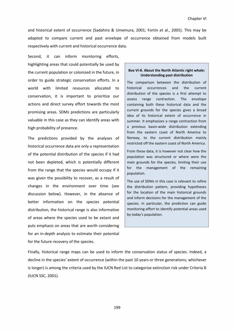
Chapter VI

199

and historical extent of occurrence (Sadahiro & Umemura, 2001; Fortin et al., 2005). This may be

adapted to compare current and past envelope of occurrence obtained from models built

respectively with current and historical occurrence data.

Second, it can inform monitoring efforts,

highlighting areas that could potentially be used by

the current population or colonized in the future, in

order to guide strategic conservation efforts. In a

world with limited resources allocated to

conservation, it is important to prioritize our

actions and direct survey effort towards the most

promising areas. SDMs predictions are particularly

valuable in this case as they can identify areas with

high probability of presence.

The predictions provided by the analyses of

historical occurrence data are only a representation

of the potential distribution of the species if it had

not been depleted, which is potentially different

from the range that the species would occupy if it

was given the possibility to recover, as a result of

changes in the environment over time (see

discussion below). However, in the absence of

better information on the species potential

distribution, the historical range is also informative

of areas where the species used to be extant and

puts emphasis on areas that are worth considering

for an in-depth analysis to estimate their potential

for the future recovery of the species.

Finally, historical range maps can be used to inform the conservation status of species. Indeed, a

decline in the species’ extent of occurrence (within the past 10 years or three generations; whichever

is longer) is among the criteria used by the IUCN Red List to categorize extinction risk under Criteria B

(IUCN SSC, 2001).

Box VI-8. About the North Atlantic right whale: Understanding past distribution

The comparison between the distribution of

historical occurrences and the current

distribution of the species is a first attempt to

assess range contraction. The envelope

containing both these historical data and the

current grounds for the species gives a broad

idea of its historical extent of occurrence in

summer. It emphasizes a range contraction from

a previous basin-wide distribution extending

from the eastern coast of North America to

Norway, to the current distribution mainly

restricted off the eastern coast of North America.

From these data, it is however not clear how the

population was structured or where were the

main grounds for the species, limiting their use

for the management of the remaining

population.

The use of SDMs in this case is relevant to refine

the distribution pattern, providing hypotheses

for the location of the main historical grounds

and inform decisions for the management of the

species. In particular, the prediction can guide

monitoring effort to identify potential areas used

by today’s population.

Chapter VI

200

This work focused on a species-centered approach, but analyses at the community level could also be

interesting, investigating the changes in species richness over time (McCorquodale et al., 2007; Grixti

et al., 2009), to identify areas of high human footprint.

Understanding past abundances and human-caused population depletions

Estimates of previous abundance can be compared with current population levels to inform how

species have been depleted. In a management context, this can help assessing the current

conservation status of species (Jeppsson et al., 2010), as population trend is among the criteria used

by the IUCN Red List to categorize the risk of extinction of species. However, this only applies to

recent cases of depletion, as the criteria concerning reduction in population size only considers the

last 10 years or 3 generations (IUCN SSC, 2001). In the case of currently exploited populations, it can

also be used as an indicator to set realistic goals for management that are not just based on recent

abundance trends (Rosenberg et al., 2005).

Spatially-explicit information on past abundance can

help us understand which areas were in fact the best

for species, guiding management efforts for their

recovery (rather than simply focusing on current range

that may well be marginal to its original habitat).

The interest of estimating populations’ past

abundance to settle appropriate management

objectives can be illustrated by the rules decided by

the International Whaling Commission (IWC) to

manage whale populations. In its attempt to regulate

quotas of baleen whales catches in 1974, the

International Whaling Commission advocated a New

Management Procedure (NMP) (International Whaling

Commission, 1976) in which the current population

size of whales would have to be compared to its

original one to set harvesting quotas and classify the

species into management categories (Allen, 1981). After the IWC placed a moratorium on

commercial whaling in 1986, the Revised Management Procedure (RMP) was created, along with a

method to determine the maximum quotas allowed if commercial whaling was to be resumed

(International Whaling Commission, 2011c; Cooke et al., 2012). The commission also stated that

“catches should not be allowed on stocks below 54% of the estimated number the environment can

Box VI-9. About the North Atlantic right whale: Understanding past abundance

Estimates of pre-exploitation abundance are

needed to set targets for the management of

NARW, but there is considerable uncertainty

regarding the original population size.

Our estimate of a pre-whaling population of

ten to twenty thousand individuals strongly

suggests that the current population is

extremely depleted (less than 6% of the total

historical population size), but also show the

realms of possibility for future recovery.

Our spatially-explicit prediction of abundance

raises hypotheses for the location of historical

grounds for the species, hence informing

future monitoring surveys to identify areas

currently occupied by the extant population,

with potential implications for the

conservation of the species.

Chapter VI

201

support, known as the ‘carrying capacity’, or the estimated unexploited population size”, specifying

that this objective should be given the “greatest priority” (IWC, 2014). Thus, assessment of baleen

whales population's status requires agreement upon a reference level, for comparison with the

present population level.

Biodiversity conservation in a changing world

How to define the historical baseline?

Assessing a species’ decline involves looking at the past for a reference point, a baseline, to be

compared with the current status of this species. While the need for this baseline is widely accepted,

its definition, notably concerning the appropriate timescale to be considered, is unclear. Choosing

the appropriate reference point to which to compare the current situation is not straightforward,

and arbitrary decisions have to be made as to which historical baseline should be used to assess such

changes. Current conservation approaches generally consider changes in relation to a relatively

recent date (e.g., the Living Planet Index uses 1970 as the reference year for measuring population

trends; WWF et al., 2014), and/or within a few years or generations (e.g., the IUCN Red List uses 10

years or three generations, whichever is longer, as the scale over which to consider population

declines; IUCN SSC, 2001 see also Frankham & Brook, 2004). Throughout this study, I highlighted the

fact that this short time-scale is not always appropriate for assessing changes in species distributions

and abundances, and advised for the consideration of a longer time scale.

Natural changes in species’ ranges and abundance have occurred since the beginning of life, as the

result of processes occurring at various time scales: from geological processes such as glacial and

interglacial periods and catastrophic events, at the scale of millions of years; to ecological processes

at the scale of years or decades, conditioned by short-term demographic and dispersion processes.

In-between, evolutionary processes also impact species distribution through the emergence and

extinction of species and evolutionary adaptations (e.g. changes in species’ niche). One could argue

that the purpose of conservation is to mitigate the impacts of humans on biodiversity, and not to

counteract natural processes, even if they induce similar patterns of change. From a management

perspective, we might thus want to define the historical baseline for species as their status before it

was impacted by human. But deciding how far back into the past to go is not straightforward,

because the further back we go the more difficult it is to distinguishing between natural and human-

caused of change.

Overexploitation is among the earliest effects on wildlife populations (Burney & Flannery, 2005),

having started centuries or even millennia ago (e.g. compared to climate change for example, which

Chapter VI

202

is relatively recent in comparison). Thus, in the case of species that have had a long history of human

exploitation, the appropriate historical baseline to assess declines in distribution in abundance could

be considered as their pre-exploitation status. However, I have here focused on the last 10,000 years

(with most of the data analyzed much more recent than that) in order to reduce the effects of

natural climatic variation, associated with the end of the last glacial period, on species’ abundances

and distributions, even though for some species and regions human impacts started earlier than that

(Burney & Flannery, 2005).

The definition of “pre-exploitation” itself suffers from a shifting perception. Species’ commercial or

industrial exploitation are often perceived as the main causes of human impact. This may be true for

many species, as these intensive operations are likely to have caused major range contractions and

population depletions. But this definition is not adapted for species that have been depleted earlier,

as a cumulative effect of smaller-scale levels of exploitation. Particularly for species that are easily

accessible to human and whose exploitation does not require advanced technologies, the impact of

early hunting, including for subsistence, may have been underestimated. In the case of whales for

example, the commercial whaling period in the 19th and 20th centuries is often considered as the first

most impacting period of exploitation, which is true for many species (e.g. blue whales, beaked

whales). But it is a simplification for others that were already heavily exploited as soon as the Middle

Ages and strongly depleted before industrial or scientific records started (e.g. the North Atlantic right

whale, the gray whale in the North Atlantic). For the latter, setting the baseline as the status of the

populations in the 19th century would seriously underestimate the level of human impact and reduce

perspectives for their recovery.

The assessment of human impact thus suffers from a shifting perception, in part explained by the

lack of information we have of early stages of exploitation. Because early impacts leave little trace in

the historical records, very early states are difficult to estimate. This case of collective amnesia can

lead to a vicious circle where the historical baseline is defined as the status of species before

industrial exploitation for a lack of earlier data, and earlier data are disregarded as not useful for

estimating the historical baseline.

Overall, the choice for an historical baseline is relative, and there is no general answer for the

appropriate period that should be considered as the reference state of a system. Efforts should be

made systematically on a case-by-case basis to consider the history of interaction with humans, as a

first step towards identifying the moment at which human activities started to have an impact on the

system considered. Only through a better understanding of the history of human exploitation of

natural resources will we be able to estimate the level of human impact on species and ecosystems

in general.

Chapter VI

203

Is the historical baseline an achievable/desirable target for conservation?

Assuming an historical baseline of abundance and/or distribution for a given species is well

understood, important questions remain concerning its usefulness in a conservation context, and in

particular its relevance as a target for conservation actions. In a globally changing and progressively

human-dominated planet, it is pertinent to ask how much space is there for the recovery of depleted

species.

Species distributions and abundances are the product of interactions between the species traits with

biotic (i.e. interactions with other species within the community) and abiotic (i.e. climatic and physic

conditions met in the environment) factors. Humans have profoundly affected all three of these

aspects, with direct and indirect effects on the current as well as potential distribution of species.

The local extirpation of entire populations may have resulted in the loss of particular physiological

and/or behavioral adaptations, for example the killing of individuals adapted to warmer waters, or

those that preferred open habitats, or of lineages with breeding philopatry. If so, recolonization of

the historical range by the remaining individuals may take a long time, even after human impacts

ceases. The loss of a particular adaptation to an environment is also likely to prevent recolonization

of a particular habitat for which the remaining individuals would not be totally adapted. For example,

the remaining individuals of an exploited population might be those that were able to seek refuges in

remote places, and the “open-habitat” adaptation might have been lost with the removal of the most

approachable individuals. To identify potential sites that a species could recolonize, it is important to

keep in mind that the remaining population may not necessarily have retained the ability to live in all

of its former range.

Species’ distributions are also shaped by abiotic factors, themselves impacted by anthropogenic

activities. It is expected that recent human-induced climate change (affecting temperature, rainfall,

extreme events, CO2 concentration and ocean dynamics) may cause range shifts, both in marine and

terrestrial systems (Walther et al., 2002; Parmesan & Yohe, 2003; Parmesan, 2006; Bellard et al.,

2012). The potential distribution of depleted species can thus be different from their former realized

distribution, as a result of shifts in the spatial extent of their bioclimatic envelope.

The physical environment encountered by species has also changed. Both on land and in the seas,

the landscape is now strongly urbanized, and the space for species to recover is more and more

reduced, as result of direct competition with human for space and increasing risks of mortality. For

example, the Mediterranean monk seal that previously had colonies in open beaches along the

French Mediterranean coast are unlikely to be able to recolonize such habitat, which is now a

hotspot for tourism and recreational activities (Johnson & Lavigne, 1999a). In the marine

Chapter VI

204

environment, increases in shipping, oil and gas exploration and fishing are likely to increase the risks

related to pollution, noise disturbance, collision with ships, bycatch and entangling in nets (Alter et

al., 2010). . The human response to mitigate climate change also has many indirect effects. For

example, the development of infrastructure to produce sustainable energies (e.g. wind farms) has

consequences on biodiversity, both in marine (Madsen et al., 2006) or terrestrial (Kuvlesky et al.,

2007) systems, through direct mortality or impacts on species’ behavior (Leung & Yang, 2012). These

are a brake to recovery, as they may lower the growth rate of populations.

The community of other species with which a given species previously interacted is likely to be very

different from what it would find today if it was to recolonize its former range. Human activities have

modified the community structure of ecosystems (through overexploitation, introduction of invasive

species, etc.) such that the guild of predators, preys, competitors and parasites have been modified.

Example of such alteration in the marine environment includes the reduction in mean trophic levels

of marine species caused by the gradual depletion by fisheries of species at higher trophic levels

(“Fishing down marine food web”; Pauly et al., 1998). Depletion of taxa can in turn impact the

structure of the food web through chain reactions. Industrial whaling is for example suspected to

have induced an indirect collapse in population of seals, sea lions and sea otters in the North Pacific

as the result of a shift in killer whales predation from baleen whales to smaller marine mammals

(Springer et al., 2003, 2008). If so, whaling may have had important impacts on the whole marine

ecosystem in this area, including the reduction of kelp forests by sea urchins (whose numbers have

increased following the depletion of their main predator, sea otters), and modifications in

physiology, demography and behavior of myriads of associated species (Estes et al., 2009). Humans

themselves can be strong competitors for resources and represent a direct obstacles for the recovery

of predator species, either because the availability of their prey is reduced by human exploitation or

through persecution of such predator species viewed as undesirable by fishers or hunters (e.g.

competition between marine mammals and fisheries; Kaschner & Pauly, 2005). The full scope of

consequences of human impacts on ecosystems is difficult to apprehend and requires extensive

amount of studies on the changes in ecosystem structures. But it should be kept in mind, as it can

cause changes in the carrying capacity of the environment for a particular species (through changes

in prey or competitor occurrence and abundance), in the predation risks and in the risk of contracting

diseases (through changes in parasites or pathogens communities). A good knowledge of the species’

ecological requirements and of the ecosystem structure (both historical and current) is thus

important to clarifying the potential for an area to be recolonized.

For all of these reasons, the environment that a species encountered before being extirpated from

an area is not necessarily the same as the one it would encounter today if it was to recolonize it. It is

Chapter VI

205

difficult to predict how such changes affect the potential for recolonization of an area from which a

species was extirpated, bringing uncertainty as to whether it is still suitable for the species. The

expectation that species can recover to their level prior to human impact is thus probably naïve.

Aiming for this level of recovery is perhaps desirable to set ambitious conservation targets but

effectively attaining the pre-exploitation baseline is most likely unachievable, except in very

particular cases where none of the factors mentioned above are limiting.

Historical baselines are nonetheless useful as a comparison point to assess the level of depletion of

species, inform monitoring and infer the potential for its recovery. Measures of the level of depletion

are lacking in current efforts to estimate species conservation status. For example, the conservation

status according to the IUCN Red List of Threatened Species is about extinction risk, which has great

importance in conservation, but misses this concept of depletion compared to an initial population

level/range. Indeed, the IUCN Red List criteria only consider a short period of time (3 generations) to

assess the decline of a species (IUCN SSC, 2001). Measures of human impact based just on extinction

risk (e.g. Red List Index; Butchart et al., 2006) or recent declines (e.g. Living Planet Index, WWF et al.,

2014) give therefore a biased perception of the overall level of impact on species, contributing to the

shifting baseline syndrome. These indicators should therefore be complemented by efforts to keep

track and quantify the absolute levels of depletion of species, to provide society with a clearer vision

of the past state of ecosystems and human impact on them. I believe that revealing the potential

diversity of ecosystems and abundance of species can encourage efforts for mitigating current

threats, so that species are given the chance and the space to recover. Finally, efforts for

understanding the history of human impacts on biodiversity should be motivated by the need to

remember our actions and avoid doing the same mistakes in the future. As the philosopher George

Santanaya summarized it, “those who cannot remember the past are condemned to repeat it”

(Santanaya, 1905).

Chapter VI

206

Box VI-10. About the North Atlantic right whale: Conservation in a changing world g world

Which baseline?

In the light of or knowledge of the history of exploitation of the species, and according to the definition of the historical baseline

provided above, I propose that the historical baseline for the NARW is defined as its status before the Basques started its exploitation

in the 11th

century. Given current knowledge, this seems to have marked the beginning of substantial human impact on NARW

populations, though I cannot rule out the possibility that forgotten whaling activities impacted the distribution and/or abundance of

the species even earlier. I therefore assume that my reconstructed distribution and abundance for this species correspond to such a

baseline.

How much human impact?

The comparison between my reconstituted baseline of distribution and abundance with current range and population size indicate

that the species is heavily depleted both in space and in numbers. Current range off the eastern coast of North America is a small

fraction of the predicted past distribution, which extended from northeastern America to northern Norway. The current population is

a mere 2.5 to 5% of the estimated past population.

Is this baseline an achievable target?

These baselines show an enormous potential for the recovery of this species. However, a number of limitations mean that they are

probably unrealistic conservation targets for such recovery. The predicted pattern of probability of presence is only a representation of

the distribution of suitable habitat for the NARW if it had not been depleted, which is not necessarily identical to the areas it could

recolonize today.

The species currently occupies a restricted portion of its historical distribution. Though highly speculative, there is a possibility that the

remaining individuals have lost the ability to recolonize their former habitat, as a result of losses in genetic lineages or particular

adaptations. This could explain the current lack of recovery in the Eastern North Atlantic, though cases of vagrancy in the northeast

Atlantic are encouraging for the recolonization of the historical range.

The species biotic and abiotic habitat has also been strongly impacted by human activities. Human influence has altered abundance

and composition of trophic level in the food web (Lotze & Milewski, 2004), with unkown implications for the recovery of baleen

whales. The depletion of the bowhead whale, a direct competitor of NARW for food, may have potentially opened new areas of low

competition in the northern part of the NARW range, which could benefit its future recovery.

Current threats for the species include collision with ships (Knowlton & Kraus, 2001; Knowlton & Brown, 2007), entanglements

(Johnson et al., 2007) and ship noise-induced stress (Rolland et al., 2012). NARW will also potentially be threatened by future offshore

infrastructure, such as wind turbines (Whitt et al., 2013), though current efforts to mitigate this threat are undertaken (Petruny et al.,

2014).

The map of cumulative impacts provided by Halpern et al. (2008) (see map below) highlight the high level of human impact on marine

ecosystem throughout the North Atlantic, and raises questions about the ability for NARW to recover in this urbanized ocean. In

addition, questions can be raised about the available space for NARW in their former breeding grounds in the Bay of Biscay, a now

highly inhabited and touristic coast. Finally, the effect of climate change on the demography of NARW may make the North Atlantic

right whale even more vulnerable than predicted (Greene & Pershing, 2004).

The eventual recovery of the NARW at its historical level is unlikely to happen in a human-dominated planet where competition with

human for resources is so important, and where direct and indirect impacts of human activities are limiting the growth rate of the

current population. Nonetheless, even if the historical target is not to be reached, efforts to mitigate these threats should be done to

give the necessary space for the species to increase in number, recolonize its former range, and eventually return to a state where it is

no longer threatened of extinction.

Map of cumulative human impact in the North Atlantic basin

(Adapted from Halpern et al., 2008)

Chapter VI

207

Chapter VI

208

References

209

REFERENCES

Acebes J.M.V., Darling J.D., & Yamaguchi M. (2007) Status and distribution of humpback whales (Megaptera novaeangliae) in northern Luzon, Philippines. Journal of Cetacean Research and Management, 9, 37.

Adam P.J. & Garcia G.G. (2003) New information on the natural history, distribution, and skull size of the extinct (?) West Indian monk seal, Monachus tropicalis. Marine mammal science, 19, 297–317.

Aguilar A. (1986) A review of old Basque whaling and its effect on the right whales (Eubalaena glacialis) of the North Atlantic. Reports of the International Whaling Commission, Special Issue 10, 191–199.

Ainsworth C.H., Pitcher T.J., & Rotinsulu C. (2008) Evidence of fishery depletions and shifting cognitive baselines in Eastern Indonesia. Biological Conservation, 141, 848–859.

Allen G.M. (1916) The whalebone whales of New England. Boston Society of Natural History, Boston.

Allen J.A. (1880) History of North American pinnipeds, a monograph of the walruses, sea-lions, sea-bears and seals of North America. Department of the Interior, United States Geological and Geographical Survey of the Territories, Washington.

Allen J.A. (1908) The North Atlantic right whale and its near allies. Bulletin of the AMNH ; v. 24, article 18. Bulletin American Museum of Natural History, XXIV, 277–329 (+plates).

Allen K.R. (1981) The optimization of management strategy for marine mammals. Mammals in the Seas: General papers and large cetaceans pp. 504. Food & Agriculture Organization,

Allouche O., Tsoar A., & Kadmon R. (2006) Assessing the accuracy of species distribution models: prevalence, kappa and the true skill statistic (TSS). Journal of Applied Ecology, 43, 1223–1232.

Alter S.E., Meyer M., Post K., Czechowski P., Gravlund P., Gaines C., Rosenbaum H.C., Kaschner K., Turvey S.T., van der Plicht J., Shapiro B., & Hofreiter M. (2015) Climate impacts on transocean dispersal and habitat in gray whales from the Pleistocene to 2100. Molecular Ecology, n/a–n/a.

Alter S.E., Rynes E., & Palumbi S.R. (2007) DNA evidence for historic population size and past ecosystem impacts of gray whales. Proceedings of the National Academy of Sciences, 104, 15162–15167.

Alter S.E., Simmonds M.P., & Brandon J.R. (2010) Forecasting the consequences of climate-driven shifts in human behavior on cetaceans. Marine Policy, 34, doi: 10.1016/j. marpool.2010.01.026.

Amante C. & Eakins B.W. (2009) ETOPO1 1 Arc-Minute Global Relief Model: Procedures, Data Sources and Analysis. NOAA, National Geophysical Data Center, Marine Geology and Geophysics Division, Boulder, Colorado.

Amorosi T., Buckland P., Dugmore A., Ingimundarson J.H., & McGovern T.H. (1997) Raiding the landscape: Human impact in the Scandinavian North Atlantic. Human Ecology, 25, 491–518.

References

210

Anderson P. (1995) Competition, predation, and the evolution and extinction of Steller’s sea cow, Hydrodamalis gigas. Marine Mammal Science, 11, 391–394.

Araújo M.B. & Guisan A. (2006) Five (or so) challenges for species distribution modelling. Journal of Biogeography, 33, 1677–1688.

Araújo M.B., Pearson R.G., Thuiller W., & Erhard M. (2005) Validation of species–climate impact models under climate change. Global Change Biology, 11, 1504–1513.

Aurioles D. & Trillmich F. (2008) Available at: http://www.iucnredlist.org/details/2059/0.

Austin M. (2007) Species distribution models and ecological theory: A critical assessment and some possible new approaches. Ecological Modelling, 200, 1–19.

Austin M.P. (2002) Spatial prediction of species distribution: an interface between ecological theory and statistical modelling. Ecological Modelling, 157, 101–118.

Azpiazu J.A. (2000) Balleneros Vascos en el Cantabrico. Ttarttalo Argitaletxea, Donostia.

Balmford A. (1999) (Less and less) great expectations. Oryx, 33, 87–88.

Banks A. & et al. (2011) Recent sightings of southern right whales in Mozambique. IWC Southern Right Whale Assessment Workshop: Buenos Aires, 13-16 September 2011,

Bannister J.L., Taylor S., & Sutherland H. (1983) Logbook Records of 19th Century American Sperm Whaling: A Report on the 12 month project, 1978-79. Rep. Int. Whal. Comm.(Special Issue 5), 243–255.

Barbet-Massin M., Jiguet F., Albert C.H., & Thuiller W. (2012) Selecting pseudo-absences for species distribution models: how, where and how many? Methods in Ecology and Evolution, 3, 327–338.

Barco S.G., McLellan W.A., Allen J.M., Asmutis-Silvia R.A., Mallon-Day R., Meagher E.M., Pabst D.A., Robbins J., Seton R.E., Swingle W.M., Weinrich M.T., & Clapham P.J. (2002) Population identity of humpback whales (Megaptera novaeangliae) in the waters of the US mid-Atlantic states. J. Cetacean Res. Manage, 4, 135–141.

Barkham M. (2000a) La industria pesquera en el País Vasco peninsular al principio de la Edad Moderna: ¿una edad de oro? Itsas Memoria. Revista de Estudios Maritimos del Pais Vasco, 3, 29–75.

Barkham M. (2000b) La industria pesquera en el País Vasco peninsular al principio de la Edad Moderna: ¿una edad de oro? Itsas Memoria. Revista de Estudios Maritimos del Pais Vasco, 3, 29–75.

Barkham S.H. (1974) The Spanish province of Terranova. Canadian Archivist, 2, 73–83.

Barry S.C. & Welsh A.H. (2002) Generalized additive modelling and zero inflated count data. Ecological Modelling, 157, 179–188.

Barthelmess K. (2003) Das erste gedruckte deutsche Walfangjournal: Christian Bullens “Tag=Register” einer Hamburger Fangreise nach Spitzbergen und Nordnorwegen im Jahre 1667. De Bataafsche Leeuw, Amsterdam; Bremerhaven.

References

211

Baumgartner M.F. & Mate B.R. (2003) Summertime foraging ecology of North Atlantic right whales. Marine Ecology Progress Series, 264, 123–135.

Baumgartner M.F., Mayo C.A., & Kenney R.D. (2007) Enormous carnivores, microscopic food, and a restaurant that’s hard to find. The urban whale: North Atlantic right whales at the crossroads (ed. by S.D. Kraus and R.M. Rolland), pp. 138–171.

BBC (2012) BBC News - Walrus basks in Orkney attention. .

Behrenfeld M.J. & Falkowski P.G. (1997) Photosynthetic rates derived from satellite-based chlorophyll concentration. Limnology and Oceanography, 42, 1–20.

Bellard C., Bertelsmeier C., Leadley P., Thuiller W., & Courchamp F. (2012) Impacts of climate change on the future of biodiversity: Biodiversity and climate change. Ecology Letters, 15, 365–377.

Best P.B. (1983) Sperm Whale Stock Assessments and the Relevance of Historical Whaling Records. Rep. Int. Whal. Comm.(Special Issue 5), 41–55.

Best P.B. (1987) Estimates of the landed catch of right (and other whalebone) whales in the American fishery. Fishery Bulletin, 85, 403–418.

Bockstoce J.R. & Botkin D.B. (1983) The historical status and reduction of the western Arctic bowhead whale (Balaena mysticetus) population by the pelagic whaling industry, 1848-1914. Rep. Int. Whal. Comm.(Special Issue 5), 107–141.

Bockstoce J.R. & Burns J.J. (1993) Chapter 14: Commercial whaling in the North Pacific Sector. The Bowhead whale (ed. by J.J. Burns, J.J. Montague, and C.J. Cowles), pp. 563–577. Society for Marine Mammalogy, Lawrence, KS.

Bockstoce V.N.J.R., Botkin D.B., Philp A., Collins B.W., & George J.C. (2010) The geographic distribution of Bowhead Whales, Balaena mysticetus, in the Bering, Chukchi, and Beaufort seas: evidence from whaleship records, 1849–1914. Marine Fisheries Review, 67, 1–43.

Boece H. (1821) The history and chronicles of Scotland. Edinburgh, Reprinted for W. and C. Tait,

Bombosch A., Zitterbart D.P., Van Opzeeland I., Frickenhaus S., Burkhardt E., Wisz M.S., & Boebel O. (2014) Predictive habitat modelling of humpback (Megaptera novaeangliae) and Antarctic minke (Balaenoptera bonaerensis) whales in the Southern Ocean as a planning tool for seismic surveys. Deep Sea Research Part I: Oceanographic Research Papers, 91, 101–114.

Bonebrake T.C., Christensen J., Boggs C.L., & Ehrlich P.R. (2010) Population decline assessment, historical baselines, and conservation. Conservation Letters, 3, 371–378.

Born E.W., Stefansson E., Mikkelsen B., Laidre K.L., Andersen L.W., Rigét F.F., Jensen M.V., & Bloch D. (2014) A note on a walrus’ European odyssey. NAMMCO Scientific Publications, 9, .

Braham H.W. (1984) Distribution and migration of gray whales in Alaska. The Gray Whale Eschrichtius robustus pp. 249–266. Academic Press,

Brito C. (2011) Medieval and early modern whaling in Portugal. Anthrozoos, 24, 287–300.

Brito C. & Sousa A. (2011) The Environmental History of Cetaceans in Portugal: Ten Centuries of Whale and Dolphin Records. PLoS ONE, 6, .

References

212

Broennimann O., Fitzpatrick M.C., Pearman P.B., Petitpierre B., Pellissier L., Yoccoz N.G., Thuiller W., Fortin M.-J., Randin C., Zimmermann N.E., Graham C.H., & Guisan A. (2012) Measuring ecological niche overlap from occurrence and spatial environmental data: Measuring niche overlap. Global Ecology and Biogeography, 21, 481–497.

Brotons L., Thuiller W., Araújo M.B., & Hirzel A.H. (2004) Presence-absence versus presence-only modelling methods for predicting bird habitat suitability. Ecography, 27, 437–448.

Brown M.W., Kraus S.D., Slay, C. K. E.A., & Garrison L.P. (2007) Surveying for Discovery, Science, and Management. The Urban Whale: North Atlantic Right Whales at the Crossroads (ed. by S.D. Kraus and R.M. Rolland), pp. 105 – 137. Harvard University Press, Cambridge, Massachusetts, USA.

Bryant P.J. (1995) Dating remains of gray whales from the eastern North Atlantic. Journal of Mammalogy, 76, 857–861.

Buckley M., Fraser S., Herman J., Melton N.D., Mulville J., & Palsdottir A. (2014) Species identification of archaeological marine mammals using collagen fingerprinting. Journal of Archaeological Science, 41, 631–641.

Burgman M.A. & Fox J.C. (2003) Bias in species range estimates from minimum convex polygons: implications for conservation and options for improved planning. Animal Conservation, 6, 19–28.

Burgman M.A., Lindenmayer D.B., & Elith J. (2005) Managing landscapes for conservation under uncertainty. Ecology, 86, 2007–2017.

Burney D. & Flannery T. (2005) Fifty millennia of catastrophic extinctions after human contact. Trends in Ecology & Evolution, 20, 395–401.

Burns J.J., Montague J.J., & Cowles C.J. (1993) The Bowhead whale. Society for Marine Mammalogy, Lawrence, KS.

Busch B.C. (1985) The War Against the Seals - A History of the North American Fishery. Kingston and Montreal.

Butchart S.H.M., Akcakaya H.R., Kennedy E., & Hilton-Taylor C. (2006) Biodiversity Indicators Based on Trends in Conservation Status: Strengths of the IUCN Red List Index. Conservation Biology, 20, 579–581.

Butchart S.H.M., Walpole M., Collen B., van Strien A., Scharlemann J.P.W., Almond R.E.A., Baillie J.E.M., Bomhard B., Brown C., Bruno J., Carpenter K.E., Carr G.M., Chanson J., Chenery A.M., Csirke J., Davidson N.C., Dentener F., Foster M., Galli A., Galloway J.N., Genovesi P., Gregory R.D., Hockings M., Kapos V., Lamarque J.-F., Leverington F., Loh J., McGeoch M.A., McRae L., Minasyan A., Morcillo M.H., Oldfield T.E.E., Pauly D., Quader S., Revenga C., Sauer J.R., Skolnik B., Spear D., Stanwell-Smith D., Stuart S.N., Symes A., Tierney M., Tyrrell T.D., Vié J.-C., & Watson R. (2010) Global Biodiversity: Indicators of Recent Declines. Science, 328, 1164–1168.

Calambokidis J., Darling J.D., Deeke V., Gearin P., Gosho M., Megill W., Tombach C.M., Goley D., Toropova C., & Gisborne B. (2002) Abundance, range and movements of a feeding aggregation of gray whales (Eschrictius robustus) from California to southeastern Alaska in 1998. Journal of Cetacean Research and Management, 4, 267–276.

References

213

Calambokidis J., Falcone E.A., Quinn T.J., Burdin A.M., Clapham P.J., Ford J.K.B., Gabriele C.M., LeDuc R., Mattila D., Rojas-Bracho L., & others (2008) SPLASH: Structure of populations, levels of abundance and status of humpback whales in the North Pacific. Cascadia Research,

Calambokidis J., Steiger G.H., Straley J.M., Herman L.M., Cerchio S., Salden D.R., Jorge U.R., Jacobsen J.K., Ziegesar O.V., Balcomb K.C., & others (2001) Movements and population structure of humpback whales in the North Pacific. Marine Mammal Science, 17, 769–794.

Cameron A.C., Hammond P., Trivedi P.K., & Holly A. (1998) Regression Analysis of Count Data.

Carlton J.T., Geller J.B., Reaka-Kudla M.L., & Norse E.A. (1999) Historical extinctions in the sea. Annual Review of Ecology and Systematics, 30, 515–538.

Cartier J., Michelant H. (Henri), & Ramé A. (1865) Voyage de Jacques Cartier au Canada en 1534. [Paris? : s.n.],

Castro C. & Merlen G. (2009) Observations of humpback whales (Megaptera novaeangliae) in the Galapagos Islands, Ecuador. Paper SC/61/SH30 presented to the IWC Scientific Committee, May 2009 (unpublished), 5pp.

Charcot J. & Joubin L. (1913) Deuxième expédition antarctique francaise (1908-1910). Masson, Paris.

Charif R.A., Clapham P.J., & Clark C.W. (2001) Acoustic detections of singing humpback whales in deep waters off the British Isles. Marine Mammal Science, 17, 751–768.

Chefaoui R.M. & Lobo J.M. (2008) Assessing the effects of pseudo-absences on predictive distribution model performance. Ecological Modelling, 210, 478–486.

Ciriquiain-Gaiztarro M. (1961) Los vascos en la pesca de la ballena. Editorial Txertoa, San Sebastian, Spain.

Citta John J., Quakenbush L.T., Okkonen S.R., Druckenmiller M.L., Maslowski W., Clement-Kinney J., George J.C., Brower H., Small R.J., Ashjian C.J., Harwood L.A., & Heide-Jørgensen M.P. (2014) Ecological characteristics of core-use areas used by Bering-Chukchi-Beaufort (BCB) bowhead whales, 2006-2012. Progress in Oceanography, .

Clapham P. (2009) Humpback whale Megaptera novaeangliae. Encyclopedia of Marine Mammals (ed. by W.F. Perrin, B. Wursig, and J.G.M. Thewissen), pp. 589–592. Academic Press,

Clapham P., Good C., Quinn S., Reeves R.R., Scarff J.E., & Brownell Jr. R.L. (2004a) Distribution of North Pacific right whales (Eubalaena japonica) as shown by 19th and 20th century whaling catch and sighting records. Journal of Cetacean Research and Management, 6, 1–6.

Clapham P.J., Berggren P., Childerhouse S., Friday N.A., Kasuya T., Kell L., Kock K.-H., Manzanilla-Naim S., Di Sciara G.N., Perrin W.F., & others (2003) Whaling as science. Bioscience, 53, 210–212.

Clapham P.J., Good C., Quinn S.E., Reeves R.R., Scarff J.E., & Brownell Jr R.L. (2004b) Distribution of North Pacific right whales (Eubalaena japonica) as shown by 19th and 20th century whaling catch and sighting records. .

Clapham P.J. & Mayo C.A. (1987) Reproduction and recruitment of individually identified humpback whales, Megaptera novaeangliae, observed in Massachusetts Bay, 1979–1985. Canadian Journal of Zoology, 65, 2853–2863.

References

214

Clark A.H. (1880) Map of the World on Mercator Projection showing The Extent and Distribution of the Present and Abandoned Whaling Grounds. Available at: http://www.photolib.noaa.gov/htmls/figb0184.htm. .

Clark A.H. (1887) Part XV - The whale fishery. 1 - History and present conditions of the fishery. The fisheries and fishery industries of the United States (ed. by G.B. Goode), pp. 3–218. United States Bureau of Fisheries, Government Printing Office, Washington.

Collett R. (1909) A few notes on the whale Balaena glacialis and its capture in recent years in the North Atlantic by Norwegian whalers. Proceedings of The Zoological Society of London, 7, 91–97.

Colwell R.K. & Futuyma J. (1971) On the measurement of niche breadth and overlap. Ecology, 52, 567–576.

Cooke J., Leaper R., Wade P., Lavigne D., & Taylor B. (2012) Management rules for marine mammal populations: A response to Lonergan. Marine Policy, 36, 389–392.

Cressey D. (2015) World’s whaling slaughter tallied. Nature, 519, 140–141.

Cumbaa S.L. (1986) Archaeological Evidence of the 16th Century Basque Right Whale Fishery in Labrador. Rep. Int. Whal. Comm.(Special Issue 10), 187–190.

Cuvier F. (1836) De l’histoire naturelle des cétacés, ou Recueil et examen des faits dont se compose l’histoire ... Roret,

Dampier W. (1697) A New Voyage Round the World. Available: Project Gutenberg Australia. http://gutenberg.net.au/ebooks05/0500461h.html,

Dawson T.P., Jackson S.T., House J.I., Prentice I.C., & Mace G.M. (2011) Beyond predictions: biodiversity conservation in a changing climate. Science, 332, 53–58.

Van Deinse A.B. & Junge G.C.. (1937) Recent and older finds of the California Gray Whale in the Atlantic. Temminckia, 2, 161–188.

Delano A. (1817) A Narrative of Voyages and Travels in the Northern and Southern Hemispheres: Comprising Three ... Printed by E.G. House for the author,

Dietl G.P. & Flessa K.W. (2011) Conservation paleobiology: putting the dead to work. Trends in Ecology & Evolution, 26, 30–37.

Diggle P.J., Menezes R., & Su T.-L. (2010) Geostatistical inference under preferential sampling. Journal of the Royal Statistical Society (C), 59, 191–232.

Dormann C.F. (2007a) Promising the future? Global change projections of species distributions. Basic and Applied Ecology, 8, 387–397.

Dormann C.F. (2007b) Effects of incorporating spatial autocorrelation into the analysis of species distribution data. Global Ecology and Biogeography, 16, 129–138.

Dudley P. (1725) An essay upon the natural history of whales. Philosophical Transactions of the Royal Society London, 256–269.

References

215

Dulvy N.K., Pinnegar J.K., & Reynolds J.D. (2009) Holocene extinctions in the sea. Holocene Extinctions (ed. by S.T. Turvey), Oxford University Press, Oxford.

Dulvy N.K., Sadovy Y., & Reynolds J.D. (2003) Extinction vulnerability in marine populations. Fish and Fisheries, 4, 25–64.

Dyke A.S. & Prest V.K. (1987) Late Wisconsinan and Holocene History of the Laurentide Ice Sheet. Géographie physique et Quaternaire, 41, 237.

Edvardsson R. & Rafnsson M. (2006) Basque whaling around Iceland: archeological investigation in Strákatangi, Steingrímsfjörður. Náttúrustofa Vestfjarða (Natural History Institute of Vestfirðir) & Strandagaldur ses, Bolungarvík.

Elith J., H. Graham C., P. Anderson R., Dudík M., Ferrier S., Guisan A., J. Hijmans R., Huettmann F., R. Leathwick J., Lehmann A., Li J., G. Lohmann L., A. Loiselle B., Manion G., Moritz C., Nakamura M., Nakazawa Y., McC. M. Overton J., Townsend Peterson A., J. Phillips S., Richardson K., Scachetti-Pereira R., E. Schapire R., Soberón J., Williams S., S. Wisz M., & E. Zimmermann N. (2006) Novel methods improve prediction of species’ distributions from occurrence data. Ecography, 29, 129–151.

Elith J. & Leathwick J.R. (2009a) Species Distribution Models: Ecological Explanation and Prediction Across Space and Time. Annual Review of Ecology, Evolution, and Systematics, 40, 677–697.

Elith J. & Leathwick J.R. (2009b) Conservation prioritisation using species distribution modelling. Spatial conservation prioritization : quantitative methods and computational tools (ed. by A. Moilanen, K.A. Wilson, and H.P. Possingham), pp. 70–93. Oxford, UK.

Elith J. & Leathwick J.R. (2009c) Species Distribution Models: Ecological Explanation and Prediction Across Space and Time. Annual Review of Ecology, Evolution, and Systematics, 40, 677–697.

Elith J., Leathwick J.R., & Hastie T. (2008) A working guide to boosted regression trees. Journal of Animal Ecology, 77, 802–813.

Ellis M. (1969) A baleia no Brasil colonial. Melhoramentos, São Paulo, Brasil.

Engler R., Guisan A., & Rechsteiner L. (2004) An improved approach for predicting the distribution of rare and endangered species from occurrence and pseudo-absence data. Journal of Applied Ecology, 41, 263–274.

Erlandson J.M., Rick T.C., Rick T., & Erlandson J. (2008) Archaeology, marine ecology, and human impacts on marine environments. Human Impacts on Ancient Marine Ecosystems: A Global Perspective, 1–20.

Eschricht D.F., Lilljeborg W., Reinhardt J. (Johannes), & Flower W.H. (1866) Recent memoirs on the Cetacea. London, Pub. for the Ray society by R. Hardwicke,

Eschricht D.F. & Reinhardt J. (1866) On the Greenland Right-Whale (Balaena mysticetus). Recent memoirs on the Cetacea (ed. by D.F. Eschricht, J. Reinhardt, W. Lilljeborg, and W.H. Flower), pp. 1–150. Published for the Ray society by R. Hardwicke, London.

Estes J.A., DeMaster D.P., & Doak D.F. (2007) Whales, Whaling, and Ocean Ecosystems. University of California Press, Berkeley, CA, USA.

References

216

Estes J.A., Doak D.F., Springer A.M., & Williams T.M. (2009) Causes and consequences of marine mammal population declines in southwest Alaska: a food-web perspective. Philosophical Transactions of the Royal Society B: Biological Sciences, 364, 1647 –1658.

Evans G.W., Jacobs S.V., & Frager N.B. (1982) Behavioral responses to air pollution. Advances in environmental psychology pp. 237–269. A. Baum & J.E. Singer, Hillsdale, NJ: Erlbaum.

Evans P.G. & Bjørge A. (2013) Impacts of climate change on marine mammals. MCCIP Science Review, 2013, 134–148.

Fay E.F. (1982) Ecology and Biology of the Pacific Walrus, Odobenus rosmarus divergens Illiger. North American Fauna, 74, 1–279.

Ficetola G.F., Thuiller W., & Miaud C. (2007) Prediction and validation of the potential global distribution of a problematic alien invasive species - the American bullfrog: Predicting the success of invasions. Diversity and Distributions, 13, 476–485.

Fielding A.H. & Bell J.F. (1997) A review of methods for the assessment of prediction errors in conservation presence/absence models. Environmental Conservation, 24, 38–49.

Findlay K.P. (2001) A review of humpback whale catches by modern whaling operations in the Southern Hemisphere. Memoirs of the Queensland Museum, 47, 411–420.

Fleming A. & Jackson J. (2011) Global Review of Humpback Whales (Megaptera novaeangliae). .

Flower W.H. (1872) On a Subfossil Whale (Eschrichtius robustus) discovered in Cornwall. Journal of Natural History Series 4, 9, 440–442.

Fonteneau A., Lucas V., Tewkai E., Delgado A., & Demarcq H. (2008) Mesoscale exploitation of a major tuna concentration in the Indian Ocean. Aquatic Living Resources, 21, 109–121.

Forney K., Ferguson M., Becker E., Fiedler P., Redfern J., Barlow J., Vilchis I., & Ballance L. (2012) Habitat-based spatial models of cetacean density in the eastern Pacific Ocean. Endangered Species Research, 16, 113–133.

Fortin M.-J., Keitt T.H., Maurer B.A., Taper M.L., Kaufman D.M., & Blackburn T.M. (2005) Species’ geographic ranges and distributional limits: pattern analysis and statistical issues. Oikos, 108, 7–17.

Frankham R. & Brook B.W. (2004) The importance of time scale in conservation biology and ecology. Annales zoologici Fennici, 41, 459–463.

Franklin J. (2009) Mapping Species Distributions: Spatial Inference and Prediction. New York.

Frantzis A., Nikolaou O., Bompar J.-M., & Cammedda A. (2004) Humpback whale (Megaptera novaeangliae) occurrence in the Mediterranean Sea. Journal of Cetacean Research and Management, 6, 25–28.

Frasier T.R., McLeod B.A., Gillett R.M., Brown M.W., & White B.N. (2007) Right whales past and present as revealed by their genes. The Urban Whale: North Atlantic Right Whales at the Crossroads (ed. by S.D. Kraus and R.M. Rolland), pp. 200–231.

References

217

Freeman E. a. & Moisen G.G. (2008) PresenceAbsence: an R package for presence-absence model analysis. Journal of Statistical Software, 23, 1–31.

Friedlaender A.S., Halpin P.N., Qian S.S., Lawson G.L., Wiebe P.H., Thiele D., & Read A.J. (2006) Whale distribution in relation to prey abundance and oceanographic processes in shelf waters of the Western Antarctic Peninsula. Marine Ecology Progress Series, 317, 297–310.

Fujiwara M. & Caswell H. (2001) Demography of the endangered North Atlantic right whale. Nature, 414, 537–541.

Garcia R.A., Burgess N.D., Cabeza M., Rahbek C., & Araújo M.B. (2012) Exploring consensus in 21st century projections of climatically suitable areas for African vertebrates. Global Change Biology, 18, 1253–1269.

Gasco F. (1878) Intorno alla balena presa in Taranto nel febbrajo 1877 : memoria. Tip. dell’ Accademia reale delle scienze, Napoli.

Gaskin D. (1991) An update on the status of the right whale, Eubalaena glacialis, in Canada. Canadian Field-Naturalist, 105, 198–205.

Giles-Pacheco F., Riquelme-Cantal J.A., Stringer C.B., Finlayson J.C., Barton R.N.E., Fernández-Jalvo Y., Cáceres I., Sabin R.C., Rhodes E.J., Currant A.P., & Rodríguez-Vidal J. (2008) Neanderthal exploitation of marine mammals in Gibraltar. Proceedings of the National Academy of Sciences, 105, 14319–14324.

Gjertz I., Henriksen G., Øritsland T., & Wiig Ø. (1993) Observations of walruses along the Norwegian coast 1967–1992. Polar Research, 12, 27–31.

Goldsworthy S. & Gales J.L. (2008) Arctocephalus forsteri. The IUCN Red List of Threatened Species. Version 2014.3. <www.iucnredlist.org>. Downloaded on 04 February 2015., .

Gowan T.A. & Ortega-Ortiz J.G. (2014) Wintering Habitat Model for the North Atlantic Right Whale (Eubalaena glacialis) in the Southeastern United States. PLoS ONE, 9, e95126.

Graham C., Ferrier S., Huettman F., Moritz C., & Peterson A. (2004) New developments in museum-based informatics and applications in biodiversity analysis. Trends in Ecology & Evolution, 19, 497–503.

Graham C.H., Elith J., Hijmans R.J., Guisan A., Townsend Peterson A., Loiselle B.A., & The Nceas Predicting Species Distributions Working Group (2007) The influence of spatial errors in species occurrence data used in distribution models: Spatial error in occurrence data for predictive modelling. Journal of Applied Ecology, 45, 239–247.

Grassle F.J. (2000) The Ocean Biogeographic Information System (OBIS): an on-line, worldwide atlas for accessing, modeling and mapping marine biological data in a multidimensional geographic context. Oceanography, 13, 5–7.

Gray J.E. (1864) Notes on the Whalebone-Whales; with a synopsis of the species. Journal of Natural History Series 3, 14, 345–353.

Gray J.E. (1866) Catalogue of seals and whales in the British Museum. London.

References

218

Greene C.H. & Pershing A.J. (2004) Climate and the conservation biology of North Atlantic right whales : the right whale at the wrong time? Frontiers in Ecology and the Environment, 2, 29–34.

Gregr E.J. (2011) Insights into North Pacific right whale Eubalaena japonica habitat from historic whaling records. Endangered Species Research, 15, 223–239.

Gregr E.J. & Coyle K.O. (2009) The biogeography of the North Pacific right whale (Eubalaena japonica). Progress in Oceanography, 80, 188–198.

Grixti J.C., Wong L.T., Cameron S.A., & Favret C. (2009) Decline of bumble bees (Bombus) in the North American Midwest. Biological Conservation, 142, 75–84.

Gudmundsson J. (1640) Um Íslands aðskiljanlegar náttúrur (On the Diverse Natures of Iceland).

Guisan A., Broennimann O., Engler R., Vust M., Yoccoz N.G., Lehmann A., & Zimmermann N.E. (2006) Using Niche-Based Models to Improve the Sampling of Rare Species. Conservation Biology, 20, 501–511.

Guisan A., Edwards Jr T.C., & Hastie T. (2002) Generalized linear and generalized additive models in studies of species distributions: setting the scene. Ecological Modelling, 157, 89–100.

Guisan A. & Thuiller W. (2005) Predicting species distribution: offering more than simple habitat models. Ecology Letters, 8, 993–1009.

Guisan A. & Zimmermann N.E. (2000) Predictive habitat distribution models in ecology. Ecological Modelling, 135, 147–186.

Guldberg G.A. (1884) Sur la présence aux temps anciens et modernes de la Baleine de Biscaye ou Nordcaper sur les côtes de Norwège. Bulletin de l’Académie Royale de Belgique, 3, 374–402.

Guo Q., Liu Y., & Wieczorek J. (2008) Georeferencing locality descriptions and computing associated uncertainty using a probabilistic approach. International Journal of Geographical Information Science, 22, 1067–1090.

Haie E. (1889) A briefe relation of the New found lande, and the commodities thereof (in: A report of the voyage and successe thereof, attempted in the yeere of our Lord 1583 by sir Humfrey Gilbert knight...). Principal Navigations, Voyages, Traffiques and Discoveries of the English Nation (Vol XII. America, Part I) (ed. by R. Hakluyt), E&G Goldsmith, Edinburgh.

Haldane R.C. (1905) Notes on Whaling in Shetland 1904. Annals of Scottish Natural History, 54, 53–56.

Haldane R.C. (1907) Whaling in Scotland. Annals of Scottish Natural History, 61, 10–15.

Halpern B.S., Walbridge S., Selkoe K.A., Kappel C.V., Micheli F., D’Agrosa C., Bruno J.F., Casey K.S., Ebert C., Fox H.E., Fujita R., Heinemann D., Lenihan H.S., Madin E.M.P., Perry M.T., Selig E.R., Spalding M., Steneck R., & Watson R. (2008) A Global Map of Human Impact on Marine Ecosystems. Science, 319, 948–952.

Hamazaki T. (2002) Spatiotemporal prediction models of cetacean habitats in the mid-western North Atlantic ocean (from Cape Hatteras, North Carolina, USA to Nova Scotia, Canada). Marine Mammal Science, 18, 920–939.

References

219

Hamazaki T. & Tanno D. (2001) Approval of Whaling and Whaling-related Beliefs: Public Opinion in Whaling and Nonwhaling Countries. Human Dimensions of Wildlife: An International Journal, 6, 131–144.

Hamilton P.K., Knowlton A.R., & Marx M.K. (2007) Right whales tell their own stories: the photo-identification catalog. The Urban Whale: North Atlantic Right Whales at the Crossroads (ed. by S.D. Kraus and R.M. Rolland), pp. 75–104. Harvard University Press, Cambridge, Massachusetts, USA.

Hamilton R. (1843) Whales. W.H. Lizars, Edinburgh :

Hastie T. & Tibshirani R. (1986) Generalized additive models. Statistical Science, 1, 297–310.

Henderson D.A. (1984) Nineteenth century gray whaling: grounds, catches and kills, practices and depletion of the whale population. The Gray Whale Eschrichtius robustus pp. 159–186. Academic Press,

Hernandez P.A., Graham C.H., Master L.L., & Albert D.L. (2006) The effect of sample size and species characteristics on performance of different species distribution modeling methods. Ecography, 29, 773–785.

Hijmans R.J. (2014) raster: Geographic data analysis and modeling. R package version 2.2-12. .

Hijmans R.J., Phillips S.J., Leathwick J.R., & Elith J. (2013) dismo: Species distribution modeling. R package version 0.9-3. .

Hirzel A.H. & Le Lay G. (2008) Habitat suitability modelling and niche theory. Journal of Applied Ecology, 45, 1372–1381.

Ver Hoef J.M. & Boveng P.L. (2007) Quasi-Poisson vs. negative binomial regression: how should we model overdispersed count data? Ecology, 88, 2766–2772.

Hoffmann A.A. & Sgrò C.M. (2011) Climate change and evolutionary adaptation. Nature, 470, 479–485.

Holm P. (2002) History of marine animal populations: a global research program of the Census of marine life. Oceanologica Acta, 25, 207–211.

Holm P., Marboe A.H., Poulsen B., & MacKenzie B.R. (2010) Marine animal populations: a new look back in time. Life in the world’s oceans: Diversity, distribution, and abundance (ed. by A. McIntyre), John Wiley & Sons, Hoboken, NJ.

Hortal J., Jiménez-Valverde A., Gómez J.F., Lobo J.M., & Baselga A. (2008) Historical bias in biodiversity inventories affects the observed environmental niche of the species. Oikos, 117, 847–858.

Huelsbeck D.R. (1988) Whaling in the precontact economy of the central Northwest coast. Arctic Anthropology, 25, 1–15.

Hurlbert S.H. (1978) The measurement of niche overlap and some relatives. Ecology, 59, 67–77.

Hutchinson G.E. (1957) Concluding remarks. Cold Spring Harbor Symp Quant Biol, 22, 415–427.

References

220

Ingerbrigtsen A. (1929) Whales Caught in the North Atlantic and other seas. Rapp PV Reun Cons Int Explor Mer, 56, 1–26.

International Whaling Commission (1976) Twenty-sixth report of the Commission. .

International Whaling Commission (2002) Report of the sub committee on the comprehensive assessment of North Atlantic humpback whales. Annex H to the report of the scientific committee. Journal of Cetacean Research and Management, (Suppl.) 4, 230–260.

International Whaling Commission (2011a) Report of the workshop on the comprehensive assessment of Southern hemisphere humpback whales. Journal of Cetacean Research and Management (Special Issue), 3, 1–53.

International Whaling Commission (2011b) Humpback whales: Status in the Southern hemisphere. .

International Whaling Commission (2011c) Report of the Sub-Committee on the Revised Management Procedure (RMP). Journal of Cetacean Research and Management, 12 (Suppl), 89–116.

International Whaling Commission (2012) Final Report on the Assessment of the Southern Hemisphere Humpback Whale Breeding Stock B. Journal of Cetacean Research and Management, 13, 395–410.

IPCC (WG I & II) (2001) Climate Change 2001. Third Assessment Report of the Intergovernmental Panel on Climate Change. .

IUCN (2011) The IUCN Red List of Threatened Species. Version 2011.2. Downloaded on 04 April 2012. .

IUCN SSC (2001) IUCN red list categories and criteria: version 3.1. .

IWC (2013) Available at: http://iwc.int/commercial (accessed 06/06/13).

IWC (2014) Available at: http://iwc.int/rmp2 (accessed 08/18/14).

Jackson J.B. (1997) Reefs since columbus. Coral reefs, 16, S23–S32.

Jackson J.B.C. (2001) What was natural in the coastal oceans? Proceedings of the National Academy of Sciences of the United States of America, 98, 5411–5418.

Jackson J.B.C., Kirby M.X., Berger W.H., Bjorndal K.A., Botsford L.W., Bourque B.J., Bradbury R.H., Cooke R., Erlandson J., Estes J.A., & others (2001) Historical overfishing and the recent collapse of coastal ecosystems. Science, 293, 629–637.

Jacobsen K.-O., Marx M., & ØIen N. (2004) Two-way trans-Atlantic migration of a North Atlantic right whale (Eubalaena glacialis). Marine Mammal Science, 20, 161–166.

Janes J. (1906) The third voyage Northwestward, made by M. John Davis Gentleman, as chiefe captaine & Pilot generall, for the discovery of a passage to the Isles of the Moluccas, or the coast of China , in the yeere 1587. Written by M. John Janes. The Principal Navigations, Voyages, Traffiques, and Discoveries of the English Nation Made by Sea or Overland to the Remote & Farthest Distant Quarters of the Earth at any time within the compasse of these 1600 Yeares (ed. by R. Hakluyt), pp. 414–422. James MacLehose and Sons, Glasgow.

References

221

Jefferson T.A. & Schiro A.J. (1997) Distribution of cetaceans in the offshore Gulf of Mexico. Mammal Review, 27, 27–50.

Jeppsson T., Lindhe A., Gärdenfors U., & Forslund P. (2010) The use of historical collections to estimate population trends: A case study using Swedish longhorn beetles (Coleoptera: Cerambycidae). Biological Conservation, 143, 1940–1950.

Jiménez-Valverde A. & Lobo J.M. (2007) Threshold criteria for conversion of probability of species presence to either–or presence–absence. Acta Oecologica, 31, 361–369.

Johnson A.J., Kraus S.D., Kenney J.F., & Mayo C.A. (2007) The entangled lives of right whales and fishermen: can they coexist? The urban whale: North Atlantic right whales at the crossroads (ed. by S.D. Kraus and R.M. Rolland), pp. 380–408.

Johnson W.M. & Lavigne D. (1999a) Mass tourism and the mediterranean monk seal. The Monachus Guardian 2 (2), .

Johnson W.M. & Lavigne D.M. (1999b) Monk Seals in Antiquity - The Mediterranean Monk Seal in ancient History and Literature.

Jones M.L. & Swartz S.L. (2009) Gray whale Eschrichtius robustus. Encyclopedia of Marine Mammals (ed. by W.F. Perrin, B. Würsig, and J.G.M. Thewissen), pp. 503–511. London.

Jones M.L., Swartz S.L., & Leatherwood S. (1984) The Gray Whale: Eschrichtius Robustus. Academic Press,

Jones T.L., Hildebrandt W.R., Kennett D.J., & Porcasi J.F. (2002) Prehistoric Marine Mammal Overkill in the Northeastern Pacific: A Review of New Evidence. Journal of California and Great Basin Anthropology, 24, .

De Jong C. (1983) The Hunt of the Greenland Whale: A Short History and Statistical Sources. Rep. Int. Whal. Comm.(Special Issue 5), 83–106.

Jonsgård A. (1977) Tables showing the catch of small whales (including minke whales) caught by Norwegians in the period 1938-75, and large whales caught in different North Atlantic waters in the period 1868-1975. Reports of the International Whaling Commission, 27, 413–426.

Josephson E.A., Smith T.D., & Reeves R.R. (2008) Depletion within a decade: The American 19th-century North Pacific right whale fishery. Oceans Past: Management Insights from the History of Marine Animal Populations (ed. by D.J. Starkey, P. Holm, and M. Barnard), pp. 109–132. Earthscan, London, UK.

Kadmon R., Farber O., & Danin A. (2004) Effect of roadside bias on the accuracy of predictive maps produced by bioclimatic models. Ecological Applications, 14, 401–413.

Kahn P.H.J. & Friedman B. (1995) Environmental views and values of children in an inner-city black community. Child Development, 66, 1403–1417.

Kaschner K. & Pauly D. (2005) Competition between Marine Mammals and Fisheries: Food for thought. The state of the animals III pp. 95–117. D.J. Salem & A.N. Rowan, Washington, DC.

Kaschner K., Quick N.J., Jewell R., Williams R., & Harris C.M. (2012) Global coverage of cetacean line-transect surveys: status quo, data gaps and future challenges. PLoS ONE, 7, e44075.

References

222

Kaschner K., Ready J.S., Agbayani E., Rius J., Kesner-Reyes K., Eastwood P.D., South A.B., Kullander S.O., Rees T., Close C.H., Watson R., Pauly D., & Froese R. (2008) AquaMaps environmental dataset: half-degree cells authority file (HCAF). World Wide Web electronic publication, www.aquamaps.org/data, Version 07/2010. .

Kaschner K., Watson R., Trites A.W., & Pauly D. (2006) Mapping world-wide distributions of marine mammal species using a relative environmental suitability (RES) model. Marine Ecology Progress Series, 316, 285–310.

Kastelein R.A. (2009) Walrus Odobenus rosmarus. Encyclopedia of Marine Mammals (ed. by W.F. Perrin, B. Wursig, and J.G.M. Thewissen), pp. 1212–1217. Academic Press,

Keller C., Garrison L., Baumstark R., Ward-Geiger L., & Hines E. (2012) Application of a habitat model to define calving habitat of the North Atlantic right whale in the southeastern United States. Endangered Species Research, 18, 73–87.

Kenney R.D. (2007) Right whales and climate change: facing the prospect of a greenhouse future. The urban whale: North Atlantic right whales at the crossroads (ed. by S.D. Kraus and R.M. Rolland), pp. 436–459.

Kenney R.D. (2009) Right whales Eubalaena glacialis, E. japonica, and E. australis. Encyclopedia of Marine Mammals (ed. by W.F. Perrin, B. Würsig, and J.G.M. Thewissen), pp. 962–972. London.

Kenney R.D., Mayo C.A., & Winn H.E. (2001) Migration and foraging strategies at varying spatial scales in western North Atlantic right whales: a review of hypotheses. Journal of Cetacean Research and Management, 2, 251–260.

Kirch P.V. (2005) Archaeology and global change: The holocene record. Annual Review of Environment and Resources, 30, 409–440.

Kittinger J.N., Houtan K.S.V., McClenachan L.E., & Lawrence A.L. (2013) Using historical data to assess the biogeography of population recovery. Ecography, no–no.

Knowlton A.R. & Brown M.W. (2007) Running the gauntlet: right whales and vessel strikes. The urban whale pp. 409–435.

Knowlton A.R. & Kraus S.D. (2001) Mortality and serious injury of northern right whales (Eubalaena glacialis) in the western North Atlantic Ocean. Journal of Cetacean Research and Management (Special Issue), 2, 193–208.

Knowlton A.R., Sigukjósson J., Ciano J.N., & Kraus S.D. (1992) Long-distance movements of North Atlantic right whales (Eubalaena glacialis). Marine Mammal Science, 8, 397–405.

Kraus C.A., Hamilton P., Kenney R., Knowlton A., & Slay C. (2001) Reproductive parameters of the North Atlantic right whale. Journal of Cetacean Research and Management, 231–236.

Krupnik I.I. (1984) Aboriginal whaling in the Pacific northwest. The Gray Whale: Eschrichtius Robustus (ed. by M.L. Jones, S.L. Swartz, and S. Leatherwood), pp. 103–120. Academic Press, Orland, Florida, USA.

Kuhn M. (2008) Building predictive models in R using the caret package. Journal of Statistical Software, 28, 1–26.

References

223

Kuvlesky W.P., Brennan L.A., Morrison M.L., Boydston K.K., Ballard B.M., & Bryant F.C. (2007) Wind Energy Development and Wildlife Conservation: Challenges and Opportunities. Journal of Wildlife Management, 71, 2487–2498.

Lacroix L. (1997) Les derniers baleiniers français. Éd. Ouest-France, Rennes, France.

Laidre K., Heide-Jørgensen M., & Nielsen T. (2007) Role of the bowhead whale as a predator in West Greenland. Marine Ecology Progress Series, 346, 285–297.

Larson L.M. (1917) The King’s Mirror (Speculum Regale - Konungs Skuggsja). Harvard University Press, Cambridge, Massachussets, USA.

Laufer B. & Pelliot P. (1913) Arabic and Chinese trade in walrus and narwhal ivory. T’oung Pao (second series), 14, 315–370.

Lawless J.F. (1987) Negative binomial and mixed Poisson regression. Canadian Journal of Statistics, 15, 209–225.

Lee S.-M. & Robineau D. (2004) Les cétacés des gravures rupestres néolithiques de Bangu-dae (Corée du Sud) et les débuts de la chasse à la baleine dans le Pacifique nord-ouest. L’Anthropologie, 108, 137–151.

Leung D.Y.C. & Yang Y. (2012) Wind energy development and its environmental impact: A review. Renewable and Sustainable Energy Reviews, 16, 1031–1039.

Levitus S. & Boyer T. (1994) World Ocean Atlas 1994, Volume 4: Temperature. NOAA Atlas NESDIS 14, U.S. Gov. Printing Office, Wash., D.C., 117.

Lien J., Sears R., Stenson G.B., Jones P.W., & Ni I.-H. (1989) Right whale, Eubalaena glacialis, sightings in waters off Newfoundland and Labrador and the Gulf of St. Lawrence, 1978-1987. Canadian Field Naturalist, 103, 91–93.

Lillie D.G. (1910) Observations on the anatomy and general biology of some members of the larger Cetacea. Proceedings of The Zoological Society of London, 1910, 769–792.

Lilljeborg W. (1861) Hvalben funna i jorden på Gräsön i Roslagen i Sverige. Föredrag vid Naturforskaremotet i Köpenhamn, 599–616.

Lindquist O. (1994) Whales, dolphins and porpoises in the economy and culture of peasant fishermen in Norway, Orkney, Shetland, Faeroe Islands and Iceland, ca. 900-1900 AD, and Norse Greenland, ca 1000-1500 AD. Faculty of Arts, University of St Andrews, Scotland,

Lindquist O. (2000a) The North Atlantic gray whale (Eschrichtius robustus): an historical outline based on Icelandic, Danish-Icelandic and Swedish sources dating from 1000 AD to 1792. 50.

Lindquist O. (2000b) The North Atlantic gray whale (Eschrichtius robustus): an historical outline based on Icelandic, Danish-Icelandic and Swedish sources dating from 1000 AD to 1792. 50.

Liu C., Berry P.M., Dawson T.P., & Pearson R.G. (2005) Selecting thresholds of occurrence in the prediction of species distributions. Ecography, 28, 385–393.

Lobo J.M., Jiménez-Valverde A., & Hortal J. (2010) The uncertain nature of absences and their importance in species distribution modelling. Ecography, 33, 103–114.

References

224

Lobo J.M. & Tognelli M.F. (2011) Exploring the effects of quantity and location of pseudo-absences and sampling biases on the performance of distribution models with limited point occurrence data. Journal for Nature Conservation, 19, 1–7.

Loiselle B.A., Howell C.A., Graham C.H., Goerck J.M., Brooks T., Smith K.G., & Williams P.H. (2003) Avoiding pitfalls of using distribution models in conservation planning. Conservation Biology, 17, 1591–1600.

Loiselle B.A., Jørgensen P.M., Consiglio T., Jiménez I., Blake J.G., Lohmann L.G., & Montiel O.M. (2007) Predicting species distributions from herbarium collections: does climate bias in collection sampling influence model outcomes? Journal of Biogeography, 0, 070908043732003–???

Lotze H.K., Coll M., & Dunne J.A. (2010) Historical Changes in Marine Resources, Food-web Structure and Ecosystem Functioning in the Adriatic Sea, Mediterranean. Ecosystems, 14, 198–222.

Lotze H.K., Lenihan H.S., Bourque B.J., Bradbury R.H., Cooke R.G., Kay M.C., Kidwell S.M., Kirby M.X., Peterson C.H., & Jackson J.B.C. (2006) Depletion, Degradation, and Recovery Potential of Estuaries and Coastal Seas. Science, 312, 1806–1809.

Lotze H.K. & McClenachan L. (2013) Marine Historical Ecology: Informing the Future by Learning from the Past. Marine Historical Ecology

Lotze H.K. & Milewski I. (2004) Two centuries of multiple human impacts and successive changes in a North Atlantic food web. Ecological Applications, 14, 1428–1447.

Lotze H.K. & Worm B. (2009) Historical baselines for large marine animals. Trends in Ecology & Evolution, 24, 254–262.

Lowry L.F. (1993) Chapter 6: Foods and Feeding Ecology. The Bowhead whale (ed. by J.J. Burns, J.J. Montague, and C.J. Cowles), pp. 201–238. Society for Marine Mammalogy, Lawrence, KS.

Lowry L.F., Sheffield G., & George J.C. (2004) Bowhead whale feeding in the Alaskan Beaufort Sea, based on stomach contents analyses. Journal of Cetacean research and Management, 6, 215–223.

Lozier J.D., Aniello P., & Hickerson M.J. (2009) Predicting the distribution of Sasquatch in western North America: anything goes with ecological niche modelling. Journal of Biogeography, 36, 1623–1627.

Lubbock B. (1978) The Arctic Whaler. Brown, Son & Ferguson Ltd, Glasgow.

Lyman R.L. (1996) Applied zooarchaeology: The relevance of faunal analysis to wildlife management. World Archaeology, 28, .

Lyman R.L. (2006) Paleozoology in the service of conservation biology. Evolutionary Anthropology: Issues, News, and Reviews, 15, 11–19.

MacLeod C.D., Perrin W.F., Pitman R.L., Barlow J., Ballance L.T., D’Amico A., Gerrodette T., Joyce G., Mullin K.D., Palka D.L., & Waring G.T. (2006) Known and inferred distributions of beaked whale species (Cetacea: Ziphiidae). Journal of Cetacean Research and Management, 7, 271–286.

References

225

Macy O. (1835) History of Nantucket; being a compendious account of the first settlement of the Island by the English, together with a rise and progress of the whale fishery. Hilliard, Gray & Co., Boston, MA, USA.

Madsen P.T., Wahlberg M., Tougaard J., Lucke K., & Tyack P.L. (2006) Wind turbine underwater noise and marine mammals: implications of current knowledge and data needs. .

Magera A.M., Mills Flemming J.E., Kaschner K., Christensen L.B., & Lotze H.K. (2013) Recovery Trends in Marine Mammal Populations. PLoS ONE, 8, e77908.

Magnus O. (1555) Historia de gentibus septentrionalibus, Chapter 9. Rome.

Mann M.E., Zhang Z., Hughes M.K., Bradley R.S., Miller S.K., Rutherford S., & Ni F. (2008) Proxy-based reconstructions of hemispheric and global surface temperature variations over the past two millennia. Proceedings of the National Academy of Sciences of the United States of America, 105, 13252–13257.

Mannocci L., Laran S., Monestiez P., Dorémus G., Van Canneyt O., Watremez P., & Ridoux V. (2013) Predicting top predator habitats in the Southwest Indian Ocean. Ecography, 37, 261–278.

Mantua N.J. & Hare S.R. (2002) The Pacific decadal oscillation. Journal of Oceanography, 58, 35–44.

Manville R.H. & Favour P.G. (1960) Southern Distribution of the Atlantic Walrus. Journal of Mammalogy, 41, 499–503.

Margain J.-B. & Pasquier J.-T.D. (2006) Les Baleiniers : Au large des îles Malouines et du Chili. Campagne de la Fanny. La Découvrance éditions,

Markham C.R. & Flower (1881) On the whale-fishery of the basque provinces of Spain. Proceedings of The Zoological Society of London, 1881, 969–976.

Martínez-Meyer E., Townsend Peterson A., & Hargrove W.W. (2004) Ecological niches as stable distributional constraints on mammal species, with implications for Pleistocene extinctions and climate change projections for biodiversity. Global Ecology and Biogeography, 13, 305–314.

Matthews J.A. & Briffa K.R. (2005) The “Little Ice Age”: Re-evaluation of an evolving concept. Geografiska Annaler: Series A, Physical Geography, 87, 17–36.

Matthews P.E. & Heath A.C. (2008) Evaluating Historical Evidence for Occurrence of Mountain Goats in Oregon. Northwest Science, 82, 286–298.

Maul G.E. & Sergeant D.E. (1977) New cetacean records from Madeira. Bocagiana, 43, 1–8.

Maury M.F. (1852) Whale chart of the world. Hydrographical Office, Washington, D.C., USA.

Mayo C.A. & Marx M.K. (1990) Surface foraging behaviour of the North Atlantic right whale, Eubalaena glacialis, and associated zooplankton characteristics. Canadian Journal of Zoology, 68, 2214–2220.

McClenachan L. & Cooper A.B. (2008) Extinction rate, historical population structure and ecological role of the Caribbean monk seal. Proceedings of the Royal Society B: Biological Sciences, 275, 1351–1358.

References

226

McClenachan L., Ferretti F., & Baum J.K. (2012) From archives to conservation: why historical data are needed to set baselines for marine animals and ecosystems. Conservation Letters, no–no.

McCorquodale D.B., Brown J.M., & Marshall S.A. (2007) A decline in the number of long-horned wood boring beetle (Coleoptera: Cerambycidae) species in Ontario during the 20th century. Journal of the Entomological Society of Ontario, 138, 107–135.

McLeod B.A., Brown M.W., Moore M.J., Stevens W., Barkham S.H., & White B.N. (2008) Bowhead whales, and not right whales, were the primary target of 16th- to 17th-century Basque whalers in the western North Atlantic. Arctic, 61, 61–75.

McLeod B.A., Frasier T.R., & Lucas Z. (2014) Assessment of the Extirpated Maritimes Walrus Using Morphological and Ancient DNA Analysis. PLoS ONE, 9, e99569.

McLeod B., Brown M., Frasier T., & White B. (2010) DNA profile of a sixteenth century western North Atlantic right whale (Eubalaena glacialis). Conservation Genetics, 11, 339–345.

Mead J.G. (1986) Twentieth-century records of right whales (Eubalaena glacialis) in the Northwestern Atlantic Ocean. Rep. Int. Whal. Comm.(Special Issue 10), 109–119.

Mead J.G. & Mitchell E.D. (1984) Atlantic Gray Whales. The Gray Whale Eschrichtius robustus pp. 33–53. Academic Press,

Mellinger D.K., Nieukirk S.L., Klinck K., Klinck H., Dziak R.P., Clapham P.J., & Brandsdóttir B. (2011) Confirmation of right whales near a nineteenth-century whaling ground east of southern Greenland. Biology Letters, 7, 411–413.

Merow C., Smith M.J., Edwards T.C., Guisan A., McMahon S.M., Normand S., Thuiller W., Wüest R.O., Zimmermann N.E., & Elith J. (2014) What do we gain from simplicity versus complexity in species distribution models? Ecography, n/a–n/a.

Mikhalev Y.A. (1997) Humpback whales Megaptera novaeangliae in the Arabian Sea. Marine Ecology Progress Series, 149, 13–21.

Millais J.G. (1907) Newfoundland and its untrodden ways. Longmans, Green, and co., London, New York [etc.].

Minton G., Collins T.J.Q., Findlay K.P., Ersts P.J., Rosenbaum H.C., Berggren P., & Baldwin R.M. (2011) Seasonal distribution, abundance, habitat use and population identity of humpback whales in Oman. Journal of Cetacean Research and Management, Special Issue 3, 185–198.

Mitchell E.D. & Reeves R.R. (1980) The Alaska Bowhead Problem: A Commentary. Arctic, 33, 686–723.

Mitchell E., Kozicki V.M., & Reeves R.R. (1986) Sightings of right whales, Eubalaena glacialis, on the Scotian Shelf, 1966-1972. Report of the International Whaling Commission, Special Issue 10, 83–107.

Mitchell E. & Reeves R.R. (1983) Catch History, Abundance, and Present Status of Northwest Atlantic Humpback Whales. Rep. Int. Whal. Comm.(Special Issue 5), 153–212.

References

227

Moffa-Sánchez P., Born A., Hall I.R., Thornalley D.J.R., & Barker S. (2014) Solar forcing of North Atlantic surface temperature and salinity over the past millennium. Nature Geoscience, 7, 275–278.

Møhl U. (1974) Subfossil finds of walrus from Denmark. Bulletin of the Geological Society of Denmark, 23, 303–310.

Monsarrat S., Pennino M.G., Smith T.D., Reeves R.R., Meynard C.N., Kaplan D.M., & Rodrigues A.S.L. (In press) Historical summer distribution of the endangered North Atlantic right whale (Eubalaena glacialis): a hypothesis based on the environmental niche of a congeneric species. Diversity and Distributions, .

Monterey G. & Levitus S. (1997) Seasonal Variability of Mixed Layer Depth for the World Ocean. NOAA Atlas NESDIS 14, U.S. Gov. Printing Office, Wash., D.C., 96 pp. 87 figs.

Moore M.J., McLellan W.A., Daoust P.-Y., Bonde S.D., & Knowlton A.R. (2007) Right whale mortality: a message from the dead to the living. The urban whale: North Atlantic right whales at the crossroads (ed. by S.D. Kraus and R.M. Rolland), pp. 358–379.

Moore S.E. & Huntington H. p. (2008) Arctic marine mammals and climate change: impacts and resilience. Ecological Applications, 18, S157–S165.

Moore S.E. & Ljungblad D.K. (1984) Gray whales in the Beaufort, Chuckchi and Bering Seas: distribution and sound production. The Gray Whale Eschrichtius robustus (ed. by M.L. Jones, S.L. Swartz, and S. Leatherwood), Academic Press,

Moore S.E. & Reeves R.R. (1993) Chapter 9: Distribution and Movement. The Bowhead whale (ed. by J.J. Burns, J.J. Montague, and C.J. Cowles), pp. 313–386. Society for Marine Mammalogy, Lawrence, KS.

Morrell B. (1832) A Narrative of Four Voyages: To the South Sea, North and South Pacific Ocean, Chinese Sea, Ethiopic and Southern Atlantic Ocean, Indian and Antarctic Ocean. From the Year 1822 to 1831. J. & J. Harper, New York.

Murison L.D. & Gaskin D.E. (1989) The distribution of right whales and Zooplankton in the Bay of Fundy, Canada. Canadian Journal of Zoology, 67, 1411–1420.

Muscovy Company (1905) A Commission for Thomas Edge our servant, appointed to goe as our Factor in the Ship called the Mary Margaret, of the burthen of one hundred and fiftie Tunnes, for the killing of the Whale and Morses upon the coast of Greenland, or any other place in the North Ocean: Given the 31. of March, 1611. Hakluytus posthumus, or Purchas His Pilgrimes : contayning a history of the world in sea voyages and lande travells by Englishmen and others (Vol 14) (ed. by S. Purchas), pp. 30–33. J. MacLehose and Sons, Glasglow.

Musset L. (1964) Quelques notes sur les baleiniers normands du Xe au XIIIe siècle. Revue d’histoire économique et sociale, 42, 147–161.

Myers R.A. & Worm B. (2003) Rapid worldwide depletion of predatory fish communities. Nature, 423, 280 – 283.

Naimi B., Skidmore A.K., Groen T.A., & Hamm N.A.S. (2011) Spatial autocorrelation in predictors reduces the impact of positional uncertainty in occurrence data on species distribution

References

228

modelling: Spatial autocorrelation and positional uncertainty. Journal of Biogeography, 38, 1497–1509.

National Institute of Invasive Species Science (2015) Available at: http://ibis.colostate.edu/DH.php?WC=/WS/Jim/Research/GrayWhales/Main.html.

Nemoto T. (1970) Feeding patterns of baleen whales in the ocean. Marine Food Chains pp. 241–252. Ed. J.H. Steele, Oakland, CA, USA.

Nerini J.G. (1984) A review of gray whale feeding ecology. The Gray Whale Eschrichtius robustus pp. 423–450. Academic Press,

Newbold T. (2010) Applications and limitations of museum data for conservation and ecology, with particular attention to species distribution models. Progress in Physical Geography, 34, 3–22.

Newman M.E., Parboosingh J.S., Bridge P.J., & Ceri H. (2002) Identification of Archaeological Animal Bone by PCR/DNA Analysis. Journal of Archaeological Science, 29, 77–84.

Nicholls J.L. (1956) The historical ecology of the indigenous forest of the Taranaki upland. New Zealand journal of forestry, 7, 17–34.

Nicholls N. (2008) Recent trends in the seasonal and temporal behaviour of the El Niño–Southern Oscillation. Geophysical Research Letters, 35, L19703.

Nielsen S.E., Johnson C.J., Heard D.C., & Boyce M.S. (2005) Can models of presence-absence be used to scale abundance? Two case studies considering extremes in life history. Ecography, 28, 197–208.

NOAA-NEFSC (2013) Available at: http://www.nefsc.noaa.gov/psb/surveys/.

Norberg J. & DeAngelis D. (1997) Temperature effects on stocks and stability of a phytoplankton-zooplankton model and the dependence on light and nutrients. Ecological Modelling, 95, 75–86.

Nordenskiöld A.E. (1881) The Voyage of the Vega Round Asia and Europe. Vol. I. (Illustrated 1881 Edition). Echo Library,

Norton A.H. (1930) The mammals of Portland, Maine, and vicinity. Portland Society of Natural History, Portland, Me.

Notarbartolo-Di-Sciara G., Zanardelli M., Jahoda M., Panigada S., & Airoldi S. (2003) The fin whale Balaenoptera physalus (L. 1758) in the Mediterranean Sea. Mammal Review, 33, 105–150.

Ohsumi S. & Kasamatsu F. (1986) Recent off-shore distribution of the Southern right whale in summer. Report of the International Whaling Commission, Special Issue 10, 177–185.

O’Leary B.L. (1984) Aboriginal whaling from the Aleutian Islands to Washington State. The Gray Whale: Eschrichtius Robustus (ed. by M.L. Jones, S.L. Swartz, and S. Leatherwood), pp. 79–102. Academic Press, Orland, Florida, USA.

Omura H. (1986) History of right whale catches in the waters around Japan. Reports of the International Whaling Commission, Special Issue 10, 34–41.

References

229

Orton D.C., Morris J., Locker A., & Barrett J.H. (2014) Fish for the city: meta-analysis of archaeological cod remains and the growth of London’s northern trade. Antiquity, 88, 516–530.

Palacios D., Baumgartner M., Laidre K., & Gregr E. (2013) Beyond correlation: integrating environmentally and behaviourally mediated processes in models of marine mammal distributions. Endangered Species Research, 22, 191–203.

Palsbøll P.J., Clapham P.J., Mattila D.K., Larsen F., Sears R., Siegismund H.R., Sigurjonsson J., Vasquez O., & Arctander P. (1995) Distribution of mtDNA haplotypes in North Atlantic humpback whales: the influence of behaviour on population structure. Marine Ecology Progress Series, 116, 1–10.

Papeş M. & Gaubert P. (2007) Modelling ecological niches from low numbers of occurrences: assessment of the conservation status of poorly known viverrids (Mammalia, Carnivora) across two continents: Ecological niche modelling of poorly known viverrids. Diversity and Distributions, 13, 890–902.

Papworth S.K., Rist J., Coad L., & Milner-Gulland E.J. (2009) Evidence for shifting baseline syndrome in conservation. Conservation Letters, .

Parmesan C. (2006) Ecological and Evolutionary Responses to Recent Climate Change. Annual Review of Ecology, Evolution, and Systematics, 37, 637–669.

Parmesan C. & Yohe B. (2003) A globally coherent fingerprint of climate change impacts across natural systems. Nature, 421, 37–42.

Du Pasquier T. (2000) Les Baleiniers Basques. Editions S.P.M., Paris.

Pauly D. (1995) Anecdotes and the shifting baseline syndrome of fisheries. Trends in Ecology & Evolution, 10, 430.

Pauly D., Christensen V., Dalsgaard J., Froese R., & Torres F. (1998) Fishing Down Marine Food Webs. Science, 279, 860–863.

Pearce J. & Ferrier S. (2000) Evaluating the predictive performance of habitat models developed using logistic regression. Ecological modelling, 133, 225–245.

Pearman P.B., Guisan A., Broennimann O., & Randin C.F. (2008) Niche dynamics in space and time. Trends in Ecology & Evolution, 23, 149–158.

Pearson R.G. & Dawson T.P. (2003) Predicting the impacts of climate change on the distribution of species: are bioclimate envelope models useful? Global Ecology and Biogeography, 12, 361–371.

Pearson R.G., Raxworthy C.J., Nakamura M., & Townsend Peterson A. (2006) Predicting species distributions from small numbers of occurrence records: a test case using cryptic geckos in Madagascar: Predicting species distributions with low sample sizes. Journal of Biogeography, 34, 102–117.

Peterson A.T. (2011) Ecological niche conservatism: a time-structured review of evidence: Ecological niche conservatism. Journal of Biogeography, 38, 817–827.

References

230

Peterson A.T., Soberon J., Pearson R.G., Anderson R.P., Martinez-Meyer E., Nakamura M., & Araujo M.B. (2011) Ecological Niches and Geographic Distributions. Princeton and Oxford.

Peterson A.T., Soberón J., & Sanchez-Cordero V. (1999) Conservatism of ecological niches in evolutionary time. Science, 285, 1265–1267.

Peterson A.T. & Vieglais D.A. (2001) Predicting species invasions using ecological niche modeling: new approaches from bioinformatics attack a pressing problem. BioScience, 51, 363–371.

Petruny L.M., Wright A.J., & Smith C.E. (2014) Getting it right for the North Atlantic right whale (Eubalaena glacialis): A last opportunity for effective marine spatial planning? Marine Pollution Bulletin, .

Pettis H. (2013) North Atlantic Right Whale Consortium 2013 annual report card. Report to the North Atlantic Right Whale Consortium, November 2013,

Pierce E. (2009) Walrus hunting and the ivory trade in early Iceland. Archaeologica Islandica, 7, 55‐63.

Pliny the Elder (1855) The natural history of Pliny. Tr., with copious notes and illustrations, by the late John Bostock and H. T. Riley. London, H. G. Bohn,

Pomerleau C., Ferguson S.H., & Walkusz W. (2011) Stomach contents of bowhead whales (Balaena mysticetus) from four locations in the Canadian Arctic. Polar Biology, 34, 615–620.

Porcasi J.F., Jones T.L., & Raab L.M. (2000) Trans-Holocene marine mammal exploitation on San Clemente Island, California: A tragedy of the commons revisited. Journal of Anthropological Archaeology, 19, 200–220.

Potts J.M. & Elith J. (2006) Comparing species abundance models. Ecological Modelling, 199, 153–163.

Prinsenberg S.J. (1986) The circulation pattern and current structure of Hudson Bay. Canadian inland seas, 187–204.

Randin C.F., Dirnböck T., Dullinger S., Zimmermann N.E., Zappa M., & Guisan A. (2006) Are niche-based species distribution models transferable in space? Journal of Biogeography, 33, 1689–1703.

Rasmussen K., Calambokidis J., & Steiger G.H. (2012) Distribution and migratory destinations of humpback whales off the Pacific coast of Central America during the boreal winters of 1996–2003. Marine Mammal Science, 28, E267–E279.

Rastogi T., Brown M.W., McLeod B.A., Frasier T.R., Grenier R., Cumbaa S.L., Nadarajah J., & White B.N. (2004a) Genetic analysis of 16th-century whale bones prompts a revision of the impact of Basque whaling on right and bowhead whales in the western North Atlantic. Canadian Journal of Zoology, 82, 1647–1654.

Rastogi T., Brown M.W., McLeod B.A., Frasier T.R., Grenier R., Cumbaa S.L., Nadarajah J., & White B.N. (2004b) Genetic analysis of 16th-century whale bones prompts a revision of the impact of Basque whaling on right and bowhead whales in the western North Atlantic. Canadian Journal of Zoology, 82, 1647–1654.

References

231

Raxworthy C.J., Martinez-Meyer E., Horning N., Nussbaum R.A., Schneider G.E., Ortega-Huerta M.A., & Townsend Peterson A. (2003) Predicting distributions of known and unknown reptile species in Madagascar. Nature, 426, 837–841.

R Development Core Team (2013) R: A language and environment for statistical computing. R Foundation for Statistical Computing, Vienna, Austria.

Record S., Fitzpatrick M.C., Finley A.O., Veloz S., & Ellison A.M. (2013) Should species distribution models account for spatial autocorrelation? A test of model projections across eight millennia of climate change: Projecting spatial species distribution models. Global Ecology and Biogeography, 22, 760–771.

Reese G.C., Wilson K.R., Hoeting J.A., & Flather C.H. (2005) Factors affecting species distribution predictions: a simulation modeling experiment. Ecological Applications, 15, 554–564.

Reeves R.R. (1980) Spitsbergen bowhead stock: a short review. Marine Fisheries Review, Sept-Oct, 65–69.

Reeves R.R. (2002) The origins and character of “aboriginal subsistence”whaling: a global review. Mammal Review, 32, 71–106.

Reeves R.R., Breiwick J.M., & Mitchell E.D. (1999) History of whaling and estimated kill of right whales, Balaena glacialis, in the Northeastern United States, 1620–1924. Marine Fisheries Review, 61, 1–36.

Reeves R.R., Clapham P.J., & Wetmore S.E. (2002a) Humpback whale (Megaptera novaeangliae) occurrence near the Cape Verde Islands, based on American 19th century whaling records. Journal of Cetacean Research and Management, 4, 235–254.

Reeves R.R. & Cosens S.E. (2003) Historical population characteristics of bowhead whales (Balaena mysticetus) in Hudson Bay. Arctic, 283–292.

Reeves R.R., Khan J.A., Olsen R.R., Swartz S.L., & Smith T.D. (2001) History of whaling in Trinidad and Tobago. Journal of Cetacean Research and Management, 3, 45–54.

Reeves R.R. & Mitchell E. (1986a) American pelagic whaling for right whales in the North Atlantic. Report of the International Whaling Commission, Special Issue 10, 221–254.

Reeves R.R. & Mitchell E. (1986b) American pelagic whaling for right whales in the North Atlantic. Report of the International Whaling Commission, Special Issue 10, 221–254.

Reeves R.R. & Mitchell E. (1986c) The Long Island, New York, right whale fishery: 1650-1924. Report of the International Whaling Commission, Special Issue 10, 201–220.

Reeves R.R., Mitchell E.D., Mansfield A., & McLaughlin M. (1983) Distribution and migration of the bowhead whale, Balaena mysticetus,in the Eastern North American Arctic. Arctic, 36, 5–64.

Reeves R.R. & Smith T.D. (2002) Historical catches of humpback whales in the North Atlantic Ocean: an overview of sources. Journal of Cetacean Research and Management, 4, 219–234.

Reeves R.R. & Smith T.D. (2006) A taxonomy of world whaling. Whales, Whaling, and Ocean Ecosystems (ed. by J.A. Estes, D.P. DeMaster, and D.F. Doak), pp. 82–101. California University Press, Berkeley CA, USA.

References

232

Reeves R.R. & Smith T.D. (2010) Commercial Whaling, Especially for Gray Whales, Eschrichtius robustus, and Humpback Whales, Megaptera novoeangliae, at California and Baja California Shore Stations in the 19th Century (1854-1899). Marine Fisheries Review, 72, 1–25.

Reeves R.R., Smith T.D., & Lund J.N. (2010) Nineteenth-century Ship-based Catches of Gray Whales, Eschrichtius robustus, in the Eastern North Pacific. Marine Fisheries Review, 72, 26–63.

Reeves R.R., Smith T.D., Webb R.L., Robbins J., & Clapham P.J. (2002b) Humpback and Fin Whaling in the Gulf of Maine from 1800 to 1918. Marine Fisheries Review, 64, 1–12.

Reeves R.R., Smith T.M., & Josephson E.A. (2007) Near-annihilation of a species: right whaling in the North Atlantic. The Urban Whale: North Atlantic Right Whales at the Crossroads (ed. by S.D. Kraus and R.M. Rolland), pp. 39–74. Harvard University Press, Cambridge, Massachusetts, USA.

Reid J.B., Evans P.G.H., & Northridge S.P. (2003) Atlas of cetacean distribution in North-West European waters. Joint Nature Conservation Committee, Peterborough, UK.

Reilly S.B., Bannister J.L., Best P.B., Brown M., Brownell Jr R., Butterworth D.S., Clapham P.J., Cooke J., Donovan G., Urban J., & Zerbini A.N. (2012) Eubalaena glacialis (North Atlantic right whale). In: The IUCN Red List of Threatened Species. Version 2014.3 <www.iucnredlist.org>, Downloaded 02 January 2015, .

Reilly S.B., Bannister J.L., Best P.B., Brown M., Brownell Jr R., Buttherworth D.S., Clapham P.J., Cooke J., Donovan G.P., Urban J., & Zerbini A.N. (2008a) Balaenoptera musculus. In: IUCN 2012. IUCN Red List of Threatened Species. Version 2014.3. <www.iucnredlist.org>. Downloaded on 10 March 2015., .

Reilly S.B., Bannister J.L., Best P.B., Brown M., Brownell Jr R., Buttherworth D.S., Clapham P.J., Cooke J., Donovan G.P., Urban J., & Zerbini A.N. (2008b) Megaptera novaeangliae (Humpback whale). In: IUCN 2012. IUCN Red List of Threatened Species. Version 2014.3. <www.iucnredlist.org>. Downloaded on 19 January 2015., .

Reilly S.B., Bannister J.L., Best P.B., Brown M., Brownell Jr R., Buttherworth D.S., Clapham P.J., Cooke J., Donovan G.P., Urban J., & Zerbini A.N. (2008c) Eschrichtius robustus (Gray whale). In: IUCN 2012. IUCN Red List of Threatened Species. Version 2014.3. <www.iucnredlist.org>. Downloaded on 19 January 2015., .

Reilly S.B., Bannister J.L., Best P.B., Brown M., Brownell Jr R.L., Buttherworth D.S., Clapham P.J., Cooke J., Donovan G.P., Urban J., & Zerbini A.N. (2008d) Available at: http://www.iucnredlist.org/details/8153/0.

Reilly S.B., Bannister J.L., Best P.B., Brown M., Brownell Jr. R.L., Buttherworth D.S., Clapham P.J., Cooke J.P., Donovan G.P., Urban J., & Zerbini A.N. (2008e) Eubalaena japonica (North Pacific Right Whale). In: IUCN 2012. IUCN Red List of Threatened Species. Version 2012.1. <www.iucnredlist.org>. Downloaded on 25 June 2012., .

Reside A.E., Watson I., VanDerWal J., & Kutt A.S. (2011) Incorporating low-resolution historic species location data decreases performance of distribution models. Ecological Modelling, 222, 3444–3448.

Rice D.W. (1998) Marine Mammals of the World : Systematics and Distribution. Society for Marine Mammalogy, Special publication 4.

References

233

Richards R. (1994) “The upland seal” of the Antipodes and Macquarie Islands: A historian’s perspective. Journal of the Royal Society of New Zealand, 24, 289–295.

Rick T.C. & Erlandson J. (2008a) Human impacts on ancient marine ecosystems. University of California Press,

Rick T.C. & Erlandson J.M. (2008b) Human Impacts on Ancient Marine Ecosystems: A Global Perspective. Berkeley and Los Angeles, California.

Rick T.C. & Lockwood R. (2013) Integrating paleobiology, archeology, and history to inform biological conservation. Conservation Biology, 27, 45–54.

Ridout M., Demétrio C.G.B., & Hinde J. (1998) Models for count data with many zeros. 19, 179–192.

Roberts C. (2007) The Unnatural History of the Sea: The Past and Future of Humanity and Fishing. Gaia Books Ltd,

Rocha R.C., Clapham P.J., & Ivashchenko Y.V. (2014) Emptying the oceans: A summary of industrial whaling catches in the 20th century. Marine Fisheries Review, 76, 37–48.

Rolland R.M., Parks S.E., Hunt K.E., Castellote M., Corkeron P.J., Nowacek D.P., Wasser S.K., & Kraus S.D. (2012) Evidence that ship noise increases stress in right whales. Proceedings of the Royal Society B: Biological Sciences, 279, 2363–2368.

Roman J., Estes J.A., Morissette L., Smith C., Costa D., McCarthy J., Nation J., Nicol S., Pershing A., & Smetacek V. (2014) Whales as marine ecosystem engineers. Frontiers in Ecology and the Environment, 140703070154008.

Roman J. & Palumbi S.R. (2003) Whales Before Whaling in the North Atlantic. Science, 301, 508–510.

Romero A. (2012a) When whales became mammals: the scientific journey of cetaceans from fish to mammals in the history of Science. New Approaches to the Study of Marine Mammals (ed. by A. Romero and E.O. Keith), pp. 3–30. InTech, Rijeka, Croatia.

Romero A. (2012b) When whales became mammals: the scientific journey of cetaceans from fish to mammals in the history of Science. New Approaches to the Study of Marine Mammals (ed. by A. Romero and E.O. Keith), pp. 3–30. InTech,

Rondinini C., Wilson K.A., Boitani L., Grantham H., & Possingham H.P. (2006) Tradeoffs of different types of species occurrence data for use in systematic conservation planning: Species data for conservation planning. Ecology Letters, 9, 1136–1145.

Root T.L., Price J.T., Hall K.R., & Schneider S.H. (2003) Fingerprints of global warming on wild animals and plants. Nature, 421, 57–60.

Rosenbaum H.C., Brownell R.L., Brown M.W., Schaeff C., Portway V., White B.N., Malik S., Pastene L.A., Patenaude N.J., & Baker C.S. (2000a) World-wide genetic differentiation of Eubalaena: questioning the number of right whale species. Molecular Ecology, 9, 1793–1802.

Rosenbaum H.C., Egan M.G., Clapham P.J., Brownell R.L., Malik S., Brown M.W., White B.N., Walsh P., & Desalle R. (2000b) Utility of North Atlantic right whale museum specimens for assessing changes in genetic diversity. Conservation Biology, 14, 1837–1842.

References

234

Rosenberg A.A., Bolster W.J., Alexander K.E., Leavenworth W.B., Cooper A.B., & McKenzie M.G. (2005) The history of ocean resources: modeling cod biomass using historical records. Front Ecol Environ, 3, 84–90.

Ross J.C. (1847) A voyage of discovery and research in the southern and Antarctic regions, during the years 1839-43. Volume I. John Murray, London.

Ross W.G. (1979) The annual catch of Greenland (bowhead) whales in waters north of Canada 1719-1915: a preliminary compilation. Arctic, 91–121.

Ross W.G. (1993) Chapter 13: Commercial whaling in the North Atlantic Sector. The Bowhead whale (ed. by J.J. Burns, J.J. Montague, and C.J. Cowles), pp. 511–561. Society for Marine Mammalogy, Lawrence, KS.

Roughgarden J. & Smith F. (1996) Why fisheries collapse and what to do about it. Proceedings of the National Academy of Sciences, 93, 5078–5083.

Rugh D.J. & Shelden K.E. (2009) Bowhead whale Balaena mysticetus. Encyclopedia of Marine Mammals (ed. by W.F. Perrin, B. Würsig, and J.G.M. Thewissen), pp. 131–133. London.

Rutherford S., D’Hondt S., & Prell W. (1999) Environmental controls on the geographic distribution of zooplankton diversity. Nature, 400, 749–753.

Sadahiro Y. & Umemura M. (2001) A computational approach for the analysis of changes in polygon distributions. Journal of geographical systems, 3, 137–154.

Sáenz-Arroyo A., Roberts C.M., Torre J., Cariño-Olvera M., & Hawkins J.P. (2006) The value of evidence about past abundance: marine fauna of the Gulf of California through the eyes of 16th to 19th century travellers. Fish and Fisheries, 7, 128–146.

Sáenz-Arroyo A., Roberts C., Torre J., Carino-Olvera M., & Enriquez-Andrade R. (2005) Rapidly shifting environmental baselines among fishers of the Gulf of California. Proceedings of the Royal Society B: Biological Sciences, 272, 1957–1962.

Sanderson E.W. (2006) How many animals do we want to save? The many ways of setting population target levels for conservation. BioScience, 56, 911–922.

Sandin S.A., Smith J.E., DeMartini E.E., Dinsdale E.A., Donner S.D., Friedlander A.M., Konotchick T., Malay M., Maragos J.E., Obura D., Pantos O., Paulay G., Richie M., Rohwer F., Schroeder R.E., Walsh S., Jackson J.B.C., Knowlton N., & Sala E. (2008) Baselines and Degradation of Coral Reefs in the Northern Line Islands. PLoS ONE, 3, e1548.

Sanger C.W. (2005) The Origins and Development of Shore-Based Commercial Whaling at Spitsbergen during the 17th Century: A Resource Utilization Assessment. The Northern Mariner/Le marin du nord, XV No. 3, 39 – 51.

Santanaya G. (1905) The Life of Reason: the Phases of Human Progress. MIT Press, MIT, US.

Sasaki T., Nikaido M., Hamilton H., Goto M., Kato H., Kanda N., Pastene L., Cao Y., Fordyce R., Hasegawa M., & Okada N. (2005) Mitochondrial phylogenetics and evolution of Mysticete whales. Systematic Biology, 54, 77–90.

References

235

Sayers H. (1984) Shore whaling for Gray Whales along the coast of the Californias. The Gray Whale: Eschrichtius Robustus (ed. by M.L. Jones, S.L. Swartz, and S. Leatherwood), pp. 121–157. Academic Press, Orland, Florida, USA.

Scammon C.M. (1874) The marine mammals of the north-western coast of North America, described and illustrated; together with an account of the American whale-fishery. San Francisco, J.H. Carmany; New York, Putnam,

Scarff J.E. (2001) Preliminary estimates of whaling-induced mortality in the 19th century North Pacific right whale (Eubalaena japonicus) fishery, adjusting for struck-but-lost whales and non-American whaling. Journal of Cetacean Research and Management, 2, 261–268.

Scheinin A.P., Kerem D., MacLeod C.D., Gazo M., Chicote C.A., & Castellote M. (2011) Gray whale ( Eschrichtius robustus) in the Mediterranean Sea: anomalous event or early sign of climate-driven distribution change? Marine Biodiversity Records, 4, null–null.

Schevill W.E. & Moore K.E. (1983) Townsend’s unmapped North Atlantic right whales (Eubalaena glacialis). Breviora, 476, 1–8.

Schmidt B.M. (2012) Video: American whaling mapped (in: Data narratives and structural histories: Melville, Maury, and American whaling). Sapping Attention, http://sappingattention.blogspot.fr/2012/11/machine-learning-on-high-seas.html, .

Schwerdtner Máñez K., Holm P., Blight L., Coll M., MacDiarmid A., Ojaveer H., Poulsen B., & Tull M. (2014) The Future of the Oceans Past: Towards a Global Marine Historical Research Initiative. PLoS ONE, 9, e101466.

Segurado P. & Araujo M.B. (2004) An evaluation of methods for modelling species distributions. Journal of Biogeography, 31, 1555–1568.

Segurado P., Araujo M.B., & Kunin W.E. (2006) Consequences of spatial autocorrelation for niche-based models. Journal of Applied Ecology, 43, 433–444.

Shaffer H.B., Fisher R.N., & Davidson C. (1998) The role of natural history collections in documenting species declines. Trends in ecology & evolution, 13, 27–30.

Shelden K.E., Moore S.E., Waite J.M., Wade P.R., & Rugh D.J. (2005) Historic and current habitat use by North Pacific right whales Eubalaena japonica in the Bering Sea and Gulf of Alaska. Mammal Review, 35, 129–155.

Sherman S.C. (1986) Whaling logbooks and journals, 1613-1927 : an inventory of manuscript records in public collections. Garland Pub., New York.

Simenstad C.A., Estes J.A., & Kenyon K.W. (1978) Aleuts, Sea Otters, and Alternate Stable-State Communities. Science, 200, 403–411.

Sinclair S.J., White M.D., & Newell G.R. (2010) How useful are species distribution models for managing biodiversity under future climates. Ecology and Society, 15, 8.

Smith A.B. & Kinahan J. (1984) The invisible whale. World Archeology, 16, 89–97.

References

236

Smith I. (2005) Retreat and Resilience: Fur Seals and Human Settlement in New Zealand. The Exploitation and Cultural Importance of Sea Mammals (ed. by G.G. Monks), pp. 6–18. Oxbow Books, Oxford : Oakville, CT.

Smith T.D., Barthelmess K., & Reeves R.R. (2006) Using historical records to relocate a long-forgotten summer feeding ground of North Atlantic right whales. Marine Mammal Science, 22, 723–734.

Smith T.D. & Pike D.G. (2009) The enigmatic whale: the North Atlantic humpback. NAMMCO Scientific Publications, 7, 161–178.

Smith T.D. & Reeves R.R. (2003) Estimating American 19th century catches of humpback whales in the West Indies and Cape Verde Islands. Caribbean Journal of Science, 39, 286–297.

Smith T.D. & Reeves R.R. (2010) Historical Catches of Humpback Whales, Megaptera novaeangliae, in the North Atlantic Ocean: Estimates of Landings and Removals. Marine Fisheries Review, 72, 1–43.

Smith T.D., Reeves R.R., Josephson E.A., & Lund J.N. (2012) Spatial and seasonal distribution of American whaling and whales in the age of sail. PLoS ONE, 7, e34905.

Soberón J. (2007) Grinnellian and Eltonian niches and geographic distributions of species. Ecology Letters, 10, 1115–1123.

Sonsthagen S.A., Jay C.V., Fischbach A.S., Sage G.K., & Talbot S.L. (2012) Spatial genetic structure and asymmetrical gene flow within the Pacific walrus. Journal of Mammalogy, 93, 1512–1524.

Southwell T. (1881) The seals and whales of the British seas. Jarrold and Sons, London,.

Speirs D.C., Gurney W.S.C., Heath M.R., Horbelt W., Wood S.N., & Cuevas B.A. de (2006) Ocean-scale modelling of the distribution, abundance, and seasonal dynamics of the copepod Calanus finmarchicus. Marine Ecology Progress Series, 313, 173–192.

Springer A.M., Estes J.A., Van Vliet G.B., Williams T.M., Doak D.F., Danner E.M., Forney K.A., & Pfister B. (2003) Sequential megafaunal collapse in the North Pacific Ocean: An ongoing legacy of industrial whaling? Proceedings of the National Academy of Sciences, 100, 12223.

Springer A.M., Estes J.A., van Vliet G.B., Williams T.M., Doak D.F., Danner E.M., & Pfister B. (2008) Mammal-eating killer whales, industrial whaling, and the sequential megafaunal collapse in the North Pacific Ocean: A reply to critics of Springer et al. 2003. Marine Mammal Science, 24, 414–442.

Starbuck A. (1878) History of the American whale fishery from its earliest inception to the year l876. Washington.

Starks E.C. (1923) A history of California shore whaling. Sacramento: California State Printing Office,

Steadman D.W. (2006) Extinction and Biogeography of Tropical Pacific Birds. The University of Chicago Press, Chicago, USA.

Stephens H.B. (1890) Jacques Cartier and his four voyages to Canada : an essay, with historical, explanatory and philological notes. Montréal : W. Drysdale & Co.,

References

237

Stockwell D.R.B. & Peterson A.T. (2002) Effects of sample size on accuracy of species distribution models. Ecological Modelling, 148, 1–13.

Stoker S.W. & Krupnik I.I. (1993) Chapter 15: Subsistence whaling. The Bowhead whale (ed. by J.J. Burns, J.J. Montague, and C.J. Cowles), pp. 279–629. Society for Marine Mammalogy, Lawrence, KS.

Swetnam T.W., Allen C.D., & Betancourt J.L. (1999) Applied historical ecology: using the past to manage for the future. Ecological applications, 9, 1189–1206.

Syfert M.M., Smith M.J., & Coomes D.A. (2013) The Effects of Sampling Bias and Model Complexity on the Predictive Performance of MaxEnt Species Distribution Models. PLoS ONE, 8, e55158.

Szabó P. & Hédl R. (2011) Advancing the Integration of History and Ecology for Conservation: History, Ecology, and Conservation. Conservation Biology, 25, 680–687.

Szabo V.E. (2005) Bad to the Bone: The Unnatural History of Monstrous Medieval Whales. The Heroic Age - A Journal of Early Medieval Northwestern Europe, 8, http://www.heroicage.org/issues/8/szabo.html.

Szabo V.E. (2008) Monstrous Fishes and the Mead-Dark Sea: Whaling in the Medieval North Atlantic. Brill, Leiden. Netherlands.

Taylor R.H. (1992) New Zealand fur seals at the Antipodes Islands. Journal of the Royal Society of New Zealand, 22, 107–122.

Teixeira A., Venâncio R., & Brito C. (2014) Archaeological remains accounting for the presence and exploitation of the North Atlantic right whale Eubalaena glacialis on the Portuguese coast (Peniche, West Iberia), 16th to 17th century. PLoS ONE, 9, e85971.

Thompson D.W. (1918) On whales landed at the Scottish whaling stations, especially during the years 1908-1914. Part I. The Northcaper. The Scottish Naturalist, 81, 197–208.

Thuiller W., Lavorel S., Araújo M.B., Sykes M.T., & Prentice I.C. (2005) Climate change threats to plant diversity in Europe. Proceedings of the National Academy of Sciences of the United States of America, 102, 8245–8250.

Tingley M.W. & Beissinger S.R. (2009) Detecting range shifts from historical species occurrences: new perspectives on old data. Trends in Ecology & Evolution, 24, 625–633.

Tomilin A.G. (1967) Mammals of the U.S.S.R. and adjacent countries, volume IX: Cetacea [translated from Russian; original publication in 1957, Moscow]. Israel Program for Scientific Translations, Jerusalem, Israel.

Torres L.G., Smith T.D., Sutton P., MacDiarmid A., Bannister J., & Miyashita T. (2013) From exploitation to conservation: habitat models using whaling data predict distribution patterns and threat exposure of an endangered whale. Diversity and Distributions, 19, 1138–1152.

Torres L.G., Sutton P.J.H., Thompson D.R., Delord K., Weimerskirch H., Sagar P.M., Sommer E., Dilley B.J., Ryan P.G., & Phillips R.A. (2015) Poor Transferability of Species Distribution Models for a Pelagic Predator, the Grey Petrel, Indicates Contrasting Habitat Preferences across Ocean Basins. PLOS ONE, 10, e0120014.

References

238

Townsend C.H. (1935) The distribution of certain whales as shown by logbook records of American whale ships. Zoologica, 19, 1–50.

Turvey S.T., Barrett L.A., Yujiang H., Lei Z., Xinqiao Z., Xianyan W., Yadong H., Kaiya Z., Hart T., & Ding W. (2010) Rapidly shifting baselines in Yangtze fishing communities and local memory of extinct species. Conservation Biology, 24, 778–787.

Turvey S.T., Pitman R.L., Taylor B.L., Barlow J., Akamatsu T., Barrett L.A., Zhao X., Reeves R.R., Stewart B.S., Wang K., Wei Z., Zhang X., Pusser L.T., Richlen M., Brandon J.R., & Wang D. (2007) First human-caused extinction of a cetacean species? Biology Letters, 3, 537–540.

Tu W. (2006) Zero-Inflated Data. Encyclopedia of Environmetrics John Wiley & Sons, Ltd,

University of Hull (2012) Available at: www.hull.ac.uk/hmap/.

VanDerWal J., Falconi L., Januchowski S., Shoo L., & Storlie C. (2014) SDMTools: Species Distribution Modelling Tools: Tools for processing data associated with species distribution modelling exercises. R package version 1.1-20. .

VanDerWal J., Shoo L.P., Johnson C.N., & Williams S.E. (2009) Abundance and the Environmental Niche: Environmental Suitability Estimated from Niche Models Predicts the Upper Limit of Local Abundance. The American Naturalist, 174, 282–291.

Vidaller C., Monsarrat S., & Rodrigues A.S.L. (In Prep) Historical breeding grounds of the Critically Endangered Mediterranean Monk Seal (Monachus monachus): a review. .

Waldick R.C., Kraus S., Brown M., & White B.N. (2002) Evaluating the effects of historic bottleneck events: an assessment of microsatellite variability in the endangered, North Atlantic right whale. Molecular Ecology, 11, 2241–2249.

Walther G.-R., Post E., Convey P., Menzel A., Parmesan C., Beebee T.J., Fromentin J.-M., Hoegh-Guldberg O., & Bairlein F. (2002) Ecological responses to recent climate change. Nature, 416, 389–395.

Wanner H., Beer J., Bütikofer J., Crowley T.J., Cubasch U., Flückiger J., Goosse H., Grosjean M., Joos F., Kaplan J.O., Küttel M., Müller S.A., Prentice I.C., Solomina O., Stocker T.F., Tarasov P., Wagner M., & Widmann M. (2008) Mid- to Late Holocene climate change: an overview. Quaternary Science Reviews, 27, 1791–1828.

Ward D.F. (2012) More than just records: analysing natural history collections for biodiversity planning. PloS one, 7, e50346.

Weller D., Burdin A., Wursig B., Taylor B., & Brownell Jr R. (2002) The western gray whale: A review of past exploitation, current status and potential threats. .

Welsh A.H., Cunningham R.B., Donnelly C.F., & Lindenmayer D.B. (1996) Modelling the abundance of rare species: statistical models for counts with extra zeros. Ecological Modelling, 88, 297–308.

Wenzel F.W., Allen J., Berrow S., Hazevoet C.J., Jann B., Seton R.E., Steiner L., Stevick P., Suárez P.L., & Whooley P. (2009) Current knowledge on the distribution and relative abundance of humpback whales (Megaptera novaeangliae) off the Cape Verde Islands, Eastern North Atlantic. Aquatic Mammals, 35, 502–510.

References

239

White A. (1855) A Collection of documents on Spitzbergen & Greenland : comprising a translation from F. Martens’ Voyage to Spitzbergen, a translation from Isaac de La Peyrère’s Histoire du Groenland, and God’s power and providence in the preservation of eight men in Greenland nine moneths and twelve dayes. Printed for the Hakluyt Society, London.

Whitecar W.B. (1860) Four years aboard the whaleship. Embracing cruises in the Pacific, Atlantic, Indian, and Antarctic oceans, in the years 1855, ’6, ’7, ’8, ’9. J. B. Lippincott & Co.; [etc., etc.], Philadelphia,.

Whitehead H. & Moore M.J. (1982) Distribution and movements of West Indian humpback whales in winter. Canadian Journal of Zoology, 60, 2203–2211.

Whitney K.D. & Gabler C.A. (2008) Rapid evolution in introduced species, “invasive traits” and recipient communities: challenges for predicting invasive potential: Evolution and invasion predictions. Diversity and Distributions, 14, 569–580.

Whitridge P. (1999) The Prehistory of Inuit and Yupik Whale Use. Journal of American Archaeology, 16, .

Whitt A., Dudzinski K., & Laliberté J. (2013) North Atlantic right whale distribution and seasonal occurrence in nearshore waters off New Jersey, USA, and implications for management. Endangered Species Research, 20, 59–69.

Wieczorek J., Guo Q., & Hijmans R. (2004) The point-radius method for georeferencing locality descriptions and calculating associated uncertainty. International Journal of Geographical Information Science, 18, 745–767.

Wiens J.J., Ackerly D.D., Allen A.P., Anacker B.L., Buckley L.B., Cornell H.V., Damschen E.I., Jonathan Davies T., Grytnes J.-A., Harrison S.P., Hawkins B.A., Holt R.D., McCain C.M., & Stephens P.R. (2010) Niche conservatism as an emerging principle in ecology and conservation biology: Niche conservatism, ecology, and conservation. Ecology Letters, 13, 1310–1324.

Wiens J.J. & Graham C.H. (2005) Niche conservationism: integrating evolution, ecology, and conservation biology. Annual Review of Ecology, Evolution, and Systematics, 36, 519–539.

Wikgren B., KitePowell H., & Kraus S. (2014) Modeling the distribution of the North Atlantic right whale Eubalaena glacialis off coastal Maine by areal co-kriging. Endangered Species Research, 24, 21–31.

Willis K.J., Gillson L., Brncic T.M., & Figueroa-Rangel B.L. (2005) Providing baselines for biodiversity measurement. Trends in Ecology & Evolution, 20, 107–108.

Wilson K.A., Westphal M.I., Possingham H.P., & Elith J. (2005) Sensitivity of conservation planning to different approaches to using predicted species distribution data. Biological Conservation, 122, 99–112.

Winn H.E., Price C.A., & Sorensen P.W. (1986) The distributional biology of the right whale (Eubalaena glacialis) in the western North Atlantic. Rep. Int. Whal. Comm., Special Issue 10, 129–138.

Wisz M.S., Hijmans R.J., Li J., Peterson A.T., Graham C.H., Guisan A., & NCEAS Predicting Species Distributions Working Group† (2008) Effects of sample size on the performance of species distribution models. Diversity and Distributions, 14, 763–773.

References

240

Woodby D.A. & Botkin D.B. (1993) Stock sizes prior to commercial whaling. The bowhead whale. Soc. Mar. Mammal., Spec. Publ, 387–407.

Wood S.N. (2003) Thin plate regression splines. Journal of the Royal Statistical Society (B), 65, 95:114.

Wood S.N. (2006) Generalized additive models : an introduction with R. Chapman & Hall/CRC, Florida, U. S. A.

Wood S.N. (2011) Fast stable restricted maximum likelihood and marginal likelihood estimation of semiparametric generalized linear models. Journal of the Royal Statistical Society (B), 73, 3–36.

Woodward B.L., Winn J.P., & Fish F.E. (2006) Morphological specializations of baleen whales associated with hydrodynamic performance and ecological niche. Journal of Morphology, 267, 1284–1294.

WWF, Zoological Society of London, Global Footprint Network, & Water Footprint Network (2014) Living Planet Report 2014: Species and spaces, people and places. .

Zurell D., Jeltsch F., Dormann C.F., & Schröder B. (2009) Static species distribution models in dynamically changing systems: how good can predictions really be? Ecography, 32, 733–744.

Zuur A., Ieno E.N., Walker N., Saveliev A.A., & Smith G.M. (2009) GLM and GAM for count data. Mixed Effects Models and Extensions in Ecology With R Springer-Verlag, New York.

Reconstruction de la distribution et de l’abondance historiques des mammifères marins : Etablir un niveau de référence pour comprendre le passé, renseigner le présent et planifier l’avenir

La mise en place d’objectifs de conservation adéquats repose sur la définition d’états de référence appropriés pour la distribution et l’abondance des espèces. Cependant, l’étendue des impacts cumulés de l’homme sur les écosystèmes est aujourd’hui largement sous-estimée. Dans ce projet, je m’intéresse aux opportunités qu’offre l’utilisation de données historiques combinées à différentes méthodes analytiques pour définir ces états de référence ainsi qu’aux défis posés par ce type d’approche. Des données de présence ont été recueillies pour sept espèces de cétacés et trois espèces de pinnipèdes à partir de sources archéologiques, historiques et industrielles, révélant des réductions dans la distribution et l’abondance des espèces depuis la préhistoire à nos jours. Des modèles de distribution d’espèces ont été développés pour cinq espèces de cétacés, combinant des données de chasse baleinière du 19ème siècle à des variables environnementales afin d’estimer la distribution historique des espèces avant qu’elles n’aient été chassées. J’ai obtenu pour la baleine franche de l’Atlantique Nord (Eubalena glacialis) une estimation détaillée de sa distribution et de son abondance avant qu’elle ne soit exploitée, en extrapolant des connaissances sur la distribution et l’abondance d’une espèce congénérique, la baleine franche du Pacifique Nord (E. japonica). Ces résultats suggèrent que la baleine franche de l’Atlantique Nord occupe une portion réduite de sa distribution historique, et que son abondance actuelle ne représente qu’une infime portion (<5%) de son abondance passée. Plus généralement, ces résultats soulignent l’importance de considérer des données historiques pour comprendre le niveau d’impact par l’homme sur les espèces, évaluer leur niveau de déplétion et renseigner leur potentiel de rétablissement dans l’avenir.

Mots-clés : Abondance, Baleine franche de l’Atlantique Nord, Distribution, Etat de référence, Eubalaena glacialis, Mammifères marins, Modèles de distribution d’espèces.

Reconstruction of marine mammal’s historical distribution and abundance: setting a baseline to understand the past, inform the present and plan the future

Relevant baselines on the historical distribution and abundance of species are needed to support appropriate conservation targets for depleted species, but the full scale of cumulative human impacts on ecosystems is highly underestimated. In this project, I investigated the challenges and opportunities of combining historical data with analytical methods to improve these historical baselines. Occurrence data from archaeological, historical and industrial sources were reviewed for seven cetacean and three pinniped species, revealing range contractions and population depletions from prehistorical times to today. For five whale species, I used species distribution modelling to combine 19th Century whaling records with environmental data, to estimate pre-whaling distributions. For the highly depleted North Atlantic right whale, (Eubalaena glacialis), I obtained a detailed estimate of pre-whaling distribution and abundance by inferring from the historical distribution and abundance of its congeneric North Pacific right whale (E. japonica). These results suggest that the North Atlantic right whale occupies a small fraction of its historical range and that its current population represents <5% of its historical abundance, with implications for the management, monitoring and conservation targets of this species. More generally, these results emphasize the utility of considering historical data to understand the extent to which species have been impacted by humans, assess their current level of depletion, and inform the options available for their future recovery.

Keywords: Abundance, Baseline, Eubalaena glacialis, Distribution, Marine mammals, North Atlantic right whale, Species distribution models