Reconstruction of environmental histories to investigate patterns of larval radiated shanny (Ulvaria...

Reconstruction of environmental histories to investigatepatterns of larval radiated shanny (Ulvaria subbifurcata)growth and selective survival in a large bay of Newfoundland

Hannes Baumann, Pierre Pepin, Fraser J. M. Davidson, Fran Mowbray,Dietrich Schnack, and John F. Dower

Baumann, H., Pepin, P., Davidson, F. J. M., Mowbray, F., Schnack, D., and Dower, J. F.2003. Reconstruction of environmental histories to investigate patterns of larval radi-ated shanny (Ulvaria subbifurcata) growth and selective survival in a large bay ofNewfoundland. – ICES Journal of Marine Science, 60: 243–258.

We used otolith microstructure analysis to reconstruct the growth histories of larval radiatedshanny (Ulvaria subbifurcata) collected over a 2-week period in Trinity Bay, Newfound-land. A dynamic 3-dimensional, eddy-resolving circulation model of the region providedlarval drift patterns, which were combined with measurements of temperature and zoo-plankton abundance to assess the environmental history of the larvae. The abundance of ju-venile and adult capelin (Mallotus villosus), the dominant planktivorous fish in this area,was monitored using five hydroacoustic surveys. The goal was to determine whetherenvironmental histories are helpful in explaining spatial and temporal differences in larvalshanny growth, measured as cumulative distribution functions (CDF) of growth rates.We found evidence for a selective loss of slower growing individuals and recognizedconsiderable spatial differences in the CDF of larval growth rates. Consistent patterns incapelin abundance suggested that faster growing survivors, sampled at the end of the 2-week period, developed in areas of low predator densities. A dome-shaped relationshipbetween temperature and larval growth was observed, explaining a significant but smallamount of the overall variability (14%). Effects of experienced prey concentrations onlarval growth rates could not be demonstrated.

� 2003 International Council for the Exploration of the Sea. Published by Elsevier Science Ltd. All rights

reserved.

Keywords: process study, otolith microstructure analysis, selective mortality, parabolicgrowth model.

Received 16 July 2002; accepted 13 January 2003.

H. Baumann: Institute for Hydrobiology and Fisheries Science, Olbersweg 24, 22767Hamburg, Germany; e-mail: [email protected]. P. Pepin and F. Mowbray:Northwest Atlantic Fisheries Centre, St. John’s, Newfoundland, Canada A1C 5X1; e-mail:[email protected]. F. J. M. Davidson: Collecte Localisation Sattellites, ParcTechnologique du Canal, 8-10 rue Hermes, 31526 Ramonville-St.Agne Cedex, France.D. Schnack: Institute for Marine Research, Kiel, Schleswig-Holstein, Germany, 24105. J. F.Dower: Department of Biology, University of Victoria, PO Box 3020 CSC, Victoria, BritishColumbia, Canada V8W 3N5. Correspondence to P. Pepin: tel.: þ1 709 772 2081; fax: þ1709 772 4105; e-mail: [email protected].

Introduction

To develop more useful predictions of recruitment, it is

critical to understand the processes that determine growth

and survival of larval fish in the sea. To acknowledge the

complexity of underlying mechanisms, it has been empha-

sized that process studies need to be based on individuals

rather than on averaged populations (Rice et al., 1987;

Miller et al., 1988). Each individual larva develops its own

set of traits (e.g. growth rate) as a result of both intrinsic

and external factors, which may confer a different

probability of survival under variable environmental con-

ditions. If we study a characteristic trait in surviving larvae

and then try to reconstruct the environmental history as

well as the prior distribution of these traits in the population,

it may be possible to gain insight into processes influencing

early survival (Letcher et al., 1996).

Daily growth rates may provide a trait appropriate to

characterize surviving larvae, for they reflect the growth

potential of an individual (intrinsic factors) as well as

1054–3139/03/040243þ16 $30.00 � 2003 International Council for the Exploration of the Sea. Published by Elsevier Science Ltd. All rights reserved.

ICES Journal of Marine Science, 60: 243–258. 2003doi:10.1016/S1054–3139(03)00019-5

environmental influences, such as temperature or feeding

conditions (Parma and Deriso, 1990). Growth rates are also

thought to be indicative of a larva’s vulnerability to preda-

tion (Rilling and Houde, 1999). In general, it has been hy-

pothesized that individuals with the highest growth rates are

more likely to survive, because larvae of a bigger size-at-

age usually have better foraging and escape abilities (Miller

et al., 1988; Folkvord et al., 1997). However, several

studies suggested that faster growth may lead to a higher

probability of encountering planktivorous fish (Litvak and

Leggett, 1992; Pepin et al., 1992), which are seen by some

as the most important source of mortality in older larvae

(Hunter, 1981; Paradis and Pepin, 2001).

The reconstruction of a larva’s growth history can be

done most effectively by means of otolith microstructure

analysis. Because increment widths are directly correlated

with daily somatic growth rates (Moksness and Wespestad,

1989), a back-calculation of previous lengths-at-age is not

necessary to recognize the effects of the environment on

individual growth rates or their distribution within a popula-

tion (Gallego et al., 1996). However, it is critical to ack-

nowledge that the widths of subsequent increments are not

independent but correlated with each other (Mosegaard

et al., 1988). Pepin et al. (2001) estimated that, due to serial

correlation, larval growth rates will not reflect the potential

influence of the local environment for at least 3 days.

Therefore, once we sample a larva, we need to reconstruct

its environmental history, rather than study the processes

based on the conditions on the day of capture. Furthermore,

because advection greatly influences the environmental

experience, a larva’s drift history must be reconstructed as

well, at least in a general sense. This can be achieved by

coupling survey observations with a dynamic circulation

model, which allows the schemes of larval transport or

dispersal to be inferred by tracking computer-generated

particles through the model domain (Gallego et al., 1999;

Voss et al., 1999; Hinrichsen et al., 2001). Using these

approaches, Pepin et al. (2003) studied larval growth

patterns in Conception Bay, Newfoundland, and found

indications of selective loss of faster growing individuals

due to predation by capelin (Mallotus villosus), the

dominant planktivorous fish in this area. However, the

authors suspected that their representation of the predator

environment was probably inadequate, and suggested that

patterns in predator abundance may be more readily de-

tected in larger study sites, where relative movements of

pelagic fish would be of less importance.

Here, we study patterns of growth and survival of larval

radiated shanny,Ulvaria subbifurcata (Storer, 1839), a small

blennoid species spawning demersal eggs in spring and early

summer (Green et al., 1987). Shanny larvae hatch after 35–40

days at average lengths of 6.5mm TL, ascend to and stay in

the surface layer until they settle at the end of the summer at

average lengths of 18.4mm TL (LeDrew and Green, 1975).

During three surveys carried out over a 2-week period

in July 2000, larval fish and environmental data were

collected in Trinity Bay, Newfoundland, a study site three

times bigger than the adjacent Conception Bay. Juvenile

and adult capelin abundancewasmonitored using five hydro-

acoustic surveys. Otolith microstructure analysis provided

larval growth histories while larval drift was simulated using

a fine-resolution, wind-driven, 3-D eddy-resolving circu-

lation model.

Materials and methods

Study site, survey design, and data collection

Three surveys of Trinity Bay (48�N, 53.5�W) were

conducted on board the research vessel CSS Wilfred

Templeman between 18 and 30 July 2000. Trinity Bay is

approximately 100 km in length and 30 km in width, and is

one of the major bays along the Atlantic coast of Newfound-

land (Figure 1). In its central area, a deep trench with a

maximum depth of 630m runs parallel to the coastline, while

the sill at the bay’s mouth has a maximum depth of 240m.

The bay is influenced by the inshore branch of the cold

Labrador Current, which is strongest in spring (Davidson

and de Young, 1995). Like other bays in Newfoundland,

Figure 1. Map of the study area and the 29 sampling locations

(crosses), laying on nine transects (numbers 1–9) of three to four

stations (TB, Trinity Bay; CB, Conception Bay; BB, Bonavista

Bay; Meteorological stations: e, St. John’s airport; ¤, Bonavista).

244 H. Baumann et al.

stratification and circulation are highly responsive to wind

forcing (Templeman, 1966; Yao, 1986). In summer, south-

westerly offshore winds prevail and induce upwelling.

Conversely, periods of onshore winds are likely to suppress

upwelling and intensify surface heating.

Each survey covered the bay with a grid of 29 sampling

stations along nine transects (three to four stations each) with

an approximate distance between stations of 8 km (Figure 1).

Each survey took 35–44 h to complete, and intervals between

surveys were 5 and 4 days, respectively.

Larval fish were collected in single oblique tows of a

4m2 Tucker trawl deployed from the surface to 40m depth.

As previously shown (De Young et al., 1994; Pepin et al.,

1995), this sampling layer was likely to contain more than

95% of the ichthyoplankton. The net had sections of 1000,

570, and 333 lm mesh nitex (Pepin and Shears, 1997) and

was towed for 10–15min at 1m s�1. The volume of water

filtered during the tow was estimated with two General

Oceanics flow meters, mounted at the mouth of the net.

This Tucker trawl configuration has been shown to reduce

sampling bias and avoidance for larvae up to 20–25mm

long (Pepin and Shears, 1997). On deck, samples were

immediately preserved in 95% ethanol. Samples were

drained after 1 week to renew the preservative. All fish

larvae were subsequently separated from other planktonic

organisms and identified to species or to the lowest

taxonomic level possible. Up to 200 specimens per taxon

and station were measured (standard length, nearest millim-

eter) using a dissecting microscope and a gridded back-

ground.

At each station, a 0.5m diameter plankton net (70lmmesh) was deployed to 40m depth and hauled vertically at

1m s�1 to the surface. The zooplankton samples were

preserved in 2% buffered formaldehyde. In the laboratory,

samples were rinsed through 500 and 65 lm sieves to

separate the microzooplankton fraction, which was then

split six to eight times using a Motoda splitter and double-

filtered seawater, until dilution was appropriate for record-

ing particle numbers with a Coulter Multisizer II� counter.

Particles were discriminated at size intervals of 1.57 lm.

Counts of all size classes >65lm were subsequently

summed to yield the overall abundance of microzooplank-

ton per station (particles l�1).

At each station, a Seabird-25 CTD (sampling rate of

8Hz) was lowered at 1m s�1 to record temperature, salinity

and fluorescence profiles of the water column down to a

maximum depth of 500 or 5m above the bottom. A value

representative for the ichthyoplankton layer was obtained

by averaging measurements of the top 30m because vari-

ability in temperature and salinity in the cold intermediate

water layer below this depth was negligible. Because we

do not know the vertical position of larval radiated shanny

accurately, the averaged temperature provides an index

of the thermal environment rather than an accurate reflec-

tion of the true temperature experienced by the larvae.

This may introduce error in underlying relationships as well

as limit our ability to make inferences about some factors

that are influencing larval growth rates.

Abundance of juvenile and adult capelin was estimated

acoustically along transects while the ship traveled at speeds

of 5–10 knots. The vessel was equipped with a calibrated

hull-mounted split-beam 38 kHz transducer and an EK500

echosounder system. High-resolution (10 cm vertical bins,

one ping per second) backscatter volume (Sv) measurements

were acquired at a threshold of�100 dB to a depth of 200m.

Echogram files were subsequently edited and integrated

using an Sv threshold of�85 dB. Echogram mark character-

istics such as shape, density and target strength distribution

were used to differentiate between fish and crustaceans

(Simard and Lavoie, 1999). Capelin were distinguished from

other fish backscatter using echogram characteristics com-

bined with species composition and biological character-

istics. Biological data originated from 26 oblique IYGPT

trawls (Koeller et al., 1986) at four different sites in Trinity

Bay conducted during the course of the study. From each

IYGPT sample, up to 200 capelin were selected at random

and measured for total length to the nearest millimeter.

Backscatter values (Sv) originating from capelin were

integrated over the whole water column in 10m depth

intervals and 100m horizontal bins to produce estimates of

the back-scatter area (Sa) in m2m�2 (MacLennan and

Simmonds, 1992). Values originating from the top 10m

were not included, because capelin above or near the

transducer are not accurately detected. The back-scatter

area (Sa) was then scaled to numbers of individuals m�2

by applying the length-frequency distribution of capelin,

sampled during IYGPT trawls, and the target strength

relationship 20� log L� 73.1, where L is length in cm

(Rose, 1998). We further estimated median capelin density

per station and day, including only observations within

4 km of each ichthyoplankton sampling location. To ascer-

tain the stability of capelin distribution patterns during the

entire period, echo data were complemented by two ad-

ditional dedicated hydroacoustic surveys along the same

transects and at the same speeds during the interval in-

between the sampling surveys.

Otolith microstructure analysis

Up to 15 radiated shanny larvae were chosen at random

from each sample for otolith microstructure analysis. Each

larva was assigned to a unique identification number and

measured for total and standard length (to the nearest

0.1mm) using an Optimas� image analysis system con-

nected to a dissecting microscope. Both sagittal otoliths of

359 larvae were extracted and each otolith was mounted on

a drop of Crystal Bond� thermoplastic cement on a micro-

scope slide. Choosing randomly the left or right sagitta,

unless one side proved impossible to read, the otolith was

then ground to near mid-plane using a 0.3 lm lapping film.

All otoliths were read under 500� magnification with an

Olympus BH-2 compound microscope connected to the

245Reconstruction of environmental histories of radiated shanny

Optimas� image analysis system. Individual increment

widths were measured along the longest otolith axis.

Because of a greater potential for measurement error for

the earliest narrow increments (Pepin et al., 2001), all

otoliths from individuals younger than 12 days were read

twice. For older larvae, measurements were repeated in

every 10th individual. In both cases, otoliths were rejected

if counts differed by more than 10%, which led to 12

exclusions. Care was taken that otolith readings were not

ordered by station number, survey, or larval length. Each

increment was considered to represent 1 day. Therefore, the

last increment was excluded from analyses, because its

formation might not have been completed on the day of

sampling. Because mean widths and variances increase

with age (Pepin et al., 2001), patterns in increment widths

were analyzed using data standardized to zero mean and

unit deviation

zij ¼ ðxij� xjÞs�1

jð1Þ

where xij is the increment width (lm) of the individual i at

age j, and xj and sj are the mean and standard deviation of

increment widths at age j, respectively, for all specimens

observed. To avoid confusion with true somatic or otolith

growth rates, we will hereafter refer to standardized incre-

ment widths as ‘relative growth rates’. Otolith growth in

radiated shanny is closely linked to somatic growth (Pepin

et al., 2001). Although there is some evidence that slower

growing individuals have slightly larger otoliths at a given

size (but older age) than individuals with high growth rates,

daily increment widths provide a good approximation of

daily growth rates. In the absence of evidence that relative

growth rates are normally or log-normally distributed, there

is no guarantee that the fundamental assumptions for using

parametric analytical methods are satisfied. We therefore

derived age-dependent, cumulative distribution functions

(CDF) of standardized increment widths by using local non-

parametric density estimations (Davison and Hinkley, 1997;

Pepin et al., 1999; Evans, 2000). This method does not

estimate a single distribution but a separate, locally weighted

CDF for each possible value of x (age), assuming that

observations nearest to the target x weremost relevant for the

distribution at x. The advantage of using CDF is that it allows

to contrast changes in the overall distribution of relative

growth rates, rather than dealing exclusivelywith themean as

is common for most statistical approaches. The 10, 50, and

90% probabilities were used to describe shape and changes

of the CDF of increment widths. The difference between

the 90 and 10% probabilities served as a measure of the

variability of relative growth rates. To decide whether

two medians differed significantly, the 95% confidence

intervals around the median were estimated from 500

randomizations of the data. If confidence intervals did not

overlap, the two medians were considered to be significantly

different.

To study patterns of selective mortality, we contrasted

CDF of relative growth rates on 18 and 24 July among

larvae, which were sampled during the three subsequent

surveys. Because of the degree of autocorrelation in

adjacent increment widths (Pepin et al., 2001), we included

not only the most recent but the last four increments formed

prior to the day of comparison. For example, to analyze

growth patterns of larvae present on 18 July, we compared

increment widths 6–9 of all 10-day-old larvae caught

during the first survey with those of all 16-day-old larvae

caught during the second survey and of 21-day-old larvae

caught during the third survey.

To determine to what extent relative growth rates show

a functional response to the environmental conditions

experienced by the larvae, a General Linear Model was

used relating all increment widths formed during the study

period (for which we have environmental information) to

two independent variables: a 3-day average of both

temperature and microzooplankton concentration experi-

enced on the day of increment formation and the 2 pre-

ceding days as inferred from larval drift paths predicted by

the circulation model.

Drift projections

Circulation patterns in Trinity Bay were simulated using

Davidson et al.’s (2001) 3-D eddy resolving CANDIE

model. The model solves 3-D non-linear Navier–Stockes

equations (i.e. the equations of x, y, and z momentum as

well as the density and continuity equations) on an f-plane

using three standard oceanographic approximations: hydro-

static and rigid lid (Gill, 1982), and the Boussinesq

approximation (Spiegel and Veronis, 1960). The equations

are finite differenced on a 3-D, Arakawa C-grid with 1 km

horizontal and 10m vertical resolution, which allows the

resolution of the dominant scale of eddies in the system

under study. The model domain consisted of a realistic

coastline geometry and bottom topography of Trinity Bay

and the two adjacent bays (Bonavista Bay, Conception

Bay). On the lateral land boundaries, a free-slip condition

was applied to avoid a flux of momentum or density

through thewater–land interface,whereas aNeumannbound-

ary condition (Greatbatch and Otterson, 1991) was used

for all three open boundaries. Because no external influ-

ence on the model domain such as the inshore branch of

the Labrador Current was applied (i.e. passive boundaries),

the model represents wind-forced circulation in the pre-

sence of realistic vertical stratification and topography.

Winds were assumed to be spatially homogeneous over

Trinity Bay (de Young et al., 1993). Because hourly

measurements by Environment Canada at St. John’s and

Bonavista airports (Figure 1) were sufficiently similar, only

the St. John’s data were eventually used in the model

(Pepin et al., 2002). All model runs were initialized at rest

(i.e. no motion) using a horizontally uniform stratification

based on the long-term mean (1957–1997) for July at


Station 27 (5 km east of St. John’s). Wind stress derived

from velocities by the quadratic formulation of Large and

Pond (1981) was smoothly introduced over 2 days using a

hyperbolic tangent ramping function. The time measure-

ment began on day 190 after winds reached 50% strength,

and ended after 35 days of simulation on day 225.

Larval drift patterns were inferred from the paths of

computer-generated particles tracked smoothly through

a finite resolution velocity field of the model domain

(Davidson and de Young, 1995). To allow for dispersion,

the drifters were given a random-walk component to their

displacement at every time step equivalent to a diffusion

coefficient of 10m2 s�1. This value is lower than estimated

by de Young and Sanderson (1995) but is appropriate

for a simulation with a circulation model with high spa-

tial resolution as used here. Because we were interested

primarily in the horizontal dynamics of particle movement

and potential patterns in larval vertical migration were

unknown, particles were constrained to one of two seeding

layers (0–10 and 10–20m), which were modeled separately,

in contrast to water masses which were allowed to flow

among layers (Davidson et al., 2001). Throughout this

study, we will focus on the second layer (10–20m), which is

less responsive to wind forcing (Pepin et al., 2003) and may

therefore provide a better approximation of the larval drift in

the ichthyoplankton layer (0–40m). The patterns for the two

layers were similar but the variability in drift trajectories

was slightly greater in the upper layer. However, the overall

conclusions are not affected by our choice.

To assess the origin of larvae associated with a given

sampling station at a given time, we used backward pro-

jections of particle tracks. In the first simulation over 6

days, particles were uniformly seeded on 19 July (500m

apart) and assigned to sampling stations on 25 July (the end

of the second survey) only if they were located within 3 km

of the station location within the model domain. A second

simulation lasting 11 days started on 19 July to assign the

source of larvae collected on 30 July (the end of the third

survey).

Future drift of larvae sampled at a particular station was

simulated by forward projections. A 12-day simulation was

run by seeding 1000 particles within a radius of 1 km

around every sampling station occupied by larvae on 19

July and a similar one on 24 July. In both cases, particle

positions were recorded at 24 h intervals until 30 July.

Results

Environmental conditions

Between 15 and 30 July 2000, winds over Trinity Bay blew

predominantly from southern or southwestern directions

with speeds ranging from 5 to 25 kmh�1. During the first 7

days, strong offshorewinds prevailed (average speed 19.8 km

h�1) and caused upwelling of cold, intermediate water

masses along the bay’s western shore (Figure 2a). This

was reflected in the observations during the first survey (18

July), when average temperature in the 5–30m layer at

western shore stations was substantially lower (3.0�C) thanin the rest of the bay (5.2�C). Offshore winds ceased

abruptly on 22 July and remained moderate until the end

of the study period (average speed¼ 9.7 kmh�1). During

the second survey (24 July), the upwelling pattern had

vanished, but cold, intermediate water masses (3.0�C) werenow observed in the surface layer of the inner half of

Trinity Bay (to approximately 48.1�N, Figure 2b). The

outer half of the bay was covered by warm water masses

(5.2�C), which appeared to propagate south into the bay.

During the third survey (July 29/30), an overall temperature

increase (Figure 2c), along with a depression of all

isotherms, indicated that the warm water masses had fully

displaced the cold water body from the surface.

Abundance of microzooplankton was lowest during the

first survey with average concentrations of 41 particles l�1

(Figure 2d). During the second survey, concentrations had

increased on the western side of the bay and at the mouth.

With 79 particles l�1 on 29 July, average microzooplankton

concentration was significantly higher (Welch’s one-way

ANOVA: F2,49¼ 23.3, p< 0.001) than during both pre-

vious surveys (Figure 2f ). The observed differences were

associated with a weak tendency for decreasing particle size

over the 2-week period.

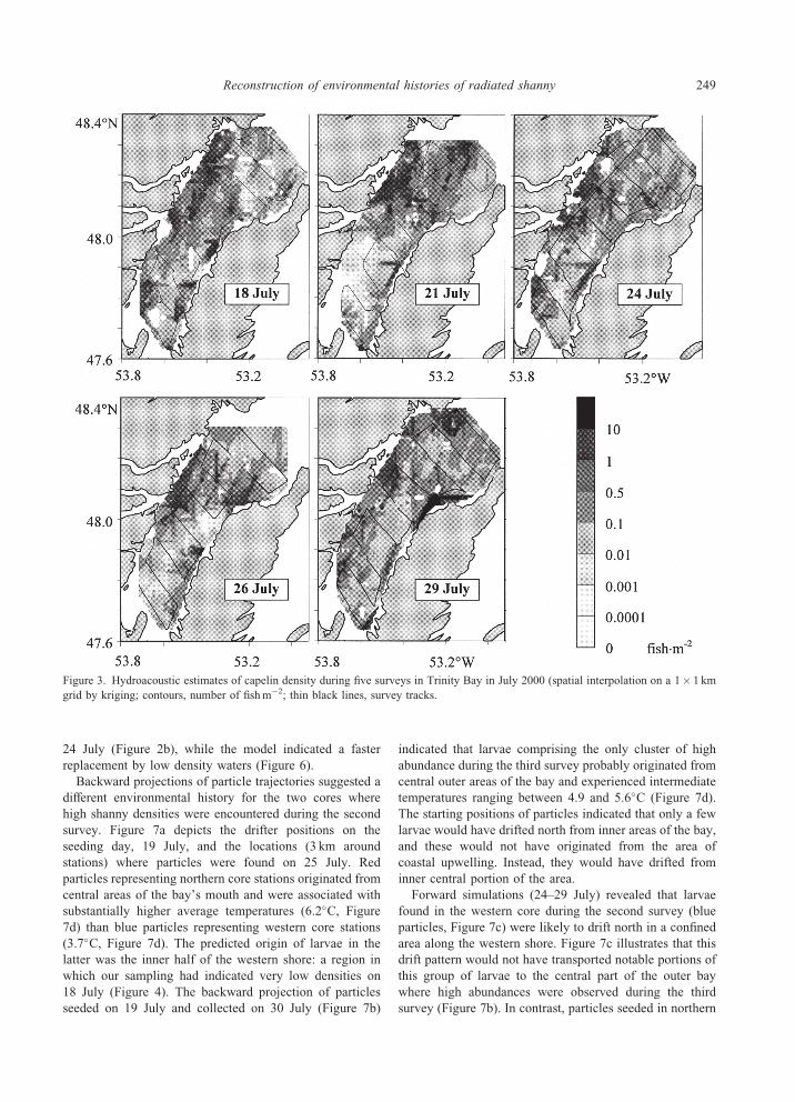
Hydroacoustic estimates of capelin abundance (10–

200m) ranged from zero to 128 fishm�2 with median

densities of 0.04 fishm�2, without major changes in the

distribution between surveys (Figure 3). Data characteristi-

cally were highly variable between consecutive 100m echo

bins. On a broader spatial scale, densities appeared to be

consistently higher along the western shore, lower along the

eastern shore, and particularly low in central areas of the

inner bay, where the deep trench is located. Median capelin

abundance, calculated for a 4 km radius around stations,

substantiated this impression and revealed significantly

higher densities at stations along the western shore than at

stations in central or eastern parts (Welch’s one-way

ANOVA: F2,197¼ 30.9, p< 0.001).

Larval distribution

The ichthyoplankton community was dominated by capelin

and radiated shanny larvae, which together comprised

about 50% of all fish larvae. The spatial distribution of

shanny larvae was very heterogeneous, with concentrations

>10 larvae 1000m�3 occurring in dense clusters limited to

the outer areas of the bay (Figure 4). In inner areas (to

approximately 47.9�N), abundance was consistently low

during the entire period. The distribution during the second

survey was suggestive of two separate larval cores, one

with higher concentrations at the western shore and one

with lower concentrations at the mouth of the bay. In the

western core, the proportion of small larvae (<7.5mm SL)

was notably higher compared with the northern core,


whereas large larvae (>11.5mm SL) were more abundant

in the northern than in the western core. Overall, the

proportion of larvae in the larger size classes increased

slightly over the period, yet relative abundance of larvae

<8.5mm SL remained high, indicating continuous produc-

tion and emergence.

A population growth rate of 0.32mmd�1 (derived from

age–length data on the day of capture) was used to estimate

larval mortality between successive surveys. Larvae were

assumed to grow 2mm SL in the 5 or 6 days between

surveys, given that measurements were to the nearest

millimeter. Negative losses, indicating production, were

found for the smallest larvae sampled (5mm SL). Mortality

rates were significantly greater than zero for larvae of

7–11mm SL (F1,26¼ 15.1, P< 0.01; Figure 5). However,

differences among size classes were never significant

(F8,26¼ 1.23, P> 0.2).

Circulation patterns and particle drift

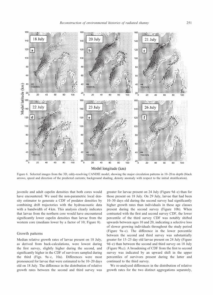
Model outputs were indicative of two major periods in

the circulation pattern coinciding with the main shifts in

strength and direction of winds during the 2 weeks. Upwell-

ing, induced by strong southwesterlies, characterized the

first period with medium, northeasterly currents on the west-

ern shore and stronger, outflowing currents close to the east-

ern shore (Figure 6a–c). Currents at the mouth of the bay

did not flow directly out of the region but instead flowed

across the mouth, possibly allowing larvae to remain within

the region. High-density water masses propagated east-

ward, covering about two-thirds of the bay on 21 July, the

day prior to the sudden relaxation of offshore winds. During

the second period, characterized by moderate and variable

winds, high-density water masses gradually disappeared

from the surface layer (Figure 6d–f ). Also currents became

weaker, with the exception of the western side of the bay,

where a narrow near-shore jet (�43 cm s�1) developed on

22 July, rapidly dragging lighter and warmer water masses

southward (Figure 6d). On the eastern shore, currents

reversed and flowed into the bay for the rest of the period

(Figure 6d–f ). Overall, model predictions corresponded

well to CTD measurements but were deviant for the inner

part of the bay during the second survey. In this area, cold

and high salinity waters still dominated the surface layer on

Figure 2. Environmental conditions in the surface layer of Trinity Bay during three subsequent surveys in July 2000 (spatial interpolation

on a 1� 1 km grid by kriging). (a–c) Average temperature (�C; 5–30m); (d–f ) average microzooplankton concentration ( particles l�1;

0–40m).


24 July (Figure 2b), while the model indicated a faster

replacement by low density waters (Figure 6).

Backward projections of particle trajectories suggested a

different environmental history for the two cores where

high shanny densities were encountered during the second

survey. Figure 7a depicts the drifter positions on the

seeding day, 19 July, and the locations (3 km around

stations) where particles were found on 25 July. Red

particles representing northern core stations originated from

central areas of the bay’s mouth and were associated with

substantially higher average temperatures (6.2�C, Figure

7d) than blue particles representing western core stations

(3.7�C, Figure 7d). The predicted origin of larvae in the

latter was the inner half of the western shore: a region in

which our sampling had indicated very low densities on

18 July (Figure 4). The backward projection of particles

seeded on 19 July and collected on 30 July (Figure 7b)

indicated that larvae comprising the only cluster of high

abundance during the third survey probably originated from

central outer areas of the bay and experienced intermediate

temperatures ranging between 4.9 and 5.6�C (Figure 7d).

The starting positions of particles indicated that only a few

larvae would have drifted north from inner areas of the bay,

and these would not have originated from the area of

coastal upwelling. Instead, they would have drifted from

inner central portion of the area.

Forward simulations (24–29 July) revealed that larvae

found in the western core during the second survey (blue

particles, Figure 7c) were likely to drift north in a confined

area along the western shore. Figure 7c illustrates that this

drift pattern would not have transported notable portions of

this group of larvae to the central part of the outer bay

where high abundances were observed during the third

survey (Figure 7b). In contrast, particles seeded in northern

Figure 3. Hydroacoustic estimates of capelin density during five surveys in Trinity Bay in July 2000 (spatial interpolation on a 1� 1 km

grid by kriging; contours, number of fishm�2; thin black lines, survey tracks.


core stations (red particles, Figure 7c) moved slowly

towards the central outer bay and into the area where high

concentrations were observed on 29 July. These results

suggest that shanny larvae sampled during the third survey

should be more similar in their characteristics to those

sampled during the second survey in the northern core than

in the western core.

The drift simulations indicate that advective losses from

the bay were small (<2%). Although particles associated

with stations on the eastern side of Trinity Bay could have

moved out of the system for part of the period, the

circulation pattern would have returned them to the area by

the end of the period (Figure 6). However, it is important to

be cautious in interpreting advective losses because the

model does not have a specific formulation for the vari-

ability in the inshore arm of the Labrador Current, which

is likely to influence the advection of plankton into and out

of the bay.

Because the forward drift projections suggest that the

western and northern cores represent distinct aggregations

of larvae, we used the average drift trajectory over the

2-week period to assess the cumulative distribution of

Figure 4. Spatial distribution (larvae per 1000m3) and relative length frequencies of radiated shanny larvae encountered. The second

survey distribution suggested a western (diamonds, black bars) and a northern core (triangles, white bars) of high abundance.

Figure 5. Daily mortality of shanny larvae (error bars: 95%

confidence intervals around the mean) in relation to their length

during the first survey.


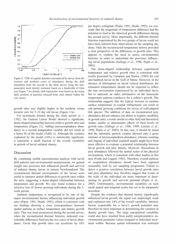
juvenile and adult capelin densities that both cores would

have encountered. We used the non-parametric local den-

sity estimator to generate a CDF of predator densities by

combining drift trajectories with the hydroacoustic data

with a bandwidth of 4 km. This analysis clearly indicates

that larvae from the northern core would have encountered

significantly lower capelin densities than larvae from the

western core (medians lower by a factor of 10; Figure 8).

Growth patterns

Median relative growth rates of larvae present on 18 July,

as derived from back-calculations, were lowest during

the first survey, slightly higher during the second, and

significantly higher in the CDF of survivors sampled during

the third (Figs. 9a–c, 10a). Differences were most

pronounced for larvae that were estimated to be 10–20 days

old on 18 July. The difference in the distribution of relative

growth rates between the second and third survey was

greater for larvae present on 24 July (Figure 9d–e) than for

those present on 18 July. On 29 July, larvae that had been

10–30 days old during the second survey had significantly

higher growth rates than individuals in these age classes

present during the second survey (Figure 10b). When

contrasted with the first and second survey CDF, the lower

percentile of the third survey CDF was notably shifted

upwards between ages 10 and 20, indicating a selective loss

of slower growing individuals throughout the study period

(Figure 9a–c). The difference in the lower percentile

between the second and third survey was substantially

greater for 15–25 day old larvae present on 24 July (Figure

9d–e) than between the second and third survey on 18 July

(Figure 9b,c). A broadening of CDF from the first to second

survey was indicated by an upward shift in the upper

percentiles of survivors present during the latter and

continued to the third survey.

We re-analyzed differences in the distribution of relative

growth rates for the two distinct aggregations separately,

Figure 6. Selected images from the 3D, eddy-resolving CANDIE model, showing the major circulation patterns in 10–20m depth (black

arrows, speed and direction of the predicted currents; background shading, density anomaly with respect to the initial stratification).


because they represented apparently separate drift and

environmental histories (Figure 7a,d). Larvae from the

western core had significantly lower median relative growth

rates than those from the northern core (Figure 11b). The

lower and upper percentiles of the CDF in the northern core

were notably shifted up relative to those observed in the

western core. The CDF of larvae from the northern core

(Figure 11a) were more similar to that observed during the

third survey for individuals present on 24 July (Figure 9e).

This suggests that individuals present during the final

survey represent a spatial subset of the overall population

present during the second survey. The variability of relative

Figure 7. Particle drift projections in model space to infer origin and fate of shanny larvae encountered. (a) Six-day backward run for

particles corresponding to the two cores of high abundance stations during the second survey (circles); (b) backward run for particles

corresponding to the region of high abundance observed during the third survey (circle; particle positions are plotted together for all 11

days of the simulation); (c) 6-day forward projection of particles seeded on 24 July, 1 km around western and northern core stations

(circles); and (d) thermal history of larvae from the western (blue) and northern (red) cores as well as from the high abundance cluster

observed during the third survey (brown) based on average particle drift tracks (black lines in a–c) and linearly interpolated (5–30m)

temperature fields. Solid lines, backward projections; dashed lines, forward projections; no environmental projections were made when

average tracks left the area of environmental interpolation).


growth rates was slightly higher in the northern versus

western core for 5–22 day old larvae (Figure 11a).

For increments formed during the study period ðn ¼1382Þ, the General Linear Model showed a significant,

dome-shaped relationship between relative growth rates and

temperature (Figure 12). Adding microzooplankton abun-

dance as a second independent variable did not result in

a better fit of the model (Table 1). Although the variance

explained by the model (14%) is statistically significant,

it represents a small fraction of the overall variability

in growth of larval radiated shanny.

Discussion

By combining otolith microstructure analysis with larval

drift patterns and environmental measurements, we gained

insight into processes that influenced growth and survival

of radiated shanny larvae in eastern Newfoundland. The

reconstructed thermal environments of the larvae were

useful to interpret spatial differences in growth rates within

the area, suggesting a dome-shaped relationship between

temperature and growth. We also found evidence for a

selective loss of slower growing individuals during the 2-

week period.

Ambient temperature is recognized to be one of the

major environmental factors influencing individual growth

rates (Pepin, 1991; Heath, 1992), which is consistent with

our findings showing a close correspondence between

spatial patterns in surface temperature and shanny growth

rates. This was most pronounced during the second survey,

when the reconstructed thermal histories indicated con-

siderable differences between the two cores of larval abun-

dance. Given that growth rates can accelerate by 10%

per degree centigrade (Pepin, 1991; Heath, 1992), we con-

clude that the magnitude of temperature difference had the

potential to lead to the observed growth differences during

the second survey. More importantly, the different thermal

histories experienced by the two groups of larvae could not

have been inferred from observations on the sampling day

alone. Only the reconstructed temperature history provided

a clear perspective of the differences in growth rates. This

appears to confirm the need to assess environmental

histories in order to understand the processes influenc-

ing larval populations (Gallego et al., 1996; Pepin et al.,

2001).

The dome-shaped relationship between experienced

temperature and relative growth rates is consistent with

results presented by Campana and Hurley (1989) for cod

and haddock larvae in the Gulf of Maine. However, in the

absence of information on larval vertical distribution, the

estimated temperatures should not be expected to reflect

the true environment experienced by an individual larva,

but to represent an index informative of the mesoscale

temperature patterns conducive for a cohort’s growth. The

relationship suggests that the typical increase in summer

surface temperature in coastal embayments can result in

sub-optimal growing conditions for larvae of cold-adapted

fish species. The addition of data on reconstructed prey

abundance did not enhance our ability to explain variability

in growth rates, a result similar to other field and theoretical

studies unable to demonstrate effects of food levels on

growth rates (Gallego et al., 1996, 1999; Letcher et al.,

1996; Pepin et al., 2003). In this case, it should be noted

that the automatic particle counter allowed only a gross

estimate of microzooplankton abundance, whereas counting

and staging of individual copepod nauplii might have been

more effective to evaluate a potential relationship between

larval growth and prey density. However, fluctuations in

prey abundance followed the spatial scales of the physical

environment, which is consistent with other studies in this

area (Frank and Leggett, 1982). Therefore, overall patterns

of zooplankton abundance should have been captured

reasonably well by our sampling programme. Failure to

detect a positive correlation between larval growth rates

and prey abundance may therefore suggest that events at

the scale of the individual are more important in deter-

mining its growth and survival potential (Pepin et al.,

2003). Unfortunately, environmental variability on such

small spatial and temporal scales has yet to be adequately

described.

Despite the evidence that thermal history significantly

influenced larval growth, the signal was surprisingly weak

and explained only 14% of the overall variability. Intrinsic

factors responsible for a larva’s growth potential may

therefore be more important in determining the variation in

shanny growth rates. The large unexplained variability

could also have resulted from partly unrepresentative en-

vironmental parameter values assigned to individual incre-

ment widths. Because spatial information was restricted

Figure 8. CDF of capelin densities encountered by larvae from the

western and northern cores of abundance during the drift

simulation from the second to the third survey using the non-

parametric local density estimator based on a bandwidth of 4 km

(see Figure 7 for details; drift trajectories were based on the mean

daily position of particles released from each station within the

core areas).


to location of capture on the sampling day, temperature

and zooplankton variables were estimated from the average

position of all particles per station tracked backwards

through the model domain. However, with every time-step

the spatial and environmental uncertainty increased as a

consequence of particle dispersion that was explicitly in-

cluded in the model.

The selective loss of slower growing individuals is

consistent with expectations based on size-dependent food

web dynamics (Peterson and Wroblewski, 1984) and

corroborates the findings of previous field and mesocosm

studies (Meekan and Fortier, 1996; Folkvord et al., 1997).

However, we were unable to detect significant size-

dependent differences in estimated mortality rates. The

selective removal of slower growth rates is in marked

contrast to Pepin et al.’s (2003) study in Conception Bay

where they found evidence for selective loss of faster grow-

ing individuals, which they assigned to larvae becoming

more vulnerable to predation by capelin because their

length was below the optimum in the predator size–prey

size relationship (10%; Paradis et al., 1996). In Trinity Bay,

the majority of shanny larvae also had not yet reached a

length corresponding to 10% of the modal length of capelin

sampled using the IYGPT trawl (Figure 13). What factors

could explain our pattern of selective loss from the

population?

Dower et al. (1998, 2002) concluded that shanny larvae

were not highly susceptible to starvation because the

incidence of feeding and the amount of food in the gut

indicate that most individuals achieve daily ingestion rates

sufficient to sustain growth. Therefore, starvation is not

likely to cause selective loss of slower growing individuals.

An alternative hypothesis is that the two distinct larval

concentrations (western and northern cores) not only had

different growth potentials but also experienced different

predation mortalities. Radiated shanny are produced from

Figure 9. Survey comparison of the CDF (solid lines: 10th, 50th, and 90th percentiles, estimated using a local non-parametric density

estimator with a bandwidth of 3 days) of standardized increment widths (SIW), formed on 14–17 July in relation to larval age on 18 July

(a–c), and of those formed on 20–23 July in relation to larval age on 24 July (d–e).


demersal eggs laid in nearshore waters after which the

larvae emerge and disperse throughout coastal waters

(Green et al., 1987). Data from the second survey indicate

that smaller individuals predominated in the western area

whereas larger individuals were more abundant in the

northern core. In addition, integrated surface temperatures

were generally lower along the western shore than in the

offshore area of the northern core. In addition to the effects

of temperature on growth rate, the median potential for

encounter with capelin was more than 10 times higher

for larvae from the western core than for those from

the northern core. The high concentration of larvae on the

Figure 10. Median of the CDF of standardized increment widths (SIW) and its 95% confidence intervals (estimated from 500

randomizations of the data) by sampling date in relation to larval age on (a) 18 July and (b) 24 July (based on the increments formed on the

4 days prior to these dates).

Figure 11. (a) CDF of standardized increment widths (SIW) formed on 20–23 July in relation to larval age on 24 July for the western (gray

circles) and northern (black triangles) core of high larval abundance observed during the second survey (see map; solid lines: 10th and 90th

percentiles of the CDF, estimated using a local non-parametric density estimator with a bandwidth of 3 days), and (b) medians and their

95% confidence intervals (estimated from 500 randomizations of the data) of these in relation to larval age on 24 July (gray lines, western

core; black lines, northern core).


western shore during the second survey had disappeared

during the third survey, whereas our forward simulations of

particle drift predicted that this distinct cluster should have

remained in the area. Although patterns of larval dispersal

unresolved by the sampling programme or circulation

model might have caused some error in our inferences, the

evidence on hand suggests the spatial distribution of growth

rates coupled with the spatial overlap with predators has

resulted in a greater overall loss of larvae from one region

over another. Although size-dependent processes may have

occurred, these spatial differences may explain the overall

selective loss of slower growing individuals.

This field study demonstrates that past rather than recent

environmental variability is an important consideration if

we are to understand the growth characteristics of larval

populations sampled in the open sea. It has also shown

some substantial difficulties still besetting such field

studies, particularly the inability to represent larval prey

abundance on appropriate scales, and the complexity of

including predators such as pelagic fish. Broad regions of

different predation pressure could be described, but to

further understand predation, we need to move beyond

descriptive studies and try to estimate the spatial structure

of encounter probabilities between fast moving predators

and the larval fish.

Acknowledgements

We thank T. Shears for his efforts to coordinate the logistic

and technical activities in the field and in the laboratory, as

well as G. Maillet, G. Redmond, and H. Maclean for their

assistance in the field. C.Mercer is thanked for her invaluable

guidance and help in the analysis of otolith microstructure.

The work could not have been carried out without the assist-

ance and expertise of the officers and crew of the Wilfred

Templeman. This study received funds from the International

Bureau of the Bundesministerium fur Bildung und For-

schung (BMBF, Project Nr. CAN 01/007) to HB, the Natural

Sciences and Engineering Research Council to PP, and the

Department of Fisheries and Oceans. The constructive criti-

cism provided by two anonymous referees and the editor

was helpful in improving the presentation of our findings.

References

Bailey, K. M., and Houde, E. D. 1989. Predation on eggs andlarvae of marine fishes and the recruitment problem. Advancesin Marine Biology, 25: 1–83.

Figure 12. Standardized increment width in relation to a 3-day

average of temperature (�C) and microzooplankton abundance

(particles l�1) experienced on the day of formation and the 2

preceding days, based on larval drift paths inferred from average

particles trajectories.

Table 1. Results of a General Linear Model analysis, relatingstandardized increment width (dependent variable) to a 3-dayaverage of temperature (T) and microzooplankton abundance(MZP), experienced on the day of formation and the 2 precedingdays, based on larval drift paths inferred from average particlestrajectories.

Source DF SS MS F-value PPar

estimate SE

Model 4 230.6 57.7 57.6 <0.0001Error 1378 1379.0 1.0

Type IIIT 1 73.7 73.7 73.6 <0.0001 3.83 0.45T2 1 115.6 115.6 115.5 <0.0001 �0.33 0.03MZP 1 2.1 2.1 2.1 0.15 0.03 0.02MZP�T 1 1.4 1.4 1.4 0.23 �0.005 0.004Intercept �10.26 1.47

Corr. total 1382 1609.6

R2 ¼ 0.14.

Figure 13. Relative length-frequency distributions of capelin

ðn ¼ 3341Þ and larval radiated shanny (2811) sampled (larval

shanny standard lengths SL were transformed to total lengths TL

according to TL¼ 1.115 SL, R2¼ 0.98, n¼ 270).


Campana, E. S., and Hurley, P. C. F. 1989. An age- and temperaturemediated growth model for Cod (Gadus morhua) and Haddock(Melanogrammus aeglefinus) larvae in the Gulf of Maine.Canadian Journal of Fisheries and Aquatic Science, 46: 603–613.

Davidson, F. J. M., and de Young, B. 1995. Modeling advection ofcod eggs and larvae on the Newfoundland Shelf. FisheriesOceanography, 4: 33–51.

Davidson, F. J. M., Greatbatch, R. J., and de Young, B. 2001.Asymmetry in the response of a stratified coastal embayment towind forcing. Journal of Geophysical Research, 106: 7001–7015.

Davison, A. C., and Hinkley, D. V. 1997. Bootstrap methodsand their application. In Cambridge Series in Statisticaland Probabilistic Mathematics. Cambridge University Press,Cambridge. 582 pp.

De Young, B., and Sanderson, B. 1995. The circulation andhydrography of Conception Bay, Newfoundland. Atmosphereand Oceans, 33: 135–162.

De Young, B., Otterson, T., and Greatbatch, R. J. 1993. The localand non-local response of Conception Bay to wind forcing.Journal of Physical Oceanography, 23: 2636–2649.

De Young, B., Anderson, J. T., Greatbatch, R. J., and Fardy, P.1994. Advection-diffusion modeling of capelin larvae inConception Bay, Newfoundland. Canadian Journal of Fisheriesand Aquatic Science, 51: 1297–1307.

Dower, J. F., Pepin, P., and Leggett, W. C. 1998. Enhanced gutfullness and an apparent shift in size selectivity by radiatedshanny (Ulvaria subbifurcata) larvae in response to increasedturbulence. Canadian Journal of Fisheries and Aquatic Science,55: 128–142.

Dower, J. F., Pepin, P., and Leggett, W. C. 2002. Using patchstudies to link mesoscale patterns of feeding and growth in larvalfish to environmental variability. Fisheries Oceanography, 11:219–232.

Evans, G. T. 2000. Local estimation of probability distribution andhow it depends on covariates. Canadian Stock AssessmentSecretariat Research Document 2000/120. 11 pp.

Folkvord, A., Rukan, K., Johannessen, A., and Moksness, E. 1997.Early life history of herring larvae in contrasting feedingenvironments determined by otolith microstructure analysis.Journal of Fish Biology, 51(Suppl A): 250–263.

Frank, K. T., and Leggett, W. C. 1982. Coastal water massreplacement: its effect on zooplankton dynamics and thepredator–prey complex associated with larval capelin (Mallotusvillosus). Canadian Journal of Fisheries and Aquatic Science, 39:991–1003.

Gallego, A., Heath, M. R., McKenzie, E., and Cargill, L. H. 1996.Environmentally induced short-termvariability in the growth ratesof larval herring. Marine Ecology Progress Series, 137: 11–23.

Gallego, A., Heath, M. R., Basford, D. J., and McKenzie, B. R.1999. Variability in growth rates of larval haddock in thenorthern North Sea. Fisheries Oceanography, 8: 77–92.

Gill, A. E. 1982. Atmosphere–Ocean Dynamics. Academic Press,San Diego. 662 pp.

Greatbatch, T. J., and Otterson, T. 1991. On the formulationof open boundary conditions at the mouth of a bay. Journalof Geophysical Research, 96: 18431–18445.

Green, J. M., Mathisen, A.-L., and Brown, J. A. 1987. Laboratoryobservations on the reproductive and agnostic behavior ofUlvaria subbifurcata (Pisces: Stichaeidae). Canadian Naturalist,114: 195–202.

Heath, M. R. 1992. Field investigations of the early life stages ofmarine fish. Advances in Marine Biology, 28: 1–174.

Hinrichsen, H.-H., St. John, M., Aro, E., Grønkjr, P., and Voss, R.2001. Testing the larval drift hypothesis in the Baltic Sea:retention versus dispersion caused by wind-driven circulation.ICES Journal of Marine Science, 58: 973–984.

Hunter, J. R. 1981. Feeding ecology and predation on marine fishlarvae. In Marine fish larvae: morphology, ecology and relation

to fisheries, pp. 34–77. Ed. by R. Lasker, University ofWashington Press, Seattle, WA. 131 pp.

Koeller, P., Hurley, P. C. F., Perley, P., and Neilson, J. D. 1986.Juvenile fish surveys on the Scotian Shelf: implications for year-class size assessments. Journal de Conseil International pourl’Exploration de la Mer, 43: 59–76.

Large, W. G., and Pond, S. 1981. Open ocean momentum fluxmeasurements in moderate to strong winds. Journal of PhysicalOceanography, 11: 324–336.

LeDrew, B. R., and Green, J. M. 1975. Biology of the radiatedshanny Ulvaria subbifurcata Storer in Newfoundland (Pisces:Stichaeidae). Journal of Fish Biology, 7: 485–495.

Letcher, B. H., Rice, J. A., Crowder, L. B., and Rose, K. A. 1996.Variability in survival of larval fish: disentangling componentswith a generalized individual-based model. Canadian Journal ofFisheries and Aquatic Science, 53: 787–801.

Litvak, M. K., and Leggett, W. C. 1992. Age and size-selectivepredation on larval fishes: the bigger-is-better hypothesis re-visited. Marine Ecology Progress Series, 81: 13–24.

MacLennan, D. N., and Simmonds, J. E. 1992. Fisheries Acoustics.Chapman and Hall, London. 344 pp.

Meekan, M. G., and Fortier, L. 1996. Selection for fast growthduring the larval life of Atlantic cod Gadus morhua onthe Scotian Shelf. Marine Ecology Progress Series, 137: 25–37.

Miller, T. J., Crowder, L. B., Rice, J. A., and Marschall, E. A. 1988.Larval size and recruitment mechanisms in fishes: toward aconceptual framework. Canadian Journal of Fisheries andAquatic Science, 45: 1657–1670.

Moksness, E., and Wespestad, V. 1989. Ageing and back-calculating growth rates of pacific herring, Clupea pallasi,larvae by reading daily otolith increments. Fishery Bulletin U.S.,87: 509–513.

Mosegaard, H., Svedang, H., and Taberman, K. 1988. Uncouplingof somatic and otolith growth rates in arctic char (Salvelinusalpinus) as an effect of differences in temperature response.Canadian Journal of Fisheries and Aquatic Science, 45: 1514–1524.

Paradis, A. R., and Pepin, P. 2001. Modeling changes in the length-frequency distributions of fish larvae using field estimates ofpredator abundance and size distributions. Fisheries Ocean-ography, 10: 217–234.

Paradis, A. R., Pepin, P., and Brown, J. A. 1996. Vulnerability offish eggs and larvae to predation: review of the influence of therelative size of prey and predator. Canadian Journal of Fisheriesand Aquatic Science, 53: 1226–1235.

Parma, A. M., and Deriso, R. B. 1990. Dynamics of age and sizecomposition in a population subject to size-selective mortality:effects of phenotypic variability in growth. Canadian Journal ofFisheries and Aquatic Science, 47: 274–289.

Pepin, P. 1991. Effect of temperature and size on development,mortality, and survival rates of the pelagic early life historystages of marine fish. Canadian Journal of Fisheries and AquaticScience, 48: 503–518.

Pepin, P., and Shears, T. H. 1997. Variability and captureefficiency of bongo and Tucker trawl samplers in thecollection of ichthyoplankton and other macrozooplankton.Canadian Journal of Fisheries and Aquatic Science, 54: 765–773.

Pepin, P., Shears, T. H., and de Lafontaine, Y. 1992. Significanceof body size to the interaction between a larval fish (Mallotusvillosus) and a vertebrate predator (Gasterosteus aculeatus).Marine Ecology Progress Series, 81: 1–12.

Pepin, P., Helbig, J. A., Laprise, R., Colbourne, E., and Shears,T. H. 1995. Variations in the contribution of transport to changesin planktonic animal abundance: a study of the flux of fish larvaein Conception Bay, Newfoundland. Canadian Journal of Fish-eries and Aquatic Science, 52: 1475–1486.


Pepin, P., Evans, G. T., and Shears, T. H. 1999. Patterns of RNA/DNA ratios in larval fish and their relationship to survival in thefield. ICES Journal of Marine Science, 56: 697–706.

Pepin, P., Dower, J. F., and Davidson, F. J. M. 2003. A spatiallyexplicit study of prey–predator interactions in larval fish:assessing the influence of food and predator abundance onlarval growth and survival. Fisheries Oceanography, 12: 19–33.

Pepin, P., Dower, J. F., and Benoit, H. P. 2001. The role ofmeasurement error on the interpretation of otolith incrementwidth in the study of growth in larval fish. Canadian Journal ofFisheries and Aquatic Science, 58: 2204–2212.

Pepin, P., Dower, J. F., Helbig, J. A., and Leggett, W. C. 2002.Estimating the relative roles of dispersion and predation ingenerating regional differences in mortality rates of larvalradiated shanny (Ulvaria subbifurcata). Canadian Journal ofFisheries and Aquatic Sciences, 59: 105–114.

Peterson, I., and Wroblewski, J. S. 1984. Mortality rate of fishesin the pelagic ecosystem. Canadian Journal of Fisheries andAquatic Science, 41: 1117–1120.

Rice, J. A., Crowder, L. B., and Holey, M. E. 1987. Exploration ofmechanisms regulating larval survival in Lake Michigan Bloater:a recruitment analysis based on characteristics of individuallarvae. Transactions of the American Fisheries Society, 116:703–718.

Rilling, G. C., and Houde, E. D. 1999. Regional and temporalvariability in growth and mortality of bay anchovy, Anchoamitchilli, larvae in Chesapeake Bay. Fishery Bulletin U.S., 97:555–569.

Rose, G. A. 1998. Acoustic target strength of capelin inNewfoundland waters. ICES Journal of Marine Science, 55:918–923.

Simard, Y., and Lavoie, D. 1999. The rich krill aggregation of theSaguenay – St. Lawrence Marine Park: hydroacoustic and geo-statistical biomass estimates, structure, variability, and signifi-cance for whales. Canadian Journal of Fisheries and AquaticScience, 56: 1182–1197.

Spiegel, E. A., and Veronis, G. 1960. On the Boussinesqapproximation for a compressible fluid. Astrophysical Journal,131: 441–447.

Templeman, W. 1966. Marine resources of Newfoundland.Bulletin of the Fisheries Research Board of Canada. 170 pp.

Voss, R., Hinrichsen, H.-H., and St. John, M. A. 1999. Variationsin the drift of larval cod (Gadus morhua L.) in the Baltic Sea:combining field observations and modeling. Fisheries Ocean-ography, 8: 199–211.

Yao, T. 1986. The response of currents in Trinity Bay,Newfoundland, to local wind forcing. Atmosphere–Ocean, 24:235–252.


Reconstruction of environmental histories to investigate patterns of larval radiated shanny (Ulvaria...

Documents

Transcript of Reconstruction of environmental histories to investigate patterns of larval radiated shanny (Ulvaria...