Reconciled Platoon Accommodations at Traffic Signals

Joint

Transportation

Research.

ProgramJTRP

FHWA/IN/JTRP-99/1

Final Report

RECONCILED PLATOON ACCOMMODATIONSAT TRAFFIC SIGNALS

Jay WassonMontasir AbbasDarcy Bullock

Avery RhodesChong Kang Zhu

December 1999

Indiana

Departmentof Transportation

PurdueUniversity

Final Report

FHWA/IN/JTRP-99/1

RECONCILED PLATOON ACCOMMODATIONS AT TRAFFIC SIGNALS

By

Jay WassonITS Engineer

Indiana Department of Transportation

(former Graduate Research Assistant)

Montasir AbbasGraduate Research Assistant

Darcy Bullock

Associate Professor

Avery RhodesUndergraduate Research Assistant

Chong Kang ZhuGraduate Research Assistant

School of Civil Engineering

Purdue University

Joint Transportation Research ProgramProject No: C-36-17VV

File No: 8-4-48

SPR-2209

In Cooperation with the


and the

U.S. Department of Transportation

Federal Highway Administration

The contents of this report reflect the views of the authors who are responsible

for the facts and the accuracy of the data represented herein. The contents do

not necessarily reflect the official views or policies of the Federal HighwayAdministration and the Indiana Department of Transportation. The report doesnot constitute a standard, specification or regulation.

Purdue University

West Lafayette, Indiana 47907December 1999

TECHNICAL REPORT STANDARD TITLE PAGE

1. Report No.

FHWA/IN/JTRP-99/l

2. Government Accession No. 3. Recipient's Catalog No.

4. Title and Subtitle

Reconciled Platoon Accommodations at Traffic Signals

5. Report Date

December 1999

6. Performing Organization Code

7. Author(s)

Jay Wasson, Montasir Abbas, Darcy Bullock. Avery Rhodes, and Chong Kang Zhu8. Performing Organization Report No.

FHWA/IN/JTRP-99/1

9. Performing Organization Name and Address

Joint Transportation Research Program

1284 Civil Engineering Building

Purdue University

West Lafayette, Indiana 47907-1284

10. Work Unit No.

11. Contract or Grant No.

SPR-2209

12. Sponsoring Agency Name and Address


State Office Building

100 North Senate Avenue

Indianapolis. IN 46204

13. Type of Report and Period Covered

Final Report

14. Sponsoring Agency Code

15. Supplementary Notes

Prepared in cooperation with the Indiana Department of Transportation and Federal Highway Administration.

16. Abstract

The use of microprocessor-based traffic signal controllers introduced in the 1960s has allowed for the development of many new

strategies to make traffic signal systems more responsive to traffic conditions. Many efforts have focused on the development of real-

time, adaptive control strategies. While some of these strategies have been shown to improve intersection performance, there are several

factors that have limited their deployment. Some of these include substantial capital cost, complicated calibration procedures, and the

reluctance of practicing engineers to deploy strategies radically different from those currently in use. Therefore, lower cost strategies that

are compatible with existing infrastructure continue to be explored. This research effort is considered to be in this category. Isolated

signalized intersections, which are operated by actuated type controllers, often do not allocate green time in an optimal manner when

compared to the temporal distribution of arriving traffic. Current detection schemes are typically used to provide localized detection near

the intersection. At isolated intersections, which do not have coordinated timing plans for allowing progression of platoons, timing

decisions are based on the binary status of localized detectors. Therefore, when platoons are forced to stop to allow the passage of a few

vehicles from a minor phase, excessive stops and delays are created at the intersection. The proposed strategy uses a detection device

located several thousand feet upstream from the intersection from which information is processed to identify platoons. When these

platoons are detected, the controller is manipulated using low-priority preemption to allow for the platoon to progress through the

intersection unimpeded. This research presents a study in which the platoon accommodation strategy was shown to reduce both the

percentage of stops and delays for vehicles in the platoon without significantly impacting any of the minor approaches. This system is

designed to be a retrofit to existing control equipment.

Since the findings were based upon the simulated traffic, an extensive evaluation was conducted comparing field-observed platooning

data with data obtained from CORSIM and the Robertson platoon distribution model. To compare field data with simulation and model

data, a new procedure that looked at the percentage of vehicles arriving during a specified window was developed. Those quantitative

numbers were summarized in easy to visualize charts. Platoon distribution charts were developed for 1) observed field data, 2) modeled

CORSIM data, and 3) theoretical models. These charts, contained in the Appendix of the report, provide a rational procedure for

estimating the upper bound on the arrival type used in the Highway Capacity calculations for signalized intersection and arterials

(Chapters 9 and 11). In general, the observed field platooning characteristics were similar to the simulation model, but not exact. The

CORSIM simulation model tended to have more overall platoon dispersion, which would likely provide slightly conservative estimates on

benefits.

17. Keywords

Platoon, traffic signal controller, vehicle detection, algorithm,

priority.

18. Distribution Statement

No restrictions. This document is available to the public through the

National Technical Information Service, Springfield, VA 22161

19. Security Classif. (of this report)

Unclassified

20. Security Classif. (of this page)

Unclassified

21. No. of Pages

217

22. Price

Form DOT F 1700.7 (8-69)

Digitized by the Internet Archive

in 2011 with funding from

LYRASIS members and Sloan Foundation; Indiana Department of Transportation

http://www.archive.org/details/reconciledplatooOOwass

TABLE OF CONTENTS

PREFACE I

TABLE OF CONTENTS II

LIST OF FIGURES IV

LIST OF TABLES XI

IMPLEMENTATION REPORT 1

CHAPTER 1 INTRODUCTION 3

CHAPTER 2 CURRENT STATE OF ADAPTIVE TRAFFIC CONTROL ALGORITHMS 6

Adaptive Control 10

Optimized Policies for Adaptive Control (OPAC) 12

Real-Time, Hierarchial, Optimized, Distributed and Effective System (RHODES) .. 16

CHAPTER 3 PROBLEM STATEMENT 21

Objective of Platoon Accommodations 21

Platoon Identification 24Platoon Accommodation 35System Architecture 42Equipment 44

CHAPTER 4 WORK PLAN 49

Data Collection 54Simulation Procedure 59Simulation Results 64

CHAPTER 5 ANALYSIS 68

System Costs 68System Benefit 76

CHAPTER 6 PLATOON DISPERSION 79

Literature Review 80FIELD WORK 82

DATA PROCESSING 86DATA ANALYSIS 89FIELD DATA REDUCTION 89CORSIM SIMULATION 90DETERMINATION OF GREEN WINDOWS FOR PARTICULAR PERCENTAGES OFPLATOONS 90

PLOTS OF GREEN WINDOWS REQUIRED BY DIFFERENT PERCENTAGES OF THEPLATOON 93THEORETICAL MODELS 97

DISCUSSION 100

CHAPTER 7 RECOMMENDATIONS 102

Parameter Sensitivity Study 102

Prototype Field Deployment 104Warrants for System Deployment 105Future Enhancements 107

LIST OF REFERENCES 108

APPENDIX A 114

PLC LADDER LOGIC FOR PLATOON DETECTION ALGORITHM 114

APPENDIX B 118

TRANSFORMING PLATOON HISTOGRAMS USING ROBERTSON'S MODEL 118

APPENDIX C 181

SIMULATION RANDOM NUMBER SEEDS 181

APPENDIX D 181

SIMULATION RESULTS 183

LIST OF FIGURES

Figure 1 Rolling Horizon Approach in ROPAC [Gartner, 1983] 15

Figure 2 Hierarchy Framework of RHODES [Head et al, 1 992] 1

8

Figure 3 RHODES Link Prediction Logic [Head etal, 1998] 19

Figure 4 Example of current control inefficiency 22Figure 5 Typical NEMA Solid State Controller [Econolite, 1998] 25Figure 6 Loop Detector Outputs Based on Vehicle Location 26Figure 7 Decision Rule for the Existence of a Platoon 29Figure 8 Programmable Logic Controller [GE Fanac, 1997] 30Figure 9 PLC Connected to a Computer Via the Serial Port [GE Fanac, 1997] 31

Figure 10 Example of a Ladder Logic Program 32Figure 1 1 Example of a FIFO Shift Register in Operation 34Figure 12 Sequential Logic of Platoon Detection Process 35Figure 13 Example of Preemption Impact on 8- Phase Timing Plan 41

Figure 14 Functional Block Diagram for Central Processing Approach 43Figure 15 Functional Block Diagram for Distributed Processing Approach 43Figure 16 ITRAF User Interface for Link Characteristics 50Figure 17 Controller Interface Device Connected to NEMA TS1 Compliant

Controller [Bullock and Catarella, 1997] 51

Figure 18 Simulation Environment Configuration 52

Figure 19 Map Showing Study Intersection Location [Adapted from Microsoft®AUTOMAP, 1997] 53

Figure 20 Arial Photo of Lafayette Area [Microsoft, 1 998] 53Figure 21 Arial Photo of Study Intersection [Microsoft, 1 998] 54Figure 22 Study Intersection Layout and Phasing , 55Figure 23 Flow Profile for US 52 East on April 8, 1998 from 16:00 to 16:15 PM 58Figure 24 Flow Profile for US 52 East on April 8, 1 998 from 1 6:25 to 1 6:39 PM 58Figure 25 File Management Strategy 61

Figure 26 RTMS Sidefire Radar Unit Installed [Electronic Integrated Systems Inc.,

1998] 69

Figure 27 Map of United States Showing Average Sun Hours a Day [Alternative

Energy Engineering, 1998] 71

Figure 28 Solar Power Supply [Alternative Energy Engineering, 1 998] 73Figure 29 6-volt220 Amp-Hour Lead-Acid Battery [Alternative Energy Engineering,

1998] 73

Figure 30 Typical Control Cabinet Used for Flashers 74

Figure 31: Example Vehicle Platoons 79

Figure 32: Data Collection Sites 83Figure 33: Sampling Procedure 85Figure 34: Database Schema 87

Figure 35: Platoon Distribution at Various Downstream Observation Points 92

Figure 36: Platoon Dispersion (20 Second Saturated Platoon, Speed: 30 MPH) 95

Figure 37: Platoon Dispersion (20 Second Saturated Platoon, Speed: 40 MPH) 96Figure 38: Green Window From Robertson's Model (20 second saturated platoon,

Speed: 30 MPH) 98Figure 39: Green Window From Robertson's Model (20 second saturated platoon,

Speed: 40 MPH) 99

Appendix Figures

FIGURE A-1 PLC PLATOON ACCOMMODATION ALGORITHM 115

FIGURE A-1 PLC PLATOON ACCOMMODATION ALGORITHM (CONTINUED) 1 1

6

FIGURE B-1: OBSERVED HISTOGRAM AT STOP-LINE 135

FIGURE B-2: TRANSFORMED HISTOGRAM AT 500 FT. DOWNSTREAM (a=0.15 (3=0.97)

135

FIGURE B-3: PLATOON DISTRIBUTION AT VARIOUS DOWNSTREAM OBSERVATIONPOINTS PARAMETERS: FOUR-LANE DIVIDED - a=0.15 (3=0.97 (MCCOY) ARTERIALCHARACTERISTICS: 20 SECOND SATURATED PLATOON, SPEED: 30 MPH 136

FIGURE B-4: PLATOON DISTRIBUTION AT VARIOUS DOWNSTREAM OBSERVATIONPOINTS PARAMETERS: LOW EXTERNAL FRICTION - a=0.25 (3=0.80 (TRANSYT)ARTERIAL CHARACTERISTICS: 20 SECOND SATURATED PLATOON, SPEED: 30 MPH

137

FIGURE B-5: PLATOON DISTRIBUTION AT VARIOUS DOWNSTREAM OBSERVATIONPOINTS PARAMETERS: MODERATE EXTERNAL FRICTION - a=0.35 (3=0.80 (TRANSYT)ARTERIAL CHARACTERISTICS: 20 SECOND SATURATED PLATOON, SPEED: 30 MPH

138

FIGURE B-6: PLATOON DISTRIBUTION AT VARIOUS DOWNSTREAM OBSERVATIONPOINTS PARAMETERS: HEAVY EXTERNAL FRICTION - a=0.50 (3=0.80 (TRANSYT)ARTERIAL CHARACTERISTICS: 20 SECOND SATURATED PLATOON, SPEED: 30 MPH

139

FIGURE B-7: PLATOON DISTRIBUTION AT VARIOUS DOWNSTREAM OBSERVATIONPOINTS PARAMETERS: FOUR-LANE DIVIDED - a=0.15 p=0.97 (MCCOY) ARTERIALCHARACTERISTICS: 20 SECOND SATURATED PLATOON, SPEED: 40 MPH 140


141


142


143

FIGURE B-1 1 : PLATOON DISTRIBUTION AT VARIOUS DOWNSTREAM OBSERVATIONPOINTS PARAMETERS: FOUR-LANE DIVIDED - cc=0.15 3=0.97 (TRANSYT) ARTERIALCHARACTERISTICS: 20 SECOND SATURATED PLATOON, SPEED: 50 MPH 144

FIGURE B-1 2: PLATOON DISTRIBUTION AT VARIOUS DOWNSTREAM OBSERVATIONPOINTS PARAMETERS: LOW EXTERNAL FRICTION - a=0.25 |3=0.80 (TRANSYT)ARTERIAL CHARACTERISTICS: 20 SECOND SATURATED PLATOON, SPEED: 50 MPH

145

FIGURE B-1 3: PLATOON DISTRIBUTION AT VARIOUS DOWNSTREAM OBSERVATIONPOINTS PARAMETERS: MODERATE EXTERNAL FRICTION - a=0.35 (3=0.80 (TRANSYT)ARTERIAL CHARACTERISTICS: 20 SECOND SATURATED PLATOON, SPEED: 50 MPH

146

FIGURE B-1 4: PLATOON DISTRIBUTION AT VARIOUS DOWNSTREAM OBSERVATIONPOINTS PARAMETERS: HEAVY EXTERNAL FRICTION - a=0.50 3=0.80 (TRANSYT)ARTERIAL CHARACTERISTICS: 20 SECOND SATURATED PLATOON, SPEED: 50 MPH

147

FIGURE B-1 5: PLATOON DISTRIBUTION AT VARIOUS DOWNSTREAM OBSERVATIONPOINTS PARAMETERS: FOUR-LANE DIVIDED - a=0.1 5 (3=0.97 (MCCOY) ARTERIALCHARACTERISTICS: 40 SECOND SATURATED PLATOON, SPEED: 30 MPH 148

FIGURE B-1 6: PLATOON DISTRIBUTION AT VARIOUS DOWNSTREAM OBSERVATIONPOINTS PARAMETERS: LOW EXTERNAL FRICTION - a=0.25 (3=0.80 (TRANSYT)ARTERIAL CHARACTERISTICS: 40 SECOND SATURATED PLATOON, SPEED: 30 MPH

149

FIGURE B-1 7: PLATOON DISTRIBUTION AT VARIOUS DOWNSTREAM OBSERVATIONPOINTS PARAMETERS: MODERATE EXTERNAL FRICTION - a=0.35 (3=0.80 (TRANSYT)ARTERIAL CHARACTERISTICS: 40 SECOND SATURATED PLATOON, SPEED: 30 MPH

150

FIGURE B-1 8: PLATOON DISTRIBUTION AT VARIOUS DOWNSTREAM OBSERVATIONPOINTS PARAMETERS: HEAVY EXTERNAL FRICTION - a=0.50 [3=0.80 (TRANSYT)ARTERIAL CHARACTERISTICS: 40 SECOND SATURATED PLATOON, SPEED: 30 MPH

151

FIGURE B-1 9: PLATOON DISTRIBUTION AT VARIOUS DOWNSTREAM OBSERVATIONPOINTS PARAMETERS: FOUR-LANE DIVIDED - a=0.15 3=0.97 (MCCOY) ARTERIALCHARACTERISTICS: 40 SECOND SATURATED PLATOON, SPEED: 40 MPH 152

FIGURE B-20: PLATOON DISTRIBUTION AT VARIOUS DOWNSTREAM OBSERVATIONPOINTS PARAMETERS: LOW EXTERNAL FRICTION - a=0.25 3=0.80 (TRANSYT)ARTERIAL CHARACTERISTICS: 40 SECOND SATURATED PLATOON, SPEED: 40 MPH

153

FIGURE B-21: PLATOON DISTRIBUTION AT VARIOUS DOWNSTREAM OBSERVATIONPOINTS PARAMETERS: MODERATE EXTERNAL FRICTION - a=0.35 3=0.80 (TRANSYT)ARTERIAL CHARACTERISTICS: 40 SECOND SATURATED PLATOON, SPEED: 40 MPH

154

VI

FIGURE B-22: PLATOON DISTRIBUTION AT VARIOUS DOWNSTREAM OBSERVATIONPOINTS PARAMETERS: HEAVY EXTERNAL FRICTION - a=0.50 3=0.80 (TRANSYT)ARTERIAL CHARACTERISTICS: 40 SECOND SATURATED PLATOON, SPEED: 40 MPH

155

FIGURE B-23: PLATOON DISTRIBUTION AT VARIOUS DOWNSTREAM OBSERVATIONPOINTS PARAMETERS: FOUR-LANE DIVIDED - a=0.15 3=0.97 (MCCOY) ARTERIALCHARACTERISTICS: 40 SECOND SATURATED PLATOON, SPEED: 50 MPH 156


157


158


159

FIGURE B-27: PLATOON DISTRIBUTION AT VARIOUS DOWNSTREAM OBSERVATIONPOINTS PARAMETERS: FOUR-LANE DIVIDED - a=0.15 3=0.97 (MCCOY) ARTERIALCHARACTERISTICS: 60 SECOND SATURATED PLATOON, SPEED: 30 MPH 160

FIGURE B-28: PLATOON DISTRIBUTION AT VARIOUS DOWNSTREAM OBSERVATIONPOINTS PARAMETERS: LOW EXTERNAL FRICTION - a=0.25 3=0.80 (TRANSYT)ARTERIAL CHARACTERISTICS: 60 SECOND SATURATED PLATOON, SPEED: 30 MPH

161

FIGURE B-29: PLATOON DISTRIBUTION AT VARIOUS DOWNSTREAM OBSERVATIONPOINTS PARAMETERS: MODERATE EXTERNAL FRICTION - a=0.35 3=0.80 (TRANSYT)ARTERIAL CHARACTERISTICS: 60 SECOND SATURATED PLATOON, SPEED: 30 MPH

162

FIGURE B-30: PLATOON DISTRIBUTION AT VARIOUS DOWNSTREAM OBSERVATIONPOINTS PARAMETERS: HEAVY EXTERNAL FRICTION - a=0.50 3=0.80 (TRANSYT)ARTERIAL CHARACTERISTICS: 60 SECOND SATURATED PLATOON, SPEED: 30 MPH

163

FIGURE B-31: PLATOON DISTRIBUTION AT VARIOUS DOWNSTREAM OBSERVATIONPOINTS PARAMETERS: FOUR-LANE DIVIDED - a=0.1 5 3=0.97 (MCCOY) ARTERIALCHARACTERISTICS: 60 SECOND SATURATION, SPEED: 40 MPH 164

FIGURE B-32: PLATOON DISTRIBUTION AT VARIOUS DOWNSTREAM OBSERVATIONPOINTS PARAMETERS: LOW EXTERNAL FRICTION - a=0.25 3=0.80 (TRANSYT)ARTERIAL CHARACTERISTICS: 60 SECOND SATURATION, SPEED: 40 MPH 165

FIGURE B-33: PLATOON DISTRIBUTION AT VARIOUS DOWNSTREAM OBSERVATIONPOINTS PARAMETERS: MODERATE EXTERNAL FRICTION - a=0.35 (3=0.80 (TRANSYT)ARTERIAL CHARACTERISTICS: 60 SECOND SATURATION, SPEED: 40 MPH 166


167

FIGURE B-35: PLATOON DISTRIBUTION AT VARIOUS DOWNSTREAM OBSERVATIONPOINTS PARAMETERS: FOUR-LANE DIVIDED - a=0.15 (3=0.97 (MCCOY) ARTERIALCHARACTERISTICS: 60 SECOND SATURATED PLATOON, SPEED: 50 MPH 168


169


170


171

FIGURE B-39: EXAMPLE ARRIVAL TIMES (THEORETICAL MODEL) 172

FIGURE B-40: THEORETICAL ARRIVAL TIMES 173

FIGURE B-41 : THEORETICAL GREEN WINDOW (ADJUSTED ARRIVAL TIMES) 173

FIGURE B-42: THEORETICAL ARRIVAL TIMES 174

FIGURE B-43: THEORETICAL GREEN WINDOW (ADJUSTED ARRIVAL TIMES) 174

FIGURE B-44: THEORETICAL GREEN WINDOW (20 SECOND SATURATED PLATOON,SPEED: 30 MPH) 175




VIII




FIGURE B-51 : THEORETICAL GREEN WINDOW (60 SECOND SATURATED PLATOON,SPEED: 40 MPH) 178



FIGURE B-54 THEORETICAL GREEN WINDOW (20 SECOND SATURATED PLATOON,SPEED: 40 MPH) 180

FIGURE D-1 PERIOD 3 CONFIGURATION A-100 184

FIGURE D-2 PERIOD 3 CONFIGURATION B-100 185

FIGURE D-3 PERIOD 3 CONFIGURATION C-100 186

FIGURE D-4 PERIOD 3 CONFIGURATION D-100 187

FIGURE D-5 PERIOD 3 CONFIGURATION E-100 188






FIGURE D-1 1 PERIOD 4 CONFIGURATION A-100 194






IX





FIGURE D-21 REJECTED SIMULATION RUN FROM TRIAL AND ERROR PERIOD .... 204

LIST OF TABLES

Table 1 States of Output Module based on Status of Input Modules for Exampleladder Logic Program 33

Table 2 Low Level Bus Preemption Parameters [Econolite, 1 996] 40Table 3 Current Available Detection Technologies [MinDOT and SRF Consultants,

1997] 46Table 4 Study Intersection Timing and Control Settings [INDOT, 1 998] 56Table 5 Volume Data For Study Intersection 57Table 6 Turning Movement Data 59Table 7 Data Input Parameters for Simulations 60Table 8 Simulation Configurations Evaluated 63Table 9 Simulation Trials Completed 64

Table 1 Summary of Simulation Results Contained in Appendix C 65Table 1 1 MOEs and Test Statistics for Period 3 Configuration D-1 00 67

Table 12 Remote Site Power Requirements [Adapted from Alternative EnergyEngineering, 1998] 71

Table 13 Remote Site Power Storage Requirements [Alternative EnergyEngineering, 1998] 72

Table 14 Component Prices for System 75Table 15 Selected Price Indexes for Computing Equivalent Dollars 76Table 1 6 Value of Time for Different Vehicle Types 77Table 17 Description of Benefits of System for Conservative Case 78Table 18: Suggested Platoon Dispersion Factors from Previous Research 81

Table 1 9: Number of Data Points Collected at Each Distance for Varying Speeds andInitial Discharge 84

Table 20: Database Field Definitions 88Table 21 : Summary of Data Contained in Database (Example Data) 89

Table 22: Regression Analysis Coefficients for Data and CORSIM Simulation 94Table 23 Summary of Information Regarding System Parameters 104

XI

APPENDIX TABLES

TABLE A-1 PLC LADDER LOGIC FUNCTIONS 117

TABLE B-2: ARRIVAL TIMES AT DIFFERENT DOWNSTREAM DISTANCES (20 SECONDSATURATED PLATOON, SPEED: 30 MPH) 126








TABLE B-10: ARRIVAL TIMES AT DIFFERENT DOWNSTREAM DISTANCES (60

SECOND SATURATED PLATOON, SPEED: 50 MPH) 134

TABLE C-1 RANDOM NUMBER SEEDS USED IN CORSIM SIMULATIONS 182

IMPLEMENTATION REPORT

Traffic signals are one of the few "active control" elements the Indiana Department of

Transportation has available for regulating the flow of traffic. The department owns and

maintains several thousand traffic signals through out the state and is constantly looking

at how to improve their operating efficiency. This study was initiated by the Indiana ITS

Program Engineer to determine if naturally occurring platoon of traffic could be identified

and a traffic controller manipulated to accommodate the progression of that platoon

through a traffic signal. Because of safety and public relation issues associated with

debugging new control algorithms, it was not feasible to develop the platoon

accommodation algorithm under live traffic conditions. Instead, a laboratory evaluation

environment was proposed to develop and evaluate the algorithm. As a result of this

research, we have developed several recommendations for implementing this research.

The first part of this study used the microscopic simulation program CORSIM connected

to an actuated controller via a Controller Interface Device (CID) to simulate field

conditions. A programmable logic controller (PLC) was introduced into the simulation

and algorithms were developed for the PLC to recognize platoons. Once a platoon was

recognized, a low priority transit preemption was introduced to facilitate the progression

of that platoon through the system. Quantitative evaluation of the proposed algorithm on

a case study intersection showed a reduction in stops and delays for the approach using

the algorithm while not significantly impacting any of the other minor approaches. Since

a "field hardened" PLC was used, this procedure could be directly implement on any

intersection that could provide the appropriate detectors and low priority transit priority

procedures.

The PLC technology used in this project to process detector inputs and implement logic

necessary for triggering the low-priority preemption has direct and immediate application

for a wide variety of low cost Intelligent Transportation System (ITS) initiatives. For

example, the former graduate student on this project, adapted the PLC concept and

wireless communication architecture to a warning sign indicating an interstate ramp was

backing up on Exit 4 (SR 1 31 ) on I-65 Northbound. Early indications are that this has

reduced accidents at that location. There are several other similar low cost ITS

initiatives currently under considerations that could use this technology.

Although the focus of this research was the development of procedures for

accommodating platoons, this project used, for the first time in Indiana, hardware-in-the-

loop simulation procedures. These hardware-in-the-loop simulation procedures proved

invaluable for evaluating novel (and more efficient) control schemes without subjecting

motorists to the occasional "glitches" experienced when developing a new system.

Further work is underway in another JTRP project to package the technology so these

procedures can be used by districts to evaluate performance of arterial traffic signal

control equipment. In conjunction with that JTRP study (which builds on this study), the

hardware in the loop evaluation procedure was been used to retime a complicated

diamond interchange down in Indianapolis at 1-465 and SR 37 reducing annual delay

over 32,000 veh-hours.

Finally, as a byproduct of evaluating the CORSIM platoon modeling characteristics,

platoon distribution charts were developed for 1 ) observed field data, 2) modeled

CORSIM data, and 3) theoretical models. These charts contained in the Appendix of the

report provide a rational procedure for estimating the upper bound on the arrival type

used in the Highway Capacity calculations for signalized intersection and arterials

(Chapters 9 and 1 1 ).

CHAPTER 1 INTRODUCTION

Over the past several years, the traffic engineering profession including public, private and

academic sectors have devoted many resources to advancing the state of traffic signal

control algorithms. Many advancements have been made since the deployment of first

generation electromechanical and vacuum tube type controllers. The advent of

microprocessor based solid state controllers allow for even more features to be incorporated

into these devices due to the increased available processing power.

Today a traffic signal may exist as a single isolated controller or may be part of a multi-signal

traffic control system. These traffic control systems are comprised of interacting

components such as signals, detectors, and a communications backbone that are arranged

in a manner which effectively and efficiently coordinate traffic flow along a corridor or

throughout a network [Homburger et al., 1992]. There currently are several different types

of these components that result in widely varying deployment architectures.

The goals associated with deploying traffic signals have not significantly changed over the

years. Traffic engineers' primary focus is to provide the control component of a road

network that will allow for the safe and efficient movement of people and goods. Traffic

engineers are continually refining the control strategies in an effort to better achieve these

goals. The increases in motor vehicle use without proportional increases in infrastructure

motivate the development of these strategies to an even greater extent.

The level of sophistication of traffic control strategies has advanced beyond the exclusive

use of time-of-day programs and local detection, such as inductive loops. Today, new

signal research is devoted to real-time traffic adaptive control. These systems not only

operate based on local detector demand but also make control decisions based on

predicted future demand. In order to make these decisions, it becomes necessary to predict

the future demand. Engineers have been looking at the need for prediction since the early

1970s when the urban traffic control system (UTCS) was under development [Tarnoff,

1 975]. Prediction becomes important in signal control if vehicle progression is to be

maintained.

In arterial and network systems, traffic is thought of as moving groups known as platoons.

Typically, signals that are located at the boundary of the system group vehicles together

during the red phase and then discharge this platoon under green. Systems in which

adjacent signal spacing is relatively small (less than 0.5 miles) allow for progression of the

platoon by coordinating adjacent signals based on an offset from some known time

reference. As the spacing between adjacent signals increases, the ability to provide

progression using traditional methods becomes more difficult due to platoon dispersion and

traffic sources and sinks. Therefore, when the spacing between intersections becomes

large, the traffic signals are usually operated as an isolated intersection.

Traffic signal control systems at isolated intersections are typically actuated systems that

use inductive loop detectors for local detection. The controller operates based on the active

timing plan and the local demand near the intersection (usually within 500' of the stop bar).

In this configuration, the control system is limited to a horizon of a few seconds for which

control decisions can be made based on perceived demand. This limitation is believed to

reduce the operational efficiency of the intersection when certain traffic patterns exist.

Platoons of vehicles can exist on approaches to isolated intersections. However, unlike the

traffic control systems that coordinate their cycles to traffic flow, isolated intersections do not

provide for smooth platoon progression. This lack of responsiveness leads to increased

vehicle delay and vehicle stops.

Although many adaptive algorithms have been developed to improve the operation of

isolated intersections, few of these have undergone wide scale deployment. Possible

reasons for this include excessive cost, difficulty in calibration, and the reluctance of the part

of practicing engineers to implement strategies radically different from those in use.

Because of this fact, this research proposes a cost-effective platoon accommodation

procedure that uses existing signal system components to provide some of the benefits as

those of adaptive control.

This document describes the development of a system within the constraints outlined above.

Chapter 2 presents a review of the current state of the practice of traffic control algorithm

development. Chapter 3 presents a new method for accommodating platoons at isolated

rural intersections. This new strategy is evaluated in Chapter 4 using hardware-in-the-loop

simulation. Chapter 5 presents a brief discussion on the expected benefits and costs

associated with the deployment of this strategy. Chapter 6 evaluates platoon dispersion

using filed data, simulation, and analytical models. Suggestions for further work is presented

in Chapter 7

CHAPTER 2 CURRENT STATE OF ADAPTIVE TRAFFIC CONTROLALGORITHMS

Modern traffic signals have evolved through several stages since the birth of the concept.

The first operating traffic signals are considered to be manually operated semaphores,

which were introduced in London in 1868. American James Hoge invented the first

automated electric traffic signal in 1913. This device, which seems to be the origin of the

standard three-color scheme used today, was first deployed in Cleveland, Ohio, in 1914.

After their initial inception, the use of traffic signals spread rapidly during the late 1 91 0's and

early 1920's. The first interconnected signals were used in Salt Lake City, Utah, in 1917. A

concept of a progressive signal system was first proposed in 1922. This lead to the

installation of actuated signal systems in 1928 at New Haven, East Norwalk and Baltimore

[Hamburger etal., 1992].

The 1960's had a very important effect on the advancement of traffic engineering technology

through the introduction of computer-based traffic signal control systems [Gartner et al.,

1995]. Through the use of computers, traffic engineers have made significant advances in

the development of optimization and control logic. Today, there are various microprocessor

based vendor products available for designing, operating, and monitoring traffic signal

installations. The constant advancement of the computer industry has resulted in the

availability of improved processors, which are capable of performing more operations in a

smaller amount of time. The fundamental objective of traffic engineers is to develop control

strategies that use available processing power to safely and efficiently move traffic.

• A properly designed traffic control system can help to reduce traffic delay, fuel

consumption, driver discomfort, and air and noise pollution by efficiently using the

capacity of existing streets [Linkenheld et al., 1992]. The positive effects of signal

installation can be any or all of the following [Homburger et al., 1992]:

• provision for the orderly movement of traffic,

• reduction in the frequency of certain types of accidents (i.e., right angle and pedestrian),

• an increase in the traffic handling capacity of the intersection,

• means of interrupting heavy traffic to allow other traffic, both vehicular and pedestrian, to

enter or cross a traffic stream,

• continual movement of traffic at a desired speed along a given route by coordination,

• economical benefits over manual control at intersections where alternate assignment of

right-of-way is required, and promotion of driver confidence by assigning right-of-way.

While the points indicated above illustrate the potential positive effects that traffic signals

can have, it is important to note that the deployment of these traffic signal systems can also

lead to less than desirable results. Some of the possible negative effects from the

installation of traffic signals are as follows [Homburger et al., 1992]:

• increase in the total intersection delay and fuel consumption, especially during off-peak

periods,

• probable increase in certain types of accidents (e.g. rear-end collisions),

• unnecessary delay when improperly located which results in disrespect for this type of

control, and

• cause excessive delay when improperly timed which increases driver irritation.

Two of the four mentioned possible negative impacts traffic signals can have are attributed

to the improper setting and location of the installation. Therefore, it is important to indicate

that traffic signals, when properly configured, can provide significant improvements to the

road network. However, it is equally as important to remember that even properly

configured signals do have the potential to provide some negative results.

The optimal setting of traffic signal control systems has been on the minds of traffic

engineering practitioners since their initial development. This is especially true since the

1960's when computer-based controllers allowed for more complex strategies to be

implemented. Although many of today's control strategies are quite complex in nature, they

focus on the manipulation of only a few configuration parameters. A particular controller

many have tens or hundreds of possible parameter settings, but there are only four that are

considered to have the most impact on system performance [Stewart et al., 1 998]. These

four variables are cycle length, split, phase sequencing, and offset. Cycle length is the time

required for one complete sequence of signal phases. Split is the percentage of a cycle

length allocated to each of the various phases. Phase sequencing is the order in which the

phases of a cycle occur. Offset is the time relationship in seconds between a defined

interval portion of the coordinated phase green and a system reference point [Gordon et al.,

1996].

There are primarily three broad types of signal control. These are pre-time control, actuated

control, and traffic responsive or adaptive control [Stewart et al., 1998]. In pre-timed control,

one of several possible predetermined signal timing plans, which were calculated off-line

using historical traffic data, is selected. These plans are implemented by time-of-day, direct

operator selection, or matching current volumes and occupancies with those stored with an

associated timing plan [Gartner et al, 1995]. The selected plan has a fixed cycle length, slit

and offset. Actuated control is similar to pre-time control in that the various parameters in

the timing plan are determined in advance using historical traffic data. However, actuated

control uses detectors, such as inductive loop detectors placed on the approach legs of

intersections, to determine if a particular phase should start early or end late [Stewart et al.,

1 998]. These two strategies are also referred to as off-line operation. Adaptive or traffic

responsive control strategies have no preset plans, which are computed in advance.

Instead only upper and lower bounds on cycle time, green split, and offset are provided to

the controller. Adaptive control logics are capable of running in either actuated or non-

actuated modes.

Currently in the United States, pre-timed and actuated control are much more used than

adaptive control. The current practice is to use non-actuated control plans if the arrival

pattern is predictable, such as when networks are heavily congested and intersections are

closely spaced. Actuated control is used when arrival patterns are less predictable, such as

during light traffic flows, and when intersections are spaced farther apart [Kell and Fullerton,

1991].

Continued growth in travel demand without similar growth in new infrastructure has forced

the traffic engineer to design traffic control strategies, that provide a higher level of

performance without reducing safety and comfort [Head et al., 1992]. There are two primary

limitations of pre-timed control strategies that have helped to motivate the development of

adaptive control algorithms. The first limitation is the inability of pre-timed controllers to

react to unexpected deviations from historical trends, such as diversions resulting from

incidents or day-to-day random variations of the magnitude and temporal distribution of the

demand peaks. The second limitation is that even for predicted traffic conditions there are a

finite number of time-of-day plans that can be handled by current controllers. During periods

of build-up or decay of the demand peak, the selected time-of-day plan may still not be

optimal. Developers of adaptive control strategies hope to capitalize on these inefficiencies

inherent in off-line control to improve intersection performance through the use of more

comprehensive algorithms [Stewart et al, 1998].

In the 1 970's the Federal Highway Administration (FHWA) sponsored a project that was

directed toward developing and testing a variety of advanced network control concepts and

strategies. This project became known as the Urban Traffic Control System (UTCS) project.

This project, which lasted nearly a decade, focused on control strategies that were broken

into three groups referred to as generations.

First generation control (1-GC) consists of pre-stored signal timing plans that are calculated

off-line, based on historical traffic data. This generation of control, which is essentially the

same as the pre-timed control strategy discussed earlier, selects a particular timing plan by

time-of-day, by direct operator selection or by matching the current traffic conditions with

those stored in a library. The frequency of updating in the later mode of selection is 15

minutes. A modification of the last plan selection method mentioned above is spin-off of 1-

GC control. It consists of the system automatically selecting a timing plan when conditions

warrant its implementation. This strategy became known as 1 .5 generation control (1 .5-GC)

[Gartner et al., 1995; McShane and Roess, 1990].

Second generation control (2-GC) consisted of an on-line strategy that computes and

implements in real-time timing plans based on surveillance data and predicted values.

Plans are optimized once every five minutes. However, to avoid transition disturbances

from one implemented plan to the next, a timing plan is updated no more than once per 10

minute period [Gartner et al.,1995; McShane and Roess, 1990].

Third generation control (3-GC) is a strategy which uses on-line optimization to update the

cycle lengths, splits, and offsets in real time. The sampling periods for these updates are

short with a duration of 60-120 seconds [McShane and Roess, 1990]. 3-GC is similar to 2-

GC except that the period after which timing plans are revised is shortened, and cycle length

is allowed to vary among the signals, as well as the same signal, during the control period

[Gartner et al., 1995].

The results of the UTCS experiments are mixed. It was found that the strategies used for 1 -

GC and 2-GC control worked. However, 3-GC control did not perform as intended

[Stephanedes et al., 1 981]. 1-GC control strategies that were implemented, typically used

fixed-time plans and sometimes allowed plan selection through the time-of-day option. The

1 .5-GC and 2-GC systems that were implemented allowed on-line selection of timing plans

responding to time-of-day or detected traffic conditions and, in some cases, timing plans

were generated online Using smoothed traffic flows [Head et al, 1 992]. After the fact, a

closer examination of the UTCS 3-GC control revealed that the goals were not met for this

particular generation. This was not because their rationale, which was that traffic

responsive control should provide benefits over fixed time control, was wrong, but because

the models and procedures failed to deliver the desired results [Gartner et al., 1995].

Adaptive Control

In the traffic engineering community, there has been a general consensus that increasing

responsiveness contributes to improved traffic performance. Therefore, the concept is that

on-line traffic control strategies should be capable of providing better results than strategies

in which off-line methods are used. Due to the inadequacies of 3-GC control in the UTCS

experiments of the 1970's, it became obvious in the early 1980's that new strategies needed

to be developed for adaptive control [Gartner et al., 1995].

Adaptive control relies on very short-term advance vehicle arrival information in an attempt

to achieve real-time optimization of signal operations. To estimate flow conditions, it is

necessary to place detectors several hundred feet upstream on the approach legs of an

intersection in order to provide advanced vehicle arrival information. Using detectors in this

manner does provide advanced information, however, the time frame in which controller has

to respond before the vehicles arrive at the intersection is usually limited to less than 120

seconds. To overcome the limitations of this small timeline of advanced information, some

strategies have been developed which predict vehicle arrival data to supplement the

detector data. The downside of this approach is that it tends to introduce errors in the

information used to formulate the timing plans. The differences between the estimated and

actual flows can be caused by several factors including lane changes, variations in speed,

traffic sources/sinks, and more [Lin, 1988].

10

Adaptive control has limitations due to its need to rely on estimated flow conditions, which

always differ from the actual conditions. It is important to note that in some cases the

discrepancies can offset the benefits of having an elaborate control logic [Lin, 1988]. The

effectiveness of the control system response is entirely dependent on the quality of the

prediction model [Gartner, 1995]. Therefore, the implementation of an adaptive optimization

logic in signal control does not always result in improved signal operations [Lin, 1988].

When traffic is highly peaked, or where the average traffic volume is high, the best results

can often be achieved through the use of a simple time-of-day strategy [Stewart et al.,

1998].

Responsive methods can provide substantial benefits compared with non-responsive

methods, but if they are not properly applied, they are likely to degrade performance

[Gartner et al., 1995]. Regardless of the level of sophistication of an adaptive control

methodology, optimal signal operations can never be achieved in a real life situation. In light

of the drawback of the discrepancies between the estimated and actual flow characteristics,

it is worth investigating whether strenuous decision-making processes can be replaced by

simple decision rules for adaptive control. Often the term optimization is used casually to

represent a process of searching for a better course of action. This search for a better

course of action can be based on a very elaborate procedure or on a simple, relatively

straightforward procedure [Lin, 1988].

Significant advances towards the development of an effective demand responsive traffic

control system were achieved during the 1980's through the introduction of two control

strategies. These two strategies were Split, Cycle, Offset Optimization Technique (SCOOT)

in the United Kingdom [Hurt et al., 1981] and by Sydney Control Algorithm for Traffic Signals

(SCATS) in Australia [Lowrie, 1 992]. SCATS is considered to be a variant of the UTCS 1 .5-

GC traffic response variant. SCOOT is considered by most to be a UTCS-3-GC, although

some authors put it into the 2-GC category [Gartner et al., 1995].

SCATS consists of a hierarchical two-layer control strategy. The local level, which is at the

bottom of the hierarchy, consists of sets of intersections grouped together at the discretion

of a traffic engineer. These subsystems make independent decisions regarding timing

parameters involving cycle, offset and phase lengths, which are based on the degree of

saturation in the subsystem. As the timing parameters of adjacent subsystems become

11

equal or nearly equal, a regional computer in the next higher level of the hierarchy "marries"

the systems into one contiguous system. Similarly, the regional computer relinquishes

control of the subsystems when their desired control parameters become different. In this

strategy, the timing plans are incrementally adjusted to varying traffic conditions [Head et al.,

1992].

SCOOT is a more successful implementation of 3-GC type control than the strategies

developed under the UTCS experiment. At the heart of the SCOOT system is a variant of

the TRANSYT optimization model that runs in the background called the SCOOT Kernel.

Since 3-GC control is an on-line strategy, the suggested timing parameters generated by the

SCOOT Kernel are immediately communicated to the controller. The controller then uses

these suggestions in combination with observed changing traffic demands to make

incremental adjustments to the cycle lengths, phase lengths, and offsets for the current and

next cycles [Head et al., 1992].

The key factor of SCATS and SCOOT is that they do generate their timing plans on-line

[Gartner et al, 1995]. SCOOT and SCATS view the control problem in a "macro" setting in

which the signal control parameters are optimized on a macroscopic traffic flow model [Sen

and Head, 1997]. There are, however, authors who feel that these systems do have some

drawbacks. The argument is that these systems are not proactive and, therefore, cannot

adequately accommodate significant fluctuations in traffic flows. A proactive system would

be one which attempts to predict future demand on the network and to accommodate this

demand as it evolves [Head et al., 1992]. The proliferation of computer technology and the

deployment of traffic management systems have led to the focus on the development of

decentralized real-time control systems which would provide this proactive functionality [Sen

and Head, 1997].

Optimized Policies for Adaptive Control (OPAC)

In 1983, Gartner introduced the concept of a new adaptive control strategy called Optimized

Policies for Adaptive Control (OPAC). Gartner was the first to document the need for

shifting away from models that optimize cycle time, splits and offsets. His model involved

the determination of when to switch between successive phases based on actual arrival

data at the intersection. It was felt that this model would be more relevant for real-time

traffic control [Sen and Head, 1997].

12

Gartner stated that predictions had problems due to their deficiency in providing good

temporally distributed results. He felt that using actual flow data instead of using average

volumes, which had been the state of practice at the time, could mitigate this problem. The

method proposed for obtaining actual flow data was to place detectors on the approach links

upstream from the intersection and use the actual flow data from these detectors to make

predictions of vehicle arrivals at the intersection [Gartner, 1981]. Therefore, OPAC allows

for proactive control based on predicted traffic flows [Head, 1992].

OPAC has gone through several different development efforts. There have been several

versions of the algorithm with varying levels of complexity that have been evaluated. The

earliest version was designed for an isolated two phase signal. The most recent version is

for controlling a system of several intersections with 8-Phase controllers.

OPAC was originally designed using dynamic programming (DP) to optimize the signal

control problem after it was divided into multiple stages. DP is a mathematical optimization

technique used in configuring multi-stage decision processes. The decision control problem

is broken into subproblems, which are individually optimized. This approach leads to a more

efficient computational process than attempting to optimize the problem in one simultaneous

effort [Gartner, 1983].

In the first version called OPAC-1 , DP is applied based on the assumption that traffic arrivals

are known for a finite amount of time, referred to as the horizon. This horizon is divided into

several stages, each having a uniform time interval. Each stage has three inputs including

the input state, vehicle arrival data, and decision input. Each stage also has two outputs

including economic return (cost) and output state. The input and output states of a

particular stage include the state of the signal (red or green) and the lengths of the queues

on all approaches at the beginning and ending of the stage, respectively. The vehicle arrival

data is obtained from the upstream detectors. The decision variable indicates whether the

current phase is to be terminated or extended. The return cost output is the performance

index for the intersection measured in total delay time. The DP optimizes the setting to

minimize this value [Gartner, 1983].

13

DP optimization is accomplished by beginning with the last time interval and moving forward

to the first. Once the DP reaches the beginning stage, it has determined the optimal phase

switching points in the planning horizon. In order for the DP approach to function, it was

mentioned that the arrival data was known for the entire planning horizon. In practice, this

horizon may be several cycles in length. The surveillance system needed to provide this

information would need to be very elaborate and most likely very costly. Additionally, this

DP framework requires "extensive computational effort." Since the program is optimized in a

backwards time sequence, it becomes impossible to implement the DP on-line in real-time,

because the time required to compute the optimal settings precludes the opportunity of

updating the input data or correcting the already established control decisions on which

preceding stages are based [Gartner, 1983].

The limitations indicated above led Gartner to develop a simplified optimization procedure

that could be implemented in real-time on-line, but would have the results comparable in

quality to those obtained using DP. This concept led to the development of OPAC-2. Like

OPAC-1 , this strategy consists of breaking the future planning horizon into stages with each

having a common length in the range of 50-100 seconds. Each stage is further subdivided

into smaller time intervals. These intervals are then sequentially optimized in a forward

direction. The optimization logic computes a performance index value for each approach in

terms of vehicle delay. Using an optimal sequential constraint search (OSCO), total delay is

calculated for ail possible phase switching options, under the constraint that each stage has

to have at least one, but no more than three, phase switches. The switching option, which

produces the lowest total delay values, determines the optimal solution. In comparison with

the OPAC-1 results, OPAC-2 was found to derive solutions with performance indexes within

10% of those generated with DP [Gartner, 1983].

Although OPAC-2 seemed to provide results which were capable of being derived in a

timely enough manner to be implemented in real-time, this procedure still has a significant

drawback. As was the case with OPAC-1 , OPAC-2 relies on vehicle arrival information for

the entire planning stage. Remembering that a planning stage is 50-100 seconds in length,

indicates that arrival data is needed for a period greater than that which can be provided

using current detection schemes. To overcome this limitation, Gartner used a rolling horizon

approach that had been used for years by operations research analysts in production

inventory control [Gartner, 1983].

14

The rolling horizon approach to OPAC became known as ROPAC. The current stage, which

was the time period being optimized, was divided into k intervals for which arrival information

was needed. Using arrival data from upstream detectors, it is possible to know the first r

intervals at the beginning or "head" of the stage. The remaining intervals (k-r) are known as

the tail of the stage. The arrival data for these intervals in the tail are obtained from a

model. The stage is optimized for all intervals but is only implemented for the first r intervals

at the head of the stage. Once these stages have been implemented, the projection horizon

is advanced by r intervals creating a new stage to be optimized. A graphical representation

of this process can be seen in Figure 1 [Gartner, 1983].

PROJECTION HORIZON

HFAP ^ T AIL

rz i ii i i i i i

STAGE I

• PROJECTION HOR1ZON-

L PERIOD, ,

HEAD d, TA 1L

i—i—r i i i i i i i i' J ,

STAGE 2

ROLLPERIOD

PROJECTION HCRirCN-

HEAO ^ TML _

I I I I II

II

I

3r

—)

STAGE 3

k«2r

Figure 1 Rolling Horizon Approach in ROPAC [Gartner, 1983]

There have been two types of models used for predicting the tail portion of the stage in the

ROPAC approach. The first model consists of a variable tail, where the arrivals are

projected. The second model consists of a fixed tail, where the tail consists of a fixed flow

that is equal to the average flow rate of the first r intervals. The variable tail model was used

only for testing the rolling horizon approach in comparison to previous experiments. The

fixed tail model, the one which was selected for ROPAC, is more practical to implement

[Gartner, 1983]. ROPAC was converted to an on-line algorithm that can be implemented in

real-time called OPAC-RT version 1 .0. This version, which was developed for a simple two-

phase fully actuated isolated intersection, was found to improve the performance based on

delay and percent stops. In situations where the traffic flow was light, it was found that

OPAC operated with nearly the same efficiency as that of actuated control. As the volumes

15

increased, however, the performance of OPAC-RT version 1 .0 improved over that of

actuated control [Gartner et al, 1991].

OPAC-RT version 2.0 was the next strategy that was implemented and consisted of the

control of an eight-phase intersection. In this version of OPAC, only the through phases are

controlled by the system. The minor phases, which are primarily the left turn phases, are

considered by OPAC to be part of the green time allocated to the corresponding approach's

through phase. Termination of these minor phases is determined by the gap/out or max/out

functionality of the actuated controller. The results from the deployment and evaluation of

this version of OPAC showed both a reduction in total delay and percent stops [Gartner et

al., 1991].

The latest version of the OPAC algorithm is version 3.0. This version has several

enhancements based on the knowledge from previous development and evaluation efforts.

These added features included optimization of all eight phases, the ability to skip phases,

and an advanced algorithm for providing coordination for adjacent signals. Therefore,

OPAC-RT is now able to address signal systems for a corridor rather than for just an

isolated signal. This strategy has been deployed and the results showed promise for future

implementation. The OPAC-RT version 3.0 showed its best performance during

oversaturated conditions and changing demand conditions for an arterial. Additionally,

version 3.0 was evaluated for an isolated intersection under light traffic conditions and was

found to reduce delay without any significant impact on percent stops [Andrews et al., 1997].

Real-Time, Hierarchial, Optimized, Distributed and Effective System (RHODES)

In 1992, Head et al. presented an adaptive control strategy entitled RHODES. This

algorithm consists of a distributed hierarchical framework that operates in real-time. The

basic premise of RHODES is to respond to the natural stochastic variation in traffic flow. It

is felt that using the knowledge of this variation and proactively responding to it will create

opportunities, which even if small in magnitude, will cumulatively provide a substantial total

improvement in intersection or corridor performance.

The formulation of RHODES is based around the decomposition of the traffic control

problem. Additionally, RHODES is developed to proactively respond to the variations in

traffic flow through the use of predictive models [Head et al., 1998]. After the introduction of

16

OPAC, adaptive control strategies began to incorporate dynamic programming in their

framework [Gartner et al., 1983]. The motivation behind the development of RHODES is

similar to that of OPAC. It formulates a strategy that will operate under a variety of traffic

conditions and will make phase switching decisions based on vehicle arrival data for an

intersection. However, unlike OPAC, RHODES is entirely based on dynamic programming

[Sen and Head, 1997].

Through the use of dynamic programming RHODES is an efficient and general procedure.

RHODES allows for phase sequencing to be optimized in addition to the various timing

parameters (cycle, split, offset, etc). This allows for more flexibility in making control

decisions, thereby, allowing this adaptive control strategy to have a greater potential impact

on intersection performance. RHODES has the ability to use a variety of performance

measures including delays, queues and stops [Sen and Head, 1997].

As was indicated earlier, the design of RHODES is based on the separation of the traffic

control problem into sub-problems. These sub-problems involve making decisions on

various aspects of the control problem, which are defined over different time and distance

horizons. These sub-problems or levels from the top down include: network loading

problem, network flow control problem and intersection control problem. The relationship of

these levels in the hierarchy is depicted in Figure 2.

Level One control at the top of the hierarchy is the network loading problem. This level

provides the estimates of the link loads as well as the prediction of the trends in the change

of loads from real-time data [Head et al., 1992]. These two elements result in providing

insight for the general travel demand over long periods of time such as one hour. RHODES

proactively uses this information to predict future platoon sizes near the boundaries of the

system [Head et al, 1998].

17

Origins/Destinations

Figure 2 Hierarchy Framework of RHODES [Head et al, 1992].

The middle level, Level Two, consists of the network flow problem. This level involves

making high-level signal timing decisions to optimize the overall flow of vehicles in the

network [Head et ai., 1992]. The decisions in this level are made every 200-300 seconds.

This level is broken into two parts. The first part involves the prediction of platoons in the

network and is known as the platoon prediction logic. These predictions are made using the

information in Level One in addition to actual detector data. The second part of this level

involves the network optimization logic, and its purpose is to optimize the signal timings in

the network to allow for the most efficient movement of these platoons. RHODES uses a

model called REALBAND created by Dell 'Olmo and Mirchandani to perform this task [Dell'

Olmo and Mirchandani, 1995]. The results from this network optimization logic are used as

constraints for the decision made in the next level [Head et al., 1998].

The lowest level of the control strategy is that of the intersection control problem. This level

is responsible for making the final second-by-second decisions regarding traffic signal

operation. As is the case in the previous level, this level is divided into two parts. One of

these is the Link Flow Prediction Logic. This logic uses data from upstream detectors, such

as those near the stop bar of an upstream intersection, as well as the target timings of the

upstream signal to estimate vehicle arrivals at the intersection being optimized. Figure 3

shows four time space diagrams depicting the possible vehicle trajectories from d(to dA

based on the status of the signal at B and the traffic detected at d,. The predictions made by

18

this logic increase the horizon of information used for making control decisions from a few

seconds, as is the case for actuated control, to well over 30 seconds. The second part of

this lowest level is the Intersection Control Logic. In 1 997, Sen and Head developed a

model called Controlled Optimization of Phases (COP) to solve the problem of finding

optimal phase sequences and their associated duration. COP uses the information from the

network flow problem, in addition to the results from link prediction logic, to make

the determination as to whether the current phase should be terminated or

,i

di-

(a) (b)

(c)'

(d)

Figure 3 RHODES Link Prediction Logic [Head et al., 1998]

extended. Additionally, COP generates target phase timings which are used by adjacent

intersections in their link prediction logic [Head et al., 1998].

Rhodes is currently being evaluated in a laboratory environment using simulation but is

scheduled for limited field deployment in Arizona in the Fall of 1998. In the simulations of

the arterial systems and diamond interchange that have been modeled, RHODES resulted

in decreasing traffic delay [Head et al, 1998]. Further evaluations of this model under a

variety of traffic conditions are needed, however, the current knowledge regarding the

strategy's performance appears promising.

The preceding discussion has introduced a variety of strategies for providing more efficient

signal control. It has been found that each of these methods perform different under certain

19

types of conditions. When the traffic network is lightly to moderately loaded, it may be more

appropriate to control traffic as freely as possible. In this strategy the focus is to

accommodate individual vehicles, thereby, reducing stops. When the traffic network is

heavily loaded, it may be more desirable to control traffic for improved network performance.

In the situation timing decisions are based on accommodating network flows and not

individual vehicles [Head et al., 1992].

Therefore, different algorithms will be needed for different situations. In some cases the use

of upstream detectors will be sufficient to provide the desired level of performance. In other

cases, more complex prediction algorithms may be required [Head, 1995]. Therefore, a

major contribution of the new technologies will be to enable identification of traffic

characteristics in a network and select the most appropriate strategy for the existing

conditions [Gartner et al., 1995].

In November 1991 the Federal Highway Administration (FHWA) issued a solicitation for the

envelopment and evaluation of a real-time, traffic adaptive signal control system referred to

as RT-TRACS [FHWA, 1991]. RT-TRACS is designed to be capable of adapting to specific

traffic conditions as they occur by selecting the appropriate optimal control strategy from a

library of real-time control strategies. It is felt that providing a menu of possible strategies

will provide improved performance over the use of one particular strategy [Gartner et al.,

1995].

While the concept of RT-TRACS may provide improved performance, it comes at a

significant price. The architecture of RT-TRACS currently being tested uses a 2070-Type

controller. The concept behind these units are that the controller and software are broken

into two distinct elements that are purchased separately [Gordon et al., 1996]. These units

cost approximately $3,500 each without any software. Since the software used for RT-

TRACS type algorithms, such as OPAC and RHODES, for the most part are still under

development, it becomes expensive to implement this type of software because system

integration costs are substantial in setting the system. It is not unreasonable to expect that

the deployment of an RT-TRACS type algorithm at a single intersection to cost at least

$10,000.

20

CHAPTER 3 PROBLEM STATEMENT

Objective of Platoon Accommodations

Dan Shamo, ITS Program Engineer, for the Indiana Department of Transportation (INDOT)

has identified an opportunity in improving the operational efficiency of isolated signalized

intersections by detecting platoons. It is felt that current control strategies may not allocate

green time in an optimal manner when compared to the temporal distribution of arriving

traffic. An example of this inefficiency is described and depicted in Figure 4. As can be seen

in Figure 4, the actuated traffic signal controller using local detection did not provide for

optimal control, since the platoon of vehicles was stopped for the one vehicle on the side

street.

The example illustrated shows a situation that occurs often at rural isolated intersections.

These locations consist of a predominate through route, usually a state or US highway, that

is intersected by a low to medium volume road, which has met the warrants for a traffic

signal installation. These types of installations consist of either semi-actuated or fully

actuated control. For actuated control, inductive loop detectors are installed on the

approach legs of the intersection. The locations of these loop detectors at isolated

intersections are typically within a range of 500 feet from the stop bar. In cases where the

running speed on a particular approach is 55 miles per hour (MPH) and the detector set

back is 500 feet, the vehicles' arrival at the intersection stop bar is within 6.5 seconds after

the time in which it was initially detected. Therefore, the controller only has a 6.5-second

horizon to plan for arriving vehicles.

Considering the fact that in most situations the clearance time (yellow and all red) is at least

5 seconds, it is clear that the ability of a controller to respond

21

t=0 ©

<t>

CD ©©©Major Street

©3©

(a) Major street has green because of existing local demand

no calls on minor street

t=5

©0©Major Street

003 I

(b) No local calls on major street, but platoon of vehicles approaching

single vehilcle call on minor street initiates major street clearance interval

t=1

5

<x> ©0©Major Street S il

©G©

(c) Local calls on major street when platoon arrives at intersection

single vehicle on minor street traverses intersection

Figure 4 Example of current control inefficiency

22

quickly to arriving traffic is significantly limited by the upstream detector placement. Current

controllers are further limited because of their inability to quantify the level of demand

detected on the various approaches. For example, an actuated controller cannot distinguish

between a single call on a minor road from several calls on a major road. If flows are high

on the major road and low on the minor road, the actuated controller has the potential to

cause excessive delay to the major street. This delay occurs because it assigns the same

priority to the single vehicle on the minor street as it assigns to the many vehicles on the

major street [Gartner et al., 1991].

The fact that current control strategies for isolated intersections have significant limitations

on their ability to adapt to arriving traffic is known. Due to the example above and other

inefficiencies, which have been observed, there have been several attempts to develop a

control methodology that will improve the operational efficiency of these intersections.

Some of the strategies include:

Modernized Optimized Vehicle Actuation Strategy [Vincent and Young, 1986],

Optimization Policies for Adaptive Control (OPAC) [Gartner, 1983],

Traffic Optimization Logic [Bang, 1996],

Stepwise Adjustment of Signal Timing Logic [Lin et al., 1987],

Split, Cycle and Offset Optimization Technique (SCOOT) [Lowrie, 1992],

Knowledge Based Expert System Logic [Linkeheld et al., 1992], and others.

There have been a great deal of resources devoted to the development of these strategies.

Adaptive control has the potential to provide improved control at isolated intersections [Lin,

1988], but there has yet to be one strategy which has shown significant potential for wide

scale deployment. The reasons for this could be due to excessive cost, calibration difficulty,

or the reluctance on the part of practicing traffic engineers to deploy strategies radically

different from those currently in use.

The focus of this research effort was to develop a control methodology that will improve the

operation of isolated signalized intersections in Indiana by addressing the inefficiency

described and illustrated in Figure 4. The basic concept of the research is that groups of

vehicles traveling together, referred to as platoons, on the major route should be given

preferential treatment by the signal. It is desired that this preferential treatment will result in

23

the platoon being able to traverse the intersection unimpeded by a red signal indication. In

other words, this control strategy is developed for platoon accommodation at isolated

intersections. Possible benefits of this system are a reduction in percent stops, reduction in

environmental emissions, and reduction in total delay.

The development of this platoon accommodation strategy is done under some constraints.

Perhaps the most important constraint that greatly impacts its chance of being deployed is

that this system is to be an economically viable solution. Secondly, this strategy should use

existing equipment to the maximum extent possible. The reason for this is to help keep

costs low, but perhaps even more importantly, to keep with the same familiar equipment

currently in use. The deployment of a radically different strategy could hinder deployment

and maintenance efforts. Other constraints are that any additional equipment used must be

rugged enough to operate under the harsh Indiana environment. The integrity of existing

safety features must be maintained, and a straight forward set of guidelines can be created

to assist the traffic engineer and technicians in deploying and maintaining the system.

To simplify the description of the developed system the problem will be addressed in three

parts. These parts are as follows:

• What is a platoon and how can it be detected?

• If a platoon is known to exist, how can the controller be manipulated to accommodate it?

• How can the above be accomplished within the existing framework that exists at these

locations?

The remainder of this chapter will focus on the answers to these three and related

questions.

Platoon Identification

As was indicated earlier, a platoon is nothing more that a group of closely spaced vehicles

traveling together along a roadway segment. In 1998, Head et al. described a platoon in

terms of detector data as "a flow density above a pre-specified level for some length of

time." The two key points in the definition are density and length of time. Density is defined

as the number of vehicles in a specified length of roadway. Measurement of actual density

along a roadway segment in real-time would require an enormous amount of detection

equipment and would be cost prohibitive. Flow density differs from density in that it is

calculated as a spot observation using data from a traffic detection device. In addition to the

24

flow density being above some prescribed threshold, it must exceed this threshold for some

period of time for a platoon to exist.

Based on the definition above, it became necessary to develop a platoon detection

algorithm that uses standard detection outputs as inputs for the model. Although there are

several detection technologies available today, inductive loop detectors are by far the most

common. A typical traffic signal controller (see Figure 5) uses the outputs from loop

detectors to monitor traffic on the approaches to the intersection.

Loop detectors use an amplifier connected to a loop of wire placed in the roadway. The

amplifier sends an electric current through the wire loop resulting in the formation of an

electric field in the vicinity of the loop. When a vehicle or any other large metal object enters

the magnetic field of the loop, it changes the inductance in the loop circuit. The amplifier

observes this change in inductance and therefore knows that a vehicle is present in the

location of the loop.

— ~- "" "* " ',—

.

Figure 5 Typical NEMA Solid State Controller [Econolite, 1998]

The amplifier communicates the status of the loop on another circuit to the traffic signal

controller. This circuit operates on 24-volts DC as do all the inputs and outputs to a traffic

signal controller. When there are no vehicles present, the amplifier allows the 24-volt

current to pass all the way through to the controller. Once the amplifier detects a vehicle by

25

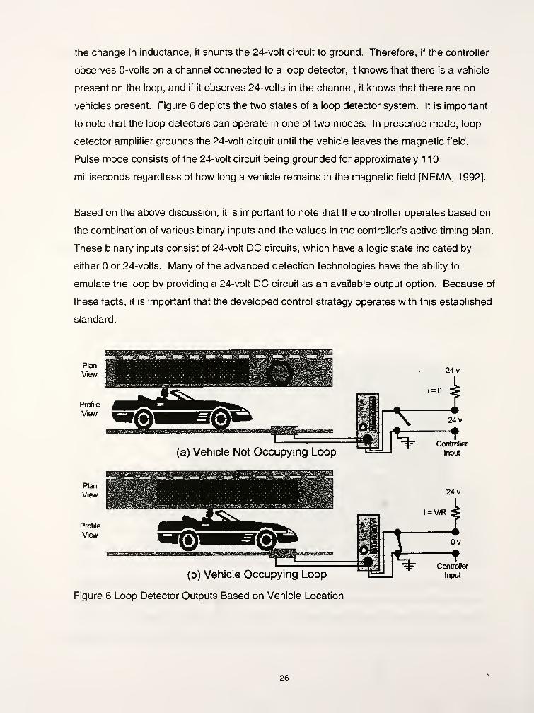
the change in inductance, it shunts the 24-volt circuit to ground. Therefore, if the controller

observes O-volts on a channel connected to a loop detector, it knows that there is a vehicle

present on the loop, and if it observes 24-volts in the channel, it knows that there are no

vehicles present. Figure 6 depicts the two states of a loop detector system. It is important

to note that the loop detectors can operate in one of two modes. In presence mode, loop

detector amplifier grounds the 24-volt circuit until the vehicle leaves the magnetic field.

Pulse mode consists of the 24-volt circuit being grounded for approximately 110

milliseconds regardless of how long a vehicle remains in the magnetic field [NEMA, 1992].

Based on the above discussion, it is important to note that the controller operates based on

the combination of various binary inputs and the values in the controller's active timing plan.

These binary inputs consist of 24-volt DC circuits, which have a logic state indicated by

either or 24-volts. Many of the advanced detection technologies have the ability to

emulate the loop by providing a 24-volt DC circuit as an available output option. Because of

these facts, it is important that the developed control strategy operates with this established

standard.

Controller

Input

(b) Vehicle Occupying Loop

Figure 6 Loop Detector Outputs Based on Vehicle Location

Controller

Input

26

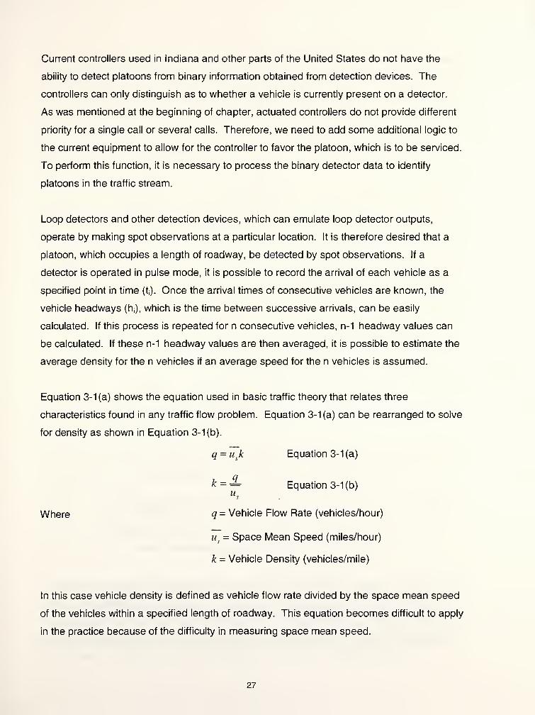
Current controllers used in Indiana and other parts of the United States do not have the

ability to detect platoons from binary information obtained from detection devices. The

controllers can only distinguish as to whether a vehicle is currently present on a detector.

As was mentioned at the beginning of chapter, actuated controllers do not provide different

priority for a single call or several calls. Therefore, we need to add some additional logic to

the current equipment to allow for the controller to favor the platoon, which is to be serviced.

To perform this function, it is necessary to process the binary detector data to identify

platoons in the traffic stream.

Loop detectors and other detection devices, which can emulate loop detector outputs,

operate by making spot observations at a particular location. It is therefore desired that a

platoon, which occupies a length of roadway, be detected by spot observations. If a

detector is operated in pulse mode, it is possible to record the arrival of each vehicle as a

specified point in time (tj). Once the arrival times of consecutive vehicles are known, the

vehicle headways (hj), which is the time between successive arrivals, can be easily

calculated. If this process is repeated for n consecutive vehicles, n-1 headway values can

be calculated. If these n-1 headway values are then averaged, it is possible to estimate the

average density for the n vehicles if an average speed for the n vehicles is assumed.

Equation 3-1 (a) shows the equation used in basic traffic theory that relates three

characteristics found in any traffic flow problem. Equation 3-1 (a) can be rearranged to solve

for density as shown in Equation 3-1 (b).

q = usk Equation 3-1 (a)

*== Equation 3-1 (b)

Where q = Vehicle Flow Rate (vehicles/hour)

us- Space Mean Speed (miles/hour)

jfc = Vehicle Density (vehicles/mile)

In this case vehicle density is defined as vehicle flow rate divided by the space mean speed

of the vehicles within a specified length of roadway. This equation becomes difficult to apply

in the practice because of the difficulty in measuring space mean speed.

27

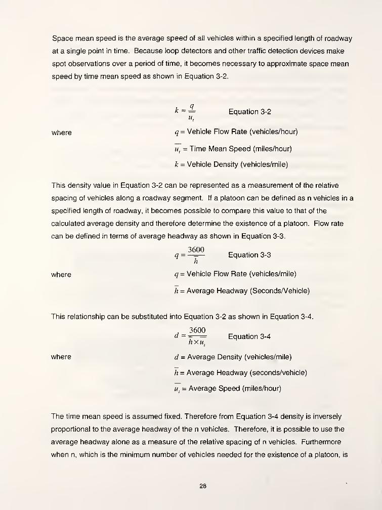
Space mean speed is the average speed of all vehicles within a specified length of roadway

at a single point in time. Because loop detectors and other traffic detection devices make

spot observations over a period of time, it becomes necessary to approximate space mean

speed by time mean speed as shown in Equation 3-2.

k~= Equation 3-2

where q = Vehicle Flow Rate (vehicles/hour)

w, = Time Mean Speed (miles/hour)

k = Vehicle Density (vehicles/mile)

This density value in Equation 3-2 can be represented as a measurement of the relative

spacing of vehicles along a roadway segment. If a platoon can be defined as n vehicles in a

specified length of roadway, it becomes possible to compare this value to that of the

calculated average density and therefore determine the existence of a platoon. Flow rate

can be defined in terms of average headway as shown in Equation 3-3.

3600q = - Equation 3-3

h

where q = Vehicle Flow Rate (vehicles/mile)

h = Average Headway (Seconds/Vehicle)

This relationship can be substituted into Equation 3-2 as shown in Equation 3-4.

, 3600« ~ =—= Equation 3-4

hxu,

where d - Average Density (vehicles/mile)

h = Average Headway (seconds/vehicle)

ut= Average Speed (miles/hour)

The time mean speed is assumed fixed. Therefore from Equation 3-4 density is inversely

proportional to the average headway of the n vehicles. Therefore, it is possible to use the

average headway alone as a measure of the relative spacing of n vehicles. Furthermore

when n, which is the minimum number of vehicles needed for the existence of a platoon, is

28

known, the average headway is directly related to the sum of the n-1 headway values for the

n vehicles considered. This value is referred to as the cumulative headway value (H). Since

the cumulative headway value for the n vehicles is equal to the headway between the first

and nth

vehicle, a platoon can be defined as the passage of n vehicles past a specific point

in a specified period of time, referred to as the critical time (T). In other words, a platoon

exists if the cumulative headway value for n vehicles is less than the critical time. This

decision rule is shown in Figure 7.

While the above definition of a platoon is fairly simple to understand and calculate, it is

important to note that there was a major assumption made in the process. This assumption

was that an average time mean speed was selected for all the vehicles instead of using

space mean speed. The potential impacts of this assumption will be discussed later in this

chapter.

n-l

If H =*Y.hi>T , then a platoon does not exist.

,=0

Where n - the minimum number of vehicles in a platoon

hi

- the headway value between vehicle nj and ni+1

H = the cumulative headway value for the n vehicles

T = the critical time for which platoon existence is

determined

Figure 7 Decision Rule for the Existence of a Platoon

The establishment of a methodology to identify platoons using spot observed data led to the

development of a process that would, perform this task in real-time using real detector

outputs. Current NEMA signal controllers do not provide any means of executing this task,

therefore, additional equipment would need to be selected. This device would need to be

able to process discrete detector outputs to identify platoons and then trigger the control

process involved in the accommodation of this platoon at the intersection.

The device that has been selected and developed to be the platoon detector is known as a

programmable logic controller (PLC). A PLC, shown in Figure 8, consists of an assembly of

solid state digital logic elements designed to make logical decisions and provide outputs

based on these decisions. A PLC operates on sequential instructions programmed in relay

ladder logic. A PLC can perform logic functions previously executed by a series of

29

electromechanical relays wired together. However, the PLC offers several advantages over

the traditional relay type of control. Some of these advantages include:

• logic configurations which can be easily changed without having to rewire individual

elements,

• solid-state reliability,

• lower power consumption, and

• ease of expansion.

345452

° ° ° oooooooooFigure 8 Programmable Logic Controller [GE Fanac, 1997]

A PLC consists of three parts. The central processor unit (CPU) contains the micro-

processor that controls the logic gate circuits, converter, timers, and other functions. The

I/O modules consist of the interface between the PLC and connected equipment. The final

part of the PLC is the programming device, which is external to the PLC, and connects to

the PLC's serial port. The programming device can be a personal computer or similar

device which facilitates the development of the logic programs used by the CPU [Petruzella,

1 989]. Figure 9 shows the configuration of a PLC connected to a personal computer for

programming.

30

oo

Series 90

Micro PLC LJ-RS-232

||RS-422

IC690CB!''"" "

10 Fe

(3 Mete

/ _ ___i—

A

-> r\ * «

(1 il_M !e

Figure 9 PLC Connected to a Computer Via the Serial Port [GE Fanac, 1997]

PLC units, which are used extensively in industrial applications, are made by several

different manufactures and are designed to operate in a wide range of temperatures and

humidity. They are manufactured in a variety of sizes to allow for increased flexibility in

development and expansion of control systems.

For this application a Micro Series 90™ PLC manufactured by GE Fanac was selected. This

model, shown in Figure 8 and Figure 9, operated on 1 10 volts AC and consisted of 8 input

modules, 6 output modules, and a serial communications port. The I/O modules were rated

for 24-volts DC. The PLC was purchased as part of a toolbox, which included the serial

cable, MS-DOS based programming software and all relevant manuals. The cost of the

complete package was approximately $270.

As was indicated earlier, the PLC has a CPU, which must be programmed before it can

operate. A PLC uses relay ladder logic as the language from which operational programs

are created. Based on the binary status of the input modules, the PLC executes the

programmed sequential instructions including timers, counters, and mathematical functions

to control the binary states of the output modules. Ladder logic is broken down into

individual lines of instructions referred to as rungs.

31

%I1 %I2 %Q1

hH <Leaend:

H h = Normally Open Contact

-H- = Normally Closed Contact

-c y = Output Contact%I3

Figure 10 Example of a Ladder Logic Program

An example of a ladder logic program is shown in Figure 10. In this example, there are

three input contacts and one output contract. This program consists of one rung. Reading

ladder logic is much like reading a text document. One progresses through the code by

beginning on the top rung and working from left to right. Once the end or right most portion

of a rung as been reached, the next rung below is executed beginning on the left. In this

example, output contact %Q1 can be energized (turned on) by one of two ways. The first is

when input %I1 is on and input %I2 is turned off. This might seem illogical that %I2 must be

off for %Q1 to be on, but %I2 is a normally closed contact. Normally closed contacts default

to having their relay closed when not receiving current. Therefore, to energize %Q1 through

%I1 , %I2 must not receive external power though the input module. The second possible

way in which output %Q1 can be energized is through %I3 being turned on. In this example

these three input contacts work together to determine the binary state of output %Q1 . Table

1 shows the state of %Q1 based on the status of the three input contacts.

The logic for the first version of the platoon detection algorithm only uses one input contact

and one output contact. However, the logic consists of several rungs containing timers,

counters, mathematical functions, and temporary memory allocations. The full program is

presented as Figure A-1 in the appendix. The program is essentially broken down into three

parts, which will be discussed individually.

32

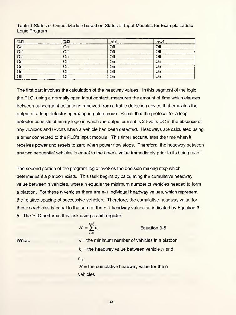
Table 1 States of Output Module based on Status of Input Modules for Example Ladder

Logic Program

%I1 %I2 %I3 %Q1On On Off Off

Off Off Off Off

Off On Off Off

On Off On OnOn On On OnOn Off Off OnOff Off On On

The first part involves the calculation of the headway values. In this segment of the logic,

the PLC, using a normally open input contact, measures the amount of time which elapses

between subsequent actuations received from a traffic detection device that emulates the

output of a loop detector operating in pulse mode. Recall that the protocol for a loop

detector consists of binary logic in which the output current is 24-volts DC in the absence of

any vehicles and 0-volts when a vehicle has been detected. Headways are calculated using

a timer connected to the PLC's input module. This timer accumulates the time when it

receives power and resets to zero when power flow stops. Therefore, the headway between

any two sequential vehicles is equal to the timer's value immediately prior to its being reset.

The second portion of the program logic involves the decision making step which

determines if a platoon exists. This task begins by calculating the cumulative headway

value between n vehicles, where n equals the minimum number of vehicles needed to form

a platoon. For these n vehicles there are n-1 individual headway values, which represent

the relative spacing of successive vehicles. Therefore, the cumulative headway value for

these n vehicles is equal to the sum of the n-1 headway values as indicated by Equation 3-

5. The PLC performs this task using a shift register.

n-1

" = 5>.- Equation 3-5

i=0

Where n = the minimum number of vehicles in a platoon

ht

= the headway value between vehicle n, and

n i+1

H = the cumulative headway value for the n

vehicles

33

The shift register is a specific memory location in which data is temporarily stored and

relocated according to a selected pattern [Simpson, 1994]. The type of shift register used

by this particular program is known as a first-in-first-out (FIFO) register. Conceptually this

FIFO register can be thought of as a sequence of slots for available data. New data is

inserted at the bottom of the stack, but before it can enter the stack, the existing values must

move or shift upward in the stack to open the bottom slot. The shifting action of the register

causes the highest value in the stack to be removed. Figure 1 1 shows this process for a

register with a length of five slots. This is the process by which the PLC stores individual

headway values. The cumulative headway is calculated using the PLC's addition function

each time a new headway value is added to the register.

(a) (b) (c)

248 ~ 248

593 i itn

"oco

593 u

264 264

375 375

871 Q 871 M-

248

176

593

264 11

375

871

176

FIFO Shift

Register with 5

slots

New data presents itself

to the stack

The existing data shifts

up in the stack and the

new data is inserted

Figure 1 1 Example of a FIFO Shift Register in Operation

Once the program logic calculates the cumulative headway value, the third and final stage of

the program begins. Using the "less than" logical function of the PLC, a comparison is made

between the calculated cumulative headway value and that of a predetermined critical value

stored in a different memory location. In this case, if the calculated headway value is less

than the critical value, it is determined that a platoon exists. Once the platoon's existence is

known, the PLC begins the process of manipulating the traffic signal controller to

accommodate the platoon at the intersection. This manipulation process will be discussed

in the next section. Figure 12 shows the sequential logic of the entire platoon detection

process.

34

Monitor Input From

Platoon Detector

No

Move HeadwayValue Into FIFO

Shift Register

1r

Calculate

Cumulative

Headway Value lor

n Vehilces

Yes

PLATOONIDENTIFIED'

Trigger Output to

Traffic Signal

Controller

Figure 12 Sequential Logic of Platoon Detection Process

Platoon Accommodation

The PLC provides for a method by which platoons of vehicles can be identified in a stream

of traffic based on spot observations. If the location of these spot observations is up stream

from a signalized intersection, the PLC is providing advanced information regarding the

future demand at the intersection for the instrumented approach. In situations where the

approach has predominate turning movements which are known, such as the through

movement of a major highway intersected by a minor road, it becomes logical to manipulate

the controller to accommodate the platoon in making this movement.

Accommodating a platoon is nothing more than ensuring that a green signal exists for the

predominate movement prior to the platoon's arrival at the intersection. In other words, this

35

green signal should be displayed no later than the point in time when the vehicles in the

platoon would normally begin to slow down if a red or amber signal were displayed. As was

indicated at the beginning of this chapter, actuated controlled intersections that are located

along high-speed roadways provide information from their local detectors, which allow for a

limited planning horizon. Since a platoon occupies a certain length of roadway and its

existence cannot be determined until the last vehicle passes the location at which the spot

observations are made, existing detector configurations at actuated controllers cannot

provide the information to the PLC for platoon detection. Allowance for the necessary time

for the controller to transition into the desired state is necessary, so the need of detecting

the arriving platoon in advance of its arrival at traditional local detectors is evident.

The accommodation of a platoon involves the identification of the platoon and then

predicting the time of its arrival at the intersection. As was discussed in the previous

section, the identification of the platoon is based on the assumption that all vehicles in the

platoon have a common speed. This assumed speed should therefore be used to predict

the time necessary for the platoon to traverse the distance form the location of the spot

observations to the intersection. Because of this assumption and other exogenous factors,

there is a trade off between the distance from the intersection to the location of the spot

observation and the accuracy of the prediction. It is true that the farther the location of the

information source is away from the intersection, the longer the potential planning horizon

the controller has with which to work to accommodate the platoon. However, the farther the

location of the source of information is from the intersection, the greater the chance of the

temporal distribution of the vehicles in the platoon to change during the planning horizon.

This change or distortion of the temporal distribution can result in platoon dispersion and

subsequently nullify the existence of the platoon downstream at the intersection. Therefore,

the location of the platoon detector becomes an important parameter in the prediction of a

platoon's arrival at an intersection.

Once the platoon detector is configured to make accurate predictions regarding the arrival of

platoons at an intersection, the process of manipulating the controller into allowing a green

window to open-up for any detected platoon is initiated. There are three methods of

manipulating the controller, which were considered for this platoon accommodation strategy.

The three methods considered are:

36

• application of phase holds and force offs to step the controller into the desired phase,

• generating and removing calls on local detector inputs to the controller, and

• low-level preemption.

Each of these methods and their potential use in this application will be discussed.

The traditional application of force off and hold inputs for a traffic signal control are for

keeping a signal, which is part of a system, in coordination with adjacent signals. Force offs

are points in a cycle in which specific phases must be terminated regardless of the traffic

demand for that phase. Holds do not have a defined location within a cycle, however they

too are used to keep adjacent signals in coordination. Holds are sometimes used to sync

the base reference point for a cycle when transitions occur in coordinated timing plans. For

accommodating platoons, the hold input would be used in cases where the current phase

needed to be extended to ensure the platoon receives the green signal. The force off inputs

would be used to terminate conflicting phases in order to cycle the controller into the desired

phase for accommodating the platoon at the desired time.

The second possible method of manipulating the controller involves the generation and

removal of calls on the detector inputs. The idea behind this concept is that when a platoon

is detected the controller can be coerced into a particular phase through a combination of

generating detector calls on the platoon's approach and removing calls for conflicting

phases. In this method the controller runs in actuated mode without the knowledge that

local detectors are detecting imaginary vehicles and actual vehicles are being ignored in

order for a phase to become green before the platoon arrives at the local detectors.

The final method is that of preemption. Traditionally, this involves the preemption of the

normal cycling of traffic signals for one of the following reasons [Gordon et al., 1996]:

• right-of-way is given to phase(s) not conflicting with movements over the track when a

signalized intersection is adjacent to a rail crossing,

• right-of-way assignment to emergency vehicles, such as fire trucks and ambulances,

and

• right-of-way provision to transit vehicles, usually buses.

While the application and transition procedure situations in which preemption is used may

differ, the purpose remains the same. Preemption involves the specification of which phase

37

or phases are allowed to be services during some specified period of time. The preemption

period begins based on the change in state of a binary input of the controller. The triggering

mechanism for this input is usually associated with the activation of the crossing gates for a

railroad preemptor or with the detection of an optical or radio signal transmitted from the

vehicle in the case of emergency and vehicle transit preemption.

A hierarchy or priority level is usually established for a preemption strategy in locations

where multiple types of preemption are enabled. This hierarchy allows the controller to

determine the desired coarse of action in cases where multiple preemption calls are

received. Typically railroad preemption is given the highest priority because of the necessity

of clearing potentially trapped vehicles from the path of an oncoming train. Railroad

preemptors are followed in level of priority by emergency vehicles and finally transit vehicles.

Emergency vehicle preemption is usually limited to fire fighting equipment because of its

lack of maneuverability at congested intersections, however, ambulances are sometimes

provided with the equipment to facilitate preemption. Bus preemption is at the lowest level

of the hierarchy, since unlike the other two, it does not greatly impact the safety of drivers at

the intersection or persons for whom emergency services were dispatched, but rather

improves the movement of a particular transportation mode.

In addition to determining which preemption call is serviced in the case of multiple calls,

priority has an impact on the aggressiveness of the actions taken by the controller to reach

the desired state. In the case of railroad preemption, the preemptor quickly begins its track

clearance phase by terminating any conflicting movements regardless of their location in the

timing sequence. Once the track clearance interval is completed, the controller begins

somewhat normal operation for the specified hold phases. The hold interval remains in

effect until the train has cleared the crossing or a maximum time has been reached.

Emergency vehicle preemption is also executed in a fairly aggressive manner, however,

unlike railroad preemption it only consists of a hold interval for a specific phase or set of

phases. The overall time of an emergency vehicle preemption sequence is usually much

less than that of railroad preemption. The lowest level of preemption is that of bus

preemption. The capabilities of this type of preemptor are limited in comparison to the

previous two. However, it does provide a mechanism for which a specified phase or

complementing phases can be serviced during a particular time interval.

38

Of the three methods considered for manipulating the controller, it was determined that

preemption would be used. This selection was based on the fact that this feature has been

built into many of today's deployed controllers and it operates based on the manipulation of

only one input pin to the controller. The other two options having been selected would have

resulted in the need to develop a more complex platoon accommodation algorithm, which

would have involved the manipulation of several of the controller's input pins. Additionally,

the use of preemption was considered the safest alternative. This was especially true when

compared to the first method proposed. The use of the hold and force off inputs to the

controller, has the risk of becoming locked in an undesirable state such as an infinite hold on

a particular phase.

It was determined that bus preemption would be the type of preemption used. This

selection was based on the fact that the platoon accommodation algorithm was to

manipulate the controller in the least intrusive manner possible. Due to the fact that bus

preemption was the selected method for manipulating the controller, it is necessary to

understand its operation. At this point it becomes important to note that bus preemption is

somewhat of a proprietary issue for each of the different manufactured brands of traffic

signal controllers available on the market. However, the difference between manufacturer's

products is likely to be small. This research made use of the Advanced System Controller

ASC/2-2100, Firmware Version 1.56, manufactured by Econolite Control Products, Inc. of

Anaheim, California. Therefore, the operation of bus preemption discussed below is based

on this particular model.

The configuration of bus preemption involves setting the values to parameters contained in

a preemptor menu. The key parameters identified for this research included: minimum hold

time, maximum time, reservice time, delay time, inhibit time, detector lock, and hold

phase(s). These parameters and their interactions will be discussed in Table 2.

39

Table 2 Low Level Bus Preemption Parameters [Econolite, 1996].

Parameter Description

Hold Phase Identifies which compatible phase of phases (up to two)

are to be serviced when a preemption call is received.

Delay Time Fixed period of time which elapses between the initial

receipt of a preemptor call and initiation of preemption.

Inhibit Time Final portion of delay time in which phases not part of the

preemption hold phase(s) are prevented form being

serviced next.

Minimum Hold

TimeFixed amount of time in which the specified preemption

phases must be held regardless of the current status of

the preemption input.

Maximum Hold

TimeTime in which preemption is terminated regardless of the

presence of a call.

Reservice Time Minimum period of time that is allowed to elapse betweensuccessive preemption sequences. The controller is

automatically required when coming out of a preemption

sequence to service any phase which has an active call

before it can accept a new preemptor call regardless of the

reservice time. Therefore, the reservice time consists of

the time required to perform this function as well as anyadditional desired time before the preemptor can be

reserviced.

Detector Lock When activated requires that a called preemption

sequence occurs even if the call is dropped during the

delay time.

There are two periods in the preemption sequence, which necessitate further explanation.

These two periods are at the point in which the preemptor becomes active and the point in

which normal service is continued.

Once a preemption call is received the process of transitioning to the selected hold phase(s)

begins when the delay time expires. (If the delay time is set to zero, this transition begins

immediately.) Before the transition beings the controller can be thought of as being in one

of two states. It is either in the desired phase or it is not. If the controller is in the desired

phase, no transition is made and the minimum hold time is initiated. In the event that the

controller is not in the desired phase, it becomes necessary to terminate the current phase

and possibly skip subsequent phases to enable the desired phase. The responsiveness of

the controller in making this necessary transition is limited. The limitation is that in order for

an active phase to be terminated, it must have been active for the duration of the minimum

green interval for that phase. In the case where a particular conflicting phase becomes

active immediately prior to a preemptor becoming active, the entire minimum green time

40

must be allowed to elapse. If the minimum green time is long, the process of beginning the

transition of the preempted phase becomes delayed. To prevent this sluggish performance,

an inhibit timer is used. As was indicated in Table 3-2, inhibit time is the final portion of the

delay time in which conflicting phases are not allowed to begin service. If the inhibit time is

greater than or equal to the longest minimum green time for all the phases normally

serviced, the longest possible transition time is equal to the longest clearance interval for all

the conflicting phases.

When the preemption sequence terminates the controller resumes normal operation in the

phase that was held by the preemptor. Depending on the state of the controller when the

preemptor became active, normal operation begins in one of two places in the timing

sequence of this phase. If the preempted phase was active at the beginning of the

preemption hold (end of delay time), and the minimum green time has elapsed, the

controller begins at the end of the minimum green interval. In all other cases, the controller

begins timing the phase at the beginning of the minimum green interval.

Platoon

Identified

Projected Platoon

Arrival

NoPreemption

Preemption

Active

01 02 03 ©4 01 / 02 03 04

05 06 07 08 05 // 06 07 08

Phase 4 & 8

Shortened

Phase 1 & 5

Skipped /

' /' /

' /

rV

01 02 03 04 02 03 04 01

05 06 07 08 06 07 08 05

tPremption

Call Received

Delay Time

tPremption

Sequence Initiated

Time of Day

Figure 13 Example of Preemption Impact on 8- Phase Timing Plan

Figure 13 shows an example of preemption used in the context of accommodating platoons

for a particular phase. This example illustrates a standard 8-phase timing plan in which a

platoon is detected on the approach tied to phase 2. The top plan shows what would

41

happen without preemption. It can be observed that for this case the platoon arrives at the

intersection during a time in which another phase is being serviced and therefore would be

required to stop. The bottom plan illustrates the effects of preemption when configured

properly. It can be seen that the initiation of the preemption sequence resulted in both

shortening phases 4 and 8 and not servicing phases 1 and 5. Note that the preempted

phase becomes active before the platoon's arrival. This serves to clear any vehicles, which

may be in the queue, and to prevent the platoon from slowing down as it nears the

intersection because of a red indication.

The previous section discussed the use of a PLC to implement this platoon accommodation

algorithm. The third portion of the sequential ladder logic programmed into the PLC involves

the manipulation of the traffic signal controller. The fact that preemption is activated by a

single binary input makes the interface between the PLC and the controller very simple. In

the particular model of controller used in this research, the bus preemptors are activated by

grounding one of the 24-volt preemptor input pins at a rate of 1 hertz per second [Econolite,

1 996]. The PLC performs this task through the use of interval timers connected to the

output module. The program logic is shown in Figure A-1 of the Appendix.

System Architecture

The first two questions posed at the beginning of this chapter have been addressed. A

strategy based on the use of a programmable logic controller has been developed to identify

platoons of vehicles in a traffic stream. Once a platoon has been identified, the same PLC

manipulates the controller into a specified phase(s). With the individual elements of the

strategy having been developed, it is necessary to establish the framework in which this

system will operate. This will answer the third and final question posed.

Figure 14 and Figure 15 depicts two possible functional block diagrams for the system.

Figure 14 has the PLC located in the traffic signal control cabinet where the other traffic

control decisions are determined and implemented. This central processing approach

requires that all data from the remote upstream traffic detector is sent through the

communications system back to the PLC. Figure 15 consists of a distributed processing

approach in which the PLC, which makes the decision as to whether a platoon exists, is

located at the remote site with the traffic detection device. While both approaches have the

42

potential to provide the same results, they each have their own positive and negative

aspects.

Upstream Traffic

Detection Device y*Communications

Medium

Remote Sitei_

-IProgramable

Logic Contoller

Traffic Signal

Contoller

Signal Cabinet

Figure 14 Functional Block Diagram for Central Processing Approach

Upstream Traffic

Detection Device

Programable

Logic Contoller

Remote Site

Communications

MediumTraffic Signal

Contoller

[_Signal Cabine

Figure 15 Functional Block Diagram for Distributed Processing Approach

The centralized approach has several positive advantages. First is that there is ample

available power to run the unit since both 1 10-volts AC and 24-volts-DC are provided for the

existing equipment located in the cabinet. Most existing cabinets have the necessary space

in which to house the PLC. Additionally, the particular model of PLC used for this project

has more input and output modules than are being used by the first generation platoon

accommodation algorithm proposed. Therefore, the PLC has the ability of allowing the

system to expand to incorporate platoon identification on multiple approaches to the

intersection and the ability to implement more sophisticated algorithms (strategies which

monitor the controller's status, etc) without any additional PLC devices. Furthermore, having

most of the intelligence of the system in the cabinet makes installation and maintenance

activities easier because cabinets are typically located well off of the roadway where

personnel have the space necessary to safely perform their work. The primary

disadvantage of the centralized approach is that extensive amounts of vehicle arrival data

are sent through the communications system from the remote site to the signal cabinet in

which the PLC resides. This extensive use of the communications system may greatly

increase the power requirements of the remote site. This may become a critical issue if the

remote site is to run on an alternative power source such as solar power.

The distributed processing approach has one primary benefit over that of a centralized

approach. The distributed approach has the PLC located in the field with the traffic

detection device. In this configuration, the PLC processes all of the detector outputs at the

remote site and only makes use of the communications network when a platoon has been

43

detected. This process greatly reduces the amount of information communicated through

the system thereby reducing the communications power requirements at the remote site. It

should be noted that the power required by the PLC is much less than that normally used in

communications equipment such as radio transmitters. Therefore, the incorporation of the

PLC with the equipment already located at the remote site does not necessitate the need for

more power, but rather reduces the overall power demand at the remote site due to the

significant reduction in communications requirements.

Chapter 5 will discuss the recommended architecture based on the cost and power

consumption of all the various devices.

Equipment

The above discussion has outlined two approaches possible in which the strategy may be

implemented. The four critical elements of both approaches that have been identified are:

• programmable logic controller (PLC),

• traffic detection device,

• communications link between the remote field site and the traffic signal controller, and

• power supply for the remote field site.

The first component has been previously discussed, so the focus of this section will be on

the remaining three. There are several different available technologies and methods that

can perform these functions.

The advancements made in the Intelligent Transportation System (ITS) initiative over the

past few years has had a significant impact on the vehicle detection segment of the traffic

control industry. There are several types of detection technologies that exist in today's

market. Table 3 lists the most common types and provides a brief description of how each

functions.

INDOT has had experience with most of these technologies in the past. Phase I of the

Borman Expressway Advanced Traffic Management System (ATMS) involved the functional

testing and evaluation of different traffic detection devices. Because of the substantial effort

made by INDOT in the process of conducting these tests, it was important to include their

44

findings as part of the information used to select a detector for the platoon accommodation

strategy. In conversations with personnel from INDOT and Iron Mountain Systems, INDOT's

system integration contractor for Phase II of the Borman ATMS project, it was recommended

that two detector technologies be considered. The technologies were inductive loop

detectors and sidefire radar [Boyd and Anderson, 1998]. Both of these detector

technologies can reliably provide vehicle presence data needed for platoon detection.

However, both technologies have different advantages and disadvantages.

45

Table 3 Current Available Detection Technologies [MinDOT and SRF Consultants, 1997].

Technology Description

Passive Infrared Passive infrared devices detect the presence of vehicles by comparing the

infrared energy naturally emanating from the road surface with the change in

energy caused by the presence of a vehicle. Since the roadway may

generate either more or less radiation that a vehicle depending on the

season, the contrast in heat energy is what is detected.

Active Infrared Active infrared devices detect the presence of vehicles by emitting a low-

energy laser beam(s) at the road surface and measuring the time for the

reflected signal to return to the device. The presence of a vehicle is

measured by the corresponding reduction in time for the signal return.

Magnetic - Passive and Active Passive magnetic devices measure the change in the earth's magnetic flux

created when a vehicle passes through a detection zone. Active magnetic

devices, such as inductive loops, apply a small electric current to a coil of

wires and detect the change in inductance caused by the passage of a

vehicle.

Microwave - Doppler, Radar and

Passive Millimeter

Doppler microwave devices transmit low-energy microwave radiation at a

target area on the pavement and then analyze the signal reflected back to the

detector. According to the Doppler principle, the motion of a vehicle in the

detection zone causes a shift in the frequency of the reflected signal. This

can be used to detect moving vehicles and to determine their speed. Radar

devices use a pulsed, frequency-modulated or phase-modulated signal to

determine the time delay of the return signal, thereby calculating the distance

to the detected vehicle. Radar devices have the additional ability to sense the

presence of stationary vehicles and to sense multiple zones through their

range finding ability. A third type of microwave detector, passive millimeter,

operates at a shorter wavelength than other microwave devices. It detects

the electromagnetic energy in the millimeter radiation frequencies from all

objects in the target area.

Passive Acoustic Passive acoustic devices consist of an array of microphones aimed at the

traffic stream. The devices are passive in that they are listening for the sound

energy of passing vehicles.

Ultrasonic - Pulse and Doppler Pulse devices emit pulses of ultrasonic sound energy and measure the time

for the signal and utilize the Doppler principle to measure the shift in the

reflected signal.

Video Video devices use a microprocessor to analyze the video image input from a

video camera. Two basic analysis techniques are used: tripline and tracking.

Tripline techniques monitor specific zones on the video image to detect the

presence of a vehicle. Video tracking techniques employ algorithms to

identify and track vehicles as they pass through the field of view. The video

devices use one or both of these techniques.

As was discussed in Chapter 2, inductive loops are not a new technology in traffic control

operations. They provide a reliable and relatively low cost form of traffic detection.

46

Depending on the type of detector arrangement used vehicle volume, presence and speeds

can be observed. The major drawback to using loop detectors is that they require lane

closures to install. This can have a significant negative impact in locations where high

volumes of traffic are present. The cost of a typical loop installation is approximately $500

per loop [Shamo, 1998].

Sidefire radar is a non-intrusive form of detection in that it does not require any disruption to

traffic flow during installation. Unlike many non-intrusive forms of detection, the sidefire

radar does not have to be located overhead of the lanes or pointed at oncoming traffic. The

sidefire radar unit can be located along the side of the roadway perpendicular to traffic and

still detect multiple lanes [MinDOT and SRF Consultants, 1997]. The sidefire unit

recommended, which will be discussed in Chapter 5, has the ability to emulate loop detector

outputs and therefore can provide vehicle presence, volumes and speeds if multiple

detection zones are configured. An additional benefit of sidefire radar is that it can be

moved from once location to another. Loop detectors do not provide this flexibility. The

major drawback of sidefire radar is its excessive cost. The base price for one unit is $3,300

[MinDOT and SRF Consultants, 1997].

The communications element of the system also has several technologies to provide the

desired functionality. The three technologies considered were that of hardwire, spread-

spectrum radio, and low-power FM radio. For the relatively small amounts of data, which

needed to be communicated in this system, the available bandwidth of all these

technologies exceed the expected amount needed. Therefore, bandwidth was not a factor

in the selection of a particular technology. The primary factors that were considered were

that of cost and amount of integration required to interface with the other components of the

system.

A hardwire connection would provide for a direct physical connection between the remote

detection site and the traffic signal control cabinet. While this type of medium is arguably

the most reliable of the three options, it has a substantial cost associated with the

installation. In discussions with INDOT's Traffic Design Section, it was estimated that the

cost to install a conduit containing the necessary wire would be $10.60 per linear foot.

Assuming that the remote detector is at least 0.5 miles (2640 feet) away from the

47

intersection, the cost of this option would be approximately $28,000. As the distance

increases between the remote site and the intersection, this cost continues to grow.

The other two types of communications technologies considered are wireless. The reliability

of the two methods when properly configured is similar. However, the FM radio, which will

be described in Chapter 5, has some distinct advantages. It costs approximately $200 less

than the spread spectrum radio and has normally open and normally closed contacts as

inputs and outputs. These are the states provided from a loop detector and detectors that

emulate the output of loop detectors as well as the type of input required by the PLC.

The final piece of equipment to be discussed is that of a remote power supply. There are

several methods that can be used for providing power to electronic devices. The most

obvious is that of energy obtained from a utility company. When this option is available, it is

usually the most economic alternative. However, when utility power lines are not available

other forms of power must be considered. Of all the various methods of generating power

available, solar power has been the method used most often in transportation related

systems, such as motorist call boxes. Therefore, the two types of power supplies

considered in Chapter 5 are that of solar and electricity provided by a public utility company.

Chapter 5 will discuss the recommended equipment for field deployment along with their

associated costs.

48

CHAPTER 4 WORK PLAN

The previous chapter described a strategy for accommodating platoons at isolated

intersections. This was a new concept for which performance characteristics were

unknown. In order to begin to gain an understanding of how this strategy performed, it was

decided to use a microscopic computer simulation as a tool from which an evaluation could

be conducted.

The Traffic Software Integrated System (TSIS) package developed by Kaman Sciences

Corporation for the Federal Highway Administration was the selected simulation software for

conducting the simulations. This package consisted of both the CORSIM microscopic traffic

simulation application and the CORSIM output processor, TRAFVU. TSIS is a Windows5

based program which runs on a standard personal computer [Kaman, 1997A]. In addition to

TSIS, the Interactive Traffic Network Data Editior (ITRAF) was used for creating the data

files that serve as inputs to CORSIM. The decision to use simulation over that of a field

experiment was due to several reasons. These were as follows [Kaman, 1997B]: simulation

was a more economical approach than a field experiment, data generated by simulation,

including measures of effectiveness criteria would be difficult to obtain in field experiments,

simulation would not disrupt actual live traffic, wide variations in traffic conditions, which may

seldom or never occur in the field, can be evaluated, and many variables of the traffic

control problem can be held constant.

At the core of the TSIS package is the use of the TRAFfic (TRAF) system, which is an

integrated set of simulation models that represent the traffic environment. TRAF was

developed by the Federal Highway Administration (FHWA) in the 1970's. The motivation for

its development was because of the need for a user friendly simulation package that was

capable of representing traffic flow in a large urban area which contained freeway and

surface street networks [Kaman, 1997B].

The CORSIM simulation model consists of both the FREESIM and NETSIM models

developed as a part of TRAF. It is a microscopic simulation model capable of simulating

very detailed strategies. In microsimulation, the models represent movements of individual

vehilces influenced by driver behavior [Kaman, 1997B].

49

The files used for the inputs to the CORSIM simulator are .trf files. As was indicated earlier,

these files can be created using the ITRAF editor. ITRAF uses a graphical user interface to

create or modify the individual records contained in each .trf file. These records contain

information on the following model inputs [Kaman, 1997B]:

• geometric data (node locations, link locations, number of lanes, length of turn lanes,

number of lanes, lane widths, etc.),

• traffic control data (control type, control settings, etc.),

• vehicle data (volumes, turning percentages, percent trucks, etc.), and

• run controls (simulation intervals, random number seeds, etc.)

• Figure 1 6 shows the ITRAF editor dialog box for entering geometric data for a link.

In 1997, Bullock and Catarella introduced a real-time simulation environment for evaluating

traffic signal systems. This environment consisted of an enhancement made to the

CORSIM package described above which allows for physical control equipment to be

connected to CORSIM. This type of simulation is refered to as hardware-in-the-loop

simulation.

^ Ffc Bode tir* BtnCtf Betfcy Option* Mood IP Vafndom ijdp

0O.W1 -JTioo PoriaM -XeoW rod SiMlT •" iXt ' -ifftxl£81^I—J——

i

=M*1

38 Slat| J»Sa3=?^)£lS£31Eraffl&3!£Sj C3if*S ' li£AMB«»«»-| »TaS-|P3o.ig_|[HlTBAFZ:0 ... gf>feo.otWord-j .J jmpm

Figure 16 ITRAF User Interface for Link Characteristics

50

The connection between CORSIM and the control hardware is achieved through the use of

the Controller Interface Device (CID) shown in Figure 17. The CID allows CORSIM to

conduct the microscopic simulation (movement of individual vehicles) and tabulation of

measures of effectivness (MOE) data, but CORSIM does not use its internal control

algorithms. CORSIM uses the CID to send detector information to the controller and to read

back phase indications. Current CID devices are made to interface with hardware

conforming to the NEMA TS1 specifications for detector inputs and phase outputs. The CID

type of CORSIM control was not found to be statistically different than than of internal

control when identical timing plans were evaluated [Bullock and Catrella, 1997]. The

advantage of hardware-in-the-loop simulation is that actual field equipment, which has more

features than CORSIM's internal control algorithm, can be used in making control decisions

in the simulation.

Figure 17 Controller Interface Device Connected to NEMA TS1 Compliant Controller

[Bullock and Catarella, 1997]

51

The platoon accommodation algorithm descripted in Chapter 3 was developed based on the

use of a programable logic controller (PLC). The use of this device was necessary to

supplement the logic contained in the typical actuated controller. Consequentially, in order

to conduct an evaluation of this strategy, it became necessary to use hardware-in-the-loop

simulation. The reasons for this are that the internal control algorithms of CORSIM do not

have preeption features and the current version of CORSIM does not have the ability to

emulate the PLC functionality. Therefore, a simulation environment using the CORSIM

computer, CID, PLC, and a NEMA TS1 complient traffic signal cabinet was constructed.

This environment is shown in Figure 18.

Once the simulation environment was established, it became necessary to define a test

case for which the new strategy could be evaluated. It was desired that an isolated

intersection would be selected near the Purdue University campus in West Lafayette,

Indiana. This intersection was to be controlled by an actuated controller and have a

significant amount of platooning behavior for traffic on at least one approach to the

intersection.

j

Platoon Detector Calls

Programable

Logic Controller

Preemotor Calls

Local Detector Calls

Phase Indication Status

L3

Controller Interface

Device

CORSIM Computer

Figure 18 Simulation Environment Configuration

NEMATS1 Cabinet

52

fc \ i^jLt

_F 35t', ;HE*!

Norfolk & Southern R.R. \ F »« s-j-

US 52 & CR 350S \

OifPitYjri S> 1953-1 996, fcfcfQSOft CwporaefOft -ni>_l/or c; SuppSsrS', ^Jriyrs^rii.-rr.e'j

Figure 19 Map Showing Study Intersection Location [Adapted from Microsoft4 Automap

1997]

Figure 20 Arial Photo of Lafayette Area [Micrcocrt 1998]

53

Figure 21 Arial Photo of Study intersection [Microsoft, 1998]

The selected intersection is shown in Figure 19, Figure 20, and Figure 21 . It is located at

the intersection of C.R. 350 South and U.S. 52 in Tippecanoe County south of Lafayette.

This intersection was controlled by an actuated controller with detection on all aproaches.

Platoons of traffic were observed to exist on the southbound apr rr>a«_. , of the intersection.

These platoons were generated by an active railroad crossing 0.6 miles to the north.

This rail line operated by Norfolk and Southern served the Suburu-lsusu Assembly plant

located northeast of the intersection. During some times of the day trains would occupy the

crossing for several minutes resulting in the formation of large platoons of southbound

vehicles north of the crossing. Once the train traversed the track, these platoons would be

released creating a significant peak in this approach's demand for green time at the

intersection. It was felt this situation would be a suitable test case because of the random

occurrences of large platoons.

Data Collection

Before simulation was initiated, relevant data was collected to serve as input into the

CORSIM simulator. Geometric data was collected through field measurements. This

information included: lane widths, turn bay lengths, and detector locations. Figure 22 shows

54

this information. Timing data for this signal was provided from the Indiana Department of

Transportation's Crawfordsville District. Table 4 shows the important controller timing

parameters for the ring structure shown in Figure 22. Dave Cochran of Purdue University's

School of Civil Engineering collected traffic volume data. Mr. Cochran provided counts for

all four approaches aggregated into 1 -minute intervals. This data spanned the course of 1

week. In addition to the volume data collected, turning movement data was collected for all

approaches during a series of 15-minute intervals during the week in which volume data

was collected.

OO

C.R. 350 South

O

C^ ooooo ooo

320'

<t>l

L

02

Y

<(>4

1 A -h05 <)>6

O

Q

b o

tN

Cf)

en /

320'

OOO ooooo Z2

/

o

oo

Figure 22 Study Intersection Layout and Phasing

55

Table 4 Study Intersection Timing and Control Settings [INDOT, 1998]

Phase 1 2 3 4 5 6 7 8

Minimum Green 6 15 8 6 15 8

Vehicle Extension 1.5 5.0 2.0 1.5 5.0 2.0

Yellow 3.5 4.5 3.5 3.5 4.5 3.5

All Red 1.5 2.0 1.5 1.5 2.0 1.5

Maximum Green 25 50 35 25 50 35

Seconds Per Actuation 1.5 1.5

Time Before Reduction 23 23

Time to Reduce 20 20

Minimum Gap 3.5 3.5

Maximum Initial 35 35

Locking Memory X X

Soft Recall X X

56

Table 5 Volume Data For Study Intersection

Southbound US 52 Northbound US 52 Eastbound CR 350S Westbound CR 350S

Interval Time Minute

VolumeEquivalent

VPHMinute

VolumeEquivalent

VPHMinute

VolumeEquivalent

VPHMinute

VolumeEquivalent

VPH

16:00 4 240 8 480 3 180

16:01 6 360 7 420 3 180

16:02 9 540 7 420 7 420

16:03 6 360 6 360 5 300

16:04 1 60 5 300 8 480 15 900

16:05 1 60 6 360 13 780

16:06 15 900 6 360 7 420

16:07 8 480 10 600 3 180

16:08 7 420 7 420 7 420

16:09 57 3420 11 660 10 600 10 600

16:10 33 1980 8 480 13 780 4 240

16:11 28 1680 9 540 15 900 7 420

16:12 9 540 3 180 6 360 6 360

16:13 13 780 2 120 9 540 8 480

16:14 4 240 7 420 6 360 4 240

16:15 15 900 9 540 9 540 10 600

16:16 7 420 4 240 11 660 3 180

16:17 9 540 8 480 9 540 2 120

16:18 14 840 6 360 8 480 5 300

16:19 17 1020 4 240 8 480 2 120

16:20 7 420 6 360 7 420 8 480

16:21 11 660 3 180 10 600 10 600

16:22 6 360 4 240 4 240 3 180

16:23 6 360 3 180 6 360 5 300

16:24 3 180 4 240 3 180 6 360

16:25 1 60 3 180 6 360 4 240

16:26 6 360 3 180 7 420

16:27 6 360 4 240 8 480

16:28 1 60 4 240 3 180 3 180

16:29 9 540 4 240 7 420

16:30 6 360 11 660

16:31 41 2460 3 180 1 60 1 60

16:32 22 1320 7 420 10 600 1 60

16:33 9 540 4 240 2 120

16:34 6 360 7 420 5 300

16:35 3 180 8 480 6 360 1 60

16:36 2 120 3 180 4 240 5 300

16:37 2 120 7 420 2 120 15 900

16:38 39 2340 1 60 4 240 3 180

16:39 5 300 6 360 4 240 7 420

16:40 7 420 5 300 10 600 7 420

16:41 14 840 4 240 4 240 8 480

16:42 3 180 9 540 8 480 6 360

16:43 10 600 5 300 6 360 3 180

16:44 10 600 4 240 2 120 5 300

57

Flow Profile for Southbound Traffic

Simulation Period 3

60 j

55

50m=45

540

|35

o30>525

JJ20

lisz

10

5

16:00 16:01 16:02 16:03 16:04 16:05 16:06 16:07 16:08 16:09 16:10 16:11 16:12 16:13 16:14

Beginning of Time Interval

Figure 23 Flow Profile for US 52 East on April 8, 1998 from 16:00 to 16:15 PM

Flow Profile for Southbond Traffic

Simulation Period 4

16:25 16:26 16:27 16:28 16:29 16:30 16:31 16:32 16:33 16:34 16:35 16:36 16:37 16:38 16:39

Beginning of Time Interval

Figure 24 Flow Profile for US 52 East on April 8, 1998 from 16:25 to 16:39 PM

Once the volume data was processed, two time periods were initially selected and denoted

as Periods 1 and Period 2. For reasons, which will be explained later, these 30-minute

intervals were later reduced to 15-minute periods referred to as Period 3 and Period 4. The

volume data for these periods are shown in Table 5. Period 3 consisted of the time interval

from 16:00 to 16:15. This first 15-minute period consisted of a period of time in which one

train occupied the crossing for approximately 9 minutes. The shaded areas in Table 5

indicates the time of the trains' presence. The second 1 5-minute period of volume data,

58

Period 4, was from 1 6:25 to 1 6:40. Period 4 included the passage of two trains, which

occupied the crossing for approximately 6 minutes and 5 minutes, respectively. These two

time intervals provided for two unique traffic flow profiles in which platooning behavior could

be easily seen. Figure 23 and Figure 24 show the southbound traffic upstream from the

intersection during Periods 3 and 4, respectively. Table 6 shows turning movement data

collected the same afternoon as that of the two selected periods.

Table 6 Turning Movement Data

Approach Left Through Right

Northbound 10% 86% 4%Southbound 12% 70% 18%Eastbound 18% 54% 28%Westbound 26% 69% 5%

Simulation Procedure

The data collection effort discussed in the previous section, allowed for the simulation

experiments to be conducted. Due to the type of simulation environment being used for this

evaluation, input data was needed for the following components:

• CORSIM (traffic and geometric data),

• Traffic Signal Controller (supplied timing plan plus supplemental bus preemptor plan),

and

• Programmable Logic Controller (platoon detection setting which consists of a specified

number of vehicles arrivals in a specified amount of time).

The input data for the simulations were broken into two groups. These groups are fixed

data, which was held constant for all simulation runs, and variable data, which was allowed

to vary. Table 7 shows the data parameters from both groups and a description of each.

59

Table 7 Data Input Parameters for Simulations

Fixed Inputs


Geometric Information relative to roadway dimensions and detector

placements

Controller Timing Data

for Normal Control

Information pertaining to the control parameters by the traffic

signal when operated under normal operation (minimumtimes, maximum times, clearance times, vehicle extension

times, etc.)

Turning Percentages Percentage of vehicles making left, through, and right

movements from a particular approach

Vehicle Classifications Vehicle classifications consisted of 98% passenger cars and2% trucks

Main Street (US 52)

VolumesVolume of northbound and southbound traffic

CORSIM RandomNumber Seed Sets

CORSIM uses three random numbers to control the

following:

Emission headwaysGenerated traffic

driver responses to traffic choices [Kaman, 1997B].

Variable Inputs


Minor Street (C.R.

350) VolumeVolume on eastbound and westbound approaches defined as

a certain percentage of the collected volume

Bus Preemption

Settings

Parameters discussed in Table 2 including: maximum time,

minimum time, reservice time, delay time, and inhibit time.

Programmable Logic

Controller Settings

The PLC determines platoon existence based on:

Minimum number of vehicles in a platoon

Maximum headway between the first and last vehicles in the

specified minimum platoon size

Platoon Detector

Location

Distance upstream from the stop bar in which the traffic

detection device used for platoon identification is located

The fixed inputs discussed in Table 7 were entered once and remained constant throughout

all the simulation periods. The last parameter in the fixed input portion of the table consisted

of 20 sets of random number seeds. The values for these random number seeds are shown

in Table B-1 of Appendix B. For this evaluation, every simulation trial consisted of 20 runs

using each group of random number seeds once.

To expedite the task of creating .trf input files and processing CORSIM output files, a set of

macros were developed for Microsoft® Word and Excel. The preprocessor operated in Word

and essentially took an established .trf file, referred to as the base file, and created 20 .trf

files each containing a different set of the random number seeds shown in Appendix B. The

preprocessor also created a script file that CORSIM used to process multiple .trf files

sequentially without operator intervention. The postprocessor consisted of two parts. The

60

first part was a Word macro that extracted various MOE performance indicators from each of

the individual output files for the 20 runs and saved these selected results as .txt files. This

was followed by the second part consisting of an Excel macro, which tabulated all of the

extracted data contained in the .txt files from part one and generated a summary page as

shown in Appendix C. Figure 25 shows the file management strategy used in this research.

Base . trfPreprocessor

(Word Macro)Seededtrf Files

CORSIM Script

Execution

Postprocessor

(Word Macro)Stripped

out Files

Postprocessor

(EXCEL Macro)

.5L \. IS

^-:-fnir?iwmMiiijI I I 1

1 1 1 1

l-H-H-Ha

TZ^HH^m—3—a-^» •?—J- -i

M—a—i »-§-§-§

\kLnn

MOE Summary Sheet

Figure 25 File Management Strategy

As can be seen above, Table 7 consists of several variable inputs which impact the

performance of the intersection. A detailed sensitivity analysis of each of these parameters

would involve a great deal of effort beyond that of this research. However, in order to begin

to gain an understanding of what the potential impact platoon accommodation can have on

intersection performance several different combinations were evaluated.

Table 8 shows the combinations evaluated in this project. The configurations designated E-

100 and E-50 represent the baseline conditions for 100% and 50% of the collected volume

along C.R. 350 South, respectively. In all cases tested, the volume along U.S. 52 was

100% of that which was collected and only CR 350 volumes were allowed to deviate from

100%. The reason for evaluating the cases in which 50% of the collected side street volume

existed was that it was felt that there was not enough discrepancy between the volume for

61

the major road (U.S. 52) and the minor road (C.R. 350). For all cases, the platoon detector

was located on the southbound approach and the through movements for the southbound

and northbound movements were tied to the preemption sequence. There were initially

many runs that were processed, but they are not shown in Table 8. These runs were a

series of trial and error procedures used to gain a preliminary understanding of the

simulation environment and to serve as a functionality test for the equipment, simulator,

preprocessor and postprocessors.

Two key elements came out of this process. The first was that 30-minute simulations

containing the level of railroad activity discussed earlier tended to mask the impact of the

platoon accommodation strategy. Once this period was shortened to 15-minutes, the effects

of the platoon accommodation could be observed. The decision of using 15-minute

simulation intervals is supported by Chapter 9 of the Highway Capacity Manual (HCM).

Equation 9-9 in the HCM shows the process by which hourly volumes are converted to peak

15-minute periods for analysis [National Research Council, 1994]. The second was the

importance of the preemption inhibit timer which limits the controller in servicing conflicting

phases at the end of the delay period. Initially this factor was set to 0, which resulted in the

sluggish response of the controller to a preemption call. Once this value was set to a higher

value the signal's response to the preemption call became more consistent.

62

Table 8 Simulation Configurations Evaluated

Configuration

Designation

Side

Street

Volume%

Platoon

Setting

MaximumHold

Time

MinimumHoldTime

Reservice

TimeDelay

Time

Inhibit

Time

Detector

Location

from Stop

Bar

A-100 100% 11 veh.

in 10

sec.

45 60 25 13 2640'

B-100 100% 16 veh.

in 15

sec.

45 60 20 13 2640'

C-100 100% 6 veh.

in 10

sec

45 60 25 13 2640'

D-100 100% 6 veh.

in 5

sec

45 60 30 13 2640'

E-100 100% Baseline Conditions for 100% Side Street Volume - No Preemption Timing

Plan UsedA-50 50% 11 veh.

in 10

sec.

45 60 25 13 2640'

B-50 50% 16 veh.

in 15

sec.

45 60 20 13 2640'

C-50 50% 6 veh.

in 10

sec

45 60 25 13 2640'

D-50 50% 6 veh.

in 5

sec

45 60 30 13 2640'

E-50 50% Baseline Conditions for 50% Side Street Volume - No Preemption Timing Plan

Used

After a good understanding of the system was grasped, the simulation trials shown inTable

9 were conducted. The results from these trials are shown in Appendix C as the figure

indicated the corresponding cell of Table 9.

63

Table 9 Simulation Trials Completed

Configuration Evaluated Period 3 Period 4

A-100 Figure C-1 Figure C-1

1

B-100 Figure C-2 Figure C-1

2

C-100 Figure C-3 Figure C-1

3

D-100 Figure C-4 Figure C-1

4

E-100 (Existing Conditions) Figure C-5 Figure C-1

5

A-50 Figure C-6 Figure C-1

6

B-50 Figure C-7 Figure C-1

7

C-50 Figure C-8 Figure C-1

8

D-50 Figure C-9 Figure C-1

9

E-50 (Existing Conditions) Figure C-1 Figure C-20

Simulation Results

The results of the trials, which are shaded in Table 9, will be discussed in detail. These

trials are for Period 3 configuration D-100 and Period 3 configuration E-100 that is the

associated baseline case. The evaluation of the different platoon accommodation strategies

was accomplished by comparing the delay time (sec/veh) and percent stops for all

movements an all approaches between the baseline conditions and that of the selected

strategy. The output generated by CORSIM and processed by the postprocessor macros

discussed in the previous section computed the average values and standard deviations for

all positive turning movements at the intersection. Computing the test statistic for two

means with unequal variances compared the two scenarios. The hypothesis for this

evaluation is H : u-i=U2.

64

Table 10 Summary of Simulation Results Contained in Appendix C

Configuration

Evaluated

Period 3 Period 4

Delay

(seconds)

% Stops Delay

(seconds)

% Stops

A-100 29.9 55 13.7 36

B-100 35.8 66 14.1 37

C-100 32.4 59 12.1 31

D-100 28.7 54 11.8 32

E-100 (Existing

Conditions)

35.7 65 13.5 35

A-50 22.0 46 9.1 25

B-50 22.7 47 8.7 24

C-50 21.5 44 9.1 25

D-50 21.1 43 9.0 24

E-50 (Existing

Conditions)

23.5 50 9.0 25

The test statistic shown in Equation 4-1 was computed to determine if there was a

statistically significant difference between the means for the two cases. For all cases

evaluated, the number of observations was 20 and these observations were assumed to

have a normal distribution. The critical values for a two-tailed test of the test statistic at the

0.05 significance level for 18 degrees of freedom are +2.101 . The magnitude of this value is

denoted as Z". The decision rule for the hypothesis is as follows:

If \Z\>Z, then H is rejected.

Therefore, if we reject the null hypothesis, we can be 95% confident that the computed

means for the baseline and platoon accommodation strategy are statistically different.

Where

Z = ^,-^2

n, n n

Equation 4-1

Z is the computed test statistic

ni

is the number of observations in group i

fi. is the mean of the observations in group i

siis the standard deviation of the observations in

group i

Table 1 1 shows the means, standard deviations, and test statistics for Period 3 configuration

D-100. It was shown that the platoon accommodation strategy implemented statistically

reduced the percent stops and delay for the southbound approach without any statistical

65

impact on the other movements. In this case the southbound movement had the percent

stops reduced from 65.5% to 53.6% and the delay time reduced from 37.8 seconds'vehicle

to 28.7 seconds/vehicle. Therefore, ft was shown that platoon accommodation can improve

the operational efficiency of isolated intersections.

It has been shown that platoon accommodation can improve the operational efficiency of

isolated intersections. However, if the system is improperly configured a less than desirable

result can occur. Figure D-21 in Appendix D shows the results from a case ran during the

trail and error period from Period 4 in which the platoon identification parameters were

improperly set. When compared to the baseline conditions (configuration E-100) for the

corresponding traffic volume, it can be observed that the platoon accommodation strategy

used in Figure D-21 actually degraded the performance of the intersection. Therefore, a

clear understanding of each of the variables" impact on performance should be examined

further prior to making recommendations for deployment configurations.

Chapter 5 describes the technical and financial issue with implementing this technology.

Chapter 6 presents an analysis of the platooning characteristics of CORSIM to determine if

the extent of platooning observed in CORSIM is reasonable to expect in the field.

56

Table 1 1 MOEs and Test Statistics for Period 3 Configuration D-100

Delay Per Vehicle (Seconds Per Vehicle)

N= 20

Average 1

(Existing)

Average 2

(Proposed)

Standard

Deviation 1

(Existing)

Standard

Deviation 2

(Proposed)

Test

Statistic

Northbound Left 33.23 38.73 7.80 11.37 -1.78

Through 12.82 13.23 1.22 1.44 -0.97

Right 8.86 8.06 5.35 3.98 0.54

Southbound Left 69.68 71.62 15.87 14.83 -0.40

Through 35.75 28.69 12.18 7.13 2.24

Right 19.15 19.01 4.48 5.34 0.09

Eastbound Left 24.51 25.55 5.64 5.33 -0.60

Through 22.90 22.07 4.13 5.03 0.57

Right 20.52 19.76 5.12 5.18 0.47

Westbound Left 20.23 21.37 6.13 6.56 -0.57

Through 22.60 23.36 3.32 3.43 -0.71

Right 20.35 21.03 4.89 4.76 -0.45

Percent Stops

N= 20Average 1

(Existing)

Average 2(Proposed)

Standard

Deviation 1

(Existing)

Standard

Deviation 2(Proposed)

Tesf

Statistic

Northbound Left 90.17 91.52 7.96 8.72 -0.51

Through 46.69 46.93 5.10 5.91 -0.13

Right 55.22 49.05 38.49 36.55 0.52

Southbound Left 94.21 92.54 8.39 9.34 0.59

Through 65.48 53.56 15.16 12.65 2.70

Right 66.43 59.53 13.70 14.05 1.57

Eastbound Left 82.89 82.48 10.13 8.89 0.14

Through 64.05 64.23 6.73 8.02 -0.07

Right 69.89 70.36 8.15 9.40 -0.17

Westbound Left 75.47 76.23 18.18 17.95 -0.13

Through 60.91 61.05 7.00 8.01 -0.06

Right 67.36 66.98 11.62 9.89 0.11

67

CHAPTER 5 ANALYSIS

Chapter 4 showed, using computer simulation, that the strategy of platoon accommodation

at isolated intersections has the potential to improve intersection efficiency. In order to gain

a preliminary understanding of the system's economic impacts, attention will now be

focused on the examination of the expected costs and benefits related to the deployment of

such a system. As was indicated at the end of Chapter 4, further research is needed to

determine the optimal setting of the system. Once this optimal configuration has been

determined, it is likely that a detailed analysis will be performed. Therefore, this analysis is

only to provide a general view of this complex process.

System Costs

Chapter 3 discussed several possible technologies that could be used in deploying this

system. The four primary components of the system that were identified are: a traffic

detection device, a remote power source, a communications system, and a programmable

logic controller (PLC). The centralized processing approach (see Figure 14) in which the

programmable logic controller was located in the traffic signal control cabinet was

considered the preferred system architecture. The primary reason for this is that the PLC

has additional capacity that could allow for the system to expand to multiple approaches.

The primary concern in using this approach is that the remote power requirements for

transmitting all the detector information may exceed that which can be supplied by an

alternative power source. Therefore, before this approach can be used it must be shown to

be feasible.

The primary question, which needs to be addressed in looking at the centralized

architecture, is that of the remote power requirements in cases where alternative energy

sources are to be used. The remote site will consist of a traffic detection device and a radio

transmitter. (Hardwire connection between the remote site and the traffic signal cabinet was

determined to be too expensive to implement.) Of the two technologies of traffic detection

discussed, inductive loops use the least amount of power. The RTMS sidefire radar unit,

shown in Figure 26, operates on 12-volts DC with a current draw of 500 milliamps

[Electronic Integrated Systems Inc., 1998]. A loop detector amplifier can be purchased that

operates on the same 12-volt DC circuit, but only draws 60 milliamps. Even in situations

68

where two loop detector amplifiers are used to detect multiple lanes, the power consumption

is still less than that of the RTMS device. Another factor, which supports the use of

inductive loop detectors, is that there is considerable capital cost savings over that of

sidefire radar. Since platoon accommodation is targeted for deployment at isolated

intersections often located in rural areas, the potential negative impact on traffic during the

installation of inductive loops is expected to be minor. However, due to the inability of a loop

installation to be relocated, it is important that they are properly placed during installation.

In addition to the two inductive loop detectors used to identify platoons in multiple lanes, a

radio transmitter is to be located at the remote site (see Figure 14). Based on the

discussion in Chapter 3, the use of the FM radio offered some distinct advantages over that

of the spread-spectrum radio system. As was previously indicated, it costs less than the

spread spectrum radio and uses the same inputs and outputs used by the detector and

PLC. The FM transmitter operates using 12-volts DC. It operates in one of two modes

which are either transmit mode or standby mode. In transmit mode the device draws 2

amps and in standby mode the device draws 15 microamps. The radio would be configured

to transmit for one second each time a vehicle entered the detection

Figure 26 RTMS Sidefire Radar Unit Installed [Electronic Integrated Systems Inc., 1998]

zone and remain in standby mode during subsequent vehicle actuations. For the basis of

making preliminary calculations it was assumed that the radio would transmit for

approximately 6 hours a day. This is considered a conservative estimate by allowing the

69

transmission of over 20,000 calls a day. The solar supply system consists of a photovoltic

module, a battery storage system, and a charge control.

Table 12 shows the calculations used to determine the solar power load requirements and

array sizing for the remote site. Table 13 shows the calculations used to determine the

power storage requirements for the remote site.

Table 1 2 shows that the remote site can be powered by solar energy. The power supply for

this site consists of a 90-watt Photovoltaic Module manufactured by BP solar (see Figure

28), which produces 12-volts DC and has a 10-year warranty. The battery storage system

for this consists of two 6-volt DC deep cycle batteries (see Figure 29) wired in series to

provide 12-volt DC current. These batteries have a life expectancy of up to 5 years. A

charge control is needed to prevent the batteries from being overcharged.

70

Table 12 Remote Site Power Requirements [Adapted from Alternative Energy Engineering,

1998]

Solar Power Load and Array Sizing Worksheet for Remote Site

Line

NumberItem Watts X Hours Used

Per Day— Watt Hours

Per Day

1 Traffic Detector 1.44 24 34.56

2 Radio Transmitting 24.00 6 144.00

3 Radio in Standby Mode 0.01 18 0.18

4 Total Watt Hours Per Day (Sum Lines 1-3) = 178.74

5 DC System Voltage = 12.00

6 Total Amp Hours Per Day (Divide Line 4 by 5) = 14.90

7 Compensation From Battery Charger Loss (Line 6 x 1 .2) = 17.87

8 Average Sun Hours Per Day (From DOE Data1

)= 4.21

9 Solar Array Amps Required (Line 7 by Line 8) = 4.25

10 Peak Amps Produced by Solar Model Used = 4.86

11 Minimum Number of Solar Modules Required in Parallel (Divide Line 9

by Line 10)

— 0.87

12 Total Number of Solar Modules (Round Line 1 1 Up) = 1.001

Figure 27 shows the average number of sun hours for the United States.

(Courtesy DOE)

Figure 27 Map of United States Showing Average Sun Hours a Day [Alternative EnergyEngineering, 1998]

71

Table 13 Remote Site Power Storage Requirements [Alternative Energy Engineering, 1998]

Solar Battery Sizing Worksheet for 12-Volts DC Remote Site

Line

Number

1 Total Amp Hours Per Day (From Line 6 Above) = 14.90

2 Maximum Number of Cloudy Days Expected in Area = 7

3 Total Amps Needed During the Cloudy Period(Line 1 Multiplied byLine 2)

= 104.27

4 Total Amps Needed to Maintain 20% Reserve After Deep Discharge

(Line 3 Divided by 0.8)

= 130.33

5 Lead-Acid Battery Temperature Multiplier (From Table) = 1.59

6 Optimum Battery Size in Amp-Hours (Line 4 Multiplied by Line 5) = 207.23

7 Amp-Hours of Selected Battery = 220

8 Minimum Number of Batteries needed in Parallel (Divide Line 6 byLine 7)

= 0.94

9 Number of Batteries Needed in Parallel (Round Line 8 Up) = 1

10 Ratio of Volts Supplied by Battery to Volts Needed = 0.5

11 Minimum Number of Batteries Needed in Series (1 Divided by Line

10)

= 2

12 Total Number of Batteries Needed in Series (Round Line 8 Up) = 2

13 Total Number of Batteries Needed for Complete System (Multiply

Line 9 by Line 12)

— 2

72

20.9"

46.8"

Figure 28 Solar Power Supply [Alternative Energy Engineering, 1 998]

Figure 29 6-volt 220 Amp-Hour Lead-Acid Battery [Alternative Energy Engineering, 1998]

73

Figure 30 Typical Control Cabinet Used for Flashers

It is envisioned that the power supply, radio transmitter, and all detection equipment will be

located on a pole adjacent to the roadway outside of the clear zone. The equipment, which

must be kept in a closed environment, will be contained in a small traffic control cabinet

mounted on the pole similar to that shown in Figure 30.

The costs of the system are calculated based on two detection zones and a 10-year life

cycle. All costs are presented in adjusted 1995 dollars. All of the capital cost is expended

at the beginning of year one except for cost of two replacement batteries at the end of year

5. No salvage values are considered in the cost calculations. An interest rate of 5.0% is

assumed for all calculations [Steckler, 1998]. While interest rates do vary, this number was

selected to provide a starting point from which the economic impact could be evaluated.

Table 14 shows the prices of the components needed to construct the system. All values

were converted to constant 1995 dollars using the Consumer Price Index (CPI) values in

contained in Table 15

74

Table 1 4 Component Prices for System

Item Purchase

Date

Price (1998

$)

Price (1995

$)

2 Reno A&E Model H-12-F Inductive Loop

Detectors Amphilfiers1

Start of

Yearl$280.00 $263.08

2 Loop Detector Instalations^ Start of

Yearl$720.00 $676.50

Flasher Type Control Cabinet Start of

Yearl$700.00 $657.71

Pole for Mounting Remote Site Equipment Start of

Yearl$300.00 $281 .87

Linear Midrange XT Transmitter (1 -Channel)

and Receiver (4-Channel)3

Start of

Yearl$300.00 $281 .87

GE Fanac Automation Series 90 Micro PLC4Start of

Yearl$200.00 $187.92

BP Solar 90-Watt Photovoltic Module" Start of

Yearl$600.00 $563.75

2-220 Amp-Hour 6-volt Golf Cart Battery* Start of

Yearl$170.00 $159.73

8-Amp 12-volt Automatic Control Regulator6

Start of

Yearl$50.00 $46.98

Miscellaneous (Connectors, etc.) Start of

Yearl$200.00 $187.92

2-220 Amp-Hour 6-volt Golf Cart Battery5

Start of

Year 6

$170.00 $159.73

'[Zabel, 1998] ^[Shamo, 1998]J[Central Security, 1998]

4[Martin, 1998]

5[Alternative Energy Engineering, 1998]

75

Table 15 Selected Price Indexes for Computing Equivalent Dollars

Index 1995 19981

Consumer Price Index, CPI (All Categories) 152.4 162.2

Producer Price Index, PPI (All Categories) 124.7 124.9

1

Average for January 1998 through May, 1998.

Therefore, the estimated net present value for the cost of the entire system for the 10-year

life cycle is $3,479. The equation used for this calculation is shown in Equation 5-1

.

Cost = X + Y-(1+0

Equation 5-1

Where Cost = Present Value of System Costs (1995

Dollars)

X = Initial Capital Costs = $3,307.32

Y = Cost at end of Year 5 = $21 8.84

i = interest rate = 5.0%

n - number of interest periods = 5

System Benefit

Chapter 4 showed that platoon accommodation can improve the operational efficiency of

isolated intersections through reducing delay and percent stops. The economic impact of

this can be expected in the form of savings in vehicle hour savings and fuel consumption.

The output from the trial for Period 3 configuration D-100 discussed in Chapter 4 was

analyzed on the basis of fuel consumption. While there appeared to be a slight reduction for

all approaches, this difference was not significant at the 0.05 significance level. Therefore,

this benefit analysis was based solely on vehicle hour savings for this trial. This is

considered to be a conservative approach to the benefit analysis.

This approach used a very conservative estimate to determine a lower bound on the

benefits. It was assumed that over the 1 0-year life of the system there would be an average

of 40 weeks a year in which 5 days of the week would have at least 4 platoons on the

southbound approach. Table 16 shows the value of time for different vehicle types.

76

Table 17 shows a detailed description of how the total benefit is calculated for the 10-year

life cycle of the system. It should be noted that in the future this process would likely involve

the calculation of benefits from the reduction in fuel consumption. This benefit will be

included into the calculation as an annual benefit added to that of the travel time reduction

amount prior to converting the annual benefits to a net present value.

Table 16 Value of Time for Different Vehicle Types

Vehicle Type Index Base

Year

Value of

Time (Base

Year $)

Value of

Time

(1995$)

Passenger Car CPI 1987 S6.001

$8.03

Single Unit Truck PPI 1990 $25.42' $27.26

Combination Truck PPI 1990 $28.33' $30.38

1

[Reiss and Dunn, 1991]a[Federal Highway Administration, 1995]

77

Table 1 7 Description of Benefits of System for Conservative Case

Description Amount

15 Minute Volume for Southbound Approach = 91

Percent Passenger Cars = 98%Percent Single Unit Trucks = 1%Percent Combination Trucks = 1%Cars per 15-minute period = 89

Single Unit Trucks per 15-minute period = 1

Combination Trucks per 15-minute period = 1

Time Saved for Autos = 622.8 Seconds

Time Saved for SU Trucks = 7.2 Seconds

Time Saved for Combination Trucks = 7.2 Seconds

Value of Passenger Car Time Saved = $1.39

Value of Single Unit Truck Time Saved = $0.05

Value of Combination Unit Truck Time Saved = $0.06

Benefit for Whole Platoon = $1.50

Number of Platoons a Day = 4

Number of Days a Week = 5

Number of Weeks a Year - 40

Year Savings = $1200

Number of Years = 10

Interest Rate = 5.0%

Net Present Benefit of 10 Year Life1 = $9266

1

Calculated using Uniform Series Present Worth Factor for 5.0% interest for 10 years

(see Equation 5-2).

_ . . (i+/y-iBenefit = A-* - Equation 5-2

WhereBenefit - Present Value of System Benefits (1 995

Dollars)

A = Annual Benefits = $1,200

i = interest rate = 5.0%

n = number of interest periods = 10

For this case it can been seen that the benefits of the system exceed those of the cost. In

the example above, the benefit/cost ratio was 2.66 and the net present value was $5,787. It

is believed that this is a conservative estimate of the system's potential benefits. Once a

better understanding of the various parameters is obtained, this value is expected to

improve.

78

CHAPTER 6 PLATOON DISPERSIO N

One of the fundamental assumptions of this research is that platoons exist and CORSIM

reasonably models their dispersion. It's well known that groups of vehicles, also known as

platoons, form at signalized intersections and behind slow moving groups of vehicles. For

example, in Figure 31a, a dense platoon is shown. If that figure is assumed to be

characteristic of a platoon arriving at a downstream intersection, significant benefits will

accrue by coordinating the start of green with the arrival of the platoon. Similarly, Figure

31b shows a moderately dense platoon. Although not as dense as Figure 31a, significant

benefits will accrue by coordinating the start of green with the arrival of the platoon shown in

Figure 31 b. However, Figure 31c shows a platoon that has almost entirely dispersed and

would not warrant coordinating a down stream signal for.

EH EE EE EE EH

Distance

a) Dense Platoon

Distance

b) Moderately Dense Platoon

Distance

c) Dispersed Platoon

Figure 31 : Example Vehicle Platoons.

79

Literature Review

There have been several papers published that describe various platoon dispersion models.

The earliest reported work is on diffusion theory [Pacey, 1956, Rouphail et al, 1992]. That

model states that if speeds in a platoon are normally distributed, then the dispersion of

vehicles in the platoon can be described by the dispersion in speeds. Subsequent research

led to the development of the recurrence model, an empirical platoon dispersion model

using a discrete iterative technique. The recurrence model is also known as the Robertson's

model [Rouphail et al, 1 992, Robertson ,1969] utilized in the TRANSYT software package.

The Robertson model operates under the assumption of the binomial distribution of vehicle

travel time and is considered an improvement on the Pacey model [Rouphail et al, 1992,

Denney, Richard ,1989] because of the ease of computation.

Many researchers have used data collection procedures similar to the one presented in

subsequent sections of this report. However, much of the previous research has focused on

calibrating the platoon dispersion parameters used in computer programs such as

TRANSYT [Rouphail et al, 1992,Manar, Baass, 1996, Baass.etal, 1988, McCoy„1983,

Castle, 1985]. Denney tested the diffusion and recurrence models that are used to replicate

platoon dispersion. Manar and Baass and Baass and Lefebvre researched the effects of

external and internal friction on the calibration factors respectively. Castle and Bonniville

researched the calibration of TRANSYT dispersion factors with respect to long road links.

Several other researchers have also suggested their own calibrated dispersion factors

[McCoy, 1983, Sneddon, 1972, Collins and Gower, 1974, Lam, 1977].

The Robertson model is represented by the following equation:

1 + a(3r 1 + a/fr

Where:

a = platoon dispersion factor,

yS = travel time factor,

r = average travel time

80

The Robertson model is a platoon diffusion model that can be used to develop histograms

that represent a platoon as it proceeds downstream. The histograms developed by this

model can be used for the purpose of signal optimization and network analysis. The

TRANSYT software uses the flow histogram at the upstream traffic stop bar and transforms

it using the Robertson model to obtain the arrival pattern at the downstream signal. The

model can be varied by changing the platoon dispersion factor, a, and the travel time factor,

(3. The TRANSYT manual suggests values for these two parameters for a variety of

conditions and many researchers have performed additional research calibrating and

analyzing these parameters [McCoy, 1983, Sneddon, 1972, Collins and Gower, 1974, Lam,

1977].Table 18 shows the suggested platoon dispersion factors from previous research.

Table 1 8: Suggested Platoon Dispersion Factors from Previous Research.

Type of Arterial a P aB Reference:

Four-lane divided 0.15 0.97 0.146 McCoyLow External Friction 0.25 0.80 0.200 TRANSYT-7F manual

Moderate External Friction 0.35 0.80 0.280 TRANSYT-7F manual

Heavy External Friction 0.50 0.80 0.400 TRANSYT-7F manual

Two-way two-lane 0.21 0.97 0.204 McCoyThree-lane dual carriageway

(10-15% commercial vehicles)

0.40 0.80 0.320 Sneddon

Two-way road w/ two narrow lanes in

direction studied

0.63 0.80 0.504 Sneddon

Three-lane dual carriageway (no

commercial traffic)

0.20 0.80 0.160 Collins and Gower

Four-lane two-way suburban arterial street

w/ left turn bays

0.24 0.80 0.192 Lam

Our research procedure was similar to those already described to obtain actual platoon

dispersion data from the field. Although previous research is invaluable for users of the

TRANSYT software it is not tabulated in a manner that allows comparison with microscopic

simulation models or useful for estimating an upper bound on the arrival types defined in

Table 9-2 of the Highway Capacity Manual. In this research we have developed a graphical

method by which the percentage of traffic arriving at a downstream traffic signal during an

allocated green time can be estimated. This is not only important for evaluating the CORSIM

model, but it is also useful to practitioners that need to estimate an upper bound on the

arrival type used in chapter 9 of the Highway Capacity Manual.

81

FIELD WORK

Several field data collection sites were selected such that a downstream-signalized

intersection would not interfere with the platoon (Figure 32). To insure that a downstream-

signalized intersection would not impact the platoon, sites were chosen with a distance of at

least 5000 feet between signalized intersections. It was also desirable to have a minimal

impact on the platoon from merging and diverging vehicles. Therefore, sites with a minimum

number of side streets and driveways were selected. Data collection occurred during peak

and off-peak hours in order to gain platoon dispersion data for varying sizes of platoons.

Table 1 9-a shows the number of platoons collected in the field for each combination of

speed, platoon discharge and downstream distance. Table 19-b shows the number of

vehicles collected for the same combinations of speed, platoon discharge and downstream

distance.

82

Intersection 1

SB 231 4 Salisbury St.

a) U.S. 231 and North Salisbury

location in West Lafayette, IN.

lota section 2SR 231 & Canal Rd.

O160A MapQu«iloom, Inc.

b) U.S. 231 and Canal Rd.

location in Lafayette, IN

Intersection 3US 52 &County Rd 350 S^

__CountyIt(L35Q.

C18OT M»pQu»5tcorr\ Inc..

c) U.S. 52 and CR 350 Slocation in Lafayette, IN.

Inter section 4US 52 « Duncan Rd.

C >B00 ^pQu»5lcom, Inc

d) U.S. 52 and Duncan Roadlocation in Lafayette, IN.

Intersection 5US 52 & Nighthawk Dr.

_ --< __ TTmtAre-

w 5tv f *S5S_5V\> KaJLBcad

kiDdsorD_r_v

ClCSfl MipQiwatcom, Inc.

a^Shor^Jj. |~O \ v.

e) U.S.52 and Nighthawk Dr.

location in West Lafayette, IN.

Intersection 6Creasy La. (CB 350)& Wal-Mart Light

C 10OT M»pQo»« com. inc.

f) Creasy Lane at Wal-Mart

location in Lafayette, IN.

Intersection 7 •

Creasy La. &McCarty La. (CR 100 S)

Rc

a

<a-

C 1SS9 MapOuasLoom, Inc.

—i^on

\

ConnTyRdlOOS

g) Creasy Lane at CR 1 00 Slocation in Lafayette, IN.

Figure 32: Data Collection Sites

83

Table 19: Number of Data Points Collected at Each Distance for Varying Speeds and Initial

Discharge.

a) Number of Platoons in Each Cell

Speed(mph)

Discharge

(sec)

D/S Distance (ft)

500 1000 1500 2000 2500 3000 3500 4000 4500

30 10 22 22 20 11 17 14 2 - -

20 8 8 19 26 19 15 8 - -

30 4 1 3 15 10 10 5 - -

40 11 17 4 7 1 1 2 - -

40 10 20 7 23 23 20 19 21 21 -

20 7 2 11 11 11 11 18 17 -

50 10 8 9 9 10 9 9 9 8 8

20 6 5 5 9 10 8 5 5 5

55 10 10 - 11 9 5 4 7 8 -

20 3 - 1 2 1 1 1 - -

60 10 5 8 12 12 8 8 5 5 5

20 10 10 9 11 12 11 5 5 5

b) Number of Vehicles in Each Cell

Speed(mph)

Discharge

(sec)

D/S Distance (ft)

500 1000 1500 2000 2500 3000 3500 4000 4500

30 10 101 108 92 67 77 73 8 - -

20 66 70 184 323 188 159 64 - -

30 50 15 39 250 142 159 63 - -

40 215 338 65 144 15 35 37 - -

40 10 78 31 87 108 79 79 88 88 -

20 92 27 117 116 92 99 150 143 -

50 10 35 37 40 41 37 42 41 60 60

20 53 64 64 113 132 109 67 67 67

55 10 36 - 45 17 13 14 17 31 -

20 25 - 7 15 10 11 4 - -

60 10 33 32 63 63 46 46 29 29 34

20 131 130 84 126 144 132 62 62 53

A Hewlett Packard 48GX scientific calculator was used to record the observations. One HP

48 was used to record the signal transition times and a second HP 48 was used to record

downstream arrival times of every vehicle. Five keys on the calculator were programmed for

the upstream observer at the traffic signal.

To start the data collection for a site, a reference time was recorded and displayed on the

calculator using two pre-programmed keys. The signal observer used three pre-programmed

keys to collect information about the intersection. The three pre-programmed buttons were

start of green, end of green and vehicle count. The signal observer used the vehicle count

key to record each time that a vehicle enters the downstream side of the arterial. This count

included vehicles performing through movements through the intersection as well as

84

vehicles making left and right turns onto the downstream side of the arterial. The start of

green and end of green was recorded using the two remaining pre-programmed buttons.

The sampling locations are illustrated in Figure 33. Initially the size of the platoon is limited

by the length of the green time, which is recorded by the signal state observer. As the

platoon travels downstream it becomes dispersed because vehicles in the platoon maintain

different speeds.

The calculator used by the downstream observer was programmed the same as the

calculator used at the upstream end. However, since the downstream observer was not

observing the traffic signal, it was only necessary to record the vehicle arrival times at the

downstream location. The downstream observations occurred at 500-foot intervals from the

upstream traffic signal. The vehicle arrival observer recorded the times that vehicles within

the platoon arrived at his location. This information is correlated with the departure times

that are recorded by the signal state observer. Relevant platoon arrivals are vehicles that

were released by the upstream traffic signal during a green time. Data obtained from these

vehicles was used to generate downstream histograms for the platoon.

Posted Speed Limit

< Posted Speed Limit

Vehicle

arrival

observerRelevant platoon

arrivals

Signal

state

observer

Figure 33: Sampling Procedure.

Time (t)

85

DATA PROCESSING

The data collected by the calculators was downloaded to a desktop computer using the

serial ports on the computer and HP 48. The data was extracted into a database using the

MS Visual Basic Data Access Object. The database consisted of six tables: the intersection

table, the observation table, the field green table, the field data table, the CORSIM green

table and the CORSIM data table. Table 20 describes the attributes of the various tables

included in the database and Figure 34 illustrates the relational schema. The intersection

table includes a sketch of the intersection and an average value for the speed of traffic at

the intersection. The observation table includes information about the location and start time

of the downstream observation. The location was recorded as the distance downstream

from the upstream signal location. It also has information regarding the physical

characteristics of the site including the number of lanes and the width of each lane. The field

green table contains the green start times and green end times for the upstream traffic

signal. The field data table has each vehicle ID number recorded and the time that they

arrived at the downstream observer. The vehicle ID number is simply a sequential number

assigned to each vehicle by the software. The first vehicle recorded would be numbered one

and each subsequent vehicle is numbered by an increment of one. The CORSIM green and

CORSIM data tables are used to save the simulation data generated by the CORSIM traffic

simulation software.

86

r§?r:-L- i.v -

-

T '

JGreenJrttJD

Loc. ID

Ref Green Start

|Ref _Green..End

Location ID

IntJD

Start_time

Leg

DS_Dist

Mumjanes

Lane width

3S32IS^K ;

Green Int ID

Loc ID

Ref Green Start

Ref_Green_End

//

/

Figure 34: Database Schema

87

Table 20: Database Field Definitions

Table Name Term Definition

Observations ObservationJD Uniquely identifies a specific data collection point andtime.

IntJD A unique identifier for each location where data wascollected.

Start_time Approximate base starting time (nearest second) anddate

Leg Number of Legs in each intersection

DSJDist Distance downstream to the observation location

measured from the upstream-signalized intersection.

Num_lanes Number of lanes at observation location.

Lane_Width Approximate lane width at observation location.

Field_Data VehJD Sequential ID numbers for each vehicle.

Observation_ID Uniquely identifies a specific data collection point and

time.

Arrival_time The time at which a vehicle arrives at the downstreamobservation location, measured in seconds since the

start of the collection time.

Field_Green GreenJntJD Sequential ID numbers for each platoon.

ObservationJD Uniquely identifies a specific data collection point and

time.

Ref_Green_Start Reference to start of green time.

Ref_Green_End Reference to end of green time.

Intersection IntJD A unique identifier for each location where data wascollected.

Leg_1 , Leg_2,

LegJ3, & Leg_4Text description of the name of LegJ , Leg_2, Leg_3and Leg_4

lnt_Sketch Sketch of the data collection site.

VehJSpeed Average speed of vehicles at the observation location.

CORSIMJData VehJD Sequential ID numbers for each vehicle in CORSIMSimulation

ObservationJD Uniquely identifies a specific data collection point andtime in CORSIM Simulation

Arrivaljime The time at which a vehicle arrives at the downstream

observation location, measured in seconds since the

start of the collection time in CORSIM Simulation

CORSIM_Green GreenJntJD Sequential ID numbers for each platoon in CORSIMSimulation

ObservationJD Uniquely identifies a specific data collection point and

time in CORSIM Simulation

Ref_GreenJ3tart Reference to start of green time in CORSIMSimulation

Ref_GreenJEnd Reference to end of green time in CORSIM Simulation

88

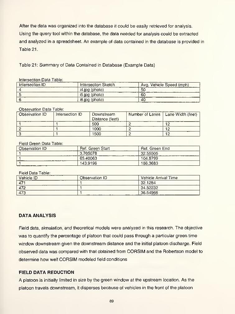
After the data was organized into the database it could be easily retrieved for analysis.

Using the query tool within the database, the data needed for analysis could be extracted

and analyzed in a spreadsheet. An example of data contained in the database is provided in

Table 21.

Table 21 : Summary of Data Contained in Database (Example Data)

Intersection Data Table:

Intersection ID Intersection Sketch Avg. Vehicle Speed (mph)

4 i4.jpg (photo) 50

5 i5.jpg (photo) 60

6 i6.jpg (photo) 40

Observation Data Table:

Observation ID Intersection ID DownstreamDistance (feet)

Number of Lanes Lane Width (feet)

1 1 500 2 12

2 1 1000 2 12

3 1 1500 2 12

Field Green Data Table:

Observation ID Ref. Green Start Ref. Green End1 3.705078 32.55505

1 65.40063 104.8799

1 143.9196 186.3683

Field Data Table:

Vehicle ID Observation ID Vehicle Arrival Time

471 1 32.1284

472 1 34.52232

473 1 36.54966

DATA ANALYSIS

Field data, simulation, and theoretical models were analyzed in this research. The objective

was to quantify the percentage of platoon that could pass through a particular green time

window downstream given the downstream distance and the initial platoon discharge. Field

observed data was compared with that obtained from CORSIM and the Robertson model to

determine how well CORSIM modeled field conditions

FIELD DATA REDUCTION

A platoon is initially limited in size by the green window at the upstream location. As the

platoon travels downstream, it disperses because of vehicles in the front of the platoon

89

traveling faster than the speed limit and vehicles at the end of the platoon traveling slower

than the speed limit. However, a platoon is expected to reach a downstream location within

an expected range of time depending on the downstream distance, average travel speed,

and initial platoon discharge length. The time ta in Figure 33 represents the expanded time

during which the dispersed platoon is expected to arrive. This time is obtained by projecting

the upstream green window using a speed faster than the speed limit to locate the start of ta

and a speed lower than the speed limit when locating the end of ta .

Field data reduction was therefore performed in two steps: The first step was to extract the

vehicle arrival times lying within the time period ta from the data base using a data base

query, and the second step was to extract the platoon from that window.

Different traffic conditions (gaps between successive platoons) were observed to affect the

speed of platoon, making it a nontrivial task to predict the exact time of platoon arrival at the

downstream location within the extracted window. A platoon was hence recognized within

the ta window as a group of narrow gapped vehicles that came immediately after a wide gap

measured from the start of ta .

CORSIM SIMULATION

CORSIM simulations were run for different combinations of travel speed and initial platoon

discharge lengths that replicated observed field data conditions. Initial platoon discharge

predetermined lengths were obtained by putting the main street traffic in oversaturated

condition and setting the main street green time to the required length. This insured that the

green time would be fully utilized by the waiting vehicles. The arrival time of vehicles at

particular downstream distances at 500 ft. intervals were obtained by the extracting vehicle

positions from the CORSIM animation file. Start of platoon was easily identified in the

simulation part of the analysis since no right turn on red were allowed in simulation. The

headway gap between different platoon was made distinguishable by setting long side-street

greens with no traffic at that period.

DETERMINATION OF GREEN WINDOWS FOR PARTICULAR PERCENTAGES OFPLATOONS

The green-windows needed for particular percentages of platoon to pass through were

determined by analyzing the vehicle arrival times. After the different platoons were identified,

arrival times of vehicles in each platoon were referenced to the arrival time of the start of

90

their platoon. A histogram analysis was then conducted for all the platoons at different

downstream locations to determine the percentage of platoons arriving at different points in

time measured from the start of platoon. Figure 35 shows the platoon distribution for a 20-

second initial platoon discharge and a 30 MPH posted speed limit.

The histogram plots were useful to find the green window required for different percentages

of the platoon at varying downstream distances. The green window needed represents the

time required for a certain percentage of the platoon to pass when the first vehicle in the

platoon arrives at the start of green at a certain downstream location. For example, t50 for

Figure 35-e would represent the time that it takes for 50% of a platoon to pass an

observation point 2000 ft. downstream. In other words, t50 is the time difference between the

passage of the 50thpercentile vehicle and the first vehicle.

In order to obtain the percentage of platoon passing at each cumulative bin time, the

histograms were standardized by dividing the number of vehicles in each bin range by the

total number of vehicles in the analysis period. The time at which specific percentages of the

platoon (e.g. 100%, 95 %, 75%, 50%, and 25%) passed were then determined by

interpolation.

91

oc 30

Z325

20LL. 1fa

> 10-t—

1

CO 5CD

nr

y ^ $> <§> # # a^ # #Time from Start of Platoon

a) Platoon at Stop-line

oc 30CDZ3

25

m 20LL 1bCD> 10

ra 5CD

rr III I! I I I II

I II I II I I I I I II I I II I I I I I I ! I I I I! I ! I I I I

%sN* ,ffo f§? <£ # A* & <$>

Time from Start of Platoon

b) 500 ft Downstream

o 30(_CD

3 25

CI)20

LL 1bCD> 10

TO 5CD

T^ \* <$> <§> «? # A* # <§>


c) 1 000 ft Downstream

oc 30CD3 25crCI)

20J_ 1b

> 10

5

T kit"l l"l"l I I IT !! 1 I I I

* \* <$> <§> <£ # A* <g> <£>


d) 1 500 ft Downstream

* \fc $> <§> <$ # A* # <£>


e) 2000 ft Downstream

30

25

20

>.ocCD

Z3cr

LL. 15

| 10

m 5n

DC u

* \* <$>*§> «? # A* <£ <£>


f) 2500 ft Downstream

Figure 35: Platoon Distribution at Various Downstream Observation Points

92

PLOTS OF GREEN WINDOWS REQUIRED BY DIFFERENT PERCENTAGES OF THEPLATOON

Times at which predetermined percentages (100%, 95 %, 75%, 50%, and 25%) of the

platoon passed when the first vehicle in the platoon arrived at the start of green were

tabulated and plotted versus several downstream locations. The plots were produced for 30

and 40 mph posted speed limit and an initial platoon discharge of 20 seconds. A regression

analysis was then conducted for arrival times for the specified percentages of the platoon

versus the downstream distance and resulting regression models were used

to plot the relationships. For example, the time at which 75% of the platoon passed could be

determined by the regression model:

tn =a15+b

75X+c

15X 2

Where:

a = the intercept,

b = the linear coefficient,

c = the quadratic coefficient,

t75 - time at which 75% of the platoon pass,

X = the downstream distance in thousand feet.

Theoretical Histograms obtained from Robertson model for 20, 40, and 60 seconds

discharge platoons and speed limit of 30, 40, and 50 miles per hour are presented in

appendix B. Arrival times and green window's plots for the same platoon discharge and

speed limits are also presented in appendix B.

Table 22 summarizes the regression analysis coefficients for reduced data and CORSIM

simulation. Figure 36 and Figure 37 show plots of row data with regression lines for the

observed field data and CORSIM data, respectively.

93

Table 22: Regression Analysis Coefficients for Data and CORSIM Simulation

Green Windowrequired to pass X%of the platoon (f

v )

Equation t = a + bX +cX 2Coefficients

a B c

a) Field Data (20 second saturated platoon, Speed: 30 MPH)

MOO20.00 9.70 0.22

'9518.00 6.24 0.02

'7515.00 -0.22 0.72

'5010.00 -2.87 1.29

*255.00 -1.87 0.61

b) Field Data (20 second saturated platoon, Speed: 40 MPH)

MOO20.00 11.38 -0.20

'9518.00 9.97 -1.17

'7515.00 1.37 0.06

ho10.00 0.47 -0.06

'255.00 -0.65 0.18

c) CORSIM Simulation (20 second saturated platoon, Speed: 30 M 3H)

'10020.00 16.56 -1.41

'9519.00 11.11 -0.33

'7515.00 10.23 -0.38

'5010.00 10.67 -0.81

'255.00 9.42 -1.13

d) CORSIM Simulation 20 second saturated platoon, Speed: 40 MPH)

MOO20.00 11.38 -0.21

'9519.00 6.90 0.45

'7515.00 6.31 0.35

'5010.00 6.62 0.03

?25

5.00 5.87 -0.25

94

100% 95% » 75% x 50% * 25%

100

500 1000 1500 2000 2500

Downstream Distance (ft)

a) Reduced field data.

3000 3500 4000

100% 95% • 75% x 50% * 25%

100

500 1000 1500 2000 2500


b) Reduced data from CORSIM simulation.

3000 3500 4000

Figure 36: Platoon Dispersion (20 Second Saturated Platoon, Speed: 30 MPH)

95

100% 95% * 75% x 50% x 25%

oD

CD

O

uu -

•

*

<*.

?0 -A -A "A

i X_i

—

A— AX

-A

X XX

X

o J ,

1 1

500 1000 1500 2000 2500 3000 3500 4000 4500


a) Reduced field data.

100% 95% • 75% x 50% ' 25%

500 1000 1500 2000 2500 3000 3500 4000 4500


b) Reduced data from CORSIM simulation.

Figure 37: Platoon Dispersion (20 Second Saturated Platoon, Speed: 40 MPH)

96

THEORETICAL MODELS

The Robertson model is a popular platoon dispersion model because it allows the user to

transform an upstream platoon histogram into a histogram representing the platoon further

downstream. With the aid of a computer spreadsheet it was relatively simple to transform

histograms using the Robertson model. The spreadsheet developed for this research

allowed the user to vary the average arterial speed, the initial platoon size and the platoon

dispersion parameters. The parameters used to generate the histograms were the ones

suggested by the TRANSYT manual for low, moderate and heavy external friction as well as

those suggested by McCoy for a typical four-lane two-way arterial. Histograms were

generated for the platoon dispersion parameters at speeds of 30 and 40 MPH for saturated

platoons of 20 seconds. Arrival times were calculated for 5, 25, 50, 75, 95, and 99 percent of

the platoon using the theoretical Robertson model. The arrival time graphs were adjusted to

reference time to the arrival time of the first vehicle in a platoon. The graphs developed

using the Robertson model are presented in Figure 38 and Figure 39. Appendix B contains

all the graphs obtained from Robertson model for 20, 40, and 60 seconds platoon discharge

and speed limit of 30, 40, and 50 miles per hours for the same model parameters of Figure

38 and Figure 39.

97

-t99 -t95 -t75 -t50 -t25 -t5 -t99 -t95 -t75 -t50 -t25 -t5

~ 100

a) a=

— 1

6CD

w

oC

C

O

c) a=

1000 2000 3000 4000

Downstream Distance (ft.)

0.15,3=0.97

-t99 -t95 -t75 -t50 -t25 ~t5

1000 2000 3000 4000


0.35, (5=0.80

oCO

goC

C(1)

5

1000 2000 3000 4000


b) a=0.25, p=0.80

-t99 -t95 -t75 -t50 -t25 ~t5

~ 100

1000 2000 3000 4000


d) a=0.50, (3=0.80

Figure 38: Green Window From Robertson's Model (20 second saturated platoon, Speed: 30MPH)

98

-t99 ~t95 -t75 ~t50 -t25 — 15

,

-t99 -t95 -t75 -t50 -t25 -t5

~ 100

1000 2000 3000 4000


a)cc=0.15, (3=0.97

— 199 -t95 -t75 -t50 -t25 -t5

~ 100

1000 2000 3000 4000


c) a=0.35, (3=0.80

1000 2000 3000 4000


b) cx=0.25, (3=0.80

-t99 -t95 — 175 -t50 ~t25 -t5

100

1000 2000 3000 4000


d) a=0.50, (3=0.80

Figure 39: Green Window From Robertson's Model (20 second saturated platoon,

Speed: 40 MPH)

99

DISCUSSION

Several interesting trends can be observed in the figures produced in this study. As the

arterial speed is increased, the platoon will obviously reach each downstream location much

more quickly. The size of the platoon discharge will also effect its behavior as it proceeds

downstream. In this paper, platoons with a saturated discharge of 20 seconds were

presented because the best sample size distribution was obtained for the field data collected

for that period. This is illustrated by examining Table 19.

Although obviously dependent on the model coefficient, the theoretical Robertson model

demonstrated platoon dispersion that was much larger than the reduced field data or

CORSIM simulation. As the product of the two platoon dispersion parameters increased, the

platoon disperses even more quickly in the Robertson model. This is illustrated by

comparing Figure 38d with Figure 38a and Figure 39d with Figure 39a.

CORSIM simulation demonstrated an overall platoon dispersion similar to the field data, as

can be seen by comparing Figure 36 and Figure 37. However, the CORSIM simulation

package tended to have more platoon dispersion in the beginning of the platoon when

compared to the real data. For example, Figure 36b and Figure 37b show that the lines for

25% of the platoon are much higher than their equivalents in Figure 36a and Figure 37a.

This trend is probably because of the car following logic in the CORSIM simulation that

tends to more aggressively disperse the front vehicles in the platoon. This logic makes

CORSIM simulation somewhat conservative in quantifying the benefits of coordinating

downstream signals for smaller green windows downstream as it suggests that a smaller

percentage of the platoon benefits from that coordination.

The graphs presented in this report provide valuable information when evaluating the

benefits of coordinating two traffic signals by quantifying the percentage of platoon that

would benefit of a particular green window provided at the downstream intersection. Or

alternatively suggesting the green time required at the downstream intersection if a certain

percentage of a platoon passage was desired.

100

The Rp ratio used in equation (9-7) in the Highway Capacity Manual uses the proportion of

all vehicles in movement arriving during the green phase, the effective green time, and the

cycle length to estimate the progression quality and hence the arrival type. The arrival type

is one of the most important factors in determining the level of service for signalized

intersections, yet it merely remains a general categorization representing the quality of

progression in an approximate manner. If the offset of the traffic signal downstream was

perfectly tuned such that the first vehicle in the platoon arrives at the start of green, then it

would be possible to use the graphs presented in this paper to quantify the percentage of

platoon that would pass through a particular green window provided downstream. This

information allows the practitioner to determine an upper bound on the Rp ratio used in

equation (9-7) in the Highway Capacity Manual to determine the arrival type, which in turn

can be used to determine the level of service for signalized intersections.

To summarize, CORSIM modeled field conditions reasonably well, but tended to introduce

more dispersion than observed in the field. Therefore, from an analysis perspective

CORSIM would tend to underestimate the benefits of accommodating platoons.

Consequently, the benefits tabulated in chapter 5 are likely on the conservative side.

101

CHAPTER 7 RECOMMENDATIONS

As was mentioned in Chapter 4, a sensitivity study is needed to provide additional insight

into the parameters' individual and collective impact on the performance of the platoon

accommodation algorithm in improving the operational efficiency of isolated intersections

(Case D-100 for Period 3). Chapter 4 illustrated an example in which platoon

accommodation had a significant positive effect on the intersection's operation. Chapter 5

has shown that the complete system can be an add-on feature to existing traffic control

systems already deployed resulting in a cost which is quite low. Chapter 6 illustrated that the

CORSIM platoon dispersion model is reasonable for this type of analysis. Because the

potential of the system has been demonstrated, it is important the maximum possible

benefits can be obtained when the system is implemented. To accomplish this additional

research is needed. Therefore, it is recommended that a follow-up study be conducted for

the following tasks:

1

)

A parameter study should be conducted to determine the sensitivity of all of the various

parameters identified in this research including:

Maximum Preemption Hold Time Platoon detector location

Minimum Preemption Hold Time Minimum platoon size

Preemption Reservice Time Maximum headway between first and

Preemption Delay Time last vehicles in minimum platoon size

Preemption Inhibit Time

2) A prototype field deployment should be conducted. This deployment will demonstrate the

functionality of the various components under live traffic and provide real world data.

3) Warrants should be developed to provide guidance to INDOT for selecting intersections

for early deployment.

Each of these tasks will be discussed below.

Parameter Sensitivity Study

As was discussed, Task 1 is necessary to provide further information as to the relative

impacts of all the various parameters identified in this research effort. Through the

development of the platoon accommodation algorithm and the preliminary evaluation of its

potential effects, several key findings have been made relating to the configuration of the

various parameters described in Table 8.

102

Table 23 summarizes these findings and defines the range of values to be examined is a

parameter study. It should be noted that some of the comments for these parameters are

based on the specific controller used in the original research effort. It is expected that the

parameter study could be completed in six months.

103

Table 23 Summary of Information Regarding System Parameters

Parameter Range CommentsMinimum Platoon

Size

5-25 This is one of the two parameters that control the sensitivity of

the PLCs identification of platoons in the traffic stream.

Through discussions held in study advisory committee

meetings, it is felt that this number should range between 5

and 25 vehicles for isolated intersections.

Maximum HeadwayBetween First andLast Vehicles in

Minimum Size

Platoon

5-20 This is the second of the two parameters that control the

sensitivity of the PLCs identification of platoons in the traffic

stream. The ranges of this parameter depend on the

minimum platoon size and the number of lanes for which

vehicles are being detected for platoon recognition.

Maximum Hold

Time0-30 It is thought that this parameter has little impact on the

performance of the platoon algorithm. The reason for this is

that one single call is placed to the controller to initiate the

preemption sequence. The controller retains this call during

the delay time if the locking memory setting of the preemptor

is active.

Minimum Hold Time 0-15 This parameter does have a significant effect on the system.

However, this value should be very low (likely zero) when the

preempted approach has localized detection. In this case, the

minimum hold is not needed because the local detectors candetermine when the platoon has traversed the intersection.

Reservice Time 0-90 In situations when the minor phases have low to moderate

volumes, this parameter should be set to zero. The controller

has a reservice element already built into the preemption logic

to guarantee that minor phases do not receive excessive

delays from multiple preemption calls occurring within a short

time span. Before the controller can reinitiate a preemption

sequence that has terminated, it must service all phases on

which detector calls are present.

Delay Time 0-45 This is an important setting for the strategy. It is a function of

the distance of the detector upstream from the intersection,

maximum platoon headway value, and average speed of

platoon. When the minimum hold time is set low this setting

must allow the proper amount of time to elapse for the platoon

to reach the area of local detection.

Inhibit Time 0-20 This parameter influences the responsiveness of the controller

to activating the beginning of a preemption hold. It should be

set no lower than the maximum clearance time for any

conflicting phase.

Detector Location 0.5 miles

1.0 miles

This parameter is likely to have an impact on the operation of

the system. Little effort has been spent on understanding the

sensitivity of this parameter. However, the minimum distance

should be no less than the average speed of the platoon

multiplied by the sum of the inhibit time and the maximumplatoon headway time.

Prototype Field Deployment

Due to the significant progress made in this research effort, the study advisory committee

has recommended that a move be made towards prototype field deployment. It is felt that

104

once the parameter study is completed, adequate information will exist to provide guidance

as to the proper setting of the system. This section will provide some preliminary

information as to how this task would be completed.

The prototype system will consist of a centralized processing approach (see Figure 14)

similar to that of the expected permanent system. However, certain components of the

prototype will differ from that of the envisioned system discussed in Chapter 5. The primary

differences include the traffic detector and remote power supply that will be used. The

RTMS unit manufactured by EIS, which was discussed in Chapter 3, will be the traffic

detector used. INDOT already has one of these units in operation along the Borman

Expressway that can be used for the prototype system [Boyd, 1998]. A portable generator

will serve as the power supply for the remote site. INDOT can provide this equipment from

one of its facilities, such as the Research Division located in West Lafayette, Indiana. The

remaining equipment described in Chapter 5 including the programmable logic controller

(PLC), radio equipment and traffic signal controller will be identical to the envisioned final

system. These indicated changes are to allow for flexibility in testing several parameter

combinations and to allow for quick set-up and take down in the field.

The prototype system is planned for deployment at one and possibly more intersections

located in central Indiana. The intersection is likely to be in the jurisdiction of INDOT's

Greenfield District Office. A site on U.S. 31 between Indianapolis and Kokomo has been

discussed. The isolated intersection should be one in which a fully actuated controller is in

use. The prototype will function as a mechanism to prove the functional operation of the

equipment under live traffic conditions. It also serves as an information source for the

completion of Tasks 1 and 3.

Warrants for System Deployment

To this date little has be done relevant to this task. A key component of this involves an

understanding of the expected benefits of a well-calibrated installation. Task 1 should help

in providing this information. Some possible concepts that may want to be incorporated into

warrant guidelines include:

Minimum total volume for intersection,

Critical ratio between volumes on the major and minor roads,

105

Relative speed difference between the major roads,

Development of some type of platooning index which could be easily applied, and

High number of rear-end type accidents along a roadway.

These concepts should serve as a starting point from which this task can develop.

106

Future Enhancements

This research has demonstrated that platoon accommodation can have a significant impact

on the operational efficiency of an isolated intersection. In the future, it is likely that this

strategy will evolve to increased levels of sophistication.

For example, the current system only detects platoons on one approach to the intersection.

It is reasonable to infer that it would be desirable to have a strategy that will accommodate

platoons from two or more directions. As this task of identifying platoons on multiple

approaches develops, it may become necessary to monitor the current state of the signal in

order to determine the accommodation technique that should be implemented.

The system architecture developed in the research effort can accommodate this expansion.

The deployment of additional remote sites connected to the same communications system,

which provides the PLC with vehicle arrival data, can be constructed. The program logic in

the PLC can be modified to deal with multiple input sources and to provide multiple outputs

enabling different accommodation strategies to be implemented. Therefore, there is great

potential for this system to evolve through multiple generations when new strategies are

conceived.

107

LIST OF REFERENCES

Alternative Energy Engineering. "Photovoltaic Solar Cells and Panels."

http://www.asis.com/aee/ , 1998.

Andrews, Christina M., S. Manzur Elahi and James E. Clark. "Evaluation of New Jersey

Route 1 8 OPAC/MIST Traffic-

Control System." Transportation Research Record 1603. TRB, National Research Council,

Washington D.C., 1997.

Baass, Karsten G. and Lefebvre, Serge. Analysis of Platoon Dispersion with Respect to

Traffic Volume. Transportation Research Record 1 194, TRB, National Research Council,

Washington, D.C., 1988, pp. 64-76

Bang, K.L. "Optimal Control of Isolated Traffic Signals." Traffic Engineering and Control .

1976.

Boyd, Troy and Rick Anderson. Phone interview on June 2, 1998.

Boyd, Troy. Phone interview. Indiana Department of Transportation, 1998.

Bullock, Darcy and Alison Caterella. "A Real-Time Simulation Environment for Evaluating

Traffic Signal Systems." Proceedings from the 77thAnnual Meeting of the Transportation

Research Board . Preprint #980837. TRB, Washington D.C., 1998.

Castle, David E., and Bonniville, John W. Platoon Dispersion over Long Road Links.

Transportation Research Record 1021, TRB, National Research Council, Washington, D.C.,

1 985, pp. 36-44

Central Security. Phone Interview with Joe Ext. 22. Indianapolis, IN 1998.

Collins, J.F., and Gower, P. Dispersion of Traffic Platoons on A4 in Hounslow. TRRL Report

SR29UC, U.K. Transport and Road Research Laboratory, Crowthorne, Berkshire, England,

1974.

108

Dell 'Olmo, P., and P.B. Mirchandani. "REALBAND: An Approach for Real-Time

Coordination of Traffic Flows on a Network." Transportation Research Record 1494. TRB,

National Research Council, Washington D.C., 1985.

Denney, Richard W. Traffic Platoon Dispersion Modeling. Journal of Transportation

Engineering, March 1989.

Econolite Control Products. "ECONOLITE ASC/2 SERIES NEMA TS1 & TS2 ACTUATED

CONTROLLERS." http://www.econolite.com/ , 1998.

Econolite Control Products. Advanced System Controller ASC/2 Programming Manual .

Anaheim, CA, 1996.

Electronic Integrated Systems Inc. RTMS User Manual . North York, Ontario, Canada, 1998.

FHWA. "Real-Time, Traffic Control for IVHS." Solicitation Number DTFH61-92-R00001 .

United States Department of Transportation, Washington D.C., 1991.

FHWA. Estimating the Impacts of Transportation Alternatives . Report Number FHWA-HI-94-

053. United States Department of Transportation, Washington D.C., 1995.

Gartner, Nathan H. "Discussion of Improved Estimation of Traffic Flow for Real Time

Control." Transportation Research Record 95. TRB, National Research Council, Washington

D.C., 1981.

Gartner, Nathan H. "OPAC: A Demand-Responsive Strategy for Traffic Signal Control."

Transportation Research Record 906. TRB, National Research Council, Washington D.C.,

1983.

Gartner, Nathan H., Chronis Stamatiadis, and Phillip J. Tarnoff. "Development of Advanced

Traffic Signal Control Strategies for Intelligent Transportation Systems: Mulitlevel Design."

Transportation Research Record 1494. TRB, National Research Council, Washington D.C.,

1995.

109

Gartner, Nathan H., Philip J. Tarnoff and Christina M. Andrews. "Evaluation of Optimized

Policies for Adaptive Control Strategy." Transportation Research Record 1324. TRB,

National Research Council, Washington D.C., 1991.

GE Fanuc Automation. Series 90™ Micro PLC User's Manual . Charlottesville, VA, 1997.

Gordon, Robert I., R.A. Reiss, H. Haenel, E.R. Case, R.L. French, A. Mohaddes, and

Wolcott. Traffic Control Systems Handbook . FHWA, United States Department of

Transportation, Washington D.C., 1996.

Head, K. Larry, Pitu B. Mirchandani and Dennis Sheppard. "Hierarchical Framework for

Real-Time Traffic Control." Transportation Research Record 1360. TRB, National Research

Council, Washington D.C., 1992.

Head, K. Larry, Pitu B. Mirchandani and Steve Shelby. "The RHODES Prototype: A

Description and Some Results." Proceedings from the 77thAnnual Meeting of the

Transportation Research Board . TRB, Washington D.C., 1998.

Head, K. Larry. "EventBased Short-Term Traffic Flow Prediction Model." Transportation

Research Record 1510. TRB, National Research Council, Washington D.C., 1995.

Homburger, Wolfgang S., James H. Kell and David D. Perkins. Fundamentals of Traffic

Engineering . 13th

Edition. Institute of Transportation Studies, University of California, 1992.

Hunt, P.B., D.I. Robertson, R.D. Bretherton and R.I. Winton. "SCOOT- A Traffic Method of

Coordingating Signals." Laboratory Report No. LR 1014 . Transportation and Road

Research, Crowthome, Bershire, England, 1981.

Kaman Sciences Corporation. TSIS User's Guide . Version 4.01 . Colorado Springs, CO,

1997A.

Kaman Sciences Corporation. CORSIM User's Manual . Version 1.03. Colorado Springs,

CO, 1997B.

110

Kell, J. H. and I. J. Fullerton. Manual of Traffic Signal Design . 2nd

Edition. Institute of

Transportation Engineers. Prentice Hall, Englewood Cliff, New Jersey, 1991.

Lam, J.K. Studies of a Platoon Dispersion Model and Its Pratical Applications. Seventh

International Symposium on Transportation and Traffic Theory, Institute of Systems Science

Research, Kyoto, Japan, 1977.

Lin, Feng-Bor, N. Wang and S. Vijayakumar. "Development of an Intelligent Adaptive Signal

Control Logic." Presented at the Engineering Foundation Conference on Management and

Control of Urban Traffic. Henniker, N.H. 1987.

Lin, Feng-Bor. "Comparative Analysis of Two Logics for Adaptive Control of Isolated

Intersections." Transportation Research Record 1194. TRB, National Research Council,

Washington D.C., 1988.

Linkenheld, J.S., R. F. Benekohal, and J. H. Garrett. "Knowledge-based System for Design

of Signalized Intersections." Journal of Transportation Engineering . Volume 118, Number 2.

American Society of Civil Engineers, New York, NY, 1992.

Lowrie, P.R. "SCATS - Sydney Co-Ordinated Adaptive Traffic System - A Traffic

Responsive Method of Controlling Urban Traffic." Roads and Traffic Authority, Sydney

Australia, 1992.

Manar, Abdelaziz, and Baass, Karsten G. Traffic Platoon Dispersion Modeling on Arterial

Streets. Transportation Research Record 1566, TRB, National Research Council,

Washington, D.C., November 1996, pp. 49-53.

Martin, Randy. Phone interview. Indianapolis GE Supply, 1998.

McCoy, Patrick T., Balderson, Elizabeth A., Hsueh, Richard T., and Mohaddes, Abbas K.

Calibration of TRANSYT Platoon Dispersion Model for Passenger Cars Under Low-Friction

Traffic Flow Conditions. Transportation Research Record 905, TRB, National Research

Council, Washington, D.C., 1983, pp. 48-52

111

McShane W.R. and R. Roess. Traffic Engineering . Prentice-Hall, New York, NY, 1990.

Microsoft* Corporation. "Microsoft* TerraServer." www.terraserver.microsoft.com/, 1998.

Microsoft® Corporation. Microsoft® Automap Streets Plus . 1997 Edition., 1996.

Minnesota Department of Transportation and SRF Consulting Group, Inc. "Field Test of

Urban Vehicle Operations Using Non-Intrusive Technologies." FHWA, Untied States

Department of Transportation, Washington D.C., 1997.

National Electrical Manufacturers Association. Traffic Controller Assemblies . Standards

Publication Number TS 2. Washington D.C., 1992.

National Research Council, Transportation Research Board. Highway Capacity Manual . 3rd

Edition. Washington D.C., 1994.

Pacey, G.M., The progress of a bunch of vehicles released from a traffic signal. Research

Note No. RN/2665/GMP, Road Research Laboratory, Crowthorne, Berkshire, England.,

1956.

Petruzella, Frank D. Programmable Logic Controllers . McGraw-Hill, Inc., 1989.

Reiss, R. and W. Dunn. Freeway Incident Management Handbook . FHWA, United States

Department of Transportation, Washington D.C., 1991

.

Robertson, D.I., TRANSYT: A Traffic Network Study Tool. Report No. LR253. Transport and

Road Research Laboratory, U.K., 1969.

Rouphail, Nagui., Tarko, Andrzej., Li, Jing. Traffic Flow at Signalized Intersections. Traffic

Flow Theory: A State-of-the-Art Report, Transportation Research Board, 1992.

Sen, Suvrajeet, and K. Larry Head. "Controlled Optimization of Phases at an Intersection."

Transportation Science . Vol. 31 , No.1 , 1 997.

Shamo, Dan. Personal interview held on July 15, 1998.

112

Simpson, Colin D., Programmable Logic Controllers . Regents/Prentice Hall, Englewood

Cliffs, NJ, 1994.

Sneddon, P.A., Another Look at Platoon Dispersion - 3: The Recurrence Relationship.

Traffic Engineering and Control, Feb. 1972, pp. 442-444.

Steckler, Brad. Interview with INDOT Preliminary Engineering Staff. July 24, 1998.

Stephanedes, Y.J., P.G. Michalopoulous, and R.A. Plum. "Improved Estimation of Traffic

Flow for Real-Time Control." Transportation Research Record 795. TRB, National Research

Council, Washington D.C., 1981.

Stewart, J. Allan, Katrin Lepik, and M. Van Aerde. "Benefit Sensitivities of Adaptive Traffic

Control Strategies at Isolated Traffic Signals" Proceedings from the 77thAnnual Meeting of

the Transportation Research Board . TRB, Washington D.C., 1998.

Tarnoff, P.J. 'The Results of FHWA Urban Traffic Control Research: An Interim Report".

Traffic Engineering . Vol. 45. 1975.

Vincent, R.A. and C.P. Young. "Self-Optimizing Traffic Signal Control Using Microprocessors

- the TREL 'MOVA' Strategy for Isolated Intersections." Traffic Engineerinig . Vol. 27, No.

7/8. 1986.

Zabel, Carl. Phone Interview. Reno A&E. Reno, NV, 1998.

113

APPENDIX A

PLC LADDER LOGIC FOR PLATOON DETECTION ALGORITHM

114

+ + + + + +

+--(+ )+ ADD_+ + ADD_+ + ADD_+

|INT

||INT

||INT

|

I I I I II%R0101 -+I1 Q+-4R0040 %R0040 -+I1 Q+-»R0041 4R0041 -+I1 Q+-%R0042

II II II»R0102 -+I2 | %R0103 -+I2 | %R0104 -+I2 |

+--(+) + ADD_+

INT|

I I

»R0042 -+I1 Q+-»R0050

I I

»R010S - + I2 I

H +

+ +

--( + ) + LE_ |+-

INT| |

I II

»R0050 -+11 Q+ +

I I

CONST -+I2|

+00050 + +

DS»6 + +

--) / [+ TMR + --

|0.10s

I I

CONST - +PV |

+00015| |

DS#20 + +

--]/ [ + TMR + -

10. 10s

|

I I

CONST -+PV

+00010 I I

DS#7 DS»8 + +

-] / I ]/[ + TMR +-

|0. 10s

|

I

CONST -+PV

+00005I

DS#9 DS«7

•-]/[ ]/(--

DS#6

DSK20

--( )-

DS«8

--( >-

DS#9

--( )-

Bus Preempt

Figure A-1 PLC Platoon Accommodation Algorithm (continued)

116

Table A-1 PLC Ladder Logic Functions

Function Description

TMR Timer that increments time while receiving

power and resets when power is lost.

MOVEJ/VORD Copies data from one memory location to

another.

ONDTR Timer that counts down time when

receiving power.

MOVEJNT Pastes data into a specified range of cells.

SHFR_WORD Shift-register of a specified number of

memory locations.

ADDJNT Adds the contents of two memory locations

and writes the answer into a different

location.

LEJNT Less than or equal logical function.

117

APPENDIX B

TRANSFORMING PLATOON HISTOGRAMS USING ROBERTSON'S MODEL

118

This appendix contains the theory used to construct the graphs summarized in chapter 6.

The following text illustrates how the observed histogram in Figure B-1 is transformed to the

histogram in Figure B-2, which represents the conditions at 500 ft. downstream. Subsequent

text, figures, and tables explain how the final tabulations in chapter 6 were derived.

q-, (j) = q, (j) + (1 )q^U -1) (Robertson Model - General Equation)

1 + apx 1 + afiz '

a and P are platoon dispersion parameters that can be changed to better represent the

conditions on a given roadway. In the following example, the two parameters were chosen

to best represent a four-lane two-way road according to McCoy. The two parameters used in

this example are:

a=0.15

13=0.97

The average travel time factor is represented by t. This factor is the average time it takes a

vehicle to travel the distance between two histograms. For example, if the stop-line

histogram is being transformed to represent the platoon at 500 ft. downstream then the

travel time factor would simply be the average time it takes a vehicle to travel 500 ft. In this

example, we are transforming the stop-line histogram to a distance of 500 ft downstream

with an average arterial speed of 30 mph. Therefore the average travel time is calculated to

be 1 1 .4 seconds.

q^) is taken from the histogram that is being transformed (Figure B-1 ) and is equal to the

number of vehicles in the bin that corresponds to the bin that is being calculated in the

transformed histogram.

q1 U) = 12.55 (Figure B-1)

q2(j-1) is taken from the transformed histogram (Figure B-2). It is equal to the number of

vehicles in the bin immediately preceding the bin that is being calculated.

q 2(j-l)= 7.09 (Figure B-2)

119

q2 (j) is the bin in the transformed histogram that is being computed. The calculation is

completed using the Robertson model as follows:

1 + apt 1 + apt

Computing: = = 0.369l + a/3r 1 + (0.15)(0.97)(11.4)

q 2 (j)= (0.369)*(1 2.55)+(1 -0.369)*(7.00)

?20')=9.15

Histograms were generated for each of the platoon dispersion parameters at speeds of 30,

40 and 50 MPH. Additionally, for each combination of parameters and arterial speeds,

theoretical histograms were developed for saturated platoons of 20, 40 and 60 seconds. The

histograms developed by the spreadsheet are presented in figures and are summarized

below.

Figure B-3, Figure B-4, Figure B-5, and Figure B-6 contain the theoretical histograms for a

20 second discharge platoon on a 30 MPH arterial using the first four a and P values shown

in Table B-1

.

Figure B-7, Figure B-8, Figure B-9, and Figure B-10 contain the theoretical histograms for a

20 second discharge platoon on a 40 MPH arterial using the first four a and P values shown

in Table B-1

.

Figure B-1 1 , Figure B-1 2, Figure B-1 3, and Figure B-1 4 contain the theoretical histograms

for a 20 second discharge platoon on a 50 MPH arterial using the first four a and p values

shown in Table B-1

.

Figure B-1 5, Figure B-1 6, Figure B-1 7, and Figure B18 contain the theoretical histograms for

a 40 second discharge platoon on a 30 MPH arterial using the first four a and p values

shown in Table B-1.

120

Figure B-19, Figure B-20, Figure B-21, and Figure B-22 contain the theoretical histograms

for a 40 second discharge platoon on a 40 MPH arterial using the first four a and (3 values

shown in Table B-1

.



shown in Table B-1

.



shown in Table B-1

.

Figure B-31 , Figure B-32, Figure B-33, and Figure B-34 contain the theoretical histograms


shown in Table B-1.



shown in Table B-1

.

The figures containing the histogram plots are again summarized in Table B-1

.

Several interesting trends can be observed in the figures that have been summarized

above. As the product of the two platoon dispersion parameters increase, the platoon

disperses more quickly. As a platoon becomes more and more dispersed the histogram

representing that platoon will spread out and become flatter. Larger dispersion parameters

will also cause the center of the platoon to take longer to arrive at the downstream location.

These trends are apparent when comparing the histograms for a location of 2000 ft.

downstream with varying dispersion parameters. Compare Figure B-3d, Figuie B-4d, Figure

B-5d, and Figure B-6d. These same trends will continue and become even more

pronounced as the platoon continues further downstream. Compare B-3h, Figure B-4h,

Figure B-5h, and Figure B-6h which represent a platoon at 8000 ft. downstream. The figures

just discussed consider an arterial with an average speed of 30 MPH and a 20-second

saturated platoon discharge. The observed trends remained similar when the size of the

121

platoon discharge and the average arterial speed was changed. With an average arterial

speed of 50 MPH the same trend can be seen by comparing Figure B-1 1h with Figure B-

14h. The only variables that are different in these two histograms are the platoon dispersion

parameters.

If the platoon dispersion parameters are held constant, changes in the histograms can be

observed which are only dependent on speed and platoon size. As the arterial speed is

increased, the center of the platoon will obviously reach each downstream location much

more quickly. Also, the platoon will not disperse quite as quickly. These trends can be

observed by comparing Figure B-3d, Figure B-7d, and Figure B-1 1d. This trend is somewhat

more obvious as the platoon travels further downstream to a distance of 8000 ft. as can be

seen in Figure B-3h, Figure B-7h, and Figure B-1 1 h.

The size of the platoon will also effect its behavior as it proceeds downstream. In this

research, saturated platoons of 20, 40 and 60 seconds were used. The same basic trends

discussed in previous paragraphs are also apparent for these larger platoon discharges.

Initially the histograms representing the different platoon discharges will be very different but

as they proceed downstream the histograms will take nearly the same shape. These trends

can be evaluated by comparing Figure B-3, Figure B-1 5, and Figure B-27. Note that in

Figure B-3d, Figure B-15d, and Figure B-27d that the histograms are very different but in

Figure B-3h, Figure B-15h, and Figure B-27h that the histograms are nearly identical.

Additional comparisons can be made with the other figures provided which will yield similar

observations.

From the histogram plots it is also useful to find the arrival times of the platoon at varying

downstream distances. The arrival times represent the time it takes for a certain percentage

of the platoon to arrive at a certain downstream location. For example, feo at 2000 ft. would

represent the time that it takes for 50% of the platoon to travel 2000 ft. Such information can

be useful when determining whether or not it is beneficial to coordinate a downstream signal

with the upstream signal that originally generates the platoon. Arrival times have been

calculated for 5, 25, 50, 75, 95, and 99 percent of the platoon. The procedure for reading

arrival times has been shown in Figure B-39. The histogram represents a 20-second

saturated platoon traveling at a speed of 30 MPH when it has a reached a point of 2000 ft.

downstream.

122

The arrival times are summarized in tables and have been organized as follows:

Table B-2: 20-second saturated platoon, Speed: 30 MPH









From the histogram plots it is possible to find the arrival times for any percentage of the

platoon at a certain distance downstream. The arrival time graphs can be adjusted to

represent the green window necessary at the downstream signal to allow a certain

percentage of the platoon to pass. The arrival times can be adjusted to green window times

by simply subtracting the time it takes for the first vehicle in the platoon to arrive at the

downstream signal. The arrival times that were found by reading Figure B-39 are plotted in

Figure B-40. The arrival times in Figure B-40 have been transformed to green window times

in Figure B-41 . The arrival times for a 20-second saturated platoon and a speed of 40 MPH

is presented in Figure B-42 and adjusted to green window time in Figure B-43.The

necessary green window for a downstream signal is valuable information when evaluating

the benefits of coordinating two traffic signals. For the purpose of this research, the

theoretical graphs that were developed are compared to graphs of data that was generated

by simulation and by data that was observed in the field. For convenience, the theoretical

green window time graphs for a 20-second platoon and arterial speeds of 30 and 40 MPH

are presented in Figure B-53 and Figure B-54.

As discussed before, as the product of the two platoon dispersion parameters increases so

does the dispersion observed in the platoon. Therefore, it would be expected that a platoon

with a higher degree of dispersion would require a larger downstream green window to

service the platoon. There is a dramatic difference in the amount of green window time

necessary when comparing parts a) and c) in Figure B-44. The arterial speed will also affect

123

the green window times. By comparing Figure B-44 and Figure B-46 it can be seen that a

higher speed will require a lower green window time when compared to a lower speed. The

times for these figures can be read in Table B-3 and Table B-4. Finally, the size of the

platoon will also impact the green window time. Obviously, a larger platoon will require more

green time than will a smaller platoon. This tendency can be seen in Figure B-44, Figure B-

47 and Figure B-50.

124

Table B-1 : Summary of histogram figures.

Platoon LengthArterial Speed(MPH)

Dispersion

Parameters Figure

a J_

Twenty (20) second

saturated platoon

30

0.15 0.97 Figure B-3

0.25 0.80 Figure B-4

0.35 0.80 Figure B-5

0.50 0.80 Figure B-6

40

0.15 0.97 Figure B-7

0.25 0.80 Figure B-8

0.35 0.80 Figure B-9

0.50 0.80 Figure B-1

50

0.15 0.97 Figure B-1

1

0.25 0.80 Figure B-12

0.35 0.80 Figure B-1

3

0.50 0.80 Figure B-1

4

Forty (40) secondsaturated platoon

30

0.15 0.97 Figure B-1

5

0.25 0.80 Figure B-1

6

0.35 0.80 Figure B-1

7

0.50 0.80 Figure B-1

8

40

0.15 0.97 Figure B-1

9

0.25 0.80 Figure B-20

0.35 0.80 Figure B-21

0.50 0.80 Figure B-22

50

0.15 0.97 Figure B-23

0.25 0.80 Figure B-24

0.35 0.80 Figure B-25

0.50 0.80 Figure B-26

Sixty (60) second

saturated platoon

30

0.15 0.97 Figure B-27

0.25 0.80 Figure B-28

0.35 0.80 Figure B-29

0.50 0.80 Figure B-30

40

0.15 0.97 Figure B-31

0.25 0.80 Figure B-32

0.35 0.80 Figure B-33

0.50 0.80 Figure B-34

50

0.15 0.97 Figure B-35

0.25 0.80 Figure B-36

0.35 0.80 Figure B-37

0.50 0.80 Figure B-38

125

Table B-2: Arrival times at different downstream distances (20 second saturated platoon,

speed: 30 MPH)

cc=0.15 &P=0.97, Four-Lane Divided (McCoy):

500 ft. 1000 ft. 2000 ft. 3000 ft. 4000 ft. 6000 ft. 8000 ft.

t5 2.4 5.2 10.5 18.6 30.0 47.0 70.9

t25 7.8 12.6 20.8 33.5 51.5 78.6 115.8

tso 13.2 18.9 30.0 47.9 72.5 109.2 158.8

t75 18.3 25.6 42.0 66.9 99.8 148.8 213.7

t95 25.1 38.7 66.2 104.6 152.4 224.7 318.1

tgg 31.9 51.1 89.4 139.6 200.2 294.0 412.3

a=0.25 & P=0.80, Low External Friction (TRANSYT):

500 ft. 1000 ft. 2000 ft. 3000 ft. 4000 ft. 6000 ft. 8000 ft.

t5 2.8 6.4 13.3 23.9 39.1 62.4 95.2

t25 8.6 14.7 25.6 42.9 67.7 104.9 156.1

tso 14.2 21.7 37.3 62.0 95.9 146.4 214.5

t75 19.4 30.2 53.1 87.5 132.8 200.2 289.4

t95 28.2 47.4 85.6 138.4 204.1 303.6 431.9

t99 37.1 63.8 116.8 185.8 269.1 398.1 560.7

g=0.35 & P=0.80, Moderate External Friction (TRANSYT):

500 ft. 1000 ft. 2000 ft. 3000 ft. 4000 ft. 6000 ft. 8000 ft.

t5 3.2 8.1 17.0 31.2 52.4 84.9 130.8

t25 9.7 17.6 32.4 56.6 91.4 143.5 215.1

tso 15.6 26.0 48.0 82.7 130.3 201.0 296.4

t75 21.3 37.2 69.6 117.9 181.3 275.6 400.5

t9s 33.1 60.4 114.2 188.2 280.2 419.4 599.0

t99 44.9 82.7 157.2 253.8 370.3 550.9 778.4

a=0.50 & P=0.80, Heavy External Friction (TRANSYT):500 ft. 1000 ft. 2000 ft. 3000 ft. 4000 ft. 6000 ft. 8000 ft.

t5 3.9 10.2 22.2 42.0 72.1 118.5 184.2

t2s 11.0 21.5 42.5 77.2 126.9 201.4 303.7

tso 17.5 32.5 64.2 113.9 181.9 282.9 419.1

t75 24.6 47.9 94.4 163.5 254.1 388.8 567.3

t95 40.8 80.2 157.3 263.0 394.3 593.2 849.7

t99 56.9 111.3 217.9 355.9 522.1 780.1 1105.1

126

Speed: 40 MPH)

<x=0.15 &P=0.97, Four-Lane Divided (McCoy):

500 ft. 1000 ft. 2000 ft. 3000 ft. 4000 ft. 6000 ft. 8000 ft.

t5 2.2 4.4 8.5 14.9 23.7 36.6 54.6

t2s 7.2 11.0 17.6 27.2 40.7 61.0 88.9

tso 12.4 16.9 25.2 38.5 56.9 84.4 121.6

t75 17.5 22.7 34.7 53.2 77.8 114.5 163.2

t95 23.2 33.1 53.4 82.1 117.9 172.1 242.2

tgg 28.6 42.8 71.2 108.8 154.3 224.6 313.4

cc=0.25 & 3=0.80, Low External Friction (TRANSYT):500 ft. 1000 ft. 2000 ft. 3000 ft. 4000 ft. 6000 ft. 8000 ft.

t5 2.4 5.3 10.7 19.0 30.7 48.3 72.9

t25 7.8 12.7 21.2 34.3 52.9 80.8 119.1

tso 13.2 19.1 30.6 49.1 74.5 112.3 163.4

t75 18.4 26.0 42.9 68.6 102.5 153.0 219.9

Us 25.4 39.4 67.8 107.4 156.7 231.3 327.5

t99 32.3 52.1 91.6 143.4 205.9 302.6 424.6

0=0.35 & 3=0.80, Moderate External Friction (TRANSYT):500 ft. 1000 ft. 2000 ft. 3000 ft. 4000 ft. 6000 ft. 8000 ft.

t5 2.8 6.6 13.8 24.8 40.8 65.2 99.7

t25 8.7 15.1 26.4 44.6 70.7 109.8 163.4

tso 14.4 22.2 38.6 64.6 100.2 153.2 224.7

trs 19.6 31.1 55.2 91.3 138.9 209.6 303.3

t95 28.8 49.0 89.2 144.6 213.6 318.1 452.8

tgg 38.0 66.1 121.8 194.3 281.7 417.2 587.9

a=0.50 & 3=0.80, Heavy External Friction (TRANSYT):500 ft. 1000 ft. 2000 ft. 3000 ft. 4000 ft. 6000 ft. 8000 ft.

ts 3.4 8.4 18.0 33.0 55.7 90.5 139.7

t2s 9.9 18.3 34.1 60.1 97.3 153.2 229.9

tso 15.9 27.1 50.7 87.9 138.9 214.7 316.8

tys 21.8 39.0 73.7 125.5 193.4 294.5 428.3

t95 34.3 63.7 121.4 200.6 299.2 448.4 640.8

tgg 46.9 87.5 167.3 270.8 395.6 589.1 832.9

127


Speed: 50 MPH)

cc=0.15&6=0.97, Four-Lane Divided (McCoy):

500 ft. 1000 ft. 2000 ft. 3000 ft. 4000 ft. 6000 ft. 8000 ft.

ts 0.4 3.8 7.2 12.5 19.8 30.3 44.8

t25 6.8 10.0 15.5 23.4 34.2 50.5 72.8

tso 12.0 15.6 22.3 32.9 47.6 69.6 99.3

t75 17.0 21.0 30.3 45.1 64.7 94.0 132.9

t95 22.0 29.8 45.8 68.7 97.3 140.6 196.6

tgg 26.7 37.9 60.4 90.4 126.8 183.0 254.0

a=0.25 & P=0.80, Low External Friction (TRANSYT):500 ft. 1000 ft. 2000 ft. 3000 ft. 4000 ft. 6000 ft. 8000 ft.

ts 2.2 4.6 9.1 16.1 25.6 39.7 59.5

t25 7.4 11.5 18.6 29.1 44.0 66.3 97.0

tso 12.6 17.5 26.6 41.3 61.6 91.9 132.7

t75 17.7 23.5 36.9 57.3 84.4 124.8 178.3

t95 23.7 34.8 57.3 88.8 128.2 187.9 264.9

tgg 29.6 45.3 76.6 118.0 168.0 245.4 342.9

cc=0.35 & P=0.80, Moderate External Friction (TRANSYT):500 ft. 1000 ft. 2000 ft. 3000 ft. 4000 ft. 6000 ft. 8000 ft.

t5 2.5 5.8 11.7 20.8 33.8 53.3 81.0

t25 8.1 13.5 22.8 37.4 58.2 89.5 132.4

tso 13.6 20.0 33.0 53.7 82.2 124.6 181.8

t75 18.7 27.5 46.6 75.4 113.4 170.0 244.9

tgs 26.3 42.3 74.2 118.5 173.7 257.3 365.1

tgg 33.9 56.3 100.7 158.7 228.6 337.0 473.6


ts 3.0 7.2 15.2 27.6 45.8 73.6 113.0

t2s 9.1 16.2 29.0 49.8 79.5 124.2 185.6

tso 14.9 23.8 42.6 72.4 113.1 173.7 255.4

t75 20.3 33.7 61.3 102.7 157.1 237.9 345.0

t95 30.6 53.9 99.9 163.3 242.1 361.5 515.5

t99 40.9 73.2 137.0 219.8 319.7 474.5 669.5

128


Speed: 30 MPH)

cc=0.15&f3=0.97, Four-Lane Divided (McCoy):

500 ft. 1000 ft. 2000 ft. 3000 ft. 4000 ft. 6000 ft. 8000 ft.

t5 4.0 7.6 14.1 23.5 36.3 54.6 79.3

tzs 13.2 18.9 28.8 42.6 61.0 88.3 125.5

tso 23.3 29.7 41.3 58.7 83.1 119.6 169.0

t7s 33.3 39.8 54.6 78.6 110.9 159.6 224.2

t95 42.2 53.8 79.4 116.7 163.9 235.8 328.9

^99 49.0 66.3 102.6 151.8 211.8 305.2 423.2


t5 4.5 9.2 17.4 29.8 46.5 70.6 104.0

t25 14.2 21.6 34.3 52.4 77.3 114.7 165.9

tso 24.5 33.0 48.4 72.7 106.3 156.7 224.7

t7s 34.5 43.8 65.1 98.8 143.6 210.7 299.8

t95 44.6 61.6 98.0 150.0 215.3 314.4 442.5

tgg 53.4 78.1 129.3 197.5 280.3 408.9 571.3

ct=0.35 & 0=0.80, Moderate External Friction (TRANSYT):500 ft. 1000 ft. 2000 ft. 3000 ft. 4000 ft. 6000 ft. 8000 ft.

t5 5.2 11.2 22.0 38.2 60.5 93.6 140.0

t25 15.6 25.2 41.7 66.3 101.1 153.4 225.0

tso 26.2 37.5 58.9 93.2 140.6 211.2 306.5

t75 36.3 50.0 81.1 128.8 191.9 286.0 410.8

t9s 48.5 73.7 126.0 199.3 291.0 430.0 609.4

t99 60.2 96.0 169.0 265.0 381.2 561.5 788.9

a=0.50 & P=0.80, Heavy External Friction (TRANSYT):500 ft. 1000 ft. 2000 ft. 3000 ft. 4000 ft. 6000 ft. 8000 ft.

t5 6.2 14.0 28.3 49.9 80.8 127.6 193.6

t2s 17.5 30.2 52.2 87.0 136.7 211.3 313.6

tso 28.6 43.8 74.8 124.2 192.1 293.1 429.2

t75 38.9 60.0 105.5 174.1 264.6 399.1 577.5

t95 55.1 92.6 168.5 273.8 404.9 603.6 860.0

t99 71.3 123.8 229.2 366.8 532.8 790.5 1115.4

129


Speed: 40 MPH)

a=0.15 &P=0.97, Four-Lane Divided (McCoy):

500 ft. 1000 ft. 2000 ft. 3000 ft. 4000 ft. 6000 ft. 8000 ft.

ts 3.6 6.5 11.6 19.1 29.1 43.4 62.4

t2s 12.4 16.9 24.8 35.8 49.9 70.5 98.6

tso 22.5 27.3 36.4 49.5 67.6 94.9 131.9

t75 32.5 37.4 47.8 65.3 89.3 125.5 173.9

tss 40.9 49.0 67.4 94.8 129.9 183.5 253.2

^99 46.2 58.9 85.3 121.7 166.4 236.1 324.5


t5 4.1 7.8 14.3 24.1 37.2 56.0 81.3

t25 13.2 19.1 29.3 43.5 62.4 90.5 128.9

tso 23.4 29.9 41.9 59.9 85.0 122.7 173.6

t75 33.4 40.2 55.4 80.2 113.6 163.8 230.5

t95 42.4 54.5 80.9 119.4 168.1 242.3 338.2

t99 49.4 67.3 104.8 155.6 217.5 313.7 435.4

a=0.35 & B=0.80, Moderate External Friction (TRANSYT):500 ft. 1000 ft. 2000 ft. 3000 ft. 4000 ft. 6000 ft. 8000 ft.

t5 4.6 9.4 18.1 30.8 48.3 73.5 108.5

t25 14.4 22.1 35.3 54.1 80.3 119.5 173.3

tso 24.7 33.5 49.7 75.2 110.6 163.5 234.9

t75 34.8 44.5 67.1 102.5 149.7 220.1 313.7

t95 45.0 63.1 101.5 156.1 224.7 328.8 463.3

tgg 54.2 80.3 134.2 205.9 292.9 428.0 598.5


t5 5.4 11.7 23.1 40.2 63.9 99.3 148.9

t25 15.9 26.1 43.5 69.8 107.1 163.0 239.8

tso 26.6 38.5 61.5 98.4 149.2 224.9 326.9

t75 36.8 51.6 85.1 136.3 204.0 304.9 438.6

t95 49.5 76.8 133.1 211.7 309.9 458.9 651.2

t99 62.0 100.6 179.0 282.0 406.4 599.6 843.3

130


Speed: 50 MPH)

a=0.15 &f3=0.97, Four-Lane Divided (McCoy):

500 ft. 1000 ft. 2000 ft. 3000 ft. 4000 ft. 6000 ft. 8000 ft.

t5 3.3 5.7 10.0 16.3 24.6 36.5 52.1

t25 12.0 15.6 22.2 31.4 43.1 59.8 82.3

tso 22.0 25.9 33.4 44.0 58.4 80.1 109.7

t75 32.0 35.9 44.0 57.6 76.5 105.3 143.8

t95 40.0 46.3 60.4 81.9 109.7 152.3 207.9

tgg 44.7 54.6 75.1 103.8 139.4 194.9 265.4


ts 3.7 6.8 12.3 20.4 31.3 46.8 67.5

t25 12.6 17.5 26.0 37.9 53.3 75.9 106.6

tso 22.7 28.0 37.9 52.3 72.2 102.3 143.0

t75 32.7 38.2 49.8 69.2 95.7 135.7 189.0

t95 41.3 50.4 70.9 101.3 140.0 199.1 275.8

tgg 47.1 61.1 90.4 130.6 180.0 256.7 354.0

a=0.35 & P=0.80, Moderate External Friction (TRANSYT):500 ft. 1000 ft. 2000 ft. 3000 ft. 4000 ft. 6000 ft. 8000 ft.

t5 4.2 8.3 15.5 26.2 40.6 61.3 89.5

t25 13.6 20.0 31.1 46.7 67.8 99.2 142.2

tso 23.8 31.0 44.2 64.5 92.7 134.9 192.0

t7s 33.8 41.4 58.9 86.9 124.4 180.7 255.4

tgs 43.2 57.0 87.0 130.4 185.1 268.2 375.8

t99 50.8 71.2 113.6 170.6 240.1 348.0 484.3

a=0.50 & P=0.80, Heavy External Friction (TRANSYT):

500 ft. 1000 ft. 2000 ft. 3000 ft. 4000 ft. 6000 ft. 8000 ft.

ts 4.9 10.2 19.8 34.1 53.5 82.2 122.0

t25 14.9 23.5 38.1 59.4 89.3 134.0 195.4

tso 25.3 35.3 53.6 82.9 123.5 184.0 265.6

t7S 35.4 46.8 73.0 113.7 167.8 248.4 355.3

tgs 46.5 67.6 111.9 174.6 253.1 372.2 525.9

tgg 56.8 87.0 149.1 231.2 330.7 485.2 680.1

131


Speed: 30 MPH)

g=0.15 & B=0.97, Four-Lane Divided (McCoy):

500 ft. 1000 ft. 2000 ft. 3000 ft. 4000 ft. 6000 ft. 8000 ft.

ts 5.3 9.5 16.7 27.1 41.0 60.6 86.5

t25 18.3 24.4 35.3 50.5 69.9 97.6 135.1

tso 33.3 39.8 52.3 69.9 93.9 130.2 179.4

t75 48.3 54.9 68.4 91.2 122.8 170.8 235.2

t9s 60.5 70.6 94.1 130.0 176.4 247.6 340.2

tgg 67.3 83.3 117.5 165.4 224.5 317.1 434.6

a=0.25 & 3=0.80, Low External Friction (TRANSYT):500 ft. 1000 ft. 2000 ft. 3000 ft. 4000 ft. 6000 ft. 8000 ft.

t5 6.0 11.3 20.5 34.0 52.1 77.7 112.0

t25 19.4 27.5 41.6 61.1 86.6 124.2 175.6

tso 34.5 43.4 59.7 83.7 117.0 167.1 235.0

t75 49.5 58.6 78.2 110.8 155.0 221.7 310.5

t95 62.3 77.5 111.8 162.5 227.1 325.7 453.4

t99 71.2 94.1 143.2 210.2 292.3 420.3 582.3

a=0.35 & 0=0.80, Moderate External Friction (TRANSYT):500 ft. 1000 ft. 2000 ft. 3000 ft. 4000 ft. 6000 ft. 8000 ft.

t5 6.8 13.7 25.7 43.4 67.2 101.5 148.5

t25 21.0 31.6 49.9 75.6 110.7 163.1 234.8

tso 36.3 48.3 70.1 104.0 151.1 221.5 316.7

t75 51.4 64.1 93.5 140.3 202.9 296.7 421.3

t95 65.5 88.6 138.9 211.2 302.3 440.9 620.1

t99 77.3 111.1 181.9 277.0 392.6 572.5 799.6

ct=0.50 & 6=0.80, Heavy External Friction (TRANSYT):500 ft. 1000 ft. 2000 ft. 3000 ft. 4000 ft. 6000 ft. 8000 ft.

ts 8.0 16.9 32.7 56.3 88.5 136.1 202.5

t25 23.2 37.3 61.3 96.6 146.5 221.1 323.5

tso 38.9 55.3 85.8 134.8 202.5 303.3 439.4

t75 54.0 73.2 117.2 185.2 275.3 409.6 587.8

t95 71.2 106.4 180.6 285.1 415.8 614.3 870.5

tgg 87.3 137.7 241.4 378.2 543.8 801.2 1126.0

132


Speed: 40 MPH)

a=0.15&P=0.97, Four- Lane Divided (McCoy):

500 ft. 1000 ft. 2000 ft. 3000 ft. 4000 ft. 6000 ft. 8000 ft.

t5 4.9 8.2 13.9 22.2 33.1 48.5 68.8

t25 17.5 22.2 30.8 42.9 58.2 79.6 107.9

tso 32.5 37.4 47.0 60.7 78.6 105.7 142.4

t75 47.5 52.4 62.3 78.6 101.6 137.2 185.1

t95 59.5 66.4 83.0 108.9 143.1 195.8 264.9

tgg 64.9 76.4 101.0 136.0 179.8 248.6 336.3

a=0.25 & 3=0.80, Low External Friction (TRANSYT):500 ft. 1000 ft. 2000 ft. 3000 ft. 4000 ft. 6000 ft. 8000 ft.

t5 5.4 9.6 17.0 27.7 42.0 62.1 88.6

tzs 18.4 24.7 35.9 51.4 71.3 99.8 138.4

tso 33.4 40.1 52.9 71.0 95.8 133.2 184.0

t75 48.4 55.2 69.2 92.8 125.4 175.0 241.4

t95 60.6 71.2 95.6 132.7 180.6 254.0 349.5

tgg 67.6 84.1 119.6 169.0 230.1 325.6 446.8

a=0.35 & B=0.80, Moderate External Friction (TRANSYT):500 ft. 1000 ft. 2000 ft. 3000 ft. | 4000 ft. 6000 ft. 8000 ft.

t5 6.1 11.6 21.2 35.2 54.1 80.7 116.6

t25 19.6 28.0 42.6 63.0 89.7 129.1 183.0

tso 34.8 44.0 61.0 86.2 121.3 173.9 245.2

t75 49.8 59.2 80.1 114.4 161.0 231.0 324.3

t95 62.7 78.8 115.1 168.6 236.5 340.1 474.2

tgg 71.9 96.2 147.9 218.5 304.8 439.3 609.5

a=0.50 & 0=0.80, Heavy External Friction (TRANSYT):

500 ft. 1000 ft. 2000 ft. 3000 ft. 4000 ft. 6000 ft. 8000 ft.

t5 7.0 14.3 26.9 45.6 70.9 107.3 157.6

t2s 21.4 32.6 51.9 79.2 116.7 172.7 249.6

tso 36.8 49.5 72.7 109.1 159.6 235.2 337.2

t75 51.8 65.6 97.4 147.7 215.0 315.5 449.1

t9s 66.4 91.5 145.8 223.5 321.2 469.8 661.8

tgg 78.9 115.4 191.8 293.8 417.8 610.6 854.0

133


Speed: 50 MPH)

a=0.15 &P=0.97, Four-Lane Divided (McCoy):

500 ft. 1000 ft. 2000 ft. 3000 ft. 4000 ft. 6000 ft. 8000 ft.

ts 4.6 7.3 12.1 19.0 28.1 40.9 57.7

t25 17.0 20.8 28.0 38.0 50.7 68.5 91.5

tso 32.0 35.9 43.7 55.0 69.5 91.0 120.3

t75 47.0 50.9 58.9 71.3 89.3 117.3 155.3

Us 59.0 64.0 76.7 96.7 123.5 165.1 220.0

tg9 63.6 72.5 91.5 118.9 153.5 207.8 277.7

a=0.25 & 3=0.80, Low External Friction (TRANSYT):

500 ft. 1000 ft. 2000 ft. 3000 ft. 4000 ft. 6000 ft. 8000 ft.

t5 5.0 8.6 14.7 23.7 35.5 52.2 74.2

t25 17.7 22.9 32.2 45.2 61.7 85.0 116.1

tso 32.7 38.2 48.6 63.5 83.2 113.0 153.5

hs 47.7 53.2 64.1 82.3 107.9 147.2 200.1

t95 59.7 67.6 86.2 115.2 153.0 211.2 287.3

tgg 65.6 78.4 105.9 144.7 193.1 269.0 365.7

a=0.35 & 6=0.80, Moderate External Friction (TRANSYT):500 ft. 1000 ft. 2000 ft. 3000 ft. 4000 ft. 6000 ft. 8000 ft.

t5 5.6 10.2 18.3 30.0 45.7 67.8 97.1

t25 18.7 25.7 38.0 55.0 76.9 108.6 151.8

tso 33.8 41.3 55.4 75.6 103.4 145.4 202.4

t75 48.8 56.4 72.4 99.2 136.0 191.8 266.2

t95 61.2 73.4 101.3 143.4 197.3 279.8 386.9

tgg 68.9 87.7 128.0 183.8 252.4 359.6 495.5


t5 6.4 12.5 23.1 38.8 59.8 89.7 130.3

t25 20.2 29.6 45.8 68.5 98.7 143.7 205.2

tso 35.4 45.9 64.9 93.8 134.0 194.3 275.8

t75 50.5 61.3 85.8 125.5 178.9 259.2 365.9

tgs 63.8 82.9 125.2 186.8 264.7 383.3 536.7

t99 74.1 102.5 162.4 243.5 342.4 496.3 690.9

134

oaCD=3O"CD

CD>JOCD

DC

14

12

10

8

6

4

2

~~V qi(j)=12.55

.-

n;

;; ;

-

n .'• ".

n n

n

nOnnnPnn

10 20 30 40

Time from Projected Start of Green

Figure B-1 : Observed Histogram at Stop-line

ocCD

crCD

it

CD>

CD

DC

14

12

10

8

6

4

2

q2(j-1)=7.09

\ rq 2G)=9.15* " r

'

fjjl

r

I n n n n n

10 20 30 40


Figure B-2: Transformed Histogram at 500 ft. downstream (a=0.15 (3=0.97)

135

14

12

10

a> 6>

I 4

DC

20 40 60 80 100 120


oc

3CT0>

CD>

14

12

10

I 4CD 2DC *

ll^_

20 40 60 80 100 120


a) Platoon at Stop-line b) 500 ft Downstream

ocCD=3

crCD

IS>

14

12

10

i 4CD pDC "

lilii.

20 40 60 80 100 120


ocCD

crCD

CD>

14

12

10

re *•

CD 9CC *

illiij

20 40 60 80 100 120


c) 1000 ft Downstream d) 2000 ft Downstream

>.ocCD

crCD

CD>re

CD

DC

14 i

12

10

8

6

4

2

* T? £ <c?#####Time from Projected Start of Green

o it

c5 12

o- 10CD

CD>re

CD

DC


e) 3000 ft Downstream f) 4000 ft Downstream

o

—CD

CD>

JOCD

DC

14

12

10

8

6

4

2


>.ocCD3CX0)

CD>re

(D

rr

14

12

10

8

6

4

2


g) 6000 ft Downstream h) 8000 ft Downstream

Figure B-3: Platoon Distribution at Various Downstream Observation Points

Parameters: Four-Lane Divided - a=0.15 (3=0.97 (McCoy)

Arterial Characteristics: 20 second saturated platoon, Speed: 30 MPH

136

14 -i

12 -

10

* 8-LL

CD>

I 4CD Prr

C-

20 40 60 80 100 120


^ 14(

)

cCD

12

10CD—

|

8

a) 6>re

4CD 2

20 40 60 80 100 120



>% 14oCD 1213IT- 10CD

U- 8

CD 6>

re 4CD pLL

Uliii

20 40 60 80 100 120

Time from Projected Start of Green20 40 60 80 100 120


c) 1000 ft Downstream

o it

§ 12

o- 10CD

CD>

15CD

rr


d) 2000 ft Downstream

14o§ 12

a 10CD „

CD D



14o§ 123CTCD

CD>

CD

rr

10

8

6

4

2


g) 6000 ft Downstream

CD

rr

14

12

10

55 *> #N #^v#v^vTime from Projected Start of Green

h) 8000 ft Downstream


Parameters: Low External Friction - a=0.25 (3=0.80 (TRANSYT)Arterial Characteristics: 20 second saturated platoon, Speed: 30 MPH

137

CD>

14 T

12

10

I 4o 2

20 40 60 80 100 120


ucCD3CT<D

CD>

CD

DC

14

12

10

20 40 60 80 100 120



>-ocCO3CTCD

CD>

CD

CC

14

12

10

8

6

4

2

20 40 60 80 100 120




>.ocCD3CTCD

£CD>

CD

EC

14 i

12

10

8

6

4

2


><ocCD3a-CD

LL

CD>TO

CD

CC

14

12

10

8

6

4

2



oc01

CB

CE

14

12

10

8

6

4

2

^> ^ oP n^> cP rP ^ o? o^ c? t^ (P oP



f) 4000 ft Downstream>>o 14cm 12_>

10o>

it 8

 6>

4mCD 2a




Parameters: Moderate External Friction - a=0.35 (3=0.80 (TRANSYT)Arterial Characteristics: 20 second saturated platoon, Speed: 30 MPH

138

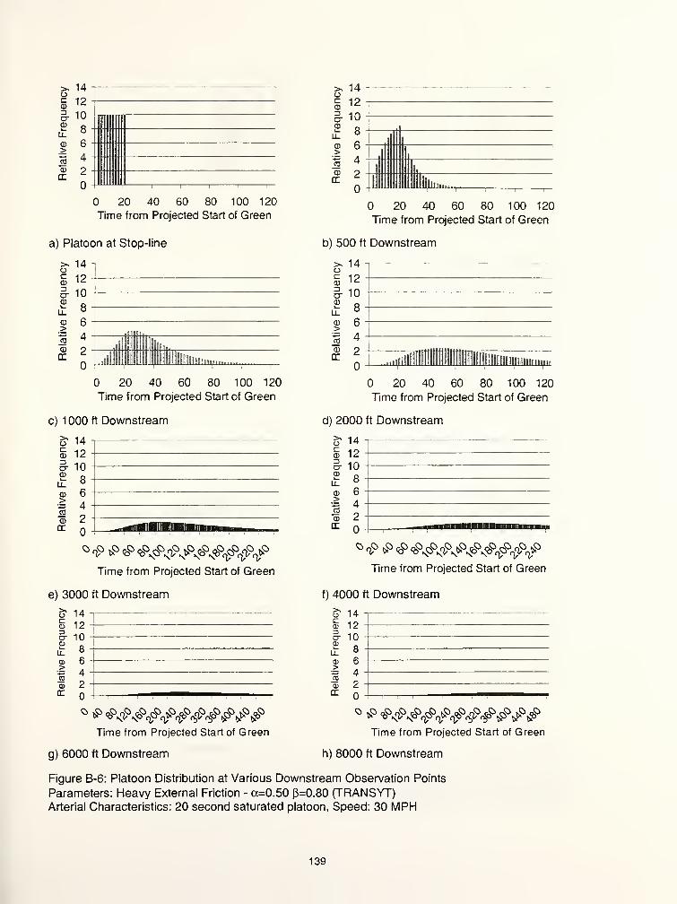
ocCD

o-CD

0)>re

a>

DC

14

12

10

8

6

4

2

20 40 60 80 100 120


ocCD

DO"CD

CD>TO

0)

rr

14 -i

12 -

10 -

8

6

4

2

,

I III

ll III I 111 inn

20 40 60 80 100 120



ocCDr;CXCD

CD>JOCD

rx

14-,

12

10

8

6

4

2

a' ||,

>i!

!

lillj: ,; II II iHSllHlin...

20 40 60 80 100 120


14 i

12

10

oc0)

3a-

I 8

CD 6

I 4CD ODC

<L

^IMlltllililllllglSllliiisUllHlilUiin

20 40 60 80 100 120


c) 1 000 ft Downstream d) 2000 ft Downstream

>>ocCD3ITCD

LL

CD>

CD

DC

14

12

10

8

6

4

2

O «£ IP# <b\o\<^\<%\^\^Time from Projected Start of Green

>.ocCD3O"<D

LL

CD

>

CD

DC

14

12

10

8

6

4

2



& 14

<E 12§ 10£ ft

6

4

2

CD>

CD

OC



14

aCD

DC

cB 123crCD

10

8

6

4

2




Parameters: Heavy External Friction - a=0.50 p=0.80 (TRANSYT)Arterial Characteristics: 20 second saturated platoon, Speed: 30 MPH

139

14 i

12

10

>.oc013IT

LL8

CD 6>

1 4

£ 2

20 40 60 80 100 120


14

12

10

£ 8

CD 6>E 4

2 H

20 40 60 80 100 120


a) Observed Platoon at Stop-line b) 500 ft Downstream

g 12

§ 10

I 8

6

1 4CD Orr

*

>. 14oCD

12

CT 10Cl)

8LL

0) 6>

eS 4CD 9LL

_J lilllllln....

20 40 60 80 100 120




>>O 14CCD 123

10Ci)

LL8

CD 6>

4rn

CD 2tz n


>.ocCD3STCD

CD>joCD

rx

14 i

12

10

8

6

42



ocCD3CTCD

CD>

<D

rx

14

12

10

8

6

4

2


ocCD3CTCD

14

12

10

1 4

CD

rr




Parameters: Four-Lane Divided - a=0.15 (3=0.97 (McCoy)Arterial Characteristics: 20 second saturated platoon, Speed: 40 MPH

140

ocCD3CXCD

CD>

14 7

12

10

I 4

I 2

20 40 60 80 100 120


a) Observed Platoon at Stop-line

CJcCD3O"

CD>

CD

rr

14

12

10

8

6

4

2

TI

,

iiiik

L llli'

lli

to itlftl Biii _

20 40 60 80 100 120


>-ocCD

3CXCD

14

12

10

£ 8

CD 6>

I 4CD 2rx

c

20 40 60 80 100 120



ocCD3D"CD

CD>

CD

CC

14

12

10

8

6

4

2

20 40 60 80 100 120



>.ocCD3CTCD

CD>

CD

DC

14

12

10

8

6

4

2


OcCD

3O"CD

CD>

CD

CC

14

12

10

8

6

4

2










141

14

12

10

£ 8

CD 6>1 4CD ?

20 40 60 80 100 120


>.ocCD=3D"CD

14

12

10

£ 8CD 6>

1 4CD 2

20 40 60 80 100 120



ST14

i 12

§ 10

I 8

cd 6

1 4CD 2

I

20 40 60 80 100 120




ocCD

crCD

CD>

isCD

rr

1"14

12

10

8

64

2


ocCD=3crCD

CD>

CD

rr

14

12

10

8

6

42



sCD

cr

14

12

108

6

4

2



TO

CD

1412

108

6

4

2





142

14

12

10

I 8

<d 6>

I 4CD ?DC

*

20 40 60 80 100 120


^ 14< >

cCD

12

rr 10CD

I

8

CD 6>

« 4CD 2

20 40 60 80 100 120



oCD

CXCD

CD>

14 T

12

10

1 4

MilUu

20 40 60 80 100 120


CD>

CD

14 -

12

10

8

6

4

2oiiid. lllHllllllllllBll.n......

20 40 60 80 100 120



ocCD

crCD

CD>

CD

cc

14

12

10

8

6

4

2


g 12

o- 10CDi_LL

CD>

CD

a:



ocCD

crCD

CO>

CD

tr

14

12

10

8

6

4

2

<^^oS>o<^c£c£>t£o£o^c&l c$»$o$>* * <^ s« r£ r}> c^ #<£>£> fcP> $Time from Projected Start of Green

14c0) 1?3CT 10mLL 8

CO 6•>

4mCD 2LL




Parameters: Heavy External Friction - oc=0.50 [3=0.80 (TRANSYT)Arterial Characteristics: 20 second saturated platoon, Speed: 40 MPH

143

>-ocCD3crCD

14

12

10

I 8

CD 6

"I 4

2

20 40 60 80 100 120


ocCD3a-CD

CD>

CD

rr

14 7

12

10

8

6

4

2Ik.

20 40 60 80 100 120



14 -t

12

10

ocCD3D"

I 8

CD 6

1 4CD QDC

4L

k...

20 40 60 80 100 120


14

12

10

1 8

CD 6

1 4CD 2DC *

iiltm,,.

20 40 60 80 100 120



>.ocCD3crCD

LL

CD>re

CD

DC

14

12

10

8

6

4

2


ilk,

>.ocCD3crCD

LL

CD>

CD

cc

14

12

10

8

6

42



S 12 H

§ 10CD

\±.

CD>TO

CD

DC

w % n> <° <£> qr <£>^ <£> s3 w* t>P


oc:CD3O"CD

CD>

CD

DC

14

12

10

8

6

42



Figure B-1 1 : Platoon Distribution at Various Downstream Observation Points

Parameters: Four-Lane Divided - a=0.15 (3=0.97 (TRANSYT)Arterial Characteristics: 20 second saturated platoon, Speed: 50 MPH

144

ocCDDCT<D

CD>

14

12

10

1 4

20 40 60 80 100 120


14 T12

10

>.ocCD

cr

I 8

CD 6>

I 4

DC

20 40 60 80 100 120



cT14

§ 12

§ 10

£ 8CD 6

I 4

2 T4 Ihm

20 40 60 80 100 120




I**

1 12

§ 10CD

LL

CD>

CD

rr

8

6

42


ocCD

CTCD

iT

CD>TO

CD

DC

14

12

10

8

6

4

2



14

i 12

o- 10

l£8

CD 6>

4mCD 2rr



14

§ 123CD

>

51CD

rr

10

8

6

4

2





145

co>

14 T

12

10

1 4CD O

20 40 60 80 100 120



=- 14 io£ 12CD

CD1—

LL

CD>

CD

rr

10

8

6

4

2liib

20 40 60 80 100 120



>> 14u12

rr 10ni

I

8

CD fi>

co 4CD 2

iljj.

1

J

I

jnl

li

.ill Ml II Ills

20 40 60 80 100 120




(1 14c<1> 12

10CD

118

CI) 6

4R!

CD 2DC



CD

cr

14

12

10

8

6

4

2

N ty <§> tjp fcr #Time from Projected Start of Green

>-oCD

crCD

CD_>

CD

rr

14

12

10

8

6

42



ocCD

crCD

LL

MCD

cc

1412108

S

4

2





Parameters: Moderate External Friction - cc=0.35 (3=0.80 (TRANSYT)Arterial Characteristics: 20 second saturated platoon, Speed: 50 MPH

146

ocID=3crCD

CD>

CD

14

12

10

8

6

4

2

20 40 60 80 100 120


CD>

14

12

10

I 4cd 9rx

*ill!

20 40 60 80 100 120



20 40 60 80 100 120


ocCD=3

crQ)

>

CD

rr

14

12

10

8

6

4

2-dill JlllillM.

20 40 60 80 100 120



ocCD3CD

CD>

CD

rr

14

12

10

8

6

4

2


a it

g 12

o- 10CD

Li.

CD>

CD

rr

8

6

4

2



14oS 12

crcu

_co

CD

cc

10

8

6

4

2

O N^ oP o'i c? r?1 t& o? n^ cP r© ^ o?




14oo 123CO

>

CD

rr

10

8

6

4

2




Parameters: Heavy External Friction - a=0.50 (3=0.80 (TRANSYT)Arterial Characteristics: 20 second saturated platoon, Speed: 50 MPH

147

>-ocCD3crCD

CD>

14

12

10

1 4CD Otr *

20 40 60 80 100 120


>.ocCD3crCD

14

12

10

£ 8

CD 6>

1 4CD 2rr -

20 40 60 80 100 120



>s 14oCD 123rr 10ci)

LL 8

CD fi>03 4CD 2DL

illllu.

20 40 60 80 100 120




o it

§j 12

§ 10CD

Li_

CD>aCD

DC


ac

14 -

12 -

10 -

8 :

6 -

4 -

2 -

CD3aCD

LL

CD>03

CD

IT ^(fiBSillfiBi.u.,

*f. & <b°<&&$&&&$$£>Time from Projected Start of Green


CJcCD3crCD

CD>joCD

rr

14

12

10

8

6

42


>.ocCD3crCD

CD>jo

CD

DC


14

12

10

8

6

42

* **&&&?&&?#f#Time from Projected Start of Green



Parameters: Four-Lane Divided - cc=0.15 (3=0.97 (McCoy)Arterial Characteristics: 40 second saturated platoon, Speed: 30 MPH

148

14 T12

10

? 8

CD>

I 4CD pDC *

14 -

20 40 60 80 100 120



>,14-

g 12

§ 10

I 8

6

4

2

CD>

(13

rx J IlllFII.......

20 40 60 80 100 120



O 14

0) 123rr 10CD

LL.8

<D 6>

4to

CD 2DL


20 40 60 80 100 120



20 40 60 80 100 120



>.ocCD

D"CD

CD>JOCD

DC

14

12

10

8

6

4

2



14 T

I 12

o- 10CD

CD>

CD

CC

° iJ5 o? o° c? cs° l? 9? oG t? c? l? ??




S is -

3- m -

2 ft -

it8

CD b -

•S A -

3 i.CD ^^ o-




Parameters: Low External Friction - ct=0.25 3=0.80 (TRANSYT)Arterial Characteristics: 40 second saturated platoon, Speed: 30 MPH

149

14 T12

10

'S 4

20 40 60 80 100 120


>.oca>

cr

CD>

rr

14

12

10

8

6

4

2

20 40 60 80 100 120



g 12

§ 10

£ 8

g> 6

1 4CD 2rr

c^illl lllllliiin.,.

20 40 60 80 100 120


>> 14CJcCD

123rr 10Q)

l

8

CI) 6>"CC

4CD

IX2

...III IIHlllllUjui

20 40 60 80 100 120



3*OCD3crCDi_LL.

CD>joCD

rr

14

12

10

8

6

4

2


o

CD

CD>TO

CD

rr

14

12

10

8

6

4

2



_co

cu

cr

141210

8

6

4

2*-^

O iS oP oQ c$ r\0 ^ o? oO cO rfi kO of)


ns

CD

14 i

12

1086

4

2



Figure B-1 7: Platoon Distribution at Various Downstream Observation Points


150

>-ucCD3O"CD

>

14

12

10

1 4CD ?DC

c

20 40 60 80 100 120




CDcCD

D"

CD>

14

12

10

I 4

DCe-

^M lUllUlllJuu

20 40 60 80 100 120


>- 14oCCD

12_3

10CD

i

8

CD 6>"5 4

CD

en2

MiMi liiummiuWill

20 40 60 80 100 120



>.ocoo-CDi_

LL

0)>

CD

DC

14

12

10

8

6

42


ocCD

crCD

CD>

CD

DC

14

12

10

8

6

4

2



$ 14

£ 12

o- 10

£ 8

6

4

2

CD>

CD

DC


o it

S 12

CT 10CD

CD>

ISCD

rr


8

6

4

2





151

>.ocID3crCD

(1)

>

14

12

10

I 4CD ODC

c

20 40 60 80 100 120



20 40 60 80 100 120



14

12

10

£ 8o> 6

1 4CD pDC

£-

>>ocCD=JCTCDk_LL

0)>

CD

DC

14

12

10

8

6

4

2

20 40 60 80 100 120













Parameters: Four-Lane Divided - a=0.15 p=0.97 (McCoy)Arterial Characteristics: 40 second saturated platoon, Speed: 40 MPH

152

ocCD3CXCD

CD

CD

cr

14 i

12

10

20 40 60 80 100 120


>>ocCD=1O"CD

CD>aCD

cr

14

12

10

8

6

4

2K.

20 40 60 80 100 120



£ 14

§ 12

§ 10CD

CD>

CD

DC

8

6

4

2llim..

20 40 60 80 100 120



14 7

20 40 60 80 100 120



ocCD13crCD

CD>JOCD

rr

14

12

10

8

6

4

2


14

12ocCD

CT 10CDi_U.

CD>

CD

DC



§ 14

i 12

cr 10

S. 8

<D 6

4

2CD

DC

£ <b\^V^>\^\°V\^Time from Projected Start of Green



o l^

<5 12It 102 p.

6

42

CD>TO

<B

CC




Parameters: Low External Friction - cc=0.25 (3=0.80 (TRANSYT)Arterial Characteristics: 40 second saturated platoon, Speed: 40 MPH

153

14

12

10

£ 8

CD 6>1 4

£ 2

20 40 60 80 100 120


>. 14oca;

123rr 10a>

i

8

CD fi>CO 4CD 2

20 40 60 80 100 120



14 i

20 40 60 80 100 120


>-oc<u=J

CD

CD>

CD

14

12

10

8

6

4

2....lllllil I IpllUuiui

20 40 60 80 100 120



ocCD3o-CD

CD_>

CD

cc

14

1210

8

6

4

2

>.ocCD

o- 10CD

CD>TO

CD

rr

14

12

Time from Projected Start of Green Time from Projected Start of Green


>

CO

cc

14

12

10

8

6

4

2

° Ii° o?> o^ c? (^ ^ oS> o° C?> f\° ^ oP


>>oc<L>

3CTCD

03

CD

DC

1412

10

8

6

4

2



Figure B-21 : Platoon Distribution at Various Downstream Observation Points


154

ocID

CTCD

CD>

14

12

10

=s 4

20 40 60 80 100 120


>-ocCD=!

O"CD

14

12

10

£ 8

CD 6

1 4CD ?rx

20 40 60 80 100 120



>. 14uCCD 12

rr 10<D

LL 8

© R>*-*

CD 4CD 2a

>- 14i)

CD12

3rr 10CD

LL8

CD 6>

ro4

CD 9CL

tllllllllllilHimi...

20 40 60 80 100 120




>.ocCD

CTCD

CD>«CD

rx

14

12

10

8

6

4

2


o£=CDDO"CD

CD>

CD

IX

14

12

10

8

6

4

2



C 14

<£ 12

S- 10

I 8

Q3 6

4

2CD

rr



o it

<5 12

o- 10CD

CD>

CD

DC

8

6

42





155

14

12

10

£ 8



I 4

£ 2

20 40 60 80 100 120



20 40 60 80 100 120



ocCD3crCD

CD>

CD

DC

14

12

10

8

6

4

2

20 40 60 80 100 120


>. 14ocCD

12

rr 10<D

I

8

CD 6>to 4CD 2

20 40 60 80 100 120



>.ocCD

crCD

III

CD>TO

CD

rr

14 -

12

10

8

64

2


O It

<5 12§ 10CD

CD>

CD

cc

8

6

4

2

oV jp ##^ft N#«#$^Time from Projected Start of Green


ocCD

£r 10CD

14

12

CO>

CD

rr



ocCD3crCD

CD>

CD

rr

14

12

10

8

6

4

2




Parameters: Four-Lane Divided - oc=0.15 3=0.97 (McCoy)Arterial Characteristics: 40 second saturated platoon, Speed: 50 MPH

156

14

12

10

E 8



1 4O

rr*

20 40 60 80 100 120




>-uc

3O"

>

rr

14

12

10

8

6

4

2

20 40 60 80 100 120


>. 14UC 123 10

LL8

<D fi>

ea4

2illili^

20 40 60 80 100 120



oc3CT

>

rr

14

12

10

8

6

4

2 '^HIlBfcitifc^,


ocCD3CX(D

>TO

rr

14

12

10

8

6

4

2



o \t

<5 12

o- 10CD

>TO

©rr

8

64

2



14o£ 123cxCD

CD>TO

©IX

10

8

6

4

2





157

14 i

12

10

? 8

>.oca>3cra>

LL

>=S 4

20 40 60 80 100 120



>> 14UcCD

123rr 10CD

T"8

Q) R>

03 4

2ilk.

20 40 60 80 100 120



oco

0>

CD>joCD

DC

14

1210

8

6

4

2

' o0Nt.\«b\%°(^( a^^ t»v ^ -S^O^



20 40 60 80 100 120



20 40 60 80 100 120



14o§ 12

o-CD

LL

CD>re

CD

cc

10

8

6

4

2


f) 4000 ft Downstream>>oC

14 -

12 -

10 -

8 -

6 -

4 -

2 -

>.uca>

trCD

LL

CD

_>

ra

CD

DC

14 -

12 -

10 -

8 -

6 -

4 -

2 -

—CD3UCD

LL

<D>CO

CD

IT

\0 o? nO cP r? iP oP o^ oP c^1 ^ o?* * s> sfo ^ <^ <^ -j?' «p t>? t»* £> PoPfi^c$>f\° ^ o& ci° c? rP fPo?>

Time from Projected Start of Green Time from Projected Start of Green



Parameters: Moderate External Friction - a=0.35 |3=0.80 (TRANSYT)Arterial Characteristics: 40 second saturated platoon, Speed: 50 MPH

158

>.ocCD3cr<D

14 i

12

10

i 8

a) 6>I 4CD pcr

*

20 40 60 80 100 120




20 40 60 80 100 120



>-oCCD=1

O"0)

>

CD

14 T

12

10

8

6

4

2Milll lUuim

20 40 60 80 100 120



o it

S 12

o- 10CD

CD>

CD

rx

8

6

4

2


ocCD3CTCD

CD>eg

CD

14

12

10

8

6

4

2



14o£ 12

cr

CD

_>

™CD

DC

10

8

6

4

2




14o<5 123crCD

>TO

CD

DC

10

8

6

42





159

ocCD3crCD

14

12

10

£ 8

CD 6>I 4

DC*

20 40 60 80 100 120


ocCD3O"CD

CD>

14

12

10

I 4

£ 2lu^

20 40 60 80 100 120



ocCD3a-03

CD>

CD

DC

14

12

10

8

6

4

2

20 40 60 80 100 120


CD>re

CD

DC

14

12

10

8

6

4

2

20 40 60 80 100 120



>>o 14c:CD 123

10

LL 8

 6>4

<n

CD 2DC



o

CD

CD>

rr

14

12

10

8

6

4

2



ocCD3CTCD

CD>

CD

DC

14

12

10

8

6

4

2

'*>&&'$$$$'Time from Projected Start of Green


14 -i

12

10

8

6

4

2

° N°#&&&$&£&&&&Time from Projected Start of Green


>.ocCD3CTCD

0)>

(D

DC


Parameters: Four-Lane Divided - a=0.15 p=0.97 (McCoy)

Arterial Characteristics: 60 second saturated platoon, Speed: 30 MPH

160

ocCD3D"CD

CD>

CD

cc

14

12

10

8

6

4

2

20 40 60 80 100 120



ocCD3crCD

CD>

14

12

10

8

1 4<D 2

20 40 60 80 100 120


20 40 60 80 100 120



ocCD3cx0)

CD>

14 T12

10

8

1 4CD orr * "^iiii lilllmi

20 40 60 80 100 120



>.ocCD3crCD

CD>

CD

rr

14

12

10

8

6

4

2



ocCD3CTCD

CD>

CD

rr

14

12

10

8

6

4

2



CJ 14cCD 123rr 10a>

8U-

<D 6>

4aCD 2cc



S1 14

c5 123

as

DC

10

8

6

4

2





161

ucCD

crID

14 T

12

10

£ 8

<d 6>1 4

£ 2

20 40 60 80 100 120


>.oca>3O"(D

CD

_>

as

<D

rr

14

12

10

8

6

4

2J llii...-

20 40 60 80 100 120



CJcCD

O"CD

CD>

14

12

10

I 4CD orr

e-

l=.

20 40 60 80 100 120


>- 14o£_CD

12JIT- 10CD

8

6>

CD 4CD ?LL

o |

.iiiiiiiiiiiiiiiiliiiiiiiiisiiiii,..,.,..,

20 40 60 80 100 120



14o§5 12

D- 10

I 8

6

42

CD>jo

tr



14o§5 12

cr<D

CD>TO

CD

cc

10

8

6

4

2



ocCO3CJID

CD

CC

14

1210

8

6

4

2

*> ^\<°\o>\%vV£V £Time from Projected Start of Green

acCD

co

ffl

CO

cc

14

1210

8

6

4

2




Parameters: Moderate External Friction - a=0.35 P=0.80 (TRANSYT)Arterial Characteristics: 60 second saturated platoon, Speed: 30 MPH

162

ocCD13CX

14

12

10

£ 8

(U 6

1 4cd ?DC

*

20 40 60 80 100 120


ocCD3D"

>

14

12

10

1 4

• 2

20 40 60 80 100 120



occd

cr

cd>

CD

rr

14

12

10

8

6

4

2- tillm limn

20 40 60 80 100 120


>. 14oc 12CD

!'

§ 10

£ 8

CD 6

CD 2DC

*.miiilllllllllllllllllllllllllllliiiiiii

20 40 60 80 100 120



§ 12

a- 10CD

CD>

CD

DC


i 12

o- 10CD

CD

aCD

rx



CO>

CD

1412

10

8

6

4

2


f) 4000 ft Downstream>.oca>uCTCD

14

12

10

* 2CD 211

^ i? o? o^ cP (^> i& o?> n^ ^ t\^ i$> a°





163

14

12

10

>.ocCD3CT

I 8

0) 6>

I 4Q) 9ir *

14 -r

20 40 60 80 100 120




>-ocCD3CTCD

CD>TO

CD

rr

14 i

12

10

8

6

4

2iiiiii

20 40 60 80 100 120




§ 12

o- 10CD

CD>joCD

rr

86

42


ocCD3crCDl_LL

CD>

CD

EC

14

12

10

86

42



>.ocCD3o-CD

CD>TO

CD

rx

14

12

10

8

6

4

2


ocCD3ITCD

CD>

CD

rr

14 i

12

10

8

6

4

2



Figure B-31 : Platoon Distribution at Various Downstream Observation Points

Parameters: Four-Lane Divided - a=0.15 p=0.97 (McCoy)

Arterial Characteristics: 60 second saturation, Speed: 40 MPH

164

Ss 14 To§ 12

g- 10CD

CD>re

CD

rx

14 i

20 40 60 80 100 120




>,14^cCD

CTCD

U_

CD>

CD

DC

12

10

8

6

4

2

20 40 60 80 100 120


>. 14 -

oc 12CD

ic-

§ 10CD

CD>

CD

rx

8

6

4

2^^jjiniiiBIIMlllllHHHllinnmUlliim

20 40 60 80 100 120



>.ocCD

o-CD

CD>

CD

rx

14

12

10

8

6

42


>>ocCD3txCD

CD>

CD

rx

14

12

10

8

6

4

2


e) 3000 ft Downstream f) 4000 ft Downstream>.ocCD

CTCO

CD>

CD

QC

14

12

10

8

6

4

2


o II

e 12or 10

ij.°

6

42

CD>

CD

OC

^ li? !? 0° t? C? N° ?? 0° 5? (^ I? «?




Parameters: Low External Friction - a=0.25 [3=0.80 (TRANSYT)Arterial Characteristics: 60 second saturation, Speed: 40 MPH

165

>. 14CIcCD

12

rr 10CD

i

8

03 6>ro 4CD 2

20 40 60 80 100 120


>. 14(

)

cCD

12=3 10CD

i

8

Cl) 6>

CD 4CD 2

llUu.

20 40 60 80 100 120



g 12

§ 10

£ 8

g> 6

1 4CD Orr

*illllllllllllllllllllli.

20 40 60 80 100 120


14

12

10s 8

O) 6

1 4CD Orr

<L

UUdlll i IHllHll...,

20 40 60 80 100 120



>.ocCDZ3

O"CD

CD>

CD

DC

14

12

10

8

6

4

2





o0)zs

CTCD

CD>

CD

rr

14

1210

8

6

4

2



g- 14

S 12

o- 10

itB

o> 6

4

2CD —




Parameters: Moderate External Friction - a=0.35 (3=0.80 (TRANSYT)Arterial Characteristics: 60 second saturation, Speed: 40 MPH

166

^ 14uca)

12

rr 10CD

i

8

at fi>

<54

CD 2

20 40 60 80 100 120


>, 14< >

cCD

12

rr 10CD

i

8

0) fi>

co4

CD 21

20 40 60 80 100 120



14 -

12 f10 -

CD>

£ 8

1 4CD prr * Hi Mi llln

20 40 60 80 100 120


>, 14 iog 12

§ 10CD

CD>

CD

rr

8

6

4

2....jiiUllllilifiminniitllliwmiiiiiim

20 40 60 80 100 120



ocCD-=,

CTCD

CD>TO

CD

DC

14

12

10

8

6

4

2


oCCD

O" 10CD

14

12

CD>13CD



14 ioc5 12

CTCD

CD>TO

CD

cc

10

8

6

4

2

T



14ocB 12

CD>

CD

10

8

6

4

2





167

CD>OS

CD

GC

14

12

10

8

6

4

2

20 40 60 80 100 120


oCD

CTCD

>

14 7

12

CD

rx

10

=5 4

k20 40 60 80 100 120



>.14n

g- 10CD

CD>

CD

rx i

20 40 60 80 100 120



>.oCCD

CTCD

CD>_CC

CD

rx

14 T

12

10

8

6

4

2 j! IllllUf..,

20 40 60 80 100 120



oCD

CTCD

CD>

CD

rx

14

12

10

8

6

42 iiik.


>>ocCD13CTCD

LL

CD>03

CD

rx

14

12

10

8

4

2





>.ocCD

CTCD

CD_>

re

CDrx

14

12

10

8

6

4

2

O kO oS> oO^ &&Time from Projected Start of Green



Parameters: Four-Lane Divided - a=0.15 (3=0.97 (McCoy)Arterial Characteristics: 60 second saturated platoon, Speed: 50 MPH

168

>- 14oc 12

g- 10

a?>

a)

DC

8

6

42

20 40 60 80 100 120



03 '<-

g- 100)

Q)>

CD

DC

8

6

4

2A llllll...

20 40 60 80 100 120



oc<r>

3cr<D

03>jo03

DC

14

12

10

8

6

4

2



cj 14

S 125- 10

6

42

03>

03

cr



20 40 60 80 100 120



20 40 60 80 100 120



>.ocCD-

03

CD>

CD

DC

14

12

10

8

6

4

2



14 i5*O£ 123crCD

03>

o>

CC

10

8

6

4

2

^ tP o?> o° C? C?> tJ1 9? 0° c? c? ^ ??





169

14

12

10

« 8u.

CD>

§ 4CD ?

20 40 60 80 100 120


>-ucCD

CCD

Q)>

CD

rr

14

12

10

8

6

4

2

20 40 60 80 100 120



cT14

cCD

CD

CD>

orr

12

10

8

6

4

2a lllllllu*

20 40 60 80 100 120


CD>

14

12

10

1 4CD 2DC

c ^illi^^20 40 60 80 100 120



ocCD3tTCD

CD>

<D

14

12

10

8

6

4

2


>.ocCD

o- 10<D

14

12

(D>joCD

rr

8

6

42






c14 -

12 -

10 -

8 -

6 -

4 -

2 -

o11)

3CD

CD CD

LL LL

U)>

CD>

03 CO

rrCD

(J "

\° o? o^ c? c\0 iP o? oO cP rP ^ o?

14

12

10

8

6

4

2

£^^VtW^isSWTime from Projected Start of Green




170

>,ocID3CTCD

14

12

10

i:8

CD 6>I 4o 2

20 40 60 80 100 120



>> 14CJcCD

123 10CD

I

8

CD 6>ffl

4CD

IX2

lllii...

20 40 60 80 100 120



>.ocCD

3O"<D

14

12

10

if 8

cd 6

1 4CD oDC

£-

:

mil Mia

20 40 60 80 100 120


ocCD3O"CD

CD>

14

12

10

iiiiiiillUHIlllll Jli l ll i ailiiim,.

20 40 60 80 100 120



o 14

123rr 10CD

I

8

a) 6>

4Cfl

CD 2LL


ocCD3O"CD

CD>

CD

DC

14 T12

10

86

4

2



14o<5 123CD

CD.>

jo0)

CC

10

8

6

4

2



14cCD 1?3

10(11

LL 8

CD 6>

4CO

CD 2DC

O ^ oP o^> cS> r? ^ o? o^ c? c\^ |J> o?




Parameters: Heavy External Friction - ct=0.50 p=0.80 (TRANSYT)Arterial Characteristics: 60 second saturated platoon, Speed: 50 MPH

171

20 40 60 80 100


120

2000 ft. Downstream, 20-second saturated platoon, Speed: 30 MPHPlatoon Dispersion Parameters: a=0.15 and (3=0.97

Figure B-39: Example Arrival Times (Theoretical Model)

172

-t99 -"-t95 -*-t75 -«-t50 -*-t25 -*-t5

100

500 1000 1500 2000 2500 3000 3500 4000 4500


20-second saturated platoon, Speed: 30 MPHPlatoon Dispersion Parameters: a=0.15 and (5=0.97

Figure B-40: Theoretical Arrival Times

— 199 -"-t95 -»-t75 -«-t50 -«-t25 —-t5

100

500 1000 1500 2000 2500 3000 3500 4000 4500



Figure B-41 : Theoretical Green Window (Adjusted Arrival Times)

173

-t99 -«-t95 -*-t75 -«-t50 -*-t25 -«-t5

100

500 1000 1500 2000 2500 3000 3500 4000 4500



Figure B-42: Theoretical Arrival Times

-t99 -»-t95 -*-t75 -*-t50 -«-t25 -»-t5

100

o

3-

oD

Co

CD

500 1000 1500 2000 2500 3000 3500 4000 4500



Figure B-43: Theoretical Green Window (Adjusted Arrival Times)

174

1-199 -195 -175 -t50 -125 -IS - 199 - 195 - 175 - 150 - 125 - 15

100

CO

2

<5

100

CO

5

1000 2000 3000 4000


1000 2000 3000 4000


a) ct=0. 15, (3=0.97 b) a=0.25, (3=0.80

j-t99 -t95 -t75 -t50 -125 -151 -t99 -t95 -175 -150 -t25 -t5

_. 100

to

S

- 100

CO

s

1000 2000 3000 4000


1000 2000 3000 4000


c) o=0.35, (3=0.80 d) a=0.50, (3=0.80

Figure B-44: Theoretical Green Window (20 second saturated platoon, Speed: 30 MPH)

-t99 -t95 -t75 -t50 -125 -t5 -t99 -195 -t75 -t50 -t25 -t5

~ 100 -\ _ 100

1000 2000 3000 4000


a) a=0.15, (3=0.97

1000 2000 3000 4000


b) <x=0.25, (3=0.80

-t99 -t95 -t75 -150 -t25 -15 -t99 -t95 -t75 -t50 -t25 -15

_ 100

1000 2000 3000 4000


c) a=0.35, 3=0.80

1000 2000 3000 4000


d) a=0.50, (3=0.80


175

-t99-15 -125 -t50 -t75 -t95 -t99 -195 -t75 -150 -t25 -t5

100

to

3

100

CO

o

1000 2000 3000 4000


1000 2000 3000 4000


a) a=0. 15, (3=0.97 b) a=0.25, (3=0.80

-t99 -195 -t75 -t50 -t25 -t5 - 199 - 195 - 175 - 150 - 125 - 15

.

— 100

1000 2000 3000 4000


1000 2000 3000 4000


c) a=0.35, p=0.80 d) a=0.50, (3=0.80


-t99 -195 -175 -t50 -125 -15; -199 -t95 -175 -t50 -125 -t5

100

CO

5

CD

100

5

1000 2000 3000 4000


a)a=0.15, (3=0.97

1000 2000 3000 4000


b) a=0.25, P=0.80

-199 -t95 -t75 -t50 -t25 -t5 -199 -t95 -175 -150 -t25 -15

100 -

1000 2000 3000 4000


c) 01=0.35, (3=0.80

1000 2000 3000 4000


d) cx=0.50, (3=0.80


176

- 199 -195 -175 - 150 -t25 —IS - 199 - 195 - 175 - 150 -125 —15

100 T

S2.

s

100

1000 2000 3000 4000


1000 2000 3000 4000


a)a=0.15, (3=0.97 b) a=0.25, (3=0.80

- 199 -195 - 175 - 150 -125 -15

100

to

s

a

- 100oCO

So1 50

O

-199 - t95 -175 -t50 -t25 -15|

7/y^y^g^l—

1000 2000 3000 4000


1000 2000 3000 4000

Downstream Distance (ft

)

c) o=0.35, |3=0.80 d) a=0.50, (3=0-80


-t99 -195 -t75 -t50 -125 -15 -t99 -t95 -175 -t50 -125 -t5

100 - 100

1000 2000 3000 4000


a) cc=0.15, (3=0.97

1000 2000 3000 4000


b) ct=0.25, (3=0.80

-t99 -t95 -t75 -t50 -125 -t5 -t99 -t95 -t75 -t50 -t25 -t5

^ 100 -

5

„ 100

26

1000 2000 3000 4000


c) a=0.35, (3=0.80

1000 2000 3000 4000


d) a=0.50, (3=0.80


177

- 199 - 195 - 175 - 150 - 125 - 15 - 199 - t95 - 175 - 150 - 125 - 15

1

100 T

OT

S

„ 100

CO

g

1000 2000 3000 4000


1000 2000 3000 4000


a)oc=0.15, |3=0.97 b) a=0.25, (3=0.80

- 199 - 195 - 175 - 150 - 125 - 15

_ 100

co

3

— 100 ioa<n

o1 50

O

-199 -t95 -t75 -t50 -t25 --«|

'i///^^^ —

-

!

1000 2000 3000 4000


1000 2000 3000 4000


c) a=0.35, (3=0.80 d) a=0.50, (3=0.80


-t99 -t95 -t75 -t50 -125 -t5 -t99 ~t95 -t75 -t50 -t25 -t5

_ 100 -. 100

CO

g

1000.0 2000.0 3000.0 4000.0


a) a=0.1 5, (3=0.97

1000 2000 3000 4000


b) a=0.25, (3=0.80

-t99 -t95 -t75 -t50 -125 -t5 -t99 -t95 -t75 -t50 -t25 -t5

- 100

5

_ 100

o

1000 2000 3000 4000


c) a=0.35, 3=0.80

1000 2000 3000 4000


d) a=0.50, (3=0.80

Figure B-51 : Theoretical Green Window (60 second saturated platoon, Speed: 40 MPH)

178

-t99 -195 -t75 -t50 -125 -t5

- 100

1000 2000 3000 4000


a)a=0.15, (3=0.97

>-t99 -t95 -t75 -150 -125 -t5

100

1000 2000 3000 4000


c) a=0.35, (3=0.80

!

- 199 - 195 - 175 - 150 - 125 - 15 i

100

1000 2000 3000 4000


b) a=0.25, (3=0.80

- 199 - 195 - 175 - 150 - 125 - 15

100

1000 2000 3000 4000

Downstream Distance (ft

)

d) a=0.50, (3=0.80


179

-t99 -*-t95 -*-t75 -*-t50 -*-t25 -»-t5

100

500 1000 1500 2000 2500 3000 3500 4000 4500



-t99 -»-t95 — 175 -^t50 -^-t25 —-t5

100

500 1000 1500 2000 2500 3000 3500 4000 4500


Figure B-54 Theoretical Green Window (20 second saturated platoon, Speed: 40 MPH)

180

APPENDIX C

SIMULATION RANDOM NUMBER SEEDS

181

Table C-1 Random [\lumber Seeds Used in CORSIM Simulations

Run Number Seed 1 Seed 2 Seed 3

1 2431 4879 6153

2 2851 5647 2189

3 1027 8347 9723

4 7353 8753 3451

5 3873 2851 4369

6 8327 6841 3753

7 4789 7257 5817

8 6751 3783 4449

9 1279 7357 9371

10 8743 4153 7853

11 9459 7847 6349

12 8351 3279 4821

13 8953 2469 5837

14 9243 4683 3979

15 2857 8241 5973

16 3473 8621 3497

17 6871 2597 3497

18 2343 7891 3631

19 8979 3741 2357

20 4697 6783 2859

182

APPENDIX D

SIMULATION RESULTS

183

7/10/98 Platoon Accommodation At Isolated Traffic Signals Jay Wasson

VPH = Flow Rate in Vehicles per Hour

STOPS = Percentage erf Vehicles Stopped

DELAY = Delay Time (Seconds/Vehde) Tottfe

. 32.9

^82X

CR350"-*?<'

DELAY STOPS VPH

IP* 25 5 82% 91

241 67% 259

Signet Phasing at Intersection12 3 4

u r> -f*] H u

V

VPHSTOPSDELAY

38

92%358

t346

47%13.1

VPH

13

54%

CMIfl

COr>

«3% : ;

Intersection Statistics

VPH 1825

STOPS 62%DELAY 24.0

22.1 re**.

roe*:'

Summary of Meeasures of Effectiveness Average Values:

Unt Ln Vahtcto VtNda MMMM Ratio SacfVah VaMBn lUwngt

PtMM 8*jrt End Oram •— Trtpa HmTkM atayTbaa ToOITkM Mow* Total Total Thaa DWyTta* QuauaTfeaa StDpTko* Stops (PCT) SpnedMPW

2

2

8

B

8

Thnj TR)gtt*

6.51

60.46

221

axn.40

707

85.70

239

544

16.86

050

1251

84 56

289

0.55

78

64

31 *fl

SB 78

54.37

35 84

iaua77

4J0

1258

aie

446

1225

Q18

91 95

47.00

5417

31 18

4293

4682

1

6

a

6

6

8

La**

ThruA

938

5*87

14 31

15 80

91.15

23.85

1017

59 40

15-54

iaoi

45.19

796

28.17

104 59

2150

0.37

058

0.67

106.63

6901

56.98

G8 73

29.91

19.86

14 'P.

24.78

250

1377

23.14

223

9558

S536

mm

2021

31-97

36 81

4

4

4

2

2

2

tj™ -»

a 38

R68

503

ZZS5

64.55

33.55

451

1Z91

6.71

9.64

28.00

1138

14 15

38.91

1609

033

0.34

0.37

37 47

36-09

3255

25.47

24.09

20, 55

743

IBM6,fp

730

1739

625

8195

66.65

7019

14 78

1511

15 89

s

s

B

4

4

4

Tlwu*-

443

31.29

1120

985

8S55

24.90

5.91

41.71

14.93

361

2652

R43

9.51

682]

23.36

Q64

0.61

0.64

57X58 60

5a49

21-32

nm20.49

227

1518

438

223

14.27

407

7533

60-36

64 59

mm2780

2857

Summary of Measure of Effectiveness Standard Deviations:

Link Law Vmhldm VaNdaMfatfaa Ratio SacWab VatVMn Awarags

*" M End Group Mm TrtOB MoaaTlma DatoyTMa Total Tk»* Hem Tom nMUM DatoyTfeaa Qu»TW atopTkM 3topa(PCT) SpaadHPH

s 8 LrflR 203 290 221 1 79 182 0.05 759 7.59 1.67 16B 758 290

2 8 Trav-T- 289 4 12 113 211 155 0.02 1.70 170 168 158 552 123

2 8 RJflU * 127 181 138 0.44 1.77 0.0B 4 12 4.02 Q19 019 37 80 389

i 6 Lrf * 228 180 248 518 7 17 aos 1507 1507 434 4.18 579 286

6 6 TTrnj* 333 555 162 1846 1644 008 1141 1141 1180 112* 15 T2 4.45

6 6 Right tf 181 101 tse 223 187 0.05 433 4.33- 1 44 128 1508 286

4 2 Left?* 083 555 mi 355 4 41 005 aoe 609 103 293 789 241

4 2 Thru-* 0.88 588 1.18 4.94 579 003 158 356 402 187 757 1.55

4 2 R^jra i. 0.78 521 1.04 252 106 O05 4.49 4.4ft 203 1.88 507 219

8 4 Loft* 131 291 1.74 164 124 0.07 633 634 123 121 17.09 320

8 4 Thm *- 3J32 ft72 4.03 4*7 827 003 122 323 143 328 829 1.53

8 4 RJghlK 252 581 136 249 528 005 4.98 4.98 1.71 184 1029 244

StOppao VamCMa Pac AppfOBGPi

|

i

Vottcto Dot*- Pw Apon-crt (SaconokWattciai

90% M 1- 80.0

80%' 1 ic t T 71% 700

70%Trp btB ItJC 60.0 H

80%

50%

40%

30% 11 152%

IIsac

4O0

30.0 1 T ^ ^^ 221

20% 1 i 1 1 HI II 2O0 1152

10%JUL l 1 Hi 100

! LH"H ' BaF'fl

Southbound Northbound Eastoour d Westbound Southbound Ncrthbound Eastbourid WestlXrund

1' Uft aTrnugti OFo</* BAA]

1llaB Througti Oftprt BAD3

Additional Mohb:

Period 3 Promotion Settings - > 00 Mm. 45 Max, 60 Reservice, 25 Delay. 13 Inhibit

Platoon Settings - > 1 1 Vehicles in 10 seconds

F:\Jay\Research\Era8 FJes\Penod3\100%\00-»5*0-25-13_11-10\

P3a-100.xls School of Civil Engineering - Purdue University Pnnted on 7/1 0/98 at 9.06 AM

Figure D-1 Period 3 Configuration A-100

184

7/1 5/98 Platoon Accommodation At Isolated Traffic Signals Jay Wasson

VPH = Flow Rate in Vehcles per Hour

STOPS = Percentage of Vehicles Stopped

DELAY Delay Time (Seconds/Vehicle)

CR350

DELAY STOPS

«?*

Sqrml Pftnsino at Intnmnann

1

I*

2 3

-J*

1 H <"

ToOla

-:-37M

:::<*9:

17 9

63%96 ~«2%


VPH 1820

STOPS 63%DELAY 247

-2i«- rotate-

VPHK * 7\

VPH 38 346 13

I STOPS 90% 45% 51%: DELAY 32.8 12.5 9.3

--

:;=397

T-30K

Toots

r 99 67% 21.1

<- 278 59% 22.3

U 40 74% 20.3 ^=^~\


IMi Urn Vafttda VvMctaHnutM Ratio SooVah V«v4*kn Av«naja

PhBB» Start End Group —

.

Trip. WovvTka* OaaayTana Total Tasa Mow* ToOi TottfTkrM DpkayThna Ctumum Ttttt* BtOpTkna 8topa(PCT) 3pBR)»H

5 8 U*K 058 940 715 5.00 1223 059 78 44 3Z01 406 401 90.28 3240

2 8 Thru f 6045 88.35 6587 18.02 S3m 078 58.19 1256 use 11.85 432B 43.34

2 8 p&tjH'' 221 115 238 0.52 2.92 Q84 54 92 933 021 0.20 son 4623

1 e Lrf 9 36 1S60 1017 19 15 2932 0.38 11227 7317 1511 14.62 9a44 1988

6 6 Thru 4- 54 58 9100 59.X 54.43 113.73 0.53 7494 35.64 31-33 2941 68.42 29 3S

6 6 fogMrr 1437 23 95 1S81 722 2283 069 5703 1783 1.97 172 63.03 38.01

4 2 Left 1 3.34 2225 445 913 1358 034 3899 2499 717 701 8459 15.13

4 2 Thru-* 973 84 85 1297 24.49 3746 OSS 3460 2280 1719 1818 63.98 1593

4 2 KpH a 502 33.45 808 1996 17.84 040 3150 19 50 6.50 596 89.45 17 78

8 4 left !i 4,48 B90 5.94 347 940 0.65 56.31 20 34 211 207 73.79 2908

8 4 Thru*- SUB 99 40 4182 25 78 67 40 082 58.30 2231 14 44 1354 58-84 27 64

8 4 Watt* nee 24 65 14.78 964 23.43 964 57.08 2107 4.64 4.28 66.83 28-64


Utah Lana VaMda VaMctalfraaM Ratio SooVah V*»Mk. Average

Ptaaaa Start End Group — Trip. Delay How TotalTkM Mom Total Total Tkau> OaatyTlow Queue Tana Stop Tana 8tDp»(PCT) SpaadHPH*OV»T«M

5 6 LaftR 210 100 228 195 3981 0.05 7.85 785- 175 ITS 8.82 298

2 8 ThruT 121 4 58 348 1.91 424 002 1.41 1.41 1.95 191 5 16 1.05

2 Right* 1.27 181 136 0.45 177 O07 4.94 486 024 022 39.80 399

1 B Loft:. 227 3 79 247 689 B76 006 16-77 18 77 5.79 661 718 116

6 6 Thru 4- 338 561 366 -KL71 1018 008 1078 1078 11.72 11.18 1690 4.27

6 6 Rig** 188 314 204 209 385 004 367 3.87 1 18 101 1441 237

2 L«ft 31 080 S33 1.07 289 349 008 7 71 771 243 235 10.95 268

2 Tr»u-» 090 6 00 1J0 6.58 722 005 5-28 5-28 5.02 485 7.40 225

2 Rights 075 501 1.00 4.36 495 007 674 6.74 336 314 9.82 122

4 Left.: 131 2» 1 74 1.62 323 007 615 615 1 16 1 14 17.79 308

4 Thnj *- 315 700 420 4.15 742 0.03 300 IX 254 242 6 28 140

8 4 Rift* 251 558 335 301 573 0.08 5.72 5.72 194 1.82 1072 276

Bloppad VaMcan Pa* Approach VaNda Daur, Par Approach (B4CondarVeNele}

90% 800

80%

70%

60%

SOS

40%

30%

20%

'89S

50%

T"BS700

800

50.0

400

3Q0

200

It v °

144

T j -3Z2 . -HIj

10% 10.0

mlM BJSoutribound Northbound Eastboutid Westbound Southbound Nc•rttibound Eastboui

|

Westbound

- La* Through Right BAI|<

Laft aVThrough ORnhi BAI

ftdafafaaBJ Mo***

P&rtod 3 Prempbon Setbngs - >00 Mn. 45 Max. 60 Reservica. 20 Delay. 13 inhibit

Platoon Settings - > 16 Vehicles in 15 seconds

F.Uay\Researcn\Excefi Fira\Pehod3\1X%\0CM5-6O-20-13_16-15\

P3b-100.xts School of Civil Engineering - Purdue University Printed on 7/15/98 at 1 1:19 AM

Figure D-2 Period 3 Configuration B-100

185

VPH

STOPSDELAY

= Row Rate In Vehides per Hour

^ Percentage of Vehicles Stopped

= Delay Tme (Seconds/Vehicle)

CR350

Tool*

362..

64%.

\$.13

18-7

62%36

324

59%358

4-

i 879 DELAY|

.; 97% STOPS :

S9 VPH •

S

DELAY STOPS

71% 134

.._ra»... : 487;.,.

S»m»? Ptiasmq at Inmrsftchnn12 3 4

L* f*it

1 4

K f i

VPH 38 344 ;

i STOPS 90% 44% !

: DELAY 41.4 11.9 :

13

46%9.0

id

CO

'425 :B3«


VPH 1820

STOPS 62%DELAY 25.0

—22.0 Tdtafa 3

283 80% 22.8

41 76% 20 7

VPH STOPS DELAY

3§S:toou:


Uf* imrn V«h*c* ViMcHHiUM Rxtto 3*c/VWi Van-Mn Amng*

PhKM StVt End Grot*? — Trip. HavcThn* Ovtay Tim* ToMTkM Mm* ToOl TottTkn* OatoyTTn* Qubu»T)bm StopTtiM Stop* (PCT) SfMdWH

5 e L«flK 8-55 B35 7.11 647 1358 Q53 87 08 41 45 544 538 90.41 29.42

2 8 Trait 60.17 85 95 6536 1634 82.X 0.79 57.48 1187 1097 ias4 44.13 43.68

2 8 Right" 234 120 243 031 295 084 54.59 ax 18 a is 46*2 46.46

1 8 U** a73 14.55 ft46 20 S3 30.41 032 126.99 8739 19X I860 97 17 1792

e Thru 4- 53.65 89 45 «a?a 46.19 106.48 OSS 71 46 3236 28.X 2644 5862 X91

e 6 Kjgfrnc 1437 23 95 1561 750 2310 0.68 57 85 1675 224 1.95 6179 37 51

4 2 Lea* 3.38 2256 451 9.58 14X a32 37 65 2565 740 725 85.44 1453

4 2 Thru-* A83 65 50 1110 27.74 40.84 a33 37JO 25 30 19.38 18-14 67.16 14 7B

4 2 Rtpt* 5X 33.35 0.67 1132 ia.se 0.37 3346 2147 734 677 70.56 165S

5 4 Lrft: 4.52 iao5 6.03 156 9.58 064 5671 20 73 213 210 76.16 28.72

8 4 Thru«- 31.76 7D.X 42.34 26.86 6920 aei 58.76 2278 14.90 13.98 60.43 27 64

8 4 KtfttK 11.29 25.10 1505 8-50 23.55 0.64 56.50 20-50 427 394 6652 28.79


Link Lam VcMdte V*ttc»Mnt*»* Ratio SeerV«n Vwhltin Avwrag*

Pftw* Start End Graap — Tr*» MovsTbM OvtxyTVn* TabdTkM Mow Tot* TaMTiRM OvterTkM OsanjvTlnM StopTki*# S»p«CPCT) SpwdMPH

5 8 LoftK 2X 294 224 3.X 489 0.06 1224 1223 230 288 7.01 ass

2 8 ThruT 3.33 4.75 3.61 225 426 0.02 1.78 ITBj 1.79 1.73 563 136

2 8 ftgrt* 128 1.7B 136 044 175 0.07 432 425 021 0L21 36.16 193

1 8 Loft* 1.78 293 1.91 7.53 131 0.07 31.88 3188 11 11 io as IX 3.91

6 6 Thru J- 182 837 4.15 1714 1643 ax 11.32 1132 1151 1284 16-51 450

8 6 north: 1.76 296 1.92 196 142 ax 4.18 4.16 126 1.09 13 45 265

4 2 Lrfa ax 571 1,14 283 151 0.04 530 5.X 216 211 5 88 194

4 2 Thru-* 0.81 5.42 1.X 8.81 7.45 0.05 526 526 5.75 546 7.98 2T2

4 2 Foot** 078 5-20 1.04 151 4.10 006 535 535 104 278 9.72 270

8 4 Late 111 291 1.75 1.42 107 ox 453 4.53 039 OX 17 59 227

8 4 Thru«- IX 6.67 4-X 487 8-02 ax 292 291 IX 327 679 134

8 4 RtgrtR 258 S75 145 221 528 ao4 376 175 1.41 133 8.34 1.93

StDpptQWlMoM P*r Approach VahfcJt May P* Approve <3*CondtfV«Hcl»)

90%OM ;

j eao 1

60%I T 72* 70.0

70% 64% I.X53% :

60.0

60%

50%

40%

*9% 500

40-0 T 38i

30%30.0 J y 243 220 j

20% 20.0 i 146

10% mo

Southbound Northbound Eastbou id Westbound Southbound Northbound Eastbourrd Westlxxjnd

!« Left Throuori DRtgrS »AI] |<

iLoft ThroLyn OR^rt«]

I

AjMrJJgal Hon*Period 3 Prempoon Settings > 00 Mm, 45 Max, 60 Resenrice. 25 Delay. 13 Inhibit


F:\Jay\Research\ExceH Rles\Pehod3\100%\00-45«>-25-13_6-10\

P3c-100.xls School of Civil Engineering - Purdue University Printed on 7/1 5/98 at 1 1 : 1 7 AM

Figure D-3 Period 3 Configuration C-100

186

STOPS Percentage of Vehicles Stopped

DELAY = Delay Time (Seconds/Vehicle) Total*

: 32* .

•.Mi '

CR350 £j«j^

190

60%96

1 2 3

-f1 4 «;r

DELAY STOPS VPH

U* 25 6 82"* 90

22.1 64% 261

r

28 7

54%366

4-

VPHSTOPSDELAY

71.6

93%63

DELAY

STOPSVPH

K f !

38 345 |

92% 47% |

38.7 13.2 !

13

49%81

CMin

to

479 -64«"


VPH 1826

STOPS 61%DELAY 236

226 Total*

STOPS DELAY

Wi.

rotate -:


Ur* UN VfjMcto VfMdaMnUM RaOo Sac/Vati VraSaaVi Awaga

PhtM Stan End Qroup — Trips ttowTto* fM^rTtaM Total Thna MomTom Total Tawa Dotty Tana QuauaTIrM fttapThTM Stop* fPCT) SpaadHPH

5

2

2

8

a

8

Laftic

Thfu-r

Right 71

6 51

8034

221

9 30

8820

a 15

707

as 56

2.39

5.80

1898

047

1287

64.54

268

055

378

035

6436

5883

5364

38 73

1323

306

4S3

1374

313

478

1237

Q12

9132

4393

49.05

9035

4264

47.25

1

6

e

8

6

6

Thru 4-

S4S

54 78

14.31

15.75

9130

23-85

1038

5849

1554

18.78

4367

753

29 04

103 16

2307

0.36

0.58

0.66

110 72

6779

5811

71.62

28.89

1901

14.62

2344

228

14 14

2161

202

9264

5356

59.53

1936

3217

37.42

4

4

4

2

2

2

LoH*

Thru-»

Right M

338

9.77

5.08

22.40

6510

33.75

4.48

13.02

6.75

949

24.06

1115

1397

37.07

17.90

032

0.36

039

3758

34 07

31.76

25.55

2Z07

19.78

755

1364

365

7.40

1550

309

6248

6423

7Q3B

14.63

1320

17.41

s

8

8

4

4

4

Left .'

Thru«-

448

3138

11.20

9.95

69.75

24 90

397

4183

14.93

365

2732

375

062

69.08

2369

064

061

064

S735

5934

57.01

2137

2336

2103

227

1377

4.59

223

14.84

4.19

7323

6105

6396

2359

2737

2359

Summary of Measure of Effectiveness Standard Deviations

LMh LfM VaNda Vahtd* aftrxjaa* Rafto 3*KfV«at) VafcJran Avorago

p*~ M End Oraup — Tripji WowoTboo Dotty Thaw Total Tkoo UowoToM Total Tana OootyTkno QuauaTono StopTWoo Stops fPCT) SpoodMPH

5 8 it** 206 294 224 213 396 007 1138 1137 1.92 1.91 372 183

2 8 Thru-f 319 438 347 225 4.82 002 146 144 1.85 1.78 591 104

2 6 Rxr*^ 127 181 138 0.42 174 0.07 404 398 014 013 3355 178

1 6 1 lor a 232 386 232 584 7.89 OOS 1433 1433 487 470 934 239

6 6 Thru 4- 330 5.51 359 11.04 1341 008 713 713 314 735 1265 329

6 6 Mgro t 132 303 197 21t 336 005 534 334 134 111 1405 298

4 2 Loft * 034 560 1 12 269 160 aw 533 533 227 219 889 185

4 2 Thru-* 0.86 5.75 115 030 7.02 06 303 303 321 497 302 267

4 2 Right :* 078 521 1.04 346 4.12 aos 518 518 281 266 940 268

e 4 LaBtc 127 282 139 161 315 007 636 6.56 1.19 116 1795 128

8 4 Thru *- 289 6 42 385 515 322 004 342 343 374 357 301 161

6 4 Right* 261 5 80 348 314 317 005 4.75 4.76 13B 131 989 237

BtOBpjdVaHdaa Par Approadt VoNda Dotty Por Approach dJoconaattoNclo)

90% 80080%

70%

60%

50%

40%

BM51%

Te9%T«4%

700

630

500

430T

321 . mm

30%300

Laaaooa 1 T T 22 1 22.6

20% 20.0 H-l-fl www\\WtWL\

10% 130 -1

Southbound Northbound Eastbou d V\pastt>ound Southbound Ncrthbound Easrbourvd West!xxind

Lot Throuoh ORJghl BAl :!«iLrt Throuoh Right Ha

AddMon.1 Holm,

Period 3 Promotion Settings - > 00 Mm. 45 Max. 60 Reservice. 30 Delay. 13 Inhibit

Platoon setbngs - > 6 Vehicles n 5 seconds

F:UaylResearcriVExcell Fle3\Pem>d3\10O%vjO45-60-30-13_&<)5\

P3-100-xls School of Civil Engineering - Purdue University Pnrited on 7/1 0/98 at 9:05 AM

Figure D-4 Period 3 Configuration D-100

187

Platoon Accommodation At Isolated Traffic Signals Jay Wasson

VPH = Flow Rate n Vehicles per Hour


DELAY = Delay Time (Seconds/Vehicle) Took36.8 '

69%

CR3S0-S21

DELAY STOPS

Signal Phfj&og fit tnl&mtKtKin12 3 4

u f>

*l 4 *

19.2

66%97

CMlf>

(/>

420 '''

: ^W*


VPH 1824

STOPS 84%DELAY 24 7

218 rotate

K 100 67% 20.3

« 280 61% 22.6

K 40 75% 20 2 ^-5==^

r< tj

VPH 38 345

i STOPS 90% 47%: DELAY 33.2 12.8

13

55%8.9

VPH STOPS DELAY

'^SBT'rJRf* ..

":3*S:-:.

To«B(» J

tNorth

I


LM Lam VaMcai VaNda moubm Rate SacrVan Varxttn Awraga

Pt»M Start End Group n Trip* UovaTana DaUyTkB* Total Tana Mos* Total ToMTlraa Daily Tarn QuauaTana StnpTaaa StopafPCT) ftpaadaPH

5

2

2

8

8

8

LOT *•

Thru t

R»gra 91

651

BOM2.21

9.30

96 20

315

7 07

8555

2.38

5.02

ia*o

asi

1209

83.98

2*1

OS8

07S

OS*

7687

58.44

5432

33 23

12.82

686

4 11

1223

019

407

1157

Q 19

9017

4669

5522

3223

43 14

46 87

i

6

6

8

8

8

Thru-i

936

5413

1448

15 eo

90-25

2415

1017

58-81

1574

iaoo

53.89

7.77

2617

112.70

2351

0.37

53

068

108 78

74.86

58.25

8968

36.75

19.15

13 96

3188

242

13.44

2957

216

9421

8648

6643

2025

29.54

3726

4

4

4

2

2

2

Loft*

Thru-*

338

8.77

508

2256

8510

33 70

451

1JUE

6.74

9.11

24.91

11.57

1162

37.93

1631

0.34

038

3651

34.90

3253

24.51

2290

20.52

696

1743

692

686

1640

638

8259

64.05

69 89

1512

1570

1704

8

8

8

4

4

4

Utaf

Thru«-

ftortK

448

3144

1125

995

66 90

25.00

5.87

4132

14 99

3.45

26 36

8.44

9 41

68 26

2344

oes

082

064

5621

5659

5634

2023

22.60

2035

208

t475

4.33

202

1180

ise

75.47

60.91

6736

2914

27.73

2&94


Group Tana Daanr Tana Total Ttma Total Tana Dajaa Tana

USA*

Thnj-T

Rlghta

207

147

127

29B

498

181

225

3.77

161

ZOO

049

367

504

005

002

DOS

779

122

535

780

1 22

535

206

021

1 51

202

020

796

510

289

091

492

287

*52

2 74

223

204

282

3 19

156

2 37

Lb". .»

Thru*

RtgHkf

230

351

353

603

3 17

250

193

206

5.56

1693

232

757

20.47

005

QOe

005

1587

1218

446

1587

1218

448

4 90

1413

1.47

4.73

13.35

130

639

1516

1370

Lena

Thru-*

053

094

0.7B

254

562

343

646

425

305

005

564

4 13

5 12

564

4 13

5 12

2 14

4 18

273

236

403

261

1013

573

615

LrfU"

Thoi*-

133

294

253

295

654

594

1 77

393

338

159

4 81

262

119

758

547

007

003

05

512

352

513

332

489

1.12

121

1 06

112

155

1616

7.00

11.82

100%,

90%

80%

70%

60%

50%

40%

30%

20%

10%

0%

'99%

11%

39%94%

r Approach (Saconda/Vahkia)

Southbound Northbound

'La* BThraugh D Rigm BAJ

1

8Q0

70.0

60.0

50.0

400 i368

30.0

200 M.0_I_ T 2ZS T T *1 -8

10.0 .

Southbound Northbound Eastbound Westbound

iBLafi Through OR>jm AJJ

Additional Hater

Period 3 Existing Conditions with 100% Side Street Volume and CID interface control

F:Uay\Research\&ccell FlestPenod3\100%\ExatingV

E3-100jds School of Civil Engineering - Purdue University Printed on 7/10/98 at 9:05 AM

Figure D-5 Period 3 Configuration E-100

188

STOPSDELAY

= Percentage of Vehicles Stopped

= Delay Tgne (Seconds/Vehicle) ToMs

CR350 isaels

14.3

Sqnat Phasing at Intftmoction12 3 4

78%

16.9

51%

I* f*

1 4 it

DELAY STOPS VPH

u^- 229 80% 43

190 65% 126

Tools, :^A3

. :?&&' 3S=r.

r

| VPH 39

: STOPS 91%DELAY 31.0

f351

35%9.2

13

49%8.2

CM

05

204 '59*


VPH 1375

STOPS 55%DELAY 19

1

-1S4 rotate

VPH

35?;

rotate ;


L» Lam VaMda Varacia UnuM Ratfo 3*crVah Vah—

n

Avaraga

Ptw m End Qrotap a. Tripa How Tana Daily Tim* Total Tana Mm Total Total Tkaa Daisy Tana Ouaua Ttoa StopTaaa Stapa<PCT) SpaadtaPH

s 8 LaRK 672 960 730 4.92 1222 0.60 76,82 30.98 392 387 90.72 33.16

2 8 Thru r 61.32 87 60 BOS 13*4 60.06 083 54 68 9l24 7.82 7.70 35.34 4597

2 8 RtffTl* 221 3 15 239 47 286 0.80 51.58 822 0.12 12 4939 44.37

1 S Left ^ 954 15.90 10.36 15.07 25,43 0.42 9500 56.90 11.10 10 73 9421 2335

6 6 Thru 4- 55.48 82.50 6026 33.97 9424 0.6S 61.12 22.02 15.78 14 29 45.96 35.69

S e Right. * 14-34 23.90 1557 8.81 2239 0.70 5601 1691 1.53 1.36 51 18 38.74

4 2 Let?* 156 lass 211 3 89 600 0.36 34 94 22.94 3.32 329 79.61 16.09

4 2 Thru-* 4.70 31.30 6-26 9 90 10.16 0.40 3097 16.97 779 750 64.51 17.74

4 2 Rtgtt* 2SB 1725 345 4 13 7.56 0*6 2625 14.26 244 226 78.47 2075

8 4 LOftk£ 194 4.30 258 142 4.00 ass 56.39 20 39 102 102 74.93 29.36

e 4 Thnj«- 15122 ague 2D.X 116B 31.96 64 56.43 20.44 6.19 7.91 65.60 2667

e 4 Rtgnt* SS6 1235 7.41 325 iaee 89 5238 1638 1.80 1.70 74.74 31.13


OaiayTan* Tool Tina

Thru T

223

3.14

242

341

201

232

037

005

002

0-20

727

138

1 77

156

a12

I.7B

1 51

12

S87

4.57

3626

298

140

11-02

36?

373

266

309

240

187

Tis227

272

Thru*

Right n:

215

299

201

234

325

2 19

6*4

9.92

234

829

11 08

4 16

0.07

0.07

0.05

16.93

639

406

5.52

620

120

540

5S4

7 0S

1255

667

Left *

Thru-*

0.56

064

056

376

428

3.75

075

085

075

147

253

123

204

307

192

007

0.05

0.04

7.71

434

227

434

227

1.39

225

0.64

1.37

216

081

11.18

956

13.34

LOftfc

Thru<-

RtgttK

ass

1.83

1 30

130

407

0.78

244

1.73

0.77

347

83

1.34

5.49

218

0.10

a. os

0.06

9.12

453

4 57

9.12

4 54

4 57

069

283

0.67

088

273

0.84

1677

11.10


L*ft rhrouflri ORighl IAS I

V«Nd* Datay Par Aporoach (SaconoWVaWcla)

80

70.0

80 C .

50.0

40.0

30.0

20.0

1 252

_L _ 163 J T 194 ;

10-0

Southbound Northbound Eastbound Westbound

Laft Through ORtghl BAIj

Additional Notes:

Period 3 Premption Settings - > 00 Mm. 45 Max, 60 Reservice. 25 Delay, 13 Inhabit

Platoon Settings- > 11 Vehicles m 10 seconds

F:Uay\Research\Excell Faes\Penod3\50%VDO-45-60-2S-13_11-10\

P3a-50.xls School of Civil Engineering - Purdue University Pnnted on 7/10/98 at 9:07 AM


189

VPH a Flow Rate in Vehicles per Hour

STOPS - Percentage of Vehicles Stopped

DE LAY = Delay Time (Seconds/Vehida) Toots

&*i':.$4%

CR350"" 529?-:

16.3 22 7 54.4 DELAY

54% 47% 95% STOPS96 368 65 VPH

K * SDELAY STOPS VPH

u>- 195 77% 43

18.2 63% 126

Sicmfl/ Phasing Rt Intnnvtchon12 3 4

..-izes

u r* -f*l 4 *

Intersection Ste&sfics

VPH 1373

STOPS 56%DELAY 188

iOi ""^39%-^- 1ST- Tools

RVPH 39

STOPS 91%DELAY 30.5

349

36%9.2

13

51%8 1

Toois'-


Ur* l™ VaNcta VMM MfcMM R*0o 3«crV«h VtiMw Aummrmgu

PhM Start End Group — Trtp» HDwTtnw QMiyTkr* ToUUm Mow* Total ToWThM DatayTlnM QuKivTlnM Stop Tim. Stew (PCT) SfMadHPH

5

2

2

8

8

TTru-T

Right*

8.72

9106

221

aao

87.25

115

7.1

66.35

239

479

1137

a46

12.09

79.72

266

060

0.83

080

78.17

54.66

51.43

30.55 3.80

7j34

tt12

374

761

0.12

91 14

3630

51 OS

33 35

45.97

44.43

1

6

8

6

Lad*

Thru 4-

Rtgn t

863

55.15

1434

18-05

9135

23.90

10.46

SUB1557

14 66

34.75

6J2

25.12

94.67

22.09

0.43

as4

a7i

93.46

61.77

55-39

54.38-

22.67

16-29

1052

W21121

10.11

1478

106

95JX

4732

54 22

23.49

3525

39.08

4

4

4

2

2

2

Thru -*

160

4.73

260

1065

31.50

17 35

213

aao

347

343

9.62

195

5.56

15JB2

742

39

Q40

Q46

31 50

3021

25-58

19.50

ia2i

1158

2.84

750

127

2-B1

723

207

77.34

63.36

T&9T

17.63

1613

21.40

a

8

8

4

4

4

Thru*-

19*

1S27

556

4.X

33.95

1240

258

2Q39

7.44

1.32

11.43

3.03

190

31.79

1048

0.67

Q6S

0.71

54 99

55.98

sags

18.99

19.98

14.99

a92

7.89

15B

82

7.63

146

75.01

67 09

73.08

3010

29.08

3169


HowvTbM DatayTkn* TotaJTIrM Tot* Tim* DwtayTtna OvauiTlaM StepTfcrx

223

3.13

1.19

3.19

447

242

140 21C

35

339

393

005

0.02

020

727

1.56

12.66

1 47

an143

13

183

3525 1094

103

124

206

285

227

257

438

Thru 4-

Rtgf-f e

Z1S

3.25

201

3.81

542

235

235

354

2.19

532

883

717

1029

155

006

ooe

004

1270

565

293

1270

565

299

428

527

056

Loft*

Thru-*

055

062

0.57

395

415

177

0.73

S3

075

1 35

245 107

Q0B

0,05

578

354

280

5-7B

164

124

Z17

101

209

0.95

1291

957

14.44

Lflft t

ThrU <-

59

-178

1.30

395

300

78

237

075

108

071

515

226

010

004

0.05

BBS

3.32

323

183

132

067

251

055

0.67

242

053

1764

1Q37

1284

VcNcto Dvfev Pw **>pra«eh [S*conoWVohle*«)

80.0

70.0

sao

5Q0

400

30.0

20.0

100

23.4

,«J ^ 17.1 T_T_ 1i7


Le« BThrtusn DRighi •.!

Addition.! nam'Periods Premp&on Semngs -> 00 Mm 45 Max 60 Reserves. 20 Delay 13 Inhibit

Platoon Settings - > 16 Vehicles »i 15 seconds

F:\Jay\ReseanSiXExcel Files\Penbc3\5u%\00-45«>-20-13_16-15\

P3b-50.xls School of Civil Engineering - Purdue University Printed on 7/1 5/98 at 1 1 :20 AM


190

STOPSDELAY

= Percentage of Vehicles Stopped

= Delay Time {Seconds/Vehicle) rotate

CR3S0SBK*

16.3

51%96

I

21.5 70.5 DELAY• 44% 93% STOPSI 365 63 VPH

i * SDELAY STOPS VPH

l>* 22.1 76% 44

18.3 64% 128

Signal Pfia^no ml Intrtrsortirxi12 3 4

u r»n "

T

*l *iik

T

ID

033

"385--"- 68%


VPH 1371

STOPS 53%DELAY 19.3

• ">8.< ToOts

r

VPH 39STOPS 91%DELAY 38.9

t348

33%8.2

13

52%

K SO 76% 15.5

« 138 64% 191

K 17 76% 21 7 .-^1

4/xrr::.

11.Z".'_

fotete


Link La*W VaMcto VrtdillnKw RjOo 8«cfV«h V«MMbn Avarag»

PIMM «« End Group — Trip* HmTVm OatoyTtaM TattfThM MowsTaM ToMThm DrtayTlm* QuauvTkM SbpTtaM Steps (PCT) SpMdftPH

6

2

2

e

8

8

L««K 869

60-87

121

9.5S

88.96

3.15

758

06.12

236

616

11J58

050

13*3

7801

2 90

ass

ass

0.80

84.56

53.83

5146

38.92

&21

8.59

521

'

ass

a i6

517

&48

016

9a 73

3265

5240

30 34

46.83

44.02

1

6

8

8

6

e

Thru-1-

945

54.73

14 37

15.75

91 25

2395

10.28

5946

1581

1827

3264

6.51

2834

92.10

22.12

0.37

0.65

0.71

109.59

00.62

55.40

70.49

21.52

iasi

1453

14.89

1 31

14 17

1342

1 17

9291

43.55

50.89

2029

3591

3914

4

4

4

2

2

2

L«Vt*

Thru-*

163

4.79

£00

iaes

31.95

17.35

217

636

347

388

9.69

4.35

8.03

16.26

7.82

tt36

tt41

0.45

34.08

30.30

2715

22.06

18.30

1515

322

7.53

2.64

318

723

245

7610

63.70

7&79

1621

1827

20.40

8

8

8

4

4

4

LrtK 191

15.52

580

4.25

34 50

1245

255

20.66

747

148

11.02

312

4.03

31.71

1059

65

066

0.70

57.74

55.12

31.45

21.74

19.13

1546

1.10

7.40

1.64

1.09

715

1.54

7576

64.41

7562

2916

29.51

31.62


Total Tbn« DatayTbM

Left*

Thnjf

223

262

1.19

243

307

129

302

194 405

1 63

0.07

002

020

1234

129

1265

1232

127

4 45

262

142

0.18

279

1.35

18

7.92

422

38.4B

3.92

1.13

taro

346

342

254

225

299

337

529

1.96

218

Thru I

224

317

202

373

520

243

1*5

220

596

853

181

756

9 22

3.52

006

006

005

19.74

5.70

3 79

1974

5.70

3.79

534

519

80

522

477

070

L4fl*

Thnj->

rjbWji

059

052

0.57

392

4 11

377

078

0.82

0.75

132

333

142

200

388

1 96

005

007

008

582

4.76

425

1.18

272

1 14

1.16

262

109

13.91

6 96

Thru«-

056

203

124

Q75

270

032

251

062

1 33

460

196

012

004

05

1340

360

364

1340

361

363


LOft aThrcuol) DRrgrt BAI

tkMTrllTT 1 ftntwi'

P«nod 3 Piemption Settings - > 00 Min. 45 Max, 60 Reservice. 25 Delay. 13 Inhibit

Platoon Settings- > 6 Vehicles in 10 seconds

FUayVtesearchVExce* R*es\Penc<i3\50%\OC>-4S430-25-13_6-10\

P3c-50.xls School of Civil Engineering - Purdue University Pnnted on 7/1 5/98 at 11:18AM


191

DELAY = Delay Tone (Seconos/Vehicto) rotate

25,0

50%

CR350IrKSBr}

Totate. .-'^ias. ...

Signal Phasing at Intarsechnn12 3 4

u V It

T

1 4 T

16.6

51%|

21 1 60.2 DELAY

: 43% 93% STOPS :

• 370 64 vph ;

1 4- a1

DELAY STOPS VPH

L>- 23.5 76% 43

19.2 66% 126

.:jS&~.

CMin

to

69%

Intersection Sfatetes

VPH 1373

STOPS 54%DELAY 19

1

33 7- -'rotate

k r \

VPH 39 350;

: STOPS 90% 35% !

! DELAY 32.0 9.1 ;

13

44%e.o

VPH STOPS DELAY

" 4D2^r41%~:

.

11.3- -:

To&te

tNorth

1


Uf* Lm VaMda VfjNOa Mnu&M Ratto S*C/Vah WMfc AMigi

PtMM Start End Group — THpa MowThna DatayTtaa Total Tk»a Mow* Total TotBJ Tim* DaaayTlata QububTItejo StOpTlBM Stopa(PCT) 8paadl*>t<

5 8 Le* k 872 »ao 730 5.07 1237 rtfiO 7784 3201 408 402 BS84 J2M

2 S Thru^ 6125 87.50 eas* 13X32 79.87 083 54 77 9.13 7.80 7,60 35.33 46 04

2 B R>ghf7i 2.21 115 2.39 0.46 265 0.81 5139 8.05 012 012 44 39 4451

1 6 L*:- 954 15S0 10.36 1S.98 26.34 040 99 29 6019 1206 1169 S2S9 2223

6 6 Thru . 56.36 9230 6015 3260 S274 066 6022 2112 14.87 13 58 42.69 3630

6 6 Rjf>-«k' 14 34 23 90 1557 668 2225 0.71 5569 18.59 1.46 1.31 5068 38.96

4 2 Ufl* 1.56 1055 211 406 617 0.35 35.52 2152 ISO 146 75.75 IS 74

4 2 Thru-* 4.73 3150 HO 10.14 1644 039 3123 1923 7.92 764 65,87 1789

4 2 Rlgrtii 259 1725 345 4 03 748 47 25.87 1187 235 220 77.01 2126

8 4 L**K 194 430 2.58 146 404 064 58.74 20.74 104 104 7326 2900

6 4 Thru<- 1SJS 3190 myx 1208 3242 063 57.36 2139 661 635 65,94 28.45

a 4 RlgWK 5.51 1225 7.35 121 1055 0.69 5230 1631 1.61 1.69 74.07 31 14


Ur* Urn Varrfda V«ttC»»nuM Rabo Sac/Yah V«n-Hn Avarsga

Mm Start End Group •M Trtpa I«bv«TIm DatayTtaa Total Ttaa MM Total Total Tkrw DatayTtaa Ouaua TVtm Stop Ttaa Stnpa fPCT) SoaadMPH

s 8 Left* 223 319 242 221 435 006 889 sas 199 1 97 892 348

2 8 Thro f 3.17 «52 3.44 227 459 0.02 %M 1.48 158 1.50 4.46 123

2 8 R>gM * 1 19 169 129 037 156 020 1278 4.55 012 0.12 3816 1108

1 6 L(* a 215 158 234 521 702 005 15J9 15.39 4.52 4.40 953 328

6 6 Thru 4* 100 5.00 326 11.91 1132 0.07 732 7.32 743 678 1166 193

6 6 RqhtU 196 328 213 220 401 005 179 179 101 091 1049 256

4 2 Loft* 0S6 166 73 168 223 006 724 724 196 164 1503 292

4 2 Thro-* 066 4.42 086 290 152 0.05 4.60 4.80 244 234 1008- 273

4 2 Rjgfrt j 056 375 075 157 214 05 181 181 129 123 1037 2.83

8 4 Lcfl*: 059 1.30 0.78 0.72 134 06 7 71 771 088 066 1789 157

6 4 Thro<- 195 434 260 139 517 006 S.18 5.17 261 273 9.50 256

8 4 R/^OK 130 290 1 74 063 210 0.05 4.11 4.12 052 0.49 1O06 231

Stoppad VaMciaa rV Approach VaNcla Datay Par Approach rSacandatVaNcla)

90% 80.0

60%i

| | f i% 7O0 T70%

60%

50%

40%

30%

20%

r T 50*

41%

60.0

50.0

400

300

20.0 Li L. k10% u 100 EL Li V1

Southbound Northbound Eastbouiid Westbound Southbound Ncrthbound Eastbourtd Westbound

Lflft BTrrougr. DRght »*."1

|iLeft Through DR»ort «A1

Additional Notes:

Period 3 Promotion Settings - > 00 Mm, 45 Max, $0 Reservtce. 30 Delay, 13 Inhtbrt

Platoon Settings - > 6 Vehicles m 05 seconds

F:Uay\Research\ExceD F3«\Penod3VS0%VX-*5-60-30-13_6-05\

P3-50jds School of Civil Engineering - Purdue University Printed on 7/10/98 at 9:06 AM


192

VPH = Flow Rate n Vehides per Hour


DELAY Delay Tine (Seconds/Vehicle) Tbaris

=2&6

CR350 338=;

Sxjrmf Phasing at Intersection12 3 4

*Sfc-:

16.5

57"*

1

23.5 51.S DELAY i

50% 92% STOPS I

! 368 64 VPH4- y

DELAY STOPS VPH

U*^ 19.9 78% 43

18.3 66% 128

u f* T

*l H 4-

VPHSTOPSDELAY

intersection Statistics

VPH 1375

STOPS 56%DELAY 18.8

*S*«

39

91%29.2

K 50 73% 14.8

<- 137 64% 18.9

tt 18 71% 17 9 ^*«=q

t349

36%9.2

13

54%86

•JSS&Z'

Toot* •'•

Summary of Meeasures of Effectiveness Average Values:Link Um VaNda VtMctoMnuU* RaBo Sac/Vah VatvWn Avwraga

PTMM Stan End Group Mm Tripa MOMThw DotayTima ToMTkM ftovaToM Total Tmm DatayThwa Ou*u* Tim* Stop Tana 8lftpa<PCT) SfkMdIVH

5 8 la** 6.69 955 736 464 nao 81 7485 29 22 369 364 9096 3387

2 8 Trnj-f 81.04 87JO 68.31 1338 7969 83 54 85 923 788 7jB7 36.31 4537

2 8 R&t -* 221 315 2.38 049 2.69 080 5198 869 016 016 5440 43 99

1 6 Loft* 951 1&8S 1033 1390 2423 044 9060 5150 962 943 9153 2425

a 9 Thru-l- 5608 9160 5982 36.04 95.66 063 82.61 2351 1650 14.96 49.74 34 66

6 Right* 14 31 23.85 15.54 6.59 22.13 070 55.82 1652 131 1 16 5671 38 93

4 2 LaB* 161 10.70 2.14 3.54 568 038 31JO 19.86 293 2.89 77 74 17.31

4 2 Thru-* 477 3180 638 9.75 1611 040 3027 1827 7.50 722 65.84 18.07

4 2 Right* 260 1730 3 46 397 743 Q47 25.74 1374 2.29 209 78.571 2126

8 4 Left* 194 430 2.58 1.25 383 068 53S2 17 92 0.85 0.84 7126 3050

8 4 Thm*- 1536 34.15 20.48 10*5 3133 066 54.92 18.92 733 7.07 64.16 2957

8 4 Right* 5.63 12.50 7.50 302 10.52 071 5081, 14.62 1.56 147 72.81 3139


ThfU'f

Right*

223

292

1.19

243

3.16

1.86

Zl5

037

ao5

002

0.20

5.88

145

159

1 51

0.13

430

33.26

151

IPSO

332

3.69

207

2.70

2.04

242

369

1.82

Thru J»

RtghtK

220

351

1 9-1

3S6

585

323

540

1075

1 63

742

1242

342

0.06

007

00*

1231

6.76

297

1231

676

297

421

596 S46

051

683

1203

11.16

Las*

Thru^

Fbghta

056

080

74

080

Q.7S

2-07

105

1 87

006

005

006

4.59

346

310

345

310

122

2.M

1 19

210

086

1652

609

1154

Left*

Thru«-

134

4 07

2.87

080

244

172

51

249

069

1 16

465

217

008

0.04

04

739

296

322

739

296

322

37

1 9©

056

037

193

054

20.11

1120

1267

StoppadWWN Par Approach

100%

90%

80%

70%

60%

50%

40%.

30%

20%

10%

56^

VaMcJa Ottay PffApproach (Saconda/VaNcta)


[Laft Through ORigol lAJI|

800!

TOO ;

600

5O0

400

3O0

20.0

TOO

It 25fl

112T _ 172 T _r_ " B

i

|Left Through ORight UM

\

_JAOdltteiwI Note:P»rtod3 Baseline Conditions wilt) 50% Side Street Volume using CID Interface

F:Uay\Researcm£xce« Ffles\Penod3\50%\E»st»>8l

E3-50.xls School of Civil Engineering - Purdue University Printed on 7/10/98 at 9:06 AM


193

DELAY Delay Tine (Seconds/Vehicle

)

Tottla

CR35033&SB

11.9 72%

123

55%65

C^13.7 36.3

36% 80%234 37

<l> £

DELAY

STOPSVPH

Intgtsecbon Statistics

VPH 1220

STOPS 55%DELAY 15.3

3ff~ »«-=?-"- iai -Tools

DELAY STOPS VPH

U^ 18.7 79% 43

16.4 63% 127

30

VPH STOPS DELAY

rotate ,.i5fe2r---««*i;i:u239 :;

Signal Phasmn at InttHvtgnn12 3 4

u f>_ll ~

T

1 4 4"

K Ti

VPH 30 234

! STOPS 93% 41%' DELAY 30.0 99

10

43%9.5

-Totmlt


Unk Lana VaMcte vat^iamrtaa RflBO Sac/Vah Var>4»Vi Avaragja

Pftaaa start End Group — Trip. MOMTtBM DatayTtaa Total Tkaa Mova Total TaWTta* DatayTaaa QuauaTana Stop Time Stops (PCT) SpMdWH

5 6 LaRK 518 740 5.83 3.80 023 061 75.62 2S99 2.90 287 9313 3359

2 S ThruT 5131 73.X 55.75 1210 67.8S a«2 56.57 984 7.16 7.01 4i.ae 45.40

2 8 rag** 1 75 250 190 0.42 232 0.79 52.84 950 0.14 ai2 42.98 4341

1 e Lrf! a 546 9.10 5.93 572 11651 0.54 75.41 3631 487 475 79.92 2953

6 Thu-t 34 97 56X 37.99 13.40 5138 tt75 5282 1172 704 6.64 36.06 4152

e a R.gr* k. MB iai5 1052 132 1184 076 5143 1233 001 ass 55.45 4204

4 2 Lafl * 1.81 10 75 215 142 557 40 30.75 18.75 285 281 78.79 18X4 2 Thru-* 475 3185 &33 aei 14JJ4 Q43 26.35 1635 BL32 6.08 63.14 1917

4 2 Fbgrtii 2.58 1750 144 140 684 asi 21 89 1189 1.69 157 71.65 22 75

8 4 L0SK 131 7.35 4.41 240 681 ass 55-79 1979 1.42 1 41 7914 2922

a 4 Thru<- 23.41 5Z05 312 16x41 47.63 aee 5467 18J7 9.00 647 8137 29-S7

a 4 RraWK 8.06 1790 10.74 461 15-34 a7o 51.33 1S34 1 78 15& 6484 31.67


ThM?

1 as

302

1 06

264

432

154

201

32B

1.T7

1 23

256

335

Total TfeM DabyTkaa

3.12

426

a os

aa3

02210

1355

6.67

210

581

1.03

1.87

015

1 82

a«

279

1 68

1101

Lflft*

Thru a

1.75

296

2JS

4LS3

315

321

20S

2.73

523

381

7.15

275

ID

0.07

003

1344

4 92

235

381

OX

;2S

363

028

2146

9 10

1531

5.38

381

Thru-*

Rjggjj

56

061

OS8

74

OBI

077

219

220

006

0.04

Q04

246

207

2*6

2-07

1.26

1.29

363

1.23

0.56

1061

051

1073

Left*:

Thru 4-

122

259

2ca

162

3.4S

Z77

1 04

3X150

253

623

ao5

aos

0C6

468

260

339

067

209

076

1717

7.48

V«4*ds Daily Par A pproac* (SacmWVaracta)

800

7O0

60.0

5O0

4O0

X.O

20.0 1691 i

11-7T 15.5 j 161

iao


LaX T*roj?» ORjgw BAJ

Addmon.i ajaaPeriod4 Prempbon Settings - > 00 Un. 45 Max. 60 Reserwce. 25 Delay. 13 Inhibit

Platoon Settings - > 1 1 Vehicles m 10 seconds

F \Jay\Research\Excell FSes\Penod4M00%\00-45-60-25-13_11-10\

P4a-100jds School of Civil Engineering - Purdue University Pnnted on 7/10/98 at 9:08 AM

Figure D-1 1 Period 4 Configuration A-1 00

194

VPH = Flow Rats in Vehicles per Hour


DELAY Delay Time (Seconds/Vehide)

CR350

Tools

'WfL.

«w.;.3&t

129

57%63

! 14.1 33.8

: 37% 84%

i 232 36

, + y

DELAY STOPS VPH

l<^ 17.5 75% 44

16 5 63% 127

12.5 72% S9

ToaU -j$&- ^*S* ...240 ~

12 3 4

c f> ~¥

ID H 4-

DELAY

STOPSVPH

CMto

CO

": 3f1=^ 6W-

/n/ereecfon Sfabsfics

VPH 1214

STOPS 55%DELAY 15.3

"18 1 ToOU '

K 72 65% 15.2

« 209 62% 19.0

U 30 77% 19.2 ^*»*1VPH STOPS DELAY

R * ;

VPH 30 292i

i STOPS 92% 42%i

: DELAY 30.0 99 j

10

40%S3


LM Lm vrtw» VaMda Mnufaa. Ratio Sac/Van Vatv4*n Avwaga

Man* start End Group HUM Trip* HtMTm MayTkM Total TtaM atom Total Total Taw* OvtayThM QoauaTtnw BtopTn* Stop* (PCT) SpatdMPH

5 a Led* 5.22 74S 5.68 163 930 061 75 57 2995 290 287 2225 33.54

2 a Thru T sua 72,90 5544 1195 87.39 0.82 5548 985 7.04 692 4188 45-47

2 a RlgM* 175 250 190 Q40 230 0.60 51.61 626 0.14 0.12 4006 4427

1 a La** 540 9.00i 587 530 11 17 ass 7295 33.85 4.33 4.20 83 8S 30.16

e 6 Thru J, 3476 57SB 37.78 13.88 5142 a74 saao 14 10 7.09 666 3716 41.00

8 6 Right e 945 15.75 1Q20 135 1362 0.75 SI 95 1286 089 0.62 5715 41.61

4 2 Lrf* tea 10.B5 217 319 5.38 0.41 2953 17.53 258 253 75.34 1652

4 2 Thru-* 47S 3165 0.33 8.72 15.05 042 28.51 1851 6.43 619 63-27 ia04

4 2 R»gm s* 257 17 15 3.43 3J6 898 049 24 50 1250 1.87 1.74 7153 2223

a 4 Lrfk.' 3.31 7.35 4.41 233 6 74 CQF, 55 16 19.18 1.38 133 7675 29 56

a 4 Thnj 1- 23.41 5205 3122 1856 47 77 088 55.02 19.03 ais 684 62-27 2949

s 4 ragta* 8,01 17.80 10.88 4.54 15.21 0.70 51.18 15.19 177 1.57 BUS 3175


Una. Lara VaMda VaMda Mnutaa Rajto BafiVaft Vatiawi fcajngi

Mm Start End Ooutj — Trip. akwaTtaa DaiayThn* Total Tim* Now* Teal Tat*ITbm DaaryTfcm QuauaTawa StopTana Stops (PCT) SpaadlaPH

S 8 LOOK 184 263 ZOO 124 112 Q05 578 579 104 103 1Q63 257

2 8 Thru f 286 409 311 2 30 4.31 002 1.76 1.76 180 155 627 1.42

2 6 RigM* 108 1.54 1 17 0.38 151 n?ri 1269 4.12 016 015 3943 1090

1 6 u*u 163 3.04 1.98 2.36 4 16 008 994 994 174 187 21.34 4-31

a 6 Thro 4> 3.13 522 340 674 7.36 08 688 666 427 408 1196 4.14

6 6 Right K 1 74 290 189 a?i 245 Q03 183, 164 OJ33 029 14 87 140

4 2 L08 71 0.S6 173 75 121 189 COS 342 142 0.93 0.92 9.46 215

4 2 Thru^ 062 4.13 063 164 233 0.03 201 201 122 118 889 138

4 2 Rigtt * 58 367 077 0.96 164 0.05 238 238 o.ee 085 7.74 201

8 4 Left.' 122 270 162 103 252 aos 458 *5B 0.70 070 17.64 239

8 4 Thru«- 240 533 3.19 102 678 ao3 238 239 219 212 764 1.30

a 4 Rtfrt* 209 464 278 1.57 4 18 ao4 321 322 0.79 075 1028 200

Stoppad VaNdaa Par Appioacti VaMda Daley Par Approach CSacondarVaHda)

100%

90%

900

80.0

80%

70%

60%

50%

40%

30%

20%

IItI-

40%

Teas To4%70

80.0

560

400

30.0

200 1 T Ui "i

111.6

_T_ 1S-5

j

161

10% 10.0

0% ^aaa

Southbound Northbound Eastbourd Westbound Southbound NorthLxHjnd Eastbourid Wes8xxjnd

1

[Loft Through Q Right BAI]

1IL«A alThrough ORight Bai]

ftddntTHHtftntm-

Period 4 Promotion Settings - > 00 Mm 45 Max. 60 Reservice, 20 Delay. 13 Inhibit

Platoon Settings •> 16 Vehicles ir 15 seconds

F Uay\Research\Excell Rles\Penod4\100%\00-»5^60-20-13_16-15\

P4b-100jds School of Civil Engineering - Purdue University Pnnted on 7/1 5/98 at 11 20 AM


195




DELAY = Delay Time (Seconds/Vehicle) Tools

15.2.

41%

CR350: _ 340: ,

1Z7

52%64

I 12- 1 41.5 DELAY

; 31% 86% STOPS241 35 VPH4- *

DELAY STOPS VPH

1-^ 174 78% 44

16.6 64% 125

-zas

Signal Phaanq at Intersection12 3 4

u r* if

*] 4 I L

rxin

to

306 "-'-66%


VPH 1220

STOPS 54%DELAY 152

'; : S53 Tdtafa

STOPS DELAYK * i

VPH 30 295i

i STOPS 95% 40% i

: DELAY 31 4 96 ;

42%87

'33S

rcate


LM Lm vancto ViNdtHiuta too 9*crV«li ValvMn Av«ng»

PTVM Start En* Group — Trtp» McmTIrw DwtayTfeM Total T km* MoraTot* ToMTIrm 0*Uy Dm* QUTaUtThM Slap Tama Stopr. (PCT) SpMdMPH

5

2

2

s

8

8

US* K

Thnj-f

515

5i.se

ITS

735

73.65

255

5.59

56.01

194

378

1174

040

915

67.76

234

080

0.83

0.80

77 01

021szos

31 39

9.58

8 74

111

694

612

108

6.80

010

94 54

3968

4185

32.88

45.67

4195

1

6

6

8

e

8

Left i.

Thru J,

R»*i*:

513

39.06

9.54

8.55

50 10

15.90

5.57

3918

10 36

604

1210

336

11 61

5157

1174

049

0.77

0.75

aoei

5151

51.83

4151

1211

1273

542

5.55

660

530

520

054

88 50

3141

52.48

2721

4245

41 74

4

4

4

2

2

2

L*ft *

Thru-*

Rights

1.62

Z5B

10.80

3125

17.05

218

625

341

124

aw168

540

14.84

729

642

0.42

0.48

29.36

28.58

25.61

17 36

1658

13 61

263

650

220

259

652

Z05

78.10

6192

7296

167B

19.05

21.54

8

8

8

4

4

4

Thru «-

RtfTi*:

nr1

2293

790

7.35

51.05

17.55

441

3082

1053

237

1681

468

677

47.43

15.21

Q.6S

0.65

0.70

54,95

5382

5181

18 95

19 64

1SJE

1.38

990

211

1 3S

9.35

187

7582

64.03

6607

29.80

29.10

3142


1 78

2S?

105

2.54

41 17

1.50

1 33

3.17

1 14

004

002

020

5.37

145

1102

5,38

145

464

107

1.33

013

621

539

3645

ThfU-*-

Right*

236

1.77

274

393

295

1 79

258

1.92

Z75

445

057

434

5.33

265

008

006

0.03

10.63

4 47

Z14

1063

447

214

Z37

Z96

O30

230

2 74

059

150

3.46

Thru-*

Right:.

059

062

QS9

3. S3

A 14

195

079

063

07B

238

219

2.16

006

004

O07

277

386

4 31

2.77

3B8

1210

678

9 45

253

I 68

309

LelW

Thru *-

ftght*

122

265

1 94

270

583

432

353

ZS9

1 14

2.91

167

267

553

406

004

004

005

378

Z60

3 74

373

3.00

375

0.80

2.37

1.07

0.79

230

102

955

1217

159

229

Vend* Datay Par Approacti pacandt/Varacia)

Southbound Nortftbound

Ufll Through QRight BAI

,

800 11

700

600

500

40.0

xo20.0

1

1i211.5 T 110

w.b

1O0Tr^^Bali


Left BThrcx^jr DR^rt BAI!

ArMition.1 MpJBPeriod 4 Premption Settings - > 00 Mir. 45 Max. 60 Reservice. 25 Delay. 13 Inhibd

Platoon Sethngs - > S Vehicles in 10 seconds

F \Jay\Research\ExceH Files\Pehod4\100%\00-4S-60-25-l3_6-10>

P4o-100.xls School of Civil Engineering - Purdue University Pnnted on 7/15/98 at 11:18 AM


196


VPHSTOPSDELAY

= Row Rate in Vehicles per Hour

= Percentage of Vehicles Stopped= Delay Time (Seconds/Vehicle)

CR350

rotate

40%,

337 :f.

12.1

48%65

DELAY STOPS VPH

U=^ 17.6 75% 43

16.7 65% 126

TotMlM -*&7.

StgrtRl Phasing at IrtttHSftctinn12 3 4

u. t>Ik

*l 4 it

VPH

! K * 71

: vph 30 294 10

STOPS 91% 40% 43%• DELAY 321 9.7 9.3

.-3JSJ5S


LH Urn varaeia VaMElvMnutM Ratio Sac/Vaft VahMn Avaraga

PtMM Staff End Group mm Trip. fctov.TW OatayTlma Total Ttaia torn Total Tod*law CMayTbM GMuaThaa Stop Tana StopafPCT) SpaadMPH

e Left* 518 740 563 383 9.48 0.59 77 67 32.05 312 3 0B 91 18 32. B7

8 Ttwu'f 51.42 7345 55 86 11 88 67.74 0.82 55.38 9.74 7.0& 891 39 88 45.58

S warn 7i 1 75 250 1.90 040 2-30 079 52.68 9.34 0.14 0.12 4298 4354

6 Loflu SS2 9 20 aoo 6 30 12.26 051 78.17 39 07 5.32 5.18 6162 26 38

6 TTwv'i' a&24 SB.75 3829 1150 48.79 Q77 50.88 11.78 5.81 5.44 31.91 4261

6 ffcgf** 9.66 iaio 1049 322 1371 0.77 51 IB 12.0B 0.47 0.45 47.58 4225

2 Left 7( 1.81 10.75 2.15 321 538 041 29.64 17 64 267 262 75-20 lase

2 Thru-* 473 31 SO 6JO 8.78 15.06 0.42 28.73 16.73 8.53 829 8528 1892

2 Rogw ji 257 17.15 3.43 360 7.03 048 24.62 12 62 1.68 1.73 70.92 2223

4 Laft* 129 7.30 438 234 6.72 0.66 54.68 iaes 1.41 1.30 78.19 29 74

4 Thfu«- 23,05 51.25 30.74 10.14 46.87 066 54.92 16.93 9.30 881 6200 2951

e 4 rjqwk 796 17.70 10.82 4.47 15.09 0.71 5a97 14.98 1.83 163 8812 31.90


Group

Left*

Thru f

1.85

3 47

1 06

264

496

1 54

201

377

1.17

Daisy Tim* Total Tana

1.33

163

032

321

443

006

002

0.20

664

1.32

1349

Taw Stop Tana

664

131

576

1.13

15

1 12

15

1020

550

41.91

276

109

1102

4.88

268

1 11

268

1i

250

258

0.87

205

FOghl tf

298

164

309

494

273

201

3.22 316

61

4.90

4.90

230

009

05

0.02

1273

320

1.34

1273

320

1.34

244

249

022

237

235

0.21

Left*

Thru-*

OSS

064

Q.SB

3S8

430

3 87

0.74

88

0.77

2.13

238

181

006

004

006

393

254

294

193

254

294

1.20

0.84

1 15

078

1248

822

10 42

Left*

Thru *-

rapt**

1 18

Z72

282

80S

4.37

157

362

262

262

5S8

006

002

005

497

184

124

497

1-64

325

088

14S

1.07

87

140

101

VaMda Daisy Par Approach fSaconoWVarada)


|alLaft Througfi ORtpw «ajij

800

70.0

600

50.0

40.0

380

20.0 MB11.7

T 117 j 180 i

180

bbW^'bH aaaalua

BBal


i efl aThrauffi DRigm BAH I

Addilion.1 ItoMPeriod 4 Premption Setbngs - > 00 Mtn. 45 Max. 60 Reservice. 30 Delay. 13 Inhibit


F:Uay\Researoh\Exos8 Hles\Penod4V100%\OO45-60J0-13_6J3S\

P4-100.xls School of Civil Engineering - Purdue University Printed on 7/10/98 at 9:08 AM


197


VPH = Row Rate in Vehicles per Hour

STOPS = Percentage of Vehictes Stopped

DELAY = Delay Time (Seconds/Vehicle) Totmix

: *5%

CR350;~2&f

Signal Phnsino m Intnrsnrtion12 3 4

68*:-.a*a3«

L f* *1 H 4

127

57%64

13.5 36.0 DELAY i

: 35% 83% STOPS :

: 231 36 VPH i

+ S

DELAY STOPS VPH

l^ 17.5 76% 44

16 63% 127

US

52

IIntersection statistics

VPH 1216

STOPS 55%DELAY 15 1

18.3 Totals'

K 72 67% 15.6

«• 209 63% 19.1

U 30 77% 19.5 ^***nK 1> 7\

VPH 30 293 11

STOPS 92% 41% 48%DELAY 298 9.8 8.4

.;38^

Summary of Meeasuras of Effectiveness Average Values:

LM Lan* VaNcai VaMd* Mnura* RaOo 3*aV«* VorvMn A**r*ga

Phaa* Start End Grajp — Trip* MM* TIM WiyTlw Total Tba* How* ToM Total Tim* DarayTte* QunaThw Stop Tan* 3tBpa(PCT) SpaadtaPH

5 8 L**K 522 745 5.06 368 915 061 75 40 29 78 297 295 9236 33 95

2 8 Thnj-r- 51 17 73.10 55.59 11.85 67 44 0.83 55J8 9.75 6.99 885 40.82 45.55

2 8 Right* 179 255 1.M O40 2.34 080 5174 8-39 013 011 47.56 44 15

1 6 .**•* 537 8.95 S83 561 11.45 OS3, 75.12 36.02 472 480 82.52 29 50

6 e Thru 4- 34.58 57.85 37.57 13.03 50.60 075 5264 1154 6-96 8.56 35.49 41.42

6 6 Rjgrnc 960 1&00 10.43 137 HBO 076 5176 1268 Q68 0,62 57 07 41 78

4 2 Laft* 162 1Q80 216 122 SJ38 042 29 45 1745 264 2.59 76 34 1663

4 2 Thru-* 4 78 31.70 93* &48 M.92 043 28.02 16.02 8 17 593 63.19 1943

4 2 R>grt a 258 17.20 144 150 59* OlSO24.32J

1232 1.77 165 71 Si 22.42

a 4 Left* 131 7.35 4 41 240 aei 065 S5.S5 1955 142 141 7B-62 29.30

8 4 Thru*- 23.48 62.15 3128 16.84 *732 86 55.06 1908 aie 6.68 62.90 29.47

8 4 F&grrtK 8.03 17 85 m7i 468 15.38 070 51.58 1555 184 160 BBJQ 3154


Start End Grew

LflftK

Thru T

Tea* May Tkaa Total Tbna

2.63

4-28

150

200

32S

1 14

213

0.36

Total T*r» Daley Taaa

325

-120

146

005

0.02

02D

1-20

1 47

0.14

12C

143

013

916

S8S

39 00

282

1.37

1035

465

4.03

UThru 4-

Right it:

3.52

1 32

303

587

320

382

206

265

5.67

083

4,36

7.72

2.78

009

007

03

1246

545

197

1246

5.45

197

221

4oe

0.35

20.64

11.84

1323

Left 71

Thai-*

Right*

as?

aei

058

178

4.07

187

075

81

077

1*5

1J7

0.97

216

248

1.62

0.05

OCX

005

169

267

248

169

267

248

1.15

145

064

10.31

9,44

234

180

212

244'

1.37

204

Left x

Thru«-

122

253

206

2.70

563

4.63

3 38

277

1 14

340

162

264

6.32

423

005

0.03

0X6

256

3-34

472

256

334

0.77

232

74

077

225

17.12

7.63

1161

Stoppad voMcta* Par Approach Varada Datvy Par Appro**) (S«KondaiVaracaH


IBLafl aThrough OFoght BAA

Additional No tes.

Period 4 Existing Condrbona wrth 100% Side Street Volume using CID interface control

F Uay\Researcn\E.xceU Fa^\Penod4\100%\Ejasting\

E4-100.xls School of Civil Engineering - Purdue University Printed on 7/1 0/98 at 9.07 AM


198

VPH = Row Rata in Vohictos per Hour

STOPSDELAY

= Percentage of Vehicles Stopped= Delay Time (Seconds/Vehicle) Tote!*

369fc3

CR350:_. 3afc~;

11.3

44%64

IO03

intersection Statistics

VPH 952

STOPS 46%DELAY 11.6

'14

9"" : To«s

DELAY STOPS VPH

U^ 179 78% 23

13.7 64% 66

rotttt riiilii-:

Signal Phasing rtt Intersartjnn12 3 4

sass£=ew«»

u f> +1 4 Ik

K t 71

VPH 30 290 11

|STOPS 91% 33% 40%

! DELAY 258 7.2 77

Summary of Meeasures of Effectiveness Average Values:Link Ln VaMda VoNdananutM Ratio 3*crV«h V«h>f) Avaraga

PtW— Start End Group — Trip* Mm Taw DatayTkrw Total Thai Mm* Total Total TItm DaajyTa—

.

OuJutTMM Stop Tana BtopafPCT) 3paadMPH

5 e LaftK 532 7.45 586 308 874 084 7144 25.81 2.35 2.33 B128 3549

2 8 Thru f- 5036 72.35 55.02 8.72 6374 8C 5287 735 4.48 4 39 33.05 47 69

2 B Rigrt * 1.79 2.55 UM 035 239 a ai 51.07 7 74 0.07 008 40 18 44.75

1 6 Left* 564 9.40 a 13 4.28 10.39 ase 60.45 27.36 3-29 319 85.93 32.85

8 Thru 4- 35-89 59.50 38.77 ase 47.76 0.81 4819 9-09 318 2.93 25.46 44 98

B 6 R^ra * 9.60 16.00 1043 101 1344 078 50 42 11.32 037 0l33 43.73 42.86

4 2 Lift* 034 5.60 1.12 1.67 279 042 29.94 1794 140 138 Taos 1887

4 2 Thru-* 2,46 16.50 3 30 aa2 7.12 0.47 25.72 13.72 2.99 2.94 64.14 21.35

4 2 Fb#t* 130 see- 1.73 1.38 311 057 21.62 9 6T 0.67 064 78.10 2546

8 4 Laftic 176 3.90 2,34 115 348 a68 54-28 1828 0.81 OBi 71.09 3044

8 4 Thru * 11S7 26.96 1556 7.17 22.73 0.69 57 30 1830 472 457 60-53 3132

8 4 F&grtK 4.16 925 535 2.02 756 73 49.54 1354 0.93 087 72.13, 32-88


LM Lana Vahtc* VaMdaMtaaaa Ratio SacrVah Vah-Mki Avtrtot

Ptaaa* Start End Group MDaa Trlpa amTtaN DatayTaB* Total TbM Mom Total TotalUM Data/ TkM OuauaTan* Stop Tire* 8tDpa<PCT) SpaodMPH

5 8 L*«K 187 237 2031 108 100 005 586 588 0.88 083 999 278

2 8 Thruf 270 386 233 1.46 149 002 1.21 1 201 936 083 4 44 109

2 8 Rigra?! 105 13C 1.14 0.30 140 0,20 1260 4 19 0.08 006 3419 11.02

1 6 Laft* 178 236 1.93 1.51 320 006 702 702 1.19 1 18 14.18 148

6 6 Thru 4- 239 as6 259 aoi 4.05 005 324 124 1.57 1.37 11 38 274

e 6 RtgMir: 1.73 2.88 188 062 240 0.C2 139 139 Oil 011 14.97 120

4 2 urf* 032 21 6 043 0.67 121 009 6.44 6 44 a78 077 20.54 4.11

4 2 Thru-* 042 28o ase 13B 173 ace 342 342 1.01 099 13.07 282

4 2 ffjgft * 035 232 046 ass 092 Q07 129 129 0.50 047 15.82 134

8 4 LaftK 0.65 145 037 55 1.28 0.10 7.88 788 030 aso 29.12 448

8 4 Thru«- 151 3.38 202 233 419 ao7 4,92 492 138 130 1637 294

a 4 BjfjhtF: 101 224 1.35 43 160 06 183 382 032 11.56 2,52

B>0pp>d VaMdaa Pw Approach Vat** Datay Par Approach (Saconda/Varicla)

90.0

BOO90%j

T

60%

70%

60%

50%

40%

30%

39%

U"MS

MSmo6Q.0

50.0

40.0

300

20% 200 113'

! ' ^ - 13-3 T T »•

10% 10.0 *Southbound Northbound Eastbound Westbound Southbound No

t

rthbound Eastbourid Westbound

[Laft Through DRtgrrt fljAS{

ILafl Through ORtort. BAIl

Additional Hot»a

Period 4 Prempton Sellings - > 00 Mm, 45 Max, 60 Reservice. 25 Delay. 1 3 Inhibit

Platoon Settings - > 1 1 Vehicles in 10 seconds

F Uay\Res*arch\Exce» Fi«\Pehod4\50oAV30-45-60-25-13_11-10\

P4a-50.xls School of Civil Engineering - Purdue University Printed on 7/10/98 at 9:09 AM


199

VPH

STOPSDELAY

= Flew Rats in venidas per Hour

= Percentage of Vehtdes Stopped= Delay Time (Seconda/Vehide)

CR350

Tot**

fiS

9.5 80%Tool* -_. 43.3 : I ,21%.

Simnl Phnanp nt Intanoaim

1 2 3 4

1 «4

113

43%64

DELAY STOPS VPH

L^" 1 s -2 61% 23

13.6 64% 67

.;t?5

K

VPH 30

STOPS 91%DELAY 26.2


VPH 949

STOPS 46%DELAY 11 6

-"1S8— T3SXk 37 73% 13 4

* 105 61% 168

K 16 73% 18 1 -^s^3*5*!

t239

33%7.3

39%78

VPH STOPS DELAY

. sags

IsSSi-loatm^.

tNorth

I


Uf* Larw VMdi VMhltaM RbBo Sac/Van VtMIn Avaraga

Ft— StDt End Group mm Tr»« Mov*Tta« OtjUrfTknt) ToWTklM dm Total Total Tha* Mr*IW CSMMaTkM Stop Tana Btoga <PCT) SpaadMPH

5 8 LaftK SJZ2 745 see 3.13 879 064 71 83 2B20 241 236 9128 353"

2 8 Tfiru-T BUM 7220 54.91 879 63.70 0B6 52.93 732 4.54 445 3344 4763

2 8 agw* 179 255 194 ass 229 0.81 51.10 778 007 ao7 38 93 44.73

1 8 Lrf a Me 9.25 803 4.30 10.33 aso 87 02 27 92 342 3-34 84 35 3274

e 8 Thru 4- 3U1 58-70 38.25 840 4&73 082 47.75 &6S 298 277 24 00 4535

6 6 rOflttK 960 16.00 1043 3.00 1343 07B 50.40 11.X 038 0.32 4298 42S9

4 2 Lrf* ass 5.65 113 170 283 41 »21 1821 143 1.40 80.58 iasB

4 2 Thru-* 249 1160 3-32 382 714 a*7 25.82 13.62 295 289 6390 2139

4 2 Rjgra u 1-30 BAB 173 1.37 310 057 21-52 952 065 383 79.54 25.59

s 4 trft 178 aso 234 1 13 347 068 54 08 18.08 0.80 0.80 7292 3Q54

8 4 Thm*- 1174 28.10 15.65 7 42 23.08 089 5278 18.78 4.82 4.68 SUB 3100

8 4 Rio^k 414 920 6LS2 198 7.50 073 49.38 13.39 093 0.87 7289 3299


Link un VaMda Iflldi !!*— R*Oo BacAMb Vah-Mn Avaraga

PtMM KM End Group — Trtps atoaaTaa* Darty Tkn, TotUnrp. UdxToU TotolTkra DaiayTam CaaadaTtoa Slop Tana StopafPCT) SpaadtVH

5 8 Left* 187 287 203 107 300 aos 587 5-88 085 084 999 279

2 B ThruT 288 381 290 161 369 0.02 190 1.29 096 0-94 446 1 15

2 8 R*8«?i I.OSj 1.50 1 14 030 140 0-20 1260 4.18 ao7 0.07 35 22 11 01

1 e Lrf J. 1.78 294 1.91 180 335 ac7 923 9-23 140 1 38 14 82 399

E 8 Thfu<*- 263 438 285 257 439 004 263 263 143 129 9 87 237

S 8 ffcgfx* 1.84 308 1.99 aes 255- ace 1.47 1.47 aio C09 1382 125

4 2 Laft* 033 221 044 0.87 1.23 aae 6.17 817 79 077 19 56 367

4 2 Thru-* ft42 282 056 128 1.75 aos 315 315 1.08 1.05 1224 265

4 2 Foflti* ass 232 aw 058 092 ao7 129 329 049 0.46J 1549 333

a 4 LmAk: aes 1.45 0.87 051 124 10 779 7.79 0.43 342 2365 440

8 4 Thro*- 1.S6 348 209 270 442 ao7 524 S25 192 134 1523 313

8 4 fcgttK 102 228 138 051 162 aos 392 391 035 032 1263 257

Stoppad WMKMal F*a* AppraacH

900

BOO

VMkfcl Da*«y Pr Approach (SacmlaVVaMcIa)

90%.j

"J" T 1

80% -fi% 1 TOO70%

60080%

50%

40% T4*39%

500

40.0

30%30

20% 200!

113 _ 133

10% 100

0%

Southbound No

i

rthbound Eastbound Westbound

1

Southbound No

[«

rthbound Eastbowid

J

West!sound

Larft Throuoti 0R>gw«AI iLdl ThrauOh OR>9ttf BAI

Additional Notta:

Penod 4 Prempbon Settings - > 00 Mr. 45 Max. SOReservce. 20 Delay. 13 Inhibit

Platoon Settings - > 16 Vehicles m 15 seconds

F:Uay\Reseajch\£xce* Rles\Penod4\50%\00-45-60-20-13_16-15\

P4b-50.xls School of Civil Engineering - Purdue University Pnnted on 7/1 5/98 at 1 1 21 AM


200

Reconciled Platoon Accommodations at Traffic Signals

Documents

Transcript of Reconciled Platoon Accommodations at Traffic Signals