Modeling and Control of a Longitudinal Platoon - KEEP

Modeling and Control of a Longitudinal Platoon

of Ground Robotic Vehicles

by

Zhichao Li

A Thesis Presented in Partial Fulfillmentof the Requirements for the Degree

Master of Science

Approved August 2016 by theGraduate Supervisory Committee:

Armando A. Rodriguez, ChairPanagiotis K. ArtemiadisSpring Melody Berman

ARIZONA STATE UNIVERSITY

December 2016

ABSTRACT

Toward the ambitious long-term goal of a fleet of cooperating Flexible Autonomous

Machines operating in an uncertain Environment (FAME), this thesis addresses sev-

eral critical modeling, design and control objectives for ground vehicles. One central

objective is formation of multi-robot systems, particularly, longitudinal control of pla-

toon of ground vehicle. In this thesis, the author use low-cost ground robot platform

shows that with leader information, the platoon controller can have better perfor-

mance than one without it.

Based on measurement from multiple vehicles, motor-wheel system dynamic model

considering gearbox transmission has been developed. Noticing the difference between

on ground vehicle behavior and off-ground vehicle behavior, on ground vehicle-motor

model considering friction and battery internal resistance has been put forward and

experimentally validated by multiple same type of vehicles. Then simplified longitu-

dinal platoon model based on on-ground test were used as basis for platoon controller

design.

Hardware and software has been updated to facilitate the goal of control a pla-

toon of ground vehicles. Based on previous work of Lin on low-cost differential-drive

(DD) RC vehicles called Thunder Tumbler, new robot platform named Enhanced

Thunder Tumbler (ETT 2) has been developed with following improvement: (1) op-

tical wheel-encoder which has 2.5 times higher resolution than magnetic based one,

(2) BNO055 IMU can read out orientation directly that LSM9DS0 IMU could not,

(3) TL-WN722N Wi-Fi USB Adapter with external antenna which can support more

stable communication compared to Edimax adapter, (4) duplex serial communication

between Pi and Arduino than single direction communication from Pi to Arduino,

(5) inter-vehicle communication based on UDP protocol.

All demonstrations presented using ETT vehicles. The following summarizes key

i

hardware demonstrations: (1) cruise-control along line, (2) longitudinal platoon con-

trol based on local information (ultrasonic sensor) without inter-vehicle communica-

tion, (3) longitudinal platoon control based on local information (ultrasonic sensor)

and leader information (speed). Hardware data/video is compared with, and corrob-

orated by, model-based simulations. Platoon simulation and hardware data reveals

that with necessary information from platoon leader, the control effort will be reduced

and space deviation be diminished among propagation along the fleet of vehicles. In

short, many capabilities that are critical for reaching the longer-term FAME goal are

demonstrated.

ii

To my parents.

iii

ACKNOWLEDGMENTS

Foremost, I would like to express my sincere gratitude to my MS thesis advisor

Professor Armando Antonio Rodriguez for his continuous support of my MS studies

and research, for his patience, motivation, enthusiasm, and immense knowledge. His

encouragement, insightful comments and guidance helped me throughout the course

of the research and writing of this thesis. I would also like to thank Zhenyu Lin for his

of contribution on building low-cost differential drive robot platform, which provided

a good start for my research. I take this opportunity to express my gratitude to all

of the ME and EE faculty members for their help and support. I also thank my

parents for their encouragement, support and attention. I am also grateful for lab

colleagues especially Duo Lv, Jesus Aldaco, Venkatraman Renganathan, Xianglong

Lu, and Nikhilesh Ravishankar. They help me throughout this tough task, their help

has been greatly appreciated.

iv

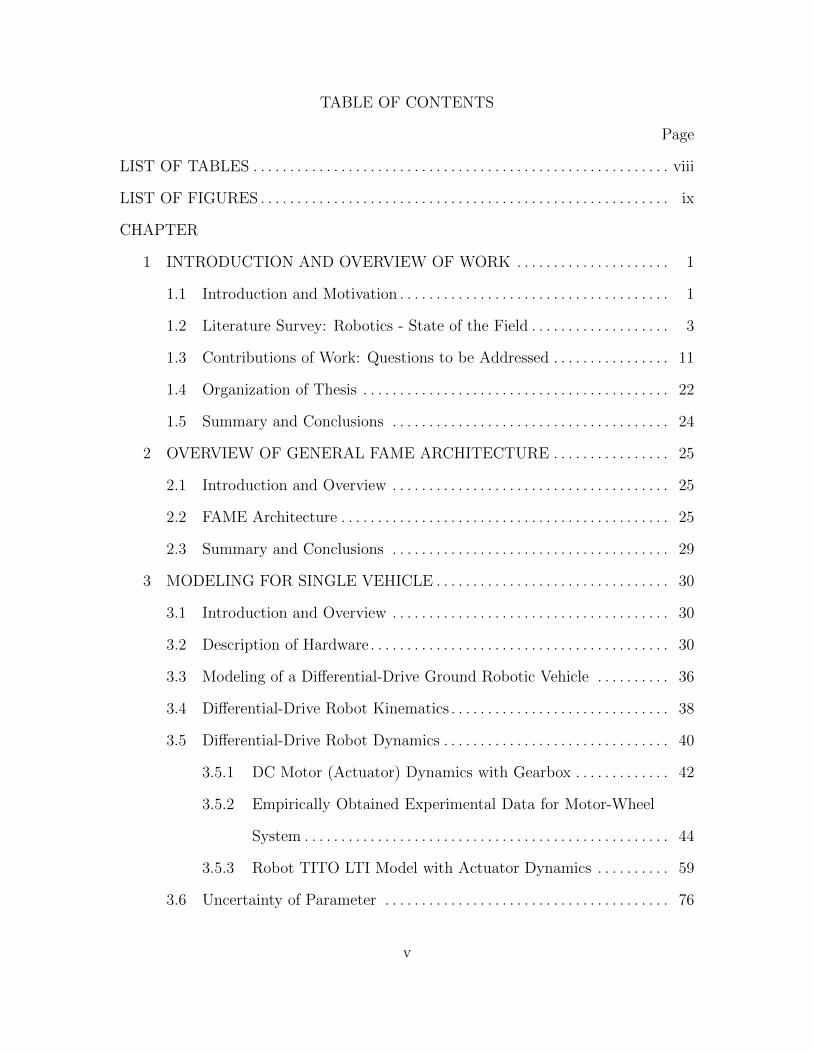
TABLE OF CONTENTS

Page

LIST OF TABLES . . . . . . . . . . . . . . . . . . . . . . . . . . . . . . . . . . . . . . . . . . . . . . . . . . . . . . . . . viii

LIST OF FIGURES . . . . . . . . . . . . . . . . . . . . . . . . . . . . . . . . . . . . . . . . . . . . . . . . . . . . . . . . ix

CHAPTER

1 INTRODUCTION AND OVERVIEW OF WORK . . . . . . . . . . . . . . . . . . . . . 1

1.1 Introduction and Motivation . . . . . . . . . . . . . . . . . . . . . . . . . . . . . . . . . . . . . 1

1.2 Literature Survey: Robotics - State of the Field . . . . . . . . . . . . . . . . . . . 3

1.3 Contributions of Work: Questions to be Addressed . . . . . . . . . . . . . . . . 11

1.4 Organization of Thesis . . . . . . . . . . . . . . . . . . . . . . . . . . . . . . . . . . . . . . . . . . 22

1.5 Summary and Conclusions . . . . . . . . . . . . . . . . . . . . . . . . . . . . . . . . . . . . . . 24

2 OVERVIEW OF GENERAL FAME ARCHITECTURE . . . . . . . . . . . . . . . . 25

2.1 Introduction and Overview . . . . . . . . . . . . . . . . . . . . . . . . . . . . . . . . . . . . . . 25

2.2 FAME Architecture . . . . . . . . . . . . . . . . . . . . . . . . . . . . . . . . . . . . . . . . . . . . . 25


3 MODELING FOR SINGLE VEHICLE . . . . . . . . . . . . . . . . . . . . . . . . . . . . . . . . 30


3.2 Description of Hardware . . . . . . . . . . . . . . . . . . . . . . . . . . . . . . . . . . . . . . . . . 30

3.3 Modeling of a Differential-Drive Ground Robotic Vehicle . . . . . . . . . . 36

3.4 Differential-Drive Robot Kinematics . . . . . . . . . . . . . . . . . . . . . . . . . . . . . . 38

3.5 Differential-Drive Robot Dynamics . . . . . . . . . . . . . . . . . . . . . . . . . . . . . . . 40

3.5.1 DC Motor (Actuator) Dynamics with Gearbox . . . . . . . . . . . . . 42

3.5.2 Empirically Obtained Experimental Data for Motor-Wheel

System . . . . . . . . . . . . . . . . . . . . . . . . . . . . . . . . . . . . . . . . . . . . . . . . . . 44

3.5.3 Robot TITO LTI Model with Actuator Dynamics . . . . . . . . . . 59

3.6 Uncertainty of Parameter . . . . . . . . . . . . . . . . . . . . . . . . . . . . . . . . . . . . . . . 76

v

CHAPTER Page

3.6.1 Frequency Response Trade Studies . . . . . . . . . . . . . . . . . . . . . . . . 76

3.6.2 Time Response Trade Studies . . . . . . . . . . . . . . . . . . . . . . . . . . . . . 79

3.7 Differential-Drive Robot Model with Dynamics on Ground . . . . . . . . . 83

3.7.1 Empirically Obtained Experimental Data for Ground Model. 85

3.7.2 Fitting Model to Collected Data. . . . . . . . . . . . . . . . . . . . . . . . . . . 86

3.7.3 On Ground Nominal Model. . . . . . . . . . . . . . . . . . . . . . . . . . . . . . . 89

3.8 Summary and Conclusion . . . . . . . . . . . . . . . . . . . . . . . . . . . . . . . . . . . . . . . 91

4 SINGLE VEHICLE CASE STUDY FOR A LOW-COST MULTI-CAPABILITY

DIFFERENTIAL-DRIVE ROBOT: ENHANCED THUNDER TUMBLE

(ETT) . . . . . . . . . . . . . . . . . . . . . . . . . . . . . . . . . . . . . . . . . . . . . . . . . . . . . . . . . . . . . . 92


4.2 Inner-Loop Speed Control Design and Implementation . . . . . . . . . . . . . 92

4.2.1 Frequency Domain (g,z) Trade Studies . . . . . . . . . . . . . . . . . . . . 104

4.2.2 Time Domain (g,z) Trade Studies . . . . . . . . . . . . . . . . . . . . . . . . . 117

4.2.3 Inner-Loop Experimental Result . . . . . . . . . . . . . . . . . . . . . . . . . . 122

4.3 Outer-Loop Control Design and Implementation . . . . . . . . . . . . . . . . . . 125

4.3.1 Outer-Loop 1: (v, θ) Cruise Control Along Line - Design

and Implementation . . . . . . . . . . . . . . . . . . . . . . . . . . . . . . . . . . . . . . 125

4.3.2 Outer-Loop 2: Separation-Direction (∆x, θ) Control - De-

sign and Implementation . . . . . . . . . . . . . . . . . . . . . . . . . . . . . . . . . 128

4.4 Summary and Conclusion . . . . . . . . . . . . . . . . . . . . . . . . . . . . . . . . . . . . . . . 150

5 LONGITUDINAL CONTROL OF A PLATOON OF VEHICLES . . . . . . . 151


5.2 Platoon Configuration . . . . . . . . . . . . . . . . . . . . . . . . . . . . . . . . . . . . . . . . . . 151

vi

CHAPTER Page

5.3 Modeling for Longitudinal Platoon of Vehicles . . . . . . . . . . . . . . . . . . . . 153

5.4 Control for Longitudinal Platoon of Vehicles . . . . . . . . . . . . . . . . . . . . . . 154

5.5 Longitudinal Platoon Separation Controller Tradeoff Study . . . . . . . . 156

5.6 Experimental Results for Controlled Platoon of Vehicles . . . . . . . . . . . 172

5.7 Platoon Simulation with model Uncertainty and Stiction Deadzone . 179


6 SUMMARY AND FUTURE DIRECTIONS . . . . . . . . . . . . . . . . . . . . . . . . . . . 181

6.1 Summary of Work . . . . . . . . . . . . . . . . . . . . . . . . . . . . . . . . . . . . . . . . . . . . . . 181

6.2 Directions for Future Research . . . . . . . . . . . . . . . . . . . . . . . . . . . . . . . . . . . 183

REFERENCES . . . . . . . . . . . . . . . . . . . . . . . . . . . . . . . . . . . . . . . . . . . . . . . . . . . . . . . . . . . . 185

APPENDIX

A C CODE . . . . . . . . . . . . . . . . . . . . . . . . . . . . . . . . . . . . . . . . . . . . . . . . . . . . . . . . . . . . 190

B MATLAB CODE . . . . . . . . . . . . . . . . . . . . . . . . . . . . . . . . . . . . . . . . . . . . . . . . . . . . 264

C ARDUINO CODE . . . . . . . . . . . . . . . . . . . . . . . . . . . . . . . . . . . . . . . . . . . . . . . . . . . 294

vii

LIST OF TABLES

Table Page

3.1 Hardware Components for Enhanced Differential-Drive Thunder Tum-

bler Robotic Vehicle . . . . . . . . . . . . . . . . . . . . . . . . . . . . . . . . . . . . . . . . . . . . . . . . 32

3.2 Thunder Tumbler Nominal Parameter Values with Uncertainty . . . . . . . . 37

3.3 Thunder Tumbler Gearbox Symbols . . . . . . . . . . . . . . . . . . . . . . . . . . . . . . . . . 47

5.1 Platoon Design Parameter . . . . . . . . . . . . . . . . . . . . . . . . . . . . . . . . . . . . . . . . . . 172

viii

LIST OF FIGURES

Figure Page

1.1 Visualization of Fully-Loaded (Enhanced) Thunder Tumbler . . . . . . . . . . 12

1.2 Optical Wheel Encoders - RPR220 photo-interrupter Sensors on Left,

code disk on Right . . . . . . . . . . . . . . . . . . . . . . . . . . . . . . . . . . . . . . . . . . . . . . . . . 13

1.3 Adafruit BNO055 9DOF Inertial Measurement Unit (IMU) . . . . . . . . . . . 13

1.4 Arduino Uno Open-Source Microcontroller Development Board . . . . . . . . 14

1.5 Adafruit Motor Shield for Arduino v2.3 - Provides PWM Signal to DC

Motors . . . . . . . . . . . . . . . . . . . . . . . . . . . . . . . . . . . . . . . . . . . . . . . . . . . . . . . . . . . . 14

1.6 Raspberry Pi 3 Model B Open-Source Single Board Computer . . . . . . . . 15

1.7 Raspberry Pi 5MP Camera Module . . . . . . . . . . . . . . . . . . . . . . . . . . . . . . . . . 15

1.8 TP-LINK Wireless High Gain USB Adapter . . . . . . . . . . . . . . . . . . . . . . . . . 16

1.9 HC-SR04 Ultrasonic Sensor . . . . . . . . . . . . . . . . . . . . . . . . . . . . . . . . . . . . . . . . . 16

1.10 Visualization of Inner- and Outer-Loop Control Laws . . . . . . . . . . . . . . . . . 19

2.1 FAME Architecture to Accommodate Fleet of Cooperating Vehicles . . . 26

3.1 Visualization of Differential-Drive Mobile Robot . . . . . . . . . . . . . . . . . . . . . . 38

3.2 Visualization of DC Motor Speed-Voltage Dynamics . . . . . . . . . . . . . . . . . . 42

3.3 dc Motor Armature Inductance of 10 ETT Motors . . . . . . . . . . . . . . . . . . . 45

3.4 dc Motor Armature Inductance of 10 ETT Motors . . . . . . . . . . . . . . . . . . . 46

3.5 Disassembled Gearbox in ETT . . . . . . . . . . . . . . . . . . . . . . . . . . . . . . . . . . . . . . 48

3.6 DC Motor back EMF Constant of Left and Right ETT Motors . . . . . . . . 49

3.7 DC Motor Output ωs Response to 1.02V Step Input - Hardware . . . . . . . 50

3.8 DC Gain Distribution of Step Response at Different Voltage Step Input 51

3.9 DC Gain Distribution of Step Response at Different Voltage Step Input 52

3.10 Equivalent Moment of Inertia Distribution of Left and Right Motors . . . 53

ix

Figure Page

3.11 Equivalent Speed Damping Constant Distribution of Left and Right

Motors . . . . . . . . . . . . . . . . . . . . . . . . . . . . . . . . . . . . . . . . . . . . . . . . . . . . . . . . . . . . 53

3.12 Motor Output ωs Response to 1.02V Step Input - Hardware and De-

coupled Model . . . . . . . . . . . . . . . . . . . . . . . . . . . . . . . . . . . . . . . . . . . . . . . . . . . . 55


coupled Model . . . . . . . . . . . . . . . . . . . . . . . . . . . . . . . . . . . . . . . . . . . . . . . . . . . . 55


coupled Model . . . . . . . . . . . . . . . . . . . . . . . . . . . . . . . . . . . . . . . . . . . . . . . . . . . . 56


coupled Model . . . . . . . . . . . . . . . . . . . . . . . . . . . . . . . . . . . . . . . . . . . . . . . . . . . . 56


coupled Model . . . . . . . . . . . . . . . . . . . . . . . . . . . . . . . . . . . . . . . . . . . . . . . . . . . . 57

3.17 DC Motor Output ωs Response to High Voltage Step Input - Hardware

and Decoupled Model . . . . . . . . . . . . . . . . . . . . . . . . . . . . . . . . . . . . . . . . . . . . . 58

3.18 TITO LTI Robot-Motor Wheel Speed (ωR, ωL) Dynamics - P(ωR,ωL) . . . . 59

3.19 Differential-Drive Mobile Robot Dynamics . . . . . . . . . . . . . . . . . . . . . . . . . . . 60

3.20 Robot Singular Values (Voltages to Wheel Speeds) - Including Low

Frequency Approximation . . . . . . . . . . . . . . . . . . . . . . . . . . . . . . . . . . . . . . . . . . 64

3.21 Robot Frequency Response (Voltages to Wheel Speeds) - Including

Low Frequency Approximation . . . . . . . . . . . . . . . . . . . . . . . . . . . . . . . . . . . . . . 65

3.22 Robot Plant Singular Values (Voltages to v and ω) - Including Low


3.23 Robot Plant Frequency Response (Voltages to [v, ω]) - Including Low


x

Figure Page

3.24 Frequency Response for Vehicle-Motor - Coupled (ωR, ωL) Model . . . . . . 70

3.25 Vehicle-Motor Response to Unit Step Input - Coupled (ωR, ωL) Model . 70

3.26 Bode Magnitude for Robot (Voltages to Wheel Speeds) - Mass Varia-

tions . . . . . . . . . . . . . . . . . . . . . . . . . . . . . . . . . . . . . . . . . . . . . . . . . . . . . . . . . . . . . 76

3.27 Bode Magnitude for Robot (Voltages to Wheel Speeds) - I Variations . 77

3.28 Bode Magnitude for Robot (Voltages to Wheel Speeds) - Kb Variations 77

3.29 Bode Magnitude for Robot (Voltages to Wheel Speeds) - Kt Variations 78

3.30 Bode Magnitude for Robot (Voltages to Wheel Speeds) - Ra Variations 79

3.31 System Wheel Angular Velocity Responses to Step Voltages - Mass

Variations . . . . . . . . . . . . . . . . . . . . . . . . . . . . . . . . . . . . . . . . . . . . . . . . . . . . . . . . . 79

3.32 System Wheel Angular Velocity Responses to Step Voltages - Moment

of Inertia Variations . . . . . . . . . . . . . . . . . . . . . . . . . . . . . . . . . . . . . . . . . . . . . . . . 80

3.33 System Wheel Angular Velocity Responses to Step Voltages - back

EMF Constant Variations . . . . . . . . . . . . . . . . . . . . . . . . . . . . . . . . . . . . . . . . . . 81

3.34 System Wheel Angular Velocity Responses to Step Voltages - Torque

Constant Variations . . . . . . . . . . . . . . . . . . . . . . . . . . . . . . . . . . . . . . . . . . . . . . . . 82

3.35 System Wheel Angular Velocity Responses to Step Voltages - Armature

Resistance Variations . . . . . . . . . . . . . . . . . . . . . . . . . . . . . . . . . . . . . . . . . . . . . . . 83

3.36 Target Characteristics of TB6612FNG . . . . . . . . . . . . . . . . . . . . . . . . . . . . . . . 84

3.37 Off Ground and On Ground Step Response to 50 PWM Command (1V) 85

3.38 Output ωs Response to PWM 50 Voltage Step Input - Hardware and

Decoupled Model . . . . . . . . . . . . . . . . . . . . . . . . . . . . . . . . . . . . . . . . . . . . . . . . . . 86

3.39 On Ground Motor Fitting Left Motor - Hardware and Decoupled Model 87

xi

Figure Page

3.40 On Ground Motor Fitting Right Motor - Hardware and Decoupled

Model . . . . . . . . . . . . . . . . . . . . . . . . . . . . . . . . . . . . . . . . . . . . . . . . . . . . . . . . . . . . 87

3.41 On Ground Approximate Transfer Function Fitting Model Distribution

of V1 . . . . . . . . . . . . . . . . . . . . . . . . . . . . . . . . . . . . . . . . . . . . . . . . . . . . . . . . . . . . . 88

3.42 On Ground Nominal Model . . . . . . . . . . . . . . . . . . . . . . . . . . . . . . . . . . . . . . . . . 89

3.43 Step Response of Nominal Model with other ETT Model . . . . . . . . . . . . . 90

3.44 On Ground Nominal Model with other ETT Model . . . . . . . . . . . . . . . . . . . 90

4.1 Visualization of (v, ω) and (ωR, ωL) Inner-Loop Control . . . . . . . . . . . . . . . 95

4.2 PK and Lo = MPKM−1 Singular Values . . . . . . . . . . . . . . . . . . . . . . . . . . . 96

4.3 So = (I + Lo)−1 = Si Singular Values - Using Decoupled Model . . . . . . . . 98

4.4 To = Lo(I + Lo)−1 = Ti Singular Values - Using Decoupled Model . . . . . 98

4.5 Tru Singular Values (No Pre-filter) - Using Decoupled Model . . . . . . . . . . 99

4.6 TruW Singular Values (with Pre-filter) - Using Decoupled Model . . . . . . 99

4.7 KSM−1 Singular Values . . . . . . . . . . . . . . . . . . . . . . . . . . . . . . . . . . . . . . . . . . . 100

4.8 Tdiy Singular Values - Using Decoupled Model . . . . . . . . . . . . . . . . . . . . . . . . 100

4.9 MSP Singular Values . . . . . . . . . . . . . . . . . . . . . . . . . . . . . . . . . . . . . . . . . . . . . 101

4.10 Inner-Loop [ωR, ωL] Filtered Step Response - Using Decoupled Model . . 101

4.11 Inner-Loop [ωR, ωL] Unfiltered Step Response - Using Decoupled Model102

4.12 Control Response to Step Command (with Pre-filter) - with Decoupled

Model . . . . . . . . . . . . . . . . . . . . . . . . . . . . . . . . . . . . . . . . . . . . . . . . . . . . . . . . . . . . . 103

4.13 Control Response to Unfiltered Step Command - with Decoupled Model103

4.14 Singular Values for L (g=0.10, 0.30, 0.50, 0.70; z=2) . . . . . . . . . . . . . . . . . 104

4.15 Singular Values for L (g=0.50; z=1, 2, 3, 4) . . . . . . . . . . . . . . . . . . . . . . . . . . 105

4.16 Singular Values for S (g=0.10, 0.30, 0.50, 0.70; z=2) . . . . . . . . . . . . . . . . . 106

xii

Figure Page

4.17 Singular Values for S (g=0.50; z=1, 2, 3, 4) . . . . . . . . . . . . . . . . . . . . . . . . . 106

4.18 Singular Values for T (g=0.10, 0.30, 0.50, 0.70; z=2) . . . . . . . . . . . . . . . . . 107

4.19 Singular Values for T (g=0.50; z=1, 2, 3, 4) . . . . . . . . . . . . . . . . . . . . . . . . . . 108

4.20 Singular Values for Tru (g=0.10, 0.30, 0.50, 0.70; z=2) - (ωR, ωL) Com-

mands . . . . . . . . . . . . . . . . . . . . . . . . . . . . . . . . . . . . . . . . . . . . . . . . . . . . . . . . . . . . 109

4.21 Singular Values for Tru (g=0.50; z=1, 2, 3, 4)- (ωR, ωL) Commands . . . 109

4.22 Singular Values for KSM−1 (g=0.10, 0.30, 0.50, 0.70; z=2) - (v, ω)

Commands . . . . . . . . . . . . . . . . . . . . . . . . . . . . . . . . . . . . . . . . . . . . . . . . . . . . . . . 110

4.23 Singular Values for KSM−1 (g=0.50; z=1, 2, 3, 4)- (v, ω) Commands . 111

4.24 Singular Values for W · Tru (g=0.10, 0.30, 0.50, 0.70; z=2) - (ωR, ωL)

Commands . . . . . . . . . . . . . . . . . . . . . . . . . . . . . . . . . . . . . . . . . . . . . . . . . . . . . . . . 112

4.25 Singular Values for W · Tru (g=0.50; z=1, 2, 3, 4) - (ωR, ωL) Commands112

4.26 Singular Values for Tdiy (g=0.10, 0.30, 0.50, 0.70; z=2) - (ωR, ωL) Re-

sponses . . . . . . . . . . . . . . . . . . . . . . . . . . . . . . . . . . . . . . . . . . . . . . . . . . . . . . . . . . . 114

4.27 Singular Values for Tdiy (g=0.50; z=1, 2, 3, 4) - (ωR, ωL) Responses . . . . 114

4.28 Singular Values for MSP (g=0.50; z=1, 2, 3, 4) - (v, ω) Responses . . . . 115

4.29 Singular Values for MSP (g=0.50; z=1, 2, 3, 4) - (v, ω) Responses . . . . 116

4.30 Output Response to Step Command (g = 0.10, 0.30, 0.50, 0.70; z = 2) . . 117

4.31 Output Response to Step Command (g = 0.50; z = 1, 2, 3, 4) . . . . . . . . . . 118

4.32 Control Response to Step Command (g = 0.10, 0.30, 0.50, 0.70; z = 2) . . 118

4.33 Control Response to Step Command (g = 0.50; z = 1, 2, 3, 4) . . . . . . . . . . 119

4.34 Output Response to Step Command (g = 0.10, 0.30, 0.50, 0.70; z = 2) . . 120

4.35 Output Response to Step Command (g = 0.50; z = 1, 2, 3, 4) . . . . . . . . . . 120

xiii

Figure Page

4.36 Control Response to Filtered Step Command g = 0.10, 0.30, 0.50, 0.70; z =

2). . . . . . . . . . . . . . . . . . . . . . . . . . . . . . . . . . . . . . . . . . . . . . . . . . . . . . . . . . . . . . . . . 121

4.37 Control Response to Filtered Step Command (g = 0.50; z = 1, 2, 3, 4) . . 121

4.38 Output Response to filtered Step Command (ωRref = 10, ωLref = 10) 122

4.39 Output Response to filtered Step Command (vref = 0.5, ωref = 0) . . . . 123

4.40 Control Response to filtered Step Command (ωRref = 10, ωLref = 10) 123

4.41 Visualization of Cruise Control Along a Line . . . . . . . . . . . . . . . . . . . . . . . . . 125

4.42 Tθref θ Frequency Response for θ Outer-Loop (P Control) . . . . . . . . . . . . . . 126

4.43 Tθref θ Frequency Response for θ Outer-Loop (PD control, Kd = 1) . . . . . 126

4.44 Cruise Control θ Response Using P Control (θo = 0.1 rad) . . . . . . . . . . . . 127

4.45 Cruise Control θ Response Using PD Control (θo = 0.1 rad) . . . . . . . . . . . 127

4.46 Visualization of (∆x, θ) Separation-Direction Control System. . . . . . . . . . 128

4.47 Vehicle Separation Control (Proportional Control: Kp = 0.5, 1.0, 1.5, 2.0;

∆xo = 1) . . . . . . . . . . . . . . . . . . . . . . . . . . . . . . . . . . . . . . . . . . . . . . . . . . . . . . . . . . 129

4.48 Vehicle Separation Control (PD control: Kp = 0.5, 1.0, 1.5, 2.0;Kd=1;

∆xo = 1) . . . . . . . . . . . . . . . . . . . . . . . . . . . . . . . . . . . . . . . . . . . . . . . . . . . . . . . . . . 130

4.49 Minimizing Counter Value Versus Desired f = xxresolution

. . . . . . . . . . . . . . . 135

4.50 Minimum Percent Error Versus Desired f = xxresolution

. . . . . . . . . . . . . . . . . 136

4.51 Cruise Control Along a Line . . . . . . . . . . . . . . . . . . . . . . . . . . . . . . . . . . . . . . . . 144

4.52 Vehicle Separation Convergence Using Proportional Control (Kp = 1;

∆x(0) ≈ 1) . . . . . . . . . . . . . . . . . . . . . . . . . . . . . . . . . . . . . . . . . . . . . . . . . . . . . . . . 147

4.53 Vehicle Separation Convergence Using Proportional Control (Kp = 1;

∆x(0) ≈ 1) . . . . . . . . . . . . . . . . . . . . . . . . . . . . . . . . . . . . . . . . . . . . . . . . . . . . . . . . 147

xiv

Figure Page

4.54 Vehicle Separation Convergence Using PD Control (Kp = 1.5;Kd = 1;

∆x(0) ≈ 1) . . . . . . . . . . . . . . . . . . . . . . . . . . . . . . . . . . . . . . . . . . . . . . . . . . . . . . . . 148

5.1 Platoon of 4 Vehicles . . . . . . . . . . . . . . . . . . . . . . . . . . . . . . . . . . . . . . . . . . . . . . . 152

5.2 Leader Model of Platoon . . . . . . . . . . . . . . . . . . . . . . . . . . . . . . . . . . . . . . . . . . . 153

5.3 i-th Vehicle Model of Platoon . . . . . . . . . . . . . . . . . . . . . . . . . . . . . . . . . . . . . . . 153

5.4 Visualization of i-th Follower in Platoon Separation Control System . . . 154

5.5 Visualization of Platoon Controller . . . . . . . . . . . . . . . . . . . . . . . . . . . . . . . . . . 155

5.6 Simulation of Vehicle Separation Control of Platoon (Proportional

Control for ∆x (Kp = 0.5) . . . . . . . . . . . . . . . . . . . . . . . . . . . . . . . . . . . . . . . . . . 156

5.7 Simulation of Control Response of Platoon (Proportional Control for

∆x (Kp = 0.5) . . . . . . . . . . . . . . . . . . . . . . . . . . . . . . . . . . . . . . . . . . . . . . . . . . . . . 157


Control for ∆x (Kp = 1.0) . . . . . . . . . . . . . . . . . . . . . . . . . . . . . . . . . . . . . . . . . . 157


∆x (Kp = 1.0) . . . . . . . . . . . . . . . . . . . . . . . . . . . . . . . . . . . . . . . . . . . . . . . . . . . . . 158


Control for ∆x (Kp = 2.0) . . . . . . . . . . . . . . . . . . . . . . . . . . . . . . . . . . . . . . . . . . 158


∆x (Kp = 2.0) . . . . . . . . . . . . . . . . . . . . . . . . . . . . . . . . . . . . . . . . . . . . . . . . . . . . . 159

5.12 Simulation of Vehicle Separation Control of Platoon (PD Control for

∆x (g = 0.2)) . . . . . . . . . . . . . . . . . . . . . . . . . . . . . . . . . . . . . . . . . . . . . . . . . . . . . . 160

5.13 Simulation of Control Response of Platoon (PD Control for ∆x (g = 0.2))160


∆x (g = 0.5)) . . . . . . . . . . . . . . . . . . . . . . . . . . . . . . . . . . . . . . . . . . . . . . . . . . . . . . 161

xv

Figure Page

5.15 Simulation of Control Response of Platoon (PD Control for ∆x (g = 0.5))161

5.16 Simulation of Vehicle Separation Control of Platoon (PID Control for

∆x (g = 1.0)) . . . . . . . . . . . . . . . . . . . . . . . . . . . . . . . . . . . . . . . . . . . . . . . . . . . . . . 163

5.17 Simulation of Control Response of Platoon (PID Control for ∆x (g =

1.0)) . . . . . . . . . . . . . . . . . . . . . . . . . . . . . . . . . . . . . . . . . . . . . . . . . . . . . . . . . . . . . . 164


∆x (g = 2.0)) . . . . . . . . . . . . . . . . . . . . . . . . . . . . . . . . . . . . . . . . . . . . . . . . . . . . . . 164


2.0)) . . . . . . . . . . . . . . . . . . . . . . . . . . . . . . . . . . . . . . . . . . . . . . . . . . . . . . . . . . . . . . 165


∆x (g = 1.0, z = 1.0) and kpff = 0.5 for FF-path) . . . . . . . . . . . . . . . . . . . . 166


1.0, z = 1.0) and kpff = 0.5 for FF-path) . . . . . . . . . . . . . . . . . . . . . . . . . . . . . 167


∆x (g = 1.0, z = 1.0) and kpff = 1.5 for FF-path) . . . . . . . . . . . . . . . . . . . . 167


1.0, z = 1.0) and kpff = 1.5 for FF-path) . . . . . . . . . . . . . . . . . . . . . . . . . . . . . 168


∆x (g = 1.0, z = 1.0) and PI Control for FF-path (gff = 0.5, zff = 1.0))169


1.0, z = 1.0) and PI Control for FF-path (gff = 0.5, zff = 1.0)) . . . . . . . 170


∆x (g = 1.0, z = 1.0) and PI Control for FF-path (gff = 0.5, zff = 2.0))170

xvi

Figure Page


1.0, z = 1.0) and PI Control for FF-path (gff = 0.5, zff = 2.0)) . . . . . . . 171


Control for ∆x (Kp = 1) . . . . . . . . . . . . . . . . . . . . . . . . . . . . . . . . . . . . . . . . . . . . 173


∆x (Kp = 1) . . . . . . . . . . . . . . . . . . . . . . . . . . . . . . . . . . . . . . . . . . . . . . . . . . . . . . . 173

5.30 Experimental Separation Response of Platoon Proportional Control for

∆x (Kp = 1) . . . . . . . . . . . . . . . . . . . . . . . . . . . . . . . . . . . . . . . . . . . . . . . . . . . . . . . 174


∆x (Kp = 1.5, Kd = 0.2) and Proportional control for FF Path (Kp =

0.5)) . . . . . . . . . . . . . . . . . . . . . . . . . . . . . . . . . . . . . . . . . . . . . . . . . . . . . . . . . . . . . . 175

5.32 Simulation of Control Response of Platoon (PD Control for ∆x (Kp =

1.5, Kd = 0.2) and Proportional control for FF Path (Kp = 0.5)) . . . . . . . 175

5.33 Experimental Separation Response of Platoon (PD Control for ∆x

(Kp = 1.5, Kd = 0.2) and Proportional control for FF Path (Kp = 0.5)) 176


∆x (Kp = 1.0, Ki = 0.5, Kd = 0.3) and Proportional control for FF

Path (Kp = 0.4, Ki = 0.6)) . . . . . . . . . . . . . . . . . . . . . . . . . . . . . . . . . . . . . . . . . . 177

5.35 Simulation of Control Response of Platoon (PID Control for ∆x (Kp =

1.0, Ki = 0.5, Kd = 0.3) and Proportional control for FF Path (Kp =

0.4, Ki = 0.6)) . . . . . . . . . . . . . . . . . . . . . . . . . . . . . . . . . . . . . . . . . . . . . . . . . . . . . 177

5.36 Experimental Separation Response of Platoon (PID Control for ∆x

(Kp = 1.0, Ki = 0.5, Kd = 0.3) and Proportional control for FF Path

(Kp = 0.4, Ki = 0.6)) . . . . . . . . . . . . . . . . . . . . . . . . . . . . . . . . . . . . . . . . . . . . . . . 178

xvii

Figure Page

5.37 Simulation of Separation Response of Platoon with model uncertainty

and stiction . . . . . . . . . . . . . . . . . . . . . . . . . . . . . . . . . . . . . . . . . . . . . . . . . . . . . . . 179

5.38 Simulation of Control Response of Platoon with model uncertainty and

stiction . . . . . . . . . . . . . . . . . . . . . . . . . . . . . . . . . . . . . . . . . . . . . . . . . . . . . . . . . . . . 180

xviii

Chapter 1

INTRODUCTION AND OVERVIEW OF WORK

1.1 Introduction and Motivation

With the rapid growth of population in the world, severe congestion and pollution

happens every day in some of the worlds most populated cities (e.g. Beijing, Tokyo,

and New Delhi). More efficient, cost-effective, and clean ground transportation sys-

tem is desperately needed. So self-driving technology and electric vehicle draw more

and more attention in recent years. In May 2012, Google’s autonomous car passed

the world’s first self-driving test in Las Vegas which sparked research on intelligent

transportation system (ITS) again. More and more automotive companies are shift-

ing their focus towards electric vehicle market, like Telsa Motors, BMW, etc. The

seminal intelligent vehicle and highway systems (IVHS) work of S.E. Sheikholeslam

[3], [6] demonstrated that a longitudinal platoon of cars can be tightly controlled

in both speed and spacing in order to promote more effective traffic flow. In this

thesis, the author will reconsider the vehicle platoon modeling, design and control

problem, providing simulation and hardware result using low-cost multi-capability

electric ground vehicles.

In previous MS thesis work of Lin [14], off-the-shelf technologies (e.g. Arduino,

Raspberry Pi, commercially available RC cars) have been exploited to develop low-

cost ground vehicles that can be used for multi-vehicle robotics research. The first

step toward the longer-term goal of achieving a fleet of Flexible Autonomous Ma-

chines operating in an uncertain Environment (FAME) has been done. Such a fleet

can involve multiple ground and air vehicles that work collaboratively to accomplish

1

coordinated tasks. Such a fleet may be called a swarm [43]. Potential applications can

include: remote sensing, mapping, intelligence gathering, intelligence-surveillance-

reconnaissance (ISR), search, rescue and much more. It is this vast application arena

as well as the ongoing accelerating technological revolution that continues to fuel

robotic vehicle research.

This thesis continues to address the modeling, design and control issues associated

with the coordination of multiple ground-based robotic vehicles. Same Framework of

[14] is used for consistency toward the same longer-term FAME goal. Central objective

of the thesis was to show how to control multiple robots in a certain formation,

particularly how to control a platoon of vehicle cruise in a straight line and keep

constant separation distance. This problem has been called longitudinal control of

vehicle platoon. This is shown for differential-drive vehicle class. Multiple Enhanced

Thunder Tumbler (ETT) vehicles were used in this research, both kinematic and

dynamical models are examined. Here, differential-drive means that the speed of

each of the rear wheels are controlled independently by separate DC motors. This

vehicle class is non-holonomic; i.e. the two (2) (x, y) or (v, θ) controllable degrees of

freedom is less than the three (3) total (x, y, θ) degrees of freedom.

This fundamentally limits the ability of a single continuous (non-switching) con-

trol law to “precisely park the vehicle” (see discussions below based on work of [61],

[63], [25]) . Despite this, it is shown how continuous linear control theory can be

used to develop suitable control laws that are essential for achieving various critical

capabilities (e.g. speed/position control along a line/path, spacing control) [14]. Fol-

lowing is a comprehensive literature survey - one that summarizes relevant literature

and how it has been used.

2

1.2 Literature Survey: Robotics - State of the Field

In an effort to shed light on the state of ground robotic vehicle modeling, hardware,

design, and control, the following topically organized literature survey is offered. An

effort is made below to highlight what technical papers/works are most relevant to

this thesis. In short, the following works are most relevant for the developments

within this thesis:

• low-cost ground robotic modeling, design and control work within [14];

• DC motor modeling work within [16] (addressing DC motor modeling with gear-

box and limitation of linear model), [46] (addressing modeling and identification

of DC motor with nonlinearity);

• non-holonomic differential-drive vehicle modeling and control work within [15]

(addressing dynamic two-input two-output LTI model for differential-drive ve-

hicles), [59] (addressing control of differential-drive vehicles);

• vision-based line/curve following work within [24];

• vehicle separation modeling and longitudinal platoon control work within [3],

[6] (presenting vehicle separation control laws);

An attempt is made below to provide relevant insightful technical details.

• Differential-Drive Robot Modeling. Within this thesis, differential-drive

(Thunder Tumbler) ground vehicles represent a central focus of the work. Here,

differential-drive means that there are two rear wheels - each with an indepen-

dent torque generating armature controlled DC motor on it [52]. As such, these

DC motors can be used to independently control the speed of the rear wheels.

nominally, we assume that the motors are identical. The motor inputs (vehicle

3

controls) are voltages. The sum of these voltages is used to control the vehicle’s

speed v. The difference is used to control the direction θ of the vehicle.

– Kinematic Model. A kinematic model for differential-drive robot (ignoring

dynamic mass-inertia effects) is presented within [19], [18]. Within this

kinematic model, it is assumed that the translational and angular veloc-

ities (v, ω) of the robot are realized instantaneously. This, of course, is

not realistic because of real-world actuator (e.g. motor) limitations and

mass-inertia constraints. From Newton’s second law of motion, we know

that an instantaneously achieved velocity generally requires infinite accel-

eration and force. The kinematic model is therefore less accurate than a

dynamical model (i.e. one which includes acceleration constraining mass-

inertia effects).

– Dynamical Model. A dynamical model can take the torques applied to the

robot wheels as inputs (controls) to the system. This is done within [21],

[23]. The model presented within these works incorporates dynamic (accel-

eration constraining) mass-inertia effects as well as friction, wheel slippage

etc. Given this, it is apparent that a dynamic model generally gives a much

more accurate model of the vehicle. Within [15], a two-input two-output

(TITO) linear time invariant (LTI) model - including DC motor dynamics

as well as vehicle mass-inertia effects - is presented for a differential-drive

ground vehicle. The model describes the TITO LTI map from the two DC

motor input voltages (vehicle controls) to the two rear wheel angular veloc-

ities (ωR, ωL). The map from the voltages to the vehicle longitudinal and

angular speeds (v, ω) is also a TITO LTI transfer function matrix. This

4

model was exploited within [59] for control design. This TITO LTI model,

and its diagonal approximation, shall be used as the main differential-drive

vehicle model within this thesis (e.g. see work within Chapters 3 and 4).

It will be used to understand the robot’s linear (voltage to wheel angular

velocity or voltages to speed and angular velocity) dynamics as well as

to develop linear inner-loop (ωR, ωL) and (v, ω) speed control laws. It is

very important to note that the vehicle model becomes nonlinear when one

considers the planar (x, y) coordinates of the vehicle.

Given the above, it should be noted that the map from the motor voltages

to (ωR, ωL) is a TITO LTI coupled model that is nearly decoupled (de-

centralized) at low frequencies; i.e. frequencies below βI, where β denotes

motor shaft rotational speed damping and I denotes rotational moment of

inertia. (This is not true for (v, ω).) It is this decoupling (and our non-

aggressive moderate-bandwidth performance objectives) that permits us to

use a decoupled (decentralized) model for control law development. This

is discussed further within Chapters 3 and 4. For our differential-drive

Thunder Tumble vehicle (Chapter 4), vehicle parameters for the fourth

order TITO LTI model from motor voltages to (v, ω) or (ωR, ωL) were

estimated by iterating between experiments and model-based time sim-

ulations. Vehicle mass m was measured. It was assumed that the DC

motors are identical. DC motor armature inductance La was neglected -

thus making the model second order. Settling time, steady state speed and

armature current were used to (approximately) solve for the three remain-

ing model parameters: angular speed damping β, back emf and torque

constant Kb = Kt, armature resistance Ra. (Additional relevant details

5

are provided within Chapter 4). While the left-right motor model param-

eters were assumed to be identical, it should be noted that the feedback

laws implemented implicitly compensate (to some extant) for real-world

parametric uncertainty.

The above summarizes basic principles regarding differential-drive ground ve-

hicles.

• Classical Controls. Classical control design fundamentals are addressed within

the text [52]. Internal model principle ideas - critical for command following

and disturbance attenuation - are presented within [50], [52]. General PID

(proportional plus integral plus derivative) control theory, design and tuning

are addressed within the text [32]. Fundamental performance limitations are

discussed with [69],[52].

• Robot Inner-Loop Control. A proportional-plus-integral-plus-derivative

(PID) inner-loop control design is addressed within [48], [49]. A PI controller

is used for inner-loop control within [51], [59]. Within Chapter 3-4, we examine

PI inner-loop speed (ωR, ωL) and (v, ω) control laws for our differential-drive

vehicles. Inner-loop control law parameter trade studies are presented within

Chapter 3. Classically-based decentralized [52] control [26] was examined in

the frequency- and time-domains. It was used to select a decentralized inner-

loop control law for implementation in the hardware. A centralized inner-loop

control law may become essential when we have stringent high bandwidth con-

straints and large plant coupling. [59].

• Robot Outer-Loop Control. Within this thesis, various outer-loop control

laws are examined. When relevant, existing work in the literature was exploited.

6

1. Cruise Control Along a Line. Within this thesis, it is important to note

the difference between trajectory tracking and path following. Trajectory

tracking addresses following x(t), y(t) commands; i.e. (x, y) commands

with very specific temporal constraints [29]. Path following addresses fol-

lowing a path/curve in the plane (without temporal constraints)[29]. To

address trajectory tracking and path following tasks, standard linear tech-

niques are used within [27]. Nonlinear approaches are used within the

following: feedback linearization within [28], Lyapunov-based techniques

within [19], [20], [30], [31].

Cruise control is a fundamentally important feature for a ground robotic

system. Within this thesis, we therefore develop an encoder-IMU-camera

based (PD with roll off) outer-loop (v, θ) control law that permits cruise

control along a camera visible line/path. The camera, here, resolves encoder-

IMU dead reckoning issues. See work within Chapter 4. The cruise control

law is based on the TITO LTI (v, ω) or (ωR, ωL) inner-loop model pre-

sented within [15] and the associated inner-loop control law (e.g. see work

within Chapters 3 and 4). The map from the reference commands (vref ,

ωref ) to the actual velocities (v, ω) looks like a simple diagonal system

(e.g. diag( as+a

, bs+b

)) at low frequencies - a consequence of a well-designed

inner-loop control system. (See inner-loop work within Chapters 3 and

4; outer-loop work in Chapter 4). The outer-loop θ controller therefore

“sees” bs(s+b)

. From classical root locus ideas [52], a proportional controller

is therefore justified - provided that the gain is not too large. If the gain

is too large, oscillations (or even limit cycle behavior) are expected in θ.

A PD controller with roll off would help with this issue. (See work within

Chapter 4).

7

2. Separation Control. Within [3], [6], vehicle separation modeling and lon-

gitudinal platoon control is presented. The ideas presented within [3], [6]

motivate the PID ultrasonics-encoder-IMU-based separation control laws

used for the separation-direction (∆x, θ) outer-loop control within this the-

sis. The ideas here are also used to have multiple differential-drive vehicles

following an autonomous or remotely controlled leader vehicle. See work

within Chapter 4. Future work will examine the related saturation preven-

tion issues within [64]. Relevant outer-loop control law parameter trade

studies are also presented within Chapter 4.

3. Robot/Car Spacing Control. Robot/car spacing control - intelligent ve-

hicles and highway systems (IVHS) - is briefly addressed within [52]. A

more comprehensive treatment of vehicle separation modeling and longi-

tudinal platoon control is presented within [3], [6]. These works provide

a theoretical foundation for the (inter- and multi-vehicle) separation con-

trol laws developed within this thesis. The ideas presented within [3], [6]

specifically motivate the PID separation control laws used within this the-

sis. (See work within Chapter 4). Future work will examine the related

saturation prevention issues within [64].

• Actuators and Sensors. Actuators and sensors are addressed within the [34].

• DC Motors. Simple armature controlled DC motor modeling concepts are ad-

dressed from a controls perspective within [52]. DC motor modeling for wheeled

robot applications is addressed within [44]. In this paper, nonlinear effects are

neglected. Nonlinear modeling and identification for DC motors is addressed

within [45], [46]. Also, see detailed discussion presented above on the TITO

LTI vehicle-motor model presented within[15]. This model will serve as the ba-

8

sis for inner-loop control law development for our differential-drive (DD) robots.

• Encoders. Rotary optical encoders are the most widely used encoder design.

They consist of an LED light source, light detector, code disc, and signal pro-

cessor [47]. Magnetic encoders consist of magnets and a hall effect sensor. They

are inherently rugged and operate reliably under shock, vibration and high tem-

perature [47]. Within this thesis, we used home-made optical encoders rather

than magnetic encoders in [14] on the wheels of our differential-drive Thunder

Tumbler ground vehicles, more accurate measurement is obtained. These wheel

encoders allow us to estimate right and left angular speed and displacement

information. From this, we then can compute the vehicle’s translational speed

v and angular speed ω. These are used to design our proportional plus integral

(PI) (ωR, ωL) or (v, ω) inner-loop control systems. (See work in Chapters 3 and

4). We will see in Chapter 4, how encoder improvement can benefit us and also

the new optical wheel encoders used (20 Counts Per Turn (CPT)) will limit how

well the inner-loop can perform. A static position error of rwheel(2π20

) ≈ 0.0157

m (where rwheel = 0.05 m is the wheel radius), for example, can result. This

error can build up as the robot stops and goes. It can also result in undesir-

able position control oscillations because the exact position cannot be achieved.

While the oscillations can be corrected with some nonlinear control logic, the

error cannot be corrected unless we have some dead-reckoning correction mech-

anism; e.g. camera, GPS, lidar. Within this thesis, a camera is used to address

dead-reckoning errors.

• Cameras. Within this research, we make use of the Raspberry Pi camera

(2592 × 1944 pixel or 5 MP static images; 1080p30 (30 fps), 720p60 and

640×480p60/90 MPEG-4 video). It connects directly to the Raspberry Pi 3’s

9

GPU (graphical processing unit). It is capable of 1080p full HD video. Because

the camera is directly connected to the GPU, there is very little impact on the

CPU (central processing unit). This makes the CPU available for other pro-

cessing tasks [57]. Within this thesis, cameras are used for outer-loop control

law implementation (e.g. (v, θ), (x, y), ∆x, θ) and as a tool for correcting the

inevitable dead-reckoning errors associated with encoders and IMUs.

• Vision Algorithms. The line/curve image processing ideas within the text

[24] are exploited within this thesis. Specifically, we use the Raspberry Pi 3 cam-

era [57] information to obtain vehicle directional information. This information

is used within the following outer-loop control laws: (v, θ) cruise control, planar

(x, y) Cartesian stabilization [25]. The vision algorithm used within this thesis

is a color filtering algorithm [24]. This algorithm can filter out irrelevant colors

(e.g. turn them into black) and select the desired color of interest (e.g. turn it

into white). After applying this algorithm, the camera only sees the color of

interest. This can be used to develop camera-based line/curve following [60]

separation-direction and platoon control laws. Within this thesis, these ideas

are used to follow a visible continuous black tape straight line on the ground.

These purposely fixed references essentially provide a very inexpensive form of

GPS. See work within Chapter 4.

• Global Positioning System (GPS). An overview of GPS is presented within

[56]. Differential GPS (DGPS) techniques are also described within [56].

• Arduino. Within this thesis, we make great use of the Arduino Uno microcon-

troller board (16MHZ ATmega328 processor, 32KB Flash Memory, 14 digital

I/O pins, 6 analog inputs, $25). More detailed specifications for the Arduino

Uno board are presented within [36]. It is used to implement inner- and outer-

10

loop control laws for our differential-drive Thunder Tumbler vehicle.

• Raspberry Pi 3. Within this thesis, we make great use of the Raspberry

Pi 3 computer board (1200 MHz quad-core ARM Cortex-A53 CPU (Pi 2: 900

MHz quad-core ARM Cortex-A7 CPU), 1GB SDRAM, 40 GPIO pins, camera

interface, $40). Introductory and technical details for the Raspberry Pi 3 are

discussed within [42]. Comparison between Pi 2 and Pi 3 can be found [66].

The Raspberry PI 3 us used to implement outer-loop (v, θ), (∆x, θ), platoon

without leader information, and platoon with leader information control laws

within this thesis.

• Commercially Available Ground Robotic Vehicles. A comprehensive

commercially available robot systems can be found in [14]. Robotic systems

with capabilities and price comparison has been done for the following: Seekur

($70K), Pioneer 3DX ($7.5K), Boebot robot ($160), AAR robot ($79), Lego

Mindstorm EV3 permits building of Track3r, R3ptar, Spik3r, Ev3rstorm, Gripp3r

($350); VEX Robotics Design System($500); APM 2.5 Arducopter.

1.3 Contributions of Work: Questions to be Addressed

Within this thesis, the following fundamental questions are addressed. When

taken collectively, the answers offered below, and details within the thesis, represent

a useful contribution to researchers in the field. Moreover, it must be emphasized

that answers to these questions are critical in order to move substantively toward the

longer-term FAME goal.

1. How can off-the-shelf “toy” vehicles be suitably augmented to yield

effective low-cost research platforms? This question was one of the main

objectives within [14], in which Thunder Tumbler ($10) toy vehicle was used and

11

converted to multi-capability ground robot platform. Based on hardware design

of him, the author make improvements about hardware on following aspects:

(1)optical wheel-encoders which 2.5 times accurate than magnetic based one

and absolute orientation sensor BNO055 IMU can give out azimuth directly that

LSM9DS0 can only get angular rate, (2)Raspberry Pi 3 with more computation

power than pi 2, this would benefit when image processing is needed. (3) TL-

WN722N Wi-Fi USB Adapter with external antenna which can support more

stable communication compared to Edimax Wi-Fi adapter in longer distance.

Other hardware setting are the same, just repeat here for completeness.

The updated fully-loaded (enhanced) Thunder Tumbler vehicle is shown in Fig-

ure 1.1.

Figure 1.1: Visualization of Fully-Loaded (Enhanced) Thunder Tumbler

12

Each differential-drive Thunder Tumbler vehicle was augmented to provide a

suite of substantive capabilities. Each augmented (“enhanced” Thunder Tum-

bler) vehicle costs less than $220 but offers the capability of commercially avail-

able vehicles costing over $500.

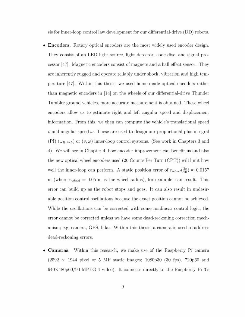
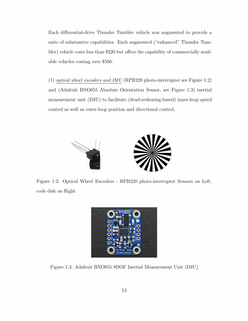
(1) optical wheel encoders and IMU (RPR220 photo-interrupter see Figure 1.2)

and (Adafruit BNO055 Absolute Orientation Sensor, see Figure 1.3) inertial

measurement unit (IMU) to facilitate (dead-reckoning-based) inner-loop speed

control as well as outer-loop position and directional control,

Figure 1.2: Optical Wheel Encoders - RPR220 photo-interrupter Sensors on Left,

code disk on Right

Figure 1.3: Adafruit BNO055 9DOF Inertial Measurement Unit (IMU)

13

(2) an Arduino Uno open-source microcontroller development board (16MHZ AT-

mega328 processor, 32KB Flash Memory, 14 digital I/O pins, 6 analog inputs,

$25, see Figure 1.4) for both encoder-IMU-based speed (v, ω) or (ωR, ωL) inner-

loop control and encoder-IMU-ultrasound-based directional-separation outer-

loop control,

Figure 1.4: Arduino Uno Open-Source Microcontroller Development Board

(3) an Arduino motor shield (see Figure 1.5) for inner-loop motor speed control.

Figure 1.5: Adafruit Motor Shield for Arduino v2.3 - Provides PWM Signal to DC

Motors

(4) a Raspberry Pi 3 Model B single board computer (1.2 GHz quad-core ARM

Cortex-A53 CPU, 1GB SDRAM, 40 GPIO pins, camera interface, $40, see

14

Figure 1.6) for more demanding vision-based cruise-position-directional outer-

loop control,

Figure 1.6: Raspberry Pi 3 Model B Open-Source Single Board Computer

(5) a Raspberry Pi 5MP camera (2592 × 1944 pixel or 5 MP static images;

1080p30 (30 fps), 720p60 and 640x480p60/90 MPEG-4 video, see Figure 1.7)

for outer-loop cruise-position-directional control,

Figure 1.7: Raspberry Pi 5MP Camera Module

15

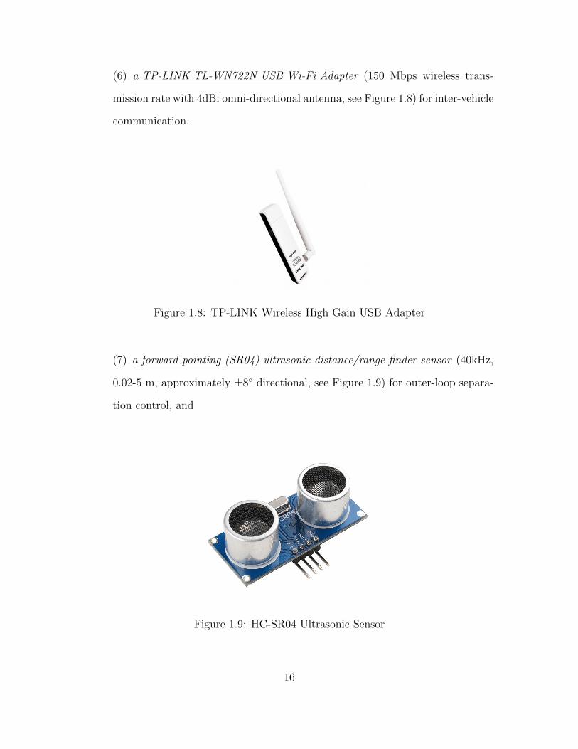
(6) a TP-LINK TL-WN722N USB Wi-Fi Adapter (150 Mbps wireless trans-

mission rate with 4dBi omni-directional antenna, see Figure 1.8) for inter-vehicle

communication.

Figure 1.8: TP-LINK Wireless High Gain USB Adapter

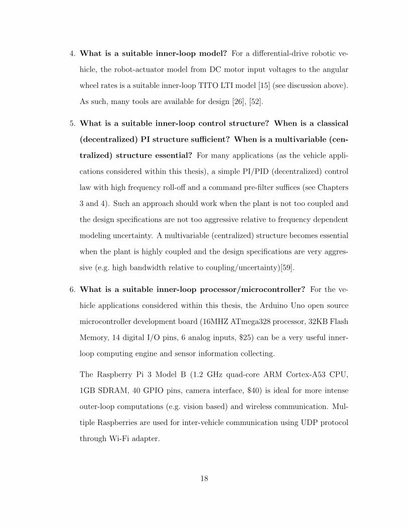
(7) a forward-pointing (SR04) ultrasonic distance/range-finder sensor (40kHz,

0.02-5 m, approximately ±8 directional, see Figure 1.9) for outer-loop separa-

tion control, and

Figure 1.9: HC-SR04 Ultrasonic Sensor

16

2. Why should a hierarchical inner-outer loop control architecture be

used?[14] Hierarchical inner-outer loop controllers are found across many in-

dustrial/commercial/military application areas (e.g. aircraft, spacecraft, robots,

manufacturing processes, etc.) where it is natural for slower (outer-loop gen-

erated) high-level commands to be followed by a faster inner control loop that

must deliver robust performance (e.g. low frequency reference command fol-

lowing, low-frequency disturbance attenuation and high-frequency sensor noise

attenuation) in the presence of significant signal and system uncertainty. A

well designed inner-loop can greatly simplify outer-loop design. An excellent

example of how inner-outer loop architectures are used is in the missile-target

application arena. Here, an autopilot (inner-loop) follows commands gener-

ated from the guidance system (outer-loop). More substantively, inner-outer

loop control structures are used to tradeoff properties at distinct loop breaking

points (e.g. outputs/errors versus inputs/controls) [53], [54].

Inner-Loop Control

3. What are typical inner-loop objectives? Typical inner-loop objectives can

be speed control; i.e. requiring the design of a speed (v, ω) or (ωR, ωL) control

system. Within this thesis, inner-loop control for our differential-drive Thun-

der Tumbler vehicles specifically refers to classical proportional-plus-integral

(PI) pulse-width-modulation (PWM) based speed control for each motor (with

high-frequency roll-off and a reference command prefilter). In Chapter 4, this is

addressed for our enhanced low-cost Thunder Tumbler. The inner-loop con-

trol laws developed in Chapters 4 is based on the TITO LTI fourth order

vehicle-motor (v, ω) or (ωR, ωL) dynamical model presented in [15] (see dis-

cussion above).

17

4. What is a suitable inner-loop model? For a differential-drive robotic ve-

hicle, the robot-actuator model from DC motor input voltages to the angular

wheel rates is a suitable inner-loop TITO LTI model [15] (see discussion above).

As such, many tools are available for design [26], [52].

5. What is a suitable inner-loop control structure? When is a classical

(decentralized) PI structure sufficient? When is a multivariable (cen-

tralized) structure essential? For many applications (as the vehicle appli-

cations considered within this thesis), a simple PI/PID (decentralized) control

law with high frequency roll-off and a command pre-filter suffices (see Chapters

3 and 4). Such an approach should work when the plant is not too coupled and

the design specifications are not too aggressive relative to frequency dependent

modeling uncertainty. A multivariable (centralized) structure becomes essential

when the plant is highly coupled and the design specifications are very aggres-

sive (e.g. high bandwidth relative to coupling/uncertainty)[59].

6. What is a suitable inner-loop processor/microcontroller? For the ve-

hicle applications considered within this thesis, the Arduino Uno open source

microcontroller development board (16MHZ ATmega328 processor, 32KB Flash

Memory, 14 digital I/O pins, 6 analog inputs, $25) can be a very useful inner-

loop computing engine and sensor information collecting.

The Raspberry Pi 3 Model B (1.2 GHz quad-core ARM Cortex-A53 CPU,

1GB SDRAM, 40 GPIO pins, camera interface, $40) is ideal for more intense

outer-loop computations (e.g. vision based) and wireless communication. Mul-

tiple Raspberries are used for inter-vehicle communication using UDP protocol

through Wi-Fi adapter.

18

7. What are suitable inner-loop sensors and actuators? For the ground

vehicle applications considered within this thesis, wheel encoders and an IMU

are useful inner-loop sensors. We used optical encoders for implementing our

differentital-drive inner-loop (ωR, ωL)-(v, ω) control laws. The IMU was used to

implement our (v, θ) differential-drive outer-loop control laws. Armature con-

trolled DC motors are useful inner-loop actuators. This is what was utilized for

our ETT.

Figure 1.10 summarizes inner- and outer-loop control laws considered, analyzed

and implemented within this thesis for our enhanced differential-drive Thunder

Tumbler vehicles: one inner-loop (v, ω) speed control law and three outer-loop

control laws: (1) (v, θ), (2) ∆x, θ), and (3) vehicular platoon separation control

Figure 1.10: Visualization of Inner- and Outer-Loop Control Laws

Outer-Loop Control

8. What are typical outer-loop objectives? For the vehicle applications con-

sidered within this thesis, three (3) outer-loop objectives are examined (see

Figure 1.10):

19

(1) speed-direction (v, θ) cruise control along a line by exploiting encoders for

speed information and IMU or camera for directional information

(2) lineal (directed) separation (∆x, θ) control by exploiting encoders for posi-

tional information, IMU or camera for directional information, and ultrasound

for nearly-lineal separation information.

(3) platoon separation control. Specifically, position control involves wrapping

a (∆x, θ) control with feed-forward path from wireless communication around

a inner-loop cruise control system.

Here, outer-loop control laws are based on proportional-plus-derivative (PD)

laws (with high-frequency roll-off). If the reference command is a ramp signal,

proportional-integral-derivative (PID) law is needed in platoon control separa-

tion design. It must be noted that local asymptotic stability is theoretically

guaranteed (and practically observed) for all of the implemented control laws.

Relevant references for each outer-loop objective are presented and described in

Section 1.2 on page 3. Also see work within Chapter 4 and 5.

9. What is a suitable outer-loop model? If the inner-loop is designed well,

after it is closed it can yield a system (seen by the outer-loop controller) that is

very simple looping (e.g. diag( as+a

, bs+b

), looks like identity at low frequencies).

This can greatly facilitate the design of the outer-loop control system. (See

work within Chapters 3 and 4.)

10. What is a suitable outer-loop control structure? When is a more com-

plex structure needed? Suppose that an inner-loop speed control system has

been designed. Suppose that it looks like as+a

. It then follows that if position is

concerned, then we have a system that looks like[

as(s+a)

]; i.e. there is an addi-

tional integrator present. Given this, classical control (root locus) concepts [52]

20

can be used to motivate an outer-loop control structure Ko = g(s + z). In an

effort to attenuate the effect of high frequency sensor noise, one might introduce

additional roll-off; e.g. Ko = g(s+ z)[

bs+b

]nwhere n = 2 or greater. (See work

within Chapters 3 and 4.) When PID is needed, the controller structure can

be e.g. Ko = g(s+z)2

s

[bs+b

]nwhere n = 2 or greater.(See work within Chapters 3

and 4.)

11. What is a suitable outer-loop processor/microcontroller? For the vehi-

cle applications considered within this thesis, both Arduino Uno and Raspberry

Pi 3 are each used for distinct outer-loop controller implementations.

Arduino Uno is used for inner-loop control and sensor information gathering.

The Raspberry Pi 3 is used for all outer-loop control in this thesis. Raspberry

Pi and Uno communicate to each other through serial communication. It is used

for more demanding vision-based cruise-position-directional outer-loop control

and wireless communication. The speed of Arduino Uno is limited. As such, it

cannot handle intense outer-loop vision-based processing. In contrast, the Rasp-

berry Pi 3 is very fast and has a large memory. It is very well-suited for intense

outer-loop vision-based processing and inter-vehicle wireless communication.

While partial answers have been provided above, the thesis (when applicable)

provides more detailed answers. When taken collectively, the contributions of this

thesis are significant - particularly to those interested in developing low-cost platforms

for conducting robotics/FAME research.

21

Key Demonstrations. To further highlight contributions of the thesis, the following

demonstrations are presented and analyzed within the thesis. All demonstrations are

based on differential-drive enhanced Thunder Tumbler vehicles.

• cruise control along a straight line

• vehicle-target spacing control

• longitudinal platoon separation control

For most cases, hardware (empirically obtained) data is compared with, and cor-

roborated by, model-based simulation data. In short, the thesis uses multiple en-

hanced/augmented low-cost ground vehicles to demonstrate many capabilities that

are critical in order to reach the longer-term FAME goal.

1.4 Organization of Thesis

The remainder of the thesis is organized as follows.

• Chapter 2 (page 25) presents an overview for a general FAME architecture de-

scribing candidate technologies (e.g. sensing, communications, computing, ac-

tuation).

• Chapter 3 (page 30) describes modeling and control issues for a differential-

drive ground vehicle. In this chapter, motor-wheel system TITO LTI model

(off ground model) and vehicle-motor model(on ground model) are developed

carefully. The ideas presented in [59] [14] provide basis for our work. Base on

this, we presents system-theoretic as well as hardware results for our differential-

drive Thunder Tumbler ground robotic vehicles.

22

• Chapter 4 (page 92) inner loop and outer loop design for a single robot was done

based on vehicle-motor on ground model. System-theoretic as well as hardware

results for our differential-drive Thunder Tumbler ground robotic vehicles will

be presented. Related demonstrations are described.

• Chapter 5 (page 151) longitudinal platoon control problem will first be stated.

Then vehicle model for leader and followers will be developed. Design with and

without leader information have been discussed. Simulation results will show

that with the leader information vehicle spacings get attenuated from the front

to the back of the platoon and control effort is decreasing along the platoon.

Without it, spacings cannot get attenuated along the platoon or even get mag-

nified.

• Chapter 6 (page 181) summarizes the thesis and presents directions for future

robotics/FAME research. While much has been accomplished in this thesis, lots

remains to be done.

• Appendix A (page 190) contains Arduino program files used to generate inner

loop results for this thesis.

• Appendix B (page 264) contains all MATLAB mfiles used to generate the re-

sults for this thesis.

• Appendix C (page 294) contains Arduino code used to generate the results for

this thesis.

23

1.5 Summary and Conclusions

In this chapter, we provided an overview of the work presented in this thesis and

the major contributions. A central contribution of the thesis is improved modeling

of DC motor, motor-wheel system with gearbox transmission, on ground longitu-

dinal model. Uncertainty of modeling parameters has been exploited by testing 9

ETT robots. A updated low-cost multi-capability differential-drive Thunder Tumbler

robotic ground vehicle that can further facilitates on ground robot research. New

platform software has been provided, lots of hardware results can be logged and ana-

lyzed. Hardware demonstrations were conducted using our differential drive vehicles.

The thesis attempts to address most critical modeling, design, and control issues

of longitudinal platoon problem and makes another step toward long-term FAME

research.

24

Chapter 2

OVERVIEW OF GENERAL FAME ARCHITECTURE

2.1 Introduction and Overview

In this chapter, we will describe a general architecture for our general FAME re-

search. This section is based on [14], small modification is made to suit this thesis.

The architecture described attempts to shed light on command, control, communi-

cations, computing (C4), and sensing (S) requirements needed to support a fleet of

collaborating vehicles. Collectively, the C4 and S requirements are referred to as C4S

requirements.

2.2 FAME Architecture

In this section, we describe a candidate system-level architecture that can be

used for a fleet of robotic vehicles. The architecture can be visualized as shown

in Figure 2.1. The architecture addresses global/central as well as local command,

control, computing, communications (C4), and sensing (C4S) needs. Elements within

the figure are now described.

• Central Command: Global/Central Command, Control, Computing.

A global/central computer (or suite of computers) can be used to perform all

of the very heavy computing requirements. This computer gathers information

from a global/central (possibly distributed) suite of sensors (e.g. GPS, radar,

cameras). The information gathered is used for many purposes. This includes

temporal/spatial mission planning, objective adaptation, optimization, decision

making (control), information transmission/broadcasting and the generation of

25

Figure 2.1: FAME Architecture to Accommodate Fleet of Cooperating Vehicles

commands that can be issued to members of the fleet. Within this thesis, we

simply use a central command laptop.

• Global/Central Sensing. In order to make global/central decisions, a suite

of sensors should be available (e.g. GPS, radar, cameras). This suite provides

information about the state of the fleet (or individual members) that can be

used by central command. Within this thesis, global sensing is achieved by

feeding back real-time video from our enhanced differential-drive robotic Thun-

der Tumbler vehicles to our central command laptop. Such a lab-based system

offers the benefit that it can be fairly easily transported for use elsewhere (with

some peruse calibration). Such a system can be used to examine a wide range

of scenarios. Also ongoing is an effort to more profoundly exploit vision on

individual vehicles [60], [24].

26

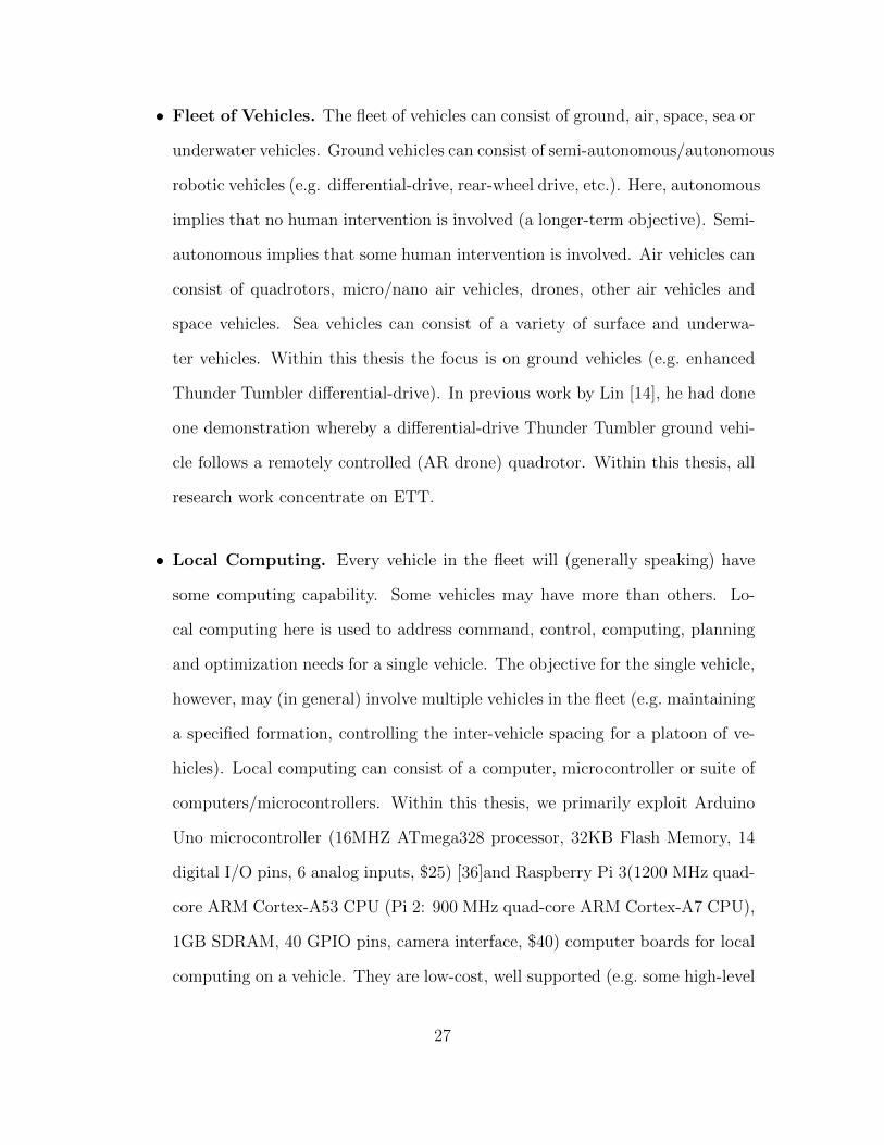
• Fleet of Vehicles. The fleet of vehicles can consist of ground, air, space, sea or

underwater vehicles. Ground vehicles can consist of semi-autonomous/autonomous

robotic vehicles (e.g. differential-drive, rear-wheel drive, etc.). Here, autonomous

implies that no human intervention is involved (a longer-term objective). Semi-

autonomous implies that some human intervention is involved. Air vehicles can

consist of quadrotors, micro/nano air vehicles, drones, other air vehicles and

space vehicles. Sea vehicles can consist of a variety of surface and underwa-

ter vehicles. Within this thesis the focus is on ground vehicles (e.g. enhanced

Thunder Tumbler differential-drive). In previous work by Lin [14], he had done

one demonstration whereby a differential-drive Thunder Tumbler ground vehi-

cle follows a remotely controlled (AR drone) quadrotor. Within this thesis, all

research work concentrate on ETT.

• Local Computing. Every vehicle in the fleet will (generally speaking) have

some computing capability. Some vehicles may have more than others. Lo-

cal computing here is used to address command, control, computing, planning

and optimization needs for a single vehicle. The objective for the single vehicle,

however, may (in general) involve multiple vehicles in the fleet (e.g. maintaining

a specified formation, controlling the inter-vehicle spacing for a platoon of ve-

hicles). Local computing can consist of a computer, microcontroller or suite of

computers/microcontrollers. Within this thesis, we primarily exploit Arduino

Uno microcontroller (16MHZ ATmega328 processor, 32KB Flash Memory, 14

digital I/O pins, 6 analog inputs, $25) [36]and Raspberry Pi 3(1200 MHz quad-

core ARM Cortex-A53 CPU (Pi 2: 900 MHz quad-core ARM Cortex-A7 CPU),

1GB SDRAM, 40 GPIO pins, camera interface, $40) computer boards for local

computing on a vehicle. They are low-cost, well supported (e.g. some high-level

27

software development tools Arduino IDE and customized Linux operation sys-

tem Raspbian on Raspberry Pi), and easy to use.

• Local Sensing. Local sensing, in general, refers to sensors on individual vehi-

cles. As such, this can involve a variety of sensors. These can include encoders,

IMUs (containing accelerometers, gyroscopes, magnetometers), ultrasonic range

sensors, LIDAR, GPS, radar, and cameras. Within this thesis, we exploit optical

encoders(RPR220 photo-interrupter REFL 6mm 800nm, home-made encoder

disk 20 black-white pair, ) [47], Adafruit BNO055 IMUs to measure vehicle ro-

tation ( 9DOF, Accelerometer ± 2,4,6,8,16g. Gyro ± 125−2000/sec. Compass

±1300 µT (x-,y-axis) ±2500 µT (z-axis)) [58], ultrasonic range sensors (40kHz,

0.02-5 m, approximately ±8 directional) [68], and Raspberry Pi cameras(2592

× 1944, 30 fps, 150 MPs, MPEG-4) [57]. LIDAR, GPS and radar are not used.

• Local Communications. Here, local communications refers to how fleet ve-

hicles communicate with one another as well as with central command. In this

thesis, vehicles exploit WiFi ( IEEE 802.11 (2.4, 5GHz) standard)[67] to send

locally obtained Raspberry Pi camera video (2592 × 1944, 30 fps, 150 MPs,

MPEG-4) [57] to a central command laptop.

28


In this chapter, we described a general (candidate) FAME architecture for a fleet

of cooperating robotic vehicles. Of critical importance to properly assess the utility

of a FAME architecture is understanding the fundamental limitations imposed by its

subsystems (e.g. bandwidth/dynamic, accuracy/static). This “fundamental limita-

tion” issue is addressed within Chapter 4 where enhanced differential-drive Thunder

Tumbler vehicles are used as the central building block for the fleet.

29

Chapter 3

MODELING FOR SINGLE VEHICLE


The purpose of this chapter is to illustrate fundamental modeling and control

design methods for a differential-drive (DD) robotic ground vehicle. This is achieved

by presenting relevant model trade studies and then illustrating the design of an

inner-loop (v, ω) speed control law and associated tradeoffs. As discussed in Chapter

1, such a control law is generally the basis for any outer-loop control law (e.g. cruise

control along a line, target-separation control, platoon separation control). A two-

input two-output (TITO) linear time invariant (LTI) model, taken from [15], is used

as the basis for all developments within the chapter. The model is analyzed and used

to conduct relevant parametric trade studies (e.g. mass, moment of inertia, motor

back EMF constant, motor armature resistance) which provided insight about the

vehicle being addressed. The decentralized controller is based on classical single-

input single-output (SISO) methods [32], [52]. Centralized controller designs for the

inner loop had been discussed within [14].

3.2 Description of Hardware

In [14], the authors has shown how to take off-the-shelf (low-cost) remote con-

trol “toy” vehicles and convert them into intelligent multi-capability robotic plat-

forms that can be used for conducting robotics/FAME research. In this section we

briefly describe each component on our low-cost robots, only hardware updates will

be discussed in detail. All discussion provided below focuses on our differential-drive

30

Thunder Tumbler vehicles (9 ETTs in total). To distinguish the work from [14], we

named the old one ETT 1 and the new one ETT 2 when needed. More specifically,

all differential-drive Thunder Tumbler vehicles (ETT 2) were augmented with the

following: Arduino Motor Shield, Arduino Uno microcontroller board, Optical wheel

encoders (Magnets wheel encoder on ETT 1), BNO055 IMU (LSM9DS0 IMU on

ETT1), Raspberry Pi 3 (Raspberry Pi 2 on ETT 1), Raspberry 5MP camera module,

HC-SR04 Ultrasonic Distance Sensor, TP-LINK WiFi adapter (Edimax WiFi adapter

on ETT 1). Only updates will be described in detail below, other overlapped work

detail can be found in his thesis [14] page 107-115, we just keep same structure and list

each item for completeness. An enhanced Thunder Tumbler is shown in Figure 1.1,

page 12.

A hardware components list for an enhanced Thunder Tumbler is given in Ta-

ble 3.1. The table shows the cost is less than $220.

31

Product Quantity Price ($)

Thunder Tumbler Vehicle 1 $10

Raspberry Pi 3 Model B 1 $40

Arduino Uno 1 $25

Adafruit Motor Shield 1 $20

Raspberry Pi 5MP Camera 1 $20

TP-LINK TL-WN722N USB Wi-Fi Adapter 1 $14

Camera Holder 1 $5

HCSR04 Ultrasonic Sensor 1 $5

EasyAcc PowerBank for Raspberry Pi 1 $13

Power Supply for Motors 4 $3.5

Optical Sensor Photo-Interrupter 2 $1.5

Adafruit 9-DOF IMU BNO055 1 $35

Miscellaneous 1 $15

Total Price $219

Table 3.1: Hardware Components for Enhanced Differential-Drive Thunder Tumbler

Robotic Vehicle

1. Differential-Drive Thunder Tumbler. Each Thunder Tumbler is a $10

“toy” vehicle, it is a differential-drive vehicle with two DC motors - one on left

wheel, one on right wheel. Each differential-drive Thunder Tumbler vehicle was

augmented/enhanced to provide a suite of substantive capabilities.

2. DC Motors. Two 6V brushed armature controlled DC motors are on each

differential-drive Thunder Tumbler vehicle. The DC motors receive voltage sig-

32

nals from an Arduino motor shield and apply the required torques to each of

the Thunder Tumbler’s wheels.

3. Arduino Uno Open-Source Microcontroller Board. Each Thunder Tum-

bler is equipped with an onboard Arduino Uno microcontroller board (see Fig-

ure 1.4 on page 14). In our thesis, Arduino only served as inner loop controller

and provide necessary sensor information to Raspberry Pi.

4. Arduino Motor Shield. An Adafruit Motor/Stepper/Servo Shield for Ar-

duino v2 Kit (v2.3) was used in this thesis see Figure 1.5 on page 14,

5. Arduino Uno Open-Source Microcontroller Board. Each Thunder Tum-

bler is equipped with an onboard Arduino Uno microcontroller board (see Fig-

ure 1.4 on page 14).

6. Optical Infra-red Reflective Photosensor-Based Encoders. A reflective

photosensor sensor (photo-interrupter) RPR220 and home-made code disk (20

black-white pairs per wheel, see Figure 1.2 on page 13) are used as wheel en-

coders. Wheel encoders are used for (dead-reckoning) speed/position control.

The wheel encoders count the pulses that black-white stripe pair passes the

photo-interrupter. This information is sent to the Arduino Uno which can then

calculate/estimate vehicle velocity and translational displacement, vehicle an-

gular velocity and angular displacement.

7. Inertial Measurement Unit (IMU). The IMU can collect acceleration, an-

gular velocity and orientation of the vehicle. In this thesis, it mainly collects

the absolute orientation information (θ) of the robot and sends the information

to the Arduino Uno. An (BNO055 9dof) inertial measurement unit (IMU) is

used for directional control (see Figure 1.3 on page 13). The 9 dof include 3

acceleration channels, 3 angular rate channels and 3 magnetic field channels.

33

Range features are as follows: ± 2/4/6/8/16 g linear acceleration full scale, ±

13 gauss (x-,y-axis) ± 25 gauss (z-axis)), magnetic full scale and ± 125-2000

degree/sec angular rate full scale. It has 16-bit data output and SPI/I2C serial

interfaces.

8. Raspberry Pi 3 Single Board Computer. Each Thunder Tumbler has an

onboard Raspberry Pi 3 Model B single board computer (see Figure 1.6 on

page 15). Raspberry Pi 3 Model B characteristics include:

Broadcom BCM2837 with a 1.2GHz quad-core ARM Cortex-A53 64-bit CPU

and VideoCore IV GPU, 1GB SDRAM (bus synchronous dynamic RAM) at

900 MHz (shared with GPU), on-board Bluetooth Low Energy (BLE), on-board

BCM43143 WiFi. Other detail hardware information can be found [14] and [39]

For raspberry pi 3 and pi 2 comparison, one can refer to online reports [41].

Summary of Raspberry Pi Use:

• Communicate with Arduino During Robot Operation. We also

used C language USB (Serial) communication between the Pi and Arduino.

There are many ways to establish communication between the Raspberry

Pi and the Arduino such as using the GPIO and Serial pins or using I2C

communication (using the SCL-clock and SDL-data pins). The simplest

way to get the two devices talking is to use the micro USB to USB adapter

that comes with the Arduino Uno. By using the open-source serial library

package, we can use C to read from and write to Arduino’s serial port.

• Implement all outer-loops include the following: (1) Outer-loop

1 (v, θ) cruise control along a line (2) Outer-loop 2 (∆x, θ) separation-

direction control along a line, (3) Outer-loop 3 is our platoon control law

with leader information.

34

• Communication with central command laptop. This remote capa-

bility permit a robot to switch between autonomous and semi-autonomous

modes of operation. Such switching has been done by keyboard command

thread running on Pi.

• Communication with other Pi When platoon control need leader

inforamtion, Pi is used to send/receive leader information

9. Raspberry 5MP Camera Module. Each Thunder Tumbler has an onboard

Raspberry Pi 5MP camera (see Figure 1.7 on page 15).The camera module col-

lects image information and sends it to the onboard Raspberry Pi.

10. Ultrasonic Distance Sensor. A forward-looking (40kHz SR04) ultrasonic dis-

tance/rangefinder sensor was placed on each robot (see Figure 1.9 on page 16).

The ultrasonic sensor collects range/separation ∆x information (at ranges of 2

cm to 5m) and sends the information to the Arduino Uno.

11. TP-Link WiFi Adapter. An TP-Link adapter (see Figure 1.8 on page 16) is

used to connect Pi via wireless router.

12. Wireless Router. A TP-LINK wireless router is used to receive radio signals

from a remotely situated WiFi adapter on the differential-drive mobile robot

and transmits the radio signals to a wireless adapter on the remotely situated

central command laptop.

35

3.3 Modeling of a Differential-Drive Ground Robotic Vehicle

Many mobile robots use a so-called differential-drive drive mechanism. Such a

mechanism involves two rear wheels that are independently controlled via torque-

generating DC motors. The inputs to the DC motors are voltages. Within this

thesis, the motors are assumed to be identical in order to simplify the presentation.

In practice, motor differences must be accounted for. This, in part, is addressed by

the motor control laws being employed. Within this section, we first examine the

TITO LTI model that was presented within [15]. This model was used for control

law design within the MS thesis [59] and [14]. It serve as the basis for plant analysis

and inner-loop control designs for differential-drive vehicle. Then we modified this

model and put forward on ground vehicle-motor dynamic model from on ground

experimental results and verify the model with hardware. The on ground model will

be used for designing inner-loop and outer-loops in this thesis. Before presenting the

model, we first discuss the robot kinematics. A great deal of insight can be gained

by first understanding the kinematics. The robot dynamics are then examined - first

without and then with the DC motor dynamics.

Before continuing with our presentation it is useful to define key robot variables

and parameters to be used for introduction of differential-drive robot modeling. The

nominal value is from ETT V1 and uncertainties from multiple ETTs. There are 9

ETTs in total, we named it from V1 to V9. This is done within Table 3.2.

36

Parameter Definition Nominal Values

m Mass (Enhanced Vehicle) 0.87 ± 0.02 kg

mo Mass (Original Vehicle) 0.56 ± 0.02 kg

Iz Moment of Inertia 0.0051 kg m2

r Wheel Radius 0.05 ± 0.005 m

dw Distance between Rear Wheels 0.14 ± 0.005 m

La Armature Inductance (2.7 ± 0.2) ×10−8 H

Ra Armature Resistance 0.9 ± 0.15 Ω

Kg Gearbox Ratio 18.48

Kb back EMF Constant (3.2 ± 0.5)×10−4 V/(rad/sec)

Kt Torque Constant (3.2 ± 0.5)×10−4 Nm/A

I Equivalent Moment of Inertia (2.91 ± 1.00) ×10−6 kg m2

β Speed Damping Constant (7.04 ± 3.00) ×10−7 Nms

vmax Max. Speed (Enhanced Vehicle) 2.1 ± 0.2 m/sec

vmaxo Max. Speed (Original Vehicle) 4.5 ± 0.2 m/sec

E Efficiency - Power Out / Power In 0.15

amax Max. Acceleration (Enhanced) 2.5 ± 0.5 m/sec2

ωsmax Max. Angular Wheel Velocity 46 ± 4 rad/sec

τsmax Max. Torque (Zero RPM) 0.048 ± 0.05 Nm

eamax Max. Motor Voltage 5.25 ± 0.05 V

Table 3.2: Thunder Tumbler Nominal Parameter Values with Uncertainty

37

3.4 Differential-Drive Robot Kinematics

Figure 3.1 can be used to understand the kinematics of a differential-drive ground

robot [17].

Figure 3.1: Visualization of Differential-Drive Mobile Robot

The point that the robot rotates about at a given instant in time is called the

instantaneous center of curvature (ICC) [17]. If (x, y) denotes the planar inertial

coordinate of the robot and θ denotes the direction of the robot’s longitudinal body

axis with respect to the x-axis, then we obtain the following nonlinear kinematic

model: x

y

θ

=

cos θ

sin θ

0

v +

0

0

1

ω (3.1)

where

v =√x2 + y2 (3.2)

denotes the translational speed of the robot and ω = θ denotes its angular speed.

38

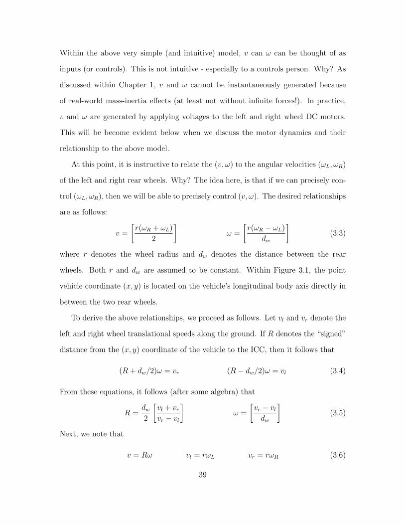
Within the above very simple (and intuitive) model, v can ω can be thought of as

inputs (or controls). This is not intuitive - especially to a controls person. Why? As

discussed within Chapter 1, v and ω cannot be instantaneously generated because

of real-world mass-inertia effects (at least not without infinite forces!). In practice,

v and ω are generated by applying voltages to the left and right wheel DC motors.

This will be become evident below when we discuss the motor dynamics and their

relationship to the above model.

At this point, it is instructive to relate the (v, ω) to the angular velocities (ωL, ωR)

of the left and right rear wheels. Why? The idea here, is that if we can precisely con-

trol (ωL, ωR), then we will be able to precisely control (v, ω). The desired relationships

are as follows:

v =

[r(ωR + ωL)

2

]ω =

[r(ωR − ωL)

dw

](3.3)

where r denotes the wheel radius and dw denotes the distance between the rear

wheels. Both r and dw are assumed to be constant. Within Figure 3.1, the point

vehicle coordinate (x, y) is located on the vehicle’s longitudinal body axis directly in

between the two rear wheels.

To derive the above relationships, we proceed as follows. Let vl and vr denote the

left and right wheel translational speeds along the ground. If R denotes the “signed”

distance from the (x, y) coordinate of the vehicle to the ICC, then it follows that

(R + dw/2)ω = vr (R− dw/2)ω = vl (3.4)

From these equations, it follows (after some algebra) that

R =dw2

[vl + vrvr − vl

]ω =

[vr − vldw

](3.5)

Next, we note that

v = Rω vl = rωL vr = rωR (3.6)

39

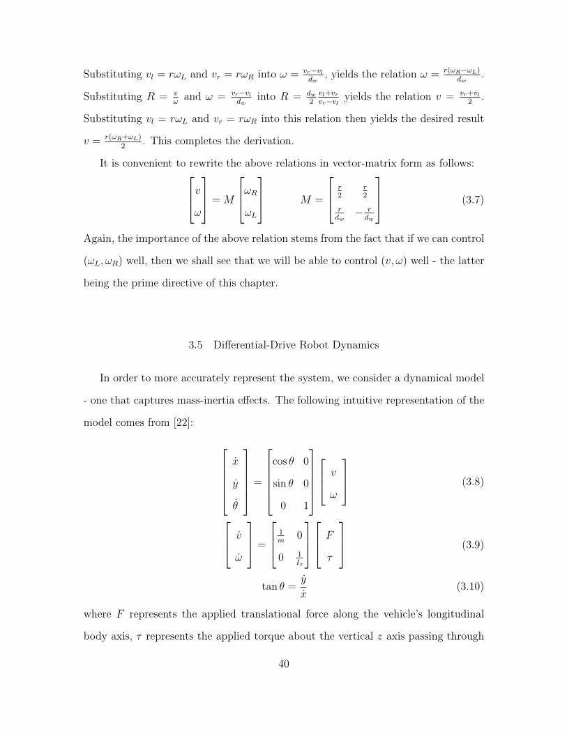
Substituting vl = rωL and vr = rωR into ω = vr−vldw

, yields the relation ω = r(ωR−ωL)dw

.

Substituting R = vω

and ω = vr−vldw

into R = dw2vl+vrvr−vl

yields the relation v = vr+vl2

.

Substituting vl = rωL and vr = rωR into this relation then yields the desired result

v = r(ωR+ωL)2

. This completes the derivation.

It is convenient to rewrite the above relations in vector-matrix form as follows:vω

= M

ωRωL

M =

r2

r2

rdw− rdw

(3.7)

Again, the importance of the above relation stems from the fact that if we can control

(ωL, ωR) well, then we shall see that we will be able to control (v, ω) well - the latter

being the prime directive of this chapter.

3.5 Differential-Drive Robot Dynamics

In order to more accurately represent the system, we consider a dynamical model

- one that captures mass-inertia effects. The following intuitive representation of the

model comes from [22]:

x

y

θ

=

cos θ 0

sin θ 0

0 1

v

ω

(3.8)

v

ω

=

1m

0

0 1Iz

F

τ

(3.9)

tan θ =y

x(3.10)

where F represents the applied translational force along the vehicle’s longitudinal

body axis, τ represents the applied torque about the vertical z axis passing through

40

the point (x, y), m denotes the mass of the vehicle and Iz denotes its moment of inertia

about the vertical z axis passing through the point (x, y). From the above, we see that

the dynamical model consists of the following five equations: three kinematic model

equations within the matrix-vector equation (3.8), two Newtonian dynamical equa-

tions within the matrix-vector equation (3.9), and the no slipping (non-holonomic)

constraint within equation (3.10). It should be noted that in practice, the force F and

torque τ are generated by the two DC motors on the rear wheels. This shall become

evident within the subsections that follow below. It should also be noted that the

above dynamical model can be derived using the classic Euler-Lagrange formulation

[22] [15].

As suggested above, the kinematic model neglects dynamic mass-inertia effects.

As such, the kinematic model is just an approximation to the dynamic model. As

expected, and it will be shown, the kinematic model is a good approximation to the

dynamical model when (v, ω) can be generated quickly. Intuitively, this occurs when

m and Iz are sufficiently small (see equation (3.9)) or the inner (v, ω) loop has a

sufficiently large bandwidth. This shall become evident below.

Finally, it is important to note the relationship between (F, τ) and the left-right

motor torques (τL, τR). The desired relationship is similar in form to the angular

velocity relationships within equation 3.3 and is given by

F =

[τR + τL

r

]τ =

[dw(τR − τL)

2r

](3.11)

Here, τL and τR represent the torques acting on the left and right wheels, respectively.

Next, we discuss the motor (actuator) dynamics. Ultimately, the motors are

responsible for producing the wheel torques (τL, τR) and hence the associated pair

(F, τ). The latter, of course, are directly responsible for producing the vehicle speeds

(v, ω).

41

3.5.1 DC Motor (Actuator) Dynamics with Gearbox

DC motors are widely used in robotics applications. They are the mostly widely

used actuator class in mobile robots. It is important to take DC motor dynamics

into account when constructing a robot’s model. There are two classes of DC motors:

(1) armature-current controlled and (2) field-current controlled [52]. Within this

thesis, we shall focus on the former; i.e. armature-current controlled DC motors.

The dynamics for a DC motor can be visualized as shown within Figure 3.2. The

associated equations are as follows:

Figure 3.2: Visualization of DC Motor Speed-Voltage Dynamics

Armature Equation:

ea = Ladiadt

+Raia + eb (3.12)

back EMF Equation:

eb = KbKgωs (3.13)

Torque Equation:

τs = KtKgia (3.14)

Load Equation:

Iωs + βωs =τs

Kg2 (3.15)

Gear Relationship:

Kg = Kg12Kg23 (3.16)

42

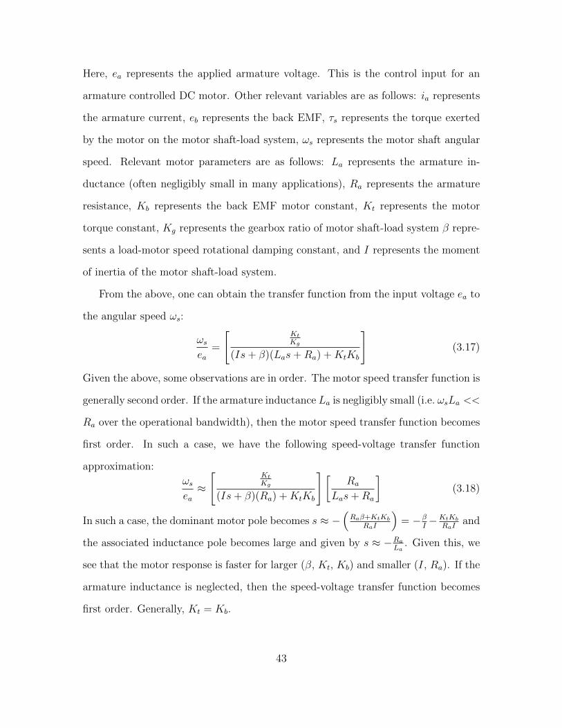
Here, ea represents the applied armature voltage. This is the control input for an

armature controlled DC motor. Other relevant variables are as follows: ia represents

the armature current, eb represents the back EMF, τs represents the torque exerted

by the motor on the motor shaft-load system, ωs represents the motor shaft angular

speed. Relevant motor parameters are as follows: La represents the armature in-

ductance (often negligibly small in many applications), Ra represents the armature

resistance, Kb represents the back EMF motor constant, Kt represents the motor

torque constant, Kg represents the gearbox ratio of motor shaft-load system β repre-

sents a load-motor speed rotational damping constant, and I represents the moment

of inertia of the motor shaft-load system.

From the above, one can obtain the transfer function from the input voltage ea to

the angular speed ωs:

ωsea

=

[KtKg

(Is+ β)(Las+Ra) +KtKb

](3.17)

Given the above, some observations are in order. The motor speed transfer function is

generally second order. If the armature inductance La is negligibly small (i.e. ωsLa <<

Ra over the operational bandwidth), then the motor speed transfer function becomes

first order. In such a case, we have the following speed-voltage transfer function

approximation:

ωsea≈

[KtKg

(Is+ β)(Ra) +KtKb

] [Ra

Las+Ra

](3.18)

In such a case, the dominant motor pole becomes s ≈ −(Raβ+KtKb

RaI

)= −β

I−KtKb

RaIand

the associated inductance pole becomes large and given by s ≈ −RaLa

. Given this, we

see that the motor response is faster for larger (β, Kt, Kb) and smaller (I, Ra). If the

armature inductance is neglected, then the speed-voltage transfer function becomes

first order. Generally, Kt = Kb.

43

3.5.2 Empirically Obtained Experimental Data for Motor-Wheel System

Model Parameters Want to Determine. Among all the symbols defined above,

finally we want the following (7) parameters for motor-wheel load system: Ra, La,

Kg, Kb, Kt, I, β.

• Armature Inductance La. Armature inductance is usually very small in toy DC

motor, we use DE5000 high performance LCR meter [37] to measure it. An

LCR meter is a type of electronic test equipment used to measure the induc-

tance (L), capacitance (C), and resistance (R) of an electronic component. In

the simpler versions of this instrument the impedance was measured internally

and converted for display to the corresponding capacitance or inductance value.

Readings should be reasonably accurate if the capacitor or inductor device un-

der test does not have a significant resistive component of impedance. More

advanced designs measure true inductance or capacitance, as well as the equiv-

alent series resistance of capacitors and the Q factor of inductive components.

The DE-5000 is a portable, high-performance LCR meter that is full-featured

yet cost effective ($140). It measures in true 4-wire Kelvin mode and rivals the

capabilities and options of many of its bench counterparts. This LCR meter

features automatic L-C-R selection, a Sorting mode, and selectable test frequen-

cies. It can transfer data to a PC via a fully isolated, optical IR-USB interface.

For 2000 mH range, the inductance accuracy is 0.1 mH. We measured (10)

motors’ armature inductance, results are shown in Figure 3.3

44

0 2 4 6 8 100

50

100

150

200

250

300

350

Armature Inductance of 10 Motors

Motor Index

Inducta

nce(µ

H)

LCR Meter

LCR Meter Avg

Figure 3.3: dc Motor Armature Inductance of 10 ETT Motors

From the figure above, we can see measurements are close to the average result

is around 270 µH.

• Armature resistance Ra. Armature resistance is usually very small in toy DC

motor, one common way is to using stall method to measure it. Stall method

means we applied constant dc voltage to the motor and stall the shaft to do

the measurement of current. From equation 3.12 and 3.13, at steady state with

0 angular velocity, armature equation reduces to ea = Raia, then apply Ohm’s

law: Ra = VIa

. We did the measurement for 10 ETT motors, using two methods

and did 5 times measurement for each motor. Results are shown in Figure 3.4

45

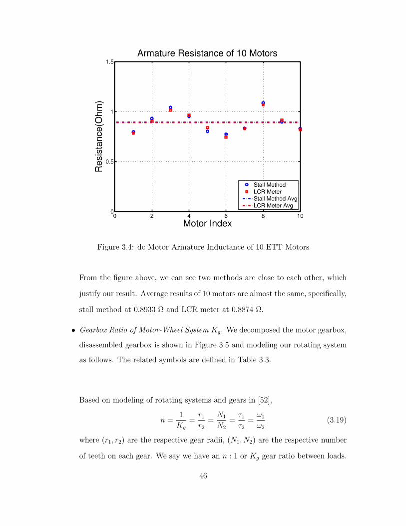
0 2 4 6 8 100

0.5

1

1.5

Armature Resistance of 10 Motors

Motor Index

Resis

tance(O

hm

)

Stall Method

LCR MeterStall Method Avg

LCR Meter Avg

Figure 3.4: dc Motor Armature Inductance of 10 ETT Motors

From the figure above, we can see two methods are close to each other, which

justify our result. Average results of 10 motors are almost the same, specifically,

stall method at 0.8933 Ω and LCR meter at 0.8874 Ω.

• Gearbox Ratio of Motor-Wheel System Kg. We decomposed the motor gearbox,

disassembled gearbox is shown in Figure 3.5 and modeling our rotating system

as follows. The related symbols are defined in Table 3.3.

Based on modeling of rotating systems and gears in [52],

n =1

Kg

=r1

r2

=N1

N2

=τ1

τ2

=ω1

ω2

(3.19)

where (r1, r2) are the respective gear radii, (N1, N2) are the respective number

of teeth on each gear. We say we have an n : 1 or Kg gear ratio between loads.

46

Parameter Definition

Kg Gear Ratio between First and Third Load

Kg12 (n12) Gear Ratio between First and Second Load

Kg23 (n23) Gear Ratio between Second and Third Load

r1 Radius of First Pinion Gear on First Load

r21 Radius of Gear Connect the First and Second Load

r23 Radius of Gear Connect to the Second and Third Load

N1 Teeth Number on First Load

N21 Teeth Number on Gear Connect the First and Second Load

N23 Teeth number on Gear Connect the Second and Third Load

τm Torque Generated by Motor at First Load

τ2 Torque Exerted by the First Gear on the Second Load

τs Torque at Output Shaft Connect to the Wheel (Third Load)

ωm Angular Speed of Pinion Gear at First Load

ω2 Angular Speed of Gears on Second Load

ωs Angular Speed of the Wheel Gear(Third Load).

Table 3.3: Thunder Tumbler Gearbox Symbols

τ1 denote the torque exerted by the second gear on the first gear and τ2 denote

the torque exerted by the first gear on the second, (ω1, ω2) are the respective

angular speed of each gear.

In ETT, the gearbox has two level transmission gear pairs. In the first level

transmission:

n12 =1

Kg12

=r1

r21

=N1

N21

=τmτ2

=ωmω2

(3.20)

47

Figure 3.5: Disassembled Gearbox in ETT

In the second level transmission:

n23 =1

Kg23

=r23

r3

=N1

N23

=τ2

τs=ω2

ωs(3.21)

We have N1 = 10, N21 = 44, N23 = 10 and N3 = 42, then gear ratio:

Kg = Kg12Kg23 =N21

N1

N3

N23

≈ 18.48 (3.22)

Other relation follows like below:

Kg =ωmωs

=τsτm

(3.23)

After obtaining La, Ra and Kg, we are ready for the rest Kb, Kt, I, β. Pre-

vious result of motor armature inductance La shows that it can be neglected

reasonably.

• back EMF Constant Kb. From armature equation 3.12 and back EMF equation

3.13, we observed that at steady state,

Kb =ea −RaiaKgωs

(3.24)

48

Given certain constant ea , we measured armature current ia and angular speed

of the wheel at steady state, using equation to estimate Kb. To fully capture

the motor dynamics, we applied different voltage from 0.5V to 6V and for each

voltage input we repeat the experiment twice. The estimate result is shown in

Figure 3.6

0 1 2 3 4 5 60

0.5

1

1.5

2

2.5

3

3.5

4

4.5

5x 10

−3 Left Motor(with Wheel)

Input Voltage (Volt)

BackE

MF

Consta

nt K

b (

V/(

rad/s

ec))

Group1

Group2

0 1 2 3 4 5 60

0.5

1

1.5

2

2.5

3

3.5

4

4.5

5x 10

−3 Right Motor(with Wheel)


BackE

MF

Consta

nt K

b (

V/(

rad/s

ec))

Group1

Group2

Figure 3.6: DC Motor back EMF Constant of Left and Right ETT Motors

From the result, we found that Kb lay down around 0.0032 V/(rad/sec) when

applied armature voltage in middle range (1V 5V) and deviation was bigger at

lower voltage and high voltage. This result is as expected, because static friction

can have significant impact on transient behavior at motor starting stage. When

applied relative high voltage (above 5V), battery internal resistance may have

apparent impact on this. The figure also shows that back EMF constant Kb of

left and right motor are almost the same. Another group (group 2) were carried

for this measurement, it corroborated the fidelity of our experiment.

• Torque Constant Kt. By assumption Kt = Kb. In practice, this may not be true

49

because of “internal phenomena”. A precise power balance can be preformed by

considering all “internal phenomena” (e.g. internal losses, field energy,etc.)[52].

• Equivalent Moment of Inertia I and Speed Damping Constant β. According to

3.17, we observe that the

Motor dc Gain =

KtKg

Raβ +KtKb

(3.25)

Motor Dominant Pole =Raβ +KtKb

RaI(3.26)

0 1 2 3 4 50

2

4

6

8

10

12

14

16

18

20

Time(sec)

ωs (

rad/s

ec)

Left Motor at 1.02 V

Group 1 Hardware

Group 2 Hardware

0 1 2 3 4 50

2

4

6

8

10

12

14

16

18

20

Time(sec)

ωs (

rad/s

ec)

Right Motor at 1.02 V

Group 1 Hardware

Group 2 Hardware

Figure 3.7: DC Motor Output ωs Response to 1.02V Step Input - Hardware

Figure 3.7 shows the hardware measured output (wheel speed) response to a

input voltage about 1V. Actually we did 24 experiments from 0.6V to 5.2V

voltage input, and for each voltage we did two groups of experiments to verify

our measurement by comparison. Through this intensive experiments, we can

fully capture the motors’ characteristic. And the big range of voltage input, we

will see the nonlinear effect due to static friction at lower voltage and saturation

50

effect at high voltage. By this, we have better understand our model limitation

and provide valuable data for future research. We processed the data set and

came up with a nominal model. The nominal model will be used as foundation

for inner loop design. This figure is a sample of the entire experiment process,

through it we can tell that nominal model is pretty accurate at a wide range.

Results from group 2 are close to group 1, which further corroborate our model.

According to the experimental (hardware obtained) result shown in Figure 3.8

and Figure 3.9 the motor has a dc gain between 15-17 and dominant pole 4-6.

0 1 2 3 4 5 60

2

4

6

8

10

12

14

16

18

20

Left Motor(with Wheel)


DC

gain

Group1

Group2

0 1 2 3 4 5 60

2

4

6

8

10

12

14

16

18

20

Right Motor(with Wheel)


DC

gain

Group1

Group2

Figure 3.8: DC Gain Distribution of Step Response at Different Voltage Step Input

51

0 1 2 3 4 5 60

1

2

3

4

5

6

7

8

9

10

Left Motor(with Wheel)


Dom

inant P

ole

Group1

Group2

0 1 2 3 4 5 60

1

2

3

4

5

6

7

8

9

10

Right Motor(with Wheel)


Dom

inant P

ole

Group1

Group2

Figure 3.9: DC Gain Distribution of Step Response at Different Voltage Step Input

The dominant pole is obtained by settling time. For example, of 1sec = 5τ =

5|real pole| implies a real pole is at s = −5 With this and the dc gain, by solving

above equations (3.25)-(3.26), we got estimated I and β, the result shown in

shown in Figure 3.10 and 3.11 respectively.

52

0 1 2 3 4 5 60

0.5

1

1.5

2

2.5

3

3.5

4

4.5

5x 10



Mom

ent of In

ert

ia(k

g*m

2)

Group1

Group2

0 1 2 3 4 5 60

0.5

1

1.5

2

2.5

3

3.5

4

4.5

5x 10



Mom

ent of In

ert

ia(k

g*m

2)

Group1

Group2

Figure 3.10: Equivalent Moment of Inertia Distribution of Left and Right Motors

0 1 2 3 4 5 60

0.5

1

1.5

2

2.5

3x 10



Moto

r S

peed D

am

pin

g C

oeffic

ient(

N*m

*sec)

Group1

Group2

0 1 2 3 4 5 60

0.5

1

1.5

2

2.5

3x 10



Moto

r S

peed D

am

pin

g C

oeffic

ient(

N*m

*sec)

Group1

Group2

Figure 3.11: Equivalent Speed Damping Constant Distribution of Left and Right

Motors

From the result, we found that left and right motor looks similar under same

armature voltage input. The trend of parameter chaining are the same, specif-

53

ically the moment of inertia goes higher as applied voltage rises, while the

angular speed damping coefficient goes down. From group 2, we can tell that

the deviation of β is huge, especially in lower applied voltage (less than 2V)

and settles at higher voltage test range; deviation of I is relatively small. Both

parameters vary a lot from low voltage to high voltage. Nonlinear effect due

to static friction play significant role in these two parameters, battery inter-

nal resistance may also have strong impact on this. The nonlinear modeling

of friction in DC motor is extensively analyzed in literature, we will not ad-

dressed in detail in this thesis. Here we take the average value as the nominal

value, I = 2.91 × 10−6Kgm2, β = 7.04 × 10−7Nm · sec. The dead-zone due

to static friction we observed is between 0.4V - 0.6V (off-ground), saturation

occurs when input voltage bigger than 5V. Future work can investigate nonlin-

ear model, consider more complex friction model and effect of battery internal

resistance.

By far, we got all the parameters needed to model DC motor dynamic characteris-

tics at low frequency. Averaging the distribution of dc gain and dominant pole, we

provided a estimated nominal numerical transfer function (from voltage to angular

velocity).

Pmotor =ωsea

= 16.246

[4.685

s+ 4.685

](3.27)

To verify our model, we compared the time domain step response of hardware and

simulation. We did the comparison for experiments from 0.6V to 5.2V voltage input,

for conciseness, only response to 1.02V 2.04V 3.06V 4.08V 5.10V (PWM signal 50

100 150 200 250) were shown in Figure 3.12, Figure 3.13, Figure 3.14, Figure 3.15,

and Figure 3.16.

54

0 1 2 3 4 50

2

4

6

8

10

12

14

16

18

20

Time(sec)

ωs (

rad/s

ec)


Nominal Model

Group 1 Hardware

Group 2 Hardware

0 1 2 3 4 50

2

4

6

8

10

12

14

16

18

20

Time(sec)

ωs (

rad/s

ec)


Nominal Model

Group 1 Hardware

Group 2 Hardware

Figure 3.12: Motor Output ωs Response to 1.02V Step Input - Hardware and Decou-

pled Model

0 1 2 3 4 50

5

10

15

20

25

30

35

40

Time(sec)

ωs (

rad/s

ec)


Nominal Model

Group 1 Hardware

Group 2 Hardware

0 1 2 3 4 50

5

10

15

20

25

30

35

40

Time(sec)

ωs (

rad/s

ec)


Nominal Model

Group 1 Hardware

Group 2 Hardware


pled Model

55

0 1 2 3 4 50

10

20

30

40

50

60

Time(sec)

ωs (

rad/s

ec)


Nominal Model

Group 1 Hardware

Group 2 Hardware

0 1 2 3 4 50

10

20

30

40

50

60

Time(sec)

ωs (

rad/s

ec)


Nominal Model

Group 1 Hardware

Group 2 Hardware


pled Model

0 1 2 3 4 50

10

20

30

40

50

60

70

80

Time(sec)

ωs (

rad/s

ec)


Nominal Model

Group 1 Hardware

Group 2 Hardware

0 1 2 3 4 50

10

20

30

40

50

60

70

80

Time(sec)

ωs (

rad/s

ec)


Nominal Model

Group 1 Hardware

Group 2 Hardware


pled Model

56

0 1 2 3 4 50

10

20

30

40

50

60

70

80

90

Time(sec)

ωs (

rad/s

ec)


Nominal Model

Group 1 Hardware

Group 2 Hardware

0 1 2 3 4 50

10

20

30

40

50

60

70

80

90

Time(sec)

ωs (

rad/s

ec)


Nominal Model

Group 1 Hardware

Group 2 Hardware


pled Model

From the above results, we see the nominal model fit well with hardware data, two

groups of result matches each other. Two motors at left and right shows almost same

behavior especially when input voltage between 1-4V. Till now, it’s safe to make the

assumption that two DC motors are identical (input voltage under 4V). The TITO

LTI (ωR, ωL) vehicle-motor model is assumed to be diagonal. It is natural to ask:

How can we explain the difference between the

hardware and simulated step responses in Figure 3.12 ?

Differences Between Simulated and Hardware Step Responses.

Transient Differences. Consider the hardware and simulated step responses in

Figure 3.12. While the transients are similar, there is a difference. The hardware

response is a bit more faster than the simulated response. This difference can be

explained by a higher fidelity model of the motor-wheel combination - one that incor-

57

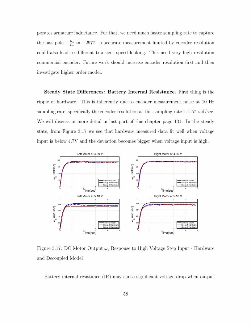
porates armature inductance. For that, we need much faster sampling rate to capture

the fast pole −RaLa≈ −2977. Inaccurate measurement limited by encoder resolution

could also lead to different transient speed looking. This need very high resolution

commercial encoder. Future work should increase encoder resolution first and then

investigate higher order model.

Steady State Differences: Battery Internal Resistance. First thing is the

ripple of hardware. This is inherently due to encoder measurement noise at 10 Hz

sampling rate, specifically the encoder resolution at this sampling rate is 1.57 rad/sec.

We will discuss in more detail in last part of this chapter page 131. In the steady

state, from Figure 3.17 we see that hardware measured data fit well when voltage

input is below 4.7V and the deviation becomes bigger when voltage input is high.

0 1 2 3 4 50

20

40

60

80

Time(sec)

ωs (

rad/s

ec)


Nominal Model

Group 1 Hardware

Group 2 Hardware

0 1 2 3 4 50

20

40

60

80

Time(sec)

ωs (

rad/s

ec)


Nominal Model

Group 1 Hardware

Group 2 Hardware

0 1 2 3 4 50

20

40

60

80

Time(sec)

ωs (

rad/s

ec)


Nominal Model

Group 1 Hardware

Group 2 Hardware

0 1 2 3 4 50

20

40

60

80

Time(sec)

ωs (

rad/s

ec)


Nominal Model

Group 1 Hardware

Group 2 Hardware

Figure 3.17: DC Motor Output ωs Response to High Voltage Step Input - Hardware

and Decoupled Model

Battery internal resistance (IR) may cause significant voltage drop when output

58

power is high. This behaves like saturation effect on motor maximum output torque.

And we cannot find out detail specification for batteries we are using (Ni-MH AA

Rechargeable Batteries from Amazon Basics). A similar product from Energizer

shows the IR of one unit of Ni-MH AA battery is around be 0.05 - 0.15 Ω [40]. We

uses 4 units as the power input to motor shield board, which could result in IR 0.2 -

0.6 Ω. Those problems will be further examined in the future.

3.5.3 Robot TITO LTI Model with Actuator Dynamics

In this section, we combine the ideas presented above in order to obtain a state

space representation TITO LTI model for our differential-drive vehicle. This model,

taken from [15], was used within [59] for inner-loop control design. It shall be used

as the basis for our inner-loop control design as well. The TITO LTI model from

motor voltages (eaR, eaL) to the wheel angular velocities (ωR, ωL) can be visualized as

shown within Figure 3.18. Note the cross-coupling introduced by the right-left motor

torques (τR, τL) at the input and a similar structure at the output.

Figure 3.18: TITO LTI Robot-Motor Wheel Speed (ωR, ωL) Dynamics - P(ωR,ωL)

59

Figure 3.19: Differential-Drive Mobile Robot Dynamics

The associated fourth order TITO LTI state space representation 1 is given by

x = Ax+Bu y = Cx+Du (3.28)

1Neglect friction, torque disturbance and distance between geometric center and mass center

60

where x = [ v ω iaR iaL ]T , y = [ ωR ωL ]T , u = [ eaR eaL ]T ,

A =

−2βK2g

mr20 KgKt

mr

KgKtmr

0 −βKg2dw2

2Izr2KgKtdw

2Izr

−KgKtdw2Izr

−KgKbLar

−KgKbdw2Lar

−RaLa

0

−KgKbLar

KgKbdw2Lar

0 −RaLa

(3.29)

B =

0 0

0 0

1La

0

0 1La

(3.30)

C =

1r

dw2r

0 0

1r−dw2r

0 0

(3.31)

D =

0 0

0 0

(3.32)

Here, (iaL, iaR) represent left and right motor armature currents, v is the vehi-

cle’s translational velocity (directed along the direction θ), ω is the vehicle’s angular

velocity, (ωL, ωR) represent left and right vehicle wheel angular velocities, (eaL, eaR)

represent left and right motor armature voltage inputs. The latter are the robot’s

control inputs. Relevant system parameters are as follows: m is the vehicle mass, dw

is the distance between the wheels, r is the vehicle wheel radius, Iz is the vehicle’s

moment of inertia, β represents a load-motor speed rotational damping constant, Kb

represents a back EMF constant, Kt represents a torque constant, Kg represents the

gearbox ratio of motor shaft-load system Ra represents armature resistance, and La

61

represents armature inductance (often negligibly small). It should be noted that dif-

ferences in the motor properties is a practical concern. This has not been captured

in the above model. It shall not be addressed within this thesis. Addressing such

uncertainty will be the subject of future work.

Given the above, the associated transfer function matrix is given by

P(ωR,ωL) = C(sI − A)−1B +D =

P11 P12

P21 P22

(3.33)

One can use Maple to verify that the symbolic transfer function matrix P(ωR, ωL) is

symmetric and the diagonal entries are identical. This pattern is expected since the

motors are identical.

Nominal Functions. The nominal values given in Table 3.2 shall be used to generate

numerical values below. For these nominal parameter values, we obtain the following

numerical TITO transfer function matrix:

P(ωR,ωL) =

186056(s+ 2977.5)(s+ 3.8722) 14533s(s+ 2981.1)

14533s(s+ 2981.1) 186056(s+ 2977.5)(s+ 3.8722)

(s+ 2977.7)(s+ 2977.2)(s+ 4.2008)(s+ 3.5914)

(3.34)

When the inductance is neglected, we obtain the following low frequency approxima-

tions:

P(ωR,ωL) ≈

62.411(s+ 3.8675) 4.8749s

4.8749s 62.411(s+ 3.8675)

1

(s+ 4.1951)(s+ 3.5872)

(3.35)

This shows that the off diagonal elements are small at low frequencies.

62

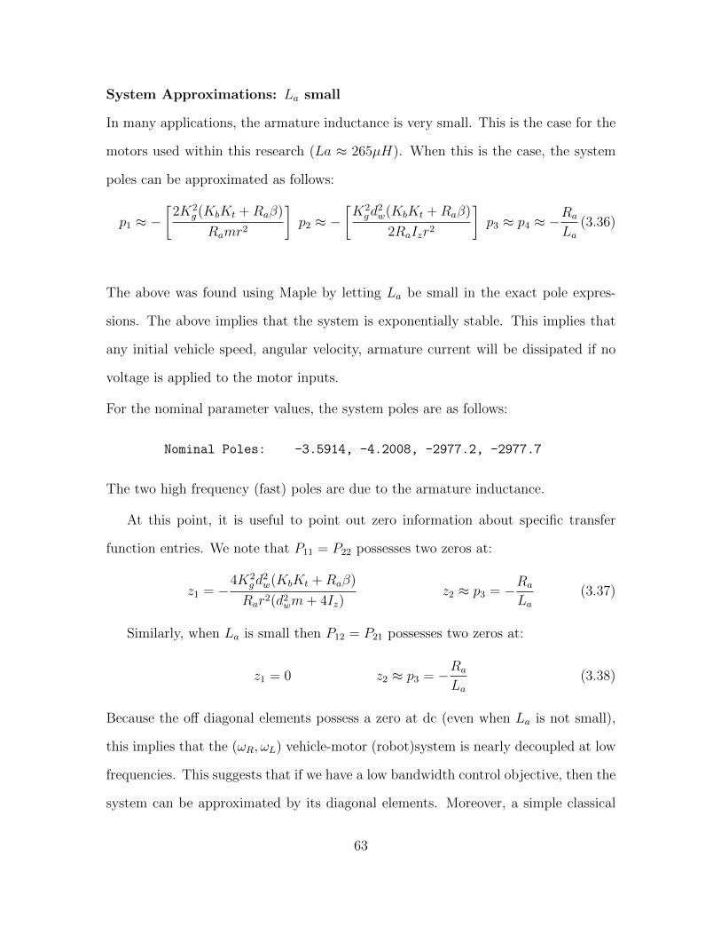
System Approximations: La small

In many applications, the armature inductance is very small. This is the case for the

motors used within this research (La ≈ 265µH). When this is the case, the system

poles can be approximated as follows:

p1 ≈ −[

2K2g (KbKt +Raβ)

Ramr2

]p2 ≈ −

[K2gd

2w(KbKt +Raβ)

2RaIzr2

]p3 ≈ p4 ≈ −

Ra

La(3.36)

The above was found using Maple by letting La be small in the exact pole expres-

sions. The above implies that the system is exponentially stable. This implies that

any initial vehicle speed, angular velocity, armature current will be dissipated if no

voltage is applied to the motor inputs.

For the nominal parameter values, the system poles are as follows:

Nominal Poles: -3.5914, -4.2008, -2977.2, -2977.7

The two high frequency (fast) poles are due to the armature inductance.

At this point, it is useful to point out zero information about specific transfer

function entries. We note that P11 = P22 possesses two zeros at:

z1 = −4K2

gd2w(KbKt +Raβ)

Rar2(d2wm+ 4Iz)

z2 ≈ p3 = −Ra

La(3.37)

Similarly, when La is small then P12 = P21 possesses two zeros at:

z1 = 0 z2 ≈ p3 = −Ra

La(3.38)

Because the off diagonal elements possess a zero at dc (even when La is not small),

this implies that the (ωR, ωL) vehicle-motor (robot)system is nearly decoupled at low

frequencies. This suggests that if we have a low bandwidth control objective, then the

system can be approximated by its diagonal elements. Moreover, a simple classical

63

(decentralized) controller should work fine. It can be shown (numerically) that gen-

erally speaking, this system has no transmission zeros. Why is this important? This

is important because it roughly suggests that we may be able to use identical classi-

cal SISO (single-input single-output) controllers with sufficient lead and a sufficiently

high bandwidth in order to reduce the sensitivity at low frequencies as much as we

want. Here, the sufficient lead will ensure an infinite upward gain margin (ideally,

of course). In practice, of course, the closed loop bandwidth will be limited by high

frequency uncertainty, actuator bandwidth limitations, sensor bandwidth limitations,

etc.

Frequency Response Properties. The singular values for the above system and

the associated low frequency approximation are plotted within Figure 3.20 for the

nominal parameter values given within Table 3.2. Note that the singular values at

DC match one another. This is because from each input, the motor-vehicle (ωR, ωL)

system looks the same.

Figure 3.20: Robot Singular Values (Voltages to Wheel Speeds) - Including Low

Frequency Approximation

64

The plot in Figure 3.20 suggests that the low frequency approximation (red, with

a 20 dB/decade high frequency roll-off) is a good approximation for the system. The

relatively high system gain at low frequencies will help achieve good low frequency

command following and low frequency disturbance attenuation (in principle, without

too much control action). The plot also suggests that as long as we keep the desired

control bandwidth below say 2 rad/sec, then a large control gain will not be required

in order to have good feedback properties.

To better examine the coupling in our (ωR, ωL) system, we have plotted the fre-

quency response in Figure 3.21. The figure clearly shows that the off-diagonal ele-

ments peak just below 1 rad/sec and that the coupling disappears at dc. This low

frequency behavior, as well as the first order low frequency behavior of the diagonal

elements, provides substantive motivation for a decentralized PI control law; i.e. the

use of identical PI controllers for each motor.

Figure 3.21: Robot Frequency Response (Voltages to Wheel Speeds) - Including Low


65

Plant. The above discussion has focused on the (ωR, ωL) system. It must be noted

that strictly speaking, the (ωR, ωL) system is not the plant for our inner-loop con-

trol system. Why? The inner-loop plant, strictly speaking, has (v, ω) as outputs

since these are the variables that we wish to command! That is, we shall be speci-

fying (vref , ωref ) reference commands to our inner-loop control system. The transfer

function matrix for our (v, ω) system - the plant P - is as follows:

P = P(v,ω) =

5014.7(s+ 3.591)(s+ 2978) 5014.7(s+ 3.591)(s+ 2978)

61258(s+ 4.201)(s+ 2977) −61258(s+ 4.201)(s+ 2977)

(s+ 3.591)(s+ 4.201)(s+ 2977)(s+ 2978)

(3.39)

When the inductances are neglected, we obtain the following low frequency approxi-

mation:

P = P(v,ω) ≈

1.6822(s+ 3.587) 1.6822(s+ 3.587)

20.549(s+ 4.195) −20.549(s+ 4.195)

1

(s+ 3.587)(s+ 4.195)

(3.40)

The above shows that unlike the (ωR, ωL) system, the (v, ω) system (the plant) is not

decoupled at low frequencies.

Plant SVD at DC. To better understand the coupling at dc, we perform a singular

value decomposition (svd) for P at dc. Doing so yields the following:

P (0) = P(v,ω)(0) =

0.401 0.401

5.73 −5.73

= UΣV H (3.41)

=

0 1

1 0

8.101 0

0 0.5671

0.7071 0.7071

−0.7071 0.7071

H

(3.42)

where the unitary matrix U = [ u1 u2 ] contains left singular vectors (output direc-

tions), Σ = diag(σ1, σ2) contains the maximum and minimum singular values, and

66

the unitary matrix V = [ v1 v2 ] contains right singular vectors (input directions).

This svd clearly shows control coupling at dc and hence at low frequencies. More

precisely, we see that the

• maximum singular value 8.101 (41.84 dB) is associated with the vehicle’s angular

velocity ω (u1 = [ 0 1 ]T ) and equal and opposite motor input voltages (v1 =

[ 0.7071 − 0.7071 ]T );

• minimum singular value 0.5671 (-11.35 dB) is associated with the vehicle’s

translational velocity v (u2 = [ 1 0 ]T ) and equal motor input voltages

(v2 = [ 0.7071 0.7071 ]T ).

Given the above, it is natural to ask: Why is the maximum singular value associated

with ω and the minimum with v? This follows from the fact that it is easier to turn

than to move forward. We also note that the input voltage directions given above are

exactly how we would expect a differential-drive system to generate ω and v. That

is, the above svd corroborates our intuition about a differential-drive motor-vehicle

system.

Plant Singular Values. The plant singular values and those of the low frequency

approximation are shown within Figure 3.22. Here, the singular values at dc are

not identical. This, fundamentally, is because we lose symmetry when we go from

(ωR, ωL) to (v, ω). More precisely, up above we showed (via svd at dc) that the

maximum singular value at low frequencies is associated with rotation ω while the

minimum singular value is associated with translation v.

Plant Frequency Response. In order to better understand and visualize the low

frequency coupling issues associated with our plant, it is useful to examine the fre-

quency response plot in Figure 3.23. Within this figure, the plant frequency response

67

Figure 3.22: Robot Plant Singular Values (Voltages to v and ω) - Including Low


is in blue and the frequency response for our low frequency approximation to the

plant is in red. Again, we see that our low frequency approximation is a very good

approximation for the plant. The approximation should be particularly good below

about 50 rad/sec. Figure 3.23 also shows while our (ωR, ωL) system is fairly decoupled

at low frequencies, this is not the case for our (v, ω) plant system. While this suggests

that a multivariable controller may be necessary for our plant, the work in this the-

sis shows that one can apply classical SISO control theory to our (fairly decoupled)

(ωR, ωL) system to indirectly control our (v, ω) plant system. This, and important

issues discussed below, will receive greater attention in future work.

68

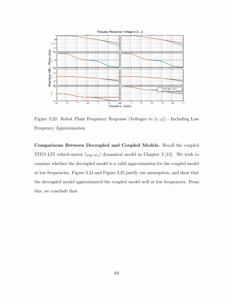
Figure 3.23: Robot Plant Frequency Response (Voltages to [v, ω]) - Including Low


Comparisons Between Decoupled and Coupled Models. Recall the coupled

TITO LTI vehicle-motor (ωR, ωL) dynamical model in Chapter 3 [15]. We wish to

examine whether the decoupled model is a valid approximation for the coupled model

at low frequencies. Figure 3.24 and Figure 3.25 justify our assumption, and show that

the decoupled model approximated the coupled model well at low frequencies. From

this, we conclude that

69

To: O

ut(

1)

-150

-100

-50

0

50From: In(1)

100

105

To: O

ut(

2)

-150

-100

-50

0

50

From: In(2)

100

105

Coupled Model

Decoupled Model

Frequency response of coupled and decoupled model

Frequency (rad/s)

Phase (

dB

)

Figure 3.24: Frequency Response for Vehicle-Motor - Coupled (ωR, ωL) Model

To

: O

ut(

1)

0

5

10

15

20From: In(1)

0 1 2 3

To

: O

ut(

2)

0

5

10

15

20

From: In(2)

0 1 2 3

Coupled Model

Decoupled Model

Output response of coupled and decoupled model

Frequency (seconds)

Ph

ase

Figure 3.25: Vehicle-Motor Response to Unit Step Input - Coupled (ωR, ωL) Model

The following is a good approximation to vehicle-motor (ωR, ωL) plant:

P[ωR,ωL] ≈ 16.246

[4.685

s+ 4.685

]× I2×2 (3.43)

70

Plant Control Issues.[14] Given the above, it is natural to ask:

If the above (v, ω) system is the plant we really want to control,

then why did we spend so much time on the (ωR, ωL) system?

A quick and simple answer to this is that

the (nearly decoupled) (ωR, ωL) system is much simpler

than the highly coupled (v, ω) plant system.

To provide a more substantive answer to this, first note that the (v, ω) plant P = P(v,ω)

is related to the “angular wheel velocity plant” P(ωR,ωL) according to the following

relationship:

P = P(v,ω) = MP(ωR,ωL) (3.44)

where M was defined above in equation (3.7) on page 40. From this, we can show

that

if we design a good simple controller for P(ωR,ωL),

then it is likely to work well for P .

Why is this? The next few pages provides support for this claim and addresses related

issues that must be considered - especially if one takes the above implied (ωR, ωL)

control approach. Lets be specific. Suppose K(ωR,ωL) = k(s)I2×2 where k(s) is a scalar

SISO transfer function (e.g. PI controller as used below and in Chapter 4). Given

this, it can be shown that if K(ωR,ωL) works well for P(ωR,ωL), then K = K(ωR,ωL)M−1

will work well for P . Why is this?

• Critical Relationship: (v, ω) and (ωR, ωL) Systems Have Identical Open

Loop Singular Values. With K = K(ωR,ωL)M−1 as the controller for P ,

71

the new open loop transfer function matrix for the (v, ω) system is PK =

PK(ωR,ωL)M−1 = MP(ωR,ωL)K(ωR,ωL)M

−1. More detailed discussion is within[14].

The following main results shown here for completeness. (Loop Singular Values

for (ωR, ωL)-(v, ω) Systems are Identical. From the structure of P , K, and M , it

can be shown that

σi [ PK ] = σi[P(ωR,ωL)K(ωR,ωL)

](3.45)

The above singular value result implies - modulo important (non-negligible) Tru and

Tdiy issues to be pointed out below - that if K(ωR,ωL) works well for P(ωR,ωL), then

K = K(ωR,ωL)M−1 will work well for P = MP(ωR,ωL).

• Same Lo, So, To Singular Values. More precisely, our main result in 3.45

implies that the two designs (P,K) and (P(ωR,ωL), K(ωR,ωL)) will possess the

same singular values for the output/error open loop transfer function matrix

Lo = PK, output sensitivity So = (I + Lo)−1, and output complementary

sensitivity To = I − So = Lo(I + Lo)−1 (i.e. at the plant output (or error)).

• Same Li, Si, Ti Singular Values. Since Li = KP = PK = Lo, it also follows

that the designs will also possess the same singular values for the input/controls

open loop transfer function matrix Li = KP , input sensitivity Si = (I + Li)−1,

and input complementary sensitivity Ti = I − Si = Li(I + Li)−1 (i.e. at the

plant input (or controls)).

The above “almost proves” that if (P(ωR,ωL), K(ωR,ωL)) is good, then (P,K) will be

good. It does prove that given the simple decentralized control structure selected,

if the singular values for (Lo, Li), (So, Si), (To, Ti) are good for the (ωR, ωL) system,

then they will be good for the (v, ω) system.

72

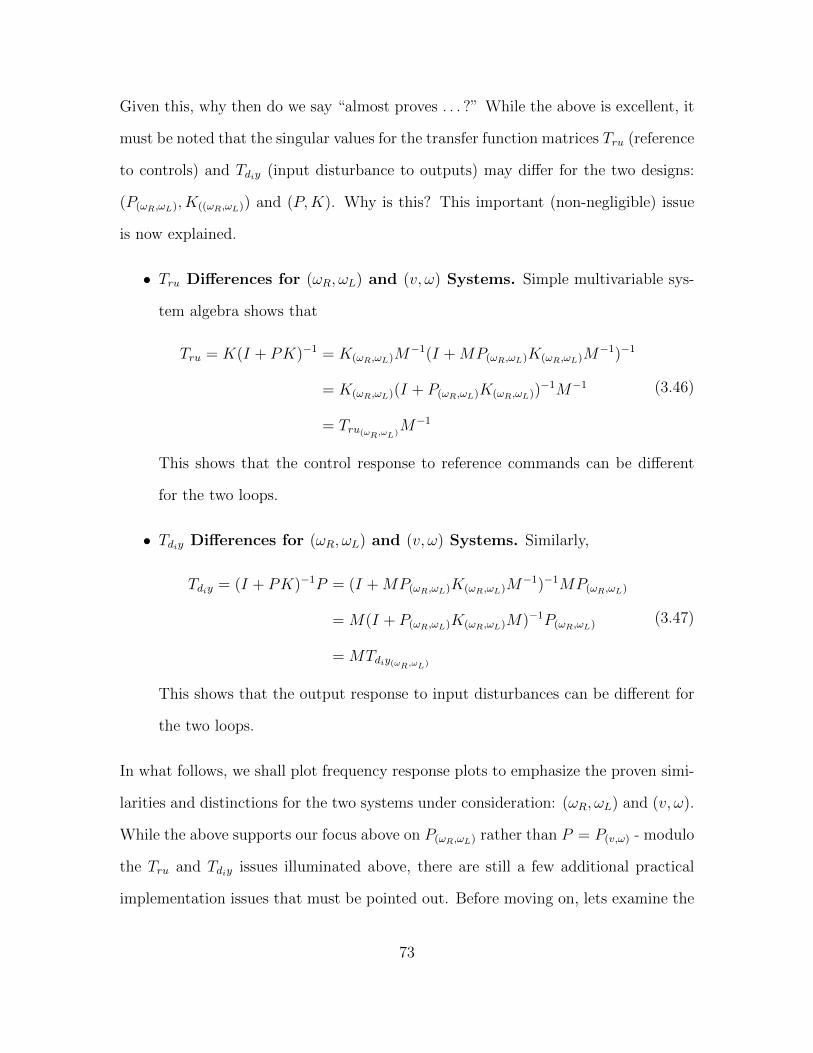
Given this, why then do we say “almost proves . . . ?” While the above is excellent, it

must be noted that the singular values for the transfer function matrices Tru (reference

to controls) and Tdiy (input disturbance to outputs) may differ for the two designs:

(P(ωR,ωL), K((ωR,ωL)) and (P,K). Why is this? This important (non-negligible) issue

is now explained.

• Tru Differences for (ωR, ωL) and (v, ω) Systems. Simple multivariable sys-

tem algebra shows that

Tru = K(I + PK)−1 = K(ωR,ωL)M−1(I +MP(ωR,ωL)K(ωR,ωL)M

−1)−1

= K(ωR,ωL)(I + P(ωR,ωL)K(ωR,ωL))−1M−1

= Tru(ωR,ωL)M−1

(3.46)

This shows that the control response to reference commands can be different

for the two loops.

• Tdiy Differences for (ωR, ωL) and (v, ω) Systems. Similarly,

Tdiy = (I + PK)−1P = (I +MP(ωR,ωL)K(ωR,ωL)M−1)−1MP(ωR,ωL)

= M(I + P(ωR,ωL)K(ωR,ωL)M)−1P(ωR,ωL)

= MTdiy(ωR,ωL)

(3.47)

This shows that the output response to input disturbances can be different for

the two loops.

In what follows, we shall plot frequency response plots to emphasize the proven simi-

larities and distinctions for the two systems under consideration: (ωR, ωL) and (v, ω).

While the above supports our focus above on P(ωR,ωL) rather than P = P(v,ω) - modulo

the Tru and Tdiy issues illuminated above, there are still a few additional practical

implementation issues that must be pointed out. Before moving on, lets examine the

73

actual numerical M and M−1 for the system being considered in this chapter. From

Table 3.2, we have r = 0.05 m and dw = 0.14 m. Given this, it follows that we have

M =

r2

r2

rdw− rdw

=

0.025 0.025

0.3571 −0.3571

(3.48)

M−1 =

1r

dw2r

1r−dw2r

=

20 1.4

20 −1.4

(3.49)

What do these numbers tell us? The singular values of M are (0.5051, 0.0354). Those

for M−1 are (28.2843, 1.9799). Using the relationships in equations (3.46) and (3.47),

as well as the sub-multiplicative property of the H∞ norm, yields the following:∥∥∥Tru(v,ω)∥∥∥H∞ ≤ ∥∥M−1∥∥H∞

∥∥∥Tru(ωR,ωL)

∥∥∥H∞

= 21.40∥∥∥Tdiy(ωR,ωL)

∥∥∥H∞

(3.50)

∥∥∥Tdiy(v,ω)∥∥∥H∞ ≤ ‖M‖H∞ ∥∥∥Tdiy(ωR,ωL)

∥∥∥H∞

= 0.7143∥∥∥Tdiy(ωR,ωL)

∥∥∥H∞

(3.51)

The first inequality imply that we should be particularly concerned about the control

response to reference commands for the (v, ω) system. It suggests that the (v, ω) sys-

tem can have up to 21.40 times the control effort of the (ωR, ωL) system (in the worst

case). The second inequality tells us that the output response to input disturbances

for the (v, ω) system will not be a concern if the (ωR, ωL) system output response to

input disturbances is satisfactory.

• Practical Implementation Issues. The following question is natural to ask:

If we are primarily interested in controlling (v, ω),

then what can happen if we control (ωR, ωL)?

74

– M is Well Known. First, we note that the matrix M is the key to the

above discussion. If it were uncertain, then we would be particularly wor-

ried. However, M is generally well known. Why? The matrix M involves

very well known system parameters (e.g. wheel radius r and distance be-

tween wheels dw). M is well known. (We assume that r and dw are well

known constants that do not change over time. We assume, for example,

that r cannot decrease because of loss of air in the tires.) The issue here

is therefore not uncertainty in M .

– Accuracy of Measurements. The issue here is what can we measure

more accurately? (ωR, ωL) or (v, ω)? Within this thesis, we use opti-

cal wheel encoders (20 CPT) to measure (ωR, ωL). From this, (v, ω) is

computed (estimated). This is done using the relationships within equa-

tion (3.7). The fundamental point here is that if an IMU (inertial mea-

surement unit) is used to measure (v, ω), then we may be able to get more

accurate measurements and hence better inner-loop performance in com-

parison to the encoder-based (ωR, ωL) approach taken within this thesis.

Within the thesis, θ information directly obtained by the IMU built-in al-

gorithm or using camera. This is done for our (v, θ) cruise control along a

path outer-loop control law. The IMU is not used to get v, future work shall

address how the IMU can be used to improve our inner-loop performance.

75

3.6 Uncertainty of Parameter

In this section, we will examine the parameter uncertainty of TITO model. Trade

studies of variations in vehicle mass, vehicle moment of inertia, motor back EMF

constant, motor torque constant and motor armature resistance has been discussed.

Both frequency and time domains analysis are provided to give insights of single

parameter uncertainty impact on the system.

3.6.1 Frequency Response Trade Studies

Mass m Variations. Figure 3.26 shows that as the mass is increased, the dc gains do

not change, the diagonal magnitudes get smaller at all frequencies, and the coupling

at all frequencies decreases.

To

: O

ut(

1)

-200

-150

-100

-50

0

50

100From: In(1)

10-1

100

101

102

103

104

105

To

: O

ut(

2)

-200

-150

-100

-50

0

50

100

From: In(2)

10-1

100

101

102

103

104

105

m = 0.5340 (kg)

m = 0.7120 (kg)

m = 0.8900 (kg)

m = 1.0680 (kg)

Bode magnitude plots of the plant for variations of mass

Frequency (rad/s)

Magnitude (

dB

)

Figure 3.26: Bode Magnitude for Robot (Voltages to Wheel Speeds) - Mass Variations

Moment of Inertia Iz Variations. Figure 3.27 shows that as the moment of iner-

tia is increased, the dc gains do not change, the diagonal magnitudes get smaller at

mid-range and high frequencies, and the coupling at low frequencies increases.

76

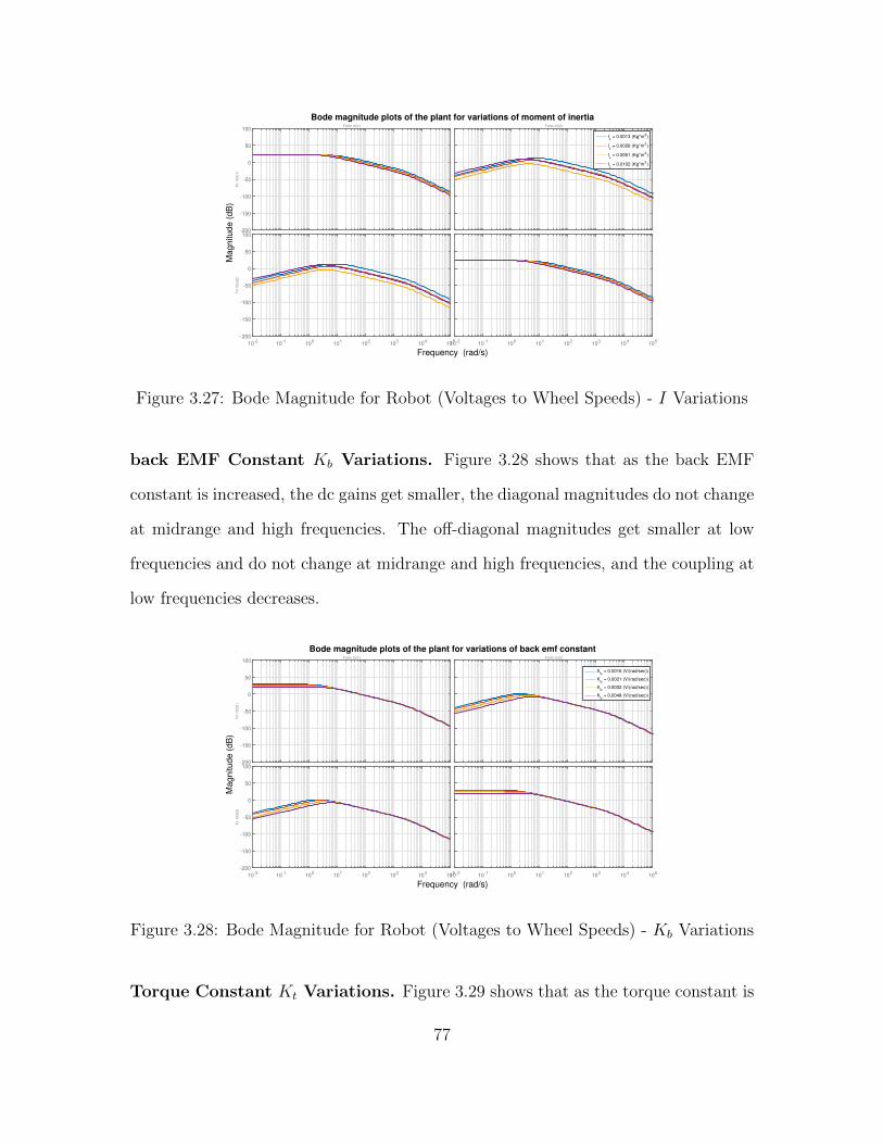
To

: O

ut(

1)

-200

-150

-100

-50

0

50

100From: In(1)

10-2

10-1

100

101

102

103

104

105

To

: O

ut(

2)

-200

-150

-100

-50

0

50

100

From: In(2)

10-2

10-1

100

101

102

103

104

105

Iz = 0.0013 (Kg*m2)

Iz = 0.0026 (Kg*m2)

Iz = 0.0051 (Kg*m2)

Iz = 0.0102 (Kg*m2)

Bode magnitude plots of the plant for variations of moment of inertia

Frequency (rad/s)

Magnitude (

dB

)

Figure 3.27: Bode Magnitude for Robot (Voltages to Wheel Speeds) - I Variations

back EMF Constant Kb Variations. Figure 3.28 shows that as the back EMF

constant is increased, the dc gains get smaller, the diagonal magnitudes do not change

at midrange and high frequencies. The off-diagonal magnitudes get smaller at low

frequencies and do not change at midrange and high frequencies, and the coupling at

low frequencies decreases.

To

: O

ut(

1)

-200

-150

-100

-50

0

50

100From: In(1)

10-2

10-1

100

101

102

103

104

105

To

: O

ut(

2)

-200

-150

-100

-50

0

50

100

From: In(2)

10-2

10-1

100

101

102

103

104

105

Kb = 0.0016 (V/(rad/sec))

Kb = 0.0021 (V/(rad/sec))

Kb = 0.0032 (V/(rad/sec))

Kb = 0.0048 (V/(rad/sec))

Bode magnitude plots of the plant for variations of back emf constant

Frequency (rad/s)

Magn

itude (

dB

)

Figure 3.28: Bode Magnitude for Robot (Voltages to Wheel Speeds) - Kb Variations

Torque Constant Kt Variations. Figure 3.29 shows that as the torque constant is

77

increased, the dc do not change, the diagonal magnitudes get larger at at midrange

and high frequencies. The off-diagonal magnitudes get smaller at low frequencies and

get larger at midrange and high frequencies.

To

: O

ut(

1)

-200

-150

-100

-50

0

50

100From: In(1)

10-2

10-1

100

101

102

103

104

105

To

: O

ut(

2)

-200

-150

-100

-50

0

50

100

From: In(2)

10-2

10-1

100

101

102

103

104

105

Kt = 0.0016 (NmA)

Kt = 0.0021 (NmA)

Kt = 0.0032 (NmA)

Kt = 0.0048 (NmA)

Bode magnitude plots of the plant for variations of torque constant

Frequency (rad/s)

Ma

gn

itud

e (

dB

)

Figure 3.29: Bode Magnitude for Robot (Voltages to Wheel Speeds) - Kt Variations

Armature Resistance Ra Variations. Figure 3.30 shows that as the armature

resistance Ra is increased, the dc gains don’t change. The magnitudes of the diagonal

elements start to get smaller with increasing Ra at mid-range frequencies below 10000

rad/sec and do not change at high frequencies. The magnitudes of the off-diagonal

elements get larger at low frequencies, start to get smaller with increasing Ra at mid-

range frequencies below 10000 rad/sec and do not change at high frequencies.

78

To

: O

ut(

1)

-200

-150

-100

-50

0

50

100From: In(1)

10-2

100

102

104

106

To

: O

ut(

2)

-200

-150

-100

-50

0

50

100

From: In(2)

10-2

100

102

104

106

Ra = 0.3950 (Ω)

Ra = 0.7900 (Ω)

Ra = 1.5800 (Ω)

Ra = 2.3700 (Ω)

Bode magnitude plots of the plant for variations of armature resistance

Frequency (rad/s)

Magnitude (

dB

)

Figure 3.30: Bode Magnitude for Robot (Voltages to Wheel Speeds) - Ra Variations

3.6.2 Time Response Trade Studies

Mass m Variations. Figure 3.31 contains the system wheel angular velocity re-

sponses to step voltage inputs for mass variations.

To

: O

ut(

1)

0

5

10

15

20From: In(1)

0 0.5 1 1.5 2 2.5 3 3.5

To

: O

ut(

2)

0

5

10

15

20

From: In(2)

0 0.5 1 1.5 2 2.5 3 3.5

m = 0.5340 (kg)

m = 0.7120 (kg)

m = 0.8900 (kg)

m = 1.0680 (kg)

Step response of the plant for variations of mass

Time (seconds)

Angula

r V

elo

city (

rad/s

ec)

Figure 3.31: System Wheel Angular Velocity Responses to Step Voltages - Mass

Variations

The figure shows that as the vehicle mass is increased, the system

79

• dc gain does not change

• settling time (bandwidth) increases (decreases)

• cross coupling decreases

The latter is a control-theoretic reason for reducing vehicle mass. (Energy savings,

of course, is generally the primary reason given for wanting to reduce vehicle mass.)

Moment of Inertia Iz Variations. Figure 3.32 contains the system wheel angular

velocity responses to step voltage inputs for moment of inertia variations.

To

: O

ut(

1)

-5

0

5

10

15

20From: In(1)

0 0.5 1 1.5 2 2.5 3 3.5 4 4.5 5

To

: O

ut(

2)

-5

0

5

10

15

20

From: In(2)

0 0.5 1 1.5 2 2.5 3 3.5 4 4.5 5

Iz = 0.0013 (Kg*m2)

Iz = 0.0026 (Kg*m2)

Iz = 0.0051 (Kg*m2)

Iz = 0.0102 (Kg*m2)

Step response of the plant for variations of moment of inertia

Time (seconds)

Angula

r V

elo

city (

rad/s

ec)

Figure 3.32: System Wheel Angular Velocity Responses to Step Voltages - Moment

of Inertia Variations

The figure shows that as the vehicle moment of inertia is increased, the system

• dc gain does not change


• cross coupling first decreases and then increases after certain range

back EMF Constant Kb Variations. Figure 3.33 contains the system wheel an-

gular velocity responses to step voltage inputs for back EMF constant variations.

80

To

: O

ut(

1)

0

5

10

15

20

25

30

35

40From: In(1)

0 1 2 3 4 5 6

To

: O

ut(

2)

0

10

20

30

40

From: In(2)

0 1 2 3 4 5 6

Kb = 0.0016 (V/(rad/sec))

Kb = 0.0021 (V/(rad/sec))

Kb = 0.0032 (V/(rad/sec))

Kb = 0.0048 (V/(rad/sec))

Step response of the plant for variations of back emf constant

Time (seconds)

Angula

r V

elo

city (

rad/s

ec)

Figure 3.33: System Wheel Angular Velocity Responses to Step Voltages - back EMF

Constant Variations

The figure shows that as the motor back EMF constant is increased, the system

• dc gain gets smaller

• settling time (bandwidth) decreases (increases)


Torque Constant Kt Variations. Figure 3.34 contains the system wheel angular

velocity responses to step voltage inputs for torque constant variations.

81

To

: O

ut(

1)

0

5

10

15

20From: In(1)

0 1 2 3 4 5 6

To

: O

ut(

2)

0

5

10

15

20

From: In(2)

0 1 2 3 4 5 6

Kt = 0.0016 (NmA)

Kt = 0.0021 (NmA)

Kt = 0.0032 (NmA)

Kt = 0.0048 (NmA)

Step response of the plant for variations of torque constant

Time (seconds)

Angula

r V

elo

city (

rad/s

ec)

Figure 3.34: System Wheel Angular Velocity Responses to Step Voltages - Torque

Constant Variations

The figure shows that as the motor torque constant is increased, the system

• dc gain gets larger

• settling time (bandwidth) decreases (increases)


Armature Resistance Ra Variations. Figure 3.35 contains the system wheel

angular velocity responses to step voltage inputs for mass variations.

82

To

: O

ut(

1)

0

5

10

15

20From: In(1)

0 1 2 3 4 5 6 7 8

To

: O

ut(

2)

0

5

10

15

20

From: In(2)

0 1 2 3 4 5 6 7 8

Ra = 0.3950 (Ω)

Ra = 0.7900 (Ω)

Ra = 1.5800 (Ω)

Ra = 2.3700 (Ω)

Step response of the plant for variations of armature resistance

Time (seconds)

Angula

r V

elo

city (

rad/s

ec)

Figure 3.35: System Wheel Angular Velocity Responses to Step Voltages - Armature

Resistance Variations

The figure shows that as the motor armature resistance is increased, the system

• dc gain gets smaller


• cross coupling increases

The above trade studies give insight into the system being examined. More specif-

ically, they are useful for understanding the impact of single parameter uncertainty.

Future work can examine the structured uncertainties of multiple parameters.

3.7 Differential-Drive Robot Model with Dynamics on Ground

Till this point, the nominal plant model 3.43 looks pretty well, however it is not

true when the following practical factors have been taken into consideration which is

necessary in our hardware platform:

Friction between vehicle tyres and ground. Friction could significantly influence

the model when torque constant Kt of the motor is small. When Kt is small, the

83

required torque to drive the vehicle will be increased a lot. Recall torque equation:

τs = KtKgia (3.52)

The torque required to overcoming friction will significantly increase armature cur-

rent.

Battery internal resistance 4 AA Ni-MH rechargeable battery pack is used

to provide power to motor shield. As discussed ahead page 59, the potential internal

resistance(IR) could be as much as 0.6 Ω. This battery internal resistance could lead

to significant voltage drop. Through off-ground high voltage step response, we ob-

served this impact on our model. The step response from voltage to angular velocity

at same PWM command of off-ground and on ground corroborates our assumption.

Power dissipation of Motor Shield Board. Motor shield board output

impedance could also play important role when current is high. From datasheet of

driver IC (TB6612FNG)[38] in motor shield board, we found out that output current

could be saturated from drive IC see Figure 3.36.

Figure 3.36: Target Characteristics of TB6612FNG

84

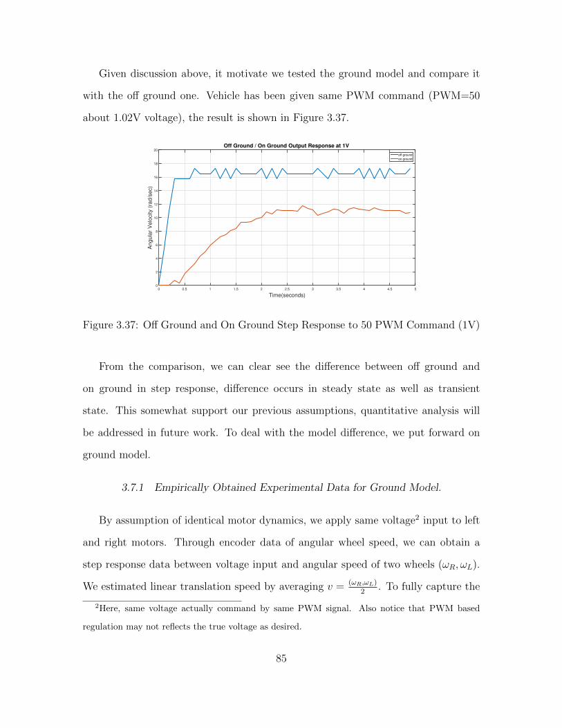
Given discussion above, it motivate we tested the ground model and compare it

with the off ground one. Vehicle has been given same PWM command (PWM=50

about 1.02V voltage), the result is shown in Figure 3.37.

Time(seconds)

0 0.5 1 1.5 2 2.5 3 3.5 4 4.5 5

Angula

r V

elo

city (

rad/s

ec)

0

2

4

6

8

10

12

14

16

18

20Off Ground / On Ground Output Response at 1V

off ground

on ground

Figure 3.37: Off Ground and On Ground Step Response to 50 PWM Command (1V)

From the comparison, we can clear see the difference between off ground and

on ground in step response, difference occurs in steady state as well as transient

state. This somewhat support our previous assumptions, quantitative analysis will

be addressed in future work. To deal with the model difference, we put forward on

ground model.

3.7.1 Empirically Obtained Experimental Data for Ground Model.

By assumption of identical motor dynamics, we apply same voltage2 input to left

and right motors. Through encoder data of angular wheel speed, we can obtain a

step response data between voltage input and angular speed of two wheels (ωR, ωL).

We estimated linear translation speed by averaging v = (ωR,ωL)2

. To fully capture the

2Here, same voltage actually command by same PWM signal. Also notice that PWM based

regulation may not reflects the true voltage as desired.

85

vehicle dynamics, we did this experiments for different voltage level. One sample for

PWM command at 50 (about 1V ideally) is shown in Figure 3.38.

Time(seconds)

0 1 2 3 4 5 6 7

An

gu

lar

Sp

ee

d (

rad

/se

c)

0

5

10

15

20

25

30

35

40Estimate Angular Speed from File #PWM 501

Left Wheel

Right Wheel

Average

Figure 3.38: Output ωs Response to PWM 50 Voltage Step Input - Hardware and

Decoupled Model

3.7.2 Fitting Model to Collected Data.

After we got the step response data from last step, we use the same method as we

did for motor modeling. Obtained the settling time and dc gain of this step response

(input voltage, output angular speed of wheel) and then approximate it by first order

model with form b as+a

. One sample of this is shown in Figure 3.39 and Figure 3.40.

86

Time(sec)

0 1 2 3 4 5

Angula

r V

elo

city(r

ad/s

ec)

0

5

10

15

20

25

30

35Model Verify TF Enc501L Group 1

Hardware

1st Order Approx.

Figure 3.39: On Ground Motor Fitting Left Motor - Hardware and Decoupled Model

Time(sec)

0 1 2 3 4 5

Angula

r V

elo

city(r

ad/s

ec)

0

5

10

15

20

25

30

35Model Verify TF Enc501R Group 1

Hardware

1st Order Approx.

Figure 3.40: On Ground Motor Fitting Right Motor - Hardware and Decoupled Model

87

These two figures shows that two motors behave similar as off ground case. The

fitting first order model is pretty accurate locally (model fits certain voltage input).

Then we proceed to next step, by average left and right angular speed: ωv = ωR+ωL2

,

where ωv denotes the equivalent angular speed of the longitudinal translation speed

ωv = vr. Approximate numerical first order transfer function distribution (in terms of

dc gain and dominant pole) is shown in Figure 3.41

40 45 50 55 60 65 70 75 800

5

10

15

DC Gain Distribution

Left Wheel Group 1

Right Wheel Group 1

Left Wheel Group 2

Right Wheel Group 2

40 45 50 55 60 65 70 75 800

0.5

1

Dominate Pole Distribution

Left Wheel Group 1

Right Wheel Group 1

Left Wheel Group 2

Right Wheel Group 2

Figure 3.41: On Ground Approximate Transfer Function Fitting Model Distribution

of V1

Final step is to take average of dc gain distribution and dominant pole and get

nominal on ground plant for V1.

ωvea

= 11.6370.9745

s+ 0.9745(3.53)

The following is a approximation to the on ground inner-loop (ωR, ωL) plant for V1:

P[ωR,ωL] ≈ 11.637

[0.9745

s+ 0.9745

]× I2×2 (3.54)

88

This plant take the friction and battery internal resistance effect implicitly, and fit

well with hardware experimental data. From result of V1 (ETT 1) the model fits well

with hardware data.

3.7.3 On Ground Nominal Model.

From above, we see on ground approximation model 3.54 fits well with hardware

for V1. The following question immediately come after: does this model applies to

all other 8 ETTs? Thus we tested all other 8 ETTs with same procedure and got

nominal on ground model for 9 ETTs see Figure 3.42.

0 1 2 3 4 5 6 7 8 9 100

5

10

15

Vehicle ID

DC Gain of 9 ETTs

0 1 2 3 4 5 6 7 8 9 100

0.5

1

1.5

2

Vehicle ID

Dominant Pole of 9 ETTs

Figure 3.42: On Ground Nominal Model

The following is a approximation to the on ground inner-loop (ωR, ωL) plant:

P[ωR,ωL] ≈ 11.268

[1.159

s+ 1.159

]× I2×2 (3.55)

To verify this nominal model, we compared the step response and frequency re-

sponse of individual ETT with the nominal model see Figure 3.43 and Figure 3.44.

89

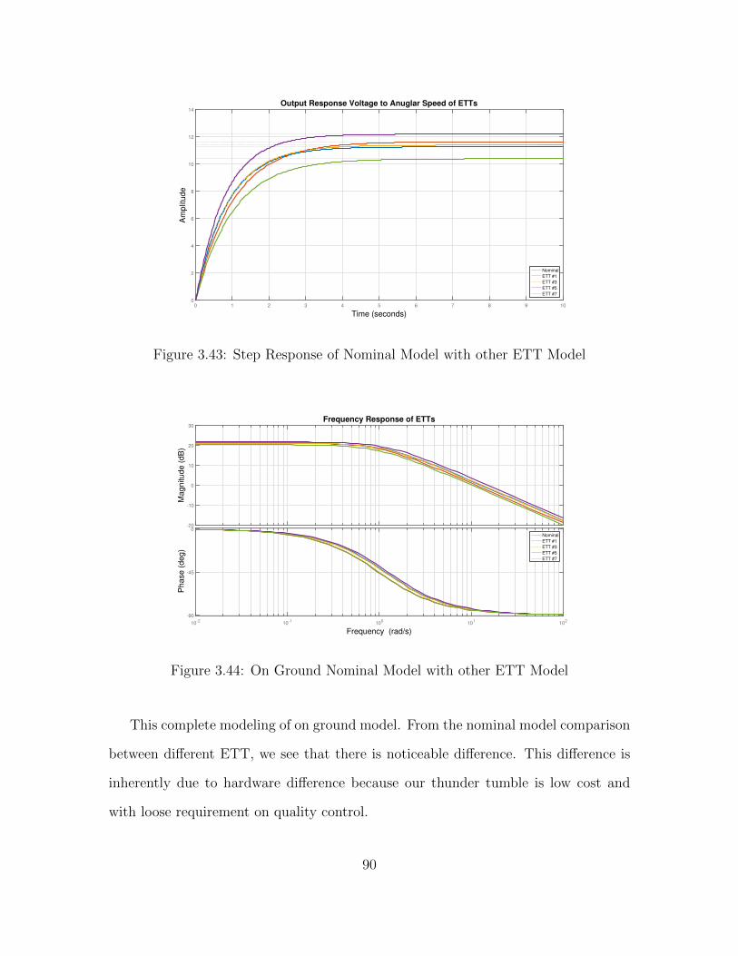
0 1 2 3 4 5 6 7 8 9 100

2

4

6

8

10

12

14

Nominal

ETT #1

ETT #3

ETT #5

ETT #7

Output Response Voltage to Anuglar Speed of ETTs

Time (seconds)

Am

plit

ude

Figure 3.43: Step Response of Nominal Model with other ETT Model

Magnitude (

dB

)

-20

-10

0

10

20

30

10-2

10-1

100

101

102

Phase (

deg)

-90

-45

0Nominal

ETT #1

ETT #3

ETT #5

ETT #7

Frequency Response of ETTs

Frequency (rad/s)

Figure 3.44: On Ground Nominal Model with other ETT Model

This complete modeling of on ground model. From the nominal model comparison

between different ETT, we see that there is noticeable difference. This difference is

inherently due to hardware difference because our thunder tumble is low cost and

with loose requirement on quality control.

90

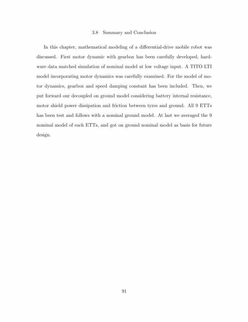
3.8 Summary and Conclusion

In this chapter, mathematical modeling of a differential-drive mobile robot was

discussed. First motor dynamic with gearbox has been carefully developed, hard-

ware data matched simulation of nominal model at low voltage input. A TITO LTI

model incorporating motor dynamics was carefully examined. For the model of mo-

tor dynamics, gearbox and speed damping constant has been included. Then, we

put forward our decoupled on ground model considering battery internal resistance,

motor shield power dissipation and friction between tyres and ground. All 9 ETTs

has been test and follows with a nominal ground model. At last we averaged the 9

nominal model of each ETTs, and got on ground nominal model as basis for future

design.

91

Chapter 4

SINGLE VEHICLE CASE STUDY FOR A LOW-COST MULTI-CAPABILITY

DIFFERENTIAL-DRIVE ROBOT: ENHANCED THUNDER TUMBLE (ETT)


In this chapter, we describe how to design controller for enhanced thunder tumbler.

Based on decoupled on ground model we put forward in last chapter, inner-loop

control has been designed and relevant control parameter trade off has been done.

Then two (2) outer-loop control law types are presented, analyzed and implemented

in hardware: (1) (v, θ) cruise control along a path (using encoders and IMU) [15], (2)

(∆x, θ) separation-direction control (using encoders, IMU/camera, and ultrasonics)

[3], [6]. The underlying theory for each control law is explained and justified. Finally,

the results from hardware demonstrations are presented and discussed.

4.2 Inner-Loop Speed Control Design and Implementation

In this section, we describe (v, ω) and (ωR, ωL) inner-loop control design for our

differential drive Thunder Tumbler. For this basic inner-loop control modality, the

angular velocity of each vehicle wheel is estimated/approximated by exploiting the

encoder pulse counts picked up by the two wheel encoders during a T sec sampling

window. This results in the following estimate for (ωR, ωL):

ωr ≈2πnr20T

= 3.142 nr (rad/sec) ωl ≈2πnl20T

= 3.142 nl (rad/sec) (4.1)

• T = 0.1 sec (100 ms or 10 Hz) was the chosen sampling (and actuation) time.

Future work will examine the benefits of a faster sampling/actuation frequency.

92

• nr is the number of counts measured by the optical encoder (photo-interrupter)

on the right wheel (with 20 counts per rotation1),

• nl is the number of counts measured by the optical encoder (photo-interrupter)

on the left wheel (with 20 counts per rotation).

We note that as the number of black-white stripe pairs used on a wheel is increased,

then the constant 3.142 would decrease. The vehicle translational and rotational

velocities (v, ω) are then estimated from the above (ωr, ωl) estimates as follows:vω

= M

ωRωL

M =

r2

r2

rdw− rdw

M−1 =

1r

dw2r

1r−dw2r

(4.2)

and

v =

(r(ωR + ωL)

2

)≈ 0.1571

(nr + nl

2

)m/sec (4.3)

ω =

(r(ωR − ωL)

dw

)≈ 1.122 (nr − nl) rad/sec (4.4)

where r = 0.05 m is the radius of each wheel and dw = 0.14 m is the distance between

the rear wheels. The above suggests that a single missed count could result in a 0.157

m/sec translation velocity error or a 1.122 rad/sec rotational velocity error! As the

number of magnets used on a wheel is increased, these errors would decrease. This

analysis can be used to select the number of black-white stripe pairs needed in order

to achieve a desired resolution. Future work will leverage this analysis. (On our ve-

hicle, we could not make stable measurement for higher resolution encoder code disk

because the photo-interrupter is sensitive to distance and this distance between the

sensor and wheel changes severely during rotation because of low-cost chassis.)

1This does not factor in the possibility of missed counts.

93

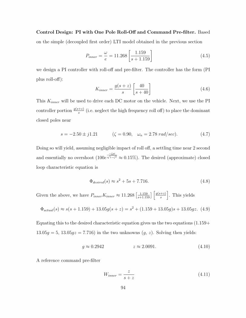
Control Design: PI with One Pole Roll-Off and Command Pre-filter. Based

on the simple (decoupled first order) LTI model obtained in the previous section

Pinner =ω

e= 11.268

[1.159

s+ 1.159

](4.5)

we design a PI controller with roll-off and pre-filter. The controller has the form (PI

plus roll-off):

Kinner =g(s+ z)

s

[40

s+ 40

](4.6)

This Kinner will be used to drive each DC motor on the vehicle. Next, we use the PI

controller portion g(s+z)s

(i.e. neglect the high frequency roll off) to place the dominant

closed poles near

s = −2.50± j1.21 (ζ = 0.90, ωn = 2.78 rad/sec). (4.7)

Doing so will yield, assuming negligible impact of roll off, a settling time near 2 second

and essentially no overshoot (100e−ζpi√1−ζ2 ≈ 0.15%). The desired (approximate) closed

loop characteristic equation is

Φdesired(s) ≈ s2 + 5s+ 7.716. (4.8)

Given the above, we have PinnerKinner ≈ 11.268[

1.159s+1.159

] [g(s+z)s

]. This yields

Φactual(s) ≈ s(s+ 1.159) + 13.05g(s+ z) = s2 + (1.159 + 13.05g)s+ 13.05gz. (4.9)

Equating this to the desired characteristic equation gives us the two equations (1.159+

13.05g = 5, 13.05gz = 7.716) in the two unknowns (g, z). Solving then yields:

g ≈ 0.2942 z ≈ 2.0091. (4.10)

A reference command pre-filter

Winner =z

s+ z(4.11)

94

will ensure that the overshoot to a step reference command approximates that dictated

by the second order theory. That is, we obtain the following single channel (SISO)

map form commanded wheel speed to actual wheel speed:

Trywheel speeds = Winner

[PinnerKinner

1 + PinnerKinner

]≈ 7.716

s2 + 5s+ 7.716. (4.12)

Figure 4.1: Visualization of (v, ω) and (ωR, ωL) Inner-Loop Control

The inner-loop control system can be visualized as shown in Figure 4.1. (v, ω)

are commanded but not directly measured. Within Figure 4.1, the matrix M is a

2× 2 vehicle-wheel speed map that relates the vehicle translational-rotational veloc-

ities (v, ω) to the wheel angular velocities (ωR, ωL); i.e. see equation (4.2) (page 93).

Although only the wheel encoder count information is fed back within the physical

inner-loop hardware implementation, the system outputs v and ω were estimated

(computed) using wheel encoder counts in accordance with equations (4.3)-(4.4)

Reference to Output Try (v, ω) Map. From Figure 4.1, it follows that one can

use the relationships in equation (4.2) to get the model-based closed loop map from

references (vref , ωref ) to outputs (v, ω). Doing so yields the following TITO LTI

95

(nearly decoupled at low frequencies) map:

Try = MPK(I + PK)−1WM−1 ≈[

7.716

s2 + 5s+ 7.716

]I2×2 (4.13)

where P ≈ PinnerI2×2 is a TITO LTI nearly decoupled system at low frequencies (see

Chapter 3 and results above) and K = KinnerI2×2 is a diagonal inner-loop controller.

Inner-Loop Open Loop Singular Values: (v, ω) and (ωR, ωL) Systems. Re-

calling the plant control issues discussion on pages (71)-(75), we plot the open loop

singular values for PK and MPKM−1 in Figure 4.2.

Their singular values are identical. This is expected from a simple algebraic anal-

ysis - one exploiting the structure of M and the fact that PK is symmetric (see

discussion on pages (71)-(75)).

10-2

10-1

100

101

102

103

-80

-60

-40

-20

0

20

40

60

PK singular values

MPKM-1 singular values

Open Loop Singular Values

Frequency (rad/s)

Sin

glu

ar

Va

lue

s (

dB

)

Figure 4.2: PK and Lo = MPKM−1 Singular Values

The main point of Figure 4.2, and the discussion on pages (71)-(75), is that

• It does not really matter whether we design for (v,ω) or (ωR, ωL) - both system

will posses the same closed loop properties except for control action differences.

This is not a negligible difference. Why? Control effort, like energy usage, is

very important!

96

• That is, they will possess the same loop L, sensitivity S = (I + L)−1, and

complementary sensitivity T = I − S singular values.

• Recall that since PK = KP (see discussion on pages (71)-(75)), it follows

that the singular values at the outputs/errors are the same as those at the

controls/inputs for the two closed loop systems (i.e. (ωR, ωL ) and (v, ω)). This

implies that

σk[Lo] = σk[Li] σk[So] = σi[Si] σk[To] = σi[Ti] k = 1, 2 . . .(4.14)

for both closed loop systems; (i.e. (ωR, ωL ) and (v, ω)). Recall that:

– For the (ωR, ωL) system, Lo = PK = KP = Li.

– For the (v, ω) system, Lo = MPKM−1 and Li = KM−1MP = PK.

For either system, σk[Lo] = σk[Li] (k = 1, 2 . . . ). While obvious for the first

(ωR, ωL) system, the proof for the second (v, ω) system requires using the struc-

ture of M (see equation (4.2) on page 93) and the fact that PK is symmetric

(see discussion on pages (71)-(75)).

Sensitivity Singular Values (Decoupled Model). The sensitivity singular values

(at outputs/controls) for either system ((v,ω) or (ωR, ωL)) are plotted in Figure 4.3.

As expected, the singular values are identical for the two systems: (ωR, ωL) and (v,ω).

Moreover, Figure 4.3 shows that the system will possess good low frequency command

following as well as nominal stability robustness properties (i.e. little sensitivity peak-

ing). Again, these properties will hold for both the (ωR, ωL) and the (v, ω) closed

loop systems.

Complementary Sensitivity Singular Values (Decoupled Model). The com-

plementary sensitivity singular values (at outputs/controls) for system (ωR, ωL)) are

97

10-2

10-1

100

101

102

103

-60

-50

-40

-30

-20

-10

0

10Sensitivity Singular Values

Frequency (rad/s)

Sin

glu

ar

Valu

es (

dB

)

Figure 4.3: So = (I + Lo)−1 = Si Singular Values - Using Decoupled Model

plotted in Figure 4.4. As expected, the singular values are identical for the two

systems: (ωR, ωL) and (v,ω).

10-2

10-1

100

101

102

103

-70

-60

-50

-40

-30

-20

-10

0

10Complementary Sensitivity Singular Values

Frequency (rad/s)

Sin

glu

ar

Valu

es (

dB

)

Figure 4.4: To = Lo(I + Lo)−1 = Ti Singular Values - Using Decoupled Model

Figure 4.4 shows that the system will possess good low frequency command following

as well as high frequency noise attenuation.

Reference to Control Singular Values (Decoupled Model). The reference to

control singular values are shown in Figures 4.5-4.6. The latter shows the utility of

98

the command pre-filter for reducing control effort.

10-2

10-1

100

101

102

103

-35

-30

-25

-20

-15

-10

Tru

Singular Values

Frequency (rad/s)

Sin

glu

ar

Valu

es (

dB

)

Figure 4.5: Tru Singular Values (No Pre-filter) - Using Decoupled Model

10-2

10-1

100

101

102

103

-90

-80

-70

-60

-50

-40

-30

-20

-10

Tru

W Singular Values

Frequency (rad/s)

Sin

glu

ar

Valu

es (

dB

)

Figure 4.6: TruW Singular Values (with Pre-filter) - Using Decoupled Model

Figure 4.6 shows that output disturbances with frequency content near 1-5 rad/sec

can be maximally amplified with respect to the controls (by a factor of 1.48 or 3.4

dB), if they occur in the worse case direction.

Figure 4.7 shows the singular values for Tru (unfiltered) for the (v, ω) system.

99

10-2

10-1

100

101

102

103

-25

-20

-15

-10

-5

0

5

10

15

20KSM

-1 Singular Values

Frequency (rad/s)

Sin

glu

ar

Valu

es (

dB

)

Figure 4.7: KSM−1 Singular Values

Input Disturbance to Output Tdiy Singular Values. The input disturbance to

output singular values are shown in Figures 4.8. The plot shows that input distur-

bances near 3 rad/sec will be maximally amplified (about 8 dB, if they occur in the

worse case direction).

10-2

10-1

100

101

102

103

-40

-35

-30

-25

-20

-15

-10

-5

0

5

10

Tdiy

Singular Values

Frequency (rad/s)

Sin

glu

ar

Valu

es (

dB

)

Figure 4.8: Tdiy Singular Values - Using Decoupled Model

Figure 4.9 shows the singular values for Tdiy for the (v, ω) system.

100

10-2

10-1

100

101

102

103

-70

-60

-50

-40

-30

-20

-10

0

10MSP Singular Values

Frequency (rad/s)

Sin

glu

ar

Valu

es (

dB

)

Figure 4.9: MSP Singular Values

Step Response Analysis Using Decoupled Model: Output Responses (ωR, ωL).

filtered step reference time responses is shown within Figure 4.10.

To

: O

ut(

1)

0

5

10

15From: In(1)

0 1 2 3 4 5

To

: O

ut(

2)

0

5

10

15

From: In(2)

0 1 2 3 4 5

Step response (Filtered)

Time (seconds)

An

gu

lar

Ve

locity (

rad

/se

c)

Figure 4.10: Inner-Loop [ωR, ωL] Filtered Step Response - Using Decoupled Model

The associated decoupled unfiltered step reference time responses is shown within

Figure 4.11.

101

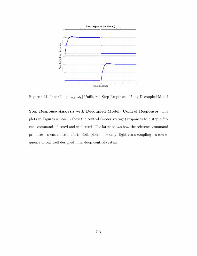
To

: O

ut(

1)

0

5

10

15From: In(1)

0 1 2 3 4 5

To

: O

ut(

2)

0

5

10

15

From: In(2)

0 1 2 3 4 5

Step response (Unfiltered)

Time (seconds)

An

gu

lar

Ve

locity (

rad

/se

c)

Figure 4.11: Inner-Loop [ωR, ωL] Unfiltered Step Response - Using Decoupled Model

Step Response Analysis with Decoupled Model: Control Responses. The

plots in Figures 4.12-4.13 show the control (motor voltage) responses to a step refer-

ence command - filtered and unfiltered. The latter shows how the reference command

pre-filter lessens control effort. Both plots show only slight cross coupling - a conse-

quence of our well designed inner-loop control system.

102

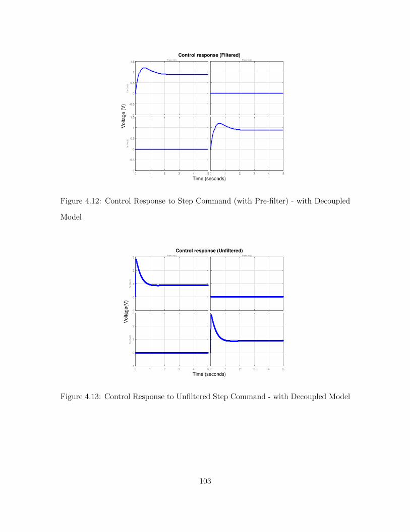
To

: O

ut(

1)

-1

-0.5

0

0.5

1

1.5From: In(1)

0 1 2 3 4 5

To

: O

ut(

2)

-1

-0.5

0

0.5

1

1.5

From: In(2)

0 1 2 3 4 5

Control response (Filtered)

Time (seconds)

Vo

lta

ge

(V

)

Figure 4.12: Control Response to Step Command (with Pre-filter) - with Decoupled

Model

To

: O

ut(

1)

-1

0

1

2

3From: In(1)

0 1 2 3 4 5

To

: O

ut(

2)

-1

0

1

2

3

From: In(2)

0 1 2 3 4 5

Control response (Unfiltered)

Time (seconds)

Vo

lta

ge

(V)

Figure 4.13: Control Response to Unfiltered Step Command - with Decoupled Model

103

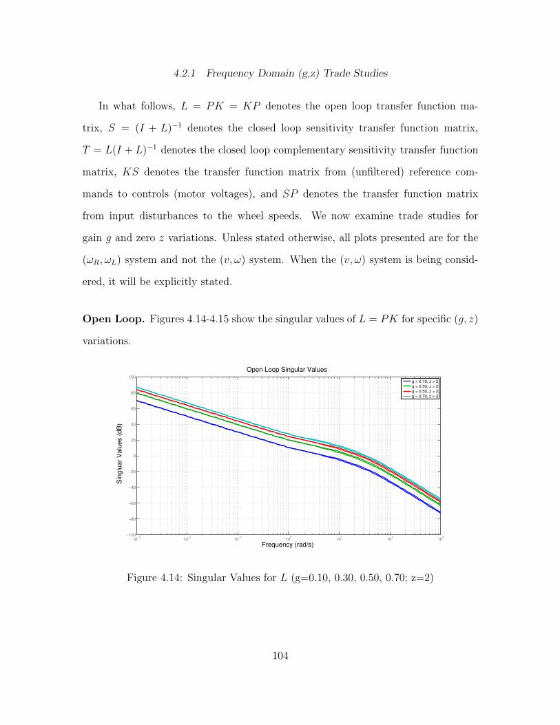
4.2.1 Frequency Domain (g,z) Trade Studies

In what follows, L = PK = KP denotes the open loop transfer function ma-

trix, S = (I + L)−1 denotes the closed loop sensitivity transfer function matrix,

T = L(I + L)−1 denotes the closed loop complementary sensitivity transfer function

matrix, KS denotes the transfer function matrix from (unfiltered) reference com-

mands to controls (motor voltages), and SP denotes the transfer function matrix

from input disturbances to the wheel speeds. We now examine trade studies for

gain g and zero z variations. Unless stated otherwise, all plots presented are for the

(ωR, ωL) system and not the (v, ω) system. When the (v, ω) system is being consid-

ered, it will be explicitly stated.

Open Loop. Figures 4.14-4.15 show the singular values of L = PK for specific (g, z)

variations.

10−3

10−2

10−1

100

101

102

103

−100

−80

−60

−40

−20

0

20

40

60

80

100


Frequency (rad/s)

Sin

glu

ar

Va

lue

s (

dB

)

g = 0.10, z = 2

g = 0.30, z = 2g = 0.50, z = 2

g = 0.70, z = 2

Figure 4.14: Singular Values for L (g=0.10, 0.30, 0.50, 0.70; z=2)

104

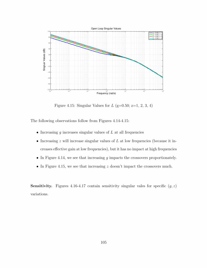
10−3

10−2

10−1

100

101

102

103

−100

−80

−60

−40

−20

0

20

40

60

80

100


Frequency (rad/s)

Sin

glu

ar

Va

lue

s (

dB

)

g = 0.50,z = 1

g = 0.50,z = 2g = 0.50,z = 3

g = 0.50,z = 4

Figure 4.15: Singular Values for L (g=0.50; z=1, 2, 3, 4)

The following observations follow from Figures 4.14-4.15:

• Increasing g increases singular values of L at all frequencies

• Increasing z will increase singular values of L at low frequencies (because it in-

creases effective gain at low frequencies), but it has no impact at high frequencies

• In Figure 4.14, we see that increasing g impacts the crossovers proportionately.

• In Figure 4.15, we see that increasing z doesn’t impact the crossovers much.

Sensitivity. Figures 4.16-4.17 contain sensitivity singular vales for specific (g, z)

variations.

105

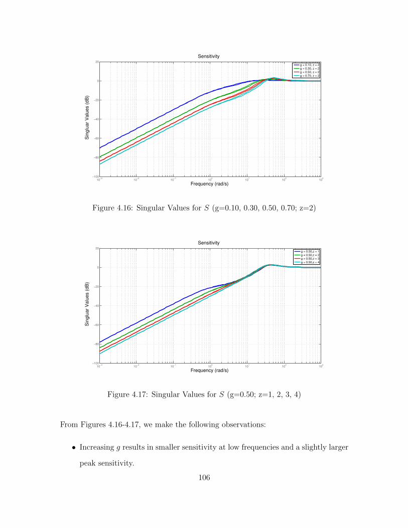
10−3

10−2

10−1

100

101

102

103

−100

−80

−60

−40

−20

0

20

Sensitivity

Frequency (rad/s)

Sin

glu

ar

Va

lue

s (

dB

)

g = 0.10, z = 2

g = 0.30, z = 2g = 0.50, z = 2

g = 0.70, z = 2

Figure 4.16: Singular Values for S (g=0.10, 0.30, 0.50, 0.70; z=2)

10−3

10−2

10−1

100

101

102

103

−100

−80

−60

−40

−20

0

20

Sensitivity

Frequency (rad/s)

Sin

glu

ar

Va

lue

s (

dB

)

g = 0.50,z = 1

g = 0.50,z = 2g = 0.50,z = 3

g = 0.50,z = 4

Figure 4.17: Singular Values for S (g=0.50; z=1, 2, 3, 4)

From Figures 4.16-4.17, we make the following observations:

• Increasing g results in smaller sensitivity at low frequencies and a slightly larger

peak sensitivity.

106

• Increasing z results in smaller sensitivity at low frequencies but increases peak

sensitivity slightly.

• peak sensitivities do not change much with increasing g

• peak sensitivities do not change much with increasing z.

Complementary Sensitivity. Figures 4.18-4.19 contain complementary sensitivity

singular vales for specific (g, z) variations.

10−3

10−2

10−1

100

101

102

103

−80

−70

−60

−50

−40

−30

−20

−10

0

10

20

Complementary Sensitivity

Frequency (rad/s)

Sin

glu

ar

Va

lue

s (

dB

)

g = 0.10, z = 2

g = 0.30, z = 2g = 0.50, z = 2

g = 0.70, z = 2

Figure 4.18: Singular Values for T (g=0.10, 0.30, 0.50, 0.70; z=2)

107

10−3

10−2

10−1

100

101

102

103

−60

−50

−40

−30

−20

−10

0

10

Complementary Sensitivity

Frequency (rad/s)

Sin

glu

ar

Va

lue

s (

dB

)

g = 0.50,z = 1

g = 0.50,z = 2g = 0.50,z = 3

g = 0.50,z = 4

Figure 4.19: Singular Values for T (g=0.50; z=1, 2, 3, 4)

From Figures 4.18-4.19, we make the following observations:

• Increasing g will result in a larger bandwidth (but worse high frequency noise at-

tenuation and larger peak complementary sensitivity;a tradeoff must be made).

• Increasing z will result in slightly larger bandwidth and a larger peak comple-

mentary sensitivity. High frequency noise attenuation is the same for different

z values.

• peak sensitivities increase with increasing g.

• peak complementary sensitivities increase slightly with increasing z.

Reference to Control (Unfiltered). Figures 4.20-4.21 contain (unfiltered) refer-

ence to control singular values for specific (g, z) variations. As the plots above, these

plots are for the (ωR, ωL) system. As such, they tell us what control responses result

from (ωR, ωL) commands - not from (v, ω) commands. This is addressed below.

108

10−3

10−2

10−1

100

101

102

103

−50

−45

−40

−35

−30

−25

−20

−15

−10

−5

0

Tru

(Unfiltered)

Frequency (rad/s)

Sin

glu

ar

Va

lue

s (

dB

)

g = 0.10, z = 2

g = 0.30, z = 2g = 0.50, z = 2

g = 0.70, z = 2

Figure 4.20: Singular Values for Tru (g=0.10, 0.30, 0.50, 0.70; z=2) - (ωR, ωL) Com-

mands

10−3

10−2

10−1

100

101

102

103

−35

−30

−25

−20

−15

−10

−5

Tru

(Unfiltered)

Frequency (rad/s)

Sin

glu

ar

Va

lue

s (

dB

)

g = 0.50,z = 1

g = 0.50,z = 2g = 0.50,z = 3

g = 0.50,z = 4

Figure 4.21: Singular Values for Tru (g=0.50; z=1, 2, 3, 4)- (ωR, ωL) Commands

From Figures 4.20 -4.21, we make the following observations when (ωR, ωL) com-

mands are issued to our inner-loop control system:

109

• Increasing g or z increases the peak Tru at all except low frequencies.

• Increasing g increases peak Tru.

• Increasing z slightly increases peak Tru.

For completeness, Figures 4.22-4.23 contain (unfiltered) reference to control singular

values for specific (g, z) variations. These plots are for the actual plant P . As such,

they tell us the control response to a (v, ω) commands - as we shall be giving in a

practical (v, ω) inner-loop control implementation (see Chapter 4).

10−3

10−2

10−1

100

101

102

103

−60

−50

−40

−30

−20

−10

0

10

20

30

40

KSM−1

Singular Values

Frequency (rad/s)

Sin

gu

lar

Va

lue

s (

dB

)

g = 0.10, z = 2

g = 0.30, z = 2g = 0.50, z = 2

g = 0.70, z = 2

Figure 4.22: Singular Values for KSM−1 (g=0.10, 0.30, 0.50, 0.70; z=2) - (v, ω)

Commands

110

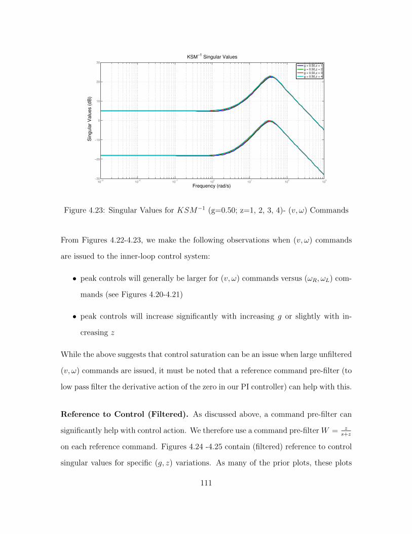
10−3

10−2

10−1

100

101

102

103

−30

−20

−10

0

10

20

30

KSM−1

Singular Values

Frequency (rad/s)

Sin

gu

lar

Va

lue

s (

dB

)

g = 0.50,z = 1

g = 0.50,z = 2g = 0.50,z = 3

g = 0.50,z = 4

Figure 4.23: Singular Values for KSM−1 (g=0.50; z=1, 2, 3, 4)- (v, ω) Commands

From Figures 4.22-4.23, we make the following observations when (v, ω) commands

are issued to the inner-loop control system:

• peak controls will generally be larger for (v, ω) commands versus (ωR, ωL) com-

mands (see Figures 4.20-4.21)

• peak controls will increase significantly with increasing g or slightly with in-

creasing z

While the above suggests that control saturation can be an issue when large unfiltered

(v, ω) commands are issued, it must be noted that a reference command pre-filter (to

low pass filter the derivative action of the zero in our PI controller) can help with this.

Reference to Control (Filtered). As discussed above, a command pre-filter can

significantly help with control action. We therefore use a command pre-filter W = zs+z

on each reference command. Figures 4.24 -4.25 contain (filtered) reference to control

singular values for specific (g, z) variations. As many of the prior plots, these plots

111

are for the (ωR, ωL) system. As such, they tell us what control responses result

from (ωR, ωL) commands. They do not tell us about control responses from (v, ω)

commands. This is addressed below.

10−3

10−2

10−1

100

101

102

103

−120

−110

−100

−90

−80

−70

−60

−50

−40

−30

−20

Tru

⋅W

Frequency (rad/s)

Sin

gu

lar

Va

lue

s (

dB

)

g = 0.10, z = 2

g = 0.30, z = 2g = 0.50, z = 2

g = 0.70, z = 2

Figure 4.24: Singular Values for W · Tru (g=0.10, 0.30, 0.50, 0.70; z=2) - (ωR, ωL)

Commands

10−3

10−2

10−1

100

101

102

103

−100

−90

−80

−70

−60

−50

−40

−30

−20

Tru

⋅W

Frequency (rad/s)

Sin

gu

lar

Va

lue

s (

dB

)

g = 0.50,z = 1

g = 0.50,z = 2g = 0.50,z = 3

g = 0.50,z = 4

Figure 4.25: Singular Values for W · Tru (g=0.50; z=1, 2, 3, 4) - (ωR, ωL) Commands

112

From Figures 4.24-4.25, we make the following observations when (ωR, ωL) commands

are issued to our inner-loop control system:

• Increasing g or z increases the size of WTru at all but low frequencies.

• Increasing g increases the peak WTru only slightly.

• Increasing z increases the peak WTru, but it does not impact WTru at low fre-

quencies.

• peak W · Tru increases slightly as g increases.

• peak W · Tru increases with increasing z.

The above plots suggest that overshoot and saturation due to filtered (ωR, ωL) com-

mands reference commands should not be too much of an issue - unless, of course,

very large reference commands are issued to the inner-loop control system.

Input Disturbance to Output Tdiy. Figures 4.26-4.27 contain input disturbance

to control singular values for specific (g, z) variations. As many of the plots above,

these plots are for the (ωR, ωL) system. As such, they tell us what (ωR, ωL) responses

result from input (voltage) disturbances. They do not tell us about (v, ω) responses.

This is addressed below.

Figures 4.26-4.27, contain the singular value plots for Tdiy for specific (g, z) vari-

ations. Figures 4.26-4.27, we make the following observations:

113

10−3

10−2

10−1

100

101

102

103

−80

−70

−60

−50

−40

−30

−20

−10

0

10

20

Tdiy

Frequency (rad/s)

Sin

gu

lar

Va

lue

s (

dB

)

g = 0.10, z = 2

g = 0.30, z = 2g = 0.50, z = 2

g = 0.70, z = 2

Figure 4.26: Singular Values for Tdiy (g=0.10, 0.30, 0.50, 0.70; z=2) - (ωR, ωL) Re-

sponses

10−3

10−2

10−1

100

101

102

103

−80

−70

−60

−50

−40

−30

−20

−10

0

10

20

Tdiy

Frequency (rad/s)

Sin

gu

lar

Va

lue

s (

dB

)

g = 0.50,z = 1

g = 0.50,z = 2g = 0.50,z = 3

g = 0.50,z = 4

Figure 4.27: Singular Values for Tdiy (g=0.50; z=1, 2, 3, 4) - (ωR, ωL) Responses

From Figures 4.26 -4.27, we make the following observations:

• peak Tdiy decreases with increasing g (z has little impact on peak)

114

• increasing g reduces Tdiy at all frequencies except at high frequencies

• increasing z reduces Tdiy at low frequencies

• frequency at which peak Tdiy occurs increases with increasing g (also with in-

creasing z but to a lesser extant)

For completeness, Figures 4.28-4.29 contain input disturbance di to output y =

[ v ω ]T singular values for specific (g, z) variations. These plots are for the ac-

tual plant P . As such, they tell us about the (v, ω) responses to input (voltage)

disturbances di.

10−3

10−2

10−1

100

101

102

103

−100

−80

−60

−40

−20

0

20

MSP Singular Values

Frequency (rad/s)

Sin

gu

lar

Va

lue

s (

dB

)

g = 0.10, z = 2

g = 0.30, z = 2g = 0.50, z = 2

g = 0.70, z = 2

Figure 4.28: Singular Values for MSP (g=0.50; z=1, 2, 3, 4) - (v, ω) Responses

115

10−3

10−2

10−1

100

101

102

103

−100

−80

−60

−40

−20

0

20

MSP Singular Values

Frequency (rad/s)

Sin

gu

lar

Va

lue

s (

dB

)

g = 0.50,z = 1

g = 0.50,z = 2g = 0.50,z = 3

g = 0.50,z = 4

Figure 4.29: Singular Values for MSP (g=0.50; z=1, 2, 3, 4) - (v, ω) Responses

From Figures 4.28-4.29, we make the following observations about the closed loop

system containing the actual actual (v, ω) plant P :

• peak Tdiy has improved for actual (v, ω) plant versus (ωR, ωL) system (see Fig-

ures 4.26 -4.27)

• peak Tdiy decreases with increasing g (z has little impact on peak)

• increasing g reduces Tdiy at all frequencies except at high frequencies

• increasing z reduces Tdiy at low frequencies

• frequency at which peak Tdiy occurs increases with increasing g (also with in-

creasing z but to a lesser extant)

The above patterns suggests that while the actual (v, ω) plant will exhibit a worse

Try, it will exhibit a better Tdiy than the (ωR, ωL) system.

116

4.2.2 Time Domain (g,z) Trade Studies

Output and Control Responses to Step Reference Commands for different

(g, z) values. Figures 4.32-4.33 contain output and control responses to unfiltered

step reference commands for specific (g, z) variations.

0

0.5

1

1.5From: In(1)

To

: O

ut(

1)

0 0.5 1 1.5 2 2.5 3 3.5 4 4.5 5

0

0.5

1

1.5

To: O

ut(

2)

From: In(2)

0 0.5 1 1.5 2 2.5 3 3.5 4 4.5 5

Step Response for Try

(Unfiltered)

Time (seconds)

An

gu

lar

Ve

locity (

rad

/s)

g = 0.10, z = 2

g = 0.30, z = 2g = 0.50, z = 2

g = 0.70, z = 2

Figure 4.30: Output Response to Step Command (g = 0.10, 0.30, 0.50, 0.70; z = 2)

117

0

0.5

1

1.5From: In(1)

To: O

ut(

1)

0 0.5 1 1.5 2 2.5 3 3.5 4 4.5 5

0

0.5

1

1.5

To:

Ou

t(2)

From: In(2)

0 0.5 1 1.5 2 2.5 3 3.5 4 4.5 5

Step Response for Try

(Unfiltered)

Time (seconds)

An

gu

lar

Ve

locity (

rad

/s)

g = 0.50,z = 1

g = 0.50,z = 2g = 0.50,z = 3

g = 0.50,z = 4

Figure 4.31: Output Response to Step Command (g = 0.50; z = 1, 2, 3, 4)

0

0.05

0.1

0.15

0.2

0.25

0.3

0.35

0.4From: In(1)

To: O

ut(

1)

0 0.5 1 1.5 2 2.5 3 3.5 4

0

0.05

0.1

0.15

0.2

0.25

0.3

0.35

0.4

To: O

ut(

2)

From: In(2)

0 0.5 1 1.5 2 2.5 3 3.5 4

Control Response for step command (Unfiltered)

Time (seconds)

Vo

lta

ge

(vo

lts)

g = 0.10, z = 2

g = 0.30, z = 2g = 0.50, z = 2

g = 0.70, z = 2

Figure 4.32: Control Response to Step Command (g = 0.10, 0.30, 0.50, 0.70; z = 2)

118

0

0.05

0.1

0.15

0.2

0.25

0.3

0.35

0.4From: In(1)

To: O

ut(

1)

0 0.1 0.2 0.3 0.4 0.5 0.6 0.7 0.8 0.9 1

0

0.05

0.1

0.15

0.2

0.25

0.3

0.35

0.4

To:

Ou

t(2)

From: In(2)

0 0.1 0.2 0.3 0.4 0.5 0.6 0.7 0.8 0.9 1

Control Response for step command (Unfiltered)

Time (seconds)

Vo

lta

ge

(vo

lts)

g = 0.50,z = 1

g = 0.50,z = 2g = 0.50,z = 3

g = 0.50,z = 4

Figure 4.33: Control Response to Step Command (g = 0.50; z = 1, 2, 3, 4)

From the above output and control responses to unfiltered step reference commands

(Figures 4.32-4.33), we obtain the following observations:

• faster settling time results from increasing g or z

• increasing g will result in a larger overshoot

• increasing z will result in a slightly more overshoot within this range of variation

• increasing g will result in larger and faster control action, little impact with

increasing z within this range of variation

Figures 4.36-4.37 contain output and control responses to filtered step reference com-

mands for specific (g, z) variations.

119

To

: O

ut(

1)

0

0.2

0.4

0.6

0.8

1From: In(1)

0 1 2 3 4 5 6

To

: O

ut(

2)

0

0.2

0.4

0.6

0.8

1

From: In(2)

0 1 2 3 4 5 6

g = 0.10, z = 2

g = 0.30, z = 2

g = 0.50, z = 2

g = 0.70, z = 2

Step Response Try

· W

Time (seconds)

An

gu

lar

Ve

locity (

rad

/s)

Figure 4.34: Output Response to Step Command (g = 0.10, 0.30, 0.50, 0.70; z = 2)

To

: O

ut(

1)

0

0.2

0.4

0.6

0.8

1From: In(1)

0 2 4 6 8

To

: O

ut(

2)

0

0.2

0.4

0.6

0.8

1

From: In(2)

0 2 4 6 8

g = 0.50,z = 1

g = 0.50,z = 2

g = 0.50,z = 3

g = 0.50,z = 4

Step Response Try

· W

Time (seconds)

An

gu

lar

Ve

locity (

rad

/s)

Figure 4.35: Output Response to Step Command (g = 0.50; z = 1, 2, 3, 4)

120

0

0.02

0.04

0.06

0.08

0.1From: In(1)

To: O

ut(

1)

0 1 2 3 4 5 6 7

0

0.02

0.04

0.06

0.08

0.1

To: O

ut(

2)

From: In(2)

0 1 2 3 4 5 6 7

Control Response for step command with pre−filter

Time (seconds)

Vo

lta

ge

(vo

lts)

g = 0.10, z = 2

g = 0.30, z = 2g = 0.50, z = 2

g = 0.70, z = 2

Figure 4.36: Control Response to Filtered Step Command g =

0.10, 0.30, 0.50, 0.70; z = 2)

0

0.02

0.04

0.06

0.08

0.1From: In(1)

To: O

ut(

1)

0 1 2 3 4 5 6 7 8

0

0.02

0.04

0.06

0.08

0.1

To: O

ut(

2)

From: In(2)

0 1 2 3 4 5 6 7 8

Control Response for step command with pre−filter

Time (seconds)

Vo

lta

ge

(vo

lts)

g = 0.50,z = 1

g = 0.50,z = 2g = 0.50,z = 3

g = 0.50,z = 4

Figure 4.37: Control Response to Filtered Step Command (g = 0.50; z = 1, 2, 3, 4)

From Figures 4.36-4.37, we obtain the following observations:

• increasing g or z will result in larger and faster control action

• command pre-filter helps with control action.

121

4.2.3 Inner-Loop Experimental Result

In this part, we will check our design for inner loop with hardware experimental

result. We examined design parameters we discussed above (g = 0.29, z= 2.01) with

simulation and hardware.

Decoupled Inner-Loop Step Response (with prefilter) g 0.29 z 2.01

Time(seconds)

0 1 2 3 4 5 6 7

An

gu

lar

Sp

ee

d o

f W

he

el (r

ad

/se

c)

0

5

10

15

Simulation

Hardware

Time(seconds)

0 1 2 3 4 5 6 7

An

gu

lar

Sp

ee

d o

f W

he

el (r

ad

/se

c)

0

5

10

15

Simulation

Hardware

Time(seconds)

0 1 2 3 4 5 6 7

An

gu

lar

Sp

ee

d o

f W

he

el (r

ad

/se

c)

-5

0

5

Simulation

Hardware

Time(seconds)

0 1 2 3 4 5 6 7

An

gu

lar

Sp

ee

d o

f W

he

el (r

ad

/se

c)

-5

0

5

Simulation

Hardware

Figure 4.38: Output Response to filtered Step Command (ωRref = 10, ωLref = 10)

For completeness, output response to (v,ω) system is shown in Figure 4.39

122

Try(v,ω) Inner-Loop Step Response (with prefilter) g 0.29 z 2.01

Time(seconds)

0 1 2 3 4 5 6 7

Tra

nsla

tio

n S

pe

ed

of

Ve

hic

le (

m/s

ec)

0

0.1

0.2

0.3

0.4

0.5

0.6

0.7

Simulation

Hardware

Time(seconds)

0 1 2 3 4 5 6 7

An

gu

lar

Sp

ee

d o

f V

eh

icle

(ra

d/s

ec)

-5

-4

-3

-2

-1

0

1

2

3

4

5

Simulation

Hardware

Figure 4.39: Output Response to filtered Step Command (vref = 0.5, ωref = 0)

Decoupled Inner-Loop Control Response (with prefilter) g 0.29 z 2.01

Time(seconds)

0 1 2 3 4 5 6 7

Vo

lta

ge

(V)

0

1

2

3

4

5Simulation

Hardware

Time(seconds)

0 1 2 3 4 5 6 7

Vo

lta

ge

(V

)

0

1

2

3

4

5Simulation

Hardware

Time(seconds)

0 1 2 3 4 5 6 7

Vo

lta

ge

(V

)

-5

0

5Simulation

Hardware

Time(seconds)

0 1 2 3 4 5 6 7

Vo

lta

ge

(V

)

-5

0

5Simulation

Hardware

Figure 4.40: Control Response to filtered Step Command (ωRref = 10, ωLref = 10)

From the above output and control responses to unfiltered step reference commands

(Figures 4.38-4.40), we obtain the following observation. Output response of hardware

follows simulation and reach steady state in almost 2 seconds, overshoot about 8% is

123

observed. Control effort from hardware is close to simulation result in steady state,

however shows much deviation at beginning. The difference comes from following

factors:

• Deadzone Effect from Stiction. When vehicle begins to start, it need overcome

static friction which is much higher than the rolling friction experienced when it

runs. This cause about 0.2 seconds delay in system response, which will cause

integration term build much higher than it should be and oscillation will be

observed as expected.

• Encoder Resolution. To improve the encoder resolution, we implemented av-

erage filter in hardware. However, it still have strong impact when reference

command is relative slow. This will cause oscillation in control effort and in-

evitable steady state error.

124

4.3 Outer-Loop Control Design and Implementation

4.3.1 Outer-Loop 1: (v, θ) Cruise Control Along Line - Design and Implementation

In this section, we examine (v, θ) cruise control along a line/curve. This outer-loop

control law can be visualized as shown in Figure 4.41. Here, (v, θ) are commanded.

Figure 4.41: Visualization of Cruise Control Along a Line

v is calculated based on wheel encoders; see equation (4.3) on page 93. For cruise

control along a line, vref = constant, θref = 0 are commanded. For cruise control

along a line, θ is directly measured by the IMU.

The use of a proportional gain controller is justified because the map from the

references vref and ωref to the actual speeds v and ω looks like a diagonal system

diag( as+a

, bs+b

) (at low frequencies). This is a consequence of a well-designed inner-

loop (see above). The outer-loop θ controller therefore sees bs(s+b)

. From classical root

locus ideas, a proportional controller is therefore justified - provided that the gain

is not too large. If the gain is too large, oscillations will be expected in θ. A PD

controller with roll off would help with this issue.

Figures 4.42 -4.43 show frequency responses for Tθref θ for proportional and PD

outer-loop control laws. Figure 4.44-4.45 show the corresponding responses to an ini-

tial condition θo = 0.1 rad. The responses corroborate what was pointed out above,

namely that a sufficiently large gain proportional control law can result in peaking

125

while a PD control law has little peaking.

−200

−150

−100

−50

0

50

100

Ma

gn

itu

de

(d

B)

10−2

10−1

100

101

102

103

−360

−180

0

Ph

ase

(d

eg

)

Frequency response of cruise control θ with P control

Frequency (rad/s)

Kp 0.50

Kp 1.00

Kp 1.50

Kp 2.00

Figure 4.42: Tθrefθ Frequency Response for θ Outer-Loop (P Control)

−200

−150

−100

−50

0

Ma

gn

itu

de

(d

B)

10−2

10−1

100

101

102

103

−360

−180

0

Ph

ase

(d

eg

)

Frequency response of cruise control θ with PD control

Frequency (rad/s)

Kp 0.50

Kp 1.00

Kp 1.50

Kp 2.00

Figure 4.43: Tθrefθ Frequency Response for θ Outer-Loop (PD control, Kd = 1)

CODE. The Raspberry Pi C code used for implementing our (v, θ) outer-loop cruise

control along a line control law can be found within Appendix A on page 242. This

outer-loop uses the (ωR, ωL)-(v, ω) inner-loop control law that has been implemented

using the Arduino code within Appendix C on page 294.

126

0 2 4 6 8 10 12 14 16 18 20−0.05

0

0.05

0.1

Cruise control θ response using P control

Time(seconds)

An

gle

(ra

d)

Kp=0.5

Kp=1.0Kp=1.5

Kp=2.0

Figure 4.44: Cruise Control θ Response Using P Control (θo = 0.1 rad)

0 2 4 6 8 10 12 14 16 18 20−0.05

0

0.05

0.1

Cruise control θ response using PD control

Time(seconds)

An

gle

(ra

d)

Kp=0.5

Kp=1.0Kp=1.5

Kp=2.0

Figure 4.45: Cruise Control θ Response Using PD Control (θo = 0.1 rad)

127

4.3.2 Outer-Loop 2: Separation-Direction (∆x, θ) Control - Design and

Implementation

In this section, separation-direction (∆x, θ) outer-loop control is discussed. Within

[3], [6], vehicle separation modeling and longitudinal platoon control is presented. The

ideas presented within [3], [6] motivate the PD ultrasonics-encoder-IMU-based sepa-

ration control laws used for the separation-direction (∆x, θ) outer-loop control within

this thesis. The ideas here are also used to have multiple differential-drive vehicles

following an autonomous or remotely controlled leader vehicle. (∆x, θ) separation-

direction control can be visualized as shown in Figure 4.46. Future work will examine

the related control saturation prevention ideas presented within [64].

Figure 4.46: Visualization of (∆x, θ) Separation-Direction Control System

Here, (∆x, θ) are commanded. ∆x is measured using an ultrasonic sensor. θ is di-

rectly measured by the IMU. Here, y position is not considered (assumed to be small)

since the ultrasonic sensor only provides almost lineal directional information.


references vref and ωref to the actual speeds (v, ω) looks like a diagonal system

128

diag(

as+a

, bs+b

)(at low frequencies). This is a consequence of a well-designed inner-


, and position con-

troller sees[

bs(s+b)

](since vy is so small, integrating v results in x position). From

classical root locus ideas, a proportional controller is therefore justified - provided

that the gain is not too large. If the gain is too large, oscillations will be expected.

A PD controller with roll off would help with this issue.

0 2 4 6 8 10 12 14 16 18 20−0.2

0

0.2

0.4

0.6

0.8

1

1.2

Constant separation using P control

Time(seconds)

An

gle

(ra

d)

Kp=0.5

Kp=1.0Kp=1.5

Kp=2.0

Figure 4.47: Vehicle Separation Control (Proportional Control: Kp = 0.5, 1.0, 1.5, 2.0;

∆xo = 1)

129

0 2 4 6 8 10 12 14 16 18 200

0.1

0.2

0.3

0.4

0.5

0.6

0.7

0.8

0.9

1

Constant separation using PD control

Time(seconds)

An

gle

(ra

d)

Kp=0.5

Kp=1.0Kp=1.5

Kp=2.0

Figure 4.48: Vehicle Separation Control (PD control: Kp = 0.5, 1.0, 1.5, 2.0;Kd=1;

∆xo = 1)

Figures 4.47-4.48 illustrate separation convergence of proportional and PD control.

A 1m initial condition was given. The desired separation L is 0.2 m. The following

observations are noted:

• For a proportional control, as we increase the value of Kp the robot moves faster

but the overshoot increases.

• For a PD control, the robot is able to move fast with no overshoot.

CODE. The Raspberry Pi C code used for implementing our (∆x, θ) outer-loop

separation-direction control control law can be found within Appendix A on page 242.

This outer-loop uses the (ωR, ωL)-(v, ω) inner-loop control law that has been imple-

mented using the Arduino code within Appendix C on page 294.

130

Fundamental Limitations Due to Sensors, Actuators, Hardware/Software.

It must be emphasized that the performance exhibited within each demonstration

is fundamentally constrained by the limitations of the sensors, actuators, and hard-

ware/software being used. Both bandwidth (speed/dynamic) and accuracy (stat-

ic/steady sate) limitations are a concern in any practical embedded system imple-

mentation. Given this, it is important to acknowledge the following sensor, actuator,

hardware/software limitations. We follow the same structure in [14] and only dif-

ference will be discussed in detail. Detailed discussion can be found in [14] at page

161-172.

• Factor-of-Ten Performance Limitation Rule. Here is a simple - commonly

used - “factor of ten rule. If we can sense/actuate/compute at a maximum (“re-

liable” or “available”) rate ω rad/sec, then the widely used factor of 10 rule

yields a maximum control bandwidth of 0.1ω rad/sec or about 160ω Hz.

The reason for this “factor-of-ten rule” is to adequately guard against the real-

world “push-pop effects” that are observed in practical embedded system appli-

cations. Generally, as we push the bandwidth higher (improving performance

at lower frequencies), we generally pay a price (e.g. increase in sensitivity) at

higher frequencies. As we get closer to the maximum available bandwidth, the

push-pop phenomenon gets worse [52], [69]. Future work will examine how far

we can really push this rule; e.g. when can we get away with a “factor-of-five

rule?”

Understanding fundamental hardware limitations is critical to understand what is

realistically achievable. This is addressed for each of the following: wheel DC motors,

encoders, ultrasonic sensors, camera, Arduino Uno, IMU, Raspberry Pi camera and

131

Raspberry Pi 3. The following is common to all demonstrations:

• 6V Brushed dc Motors. Within this thesis, we use 6V brushed armature

controlled DC motors on our Thunder Tumbler vehicles. When the applied

voltage is less than 0.3V, there is a dead zone and the wheels do not spin

(wheels off ground). ) With a 1V voltage input, the wheel which connects to

the shaft runs at about 16 rad/sec (measured via encoders, wheels off ground).

– Original Unloaded Vehicle (Not Enhanced). [14]. The original vehi-

cle (unloaded, unenhanced) has a mass of 0.56 kg. The maximum vehicle

speed observed was around 4.5 m/sec (obtained via measuring tape and

clock). The associated wheel angular velocity is ( 4.50.05

) 90 rad/sec (or 859

rpm). The unloaded torque-speed profile for the motor-wheel system (off

the ground) can be found in [14] at page 162. the maximum motor torque

as 0.048 Nm.

– Fully Loaded (Enhanced) Vehicle. When the vehicle is fully loaded

(i.e. enhanced), the vehicle mass increases by 55% (with respect to the

original mass) to 0.87kg. We observed a maximum (fully loaded) “aver-

age” vehicle acceleration of about 3m/sec2 (obtained via measuring tape

and clock). The maximum (fully loaded) vehicle speed (wheels on ground)

observed was about 2.3 m/sec. The associated wheel angular velocity is

( 2.30.05

) 46 rad/sec (or 439 rpm). A more powerful DC motors would help.

This will be investigated in future work.

• Arduino D-to-A (Actuation). In this thesis, the Arduino actuation rate to

the motor shield is 10Hz (0.1 sec actuation interval) or about 60rad/sec. Given

this, the widely used factor-of-ten rule yields maximum control bandwidth of 6

rad/s. Associated with classic D-to-A actuation is a zero order hold half sample

132

time delay [55]. Why?

ZOH(jω) =1− e−jωT

jω= e−jω0.5T j2 sinω0.5T

jω= Te−jω0.5T

[sin 0.5ωT

0.5ωT

](4.15)

The half sample time delay is seen in the term e−jω0.5T . From the following first

order Pade approximation

e−s∆ =e−s0.5∆

es0.5∆≈ 1− s0.5∆

1 + s0.5∆=

[ 2∆− s

2∆

+ s

](4.16)

it follows that a time delay ∆ has a right half plane (non-minimum phase) zero

at z = 2∆

. With ∆ = 0.05 (half sample time delay associated with ZOH), we get

z = 20.05

= 40. This then yields, using our factor-of-ten rule, a maximum control

bandwidth of about 4 rad/s. We thus see that a maximum inner-loop control

bandwidth of about 4-6 rad/sec is about all we should be willing to push with-

out further (more detailed) modeling.

• Arduino A-to-D (Sampling). In this thesis, the sampling time for all exper-

imental hardware demonstrations is 10 Hz (0.1 sec actuation interval) or about

60 rad/sec. Given this, the widely used factor-of-ten rule yields maximum con-

trol bandwidth of 6 rad/s. It should be noted that the Arduino has a 10-bit

ADC (210 = 1024) capability [36]. How does this impact us? This translates

to about 0.1% of the maximum speed. If we associate a maximum voltage 5

V with 10 bits and a maximum speed of 3 m/sec, it follows that a 1 bit error

translates into a 31024≈ 0.003 m/sec speed error. This is not very significant so

long as the speeds that our vehicles are likely to operate at are not too low. If

the speed is greater than 3 cm/sec, then this 1 bit error (0.003) will represent

less than 10%; 5% for speeds exceeding 6 cm/sec. Again, we’d have to travel

very slowly for this 1 bit error to matter.

• Wheel Encoder Limitations. Encoders on a vehicle’s wheels can be used

to measure wheel angular speed, wheel angular rotation, wheel translational

133

speed, wheel linear translation. Lets focus on the latter because it corre-

sponds to vehicle linear translation when moving along a straight line. For

our differential-drive Thunder Tumbler vehicles, we use eight encoders on each

wheel. As such, our angular resolution is 2π20

= 18. This amount of error seems

very large. Because we could not make stable measurement for high resolu-

tion encoder code disk. We then decided to see what we could achieve with

this low-cost speed-position measuring solution. A consequence of using wheel

encoders for measuring distance traveled is the inevitable accumulation of dead-

reckoning error. The spatial resolution associated with an 20 CPT system is

xresolution = rwheelθoptresolution = (5cm)(2π20

) = 0.0157 ≈ 1.6 cm. How do we use

this information? Let the variable ‘counter’ denote the number of pulses that

we have counted due to wheel rotation. (The count increments each time a

magnet crosses the photo-interrupter.) The distance traveled at each count is

∆x = 0.016 × counter m. In between counts, we have a maximum error of

1.6 cm. In [14], the author discuss the following thing in detail. (1) Given a

desired x, how do we issue reference commands? That is, how do we decide

on the number of counts needed? (2) How can the dead reckoning error build

up? (3) What control bandwidth limitations do the encoders impose? (4) What

speed estimation and following issues can arise? We now address them briefly

for completeness.

1. Issuing Reference Commands: Determining Desired Count. Lets suppose

that we wish to reach a point x = fxresolution where f ∈ [0,∞) is a desired

position factor. We wish to minimize the following fractional error (number

between 0 and 1) over all integer counter values:

134

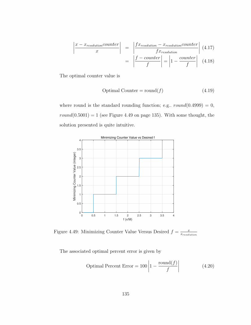
∣∣∣∣x− xresolutioncounterx

∣∣∣∣ =

∣∣∣∣fxresolution − xresolutioncounterfxresolution

∣∣∣∣ (4.17)

=

∣∣∣∣f − counterf

∣∣∣∣ =

∣∣∣∣1− counter

f

∣∣∣∣ (4.18)

The optimal counter value is

Optimal Counter = round(f) (4.19)

where round is the standard rounding function; e.g.. round(0.4999) = 0,

round(0.5001) = 1 (see Figure 4.49 on page 135). With some thought, the

solution presented is quite intuitive.

f (x/M)

0 0.5 1 1.5 2 2.5 3 3.5 4

Min

imiz

ing

Co

un

ter

Va

lue

(in

teg

er)

0

0.5

1

1.5

2

2.5

3

3.5

4Minimizing Counter Value vs Desired f

Figure 4.49: Minimizing Counter Value Versus Desired f = xxresolution

The associated optimal percent error is given by

Optimal Percent Error = 100

∣∣∣∣1− round(f)

f

∣∣∣∣ (4.20)

135

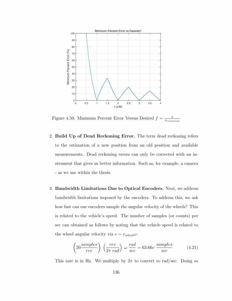
f (x/M)

0 0.5 1 1.5 2 2.5 3 3.5 4

Min

imu

m P

erc

en

t E

rro

r (%

)

0

10

20

30

40

50

60

70

80

90

100Minimum Percent Error vs Desired f

Figure 4.50: Minimum Percent Error Versus Desired f = xxresolution

2. Build Up of Dead Reckoning Error. The term dead reckoning refers

to the estimation of a new position from an old position and available

measurements. Dead reckoning errors can only be corrected with an in-

strument that gives us better information. Such as, for example, a camera

- as we use within the thesis.

3. Bandwidth Limitations Due to Optical Encoders. Next, we address

bandwidth limitations imposed by the encoders. To address this, we ask

how fast can our encoders sample the angular velocity of the wheels? This

is related to the vehicle’s speed. The number of samples (or counts) per

sec can obtained as follows by noting that the vehicle speed is related to

the wheel angular velocity via v = rwheelω:(20samples

rev

) ( rev

2π rad

)ωrad

sec= 63.66v

samples

sec(4.21)

This rate is in Hz. We multiply by 2π to convert to rad/sec. Doing so

136

yields 400v radsec

. Using our factor-of-ten rule then gives BWencoderlimit =

0.1(400v) = 40v radsec

where the vehicle speed v is measured in m/sec; i.e. we

will have an associated 40 v rad/sec encoder-based maximum control band-

width constraint. We see that 40v will be larger than our limit 4 rad/sec

(due to half sample A-to-D zero order hold effect with T = 0.1, see above) if

v > 0.1 msec

or about 8 inchessec

. While this minimum speed constraint is easy to

satisfy, the result suggests that we can have problems at low vehicle speeds.

Speed Estimation and Following Issues. Given the position error

discussion above, it is natural to discuss speed issues. The vehicle speed

can be estimated using equation (4.3) (page 93)

v = rwheelω ≈ (0.05m)

(counts

T sec

) ( rev

8 counts

) ( 2π

rev

)(4.22)

= 0.1571countsm

sec(4.23)

From this, we therefore see that if we give a speed command between

0.1571 counts and 0.1571 (counts + 1), then the speed can oscillate be-

tween these two values and the associated maximum percent speed error

can be 100(

0.1571(counts+1)−0.1571counts0.1571counts

)=(

100counts

)%. Given this, the error

will be less than 10% if counts > 10; i.e. 10counts in a T = 0.1 sam-

pling window or (0.1571)(10) = 1.57 msec

(100 counts/sec). This is smaller

than the maximum observed speed of the fully loaded vehicle (i.e. about

2.3 m/sec). When we observe only count = 5 counts in a T = 0.1 sec

sampling window (or 50 countssec

), the percent error rises to 20%. This corre-

sponds to a speed of (0.1571)(5) = 0.785 msec

. Since the maximum speed is

2.3 m/sec, we are likely to observe at most 2.30.1571

= 14.65 or 14-15 counts

in a T = 0.1 sec sampling window. This will result in a maximum percent

137

speed error of 10015− 100

14or 6.7 − 7.1%. This suggests that we can have

significant speed following issues when low speed reference commands are

issued. The above analysis also suggest that a

single miss count will, at best, result in 6.7− 7.1% speed percent error.

At very low speeds, a single miss count can result in a far greater error.

• IMU Limitations. We now summarize IMU limitations. Within this thesis,

the IMU is used for measuring the orientation θ of the differential-drive Thun-

der Tumbler vehicle. The IMU has a 16 bit output, it has internal built-in

algorithm to calculate absolute angle. Then it follows that we will have an θ

resolution of 360216−1

≈ 0.0055.

From a dynamic standpoint, the IMU is able to provide 100 readings per second

[58], which is 100 Hz. Using our factor-of-ten rule, it follows that BWIMUlimit =

0.1 × 2π(100) ≈ 60rad/s. In our work, we used 10 Hz or 60 rad/sec which

then gives an IMU-based maximum control bandwidth constraint of 6 rad/sec.

Given the above discussions (e.g. 4 rad/sec Arduino A-to-D limitation), this is

not limiting.

For completeness, other IMU properties (although not relevant to the thesis) are

as follows. The IMU possesses the following range characteristics: Accelerome-

ter - ± 2, 4, 6, 8, 16g; Gyro - ± 245, 500, 2000/sec.

Given the above, possibilities for improvement include the following: (1) Com-

bine IMU with wheel encoders (and possibly more encoders) for better estima-

tion of speed/position, (2) Use a higher fidelity IMU together with a camera

and LIDAR.

• Camera Field of View (FOV) Limitations. The Raspberry Pi 5MP cam-

era FOV is limited at 53.5 horizontally and a 41.41 vertically (independent

138

of how it is pointed). A pan-tilt servomechanism could significantly extend the

above FOVs. For a ground robot tracking a quadrotor flying overhead, the

performance can be improved by putting in a pan-tile servomechanism for the

camera. In that way, the camera is able to view a larger area.

• Camera Frame Rate Limitations. According to the Raspberry Pi camera

datasheet [57], the Raspberry Pi camera is capable of 15 fps (frames per second)

at a resolution of 2592 × 1944, 30 fps at 1980 × 1080, 42 fps at 1296 × 972,

and 60 fps at 640 × 480. The lowest frame rate corresponds to 15 Hz or

about 90 rad/sec. Using our factor-of-ten rule, this will constrain performance

to a camera-based maximum control bandwidth constraint of about 9 rad/sec.

Given the above discussions (e.g. 4 rad/sec Arduino A-to-D limitation), this is

not limiting. For our experiments, we used the lowest resolution and hence the

highest frame rate.

• Image Processing Limitations. The algorithm we used for image processing

within this thesis is a color filtering algorithm from [24]. The image is processed

on a Raspberry Pi 3 using Opencv [24]. Given this, the relationship between

frame rate and resolution is given as follows: 1 fps at a resolution of 1080 ×

720 (0.78 MP), 2.5 fps at a resolution of 640 × 480 (0.31 MP), and 10 fps at a

resolution of 320 × 240 (0.08 MP). The image processing has a maximum speed

of 10 fps (10 Hz). Even when the resolution is lower than 320 × 240, the frame

rate does not increase significantly. In the demos which involve image process-

ing, a resolution of 320 × 240 is selected. This gives a processing speed of 10

fps or 10 Hz or about 60 rad/sec. Using our factor-of-ten rule, then gives an

image processing-based maximum control bandwidth of 6 rad/sec. Given the

above discussions (e.g. 4 rad/sec Arduino A-to-D zero order hold half sam-

ple limitation), this is not limiting.

139

• Ultrasonic Sensor Limitations. The SR04 ultrasonic sensor detection range

is from 2 cm to 5 m, and has a maximum reflection (utilization) angle2 of 45

[68]. It can send out a 40 kHz ultrasonic signal every 200 µsec. Consider an

object sitting 2 m away from the sensor. The time delay can be calculated as

∆ = 2×2m340 m

sec≈ 0.0118 sec. This gives a right half plane zero at around z = 2

∆≈

170. Using our factor-of-ten rule, this will constrain the control bandwidth to

(about) an ultrasonics constrained maximum control bandwidth of 17 rad/sec.

Given the above discussions (e.g. 4 rad/sec Arduino A-to-D zero order hold half

sample limitation), this is not limiting.

• Inner-loop Controller: PI vs PID. For all the demos within this thesis, a

PI controller is used within the inner-loop. (See discussions provided in Section

1.2 as well as in Chapter 3.) A PID controller is able to provide more phase

lead than a PI controller. This could be necessary if the armature inductance

is significant. However, our DC motor has an armature inductance around

La ≈ 0.3mH and an armature resistance around Ra ≈ 1 Ω. This combination

gives an approximate high frequency pole at s ≈ −RaLa

= −333. As such, it does

not affect the phase at low frequencies too much. Given this, the choice of a PI

controller within the thesis for inner-loop control, and not a PID controller, is

justified.

2If the ultrasonic sensor is pointed directly at a wall (i.e. 0 pointing angle - measure with respect

to horizontal), it will get a clean reflection. If the angle is increased to 45, the sensor may not get

any reflection back.

140

Differential-Drive Inner-Loop Control Attributes. The following differential-

drive inner-loop attributes are common to all of our demonstrations.

• Thunder Tumbler Differential-Drive Vehicle

• Inner-loop Model: A linear TITO model was examined then ground model was

used for inner-loop control design [15]. The model was discussed earlier in this

chapter as well as in Chapters 1 and 3.

• Inner-Loop Actuators: Two 6V DC motors - one on right wheel, one on left

wheel

• Inner-Loop Sensor: Optical wheel encoders for speed

• Inner-Loop Outputs: Vehicle speed and angular rate; while these are the (com-

puted, not measured) outputs, we actually feed back the encoder measured

quantities (ωR, ωL); all computations are based on equation (4.1) (page 92),

equation (4.2) (page 93), equation (4.3)-(4.4) (page 93).

• Inner-Loop Reference Commands: Speed reference command and angular rate

reference command (vref , ωref )

• Inner-Loop Controller: PI controller with roll-off (on each motor) and reference

command prefilter; PI controller is justified because the map from the references

(vref , ωref ) to the actual speeds (v, ω) looks like a diagonal system diag( as+a

, bs+b

)

after closing the (ωR, ωL) inner-loop; (ωR, ωL) inner-loop is used within in each

of the demonstrations discussed below.

• Inner-Loop Limitations: In this thesis, the actuation rate is 0.1sec, which is

10 Hz or 60 rad/sec. Our factor-of-ten rule then yields a maximum control

bandwidth of 6 rad/sec. The magnetic encoder-based distance traveled along a

straight line is 0.314 counter m.

141

• Possibilities for Improvement: More precise inner-loop sensor (e.g. higher res-

olution commercial optical encoder).

• Summary of Frequency Response Data: Try looks like unity at low frequency;

No peaking; 3dB bandwidth near 2.5 rad/sec

• Summary of Time Responses from Simulations: zero steady state error; No

overshoot; Settling time around 2 sec

• Summary of Time Response from Hardware/Experiments: Some oscillation was

observed in experiments. This is due to wheel encoder limitations (see inner-

loop limitations discussion above). Other nonlinearities to consider include:

stiction in wheels, backlash in gears (due to some spacing between gears), dead-

zone of motors (minimum voltage required to move the robot - loaded/unloaded

Thunder Tumbler), wheel structure (smooth and soft for maximum contact on

hard track vs dimpled and hard for better gripping on soft track)

• Outer Loop Proportional Controller Limitations. All proportional controllers

designed for the (v, θ) outer-loop do not have roll off. While this may amplify

high frequency sensor noise (speed noise from encoders, directional noise from

IMU), it should be noted that the Arduino A-to-D zero order hold ZOH =

1−e−sTs

provides high frequency noise attenuation. This will be examined in

future work.

The following relevant theory (see Chapter 1 for more details) applies to all of our

hardware demonstrations since all demonstrations involve differential-drive Thunder

Tumbler vehicles:

• differential-drive robot modeling [15],[59]

• vision-based line/curve following work within [24]

142

• vehicle separation modeling and longitudinal platoon control work within [3],

[6] (presenting vehicle separation control laws)

Key Hardware Demonstrations. The following describes each demonstration.

1. Cruise Control Along a Line. An effective speed-directional (v, θ) cruise

control system - one that follows speed and direction commands - is an essential

cornerstone to build more complex control capabilities. It builds on the (ωR, ωL)

or (v, ω) inner-loop control law (discussed above).

This demonstration involves the following:

• Outer-Loop Model: A simplified on ground decoupled TITO LTI model is

used for outer-loop control design because of a well-designed (v, ω) inner-

loop control law [15]. See justification of outer-loop below.

• Outer-Loop Sensor: Vehicle orientation θ directly measured by IMU/Cam-

era is to be fed back

• Outer-Loop Output: Vehicle actual speed v is generated by inner-loop and

orientation θ is obtained by IMU/Camera

• Outer-Loop Reference Command: An orientation reference command θref =

0 and a constant speed reference command v = constant is issued to pro-

mote motion along a straight line

• Outer-Loop Controller: A proportional controller (with no roll off) for vehi-

cle orientation θ (direction); vehicle speed is also commanded to inner-loop

– The use of a proportional gain controller is justified because the map

from the references vref and ωref to the actual speeds v and ω looks

like a diagonal system diag( as+a

, bs+b

) (at low frequencies). The outer-

loop θ controller therefore sees bs(s+b)

. From classical root locus ideas,

a proportional controller is therefore justified - provided that the gain

143

is not too large. If the gain is too large, oscillations will be expected

in θ. A PD controller with roll off would help with this issue.

• Performance Tradeoffs: If the proportional gain kθ is large, there will be

oscillations in θ. A PD controller with roll off would help with this issue.

• Limitations: BWencoderlimit ≈ 40v; will be greater than 4 rad/sec if v > 0.1

m/sec. Each vehicle stop and go can result in a 1.5 cm static position error

(see discussion above).

• Possibilities for Improvement: A more precise inner-loop sensor (e.g. more

white-black pair on optical code disk.

• Summary of Frequency Response Data: For θ outer-loop, large kp yields

large bandwidth, large frequency response peaking; small kp yields small

bandwidth, small frequency response peaking; PD control yields large

bandwidth, large frequency response peaking.

• Summary of Time Responses from Simulations: Large kp yields fast re-

sponse, overshoot; small kp yields slow response, no overshoot; PD control

yields fast response, no overshoot.

0 0.5 1 1.5 2 2.5 3 3.5

−1.5

−1

−0.5

0

0.5

1

1.5

Cruise control along a line vref

= 0.5 m/sec

X position (m)

Y p

ositio

n (

m)

Simulation

Hardware

Figure 4.51: Cruise Control Along a Line

144

• Summary of Time Response from Hardware/Experiments: Experiment

data is close to simulation results. Differences can be explained by consid-

ering the following possibilities: stiction in wheels, backlash in gears (due

to some spacing between gears), dead-zone of motors (minimum voltage

required to move the robot - loaded/unloaded Thunder Tumbler), wheel

structure (smooth and soft for maximum contact on hard track vs dimpled

and hard for better gripping on soft track).

• Overview/Conclusion: The robot is issued a reference speed command of

0.5 m/s with θref = 0. The hardware result shows little drift from straight

along the time due to dead reckoning error.

• Relevant Theory: Dhaouadi, et. al. (2013) [15] provides basic TITO LTI

vehicle-motor (v, ω) model for inner-loop design.

2. Separation-Direction Control. When the outer-loop properly exploits an

ultrasonic distance/range-finding sensor, vehicle-target spacing control can be

achieved. Separation-direction (∆x, θ) outer loop and (v, ω) inner loop are

involved. ∆x is measured using ultrasonic sensor, and θ is directly measured by

IMU. Here, y position is not considered, since ultrasonic sensor only provides

almost lineal directional information.

This demonstration involves the following:

• Outer-Loop Model: A simple (decoupled) TITO LTI on ground model is

used for outer-loop control - a consequence of a well-designed inner-loop

- the latter based on the TITO LTI vehicle-motor model within [15]. See

control law justification below.

• Outer-Loop Sensor: Ultrasonic sensor for nearly-lineal separation informa-

tion, vehicle angular velocity ω measured by IMU is integrated to yield the

145

vehicle orientation θ to be fed back

• Outer-Loop Outputs: Position and orientation

• Outer-Loop Reference Commands: A desired separation distance and ori-

entation (θref = 0)

• Outer-Loop Controller: P controller(with no roll off) or PD controller with

roll off

– The use of a proportional gain controller is justified because the map

from the references vref and ωref to the actual speeds v and ω looks

like a diagonal system diag( as+a

, bs+b

) (at low frequencies). The outer-

loop θ controller therefore sees[

bs(s+b)

], and position controller sees

as(s+a)

(since vy is so small, integrating v results in x position). From

classical root locus ideas, a proportional controller is therefore justi-

fied - provided that the gain is not too large. If the gain is too large,

oscillations will be expected. A PD controller with roll off would help

with this issue.

• Performance Tradeoffs: Large kp - fast with large overshoot, small kp -

slow with no overshoot.PD - fast with small overshoot. These are shown

in Figure 4.52 4.53 and 4.54.

146

0 0.5 1 1.5 2 2.5 3 3.5 4 4.5−0.4

−0.2

0

0.2

0.4

0.6

0.8

1

Vehicle separtion convergence Kp = 1.0

Time(seconds)

Po

sitio

n (

m)

Simulation

Hardware

Figure 4.52: Vehicle Separation Convergence Using Proportional Control (Kp = 1;

∆x(0) ≈ 1)

0 2 4 6 8 10 12 14−0.4

−0.2

0

0.2

0.4

0.6

0.8

1

Vehicle separtion convergence Kp = 0.5

Time(seconds)

Po

sitio

n (

m)

Simulation

Hardware

Figure 4.53: Vehicle Separation Convergence Using Proportional Control (Kp = 1;

∆x(0) ≈ 1)

147

0 2 4 6 8 10 12−0.4

−0.2

0

0.2

0.4

0.6

0.8

1

Vehicle separtion convergence Kp = 1.5 Kd = 1

Time(seconds)

Po

sitio

n (

m)

Simulation

Hardware

Figure 4.54: Vehicle Separation Convergence Using PD Control (Kp = 1.5;Kd = 1;

∆x(0) ≈ 1)

• Limitations: The HCSR04 ultrasonic sensor detection range is from 2cm

to 5m, and has a minimum reflection angle of 45. It can send out 40KHz

ultrasonic signal every 200 µs. Consider an object sitting 2m away from

the sensor. The time delay can be calculated as ∆ = 4340≈ 0.0118s. This

gives a (non-minimum phase) right half plane zero at around z = 2∆≈ 170.

This, in turn, imposes a maximum control bandwidth constraint of 17

rad/sec (using standard factor-of-ten rule). It should be noted that the

dead-reckoning error associated with the wheel encoders does not apply

here, since the separation information is measured via ultrasonic sensor

and hence is not cumulative.

• Possibilities for Improvement: While a more precise inner-loop sensor

(e.g. commercial optical rotary encoder) could help, something like a cam-

era or Lidar or GPS can provide useful measurements that can be used to

correct the accumulated dead reckoning error.

• Summary of Frequency Response Data: For the ∆x outer-loop, large kp

148

yields large bandwidth, large frequency response peaking, small kp yields

small bandwidth, small frequency response peaking, PD control yields large

bandwidth, and small frequency response peaking.

• Summary of Time Response from Simulation: Large kp yields fast response,

overshoot; small kp yields slow response, no overshoot; PD control yields

fast response, no overshoot.

• Summary of Time Response from Hardware/Experiment: Data from exper-

iments was found to be close to simulation results (see Figures 4.52-4.54).

The following needs to be considered to adequately explain differences be-

tween simulation and experiment: stiction in wheels, backlash in gears (due

to some spacing between gears), dead-zone of motors (minimum voltage

required to move the robot - loaded/unloaded Thunder Tumbler), wheel

structure (smooth and soft for maximum contact on hard track vs dimpled

and hard for better gripping on soft track).

• Overview/Conclusion: Initially the robot is about 1 meter away from the

target, and we want to keep a 20cm constant spacing through ultrasonic

sensor. Proportional control and PD control is examined. It is shown that

Small kp - slow with no overshoot, large kp - fast with large overshoot. PD

- fast with no overshoot.

• Relevant Theory: Vehicle separation modeling and longitudinal platoon

control work is presented within [3], [6]. Future work will examine more

about the related control saturation prevention ideas presented within [64].

149

4.4 Summary and Conclusion

This chapter has provided a comprehensive case study for our enhanced differential-

drive Thunder Tumbler vehicle. Both simulation and hardware results were presented.

Many demonstrations were thoroughly discussed. All control law developments were

supported by theory. Differences between hardware results and simulation results

were also addressed. Particular focus was placed on the fundamental limitations

impose by system components/subsystems.

150

Chapter 5

LONGITUDINAL CONTROL OF A PLATOON OF VEHICLES


The subject of design and analysis of longitudinal control laws has been studied

extensively from 1960s to 21st new century [1] - [13]. Numerous topics such as vehicle-

follower controllers, nonlinear vehicle dynamics, automated guideway transit systems

has been reported. Even though much effort has been spent on various control laws for

longitudinal control of a platoon of vehicles, however, few experiments had been done

due to expensive hardware. This paper will propose classical control law for platoon

model of electrical vehicles. The concept of this study is to take full advantage of

advances in communication and measurement, using ETT low-cost differential-drive

robots to show how a platoon of vehicles can maintain constant spacing and how

communication among the vehicle network will improve the performance.

Longitudinal platoon of identical vehicles layout is shown in Figure 5.1. For a

change in the lead vehicles velocity, the resulting changes in the spacing can have

different behavior due to different controller design. Simulation results show that

through the appropriate choice of coefficients in the control law, the deviations in

vehicle spacings from their respective steady-state values do not get magnified along

the platoon and in fact get attenuated as one goes down the platoon.

5.2 Platoon Configuration

Figure 5.1 shows the a platoon configuration for a platoon of one leader with 4

followers [3]. The platoon is assumed to move in a straight line. The position of the

151

Figure 5.1: Platoon of 4 Vehicles

i− th vehicles rear bumper with respect to a fixed reference point 0 on the roadside is

denoted by x. The position of the lead vehicles rear bumper with respect to the same

fixed reference point 0 is denoted by xl or x0. Each vehicle is assigned a slot of length

L along the road. As shown, ∆ is the deviation of the i − th vehicle position from

its assigned position. The subscript i is used because ∆i is measured by ultrasonic

sensor located in the i− th vehicle.

Given the platoon configuration in Figure 5.1, elementary geometry shows that:

for i= 2,3,...

∆i(t) := xi−1(t)− xi(t)− L (5.1)

∆i(t) := xi−1(t)− xi(t) (5.2)

∆i(t) := xi−1(t)− xi(t) (5.3)

Kinematics The corresponding kinematic equations for the lead vehicle and the first

vehicle are as follows:

∆1(t) := xl(t)− x1(t)− L (5.4)

∆1(t) := vl(t)− x1(t) (5.5)

∆1(t) := al(t)− x1(t) (5.6)

152

5.3 Modeling for Longitudinal Platoon of Vehicles

As we discussed in 3.7.3, the on ground inner-loop (ωR, ωL) plant:

P[ωR,ωL] ≈ 11.268

[1.159

s+ 1.159

]× I2×2 (5.7)

will be used to as basis our vehicle model for platoon. The vehicle model for lon-

gitudinal control is shown in Figure 5.2 and 5.3, where bypass signal to inner loop

controller is a safety feature to realize negative control informally due to encoder lim-

itation. When this signal is set to 1, we applied constant negative PWM command

in that control period to our motor neglecting the current control signal generated by

inner loop controller. More detailed discussion can be found in later section about

platoon experimental result.

Figure 5.2: Leader Model of Platoon

Figure 5.3: i-th Vehicle Model of Platoon

In this model, we made the following assumption: all vehicles are identical, in

each vehicle left and right sides are symmetric, and no wind gust. In practical, lateral

153

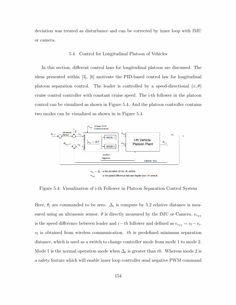
deviation was treated as disturbance and can be corrected by inner loop with IMU

or camera.

5.4 Control for Longitudinal Platoon of Vehicles

In this section, different control laws for longitudinal platoon are discussed. The

ideas presented within [3], [6] motivate the PID-based control law for longitudinal

platoon separation control. The leader is controlled by a speed-directional (v, θ)

cruise control controller with constant cruise speed. The i-th follower in the platoon

control can be visualized as shown in Figure 5.4. And the platoon controller contains

two modes can be visualized as shown in in Figure 5.4.

Figure 5.4: Visualization of i-th Follower in Platoon Separation Control System

Here, θi are commanded to be zero. ∆i is compute by 5.2 relative distance is mea-

sured using an ultrasonic sensor. θ is directly measured by the IMU or Camera. evff

is the speed difference between leader and i− th follower and defined as evff = vl−vi.

vl is obtained from wireless communication. th is predefined minimum separation

distance, which is used as a switch to change controller mode from mode 1 to mode 2.

Mode 1 is the normal operation mode when ∆i is greater than th. Whereas mode 2 is

a safety feature which will enable inner loop controller send negative PWM command

154

Figure 5.5: Visualization of Platoon Controller

to motor directly and bypass PWM command generated by inner loop controller. Kx

is a PID controller with respect to separation error exi (∆i), we named it ∆x path .

Kθ is a PD controller with respect to orientation error eθ. Kff is a PI controller with

respect to speed difference between leader and follower, we named it feed-forward

path (FF-path).


references vref and ωref to the actual speeds (v, ω) looks like a diagonal system

diag(

as+a

, bs+b

)(at low frequencies). This is a consequence of a well-designed inner-


, and position con-

troller sees[

bs(s+b)

](since vy is so small, integrating v results in x position). From

classical root locus ideas, a proportional controller is therefore justified - provided

that the gain is not too large. If the gain is too large, oscillations will be expected.

A PD controller with roll off would help with this issue. The additional control effort

from communication path works like feed-forward and help reduced overshoot.

155

5.5 Longitudinal Platoon Separation Controller Tradeoff Study

In this section, we examined different types of controller design. Specifically,

• Proportional Control for ∆x path

• PD Control for ∆x path

• PID Control for ∆x path

• PID Control for ∆x path

• PID Control for ∆x path + Proportional Control for FF-path

• PID Control for ∆x path + PI control for FF-path

Proportional Control for ∆x path. Proportional control for ∆x is used, and no

leader information.

0 5 10 15 20 25 300

0.5

1

1.5

Simulation result of platoon of 5 vehicle

Time(seconds)

Ve

hic

le S

ep

ratio

n (

m)

Reference

Follower 1

Follower 2Follower 3

Follower 4

Follower 5

Figure 5.6: Simulation of Vehicle Separation Control of Platoon (Proportional Control

for ∆x (Kp = 0.5)

156

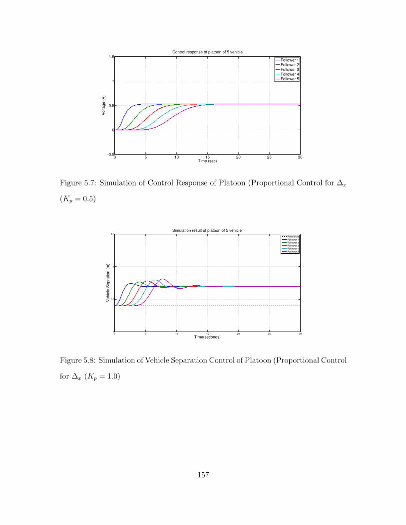
0 5 10 15 20 25 30−0.5

0

0.5

1

1.5Control response of platoon of 5 vehicle

Time (sec)

Vo

lta

ge

(V

)

Follower 1Follower 2Follower 3Follower 4Follower 5

Figure 5.7: Simulation of Control Response of Platoon (Proportional Control for ∆x

(Kp = 0.5)

0 5 10 15 20 25 300

0.5

1

1.5


Time(seconds)

Ve

hic

le S

ep

ratio

n (

m)

Reference

Follower 1


Follower 4

Follower 5

Figure 5.8: Simulation of Vehicle Separation Control of Platoon (Proportional Control

for ∆x (Kp = 1.0)

157

0 5 10 15 20 25 30−0.5

0

0.5

1


Time (sec)

Vo

lta

ge

(V

)



(Kp = 1.0)

0 5 10 15 20 25 300

0.5

1

1.5


Time(seconds)

Ve

hic

le S

ep

ratio

n (

m)

Reference

Follower 1


Follower 4

Follower 5

Figure 5.10: Simulation of Vehicle Separation Control of Platoon (Proportional Con-

trol for ∆x (Kp = 2.0)

158

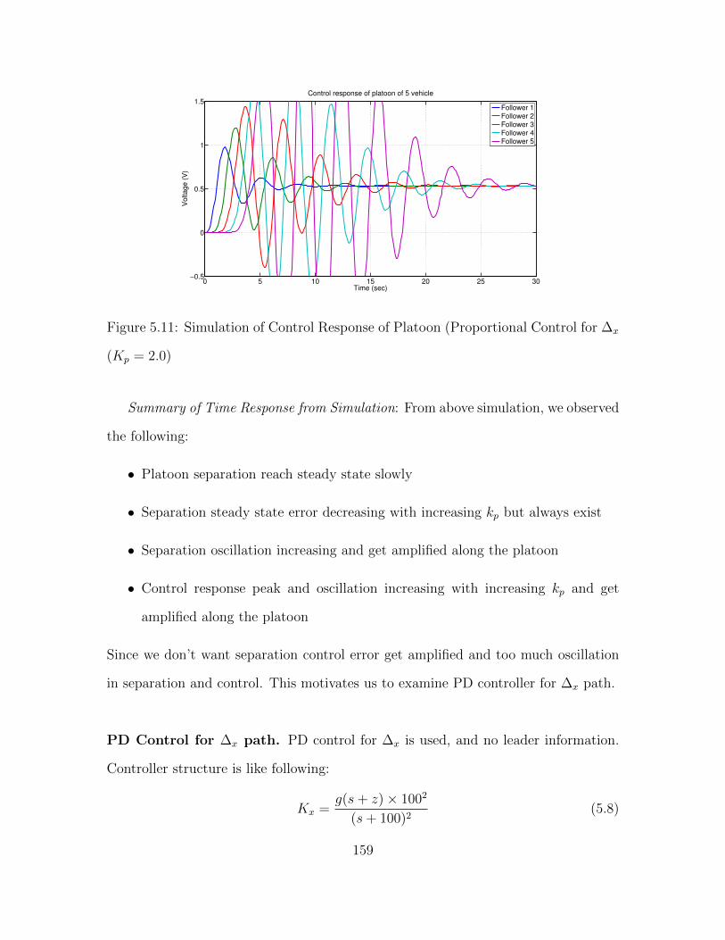
0 5 10 15 20 25 30−0.5

0

0.5

1


Time (sec)

Vo

lta

ge

(V

)



(Kp = 2.0)

Summary of Time Response from Simulation: From above simulation, we observed

the following:

• Platoon separation reach steady state slowly

• Separation steady state error decreasing with increasing kp but always exist

• Separation oscillation increasing and get amplified along the platoon

• Control response peak and oscillation increasing with increasing kp and get

amplified along the platoon

Since we don’t want separation control error get amplified and too much oscillation

in separation and control. This motivates us to examine PD controller for ∆x path.

PD Control for ∆x path. PD control for ∆x is used, and no leader information.

Controller structure is like following:

Kx =g(s+ z)× 1002

(s+ 100)2(5.8)

159

where, z = 5 and two roll-off is used to reduce overshoot from derivation-term. Note

here kd = g and kp = gz.

0 5 10 15 20 25 300

0.5

1

1.5


Time(seconds)

Ve

hic

le S

ep

ratio

n (

m)

Reference

Follower 1


Follower 4

Follower 5

Figure 5.12: Simulation of Vehicle Separation Control of Platoon (PD Control for ∆x

(g = 0.2))

0 5 10 15 20 25 30−0.5

0

0.5

1


Time (sec)

Vo

lta

ge

(V

)


Figure 5.13: Simulation of Control Response of Platoon (PD Control for ∆x (g = 0.2))

160

0 5 10 15 20 25 300

0.5

1

1.5


Time(seconds)

Ve

hic

le S

ep

ratio

n (

m)

Reference

Follower 1


Follower 4

Follower 5


(g = 0.5))

0 5 10 15 20 25 30−0.5

0

0.5

1


Time (sec)

Vo

lta

ge

(V

)


Figure 5.15: Simulation of Control Response of Platoon (PD Control for ∆x (g = 0.5))


the following:

• Platoon separation reach steady state faster than proportional control

• Separation steady state error getting smaller and with increasing g, but still

exist

161

• Separation oscillation don’t get amplified along the platoon with small g

• Control response peak and oscillation get smaller with small g and get attenu-

ated along the platoon

While a bigger g (kd) can reach smaller steady state separation error, more oscilla-

tion is observed in transient response for separation as well as control. To reach zero

steady state error in platoon separation control, PID controller for ∆x path will be

examined first, then feed-forward path is introduced to reduce oscillation.

162

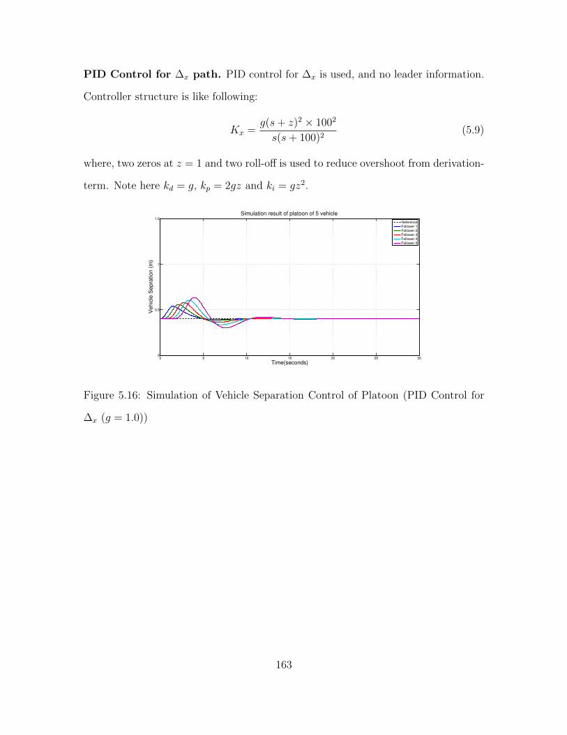
PID Control for ∆x path. PID control for ∆x is used, and no leader information.

Controller structure is like following:

Kx =g(s+ z)2 × 1002

s(s+ 100)2(5.9)

where, two zeros at z = 1 and two roll-off is used to reduce overshoot from derivation-

term. Note here kd = g, kp = 2gz and ki = gz2.

0 5 10 15 20 25 300

0.5

1

1.5


Time(seconds)

Ve

hic

le S

ep

ratio

n (

m)

Reference

Follower 1


Follower 4

Follower 5

Figure 5.16: Simulation of Vehicle Separation Control of Platoon (PID Control for

∆x (g = 1.0))

163

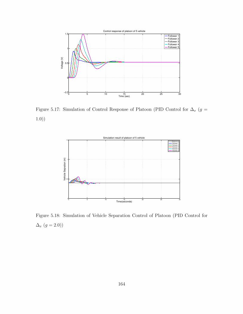
0 5 10 15 20 25 30−0.5

0

0.5

1


Time (sec)

Vo

lta

ge

(V

)


Figure 5.17: Simulation of Control Response of Platoon (PID Control for ∆x (g =

1.0))

0 5 10 15 20 25 300

0.5

1

1.5


Time(seconds)

Ve

hic

le S

ep

ratio

n (

m)

Reference

Follower 1


Follower 4

Follower 5


∆x (g = 2.0))

164

0 5 10 15 20 25 30−0.5

0

0.5

1


Time (sec)

Vo

lta

ge

(V

)



2.0))


the following:

• Platoon separation reach steady state faster than proportional control

• Separation steady state error becomes zero

• Separation oscillation get amplified along the platoon

• Control response peak and oscillation get amplified along the platoon

While a PID controller can reach zero steady state error in separation, more oscillation

is observed in transient response for separation as well as control. Feed-forward path

is needed to reduce oscillation.

165

PID Control for ∆x path + Proportional Control for Feed-forward. Here,

PID control for ∆x is used, and wireless communication is used to get leader speed

information and proportional control for feed-forward error ev = vl−vi. The controller

output is sum of ∆x path and feed-forward path. Controller structure is like following:

Klongitudinal = Kx +Kff (5.10)

Kx =g(s+ z)2 × 1002

s(s+ 100)2(5.11)

Kff = kpff (5.12)

where, two zeros at z = 1, g = 1 and two roll-off is used to reduce overshoot from

derivation-term. kpff denotes the proportional gain using at FF path. Note here

kd = g, kp = 2gz and ki = gz2.

0 5 10 15 20 25 300

0.5

1

1.5


Time(seconds)

Ve

hic

le S

ep

ratio

n (

m)

Reference

Follower 1


Follower 4

Follower 5


∆x (g = 1.0, z = 1.0) and kpff = 0.5 for FF-path)

166

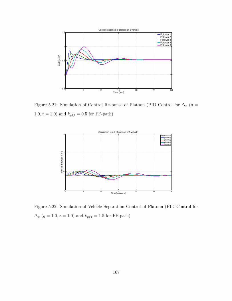
0 5 10 15 20 25 30−0.5

0

0.5

1


Time (sec)

Vo

lta

ge

(V

)



1.0, z = 1.0) and kpff = 0.5 for FF-path)

0 5 10 15 20 25 300

0.5

1

1.5


Time(seconds)

Ve

hic

le S

ep

ratio

n (

m)

Reference

Follower 1


Follower 4

Follower 5


∆x (g = 1.0, z = 1.0) and kpff = 1.5 for FF-path)

167

0 5 10 15 20 25 30−0.5

0

0.5

1


Time (sec)

Vo

lta

ge

(V

)



1.0, z = 1.0) and kpff = 1.5 for FF-path)


the following:

• Platoon separation reach steady state slower than PID control


• Separation oscillation don’t get amplified significantly along the platoon

• Control response peak and oscillation get amplified along the platoon

Compared to a PID controller, zero steady state error in separation is also reached.

Moreover smaller oscillation is observed in transient response for separation. But

control transient response still shows clear oscillation and get amplified along the

platoon and cannot easily solved by increasing kpff , which lead to using PI control

in Feed-forward path.

168

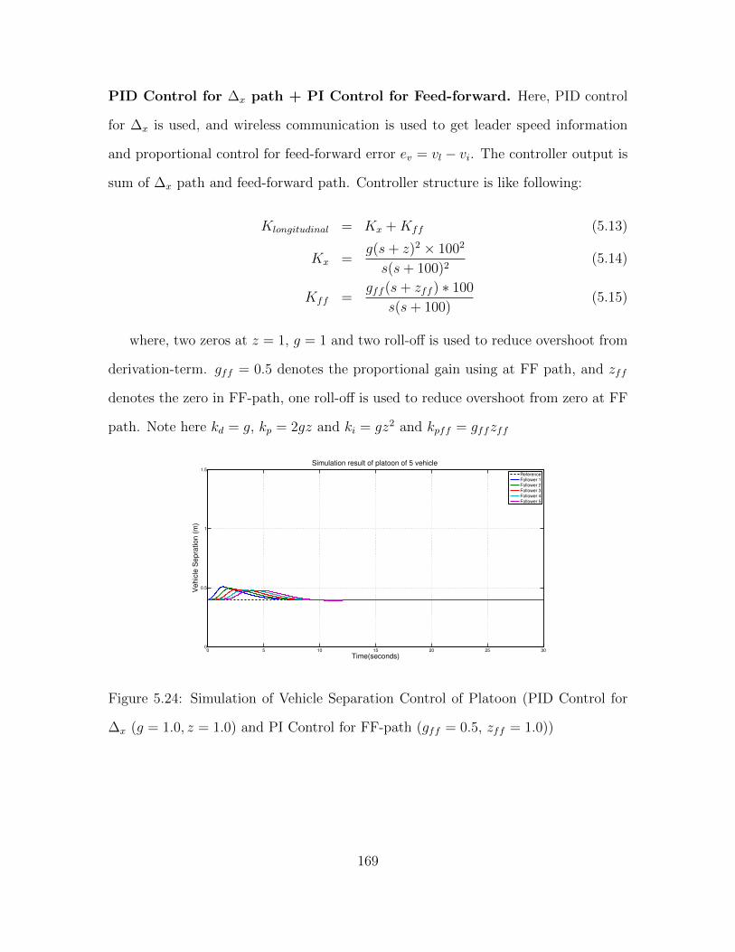
PID Control for ∆x path + PI Control for Feed-forward. Here, PID control

for ∆x is used, and wireless communication is used to get leader speed information

and proportional control for feed-forward error ev = vl − vi. The controller output is

sum of ∆x path and feed-forward path. Controller structure is like following:

Klongitudinal = Kx +Kff (5.13)

Kx =g(s+ z)2 × 1002

s(s+ 100)2(5.14)

Kff =gff (s+ zff ) ∗ 100

s(s+ 100)(5.15)

where, two zeros at z = 1, g = 1 and two roll-off is used to reduce overshoot from

derivation-term. gff = 0.5 denotes the proportional gain using at FF path, and zff

denotes the zero in FF-path, one roll-off is used to reduce overshoot from zero at FF

path. Note here kd = g, kp = 2gz and ki = gz2 and kpff = gffzff

0 5 10 15 20 25 300

0.5

1

1.5


Time(seconds)

Ve

hic

le S

ep

ratio

n (

m)

Reference

Follower 1


Follower 4

Follower 5


∆x (g = 1.0, z = 1.0) and PI Control for FF-path (gff = 0.5, zff = 1.0))

169

0 5 10 15 20 25 30−0.5

0

0.5

1


Time (sec)

Vo

lta

ge

(V

)



1.0, z = 1.0) and PI Control for FF-path (gff = 0.5, zff = 1.0))

0 5 10 15 20 25 300

0.5

1

1.5


Time(seconds)

Ve

hic

le S

ep

ratio

n (

m)

Reference

Follower 1


Follower 4

Follower 5


∆x (g = 1.0, z = 1.0) and PI Control for FF-path (gff = 0.5, zff = 2.0))

170

0 5 10 15 20 25 30−0.5

0

0.5

1


Time (sec)

Vo

lta

ge

(V

)



1.0, z = 1.0) and PI Control for FF-path (gff = 0.5, zff = 2.0))


the following:

• Platoon separation reach steady state fast


• Separation oscillation get attenuated along the platoon

• Control response peak and oscillation get attenuated along the platoon

Compared to a last design, zero steady state error in separation is also reached and

much smaller oscillation is observed in transient response for separation. Besides,

control transient response also get attenuated along the platoon. Oscillatory behav-

ior in control is observed when zff it too big.

Summary of Tradeoff Study In this section, we examined five different controllers

design with and without feed-forward path enabled by wireless communication. From

171

the discussion, we noticed that ultrasonic-based PID controller for ∆x path is sufficient

to stabilize the platoon separation control. However, increasing control effort of the

platoon reveals that the size of the platoon cannot be scaled arbitrarily because of

hardware saturation limitation on control. By introducing integration term in feed-

forward path and properly choosing the controller parameters, we can not only get

monotonically decreasing separation error, but also have decreasing control response

in transient.

5.6 Experimental Results for Controlled Platoon of Vehicles

In this section, we examined our controller design through three controller design:

Design parameters of three different controllers are given in Table 5.1.

Design No. ∆x Path Feed-Forward Path

1 Kp = 1 N/A

2 Kp = 1.5, Kd = 0.2 Kp = 0.5

3 Kp = 1.0, Ki = 0.5, Kd = 0.3 Kp = 0.4, Ki = 0.6

Table 5.1: Platoon Design Parameter

For all the experiments six(6) ETTs are used. Simulation as well as hardware

will be provided to verify our design. For all simulation and hardware experiment,

∆xref = 0.4, and leader cruise speed is set to 0.3m/sec.

172

Design 1. Proportional control for ∆x is used, and no leader information. Simulation

result is shown in Figure 5.28 and 5.29

0 5 10 15 20 25 300

0.5

1

1.5


Time(seconds)

Ve

hic

le S

ep

ratio

n (

m)

Reference

Follower 1


Follower 4

Follower 5

Figure 5.28: Simulation of Vehicle Separation Control of Platoon (Proportional Con-

trol for ∆x (Kp = 1)

0 5 10 15 20 25 30−0.5

0

0.5

1


Time (sec)

Vo

lta

ge

(V

)



(Kp = 1)

Hardware result of platoon of 6 vehicles is shown in Figure 5.30

173

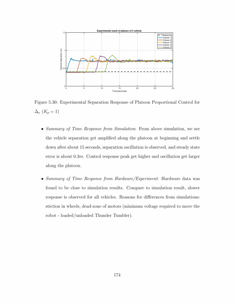
0 5 10 15 20 25 30

Time(seconds)

0

0.5

1

1.5

Ve

hic

le S

ep

ratio

n (

m)

Experimental result of platoon of 5 vehicle

Reference

Follower 1

Follower 2

Follower 3

Follower 4

Follower 5

Figure 5.30: Experimental Separation Response of Platoon Proportional Control for

∆x (Kp = 1)

• Summary of Time Response from Simulation: From above simulation, we see

the vehicle separation get amplified along the platoon at beginning and settle

down after about 15 seconds, separation oscillation is observed, and steady state

error is about 0.3m. Control response peak get higher and oscillation get larger

along the platoon.

• Summary of Time Response from Hardware/Experiment: Hardware data was

found to be close to simulation results. Compare to simulation result, slower

response is observed for all vehicles. Reasons for differences from simulations:

stiction in wheels, dead-zone of motors (minimum voltage required to move the

robot - loaded/unloaded Thunder Tumbler).

174

Design 2. PD control for ∆x and proportional control for feed-forward path (FF-

Path) speed difference between leader and follower. Leader speed information is

broadcasted to followers through wireless communication. Simulation result is shown

in Figure 5.31 and 5.32

0 5 10 15 20 25 300

0.5

1

1.5


Time(seconds)

Ve

hic

le S

ep

ratio

n (

m)

Reference

Follower 1


Follower 4

Follower 5


(Kp = 1.5, Kd = 0.2) and Proportional control for FF Path (Kp = 0.5))

0 5 10 15 20 25 300

0.1

0.2

0.3

0.4

0.5

0.6

0.7


Time (sec)

Vo

lta

ge

(V

)


Figure 5.32: Simulation of Control Response of Platoon (PD Control for ∆x (Kp =

1.5, Kd = 0.2) and Proportional control for FF Path (Kp = 0.5))

175


0 5 10 15 20 25 30

Time(seconds)

0

0.5

1

1.5

Ve

hic

le S

ep

ratio

n (

m)


Reference

Follower 1

Follower 2

Follower 3

Follower 4

Follower 5

Figure 5.33: Experimental Separation Response of Platoon (PD Control for ∆x (Kp =

1.5, Kd = 0.2) and Proportional control for FF Path (Kp = 0.5))


the vehicle separation does not get amplified along the platoon at beginning

and settle down after about 8 seconds, no oscillation is observed, and steady

state error is about 0.2m. Control response peak get smaller along the platoon

and smaller oscillation is observed, no negative control is observed.


found to be close to simulation results. Compare to simulation result, higher

separation error and little oscillation at beginning is shown in hardware result.

Reasons for differences from simulations: stiction in wheels, backlash in gears ,

dead-zone of motors , wheel structure, negative control is informally applied to

motor directly using bypass mechanism.

176

Design 3. PID control for ∆x and PI control for feed-forward path (FF-Path) speed

difference between leader and follower. Leader speed information is broadcasted to

followers through wireless communication. Simulation result is shown in Figure 5.34

and 5.35

0 5 10 15 20 25 300

0.5

1

1.5


Time(seconds)

Ve

hic

le S

ep

ratio

n (

m)

Reference

Follower 1


Follower 4

Follower 5


∆x (Kp = 1.0, Ki = 0.5, Kd = 0.3) and Proportional control for FF Path (Kp =

0.4, Ki = 0.6))

0 5 10 15 20 25 30−0.5

0

0.5

1


Time (sec)

Vo

lta

ge

(V

)


Figure 5.35: Simulation of Control Response of Platoon (PID Control for ∆x (Kp =

1.0, Ki = 0.5, Kd = 0.3) and Proportional control for FF Path (Kp = 0.4, Ki = 0.6))

177


0 5 10 15 20 25 300

0.5

1

1.5


Time(seconds)

Ve

hic

le S

ep

ratio

n (

m)

Reference

Follower 1


Follower 4

Follower 5

Figure 5.36: Experimental Separation Response of Platoon (PID Control for ∆x

(Kp = 1.0, Ki = 0.5, Kd = 0.3) and Proportional control for FF Path (Kp = 0.4, Ki =

0.6))


the vehicle separation get attenuated along the platoon and settle down after

about 10 seconds, no oscillation is observed, zero steady state error is reached.

Control response peak get smaller along the platoon and small oscillation is

observed, no negative control is observed.


found to be close to simulation results. Compare to simulation result, higher

separation error and little oscillation at beginning is shown in hardware result.

Reasons for differences from simulations: stiction in wheels, backlash in gears,

dead-zone of motors, wheel structure, negative control is informally applied to

motor directly using bypass mechanism.

178

5.7 Platoon Simulation with model Uncertainty and Stiction Deadzone

In this section, we will show how platoon controller performance degrades when

model variation and deadzone effect from stiction has been considered into simulation.

The result is only shown for design 3 last section to show future research direction.

For model uncertainty, we choose 5 ETTs ground model arbitrarily from all 9 ETTs.

Stiction deadzone is randomly set to be 0.82V ,1.24V ,0.99V, 0.58V, 0.83V.

0 5 10 15 20 25 30

Time (sec)

-0.5

0

0.5

1

1.5

Vo

lta

ge

(V

)

Control response of platoon of 5 vehicle

Follower 1

Follower 2

Follower 3

Follower 4

Follower 5

Figure 5.37: Simulation of Separation Response of Platoon with model uncertainty

and stiction

179

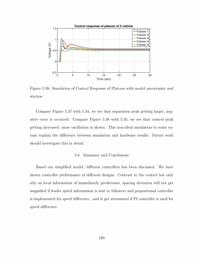
0 5 10 15 20 25 30

Time (sec)

-0.5

0

0.5

1

1.5

Vo

lta

ge

(V

)

Control response of platoon of 5 vehicle

Follower 1

Follower 2

Follower 3

Follower 4

Follower 5

Figure 5.38: Simulation of Control Response of Platoon with model uncertainty and

stiction

Compare Figure 5.37 with 5.34, we see that separation peak getting larger, neg-

ative error is occurred. Compare Figure 5.38 with 5.35, we see that control peak

getting increased, more oscillation is shown. This non-ideal simulation to some ex-

tant explain the difference between simulation and hardware results. Future work

should investigate this in detail.


Based our simplified model, different controllers has been discussed. We have

shown controller performance of different designs. Contrast to the control law only

rely on local information of immediately predecessor, spacing deviation will not get

magnified if leader speed information is sent to followers and proportional controller

is implemented for speed difference , and it get attenuated if PI controller is used for

speed difference.

180

Chapter 6

SUMMARY AND FUTURE DIRECTIONS

6.1 Summary of Work

This thesis addressed many design, analysis, and control issues that are critical

to achieve the longer-term FAME objective. The following summarizes key themes

within the thesis.

1. Update Low-Cost FAME Mobile Robot Platform. In previous work of

Lin [14], It was shown how off-the-shelf components could be used to build a low-

cost multi-capability ground vehicle that can be used for serious robotics/FAME

research. Based on his work, we carefully redesign the platform. Main improve-

ment as following:

• Encoder. Optical wheel-encoders which 2.5 times accurate than magnetic

based one was developed to increase measuring accuracy of speed.

• IMU. Absolute orientation sensor BNO055 IMU can give out vehicle ori-

entation directly that LSM9DS0 can only get angular rate and, this can

benefit outer-loop design when θ is needed.

• Onboard Microcontroller. Raspberry Pi 3 with more computation

power than pi 2, this would benefit when image processing is needed, ex-

perimental results showed FPS increase from 8 to 10.

• Communication Capability. TL-WN722N WiFi USB adapter with ex-

ternal antenna which can support more stable communication compared

181

to Edimax Wi-Fi adapter in longer distance. Duplex serial communication

protocol is designed, we can record more vehicle running states on SD card

on Pi 3. Previously, we just have 1K EEPROM on Uno can be used for

this purpose.

• Unified Software Architecture. All outer loops have been implemented

on Pi 3, inner loop is fixed on Arduino Uno. One can switch different

controllers easily by command interface written in C.

2. FAME Architecture. A general FAME architecture has been described one

that can accommodate a large fleet of vehicles.

3. Literature Survey. A fairly comprehensive literature survey of relevant work

was presented.

4. Modeling. Kinematic and dynamic models for both vehicle types were pre-

sented and analyzed to understand the full utility of each model. Motor dynam-

ics includes gearbox transmission was developed, all modeling parameters have

been carefully measured. Uncertainty of those parameters has been captured

using several enhanced thunder tumbler. A TITO LTI differential-drive vehicle-

motor model was first examined as the basis for inner-loop control, then has

been modified as on ground model which including practical factors like friction

and battery internal resistance. This on ground model becomes foundation of

inner loop design, and all other works follows. Outer-loop control was facili-

tated by having a well-designed inner-loop - thus permitting a simple classical

outer-loop design. Relevant model trade studies were conducted in order to

understand the impact of vehicle parameters for differential-drive.

182

5. Control for Single Vehicle. Both inner-loop and outer-loop control designs

were discussed in the context of an overall hierarchical control inner-outer loop

framework. This framework lends itself to accommodate multiple modes of

operation; e.g. cruise control along a line, separation control. Comprehensive

inner-loop trade studies were conducted for the differential-drive class of vehi-

cles.

6. Control for Multiple Vehicle. For longitudinal platoon separation control,

we proposed platoon controller framework based on classical control with feed-

forward path. Comprehensive platoon controller trade studies were conducted

for the differential-drive class of vehicles.

7. Hardware Demonstrations. Many hardware demonstrations were conducted

- with simulation data corroborating the hardware results. The limitations of

the hardware (e.g. encoders, A-to-D, vehicle) was discussed to shed light on

differences between the data sets.

6.2 Directions for Future Research

Future work will involve each of the following:

• Localization. Development of a lab-based localization system using a variety

of technologies (e.g. cameras, lidar, ultrasonic, etc.). Localization is essential

for multi-robots cooperating. Once each robot knows where it is and where the

other robots are, more complicated robot cooperation can be performed.

• Onboard Sensing. Addition of multiple onboard sensors; e.g. additional ul-

trasonics, cameras, lidar, GPS, etc.

183

• Advanced Image Processing. Use of advanced image processing and opti-

mization algorithms [60]

• Multi-Vehicle Cooperation. Cooperation between ground, air, and sea ve-

hicles - including quadrotors, micro-air vehicles and eventually nano-air vehicles.

• Parallel Onboard Computing. Use of multiple processors on a robot for

computationally intense work; e.g. onboard optimization and decision making.

• Environment Mapping. Rapid and efficient mapping of unknown and par-

tially known areas via multiple robotic agents.

• Modeling and Control. More accurate dynamic models and control laws.

This can include the development of multi-rate control laws that can signifi-

cantly lower sampling requirements.

• Control-Centric Vehicle Design. Understanding when simple control laws

are possible and when complex control laws are essential. This includes under-

standing how control-relevant specifications impact (or can drive) the design of

a vehicle.

184

REFERENCES

[1] Caudill R. J., Garrard W. L., “Vehicle-follower longitudinal control for auto-mated transit vehicles,” Journal of Dynamic Systems, Measurement, and Control, pp. 241-248, 1977.

[2] Chiu, Harry Y, George B. Stupp., “Vehicle-follower control with variable-gainsfor short headway automated guideway transit systems,” Journal of DynamicSystems, Measurement, and Control , pp. 183-189, 1977.

[3] S.E. Sheikholeslam, C. Desoer, “Longitudinal Control of a Platoon of Vehicles,”American Control Conference, IEEE, pp. 291-296, 1990.

[4] S.E. Sheikholeslam, C. Desoer, “Longitudinal Control Of A Platoon Of Vehicles. I,Linear Model,” California Partners for Advanced Transit and Highways (PATH),1989.

[5] S.E. Sheikholeslam, C. Desoer, “Longitudinal control of a platoon of vehicles.III, Nonlinear model,” California Partners for Advanced Transit and Highways(PATH), 1990.

[6] S.E. Sheikholeslam, “Longitudinal control of a platoon of vehicles with no com-munication of lead vehicle information: a system level study,” IEEE Transactionson vehicular technology , vol. 42, pp.546-554, 1991.

[7] Hedrick, J. K., Mcmahnon D. H., and Swaroop D., “Vehicle modeling and controlfor automated highway systems,” California Partners for Advanced Transit andHighways (PATH), 1993.

[8] Varaiya, P., “Smart cars on smart roads: problems of control.,” IEEE Transac-tions on automatic control , vol. 38 , pp.195-207, 1993.

[9] Hedrick, J. K., Mcmahnon D. H., and Swaroop D., “Longitudinal control de-velopment for IVHS fully automated and semi-automated systems: Phase III,”California Partners for Advanced Transit and Highways (PATH), 1996.

[10] Datta N. G., and Lygeros J., “Longitudinal control of the lead car of a platoon,”IEEE Transactions On Vehicular Technology, vol. 43 , pp.1125-1135, 1994.

[11] Liang N. G., and Lygeros J., “Optimal adaptive cruise control with guaranteedstring stability,” Vehicle System Dynamics, vol. 32 , pp.313-330, 1999.

[12] Stankovic, S. S., Stanojevic M. J., and Siljak D. D., “Decentralized Overlap-ping Control of a Platoon of Vehicles,” IEEE Transactions on Control SystemsTechnology , vol. 8 , pp.816-832, 2000.

[13] Jovanovic, M. R., Bamieh B.,, “On the ill-posedness of certain vehicular platooncontrol problems,” IEEE Transactions on Automatic Control , vol. 50 , pp.1307-1321, 2005.

185

[14] Lin Z., Modeling, Design and Control of Multiple Low-Cost Robotic Ground Ve-hicles, Arizona State University, MS Thesis, 2015.

[15] Dhaouadi R. and A. A. Hatab, “Dynamic Modeling of Differential-Drive MobileRobots using Lagrange and Newton-Euler Methodologies: A Unified Framework,”Adv Robot Autom 2.107, 2013.

[16] “Rotary Electrodynamics of a DC Motor: Motor as Mechanical Capacitor,”http://www2.ece.ohio-state.edu/~passino/lab2_rotary_dynamics.pdf.

[17] Ribeiro M. I., Lima P., “Kinematic models of mobile robots,” Instituto de Sis-temas e Robotica, 2002: 1000-1049.

[18] R. Fierro and F.L. Lewis, “Control of a nonholonomic mobile robot: backstep-ping kinematics into dynamics,” Proceedings of the 34th IEEE Conference In De-cision and Control, volume 4, 1995.

[19] Kanayama Y, Kimura Y, Miyazaki F, et al, “A stable tracking control methodfor an autonomous mobile robot,” Proceedings of IEEE International Conferenceon Robotics and Automation, pp. 384-389, 1990.

[20] Petrov P., “Modeling and adaptive path control of a differential drive mobilerobot,” Proceedings of the 12th WSEAS international Conference on AutomaticControl, Modelling & Simulation, pp. 403-408, 2010.

[21] A.M. Bloch, M. Reyhanoglu and H. McClamorch, “Control and stabilization ofnonholonomic dynamic systems,” IEEE Transactions On Automatic Control, 37,11, pp. 1746-1757, 1992.

[22] Gholipour A, Yazdanpanah M J., “Dynamic Tracking Control of NonholonomicMobile Robot with Model Reference Adaptation for Uncertain Parameters,” Eu-ropean Control Conference (ECC), University of Cambridge, UK, 2003.

[23] Pepy R., Lambert A., and Mounier H., “Path Planning using a Dynamic VehicleModel,” Information and Communication Technologies, ICTTA’06. 2nd. IEEE,1: 781-786, 2006.

[24] Bradski G. and Kaehler A., “Learning OpenCV: Computer vision with theOpenCV library,” O’Reilly Media, Inc., 2008.

[25] Vieira, F.C., Medeiros, A.A.D., Alsina, P.J., Araujo, A.P., “Position and Ori-entation Control of a Two-Wheeled Differentially Driven Nonholonomic MobileRobot,” ICINCO Proceedings, 7 pages, 2004.

[26] Rodriguez, A.A., Analysis and Design of Multivariable Feedback Control Systems,Control3D, L.L.C., Tempe, AZ, 2002.

[27] R. DeSantis, “Path-tracking for a tractor-trailer-like robot,” Int. J. Rob. Re-search, Vol. 13, No. 6, pp. 533-543, 1994.

186

http://www2.ece.ohio-state.edu/~passino/lab2_rotary_dynamics.pdf

[28] B. Andrea-Novel, B. Campion, G. Bastin, “Control of nonholonomic wheeledmobile robots by state feedback linearization,” The Int. J.

[29] Aguiar A. P., Dacic D. B., Hespanha J. P., et al., “Path-following or reference-tracking,” 2004.

[30] F. del Rio, G. Jimenez, J. Sevillano, S. Vicente, A.Balcells, “A path followingcontrol for unicycle robots, ” J. Rob. Systems, Vol. 18, No.7, pp.325-342, 2001.

[31] M. El-Hawwary, M. Maggiore, “Global path following for unicycle and otherresults,” Proc. IEEE American Contr. Conference, pp. 3500-3505, 2008.

[32] K. J. Astrom and T. Hagglund, PID Controllers: Theory, Design, and Tuning,Instrument Society of America, Research Triangle Park, North Carolina, 1995.

[33] Marino R, Scalzi S, Cinili F., “Nonlinear PI front and rear steering control infour wheel steering vehicles,” Vehicle System Dynamics, 2007, 45(12): 1149-1168.

[34] De Silva C. W., Sensors and actuators: control system instrumentation, CRCPress, 2007.

[35] FUJH T, MIZUSHIMA N. A New Approach to LQ Design: Application to theDesign of Optimal Servo Systems. 1987.

[36] Arduino Uno description, https://www.arduino.cc/en/Main/arduinoBoardUno

[37] LCR meter, https://en.wikipedia.org/wiki/LCR_meter.

[38] TB6612FNG datasheet, https://www.sparkfun.com/datasheets/Robotics/TB6612FNG.pdf.

[39] Raspberry Pi 3 benchmarks, https://www.raspberrypi.org/magpi/raspberry-pi-3-specs-benchmarks/.

[40] Energizer AA Battery, http://data.energizer.com/PDFs/nickelmetalhydrideappman.pdf.

[41] Raspberry Pi 3 v.s. Pi 2, http://www.techrepublic.com/article/raspberry-pi-3-how-much-better-is-it-than-the-raspberry-pi-2/.

[42] Introducing the Raspberry Pi 2 - Model B - Adafruit Learning.https://learn.adafruit.com/introducing-the-raspberry-pi-2-model-b/overview.

[43] Brambilla M, Ferrante E, Birattari M, et al., “Swarm robotics: a review fromthe swarm engineering perspective,” Swarm Intelligence, 2013, 7(1): 1-41.

[44] Aung W. P., “Analysis on modeling and Simulink of DC motor and its drivingsystem used for wheeled mobile robot,” World Academy of Science, Engineeringand Technology, 2007, 32: 299-306.

187

https://www.arduino.cc/en/Main/arduinoBoardUno

https://www.arduino.cc/en/Main/arduinoBoardUno

https://en.wikipedia.org/wiki/LCR_meter

https://www.sparkfun.com/datasheets/Robotics/TB6612FNG.pdf

https://www.sparkfun.com/datasheets/Robotics/TB6612FNG.pdf

https://www.raspberrypi.org/magpi/raspberry-pi-3-specs-benchmarks/

https://www.raspberrypi.org/magpi/raspberry-pi-3-specs-benchmarks/

http://data.energizer.com/PDFs/nickelmetalhydride appman.pdf

http://data.energizer.com/PDFs/nickelmetalhydride appman.pdf

[45] Lyshevski SE. Nonlinear control of mechatronic systems with permanent-magnetDC motors. Mechatronics 1999;9:53952.

[46] Kara T, Eker I., “Nonlinear modeling and identification of a DC motor for bidi-rectional operation with real time experiments,” Energy Conversion and Manage-ment, 2004, 45(7): 1087-1106.

[47] “Basics of rotary encoders: Overview and new technologies,”http://machinedesign.com/sensors/basics-rotary-encoders-overview-and-new-technologies-0

[48] Batten C., “Control for Mobile Robots,” Maslab IAP Robotics Course, 2005.

[49] Singh B, Payasi R P, Verma K S, et al., “Design of Controllers PD, PI & PIDfor Speed Control of DC Motor Using IGBT Based Chopper,” German Journalof Renewable and Sustainable Energy Research (GJRSER), 2013, 1(1).

[50] Francis B A, Wonham W M., “The internal model principle of control theory,”Automatica, 1976, 12(5): 457-465.

[51] Feng L, Koren Y, Borenstein J., “Cross-coupling motion controller for mobilerobots,” IEEE Control Systems, 1993, 13(6): 35-43.

[52] Rodriguez, A., Analysis and Design of Feedback Control Systems, Con-trol3D,L.L.C., Tempe, AZ, 2002.

[53] Puttannaiah K, Echols J, and Rodriguez A, “A Generalized H∞ Control DesignFramework for Stable Multivariable Plants subject to Simultaneous Output andInput Loop Breaking Specifications,” American Control Conf. (ACC), IEEE, 2015.

[54] Puttannaiah K, Echols J, Mondal K and Rodriguez A, “Analysis and Use of Sev-eral Generalized H-Infinity Mixed Sensitivity Framework for Stable MultivariablePlants Subject to Simultaneous Output and Input Loop Breaking Specifications,”Accepted for publication in Conf. on Decision and Control (CDC), IEEE, 2015.

[55] Rodriguez, A., EEE481: Computer Control Systems, course notes, 2014.

[56] Kaplan, Elliott, and Christopher Hegarty, eds., “Understanding GPS: principlesand applications.” Artech house, 2005.

[57] Raspberry Pi 5MP camera, https://www.raspberrypi.org/products/camera-module-v2/.

[58] Building an Arduino-based self-balancing robot,https://roboticdreams.wordpress.com/

[59] Anvari I., Non-holonomic Differential-Drive Mobile Robot Control & Design:Critical Dynamics and Coupling Constraints, Arizona State University, MS The-sis, 2013.

188

https://www.raspberrypi.org/products/camera-module-v2/

https://www.raspberrypi.org/products/camera-module-v2/

[60] Aldaco J., Image Processing Based Control of Mobile Robotics, Arizona StateUniversity, MS Thesis, 2016.

[61] R. W. Brockett, “Asymptotic stability and feedback stabilization,” in R. W.Brockett, R. S. Millman, and H. J. Sussmann, editors, Differential GeometricControl Theory, Birkhauser, Boston, MA, 1983

[62] Kolmanovsky I, McClamroch N H., “Developments in nonholonomic controlproblems,” IEEE Control Systems, 1995, 15(6): 20-36.

[63] A. Astolfi, “On the Stabilization of Nonholonomic Systems,” Proceedings of the33rd IEEE Conference on Decision and Control, vol.4, no., pp. 3481-3486, vol.4,14-16 Dec 1994.

[64] S.C. Warnick and A.A. Rodriguez, “A Systematic Anti-windup Strategy and theLongitudinal Control of a Platoon of Vehicles with Control Saturations,” IEEETransactions on Vehicular Technology, Vol. 49, No. 3, May 2000, pp. 1006-101

[65] J.K. Hedrick and A. Girard, Control of Nonlinear Dynamic Systems: Theoryand Applications, 2005.

[66] Pi 2 and Pi 3 Comparison, http://www.techrepublic.com/article/raspberry-pi-3-how-much-better-is-it-than-the-raspberry-pi-2/

[67] Wi-Fi technology, https://en.wikipedia.org/wiki/Wi-Fi 2015

[68] HCSR04 Ultrasonic sensor, http://www.micropik.com/PDF/HCSR04.pdf

[69] G. Stein, “Respect the Unstable,” IEEE Control Systems Magazine, 2003.

189

APPENDIX A

C CODE

190

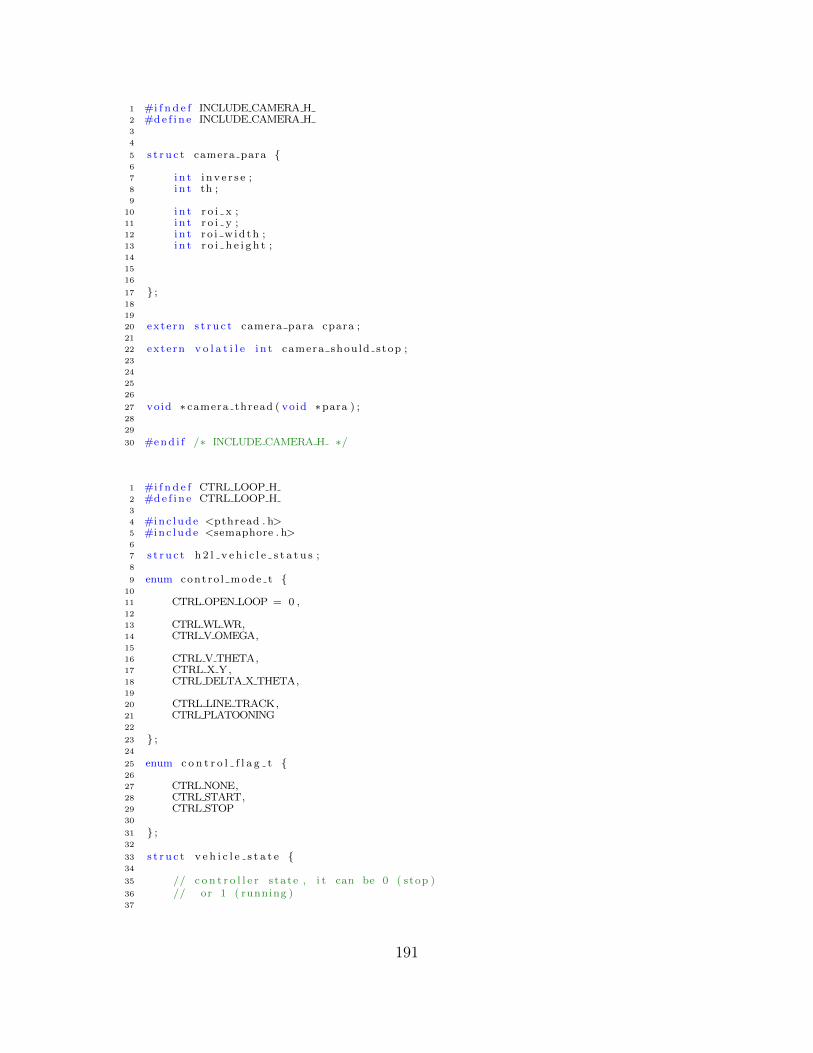
1 #i f n d e f INCLUDE CAMERA H2 #d e f i n e INCLUDE CAMERA H3

4

5 s t r u c t camera para 6

7 i n t i n v e r s e ;8 i n t th ;9

10 i n t r o i x ;11 i n t r o i y ;12 i n t r o i w id th ;13 i n t r o i h e i g h t ;14

15

16

17 ;18

19

20 extern s t r u c t camera para cpara ;21

22 extern v o l a t i l e i n t camera should stop ;23

24

25

26

27 void ∗ camera thread ( void ∗para ) ;28

29

30 #e n d i f /∗ INCLUDE CAMERA H ∗/

1 #i f n d e f CTRL LOOP H2 #d e f i n e CTRL LOOP H3

4 #inc lude <pthread . h>5 #inc lude <semaphore . h>6

7 s t r u c t h 2 l v e h i c l e s t a t u s ;8

9 enum contro l mode t 10

11 CTRL OPEN LOOP = 0 ,12

13 CTRL WL WR,14 CTRL V OMEGA,15

16 CTRL V THETA,17 CTRL X Y,18 CTRL DELTA X THETA,19

20 CTRL LINE TRACK,21 CTRL PLATOONING22

23 ;24

25 enum c o n t r o l f l a g t 26

27 CTRL NONE,28 CTRL START,29 CTRL STOP30

31 ;32

33 s t r u c t v e h i c l e s t a t e 34

35 // c o n t r o l l e r s ta te , i t can be 0 ( stop )36 // or 1 ( running )37

191

38 i n t c t r l s t a t e ; // running or stopped39 i n t c t r l f l a g ;40 i n t c t r l o u t e r l o o p m o d e ;41 i n t c t r l i n n e r l o o p m o d e ;42

43 // senso r measured s t a t e s ( low l e v e l )44

45 u i n t 3 2 t timestamp ;46 f l o a t imu theta ;47 f l o a t camera de l t a the ta ;48 f l o a t camera de l t a the ta p ;49 f l o a t imu accx ;50 f l o a t imu omega ;51 f l o a t encoder wl ;52 f l o a t encoder wr ;53 f l o a t u l t r a s o n i c d e l t a x ;54 f l o a t u l t r a s o n i c d e l t a x b k ;55 f l o a t u l t r a s o n i c d e l t a x f i t l e r e d ;56

57 // c a l c u l a t e d / fused s t a t e s58

59 // NOTE: these s t a t e s are in XI−O−YI coo rd ina t e s60 double accx ;61

62 double v ;63 double omega ;64

65 double x ;66 double y ;67 double theta ;68 // new 0801 f o r p latoon f a s t e r s t a r t69 double v ds r ;70

71 ;72

73 // Inner loop parameter ( p r e v i o u s l y in mc in i t )74 s t r u c t c t r l i n n e r p a r a 75

76 f l o a t p r e f i l t e r c o e f f i c i e n t ;77 f l o a t r o l l o f f c o e f f i c i e n t ;78 f l o a t k p l e f t ;79 f l o a t k i l e f t ;80 f l o a t k d l e f t ;81 f l o a t kp r i gh t ;82 f l o a t k i r i g h t ;83 f l o a t kd r i gh t ;84 f l o a t deadzone thresho ld ;85 f l o a t deadzone sa tura t i on ;86

87 ;88

89

90

91

92 // These are s t a t e s only used by a s p e c i f i c c o n t r o l l e r93

94 // I f you need to hack the c o n t r o l l e r or add a new c o n t r o l l e r ,95 // j u s t add v a r i a b l e s in these s t r u c t u r e96 // or c r e a t e a new s t r u c t u r e .97

98 s t r u c t c t r l o p e n l o o p s t a t e 99

100 // d e s i r e d value101 i n t 1 6 t pwm le f t ds r ;102 i n t 1 6 t pwm right dsr ;103

104

105 ;106

107 s t r u c t c t r l w l w r s t a t e

192

108

109 // d e s i r e d value110 double w l ds r ;111 double wr dsr ;112

113 ;114

115 s t r u c t c t r l v o m e g a s t a t e 116

117 // d e s i r e d value118 double v ds r ;119 double omega dsr ;120

121

122 ;123

124

125 // outer loop v theta c o n t r o l126

127 s t r u c t c t r l v t h e t a p a r a 128

129

130 double kp theta ;131 double k i t h e t a ;132 double kd theta ;133

134

135 ;136

137 s t r u c t c t r l v t h e t a s t a t e 138

139 // d e s i r e d value140 double v ds r ;141 double t h e t a d s r ;142

143

144 double w l ds r ;145 double wr dsr ;146 double u v ;147 double u omega ;148

149 double e r r o r t h e t a ;150 double e r r o r t h e t a p ;151 double e r ro r the ta sum p ;152

153 double u omega r f1 p ;154 double u omega r f2 p ;155

156 // debug157

158 double up omega out ;159 double ui omega out ;160 double ud omega out ;161

162 double u omega wo rf ; // without r o l l o f f163

164 FILE ∗ l o g f i l e ;165 FILE ∗ r e c e n t l o g f i l e ;166

167 ;168

169

170 // outer loop x y c o n t r o l171

172 s t r u c t c t r l x y p a r a 173

174 double k p d i s t ;175 double k i d i s t ;176 double k d d i s t ;177

193

178 double kp ang le ;179 double k i a n g l e ;180 double kd ang le ;181

182 ;183

184 s t r u c t c t r l x y s t a t e 185

186 // d e s i r e d value187 double x ds r ;188 double y ds r ;189


195 double e r r o r d i s t ;196 double e r r o r d i s t p ;197 double e r r o r d i s t s u m p ;198

199 // double u v r f 1 p ;200 // double u v r f 2 p ;201

202 double e r r o r a n g l e ;203 double e r r o r a n g l e p ;204 double e r ro r ang l e sum p ;205

206 // double u omega r f1 p ;207 // double u omega r f2 p ;208

209 // debug210

211 double u p d i s t o u t ;212 double u i d i s t o u t ;213 double u d d i s t o u t ;214 double up ang le out ;215 double u i a n g l e o u t ;216 double ud ang le out ;217


221 ;222

223 // outer loop d e l t a x t h e t a224

225 s t r u c t c t r l d e l t a x t h e t a p a r a 226

227 double kp de l t a x ;228 double k i d e l t a x ;229 double kd de l t a x ;230

231 // NOTE: Current ly only kp theta i s in usage232 double kp theta ;233 double k i t h e t a ;234 double kd theta ;235

236 ;237

238 s t r u c t c t r l d e l t a x t h e t a s t a t e 239

240 // d e s i r e d value241 double d e l t a x d s r ;242 double t h e t a d s r ;243

244 // prev ious s t a t e and cur rent in t e rmed ia t e s t a t e245

246 double w l ds r ;247 double wr dsr ;

194

248

249 double u v ;250 double u omega ;251

252 double e r r o r d e l t a x ;253 double e r r o r d e l t a x p ;254 double e r r o r d e l t a x p p ;255

256 double u v r f 1 p ;257 double u v r f 2 p ;258

259 double u v out p ;260

261

262 double e r r o r t h e t a ;263 double e r r o r t h e t a p ;264 double e r ro r the ta sum p ;265


269 // debug s t a t e270 double up v out ;271 double u i v o u t ;272 double ud v out ;273 double u v out ;274

275 double up omega out ;276 double ui omega out ;277 double ud omega out ;278 double u omega out ;279

280

281 FILE ∗ l o g f i l e ;282 FILE ∗ r e c e n t l o g f i l e ;283 ;284

285

286

287 // outer loop l i n e t rack288

289 s t r u c t c t r l l i n e t r a c k p a r a 290

291

292 double kp ;293 double k i ;294 double kd ;295

296

297 ;298

299 s t r u c t c t r l l i n e t r a c k s t a t e 300

301 // d e s i r e d value302 double v ds r ;303


309 double d e l t a t h e t a ;310 double d e l t a t h e t a p ;311 double de l ta the ta sum p ;312


316 // debug317

318 double up omega out ;

195

319 double ui omega out ;320 double ud omega out ;321 double u omega out ;322


326 ;327

328

329 // p la toon ing330

331 s t r u c t c t r l p l a t o o n i n g p a r a 332

333 i n t l e a d e r i d ;334

335 double kp de l t a x ;336 double k i d e l t a x ;337 double kd de l t a x ;338

339 double k p f f l e a d e r ;340 double k i f f l e a d e r ;341 double k d f f l e a d e r ;342

343 double k a f f l e a d e r ;344

345 double k p f f p r e ;346 double k i f f p r e ;347 double k d f f p r e ;348

349 double k a f f p r e ;350

351 // NOTE: Current ly only kp theta i s in usage352 double kp theta ;353 double k i t h e t a ;354 double kd theta ;355

356

357

358 ;359

360 s t r u c t c t r l p l a t o o n i n g s t a t e 361

362 // d e s i r e d value363 double d e l t a x d s r ;364 double t h e t a d s r ;365

366 // prev ious s t a t e and cur rent in t e rmed ia t e s t a t e367 double v d s r l e a d e r ;368 double v l e a d e r ;369 double v l e a d e r p ;370 double a c c l e a d e r ;371 i n t c t r l f l a g l e a d e r ;372

373

374 double v pre ;375 double acc pre ;376 double x l e a d e r p ;377 double x l e a d e r ;378

379 double w l ds r ;380 double wr dsr ;381

382 double u v ;383 double u v r f p ;384 double u omega ;385

386 // s t a t e der ived from d e l t a x387 double u v x ;388

389 double e r r o r d e l t a x ;

196

390 double e r r o r d e l t a x p ;391 double e r r o r d e l t a x p p ;392

393 double d e l t a x f i l t e r e d ;394

395 double u v x r f 1 p ;396 double u v x r f 2 p ;397

398 // debug s t a t e ( d e l t a x )399 double up v x out ;400 double u i v x o u t ;401 double ud v x out ;402 double u v x out p ;403 double u v x out ;404

405

406

407 // s t a t e der ived from l e a d e r408 double u v f f l e a d e r ;409

410 double e r r o r l e a d e r ;411 double e r r o r l e a d e r p ;412 // double e r r o r l e a d e r p p ;413 double e r r o r l e a d e r s u m p ;414 double u v f f l e a d e r r f p ;415

416 double u v f f l e a d e r a c c ;417

418 // debug s t a t e ( l e a d e r )419

420 double u p v f f l e a d e r o u t ;421 double u i v f f l e a d e r o u t ;422 double u d v f f l e a d e r o u t ;423 double u v f f l e a d e r o u t p ;424 double u v f f l e a d e r o u t ;425 double u v f f l e a d e r r f b e f o r e s a t ;426

427

428 // s t a t e der ived from prev ious v e h i c l e429 double u v f f p r e ;430

431 double e r r o r p r e ;432 double e r r o r p r e p ;433 double e r r o r p r e p p ;434

435 double u v f f p r e r f p ;436

437 double u v f f p r e a c c ;438

439 // debug s t a t e ( l e a d e r )440

441 double u p v f f p r e o u t ;442 double u i v f f p r e o u t ;443 double u d v f f p r e o u t ;444 double u v f f p r e o u t p ;445 double u v f f p r e o u t ;446

447

448 // s t a t e der ived from theta449 double e r r o r t h e t a ;450 double e r r o r t h e t a p ;451 double e r ro r the ta sum p ;452


456

457 double up omega out ;458 double ui omega out ;459 double ud omega out ;460 double u omega wo rf ;

197

461

462


466 ;467

468

469

470 // exported g l o b a l v a r i a b l e471

472

473 extern v o l a t i l e i n t c t r l l o o p s h o u l d s t o p ;474 extern sem t c t r l l o o p s e m ;475

476 extern i n t c t r l l o o p c u r r e n t r t ;477

478 // v e h i c l e s t a t e479

480 extern v o l a t i l e s t r u c t v e h i c l e s t a t e v s ta t e ;481

482 // s t a t e s and parameter o f inner loop483

484 extern v o l a t i l e s t r u c t c t r l i n n e r p a r a c t r l i n n e r p a r a ;485

486 // s t a t e s and parameter o f outer loop487

488 extern v o l a t i l e s t r u c t c t r l o p e n l o o p s t a t e489 c t r l o p e n l o o p s t a t e ;490

491 extern v o l a t i l e s t r u c t c t r l w l w r s t a t e492 c t r l w l w r s t a t e ;493

494 extern v o l a t i l e s t r u c t c t r l v o m e g a s t a t e495 c t r l v o m e g a s t a t e ;496

497 extern v o l a t i l e s t r u c t c t r l v t h e t a p a r a498 c t r l v t h e t a p a r a ;499 extern v o l a t i l e s t r u c t c t r l v t h e t a s t a t e500 c t r l v t h e t a s t a t e ;501

502 extern v o l a t i l e s t r u c t c t r l x y p a r a c t r l x y p a r a ;503 extern v o l a t i l e s t r u c t c t r l x y s t a t e c t r l x y s t a t e ;504

505 extern v o l a t i l e s t r u c t c t r l d e l t a x t h e t a p a r a506 c t r l d e l t a x t h e t a p a r a ;507 extern v o l a t i l e s t r u c t c t r l d e l t a x t h e t a s t a t e508 c t r l d e l t a x t h e t a s t a t e ;509

510 extern v o l a t i l e s t r u c t c t r l l i n e t r a c k p a r a511 c t r l l i n e t r a c k p a r a ;512 extern v o l a t i l e s t r u c t c t r l l i n e t r a c k s t a t e513 c t r l l i n e t r a c k s t a t e ;514

515 extern v o l a t i l e s t r u c t c t r l p l a t o o n i n g p a r a516 c t r l p l a t o o n i n g p a r a ;517 extern v o l a t i l e s t r u c t c t r l p l a t o o n i n g s t a t e518 c t r l p l a t o o n i n g s t a t e ;519

520

521

522

523

524

525 void u p d a t e v e h i c l e s t a t e ( s t r u c t h 2 l v e h i c l e s t a t u s ∗ s t a t e ) ;526

527 void ∗ c t r l l o o p t h r e a d ( void ∗para ) ;528

529 void c t r l s e t u p ( ) ;530 void c t r l s t a r t ( ) ;

198

531 void c t r l s t o p ( ) ;532

533 void c t r l open loop se t pwm ( i n t 1 6 t pwm left , i n t 1 6 t pwm right ) ;534 void c t r l s e t w l w r ( double wl dsr , double wr dsr ) ;535 void c t r l s e t v o m e g a ( double v dsr , double omega dsr ) ;536 void c t r l s e t v t h e t a ( double v dsr , double t h e t a d s r ) ;537 void c t r l s e t x y ( double x dsr , double y ds r ) ;538 void c t r l s e t d e l t a x t h e t a ( double d e l t a x d s r , double t h e t a d s r ) ;539 void c t r l s e t l i n e t r a c k ( double v ds r ) ;540 void c t r l s e t p l a t o o n i n g ( double d e l t a x d s r , double t h e t a d s r ) ;541 double c t r l o u t e r l o o p t h r e s h o l d a n d s a t u r a t i o n v542 ( double In , double Th, double Min , double Max ) ;543 double c t r l o u t e r l o o p t h r e s h o l d a n d s a t u r a t i o n w544 ( double In , double Th, double Min , double Max ) ;545

546 #e n d i f /∗ CTRL LOOP H ∗/

1 #inc lude <s t d i n t . h>2 #inc lude <s t r i n g . h>3

4 s t r u c t mc in i t ;5

6

7 #i f n d e f H2L PROTOCOL H8 #d e f i n e H2L PROTOCOL H9

10

11

12

13 #d e f i n e MC PROTO HEADER SIZE 414

15 #d e f i n e SERIAL STATE INIT 016 #d e f i n e SERIAL STATE MAGIC1 117 #d e f i n e SERIAL STATE MAGIC2 218 #d e f i n e SERIAL STATE PROTO 319

20 #d e f i n e SERIAL MAGIC 1 'A '21 #d e f i n e SERIAL MAGIC 2 'F '22

23 #d e f i n e OPCODE OPEN LOOP 0x0024

25 #d e f i n e OPCODE CTRL WL WR 0x1026

27 #d e f i n e OPCODE SETUP 0xF028 #d e f i n e OPCODE START 0xF129 #d e f i n e OPCODE STOP 0xF230 #d e f i n e OPCODE DEBUG ENABLE 0xF331 #d e f i n e OPCODE DEBUG DISABLE 0xF432

33

34 #d e f i n e OPCODE VEHICLE STATUS 0xE035 #d e f i n e OPCODE CTRL STATUS DEBUG 0xE136

37

38 s t r u c t h2 l header 39

40 u i n t 8 t magic1 ;41 u i n t 8 t magic2 ;42 u i n t 8 t l en ;43 u i n t 8 t opcode ;44 ;45

46 // message from HLC to LLC47

48 s t r u c t h2 l open loop 49

50 s t r u c t h2 l header header ;51 i n t 1 6 t v l e f t ;

199

52 i n t 1 6 t v r i g h t ;53

54 ;55

56 s t r u c t h2 l wl wr 57

58 s t r u c t h2 l header header ;59 f l o a t w l ds r ;60 f l o a t wr dsr ;61 ;62

63 s t r u c t h2 l s e tup 64

65 s t r u c t h2 l header header ;66 f l o a t r o l l o f f c o e f f i c i e n t ;67 f l o a t p r e f i l t e r c o e f f i c i e n t ;68 f l o a t k p l e f t ;69 f l o a t k i l e f t ;70 f l o a t k d l e f t ;71 f l o a t kp r i gh t ;72 f l o a t k i r i g h t ;73 f l o a t kd r i gh t ;74 f l o a t deadzone thresho ld ;75 f l o a t deadzone sa tura t i on ;76

77 ;78

79

80

81

82

83

84

85 // message from LLC to HLC86

87 s t r u c t h 2 l v e h i c l e s t a t u s 88

89 s t r u c t h2 l header header ;90

91 u i n t 3 2 t timestamp ;92 f l o a t imu theta ; // from IMU93 f l o a t imu accx ; // from IMU94 f l o a t imu omega ; // from IMU95 f l o a t encoder wl ;96 f l o a t encoder wr ;97 f l o a t u l t r a s o n i c d e l t a x ;98 // from u l t r a s o n i c s enso r99 ;

100

101

102

103 s t r u c t h 2 l c t r l s t a t u s d e b u g 104

105 s t r u c t h2 l header header ;106 u i n t 3 2 t timestamp ; // Arduino timestamp in ms107

108 f l o a t w l ds r ;109 f l o a t wr dsr ;110 f l o a t w l d s r f i l t e r e d ;111 f l o a t w r d s r f i l t e r e d ;112

113 // debug114

115 i n t 1 6 t pwml ; // with r o l l o f f116 i n t 1 6 t pwmr ;117 i n t 1 6 t pwml out ; // without r o l l o f f118 i n t 1 6 t pwmr out ;119 i n t 1 6 t pwml out p ;120 i n t 1 6 t pwmr out p ;121

200

122 f l o a t e r r w l ;123 f l o a t e r r wr ;124 f l o a t e r r w l p ;125 f l o a t e r r wr p ;126 f l o a t e r r w l pp ;127 f l o a t e r r wr pp ;128

129 f l o a t pwml up ;130 f l o a t pwml ui ;131 f l o a t pwml ud ;132 f l o a t pwmr up ;133 f l o a t pwmr ui ;134 f l o a t pwmr ud ;135

136 u i n t 3 2 t timestamps [ 8 ] ;137 ;138

139

140

141

142 // he lpe r func t i on143

144 s t a t i c i n l i n e void s e t u i n t 1 6 ( char ∗ buf f , i n t o f f s e t , u i n t 1 6 t va lue ) 145

146 char ∗p = ( char ∗)& value ;147 memcpy( bu f f + o f f s e t , p , s i z e o f ( va lue ) ) ;148 149

150 s t a t i c i n l i n e void s e t u i n t 3 2 ( char ∗ buf f , i n t o f f s e t , u i n t 3 2 t va lue ) 151


156 s t a t i c i n l i n e void s e t f l o a t ( char ∗ buf f , i n t o f f s e t , f l o a t va lue ) 157


162

163 s t a t i c i n l i n e u i n t 1 6 t g e t u in t 16 ( char ∗ buf f , i n t o f f s e t ) 164

165 u i n t 1 6 t r e t ;166 u i n t 1 6 t ∗p = &r e t ;167

168 memcpy(p , bu f f + o f f s e t , s i z e o f ( r e t ) ) ;169

170 r e turn r e t ;171 172

173 s t a t i c i n l i n e u i n t 3 2 t g e t u in t 32 ( char ∗ buf f , i n t o f f s e t ) 174

175 u i n t 3 2 t r e t ;176 u i n t 3 2 t ∗p = &r e t ;177


180 r e turn r e t ;181 182

183 s t a t i c i n l i n e f l o a t g e t f l o a t ( char ∗ buf f , i n t o f f s e t ) 184

185 f l o a t r e t ;186 f l o a t ∗p = &r e t ;187


190 r e turn r e t ;

201

191 192

193 s t a t i c i n l i n e void h 2 l s e t h e a d e r ( s t r u c t h2 l header ∗pheader ,194 u i n t 8 t len , u i n t 8 t opcode ) 195

196 pheader−>magic1 = SERIAL MAGIC 1 ;197 pheader−>magic2 = SERIAL MAGIC 2 ;198 pheader−>l en = len ;199 pheader−>opcode = opcode ;200

201 202

203 // send command message to LLC204

205 // CAUTION: only c a l l the se func t i on in c o n t r o l loop206

207 i n t h2 l send open loop msg ( i n t 1 6 t pwm left , i n t 1 6 t pwm right ) ;208 i n t h2 l send wl wr msg ( f l o a t wl dsr , f l o a t wr dsr ) ;209 i n t h2 l s end setup msg ( ) ;210 i n t h 2 l s e n d s t a r t m s g ( ) ;211 i n t h2 l s end stop msg ( ) ;212 i n t h2 l send debug enab le msg ( ) ;213 i n t h2 l s end debug d i sab l e msg ( ) ;214

215

216 // void h 2 l p r i n t v e h i c l e s t a t u s (FILE ∗ fd ,217 // s t r u c t h 2 l v e h i c l e s t a t u s ∗msg ) ;218 void h 2 l p r i n t c t r l s t a t u s d e b u g (FILE ∗ fd ,219 s t r u c t h 2 l c t r l s t a t u s d e b u g ∗msg ) ;220

221 // h2l r e c e i v i n g thread222 // ( note that the sending thread i s c o n t r o l loop )223 void ∗ h 2 l r e c e i v e t h r e a d ( void ∗para ) ;224

225

226

227 extern v o l a t i l e i n t s e r i a l s h o u l d s t o p ;228 extern i n t s e r i a l f d ;229

230 #e n d i f /∗ H2L PROTOCOL H ∗/

1 #i f n d e f PI MC H2 #d e f i n e PI MC H3

4 s t r u c t mc in i t 5

6 i n t v e h i c l e i d ;7

8 char t t y f i l e n a m e [ 6 4 ] ;9 i n t t ty baud ra t e ;

10

11

12 char l o g f i l e n a m e [ 6 4 ] ;13 char meta f i l e name [ 6 4 ] ;14

15 // v2 i and v2v parameter16

17 char manager ip [ 1 6 ] ;18 i n t manager port ;19

20 i n t v2v per iod ;21

22 // gene ra l c o n t r o l l e r parameter23

24 i n t running t ime ; // in m i l l i s e c o n d s25

202

26 i n t c t r l l o o p p e r i o d ; // in m i l l i s e c o n d s27

28 i n t debug mode ;29

30 double whee l r ad iu s ;31 double d i s t a n c e o f w h e e l s ;32

33 ;34

35 extern s t r u c t mc in i t mc in i t ;36

37 extern FILE ∗ m e t a f i l e ;38 extern FILE ∗ l o g f i l e ;39 extern FILE ∗ r e c e n t l o g f i l e ;40 extern FILE ∗ r e c e n t m e t a f i l e ;41

42 #e n d i f /∗ PI MC H ∗/

1 #inc lude <s tdde f . h>2

3 #i f n d e f SERIAL H4 #d e f i n e SERIAL H5

6 i n t s e r i a l i n i t ( const char ∗ s e r i a l p o r t , i n t baud ) ;7 i n t s e r i a l c l o s e ( i n t fd ) ;8

9 // CAUTION: these send and r e c e i v i n g are b lock ing10 // busy wai t ing11 i n t s e r i a l s e n d n b y t e s ( i n t fd , const char ∗ buf f , s i z e t n ) ;12 i n t s e r i a l r e c v n b y t e s ( i n t fd , char ∗ buf f , s i z e t n ) ;13

14 i n t s e r i a l f l u s h ( i n t fd ) ;15

16 // CAUTION: t h i s i s nonblocking r e c e i v e17 i n t s e r i a l r e c v b y t e ( i n t fd , char ∗ bu f f ) ;18

19

20 #e n d i f /∗ SERIAL H ∗/

1 #i f n d e f V2V H2 #d e f i n e V2V H3

4

5

6

7

8 s t r u c t v2v msg 9

10 u i n t 3 2 t t s ;11 u i n t 3 2 t vid ;12 double theta ;13 double accx ;14 double v ;15 double omega ;16 double v ds r ;17 i n t c t r l f l a g ;18

19 ;20

21 s t r u c t v2v msg ∗ ge t r ecent msg ( i n t vid ) ;22 void pr int v2v msg (FILE ∗ fd , s t r u c t v2v msg ∗msg ) ;23

24 void ∗ v2v send ing thread ( void ∗para ) ;25 void ∗ v 2 v r e c e i v i n g t h r e a d ( void ∗para ) ;26

27 extern v o l a t i l e i n t v2v send ing shou ld s top ;

203

28 extern v o l a t i l e i n t v 2 v r e c e i v i n g s h o u l d s t o p ;29

30 extern sem t v2v send sem ;31

32 #e n d i f /∗ V2V H ∗/

1

2 #inc lude <opencv2/ core / core .hpp>3 #inc lude <opencv2/ h ighgu i / highgui .hpp>4 #inc lude <opencv2/ imgproc/ imgproc.hpp>5

6 #inc lude <iostream>7 #inc lude <fstream>8

9 #inc lude <ctime>10

11 #inc lude <uni s td .h>12

13 #inc lude ” raspicam / rasp icam cv .h ”14

15 #inc lude ” c t r l l o o p . h ”16 #inc lude ” pi mc.h ”17 #inc lude ” camera.h ”18

19 us ing namespace cv ;20 us ing namespace raspicam ;21 us ing namespace std ;22

23 s t r u c t camera para cpara ;24

25 v o l a t i l e i n t camera should stop ;26

27 long g e t m i l l i s ( ) 28

29 s t r u c t t imespec spec ;30

31 c l o c k g e t t i m e (CLOCK MONOTONIC, &spec ) ;32

33 long ms = s p e c . t v s e c ∗ 1000 + s p e c . t v n s e c / 1000000;34

35 r e turn ms ;36 37

38 /∗∗ Sets a property in the VideoCapture.39 ∗40 ∗41 ∗ Implemented p r o p e r t i e s :42 ∗ CV CAP PROP FRAME WIDTH,CV CAP PROP FRAME HEIGHT,43 ∗ CV CAP PROP FORMAT: CV 8UC1 or CV 8UC344 ∗ CV CAP PROP BRIGHTNESS: [ 0 , 1 0 0 ]45 ∗ CV CAP PROP CONTRAST: [ 0 , 1 0 0 ]46 ∗ CV CAP PROP SATURATION: [ 0 , 1 0 0 ]47 ∗ CV CAP PROP GAIN: ( i s o ) : [ 0 , 1 0 0 ]48 ∗ CV CAP PROP EXPOSURE: −1 auto . [ 1 , 1 0 0 ]49 // shut t e r speed from 0 to 33ms50 ∗ CV CAP PROP WHITE BALANCE RED V : /51 / [ 1 , 1 0 0 ] −1 auto whiteba lance52 ∗ CV CAP PROP WHITE BALANCE BLUE U :53 / / [ 1 , 1 0 0 ] −1 auto whiteba lance54 ∗55 ∗/56 // LEE57 // 0725 ed i t ed the o r i g i n a l l i b r a r y add new s e t f e a t u r e by58 // adding two more ca s e s in switch s e c t i o n in rasp icam cv.cpp59

60

61 void se t p i cam proper ty ( RaspiCam Cv &picam )

204

62 p icam.se t (CV CAP PROP FRAME WIDTH, 32 0 ) ;63 p icam.se t (CV CAP PROP FRAME HEIGHT, 24 0 ) ;64 p icam.se t (CV CAP PROP FORMAT, CV 8UC3 ) ;65 p icam.se t (777 , 1 ) ; / / HFlip66 p icam.se t (888 , 1 ) ; / / VFlip67 // p i cam.se t (CV CAP PROP BRIGHTNESS, 5 0 ) ;68 // p i cam.se t (CV CAP PROP CONTRAST, 5 0 ) ;69 // p i cam.se t (CV CAP PROP SATURATION, 5 0 ) ;70 // p i cam.se t (CV CAP PROP GAIN, 5 0 ) ;71 // p i cam.se t (CV CAP PROP EXPOSURE, −1);72 // p i cam.se t (CV CAP PROP WHITE BALANCE RED V, −1);73 // p i cam.se t (CV CAP PROP WHITE BALANCE BLUE U, −1);74 75

76 double d e l t a t h e t a b k = 0 ;77 void ∗ camera thread ( void ∗para ) 78

79 ofstream camlog (” camera . txt ” ) ;80

81 RaspiCam Cv picam ;82

83 s e t p i cam proper ty ( picam ) ;84

85 i f ( ! picam.open ( ) ) 86 c e r r << ” Error opening camera” << endl ;87 88

89 cout << ”<camera> Connected to camera =”90 << picam.get Id ( ) << endl ;91

92 double frame width = picam.get (CV CAP PROP FRAME WIDTH) ;93 double f rame he ight = picam.get (CV CAP PROP FRAME HEIGHT) ;94

95 cout << ”Frame S i z e = ” << f rame width96 << ”x” << f rame he ight << endl ;97 cout << ”ROI S i z e = ” << c p a r a . r o i w i d t h98 << ”x” << c p a r a . r o i h e i g h t << endl ;99

100 S i z e f r a m e s i z e ( s t a t i c c a s t <int >( frame width ) ,101 s t a t i c c a s t <int >( f rame he ight ) ) ;102

103 VideoWriter w r i t e r (” . / camera .av i ” ,104 CV FOURCC( 'P ' , ' I ' , 'M' , ' 1 ' ) ,105 20 , f r ame s i z e , t rue ) ;106 // i n i t i a l i z e the VideoWriter ob j e c t107 // i f not i n i t i a l i z e the VideoWriter s u c c e s s f u l l y ,108 // e x i t the program109 i f ( ! wr i t e r . i sOpened ( ) )110 111 cout << ”ERROR: Fa i l ed to wr i t e the frame video ”112 << endl ;113 r e turn NULL;114 115

116 S i z e r o i s i z e ( s t a t i c c a s t <int >( c p a r a . r o i w i d t h ) ,117 s t a t i c c a s t <int >( c p a r a . r o i h e i g h t ) ) ;118

119 VideoWriter r o i w r i t e r (” . / r o i . a v i ” ,120 CV FOURCC( 'P ' , ' I ' , 'M' , ' 1 ' ) ,121 20 , r o i s i z e , t rue ) ;122 // i n i t i a l i z e the VideoWriter ob j e c t123 // i f not i n i t i a l i z e the VideoWriter s u c c e s s f u l l y ,124 // e x i t the program125 i f ( ! r o i w r i t e r . i s O p e n e d ( ) )126 127 cout << ”ERROR: Fa i l ed to wr i t e the ROI video ” << endl ;128 r e turn NULL;

205

129 130

131

132 // namedWindow(” Control ” , CV WINDOW AUTOSIZE) ;133 // createTrackbar (” th r e sho ld ” , ” Control ” , &th , 25 5 ) ;134

135 long t s = g e t m i l l i s ( ) ;136 ;137

138 whi le ( ! camera should stop ) 139

140 Mat frame ;141 Mat imgray ;142 Mat imthresh ;143

144

145 picam.grab ( ) ;146 p i c a m . r e t r i e v e ( frame ) ;147

148 // convert to grey s c a l e149 cvtColor ( frame , imgray , CV RGB2GRAY) ;150 // binary th r e sho ld151 th r e sho ld ( imgray , imthresh , cpara . th , 255 ,152 THRESH BINARY INV ) ;153

154 // get subimage155 // Rect r e c t (80 , 20 , 160 , 10 0 ) ;156 Rect r e c t ( c p a r a . r o i x , c p a r a . r o i y ,157 cpa ra . r o i w id th , c p a r a . r o i h e i g h t ) ;158 Mat r o i = imthresh ( r e c t ) ;159

160 // morpho log ica l opening161 //( remove smal l o b j e c t s from the foreground )162 erode ( ro i , ro i ,163 getStructur ingElement (MORPH ELLIPSE, S i z e (5 , 5 ) ) ) ;164 d i l a t e ( ro i , ro i ,165 getStructur ingElement (MORPH ELLIPSE, S i z e (5 , 5 ) ) ) ;166

167 // morpho log ica l c l o s i n g ( f i l l smal l ho l e s in the foreground )168 d i l a t e ( ro i , ro i ,169 getStructur ingElement (MORPH ELLIPSE, S i z e (5 , 5 ) ) ) ;170 erode ( ro i , ro i ,171 getStructur ingElement (MORPH ELLIPSE, S i z e (5 , 5 ) ) ) ;172

173 // c a l c u l a t e the moments o f the thre sho lded image174 Moments m = moments ( r o i ) ;175

176 double m01 = m.m01 ;177 double m10 = m.m10 ;178 double m00 = m.m00 ;179

180 double u1 = m10 / m00 ;181 double v1 = m01 / m00 ;182

183 // double width = c p a r a . r o i w i d t h ;184 // double he ight = c p a r a . r o i h e i g h t ;185 //186 // double d e l t a t h e t a r a d = atan ( ( u1 − width / 2) / he ight ) ;187 // double d e l t a t h e t a d e g r e e = d e l t a t h e t a r a d ∗ 180 / 3 .1416 ;188

189 double width = c p a r a . r o i w i d t h ;190 double he ight = c p a r a . r o i h e i g h t ;191 // 32 = 20 ( Look ahead ) + 12( r ea r wheel 2 camera )192 // v e r t i c a l d i s t ance c a l i b r a t i o n 32cm193 double l a t p i x e l 2 c m g a i n = (1 . 7 /26 . 0 ) ;194 double l a t e r r c m = ( u1 − width / 2)∗ l a t p i x e l 2 c m g a i n ;195 double d e l t a t h e t a r a d = −atan ( l a t e r r c m / 32 . 0 ) ;

206

196

197 // camera f a i l u r e handl ing198 // 0 .32 i s the maximum d e l t a t h e t a we can get199 // given 20cm look ahead d i s t anc e200 i f ( f abs ( d e l t a t h e t a r a d )>=0.32 )201 cout << ”<camera> o f f t rack ” << endl ;202 d e l t a t h e t a r a d = d e l t a t h e t a b k ;203

204 e l s e i f ( u1>=10 && u1<=310)205 // update backup data206 d e l t a t h e t a b k = d e l t a t h e t a r a d ;207 208 e l s e i f ( u1<10 | | u1>310)209 // update backup data210 // cout << ”<camera> e r r o r ” << endl ;211 d e l t a t h e t a r a d= 0 ;212 d e l t a t h e t a b k = 0 ;213 e l s e 214 ;215 216 double d e l t a t h e t a d e g r e e = d e l t a t h e t a r a d ∗ 180 / 3 .1416 ;217

218 // show the ROI and the image219

220 // r e c t a n g l e ( frame , rect , Sca l a r (127 , 127 , 1 2 7 ) ) ;221 //222 // imshow (” o r i g i n a l ” , frame ) ; //show the o r i g i n a l image223 // imshow (” r o i ” , r o i ) ;224

225 long t2 = g e t m i l l i s ( ) ;226

227 camlog << ”FPS : ” << 1000 / ( t2 − t s ) << ” , ” ;228 camlog << ” cente r o f mass : (” << u1 << ” , ” << v1 ;229 camlog << ”) d e l t a t h e t a : ” << d e l t a t h e t a r a d << ” (”230 << d e l t a t h e t a d e g r e e << ” ) ” ;231 camlog << ” l a t e r r c m : ”<< l a t e r r cm<<endl ;232

233 t s = t2 ;234

235 v s t a t e . c a m e r a d e l t a t h e t a = d e l t a t h e t a r a d ;236

237 Mat r o i r g b ;238 cvtColor ( ro i , r o i r gb , CV GRAY2RGB) ;239

240 w r i t e r . w r i t e ( frame ) ;241 r o i w r i t e r . w r i t e ( r o i r g b ) ;242

243 // s l e e p 20 ms244 us l e ep (20000 ) ;245

246 247

248 p i c a m . r e l e a s e ( ) ;249

250 cout << ”<camera> camera thread e x i t i n g . . . ” << endl ;251

252 r e turn 0 ;253

254

1 #inc lude <s t d i o . h>2 #inc lude <s t d l i b . h>3 #inc lude <s t r i n g . h>4 #inc lude <errno . h>5

6 #inc lude <math . h>

207

7

8 #inc lude <un i s td . h>9 #inc lude <sys / types . h>

10

11 #inc lude ” h2l . h”12 #inc lude ” c t r l l o o p . h”13 #inc lude ”v2v . h”14 #inc lude ”pi mc . h”15

16 v o l a t i l e i n t c t r l l o o p s h o u l d s t o p = 0 ;17 sem t c t r l l o o p s e m ;18

19 i n t c t r l l o o p c u r r e n t r t = 0 ;20

21 // −−−−− v e h i c l e s t a t e and c o n t r o l l e r s t a t e −−−−−−−−−−−−−−−22

23 v o l a t i l e s t r u c t v e h i c l e s t a t e v s ta t e ;24

25 // s t a t e s and parameter o f inner loop26

27 v o l a t i l e s t r u c t c t r l i n n e r p a r a c t r l i n n e r p a r a ;28

29 // s t a t e s and parameter o f outer loop30

31 v o l a t i l e s t r u c t c t r l o p e n l o o p s t a t e c t r l o p e n l o o p s t a t e ;32

33 v o l a t i l e s t r u c t c t r l w l w r s t a t e c t r l w l w r s t a t e ;34

35 v o l a t i l e s t r u c t c t r l v o m e g a s t a t e c t r l v o m e g a s t a t e ;36

37 v o l a t i l e s t r u c t c t r l v t h e t a p a r a c t r l v t h e t a p a r a ;38 v o l a t i l e s t r u c t c t r l v t h e t a s t a t e c t r l v t h e t a s t a t e ;39

40 v o l a t i l e s t r u c t c t r l x y p a r a c t r l x y p a r a ;41 v o l a t i l e s t r u c t c t r l x y s t a t e c t r l x y s t a t e ;42

43 v o l a t i l e s t r u c t c t r l d e l t a x t h e t a p a r a44 c t r l d e l t a x t h e t a p a r a ;45 v o l a t i l e s t r u c t c t r l d e l t a x t h e t a s t a t e46 c t r l d e l t a x t h e t a s t a t e ;47

48 v o l a t i l e s t r u c t c t r l l i n e t r a c k p a r a49 c t r l l i n e t r a c k p a r a ;50 v o l a t i l e s t r u c t c t r l l i n e t r a c k s t a t e51 c t r l l i n e t r a c k s t a t e ;52

53 v o l a t i l e s t r u c t c t r l p l a t o o n i n g p a r a54 c t r l p l a t o o n i n g p a r a ;55 v o l a t i l e s t r u c t c t r l p l a t o o n i n g s t a t e56 c t r l p l a t o o n i n g s t a t e ;57

58 // LEE 0726 new g l o b a l v a r i a b l e59 i n t d e l t a x n e g e r r o r f l a g = 0 ;60 i n t d e l t a x n e g e r r o r f l a g p = 0 ;61

62 i n t s t a r t e d f l a g = 0 ;63 i n t s h o u l d s t o p f l a g = 0 ;64 // c o n t r o l l e r bypass f l a g s65 // be caut i ous when use i t66 i n t n o t s t a r t b y p a s s = 1 ;67 i n t s top bypass = 0 ;68 i n t t o o c l o s e b y p a s s = 0 ;69 i n t brake bypass = 0 ;70 // gene ra l system f l a g s71 i n t v e h i c l e s t a t u s = 0 ;72 i n t s e p a r a t i o n t o o c l o s e f l a g = 0 ;73 i n t f o l l o w e r c a t c h e d u p f l a g = 0 ;74 i n t l e a d e r s t o p p e d f l a g = 0 ;75

76 long runn ing t ime s ta r t ms = 0 ;77 // s t o r e s t a r t time

208

78 long run lapsed t ime ms = 0 ;79 i n t n e g a t i v e f l a g c n t = 0 ;80 // f l a g up when d e l t a x e r r o r i s negat ive81

82 // −−−−−−−−−−−−−−−−−− v e h i c l e s t a t e u t i l i t y −−−−−−−−−−−−−−−83

84

85

86

87 void k inemat ic s ( double wl , double wr ,88 double ∗v , double ∗omega ) 89

90 ∗v = ( wl + wr) ∗ mc in i t . whee l r ad iu s / 2 ;91 ∗omega = (wr − wl ) ∗ mc in i t . whee l r ad iu s92 / mc in i t . d i s t a n c e o f w h e e l s ;93 94

95 void i n v e r s e k i n e m a t i c s ( double v , double omega ,96 double ∗wl , double ∗wr) 97

98 ∗wl = (2 ∗ v − mc in i t . d i s t a n c e o f w h e e l s ∗ omega )99 / (2 ∗ mc in i t . whee l r ad iu s ) ;

100 ∗wr = (2 ∗ v + mc in i t . d i s t a n c e o f w h e e l s ∗ omega )101 / (2 ∗ mc in i t . whee l r ad iu s ) ;102 103

104 void u p d a t e v e h i c l e s t a t e ( s t r u c t h 2 l v e h i c l e s t a t u s ∗ s t a t e ) 105

106 vs ta t e . timestamp = state−>timestamp ;107 vs ta t e . imu theta = state−>imu theta ;108 vs ta t e . imu accx = state−>imu accx ;109 vs ta t e . imu omega = state−>imu omega ;110 vs ta t e . encoder wl = state−>encoder wl ;111 vs ta t e . encoder wr = state−>encoder wr ;112 vs ta t e . u l t r a s o n i c d e l t a x = state−>u l t r a s o n i c d e l t a x ;113

114 // c a l c u l a t e / f u s e s t a t e s115

116 vs ta t e . accx = vs ta t e . imu accx ;117

118 k inemat ic s ( v s t a t e . encoder wl , v s t a t e . encoder wr ,119 ( double ∗) &vs ta t e . v ,120 ( double ∗) &vs ta t e . omega ) ;121

122 // de r i v e x and y through dead reckon ing123 // FIXIT : imu theta i s abso lu t e theta der ived124 // from IMU in XI−O−YI coo rd ina t e s125 s t a t i c i n t i n t e g r a t i o n e r r o r p r i n t f l a g = 0 ;126 vs ta t e . theta = vs ta t e . imu theta ;127 // sometimes abnormal i n i t i a l e r r o r happens128 // dea l with them c a r e f u l l y129 i f ( f abs ( v s ta t e . x ) > 100) v s ta t e . x = 0 ;130 vs ta t e . x += vs ta t e . v ∗ cos ( v s ta t e . theta )131 ∗ mc in i t . c t r l l o o p p e r i o d132 / 1 0 0 0 . 0 ;133 i f ( v s t a t e . x < 0 )134 i n t e g r a t i o n e r r o r p r i n t f l a g ++;135 i f (1 == i n t e g r a t i o n e r r o r p r i n t f l a g )136 p r i n t f ( ” I n t e g r a t i o n o f X Error !\n x : ”137 ”%6.2 f , theta : %6.2 f ” ,138 vs ta t e . x , v s t a t e . theta ) ;139 140 vs ta t e . y += vs ta t e . v ∗ s i n ( v s ta t e . theta )141 ∗ mc in i t . c t r l l o o p p e r i o d142 / 1 0 0 0 . 0 ;143

144

209

145

146 // −−−−−−−−−−−−−−−−−− outer loop u t i l i t y −−−−−−−−−−−−−−−147

148 // PID c o n t r o l l e r abso lu t e s t y l e149 double c t r l p i d w i t h d r o l l o f f (150 double err , double err sum , double er r p ,151 double kp , double ki , double kd ,152 double ud lp f n , double ∗ud save ,153 double ud p , double t s ) 154

155 double up = kp ∗ e r r ;156 double u i = k i ∗ t s ∗ err sum ;157

158 // Apply low pass f i l t e r f o r ud , so that i t //159 // i s l e s s s e n s i t i v e to no i s e .160 double alpha = 1 .0 / ( 1 . 0 + u d l p f n ∗ t s ) ;161 double ud = alpha ∗ ud p + (1 − alpha ) ∗162 kd ∗ ( e r r − e r r p ) / t s ;163

164 ∗ ud save = ud ;165

166 double u = up + ui + ud ;167

168 r e turn u ;169 170 // PID c o n t r o l l e r p o s i t i o n s t y l e171 // us ing back Euler d i s c r e t i z a t i o n172 double c t r l p i d ( double err , double err sum , double er r p ,173 double kp , double ki , double kd ,174 double ∗up out , double ∗ ui out , double ∗ud out ,175 double t s ) 176

177 double up = kp ∗ e r r ;178 double u i = k i ∗ t s ∗ err sum ;179 double ud = kd ∗ ( e r r − e r r p ) / t s ;180 double u = up + ui + ud ;181

182 i f ( up out != NULL)183 ∗up out = up ;184 i f ( u i ou t != NULL)185 ∗ u i ou t = ui ;186 i f ( ud out != NULL)187 ∗ud out = ud ;188

189 r e turn u ;190 191 // PID c o n t r o l l e r incrementa l s t y l e us ing192 // back Euler d i s c r e t i z a t i o n193 double c t r l t h r e s h o l d a n d s a t u r a t i o n ( double in , double th ,194 double min , double max ) ;195

196 double c t r l p i d i n c ( double u p , double err ,197 double er r p , double err pp ,198 double kp , double ki , double kd ,199 double ∗up out , double ∗ ui out ,200 double ∗ud out , double t s ) 201

202 double up = kp ∗ ( e r r − e r r p ) ;203 double u i = k i ∗ t s ∗ e r r ;204 double ud = kd ∗ ( ( e r r − e r r p ) − ( e r r p − e r r pp ) ) / t s ;205 double ud temp = ud ;206

207 double de l tau = up+ ui + ud ;208 double u = u p + de l tau ;209

210 i f ( up out != NULL)211 ∗up out = up ;212 i f ( u i ou t != NULL)

210

213 ∗ u i ou t = ui ;214 i f ( ud out != NULL)215 ∗ud out = ud ;216 r e turn u ;217 218

219 const double r f c o e f f = 0 . 8 ; // backward Euler 40/( s +40)220

221 double c t r l r o l l o f f o n c e ( double u r f p ,222 double u in , double r f c o e f f ) 223

224 double u r f = (1 − r f c o e f f ) ∗ u r f p + r f c o e f f ∗ u in ;225

226 r e turn u r f ;227 228

229 // wr wl sa tu ra t e u t i l i t y func t i on230 const double wl wr hw sat lower bound = 0 ;231 const double wl wr hw sat upper bound = 20 ;232

233

234 // CAUTION: t h i s i s j u s t a temporary s o l u t i o n235 void c t r l s a t u r a t e w l w r ( double ∗wl , double ∗wr) 236 i f (∗ wl < wl wr hw sat lower bound ) 237 ∗wl = wl wr hw sat lower bound ;238 e l s e i f (∗ wl > wl wr hw sat upper bound ) 239 ∗wl = wl wr hw sat upper bound ;240 241

242 i f (∗wr < wl wr hw sat lower bound ) 243 ∗wr = wl wr hw sat lower bound ;244 e l s e i f (∗wr > wl wr hw sat upper bound ) 245 ∗wr = wl wr hw sat upper bound ;246 247 248

249 // c o n t r o l e f f o r t r e s t r i c t i o n250 double c t r l t h r e s h o l d a n d s a t u r a t i o n ( double in , double th ,251 double min ,252 double max) 253

254 double out = in ;255

256 // th r e sho ld means no response r eg i on i s [−th , th ]257 i f ( f abs ( in ) < th ) 258 out = 0 ;259 e l s e i f ( in > max) 260 out = max ;261 e l s e i f ( in < min) 262 out = min ;263 264 r e turn out ;265 266

267 // −−−−−−−−−−−−−−−−−− outer loop c o n t r o l l e r −−−−−−−−−−−−−−−268

269 // outer loop framework270 // 1) in fo rmat ion gather ing from senso r or communication271 // 2) c a l c u l a t e e r r o r272 // 3) pid c o n t r o l + r o l l o f f273 // 4) c o n t r o l e f f o r t r e s t r i c t i o n ( sa tura t i on , deadzone )274 // 5) obta in wl dsr , wr dsr through i n v e r s e k inemat ic s275 // 6) s t a t e s update276 // when bypass mechanism invo lved th ing s becomes277 // more compl icated f i n a l cmd i s bypass c o n t r o l l e r278 // and c o n t r o l l e d by d i f f e r e n t bypass f l a g s t r i g g e d279 // by d i f f e r e n t events

211

280

281 void c t r l o p e n l o o p ( ) 282

283 h2 l send open loop msg ( c t r l o p e n l o o p s t a t e . pwm left dsr ,284 c t r l o p e n l o o p s t a t e . pwm right dsr ) ;285

286 287

288 void c t r l w l w r l o o p ( ) 289

290 h2l send wl wr msg ( c t r l w l w r s t a t e . wl dsr ,291 c t r l w l w r s t a t e . wr dsr ) ;292

293 294

295 // d i r e c t v omgega296 void c t r l v omega l oop ( ) 297


301 i n v e r s e k i n e m a t i c s ( c t r l v o m e g a s t a t e . v dsr ,302 c t r l v o m e g a s t a t e . omega dsr ,303 &wl dsr , &wr dsr ) ;304

305 // send to inner loop ;306 h2l send wl wr msg ( ( f l o a t ) wl dsr , ( f l o a t ) wr dsr ) ;307 308

309 // −−−−−−−−−−−−− (v , theta ) c o n t r o l −−−−−−−−−−−−−−−−−310

311 void c t r l v t h e t a i n i t ( ) 312

313 char f n b u f f [ 6 4 ] ;314 char s u f f i x [ 1 2 8 ] ;315

316 t ime t t = time (NULL) ;317 s t r u c t tm tm = ∗ l o c a l t i m e (&t ) ;318

319 s n p r i n t f ( s u f f i x , s i z e o f ( s u f f i x ) ,320 ”%04d %02d %02 d %02d %02d %02d” ,321 tm . tm year + 1900 ,322 tm . tm mon + 1 ,323 tm . tm mday ,324 tm . tm hour ,325 tm . tm min ,326 tm . tm sec ) ;327

328 s n p r i n t f ( f n b u f f , s i z e o f ( f n b u f f ) ,329 ” v t h e t a %s . txt ” , s u f f i x ) ;330

331 c t r l v t h e t a s t a t e . l o g f i l e = fopen ( f n b u f f , ”w+” ) ;332 c t r l v t h e t a s t a t e . r e c e n t l o g f i l e333 = fopen ( ” v theta . txt ” , ”w+” ) ;334 335

336 void c t r l v t h e t a e x i t ( ) 337

338 f c l o s e ( c t r l v t h e t a s t a t e . l o g f i l e ) ;339 f c l o s e ( c t r l v t h e t a s t a t e . r e c e n t l o g f i l e ) ;340

341 342

343 void c t r l v t h e t a p r i n t (FILE ∗ fd ) 344

345 s t r u c t t imespec now ;346 c l o c k g e t t i m e (CLOCK MONOTONIC, &now ) ;347

212

348 u i n t 3 2 t t s = now . t v s e c ∗ 1000 + now . tv ns e c / 1000000;349

350 // p r i n t v e h i c l e s t a t e f i r s t351 f p r i n t f ( fd , ”%08u , %08u , ”352 ”% 6 .2 f , %6.2 f , %6.2 f , ”353 ”% 6 .2 f , % 6 .2 f , % 6 .2 f , % 6 .2 f , % 6 .2 f , \ t \ t ” ,354 ts , v s t a t e . timestamp ,355

356 vs ta t e . u l t r a s o n i c d e l t a x ,357 vs ta t e . encoder wl , v s t a t e . encoder wr ,358 vs ta t e . v , v s t a t e . omega ,359 vs ta t e . x , v s t a t e . y , v s t a t e . theta ) ;360

361 // c o n t r o l l e r s t a t e s362 f p r i n t f ( fd , ”%6.2 f , %6.2 f , % 6 .2 f , % 6 .2 f , ”363 ”\ t \ t% 6 .2 f , % 6 .2 f , \ t \ t ” ,364 c t r l v t h e t a s t a t e . wl dsr ,365 c t r l v t h e t a s t a t e . wr dsr ,366 c t r l v t h e t a s t a t e . u v ,367 c t r l v t h e t a s t a t e . u omega ,368

369 c t r l v t h e t a s t a t e . v dsr ,370 c t r l v t h e t a s t a t e . t h e t a d s r ) ;371

372 // e r r o r va lue373 f p r i n t f ( fd , ”% 6 .2 f , % 6 .2 f , % 6 .2 f ,\ t \ t ” ,374 c t r l v t h e t a s t a t e . e r r o r t h e t a ,375 c t r l v t h e t a s t a t e . e r r o r t h e t a p ,376 c t r l v t h e t a s t a t e . e r ro r the ta sum p ) ;377

378 // debug value379 f p r i n t f ( fd , ”% 6 .2 f , % 6 .2 f , % 6 .2 f , % 6 .2 f \n” ,380 c t r l v t h e t a s t a t e . up omega out ,381 c t r l v t h e t a s t a t e . ui omega out ,382 c t r l v t h e t a s t a t e . ud omega out ,383 c t r l v t h e t a s t a t e . u omega wo rf ) ;384

385 f f l u s h ( fd ) ;386 387

388 void c t r l v t h e t a l o o p ( ) 389

390 // c a l c u l a t e e r r o r391 // sum update be f o r e PID because392 // I term ( k ) = sum( i =1˜k ) e ( i )393

394 double e r r o r t h e t a =395 c t r l v t h e t a s t a t e . t h e t a d s r − vs ta t e . theta ;396 double e r ro r the ta sum =397 c t r l v t h e t a s t a t e . e r ro r the ta sum p+ e r r o r t h e t a ;398 double e r r o r t h e t a p = c t r l v t h e t a s t a t e . e r r o r t h e t a p ;399

400 double up v out ;401 double u i v o u t ;402 double ud v out ;403

404 //PID c o n t r o l l e r main body405

406 // NOTE: v i s not c o n t r o l l e d here .407 double u v = c t r l v t h e t a s t a t e . v ds r ;408


413 double u omega out = c t r l p i d (414 e r r o r t h e t a , e r ror theta sum , e r r o r t h e t a p ,415 c t r l v t h e t a p a r a . kp theta ,416 c t r l v t h e t a p a r a . k i the ta ,

213

417 c t r l v t h e t a p a r a . kd theta ,418 &up omega out , &ui omega out ,419 &ud omega out , mc in i t . c t r l l o o p p e r i o d / 1 0 0 0 . 0 ) ;420

421 // NOTE: I f you has d−term then r o l l o f f twice ,422 // ( low pass f i l t e r )423

424 double u omega rf1 = c t r l r o l l o f f o n c e425 ( c t r l v t h e t a s t a t e . u omega rf1 p ,426 u omega out , r f c o e f f ) ;427 double u omega rf2 = c t r l r o l l o f f o n c e428 ( c t r l v t h e t a s t a t e . u omega rf2 p ,429 u omega rf1 , r f c o e f f ) ;430

431 // outer loop c o n t r o l e f f o r t r e s t r i c t i o n432 // not r e s t r i c t i o n f o r u v433 double u omega =434 c t r l t h r e s h o l d a n d s a t u r a t i o n ( u omega rf2 , 0 , −2, 2 ) ;435

436 double w l ds r ;437 double wr dsr ;438 i n v e r s e k i n e m a t i c s ( u v , u omega , &wl dsr , &wr dsr ) ;439

440 // send to inner loop ;441 h2l send wl wr msg ( ( f l o a t ) wl dsr , ( f l o a t ) wr dsr ) ;442

443 // update cur rent s t a t e s444 c t r l v t h e t a s t a t e . e r r o r t h e t a = e r r o r t h e t a ;445 c t r l v t h e t a s t a t e . w l ds r = wl ds r ;446 c t r l v t h e t a s t a t e . wr dsr = wr dsr ;447 c t r l v t h e t a s t a t e . u v = u v ;448 c t r l v t h e t a s t a t e . u omega = u omega ;449

450 // update debug s t a t e s451 c t r l v t h e t a s t a t e . up omega out = up omega out ;452 c t r l v t h e t a s t a t e . ui omega out = ui omega out ;453 c t r l v t h e t a s t a t e . ud omega out = ud omega out ;454 c t r l v t h e t a s t a t e . u omega wo rf = u omega out ;455

456 // p r i n t c o n t r o l s t a t e to f i l e457 c t r l v t h e t a p r i n t ( c t r l v t h e t a s t a t e . l o g f i l e ) ;458 c t r l v t h e t a p r i n t ( c t r l v t h e t a s t a t e . r e c e n t l o g f i l e ) ;459

460 // update prev ious s t a t e s461

462 c t r l v t h e t a s t a t e . e r r o r t h e t a p = e r r o r t h e t a ;463 c t r l v t h e t a s t a t e . e r ro r the ta sum p = er ro r the ta sum ;464

465 c t r l v t h e t a s t a t e . u omega r f1 p = u omega rf1 ;466 c t r l v t h e t a s t a t e . u omega r f2 p = u omega rf2 ;467

468 469

470 // −−−−−−−−−−−−− (x , y ) c o n t r o l −−−−−−−−−−−−−−−−−471

472 void c t r l x y i n i t ( ) 473



480 s n p r i n t f ( s u f f i x , s i z e o f ( s u f f i x ) ,481 ”%04d %02d %02 d %02d %02d %02d” ,482 tm . tm year + 1900 ,483 tm . tm mon + 1 ,484 tm . tm mday ,

214

485 tm . tm hour ,486 tm . tm min ,487 tm . tm sec ) ;488

489 s n p r i n t f ( f n b u f f , s i z e o f ( f n b u f f ) , ” x y %s . txt ” , s u f f i x ) ;490

491 c t r l x y s t a t e . l o g f i l e = fopen ( f n b u f f , ”w+” ) ;492 c t r l x y s t a t e . r e c e n t l o g f i l e = fopen ( ” x y . txt ” , ”w+” ) ;493 494

495 void c t r l x y e x i t ( ) 496

497 f c l o s e ( c t r l x y s t a t e . l o g f i l e ) ;498 f c l o s e ( c t r l x y s t a t e . r e c e n t l o g f i l e ) ;499

500 501

502 void c t r l x y p r i n t (FILE ∗ fd ) 503





520 f p r i n t f ( fd , ”%6.2 f , %6.2 f , % 6 .2 f , % 6 .2 f , ”521 ”\ t \ t% 6 .2 f , % 6 .2 f , \ t \ t ” ,522 c t r l x y s t a t e . wl dsr ,523 c t r l x y s t a t e . wr dsr , c t r l x y s t a t e . u v ,524 c t r l x y s t a t e . u omega ,525

526 c t r l x y s t a t e . x dsr , c t r l x y s t a t e . y ds r ) ;527

528 f p r i n t f ( fd , ”% 6 .2 f , % 6 .2 f , % 6 .2 f , % 6 .2 f , ”529 ”% 6 .2 f , % 6 .2 f , \ t \ t ” ,530 c t r l x y s t a t e . e r r o r d i s t ,531 c t r l x y s t a t e . e r r o r d i s t p ,532 c t r l x y s t a t e . e r r o r d i s t sum p ,533 c t r l x y s t a t e . e r r o r a n g l e ,534 c t r l x y s t a t e . e r r o r a n g l e p ,535 c t r l x y s t a t e . e r ro r ang l e sum p ) ;536

537 f p r i n t f ( fd , ”% 6 .2 f , % 6 .2 f , % 6 .2 f , % 6 .2 f , ”538 ”% 6 .2 f , % 6 .2 f \n” ,539 c t r l x y s t a t e . up d i s t out ,540 c t r l x y s t a t e . u i d i s t o u t ,541 c t r l x y s t a t e . ud d i s t out ,542 c t r l x y s t a t e . up angle out ,543 c t r l x y s t a t e . u i ang l e ou t ,544 c t r l x y s t a t e . ud ang l e out ) ;545

546 f f l u s h ( fd ) ;547 548

549 void c t r l x y l o o p ( ) 550

551 i n t r e t ;552

215

553 double phi = atan (554 ( c t r l x y s t a t e . y ds r − vs ta t e . y )555 / ( c t r l x y s t a t e . x ds r − vs ta t e . x ) ) ;556

557 double e r r o r x = c t r l x y s t a t e . x ds r − vs ta t e . x ;558 double e r r o r y = c t r l x y s t a t e . y ds r − vs ta t e . y ;559

560 double e r r o r d i s t = e r r o r x + fabs ( e r r o r y ) ;561 double e r r o r d i s t s q r t = s q r t ( e r r o r x ∗ e r r o r x +562 e r r o r y ∗ e r r o r y ) ;563

564 // deadzone565 i f ( e r r o r d i s t s q r t < 0 .04 && e r r o r d i s t s q r t > −0.04) 566 e r r o r d i s t = 0 ;567 568

569 double e r r o r d i s t s u m = c t r l x y s t a t e . e r r o r d i s t s u m p570 + e r r o r d i s t ;571 double e r r o r d i s t p = c t r l x y s t a t e . e r r o r d i s t p ;572

573 double e r r o r a n g l e = phi − vs ta t e . theta ;574

575 // deadzone576 i f ( ( e r r o r x < 0 .02 && e r r o r x > −0.02)577 && ( e r r o r y < 0 .02 && e r r o r y > −0.02)) 578 e r r o r a n g l e = 0 ;579 580

581

582 double e r ro r ang l e sum = c t r l x y s t a t e . e r ro r ang l e sum p583 + e r r o r a n g l e ;584 double e r r o r a n g l e p = c t r l x y s t a t e . e r r o r a n g l e p ;585

586 double u p d i s t o u t ;587 double u i d i s t o u t ;588 double u d d i s t o u t ;589 double up ang le out ;590 double u i a n g l e o u t ;591 double ud ang le out ;592

593 double u v = c t r l p i d ( e r r o r d i s t , e r r o r d i s t sum ,594 e r r o r d i s t p ,595 c t r l x y p a r a . kp d i s t ,596 c t r l x y p a r a . k i d i s t ,597 c t r l x y p a r a . kd d i s t ,598 &up d i s t out , &u i d i s t o u t , &ud d i s t out ,599 mc in i t . c t r l l o o p p e r i o d / 1 0 0 0 . 0 ) ;600

601 double u omega = c t r l p i d ( e r r o r a n g l e , e r ror ang le sum ,602 e r r o r a n g l e p ,603 c t r l x y p a r a . kp angle , c t r l x y p a r a . k i ang l e ,604 c t r l x y p a r a . kd angle ,605 &up angle out , &u i ang l e ou t , &ud angle out ,606 mc in i t . c t r l l o o p p e r i o d / 1 0 0 0 . 0 ) ;607

608

609 // s a t u r a t i o n610 u v = c t r l t h r e s h o l d a n d s a t u r a t i o n ( u v , 0 , −0.5 , 0 . 5 ) ;611 u omega = c t r l t h r e s h o l d a n d s a t u r a t i o n ( u omega , 0 , −3, 3 ) ;612


616 i n v e r s e k i n e m a t i c s ( u v , u omega , &wl dsr , &wr dsr ) ;617

618 // send to inner loop ;619 r e t = h2l send wl wr msg ( ( f l o a t ) wl dsr , ( f l o a t ) wr dsr ) ;620 i f ( r e t < 0) 621 p r i n t f ( ”<c t r l l o o p> Out o f c o n t r o l ! ! ! \ n” ) ;

216

622 623

624 // update cur rent s t a t e625 c t r l x y s t a t e . e r r o r d i s t = e r r o r d i s t ;626 c t r l x y s t a t e . e r r o r a n g l e = e r r o r a n g l e ;627

628 c t r l x y s t a t e . w l ds r = wl ds r ;629 c t r l x y s t a t e . wr dsr = wr dsr ;630 c t r l x y s t a t e . u v = u v ;631 c t r l x y s t a t e . u omega = u omega ;632

633 // update debug s t a t e s634 c t r l x y s t a t e . u p d i s t o u t = u p d i s t o u t ;635 c t r l x y s t a t e . u i d i s t o u t = u i d i s t o u t ;636 c t r l x y s t a t e . u d d i s t o u t = u d d i s t o u t ;637

638 c t r l x y s t a t e . up ang l e out = up ang le out ;639 c t r l x y s t a t e . u i a n g l e o u t = u i a n g l e o u t ;640 c t r l x y s t a t e . ud ang l e out = ud ang le out ;641

642 // p r i n t c o n t r o l s t a t e to f i l e643 c t r l x y p r i n t ( c t r l x y s t a t e . l o g f i l e ) ;644 c t r l x y p r i n t ( c t r l x y s t a t e . r e c e n t l o g f i l e ) ;645

646 // update prev ious s t a t e647

648 c t r l x y s t a t e . e r r o r d i s t p = e r r o r d i s t ;649 c t r l x y s t a t e . e r r o r d i s t s u m p = e r r o r d i s t s u m ;650

651 c t r l x y s t a t e . e r r o r a n g l e p = e r r o r a n g l e ;652 c t r l x y s t a t e . e r ro r ang l e sum p = er ro r ang l e sum ;653

654 655

656 // −−−−−−−−−−−−− ( de l ta x , theta ) c o n t r o l −−−−−−−−−−−−−−−−−657

658 void c t r l d e l t a x t h e t a i n i t ( ) 659



666 s n p r i n t f ( s u f f i x , s i z e o f ( s u f f i x ) ,667 ”%04d %02d %02 d %02d %02d %02d” ,668 tm . tm year + 1900 , tm . tm mon + 1 ,669 tm . tm mday , tm . tm hour , tm . tm min ,670 tm . tm sec ) ;671

672 s n p r i n t f ( f n b u f f , s i z e o f ( f n b u f f ) ,673 ” d e l t a x t h e t a %s . txt ” , s u f f i x ) ;674 c t r l d e l t a x t h e t a s t a t e . l o g f i l e = fopen ( f n b u f f , ”w+” ) ;675 c t r l d e l t a x t h e t a s t a t e . r e c e n t l o g f i l e676 = fopen ( ” d e l t a x t h e t a . txt ” , ”w+” ) ;677

678 679

680 void c t r l d e l t a x t h e t a e x i t ( ) 681

682 f c l o s e ( c t r l d e l t a x t h e t a s t a t e . l o g f i l e ) ;683 f c l o s e ( c t r l d e l t a x t h e t a s t a t e . r e c e n t l o g f i l e ) ;684

685 686

687 void c t r l d e l t a x t h e t a p r i n t (FILE ∗ fd ) 688

689 s t r u c t t imespec now ;

217

690 c l o c k g e t t i m e (CLOCK MONOTONIC, &now ) ;691


694



706 // p r i n t c o n t r o l v a r i a b l e707 f p r i n t f ( fd , ”%6.2 f , %6.2 f , %6.4 f , %6.4 f , ”708 ”%6.4 f , %6.4 f , \ t \ t ” ,709 c t r l d e l t a x t h e t a s t a t e . wl dsr ,710 c t r l d e l t a x t h e t a s t a t e . wr dsr ,711 c t r l d e l t a x t h e t a s t a t e . u v ,712 c t r l d e l t a x t h e t a s t a t e . u omega ,713 c t r l d e l t a x t h e t a s t a t e . d e l t a x d s r ,714 c t r l d e l t a x t h e t a s t a t e . t h e t a d s r715 ) ;716

717 f p r i n t f ( fd , ”%6.4 f , %6.4 f , %6.4 f , %6.4 f , ”718 ”%6.4 f , %6.4 f , \ t \ t ” ,719 c t r l d e l t a x t h e t a s t a t e . e r r o r d e l t a x ,720 c t r l d e l t a x t h e t a s t a t e . e r r o r d e l t a x p ,721 c t r l d e l t a x t h e t a s t a t e . e r r o r d e l t a x p p ,722 c t r l d e l t a x t h e t a s t a t e . e r r o r t h e t a ,723 c t r l d e l t a x t h e t a s t a t e . e r r o r t h e t a p ,724 c t r l d e l t a x t h e t a s t a t e . e r ro r the ta sum p725 ) ;726

727 f p r i n t f ( fd , ”%6.4 f , %6.4 f , %6.4 f , %6.4 f , ”728 ”%6.4 f , %6.4 f , %6.4 f , %6.4 f ,\ t \ t ” ,729 c t r l d e l t a x t h e t a s t a t e . up v out ,730 c t r l d e l t a x t h e t a s t a t e . u i v out ,731 c t r l d e l t a x t h e t a s t a t e . ud v out ,732 c t r l d e l t a x t h e t a s t a t e . u v out p ,733 c t r l d e l t a x t h e t a s t a t e . u v out ,734 c t r l d e l t a x t h e t a s t a t e . up omega out ,735 c t r l d e l t a x t h e t a s t a t e . ui omega out ,736 c t r l d e l t a x t h e t a s t a t e . ud omega out737 ) ;738 f p r i n t f ( fd , ”%d , %d , %d , %d\n” ,739 s t a r t e d f l a g ,740 s h o u l d s t o p f l a g ,741 not s t a r t bypas s ,742 s top bypass743 ) ;744 f f l u s h ( fd ) ;745 746

747 // NOTE: This outer loop only c o n t r o l d e l t a x748 // i t can be used as platoon s epa ra t i on c o n t r o l a l s o749 // when communication i s not used750 void c t r l d e l t a x t h e t a l o o p ( ) 751 // get s enso r read ing752

753 double d e l t a x = vs ta t e . u l t r a s o n i c d e l t a x ;754

755 i f ( f abs ( d e l t a x − vs ta t e . u l t r a s o n i c d e l t a x b k)>= 0.1756 && s t a r t e d f l a g == 1)757 p r i n t f ( ”ULTRASONIC ABNORMAL!\n” ) ;

218

758 d e l t a x= vs ta t e . u l t r a s o n i c d e l t a x b k ;759 760

761 i f (0 == d e l t a x | | d e l t a x >= 3 )762 d e l t a x = vs ta t e . u l t r a s o n i c d e l t a x b k ;763 // s e t l i m i t on senso r read ing764 // to prevent unexpected e r r o r765 i f ( d e l t a x >= 2) d e l t a x = 1 ;766 p r i n t f ( ”ULTRASONIC ERROR!\n” ) ;767 768

769

770 // g e t t i n g d e l t a t h e t a by camera771 double d e l t a t h e t a = vs ta t e . camera de l t a the ta ;772

773 // LEE 0623 d e f i n e v a r i a b l e and i n i t i a l i z e them to be 0774 // i f not in the normal opera t i on status ,775 // they w i l l be l e f t as 0776

777 double e r r o r d e l t a x = 0 ;778 double e r r o r d e l t a x p = 0 ;779 double e r r o r d e l t a x p p = 0 ;780

781 double e r r o r t h e t a = 0 ;782 double e r ro r the ta sum = 0 ;783 double e r r o r t h e t a p = 0 ;784

785

786

787 // CAUTION: Here we use ( d e l t a x − d e l t a x d s r ) .788 // This i s i n t e n t i o n a l .789 // i . e . i f d e l t a x i s b i gge r than d e s i r e d value , speed up .790

791 // LEE 0623 adding new s t a r t s t a t u s check ing792 //by d e t e c t i n g r i s i n g edge o f793 // d e l t a x e r r o r794 e r r o r d e l t a x =795 d e l t a x − c t r l d e l t a x t h e t a s t a t e . d e l t a x d s r ;796 e r r o r t h e t a = d e l t a t h e t a ;797

798 i f ( e r r o r d e l t a x <= 0)799 d e l t a x n e g e r r o r f l a g =1;800 e l s e 801 d e l t a x n e g e r r o r f l a g =0;802 803

804 // v e h i c l e s t a t u s check ing805 // stop s t a t u s check ing806 // v e h i c l e w i l l s top i f too c l o s e //807 to p r edec e s s o r or o f f−t rack808 // or reach pre−de f ined maximum run lap s e time809 // only works i f810 // running time MAX ms < ( running t ime =20000 in i n i t . conf )811 long run lapsed t ime ms = 0 ;812 i f ( runn ing t ime s ta r t ms >0 )813 run lapsed t ime ms =814 vs ta t e . timestamp − runn ing t ime s ta r t ms ;815 816

817 // a f t e r s t a r t and g e t t i n g too c l o s e818 s t a t i c i n t s t o p p r i n t f l a g = 0 ;819 i f ( d e l t a x <= 0.15 && s t a r t e d f l a g == 1)820 // too c l o s e s e t stop f l a g821 // and r e s e t f l a g s and s t a r t time822 s h o u l d s t o p f l a g = 1 ;823 s top bypass++;824 d e l t a x n e g e r r o r f l a g p = 1 ;825 d e l t a x n e g e r r o r f l a g = 1 ;

219

826 s t a r t e d f l a g = 0 ;827 runn ing t ime s ta r t ms = 0 ;828 s t o p p r i n t f l a g ++;829 i f (1 == s t o p p r i n t f l a g )830 p r i n t f ( ”DELTA X at %5.2 f STOP!\n” , d e l t a x ) ;831 832 833 s t a t i c i n t o f f t r a c k f l a g = 0 ;834 i f ( f abs ( e r r o r t h e t a ) >= 0.30 )835 // o f f−t rack836 s h o u l d s t o p f l a g = 1 ;837 s top bypass++;838 o f f t r a c k f l a g ++;839 i f (1 == o f f t r a c k f l a g )840 p r i n t f ( ”OFF TRACK AND STOP\n” ) ;841 842

843 // s t a r t s t a t u s check ing844 i f (0 == s t a r t e d f l a g )845 // i f not s t a r t yet846 c t r l d e l t a x t h e t a s t a t e . e r r o r d e l t a x p = 0 ;847 c t r l d e l t a x t h e t a s t a t e . e r r o r d e l t a x p p = 0 ;848 c t r l d e l t a x t h e t a s t a t e . u v r f 1 p = 0 ;849 c t r l d e l t a x t h e t a s t a t e . u v r f 2 p = 0 ;850 c t r l d e l t a x t h e t a s t a t e . u v out p = 0 ;851

852 c t r l d e l t a x t h e t a s t a t e . e r r o r t h e t a p = 0 ;853 c t r l d e l t a x t h e t a s t a t e . e r ro r the ta sum p = 0 ;854 c t r l d e l t a x t h e t a s t a t e . u omega r f1 p = 0 ;855 c t r l d e l t a x t h e t a s t a t e . u omega r f2 p = 0 ;856

857 // e r r o r at beg inning c r o s s 0 from negat ive to p o s i t i v e858 // i . e . r i s i n g edge s e t s t a r t e d f l a g on859 i f (1 == d e l t a x n e g e r r o r f l a g p860 && 0 == d e l t a x n e g e r r o r f l a g )861 s t a r t e d f l a g = 1 ;862 n o t s t a r t b y p a s s = 0 ;863 s top bypass = 0 ;864 s h o u l d s t o p f l a g = 0 ;865 s e p a r a t i o n t o o c l o s e f l a g = 0 ;866 s t o p p r i n t f l a g = 0 ;867

868 // s t o r e s t a r t time869 runn ing t ime s ta r t ms = vs ta t e . timestamp ;870 p r i n t f ( ” Veh ic l e Sta r t at %ld !\n” ,871 runn ing t ime s ta r t ms ) ;872

873 e l s e 874 // i f not s t a r t yet , s e t up not s t a r t bypass875 // f l a g and update d e l t a x n e g e r r o r f l a g p876 n o t s t a r t b y p a s s = 1 ;877 878 e l s e // to d i s t i n g u i s h s t a r t be f o r e and a f t e r879 d e l t a x n e g e r r o r f l a g p = 9 ;880 d e l t a x n e g e r r o r f l a g = 9 ;881 882

883 // PID c o n t r o l l e r on de l ta x , which de r i v e u v884 double u v out =0;885 double u omega out =0;886

887 double up v out =0;888 double u i v o u t =0;889 double ud v out =0;890

891 double up omega out =0;892 double ui omega out =0;893 double ud omega out =0;894

220

895

896 // c o n t r o l e f f o r t r e s t r i c t i o n897 double l o w e s t c r u i s e s p e e d = 0 . 1 ;898

899 double u v ;900 double u omega = 0 ;901

902 double u v r f 1 = 0 ;903 double u v r f 2 = 0 ;904

905 double u omega rf1 = 0 ;906 double u omega rf2 = 0 ;907

908 double k d l o c a l = 0 ;909

910

911 s t a t i c i n t c a n c e l k d f l a g = 0 ;912 i f ( run lapsed t ime ms > 3000)913 k d l o c a l = 0 ;914 c a n c e l k d f l a g ++;915 i f (1 == c a n c e l k d f l a g )916 p r i n t f ( ” cance l kd term \ r \n” ) ;917 918 e l s e i f (1 == d e l t a x n e g e r r o r f l a g )919 k d l o c a l = 0 ;920 i f (1 == s t a r t e d f l a g )921 c a n c e l k d f l a g ++;922 i f (1 == c a n c e l k d f l a g )923 p r i n t f ( ” cance l kd term \ r \n” ) ;924 925 926 e l s e 927 k d l o c a l = c t r l d e l t a x t h e t a p a r a . kd de l t a x ;928 929

930

931 // normal opera t i on case check ing i f pass then get932 // r e l a t i v e e r r o r s933 i f (0 == s h o u l d s t o p f l a g && 1 == s t a r t e d f l a g )934 // e r r o r d e l t a x and e r r o r d e l t a t h e t a935 // has been computed ahead936 e r r o r d e l t a x p =937 c t r l d e l t a x t h e t a s t a t e . e r r o r d e l t a x p ;938 e r r o r d e l t a x p p =939 c t r l d e l t a x t h e t a s t a t e . e r r o r d e l t a x p p ;940

941 e r ro r the ta sum =942 c t r l d e l t a x t h e t a s t a t e . e r ro r the ta sum p943 + e r r o r t h e t a ;944 e r r o r t h e t a p =945 c t r l d e l t a x t h e t a s t a t e . e r r o r t h e t a p ;946

947 // normal operat i on pid incrementa l948 // be c a r e f u l about memory c t r l s t a t e s u v out p949 u v out = c t r l p i d i n c (950 c t r l d e l t a x t h e t a s t a t e . u v out p ,951 e r r o r d e l t a x ,952 e r r o r d e l t a x p ,953 e r r o r d e l t a x p p ,954 c t r l d e l t a x t h e t a p a r a . kp de l ta x ,955 c t r l d e l t a x t h e t a p a r a . k i d e l t a x ,956 kd lo ca l ,957 &up v out ,958 &ui v out ,959 &ud v out ,960 mc in i t . c t r l l o o p p e r i o d / 1000 .0961 ) ;962 i f ( f abs ( u v out )>3)963 p r i n t f ( ” u v out e r r o r at %6.2 f , ”

221

964 ”P:%6.2 f , I :%6.2 f , D:%6.2 f \n” ,965 u v out , up v out , u i v out , ud v out ) ;966 // u v out = l o w e s t c r u i s e s p e e d ;967 u v out = c t r l d e l t a x t h e t a s t a t e . u v out p ;968 u omega out = 0 ;969 970 u omega out = c t r l p i d (971 e r r o r t h e t a ,972 er ror theta sum ,973 e r r o r t h e t a p ,974 c t r l d e l t a x t h e t a p a r a . kp theta ,975 c t r l d e l t a x t h e t a p a r a . k i the ta ,976 c t r l d e l t a x t h e t a p a r a . kd theta ,977 &up omega out ,978 &ui omega out ,979 &ud omega out ,980 mc in i t . c t r l l o o p p e r i o d / 1000 .0981 ) ;982

983 // c o n t r o l l e r r o l l o f f on the output v984 // ( low pass f i l t e r )985 u v r f 1 = c t r l r o l l o f f o n c e986 ( c t r l d e l t a x t h e t a s t a t e . u v r f 1 p , u v out , r f c o e f f ) ;987 u v r f 2 = c t r l r o l l o f f o n c e988 ( c t r l d e l t a x t h e t a s t a t e . u v r f 2 p , u v r f 1 , r f c o e f f ) ;989

990

991 // c o n t r o l l e r r o l l o f f on the output omega992 // ( low pass f i l t e r )993 u omega rf1 = c t r l r o l l o f f o n c e994 ( c t r l d e l t a x t h e t a s t a t e . u omega rf1 p ,995 u omega out , r f c o e f f ) ;996 u omega rf2 = c t r l r o l l o f f o n c e997 ( c t r l d e l t a x t h e t a s t a t e . u omega rf2 p ,998 u omega rf1 , r f c o e f f ) ;999

1000

1001

1002 i f ( f abs ( u omega out )>100)1003 p r i n t f ( ” u omega out e r r o r \n” ) ;1004 u omega out = 0 ;1005 1006

1007 i f ( e r r o r d e l t a x <= −0.03 && 1== s t a r t e d f l a g )1008 n e g a t i v e f l a g c n t ++;1009 u v = 0 ;1010 c t r l d e l t a x t h e t a s t a t e . u v out p = 0 ;1011 c t r l d e l t a x t h e t a s t a t e . u v r f 1 p = 0 ;1012 c t r l d e l t a x t h e t a s t a t e . u v r f 1 p = 0 ;1013 i f ( brake bypass < 2)1014 brake bypass = ( i n t ) ( f abs ( e r r o r d e l t a x ) / 0 . 0 1 ) ;1015 p r i n t f ( ” e r r o r d e l t a x %”1016 ” 6 .2 f , brake time %d : \n ” ,1017 e r r o r d e l t a x , brake bypass ) ;1018 e l s e 1019 u v = c t r l t h r e s h o l d a n d s a t u r a t i o n1020 ( u v r f 2 , 0 , 0 , 0 . 8 ) ;1021 1022

1023 i f ( e r r o r d e l t a x >= 0.03 )1024 n e g a t i v e f l a g c n t = 0 ;1025 brake bypass = 0 ;1026 1027

1028

1029 u omega = c t r l t h r e s h o l d a n d s a t u r a t i o n1030 ( u omega rf2 , 0 , −2 ,2);1031 i f ( u v <= l o w e s t c r u i s e s p e e d )

222

1032 u omega=0;1033

1034 1035

1036 // normal operat i on but v e h i c l e i s1037 // too c l o s e to p r edec e s s o r1038 // look ahead d i s t ance has been obst ructed1039 // by predec e s s o r1040 // handle t h i s unexpected senso r f a i l u r e1041 // d e l t a x l e s s than 30cm may cause1042 // unexpected camera read ing e r r o r1043 // camera look ahead d i s t ance i s s e t to 20cm1044 // too c l o s e look ahead d i s t ance v e h i c l e1045 // w i l l e a s i l y l o s e the t rack1046 i f ( de l ta x<= 0.30 )1047 s e p a r a t i o n t o o c l o s e f l a g ++;1048 i f ( s e p a r a t i o n t o o c l o s e f l a g == 1)1049 p r i n t f ( ” ! SEPARATION TOO CLOSE SENSOR ”1050 ”CHANGE TO IMU TEMPORARILY !\ r \n” ) ;1051 e r r o r t h e t a = 0 − vs ta t e . imu theta ;1052 1053 u v = 0 ;1054 u omega = 0 ;1055 e l s e 1056 s e p a r a t i o n t o o c l o s e f l a g = 0 ;1057 1058

1059 e l s e 1060 // abnormal case dea l i ng1061 // should r e s e t c t r l memory s t a t e s to zero ! ! !1062 u v out = 0 ;1063 u omega out = 0 ;1064 u v = 0 ;1065 u omega = 0 ;1066

1067 c t r l d e l t a x t h e t a s t a t e . e r r o r d e l t a x p = 0 ;1068 c t r l d e l t a x t h e t a s t a t e . e r r o r d e l t a x p p = 0 ;1069 c t r l d e l t a x t h e t a s t a t e . u v r f 1 p = 0 ;1070 c t r l d e l t a x t h e t a s t a t e . u v r f 2 p = 0 ;1071 c t r l d e l t a x t h e t a s t a t e . u v out p = 0 ;1072

1073 c t r l d e l t a x t h e t a s t a t e . e r r o r t h e t a p = 0 ;1074 c t r l d e l t a x t h e t a s t a t e . e r ro r the ta sum p = 0 ;1075 c t r l d e l t a x t h e t a s t a t e . u omega r f1 p = 0 ;1076 c t r l d e l t a x t h e t a s t a t e . u omega r f2 p = 0 ;1077 1078

1079

1080



1086 // c t r l s a t u r a t e w l w r (&wl dsr , &wr dsr ) ;1087

1088 // send to inner loop1089 i f ( w l ds r < 0) wl ds r = 0 ;1090 i f ( wr dsr < 0) wr dsr = 0 ;1091 // f i n a l s a f e t y to prevent backward r o t a t i o n in ETT1092 // LEE abnormal case bypass1093

1094 i f (1 == n o t s t a r t b y p a s s | | s top bypass >01095 | | brake bypass > 0)1096 // send 0 r e f e r e n c e command1097 i f (1 == n o t s t a r t b y p a s s )1098 h2l send wl wr msg (0 , 0 ) ;1099

223

1100 i f (1 == stop bypass )1101 p r i n t f ( ”STOP! send wl ds r −1 wr dsr −1\n” ) ;1102 h2l send wl wr msg (−1 , −1);1103 // p r i n t f (”STOP! send wl ds r −1 wr dsr −1\n ” ) ;1104 1105 i f ( brake bypass > 0)1106 p r i n t f ( ”BRAKE! send wl ds r −1 wr dsr −1\n” ) ;1107 h2l send wl wr msg (−1 , −1);1108 brake bypass−−;1109 1110 1111 e l s e // normal operat i on1112 h2l send wl wr msg ( ( f l o a t ) wl dsr , ( f l o a t ) wr dsr ) ;1113 1114

1115

1116 // save cur rent in t e rmed ia t e s ta te , f o r debug1117

1118 c t r l d e l t a x t h e t a s t a t e . w l ds r = wl ds r ;1119 c t r l d e l t a x t h e t a s t a t e . wr dsr = wr dsr ;1120 c t r l d e l t a x t h e t a s t a t e . u v = u v ;1121 c t r l d e l t a x t h e t a s t a t e . u omega = u omega ;1122

1123 c t r l d e l t a x t h e t a s t a t e . e r r o r d e l t a x = e r r o r d e l t a x ;1124 c t r l d e l t a x t h e t a s t a t e . e r r o r t h e t a = e r r o r t h e t a ;1125

1126 c t r l d e l t a x t h e t a s t a t e . up v out = up v out ;1127 c t r l d e l t a x t h e t a s t a t e . u i v o u t = u i v o u t ;1128 c t r l d e l t a x t h e t a s t a t e . ud v out = ud v out ;1129 c t r l d e l t a x t h e t a s t a t e . u v out = u v out ;1130

1131 c t r l d e l t a x t h e t a s t a t e . up omega out = up omega out ;1132 c t r l d e l t a x t h e t a s t a t e . ui omega out = ui omega out ;1133 c t r l d e l t a x t h e t a s t a t e . ud omega out = ud omega out ;1134 c t r l d e l t a x t h e t a s t a t e . u omega out = u omega out ;1135

1136 // p r i n t c o n t r o l s t a t e to f i l e1137 c t r l d e l t a x t h e t a p r i n t ( c t r l d e l t a x t h e t a s t a t e . l o g f i l e ) ;1138 c t r l d e l t a x t h e t a p r i n t1139 ( c t r l d e l t a x t h e t a s t a t e . r e c e n t l o g f i l e ) ;1140

1141 // update prev ious s t a t e1142 c t r l d e l t a x t h e t a s t a t e . e r r o r d e l t a x p1143 = e r r o r d e l t a x ;1144 c t r l d e l t a x t h e t a s t a t e . e r r o r d e l t a x p p1145 = e r r o r d e l t a x p ;1146 c t r l d e l t a x t h e t a s t a t e . u v r f 1 p1147 = u v r f 1 ;1148 c t r l d e l t a x t h e t a s t a t e . u v r f 2 p1149 = u v r f 2 ;1150 c t r l d e l t a x t h e t a s t a t e . u v out p1151 = u v out ;1152

1153 c t r l d e l t a x t h e t a s t a t e . e r r o r t h e t a p1154 = e r r o r t h e t a ;1155 c t r l d e l t a x t h e t a s t a t e . e r ro r the ta sum p1156 = erro r the ta sum ;1157 c t r l d e l t a x t h e t a s t a t e . u omega r f1 p1158 = u omega rf1 ;1159 c t r l d e l t a x t h e t a s t a t e . u omega r f2 p1160 = u omega rf2 ;1161

1162 // other s t a t e1163 d e l t a x n e g e r r o r f l a g p1164 = d e l t a x n e g e r r o r f l a g ;1165 vs ta t e . u l t r a s o n i c d e l t a x b k1166 = vsta t e . u l t r a s o n i c d e l t a x ;1167

1168

224

1169

1170 // −−−−−−−−−−−−− l i n e t rack c o n t r o l −−−−−−−−−−−−−−−−−1171

1172 void c t r l l i n e t r a c k i n i t ( ) 1173



1180 s n p r i n t f ( s u f f i x , s i z e o f ( s u f f i x ) ,1181 ”%04d %02d %02 d %02d %02d %02d” ,1182 tm . tm year + 1900 ,1183 tm . tm mon + 1 , tm . tm mday , tm . tm hour , tm . tm min ,1184 tm . tm sec ) ;1185

1186 s n p r i n t f ( f n b u f f , s i z e o f ( f n b u f f ) ,1187 ” l i n e t r a c k %s . txt ” , s u f f i x ) ;1188

1189 c t r l l i n e t r a c k s t a t e . l o g f i l e1190 = fopen ( f n b u f f , ”w+” ) ;1191 c t r l l i n e t r a c k s t a t e . r e c e n t l o g f i l e1192 = fopen ( ” l i n e t r a c k . txt ” , ”w+” ) ;1193 1194

1195 void c t r l l i n e t r a c k e x i t ( ) 1196

1197 f c l o s e ( c t r l l i n e t r a c k s t a t e . l o g f i l e ) ;1198 f c l o s e ( c t r l l i n e t r a c k s t a t e . r e c e n t l o g f i l e ) ;1199

1200 1201 void c t r l l i n e t r a c k p r i n t (FILE ∗ fd ) 1202



1208 // p r i n t v e h i c l e s t a t e f i r s t1209 f p r i n t f ( fd , ”%08u , %08u , ”1210 ”% 6 .2 f , % 6 .2 f , % 6 .2 f ,% 6 .2 f ,% 6 .2 f ,\ t \ t ” ,1211 ts , v s t a t e . timestamp ,1212 vs ta t e . encoder wl , v s t a t e . encoder wr ,1213 vs ta t e . v , v s t a t e . x , v s t a t e . v ds r1214 ) ;1215

1216 // c o n t r o l l e r s t a t e s1217 f p r i n t f ( fd , ”%6.2 f , %6.2 f , % 6 .2 f , % 6 .2 f ,\ t \ t ” ,1218 c t r l l i n e t r a c k s t a t e . wl dsr ,1219 c t r l l i n e t r a c k s t a t e . wr dsr ,1220 c t r l l i n e t r a c k s t a t e . u v ,1221 c t r l l i n e t r a c k s t a t e . u omega1222 ) ;1223

1224 // debug value1225 f p r i n t f ( fd , ”% 6 .3 f , % 6 .3 f , % 6 .3 f , %d \n” ,1226 vs ta t e . camera de l ta theta ,1227 c t r l l i n e t r a c k s t a t e . u omega out ,1228 (0− vs ta t e . imu theta ) ,1229 vs ta t e . c t r l f l a g ) ;1230

1231

1232 f f l u s h ( fd ) ;1233 1234

1235 void c t r l l i n e t r a c k l o o p ( ) 1236

225

1237 // c a l c u l a t e e r r o r1238

1239

1240 double d e l t a t h e t a = vs ta t e . camera de l t a the ta ;1241 double de l ta theta sum1242 = c t r l l i n e t r a c k s t a t e . de l ta the ta sum p1243 + d e l t a t h e t a ;1244 double d e l t a t h e t a p1245 = c t r l l i n e t r a c k s t a t e . d e l t a t h e t a p ;1246

1247 double up v out ;1248 double u i v o u t ;1249 double ud v out ;1250

1251 //PID c o n t r o l l e r main body1252

1253 // NOTE: v i s not c o n t r o l l e d here .1254 double u v = c t r l l i n e t r a c k s t a t e . v ds r ;1255


1260 double u omega out = c t r l p i d (1261 de l t a the ta , de l ta theta sum , d e l t a th e ta p ,1262 c t r l l i n e t r a c k p a r a . kp , c t r l l i n e t r a c k p a r a . ki ,1263 c t r l l i n e t r a c k p a r a . kd ,1264 &up omega out , &ui omega out ,1265 &ud omega out , mc in i t . c t r l l o o p p e r i o d / 1 0 0 0 . 0 ) ;1266

1267 // NOTE: I f you has d−term then r o l l o f f , ( low pass f i l t e r )1268

1269 double u omega rf1 = c t r l r o l l o f f o n c e1270 ( c t r l l i n e t r a c k s t a t e . u omega rf1 p ,1271 u omega out , r f c o e f f ) ;1272 double u omega rf2 = c t r l r o l l o f f o n c e1273 ( c t r l l i n e t r a c k s t a t e . u omega rf2 p ,1274 u omega rf1 , r f c o e f f ) ;1275

1276 // outer loop c o n t r o l e f f o r t r e s t r i c t i o n1277 // not r e s t r i c t i o n f o r u v1278 double u omega = c t r l t h r e s h o l d a n d s a t u r a t i o n1279 ( u omega rf2 , 0 , −2, 2 ) ;1280

1281 double w l ds r ;1282 double wr dsr ;1283 i n v e r s e k i n e m a t i c s ( u v , u omega , &wl dsr , &wr dsr ) ;1284

1285 // send to inner loop ;1286 h2l send wl wr msg ( ( f l o a t ) wl dsr , ( f l o a t ) wr dsr ) ;1287

1288 // update cur rent s t a t e s1289 c t r l l i n e t r a c k s t a t e . d e l t a t h e t a = d e l t a t h e t a ;1290 c t r l l i n e t r a c k s t a t e . w l ds r = wl ds r ;1291 c t r l l i n e t r a c k s t a t e . wr dsr = wr dsr ;1292 c t r l l i n e t r a c k s t a t e . u v = u v ;1293 c t r l l i n e t r a c k s t a t e . u omega = u omega ;1294

1295 // update debug s t a t e s1296 c t r l l i n e t r a c k s t a t e . up omega out = up omega out ;1297 c t r l l i n e t r a c k s t a t e . ui omega out = ui omega out ;1298 c t r l l i n e t r a c k s t a t e . ud omega out = ud omega out ;1299 c t r l l i n e t r a c k s t a t e . u omega out = u omega out ;1300

1301 // p r i n t c o n t r o l s t a t e to f i l e1302 c t r l l i n e t r a c k p r i n t1303 ( c t r l l i n e t r a c k s t a t e . l o g f i l e ) ;1304 c t r l l i n e t r a c k p r i n t1305 ( c t r l l i n e t r a c k s t a t e . r e c e n t l o g f i l e ) ;

226

1306

1307 // update prev ious s t a t e s1308

1309 c t r l l i n e t r a c k s t a t e . d e l t a t h e t a p = d e l t a t h e t a ;1310 c t r l l i n e t r a c k s t a t e . de l ta the ta sum p1311 = de l ta theta sum ;1312

1313 c t r l l i n e t r a c k s t a t e . u omega r f1 p = u omega rf1 ;1314 c t r l l i n e t r a c k s t a t e . u omega r f2 p = u omega rf2 ;1315

1316 1317

1318 // −−−−−−−−−−−−− p latoon ing c o n t r o l −−−−−−−−−−−−−−−−−1319

1320 void c t r l p l a t o o n i n g i n i t ( ) 1321



1328 s n p r i n t f ( s u f f i x , s i z e o f ( s u f f i x ) ,1329 ”%04d %02d %02 d %02d %02d %02d” ,1330 tm . tm year + 1900 ,1331 tm . tm mon + 1 ,1332 tm . tm mday ,1333 tm . tm hour ,1334 tm . tm min ,1335 tm . tm sec ) ;1336

1337 s n p r i n t f ( f n b u f f , s i z e o f ( f n b u f f ) ,1338 ” p l a toon ing %s . txt ” , s u f f i x ) ;1339

1340 c t r l p l a t o o n i n g s t a t e . l o g f i l e = fopen ( f n b u f f , ”w+” ) ;1341 c t r l p l a t o o n i n g s t a t e . r e c e n t l o g f i l e1342 = fopen ( ” p la toon ing . txt ” , ”w+” ) ;1343 1344

1345 void c t r l p l a t o o n i n g e x i t ( ) 1346

1347 f c l o s e ( c t r l p l a t o o n i n g s t a t e . l o g f i l e ) ;1348 f c l o s e ( c t r l p l a t o o n i n g s t a t e . r e c e n t l o g f i l e ) ;1349

1350 1351

1352 void c t r l p l a t o o n i n g p r i n t (FILE ∗ fd ) 1353



1359 // p r i n t v e h i c l e s t a t e f i r s t c o l : 1−101360 f p r i n t f ( fd , ”%08u , %08u , ”1361 ”%6.4 f , %6.2 f , %6.2 f , %6.4 f , %6.4 f , ”1362 ”%6.4 f , %6.4 f , %6.4 f , \ t \ t ” ,1363 ts , v s t a t e . timestamp ,1364 vs ta t e . u l t r a s o n i c d e l t a x ,1365 vs ta t e . encoder wl ,1366 vs ta t e . encoder wr ,1367 vs ta t e . v ,1368 vs ta t e . omega ,1369 vs ta t e . x ,1370 vs ta t e . y ,1371 vs ta t e . theta ) ;1372

1373 // p r i n t c o n t r o l v a r i a b l e c o l : 11−16

227

1374 f p r i n t f ( fd , ”%6.2 f , %6.2 f , %6.4 f , %6.4 f , ”1375 ”%6.4 f , %6.4 f , \ t \ t ” ,1376 c t r l p l a t o o n i n g s t a t e . wl dsr ,1377 c t r l p l a t o o n i n g s t a t e . wr dsr ,1378 c t r l p l a t o o n i n g s t a t e . u v ,1379 c t r l p l a t o o n i n g s t a t e . u omega ,1380 c t r l p l a t o o n i n g s t a t e . d e l t a x d s r ,1381 c t r l p l a t o o n i n g s t a t e . t h e t a d s r ) ;1382

1383 // e r r o r c o l : 17−251384 f p r i n t f ( fd , ”%6.4 f , %6.4 f , %6.4 f , ”1385 ”%6.4 f , %6.4 f , %6.4 f , ”1386 ”%6.4 f , %6.4 f , %6.4 f , \ t \ t ” ,1387 c t r l p l a t o o n i n g s t a t e . e r r o r t h e t a ,1388 c t r l p l a t o o n i n g s t a t e . e r r o r t h e t a p ,1389 c t r l p l a t o o n i n g s t a t e . e r ror theta sum p ,1390

1391 c t r l p l a t o o n i n g s t a t e . e r r o r d e l t a x ,1392 c t r l p l a t o o n i n g s t a t e . e r r o r d e l t a x p ,1393 c t r l p l a t o o n i n g s t a t e . e r r o r d e l t a x p p ,1394

1395 c t r l p l a t o o n i n g s t a t e . e r r o r l e a d e r ,1396 c t r l p l a t o o n i n g s t a t e . e r r o r l e a d e r p ,1397 c t r l p l a t o o n i n g s t a t e . e r r o r l e a d e r s u m p ) ;1398

1399 // c o l : 26 −401400 f p r i n t f ( fd , ”%6.4 f , %6.4 f , %6.4 f , %6.4 f , %6.4 f , ”1401 ”%6.4 f , \ t \ t ”1402 ”%6.4 f , %6.4 f , %6.4 f , %6.4 f , %6.4 f , \ t ”1403 ”%6.4 f , %6.4 f , %6.4 f , %6.4 f , %6.4 f , \ t ”1404 ”%6.4 f , %6.4 f , %6.4 f , %6.4 f , %6.4 f , \ t ”1405 ”%6.4 f , %6.4 f , %6.4 f , %6.4 f ,\ t \ t ” ,1406

1407 c t r l p l a t o o n i n g s t a t e . v l eade r ,1408 c t r l p l a t o o n i n g s t a t e . u v x ,1409 c t r l p l a t o o n i n g s t a t e . u v f f l e a d e r ,1410 c t r l p l a t o o n i n g s t a t e . u v f f l e a d e r a c c ,1411 c t r l p l a t o o n i n g s t a t e . u v f f p r e ,1412 c t r l p l a t o o n i n g s t a t e . u v f f p r e a c c ,1413

1414 c t r l p l a t o o n i n g s t a t e . up v x out ,1415 c t r l p l a t o o n i n g s t a t e . u i v x out ,1416 c t r l p l a t o o n i n g s t a t e . ud v x out ,1417 c t r l p l a t o o n i n g s t a t e . u v x out p ,1418 c t r l p l a t o o n i n g s t a t e . u v x out ,1419

1420 c t r l p l a t o o n i n g s t a t e . u p v f f l e a d e r o u t ,1421 c t r l p l a t o o n i n g s t a t e . u i v f f l e a d e r o u t ,1422 c t r l p l a t o o n i n g s t a t e . u d v f f l e a d e r o u t ,1423 c t r l p l a t o o n i n g s t a t e . u v f f l e a d e r o u t p ,1424 c t r l p l a t o o n i n g s t a t e . u v f f l e a d e r o u t ,1425

1426 c t r l p l a t o o n i n g s t a t e . u p v f f p r e o u t ,1427 c t r l p l a t o o n i n g s t a t e . u i v f f p r e o u t ,1428 c t r l p l a t o o n i n g s t a t e . u d v f f p r e o u t ,1429 c t r l p l a t o o n i n g s t a t e . u v f f p r e o u t p ,1430 c t r l p l a t o o n i n g s t a t e . u v f f p r e o u t ,1431

1432 c t r l p l a t o o n i n g s t a t e . up omega out ,1433 c t r l p l a t o o n i n g s t a t e . ui omega out ,1434 c t r l p l a t o o n i n g s t a t e . ud omega out ,1435 c t r l p l a t o o n i n g s t a t e . u omega wo rf ) ;1436

1437 f p r i n t f ( fd , ”%d , %d , %d , %d , \ t \ t ” ,1438 s t a r t e d f l a g ,1439 s h o u l d s t o p f l a g ,1440 not s t a r t bypas s ,1441 s top bypass1442 ) ;1443 f p r i n t f ( fd , ”% 6 .2 f , % 6 .2 f , % 6 .2 f ,\ t \ t ” ,

228

1444 vs ta t e . u l t r a s o n i c d e l t a x ,1445 vs ta t e . u l t r a s o n i c d e l t a x b k ,1446 c t r l p l a t o o n i n g s t a t e . d e l t a x f i l t e r e d1447 ) ;1448 f p r i n t f ( fd , ”% 6 .2 f , % 6 .2 f , % 6 .2 f , % 6 .2 f , ”1449 ”% 6 .2 f ,% 6 .2 f , %d\n” ,1450 c t r l p l a t o o n i n g s t a t e . a c c l e ade r ,1451 vs ta t e . imu accx ,1452 c t r l p l a t o o n i n g s t a t e . x l eade r ,1453 vs ta t e . x ,1454 c t r l p l a t o o n i n g s t a t e . u v f f l e a d e r r f b e f o r e s a t ,1455 c t r l p l a t o o n i n g s t a t e . v d s r l e a d e r ,1456 c t r l p l a t o o n i n g s t a t e . c t r l f l a g l e a d e r1457 ) ;1458

1459

1460 f f l u s h ( fd ) ;1461 1462 void c t r l p l a t o o n i n g l o o p ( ) 1463

1464 s t a t i c i n t l e a d e r v d s r p r i n t f l a g = 0 ;1465 // in fo rmat ion gather ing from senso r or communication1466

1467 // senso r1468 double d e l t a x = vs ta t e . u l t r a s o n i c d e l t a x ;1469 double d e l t a x f i t l e r e d = 0 . 4 ;1470

1471 // // get l e a d e r i n f o from communicaiton1472 s t r u c t v2v msg ∗ l eader msg1473 = get recent msg ( c t r l p l a t o o n i n g p a r a . l e a d e r i d ) ;1474 // get msg from immediately p r edec e s s o r not enable yet1475 i f ( l eader msg == NULL) 1476 p r i n t f ( ”BUG! ! ! l eader msg = NULL, l e a d e r i d = %d\n” ,1477 c t r l p l a t o o n i n g p a r a . l e a d e r i d ) ;1478 r e turn ;1479 1480 e l s e 1481 c t r l p l a t o o n i n g s t a t e . c t r l f l a g l e a d e r1482 = leader msg−>c t r l f l a g ;1483 i f ( f abs ( leader msg−>v ) >0.0011484 && 0 == s t a r t e d f l a g )1485 p r i n t f ( ” Leader #v# nonzero r e c e i v e d ”1486 ” : % 6 .2 f \n” , leader msg−>v ) ;1487 i f ( f abs ( leader msg−>v ) < 1)1488 s t a r t e d f l a g = 1 ;1489 n o t s t a r t b y p a s s = 0 ;1490 v e h i c l e s t a t u s = 1 ;1491 runn ing t ime s ta r t ms = vs ta t e . timestamp ;1492 p r i n t f ( ” Veh ic l e Sta r t at %ld ms !\n” ,1493 runn ing t ime s ta r t ms ) ;1494 i f ( d e l t a x > 0 .01 && d e l t a x < 3)1495 vs ta t e . u l t r a s o n i c d e l t a x b k = d e l t a x ;1496 p r i n t f ( ”<Ul t r a son i c bk I n i t i a l i z e d at ”1497 ”% 6 .2 f !>\n” , d e l t a x ) ;1498 e l s e 1499 vs ta t e . u l t r a s o n i c d e l t a x b k = d e l t a x ;1500 p r i n t f ( ” U l t r a son i c bk I n i t i a l i z e d Error ! ”1501 ” d e l t a x at % 6 .2 f !\n” , d e l t a x ) ;1502 p r i n t f ( ” U l t r a son i c bk I n i t i a l i z e d ”1503 ” at % 6 .2 f , ”1504 ” r e p l a c e bk with 0 .4m \n” ,1505 vs ta t e . u l t r a s o n i c d e l t a x b k ) ;1506 vs ta t e . u l t r a s o n i c d e l t a x b k = 0 . 4 ;1507 1508 vs ta t e . x = 0 ;1509 vs ta t e . y = 0 ;1510 e l s e

229

1511 p r i n t f ( ”Communication Error ?”1512 ” : v recv : % 6 .2 f \n” , leader msg−>v ) ;1513 1514

1515 1516 // v−dsr in fo rmat ion g e t t i n g1517 i f ( f abs ( leader msg−>v ds r > 0 .001 )1518 && 0 == s t a r t e d f l a g )1519 p r i n t f ( ” Leader #v dsr# nonzero r e c e i v e d ”1520 ” : % 6 .2 f \n” , leader msg−>v ds r ) ;1521 i f ( f abs ( leader msg−>v ds r − 0 . 3 ) < 0 .01 )1522 runn ing t ime s ta r t ms = vs ta t e . timestamp ;1523 p r i n t f ( ” Veh ic l e Sta r t at %ld ms !\n”1524 , runn ing t ime s ta r t ms ) ;1525 s t a r t e d f l a g = 1 ;1526 n o t s t a r t b y p a s s = 0 ;1527 v e h i c l e s t a t u s = 1 ;1528

1529 i f ( d e l t a x > 0 .01 && d e l t a x < 3)1530 vs ta t e . u l t r a s o n i c d e l t a x b k = d e l t a x ;1531 p r i n t f ( ”<Ul t r a son i c bk I n i t i a l i z e d at ”1532 ”% 6 .2 f !>\n” , d e l t a x ) ;1533 e l s e 1534 vs ta t e . u l t r a s o n i c d e l t a x b k = d e l t a x ;1535 p r i n t f ( ” U l t r a son i c bk I n i t i a l i z e d Error ! ”1536 ” d e l t a x at % 6 .2 f !\n” , d e l t a x ) ;1537 p r i n t f ( ” U l t r a son i c bk I n i t i a l i z e d ”1538 ” at % 6 .2 f , ”1539 ” r e p l a c e bk with 0 .4m \n” ,1540 vs ta t e . u l t r a s o n i c d e l t a x b k ) ;1541 vs ta t e . u l t r a s o n i c d e l t a x b k = 0 . 4 ;1542 1543

1544

1545 vs ta t e . x = 0 ;1546 vs ta t e . y = 0 ;1547 e l s e 1548 p r i n t f ( ”Communication Error ?”1549 ” : v ds r recv : % 6 .2 f \n” ,1550 leader msg−>v ds r ) ;1551 1552 1553 c t r l p l a t o o n i n g s t a t e . v d s r l e a d e r = leader msg−>v ds r ;1554 1555

1556 i f (1 == s t a r t e d f l a g )1557 i f ( d e l t a x >= 3 | | d e l t a x < 0 .03 )1558

1559 p r i n t f ( ”ULTRASONIC ERROR OUT OF RANGE! ”1560 ”% 6 .2 f \n” , d e l t a x ) ;1561

1562 i f ( v s t a t e . u l t r a s o n i c d e l t a x b k < 0 .05 | |1563 vs ta t e . u l t r a s o n i c d e l t a x b k > 2 )1564 p r i n t f ( ”ULTRASONIC BK OUT OF RANGE! ”1565 ”% 6 .2 f \n” , d e l t a x ) ;1566 p r i n t f ( ” change cur rent and bk to 0 .4\n” ) ;1567 d e l t a x = 0 . 4 ;1568 vs ta t e . u l t r a s o n i c d e l t a x b k = 0 . 4 ;1569 e l s e 1570 d e l t a x = vs ta t e . u l t r a s o n i c d e l t a x b k ;1571 1572

1573 e l s e 1574 // senso r read ing i s in the range1575 i f ( f abs ( d e l t a x − vs ta t e . u l t r a s o n i c d e l t a x b k )1576 >= 0 . 1 )

230

1577

1578 i f ( f abs ( d e l t a x − vs ta t e . u l t r a s o n i c d e l t a x b k )1579 >= 0 . 3 )1580 p r i n t f ( ”ULTRASONIC JUMP HUGE\n” ) ;1581 d e l t a x = vs ta t e . u l t r a s o n i c d e l t a x b k ;1582

1583 e l s e 1584 // only update bk when surge1585 // l e s s than c e r t a i n bound1586 p r i n t f ( ”ULTRASONIC NOISE ! ”1587 ” d e l t a x now : % 6 .2 f bk : % 6 .2 f \n” ,1588 de l ta x ,1589 vs ta t e . u l t r a s o n i c d e l t a x b k ) ;1590 d e l t a x f i t l e r e d1591 = 0 . 5∗ ( d e l t a x +1592 vs ta t e . u l t r a s o n i c d e l t a x b k ) ;1593 vs ta t e . u l t r a s o n i c d e l t a x b k1594 = d e l t a x f i t l e r e d ;1595 1596 e l s e 1597 d e l t a x f i t l e r e d = d e l t a x ;1598 vs ta t e . u l t r a s o n i c d e l t a x b k1599 = d e l t a x f i t l e r e d ;1600 1601 // only use f i l t e r when senso r read ing in range1602

1603 1604 1605

1606

1607

1608 // g e t t i n g d e l t a t h e t a by camera1609 double d e l t a t h e t a = vs ta t e . camera de l t a the ta ;1610 i f ( f abs ( d e l t a t h e t a ) >= 0.30 )1611 p r i n t f ( ”CAMERA ERROR!\n” ) ;1612 // use 0/ imu data as backup1613 // d e l t a t h e t a = 0 ;1614 d e l t a t h e t a = vs ta t e . camera de l t a the ta p ;1615 i f ( f abs ( d e l t a t h e t a ) >= 0.30 )1616 p r i n t f ( ”CAMERA BK Error !\n” ) ;1617 d e l t a t h e t a = 0 ;1618 1619 1620 vs ta t e . camera de l t a the ta p = d e l t a t h e t a ;1621

1622

1623

1624

1625 double x l e a d e r ;1626

1627 double v l e a d e r = leader msg−>v ;1628

1629

1630 i f ( v l e a d e r >0.5 | | v l e a d e r < 0)1631 p r i n t f ( ”LEADER INFO BACKUP ERROR v l e a d e r ”1632 ” : % 6 .2 f ues bk : %6.2 f !\n” ,1633 v l eader ,1634 c t r l p l a t o o n i n g s t a t e . v l e a d e r p ) ;1635 v l e a d e r = c t r l p l a t o o n i n g s t a t e . v l e a d e r p ;1636 1637

1638 v l e a d e r1639 = 0 . 5∗ ( v l e a d e r + c t r l p l a t o o n i n g s t a t e . v l e a d e r p ) ;1640

1641 x l e a d e r1642 = c t r l p l a t o o n i n g s t a t e . x l e a d e r p + v l e a d e r ∗ 0 . 1 ;1643

1644 double a c c l e a d e r = leader msg−>accx ;

231

1645

1646 i f ( v s t a t e . v < 0 | | vs ta t e . v > 1)1647 p r i n t f ( ” v s ta t e . v at % 6 .2 f ”1648 ” e r r o r r e p l a c e by 0 .3 \n” , v s t a t e . v ) ;1649 p r i n t f ( ” encoder i n f o wl : % 6 .2 f wr : % 6 .2 f \n” ,1650 vs ta t e . encoder wl , v s t a t e . encoder wl ) ;1651 vs ta t e . v = 0 . 3 ;1652 1653

1654

1655 // cur rent e r r o r computing1656 double e r r o r d e l t a x1657 = d e l t a x f i t l e r e d − c t r l p l a t o o n i n g s t a t e . d e l t a x d s r ;1658 double e r r o r t h e t a = d e l t a t h e t a ;1659 double e r r o r l e a d e r = v l e a d e r − vs ta t e . v ;1660 double e r r o r l e a d e r a c c = a c c l e a d e r − vs ta t e . accx ;1661 double u v = 0 ;1662 double u omega = 0 ;1663

1664 // s t a t u s check ing1665 // v e h i c l e s t a t u s check ing1666

1667 // stop s t a t u s check ing1668

1669 // v e h i c l e w i l l s top i f1670 // too c l o s e to p r edec e s s o r1671 // o f f−track ,1672

1673

1674 i f ( v l e a d e r < 0 .25 && 1 == s t a r t e d f l a g )1675 // l e a d e r stop check1676 // p r i n t f (” Leader speed l e s s than 0 .25 and s t a r t e d \n ” ) ;1677 i f ( run lapsed t ime ms >3000)1678 l e a d e r s t o p p e d f l a g ++;1679 i f (1 == l e a d e r s t o p p e d f l a g )1680 p r i n t f ( ”LEADER STOPPED a f t e r t h i s v e h i c l e ”1681 ”run % 6.2 f s ec \n” ,1682 ( double ) ( run lapsed t ime ms ) / 1 0 0 0 . 0 ) ;1683 // s h o u l d s t o p f l a g = 1 ;1684 1685 e l s e 1686 ;1687 1688

1689 1690 // i f camera i s too c l o s e to ob j e c t ahead1691 // r e p l a c e theta i n f o from imu1692 s t a t i c i n t c a m e r a t o o c l o s e f l a g = 0 ;1693

1694

1695 // double l o w e s t c r u i s e s p e e d = 0 . 0 5 ;1696 i f ( de l ta x<= 0.30 && 1 == s t a r t e d f l a g )1697 c a m e r a t o o c l o s e f l a g ++;1698 i f ( c a m e r a t o o c l o s e f l a g == 1)1699 p r i n t f ( ”camera view too c l o s e brake bypass 1\n” ) ;1700 // e r r o r t h e t a = 0 − vs ta t e . imu theta ;1701 e r r o r t h e t a = c t r l p l a t o o n i n g s t a t e . e r r o r t h e t a p ;1702 i f ( f abs ( d e l t a t h e t a ) >= 0.30 )1703 p r i n t f ( ”CAMERA BK Error !\n” ) ;1704 d e l t a t h e t a = 0 ;1705 1706 i f ( brake bypass<= 0)1707 brake bypass = 1 ;1708 e l s e 1709 ;1710 1711

232

1712

1713

1714

1715

1716 s t a t i c i n t o f f t r a c k s t o p p r i n t f l a g = 0 ;1717 i f ( f abs ( e r r o r t h e t a ) >= 0.25 )1718 // o f f−t rack1719 o f f t r a c k s t o p p r i n t f l a g ++;1720 i f (5 == o f f t r a c k s t o p p r i n t f l a g )1721 p r i n t f ( ”OFF TRACK AND STOP o f f t r a c k c n t %d \n” ,1722 o f f t r a c k s t o p p r i n t f l a g ) ;1723

1724 1725

1726 1727

1728

1729 s t a t i c i n t e m e r g e n c y s t o p p r i n t f l a g = 0 ;1730 i f ( d e l t a x <= 0.10 && s t a r t e d f l a g == 1 && d e l t a x > 0)1731 // too c l o s e s e t stop f l a g1732 // >= 0 to prevent e r r o r read ing at beg inning1733 e m e r g e n c y s t o p p r i n t f l a g++;1734 i f ( brake bypass<= 0)1735 brake bypass = 10 ;1736

1737 i f (1 == e m e r g e n c y s t o p p r i n t f l a g )1738 p r i n t f ( ”TOO CLOSE at %5.2 f AND STOP!\n” , d e l t a x ) ;1739 1740 1741

1742

1743

1744 i f ( e m e r g e n c y s t o p p r i n t f l a g > 01745 | | o f f t r a c k s t o p p r i n t f l a g >4)1746 // s t a r t e d f l a g = 0 ;1747 // be caution , when stop f l a g i s on1748 // don ' t c l e a r s t a r t e d f l a g immediately1749 s h o u l d s t o p f l a g = 1 ;1750 n o t s t a r t b y p a s s = 0 ;1751 s top bypass++;1752 v e h i c l e s t a t u s −−;1753 i f (−1 == v e h i c l e s t a t u s )1754 p r i n t f ( ”VEHICLE SHOULD STOP!\n” ) ;1755 p r i n t f ( ”STOP FLAGS STATUS: emgcy : ”1756 ”%d o f f t r a c k : %d \n” ,1757 e mer ge nc y s t op p r in t f l a g ,1758 o f f t r a c k s t o p p r i n t f l a g ) ;1759 1760 1761 i f ( runn ing t ime s ta r t ms >0 )1762 run lapsed t ime ms1763 = vsta t e . timestamp − runn ing t ime s ta r t ms ;1764 1765

1766 // e r r o r update1767 // CAUTION: Here we use ( d e l t a x − d e l t a x d s r ) .1768 // This i s i n t e n t i o n a l .1769

1770 double e r r o r d e l t a x p1771 = c t r l p l a t o o n i n g s t a t e . e r r o r d e l t a x p ;1772 double e r r o r d e l t a x p p1773 = c t r l p l a t o o n i n g s t a t e . e r r o r d e l t a x p p ;1774

1775

1776 double e r r o r l e a d e r p1777 = c t r l p l a t o o n i n g s t a t e . e r r o r l e a d e r p ;1778 // double e r r o r l e a d e r p p1779 = c t r l p l a t o o n i n g s t a t e . e r r o r l e a d e r p p ;

233

1780 double e r r o r l e a d e r s u m1781 = c t r l p l a t o o n i n g s t a t e . e r r o r l e a d e r s u m p1782 + e r r o r l e a d e r ;1783

1784 double e r ro r the ta sum1785 = c t r l p l a t o o n i n g s t a t e . e r ro r the ta sum p1786 + e r r o r t h e t a ;1787 double e r r o r t h e t a p1788 = c t r l p l a t o o n i n g s t a t e . e r r o r t h e t a p ;1789

1790 i f ( v e h i c l e s t a t u s <= 0)1791 e r r o r d e l t a x = 0 ;1792 e r r o r l e a d e r a c c = 0 ;1793 e r r o r t h e t a = 0 ;1794

1795 e r r o r d e l t a x p = 0 ;1796 e r r o r d e l t a x p p = 0 ;1797 e r r o r l e a d e r s u m = 0 ;1798

1799 e r ro r the ta sum = 0 ;1800 e r r o r t h e t a p = 0 ;1801 1802 // Derive v e l o c i t y component from d e l t a x i n f o .1803 // CAUTION: This i s PID incrementa l s t y l e1804 double up v x out = 0 ;1805 double u i v x o u t = 0 ;1806 double ud v x out = 0 ;1807 double u v x out = 0 ;1808 double u v x r f 1 = 0 ;1809 double u v x r f 2 = 0 ;1810

1811 double x v k d l o c a l = 0 ;1812 // Derive v e l o c i t y component from l e a d e r i n f o .1813 // CAUTION: This i s PID incrementa l s t y l e ! ! !1814 double u p v f f l e a d e r o u t =0;1815 double u i v f f l e a d e r o u t =0;1816 double u d v f f l e a d e r o u t =0;1817

1818

1819 double f f v k p l o c a l = c t r l p l a t o o n i n g p a r a . k p f f l e a d e r ;1820 double f f v k i l o c a l = c t r l p l a t o o n i n g p a r a . k i f f l e a d e r ;1821 double f f v k d l o c a l = c t r l p l a t o o n i n g p a r a . k d f f l e a d e r ;1822

1823

1824

1825 i f ( v s t a t e . v > v l e a d e r && vs ta t e . v > 0 . 3 )1826 f o l l o w e r c a t c h e d u p f l a g ++;1827

1828 i f (1 == f o l l o w e r c a t c h e d u p f l a g )1829 p r i n t f ( ”<CATCH UP!> v l e a d e r ”1830 ” : %6.2 f v : %6.2 f \n” ,1831 v l eader , v s t a t e . v ) ;1832 p r i n t f ( ” f f v PID now i s : ”1833 ”%6.2 f , %6.2 f , % 6 .2 f \n” ,1834 f f v k p l o c a l ,1835 f f v k i l o c a l ,1836 f f v k d l o c a l ) ;1837 1838 1839

1840

1841 s t a t i c i n t c a n c e l k d f l a g = 0 ;1842 i f ( run lapsed t ime ms > 3000)1843 x v k d l o c a l = 0 ;1844 c a n c e l k d f l a g ++;1845 i f (1 == c a n c e l k d f l a g )1846 p r i n t f ( ” cance l kd term \ r \n” ) ;1847 1848 e l s e i f (1 == f o l l o w e r c a t c h e d u p f l a g )

234

1849 x v k d l o c a l = 0 ;1850 i f (1 == s t a r t e d f l a g )1851 c a n c e l k d f l a g ++;1852 i f (1 == c a n c e l k d f l a g )1853 1854 1855 e l s e 1856 x v k d l o c a l = c t r l d e l t a x t h e t a p a r a . kd de l t a x ;1857 1858

1859 u v x out = c t r l p i d i n c (1860 c t r l p l a t o o n i n g s t a t e . u v x out p ,1861 e r r o r d e l t a x , e r r o r d e l t a x p ,1862 e r r o r d e l t a x p p ,1863 c t r l p l a t o o n i n g p a r a . kp de l ta x ,1864 c t r l p l a t o o n i n g p a r a . k i d e l t a x ,1865 x v k d l o c a l , &up v x out , &u i v x out ,1866 &ud v x out , mc in i t . c t r l l o o p p e r i o d / 1 0 0 0 . 0 ) ;1867

1868

1869 // c o n t r o l l e r r o l l o f f on the output v ( low pass f i l t e r )1870 u v x r f 1 = c t r l r o l l o f f o n c e1871 ( c t r l p l a t o o n i n g s t a t e . u v x r f 1 p ,1872 u v x out ,1873 r f c o e f f ) ;1874 u v x r f 2 = c t r l r o l l o f f o n c e1875 ( c t r l p l a t o o n i n g s t a t e . u v x r f 2 p ,1876 u v x r f 1 ,1877 r f c o e f f ) ;1878 // u v x r f 2 = u v x r f 1 ;1879 i f ( runn ing t ime s ta r t ms < 1000 | | s t a r t e d f l a g == 0)1880 i f ( u v x r f 2 < 0)1881 c t r l p l a t o o n i n g s t a t e . u v x out p = 0 ;1882 c t r l p l a t o o n i n g s t a t e . u v x r f 1 p = 0 ;1883 c t r l p l a t o o n i n g s t a t e . u v x r f 2 p = 0 ;1884 up v x out = 0 ;1885 u v x r f 1 = 0 ;1886 u v x r f 2 = 0 ;1887 1888 1889 i f ( f o l l o w e r c a t c h e d u p f l a g > 1)1890 f f v k p l o c a l = 0 ;1891 1892 double u v f f l e a d e r o u t = c t r l p i d ( e r r o r l e a d e r ,1893 e r ro r l eade r sum ,1894 e r r o r l e a d e r p ,1895 f f v k p l o c a l ,1896 f f v k i l o c a l ,1897 f f v k d l o c a l ,1898 &u p v f f l e a d e r o u t , &u i v f f l e a d e r o u t ,1899 &u d v f f l e a d e r o u t ,1900 mc in i t . c t r l l o o p p e r i o d / 1 0 0 0 . 0 ) ;1901

1902

1903 double u v f f l e a d e r r f = c t r l r o l l o f f o n c e (1904 c t r l p l a t o o n i n g s t a t e . u v f f l e a d e r r f p ,1905 u v f f l e a d e r o u t ,1906 r f c o e f f ) ;1907

1908 // u v f f l e a d e r r f = u v f f l e a d e r o u t ;1909 // bypass r o l l i f only P c o n t r o l1910 c t r l p l a t o o n i n g s t a t e . u v f f l e a d e r r f b e f o r e s a t1911 = u v f f l e a d e r r f ;1912

1913

1914 u v f f l e a d e r r f = c t r l t h r e s h o l d a n d s a t u r a t i o n1915 ( u v f f l e a d e r r f , 0 , 0 , 0 . 3 ) ;1916 // i f ( u v f f l e a d e r r f )

235

1917

1918 double u v f f l e a d e r a c c1919 = c t r l p l a t o o n i n g p a r a . k a f f l e a d e r1920 ∗ e r r o r l e a d e r a c c ;1921

1922

1923 // merge s e v e r a l c o n t r o l e f f o r t s1924

1925

1926 double u v t o t a l1927 = u v x r f 2 + u v f f l e a d e r r f + u v f f l e a d e r a c c ;1928 double u v r f1929 = c t r l r o l l o f f o n c e ( c t r l p l a t o o n i n g s t a t e . u v r f p ,1930 u v t o t a l , 0 . 8 ) ;1931


1936 double u omega out = c t r l p i d (1937 e r r o r t h e t a ,1938 er ror theta sum ,1939 e r r o r t h e t a p ,1940 c t r l p l a t o o n i n g p a r a . kp theta ,1941 c t r l p l a t o o n i n g p a r a . k i the ta ,1942 c t r l p l a t o o n i n g p a r a . kd theta ,1943 &up omega out ,1944 &ui omega out ,1945 &ud omega out ,1946 mc in i t . c t r l l o o p p e r i o d / 1000 .01947 ) ;1948

1949 // NOTE: I f you has d−term then r o l l o f f ,1950 // ( low pass f i l t e r twice )1951

1952 double u omega rf11953 = c t r l r o l l o f f o n c e ( c t r l p l a t o o n i n g s t a t e . u omega rf1 p ,1954 u omega out , r f c o e f f ) ;1955 double u omega rf21956 = c t r l r o l l o f f o n c e ( c t r l p l a t o o n i n g s t a t e . u omega rf2 p ,1957 u omega rf1 , r f c o e f f ) ;1958

1959

1960 i f ( f abs ( u omega out )>10 | | f abs ( u v ) >2)1961 p r i n t f ( ” C o n t r o l l e r f a i l u r e , uw : ”1962 ”% 6 .2 f , u v : % 6 .2 f \n” , u omega out , u v ) ;1963 i f ( f abs ( u v ) >2)1964 u v = c t r l p l a t o o n i n g s t a t e . u v r f p ;1965 1966 i f ( f abs ( u omega out )>10)1967 u omega out = 0 ;1968 1969 1970 // c o n t r o l e f f o r t r e s t r i c t i o n1971 u v = c t r l t h r e s h o l d a n d s a t u r a t i o n ( u v r f , 0 , 0 , 0 . 6 ) ;1972

1973 u omega = c t r l t h r e s h o l d a n d s a t u r a t i o n1974 ( u omega rf2 , 0 , −2, 2 ) ;1975

1976 // no d i r e c t i o n c o n t r o l at very low speed1977 // i f ( u v < 0 . 1 )1978 // u omega = 0 ;1979 // 1980 double w l ds r ;1981 double wr dsr ;1982

1983 i f (1== s t a r t e d f l a g && 0 == l e a d e r s t o p p e d f l a g1984 && 0 == f o l l o w e r c a t c h e d u p f l a g )

236

1985 u v = c t r l t h r e s h o l d a n d s a t u r a t i o n1986 ( u v r f , 0 , 0 , 0 . 6 ) ;1987 1988


1991 // f i n a l s a f e t y check to prevent backward r o t a t i o n in ETT1992 i f ( w l ds r < 0) wl ds r = 0 ;1993 i f ( wr dsr < 0) wr dsr = 0 ;1994 s t a t i c i n t s t o p i n a d v a n c e f l a g = 0 ;1995 i n t h 2 l s t a t u s = 1 ;1996

1997 i f ( l e a d e r s t o p p e d f l a g >0 && d e l t a x f i t l e r e d <= 0.44 )1998

1999 s t o p i n a d v a n c e f l a g ++;2000 s h o u l d s t o p f l a g = 1 ;2001 i f (1== s t o p i n a d v a n c e f l a g )2002 p r i n t f ( ”STOP IN ADVANCE at d e l t a x ”2003 ” : % 6 .2 f and BRAKE at %ld \n” ,2004 d e l t a x f i t l e r e d ,2005 run lapsed t ime ms ) ;2006 brake bypass = 10 ;2007 h 2 l s t a t u s = −1;2008 e l s e 2009 h 2 l s t a t u s = 0 ;2010 2011 u v = 0 ;2012 u v x r f 2 = 0 ;2013 c t r l p l a t o o n i n g s t a t e . u v x out p = 0 ;2014 c t r l p l a t o o n i n g s t a t e . u v x r f 1 p = 0 ;2015 c t r l p l a t o o n i n g s t a t e . u v x r f 2 p = 0 ;2016

2017 2018

2019 // h2l handl ing bypass and normal ca s e s2020 i f (1 == n o t s t a r t b y p a s s )2021 h 2 l s t a t u s = 0 ;2022 2023

2024 i f ( s top bypass >0)2025 i f (1 == stop bypass )2026 h 2 l s t a t u s = −1;2027 e l s e2028 h 2 l s t a t u s = 0 ;2029 2030

2031 i f ( brake bypass > 0)2032 h 2 l s t a t u s = −1;2033 p r i n t f ( ” brake bypass : %d\n ” , brake bypass ) ;2034 brake bypass−−;2035 2036

2037 // sending lower l e v e l command accord ing to h 2 l s t a t u s2038 i f (1 == h 2 l s t a t u s )2039 // normal operat i on2040 h2l send wl wr msg ( ( f l o a t ) wl dsr , ( f l o a t ) wr dsr ) ;2041 e l s e i f (0 == h 2 l s t a t u s )2042 // turn o f f motor2043 h2l send wl wr msg (0 , 0 ) ;2044 // p r i n t f (” send 0 0\ r \n ” ) ;2045 e l s e 2046 // brake ac t i on2047 h2l send wl wr msg (−1 , −1);2048 p r i n t f ( ” send −1 −1\r \n” ) ;2049 2050

2051

237

2052

2053

2054 // save cur rent in t e rmed ia t e s ta te , f o r debug2055 c t r l p l a t o o n i n g s t a t e . d e l t a x f i l t e r e d = d e l t a x f i t l e r e d ;2056

2057 c t r l p l a t o o n i n g s t a t e . x l e a d e r = x l e a d e r ;2058 c t r l p l a t o o n i n g s t a t e . v l e a d e r = v l e a d e r ;2059 c t r l p l a t o o n i n g s t a t e . a c c l e a d e r = a c c l e a d e r ;2060

2061 c t r l p l a t o o n i n g s t a t e . w l ds r = wl ds r ;2062 c t r l p l a t o o n i n g s t a t e . wr dsr = wr dsr ;2063 c t r l p l a t o o n i n g s t a t e . u v = u v ;2064 c t r l p l a t o o n i n g s t a t e . u omega = u omega ;2065

2066 c t r l p l a t o o n i n g s t a t e . e r r o r d e l t a x = e r r o r d e l t a x ;2067 c t r l p l a t o o n i n g s t a t e . e r r o r l e a d e r = e r r o r l e a d e r ;2068

2069 c t r l p l a t o o n i n g s t a t e . e r r o r t h e t a = e r r o r t h e t a ;2070

2071 c t r l p l a t o o n i n g s t a t e . u v x = u v x r f 2 ;2072 c t r l p l a t o o n i n g s t a t e . u v f f l e a d e r = u v f f l e a d e r r f ;2073 c t r l p l a t o o n i n g s t a t e . u v f f l e a d e r a c c = u v f f l e a d e r a c c ;2074

2075

2076 c t r l p l a t o o n i n g s t a t e . up v x out = up v x out ;2077 c t r l p l a t o o n i n g s t a t e . u i v x o u t = u i v x o u t ;2078 c t r l p l a t o o n i n g s t a t e . ud v x out = ud v x out ;2079 c t r l p l a t o o n i n g s t a t e . u v x out = u v x out ;2080

2081 c t r l p l a t o o n i n g s t a t e . u p v f f l e a d e r o u t2082 = u p v f f l e a d e r o u t ;2083 c t r l p l a t o o n i n g s t a t e . u i v f f l e a d e r o u t2084 = u i v f f l e a d e r o u t ;2085 c t r l p l a t o o n i n g s t a t e . u d v f f l e a d e r o u t2086 = u d v f f l e a d e r o u t ;2087 c t r l p l a t o o n i n g s t a t e . u v f f l e a d e r o u t2088 = u v f f l e a d e r o u t ;2089

2090

2091 c t r l p l a t o o n i n g s t a t e . up omega out = up omega out ;2092 c t r l p l a t o o n i n g s t a t e . ui omega out = ui omega out ;2093 c t r l p l a t o o n i n g s t a t e . ud omega out = ud omega out ;2094 c t r l p l a t o o n i n g s t a t e . u omega wo rf = u omega out ;2095

2096 // p r i n t c o n t r o l s t a t e to f i l e2097 c t r l p l a t o o n i n g p r i n t ( c t r l p l a t o o n i n g s t a t e . l o g f i l e ) ;2098 c t r l p l a t o o n i n g p r i n t2099 ( c t r l p l a t o o n i n g s t a t e . r e c e n t l o g f i l e ) ;2100

2101 // update prev ious s t a t e2102 c t r l p l a t o o n i n g s t a t e . u v r f p = u v r f ;2103 // from d e l t a x2104

2105 c t r l p l a t o o n i n g s t a t e . u v x out p = u v x out ;2106

2107 c t r l p l a t o o n i n g s t a t e . e r r o r d e l t a x p = e r r o r d e l t a x ;2108 c t r l p l a t o o n i n g s t a t e . e r r o r d e l t a x p p = e r r o r d e l t a x p ;2109

2110 c t r l p l a t o o n i n g s t a t e . u v x r f 1 p = u v x r f 1 ;2111 c t r l p l a t o o n i n g s t a t e . u v x r f 2 p = u v x r f 2 ;2112

2113 // from l e a d e r v e h i c l e2114 c t r l p l a t o o n i n g s t a t e . v l e a d e r p = v l e a d e r ;2115 c t r l p l a t o o n i n g s t a t e . x l e a d e r p = x l e a d e r ;2116 c t r l p l a t o o n i n g s t a t e . u v f f l e a d e r o u t p2117 = u v f f l e a d e r o u t ;2118

2119 c t r l p l a t o o n i n g s t a t e . e r r o r l e a d e r p2120 = e r r o r l e a d e r ;2121 c t r l p l a t o o n i n g s t a t e . e r r o r l e a d e r s u m p2122 = e r r o r l e a d e r s u m ;

238

2123

2124 c t r l p l a t o o n i n g s t a t e . u v f f l e a d e r r f p2125 = u v f f l e a d e r r f ;2126

2127

2128 // from theta2129

2130 c t r l p l a t o o n i n g s t a t e . e r r o r t h e t a p = e r r o r t h e t a ;2131 c t r l p l a t o o n i n g s t a t e . e r ro r the ta sum p2132 = erro r the ta sum ;2133

2134 c t r l p l a t o o n i n g s t a t e . u omega r f1 p = u omega rf1 ;2135 c t r l p l a t o o n i n g s t a t e . u omega r f2 p = u omega rf2 ;2136

2137 2138

2139 // −−−−−−−−−−−−−−−−−− outer loop thread −−−−−−−−−−−−−−−2140

2141 void ∗ c t r l l o o p t h r e a d ( void ∗para ) 2142

2143 p r i n t f ( ”<c t r l l o o p> Control loop thread s t a r t e d .\n” ) ;2144

2145 c t r l v t h e t a i n i t ( ) ;2146 c t r l x y i n i t ( ) ;2147 c t r l d e l t a x t h e t a i n i t ( ) ;2148

2149 c t r l l i n e t r a c k i n i t ( ) ;2150 c t r l p l a t o o n i n g i n i t ( ) ;2151

2152 whi le ( ! c t r l l o o p s h o u l d s t o p ) 2153

2154 sem wait(& c t r l l o o p s e m ) ;2155

2156 i f ( v s t a t e . c t r l s t a t e > 0) 2157

2158 c t r l l o o p c u r r e n t r t −= mc in i t . c t r l l o o p p e r i o d ;2159 i f ( c t r l l o o p c u r r e n t r t < 0) 2160 vs ta t e . c t r l s t a t e = 0 ;2161 h2 l send stop msg ( ) ;2162 2163

2164 // p r i n t f (”< c t r l l o o p> i t e r a t i v e .\n ” ) ;2165

2166 switch ( v s ta t e . c t r l o u t e r l o o p m o d e ) 2167

2168 case CTRL OPEN LOOP: 2169 c t r l o p e n l o o p ( ) ;2170 break ;2171 2172 case CTRL WL WR: 2173 c t r l w l w r l o o p ( ) ;2174 break ;2175 2176 case CTRL V OMEGA: 2177 c t r l v omega l oop ( ) ;2178 break ;2179 2180 case CTRL V THETA: 2181 c t r l v t h e t a l o o p ( ) ;2182 break ;2183 2184 case CTRL X Y: 2185 c t r l x y l o o p ( ) ;2186 break ;2187 2188 case CTRL DELTA X THETA: 2189 c t r l d e l t a x t h e t a l o o p ( ) ;2190 break ;

239

2191 2192 case CTRL LINE TRACK: 2193 c t r l l i n e t r a c k l o o p ( ) ;2194 break ;2195 2196 case CTRL PLATOONING: 2197 c t r l p l a t o o n i n g l o o p ( ) ;2198 break ;2199 2200 d e f a u l t :2201 break ;2202 2203

2204 i f ( v s t a t e . c t r l f l a g == CTRL START) 2205

2206 h 2 l s e n d s t a r t m s g ( ) ;2207 vs ta t e . c t r l f l a g = CTRL NONE;2208

2209 2210

2211 2212

2213 i f ( v s t a t e . c t r l f l a g == CTRL STOP) 2214

2215 h2 l send stop msg ( ) ;2216 vs ta t e . c t r l f l a g = CTRL NONE;2217 vs ta t e . c t r l s t a t e = 0 ;2218 p r i n t f ( ” stop executed ! ! ! \ n” ) ;2219 2220

2221 2222

2223 c t r l v t h e t a e x i t ( ) ;2224 c t r l x y e x i t ( ) ;2225 c t r l d e l t a x t h e t a e x i t ( ) ;2226

2227 c t r l l i n e t r a c k e x i t ( ) ;2228 c t r l p l a t o o n i n g e x i t ( ) ;2229

2230 p r i n t f ( ”<c t r l l o o p> Control loop thread e x i t i n g . . . \ n” ) ;2231

2232 r e turn NULL;2233 2234

2235 // −−−−−−−−−−−−−−−−−− outer loop i n t e r f a c e −−−−−−−−−−−−−−−2236

2237 // CAUTION: c t r l s e t u p ( ) are c a l l e d by command thread2238

2239 // FIXIT : f o r setup , s t a r t , and stop , /2240 //we should put these h2 l send xxx ( )2241 // func t i on c a l l to c t r l loop thread2242

2243 void c t r l s e t u p ( ) 2244

2245 h2 l send setup msg ( ) ;2246 2247

2248 void c t r l s t a r t ( ) 2249

2250 c t r l l o o p c u r r e n t r t = mc in i t . running t ime ;2251 vs ta t e . c t r l s t a t e = 1 ;2252 vs ta t e . c t r l f l a g = CTRL START;2253 2254

2255 void c t r l s t o p ( ) 2256

2257 vs ta t e . c t r l f l a g = CTRL STOP;2258

240

2259

2260 void c t r l open loop se t pwm ( i n t 1 6 t pwm left dsr ,2261 i n t 1 6 t pwm right dsr ) 2262

2263 i f ( v s t a t e . c t r l s t a t e == 02264 | | ( v s t a t e . c t r l s t a t e == 12265 && vsta t e . c t r l o u t e r l o o p m o d e2266 == CTRL OPEN LOOP) ) 2267 c t r l o p e n l o o p s t a t e . pwm le f t ds r = pwm le f t ds r ;2268 c t r l o p e n l o o p s t a t e . pwm right dsr = pwm right dsr ;2269 vs ta t e . c t r l o u t e r l o o p m o d e = CTRL OPEN LOOP;2270 vs ta t e . c t r l i n n e r l o o p m o d e = CTRL OPEN LOOP;2271 e l s e 2272

2273 2274 2275

2276 void c t r l s e t w l w r ( double wl dsr , double wr dsr ) 2277

2278 i f ( v s t a t e . c t r l s t a t e == 02279 | | ( v s t a t e . c t r l s t a t e == 12280 && vsta t e . c t r l o u t e r l o o p m o d e2281 == CTRL WL WR) ) 2282 c t r l w l w r s t a t e . w l ds r = wl ds r ;2283 c t r l w l w r s t a t e . wr dsr = wr dsr ;2284 vs ta t e . c t r l o u t e r l o o p m o d e = CTRL WL WR;2285 vs ta t e . c t r l i n n e r l o o p m o d e = CTRL WL WR;2286 e l s e 2287

2288 2289 2290

2291 void c t r l s e t v o m e g a ( double v dsr , double omega dsr ) 2292

2293 i f ( v s t a t e . c t r l s t a t e == 02294 | | ( v s t a t e . c t r l s t a t e == 12295 && vsta t e . c t r l o u t e r l o o p m o d e2296 == CTRL V OMEGA) ) 2297 c t r l v o m e g a s t a t e . v ds r = v dsr ;2298 c t r l v o m e g a s t a t e . omega dsr = omega dsr ;2299 vs ta t e . c t r l o u t e r l o o p m o d e = CTRL V OMEGA;2300 vs ta t e . c t r l i n n e r l o o p m o d e = CTRL WL WR;2301 e l s e 2302

2303 2304 2305

2306 void c t r l s e t v t h e t a ( double v dsr , double t h e t a d s r ) 2307

2308 i f ( v s t a t e . c t r l s t a t e == 02309 | | ( v s t a t e . c t r l s t a t e == 12310 && vsta t e . c t r l o u t e r l o o p m o d e2311 == CTRL V THETA) ) 2312 c t r l v t h e t a s t a t e . v ds r = v dsr ;2313 c t r l v t h e t a s t a t e . t h e t a d s r = t h e t a d s r ;2314 vs ta t e . c t r l o u t e r l o o p m o d e = CTRL V THETA;2315 vs ta t e . c t r l i n n e r l o o p m o d e = CTRL WL WR;2316 e l s e 2317

2318 2319 2320

2321 void c t r l s e t x y ( double x dsr , double y ds r ) 2322

2323 i f ( v s t a t e . c t r l s t a t e == 02324 | | ( v s t a t e . c t r l s t a t e == 12325 && vsta t e . c t r l o u t e r l o o p m o d e2326 == CTRL X Y) )

241

2327 c t r l x y s t a t e . x ds r = x dsr ;2328 c t r l x y s t a t e . y ds r = y dsr ;2329 vs ta t e . c t r l o u t e r l o o p m o d e = CTRL X Y;2330 vs ta t e . c t r l i n n e r l o o p m o d e = CTRL WL WR;2331 e l s e 2332

2333 2334 2335

2336 void c t r l s e t d e l t a x t h e t a2337 ( double d e l t a x d s r , double t h e t a d s r ) 2338

2339 i f ( v s t a t e . c t r l s t a t e == 02340 | | ( v s t a t e . c t r l s t a t e == 12341 && vsta t e . c t r l o u t e r l o o p m o d e2342 == CTRL DELTA X THETA) ) 2343 c t r l d e l t a x t h e t a s t a t e . d e l t a x d s r = d e l t a x d s r ;2344 c t r l d e l t a x t h e t a s t a t e . t h e t a d s r = t h e t a d s r ;2345 vs ta t e . c t r l o u t e r l o o p m o d e = CTRL DELTA X THETA;2346 vs ta t e . c t r l i n n e r l o o p m o d e = CTRL WL WR;2347 e l s e 2348

2349 2350 2351

2352 void c t r l s e t l i n e t r a c k ( double v ds r ) 2353

2354 i f ( v s t a t e . c t r l s t a t e == 02355 | | ( v s t a t e . c t r l s t a t e == 12356 && vsta t e . c t r l o u t e r l o o p m o d e2357 == CTRL LINE TRACK) ) 2358 c t r l l i n e t r a c k s t a t e . v ds r = v dsr ;2359 vs ta t e . c t r l o u t e r l o o p m o d e = CTRL LINE TRACK;2360 vs ta t e . c t r l i n n e r l o o p m o d e = CTRL WL WR;2361 e l s e 2362

2363 2364 2365

2366 void c t r l s e t p l a t o o n i n g ( double d e l t a x d s r , double t h e t a d s r )2367

2368 i f ( v s t a t e . c t r l s t a t e == 02369 | | ( v s t a t e . c t r l s t a t e == 12370 && vsta t e . c t r l o u t e r l o o p m o d e2371 == CTRL PLATOONING) ) 2372 c t r l p l a t o o n i n g s t a t e . d e l t a x d s r = d e l t a x d s r ;2373 c t r l p l a t o o n i n g s t a t e . t h e t a d s r = t h e t a d s r ;2374 vs ta t e . c t r l o u t e r l o o p m o d e = CTRL PLATOONING;2375 vs ta t e . c t r l i n n e r l o o p m o d e = CTRL WL WR;2376 e l s e 2377

2378 2379

2380

1

2 #inc lude <s t d i o . h>3 #inc lude <s t d l i b . h>4 #inc lude <errno . h>5

6 #inc lude <un i s td . h>7

8 #inc lude ” h2l . h”9 #inc lude ” s e r i a l . h”

10 #inc lude ” c t r l l o o p . h”11 #inc lude ”pi mc . h”12

242

13

14 v o l a t i l e i n t s e r i a l s h o u l d s t o p = 0 ;15

16 i n t s e r i a l f d = −1;17

18

19 i n t h2 l send open loop msg ( i n t 1 6 t pwm left , i n t 1 6 t pwm right )20

21 i n t r e t = 0 ;22 s t r u c t h2 l open loop msg ;23

24 h 2 l s e t h e a d e r (&msg . header , s i z e o f (msg)25 − s i z e o f (msg . header ) ,26 OPCODE OPEN LOOP) ;27 msg . v l e f t = pwm left ;28 msg . v r i g h t = pwm right ;29

30 r e t = s e r i a l s e n d n b y t e s ( s e r i a l f d ,31 ( char ∗)&msg , s i z e o f (msg ) ) ;32 s e r i a l f l u s h ( s e r i a l f d ) ;33

34 r e turn r e t ;35 36

37 i n t h2 l send wl wr msg ( f l o a t wl dsr , f l o a t wr dsr ) 38

39 i n t r e t = 0 ;40 s t r u c t h2 l wl wr msg ;41

42 h 2 l s e t h e a d e r (&msg . header , s i z e o f (msg)43 − s i z e o f (msg . header ) ,44 OPCODE CTRL WL WR) ;45 msg . w l ds r = wl ds r ;46 msg . wr dsr = wr dsr ;47

48 r e t = s e r i a l s e n d n b y t e s ( s e r i a l f d ,49 ( char ∗)&msg , s i z e o f (msg ) ) ;50 s e r i a l f l u s h ( s e r i a l f d ) ;51

52 r e turn r e t ;53

54 55

56 i n t h2 l s end setup msg ( ) 57

58 i n t r e t = 0 ;59 s t r u c t h2 l s e tup msg ;60

61 h 2 l s e t h e a d e r (&msg . header , s i z e o f (msg)62 − s i z e o f (msg . header ) ,63 OPCODE SETUP) ;64

65 msg . p r e f i l t e r c o e f f i c i e n t66 = c t r l i n n e r p a r a . p r e f i l t e r c o e f f i c i e n t ;67 msg . r o l l o f f c o e f f i c i e n t68 = c t r l i n n e r p a r a . r o l l o f f c o e f f i c i e n t ;69 msg . k p l e f t = c t r l i n n e r p a r a . k p l e f t ;70 msg . k i l e f t = c t r l i n n e r p a r a . k i l e f t ;71 msg . k d l e f t = c t r l i n n e r p a r a . k d l e f t ;72 msg . kp r i gh t = c t r l i n n e r p a r a . kp r i gh t ;73 msg . k i r i g h t = c t r l i n n e r p a r a . k i r i g h t ;74 msg . kd r i gh t = c t r l i n n e r p a r a . kd r i gh t ;75 msg . deadzone thresho ld76 = c t r l i n n e r p a r a . deadzone thresho ld ;77 msg . deadzone sa tura t i on78 = c t r l i n n e r p a r a . deadzone sa tura t i on ;79

80 r e t = s e r i a l s e n d n b y t e s ( s e r i a l f d ,81 ( char ∗)&msg , s i z e o f (msg ) ) ;

243

82 s e r i a l f l u s h ( s e r i a l f d ) ;83 // p r i n t f (” setup : %d , %d\n” , ret , s i z e o f (msg ) ) ;84

85 r e turn r e t ;86 87

88 s t a t i c i n t h2 l s end header on ly msg ( u i n t 8 t opcode ) 89

90 i n t r e t = 0 ;91 s t r u c t h2 l header header ;92

93 h 2 l s e t h e a d e r (&header , 0 , opcode ) ;94

95 r e t = s e r i a l s e n d n b y t e s ( s e r i a l f d ,96 ( char ∗)&header , s i z e o f ( header ) ) ;97 s e r i a l f l u s h ( s e r i a l f d ) ;98

99 r e turn r e t ;100 101

102 i n t h 2 l s e n d s t a r t m s g ( ) 103

104 r e turn h2 l s end header on ly msg (OPCODE START) ;105 106

107 i n t h2 l s end stop msg ( ) 108

109 r e turn h2 l s end header on ly msg (OPCODE STOP) ;110 111

112 i n t h2 l send debug enab le msg ( ) 113

114 r e turn h2 l s end header on ly msg (OPCODE DEBUG ENABLE) ;115 116

117 i n t h2 l s end debug d i sab l e msg ( ) 118

119 r e turn h2 l s end header on ly msg (OPCODE DEBUG DISABLE) ;120 121

122

123

124 void h 2 l u p d a t e v e h i c l e s t a t e125 ( s t r u c t h 2 l v e h i c l e s t a t u s ∗msg) 126

127 u p d a t e v e h i c l e s t a t e (msg ) ;128

129

130 131

132

133 void h 2 l p r i n t v e h i c l e s t a t u s (FILE ∗ fd ) 134

135 i f ( fd == NULL) 136 r e turn ;137 // fd = stdout ;138 139 f p r i n t f ( fd , ”%08u , %5.4 f , %5.4 f , %5.4 f , %5.2 f , ”140 ”%5.2 f , %5.3 f , \ t \ t ” ,141 vs ta t e . timestamp ,142 vs ta t e . imu theta , v s t a t e . imu accx ,143 vs ta t e . imu omega ,144 vs ta t e . encoder wl , v s t a t e . encoder wr ,145 vs ta t e . u l t r a s o n i c d e l t a x ) ;146 147

148 void h 2 l p r i n t c t r l s t a t u s d e b u g (FILE ∗ fd ,149 s t r u c t h 2 l c t r l s t a t u s d e b u g ∗msg)

244

150

151 i n t i ;152

153 i f ( fd == NULL) 154 r e turn ;155 // fd = stdout ;156 157

158 // update v s ta t e v ds r ;159 vs ta t e . v ds r = (msg−>wl ds r + msg−>wr dsr )160 ∗ mc in i t . whee l r ad iu s / 2 ;161

162 h 2 l p r i n t v e h i c l e s t a t u s ( fd ) ;163

164 f p r i n t f ( fd , ”%5.2 f , %5.2 f , %5.2 f , %5.2 f , \ t \ t ” ,165 msg−>wl dsr , msg−>wr dsr ,166 msg−>w l d s r f i l t e r e d , msg−>w r d s r f i l t e r e d ) ;167

168

169 f p r i n t f ( fd , ”%4d , %4d , %4d , %4d , %4d , %4d , \ t \ t ” ,170 msg−>pwml , msg−>pwmr , msg−>pwml out ,171 msg−>pwmr out ,172 msg−>pwml out p , msg−>pwmr out p ) ;173

174 f p r i n t f ( fd , ”%5.4 f , %5.4 f , %5.4 f , ”175 ”%5.4 f , %5.4 f , %5.4 f , \ t \ t ” ,176 msg−>e r r w l , msg−>err wr ,177 msg−>e r r w l p , msg−>err wr p ,178 msg−>er r wl pp , msg−>er r wr pp ) ;179

180 f p r i n t f ( fd , ”%5.4 f , %5.4 f , %5.4 f , %5.4 f , ”181 ”%5.4 f , %5.4 f , \ t \ t ” ,182 msg−>pwml up , msg−>pwml ui , msg−>pwml ud ,183 msg−>pwmr up , msg−>pwmr ui , msg−>pwmr ud ) ;184

185 f o r ( i = 0 ; i < s i z e o f (msg−>timestamps )186 / s i z e o f (msg−>timestamps [ 0 ] ) ; i++) 187

188 f p r i n t f ( fd , ”%8u , ” , msg−>timestamps [ i ] ) ;189 190

191

192 f p r i n t f ( fd , ”\n” ) ;193

194 f f l u s h ( fd ) ;195 196

197

198

199

200

201

202

203 // −−−−−−−−−−−−−−−−−− r e c e i v e and d i spatch −−−−−−−−−−−−−−−204

205

206

207 s t a t i c i n t h 2 l r e c v p r o c e s s ( char s e r i a l b u f f [ ] ) 208

209 i n t r e t ;210 i n t i ;211

212 i n t opcode = s e r i a l b u f f [ 3 ] ;213 i n t l en = s e r i a l b u f f [ 2 ] ;214

215 // r e c e i v e payload216 r e t = s e r i a l r e c v n b y t e s ( s e r i a l f d , s e r i a l b u f f217 + MC PROTO HEADER SIZE,

245

218 l en ) ;219

220 // f o r ( i = 0 ; i < l en ; i++) 221 // p r i n t f (”%02X ” , s e r i a l b u f f [ i ] ) ;222 // 223 // p r i n t f (”\n ” ) ;224

225 switch ( opcode ) 226

227 case OPCODE VEHICLE STATUS: 228

229 s t r u c t h 2 l v e h i c l e s t a t u s ∗msg230 = ( s t r u c t h 2 l v e h i c l e s t a t u s ∗) ( s e r i a l b u f f ) ;231

232 u p d a t e v e h i c l e s t a t e (msg ) ;233 break ;234 235 case OPCODE CTRL STATUS DEBUG: 236

237 s t r u c t h 2 l c t r l s t a t u s d e b u g ∗msg =238 ( s t r u c t h 2 l c t r l s t a t u s d e b u g ∗)239 ( s e r i a l b u f f ) ;240

241 h 2 l p r i n t c t r l s t a t u s d e b u g ( l o g f i l e , msg ) ;242 h 2 l p r i n t c t r l s t a t u s d e b u g ( r e c e n t l o g f i l e , msg ) ;243 // h 2 l p r i n t c t r l s t a t u s d e b u g ( stdout , msg ) ;244 break ;245 246 d e f a u l t : break ;247 248

249 r e turn 0 ;250 251

252 void ∗ h 2 l r e c e i v e t h r e a d ( void ∗para ) 253

254 i n t r e t = 0 ;255 i n t i = 0 ;256

257 char c ;258

259 i n t comm state = SERIAL STATE INIT ;260

261 char ∗ a r d u i n o s e r i a l d e v = mc in i t . t t y f i l e n a m e ;262

263 // Open s e r i a l port264 s e r i a l f d = s e r i a l i n i t ( a r d u i n o s e r i a l d e v ,265 mc in i t . t ty baud ra t e ) ;266 i f ( s e r i a l f d < 0) 267 p r i n t f ( ”Unable to open s e r i a l port ! ! ! \ n” ) ;268 e x i t (−1);269 270

271 p r i n t f ( ”<mc h2l thread>”272 ” S e r i a l port open s u c c e s s f u l l y .\n” ) ;273

274 char s e r i a l b u f f [ 1 2 8 ] ;275

276 whi le ( ! s e r i a l s h o u l d s t o p ) 277

278 // CAUTION: This i s p o l l i n g every 1 ms ! ! !279 // r e c e i v e p ro to co l header280 r e t = s e r i a l r e c v b y t e ( s e r i a l f d , &c ) ;281 i f ( r e t < 0) 282 p r i n t f ( ” S e r i a l read e r r o r ! ! ! \ n” ) ;283 break ;284 e l s e i f ( r e t == 0)

246

285

286 us l e ep ( 1 0 0 0 ) ;287 cont inue ;288 289

290

291 s e r i a l b u f f [ comm state ] = c ;292

293 // p r i n t f (”%02X ” , c ) ;294

295 switch ( comm state ) 296 case SERIAL STATE INIT : 297 i f ( c == SERIAL MAGIC 1)298 comm state = SERIAL STATE MAGIC1 ;299 e l s e300 comm state = SERIAL STATE INIT ;301 break ;302 303 case SERIAL STATE MAGIC1 : 304 i f ( c == SERIAL MAGIC 2)305 comm state = SERIAL STATE MAGIC2 ;306 e l s e307 comm state = SERIAL STATE INIT ;308 break ;309 310 case SERIAL STATE MAGIC2 : 311 comm state = SERIAL STATE PROTO;312 break ;313 314 case SERIAL STATE PROTO: 315

316 h 2 l r e c v p r o c e s s ( s e r i a l b u f f ) ;317

318 comm state = SERIAL STATE INIT ;319 break ;320 321 d e f a u l t : 322 comm state = SERIAL STATE INIT ;323 break ;324 325

326 327

328 329

330 p r i n t f ( ”<mc h2l thread> S e r i a l thread e x i t i n g . . . \ n” ) ;331

332 s e r i a l c l o s e ( s e r i a l f d ) ;333

334 r e turn NULL;335


6 #inc lude <un i s td . h>7 #inc lude <time . h>8 #inc lude <s i g n a l . h>9 #inc lude <sys / types . h>

10


14 #inc lude ” s e r i a l . h”15 #inc lude ” h2l . h”

247

16 #inc lude ”v2v . h”17 #inc lude ” c t r l l o o p . h”18 #inc lude ”camera . h”19 #inc lude ”pi mc . h”20

21 s t r u c t mc in i t mc in i t ;22

23 FILE ∗ m e t a f i l e = NULL;24 FILE ∗ r e c e n t m e t a f i l e = NULL;25 FILE ∗ l o g f i l e = NULL;26 FILE ∗ r e c e n t l o g f i l e = NULL;27

28 // −−−−−−−−−−−−−−−−−− c o n f i g −−−−−−−−−−−−−−−29

30 void p r i n t c o n f i g (FILE ∗ f i l e ) 31

32 f p r i n t f ( f i l e , ” v e h i c l e i d=%d\n” , mc in i t . v e h i c l e i d ) ;33 f p r i n t f ( f i l e , ” t t y f i l e n a m e=%s \n” , mc in i t . t t y f i l e n a m e ) ;34 f p r i n t f ( f i l e , ” l o g f i l e n a m e=%s \n” , mc in i t . l o g f i l e n a m e ) ;35 f p r i n t f ( f i l e , ” meta f i l e name=%s \n” , mc in i t . meta f i l e name ) ;36 f p r i n t f ( f i l e , ”manager=%s :%d\n” ,37 mc in i t . manager ip , mc in i t . manager port ) ;38 f p r i n t f ( f i l e , ” v2v per iod=%d , c t r l l o o p p e r i o d=%d\n” ,39 mc in i t . v2v per iod ,40 mc in i t . c t r l l o o p p e r i o d ) ;41 f p r i n t f ( f i l e , ” running t ime=%d\n” , mc in i t . running t ime ) ;42 f p r i n t f ( f i l e , ”debug mode=%d\n” , mc in i t . debug mode ) ;43

44 f p r i n t f ( f i l e , ” l e f t PID c o n t r o l l e r : kp=%f , k i=%f , kd=%f \n” ,45 c t r l i n n e r p a r a . k p l e f t , c t r l i n n e r p a r a . k i l e f t ,46 c t r l i n n e r p a r a . k d l e f t ) ;47 f p r i n t f ( f i l e , ” r i g h t PID c o n t r o l l e r : kp=%f , k i=%f , kd=%f \n” ,48 c t r l i n n e r p a r a . kp r ight , c t r l i n n e r p a r a . k i r i g h t ,49 c t r l i n n e r p a r a . kd r i gh t ) ;50 f p r i n t f ( f i l e , ”deadzone : th r e sho ld=%f , s a t u r a t i o n=%f \n” ,51 c t r l i n n e r p a r a . deadzone thresho ld ,52 c t r l i n n e r p a r a . deadzone sa tura t i on ) ;53

54 f p r i n t f ( f i l e , ” p w m l e f t i n i t=%d , pwm r ight in i t=%d\n” ,55 c t r l o p e n l o o p s t a t e . pwm left dsr ,56 c t r l o p e n l o o p s t a t e . pwm right dsr ) ;57 f p r i n t f ( f i l e , ” w l d s r i n i t=%f , w r d s r i n i t=%f \n” ,58 c t r l w l w r s t a t e . wl dsr ,59 c t r l w l w r s t a t e . wr dsr ) ;60 f p r i n t f ( f i l e , ” v d s r i n i t=%f , omega ds r i n i t=%f \n” ,61 c t r l v o m e g a s t a t e . v dsr ,62 c t r l v o m e g a s t a t e . omega dsr ) ;63

64 f f l u s h ( f i l e ) ;65 66

67 i n t s e t c o n f i g ( char ∗key , char ∗ value ) 68

69 i f ( strcmp ( key , ” v e h i c l e i d ” ) == 0) 70 mc in i t . v e h i c l e i d = a t o i ( va lue ) ;71 e l s e i f ( strcmp ( key , ” t t y f i l e n a m e ” ) == 0) 72 i n t l en = s t r l e n ( va lue ) ;73 value [ l en − 1 ] = 0 ;74 s t rncpy ( mc in i t . t t y f i l e n a m e , value ,75 s i z e o f ( mc in i t . t t y f i l e n a m e ) ) ;76 e l s e i f ( strcmp ( key , ” t ty baud ra t e ” ) == 0) 77 mc in i t . t ty baud ra t e = a t o i ( va lue ) ;78 e l s e i f ( strcmp ( key , ” l o g f i l e n a m e ” ) == 0) 79 i n t l en = s t r l e n ( va lue ) ;80 value [ l en − 1 ] = 0 ;81 s t rncpy ( mc in i t . l o g f i l e n a m e , value ,82 s i z e o f ( mc in i t . l o g f i l e n a m e ) ) ;

248

83 e l s e i f ( strcmp ( key , ” meta f i l e name ” ) == 0) 84 i n t l en = s t r l e n ( va lue ) ;85 value [ l en − 1 ] = 0 ;86 s t rncpy ( mc in i t . meta f i l e name , value ,87 s i z e o f ( mc in i t . meta f i l e name ) ) ;88 e l s e i f ( strcmp ( key , ” manager ip ” ) == 0) 89 i n t l en = s t r l e n ( va lue ) ;90 value [ l en − 1 ] = 0 ;91 s t rncpy ( mc in i t . manager ip , value ,92 s i z e o f ( mc in i t . manager ip ) ) ;93 e l s e i f ( strcmp ( key , ” manager port ” ) == 0) 94 mc in i t . manager port = a t o i ( va lue ) ;95 e l s e i f ( strcmp ( key , ” v2v per iod ” ) == 0) 96 mc in i t . v2v per iod = a t o i ( va lue ) ;97 98

99 // camera c o n f i g u r a t i o n100 e l s e i f ( strcmp ( key , ” camera inver se ” ) == 0) 101 cpara . i n v e r s e = a t o i ( va lue ) ;102 e l s e i f ( strcmp ( key , ” camera thresho ld ” ) == 0) 103 cpara . th = a t o i ( va lue ) ;104 e l s e i f ( strcmp ( key , ” camera ro i x ” ) == 0) 105 cpara . r o i x = a t o i ( va lue ) ;106 e l s e i f ( strcmp ( key , ” camera ro i y ” ) == 0) 107 cpara . r o i y = a t o i ( va lue ) ;108 e l s e i f ( strcmp ( key , ” camera ro i width ” ) == 0) 109 cpara . r o i w id th = a t o i ( va lue ) ;110 e l s e i f ( strcmp ( key , ” camera ro i h e i gh t ” ) == 0) 111 cpara . r o i h e i g h t = a t o i ( va lue ) ;112 113

114

115

116 e l s e i f ( strcmp ( key , ” running t ime ” ) == 0) 117 mc in i t . running t ime = a t o i ( va lue ) ;118 e l s e i f ( strcmp ( key , ” c t r l l o o p p e r i o d ” ) == 0) 119 mc in i t . c t r l l o o p p e r i o d = a t o i ( va lue ) ;120 e l s e i f ( strcmp ( key , ” cont ro l l e r mode ” ) == 0) 121 vs ta t e . c t r l o u t e r l o o p m o d e = a t o i ( va lue ) ;122 i f ( v s t a t e . c t r l o u t e r l o o p m o d e == CTRL OPEN LOOP)123 vs ta t e . c t r l i n n e r l o o p m o d e = CTRL OPEN LOOP;124 e l s e125 vs ta t e . c t r l i n n e r l o o p m o d e = CTRL WL WR;126 e l s e i f ( strcmp ( key , ”debug mode” ) == 0) 127 mc in i t . debug mode = a t o i ( va lue ) ;128 129

130 // v e h i c l e c o n f i g u r a t i o n131 e l s e i f ( strcmp ( key , ” whee l r ad iu s ” ) == 0) 132 mc in i t . whee l r ad iu s = a t o f ( va lue ) ;133 e l s e i f ( strcmp ( key , ” d i s t a n c e o f w h e e l s ” ) == 0) 134 mc in i t . d i s t a n c e o f w h e e l s = a t o f ( va lue ) ;135 136

137 // gene ra l c o n t r o l l e r parameter138

139 // parameter o f outer loop140

141 // outer loop v theta c o n t r o l142 e l s e i f ( strcmp ( key , ” o u t e r v t h e t a k p t h e t a ” ) == 0) 143 c t r l v t h e t a p a r a . kp theta = a t o f ( va lue ) ;144 e l s e i f ( strcmp ( key , ” o u t e r v t h e t a k i t h e t a ” ) == 0) 145 c t r l v t h e t a p a r a . k i t h e t a = a t o f ( va lue ) ;146 e l s e i f ( strcmp ( key , ” o u t e r v t h e t a k d t h e t a ” ) == 0) 147 c t r l v t h e t a p a r a . kd theta = a t o f ( va lue ) ;

249

148 149

150 // outer loop x y c o n t r o l151 e l s e i f ( strcmp ( key , ” o u t e r x y k p d i s t ” ) == 0) 152 c t r l x y p a r a . k p d i s t = a t o f ( va lue ) ;153 e l s e i f ( strcmp ( key , ” o u t e r x y k i d i s t ” ) == 0) 154 c t r l x y p a r a . k i d i s t = a t o f ( va lue ) ;155 e l s e i f ( strcmp ( key , ” o u t e r x y k d d i s t ” ) == 0) 156 c t r l x y p a r a . k d d i s t = a t o f ( va lue ) ;157 e l s e i f ( strcmp ( key , ” o u t e r x y k p a n g l e ” ) == 0) 158 c t r l x y p a r a . kp ang le = a t o f ( va lue ) ;159 e l s e i f ( strcmp ( key , ” o u t e r x y k i a n g l e ” ) == 0) 160 c t r l x y p a r a . k i a n g l e = a t o f ( va lue ) ;161 e l s e i f ( strcmp ( key , ” o u t e r x y k d a n g l e ” ) == 0) 162 c t r l x y p a r a . kd ang le = a t o f ( va lue ) ;163 164

165 // outer loop d e l t a x t h e t a166 e l s e i f ( strcmp ( key , ” o u t e r d e l t a x t h e t a k p d e l t a x ” ) == 0) 167 c t r l d e l t a x t h e t a p a r a . kp de l t a x = a t o f ( va lue ) ;168 e l s e i f ( strcmp ( key , ” o u t e r d e l t a x t h e t a k i d e l t a x ” ) == 0) 169 c t r l d e l t a x t h e t a p a r a . k i d e l t a x = a t o f ( va lue ) ;170 e l s e i f ( strcmp ( key , ” o u t e r d e l t a x t h e t a k d d e l t a x ” ) == 0) 171 c t r l d e l t a x t h e t a p a r a . kd de l t a x = a t o f ( va lue ) ;172 e l s e i f ( strcmp ( key , ” o u t e r d e l t a x t h e t a k p t h e t a ” ) == 0) 173 c t r l d e l t a x t h e t a p a r a . kp theta = a t o f ( va lue ) ;174 e l s e i f ( strcmp ( key , ” o u t e r d e l t a x t h e t a k i t h e t a ” ) == 0) 175 c t r l d e l t a x t h e t a p a r a . k i t h e t a = a t o f ( va lue ) ;176 e l s e i f ( strcmp ( key , ” o u t e r d e l t a x t h e t a k d t h e t a ” ) == 0) 177 c t r l d e l t a x t h e t a p a r a . kd theta = a t o f ( va lue ) ;178 179

180

181 // outer loop l i n e t rack182 e l s e i f ( strcmp ( key , ” o u t e r l i n e t r a c k k p ” ) == 0) 183 c t r l l i n e t r a c k p a r a . kp = a t o f ( va lue ) ;184 e l s e i f ( strcmp ( key , ” o u t e r l i n e t r a c k k i ” ) == 0) 185 c t r l l i n e t r a c k p a r a . k i = a t o f ( va lue ) ;186 e l s e i f ( strcmp ( key , ” o u t e r l i n e t r a c k k d ” ) == 0) 187 c t r l l i n e t r a c k p a r a . kd = a t o f ( va lue ) ;188 189

190

191

192 // outer loop p latoon ing193 e l s e i f ( strcmp ( key , ” o u t e r p l a t o o n i n g l e a d e r i d ” ) == 0) 194 c t r l p l a t o o n i n g p a r a . l e a d e r i d = a t o i ( va lue ) ;195 196

197 e l s e i f ( strcmp ( key , ” o u t e r p l a t o o n i n g k p d e l t a x ” ) == 0) 198 c t r l p l a t o o n i n g p a r a . kp de l t a x = a t o f ( va lue ) ;199 e l s e i f ( strcmp ( key , ” o u t e r p l a t o o n i n g k i d e l t a x ” ) == 0) 200 c t r l p l a t o o n i n g p a r a . k i d e l t a x = a t o f ( va lue ) ;201 e l s e i f ( strcmp ( key , ” o u t e r p l a t o o n i n g k d d e l t a x ” ) == 0) 202 c t r l p l a t o o n i n g p a r a . kd de l t a x = a t o f ( va lue ) ;203 204

205 e l s e i f ( strcmp ( key , ” o u t e r p l a t o o n i n g k p f f l e a d e r ” ) == 0) 206 c t r l p l a t o o n i n g p a r a . k p f f l e a d e r = a t o f ( va lue ) ;207 e l s e i f ( strcmp ( key , ” o u t e r p l a t o o n i n g k i f f l e a d e r ” ) == 0) 208 c t r l p l a t o o n i n g p a r a . k i f f l e a d e r = a t o f ( va lue ) ;209 e l s e i f ( strcmp ( key , ” o u t e r p l a t o o n i n g k d f f l e a d e r ” ) == 0) 210 c t r l p l a t o o n i n g p a r a . k d f f l e a d e r = a t o f ( va lue ) ;211 e l s e i f ( strcmp ( key , ” o u t e r p l a t o o n i n g k a f f l e a d e r ” ) == 0) 212 c t r l p l a t o o n i n g p a r a . k a f f l e a d e r = a t o f ( va lue ) ;

250

213 214

215 e l s e i f ( strcmp ( key , ” o u t e r p l a t o o n i n g k p f f p r e ” ) == 0) 216 c t r l p l a t o o n i n g p a r a . k p f f p r e = a t o f ( va lue ) ;217 e l s e i f ( strcmp ( key , ” o u t e r p l a t o o n i n g k i f f p r e ” ) == 0) 218 c t r l p l a t o o n i n g p a r a . k i f f p r e = a t o f ( va lue ) ;219 e l s e i f ( strcmp ( key , ” o u t e r p l a t o o n i n g k d f f p r e ” ) == 0) 220 c t r l p l a t o o n i n g p a r a . k d f f p r e = a t o f ( va lue ) ;221 e l s e i f ( strcmp ( key , ” o u t e r p l a t o o n i n g k a f f p r e ” ) == 0) 222 c t r l p l a t o o n i n g p a r a . k a f f p r e = a t o f ( va lue ) ;223 224

225 e l s e i f ( strcmp ( key , ” o u t e r p l a t o o n i n g k p t h e t a ” ) == 0) 226 c t r l p l a t o o n i n g p a r a . kp theta = a t o f ( va lue ) ;227 e l s e i f ( strcmp ( key , ” o u t e r p l a t o o n i n g k i t h e t a ” ) == 0) 228 c t r l p l a t o o n i n g p a r a . k i t h e t a = a t o f ( va lue ) ;229 e l s e i f ( strcmp ( key , ” o u t e r p l a t o o n i n g k d t h e t a ” ) == 0) 230 c t r l p l a t o o n i n g p a r a . kd theta = a t o f ( va lue ) ;231 232

233

234

235

236 // parameter o f inne r loop237

238 e l s e i f ( strcmp ( key , ” p r e f i l t e r c o e f f i c i e n t ” ) == 0) 239 c t r l i n n e r p a r a . p r e f i l t e r c o e f f i c i e n t = a t o f ( va lue ) ;240 e l s e i f ( strcmp ( key , ” r o l l o f f c o e f f i c i e n t ” ) == 0) 241 c t r l i n n e r p a r a . r o l l o f f c o e f f i c i e n t = a t o f ( va lue ) ;242 e l s e i f ( strcmp ( key , ” i n n e r k p l e f t ” ) == 0) 243 c t r l i n n e r p a r a . k p l e f t = a t o f ( va lue ) ;244 e l s e i f ( strcmp ( key , ” i n n e r k i l e f t ” ) == 0) 245 c t r l i n n e r p a r a . k i l e f t = a t o f ( va lue ) ;246 e l s e i f ( strcmp ( key , ” i n n e r k d l e f t ” ) == 0) 247 c t r l i n n e r p a r a . k d l e f t = a t o f ( va lue ) ;248 e l s e i f ( strcmp ( key , ” i n n e r k p r i g h t ” ) == 0) 249 c t r l i n n e r p a r a . kp r i gh t = a t o f ( va lue ) ;250 e l s e i f ( strcmp ( key , ” i n n e r k i r i g h t ” ) == 0) 251 c t r l i n n e r p a r a . k i r i g h t = a t o f ( va lue ) ;252 e l s e i f ( strcmp ( key , ” i n n e r k d r i g h t ” ) == 0) 253 c t r l i n n e r p a r a . kd r i gh t = a t o f ( va lue ) ;254 e l s e i f ( strcmp ( key , ” deadzone thresho ld ” ) == 0) 255 c t r l i n n e r p a r a . deadzone thresho ld = a t o f ( va lue ) ;256 e l s e i f ( strcmp ( key , ” deadzone sa tura t i on ” ) == 0) 257 c t r l i n n e r p a r a . deadzone sa tura t i on = a t o f ( va lue ) ;258 259

260 // i n i t i a l va lue261

262 e l s e i f ( strcmp ( key , ” p w m l e f t i n i t ” ) == 0) 263 c t r l o p e n l o o p s t a t e . pwm le f t ds r = a t o i ( va lue ) ;264 e l s e i f ( strcmp ( key , ” pwm r ight in i t ” ) == 0) 265 c t r l o p e n l o o p s t a t e . pwm right dsr = a t o i ( va lue ) ;266 e l s e i f ( strcmp ( key , ” w l d s r i n i t ” ) == 0) 267 c t r l w l w r s t a t e . w l ds r = a t o f ( va lue ) ;268 e l s e i f ( strcmp ( key , ” w r d s r i n i t ” ) == 0) 269 c t r l w l w r s t a t e . wr dsr = a t o f ( va lue ) ;270 e l s e i f ( strcmp ( key , ” v d s r i n i t ” ) == 0) 271 c t r l v o m e g a s t a t e . v ds r = a t o f ( va lue ) ;272 e l s e i f ( strcmp ( key , ” omega ds r i n i t ” ) == 0) 273 c t r l v o m e g a s t a t e . omega dsr = a t o f ( va lue ) ;274 e l s e i f ( strcmp ( key , ” o u t e r v t h e t a v d s r i n i t ” ) == 0) 275 c t r l v t h e t a s t a t e . v ds r = a t o f ( va lue ) ;276 e l s e i f ( strcmp ( key , ” o u t e r v t h e t a t h e t a d s r i n i t ” ) == 0) 277 c t r l v t h e t a s t a t e . t h e t a d s r = a t o f ( va lue ) ;

251

278 e l s e i f ( strcmp ( key , ” o u t e r x y x d s r i n i t ” ) == 0) 279 c t r l x y s t a t e . x ds r = a t o f ( va lue ) ;280 e l s e i f ( strcmp ( key , ” o u t e r x y y d s r i n i t ” ) == 0) 281 c t r l x y s t a t e . y ds r = a t o f ( va lue ) ;282 e l s e i f ( strcmp ( key , ” o u t e r d e l t a x t h e t a d e l t a x d s r i n i t ” )283 == 0) 284 c t r l d e l t a x t h e t a s t a t e . d e l t a x d s r = a t o f ( va lue ) ;285 e l s e i f ( strcmp ( key , ” o u t e r d e l t a x t h e t a t h e t a d s r i n i t ” )286 == 0) 287 c t r l d e l t a x t h e t a s t a t e . t h e t a d s r = a t o f ( va lue ) ;288 e l s e i f ( strcmp ( key , ” o u t e r p l a t o o n i n g d e l t a x d s r i n i t ” )289 == 0) 290 c t r l p l a t o o n i n g s t a t e . d e l t a x d s r = a t o f ( va lue ) ;291 e l s e i f ( strcmp ( key , ” o u t e r p l a t o o n i n g t h e t a d s r i n i t ” )292 == 0) 293 c t r l p l a t o o n i n g s t a t e . t h e t a d s r = a t o f ( va lue ) ;294 e l s e i f ( strcmp ( key , ” o u t e r l i n e t r a c k v d s r i n i t ” )295 == 0) 296 c t r l l i n e t r a c k s t a t e . v ds r = a t o f ( va lue ) ;297 298

299 e l s e 300 r e turn −1;301 302

303 r e turn 0 ;304 305

306 i n t p a r s e c o n f f i l e ( char ∗ c o n f f n ) 307

308 i n t r e t = 0 ;309 i n t i ;310 char ∗ l i n e = NULL;311 i n t l i n e c o u n t = 1 ;312 s i z e t n ;313

314 FILE ∗ fd ;315

316 fd = fopen ( con f fn , ” r ” ) ;317 i f ( ! fd ) 318 p r i n t f ( ”Unable to open c o n f i g u r a t i o n f i l e : %s \n” , c o n f f n ) ;319 r e turn −1;320 321

322 whi le ( ( r e t = g e t l i n e (& l i n e , &n , fd ) ) != −1) 323

324 i f ( l i n e [ 0 ] == '# ' | | l i n e [ 0 ] == ' \n ' ) 325

326 // The l i n e i s comment , do nothing .327

328 e l s e 329

330 char ∗ ch = s t r c h r ( l i n e , '= ' ) ;331 i f ( ! ch ) 332 p r i n t f ( ”Bad c o n f i g f i l e at l i n e %d : %s \n” ,333 l i n e count , l i n e ) ;334 r e turn −1;335 break ;336 337

338 ∗ch = 0 ;339 char ∗key = l i n e ;340 char ∗ value = ch + 1 ;341

342 // p r i n t f (” key = %s , va lue = %s \n” , key , va lue ) ;343

344 i f ( s e t c o n f i g ( key , va lue ) < 0)

252

345 p r i n t f ( ”Bad parameter at l i n e %d : %s , %s \n” ,346 l i n e count , key ,347 value ) ;348 r e turn −1;349 break ;350 351 352

353 l i n e c o u n t ++;354 355

356 f r e e ( l i n e ) ;357 f c l o s e ( fd ) ;358 r e turn 0 ;359 360

361 // −−−−−−−−−−−−−−−−−−− command −−−−−−−−−−−−−−−−−−−−−−−362

363 v o l a t i l e i n t command should stop = 0 ;364

365 i n t dispatch command ( char ∗cmd , char ∗argv ) 366

367 i n t r e t = −1;368

369 i f ( strcmp (cmd , ” open loop ” ) == 0) 370 i n t v l e f t ;371 i n t v r i g h t ;372 s s c a n f ( argv , ”%d %d” , &v l e f t , &v r i g h t ) ;373 // p r i n t f (” open loop command : v l e f t=%d , v r i g h t=%d\n” ,374 // v l e f t , v r i g h t ) ;375 c t r l open loop se t pwm ( ( i n t 1 6 t ) v l e f t ,376 ( i n t 1 6 t ) v r i g h t ) ;377

378 e l s e i f ( strcmp (cmd , ”wl wr” ) == 0) 379 f l o a t w l ds r ;380 f l o a t wr dsr ;381 s s c a n f ( argv , ”%f %f ” , &wl dsr , &wr dsr ) ;382 // p r i n t f (” c l o s e loop wl wr command : w l ds r=%f , wr dsr=%f \n” ,383 // wl dsr , wr dsr ) ;384 c t r l s e t w l w r ( wl dsr , wr dsr ) ;385

386 e l s e i f ( strcmp (cmd , ”v omega” ) == 0) 387 f l o a t v ds r ;388 f l o a t omega dsr ;389 s s c a n f ( argv , ”%f %f ” , &v dsr , &omega dsr ) ;390 // p r i n t f (” c l o s e loop v omega command : v ds r=%f ,391 // omega dsr=%f \n” ,392 // v dsr , omega dsr ) ;393 c t r l s e t v o m e g a ( v dsr , omega dsr ) ;394

395 e l s e i f ( strcmp (cmd , ” v theta ” ) == 0) 396 f l o a t v ds r ;397 f l o a t t h e t a d s r ;398 s s c a n f ( argv , ”%f %f ” , &v dsr , &t h e t a d s r ) ;399 c t r l s e t v t h e t a ( v dsr , t h e t a d s r ) ;400

401 e l s e i f ( strcmp (cmd , ” x y ” ) == 0) 402 f l o a t x ds r ;403 f l o a t y ds r ;404 s s c a n f ( argv , ”%f %f ” , &x dsr , &y dsr ) ;405 c t r l s e t x y ( x dsr , y ds r ) ;406

407 e l s e i f ( strcmp (cmd , ” d e l t a x t h e t a ” ) == 0) 408 f l o a t d e l t a x d s r ;409 f l o a t t h e t a d s r ;410 s s c a n f ( argv , ”%f %f ” , &d e l t a x d s r , &t h e t a d s r ) ;411 c t r l s e t d e l t a x t h e t a ( d e l t a x d s r , t h e t a d s r ) ;412

253

413 e l s e i f ( strcmp (cmd , ” l i n e t r a c k ” ) == 0) 414 f l o a t v ds r ;415 s s c a n f ( argv , ”%f ” , &v dsr ) ;416 c t r l s e t l i n e t r a c k ( v ds r ) ;417

418 e l s e i f ( strcmp (cmd , ” p la toon ing ” ) == 0) 419 f l o a t d e l t a x d s r ;420 f l o a t t h e t a d s r ;421 s s c a n f ( argv , ”%f %f ” , &d e l t a x d s r , &t h e t a d s r ) ;422 c t r l s e t p l a t o o n i n g ( d e l t a x d s r , t h e t a d s r ) ;423

424 e l s e i f ( strcmp (cmd , ” setup ” ) == 0) 425

426 c t r l s e t u p ( ) ;427 p r i n t f ( ” setup command\n” ) ;428

429 e l s e i f ( strcmp (cmd , ” s t a r t ” ) == 0) 430

431 c t r l s t a r t ( ) ;432 p r i n t f ( ” s t a r t command\n” ) ;433

434 e l s e i f ( strcmp (cmd , ” stop ” ) == 0) 435

436 c t r l s t o p ( ) ;437 p r i n t f ( ” stop command\n” ) ;438

439 e l s e i f ( strcmp (cmd , ” e x i t ” ) == 0) 440

441 command should stop = 1 ;442 s e r i a l s h o u l d s t o p = 1 ;443 c t r l l o o p s h o u l d s t o p = 1 ;444 v2v send ing shou ld s top = 1 ;445 v 2 v r e c e i v i n g s h o u l d s t o p = 1 ;446 camera should stop = 1 ;447

448 e l s e 449

450 p r i n t f ( ”Unknown command ! ! ! \ n” ) ;451 452

453 r e turn r e t ;454 455

456 void ∗command thread ( void ∗para ) 457

458 i n t r e t ;459 i n t i ;460 char ∗ l i n e = ( char ∗) mal loc ( 1 0 2 4 ) ;461 s i z e t n ;462

463 p r i n t f ( ”<command> Command thread s t a r t e d .\n” ) ;464

465 whi le ( ! command should stop ) 466

467 // read a l i n e from keyboard468 r e t = g e t l i n e (& l i n e , &n , s td in ) ;469 i f ( r e t < 0) 470 p r i n t f ( ”Unable to r e c e i v e command ! r e t = %d(%s )\n” ,471 ret , s t r e r r o r ( er rno ) ) ;472 cont inue ;473 474

475 // remove the '\n '476 l i n e [ s t r l e n ( l i n e ) − 1 ] = 0 ;477

478 char ∗cmd = l i n e ;479

480 char ∗ch = s t r c h r ( l i n e , ' ' ) ;

254

481 i f ( ch != NULL) 482 ∗ch = 0 ;483 ch++;484 485

486 dispatch command (cmd , ch ) ;487

488 489 f r e e ( l i n e ) ;490

491 p r i n t f ( ”<command> Command thread e x i t i n g . . . \ n” ) ;492

493 r e turn NULL;494 495

496 // −−−−−−−−−−−−−−−−−−− t imer −−−−−−−−−−−−−−−−−−−−−−−497

498 t i m e r t t i d ;499 i n t t imer v2v count = 0 ;500 i n t t i m e r c t r l l o o p c o u n t = 0 ;501

502 void handler ( i n t s i gno ) 503

504 // s t r u c t t imespec now ;505 //506 // c l o c k g e t t i m e (CLOCK MONOTONIC, &now ) ;507 // p r i n t f (”[%d ] D i f f time :% ld us\n” , count++,508 // t i m e r d i f f (&now , &prev ) ) ;509 // prev = now ;510

511 t imer v2v count++;512 t i m e r c t r l l o o p c o u n t ++;513

514 i f ( t imer v2v count >= mc in i t . v2v per iod ) 515 // wake up v2v thread516 sem post(&v2v send sem ) ;517 t imer v2v count = 0 ;518 519 i f ( t i m e r c t r l l o o p c o u n t >= mc in i t . c t r l l o o p p e r i o d ) 520 // wake up c o n t r o l thread521 sem post(& c t r l l o o p s e m ) ;522 t i m e r c t r l l o o p c o u n t = 0 ;523 524 525

526 void t i m e r i n i t ( ) 527

528 i n t i = 0 ;529

530 // setup s i g n a l handler531 s t r u c t s i g a c t i o n s i g a c t ;532 s i g s e t t s e t ;533

534 s igemptyset (& s e t ) ;535 s i g ad ds e t (&set , SIGALRM) ;536

537 s i g a c t . s a f l a g s = SA RESTART;538 s i g a c t . sa mask = s e t ;539 s i g a c t . s a hand l e r = &handler ;540

541 // r e g i s t e r s i g n a l handler542 s i g a c t i o n ( SIGALRM, &s i gac t , NULL) ;543

544 // setup t imer i n t e r v a l545 s t r u c t i t i m e r s p e c t im spec ;546 t im spec . i t i n t e r v a l . t v s e c = 0 ;547 t im spec . i t i n t e r v a l . t v n s e c = 1000 ∗ 1000 ;548 t im spec . i t v a l u e . t v s e c = 0 ;

255

549 t im spec . i t v a l u e . tv n s e c = 1000 ∗ 1000 ;550

551 // S p e c i f y i n g sevp as NULL i s equ iva l en t to552 // s p e c i f y i n g a po in t e r to a553 // s i g e v e n t s t r u c t u r e in which s i g e v n o t i f y i s554 //SIGEV SIGNAL , s i g e v s i g n o555 // i s SIGALRM, and s i g e v v a l u e . s i v a l i n t i s the t imer ID .556 i f ( t i m e r c r e a t e (CLOCK MONOTONIC, NULL, &t i d ) )557 pe r ro r ( ” t i m e r c r e a t e ” ) ;558

559 i f ( t ime r s e t t ime ( t i d , 0 , &tim spec , NULL) )560 pe r ro r ( ” t ime r s e t t ime ” ) ;561

562 s e m i n i t (&v2v send sem , 0 , 0 ) ;563

564 565

566 void t i m e r e x i t ( ) 567

568 t i m e r d e l e t e ( t i d ) ;569

570 sem destroy(&v2v send sem ) ;571

572 573

574 i n t main ( i n t argc , char ∗∗ argv ) 575


579 char c o n f f n [ ] = ” i n i t . conf ” ;580

581 i f ( argc == 1) 582 t ime t t = time (NULL) ;583 s t r u c t tm tm = ∗ l o c a l t i m e (&t ) ;584

585 s n p r i n t f ( s u f f i x , s i z e o f ( s u f f i x ) ,586 ”%04d %02d %02 d %02d %02d %02d” ,587 tm . tm year + 1900 , tm . tm mon + 1 ,588 tm . tm mday , tm . tm hour , tm . tm min ,589 tm . tm sec ) ;590

591 e l s e i f ( argc == 2) 592 s t rncpy ( s u f f i x , argv [ 1 ] , s i z e o f ( s u f f i x ) ) ;593 e l s e 594 p r i n t f ( ”Usage : pi mc i n i t . conf \n” ) ;595 596

597 // open log f i l e and meta f i l e598

599

600 s n p r i n t f ( f n b u f f , s i z e o f ( f n b u f f ) , ” l o g %s . txt ” , s u f f i x ) ;601 l o g f i l e = fopen ( f n b u f f , ”w+” ) ;602

603 s n p r i n t f ( f n b u f f , s i z e o f ( f n b u f f ) , ”meta %s . txt ” , s u f f i x ) ;604 m e t a f i l e = fopen ( f n b u f f , ”w+” ) ;605

606 // Read and parse c o n f i g f i l e607 i f ( p a r s e c o n f f i l e ( c o n f f n ) >= 0) 608 p r i n t c o n f i g ( m e t a f i l e ) ;609 e l s e 610 p r i n t f ( ”<main> Error in read ing c o n f i g f i l e ! ! ! \ n” ) ;611 r e turn −1;612 613 r e c e n t m e t a f i l e = fopen ( mc in i t . meta f i l e name , ”w+” ) ;614 p r i n t c o n f i g ( r e c e n t m e t a f i l e ) ;615

256

616 r e c e n t l o g f i l e = fopen ( mc in i t . l o g f i l e n a m e , ”w+” ) ;617

618 p r i n t f ( ”<main> l og f i l e and meta f i l e s u c c e s s f u l l y c r ea ted .\n” ) ;619

620 p r i n t f ( ”<main> My VID i s %d\n” , mc in i t . v e h i c l e i d ) ;621

622 // i n i t i a l i z e t imer623 t i m e r i n i t ( ) ;624

625 // c r e a t e threads626

627 pthread t command thread tid ;628

629 pthread t h 2 l t h r e a d t i d ;630 pthread t c t r l l o o p t h r e a d t i d ;631

632 pthread t v 2 v s e n d i n g t h r e a d t i d ;633 pthread t v 2 v r e c e i v i n g t h r e a d t i d ;634

635 pthread t camera thread t id ;636

637 // keyboard command thread638 pthr ead c r ea t e (&command thread tid , NULL, command thread , NULL) ;639

640 us l e ep ( 1 0 0 0 ) ;641

642 // h2l r e c e i v i n g thread (HLC <− LLC)643 pthr ead c r ea t e (& h 2 l t h r e a d t i d , NULL, h 2 l r e c e i v e t h r e a d , NULL) ;644

645 // Make sure s e r i a l port i s c o r r e c t l y646 // opened be f o r e c t r l l o o p i s s t a r t e d .647 us l e ep ( 1 0 0 0 ) ;648

649 // h2l sending thread (HLC −> LLC)650 pthr ead c r ea t e (& c t r l l o o p t h r e a d t i d , NULL,651 c t r l l o o p t h r e a d , NULL) ;652

653 us l e ep ( 1 0 0 0 ) ;654

655 // v2v thread656 pthr ead c r ea t e (& v2v send ing th r ead t id , NULL,657 v2v sending thread , NULL) ;658 pthr ead c r ea t e (& v 2 v r e c e i v i n g t h r e a d t i d , NULL,659 v2v r e c e i v ing th r ead , NULL) ;660

661 pthr ead c r ea t e (&camera thread t id , NULL, camera thread , NULL) ;662

663 p t h r e a d j o i n ( command thread tid , NULL) ;664

665 p t h r e a d j o i n ( h 2 l t h r e a d t i d , NULL) ;666 p t h r e a d j o i n ( c t r l l o o p t h r e a d t i d , NULL) ;667

668 p t h r e a d j o i n ( v2v s end ing th r ead t id , NULL) ;669 p t h r e a d j o i n ( v 2 v r e c e i v i n g t h r e a d t i d , NULL) ;670

671 p t h r e a d j o i n ( camera thread t id , NULL) ;672

673 // e x i t674

675 t i m e r e x i t ( ) ;676

677 f c l o s e ( m e t a f i l e ) ;678 f c l o s e ( r e c e n t m e t a f i l e ) ;679 f c l o s e ( l o g f i l e ) ;680 f c l o s e ( r e c e n t l o g f i l e ) ;681

682 p r i n t f ( ” Exit .\n” ) ;

257

683

684 r e turn EXIT SUCCESS ;685

1 #inc lude <s t d i o . h>2

3 #inc lude <un i s td . h>4 #inc lude < f c n t l . h>5 #inc lude <te rmios . h>6

7 #inc lude <sys / types . h>8

9 // see http ://www. cmrr .umn. edu/˜ strupp / s e r i a l . html10

11 // takes the s t r i n g name o f the s e r i a l port12 // ( e . g . ”/dev/ tty . u s b s e r i a l ” ,”COM1”)13 // and a baud ra t e ( bps ) and connects to14 // that port at that speed and 8N1 .15 // opens the port in f u l l y raw mode so you can send binary data .16 // r e tu rn s v a l i d fd , or −1 on e r r o r17 i n t s e r i a l i n i t ( const char ∗ s e r i a l p o r t , i n t baud ) 18 s t r u c t termios t op t i on s ;19 i n t fd ;20

21 // fd = open ( s e r i a l p o r t , ORDWR | O NOCTTY | O NDELAY) ;22 fd = open ( s e r i a l p o r t , ORDWR | O NOCTTY) ;23 // fd = open ( s e r i a l p o r t , ORDWR | O NONBLOCK) ;24 // fd = open ( s e r i a l p o r t , ORDWR) ;25

26 i f ( fd == −1) 27 pe r ro r ( ” s e r i a l p o r t i n i t : Unable to open port ” ) ;28 r e turn −1;29 30

31 // i n t i f l a g s = TIOCM DTR;32 // i o c t l ( fd , TIOCMBIS, &i f l a g s ) ; // turn on DTR33 // i o c t l ( fd , TIOCMBIC, &i f l a g s ) ; // turn o f f DTR34

35 i f ( t c g e t a t t r ( fd , &top t i on s ) < 0) 36 pe r ro r ( ” s e r i a l p o r t i n i t : Couldn ' t get term a t t r i b u t e s ” ) ;37 r e turn −1;38 39 speed t brate = baud ; // l e t you o v e r r i d e switch below i f needed40 switch ( baud ) 41 case 4800 :42 brate = B4800 ;43 break ;44 case 9600 :45 brate = B9600 ;46 break ;47 #i f d e f B1440048 case 14400 : brate=B14400 ; break ;49 #e n d i f50 case 19200 :51 brate = B19200 ;52 break ;53 #i f d e f B2880054 case 28800 : brate=B28800 ; break ;55 #e n d i f56 case 38400 :57 brate = B38400 ;58 break ;59 case 57600 :60 brate = B57600 ;61 break ;62 case 115200:63 brate = B115200 ;

258

64 break ;65 case 230400:66 brate = B230400 ;67 break ;68 case 460800:69 brate = B460800 ;70 break ;71 case 576000:72 brate = B576000 ;73 break ;74 case 921600:75 brate = B921600 ;76 break ;77 case 1152000:78 brate = B1152000 ;79 break ;80 case 1500000:81 brate = B1500000 ;82 break ;83 case 2000000:84 brate = B2000000 ;85 break ;86 case 2500000:87 brate = B2500000 ;88 break ;89 case 3000000:90 brate = B3000000 ;91 break ;92 case 3500000:93 brate = B3500000 ;94 break ;95 case 4000000:96 brate = B4000000 ;97 break ;98 99 c f s e t i s p e e d (&topt ions , brate ) ;

100 c f s e t o s p e e d (&topt ions , brate ) ;101

102 // 8N1103 t op t i on s . c c f l a g &= ˜PARENB;104 t op t i on s . c c f l a g &= ˜CSTOPB;105 t op t i on s . c c f l a g &= ˜CSIZE ;106 t op t i on s . c c f l a g |= CS8 ;107 // no f low c o n t r o l108 t op t i on s . c c f l a g &= ˜CRTSCTS;109

110 // d i s a b l e hang−up−on−c l o s e to avoid r e s e t111 // top t i on s . c c f l a g &= ˜HUPCL;112

113 // turn on READ & ignore c t r l l i n e s114 t op t i on s . c c f l a g |= CREAD | CLOCAL;115 // turn o f f s /w f low c t r l116 t op t i on s . c i f l a g &= ˜(IXON | IXOFF | IXANY) ;117

118 // make raw119 t op t i on s . c l f l a g &= ˜(ICANON | ECHO | ECHOE | ISIG ) ;120 t op t i on s . c o f l a g &= ˜OPOST;121

122 // see : http :// unixwiz . net / t e c h t i p s / termios−vmin−vtime . html123 t op t i on s . c c c [VMIN] = 0 ;124 t op t i on s . c c c [VTIME] = 0 ;125 // top t i on s . c c c [VTIME] = 20 ;126

127 t c s e t a t t r ( fd , TCSANOW, &topt i on s ) ;128 i f ( t c s e t a t t r ( fd , TCSAFLUSH, &topt i on s ) < 0) 129 pe r ro r ( ” i n i t s e r i a l p o r t : Couldn ' t s e t term a t t r i b u t e s ” ) ;130 r e turn −1;131 132

259

133 r e turn fd ;134 135

136 //137 i n t s e r i a l c l o s e ( i n t fd ) 138 r e turn c l o s e ( fd ) ;139 140

141 i n t s e r i a l r e c v b y t e ( i n t fd , char ∗ bu f f ) 142

143 r e turn read ( fd , buf f , 1 ) ;144 145

146 // CAUTION: b lock ing / busy wai t ing send147 i n t s e r i a l s e n d n b y t e s ( i n t fd , const char ∗ buf f , s i z e t n) 148

149 i n t r e t = 0 ;150 i n t count = 0 ;151

152 whi le ( count < n) 153 r e t = wr i t e ( fd , buf f , n ) ;154 i f ( r e t < 0) 155 r e turn r e t ;156 157 count += r e t ;158 159 r e turn 0 ;160 161

162 // CAUTION: b lock ing / busy wai t ing r e c e i v e163 i n t s e r i a l r e c v n b y t e s ( i n t fd , char ∗ buf f , s i z e t n) 164

165 i n t r e t = 0 ;166 i n t count = 0 ;167

168 whi le ( count < n) 169 r e t = read ( fd , bu f f + count , n − count ) ;170 i f ( r e t < 0) 171 r e turn r e t ;172 173 count += r e t ;174 175

176 r e turn count ;177 178

179 //180 i n t s e r i a l f l u s h ( i n t fd ) 181 r e turn t c f l u s h ( fd , TCIOFLUSH) ;182


6 #inc lude <un i s td . h>7 #inc lude <time . h>8 #inc lude <s i g n a l . h>9 #inc lude <sys / types . h>

10


14 #inc lude <sys / socke t . h>15 #inc lude <n e t i n e t / in . h>

260

16 #inc lude <arpa / i n e t . h>17

18 #inc lude ”v2v . h”19 #inc lude ” c t r l l o o p . h”20 #inc lude ”pi mc . h”21

22 sem t v2v send sem ;23

24 v o l a t i l e i n t v2v send ing shou ld s top = 0 ;25 v o l a t i l e i n t v 2 v r e c e i v i n g s h o u l d s t o p = 0 ;26

27 const i n t n r d s t = 10 ;28 s t r u c t sockaddr in servaddr [ 1 0 ] ;29

30 s t r u c t v2v msg recent msgs [ 1 0 ] ;31

32 s t r u c t v2v msg ∗ ge t r ecent msg ( i n t vid ) 33

34 i f ( v id < 1 | | vid > 9)35 r e turn NULL;36 e l s e37 r e turn &recent msgs [ v id ] ;38 39

40 void pr int v2v msg send (FILE ∗ fd , s t r u c t v2v msg ∗msg ,41 i n t d s t id , i n t f l a g ) 42

43

44 f p r i n t f ( fd , ” [%08d]<%1d −> %1d><%1d>”45 ”(%.4 f , %.4 f , %.4 f , %.4 f , %.4 f , c t r l f l a g %d)\n” ,46 msg−>ts , msg−>vid , d s t id , f l a g ,47 msg−>theta , msg−>accx , msg−>v , msg−>omega ,48 msg−>v dsr , msg−>c t r l f l a g ) ;49 f f l u s h ( fd ) ;50 51

52 void pr in t v2v msg recv (FILE ∗ fd , s t r u c t v2v msg ∗msg , i n t my id ) 53



59 f p r i n t f ( fd , ” [%08d ][%08d]<%1d −> %1d>”60 ”(%.4 f , %.4 f , v : %.4 f , %.4 f , %.4 f , c t r l f l a g %d\n” ,61 ts , msg−>ts , msg−>vid , my id ,62 msg−>theta , msg−>accx , msg−>v , msg−>omega ,63 msg−>v dsr , msg−>c t r l f l a g ) ;64 f f l u s h ( fd ) ;65 66

67 void ∗ v2v send ing thread ( void ∗para ) 68

69 i n t i , r e t ;70 s t r u c t t imespec now ;71

72 char addbuff [ 6 4 ] ;73

74 FILE ∗ v2v send fd = fopen ( ”v2v−send . txt ” , ”w+” ) ;75

76 i n t sendsockfd = socket (AF INET , SOCK DGRAM, 0 ) ;77

78 f o r ( i = 1 ; i < nr d s t ; i++) 79 s n p r i n t f ( addbuff , s i z e o f ( addbuff ) , ” 192 .168 .0 .10%d” , i ) ;80 memset(&servaddr [ i ] , 0 , s i z e o f ( servaddr [ i ] ) ) ;81 servaddr [ i ] . s i n f a m i l y = AF INET ;82 servaddr [ i ] . s i n addr . s addr = ine t addr ( addbuff ) ;83 servaddr [ i ] . s i n p o r t = htons (32000 ) ;

261

84 85

86 memset(&servaddr [ 0 ] , 0 , s i z e o f ( servaddr [ 0 ] ) ) ;87 servaddr [ 0 ] . s i n f a m i l y = AF INET ;88 servaddr [ 0 ] . s i n addr . s addr = ine t addr ( mc in i t . manager ip ) ;89 servaddr [ 0 ] . s i n p o r t = htons (32000 ) ;90

91 p r i n t f ( ”<v2v> V2V sending thread s t a r t e d .\n” ) ;92

93 whi le ( ! v2v s end ing shou ld s top ) 94

95 sem wait(&v2v send sem ) ;96

97

98

99 c l o c k g e t t i m e (CLOCK MONOTONIC, &now ) ;100 u i n t 3 2 t t s = ( u i n t 3 2 t ) (now . t v s e c ∗ 1000UL101 + now . tv ns e c / 1000000) ;102

103 s t r u c t v2v msg vmsg ;104

105 vmsg . t s = t s ;106 vmsg . vid = ( u i n t 3 2 t ) mc in i t . v e h i c l e i d ;107 vmsg . theta = vs ta t e . imu theta ;108 vmsg . accx = vs ta t e . imu accx ;109 vmsg . v = vs ta t e . v ;110 vmsg . omega = vs ta t e . omega ;111 vmsg . v ds r = vs ta t e . v ds r ;112 vmsg . c t r l f l a g = vs ta t e . c t r l f l a g ;113

114 i f ( mc in i t . v e h i c l e i d == 1) 115

116 // Platooning header broadcast i t s s t a t e s117 f o r ( i = 2 ; i < nr d s t ; i++) 118 r e t = sendto ( sendsockfd , &vmsg , s i z e o f (vmsg ) ,119 MSG DONTWAIT,120 ( s t r u c t sockaddr ∗) &servaddr [ i ] ,121 s i z e o f ( servaddr [ i ] ) ) ;122 pr int v2v msg send ( v2v send fd , &vmsg , i , r e t ) ;123 124 e l s e 125 // Features not enable yet126 // // Each v e h i c l e sends i t s s t a t e to immediate succe s so r ,127 // // except f o r the l a s t one .128 // i f ( mc in i t . v e h i c l e i d != nr ds t − 1) 129 // i n t d s t i d = mc in i t . v e h i c l e i d + 1 ;130 // r e t = sendto ( sendsockfd , &vmsg , s i z e o f (vmsg ) ,131 // MSG DONTWAIT,132 // ( s t r u c t sockaddr ∗) &servaddr [ d s t i d ] ,133 // s i z e o f ( servaddr [ d s t i d ] ) ) ;134 // pr int v2v msg send ( v2v send fd , &vmsg , d s t id , r e t ) ;135 // 136 ;137

138 139

140

141 142

143 f c l o s e ( v2v send fd ) ;144

145 p r i n t f ( ”<v2v> V2V sending thread e x i t i n g . . . \ n” ) ;146

147 r e turn NULL;148 149

150 void ∗ v 2 v r e c e i v i n g t h r e a d ( void ∗para )

262

151

152 i n t r e t ;153 i n t sock fd ;154 s t r u c t sockaddr in servaddr ;155 s t r u c t sockaddr in c l i a d d r ;156 s o c k l e n t l en ;157 char r e c v b u f f [ 1 0 2 4 ] ;158

159 FILE ∗ v2v recv = fopen ( ”v2v−recv . txt ” , ”w+” ) ;160

161 sock fd = socket (AF INET , SOCK DGRAM, 0 ) ;162

163 memset(&servaddr , 0 , s i z e o f ( servaddr ) ) ;164 servaddr . s i n f a m i l y = AF INET ;165 servaddr . s i n addr . s addr = htonl (INADDR ANY) ;166 servaddr . s i n p o r t = htons (32000 ) ;167 bind ( sockfd , ( s t r u c t sockaddr ∗) &servaddr , s i z e o f ( servaddr ) ) ;168

169 // r e c e i v i n g func t i on timeout every 1 second ,170 // so as to check v 2 v r e c e i v i n g s h o u l d s t o p .171 s t r u c t t imeva l tv ;172 tv . t v s e c = 1 ;173 tv . tv u s e c = 0 ;174 i f ( s e t sockopt ( sockfd , SOL SOCKET, SO RCVTIMEO,175 &tv , s i z e o f ( tv ) ) < 0) 176 pe r ro r ( ” Error in s e t t i n g r e c e i v i n g timeout ” ) ;177 178

179 p r i n t f ( ”<v2v> V2V r e c e i v i n g thread s t a r t e d .\n” ) ;180

181 whi le ( ! v 2 v r e c e i v i n g s h o u l d s t o p ) 182

183 r e t = recvfrom ( sockfd , r e cv bu f f , s i z e o f ( r e c v b u f f ) , 0 ,184 ( s t r u c t sockaddr ∗) &c l i addr , &l en ) ;185 i f ( r e t > 0) 186 s t r u c t v2v msg ∗msg = ( s t r u c t v2v msg ∗) r e c v b u f f ;187

188 pr in t v2v msg recv ( v2v recv , msg , mc in i t . v e h i c l e i d ) ;189

190 // update r e c e i v e d s t a t e191 u i n t 3 2 t t s = msg−>t s ;192 u i n t 3 2 t id = msg−>vid ;193 i f ( id >= 1 && id <= 9) 194 // i f ( t s > recent msgs [ id ] . t s )195 recent msgs [ id ] = ∗msg ;196 197 198 199

200 f c l o s e ( v2v recv ) ;201

202

203 p r i n t f ( ”<v2v> V2V r e c e i v i n g thread e x i t i n g . . . \ n” ) ;204

205 r e turn NULL;206

263

APPENDIX B

MATLAB CODE

264

1 c l e a r a l l ;2 c l o s e a l l ;3 c l c4

5 %% Load Model6 P2wrwl = load ( ' ETT TITO Model 2nd order.mat ' ) ;7 P4wrwl = load ( ' ETT TITO Model 4th order.mat ' ) ;8 P2vw = load ( ' ETT Pvw Model 2nd order.mat ' ) ;9 P4vw = load ( ' ETT Pvw Model 4th order.mat ' ) ;

10

11 %% Robot S ingu la r Values ( Voltages to Wheel Speeds ) −12 %%Inc lud ing Low Frequency Approximation13

14 f i g 3 4 = f i g u r e ( 3 4 ) ;15 sigma ( P4wrwl.TITO SS , P2wrwl.TITO SS )16 hold on ; g r id on ;17 t i t l e ( ' S ingu la r Values f o r TITO Model ' , ' FontSize ' , 2 4 ) ;18 l egend ( ' Without approximation ' , 'Low frequency approximation ' )19 h l i n e = f i n d o b j ( f i g34 , ' type ' , ' l i n e ' ) ;20 s e t ( h l i n e , ' LineWidth ' , 3 ) ;21 h axes = f i n d o b j ( f i g34 , ' type ' , ' axes ' ) ;22 s e t ( h axes , ' l i n ew id th ' , 2 ) ;23 s e t ( h axes , ' FontSize ' , 1 5 ) ;24 x l a b e l ( ' Frequency ' , ' FontSize ' , 24)25 y l a b e l ( ' S ing lua r Values ' , ' FontSize ' , 2 4 ) ;26 %27 % pr in t ( f i g34 , ' S ingu la r Values f o r TITO Model ' , '− depsc ' , '− t i f f ' )28 % pr in t ( f i g34 , ' S ingu la r Values f o r TITO Model ' , '−dpng ' , '− r0 ' )29

30

31 %% Robot Frequency Response ( Voltages to Wheel Speeds ) −32 % Inc lud ing Low Frequency Approximation33 f i g 3 5 = f i g u r e ( 3 5 ) ;34 bode ( P4wrwl.TITO SS , P2wrwl.TITO SS )35 hold on ; g r id on ;36 t i t l e ( ' Frequecy Response : Voltage to [\ omega R , \omega L ] ' , . . .37 ' FontSize ' , 2 4 ) ;38 l egend ( ' Without approximation ' , 'Low frequency approximation ' )39 h l i n e = f i n d o b j ( gcf , ' type ' , ' l i n e ' ) ;40 s e t ( h l i n e , ' LineWidth ' , 3 ) ;41 h axes = f i n d o b j ( gcf , ' type ' , ' axes ' ) ;42 s e t ( h axes , ' l i n ew id th ' , 2 ) ;43 s e t ( h axes , ' FontSize ' , 1 5 ) ;44 x l a b e l ( ' Frequency ' , ' FontSize ' , 24)45 y l a b e l ( ' Phase ' , ' FontSize ' , 2 4 ) ;46

47

48

49

50 %% SVD a n a l y s i s51 % Figure 3 . 6 : Robot Plant S ingu la r Values ( Voltages to v and w) −52 % Inc lud ing Low Frequency Approximation53 f i g 3 6 = f i g u r e ( 3 6 ) ;54 sigma (P4vw.TITO SS , P2vw.TITO SS )55 hold on ; g r id on ;56 t i t l e ( ' S ingu la r Values f o r Plant ' , ' FontSize ' , 2 4 ) ;57 l egend ( ' Without approximation ' , 'Low frequency approximation ' )58 h l i n e = f i n d o b j ( gcf , ' type ' , ' l i n e ' ) ;59 s e t ( h l i n e , ' LineWidth ' , 3 ) ;60 h axes = f i n d o b j ( gcf , ' type ' , ' axes ' ) ;61 s e t ( h axes , ' l i n ew id th ' , 2 ) ;62 s e t ( h axes , ' FontSize ' , 1 5 ) ;63 x l a b e l ( ' Frequency ' , ' FontSize ' , 24)64 y l a b e l ( ' S ing lua r Values ' , ' FontSize ' , 2 4 ) ;65 %% Figure 3 . 7 : Robot Plant Frequency Response ( Voltages to [ v ;w] ) −66 % Inc lud ing Low Frequency Approximation

265

67 f i g 3 7 = f i g u r e ( 3 7 ) ;68

69 opts = bodeopt ions ;70 % opt s . InputLabe l s .Fon tS i z e = 20 ;71 % opts .OutputLabe l s .FontS ize = 20 ;72

73

74 bode (P4vw.TITO SS , P2vw.TITO SS )75 hold on ; g r id on ;76 t i t l e ( ' Frequecy Response : Voltage to [ v , \omega ] ' , ' FontSize ' , 2 4 ) ;77 l egend ( ' Without approximation ' , 'Low frequency approximation ' )78 h l i n e = f i n d o b j ( gcf , ' type ' , ' l i n e ' ) ;79 s e t ( h l i n e , ' LineWidth ' , 3 ) ;80 h axes = f i n d o b j ( gcf , ' type ' , ' axes ' ) ;81 s e t ( h axes , ' l i n ew id th ' , 2 ) ;82 s e t ( h axes , ' FontSize ' , 1 5 ) ;83 x l a b e l ( ' Frequency ' , ' FontSize ' , 24)84 y l a b e l ( ' Phase ' , ' FontSize ' , 2 4 ) ;85

86 %% Singu la r Value o f M87 M = P4wrwl.ETT M88 M inv = inv (M)89 svd (M)90 svd ( M inv )91

92 norm(M, i n f )93

94 norm( M inv , i n f )95

96

97 %% FIGURE in Chapter 498 % Robot Frequency Response ( Voltages to Wheel Speeds ) −99 % Inc lud ing Low Frequency Approximation

100 f i g 4 5 = f i g u r e ( 4 5 ) ;101 bode ( P4wrwl.TITO SS , P2wrwl.TITO SS )102 hold on ; g r id on ;103 t i t l e ( ' Frequecy Response : Voltage to [\ omega R , \omega L ] ' ) ;104 l egend ( ' Without approximation ' , 'Low frequency approximation ' )105 %% Robot Step Response ( Voltages to Wheel Speeds )106 f i g 4 6 = f i g u r e ( 4 6 ) ;107 s tep ( P4wrwl.TITO SS , P2wrwl.TITO SS )108 hold on ; g r id on ;109 t i t l e ( ' Step Response : Voltage to [\ omega R , \omega L ] ' ) ;110 l egend ( ' Without approximation ' , 'Low frequency approximation ' )111

112 %% Auto Pr int Figure a f t e r en l a rg e a l l o f them113 % pr in t ( f i g34 , ' S ingu la r Values f o r TITO Model ' , '− depsc ' , '− t i f f ' )114 % pr in t ( f i g34 , ' S ingu la r Values f o r TITO Model ' , '−dpng ' , '− r0 ' )115

116 % pr in t ( f i g35 , ' S ingu la r Values f o r TITO Model ' , '− depsc ' , '− t i f f ' )117 % pr in t ( f i g35 , ' S ingu la r Values f o r TITO Model ' , '−dpng ' , '− r0 ' )

1 c l e a r a l l2 c l c3 syms m beta r I z Kg Kt Kb dw Ra La4 a11 = −2∗beta ∗Kgˆ2/(m∗ r ˆ 2 ) ;5 a12=0;6 a13 = Kg∗Kt/(m∗ r ) ;7 a14 = a13 ;8

9 a21=0;10 a22 =−beta ∗Kgˆ2∗dwˆ2/(2∗ I z ∗ r ˆ 2 ) ;11 a23 =Kg∗Kt∗dw/(2∗ I z ∗ r ) ;12 a24 =−a23 ;13

266

14 a31=−Kb∗Kg/(La∗ r ) ;15 a32=−Kb∗Kg∗dw/(2∗La∗ r ) ;16 a33=−Ra/La ;17 a34=0;18

19 a41=a31 ;20 a42=−a32 ;21 a43=0;22 a44=a33 ;23

24 M=[ r /2 r /2 ; r /dw −r /dw ] ;25 A=[ a11 a12 a13 a14 ;26 a21 a22 a23 a24 ;27 a31 a32 a33 a34 ;28 a41 a42 a43 a44 ] ;29 B=[ ze ro s ( 2 , 2 ) ; eye (2 ) . /La ] ;30 C=[ inv (M) ze ro s ( 2 , 2 ) ] ;31 D=ze ro s ( 2 , 2 ) ;32 %% S t i l l Looks very Ugly Use Maple To Get i t33 % syms s34 % I4=eye ( 4 ) ;35 % P=C/( s ∗ I4−A)∗B+D36 % pret ty ( s i m p l i f y (P) )37

38

39 %% Vehic l e Parameters f o r Our Experimental Enhanced Thunder Tumbler40 c l o s e a l l41 ETT m=0.89 ;42 ETT beta=7.04e −7;43 ETT r=0.05 ;44 ETT Iz=0.0051 ;%1/12∗ETT m∗(0 . 19 ˆ2+0 .18 ˆ2);% Iz=m∗1/12∗(Lˆ2+Wˆ2)45 % Vicent 0 .0051 ; LIN 0 .001346 ETT Kg=18 .48 ;47 ETT Kt=0.0032 ;48 ETT Kb=0.0032 ;49 ETT dw=0.14 ;50 ETT Ra=0.79 ;51 ETT La=265e−6;52

53 % beta v a r i a t i o n54 % v a r i a t i o n v e c = [ ETT beta/4 ETT beta/2 ETT beta ETT beta ∗ 2 ] ;55 % t i t l e s t r b o d e m a g56 %= 'Bode magnitude p l o t s o f the p lant f o r v a r i a t i o n s o f damping costant ' ;57 % t i t l e s t r s t e p58 %= ' Step response o f the p lant f o r v a r i a t i o n s o f damping costant ' ;59 % l e g e n d s t r c e l l60 %= '\ beta = 0 .0176e−5 (Nms) ' , '\ beta = 0 .0352e−5 (Nms) ' , . . .61 % '\ beta = 0 .0704e−5 (Nms) ' ,62 % '\ beta = 0 .1408e−5 (Nms) ' ;63

64

65 % moment o f i n e r t i a I z vara t i on66 % v a r i a t i o n v e c = [ ETT Iz/4 ETT Iz/2 ETT Iz ETT Iz ∗ 2 ] ;67 % t i t l e s t r b o d e m a g68 %= 'Bode magnitude p l o t s o f the p lant69 %f o r v a r i a t i o n s o f moment o f i n e r t i a ' ;70 % t i t l e s t r s t e p71 %= ' Step response o f the p lant f o r v a r i a t i o n s o f moment o f i n e r t i a ' ;72 % l e g e n d s t r c e l l = ' I z = 0 .0013 (Kg∗mˆ2) ' , ' I z = 0 .0026 (Kg∗mˆ2) ' , . . .73 % ' I z = 0 .0051 (Kg∗mˆ2) ' , ' I z = 0 .0102 (Kg∗mˆ 2 ) ' ;74

75

76 % moment o f i n e r t i a Ra varat i on77 % v a r i a t i o n v e c = [ ETT Ra/2 ETT Ra ETT Ra∗2 ETT Ra ∗ 3 ] ;78 % t i t l e s t r b o d e m a g79 %= 'Bode magnitude p l o t s o f the p lant80 % f o r v a r i a t i o n s o f armature r e s i s t a n c e ' ;

267

81 % t i t l e s t r s t e p82 %= ' Step response o f the p lant f o r v a r i a t i o n s o f armature r e s i s t a n c e ' ;83 % l e g e n d s t r c e l l = ' R a = 0 .3950 (\Omega) ' , ' R a = 0 .7900 (\Omega) ' , . . .84 % ' R a = 1 .5800 (\Omega) ' , ' R a = 2 .3700 (\Omega ) ' ;85

86

87 % moment o f i n e r t i a Kt varat i on88 % v a r i a t i o n v e c = [ ETT Kt/2 ETT Kt/1 . 5 ETT Kt ETT Kt∗1 . 5 ] ;89 % t i t l e s t r b o d e m a g90 %= 'Bode magnitude p l o t s o f the p lant f o r v a r i a t i o n s o f torque constant ' ;91 % t i t l e s t r s t e p92 %= ' Step response o f the p lant f o r v a r i a t i o n s o f torque constant ' ;93 % l e g e n d s t r c e l l = ' K t = 0 .0016 (NmA) ' , ' K t = 0 .0021 (NmA) ' , . . .94 % ' K t = 0 .0032 (NmA) ' , ' K t = 0 .0048 (NmA) ' ;95

96

97

98

99 % moment o f i n e r t i a Kb varat i on100 % v a r i a t i o n v e c = [ETT Kb/2 ETT Kb/1 . 5 ETT Kb ETT Kb∗1 . 5 ] ;101 % t i t l e s t r b o d e m a g102 %= 'Bode magnitude p l o t s o f the p lant f o r103 % v a r i a t i o n s o f back emf constant ' ;104 % t i t l e s t r s t e p105 %= ' Step response o f the p lant f o r v a r i a t i o n s o f back emf constant ' ;106 % l e g e n d s t r c e l l107 %= 'K b = 0 .0016 (V/( rad/ sec ) ) ' , ' K b = 0 .0021 (V/( rad/ sec ) ) ' , . . .108 % 'K b = 0 .0032 (V/( rad/ sec ) ) ' , ' K b = 0 .0048 (V/( rad/ sec ) ) ' ;109

110

111 % Mass m varat i on112

113 v a r i a t i o n v e c = [ETT m∗0 . 6 ETT m∗0 . 8 ETT m∗1 ETT m∗1 . 2 ] ;114 t i t l e s t r b o d e m a g115 = 'Bode magnitude p l o t s o f the p lant f o r v a r i a t i o n s o f mass ' ;116 t i t l e s t r s t e p117 = ' Step response o f the p lant f o r v a r i a t i o n s o f mass ' ;118 l e g e n d s t r c e l l = 'm = 0 .5340 ( kg ) ' , 'm = 0 .7120 ( kg ) ' , . . .119 'm = 0 .8900 ( kg ) ' , 'm = 1 .0680 ( kg ) ' ;120

121

122 P l a n t c e l l= c e l l ( l ength ( v a r i a t i o n v e c ) , 1 ) ;123

124

125

126

127 f o r i i= 1 : 1 : 4128 % ETT beta = v a r i a t i o n v e c ( i i ) ;129 % ETT Iz = v a r i a t i o n v e c ( i i ) ;130 % ETT Ra = v a r i a t i o n v e c ( i i ) ;131 % ETT Kt = v a r i a t i o n v e c ( i i ) ;132 % ETT Kb = v a r i a t i o n v e c ( i i ) ;133 ETT m = v a r i a t i o n v e c ( i i ) ;134

135 ETT M = subs (M, r , dw ,ETT r ,ETT dw ) ;136 ETT A=subs (A,m, beta r I z Kg Kt Kb dw Ra La , . . .137 ETT m, ETT beta , ETT r , ETT Iz , . . .138 ETT Kg, ETT Kt ,ETT Kb, ETT dw, ETT Ra, ETT La ) ;139

140 % Eigenva lues For the C h a r a c t e r i s t r i c Equations141 ETT eig=vpa ( e i g (ETT A) , 3 )142

143

144 ETT M = double ( subs (M, r dw ,ETT r ,ETT dw ) ) ;145 ETT Minv = inv (ETT M) ;146

147 ETT A=double (ETT A ) ;

268

148 ETT B=double ( subs (B, La , ETT La ) ) ;149 ETT C=double ( subs (C, r dw ,ETT r ,ETT dw ) ) ;150 ETT D=D;151 TITO SS=ss (ETT A,ETT B,ETT C,ETT D) ;%152

153

154 P l a n t c e l l i i = TITO SS ;155

156 f i g 1 0 = f i g u r e ( 1 0 ) ;157 bodemag (TITO SS ) ;158 hold on ; g r id on ;159 t i t l e ( t i t l e s t r bodemag , ' FontSize ' , 24)160 x l a b e l ( ' Frequency ' , ' FontSize ' , 24)161 y l a b e l ( ' Magnitude ' , ' FontSize ' , 2 4 ) ;162 l egend ( l e g e n d s t r c e l l ) ;163

164 h l i n e = f i n d o b j ( gcf , ' type ' , ' l i n e ' ) ;165 s e t ( h l i n e , ' LineWidth ' , 3 ) ;166 h axes = f i n d o b j ( gcf , ' type ' , ' axes ' ) ;167 s e t ( h axes , ' l i n ew id th ' , 2 ) ;168 s e t ( h axes , ' FontSize ' , 1 5 ) ;169

170

171

172 f i g 2 0 = f i g u r e ( 2 0 ) ;173 s tep (TITO SS ) ;174 hold on ; g r id on ;175 t i t l e ( t i t l e s t r s t e p , ' FontSize ' , 24)176 x l a b e l ( 'Time ' , ' FontSize ' , 24)177 y l a b e l ( ' Angular Ve loc i ty ( rad / sec ) ' , ' FontSize ' , 2 4 ) ;178 l egend ( l e g e n d s t r c e l l ) ;179 hold on ; g r id on ;180 h l i n e = f i n d o b j ( gcf , ' type ' , ' l i n e ' ) ;181 s e t ( h l i n e , ' LineWidth ' , 3 ) ;182 h axes = f i n d o b j ( gcf , ' type ' , ' axes ' ) ;183 s e t ( h axes , ' l i n ew id th ' , 2 ) ;184 s e t ( h axes , ' FontSize ' , 1 5 ) ;185

186

187 end188

189

190 %%191 I4=eye ( 4 ) ;192 P dc=ETT C/( I4−ETT A)∗ETT B+ETT D;193 P dc=vpa ( P dc , 3 )194 %195 % % % P11=vpa (P( 1 , 1 ) , 3 )196

197 %%198 TF=ss2t fm (ETT A,ETT B,ETT C,ETT D) ;199 % TF=zpk (TF)200 TF zpk=zpk (TF)201

202 %% Frequency and Step Response o f couple model203

204 %205 % c l o s e a l l206 % f i g 1 0 = f i g u r e ( 1 0 ) ;207 % bodemag (TITO SS ) ;208 % hold on ; g r id on ;209 % t i t l e ( ' Frequency response o f coupled model ' )210 %211 % f i g 2 0 = f i g u r e ( 2 0 ) ;212 % step (TITO SS ) ;213 % hold on ; g r id on ;

269

214 % t i t l e ( ' Output re sponse o f coupled model ' )215 %216 %217 % Frequency and Step Response o f decoupled model218 % f i r s t get decouped model by removing o f f−d iagona l element in TFM219

220 % TF decoupled (1 ,1)= TF( 1 , 1 ) ;221 % TF decoupled (2 ,2)= TF( 2 , 2 ) ;

1 % Inner loop trade study on TITO model2

3 c l e a r a l l4 c l o s e a l l5 c l c6

7 %% Load Model8 P2wrwl = load ( ' ETT TITO Model 2nd order.mat ' ) ;9 P4wrwl = load ( ' ETT TITO Model 4th order.mat ' ) ;

10 P2vw = load ( ' ETT Pvw Model 2nd order.mat ' ) ;11 P4vw = load ( ' ETT Pvw Model 4th order.mat ' ) ;12

13 P = P2wrwl.TITO SS ;14

15 dw = 0 .14 ;16 r = 0 .05 ;17

18 M = [ r /2 r /219 r /dw −r /dw ] ;20 Minv = inv (M) ;21

22

23 Ap = P.a ; Bp = P.b ; Cp = P.c ; Dp = P.d ;24

25 s = t f ( ' s ' ) ;26

27 % Open loop s i n g u l a r values , s e n s i t i v i t y , comp s e n s i t i v i t y f o r 4 d i f f28 % values o f g29 w = logspace (−3 ,3 ,100) ;30

31 % z = 1 .26 ;32 % g = [ 0 .07 , 0 .1 , 0 . 15 ] ;33 z = 2 ;34 g = [ 1 3 5 7 ] . ∗0 . 1 ;35 %%36 f o r i i =1:1 : l ength ( g )37 % f o r i i =1:1 :138 K = [ g ( i i )∗ ( ( s + z )/ s )∗ (40/( s +40)) 039 0 g ( i i )∗ ( ( s + z )/ s )∗ (40/( s +40) ) ] ;40

41 K = ss (K) ;42

43 W = [ z /( s+z ) 044 0 z /( s+z ) ] ;45

46 %%47 f i g u r e (10)48 sigma (K,w) ;49 %sv = 20∗ l og10 ( sv ) ;50 %semi logx (w, sv , s t r ( i , : ) )51 t i t l e ( ' C o n t r o l l e r S ingu la r Values ' , ' FontSize ' , 24)52 x l a b e l ( ' Frequency ' , ' FontSize ' , 24)53 y l a b e l ( ' S ing lua r Values ' , ' FontSize ' , 2 4 ) ;54 l egend ( ' g = 0 .10 , z = 2 ' , ' g = 0 .30 , z = 2 ' , . . .55 ' g = 0 .50 , z = 2 ' , ' g = 0 .70 , z = 2 ' )56 g r id on

270

57 hold on58

59


66 %%67 L = P∗K;68

69 f i g u r e (11)70 sigma (L ,w) ;71 %sv = 20∗ l og10 ( sv ) ;72 %semi logx (w, sv , s t r ( i , : ) )73 t i t l e ( 'Open Loop S ingu la r Values ' , ' FontSize ' , 24)74 x l a b e l ( ' Frequency ' , ' FontSize ' , 24)75 y l a b e l ( ' S ing lua r Values ' , ' FontSize ' , 2 4 ) ;76 l egend ( ' g = 0 .10 , z = 2 ' , ' g = 0 .30 , z = 2 ' , . . .77 ' g = 0 .50 , z = 2 ' , ' g = 0 .70 , z = 2 ' )78 g r id on79 hold on80

81


88 %%89 % S e n s i t i v i t y90 asen = L.a − L.b∗ L.c ;91 bsen = L.b ;92 csen = −L.c ;93 [ row , c o l ] = s i z e ( csen ) ;94 [ row1 , co l 1 ] = s i z e ( bsen ) ;95 dsen = eye ( row , co l 1 ) ;96

97 f i g u r e (12)98 sigma ( s s ( asen , bsen , csen , dsen ) ,w) ;99 %sv = 20∗ l og10 ( sv ) ;

100 %semi logx (w, sv , s t r ( i , : ) )101 t i t l e ( ' S e n s i t i v i t y ' , ' FontSize ' , 24)102 x l a b e l ( ' Frequency ' , ' FontSize ' , 24)103 y l a b e l ( ' S ing lua r Values ' , ' FontSize ' , 2 4 ) ;104 l egend ( ' g = 0 .10 , z = 2 ' , ' g = 0 .30 , z = 2 ' , . . .105 ' g = 0 .50 , z = 2 ' , ' g = 0 .70 , z = 2 ' )106

107 hold on108 g r id on109


116 %%117

118 %Complementary s e n s i t i v i t y119 a c l = L.a − L.b∗ L.c ;120 bc l = L.b ;121 c c l = L.c ;122 dc l = L.d ;123 c l s = s s ( ac l , bcl , c c l , dc l ) ;

271

124

125 f i g u r e (13)126 sigma ( s s ( ac l , bcl , c c l , dc l ) ,w) ;127 %sv = 20∗ l og10 ( sv ) ;128 %semi logx (w, sv , s t r ( i , : ) )129 t i t l e ( ' Complementary S e n s i t i v i t y ' , ' FontSize ' , 24)130 x l a b e l ( ' Frequency ' , ' FontSize ' , 24)131 y l a b e l ( ' S ing lua r Values ' , ' FontSize ' , 2 4 ) ;132

133 g r id on134 hold on135 l egend ( ' g = 0 .10 , z = 2 ' , ' g = 0 .30 , z = 2 ' , . . .136 ' g = 0 .50 , z = 2 ' , ' g = 0 .70 , z = 2 ' ) ;137


144 %%145 % Step response u n f i l t e r e d146 f i g u r e (14)147 s tep ( c l s )148

149

150 t i t l e ( ' Step Response f o r T ry ( U n f i l t e r e d ) ' , ' FontSize ' , 24)151 x l a b e l ( 'Time ' , ' FontSize ' , 24)152 y l a b e l ( ' Angular Ve loc i ty ( rad / s ) ' , ' FontSize ' , 24)153 g r id on154 hold on155

156 l egend ( ' g = 0 .10 , z = 2 ' , ' g = 0 .30 , z = 2 ' , . . .157 ' g = 0 .50 , z = 2 ' , ' g = 0 .70 , z = 2 ' )158


165 %%166 % Reference to c o n t r o l Tru no f i l t e r167 % s t a t e s [ xp xk ] ˆT168 Aru = [Ap−Bp∗K.d∗Cp Bp∗K.c169 −K.b∗Cp K.a ] ;170

171 Bru = [ Bp∗K.d172 K.b ] ;173 Cru = [−K.d∗Cp K.c ] ;174 Dru = K.d ;175 Tru = ss (Aru , Bru , Cru , Dru ) ;176

177 f i g u r e (15)178 sigma ( s s (Aru , Bru , Cru , Dru ) ,w) ;179 %sv = 20∗ l og10 ( sv ) ;180 %semi logx (w, sv , s t r ( i , : ) )181 t i t l e ( ' T ru ( U n f i l t e r e d ) ' , ' FontSize ' , 24)182

183 x l a b e l ( ' Frequency ' , ' FontSize ' , 24)184 y l a b e l ( ' S ing lua r Values ' , ' FontSize ' , 2 4 ) ;185

186 g r id on187 hold on188 l egend ( ' g = 0 .10 , z = 2 ' , ' g = 0 .30 , z = 2 ' , . . .189 ' g = 0 .50 , z = 2 ' , ' g = 0 .70 , z = 2 ' )

272

190


197 %%198 % Control r e sponse to s tep command199 f i g u r e (16)200 s tep ( Tru )201

202 g r id on203 hold on204 t i t l e ( ' Control Response f o r s tep command ( U n f i l t e r e d ) ' , . . .205 ' FontSize ' , 24)206 x l a b e l ( 'Time ' , ' FontSize ' , 24)207 y l a b e l ( ' Voltage (V) ' , ' FontSize ' , 24)208 l egend ( ' g = 0 .10 , z = 2 ' , ' g = 0 .30 , z = 2 ' , . . .209 ' g = 0 .50 , z = 2 ' , ' g = 0 .70 , z = 2 ' )210


217

218 %%219 % Reference to c o n t r o l f i l t e r e d Tru∗W220 F Tru = Tru∗W;221

222 f i g u r e (17)223 sigma ( F Tru ,w) ;224 %sv = 20∗ l og10 ( sv ) ;225 %semi logx (w, sv , s t r ( i , : ) )226 t i t l e ( ' T ru \cdotW ' , ' FontSize ' , 24)227 g r id on228 x l a b e l ( ' Frequency ' , ' FontSize ' , 24)229 y l a b e l ( ' S ingu la r Values ' , ' FontSize ' , 24)230 hold on231 l egend ( ' g = 0 .10 , z = 2 ' , ' g = 0 .30 , z = 2 ' , . . .232 ' g = 0 .50 , z = 2 ' , ' g = 0 .70 , z = 2 ' )233 h l i n e = f i n d o b j ( gcf , ' type ' , ' l i n e ' ) ;234 s e t ( h l i n e , ' LineWidth ' , 3 ) ;235 h axes = f i n d o b j ( gcf , ' type ' , ' axes ' ) ;236 s e t ( h axes , ' l i n ew id th ' , 2 ) ;237 s e t ( h axes , ' FontSize ' , 1 5 ) ;238

239 %%240 % Control r e sponse to f i l t e r e d step command241 f i g u r e (18)242 s tep ( F Tru )243 g r id on244 hold on245 t i t l e ( ' Control Response f o r s tep command with pre− f i l t e r ' , . . .246 ' FontSize ' , 24)247 x l a b e l ( 'Time ' , ' FontSize ' , 24)248 y l a b e l ( ' Voltage (V) ' , ' FontSize ' , 24)249 l egend ( ' g = 0 .10 , z = 2 ' , ' g = 0 .30 , z = 2 ' , . . .250 ' g = 0 .50 , z = 2 ' , ' g = 0 .70 , z = 2 ' )251 h l i n e = f i n d o b j ( gcf , ' type ' , ' l i n e ' ) ;252 s e t ( h l i n e , ' LineWidth ' , 3 ) ;253 h axes = f i n d o b j ( gcf , ' type ' , ' axes ' ) ;254 s e t ( h axes , ' l i n ew id th ' , 2 ) ;255 s e t ( h axes , ' FontSize ' , 1 5 ) ;

273

256

257 %%258 % Step response with p r e f i l t e r Try W259 f i g u r e (19)260 s tep ( c l s ∗W)261 g r id on262 hold on263 t i t l e ( ' Step Response T ry \ cdot W' , ' FontSize ' , 24)264 x l a b e l ( 'Time ' , ' FontSize ' , 24)265 y l a b e l ( ' Angular Ve loc i ty ( rad / s ) ' , ' FontSize ' , 24)266

267

268 l egend ( ' g = 0 .10 , z = 2 ' , ' g = 0 .30 , z = 2 ' , . . .269 ' g = 0 .50 , z = 2 ' , ' g = 0 .70 , z = 2 ' )270 h l i n e = f i n d o b j ( gcf , ' type ' , ' l i n e ' ) ;271 s e t ( h l i n e , ' LineWidth ' , 3 ) ;272 h axes = f i n d o b j ( gcf , ' type ' , ' axes ' ) ;273 s e t ( h axes , ' l i n ew id th ' , 2 ) ;274 s e t ( h axes , ' FontSize ' , 1 5 ) ;275

276 %%277 % Tdiy s t a t e s : [ xp xk ] ˆT278 Adiy = [Ap−Bp∗K.d∗Cp Bp∗K.c279 −K.b∗Cp K.a ] ;280 [ row , c o l ]= s i z e ( K.b ) ;281 Bdiy = [ Bp282 0∗ ones ( row , 2 ) ] ;283 [ row1 , co l 1 ]= s i z e ( K.a ) ;284 Cdiy = [Cp 0∗ ones (2 , co l 1 ) ] ;285 Ddiy = 0∗ ones ( 2 , 2 ) ;286 Tdiy = s s ( Adiy , Bdiy , Cdiy , Ddiy ) ;287

288 f i g u r e (191)289 sigma ( Tdiy ,w) ;290 %sv = 20∗ l og10 ( sv ) ;291 %semi logx (w, sv , s t r ( i , : ) )292 t i t l e ( ' T diy ' , ' FontSize ' , 24)293 x l a b e l ( ' Frequency ' , ' FontSize ' , 24)294 y l a b e l ( ' S ingu la r Values ' , ' FontSize ' , 2 4 ) ;295

296 l egend ( ' g = 0 .10 , z = 2 ' , ' g = 0 .30 , z = 2 ' , . . .297 ' g = 0 .50 , z = 2 ' , ' g = 0 .70 , z = 2 ' )298 g r id on299 hold on300


307

308 %%309 % MSP Tdiy f o r (v ,w)310 Tdiy vw = M∗Tdiy ;311 f i g u r e (192)312 sigma ( Tdiy vw ,w) ;313 t i t l e ( ' MSP Singu la r Values ' , ' FontSize ' , 24)314 x l a b e l ( ' Frequency ' , ' FontSize ' , 24)315 y l a b e l ( ' S ingu la r Values ' , ' FontSize ' , 24)316

317 g r id on318 hold on319

320 l egend ( ' g = 0 .10 , z = 2 ' , ' g = 0 .30 , z = 2 ' , . . .321 ' g = 0 .50 , z = 2 ' , ' g = 0 .70 , z = 2 ' )

274

322

323 h l i n e = f i n d o b j ( gcf , ' type ' , ' l i n e ' ) ;324 s e t ( h l i n e , ' LineWidth ' , 3 ) ;325 h axes = f i n d o b j ( gcf , ' type ' , ' axes ' ) ;326 s e t ( h axes , ' l i n ew id th ' , 2 ) ;327 s e t ( h axes , ' FontSize ' , 1 5 ) ;328 %%329 % KSMˆ−1 u n f i l t e r e d Tru f o r (v ,w)330 Tru vw = Tru∗Minv ;331 f i g u r e (193)332 sigma ( Tru vw ,w) ;333 t i t l e ( ' KSMˆ−1 S ingu la r Values ' , ' FontSize ' , 24)334 x l a b e l ( ' Frequency ' , ' FontSize ' , 24)335 y l a b e l ( ' S ingu la r Values ' , ' FontSize ' , 24)336



348 end349

350

351 %% Open loop s i n g u l a r values , s e n s i t i v i t y ,352 %%comp s e n s i t i v i t y f o r 4 d i f f353 % values o f z354

355 g = 0 . 5 ;356 z = [ 1 2 3 4 ] ;357

358 f o r j j =1:1 : l ength ( z )359 % f o r j j =1:1:1360 K = [ g ∗ ( ( s + z ( j j ) )/ s )∗ (40/( s +40)) 0 ;361 0 g ∗ ( ( s + z ( j j ) )/ s )∗ (40/( s +40) ) ] ;362

363 K = ss (K) ;364

365 W = [ z ( j j ) / ( s+z ( j j ) ) 0366 0 z ( j j ) / ( s+z ( j j ) ) ] ;367

368 %%369 f i g u r e (20)370 sigma (K,w) ;371 %sv = 20∗ l og10 ( sv ) ;372 %semi logx (w, sv , s t r ( i , : ) )373 t i t l e ( ' C o n t r o l l e r S ingu la r Values ' , ' FontSize ' , 24)374 x l a b e l ( ' Frequency ' , ' FontSize ' , 24)375 y l a b e l ( ' S ing lua r Values ' , ' FontSize ' , 2 4 ) ;376

377 l egend ( ' g = 0 .50 , z = 1 ' , ' g = 0 .50 , z = 2 ' , . . .378 ' g = 0 .50 , z = 3 ' , ' g = 0 .50 , z = 4 ' )379 g r id on380 hold on381

382

383 h l i n e = f i n d o b j ( gcf , ' type ' , ' l i n e ' ) ;384 s e t ( h l i n e , ' LineWidth ' , 3 ) ;385 h axes = f i n d o b j ( gcf , ' type ' , ' axes ' ) ;386 s e t ( h axes , ' l i n ew id th ' , 2 ) ;387 s e t ( h axes , ' FontSize ' , 1 5 ) ;

275

388 %%389

390 L = P∗K;391

392 f i g u r e (21)393 sigma (L ,w) ;394 %sv = 20∗ l og10 ( sv ) ;395 %semi logx (w, sv , s t r ( i , : ) )396 t i t l e ( 'Open Loop S ingu la r Values ' , ' FontSize ' , 24)397 x l a b e l ( ' Frequency ' , ' FontSize ' , 24)398 y l a b e l ( ' S ing lua r Values ' , ' FontSize ' , 2 4 ) ;399 l egend ( ' g = 0 .50 , z = 1 ' , ' g = 0 .50 , z = 2 ' , . . .400 ' g = 0 .50 , z = 3 ' , ' g = 0 .50 , z = 4 ' )401 g r id on402 hold on403

404 h l i n e = f i n d o b j ( gcf , ' type ' , ' l i n e ' ) ;405 s e t ( h l i n e , ' LineWidth ' , 3 ) ;406 h axes = f i n d o b j ( gcf , ' type ' , ' axes ' ) ;407 s e t ( h axes , ' l i n ew id th ' , 2 ) ;408 s e t ( h axes , ' FontSize ' , 1 5 ) ;409 %%410 % S e n s i t i v i t y411 asen = L.a − L.b∗ L.c ;412 bsen = L.b ;413 csen = −L.c ;414 [ row , c o l ] = s i z e ( csen ) ;415 [ row1 , co l 1 ] = s i z e ( bsen ) ;416 dsen = eye ( row , co l 1 ) ;417

418 f i g u r e (22)419 sigma ( s s ( asen , bsen , csen , dsen ) ,w) ;420 %sv = 20∗ l og10 ( sv ) ;421 %semi logx (w, sv , s t r ( i , : ) )422 t i t l e ( ' S e n s i t i v i t y ' , ' FontSize ' , 24)423 x l a b e l ( ' Frequency ' , ' FontSize ' , 24)424 y l a b e l ( ' S ing lua r Values ' , ' FontSize ' , 2 4 ) ;425 l egend ( ' g = 0 .50 , z = 1 ' , ' g = 0 .50 , z = 2 ' , . . .426 ' g = 0 .50 , z = 3 ' , ' g = 0 .50 , z = 4 ' )427

428 hold on429 g r id on430


437 %%438

439 %Closed loop dynamics440 a c l = L.a − L.b∗ L.c ;441 bc l = L.b ;442 c c l = L.c ;443 dc l = L.d ;444 c l s = s s ( ac l , bcl , c c l , dc l ) ;445

446 f i g u r e (23)447 sigma ( s s ( ac l , bcl , c c l , dc l ) ,w) ;448 %sv = 20∗ l og10 ( sv ) ;449 %semi logx (w, sv , s t r ( i , : ) )450 t i t l e ( ' Complementary S e n s i t i v i t y ' , ' FontSize ' , 24)451 x l a b e l ( ' Frequency ' , ' FontSize ' , 24)452 y l a b e l ( ' S ing lua r Values ' , ' FontSize ' , 2 4 ) ;453

454 g r id on

276

455 hold on456

457 l egend ( ' g = 0 .50 , z = 1 ' , ' g = 0 .50 , z = 2 ' , . . .458 ' g = 0 .50 , z = 3 ' , ' g = 0 .50 , z = 4 ' )459


466

467 %%468 % Step response u n f i l t e r e d469 f i g u r e (24)470 s tep ( c l s )471

472

473 t i t l e ( ' Step Response f o r T ry ( U n f i l t e r e d ) ' , . . .474 ' FontSize ' , 24)475 x l a b e l ( 'Time ' , ' FontSize ' , 24)476 y l a b e l ( ' Angular Ve loc i ty ( rad / s ) ' , ' FontSize ' , 24)477 g r id on478 hold on479

480 l egend ( ' g = 0 .50 , z = 1 ' , ' g = 0 .50 , z = 2 ' , . . .481 ' g = 0 .50 , z = 3 ' , ' g = 0 .50 , z = 4 ' )482

483 h l i n e = f i n d o b j ( gcf , ' type ' , ' l i n e ' ) ;484 s e t ( h l i n e , ' LineWidth ' , 3 ) ;485 h axes = f i n d o b j ( gcf , ' type ' , ' axes ' ) ;486 s e t ( h axes , ' l i n ew id th ' , 2 ) ;487 s e t ( h axes , ' FontSize ' , 1 5 ) ;488 %%489

490 % Reference to c o n t r o l Tru no f i l t e r491 % s t a t e s [ xp xk ] ˆT492 Aru = [Ap−Bp∗K.d∗Cp Bp∗K.c493 −K.b∗Cp K.a ] ;494

495 Bru = [ Bp∗K.d496 K.b ] ;497 Cru = [−K.d∗Cp K.c ] ;498 Dru = K.d ;499 Tru = ss (Aru , Bru , Cru , Dru ) ;500

501 f i g u r e (25)502 sigma ( s s (Aru , Bru , Cru , Dru ) ,w) ;503 %sv = 20∗ l og10 ( sv ) ;504 %semi logx (w, sv , s t r ( i , : ) )505 t i t l e ( ' T ru ( U n f i l t e r e d ) ' , ' FontSize ' , 24)506 x l a b e l ( ' Frequency ' , ' FontSize ' , 24)507 y l a b e l ( ' S ing lua r Values ' , ' FontSize ' , 2 4 ) ;508


512 l egend ( ' g = 0 .50 , z = 1 ' , ' g = 0 .50 , z = 2 ' , . . .513 ' g = 0 .50 , z = 3 ' , ' g = 0 .50 , z = 4 ' ) ;514


277

521 %%522

523 % Control r e sponse to s tep command524 f i g u r e (26)525 s tep ( Tru )526 hold on ; g r id on ;527 t i t l e ( ' Control Response f o r s tep command ( U n f i l t e r e d ) ' , . . .528 ' FontSize ' , 24)529 x l a b e l ( 'Time ' , ' FontSize ' , 24)530 y l a b e l ( ' Voltage (V) ' , ' FontSize ' , 24)531


540

541 %%542 % Reference to c o n t r o l f i l t e r e d Tru∗W543 F Tru = Tru∗W;544

545 f i g u r e (27)546 sigma ( F Tru ,w) ;547 %sv = 20∗ l og10 ( sv ) ;548 %semi logx (w, sv , s t r ( i , : ) )549 t i t l e ( ' T ru \cdotW ' , ' FontSize ' , 24)550 x l a b e l ( ' Frequency ' , ' FontSize ' , 24)551 y l a b e l ( ' S ingu la r Values ' , ' FontSize ' , 24)552 g r id on553 hold on554


563

564 %%565 % Control r e sponse to f i l t e r e d step command566 f i g u r e (28)567 s tep ( F Tru )568 g r id on569 hold on570 t i t l e ( ' Control Response f o r s tep command with pre− f i l t e r ' , . . .571 ' FontSize ' , 24)572 x l a b e l ( 'Time ' , ' FontSize ' , 24)573 y l a b e l ( ' Voltage (V) ' , ' FontSize ' , 24)574 l egend ( ' g = 0 .50 , z = 1 ' , ' g = 0 .50 , z = 2 ' , . . .575 ' g = 0 .50 , z = 3 ' , ' g = 0 .50 , z = 4 ' )576 h l i n e = f i n d o b j ( gcf , ' type ' , ' l i n e ' ) ;577 s e t ( h l i n e , ' LineWidth ' , 3 ) ;578 h axes = f i n d o b j ( gcf , ' type ' , ' axes ' ) ;579 s e t ( h axes , ' l i n ew id th ' , 2 ) ;580 s e t ( h axes , ' FontSize ' , 1 5 ) ;581

582

583 %%584 % Step response with p r e f i l t e r Try W585 f i g u r e (29)586 s tep ( c l s ∗W)

278

587 g r id on588 hold on589 t i t l e ( ' Step Response T ry \ cdot W ' , ' FontSize ' , 24)590 x l a b e l ( 'Time ' , ' FontSize ' , 24)591 y l a b e l ( ' Angular Ve loc i ty ( rad / s ) ' , ' FontSize ' , 24)592


601 %%602 % Tdiy s t a t e s : [ xp xk ] ˆT603 Adiy = [Ap−Bp∗K.d∗Cp Bp∗K.c604 −K.b∗Cp K.a ] ;605 [ row , c o l ]= s i z e ( K.b ) ;606 Bdiy = [ Bp607 0∗ ones ( row , 2 ) ] ;608 [ row1 , co l 1 ]= s i z e ( K.a ) ;609 Cdiy = [Cp 0∗ ones (2 , co l 1 ) ] ;610 Ddiy = 0∗ ones ( 2 , 2 ) ;611 Tdiy = s s ( Adiy , Bdiy , Cdiy , Ddiy ) ;612

613

614 f i g u r e (291)615 sigma ( Tdiy ,w) ;616 g r id on617 hold on618 %sv = 20∗ l og10 ( sv ) ;619 %semi logx (w, sv , s t r ( i , : ) )620 t i t l e ( ' T diy ' , ' FontSize ' , 24)621 x l a b e l ( ' Frequency ' , ' FontSize ' , 24)622 y l a b e l ( ' S ingu la r Values ' , ' FontSize ' , 2 4 ) ;623

624

625 l egend ( ' g = 0 .50 , z = 1 ' , ' g = 0 .50 , z = 2 ' , . . .626 ' g = 0 .50 , z = 3 ' , ' g = 0 .50 , z = 4 ' )627


634 %%635 % MSP Tdiy f o r (v ,w)636 Tdiy vw = M∗Tdiy ;637 f i g u r e (292)638 sigma ( Tdiy vw ,w) ;639 t i t l e ( ' MSP Singu la r Values ' , ' FontSize ' , 24)640 x l a b e l ( ' Frequency ' , ' FontSize ' , 24)641 y l a b e l ( ' S ingu la r Values ' , ' FontSize ' , 24)642


646 l egend ( ' g = 0 .50 , z = 1 ' , ' g = 0 .50 , z = 2 ' , . . .647 ' g = 0 .50 , z = 3 ' , ' g = 0 .50 , z = 4 ' )648

649 h l i n e = f i n d o b j ( gcf , ' type ' , ' l i n e ' ) ;650 s e t ( h l i n e , ' LineWidth ' , 3 ) ;651 h axes = f i n d o b j ( gcf , ' type ' , ' axes ' ) ;652 s e t ( h axes , ' l i n ew id th ' , 2 ) ;

279

653 s e t ( h axes , ' FontSize ' , 1 5 ) ;654 %%655 % KSMˆ−1 u n f i l t e r e d Tru f o r (v ,w)656 Tru vw = Tru∗Minv ;657 f i g u r e (293)658 sigma ( Tru vw ,w) ;659 t i t l e ( ' KSMˆ−1 S ingu la r Values ' , ' FontSize ' , 24)660 x l a b e l ( ' Frequency ' , ' FontSize ' , 24)661 y l a b e l ( ' S ingu la r Values ' , ' FontSize ' , 24)662



674

675 end

1 % inner loop des ign2 c l e a r a l l3 c l o s e a l l4 c l c5

6

7 %%8 S avg = load ( ' ETT avg.mat ' )9 S2 = load ( ' ETT TITO Model 2nd order.mat ' )

10

11 M = S2.ETT M ;12 Minv = inv (M) ;13

14 p11 = S a v g . t f e t t ;15 P t f = [ p11 0 ;16 0 p11 ]17 P = ss ( P t f ) ; %(wr , wl ) system18 Ap = P.a ; Bp = P.b ; Cp = P.c ; Dp = P.d ;19

20

21 s = t f ( ' s ' ) ;22

23 %%24 f i g u r e (1 )25 s tep (P, 5)26

27

28 t i t l e ( ' Plant Step Response ' , ' FontSize ' , 24)29 x l a b e l ( 'Time ' , ' FontSize ' , 24)30 y l a b e l ( ' Angular Ve loc i ty ( rad/ sec ) ' , ' FontSize ' , 2 4 ) ;31


35

36 h l i n e = f i n d o b j ( gcf , ' type ' , ' l i n e ' ) ;37 s e t ( h l i n e , ' LineWidth ' , 3 ) ;38 h axes = f i n d o b j ( gcf , ' type ' , ' axes ' ) ;39 s e t ( h axes , ' l i n ew id th ' , 2 ) ;40 s e t ( h axes , ' FontSize ' , 1 5 ) ;41 %%42

280

43

44 f i g u r e (2 )45 bode (P)46 t i t l e ( ' Plant Frequency Response ' , ' FontSize ' , 2 4 ) ;47 x l a b e l ( ' Frequency ' , ' FontSize ' , 24)48 y l a b e l ( ' Phase ' , ' FontSize ' , 2 4 ) ;49 hold on ; g r id on ;50

51


58

59

60

61 %%62

63 g = 0 .2942 ;64 z = 2 .0091 ;65

66 Kinne r t f = [ g ∗( s+z )∗100/( s ∗( s +100)) 067 0 g ∗( s+z )∗100/( s ∗( s +100)) ] ;68

69 Kinner = s s ( K inne r t f ) ;70

71 Linner = P∗Kinner ; %open loop72

73

74 asen = Linner . a − Linner .b ∗ L inne r . c ; % s e n s i t i v i t y75 bsen = Linner .b ;76 csen = −L inne r . c ;77 [ row , c o l ] = s i z e ( csen ) ;78 [ row1 , co l 1 ] = s i z e ( bsen ) ;79 dsen = eye ( row , co l 1 ) ;80 Sinner = s s ( asen , bsen , csen , dsen ) ;81

82 a c l = Linner . a − Linner .b ∗ L inne r . c ;83 % comp s e n s i t i v i t y u n f i l t e r e d84 bc l = Linner .b ;85 c c l = L inne r . c ;86 dc l = Linner .d ;87 T = ss ( ac l , bcl , c c l , dc l ) ;88

89

90 W tf = [ z /( s+z ) 091 0 z /( s+z ) ] ;92 W = ss ( W tf ) ;93

94 Try = T∗W; % try = comp s e n s i t i v i t y f i l t e r e d95

96 % Tdiy97 Adiy = [Ap−Bp∗ Kinner.d ∗Cp Bp∗ Kinner .c98 −Kinner.b ∗Cp Kinner .a ] ;99 [ row , c o l ]= s i z e ( Kinner .b ) ;

100 Bdiy = [ Bp101 0∗ ones ( row , 2 ) ] ;102 [ row1 , co l 1 ]= s i z e ( Kinner .a ) ;103 Cdiy = [Cp 0∗ ones (2 , co l 1 ) ] ;104 Ddiy = 0∗ ones ( 2 , 2 ) ;105 Tdiy = s s ( Adiy , Bdiy , Cdiy , Ddiy ) ;106

107

108 Tru = Kinner∗ Sinner ; % Tru u n f i l t e r e d109 Truf = Kinner∗ Sinner ∗W; % Tru f i l t e r e d

281

110

111 Tru vw = Tru∗Minv ; % Tru vw u n f i l t e r e d112 Tdiy vw = M∗Tdiy ; % Tdiy vw113

114

115 %%116 f i g u r e (3 ) % open loop s i g u l a r va lue117 w = logspace (−2 ,3 ,100) ;118 Lvw = Minv ∗ Linner ∗ M119 sigma ( Linner , Lvw,w) ;120 t i t l e ( 'Open Loop S ingu la r Values ' , ' FontSize ' , 24)121 x l a b e l ( ' Frequency ' , ' FontSize ' , 24)122 y l a b e l ( ' S ing lua r Values ' , ' FontSize ' , 2 4 ) ;123 l egend ( 'PK s i n g u l a r va lue s ' , 'MPKM −1 s i n g u l a r va lue s ' )124 g r id on125 hold on126

127


134

135

136

137

138

139

140 %%141

142 f i g u r e (4 ) %s e n s i t i v i t y143 sigma ( Sinner ,w) ;144 t i t l e ( ' S e n s i t i v i t y S ingu la r Values ' , ' FontSize ' , 24)145 x l a b e l ( ' Frequency ' , ' FontSize ' , 24)146 y l a b e l ( ' S ing lua r Values ' , ' FontSize ' , 2 4 ) ;147 % legend (XXX)148 g r id on149 hold on150

151


158

159

160 %%161

162 f i g u r e (5 ) %comp s e n s i t i v i t y163

164 sigma (T,w) ;165 t i t l e ( ' Complementary S e n s i t i v i t y S ingu la r Values ' , . . .166 ' FontSize ' , 24)167 x l a b e l ( ' Frequency ' , ' FontSize ' , 24)168 y l a b e l ( ' S ing lua r Values ' , ' FontSize ' , 2 4 ) ;169 % legend (XXX)170 g r id on171 hold on172

173

174 h l i n e = f i n d o b j ( gcf , ' type ' , ' l i n e ' ) ;175 s e t ( h l i n e , ' LineWidth ' , 3 ) ;176 h axes = f i n d o b j ( gcf , ' type ' , ' axes ' ) ;

282

177 s e t ( h axes , ' l i n ew id th ' , 2 ) ;178 s e t ( h axes , ' FontSize ' , 1 5 ) ;179

180

181

182 %%183 f i g u r e (6 ) %td iy184

185 sigma ( Tdiy ,w) ;186 t i t l e ( 'T diy S ingu la r Values ' , ' FontSize ' , 24)187 x l a b e l ( ' Frequency ' , ' FontSize ' , 24)188 y l a b e l ( ' S ing lua r Values ' , ' FontSize ' , 2 4 ) ;189 % legend (XXX)190 g r id on191 hold on192

193


200

201

202

203

204 %%205 f i g u r e (7 ) %tru206

207 sigma (Tru ,w) ;208 t i t l e ( ' T ru S ingu la r Values ' , ' FontSize ' , 24)209 x l a b e l ( ' Frequency ' , ' FontSize ' , 24)210 y l a b e l ( ' S ing lua r Values ' , ' FontSize ' , 2 4 ) ;211 % legend (XXX)212 g r id on213 hold on214

215


222

223

224

225 %%226 f i g u r e (8 ) %t r u f i l t e r e d227 sigma ( Truf ,w) ;228 t i t l e ( ' T ru W Singu la r Values ' , ' FontSize ' , 24)229 x l a b e l ( ' Frequency ' , ' FontSize ' , 24)230 y l a b e l ( ' S ing lua r Values ' , ' FontSize ' , 2 4 ) ;231 % legend (XXX)232 g r id on233 hold on234

235


242

243

283

244 %% step opt s e t t i n g245 opt = stepDataOptions ( ' StepAmplitude ' , 1 0 ) ;246 %%247 f i g u r e (9 ) % Try W248 s tep (Try , 5 , 'b ' , opt ) ;249 t i t l e ( ' Step response ( F i l t e r e d ) ' , ' FontSize ' , 24)250 x l a b e l ( 'Time ' , ' FontSize ' , 24)251 y l a b e l ( ' Angular Ve loc i ty ( rad / sec ) ' , ' FontSize ' , 2 4 ) ;252 hold on ; g r id on ;253


260

261

262

263 %%264 f i g u r e (10) % Try265 s tep (T, 5 , 'b ' , opt )266 t i t l e ( ' Step response ( U n f i l t e r e d ) ' , ' FontSize ' , 24)267 x l a b e l ( 'Time ' , ' FontSize ' , 24)268 y l a b e l ( ' Angular Ve loc i ty ( rad / sec ) ' , ' FontSize ' , 2 4 ) ;269 hold on ; g r id on ;270


277

278

279 %%280

281 f i g u r e (11) % Tru282 s tep (Tru , 5 , 'b ' , opt )283 t i t l e ( ' Control r e sponse ( U n f i l t e r e d ) ' , ' FontSize ' , 24)284 x l a b e l ( 'Time ' , ' FontSize ' , 24)285 y l a b e l ( ' Voltage (V) ' , ' FontSize ' , 2 4 ) ;286 hold on ; g r id on ;287


294

295

296 %%297 f i g u r e (12) % Tru W298 s tep ( Truf , 5 , 'b ' , opt )299 t i t l e ( ' Control r e sponse ( F i l t e r e d ) ' , ' FontSize ' , 24)300 x l a b e l ( 'Time ' , ' FontSize ' , 24)301 y l a b e l ( ' Voltage (V) ' , ' FontSize ' , 2 4 ) ;302 hold on ; g r id on ;303


284

310

311 %%312 f i g u r e (13) %MSP313 sigma ( Tdiy vw ,w) ;314 t i t l e ( 'MSP Singu la r Values ' , ' FontSize ' , 24)315 x l a b e l ( ' Frequency ' , ' FontSize ' , 24)316 y l a b e l ( ' S ing lua r Values ' , ' FontSize ' , 2 4 ) ;317 % legend (XXX)318 g r id on319 hold on320

321


328

329

330 %%331 f i g u r e (14) %KSMˆ−1332 sigma ( Tru vw ,w) ;333 t i t l e ( 'KSMˆ−1 S ingu la r Values ' , ' FontSize ' , 24)334 x l a b e l ( ' Frequency ' , ' FontSize ' , 24)335 y l a b e l ( ' S ing lua r Values ' , ' FontSize ' , 2 4 ) ;336 % legend (XXX)337 g r id on338 hold on339

340


347 %%348 % loopsens func t i on t e s t i n g349 K tf = Kinne r t f ;350 SF = loopsens ( P tf , K tf )351 Twrwl = s e r i e s ( W tf , SF.To )352 % f i g u r e ( 1 0 0 0 ) ;353 % bode (Twrwl , ' b ˆ ' , Try , ' r− ')354

355 %%356 [ num1 , den1 ] = s s 2 t f ( Try.a , Try.b , Try.c , Try.d , 1 ) ;357

358 n11 = num1 ( 1 , : ) ;359 d11 = den1 ( 1 , : ) ;360 Try t f11 = zpk ( minrea l ( t f ( n11 , d11 ) ) )361

362 [ num2 , den2 ] = s s 2 t f ( Try.a , Try.b , Try.c , Try.d , 2 ) ;363

364 n22 = num2 ( 2 , : ) ;365 d22 = den2 ( 1 , : ) ;366 Try t f22 = zpk ( minrea l ( t f ( n22 , d22 ) ) )367

368 %%369 Tvw = s e r i e s ( s e r i e s (Minv , Twrwl ) ,M)370 Tvw test = M∗ Twrwl ∗ Minv371 f i g u r e ( 2 0 0 0 ) ;372 bode (Tvw, 'bˆ ' , Tvw test , ' r− ' )373

374 %%375 [ num1 , den1 ] = s s 2 t f ( Tvw.a , Tvw.b , Tvw.c , Tvw.d , 1 ) ;

285

376

377 n11 = num1 ( 1 , : ) ;378 d11 = den1 ( 1 , : ) ;379 Tvw tf11 = zpk ( minrea l ( t f ( n11 , d11 ) ) )380

381

382 f i g u r e ( 3 0 0 0 ) ;383 bode ( Tvw tf11 , 'bˆ ' , Try tf11 , ' r− ' )

1

2 % Outer−l oops c o n t r o l l e r f o r s i n g l e v e h i c l e3 % 2016−07−064 % P c o n t r o l Freq5 c l o s e a l l6 Kp vec = [ 0 . 5 1 1 . 5 2 ] ;7 c e l l s i z e = length ( Kp vec ) ;8

9 f o r i i =1:1 : c e l l s i z e10 f i g 1 0 1 = f i g u r e ( 1 0 1 ) ;11 K = t f ( Kp vec ( i i ) ) ;12 S = s i s o t f g e n e r a t o r (1 ,P,K) ;13 % theta Frequency Response f o r Outer−Loop (P Control )14 bode ( S.Try ) ;15 t i t l e ( ' Frequency response o f c r u i s e c o n t r o l . . .16 \ theta with P c o n t r o l ' , . . .17 ' FontSize ' , 24)18 hold on ; g r id on ;19 a d d l e g e n d i n f o r l o o p ( ' ' , 'Kp ' , Kp vec , ' f l o a t ' , i i , c e l l s i z e ) ;20


27 x l a b e l ( ' Frequency ' , ' FontSize ' , 24)28 y l a b e l ( ' Phase ' , ' FontSize ' , 2 4 ) ;29

30 end31 %% P c o n t r o l the ta 0 = 0 .1 rad32

33 time = t h e t a P r e s p . t i m e ;34 y1 = t h e t a P r e s p . s i g n a l s . v a l u e s ( : , 2 ) ;35 y2 = t h e t a P r e s p . s i g n a l s . v a l u e s ( : , 3 ) ;36 y3 = t h e t a P r e s p . s i g n a l s . v a l u e s ( : , 4 ) ;37 y4 = t h e t a P r e s p . s i g n a l s . v a l u e s ( : , 5 ) ;38

39 f i g 1 0 3 = f i g u r e ( 1 0 3 ) ;40 p lo t ( time , [ y1 y2 y3 y4 ] ) ;41 h l i n e = f i n d o b j ( gcf , ' type ' , ' l i n e ' ) ;42 s e t ( h l i n e , ' LineWidth ' , 3 ) ;43 h axes = f i n d o b j ( gcf , ' type ' , ' axes ' ) ;44 s e t ( h axes , ' l i n ew id th ' , 2 ) ;45 s e t ( h axes , ' FontSize ' , 1 5 ) ;46

47 t i t l e ( ' Cruise c o n t r o l \ theta response us ing P c o n t r o l ' , . . .48 ' FontSize ' , 24)49 x l a b e l ( 'Time( seconds ) ' , ' FontSize ' , 24)50 y l a b e l ( ' Angle ( rad ) ' , ' FontSize ' , 2 4 ) ;51 a x i s ( [ 0 20 −0.05 0 . 1 ] )52 hold on ; g r id on ;53 % a d d l e g e n d i n f o r l o o p ( ' ' , 'Kp ' , Kp vec , ' f l o a t ' , i i , c e l l s i z e ) ;54 l egend ( 'Kp=0. 5 ' , 'Kp=1. 0 ' , 'Kp=1. 5 ' , 'Kp=2. 0 ' ) ;55

56

286

57 %% PD c o n t r o l Frequency58

59 % Kp = g∗z;% g = Kd; K = Kd( s+Kp/Kd) ;60 N = 40 ;61 % g vec = [ 0 . 3 : 0 . 1 : 0 . 6 ] ; z = 2 ;62 % c e l l s i z e = length ( g vec ) ;63 Kd = 1 ;64 c e l l s i z e = length ( Kp vec ) ;65 K pd ce l l = c e l l ( c e l l s i z e , 1 ) ;66 f o r i i =1:1 : c e l l s i z e67 f i g 1 0 2 = f i g u r e ( 1 0 2 ) ;68 Kp = Kp vec ( i i ) ;69 % K = zpk(−z ,−N, g∗N) ;70 K = pid (Kp, 0 ,Kd) ;71 r f = t f (N, [ 1 N ] ) ;72 K rf = s e r i e s (K, r f ) ;73 K pd ce l l i i = t f ( K rf ) ;74 S = s i s o t f g e n e r a t o r (1 ,P, K rf ) ;75 bode ( S.Try ) ;76 t i t l e ( ' Frequency response o f c r u i s e c o n t r o l . . .77 \ theta with PD c o n t r o l ' , . . .78 ' FontSize ' , 24)79 hold on ; g r id on ;80 a d d l e g e n d i n f o r l o o p ( ' ' , 'Kp ' , Kp vec , ' f l o a t ' , i i , c e l l s i z e ) ;81


88 x l a b e l ( ' Frequency ' , ' FontSize ' , 24)89 y l a b e l ( ' Phase ' , ' FontSize ' , 2 4 ) ;90

91 end92

93

94

95 %% PD c o n t r o l time response96 time = theta PD resp . t ime ;97 y1 = t h e t a P D r e s p . s i g n a l s . v a l u e s ( : , 2 ) ;98 y2 = t h e t a P D r e s p . s i g n a l s . v a l u e s ( : , 3 ) ;99 y3 = t h e t a P D r e s p . s i g n a l s . v a l u e s ( : , 4 ) ;

100 y4 = t h e t a P D r e s p . s i g n a l s . v a l u e s ( : , 5 ) ;101

102 f i g 1 0 4 = f i g u r e ( 1 0 4 ) ;103 p lo t ( time , [ y1 y2 y3 y4 ] ) ;104

105

106 t i t l e ( ' Cruise c o n t r o l \ theta response us ing PD c o n t r o l ' , . . .107 ' FontSize ' , 24)108 x l a b e l ( 'Time( seconds ) ' , ' FontSize ' , 24)109 y l a b e l ( ' Angle ( rad ) ' , ' FontSize ' , 2 4 ) ;110 a x i s ( [ 0 20 −0.05 0 . 1 ] )111 hold on ; g r id on ;112 l egend ( 'Kp=0. 5 ' , 'Kp=1. 0 ' , 'Kp=1. 5 ' , 'Kp=2. 0 ' ) ;113 h l i n e = f i n d o b j ( gcf , ' type ' , ' l i n e ' ) ;114 s e t ( h l i n e , ' LineWidth ' , 3 ) ;115 h axes = f i n d o b j ( gcf , ' type ' , ' axes ' ) ;116 s e t ( h axes , ' l i n ew id th ' , 2 ) ;117 s e t ( h axes , ' FontSize ' , 1 5 ) ;118

119

120 save t h e t a s i m l i n k theta ∗

287

1

2 % Outer−l oops c o n t r o l l e r f o r s i n g l e v e h i c l e3 % separa t i on c o n t r o l4 % 2016−07−205

6

7 %%8 c l c9 c l o s e a l l

10

11 %%12 load ( ' b a s i s f o r o u t e r l o o p . m a t ' )13 s p e e d l o w e r l i m i t = −1;14

15 %%16 Kp vec =[0 . 5 0 . 6 0 . 7 1 ] ;17 c e l l s i z e = length ( Kp vec ) ;18 %19 f o r i i =1:1 : c e l l s i z e20

21 K = t f ( Kp vec ( i i ) ) ;22 S = s i s o t f g e n e r a t o r (1 ,P,K) ;23 % theta Frequency Response f o r Outer−Loop (P Control )24 % f i g 1 0 1 = f i g u r e ( 1 0 1 ) ;25 % bode ( S.Try ) ;26 % t i t l e ( ' Frequency response o f outer loop with P contro l ' , . . .27 % ' FontSize ' , 24)28 % hold on ; g r id on ;29 % a d d l e g e n d i n f o r l o o p ( ' ' , 'Kp ' , Kp vec , ' f l o a t ' , i i , c e l l s i z e ) ;30 %31 % h l i n e = f i n d o b j ( gcf , ' type ' , ' l i n e ' ) ;32 % s e t ( h l i n e , ' LineWidth ' , 3 ) ;33 % h axes = f i n d o b j ( gcf , ' type ' , ' axes ' ) ;34 % s e t ( h axes , ' l inewidth ' , 2 ) ;35 % s e t ( h axes , ' FontSize ' , 1 5 ) ;36 %37 % x l a b e l ( ' Frequency ' , ' FontSize ' , 24)38 % y l a b e l ( ' Phase ' , ' FontSize ' , 2 4 ) ;39

40 end41

42

43

44 %% PD c o n t r o l45 Kp vec =[0 . 5 1 1 . 5 2 ] ;46 % Kp vec =[1 2 ] ;47 % Kp = g∗z;% g = Kd; K = Kd( s+Kp/Kd) ;48 N = 40 ;49 Kd = 1 ; % in t h e s i s now50 c e l l s i z e = length ( Kp vec ) ;51 K pd ce l l = c e l l ( c e l l s i z e , 1 ) ;52

53 % Frequency54 f o r i i =1:1 : c e l l s i z e55

56 Kp = Kp vec ( i i ) ;57 K = pid (Kp, 0 ,Kd) ;58 r f = t f (N, [ 1 N ] ) ;59 K rf = s e r i e s (K, r f ) ;60 K pd ce l l i i = t f ( K rf ) ;61 S = s i s o t f g e n e r a t o r (1 ,P, K rf ) ;62 % f i g 1 0 2 = f i g u r e ( 1 0 2 ) ;63 % bode ( S.Try ) ;64 % t i t l e ( ' Frequency response o f . . .65 % outer loop with PD contro l ' , . . .66 % ' FontSize ' , 24)

288

67 % hold on ; g r id on ;68 % a d d l e g e n d i n f o r l o o p ( ' ' , 'Kp ' , Kp vec , ' f l o a t ' , i i , c e l l s i z e ) ;69 %70 % h l i n e = f i n d o b j ( gcf , ' type ' , ' l i n e ' ) ;71 % s e t ( h l i n e , ' LineWidth ' , 3 ) ;72 % h axes = f i n d o b j ( gcf , ' type ' , ' axes ' ) ;73 % s e t ( h axes , ' l inewidth ' , 2 ) ;74 % s e t ( h axes , ' FontSize ' , 1 5 ) ;75 %76 % x l a b e l ( ' Frequency ' , ' FontSize ' , 24)77 % y l a b e l ( ' Phase ' , ' FontSize ' , 2 4 ) ;78

79 end80

81

82

83 %% P c o n t r o l d e l t a x = 0 . 2 de l t a x0 = 184 % P vec = [ 0 . 4 : 0 . 2 : 1 ]85 time = s e p a r a t i o n P r e s p . t i m e ;86 y1 = s e p a r a t i o n P r e s p . s i g n a l s . v a l u e s ( : , 2 ) ;87 y2 = s e p a r a t i o n P r e s p . s i g n a l s . v a l u e s ( : , 3 ) ;88 y3 = s e p a r a t i o n P r e s p . s i g n a l s . v a l u e s ( : , 4 ) ;89 y4 = s e p a r a t i o n P r e s p . s i g n a l s . v a l u e s ( : , 5 ) ;90


99 t i t l e ( ' Constant s epa ra t i on us ing P c o n t r o l ' , . . .100 ' FontSize ' , 24)101 x l a b e l ( 'Time( seconds ) ' , ' FontSize ' , 24)102 y l a b e l ( ' Distance (m) ' , ' FontSize ' , 2 4 ) ;103

104 hold on ; g r id on ;105 % a d d l e g e n d i n f o r l o o p ( ' ' , 'Kp ' , P vec , ' f l o a t ' , i i , c e l l s i z e ) ;106 % legend ( 'Kp=0.4 ' , 'Kp=0.6 ' , 'Kp=0.8 ' , 'Kp=0.1 ' ) ;107 % legend ( 'Kp=0.5 ' , 'Kp=1.0 ' , 'Kp=1.5 ' , 'Kp=2.0 ' ) ;108 % legend ( 'Kp=0.7 ' , 'Kp=1.0 ' , 'Kp=1.2 ' , 'Kp=1.5 ' ) ;109 l egend ( 'Kp=0. 5 ' , 'Kp=0. 6 ' , 'Kp=0. 7 ' , 'Kp=1. 0 ' ) ;110

111

112 %% Tru f o r P c o n t r o l113 time = s e p a r a t i o n P r e s p . t i m e ;114 u1 = s e p a r a t i o n P r e s p v e l . s i g n a l s . v a l u e s ( : , 1 ) ;115 u2 = s e p a r a t i o n P r e s p v e l . s i g n a l s . v a l u e s ( : , 2 ) ;116 u3 = s e p a r a t i o n P r e s p v e l . s i g n a l s . v a l u e s ( : , 3 ) ;117 u4 = s e p a r a t i o n P r e s p v e l . s i g n a l s . v a l u e s ( : , 4 ) ;118

119 f i g 3 0 1 = f i g u r e ( 3 0 1 ) ;120 p lo t ( time , [ u1 u2 u3 u4 ] ) ;121 h l i n e = f i n d o b j ( gcf , ' type ' , ' l i n e ' ) ;122 s e t ( h l i n e , ' LineWidth ' , 3 ) ;123 h axes = f i n d o b j ( gcf , ' type ' , ' axes ' ) ;124 s e t ( h axes , ' l i n ew id th ' , 2 ) ;125 s e t ( h axes , ' FontSize ' , 1 5 ) ;126

127 t i t l e ( 'Tru o f P c o n t r o l ' , . . .128 ' FontSize ' , 24)129 x l a b e l ( 'Time( seconds ) ' , ' FontSize ' , 24)130 y l a b e l ( ' Speed (m/ sec ) ' , ' FontSize ' , 2 4 ) ;131 a x i s ( [ 0 max( time ) −0 . 1 2 . 5 ] )132 hold on ; g r id on ;

289

133 % a d d l e g e n d i n f o r l o o p ( ' ' , 'Kp ' , P vec , ' f l o a t ' , i i , c e l l s i z e ) ;134 % legend ( 'Kp=0.4 ' , 'Kp=0.6 ' , 'Kp=0.8 ' , 'Kp=0.1 ' ) ;135 % legend ( 'Kp=0.5 ' , 'Kp=1.0 ' , 'Kp=1.5 ' , 'Kp=2.0 ' ) ;136 % legend ( 'Kp=0.5 ' , 'Kp=0.7 ' , 'Kp=1.5 ' , 'Kp=2.0 ' ) ;137 l egend ( 'Kp=0. 5 ' , 'Kp=0. 6 ' , 'Kp=0. 7 ' , 'Kp=1. 0 ' ) ;138

139

140

141

142 %% PD c o n t r o l Simulink s epa ra t i on143 time = separa t i on PD resp . t ime ;144 y1 = s e p a r a t i o n P D r e s p . s i g n a l s . v a l u e s ( : , 2 ) ;145 y2 = s e p a r a t i o n P D r e s p . s i g n a l s . v a l u e s ( : , 3 ) ;146 y3 = s e p a r a t i o n P D r e s p . s i g n a l s . v a l u e s ( : , 4 ) ;147 y4 = s e p a r a t i o n P D r e s p . s i g n a l s . v a l u e s ( : , 5 ) ;148


157 t i t l e ( ' Constant s epa ra t i on us ing PD c o n t r o l ' , . . .158 ' FontSize ' , 24)159 x l a b e l ( 'Time( seconds ) ' , ' FontSize ' , 24)160 y l a b e l ( ' Distance (m) ' , ' FontSize ' , 2 4 ) ;161 a x i s ( [ 0 20 0 1 .05 ] )162 hold on ; g r id on ;163 % legend ( 'Kd=0.4 ' , 'Kd=0.6 ' , 'Kd=0.8 ' , 'Kd=1.0 ' ) ;164 l egend ( 'Kp=0. 5 ' , 'Kp=1. 0 ' , 'Kp=1. 5 ' , 'Kp=2. 0 ' ) ;165 % legend ( 'Kp=0.5 ' , 'Kp=0.7 ' , 'Kp=1.5 ' , 'Kp=2.0 ' ) ;166

167

168

169 %% Tru f o r PD c o n t r o l170 time = separa t i on PD resp . t ime ;171 u1 = s e p a r a t i o n P D r e s p v e l . s i g n a l s . v a l u e s ( : , 1 ) ;172 u2 = s e p a r a t i o n P D r e s p v e l . s i g n a l s . v a l u e s ( : , 2 ) ;173 u3 = s e p a r a t i o n P D r e s p v e l . s i g n a l s . v a l u e s ( : , 3 ) ;174 u4 = s e p a r a t i o n P D r e s p v e l . s i g n a l s . v a l u e s ( : , 4 ) ;175

176 f i g 3 0 2 = f i g u r e ( 3 0 2 ) ;177 p lo t ( time , [ u1 u2 u3 u4 ] ) ;178 h l i n e = f i n d o b j ( gcf , ' type ' , ' l i n e ' ) ;179 s e t ( h l i n e , ' LineWidth ' , 3 ) ;180 h axes = f i n d o b j ( gcf , ' type ' , ' axes ' ) ;181 s e t ( h axes , ' l i n ew id th ' , 2 ) ;182 s e t ( h axes , ' FontSize ' , 1 5 ) ;183

184 t i t l e ( 'Tru o f PD c o n t r o l with Kd = 1 ' , . . .185 ' FontSize ' , 24)186 x l a b e l ( 'Time( seconds ) ' , ' FontSize ' , 24)187 y l a b e l ( ' Speed (m/ sec ) ' , ' FontSize ' , 2 4 ) ;188 a x i s ( [ 0 max( time ) −0 . 1 2 . 5 ] )189 hold on ; g r id on ;190 % a d d l e g e n d i n f o r l o o p ( ' ' , 'Kp ' , P vec , ' f l o a t ' , i i , c e l l s i z e ) ;191 % legend ( 'Kp=0.4 ' , 'Kp=0.6 ' , 'Kp=0.8 ' , 'Kp=0.1 ' ) ;192 l egend ( 'Kp=0. 5 ' , 'Kp=1. 0 ' , 'Kp=1. 5 ' , 'Kp=2. 0 ' ) ;193 % legend ( 'Kp=0.5 ' , 'Kp=0.7 ' , 'Kp=1.5 ' , 'Kp=2.0 ' ) ;

1 % Outer−l oops c o n t r o l l e r f o r Platoon2 % 2016−08−04 Var i a t i on s

290

3 c l o s e a l l4 load ( ' b a s i s f o r o u t e r l o o p . m a t ' )5 P out = t f (P)6 t r a n l a t i o n s p e e d s a t u r a t i o n = [−2 2 ] ;7 a n g u l a r s p e e d s a t u r a t i o n = t r a n l a t i o n s p e e d s a t u r a t i o n . /RADIUS;8 % voltage2pwm gain = 255/BV;9 voltage2pwm gain = 1 ;% uncomment t r a n s l a t i o n cance l t h i s time

10 % I n i t i a l Condtions ! ! ! ! ! DON'T FORGET11 vehic le num = 7 ;% inc lude l e a d e r12 fo l lower num = vehic le num − 1 ;13 v e l i c l e a d e r = 0 ;14

15 % f o l l o w e r i n i t i a l c o n d i t i o n s16 a c c i c = ze ro s (1 , fo l lower num ) ;17 a s s i gn ed sp ac e = 0 . 4 ;18 p o s i c = −a s s i g n e d s p a c e . ∗ ( 1 : 1 : fo l lower num )19 v e h i c l e i d = 1 : 1 : fo l lower num ;20

21 N = 100 ;22 r f = t f (N, [ 1 N] )23

24

25 %Nominal Model Var i a t i on s26

27 % Non i d e n t i c a l model28 % P in =29

30 % 13 .0631 % −−−−−−−−−32 % s + 1 .15933

34 dp nominal = P in .den 1 ( 2 ) ;35 dc nominal = P in.num 1 (2) . / dp nominal ;%11 .36 ;36

37 % dc ar r = [12 12 10 12 10 1 2 ] ;38 % dp arr = dp nominal . ∗ [ 0 . 7 2 1 . 2 2 1 2 ]39

40 % dc ar r = dc nominal ∗ [ 0 . 9 1 . 1 0 . 9 1 1 . 2 1 ] ;41 % dp arr = dp nominal . ∗ [ 1 . 2 1 . 5 1 . 2 0 . 9 1 . 2 1 ] ;42

43 dc a r r = dc nominal ∗ [ 1 1 1 1 1 1 ] ;44 dp arr = dp nominal . ∗ [ 1 1 1 1 1 1 ] ;45

46 % S = load ( ' model uncerta in.mat ' ) ;47 %48 % dc ar r = [ S . d c a r r ( 3 ) , S . d c a r r ( 4 ) , S . d c a r r ( 5 ) , . . .49 % S . d c a r r ( 7 ) , S . d c a r r ( 8 ) , S . d c a r r ( 9 ) ]50 % dp arr = [ S .dp a r r ( 3 ) , S .dp a r r ( 4 ) , S .dp a r r ( 5 ) , . . .51 % S.dp ar r ( 7 ) , S .dp a r r ( 8 ) , S .dp a r r ( 9 ) ]52

53 %%54 f o r i i =1:1 :655 n ar r ( i i ) = dp arr ( i i )∗ dc a r r ( i i ) ;56 end57

58 P in1 = t f ( [ n a r r ( 1 ) ] , [ 1 dp arr ( 1 ) ] ) ;59 P in2 = t f ( [ n a r r ( 2 ) ] , [ 1 dp arr ( 2 ) ] ) ;60 P in3 = t f ( [ n a r r ( 3 ) ] , [ 1 dp arr ( 3 ) ] ) ;61 P in4 = t f ( [ n a r r ( 4 ) ] , [ 1 dp arr ( 4 ) ] ) ;62 P in5 = t f ( [ n a r r ( 5 ) ] , [ 1 dp arr ( 5 ) ] ) ;63 P in6 = t f ( [ n a r r ( 6 ) ] , [ 1 dp arr ( 6 ) ] ) ;64

65

66 dz nominal = 40/255∗BV;67

68 % dz ar r = dz nominal ∗ [ 1 1 . 5 1 . 2 1 1 1 . 4 ]69 dz a r r = dz nominal ∗ [ 1 1 . 5 1 . 2 0 . 7 1 2 ] ∗ 0 ;

291

70

71

72

73 %% −−−−−−−−−−−−−−−−−−−−−−−−−−−−−−−−−−PID + PI −−−−−−−−−−−−−−−−−−−−−74

75 %76 K out = pid (1 ,0 .5 , 0 . 3 )77 K out = s e r i e s ( K out , r f ) ;78 K out = s e r i e s ( K out , r f )79 zpk ( K out )80 % PI feed forward path wrt speed81 % z f f = 3 ;82 % g f f = 1 ;83 z f f = 1 . 5 ;84 g f f = 0 . 4 ;85

86 K FF = zpk ([− z f f ] , [ 0 −100] , [100∗ g f f ] )87 K FF = t f (K FF)88 PI FF vec = [ g f f g f f ∗ z f f 0 ]89

90

91

92 %% Retr i eve data from s imul ink and p lo t93 c l o s e a l l94 % t i t l e s t r = ' Platoon o f 7 Veh ic l e without Feed Forward Information ' ;95 % t i t l e ( t i t l e s t r ) ;96

97 % i f you want to upadate s imu la t i on r e s u l t98 % Run SIMLINK model be f o r e t h i s s e c t i o n99 % p l a t o o n c o n t r o l n o f e e d f o r w a r d 0 5 3 1

100 % Figure 10X101 di sp ( ' Plo t t i ng Simulat ion R e s u l t . . . ' )102 Time FF = Platoon ve l FF. t ime ;103 Vel FF = P l a t o o n v e l F F . s i g n a l s . v a l u e s ;104 Pos FF = P l a t o o n p o s F F . s i g n a l s . v a l u e s ;105 Delta X FF = P l a t o o n d e l t a X F F . s i g n a l s . v a l u e s ;106 % l i n e T y p e c e l l = 'k−− ' , 'b ' , ' r ' , ' g ' , ' ' , ' ' , 'm' ;107

108

109 % Try sepa ra t i on o f p latoon110

111 Platoon Separat ion = Delta X FF + 0 . 4 ;112 f i g 2 0 3 = f i g u r e ( 2 0 3 ) ;113 p lo t (Time FF , Platoon Separat ion ( : , 1 ) , 'k−− ' , . . .114 Time FF , Platoon Separat ion ( : , 2 ) , . . .115 Time FF , Platoon Separat ion ( : , 3 ) , . . .116 Time FF , Platoon Separat ion ( : , 4 ) , . . .117 Time FF , Platoon Separat ion ( : , 5 ) , . . .118 Time FF , Platoon Separat ion ( : , 6 ) ) ;119

120 t i t l e ( ' Simulat ion r e s u l t o f p latoon o f 5 v e h i c l e ' , ' FontSize ' , 24)121 x l a b e l ( 'Time( seconds ) ' , ' FontSize ' , 24)122 y l a b e l ( ' Vehic l e Seprat ion (m) ' , ' FontSize ' , 2 4 ) ;123 hold on ; g r id on ;124 % legend ( '\ Delta 1 ' , ' \ Delta 2 ' , ' \ Delta 3 ' , ' \ Delta 5 ' )125 a x i s ( [ 0 30 0 . 3 0 . 7 ] )126 l egend ( ' Reference ' , ' Fol lower 1 ' , ' Fol lower 2 ' , ' Fol lower 3 ' , . . .127 ' Fol lower 4 ' , ' Fol lower 5 ' )128 h l i n e = f i n d o b j ( gcf , ' type ' , ' l i n e ' ) ;129 s e t ( h l i n e , ' LineWidth ' , 3 ) ;130 h axes = f i n d o b j ( gcf , ' type ' , ' axes ' ) ;131 s e t ( h axes , ' l i n ew id th ' , 2 ) ;132 s e t ( h axes , ' FontSize ' , 1 5 ) ;133

134 % c o n t r o l135

136 u1 = Platoon u1 ( : , 2 ) ;

292

137 u2 = Platoon u2 ( : , 2 ) ;138 u3 = Platoon u3 ( : , 2 ) ;139 u4 = Platoon u4 ( : , 2 ) ;140 u5 = Platoon u5 ( : , 2 ) ;141 u6 = Platoon u6 ( : , 2 ) ;142

143 f i g 3 0 0 = f i g u r e ( 3 0 0 ) ;144 p lo t (Time FF , u1 , . . .145 Time FF , u2 , . . .146 Time FF , u3 , . . .147 Time FF , u4 , . . .148 Time FF , u5 )149 h l i n e = f i n d o b j ( gcf , ' type ' , ' l i n e ' ) ;150 s e t ( h l i n e , ' LineWidth ' , 3 ) ;151 h axes = f i n d o b j ( gcf , ' type ' , ' axes ' ) ;152 s e t ( h axes , ' l i n ew id th ' , 2 ) ;153 s e t ( h axes , ' FontSize ' , 2 4 ) ;154

155 hold on ; g r id on ;156 a x i s ( [ 0 30 −0 . 5 1 . 5 ] )157 t i t l e ( ' Control r e sponse o f p latoon o f 5 v e h i c l e ' , ' FontSize ' , 2 4 ) ;158 x l a b e l ( 'Time ( sec ) ' )159 y l a b e l ( ' Voltage (V) ' )160

161 l egend ( ' Fol lower 1 ' , ' Fol lower 2 ' , ' Fol lower 3 ' , . . .162 ' Fol lower 4 ' , ' Fol lower 5 ' ) ;

293

APPENDIX C

ARDUINO CODE

294

1 // motion c o n t r o l ( d i f f e r e n t i a l d r i v e )2 // Zhichao Li3 // 2016−08−144 #inc lude <Wire . h>5 #inc lude <math . h>6 #inc lude <TimerOne . h>7

8 // Veh ic l e Se t t i ng Macro9 #d e f i n e CONFIG PLATFORM ETT

10

11

12 // system s t a t e can be 0 ( stopped ) or 1 ( running ) ,13 // i . e . motor power s t a t e14 i n t motor power state = 0 ;15

16 // The c o n t r o l l e r mode can be e i t h e r 0 ( open loop )17 // or 1 ( c l o s e l o o p )18 i n t ct r l mode = 0 ;19

20 // deug f l a g21 i n t debug mode = 1 ;22

23 long timestamps [ 8 ] ;24

25 // −−−−−−−−−−−−−−−−−− f unc t i on forward d e c l a r a t i o n −−−−−−−−−−−−−−−−26

27 void ser ia l parse command ( i n t opcode ) ;28 void s e r i a l s t a t e m a c h i n e p r o c e e d ( i n t c ) ;29 void s e r i a l s e n d h e a d e r ( byte len , byte opcode ) ;30

31 // hardware a b s t r a c t i o n l a y e r32 void m set pwm ( i n t v l e f t new , i n t v l e f t d i r e c t i o n ,33 i n t v r ight new , i n t v r i g h t d i r e c t i o n ) ;34 void m stop ( ) ;35

36 long e n c o d e r l e f t r e a d ( ) ;37 long e n c o d e r r i g h t r e a d ( ) ;38 long e n c o d e r l e f t w r i t e ( ) ;39 long e n c o d e r r i g h t w r i t e ( ) ;40

41 // c o n t r o l i n t e r f a c e42 void c t r l r e s e t ( ) ;43 void c t r l s e t o p e n l o o p ( ) ;44 void c t r l s e t w l w r ( f l o a t wl dsr new , f l o a t wr dsr new ) ;45

46 // −−−−−−−−−−−−−−−−−−−−− hardware dependent code−−−−−−−−−−47

48 // −−−−−−−−−−−−−−− ETT −−−−−−−−−−−−−−−−49

50 #i f de f ined (CONFIG PLATFORM ETT)51

52 // Motor53 #d e f i n e CONFIG MOTOR 2WD ADAFRUIT54

55 #d e f i n e M LEFT MOTOR INDEX 356 #d e f i n e M RIGHT MOTOR INDEX 257

58 // Encoder59 #d e f i n e CONFIG ENCODER 2WD60

61 #d e f i n e ENC LEFT PIN A 262 #d e f i n e ENC LEFT PIN B 263 #d e f i n e ENC RIGHT PIN A 364 #d e f i n e ENC RIGHT PIN B 365

66 // Count Per Turn o f Encoder67 const long ENCODER CPT GEARED = 80 ;68

295

69 // IMU70 #d e f i n e CONFIG IMU BNO05571

72 #d e f i n e CONFIG ULTRASONIC HC SR0473

74 #d e f i n e ULTRASONIC TRIGGER PIN 475 #d e f i n e ULTRASONIC ECHO PIN 576 #d e f i n e ULTRASONIC MAX DISTANCE 30077

78 // Control79 i n t PWMMAX = 255 ;80 i n t PWM MIN = −20;81

82 i n t PWM D2A FACTOR = 49 ;83

84 i n t CTRL LOOP PERIOD = 100 ;85

86 #e n d i f // de f ined (CONFIG PLATFORM ETT)87

88

89 // −−−−−−−−−−−−−−− Device code −−−−−−−−−−−−−−−−90

91 // −−−−−−−−− Motor −−−−−−−−−−92

93

94 #i f de f ined (CONFIG MOTOR 2WD ADAFRUIT)95

96 #inc lude <Adafru i t MotorSh ie ld . h>97 #inc lude ” u t i l i t y /Adafruit PWMServoDriver . h”98

99 Adafru i t MotorSh ie ld AFMS = Adafru i t MotorSh ie ld ( ) ;100 Adafruit DCMotor ∗ m l e f t = AFMS. getMotor (M LEFT MOTOR INDEX) ;101 Adafruit DCMotor ∗ m right = AFMS. getMotor (M RIGHT MOTOR INDEX) ;102

103 void m set pwm ( i n t v l e f t new ,104 i n t v l e f t d i r e c t i o n ,105 i n t v r ight new ,106 i n t v r i g h t d i r e c t i o n ) 107 i f ( v l e f t d i r e c t i o n == 1 | | v l e f t d i r e c t i o n == '+ ' ) 108 m le f t−>setSpeed ( v l e f t n e w ) ;109 m le f t−>run (FORWARD) ;110 e l s e i f ( v l e f t d i r e c t i o n == −1 | | v l e f t d i r e c t i o n == 2111 | | v l e f t d i r e c t i o n == '− ' ) 112 m le f t−>setSpeed ( v l e f t n e w ) ;113 m le f t−>run (BACKWARD) ;114 e l s e 115 m le f t−>run (RELEASE) ;116 117

118 i f ( v r i g h t d i r e c t i o n == 1 | | v r i g h t d i r e c t i o n == '+ ' ) 119 m right−>setSpeed ( v r ight new ) ;120 m right−>run (FORWARD) ;121 e l s e i f ( v r i g h t d i r e c t i o n == −1122 | | v r i g h t d i r e c t i o n == 2123 | | v r i g h t d i r e c t i o n == '− ' ) 124 m right−>setSpeed ( v r ight new ) ;125 m right−>run (BACKWARD) ;126 e l s e 127 m right−>run (RELEASE) ;128 129

130 131

132 void m stop ( ) 133 // LEE Release may not equal to setSpeed (0 )134 m le f t−>run (RELEASE) ;135 m right−>run (RELEASE) ;

296

136 137

138 void m setup ( ) 139

140 AFMS. begin ( ) ;141 142

143 #e n d i f // de f ined (CONFIG MOTOR 2WD ADAFRUIT)144

145

146

147 // −−−−−−−−− Encoder −−−−−−−−−−148

149 #i f de f ined (CONFIG ENCODER 2WD)150

151 // Encoder152

153 #inc lude <Encoder . h>154

155 Encoder EncL(ENC LEFT PIN A , ENC LEFT PIN B ) ;156 Encoder EncR(ENC RIGHT PIN A , ENC RIGHT PIN B ) ;157

158 long e n c o d e r l e f t r e a d ( ) 159 r e turn EncL . read ( ) ;160 161

162 long e n c o d e r r i g h t r e a d ( ) 163 r e turn EncR . read ( ) ;164 165

166 void e n c o d e r l e f t w r i t e ( long va l ) 167 EncL . wr i t e ( va l ) ;168 169

170 void e n c o d e r r i g h t w r i t e ( long va l ) 171 EncR . wr i t e ( va l ) ;172 173

174 void e n c o d e r r e s e t ( ) 175

176 EncL . wr i t e ( 0 ) ;177 EncR . wr i t e ( 0 ) ;178 179

180 f l o a t e n c o d e r c a l c u l a t e a n g u l a r s p e e d ( long d e l t a t i c k ,181 long d e l t a t im e )182

183 r e turn 1 .0 ∗ ( d e l t a t i c k ) / ( d e l t a t im e / 1000 .0 )184 ∗ 2 ∗ PI / ENCODER CPT GEARED;185 186

187 #e n d i f // de f ined (CONFIG ENCODER 2WD)188

189 // −−−−−−−−− IMU −−−−−−−−−−190

191 #i f de f ined (CONFIG IMU BNO055)192

193 #inc lude <Adaf ru i t Senso r . h>194 #inc lude <Adafruit BNO055 . h>195

196 Adafruit BNO055 imu bno055 = Adafruit BNO055 ( ) ;197

198 imu : : Vector<3> e u l e r i n i t ;199

200 imu : : Vector<3> e u l e r ;201 imu : : Vector<3> acc ;202 imu : : Vector<3> gyro ;203

297

204 void imu setup ( ) 205

206 imu bno055 . begin ( ) ;207

208 delay ( 1 0 0 0 ) ;209

210 e u l e r i n i t = imu bno055 . getVector (211 Adafruit BNO055 : :VECTOR EULER) ;212

213 214

215 void imu read ( ) 216

217 e u l e r = imu bno055 . getVector ( Adafruit BNO055 : :VECTOR EULER) ;218 acc = imu bno055 . getVector (219 Adafruit BNO055 : : VECTOR LINEARACCEL) ;220 gyro = imu bno055 . getVector (221 Adafruit BNO055 : :VECTOR GYROSCOPE) ;222 223

224 f l o a t imu get theta ( ) 225

226 r e turn −( e u l e r . x ( ) − e u l e r i n i t . x ( ) ) ∗ 3 .14 / 1 8 0 . 0 ;227 228

229 f l o a t imu get accy ( ) 230

231 r e turn −acc . y ( ) ;232 233

234 f l o a t imu get omega ( ) 235

236 r e turn gyro . z ( ) ;237 238

239 #e n d i f240

241 // −−−−−−−−− Ul t r a son i c s enso r −−−−−−−−−−242

243 #i f de f ined (CONFIG ULTRASONIC HC SR04)244

245 #inc lude <NewPing . h>246

247 NewPing sonar (ULTRASONIC TRIGGER PIN,248 ULTRASONIC ECHO PIN, ULTRASONIC MAX DISTANCE) ;249

250

251 // LEE 0702 to eml inate unexpected abnormal measurement252 // We backup l a s t measurement i f cur r ent us i s wrong ,253 // r e p l a c e us = u s s a f e t y p254 i n t u s s a f e t y p = 0 ;255 f l o a t u l t r a s o n i c g e t d e l t a x ( ) 256

257 // get d e l t a x from u l t r a s o n i c s enso r258 i n t us = sonar . ping ( ) ;259 f l o a t d i s t anc e ;260

261 i f ( us == 0) 262 // d i s t anc e = 5 ;263 us = u s s a f e t y p ;264 e l s e 265 // CAUTION: d i s t anc e i s in meter , not cent imete r266 d i s t ance = us / 57 .0 / 1 0 0 . 0 ;267 268 i f ( d i s t anc e >= ULTRASONIC MAX DISTANCE)269 r e turn ( f l o a t )ULTRASONIC MAX DISTANCE;270

298

271 r e turn d i s t anc e ;272 273

274 #e n d i f275

276 // −−−−−−−−−−−− c o n t r o l l e r parameter −−−−−−−−−−−−−−−−−−277

278 // CAUTION: c t r l l o o p p e r i o d i s a l s o acce s s ed in i n t e r r u p t279 // CAUTION: c t r l l o o p p e r i o d can not be280 // changed at running time281 // loop per iod i s in ms282 v o l a t i l e long c t r l l o o p p e r i o d = CTRL LOOP PERIOD;283

284

285 // PID c o n t r o l l e r parameter286

287 f l o a t p r e f i l t e r c o = 0 . 1 6 7 ;288

289 f l o a t k p l e f t = 0 . 2 9 ;290 f l o a t k i l e f t = 0 . 5 8 ;291 f l o a t k d l e f t = 0 ;292

293 f l o a t kp r i gh t = 0 . 2 9 ;294 f l o a t k i r i g h t = 0 . 5 8 ;295 f l o a t kd r i gh t = 0 ;296

297 f l o a t r o l l o f f c o = 0 . 8 ; // 40/( s +40)298

299 // −−−−−−−−−−−−−−−−−− c o n t r o l g l o b a l v a r i a b l e s −−−−−−−−−−300

301 // robot s t a t e302

303 f l o a t imu theta = 0 ;304 f l o a t imu accy = 0 ;305 f l o a t imu omega = 0 ;306

307 f l o a t d e l t a x = 0 ;308

309 // Current angular v e l o c i t y310 f l o a t wl = 0 ;311 f l o a t wr = 0 ;312

313 f l o a t wl p = 0 ;314 f l o a t wr p = 0 ;315

316 // Des i red angular v e l o c i t y317 f l o a t w l ds r = 0 ;318 f l o a t wr dsr = 0 ;319

320 f l o a t w l d s r f i l t e r e d = 0 ;321 f l o a t w r d s r f i l t e r e d = 0 ;322

323 f l o a t w l d s r f i l t e r e d p = 0 ;324 f l o a t w r d s r f i l t e r e d p = 0 ;325

326 f l o a t e r r w l = 0 ;327 f l o a t e r r wr = 0 ;328

329 f l o a t e r r w l p = 0 ;330 f l o a t e r r wr p = 0 ;331

332 f l o a t e r r w l pp = 0 ;333 f l o a t e r r wr pp = 0 ;334

335 // c o n t r o l l e r output PWM336 i n t pwml = 0 ;337 i n t pwmr = 0 ;338

339 i n t pwml out = 0 ;340 i n t pwmr out = 0 ;

299

341

342 i n t pwml out p = 0 ;343 i n t pwmr out p = 0 ;344

345 f l o a t pwml up ;346 f l o a t pwml ui ;347 f l o a t pwml ud ;348

349 f l o a t pwmr up ;350 f l o a t pwmr ui ;351 f l o a t pwmr ud ;352

353

354 // −−−−−−−−−−−−−−− c o n t r o l u t i l i t y func t i on −−−−−−−−−−−−−355

356 void c t r l r e s e t ( ) 357

358 w l d s r f i l t e r e d = 0 ;359 w r d s r f i l t e r e d = 0 ;360

361 w l d s r f i l t e r e d p = 0 ;362 w r d s r f i l t e r e d p = 0 ;363

364 e r r w l p = 0 ;365 e r r wr p = 0 ;366

367 e r r w l pp = 0 ;368 er r wr pp = 0 ;369

370 pwml out p = 0 ;371 pwmr out p = 0 ;372 373

374

375

376 // Determine d i r e c t i o n and c o n t r o l s a t u r a t i o n377 void ct r l s e t pwm ( ) 378

379 i n t pwml ctr l = pwml ;380 i n t pwmr ctrl = pwmr ;381 i n t pwml motor ;382 i n t pwmr motor ;383 i n t r i g h t d i r = 0 ;384 i n t l e f t d i r = 0 ;385

386 pwml motor = pwml ctr l ;387 i f ( pwml ctr l > PWMMAX) 388 pwml motor = PWMMAX;389 390 i f ( pwml ctr l < PWM MIN) 391 pwml motor = PWM MIN;392 393 pwmr motor = pwmr ctrl ;394 i f ( pwmr ctrl > PWMMAX) 395 pwmr motor = PWMMAX;396 397 i f ( pwmr ctrl < PWM MIN) 398 pwmr motor = PWM MIN;399 400

401 i f ( pwml motor > 0) 402 l e f t d i r = '+ ' ;403 e l s e i f ( pwml motor < 0) 404 pwml motor = −pwml motor ;405 l e f t d i r = '− ' ;406 e l s e 407 // note that s e t pwm as 0 i s not r e l e a s e motor408 l e f t d i r = '+ ' ;409 410

300

411 i f ( pwmr motor > 0) 412 r i g h t d i r = '+ ' ;413 e l s e i f ( pwmr motor < 0) 414 pwmr motor = −pwmr motor ;415 r i g h t d i r = '− ' ;416 e l s e 417 r i g h t d i r = '+ ' ;418 419

420 // c a l l lower l e v e l i n t e r f a c e421 m set pwm ( pwml motor , l e f t d i r , pwmr motor , r i g h t d i r ) ;422

423 424

425 void c t r l g e t t h e t a a c c x o m e g a ( ) 426

427 imu read ( ) ;428 imu theta = imu get theta ( ) ;429 imu accy = imu get accy ( ) ;430 imu omega = imu get omega ( ) ;431 432

433 void c t r l g e t d e l t a x ( ) 434

435 d e l t a x = u l t r a s o n i c g e t d e l t a x ( ) ;436

437 438

439 // compute angular v e l o c i t y o f each wheel440 // through Encoder Measurement441 void c t r l g e t c u r r e n t w l w r ( ) 442

443 long l e f t = e n c o d e r l e f t r e a d ( ) ;444 long r i g h t = e n c o d e r r i g h t r e a d ( ) ;445

446 wl = e n c o d e r c a l c u l a t e a n g u l a r s p e e d ( l e f t , c t r l l o o p p e r i o d ) ;447 wr = e n c o d e r c a l c u l a t e a n g u l a r s p e e d ( r ight , c t r l l o o p p e r i o d ) ;448

449 // average f i l t e r450 wl = ( wl + wl p ) / 2 ;451 wr = (wr + wr p ) / 2 ;452

453

454 wl p = wl ;455 wr p = wr ;456

457 // r e s e t encoder value ,458 // so that every time we get increment from l a s t time459 e n c o d e r l e f t w r i t e ( 0 ) ;460 e n c o d e r r i g h t w r i t e ( 0 ) ;461

462 463

464 // PID c o n t r o l l e r465 f l o a t c t r l p i d ( f l o a t err , f l o a t err sum , f l o a t er r p ,466 f l o a t kp , f l o a t ki , f l o a t kd ,467 f l o a t ∗up out , f l o a t ∗ ui out , f l o a t ∗ud out ,468 f l o a t t s ) 469

470 f l o a t u = 0 ;471 f l o a t up = kp ∗ e r r ;472 f l o a t u i = k i ∗ t s ∗ err sum ;473 f l o a t ud = kd ∗ ( e r r − e r r p ) / t s ;474

475 u = up + ui + ud ;476

477 i f ( up out != NULL)478 ∗up out = up ;

301

479 i f ( u i ou t != NULL)480 ∗ u i ou t = ui ;481 i f ( ud out != NULL)482 ∗ud out = ud ;483

484 r e turn u ;485 486

487 // PID c o n t r o l l e r Incrementa l S ty l e488 i n t c t r l p i d i n c ( i n t u p ,489 f l o a t err , f l o a t er r p , f l o a t err pp ,490 f l o a t kp , f l o a t ki , f l o a t kd ,491 f l o a t ∗up out , f l o a t ∗ ui out , f l o a t ∗ud out ,492 f l o a t t s ) 493

494 f l o a t up = kp ∗ ( e r r − e r r p ) ;495 f l o a t u i = k i ∗ t s ∗ e r r ;496 f l o a t ud = kd ∗ ( ( e r r − e r r p ) − ( e r r p − e r r pp ) ) / t s ;497

498 f l o a t d e l t a u = (up + ui + ud) ∗ PWM D2A FACTOR;499

500 i n t u = u p + ( i n t ) d e l t a u ;501

502 i f ( up out != NULL)503 ∗up out = up ;504 i f ( u i ou t != NULL)505 ∗ u i ou t = ui ;506 i f ( ud out != NULL)507 ∗ud out = ud ;508

509 r e turn ( i n t )u ;510 511

512 // −−−− c o n t r o l inne r loop , i . e . (wL, wR) c o n t r o l −−−−−−−−513

514 // I f e r r o r i s sma l l e r than the thresho ld , then s e t e r r o r to 0515 f l o a t c t r l d e a d z o n e t h r e s h o l d ( f l o a t e r r i n ) 516

517 f l o a t e r r o u t = e r r i n ;518 i f ( abs ( e r r i n ) < deadzone thresho ld ) 519 e r r o u t = 0 ;520 521 r e turn e r r o u t ;522 523

524 // Saturate the c o n t r o l v a r i a b l e change , i . e . we do not a l low525 // rap id change o f PWM between i n t e r a t i o n s .526 i n t c t r l d e a d z o n e s a t u r a t i o n ( i n t u in , i n t u in p ) 527

528 i n t u out = u in ;529 i f ( abs ( u in − u in p ) > deadzone sa tura t i on ) 530 u out = ( i n t ) ( u in + deadzone sa tura t i on ) ;531 532 r e turn u out ;533 534

535

536 // r o l l o f f f o r c o n t r o l l e r output ( p lant ( motor s h i e l d ) input )537 // u r f = (1− r f c o e f f ) u r f p + r f c o e f f ∗ u in538 f l o a t c t r l o u t p u t r o l l o f f ( i n t u r f p , i n t u in )539 f l o a t u r f = (1 − r o l l o f f c o )∗ u r f p + r o l l o f f c o ∗ u in ;540 r e turn u r f ;541 542

543

544

545 // Update d e s i r e d angular v e l o c i t y and use PID c o n t r o l l e r546 // Thus c o n t r o l inner loop ( angular v e l o c i t y )

302

547

548

549 void c t r l i n n e r l o o p ( ) 550

551 i f ( c t r l mode == 0) 552

553 // c o n t r o l l e r mode i s open loop554 c t r l s e t pwm ( ) ;555 r e turn ;556 557 // r e s t r i c t i o n d e s i r e speed to po s t i v e558 // to prevent unprecd i tab l e e r r o r559 i n t s t o p a c t i o n l e v e l = 0 ;560 i f ( w l ds r <= 0.02 | | wr dsr <= 0 . 02 ) 561 i f ( wl dsr<0 | | wr dsr <0 )562 s t o p a c t i o n l e v e l = 2 ;563 e l s e 564 s t o p a c t i o n l e v e l = 1 ;565 566

567

568 wl ds r = 0 ;569 wr dsr = 0 ;570 e l s e 571 s t o p a c t i o n l e v e l = 0 ;572 573

574 w l d s r f i l t e r e d = (1 − p r e f i l t e r c o ) ∗ w l d s r f i l t e r e d p575 + p r e f i l t e r c o ∗ wl ds r ;576 w r d s r f i l t e r e d = (1 − p r e f i l t e r c o ) ∗ w r d s r f i l t e r e d p577 + p r e f i l t e r c o ∗ wr dsr ;578

579 // c a l c u l a t e e r r o r between measured output580 //and d e s i r e va lue581 e r r w l = w l d s r f i l t e r e d − wl ;582 e r r wr = w r d s r f i l t e r e d − wr ;583

584

585 // PID Inner loop C o n t r o l l e r586

587 pwml out = c t r l p i d i n c ( pwml out p ,588 e r r w l , e r r w l p , e r r wl pp ,589 k p l e f t , k i l e f t , k d l e f t ,590 &pwml up , &pwml ui , &pwml ud ,591 ( f l o a t ) c t r l l o o p p e r i o d / 1 0 0 0 . 0 ) ;592 pwmr out = c t r l p i d i n c ( pwmr out p ,593 err wr , er r wr p , err wr pp ,594 kp r ight , k i r i g h t , kd r ight ,595 &pwmr up , &pwmr ui , &pwmr ud ,596 ( f l o a t ) c t r l l o o p p e r i o d / 1 0 0 0 . 0 ) ;597

598

599 pwml = ( i n t ) c t r l o u t p u t r o l l o f f ( pwml out p , pwml out ) ;600 pwmr = ( i n t ) c t r l o u t p u t r o l l o f f ( pwmr out p , pwmr out ) ;601

602 i f ( s t o p a c t i o n l e v e l >0 )603 i f ( s t o p a c t i o n l e v e l<= 1)604 // r e l e a s e motor605 pwmr = 0 ;606 pwml = 0 ;607 e l s e 608 // take brake ac t i on609 pwmr = −5;610 pwml = −5;611 612

613 614

303

615 616

617

618 void c t r l i n n e r l o o p u p d a t e ( ) 619 // I t e r a t i o n620 pwml out p = pwml out ;621 pwmr out p = pwmr out ;622 e r r w l p = e r r w l ;623 e r r wr p = er r wr ;624 e r r w l pp = e r r w l p ;625 er r wr pp = er r wr p ;626 w l d s r f i l t e r e d p = w l d s r f i l t e r e d ;627 w r d s r f i l t e r e d p = w r d s r f i l t e r e d ;628

629

630 631

632

633 // −−−−−−−−−−−−−−−−− c o n t r o l i n t e r f a c e −−−−−−−−634

635 void c t r l s e t o p e n l o o p ( i n t pwml new , i n t pwmr new) 636

637 pwml = pwml new ;638 pwmr = pwmr new ;639

640 ctr l mode = 0 ;641 642

643 void c t r l s e t w l w r ( f l o a t wl dsr new , f l o a t wr dsr new ) 644

645 wl ds r = wl dsr new ;646 wr dsr = wr dsr new ;647

648 ctr l mode = 1 ;649 650

651

652

653

654

655

656

657

658 // −−−−−−−−−−−−−−−−−−−−−− s e r i a l p ro to co l −−−−−−−−−−−−−−659

660 #d e f i n e SERIAL STATE INIT 0661 #d e f i n e SERIAL STATE MAGIC1 1662 #d e f i n e SERIAL STATE MAGIC2 2663 #d e f i n e SERIAL STATE PROTO 3664

665 #d e f i n e SERIAL MAGIC 1 'A '666 #d e f i n e SERIAL MAGIC 2 'F '667

668 // command sent from HLC to LLC669

670 #d e f i n e OPCODE OPEN LOOP 0x00671

672 #d e f i n e OPCODE CTRL WL WR 0x10673

674 //#d e f i n e OPCODE PAN TILT 0x20675 //676 //#d e f i n e OPCODE IMU CONFIG 0x40677 //#d e f i n e OPCODE IMU RESET 0x41678

679

680

681 #d e f i n e OPCODE SETUP 0xF0682 #d e f i n e OPCODE START 0xF1683 #d e f i n e OPCODE STOP 0xF2684 #d e f i n e OPCODE DEBUG ENABLE 0xF3

304

685 #d e f i n e OPCODE DEBUG DISABLE 0xF4686

687

688 // s t a t e r epor t from LLC to HLC689

690 #d e f i n e OPCODE VEHICLE STATUS 0xE0691 #d e f i n e OPCODE CTRL STATUS DEBUG 0xE1692

693

694

695 // −−−−−−−−−−−− s e r i a l u t i l i t y func t i on −−−−−−−696

697 // CAUTION: t h i s i s b lock ing wr i t e ! ! !698

699 void s e r i a l p u t c h a r ( byte c ) 700

701 whi le ( S e r i a l . wr i t e ( c ) <= 0)702 ;703 704

705 void s e r i a l s e n d h e a d e r ( byte len , byte opcode ) 706

707 s e r i a l p u t c h a r (SERIAL MAGIC 1 ) ;708 s e r i a l p u t c h a r (SERIAL MAGIC 2 ) ;709 s e r i a l p u t c h a r ( l en ) ;710 s e r i a l p u t c h a r ( opcode ) ;711 S e r i a l . f l u s h ( ) ;712 713

714 void s e r i a l s e n d i n t ( i n t i ) 715

716 byte ∗cp = ( byte ∗) &i ;717

718 byte c0 = cp [ 0 ] ;719 byte c1 = cp [ 1 ] ;720

721 s e r i a l p u t c h a r ( c0 ) ;722 s e r i a l p u t c h a r ( c1 ) ;723 S e r i a l . f l u s h ( ) ;724 725

726 void s e r i a l s e n d l o n g ( long l ) 727

728 byte ∗cp = ( byte ∗) &l ;729

730 // byte c0 = ( byte ) ( l & 0x000000FF ) ;731 // byte c1 = ( byte ) ( ( l & 0x0000FF00 ) >> 8 ) ;732 // byte c2 = ( byte ) ( ( l & 0x00FF0000 ) >> 1 6 ) ;733 // byte c3 = ( byte ) ( ( l & 0xFF000000 ) >> 2 4 ) ;734

735 byte c0 = cp [ 0 ] ;736 byte c1 = cp [ 1 ] ;737 byte c2 = cp [ 2 ] ;738 byte c3 = cp [ 3 ] ;739

740 s e r i a l p u t c h a r ( c0 ) ;741 s e r i a l p u t c h a r ( c1 ) ;742 s e r i a l p u t c h a r ( c2 ) ;743 s e r i a l p u t c h a r ( c3 ) ;744 S e r i a l . f l u s h ( ) ;745 746

747 void s e r i a l s e n d f l o a t ( f l o a t f ) 748

749 byte ∗cp = ( byte ∗) &f ;750

751 byte c0 = cp [ 0 ] ;

305

752 byte c1 = cp [ 1 ] ;753 byte c2 = cp [ 2 ] ;754 byte c3 = cp [ 3 ] ;755

756 s e r i a l p u t c h a r ( c0 ) ;757 s e r i a l p u t c h a r ( c1 ) ;758 s e r i a l p u t c h a r ( c2 ) ;759 s e r i a l p u t c h a r ( c3 ) ;760 S e r i a l . f l u s h ( ) ;761 762

763 // CAUTION: t h i s i s b lock ing read ! ! !764

765 i n t s e r i a l g e t c h a r ( ) 766

767 whi le ( S e r i a l . a v a i l a b l e ( ) <= 0)768 ;769 r e turn ( char ) S e r i a l . read ( ) ;770

771 772 i n t s e r i a l g e t i n t ( ) 773

774 char bytearray [ 2 ] ;775

776 bytearray [ 0 ] = s e r i a l g e t c h a r ( ) ;777 bytearray [ 1 ] = s e r i a l g e t c h a r ( ) ;778

779 r e turn ∗ ( ( i n t ∗) bytearray ) ;780 781

782 long s e r i a l g e t l o n g ( ) 783


786 bytearray [ 0 ] = s e r i a l g e t c h a r ( ) ;787 bytearray [ 1 ] = s e r i a l g e t c h a r ( ) ;788 bytearray [ 2 ] = s e r i a l g e t c h a r ( ) ;789 bytearray [ 3 ] = s e r i a l g e t c h a r ( ) ;790

791 r e turn ∗ ( ( long ∗) bytearray ) ;792 793

794 f l o a t s e r i a l g e t f l o a t ( ) 795


798 bytearray [ 0 ] = s e r i a l g e t c h a r ( ) ;799 bytearray [ 1 ] = s e r i a l g e t c h a r ( ) ;800 bytearray [ 2 ] = s e r i a l g e t c h a r ( ) ;801 bytearray [ 3 ] = s e r i a l g e t c h a r ( ) ;802

803 r e turn ∗ ( ( f l o a t ∗) bytearray ) ;804 805

806

807 i n t s e r i a l s t a t e = SERIAL STATE INIT ;808 i n t s e r i a l l e n g t h = 0 ;809

810 // −−− d i spatch s e r i a l message accord ing to the opcode −−−811

812

813 void ser ia l parse command ( i n t opcode ) 814

815 switch ( opcode ) 816

817 case OPCODE OPEN LOOP: 818

306

819 // I f d i r e c t i o n v a r i a b l e i s + ,820 // then i t means r o t a t i n g forward ;821 // I f d i r e c t i o n v a r i a b l e i s − ,822 // then i t means r o t a t i n g backward ;823 // Al l other d i r e c t i o n value i s stop824 i n t pwm le f t ds r = s e r i a l g e t i n t ( ) ;825 i n t pwm right dsr = s e r i a l g e t i n t ( ) ;826 i f ( motor power state == 0 | |827 motor power state == 1828 && ctr l mode == 0)829 c t r l s e t o p e n l o o p ( pwm left dsr , pwm right dsr ) ;830

831 break ;832 833

834 case OPCODE CTRL WL WR: 835

836 f l o a t wl dsr new = s e r i a l g e t f l o a t ( ) ;837 f l o a t wr dsr new = s e r i a l g e t f l o a t ( ) ;838

839 i f ( motor power state == 0 | |840 motor power state == 1841 && ctr l mode == 1)842 c t r l s e t w l w r ( wl dsr new , wr dsr new ) ;843 break ;844 845

846 case OPCODE SETUP: 847

848 // Setup only works i f the system i s stopped .849 i f ( motor power state == 0) 850

851 // The order must d e f i n e s exa t ly852 // the same as h2l setup func i t on853 p r e f i l t e r c o = s e r i a l g e t f l o a t ( ) ;854 r o l l o f f c o = s e r i a l g e t f l o a t ( ) ;855 k p l e f t = s e r i a l g e t f l o a t ( ) ;856 k i l e f t = s e r i a l g e t f l o a t ( ) ;857 k d l e f t = s e r i a l g e t f l o a t ( ) ;858 kp r i gh t = s e r i a l g e t f l o a t ( ) ;859 k i r i g h t = s e r i a l g e t f l o a t ( ) ;860 kd r i gh t = s e r i a l g e t f l o a t ( ) ;861 deadzone thresho ld = s e r i a l g e t f l o a t ( ) ;862 deadzone sa tura t i on = s e r i a l g e t f l o a t ( ) ;863

864 865

866 break ;867 868 case OPCODE START: 869

870 motor power state = 1 ;871

872

873 break ;874 875 case OPCODE STOP: 876

877 motor power state = 0 ;878 m stop ( ) ;879 c t r l r e s e t ( ) ;880

881

882 break ;883 884 case OPCODE DEBUG ENABLE: 885

307

886 debug mode = 1 ;887

888 break ;889 890 case OPCODE DEBUG DISABLE: 891

892 debug mode = 0 ;893

894 break ;895 896

897 // case OPCODE XXX: 898 //899 // // add new func t i on here900 // // use these comments as template901 // break ;902 // 903 d e f a u l t : 904

905 break ;906 907

908 909

910 911

912 // s e r i a l s t a t e machine913 void s e r i a l s t a t e m a c h i n e p r o c e e d ( i n t c ) 914

915 // S e r i a l . p r i n t ( c , HEX) ;916 // S e r i a l . p r i n t ( ' ' ) ;917

918 switch ( s e r i a l s t a t e ) 919 case SERIAL STATE INIT : 920 i f ( c == SERIAL MAGIC 1)921 s e r i a l s t a t e = SERIAL STATE MAGIC1 ;922 e l s e923 s e r i a l s t a t e = SERIAL STATE INIT ;924 break ;925 926 case SERIAL STATE MAGIC1 : 927 i f ( c == SERIAL MAGIC 2)928 s e r i a l s t a t e = SERIAL STATE MAGIC2 ;929 e l s e930 s e r i a l s t a t e = SERIAL STATE INIT ;931 break ;932 933 case SERIAL STATE MAGIC2 : 934 s e r i a l l e n g t h = c ;935 s e r i a l s t a t e = SERIAL STATE PROTO;936 break ;937 938 case SERIAL STATE PROTO: 939

940 // opcode = c941 ser ia l parse command ( c ) ;942

943 s e r i a l s t a t e = SERIAL STATE INIT ;944 break ;945 946 d e f a u l t : 947 s e r i a l s t a t e = SERIAL STATE INIT ;948 break ;949 950

951 952

953

308

954

955 // −−−−−−−−−− s e r i a l sending −−−−−−−−−−−956

957 void s e r i a l s e n d v e h i c l e s t a t u s ( long timestamp ) 958

959 s e r i a l s e n d h e a d e r (28 , OPCODE VEHICLE STATUS) ;960 // the f i r s t argument o f send header i s the961 // t o t a l sum of payload below962 s e r i a l s e n d l o n g ( timestamp ) ;963

964 s e r i a l s e n d f l o a t ( imu theta ) ;965 s e r i a l s e n d f l o a t ( imu accy ) ;966 s e r i a l s e n d f l o a t ( imu omega ) ;967 s e r i a l s e n d f l o a t ( wl ) ;968 s e r i a l s e n d f l o a t (wr ) ;969 s e r i a l s e n d f l o a t ( d e l t a x ) ;970

971 972

973

974 void s e r i a l s e n d c t r l s t a t u s d e b u g ( long timestamp ) 975

976 i n t i ;977

978 s e r i a l s e n d h e a d e r (112 , OPCODE CTRL STATUS DEBUG) ;979

980 s e r i a l s e n d l o n g ( timestamp ) ;981

982 s e r i a l s e n d f l o a t ( w l ds r ) ;983 s e r i a l s e n d f l o a t ( wr dsr ) ;984 s e r i a l s e n d f l o a t ( w l d s r f i l t e r e d ) ;985 s e r i a l s e n d f l o a t ( w r d s r f i l t e r e d ) ;986

987 s e r i a l s e n d i n t (pwml ) ;988 s e r i a l s e n d i n t (pwmr ) ;989 s e r i a l s e n d i n t ( pwml out ) ;990 s e r i a l s e n d i n t ( pwmr out ) ;991 s e r i a l s e n d i n t ( pwml out p ) ;992 s e r i a l s e n d i n t ( pwmr out p ) ;993

994 s e r i a l s e n d f l o a t ( e r r w l ) ;995 s e r i a l s e n d f l o a t ( e r r w l p ) ;996 s e r i a l s e n d f l o a t ( e r r w l pp ) ;997 s e r i a l s e n d f l o a t ( e r r wr ) ;998 s e r i a l s e n d f l o a t ( e r r wr p ) ;999 s e r i a l s e n d f l o a t ( e r r wr pp ) ;

1000

1001 s e r i a l s e n d f l o a t ( pwml up ) ;1002 s e r i a l s e n d f l o a t ( pwml ui ) ;1003 s e r i a l s e n d f l o a t ( pwml ud ) ;1004 s e r i a l s e n d f l o a t (pwmr up ) ;1005 s e r i a l s e n d f l o a t ( pwmr ui ) ;1006 s e r i a l s e n d f l o a t (pwmr ud ) ;1007

1008 f o r ( i = 0 ; i < 8 ; i++) 1009

1010 s e r i a l s e n d l o n g ( timestamps [ i ] ) ;1011

1012 1013 1014

1015

1016

1017

1018 // −−−−−−−−−−−−−−− i n t e r r u p t −−−−−−−−−−−−−−−1019

309

1020 // Timer i n t e r r u p t counter .1021 // I t i s r e s e t when new loop per iod comes .1022 i n t t imer counte r = 0 ;1023

1024 // Timer f l a g f o r the c o n t r o l l e r loop1025 v o l a t i l e i n t t i m e r i n n e r l o o p f l a g = 0 ;1026

1027 // Update Encoder Reg i s t e r in i n t e r r u p t1028 // when i n t e r r u p t happens s e t Flag TimerUpdate1029 // Remember to r e s e t Encoder i f Encoder CPT i s high1030 // then you can use Enc∗ Ticks1031 // as counter in one sampling per iod1032 // DistMax=Longmax/Enc CPT MotorShaft/GearboxRatio1033 // ∗(2∗ pi ∗ rad iu s )1034

1035 // CAUTION: This func t i on i s c a l l e d in i n t e r r u p t ! ! !1036 // Must make i t shor t ! ! !1037 void t imer update ( ) 1038

1039 t imer counte r++;1040

1041 i f ( t imer counte r >= c t r l l o o p p e r i o d ) 1042 t i m e r i n n e r l o o p f l a g = 1 ;1043 t imer counte r = 0 ;1044 1045

1046 1047

1048 // −−−−−−−−−−−−−−−−− setup −−−−−−−−−−−−−−−−−−−−−−−−−−1049

1050 // forward d e c l a r a t i o n1051 void t imer update ( ) ;1052

1053 void setup ( ) 1054

1055 S e r i a l . begin (115200 ) ; // S e r i a l Setup1056

1057 Timer1 . i n i t i a l i z e ( 1 0 0 0 ) ; // NOTE: per iod i s in us1058 // LEE Note may change to 10ms f o r ETT1059 Timer1 . a t t a ch In t e r rup t ( t imer update ) ;1060

1061 // motor setup1062 m setup ( ) ;1063

1064 imu setup ( ) ;1065 // in case o f unexpected s t a r t s ta te , r e s e t everyth ing1066 m stop ( ) ;1067 e n c o d e r r e s e t ( ) ;1068 c t r l r e s e t ( ) ;1069

1070 1071

1072 // −−−−−−−−−−−−−− loop −−−−−−−−−−−−−−−−−−−−−−−−−1073

1074 unsigned long loop count = 0 ;1075

1076 void loop ( ) 1077

1078 // Run S e r i a l State Machine1079 // CAUTION: Never block or de lay or spend too much time1080 i f ( S e r i a l . a v a i l a b l e ( ) > 0) 1081 i n t c = S e r i a l . read ( ) ;1082 s e r i a l s t a t e m a c h i n e p r o c e e d ( c ) ;1083 1084

1085 i f ( t i m e r i n n e r l o o p f l a g > 0) 1086

310

1087 l oop count++;1088

1089 unsigned long timestamp = m i l l i s ( ) ;1090 timestamps [ 0 ] = m i l l i s ( ) − timestamp ;1091

1092 // senso r data gather ing1093 c t r l g e t c u r r e n t w l w r ( ) ; // l e s s than 1 ms1094 timestamps [ 1 ] = m i l l i s ( ) − timestamp ;1095 c t r l g e t t h e t a a c c x o m e g a ( ) ; // roughly 5 ˜ 6 ms1096 // ( I2C bus needs time )1097 timestamps [ 2 ] = m i l l i s ( ) − timestamp ;1098

1099 c t r l g e t d e l t a x ( ) ;1100 timestamps [ 3 ] = m i l l i s ( ) − timestamp ;1101

1102 s e r i a l s e n d v e h i c l e s t a t u s ( timestamp ) ; // at most 1 ms1103 timestamps [ 4 ] = m i l l i s ( ) − timestamp ;1104

1105 i f ( motor power state > 0) 1106

1107 // Run c o n t r o l l e r .1108 c t r l i n n e r l o o p ( ) ; // l e s s than 1 ms1109 timestamps [ 5 ] = m i l l i s ( ) − timestamp ;1110

1111 // Set c o n t r o l l e r output to motor .1112 c t r l s e t pwm ( ) ;1113 // roughly 3 ˜ 4 ms on Adafru i t motor sh i e l d ,1114 timestamps [ 6 ] = m i l l i s ( ) − timestamp ;1115

1116 s e r i a l s e n d c t r l s t a t u s d e b u g ( timestamp ) ;1117 // roughly 2 ˜ 3 ms1118 c t r l i n n e r l o o p u p d a t e ( ) ;1119 timestamps [ 7 ] = m i l l i s ( ) − timestamp ;1120

1121 1122 t i m e r i n n e r l o o p f l a g = 0 ;1123 1124

1125

1126

311

Modeling and Control of a Longitudinal Platoon - KEEP

Documents

Transcript of Modeling and Control of a Longitudinal Platoon - KEEP