
Reasoning in Description Logics using Resolution and ...
261
Zur Erlangung des akademischen Grades eines Doktors der Wirtschaftswissenschaften (Dr. rer. pol.) von der Fakult¨ at f¨ ur Wirtschaftswissenschaften der Universit¨ at Fridericiana zu Karlsruhe genehmigte Dissertation. This dissertation was updated on 12.07.2006 to correct a couple of minor errors. The original version is available at the following address: http://www.ubka.uni-karlsruhe.de/cgi-bin/psview?document=2006/wiwi/1 Reasoning in Description Logics using Resolution and Deductive Databases M.Sc. Boris Motik Tag der m¨ undlichen Pr¨ ufung: 09. Januar 2006 Referent: Prof. Dr. Rudi Studer, Universit¨ at Karlsruhe (TH) Korreferentin 1: Dr. habil. Ulrike Sattler, University of Manchester Korreferent 2: Prof. Dr. Karl-Heinz Waldmann, Universit¨ at Karlsruhe (TH) 2006 Karlsruhe
-
Upload
khangminh22 -
Category
Documents
-
view
0 -
download
0
Transcript of Reasoning in Description Logics using Resolution and ...

Zur Erlangung des akademischen Grades einesDoktors der Wirtschaftswissenschaften (Dr. rer. pol.)
von der Fakultat fur Wirtschaftswissenschaftender Universitat Fridericiana zu Karlsruhe
genehmigte Dissertation.
This dissertation was updated on 12.07.2006 to correct a couple of minor errors.The original version is available at the following address:
http://www.ubka.uni-karlsruhe.de/cgi-bin/psview?document=2006/wiwi/1
Reasoning in Description Logics usingResolution and Deductive Databases
M.Sc. Boris Motik
Tag der mundlichen Prufung: 09. Januar 2006Referent:
Prof. Dr. Rudi Studer, Universitat Karlsruhe (TH)Korreferentin 1:
Dr. habil. Ulrike Sattler, University of ManchesterKorreferent 2:
Prof. Dr. Karl-Heinz Waldmann, Universitat Karlsruhe (TH)
2006 Karlsruhe

ii

Abstract
Description logics (DLs) are knowledge representation formalisms with well-understoodmodel-theoretic semantics and computational properties. The DL SHIQ(D) providesthe logical underpinning for the family of Semantic Web ontology languages. Metadatamanagement applications, such as the Semantic Web, often require reasoning with largequantities of assertional information; however, existing algorithms for DL reasoninghave been optimized mainly for efficient terminological reasoning. Although techniquesfor terminological reasoning can be used for assertional reasoning as well, they oftendo not exhibit good performance in practice.
Deductive databases are knowledge representation systems specifically designed toefficiently reason with large data sets. To see if deductive database techniques canbe used to optimize assertional reasoning in DLs, we studied the relationship betweenthe two formalisms. Our main result is a novel algorithm that reduces a SHIQ(D)knowledge base KB to a disjunctive datalog program DD(KB) such that KB andDD(KB) entail the same set of ground facts. In this way, we allow DL reasoning to beperformed in DD(KB) using known, optimized algorithms.
The reduction algorithm is based on several novel results. In particular, we devel-oped a resolution-based algorithm for deciding satisfiability of SHIQ knowledge bases.Furthermore, to enable representation of concrete data, such as strings or integers, wedeveloped a general approach for reasoning with concrete domains in the framework ofresolution, and we use it to extend our algorithms to SHIQ(D). For unary coding ofnumbers, these algorithms run in exponential time, and are thus worst-case optimal.
These results allowed us to derive tighter data complexity bounds. Namely, assum-ing that the size of the assertional knowledge dominates the size of the terminologicalknowledge, the reduction algorithm runs in nondeterministic polynomial time; further-more, if disjunctions are not used, it runs in deterministic polynomial time.
Finally, we extended these algorithms in several ways. First, we showed that so-called DL-safe rules can be combined with disjunctive programs obtained by the re-duction to increase the expressivity of the logic, without affecting decidability. Second,we derived an algorithm for answering conjunctive queries. Third, we extended thealgorithms to support metamodeling.
To estimate the practicability of our algorithms, we implemented KAON2—a newDL reasoning system. Our experiments show a performance increase in query answer-ing over existing DL systems of one or more orders of magnitude.
iii

iv

Contents
I Foundations 1
1 Introduction 3
2 Preliminary Definitions 92.1 Multi-Sorted First-Order Logic . . . . . . . . . . . . . . . . . . . . . . . 92.2 Relations and Orderings . . . . . . . . . . . . . . . . . . . . . . . . . . . 132.3 Rewrite Systems . . . . . . . . . . . . . . . . . . . . . . . . . . . . . . . 142.4 Ordered Resolution . . . . . . . . . . . . . . . . . . . . . . . . . . . . . . 142.5 Basic Superposition . . . . . . . . . . . . . . . . . . . . . . . . . . . . . 162.6 Splitting . . . . . . . . . . . . . . . . . . . . . . . . . . . . . . . . . . . . 232.7 Disjunctive Datalog . . . . . . . . . . . . . . . . . . . . . . . . . . . . . 24
3 Introduction to Description Logics 273.1 The Description Logic SHIQ . . . . . . . . . . . . . . . . . . . . . . . . 27
3.1.1 Example . . . . . . . . . . . . . . . . . . . . . . . . . . . . . . . . 333.2 Description Logics with Concrete Domains . . . . . . . . . . . . . . . . . 35
3.2.1 Concrete Domains . . . . . . . . . . . . . . . . . . . . . . . . . . 363.2.2 The Description Logic SHIQ(D) . . . . . . . . . . . . . . . . . . 373.2.3 Example . . . . . . . . . . . . . . . . . . . . . . . . . . . . . . . . 39
II From Description Logics to Disjunctive Datalog 41
4 Reduction Algorithm at a Glance 434.1 The Main Difficulty in Reducing DLs to Datalog . . . . . . . . . . . . . 434.2 The General Idea . . . . . . . . . . . . . . . . . . . . . . . . . . . . . . . 444.3 Translating KB into Clauses . . . . . . . . . . . . . . . . . . . . . . . . 454.4 Deciding Satisfiability of Ξ(KB) by R . . . . . . . . . . . . . . . . . . . 474.5 Translating ALC to Disjunctive Datalog . . . . . . . . . . . . . . . . . . 504.6 Examples . . . . . . . . . . . . . . . . . . . . . . . . . . . . . . . . . . . 524.7 Extending the Algorithms to SHIQ(D) . . . . . . . . . . . . . . . . . . 554.8 Discussion . . . . . . . . . . . . . . . . . . . . . . . . . . . . . . . . . . . 56
4.8.1 Independence of the Reduction and the Query . . . . . . . . . . 56
v
vi CONTENTS
4.8.2 Minimal vs. Arbitrary Models . . . . . . . . . . . . . . . . . . . . 564.8.3 Complexity . . . . . . . . . . . . . . . . . . . . . . . . . . . . . . 574.8.4 Descriptive vs. Minimal-Model Semantics . . . . . . . . . . . . . 584.8.5 Unique Name Assumption . . . . . . . . . . . . . . . . . . . . . . 594.8.6 The Size of DD(KB) . . . . . . . . . . . . . . . . . . . . . . . . . 604.8.7 The Benefits of Reducing DLs to Disjunctive Datalog . . . . . . 61
5 Deciding SHIQ by Basic Superposition 635.1 Decision Procedure Overview . . . . . . . . . . . . . . . . . . . . . . . . 635.2 Eliminating Transitivity Axioms . . . . . . . . . . . . . . . . . . . . . . 655.3 Deciding ALCHIQ− . . . . . . . . . . . . . . . . . . . . . . . . . . . . . 68
5.3.1 Preprocessing . . . . . . . . . . . . . . . . . . . . . . . . . . . . . 685.3.2 Parameters for Basic Superposition . . . . . . . . . . . . . . . . . 705.3.3 Closure of ALCHIQ−-Closures under Inferences by BSDL . . . . 715.3.4 Termination and Complexity Analysis . . . . . . . . . . . . . . . 77
5.4 Removing the Restriction to Very Simple Roles . . . . . . . . . . . . . . 795.4.1 Transformation by Decomposition . . . . . . . . . . . . . . . . . 815.4.2 Deciding ALCHIQ by Decomposition . . . . . . . . . . . . . . . 855.4.3 Safe Role Expressions . . . . . . . . . . . . . . . . . . . . . . . . 88
5.5 Example . . . . . . . . . . . . . . . . . . . . . . . . . . . . . . . . . . . . 915.6 Related Work . . . . . . . . . . . . . . . . . . . . . . . . . . . . . . . . . 96
6 Reasoning with a Concrete Domain 996.1 Resolution with a Concrete Domain . . . . . . . . . . . . . . . . . . . . 100
6.1.1 Preliminaries . . . . . . . . . . . . . . . . . . . . . . . . . . . . . 1006.1.2 d-Satisfiability . . . . . . . . . . . . . . . . . . . . . . . . . . . . 1016.1.3 Concrete Domain Resolution with Ground Clauses . . . . . . . . 1036.1.4 Most General Partitioning Unifiers . . . . . . . . . . . . . . . . . 1076.1.5 Concrete Domain Resolution with General Clauses . . . . . . . . 1086.1.6 Deleting D-Tautologies . . . . . . . . . . . . . . . . . . . . . . . 1106.1.7 Combining Concrete Domains with Other Resolution Calculi . . 112
6.2 Deciding SHIQ(D) . . . . . . . . . . . . . . . . . . . . . . . . . . . . . 1136.2.1 Closures with Concrete Predicates . . . . . . . . . . . . . . . . . 1146.2.2 Closure of ALCHIQ(D)-Closures under Inferences . . . . . . . . 1156.2.3 Termination and Complexity Analysis . . . . . . . . . . . . . . . 116
6.3 Example . . . . . . . . . . . . . . . . . . . . . . . . . . . . . . . . . . . . 1186.4 Related Work . . . . . . . . . . . . . . . . . . . . . . . . . . . . . . . . . 120
7 Reducing Description Logics to Disjunctive Datalog 1237.1 Overview . . . . . . . . . . . . . . . . . . . . . . . . . . . . . . . . . . . 1237.2 Eliminating Function Symbols . . . . . . . . . . . . . . . . . . . . . . . . 1247.3 Removing Irrelevant Clauses . . . . . . . . . . . . . . . . . . . . . . . . . 1307.4 Reduction to Disjunctive Datalog . . . . . . . . . . . . . . . . . . . . . . 131

CONTENTS vii
7.5 Equality Reasoning in DD(KB) . . . . . . . . . . . . . . . . . . . . . . . 1327.6 Answering Queries in DD(KB) . . . . . . . . . . . . . . . . . . . . . . . 1347.7 Example . . . . . . . . . . . . . . . . . . . . . . . . . . . . . . . . . . . . 1377.8 Related Work . . . . . . . . . . . . . . . . . . . . . . . . . . . . . . . . . 145
8 Data Complexity of Reasoning 1478.1 Data Complexity of Satisfiability . . . . . . . . . . . . . . . . . . . . . . 1488.2 A Horn Fragment of SHIQ(D) . . . . . . . . . . . . . . . . . . . . . . . 1508.3 Discussion . . . . . . . . . . . . . . . . . . . . . . . . . . . . . . . . . . . 1568.4 Related Work . . . . . . . . . . . . . . . . . . . . . . . . . . . . . . . . . 157
III Extensions 159
9 Integrating Description Logics with Rules 1619.1 Reasons for Undecidability of SHIQ(D) with Rules . . . . . . . . . . . 1629.2 Combining Description Logics and Rules . . . . . . . . . . . . . . . . . . 1649.3 DL-Safety Restriction . . . . . . . . . . . . . . . . . . . . . . . . . . . . 1659.4 Expressivity of DL-Safe Rules . . . . . . . . . . . . . . . . . . . . . . . . 1669.5 Query Answering for DL-Safe Rules . . . . . . . . . . . . . . . . . . . . 1689.6 Related Work . . . . . . . . . . . . . . . . . . . . . . . . . . . . . . . . . 170
10 Answering Conjunctive Queries 17310.1 Definition of Conjunctive Queries . . . . . . . . . . . . . . . . . . . . . . 17310.2 Answering Conjunctive Queries . . . . . . . . . . . . . . . . . . . . . . . 17510.3 Deciding Conjunctive Query Containment . . . . . . . . . . . . . . . . . 18010.4 Related Work . . . . . . . . . . . . . . . . . . . . . . . . . . . . . . . . . 181
11 The Semantics of Metamodeling 18311.1 Undecidability of Metamodeling in OWL-Full . . . . . . . . . . . . . . . 18411.2 Extending DLs with Decidable Metamodeling . . . . . . . . . . . . . . . 188
11.2.1 Metamodeling Semantics for ALCHIQ(D) . . . . . . . . . . . . 18811.2.2 Deciding ν-Satisfiability . . . . . . . . . . . . . . . . . . . . . . . 19111.2.3 Metamodeling and Transitivity . . . . . . . . . . . . . . . . . . . 195
11.3 Expressivity of Metamodeling . . . . . . . . . . . . . . . . . . . . . . . . 19711.4 Related Work . . . . . . . . . . . . . . . . . . . . . . . . . . . . . . . . . 198
IV Practical Considerations 201
12 Implementation of KAON2 20312.1 KAON2 Architecture . . . . . . . . . . . . . . . . . . . . . . . . . . . . . 20312.2 Ontology Clausification . . . . . . . . . . . . . . . . . . . . . . . . . . . 204
12.2.1 Reusing Replacement Predicates . . . . . . . . . . . . . . . . . . 205

viii CONTENTS
12.2.2 Optional Positions . . . . . . . . . . . . . . . . . . . . . . . . . . 20512.2.3 Handling Functional Roles . . . . . . . . . . . . . . . . . . . . . . 20712.2.4 Discussion . . . . . . . . . . . . . . . . . . . . . . . . . . . . . . . 207
12.3 The Theorem Prover for BS . . . . . . . . . . . . . . . . . . . . . . . . . 20812.3.1 Inference Loop . . . . . . . . . . . . . . . . . . . . . . . . . . . . 20912.3.2 Representing ALCHIQ-Closures . . . . . . . . . . . . . . . . . . 20912.3.3 Inference Rules . . . . . . . . . . . . . . . . . . . . . . . . . . . . 21112.3.4 Redundancy Elimination Rules . . . . . . . . . . . . . . . . . . . 21112.3.5 Optimizing Number Restrictions . . . . . . . . . . . . . . . . . . 21412.3.6 Tuning the Calculus Parameters . . . . . . . . . . . . . . . . . . 21412.3.7 Choosing the Given Closure . . . . . . . . . . . . . . . . . . . . . 21512.3.8 Indexing Terms and Closures . . . . . . . . . . . . . . . . . . . . 215
12.4 Disjunctive Datalog Engine . . . . . . . . . . . . . . . . . . . . . . . . . 21712.4.1 Magic Sets . . . . . . . . . . . . . . . . . . . . . . . . . . . . . . 21812.4.2 Bottom-Up Saturation . . . . . . . . . . . . . . . . . . . . . . . . 219
13 Performance Evaluation 22113.1 Test Setting . . . . . . . . . . . . . . . . . . . . . . . . . . . . . . . . . . 22113.2 Test Ontologies . . . . . . . . . . . . . . . . . . . . . . . . . . . . . . . . 22313.3 Querying Large ABoxes . . . . . . . . . . . . . . . . . . . . . . . . . . . 225
13.3.1 VICODI . . . . . . . . . . . . . . . . . . . . . . . . . . . . . . . . 22513.3.2 SEMINTEC . . . . . . . . . . . . . . . . . . . . . . . . . . . . . . 22613.3.3 LUBM . . . . . . . . . . . . . . . . . . . . . . . . . . . . . . . . . 22613.3.4 Wine . . . . . . . . . . . . . . . . . . . . . . . . . . . . . . . . . . 228
13.4 TBox Reasoning . . . . . . . . . . . . . . . . . . . . . . . . . . . . . . . 228
14 Conclusion 231

List of Figures
9.1 Two Similar Models . . . . . . . . . . . . . . . . . . . . . . . . . . . . . 163
11.1 Grid Structure in a Model of KBD . . . . . . . . . . . . . . . . . . . . . 18711.2 π- and ν-models of the Example Knowledge Base . . . . . . . . . . . . . 191
12.1 KAON2 Architecture . . . . . . . . . . . . . . . . . . . . . . . . . . . . . 204
13.1 VICODI Ontology Test Results . . . . . . . . . . . . . . . . . . . . . . . 22513.2 SEMINTEC Ontology Test Results . . . . . . . . . . . . . . . . . . . . . 22613.3 LUBM Ontology Test Results . . . . . . . . . . . . . . . . . . . . . . . . 22713.4 Wine Ontology Test Results . . . . . . . . . . . . . . . . . . . . . . . . . 22813.5 TBox Test Results . . . . . . . . . . . . . . . . . . . . . . . . . . . . . . 229
ix

x LIST OF FIGURES

List of Tables
3.1 Semantics of SHIQ by Mapping to FOL . . . . . . . . . . . . . . . . . . 303.2 Direct Model-Theoretic Semantics of SHIQ . . . . . . . . . . . . . . . . 313.3 Example Terminology Used in ACME’s Catalog . . . . . . . . . . . . . . 343.4 Semantics of SHIQ(D) by Mapping to FOL . . . . . . . . . . . . . . . 393.5 Direct Model-Theoretic Semantics of SHIQ(D) . . . . . . . . . . . . . . 40
4.1 Clause Types after Preprocessing . . . . . . . . . . . . . . . . . . . . . . 474.2 Types of ALC-Clauses . . . . . . . . . . . . . . . . . . . . . . . . . . . . 494.3 Possible Inferences by RDL on ALC-Clauses . . . . . . . . . . . . . . . . 50
5.1 Closure Types after Preprocessing . . . . . . . . . . . . . . . . . . . . . 705.2 ALCHIQ−-Closures . . . . . . . . . . . . . . . . . . . . . . . . . . . . . 725.3 Semantics of Role Expressions . . . . . . . . . . . . . . . . . . . . . . . . 89
6.1 Closures after Preprocessing Stemming from Concrete Datatypes . . . . 1146.2 ALCHIQ(D)-Closures . . . . . . . . . . . . . . . . . . . . . . . . . . . . 115
8.1 Definitions of pl+ and pl− . . . . . . . . . . . . . . . . . . . . . . . . . . 152
9.1 Example Knowledge Base . . . . . . . . . . . . . . . . . . . . . . . . . . 1629.2 Example with DL-Safe Rules . . . . . . . . . . . . . . . . . . . . . . . . 167
11.1 Semantics of ALC-Full . . . . . . . . . . . . . . . . . . . . . . . . . . . . 18511.2 Two Semantics for SHIQ(D) with Metamodeling . . . . . . . . . . . . 19011.3 Semantics of Metamodeling by Mapping into First-Order Logic . . . . . 192
13.1 Statistics of Test Ontologies . . . . . . . . . . . . . . . . . . . . . . . . . 223
xi

xii LIST OF TABLES

Part I
Foundations
1


Chapter 1
Introduction
Description Logics (DLs) are a family of knowledge representation formalisms thatallow representation of domain knowledge and reasoning with it in a formally well-understood way. The first description logic KL-ONE [24] was proposed in order toaddress the deficiencies of semantic networks [111] and frame-based knowledge rep-resentation systems [94]. KL-ONE is based on a model-theoretic semantics, whichprovides a formal foundation for the vague and imprecise semantics of earlier systems.
Although there are DLs that do not fall into this category, most DLs are fragmentsof first-order logic. A description logic terminology (also called a TBox) describesconcepts (that is, unary predicates representing sets of individuals) and roles (that is,binary predicates representing links between individuals). Concepts can be atomic,which means that they are denoted by name, or complex, built using constructorsthat specify necessary and sufficient conditions for concept membership. Apart froma terminology, a description logic knowledge base usually has an assertional compo-nent (also called an ABox), which specifies the membership of individuals or pairs ofindividuals in concepts and roles, respectively. Historically, the fundamental reasoningproblem in description logics is to determine whether one concept subsumes another,which is the case if the extension of the former necessarily includes the extension of thelatter concept. Apart from subsumption, other reasoning problems, such as checkingsatisfiability of a knowledge base or retrieving concept individuals, are also importantin many applications.
Soon after KL-ONE was introduced, the subsumption problem for KL-ONE con-cepts was found to be undecidable [130]. From this point on, a large body of descriptionlogic research focused on investigating the fundamental trade-offs between expressivityand computational complexity. This line of research culminated in a detailed taxonomyof complexity and undecidability results for various DLs; an overview can be found in[4, Chapter 5].
In parallel, an important goal of description logic research was to develop practicalreasoning algorithms and to implement them in practical knowledge representationand reasoning systems. Initially, reasoning algorithms were based on structural sub-sumption. Roughly speaking, such algorithms transform each concept description to
3

4 1. Introduction
a certain normal form; the structures of normal forms are then compared to decideconcept subsumption. After initial experiments with systems based on structural sub-sumption, such as CLASSIC [22] and LOOM [91], it became evident that sound andcomplete structural subsumption algorithms are possible only for inexpressive logics.
As a reaction to these deficiencies, tableau algorithms were proposed in [131] asan alternative for description logic reasoning. A tableau algorithm demonstrates sat-isfiability of a knowledge base by trying to build a model.1 If such a model can bebuilt, the knowledge base is evidently satisfiable, and if it cannot, the knowledge baseis unsatisfiable. Most other reasoning problems can be reduced to satisfiability check-ing. Tableau algorithms have been built for very expressive logics, so that they arenowadays considered the state of the art for DL reasoning.SHIQ [73] is a very expressive description logic, which, apart from the usual
Boolean operations on concepts and existential and universal quantification on roles,supports advanced features, such as inverse and transitive roles, role hierarchies, andnumber restrictions. SHIQ(D) is an extension of SHIQ with datatypes—a simplifiedvariant of concrete domains [5]—, which allow reasoning with concrete data, such asstrings or integers. A tableau algorithm for SHIQ was presented in [73, 74], and it canbe easily extended with datatypes in the same way as this was done for the related logicSHOQ(D) [70]. SHIQ(D) is important, since it provides the basis of OWL-DL [106]—a W3C recommendation language for ontology representation in the Semantic Web.Namely, OWL-DL is a notational variant of the SHOIN (D) description logic, whichdiffers from SHIQ(D) mainly by supporting nominals—singleton concepts containingonly the specified individual.
Reasoning in SHIQ is ExpTime-complete [144]. Moreover, tableau algorithmsfor SHIQ run in 2NExpTime. Because of their high worst-case complexity, effectiveoptimization techniques are essential to make tableau algorithms usable in practice.Numerous optimization techniques were presented in [66], along with practical evidenceof their usefulness. These techniques were implemented in the SHIQ reasoner FaCT[67], allowing the latter to be successfully applied to practical problems. Another state-of-the-art reasoner for SHIQ(D) is Racer [59], distinguished from FaCT mainly bysupporting assertional knowledge. The reasoner Pellet [105] was implemented recentlywith the goal of faithfully realizing all the intricacies of the OWL-DL standard.
Description logics were successfully applied to numerous problems, such as informa-tion integration [4, Chapter 16] [85, 19, 51], software engineering [4, Chapter 11], andconceptual modeling [4, Chapter 10] [31]. The performance of reasoning algorithmswas found to be quite adequate for applications mainly requiring terminological rea-soning. However, new applications, such as metadata management in the SemanticWeb, require efficient query answering over large ABoxes. So far, attempts have beenmade to answer queries by a reduction to ABox consistency checking, which can beperformed using tableau algorithms. From a theoretical point of view, this approach
1For some logics, tableau algorithms actually build finite abstractions of possibly infinite models.

5
is quite elegant, but from a practical point of view, it has a significant drawback: asthe number of ABox individuals increases, the performance becomes quite poor.
We believe that there are two main reasons why tableau algorithms scale poorly toABox reasoning. First, tableau algorithms treat all individuals separately: to answera query, a tableau check is needed for each individual to see whether it is an answerto the query. Second, only a small subset of ABox information is usually needed tocompute the query answer. These deficiencies have already been acknowledged by theresearch community, and certain optimization techniques for instance retrieval havebeen developed [60, 61]. However, the performance of query answering is still notsatisfactory in practice.
In parallel to description logic research, many techniques were developed to opti-mize query answering in deductive databases—a family of knowledge representationformalisms that extend the relational model with deductive features [1, 42]. For exam-ple, the first deficiency outlined in the previous paragraph is addressed by managingindividuals in sets [1]. This opens the door to various optimization techniques, suchas the join-order optimization. Consider the query worksAt(P, I), hasName(I, ‘FZI’).It is reasonable to evaluate hasName(I, ‘FZI’) first, and then join the result with thetuples in the worksAt relation: the second conjunct contains a constant, so evaluatingit should return a small number of tuples. Join-order optimizations are usually basedon database statistics and are very effective in practice.
The second deficiency can be addressed by identifying the subset of the ABox thatis relevant to the query, and then running the reasoning algorithm only on this subset.Magic sets transformation [18] is the primary technique developed to achieve this goal,and it has been used mainly in the context of Horn deductive databases to optimizeevaluation of recursive queries. Roughly speaking, the query is modified to ensure thata set of relevant facts is derived during query evaluation; the original query is thenevaluated only within this set. The magic sets transformation for disjunctive programshas been presented in [55, 34], along with empirical evidence of its usefulness.
Since techniques for reasoning in deductive databases are now mature, it is naturalto investigate whether they can be used to improve query answering over large ABoxes.To facilitate that, we studied the relationship between DLs and disjunctive datalog,with the goal of deriving an algorithm for reducing a SHIQ(D) knowledge base toa disjunctive datalog program [42] that entails the same set of ground facts as theoriginal knowledge base. Thus, ABox reasoning is reduced to query answering indisjunctive datalog, which allows reusing existing techniques and optimizations forquery answering in deductive databases.
The reduction algorithm is based on several novel results, which are interesting intheir own right. Next, we overview our contributions:
• In Chapter 5 we present a decision procedure for checking satisfiability of SHIQknowledge bases based on basic superposition [14, 96]—a clausal refutation cal-culus optimized for theorem proving with equality. Parameterized by a suit-able term ordering and a selection function, basic superposition decides only a

6 1. Introduction
slightly weaker logic SHIQ−, in which number restrictions are allowed only onroles not having subroles. For full SHIQ, saturation by basic superposition doesnot necessarily terminate. To remedy that, we introduce a decomposition rule,which transforms certain clauses into simpler ones, thus ensuring termination.We show that decomposition is a very general rule that can be used with anycalculus compatible with the standard notion of redundancy [13]. This decisionprocedure runs in worst-case exponential time, provided that numbers are codedin unary. Unary coding of numbers is standard in description logic algorithms,and, to the best of our knowledge, it is used in all existing reasoning systems.Hence, our algorithms are worst-case optimal under common assumptions.
• Until now, reasoning with concrete domains was predominantly studied in thecontext of tableau algorithms. Since our algorithms are based on a clausal calcu-lus, existing approaches are not directly applicable to our setting. Therefore, inChapter 6 we present a general approach for reasoning with a concrete domainin the framework of resolution. Our approach is applicable to any calculus whosecompleteness proof is based on the model generation method [13], so it can becombined with basic superposition. We apply this approach to the algorithmfrom Chapter 5 to obtain a procedure for deciding satisfiability of SHIQ(D)knowledge bases. We show that, assuming a bound on the arity of concretepredicates and an exponential bound on the oracle for concrete domain reason-ing, adding datatypes does not increase the complexity of reasoning.
• In Chapter 7 we present an algorithm for reducing a SHIQ(D) knowledge base toa disjunctive datalog program. Roughly speaking, the algorithms from Chapter5 and Chapter 6 are first used to compute all nonground consequences of aknowledge base, which are then transformed in a way that allows simulating allremaining ground inferences by basic superposition in disjunctive datalog.
• Based on the algorithm from Chapter 7, in Chapter 8 we analyze the data com-plexity of reasoning in SHIQ(D)—that is, the complexity measured only in thesize of the ABox, while assuming that the TBox is fixed in size. In applicationswhere the size of the ABox is much larger than the size of the TBox, data com-plexity provides a better estimate of the practical applicability of an algorithm.Surprisingly, the data complexity of satisfiability checking in SHIQ(D) turnsout to be NP-complete, which is better than the ExpTime combined complexity(assuming NP ⊂ ExpTime). Moreover, we identify the Horn-SHIQ(D) frag-ment of SHIQ(D), which does not provide for modeling disjunctive knowledge,but exhibits polynomial data complexity. This provides theoretical justificationfor hoping that efficient reasoning with large ABoxes is possible in practice.
• In Chapter 9 we consider a hybrid knowledge representation system consisting ofSHIQ(D) extended with rules. The integration of rules and description logics isachieved by allowing concepts and roles to occur as unary and binary predicates,

7
respectively, in the atoms of the rule head or body. To achieve decidability,the rules are required to be DL-safe: each variable in the rule must occur ina body atom whose predicate is neither a concept nor a role. Intuitively, thismakes query answering decidable, since it ensures that rules are applicable onlyto individuals explicitly occurring in the knowledge base. We show that queryanswering in such a logic can be performed simply by appending DL-safe rulesto the disjunctive datalog program obtained by the reduction.
• In Chapter 10 we extend our algorithms to handle answering and checking sub-sumption of conjunctive queries [32] over SHIQ(D) knowledge bases. It is widelybelieved that conjunctive queries provide a formal foundation for the vast ma-jority of commonly used database queries, so they lend themselves naturally asan expressive query language for description logics.
• In Chapter 11 we consider the problems of extending description logics withmetamodeling—a style of modeling that allows concepts to be treated as indi-viduals and vice versa. We show that extending the basic description logic ALCwith metamodeling in the way as this was done in the Semantic Web languageOWL-Full [106] leads to undecidability of basic reasoning problems. Therefore,we propose an alternative approach based on HiLog [33]—a logic that aims tosimulate second-order reasoning in a first-order framework. We show that, un-der some minor restrictions, our algorithms can easily be extended to provide adecision procedure for SHIQ(D) extended with metamodeling.
• To estimate the applicability of our algorithms in practice, we implemented anew DL reasoner KAON2. In Chapter 12 we describe the system architecture,as well as several optimizations required to obtain a system offering competitiveperformance of reasoning.
• In Chapter 13 we present an evaluation of the performance of KAON2. Foranswering queries over large ABoxes, our system exhibits performance improve-ments over Pellet and RACER of one or more orders of magnitude. For TBoxreasoning, our system does not match the performance of tableau-based systems;however, it is still capable of solving certain nontrivial problems.
Many of our results were published previously: the resolution decision procedureand the reduction to disjunctive datalog for SHIQ− were published in [151]; thedecomposition rule and the algorithm for answering conjunctive queries over SHIQknowledge bases were published in [152]; the algorithms for reasoning with a concretedomain were published in [150]; reasoning with DL-safe rules was published in [155]and [156]; the results on data complexity were published in [153]; and the resultsrelated to metamodeling were published in [154].

8 1. Introduction

Chapter 2
Preliminary Definitions
In this chapter we introduce all necessary terminology and recapitulate relevant de-finitions and results. This chapter is not intended to be of a tutorial nature; pleaseconsult the references for a more detailed presentation.
2.1 Multi-Sorted First-Order Logic
We recapitulate standard definitions of first-order logic ([46] is a good textbook) ex-tended with multi-sorted signatures.
A multi-sorted first-order signature Σ is a 4-tuple (P,F ,V,S), where P is a finiteset of predicate symbols, F a finite set of general function symbols, V a countable setof variables, and S a finite set of sorts. Each predicate and general function symbol isassociated with a nonnegative arity n. General function symbols of zero arity are calledconstants; all other general function symbols are called simply function symbols.1
Each n-ary general function symbol f ∈ F is associated with a sort signaturer1 × . . . × rn → r, and each n-ary predicate symbol P ∈ P is associated with a sortsignature r1 × . . . × rn, for r(i) ∈ S. The sort of each variable is determined by thefunction sort : V → S.
The set of terms T (Σ) and the extension of the function sort to terms are definedas follows: T (Σ) is the smallest set such that (i) V ⊆ T (Σ), and (ii) if f ∈ F hasthe signature r1 × . . . × rn → r and ti ∈ T (Σ) with sort(ti) = ri for 1 ≤ i ≤ n, thent = f(t1, . . . , tn) ∈ T (Σ) with sort(t) = r. The set of atoms A(Σ) is the smallest setsuch that, if P ∈ P has the signature r1 × . . . × rn and ti ∈ T (Σ) with sort(ti) = rifor 1 ≤ i ≤ n, then P (t1, . . . , tn) ∈ A(Σ). Terms (atoms) not containing variables arecalled ground terms (atoms).
A position p is a finite sequence of integers and is usually written as i1.i2 . . . in.The empty position is denoted with ε. If a position p1 is a proper prefix of a position
1Many authors do not distinguish constants from function symbols, because this makes the pre-sentation of first-order logic simpler. However, for our results presented in subsequent chapters, thisdistinction is essential.
9

10 2. Preliminary Definitions
p2, then p1 is above p2, and p2 is below p1. A subterm of t at position p, written t|p, isdefined inductively as t|ε = t and, if t = f(t1, . . . , tn), then t|i.p = ti|p. A replacementof a subterm of t at position p with the term s, written t[s]p, is defined inductively ast[s]ε = s and, if t = f(t1, . . . , tn), then t[s]i.p = f(t1, . . . , ti[s]p, . . . , tn).
The set of formulae L(Σ) defined over the signature Σ is the smallest set such that> and ⊥ are in L(Σ), A(Σ) ⊆ L(Σ), and, if ϕ,ϕ1, ϕ2 ∈ L(Σ) and x ∈ V, then ¬ϕ,ϕ1 ∧ϕ2, ϕ1 ∨ϕ2, ∃x : ϕ, and ∀x : ϕ are in L(Σ). As usual, ϕ1 → ϕ2 is an abbreviationfor ¬ϕ1∨ϕ2, ϕ1 ← ϕ2 is an abbreviation for ϕ1∨¬ϕ2, and ϕ1 ↔ ϕ2 is an abbreviationfor (ϕ1 → ϕ2) ∧ (ϕ1 ← ϕ2). A variable x in a formula ϕ is free if it does not occurunder the scope of a quantifier. If ϕ does not have free variables, it is closed.
The notion of a subformula of ϕ at position p, written ϕ|p, is defined inductivelyas ϕ|ε = ϕ; (ϕ1 ϕ2)|i.p = ϕi|p for ∈ ∧,∨,←,→,↔ and i ∈ 1, 2; and ϕ|1.p = ψ|pfor ϕ = ¬ψ, ϕ = ∀x : ψ, or ϕ = ∃x : ψ. A replacement of the subformula ϕ|p in aformula ϕ with a formula ψ is denoted with ϕ[ψ]p, and is defined in the obvious way.
The polarity of the subformula ϕ|p at position p in a formula ϕ, written pol(ϕ, p),is defined as follows: pol(ϕ, ε) = 1; pol(¬ϕ, 1.p) = −pol(ϕ, p); pol(ϕ1 ϕ2, i.p) =pol(ϕi, p) for ∈ ∧,∨ and i ∈ 1, 2; pol(ϕ, 1.p) = pol(ψ, p) for ϕ = ∃x : ψ orϕ = ∀x : ψ; pol(ϕ, 1.p) = −pol(ϕ1, p) and pol(ϕ, 2.p) = pol(ϕ2, p) for ϕ = ϕ1 → ϕ2;finally, pol(ϕ1 ↔ ϕ2, i.p) = 0 for i ∈ 1, 2.
A substitution σ is a function from V into T (Σ) such that σ(x) 6= x only for a finitenumber of variables x and, if σ(x) = t, then sort(x) = sort(t). We often write a substitu-tion σ as a finite set of mappings x1 7→ t1, . . . , xn 7→ tn. The empty substitution (alsoknown as the identity substitution), denoted with , is the substitution σ such thatxσ = x for each variable x. The result of applying a substitution σ to a term t, writtentσ, is defined recursively as follows: xσ = σ(x) and f(t1, . . . , tn)σ = f(t1σ, . . . , tnσ).For a substitution σ and a variable x, the substitution σx is defined as follows:
yσx =yσ if y 6= xy if y = x
An application of a substitution σ to a formula ϕ, written ϕσ, is defined as follows:P (t1, . . . , tn)σ = P (t1σ, . . . , tnσ); (ϕ1 ϕ2)σ = ϕ1σ ϕ2σ for = ∧,∨,←,→,↔;(¬ϕ)σ = ¬(ϕσ); (∀x : ϕ)σ = ∀x : (ϕσx); and (∃x : ϕ)σ = ∃x : (ϕσx).
A composition of substitutions τ and σ, written στ , is defined as xστ = (xσ)τ . Asubstitution σ is called a variable renaming if it contains only mappings of the formx 7→ y. A substitution σ is equivalent to θ up to variable renaming if there is a variablerenaming η such that θ = ση; in such a case, θ is also equivalent to σ up to variablerenaming [7]. A substitution σ is more general than a substitution θ if there is asubstitution η such that θ = ση.
A substitution σ is a unifier of terms s and t if sσ = tσ. A unifier σ of s and tis called a most general unifier if it is more general than any other unifier of s and t.The notion of unifiers extends to atoms in the obvious way. If a most general unifier σof s and t exists, it is unique up to variable renaming [7], so we write σ = MGU(s, t).

2.1 Multi-Sorted First-Order Logic 11
The semantics of multi-sorted first-order logic is defined as follows. An interpre-tation is a pair I = (D, ·I) where (i) D is a function assigning to each sort s ∈ S aninterpretation domain Ds such that, if ri, rj ∈ S and ri 6= rj , then Dri ∩ Drj = ∅; and(ii) ·I is a function assigning to each predicate symbol A with a signature r1× . . .× rnan interpretation relation AI ⊆ Dr1× . . .×Drn , and to each general function symbol fwith a signature r1× . . .×rn → r an interpretation function f I : Dr1× . . .×Drn → Dr.A variable assignment is a function B assigning to each variable x ∈ V a value fromDsort(x). An x-variant of B, denoted with Bx, is a variable assignment assigning thesame values as B to all variables, except possibly to the variable x. The value of a termt ∈ T (Σ) under I and B, written tI,B, is defined as follows: if t = x, then tI,B = B(x),and, if t = f(t1, . . . , tn), then tI,B = f I(tI,B
1 , . . . , tI,Bn ). The truth value of a formula
ϕ under I and B, written ϕI,B, is defined as follows: [>]I,B = true, [⊥]I,B = false,[P (t1, . . . , tn)]I,B = true if and only if (tI,B
1 , . . . , tI,Bn ) ∈ AI ; [¬ϕ]I,B = true if and
only if ϕI,B = false; [ϕ1 ∧ ϕ2]I,B = true if and only if ϕI,B1 = true and ϕI,B
2 = true;[ϕ1 ∨ϕ2]I,B = true if and only if ϕI,B
1 = true or ϕI,B2 = true; [∃x : ϕ]I,B = true if and
only if ϕI,Bx = true for some Bx; and [∀x : ϕ]I,B = true if and only if ϕI,Bx = true forall Bx. If ϕ is closed, then ϕI,B does not depend on B, so we simply write ϕI . For aclosed formula ϕ, an interpretation I is a model of ϕ, written I |= ϕ, if ϕI = true. Aclosed formula ϕ is valid, written |= ϕ, if I |= ϕ for all interpretations I; such formu-lae are also called tautologies. Furthermore, ϕ is satisfiable if I |= ϕ for at least oneinterpretation I, and ϕ is unsatisfiable if no interpretation I exists such that I |= ϕ.A closed formula ϕ1 entails a formula ϕ2, written ϕ1 |= ϕ2, if I |= ϕ2 for each inter-pretation I such that I |= ϕ1. It is well known that ϕ1 |= ϕ2 if and only if ϕ1 ∧ ¬ϕ2
is unsatisfiable. Formulae ϕ1 and ϕ2 are equisatisfiable if ϕ1 is satisfiable if and onlyif ϕ2 is satisfiable; ϕ1 and ϕ2 are equivalent if the formula ϕ1 ↔ ϕ2 is valid.
We often assume that a first-order signature Σ contains equality; that is, for eachsort r ∈ S, there is a predicate ≈r with a sort signature r× r. If the sort is clear fromthe context, we do not state it explicitly, and simply write ≈. An atom ≈(s, t) is usuallywritten as s ≈ t, and a negated atom ¬≈(s, t) is usually written as s 6≈ t. Models,(un)satisfiability and entailment w.r.t. an equational theory are defined as usual, byconsidering only such models I where all ≈I
r are equality relations. The latter is thecase if (α, β) ∈ ≈I
r if and only if α = β, for each α, β ∈ Dr.Let ϕ be a closed first-order formula and Λ a set of positions in ϕ. Then DefΛ(ϕ)
is the definitional normal form of ϕ with respect to Λ and is defined inductively asfollows, where p is maximal in Λ∪p with respect to the prefix ordering on positions,Q is a new predicate not occurring in ϕ, the variables x1, . . . , xn are the free variablesof ϕ|p, and is → if pol(ϕ, p) = 1, ← if pol(ϕ, p) = −1, and ↔ if pol(ϕ, p) = 0:
Def∅(ϕ) = ϕDefΛ∪p(ϕ) = DefΛ(ϕ[Q(x1, . . . , xn)]p) ∧ ∀x1, . . . , xn : Q(x1, . . . , xn) ϕ|p
It is well known [108, 8, 99] that, for any Λ, the formulae ϕ and DefΛ(ϕ) are equisat-isfiable, and that DefΛ(ϕ) can be computed in polynomial time.

12 2. Preliminary Definitions
Let ϕ be a formula and p a position in ϕ such that either pol(ϕ, p) = 1 andϕ|p = ∃x : ψ, or pol(ϕ, p) = −1 and ϕ|p = ∀x : ψ, where x, x1, . . . , xn are exactlythe free variables of ψ. Then ϕ[ψx 7→ f(x1, . . . , xn)]p, where f is a new generalSkolem function symbol not occurring in ϕ, is a formula obtained by skolemizationof ϕ at position p. With sk(ϕ) we denote the formula obtained from ϕ iterative byskolemization at all positions where this is possible. Usually, we assume that sk(ϕ)is computed by outer skolemization, by skolemizing a position p before any positionbelow it. The result of skolemization is unique up to renaming of Skolem functionsymbols. Formulae ϕ and sk(ϕ) are equisatisfiable [46].
The subset of ground terms of F(Σ) is called the Herbrand universe HU of Σ. LetHU r be the subset of HU containing exactly those ground terms t such that sort(t) = r.A Herbrand interpretation I is an interpretation such that (i) Dr = HU r; (ii) generalfunction symbols are interpreted by themselves—that is, for each f ∈ F and ti ∈ HU ,we have f I(t1, . . . , tn) = f(t1, . . . , tn); and (iii) ≈I
r are reflexive, symmetric, transitive,and satisfy the usual equality replacement axioms [46]. The Herbrand base HB ofΣ is the set of all ground atoms built over the Herbrand universe of Σ. A Herbrandinterpretation can equivalently be considered a subset of the Herbrand base. A formulaϕ is satisfiable if and only if sk(ϕ) is satisfiable in a Herbrand interpretation [46].
A multiset M over a set N is a function M : N → N0, where N0 is the set of allnonnegative integers. A multiset M is finite if M(x) 6= 0 for a finite number of x; inthe remaining sections, we consider only finite multisets. M is empty, written M = ∅,if M(x) = 0 for all x ∈ N . The cardinality of M is defined as |M | = Σx∈N M(x).For two multisets M1 and M2, M1 ⊆ M2 if M1(x) ≤ M2(x) for each x ∈ N , andM1 = M2 if M1 ⊆M2 and M2 ⊆M1. The union of multisets M1 and M2 is defined as(M1∪M2)(x) = M1(x)+M2(x), the intersection as (M1∩M2)(x) = min(M1(x),M2(x)),and the difference as (M1 \M2)(x) = max(0,M1(x)−M2(x)).
A literal is an atom A or a negated atom ¬A. For a literal L, we define L = Aif L = ¬A, and L = ¬A if L = A; that is, L is the complement of L. A clause isa multiset of literals and is usually written as C = L1 ∨ . . . ∨ Ln. For n = 1, C iscalled a unit clause; for n = 0, C is the empty clause, and is written as . A clauseC is semantically equivalent to ∀x : C, where x is the set of the free variables of C.Satisfiability of clauses is usually considered in a Herbrand interpretation I as follows:for a ground clause CG, I |= CG if a literal Ai ∈ CG exists such that Ai ∈ I, or elsea literal ¬Aj ∈ CG exists such that Aj /∈ I; for a nonground clause C, I |= C if andonly if I |= CG for each ground instance CG of C. For a first-order formula ϕ, Cls(ϕ)is the set of clauses obtained by clausifying ϕ—that is, by transforming sk(ϕ) intoconjunctive normal form by exhaustive application of well-known logical equivalences.The formula ϕ is satisfiable if and only if Cls(ϕ) is satisfiable in a Herbrand model [46].A variable x in a clause C is safe if it occurs in a negative literal of C; moreover, C issafe if all its variables are safe.
Unless otherwise noted, we denote atoms by letters A and B, clauses by C and D,literals by L, predicates by P , R, S, T , and U , constants by a, b, c, and d, variablesby x, y, and z, and terms by s, t, u, v, and w.

2.2 Relations and Orderings 13
2.2 Relations and Orderings
For a set of objects D, a binary relation R on D is a subset of D × D. The inverseof a relation R is defined as R− = (y, x) | (x, y) ∈ R. A relation R is (i) reflexive ifx ∈ D implies (x, x) ∈ R; (ii) irreflexive if x ∈ D implies (x, x) /∈ R; (iii) symmetricif R− ⊆ R; (iv) asymmetric if (x, y) ∈ R implies (y, x) /∈ R; (v) antisymmetric if(x, y) ∈ R and (y, x) ∈ R imply x = y; (vi) transitive if (x, y) ∈ R and (y, z) ∈ R imply(x, z) ∈ R; and (vii) total if, for each x, y ∈ D, at least one of (x, y) ∈ R, (y, x) ∈ R, orx = y holds. A -closure (where is a combination of the relation properties), writtenR, is the smallest relation on D such that R ⊆ R and is satisfied for R. Thetransitive closure of R is usually written as R+, and the reflexive–transitive closure ofR is usually written as R∗.
A relation R is well-founded if there is no infinite sequence (α0, α1), (α1, α2), . . . ofpairs in R. An object α ∈ D is in normal form w.r.t. R if R does not contain a pair(α, β) for any β; we also say that α is irreducible w.r.t. R. Reducible is the oppositeof irreducible. An object β is a normal form of α w.r.t. R if β is in normal form w.r.t.R and (α, β) ∈ R∗. For a general relation R, an object can have none, one, or morenormal forms.
A partial ordering over D is a relation on D that is reflexive, antisymmetric,and transitive. A strict ordering over D is a relation on D that is irreflexive andtransitive. A strict ordering on D can be extended to a strict ordering mul onfinite multisets on D, called the multiset extension of , as follows: M mul N if(i) M 6= N , and (ii) if N(x) > M(x) for some x, then there is some y x such thatM(y) > N(y). If is total, then mul is total as well.
For i orderings on sets Di, 1 ≤ i ≤ n, a lexicographic combination of i, de-noted with lex, is an ordering on D = D1 × . . . × Dn that is defined as follows:(a1, . . . , an) lex (b1, . . . , bn) if and only if an index i exists, 1 ≤ i ≤ n, such thataj = bj for j < i and ai i bi.
A term ordering is an ordering where D is the set of terms T (Σ) for some multi-sorted first-order signature Σ. A term ordering is stable under substitutions if s timplies sσ tσ for all terms s and t, and all substitutions σ; it is stable under contextsif s t implies u[s]p u[t]p for all terms s, t, and u, and all positions p; it satisfiesthe subterm property if u[s]p s for all terms u and s, and all positions p 6= ε. Arewrite ordering is an ordering stable under contexts and stable under substitutions;a reduction ordering is a well-founded rewrite ordering; and a simplification orderingis a reduction ordering with a subterm property.
The lexicographic path ordering (LPO) [38, 6] is a term ordering induced by a well-founded strict ordering over general function symbols > (the latter is also called aprecedence). Each LPO has the subterm property; furthermore, if > is total, the LPOinduced by > is total on ground terms. It is defined as follows:

14 2. Preliminary Definitions
s lpo t if
1. t is a variable occurring as a proper subterm of s, or
2. s = f(s1, . . . , sm), t = g(t1, . . . , tn), and at least one of the following holds:
(a) f > g and, for all i with 1 ≤ i ≤ n, we have s lpo ti, or
(b) f = g and, for some j, we have (s1, . . . , sj−1) = (t1, . . . tj−1), sj lpo tj , ands lpo tk for all k with j < k ≤ n, or
(c) sj lpo t for some j with 1 ≤ j ≤ m.
2.3 Rewrite Systems
An excellent textbook introduction to rewrite systems can be found in [6], and anoverview of the major results can be found in [38]. A rewrite system R is a set ofrewrite rules s⇒ t where s and t are terms. A rewrite relation induced by R, denotedwith ⇒R, is the smallest relation such that s ⇒ t ∈ R implies u[sσ]p ⇒R u[tσ]p forall terms s, t, and u, all substitutions σ, and all positions p. For two terms s andt, we write s ⇓R t if there is a term u such that s ⇒∗
R u and t ⇒∗R u, where ⇒∗
R
is the reflexive–transitive closure of ⇒R. A rewrite system R is confluent if ⇓R and⇔∗
R coincide, where ⇔∗R is the symmetric–reflexive–transitive closure of ⇒R. For a
confluent, well-founded rewrite system R, each element α has a unique normal formw.r.t. ⇒R, which we denote with nfR(α).
For a confluent well-founded rewrite system R consisting of ground rewrite rulesonly, R∗ is the smallest set of ground equalities s ≈ t such that, for all ground termss and t, if nfR(s) = nfR(t), then s ≈ t ∈ R∗.
2.4 Ordered Resolution
Ordered resolution [13] is one of the most widely used calculi for theorem provingin first-order logic. The rules of the calculus are parameterized with an admissibleordering on literals and a selection function.
An ordering on literals is admissible if (i) it is well-founded, stable under sub-stitutions, and total on ground literals; (ii) ¬A A for all ground atoms A; and(iii) B A implies B ¬A for all atoms A and B. A literal L is (strictly) maximalwith respect to a clause C if there is no literal L′ ∈ C such that L′ L (L′ L).A literal L ∈ C is (strictly) maximal in C if and only if L is (strictly) maximal withrespect to C \ L. By taking its multiset extension, each ordering on literals canbe extended to an ordering on clauses, which we ambiguously denote with as well.Because the literal ordering is total and well-founded on ground literals, the clauseordering is total and well-founded on ground clauses.

2.4 Ordered Resolution 15
A selection function S assigns to each clause C a possibly empty subset of negativeliterals of C; the literals in S(C) are said to be selected. No other restrictions areimposed on the selection function.
With R we denote the ordered resolution calculus, consisting of the following in-ference rules, where the clauses C ∨A ∨B and D ∨ ¬B are called the main premises,C ∨A is called the side premise, and Cσ ∨Aσ and Cσ ∨Dσ are called conclusions (asusual in resolution theorem proving, we make a technical assumption that the premisesdo not have variables in common):
Positive factoring:C ∨A ∨B
Cσ ∨Aσ
where (i) σ = MGU(A,B), (ii) Aσ is strictly maximal with respect to Cσ ∨ Bσ, andno literal is selected in Cσ ∨Aσ ∨Bσ.
Ordered resolution:C ∨A D ∨ ¬B
Cσ ∨Dσ
where (i) σ = MGU(A,B), (ii) Aσ is strictly maximal with respect to Cσ, and no literalis selected in Cσ∨Aσ, (iii) ¬Bσ is either selected in Dσ∨¬Bσ, or it is maximal withrespect to Dσ and no literal is selected in Dσ ∨ ¬Bσ.
It is important to distinguish an inference rule from an inference. An inference rulecan be understood as a template that specifies actions to be applied to any premises.An inference is an application of an inference rule to concrete premises. An inferenceξ′ is an instance of an inference ξ if ξ′ is obtained by applying a substitution σ to allpremises and the conclusion of ξ; the inference ξ′ is also written as ξσ. An inferenceis ground if all its clauses are ground.
Ordered resolution is compatible with powerful redundancy elimination techniques,which allow deleting certain clauses during the theorem proving process without loss ofcompleteness. A ground clause C is redundant in a set of ground clauses N if there areclauses Di ∈ N , 1 ≤ i ≤ n, such that C Di for all i, and D1, . . . , Dn |= C. A groundinference ξ of R with premises C1 and C2, and a conclusion C is redundant in a set ofground clauses N if there are clauses Di ∈ N , 1 ≤ i ≤ n, such that max(C1, C2) Di
and C1, C2, D1, . . . , Dn |= C, where max(C1, C2) is the larger clause of C1 and C2 w.r.t.. A nonground clause C (inference ξ) is redundant in a nonground set of clauses N ifeach ground instance of C (ξ) is redundant in the set of ground instances of N . A setof clauses N is saturated by R up to redundancy if each inference by R from premisesin N is redundant in N . Ordered resolution is sound and complete: if a set of clausesN is saturated up to redundancy by R, then N is satisfiable if and only if it does notcontain the empty clause.
If a clause C is a tautology, then C is redundant in any set of clauses N . Asound and complete tautology check would itself require theorem proving, and wouldtherefore be difficult to realize. Therefore, in practice one usually only checks forsyntactic tautologies, which are clauses containing a pair of literals A and ¬A.

16 2. Preliminary Definitions
A clause C subsumes a clause D if there is a substitution σ such that Cσ ⊆ D and|C| < |D|. If a clause C is subsumed by a clause from a set of clauses N , then C isredundant in N .
A theorem proving derivation by R from a set of clauses N is a sequence of sets ofclauses N = N0, N1, . . . such that, for each i > 0, either (i) Ni+1 = Ni ∪ C whereC is the conclusion of an inference by R from premises in Ni, or (i) Ni+1 = Ni \ Cwhere C is redundant in Ni. A refutation for N is a derivation from N such that someNj contains the empty clause. A derivation is fair with limit N∞ =
⋃j
⋂k≥j Nk if
each clause C that can be deduced from nonredundant premises in N∞ is contained insome set Nj . In [13] it was shown that under the standard notion of redundancy, eachinference from premises in N∞ is redundant in N∞.
Hence, unsatisfiability of a set of clauses N can be demonstrated by a fair derivationfrom N . If N is unsatisfiable, then we shall eventually derive the empty clause; if Nis satisfiable, then the limit of the derivation N∞ does not contain the empty clause.
2.5 Basic Superposition
In order to deal with first-order theories containing equality, ordered resolution wasextended in [120] to paramodulation—a calculus with explicit rules for equality rea-soning. A refinement of paramodulation, known as superposition, was presented in [9],where ordering restrictions restrict certain unnecessary inferences. Further optimiza-tions of paramodulation and superposition were presented in [14]. These optimizationsare very general, but a simplified version of the calculus, called basic superposition, waspresented in [10, 12]. A very related calculus, based on an inference model with con-strained clauses, was presented in [96].
The idea of basic superposition is to render superposition inferences into termsintroduced by previous unification steps redundant. In practice, this technique hasbeen shown essential for solving some particularly difficult problems in first-order logicwith equality [92]. Furthermore, basic superposition shows that superposition intoarguments of Skolem function symbols is not necessary for completeness. Namely, anySkolem function symbol f occurs in the initial clause set with variable arguments, so,in any term f(t), if t is not a variable, it was introduced by a previous unification step.
It is common practice in equational theorem proving to consider logical theoriescontaining only the equality predicate. This simplifies the theoretical treatment with-out loss of generality. Literals P (t1, . . . , tn), where P is not the equality predicate, areencoded as P (t1, . . . , tn) ≈ T, where T is a new propositional symbol. Thus, predicatesymbols actually become general function symbols. It is well known that this trans-formation preserves satisfiability. To avoid considering terms where predicate symbolsoccur as proper subterms, one usually employs a multi-sorted framework, where allpredicate symbols and the symbol T are of one sort, which is different from the sortof general function symbols and variables. We consider P (t1, . . . , tn) to be a syntacticshortcut for P (t1, . . . , tn) ≈ T. To avoid ambiguity, we use the following terminol-ogy: first-order terms (general function symbols) obtained by the encoding are called

2.5 Basic Superposition 17
E-terms (E-general function symbols), predicate symbols are ≈ and the E-general func-tion symbols corresponding to predicate symbols before encoding, whereas constants(function symbols) are E-general function symbols corresponding to constants (func-tion symbols) before encoding. For example, the literal P (c, f(x)) is a shortcut forP (c, f(x)) ≈ T; furthermore, P (c, f(x)) is an E-term containing E-general functionsymbols P , c, and f ; however, P is a predicate symbol, f is a function symbol, c is aconstant, and only c, f(x), and x are terms.
Furthermore, it is common to assume that the predicate ≈ has built-in symmetry:a literal s ≈ t should also be interpreted as t ≈ s (the same holds for negative equalityliterals as well).
The inference rules of basic superposition are formulated by breaking a clauseinto two parts: (i) the skeleton clause C and (ii) the substitution σ representing thecumulative effects of previous unifications. These two components together are calleda closure, which is written as C · σ and is logically equivalent to a clause Cσ. Aclosure C · σ can, for convenience, equivalently be represented as Cσ, where the termsoccurring at variable positions of C are marked2 by [ ]. Any position at or below amarked position is called a substitution position. Note that all variables of Cσ occurat substitution positions, so we do not mark them for readability purposes.
The following closure is logically equivalent to the clause P (f(y)) ∨ g(b) ≈ b. Onthe left-hand side, the closure is represented by a skeleton and a substitution explicitly,whereas, on the right-hand side, it is represented by marking the positions of variablesin the skeleton.
(P (x) ∨ z ≈ b) · x 7→ f(y), z 7→ g(b) ≡ P ([f(y)]) ∨ [g(b)] ≈ b(2.1)
A closure C ·σ is ground if Cσ is ground. To technically simplify the presentation,we consider each closure to be in the standard form, which is the case if (i) the sub-stitution σ does not contain trivial mappings of the form x 7→ y, and (ii) all variablesfrom dom(σ) occur in C. A closure C ·σ can be brought into the standard form in thefollowing way: if x 7→ t is a mapping in σ that violates the conditions of the standardform, then let σ′ be σ \ x 7→ t, and replace C · σ with Cx 7→ t · σ′x 7→ t.
A closure (Cσ1) · σ2 is a retraction of a closure C · σ if σ = σ1σ2. Intuitively,a retraction is obtained by moving some marked positions lower in the closure. Forexample, the following is a retraction of the closure (2.1):
(P (x) ∨ g(z) ≈ b) · x 7→ f(y), z 7→ b ≡ P ([f(y)]) ∨ g([b]) ≈ b(2.2)
Parameters for Basic Superposition. Basic superposition is parameterized witha selection function S, which is defined exactly as for ordered resolution. However,whereas ordered resolution is parameterized with an ordering on literals, basic su-perposition is parameterized with an ordering on E-terms. Such an ordering is
2In [14], terms at marked positions are enclosed in a frame. We decided to use a different notation,because framing introduced problems with text layout. Our notation should not be confused with thenotation for modalities in multi-modal logic.

18 2. Preliminary Definitions
admissible for basic superposition if it is a reduction ordering total on ground termsand T is the smallest element. An ordering can be extended to an ordering onliterals (ambiguously denoted with as well) by identifying each positive literal s ≈ twith a multiset s, t and each negative literal s 6≈ t with a multiset s, t, andby comparing these multisets using a two-fold multiset extension (mul)mul of . Theliteral ordering obtained in such a way is total on ground literals. The literal L · σis (strictly) maximal with respect to a closure C · σ if there is no literal L′ ∈ C suchthat L′σ Lσ (L′σ Lσ) (observe that this definition does not assume that L ∈ C).Similarly, for a closure C · σ and a literal L ∈ C, the literal L · σ is (strictly) maximalin C · σ if and only if it is (strictly) maximal with respect to (C \ L) · σ.
Inference Rules. In the rules of basic superposition, we make the technical assump-tion that all premises are variable disjoint, and that they are expressed using the samesubstitution. A literal L · θ is (strictly) eligible for superposition in a closure (C ∨L) · θif there are no selected literals in (C ∨L) · θ and L · θ is (strictly) maximal with respectto C · θ. A literal L · θ is eligible for resolution in a closure (C ∨L) · θ if it is selected in(C∨L) ·θ, or there are no selected literals in (C∨L) ·θ and L ·θ is maximal with respectto C · θ. The basic superposition calculus, BS for short, consists of the following rules:
Positive superposition:(C ∨ s ≈ t) · ρ (D ∨ w ≈ v) · ρ
(C ∨D ∨ w[t]p ≈ v) · θ
where (i) σ = MGU(sρ, wρ|p) and θ = ρσ, (ii) tθ sθ and vθ wθ, (iii) (s ≈ t) · θ isstrictly eligible for superposition in (C ∨ s ≈ t) · θ, (iv) (w ≈ v) · θ is strictly eligiblefor superposition in (D ∨w ≈ v) · θ, (v) sθ ≈ tθ wθ ≈ vθ, (vi) w|p is not a variable.
Negative superposition:(C ∨ s ≈ t) · ρ (D ∨ w 6≈ v) · ρ
(C ∨D ∨ w[t]p 6≈ v) · θ
where (i) σ = MGU(sρ, wρ|p) and θ = ρσ, (ii) tθ sθ and vθ wθ, (iii) (s ≈ t) · θis strictly eligible for superposition in (C ∨ s ≈ t) · θ, (iv) (w 6≈ v) · θ is eligible forresolution in (D ∨ w 6≈ v) · θ, (v) w|p is not a variable.
Reflexivity resolution:(C ∨ s 6≈ t) · ρ
C · θ
where (i) σ = MGU(sρ, tρ) and θ = ρσ, (ii) (s 6≈ t) · θ is eligible for resolution in(C ∨ s 6≈ t) · θ.
Equality factoring:(C ∨ s ≈ t ∨ s′ ≈ t′) · ρ
(C ∨ t 6≈ t′ ∨ s′ ≈ t′) · θ
where (i) σ = MGU(sρ, s′ρ) and θ = ρσ, (ii) tθ sθ and t′θ s′θ, (iii) (s ≈ t) · θ iseligible for superposition in (C ∨ s ≈ t ∨ s′ ≈ t′) · θ.

2.5 Basic Superposition 19
Ordered Hyperresolution:E1 . . . En N
(C1 ∨ . . . ∨ Cn ∨D) · θ
where (i) Ei are of the form (Ci ∨ Ai) · ρ, for 1 ≤ i ≤ n, (ii) N is of the form(D ∨¬B1 ∨ . . .∨¬Bn) · ρ, (iii) σ is the most general substitution such that Aiθ = Biθfor 1 ≤ i ≤ n and θ = ρσ, (iv) each Ai · θ is strictly eligible for superposition in Ei,(v) either ¬Bi · θ are selected, or nothing is selected, n = 1, and ¬B1 · θ is maximalw.r.t. D · θ.
In an inference by ordered hyperresolution, the closures Ei are called the electronsor the side premises, and the closure N is called the nucleus or the main premise.BS was presented in [14, 96] without the hyperresolution rule. However, as notedin [9], hyperresolution is analogous to a macro: it combines the effects of n negativesuperpositions of (Ai ≈ T) · ρ from Ei into (Bi 6≈ T) · ρ of N , resulting in (T 6≈ T) · θ,which is immediately eliminated by reflexivity resolution. Furthermore, note that apositive superposition of a main premise into a positive literal (B ≈ T) · ρ resultsin a tautology (T ≈ T) · θ, which can be deleted. Hence, ordered hyperresolutioncaptures all inferences involving several premises and literals with predicates otherthan ≈. One might also consider ordered factoring, which combines equality resolutionon (C ∨ A ≈ T ∨ B ≈ T) · ρ with reflexivity resolution. We decided not to do this tokeep the presentation simpler.
Basic superposition is a sound and complete refutation calculus: for N a set ofclosures saturated up to redundancy, N is unsatisfiable if and only if it contains theempty closure.
Completeness of Basic Superposition. We now briefly overview the completenessproof of basic superposition. We base our presentation on the proof by Nieuwenhuisand Rubio from [96, 97], which is compatible with the one from [14].
The literal ordering is extended to closures by a multiset extension, where clo-sures are treated as multisets of literals. We denote such an ordering on closures by as well. Because the literal ordering is total on ground literals, the closure ordering istotal on ground closures.
Let C · σ be a closure and τ a ground substitution. The set of succedent-top-leftvariables of C ·σ w.r.t. τ , written stlvars(C ·σ, τ), is the set of all variables x occurringin a literal x ≈ s ∈ C such that xστ sστ .
Let R be a ground and convergent rewrite system and τ a ground substitution. Avariable x occurring in the skeleton C of a closure C · σ is variable irreducible w.r.t.R if (i) xστ is irreducible by R, or (ii) x ∈ stlvars(C · σ, τ) and, for all x ≈ s ∈ C,xστ is irreducible by those rules l ⇒ r from R for which xστ ≈ sστ l ≈ r. Aground instance C · στ is variable irreducible w.r.t. R if all variables x from C arevariable irreducible w.r.t. R. Let irredR(C · σ) be the set of all variable irreducibleground instances of C · σ w.r.t. R. For a set of closures N , let irredR(N) be theset of all variable irreducible ground instances of closures in N w.r.t. R. Finally, let

20 2. Preliminary Definitions
irredR(N)≺D be the subset of closures of irredR(N) smaller than a ground closure D(w.r.t. the ordering ≺ on closures).
Let ξ be a BS inference with premises D1 · σ and D2 · σ, and a conclusion C · ρ; Ra rewrite system; and τ a ground substitution such that ξτ is a ground instance of ξ.Then, ξτ is variable irreducible w.r.t. R if all D1 · στ , D2 · στ , and C · ρτ are variableirreducible w.r.t. R.
The notion of redundancy for BS is defined as follows. A closure C ·σ is redundant inN if, for all rewrite systems R and all ground substitutions τ such that C ·στ is variableirreducible w.r.t. R, we have R∪irredR(N)≺C·στ |= C ·στ . An inference ξ with premisesD1 ·σ and D2 ·σ, and a conclusion C · ρ is redundant in N if, for all rewrite systems Rand all ground substitutions τ such that ξτ is a variable irreducible ground instanceof ξ w.r.t. R, we have R ∪ irredR(N)≺D |= C · ρτ , for D = max(D1 · στ,D2 · στ). Theset of closures N is saturated up to redundancy by BS if all inferences from premisesin N are redundant in N .
A set of closures N is well-constrained if irredR(N)∪R |= N for any rewrite systemR. If, for all C · ρ ∈ N , ρ is the empty substitution, then N is well-constrained: anyvariable reducible position of a ground instance of C ·ρ can be reduced with rules fromR to a closure in irredR(N). Furthermore, if N ′ is obtained from a well-constrained setN by a sound inference rule, then N ′ is also well-constrained.
Let N be the set of closures obtained by saturating a well-constrained set N0
up to redundancy by BS. Then, N is satisfiable if it does not contain the emptyclosure. Namely, using a variant of the model building technique [14, 96], one cangenerate a ground convergent rewrite system RN , which uniquely defines the Herbrandinterpretation RN
∗ such that RN∗ |= irredRN
(N). Finally, since N0 is well-constrained,N is well-constrained as well. Since RN ⊆ RN
∗, it follows that RN∗ |= N . Hence, N
is satisfiable, and so is N0.
Redundancy Elimination. Based on the general redundancy notion for basic su-perposition, several effective redundancy elimination rules were presented in [14]. Theyallow deleting certain closures or replacing them with simpler ones in a derivation, with-out jeopardizing completeness. Next, we overview the most important redundancyelimination rules from [14].
A closure C ·σ is reduced modulo substitution η relative to a closure D ·θ if, for eachrewrite systems R and each ground substitution τ , C ·σητ is variable irreducible w.r.t.R whenever D · θτ is variable irreducible w.r.t. R. Checking this condition is difficult,since one needs to consider all ground substitutions and all rewrite systems; however,approximate checks suitable for practice are known. One such check is based on thenotion of η-domination: for two terms s · σ and t · θ, we say that s is η-dominated byt, written s · σ vη t · θ, if and only if (i) sση = tθ, and (ii) whenever some variable xfrom σ occurs in s at position p, then p is in t at or below a position of a variable.
For example, let s · σ = f(g(x), [g(y)]) and t · θ = f([g(c)] , [g(h(z))]). For asubstitution η = x 7→ c, y 7→ h(z), obviously sση = tθ. Also, each marked positionfrom s · σ can be overlaid at or inside a marked position of t · θ, so s · σ vη t · θ.

2.5 Basic Superposition 21
This notion can be extended to literals as follows: (s ≈ t) · σ vη (w ≈ v) · θ if andonly if s · σ vη w · θ and t · σ vη v · θ, or s · σ vη v · θ and t · σ vη w · θ. The definitionis analogous for negative literals. Furthermore, a positive literal does not η-dominatea negative literal and vice versa. The extension to closures is performed as follows:C · σ vη D · θ if and only if, for each literal L1 · σ from C · σ, there exists a distinctliteral L2 · θ from D · θ such that L1 · σ vη L2 · θ. Note that D · θ is allowed to havemore literals than C · σ.
Now if C · σ vη D · θ, then C · σ is reduced relative to D · θ modulo η. For some η,it can happen that L′ση = Lθ holds, but L′ · σ vη L · θ does not. Then, L′ · σ can bemade reduced relative to L · θ by retracting those positions in L ·σ that do not overlayinto a substitution position of L′. Such a transformation enables an application of asimplification or deletion rule, while retracting as little information in L′ ·σ as possible.
A closure C · σ is a basic subsumer of D · θ if there is a substitution η such thatCση ⊆ Dθ and C · σ is reduced relative to D · θ modulo η. Additionally, if C · σ hasfewer literals than D · θ, then D · θ can be deleted.
A closure (C ∨ A ∨ B) · σ can be replaced with (C ∨ A) · σ if A · σ v B · σ; thisrule is called duplicate literal deletion.
A closure C · σ can be deleted if Cσ is a tautology; this rule is called tautologydeletion. Testing whether Cσ is a tautology itself requires theorem proving, so asemantic check is practically unfeasible. However, the following simple syntactic checksare effective in practice: C · σ is a syntactic tautology if it contains a pair of literals(s ≈ t) · σ and (s′ 6≈ t′) · σ such that sσ = s′σ and tσ = t′σ, or a literal of the form(s ≈ t) · σ such that sσ = tσ.
A closure (C ∨ x 6≈ s) · σ with xσ sσ is called a basic tautology and can besafely deleted. For example, if f(x) g(x), then the closure [f(x)] 6≈ g(x) is a basictautology. Note that f(x) 6≈ g(x) is not a basic tautology, since f(x) does not occurat a substitution position.
All presented redundancy elimination rules are decidable. In fact, duplicate literaldeletion and tautology deletion can be performed in polynomial time. The subsump-tion check is NP-complete in the number of literals [53], and η-domination can bechecked in polynomial time. The complexity of basic tautology deletion is determinedby the complexity of checking ordering constraints. Finally, terms s and t can becompared by a lexicographic path ordering in time O(|s| · |t|) [86, 138].
Examples. We now give several examples of BS inferences. We first consider aresolution inference, with an assumption that the parameters of BS make the literalR(x, f(x)) maximal in the first, and the literal ¬R(x, y) selected in the second premise.The E-terms that participate in an inference are denoted like this . The closure on theleft-hand side is the side premise, whereas the closure on the right-hand side is the mainpremise. To apply the inference rule, we separate the variables in premises, compute themost general unifier σ = MGU(R(x, f(x)), R(x′, y)) = x′ 7→ x, y 7→ f(x), and applyit to the premises. By doing so, the literals on which the resolution takes place become

22 2. Preliminary Definitions
identical to R(x, f(x)), which allows the resolution to be performed. However, notethat we actually apply σ to the substitution part of the premises, so the substitutionpart effectively accumulates the terms introduced by unification. After resolution, theobtained closure is not in the standard form, since the substitution contains a trivialmapping x′ 7→ x; we bring the closure into standard form by applying the mapping tothe skeleton and the substitution.
C(x) ∨ R(x, f(x)) · ¬D(x) ∨ ¬R(x, y) ∨ E(y) · ⇓ ⇓
C(x) ∨ R(x, f(x)) · ¬D(x′) ∨ ¬R(x′, y) ∨ E(y) · ⇓ ⇓
C(x) ∨ R(x, f(x)) · ¬D(x′) ∨ ¬R(x′, y) ∨ E(y) · x′ 7→ x, y 7→ f(x)
C(x) ∨ ¬D(x′) ∨ E(y) · x′ 7→ x, y 7→ f(x)⇓
C(x) ∨ ¬D(x) ∨ E(y) · y 7→ f(x)
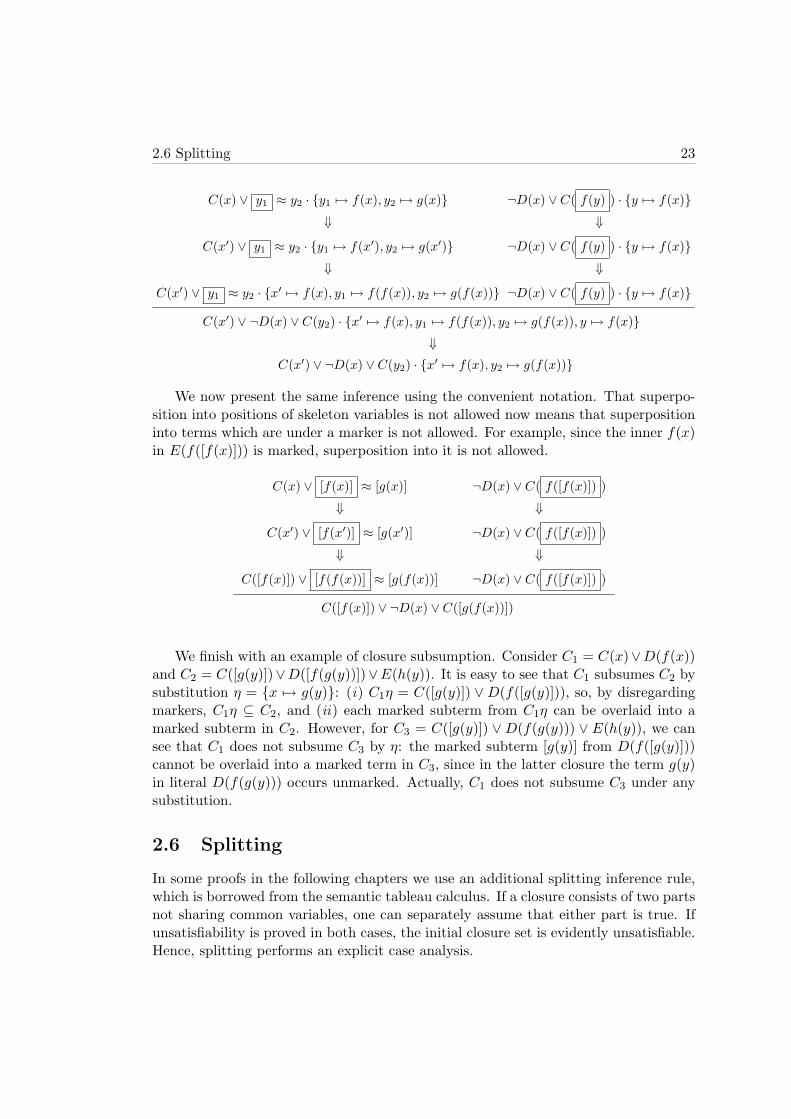
The previous inference is written using the notation that explicitly distinguishesthe skeleton from the substitution part of a closure. Next, we show the same inferencewritten using the convenient notation, where terms occurring at positions of skeletonvariables are marked. Note that, in the second step, the term f(x) in the literalE([f(x)]) is introduced by unification and is therefore marked.
C(x) ∨ R(x, f(x)) ¬D(x) ∨ ¬R(x, y) ∨ E(y)
⇓ ⇓
C(x) ∨ R(x, f(x)) ¬D(x′) ∨ ¬R(x′, y) ∨ E(y)
⇓ ⇓
C(x) ∨ R(x, f(x)) ¬D(x) ∨ ¬R(x, [f(x)]) ∨ E([f(x)])
C(x) ∨ ¬D(x) ∨ E([f(x)])
Next, we give an example of a positive superposition inference. We assume that noliteral in either premise is selected, that literals y1 ≈ y2 · y1 7→ f(x), y2 7→ g(x) andC(f(y)) · y 7→ f(x) are maximal, and that f(x) g(x). Superposition is performedfrom y1 into f(y). To apply the inference rule, we separate the variables in the premises,compute the most general unifier σ = MGU(f(x′), f(f(x))) = x′ 7→ f(x), and applyit to the premises. We then perform superposition, after which we remove from thesubstitution all mappings of variables that do not occur in the skeleton. Observe thatthe literal C(f(y)) · y 7→ f(x) is equivalent to C(f(f(x))), so one might attemptto perform superposition into inner f(x). However, this is not allowed: the skeletoncontains the variable y at the position of inner f(x), and, by superposition conditions,the term into which superposition is performed should not be a variable.
2.6 Splitting 23
C(x) ∨ y1 ≈ y2 · y1 7→ f(x), y2 7→ g(x) ¬D(x) ∨ C( f(y) ) · y 7→ f(x)⇓ ⇓
C(x′) ∨ y1 ≈ y2 · y1 7→ f(x′), y2 7→ g(x′) ¬D(x) ∨ C( f(y) ) · y 7→ f(x)⇓ ⇓
C(x′) ∨ y1 ≈ y2 · x′ 7→ f(x), y1 7→ f(f(x)), y2 7→ g(f(x)) ¬D(x) ∨ C( f(y) ) · y 7→ f(x)
C(x′) ∨ ¬D(x) ∨ C(y2) · x′ 7→ f(x), y1 7→ f(f(x)), y2 7→ g(f(x)), y 7→ f(x)⇓
C(x′) ∨ ¬D(x) ∨ C(y2) · x′ 7→ f(x), y2 7→ g(f(x))
We now present the same inference using the convenient notation. That superpo-sition into positions of skeleton variables is not allowed now means that superpositioninto terms which are under a marker is not allowed. For example, since the inner f(x)in E(f([f(x)])) is marked, superposition into it is not allowed.
C(x) ∨ [f(x)] ≈ [g(x)] ¬D(x) ∨ C( f([f(x)]) )
⇓ ⇓
C(x′) ∨ [f(x′)] ≈ [g(x′)] ¬D(x) ∨ C( f([f(x)]) )
⇓ ⇓
C([f(x)]) ∨ [f(f(x))] ≈ [g(f(x))] ¬D(x) ∨ C( f([f(x)]) )
C([f(x)]) ∨ ¬D(x) ∨ C([g(f(x))])
We finish with an example of closure subsumption. Consider C1 = C(x)∨D(f(x))and C2 = C([g(y)])∨D([f(g(y))])∨E(h(y)). It is easy to see that C1 subsumes C2 bysubstitution η = x 7→ g(y): (i) C1η = C([g(y)]) ∨D(f([g(y)])), so, by disregardingmarkers, C1η ⊆ C2, and (ii) each marked subterm from C1η can be overlaid into amarked subterm in C2. However, for C3 = C([g(y)]) ∨D(f(g(y))) ∨ E(h(y)), we cansee that C1 does not subsume C3 by η: the marked subterm [g(y)] from D(f([g(y)]))cannot be overlaid into a marked term in C3, since in the latter closure the term g(y)in literal D(f(g(y))) occurs unmarked. Actually, C1 does not subsume C3 under anysubstitution.
2.6 Splitting
In some proofs in the following chapters we use an additional splitting inference rule,which is borrowed from the semantic tableau calculus. If a closure consists of two partsnot sharing common variables, one can separately assume that either part is true. Ifunsatisfiability is proved in both cases, the initial closure set is evidently unsatisfiable.Hence, splitting performs an explicit case analysis.

24 2. Preliminary Definitions
Splitting:N ∪ C ∨D
N ∪ C | N ∪ D
where (i) N is a set of closures, (ii) C and D do not have variables in common.Splitting changes the nature of resolution significantly: a derivation is now not
unique, but is computed nondeterministically. More formally, a derivation by splittingfrom a set of closures N0 is a finitely branching tree whose nodes are closure sets, andwhose root is N0. The children of each node Ni are closure sets obtained by applyingan inference rule or a redundancy elimination rule to Ni. A set of closures N0 issatisfiable if and only if there is a saturated node Ni not containing the empty closure.
2.7 Disjunctive Datalog
The following presentation of the syntax and the semantics of disjunctive datalog isbased on [42, 55]. Let Σ be a first-order signature such that (i) F(Σ) contains onlyconstants, and (ii) ≈ ∈ P(Σ) is a special equality predicate with the arity of two. Adisjunctive datalog program with equality P is a finite set of rules of the form
A1 ∨ ... ∨An ← B1, ..., Bm
where n ≥ 0, m ≥ 0, and Ai and Bi are atoms defined over Σ. Furthermore, each rulemust be safe; that is, each variable occurring in a head literal must occur in a bodyliteral as well. For a rule r, the set of atoms head(r) = Ai | 1 ≤ i ≤ n is called therule head, whereas the set of atoms body(r) = Bi | 1 ≤ i ≤ m is called the rule body.A rule with an empty body is called a fact.
Typical definitions of a disjunctive datalog program, such as [42, 55], allow negatedatoms in the body. This negation is usually nonmonotonic, and is thus different fromnegation in first-order logic. Our algorithms from the following chapters produce onlypositive disjunctive datalog programs, so we omit nonmonotonic negation from thedefinitions. Disjunctive datalog programs without negation-as-failure are often calledpositive programs.
The ground instance of P over the Herbrand universe of P , written ground(P,HU ),is the set of ground rules obtained by replacing all variables in each rule of P withconstants from HU in all possible ways. The Herbrand base HB of P is the set ofall ground atoms defined over predicates from P(Σ). An interpretation M of P is asubset of HB . An interpretation M is a model of P if the following conditions aresatisfied: (i) body(r) ⊆M implies head(r) ∩M 6= ∅, for each rule r ∈ ground(P,HU );and (ii) all atoms from M with the ≈ predicate yield a congruence relation—that is,a relation that is reflexive, symmetric, transitive, and R(a1, . . . , ai, . . . , an) ∈ M andai ≈ bi ∈M imply R(a1, . . . , bi, . . . , an) ∈M , for each predicate symbol R ∈ P(Σ).
A model M of P is minimal if no subset of M is a model of P . The semanticsof P is defined as the set of all minimal models of P , denoted by MM(P ). Finally,the notion of query answering is defined as follows. A ground literal A is a cautious

2.7 Disjunctive Datalog 25
answer of P , written P |=c A, if A ∈M for all M ∈MM(P ); A is a brave answer ofP , written P |=b A, if A ∈ M for at least one M ∈ MM(P ). First-order entailmentcoincides with cautious entailment for positive ground atoms on positive programs.
The size of a rule r is defined as |r| = 1 +∑
1≤i≤n |Ai| +∑
1≤j≤m |Bj |, where thesize of atoms Ai and Bj is defined as |S(t1, . . . , tn)| = 1 + n: predicates and termsare encoded with one symbol, and the leading 1 in the definition of |r| accounts forthe implication symbol separating the head from the body. The size of a program P ,written |P |, is the sum of the sizes of all its rules.

26 2. Preliminary Definitions

Chapter 3
Introduction to DescriptionLogics
In this chapter, we present a formal definition of the syntax and the semantics ofdescription logics, as well as of the interesting inference problems. We introduce thebasic description logic SHIQ in Section 3.1, and extend it to SHIQ(D) in Section 3.2by adding datatypes. We also give examples of SHIQ and SHIQ(D) knowledge bases,and of interesting conclusions that can be drawn from them. We use these examplesin the latter chapters to demonstrate our reasoning algorithms.
3.1 The Description Logic SHIQThe syntax of the description logic SHIQ [73] is defined as follows.
Definition 3.1.1. For a set of abstract role names NRa, the set of SHIQ abstractroles is NRa ∪ R− | R ∈ NRa. Let Inv(R) = R− and Inv(R−) = R for R ∈ NRa. ASHIQ RBox KBR over NRa is a finite set of transitivity axioms Trans(R) and abstractrole inclusion axioms R v S such that R v S ∈ KBR implies Inv(R) v Inv(S) ∈ KBR,and Trans(R) ∈ KBR implies Trans(Inv(R)) ∈ KBR.
Let v∗ be the reflexive–transitive closure of v. A role R is transitive if there is arole S such that Trans(S) ∈ R with S v∗ R and R v∗ S; R is simple if there is norole S such that S v∗ R and S is transitive; and R is complex if it is not simple.
Let NC be a set of atomic concepts. The set of SHIQ concepts over NC and NRa
is defined inductively as the minimal set for which the following holds: > and ⊥ areSHIQ concepts; each atomic concept A ∈ NC is a SHIQ concept; and, if C and Dare SHIQ concepts, R is an abstract role, S is an abstract simple role, and n is aninteger, then ¬C, C uD, C tD, ∃R.C, ∀R.C, ≤ nS.C, and ≥ nS.C are also SHIQconcepts. Concepts that are not in NC are called complex. Possibly negated atomicconcepts are called literal concepts. A concept C is a subconcept of a concept D if Csyntactically occurs in D.
27

28 3. Introduction to Description Logics
A SHIQ TBox KBT over NC and KBR is a finite set of concept inclusion axiomsC v D or concept equivalence axioms C ≡ D, where C and D are SHIQ concepts.
Let NIa be a set of abstract individuals. A SHIQ ABox KBA is a set of conceptand abstract role membership axioms C(a), R(a, b), ¬S(a, b), and (in)equality axiomsa ≈ b and a 6≈ b, where C is a SHIQ concept, R is an abstract role, S is an abstractsimple role, and a and b are abstract individuals. An ABox is extensionally reduced ifall ABox axioms contain only literal concepts.
A SHIQ knowledge base KB is a triple (KBR,KBT ,KBA), where KBR is anRBox, KBT is a TBox, KBA is an ABox, and where the sets NRa, NC , and NIa aremutually disjoint.
Definition 3.1.1 differs from typical definitions in two aspects. First, OWL-DLlacks the unique name assumption (UNA), so we do not incorporate UNA into thedefinition of SHIQ, but allow the user to axiomatize it by including an inequalityaxiom ai 6≈ aj for each pair of distinct abstract individuals [4, page 60]. Second, usualdefinitions do not provide for ABox axioms involving negative roles. We allow suchassertions, because they allow checking entailment of ground role facts. Third, it wouldbe possible to allow complex roles in negative role membership axioms. However, ourapproach for dealing with transitivity from Section 5.2 cannot handle such axioms, sowe adopt this weaker definition.
Definition 3.1.2. The semantics of a SHIQ knowledge base KB is given by the map-ping π that transforms KB axioms into a first-order formula, as shown in Table 3.1.An atomic concept is mapped into a unary predicate, an abstract role is mapped intoa binary predicate, and an abstract individual is mapped into a constant.
The basic inference problem for SHIQ is checking satisfiability of KB—that is,determining whether a first-order model of π(KB) exists. Other interesting inferenceproblems can be reduced to satisfiability as follows, where ι is a new abstract individualnot occurring in the knowledge base:
• Concept satisfiability: A concept C is satisfiable with respect to KB if and onlyif there exists a model of KB in which the interpretation of C is not empty. Thisis the case if and only if KB ∪ C(ι) is satisfiable.
• Subsumption: A concept C is subsumed by a concept D with respect to KB,written KB |= C v D, if and only if π(KB) |= π(C v D). This is the case ifand only if KB ∪ (C u ¬D)(ι) is unsatisfiable.
• Concept equivalence: A concept C is equivalent to a concept D with respect toKB, written KB |= C ≡ D, if and only if C subsumes D with respect to KB andvice versa.
• Instance checking: An individual a is an instance of a concept C with respect toKB, written KB |= C(a), if and only if π(KB) |= π(C(a)). This is the case ifand only if KB ∪ ¬C(a) is unsatisfiable.

3.1 The Description Logic SHIQ 29
• Role checking: A simple abstract role S relates abstract individuals a and b withrespect to KB, written KB |= R(a, b), if and only if π(KB) |= π(S(a, b)). Thisis the case if and only if KB ∪ ¬S(a, b) is unsatisfiable.
The semantics of description logics is usually given by a direct model-theoreticsemantics. An interpretation I = (4I , ·I) consists of a nonempty domain set 4I andan interpretation function ·I that assigns an element aI ∈ 4I to each individual a, a setAI ⊆ 4I to each atomic concept A, and a relation RI ⊆ 4I ×4I to each role R. Thesemantics of complex concepts and axioms is given in Table 3.2, where C and D areconcepts, R and S are roles, a and b are individuals, and ]N is the number of elementsin a set N . The direct model-theoretic semantics and the semantics by translation intofirst-order logic coincide, as first shown by Borgida [21]. For a role R and an objectx ∈ 4I , an object y ∈ 4I is called an R-successor of x in I if (x, y) ∈ RI .
Often, we need a way to compare the expressivity of different description logics.The following definition provides means for that by a simple syntactic comparison.
Definition 3.1.3. Let L, L1, and L2 be three description logics.
• The logic L is a fragment of L1 if each axiom of L is also an axiom of L1.
• The logic L is between L1 and L2 if L1 is a fragment of L, and L is a fragmentof L2.
We now define several fragments of SHIQ, which we use in the following chapters.
Definition 3.1.4. For a knowledge base KB, a role R is called very simple if no role Sexists such that S v R ∈ KBR. The description logic SHIQ− is a fragment of SHIQ,where only very simple roles are allowed to occur in number restrictions ≤ nR.C and≥ nR.C.ALCHIQ (ALCHIQ−) is a fragment of SHIQ (SHIQ−) that does not allow
transitivity axioms in RBoxes. ALC is the fragment of ALCHIQ that does not providefor role inclusion axioms, inverse roles, and number restrictions.
Observe that, if KB is not extensionally reduced, it can be easily transformed intoan extensionally reduced knowledge base: for each axiom C(a) where C is not a literalconcept, one can introduce a new atomic concept AC , add the axiom AC v C to theTBox, and replace C(a) with AC(a). Such a transformation is obviously polynomialin the number of individuals, so, without loss of generality, it is safe to assume that aknowledge base is extensionally reduced.
Note that, by Definition 3.1.1, the relation v∗ can be cyclic in general. In [144]it was shown that we can reduce each SHIQ knowledge base KB with a cyclic rolehierarchy to a SHIQ knowledge base KB ′ with an acyclic role hierarchy using thefollowing algorithm. First, we compute the set of maximal, strongly connected com-ponents (or maximal cycles) of the role inclusion relation v of KB . For each stronglyconnected component Γ, we select one representative role, denoted with role(Γ), such

30 3. Introduction to Description Logics
Table 3.1: Semantics of SHIQ by Mapping to FOL
Mapping Concepts to FOLπy(>, X) = >πy(⊥, X) = ⊥πy(A,X) = A(X)πy(¬C,X) = ¬πy(C,X)
πy(C uD,X) = πy(C,X) ∧ πy(D,X)πy(C tD,X) = πy(C,X) ∨ πy(D,X)πy(∀R.C,X) = ∀y : R(X, y)→ πx(C, y)πy(∃R.C,X) = ∃y : R(X, y) ∧ πx(C, y)
πy(≤ nR.C,X) = ∀y1, . . . , yn+1 :∧n+1
i=1 [R(X, yi) ∧ πx(C, yi)]→∨n+1
i=1n+1j=i+1 yi ≈ yj
πy(≥ nR.C,X) = ∃y1, . . . , yn :∧n
i=1[R(X, yi) ∧ πx(C, yi)] ∧∧n
i=1nj=i+1 yi 6≈ yj
Mapping Axioms to FOLπ(C v D) = ∀x : πy(C, x)→ πy(D,x)π(C ≡ D) = ∀x : πy(C, x)↔ πy(D,x)π(R v S) = ∀x, y : R(x, y)→ S(x, y)
π(Trans(R)) = ∀x, y, z : R(x, y) ∧R(y, z)→ R(x, z)π(C(a)) = πy(C, a)
π(R(a, b)) = R(a, b)π(¬S(a, b)) = ¬S(a, b)
π(a b) = a b for ∈ ≈, 6≈Mapping KB to FOL
π(R) = ∀x, y : R(x, y)↔ R−(y, x)π(KBR) =
∧α∈KBR
π(α) ∧∧
R∈NRaπ(R)
π(KBT ) =∧
α∈KBTπ(α)
π(KBA) =∧
α∈KBAπ(α)
π(KB) = π(KBR) ∧ π(KBT ) ∧ π(KBA)Notes:(i): X is a meta-variable and is substituted by the actual term;(ii): πx is obtained from πy by simultaneously substituting in the definition
all y(i) with x(i), πy with πx, and vice versa.

3.1 The Description Logic SHIQ 31
Table 3.2: Direct Model-Theoretic Semantics of SHIQ
Interpreting Concepts>I = 4I
⊥I = ∅(¬C)I = 4I \ CI
(C uD)I = CI ∩DI
(C tD)I = CI ∪DI
(∀R.C)I = x | ∀y : (x, y) ∈ RI → y ∈ CI(∃R.C)I = x | ∃y : (x, y) ∈ RI ∧ y ∈ CI
(≤ nR.C)I = x | ]y | (x, y) ∈ RI ∧ y ∈ CI ≤ n(≥ nR.C)I = x | ]y | (x, y) ∈ RI ∧ y ∈ CI ≥ n
Semantics of AxiomsC v D CI ⊆ DI
C ≡ D CI = DI
R v S RI ⊆ SI
Trans(R) (RI)+ ⊆ RI
C(a) aI ∈ CI
R(a, b) (aI , bI) ∈ RI
¬S(a, b) (aI , bI) /∈ SI
a ≈ b aI = bI
a 6≈ b aI 6= bI
that, if R ∈ Γ and Inv(R) ∈ Γ′ (where Γ′ is a strongly connected component pos-sibly different from Γ) and role(Γ) = R, then role(Γ′) = Inv(R). Since we assumethat R v S ∈ KBR implies Inv(R) v Inv(S) ∈ KBR, we have that, if R,S ∈ Γ andInv(R) ∈ Γ′, then Inv(S) ∈ Γ′, so the definition of role(Γ) is correct. Next, we formthe new TBox KB ′
T and ABox KB ′A by replacing, in all axioms of KBA and KBT ,
each role R with role(Γ), where Γ is the maximal, strongly connected component thatR belongs to. Finally, we construct the new RBox KB ′
R as follows. For each pairof strongly connected components Γ 6= Γ′, if there are roles R ∈ Γ and R′ ∈ Γ′ withR v R′, we add the axiom role(Γ) v role(Γ′) to KB ′
R. Next, for each strongly con-nected component Γ, we add the axiom Inv(role(Γ)) v role(Γ) to KB ′
R if there is a roleR ∈ Γ such that Inv(R) ∈ Γ. Since the strongly connected components of v can becomputed in time quadratic in the number of roles, this reduction can be performed inpolynomial time. Hence, we can assume without loss of generality that v∗ is acyclic.
A concept C is in negation-normal form if all negations in C occur in front ofatomic concepts only. A concept C can be transformed in time linear in the size of Cinto an equivalent concept in negation-normal form, written NNF(C), by exhaustivelyapplying the following rewrite rules to subconcepts of C:

32 3. Introduction to Description Logics
¬> ⊥ ¬⊥ >¬(C1 u C2) ¬C1 t ¬C2 ¬(C1 t C2) ¬C1 u ¬C2
¬(∃R.C) ∀R.¬C ¬(∀R.C) ∃R.¬C¬(≥ (n+ 1)R.C) ≤ nR.C ¬(≤ nR.C) ≥ (n+ 1)R.C
¬(≥ 0R.C) ⊥ ¬¬C C
With |KB | we denote the size of the knowledge base assuming unary coding ofnumbers, which is computed recursively in the following way, for C and D concepts,A an atomic concept, and R and S roles:
|>| = 1 |⊥| = 1|A| = 1 |¬C| = 1 + |C|
|C tD| = |C|+ |D|+ 1 |C uD| = |C|+ |D|+ 1|∃R.C| = 2 + |C| |∀R.C| = 2 + |C|
|≥ nR.C| = n+ 2 + |C| |≤ nR.C| = n+ 2 + |C||C v D| = |C|+ |D|+ 1 |C ≡ D| = |C|+ |D|+ 1|R v S| = 3 |Trans(R)| = 2|C(a)| = |C|+ 1 |R(a, b)| = 3|KBR| =
∑α∈KBR
|α| |KBT | =∑
α∈KBT|α|
|KBA| =∑
α∈KBA|α| |KB | = |KBR|+ |KBT |+ |KBA|
Intuitively, |KB | is the number of symbols needed to encode KB on the inputtape of a Turing machine. We use a single symbol for each atomic concept, role, andindividual. The n in the definition of the length of concepts ≥ nR.C and ≤ nR.Cstems from the assumption on number coding: a number n can be encoded in unarywith n bits.
The notion of positions is extended to SHIQ concepts and axioms in the obviousway:
• α|ε = α for α a concept or an axiom;
• (¬D)|1.p = D|p;
• (D1 D2)|i.p = Di|p for ∈ u,t,v,≡ and i ∈ 1, 2;
• For C = ./ R.D with ./ ∈ ∃,∀, C|1 = R, and C|2.p = D|p;
• For C = ./ nR.D with ./ ∈ ≤,≥, C|1 = n, C|2 = R, and C|3.p = D|p;
• Trans(R)|1 = R;
• For α = C(a), α|1.p = C|p, and α|2 = a;
• For α = R(a, b), α|1 = R, α|2 = a, and α|3 = b;
• (¬S(a, b))|1.p = S(a, b)|p;
• (a1 a2)|i = ai for ∈ ≈, 6≈ and i ∈ 1, 2.

3.1 The Description Logic SHIQ 33
For α a SHIQ concept or axiom and p a position in α, replacing α|p with β isdenoted with α[β]p, and is defined in the obvious way (we assume that the result isa syntactically correct term). Furthermore, if α|p is a concept, then the polarity of pis defined to agree with the polarity of the corresponding position in translation of αinto first-order logic, and is defined as follows:
pol(C, ε) = 1 pol(¬C, 1.p) = −pol(C, p)pol(C1 u C2, i.p) = pol(Ci, p) for i ∈ 1, 2 pol(∃R.C, 2.p) = pol(C, p)pol(C1 t C2, i.p) = pol(Ci, p) for i ∈ 1, 2 pol(∀R.C, 2.p) = pol(C, p)
pol(≤ nR.C, 3.p) = −pol(C, p) pol(≥ nR.C, 3.p) = pol(C, p)pol(C1 v C2, 1.p) = −pol(C1, p) pol(C1 v C2, 2.p) = pol(C2, p)pol(C1 ≡ C2, i.p) = 0 for i ∈ 1, 2 pol(C(a), 1.p) = pol(C, p)
3.1.1 Example
In this subsection, we give an example of a SHIQ knowledge base and show someinferences that can be drawn from it. DLs were often used for solving configurationproblems [93]. Configurations usually consist of many different parts, catalogs of partsthat configurations are assembled from are usually hierarchical, and valid configura-tions can, to a large degree, be described using logical assertions. Hence, we embedour example in a configuration scenario.
Let ACME be a computer manufacturing company. As all modern suppliers ofcomputer equipment, ACME allows its customers to assemble a computer configura-tion that best suits their needs. However, assembling a configuration is a nontrivialtask, due to interdependencies among different components. For example, the choiceof the motherboard usually constrains the types of compatible memory chips, diskcontrollers, and other components. To aid its customers in assembling a valid config-uration, ACME creates a formal ontology of catalog parts. This ontology can be usedin an application that guides the users in choosing their components, thus ensuringthat chosen components work together correctly in an assembled computer.
To represent objects from the ACME catalog and the relationships between them,we use the concepts and roles from Table 3.3.
We now describe some relations that hold for all computers in all configurations.First, we would like to constrain the role hasAdpt to point only to instances of theAdpt concept; we often say that the range of the hasAdpt role is the Adpt concept.Similarly, the range of has3DAcc is 3DAcc. These constraints can be specified usingthese axioms:
> v ∀ hasAdpt .Adpt(3.1)> v ∀ has3DAcc.3DAcc(3.2)
Next, we specify taxonomical relationships that hold between items in the catalog.Axiom (3.3) states that things that are adapters and 3D accelerators are adapterswith built-in 3D accelerators. Furthermore, (3.4) and (3.5) state that adapters and 3D
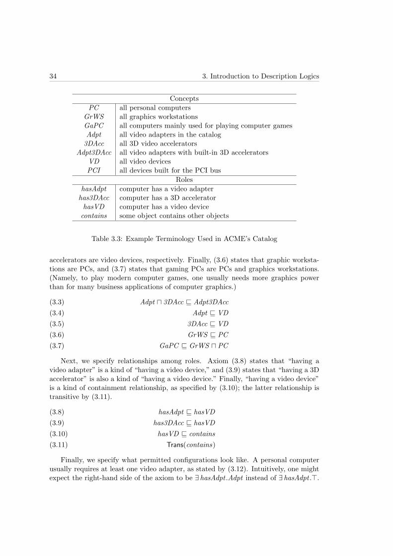
34 3. Introduction to Description Logics
ConceptsPC all personal computers
GrWS all graphics workstationsGaPC all computers mainly used for playing computer gamesAdpt all video adapters in the catalog
3DAcc all 3D video acceleratorsAdpt3DAcc all video adapters with built-in 3D accelerators
VD all video devicesPCI all devices built for the PCI bus
RoleshasAdpt computer has a video adapter
has3DAcc computer has a 3D acceleratorhasVD computer has a video devicecontains some object contains other objects
Table 3.3: Example Terminology Used in ACME’s Catalog
accelerators are video devices, respectively. Finally, (3.6) states that graphic worksta-tions are PCs, and (3.7) states that gaming PCs are PCs and graphics workstations.(Namely, to play modern computer games, one usually needs more graphics powerthan for many business applications of computer graphics.)
Adpt u 3DAcc v Adpt3DAcc(3.3)Adpt v VD(3.4)
3DAcc v VD(3.5)GrWS v PC(3.6)
GaPC v GrWS u PC(3.7)
Next, we specify relationships among roles. Axiom (3.8) states that “having avideo adapter” is a kind of “having a video device,” and (3.9) states that “having a 3Daccelerator” is also a kind of “having a video device.” Finally, “having a video device”is a kind of containment relationship, as specified by (3.10); the latter relationship istransitive by (3.11).
hasAdpt v hasVD(3.8)has3DAcc v hasVD(3.9)hasVD v contains(3.10)
Trans(contains)(3.11)
Finally, we specify what permitted configurations look like. A personal computerusually requires at least one video adapter, as stated by (3.12). Intuitively, one mightexpect the right-hand side of the axiom to be ∃ hasAdpt .Adpt instead of ∃ hasAdpt .>.

3.2 Description Logics with Concrete Domains 35
However, since the range of hasAdpt is Adpt by (3.1), the axiom (3.12) is sufficient.Next, (3.13) states that graphics workstations require a 3D accelerator. Axiom (3.14)states that gaming PCs, being destined for the lower market segment, should have atmost one video device. Finally, (3.15) ensures that all parts of a PCI-based computerare really built for the PCI bus.
PC v ∃ hasAdpt .>(3.12)GrWS v ∃ has3DAcc.>(3.13)
GaPC v ≤ 1 hasVD .VD(3.14)PCI v ∀ contains.PCI(3.15)
With KB1 we denote a SHIQ knowledge base that contains exactly the axioms(3.1)–(3.15).
We now show how KB1 can be used to solve configuration tasks. Let us now assumethat a customer wants to buy a gaming PC, and that an ACME sales representative istrying to help the customer to decide what kind of video or 3D accelerator should beadded to the computer. He represents the choices of the customer using the followingassertion:
GaPC (pc1 )(3.16)
Axiom (3.16) gives a name, pc1 , to the computer that the customer wants to buy,and states that it is a gaming PC; let KB2 be a SHIQ ABox containing only theaxiom (3.16).
The knowledge about the configuration and the user’s choices can now be used toguide the construction of a valid configuration as follows. Namely, it is easy to see thatthe following holds:
KB1 ∪KB2 |= ∃hasVD .Adpt3DAcc(pc1 )(3.17)
In other words, the video device that the customer needs must be a video adapterwith a built-in 3D accelerator. Namely, since pc1 is a gaming PC by (3.16), it hasa video adapter by (3.12) and a 3D accelerator by (3.13). However, all gaming PCsare allowed to have only one video device by (3.14), so the video adapter and the 3Daccelerator must be one and the same. Hence, the video device must be the videoadaptor and the 3D accelerator.
3.2 Description Logics with Concrete Domains
Practical applications of description logics often need to represent concrete proper-ties, such as height, name, or age, which assume values from a fixed domain, such asintegers or strings. This requirement led to the extension of description logics withconcrete domains [5]. Informally, a concrete domain provides a set of predicates with

36 3. Introduction to Description Logics
a predefined interpretation. If a decision procedure for checking satisfiability of finiteconjunctions over concrete domain predicates exists, many DLs can be combined witha concrete domain while retaining decidability. Unfortunately, in [89] it was shown thata logic with general inclusion axioms and concrete domains is undecidable. Therefore,in [70, 101, 62] several restrictions of the general approach were investigated; a surveyof the main results was presented in [88]. The cumulative results of this research haveinfluenced the design of OWL-DL [106], which supports datatypes—a basic form ofconcrete domains.
3.2.1 Concrete Domains
With x we denote a vector of variables x1, . . . , xn, and for a function δ, with δ(x) wedenote the application of δ to each element xi of x—that is, a vector δ(x1), . . . , δ(xn).A concrete domain is defined as follows:
Definition 3.2.1. A concrete domain D is a pair (4D,ΦD), where 4D is a set, calledthe domain of D, and ΦD is a finite set of concrete predicate names. Each d ∈ ΦD
is associated with an arity n and an extension dD ⊆ 4nD. A concrete domain D is
admissible if the following conditions hold:
• ΦD is closed under negation; that is, for each d ∈ ΦD, there exists d ∈ ΦD withdD = 4n
D \ dD;
• ΦD contains a unary predicate >D interpreted as 4D;
• ΦD contains a binary predicate ≈D interpreted as (x, y) | x = y;
• ΦD contains a unary predicate =α for each α ∈ 4D, interpreted as α;
• D-satisfiability of finite conjunctions of the form∧n
i=1 di(xi)—that is, checkingif an assignment δ of variables to elements of 4D exists such that δ(xi) ∈ dDifor each 1 ≤ i ≤ n—is decidable.
The definition of admissibility from [5] does not require the existence of ≈D pred-icate. However, the algorithms we develop in the subsequent chapters depend on thispredicate, so we extend the notion of admissibility appropriately. Furthermore, theusual definition does not require the existence of predicates =α. We introduce thisrestriction to allow accessing concrete domain individuals explicitly. Thus, we canstate that the age of Peter is 15 using the axiom hasAge(peter , 15); this is equivalentto hasAge(peter , a15) ∧ =15(a15), where =15 is a concrete domain predicate with theinterpretation 15.
Extending first-order logic with a concrete domain is significantly simplified if theinterpretation of concrete objects is separated from the interpretation of other objects.Hence, we assume that the set of sorts S of a signature Σ contains the sort c for theconcrete objects, which is different from other abstract objects. When there is a need todistinguish the sorts syntactically, we denote the variables (general function symbols)of sort c with xc (f c).

3.2 Description Logics with Concrete Domains 37
Definition 3.2.2. A signature Σ = (P,F ,V,S) is compatible with an admissibleconcrete domain D if it satisfies the following conditions:
• c ∈ S is a concrete sort;
• ΦD ⊆ P;
• The signature of each predicate from ΦD is c× . . .× c;
• For each general function symbol f with a signature r1 × . . . × rn → r, we haveri 6= c for each i.
We assume that the concrete predicate ≈D is used in formulae instead of ≈c forexpressing equality between concrete terms. An interpretation I over the D-signature Σis a D-interpretation if Dc = 4D, and, for each concrete predicate d ∈ ΦD, dI = dD.The usual notions of models, validity, satisfiability, and entailment are generalized toD-models, D-validity, D-satisfiability, and D-entailment (written |=D) as usual.
When ambiguity does not arise, we do not stress D for satisfiability, equisatisfia-bility, entailment, and so on. Next, we discuss the restrictions of Definition 3.2.2.
First, the concrete domain does not specify the interpretation for general func-tion symbols of sort c. Hence, to simplify the treatment, we prohibit nesting of con-crete terms into other (concrete or nonconcrete) terms. Hence, for a term t, we havesort(t|p) = c only if p = ε.
Second, the equality and inequality between concrete terms are expressed onlyusing the concrete predicates ≈D and 6≈D, respectively. Note that both ≈D and 6≈D
are concrete predicates without any special status; also, a literal sc 6≈D tc is a positiveliteral with a concrete predicate 6≈D. If a literal sc tc with ∈ ≈D, 6≈D is tobe represented as an E-term (for example, in order to apply basic superposition), itis encoded as a positive literal (sc tc) ≈ T. Therefore, ≈D and 6≈D are opaqueto equational calculi, such as basic superposition, and they are handled only by theextensions we present in Subsection 6.1.1.
Third, practical applications require several different concrete domains at once. Anapproach for combining two or more concrete domains into one concrete domain hasbeen presented in [5]. Therefore, without loss of generality we can consider only oneconcrete domain at the time.
3.2.2 The Description Logic SHIQ(D)
We now present the formal definition of the description logic SHIQ(D), which isobtained by combining SHIQ with concrete datatypes. The syntax of SHIQ fromDefinition 3.1.1 is extended as follows:

38 3. Introduction to Description Logics
Definition 3.2.3. Let NRc be the set of concrete roles. Additionally to SHIQ RBoxaxioms, a SHIQ(D) RBox KBR can contain a finite number concrete role inclusionaxioms T v U .1
Let D be an admissible concrete domain. In addition to SHIQ concepts, the set ofSHIQ(D) concepts contains ∃T1, . . . , Tm.d, ∀T1, . . . , Tm.d, ≤ nT , and ≥ nT , for T(i)
concrete roles, d an m-ary concrete domain predicate, and n an integer. A SHIQ(D)TBox KBT is defined analogously to Definition 3.1.1.
Let NIc be a set of concrete individuals. Additionally to SHIQ ABox axioms, aSHIQ(D) ABox KBA can contain a finite number of concrete role membership axioms(¬)T (a, bc), and (in)equality axioms ac ≈ bc and ac 6≈ bc, where T is a concrete role,a is an abstract individual, and ac and bc are concrete individuals.
A SHIQ(D) knowledge base is defined as in Definition 3.1.1, where the sets NRa,NRc, NC , NIa, and NIc are mutually disjoint.
The semantics of SHIQ from Definition 3.1.2 is extended to SHIQ(D) as follows:
Definition 3.2.4. The semantics of a SHIQ(D) knowledge base KB is given byextending the mapping π from Definition 3.1.2 to translate KB into a multi-sortedfirst-order formula, as shown in Table 3.4. We assume the existence of a separate sorta for abstract objects, which is different from c. Atomic concept predicates have thesignature a, abstract roles have the signature a × a, concrete roles have the signaturea× c, and n-ary concrete domain predicates have the signature c× . . .× c.
The basic inference problem for SHIQ(D) is checking satisfiability of KB—thatis, determining whether a D-model of π(KB) exists. The other inference problems aredefined analogously to Definition 3.1.2.
The direct model-theoretic semantics is easily extended to SHIQ(D), by extend-ing the interpretation function ·I to assign an element (ac)I ∈ 4D to each concreteindividual ac, and a relation T I ⊆ 4I ×4D to each concrete role T . The semanticsof new concepts and axioms is given in Table 3.5, where T(i) and U are concrete rolesand d is a concrete predicate.SHIQ(D) concepts can be rewritten into negation-normal form as follows:
¬(∃T1, . . . , Tn.d) ∀T1, . . . , Tn.d ¬(∀T1, . . . , Tn.d) ∃T1, . . . , Tn.d¬(≥ (n+ 1)T ) ≤ nT ¬(≤ nT ) ≥ (n+ 1)T
¬(≥ 0T ) ⊥
The size of a SHIQ(D) knowledge base KB is obtained by extending the definitionfrom Section 3.1 to handle the new constructs in the following way:
|∃T1, . . . , Tm.d| = 2 +m |≥ nT | = n+ 2|∀T1, . . . , Tm.d| = 2 +m |≤ nT | = n+ 2
The notion of positions is extended to the new SHIQ(D) constructs as follows:1Inverse concrete roles do not make sense semantically, so we do not distinguish between con-
crete roles and concrete role names. Furthermore, transitive concrete roles also do not make sensesemantically, so they are not allowed. Note that this makes all concrete roles simple.

3.2 Description Logics with Concrete Domains 39
Table 3.4: Semantics of SHIQ(D) by Mapping to FOL
Mapping Concepts to FOLπy(∀T1, . . . , Tm.d,X) = ∀yc
1, . . . , ycm :
∧mi=1 Ti(X, yc
i )→ d(yc1, . . . , y
cm)
πy(∃T1, . . . , Tm.d,X) = ∃yc1, . . . , y
cm :
∧mi=1 Ti(X, yc
i ) ∧ d(yc1, . . . , y
cm)
πy(≤ nT ,X) = ∀yc1, . . . , y
cn+1 :
∧n+1i=1 T (X, yc
i )→∨n+1
i=1n+1j=i+1 y
ci ≈D yc
j
πy(≥ nT ,X) = ∃yc1, . . . , y
cn :
∧ni=1 T (X, yc
i ) ∧∧n
i=1nj=i+1 y
ci 6≈D yc
j
Mapping Axioms to FOLπ(T v U) = ∀x, yc : T (x, yc)→ U(x, yc)π(T (a, bc)) = T (a, bc)
π(¬T (a, bc)) = ¬T (a, bc)π(ac bc) = ac D bc for ∈ ≈, 6≈
• For C = ./ T1, . . . , Tm.d with ./ ∈ ∃,∀, C|i = Ti for 1 ≤ i ≤ m, and C|m+1 = d;
• For C = ./ nT with ./ ∈ ≤,≥, C|1 = n and C|2 = T .
Since the new constructs do not contain nested concepts, the notion of polaritycarries over from SHIQ to SHIQ(D) without change.
3.2.3 Example
To demonstrate how concrete domains can be applied in practice, we extend the con-figuration example from Subsection 3.1.1 with a concrete domain N, where the domainis the set of all nonnegative integers, and the predicates have the form ≥100 and areinterpreted in the obvious way.
An important aspect of any item catalog is the item’s price, which we representusing the role price. In a more realistic scenario, one would probably represent aprice with the pair specifying the amount and the currency; however, for simplicity,we assume that all prices are represented in euros. An item has at most one price, sowe declare price to be functional by (3.18).
> v ≤ 1 price(3.18)
We now represent additional classes of items in our catalog. For example, using(3.19) we state that high-end PCs are either graphics workstations, or PCs with a pricehigher than 2000 EUR.
HighEnd v GrWS t (PC u ∃price.≥2000)(3.19)
We denote with KB3 the knowledge base KB1 from Subsection 3.1.1 extended withaxioms (3.18) and (3.19).

40 3. Introduction to Description Logics
Table 3.5: Direct Model-Theoretic Semantics of SHIQ(D)
Interpreting Concepts(∀T1, . . . , Tm.d)I = x | ∀y1, . . . , ym : (x, y1) ∈ T I
1 ∧ . . . ∧ (x, ym) ∈ T Im →
(y1, . . . , ym) ∈ dD(∃T1, . . . , Tm.d)I = x | ∃y1, . . . , ym : (x, y1) ∈ T I
1 ∧ . . . ∧ (x, ym) ∈ T Im∧
(y1, . . . , ym) ∈ dD(≤ nT )I = x | ]y | (x, y) ∈ T I ≤ n(≥ nT )I = x | ]y | (x, y) ∈ T I ≥ n
Semantics of AxiomsT v U T I ⊆ U I
T (a, bc) (aI , (bc)I) ∈ T I
¬T (a, bc) (aI , (bc)I) /∈ T I
ac ≈ bc (ac)I = (bc)I
ac 6≈ bc (ac)I 6= (bc)I
Let us now assume that a customer wants to buy a high-end PC with a price of1500 EUR at most. These choices are represented by axioms (3.20) and (3.21); letKB4 be the knowledge base containing them.
HighEnd(pc2 )(3.20)∃price.≤1500(pc2 )(3.21)
Based on the user’s choices, the configuration system can conclude that pc2 mustbe a graphics workstation:
KB3 ∪KB4 |= GrWS (pc2 )(3.22)
Namely, pc2 is declared to be a high-end PC with a price lower than 1500 EUR.Since each PC has only one price, the price cannot be also higher than 2000 EUR;formally stated, the conjunction of concrete domain predicates ≥2000(x) ∧ ≤1500(x) isunsatisfiable. Hence, if axioms (3.19) and (3.19) are to be satisfied, pc2 must be agraphics workstation.

Part II
From Description Logics toDisjunctive Datalog
41


Chapter 4
Reduction Algorithm at a Glance
The algorithm for reducing a SHIQ(D) knowledge base to a disjunctive datalog pro-gram is fairly complex and technical. This is so because SHIQ(D) encompassesdifferent features, each of which raises special concerns for resolution-based theoremproving. For example, handling number restrictions requires equality reasoning, whichin turn requires a complex calculus, such as basic superposition. Similarly, a newapproach for reasoning with concrete domains is required to handle datatypes.
To make our work easier to follow, in this chapter we present a simpler versionof all algorithms, scaled down to the basic description logic ALC. Even though itis quite simple, ALC is an ExpTime-complete logic [144], with features common tomost of the more complex DLs, such as existential and universal quantification, andgeneral concept inclusion axioms. The reduction algorithm for ALC conveys all thebasic ideas, without overloading the presentation with details. We hope that this willhelp the reader to understand the intuition behind the algorithms presented in thefollowing chapters.
This chapter is of tutorial character, and as such we tried to make it self-contained(apart from the general definitions that we presented in Chapter 2). However, it is notstrictly necessary for understanding the other chapters and may be skipped. To makeother chapters self-contained as well, some definitions and clarifications are repeatedin the latter chapters.
4.1 The Main Difficulty in Reducing DLs to Datalog
For an ALC knowledge base KB , our goal is to derive a disjunctive datalog programDD(KB) such that KB |= α if and only if DD(KB) |= α for α of the form A(a) orR(a, b). In other words, KB and DD(KB) should entail the same set of positive groundfacts. We can thus use DD(KB) instead of KB for query answering, and in doing sowe can apply all optimization techniques known in deductive databases.
43

44 4. Reduction Algorithm at a Glance
As shown by Definition 3.1.2 and [21], there is a close correspondence betweendescription logics and first-order logic. Consider the following knowledge base:
KB = A v ∃R.A,∃R.∃R.A v B,A(a)(4.1)
A naıve attempt to reduce KB into disjunctive datalog is to translate KB into first-order logic as π(KB), skolemize it, translate it into conjunctive normal form, andrewrite the obtained set of clauses into rules. On KB , such an approach produces thefollowing logic program LP(KB):
R(x, f(x))← A(x)(4.2)A(f(x))← A(x)(4.3)
B(x)← R(x, y), R(y, z), A(z)(4.4)A(a)(4.5)
Clearly, KB and LP(KB) entail the same set of ground facts. However, LP(KB)contains a function symbol in a recursive rule (4.3). This raises the issue of how toanswer queries in LP(KB). Namely, well-known query evaluation techniques, such asbottom-up saturation, will not terminate on LP(KB): using bottom-up saturation,we shall derive A(f(a)), R(a, f(a)), A(f(f(a))), R(f(a), f(f(a))), B(a), and so on.Obviously, such an algorithm will continue deriving ever deeper facts, and will thereforenever terminate. Note that we need all previously derived facts to derive B(a) fromLP(KB), and that we do not know a priori when all relevant ground facts have beenderived, so that we might stop the saturation.
This problem could be solved by employing an appropriate cycle detection mech-anism. The authors use such an approach in [49] to derive a hyperresolution decisionprocedure for a variant of the guarded fragment. However, using specialized algorithmsfor evaluating queries in LP(KB) takes us further away from our original goal of apply-ing deductive database optimization techniques to description logics. In a way, suchan algorithm could be understood as an alternative syntactic notation for the tableaucalculus, for which it is still unclear how to apply known optimization techniques, suchas magic sets.
To avoid potential problems with termination, our goal is to derive a true disjunc-tive datalog program DD(KB) without function symbols. For such a program, queriescan be evaluated using any standard technique; furthermore, all existing optimizationtechniques known in deductive databases can be applied directly. Hence, the mainproblem that we deal with is the elimination of function symbols from LP(KB).
4.2 The General Idea
To obtain the reduction of an ALC knowledge base KB to a disjunctive datalog pro-gram entailing the same set of ground facts, we start off with a slightly simpler taskof deriving a program DD(KB) that is satisfiable if and only if KB is satisfiable. The

4.3 Translating KB into Clauses 45
intuitive principle used to ensure the equisatisfiability of KB and DD(KB) is relativelysimple. Let us assume that unsatisfiability of KB can be demonstrated by a refutationin some sound and complete calculus C. If it is possible to simulate inferences of C onKB using a datalog program DD(KB), a refutation in KB by C can be reduced to arefutation in DD(KB). Conversely, if DD(KB) is unsatisfiable, there is a refutation inDD(KB). If it is possible to simulate inferences in DD(KB) by the calculus C on KB ,then a refutation in DD(KB) can be reduced to a refutation in KB . To summarize, ifinferences can be simulated in both directions, DD(KB) and KB are equisatisfiable.
To obtain a sound, complete, and terminating algorithm from the high-level ideaoutlined in the previous paragraph, it is necessary to select an appropriate calculusC, capable of effectively deciding satisfiability of KB . Positive disjunctive datalogis strongly related to clausal first-order logic. Intuitively, simulating inferences indisjunctive datalog is easier if C is a clausal refutation calculus. Therefore, we firstderive a decision procedure for ALC based on the ordered resolution calculus R (for adefinition of R, see Section 2.4). In particular, we show in Section 4.3 how to translateKB into an equisatisfiable set of clauses Ξ(KB), and in Section 4.4 that exhaustiveapplication of the inference rules of R on Ξ(KB) eventually terminates. Since R issound and complete, termination implies that R decides satisfiability of Ξ(KB), andtherefore of KB as well.
Based on such a procedure, we derive in Section 4.5 the desired reduction of KBto a disjunctive datalog program. It turns out that, for ALC, simulating inferences ofR in disjunctive datalog and vice versa is quite straightforward.
After presenting several simple examples in Section 4.6, in Section 4.7 we summarizethe issues that need to be dealt with in order to extend the algorithms to SHIQ(D).Finally, in Section 4.8 we discuss some interesting aspects of our algorithms.
4.3 Translating KB into Clauses
The first step in deciding satisfiability of an ALC knowledge base KB by R is to trans-form KB into an equisatisfiable set of clauses Ξ(KB). A straightforward way of doingso is to compute the formula π(KB) (where π is the operator from Definition 3.1.2),and then to apply the clausification operator Cls to it (that is, to skolemize π(KB)and to transform the result into conjunctive normal form using well-known identities,as explained in Section 2.1).
However, such an algorithm has two important drawbacks. First, the size ofCls(π(KB)) could be exponential in the size of π(KB), due to nesting of u and tconnectives. Second, since KB is an ALC knowledge base, the formula π(KB) is ofa particular syntactic structure, which we exploit to derive the decision procedure.Direct clausification of π(KB) would destroy this structure, and thus make it difficult,if not impossible, to obtain a decision procedure for ALC by R.
In order to avoid the exponential blowup and to preserve the structure of formulae,we apply the structural transformation, introduced in [108, 99, 8]. Next, we presentan alternative, but equivalent definition.

46 4. Reduction Algorithm at a Glance
Definition 4.3.1. Let C be an ALC concept in negation-normal form. A positionp 6= ε in C is eligible for replacement if C|p is of the form
⊔Li,
dLi, ∀R.L, or
∃R.L, where L(i) are all literal concepts. The definitorial form of C, written Def(C),is defined recursively as follows:
Def(C) =
¬Q t C|p ∪ Def(C[Q]p) if C is a nonliteral concept and
p is eligible for replacement in CC otherwise
For example, Def(∃R.(∀S.¬A)) = ∃R.Q, ¬Q t ∀S.¬A. Note that ¬Q t ∀S.¬Acan be interpreted as Q v ∀S.¬A, which allows us to use Q as a new name for ∀S.¬Ain ∃R.(∀S.¬A). Furthermore, as shown by the following lemma, this transformationdoes not affect satisfiability: > v ∃R.(∀S.¬A) and > v ∃R.Q,> v ¬Qt ∀S.¬A areequisatisfiable.
Lemma 4.3.2. For an ALC concept C in negation-normal form, the axiom > v C issatisfiable if and only if the set of axioms > v Di |Di ∈ Def(C) is satisfiable.
Proof. The proof is by induction on the number of recursive invocations of Def. Theinduction base is trivial, so we consider the induction step, which replaces the sub-concept C|p in C with Q, resulting in D = C[Q]p. For the (⇒) direction, let I bea model satisfying > v C. Obviously, an interpretation I ′, obtained by extending Iwith QI′ = DI , satisfies > v D and > v ¬Q t C|p. For the (⇐) direction, let I be amodel of > v D and > v ¬Q tC|p. The following property can be shown by an easyinduction on the structure of D: for each position q in D, (D|q)I ⊆ (C|q)I . But then,for q = ε, we have DI ⊆ CI . Since 4I ⊆ DI , we have that I is a model of > v C.
The set of clauses Ξ(KB), encoding an ALC knowledge base KB in first-order logic,is defined as follows:
Definition 4.3.3. We extend the clausification operator Cls from Section 2.1 to ALCconcepts as follows:
Cls(C) =⋃
D∈Def(NNF(C))
Cls(∀x : πy(D,x))
For an extensionally reduced ALC knowledge base KB, Ξ(KB) is the smallest setof clauses satisfying the following conditions:
• For each ABox axiom α in KB, Cls(π(α)) ⊆ Ξ(KB);
• For each TBox axiom C v D in KB, Cls(¬C tD) ⊆ Ξ(KB);
• For each TBox axiom C ≡ D in KB, Cls(¬C tD) ⊆ Ξ(KB) andCls(¬D t C) ⊆ Ξ(KB).

4.4 Deciding Satisfiability of Ξ(KB) by R 47
Table 4.1: Clause Types after Preprocessing
1∨
(¬)Ci(x) ∨R(x, f(x))2
∨(¬)Ci(x) ∨ (¬)D(f(x))
3∨
(¬)Ci(x)4
∨(¬)C(x) ∨ ¬R(x, y) ∨ (¬)D(y)
5 (¬)C(a)6 (¬)R(a, b)
If KB is not extensionally reduced, then Ξ(KB) = Ξ(KB ′), where KB ′ is an exten-sionally reduced knowledge base obtained from KB as explained in Section 3.1.
We now show that clausification does not affect the semantics of a knowledge base,and that it produces clauses of a certain syntactic structure:
Lemma 4.3.4. Let KB be an ALC knowledge base. Then, the following claims hold:
• KB is satisfiable if and only if Ξ(KB) is satisfiable.
• Ξ(KB) can be computed in time polynomial in |KB |.
• Each clause in Ξ(KB) is of one of the types given in Table 4.1.
Proof. Equisatisfiability of KB and Ξ(KB) is an easy consequence of Lemma 4.3.2.Furthermore, the number of recursive invocations of Def and the number of new con-cepts Q are linear in the number of subconcepts of C. Hence, |Def(C)| is linear in|C|, so |Ξ(KB)| is polynomial in |KB |. Finally, observe that Def(C) can contain onlyconcepts of the form D or ¬QtD, where D is of the form
⊔Li,
dLi, ∀R.L, or ∃R.L,
and all L(i) are literal concepts. Hence, for D = ∃R.L, Cls(D) contains clauses of type1 and 2; for D = ∀R.L a clause of type 4; and for D =
⊔Li or D =
dLi clauses of
type 3. Clauses of type 5 and 6 are obtained by clausifying ABox axioms.
4.4 Deciding Satisfiability of Ξ(KB) by RSinceR is a sound and complete calculus, we can use it to check satisfiability of Ξ(KB).To obtain a decision procedure, we just need to ensure that each saturation of Ξ(KB)by R terminates. Joyner outlined the basic principle to achieve this in [80]: we simplyensure that the number of clauses that can be derived in a saturation is bounded.
There are two main reasons why deriving an infinite number of clauses from a setof clauses N might be possible. First, we might keep deriving clauses with deeperand deeper terms. Consider N1 = C(a), ¬C(x) ∨ C(f(x)). If we select ¬C(x) inthe second clause and apply resolution, we derive C(f(a)), C(f(f(a))), and so forth.

48 4. Reduction Algorithm at a Glance
Second, we might keep deriving clauses containing more and more variables. ConsiderN2 = ¬R(x, y) ∨ ¬R(y, z) ∨ R(x, z), C(x) ∨ R(x, y) ∨ D(y), E(x) ∨ R(x, y) ∨ F (y).If we select ¬R(x, y) and ¬R(y, z) in the first clause and apply resolution twice, weobtain C(x) ∨ D(y) ∨ E(y) ∨ F (z) ∨ R(x, z), which contains more variables than theside premises involved in the inference. It is easy to see that further inferences withthis clause will additionally increase the number of variables.
The resolution inferences performed on certain clauses are determined by the para-meters of the calculus—namely, the literal ordering and the selection function. Hence,by choosing these parameters appropriately, we can often restrict the resolution infer-ences in a way that allows us to establish a bound on the term depth and on the numberof variables. Consider again the set of clauses N1: instead of selecting ¬C(x), if weensure that C(f(x)) ¬C(x), then the second clause can participate in an inferenceonly on literal C(f(x)). Furthermore, C(f(x)) and C(a) do not unify, so no inferenceof R is applicable to N1. Hence, N1 is saturated, and, since it does not contain theempty clause, it is satisfiable. In the following definition, we choose the parameters forR that achieve such an effect on clauses from Ξ(KB).
Definition 4.4.1. Let RDL denote the calculus R parameterized as follows:
• The literal ordering is an admissible ordering such that R(x, f(x)) ¬C(x)and D(f(x)) ¬C(x), for all function symbols f , and predicates R, C, and D.
• The selection function selects every negative binary literal in each clause.
An ordering satisfying Definition 4.4.1 can be obtained by instantiating an ap-propriate lexicographic path ordering. Technically speaking, negative literals are notterms, but for the purposes of comparing literals by an LPO, we consider ¬ to be aunary general function symbol. To make an LPO compatible with RDL, we chooseany precedence > over predicate and general function symbols such that f > P > ¬,for each function symbol f and each predicate symbol P . Namely, LPOs have thesubterm property, so ¬A A; furthermore, since ¬ is the smallest symbol in >, wecannot have ¬A B A. Hence, such an LPO is admissible for R. Moreover, by thedefinition of LPOs from Section 2.2, it is easy to check that D(f(x)) f(x) ¬C(x),and R(x, f(x)) f(x) ¬C(x).
To obtain a decision procedure for ALC, we next identify the type of clauses thatcan be derived in a saturation of Ξ(KB) by RDL. We generalize the clauses fromTable 4.1 to ALC-clauses, presented in Table 4.2. For a term t, with P(t) we denotea possibly empty disjunction of the form (¬)P1(t) ∨ . . . ∨ (¬)Pn(t). With P(f(x)) wedenote a possibly empty disjunction of the form P1(f1(x)) ∨ . . . ∨ Pm(fm(x)). Notethat this definition allows each Pi(fi(x)) to contain positive and negative literals.
We now prove the following central lemma:
Lemma 4.4.2. Each RDL inference, when applied to ALC-clauses, produces an ALC-clause.
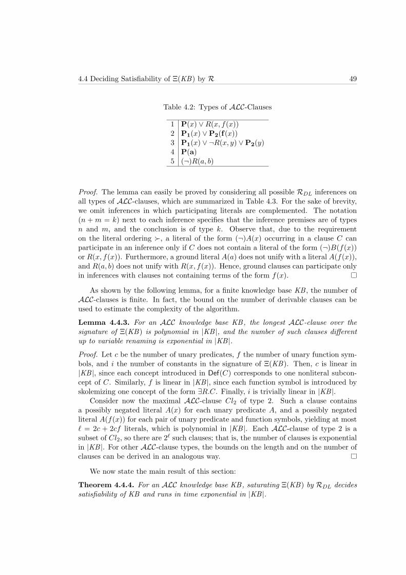
4.4 Deciding Satisfiability of Ξ(KB) by R 49
Table 4.2: Types of ALC-Clauses
1 P(x) ∨R(x, f(x))2 P1(x) ∨P2(f(x))3 P1(x) ∨ ¬R(x, y) ∨P2(y)4 P(a)5 (¬)R(a, b)
Proof. The lemma can easily be proved by considering all possible RDL inferences onall types of ALC-clauses, which are summarized in Table 4.3. For the sake of brevity,we omit inferences in which participating literals are complemented. The notation(n + m = k) next to each inference specifies that the inference premises are of typesn and m, and the conclusion is of type k. Observe that, due to the requirementon the literal ordering , a literal of the form (¬)A(x) occurring in a clause C canparticipate in an inference only if C does not contain a literal of the form (¬)B(f(x))or R(x, f(x)). Furthermore, a ground literal A(a) does not unify with a literal A(f(x)),and R(a, b) does not unify with R(x, f(x)). Hence, ground clauses can participate onlyin inferences with clauses not containing terms of the form f(x).
As shown by the following lemma, for a finite knowledge base KB , the number ofALC-clauses is finite. In fact, the bound on the number of derivable clauses can beused to estimate the complexity of the algorithm.
Lemma 4.4.3. For an ALC knowledge base KB, the longest ALC-clause over thesignature of Ξ(KB) is polynomial in |KB |, and the number of such clauses differentup to variable renaming is exponential in |KB |.
Proof. Let c be the number of unary predicates, f the number of unary function sym-bols, and i the number of constants in the signature of Ξ(KB). Then, c is linear in|KB |, since each concept introduced in Def(C) corresponds to one nonliteral subcon-cept of C. Similarly, f is linear in |KB |, since each function symbol is introduced byskolemizing one concept of the form ∃R.C. Finally, i is trivially linear in |KB |.
Consider now the maximal ALC-clause Cl2 of type 2. Such a clause containsa possibly negated literal A(x) for each unary predicate A, and a possibly negatedliteral A(f(x)) for each pair of unary predicate and function symbols, yielding at most` = 2c + 2cf literals, which is polynomial in |KB |. Each ALC-clause of type 2 is asubset of Cl2, so there are 2` such clauses; that is, the number of clauses is exponentialin |KB |. For other ALC-clause types, the bounds on the length and on the number ofclauses can be derived in an analogous way.
We now state the main result of this section:
Theorem 4.4.4. For an ALC knowledge base KB, saturating Ξ(KB) by RDL decidessatisfiability of KB and runs in time exponential in |KB |.

50 4. Reduction Algorithm at a Glance
Table 4.3: Possible Inferences by RDL on ALC-Clauses
P1(x) ∨P2(f(x)) ∨ ¬A(g(x)) A(x) ∨P3(x)
P1(x) ∨P2(f(x)) ∨P3(g(x))(2+2=2)
P1(x) ∨ ¬A(x) A(x) ∨P2(x)
P1(x) ∨P2(x)(2+2=2)
P1(x) ∨P2(f(x)) ∨ ¬A(g(x)) A(g(x)) ∨P3(h(x)) ∨P4(x)
P1(x) ∨P2(f(x)) ∨P3(h(x)) ∨P4(x)(2+2=2)
P(x) ∨R(x, f(x)) P1(x) ∨ ¬R(x, y) ∨P2(y)
P(x) ∨P1(x) ∨P2(f(x))(1+3=2)
P1(a) ∨ ¬A(b) A(x) ∨P2(x)
P1(a) ∨P2(b)(4+2=4)
P1(a) ∨ ¬A(b) A(b) ∨P2(c)
P1(a) ∨P2(c)(4+4=4)
R(a, b) P1(x) ∨ ¬R(x, y) ∨P2(y)
P1(a) ∨P2(b)(5+3=4)
R(a, b) ¬R(a, b)
(5+5=2)
Proof. By Lemma 4.4.3, the number of clauses derivable by RDL from Ξ(KB) is ex-ponential in |KB |. Each inference can be performed in time polynomial in the size ofclauses. Subsumption checking is NP-complete in the size of clauses [52], so it can beperformed in exponential time. Hence, the saturation terminates after performing atmost an exponential number of steps. Since RDL is sound and complete, it decidessatisfiability of Ξ(KB), and by Lemma 4.3.4 of KB as well, in time that is exponentialin |KB |.
4.5 Translating ALC to Disjunctive Datalog
Given a decision procedure for checking satisfiability of an ALC knowledge base KB ,it is now easy to obtain the desired reduction to disjunctive datalog. From Table 4.3,we see that (i) a ground clause cannot participate in an inference with a nongroundclause containing a function symbol, and (ii) as soon as one premise in an inference byRDL is ground, the conclusion is ground as well. Hence, we can perform all inferencesamong nonground clauses first, after which we can simply delete all nonground clauses
4.5 Translating ALC to Disjunctive Datalog 51
containing function symbols. The remaining clause set consists of clauses withoutfunction symbols, which can easily be translated into a disjunctive datalog program,by moving positive literals into rule heads and negative literals into rule bodies. Aminor problem arises if the resulting rules contain unsafe variables—that is, variablesoccurring only in the head, but not in the body. We deal with such clauses by asimple trick: we introduce a new predicate HU and add an assertion HU (a) for eachindividual a; next, we append HU (x) to the body of each rule in which x is an unsafevariable. We now present this algorithm formally.
Definition 4.5.1. Let KB be an extensionally reduced ALC knowledge base. Then,Γ(KBT ) is the set of clauses obtained by saturating Ξ(KBT ) by RDL, and then deletingall clauses containing function symbols. Furthermore, the operator λ maps clauses toclauses as follows:
λ(C) = C ∪ ¬HU (x) | for each unsafe variable x in C
For a set of clauses N , λ(N) is the set of clauses obtained by applying λ to eachelement of N . The function-free version of KB is defined as follows:
FF(KB) = λ(Γ(KBT )) ∪ Ξ(KBA) ∪ HU (a) | for each individual a occurring in KB
Finally, a disjunctive datalog program DD(KB) is the set of rules obtained by mov-ing in each clause from FF(KB) all positive literals into the rule head, and all negativeliterals into the rule body.
If KB is not extensionally reduced, then DD(KB) = DD(KB ′), where KB ′ is anextensionally reduced knowledge base obtained from KB as explained in Section 3.1.
We now state the properties of DD(KB):
Theorem 4.5.2. Let KB be an ALC knowledge base. Then, the following claims hold:
1. KB is unsatisfiable if and only if DD(KB) is unsatisfiable.
2. KB |= α if and only if DD(KB) |=c α, where α is of the form A(a) or R(a, b),and A is an atomic concept.
3. KB |= C(a) for a nonliteral concept C if and only if, for Q a new atomic concept,DD(KB ∪ C v Q) |=c Q(a).
4. The number of literals in each rule in DD(KB) is at most polynomial, the numberof rules in DD(KB) is at most exponential, and DD(KB) can be computed in timeexponential in |KB |.
Proof. (Claim 1.) Table 4.3 shows that each inference with at least one ground premisealways produces a ground conclusion. Hence, in saturating Ξ(KB) by RDL, it is pos-sible to perform all inferences among nonground clauses first. Furthermore, Table 4.3

52 4. Reduction Algorithm at a Glance
also shows that ground clauses can participate in inferences only with clauses not con-taining function symbols. Hence, after performing all inferences among nongroundclauses of Ξ(KB), one can delete all clauses containing terms of the form f(x).
By Definition 4.3.3, Ξ(KBT ) is exactly the set of nonground clauses of Ξ(KB), soΓ(KBT ) is exactly the set of clauses obtained by saturating the nonground part ofΞ(KB) and deleting the clauses containing function symbols. Furthermore, it is easyto see that Γ = Γ(KBT ) ∪ Ξ(KBA) is satisfiable if and only if FF(KB) is satisfiable.Namely, both Γ and FF(KB) are function-free sets of clauses, whose sets of groundinstances differ only on clauses containing unsafe variables. However, for a clauseC ∈ Γ containing an unsafe variable x and a ground substitution τ = x 7→ a, FF(KB)contains clauses C∨¬HU (x) and HU (a), which together imply Cτ . Hence, the groundinstances of FF(KB) imply all ground instances of Γ, so, if FF(KB) is satisfiable, Γ issatisfiable as well. Furthermore, since HU is a new predicate not occurring in Γ, eachmodel of Γ can easily be extended to a model of FF(KB). Therefore, Γ and FF(KB)are equisatisfiable.
Finally, DD(KB) is a positive datalog program whose rules are syntactic variantsof the clauses from FF(KB). Hence, DD(KB) is satisfiable if and only if FF(KB) issatisfiable.
(Claim 2.) Simply observe that KB |= α if and only if KB ∪ ¬α is unsatisfi-able. The latter is the case if and only if DD(KB ∪ ← α) = DD(KB) ∪ ← α isunsatisfiable, which is the case if and only if DD(KB) |=c α.
(Claim 3.) Follows in the same manner as Claim 2.(Claim 4.) Follows immediately from Lemma 4.4.3.
4.6 Examples
We now present several rather simple examples that point out important properties ofthe reduction algorithm.
Readers familiar with more common approaches to DL reasoning might ask them-selves how role successors are encoded in datalog programs. As we show next, rolesuccessors are not at all encoded in the datalog program. Let KB1 = C v ∃R.D,so Ξ(KB1) = ¬C(x) ∨ R(x, f(x)), ¬C(x) ∨ D(f(x)). Now Ξ(KB1) is already sat-urated by RDL, so after removing all clauses containing function symbols, we getDD(KB1) = ∅. This may seem quite confusing: KB1 implies the existence of at leastone R-successor for each member of C, whereas DD(KB1) does not reflect that. How-ever, Theorem 4.5.2 is not invalidated. Namely, the individuals introduced by theexistential quantifier in KB1 are unnamed, so they cannot be used in queries. Hence,for an arbitrary extensionally reduced ABox KBA, KB1 ∪ KBA does not imply anynew facts of the form A(a) or R(a, b). Also, note that the models of DD(KB1) arecompletely unrelated to the models of KB1. Intuitively, this is so because the reductionalgorithm is based on a proof-theoretic correspondence between refutations in Ξ(KB)and DD(KB). The models of KB and DD(KB) coincide only on positive ground facts,whereas, for unnamed individuals, the models are completely unrelated.

4.6 Examples 53
In order to be able to draw additional consequences from KB1, we need to extendit with additional statements about C, D, or R. Let KB2 = KB1 ∪ D v ⊥, soΞ(KB2) = Ξ(KB1) ∪ ¬D(x). Saturation of Ξ(KB2) produces one additional clause¬C(x), so we get DD(KB2) = ← C(x),← D(x). This shows that the reduction isnot modular: for arbitrary knowledge bases KB1 and KB2, DD(KB1) ∪ DD(KB2) isnot necessarily equal to DD(KB1 ∪KB2).
The key step in the reduction is the saturation of Ξ(KBT ) by RDL. It computes allrelevant nonground consequences of Ξ(KBT ), which ensures that subsequent removalof clauses containing function symbols does not change the set of drawn ground conse-quences. One can think of RDL as producing shortcut clauses that derive facts aboutobjects without explicitly expanding the successors of each object. This is demon-strated by the following knowledge base:
KB3 = A v ∃R.B, B v C, ∃R.C v D(4.6)
Now Ξ(KB3) consists of the following clauses:
¬A(x) ∨R(x, f(x))(4.7)¬A(x) ∨B(f(x))(4.8)¬B(x) ∨ C(x)(4.9)
D(x) ∨ ¬R(x, y) ∨ ¬C(y)(4.10)
Assuming literals are ordered as D(x) C(x) B(x) A(x), by saturatingΞ(KB3) we obtain the following clauses (the notation R(xx; yy) means that a clauseis derived by resolving clauses xx and yy):
¬A(x) ∨D(x) ∨ ¬C(f(x)) R(4.7;4.10)(4.11)¬A(x) ∨D(x) ∨ ¬B(f(x)) R(4.11;4.9)(4.12)
¬A(x) ∨D(x) R(4.12;4.8)(4.13)
By eliminating clauses containing function symbols, we get DD(KB3) as follows:
C(x)← B(x)(4.14)D(x)← R(x, y), C(y)(4.15)
D(x)← A(x)(4.16)
It is instructive to consider the role of each rule in DD(KB3). Whereas the axiomB v C in KB3 is applicable to all individuals in a model, the rule (4.14) is applicableonly to named individuals. The relationship between ∃R.C v D and (4.15) is analo-gous. However, to compensate for the fact that (4.14) and (4.15) derive consequencesonly about named individuals, DD(KB3) contains the rule (4.16), which is producedby the saturation of Ξ(KBT ) by RDL. This rule can be thought of as a shortcut:instead of introducing for each x in A an R-successor y in B, propagating y to C,

54 4. Reduction Algorithm at a Glance
and then concluding that x is in D, the rule (4.16) derives that all members of A aremembers of D in one step, and thus ensures that DD(KB3) and KB3 entail the sameset of ground facts.
Finally, we take KB4 to be the knowledge base introduced in Section 4.1. Notethat the concept ∃R.∃R.A contains a nonatomic subconcept ∃R.A, to which we applystructural transformation, and replace it by a new atomic concept Q.1 Hence, the setof clauses Ξ(KB4) consists of the following clauses:
¬A(x) ∨R(x, f(x))(4.17)¬A(x) ∨A(f(x))(4.18)
Q(x) ∨ ¬R(x, y) ∨ ¬A(y)(4.19)B(x) ∨ ¬R(x, y) ∨ ¬Q(y)(4.20)
Assuming literals are ordered as Q(x) B(x) A(x), by saturating Ξ(KB4) usingRDL we obtain the following new clauses:
¬A(x) ∨Q(x) ∨ ¬A(f(x)) R(4.17;4.19)(4.21)¬A(x) ∨Q(x) R(4.21;4.18)(4.22)
¬A(x) ∨B(x) ∨ ¬Q(f(x)) R(4.17;4.20)(4.23)¬A(x) ∨B(x) ∨ ¬A(f(x)) R(4.23;4.22)(4.24)
¬A(x) ∨B(x) R(4.24;4.18)(4.25)
After eliminating clauses containing function symbols, we obtain DD(KB) as thefollowing set of rules:
Q(x)← R(x, y), A(y)(4.26)B(x)← R(x, y), Q(y)(4.27)
Q(x)← A(x)(4.28)B(x)← A(x)(4.29)
The intuitive meaning behind these rules is somewhat obscured because we intro-duced a new predicate Q. However, we are not interested in ground consequencesrelated to Q, and, since Q is a new predicate, it cannot occur in any ABox one mightconsider in conjunction with KB4. Hence, we can perform all possible resolution in-ferences with the Q predicate in advance (that is, we can apply rule unfolding to Q),which yields the following datalog program:
B(x)← A(x)(4.30)B(x)← R(x, y), A(y)(4.31)
B(x)← R(x, y), R(y, z), A(z)(4.32)
1The rules (4.2)–(4.4) do not contain Q because they are obtained by direct clausification, withoutapplying structural transformation.

4.7 Extending the Algorithms to SHIQ(D) 55
Now the intuitive meaning of these rules can be explained as follows. The rule(4.30) takes into account that each named individual that is in A has a chain of atleast two unnamed R-successors. The rule (4.31) takes into account that a namedindividual may be explicitly linked through R to another individual in A that thenhas at least one unnamed R-successor. Finally, the rule (4.32) takes into account thata named individual may be explicitly linked through an R-chain of length two to anamed individual that is in A. Only R-chains of length two are considered, becauseKB4 contains the concept ∃R.∃R.A, which effectively checks for such R-chains.
4.7 Extending the Algorithms to SHIQ(D)
The algorithms for reducing a SHIQ(D) knowledge base to a disjunctive datalogprogram, presented in the subsequent chapters, are based on the same ideas as thealgorithms for ALC. Next, we outline the issues that must be addressed to extend thebasic algorithms:
• The most important difference is that SHIQ provides for number restrictions,which we translate into first-order logic with equality. This requires using ba-sic superposition [14, 96] instead of ordered resolution. The decision procedurefor SHIQ by basic superposition is derived along the same principles as forALC; however, due to more complex clause types and a more complex calculus,establishing closure under inferences is significantly more involved.
• As we discuss in Section 5.4, we were able to derive a decision procedure by basicsuperposition only for a slightly weaker logic SHIQ−. Namely, even though basicsuperposition is a fairly optimized calculus, it does not restrict the inferencesenough to obtain a decision procedure for full SHIQ. The problems are causedby an interaction of inverse properties, number restrictions, and role hierarchies.To solve these problems, we extend basic superposition with a new decompositioninference rule. We show that such a calculus is sound and complete, and that itdecides SHIQ.
• The reduction into disjunctive datalog is also more involved. Namely, due tonumber restrictions, the ground clauses derivable by basic superposition cancontain literals of the form A(f(a)). It is now not possible to simply throw awayall clauses containing function symbols after saturation. Instead, we encode aground functional term f(a) using a fresh constant af .
• To be able to handle datatypes, in Chapter 6 we first derive a general approach forreasoning with concrete domains in the framework of resolution. Then, we applythis approach to derive a decision procedure, and, consequently, the reductionalgorithm for SHIQ(D).
• SHIQ provides for transitivity axioms, which, in their clausal form, raise anumber of issues for resolution decision procedures [82]. Hence, in Section 5.2 we

56 4. Reduction Algorithm at a Glance
show how to eliminate transitivity axioms from knowledge bases without affectingsatisfiablity, using a transformation similar to the ones from [144] and [129].
• A slight technical complication with clausifying SHIQ axioms arises because,even though a concept D = ≤ nR.A is in negation-normal form, the concept Aoccurs in D under negative polarity. Hence, the structural transformation forSHIQ is modified to take this into account.
4.8 Discussion
In this section we discuss some aspects of our algorithms that may seem surprising atthe first glance.
4.8.1 Independence of the Reduction and the Query
Theorem 4.5.2 shows that the program DD(KB) is independent of the query, as longas the query is a positive atomic concept or a role.2 Hence, DD(KB) can be computedonce, and can be used to answer any number of atomic queries.
On the contrary, if the query involves a nonatomic concept C (even if C is a negatedatomic concept), then query answering can be reduced to entailment of positive groundfacts, by introducing a new name Q, and by adding the axiom C v Q to the TBox.Obviously, DD(KB ∪ C v Q) may depend on the query concept C.
Intuitively, the reduction algorithm effectively derives all nonground facts followingfrom the terminological part of a knowledge base. Moreover, a complex concept C,even if used only in the query, introduces terminological knowledge. Therefore, thereduction is independent of atomic query concepts, but depends on nonatomic ones.
We point out that, if DD(KB) is interpreted under standard first-order semantics,then KB and DD(KB) also entail the same set of negative ground facts. However,disjunctive datalog programs are usually interpreted under minimal model semantics.As we discuss in the following subsection, minimal models do affect the entailment ofnegative ground facts; therefore, we restrict Theorem 4.5.2 to positive facts only.
4.8.2 Minimal vs. Arbitrary Models
Disjunctive datalog programs are usually interpreted under minimal model semantics:P |=c α means that α is true in all minimal models of a program P , where minimalityis defined w.r.t. set inclusion. In this way, disjunctive datalog implements a kindof closed-world semantics. On the contrary, description logics assume the standardfirst-order semantics: KB |= α means that α is true in all models of KB . Thus,description logics implement open-world semantics. It may come as a surprise that alogic whose semantics is defined for arbitrary models can be embedded in a logic thatconsiders only minimal models. The answer is found in two important observations:
2Note that the algorithm for full SHIQ allows only simple roles in queries.

4.8 Discussion 57
(i) our reduction produces only positive datalog programs (that is, programs withoutnegation-as-failure), and (ii) the distinction between first-order and minimal-modelsemantics is not relevant for certain types of questions.
Assume that P is a positive datalog program and that α is a positive ground atom.Then, P |= α if and only if P |=c α. Namely, if α is true in each model of P , it istrue in each minimal model of P as well, and vice versa. Therefore, for entailment ofpositive ground atoms, it is not important whether the semantics of P is defined w.r.t.minimal or w.r.t. general first-order models.
Assume now that α is a negative ground atom. Then, the difference between min-imal model semantics and first-order semantics is relevant, as shown by the followingexample. For α = ¬A(b) and P = A(a), it is clear that P 6|= α. Namely, ¬A(b) isnot explicitly derivable from the facts in P : M1 = A(a), A(b) is a first-order modelof P , and α is false in M1. However, P has exactly one minimal model M2 = A(a),and ¬A(b) is obviously true in M2, so P |=c α.
The choice of semantics also affects subsumption. For α = ∀x : [C(x) → D(x)]and P = C(a), D(a), we have P 6|= α: M1 = C(a), D(a), C(b) is a first-ordermodel of P , in which α is false. On the contrary, the only minimal model of P isM2 = C(a), D(a), and α is true in M2, so P |=c α. The distinction between minimaland general first-order models fundamentally changes the computational properties ofconcept subsumption: equivalence of general programs under minimal model semanticsis undecidable [136] whereas, under first-order semantics, it is decidable and can bereduced to satisfiability checking using standard transformations.
To summarize, the difference between first-order and minimal model semantics isnot relevant for answering positive queries in positive datalog programs; however, it isrelevant for queries that involve negation or for concept subsumption. Theorem 4.5.2reflects this: it does not say that minimal models of DD(KB) are somehow related toKB ; it simply says that all positive ground facts entailed by KB are contained in eachminimal model of DD(KB) and vice versa.
It would therefore be incorrect to check whether KB |= ¬A(a) by checking ifDD(KB) |=c ¬A(a). To solve this task using our algorithms, we must reduce it toentailment of positive ground facts: for NotA a new concept, KB |= ¬A(a) if and onlyif DD(KB ∪ ¬A v NotA) |=c NotA(a).
Similarly, it would be incorrect to check whether KB |= C v D by checking whetherDD(KB) |=c ∀x : [C(x) → D(x)]. To solve the task using our algorithms, we againmust reduce it to entailment of positive ground facts. If C and D are atomic concepts,KB |= C v D if and only if DD(KB) ∪ C(ι) |=c D(ι), where ι is a new individualnot occurring in KB .
4.8.3 Complexity
The complexity of cautious query answering in a nonground positive disjunctive datalogprogram P is co-NExpTime [42], due to the following reasons. Let c be the number ofconstants, v the maximal number of variables per rule, p the number of predicates, and

58 4. Reduction Algorithm at a Glance
a the maximal arity of a predicate in P ; in general, all of these parameters are linearin |P |. Since P is assumed to be a positive program, query answering in P can bereduced to checking unsatisfiability of P in the usual way. To decide satisfiability of P ,we compute the ground program PG = ground(P ) by replacing, in each rule, at most vvariables with one of the c constants. This gives cv combinations, so |PG| is exponentialin |P |. Furthermore, the number of ground atoms in PG is also exponential in |P |, asit is bounded by p · ca: each of the c constants can occur at each of the a positionsin a ground atom in PG. Now satisfiability of PG can be performed by guessing aninterpretation I for PG, and then checking whether I is a model of PG. The first steprequires choosing a truth value for each ground atom of PG; this can obviously beperformed in time exponential in |P |. The second step can be performed by checkingthe truth value of each rule of PG; since the length of the rules is linear in |P |, butthe number of rules is exponential in |P |, this step can also be performed in timeexponential in |P |. Since the algorithm is nondeterministic, these two steps togethergive NExpTime complexity of satisfiability checking, and co-NExpTime complexityof unsatisfiability checking and query answering.
Note that the results in [42] actually give co-NExpTimeNPas the complexity ofquery answering. This is because the authors consider a more general case of disjunctivedatalog programs with negation-as-failure under stable model semantics. In such acase, it does not suffice to find an arbitrary model; one must additionally check if themodel is minimal, which can be performed using an NP oracle. For positive datalogprograms without negation-as-failure this is not needed: if we find a model, we knowthat a minimal model exists as well.
These results suggest that reducing DLs to disjunctive datalog might increase thecomplexity of reasoning. We show, however, that the previous calculation overesti-mates the complexity in case of DD(KB). Let PG
DL = ground(DD(KB)). Now thenumber of variables in a rule from DD(KB) is at most two, so |PG
DL| is still exponentialin |KB |. Furthermore, the arity of literals in DD(KB) is at most two, so the number ofground literals in PG
DL is polynomial in |KB |. Hence, an interpretation IDL for PGDL can
be guessed in time polynomial in |KB |, and all such interpretations can be examinedin time exponential in |KB |. Checking if IDL is a model of PG
DL can be performed intime exponential in |KB |. These two steps combined give us the ExpTime complexityfor satisfiability checking, and also for unsatisfiability checking and query answering.To summarize, even though |DD(KB)| is exponential in |KB |, query answering can beperformed in time exponential in |KB | because (i) the length of the rules in DD(KB)is polynomial in |KB |, and (ii) the arity of the literals is bounded.
4.8.4 Descriptive vs. Minimal-Model Semantics
Our reduction preserves the so-called descriptive semantics. Namely, Nebel has shownthat knowledge bases containing terminological cycles are not definitorial [95]: for afixed partial interpretation of atomic concepts, several interpretations of nonatomicconcepts may exist. In such a case, it might be reasonable to designate a particular

4.8 Discussion 59
interpretation as the intended one, with least and greatest fixpoint models being theobvious candidates. However, Nebel argues that it is not clear which interpretationbest matches the intuition, as choosing either of the fixpoint models has its drawbacks.Consequently, most description logic systems implement the descriptive semantics,which coincides with that of Definition 3.1.2.
By Theorem 4.5.2, our decision procedure implements exactly the descriptive se-mantics. Namely, DD(KB) entails exactly those ground facts that are derivable usingthe resolution decision procedure, and the latter implements the descriptive semantics.
4.8.5 Unique Name Assumption
The semantics of ALC and SHIQ(D) does not require different symbols to be in-terpreted as different objects, whereas the standard semantics of disjunctive datalogdoes require it. Therefore, it may seem surprising that a logic without unique nameassumption (UNA) can be embedded into a logic that strictly requires it.
To understand why our algorithms are correct, note that UNA can be used to derivenew consequences from a theory only if the theory employs equality. For example,ALC provides neither number restrictions, nor explicit individual equality statements,so it actually does not require equality reasoning. Given a knowledge base KB , toenforce UNA we can append an axiom ai 6≈ aj for each ai 6= aj . However, since KBdoes not contain the equality predicate, these inequality axioms do not participate inany inference with ALC-clauses, so they are not needed in the first place. A model-theoretic explanation is given by the following claim, which can easily be proved forlogics without any form of equality:3 for each model I, where distinct constants areinterpreted by the same objects, there is a model I ′ where all constants are interpretedby distinct objects. To summarize, in the case of a logic such as ALC, we simply donot care whether either KB or DD(KB) employs UNA, as this does not change theentailed set of facts.
The situation changes slightly for logics such as SHIQ, which require a form ofequality reasoning. Consider KB = > v ≤ 1R, R(a, b), R(a, c). Without UNA, KBis satisfiable, and KB |= b ≈ c. Namely, the first axiom requires R to be functional, sob and c must be interpreted as the same object. On the contrary, with UNA, KB isunsatisfiable.
It is easy to see that DD(KB) consists of the rules (4.33)–(4.35). Note that DD(KB)is now a disjunctive datalog program with equality, which is quite different from thetype of equality usually considered in disjunctive datalog.
y1 ≈ y2 ← R(x, y1), R(x, y2)(4.33)R(a, b)(4.34)R(a, c)(4.35)
In [42], the authors consider disjunctive datalog in which equality atoms can occurin rule bodies under negation-as-failure. Such programs are interpreted under UNA, so
3Note that number restrictions typically require equality.

60 4. Reduction Algorithm at a Glance
an inequality atom ¬(x ≈ y) actually checks whether x and y are bound to syntacticallydifferent individuals.
In our case, however, we allow equality to occur not only in the rule bodies, butalso in the rule heads. This means we can actually derive two individuals to be equal.Such inferences are not directly supported in disjunctive datalog; however, they canbe simulated using the well-known encoding from [46]. The main idea is to treat ≈ asan ordinary predicate, for which the properties of equality are explicitly axiomatized.Hence, for a disjunctive datalog program P with equality, we compute the program P≈that states that ≈ is reflexive, symmetric, and transitive, and contains the followingrule for each distinct predicate R from P and a position i in R:
R(x1, . . . , yi, . . . , xn)← R(x1, . . . , xi, . . . , xn), xi ≈ yi(4.36)
The program P ∪ P≈ is now a disjunctive datalog program in which ≈ is justanother predicate, so we are free to interpret P ∪P≈ with or without UNA, just as wediscussed previously. Furthermore, in each Herbrand model I≈ of P ∪P≈, the rules inP≈ ensure that ≈ is interpreted as a congruence relation, so we can always transformI≈ to an interpretation I by replacing each individual a with the equivalence class of≈ to which a belongs. The resulting interpretation I is a model of P [46].
Observe that the encoding sketched in the previous paragraph is polynomial in thesize of P , so it does not increase the worst-case complexity of reasoning. However, itis known that the replacement rules do introduce problems in practice. Therefore, inSection 7.5 we present a slight optimization of this technique, which explores the ideaof the basic superposition to reduce the number of required replacement rules.
To summarize, DD(KB) can freely be interpreted under UNA, as long as we keepthe following issues in mind. If DD(KB) does not contain equality, we do not careabout UNA, as we cannot tell the difference. Otherwise, DD(KB) can be interpretedunder UNA if we treat ≈ as a normal predicate whose properties are explicitly axioma-tized. Finally, note that DD(KB) does not contain negation-as-failure. Nonmonotonicreasoning without UNA is an open problem; however, it is not relevant in our case.
4.8.6 The Size of DD(KB)
By Theorem 4.5.2, the number of the rules of |DD(KB)| can be exponential in |KB |,which may seem discouraging in practice. We address this issue in two ways.
On the theoretical side, in Chapter 8 we observe that this blowup is only in thesize of the TBox of KB . Hence, a sufficiently large ABox may actually dominate thesize of the rules. This observation leads to novel data complexity results: in general,checking satisfiability of KB is NP-complete in |KBA|; furthermore, we identify a newfragment of SHIQ(D) for which satisfiability checking is even polynomial in |KBA|.
On the practical side, in Section 7.3 we present an important optimization thatallows us to remove many rules from |DD(KB)|. Intuitively, the saturation of Ξ(KB)introduces clauses that are entailed by other clauses. Such clauses are needed to deriveall relevant clauses without function symbols. However, after saturation, the rules in

4.8 Discussion 61
DD(KB) that are entailed by other rules in DD(KB) can freely be removed. Ourexperiments show that this drastically reduces the size of DD(KB).
4.8.7 The Benefits of Reducing DLs to Disjunctive Datalog
We see two main benefits of our approach. On the theoretical side, our reduction makesit easier to derive novel data complexity results that we present in Chapter 8. Namely,the distinction between combined and data complexity has traditionally been studied inthe context of (deductive) databases. Furthermore, we believe that our work sheds newlight on the relationship between description logics and deductive databases, pointingout similarities and differences between the two knowledge representation formalisms.For example, as we extend description logics with rules in Chapter 9, we show that therules can simply be appended to the result of the reduction; a result that is conceptuallyvery easy to grasp.
On the practical side, the reduction to disjunctive datalog allows applying themagic sets transformation [18, 55, 34] and other optimization techniques, which areindependent of the query answering algorithm, and can be reused as-is. Furthermore,in Section 7.6 we present an alternative technique for answering queries in datalogprograms. If the program is not disjunctive, this technique falls back to the standardfixpoint saturation, which has been efficiently implemented in practice. Our algorithmsthus follow the principle of graceful degradation: one pays a performance penalty onlyfor features that one actually uses.

62 4. Reduction Algorithm at a Glance

Chapter 5
Deciding SHIQ by BasicSuperposition
In this chapter we present a resolution-based decision procedure for SHIQ, which wethen use in Chapter 7 to derive an algorithm for reducing a SHIQ knowledge base toa disjunctive datalog program.
Decision procedures based on clausal calculi have been derived for numerous frag-ments of first-order logic (an overview is given in Section 5.6). However, SHIQ cannotbe directly embedded into any of these fragments. An exception is the two-variablefragment with counting quantifiers; however, our attempts to derive the reduction todisjunctive datalog using the decision procedure from [110] were unsuccessful. Hence,we designed a new, worst-case optimal decision procedure for SHIQ, which itself hasseveral novel aspects.
It is well known that the combination of inverse roles and counting quantifiers isdifficult to handle algorithmically. On the model-theoretic side, such a combinationof constructs easily causes a logic to lose the finite-model property; on the proof-theoretic side, it makes the tableau decision procedures more complex, by requiringsophisticated pair-wise blocking techniques to ensure termination [73]. This combina-tion of constructs makes a resolution-based decision procedure more complex as well:contrary to most existing decision procedures for related logics (such as the ones pre-sented in [47, 129]), to decide SHIQ it is necessary to consider clauses containingterms of depth two. To block certain inferences on such clauses, a calculus for equalitystronger than superposition [9] is needed, so we use basic superposition [14, 96].
5.1 Decision Procedure Overview
The fundamental principles for deciding a first-order fragment L by resolution areknown from [80]. First, one selects a sound and complete resolution calculus C. Second,one identifies the set of clauses NL such that NL is finite for a finite signature, andthat clausifying each formula ϕ ∈ L produces only clauses from NL. Third, one
63

64 5. Deciding SHIQ by Basic Superposition
demonstrates that NL is closed under C; that is, one shows that applying an inferenceof C to clauses fromNL produces a clause inNL. This is sufficient to obtain a refutationdecision procedure for L, since, in the worst case, C will derive all clauses of NL.
A minor problem in deciding satisfiability of a SHIQ knowledge base KB is causedby transitivity axioms, as they produce clauses without covering literals—literals con-taining all variables of a clause [76]. As shown in [82], termination of resolution on suchclauses is very difficult to achieve. To address this, we show in Section 5.2 how to elim-inate transitivity axioms by polynomially encoding a SHIQ knowledge base KB intoan equisatisfiable ALCHIQ knowledge base Ω(KB). After this initial transformationstep, we consider only ALCHIQ knowledge bases.
A significantly more complex problem is that basic superposition alone decidesonly the ALCHIQ− fragment of ALCHIQ, in which number restrictions are allowedonly on roles not having subroles. Namely, the combination of role hierarchies, inverseroles, and number restrictions may cause a saturation by basic superposition to produceterms of ever increasing depth, thus preventing termination. We address this problemin two stages.
In Section 5.3 we present a procedure for deciding satisfiability of an ALCHIQ−knowledge base KB . We start by preprocessing KB into a set of closures Ξ(KB) asexplained in Subsection 5.3.1. It is not difficult to see that Ξ(KB) contains closuresonly of a syntactic form as in Table 5.1. We then saturate Ξ(KB) under BSDL witheager application of redundancy elimination rules, where BSDL is the BS calculusparameterized according to Definition 5.3.3. We denote the saturated set of closuresby Sat(Ξ(KB)). Since BSDL is sound and complete [14], Sat(Ξ(KB)) contains theempty closure if and only if Ξ(KB) is unsatisfiable. To obtain a decision procedure, weshow that saturation always terminates. This is done in a proof-theoretic way alongthe lines outlined at the beginning of this section:
• We generalize the types of closures from Table 5.1 to ALCHIQ−-closures, whichare presented in Table 5.2. In Lemma 5.3.4 we show that Ξ(KB) is a set ofALCHIQ−-closures.
• In Lemma 5.3.6 we show that, in any BSDL-derivation starting from Ξ(KB), eachinference produces either an ALCHIQ−-closure, or a closure that is redundant(and can therefore be deleted).
• In Lemma 5.3.10 we show that, for a finite knowledge base, the set of possibleALCHIQ−-closures occurring in any BSDL-derivation is finite.
• Termination is a simple consequence of these two lemmata: in the worst case, allpossible ALCHIQ−-closures are derived in a saturation, after which all furtherinferences are redundant. The bound on the number of ALCHIQ−-closuresyields the complexity of the algorithm, as demonstrated in Theorem 5.3.11.
To handle ALCHIQ, in Subsection 5.4.1 we extend the basic superposition cal-culus with a new decomposition inference rule that transforms certain closures with

5.2 Eliminating Transitivity Axioms 65
undesirable terms into several simpler closures. We show that decomposition is soundand complete. Furthermore, in Subsection 5.4.2 we show that it guarantees the termi-nation of basic superposition for ALCHIQ. It turns out that decomposition is quitea general and versatile rule: in Subsection 5.4.3 we use it to decide a slightly strongerlogic ALCHIQb that allows certain safe role expressions.
5.2 Eliminating Transitivity Axioms
In this section, we show how to eliminate transitivity axioms from a SHIQ knowledgebase KB by transforming it polynomially into an equisatisfiable ALCHIQ knowledgebase Ω(KB). Since Ω(KB) is satisfiable if and only if KB is, in the remaining sectionswe restrict our attention to ALCHIQ knowledge bases without loss of generality. Fora SHIQ− knowledge base KB , Ω(KB) is an ALCHIQ− knowledge base, so we do notconsider very simple roles explicitly in the definition of Ω.
The transformation presented here is similar to the algorithm for transformingSHIQ concepts to ALCIQb concepts presented in [144] (ALCIQb does not providefor a role hierarchy, but allows certain types of Boolean operations on roles). A similartransformation for encoding formulae of the modal logic K4 (that is, the propositionalmodal logic with a transitive modality) into formulae of the modal logic K (that is,the propositional modal logic with an unrestricted modality) was presented in [129].
Definition 5.2.1. For a SHIQ knowledge base KB, let clos(KB) denote the conceptclosure of KB, defined as the smallest set of concepts satisfying the following conditions:
• If C v D ∈ KBT , then NNF(¬C tD) ∈ clos(KB);
• If C ≡ D ∈ KBT , then NNF(¬CtD) ∈ clos(KB) and NNF(¬DtC) ∈ clos(KB);
• If C(a) ∈ KBA, then NNF(C) ∈ clos(KB);
• If C ∈ clos(KB) and D is a subconcept of C, then D ∈ clos(KB);
• If ≤ nR.C ∈ clos(KB), then NNF(¬C) ∈ clos(KB);
• If ∀R.C ∈ clos(KB), S v∗ R, and Trans(S) ∈ KBR, then ∀S.C ∈ clos(KB).
Note that all concepts in clos(KB) are in NNF. We now define the operator Ω:
Definition 5.2.2. For a SHIQ knowledge base KB, Ω(KB) is an ALCHIQ knowl-edge base constructed as follows:
• Ω(KB)R is obtained from KBR by removing all axioms Trans(R);
• Ω(KB)T is obtained by adding to KBT the axiom ∀R.C v ∀S.(∀S.C), for eachconcept ∀R.C ∈ clos(KB) and role S such that S v∗ R and Trans(S) ∈ KBR;
• Ω(KB)A = KBA.
66 5. Deciding SHIQ by Basic Superposition
The encoding is polynomial in |KB |: the number of concepts in clos(KB) generatedby a concept C is bounded by 2 · |C| · |NR|, and, for each concept from clos(KB), wegenerate at most |NR| axioms in Ω(KB)T . Next, we show that it does not affectsatisfiability.
Theorem 5.2.3. KB is satisfiable if and only if Ω(KB) is satisfiable.
Proof. (⇒) Assume that I is a model of KB , but not of Ω(KB); that is, Ω(KB) containsan axiom that is not satisfied in I. Since Ω(KB)R ⊆ KBR and KBT ⊆ Ω(KB)T , suchan axiom must have been added in the second point of Definition 5.2.2. Hence, thereis a domain element α such that α ∈ (∀R.C)I , but α /∈ (∀S.(∀S.C))I . There are twopossibilities:
• There is no domain element β for which (α, β) ∈ SI . Then α ∈ (∀S.X)I , regard-less of X. Hence, α ∈ (∀S.(∀S.C))I holds, which is a contradiction.
• There is a domain element β such that (α, β) ∈ SI . There are two possibilities:
– If no domain element γ exists such that (β, γ) ∈ SI , then β ∈ (∀S.C)I .
– If there is γ such that (β, γ) ∈ SI , by transitivity of S we have (α, γ) ∈ SI .Since SI ⊆ RI and α ∈ (∀R.C)I , we have γ ∈ CI . Since this holds for anyγ, we have β ∈ (∀S.C)I .
Either way, for any β, we have β ∈ (∀S.C)I , so α ∈ (∀S.(∀S.C))I , which is acontradiction.
(⇐) As explained in Section 3.1, without loss of generality we can consider only knowl-edge bases with acyclic RBoxes. Let I be a model of Ω(KB), and I ′ an interpretationconstructed from I as follows:
• 4I′ = 4I ;
• For each individual a, aI′ = aI ;
• For each atomic concept A ∈ clos(KB), AI′ = AI ;
• If Trans(R) ∈ KBR, then RI′ = (RI)+;
• If Trans(R) /∈ KBR, then RI′ = RI ∪⋃
Sv∗R,S 6=R SI′ .
Since we assume that KBR is acyclic, the induction is well-founded. By construc-tion, I ′ satisfies all transitivity axioms in KBR. Furthermore, I ′ satisfies each inclusionaxiom in KBR: if R is not transitive, this is obvious from the construction; otherwise,this follows because A+ ∪ B+ ⊆ (A ∪ B)+ for all binary relations A and B. For eachrole R, we have RI ⊆ RI′ ; furthermore, if R is simple, then RI′ = RI .
For concepts C and D from clos(KB), let ClD if and only if C or NNF(¬C) occurin D. We now show by induction on l that, for each D ∈ clos(KB), DI ⊆ DI′ . The

5.2 Eliminating Transitivity Axioms 67
relation l is obviously acyclic, so the induction is well-founded. For the base case,where D is an atomic concept A or a negation of an atomic concept ¬A, the claimfollows immediately from the definition of I ′. For the induction step, we examinepossible forms that D might have.
• For D = C1 u C2, assume that α ∈ (C1 u C2)I for some α. Then, α ∈ CI1 and
α ∈ CI2 . By the induction hypothesis, α ∈ CI′
1 and α ∈ CI′2 , so α ∈ (C1 u C2)I′ .
• For D = C1 t C2, assume that α ∈ (C1 t C2)I for some α. If α ∈ CI1 , by the
induction hypothesis, we have α ∈ CI′1 ; if α ∈ CI
2 , by the induction hypothesis,we have α ∈ CI′
2 . Either way, α ∈ (C1 t C2)I′ .
• For D = ∃R.C, assume that α ∈ (∃R.C)I for some α. Then, β exists suchthat (α, β) ∈ RI and β ∈ CI , so, by the induction hypothesis, β ∈ CI′ . SinceRI ⊆ RI′ , we have (α, β) ∈ RI′ , so α ∈ (∃R.C)I′ .
• For D = ∀R.C, assume that α ∈ (∀R.C)I for some α. If there is no object βsuch that (α, β) ∈ RI′ , then α ∈ (∀R.C)I′ . Otherwise, assume that such β exists.There are two possibilities:
– (α, β) ∈ RI . Then, β ∈ CI , so, by the induction hypothesis, β ∈ CI′ .
– (α, β) /∈ RI . Then, a role S v∗ R with Trans(S) ∈ KBR exists, as well asa path (α, γ1) ∈ SI , (γ1, γ2) ∈ SI , . . ., (γn, β) ∈ SI with n ≥ 0. But then,∀R.C v ∀S.(∀S.C) ∈ Ω(KB)T , so α ∈ (∀S.(∀S.C))I and γ1 ∈ (∀S.C)I .Furthermore, ∀S.C v ∀S.(∀S.C) ∈ Ω(KB)T , so γi ∈ (∀S.C)I for 0 ≤ i ≤ n.For i = n, we get that β ∈ CI , so, by the induction hypothesis, β ∈ CI′ .
For any β, in both cases we have that β ∈ CI′ , so we conclude that α ∈ (∀R.C)I′ .
• For D = ≥ nR.C, assume that α ∈ (≥ nR.C)I . Then, there are at least ndistinct domain elements βi such that (α, βi) ∈ RI and βi ∈ CI . By the inductionhypothesis, we have βi ∈ CI′ , and, because RI ⊆ RI′ , we have α ∈ (≥ nR.C)I′ .
• For D = ≤ nR.C, because R is simple, we have RI = RI′ . Let E = NNF(¬C).Assume now that α ∈ (≤ nR.C)I , but α /∈ (≤ nR.C)I′ . Then, β exists suchthat (α, β) ∈ RI , β /∈ CI , β ∈ CI′ , β ∈ EI , and β /∈ EI′ . However, sinceE ∈ clos(KB), by induction hypothesis we have β ∈ EI′ , which is a contradiction.Hence, α ∈ (≤ nR.C)I′ .
It is now obvious that each ABox axiom of the form C(a) from KB is satisfied in I ′:since I is a model of Ω(KB), we have aI ∈ CI , but since CI ⊆ CI′ , we have aI′ ∈ CI′
as well. Also, any ABox axiom of the form R(a, b) from KB is satisfied in I ′: since I isa model of Ω(KB), we have (aI , bI) ∈ RI , but since RI ⊆ RI′ , we have (aI′ , bI
′) ∈ RI′ .
For an ABox axiom of the form ¬S(a, b), S must be a simple role, so SI = SI′ , and(aI , bI) /∈ SI implies (aI′ , bI
′) /∈ SI′ . Finally, any TBox axiom of the form C ⊆ D from

68 5. Deciding SHIQ by Basic Superposition
KB is satisfied in I ′: since I is a model of Ω(KB), we have that 4I ⊆ (¬C tD)I , butsince (¬C tD)I ⊆ (¬C tD)I′ , we have 4I′ ⊆ (¬C tD)I′ . Similar arguments hold forany TBox axiom of the form C ≡ D.
Note that, for α of the form (¬)A(a) with A an atomic concept, or of the form(¬)S(a, b) with S a simple role, Ω(KB ∪ α) = Ω(KB) ∪ α, so KB |= α if andonly if Ω(KB) |= α. Hence, transitivity axioms can be eliminated once, and theresulting knowledge base can be used for query answering. Unfortunately, the modelsof KB and Ω(KB) may differ in the interpretation of complex roles. Therefore, Ω(KB)cannot be used to answer ground queries where S is a complex role. This is why, inDefinition 3.1.1, we restrict negative role membership axioms to simple roles only.
5.3 Deciding ALCHIQ−
In this section, we present an algorithm for deciding satisfiability of an ALCHIQ−knowledge base KB by basic superposition.
5.3.1 Preprocessing
To decide satisfiability of KB , we must transform it into a clausal form. As discussedin Section 4.3, a straightforward transformation of π(KB) into disjunctive normal formmight exponentially increase the formula size and could destroy the structure of theformula. Therefore, before clausification, we apply to KB the structural transformation[108, 99, 8], also known as renaming.
Definition 5.3.1. Let C be a concept and Λ a function assigning to C the set ofpositions p 6= ε such that C|p is not a literal concept and, for all positions q below p,C|q is a literal concept. Then, Def(C) is defined recursively as follows:
• If Λ(C) = ∅, then Def(C) = C;
• If Λ(C) 6= ∅, then choose p ∈ Λ(C) and let Def(C) be as follows, where Q is anew globally unique atomic concept:
Def(C) =¬Q t C|p ∪ Def(C[Q]p) if pol(C, p) = 1Q t ¬C|p ∪ Def(C[Q]p) if pol(C, p) = −1
The operator Cls for clausifying a first-order formula, defined in Section 2.1, isextended to concepts as follows:
Cls(C) =⋃
D∈Def(C)
Cls(∀x : πy(D,x))
For an extensionally reduced ALCHIQ knowledge base KB, Ξ(KB) is the smallestset of closures satisfying the following conditions:

5.3 Deciding ALCHIQ− 69
• For each abstract role name R ∈ NRa, Cls(π(R)) ⊆ Ξ(KB);
• For each RBox or ABox axiom α in KB, Cls(π(α)) ⊆ Ξ(KB);
• For each TBox axiom C v D in KB, Cls(¬C tD) ⊆ Ξ(KB);
• For each TBox axiom C ≡ D in KB, Cls(¬C tD) ⊆ Ξ(KB) andCls(¬D t C) ⊆ Ξ(KB).
If KB is not extensionally reduced, then Ξ(KB) = Ξ(KB ′), where KB ′ is an exten-sionally reduced knowledge base obtained from KB as explained in Section 3.1.
The following lemma summarizes the properties of Ξ(KB):
Lemma 5.3.2. For KB an ALCHIQ− knowledge base, the following claims hold:
1. KB is satisfiable if and only if Ξ(KB) is satisfiable.
2. Ξ(KB) can be computed in time polynomial in |KB | for unary coding of numbersin input.
3. Each closure from Ξ(KB) is of one of the types given in Table 5.1.
Proof. (Claim 1.) It is easy to see that ψC =∧
D∈Def(C) ∀x : πy(D,x) is actuallythe definitional normal form of ϕ = ∀x : πy(C, x) with respect to the set of positionsof all nonatomic subformulae of ϕ. By the definitions of π and Cls, and becausetransformation into definitional normal form does not affect satisfiability [108, 99, 8],KB and Ξ(KB) are equisatisfiable.
(Claim 2.) The inductive step of Def(C) is applied at most once for each subconceptof C, so the number of new concepts Q introduced by Def is linear in |C|, and Def(C)can be computed in polynomial time. For each D ∈ Def(C), the number of functionsymbols f introduced by skolemizing ∀x : πy(D,x) is bounded by the maximal numberoccurring in a number restriction in D. For unary coding of numbers, f is linear in|D|, so Cls(D) can be computed in time polynomial in |D|.
(Claim 3.) Observe that Def(C) contains only concepts of the form Dt⊔Li, where
D is a SHIQ concept containing only literal subconcepts and Li are literal concepts.By the definition of π from Table 3.1, closures of type 1 axiomatize inverse properties;closures of type 2 correspond to role inclusion axioms; closures of types 3 and 4 areobtained for D = ∃R.C; closures of types 3, 4, and 5 are obtained for D = ≥ nR.C;closures of type 6 are obtained for D =
⊔Li or D =
dLi; closures of type 7 are
obtained for D = ∀R.C or D = ≤ nR.C; finally, closures of types 8–11 correspond toABox axioms.
Using binary coding, a number n can be represented using dlog2 ne bits, so thenumber of function symbols introduced by skolemization is exponential in the size ofthe input. Hence, for binary coding of numbers, translation into first-order logic incursan exponential blowup.

70 5. Deciding SHIQ by Basic Superposition
Table 5.1: Closure Types after Preprocessing
1 ¬R(x, y) ∨ Inv(R)(y, x)2 ¬R(x, y) ∨ S(x, y)3
∨(¬)Ci(x) ∨R(x, f(x))
4∨
(¬)Ci(x) ∨ (¬)D(f(x))5
∨(¬)Ci(x) ∨ fi(x) 6≈ fj(x)
6∨
(¬)Ci(x)7
∨(¬)Ci(x) ∨
∨ni=1 ¬R(x, yi) ∨
∨ni=1D(yi) ∨
∨ni=1
nj=i+1yi ≈ yj
8 (¬)C(a)9 (¬)R(a, b)
10 a ≈ b11 a 6≈ b
5.3.2 Parameters for Basic Superposition
To understand the following definition, it is necessary to keep in mind that literalsP (t1, . . . , tn) are encoded as P (t1, . . . , tn) ≈ T, as discussed in Section 2.5. Due to thisencoding, predicate symbols become E-function symbols, and atoms become E-terms.
Definition 5.3.3. Let BSDL denote the BS calculus parameterized as follows:
• The E-term ordering is a lexicographic path ordering induced by a total prece-dence > over function, constant, and predicate symbols such that f > c > P > T,for each function symbol f , constant symbol c, and predicate symbol P .
• The selection function selects every negative binary literal in each closure C · σ.
We make a technical assumption that all inferences of BSDL additionally eliminateall literals of the form x 6≈ x from conclusions.
We show in Subsection 5.3.3 that, in applying BSDL to Ξ(KB), we need to compareonly E-terms occurring in closures of types 3–6 and 8 from Table 5.2. These closurescontain at most one variable, so any LPO is total on E-terms from such closures. Thisallows us to use a simpler extension of the E-term ordering to literals than the oneobtained by the two-fold multiset extension as explained in Section 2.5. We assign toeach literal L = s t with ∈ ≈, 6≈ the triple cL = (max(s, t), pL,min(s, t)), where(i) max(s, t) is the larger of the two E-terms, (ii) pL = 1 if is 6≈, (iii) pL = 0 if is ≈, and (iv) min(s, t) is the smaller of the two E-terms. Then, L1 L2 if and onlyif cL1 cL2 , where cLi are compared lexicographically. The E-term ordering is usedto compare the first and the third position of cL whereas, for the second position, wetake 1 0. It is easy to see that this definition is equivalent to the one based on thetwo-fold multiset extension.
5.3 Deciding ALCHIQ− 71
Ordering and selection constraints in BS are checked a posteriori—that is, aftercomputing the unifier. This is more general, because some E-terms may be comparableonly after unification. For example, s = f(x) and t = y are not comparable under anyLPO. For σ = x 7→ a, y 7→ g(f(a)), however, we have tσ sσ. The drawback ofa posteriori checking of ordering constraints is that the unifier is often computed invain, just to determine that constraints are not satisfied. However, LPOs are total onE-terms from closures 3–6 and 8, so we can check ordering and selection constraints apriori—that is, before computing the unifier. Namely, if s and t are two E-terms tobe compared, they are either both ground or both have the same, single free variable,so they are always comparable by an LPO. Also, if s t, then sσ tσ for eachsubstitution σ, because LPOs are stable under substitutions.
Note that reflexivity resolution, when applied to the literal x 6≈ x in a closureC · ρ ∨ x 6≈ x produces a closure C · ρ; this conclusion subsumes the premise, so thepremise can always be deleted. We incorporate these inferences into BSDL directly tosomewhat simplify the presentation in the following sections.
5.3.3 Closure of ALCHIQ−-Closures under Inferences by BSDL
We say that a set of closures N is a set of ALCHIQ−-closures if each closure in Nis of type from Table 5.2. These closures capture the types of closures that can bederived in a saturation of closures from Table 5.1 by BSDL.
Lemma 5.3.4. The set Ξ(KB) is a set of ALCHIQ−-closures.
Proof. By Lemma 5.3.2, all closures in Ξ(KB) are of structure from Table 5.1, whichobviously have the structure of the closures from Table 5.2. Conditions (i), (ii), and(iv)–(vii) are trivially true for Ξ(KB). For Condition (iii), notice that each functionsymbol f is obtained by skolemizing ∃R.C or ≥ nR.C, producing a closure of type 3for each f .
Next, we prove a lemma that shows which literals can be maximal in closures oftypes 3, 4, 5, 6, and 8 under the ordering and the selection function of BSDL.
Lemma 5.3.5. The maximal literal of an ALCHIQ−-closure that participates in aninference by BSDL satisfies the following conditions:
• In a closure of type 3, the literal R(x, 〈f(x)〉) is always maximal.
• In a closure of type 4, the literal R([f(x)] , x) is always maximal.
• In a closure of type 5, a literal (¬)P (x) can be maximal only if the closure doesnot contain a term f(x).
• In a closure of type 6, only a literal containing a term f([g(x)]) can be maximal.
• In a closure of type 8, a literal (¬)R(a, b), (¬)P (a), a ≈ b, or a 6≈ b can bemaximal only if the closure does not contain a function symbol.

72 5. Deciding SHIQ by Basic Superposition
Table 5.2: ALCHIQ−-Closures
1 ¬R(x, y) ∨ Inv(R)(y, x)2 ¬R(x, y) ∨ S(x, y)3 Pf (x) ∨R(x, 〈f(x)〉)4 Pf (x) ∨R([f(x)] , x)5 P1(x) ∨P2(〈f(x)〉) ∨
∨〈fi(x)〉≈/6≈ 〈fj(x)〉
6 P1(x) ∨P2([g(x)]) ∨P3(〈f([g(x)])〉) ∨∨〈ti〉≈/ 6≈ 〈tj〉
where ti and tj are either of the form f([g(x)]) or of the form x
7 P1(x) ∨∨n
i=1 ¬R(x, yi) ∨∨n
i=1 P2(yi) ∨∨n
i=1nj=i+1yi ≈ yj
8 R(〈a〉 , 〈b〉) ∨P(〈t〉) ∨∨〈ti〉≈/6≈ 〈tj〉
where t, ti, and tj are either a constant b or a term fi([a])Conditions:
(i). In any term f(t), the inner term t occurs marked.
(ii). In all positive equality literals with at least one function symbol, both sidesare marked.
(iii). For each function symbol f occurring in N , the set N contains exactlyone generator closure Pf (x)∨R(x, f(x)) with f(x) unmarked; R = role(f)is the designated role for f , and Pf (x) is the unique disjunction of unaryliterals from the generator for f .
(iv). Any closure that contains a term f(t), contains Pf (t) as well.
(v). In a literal [fi(t)] ≈ [fj(t)], role(fi) = role(fj).
(vi). In a literal [f(g(x))] ≈ x, role(f) = Inv(role(g)).
(vii). For each [fi(a)] ≈ [b] in a closure C, a witness closure of C exists that is ofthe form R(〈a〉 , 〈b〉)∨D, role(fi) = R, D does not contain function symbolsor negative binary literals, and D is contained in C.
Notation:
• P(t) is a possibly empty disjunction (¬)P1(t) ∨ . . . ∨ (¬)Pn(t);
• P(f(x)) is a possibly empty disjunction P1(f1(x)) ∨ . . . ∨Pm(fm(x));
• 〈t〉 denotes that the term t may, but need not be marked;
• each closure of type 6 contains at least one term f(g(x));
• ≈/ 6≈ denotes a positive or a negative equality predicate.

5.3 Deciding ALCHIQ− 73
Proof. For each term t, function symbol f , and predicate symbol P , since f > P byDefinition 5.3.3 and f(t) t, we have f(t) P (t). Hence, R(x, f(x)) f(x) P (x),so R(x, f(x)) is always maximal in a closure of type 3; the claim for a closure of type 4follows analogously. Furthermore, P ′′(f(g(x))) f(g(x)) P ′(g(x)) g(x) P (x),thus implying the claims for closures of types 5 and 6. Finally, for each function symbolf , constants a, b, and c, unary predicate symbol P , and binary predicate symbol R,by Definition 5.3.3 we have f(a) P (b), f(a) R(b, c), and f(a) b, thus implyingthe claim for a closure of type 8.
We now prove the core result that our decision procedure is based upon.
Lemma 5.3.6. Let N be a set of ALCHIQ−-closures, and C · ρ a closure obtained byapplying a BSDL inference to premises from N . Then, either C · ρ is redundant in N ,or N ∪ C · ρ is a set of ALCHIQ−-closures.
Proof. We show that all possible inferences by BSDL on all types of ALCHIQ−-closures produce a closure with syntactic structure from Table 5.2, for which we thenverify Conditions (i)–(vii).
Inferences with closures of types 1 and 2. Since negative binary literals arealways selected and superposition into variables is not necessary, closures of types 1and 2 can participate only as main premises in resolution inferences with closures oftypes 3, 4, and 8. Obviously, the unifier binds the variables x and y to correspondingterms in the positive premise, and the result is of type 3, 4, or 8.
Inferences between closures of types 5, 6, and 8. Consider any inference be-tween closures of types 5 or 6 with free variables x and x′, respectively. Since theterm g(x) in some f([g(x)]) is always marked, terms can be unified only at their rootpositions. The following pairs of terms from premises are unifiable:
• For x and x′, f(x) and f(x′), or f([g(x)]) and f([g(x′)]), the unifier has theform σ = x 7→ x′, and the conclusion is a closure of type 5 or 6. Note thatsuperposition from f(g(x)) ≈ x into f(g(x′)) 6≈ x′ results in x′ 6≈ x′, which iseagerly eliminated by reflexivity resolution.
• For x and g(x′), or f(x) and f([g(x′)]), the unifier is σ = x 7→ g(x′), and theconclusion is a closure of type 5 or 6.
• For x and f(g(x′)), the unifier is σ = x 7→ f(g(x′)), and the conclusion is aclosure of type 5 or 6.
Inferences between closures of type 6 and 8 are not possible, because a term of theform f(g(x)) does not unify with a term of the form a or f(a). For closures of types5 and 8, the unifier is either σ = x 7→ a or σ = x 7→ f(a), and the conclusion is oftype 8. Inferences between closures of type 8 have an empty unifier, so the conclusionis trivially of type 8.
74 5. Deciding SHIQ by Basic Superposition
Inferences with a closure of type 7. Since all binary literals are always selected,a closure of type 7 can participate only in a hyperresolution inference as the mainpremise C. The side premises can have the maximal literals of the form R(xi, 〈fi(xi)〉),R([gi(xi)] , xi), or R(〈a〉 , 〈bi〉). These combinations are possible:
• Assume that there are two (or more) side premises with the maximal literal of theform R([gi(xi)] , xi). Without loss of generality, these premises can be assignedindices 1 and 2. Since g1(x1) and g2(x2) are unified with x, we have g1 = g2.Moreover, σ contains mappings y1 7→ x1, y2 7→ x1, and x2 7→ x1. Since C containsa literal yi ≈ yj for each pair of indices i and j, the conclusion contains x1 ≈ x1,so it is a tautology.
• Assume that the first side premise has the maximal literal R([g(x′)] , x′). Sinceg(x′) does not unify with a constant, no side premise can be of type 8. The unifierσ is of the form x 7→ g(x′), xi 7→ g(x′), y1 7→ x′, yi 7→ fi(g(x′)) for 2 ≤ i ≤ n. Ifn = 1, the conclusion is of type 5; otherwise, it is of type 6.
• Assume that all side premises have the maximal literals R(xi, 〈fi(xi)〉). Theunifier σ is of the form xi 7→ x, yi 7→ fi(x), so the conclusion is of type 5.
• Assume that some side premises have the maximal literal R(xi, 〈fi(xi)〉), for1 ≤ i ≤ k, and R(〈a〉 , 〈bi〉) for k < i ≤ n (all ground premises must have the samefirst argument in the maximal literal, because all these arguments should unifywith x). The unifier σ contains mappings of the form x 7→ a, xi 7→ a, yi 7→ fi(a)for 1 ≤ i ≤ k, and yi 7→ bi for k + 1 ≤ i ≤ n, so the conclusion is of type 8.
Superposition into a closure of type 3. Consider a superposition into a closureof type 3 with a free variable x′. By Lemma 5.3.5, (w ≈ v) · ρ can only be the literalR(x′, f(x′)), with R being the designated role for f . There are three possibilities:
• (C ∨ s ≈ t) · ρ is of type 5, 6, or 8 with (s ≈ t) · ρ being [f(u)] ≈ [g(u)]. Then,σ = x′ 7→ u, so the conclusion is S = Pf ([u]) ∨ R([u] , [g(u)]) ∨ C · ρ, wherePg([u]) ⊆ C · ρ. By Condition (v), role(f) = role(g), so by Condition (iii),the generator Pg(y) ∨ R(y, g(y)) exists, and it subsumes S via the substitutiony 7→ u.
• (C ∨ s ≈ t) · ρ is of type 6 with (s ≈ t) · ρ being [f(g(x))] ≈ x. Then, σ =x′ 7→ g(x), so the conclusion is S = Pf ([g(x)]) ∨ R([g(x)] , x) ∨ C · ρ, wherePg(x) ⊆ C · ρ. By Condition (vi), role(f) = Inv(role(g)), so by Condition (iii),the closure Pg(y)∨ Inv(R)(y, g(y)) exists. Because Inv(R)(y, g(y)) and R(g(y), y)are semantically equivalent, the latter closure subsumes S via the substitutiony 7→ x.
• (C ∨ s ≈ t) · ρ is of type 8 with (s ≈ t) · ρ being [f(a)] ≈ [b]. The unifier isσ = x′ 7→ a, so the conclusion is S = Pf ([a])∨R([a] , [b])∨C · ρ. By Condition

5.3 Deciding ALCHIQ− 75
(vii), a witness of the form R(〈a〉 , 〈b〉) ∨ D, where D ⊆ C · ρ, exists, and itsubsumes S via the empty substitution.
Hence, a superposition inference into a closure of type 3 always produces a redun-dant closure.
Equality factoring. Ordering constraints allow us to optimize the application ofequality factoring. Only closures of types 5, 6, or 8 are candidates for equality factoring.The premise has the form (C ∨ s ≈ t ∨ s′ ≈ t′) · ρ, where sρ ≈ tρ is maximal withrespect to Cρ ∨ s′ρ ≈ t′ρ, tρ sρ, and t′ρ s′ρ. The unifier σ is always empty. If weassume that simplification by duplicate literal elimination is applied eagerly, we safelyconclude that (s ≈ t) · ρ is strictly maximal, so t′ and t cannot be T. Hence, termssρ, tρ, s′ρ and t′ρ are either all ground, or all contain the same free variable x. Theordering is total on such terms, so the ordering constraints are equivalent to tρ ≺ sρand t′ρ ≺ s′ρ. Because sρ ≈ tρ is strictly maximal, we have tρ t′ρ.
Consider now the case where all equalities involved in the inference are marked, sos, t, s′, and t′ are variables. This is the case for all closures of types 5 and 6, and forsome closures of type 8. The conclusion has the form (C ∨ t 6≈ t′ ∨ s′ ≈ t′) · ρ, wheret is a variable and tρ t′ρ; such a conclusion is a basic tautology, which is redundantand can be deleted.
Hence, provided that duplicate literal elimination is applied eagerly, equality factor-ing is redundant for all closures, apart from closures of type 8, where it can be appliedto equalities of the form 〈a〉 ≈ 〈b〉 in which at least one term is not marked. Dependingon the marking, equality factoring either yields a basic tautology, which is redundant,or a closure of type 8. Note that a closure of type 8 can contain disjunctions of theform R([a] , b) ∨ R(a, [b]), to which duplicate literal removal does not apply directlydue to incompatible markers. However, we assume that in such a case the markers areeagerly retracted. Thus, such a disjunction is converted into R(a, b) ∨ R(a, b), whichis then collapsed into R(a, b).
Reflexivity resolution. Reflexivity resolution can only be applied to a closure oftype 5, 6, and 8 with the empty unifier, so it produces a closure of type 5, 6, or 8.Since the unifier is always empty, the conclusion always subsumes the premise, so thisinference rule should be applied eagerly.
Conditions. No inference removes markers from a closure. Condition (i) holds fora conclusion of each inference, since each term f(t) in the conclusion either stemsfrom some premise, or it is obtained by instantiating some f(x) to f([t]). Condition(ii) holds because all equality literals containing functional terms are generated byinstantiating a literal yi ≈ yj in a hyperresolution inference with a closure of type7. Condition (iii) holds as well: all conclusions of type 3 are produced by resolvinga closure of type 3 or 4 with a closure of type 1 or 2, so [f(x)] is marked in such aconclusion.

76 5. Deciding SHIQ by Basic Superposition
If a closure contains f([t]) and satisfies Condition (iv), by Lemma 5.3.5, literals fromPf ([t]) cannot participate in an inference. Furthermore, a variable x is instantiatedsimultaneously in f([t]) and Pf ([t]). The terms containing function symbols occurringin an inference conclusion always stem from one of the inference premises, so Condition(iv) holds for any conclusion.
All equality literals containing function symbols are generated by hyperresolutionwith a main premise of type 7. Since the role R occurring in the premise is verysimple, a closure of type 3 or 4 containing R cannot be resolved with a closure of type2. Hence, for all side premises Pf (x)∨R(x, 〈f(x)〉), we have role(f) = R, and, for a sidepremise Pg(x)∨R([g(x)] , x), we have role(g) = Inv(R). Hence, Conditions (v) and (vi)are satisfied for each conclusion of such a hyperresolution inference. Furthermore, byCondition (ii), superposition into positive equality literals containing function symbolsis not possible, and, in each literal [fi(x)] ≈ [fj(x)], x is instantiated simultaneously.Hence, Conditions (v) and (vi) hold for any conclusion of any inference.
Finally, all literals of the form [f(a)] ≈ [b] are generated by hyperresolution involv-ing a side premise E1 of type 8 with the maximal literal R(〈a〉 , 〈b〉), and a side premiseE2 of type Pf (x) ∨ R(x, 〈f(x)〉). Since the role associated with R occurring in suchC is very simple, a closure of type 8 cannot be resolved on R with a closure of type2, so role(f) = R. Since the literal R(〈a〉 , 〈b〉) is maximal in E1, by Lemma 5.3.5, noliteral from E1 contains a function symbol, and E2 does not contain a negative binaryliteral. Hence, the conclusion of such an inference satisfies Condition (vii). Assumenow that Condition (vii) holds for some closure C, which contains a literal [f(a)] ≈ [b]whose witness is some closure D. Since no literal from D contains a function symbol,or is a negative binary literal, by Lemma 5.3.5, no literal from C occurring in D canparticipate in an inference, so all literals from D are present in each conclusion; hence,Condition (vii) holds for a conclusion of any inference.
The following two corollaries follow from the proof of Lemma 5.3.6:
Corollary 5.3.7. Superposition into an ALCHIQ−-closure of type 3 always resultsin a redundant conclusion.
Corollary 5.3.8. If a closure of type 8 participates in a BSDL inference in a derivationfrom Lemma 5.3.6, the unifier σ contains only ground mappings of the form x 7→ aand x 7→ f(b), and the conclusion is a closure of type 8. Furthermore, a closure oftype 8 cannot participate in an inference with a closure of type 4 or 6.
The following corollary is useful for optimizing the algorithm in Chapter 7.
Corollary 5.3.9. Let KB be an ALCHIQ− knowledge base, containing neither at-most number restrictions occurring under positive, nor at-least number restrictionsoccurring under negative polarity. Then, in a saturation of Ξ(KB) by BSDL, closures oftype 8 do not contain function symbols. Furthermore, a closure of type 8 can participatein an inference only with closures not containing function symbols.

5.3 Deciding ALCHIQ− 77
Proof. Let KB be as specified in the corollary, and let (*) denote the following property:for each closure C of type 7 from Ξ(KB), C contains exactly one literal ¬R(x, y) andit does not contain equality literals. We now prove the first claim by induction on thederivation length. The base case is obvious, since each ABox closure in Ξ(KB) = N0 isof a type from Table 5.1, and it does not contain a function symbol. For the inductionstep, we consider all inferences generating a closure of type 8 in Ni+1. A closurewith an equality literal containing a function symbol might be generated only by ahyperresolution with a closure of type 7 containing equality literals; however, this isnot possible by (*). A literal (¬)C([g(a)]) might be derived by hyperresolving a closureof type 7 with a side premise of type 3 and of type 8, but this is again not possible by(*). The only remaining possibility to derive a literal (¬)C([g(a)]) is by superpositionfrom [f(a)] ≈ [g(a)] into (¬)C(f(x)); however, this is not possible, since Ni does notcontain equality literals with function symbols.
For the second claim, note that, since a closure of type 8 does not contain a functionsymbol, it can participate in an inference only with a literal not containing a functionsymbol; since such a literal must be maximal, it can occur only in a closure notcontaining a function symbol.
5.3.4 Termination and Complexity Analysis
We now show that the number of closures in a set of ALCHIQ−-closures is finite fora finite signature. This, in combination with Lemma 5.3.6 and the soundness andcompleteness of BSDL, shows that saturation of BSDL with eager application of re-dundancy elimination rules decides satisfiability of ALCHIQ− knowledge bases. Tosimplify the following presentation, we make several technical assumptions about theimplementation of the saturation process. First, instead of physically deleting redun-dant closures, we just mark them as deleted, thus preventing them from participatingin future inferences. Namely, generator or witness closures might get deleted fromthe closure set due to subsumption, which would invalidate Conditions (iii) and (vii);furthermore, in this way we ensure that no inference between the same set of premisesis performed twice. Second, due to Corollary 5.3.7, we assume that BSDL does notperform any inferences into ALCHIQ−-closures of type 3.
Lemma 5.3.10. Let Ξ(KB) = N0, N1, . . . , Ni be a BSDL derivation, and C a closurefrom some Ni. Then, |C| is at most polynomial in |KB |, and |Ni| is at most exponentialin |KB |, for unary coding of numbers in input.
Proof. By Lemma 5.3.6, Ni is a set of ALCHIQ−-closures. Since redundant closuresare eliminated eagerly, Ni cannot contain closures with duplicate literals or closuresidentical up to variable renaming. Let r denote the number of role predicates, a thenumber of atomic concept predicates, c the number of constants, and f the number offunction symbols occurring in the signature of Ξ(KB). By definition of |KB |, r and care obviously linear in |KB |. Furthermore, a is also linear in |KB |, since the numberof new atomic concept predicates introduced during preprocessing is bounded by the

78 5. Deciding SHIQ by Basic Superposition
number of subconcepts of each concept, which is linear in |KB |. The number f isbounded by the sum of all numbers n in ≥ nR.C and ≤ nR.C, plus one for each ∃R.Cand ∀R.C occurring in KB . Since numbers are coded in unary, f is linear in |KB |. Letn denote the maximal number occurring in any number restriction; for unary codingof numbers, n is linear in |KB |.
Consider now the maximal number of literals in a closure of type 5. The maximalnumber of literals for P1(x) is 2a (factor 2 allows for each atomic concept predicate tooccur positively or negatively), for P2(〈f(x)〉) it is 2a · 2f (f is multiplied by 2 sinceeach term may or may not be marked), for equalities it is f2 (both terms are alwaysmarked), and for inequalities it is 4f2 (factor 4 allows for each side of the equality tobe marked or not). Hence, the maximal number of literals is 2a+4af+f2 +4f2. For aclosure of type 6, the maximal number of literals is 2a+2a+4af+(f2+f)+(4f2+2f):possible choices for g do not contribute to the closure length, and the expressions inparenthesis take into account that each term in an equality or an inequality can befi(g(x)) or x. For a closure of type 8, the maximal number of literals is bounded by2r · 2c · 2c + 2a · 2c + 2a · 2f · c + 2 · (4c2 + c · f2 + cf · 2c): the factor 2 in front ofthe parenthesis takes into account that equalities and inequalities can have the sameform, and the expression in the parenthesis counts all possible forms these literals canhave. The maximal number of literals of closures of type 1 and 2 is obviously 2, andfor closures of type 3 and 4 it is a+ 1. For a closure of type 7, the number of variablesyi is bounded by n: each such closure in Ξ(KB) contains at most n variables, andno inference increases the number of variables. The maximal number of literals in aclosure of type 7 is n+4c+n2, since the choice for R does not contribute to the closurelength. Hence, the maximal number of literals in any closure in Ni is polynomial in|KB |, for unary coding of numbers.
The maximal number of closures of types 1–6 and 8 in Ni is now easily obtainedas follows: if C` is the closure with the maximal number of literals ` for some closuretype, then there are 2` subsets of literals of C`. To obtain the total number of closures,one must multiply 2` with the number of closure-wide choices. For closures of type6, the function symbol g can be chosen in f ways. For closures of type 3 and 4, onecan choose R and f in rf ways. For closures of type 1, one can choose R in r ways.For closures of type 2, one can choose R and S in r2 ways. Since all these factors arepolynomial in |KB | for unary coding of numbers, we obtain an exponential bound onthe number of closures of types 1–6 and 8. Finally, no inference derives a new closureof type 7, so Ni contains only those closures of type 7 that are contained in Ξ(KB).
Theorem 5.3.11. For an ALCHIQ− knowledge base KB, saturation of Ξ(KB) byBSDL with eager application of redundancy elimination rules decides satisfiability ofKB, and runs in time exponential in |KB |, for unary coding of numbers in input.
Proof. Translation of KB into Ξ(KB) can be performed in time polynomial in |KB |by Lemma 5.3.2, and Ξ(KB) is a set of ALCHIQ−-closures by Lemma 5.3.4. Let `denote the maximal number of closures occurring in the closure set in a derivation asspecified in Lemma 5.3.6, and let l denote the maximal number of literals in a closure.

5.4 Removing the Restriction to Very Simple Roles 79
By Lemma 5.3.10, ` is exponential, and l is polynomial in |KB |, for unary coding ofnumbers. Since all terms are bounded in size, they can be compared in constant time,and a maximal term in a closure can be selected in time linear in l. A subsumptionalgorithm, running in time exponential in l, was presented in [53]. Furthermore, thesubsumption check is performed at most for each pair of closures, so it takes at mostexponential time. For closures other than of type 7, each of the four inference rules canpotentially be applied to any closure pair, so, because exactly one literal of each closureis eligible for inference, we get at most 4`2 inferences. For a hyperresolution inferencewith a closure of type 7, n side premises can be chosen in `n ways. Hence, the numberof applications of inference rules of BSDL is bounded by 4`2 + `n, which is exponentialin |KB |, for unary coding of numbers in input. Now it is obvious that Ξ(KB) issaturated after performing at most an exponential number of steps, after which thesaturation terminates. Since BSDL is sound and complete with eager application ofredundancy elimination rules, the claim of the theorem follows.
In the proof of Theorem 5.3.11, we assumed an exponential algorithm for checkingsubsumption. In practice, it is known that modern theorem provers spend up to 90percent of their time in subsumption checking, so efficient subsumption checking iscrucial for practical applicability of resolution theorem proving.
Fortunately, subsumption checks for ALCHIQ−-closures can be performed in poly-nomial time as follows. In [53], it was shown that subsumption between closures havingat most one variable can be checked in polynomial time. This algorithm can be easilyextended with an additional η-reducibility test, yielding a polynomial algorithm forchecking subsumption of closures of type 3, 4, 5, 6, and 8. Checking whether a closureof type 1 or 2 subsumes some other closure can be performed by matching the negativeliteral first, and then checking whether the positive literal matches as well, which canbe performed in quadratic time.
Let C and C ′ be two closures of type 7. For C to subsume C ′, the only possibilityis that σ contains mappings yi 7→ y′i and x 7→ x′. Hence, C subsumes C ′ only ifthe number of variables yi in C is smaller than in C ′, both closures contain the samerole R, and the predicates occurring in P1(x) and P2(y) of C are a subset of thepredicates occurring in C ′, respectively. These checks can obviously be performed inpolynomial time. Finally, a closure C of type 5 can subsume a closure C ′ of type 7only if C subsumes P1(x) or P2(yi). These checks can be performed in polynomialtime, because C, P1(x), and P2(yi) contain only one variable.
5.4 Removing the Restriction to Very Simple Roles
In this section, we remove the restriction to very simple roles from the algorithm fromSection 5.3, and thus obtain an algorithm for deciding satisfiability of an ALCHIQknowledge base KB . Our main problem is that, during saturation of Ξ(KB) by BSDL,we can obtain closures whose structure corresponds to Table 5.2, but for which condi-tions (iii)–(vii) do not hold; we call such closures ALCHIQ-closures.

80 5. Deciding SHIQ by Basic Superposition
For example, let KB be a knowledge base containing axioms (5.1)–(5.9). On theright-hand side, we show the translation of KB into closures Ξ(KB):
R v T ¬R(x, y) ∨ T (x, y)(5.1)S v T ¬S(x, y) ∨ T (x, y)(5.2)
C v ∃R.> ¬C(x) ∨R(x, f(x))(5.3)> v ∃S−.> S−(x, g(x))(5.4)> v ≤ 1T ¬T (x, y1) ∨ ¬T (x, y2) ∨ y1 ≈ y2(5.5)∃S.> v D ¬S(x, y) ∨D(x)(5.6)∃R.> v ¬D ¬R(x, y) ∨ ¬D(x)(5.7)
> v C C(x)(5.8)¬S−(x, y) ∨ S(y, x)(5.9)
Consider a saturation of Ξ(KB) by BSDL (the notation R(xx; yy) means that aclosure is derived by resolving closures xx and yy):
S([g(x)] , x) R(5.4;5.9)(5.10)¬C(x) ∨ T (x, [f(x)]) R(5.1;5.3)(5.11)
T ([g(x)] , x) R(5.2;5.10)(5.12)¬C([g(x)]) ∨ [f(g(x))] ≈ x R(5.5;5.11;5.12)(5.13)
For the closure (5.13), condition (v) from Table 5.2 is not satisfied. Namely, wehave role(f) = R 6= Inv(role(g)) = Inv(S−) = S; this is because a number restrictionwas stated in (5.5) on a role that is not very simple. Now (5.13) can be superposedinto (5.3), resulting in (5.14):
(5.14) ¬C([g(x)]) ∨R([g(x)] , x)
Since condition (v) is not satisfied for (5.13), we cannot assume that a closuresubsuming (5.14) exists, as we did in the proof of Lemma 5.3.6. Hence, we must keep(5.14), which is obviously not an ALCHIQ-closure. This might cause terminationproblems since, in general, (5.14) might be resolved with some closure of type 6 ofthe form C([g(h(x))]), producing a closure of the form R([g(h(x))] , [h(x)]). The termdepth in a binary literal is now two; resolving such a closure with a closure of type7 can yield closures with even deeper terms. Hence, Lemma 5.3.10, stating that thenumber of closures that can be derived is finite, does not hold any more, so saturationdoes not necessarily terminate.
We did not find a way to refine the ordering or the selection function that wouldsolve this problem. Furthermore, (5.14) is necessary for completeness. Namely, KBis unsatisfiable, and the empty closure is derived by the following derivation, whichinvolves (5.14):

5.4 Removing the Restriction to Very Simple Roles 81
D([g(x)]) R(5.6;5.10)(5.15)¬D([g(x)]) ∨ ¬C([g(x)]) R(5.7;5.14)(5.16)
¬C([g(x)]) R(5.15;5.16)(5.17) R(5.8;5.17)(5.18)
5.4.1 Transformation by Decomposition
To solve the termination problems for ALCHIQ, in this subsection we introduce de-composition—a transformation that can be applied to the result of certain BS infer-ences. This transformation is generally applicable, and is not limited to descriptionlogic reasoning. We show that decomposition can be combined with basic superpo-sition, but in a similar way one can show that it can be combined with any clausalcalculus compatible with the standard notion of redundancy [13].
In the following, for x a vector of distinct variables x1, . . . , xn and t a vectorof (not necessarily distinct) terms t1, . . . , tn, let x 7→ t denote the substitutionx1 7→ t1, . . . , xn 7→ tn, and let Q([t]) denote Q([t1] , . . . , [tn]).
Definition 5.4.1. An application of decomposition to a closure C · ρ in a BS deriva-tion N0, N1, . . . , Nn∪C ·ρ is defined as replacing C ·ρ with the closures C1 ·ρ∨Q([t])and ¬Q(x) ∨ C2 · θ that satisfy the following properties:
• x is exactly the vector of m free variables of C2θ and t is a vector of m terms;
• C · ρ = C1 · ρ ∨ C2 · θx 7→ t;
• If decomposition has already been applied in the derivation with the same C2 · θ,then the predicate Q is reused; otherwise, Q is a fresh predicate.
The closure C2 ·θ is called the fixed part, the closure C1 ·ρ is called the variable part,and the predicate Q is called the definition predicate. An application of decompositionis written as follows:
C · ρ C1 · ρ ∨ Q([t])C2 · θ ∨ ¬Q(x)
Let ξ be a BS inference with a side premise Ds · η, a main premise Dm · η, a mostgeneral unifier σ, and a conclusion C ·ρ; furthermore, let Lm ·η be the literal from Dm ·ηon which the inference takes place. Then, C ·ρ is eligible for decomposition if, for eachground substitution τ such that ξτ satisfies the ordering constraints of BS, we have¬Q(t)τ ≺ Lmηστ . If the conclusion of a BS inference ξ is eligible for decomposition,then we also say that ξ itself is eligible for decomposition. Finally, BS+ is the BScalculus in which conclusions of eligible inferences are possibly decomposed.

82 5. Deciding SHIQ by Basic Superposition
As an example, consider superposition from a closure [f(g(x))] ≈ [h(g(x))] into aclosure C(x) ∨ R(x, f(x)), resulting in a closure C([g(x)]) ∨ R([g(x)] , [h(g(x))]). Thisis obviously not an ALCHIQ-closure, so performing further inferences with it mightprevent a saturation from terminating. However, this closure can be decomposed intoC([g(x)])∨QR,f ([g(x)]) and ¬QR,f (x)∨R(x, [h(x)]), which are bothALCHIQ-closures,so they do not cause termination problems. The inference is eligible for decompositionif we ensure that ¬QR,f ([g(x)]) ≺ R(g(x), f(g(x))) = Lmησ; this can be done by usingan LPO with a precedence in which R > QR,f .
The following lemma demonstrates that decomposition is a sound inference rule.
Lemma 5.4.2. If a set of closures N0 is satisfiable, then each set Ni in a derivationN0, N1, . . . , Ni by BS+ is satisfiable as well.
Proof. We inductively construct a model Ii of Ni satisfying the property (*): eachdefinition predicate Q is interpreted exactly as the corresponding variable part C2θ.For the base case, any model I0 ofN0 satisfies (*) becauseN0 does not contain definitionpredicates. For the induction step, we consider the inference steps deriving a closureC ·ρ from premises in Ni−1. The inference rules of BS ensure that C ·ρ is true in Ii−1.There are three possibilities, depending on whether decomposition is applied to C · ρand whether it introduces a new predicate.
If C · ρ is not decomposed, then Ii := Ii−1 is a model of Ni satisfying (*). Considera positive superposition inference from (s ≈ t∨C) ·ρ into (w ≈ v∨D) ·ρ with a unifierσ, resulting in (C∨D∨w[t]p ≈ v) ·θ, where θ = ρσ, and let τ be a ground substitution.If (s ≈ t) · θτ is false in Ii−1, then C · θτ is true in Ii−1; if (w ≈ v) · θτ is false in Ii−1,then D · θτ is true in Ii−1; and if both (s ≈ t) · θτ and (w ≈ v) · θτ are true in Ii−1,then (w[t]p ≈ v) · θτ is true in Ii−1. The cases for other inference rules are completelyanalogous to this one.
If C · ρ is decomposed into C1 · ρ ∨Q([t]) and ¬Q(x) ∨C2 · θ, and the predicate Qis not new, then we set Ii := Ii−1. Now C · ρ is true in Ii−1, and, because Ii−1 satisfies(*) by assumption, C1 · ρ ∨Q([t]) is true in Ii. Furthermore, Ii obviously satisfies (*).
If C · ρ is decomposed into C1 · ρ ∨Q([t]) and ¬Q(x) ∨C2 · θ, and the predicate Qis new, then we extend Ii−1 to Ii by making Q(x) true exactly for those x for whichC2θ is true in Ii−1. Clearly, Ii is a model of Ni satisfying (*).
We next show that decomposition is compatible with the standard notion of re-dundancy. This is the key step in showing completeness of BS+.
Lemma 5.4.3. Let ξ be a BS inference applied to premises from a closure set N ,resulting in a closure C · ρ. If ξ is eligible for decomposition of C · ρ into C1 · ρ∨Q([t])and C2 · θ ∨ ¬Q(x), and the two latter closures are both redundant in N , then ξ isredundant in N as well.
Proof. Let ξ be an inference on a literal Lm · η from a main premise Dm · η and aside premise Ds · η, with a most general unifier σ, resulting in C · ρ. Furthermore,let R be a rewrite system and τ a ground substitution such that ξτ satisfies the

5.4 Removing the Restriction to Very Simple Roles 83
ordering constraints of BS, and it is a variable irreducible ground instance of ξ w.r.t.R. Finally, let E1 = (C1 · ρ ∨Q([t]))τ and E2 = (¬Q(x) ∨ C2 · θ)x 7→ tτ . Note thatD = max(Dm · ηστ,Ds · ηστ) = Dm · ηστ .
By the ordering constraints of BS inference rules, Dsηστ ≺ Lmηστ . Furthermore,superposition inferences are allowed only from the maximal side of an equality, so theinference always produces a literal L′ηστ ≺ Lmηστ . Finally, because ξ is eligible fordecomposition, ¬Q(t)τ ≺ Lmηστ . Thus, if a literal Lηστ Lmηστ occurs n times inE1 ∪ E2, then it also occurs n times in D. In other words, both E1 and E2 containat most those literals larger than Lmηστ that also occur in D. All other literals inE1 or E2 are smaller than Lmηστ . Since Lmηστ ∈ D, we conclude that E1 ≺ D andE2 ≺ D.
The vector of terms t is “extracted” from the substitution part of C · ρ. Hence, ifa term t occurs in E1 and E2 at a substitution position, then t occurs in C · ρτ alsoat a substitution position. Therefore, if ξτ is variable irreducible w.r.t. R, so is C · ρτ ,and so are E1 and E2.
By assumption, E1 is redundant in N , so R∪ irredR(N)≺E1 |= E1; since E1 ≺ D, wehave R∪irredR(N)≺D |= E1. Similarly, R∪irredR(N)≺D |= E2. Since E1, E2 |= C ·ρτ ,we have R ∪ irredR(N)≺D |= C · ρτ .
Soundness and compatibility with the standard notion of redundancy imply thatBS+ is a sound and complete calculus, as shown by Theorem 5.4.4. Note that, toobtain the saturated set N , we can use any fair saturation strategy [13]. Furthermore,the decomposition rule can be applied an infinite number of times in a saturation, andit is even allowed to introduce an infinite number of definition predicates. In the lattercase, we just need to ensure we use a well-founded E-term ordering.
Theorem 5.4.4. For N0 a set of closures of the form C · , let N be a set of closuresobtained by saturating N0 under BS+. Then, N0 is satisfiable if and only if N doesnot contain the empty closure.
Proof. The (⇒) direction follows immediately from Lemma 5.4.2. For the (⇐) di-rection, assume that N is saturated under BS+. Then, by Lemma 5.4.3, N is satu-rated under BS as well. Using the model generation method [14, 96], we can builda rewrite system R such that R∗ |= irredR(N). Unlike for basic superposition with-out decomposition, the set of closures N does not need to be well-constrained, so wecannot immediately assume that R∗ is a model of N . However, we can conclude thatR∗ |= irredR(N0): consider a closure C ∈ N0 and its variable irreducible ground in-stance Cτ . If C ∈ N , then R∗ is obviously a model of Cτ . Furthermore, C /∈ N only ifit is redundant in N ; then, for any τ , there are ground closures Diτ ∈ irredR(N) suchthat D1τ, . . . ,Dnτ |= Cτ . Since R∗ |= Diτ by assumption, we have R∗ |= Cτ as well.
Now consider a closure C ∈ N0 and its (not necessarily variable irreducible) groundinstance Cη. Let η′ be a substitution obtained by replacing each mapping x 7→ t in ηwith x 7→ t′, where t′ is the normal form of t w.r.t. R. Since the substitution part ofC is empty, Cη′ ∈ irredR(N0), so R∗ |= Cη′ implies R∗ |= Cη. Hence, R∗ |= N0, andby Lemma 5.4.2, there is a model of N .

84 5. Deciding SHIQ by Basic Superposition
Discussion. We discuss the intuition behind the Theorem 5.4.4. Decomposition isessentially the structural transformation applied in the course of the theorem provingprocess. Since the formulae obtained by the structural transformation are equisatisfi-able with the original formula, the application of the structural transformation doesnot affect the soundness of the calculus.
A potential problem might be that decomposition somehow interferes with mark-ers of basic superposition. This does not occur because, for any rewrite system R,decomposing C ·ρ into C1 ·ρ∨Q([t]) and C2 · θ∨¬Q(x) actually decomposes any vari-able irreducible ground instance of the premise into corresponding variable irreducibleground instances of the conclusions. In this way, we do not lose any variable irreducibleground instance used in detecting a potential inconsistency of the closure set. Notethat, for an arbitrary rewrite system R, closures C1 · ρ∨Q([t]) and C2 · θ ∨¬Q(x) canhave variable irreducible ground instances that do not correspond to a variable irre-ducible ground instance of C · ρ. However, these variable irreducible ground instancesdo not cause problems, since decomposition is sound.
Another potential problem might arise if a closure C · ρ is derived and decomposedinto C1 · ρ∨Q([t]) and C2 · θ ∨¬Q(x) an infinite number of times. This might happenif the ordering constraints on predicates require the fixed and the variable parts tobe resolved on Q([t]) and ¬Q(x): obviously, the theorem proving process would bestuck in an infinite loop. This is avoided by requiring an inference to be eligiblefor decomposition, which makes decomposition compatible with the standard notionof redundancy. Hence, the fixed and the variable parts together make the originalinference redundant, so the inference does not need to be repeated in a derivation.
Notion of Eligibility. We briefly discuss the way eligibility condition was definedin Definition 5.4.1. It essentially ensures that the closures obtained by decompositionof the conclusion of an inference ξ are smaller than the main premise of ξ. Considerthe example BS inference ξ, followed by decomposition (the unifier is σ = x′ 7→ x):
¬A(x) ∨B(x) ∨ C(y) ∨D(y) A(x′) ∨ E(x′)
B(x) ∨ E(x) ∨ C(y) ∨D(y) B(x) ∨ C(y) ∨Q(x, y)¬Q(x, y) ∨ E(x) ∨D(y)
To determine if ξ is eligible for decomposition, we have a problem: ¬A(x) is themain literal on which the inference takes place, and it is not comparable with ¬Q(x, y)(sinceQ(x, y) contains an additional variable y). The remedy is to consider each groundsubstitution τ such that ξτ satisfies the ordering constraints of BS. For comparingterms, we shall assume an LPO as in Definition 5.3.3. Provided that ¬A(x) is notselected, ¬A(x)στ (B(x) ∨ C(y))στ must hold, implying that xστ yστ . If weensure that A > Q in the LPO precedence, then ¬A(x)στ ¬Q(x, y)στ , so theeligibility condition is satisfied.
On the contrary, assume that ¬A(x) is selected. Then, ¬A(x)στ is not necessarilylarger than (B(x) ∨ C(y))στ . Therefore, we cannot conclude that xστ yστ , andthat ¬A(x)στ ¬Q(x, y)στ . Indeed, it is possible to take τ = x 7→ a, y 7→ f(a);

5.4 Removing the Restriction to Very Simple Roles 85
now A(x)στ ≺ Q(x, y)στ , regardless of the relation between Q and A in the LPOprecedence. Hence, the eligibility condition is not satisfied.
By defining the eligibility condition based on the ground instances of closures, weachieve a higher level of generality. However, in most cases decomposition is applied toclosures of simpler syntactic structure, for which we next derive simpler and sufficienteligibility tests.
Proposition 5.4.5. Let ξ be a BS inference as in Definition 5.4.1. If ¬Q(t) ≺ Lmησ,then ξ is eligible for superposition.
Proof. Since ≺ is stable under substitutions, we have ¬Q(t)τ ≺ Lmηστ for each τ .
Proposition 5.4.6. Let ξ be a BS inference as in Definition 5.4.1. If the side premiseDs ·η contains a literal L ·η such that ¬Q(t) ≺ Lησ, then ξ is eligible for superposition.
Proof. For ξ a BS inference and τ a ground substitution as in Definition 5.4.1, bythe ordering conditions of BS, we have Lsηστ ≺ Lmηστ , where Ls · η is the maximalliteral of the side premise. Since ¬Q(t) ≺ Lησ by assumption, and ≺ is stable undersubstitutions, we also have that ¬Q(t)τ ≺ Lηστ ≺ Lsηστ ≺ Lmηστ .
Combining Decomposition with Other Calculi. For any other sound clausalcalculus, Lemma 5.4.2 applies identically. Furthermore, for any calculus compatiblewith the standard notion of redundancy [13], Lemma 5.4.3 can be proved in a similarmanner with minor modifications.
5.4.2 Deciding ALCHIQ by Decomposition
In this subsection, we extend the decision procedure from Section 5.3 with the decom-position rule from Subsection 5.4.1, and thus obtain a decision procedure for checkingsatisfiability of ALCHIQ knowledge bases.
Definition 5.4.7. Let BS+DL be the BSDL calculus, where conclusions are decomposed
according to the following table whenever possible, for an arbitrary term t:
D · ρ ∨R([t] , [f(t)]) D · ρ ∨ QR,f ([t])
¬QR,f (x) ∨ R(x, [f(x)])
D · ρ ∨R([f(x)] , x) D · ρ ∨ QInv(R),f (x)
¬QInv(R),f (x) ∨ R([f(x)] , x)
The precedence of an LPO is f > c > P > QS,f > T, for each function symbol f ,constant symbol c, nondefinition predicate P , and definition predicate QS,f .
By Definition 5.4.1, for a (possibly inverse) role S and a function symbol f , thedefinition predicate QS,f is unique. Furthermore, a strict application of Definition5.4.1 would require introducing a distinct definition predicate Q′R,f for R([f(x)] , x).

86 5. Deciding SHIQ by Basic Superposition
However, by the operator π for translating KB into first-order logic, R([f(x)] , x) andInv(R)(x, [f(x)]) are logically equivalent. Therefore, QInv(R),f can be used as the defi-nition predicate for R([f(x)] , x) instead of Q′R,f , thus avoiding the need to introducean additional predicate in the second form of decomposition in Definition 5.4.7. Thisoptimization is not essential for the correctness of our results; however, it is goodpractice to keep the number of predicate symbols minimal.
Because decomposition ensures that all non-ALCHIQ-closures derived in a satu-ration are replaced with ALCHIQ-closures, BS+
DL decides satisfiability of ALCHIQknowledge bases. Furthermore, since the definition predicate QR,f is unique for a pairof role and function symbols R and f , at most a polynomial number of definition pred-icates is introduced during saturation, so the result of Theorem 5.4.4 applies. Since thenumber of closures in a set of ALCHIQ-closures is finite according to Lemma 5.3.10,a saturation by BS+
DL terminates.
Theorem 5.4.8. For an ALCHIQ knowledge base KB, saturation of Ξ(KB) by BS+DL
decides satisfiability of KB, and runs in time exponential in |KB |, for unary coding ofnumbers in input.
Proof. We first show that inferences of BS+DL, when applied to a set of ALCHIQ-
closures, always produce a set of ALCHIQ-closures. The proof of Lemma 5.3.6 ap-plies even if conditions (iii)–(vii) from Table 5.2 do not hold; the only exception isa superposition into a generator closure Pf (x) ∨ R(x, f(x)). For the latter, there arethese three possibilities, depending on the structure of the premise that superpositionis performed from:
• Superposition from a closure of type 5, 6, or 8 of the form [f(t)] ≈ [g(t)] ∨D · ρ,where t is either a variable x′, a term g(x′) or a constant a, results in a closureof the form Pf ([t]) ∨ R([t] , [g(t)]) ∨D · ρ, which is decomposed into a closure oftype 3 and a closure of type 5, 6, or 8.
• Superposition from a closure of type 6 of the form [f(g(x′))] ≈ x′∨D ·ρ results ina closure of the form Pf ([g(x′)])∨R([g(x′)] , x′)∨D·ρ. This closure is decomposedinto a closure of type 4, and a closure of type 5 or 6. Since R([g(x′)] , x′) andInv(R)(x′, [g(x′)]) are logically equivalent due to the translation operator π, thepredicate QInv(R),f can be used as the definition predicate for R([g(x′)] , x′).
• Superposition from a closure of type 8 of the form [f(a)] ≈ [b] ∨D · ρ results ina closure of the form Pf (a) ∨R([a] , [b]) ∨D · ρ, which is of type 8.
Hence, decomposition ensures that the conclusion of each inference of BS+DL is
an ALCHIQ-closure. Note that R(t, f(t)) = Lmησ is the maximal literal of the mainpremise after applying the most general unifier σ and, since R > QR,g in the precedenceof the LPO of BS+
DL, ¬QR,g(t) ≺ R(t, f(t)). Hence, by Proposition 5.4.5, the first twosuperposition inferences from the previous list are eligible for decomposition. Also,note that decomposition can be performed after resolving a closure of type 3 or 4 with

5.4 Removing the Restriction to Very Simple Roles 87
a closure of type 2 (eligibility is ensured also by Proposition 5.4.5), but this is notessential to obtain a decision procedure.
To show the claim of this theorem, let r be the number of roles, and f the numberof function symbols occurring in Ξ(KB); as in Lemma 5.3.10, both r and f are linearin |KB | for unary coding of numbers. The number of definition predicates QR,f intro-duced by decomposition is bounded by r ·f , which is quadratic in |KB |, so the numberof different predicates is polynomial in |KB |. Hence, Lemma 5.3.10 applies in this caseas well, so the maximal set of closures derived in a saturation is at most exponentialin |KB | for unary coding of numbers. After deriving this set, all inferences of BS+
DL
are redundant and the saturation terminates. Since BS+DL is a sound and complete
calculus by Theorem 5.4.4, it decides satisfiability of Ξ(KB) and, by Lemma 5.3.2, ofKB as well, in time that is exponential in |KB |.
Although Theorem 5.4.8 supersedes Theorem 5.3.11, in practice it is useful to knowthat superposition into an R-generator is not necessary, provided that there is no roleS such that R v S. In this way a practical implementation can be optimized not toperform inferences whose conclusions are immediately subsumed.
Note that Definition 5.4.7 applies decomposition eagerly. For example, a resolutionof a closure of type 3 or 4 with a closure of type 1 or 2 produces a closure of type 3;similarly, a superposition from [f(x)] ≈ [g(x)] ∨C(x) into D(x) ∨R(x, f(x)) producesD(x) ∨ C(x) ∨ R(x, [g(x)]), which is also of type 3. By Definition 5.4.7, all theseconclusions will be decomposed, even though they are ALCHIQ-closures. In suchcases, decomposition could be made optional: it may be performed, but it is notstrictly necessary to obtain termination.
For most knowledge bases, not all possible predicates QR,f are introduced in asaturation of Ξ(KB). Rather, only predicates from the set gen(KB), defined in thefollowing definition, can be introduced by decomposition. This set is used in the algo-rithm for reducing an ALCHIQ knowledge base KB to a disjunctive datalog programfrom Chapter 7. Namely, the algorithm presented there requires all inferences amongnonground clauses to be performed before any ground inferences, so, in Section 7.2,we append gen(KB) to Ξ(KB) in advance, before saturation.
Definition 5.4.9. For an ALCHIQ knowledge base KB, gen(KB) is the set of allclosures of the form ¬QR,f (x) ∨ R(x, [f(x)]), where R 6= role(f) and a role S existssuch that the following conditions are satisfied:
• S occurs in an at-least number restriction under positive, or in an at-most numberrestriction under negative polarity in KB;
• R v∗ S or Inv(R) v∗ S;
• role(f) v∗ S or Inv(role(f)) v∗ S.
Lemma 5.4.10. In a saturation of Ξ(KB) by BS+DL, the decomposition rule introduces
only definition closures from the set gen(KB).

88 5. Deciding SHIQ by Basic Superposition
Proof. A definition predicate QR,f is introduced in a saturation by decomposing theconclusion of superposition from a literal [g(f(x))] ≈ x with role(g) 6= Inv(role(f)), orfrom a literal [g(t)] ≈ [f(t)] with role(g) 6= role(f), into Pg(x)∨R(x, g(x)). Literals ofthe form [g(f(x))] ≈ x or [g(t)] ≈ [f(t)] are generated only by a hyperresolution witha closure of type 7, obtained by translating an at-least restriction on some role S intoclausal form. Such a hyperresolution inference is possible only if there are closures ofthe form P1(x)∨S(x, 〈f(x)〉) or P1(x)∨ Inv(S)([f(x)] , x), and P2(x)∨S(x, 〈g(x)〉) orP2(x) ∨ Inv(S)([g(x)] , x). Finally, the closures of the latter form can be derived onlyif R v∗ S or Inv(R) v∗ S, and role(f) v∗ S or Inv(role(f)) v∗ S.
5.4.3 Safe Role Expressions
A prominent limitation of ALCHIQ is a rather restricted form of axioms on roles.These limitations can be partially overcome by allowing safe Boolean role expressionsto occur in TBox and ABox axioms. The resulting logic is called ALCHIQb, and canbe viewed as the union of ALCHIQ and ALCIQb [144]. Roughly speaking, safe roleexpressions are built by combining simpler role expressions using union, disjunction,and relativized negation of roles: relativized statements such as
∀x, y : isParentOf (x, y)→ isMotherOf (x, y) ∨ isFatherOf (x, y)
are allowed; however, fully negated statements such as
∀x, y : ¬isMotherOf (x, y)→ isFatherOf (x, y)
are not allowed. The safety restriction is needed for the algorithm to remain inExpTime; namely, reasoning with unsafe role expressions is NExpTime-complete [90].
Definition 5.4.11. A role expression is a finite expression built over the set of abstractroles using the connectives t, u, and ¬ in the usual way. Let safe+ and safe− befunctions defined on the set of all role expressions as follows, where R is an abstractrole and E(i) are role expressions:
safe+(R) = true safe−(R) = falsesafe+(¬E) = ¬safe−(E) safe−(¬E) = ¬safe+(E)
safe+(⊔Ei) =
∧safe+(Ei) safe−(
⊔Ei) =
∨safe+(Ei)
safe+(dEi) =
∨safe+(Ei) safe−(
dEi) =
∧safe+(Ei)
A role expression E is safe if safe+(E) = true. The description logic ALCHIQbis obtained from ALCHIQ by allowing concepts ∃E.C, ∀E.C, ≥ nE.C and ≤ nE.C,inclusion axioms E v F , and ABox axioms E(a, b), where E is a safe role expression,and F is any role expression. The semantics of ALCHIQb is obtained by extendingthe translation operator π as specified in Table 5.3, where E(i) are role expressions.

5.4 Removing the Restriction to Very Simple Roles 89
A similar logic ALCIQb was considered in [144], where it was required that eachdisjunct in the disjunctive normal form of the role expression contains at least onenonnegated conjunct. These two definitions coincide; we use Definition 5.4.11 becausetransformation into disjunctive normal form can introduce exponential blowup, whichwe avoid using structural transformation.
To decide satisfiability of an ALCHIQb knowledge base KB , we extend the pre-processing of KB to transform each role expression into negation-normal form, and tointroduce a new name for each nonatomic role expression. The set of closures obtainedby preprocessing we also denote with Ξ(KB). From [99] we know that Ξ(KB) can becomputed in polynomial time.
Theorem 5.4.12. For an ALCHIQb knowledge base KB, saturation of Ξ(KB) byBS+
DL decides satisfiability of KB in time that is exponential in |KB |, for unary codingof numbers in input.
Proof. In addition to ALCHIQ closures, Ξ(KB) can contain closures obtained bytranslating role expressions. For a role expression E occurring in concepts ∃E.C and≥ nE.C under positive polarity, or in concepts ∀E.C and ≤ nE.C under negativepolarity, structural transformation introduces a formula of the following form, whereQ is a predicate:
(5.19) ∀x, y : Q(x, y)→ π(E, x, y)
For a role expression E occurring in concepts ∃E.C and ≥ nE.C under negativepolarity, or in concepts ∀E.C and ≤ nE.C under positive polarity, the structuraltransformation introduces a formula of the following form, where Q is a predicate:
(5.20) ∀x, y : π(E, x, y)→ Q(x, y)
Finally, for an inclusion axiom E v F , the structural transformation introduces oneformula of the form (5.19) and one of the form (5.20). Regardless of whether E is safein (5.19) or not, the structural transformation and clausification of (5.19) producesclosures containing the literal ¬Q(x, y). Furthermore, E is safe in (5.20), so eachdisjunct in the disjunctive normal form of E contains at least one positive conjunct.Hence, each disjunct in the conjunctive normal form of ¬π(E, x, y) contains at leastone literal of the form ¬S(x, y), so the structural transformation and clausification of
Table 5.3: Semantics of Role Expressions
π(R,X, Y ) = R(X,Y )π(¬E,X, Y ) = ¬π(E,X, Y )π(
dEi, X, Y ) =
∧π(Ei, X, Y )
π(⊔Ei, X, Y ) =
∨π(Ei, X, Y )

90 5. Deciding SHIQ by Basic Superposition
(5.20) also produce a closure with at least one such literal. Hence, all closures producedby role expressions have the form (5.21), where n > 0 and m ≥ 0:
(5.21) ¬R1(x, y) ∨ . . . ∨ ¬Rn(x, y) ∨ S1(x, y) ∨ . . . ∨ Sm(x, y)
Such a closure always contains at least one negative literal that is selected, so theclosure can participate only in hyperresolution on all negative literals. If one of theside premises is a closure of type 8 with a maximal literal R(〈a〉 , 〈b〉), no side premisecan have a maximal literal of the form R(x, 〈f(x)〉) or R([f(x)] , x) (because f(x)does not unify with a constant). Hence, the resolvent is a ground closure of type 8.Furthermore, if one side premise has a maximal literal of the form R(x, 〈f(x)〉), then noside premise can have a maximal literal of the form R′([g(x′)] , x′), as this would requireunifying x with g(x′) and f(x) with x′ simultaneously, which is not possible due to theoccurs-check in unification [7]. If all side premises have a maximal literal of the formRi(xi, 〈f(xi)〉), the resolvent has the form (5.22), for S(s, t) = S1(s, t) ∨ . . . ∨ Sm(s, t):
(5.22) P(x) ∨ S(x, [f(x)])
This closure can be decomposed into (5.23)–(5.25):
P(x) ∨QS1,f (x) ∨ . . . ∨QSm,f (x)(5.23)¬QS1,f (x) ∨ S1(x, [f(x)])(5.24)
...¬QSm,f (x) ∨ Sm(x, [f(x)])(5.25)
Finally, if all side premises have a maximal literal of the form Ri([f(xi)] , xi), theresolvent has the form (5.26):
(5.26) P(x) ∨ S([f(x)] , x)
This closure can further be decomposed into (5.27)–(5.29). Since Si([f(x)] , x) andInv(Si)(x, [f(x)]) are logically equivalent due to the translation operator π, the predi-cate QInv(Si),f can be used as the definition predicate for Si([f(x)] , x).
P(x) ∨QInv(S1),f (x) ∨ . . . ∨QInv(Sm),f (x)(5.27)
¬QInv(S1),f (x) ∨ S1([f(x)] , x)(5.28)...
¬QInv(Sm),f (x) ∨ Sm([f(x)] , x)(5.29)
Hence, we ensure that the conclusions of all inferences are ALCHIQ-closures, soLemma 5.3.6 applies for ALCHIQb as well. Furthermore, the number of literals in aclosure of type (5.21) is linear in the size of the role expression, so the claim of thistheorem holds in the same way as for Theorem 5.4.8.

5.5 Example 91
Note that role safety is important for Theorem 5.4.12 because it ensures that clo-sures of type (5.21) always contain a negative literal, which is then selected. If thiswere not the case, a closure of the form R(x, y) might participate in resolution with aclosure P1(x)∨¬R(x, y)∨P2(x), producing a closure P1(x)∨P2(y). This closure doesnot match any closure from Table 5.2, which complicates the decision procedure. SinceP1(x) and P2(y) do not have variables in common, a possible solution is to don’t-knownondeterministically assume that either disjunct is true, and thus reduce the problem-atic closure to an ALCHIQ closure. This increases the complexity of the algorithmfrom ExpTime to NExpTime as required: in [90] it was shown that reasoning in adescription logic with unsafe role expressions is NExpTime-complete. Unfortunately,the presented transformation is not applicable to all problematic closures, so we leavesolving the general problem to future research.
5.5 Example
In Subsection 3.1.1, we introduced two knowledge bases KB1 and KB2, and showed,by a model-theoretic argument, that KB1 ∪KB2 |= ∃hasVD .Adpt3DAcc(pc1 ). In thissection, we show that this entailment holds using a proof-theoretic argument.
Our algorithm is refutational—that is, it is capable only of detecting a contradic-tion. Since ¬(∃hasVD .Adpt3DAcc(pc1 )) ≡ ∀hasVD .¬Adpt3DAcc(pc1 ), we set KB ′ tobe defined as follows, and show it to be unsatisfiable:
(5.30) KB ′ = KB1 ∪KB2 ∪ ∀hasVD .¬Adpt3DAcc(pc1 )
Eliminating Transitivity Axioms. The first step in checking satisfiability of KB ′
is to eliminate transitivity axioms by computing Ω(KB ′). We start with computingthe concept closure of KB ′. For the sake of brevity, we omit concepts that can besimplified using standard identities.
clos(KB ′) = ∀ hasAdpt .Adpt ,Adpt , (from 3.1)∀ has3DAcc.3DAcc, 3DAcc, (from 3.2)¬Adpt t ¬3DAcc tAdpt3DAcc,¬Adpt ,¬3DAcc,Adpt3DAcc, (from 3.3)¬Adpt tVD ,VD , (from 3.4)¬3DAcc tVD , (from 3.5)¬GrWS t PC ,¬GrWS ,PC , (from 3.6)¬GaPC t (GrWS u PC ),¬GaPC ,GrWS u PC ,GrWS , (from 3.7)¬PC t ∃ hasAdpt .>,¬PC ,∃ hasAdpt .>, (from 3.12)¬GrWS t ∃ has3DAcc.>,∃ has3DAcc.>, (from 3.13)¬GaPC t ≤ 1 hasVD .VD ,≤ 1 hasVD .VD ,¬VD , (from 3.14)¬PCI t ∀ contains.PCI ,¬PCI ,∀ contains.PCI ,PCI , (from 3.15)GaPC , (from 3.16)∀hasVD .¬Adpt3DAcc,¬Adpt3DAcc (from 5.30)

92 5. Deciding SHIQ by Basic Superposition
We next select all concepts of the form ∀R.C from clos(KB ′), where R is transitiveor has a transitive subrole; in our example, the only such concept is ∀ contains.PCI .Finally, to construct Ω(KB ′), we remove from KB ′ the transitivity axiom (3.11) andadd the axiom (5.31):
(5.31) ∀ contains.PCI v ∀ contains.∀ contains.PCI
Translation into Closures. To check satisfiability of Ω(KB ′) using basic superpo-sition, the knowledge base must be extensionally reduced; that is, ABox axioms shouldonly contain literal concepts. Hence, we replace (5.30) by (5.32) and (5.33):
Q1 v ∀hasVD .¬Adpt3DAcc(5.32)Q1(pc1 )(5.33)
We now apply the clausification algorithm from Definition 5.3.1. The followingclosures correspond to TBox and RBox axioms of Ω(KB ′) other than (5.31):
(5.34) ¬hasAdpt(x, y) ∨Adpt(y) (3.1)(5.35) ¬has3DAcc(x, y) ∨ 3DAcc(y) (3.2)(5.36) ¬Adpt(x) ∨ ¬3DAcc(x) ∨Adpt3DAcc(x) (3.3)(5.37) ¬Adpt(x) ∨VD(x) (3.4)(5.38) ¬3DAcc(x) ∨VD(x) (3.5)(5.39) ¬GrWS (x) ∨ PC (x) (3.6)(5.40) ¬GaPC (x) ∨GrWS (x) (3.7)(5.41) ¬GaPC (x) ∨ PC (x) (3.7)(5.42) ¬hasAdpt(x, y) ∨ hasVD(x, y) (3.8)(5.43) ¬has3DAcc(x, y) ∨ hasVD(x, y) (3.9)(5.44) ¬hasVD(x, y) ∨ contains(x, y) (3.10)(5.45) ¬PC (x) ∨ hasAdpt(x, f(x)) (3.12)(5.46) ¬GrWS (x) ∨ has3DAcc(x, g(x)) (3.13)(5.47) ¬GaPC (x)∨¬hasVD(x, y1)∨¬hasVD(x, y2)∨ y1 ≈ y2 ∨¬VD(y1)∨¬VD(y2) (3.14)(5.48) ¬PCI (x) ∨ ¬contains(x, y) ∨ PCI (y) (3.15)(5.49) ¬Q1(x) ∨ ¬hasVD(x, y) ∨ ¬Adpt3DAcc(y) (5.32)
Axiom (5.31) contains nonliteral subconcepts, so it must be transformed usingstructural transformation. Hence, we compute Def(C) for C as follows:
C = ¬(∀ contains.PCI ) t ∀ contains.∀ contains.PCI
We start by setting Λ(C) = 1.1, 2.2. Namely, C|1.1 = ∀ contains.PCI , and eachsubconcept of C|1.1 is atomic; the situation is similar for C|2.2 = ∀contains.PCI . Next,we introduce new names Q2 and Q3 for C|1.1 and C|2.2, respectively. Furthermore,pol(C, 1.1) = −1, but pol(C, 2.2) = 1, so, after skipping some intermediate steps, weobtain the following set Def(C):
Def(C) = Q2t¬(∀ contains.PCI ),¬Q3t∀ contains.PCI ∪Def(¬Q2t∀ contains.Q3)

5.5 Example 93
Let D = ¬Q2 t ∀ contains.Q3. Since ∀ contains.Q3 is the only nonatomic subcon-cept in D, it need not be renamed, so Def(D) = D. We get these closures:
(5.50) Q2(x) ∨ contains(x, h(x)) (5.31)(5.51) Q2(x) ∨ ¬PCI (h(x)) (5.31)(5.52) ¬Q3(x) ∨ ¬contains(x, y) ∨ PCI (y) (5.31)(5.53) ¬Q2(x) ∨ ¬contains(x, y) ∨Q3(y) (5.31)
Finally, we append the following ABox closures:
(5.54) GaPC (pc1 ) (3.16)(5.55) Q1(pc1 ) (5.33)
Term Ordering. To obtain the lexicographic ordering for BS+DL, we use the prece-
dence > where all function symbols are larger than all constants, all constants arelarger than all predicate symbols, and symbols of equal type are compared alphabeti-cally. An exception are definition predicates starting with the letter Q, which, becauseof Definition 5.4.7, must be smallest. Furthermore, we select all negative binary lit-erals. The E-terms that participate in inferences because they are either selected ormaximal in the E-term ordering are displayed like this .
Saturation by BS+DL. We now saturate the set of closures by basic superposition.
Since this set is fairly large, we need a strategy in applying BS+DL inferences that
ensures we do not miss an inference. To that purpose, we use the DISCOUNT loopalgorithm [133]. The algorithm is presented formally in Subsection 12.3.1; here, we givea brief overview in order to make this section self-contained. The algorithm maintainstwo sets of closures: the set U of unprocessed closures, and the set W of worked-offclosures. Initially, U = Ξ(Ω(KB ′)), and W = ∅. In each iteration of the algorithm, agiven closure C is (don’t-care nondeterministically) selected in U . Then, all possibleBS+
DL inferences with C and premises from W are computed; we denote the set ofconsequences with S. Next, C is removed from U and added to W . Finally, all closuresfrom S that are nonredundant w.r.t. W are added to U . The algorithm terminateswhen U becomes empty. Note that the algorithm has an important property: after eachiteration, all possible inferences among closures in W have been performed. Therefore,when the algorithm terminates, W is the saturated set of closures.
An iteration of the algorithm is presented using the following notation. C is thegiven closure, and is numbered in the set W with (xx.xx). Closures S1, . . . , Sn are theconclusions of all inferences involving C and closures from W . A label R(yy.yy) meansthat S1 is derived by resolving C with the closure (yy.yy) from W ; a label S(zz.zz)means that Sn is derived by superposition of C and the closure (zz.zz) from W . Thus,at any given instant, the set W consists of closures marked with ⇒. At start, the setU consists of closures (5.34)–(5.55); as the algorithm proceeds, it also contains closuresderived in a previous iteration, but not yet moved to W .

94 5. Deciding SHIQ by Basic Superposition
⇒ (xx.xx) CR(yy.yy) S1
...S(zz.zz) Sn
We now show the inferences of BS+DL on Ξ(Ω(KB ′)). To make the presentation
shorter, we perform only decomposition inferences that are strictly necessary.
⇒ (5.56) ¬PC (x) ∨ hasAdpt(x, f(x))
⇒ (5.57) ¬GrWS (x) ∨ has3DAcc(x, g(x))
⇒ (5.58) ¬hasAdpt(x, y) ∨ hasVD(x, y)R(5.56) ¬PC (x) ∨ hasVD(x, [f(x)])
⇒ (5.59) ¬has3DAcc(x, y) ∨ hasVD(x, y)R(5.57) ¬GrWS (x) ∨ hasVD(x, [g(x)])
⇒ (5.60) ¬PC (x) ∨ hasVD(x, [f(x)])
⇒ (5.61) ¬GrWS (x) ∨ hasVD(x, [g(x)])
⇒ (5.62) ¬hasAdpt(x, y) ∨Adpt(y)R(5.56) ¬PC (x) ∨Adpt([f(x)])
⇒ (5.63) ¬has3DAcc(x, y) ∨ 3DAcc(y)R(5.57) ¬GrWS (x) ∨ 3DAcc([g(x)])
⇒ (5.64) ¬PC (x) ∨ Adpt([f(x)])
⇒ (5.65) ¬GrWS (x) ∨ 3DAcc([g(x)])
⇒ (5.66) ¬Adpt(x) ∨ VD(x)
⇒ (5.67) ¬3DAcc(x) ∨ VD(x)
⇒ (5.68) ¬GaPC (x) ∨ ¬hasVD(x, y1) ∨ ¬hasVD(x, y2) ∨ y1 ≈ y2¬VD(y1) ∨ ¬VD(y2)R(5.60;5.61) ¬GaPC (x)∨¬PC (x)∨¬GrWS (x)∨ [g(x)] ≈ [f(x)]∨¬VD([g(x)])∨¬VD([f(x)])
⇒ (5.69) ¬GaPC (x)∨¬PC (x)∨¬GrWS (x)∨[g(x)] ≈ [f(x)]∨ ¬VD([g(x)]) ∨¬VD([f(x)])R(5.66) ¬GaPC (x)∨¬PC (x)∨¬GrWS (x)∨ [g(x)] ≈ [f(x)]∨¬Adpt([g(x)])∨¬VD([f(x)])R(5.67) ¬GaPC (x)∨¬PC (x)∨¬GrWS (x)∨[g(x)] ≈ [f(x)]∨¬3DAcc([g(x)])∨¬VD([f(x)])
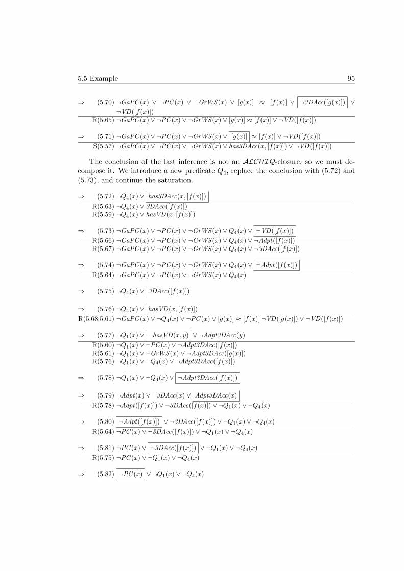
5.5 Example 95
⇒ (5.70) ¬GaPC (x) ∨ ¬PC (x) ∨ ¬GrWS (x) ∨ [g(x)] ≈ [f(x)] ∨ ¬3DAcc([g(x)]) ∨¬VD([f(x)])
R(5.65) ¬GaPC (x) ∨ ¬PC (x) ∨ ¬GrWS (x) ∨ [g(x)] ≈ [f(x)] ∨ ¬VD([f(x)])
⇒ (5.71) ¬GaPC (x) ∨ ¬PC (x) ∨ ¬GrWS (x) ∨ [g(x)] ≈ [f(x)] ∨ ¬VD([f(x)])S(5.57) ¬GaPC (x) ∨ ¬PC (x) ∨ ¬GrWS (x) ∨ has3DAcc(x, [f(x)]) ∨ ¬VD([f(x)])
The conclusion of the last inference is not an ALCHIQ-closure, so we must de-compose it. We introduce a new predicate Q4, replace the conclusion with (5.72) and(5.73), and continue the saturation.
⇒ (5.72) ¬Q4(x) ∨ has3DAcc(x, [f(x)])R(5.63) ¬Q4(x) ∨ 3DAcc([f(x)])R(5.59) ¬Q4(x) ∨ hasVD(x, [f(x)])
⇒ (5.73) ¬GaPC (x) ∨ ¬PC (x) ∨ ¬GrWS (x) ∨Q4(x) ∨ ¬VD([f(x)])R(5.66) ¬GaPC (x) ∨ ¬PC (x) ∨ ¬GrWS (x) ∨Q4(x) ∨ ¬Adpt([f(x)])R(5.67) ¬GaPC (x) ∨ ¬PC (x) ∨ ¬GrWS (x) ∨Q4(x) ∨ ¬3DAcc([f(x)])
⇒ (5.74) ¬GaPC (x) ∨ ¬PC (x) ∨ ¬GrWS (x) ∨Q4(x) ∨ ¬Adpt([f(x)])R(5.64) ¬GaPC (x) ∨ ¬PC (x) ∨ ¬GrWS (x) ∨Q4(x)
⇒ (5.75) ¬Q4(x) ∨ 3DAcc([f(x)])
⇒ (5.76) ¬Q4(x) ∨ hasVD(x, [f(x)])R(5.68;5.61) ¬GaPC (x) ∨ ¬Q4(x) ∨ ¬PC (x) ∨ [g(x)] ≈ [f(x)]¬VD([g(x)]) ∨ ¬VD([f(x)])
⇒ (5.77) ¬Q1(x) ∨ ¬hasVD(x, y) ∨ ¬Adpt3DAcc(y)R(5.60) ¬Q1(x) ∨ ¬PC (x) ∨ ¬Adpt3DAcc([f(x)])R(5.61) ¬Q1(x) ∨ ¬GrWS (x) ∨ ¬Adpt3DAcc([g(x)])R(5.76) ¬Q1(x) ∨ ¬Q4(x) ∨ ¬Adpt3DAcc([f(x)])
⇒ (5.78) ¬Q1(x) ∨ ¬Q4(x) ∨ ¬Adpt3DAcc([f(x)])
⇒ (5.79) ¬Adpt(x) ∨ ¬3DAcc(x) ∨ Adpt3DAcc(x)R(5.78) ¬Adpt([f(x)]) ∨ ¬3DAcc([f(x)]) ∨ ¬Q1(x) ∨ ¬Q4(x)
⇒ (5.80) ¬Adpt([f(x)]) ∨ ¬3DAcc([f(x)]) ∨ ¬Q1(x) ∨ ¬Q4(x)R(5.64) ¬PC (x) ∨ ¬3DAcc([f(x)]) ∨ ¬Q1(x) ∨ ¬Q4(x)
⇒ (5.81) ¬PC (x) ∨ ¬3DAcc([f(x)]) ∨ ¬Q1(x) ∨ ¬Q4(x)R(5.75) ¬PC (x) ∨ ¬Q1(x) ∨ ¬Q4(x)
⇒ (5.82) ¬PC (x) ∨ ¬Q1(x) ∨ ¬Q4(x)

96 5. Deciding SHIQ by Basic Superposition
⇒ (5.83) ¬GaPC (x) ∨ ¬PC (x) ∨ ¬GrWS (x) ∨Q4(x)
⇒ (5.84) ¬GaPC (x) ∨ PC (x)R(5.82) ¬GaPC (x) ∨ ¬Q1(x) ∨ ¬Q4(x)R(5.83) ¬GaPC (x) ∨ ¬GrWS (x) ∨Q4(x)
⇒ (5.85) ¬GaPC (x) ∨ ¬GrWS (x) ∨Q4(x)
⇒ (5.86) ¬GaPC (x) ∨ GrWS (x)R(5.85) ¬GaPC (x) ∨ ∨Q4(x)
⇒ (5.87) ¬GaPC (x) ∨Q4(x)
⇒ (5.88) ¬GaPC (x) ∨ ¬Q1(x) ∨ ¬Q4(x)
⇒ (5.89) GaPC (pc1 )R(5.87) Q4([pc1 ])R(5.88) ¬Q1([pc1 ]) ∨ ¬Q4([pc1 ])
⇒ (5.90) Q4([pc1 ])
⇒ (5.91) ¬Q1([pc1 ]) ∨¬Q4([pc1 ])R(5.90) ¬Q1([pc1 ])
⇒ (5.92) ¬Q1([pc1 ])
⇒ (5.93) Q1(pc1 )R(5.92)
⇒ (5.94)
In step (5.94), we added the empty closure to W . This makes all other closuresredundant, so the saturation terminates. Moreover, Ξ(Ω(KB ′)) is unsatisfiable, and sois KB ′, so KB1 ∪KB2 |= ∃hasVD .Adpt3DAcc(pc1 ).
5.6 Related Work
Decision procedures for various logics were investigated in the field of automated theo-rem proving from its early days. Three such procedures were already implemented byWang in 1960: a procedure capable of deciding validity in propositional logic, a proce-dure for deriving theorems in propositional logic, and a procedure for deciding validityin the so-called AE-fragment of first-order logic, consisting of first-order formulae witha quantifier prefix of the form ∀x1 . . .∀xm∃y1 . . .∃yn.

5.6 Related Work 97
At the beginning of the sixties, Robinson introduced the resolution principle [121]for first-order logic. Due to its simplicity, resolution soon gained popularity. Namely,a resolution-based theorem prover must implement only one inference rule, thus elim-inating the complexity involved in choosing the rule to apply next. Soon after theinitial work by Robinson, various refinements of resolution were developed, such as hy-perresolution [122], ordered resolution [115], paramodulation [120], or lock resolution[23], to name just a few. The common goal of all of these refinements is to reducethe number of consequences generated in the theorem proving process without losingcompleteness. A good overview of resolution and related refinements is given in theclassical textbook by Chang and Lee [26].
Soon after the introduction of the resolution principle and its refinements, attemptswere made to use them to obtain efficient decision procedures for various classes offirst-order logic. The first such procedure was presented by Kallick [81] for the classof formulae with the quantification prefix ∀x1∀x2∃y. This decision procedure is basedon a refinement of resolution that is incomplete for first-order logic, and is thereforedifficult to extend.
In [80], Joyner has established the basic principles for deriving resolution-based de-cision procedures. He observed that, if clauses derivable in a saturation by a resolutionrefinement have a bounded term depth and clause length, then saturation necessarilyterminates. By choosing appropriate refinements, he presented decision procedures forthe Ackermann class (where the formulae are restricted to the quantification prefix∃∗∀∃∗), the Monadic class (where only unary predicates are allowed), and the Maslovclass (where formulae are restricted to quantification prefix ∃∗∀∗∃∗, and the formulaunder the quantifiers is a conjunction of binary disjunctions).
In the years to follow, the approach by Joyner was applied to numerous otherdecidable classes, such as the E+ class [142], the PVD class [83], and the PVDg
= class[107], to name just a few. An overview of these results is given in [45].
Decidability of description logics in the resolution framework has been studiedextensively in [98, 77, 76]. There, the description logic ALB is embedded in theDL* clausal class, which is then decided using the resolution framework by Bachmairand Ganzinger [13]. The main advantage of using this framework lies in its effectiveredundancy elimination methods, which were shown to be essential for the practicalapplicability of resolution calculi. ALB is a very expressive logic and allows for unsaferole expressions, but does not provide for counting quantifiers.
In [48], a decision procedure for the modal logic with a single transitive modalityK4 was presented. To deal with transitivity, the algorithm is based on the orderedchaining calculus [11]. This calculus consists of inference rules aimed at optimizingtheorem proving with chains of binary roles. Unfortunately, our attempts to decideSHIQ using ordered chaining proved unsuccessful, mainly due to certain negativechaining inferences that produced undesirable equality literals. Therefore, we adoptedthe approach for eliminating transitivity presented in Section 5.2.
The guarded fragment was introduced in [3] to explain and generalize the goodproperties of modal and description logic, such as decidability. A decision procedure

98 5. Deciding SHIQ by Basic Superposition
by resolution with a nonliftable ordering was presented in [36]; it was later modified tohandle the (loosely) guarded fragment with equality in [47] by basing the algorithm onsuperposition [9]. Since the basic description logic ALC is actually a syntactic variantof the multi-modal logic Km [127], it can be embedded into the guarded fragment anddecided by [47]. Using the approach from [129], certain extensions of ALC, such asrole transitivity, can be encoded into ALC knowledge bases, so the algorithm from[47] can decide these extensions as well. However, SHIQ is not a fragment of the(loosely) guarded fragment because of the counting quantifiers: equality is available inthe guarded fragment, but each two pairs of free variables of a guarded formula mustoccur in a guard atom. In fact, in [65] it was shown that the guarded fragment hasthe finite-model property, which is known not to hold for SHIQ [4, Chapter 2], thussuggesting that other mechanisms are necessary for handling the latter logic.SHIQ can easily be embedded into the two-variable fragment of first-order logic
with counting quantifiers C2. This fragment was shown to be decidable in [54, 100], anda decision procedure based on a combination of resolution and integer programmingwas presented in [110]. However, deciding satisfiability of C2 is NExpTime-complete[100], and SHIQ is an ExpTime-complete logic [144]. Thus, the decision procedurefrom [110] introduces an unnecessary overhead for SHIQ. Furthermore, we do not seehow to use this procure to derive the desired reduction to disjunctive datalog.
The decomposition rule is closely related to the structural transformation [108,99, 8]. However, structural transformation is usually applied as a preprocessing stepand not in the theorem proving process. In [37] and [118], splitting by propositionalsymbols was proposed that allows splitting variable-disjoint subsets of a clause andconnect them by a propositional symbol. Finally, a separation rule was used to decidefluted logic in [128]. It was shown that resolution remains complete if the separationrule is applied a finite number of times during saturation. In contrast to these re-lated approaches, our rule can decompose complex terms. Moreover, we demonstratecompatibility of the decomposition rule with the standard redundancy notion. Finally,extending basic superposition with decomposition is not trivial, due to the nonstandardapproach to lifting employed by basic superposition.

Chapter 6
Reasoning with a ConcreteDomain
As argued in [5], representing concrete data is essential for practical knowledge repre-sentation systems. However, existing algorithms for reasoning with concrete domainsfrom [5, 70, 62, 87] mainly operate in tableau and automata frameworks, which nonde-terministically check satisfiability of conjunctions of ground atoms. On the contrary,the algorithm from Chapter 5 is based on resolution, and it works with conjunctionsof nonground disjunctions. Hence, extending the results from Chapter 5 with concretedomain reasoning is not trivial. In order to support the description logic SHIQ(D),in this chapter we present two new results.
First, in Section 6.1 we present a general approach for combining concrete domainreasoning with clausal calculi. The approach consists of two steps. A c-factoring pre-processing transformation is applied first to bring a clause set into a suitable form.Next, we introduce a concrete domain resolution inference rule, for which we showsoundness and completeness when combined with a clausal calculus whose complete-ness proof is based on the model generation method. Note that this is the standardtechnique for proving completeness of many state-of-the-art calculi, such as orderedresolution [13], basic superposition [14], or ordered chaining [11], so concrete domainresolution is applicable to a wide range of calculi.
Second, in Section 6.2 we apply these techniques to the algorithm from Chapter 5,and thus obtain a procedure for deciding satisfiability of SHIQ(D) knowledge bases.Assuming a bound on the arity of concrete predicates and an exponential procedurefor checking D-satisfiability of conjunctions of concrete predicates, extending the logicdoes not increase the complexity of reasoning—that is, it remains in ExpTime.
Results from this chapter were published in [150]. Due to space limitations, wedid not consider there the distinction between D- and d-satisfiability, as discussed inSubsection 6.1.2 (for SHIQ(D) without ABox assertions of the form ¬T (a, bc), thesetwo notions coincide).
99

100 6. Reasoning with a Concrete Domain
6.1 Resolution with a Concrete Domain
In this section we develop a general algorithm for reasoning in first-order logic extendedwith an admissible concrete domain.
6.1.1 Preliminaries
The key step in computing the set of clauses Cls(ϕ) from a first-order formula ϕ is toskolemize existential quantifiers, as explained in Section 2.1. Similarly, to check D-satisfiability of ϕ, skolemization can be applied as well, since, as shown by the followinglemma, it does not affect D-satisfiability:
Lemma 6.1.1. A formula ϕ is D-satisfiable if and only if sk(ϕ) is D-satisfiable.
Proof. The proof is identical to the case of ordinary satisfiability presented in [46]:given a D-model I of ϕ, one can build a D-model I ′ of sk(ϕ) by extending I with theappropriate interpretations of new general function symbols. Conversely, new generalfunction symbols ensure existence of existentially implied individuals.
Hence, to check D-satisfiability of a formula ϕ, we first compute a D-equisatisfiableset of clauses N = Cls(ϕ). Furthermore, since the concrete domain D is admissible, wereplace each literal ¬d(t) with d(t). Thus, we assume without loss of generality thatconcrete domain predicates occur only in positive literals.
Checking satisfiability of a set of clauses N in an arbitrary model is problematic,because one should consider arbitrary domains. In the case of first-order logic with-out concrete domains, this can conveniently be avoided by considering only Herbrandmodels. For the case of first-order logic extended with a concrete domain, we introducethe notion of Herbrand D-interpretations, as follows:
Definition 6.1.2. For a function δ : HU c → 4D and a ground formula ϕ, δ(ϕ) isthe ground formula obtained by replacing each term tc with δ(tc). The extension of δto sets of formulae is defined by applying δ to each set member.
A Herbrand D-interpretation over a signature Σ is a pair (I, δ), where I is aclassical Herbrand interpretation over Σ and δ : HU c → 4D is an assignment ofconcrete individuals to concrete terms of HU c. A Herbrand D-interpretation is well-formed if the following two conditions are true:
• si ≈ ti ∈ I for 1 ≤ i ≤ n imply δ(f c(s1, . . . sn)) = δ(f c(t1, . . . tn)), for eachgeneral function symbol f c;
• δ(t) ∈ dD for each concrete literal d(t) ∈ I.
A ground clause CG is D-satisfied in a Herbrand D-interpretation (I, δ), written(I, δ) |=D CG, if (I, δ) is well-formed and δ(CG) is true in δ(I). A nonground clause Cis D-satisfied in (I, δ) if all its ground instances are D-satisfied in (I, δ). The notionsof D-models, D-satisfiability and so on extend to Herbrand D-interpretations as usual.

6.1 Resolution with a Concrete Domain 101
There is a slight problem with Herbrand D-models as defined in the previousdefinition. Namely, Definition 6.1.2 does not ensure that the number of constants inthe Herbrand universe matches the number of objects in 4D. Consider the set ofclauses N = =1(x) with the concrete domain D such that 4D = 1, 2. Obviously,N is D-unsatisfiable (since 2 is not equal to 1); however, the Herbrand D-interpretationdefined by I = =1(a) and δ(a) = 1 is a Herbrand D-model of N . This discrepancyarises because I does not contain a distinct constant for each element of4D. To ensurethat considering only Herbrand models does not affect satisfiability, we append to Nthe (possibly infinite) set of clauses ℵD = =α (aα) | for each α ∈ 4D, where aα arenew constants (note that the notion of admissibility from Definition 3.2.1 ensures thatthe predicates =α exist). A set of clauses N that contains ℵD is said to be D-extended.
We now show that, for D-extended clause sets, we can consider D-satisfiabilityonly in Herbrand D-models.
Lemma 6.1.3. A set of D-extended clauses N is D-satisfiable if and only if a well-formed Herbrand D-model of N exists.
Proof. (⇐) Let (I, δ) be a Herbrand D-model of N . We construct a model I ′ by settingthe domain Dr = HU r for each sort r 6= c, Dc = 4D, tI
′= t for each term t of sort
other than c, (f c)I′(t1, . . . , tn) = δ(f c(t1, . . . , tn)), and (tI′
1 , . . . , tI′n ) ∈ P I′ if and only if
P (t1, . . . , tn) ∈ I for a predicate P . Because N is D-extended, each object from 4D
is represented as a constant in HU c, so I ′ is a D-model of N .(⇒) Let N be D-satisfiable in a D-model I. Let I ′ be an interpretation containing
those ground atoms A from the Herbrand base of N such that AI are true in I.Furthermore, for each ground concrete term tc ∈ HU c, let δ(tc) = (tc)I . In the sameway as for first-order logic without concrete domains in [46], I ′ is a classical Herbrandmodel of N , and (I ′, δ) is a D-model of N .
6.1.2 d-Satisfiability
The task of finding a Herbrand D-model (I, δ) of a set of clauses N essentially consistsof two subtasks. The first one is to ensure that a Herbrand model I exists; this canbe done using resolution in the standard way. The second one is to ensure that anappropriate assignment δ exists. To solve the latter problem, we first consider thesimpler task of finding δ that only satisfies the concrete predicates.
Definition 6.1.4. A ground clause CG is d-satisfied in a Herbrand D-interpretation(I, δ), written (I, δ) |=d C
G, if and only if (I, δ) is well-formed and CG is classicallysatisfied in I (that is, it is satisfied without taking special care of concrete individuals).A nonground clause C is d-satisfied in (I, δ) if all ground instances of C are d-satisfiedin (I, δ). Other notions are defined analogously.
Note that d-satisfiability is a strictly weaker notion than D-satisfiability: if Nis D-satisfiable, it is obviously d-satisfiable, but the converse does not hold. Forexample, consider a set of clauses N = R(a, bc),¬R(a, cc), d(bc, cc) and a concrete

102 6. Reasoning with a Concrete Domain
domain D such that dD = (1, 1). Obviously, I = R(a, bc), d(bc, cc) is a classicHerbrand model of N ; furthermore, for a function δ such that δ(bc) = δ(cc) = 1,we have (δ(bc), δ(cc)) ∈ dD, so N is d-satisfiable. However, N is not D-satisfiable:δ(I) = R(a, 1), d(1, 1), but then δ(R(a, cc)) is true in δ(I), so the clause δ(¬R(a, cc))is not true in δ(I). Intuitively, d-satisfiability ensures consistency of literals containingconcrete domain predicates, but not of literals with ordinary predicates containing bothconcrete and abstract terms. The relationship between d- and D-satisfiability can becaptured using c-factors, introduced below. Please keep in mind that, as discussed inSubsection 3.2.1, sc 6≈D tc is a positive literal with a concrete predicate 6≈D.
Definition 6.1.5. Let C be a clause containing a literal ¬A. The c-factor of ¬A w.r.t.C is the disjunction
¬A[xc1]p1 . . . [x
cn]pn ∨ xc
1 6≈D A|p1 ∨ . . . ∨ xcn 6≈D A|pn
where xci are globally new variables, and p1, . . . , pn are exactly those positions in A
such that sort(A|pi) = c and at least one condition from the following list holds:
• A|pi is not a variable;
• A|pi is a variable occurring in some negative literal in C \ ¬A;
• A|pi is a variable occurring in ¬A at some position other than pi.
A clause C ′ is a c-factor of C if no literal from C ′ has a c-factor w.r.t. C ′, and ifa sequence of clauses C = C0, . . . , Cn = C ′ exists such that, for i ≥ 1, Ci is obtainedfrom Ci−1 by replacing a literal Li ∈ C with its c-factor w.r.t. Ci−1.
A c-factor of a set of clauses N is obtained from N by replacing each clause C ∈ Nwith an (arbitrary) c-factor of N . A clause (clause set) is said to be c-factored if it isequal to one of its c-factors.
Note that a clause can have several c-factors, depending on the order in which theliterals are c-factored. For example, the clause ¬R(x, yc) ∨ ¬S(x, yc) ∨ T (x, yc) hasthese two c-factors:
¬R(x, zc) ∨ zc 6≈D yc ∨ ¬S(x, yc) ∨ T (x, yc)¬R(x, yc) ∨ ¬S(x, zc) ∨ zc 6≈D yc ∨ T (x, yc)
In the remaining sections, we can pick any c-factor of N ; that is, an arbitrary c-factorof C can be used to replace a clause C ∈ N .
Note that, for a c-factored clause C and for each literal ¬A ∈ C, if sort(A|p) = c,then A|p is a variable that can occur in C \ ¬A only in a positive literal. As shownby the following lemma, c-factoring modifies the set of clauses such that d-satisfiabilityensures D-satisfiability:
Lemma 6.1.6. Let N be a D-extended set of clauses, and N ′ a c-factor of N . Then,the following claims hold:

6.1 Resolution with a Concrete Domain 103
• N is D-satisfiable if and only if N ′ is D-satisfiable.
• N ′ is d-satisfiable if and only if it is D-satisfiable.
Proof. For the first claim, observe that the literal A is equivalent to the followingformula:
∃xc1, . . . , x
cn : A[xc
1]p1 . . . [xcn]pn ∧ xc
1 ≈D A|p1 ∧ . . . ∧ xcn ≈D A|pn
Moreover, the c-factor of ¬A is obtained from the previous formula using the applica-tion of de Morgan laws, so ¬A and its c-factor are equivalent. Therefore, N and N ′
are equivalent, so they are D-equisatisfiable.For the second claim, the (⇐) direction follows trivially from the definitions of D-
and d-satisfiability. For the (⇒) direction, let I be a classic Herbrand model of N ′,and δ an assignment satisfying Definition 6.1.4. If (I, δ) is not a D-model of N ′, thenthere is a clause C ∈ N ′ with a ground instance Cτ that is true in I, but for whichδ(Cτ) is false in δ(I). For each positive literal A ∈ C, if Aτ ∈ I, then δ(Aτ) is truein δ(I), so C must be of the form D ∨ ¬A1 ∨ . . . ∨ ¬An where Dτ is false in I, and,for all i, Aiτ /∈ I but δ(Aiτ) is true in δ(I). The latter is the case only if there areA′i ∈ I such that δ(A′i) = δ(Aiτ). Let pij be positions in Ai such that sort(Ai|pij ) = c.Since each Ai is c-factored w.r.t. C, then, for all j, Ai|pij is a variable xc
ij occurringin C \ Ai only in positive literals. Let σ be a ground substitution that is identicalto τ except for the mappings xc
ij 7→ A′i|pij . Obviously, A′i = Aiσ. Since I is a modelof N ′, Dσ ∨ ¬A1σ ∨ . . . ∨ ¬Anσ is true in I; this is possible only if Dσ is true in I.Since Dτ is false in I, a literal L′ ∈ D must exist such that L′σ is true in I, but L′τis false in I. Since, for each i, all variables of sort c from ¬Ai occur only in positiveliterals of C, the truth value of all negative literals in Dσ and Dτ is identical, so L′
must be a positive literal. However, since δ(L′σ) is true in δ(I) and δ(L′σ) = δ(L′τ),we have that δ(L′τ) is true in δ(I), which contradicts the assumption that δ(Cτ) isfalse in δ(I).
Intuitively, c-factoring allows us to move the concrete terms from literals with-out concrete predicates into concrete inequalities. In Subsection 6.1.3, we present aprocedure for checking d-satisfiability of a set of ground clauses, which we lift to non-ground clauses in Subsections 6.1.4 and 6.1.5. Combined with c-factoring, this yieldsa refutation procedure for D-satisfiability.
6.1.3 Concrete Domain Resolution with Ground Clauses
We now develop the ground concrete domain resolution calculus, GD for short, forchecking d-satisfiability of a set of clauses, where D is an admissible concrete domain.In order to prevent the presentation from being too technical, we add the concretedomain resolution rule to the ordered resolution calculus [13] (see Section 2.4) only,and argue later that the rule can be combined with other calculi as well. As forordinary resolution, GD is parameterized with an admissible ordering on literals,which is extended to clauses by a multiset extension (see Section 2.4).

104 6. Reasoning with a Concrete Domain
Definition 6.1.7. Let S = di(ti) be a set of literals, where ti is a vector of termsti1, . . . , tik. Then, S is a conjunction C =
∧di(xi), obtained from S by replacing each
occurrence of a term with the same variable such that different terms are replaced withdistinct variables. For two conjunctions C1 and C2, we write C1 ≡ C2 if they areequivalent up to variable renaming.
A set S = di(ti) of positive concrete literals is a D-constraint if S is not D-satisfiable. A D-constraint S is minimal if S′ is D-satisfiable for each S′ ( S; S isconnected if it cannot be decomposed into two disjoint nonempty subsets S1 and S2 notsharing a common term (S1 and S2 do not share a common term if, for all di(ti) ∈ S1
and dj(tj) ∈ S2, we have ti ∩ tj = ∅).
Lemma 6.1.8. Each minimal D-constraint S is connected.
Proof. Assume that S is a D-constraint, but it is not connected. Hence, S can bedecomposed into subsets S1 and S2 not sharing a common term. Since S is a minimalD-constraint, S1 and S2 are D-satisfiable. However, since S1 and S2 do not have acommon variable, S1 ∧ S2 = S is D-satisfiable as well, which is a contradiction.
The ground concrete domain resolution calculus GD consists of the following infer-ence rules:
Positive factoring:C ∨A ∨ . . . ∨A
C ∨A
where (i) A is strictly maximal with respect to C.
Ordered resolution:C ∨A D ∨ ¬A
C ∨D
where (i) A is strictly maximal with respect to C, (ii) ¬A is maximal with respect toD.
Concrete domain resolution:C1 ∨ d1(t1) . . . Cn ∨ dn(tn)
C1 ∨ . . . ∨ Cn
where (i) di(ti) are strictly maximal with respect to Ci, (ii) S = di(ti) is a minimalD-constraint.
In GD, the clauses C∨A∨ . . .∨A and D∨¬A are called the main premises, whereasthe clauses C ∨ A and Ci ∨ d1(t1) are called the side premises. Note that, under thisdefinition, the concrete domain resolution rule does not have a main premise.
It is well known that effective redundancy elimination criteria are necessary fortheorem proving to be applicable in practice. A powerful standard notion of redundancywas introduced in [13]. We adapt this notion slightly to take into account that theconcrete domain resolution rule does not have a main premise.
Definition 6.1.9. Let N be a set of ground clauses. A ground clause C is redundantin N if clauses Di ∈ N exist such that C Di and D1, . . . , Dm |= C. A ground

6.1 Resolution with a Concrete Domain 105
inference ξ with side premises Ci and a conclusion D is redundant in N if clausesDi ∈ N exist such that C1, . . . , Cn, D1, . . . , Dm |= D; if ξ has a main premise C, thenC Di is required in addition.
We now prove the soundness and completeness of GD under the standard notionof redundancy.
Lemma 6.1.10 (Soundness). Let N be a set of ground clauses, I a d-model of N , andN ′ = N ∪ C, where C is the conclusion of an inference by GD with premises fromN . Then, I is a d-model of N ′.
Proof. For an inference by positive factoring or ordered resolution, the claim is trivialand is shown in the same way as in [13]. Let C be obtained by the concrete domainresolution rule, with S being as in the rule definition. Since S is a D-constraint, ad-model (I, δ) of N can exist only if there is a literal di(ti) ∈ S such that di(ti) /∈ I.Since Ci ∨ di(ti) is by assumption true in I, some literal from Ci is true in I. SinceCi ⊆ C, we have that C is true in I as well.
Lemma 6.1.11 (Completeness). Let N be a set of ground clauses such that eachinference by GD from premises in N is redundant in N . If N does not contain theempty clause, then N is d-satisfiable.
Proof. We extend the model building method from [13] to handle the concrete domainresolution rule. For a set of ground clauses N , we define an interpretation I by induc-tion on the clause ordering as follows: for a clause C, we set IC =
⋃CD εD, where
εD = A if (i) D ∈ N , (ii) D is of the form D′ ∨ A such that A is strictly maximalwith respect to D′, and (iii) D is false in ID; otherwise, εD = ∅. Let I =
⋃D∈N εD. A
clause D such that εD = A is called productive, and it is said to produce the atomA in I. Before proving the lemma, we show the following three properties.
Invariant (*): if C is false in ID∪εD for C D, then C is false in I. Since C is falsein ID ∪ εD, all negative literals from C are false in ID ∪ εD, and, since ID ∪ εD ⊆ I,all negative literals from C are false in I as well. Furthermore, since ¬A A andthere is no literal between ¬A and A, any atom produced by a clause D′ D is largerthan any literal occurring in C, so no clause greater than C can produce an atom thatwould make C true.
Invariant (**): if C is true in IC ∪ εC , then C is true in I. If C is true in IC ∪ εCbecause some positive literal is true in IC ∪ εC , since IC ∪ εC ⊆ I, the clause C istrue in I as well. Otherwise, C is true in IC ∪ εC because some negative literal ¬A istrue in IC ∪ εC . Since ¬A A and there is no literal between ¬A and A, any atomproduced by a clause D C is larger than any literal occurring in C. Hence, no suchclause D can produce A, so ¬A is true in I as well. We often use this invariant in itscontrapositive form: if C is false in I, then it is false in IC ∪ εC as well.
Property (***): if an inference ξ with a main premise C, side premises Ci, and aconclusion D is redundant in N , then there are clauses Di ∈ N that are not redundantin N such that D1, . . . , Dm, C1, . . . , Cn |= D and C Di. If ξ is redundant, by

106 6. Reasoning with a Concrete Domain
definition of the standard notion of redundancy, there are clauses D′j ∈ N such that
D′1, . . . , D
′m, C1, . . . , Cn |= D and C D′
i. Now if some D′j is redundant, then there are
clauses D′′k such that D′′
1 , . . . , D′′m′ |= D′
j and D′j D′′
k . Since is well-founded, thisprocess can be continued recursively until we obtain the set of smallest nonredundantclauses for which (***) obviously holds. This property holds analogously if ξ does nothave a main premise.
We now prove the claim of Lemma 6.1.11 by contradiction: let us assume that allinferences by GD from premises in N are redundant in N , but no δ exists such that(I, δ) is a d-model of N . There can be two causes for that:
• There is a clause C ∈ N that is false in I; such a clause is called a counterexamplefor I. Since is well-founded and total, we can assume without loss of generalitythat C is the smallest counterexample. C is obviously not productive, since allproductive clauses are true in I. C can be nonproductive and false in I if it hasone of the following two forms:
– C = C ′ ∨ A ∨ . . . ∨ A. Then, C is not productive since A is not strictlymaximal in C. Since C is false in I, by (**) it is false in IC ∪ εC . Hence,C ′ is false in IC ∪ εC , and, since C ′ ≺ C, by (*) C ′ is false in I. Since Nis saturated, the inference by positive factoring resulting in D = C ′ ∨ A isredundant in N . D is obviously false in I. By the fact that N is saturatedand by (***), clauses Di ∈ N exist, such that C Di and D1, . . . , Dn |= D.Since C is the smallest counterexample, all Di are true in I, but then D istrue in I as well, which is a contradiction.
– C = C ′ ∨¬A. Since C is false in I, we have A ∈ I, where A is produced bya smaller clause D = D′∨A. Similarly as in the previous case, C ′ is false inI. Since D is productive, D′ is false in ID, and since A is strictly maximalw.r.t. D′, D′ is false in ID ∪ εD as well. Since D′ ≺ D, by (*) D′ is falsein I. Since N is saturated, the inference by ordered resolution resultingin E = C ′ ∨ D′ is redundant in N . E is obviously false in I. Because Nis saturated and by (***), clauses Di ∈ N exist, such that C Di andD1, . . . , Dn, D
′∨A |= E. Since C is the smallest counterexample, all Di aretrue in I, and, since D′ ∨ A is productive, it is also true in I. Hence, E istrue in I, which is a contradiction.
• All clauses from N are true in I, but I contains a set of concrete domain literalsS = di(ti) such that S is D-unsatisfiable. We can assume without loss ofgenerality that S is minimal. The literals from S must have been producedby clauses Ei = Ci ∨ di(ti) ∈ N , where Ci is false in IEi ∪ εEi . For each i,we conclude that Ci is false in I as in the case of ordered resolution. Since Nis saturated, the inference by concrete domain resolution from Ei resulting inD = C1 ∨ . . . ∨ Cn is redundant in N . Obviously, D is false in I. Since the

6.1 Resolution with a Concrete Domain 107
inference is redundant, by property (***), nonredundant clauses Di ∈ N existsuch that D1, . . . , Dm, C1∨d1(t1), . . . , Cn∨dn(tn) |= D. All Di and Ci∨di(ti) areby assumption true in I, implying that D is true in I, which is a contradiction.
Hence, an assignment δ must exist such that (I, δ) is a d-model of N (because wedo not consider theories with equality, the first condition of Definition 6.1.2 related to≈ is trivially satisfied), so N is d-satisfiable.
A fair derivation by GD from a set of clauses N with a limit N∞ is defined as usual(see Section 2.4). By lemmata 6.1.10 and 6.1.11, we get the following result:
Theorem 6.1.12. The set of ground clauses N is d-unsatisfiable if and only if thelimit N∞ of a fair derivation by GD contains the empty clause.
6.1.4 Most General Partitioning Unifiers
Lifting the concrete domain resolution rule to general clauses is not trivial, becauseunification can only partly guide the rule application. Consider, for example, the set ofclauses N = d1(x1, y1), d2(x2, y2). N has ground instances d1(a1, b1) and d2(a2, b2),which do not share a common term. Hence, a conjunction consisting of these literalsis not connected, so, by the contrapositive of Lemma 6.1.8, it cannot be minimal, andthe conditions of the concrete domain resolution are not satisfied. However, clausesd1(a, b1) and d2(a, b2) are also ground instances of N , but they do share commonterms. Hence, a conjunction of these literals is connected, so the conditions of theconcrete domain resolution rule could be satisfied. This is so because it is possibleto unify x1 and x2 from d1(x1, y1) and d2(x2, y2). Another possibility is to unify x2
and y1. Even for a set consisting of a single clause, such as M = d(x, y), it ispossible to obtain a D-constraint d(x, x) by unifying x and y. These examples showthat, to check all potential D-constraints at the ground level, one has to consider allpossible substitutions that produce a minimal D-constraint at the nonground level.We formalize this idea in the following definition.
Definition 6.1.13. Let S = di(ti) be a set of positive concrete domain literals. Asubstitution σ is a partitioning unifier of S if the set Sσ is connected. Furthermore,σ is a most general partitioning unifier if, for any partitioning unifier θ such thatSσ ≡ Sθ, a substitution η exists such that θ = ση. With MGPU(S) we denote the setof all most general partitioning unifiers of S unique up to variable renaming.
If no terms from literals in S are unifiable, a most general partitioning unifier of Sdoes not exist. Furthermore, the previous example shows that S can have several mostgeneral partitioning unifiers. However, for a given conjunction of concrete literalsSσ, all most general partitioning unifiers are identical up to variable renaming, asdemonstrated next.
Let S = di(ti) be a set of positive concrete domain literals, and C a conjunctionover literals in S, obtained by replacing terms of each di(ti) with arbitrary variables

108 6. Reasoning with a Concrete Domain
(it is not necessary to use different variables in C for different terms from S, but thesame term in S should always be replaced with the same variable in C). For such a C,let m be the number of distinct variables in C; for each such variable xi, 1 ≤ i ≤ m,let Txi be a list of all terms occurring in a literal in S at a position corresponding to anoccurrence of xi in C; finally, let n = max |Txi |. With SC we denote the set of termstj = f(sj
x1 , . . . , sjxm), where sj
xi is the j-th term of Txi if j ≤ |Txi |, and a fresh variableif j > |Txi |, for 1 ≤ j ≤ n. Most general partitioning unifiers of S and most generalunifiers of SC are closely related, as shown by the following lemma.
Lemma 6.1.14. Let θ be a partitioning unifier of a set of concrete domain literalsS = di(ti), and let C = Sθ. Then, the substitution σ = MGU(SC) is the mostgeneral partitioning unifier of S such that Sσ ≡ C, and it is unique up to variablerenaming.
Proof. To obtain the variable xi in C, θ must be such that s1xiθ = . . . = sn
xiθ = Txiθ.
Furthermore, xi 6= xj for i 6= j, so Txiθ 6= Txjθ. Because of the first property, θ isobviously a unifier of SC , so σ = MGU(SC) exists, and it is unique up to variableremaining [7]. Furthermore, σ is the most general unifier of SC , so a substitution ηexists such that θ = ση. Hence, it is impossible that Txiσ = Txjσ and Txiση 6= Txjση.Thus, s1xi
σ = . . . = snxiσ = Txiσ and Txiσ 6= Txjσ for i 6= j, so Sσ ≡ C.
Lemma 6.1.15. For a set of concrete domain literals S = di(ti), MGPU(S) containsexactly all MGU(SC), for each connected conjunction C over literals of S.
Proof. For σ ∈ MGPU(S), C = Sσ is obviously a connected conjunction over literalsof S satisfying conditions of Lemma 6.1.14, so σ is equivalent to MGU(SC) up tovariable renaming. Conversely, let C be a connected conjunction over literals of S.Now σ = MGU(SC) is a partitioning unifier of S. Let C ′ = Sσ. Observe that C ≡ C ′
does not necessarily hold: it is possible that Txiσ = Txjσ for i 6= j. However, C ′ isa connected conjunction over concrete domain literals satisfying conditions of Lemma6.1.14, so MGU(SC′) exists, and it is a most general partitioning unifier of S.
Hence, Lemma 6.1.15 gives a brute-force algorithm for computing MGPU(S): oneshould systematically enumerate all connected conjunctions C over literals in S andcompute MGU(SC). The main performance drawback of this algorithm is that all suchconjunctions C must be enumerated. For n literals in S of maximal aritym, the numberof possible assignments of variables in C is bounded by (nm)nm, which is obviouslyexponential. However, for certain logics, it is possible to construct a specialized, butmuch more efficient algorithm. In Section 6.2, we present such an algorithm applicableto SHIQ(D).
6.1.5 Concrete Domain Resolution with General Clauses
As usual in a resolution setting, we assume that no two premises of an inference rulehave any variables in common. The concrete domain resolution calculus, RD for short,consists of the following rules:

6.1 Resolution with a Concrete Domain 109
Positive factoring:C ∨A ∨B
Cσ ∨Aσ
where (i) σ = MGU(A,B), (ii) Aσ is strictly maximal with respect to Cσ.
Ordered resolution:C ∨A D ∨ ¬B
Cσ ∨Dσ
where (i) σ = MGU(A,B), (ii) Aσ is strictly maximal with respect to Cσ, (iii) ¬Bσis maximal with respect to Dσ.
Concrete domain resolution:C1 ∨ d1(t1) . . . Cn ∨ dn(tn)
C1σ ∨ . . . ∨ Cnσ
where (i) clauses Ci ∨ di(ti) are not necessarily unique, (ii) for the set S = di(ti),σ ∈ MGPU(S), (iii) di(ti)σ are strictly maximal with respect to Ciσ, (iv) Sσ is aminimal D-constraint.
We briefly comment on Constraint (i) of the concrete domain resolution rule. Con-sider a set of clauses N = d(f c(x), bc), f c(a) 6≈D f c(c) and dD = (1, 2). Then,S = d(f c(a), bc), d(f c(c), bc), f c(a) 6≈D f c(c) is a set of instances of N such thatthe conjunction S is D-unsatisfiable. Also, for each proper subset S′ ⊂ S, the con-junction S′ is D-satisfiable. Hence, unsatisfiability is detected only if several copiesof d(f c(x), bc) are considered simultaneously in the concrete domain resolution rule.Without any assumptions on the nature of the concrete predicates, there is no upperbound on the number of copies that should be considered simultaneously. This prop-erty of the calculus obviously leads to undecidability in the general case. To obtain adecision procedure for SHIQ(D), in Section 6.2 we show that the number of copiesthat must be considered is bounded.
To prove the completeness of RD, we show now that, for each ground derivation,there is a corresponding nonground derivation.
Lemma 6.1.16 (Lifting). Let N be a set of clauses and NG the set of ground instancesof N . For each ground inference ξG by GD applicable to premises CG
i ∈ NG, there isan inference ξ by RD applicable to premises Ci ∈ N such that ξG is an instance of ξ.
Proof. Let CGi be ground premises from NG participating in ξG, resulting in a ground
clause DG. The ground inference ξG of GD can be simulated by a correspondingnonground inference ξ where, for each ground premise CG
i , we take the correspondingnonground premise Ci. Since all Ci are variable disjoint, there is a ground substitutionτ such that CG
i = Ciτ . Let us denote with D the result of ξ on Ci. We now show thatξ is an inference of RD.
Let ξG be an inference by positive factoring on ground literals AGi of CG. Substi-
tution τ is obviously a unifier for the corresponding nonground literals Ai of C. Sinceany unifier is an instance of the most general unifier σ of Ai, a substitution η existssuch that τ = ση. Furthermore, if AG
i is strictly maximal with respect to CG, since

110 6. Reasoning with a Concrete Domain
is a reduction ordering, the corresponding literal Ai is strictly maximal with respectto Cσ, so DG = Dη. Hence, ξ is an inference of RD. Similar reasoning applies in thecase of ordered resolution.
Let ξG be an inference by concrete domain resolution, and S = di(ti) be the setof corresponding nonground literals. Since Sτ is a minimal D-constraint, by Lemma6.1.8, Sτ is connected, so τ is obviously a partitioning unifier of S. Then, by Lemma6.1.14, a most general partitioning unifier σ exists such that τ = ση for some η andSσ ≡ Sτ . Obviously, if Sτ is a minimal D-constraint, so is Sσ. Furthermore, if literalsfrom Sτ are strictly maximal with respect to CG
i , since is a reduction ordering, thecorresponding literals from Sσ are strictly maximal with respect to Ciσ, so DG = Dη.Hence, ξ is an inference of RD.
The notion of redundancy is lifted to the nonground case as usual [13]: a clause C(an inference ξ) is redundant in a set of clauses N if all ground instances of C (ξ) areredundant in NG. This is enough for soundness and completeness of RD.
Theorem 6.1.17. A set of clauses N is d-unsatisfiable if and only if the limit N∞ ofa fair derivation by RD contains the empty clause.
Proof. A set N is d-unsatisfiable if and only if the set of its ground instances NG is d-unsatisfiable. By Theorem 6.1.12, NG is d-unsatisfiable if and only if there is a groundderivation NG = NG
0 , NG1 , . . . , N
G∞, where the limit NG
∞ contains the empty clause. ByLemma 6.1.16 and the definition of the redundancy for nonground clauses, for eachground derivation, a nonground derivation N = N0, N1, . . . , N∞ exists, in which eachNG
i is a subset of the set of ground instances of Ni. Hence, NG∞ contains the empty
clause if and only if N∞ contains the empty clause, so the claim follows.
D-satisfiability of a set of clauses N can now be checked by the following steps:
• Extend N with ℵD;
• Compute N ′—the c-factor of N ∪ ℵD;
• Check d-satisfiability of N ′ by RD.
By Lemma 6.1.6, N ′ is d-satisfiable if and only if N ∪ ℵD is D-satisfiable, whichis the case if and only if N is D-satisfiable by Lemma 6.1.3. A practical problemin applying RD to N ′ is that ℵD can be infinite. In general, this obviously leads toundecidability. However, we show in Section 6.2 that, the clauses from ℵD are notneeded to decide SHIQ(D).
6.1.6 Deleting D-Tautologies
In ordinary resolution, clauses that are true in any model can be removed withoutjeopardizing completeness of the calculus. Removing such clauses is crucial for practicalapplicability of resolution, because this drastically reduces the search space. To achieve

6.1 Resolution with a Concrete Domain 111
the same effect forRD, we now define the notion of D-tautologies—clauses that are truein any D-model due to properties of the concrete domain. We show that D-tautologiescan be deleted eagerly in a saturation process while preserving completeness.
Definition 6.1.18. A literal d(t) is a D-tautology if d(t) = d(x) is satisfied for anyassignment δ of variables x to elements of 4D. A clause is a D-tautology if it containsa D-tautology literal.
For example, the clauses C ∨ f(x) ≈D f(x) and C ∨ >D(x) are D-tautologies.Similarly, if 4D is the set of nonnegative integers, then the clause C ∨ ≥0 (x) is alsoa D-tautology. We now show that such clauses are redundant and can be deleted in asaturation process.
Lemma 6.1.19. D-tautologies can be eagerly deleted in a saturation by RD withoutloosing completeness.
Proof. Let S = di(ti) be a minimal D-constraint. Obviously, S cannot contain a D-tautology literal d(t), since S \ d(t) would be an even smaller D-constraint. Hence,D-tautologies do not participate in inferences by the concrete domain resolution rule.
Let N be a set of ground clauses saturated under GD not containing the emptyclause. Furthermore, let I be a model obtained by applying the model building methodfrom Lemma 6.1.11 to all clauses from N that are not D-tautologies, and let δ be anassignment of elements from 4D to elements of HU c (such an assignment exists byLemma 6.1.11, because N is saturated and does not contain the empty clause). Let I ′
be a model obtained by adding d(t) to I for each D-tautology literal d(t) of a groundclause C ∈ N . Since all concrete domain literals occur positively in clauses in N ,adding concrete literals to I cannot make any clause in N false. For each such literal,we have δ(t) ∈ dD, so (I ′, δ) is a Herbrand d-model of N . Effectively, a D-tautology Cgenerates in I ′ only D-tautology concrete literals that cannot participate in a concretedomain resolution rule; thus C can be deleted from N .
For the nonground calculus RD, simply observe that, if a nonground literal d(t) isa D-tautology, then for all ground substitutions τ , the literal d(t)τ is a D-tautologyas well, so the lifting argument from Lemma 6.1.16 holds without change.
Note that a clause containing a complementary pair of concrete literals is not aD-tautology and should not be deleted. Consider the following d-unsatisfiable set ofclauses (recall that ≈D and 6≈D are just a special concrete domain predicates):
a ≈D b ∨ a ≈D c(6.1)
b ≈D c(6.2)
a 6≈D b ∨ a 6≈D c(6.3)
Let a > b > c > 6≈D>≈D; the maximal literal in a clause is denoted like this .Now d-unsatisfiability can be demonstrated as follows (the notation D(xx; yy) meansthat a clause is derived by concrete domain resolution from clauses xx and yy):

112 6. Reasoning with a Concrete Domain
a ≈D c ∨ a 6≈D c D(6.1;6.3)(6.4)
a ≈D c D(6.1;6.2;6.4)(6.5)
a 6≈D c D(6.2;6.3;6.5)(6.6)
D(6.5;6.6)(6.7)
The clause (6.4) is derived because a ≈D b, a 6≈D b is a D-constraint; the clause(6.5) is derived because a ≈D b, b ≈D c, a 6≈D c is a D-constraint; the clause (6.6)is derived because b ≈D c, a 6≈D b, a ≈D c is a D-constraint; and the clause (6.7) isderived because a ≈D c, a 6≈D c is a D-constraint.
Note that (6.4) contains a complementary pair of concrete literals, but it shouldnot be deleted, as the empty clause cannot be derived without it. Intuitively, thisclause is needed to produce the literal a 6≈D c in the model, which is then used infurther applications of concrete domain resolution to detect inconsistency.
6.1.7 Combining Concrete Domains with Other Resolution Calculi
The proof of Lemma 6.1.6 is model-theoretic and does not depend on a calculus. Hence,c-factoring can be applied as a preprocessing step, regardless of the calculus.
In order to make the presentation less technical, we considered the concrete domainresolution rule only in combination with ordered resolution. However, from the proofof Lemma 6.1.11, one may see that the concrete domain resolution rule is largelyindependent from the actual calculus, and can be combined with other calculi whosecompleteness proof is based on the model generation method [13].
To apply the concrete domain resolution rule to other calculi, the premises of theconcrete domain resolution rule must be those clauses that have at least one produc-tive ground instance. For ordered resolution with selection, this means that premisesshould not contain selected literals (since such clauses do not have productive groundinstances). The usual arguments for the calculus under consideration show that, ifN∞ does not contain the empty clause, one can generate an interpretation I using themodel generation method such that all clauses from N∞ are true in I. Furthermore,the argument from the second part of Lemma 6.1.11 shows independently that, if allinferences by the concrete domain resolution rule are redundant in N∞, then there isan assignment δ such that (I, δ) is a d-model of N .
We denote with BSD the extension of the basic superposition calculus with aconcrete domain resolution rule. We stress that ≈D is a concrete predicate like anyother. Hence, due to encoding of atoms as E-terms (see Section 2.5), a literal s twith ∈ ≈D, 6≈D is actually a shortcut for a positive literal (s t) ≈ T. Therefore,superposition and reflexivity resolution are not applicable to such literals; rather, theyparticipate only in inferences by concrete domain resolution.

6.2 Deciding SHIQ(D) 113
Theorem 6.1.20. Let N∞ be the set of closures obtained by saturating a set of closuresN by BSD. Then N is d-satisfiable if and only if N∞ does not contain the emptyclosure.
Proof. The inference rules of BS are sound, and the soundness of the concrete domainresolution rule follows exactly as in Lemma 6.1.10. For completeness, let us assumethat N∞ does not contain the empty closure. By [14, 96], it is possible to generate arewrite system RN , which uniquely defines the Herbrand interpretation RN
∗ such thatRN
∗ |= irredRN(N). Furthermore, by exactly the same argument as in Lemma 6.1.11,
a function δ assigning concrete individuals to concrete terms from irredRN(N) exists
such that, for each d(t) ∈ RN∗, we have δ(t) ∈ dD.
However, (I, δ) is not necessarily a well-formed Herbrand d-model of irredRN(N),
because it need not satisfy the first condition of Definition 6.1.2: it may be that wehave si ≈ ti ∈ RN
∗ for 1 ≤ i ≤ n, but, for some general function symbol f c, wehave δ(f c(s1, . . . , sn)) 6= δ(f c(t1, . . . , tn)). However, consider an assignment δ′ definedas δ′(f c(s1, . . . , sn)) = δ(f c(nfRN
(s1), . . . , nfRN(sn))). Obviously, δ′ satisfies the first
condition of Definition 6.1.2. Furthermore, by the definition of RN∗, if d(t) ∈ RN
∗,then d(nfRN
(t)) ∈ RN∗. Because δ fulfills the second condition of Definition 6.1.2, δ′
fulfills it as well. Hence, (RN∗, δ′) is a d-model of irredRN
(N). Finally, by the standardlifting argument for basic superposition, (RN
∗, δ′) is a d-model of N .
The proof of Theorem 6.1.20 ensures by a model-theoretic argument that the prop-erties of the model related to equality (the first condition of Definition 6.1.2) aresatisfied. To develop an intuition behind this result, we present an alternative, proof-theoretic argument. The first condition of Definition 6.1.2 is obviously fulfilled if, foreach general function symbol f c of arity n, we add the following closure:
x1 6≈ y1 ∨ . . . ∨ xn 6≈ yn ∨ f c(x1, . . . , xn) ≈D f c(y1, . . . , yn)(6.8)
If we select all literals xi 6≈ yi, such a closure can only participate in a reflexivityresolution inference, producing a closure of the following form:
f c(x1, . . . , xn) ≈D f c(x1, . . . , xn)(6.9)
Such a closure is obviously a D-tautology, so by Lemma 6.1.19 it can be removed fromthe closure set. Effectively, the first condition of Definition 6.1.2 is always triviallysatisfied; however, it is needed in Definition 6.1.2 to ensure that replacing subterms ofconcrete terms with equal terms has the usual semantics.
6.2 Deciding SHIQ(D)
In this section, we combine the concrete domain resolution rule from Section 6.1 withthe algorithm from Chapter 5 to obtain a decision procedure for checking satisfiabilityof SHIQ(D) knowledge bases.

114 6. Reasoning with a Concrete Domain
Table 6.1: Closures after Preprocessing Stemming from Concrete Datatypes
12 ¬T (x, yc) ∨ U(x, yc)13
∨(¬)Ci(x) ∨ T (x, f c(x))
14∨
(¬)Ci(x) ∨ d(f c1(x), . . . , f c
m(x))15
∨(¬)Ci(x) ∨ f c
i (x) 6≈D f cj (x)
16∨
(¬)Ci(x) ∨∨n
i=1 ¬Ti(x, yci ) ∨ d(yc
1, . . . , ycn)
17∨
(¬)Ci(x) ∨∨n
i=1 ¬T (x, yci ) ∨
∨ni=1
nj=i+1y
ci ≈D yc
j
18 T (a, bc)19 ¬T (a, yc) ∨ yc 6≈D bc
20 ac ≈D bc
21 ac 6≈D bc
The operator Ω from Section 5.2 can be used to eliminate transitivity axioms froma SHIQ(D) knowledge base KB by encoding it into an equisatisfiable knowledge baseΩ(KB): concrete roles cannot be transitive, so Theorem 5.2.3 applies without changes.Hence, without loss of generality, in the rest of this section we consider ALCHIQ(D)knowledge bases only.
With BSD,+DL we denote the BS+ calculus extended with the concrete domain resolu-
tion rule, parameterized as specified in Definition 5.3.3. To obtain a decision procedurefor ALCHIQ(D), we show that the results of Lemma 5.3.6 remain valid when a setof ALCHIQ(D)-closures is saturated under BSD,+
DL . In particular, we show that theapplication of the concrete domain resolution rule does not cause generating terms ofarbitrary depth. Furthermore, we show that the maximal length of a D-constraintto be considered is polynomial in |KB |, assuming a limit on the arity of concretepredicates, so the complexity of reasoning does not increase.
6.2.1 Closures with Concrete Predicates
With Ξ(KB) we denote the set of closures obtained from KB by structural transfor-mation (see Definition 5.3.1) and c-factoring. By definition of π from Table 3.1 andTable 3.4, it is easy to see that Ξ(KB) can contain only closures with structure given inTable 5.1, with all variables, function symbols, and predicate arguments being of thesort a, and, additionally, closures with structure given in Table 6.1. Note that closuresof type 21 are obtained by applying c-factoring to closures of the form ¬T (a, bc).
We now generalize the closures from Table 6.1 to include closure types producedin a saturation of Ξ(KB) by BSD,+
DL : the set N is a set of ALCHIQ(D)-closures ifit contains the closures of types from Tables 5.2 and 6.2, without Conditions (iii)–(vii). By the definition of Ξ, it is obvious that Lemma 5.3.2 and Lemma 5.3.4 hold forALCHIQ(D)-closures as well.

6.2 Deciding SHIQ(D) 115
6.2.2 Closure of ALCHIQ(D)-Closures under Inferences
We now extend Lemma 5.3.6 to handle ALCHIQ(D)-closures.
Lemma 6.2.1. Let N be a set of ALCHIQ(D)-closures and C1 · ρ, . . . , Ck · ρ thenonredundant closures obtained by applying a BSD,+
DL inference to premises from N .Then, N ∪ C1 · ρ, . . . , Ck · ρ is a set of ALCHIQ(D)-closures.
Proof. The sorts of the abstract and concrete domain predicates are disjoint; further-more, in closures of type 11 literals with concrete predicates or concrete equalities arealways maximal. Hence, an inference between closures of types 1–7 and 9–13 is notpossible. Also, a closure of type 8 can participate in an inference with a closure of type1–7 only on abstract roles and concepts, and in an inference with a closure of type9–13 only on concrete roles and concrete literals. Hence, the proof of Lemma 5.3.6remains valid for closures of types 1–8. Furthermore, decomposition can be appliedanalogously as in Theorem 5.4.8.
Since equality among concrete terms is actually a concrete predicate, it does notparticipate in superposition inferences; rather, it participates only in concrete domainresolution. Hence, there are no superposition inferences into closures of type 10, sothere are no termination problems as in Lemma 5.3.6. Finally, in a closure of type 8containing a literal L = ¬T (〈a〉 , yc), the literal L is selected. Hence, such a closurecan only participate in superposition into the first argument of L, or in resolution witha closure of type 3 or 8. In both cases, the result is a closure of type 8.
The most important difference to the proof of Lemma 5.3.6 lies in the applicationof the concrete domain resolution rule, with n side premises of the form Ci ∨ di(〈ti〉).Let xi be the free variables of the side premises of type 11, and let S = di(ti). Forany most general partitioning unifier σ of S, Sσ must be connected, so there are twopossibilities:
• If all side premises are of type 11, σ is of the form x2 7→ x1, . . . , xn 7→ x1. Theresult is obviously a closure of type 11.
Table 6.2: ALCHIQ(D)-Closures
8 in addition to literals from Table 5.2, a closure can additionally containT(〈a〉 , 〈bc〉) ∨ d(〈tc
1〉 , . . . , 〈tcn〉) ∨
∨〈tci 〉≈D/ 6≈D 〈tcj〉 ∨
∨¬T (〈a〉 , yc) ∨ yc 6≈D bc
where tci and tcj are either a constant bc, or a term f ci ([a])
9 ¬T (x, yc) ∨ U(x, yc)10 Pf c
(x) ∨ T (x, 〈f c(x)〉)11 P(x) ∨ d(〈f c
1(x)〉 , . . . , 〈f cn(x)〉) ∨
∨〈f c
i (x)〉≈D/ 6≈D
⟨f c
j(x)⟩
12 P(x) ∨∨n
i=1 ¬T (x, yci ) ∨
∨ni=1
nj=i+1y
ci ≈D yc
j
13 P(x) ∨∨n
i=1 ¬Ti(x, yci ) ∨ d(yc
1, . . . , ycn)

116 6. Reasoning with a Concrete Domain
• Assume there is a side premise of type 8, and that Sσ is connected. If Sσ wouldcontain a variable xi, then the literal di(f c
i(xi)) would not contain a groundterm, so Sσ would not be connected. Hence, all literals from Sσ are ground, andσ is of the form x1 7→ c1, . . . , xn 7→ cn. The result is a closure of type 8.
Hence, all nonredundant inferences of BSD,+DL applied to ALCHIQ(D)-closures
produce an ALCHIQ(D)-closure.
By inspecting the proof of Lemma 6.2.1, one may easily extend the Corollary 5.3.8to include ALCHIQ(D) closures:
Corollary 6.2.2. If a closure of type 8 participates in a BSD,+DL inference in a deriva-
tion from Lemma 6.2.1, the unifier σ contains only ground mappings, and the conclu-sion is a closure of type 8. Furthermore, a closure of type 8 cannot participate in aninference with a closure of type 4 or 6.
The proof of Lemma 6.2.1 also shows that closures from ℵD cannot participatein inferences by concrete domain resolution. Namely, in nonground inferences, anindividual aα does not unify with f c(x), and for ground inferences, an individual aα
does not occur in any ABox clause. Hence, it is not necessary to ensure that Ξ(KB)is D-extended.
Corollary 6.2.3. In any BSD,+DL derivation from Ξ(KB) ∪ ℵD, the closures from ℵD
do not participate in any inferences.
6.2.3 Termination and Complexity Analysis
Establishing termination and determining the complexity is slightly more difficult.Let m denote the maximal arity of a concrete domain predicate, d the number ofconcrete domain predicates, and f the number of function symbols. By skolemizing∃T1, . . . , Tm.d, we introduce m function symbols, so f is linear in |KB | for unarycoding of numbers as in Lemma 5.3.10. In addition to literals from ALCHIQ-closures,ALCHIQ(D)-closures can contain literals of the form d(〈f1(x)〉 , . . . , 〈fm(x)〉). Themaximal nonground closure contains all such literals, of which there can be d(2f)m
many (the factor 2 takes into account that each term can be marked or not); moreover,there are 2d(2f)m
different combinations of concrete domain literals. This presents uswith a problem: in general, m is linear in |KB |, so the number of closures is doubly-exponential, thus invalidating Lemma 5.3.10.
A possible solution to this problem is to assume a bound on the arity of concretepredicates. This is justifiable from a practical point of view: it is hard to imaginea practically useful concrete domain with predicates of unbounded arity. Thus, mbecomes a constant, and does not depend on |KB |. The maximal length of a closureis now polynomial in |KB |, and the number of closures is exponential in |KB | in thesame way as in Lemma 5.3.10. The following lemma provides the last step necessaryto determine the complexity of the algorithm.
6.2 Deciding SHIQ(D) 117
Lemma 6.2.4. The maximal number of side premises participating in a concrete do-main resolution rule in a BSD,+
DL derivation from Lemma 6.2.1 is at most polynomialin |KB |, assuming a bound on the arity of concrete predicates.
Proof. Let S = di(ti) be the multiset of maximal concrete domain literals of n sidepremises Ci∨di(ti), and let σ be a most general partitioning unifier of S. Obviously, Sσshould not contain repeated literals di(ti)σ; otherwise, Sσ contains repeated conjunctsand is not minimal. Hence, the longest set Sσ is the one in which each di(ti)σ isdistinct.
Let m be the maximal arity of a concrete domain predicate, f the number offunction symbols, d the number of concrete domain predicates, and c the number ofconstants in the signature of Ξ(KB). Then, there are at most `ng = dfm distinctnonground concrete domain literals, and at most `g = d(c + cf)m distinct groundconcrete domain literals. Assuming a bound on m and for unary coding of numbers,both `ng and `g are polynomial in |KB |.
If all side premises are of type 11, the maximal literals are not ground. Since Sσshould be connected, the only possible form that σ can take is x2 7→ x1, . . . , xn 7→ x1.Hence, Sσ contains only one variable x1, so the maximal number of distinct literals inSσ is `ng. Thus, the maximal number of nonground side premises n to be consideredis bounded by `ng, and all side premises are unique up to variable renaming.
If there is a side premise of type 8, at least one maximal literal is ground. Since Sσshould be connected, σ can be of the form x1 7→ c1, . . . , xn 7→ cn. All literals in Sσare ground, so the maximum number of distinct literals in Sσ is `g. Thus, the maximalnumber of side premises n (by counting each possible copy of a premise separately) tobe considered is bounded by `g.
Along with the technical assumptions mentioned in Subsection 5.3.4, we get thefollowing result:
Theorem 6.2.5. Let KB be an ALCHIQ(D) knowledge base, defined over an ad-missible concrete domain D, for which D-satisfiability of finite conjunctions over ΦD
can be decided in deterministic exponential time. Then, saturation of Ξ(KB) by BSD,+DL
with eager application of redundancy elimination rules decides satisfiability of KB, andruns in time exponential in |KB |, for unary coding of numbers and assuming a boundon the arity of concrete predicates.
Proof. As already explained, a polynomial bound on the length, and an exponentialbound on the number of closures in a set of ALCHIQ(D)-closures follows in thesame way as in Lemma 5.3.10 and Theorem 5.4.8. By substituting Lemma 6.2.1 forLemma 5.3.6, the proof of the Theorem 5.3.11 also holds in the case of ALCHIQ(D)knowledge bases for all inferences apart from the concrete domain resolution rule. Theonly remaining problem is to show that, in applying the concrete domain resolutionrule, the number of satisfiability checks of conjunctions over D is exponential in |KB |,and that the length of each conjunction is polynomial in |KB |.

118 6. Reasoning with a Concrete Domain
To apply the concrete domain resolution rule to a set of closures N , a subsetN ′ ⊆ N must be selected, for which maximal concrete domain literals are uniqueup to variable renaming. By Lemma 6.2.4, ` = |N ′| is polynomial in |KB |, and N ′
contains at most ` variables. If N ′ does not contain a closure of type 8, there isexactly one substitution σ that unifies all ` variables. If there is at least one closure oftype 8, then each one of ` variables can be assigned to one of c constants, producingc` combinations, which is exponential in |KB |. Closures in N ′ are chosen from themaximal set of all closures, which is exponential in |KB |, and since |N ′| is polynomialin |KB |, the number of different sets N ′ is exponential in |KB |. Hence, the maximalnumber of D-constraints that should be examined by the concrete domain resolutionrule is exponential in |KB |, where the length of each D-constraint is polynomial in|KB |. Under the assumption that the satisfiability of each D-constraint can be checkedin deterministic exponential time, all inferences by the concrete domain resolution rulecan be performed in exponential time, so the claim of the theorem follows.
The proof of Lemma 6.2.4 demonstrates how to implement the concrete domainresolution rule in practice. There are two cases:
• For concrete domain resolution without a side premise of type 8, the most generalpartitioning unifier is of the form σ = x2 7→ x1, . . . , xn 7→ x1. Hence, we shouldconsider only closures with maximal literals unique up to variable renaming,without several copies of one and the same closure.
• For concrete domain resolution where at least one side premise is of type 8,we first choose a connected set of closures ∆g
0 of type 8. Let ∆c0 be the set of
constants, and ∆f0 the set of function symbols occurring in a ground term f(c) in
a closure from ∆g0. We then select the set of closures ∆ng
0 of type 11 containinga function symbol from ∆f
0. To obtain a connected constraint, a most generalpartitioning unifier σ of ∆g
0 ∪∆ng0 contains mappings of the form xi 7→ c, for
c ∈ ∆c0. To make all literals in the constraint unique, a closure from ∆ng
0 can beused at most |∆c
0| times. For each such unifier σ, let ∆g1 = ∆g
0σ ∪∆ng0. It is
possible that, for ∆f1 the set of function symbols occurring in a ground term f(c)
in ∆g1, we have ∆f
0 ( ∆f1; in this case we repeat the process iteratively. The
process will terminate, since the set of closures is finite, and will yield a maximalpossible set of connected concrete literals. A minimal connected constraint isthen a subset of this maximal literal set.
6.3 Example
To better understand how to apply the concrete domain resolution rule in practice, weapply BSD,+
DL to the example from Subsection 3.2.3, and show proof-theoretically thatKB3∪KB4 |=D GrWS (pc2 ). This is the case if and only if KB ′ is unsatisfiable, whereKB ′ is defined as follows:
(6.10) KB ′ = KB3 ∪KB4 ∪ ¬GrWS (pc2 )

6.3 Example 119
Translation into Closures. Note that, in Subsection 3.2.3, the knowledge baseKB3 is defined as KB1 form Subsection 3.1.1, extended with axioms (3.18)–(3.19).The translation of KB1 into closures has been presented in Section 5.5, and it consistsof closures (5.34)–(5.53); we now translate the axioms (3.18)–(3.19) from KB4.
The axiom (3.19) contains a nonatomic subconcept PC u ∃price.≥2000, so we in-troduce a new concept Q4, and replace (3.19) with (6.11) and (6.12). Furthermore,(3.21) contains a nonliteral concept ∃price.≤1500, so we introduce a new concept Q5,and replace (3.21) with (6.13) and (6.14).
HighEnd v GrWS tQ4(6.11)Q4 v PC u ∃price.≥2000(6.12)
Q5 v ∃price.≤1500(6.13)Q5(pc2 )(6.14)
The clausification algorithm can now be applied directly, yielding the followingclosures:
(6.15) ¬price(x, y1) ∨ ¬price(x, y2) ∨ y1 ≈D y2 (3.18)(6.16) ¬HighEnd(x) ∨GrWS (x) ∨Q4(x) (6.11)(6.17) ¬Q4(x) ∨ PC (x) (6.12)(6.18) ¬Q4(x) ∨ price(x, h(x)) (6.12)(6.19) ¬Q4(x) ∨ ≥2000(h(x)) (6.12)(6.20) ¬Q5(x) ∨ price(x, i(x)) (6.13)(6.21) ¬Q5(x) ∨ ≤1500(i(x)) (6.13)(6.22) Q5(pc2 ) (6.14)(6.23) HighEnd(pc2 ) (3.20)(6.24) ¬GrWS (pc2 ) (6.10)
Saturation by BSD,+DL . The E-term ordering, the selection function, and the notation
are the same as in Section 5.5. D(. . .) denotes the application of the concrete domainresolution rule. We now show the inference steps in saturating Ξ(Ω(KB ′)) by BSD,+
DL .
⇒ (6.25) ¬Q4(x) ∨ ≥2000(h(x))
⇒ (6.26) ¬Q5(x) ∨ ≤1500(i(x))
⇒ (6.27) ¬Q4(x) ∨ price(x, h(x))
⇒ (6.28) ¬Q5(x) ∨ price(x, i(x))
⇒ (6.29) ¬price(x, y1) ∨ ¬price(x, y2) ∨ y1 ≈D y2
R(6.27;6.28) ¬Q4(x) ∨ ¬Q5(x) ∨ [h(x)] ≈D [i(x)]

120 6. Reasoning with a Concrete Domain
⇒ (6.30) ¬Q4(x) ∨ ¬Q5(x) ∨ [h(x)] ≈D [i(x)]D(6.25;6.26) ¬Q4(x) ∨ ¬Q5(x)
We briefly explain the last inference. The maximal literals of closures (6.25), (6.26)and (6.30) are S = ≥2000(h(x)), ≤1500(i(x1)), h(x2) ≈D i(x2) (since the premises ofeach inference rule are assumed to be variable disjoint, the variables in closures (6.25)and (6.26) are renamed appropriately). The substitution σ = x1 7→ x, x2 7→ xis the only MGPU of S, and Sσ = ≥2000(h(x)), ≤1500(i(x)), h(x) ≈D i(x). Theconjunction Sσ = ≥2000(y) ∧ ≤1500(z) ∧ y ≈D z is obtained from Sσ by replacing theterm h(x) with y, and the term i(x) with z. Obviously, Sσ is D-unsatisfiable, so weapply the concrete domain resolution rule. We now continue the saturation.
⇒ (6.31) HighEnd(pc2 )
⇒ (6.32) ¬HighEnd(x) ∨GrWS (x) ∨Q4(x)R(6.31) GrWS ([pc2 ]) ∨Q4([pc2 ])
⇒ (6.33) GrWS ([pc2 ]) ∨Q4([pc2 ])
⇒ (6.34) ¬GrWS (pc2 )R(6.33) Q4([pc2 ])
⇒ (6.35) ¬Q4(x) ∨ ¬Q5(x)
⇒ (6.36) Q5(pc2 )R(6.35) ¬Q4([pc2 ])
⇒ (6.37) Q4([pc2 ])
⇒ (6.38) ¬Q4([pc2 ])R(6.37)
⇒ (6.39)
In (6.39), the empty closure is added to W , so Ξ(Ω(KB ′)) is d-unsatisfiable. Also,Ξ(Ω(KB ′)) is c-factored (it does not contain a negative literal containing a concreteterm), so it is D-unsatisfiable as well, thus implying KB3 ∪KB4 |=D GrWS (pc2 ).
6.4 Related Work
The need to represent and reason with concrete data in description logic systems wasrecognized early on. Early systems, such as MESON [40] and CLASSIC [22], providedsuch features, mostly in an ad-hoc manner by means of built-in predicates.

6.4 Related Work 121
The first rigorous treatment of reasoning with concrete data in description logicswas presented by Baader and Hanschke in [5]. The authors introduce the notion ofa concrete domain and consider reasoning in ALC(D), a logic allowing feature chains(chains of functional roles) to occur in existential and universal restrictions. The au-thors show that adding a concrete domain does not increase the complexity of checkingconcept satisfiability—that is, it remains in PSpace. Sound and complete reasoningcan be performed by extending the standard tableau algorithm for ALC with an addi-tional branch closure check, which detects potential unsatisfiability of concrete domainconstraints on a branch. Furthermore, if transitive closure of roles is allowed, the au-thors show that checking concept satisfiability becomes undecidable. The approach ofBaader and Hanschke was implemented in the TAXON system [63].
Contrary to modern description logic systems, the approach presented in [5] doesnot allow TBoxes. In [89] it was shown that allowing cyclic TBoxes makes reasoningwith a concrete domain undecidable in general. More important, undecidability holdsfor all numeric concrete domains, which are probably the most practically relevantones. Still, in [87] it was shown that reasoning with a temporal concrete domain isdecidable even with cyclic TBoxes, thus providing for an expressive description logicwith features for temporal modeling.
It turned out that even without cyclic TBoxes, extending the logic is difficult. In[89] it was shown that extending ALC(D) with either acyclic TBoxes, inverse roles,or role-forming concrete domain constructor makes reasoning NExpTime-hard. Themain reason for this is the presence of the feature chain concept constructor, which canbe used to force equality of objects at the end of two distinct chains of features in amodel. Hence, feature chains with concrete domains destroy the tree-model property,which was identified in [147] as the main explanation for the good properties of modaland description logics.
Since obtaining expressive logics with concrete domains turned out to be difficult,another path to extending the logic was taken in [62], by prohibiting feature chains.In this way, concrete domain reasoning is restricted only to immediate successors ofan abstract individual, so the tree-model property remains preserved. A decisionprocedure for an expressive ALCNHR+ logic extended with concrete domains withoutfeature chains was presented in [62], obtained by extending the tableau algorithmwith concrete domain constraint checking. In [70], the term datatypes was introducedfor a concrete domain without feature chains, and a tableau decision procedure forSHOQ(D) (a logic providing nominals and datatypes) was presented. This approachwas extended to allow for n-ary concrete roles in [101]. The results of this researchinfluenced significantly the development of the Semantic Web ontology language OWL[106], which also supports datatypes.
Apart from fundamental issues, such as decidability and complexity or reasoning,other issues were considered to make concrete domains practically applicable. In prac-tice, usually several different datatypes are needed. For example, an application mightuse the string datatype to represent a person’s name, and the integer datatype torepresent a person’s age. It is natural to model each datatype as a separate concrete

122 6. Reasoning with a Concrete Domain
domain, and then to integrate several concrete domains for reasoning purposes. Anapproach for integrating concrete domains was already presented in [5], and was fur-ther extended to datatype groups in [103], which simplify the integration process bytaking care of the extensions of negative concrete literals.
Until now, all existing approaches consider reasoning with a concrete domain intableau and automata frameworks. In the resolution setting, many Prolog-like systems,such as XSB,1 provide built-in predicates to handle datatypes. However, to the best ofour knowledge, none of these approaches is complete for even the basic logic ALC(D).Built-in predicates are only capable of handling explicit datatype constants, and cannotcope with individuals introduced by existential quantification. Hence, ours is the firstapproach that we are aware of that supports reasoning with a concrete domain in theresolution setting and is complete w.r.t. the semantics from [5].
Concrete domain resolution calculus can be viewed as an instance of theory reso-lution [139]. In fact, it is similar to ordered theory resolution [15], in which inferenceswith theory literals are restricted to maximal literals only. It has been argued in [15]that tautology deletion is not compatible with ordered theory resolution. However,the concrete domain resolution calculus is fully compatible with the standard notionof redundancy, so all existing deletion and simplification techniques can be freely used.Furthermore, in our work we explicitly address the issues specific to concrete domains,such as the necessity to consider several copies of a clause in an inference by theconcrete domain resolution ruls.
1http://xsb.sourceforge.net/

Chapter 7
Reducing Description Logics toDisjunctive Datalog
Based on the algorithms presented in Chapters 5 and 6, we now develop an algo-rithm for reducing a SHIQ(D) knowledge base KB to a disjunctive datalog programDD(KB). The program DD(KB) entails the same set of ground facts as KB , so itcan be used to answer queries in KB . Furthermore, we also present an algorithm foranswering queries in DD(KB) that runs in exponential time, and thus show that ourapproach does not increase the complexity of reasoning.
For the algorithms in this chapter, the distinction between the skeleton and thesubstitution part of a closure is not important. Hence, instead of “closure,” we use amore common term “clause.”
7.1 Overview
Our reduction algorithm is based on the observation that, while saturating Ξ(KB)using BSD,+
DL , after performing all inferences with nonground clauses, all remaininginferences involve a clause of type 8 containing terms whose depth is at most one.Intuitively, we simulate these terms with fresh constants, and thus allow transform-ing each BSD,+
DL refutation from Ξ(KB) to a refutation in DD(KB). The reductionalgorithm consists of the following steps:
• Transitivity axioms are eliminated using the transformation from Section 5.2.Hence, we consider onlyALCHIQ(D) knowledge bases in the remaining sections.
• The TBox and the RBox clauses of Ξ(KB) are saturated together with the clausesfrom gen(KB) (see Definition 5.4.9) using BSD,+
DL , thus performing all inferenceswith nonground clauses. As shown in Lemma 7.2.1, certain clauses can be re-moved from the saturated set, as they cannot participate in further inferences.
• If the saturated set does not contain the empty clause, function symbols areeliminated from the clauses as explained in Section 7.2. Lemma 7.2.4 demon-
123

124 7. Reducing Description Logics to Disjunctive Datalog
strates that this transformation does not affect satisfiability. Intuitively, if ABoxclauses are added to the saturated set and saturation is continued, all remaininginferences involve a clause of type 8 and produce a clause of type 8, and eachsuch inference can be simulated in the function-free clause set.
• In order to reduce the size of the datalog program, some irrelevant clauses areremoved as explained in Section 7.3. Lemma 7.3.2 demonstrates that this trans-formation also does not affect satisfiability.
• Transformation of KB into DD(KB) is explained in Section 7.4 and it is straight-forward: it suffices to transform each clause into the equivalent sequent form.Theorem 7.4.2 summarizes the properties of the resulting datalog program. Asdiscussed in Subsection 4.8.2, such a program can be interpreted under minimalor standard first-order semantics, as long as it is used only for answering positiveground queries.
7.2 Eliminating Function Symbols
Let KB be an extensionally reduced ALCHIQ(D) knowledge base KB ; furthermore,let ΓT Rg = Ξ(KBT ∪KBR)∪ gen(KB). By the definitions of Ξ and gen, the set ΓT Rg
does not contain clauses of type 8. Furthermore, let Γ = SatR(ΓT Rg)∪Ξ(KBA), whereSatR(ΓT Rg) is the relevant set of saturated clauses—that is, clauses of types 1, 2, 3, 5, 7,and 9–13 obtained by saturating ΓT Rg by BSD,+
DL with eager application of redundancyelimination rules. Intuitively, Sat(ΓT Rg) contains all nonredundant clauses derivableby BSD,+
DL from the TBox and the RBox, so each further inference in the saturationof Γ involves a clause of type 8. Such a clause cannot participate in an inferencewith a clause of type 4 or 6, so we can safely delete the latter clauses, and consideronly the SatR(ΓT Rg) subset. Adding gen(KB) is necessary to compute all nongroundconsequences of clauses possibly introduced by decomposition.
Lemma 7.2.1. KB is D-unsatisfiable if and only if Γ is D-unsatisfiable, for an ex-tensionally reduced ALCHIQ(D) knowledge base KB,
Proof. Let Γ′ = Ξ(KB) ∪ gen(KB). Because it does not contain clauses of type 8,Γ′ is c-factored. Since all clauses from gen(KB) contain a new predicate QR,f , anyinterpretation of Ξ(KB) can be extended to an interpretation of Γ′ by adjusting theinterpretation of QR,f as needed. Hence, KB is D-equisatisfiable with Ξ(KB) byLemma 5.3.2, Ξ(KB) is D-equisatisfiable with Γ′, and, by Lemma 6.1.6 and Theorem6.1.20, Γ′ is D-unsatisfiable if and only if the set of clauses derived by saturating Γ′
with BSD,+DL contains the empty clause. Since the order in which the inferences are
performed in a derivation Γ′ = N0, N1, . . . can be chosen don’t-care nondeterminis-tically, we perform all nonredundant inferences among clauses from ΓT Rg first. LetNi = Sat(ΓT Rg) ∪ Ξ(KBA) be the resulting intermediate set of clauses.

7.2 Eliminating Function Symbols 125
If Ni contains the empty clause, Γ contains it as well (the empty clause is of type5), and the claim of the lemma follows. Otherwise, we continue the saturation of Ni.In such a derivation, each Nj , j > i, is obtained from Nj−1 by an inference involving atleast one clause not in Ni. By induction on the derivation length, one can show thatNj \Ni contains only clauses of type 8: namely, all nonredundant inferences betweenclauses of type other than 8 have been performed in Ni, and, by Corollary 6.2.2, eachinference involving a clause of type 8 produces a clause of type 8. A conclusion of aninference can be decomposed into a clause of type 8 and a clause of type 3; however,the resulting clause of type 3 has the form ¬QR,f (x) ∨R(x, [f(x)]) and is, by Lemma5.4.10, contained in gen(KB), so only a clause of type 8 is added to Nj .
Furthermore, by Corollary 6.2.2, a clause of type 4 and 6 can never participate inan inference with a clause of type 8. Hence, such a clause cannot be used to derive aclause in Nj \Ni, j > i, so Ni can safely be replaced by Γ. Any set of clauses Nj , j > i,that can be obtained by saturation from Γ′, can be obtained by saturation from Γ aswell, modulo clauses of type 4 and 6. Hence, the saturation of Γ′ by BSD,+
DL derivesthe empty clause if and only if the saturation of Γ by BSD,+
DL derives the empty clause,so the claim of the lemma follows.
If KB does not use number restrictions, further optimizations are possible. ByCorollary 5.3.9, clauses of types 3 or 5 containing a function symbol cannot participatein an inference with a clause of type 8. Hence, such clauses can also be eliminatedfrom the saturated set; that is, they need not be included in SatR(ΓT Rg). Observethat this does not necessarily hold for clauses of type 10 and 11: if there is a clauseof type 13 with more than one literal ¬Ti(xi, y
ci ), then such a clause might derive a
ground concrete literal containing a function symbol.We now show how to eliminate function symbols from clauses in Γ. Intuitively,
the idea is to replace each ground term f(a) with a new constant, denoted with af .For each function symbol f we introduce a new predicate symbol Sf that contains,for each abstract constant a, a tuple of the form Sf (a, af ). Thus, Sf contains thef -successor of each constant. A clause C is transformed by replacing each occurrenceof a term f(x) with a new variable xf , and appending the literal ¬Sf (x, xf ). TheHerbrand universe of the transformed clause set is finite and can be enumerated in afinite predicate HU ; this predicate is used to bind unsafe variables in clauses. Thistransformation is formalized in the following definition:
Definition 7.2.2. The operator λ maps terms to terms as follows:
• λ(a) = a;
• λ(f(a)) = af , for af a new globally unique constant1 with sort(af ) = sort(f(a));
• λ(x) = x;
• λ(f(x)) = xf , for xf a new globally unique variable with sort(xf ) = sort(f(x)).1Globally unique means that, for some f and a, the constant af is uniquely defined.

126 7. Reducing Description Logics to Disjunctive Datalog
We extend λ to ALCHIQ(D)-clauses such that, for an ALCHIQ(D)-clause C,λ(C) gives a function-free clause as follows:
1. Each term t in the clause is replaced with λ(t).
2. For each variable xf introduced in step 1, the literal ¬Sf (x, xf ) is appended tothe clause.
3. If, after steps 1 and 2, a variable x occurs in a positive, but not in a negativeliteral, the literal ¬HU (x) is appended to the clause.
For a position p in a clause C, let λ(p) denote the corresponding position in λ(C).For a substitution σ, let λ(σ) denote the substitution obtained from σ by replacingeach assignment x 7→ t with x 7→ λ(t). With λ− we denote the inverse of λ (that is,λ−(λ(α)) = α for any term, clause, position, or a substitution α).2
For KB an extensionally reduced ALCHIQ(D) knowledge base, the function-freeversion of Ξ(KB), denoted with FF(KB), is defined as follows:
FF(KB) = FFλ(KB) ∪ FFSucc(KB) ∪ FFHU (KB) ∪ Ξ(KBA)FFλ(KB) = λ(C) | C ∈ SatR(ΓT Rg)
FFSucc(KB) = Sf (a, af ) | for each a and f from Ξ(KB)FFHU (KB) = HU (a) | for each a from Ξ(KB) ∪
HU (af ) | for each a and f of sort a from Ξ(KB)
Note that, if a variable occurs in a positive, but not in a negative literal in a clausefrom SatR(ΓT Rg), such a variable must be of the abstract sort. Therefore, it sufficesto enumerate in HU only the abstract part of the Herbrand universe. We now provea lemma about the syntactic structure of clauses in FF(KB).
Lemma 7.2.3. If Ξ(KBA) is c-factored, then FF(KB) is c-factored as well. Further-more, nonground negative equality literals occur in clauses of FF(KB) only in disjunc-tions of the form xf 6≈ xg ∨ ¬Sf (x, xf ) ∨ ¬Sg(x, xg).
Proof. For the first claim, observe that each clause C of type 9, 12, or 13 is c-factored,so λ(C) is c-factored as well. Furthermore, for a clause C of type 10 and 11, a termof sort c occurs only in positive literals of C, so such terms can occur in λ(C) only innegative literals of the form ¬Sf (x, xc
f ). Moreover, each variable xcf occurs in exactly
one such literal, so λ(C) is c-factored.For the second claim, observe that λ(C) can contain nonground equalities only if
C is a clause of type 5. Since such clauses only contain negative equality literals of theform f(x) 6≈ g(x), λ(C) contains xf 6≈ xf ∨ ¬Sf (x, xf ) ∨ ¬Sg(x, xg).
We now show that eliminating function symbols does not affect satisfiability—thatis, that KB and FF(KB) are D-equisatisfiable.
2Note that λ is injective, but not surjective, so to make the definition of λ− is correct, we assumethat λ− is applicable only to the range of λ.

7.2 Eliminating Function Symbols 127
Lemma 7.2.4. KB is D-unsatisfiable if and only if FF(KB) is D-unsatisfiable, for anextensionally reduced ALCHIQ(D) knowledge base KB.
Proof. Since KB and Γ are D-equisatisfiable by Lemma 7.2.1, the claim of this lemmacan be demonstrated by showing that Γ and FF(KB) are D-equisatisfiable. Further-more, since Γ and FF(KB) are c-factored, by Lemma 6.1.6 it suffices to show that theyare d-equisatisfiable.
(⇐) Let C denote the calculus consisting of hyperresolution with superposition, eagersplitting, and concrete domain resolution, where all negative nonequality literals areselected. Assume that FF(KB) is d-unsatisfiable. Then, a derivation B from FF(KB)by C deriving the empty clause exists. By induction on the depth of B, we construct aderivation B′ from Γ by sound inference steps and splitting such that each node Nn inB corresponds one-to-one to a node N ′
n in B′ satisfying the following property (*): if Cis a clause in Nn not of the form Sf (u, v) or HU (u), then N ′
n contains the counterpartclause of C that is equal to λ−(C). To simplify the presentation, we allow the childrenof a node in B′ to be obtained by applying zero or more sound inferences to the parentnode. The induction base n = 0 is obvious. Now assume that, for some node Nn in B,we have a node N ′
n in B′ satisfying (*), and consider all possible inferences applicableto clauses in Nn.
• For a superposition inference, the clause that superposition is performed frommust be ground; namely, each nonground clause is safe, so it contains negativeliterals, which are selected. Furthermore, because of splitting, all ground clausesare unit clauses, so superposition can be performed only from a clause of the forms ≈ t. Consider now superposition into a ground unit clause L. If L = HU (s),superposition is redundant, since HU is instantiated for each constant occurringin FF(KB), so the conclusion is already contained in Nn. If L = Sf (s, u) orL = Sf (u, s), then the proposition holds trivially. Otherwise, by the inductionhypothesis, counterpart clauses λ−(s ≈ t) and λ−(L) are contained in N ′
n, sosuperposition can be performed on these clauses on N ′
n to derive the requiredcounterpart clause. Identical arguments hold for a superposition inference into¬T (s, yc) ∨ yc 6≈D bc. Because nonground clauses of other types contain onlyvariables, superposition into such clauses is not possible.
• Reflexivity resolution can be applied to a ground clause u 6≈ u. By the inductionhypothesis, the set N ′
n contains λ−(u 6≈ u), so reflexivity resolution can be ap-plied to it to derive the required counterpart clause. Reflexivity resolution is notapplicable to nonground closures: by Lemma 7.2.3, negative literals xf 6≈ xg al-ways occur in disjunctions xf 6≈ xg∨¬Sf (x, xf )∨¬Sg(x, xg), in which ¬Sf (x, xf )and ¬Sg(x, xg) are selected.
• Equality factoring is not applicable to a clause from Nn, since all positive clausesfrom Nn are ground unit clauses.

128 7. Reducing Description Logics to Disjunctive Datalog
• Consider a hyperresolution with a main premise C, side premises E1, . . . , Ek,and a unifier σ, resulting in a hyperresolvent H. The side premises Ei are notallowed to contain selected literals, so they are ground unit clauses. Furthermore,the clause C is safe, and, by Lemma 7.2.3, for each literal of the form xf 6≈ xg,C contains literals ¬Sf (x, xf ) and ¬Sg(x, xg), respectively, which are selected.Hence, all variables in C are bound, so H is a ground clause. Let σ′ be thesubstitution such that xσ′ = λ−(xσ) for each variable x not of the form xf (sincethe clauses from Γ do not contain variables of the form xf , the definition of σ′
on them is not relevant). We then perform an instantiation step C ′ = λ−(C)σ′
on clauses from N ′n. Obviously, λ−(Cσ) and C ′ can differ only at a position p of
a variable xf in C. Let p′ = λ−(p). The term in λ−(C) at p′ is of the form f(x),so with p′x we denote the position of the inner x in f(x). In the hyperresolutioninference generating H, the variable xf is instantiated by resolving ¬Sf (x, xf )with some ground literal Sf (u, v). Hence, Cσ contains the term v at p, whereasC ′ contains the term f(u) at p′, and λ−(v) 6= f(u). We show that all suchdiscrepancies can be eliminated with sound inferences in N ′
n. The literal Sf (u, v)in Nn is obtained from some Sf (a, af ) by several superposition inference steps.Let us with ∆1 (∆2) denote the sequence of ground unit equalities applied to thefirst (second) argument of Sf (a, af ). By induction hypothesis, for each equalitysi ≈ ti from ∆1 and ∆2, the set N ′
n contains the corresponding equality literalλ−(si ≈ ti); we denote the sequences of corresponding equalities with ∆′
1 and∆′
2. We now perform superposition with equalities from ∆′1 into C ′ at p′x in
the reverse order. After this, p′x contains the constant a, and p′ contains theterm f(a). Hence, we can apply superposition with equalities from ∆′
2 at p′ inthe original order. After this is done, each position p′ contains the term λ−(v).Let C ′′ denote the result of removing discrepancies at all positions; obviously,C ′′ = λ−(Cσ). For each side premise Ei not of the form Sf (u, v) or HU (u), theset N ′
n contains λ−(Ei) by induction hypothesis. We now hyperresolve λ−(Ei)premises with C ′′ to obtain H ′. Obviously, H ′ = λ−(H), so the counterpartclause is derivable from N ′
n.
• Since nonground clauses contain selected literals and all concrete domain literalsare positive, concrete domain resolution can be applied only to a set of positiveground clauses Ci. By the induction hypothesis, N ′
n contains all λ−(Ci), soconcrete domain resolution can be applied on N ′
n in the same way as on Nn, thusderiving the necessary counterpart clause.
• All ground clauses from Nn are unit clauses, and no clause in FF(KB) contains apositive literal with Sf or HU predicates, so a ground nonunit clause C from Nn
cannot contain literals of the form Sf (u, v) and HU (a). Hence, if C is of lengthk and it causes Nn to be split into k child nodes, then λ−(C) is of length k andit causes N ′
n to be split into k child nodes, each of them satisfying (*).

7.2 Eliminating Function Symbols 129
Because the nodes of B and B′ correspond one-to-one, if B derives the empty clauseon all paths from FF(KB), then B′ derives the empty clause on all paths from Γ.
(⇒) Assume that Γ is d-unsatisfiable. Then, a derivation B′ from Γ by BSD,+DL deriving
the empty clause exists. By induction on n, we construct a derivation B from FF(KB)by sound inference steps such that each clause set Nn in B corresponds one-to-one to aclause set N ′
n in B′ satisfying the following property (**): if C ′ is a clause in N ′n, then
Nn contains the counterpart clause C = λ(C ′). To simplify the presentation, we alloweach Nn, n > 0, to be obtained from Nn−1 by zero or more sound inference steps. Theinduction base n = 0 is trivial. Now assume that, for some clause set N ′
n in B′, thereis a clause set Nn in B satisfying (**), and consider all possible inferences deriving aclause C ′ from premises P ′i ∈ N ′
n, 1 ≤ i ≤ k.By the induction hypothesis, Nn contains the counterpart clause Pi of each P ′i . Let
σ′ be the unifier of the inference deriving C ′. Since all nonredundant inference amongnonground clauses were performed in deriving SatR(ΓT Rg), the inference deriving C ′
must involve at least one ground clause. By Corollary 6.2.2, σ′ is ground and it containsonly assignments of the form xi 7→ a or xi 7→ f(a). For σ = λ(σ′), we instantiate eachPi into Piσ. Consider now possible differences between Piσ and λ(P ′iσ
′), apart fromthe literals involving Sf and HU . A difference can occur if P ′i contains at position p′
a term f(x), which is instantiated by σ′ to a; then, Pi contains at p = λ(p′) the termxf which is not instantiated by σ. Hence, at p, the clause Piσ contains xf and theclause λ(P ′iσ
′) contains af . However, by definition of λ, the clause Pi then contains aliteral ¬Sf (x, xf ), so Piσ contains ¬Sf (a, xf ). But then, this literal can be resolvedwith Sf (a, af ) to produce af at p. All such differences can be removed iteratively,and, since FF(KB) contains HU (a) for each constant a, the remaining ground literalsinvolving HU can be resolved away. Hence, λ(P ′iσ
′) is derivable from premises in Nn.In all terms of the form f(a) occurring on B′, the inner term a is marked. Hence,
superposition inferences are possible only on the outer position of such terms, whichcorrespond via λ to af . Therefore, regardless of the inference type, C = λ(C ′) can bederived from λ(P ′iσ
′) by the same inference on the corresponding literals.The result of a superposition inference in B′ may be a clause C ′ containing a literal
R([a] , [f(a)]), which is decomposed into a clause C ′1 of type 8 and a clause C ′2 of type3. However, since gen(KB) ⊆ Γ, we have C ′2 ∈ Γ, so the conclusion C ′ should only bereplaced with the conclusion C ′1. The decomposition inference rule can obviously beapplied on B as well to produce the counterpart clause C1 = λ(C ′1). Since λ(C ′2) ∈ Nm,this inference is sound by Lemma 5.4.2, so the property (**) holds.
Clearly, if the empty clause is derivable on B′, then it is derivable on B as well.
Lemma 7.2.4 also implies that KB |= α if and only if FF(KB) |= α, where α is ofthe form (¬)A(a) or (¬)R(a, b), for A an atomic concept and R a simple role. Theproof also reveals that, in checking D-satisfiability of FF(KB), it is not necessary toperform a superposition inference into a literal of the form HU (a).

130 7. Reducing Description Logics to Disjunctive Datalog
It is interesting to consider the role of the new constants af in FF(KB). As dis-cussed in Section 4.6, our transformation does not preserve the semantics of KB—themodels of FF(KB) and KB are, in general, not related, and they coincide only onpositive ground facts. Therefore, a constant af can be intuitively best understoodas a proof-theoretic means used to simulate the term f(a) from a refutation by basicsuperposition. We do not provide any results about a deeper correspondence betweenaf and unnamed individuals in a model of KB .
7.3 Removing Irrelevant Clauses
The saturation of ΓT Rg derives new clauses that enable the reduction to FF(KB).However, the same process introduces many clauses that are not necessary. Consider,for example, the knowledge base KB = A v C,C v B. If the precedence of thepredicate symbols is C > B > A, the saturation process derives ¬A(x)∨B(x); however,this clause is entailed by the premises, and it can be deleted. Hence, we present anoptimization, by which we reduce the number of rules in the resulting disjunctivedatalog program.
Definition 7.3.1. For N ⊆ FF(KB), let C ∈ N be a clause such that λ−(C) isderived in the saturation of ΓT Rg from premises Pi, 1 ≤ i ≤ k, by an inference with asubstitution σ. Then, C is irrelevant w.r.t. N if the following conditions hold:
• λ−(C) is not derived by the decomposition rule;
• For each premise Pi, λ(Pi) ∈ N ;
• Each variable occurring in λ(Piσ) occurs in C.
Relevant is the opposite of irrelevant. Let C1, C2, . . . , Cn be a sequence of clausesfrom FF(KB) such that λ−(Cn), . . . , λ−(C2), λ−(C1) is the order in which the clausesare derived in the saturation of ΓT Rg. Let FF(KB) = N0, N1, . . . , Nn be a sequence ofclause sets such that Ni = Ni−1 if Ci is relevant w.r.t. Ni−1, and Ni = Ni−1 \ Ci ifCi is irrelevant w.r.t. Ni−1, for 1 ≤ i ≤ n. Then, FFR(KB) = Nn is called the relevantsubset of FF(KB).
Removing irrelevant clauses preserves D-satisfiability, as demonstrated by the fol-lowing lemma.
Lemma 7.3.2. FFR(KB) is D-unsatisfiable if and only if FF(KB) is D-unsatisfiable.
Proof. Let N be a subset of FF(KB), C ∈ N a clause that is irrelevant w.r.t. N , and ξan inference deriving λ−(C) in the saturation of ΓT Rg from premises Pi with a unifierσ. Finally, assume λ(Pi) ∈ N , i ≤ i ≤ k. We now show the following property (*):N is D-satisfiable if and only if N \ C is D-satisfiable. The (⇒) direction is trivial,since N \C ⊂ N . For the (⇐) direction, let C ′ be the clause obtained by an inference

7.4 Reduction to Disjunctive Datalog 131
corresponding to ξ from λ(Pi). Obviously, each literal not of the form ¬Sf (x, xf ) fromC is contained in C ′ as well. Consider now each literal ¬Sf (x, xf ) in C ′, stemming froma premise λ(Piσ) containing xf . Since C is irrelevant, it contains xf , so, by definitionof λ, C contains ¬Sf (x, xf ) as well. Thus, C = C ′, so λ(P1σ), . . . , λ(Pkσ) |= C, and(*) holds.
In the sequence of sets N0, N1, . . . , Nn with N0 = FF(KB) and FFR(KB) = Nn fromDefinition 7.3.1, the preconditions of (*) are satisfied for each Ni = Ni−1 \ Ci, i ≥ 1,so, by (*), Ni is satisfiable if and only if Ni−1 is satisfiable. The claim of the lemmanow follows by a straightforward induction on i.
7.4 Reduction to Disjunctive Datalog
Reduction of an ALCHIQ(D) knowledge base KB to a disjunctive datalog programis now easy: for each clause from FFR(KB), simply move all positive literals into therule head, and all negative literals into the rule body.
Definition 7.4.1. For an extensionally reduced ALCHIQ(D) knowledge base KB,DD(KB) is the disjunctive datalog program that contains the rule
A1 ∨ . . . ∨An ← B1, . . . , Bm
for each clause A1∨. . .∨An∨¬B1∨. . .∨¬Bm from FFR(KB). If KB is not extensionallyreduced, then DD(KB) = DD(KB ′), where KB ′ is an extensionally reduced knowledgebase obtained from KB as explained in Section 3.1.
Theorem 7.4.2. Let KB be an ALCHIQ(D) knowledge base, defined over a concretedomain D such that D-satisfiability of finite conjunctions over ΦD can be decided indeterministic exponential time. Then, the following claims hold:
1. KB is D-unsatisfiable if and only if DD(KB) is D-unsatisfiable.
2. KB |=D α if and only if DD(KB) |=c α, where α is of the form A(a) or R(a, b),and A is an atomic concept.
3. KB |=D C(a) for a nonatomic concept C if and only if, for Q a new atomicconcept, DD(KB ∪ C v Q) |=c Q(a).
4. The number of literals in each rule in DD(KB) is at most polynomial, the numberof rules in DD(KB) is at most exponential, and DD(KB) can be computed inexponential time in |KB |, assuming a bound on the arity of the concrete domainpredicates and for unary coding of numbers in input.
Proof. The first claim follows directly from Lemma 7.3.2. The second claim followsfrom the first one, since DD(KB ∪ ¬α) = DD(KB) ∪ ¬α is D-unsatisfiable if and

132 7. Reducing Description Logics to Disjunctive Datalog
only if DD(KB) |=c α. Furthermore, KB |= C(a) if and only if KB ∪ ¬C(a) is D-unsatisfiable, which is the case if and only if KB ∪¬Q(a), C v Q is D-unsatisfiable.Now, because Q is atomic, the third claim follows from the second one.
By Lemma 5.3.10, for each clause C ∈ Sat(ΓT Rg), the number of literals in C is atmost polynomial in |KB |, and |Sat(ΓT Rg)| is at most exponential in |KB |. It is easy tosee that the application of λ to C can be performed in time polynomial in the numberof terms and literals in C. The number of constants af added to DD(KB) is equal toc · f , where c is the number of constants, and f the number of function symbols in thesignature of Ξ(KB). If numbers are coded in unary, both c and f are polynomial in|KB |, so the number of constants af is also polynomial in |KB |. By Theorem 6.2.5,Sat(ΓT Rg) can be computed in time that is at most exponential in |KB |.
We point out that basic superposition is crucial for the correctness of the reduc-tion. Namely, in basic superposition, superposition into Skolem function symbols isredundant, which allows encoding ground terms of the form f(a) using new constants.
7.5 Equality Reasoning in DD(KB)
The program DD(KB) can contain the equality predicate in the rule heads, which isnot allowed in usual definitions of disjunctive datalog, such as [42]. Hence, to answerqueries over DD(KB), we apply a well-known transformation from [46], which allows usto treat ≈ as an ordinary predicate. The effects of this transformation were discussedin more detail in Subsection 4.8.5.
For a disjunctive datalog program P , with P≈ we denote the program consistingof the rules (7.1)–(7.4), where (7.1) is instantiated for each individual a occurring inP , and (7.4) is instantiated for each predicate symbol R occurring in P . (Note that itis not necessary to instantiate (7.4) for R = ≈, since such a rule logically follows fromsymmetry and transitivity.) From [46, 26], it is well known that, for ϕ a first-orderformula, P |= ϕ (where |= denotes the usual first-order entailment w.r.t. an equationaltheory) if and only if P ∪ P≈ |=f ϕ (where |=f denotes first-order entailment whereequality is not given any special meaning). In other words, appending P≈ to P allowsus to treat ≈ as an ordinary predicate, and to use any existing reasoning technique fordisjunctive datalog without equality.
a ≈ a(7.1)x ≈ y ← y ≈ x(7.2)
x ≈ z ← x ≈ y, y ≈ z(7.3)R(x1, . . . , yi, . . . , xn)← R(x1, . . . , xi, . . . , xn), xi ≈ yi(7.4)
The results in [46, 26] consider only first-order logic without concrete domains.However, by Definition 3.2.2, only concrete equality ≈D is allowed for concrete terms.Since ≈D is treated like any other concrete predicate, by instantiating (7.4) in P≈ only

7.5 Equality Reasoning in DD(KB) 133
for positions of predicates that are of sort other than c, the encoding is sound andcomplete even if P contains concrete predicates.
Observe also that (7.4) is instantiated at most for each predicate R and eachposition i in R. Since the number of predicates and the number of positions areboth linear in |P |, this does not increase the complexity of reasoning.
The presented approach to handling equality may prove inefficient in practice, sincethe rules from P≈ can be used to derive the same conclusion multiple times. Therefore,we present an optimization that allows us to omit certain instances of (7.4).
Theorem 7.5.1. For a disjunctive datalog program P , let PF≈ be the subset of P≈,
where (7.4) is instantiated only for those predicates R and positions i, for which Roccurs either in a head or a body atom R(t) of some rule in P , and t contains aconstant at position i. Then, the following claims hold:
1. P ∪ P≈ is satisfiable if and only if P ∪ PF≈ is satisfiable.
2. P ∪ P≈ |=f Q(a) if and only if P ∪ PF≈ ∪ P
Q≈ |=f Q(a) for a ground atom Q(a),
where PQ≈ is obtained by instantiating (7.4) for all positions in Q.
Proof. (Claim 1.) Since PF≈ ⊆ P≈, the (⇒) direction is trivial. For the (⇐) direction,
let I be a Herbrand model of P ∪ PF≈ . Because PF
≈ contains the axioms (7.1), (7.2),and (7.3), the relation ≈ is an equivalence relation. Let us choose a distinct objectfor each equivalence class of ≈, and let a denote the object chosen for the equivalenceclass that a belongs to. For α a substitution, atom, literal, or a rule, with α we denotethe result of replacing each a in α with a. Finally, let I≈ be the smallest Herbrandinterpretation such that I ⊆ I≈ and R(a1, . . . , an) ∈ I implies R(a1, . . . , an) ∈ I for alldistinct constants ai. We now show that I≈ is a model of P ∪ P≈.
The interpretation I≈ obviously satisfies all rules from P≈. Let C be a rule fromP (for the purpose of this proof, we consider a rule to be equivalent to a clause) and τa substitution such that Cτ is ground. Because I |=f P ∪ PF
≈ , we have I |=f Cτ . LetL ∈ C be a literal such that I |=f Lτ . Because the rule (7.4) is instantiated in PF
≈ forpositions at which L contains constants, I |=f Lτ . By definition, I and I≈ coincide forground atoms such that A = A; hence, I≈ |=f Lτ . Finally, I≈ is an interpretation inwhich ≈ is a congruence relation, so I≈ |=f Lτ , and therefore I≈ |=f Cτ . Because thisholds for all substitutions τ and rules C, we have I≈ |=f P .
(Claim 2.) Observe that P ∪ P≈ |=f Q(a) if and only if P ∪ P≈ ∪ ¬Q(a) = P ′ isunsatisfiable. Since Q occurs in ¬Q(a) in a negative literal, we instantiate (7.4) for Q,which yields the set of rules PQ
≈ . By the first claim of the theorem, P ′ is unsatisfiableif and only if P ∪ PF
≈ ∪ PQ≈ ¬Q(a) is unsatisfiable, which is the case if and only if
P ∪ PF≈ ∪ P
Q≈ |=f Q(a).
Usually, in (disjunctive) datalog one distinguishes extensional predicates, whichoccur only in facts and rule bodies, from intensional predicates, which occur in theheads of rules with a nonempty body. If the rules of P do not contain constants,

134 7. Reducing Description Logics to Disjunctive Datalog
Theorem 7.5.1 states that, to compute the set of positive ground consequences of Pw.r.t. an equational theory, it suffices to instantiate (7.4) only for extensional predicatesand the query predicate.
Another optimization is applicable to an atom A of the form x ≈ t occurring inthe body of a rule r ∈ P . Namely, for a first-order formula ϕ, a variable x, and aterm t that does not contain x as a proper subterm, the formulae ∀x : (x ≈ t → ϕ)and ϕx 7→ t are equisatisfiable [99]. Hence, we can delete A from the body of r, andreplace all occurrences of x with t; if the resulting rule contains an unsafe variable y,we append the literal HU (y). (As explained in Section 7.2, HU contains all constantsoccurring in P .) Furthermore, a literal of the form a ≈ a can simply be deleted fromthe body of r, since such a literal is always true. This optimization has an importantside-effect: it allows us to omit all instances of (7.1) from PF
≈ . Namely, the reflexivityaxioms a ≈ a can only participate in an inference with a body literal x ≈ y or a ≈ a;however, the literals of the latter form are eagerly eliminated as explained previously.
7.6 Answering Queries in DD(KB)
Currently, the state-of-the-art technique for reasoning in disjunctive datalog is intelli-gent grounding [43]. It is based on model building, which is performed by generating aground instantiation of the program rules, generating candidate models, and eliminat-ing those candidates that do not satisfy the ground rules. In order to avoid generatingthe entire grounding of the program, carefully designed heuristics are applied to gener-ate the subset of the ground rules that have exactly the same set of the stable modelsas the original program. This technique has been successfully implemented in thedisjunctive datalog engine DLV [43].
Model building is of central interest in many applications of disjunctive datalog. Forexample, disjunctive datalog has been successfully applied to planning problems, whereplans are decoded from models. Query answering is easily reduced to model building:A is not a certain answer if and only if there is a model not containing A. In our view,the main drawback of query answering by model building is that such an approachprovides answering of ground queries only; nonground queries are typically answeredby considering all ground instances of the query. Furthermore, the algorithm computesthe grounded program, which can be large even for small nonground programs.
Note that the models of DD(KB) are of no interest, as they do not reflect thestructure of the models of KB (see Section 4.6 for an example). Hence, we proposeto answer nonground queries in DD(KB) by ordered hyperresolution, which may beviewed as an extension of the fixpoint computation of plain datalog. This algorithmcomputes the set of all answers to a nonground query in one pass, and does not considereach ground instance separately. Furthermore, the algorithm does not compute theprogram grounding, but works with the nonground program directly. Finally, thealgorithm exhibits optimal worst-case complexity. A similar technique was presentedin [25]; however, the algorithm presented there does not specify whether application of

7.6 Answering Queries in DD(KB) 135
redundancy elimination techniques is allowed during hyperresolution. Both techniquesare actually extensions of the answer literal technique, first proposed in [56].
Roughly speaking, we saturate DD(KB) ∪ DD(KB)≈ by RD, with all negativeliterals selected, under an ordering in which all ground query literals are smallest.Additionally, we require that the query predicate does not occur in the body of anyrule. Under these assumptions, the saturated set of clauses contains the cautiousconsequences w.r.t. the query predicate as unit clauses. Because the ordering is total, ineach ground disjunction there is exactly one maximal literal, so the seminaıve bottom-up saturation [112] or various join order optimizations can easily be adapted to thedisjunctive case.
Definition 7.6.1. For a predicate symbol Q, let RDQ denote the RD calculus parame-
terized as follows:
• All negative literals are selected.
• All ground atoms of the form Q(a) are smallest in the ordering .
A simple ordering compatible with RDQ can be obtained in the following way. Let
P and C be orderings on predicate and constant symbols, respectively, such that thequery predicate Q is the smallest element in P . Now A(a1, . . . , an) Q B(b1, . . . , bm)if and only if A P B, or A = B and an index i exists such that aj = bj for j < i andai C bi. It is easy to see that the ordering Q is compatible with Definition 7.6.1.Since in RD all negative literals are selected, the definition of Q on negative literalsis not important.
Lemma 7.6.2. Let P be a positive satisfiable disjunctive datalog program, Q a predi-cate not occurring in the body of any rule in P , and Q(a) a ground literal not containingconcrete terms. Then P |=c Q(a) if and only if Q(a) ∈ N , where N is the set of clausesobtained by saturating a c-factor of P under RD
Q up to redundancy.
Proof. Let P ′ be a c-factor of P . Since RDQ is sound and complete, P |=c Q(a) if
and only if the set of clauses N ′, obtained by saturating P ′ ∪ ¬Q(a) by RDQ up to
redundancy, contains the empty clause. Note that, since all clauses in P ′ are safe andall negative literals are selected, all hyperresolvents are positive ground clauses.
Since P is satisfiable, N ′ contains the empty clause if and only if a hyperresolutionstep with ¬Q(a) is performed in the saturation by RD
Q . Since the literals containingQ are smallest in the ordering of RD
Q , a positive literal Q(a) can be maximal only in aclause C = Q(a)∨D, where D contains only literals with the Q predicate. Since ¬Q(a)is the only clause where Q occurs negatively, if D is not empty, no literal from D canbe eliminated by a subsequent hyperresolution inference. Hence, the empty clause canbe derived from such C if and only if D is empty, but then Q(a) ∈ N .
Assuming that Q does not occur in the body of any rule in P does not reduce thegenerality of the approach, as one can always add a new rule of the form AQ(x)← Q(x)

136 7. Reducing Description Logics to Disjunctive Datalog
to satisfy the lemma conditions. Also, note that redundancy elimination techniquescan freely be applied in the saturation. We now consider the complexity of answeringqueries in DD(KB) by RD
Q .
Theorem 7.6.3. Let KB be an ALCHIQ(D) knowledge base, defined over a concretedomain D such that D-satisfiability of finite conjunctions over ΦD can be decided indeterministic exponential time. Then, the set of all α such that DD(KB) |=c α, forα the form C(a) or R(a, b) with R an abstract role, can be computed by saturating ac-factor of DD(KB) ∪ DD(KB)≈ with RD
Q in time exponential in |KB |, assuming abound on the arity of concrete predicates and unary coding of numbers in input.
Proof. Let P be the c-factor of DD(KB) ∪DD(KB)≈. Since the number of predicatesin DD(KB) is linear in |KB |, the number of rules in DD(KB)≈ is linear in |KB |. In away similar as in the proof of Lemma 5.3.10, it is easy to see that the maximal length ofeach ground clause obtained in the saturation of P by RD
Q is polynomial in |KB |, so thenumber of ground clauses is exponential in |KB |. Furthermore, in each application ofthe hyperresolution inference to some rule r, one selects a ground clause for each bodyliteral of r. Since the length of the rules is polynomial in |KB |, there are exponentiallymany selections of ground clauses, giving rise to exponentially many hyperresolutioninferences. Hence, the saturation of P can be performed in time exponential in |KB |and, by Lemma 7.6.2, it computes all certain consequences of P regarding the querypredicate, so the claim of the theorem follows.
We briefly discuss the restriction of Theorem 7.6.3 that R is an abstract role.Consider the knowledge base KB containing only the axiom ∃T.=5(a). Obviously,KB |= T (a, 5), where, by convention from Subsection 3.2.1, T (a, 5) is a shortcut forT (a, a5) ∧=5(a5). The disjunctive datalog program DD(KB) consists of these rules:
T (x, xf )← Q1(x), Sf (x, xf )(7.5)=5(xf )← Q1(x), Sf (x, xf )(7.6)
Q1(a)(7.7)Sf (a, af )(7.8)
The translation into disjunctive datalog does not change the set of entailed facts:DD(KB) |=c T (a, 5) as well. The latter we demonstrate proof-theoretically by showingthat P = DD(KB)∪¬T (a, 5) is unsatisfiable. To translate ¬T (a, 5) into clauses, weapply c-factoring and obtain (7.9):
x 6≈D 5← T (a, x)(7.9)

7.7 Example 137
We now saturate P under RDQ . Observe that (7.13) is derived by concrete domain
resolution, since the set S = af 6≈D 5, =5(af ) is a D-constraint.
T (a, af ) R(7.5;7.7;7.8)(7.10)af 6≈D 5 R(7.9;7.10)(7.11)=5(af ) R(7.6;7.7;7.8)(7.12)
D(7.11;7.12)(7.13)
However, DD(KB) does not contain the constant 5; this constant was added in therefutation only by assuming the negation of the goal T (a, 5). Hence, the fact T (a, 5)cannot be derived by saturating DD(KB) by RD
Q . To summarize, we can freely useDD(KB) to answer queries by refutation, but we cannot use RD
Q to answer queriesregarding concrete roles or concrete literals.
7.7 Example
We now show how to translate a subset of KB1 ∪KB2 ∪KB3 ∪KB4 into disjunctivedatalog (KB1 and KB2 are given in Subsection 3.1.1, while KB3 and KB4 are givenin Subsection 3.2.3). Namely, the axioms involving the role contains (in particular thetransitivity axiom) generate many closures that participate in many inferences, butdo not contribute significantly to understanding the algorithm. Hence, to make theexample easier to follow, let KB5 contain the axioms (3.1)–(3.9), (3.12)–(3.14), (3.16),(3.18)–(3.21), and the following axiom (7.14):
(7.14) ∃hasVD .Adpt3DAcc v Q1
The axiom (7.14) introduces a new name for the concept ∃hasVD .Adpt3DAcc. Hence,to show that KB5 |= ∃hasVD .Adpt3DAcc(pc1 ), we check whether KB5 |= ∃Q1(pc1 ).
Translation into Closures. Translating KB5 into closures is explained in Subsec-tions 5.5 and 6.3. We recapitulate all closures from Ξ(KB5), but we renumber thepredicates in Ξ(KB5) introduced by structural transformation to use consecutive in-dices. We also reorder the closures to make the order of applying inferences easier tofollow. The following closures correspond to axioms from KB1 and KB2:
¬PC (x) ∨ hasAdpt(x, f(x))(7.15)¬GrWS (x) ∨ has3DAcc(x, g(x))(7.16)¬hasAdpt(x, y) ∨ hasVD(x, y)(7.17)¬has3DAcc(x, y) ∨ hasVD(x, y)(7.18)
¬hasAdpt(x, y) ∨Adpt(y)(7.19)¬has3DAcc(x, y) ∨ 3DAcc(y)(7.20)
¬GaPC (x) ∨ ¬hasVD(x, y1) ∨ ¬hasVD(x, y2) ∨ y1 ≈ y2 ∨ ¬VD(y1) ∨ ¬VD(y2)(7.21)¬Adpt(x) ∨VD(x)(7.22)

138 7. Reducing Description Logics to Disjunctive Datalog
¬3DAcc(x) ∨VD(x)(7.23)¬Adpt(x) ∨ ¬3DAcc(x) ∨Adpt3DAcc(x)(7.24)
¬GrWS (x) ∨ PC (x)(7.25)¬GaPC (x) ∨ PC (x)(7.26)
¬GaPC (x) ∨GrWS (x)(7.27)GaPC (pc1 )(7.28)
The following closure corresponds to the axiom (7.14):
Q1(x) ∨ ¬hasVD(x, y) ∨ ¬Adpt3DAcc(y)(7.29)
The following closures correspond to axioms from KB3 and KB4:
¬Q2(x) ∨ price(x, h(x))(7.30)¬Q2(x) ∨ ≥2000(h(x))(7.31)¬Q3(x) ∨ price(x, i(x))(7.32)¬Q3(x) ∨ ≤1500(i(x))(7.33)
¬price(x, y1) ∨ ¬price(x, y2) ∨ y1 ≈D y2(7.34)¬HighEnd(x) ∨GrWS (x) ∨Q2(x)(7.35)
¬Q2(x) ∨ PC (x)(7.36)Q3(pc2 )(7.37)
HighEnd(pc2 )(7.38)
Finally, we introduce the closures from gen(KB5). To make the notation morecompact, we use Q4 for QhasAdpt ,g and Q5 for Qhas3DAcc,f .
¬Q4(x) ∨ hasAdpt(x, [g(x)])(7.39)¬Q5(x) ∨ has3DAcc(x, [f(x)])(7.40)
Saturation of Nonground Closures by BSD,+DL . We now saturate the nonground
closures of Ξ(KB5) ∪ gen(KB5) by BSD,+DL . We perform all decomposition inferences,
as in this particular example this reduces the total number of inferences, using Q6 forQhasVD ,f , and Q7 for QhasVD ,g. Conclusions that are tautologies are denoted with †.
⇒ (7.41) ¬PC (x) ∨ hasAdpt(x, f(x))
⇒ (7.42) ¬Q4(x) ∨ hasAdpt(x, [g(x)])
⇒ (7.43) ¬GrWS (x) ∨ has3DAcc(x, g(x))

7.7 Example 139
⇒ (7.44) ¬Q5(x) ∨ has3DAcc(x, [f(x)])
⇒ (7.45) ¬hasAdpt(x, y) ∨ hasVD(x, y)R(7.41) ¬Q6(x) ∨ hasVD(x, [f(x)])R(7.41) ¬PC (x) ∨Q6(x)R(7.42) ¬Q7(x) ∨ hasVD(x, [g(x)])R(7.42) ¬Q4(x) ∨Q7(x)
⇒ (7.46) ¬has3DAcc(x, y) ∨ hasVD(x, y)R(7.43) ¬GrWS (x) ∨Q7(x)R(7.44) ¬Q5(x) ∨Q6(x)
⇒ (7.47) ¬hasAdpt(x, y) ∨Adpt(y)R(7.41) ¬PC (x) ∨Adpt([f(x)])R(7.42) ¬Q4(x) ∨Adpt([g(x)])
⇒ (7.48) ¬has3DAcc(x, y) ∨ 3DAcc(y)R(7.43) ¬GrWS (x) ∨ 3DAcc([g(x)])R(7.44) ¬Q5(x) ∨ 3DAcc([f(x)])
⇒ (7.49) ¬Q6(x) ∨ hasVD(x, [f(x)])
⇒ (7.50) ¬Q7(x) ∨ hasVD(x, [g(x)])
⇒ (7.51) Q1(x) ∨ ¬hasVD(x, y) ∨ ¬Adpt3DAcc(y)R(7.49) Q1(x) ∨ ¬Q6(x) ∨ ¬Adpt3DAcc([f(x)])R(7.50) Q1(x) ∨ ¬Q7(x) ∨ ¬Adpt3DAcc([g(x)])
⇒ (7.52) ¬GaPC (x)∨ ¬hasVD(x, y1) ∨ ¬hasVD(x, y2) ∨ y1 ≈ y2 ∨¬VD(y1)∨¬VD(y2)R(7.49;7.50) ¬GaPC (x) ∨ ¬Q6(x) ∨ ¬Q7(x) ∨ [g(x)] ≈ [f(x)] ∨ ¬VD([g(x)]) ∨ ¬VD([f(x))]
⇒ (7.53) ¬PC (x) ∨ Adpt([f(x)])
⇒ (7.54) ¬Q4(x) ∨ Adpt([g(x)])
⇒ (7.55) ¬GrWS (x) ∨ 3DAcc([g(x)])
⇒ (7.56) ¬Q5(x) ∨ 3DAcc([f(x)])
⇒ (7.57) ¬Adpt(x) ∨ VD(x)
⇒ (7.58) ¬3DAcc(x) ∨ VD(x)

140 7. Reducing Description Logics to Disjunctive Datalog
⇒ (7.59) ¬GaPC (x) ∨ ¬Q6(x) ∨ ¬Q7(x) ∨ [g(x)] ≈ [f(x)] ∨ ¬VD([g(x)]) ∨ ¬VD([f(x)])R(7.57) ¬GaPC (x) ∨ ¬Q6(x) ∨ ¬Q7(x) ∨ [g(x)] ≈ [f(x)] ∨ ¬Adpt([g(x)]) ∨ ¬VD([f(x)])R(7.58) ¬GaPC (x) ∨ ¬Q6(x) ∨ ¬Q7(x) ∨ [g(x)] ≈ [f(x)] ∨ ¬3DAcc([g(x)]) ∨ ¬VD([f(x)])
⇒ (7.60) ¬GaPC (x) ∨ ¬Q6(x) ∨ ¬Q7(x) ∨ [g(x)] ≈ [f(x)] ∨ ¬Adpt([g(x)]) ∨ ¬VD([f(x)])R(7.54) ¬GaPC (x) ∨ ¬Q6(x) ∨ ¬Q7(x) ∨ [g(x)] ≈ [f(x)] ∨ ¬Q4(x) ∨ ¬VD([f(x)])
⇒ (7.61) ¬GaPC (x)∨¬Q6(x)∨¬Q7(x)∨ [g(x)] ≈ [f(x)]∨ ¬3DAcc([g(x)]) ∨¬VD([f(x)])R(7.55) ¬GaPC (x) ∨ ¬Q6(x) ∨ ¬Q7(x) ∨ [g(x)] ≈ [f(x)] ∨ ¬GrWS (x) ∨ ¬VD([f(x)])
⇒ (7.62) ¬GaPC (x) ∨ ¬Q6(x) ∨ ¬Q7(x) ∨ [g(x)] ≈ [f(x)] ∨ ¬Q4(x) ∨ ¬VD([f(x)])S(7.43) ¬GaPC (x) ∨ ¬Q6(x) ∨ ¬Q7(x) ∨Q5(x) ∨ ¬Q4(x) ∨ ¬VD([f(x)])
⇒ (7.63) ¬GaPC (x) ∨ ¬Q6(x) ∨ ¬Q7(x) ∨ [g(x)] ≈ [f(x)] ∨ ¬GrWS (x) ∨ ¬VD([f(x)])S(7.43) ¬GaPC (x) ∨ ¬Q6(x) ∨ ¬Q7(x) ∨Q5(x) ∨ ¬GrWS (x) ∨ ¬VD([f(x)])
We have performed all inferences involving closures of KB1 containing binary lit-erals; next we perform inferences with unary literals containing a function symbol.
⇒ (7.64) ¬GaPC (x) ∨ ¬Q6(x) ∨ ¬Q7(x) ∨Q5(x) ∨ ¬Q4(x) ∨ ¬VD([f(x)])R(7.57) ¬GaPC (x) ∨ ¬Q6(x) ∨ ¬Q7(x) ∨Q5(x) ∨ ¬Q4(x) ∨ ¬Adpt([f(x)])R(7.58) ¬GaPC (x) ∨ ¬Q6(x) ∨ ¬Q7(x) ∨Q5(x) ∨ ¬Q4(x) ∨ ¬3DAcc([f(x)])
⇒ (7.65) ¬GaPC (x) ∨ ¬Q6(x) ∨ ¬Q7(x) ∨Q5(x) ∨ ¬GrWS (x) ∨ ¬VD([f(x)])R(7.57) ¬GaPC (x) ∨ ¬Q6(x) ∨ ¬Q7(x) ∨Q5(x) ∨ ¬GrWS (x) ∨ ¬Adpt([f(x)])R(7.58) ¬GaPC (x) ∨ ¬Q6(x) ∨ ¬Q7(x) ∨Q5(x) ∨ ¬GrWS (x) ∨ ¬3DAcc([f(x)])
⇒ (7.66) ¬GaPC (x) ∨ ¬Q6(x) ∨ ¬Q7(x) ∨Q5(x) ∨ ¬Q4(x) ∨ ¬Adpt([f(x)])R(7.53) ¬GaPC (x) ∨ ¬Q6(x) ∨ ¬Q7(x) ∨Q5(x) ∨ ¬Q4(x) ∨ ¬PC (x)
⇒ (7.67) ¬GaPC (x) ∨ ¬Q6(x) ∨ ¬Q7(x) ∨Q5(x) ∨ ¬Q4(x) ∨ ¬3DAcc([f(x)])R(7.56)† ¬GaPC (x) ∨ ¬Q6(x) ∨ ¬Q7(x) ∨Q5(x) ∨ ¬Q4(x) ∨ ¬Q5(x)
⇒ (7.68) ¬GaPC (x) ∨ ¬Q6(x) ∨ ¬Q7(x) ∨Q5(x) ∨ ¬GrWS (x) ∨ ¬Adpt([f(x)])R(7.53) ¬GaPC (x) ∨ ¬Q6(x) ∨ ¬Q7(x) ∨Q5(x) ∨ ¬GrWS (x) ∨ ¬PC (x)
⇒ (7.69) ¬GaPC (x) ∨ ¬Q6(x) ∨ ¬Q7(x) ∨Q5(x) ∨ ¬GrWS (x) ∨ ¬3DAcc([f(x)])R(7.56)† ¬GaPC (x) ∨ ¬Q6(x) ∨ ¬Q7(x) ∨Q5(x) ∨ ¬GrWS (x) ∨ ¬Q5(x)
⇒ (7.70) Q1(x) ∨ ¬Q6(x) ∨ ¬Adpt3DAcc([f(x)])
⇒ (7.71) Q1(x) ∨ ¬Q7(x) ∨ ¬Adpt3DAcc([g(x)])
⇒ (7.72) ¬Adpt(x) ∨ ¬3DAcc(x) ∨Adpt3DAcc(x)R(7.70) ¬Adpt([f(x)]) ∨ ¬3DAcc([f(x)]) ∨Q1(x) ∨ ¬Q6(x)R(7.71) ¬Adpt([g(x)]) ∨ ¬3DAcc([g(x)]) ∨Q1(x) ∨ ¬Q7(x)

7.7 Example 141
⇒ (7.73) ¬Adpt([f(x)]) ∨ ¬3DAcc([f(x)]) ∨Q1(x) ∨ ¬Q6(x)R(7.53) ¬PC (x) ∨ ¬3DAcc([f(x)]) ∨Q1(x) ∨ ¬Q6(x)
⇒ (7.74) ¬Adpt([g(x)]) ∨ ¬3DAcc([g(x)]) ∨Q1(x) ∨ ¬Q7(x)R(7.54) ¬Q4(x) ∨ ¬3DAcc([g(x)]) ∨Q1(x) ∨ ¬Q7(x)
⇒ (7.75) ¬PC (x) ∨ ¬3DAcc([f(x)]) ∨Q1(x) ∨ ¬Q6(x)R(7.56) ¬PC (x) ∨ ¬Q5(x) ∨Q1(x) ∨ ¬Q6(x)
⇒ (7.76) ¬Q4(x) ∨ ¬3DAcc([g(x)]) ∨Q1(x) ∨ ¬Q7(x)R(7.55) ¬Q4(x) ∨ ¬GrWS (x) ∨Q1(x) ∨ ¬Q7(x)
Next we perform the inferences with closures from KB3 containing function sym-bols:
⇒ (7.77) ¬Q2(x) ∨ price(x, h(x))
⇒ (7.78) ¬Q3(x) ∨ price(x, i(x))
⇒ (7.79) ¬price(x, y1) ∨ ¬price(x, y2) ∨ y1 ≈D y2
R(7.77;7.78) ¬Q2(x) ∨ ¬Q3(x) ∨ [h(x)] ≈D [i(x)]
⇒ (7.80) ¬Q2(x) ∨ ≥2000(h(x))
⇒ (7.81) ¬Q3(x) ∨ ≤1500(i(x))
⇒ (7.82) ¬Q2(x) ∨ ¬Q3(x) ∨ [h(x)] ≈D [i(x)]D(7.80;7.81) ¬Q2(x) ∨ ¬Q3(x)
We recapitulate in the following table the closures from the unused set at thispoint. Obviously, all closures produced by remaining inferences do not contain functionsymbols; such closures are irrelevant in the sense of Definition 7.3.1, and, by Lemma7.3.2, are not needed in DD(KB5). Therefore, we do not show the remaining inferences.
¬GrWS (x) ∨ PC (x)(7.83)¬GaPC (x) ∨ PC (x)(7.84)
¬GaPC (x) ∨GrWS (x)(7.85)¬PC (x) ∨Q6(x)(7.86)¬Q4(x) ∨Q7(x)(7.87)
¬GrWS (x) ∨Q7(x)(7.88)¬Q5(x) ∨Q6(x)(7.89)
¬GaPC (x) ∨ ¬Q6(x) ∨ ¬Q7(x) ∨Q5(x) ∨ ¬Q4(x) ∨ ¬PC (x)(7.90)¬GaPC (x) ∨ ¬Q6(x) ∨ ¬Q7(x) ∨Q5(x) ∨ ¬GrWS (x) ∨ ¬PC (x)(7.91)

142 7. Reducing Description Logics to Disjunctive Datalog
¬PC (x) ∨ ¬Q5(x) ∨Q1(x) ∨ ¬Q6(x)(7.92)¬Q4(x) ∨ ¬GrWS (x) ∨Q1(x) ∨ ¬Q7(x)(7.93)
¬HighEnd(x) ∨GrWS (x) ∨Q2(x)(7.94)¬Q2(x) ∨ PC (x)(7.95)¬Q2(x) ∨ ¬Q3(x)(7.96)
Conversion to Disjunctive Datalog. The saturated set of closures is convertedinto a disjunctive datalog program by eliminating function symbols (see Section 7.2),eliminating irrelevant clauses (see Section 7.3), and translating the obtained clauses tothe rule form (see Section 7.4).
To understand how to eliminate function symbols, consider the closure (7.41). Itcontains the term f(x). This term is replaced with a new variable xf and a literal¬Sf (x, xf ) is appended. Then, the positive literals are moved to the rule head, andthe negative literals to the rule body, yielding the rule (7.97). The following rules areobtained by applying the process:
(7.97) hasAdpt(x, xf )← PC (x), Sf (x, xf ) (7.41)(7.98) hasAdpt(x, xg)← Q4(x), Sg(x, xg) (7.42)(7.99) has3DAcc(x, xg)← GrWS (x), Sg(x, xg) (7.43)
(7.100) has3DAcc(x, xf )← Q5(x), Sf (x, xf ) (7.44)(7.101) hasVD(x, y)← hasAdpt(x, y) (7.45)(7.102) hasVD(x, y)← has3DAcc(x, y) (7.46)(7.103) Adpt(y)← hasAdpt(x, y) (7.47)(7.104) 3DAcc(y)← has3DAcc(x, y) (7.49)(7.105) hasVD(x, xf )← Q6(x), Sf (x, xf ) (7.49)(7.106) hasVD(x, xg)← Q7(x), Sg(x, xg) (7.50)(7.107) Q1(x)← hasVD(x, y),Adpt3DAcc(y) (7.51)(7.108) y1 ≈ y2 ← GaPC (x), hasVD(x, y1), hasVD(x, y2),VD(y1),VD(y2) (7.52)
Consider the closure (7.53); to understand why this closure is irrelevant, we nextshow the BSD,+
DL inference deriving the closure.
¬PC (x) ∨ hasAdpt(x, f(x)) ¬hasAdpt(x1, y1) ∨Adpt(y1)
¬PC (x) ∨Adpt([f(x)])
The most general unifier used in the inference is σ = x1 7→ x, y1 7→ f(x). Theresult of applying σ and λ to the clauses is as follows:
¬PC (x) ∨ hasAdpt(x, f(x)) ¬hasAdpt(x, [f(x)]) ∨Adpt([f(x)])
¬PC (x) ∨Adpt([f(x)])
⇓λ
¬Sf (x, xf ) ∨ ¬PC (x) ∨ hasAdpt(x, xf ) ¬hasAdpt(x, xf ) ∨Adpt(xf ) ∨ ¬Sf (x, xf )
¬PC (x) ∨Adpt(xf ) ∨ ¬Sf (x, xf )

7.7 Example 143
Now all variables in the inference premises occur in the inference conclusion. Also,all premises are members of the set of saturated closures. It is now clear that (7.53) isirrelevant, since it fulfills the conditions of Definition 7.3.1. In a similar way one cansee that all closures (7.54)–(7.56) are irrelevant. Intuitively, a closure C derived by aninference ξ from premises Pi is irrelevant if λ(C) is obtained from λ(Pi) by the inferenceλ(ξ); in such a case, the premises λ(Pi) imply the conclusion λ(C). In the previousexample this is obviously the case, so by removing (7.53) we perform “unresolution.”
We contrast this with the relevant closure (7.93). The inference deriving the closureis as follows:
¬Q4(x) ∨ ¬3DAcc([g(x)]) ∨Q1(x) ∨ ¬Q7(x) ¬GrWS(x1) ∨ 3DAcc([g(x1)])
¬Q4(x) ∨ ¬GrWS(x) ∨Q1(x) ∨ ¬Q7(x)
The most general unifier is σ = x1 7→ x; we now show the effects of applying σand λ to the inference:
¬Q4(x) ∨ ¬3DAcc([g(x)]) ∨Q1(x) ∨ ¬Q7(x) ¬GrWS(x) ∨ 3DAcc([g(x)])
¬Q4(x) ∨ ¬GrWS(x) ∨Q1(x) ∨ ¬Q7(x)
⇓λ
¬Sg(x, xg) ∨ ¬Q4(x) ∨ ¬3DAcc(xg) ∨Q1(x) ∨ ¬Q7(x) ¬GrWS(x) ∨ 3DAcc(xg) ∨ ¬Sg(x, xg)
¬Q4(x) ∨ ¬GrWS(x) ∨Q1(x) ∨ ¬Q7(x)
In this case, λ(C) is not obtained by the resolution of λ(P1) and λ(P2), since λ(C)does not contain ¬Sg(x, xg). The inference deriving (7.93) eliminates the functionsymbol g from the premises. Such inferences are crucial in the reduction, since theyensure that the obtained disjunctive datalog program entails the same set of groundfacts as the original knowledge base.
Note that, although irrelevant closures are removed in the translation to disjunctivedatalog, they still have to be derived during saturation. Namely, the irrelevant closure(7.53) is used (indirectly) in the saturation to derive the relevant closure (7.93).
We now translate the remaining (relevant) closures into disjunctive datalog rules.
(7.109) VD(x)← Adpt(x) (7.57)(7.110) VD(x)← 3DAcc(x) (7.58)(7.111) Q5(x)← GaPC (x), Q6(x), Q7(x), Q4(x),VD(xf ), Sf (x, xf ) (7.64)(7.112) Q5(x)← GaPC (x), Q6(x), Q7(x),GrWS (x),VD(xf ), Sf (x, xf ) (7.65)(7.113) Adpt3DAcc(x)← Adpt(x), 3DAcc(x) (7.72)(7.114) price(x, xh)← Q2(x), Sh(x, xh) (7.77)(7.115) price(x, xi)← Q3(x), Si(x, xi) (7.78)(7.116) y1 ≈D y2 ← price(x, y1), price(x, y2) (7.79)(7.117) ≥2000(xh)← Q2(x), Sh(x, xh) (7.80)(7.118) ≤1500(xi)← Q3(x), Si(x, xi) (7.81)(7.119) PC (x)← GrWS (x) (7.83)(7.120) PC (x)← GaPC (x) (7.84)(7.121) GrWS (x)← GaPC (x) (7.85)

144 7. Reducing Description Logics to Disjunctive Datalog
(7.122) Q6(x)← PC (x) (7.86)(7.123) Q7(x)← Q4(x) (7.87)(7.124) Q7(x)← GrWS (x) (7.88)(7.125) Q6(x)← Q5(x) (7.89)(7.126) Q5(x)← GaPC (x), Q6(x), Q7(x), Q4(x),PC (x) (7.90)(7.127) Q5(x)← GaPC (x), Q6(x), Q7(x),GrWS (x),PC (x) (7.91)(7.128) Q1(x)← PC (x), Q5(x), Q6(x) (7.92)(7.129) Q1(x)← Q4(x),GrWS (x), Q7(x) (7.93)(7.130) GrWS (x) ∨Q2(x)← HighEnd(x) (7.94)(7.131) PC (x)← Q2(x) (7.95)(7.132) ← Q2(x), Q3(x) (7.96)
We finally append the ABox clauses:
(7.133) GaPC (pc1 ) (7.28)(7.134) Q3(pc2 ) (7.37)(7.135) HighEnd(pc2 ) (7.38)(7.136) Sf (pc1 , pc1 f )(7.137) Sf (pc2 , pc2 f )(7.138) Sg(pc1 , pc1 g)(7.139) Sg(pc2 , pc2 g)(7.140) Sh(pc1 , pc1 h)(7.141) Sh(pc2 , pc2 h)(7.142) Si(pc1 , pc1 i)(7.143) Si(pc2 , pc2 i)
We now make DD(KB5) to be a program consisting of rules (7.97)–(7.143). In thisprogram, of all predicates Q∗, the predicate Q1 is introduced for query answering, andthe predicate Q3 occurs in the ABox. The predicates Q2, Q4, Q5, Q6 and Q7 areintroduced by decomposition, and are not of interest in query answering. Therefore,to reduce the size of the program, it is possible to apply the standard rule-unfoldingstrategy. Here we refrain from doing so for the sake of brevity.
Answering Queries in DD(KB5). The program DD(KB5) can be used to answerqueries. We show that KB5 |= ∃hasVD .Adpt3DAcc(pc1 ), see Subsection 3.1.1, bydemonstrating that DD(KB5) |=c Q1(pc1 ). Since DD(KB5) is large, we do not showall inferences in the bottom-up saturation, but only those leading to the goal.
PC (pc1 ) R(7.120;7.133)(7.144)GrWS (pc1 ) R(7.121;7.133)(7.145)
Q6(pc1 ) R(7.122;7.144)(7.146)Q7(pc1 ) R(7.124;7.145)(7.147)Q5(pc1 ) R(7.127;7.133;7.146;7.147;7.145;7.144)(7.148)Q1(pc1 ) R(7.128;7.144;7.148;7.146)(7.149)

7.8 Related Work 145
In a similar way, we show that KB5 |= GrWS (pc2 ), see Subsection 3.2.3. Thequery GrWS (x) cannot be answered directly, since the predicate GrWS occurs in thebody of several rules, so we add a new rule (7.150). We use an ordering as in Section7.6, with Q8 being the smallest predicate.
Q8(x)← GrWS (x)(7.150)
GrWS (pc2 ) ∨Q2(pc2 ) R(7.130;7.135)(7.151)
Q8(pc2 ) ∨ Q2(pc2 ) R(7.150;7.151)(7.152)
Q8(pc2 ) R(7.132;7.152;7.134)(7.153)
7.8 Related Work
Our work was largely motivated by [57], where the authors investigated a decidableintersection of description logic and logic programming. In particular, the authors iden-tify the description logic constructs that can be encoded and executed using existingrule engines. Thus, the description logic component allows only existential quantifiersto occur under negative, and universal quantifiers to occur under positive polarity. Theauthors present an operator for translating a description logic knowledge base into alogic program. This approach was later extended in [148] to support more expressivedescription logic, provided that the rule engine supports advanced features. However,our approach is a significant extension since we handle full SHIQ(D).
In [64], it was shown how to convert SHIQ∗ knowledge bases into conceptual logicprograms (CLP). CLPs generalize the good properties of description logic to the frame-work of answer set programming. Apart from the usual constructs, SHIQ∗ supportsthe transitive closure of roles. Although the presented transformation preserves thesemantics of the knowledge base, the obtained answer set program is not safe. Hence,its grounding is infinite, so the program cannot be evaluated using existing answer setsolvers. The problem of decidable reasoning for CLPs is addressed by an automata-based technique. On the contrary, our transformation produces a safe program witha finite grounding. Hence, issues related to decidability of reasoning are handled bythe transformation, and not by the query answering algorithm: the disjunctive pro-gram obtained by our approach can be evaluated using any technique for reasoning indisjunctive datalog programs.
Another approach for reducing description logic knowledge bases to answer set pro-gramming was presented in [2]. To deal with existential quantification, this approachuses function symbols. Thus, the Herbrand universe of the programs obtained by thereduction is infinite, so existing answer set solvers cannot be used for reasoning. Infact, decidability is not considered at all.
The query answering algorithm from Section 7.6 was inspired by [25], where theauthors suggested that the fixpoint computation of disjunctive semantics can be opti-mized by introducing an appropriate literal ordering. Our approach extends the one

146 7. Reducing Description Logics to Disjunctive Datalog
from [25] by showing that redundancy elimination techniques can be applied in thefixpoint computation. Both algorithms are based on the idea of using answer literalsto compute answers, which was first proposed in [56].
As discussed in Section 7.6, the state-of-the-art technique for reasoning in dis-junctive datalog is intelligent grounding [43]. It is actually a nondeterministic modelbuilding technique. Ground query answering problems are reduced to model building,and nonground query answering is solved by grounding the query and checking eachground answer separately. Our query answering algorithm from Section 7.6 is notbased on model building. It does not require grounding the disjunctive program, itcomputes all answers to nonground queries in one pass, and does not require nonde-terministic guessing. However, it requires exponential space in the worst case, whereasintelligent ground requires only polynomial space.

Chapter 8
Data Complexity of Reasoning
Algorithms from Chapters 5, 6, and 7 run in worst-case exponential time in |KB |,assuming unary coding of numbers, a bound on the arity of concrete predicates, andan exponential oracle for reasoning with a concrete domain. In [144], SHIQ was shownto be ExpTime-complete for any coding of numbers, so our algorithms are (almost)worst-case optimal. However, our complexity results, as well as the results from [144],actually address the combined complexity of reasoning, which is measured in the sizeof the entire knowledge base KB , including the RBox, the TBox, and the ABox.
ExpTime-completeness is a rather discouraging result, since |KB | can be large inpractice. However, by drawing a parallel with traditional database applications, |KB |often depends mainly on the size of the ABox, while the sizes of the TBox and theRBox are usually negligible. Namely, in many applications of description logics, theTBox and the RBox are used as the database schema, whereas the ABox is used as thedatabase instance. For such applications, a much better performance estimate is givenby data complexity—the complexity measured only in |KBA|, under the assumptionthat |KBR ∪ KBT | is bound by a constant. In practice, data complexity provides agood performance estimate if |KBR|+ |KBT | = |KBT R| |KBA|.
To fully separate the terminological from the assertional knowledge, we assumein this chapter that KB is extensionally reduced; that is, the ABox axioms of KBcontain only (negations of) atomic concepts. Namely, complex concept axioms inABox assertions actually specify terminological knowledge, so, for extensionally re-duced knowledge bases, |KBA| is the measure of raw input data processed by thealgorithm.
To the best of our knowledge, data complexity of testing knowledge base satisfiabil-ity even for the basic logic ALC with general TBoxes was previously unknown. Basedon the results from Chapter 7, in Section 8.1 we show that satisfiability checking isNP-complete in the size of ABox for any logic between ALC and SHIQ(D) (regardlessof how numbers are encoded), and that instance and role checking—the basic queryanswering problems for description logics—are co-NP-complete.
To obtain a formalism with an even better data complexity, in Section 8.2 we defineHorn-SHIQ(D)—a logic related to SHIQ(D) analogously as Horn logic is related to
147

148 8. Data Complexity of Reasoning
full first-order logic. Namely, Horn-SHIQ(D) provides existential and universal quan-tifiers, but does not provide for modeling disjunctive knowledge. This restriction allowsus to show that basic reasoning problems for Horn-SHIQ(D) are P-complete in |KBA|.Hence, along the traditional lines of knowledge representation research, the capabilityof representing disjunctive information is traded for polynomial data complexity. Sincedisjunctive reasoning is not needed for many applications, Horn-SHIQ(D) is a veryappealing logic because it is still very expressive, but there is theoretical evidence thatit can be implemented efficiently in practice. Furthermore, Horn-SHIQ(D) extendsDL-lite [27], a logic aiming to capture most constructs of formalisms for conceptualmodeling, such as Entity–Relationship (ER) diagrams or the Unified Modeling Lan-guage (UML), while providing polynomial algorithms for satisfiability checking andconjunctive query answering (assuming an unbounded knowledge base, but a boundon the query size). Horn-SHIQ(D) additionally provides for concrete predicates,qualified existential quantification, conditional functionality and role inclusions, whileproviding a reasoning algorithm polynomial in the size of data.
To develop an intuition and to provide a more detailed account behind our results,in Section 8.3 we compare our results with the similar results for datalog and itsvariants [35].
8.1 Data Complexity of Satisfiability
Our results from Chapter 7 show almost immediately that checking satisfiability of aSHIQ(D) knowledge base KB is NP-complete in the size of data.
Lemma 8.1.1 (Membership). For an extensionally reduced SHIQ(D) knowledge baseKB, data complexity of checking D-satisfiability of KB is in NP, assuming a boundon the arity of concrete predicates and that D-satisfiability of finite conjunctions overΦD can be decided in polynomial time.
Proof. Let c be the number of constants, f the number of function symbols in thesignature of Ξ(KB), and s the number of facts in Ξ(KB). By Definition 7.2.2, thenumber of constants in DD(KB) is bounded by `1 = c+ cf (cf accounts for constantsof the form af ), and the number of facts in DD(KB) is bounded by `2 = s + c + 2cf(c accounts for facts of the form HU (a), one cf accounts for the facts of the formSf (a, af ), and the other cf accounts for the facts of the form HU (af )). Since weassume that |KBT R| is bounded by a constant, f is bounded by a constant (regardlessof how numbers are encoded), so both `1 and `2 are linear in |KBA|.
Hence, |DD(KB)| is exponential in |KB | only because the number of rules inDD(KB) is bounded by the number of closures obtained by saturating the set of clo-sures ΓT Rg = Ξ(KBT ∪ KBR) ∪ gen(KB) by BSD,+
DL . Since ΓT Rg does not containABox closures, by Lemma 5.3.10, the number of closures in Sat(ΓT Rg) is exponen-tial in |KBT R|. Since we assume that the latter is bounded by a constant, both thenumber of rules in DD(KB) and their length are bounded by constants, so |DD(KB)|is linear in |KBA|, and can be computed from KB in linear time. Now the claim of

8.1 Data Complexity of Satisfiability 149
the lemma follows from a well-known fact that checking satisfiability of a disjunctivedatalog program is NP-complete [35]. A minor difference is that DD(KB) can containconcrete predicates, so for the sake of completeness we prove this result as well.
The program DD(KB) can be c-factored in time linear in |KBA|, so it sufficesto show that the result is d-satisfiable. Let n be the number of rules introducedby c-factoring; obviously, n is linear in |KBA|. Assuming that DD(KB) contains rrules with at most v variables per rule, the number of literals in a ground instanti-ation ground(DD(KB)) is bounded by r · `v1 + n · `1 + `2 (in each rule, each variablecan be replaced in `1 possible ways). Assuming r and v are bounded by constants,|ground(DD(KB))| is polynomial in |KBA|. Now d-satisfiability of ground(DD(KB))can be checked by nondeterministically generating an interpretation I, and then check-ing whether it is a d-model. Checking whether I is a model can be performed inpolynomial time. To additionally check whether I is a d-model, it is sufficient to checkwhether S is D-satisfiable, where S is the subset of I containing all literals with a con-crete predicate. This can be done in polynomial time by assumption. Since DD(KB)and KB are D-equisatisfiabile by Theorem 7.4.2, the claim of the lemma follows.
Schaerf showed in [126, Lemma 4.2.7] that the problem of instance checking ina very simple logic ALE is co-NP-hard in the size of data. The proof employs areduction from 2-2-Satisfiability—the problem of checking satisfiability of CNFformulae where each clause contains exactly two positive and two negative literals—,which is known to be NP-complete. This reduction produces an extensionally reducedknowledge base, so it immediately provides a lower bound for data complexity ofsatisfiability checking. For the sake of completeness, we give a simple, alternativehardness proof.
Lemma 8.1.2 (Hardness). Checking satisfiability of an ALC knowledge base KB isNP-hard in |KBA|.Proof. The proof is by the reduction from 3-Graph Coloring: a graph G is saidto be 3-colorable if and only if it is possible to assign a singe color from the setRed ,Green,Blue to each of the graph’s vertices such that no two adjoining verticeshave the same color. Deciding whether G is 3-colorable is NP-complete [104].
For a graph G, we construct the knowledge base KBG, whose ABox contains theassertions edge(e, f) and edge(f, e) for each edge 〈e, f〉 in G, and whose TBox containsthe following axioms:
> v Red tGreen t Blue(8.1)Red uGreen v ⊥(8.2)Green u Blue v ⊥(8.3)
Red u Blue v ⊥(8.4)Red v ∀edge.¬Red(8.5)
Green v ∀edge.¬Green(8.6)Blue v ∀edge.¬Blue(8.7)

150 8. Data Complexity of Reasoning
Obviously, G is 3-colorable if and only if KBG is satisfiable. Namely, (8.1) statesthat each individual (that is, each vertex) in a model is assigned at least one color;(8.2)–(8.4) specify that colors are pair-wise disjoint so each vertex is assigned at mostone color; and (8.5)–(8.7) specify the conditions of 3-colorability. Hence, each modelof KBG gives an assignment of colors to vertices of G; conversely, each assignment ofcolors of G defines a model of KBG. Since the size of the TBox of KBG is constant,and the size of ABox of KBG is double the number of edges of G, the claim of thelemma follows.
We now state the main result of this section.
Theorem 8.1.3. Let KB be an extensionally reduced knowledge base expressed in anylogic between ALC and SHIQ(D). Assuming a polynomial oracle for reasoning withconcrete domains and a bound on the arity of concrete domain predicates, the followingclaims hold:
• Checking KB (D-)satisfiability is data complete for NP.
• Checking KB (D-)unsatisfiability is data complete for co-NP.
• Checking whether KB |=(D) α, for α of the form (¬)C(a) with |C| bounded or ofthe form (¬)R(a, b), is also data complete for co-NP.
Proof. The first claim is a direct consequence of lemmata 8.1.1 and 8.1.2. Checking(D-)unsatisfiability is a complementary problem to checking (D-)satisfiability, so thesecond claim follows from the first one. Furthermore, both instance checking (assuming|C| is bounded) and role checking can be reduced to (D-)unsatisfiability in constanttime, so the third claim follows from the second.
We finish this section with a remark that, in an extensionally reduced knowledgebase, ABox assertions do not contain number restrictions, so |KBA| does not dependon the used number coding. Hence, the results of Theorem 8.1.3 also do not dependon the coding of numbers.
8.2 A Horn Fragment of SHIQ(D)
Horn logic is a well-known fragment of first-order logic in which formulae are restrictedto clauses containing at most one positive literal. Because of this restriction, a Hornclause can be understood as a rule in which a conjunction of several body literalsimply one head literal. The main limitation of Horn logic is the inability to representdisjunctive information; however, its main benefit are practical refutation procedures,such as SLD-resolution [109]. Furthermore, if function symbols are not used, queryanswering in Horn logic is data complete for P [145, 78, 35], thus making function-freeHorn logic appealing for practical usage.

8.2 A Horn Fragment of SHIQ(D) 151
Following this idea, in this section we identify the Horn fragment of SHIQ(D)that provides similar properties. In Horn-SHIQ(D), the capability of representingdisjunctive information is traded for P-complete data complexity of reasoning. Roughlyspeaking, only TBox axioms of the form
dCi v D are allowed, where Ci is A, ∃R.A,
or ≥ nR.A, and D is A, ⊥, ∃R.A, ∀R.A, ≥ nR.A, or ≤ 1R; additionally, Horn-SHIQ(D) allows role inclusion axioms and, in certain situations, transitivity axioms,as discussed after Definition 8.2.1. Whereas such a definition succinctly demonstratesthe expressivity of the fragment, it is too restricting in general. For example, theaxiom A1 t A2 v ¬B is not Horn, but it is equivalent to Horn axioms A1 u B v ⊥and A2 u B v ⊥. Similarly, a non-Horn axiom A v ∃R.(∃R.B) can be transformedinto Horn axioms A v ∃R.Q and Q v ∃R.B by introducing a new name Q for thesubconcept ∃R.B. To avoid dependency on such obvious syntactic transformations,we use the following, rather technical definition of Horn-SHIQ(D):
Definition 8.2.1. Let pl+ and pl− be two mutually recursive functions assigning anonnegative integer to a SHIQ(D) concept D, defined inductively as in Table 8.1,where sgn(0) = 0, and sgn(n) = 1 for n > 0. For a concept D and a position p of asubconcept in D, let pl(D, p) be defined as follows:1
pl(D, p) =
pl+(D|p) if pol(D, p) = 1pl−(D|p) if pol(D, p) = −1
A SHIQ(D) concept C is a Horn concept if pl(C, p) ≤ 1 for each position pof a subconcept in C (including the empty position ε). An extensionally reducedALCHIQ(D) knowledge base KB is Horn if, for each axiom C v D ∈ KBA, theconcept ¬C tD is Horn. An extensionally reduced SHIQ(D) knowledge base KB isHorn if Ω(KB) is Horn.
Observe that, for a concept C without nonatomic subconcepts, pl+(C) yields themaximal number of positive literals in clauses obtained by clausifying ∀x : πy(C, x).To clausify a concept C containing a nonatomic subconcept at position p, one shouldconsider if C|p occurs in C under positive or negative polarity. For example, in aconcept ¬(¬Au¬B), the concepts A and B actually occur positively, and u is actuallyt. Hence, pl+(C|p) (pl−(C|p)) counts the number of positive literals used to clausifyC|p, provided that C|p occurs in C under positive (negative) polarity.
The function sgn(·) takes into account that C|p is replaced in C by structuraltransformation with only one atomic concept, even if clausification of C|p producesmore than one positive literal. For example, to clausify C = ∀R.(D1 t D2), thestructural transformation replaces D1 t D2 with a new atomic concept Q, yieldingC ′ = ∀R.Q; now clausifying C ′ produces a clause with only one positive literal.
A concept C is Horn if the maximal number of positive literals obtained by clausi-fying subconcepts of C is at most one. Recall that, although transitivity axioms aretranslated by π into Horn clauses, the algorithm from Section 5.2 replaces them by
1The abbreviation pl stems from “[the number of] positive literals.”

152 8. Data Complexity of Reasoning
Table 8.1: Definitions of pl+ and pl−
D pl+(D) pl−(D)> 0 0⊥ 0 0A 1 0¬C pl−(C) pl+(C)C1 u . . . u Cn max1≤i≤n sgn(pl+(Ci))
∑1≤i≤n sgn(pl−(Ci))
C1 t . . . t Cn
∑1≤i≤n sgn(pl+(Ci)) max1≤i≤n pl−(Ci)
∃R.C 1 sgn(pl−(C))∀R.C sgn(pl+(C)) 1≥ nR.C 1 (n−1)n
2 + n · sgn(pl−(C))≤ nR.C n(n+1)
2 + (n+ 1) · sgn(pl−(C)) 1∃T1, . . . , Tm.d 1 1∀T1, . . . , Tm.d 1 1≥ nT 1 (n−1)n
2
≤ nT n(n+1)2 1
axioms of the form ∀R.C v ∀S.(∀S.C). Now pl+(∃R.¬Ct∀S.(∀S.C)) = 1+pl+(C), soif pl+(C) > 0, Ω(KB) is not a Horn knowledge base. Hence, the presence of transitivityaxioms can make KB non-Horn.
If a concept C has a nonatomic subconcept at position p, special care has tobe taken when introducing a new name α for C|p. For example, consider the Hornconcept C = ∀R.D1 t ∀R.¬D2. To apply the structural transformation to C, onemight replace ∀R.D1 and ∀R.¬D2 with new atomic concepts Q1 and Q2, yielding¬Q1t∀R.D1, ¬Q2t∀R.¬D2, and Q1tQ2. The problem is that the concept C is Horn,but Q1 t Q2 is not. The previous example shows that a straightforward applicationof the structural transformation can destroy Hornness. To remedy this, we modifythe structural transformation to replace each C|p with α chosen in a way such thatclausifying α and C|p requires the same number of positive literals. In the previousexample, this would mean that ∀R.D1 should be replaced with Q1, but ∀R.¬D2 shouldbe replaced with ¬Q2, yielding concepts ¬Q1 t ∀R.D1, Q2 t ∀R.¬D2, and Q1 t ¬Q2,which are all Horn.
We formalize these considerations in the following definition. Intuitively, to producea clausal form of ∀x : πy(C, x), each nonatomic subconcept at a position p in C isreplaced with α or ¬α, depending on the polarity of C|p in C, where α requires thesame number of positive literals as C|p.
Definition 8.2.2. A Horn-compatible structural transformation is identical to the onefrom Definition 5.3.1, with the following difference in the definition of Def(C):
• If Λ(C) = ∅, then Def(C) = C;

8.2 A Horn Fragment of SHIQ(D) 153
• Otherwise, choose p ∈ Λ(C) and let Def(C) be as follows, where α = Q ifpl(C, p) > 0, and α = ¬Q if pl(C, p) = 0, for Q a new concept and ¬(¬Q) = Q:
Def(C) =¬α t C|p ∪ Def(C[α]p) if p ∈ Λ(C) and pol(C, p) = 1¬α t (¬C)|p ∪ Def(C[¬α]p) if p ∈ Λ(C) and pol(C, p) = −1
In the rest of this section, we assume that Ξ(KB) is computed using the Horn-compatible structural transformation. It is obvious that Lemma 5.3.2 holds in thiscase as well; that is, KB and Ξ(KB) are D-equisatisfiable. The only difference toDefinition 5.3.1 is that a concept at a position p in C can be replaced with ¬Q insteadof with Q, depending on pol(C, p) and pl(C, p). This obviously does not affect thecorrectness of the transformation.
We now show that applying the Horn-compatible structural transformation to Hornconcepts produces Horn clauses.
Lemma 8.2.3. For a Horn-SHIQ(D) knowledge base KB, each closure from Ξ(KB)contains at most one positive literal.
Proof. We first show the following property (*): for a Horn concept C, all conceptsin Def(C) are Horn concepts. The proof is by induction on the application of theoperator Def. The induction base for Λ(C) = ∅ is obvious. Consider an applicationof Def(C), where C is a Horn concept and p is a position in C such that C|p is nota literal concept, and for each position q below p, C|q is a literal concept. Observethat, in all cases, we have pl+(α) = pl(C, p) and pl+(¬α) = 1− pl(C, p). Depending onpol(C, p), we consider two cases:
• For pol(C, p) = 1, we have pl+(¬α t C|p) = pl+(¬α) + pl+(C|p) = pl+(¬α) +pl(C, p) = 1. Furthermore, since pl(C, p) = pl(C[α]p, p), C[α]p is a Horn concept.
• For pol(C, p) = −1, we have pl+(¬αt (¬C)|p) = pl+(¬α)+pl−(C|p) = pl+(¬α)+pl(C, p) = 1. Furthermore, since pl(C, p) = pl(C[¬α]p, p), C[¬α]p is a Hornconcept.
Hence, each application of the operator Def decomposes a Horn concept C into twosimpler Horn concepts, so (*) holds. Furthermore, each immediate subconcept of C|por (¬C)|p is a literal concept.
For D ∈ Def(C), by definition of π it is easy to see that pl+(D) gives the maximalnumber of positive literals occurring in a closure from Cls(∀x : πy(D,x)). Thus, if C isa Horn concept, all closures from Cls(C) have at most one positive literal. All closuresobtained by translating RBox and ABox axioms of Ω(KB) obviously contain at mostone positive literal, so the claim of the lemma follows.
We now show that BSD,+DL , when applied to Horn premises, produces only Horn
conclusions.

154 8. Data Complexity of Reasoning
Lemma 8.2.4. If all premises of an inference by BSD,+DL contain at most one positive
literal, the inference conclusions contain at most one positive literal as well.
Proof. In ordered hyperresolution and positive or negative superposition, each sidepremise participates in an inference on the positive literal, which does not occur inthe conclusion. Hence, the number of positive literals in the conclusion is equal tothe number of positive literals in the main premise. Furthermore, reflexivity resolutiononly reduces the number of negative literals in a closure, and equality factoring is neverapplicable to a closure with only one positive literal. All side premises of a concretedomain resolution inference participate in the inference on the positive literals, sothe conclusion contains only negative literals. Finally, a closure participating in adecomposition inference contains the single positive literal R(t, f(t)), so both resultingclosures have exactly one positive literal.
The following corollary is a direct consequence of Lemmas 8.2.3 and 8.2.4:
Corollary 8.2.5. If KB is a Horn ALCHIQ(D) knowledge base, then DD(KB) is aHorn datalog program.
We are now ready to show the main result of this section.
Lemma 8.2.6 (Membership). For an extensionally reduced Horn-SHIQ(D) knowl-edge base KB, data complexity of checking D-satisfiability of KB is in P, assuming abound on the arity of concrete predicates, and that D-satisfiability of finite conjunctionsover ΦD can be decided in polynomial time,
Proof. Since KB is D-satisfiable if and only if DD(KB) is D-satisfiable, data complex-ity of checking D-satisfiability of KB is bounded by the data complexity of checkingD-satisfiability of a Horn program DD(KB). The program DD(KB) can be c-factoredin time linear in |KBA|, so it suffices to show that the result is d-satisfiable. Satisfiabil-ity of datalog programs without concrete predicates can be decided using bottom-upfixpoint saturation in polynomial time [145, 78, 35]. If DD(KB) contains concretepredicates, d-satisfiability can be decided by first saturating DD(KB) (which can alsobe performed in time polynomial in the number of facts), followed by checking theD-satisfiability of derived facts with concrete literals (which can be performed in poly-nomial time by the assumption). As in Lemma 8.1.2, |DD(KB)| is polynomial in|KBA|, so the claim of this lemma follows.
Lemma 8.2.7 (Hardness). For a Horn ALC knowledge base KB, instance checkingw.r.t. KB is P-hard in |KBA|.
Proof. The proof is implemented by the reduction from the well-known Boolean circuitvalue problem [104]. A Boolean circuit C is a graph (G, δ,E) defined as follows:
• G = γ1, ..., γn is the set of nodes, also called gates;
• δ : G→ T, F,∧,∨,¬ is a function assigning a label to each gate;

8.2 A Horn Fragment of SHIQ(D) 155
• E ⊆ G×G is the set of edges such that (i) E is acyclic—that is, i < j for each(γi, γj) ∈ E; and (ii) the in-degree of gates labeled with T or F is zero, of gateslabeled with ¬ is one, and of gates labeled with ∧ or ∨ is two.
A valuation µ : G→ T, F over gates of C is defined inductively as follows (sinceE is acyclic, the induction is well-founded):
• If δ(γ) ∈ T, F, then µ(γ) = δ(γ);
• If δ(γ) = ¬ and (γ1, γ) ∈ E, then µ(γ) = T if and only if µ(γ1) = F ;
• If δ(γ) = ∧, (γ1, γ) ∈ E, and (γ2, γ) ∈ E, then µ(γ) = T if and only if µ(γ1) = Tand µ(γ2) = T ;
• If δ(γ) = ∨, (γ1, γ) ∈ E, and (γ2, γ) ∈ E, then µ(γ) = T if and only if µ(γ1) = Tor µ(γ2) = T .
The value of C is defined as µ(C) = µ(γn). For an arbitrary circuit C, checking ifµ(C) = T is P-complete [104].
For a circuit C, we construct the knowledge base KBC in which each gate γi
corresponds to the individual γi. We convert the graph structure of C into ABoxassertions as follows:
• If δ(γ) = ¬ and (γ1, γ) ∈ E, we add the ABox assertion not(γ, γ1);
• If δ(γ) = ∧, (γ1, γ) ∈ E, and (γ2, γ) ∈ E, we add the ABox assertions and1(γ, γ1)and and2(γ, γ2);
• If δ(γ) = ∨, (γ1, γ) ∈ E, and (γ2, γ) ∈ E, we add the ABox assertions or1(γ, γ1)and or2(γ, γ2);
• If δ(γ) = T , we add the ABox assertion T (γ);
• If δ(γ) = F , we add the ABox assertion F (γ).
Furthermore, the TBox of KBC contains the following axioms:
∃not .T v F T u F v ⊥∃not .F v T
∃and1.T u ∃and2.T v T ∃or1.T u ∃or2.T v T∃and1.T u ∃and2.F v F ∃or1.T u ∃or2.F v T∃and1.F u ∃and2.T v F ∃or1.F u ∃or2.T v T∃and1.F u ∃and2.F v F ∃or1.F u ∃or2.F v F
It is now easy to see that µ(C) = T if and only if KBC |= T (γn). Namely, theTBox axioms ensure that that concept membership is propagated through the circuit

156 8. Data Complexity of Reasoning
according to the standard semantics of propositional connectives. Hence, for each gateγ, µ(γ) = T if and only if KBC |= T (γ), and µ(γ) = F if and only if KBC |= F (γ).2
Now the claim of the lemma follows because the size of the TBox of KBC is con-stant, the size of the ABox of KBC is linear in the size of C, and KBC is a Hornknowledge base.
The following theorem is an immediate consequence of these two lemmata.
Theorem 8.2.8. Let KB be an extensionally reduced Horn knowledge base expressedin any logic between ALC and SHIQ(D). Assuming a polynomial oracle for reasoningwith a concrete domain and a bound on the arity of concrete domain predicates, theproblems of checking KB (D-)(un)satisfiability, and checking if KB |=(D) α are datacomplete for P, for α of the form (¬)R(a, b) or of the form (¬)C(a) with C a Hornconcept of bounded size.
8.3 Discussion
To better understand the results from the previous two sections, we contrast themwith the well-known results for (disjunctive) datalog [35]. Since datalog has beensuccessfully applied in practice, this analysis gives interesting insights into the practicalapplicability of description logics.
Note that the complexities of datalog variants and of corresponding SHIQ frag-ments seem to coincide. Without disjunctions, a SHIQ knowledge base and a datalogprogram always have at most one model, which can be computed in polynomial time.With disjunctions, several models are possible, and this must be dealt with using rea-soning by case. Intuitively, one needs to guess a model, which increases data complexityto NP.
The key difference between datalog and description logics is revealed by consideringthe effects that various parameters have on the complexity. For a datalog program Pand a ground atom α, checking whether P |= α can be performed in time O(|P |v),where v is the maximal number of distinct variables in a rule of P [146]. Namely,the problem can be solved by grounding P—that is, by replacing in each rule of P allvariables with individuals from P in all possible ways. The size of the grounding isbounded by |P |v, and propositional Horn logic is P-complete, which implies O(|P |v)complexity. In general, v is linear in |P |, so the size of the grounding is exponential;thus, the combined complexity of datalog coincides with the combined complexity ofSHIQ. However, in practical applications, v is usually small, so it makes sense toassume it is bounded; then, datalog actually exhibits polynomial behavior.
An intuitive analogous limitation for DLs might be to restrict the size of concepts inaxioms. However, this is not an adequate limitation. Namely, DLs are closely related
2Note that the structure of KBC ensures that each gate is a member of either T or F concept, eventhough the TBox does not contain an axiom > v T t F . Furthermore, including such an axiom intoKBC would invalidate the proof, because this would make KBC a non-Horn knowledge base.

8.4 Related Work 157
to the two-variable fragment of first-order logic [21]: ALC concepts correspond to first-order formulae with only two variables, regardless of nesting. By limiting the numbersoccurring in number restrictions to n, the number of variables in SHIQ axioms islimited to n + 2. Axioms with complex concepts can be polynomially reduced toaxioms with atomic concepts using structural transformation.
We summarize our observations as follows: assuming a bound on the axiom length,but not on the number of axioms, satisfiability checking in datalog is (nondeterminis-tically) polynomial, but in DLs it is exponential. This is so because DLs such as ALCprovide the existential quantifier and general inclusion axioms, which can be used tosuccinctly encode models with paths of exponential length. The saturation step elim-inates the function symbols, but it also incurs an exponential blowup in the programsize to account for such paths. Hence, although combined complexity of both datalogand DLs is exponential, the reasons for this are different.
In [4, Chapter 5], two sources of complexity in DLs have been identified: OR-branching caused by the existence of numerous possible models, and AND-branchingcaused by the existence of paths within a model. Our results show that OR-branchingis not as difficult as AND-branching: the former increases the complexity to NP,whereas the latter increases the complexity to ExpTime.
8.4 Related Work
Data complexity of reasoning in description logics has so far been rarely considered.The only work we are aware of is [126, 125], where the complexity bounds of instancechecking for certain description logics were considered. In particular, it was shown thatcombined complexity of instance checking for languages with polynomial subsumptionalgorithm, such as AL and ALN , is also polynomial. For ALE it was shown thatinstance checking is co-NP-hard in the size of data; however, ΠP
2 is given as the upperbound. Furthermore, it was shown that the combined complexity of instance checkingin ALE is PSpace-complete. Finally, for ALR, it was shown that the combinedcomplexity of instance checking is NP-complete. It was pointed out that the additionalsource of complexity in ALE over ALR arises from qualified existential quantification.
Whereas the hardness proof for ALE provides a lower bound for data complexityof satisfiability, the upper bound does not follow from [126], since none of the logicsconsidered is as expressive as ALC or SHIQ(D). In particular, no considered logicallows for general inclusion axioms, which are known to have a significant impact onthe complexity. Furthermore, the complexity of reasoning in [126] is measured in thesize of the ABox that is allowed to contain complex concept expressions. Our workaddresses the logic with general inclusion axioms, but restricts the ABox to containonly literal concepts. Hence, our results measure the complexity in the number ofsimple facts, without any terminological knowledge in the ABox.

158 8. Data Complexity of Reasoning

Part III
Extensions
159


Chapter 9
Integrating Description Logicswith Rules
Although SHIQ(D) is very expressive, it is a decidable fragment of first-order logic,and thus cannot express arbitrary axioms. In fact, it can express only axioms ofa certain tree-structure [57]. Decidable rule-based formalisms, such as function-freeHorn rules,1 do not have this restriction, but lack some of the expressive power ofSHIQ(D), since they are restricted to universal quantification and, in their basic form,provide no negation. To overcome the limitations of both approaches, description logicswere extended with rules [69], but this extension is undecidable [69]. Intuitively, theundecidability arises because adding rules to SHIQ(D) causes the loss of any form oftree model property [147]. In a logic with such a property, every satisfiable knowledgebase has a model of a certain tree-shaped form, so, to decide satisfiability, it sufficesto search only for such a model. For most DLs, it is possible to ensure termination ofsuch a search.
It is natural to ask what kind of rules can be added to SHIQ(D) while preservingdecidability. This follows a classic line of research in knowledge representation ofinvestigating the trade-off between expressivity and complexity, and providing differentformalisms with varying expressive power and complexity. This not only provides forbetter understanding of the causes for the undecidability of the full combination, butalso enables a more detailed analysis of the complexity and, ultimately, the design ofspecialized reasoning procedures. Applications that do not require the expressive powerof the full combination can use such procedures, and rely on the known upper timeand space bounds required to return a correct answer. Finally, in the last decade, itturned out that these specialized decision procedures are amenable to optimizations,thus achieving surprisingly good performance in practice even for logics with highworst-case complexity [4, Chapter 9].
In this chapter, we present a decidable combination of SHIQ(D) with rules, wheredecidability is achieved by requiring the rules to be DL-safe: concepts (roles) are
1Throughout this chapter, we use “rules” and “clauses” as synonyms, following [69].
161

162 9. Integrating Description Logics with Rules
Table 9.1: Example Knowledge Base
Person(Peter) Peter is a person.Person v ∃father .Person Each person has a father who is a person.∃father .(∃father .Person) v Grandchild Things having a father of a father who
is a person are grandchildren.
allowed to occur in both rule bodies and heads as unary (binary) predicates in atoms,but each variable in a rule is required to occur in a body literal whose predicate isneither a concept nor a role. Intuitively, this restriction makes the logic decidablebecause the rules are applicable only to individuals explicitly introduced in the ABox.Our formalism is a generalization of existing hybrid approaches presented in [84, 39],and a special case of approaches presented in [123, 69]. We discuss the expressivepower and the limitations of our approach in a nontrivial example. Moreover, we showthat query answering with DL-safe rules can be performed by simply appending therules to a program obtained by the reduction from Chapter 7.
9.1 Reasons for Undecidability of SHIQ(D) with Rules
An approach for integrating an OWL-DL knowledge base KB with a datalog program Pwas presented in [69]. The integration is achieved by assuming NC ∪NRa ∪NRc ⊆ NP ,and by interpreting the resulting hybrid knowledge base under standard first-ordersemantics (that is, the rules in P are interpreted as clauses). In other words, conceptsand roles can be used in rules as unary and binary predicates, respectively. It wasshown that checking satisfiability of such a hybrid knowledge base is undecidable; asa consequence, subsumption and query answering w.r.t. hybrid knowledge bases arealso undecidable. Investigating the proof from [69] and [84] more closely, we note thatthe undecidability is caused by the interaction between some very basic features ofdescription logics and rules. In this section, we try to give an intuitive explanation ofthis result and its consequences.
Consider the simple knowledge base KB from Table 9.1. This knowledge baseimplies the existence of an infinite chain of fathers: since Peter must have a father,there is some x1 who is a Person. In turn, x1 must have some father x2 , who mustbe a Person, and so on. An infinite model with such a chain is shown in Figure 9.1,upper part (a). Observe that Peter is a grandchild, since he has a father of a father,who is a person.
Let us now check whether KB |= Grandchild(Jane); this is the case if and only ifKB∪¬Grandchild(Jane) is unsatisfiable. We can perform this task by trying to builda model; if we fail, then we conclude that KB ∪ ¬Grandchild(Jane) is unsatisfiable.However, we have a problem: starting from Peter , a naıve approach will expand thechain of Peter’s fathers indefinitely, and will therefore not terminate.

9.1 Reasons for Undecidability of SHIQ(D) with Rules 163
This very simple example intuitively shows that we have to be careful if we want toensure termination of a model building algorithm. For many DLs, termination can beensured without losing completeness because we can restrict our attention to certain“nice” models. For numerous DLs, we can consider only tree models—that is, modelsin which the underlying relational structure forms a tree [147]. This is so becauseevery satisfiable knowledge base has such a tree model (to be precise, for certain logicswe consider tree-like abstractions of possibly nontree models, but this distinction isnot relevant here). Even if such a tree model is infinite, we can wind this infinite treemodel into a finite one. In our example, since KB does not require each father in thechain to be distinct (that is, there is no axiom requiring the role father to be acyclic),the model in Figure 9.1, lower part (b), is the result of winding an infinite tree intoa “nice,” finite model. Due to their regular structure, such windings of tree modelscan be easily constructed in an automated way. To understand why every satisfiableSHIQ(D) knowledge base has a tree model [73], consider the mapping π from Tables3.1 and 3.4 more closely (we ignore some technicalities caused by transitive roles): in allformulae obtained by transforming the result of π into prenex normal form, variablesare connected by roles only in a tree-like manner, as shown in the following example:
∃S.(∃R.C u ∃R.D) v Q ⇒∀x : [∃y : S(x, y) ∧ (∃x : R(y, x) ∧ C(x)) ∧ (∃x : R(y, x) ∧D(x))]→ Q(x) ⇒∀x, x1, x2, x3 : S(x, x1) ∧R(x1, x2) ∧ C(x2) ∧R(x1, x3) ∧D(x3)→ Q(x)
Let us contrast these observations with the kind of reasoning required for function-free Horn rules. In such rules, all variables are universally quantified; that is, thereare no existentially quantified variables in rule consequents. Hence, we never haveto infer the existence of objects not enumerated in the Herbrand universe. Thus,reasoning algorithms can consider only individuals that are explicitly introduced andare given a name in the knowledge base. Reasoning can be performed by groundingthe rules—that is, by replacing the variables in the rules with all individuals from theknowledge base in all possible ways. Through grounding, first-order reasoning becomespropositional, since a ground rule is essentially equivalent to a propositional clause.For a finite program, the number of ground rules is also finite, and satisfiability of a setof propositional clauses is decidable. Hence, non-tree-like rules are allowed to enforcearbitrary, but finite, nontree models, and not only “nice” models.
Figure 9.1: Two Similar Models

164 9. Integrating Description Logics with Rules
Now let us see what happens if we extend SHIQ(D) with function-free Horn rules.Then, we combine a logic that can be decided by restricting our attention to “nice”models (but with possibly infinitely many individuals whose existence is implied bya knowledge base) with a logic that can be decided by restricting our attention toknown individuals (but with arbitrary relations between them). Unsurprisingly, thisand similar combinations are undecidable [84, 69].
9.2 Combining Description Logics and Rules
We now formalize the interface between SHIQ(D) and rules.
Definition 9.2.1 (DL-Rules). Let KB be a SHIQ(D) knowledge base. For s and tconstants or variables, a DL-atom is an atom of the form A(s), where A is an atomicconcept in KB, of the form R(s, t) where R is simple (abstract or concrete) role in KB,or of the form s ≈ t. A non-DL-atom is an atom with a predicate other than ≈, anatomic concept in KB, or a role in KB. A (disjunctive) DL-rule is a (disjunctive) rulewith DL- and non-DL-atoms in the head and the body. A (disjunctive) DL-program Pis a set of (disjunctive) DL-rules. A combined knowledge base is a pair (KB , P ).
We define the translation operator π on rules to interpret them as first-order clauses(x is the vector of all free variables of the rule):
π(A1 ∨ ... ∨An ← B1, ..., Bm) = ∀x : A1 ∨ ... ∨An ∨ ¬B1 ∨ ... ∨ ¬Bm
For a DL-program P , we define π(P ) =∧
r∈P π(r), and, for a combined knowledge base(KB , P ), we define π((KB , P )) = π(KB) ∧ π(P ). The main inferences for combinedknowledge bases are defined as follows:
• Satisfiability checking: (KB , P ) is satisfiable if and only if π((KB , P )) is D-satisfiable.
• Query answering: A ground atom α is an answer of (KB , P ), denoted with(KB , P ) |= α, if and only if π((KB , P )) |=D π(α).
A few remarks regarding Definition 9.2.1 are in order.
Minimal vs. First-order Models. Rules are usually interpreted under minimalmodel semantics. In contrast, the semantics of DL-rules is classical, in the sensethat it considers arbitrary models. An in-depth comparison between the two types ofsemantics was presented in Subsection 4.8.2.
Transitive Roles. It is straightforward to extend Definition 9.2.1 to allow DL-atomsto contain complex roles. However, our algorithms deal with transitivity axioms by en-coding a SHIQ(D) knowledge base KB into a D-equisatisfiable ALCHIQ(D) knowl-edge base Ω(KB). As mentioned in Section 5.2, this transformation does not preserveentailment of ground complex role atoms. Therefore, we prohibit the usage of complexroles in rules (such roles can still be used in KB).

9.3 DL-Safety Restriction 165
(In)equality Literals. Without loss of generality, we allow only positive equalityliterals in DL-rules. Namely, DL-rules can be disjunctive and are interpreted understandard first-order semantics, so a negative equality literal in the body can be movedas a positive literal into the head. For example, the following rule defines Commuteras a person who lives and works at different places:
Commuter(x)← livesAt(x, y),worksAt(x, y), x 6≈ y
By standard properties of first-order logic, this rule is equivalent to the following one:
Commuter(x) ∨ x ≈ y ← livesAt(x, y),worksAt(x, y)
By allowing only positive equality literals in rules, we make Definition 9.2.1 consis-tent with the definition of disjunctive datalog from Section 2.7, which allows only forpositive atoms in rule bodies.
Note also that positive equality literals in the rule body do not increase the expres-sivity of the formalism. Namely, for a first-order formula ϕ, a variable x, and a termt that does not contain x as a proper subterm, the formulae ∀x : (x ≈ t → ϕ) andϕx 7→ t are equisatisfiable [99]. However, positive equality literals in the rule headsdo increase the expressivity, as they allow deriving two objects to be equal. In ordernot to make Definition 9.2.1 too technical, we do not distinguish these two cases.
Relationship with Existing Formalisms. Definition 9.2.1 yields a formalism com-patible with the ones from [69, 84, 123]. The main differences from [69] are that DL-rules can additionally contain non-DL-atoms; furthermore, DL-atoms cannot containinequality, and they can contain only simple roles and atomic concepts. The latter isa technical assumption and is not really a restriction: for a complex concept C, onecan always introduce a new atomic concept AC , add the axiom AC ≡ C to the TBox,and use AC in the rule. This transformation is obviously linear in the size of P .
Decidability. Since the formalism is compatible with [69], reasoning with combinedknowledge bases is undecidable. To achieve decidability, we introduce the notion ofDL-safety in the following section.
9.3 DL-Safety Restriction
A possible way to obtain a decidable logic is to require DL-rules to be DL-safe.
Definition 9.3.1 (DL-Safe Rules). A (disjunctive) DL-rule r is DL-safe if each vari-able occurring in r also occurs in a non-DL-atom in the body of r. A (disjunctive)DL-program P is DL-safe if all its rules are DL-safe.
DL-safety is similar to safety in datalog. In a safe rule, each variable occurs ina positive atom in the body, and can therefore be bound only to constants explicitly

166 9. Integrating Description Logics with Rules
present in the database. Similarly, DL-safety ensures that each variable is bound onlyto individuals explicitly introduced in the ABox. For example, if Person, livesAt , andworksAt are concepts and roles from KB , the following rule is not DL-safe, becauseboth x and y occur in DL-atoms, but not in an atom with a predicate outside of KB :
Homeworker(x)← Person(x), livesAt(x, y),worksAt(x, y)
The previous rule can be made DL-safe by adding special non-DL-atoms O(x),O(y), and O(z) to the body of the rule, and by adding a fact O(a) for each individuala occurring in KB and P . Thus, the previous rule is transformed as follows:
Homeworker(x)← Person(x), livesAt(x, y),worksAt(x, y),O(x),O(y),O(z)
9.4 Expressivity of DL-Safe Rules
To achieve decidability, we do not restrict the component languages; rather, we com-bine full SHIQ(D) with function-free Horn rules, and thus extend both formalisms.However, DL-safety restricts the interaction between the component languages to in-volve only individuals explicitly introduced in the ABox.
To illustrate the expressive power of DL-safe rules, consider the combined knowl-edge base (KB , P ), containing DL axioms and rules from Table 9.2. We use a ruleto define the only non-DL-predicate BadChild as a grandchild who hates some of hissiblings (or himself). Note that this rule involves relations forming a triangle betweentwo siblings and a parent, and thus cannot be expressed in SHIQ(D); furthermore,the rule is not DL-safe.
Now consider the first group of ABox facts. Since Cain is a Person, as shown inSection 9.1, one can infer that Cain is a Grandchild . Since Cain and Abel are childrenof Adam, and Cain hates Abel , we derive that Cain is a BadChild .
Similarly, since Romulus and Remus are persons, they have a father. Due to thesecond rule, the father of Romulus and Remus must be the same. Now Romulus hatesRemus, so Romulus is a BadChild as well. We are able to derive this without knowingexactly who the father of Romulus and Remus is.2
Consider now the DL-safe rule defining BadChild ′: since the father of Cain andAbel is known by name—that is, Adam is in the ABox—, the literal O(y) from therule for BadChild ′ can be matched to O(Adam), allowing us to conclude that Cain isa BadChild ′. In contrast, the father of Romulus and Remus is not known in the ABox.Hence, in the DL-safe version of the second rule, O(x) and O(y) cannot be matched tothe father’s name, so the rule does not derive that the fathers of Romulus and Remusare the same. Similarly, in the rule defining BadChild ′, the literal O(y) cannot bematched to the father’s name, so we cannot derive that Romulus is a BadChild ′.
This may seem confusing. However, DL-safe rules do have a natural reading: justappend the phrase “where the identity of all objects is known” to the intuitive meaning
2Actually, the father of Romulus and Remus is the god Mars, but we assume that this is not knownto the modeler of KB . Still, the father’s existence is certain, which is reflected by KB .

9.4 Expressivity of DL-Safe Rules 167
Table 9.2: Example with DL-Safe Rules
Person v ∃father .Person Each person has a father who is a person.∃father .(∃father .Person) v Grandchild Things having a father of a father who
is a person are grandchildren.father v parent Fatherhood is a kind of parenthood.BadChild(x)← Grandchild(x), A bad child is a grandchild who hates
parent(x, y), parent(z, y), hates(x, z) one of his siblings.BadChild ′(x)← Grandchild(x), DL-safe version of a bad child.
parent(x, y), parent(z, y), hates(x, z),O(x),O(y),O(z)
Person(Cain) Cain is a person.father(Cain,Adam) Cain’s father is Adam.father(Abel ,Adam) Abel’s father is Adam.hates(Cain,Abel) Cain hates Abel.
Person(Romulus) Romulus is a person.Person(Remus) Remus is a person.x ≈ y ← father(Romulus, x), father(Remus, y) Romulus and Remus have the same father.x ≈ y ← father(Romulus, x), father(Remus, y), DL-safe version.O(x),O(y)
hates(Romulus,Remus) Romulus hates Remus.
Child(x)← GoodChild(x),O(x) Good children are children.Child(x)← BadChild ′(x),O(x) Bad children are children.(GoodChild t BadChild ′)(Oedipus) Oedipus is a good or a bad child.
O(α) for each explicitly named individual α Enumeration of all ABox individuals.
of the rule. For example, the rule defining BadChild ′ should be read as “A BadChild ′ isa known grandchild whose parent is known, and who hates one of his known siblings.”
Combining description logics with DL-safe rules increases the expressivity of bothcomponents. Namely, a SHIQ(D) knowledge base cannot imply that Cain is aBadChild ′, because the rule expressing a triangular relationship cannot be expressedin SHIQ(D). Similarly, function-free Horn rules cannot imply this either: we knowthat Cain has a grandfather because Cain is a person, but we do not know who he is.Hence, we need the existential quantifier to infer the existence of ancestors, and thento infer that Cain is a Grandchild .
Note that it is incorrect to compute all consequences of the DL component first, andthen to apply the rules to these consequences. Consider the KB part about Oedipus:he is a GoodChild or a BadChild ′, but we do not know exactly what is true. Eitherway, one of the rules derives that Oedipus is a Child , so (KB , P ) |= Child(Oedipus).This would not be derived by applying the rules for Child to the consequences of KB ,since KB 6|= GoodChild(Oedipus) and KB 6|= BadChild ′(Oedipus).

168 9. Integrating Description Logics with Rules
9.5 Query Answering for DL-Safe Rules
We now show that reasoning in (KB , P ) can be performed by simply appending P toDD(KB). To do that, we extend several lemmata used in the proof of Theorem 7.4.2.
For a SHIQ(D) knowledge base KB , the first step in query answering is to elim-inate transitivity axioms by encoding KB into an D-equisatisfiable ALCHIQ(D)knowledge base Ω(KB), as explained in Section 5.2. Observe that Definition 9.3.1allows only simple roles to occur in DL-atoms, and that, as discussed in Section 5.2,this encoding preserves entailment of such atoms. Hence, for P a DL-safe program,(KB , P ) and (Ω(KB), P ) are equisatisfiable. Hence, in the rest of this section weassume without loss of generality that KB is an ALCHIQ(D) knowledge base.
Let P c be a c-factor of π(P ). Without loss of generality, we can assume that P c
is computed by first applying c-factoring to all negative DL-atoms, and then to non-DL-atoms in a rule. Thus, for a clause C from P c, negative DL-atoms containing aconcrete role occur in C only in disjunctions of the form ¬T (x, zc)∨zc 6≈D yc, where yc
occurs in a non-DL-atom because of DL-safety. Furthermore, in all positive DL-atomsT (x, yc) of C, yc also occurs in a negative non-DL-atom because of DL-safety.
By Lemma 6.1.6, D-satisfiability of Ξ(KB) ∪ P coincides with d-satisfiability ofΞ(KB)∪P c, and the latter can be decided by BSD,+
DL . To obtain a decision procedure,we extend the selection function of BSD,+
DL as follows: if a closure contains negativenon-DL-atoms, then all such atoms are selected and nothing else is selected; otherwise,if there are no negative non-DL-atoms, the selection function is as in Definition 5.3.3—that is, it selects all negative binary literals.
We say that N is a set of extended ALCHIQ(D)-closures if each closure is of typefrom Table 5.2 without conditions (iii)–(vii), of type from Table 6.2, or a closure cor-responding to c-factors of DL-safe rules. Furthermore, closures of type 8 are allowed tocontain positive ground non-DL-atoms and negative non-DL-atoms whose argumentsare either variables or constants.
Lemma 9.5.1. For an ALCHIQ(D) knowledge base KB, saturation by BSD,+DL decides
d-satisfiability of Ξ(KB) ∪ P c.
Proof. Obviously, Ξ(KB) ∪ P c is a set of extended ALCHIQ(D)-closures. To provethe lemma, it is sufficient to show the following property (*): if N is a set of extendedALCHIQ(D)-closures and C1 ·ρ, . . . , Ck ·ρ are the nonredundant closures obtained byapplying a BSD,+
DL inference to premises from N , then N ∪ C1 · ρ, . . . , Ck · ρ is a setof extended ALCHIQ(D)-closures.
All ground non-DL-atoms in Ξ(KB) ∪ P c contain constants. Hence, a superpo-sition into a ground non-DL-atom is possible only from a literal 〈a〉 ≈ 〈b〉, and inthe superposition conclusion all non-DL-atoms contain constants. Consider an infer-ence with a rule r. Since r is DL-safe, it can participate only in a hyperresolutioninference with side premises of type 8 on non-DL-literals. Furthermore, r is safe, so,since all ground non-DL-atoms contain constants, hyperresolution binds all variablesin a rule to constants. An exception is variables zc in literals of the form ¬T (x, zc)

9.5 Query Answering for DL-Safe Rules 169
with T a concrete role. However, due to c-factoring and DL-safety, such literals occurin rules always as part of a disjunction ¬T (x, zc) ∨ zc 6≈D yc, where x and yc occurin non-DL-atoms, so these literals have in the hyperresolution conclusion the form¬T (a, zc) ∨ zc 6≈D bc. Obviously, the conclusion is a closure of type 8. Furthermore,closures of type 8 can participate in BSD,+
DL inferences with other closures in exactlythe same way as in Lemma 5.3.6, Lemma 6.2.1, and Theorem 5.4.8, so the property(*) holds. Since BSD,+
DL is sound and complete calculus for checking d-satisfiability,the claim of the lemma follows.
The next step is to show that rules can simply be appended to the function-freeversion of KB .
Lemma 9.5.2. (KB , P ) is unsatisfiable if and only if FF(KB)∪P c is d-unsatisfiable.
Proof. By Theorem 6.1.20, d-satisfiability of FF(KB)∪P c can be decided by a BSD,+DL
saturation, in which we can choose to perform all nonground inferences before allground inferences. Since all non-DL-atoms in rules from P c are selected and each ruleby the DL-safety requirement must contain at least one such atom, the rules cannotparticipate in an inference with nonground closures from Ξ(KB) ∪ P c. Hence, as inLemma 7.2.1, Ξ(KB)∪P c is d-satisfiable if and only if Γ = SatR(ΓT Rg)∪Ξ(KBA)∪P c
is d-satisfiable.It is now straightforward to extend Lemma 7.2.4 to show that Γ is d-unsatisfiable if
and only if FF(KB)∪P c is d-unsatisfiable. For both directions of the proof, a hyperres-olution with a rule r in one closure set can directly be simulated by a hyperresolutionwith r in the other closure set.
We now state the main result of this section:
Theorem 9.5.3. Let KB be an ALCHIQ(D) knowledge base, and P a DL-safe dis-junctive datalog program. Then, (KB , P ) is unsatisfiable if and only if DD(KB)∪P isD-unsatisfiable. Furthermore, (KB , P ) |= α if and only if DD(KB) ∪ P |=c α, whereα is a ground DL- or a non-DL-atom.
Proof. Because FF(KB)∪P is D-satisfiable if and only FF(KB)∪P c is d-satisfiable, thefirst claim follows from Lemma 9.5.2. For the second claim, observe that (KB , P ) |= αif and only if (KB ∪ ¬α, P ) is unsatisfiable. The latter is the case if and only ifFF(KB ∪ ¬α)∪ P = FF(KB)∪ P ∪ ¬α is D-unsatisfiable, which is the case if andonly if DD(KB) ∪ P |=c α.
Query answering in DD(KB)∪P can be performed using the algorithm from Section7.6, for which we now determine the complexity. As explained in Section 7.5, P≈ isthe axiomatization of the equality semantics for predicates occurring in a program P .
Theorem 9.5.4. Let KB be an ALCHIQ(D) knowledge base, defined over a concretedomain D such that D-satisfiability of finite conjunctions over ΦD can be decided indeterministic exponential time. Also, let P be a DL-safe program, Γ′ = DD(KB) ∪ P ,

170 9. Integrating Description Logics with Rules
and Γ = Γ′ ∪ Γ′≈. Finally, let numbers be coded in unary, and the arity of concretepredicates be bounded. Then, computing all answers to a nonground query in (KB , P )can be done by saturating a c-factor of Γ by RD
Q in time exponential in |KB | + |P |assuming a bound on the arity of predicates in P , and in time doubly exponential in|KB |+ |P | otherwise.
Proof. The number of clauses in Γ′≈ is polynomial in |KB | + |P |. As done in Lemma5.3.10, to determine the complexity of the algorithm, we compute the maximal numberof clauses derivable in a saturation by RD
Q . Let p denote the number of non-DL-predicates, r the maximal arity of a predicate, c the number of constants occurring in(KB , P ), and b the maximal number of literals in a body of a rule from P . Under thetheorem assumptions, p, c, and b are linear in |KB | + |P |. If r is not bounded, it isalso linear in |KB |+ |P |.
The number of non-DL-literals occurring in a maximal ground clause is boundedby `1 = 2pcr (the factor 2 allows each literal to occur positively or negatively). Ifthe predicate arity is bounded, then `1 is polynomial, and if the predicate arity isunbounded, it is exponential in |KB | + |P |. By Lemma 5.3.10, we know that themaximal number of DL-atoms in a clause, denoted with `2, is polynomial in |KB |assuming a bound on the arity of concrete domain predicates and for unary coding ofnumbers. Since each ground clause can contain an arbitrary subset of these literals,the maximal number of ground clauses derived by RD
Q is bounded by k = 2`1+`2 ,which is exponential for bounded arity, and doubly exponential for unbounded arityof predicates in P .
Each rule from Γ can participate in a hyperresolution inference with ground clausesin kb ways, which is exponential in |P |. Furthermore, by Theorem 7.4.2 the numberof rules t in Γ is exponential in |KB | + |P |. Hence, the number of hyperresolutioninference steps is bounded by tkb = t · 2b·(`1+`2). For bounded arity of predicates inP , this number is exponential, and doubly exponential otherwise. Hence, in the sameway as in Lemma 6.2.5, the number of concrete domain inference steps is exponentialfor bounded arity of predicates in P , and doubly exponential otherwise, thus implyingthe claim of the theorem.
Note that most applications require predicates of small arity. Hence, the assump-tion that the arity of predicates is bounded is realistic in practice, thus giving a worst-case optimal algorithm.
9.6 Related Work
AL-log [39] is a hybrid logic that combines an ALC knowledge base with datalogrules, where the latter can be constrained with unary atoms having ALC conceptsas predicates in rule bodies. Query answering in AL-log is decided by a variant ofconstrained resolution combined with a tableau algorithm for ALC. The combinedalgorithm is shown to run in single nondeterministic exponential time. Because atoms

9.6 Related Work 171
with concept predicates can occur only as constraints in rule bodies, the rules areapplicable only to explicitly named objects. Our restriction to DL-safe rules has thesame effect. However, our approach is more general in the following ways: (i) itsupports a more expressive description logic, (ii) it allows using both concepts and rolesin DL-atoms, and (iii) DL-atoms can be used in rule heads as well. Furthermore, wepresent a query answering algorithm as an extension of deductive database techniquesrunning in deterministic exponential time.
A comprehensive study of combining datalog rules with description logics was pre-sented in [84]. The logic considered is ALCNR, which, although less expressive thanSHIQ, provides constructors characteristic of most DL languages. The results of thestudy can be summarized as follows: (i) answering conjunctive queries over ALCNRknowledge bases is decidable, (ii) query answering in the extension of ALCNR withnonrecursive datalog rules, where both concepts and roles can occur in rule bodies, isalso decidable, because it can be reduced to computing a union of conjunctive queryanswers, (iii) if rules are recursive, query answering becomes undecidable, (iv) decid-ability can be regained by disallowing certain combinations of constructors in the logic,and (v) decidability can be regained by requiring rules to be role-safe, where at leastone variable from each role literal must occur in a non-DL-atom. As in AL-log, queryanswering is decided using constrained resolution and a modified version of the tableaucalculus. Apart from treating a more expressive logic, in our approach all variables ina rule must occur in at least one non-DL-atom, but concepts and roles are allowed tooccur in rule heads. Hence, when compared to the variant (v), our approach is slightlyless general in some, and slightly more general in other aspects.
The Semantic Web Rule Language (SWRL) [69] combines OWL-DL with rules inwhich concept and role predicates are allowed to occur in the head and in the bodywithout any restrictions. Hence, apart from technicalities such as allowing conceptexpressions to occur in rules, SWRL is compatible with DL-rules. As mentioned be-fore, this combination is undecidable but, as pointed out by the authors, (incomplete)reasoning in such a logic can be performed using general first-order theorem provers.By restricting DL-safe rules to contain only DL-atoms and the special predicate O, weobtain a proper subset of SWRL, in which expressivity is traded for decidability. Also,we provide an optimal query answering algorithm for a fragment of SWRL.
An approach for combining rules and description logics under a nonmonotonicsemantics was presented in [123]. To achieve decidability, the author also employsDL-safety. Furthermore, rules are allowed to contain non-DL-atoms under negation-as-failure, which is interpreted under stable-model semantics. Finally, unique nameassumption was assumed in [123], but this was later dropped in [124]. Hence, forprograms without negation-as-failure and for answering positive ground queries, thisapproach coincides with ours. Also, in [123], a reasoning algorithm was presented,which don’t-know nondeterministically reduces satisfiability and query answering w.r.t.combined knowledge bases to satisfiability of a DL knowledge base. Due to a hugeamount guessing, such an algorithm is likely to be unsuitable for practice; on thecontrary, we present a deterministic reasoning algorithm that can be combined with

172 9. Integrating Description Logics with Rules
existing optimization techniques of disjunctive deductive databases.Another approach for combining answer set programming with description logics
was presented in [44]. The interaction between the subsystems is enabled by exchangingonly unit ground consequences between the two components. The set of derivable factsis obtained by fixpoint computation. In this approach, the two systems are not tightlyintegrated, since the interaction between the systems is performed only through theexchange of unit consequences, resulting in a semantics that is not compatible withthe first-order semantics. In the example in Section 9.4, this approach cannot derivethat Oedipus is a child from the fact that Oedipus is a GoodChild or a BadChild ′.
The approaches from [57] and [148] for reducing certain DL fragments to logicprogramming can easily be extended with rules, by simply appending the rules to theresult of the transformation. However, the DL considered there does not support exis-tential quantifiers, negation, or disjunction under positive polarity, so it is significantlyless expressive than Horn-SHIQ(D). Hence, our approach is a proper extension.

Chapter 10
Answering Conjunctive Queries
Conjunctive queries were introduced in [32] as a formalism capable of expressing theclass of selection–projection–join–renaming relational queries [1]. The vast majority ofrelational queries used in practice falls into this fragment, so a great deal of databaseresearch has been devoted to devising efficient algorithms for query answering anddeciding query containment.
Because conjunctive queries have been found useful in diverse practical applications,it is natural to use them as an expressive formalism for querying description logicknowledge bases. Algorithms for answering conjunctive queries over DL knowledgebases expressed in various DL variants were presented in [143, 28, 72]. A commonapproach used in these algorithms is to reduce the problem of query answering tostandard DL reasoning problems, as this enables reusing existing DL reasoning systemsand services.
It is well known that complex encodings usually yield relatively poor performancein practice. Hence, in this chapter, we extend the algorithms from Chapters 5 and 6to obtain an algorithm for answering conjunctive queries that works directly withthe query and the knowledge base, without any encoding. In this way, we obtain analgorithm suitable for practical application. Furthermore, to the best of our knowledge,this is the first attempt to realize conjunctive query answering over description logicknowledge bases in the framework of resolution.
10.1 Definition of Conjunctive Queries
We first define conjunctive queries over ALCHIQ(D) knowledge bases.
Definition 10.1.1. Let KB be an ALCHIQ(D) knowledge base, and let x1, . . . , xn
and y1, . . . , ym be sets of distinguished and nondistinguished variables, denoted withx and y, respectively. A conjunctive query over KB, denoted with Q(x,y), is a finiteconjunction of DL-atoms of the form (¬)A(s) or R(s, t), for A an atomic concept,R an abstract role, and s and t individuals from KB or variables from x or y. Theinference problems for conjunctive queries are defined as follows:
173

174 10. Answering Conjunctive Queries
• Query answering: An answer of a query Q(x,y) w.r.t. KB is an assignment θof individuals to distinguished variables such that π(KB) |=D ∃y : Q(xθ,y).
• Query containment: A query Q2(x,y2) is contained in a query Q1(x,y1) w.r.t.KB if π(KB) |=D ∀x : [∃y2 : Q2(x,y2)→ ∃y1 : Q1(x,y1)].
A few remarks regarding Definition 10.1.1 are in order.
Negative Atoms. Negative concept atoms are usually not allowed to occur in con-junctive queries. However, including such atoms in Definition 10.1.1 makes the follow-ing presentation simpler, and does not change the formalism in any significant way.
Abstract Roles. The restriction to abstract roles in queries has been introducedin order not to require c-factoring of the query, which introduces problems for ouralgorithms. Note that concrete roles can still be used in the knowledge base.
Transitive Roles. It is straightforward to extend Definition 10.1.1 to SHIQ(D)knowledge bases; however, handling transitivity in queries seems to be quite difficult inthe framework developed in previous chapters. Namely, our algorithms deal with tran-sitivity axioms by encoding a SHIQ(D) knowledge base KB into a D-equisatisfiableALCHIQ(D) knowledge base Ω(KB). As mentioned in Section 5.2, this transfor-mation does not preserve entailment of ground complex role atoms. Therefore, weprohibit the usage of complex roles in conjunctive queries (note that such roles canstill be used in KB). Under this assumption, π(KB) |=D ∃y : Q(xθ,y) if and onlyif π(Ω(KB)) |=D ∃y : Q(xθ,y), which allows us to assume in the rest of this chapterthat KB is an ALCHIQ(D) knowledge base.
(In)equality DL-Atoms. Contrary to Definition 9.2.1 that defines DL-atoms forDL-rules, Definition 10.1.1 does not allow the (in)equality predicate to occur in DL-atoms of conjunctive queries. Namely, positive equality literals do not increase theexpressivity of conjunctive queries: for a first-order formula ϕ, a variable x, and aterm t that does not contain x as a proper subterm, the formulae ∃x : (ϕ ∧ x ≈ t)and ϕx 7→ t are equisatisfiable [99]. Furthermore, based on unpublished results from[30], allowing negative equality literals to occur in a conjunctive query in all likelihoodmakes query answering undecidable.
Conjunctive Queries vs. DL-safe Rules. Querying DL knowledge bases might beperformed using DL-safe rules, presented in Chapter 9; however, DL-safe rules are lessexpressive than conjunctive queries. To understand the practical implications of usingeither formalism, consider KB = ∃hasParent .Person(Peter), and a query retrieving“all objects having a parent.” Note that KB states that Peter has a parent, but doesnot reveal his identity (that is, the name of the parent is not in the ABox).

10.2 Answering Conjunctive Queries 175
Our question corresponds to the conjunctive query Q(x, y) = ∃y : hasParent(x, y).Obviously, KB |= ∃y : hasParent(Peter , y), so Peter is an answer to Q(x, y) in KB .
Our question also corresponds to the DL-safe rule Q(x) ← hasParent(x, y),O(y);the literal O(y) is required in the rule body to ensure DL-safety. For P a programcontaining the rule, (KB , P ) 6|= Q(Peter): namely, the name of the father is notknown, and is therefore not contained in the predicate O. The requirement on DL-safety requires y to be bound to a named individual, which is the same as making ya distinguished variable in the conjunctive query. Hence, querying by DL-safe rules isthe same as using conjunctive queries without nondistinguished variables.
In certain circumstances, it is possible to use DL-safe rules for querying withouthaving to completely give up on nondistinguished variables. In [75], the authors presentthe query roll-up technique, by means of which certain tree-like queries with nondis-tinguished variables can be transformed to queries without nondistinguished variables.In the previous example, this amounts to adding an axiom ∃R.C v D to KB , and thenanswering the DL-safe query Q(x) ← D(x),O(x). As discussed in [75], query roll-upis easy for conjunctive queries where nondistinguished variables do not occur in cyclesof the query graph (as defined in the following section). Hence, conjunctive queriesare more expressive than DL-safe rules only if they contain cycles involving nondis-tinguished variables; furthermore, dealing with such cycles is the main issue that thealgorithm presented in this chapter has to deal with.
10.2 Answering Conjunctive Queries
Let KB be an ALCHIQ(D) knowledge base. For a conjunctive query Q(x,y), theassignment θ such that θx = a is an answer to the query w.r.t. KB if and only if theset of closures Γ′ = Ξ(KB) ∪ ¬Q(a,y) is unsatisfiable, where ¬Q(a,y) is a closureobtained by negating each conjunct of Q(a,y). In the following, we show how to decidesatisfiability of Γ′ by basic superposition. For that purpose, we first define the notionof a query graph:
Definition 10.2.1. A query graph for a conjunctive query Q(a,y) is a directed graphwith the following structure:
• Each variable y ∈ y is associated with a unique node;
• Each occurrence of a constant in Q(a,y) is associated with a unique node (thatis, different occurrences of the same constant are associated with distinct nodes);
• For each literal (¬)A(s) ∈ Q(a,y), the node s is labeled with (¬)A;
• For each literal R(s, t) ∈ Q(a,y), the graph contains a directed arc labeled withR, pointing from s to t.
Each conjunctive query defines a distinct query graph, so we do not make an explicitdistinction between the two. Hence, by saying that a query is connected, tree-like, oracyclic, we refer to the properties of the query graph.

176 10. Answering Conjunctive Queries
Without loss of generality, we can assume that a query graph is weakly con-nected; that is, for each two nodes s and t in the graph, there is a path either froms to t, or from t to s. Namely, assume that a query Q(a,y) can be split into nweakly connected, mutually disjoint subqueries Q1(a1,y1), . . . , Qn(an,yn). Obviously,π(KB) |=D
∧1≤i≤n ∃yi : Qi(ai,yi) if and only if π(KB) |=D ∃yi : Qi(ai,yi), for all
1 ≤ i ≤ n. Splitting Q(a,y) into Qi(ai,yi) can be performed in time that is polynomialin |Q(a,y)|, so this assumption does not increase the complexity of reasoning.
A slight problem arises if ¬Q(a,y) contains constants that do not occur at substi-tution positions. Consider the following closures:
a1 ≈ a′1 ∨ a2 ≈ a′2(10.1)¬Q1(a1,y1)(10.2)¬Q2(a2,y2)(10.3)
Assuming that ai ∈ ai and a′i ∈ a′i for i ∈ 1, 2, one can perform superpositionfrom (10.1) into (10.2), and then into (10.3), which produces the following closure:
¬Q1(a′1,y1) ∨ ¬Q2(a′2,y2)(10.4)
Now (10.4) contains more variables than either of the premises it was derived from,and therefore causes termination problems.
We deal with this problem by applying the structural transformation to ¬Q(a,y).In particular, we replace Γ′ with Γ defined as follows, where, for each a ∈ a, Oa is anew predicate unique for a, xa is a new variable unique for a, and xa is the vector ofvariables obtained from a by replacing each a with xa:
Γ = Ξ(KB) ∪ ¬Q(xa,y) ∨∨a∈a
¬Oa(xa) ∪⋃a∈a
Oa(a)
The sets of closures Γ′ and Γ are obviously equisatisfiable. In the rest of this section,we write ¬Oa(xa) for
∨a∈a ¬Oa(xa).
This transformation solves the problem in the following way. By Definition 10.2.2,the literals Oa(xa) are selected, so a closure (10.5) can participate only in resolutionwith closures of the form (10.6) to produce a closure of the form (10.7):
¬Q(xa,y) ∨∨a∈a
¬Oa(xa)(10.5)
Oa(a)(10.6)¬Q([a] ,y)(10.7)
In (10.7), all constants [a] are marked, which prevents superposition inferences from(10.1) into (10.7).
We now define the calculus for checking satisfiability of Γ:
Definition 10.2.2. With BSD,+CQ we denote the BSD calculus, extended with decom-
position, and parameterized as follows:

10.2 Answering Conjunctive Queries 177
• Inference conclusions, whenever possible, are decomposed according to the follow-ing table, where s is a term of the form f1(. . . fm(u) . . .) with u a variable or aconstant, and ti are terms of the form fi,1(. . . fi,m(x) . . .) for m ≥ 1:
D · ρ ∨R([s] , [f(s)]) D · ρ ∨ QR,f ([s])
¬QR,f (x) ∨ R(x, [f(x)])
D · ρ ∨R([f(s)] , [s]) D · ρ ∨ QInv(R),f ([s])
¬QInv(R),f (x) ∨ R([f(x)] , x)
(¬)A1([t1]) ∨ . . . ∨ (¬)An([tn]) Q(¬)A1,t1(x) ∨ . . . ∨Q(¬)An,tn(x)
¬Q(¬)Ai,ti(x) ∨ (¬)Ai([ti]), 1 ≤ i ≤ n
• The precedence for LPO is f > c > P > QR,f > T for each function symbol f ,constant c, nondefinition predicate P , and definition predicate QR,f .
• If a closure C contains a literal ¬Oa(xa), then all such literals are selected;otherwise, all negative binary literals are selected.
We make a technical assumption that all inferences of BSDL additionally elimi-nate all literals of the form x 6≈ x from conclusions (please refer to discussion afterDefinition 5.3.3 for more information).
The following definition captures the closures derivable by saturating Γ by BSD,+CQ :
Definition 10.2.3. A set of closures N is a set of CQ-closures w.r.t. a conjunctivequery Q(a,y) over an ALCHIQ(D) knowledge base KB if all the closures from N areas in Tables 5.2 and 6.2, with the following changes:
• Conditions ( iii)–( vii) are dropped.
• Closure types 5 and 6 are replaced with a new type 5′ that contains each closureC satisfying all of the following conditions:
1. C contains only equality or unary literals;
2. C contains only one variable x;
3. The depth of a term in C is bounded by the number of literals in Q(a,y);
4. If C contains a term of the form f(t), then all terms of the same depth inC are of the form g(t), and all terms of smaller depth are (not necessarilyproper) subterms of t;
5. Only the outmost position of a term in C can be unmarked; that is, a termcontaining a function symbol is either of the form [f(t)] or of the form f([t]);
6. Equality and inequality literals in C can have the form [f(t)] [g(t)] or[f(g(t))] [t] for ∈ ≈, 6≈.
178 10. Answering Conjunctive Queries
• Closure type 8 is modified to allow unary and (in)equality literals to contain unaryterms whose depth is bounded by the number of literals in Q(a,y); only outermostpositions in a term can be unmarked; and all (in)equality literals are of the form[f(a)] [b], [f(t)] [g(t)], [f(g(t))] [t] or 〈a〉 〈b〉, for ∈ ≈, 6≈ and t a groundterm.
• A new query closure type contains closures of the form ¬Q([a] ,y) ∨ C8, whereQ([a] ,y) is weakly connected, it contains at least one binary literal, and C8 is apossibly empty closure of type 8, which is empty if a is empty.
• A new initial closure type contains closures of the form ¬Oa(xa) ∨ ¬Q(xa,y).
We now show that saturation of Γ by BSD,+CQ terminates for each Γ, thus yielding
a decision procedure for conjunctive query answering:
Theorem 10.2.4. For a conjunctive query Q(a,y) over an ALCHIQ(D) knowledgebase KB, saturation of Γ by BSD,+
CQ decides satisfiability of Γ in time doubly exponentialin |KB |+ |Q(a,y)|, assuming a bound on the arity of the concrete domain predicates,and for unary coding of numbers in input.
Proof. As in Lemma 5.3.5, Condition 5 of Definition 10.2.3 ensures that, in eachCQ-closure of type 5′, the maximal literal contains the deepest term of a closure.This allows us to show the following property (*): if N is a set of CQ-closures andC1 · ρ, . . . , Ck · ρ are the nonredundant closures obtained by applying a BSD,+
CQ infer-ence to premises from N , then N ∪ C1 · ρ, . . . , Ck · ρ is a set of CQ-closures, and noCi · ρ, 1 ≤ i ≤ k, is a query closure.
Namely, hyperresolution with a closure of type 7 is possible only with closures oftypes 3, 4, and 8, and results in a closure of type 5′ or 8. Furthermore, each conclusionof a superposition inference into a generator closure is decomposed into a generator anda closure of type 5′; eligibility of the inference for decomposition follows by the sameargument as in Theorem 5.4.8. Note that, since R([f(t)] , [t]) and Inv(R)([t] , [f(t)]) arelogically equivalent, the predicate QInv(R),f can be used as the definition predicate forR([f(x)] , x). Finally, since only the outermost position of any term can be unmarked,two terms t1 and t2 can be unified only at the outer positions. Since both terms areunary, they can be unified only if one of them is of the form f1(. . . fi(x) . . .), andthe other one is of the form f1(. . . fi(. . . fn(x′) . . .) . . .), so the unifier is of the formx 7→ fi+1(. . . fn(x′) . . .). Therefore, the maximal term depth in the conclusion is n,and the conclusion is a CQ-closure.
Consider an inference with an initial closure of the form ¬Oa(xa) ∨ ¬Q(xa,y).For each variable xa, such a closure contains a literal ¬Oa(xa), all of which are se-lected. Hence, the only possible inference is hyperresolution on all ¬Oa(xa) withground premises of the form Oa(a) ∨ C, which yields a query closure of the form¬Q([a] ,y) ∨ C8.
A more complex case is an inference with a query closure ¬Q([a] ,y) ∨ C8. Allconstants in such a closure are marked, so superposition into it is not possible. Fur-thermore, since the closure always contains at least one binary literal, it can only

10.2 Answering Conjunctive Queries 179
participate as the main premise in hyperresolution on all binary literals, with a unifierσ, and with side premises Ei being of type 3, 4, or 8. For side premises of types 3 and4, with xi we denote the free variable of the i-th side premise.
Assume that at least one side premise is of type 8, or that Q([a] ,y) contains aconstant term. Then, some term in Q([a] ,y)σ is a ground term α. Let Ei be theside premise matched to the binary literal containing α and some other term β. If Ei
is ground, then βσ is obviously a ground term. On the contrary, if Ei is nonground,since the maximal literal of Ei is of the form R(xi, 〈f(xi)〉) or R([f(xi)] , xi), Eiσ isground, so βσ is again a ground term. Since Q([a] ,y) is weakly connected, constantsare propagated to the entire query, so Q([a] ,y)σ is ground. Since all terms containingfunction symbols in side premises are of the form fi(xi), and they are of depth one,the maximal depth of a term after unification is bounded by the maximal length ofa path in Q([a] ,y), which is bounded by the number of binary literals in Q([a] ,y).Hence, the conclusion is a CQ-closure of type 8.
Assume that no side premise is of type 8, and that Q([a] ,y) does not contain aconstant; then, C8 is empty, and we write simplyQ(y). SinceQ(y) is weakly connected,similarly as in the previous case, we conclude that the unifier σ contains mappings ofthe form xi 7→ si and yi 7→ ti, where si and ti are terms of the form fi,1(. . . fi,m(x) . . .),and m is bounded by the maximal length of a path in Q(y). Hence, the hyperresolutionconclusion C contains only unary literals of the form (¬)A([ti]), where ti is of the formfi,1(. . . fi,m(x) . . .) and m is bounded by the number of binary literals in Q(y). Sincethe conclusion does not have equality literals, it satisfies Conditions 1, 2, 3, 5, and 6 ofthe CQ-closure type 5′; however, terms ti need not satisfy Condition 4. However, theclosure is decomposed by BSD,+
CQ into several CQ-closures. Since in the LPO we ensurethatA > Q(¬)Ai,ti , we also have that ¬Q(¬)Ai,ti(x) ≺ (¬)A([ti]); furthermore, (¬)A([ti])originates from some side premise Ej , so the inference is eligible for decomposition byProposition 5.4.6.
This covers all BSD,+CQ inferences on CQ-closures, so the property (*) holds.
Let p and f be the number of predicates and function symbols occurring in Ξ(KB);both are linear in |KB | for unary coding of numbers. The number p′ of predicates QS,f ,introduced by decomposition after superposition into a generator, is quadratic in |KB |.For n the number of literals in Q(a,y), the number of terms of the form f1(. . . fi(x) . . .)is bounded by ` = f + f2 + . . .+ fn, which is exponential in |KB |+ |Q(a,y)|.
Consider a hyperresolution inference with a query closure. The conclusion of suchan inference is decomposed only if the conclusion is nonground, which is possible onlyif all premises are of type 3 or 4. Therefore, the hyperresolution conclusion can onlycontain predicates from Ξ(KB) and definition predicates QS,f . The number of suchpredicates is bounded by 2(p+ p′) (the factor 2 takes into account that unary literalscan occur positively or negatively), so the number of predicates Q(¬)A,t introduced bydecomposition after resolution with a query closure is bounded by ℘ = 2(p+p′)`, whichis exponential in |KB |+ |Q(a,y)|. Furthermore, the number of literals in the longestclosure of type 5′ is bounded by 2(℘+p+p′)`, which is exponential in |KB |+ |Q(a,y)|.

180 10. Answering Conjunctive Queries
Similarly, the maximal number of ground terms containing function symbols is c · `,where c is the number of constants in Ξ(KB), which gives an exponential bound onthe length of the maximal closure of type 8. In all cases, a maximal closure is at mostexponential in length, so the number of possible closures in a set of CQ-closures isdoubly exponential in |KB |+ |Q(a,y)|.
For Γ as assumed by the theorem, Γ is a set of CQ-closures: Ξ(KB) is a set ofALCHIQ-closures, and ¬Oa(xa) ∨ ¬Q(xa,y) is either an initial or a query closure(depending on whether xa is empty), or it is of type 5′, 7, or 8. By property (*),in any derivation Γ = N0, . . . , Ni, each Ni is a set of CQ-closures. Since the numberof closures in each Ni is at most doubly exponential in |KB | + |Q(a,y)|, saturationby BSD,+
CQ terminates in doubly exponential time. Since all decomposition inferences
are eligible for decomposition, by Theorem 5.4.4 BSD,+CQ is sound and complete, so it
decides satisfiability of Γ.
Note that, by assuming a bound on |Q(x,y)|, the query answering algorithm be-comes exponential. Namely, the depth of the terms of the form f1(. . . fi(x) . . .) is thenpolynomial in |KB |, so ` from the proof of Theorem 10.2.4 becomes polynomial.
10.3 Deciding Conjunctive Query Containment
We now apply the query answering algorithm to decide query containment.
Theorem 10.3.1. Let Q1(x,y1) and Q2(x,y2) be two conjunctive queries with thesame set of distinguished variables, defined over an ALCHIQ(D) knowledge base KB.The query Q2(x,y1) is contained in the query Q1(x,y2) w.r.t. KB if a is an answerto Q1(x,y1) over KB ∪Q2(a,b), where a and b are sets of new distinct individuals,not occurring in Q1(x,y1), Q2(x,y2), and KB.
Proof. The claim can easily be established by transforming the definition of querycontainment using the following well-known equivalences:
π(KB) |=D ∀x : [∃y2 : Q2(x,y2)→ ∃y1 : Q1(x,y1)] ⇔π(KB) ∪ ¬∀x : [¬∃y2 : Q2(x,y2) ∨ ∃y1 : Q1(x,y1)] is D-unsatisfiable ⇔π(KB) ∪ ∃x,y2 : Q2(x,y2) ∧ ∀y1 : ¬Q1(x,y1) is D-unsatisfiable ⇔
π(KB) ∪ Q2(a,b),∀y1 : ¬Q1(a,y1) is D-unsatisfiable ⇔π(KB) ∪ Q2(a,b) |=D ∃y1 : Q1(a,y1) ⇔
a is an answer to Q1(x,y1) over KB ∪ Q2(a,b)
The constants a and b are introduced by skolemizing ∃x,y2.
The following corollary follows immediately from Theorem 10.3.1:
Corollary 10.3.2. Let Q1(x,y1) and Q2(x,y2) be conjunctive queries defined over anALCHIQ(D) knowledge base KB. Then, deciding if Q2(x,y2) is contained in a queryQ1(x,y1) w.r.t. KB by saturation with BSD,+
CQ runs in time that is doubly exponential

10.4 Related Work 181
in |KB | + |Q1(x,y1)| + |Q2(x,y2)|, assuming a bound on the arity of the concretedomain predicates and for unary coding of numbers in input.
10.4 Related Work
Conjunctive queries were introduced in [32] as a query language for the relationalmodel, capable of expressing a large number of practically relevant queries. The prob-lem of deciding conjunctive query containment was shown to be NP-complete, using analgorithm based on deciding whether a homomorphism—an embedding of nondistin-guished variables—between the subsumed and the subsuming query exists. Further-more, the authors identify the close relationship between query answering and querycontainment. In practice, query equivalence is used extensively for query optimizationin relational databases: a complex query is usually transformed into an equivalent butsimpler query, which can be executed more efficiently [1].
In [135], conjunctive queries were extended to recursive queries, for which decidingequivalence was shown to be undecidable. However, note that this is so only if theminimal fixpoint semantics is assumed for the queries. Such a semantics is common inlogic programming; however, it is principally different from the first-order semantics.Hence, the results from [135] do not apply in our case.
Answering conjunctive queries and conjunctive query containment over descriptionlogic knowledge bases was studied in the CARIN system [84]. The description logicconsidered is ALCNR, and is significantly less expressive than SHIQ(D). The deci-sion procedure for query answering is based on constrained resolution, which combinesSLD-resolution backward chaining with tableau reasoning.
In [28], the authors study the containment of conjunctive queries over constraints,expressed in the description logic DLRreg. This logic is distinguished by allowing forn-ary relations and regular expressions over projections of relations. The techniqueused to handle query containment is based on a reduction to satisfiability of CPDLg
(propositional dynamic logic with converse and graded modalities) programs. A similartechnique was used to derive a procedure for rewriting queries over description logicsusing views in [29]. However, as pointed out in [50], the presented algorithm is incorrectin the presence of transitive roles.
In [72], a procedure for deciding containment of conjunctive queries over con-straints, based on the reduction to SHIQ, was presented. In this way the authorsobtain a practical procedure. Namely, they argue that the approach from [28] is notpractical, since a reasoner for CPDLg does not exists.
In [75], conjunctive queries have been proposed as the query language for theSemantic Web. The approach presented there is restricted only to tree-like queries,possibly containing constants. However, the approach was generalized later in [143]to an algorithm for answering conjunctive queries over SHf knowledge bases, and isthus the first algorithm for answering conjunctive queries over a logic with transitiveroles. The algorithm is based on a reduction of query answering to standard reasoningproblems in SHIQ.

182 10. Answering Conjunctive Queries
Contrary to the approach from [143], our approach supports inverse roles, but itallows only simple roles to occur in the queries. To the best of our knowledge, this isthe first algorithm for query answering and query containment based on resolution.

Chapter 11
The Semantics of Metamodeling
A common practice in DL modeling is to divide a model into an intensional and anextensional part. The intensional part is analogous to a database schema, and itdescribes the general structure and the regularities of the world; the extensional partis analogous to a database instance, and it describes a particular state of the world.
To better understand this duality, consider the following example, originally pre-sented in [149]; a similar example can be found in [132]. A natural way to representkinship between animal species is to organize them in a hierarchy of concepts. Forexample, the concept Bird represents the set of all birds, and the concept Eagle is asubconcept of Bird . The subconcept relationship states that all eagles are birds. Thisis an example of intensional knowledge, as it is concerned with defining the generalnotions of birds and eagles. Knowledge about concrete animals is extensional; for ex-ample, we may state that the individual Harry is an instance of the concept Eagle.Now the intensional knowledge implies that Harry is a Bird as well.
However, one might also make statements about individual species, such as “Eaglesare listed in the IUCN Red List1 of endangered species.” Note an important distinction:we do not say that each individual eagle is listed in the Red List, but that the eaglespecies as a whole is. Hence, we may introduce a concept RedListSpecies, but thisraises some concerns about the proper relationship between RedListSpecies and Eagle.Making the former a superconcept of the latter is incorrect, as it would imply thatHarry is a RedListSpecies—clearly an undesirable conclusion. It is better to say thatEagle is type of RedListSpecies. Thus, RedListSpecies acts as a metaconcept for Eagle.Modeling with metaconcepts we call metamodeling.
Metamodeling can be used to build concise models if we axiomatize the propertiesof metaconcepts. For example, by stating that “It is not allowed to hunt the individualsof species listed in the Red List,” we formalize the logical properties of the metaconceptRedListSpecies, which allows us to deduce that “It is not allowed to hunt Harry .”
The examples, such as the one given previously, are often dismissed with an argu-ment that “eagle as a species” and “eagle as a set of all individual eagles” are not the
1http://www.redlist.org/
183

184 11. The Semantics of Metamodeling
one and the same thing, and should therefore not be referred to using the same symbol.Whereas an in-depth philosophical investigation might provide a more definitive an-swer, we believe that the notion of an “eagle” in most people’s minds invokes a notionof a “mighty bird of prey.” The interpretation of this notion as a concept or as anindividual is of secondary concern, and is often context-dependent, so using differentsymbols for the same intuitive notion makes the model unnecessarily complex.
Metamodeling is supported in OWL-Full [106], the most expressive language of theOWL family. However, its semantics is controversial, mainly because it is nonstandard,which makes realizing practical reasoning systems difficult [68]. Therefore, OWL-DLwas conceived as a “well-behaved” subset of OWL-Full by imposing the following re-strictions: (i) logical and metalogical symbols are strictly separated, (ii) the symbolsused as concepts, roles, and individuals are strictly separated, and (iii) restrictionsrequired to yield a decidable logic, such as using only simple roles in number restric-tions [73], are enforced. These restrictions make OWL-DL a syntactical variant of theSHOIN (D) description logic, which is decidable. This is desirable since, to practi-cally implement reasoners for expressive logics, advanced optimization techniques areessential, and these are much easier to develop for decidable logics [4, Chapter 9].
Since it does not enforce (iii), OWL-Full is trivially undecidable. To obtain adecidable logic supporting metamodeling, it is natural to ask whether OWL-DL, ex-tended with metamodeling in the style of OWL-Full, remains decidable. However, inSection 11.1 we show that even the basic description logic ALC becomes undecidableif restrictions (i) and (ii) are not enforced.
We analyze this result, and show that it is actually due to (i)—that is, to freemixing of logical and metalogical symbols. In a way, metamodeling in OWL-Full goesbeyond its original purpose, and allows the user to tamper with the semantics of themodeling primitives themselves. In Section 11.2 we address this issue and present twoalternative semantics: a contextual or π-semantics, which is essentially first-order, anda HiLog or ν-semantics, which is based on HiLog [33]—a logic that provides a second-order flavor to first-order logic. We show that, under some technical assumptions,both semantics can be combined with SHIQ(D), yielding a decidable fragment ofOWL-Full. We show that this does not increase the complexity of reasoning, so ourresults may provide a basis for practical implementation. Finally, in Section 11.3 wediscuss the added expressivity of metamodeling on a concrete example.
11.1 Undecidability of Metamodeling in OWL-Full
In this section we show that the style of metamodeling adopted in OWL-Full leads toundecidability, even if combined with a very simple description logic ALC. We start bypresenting the definition of the ALC-Full syntax and semantics. We base the semanticson the one of OWL-Full [106]; however, the latter is quite complex, so for readabilitywe abstract from numerous technical details. We assume rdf:, rdfs: and owl: to be theRDF, RDFS, and OWL namespace prefixes, respectively [106].

11.1 Undecidability of Metamodeling in OWL-Full 185
Table 11.1: Semantics of ALC-Full
1. 〈s, p, o〉 ∈ KB implies (sI , oI) ∈ EXTI(pI)2. CEXTI(owl:ThingI) = 4I
3. CEXTI(owl:NothingI) = ∅4. (x, y) ∈ EXTI(rdfs:subClassOf I) implies CEXTI(x) ⊆ CEXTI(y)5. (x, y) ∈ EXTI(owl:sameAsI) implies x = y
6. (x, y) ∈ EXTI(owl:differentFromI) implies x 6= y
7. (x, y) ∈ EXTI(owl:complementOf I) implies CEXTI(x) = 4I \ CEXTI(y)8. (x, y) ∈ EXTI(owl:unionOf I
1 ) and (x, z) ∈ EXTI(owl:unionOf I2 ) imply
CEXTI(x) = CEXTI(y) ∪ CEXTI(z)9. (x, y) ∈ EXTI(owl:intersectionOf I
1 ) and (x, z) ∈ EXTI(owl:intersectionOf I2 ) imply
CEXTI(x) = CEXTI(y) ∩ CEXTI(z)10. (x, y) ∈ EXTI(owl:someValuesFromI) and (x, p) ∈ EXTI(owl:onProperty I) imply
CEXTI(x) = w | (w, z) ∈ EXTI(p) ∧ z ∈ CEXTI(y)11. (x, y) ∈ EXTI(owl:allValuesFromI) and (x, p) ∈ EXTI(owl:onProperty I) imply
CEXTI(x) = w | (w, z) ∈ EXTI(p)→ z ∈ CEXTI(y)
Definition 11.1.1. Let V be the vocabulary set consisting of these symbols:
owl:Thing, owl:Nothing, rdf:type, rdfs:subClassOf, owl:sameAs,owl:differentFrom, owl:complementOf, owl:unionOf1, owl:unionOf2,owl:intersectionOf1, owl:intersectionOf2, owl:someValuesFrom,owl:allValuesFrom, owl:onProperty
Let N be the set of names such that V ⊆ N . An ALC-Full knowledge base KB is afinite set of triples of the form 〈s, p, o〉, where s, p, o ∈ N .
An interpretation I is a triple (4I , ·I ,EXTI), where 4I is a nonempty domainset, ·I : N → 4I is a name interpretation function, and EXTI : 4I → 24
I×4Iis an
extension function. Let CEXTI : 4I → 24I
be the concept extension function definedas CEXTI(x) = y | (y, x) ∈ EXTI(rdf:typeI). An interpretation I is a model of KBif it satisfies all conditions from Table 11.1. KB is satisfiable if and only if a modelof KB exists.
ALC-Full differs from OWL-Full in that (i) it does not provide for concrete predi-cates; (ii) it does not include the axiomatic triples that define the semantics for built-inresources, such as rdf:type; and (iii) it allows only binary union and intersection. Thesedistinctions are not relevant for our undecidability proof. In the rest of this section, weuse 〈at b, p, o〉 as a syntactic shortcut for the triples 〈x, p, o〉, 〈x, owl:unionOf1, a〉, and〈x, owl:unionOf2, b〉, where x is a new name. We use similar shortcuts for 〈s, p, a t b〉and for u.

186 11. The Semantics of Metamodeling
We show now that checking satisfiability of an ALC-Full knowledge base KB isundecidable by a reduction from the Domino Tiling problem [20]. A domino systemis a triple D = (D,H, V ), where D = D1, . . . , Dn is a finite set of domino types,H ⊆ D × D is the horizontal compatibility relation, and V ⊆ D × D is the verticalcompatibility relation. A D-tiling of an infinite grid is a function t : N×N→ D suchthat t(0, 0) = D1 and, for all i, j ∈ N, (t(i, j), t(i, j+1)) ∈ H and (t(i, j), t(i+1, j)) ∈ V .For a domino system D, determining whether a D-tiling exists is undecidable [20].
For a domino system D, let KBD be the ALC-Full knowledge base containingaxioms (11.1)–(11.9). Lemma 11.1.2 shows that KBD exactly encodes the dominotiling problem.
〈Di uDj , rdfs:subClassOf, owl:Nothing〉 for 1 ≤ i < j ≤ n(11.1)〈GRID , rdfs:subClassOf, D1 t . . . tDn〉(11.2)〈NotGRID , owl:complementOf,GRID〉(11.3)
〈Di, rdfs:subClassOf, αi〉, 〈αi, owl:onProperty, owl:allValuesFrom〉,(11.4)〈αi, owl:allValuesFrom,NotGRID t
⊔(Di,d)∈H d〉 for 1 ≤ i ≤ n
〈Di, rdfs:subClassOf, βi〉, 〈βi, owl:onProperty, rdf:type〉,(11.5)〈βi, owl:allValuesFrom,NotGRID t
⊔(Di,d)∈V d〉 for 1 ≤ i ≤ n
〈GRID , owl:someValuesFrom,GRID〉(11.6)〈GRID , owl:onProperty, owl:allValuesFrom〉(11.7)
〈GRID , owl:onProperty, rdf:type〉(11.8)〈GRID , rdfs:subClassOf, owl:allValuesFrom〉(11.9)
〈rdf:type, owl:sameAs, owl:onProperty〉(11.10)〈a0,0, rdf:type,GRID uD1〉(11.11)
Lemma 11.1.2. A D-tiling exists if and only if KBD is satisfiable.
Proof. (⇒) For a D-tiling t, let I be an interpretation depicted in Figure 11.1, withCEXTI(GRIDI) = ai,j and CEXTI(DI
k) = ai,j | t(i, j) = Dk, for i, j ≥ 0 and1 ≤ k ≤ n. The triples (11.3)–(11.5) encode the compatibility relations of D (includingNotGRID into (11.3) and (11.4) ensures that compatibility is enforced only amonginstances of GRID). It is easy to see that I is a model of KBD.
(⇐) Let I be a model of KBD. An excerpt of I is shown in Figure 11.1, inwhich a triple 〈s, p, o〉 is represented as an arc pointing from the node s to the nodeo, whereas p is encoded by the line type according to the legend. To refer easilyto arcs, we assign them labels ti, hi, and vi (these do not correspond to p). Forexample, the arc s1 represents the triple 〈a0,0, rdf:type, owl:allValuesFrom〉. Due to(11.10), rdf:type and owl:onProperty are synonyms, so s1 also represents the triple〈a0,0, owl:onProperty, owl:allValuesFrom〉. By an abuse of notation, we do not distin-guish between the symbols and their interpretations.
Due to (11.11), a0,0 is linked by t1 to GRID . Due to (11.6), (11.7), and (11.8), a0,0
is linked to a0,1 and a1,0 through h1 and v1, respectively, and a0,1 and a1,0 are in the

11.1 Undecidability of Metamodeling in OWL-Full 187
Figure 11.1: Grid Structure in a Model of KBD
concept extension of GRID by t2 and t3, respectively. Due to (11.6) and (11.7), a1,0 islinked by h2 to a1,1, and by t4 to GRID . Finally, by (11.9), all ai,j are in the conceptextension of owl:allValuesFrom; that is, all ai,j have an sl arc to it.
Consider now the arcs at the node a1,0. The arc s3 can, due to (11.10), be readas 〈a1,0, owl:onProperty, owl:allValuesFrom〉. By applying Item 11 of Table 11.1 forx = a1,0 and y = a1,1, we see that, if w is in the concept extension of a1,0 and itis connected via p = owl:allValuesFrom to some z, then z must be in the conceptextension of a1,1. By setting w = a0,0 due to v1 and z = a0,1 due to h1, we get thata0,1 is in the concept extension of a1,1. Hence, a0,1 is connected to a1,1 by v2, so a0,0,a0,1, a1,0, and a1,1 are arranged in a two-dimensional grid, which continues indefinitelydue to (11.6)–(11.8).
A node ai,j in I is allowed to have multiple owl:allValuesFrom and rdf:type suc-cessors, and all ai,j need not be distinct, so I need not be a two-dimensional grid.However, a two-dimensional grid can easily be extracted from I: one can choose anyowl:allValuesFrom successor ai,j+1 and any rdf:type successor ai+1,j of ai,j , as well asany owl:allValuesFrom successor ai+1,j+1 of ai+1,j . Regardless of the choices, ai,j+1
is always connected to ai+1,j+1 by rdf:type, so ai,j , ai,j+1, ai+1,j , and ai+1,j+1 areconnected in a grid-like manner.
Hence, I contains a two-dimensional infinite grid in which owl:allValuesFrom arehorizontal, and rdf:type are vertical arcs. The triples (11.1)–(11.5) ensure that each gridnode is assigned a single domino type that corresponds to the compatibility relationsH and V of D, so a D-tiling can easily be constructed from I.
We briefly comment on an important issue in the proof of Lemma 11.1.2. Namely,the main difficulty in the reduction is to ensure that each member of the GRID con-cept has an owl:onProperty arc to the owl:allValuesFrom node, so that we can applyItem 11 of Table 11.1. In the case of OWL-Full, this might be done using nominals,by adding to the GRID concept an existential restriction on owl:onProperty to thenominal owl:allValuesFrom. However, to obtain a more general result, we refrain from

188 11. The Semantics of Metamodeling
using nominals, and employ the following trick instead. By (11.9) we say that GRIDis a subclass of owl:allValuesFrom, which ensures that every member of GRID hasan rdf:type arc to the owl:allValuesFrom node. Furthermore, by (11.10) we say thatrdf:type and owl:onProperty are synonyms. Now these two axioms are sufficient toobtain the necessary owl:onProperty arc pointing to the owl:allValuesFrom node foreach member of the GRID concept.
Undecidability of ALC-Full follows as an immediate consequence of Lemma 11.1.2and the known undecidability result for the domino tiling problem [20]:
Theorem 11.1.3. Checking satisfiability of an ALC-Full knowledge base KB is unde-cidable.
11.2 Extending DLs with Decidable Metamodeling
The proof of Lemma 11.1.2 reveals the causes for the undecidability of metamodelingin OWL-Full. Namely, this logic not only allows treating concepts as individuals,but it also allows mixing logical and metalogical symbols, thus exposing its modelingprimitives as individuals. We exploited this in axioms (11.5) and (11.6) of KBD,by stating an existential restriction on owl:allValuesFrom and rdf:type symbols, thusaffecting their semantics. One would easily agree that tampering with the semanticsof the ontology language is hardly desirable in practice, so in this section we presenttwo alternative semantics for metamodeling. Due to certain technical problems, weadd metamodeling to ALCHIQ(D) first, and consider transitive roles subsequently.
11.2.1 Metamodeling Semantics for ALCHIQ(D)
To allow for metamodeling, we extend the syntax of description logics (Definitions3.1.1 and 3.2.3) such that NC , NIa , NRa , and NRc are not necessarily disjoint, and arecontained in a set of names N , for which n ∈ N implies Inv(n) ∈ N . Hence, the samesymbol can be used to denote a concept, an abstract individual, an abstract role, anda concrete role. This causes problems for axioms of the form A v B: from the axiomalone, it is not clear whether the inclusion refers to concept, to abstract role, or toconcrete role interpretations of A and B. To distinguish these three types of inclusions,we write A va B for abstract role inclusion, A vc B for concrete role inclusion, andA vn B for concept inclusion. To simplify the presentation, we do not consider axiomsof the form A ≡ B, as they are simply shortcuts for A vn B and B vn A.
To avoid technical complications, we assume that the set of names N , the set ofconcrete predicates ΦD, and the set of concrete individuals RIc are pair-wise disjoint.We believe that this is not a practically important restriction: we cannot think of anexample in which treating concrete predicates as individuals, or mixing abstract andconcrete individuals might be required. This also allows us to syntactically distinguishcomplex concepts: because A ∈ N and d ∈ ΦD, it is clear that ∃R.A denotes existentialquantification over the abstract domain, whereas ∃T.d denotes existential quantifica-

11.2 Extending DLs with Decidable Metamodeling 189
tion over the concrete domain. Similarly, this allows us to syntactically distinguishabstract and concrete ABox axioms, such as S(a, b) and T (a, bc).
For thus modified syntax, we now define the contextual semantics of metamodeling,whose name reflects that a symbol in the knowledge base is interpreted as a concept, arole, or an individual according to the syntactic context where it occurs. We use thissemantics mainly for comparison with the HiLog semantics, which we introduce later.
Definition 11.2.1 (Contextual Semantics). Let KB be an ALCHIQ(D) knowledgebase over an admissible concrete domain D. A π-interpretation I = (4I , ·I , CI
n, RIa, R
Ic)
is a 5-tuple where 4I is a domain set, ·I : N →4I is a symbol interpretation function,CI
n : N → 24I
is an atomic concept extension function, RIa : N → 24
I×4Iis an
abstract role extension function, and RIc : N → 24
I×4D is a concrete role extensionfunction.
The function CIn is extended to concepts as specified in Table 11.2, upper left sec-
tion, where symbols are interpreted contextually—that is, depending on their syntacticposition. A π-interpretation I is a π-model of KB if it satisfies all conditions fromTable 11.2, lower left section. The notions of π-satisfiability, π-unsatisfiability, andπ-entailment (written |=π) are defined as usual.
The contextual semantics is essentially equivalent to the contextual semantics from[33], and to the standard first-order semantics. Namely, in a first-order formula, therole of a symbol can be inferred from the place at which the symbol occurs in a formula,so the sets of constant, function, and predicate symbols do not need to be pairwisedisjoint. Hence, KB is π-satisfiable if and only if π(KB) is (first-order) satisfiable,which can be decided, for example, using the algorithms from Chapters 5 and 6. Notethat, as mentioned in Section 2.5, in basic superposition we encode literals as E-terms.For a correct encoding under the contextual semantics, we additionally use a separatesort for the E-general function symbols obtained by encoding predicate symbols.
We now define the HiLog semantics for metamodeling, which follows the ideas ofOWL-Full more closely.
Definition 11.2.2 (HiLog Semantics). Let KB be an ALCHIQ(D) knowledge baseover an admissible concrete domain D. A ν-interpretation I = (4I , ·I , CI
n, RIa, R
Ic) is
a 5-tuple where 4I is a domain set, ·I : N →4I is a symbol interpretation function,CI
n : 4I → 24I
is an atomic concept extension function, RIa : 4I → 24
I×4Iis an
abstract role extension function, and RIc : 4I → 24
I×4D is a concrete role extensionfunction.
The extension of the function CIn to concepts, and the interpretation of axioms are
specified in Table 11.2, right section. The notions of ν-satisfiability, ν-unsatisfiability,and ν-entailment (written |=ν) are defined as usual.
We briefly discuss the essential difference between these two semantics. Considerthe knowledge base consisting only of one axiom a(a), where the symbol a is used as anindividual and as a concept. A π-model of such a knowledge base is depicted on the left-hand side of Figure 11.2, where both the individual interpretation ·I and the concept

190 11. The Semantics of Metamodeling
Table 11.2: Two Semantics for SHIQ(D) with Metamodeling
π-semantics ν-semanticsExtending CI
n to conceptsA CI
n(A) ⊆ 4I
¬D 4I \ CIn(D)
D1 uD2 CIn(D1) ∩ CI
n(D2)D1 tD2 CI
n(D1) ∪ CIn(D2)
∃S.D x | (x, y) ∈ RIa(S) ∧ y ∈ CI
n(D)∀S.D x | (x, y) ∈ RI
a(S)→ y ∈ CIn(D)
≤ nS.D x | ]y | (x, y) ∈ RIa(S) ∧ y ∈ CI
n(D) ≤ n≥ nS.D x | ]y | (x, y) ∈ RI
a(S) ∧ y ∈ CIn(D) ≥ n
(∀T1, . . . , Tm.d)I x | ∀y1, . . . , ym :∧
(x, yi) ∈ RIc(Ti)→
(y1, . . . , ym) ∈ dD(∃T1, . . . , Tm.d)I x | ∃y1, . . . , ym :
∧(x, yi) ∈ RI
c(Ti)∧(y1, . . . , ym) ∈ dD
(≤ nT )I x | ]y | (x, y) ∈ RIc(T ) ≤ n
(≥ nT )I x | ]y | (x, y) ∈ RIc(T ) ≥ n
Interpretation of axiomsRI
a(S) = RIa(Inv(S))−
S va T RIa(S) ⊆ RI
a(T )S vc T RI
c(S) ⊆ RIc(T )
D1 vn D2 CIn(D1) ⊆ CI
n(D2)Trans(S) RI
a(S)+ ⊆ RIa(S)
D(a) aI ∈ CIn(D)
S(a, b) (aI , bI) ∈ RIa(S)
¬S(a, b) (aI , bI) /∈ RIa(S)
T (a, bc) (aI , (bc)I) ∈ RIc(T )
¬T (a, bc) (aI , (bc)I) /∈ RIc(T )
a(c) ≈ b(c) (a(c))I = (b(c))I
a(c) 6≈ b(c) (a(c))I 6= (b(c))I
CIn and the interpretation of
axioms are obtained from theones for π-semantics by ap-plying the following changes:
CIn(A) CI
n(AI)
RIa(Inv(S)) RI
a(Inv(S)I)
RIa(S) RI
a(SI)
RIa(T ) RI
a(T I)
RIc(S) RI
c(SI)
RIc(T ) RI
c(TI)
Note: ]N is the number of elements in N ; S+ is the transitive closure of S;and S− is the inverse relation of S.
interpretation CIn are assigned directly to the symbol a. On the contrary, a ν-model
of the knowledge base is depicted on the right-hand side of Figure 11.2. There, theindividual interpretation ·I assigns the domain individual x to the symbol a; however,the concept interpretation is not assigned to a, but to the domain individual x. Wediscuss the practical consequences of such a definition on entailment in Section 11.3.
Since our algorithms are based on resolution calculi, we present an alternative butequivalent definition of ν-models by translation into first-order logic. This translationfollows the principles of transforming HiLog formulae into first-order formulae: it reifiesconcept, abstract, and concrete role symbols into constants, and represents functionsCI
n, RIa, and RI
c explicitly by predicates isa, arole, and crole, respectively.

11.2 Extending DLs with Decidable Metamodeling 191
Figure 11.2: π- and ν-models of the Example Knowledge Base
Definition 11.2.3. For an ALCHIQ(D) knowledge base KB, let ν(KB) be the trans-lation of KB into first-order formulae, as specified in Table 11.3, where isa is a binarypredicate with signature a× a, arole is a ternary predicate with signature a× a× a, andcrole is a ternary predicate with signature a× a× c.
Lemma 11.2.4. For an ALCHIQ(D) knowledge base KB, KB is ν-satisfiable if andonly if a first-order model of ν(KB) exists.
Proof. For the (⇒) direction, let Iν be a ν-model of KB . We construct a first-orderinterpretation I for ν(KB) by setting 4I = 4Iν , aI = aIν , (x, y) ∈ isaI if y ∈ CIν
n (x),(x, y, z) ∈ aroleI if (y, z) ∈ RIν
a (x), and (x, y, z) ∈ croleI if (y, z) ∈ RIνc (x). By induction
on the structure of formulae in ν(KB), one can easily show that I is a model of ν(KB).The (⇐) direction is similar.
In [106], it was stressed that the semantics of OWL-Full and OWL-DL coincide,provided that resources defining modeling primitives are not used in the knowledgebase axioms, and that the sets of concept, role, and individual symbols are disjoint.Similarly, it is possible to show that the HiLog semantics coincides with the OWL-Fullsemantics if resources defining modeling primitives are not used in knowledge baseaxioms. The formal proof for this is simple, but it is lengthy due to the very complexsemantics of OWL-Full, so we omit it for the sake of brevity.
11.2.2 Deciding ν-Satisfiability
We now show that ν-satisfiability can be decided by extending the algorithms fromChapters 5 and 6, without increasing the complexity of reasoning.
It is difficult to ensure termination of direct saturation of closures obtained bystructural transformation of ν(KB), since such closures contain unmarked constantscorresponding to names of concepts and roles. Consider, for example, the following setof closures obtained during saturation:

192 11. The Semantics of Metamodeling
Table 11.3: Semantics of Metamodeling by Mapping into First-Order Logic
Mapping Concepts to FOLνy(A,X) = isa(A,X)
νy(¬D,X) = ¬νy(D,X)νy(D1 uD2, X) = νy(D1, X) ∧ νy(D2, X)νy(D1 tD2, X) = νy(D1, X) ∨ νy(D2, X)νy(∀R.D,X) = ∀y : arole(R,X, y)→ νx(D, y)νy(∃R.D,X) = ∃y : arole(R,X, y) ∧ νx(D, y)
νy(≤ nR.D,X) = ∀y1, . . . , yn+1 :∧n+1
i=1 [arole(R,X, yi) ∧ νx(D, yi)]→∨n+1
i=1n+1j=i+1 yi ≈ yj
νy(≥ nR.D,X) = ∃y1, . . . , yn :∧n
i=1[arole(R,X, yi) ∧ νx(D, yi)] ∧∧n
i=1nj=i+1 yi 6≈ yj
νy(∀T1, . . . , Tm.d,X) = ∀yc1, . . . , y
cm :
∧mi=1 crole(Ti, X, y
ci )→ d(yc
1, . . . , ycm)
νy(∃T1, . . . , Tm.d,X) = ∃yc1, . . . , y
cm :
∧mi=1 crole(Ti, X, y
ci ) ∧ d(yc
1, . . . , ycm)
νy(≤ nT ,X) = ∀yc1, . . . , y
cn+1 :
∧n+1i=1 crole(T,X, yc
i )→∨n+1
i=1n+1j=i+1 y
ci ≈D yc
j
νy(≥ nT ,X) = ∃yc1, . . . , y
cn :
∧ni=1 crole(T,X, yc
i ) ∧∧n
i=1nj=i+1 y
ci 6≈D yc
j
Mapping Axioms to FOLν(R va S) = ∀x, y : arole(R, x, y)→ arole(S, x, y)ν(T vc U) = ∀x, y : crole(T, x, y)→ crole(U, x, y)
ν(D1 vn D2) = ∀x : νy(D1, x)→ νy(D2, x)ν((¬)D(a)) = (¬)νy(D, a)
ν((¬)R(a, b)) = (¬)arole(R, a, b)ν((¬)T (a, bc)) = (¬)crole(T, a, bc)
ν(a b) = a b for ∈ ≈, 6≈ν(ac bc) = ac D bc for ∈ ≈, 6≈
Mapping KB to FOLν(R) = ∀x, y : arole(R, x, y)↔ arole(R−, y, x)
ν(KBR) =∧
α∈KBRν(α) ∧
∧R∈N ν(R)
ν(KBT ) =∧
α∈KBTν(α)
ν(KBA) =∧
α∈KBAν(α)
ν(KB) = ν(KBR) ∧ ν(KBT ) ∧ ν(KBA)Notes:(i): X is a meta-variable and is substituted by the actual term;(ii): νx is obtained from νy by simultaneously substituting in the definition
all y(i) with x(i), νy with νx, and vice versa.
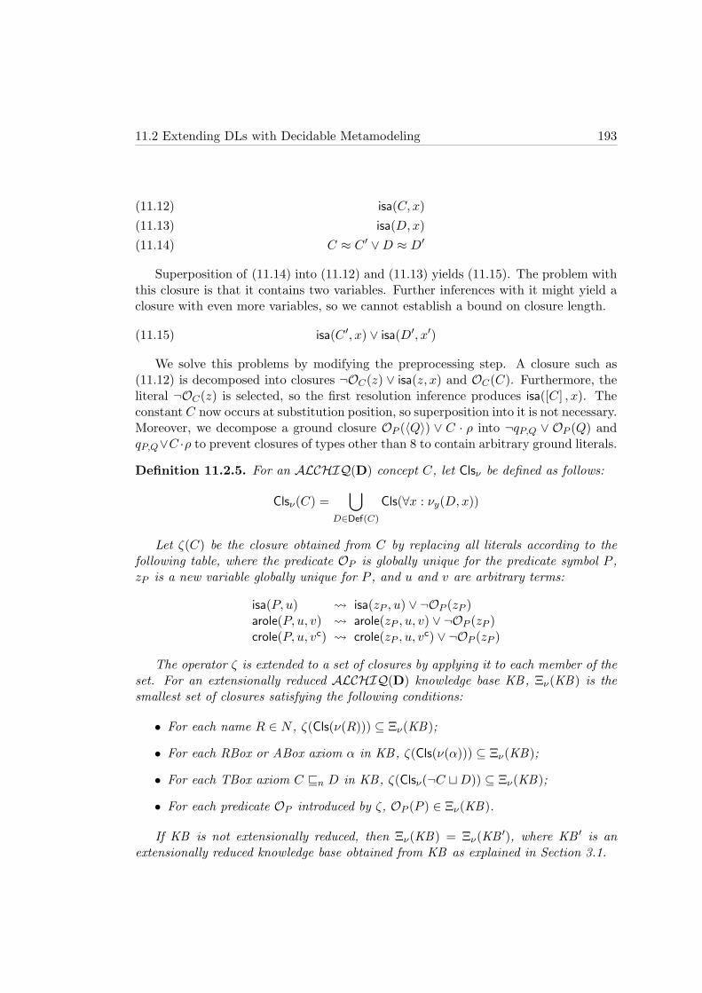
11.2 Extending DLs with Decidable Metamodeling 193
isa(C, x)(11.12)isa(D,x)(11.13)
C ≈ C ′ ∨D ≈ D′(11.14)
Superposition of (11.14) into (11.12) and (11.13) yields (11.15). The problem withthis closure is that it contains two variables. Further inferences with it might yield aclosure with even more variables, so we cannot establish a bound on closure length.
isa(C ′, x) ∨ isa(D′, x′)(11.15)
We solve this problems by modifying the preprocessing step. A closure such as(11.12) is decomposed into closures ¬OC(z) ∨ isa(z, x) and OC(C). Furthermore, theliteral ¬OC(z) is selected, so the first resolution inference produces isa([C] , x). Theconstant C now occurs at substitution position, so superposition into it is not necessary.Moreover, we decompose a ground closure OP (〈Q〉) ∨ C · ρ into ¬qP,Q ∨ OP (Q) andqP,Q∨C ·ρ to prevent closures of types other than 8 to contain arbitrary ground literals.
Definition 11.2.5. For an ALCHIQ(D) concept C, let Clsν be defined as follows:
Clsν(C) =⋃
D∈Def(C)
Cls(∀x : νy(D,x))
Let ζ(C) be the closure obtained from C by replacing all literals according to thefollowing table, where the predicate OP is globally unique for the predicate symbol P ,zP is a new variable globally unique for P , and u and v are arbitrary terms:
isa(P, u) isa(zP , u) ∨ ¬OP (zP )arole(P, u, v) arole(zP , u, v) ∨ ¬OP (zP )crole(P, u, vc) crole(zP , u, vc) ∨ ¬OP (zP )
The operator ζ is extended to a set of closures by applying it to each member of theset. For an extensionally reduced ALCHIQ(D) knowledge base KB, Ξν(KB) is thesmallest set of closures satisfying the following conditions:
• For each name R ∈ N , ζ(Cls(ν(R))) ⊆ Ξν(KB);
• For each RBox or ABox axiom α in KB, ζ(Cls(ν(α))) ⊆ Ξν(KB);
• For each TBox axiom C vn D in KB, ζ(Clsν(¬C tD)) ⊆ Ξν(KB);
• For each predicate OP introduced by ζ, OP (P ) ∈ Ξν(KB).
If KB is not extensionally reduced, then Ξν(KB) = Ξν(KB ′), where KB ′ is anextensionally reduced knowledge base obtained from KB as explained in Section 3.1.

194 11. The Semantics of Metamodeling
It is easy to see that Ξν(KB) is satisfiable if and only if KB is ν-satisfiable.
Lemma 11.2.6. Let KB be an ALCHIQ(D) knowledge base. Then KB is ν-satisfiableif and only if Ξν(KB) is satisfiable. Furthermore, Ξν(KB) can be computed in timepolynomial in |KB |, for unary coding of numbers in input.
Proof. By Lemma 11.2.4, KB is ν-satisfiable if and only if ν(KB) is satisfiable. Ξν(KB)is obtained from ν(KB) by applying structural transformation, which is known not toaffect satisfiability, and by applying decomposition to literals isa(P, u), arole(P, u, v),and crole(P, u, vc), which does by affect satisfiability by Theorem 5.4.4.
Definition 11.2.7. Let BSD,+ν be the BSD calculus parameterized as follows:
• The E-term ordering is a lexicographic path ordering induced by a total prece-dence > over function, constant, and predicate symbols such that, for any func-tion symbol f , constant symbol c, predicate symbol P , and a propositional symbolqP,Q, we have f > c > P > qP,Q > T.
• If a closure contains a literal of the form ¬OC(z), then all such literals areselected; otherwise, all negative arole and crole literals are selected.
• Inference conclusions, whenever possible, are decomposed according to the follow-ing table, for an arbitrary term t:
D · ρ ∨ arole([R] , [t] , [f(t)]) D · ρ ∨ QR,f ([t])
¬QR,f (x) ∨ arole([R] , x, [f(x)])
D · ρ ∨ arole([R] , [f(x)] , x) D · ρ ∨ QInv(R),f (x)
¬QInv(R),f (x) ∨ arole([R] , [f(x)] , x)
OP (〈Q〉) ∨ C · ρ C · ρ ∨ qP,Q
¬qP,Q ∨ OP (Q)
We say that N is a set of ν-ALCHIQ(D)-closures if each closure in N is of typesfrom Tables 5.1 and 6.1 with the following differences:
• Conditions (iii)–(vii) are dropped;
• Atoms of the form C(t) take the form isa([C] , t);
• Atoms of the form R(u, v) take the form arole([R] , u, v);
• Atoms of the form T (u, vc) take the form crole([T ] , u, vc);
• All closures can contain a disjunction of the form q =∨
(¬)qP,Q;
• A new type of initial closures contains the closures from Ξν(KB) (instead ofliterals (¬)isa([C] , x), these closures contain a disjunction (¬)isa(z, x)∨¬OC(z)).

11.2 Extending DLs with Decidable Metamodeling 195
We now prove the following lemma:
Lemma 11.2.8. Let N be a set of ν-ALCHIQ(D)-closures, and let C1 · ρ, . . . , Ck · ρbe the nonredundant closures obtained by applying a BSD,+
ν inference to premises fromN . Then, N ∪ C1 · ρ, . . . , Ck · ρ is a set of ν-ALCHIQ(D)-closures, and no Ci · ρ,1 ≤ i ≤ k, is an initial closure.
Proof. Due to decomposition, it is obvious that the following property (*) holds: pos-itive literals of the form OP (Q) occur only in unit closures, or in closures of the formOP (Q) ∨ ¬qP,Q.
Now consider an inference with an initial closure C. Since C contains literalsof the form ¬OP (z), and all such literals are selected, C can participate only in ahyperresolution inference on all ¬OP (zi). Because of (*), the inference instantiates allvariables zi, and the conclusion is a ν-ALCHIQ(D)-closure, but not an initial closure.
Due to the E-term ordering of BSD,+ν , only a literal with a term of the maximum
depth can be maximal in a ν-ALCHIQ(D)-closure. Also, the E-term ordering ensuresthat a propositional letter qP,Q is not maximal if a closure contains some other literal.Finally, appropriate inferences are eligible for decomposition in the same way as inTheorem 5.4.8. Hence, the claim of this lemma can be shown in the same way as inthe proofs of Lemma 5.3.6, Theorem 5.4.8, and Lemma 6.2.1.
Theorem 11.2.9. Let KB be an ALCHIQ(D) knowledge base, defined over an admis-sible concrete domain D, for which D-satisfiability of finite conjunctions over ΦD canbe decided in deterministic exponential time. Then, saturation of Ξν(KB) by BSD,+
ν
with eager application of redundancy elimination rules decides ν-satisfiability of KB,and runs in time exponential in |KB |, for unary coding of numbers and assuming abound on the arity of concrete predicates.
Proof. The number of propositional letters qP,Q is quadratic in |KB |, and the numberof predicates OP is linear in |KB |. Therefore, it is possible to obtain an exponentialbound on the number of closures derived in the same way as in Lemma 5.3.10, Theorem5.4.8, and Theorem 6.2.5. Since decomposition is sound and complete by Theorem5.4.4, the claim of this theorem follows.
Note that ν-semantics reifies concept and roles; however, it is more like π-semantics,and less like OWL-Full semantics in the way it handles modeling primitives. In ν- andπ-semantics, the modeling primitives are expressed as formulae, so they cannot betampered with. On the contrary, OWL-Full reifies the modeling primitives as well, sotheir semantics can be affected by statements in the knowledge base.
11.2.3 Metamodeling and Transitivity
Since the algorithm for checking ν-satisfiability of an ALCHIQ(D) knowledge baseKB does not differ essentially from the algorithm for checking π-satisfiability of KB ,

196 11. The Semantics of Metamodeling
one might intuitively expect that allowing transitivity axioms in KB does not causeproblems. However, consider the following knowledge base KB :
> vn ≥ 3R(11.16)R ≈ S(11.17)
Trans(S)(11.18)
Note that KB is a SHIQ knowledge base: the role S is simple, since it passesthe syntactic criterion specified in Definition 3.1.1 (it is neither transitive, nor it has atransitive subrole). However, in any ν-interpretation I, the axiom (11.17) ensures thatSI = T I = α. Furthermore, due to (11.18), RI
a(α) is transitive. Effectively, in (11.16)a transitive role R is used in a number restriction, even though it is syntactically asimple role.
Since equality of roles might be nontrivially entailed by KB , identifying simpleroles would itself require theorem proving. Therefore, it is difficult, if not impossible,to define simple roles under ν-semantics. In [73], it was shown that transitive roles innumber restrictions lead to undecidability, so we get the following result:
Proposition 11.2.10. Checking ν-satisfiability of a SHIQ knowledge base KB isundecidable.
Decidability can be regained by using unique role assumption. Intuitively, thisassumption requires two distinct role symbols to be interpreted as distinct domainindividuals. In such a case, simple roles can be defined and checked as usual.
Definition 11.2.11 (Unique Role Assumption). A SHIQ(D) knowledge base KBemploys the unique role assumption if it contains an axiom R 6≈ S, for each twodistinct symbols R and S occurring as roles in KB.
It is easy to see that transitivity axioms can be eliminated from knowledge basesemploying unique roles assumption using the transformation from Section 5.2, so wethus obtain an algorithm for checking ν-satisfiability of such knowledge bases.
Theorem 11.2.12. Let KB be a SHIQ(D) knowledge base KB employing the uniquerole assumption, or containing neither explicit equality statements, nor number restric-tions. Then, KB is ν-satisfiable if and only if Ω(KB) is ν-satisfiable.
Proof. The (⇒) direction of the proof of Theorem 5.2.3 obviously holds in this caseas well. For the (⇐) direction, by the lemma assumptions on KB , if Ω(KB) is ν-satisfiable, then it has a ν-model such that RIν 6= SIν , for each two distinct symbolsR and S occurring as roles in KB . Hence, it is possible to construct a ν-model of KBin the same way as in the proof of the (⇐) direction of Theorem 5.2.3.

11.3 Expressivity of Metamodeling 197
11.3 Expressivity of Metamodeling
In this section we investigate in which way metamodeling increases the expressivityof the logic. Here we consider only the logical aspects—that is, what kinds of newconsequences can be drawn. Our discussion in this section does not consider nonlogicalaspects that may be relevant in practice (such as increased search flexibility). Thefollowing results are similar to the ones for HiLog [33].
It is easy to see that ν-satisfiability is a strictly stronger notion than π-satisfiability.Consider the following knowledge base KB :2
Eagle(Harry)(11.19)¬Aquila(Harry)(11.20)Eagle ≈ Aquila(11.21)
Under the contextual semantics, the interpretations of symbols C andD as conceptsand as individuals are completely independent, so KB is π-satisfiable. However, KBis ν-unsatisfiable: in each ν-interpretation, EagleI = AquilaI = α, so it cannot be thatHarryI ∈ CI
n(EagleI) and HarryI /∈ CIn(AquilaI). For the other direction, we have the
following lemma:
Lemma 11.3.1. Each ν-satisfiable ALCHIQ(D) knowledge base is π-satisfiable.
Proof. Let Iν be a ν-model of an ALCHIQ(D) knowledge base KB . We constructfrom Iν a π-interpretation Iπ as follows: 4Iπ = 4Iν , nIπ = nIν , CIπ
n (n) = CIνn (nIν ),
RIπa (n) = RIν
a (nIν ), and RIπc (n) = RIν
c (nIν ), for each n ∈ N . By a simple induction onthe concept structure, it can be shown that, for each concept X, CIπ
n (X) = CIνn (X),
so Iπ is a π-model of KB .
Furthermore, for a knowledge base with unique name assumption or without equal-ity (either explicit or implicit, introduced through number restrictions), π-satisfiabilityand ν-satisfiability coincide:
Lemma 11.3.2. Let KB be an ALCHIQ(D) knowledge base such that it employsunique name assumption, or it contains neither explicit equality statements, nor num-ber restrictions. Then, KB is π-satisfiable if and only if it is ν-satisfiable.
Proof. The (⇐) direction follows from Lemma 11.3.1. For the (⇒) direction, let KBbe π-satisfiable in some model Iπ. Due to the lemma assumptions, we can assumewithout loss of generality that ni 6= nj implies ni
Iπ 6= njIπ , for all for ni, nj ∈ N (in
the first case, this is because KB employs unique name assumption, and in the secondcase this is because KB does not employ equality).
Given such a π-model Iπ, we construct a ν-interpretation Iν by setting 4Iν = 4Iπ ,nIν = nIπ , CIν
n (nIν ) = CIπn (n), RIν
a (nIν ) = RIπa (n), and RIν
c (nIν ) = RIπc (n), where
n ∈ N . Furthermore, for all x ∈ 4Iν such that there is no n ∈ N with x = aIν , let2Aquila is the Latin name for eagle.

198 11. The Semantics of Metamodeling
CIνn (x) = RIν
a (x) = RIνc (x) = ∅. Since we can assume that different names from N
are interpreted as different elements from 4Iν , such a construction defines exactly onevalue of CIν
n (x), RIνa (x), and RIν
c (x) for each x ∈ 4Iν , so Iν is correctly defined. Bya simple induction on the concept structure, it can be shown that CIν
n (X) = CIπn (X)
for each concept X, so Iν is a ν-model of KB .
To summarize, ν-semantics derives new consequences only if two symbols can bederived to be equal: for example, from (11.19) and (11.21) it is possible to deriveAquila(Harry). Furthermore, under unique name assumption (which is often used inpractice), ν-semantics does not produce any new consequences. This seems to suggestthat the benefits of ν-semantics do not outweigh its drawbacks—that it is nonstandard,and that it introduces problems for transitive roles. Moreover, π-semantics might besufficient for many practical applications.
However, ν-semantics unlocks its full potential when combined with a languagemore expressive than OWL. For example, by combining ν-semantics with the Seman-tic Web Rule Language (SWRL) [69], one can explicitly axiomatize the semantics ofmetaclasses. Returning to the example from the beginning of this chapter, by (11.22)we state that Eagle is a RedListSpecies, and by a SWRL rule (11.23) we state thatinstances of species listed in the Red List are not allowed to be hunted. Note thatwe use in atom x(y) the variable x at the predicate position. Under ν-semantics thisis equivalent to isa(x, y), but under π-semantics this would not be possible withoutleaving the confines of first-order logic. Now from (11.19), (11.22), and (11.23), we caninfer CannotHunt(Harry); hence, RedListSpecies semantically acts as a metaconceptof the Eagle concept.
RedListSpecies(Eagle)(11.22)RedListSpecies(x) ∧ x(y)→ CannotHunt(y)(11.23)
To summarize, from the logical perspective ν-semantics alone does not make muchof a difference, and π-semantics may be sufficient for numerous applications. However,ν-semantics provides a sound foundation for metamodeling, which, when combinedwith a more expressive logic, such as SWRL, allows us to precisely axiomatize theinteraction between classes and metaclasses. It is easy to see that, if ν-semantics iscombined with DL-safe rules from Chapter 9, it yields a decidable formalism. Thus,we believe ν-semantics to be very relevant for future extensions of OWL.
11.4 Related Work
The definition of ν-satisfiability given in Section 11.2 is inspired by HiLog [33], a logicin which general terms are allowed to occur in place of function and predicate symbolsin formulae. The semantics is defined by interpreting each individual as a member ofthe interpretation domain, and by assigning a functional and a relational interpretationto domain objects. The authors show that HiLog can be considered “syntactic sugar,”

11.4 Related Work 199
since each HiLog formula can be encoded into an equisatisfiable first-order formula; thedefinition of the ν operator in Table 11.3 closely resembles this encoding. Finally, theauthors show that a satisfiable first-order formula without equality is also satisfiableunder HiLog semantics.
In [102], the RDFS Model Theory was criticized for allowing infinitely many meta-layers. The authors argue that such a semantics is inadequate for the Semantic Websince (i) it does not provide adequate support for inferencing; (ii) it allows definingclasses that contain themselves, which may potentially lead to paradoxes; and (iii) byadding classes, one necessarily introduces objects in the interpretation universe. Theauthors propose RDFS-FA, a stratified four-level approach, consisting of the meta-language layer, the language layer, the ontology layer, and the instance layer. In[68], similar arguments were used to criticize the semantics of OWL-Full. We followthe principles of RDFS-FA by strictly separating the modeling primitives from theontology and the instance layers; however, to provide for metamodeling, our definitionof ν-semantics merges the ontology and the instance layers. Furthermore, we showthat the consequences of (iii) actually match the intuition behind metamodeling.
In [149], the authors point out the usefulness of metamodeling in many applicationdomains. They propose separation of modeling layers, which are connected usingspanning instances. However, the authors do not consider the logical consequences oftheir approach.
By means of an example very similar to ours, in [132] the author argues for thecompelling need of metamodeling in practical knowledge representation systems.

200 11. The Semantics of Metamodeling

Part IV
Practical Considerations
201


Chapter 12
Implementation of KAON2
Whereas the techniques presented in previous chapters provide new theoretical insightsinto the relationship between description logics and disjunctive datalog, our primarymotivation for developing them was to obtain a practical alternative to tableau cal-culi, capable of handling knowledge bases with reasonably large ABoxes. To validatepracticability of our algorithms, we implemented them in a new DL reasoning systemKAON2.1 In this chapter, we describe the implementation of the system, and discussnumerous practical aspects. Namely, the implemented algorithms are of high computa-tional complexity, so it is unrealistic to expect that one can directly cast them into codeand obtain an efficient implementation. To avoid unnecessary overhead, we developedseveral important optimizations. In the following section we present the architectureof the system, followed by a detailed discussion of important system components.
12.1 KAON2 Architecture
KAON2 fully implements the satisfiability checking algorithm from Chapter 5, thereduction algorithm from Chapter 7, and the DL-safe rules from Chapter 9. Hence,the supported logic is SHIQ extended with DL-safe rules. Datatypes are not sup-ported yet because it is currently not clear how to combine concrete domain resolutionwith optimization techniques, such as magic sets. Furthermore, answering conjunctivequeries and metamodeling are not supported because it is currently unclear how tocast the presented algorithms into the setting of disjunctive datalog.
KAON2 was implemented completely in Java 1.5. Figure 12.1 describes its technicalarchitecture. The Ontology API provides ontology manipulation tasks, such as addingand retrieving ontology axioms. The API fully supports OWL and the Semantic WebRule Language (SWRL) at the syntactic level. Several similar APIs already exist,such as OWL API [17] or Jena.2 However, to obtain an efficient system, we had toexert complete control over the internals of the API, which we could not have achieved
1http://kaon2.semanticweb.org/2http://jena.sourceforge.net/
203

204 12. Implementation of KAON2
Figure 12.1: KAON2 Architecture
by reusing an existing implementation. Ontologies can be saved in files, using eitherOWL RDF3 or OWL XML4 syntax. Alternatively, ABox assertions can be storedin a relational database (RDBMS): by mapping ontology entities to database tables,KAON2 will query the database on the fly during reasoning.
The Reasoning API allows invoking various reasoning tasks, and retrieving theirresults.
KAON2 can be used as a dynamic library, or as a stand-alone server. In thelatter case, the client applications can access KAON2 through either Remote MethodInvocation (RMI) protocol or the DL Implementors Group (DIG) API [16]. Thus, thesystem can be used with Protege5 and OilEd6 ontology editors.
The Reasoning Engine is the central component of KAON2, consisting of threesubcomponents. The Ontology Clausification subcomponent is responsible for trans-lating a SHIQ knowledge base KB into a set of first-order clauses Ξ(KB). In Section12.2 we preset several optimizations of the basic clausification algorithm. The Theo-rem Prover for BS implements the basic superposition calculus [14], which is used inthe reduction algorithm. The design of this component is discussed in more detail inSection 12.3. Finally, the Disjunctive Datalog Engine is used for answering queries inthe program obtained by the reduction. The design of this component is discussed inmore detail in Section 12.4.
12.2 Ontology Clausification
The saturation of TBox and ABox clauses by basic superposition is a critical step ofthe reduction algorithm, because it can introduce an exponential blowup. Each clause
3http://www.w3.org/TR/owl-semantics/4http://www.w3.org/TR/owl-xmlsyntax/5http://progete.stanford.edu/6http://oiled.man.ac.uk/

12.2 Ontology Clausification 205
can potentially participate in an inference that generates many conclusions, so it isimportant to keep the size of the input clause set minimal. To achieve this, we presentseveral optimizations of the clausification algorithm from Definition 5.3.1; they are alsoapplicable to the clausification algorithm from Definition 8.2.2.
12.2.1 Reusing Replacement Predicates
A concept often occurs in many other concepts in KB , which allows us to reuse thereplacement concepts:
Definition 12.2.1. For QD and QD new concepts unique for D, the optimized clausi-fication is obtained by modifying Definition 5.3.1 to use for Q the concept as follows:
Q =QD if pol(C, p) = 1 and C|p = DQD if pol(C, p) = −1 and C|p = D
For example, consider the knowledge base KB , consisting of axioms (12.1)–(12.3)shown on the left-hand side:
A v ∃S.∃R.D A v ∃S.Q∃R.D
Q∃R.D v ∃R.D(12.1)
B v ∃T.∃R.D B v ∃T.Q∃R.D(12.2)
∃U.∃R.D v C ∃U.Q∃R.D v C∃R.D v Q∃R.D
(12.3)
The concept ∃R.D occurs in KB twice under positive, and once under negativepolarity. Hence, we replace ∃R.D in (12.1) and (12.2) with Q∃R.D, and in (12.3) withQ∃R.D, yielding the axioms shown in (12.1)–(12.3) on the right-hand side.
Note that Q∃R.D should not be used to replace ∃R.D in (12.3): the negation-normalform of (12.3) is ∀U.∀R.¬DtC, and it does not contain ∃R.D. Hence, the subconcept∀R.¬D must be replaced by a concept different from Q∃R.D.
Lemma 12.2.2. KB and Ξ(KB) are equisatisfiable, even if optimized structural trans-formation is applied to an ALCHIQ(D) knowledge base KB.
Proof. The (⇐) direction is trivial, and the (⇒) direction can be proved by choosingthe interpretation of QD and QD as done for decomposition in Subsection 5.4.1.
12.2.2 Optional Positions
Certain nonliteral predicates need not be replaced with an atomic concept in theclausification process. Consider clausification of an axiom A v ∃R.B: by Definition5.3.1, Cls(¬At∃R.B) = ¬AtQ1, ¬Q1t∃R.B; that is, the concept ∃R.B is replacedby Q1. However, clausifying ¬A t ∃R.B produces clauses of the form from Table 5.2even without replacing the nonliteral subconcept ∃R.B. This allows for the followingoptimization:

206 12. Implementation of KAON2
Definition 12.2.3. In a concept C = Dt⊔Li, where D is a possibly complex concept
and all Li are literal concepts, the positions of D and Li are optional for renaming.
Lemma 12.2.4. Each clause in Ξ(KB) is of a type from Table 5.2, even if Def(C) iscomputed by omitting in Λ(C) the positions that are optional for renaming.
Proof. By definition of π from Table 3.1, clausifying a concept C = Dt⊔Li produces
clauses from Table 5.2.
Renaming optional positions can sometimes be beneficial. Consider the knowledgebase KB , consisting of axioms shown in (12.4)–(12.6) on the left-hand side:
A v ∃R.C ¬A(x) ∨R(x, f(x))¬A(x) ∨ C(f(x))
(12.4)
B v ∃R.C ¬B(x) ∨R(x, g(x))¬B(x) ∨ C(g(x))
(12.5)
> v ≤ 1R ¬R(x, y1) ∨ ¬R(x, y2) ∨ y1 ≈ y2(12.6)
In ¬At∃R.C and ¬B t∃R.C, the positions of ∃R.C are optional for renaming, soKB can be clausified without introducing new predicates. This yields clauses shownin (12.4)–(12.6) on the right-hand side.
The concept ∃R.C is now skolemized twice, yielding clauses ¬A(x)∨R(x, f(x)) and¬B(x) ∨ R(x, g(x)) as candidates for an inference with (12.6). Additional axioms ofthe form Ai v ∃R.C would produce additional clauses of the form ¬Ai(x)∨R(x, f(x)),which could participate in an inference with (12.6), thus significantly increasing thesearch space.
The search space can be reduced by renaming ∃R.C, although it occurs at optionalpositions in axioms. The axioms and the clauses obtained by applying the structuraltransformation to KB are shown in (12.7)–(12.10):
A v Q ¬A(x) ∨Q(x)(12.7)B v Q ¬B(x) ∨Q(x)(12.8)
Q v ∃R.C ¬Q(x) ∨R(x, f(x))¬Q(x) ∨ C(g(x))
(12.9)
> v ≤ 1R ¬R(x, y1) ∨ ¬R(x, y2) ∨ y1 ≈ y2(12.10)
This set contains one clause ¬Q(x) ∨ R(x, f(x)), which can participate in an in-ference with (12.10); also, any additional axiom Ai v ∃R.C produces only a clause¬Ai(x) ∨ Q(x). Note that renaming ∃R.C pays off because the concept ∃R.C occursin KB twice.
Hence, in Definition 5.3.1, Λ(C) should be the set of all positions p 6= ε in C suchthat (i) C|p is not a literal concept, and, for all positions q below p, C|q is a literalconcept; and (ii) p is either not optional for renaming, or C|p occurs in KB more thanonce.

12.2 Ontology Clausification 207
12.2.3 Handling Functional Roles
Consider the knowledge base KB , containing the axioms shown in (12.11)–(12.13) onthe left-hand side:
> v ≤ 1R ¬R(x, y1) ∨ ¬R(x, y2) ∨ y1 ≈ y2(12.11)
A v ∃R.C ¬A(x) ∨R(x, f(x))¬A(x) ∨ C(f(x))
(12.12)
B v ∃R.D ¬B(x) ∨R(x, f(x))¬B(x) ∨D(f(x))
(12.13)
The role R is functional by (12.11), which means that an object in a model can haveat most one R-successor. This allows using the same function symbol f in skolemizing∃R.C and ∃R.D, yielding clauses (12.11)–(12.13) shown on the right-hand side.
The main benefit of such clausification is that resolving ¬A(x) ∨ R(x, f(x)) and¬B(x) ∨ R(x, f(x)) with (12.11) produces a clause with a literal f(x) ≈ f(x); such aclause is a tautology (and can be deleted). Without reusing function symbols, clausify-ing (12.12) would produce ¬B(x)∨R(x, g(x)), which, resolved with ¬A(x)∨R(x, f(x))and (12.11), produces a clause containing a literal f(x) ≈ g(x). Such a clause is not atautology, and should be used in further inferences.
This optimization is also very important for the reduction to disjunctive datalog.Namely, for each function symbol f occurring in Ξ(KB), the program DD(KB) containsa new predicate Sf . By reducing the number of function symbols, we reduce the numberof datalog predicates.
Definition 12.2.5. Clausification with optimized skolemization is obtained from De-finition 5.3.1 such that, if > v ≤ 1R ∈ KB, then the existential quantifiers in ∃R.Cand ≥ nR.C are skolemized using a function symbol fR unique for R.
Lemma 12.2.6. KB and Ξ(KB) are equisatisfiable, even if clausification with opti-mized skolemization is used.
Proof. If R is functional, then an object x is allowed to have at least one R-successorin a model I, which is represented by the functional term fR(x).
12.2.4 Discussion
The techniques presented in this chapter are all geared towards reducing the numberof clauses in Ξ(KB). It is instructive to compare the effects that such optimizationswould have in a tableau calculus such as [73].
Tableau calculi try to construct a model of a knowledge base by applying tableauexpansion rules if some tableau constraint is not satisfied. Consider, for example, aknowledge base KB consisting of the following axioms:

208 12. Implementation of KAON2
C(a)(12.14)R(a, b)(12.15)D(b)(12.16)
C v ∃R.D(12.17)
The axiom (12.17), when applied to (12.14), yields a constraint ∃R.D(a), whichdoes not need to be further expanded: a already has an R-successor b that is a memberof D, so there is no need to introduce a new R-successor for a.
The situation is quite different in resolution calculi. The clausification algorithmtranslates (12.17) into these two clauses:
¬C(x) ∨R(x, f(x))(12.18)¬C(x) ∨D(f(x))(12.19)
In resolution, skolemization plays a role that is analogous to expanding existentialconcepts in tableau calculi: in clauses (12.18) and (12.19), the term f(x) plays therole of the existentially implied R-successor for x. Thus, skolemization expands allexistential quantifiers before the theorem proving process starts, regardless of whetherit is actually necessary to do so in order to build a model.
Another important difference between resolution and tableau is that clauses ob-tained by skolemization are nonground; that is, they encode successor information formany individuals. For example, (12.18) and (12.19) encode successor information forany individual x that is a member of C. When resolution inferences are applied tosuch nonground clauses, they act on the set of all those successors. In contrast, atableau calculus expands each successor separately, and repeats an inference step foreach successor separately.
The optimizations from Subsections 12.2.1, 12.2.2, and 12.2.3 can be understoodas an attempt to reduce the number of existential individuals introduced in advance.
12.3 The Theorem Prover for BSAs discussed in [116], implementing an efficient theorem prover is a very complex task.Apart from excellent software engineering skills, it also requires knowledge of numeroustechniques in order to implement various modules of the system.
However, our goal is not to provide a general first-order theorem prover applicableto any first-order problem. Rather, we need a theorem prover that can handle onlyALCHIQ-closures. As shown in Table 5.2, such closures are of a rather limited form.Hence, general implementation techniques can be radically simplified, thus yielding asimpler, leaner, and more efficient implementation.

12.3 The Theorem Prover for BS 209
12.3.1 Inference Loop
The main design element of a resolution-based theorem prover is the inference loop,which is responsible for saturating a set of closures under the given set of inferenceand redundancy elimination rules. In KAON2, we use a simplified variant of theDISCOUNT loop, introduced first in the equational theorem prover E [133]. Thepseudo-code of the inference loop is presented in Algorithm 12.1.
The inference loop is parameterized with a set of inference rules C (explained inmore detail in Subsection 12.3.3) and a set of redundancy elimination rules D (ex-plained in more detail in Subsection 12.3.4), and is given a set of closures N to besaturated. To ensure that the saturation is fair—that is, that each nonredundant in-ference is eventually performed—, the closures are partitioned into two sets. The setU is the set of unprocessed closures—that is, closures that have not taken part in anyinference. The set W is the set of worked-off closures—that is, closures for which allinferences with other members from W have been performed.
In the beginning, U contains the set of closures N to be saturated and W is empty.In each step of the saturation, a given closure g is don’t-care nondeterministicallychosen and removed from U . We describe the algorithm for choosing the given closure,encapsulated in the function PickGivenClosure, in more detail in Subsection 12.3.7.
Next, redundancy elimination rules are applied sequentially to g, transforming itinto a potentially simpler closure. We use a convention that, if a closure is maderedundant by a simplification rule, then SimplifyClosure returns null. We discussthe redundancy elimination rules of KAON2 in Subsection 12.3.4.
If the simplified closure is not redundant and it is not equal to the empty closure,then backward subsumption is performed: using RetrieveSubsumedClosures, allclosures from W that are properly subsumed by g are retrieved and removed from W .We describe the index structures used to optimize the retrieval of subsumed closuresin Subsection 12.3.8.
Finally, all inferences between g and the closures from W are performed. Allconclusions that are not syntactic tautologies are added to the set of unprocessedclosures U , after which the entire process is repeated.
If the given closure is the empty closure, then N is unsatisfiable. Otherwise, theprocess terminates if U becomes empty; at this point, W is the saturated set.
12.3.2 Representing ALCHIQ-Closures
ALCHIQ-closures of types 3, 4, 5, 6, and 8 have at most one variable, and any LPO istotal on such terms and literals. This allows us to represent closures as totally orderedarrays without repeated literals. This has two main benefits. First, the maximal literalis the first literal, so the literal on which an inference should take place can be locatedin constant time. Second, conclusions between inferences can be computed using mergesort in time that is linear in the size of the premises.
Moreover, the restricted form of ALCHIQ-closures allows us to use a polynomialsubsumption checking algorithm. Namely, the general subsumption problem is known

210 12. Implementation of KAON2
Algorithm 12.1 The Inference Loop of KAON2Input:C: the set of inference rulesD: the set of redundancy elimination rulesN : the set of closures to be saturated
Output:the set of closures W obtained by saturating N by C and D
Local variables:W : the set of worked-off closuresU : the set of unprocessed closures
1: W ←− ∅2: U ←− N3: while U 6= ∅ do4: g ←− PickGivenClosure(U)5: U ←− U \ g6: for each redundancy elimination rule r ∈ D do7: g ←− SimplifyClosure(g, r,W )8: end for9: if g 6= null then
10: if g = then11: return . N is unsatisfiable12: end if13: S ←− RetrieveSubsumedClosures(g,W )14: W ←− (W \ S) ∪ g15: T ←− ∅16: for each inference rule r ∈ C do17: T ←− T ∪ComputeConclusions(r, g,W )18: end for19: for each conclusion t ∈ T do20: if IsSyntacticTautology(t) = false then21: U ←− U ∪ t22: end if23: end for24: end if25: end while26: return W . W is the saturated set

12.3 The Theorem Prover for BS 211
to be NP-complete [52], and experience has shown that theorem provers spend up to 90percent of running time in subsumption checking. Therefore, improving the efficiencyof subsumption is expected to have a significant effect on the performance.
The subsumption checking procedure for closures of types 3, 4, 5, 6, and 8 is shownin Algorithm 12.2. To determine if C subsumes D, the algorithm essentially scans theliterals of D (lines 1–14), trying to match then with the first literal of C (line 2). If asubstitution σ exists such that C1σ = Di, because C1 contains all variables of C, thesubstitution σ binds all variables in C. Hence, in lines 5–8 the algorithm simply checkswhether, for each literal Ci, one can find a literal Dj such that Ciσ = Dj and thateach marked position of Ciσ can be overlaid in a substitution position in Dj . Sincethe closures are totally ordered, the literals can be matched sequentially. To estimatethe complexity, note that the inner loop (lines 1–14) is executed at most |D| times,whereas the inner loop (lines 5–8) is executed at most |C| + |D| times. Hence, thealgorithm runs in time O(|C| · (|C|+ |D|)), which is obviously polynomial.
Additionally, we store with each closure a flag specifying its type, as this enablesfurther optimizations. For example, a closure of type 3 or 4 cannot subsume a closureof any other type. Similarly, closures of types 1, 2, or 7 can subsume only closures ofthe same type. Hence, a quick check whether closure types are compatible can be usedto quickly identify subsumption tests that are bound to fail.
12.3.3 Inference Rules
The theorem prover of KAON2 encodes the literals with a predicate other than equalityas E-terms (see Section 2.5), allowing a more or less straightforward implementationof the inferences rules of the BS calculus. The implementation can be somewhatsimplified by observing that closures of types 1, 2, and 7 can only participate in hyper-resolution inferences, in which unification can be performed in constant time. Hence,the theorem prover handles closures of types 1, 2, and 7 by a separate hyperresolutioninference rule, whereas inferences among other closures are handled using positive andnegative superposition.
Furthermore, negative superposition inferences can result in closures containingliterals of the form T 6≈ T and x 6≈ x. For such closures, reflexivity resolution producesa closure that always subsumes the superposition conclusion, and is therefore appliedeagerly to each conclusion.
12.3.4 Redundancy Elimination Rules
The simplification rules are applied to the given closure in the order as explained inthe following paragraphs. It may come as a surprise that KAON2 does not implementso-called rewriting simplification inferences. Namely, given a unit closure s ≈ t and aclosure A∨C, under certain conditions, A∨C can be replaced with A[tσ]p ∨C, whereσ is a substitution such that A|p = sσ. In general first-order theorem provers, suchas E [133] or Vampire [119], such inferences are essential for solving hard problems.However, most DL problems do not contain unit equalities at all. Equalities occur only

212 12. Implementation of KAON2
Algorithm 12.2 Closure Subsumption Algorithm in KAON2Input:
C: the potential subsumerD: the potential subsuming closure
Output:a substitution σ such that Cσ ⊆ D
Note:Ci is the i-th literal of a closure C, and |C| is the number of literals in C.
1: for i = 1 . . . |D| do2: σ = Match(C1, Di)3: if σ 6= null then4: j ←− 05: for k = i . . . |D| and j < |C| do6: if Cjσ = Dk and MarkersCompatible(Cjσ,Dk) then7: j ←− j + 18: end if9: end for
10: if j = |C| then11: return σ12: end if13: end if14: end for15: return null . No subsumption
16: function Match(s,t)17: if s is a variable x then18: return x 7→ t19: else if s = f(s1, . . . , sn) and t = f(t1, . . . , tn) then20: σ ←− 21: for i = 1 . . . n do22: θ ←−Match(siσ, ti)23: if θ = null then24: return null25: else26: σ ←− σθ27: end if28: end for29: return σ30: else31: return null32: end if33: end function
34: function MarkersCompatible(s,t)35: true if t|p is at substitution position whenever s|p is marked, for each position p36: end function

12.3 The Theorem Prover for BS 213
in ALCHIQ-closures of type 5, 6, or 8, where they are usually accompanied by at leastone literal with a predicate other than ≈. Hence, rewriting is not applicable to the vastmajority of DL problems, and we therefore do not include it into our implementation.
Semantic Tautology Deletion. As mentioned in Section 2.4, checking if a closureis a tautology requires theorem proving, so simple syntactic approximate checks areused in practice. However, a feasible semantic check was presented in [133]: a closureis a tautology if it contains a disjunction of the form s1 6≈ t1 ∨ . . . ∨ sn 6≈ tn ∨ s ≈ tsuch that s1σ ≈ t1σ, . . . , snσ ≈ tnσ |= sσ ≈ tσ, where σ is a substitution mapping allvariables in the closure to distinct new constants.
Since deciding entailment in a ground equality theory is decidable, the check fromthe previous paragraph is decidable, but implementing it may introduce a significantamount of overhead. However, the syntactic structure of ALCHIQ-closures makesthe check easy to implement in certain situations. Namely, it is easy to see that theconditions of semantic tautology deletion are satisfied for any closure of type 5 or 6that contains a disjunction of the following form:
f1(t) 6≈ f2(t) ∨ f2(t) 6≈ f3(t) ∨ . . . ∨ fn−1(t) 6≈ fn(t) ∨ f1(t) ≈ fn(t)
Namely, for any substitution σ, it is easy to see that the following condition holds:
f1(tσ) ≈ f2(tσ) ∧ f2(tσ) ≈ f3(tσ) ∧ . . . ∧ fn−1(tσ) ≈ fn(tσ) |= f1(tσ) ≈ fn(tσ)
Hence, semantic tautology deletion can be applied to a closure C of type 5 or 6 asfollows. We first construct an unoriented graph GC whose nodes are function symbolsfrom C, and where nodes fi and fj are connected if C contains a literal fi(t) 6≈ fj(t).Next, we compute the transitive closure G+
C of GC . Finally, we check if C contains aliteral fi(t) ≈ fj(t) such that fi and fj are connected by an edge in G+
C . This checkcan be performed in time that is polynomial in |C|, and, if it succeeds, C is deleted.
Forward Subsumption. A closure C is deleted if the set of worked-off closuresW contains a closure D that subsumes C. We discuss the index structures used tooptimize subsumption checking in more detail in Subsection 12.3.8.
Contextual Literal Cutting. This subsumption-based simplification rule [134] al-lows eliminating certain literals from a closure. Namely, a closure C∨L can be replacedwith C, provided that C ∨ L is subsumed in the set of worked-off closures W . Hence,contextual literal cutting can be implemented by complementing each literal, and thenchecking whether the resulting closure is subsumed in W .
The correctness of the rule can intuitively be explained as follows: let D be aclosure from W that subsumes C ∨ L through a substitution σ—that is, Dσ ⊆ C ∨ L.Furthermore, because D is in W , we have W |= Dσ∨L. But now we can resolve C ∨Lwith Dσ ∨ L; because Dσ ∈ C, we obtain the closure C, which obviously subsumesC ∨L. Hence, contextual literal cutting can be understood as a macro, combining theeffects of the mentioned inferences.

214 12. Implementation of KAON2
12.3.5 Optimizing Number Restrictions
It is not difficult to see that resolution-based techniques are not well suited for rea-soning with number restrictions. Namely, a concept of the form ≤ nR.C is translatedinto a closure of type 7, containing (n+1)n
2 literals of the form yi ≈ yj . If such a clo-sure is hyperresolved with m R-generators of type 3, each hyperresolution producesclosures containing many literals of the form [fi(x)] ≈ [fj(x)]. Furthermore, such aliteral is produced by each inference with a pair of side premises containing fi and fj ,thus resulting in many similar closures. Because each literal fi(x) ≈ fj(x) is a poten-tial source of a superposition inference, number restrictions dramatically increase thenumber of superposition inferences in a saturation.
The number of superposition inferences can be somewhat reduced by applying de-composition and replacing literals of the form [fi(t)] ≈ [fj(t)] with Qfi,fj
([t]). Considerthe closures (12.20)–(12.21), obtained by resolving Ci(x)∨R(a, fi(x)), 1 ≤ i ≤ 4, with¬R(x, y1) ∨ ¬R(x, y2) ∨ ¬R(x, y3) ∨ y1 ≈ y2 ∨ y2 ≈ y3 ∨ y1 ≈ y3:
C ∨ [f1(x)] ≈ [f2(x)] ∨ [f1(x)] ≈ [f3(x)] ∨ [f2(x)] ≈ [f3(x)](12.20)D ∨ [f1(x)] ≈ [f2(x)] ∨ [f1(x)] ≈ [f4(x)] ∨ [f2(x)] ≈ [f4(x)](12.21)
Using decomposition, (12.20)–(12.21) can be transformed into (12.22)–(12.28):
C ∨Qf1,f2(x) ∨Qf1,f3(x) ∨Qf2,f3(x)(12.22)D ∨Qf1,f2(x) ∨Qf1,f4(x) ∨Qf2,f4(x)(12.23)
¬Qf1,f2(x) ∨ [f1(x)] ≈ [f2(x)](12.24)¬Qf1,f3(x) ∨ [f1(x)] ≈ [f3(x)](12.25)¬Qf1,f4(x) ∨ [f1(x)] ≈ [f4(x)](12.26)¬Qf2,f3(x) ∨ [f2(x)] ≈ [f3(x)](12.27)¬Qf2,f4(x) ∨ [f2(x)] ≈ [f4(x)](12.28)
Now there is exactly one closure containing a literal of the form [fi(x)] ≈ [fj(x)], sosuperposition from such a literal is performed only once, and not for each closure where[fi(x)] ≈ [fj(x)] occurs.
A disadvantage of this transformation is that it does not allow us to apply semantictautology deletion (see Subsection 12.3.4), since literals fi(x) ≈ fj(x) occur only inisolation. This can be remedied as follows: for each pair of function symbols fi and fj ,we additionally introduce a closure Qfi,fj
(x)∨ [fi(x)] 6≈ [fj(x)], which makes Qfi,fj(x)
equivalent to [fi(x)] ≈ [fj(x)]. Now semantic tautology deletion can be applied asdescribed previously with the difference that, instead of [fi(x)] ≈ [fj(x)], the literalsQfi,fj
([t]) are used in building the graph GC .
12.3.6 Tuning the Calculus Parameters
The main role of the parameters of BSDL is to guarantee termination of the calculus.However, Definition 5.3.3 provides some room for fine-tuning the parameters.

12.3 The Theorem Prover for BS 215
More concretely, we can choose the precedence of predicate symbols > based onthe frequency of occurrences of symbols in a knowledge base. Practical experimentshave shown that in many cases, it is beneficial to use a precedence based on decreasingfrequency of symbols—that is, a precedence where the most-frequent predicate is thesmallest in the precedence.
Furthermore, we can tweak the selection function. It is known that selecting andhyperresolving multiple negative literals in practice often leads to better performance.Intuitively, such inferences are efficient because they do not derive many intermediaryconsequences. In the case of BSDL, we can use a selection function that selects negativeliterals containing the deepest terms in a closure. Lemma 5.3.6 still holds in such acase, because Lemma 5.3.5 is still satisfied.
12.3.7 Choosing the Given Closure
General theorem provers are geared towards solving hard problems in first-order logic.However, first-order logic is semidecidable: given a finite amount of time, we canhope only to detect unsatisfiability. For satisfiable problems, no guarantee of finding asolution exists. Therefore, most existing theorem provers are geared towards detectingunsatisfiability.
It is widely believed that many hard first-order problems have relatively shortproofs. Hence, the performance of first-order reasoning is expected to depend a loton choosing a good proof strategy, which is mainly determined by the algorithm forchoosing the given closure (line 4 of Algorithm 12.1). Therefore, numerous differentheuristics for choosing the given closure have been explored.
Unlike most general first-order provers, the theorem prover in KAON2 is appliedmostly to satisfiable problems. Namely, ontologies are typically satisfiable (if this is notso, they usually contain an error). Furthermore, in computing a reduction to disjunc-tive datalog, the saturation of the TBox axioms is computed. Finally, our experienceand that of other authors of DL reasoning systems shows that most problems encoun-tered while computing a subsumption hierarchy are satisfiable. Hence, the strategy forchoosing the given closure is less important in our case, because the theorem prover inmost cases performs all inferences anyway.
Therefore, we adopt a simple strategy of always choosing a closure from U that hasthe smallest number of literals, and of resolving ties in an arbitrary manner. Intuitively,a short closure is more likely to subsume a closure in W .
12.3.8 Indexing Terms and Closures
As discussed in [116], a critical aspect of an implementation of a first-order theoremprover is to provide appropriate clause indexes—auxiliary data structures used to effi-ciently identify closures used at particular steps in the saturation. Unification indexesare used to retrieve potential candidate closures that can participate in an inference,whereas subsumption indexes are used to retrieve closures that subsume or that aresubsumed by a certain closure.

216 12. Implementation of KAON2
Many different indexing techniques were developed; for an extensive overview,please refer to [79]. A prominent indexing technique is partially adaptive code trees[117], pioneered in the theorem prover Vampire [119]. Whereas this technique is knownto give excellent performance, the restricted structure of ALCHIQ-closures allows usto employ simpler, but still efficient indexing techniques.
Unification Indexes. The problem of unification indexing can be formalized asfollows: given a query term s, a unification index identifies the subset M of a setof terms N such that each term t ∈ M unifies with s. In practice, one usually alsoassociates with each term t a closure in which t occurs.
Consider now the type of BSDL inferences applicable to ALCHIQ-closures. Thecandidates for (hyper)resolution with a closure of type 1, 2, or 7 are closures of types3, 4, or 8, and their suitability is determined uniquely by the role symbol. Hence,indexing can be simply performed by hashing the closures on the role symbol.
More complex are superposition inferences between closures of types 5 and 6, su-perposition into generator closures, and superposition into unary literals of closures oftype 8. These closures can be indexed using a simplified variant of the well-known pathindexing technique [140, 113]. Namely, inferences with these closures take place onlyon unary E-terms, which contain at most one variable. This allows for the followingsimple indexing strategy. Each unary E-term f1(f2(. . .)) can be represented as a stringof function symbols f1.f2 . . ., and by encoding variables using a special symbol ∗. Tobuild an index over a set of terms, we use the well-known trie data structure over thestrings (for more information on the trie data structures, please refer to [137]). Givena term s, locating all terms from the trie can be performed by traversing the trie usingthe string corresponding to s. The trie traversal algorithm is standard, with a minordifference that the symbol ∗ can be matched with zero or more arbitrary symbols.
Moreover, observe that, for closures as described in the previous paragraph, asuperposition inference can be performed either into the outermost position p = ε (forexample, on a literal A(f(x))), into the position p = 1 (for example, at position off(x) in a literal A(f(x))), or into the position p = 2 (for example, at position of f(x)in a literal R(x, f(x))); at all other positions, the terms are always marked. Hence, theclosures that are possible targets of superposition inferences are indexed using threeindexes Iε, I1, and I2. Furthermore, superposition can be performed only from theoutermost position of a positive equality, so the closures that are possible sources ofsuperposition inferences are indexed using a single index Fε.
A closure C is then indexed as follows. First, the literal L eligible for inference isdetermined. Then, if L is a positive literal of the form s ≈ t, the term s is added to Fε.Finally, all positions p ∈ ε, 1, 2 are examined. If L|p is not at substitution position,and either p 6= ε or L is not of the form A ≈ T, then the term L|p is added to Ip.The case of p = ε and L of the form A ≈ T is treated differently because performingsuperposition into such A always results in a tautology T ≈ T; such inferences areprevented by simply not entering A into Iε.

12.4 Disjunctive Datalog Engine 217
Subsumption Indexes. Subsumption indexes are used for two related problems.Forward subsumption is the problem of determining whether a set of closures N con-tains a closure that subsumes some closure C, whereas backward subsumption is theproblem of determining the subset M of a set of closures N such that C subsumeseach closure in M .
The main problem in subsumption indexing is that, if Cσ ⊆ D for some substitutionσ, the literals in D matched to the literals of Cσ need not be consecutive. For example,let C = A2(x)∨A5(x) and let D = A1(x)∨A2(x)∨A3(x)∨A4(x)∨A5(x)∨A6(x). It isclear that C subsumesD; however, the closureD contains the disjunction A3(x)∨A4(x)between literals A2(x) and A5(x). Because C can be matched in general to an arbitrarysubset of D and there are exponentially many such subsets, it is difficult to design anefficient indexing structure.
In KAON2, we apply an approximate technique, inspired by feature vector indexingfrom [134]. Our algorithm works as follows. To index a closure C, we build a stringC1.C2 . . . Cn of predicate names occurring in C, order it by the LPO precedence >,and insert it into a trie.
For forward subsumption, given a closureD, we build a string ∗.D1.∗.D2.∗. . .∗.Dn.∗of predicate names occurring in D, order it by the LPO precedence >, and use it tosearch the trie. As a result, we obtain a set of closures containing the predicates of D.Hence, the retrieved closures are potential subsumers of D. For each such closure, wecheck subsumption using Algorithm 12.2.
For backward subsumption, given a closure D, we build a string D1.D2 . . . Dn ofpredicate names occurring in D and order it by the LPO precedence >. We then searchthe trie using this string, but we treat each trie entry as ∗.C1. ∗ .C2. ∗ . . . ∗ .Cn.∗. Thisagain gives us the set of potential subsumption candidates, which is then filtered usingAlgorithm 12.2.
12.4 Disjunctive Datalog Engine
Several disjunctive datalog engines, such as DLV [41] or Smodels [141], were imple-mented and successfully applied to practical problems. However, we decided to imple-ment a new datalog engine for KAON2 because of the following three reasons.
First, interfacing with existing engines is currently difficult. Available systems wereimplemented in different programming languages. Furthermore, the primary mode ofinteraction with them is through command line. Efforts to enable access to existingsystems by means of an established API are currently in progress, but such an APIhas not been available at the time of writing. Hence, implementing our own systemseemed preferable to having to struggle with low-level implementation issues.
Second, available disjunctive datalog engines are designed to provide practical sup-port for nonmonotonic reasoning under stable models. In contrast, disjunctive pro-grams obtained by our algorithms are positive, so they do not require nonmonotonicreasoning. Hence, it seemed reasonable to expect that a more specialized implementa-tion will provide better performance.
218 12. Implementation of KAON2
Third, nonground query answering in existing systems is typically solved by re-ducing the problem to ground query answering, and then checking the correctness ofeach answer using model building. We wanted to investigate whether nonground queryanswering can be better realized using direct methods, without grounding.
In the rest of this section we describe the important aspects of the implementationof our disjunctive datalog engine.
12.4.1 Magic Sets
After eliminating the equality predicate using the algorithm from Section 7.5, the magicsets transformation, presented in [34], is applied to P ∪P≈. A detailed presentation ofthe transformation is beyond the scope of this subsection; we just explain the intuitionbehind this technique.
Magic sets were motivated by a significant advantage of top-down over bottom-upquery evaluation techniques. Namely, in a top-down algorithm, the query guides thecomputation. Consider the following program P :
T (x, y)← R(x, y)(12.29)T (x, z)← R(x, y), T (y, z)(12.30)
A bottom-up algorithm for answering a query T (a, x) in P first computes all factsthat follow from P , and then selects the tuples from T containing a in the first position.This is inefficient, because the algorithm computes entire transitive closure of R.
However, starting from the query, a top-down technique first retrieves only thosetuples from R that contain a at the first position, and, for each such tuple, it recursivelyinvokes T (y, z). Hence, the bindings for y, determined by querying R(a, y), guide thequery answering process; this is also called binding propagation. Hence, a top-downengine does not compute the entire relation T , but only the part receiving the bindingsfrom the query and the data.
Magic sets [18] simulate top-down binding propagation in bottom-up query eval-uation. A program P is modified by introducing magic predicates, whose role is tokeep track of the bindings that would be propagated during top-down evaluation of aquery Q in P . Magic predicates are then used to constrain the rules of P such thatevaluating them performs only those inferences that are relevant to the query. Notethat the magic program depends on the query Q; that is, for different queries, themagic program must be computed from scratch.
To the best of our knowledge, the first generalization of the magic sets techniques tonondisjunctive programs was presented in [55]. Apart from the theoretical results, theauthor provides empirical evidence for the benefits of the technique. The technique wasfurther refined in [34]. Because of the simpler structure of the transformed programs,we decided to use the latter variant in KAON2.

12.4 Disjunctive Datalog Engine 219
In the presence of equality, magic set transformation becomes less effective. Con-sider, for example, the following equality-free program P :
C(x)← D(x, y), E(y, z)(12.31)R(x, y)← S(x, y)(12.32)
To answer the query C(x) in P , only the extensions of C, D, and E are relevant;the extensions of R and S need not be considered. Moreover, magic sets are veryeffective at identifying the relevant parts of D and E. Now let P ′ be the program Pextended with (12.33), stating that R is functional:
y1 ≈ y2 ← R(x, y1), R(x, y2)(12.33)
Answering the query C(x) in P ′ is now more involved because (12.33) can poten-tially make any two objects equal. If C(a) is an answer in P , then in P ′ the rule(12.33) should be invoked to check whether any other object is equal to a. Thus, theextensions of R and S are now relevant for the query.
12.4.2 Bottom-Up Saturation
After applying the magic sets, the query Q is answered in P ∪P≈ using the algorithmfrom Definition 7.6.1. To avoid redundant computation of facts derived by rules, weapply the general seminaıve strategy [112]. A detailed presentation of the algorithm isbeyond the scope of this subsection; we just explain the intuition behind it.
The algorithm is an optimization of the bottom-up saturation, developed to preventrecomputing the same conclusions. Consider a datalog program P containing only thefollowing rule:
C(y)← R(x, y), C(x)(12.34)
Moreover, let F0 contain the facts C(a0) and R(ai−1, ai) for 0 < i ≤ n. A queryC(x) can be answered in P and F0 using bottom-up saturation: we compute sets offacts F0, F1, . . . , Fm, where each Fi is obtained by applying the rules of P to the factsin Fi−1. The saturation terminates when no new facts are derived—that is, whenFm = Fm−1. In our example, the saturation yields Fi = Fi−1 ∪ C(ai). Note thatFi−1 ⊆ Fi; hence, the rules of P that are applicable to facts in Fk for k < i, are alsoapplicable to Fi. Hence, each iteration computes only one additional fact, but to doso, it also recomputes all facts from Fi−1 \ F0.
Recomputing facts might be avoided by evaluating, instead of P , a sequence ofprograms P0, P1, . . . , Pm, where each Pi contains the following rule:
∆Ci(y)← R(x, y),∆Ci−1(x)
The iteration is initialized by asserting ∆C0(α) for each C(α) ∈ F0, and the result isobtained as C =
⋃∆Ci. By evaluating each Pi, only facts derived by Pi−1 are used,
and no fact is computed twice.

220 12. Implementation of KAON2
The seminaıve evaluation algorithm uses this basic idea, while solving several prac-tical issues, such as minimizing the number of extensions ∆Ci used in the computation.Furthermore, it can be combined with our resolution approach for answering queriesin a disjunctive program from Section 7.6.

Chapter 13
Performance Evaluation
In this chapter we present a comparison of the performance of KAON2 with that ofexisting tableau DL reasoning systems, and thus obtain an insight into the practicalapplicability of our algorithms.
While conducting the experiments, we observed that it is very difficult, if notimpossible, to separate the reasoning method from its implementation. Reasoningalgorithms in general are quite complex, and to implement them efficiently, a lot oftime should be invested in low-level implementation details. Overheads in maintainingvarious data structures or memory management can easily dominate the reasoningtime. The choice of the implementation language also matters a lot, as its limitationsmay easily become critical in dealing with large data sets.
Therefore, the results we present in this chapter should not be taken as a definitivemeasure of practicability of either algorithm. However, they do show that deduc-tive database techniques can significantly improve the performance of reasoning. Thisseems to hold even if the TBox is complex, as long as it is relatively small. For TBoxreasoning, our results reflect a mixed picture: on certain ontologies the resolution al-gorithms perform relatively well, whereas, on other ontologies, they are slower thanthe tableau algorithms. This suggests that resolution-based techniques might be in-teresting in practice, but that further research is needed to match the robustness oftableau algorithms on TBox reasoning problems.
13.1 Test Setting
We compared KAON2 with RACER and Pellet. We did not consider other DL rea-soners because they follow different design choices: FaCT1 [67], FaCT++,2 and DLP3
do not support ABoxes; LOOM [91] is incomplete; and CLASSIC [22] supports only avery inexpressive logic.
1http://www.cs.man.ac.uk/∼horrocks/FaCT/2http://owl.man.ac.uk/factplusplus/3http://www.bell-labs.com/user/pfps/dlp/
221

222 13. Performance Evaluation
RACER4 [59] was developed at the Concordia University and the Hamburg Uni-versity of Technology, and is written in Common Lisp. We used the version 1.8.2, towhich we connected using the JRacer library. RACER provides an optimized reasoningmode (so-called nRQL mode 1) that provides significant performance improvements,but which is complete only for certain types of knowledge bases. At the time of writing,RACER did not automatically recognize whether the optimized mode is applicable toa particular knowledge base, so we used RACER in the mode that guarantees com-pleteness (so-called nRQL mode 3). Namely, determining whether optimizations areapplicable is a form of reasoning that, we believe, should be taken into account in afair comparison.
Pellet5 [105] was developed at the University of Maryland, and it is the first systemthat fully supports OWL-DL, taking into account all the nuances of the specification.It is implemented in Java, and is freely available with the source code. We used theversion 1.3 beta.
We asked the authors of each tool for an appropriate sequence of API calls forrunning tests. For each reasoning task, we started a fresh instance of the reasoner andloaded the test knowledge base. Then, we measured the time required to execute thetask. We made sure that all systems return the same answers.
Many optimizations of tableau algorithms involve caching computation results,so the performance of query answering should increase with each subsequent query.Furthermore, both RACER and Pellet check ABox consistency before answering thefirst query, which typically takes much longer than computing query results. Hence,starting a new instance of the reasoner for each query might seem unfair. We justifyour approach as follows.
First, the effectiveness of caching depends on the type of application: if an ABoxchanges frequently, caching is not very useful. Second, usefulness of caches also dependson the degree of similarity between queries. Third, we did not yet consider caching forKAON2; however, materialized views were extensively studied in deductive databases,and were applied in [148] to ontology reasoning. Finally, KAON2 does not perform aseparate ABox consistency test because ABox inconsistency is discovered automaticallyduring query evaluation. Hence, we decided to measure only the performance of theactual reasoning algorithm, and to leave a study of possible materialization and cachingstrategies for future work. Since ABox consistency check is a significant source ofoverhead for tableau systems, we measured the time required to execute it separately.Hence, in our tables, we distinguish one-time setup time (S) and query processing time(Q) for Pellet and Racer. The time for computing the datalog program in KAON2 wasnot significant, so we include it into the query processing time.
All tests were performed on a laptop computer with a 2 GHz Intel processor, 1 GBof RAM, running Windows XP Service Pack 2. For Java-based tools, we used Sun’sJava 1.5.0 Update 5. The virtual memory of the Java virtual machine was limited to
4http://www.racer-systems.com/5http://www.mindswap.org/2003/pellet/index.shtml

13.2 Test Ontologies 223
Table 13.1: Statistics of Test Ontologies
KB C v D C ≡ D C uD v ⊥ functional domain range RBox C(a) R(a, b)vicodi 0 16942 36711vicodi 1 33884 73422vicodi 2 193 0 0 0 10 10 10 50826 110133vicodi 3 67768 146844vicodi 4 84710 183555
semintec 0 17941 47248semintec 1 35882 94496semintec 2 55 0 113 16 16 16 6 53823 141744semintec 3 71764 188992semintec 4 89705 236240
lubm 1 18128 49336lubm 2 36 6 0 0 25 18 9 40508 113463lubm 3 58897 166682lubm 4 83200 236514wine 0 247 246wine 1 741 738wine 2 1235 1230wine 3 1729 1722wine 4 2223 2214wine 5 126 61 1 6 6 9 9 2717 2706wine 6 5187 5166wine 7 10127 10086wine 8 20007 19926wine 9 39767 39606wine 10 79287 78966dolce 203 27 42 2 253 253 522 0 0galen 3237 699 0 133 0 0 287 0 0
800 MB, and each reasoning task was allowed to run for at most 5 minutes. Tests thatran either out of memory or out of time are denoted in tables with a value of 10000.
13.2 Test Ontologies
We based our tests on ontologies available in the Semantic Web community. To obtainsufficiently large test ontologies, we used ABox replication—duplication of ABox ax-ioms with appropriate renaming of individuals. The information about the structureof ontologies we used is summarized in Table 13.1. All test ontologies are available onthe KAON2 Web site.6
6http://kaon2.semanticweb.org/download/test ontologies.zip

224 13. Performance Evaluation
An ontology about European history was manually created in the EU-funded VI-CODI project.7 The TBox is relatively small and simple: it consists of role andconcept inclusion axioms, and domain and range specifications; it does not containdisjunctions, existential quantification, or number restrictions. However, the ABox isrelatively large, with many interconnected instances. With vicodi 0, we denote theontology from the project, and with vicodi n the one obtained by replicating n timesthe ABox of vicodi 0.
An ontology about financial services was created in the SEMINTEC project8 atthe University of Poznan. Like VICODI, this ontology is relatively simple: it doesnot use existential quantifiers or disjunctions; it does, however, contain functionalityassertions and disjointness. With semintec 0, we denote the ontology from the project,and with semintec n the one obtained by replicating n times the ABox of semintec 0.
Lehigh University Benchmark (LUBM)9 was developed by [58] as a benchmark fortesting performance of ontology management and reasoning systems. The ontologydescribes organizational structure of universities, and is relatively simple: it does notuse disjunctions or number restrictions, but it does use existential quantifiers, so it isin Horn-ALCHI fragment. Each lubm n is generated automatically by specifying thenumber n of universities.
The Wine10 ontology contains a classification of wines. It uses nominals, whichour algorithms cannot handle. Therefore, we apply a sound but an incomplete ap-proximation: we replace each enumerated concept i1, . . . , in with a new concept O,and add assertions O(ik). The resulting ontology is relatively complex: it containsfunctionality axioms, disjunctions, and existential quantifiers. With wine 0, we denotethe original ontology, and with wine n the one obtained by replicating 2n times theABox of wine 0.
This approximation of nominals is incomplete for query answering: for complete-ness one should further add a clause ¬O(x)∨x ≈ i1∨ . . .∨x ≈ in. Furthermore, Pelletfully supports nominals, so one may question whether the Wine ontology is suitablefor our tests. Unfortunately, in our search for test data, we could easily find ontologieswith a complex TBox but without an ABox, or ontologies with an ABox and onlya simple TBox, or a TBox with nominals. The (approximated) Wine ontology wasthe best ontology we found that contained both a nontrivial TBox and an ABox. Wealso used this approximated ontology in tests with Pellet, in order to ensure that allsystems are dealing with the same problem.
DOLCE11 is a foundational ontology developed at the Laboratory for AppliedOntology of Italian National Research Council. It is very complex, and no reasonercurrently available can handle it. Therefore, the ontology has been factored into several
7http://www.vicodi.org/8http://www.cs.put.poznan.pl/alawrynowicz/semintec.htm9http://swat.cse.lehigh.edu/projects/lubm/index.htm
10http://www.schemaweb.info/schema/SchemaDetails.aspx?id=6211http://www.loa-cnr.it/DOLCE.html

13.3 Querying Large ABoxes 225
Figure 13.1: VICODI Ontology Test Results
modules. We used the DOLCE OWL version 397, up to the Common module (thisincludes the DOLCE-Lite, ExtDnS, Modal, and Common modules).
GALEN12 is a medical terminology ontology developed in the GALEN project[114]. It has a very large and complex TBox, and has traditionally been used as abenchmark for terminological reasoning.
13.3 Querying Large ABoxes
We now show the results of our tests of querying large ABoxes.
13.3.1 VICODI
Because VICODI does not contain existential quantifiers or disjunctions, it can beconverted into disjunctive datalog directly, without invoking the reduction algorithm.Hence, reasoning with VICODI requires only an efficient deductive database. Fromthe ontology author we received the following two queries, used in the project:
QV1(x) ≡ Individual(x)QV2(x, y, z) ≡ Military-Person(x), hasRole(y, x), related(x, z)
The results in Figure 13.1 show that Pellet and RACER spend the bulk of theirtime in checking ABox consistency by computing a completion of the ABox. Becausethe ontology is simple, no branch splits are performed, so the process yields a singlecompletion representing a model. Query answering is then very fast, as it amounts tomodel lookup.
According to the authors of Racer, the gap in performance between Pellet andRacer should be resolved in the next release of Racer.
12We obtained GALEN through private communication with Ian Horrocks.

226 13. Performance Evaluation
Figure 13.2: SEMINTEC Ontology Test Results
13.3.2 SEMINTEC
The SEMINTEC ontology is also very simple; however, it is interesting because itcontains functional roles and therefore requires equality reasoning. From the ontologyauthor we obtained the following two queries, used in the project:
QS1(x) ≡ Person(x)QS2(x, y, z) ≡ Man(x), isCreditCardOf (y, x),Gold(y), livesIn(x, z),Region(z)
The results of running the queries are shown in Figure 13.2. The SEMINTEContology is roughly of the same size as the VICODI ontology; however, the time thatKAON2 takes to answer a query on SEMINTEC are one order of magnitude largerthan for the VICODI ontology. This is mainly due to equality, which is difficult fordeductive databases.
13.3.3 LUBM
LUBM is comparable in size to the VICODI and the SEMINTEC ontologies, but itsTBox contains complex concepts. It uses existential quantifiers, so our reduction algo-rithm must be used to eliminate function symbols. Also, the ontology does not containdisjunctions or equality, so the translation yields an equality-free Horn program.
We wanted a mix of simple and complex queries, so we selected the following threequeries from the LUBM Web site:
QL1(x) ≡ Chair(x)QL2(x, y) ≡ Chair(x),worksFor(x, y),Department(y),
subOrganizationOf (y,http://www.University0.edu)QL3(x, y, z) ≡ Student(x),Faculty(y),Course(z), advisor(x, y), takesCourse(x, z),
teacherOf (y, z)
As our results from Figure 13.3 show, LUBM does not pose significant problemsfor KAON2; namely, the translation produces an equality-free Horn program, which

13.3 Querying Large ABoxes 227
Figure 13.3: LUBM Ontology Test Results
KAON2 evaluates in polynomial time. Although LUBM is roughly of the same size asVICODI, both Pellet and Racer performed better on the latter; namely, Pellet was notable to answer any of the LUBM queries within the given resource constraints, andRacer performed significantly better on VICODI than on LUBM. We were surprisedby this result: the ontology is still Horn, so an ABox completion can be computedin advance and used as a cache for query answering. By analyzing a run of Pelleton lubm 1 in a debugger, we observed that the system performs disjunctive reasoning(that is, it performs branch splits). Further investigation showed that this is due toabsorption [66]—a well-known optimization technique used by all tableau reasoners.Namely, an axiom of the form C v D, where C is a complex concept, increases theamount of don’t-know nondeterminism in a tableau because it yields a disjunction¬C t D in the label of each node. If possible, such an axiom is transformed into anequivalent definition axiom A v C ′ (where A is an atomic concept), which can behandled in a deterministic way. The LUBM ontology contains several axioms that areequivalent to A v B u ∃R.C and B u ∃R.C v A. Now the latter axiom contains acomplex concept on the left-hand side of v, so it is absorbed into an equivalent axiomB v A t ∀R.¬C. Whereas this is a definition axiom, it contains a disjunction on theright-hand side, and thus causes branch splits.

228 13. Performance Evaluation
Figure 13.4: Wine Ontology Test Results
13.3.4 Wine
The Wine ontology is a fairly complex ontology, using advanced DL constructors, suchas disjunctions and equality. The translation of nominals is incomplete, so we ran onlythe following query:
QW1(x) ≡ AmericanWine(x)
The results from Figure 13.4 show that the ontology complexity affects the per-formance: wine 0 is significantly smaller than, say, lubm 1, but the time required toanswer the query is roughly the same. The degradation of performance in KAON2is mainly due to disjunctions. On the theoretical side, disjunctions increase the datacomplexity of our algorithm from P to NP [153]. On the practical side, the tech-nique for answering queries in disjunctive programs used in KAON2 should be furtheroptimized.
13.4 TBox Reasoning
Although TBox reasoning was not in the focus of our work, to better understand thelimitations of our algorithms, we also conducted several TBox reasoning tests. Inparticular, we measured the time required to compute the subsumption hierarchies ofWine, DOLCE, and GALEN. Furthermore, we observed that a considerable source ofcomplexity for KAON2 on DOLCE are the transitivity axioms, so we also performedthe tests for a version of DOLCE in which all transitivity axioms were removed.
The results from Figure 13.5 show that the performance of TBox reasoning inKAON2 lags behind the performance of the state-of-the-art tableau reasoners. Thisshould not come as a surprise: in the past decade, many techniques for optimizing

13.4 TBox Reasoning 229
Figure 13.5: TBox Test Results
TBox reasoning in tableau algorithms were developed; these techniques are not di-rectly applicable to the resolution setting. Still, KAON2 can classify DOLCE withouttransitivity axioms, which is known to be a fairly complex ontology. Hence, we believethat developing additional optimization techniques for resolution algorithms mightyield some interesting and practically useful results.
By analyzing the ontologies for which KAON2 was unable to compute the sub-sumption hierarchy within given resource limits, we noticed that they all contain manyALCHIQ-closures of types 3 and 7 with the same role symbol, which generate manyconsequences. This explains why KAON2 is not able to classify the original DOLCEontology, but why it works well if the transitivity axioms are removed: the transfor-mation used to deal with transitivity introduces axioms that, when clausified, producemany closures of types 3 and 7.

230 13. Performance Evaluation

Chapter 14
Conclusion
Motivated primarily by the prospects of reusing well-known deductive database tech-niques to optimize query answering in description logics, we developed several novelalgorithms for reasoning with description logics related to SHIQ.
Our algorithms can handle the description logic SHIQ(D), which is closely relatedto the ontology language for the Semantic Web OWL-DL. The logical underpinning ofOWL-DL is actually the SHOIN (D) description logic, which differs from SHIQ(D)in that it supports nominals, but does not provide for qualified number restrictions.
The first algorithm we presented is an algorithm for checking satisfiability of SHIQknowledge bases based on basic superposition, a clausal calculus for theorem provingwith equality. The novel aspect is that the procedure allows clauses to contain termsof depth two, and relies on basic superposition to block certain undesirable inferences.Furthermore, it relies on subsumption to restrict the term depth, and not just theclause length. Our procedure runs in time exponential in the size of the knowledgebase for unary coding of numbers, which makes it worst-case optimal. It is worth notingthat the assumption on unary coding of numbers is standard in practical descriptionlogic reasoning systems. Basic superposition alone decides only a slightly weaker logicSHIQ−, so to handle SHIQ, we extend basic superposition with the decompositionrule, for which we show soundness and completeness.
An important aspect of OWL-DL is that it provides constructs for representingconcrete data, such as strings or integers. Generally, such capabilities are integratedinto description logics using so-called concrete domains. Until now, reasoning with aconcrete domain has been studied predominantly in the context of tableaux and au-tomata calculi. These existing approaches to reasoning with a concrete domain arenot directly applicable to clausal calculi, so we devised an algorithm for reasoningwith a concrete domain in the resolution framework. This approach is general and isapplicable to any clausal calculus whose completeness proof is based on the model gen-eration method. Furthermore, we applied this approach to derive a decision procedurefor SHIQ(D). Assuming unary coding of numbers, an upper bound on the arity ofconcrete predicates, and an exponential decision procedure for checking satisfiability
231

232 14. Conclusion
of concrete predicates, adding a concrete domain does not increase the complexity ofreasoning; that is, our algorithm still runs in exponential time.
We applied the decision procedure for SHIQ(D) to obtain an algorithm for reduc-ing a SHIQ(D) knowledge base to a disjunctive datalog program. The reduction isbased on the idea of simulating the inference steps of basic superposition in disjunctivedatalog. This allows reusing various optimizations for ABox query answering, such asjoin order optimizations or the magic sets transformation.
Based on this reduction, we showed that checking satisfiability of SHIQ(D) knowl-edge bases is data complete for NP. This is a somewhat surprising result, since, underthe assumption that NP ⊂ ExpTime, it is better than the combined complexity of thesame problem. To further reduce data complexity, we proposed a Horn fragment ofSHIQ(D), in which the capability for modeling disjunctive information is traded forpolynomial data complexity. We believe that this fragment is very relevant in practice,since it is still very expressive, but provides hope for a tractable implementation.
We extended our algorithms with a simple, but useful feature. Namely, we showedthat so-called DL-safe rules can freely be appended to the resulting disjunctive pro-gram. The DL-safe rules are characterized by the restriction that each variable oc-curring in a rule also occurs in a non-DL-atom in the rule body, which limits theapplicability of rules to individuals introduced explicitly in the ABox. Since the num-ber of such individuals is finite, adding DL-safe rules to SHIQ(D) does not causetermination problems.
We also showed that basic superposition can be used to answer conjunctive queriesover SHIQ(D) knowledge bases. Using the well-known reduction of conjunctive querycontainment to query answering, this algorithm can be used for deciding query con-tainment as well. Conjunctive queries provide an expressive language for queryingdescription logic knowledge bases.
We also considered extending SHIQ(D) with metamodeling. We showed that theapproach to metamodeling adopted in the Semantic Web standard OWL-Full leads toundecidability. Therefore, we proposed an alternative semantics for metamodeling, forwhich we give a decision procedure.
To show that our algorithms are practically relevant, we implemented them ina new DL reasoning system KAON2, and conducted a performance evaluation. ForABox query answering, our measurements show an increase of one and more ordersof magnitude, when compared to the performance of existing tableaux-based systems,such as Pellet or RACER. For TBox reasoning, our system does not match the per-formance of tableaux-based ones; however, it is still able to solve certain nontrivialproblems. Hence, we believe that developing additional optimization techniques mightyield additional improvements, making resolution match and perhaps even outperformtableau-based reasoners.
For our future work, an important theoretical challenge is to extend the algorithmsto handle nominals. A tableau decision procedure for SHIQ extended with nominalshas been presented recently in [71]; it is interesting to see whether the ideas presentedthere can be transferred into the framework of resolution.

233
Another theoretical challenge is to provide a decision procedure capable of dealingwith transitivity directly, without encoding transitivity axioms. Namely, practicalexperience has shown that dealing with constructors by an encoding usually resultsin suboptimal performance. Furthermore, a method for handling transitivity directlywould allow using transitive roles in conjunctive queries and DL-safe rules.
Finally, an important challenge is to extend our approach by some form of non-monotonic reasoning. Namely, recent experience has shown that features such asclosed-world and default reasoning are very important in numerous applications ofdescription logics. Furthermore, disjunctive datalog has been traditionally consid-ered a platform for nonmonotonic reasoning. Hence, it is interesting to see whethernonmonotonic features of disjunctive datalog can be reused to provide some kind ofnonmonotonic reasoning in description logics.

234 14. Conclusion

References
[1] S. Abiteboul, R. Hull, and V. Vianu. Foundations of Databases. Addison Wesley,1995.
[2] G. Alsac and C. Baral. Reasoning in description logics using declarative logicprogramming. Technical report, Arizona State University, Arizona, USA, 2002.http://www.public.asu.edu/∼cbaral/papers/descr-logic-aaai2.pdf.
[3] H. Andreka, J. van Benthem, and I. Nemeti. Modal Languages and BoundedFragments of Predicate Logic. Journal of Philosophical Logic, 27(3):217–274,1998.
[4] F. Baader, D. Calvanese, D. McGuinness, D. Nardi, and P. F. Patel-Schneider,editors. The Description Logic Handbook: Theory, Implementation and Applica-tions. Cambridge University Press, January 2003.
[5] F. Baader and P. Hanschke. A Scheme for Integrating Concrete Domains intoConcept Languages. In J. Mylopoulos and R. Reiter, editors, Proc. of the 12thInt. Joint Conf. on Artificial Intelligence (IJCAI ’91), pages 452–457, Sydney,Australia, August 24–30 1991. Morgan Kaufmann Publishers.
[6] F. Baader and T. Nipkow. Term Rewriting and All That. Cambridge UniversityPress, 1998.
[7] F. Baader and W. Snyder. Unification Theory. In A. Robinson and A. Voronkov,editors, Handbook of Automated Reasoning, volume I, chapter 8, pages 445–532.Elsevier Science, 2001.
[8] M. Baaz, U. Egly, and A. Leitsch. Normal Form Transformations. In A. Robin-son and A. Voronkov, editors, Handbook of Automated Reasoning, volume I,chapter 5, pages 273–333. Elsevier Science, 2001.
[9] L. Bachmair and H. Ganzinger. Rewrite-based Equational Theorem Proving withSelection and Simplification. Journal of Logic and Computation, 4(3):217–247,1994.
[10] L. Bachmair and H. Ganzinger. Equational Reasoning in Saturation-Based The-orem Proving. In W. Bibel and P. H. Schmidt, editors, Automated Deduction: A
235

236 REFERENCES
Basis for Applications, volume I: Foundations, Calculi and Methods, chapter 11,pages 353–397. Kluwer, 1998.
[11] L. Bachmair and H. Ganzinger. Ordered Chaining Calculi for First-Order The-ories of Transitive Relations. Journal of the ACM, 45(6):1007–1049, 1998.
[12] L. Bachmair and H. Ganzinger. Strict Basic Superposition. In Proc. of the 15thInt. Conf. on Automated Deduction (CADE-15), volume 1421 of LNAI, pages160–174, Lindau, Germany, July 5–10 1998. Springer.
[13] L. Bachmair and H. Ganzinger. Resolution Theorem Proving. In A. Robinson andA. Voronkov, editors, Handbook of Automated Reasoning, volume I, chapter 2,pages 19–99. Elsevier Science, 2001.
[14] L. Bachmair, H. Ganzinger, C. Lynch, and W. Snyder. Basic Paramodulation.Information and Computation, 121(2):172–192, 1995.
[15] P. Baumgartner. An Ordered Theory Resolution Calculus. In A. Voronkov, edi-tor, Proc. of the 3rd Int. Conf. on Logic Programming and Automated Reasoning(LPAR ’92), volume 624 of LNAI, pages 119–130, St. Petersburg, Russia, July15–20 1992. Springer.
[16] S. Bechhofer, R. Moller, and P. Crowther. The DIG Description Logic Interface.In D. Calvanese, G. de Giacomo, and F. Franconi, editors, Proc. of the 2003Int. Workshop on Description Logics (DL 2003), volume 81 of CEUR WorkshopProceedings, Rome, Italy, September 5–7 2003.
[17] S. Bechhofer, R. Volz, and P. W. Lord. Cooking the Semantic Web with theOWL API. In D. Fensel, K. P. Sycara, and J. Mylopoulos, editors, Proc. of the2nd Int. Semantic Web Conference (ISWC 2003), volume 2870 of LNCS, pages659–675, Sanibel Island, FL, USA, October 20–23 2003. Springer.
[18] C. Beeri and R. Ramakrishnan. On the power of magic. In Proc. of the 6thACM SIGACT-SIGMOD-SIGART Symposium on Principles of Database Sys-tems (PODS ’87), pages 269–283, San Diego, CA, USA, March 23–25 1987.ACM Press.
[19] S. Bergamaschi, S. Castano, M. Vincini, and D. Beneventano. Semantic Inte-gration of Heterogeneous Information Sources. Data & Knowledge Engineering,36(3):215–249, 2001.
[20] R. Berger. The undecidability of the dominoe problem. Memoirs of the AmericanMathematical Society, 66:1–72, 1966.
[21] A. Borgida. On the Relative Expressiveness of Description Logics and PredicateLogics. Artificial Intelligence, 82(1–2):353–367, 1996.

REFERENCES 237
[22] A. Borgida, R. J. Brachman, D. L. McGuinness, and L. A. Resnick. CLASSIC:a structural data model for objects. ACM SIGMOD Record, 18(2):58–67, 1989.
[23] R. Boyer. Locking: A Restriction of Resolution. PhD thesis, University of Texasat Austin, TX, USA, 1971.
[24] R. J. Brachman and J. G. Schmolze. An Overview of the KL-ONE KnowledgeRepresentation System. Cognitive Science, 9(2):171–216, 1985.
[25] S. Brass and U. W. Lipeck. Generalized Bottom-Up Query Evaluation. InA. Pirotte, C. Delobel, and G. Gottlob, editors, Proc. of the 3rd Int. Conf. onExtending Database Technology (EDBT ’92), volume 580 of LNCS, pages 88–103,Vienna, Austria, March 23–27 1992. Springer.
[26] C.-L. Chang and R. C.-T. Lee. Symbolic Logic and Mechanical Theorem Proving.Academic Press, Inc., 1997.
[27] D. Calvanese, G. De Giacomo, D. Lembo, M. Lenzerini, and R. Rosati. DL-Lite:Tractable Description Logics for Ontologies. In M. M. Veloso and S. Kambham-pati, editors, Proc. of the 20th National Conf. on Artificial Intelligence (AAAI2005), pages 602–607, Pittsburgh, PA, USA, July 9–13 2005. AAAI Press.
[28] D. Calvanese, G. De Giacomo, and M. Lenzerini. On the Decidability of QueryContainment under Constraints. In Proc. of the 17th ACM SIGACT-SIGMOD-SIGART Symposium on Principles of Database Systems (PODS ’98), pages 149–158, Seattle, WA, USA, June 1–3 1998. ACM Press.
[29] D. Calvanese, G. De Giacomo, and M. Lenzerini. Answering queries using viewsover description logics knowledge bases. In Proc. of the 17th National Conf.on Artificial Intelligence (AAAI 2000), pages 386–391, Austin, TX, USA, July30–August 3 2000. AAAI Press.
[30] D. Calvanese, G. De Giacomo, and M. Lenzerini. Conjunctive Query Contain-ment and Answering under Description Logics Constraints. Submitted to aninternational journal, 2005.
[31] D. Calvanese, M. Lenzerini, and D. Nardi. Unifying Class-Based RepresentationFormalisms. Journal of Artificial Intelligence Research (JAIR), 11:199–240, 1999.
[32] A. K. Chandra and P. M. Merlin. Optimal implementation of conjunctive queriesin relational data bases. In J. E. Hopcroft, E. P. Friedman, and M. A. Harri-son, editors, Proc. of the 9th annual ACM Symposium on Theory of Computing(STOC ’77), pages 77–90, Boulder, CO, USA, May 2–4 1977. ACM Press.
[33] W. Chen, M. Kifer, and D. S. Warren. A Foundation for Higher-Order LogicProgramming. Journal of Logic Programming, 15(3):187–230, 1993.

238 REFERENCES
[34] C. Cumbo, W. Faber, G. Greco, and N. Leone. Enhancing the Magic-Set Methodfor Disjunctive Datalog Programs. In B. Demoen and V. Lifschitz, editors, Proc.of the 20th Int. Conf. on Logic Programming (ICLP 2004), volume 3132 of LNCS,pages 371–385, Saint-Malo, France, September 6–10 2004. Springer.
[35] E. Dantsin, T. Eiter, G. Gottlob, and A. Voronkov. Complexity and expressivepower of logic programming. ACM Computing Surveys, 33(3):374–425, 2001.
[36] H. de Nivelle. A Resolution Decision Procedure for the Guarded Fragment. InC. Kirchner and H. Kirchner, editors, Proc. of the 15th Int. Conf. on AutomatedDeduction (CADE-15), volume 1421 of LNAI, pages 191–204, Lindau, Germany,July 5–10 1998. Springer.
[37] H. de Nivelle. Splitting Through New Proposition Symbols. In R. Nieuwenhuisand A. Voronkov, editors, Proc. of the 8th Int. Conf. on Logic for Programming,Artificial Intelligence, and Reasoning (LPAR 2001), volume 2250 of LNAI, pages172–185, Havana, Cuba, December 3–7, 2001. Springer.
[38] N. Dershowitz and D. A. Plaisted. Rewriting. In A. Robinson and A. Voronkov,editors, Handbook of Automated Reasoning, volume I, chapter 9, pages 535–610.Elsevier Science, 2001.
[39] F. M. Donini, M. Lenzerini, D. Nardi, and A. Schaerf. AL-log: IntegratingDatalog and Description Logics. Journal of Intelligent Information Systems,10(3):227–252, 1998.
[40] J. Edelmann and B. Owsnicki. Data Models in Knowledge Representation Sys-tems: A Case Study. In C.-R. Rollinger and W. Horn, editors, Proc. of the10th German Workshop on Artificial Intelligence (GWAI’86) and the 2nd Aus-trian Symposium on Artificial Intelligence (OGAI’86), volume 124 of Informatik-Fachberichte, pages 69–74. Springer, Ottenstein/Niederosterreich, September 22–26 1986.
[41] T. Eiter, W. Faber, N. Leone, and G. Pfeifer. Declarative problem-solving usingthe DLV system. Logic-Based Artificial Intelligence, pages 79–103, 2000.
[42] T. Eiter, G. Gottlob, and H. Mannila. Disjunctive Datalog. ACM Transactionson Database Systems, 22(3):364–418, 1997.
[43] T. Eiter, N. Leone, C. Mateis, G. Pfeifer, and F. Scarcello. A Deductive Systemfor Non-Monotonic Reasoning. In J. Dix, U. Furbach, and A. Nerode, editors,Proc. of the 4th Int. Conf. on Logic Programming and Non-monotonic Reasoning(LPNMR ’97), volume 1265 of LNAI, pages 364–375, Dagstuhl, Germany, July28–31 1997. Springer.
[44] T. Eiter, T. Lukasiewicz, R. Schindlauer, and H. Tompits. Combining AnswerSet Programming with Description Logics for the Semantic Web. In D. Dubois,

REFERENCES 239
C. A. Welty, and M.-A. Williams, editors, Proc. of the 9th Int. Conf. on thePrinciples of Knowledge Representation and Reasoning (KR 2004), pages 141–151, Whistler, Canada, June 2–5, 2004 2004. AAAI Press.
[45] C. Fermuller, T. Tammet, N. Zamov, and A. Leitsch. Resolution Methods forthe Decision Problem, volume 679 of LNAI. Springer, 1993.
[46] M. Fitting. First-Order Logic and Automated Theorem Proving, 2nd Edition.Texts in Computer Science. Springer, 1996.
[47] H. Ganzinger and H. de Nivelle. A Superposition Decision Procedure for theGuarded Fragment with Equality. In Proc. of the 14th IEEE Symposium onLogic in Computer Science (LICS ’99), pages 295–305, Trento, Italy, July 2–51999. IEEE Computer Society.
[48] H. Ganzinger, U. Hustadt, C. Meyer, and R. A. Schmidt. A Resolution-BasedDecision Procedure for Extensions of K4. In M. Zakharyaschev, K. Segerberg,M. de Rijke, and H. Wansing, editors, Proc. of the 2nd Int. Workshop on Ad-vances in Modal Logic (AiML ’98), pages 243–263, Uppsala, Sweden, October16–18 2000. CSLI Publications.
[49] L. Georgieva, U. Hustadt R. A., and Schmidt. Hyperresolution for GuardedFormulae. Journal of Symbolic Computation, 36(1–2):163–192, 2003.
[50] B. Glimm and I. Horrocks. Handling Cyclic Conjunctive Queries. In I. Horrocks,U. Sattler, and F. Wolter, editors, Proc. of the 2005 Int. Workshop on Descrip-tion Logics (DL 2005), volume 147 of CEUR Workshop Proceedings, Edinburgh,UK, July 26-28 2005. Poster.
[51] F. Goasdoue and M.-C. Rousset. Answering Queries using Views: A KRDBPerspective for the Semantic Web. ACM Transactions on Internet Technology,4(3):255–288, 2004.
[52] G. Gottlob and C. G. Fermueller. Removing redundancy from a clause. ArtificialIntelligence, 61(2):263–289, 1993.
[53] G. Gottlob and A. Leitsch. On the Efficiency of Subsumption Algorithms. Jour-nal of the ACM, 32(2):280–295, 1985.
[54] E. Gradel, M. Otto, and E. Rosen. Two-Variable Logic with Counting is De-cidable. In Proc. of the 12th IEEE Symposium on Logic in Computer Science(LICS ’97), pages 306–317, Warsaw, Poland, June 29–July 2 1997. IEEE Com-puter Society.
[55] S. Greco. Binding Propagation Techniques for the Optimization of Bound Dis-junctive Queries. IEEE Transactions on Knowledge and Data Engineering,15(2):368–385, 2003.
240 REFERENCES
[56] C. Green. Theorem proving by resolution as a basis for question-answeringsystems. In B. Meltzer and D. Michie, editors, Proc. of the 4th Annual MachineIntelligence Workshop, pages 183–208. Edinburgh University Press, 1969.
[57] B. N. Grosof, I. Horrocks, R. Volz, and S. Decker. Description Logic Programs:Combining Logic Programs with Description Logic. In Proc. of the 12th Int.World Wide Web Conference (WWW 2003), pages 48–57, Budapest, Hungary,May 20–24 2003. ACM Press.
[58] Y. Guo, Z. Pan, and J. Heflin. An Evaluation of Knowledge Base Systems forLarge OWL Datasets. In S. A. McIlraith, D. Plexousakis, and F. van Harmelen,editors, Proc. of the 3rd Int. Semantic Web Conference (ISWC 2004), volume3298 of LNCS, pages 274–288, Hiroshima, Japan, November 7–11 2004. Springer.
[59] V. Haarslev and R. Moller. RACER System Description. In R. Gore, A. Leitsch,and T. Nipkow, editors, Proc. of the 1st Int. Joint Conf. on Automated Reasoning(IJCAR 2001), volume 2083 of LNAI, pages 701–706, Siena, Italy, June 18–232001. Springer.
[60] V. Haarslev and R. Moller. Optimization Strategies for Instance Retrieval. InI. Horrocks, S. Tessaris, and J. Z. Pan, editors, Proc. of the 2002 Int. Workshopon Description Logics (DL 2002), volume 53 of CEUR Workshop Proceedings,Toulouse, France, April 19–21 2002.
[61] V. Haarslev and R. Moller. Incremental Query Answering for ImplementingDocument Retrieval Services. In D. Calvanese, G. de Giacomo, and F. Fran-coni, editors, Proc. of the 2003 Int. Workshop on Description Logics (DL 2003),volume 81 of CEUR Workshop Proceedings, Rome, Italy, September 5–7 2003.
[62] V. Haarslev, R. Moller, and M. Wessel. The Description Logic ALCNHR+ Ex-tended with Concrete Domains: A Practically Motivated Approach. In R. Gore,A. Leitsch, and T. Nipkow, editors, Proc. of the 1st Int. Joint Conf. on Au-tomated Reasoning (IJCAR 2001), volume 2083 of LNAI, pages 29–44, Siena,Italy, June 18–23 2001. Springer.
[63] P. Hanschke, A. Abecker, and D. Drollinger. TAXON: A Concept Language withConcrete Domains. In H. Boley and M. M. Richter, editors, Proc. of the Int.Workshop on Processing Declarative Knowledge (PDK’91), volume 567 of LNAI,pages 411–413, Kaiserslautern, Germany, July 1–3 1991. Springer.
[64] S. Heymans and D. Vermeir. Integrating Semantic Web Reasoning and AnswerSet Programming. In M. De Vos and A. Provetti, editors, Proc. of the 2nd Int.Workshop on Answer Set Programming, Advances in Theory and Implementation(ASP’03), volume 78 of CEUR Workshop Proceedings, pages 194–208, Messina,Italy, September 26–28 2003.
REFERENCES 241
[65] I. Hodkinson. Loosely Guarded Fragment of First-Order Logic has the FiniteModel Property. Studia Logica, 70(2):205–240, 2002.
[66] I. Horrocks. Optimising Tableaux Decision Procedures for Description Logics.PhD thesis, University of Manchester, UK, 1997.
[67] I. Horrocks. Using an Expressive Description Logic: FaCT or Fiction? In A. G.Cohn, L. Schubert, and S. C. Shapiro, editors, Proc. of the 6th Int. Conf. on thePrinciples of Knowledge Representation and Reasoning (KR ’98), pages 636–647,Trento, Italy, June 2–5 1998. Morgan Kaufmann Publishers.
[68] I. Horrocks and P. F. Patel-Schneider. Three Theses of Representation in theSemantic Web. In Proc. of the 12th Int. World Wide Web Conference (WWW2003), pages 39–47, Budapest, Hungary, May 20–24 2003. ACM Press.
[69] I. Horrocks and P. F. Patel-Schneider. A Proposal for an OWL Rules Language.In Proc. of the 13th Int. World Wide Web Conference (WWW 2004), pages723–731, New York, NY, USA, May 17–22 2004. ACM Press.
[70] I. Horrocks and U. Sattler. Ontology Reasoning in the SHOQ(D) DescriptionLogic. In B. Nebel, editor, Proc. of the 7th Int. Joint Conf. on Artificial In-telligence (IJCAI 2001), pages 199–204, Seattle, WA, USA, August 4–10 2001.Morgan Kaufmann Publishers.
[71] I. Horrocks and U. Sattler. A Tableaux Decision Procedure for SHOIQ. InProc. of the 19th Int. Joint Conf. on Artificial Intelligence (IJCAI 2005), pages448–453, Edinburgh, UK, July 30–August 5 2005. Morgan Kaufmann Publishers.
[72] I. Horrocks, U. Sattler, S. Tessaris, and S. Tobies. How to decide Query Con-tainment under Constraints using a Description Logic. In M. Parigot andA. Voronkov, editors, Proc. of the 7th Int. Conf. on Logic for Programmingand Automated Reasoning (LPAR 2000), volume 1955 of LNAI, pages 326–343,Reunion Island, France, November 11–12 2000. Springer.
[73] I. Horrocks, U. Sattler, and S. Tobies. Practical Reasoning for Very ExpressiveDescription Logics. Logic Journal of the IGPL, 8(3):239–263, 2000.
[74] I. Horrocks, U. Sattler, and S. Tobies. Reasoning with Individuals for the De-scription Logic SHIQ. In D. MacAllester, editor, Proc. of the 17th Int. Conf. onAutomated Deduction (CADE-17), volume 1831 of LNAI, pages 482–496, Pitts-burgh, PA, USA, June 17–20 2000. Springer.
[75] I. Horrocks and S. Tessaris. Querying the Semantic Web: a Formal Approach.In I. Horrocks and J. A. Hendler, editors, Proc. of the 1st Int. Semantic WebConference (ISWC 2002), volume 2342 of LNCS, pages 177–191, Sardinia, Italy,June 9–12 2002. Springer.

242 REFERENCES
[76] U. Hustadt. Resolution-Based Decision Procedures for Subclasses of First-OrderLogic. PhD thesis, Universitat des Saarlandes, Germany, 1999.
[77] U. Hustadt and R. A. Schmidt. Issues of Decidability for Description Logicsin the Framework of Resolution. In R. Caferra and G. Salzer, editors, SelectedPapers from Automated Deduction in Classical and Non-Classical Logics, volume1761 of LNAI, pages 191–205. Springer, 1999.
[78] N. Immerman. Relational queries computable in polynomial time. Informationand Control, 68(1–3):86–104, 1986.
[79] I.V. Ramakrishnan and R. Sekar and A. Voronkov. Term indexing. In A. Robin-son and A. Voronkov, editors, Handbook of Automated Reasoning, volume II,chapter 26, pages 1853–1964. Elsevier Science, 2001.
[80] W. H. Joyner Jr. Resolution Strategies as Decision Procedures. Journal of theACM, 23(3):398–417, 1976.
[81] B. Kallick. A decision procedure based on the resolution method. In A. J. H.Morrell, editor, Proc. of the Int. Federation for Information Processing Congress(IFIP ’68), volume 1 - Mathematics, Software, pages 269–275, Edinburgh, UK,August 5–10 1968. Horth-Holland.
[82] Y. Kazakov and H. de Nivelle. A Resolution Decision Procedure for the GuardedFragment with Transitive Guards. In D. Basin and M. Rusinowitch, editors, Proc.of 2nd Int. Joint Conf. on Automated Reasoning (IJCAR 2004), volume 3097 ofLNAI, pages 122–136, Cork, Ireland, July 4–8 2004. Springer.
[83] A. Leitsch. Deciding clause classes by semantic clash resolution. FundamentaInformaticae, 18:163–182, 1993.
[84] A. Y. Levy and M.-C. Rousset. Combining Horn Rules and Description Logicsin CARIN. Artificial Intelligence, 104(1–2):165–209, 1998.
[85] A. Y. Levy, D. Srivastava, and T. Kirk. Data Model and Query Evaluationin Global Information Systems. Journal of Intelligent Information Systems,5(2):121–143, 1995.
[86] B. Lochner. Things to know when implementing LPO. In S. Schulz, G. Sutcliffe,and T. Tammet, editors, The IJCAR 2004 Workshop on Empirically SuccessfulFirst OrderReasoning (ESFOR), Cork, Ireland, July 4–8 2004.
[87] C. Lutz. The Complexity of Reasoning with Concrete Domains. PhD thesis,Teaching and Research Area for Theoretical Computer Science, RWTH Aachen,Germany, 2002.

REFERENCES 243
[88] C. Lutz. Description Logics with Concrete Domains—A Survey. In P. Balbiani,N.-Y. Suzuki, F. Wolter, and M. Zakharyaschev, editors, Proc. of the 4th Int.Workshop on Advances in Modal Logic (AiML 2002), pages 265–296, Toulouse,France, September 30–October 2 2003. King’s College Publications.
[89] C. Lutz. NExpTime-complete Description Logics with Concrete Domains. ACMTransactions on Computational Logic, 5(4):669–705, 2004.
[90] C. Lutz and U. Sattler. The Complexity of Reasoning with Boolean ModalLogics. In F. Wolter, H. Wansing, M. de Rijke, and M. Zakharyaschev, editors,Proc. of the 3rd Int. Conf. on Advances in Modal Logic (AiML 2000), pages329–348, Leipzig, Germany, October 4–7 2001. World Scientific.
[91] R. M. MacGregor. Inside the LOOM Description Classifier. SIGART Bulletin,2(3):88–92, 1991.
[92] W. McCune. Solution of the Robbins Problem. Journal of Automated Reasoning,19(3):263–276, 1997.
[93] D. L. McGuinness and J. R. Wright. An Industrial-Strength Description-Logics-Based Configurator Platform. IEEE Intelligent Systems, 13(4):69–77, 1998.
[94] M. Minsky. A Framework for Representing Knowledge. In J. Haugeland, editor,Mind Design: Philosophy, Psychology, Artificial Intelligence, pages 95–128. MITPress, Cambridge, MA, USA, 1981.
[95] B. Nebel. Terminological Cycles: Semantics and Computational Properties. InJ. F. Sowa, editor, Principles of Semantic Networks: Explorations in the Rep-resentation of Knowledge, pages 331–361. Morgan Kaufmann Publishers, SanMateo, CA, USA, 1991.
[96] R. Nieuwenhuis and A. Rubio. Theorem Proving with Ordering and EqualityConstrained Clauses. Journal of Symbolic Computation, 19(4):312–351, 1995.
[97] R. Nieuwenhuis and A. Rubio. Paramodulation-Based Theorem Proving. InA. Robinson and A. Voronkov, editors, Handbook of Automated Reasoning, vol-ume I, chapter 7, pages 371–443. Elsevier Science, 2001.
[98] H. De Nivelle, R. A. Schmidt, and U. Hustadt. Resolution-Based Methods forModal Logics. Logic Journal of the IGPL, 8(3):265–292, 2000.
[99] A. Nonnengart and C. Weidenbach. Computing Small Clause Normal Forms.In A. Robinson and A. Voronkov, editors, Handbook of Automated Reasoning,volume I, chapter 6, pages 335–367. Elsevier Science, 2001.
[100] L. Pacholski, W. Szwast, and L. Tendera. Complexity Results for First-OrderTwo-Variable Logic with Counting. SIAM Journal on Computing, 29(4):1083–1117, 2000.

244 REFERENCES
[101] J. Z. Pan and I. Horrocks. Extending Datatype Support in Web Ontology Rea-soning. In R. Meersman and Z. Tari, editors, Proc. of the 2002 Int. Conf. onOntologies, Databases and Applications of SEmantics (ODBASE 2002), volume2519 of LNCS, pages 1067–1081, Irvine, CA, USA, October 30–November 1 2002.Springer.
[102] J. Z. Pan and I. Horrocks. RDFS(FA) and RDF MT: Two Semantics for RDFS.In D. Fensel, K. P. Sycara, and J. Mylopoulos, editors, Proc. of the 3rd Int.Semantic Web Conference (ISWC 2003), volume 2870 of LNCS, pages 30–46,Sanibel Island, FL, USA, October 20–23 2003. Springer.
[103] J. Z. Pan and I. Horrocks. Web Ontology Reasoning with Datatype Groups.In D. Fensel, K. P. Sycara, and J. Mylopoulos, editors, Proc. of the 2nd Int.Semantic Web Conference (ISWC 2003), volume 2870 of LNCS, pages 47–63,Sanibel Island, FL, USA, October 20–23 2003. Springer.
[104] C. H. Papadimitriou. Computational Complexity. Addison Wesley, 1993.
[105] B. Parsia and E. Sirin. Pellet: An OWL-DL Reasoner. Poster, In Proc. of the3rd Int. Semantic Web Conference (ISWC 2004), Hiroshima, Japan, November7–11, 2004.
[106] P. F. Patel-Schneider, P. Hayes, and I. Horrocks. OWL Web Ontology Language:Semantics and Abstract Syntax, W3C Recommendation, February 10 2004.http://www.w3.org/TR/owl-semantics/.
[107] N. Peltier. On the decidability of the PVD class with equality. Logic Journal ofthe IGPL, 9(4):601–624, 2001.
[108] D. A. Plaisted and S. Greenbaum. A Structure-Preserving Clause Form Trans-lation. Journal of Symbolic Logic and Computation, 2(3):293–304, 1986.
[109] D. Poole, A. Mackworth, and R. Goebel. Computational Intelligence: A LogicalApproach. Oxford University Press, New York, NY, USA, 1997.
[110] I. Pratt-Hartmann. Counting Quantifiers and the Stellar Fragment. Technicalreport, University of Manchester, UK, 2003. submitted for publishing.
[111] M. R. Quillian. Word concepts: A theory and simulation of some basic capabil-ities. Behavioral Science, 12:410–430, 1967.
[112] R. Ramakrishnan, D. Srivastava, and S. Sudarshan. Rule Ordering in Bottom-Up Fixpoint Evaluation of Logic Programs. IEEE Transactions on Knowledgeand Data Engineering, 6(4):501–517, 1994.
[113] R. Ramesh, I. V. Ramakrishnan, and D. S. Warren. Automata-Driven Indexingof Prolog Clauses. Journal of Logic Programming, 23(2):151–202, 1995.

REFERENCES 245
[114] A. L. Rector, W. A. Nowlan, and A. Glowinski. Goals for concept representationin the galen project. In C. Safran, editor, Proc. of the 17th Annual Sympo-sium on Computer Applications in Medical Care (SCAMC ’93), pages 414–418,Washington DC, USA, November 1–3 1993. McGraw-Hill.
[115] R. Reiter. Two Results on Ordering for Resolution with Merging and LinearFormat. Journal of the ACM, 18(4):630–646, 1971.
[116] A. Riazanov. Implementing an Efficient Theorem Prover. PhD thesis, Universityof Manchester, UK, 2003.
[117] A. Riazanov and A. Voronkov. Partially Adaptive Code Trees. In M. Ojeda-Aciego, I. P. de Guzman, G. Brewka, and L. Moniz Pereira, editors, Proc. Euro-pean Workshop on Logics in Artificial Intelligence, European Workshop (JELIA2000), volume 1919 of LNAI, pages 209–223, Malaga, Spain, September 29–October 2 2000. Springer.
[118] A. Riazanov and A. Voronkov. Splitting Without Backtracking. In B. Nebel,editor, Proc. of the 7th Int. Joint Conf. on Artificial Intelligence (IJCAI 2001),pages 611–617, Seattle, WA, USA, August 4–10 2001. Morgan Kaufmann Pub-lishers.
[119] A. Riazanov and A. Voronkov. The design and implementation of VAMPIRE.AI Communications, 15(2–3):91–110, 2002.
[120] G. Robinson and L. Wos. Paramodulation and theorem-proving in first-ordertheories with equality. In B. Meltzer and D. Michie, editors, Proc. of the 4thAnnual Machine Intelligence Workshop, pages 135–158. Edinburgh UniversityPress, 1969.
[121] J. A. Robinson. A Machine-Oriented Logic Based on the Resolution Principle.Journal of the ACM, 12(1):23–41, 1965.
[122] J. A. Robinson. Automatic deduction with hyper-resolution. International Jour-nal of Computational Mathematics, 1(3):227–234, 1965.
[123] R. Rosati. On the decidability and complexity of integrating ontologies andrules. Journal of Web Semantics: Science, Services and Agents on the WorldWide Web, 3(1):61–73, 2005.
[124] R. Rosati. Semantic and Computational Advantages of the Safe Integration ofOntologies and Rules. In F. Fages and S. Soliman, editors, Proc. of the 3rdInt. Workshop on Principles and Practice of Semantic Web Reasoning (PPSWR2005), volume 3703 of LNCS, pages 50–64, Dagstuhl Castle, Germany, September11–16 2005. Springer.

246 REFERENCES
[125] A. Schaerf. On the Complexity of the Instance Checking Problem in ConceptLanguages with Existential Quantification. Journal of Intelligent InformationSystems, 2(3):265–278, 1993.
[126] A. Schaerf. Query Answering in Concept-Based Knowledge Representation Sys-tems: Algorithms, Complexity, and Semantic Issues. PhD thesis, Dipartimentodi Informatica e Sistemistica, Universita di Roma “La Sapienza”, Italy, 1994.
[127] K. Schild. A Correspondence Theory for Terminological Logics: PreliminaryReport. In J. Mylopoulos and R. Reiter, editors, Proc. of 12th Int. Joint Conf.on Artificial Intelligence (IJCAI ’91), pages 466–471, Sydney, Australia, August24–30 1991. Morgan Kaufmann Publishers.
[128] R. A. Schmidt and U. Hustadt. A Resolution Decision Procedure for FlutedLogic. In D. McAllester, editor, Proc. of the 17th Int. Conf. on AutomatedDeduction (CADE-17), volume 1831 of LNAI, pages 433–448, Pittsburgh, PA,USA, June 17–20 2000. Springer.
[129] R. A. Schmidt and U. Hustadt. A Principle for Incorporating Axioms into theFirst-Order Translation of Modal Formulae. In F. Baader, editor, Proc. of the19th Int. Conf. on Automated Deduction (CADE-19), volume 2741 of LNAI,pages 412–426, Miami Beach, FL, USA, July 28–August 2 2003. Springer.
[130] M. Schmidt-Schauß. Subsumption in KL-ONE is undecidable. In R. J. Brach-man, H. J. Levesque, and R. Reiter, editors, Proc. of the 1st Int. Conf. on thePrinciples of Knowledge Representation and Reasoning (KR ’89), pages 421–431,Toronto, Canada, May 15–18 1989. Morgan Kaufmann Publishers.
[131] M. Schmidt-Schauß and G. Smolka. Attributive Concept Descriptions with Com-plements. Artificial Intelligence, 48(1):1–26, 1991.
[132] G. Schreiber. The Web is not well-formed. IEEE Intelligent Systems, 17(2):79–80,2002. Contribution to the section “Trends & Controversies: Ontologies KISSESin Standardization”, edited by S. Staab.
[133] S. Schulz. E—A Brainiac Theorem Prover. AI Communications, 15(2–3):111–126, 2002.
[134] S. Schulz. Simple and Efficient Clause Subsumption with Feature Vector In-dexing. In S. Schulz, G. Sutcliffe, and T. Tammet, editors, The IJCAR 2004Workshop on Empirically Successful First OrderReasoning (ESFOR), Cork, Ire-land, July 4–8 2004.
[135] O. Shmueli. Decidability and expressiveness aspects of logic queries. In Proc. ofthe 6th ACM SIGACT-SIGMOD-SIGART Symposium on Principles of DatabaseSystems (PODS ’87), pages 237–249, San Diego, CA, USA, March 23–25 1987.ACM Press.

REFERENCES 247
[136] O. Shmueli. Equivalence of DATALOG Queries is Undecidable. Journal of LogicProgramming, 15(3):231–241, 1993.
[137] S. S. Skiena. The Algorithm Design Manual. Springer, 1997.
[138] W. Snyder. On the complexity of recursive path orderings. Information Process-ing Letters, 46(5):257–262, 1993.
[139] M. E. Stickel. Automated Deduction by Theory Resolution. Journal of Auto-mated Reasoning, 1(4):333–355, 1985.
[140] M. E. Stickel. The Path-Indexing Method For Indexing Terms. Technical Report473, Artificial Intelligence Center, SRI International, Menlo Park, California,October 1989.
[141] T. Syrjanen and I. Niemela. The Smodels System. In T. Eiter, W. Faber,and M. Truszczynski, editors, Proc. 6th Int. Conf. on Logic Programming andNonmonotonic Reasoning (LPNMR 2001), volume 2173 of LNAI, pages 434–438,Vienna, Austria, September 17–19 2001. Springer.
[142] T. Tammet. Resolution Methods for Decision Problems and Finite-Model Build-ing. PhD thesis, Goteborg University, Sweden, 1992.
[143] S. Tessaris. Questions and answers: reasoning and querying in Description Logic.PhD thesis, University of Manchester, UK, 2001.
[144] S. Tobies. Complexity Results and Practical Algorithms for Logics in KnowledgeRepresentation. PhD thesis, RWTH Aachen, Germany, 2001.
[145] M. Vardi. The Complexity of Relational Query Languages (Extended Abstract).In H. R. Lewis, B. B. Simons, W. A. Burkhard, and L. Landweber, editors, Proc.of the 14th annual ACM Symposium on Theory of Computing (STOC ’82), pages137–146, San Francisco, CA, USA, May 5–7 1982. ACM Press.
[146] M. Y. Vardi. On the Complexity of Bounded-Variable Queries. In Proc. of the14th ACM SIGACT-SIGMOD-SIGART Symposium on Principles of DatabaseSystems (PODS ’95), pages 266–276, San Jose, CA, USA, May 22–25 1995. ACMPress.
[147] M. Y. Vardi. Why Is Modal Logic So Robustly Decidable? In N. Immermanand P. Kolaitis, editors, Proc. of a DIMACS Workshop on Descriptive Complex-ity and Finite Models, volume 31 of DIMACS Series in Discrete Mathematicsand Theoretical Computer Science, pages 149–184, Princeton University, USA,January 14–17 1996. American Mathematical Society.
[148] R. Volz. Web Ontology Reasoning With Logic Databases. PhD thesis, UniversitatFridericiana zu Karlsruhe (TH), Germany, 2004.

248 REFERENCES
[149] C. Welty and D. Ferrucci. What’s in an instance? Technical Report 94–18, RPIComputer Science, 1994.

Relevant Publications
[150] U. Hustadt, B. Motik, and U. Sattler. Reasoning in Description Logics with aConcrete Domain in the Framework of Resolution. In R. Lopez de Mantarasand L. Saitta, editors, Proc. of the 16th European Conf. on Artificial Intelligence(ECAI 2004), pages 353–357, Valencia, Spain, August 22–27 2004. IOS Press.
[151] U. Hustadt, B. Motik, and U. Sattler. Reducing SHIQ− Description Logic toDisjunctive Datalog Programs. In D. Dubois, C. A. Welty, and M.-A. Williams,editors, Proc. of the 9th Int. Conf. on the Principles of Knowledge Representationand Reasoning (KR 2004), pages 152–162, Whistler, Canada, June 2–5, 20042004. AAAI Press.
[152] U. Hustadt, B. Motik, and U. Sattler. A Decomposition Rule for Decision Proce-dures by Resolution-based Calculi. In F. Baader and A. Voronkov, editors, Proc.of the 11th Int. Conf. on Logic for Programming Artificial Intelligence and Rea-soning (LPAR 2004), volume 3452 of LNAI, pages 21–35, Montevideo, Uruguay,March 14–18 2005. Springer.
[153] U. Hustadt, B. Motik, and U. Sattler. Data Complexity of Reasoning in VeryExpressive Description Logics. In Proc. of the 19th Int. Joint Conf. on ArtificialIntelligence (IJCAI 2005), pages 466–471, Edinburgh, UK, July 30–August 52005. Morgan Kaufmann Publishers.
[154] B. Motik. On the Properties of Metamodeling in OWL. In Y. Gil, E. Motta, V.R.Benjamins, and M. Musen, editors, Proc. of the 4th Int. Semantic Web Conf.(ISWC 2005), volume 3729 of LNCS, pages 548–562, Galway, Ireland, November6–10 2005. Springer.
[155] B. Motik, U. Sattler, and R. Studer. Query Answering for OWL-DL with Rules.In S. A. McIlraith, D. Plexousakis, and F. van Harmelen, editors, Proc. of the 3rdInt. Semantic Web Conf. (ISWC 2004), volume 3298 of LNCS, pages 549–563,Hiroshima, Japan, November 7–11 2004. Springer.
[156] B. Motik, U. Sattler, and R. Studer. Query Answering for OWL-DL with rules.Journal of Web Semantics: Science, Services and Agents on the World WideWeb, 3(1):41–60, 2005.
249