Real-time identification of vehicle chassis dynamics using a novel reparameterization based on...

INTERNATIONAL JOURNAL OF ADAPTIVE CONTROL AND SIGNAL PROCESSINGInt. J. Adapt. Control Signal Process. 2004; 18:103–123 (DOI: 10.1002/acs.784)

Real-time identification of vehicle chassis dynamics using anovel reparameterization based on sensitivity invariance

S. Brennan1,n,y and A. Alleyne2

1Pennsylvania Transportation Institute, Department of Mechanical and Nuclear Engineering, Pennsylvania State

University, 318 Leonhard Building, University Park, PA 16802, U.S.A.2Department of Mechanical and Industrial Engineering, University of Illinois at Urbana-Champaign, 1206 W. Green Street,

Urbana, IL 61801, U.S.A.

SUMMARY

This work presents a novel methodology to identify model parameters using the concept of sensitivityinvariance. Within many classical system representations, relationships between Bode parametersensitivities may exist that are not explicitly accounted for by the formal system model. These relationships,called sensitivity invariances, will explicitly limit the possible parameter variation of the system model to asmall subspace of the possible parameter gradients. By constraining the parameter identification oradaptation to a model structure with uncoupled parameter sensitivities, a more efficient identification canbe obtained at a reduced computational and modelling cost. As illustration, an identification method ofusing sensitivity invariance is demonstrated on an experimental problem to identify, in real time, a time-varying tire parameter associated with the chassis dynamics of passenger vehicles at highway speeds. Theresults are validated with simulations as well as an experimental implementation on a research vehicledriven under changing road conditions. Copyright # 2004 John Wiley & Sons, Ltd.

KEY WORDS: vehicle; dimensional analysis; identification; adaptation

1. INTRODUCTION

Modern passenger vehicles offer increasing safety due in large part to automated controlenhancements such as anti-lock braking systems (ABS), direct yaw control (DYC) andelectronic stability programs (ESP). A review of literature pertaining to such systems [1]illustrates that identification of the vehicle system parameters can greatly assist in the schedulingof the control laws as well as implementation of a single design on different vehicles [2]. Themathematical models describing passenger vehicle behaviour at highway speeds depend on anumber of physical parameters whose values must be measured or determined in the modeldevelopment stage. While many of these parameters can be measured or estimated off-line, the

Copyright # 2004 John Wiley & Sons, Ltd.

yE-mail: [email protected]

nCorrespondence to: Prof. S. Brennan, Mechanical and Nuclear Engineering, Pennsylvania State University, 318Leonhard Building, University Park, PA 16802, U.S.A.

specific model parameters associated with tire/road interaction strongly depend on time-varyingroad and tire conditions.

In identifying the tire/road interaction behaviour, one key issue is to determine the level ofmodel complexity suitable for appropriate identification. Some authors have assumed that if theidentification model is more complete, i.e. higher order and possibly non-linear, then theestimated values will be closer to the true values [3]. Others have questioned this complexityrequirement [4, 5], especially with regard to control implementation. Most published model-basedidentification algorithms compromise on the issue of complexity, and therefore many vehicleidentification implementations utilize linear or locally linear vehicle models along with Kalman-filter approaches and similar adaptive filter-based methods [3, 6, 7]. Such algorithms generallyinvolve computational demands on the order of 104–106 computations per sample period [6], witheven higher implied computational demand and slower convergence for non-linear models [3].

Another issue with on-line vehicle parameter identification is the existence of sufficientlyexciting inputs for parameter convergence. For a complex identification model, aggressivedriving maneuvers may be needed to excite all the represented dynamic modes. While aggressivesteering inputs may be the best for identification, they may be clearly unsuitable for dangerousdriving situations when the chassis control system may be most expected to perform. Even withpersistently exciting control inputs, the convergence time for many of these algorithms makesthem unsuitable for identifying time-varying driving situations that may be changing on theorder of seconds. Both problems of convergence time and sufficient excitation can be alleviatedif a theoretical model structure is chosen where only a very small number of parameters areestimated.

In this work, the non-linear tire/road interaction as well as the Newtonian chassis behaviour isapproximated by a linear representation of vehicle dynamics. The non-linear friction curve of thetire and associated vehicle dynamics are approximated by a linear model with dependence ontime-varying parameters. The linear model approximation is obviously inappropriate if theidentification goal is to estimate the peak friction available or other non-linear characteristics ofthe friction curve [8, 9]. However, the linear approximation can be quite useful to detect whethera change in road friction has occurred. Some have already demonstrated this method in practiceby using neural networks to correlate input–output behaviour of the linear model approximationto an equivalent system operating on a non-linear friction curve [10]. Even with the linear model,previous work has shown that in experimental testing there is often insufficient excitation, evenduring fairly aggressive driving, to use classical identification methods to appropriately identifythe seven-parameter linear model representing vehicle yaw rate dynamics [11, 12].

The identification approach presented in this work obtains a one-parameter simplification ofthe seven-parameter linear representation of vehicle yaw rate dynamics using a method ofsensitivity invariance. The discovery of sensitivity invariance by the authors was serendipitousand the result of a novel and experimental approach to vehicle studies [13]. In order to studydangerous vehicle controllers in a safe and affordable manner, a scale vehicle testbed wasdeveloped where autonomous and remotely human-driven scale-sized vehicles are driven on alarge treadmill ‘roadway’ to simulate highway driving [14, 15]. An analogy to this vehicle/treadmill system would be the well-known aircraft/wind-tunnel testing system in aerodynamicstudies. In order to guarantee that the research results scale correctly with respect to sizechanges, careful analysis of system sensitivity with respect to spatial and temporal scales wasconsidered in a dimensionless parameter framework generally used in fluid dynamics, heat-transfer problems and wind-tunnel testing. This technique, known as dimensional analysis, was

Copyright # 2004 John Wiley & Sons, Ltd. Int. J. Adapt. Control Signal Process. 2004; 18:103–123

S. BRENNAN AND A. ALLEYNE104

investigated further to examine parameter sensitivity implications in a control-theoretic context.The result was the discovery of explicit relationships between the system Bode sensitivities withrespect to model parameters.

The remainder of the paper is summarized as follows: Section 2 presents the vehicle dynamicsof interest and governing equations of motion. Section 3 introduces concepts of sensitivityinvariance and how it represents coupled Bode parameter sensitivities within the system model.Section 4 examines the vehicle equations with a simple temporal and spatial reparameterizationthat eliminates sensitivity invariance. Section 5 develops an identification model to specificallyestimate tire properties from the reduced parameter model based only on input–outputmeasurements of the vehicle’s yaw dynamics. Section 6 presents implementation results fromsimulations and from testing on an experimental vehicle. The results of this testing are discussed,and conclusions summarize the primary contributions.

2. VEHICLE DYNAMICS

Modelling of the vehicle dynamics is accomplished by fixing a co-ordinate system to the Centerof Gravity (CG) of the vehicle and solving for the equations of motion. Roll, pitch, bounce,aerodynamics, and deceleration dynamics are neglected to simplify the vehicle dynamics to twodegrees of freedom: the lateral position and yaw angle. The model is further simplified byassuming that each axle shares the same steering angles, and that consequently each wheelproduces the same wheel angle steering forces. The resulting dynamic model is known as thebicycle model because the simplified dynamics conceptually model a bicycle whose motion isconstrained to planar maneuvers [16].

Traditionally, the bicycle model is formulated in transfer-function or state-space form usingthe front wheels as steering inputs and is derived directly from linearizations of Newtoniandynamics. This work will primarily focus on Laplace and z-transform domains; however, thestate-space form is also presented as it was used to design a controller to automate the drivingtask during experimental driving studies presented later in this work. As a co-ordinate systemconvention, the Society of Automotive Engineers standard is used with the z-axis pointing intothe road surface as shown in Figure 1.

Figure 1. Vehicle co-ordinates.


REAL-TIME IDENTIFICATION 105

The state-space representation in path error co-ordinates is given in the standard form ofEquation (1):

’xxðtÞ ¼ A � xðtÞ þ B � uðtÞ

yðtÞ ¼ C � xðtÞ þ D � uðtÞð1Þ

with

A ¼

0 1 0 0

0 �Caf þ Car

m � UCaf þ Car

mb � Car � a � Caf

m � U

0 0 0 1

0b � Car � a � Caf

Iz � Ua � Caf � b � Car

Iz�a2 � Caf þ b2 � Car

Iz � U

26666666664

37777777775

B ¼ 0Caf

m0

a � Caf

Iz

� �T

ð2Þ

with the C matrix depending on the desired state of interest, and the D matrix is generally zero.The four states are given by [lateral position error, lateral velocity error, yaw angle, yaw rate], orsymbolically:

x � y _yy c ’cch iT

ð3Þ

and front steering input, u � df ; as the sole control channel. Note that all states are measuredwith respect to the vehicle’s CG. The transfer function of interest in this study may be obtainedfrom the state-space form, and it represents the system yaw rate response given a front steeringinput:

’ccðsÞdf ðsÞ

¼

Caf � aIz

� sþCaf � Car � Lm � Iz � U

s2 þCaf þ Car

m � Uþ

Caf � a2 þ Car � b2

Iz � U

� �� sþ

Caf � Car � L2

m � Iz � U 2�

a � Caf � b � Car

Iz

With the parameters given by

m ¼ vehicle mass ð5:451 kgÞ

Iz ¼ vehicle moment of inertia ð0:1615 kgm2Þ

U ¼ vehicle longitudinal velocity ð4:0 m=sÞ

a ¼ distance from CG to front axle ð0:1461 mÞ

b ¼ distance from CG to rear axle ð0:2191 mÞ

L ¼ vehicle length; aþ b ð0:3652 mÞ

Caf ¼ cornering stiffness; front 2 tires ð65 N=radÞ

Car ¼ cornering stiffness; rear 2 tires ð110 N=radÞ

ð4Þ



The second-order transfer function for yaw rate is reduced in order from the fourth-order state-space bicycle model because only rotational motion is considered; thus, the two free integratorsin the bicycle model are dropped. The values in parenthesis correspond to the measured valuesfor the experimental scale vehicle used later to validate the identification approach. Thederivation use of the bicycle model was historically explained in detail by Dugoff et al. [17].Although the bicycle model is relatively simple, many investigations have verified that it remainsa good approximation for full-size vehicle dynamics as long as accelerations are limited to0:3g’s [18].

With regard to the underlying model, the bicycle model does not account for non-linear tiredynamics, and the only knowledge of the tire–road interface is represented by the front and rearcornering stiffness parameters, Caf and Car: The cornering stiffness represents the slope near theorigin of the curve of the lateral tire forces as the dependent variable and the sliding angle of thetire with respect to the road, a.k.a. the slip-angle, as the independent variable. Thus, inthe presence of changing road conditions, the only time-dependent parameters within the bicyclemodel are the cornering stiffness values and the vehicle velocity. Estimation of the tire variableswill be a primary goal of this study.

The yaw rate transfer function was specifically presented because the implementation of theidentification algorithm presented here utilizes the yaw rate measurement. While other states orstate-combinations could be used, with possibly improved results, a sensor for the yaw rate stateis already packaged with many vehicle chassis control systems and the purpose of this sensor isto provide a measurement that correlates well with human driver demands. Specifically, on-board vehicle controllers often act under little or no preview of the road error. Under theseconditions, human drivers generally correlate their steering inputs to the yaw rate of the vehicle[19]. Therefore, a primary task for many driver-assist systems is to maintain propercorrelation between human steering input and vehicle yaw rate [2, 20]. To assist automatedcontroller designs in that task, identification of parameters governing yaw rate motion is ofgreat utility.

3. SENSITIVITY INVARIANCE

The concepts of sensitivity invariance as presented in this work are based on the results of twotheorems: Euler’s homogenous function theorem (EHFT), and the Buckingham Pi Theorem.Both theorems offer important statements regarding coupling of system parameter sensitivity, acentral topic to the field of system identification [21]. The first theorem was developed byEuler in the late 1700s and is based on the notion of homogenous functions. A functiony ¼ f ðx1; x2; . . .Þ is defined to be homogenous of order N if substitution of a constantgain multiplied by each of the parameters yields an output scaled by a factor, kN , i.e. kN � y ¼f ðk � x1; k � x2; . . .Þ: For example, the function y ¼ f ðx1; x2Þ ¼ 7 � x21 þ 2 � x22 is homogenous oforder 2 because

f ðk � x1; k � x2Þ ¼ 7 � ðk � x1Þ2 þ 2 � ðk � x2Þ

2

¼ k2 � y ð5Þ



The EHFT states that, given an arbitrary function of the form

y ¼ f ðx1; x2; . . . ; xnÞ ð6Þ

that is made homogenous to the constants, A;B;C; . . . ; when the function is written as

K � y ¼ f ðK1 � x1;K2 � x2; . . . ;Kn � xnÞ ð7Þ

where the constants K and Ki are constrained by

K ¼ Aa � Bb � Cc � � �

Ki ¼ Aai � Bbi � Cci � � �ð8Þ

then the function y is also a solution to the following sets of equations:

a � y ¼ a1 � x1 �@y@x1

þ a2 � x2 �@y@x2

þ � � � þ an � xn �@y@xn

b � y ¼ b1 � x1 �@y@x1

þ b2 � x2 �@y@x2

þ � � � þ bn � xn �@y@xn

c � y ¼ c1 � x1 �@y@x1

þ c2 � x2 �@y@x2

þ � � � þ cn � xn �@y@xn

..

.

ð9Þ

A simple example of the equation for the volume of a cube illustrates the above theorem.Assuming a volume of a cube, V ; with sides of length, S; then the volume is given by

V ¼ S3 ð10Þ

The equation is homogenous to changes in the length units. That is, if we change the unit systemused to measure length of one side of the cube by a arbitrary factor, A; then the equation mustbe satisfied for every value of A: We find that the volume must scale by a factor A3:

A3 � V ¼ ðA � SÞ3 ð11Þ

Comparing to Equation (7), the values of K and K1 for this equation are K ¼ A3 and K1 ¼ A1;and therefore a ¼ 3 and a1 ¼ 1: Equation (9) therefore predicts that the following equation mustbe valid:

3 � V ¼ 1 � S �@V@s

ð12Þ

This equation is derived from the dimensioning constraints on the equation. While it mayappear trivial because the closed-form expression of V is known in terms of S; it is in generalvery useful for problems where closed-form solutions are unknown or are difficult to derive for ageneralized case.

As an example of the applicability of this equation to a system dynamic framework, the yaw-rate dynamics of Equation (4) are considered. Since these dynamics and the system parametershave dimensional units, they are required to be homogenous to changes in unit scales.Specifically, if we change the mass, length, and time scales by a factor of A; B and C; respectively,then the yaw-rate measurement}the y term in Equation (9)}will change by a scale of inverse



time, or of A0 � B0 � C�1: Thus, the coefficients, a; b and c in Equation (9) are 0, 0 and 1,respectively. Similarly, the mass, m; will scale by a factor of A1 � B0 � C0: The mass appears as thex1 term in Equation (9), so a1; b1 and c1 are 1, 0 and 0, respectively. We continue with eachparameter: m; Iz; U ; a; b; L; Caf ; Car to obtain the three sensitivity invariance equations for thesystem predicted by Equation (9):

0 � ’cc ¼ 1 � m �@ ’cc@m

þ 1 � Iz �@ ’cc@Iz

þ � � � þ 1 � Car �@ ’cc@Car

0 � ’cc ¼ 0 � m �@ ’cc@m

þ 2 � Iz �@ ’cc@Iz

þ � � � þ 1 � Car �@ ’cc@Car

1 � ’cc ¼ 0 � m �@ ’cc@m

þ 0 � Iz �@ ’cc@Iz

þ � � � � 2 � Car �@ ’cc@Car

ð13Þ

One can perform the necessary partial derivatives to confirm that these equations are indeedsatisfied. Similar examples are given in Reference [13], and the interested reader is referred toReference [22] for further details on dimensional homogeneity.

The expression of Equation (9) generally concludes the mathematical presentation of theEHFT, but it is better understood in a systems analysis context by rewriting it as

a

b

c

..

.

26666666664

37777777775¼

a1 a2 � � � an

b1 b2 � � � bn

c1 c2 � � � cn

..

. ... ..

.

26666666664

37777777775�

x1y�@y@x1

x2y�@y@x2

..

.

xny�@y@xn

26666666666666664

37777777777777775

ð14Þ

To understand this statement, the classical definition of Bode sensitivity is given by thefollowing definition: Let G ¼ Gðs; aÞ and G0 ¼ Gðs; a0Þ be the actual and nominal systemrepresentations, respectively, with a0 as the nominal parameter vector. The partial derivativerepresenting the relative change in the system given a relative parameter change:

SGaj ¼@G=G@aj=aj

��a0

¼@G@aj

��a0

�aj0G0

ð15Þ

is called the sensitivity function of Bode or the classical sensitivity function. Notethat this definition generalizes well to time-domain, Laplace, state-space anddiscrete-time representations [21] and is a fundamental concept of system analysis andfeedback control theory. Assuming a system representation satisfies conditions of homogeneity,the EHFT is a mathematical statement of coupling between parametric sensitivity functions of



the form

a

b

c

..

.

2666666664

3777777775¼

a1 a2 � � � an

b1 b2 � � � bn

c1 c2 � � � cn

..

. ... ..

.

2666666664

3777777775�

Syx1

Syx2

..

.

Syxn

2666666664

3777777775

ð16Þ

where each Syxi represents the sensitivity of the output with respect to the parameter xi: Each ofthe above rows represents a linear, algebraic coupling between parameter gradients with regardto the system output. Owing to this coupling, each row of Equation (16) allows the solution ofthe system sensitivity with respect to one parameter if the sensitivities with respect to the otherparameters are known. For each row, one degree of freedom is lost in the mathematicalequations describing the system sensitivities, i.e. each row represents a sensitivity constraint inthe system representation. This coupling of parameter sensitivities was encountered earlier in theframework of circuit network analysis in the period of the 1970s and was termed sensitivityinvariance at that time [23], yet the usage of sensitivity invariance outside of a networkframework has been limited by lack of appropriate methods to easily modify systemrepresentations to eliminate these invariances [21].

The EHFT was extensively examined by Fourier, Maxwell, and Lord Rayleigh in the 1800s[24]. A result of this study, obtained at the start of the 1900s, is addressed in the theorem knownas the Buckingham Pi Theorem, named for Buckingham, who first introduced it to the U.S. in1915. It was later understood that Buckingham had relied strongly on the work of others whohad already discovered the main theorem result, and for this reason, more modern publicationsnow refer to the theorem simply as the Pi Theorem [22, 25, 26].

The system identification task in the context of dimensionless dynamic descriptions is arelatively novel approach, but the approach generalizes to nearly all systems of interest to asystems engineer. Specifically, all mathematical descriptions of physical systems must satisfy theconditions of the EHFT under changes in the units of measurement, and therefore all truemathematical descriptions of physical systems are homogenous of integer order when changes inthe units of length, mass, time, charge, temperature or when any consistently applied change inthe unit system is applied. The Pi Theorem is a special extension of the EHFT [13], and it statesthat only systems descriptions whose parameters and outputs are all dimensionless will decouplethe parameter inter-sensitivities predicted by the EHFT due to unit scaling effects. The term‘dimensionless’ refers to the lack of physical units on a quantity, and is chosen over the word‘unitless’ in keeping with the convention of the field of dimensional analysis. The Pi Theorem isparticularly useful because it additionally suggests a simple methodology of reparameterizingsystem models to obtain dimensionless system descriptions. A simple example is given below inSection 4, but the interested reader is referred to References [13, 15] for further details.

4. REPARAMETERIZATIONS THAT ELIMINATE SENSITIVITY INVARIANCE

As mentioned earlier, the authors’ use of the dimensionless approach was motivated by the needto address size scaling and a desire to represent the most average full-sized vehicle system



possible with a scale-sized vehicle testbed. This led to a control-theoretic usage of the PiTheorem commonly used in aerodynamic testing. The method of the Pi Theorem begins with anexamination of all the parameters that may be assumed to enter in a system description. In manystudies, the exact parameters may be unknown, but in the case of the vehicle yaw rate dynamicsthe seven parameters of the bicycle model in Equation (1) are the most obvious choice. Fromthese parameters, the dimensional span of the parameters must be inferred by the units on theparameters, i.e. a span of length–mass–time for Newtonian systems, or length–time forkinematics, or voltage–current–time for circuits, etc. A small set of the parameters are thenchosen as a new unit basis, and the remaining parameters are ‘measured’ with respect to thesenew ‘units’ to form a new dimensionless parameterization. The new parameters are commonlyreferred to as Pi parameters in deference to Buckingham’s use of the p symbol to represent suchgroupings.

An example illustration of the Pi Theorem applied to the vehicle system is relativelystraightforward. For vehicle dynamics, the unit system spans the mass–length–time dimensions.A natural parameter-unit to measure mass is the vehicle’s mass, m; for length would be thevehicle’s length, L; and for time would be the time to traverse the vehicle length at a constantforward velocity, U=L: The five remaining parameters in the bicycle model, namely a; b;Caf ;Car

and Iz; are ‘measured’ in this parameter-unit system to produce the five Pi parameters [13, 15]:

p1 ¼aL; p2 ¼

bL; p3 ¼

Caf � Lm � U 2

; p4 ¼Car � Lm � U2

; p5 ¼Iz

m � L2ð17Þ

In the dimensionless form, the model consists of only five parameters, a fact that considerablyimproves excitation conditions and convergence rates with regard to identification. In state-space, the result of a Pi parameterization can be considered a very special type of similaritytransform or a numerical balancing method. A discussion comparing Pi parameterizations tonumerical balancing methods is given in Reference [13].

One problem with developing identification algorithms that are useful over a wide range ofvehicles is that model parameter distributions are highly skewed, which makes definition ofnominal system behaviour difficult. As an example, the relative distribution of z-axis momentsof inertia calculated from a National Highway Transportation Safety Administration (NHTSA)vehicle database [27] is shown in Figure 2. The figure shows approximately 700 vehicles from thedatabase in light grey and an additional 70 vehicles from a survey of vehicle dynamics literature[13] in dark grey. Among production models between 1990 and 2000, there is a long tail towardheavier vehicles and large inertias, and no tail toward lighter vehicles with small inertias. Anattempt to fit a normal probability distribution, or any symmetric distribution, to the aboveinertias clearly allows a large section of the probability distribution function with negativeinertias! This is inappropriate in an on-line adaptive control approach, as such estimates wouldgenerate unstable and/or non-minimum phase estimates of dynamics that are in reality stableand minimum phase. Thus, the use of traditional measures of parameters would beinappropriate for such identification over a large range of vehicles. A poor fix would be toexamine only one specific type of vehicle and create distributions representative of only thatspecific vehicle model. In such a situation, a large effort would be required for each vehicle toboth measure parameter distributions beforehand and bound the estimates during implementa-tion. Such work largely negates the advantage of using an adaptive or on-line identificationapproach.



There are several advantages to the use of dimensionless Pi parameters over traditionalparameterizations. The vehicle Pi parameters are well scaled and always positive. Additionally,Pi parameters of the vehicle dynamics}and most systems in general}are all of magnitudeapproximately equal to 1 (i.e. 1.3, 0.4) if the appropriate scaling has been applied. That is, onewould not expect Pi parameters to be of order 106 or 10�6: As illustration, a distribution of onePi parameter is shown in Figure 3. In contrast, the traditional parameters exhibit vehicle-to-vehicle variations of up to an order of magnitude, as seen in Figure 2. Pi parameters are verytightly grouped in Pi space, and so their relative-distributions are localized and generally well-defined. Compare this to dimensioned parameters whose relative-frequency distributions areoften noticeably skewed, for instance Figure 2. The Pi parameters, because they aredimensionless, are independent of the unit system used, whether it is SI, MKS, BritishStandard, etc., and thus Pi measurements are somewhat universal. The seemingly Gaussiandistribution of the Pi parameters allows a direct definition of an average parameter. Thisaverage allows a nominal system definition that exhibits properties of the central-limit theorem,namely additional vehicle measurements do not much affect the average Pi values. To illustratethis last point, the average Pi values from over 700 vehicle Pi parameters are shown below. Ifthese are compared to previous reported values calculated earlier when the database was only 30vehicles [15], the values will be seen to be nearly identical:

p1;ave ¼ 0:4431; p2;ave ¼ 1� p1;ave; p3;ave ¼ 145:68=U 2

p4;ave ¼ 1:0977 � p3;ave; p5;ave ¼ 0:2510ð18Þ

-1000 0 1000 2000 3000 4000 5000 6000 7000 80000

10

20

30

40

50

60

Iz

Occ

uren

ce F

requ

ency

Figure 2. Relative distribution of Iz:



While the Pi Theorem method of reparameterizing the system model explicitly eliminatessensitivity invariances due to dimensional scaling, the Bode sensitivities will often be constrainedin addition to these explicit sensitivity constraints. These invariances arise because systems ofsimilar construction, like passenger vehicles, are often optimized in their design. However, thisoptimization occurs within constraints that are often imposed for reasons completely outside thescope of the dynamics under consideration. While the authors use of dimensional analysis hasfocused largely on the vehicle applications, investigations in fields outside of control theory haveshown that sensitivity invariance is explicitly present in nearly all physical system modelsdescribing physical processes ranging from mechanical systems to biological organisms. Forinstance, McMahon and Bonner [24] demonstrate within their many examples that the size ofdifferent species of animals will scale to preserve elastic similarity, that the size of nails in ahardware store scale to maintain a constant factor of safety to buckling loads, and that the ratioof the mass of internal combustion engines to their most-efficient RPM scales to preserve theMach number of the air entering the cylinder. In modelling the behaviour of a dynamic systemfor identification purposes, such sensitivity relationships are hereafter referred to as implicitsensitivity invariances to distinguish them from the explicit sensitivity invariances predicted bythe EHFT.

Implicit sensitivity relationships may be easily found by plotting the explicitly determined Piparameters against each other to search for additional coupling relationships. In many cases,very well-defined curves can be observed or approximated in the form of simple lines orpolynomials. These simple Pi relationships often map to logarithmic or power-law relationships

0.16 0.18 0.2 0.22 0.24 0.26 0.28 0.3 0.32 0.340

10

20

30

40

50

60

Pi5

Occ

uren

ce F

requ

ency

Figure 3. Relative distribution of p5:



in the dimensioned-parameter domain that can be easily overlooked, especially when there maybe a non-trivial amount of scatter or measurement error. In the vehicle dynamics case, therelationship between the third and fourth Pi parameter is scattered normally about a line,p4ffi1:0977 � p3: Also, the first and second Pi parameters are related exactly by a line, p2 ¼1� p1: The first implicit invariance relationship represents the heuristic that the corneringstiffness of the back tires will generally be a constant multiple of the cornering stiffness of thefront tires. The second relationship represents the geometric constraint that, by definition, thevehicle length is the sum of the measured lengths, a and b: Such implicit sensitivity invariancesrequire analysis by the engineer developing the model, but their discovery can greatly simplifymodel representation and can often indicate additional physics equations governing the systembehaviour that are being overlooked [13].

5. DEVELOPMENT OF THE IDENTIFICATION MODEL

The transfer function representation of Equation (4) is easily reparameterized in dimensionlessform either by direct substitution of the Pi values or by simple rescaling of the time and spatialunits using the new unit system. Time scaling must be implemented consistently; specifically, thetraditional Laplace variable carries units of inverse-time (rad/s) and must be scaled as well. Thescaled Laplace variable will be denoted hereafter by the symbol, %ss: The notion of ‘dimensionlesstime’ is counterintuitive for some, as it denotes a time duration that changes as a function of aninternal parameter, in this case vehicle velocity and vehicle length. However, in the vehiclecommunity, such changes in time units are fairly common, for instance, the use of crank-angleto determine the time-base for engine control functions. In this application, the wheel-encoderpulses from the ABS system can provide the needed time-base because they are spaced evenly inthe required time units of vehicle length divided by vehicle velocity, L=U :

The yaw rate transfer function, with bars representing time-units that are scaled todimensionless time, is as follows:

%’cc’ccð%ssÞdf ð%ssÞ

¼p1�p3p5

� %ssþ p3�p4p5

%ss 2 þ ðp3 þ p4 þp21�p3þp2

2�p4

p5Þ � %ssþ p3�p4�p1�p3þp2�p4

p5

ð19Þ

Regarding this dimensionless model and the previous discussion on dimensionless parameters,nearly all the Pi parameters are constant and approximately given by the average measurementsreported in Equation (18). The exception is the p3 parameter, which remains as the only varying,unknown parameter due to the time-varying vehicle velocity or cornering stiffness. Explicitlyextracting the p3 variable from the transfer function, one obtains

%’cc’ccð%ssÞdf ð%ssÞ

¼p1

p5� p3 � %ssþ

p4

p5� p23

%ss2 þ ð1þ p4 þp21þð1�p1Þ2�p4

p5Þ � p3 � %ssþ

p23�p4�p1�p3þð1�p1Þ�p4�p3

p5

ð20Þ

with p1 and p5 equal to 0.4431, 0.2510, respectively, i.e. the average values of p1 and p5: Thevalue of p4 is set to 1.0977, i.e. the slope of the implicit p3–p4 relationship discussed earlier.While this relationship is not plotted in this work, it is presented in Reference [15].

Although the Laplace transfer function coefficients are non-linear with respect to changes inthe p3 parameter, the discretized form has coefficients that are almost perfectly linear in the



parameters assuming p3 variations within the expected range of this parameter as shown inFigure 4. The dimensionless, discrete z-transform model is obtained from a zero-order holdcorresponding to a dimensionless time T given by T ¼ Ts � U=L ¼ 0:011 s; where U and L aredefined in Equation (4) and the seconds-bar is to denote a dimensionless time unit derived fromseconds. This dimensionless time corresponds to a dimensioned sample time, Ts ¼ 0:001 s: Theresulting z-transform from steering input to dimensionless yaw rate is given by

’ccðzÞdf ðzÞ

¼b1 � z�1 þ b2 � z�2

1þ a1 � z�1 þ a2 � z�2ð21Þ

The linear dependence of the coefficients on the Pi parameter was unexpected, so theconversion from the Laplace to the z-domain via a zero-order hold was found algebraically[28, 29]. Under the unrestrictive assumption, T{pi; one obtains for the z-transfer functioncoefficients for Equation (21):

b1ffim1 � p3

b2ffi� b1

a1ffið�2þ m2 � T Þ � p3

a2ffið1� m2 � T Þ � p3

ð22Þ

0.2 0.4 0.6 0.8 1 1.2 1.40

0.005

0.01

0.015

0.02

0.025

0.03

π3

Dis

cret

e C

oeffi

cien

ts

b1

b2

a1 + 2 a2 - 1

Figure 4. Linearity of Z-transform coefficients.



With

m1 ¼p1

p5� T

m2 ¼ 1þ p4 þp21 þ ð1� p1Þ

2 � p4

p5

In the dimensioned representation, it may not be clear that the coefficients of the z-transform ofthe standard bicycle model transfer function exhibit such linearity when a coupled gain-scheduling approach is used between the velocity and cornering stiffness. Additionally withthe classical system representation, one must be careful to scale signals and parameters such thatthe assumptions of Equation (22) are satisfied. The Laplace transfer-function coefficients of thetraditional bicycle model representation may vary over many orders of magnitude, and largecoefficients violate these assumptions. Since the velocity/cornering stiffness coupling arisesdirectly from the Pi parameterization and these parameters are inherently well scaled, there isclear advantage to using the dimensionless parameterization.

Substitution of the above relationships into the z-transfer function representation yields thefollowing relationship:

’ccðzÞdf ðzÞ

¼ðm1 � p3Þ � z�1 � ðm1 � p3Þ � z�2

1þ ð�2þ m2 � p3Þ � z�1 þ ð1� m2 � p3Þ � z�2ð23Þ

Note that the problem is now parameterized explicitly in one parameter, and the coefficients areall linear in this one parameter. One may now easily identify this function using standardidentification algorithms, and to do so the z-transform is rewritten in difference-equation form

’ccðzÞ ¼ 2 � ’ccðz� 1Þ � m2 � p3 � ’ccðz� 1Þ � ’ccðz� 2Þ

þ m2 � p3 � ’ccðz� 2Þ þ m1 � p3 � df ðz� 1Þ � m1 � p3 � df ðz� 2Þ ð24Þ

This can be rewritten as

’ccðzÞ � 2 � ’ccðz� 1Þ þ ’ccðz� 2Þ ¼ � m2 � p3 � ’ccðz� 1Þ þ m2 � p3 � ’ccðz� 2Þ

þ m1 � p3 � df ðz� 1Þ � m1 � p3 � df ðz� 2Þ ð25Þ

Using the delay-operator notation, define the following:

yðqÞ ¼ ’ccðqÞ � 2 � ’ccðq� 1Þ þ ’ccðq� 2Þ

yT ¼ p3

jTðq� 1Þ ¼ �m2 � ’ccðq� 1Þ þ m2 � ’ccðq� 2Þ þ m1 � df ðq� 1Þ � m1 � df ðq� 2Þ

ð26Þ

These definitions then produce a simple, one-parameter regression model of the form

yðqÞ ¼ jTðq� 1Þ � y ð27Þ

This linear, one-parameter form of the yaw rate equation is very well suited for recursive least-squares estimation (RLSE). A standard RLSE algorithm with a forgetting factor is given by



Astrom and Wittenmark [30] as

KðqÞ ¼ P ðq� 1Þjðq� 1Þ � ðlþ jTðq� 1ÞP ðq� 1Þjðq� 1ÞÞ�1

#yyðqÞ ¼ #yyðq� 1Þ þ KðqÞ � ðyðqÞ � jTðq� 1Þ � #yyðq� 1ÞÞ

P ðqÞ ¼ ðI � KðqÞjTðq� 1ÞÞP ðq� 1Þ=l

with the condition that the initial values of the parameter estimate, #yyðq0Þ; and covariance matrix,P ðq0Þ are specified by the user. In the derivation of this algorithm, it is assumed that the termFTðq� 1Þ � Fðq� 1Þ is non-singular for all q > q0; with Fðq� 1Þ defined as

Fðq� 1Þ ¼

jTð1Þ

..

.

jTðq� 1Þ

2666664

3777775

ð28Þ

The forgetting factor is given by the term l: A step-by-step derivation and explanation of thisprocedure is presented by Astrom and Wittenmark [30].

The calculation of yðqÞ in Equation (26) can be seen to be a scaled, central-differenceapproximation of the second-derivative of the yaw rate measurement. The estimation algorithmtherefore depends strongly on the high-frequency content of the yaw rate measurement. Testingof the experimental yaw rate sensor which utilizes an encoder attached to the vehicle’s center ofgravity [14] showed slightly biased measurements at high frequencies when operating about thesteady-state operating conditions, i.e. at yaw rate measurements near zero. The source of thiserror is unknown, but it is suspected to be due to aliasing of higher-frequency external chassisvibration. Since this bias is not noticeable if the measured yaw rate exceeds backgroundoperating measurements, a deadzone was added to the estimator such that the yaw ratemeasurement had to exceed a pre-defined background noise level of 0:1 rad=s for the estimatorto be updated.

The procedure for identification can now be summarized in the following steps:

1. Choose a sample time, Ts; to sample the yaw rate and front steering inputs.2. Calculate the corresponding dimensionless sampling time, T ; by multiplying Ts by the

vehicle velocity and dividing by the vehicle length.3. Calculate m1 and m2 from Equation (23) using the average Pi values from Equation (18).4. At each time instant Ts; sample the yaw-rate and control input, filter both using the

appropriate filters to remove noise and DC biases, and create a dimensionless yaw rate bymultiplying the dimensioned measurement by the vehicle length and dividing by the vehiclevelocity. The control input does not require transformation as it is already dimensionless.

5. If the dimensioned yaw rate exceeds the background threshold, use the dimensionless yawrate to calculate the values yðqÞ and jTðq� 1Þ in Equation (26).

6. Update the parameter estimates using the desired algorithm, in this case the RLSE ofEquation (28).

The algorithm is tested in both simulation and experimental studies.



6. TESTING AND IMPLEMENTATION OF THE IDENTIFICATION ALGORITHM

To test the identification algorithm, an autonomous driving controller was developed based onthe continuous system representation as in Equation (1). The controller was designed using astandard LQR approach which minimizes the following cost function:

Cost ¼Z 1

0

xT � Q � xþ uT � R � u dt ð29Þ

For the purposes of rejecting constant disturbances acting on the vehicle, the state vector andsystem matrices were augmented with the integral of the lateral error to form the following staterepresentation:

x �R t0y � dt y _yy c

dcdt

� �Tð30Þ

with y representing the lateral error between the desired path and the vehicle CG. The weightingmatrices were chosen to be diagonal matrices of the following values:

Q ¼ diag½ 0:03 5 0:02 0:1 0:001 �

R ¼ 1ð31Þ

For the design of the controller, the bicycle model parameters presented in Equation (4) wereused with a design velocity, U ; of 3:0 m=s: The scale testing velocity of 4:0 m=s; correspondingto approximately 65 mph at full-scale speeds, was not used for the controller design because thishigh-speed LQR controller exhibited poor performance at low driving speeds. The 3:0 m=s LQRdesign gives moderately good performance over a wide range of speeds from 0 to 4 m=s; therebyenabling a single vehicle controller to be used for start-up, testing and shut-down procedures.The resulting LQR state-feedback gain, KLQR; is as follows:

KLQR ¼ ½ 0:1732 2:2871 0:3275 1:0179 0:0722 � ð32Þ

Additional information on LQR controller designs can be found in nearly any standard text onthe control of linear systems.

The identification method was then tested in simulation as the scale-sized vehicle was made tofollow a reference square wave of amplitude 0:06 m to represent repeated, aggressive lane-change maneuvers. The steering output of the controller design was filtered with a 5 Hz; second-order filter of unity gain and damping ratio of 0.707 to simulate a steering actuator that will bepresent on the test vehicle. Every 10 s; the front and rear cornering stiffness are changed betweenthe nominal values of Equation (4) and a value of 50% nominal to simulate a reduced road-friction situation. The instances of friction change are indicated in Figure 5 with vertical dashedlines in each of the plots. The plant input, steer angle in radians and plant output, simulated yawrate in rad/s, were sampled every 0:001 s: The sampled signals were then filtered digitally with afourth-order high-pass Bessel filter with a passband edge frequency of 45 rad=s: The purpose ofthe high-pass filtering is to remove DC-gain and low-frequency signal biases due to constantdisturbances such as slight wheel misalignment yet allow the high-frequency components usedby the estimation algorithm to pass-through the filter. The forgetting factor was set to 0.99995for both the simulation and experimental studies. This value was chosen by manual tuning of



the simulation until an acceptable trade-off between rate of convergence and forgetting wasachieved.

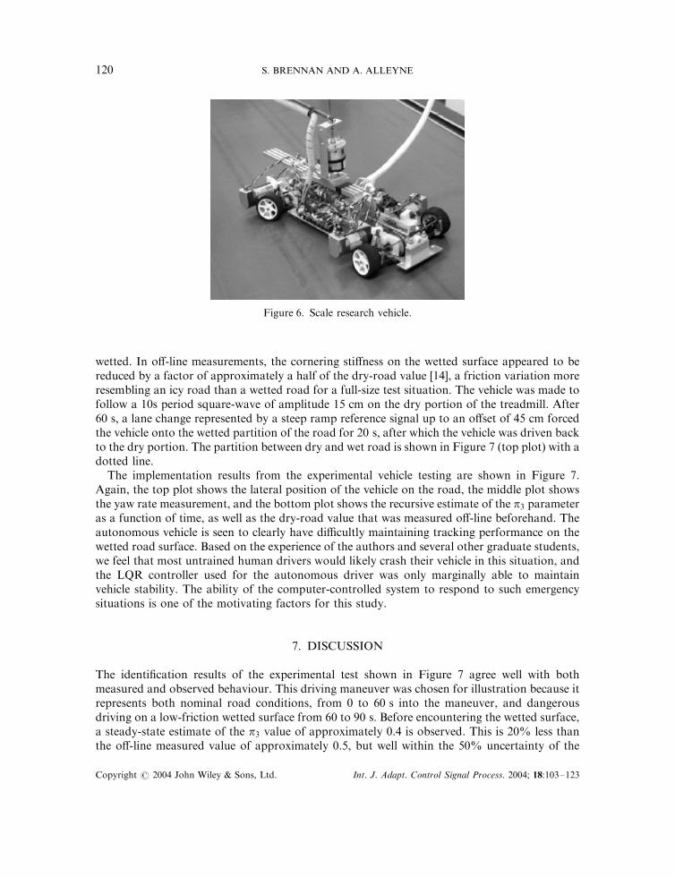
The top plot of Figure 5 shows the lateral position of the vehicle as it attempts to track thesquare-wave reference position shown in dotted lines. The middle plot is the corresponding yawrate measurement. The bottom plot is the estimated p3 parameter using the identificationalgorithm previously described plotted alongside actual values of the parameter. Note the smallsteady-state bias in the estimate due to the use of the reduced-parameter model. Based on thegood convergence exhibited by the simulation study, an experimental investigation wasimplemented on the actual test vehicle shown in Figure 6. The test vehicle is approximately a 1

7

scale vehicle, and its bicycle-model parameters were measured off-line and are the same values asreported in Equation (4). However, these values were recorded with a very large uncertainty,especially in the inertia and cornering stiffness measurements. The experimental vehicle is usedto introduce a real-world plant that exhibits non-linearities, unmodelled dynamics, anddisturbances that are also present in passenger vehicles that are otherwise ignored in asimulation study. For the experimental vehicle, the defining length, mass and velocity correlatewell to an ‘average’ full-sized vehicle at a speed of 63 mph [13, 15].

To test the vehicle under a driving situation that exhibited a severe change in road friction, thevehicle was driven on a treadmill where one-half of the treadmill was dry and one-half was

0 5 10 15 20 25 30 35 40 45 50

0

0.05

0.1

Lat.

Pos

. (m

)

0 5 10 15 20 25 30 35 40 45 50-0.5

0

0.5

Yaw

Rat

e (r

ad/s

ec)

0 5 10 15 20 25 30 35 40 45 500

0.2

0.4

0.6

Pi3

(un

itles

s)

Time (sec)

RLS EstimateActual value

Measured

MeasuredDesired (reference)

Figure 5. Identification algorithm applied to the simulated vehicle.



wetted. In off-line measurements, the cornering stiffness on the wetted surface appeared to bereduced by a factor of approximately a half of the dry-road value [14], a friction variation moreresembling an icy road than a wetted road for a full-size test situation. The vehicle was made tofollow a 10s period square-wave of amplitude 15 cm on the dry portion of the treadmill. After60 s; a lane change represented by a steep ramp reference signal up to an offset of 45 cm forcedthe vehicle onto the wetted partition of the road for 20 s; after which the vehicle was driven backto the dry portion. The partition between dry and wet road is shown in Figure 7 (top plot) with adotted line.

The implementation results from the experimental vehicle testing are shown in Figure 7.Again, the top plot shows the lateral position of the vehicle on the road, the middle plot showsthe yaw rate measurement, and the bottom plot shows the recursive estimate of the p3 parameteras a function of time, as well as the dry-road value that was measured off-line beforehand. Theautonomous vehicle is seen to clearly have difficultly maintaining tracking performance on thewetted road surface. Based on the experience of the authors and several other graduate students,we feel that most untrained human drivers would likely crash their vehicle in this situation, andthe LQR controller used for the autonomous driver was only marginally able to maintainvehicle stability. The ability of the computer-controlled system to respond to such emergencysituations is one of the motivating factors for this study.

7. DISCUSSION

The identification results of the experimental test shown in Figure 7 agree well with bothmeasured and observed behaviour. This driving maneuver was chosen for illustration because itrepresents both nominal road conditions, from 0 to 60 s into the maneuver, and dangerousdriving on a low-friction wetted surface from 60 to 90 s: Before encountering the wetted surface,a steady-state estimate of the p3 value of approximately 0.4 is observed. This is 20% less thanthe off-line measured value of approximately 0.5, but well within the 50% uncertainty of the

Figure 6. Scale research vehicle.



offline measurement. When entering the wetted lane at 65 s; the experimental results exhibit avery sudden decline in the p3 estimate. Observation of the maneuver showed that the vehiclebecame increasingly destabilized as the tires begin to hydroplane from 70 to 80 s: During thistime, the friction estimate drops significantly lower. At around 85 s; the vehicle is being drivenagain toward the dry side of the road representing the high-friction road surface. At around88 s; the first front wheel enters the dry side of the road and the vehicle was seen to fish-tail backonto the wetted surface due to the destabilizing moment caused by driving on a split-mu surface,i.e. a road high in friction on one side of the vehicle but low on the other. A correspondingsudden decrease in the p3 parameter can be observed 87 s due to the sudden amount ofadditional excitation caused by the fish-tail behaviour. While this excitation is good forparameter convergence from an algorithm perspective, it is obviously undesirable from thedriver perspective. For a short duration, the tires on the slippery side appear to have saturatedtheir force capabilities and were unable to reject the moment induced from the high-tractionside, and this indicates that the linear cornering stiffness model is no longer valid. It is notsurprising then that the estimator suddenly reacts as if a new, lower friction model wasidentified; the plant assumptions made by the estimator are no longer valid. After the fish-tail,the automated computer driver regains control of the vehicle and is able to maneuver the vehicle

0 10 20 30 40 50 60 70 80 90 100-0.5

0

0.5La

t. P

os. (

m)

Low friction sideHigh friction side



0 10 20 30 40 50 60 70 80 90 100-5

0

5

Yaw

Rat

e (r

ad/s

ec)

0 10 20 30 40 50 60 70 80 90 1000.25

0.3

0.35

0.4

0.45

Pi3

(un

itles

s)

Time (sec)

RLSE EstimateMeasured offline

Measured

MeasuredDesired (reference)

Figure 7. Identification algorithm applied to the experimental vehicle.



back onto the dry road surface, where both wheels rapidly dry off and regain their traction from90 to 100 s: A corresponding rise in the friction estimate is also observed over this time frame.

Both simulation and experimental results appear to validate the use of a low-parameter ordermodel for the identification of the time-varying p3 parameter. The simulation of theidentification algorithm based on sensitivity invariance showed distinctive changes in the Piparameter estimate when the cornering stiffness was varied, and the experimental study showeda definite decrease in estimated cornering stiffness from steady-state values when the vehicle wasdriven onto the wetted lane. Both simulation and experimental results exhibited a slight lag inthe response to the parameter change, but repeated testing seemed to show that this lag is relatedto primarily to lack of excitation of the system and the choice of a relatively large amount ofmemory in past estimates i.e. a forgetting factor that was chosen to be very close to 1.

The computational overhead of this simplified algorithm is especially low due to the low orderof the model, requiring on the order of 10 floating point computations per sample cycle. Suchsimplicity allows the algorithm to be implemented even on very basic and low cost embeddedmicroprocessors. This computational simplicity, due again to sensitivity invariance, is muchmore favourable than the Kalman-filter and non-linear gradient-based approaches discussed inthe introduction with reported computational demands on the order of 104 or higher. It wouldbe possible to use the algebraic relationships previously defined in Section 5 to determinereasonably accurate estimates of other system parameters, both dimensional and non-dimensional.

Note that the discrete function to be identified was developed as a discrete approximation toan average continuous-time system representation, which itself is an average approximation tothe specific vehicle dynamic. Additionally, operation along a non-linear friction curve is beingapproximated by a linear parameter. Thus, one should not expect exact matching of theidentified parameter and the true parameter. Such mismatch is a simple trade-off of accuracyversus faster estimation. For obvious safety reasons, this work focused on a biased algorithmsuitable for very fast, possibly real-time parameter estimation with minimal excitationconditions. Although the estimate may be biased, it is very useful as an indication of parametervariation and for the scheduling of different control designs.

8. CONCLUSIONS AND FUTURE WORK

This study presents the concept of sensitivity invariance within a system identificationframework. An overview of the fundamental theorems of sensitivity invariance was given. Anexample problem of identifying friction parameters of the chassis dynamics of an experimentalvehicle was used to demonstrate these primary concepts in both simulation and experimentalstudies. Previous efforts to estimate the seven vehicle system parameters of the yaw rate input–output chassis dynamics using on-line identification met with serious problems [11, 12].However, by using both explicit and implicit sensitivity invariance, the identification problemwas reduced from a seven-parameter to a one-parameter linear representation. Experimentalresults validated the method.

The range of engineering systems that would benefit from a dimensionless approach iscertainly much more broad than vehicle chassis control, as sensitivity invariance and scalinglaws arise throughout complex biological and mechanical systems [24]. In a theoretical context,much work remains in the study of the use of sensitivity invariance in system identification and



adaptive control, including a need to develop automated methods of identifying andincorporating such invariance information into a control and/or identification algorithm.

REFERENCES

1. Furukawa Y, Abe M. Advanced chassis control systems for vehicle handling and active safety. Vehicle SystemDynamics 1997; 28:59–86.

2. Ackermann J, Sienel W. Robust yaw rate control. IEEE Transactions on Control and System Technology 1993; 1:15–20.

3. Russo M, Russo R, Volpe A. Car parameters identification by handling manoeuvres. Vehicle System Dynamics 2000;34(6):423–436.

4. Smith DE, Starkey JM. Effects of model complexity on the performance of automated vehicle steering controllers:model development, validation and comparison. Vehicle System Dynamics 1995; 24:163–181.

5. Smith DE, Starkey JM. Effects of model complexity on the performance of automated vehicle steering controllers:Controller Development and Evaluation. Vehicle System Dynamics 1994; 23:627–645.

6. Samadi B, Kazemi R, Nikravesh KY, Kabganian M. Real-time estimation of vehicle state and tire-road frictionForces. Proceedings of the 2001 American Control Conference, Arlington, VA, 2001; 3318–3323.

7. Venhovens PJTh, Naab K. Vehicle dynamics estimation using Kalman filters. Vehicle System Dynamics 1999;32:171–184.

8. Liu CS, Peng H. Road friction coefficient estimation for vehicle path prediction. Vehicle System Dynamics 1996;25:413–425.

9. Miller SL, Youngberg B, Millie A, Schweizer P, Gerdes JC. Calculating longitudinal wheel slip and tire parametersusing GPS velocity. Proceedings of the 2001 American Control Conference, Arlington, VA, 2001; 1800–1805.

10. Wakamatsu K, Akuta Y, Ikegaya M, Asanuma N. Adaptive yaw rate feedback 4WS with tire/road frictioncoefficient estimator. Vehicle System Dynamics 1997; 27:305–326.

11. DePoorter M. The Illinois roadway simulator. M.S. Thesis, University of Illinois at Urbana-Champaign,Department of Mechanical and Industrial Engineering, 1997.

12. DePoorter M, Brennan S, Alleyne A. Driver assisted control strategies: theory and experiment. Proceedings of the1998 ASME IMECE, Anaheim, CA, 1998; 721–728.

13. Brennan S. On size and control: the use of dimensional analysis in controller design. Ph.D. Thesis, University ofIllinois at Urbana-Champaign, Department of Mechanical and Industrial Engineering, 2002.

14. Brennan S. Modeling and control issues associated with scale vehicles.M.S. Thesis, University of Illinois at Urbana-Champaign, Department of Mechanical and Industrial Engineering, 1999.

15. Brennan S, Alleyne A. Using a scale testbed: controller design and evaluation. IEEE Control Systems Magazine2001; 21(3):15–26.

16. Alleyne A. A comparison of alternative intervention strategies for unintended roadway departure (URD) control.Vehicle System Dynamics 1997; 27:157–186.

17. Dugoff H, Fancher PS, Segel L. An analysis of tire traction properties and their influence on vehicle dynamicperformance. SAE Transactions 1970; 79:341–366.

18. LeBlanc DJ, Johnson GE, Venhovens PJTh, Gerber G, DeSonia R, Ervin RD, Lin CF, Ulsoy AG, Pilutti TE.CAPC: a road-departure prevention system. IEEE Control Systems Magazine 1996; 16(6):67–71.

19. McLean JR, Hoffman ER. The effects of restricted preview on driver steering control and performance. HumanFactors 1973; 15:421–430.

20. Peng H, Tomizuka M. Preview control for vehicle lateral guidance in highway automation. ASME Journal ofDynamic Systems, Measurement and Control 1993; 115:679–686.

21. Frank PM. Introduction to System Sensitivity Theory. Academic Press: New York, 1978.22. Taylor ES. Dimensional Analysis for Engineers. Clarendon Press: Oxford, 1974.23. Eslami M. Theory of Sensitivity in Dynamic Systems, An Introduction. Springer: New York, 1994.24. McMahon TA, Bonner JT. On Size and Life. Scientific American Books, Inc.: New York, 1983.25. Buckingham E. On physically similar systems; illustrations of the use of dimensional equations. Physical Review

1914; 42nd series:345–376.26. Bridgman PW. Dimensional Analysis. Yale University Press: New Haven, 1943.27. Heydinger GJ, Bixel RA, Garrot WR, Pyne M, Howe JG, Guenther DA. Measured vehicle inertial

parameters}NHTSA’s data through November 1998. Society of Automotive Engineers 1999; (SAE 930897).28. Franklin GF, Powell JD, Workman M. Digital Control of Dynamic Systems (3rd edn). Addison-Wesley: Menlo

Park, CA, 1998.29. Astrom KJ, Wittenmark B. Computer-Controlled Systems: Theory and Design. Prentice-Hall: Upper Saddle River,

NJ, 1997.30. Astrom KJ, Wittenmark B. Adaptive Control. Addison-Wesley: Reading, MA, 1995.



Real-time identification of vehicle chassis dynamics using a novel reparameterization based on...

Documents

Transcript of Real-time identification of vehicle chassis dynamics using a novel reparameterization based on...