Real Life Problem Solved by Dynamic Programming Technique

Rahidas Kumar Assistant Professor, Department of Science and Humanities (Mathematics)

R.V.S.C.E.T. Jamshedpur, Jharkhand, India. E-mail: kumarahidas@gmail.com

Abstract:

Dynamic programming is employed in conjunction with complex real life problems. This is an approach to optimization, based on the principle of taking a single complex problem and breaking into sequence of simpler and more easily solvable sub problems. This article we approach to propose how to handle Complexity problems and get the optimal solution. Here we represent the technique of dynamic programming to solve the knapsack problem and shortest path problem.

Keywords:

Dynamic programming problem, knapsack problem and shortest path problem

1. Introduction:

Dynamic programming concept has been invented 1950’s by American Mathematician Richard Bellman [1]. Dynamic means we are taking decision at several stages and programming stands for planning or to just set the actions in the best possible way[2]. Also we can say that dynamic programming as a recursive optimization problem or multi stage optimization process [1, 2]. Dynamic Programming Problem (DPP) is a many decision making problem involving a process that take place in multistage in such way that at each stage, the process depend on the strategy chosen. Mathematically, a D.P.P is a decision making problem in n-variables, the problem being sub divided in to n sub- problems each sub problem being a decision- making problem in one variable only. The solution to a DPP is achieved sequentially starting from one (initial) stage to the next till the final stage is reached [3].

1.1 Principal of Optimality’s

It may be interesting to note that the concept of dynamic programming is largely based upon the principle of optimality due to Bellman ‘‘ An optimal policy has the property that whatever the initial state and initial decision are, the remaining decisions must constitute an optimal policy with regard to the state resulting from the first decision ’’[1].

1 .2 Characteristic of DPP [1, 2]

The basic features which characterize the DPP are as follows:

(a)The problem can be subdivided into stages with a policy decision required at each stage. A stage is a device to sequence the decisions i.e., it decomposes a problem into sub-problem such that an optimal solution to the problem can be obtained from the optimal solution to the sub problems.

(b) Every stage consists of number states associated with it.

(c) Decision at each stage converts the current stage into state associated with the next stage.

(d) The state of the system at a stage is describe by a set of variables, called state variables

(e) To identify the optimal policy for each state of the system, a recursive equation is formulated with n stages remaining, given the optimal policy for each state with (n-1) stages left.

(f) Using recursive equation approach each time the solution procedure moves backward stage by stage for obtaining the optimum policy of each state for that particular stage, till it attains the optimum policy beginning at the initial stage.

2. Dynamic Programming Algorithm [1]

DPP can be summarized in the following steps:

Step 1: Identify the decision variable and specify objective function to be optimized under certain limitation, if any. Step 2: Decompose (or divide) the given problem into a number of smaller sub problems (or

stages). Identify the state variables at each stage and write down the transformation function as a function of the state variables and decision variables at the next stage.

Step 3: Write down a general recursive relationship for computing the optimal policy. Decide whether forward or backward method is to follow to solve the problem.

Step 4: Construct appropriate stages to show the required values of the return function at eachstage.

Step 5: Determine the overall optimal policy or decisions and its value at each stage. There may one optimal such policy.

DPP is solved by using the recursive equation starting from the first through the last stage, i.e, obtaining the sequence f1 →f2 →…→fn , this is called the forward computational procedure. If recursive equation is formulated in a different way so as to obtain the sequence fn →fn-1

→…→f1, this is called the backward computational procedure.

Multistage decision making problem

Mathematically,

Fn (dn) = Max { rn(dn, Sn) + rn-1(dn-1, Sn-1) + …+ r1(d1, S1)}

Stages transformation equation Sm-1 =Tm (dm, Sm) where m belongs to {2, 3,…, n}

Decision space dn belongs to Dm

Also it is written as fn(dn)= Max { rn(dn, Sn) + fn-1(dn-1)}

3. Complexity Classes, P and NP problems

A complexity class is the set of all computational problems which can be solved using a certain amount of a certain computational resource. The complexity class P is the set of decision problems that can be solved by a deterministic machine in polynomial time. This class corresponds to an intuitive idea of the problems which can be effectively in the worst cases. P is often taken to be the class of computational problems which are effectively solvable or tractable.

The complexity class NP is the set of decision problems that can be solved by a non deterministic machine in polynomial time. This class contains many problems that people would like to be able to solve effectively. All the problems in this class has the properly that their solutions can be checked effectively. To solve an NP complete problem for any non trivial problem size generally one of the following approaches is used.

(i) Approximation

State Sn

Stage n

Tn (Sn, dn)

State Sn-1

Stage n-1

Tn-1(Sn-1, dn-1)

Decision dn Decision dn-1

The optimal return

rn(dn, Sn)

Again the optimal return rn-1(dn-1, Sn-1)

(ii) Probabilistic (iii) Special cases (iv) Heuristic

Some well known problems that are NP complete which are in bellow:

(i) N- puzzle (ii) Knapsack problem (iii) Hamiltonian cyclic problem (iv) Traveling salesman problem (v) Sub graph isomorphic problem (vi) Sub set sum problem (vii) Clique problem (viii) Graph coloring problem.

4. Introduction of Knapsack Problem [4, 5]

The knapsack problem is a problem in combinatorial optimization which appears in real-world decision-making processes in a wide variety of fields, such as finding the least wasteful way to cut raw materials. Given a set of items, each with a weight and a value, determine the number of each item to include in a collection so that the total weight is less than or equal to a given limit and the total value is as large as possible. The problem often arises in resource allocation where there are financial constraints and is studied in fields such as combinatorics, computer science, complexity theory, cryptography, applied mathematics, daily fantasy sports.

The knapsack problem has been studied for more than a century, with early works dating as far back as 1897. The name "knapsack problem" dates back to the early works of mathematician Tobias Dantzig (1884–1956) and refers to the commonplace problem of packing the most valuable or useful items without overloading the luggage.

5. Introducing the Shortest Path Problem: [6, 7, 8]

In graph theory, the shortest path problem is the problem of finding a path between two vertices (or nodes) in a weighted graph such that the sum of the weights of its constituent edges is minimized. The problem of finding the shortest path between two intersections on a road map (the graph’s vertices correspond to intersections and the edges correspond to road segments, each weighted by the length of its road segment) may be modelled by a special case of the shortest path problem in graphs. The shortest path problem can be defined for graphs whether undirected, directed, or mixed. It is defined here for undirected graphs; for directed graphs the definition of path requires that consecutive vertices be connected by an appropriate directed edge.

A road network can be considered as a graph with positive weights. The nodes represent road junctions and each edge of the graph is associated with a road segment between two junctions. The weight of an edge may correspond to the length of the associated road segment, the time needed to traverse the segment, or the cost of traversing the segment. Using directed edges it is also possible to model one-way streets. Such graphs are special in the sense that some edges are more important than others for long distance travel (e.g. highways). This property has been formalized using the notion of highway dimension. There are a great number of algorithms that exploit this property and are therefore able to compute the shortest path a lot quicker than would be possible on general graphs. All of these algorithms work in two phases. In the first phase, the graph is pre-processed without knowing the source or target node. The second phase is the query phase. In this phase, source and target node are known. The idea is that the road network is static, so the pre-processing phase can be done once and used for a large number of queries on the same road network.

The travelling salesman problem is the problem of finding the shortest path that goes through every vertex exactly once, and returns to the start. Unlike the shortest path problem, which can be solved in polynomial time in graphs without negative cycles, the travelling salesman problem is NP-complete and, as such, is believed not to be efficiently solvable for large sets of data (see P = NP problem). The problem of finding the longest path in a graph is also NP-complete. The Canadian traveller problem and the stochastic shortest path problem are generalizations where either the graph isn't completely known to the mover, changes over time, or where actions (traversals) are probabilistic. The shortest multiple disconnected paths are a representation of the primitive path network within the frame work of Repetition theory. The widest path problem seeks a path so that the minimum label of any edge is as large as possible.

6. Numerical example of Knapsack Problem

A young man is on his trekking way, he is trying to fix- how to choose among three simple items that he can pack for his trip. He can carry 10 kgs into his knapsack. Three possible items whose weight and utility values are given

Item Weight Utility value (Uselessness) 1. Foot Pack 3 7 2. Bottle of water 4 8 3. Tent 6 11

Let x1 is the no. of Foot Pack, x2 is the no. of bottle of water and x3 is the no. of Tent. Then the total maximization utility value that is Max Z= 7 x1 + 8x2 + 11x3

Subject to 3x1 + 4x2 + 6x3 ≤ 10, here x1, x2, and x3 all are integer values.

Now we solve this problem by dynamic programming technique

Stage3 – No. of Tent

Stage2 – No. of (Tent + bottle of water)

Stage1 – No of (Tent + bottle of water + Foot Pack)

This process formally named in Dynamic Programming problem as a backward recursive process. Because we are starting from stages 3, then stage 2 then stage1, we are considering the whole. We can do the reverse way as well.

Stage 3: d3 decision regarding the weight

d3 x3 =0 x3=1 f3(d3)- max utility value and x3 ∈ {0, 3} 0 0 - 0 1 0 - 0 2 0 - 0 3 0 - 0 4 0 - 0 5 0 - 0 6 0 11 11 7 0 11 11 8 0 11 11 9 0 11 11 10 0 11 11

Stage 2: d2 = weight of (Tent + bottle of water) = (d3 +4x2) and x2 = {0, 1, 2}

d2 x2 = 0 x2= 1 x2 = 2 f2(d2)- max utility value and x2 ∈ {0, 1, 2}

0 0 - - 0 1 0 - - 0 2 0 - - 0 3 0 - - 0 4 0 8 - 8 5 0 8 - 8 6 11 8 - 11 7 11 8 - 11 8 11 8 16 16 9 11 8 16 16 10 11 (11+8)=19 16 19*

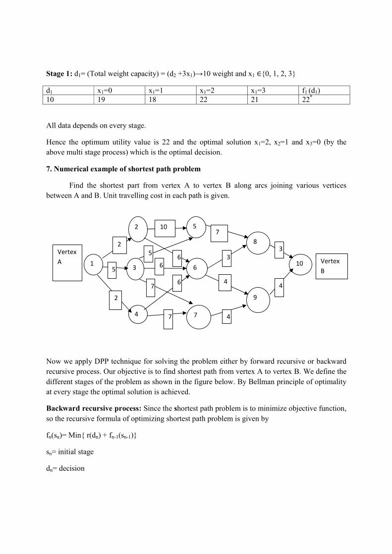
Stage 1: d1= (Total weight capacity) = (d2 +3x1)→10 weight and x1 ∈{0, 1, 2, 3}

d1 x1=0 x1=1 x1=2 x1=3 f1 (d1) 10 19 18 22 21 22*

All data depends on every stage.

Hence the optimum utility value is 22 and the optimal solution x1=2, x2=1 and x3=0 (by the above multi stage process) which is the optimal decision.

7. Numerical example of shortest path problem

Find the shortest part from vertex A to vertex B along arcs joining various vertices between A and B. Unit travelling cost in each path is given.

Now we apply DPP technique for solving the problem either by forward recursive or backward recursive process. Our objective is to find shortest path from vertex A to vertex B. We define the different stages of the problem as shown in the figure below. By Bellman principle of optimality at every stage the optimal solution is achieved.

Backward recursive process: Since the shortest path problem is to minimize objective function, so the recursive formula of optimizing shortest path problem is given by

fn(sn)= Min{ r(dn) + fn-1(sn-1)}

sn= initial stage

dn= decision

1

2

3

4

5

6

7

8

9

10

Vertex A Vertex

B

2

10

5

2

5 6 6

7 6

7

7

3

4

4

3

4

T(dn, Sn)= resulting state

fn-1(sn-1) = optimal return of the previous state

Stage n = 0, state S0 = 10

n= 1, state S1 =(8,9) ,f1(8) = 3* ; f1(9) = 4

since f1(s1)= min {r(d1) + f0(s0)}=min{3+0, 4+0}= min{3,4}= 3

n= 2 then state S2= (5,6,7)

5-8; 7+3 = 10

6-8; 3+3 = 6*

6-9; 4+3 = 7

7-9; 4+3 = 7

Figure showing stages

1

2

3

4

5

6

7

8

9

10 Vertex A

Vertex B

2

10

5

2

5 6 6

7 6

7

7

3

4

4

3

4

Stage 0 Stage 1 Stage 2 Stage 3 Stage 4

The calculation is shown in the table

Initial stage (Sn)

Decision (dn)

Immediate cost

Resulting state T(Sn, dn)

Optimal return fn-1(dn-1)

fn(Sn) Optimal cost policy

5 5-8 7 8 3 10* 5-8 6 6-8 3 8 3 6* 6-8 6-9 4 9 3 7 7 7-9 4 9 3 7* 7-9 2 2-5 10 5 10 20 2-6 6 6 6 12* 2-6 3 3-5 5 5 10 15 3-6 6 6 6 12* 3-6 3-7 7 7 7 14 4 4-6 6 6 6 12* 4-6 4-7 7 7 7 14 1 1-2 2 2 12 14* 1-2 1-3 5 3 12 15 1-4 2 4 12 14* 1-4

Therefore by the minimal policy, the shortest paths are

1-2-6-8-10 and 1-4-6-8-10 and weight of the paths are 14 units in both cases.

8. Conclusion:

Dynamic programming provides a systematic procedure for determining the optimal combination of decisions. It can be use in solving knapsack problem and shortest path problem for optimality.

References

[1] Kanti Swarup, P.K Gupta, Man Mohan.,Operation Research, Sultan Chand & Sons, 2004. [2] Hiller, F.S., G. J., Lieberman and G. Lieberman, Introduction to Operation Research.

McGraw- Hill Book Co. New York, 2004.

[3] Taha, H. H., Integer Programming: Theory, Applications and Computations, Academic Press, New York, 1975.

[4] Kellerer, Hans; Pferschy, Ulrich;Pisinger, David, Knapsack Problems, Springer. doi:10.1007/978-3-540-24777-7, ISBN 3-540-40286-1, 2004.

[5] Martello, Silvano; Toth, Paolo, Knapsack problems: Algorithms and computer implementations. Wiley- Inter science. ISBN 0-471-92420-2, 1990.

[6] Abraham, Ittai; Fiat, Amos; Goldberg, Andrew V.; Werneck, Renato F. "Highway Dimension, Shortest Paths, and Provably Efficient Algorithms". ACM-SIAM Symposium on Discrete Algorithms, pages 782–793, 2010.

[7] Ahuja, Ravindra K.; Magnanti, Thomas L.; Orlin, James B., Network Flows: Theory, Algorithms and Applications. Prentice Hall. ISBN 0-13-617549-X, 1993.

[8] Garey, Michael R.; David S. Johnson, Computers and Intractability: A Guide to the Theory of NP-Completeness. W.H. Freeman. ISBN 0-7167-1045-5. A6: MP9, pg.247, 1979.