Real interest rate persistence in South Africa: evidence

1 23

Economic Change and RestructuringEmpirical and Policy Research on theTransitional and Emerging Economies ISSN 1573-9414Volume 47Number 1 Econ Change Restruct (2014) 47:41-62DOI 10.1007/s10644-012-9132-5

Real interest rate persistence in SouthAfrica: evidence and implications

Sonali Das, Rangan Gupta, PatrickT. Kanda, Monique Reid, ChristianK. Tipoy & Mulatu F. Zerihun

1 23

Your article is protected by copyright and all

rights are held exclusively by Springer Science

+Business Media New York. This e-offprint is

for personal use only and shall not be self-

archived in electronic repositories. If you wish

to self-archive your article, please use the

accepted manuscript version for posting on

your own website. You may further deposit

the accepted manuscript version in any

repository, provided it is only made publicly

available 12 months after official publication

or later and provided acknowledgement is

given to the original source of publication

and a link is inserted to the published article

on Springer's website. The link must be

accompanied by the following text: "The final

publication is available at link.springer.com”.

Real interest rate persistence in South Africa: evidenceand implications

Sonali Das • Rangan Gupta • Patrick T. Kanda •

Monique Reid • Christian K. Tipoy •

Mulatu F. Zerihun

Received: 2 June 2012 / Accepted: 27 November 2012 / Published online: 12 December 2012

� Springer Science+Business Media New York 2012

Abstract The real interest rate is a very important variable in the transmission of

monetary policy. It features in vast majority of financial and macroeconomic

models. Though the theoretical importance of the real interest rate has generated a

sizable literature that examines its long-run properties, surprisingly, there does not

exist any study that delves into this issue for South Africa. Given this, using

quarterly data (1960:Q2-2010:Q4) for South Africa, our paper endeavors to analyze

the long-run properties of the ex post real rate by using tests of unit root, cointe-

gration, fractional integration and structural breaks. In addition, we also analyze

whether monetary shocks contribute to fluctuations in the real interest rate based on

test of structural breaks of the rate of inflation, as well as, Bayesian change point

analysis. Based on the tests conducted, we conclude that the South African EPPR

can be best viewed as a very persistent but ultimately mean-reverting process. Also,

the persistence in the real interest rate can be tentatively considered as a monetary

phenomenon.

Keywords Real interest rate � Monetary policy � Persistence � Mean reversion

JEL Classifications C22 � E21 � E44 � E52 � E62 � G12

S. Das

Logistics and Quantitative Methods, CSIR Built Environment,

P.O. Box: 395, Pretoria 0001, South Africa

R. Gupta (&) � P. T. Kanda � C. K. Tipoy � M. F. Zerihun

Department of Economics, University of Pretoria, Pretoria 0002, South Africa

e-mail: [email protected]

M. Reid

Department of Economics, University of Stellenbosch,

Private Bag X1, Matieland 7602, South Africa

123

Econ Change Restruct (2014) 47:41–62

DOI 10.1007/s10644-012-9132-5

Author's personal copy

1 Introduction

Macroeconomic and financial theoretical models, e.g. the consumption-based asset

pricing model (Lucas 1978; Breeden 1979; Hansen and Singleton 1982, 1983),

neoclassical growth models (Cass 1965; Koopmans 1965), central bank policy

models (Taylor 1993) and many monetary transmission mechanism models include

the real interest rate (interest rate less expected or realized inflation rate) as a key

variable. Hence, the viability of these models would depend upon the time-series

properties of the real interest rate. Further, the answer to the question as to whether

financial markets fluctuate excessively is also determined by the movement of real

interest rate (Shiller 1979). Finally, the fact that the real interest rate is a crucial

determinant of investment, savings and virtually all intertemporal decisions, makes

an analysis dealing with the characteristics of the real interest rate a highly

pertinent. The behavior of the real interest rate, thus tend to provide an implicit test

of the different theoretical models. There are two types of real interest rates: the ex

ante real interest rate (EARR) and the ex post real rate (EPRR). Economic agents

base their decisions on their expectations about the inflation level over the decision

horizon. As such, the EARR turns out to be the appropriate gauge for assessing

economic decisions. However, given that the EARR cannot be directly observable,

we cannot evaluate its time-series properties.

Though the theoretical importance of the real interest rate has generated a sizable

empirical literature1 that examines its long-run properties, surprisingly, to the best

of our knowledge, there does not exist any study that delves into this issue for South

Africa.2 Against this backdrop, using quarterly data (1960:Q2-2010:Q4) for South

Africa, our paper endeavors to analyze the long-run properties of the EPRR by using

tests of unit root, cointegration, confidence intervals for the sum of the

autoregressive coefficients, fractional integration and structural breaks. The time-

series properties of the real interest rate would allow us to draw inferences regarding

the viability of the theoretical models in the context of South Africa. While, unit

root and cointegration tests would help us analyze whether real interest rate is mean-

reverting in South Africa, given that unit root and cointegration tests suffer from

low power if the true model is a highly persistent but stationary process, we directly

analyze the persistence property of the real interest rate using fractional integration

and estimating confidence intervals for the sum of the autoregressive coefficients.

Note that, from a policy perspective as well, there is a tremendous need to determine

whether the process of real interest rate is stationary or not. Given that the central

bank implements monetary policy by controlling the nominal interest rate to

appropriately choose the direction of the movement of the real interest rate

ultimately, since it is the latter that affects the marginal decisions in the economy,

then changes in the real rate, when the real rate is nonstationary, implies that the

policy will have a permanent and not a transitory effect. Thus, if the central bank

1 See Neely and Rapach (2008) for a detailed literature review.2 Studies that exists for South Africa only deals with the uncovered interest rate parity condition, or in

other words, the interest rate behavior of South Africa relative to other developed or emerging economies.

See for example Kahn and Farrell (2002), Kryshko (2006), Lacerda et al. (2010) and de Bruyn et al.

(2011).

42 Econ Change Restruct (2014) 47:41–62

123


wants a temporary effect, it will have to intervene in the future to offset its initial

effect. On the other hand, if the real interest rate is stationary, then a monetary

policy change in the real interest rate rate will eventually return to its ‘‘equilibrium’’

level without further intervention by the central bank. Clearly then, there are

implications, especially in terms of monetary policy intervention and proper

functionality of the markets, depending on the knowledge about the mean-reversion

and persistence properties of the real interest rate. Hence, the exact knowledge of

the property of real interest rate is always important, but it is moreso now for South

Africa, given that it has moved to an inflation-targeting regime since the first quarter

of 2000.3 The success of an inflation-targeting regime is dependant on keeping the

inflation expectations pegged, which in turn, depends on clear communication to the

market, and hinges crucially to a great extent on whether the real interest rate is

stationary or not. Since if the real interest rate is believed to have an unit root

process, the South African Reserve Bank might have to intervene regularly to

neutralize the possibility of a permanent effect on the market; in the process

confusing agents and their inflation expectations, and thus leading the inflation to

deviate away from the target.

In addition to analyzing the mean-reverting and persistence properties of the real

interest rate, we also analyze whether monetary shocks contribute to fluctuations in

the real interest rate based on the Bai and Perron (1998) test of structural breaks of

the rate of inflation, as well as, Bayesian change point analysis proposed by Barry

and Hartigan (1993)—a methodology, though widely-used in the statistical

literature to analyze change-points,4 has never been used in the literature pertaining

to the sources behind the fluctuations of the real interest rate. So our study

contributes to the the literature on the time-series properties of the real interest rate

by being the first to provide a case-study for South Africa, and also, the being first

study to use the novel approach of Bayesian change point analysis in looking for a

reason behind that explains the variation in the real interest rate. Our main results

can be summarized as follows: Though, the unit root tests reveal that the real

interest rate is stationary, cointegration analysis tends to suggest otherwise, unless

one imposes restrictions on the nominal interest rate and the inflation rate to obtain

the definition of EPRR.5 Realizing that unit root and cointegration tests suffer from

low power if the true model is a highly persistent but stationary process, we directly

analyzed the persistence property of the real interest rate. Fractional integration and

estimation of the confidence intervals for the sum of the autoregressive coefficients,

suggested that the unit real interest rate is a persistent process. So, in general, these

results on persistence, coupled with the unit root tests led us to conclude that the real

interest rate in South Africa is a persistent but mean-reverting process. Further, we

observed that, real interest is far more persistent than the consumption growth rate,

thus raising doubts about the validity of the consumption-based asset pricing

3 In February of 2000, the Minister of Finance announced that inflation targeting would be the sole

objective of the South African Reserve Bank. Currently, the Reserve Bank’s main monetary policy

objective is to maintain CPI inflation between a target-band of 3–6 %, using discretionary changes in the

repo rate as its main policy instrument.4 See Erdman and Emerson (2007) for a detailed literature review in this regard.5 See Sect. 3 for further details.

Econ Change Restruct (2014) 47:41–62 43

123


models. Complex equilibrium growth models tend to potentially explain this

persistence mismatch through changing fiscal and monetary policy, as well as

temporary technology growth shocks. Given this we considered fiscal, monetary,

and transient technology shocks as potential causes of persistent fluctuations in the

South African real interest rate. Our results based on test of structural breaks of the

rate of inflation, and in particular, Bayesian change point analysis, tentatively

concludes that real interest rate persistence is more likely to be a monetary

phenomenon than a outcome of fiscal policy and transient technology growth

shocks. In other words, the mismatch between the persistence properties of

consumption growth and the real interest rate is possible due to monetary policy

shocks. The remainder of the paper is organized as follows: Sect. 2 discusses the

theoretical background on the long-run behavior of the real interest rate. Section 3

lays out the difference between the EARR and EPRR and presents the results from

the unit root, cointegration and fractional integration tests; while Sect. 4 analyzes

structural breaks in the real interest rate. Section 5 investigates the monetary

explanation of persistence, and finally Sect. 6 concludes the paper.

2 Theoretical background

2.1 Consumption-based asset pricing model

Lucas (1978), Breeden (1979), and Hansen and Singleton (1982, 1983)’s canonical

consumption based asset pricing model hypothesizes a representative household

choosing a real consumption sequence, fctg1t¼0, to solve the problem:

maxX1

t¼0

btuðctÞ;

subject to an intertemporal budget constraint. b is a discount factor and u(ct) rep-

resents an instantaneous utility function. The first-order condition yields the inter-

temporal Euler equation,

Etfb½u0ðctþ1Þ=u0ðctÞ�ð1þ rtÞg ¼ 1; ð1Þ

where 1 ? rt represents the gross one-period real interest rate with payoff at period

t ? 1 and Et is the conditional expectation operator. Many studies often consider the

utility function to have the constant relative risk aversion (CRRA) form,

u(ct) = ct1 - c/(1 - c), where c is the coefficient of relative risk aversion. Com-

bining the CRRA form of the utility function with the assumption of joint log-

normality of consumption growth and the real interest rate, the log-linear version of

Eq. (1) can be written as (Hansen and Singleton 1982, 1983):

j� cEt½Dlogðctþ1Þ� þ Et½logð1þ rtÞ� ¼ 0; ð2Þ

where Dlogðctþ1Þ ¼ logðctþ1Þ � logðctÞ ¼ logðbÞ þ 0:5r2, and r2 is the constant

conditional variance of log[b(cl?1/cl)-a(1 ? rl)]. Equation (2) relates the condi-

tional expectations of the per capita real consumption growth rate ½Dlogðctþ1Þ� with


123


the (net) real interest rate ½logð1þ rtÞrt�. According to Rose (1988), if Eq. (2) is to

hold, then the per capita real consumption growth rate and the (net) real interest rate

series must have the same integration properties. Bearing in mind that ½Dlogðctþ1Þ�is nearly without doubt a stationary process, Rose (1988) shows that the real interest

rate is non-stationary i.e. rtv Ið1Þ in many industrialized countries. A unit root in

the real interest rate together with stationary consumption growth imply that per-

manent changes in the level of the real rate will be unmatched by such changes in

consumption growth. Therefore, Eq. (2) seemingly cannot hold. The problem

identified by Rose (1988) is vindicated in Fig. 1, which plots South Africa’s ex post

3-month Treasury bill based real interest rate and annualized per capita con-

sumption growth rate for the period from 1960:Q2 to 2010:Q4. Figure 1 shows that

the two series seem to be divergent for most of the period prior to the 1980s whereas

the series appear to track each other quite well during the early 1980s and from the

late 1980s to the last date of the sample.

The most elementary consumption-based asset pricing model is based on an

endowment economy with a representative household and constant preferences.

However, more elaborate theoretical models allowing for changes in fiscal or

monetary policy to affect the steady-state real interest rate, while leaving the

steady-state consumption growth rate unaffected have been proposed in the

literature. These models allow a disparity in the integration properties of

the consumption growth and real interest rates. These models are summarized in

the next subsections.

-20

-15

-10

-5

0

5

10

15

20

1960

:219

61:3

1962

:419

64:1

1965

:219

66:3

1967

:419

69:1

1970

:219

71:3

1972

:419

74:1

1975

:219

76:3

1977

:419

79:1

1980

:219

81:3

1982

:419

84:1

1985

:219

86:3

1987

:419

89:1

1990

:219

91:3

1992

:419

94:1

1995

:219

96:3

1997

:419

99:1

2000

:220

01:3

2002

:420

04:1

2005

:220

06:3

2007

:420

09:1

2010

:2

%

Per Capita Consumption Growth Ex Post Real Interest Rate

Fig. 1 Ex post real interest rate and real per capita consumption growth, 1960:Q2-2010:Q4. Note: Thefigure plots SA ex post 3-month real interest rate and annualized per capita consumption growth.Consumption includes nondurable goods and services consumption


123


2.2 Equilibrium growth models and the steady-state real interest rate

Euler equations such as Eqs. (1) and (2) and suggesting sources of a unit root in real

interest rates emanate from general equilibrium growth models with a production

technology. In particular, the neoclassical growth model by Cass (1965) and

Koopmans (1965), featuring a representative profit-maximizing firm and utility-

maximising household, hypothesizes that the steady state real interest rate is a

function of time preference, risk aversion, and the steady-state growth rate of

technological change (Blanchard and Fischer 1989, Chap. 2; Barro and Sala-i-

Martin 2003, Chap. 3; Romer 2006, Chap. 2; Neely and Rapach 2008). The

assumption of constant relative risk aversion utility in the neoclassical growth

model by Cass (1965) and Koopmans (1965) implies the steady-state condition:

r� ¼ fþ cz; ð3Þ

where r* is the steady-state real interest rate, f ¼ �logðbÞ is the rate of time

preference, and z represents the (expected) steady-state growth rate of labor aug-

menting technological change. Equation (3) suggests that the steady state real

interest rate is affected by a permanent change in the exogenous rate of time

preference, risk aversion, or long-run growth rate6. The steady-state version of

Eq. (2) is given by:

�f� c½DlogðcÞ�� þ r� ¼ 0; ð4Þ

where ½DlogðcÞ�� is the steady-state growth rate of ct. Substituting the right-hand

side of Eq. (3) into Eq. (4) for r*, we get the expression ½DlogðcÞ�� ¼ z i.e. steady-

state consumption growth is a function of the steady-state technology growth.

A change in the rate of time preference ðfÞ, risk aversion (c), and/or steady-state

rate of technology growth (z) will require corresponding changes in the steady-state

real interest rate as defined in Eq. (3). The size and frequency of such changes

determine whether real interest rates is very persistent and exhibit unit root behavior

and/or structural breaks. Only a change in the steady-state growth rate of technology

can alter both the real interest rate and consumption growth, generating non-

stationary behavior in both variables. Therefore, it cannot explain the difference in

the integration properties of the real interest rate and consumption growth as

identified by Rose (1988).

On the other hand, shocks to the preference parameters ðfÞ and (c) will only

affect the steady state real interest rate and not steady-state consumption growth.

Thus, changes in preferences represent a potential disconnecting factor between the

integration properties of real interest rates and consumption growth. Studies

generally consider preferences to be stable, however, making it difficult to attribute

the persistence mismatch to such changes.

Other factors e.g. permanent changes in government purchases and their

financing can change the steady-state real interest rate without affecting steady-state

consumption growth in more complex models such as overlapping-generations

6 The steady state real interest rate could also be affected by changes in distortionary tax rates (See

Blanchard and Fischer 1989, pp. 56–59).


123


models with heterogeneous households (Samuelson 1958; Diamond 1965; Blan-

chard 1985; Blanchard and Fischer 1989, Chap. 3; Romer 2006, Chap. 2).

Therefore, these models potentially explain the disparity in the integration

properties of the real interest rate and consumption growth as observed in Rose

(1988).

Lastly, some monetary growth models (Mundell 1963; Tobin 1965; Weiss 1980;

Espinosa-Vega and Russell 1998a, b; Bullard and Russell 2004; Reis 2007; Lioui

and Poncet 2008) permit for changes in steady-state money growth to alter the

steady-state real interest rate without matching changes in consumption growth,

potentially justifying a disparity in the integration properties of the real interest rate

and consumption growth. Mundell (1963) and Tobin (1965) hypothesize that an

increase in steady-state money growth decreases the steady-state real interest rate.

Other recent microfounded monetary models (Weiss 1980; Espinosa-Vega and

Russell 1998a, b; Bullard and Russell 2004; Reis 2007; Lioui and Poncet 2008) have

corroborated the findings of Mundell (1963) and Tobin (1965).

2.3 Transitional dynamics

The previous subsection discussed factors that affects the steady-state real interest

rate. There are, however, other shocks that can have persistent, but transitory,

effects on the real interest rate. To illustrate, a temporary increase in government

purchases or technology growth in the neoclassical growth model results in a

constantly (but not permanently) higher real interest rate (Romer 2006, Chap. 2).

Furthermore, monetary shocks can persistently alter the real interest rate through

different types of frictions e.g. ‘‘sticky’’ prices and information, adjustment costs,

and learning by agents about policy regimes. Transient technology and fiscal

shocks, as well as monetary shocks, can also explain differences in the persistence

of real interest rates and consumption growth. For instance, based on a calibrated

neoclassical equilibrium growth model, Baxter and King (1993) argue that a fiscal

shock in the form of a 4-year increase in government purchases persistently

increases the real interest rate. However, the effect is temporary as the real interest

rate eventually returns to its initial level. On the other hand, the fiscal shock

generates a much less persistent effect on consumption growth. So, the evidence of

highly persistent but mean-reverting behavior, if obtained in real interest rates,

could provide support to the empirical relevance of these shocks for South Africa.

3 Testing the integration properties of real interest sates

3.1 Ex ante versus ex post real interest rates

The ex ante real interest rate (EARR) refers to the nominal interest rate less the

expected inflation rate. On the other hand, the ex post real rate (EPRR) refers to the

nominal interest rate less actual inflation. Economic agents base their decisions on

their expectations about the inflation level over the decision horizon. To illustrate,

the Euler Eqs. (1) and (2) link the expected marginal utility of consumption to the


123


expected real return. Consequently, the EARR turns out to be the appropriate gauge

for assessing economic decisions. However, given that expected inflation is not

directly observable, the EARR cannot be directly observable as well. Hence,

implying that we cannot evaluate its time-series properties. One immediate solution

is to use some measure of inflation expectations based on a survey. However,

economists often are not ready to accept survey forecasts as measure of

expectations, citing doubts over the quality of the surveys conducted (Mishkin

1981). Further, obtaining survey based inflation expectations measure at the desired

frequency is also an obstacle (Neely and Rapach 2008).

Two alternative approaches to the problem of unobserved expectations exists.

The first approach uses econometric forecasting methods to construct inflation

forecasts (Mishkin 1981, 1984; Huizinga and Mishkin 1986). However, all the

appropriate information used by economic agents when forming their inflation

expectations might not included in econometric forecasting methods, and hence,

these forecasting models fail to change with the structure of the economy.

The second approach uses the actual inflation rate as a proxy for inflation

expectations. By definition, the actual inflation rate at time t(pt) is the sum of the

expected inflation rate and a forecast error term ðetÞ:pt ¼ Et�1pt þ et: ð5Þ

If expectations are formed rationally, as argued by the literature on real interest

rates, Et-1pt should be an optimal forecast of inflation (Nelson and Schwert 1977),

and et should therefore be a white noise process. The EARR can then be approxi-

mately expressed as:

reat ¼ it � Etptþ1; ð6Þ

where it is the nominal interest rate. Solving Eq. (3) for Et(pt?1) and substituting it

into Eq. (4), we obtain

reat ¼ it � ðptþ1 � etþ1Þ¼ it � ptþ1 þ etþ1 ¼ rep

t þ etþ1;ð7Þ

where rtep = it - pt?1 is the EPRR. Equation (5) implies that, under rational

expectations, only a white noise component distinguishes the EPRR from the

EARR. Consequently, the EPRR and EARR will have the same long-run (inte-

gration) properties. Note that, this result holds if the expectation errors ðetþ1Þ are

stationary, and does not necessarily requires expectations to be formed rationally

(Pelaez 1995; Andolfatto et al. 2008). Following the work of Rose (1988), by

assuming that inflation-expectation errors are stationary, the empirical literature, in

general, tests the integration properties of the EARR with the EPRR.

The literature usually assesses the integration properties of the EPRR through a

decision rule. First, the individual components of the EPRR i.e. it and pt?1 are

analyzed. If unit root tests reveal that both it and pt?1 are I(0), then EPRR is

stationary. On the other hand, if it and pt?1 have different orders of integration e.g.

itv Ið1Þ and ptþ1v Ið0Þ, then EPRR must be non-stationary, as a linear combina-

tion of an I(0) process and an I(1) process results in an I(1) process. Lastly, if both it


123


and pt?1 are I(1), then stationarity of the EPRR is assessed through a cointegration

test of it and pt?1 i.e. testing if the linear combination it - [h0 ? h1pt?1] is

stationary. Two approaches are used in the literature: First, a cointegrating vector of

ð1;�h1Þ0¼ ð1;�1Þ

0is imposed and thereafter a a unit root test of rt

ep = it - pt?1 is

applied. Such an approach usually has more power to reject the null of cointegration

when the true cointegrating vector is ð1;�1Þ0. Alternatively, the second approach

involves freely estimating the cointegrating vector between it and pt?1 thereby

allowing for tax effects (Darby 1975). If it and pt?1 are I(1) processes then EPRR

requires h1 =1 or 11�s with s being the marginal tax rate on the nominal interest

income. Generally, estimates of h1 in the range of 1.30–1.40 is considered plausible

when allowing for tax effects, since this would imply a marginal tax rate of

20–30 % (see Crowder and Wohar (1998) for an empirical exposition in this

regard.). Note that cointegration between it and pt?1 does not necessarily imply that

the EPRR is stationary, one requires h1 = 1 or 1s in addition, since other values of h1

would imply that the equilibrium real interest rate varies with inflation.7

3.2 Unit root and cointegration tests

There exist a vast literature on unit root and cointegration tests applied to assessing

the time series properties of the real interest rate.8 Table 1 illustrates the unit root

tests based on the augmented Dickey and Fuller (1979) [ADF], the Dickey and

Fuller test with Generalized Least Squares detrending (DFGLS) developed by Elliot

et al. (1996), and the MZa test proposed by Ng and Perron (2001) for the South

African 3-month Treasury bill rate, the Consumer Price Index (CPI) inflation, the ex

post real interest rate and the per capita consumption growth rate. The MZa statistic

is designed to have better size and power properties than the ADF test. Note that the

data for the Treasury bill rate and CPI are obtained from International Monetary

Fund’s International Financial statistics (IFS), while, the data on consumption is

obtained from the Quarterly Bulletins of the South African Reserve Bank, and are

converted to per capita form using population figures obtained from the World

Bank’s World Development Indicators (WDI).9 The raw data covers the quarterly

period of 1960:Q1-2010:Q4, which post transformations yields a data set that starts

in 1960:Q2.10

7 Although much of the empirical literature analyzes EPRR in this manner, the time-series properties of

EPRR can differ from those of the EARR, mainly because of two reasons: First, at short-horizons, the

behavior of EPRR could differ from that of the EARR, and; second, some estimation techniques can

generate different persistence properties between the EARR and EPRR. The reader is referred to Neely

and Rapach (2008) for further details.8 This can be found in Neely and Rapach (2008).9 The annual population figures are interpolated to quarterly values.10 Specifically as far as the data is concerned, the 3-month Treasury constant maturity rate monthly data

are converted to quarterly frequency by averaging over the three months comprising a quarter. The

annualized CPI inflation rate is based on the seasonally adjusted (at an annual rate) CPI with the base year

of 2005. Ex post real interest rate is defined as the three-month Treasury bill rate minus the realized

inflation rate in the subsequent quarter. Finally, the annualized consumption growth rate is based on real

personal consumption expenditures (base year of 2005) adjusted seasonally at an annual rate. Annualized


123


Consistent with the literature, none of the tests rejects the null hypothesis of unit

root for the nominal interest rate, when we look at the critical values at the 5 %

level. Note that, the MZa statistic fails to reject the null of unit root at the 10 % level

of significance for the nominal Treasury bill rate.11 For the inflation rate though,

evidence against stationarity is exceptionally strong. The failure of the MZa statistic

to reject the null of unit root for either inflation and the nominal interest rate at the

conventional (5 %) level of significance argues for cointegration analysis of these

two variables to determine the EPRR’s integration properties. When we prespecify a

(1,-1)0 cointegrating vector and apply unit root tests to the EPRR, we reject the null

at the 1 % level of significance for the DFGLS, 5 % level of significance for the

MZa statistic and at the 10 % level for the ADF statistic. Thus, the EPRR appears to

be stationary for South Africa.

To test the null hypothesis of no cointegration without pre-specifying a

cointegrating vector, Table 2 reports the single-equation augmented Engle and

Granger (1987) [AEG] and MZa statistic from Perron and Rodriguez (2001), and

trace statistic from Johansen (1991). All these statistics fail to reject the null

hypothesis that the Treasury bill rate and inflation are not cointegrated, with no

restrictions imposed on the nominal interest rate and the inflation rate to obtain the

definition of the EPRR. Note that, lack of evidence for cointegration between the

nominal interest rate and the inflation rate when left unrestricted, does not imply that

the EPRR is non-stationary (since an unrestricted cointegrating relationship does not

define the EPRR); it just suggests that the residual for the unrestricted cointegrating

relationship between the nominal interest rate and the inflation rate is non-

stationary.12 Though the evidence on stationarity of the EPRR is mixed depending

Footnote 10 continued

inflation and consumption growth rates are computed by taking 400 times the first differences of the

natural logs of the CPI deflator and consumption.11 Given this, we also conducted the Phillips and Perron (1988) [PP], Elliot et al. (1996) [ERS] point-

optimal test and the Kwiatkowski et al. (1992) [KPSS] unit root tests on the treasury bill rate. The PP test

could not reject the null of unit root even at the 10 % level, while the KPSS test rejected the null of

stationarity at 1 % level of significance. However, the ERS point-optimal test rejected the null of unit root

even at 1 % level. In addition, we also tested the EPRR based on the PP, ERS point-optimal test and

KPSS test. The null of unit root was rejected even at 1 % based on the PP test, while the null of

stationarity could not be rejected at 5 % based on the KPSS, but the ERS could not reject the null of unit

root at even 10 %. Further, nonlinear unit root test proposed by Kapetanios et al. (2003) [KSS] and the

Bayesian unit root test developed by Sims (1988) was also used. Both the KSS and the Bayesian tests

rejected the null of unit root. These results are available upon request from the authors.12 Following Gregory and Hansen (1996), we also tested for cointegration using residual based tests that

allows for regime shifts, but the null of no cointegration could not be rejected even at 10 % level of

significance. Similar conclusions were also reached based on both the Bierens (1997) and Breitung (2002)

nonparametric cointegration tests, as these tests too failed to reject the null of no cointegration. Note that

both these tests allow for nonlinearity of an unknown form in the short-run dynamics of the the two

variables. Interestingly, even though no cointegration could be detected, estimates of h1 based on the

dynamic ordinary least squares (DOLS) or the Johansen (1991) methods are not significantly different

from unity. However, this result, perhaps, explains as to why we detect stationarity for the EPRR based on

the unit root tests with a prespecified cointegrating vector of (1, -1)0. Further, using the nonparametric

nonlinear co-trending analysis developed by Bierens (2000), the null hypothesis that there exists one co-

trending vector between the nominal Treasury bill and the inflation rate could not be rejected. These

results are available upon request from the authors.


123


on whether we use unit root or cointegration tests,13 per capita consumption growth

is clearly stationary based on the ADF, DFGLS and MZa statistics, thus highlighting

the difference that may exist in the persistence properties of these two variables. As

unit root and cointegration tests have low power to reject the null if the true model is

a highly persistent but stationary process (Dejong et al. 1992), the next step will be

to analyze the specifically the persistence property of the EPRR.

Table 1 Unit root test statistics, 1960:Q2-2010:Q4

Variable ADF DFGLS MZa

3-Month Treasury bill rate -2.48 [1] -1.38 [7] -7.00* [1]

Inflation rate -1.80 [7] -1.45 [6] -2.51 [7]

Ex post real interest rate -2.60* [8] -6.19*** [0] -10.27** [7]

Per capita consumption growth -4.14*** [7] -12.43*** [0] -9.24** [8]

The ADF and MZa statistics correspond to a one-sided (lower-tail) test of the null hypothesis that the

variable has a unit root against the alternative hypothesis that the variable is stationary. -2.58, -2.89

and -3.51 are the 10, 5 and 1 % critical values respectively for the ADF statistic and, -2.58, -2.89 and

-3.51 are the 10, 5 and 1 % critical values respectively for the DFGLS statistic -1.62, -1.94 and -2.58,

while, -5.70, -8.10 and -13.80 are the 10, 5 and 1 critical values for the MZa statistic respectively. The

lag order for the regression model used to compute the test statistic is reported in brackets and is chosen

by the Modified AIC based on a mximum lag of 14

*, ** and *** indicate significance at the 10 , 5 and 1 % levels

Table 2 Cointegration test statistics, 3-month Treasury bill rate and inflation rate (1960:Q2-2010:Q4)

Cointegration tests

AEG MZa Trace

-2.39 [7] -10.46 [3] 13.53 [4]

The AEG and MZa statistics correspond to a one-sided lower tail test of the null hypothesis that the

3-month T-bill and inflation rate are not cointegrated against the alternative hypothesis that the variables

are cointegrated. The 10, 5 and 1 % critical values for the AEG statistic are -3.14, -3.37 and -3.95. The

10, 5 and 1 % critical values for the MZa are -12.80, -15.84 and -22.84. The trace statistic corresponds

to a one-sided upper-tail test of the null hypothesis that the 3-month treasury bill rate and inflation are not

cointegrated against the alternative that the variables are cointegrated. The 10, 5 and 1 % critical values

for the trace statistic are 17.77, 20.87 and 27.70. The lag order for the regression model used to compute

the test statistic is reported in bracket

13 Until recently, researchers used models of cointegration that assumed both the cointegrating

relationship and short-run dynamics to be linear. But now studies have started to relax these linearity

assumptions based on nonlinear cointegration or threshold dynamics, which in turn, allow the

cointegrating relationship and mean reversion to be contingent on the current values of the variables.

Given this, when we tested for nonlinear cointegration between the 3-month Treasury bill rate and the the

inflation rate based on the test proposed by Li and Lee (2010), the null of no cointegration could not be

rejected even at the 10 % level of significance. This result is available upon request from the authors. It

must be pointed out that, although evidence of threshold behavior could be interesting, these models do

not obviate the persistence in the EPRR, since there are still regimes where the real interest rate behaves

like an unit root process.


123


3.3 Confidence intervals for the sum of the autoregressive coefficients

The sum of the AR coefficients, q, in the AR representation of it - pt?1 equals

unity for an I(1) process, while q\ 1 for an I(0) process. However, it is inherently

difficult to differentiate an I(1) process from a highly persistent I(0) process, as the

two types of processes can be observationally equivalent (Blough 1992; Faust

1996). We need to determine a range of values for q that are consistent with the data

to analyze the theoretical implications of the time-series properties of the real

interest rate, over and above whether q is B1. That is, a series with a q value of 0.95

is highly persistent even if it does not contain a unit root as such, and it is much

more persistent than a series with a q value of 0.4 for example (Neely and Rapach

2008).

Following the work of Rapach and Wohar (2004), the Hansen (1999) grid

bootstrap and the Romano and Wolf (2001) sub-sampling procedures were used to

compute a 95 % confidence interval for q in the it - pt?1 process. The grid

bootstrap for the EPRR is (0.70, 0.95) while the sub-sampling is (0.68, 0.92). The

upper bounds are consistent with a highly persistent process. The grid bootstrap and

sub-sampling intervals for per capita consumption growth are (-0.63, -0.09) and

(-1.18, 0.45). The discrepancy between the upper bounds of the q for per capita

growth rate of consumption and those of the lower bounds of the q for the EPRR

confirm the difference in persistence properties between the two variables again.

3.4 Testing for fractional integration

Unit root and cointegration tests determine whether a process is stationary or non-

stationary (i.e., I(0) or I(1)). The distinction between I(0) and I(1) implicitly restricts

the types of allowed dynamic processes. As a result, studies such as Granger (1980),

Granger and Joyeux (1980) and Hosking (1981) test for fractional integration in the

EARR and EPRR. A fractionally integrated series is denoted by I(d), 0 B d B 1. If

d = 0, then the series is I(0) and shocks decay at a geometric rate. If d = 1, then the

series is I(1), and shocks have permanent effects. If 0 \ d \ 1 then the series is

mean-reverting as in the I(0) case. However, shocks vanish at a much slower

hyperbolic rate. Such series can be considerably more persistent than a very

persistent I(0) series (Neely and Rapach 2008).

Testing for fractional integration in this paper is carried out by estimating the

d parameter using the Shimotsu (2008) semi-parametric two-step feasible exact

local Whittle estimator, which allows for an unknown mean in the series. The

estimate of d for the South African EPRR is found to be 0.69 with a 95 %

confidence interval of (0.49, 0.89), suggesting long-memory, but mean-reverting

behavior. So we can reject the hypothesis that d = 0 or d = 1.14 The estimate of

d for per capita consumption growth is equal to 0.18, with a 95 % confidence

14 Similar results were obtained for the fractional integration parameter of EPRR using the Geweke and

Porter-Hudak (1983) and the Robinson (1992) methods, though the latter estimation strategy produced a

relatively lower value of d. In addition, when we used the modified R/S statistic developed by Lo (1991),

we confirmed the EPRR to be a long-memory process. These results are available upon request from the

authors.


123


interval of (-0.02, 0.38), suggesting that we cannot reject the null hypothesis of d =

0 at conventional significance levels.15 The fractional integration results further

corroborate the difference in persistence between the EPRR and per capita

consumption growth.

4 Testing for regime switching and structural breaks in real interest rate

Some studies test for structural breaks in real interest rate following Huizinga and

Mishkin (1986). Taking into account the possibility for structural breaks can

significantly lower the persistence within the identified regimes (Perron 1989). Also,

Jouini and Nouira (2006) argue that ignoring the possibility of the presence of

structural breaks can generate spurious evidence of fractional integration (Neely and

Rapach 2008). Researchers, in general, have relied on Hamilton’s (1989) Markov-

switching approach to test for regime switching in the EPRR, whereby the model is

assumed to be ergodic, implying that the current state will eventually cycle back to

any possible state. Just as these models, structural breaks too have similar properties

without being ergodic, suggesting that they do not necessarily tend to revert to

previous conditions. Given that the literature on real interest rate tend to show no

obvious tendency to return to previous state, structural breaks are considered to be

more appropriate for modeling the EPRR than Markov-switching (Neely and

Rapach 2008).

We test for structural breaks in the unconditional mean of the EPRR using use the

powerful methodology of Bai and Perron (1998) for testing for multiple structural

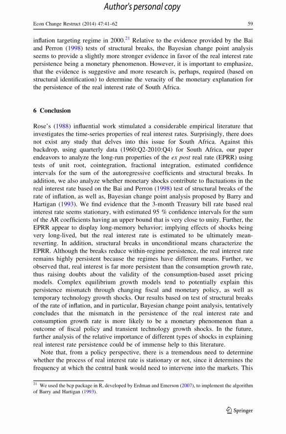
breaks in a regression model. The results for the EPRR are reported in Table 3. The

procedure based on the sequential estimation finds one change in the mean of EPRR

Table 3 Bai and Perron (1988) test statistics and estimation results for ex post real interest rate

(1960:Q2-2010:Q4)

Test statistic Regime Estimated ex post real

interest rate mean

UDmax 32.08*** 1960:Q2-1989:Q1 [1985:Q2-1994:Q1] -1.47*** (0.43)

WDmax (5%) 38.13** 1989:Q2-2010:Q4 4.15*** (0.49)

F(1|0) 22.57***

F(2|1) 10.45**

F(3|2) 4.86

F(4|3) 4.39

F(5|4) 0

*, **, *** indicate significance at the 10, 5, 1 % levels. The bracketed dates in the Regime column denote

a 90 % confidence interval for the end of the regime. Numbers in parentheses in the last column denote

standard errors for the estimated mean

15 This short-memory behavior of the per capita consumption growth rate was also confirmed by the

Geweke and Porter-Hudak (1983) and the Robinson (1992) estimation of d, as well as by the modified

R/S statistic which failed to reject the null hypothesis of the per capita consumption growth being a short-

memory process. These results are available upon request from the authors.


123


that has occurred in 1989:Q1.16 This break is associated with a significant change in

the average annualized real interest rate in the two regimes. For the period between

1960:Q2 and 1989:Q1, the average real interest rate is at -1.47 %, and then

increases significantly at 4.15 % for the period between 1989:Q2 and 2010:Q4.17

The finding of a significant break implies only a reduction in within-regime (local)

persistence, but high degree of global persistence for the EPRR still remains.18.

Figure 2 plots the South African EPRR and the means for the regimes defined by the

structural break estimated using the Bai and Perron (1998) methodology.

-20

-15

-10

-5

0

5

10

15

1960

Q2

1961

Q4

1963

Q2

1964

Q4

1966

Q2

1967

Q4

1969

Q2

1970

Q4

1972

Q2

1973

Q4

1975

Q2

1976

Q4

1978

Q2

1979

Q4

1981

Q2

1982

Q4

1984

Q2

1985

Q4

1987

Q2

1988

Q4

1990

Q2

1991

Q4

1993

Q2

1994

Q4

1996

Q2

1997

Q4

1999

Q2

2000

Q4

2002

Q2

2003

Q4

2005

Q2

2006

Q4

2008

Q2

2009

Q4

%

Ex Post Real Interest Rate Regime-Specific Means

Fig. 2 Ex post real interest rate and regime specific means, 1960:Q2-2010:Q4. Note: based on the Baiand Perron (1998) methodology, the figure plots the SA ex post real interest rate and means for theregimes defined by the structural breaks

16 Note that in Table 3, we see that F(2|1) is rejected meaning that we reject 1 break in favor of 2 breaks.

Also, F(3|2) is not significant, implying that we cannot reject 2 breaks in favor of 3 breaks. These results

suggest 2 breaks. However, the 10 % confidence interval around the endpoint of the first break, identified

at 1974:1, so was so wide that it included the starting point of the sample. In light of this, we decided to

choose one break rather than 2 for the EPRR. Further, if we allowed for two breaks, suggesting three

regimes, the estimate of the mean EPRR (0.89) under the first regime was insignificant with a t-statistic of

1.42. The details of these results are available upon request from the authors.17 In contrast to this evidence of a unique break in the EPRR, the Bai and Perron (1998) methodology

obtained no structural break in the mean of per capita consumption growth. These results are available

upon request from the authors.18 Note that, when we conducted the Zivot and Andrews (1992) unit root test allowing for a break in the

intercept, it rejected the null of unit root at the 10 % level of significance for the EPRR. This test

identified a break for the series at 1987:Q4. In addition, the Lee and Strazicich (2003) unit root test

allowing for 2 breaks, also rejected the null hypothesis of unit root test, with the breaks identified in

1972:Q3 and 1999:Q3.


123


5 Is the persistence of EPRR a monetary phenomenon?

Based on the tests conducted above, we can conclude that the South African EPPR

can be best viewed as a very persistent but ultimately mean-reverting process. This

section considers what types of shocks are most likely to produce the persistence in

the South African real interest rate. Let us recall the underlying motivation for

learning about real interest rate persistence: In a simple endowment economy, the

real interest rate should have the same persistence properties as consumption

growth. However, our empirical analyses reveal that the real rate is much more

persistent than consumption growth. Given that, permanent technology growth

shocks can create a non-stationary real rate, but also affects consumption growth in

the same way, they cannot account for the mismatch in persistence. So now, we

consider fiscal, monetary, and transient technology shocks as potential causes of

persistent fluctuations in the real interest rate.

Figures 1 and 2 and the Bai and Perron (1998) structural break tests reveal a

sharp increase in the real rate since 1989:Q2. The South African government did not

undertake the sort of expansionary fiscal policy that would be necessary for such a

rise in real rates. In fact, the budget deficits have been consistently declining over

this period (until the ‘‘Great Recession’’ recently), as deduced from the data on

budget deficit as a %age of Gross Domestic Product published by the South African

Reserve Bank. In fact, the average deficits over 1960:Q2-1989:Q1 and 1989:Q2-

2010:Q4 have been virtually the same. Hence, fiscal shocks cannot be really viewed

as a plausible candidate for the increase in real rates during this period. Turning to

technology shocks, the lack of independent data on technology shocks makes it

difficult to relate such changes with real interest rates. Besides, technology growth

has been traditionally viewed as reasonably stable. Having said that, using a

structural vector autoregressive framework to estimate the long-run effects of

exogenous changes in the inflation rate on output and the real interest rate, Amusa

et al. (forthcoming) indicate that persistence in real interest rate could be explained

to some extent by technology shocks. Further, one could suggest that oil price

increases, might influence the real rate, as can be seen from the negative real interest

rate that prevailed over the decade of 1970. However, it is less likely for oil price

shocks alone to account for the pronounced swings in the South African real interest

rate. This leaves us with the monetary policy shocks as an explanation for the

persistence of EPRR.

When one delves into the history of monetary policy of South Africa, one realizes

that the financial markets were regulated till the mid 1980, resulting in low nominal

rates. Coupled with high rates of inflation, the negative real rates over the decade of

the 1970 was obvious. After, the financial markets got liberalized, the South African

Reserve Bank started pursuing a contractionary monetary policy since the 1990s as

part of an informal inflation targeting framework.19 So, the increase in the average

EPRR seems natural post 1989. While we interpret the timing of the major swing in

the real rate to suggest a monetary explanation, we ultimately need to provide

19 Refer to Ludi and Ground (2006) for a detail discussion of the history of monetary policy in South

Africa.


123


formal evidence for this line of reasoning. Hence, following Rapach and Wohar

(2005), we use the Bai and Perron (1998) methodology to try and explain the

deterministic regime shifts in the EPRR by considering regime shifts in the mean

inflation rate. According to Friedman (1963), changes in the mean inflation rate can

be considered to be a monetary phenomenon. Table 4 reports the results of the Bai

and Perron (1998) methodology for the inflation rate. Two significant changes in the

mean of inflation rate are identified to occur in 1971:Q1 and in 1993:Q2. For the

period between 1960:Q2 and 1971:Q1, the average inflation rate was at 2.79 %; for

the period between 1971:Q2 and 1993:Q2 it averaged at 12.40 % and for the period

between 1993:Q3 and 2010:Q4, the average mean decreased to 6.23 %. Figure 3

plots the South African inflation rate and the means for the regimes defined by the

structural breaks estimated. In general, it can be seen that periods of low inflation

are associated with periods of high rates of the EPRR. However, the break in the

inflation rate in 1990:Q3 is about four years later than the only identified break in

the real interest rate. Though, it must be said that the lower limit of the 90 %

confidence band for the structural break of the inflation rate falls within the

corresponding 90 % confidence interval of the EPRR. Thus, the evidence that a

regime shift in the mean inflation rate tend to correspond to the regime shift in the

mean real interest rate is weak.20

5.1 Bayesian change point analysis

Given the weak evidence that the EPRR persistence is a monetary phenomenon

based on the structural break test, we decided to look into this issue further using a

Bayesian change point analysis for the real rate and the inflation rate. This method

allows us to obtain posterior probabilities of a change for each point of the two

series, thus, (possibly) allowing us to better relate inflation with the persistence of

the EPRR. In the following paragraphs, we describe the Barry and Hartigan (1993)

algorithm for the Bayesian change point methodology.

The Barry and Hartigan (1993) algorithm models the series generating process by

assuming that there is an underlying sequence of parameters partitioned into

contiguous blocks of equal parameter values. The beginning of each block is then a

change point, while observations are assumed to be independent in different blocks

given the sequence of parameter. Let X1;X2; . . .;Xn be independent observations,

with each Xi having a density dependent on hi; i ¼ 1; . . .; n. Furthermore, there

20 Using a measure of monetary policy surprise developed by Reid (2009) and Gupta and Reid

(forthcoming), we analyzed the impulse response function of the EPRR obtained from an autoregressive

distributed lag (ARDL) model following a contractionary monetary policy shock over the period of

2002:Q2-2010:Q4. The results, based on Romer and Romer’s (2004) Monte Carlo methods to generate

confidence bands for the impulse response functions, indicated a delayed very short-lived (1 quarter)

positive effect on the EPRR, suggesting again a weak monetary explanation of the persistence of the real

rate—a result in line with the findings of Amusa et al. (forthcoming). The impulse response functions

from the ARDL model is available upon request from the authors. Note, Reid (2009) and Gupta and Reid

(forthcoming) used the change in the 3-months Banker’s Acceptance rate on the day after the monetary

policy committee makes its statement as a proxy for the surprise component of monetary policy. This

event-based data was converted to a quarterly frequency by averaging the shocks over a three month

period.


123


exists an unknown number of contiguous blocks with partitions q ¼ fi0; i1; . . .; ibgsuch that 0 ¼ i0\i1\� � �\in ¼ n and hi = hi_b when ir-1 \ i B ir.

In the notation used by Barry and Hartigan (1993), let Xij denote the sequence of

points Xiþ1; . . .;Xj in time. Let fij(xij| hj) denote the density of xij when

hiþ1 ¼ hiþ2 ¼ . . . ¼ hj. For constant blocks, a transition distribution is defined as

follows: Given hi, hi?1 equals hi with probability 1 - pi or has density f(hi?1| hi)

with probability pi. This in essence implies that smaller values of pi will result in

longer hi blocks.

Further, the probability of a partition q ¼ i0; i1; . . .; ib is given by f ðqÞ ¼Kci0ii ci1i2 . . .cib�1ib where cij are prior cohesion for adjacent blocks ij. In notations, let

Table 4 Bai and Perron (1988) test statistics and estimation results for inflation rate (1960:Q2-2010:Q4)

Test statistic Regime Estimated inflation rate mean

UDmax 113.64*** 1960:Q2-1971:Q1 [1970:Q2-1971:Q2] 2.79*** (0.55)

WDmax (5%) 163.60*** 1971:Q2-1993:Q2 [1990:Q3-1994:Q4] 12.40*** (0.39)

F(1|0) 64.78*** 1993:Q3-2010:Q4 6.23*** (0.43)

F(2|1) 36.88***

F(3|2) 8.75

F(4|3) 2.14

F(5|4) 0

*, **, *** indicate significance at the 10, 5, 1 % levels. The bracketed dates in the Regime column denote

a 90 % confidence interval for the end of the regime. Numbers in parentheses in the last column denote

standard errors for the estimated mean

-5

0

5

10

15

20

25

1960

Q2

1961

Q3

1962

Q4

1964

Q1

1965

Q2

1966

Q3

1967

Q4

1969

Q1

1970

Q2

1971

Q3

1972

Q4

1974

Q1

1975

Q2

1976

Q3

1977

Q4

1979

Q1

1980

Q2

1981

Q3

1982

Q4

1984

Q1

1985

Q2

1986

Q3

1987

Q4

1989

Q1

1990

Q2

1991

Q3

1992

Q4

1994

Q1

1995

Q2

1996

Q3

1997

Q4

1999

Q1

2000

Q2

2001

Q3

2002

Q4

2004

Q1

2005

Q2

2006

Q3

2007

Q4

2009

Q1

2010

Q2

%

Inflation Rate Regime-Specific Means

Fig. 3 Inflation rate and regime specific means, 1960:Q2-2010:Q4. Note: based on the Bai and Perron(1998) methodology, the figure plots the SA inflation rate and means for the regimes defined by thestructural breaks


123


X1, X2, ..., Xn are assumed to be an independent for a given sequence of li, such that

XivNðli; r2Þ; i ¼ 1; 2; . . .; n. A prior cohesion cij following Yao (1984) is

introduced as follows:

cij ¼ ð1� pÞj�i�1p; j\n

ð1� pÞj�i�1j ¼ n

�ð8Þ

Also, a block prior is introduced as follows:

fijðljÞvN l0;r2

0

j� i

� �ð9Þ

The priors distribution for each of l0; r20; p;w ¼ r2

ðr20þr2Þ are as follows:

f ðl0Þ ¼ 1;�1� l0�1f ðr2Þ ¼ 1=r2; 0� r2�1f ðpÞ ¼ 1=p0; 0� p� p0

f ðwÞ ¼ 1=w0; 0�w�w0

After experimenting with different values of w0 and p0, we initialize (p0,w0) with

(0.002, 0.2) to ensure that the change points in the two series matches major local

and global events that took place over the period of 1960:Q2-2010:Q4. As can be

seen from Fig. 4, a major change point in the inflation rate in 1972:Q1 preceded a

major change point in the EPRR in 1972:Q2. Also, a major change point in the

EPRR in 1992:Q3 followed a change point in the inflation rate in 1989:Q1, and is

followed by couple of major changes in the inflation rate in 19954:Q4 and 1995:Q1.

The other major change points in inflation in 1981 and 1985, seems to be in line

with the move to a flexible exchange rate regime and liberalization of the domestic

financial markets. While, the changes in the inflation rate in 1995 and late 1999

corresponds closely to the creation of democratic South Africa and its move to an

0

0.1

0.2

0.3

0.4

0.5

0.6

1960

:219

61:3

1962

:419

64:1

1965

:219

66:3

1967

:419

69:1

1970

:219

71:3

1972

:419

74:1

1975

:219

76:3

1977

:419

79:1

1980

:219

81:3

1982

:419

84:1

1985

:219

86:3

1987

:419

89:1

1990

:219

91:3

1992

:419

94:1

1995

:219

96:3

1997

:419

99:1

2000

:220

01:3

2002

:420

04:1

2005

:220

06:3

2007

:420

09:1

2010

:2

prob

abili

ties

Inflation EPRR

Fig. 4 Posterior probabilities of change for the ex post real rate and the inflation rate


123


inflation targeting regime in 2000.21 Relative to the evidence provided by the Bai

and Perron (1998) tests of structural breaks, the Bayesian change point analysis

seems to provide a slightly more stronger evidence in favor of the real interest rate

persistence being a monetary phenomenon. However, it is important to emphasize,

that the evidence is suggestive and more research is, perhaps, required (based on

structural identification) to determine the veracity of the monetary explanation for

the persistence of the real interest rate of South Africa.

6 Conclusion

Rose’s (1988) influential work stimulated a considerable empirical literature that

investigates the time-series properties of real interest rates. Surprisingly, there does

not exist any study that delves into this issue for South Africa. Against this

backdrop, using quarterly data (1960:Q2-2010:Q4) for South Africa, our paper

endeavors to analyze the long-run properties of the ex post real rate (EPRR) using

tests of unit root, cointegration, fractional integration, estimated confidence

intervals for the sum of the autoregressive coefficients and structural breaks. In

addition, we also analyze whether monetary shocks contribute to fluctuations in the

real interest rate based on the Bai and Perron (1998) test of structural breaks of the

rate of inflation, as well as, Bayesian change point analysis proposed by Barry and

Hartigan (1993). We find evidence that the 3-month Treasury bill rate based real

interest rate seems stationary, with estimated 95 % confidence intervals for the sum

of the AR coefficients having an upper bound that is very close to unity. Further, the

EPRR appear to display long-memory behavior; implying effects of shocks being

very long-lived, but the real interest rate is estimated to be ultimately mean-

reverting. In addition, structural breaks in unconditional means characterize the

EPRR. Although the breaks reduce within-regime persistence, the real interest rate

remains highly persistent because the regimes have different means. Further, we

observed that, real interest is far more persistent than the consumption growth rate,

thus raising doubts about the validity of the consumption-based asset pricing

models. Complex equilibrium growth models tend to potentially explain this

persistence mismatch through changing fiscal and monetary policy, as well as

temporary technology growth shocks. Our results based on test of structural breaks

of the rate of inflation, and in particular, Bayesian change point analysis, tentatively

concludes that the mismatch in the persistence of the real interest rate and

consumption growth rate is more likely to be a monetary phenomenon than a

outcome of fiscal policy and transient technology growth shocks. In the future,

further analysis of the relative importance of different types of shocks in explaining

real interest rate persistence could be of immense help to this literature.

Note that, from a policy perspective, there is a tremendous need to determine

whether the process of real interest rate is stationary or not, since it determines the

frequency at which the central bank would need to intervene into the markets. This

21 We used the bcp package in R, developed by Erdman and Emerson (2007), to implement the algorithm

of Barry and Hartigan (1993).


123


information is of paramount importance for South Africa specifically, given that it

has moved to an inflation-targeting regime since the first quarter of 2000.The

success of an inflation-targeting regime is dependant on keeping the inflation

expectations pegged, which in turn, depends on clear communication to the market,

and hinges crucially to a great extent on whether the real interest rate is stationary or

not. Since if the real interest rate is believed to have an unit root process, the South

African Reserve Bank might have to intervene regularly to neutralize the possibility

of a permanent effect on the market; in the process confusing agents and their

inflation expectations, and thus leading the inflation to deviate away from the target.

In light of this, it seems that it is better to err on the side of stationarity, even when

the interest rate process might be an unit root, since if the South African Reserve

Bank observes that their policies are actually having permanent effect when they

want it to be temporary, they could always intervene as required. However, if the

real interest rate is actually mean-reverting, but the South African Reserve Bank

believes it to be an unit root process, they are likely to end up frequently intervening

in the market, when they do not actually need to, and thus making it difficult for

agents to appropriately form their expectations.

References

Andolfatto D, Hendry S, Moran K (2008) Are inflation expectations rational. J Monet Econ 55(2):

406–422

Amusa K, Gupta R, Karolia S, Simo-Kengne BD The long-run impact of inflation in South Africa.

J Policy Model (Forthcoming)

Bai J, Perron P (1998) Estimating and testing linear models with multiple structural changes.

Econometrica 66(1):47–78

Barro RJ, Sala-i-Martin X (2003) Economic growth, 2nd edn. MIT Press, Cambridge, MA

Barry D, Hartigan JA (1993) A Bayesian analysis for change point problems. J Am Stat Assoc 88:

309–319

Baxter M, King RG (1993) Fiscal policy in general equilibrium. Am Econ Rev 83(3):315–334

Bierens HJ (1997) Nonparametric cointegration analysis. J Econ 77:379–404

Bierens HJ (2000) Nonparametric nonlinear cotrending analysis, with an application to interest and

inflation in the United States. J Bus Econ Stat 18(3):323–337

Blanchard OJ (1985) Debt, deficits, and finite horizons. J Polit Econ 93(2):223–247

Blanchard OJ, Fischer S (1989) Lectures on macroeconomics. MIT Press, Cambridge, MA

Blough SR (1992) The relationship between power and level for generic unit root tests in finite samples.

J Appl Econ 7(3):295–308

Breeden DT (1979) An intertemporal asset pricing model with stochastic consumption and investment

opportunities. J Finance Econ 7(3):265–296

Breitung J (2002) Nonparametric tests for unit roots and cointegration. J Econ 108(2):343–363

Bullard JB, Russell SH (2004) How costly is sustained low inflation for the U.S. economy? Fed Reserv

Bank St.Louis Rev 86(3):35–67

Cass D (1965) Optimum growth in an aggregate model of capital accumulation. Rev Econ Stud

32(3):233–240

Crowder WJ, Wohar ME (1998) Are tax effects important in the long-run fisher relation? Evidence from

the municipal bond market. J Finance 54(1):307–317

Darby MR (1975) The financial and tax effects of monetary policy on interest rates. Econ Inq 13(2):

266–276

de Bruyn R, Gupta R, Stander L (2011) Testing the monetary model for exchange rate determination in

South Africa: evidence from 101 years of data. University of Pretoria Department of Economics

Working Paper 201134


123


DeJong DN, Nankervis JC, Savin NE, Whiteman CH (1992) The power problems of unit root tests in time

series with autoregressive errors. J Econ 53(1-3):323–343

Diamond PA (1965) National debt in a neoclassical growth model. Am Econ Rev 55(5):1126–1150

Dickey DA, Fuller WA (1979) Distribution of the estimators for autoregressive time series with a unit

root. J Am Stat Assoc 74(366):427–431

Elliott G, Rothenberg TJ, Stock JH (1996) Efficient tests for an autoregressive unit root. Econometrica

64(4):813–836

Engle RF, Granger CWJ (1987) Co-integration and error correction: representation, estimation, and

testing. Econometrica 55(2):251–276

Erdman C, Emerson JW (2007) bcp; an r package for performing a Bayesian analysis of change point

problems. J Stat Softw 23(3):1–13

Espinosa-Vega MA, Russell SH (1998a) Can higher inflation reduce real interest rates in the long run?

Can J Econ 31(1):92–103

Espinosa-Vega MA, Russell SH (1998b) The long-run real effects of monetary policy: Keynesian

predictions from a neoclassical model. Federal Reserve Bank of Atlanta. Working Paper No: 98–6

Faust J (1996) Near observational equivalence and theoretical size problems with unit root tests. Econo

Theory 12(4):724–31

Friedman M (1963) Inflation: causes and consequences. Asia Publishing House, New York

Geweke J, Porter-Hudak S (1983) The estimation and application of long memory time series models.

J Time Ser Anal 221–238

Granger CWJ (1980) Long memory relationships and the aggregation of dynamic models. J Econ

14(2):227–238

Granger CWJ, Joyeux R (1980) An introduction to long-memory time series models and fractional

differencing. J Time Ser Anal 1:15–39

Gregory AW, Hansen BE (1996) Residual-based tests for cointegration in models with regime shifts.

J Econ 70(1):99–126

Gupta R, Reid M Macroeconomic surprises and stock returns in South Africa. Stud Econ Finance

(forthcoming)

Hamilton JD (1989) A new approach to the economic analysis of nonstationary time series and the

business cycle. Econometrica 57(2):357–384

Hansen BE (1999) The grid bootstrap and the autoregressive model. Rev Econ Stat 81(4):594–607

Hansen LP, Singleton KJ (1982) Generalized instrumental variables estimation of nonlinear rational

expectations models. Econometrica 50(5):1269–1286

Hansen LP, Singleton KJ (1983) Stochastic consumption, risk aversion, and the temporal behavior of

asset returns. J Polit Econ 91(2):249–265

Hosking JRM (1981) Fractional differencing. Biometrika 68(1):165–176

Huizinga J, Mishkin FS (1986) monetary policy regime shifts and the unusual behavior of real interest

rates. Carnegie-Rochester Conf Ser Pub Policy 24:231–274

Johansen S (1991) Estimation and hypothesis testing of cointegration vectors in Gaussian vector

autoregressive model. Econometrica 59(6):1551–1580

Jouini J, Nouira L (2006) Mean-shifts and long-memory in the U.S. ex post real interest rate. Universit de

la Mditerrane, GREQAM, Mimeo

Kahn B, Farrell G (2002) South African real interest rates in comparative perspective: theory and

evidence. South African Reserve Bank Occasional Paper 17

Kapetanios G, Shin Y, Snell A (2003) Testing for a unit root in the non-linear star framework. J Econ

112:359–379

Koopmans TC (1965) On the concept of optimal economic growth. In: The economic approach to

development planning. Elsevier, Amsterdam, pp 225–300

Kryshko M (2006) Nominal exchange rates and uncovered interest parity: non-parametric co-integration

analysis. University of Pennsylvania Department of Economics, Mimeo

Kwiatkowski D, Phillips PCB, Schmidt P, Shin Y (1992) Testing the null hypothesis of stationarity

against the alternative of a unit root: how sure are we that economic time series have a unit root.

J Econ 54(1-3):159–178

Lacerda M, Fedderke JW, Haines LM (2010) Testing for purchasing power parity and uncovered interest

parity in the presence of monetary and exchange rate regime shifts. S Afr J Econ 78(4):363–382

Lee J, Strazicich MC (2003) Minimum LM unit root test with two structural breaks. Rev Econ Stat

85(4):1082–1089

Li J, Lee J (2010) Adl tests for threshold cointegration. J Time Ser Anal 31(4):241–254


123


Lioui A, Poncet P (2008) Monetary non-neutrality in the Sidrauski model under uncertainty. Econ Lett

100(1):22–26

Lucas RE (1978) Asset prices in an exchange economy. Econometrica 46(6):1429–1445

Ludi K, Ground M (2006) Investigating the bank lending channel in South Africa: a VAR approach.

University of Pretoria Department of Economics Working Paper: 200604

Lo AW (1991) Long-term memory in stock market prices. Econometrica 59:1279–1313

Mishkin FS (1981) The real rate of interest: an empirical investigation. Carnegie-Rochester Conf Ser Pub

Policy 15:151–200

Mishkin FS (1984) The real interest: rate: a multi-country empirical study. Can J Econ 17(2):283–311

Mundell R (1963) Inflation and real interest. J Polit Econ 71(3):280–283

Neely CJ, Rapach DE (2008) Real interest rate persistence: evidence and implications. Fed Reserv Bank

St. Louis Rev 90(6):609–641

Nelson CR, Schwert GW (1997) Short-term interest rates as predictors of inflation: on testing the

hypothesis that the real interest rate is constant. Am Econ Rev 67(3):478–486

Ng S, Perron P (2001) Lag length selection and the construction of unit root tests with good size and

power. Econometrica 69(6):1519–554

Pelaez RF (1995) The Fisher effect: reprise. J Macroecon 17(2):333–346

Perron P (1989) The great crash, the oil price shock and the unit root hypothesis. Econometrica 57(6):

1361–1401

Perron P, Rodriguez GH (2001) Residual based tests for cointegration with GLS detrended data. Boston

University, Mimeo

Phillips PCB, Perron P (1988) Testing for a unit root in time series regression. Biometrika 75(2):335–346

Rapach DE, Wohar ME (2004) The persistence in international real interest rates. Int J Finance Econ

9(4):339–346

Rapach DE, Wohar ME (2005) Regime changes in international real interest rates: are they a monetary

phenomenon. J Money Credit Bank 37(5):887–906

Reid M (2009) The sensitivity of South African inflation expectations to surprises. S Afr J Econ 77(3):

414–429

Reis R (2007) The analytics of monetary non-neutrality in the Sidrauski model. Econ Lett 94(1):129–135

Robinson PM (1992) Semi-parametric analysis of long-memory time series. Ann Stat 22:515–539

Romano JP, Wolf M (2001) Subsampling intervals in autoregressive models with linear time trends.

Econometrica 69(5):1283–1314

Romer DH (2006) Advanced macroeconomics, 3rd edn. McGraw-Hill, New York

Romer CD, Romer DH (2004) A new measure of monetary shocks: derivation and implications. Am Econ

Rev 94(4):1055–1084

Rose AK (1988) Is the real interest rate stable. J Finance 43(5):1095–1112

Samuelson PA (1958) An exact consumption-loan model of interest with or without the social contrivance

of money. J Polit Econ 66(6):467–482

Shiller RJ (1979) The volatility of long-term interest rates and expectations models of the term structure.

J Polit Econ 87(6):1190–1219

Shimotsu K (2008) Exact local whittle estimation of fractional integration with an unknown mean and

time trend. Queen’s University Working Paper

Sims C (1988) Bayesian skeptism on unit root econometrics. Institute for Empirical Macroeconomics,

University of Minnesota

Taylor JB (1993) Discretion versus policy rules in practice. Carnegie-Rochester Conf Ser Pub Policy

39:195–214

Tobin J (1965) Money and economic growth. Econometrica 33(4):671–684

Weiss LM (1980) The effects of money supply on economic welfare in the steady state. Econometrica

48(3):565–576

Yao Y (1984) Estimation of a noisy discrete-time step function: bayes and empirical bayes approaches.

Annal Stat 12(4):1434–1447

Zivot E, Andrews W (1992) Further evidence on the great crash, the oil price shock and the unit root

hypothesis. J Bus Econ Stat 10:251–270


123


Real interest rate persistence in South Africa: evidence

Documents

Transcript of Real interest rate persistence in South Africa: evidence