Rbbt: A Framework for Fast Bioinformatics Development with Ruby
244
-
Upload
independent -
Category
Documents
-
view
3 -
download
0
Transcript of Rbbt: A Framework for Fast Bioinformatics Development with Ruby


Advances in Intelligent andSoft Computing 74Editor-in-Chief: J. Kacprzyk

Advances in Intelligent and Soft Computing
Editor-in-Chief
Prof. Janusz KacprzykSystems Research InstitutePolish Academy of Sciencesul. Newelska 601-447 WarsawPolandE-mail: [email protected]
Further volumes of this series can be found on our homepage: springer.com
Vol. 58. J. Mehnen, A. Tiwari,M. Köppen, A. Saad (Eds.)Applications of Soft Computing, 2009ISBN 978-3-540-89618-0
Vol. 59. K.A. Cyran,S. Kozielski, J.F. Peters,U. Stanczyk, A. Wakulicz-Deja (Eds.)Man-Machine Interactions, 2009ISBN 978-3-642-00562-6
Vol. 60. Z.S. Hippe,J.L. Kulikowski (Eds.)Human-Computer Systems Interaction, 2009ISBN 978-3-642-03201-1
Vol. 61. W. Yu, E.N. Sanchez (Eds.)Advances in ComputationalIntelligence, 2009ISBN 978-3-642-03155-7
Vol. 62. B. Cao,T.-F. Li, C.-Y. Zhang (Eds.)Fuzzy Information andEngineering Volume 2, 2009ISBN 978-3-642-03663-7
Vol. 63. Á. Herrero, P. Gastaldo,R. Zunino, E. Corchado (Eds.)Computational Intelligence in Security forInformation Systems, 2009ISBN 978-3-642-04090-0
Vol. 64. E. Tkacz, A. Kapczynski (Eds.)Internet – Technical Development andApplications, 2009ISBN 978-3-642-05018-3
Vol. 65. E. Kacki, M. Rudnicki,J. Stempczynska (Eds.)Computers in Medical Activity, 2009ISBN 978-3-642-04461-8
Vol. 66. G.Q. Huang,K.L. Mak, P.G. Maropoulos (Eds.)Proceedings of the 6th CIRP-SponsoredInternational Conference on DigitalEnterprise Technology, 2009ISBN 978-3-642-10429-9
Vol. 67. V. Snášel, P.S. Szczepaniak,A. Abraham, J. Kacprzyk (Eds.)Advances in Intelligent Web Mastering - 2, 2010ISBN 978-3-642-10686-6
Vol. 68. V.-N. Huynh, Y. Nakamori,J. Lawry, M. Inuiguchi (Eds.)Integrated Uncertainty Management andApplications, 2010ISBN 978-3-642-11959-0
Vol. 69. E. Pietka and J. Kawa (Eds.)Information Technologies in Biomedicine, 2010ISBN 978-3-642-13104-2
Vol. 70. XXX
Vol. 71. XXX
Vol. 72. J.C. Augusto, J.M. Corchado,P. Novais, C. Analide (Eds.)Ambient Intelligence and Future Trends, 2010ISBN 978-3-642-13267-4
Vol. 73. J.M. Corchado, P. Novais,C. Analide, J. Sedano (Eds.)Soft Computing Models in Industrial andEnvironmental Applications, 5th InternationalWorkshop (SOCO 2010), 2010ISBN 978-3-642-13160-8
Vol. 74. M.P. Rocha, F.F. Riverola, H. Shatkay,J.M. Corchado (Eds.)Advances in BioinformaticsISBN 978-3-642-13213-1

Miguel P. Rocha,Florentino Fernández Riverola, Hagit Shatkay,and Juan Manuel Corchado (Eds.)
Advances in Bioinformatics
4th International Workshop on PracticalApplications of Computational Biologyand Bioinformatics 2010 (IWPACBB 2010)
ABC

Editors
Miguel P. RochaDep. Informática / CCTCUniversidade do MinhoCampus de Gualtar4710-057 BragaPortugal
Florentino Fernández RiverolaEscuela Superior deIngeniería InformáticaEdificio Politécnico,Despacho 408Campus UniversitarioAs Lagoas s/n32004 OurenseSpainE-mail: [email protected]
Hagit ShatkayComputational Biology andMachine Learning LabSchool of ComputingQueen’s University KingstonOntario K7L 3N6CanadaE-mail: [email protected]
Juan Manuel CorchadoDepartamento de Informáticay AutomáticaFacultad de CienciasUniversidad de SalamancaPlaza de la Merced S/N37008 SalamancaSpainE-mail: [email protected]
ISBN 978-3-642-13213-1 e-ISBN 978-3-642-13214-8
DOI 10.1007/978-3-642-13214-8
Advances in Intelligent and Soft Computing ISSN 1867-5662
Library of Congress Control Number: 2010928117
c© 2010 Springer-Verlag Berlin Heidelberg
This work is subject to copyright. All rights are reserved, whether the whole or part of the material isconcerned, specifically the rights of translation, reprinting, reuse of illustrations, recitation, broadcasting,reproduction on microfilm or in any other way, and storage in data banks. Duplication of this publicationor parts thereof is permitted only under the provisions of the German Copyright Law of September 9,1965, in its current version, and permission for use must always be obtained from Springer. Violationsare liable for prosecution under the German Copyright Law.
The use of general descriptive names, registered names, trademarks, etc. in this publication does notimply, even in the absence of a specific statement, that such names are exempt from the relevant protectivelaws and regulations and therefore free for general use.
Typeset & Cover Design: Scientific Publishing Services Pvt. Ltd., Chennai, India.
Printed on acid-free paper
5 4 3 2 1 0
springer.com

Preface
The fields of Bioinformatics and Computational Biology have been growing steadily over the last few years boosted by an increasing need for computational techniques that can efficiently handle the huge amounts of data produced by the new experimental techniques in Biology. This calls for new algorithms and ap-proaches from fields such as Data Integration, Statistics, Data Mining, Machine Learning, Optimization, Computer Science and Artificial Intelligence.
Also, new global approaches, such as Systems Biology, have been emerging replacing the reductionist view that dominated biological research in the last dec-ades. Indeed, Biology is more and more a science of information needing tools from the information technology field. The interaction of researchers from differ-ent scientific fields is, more than ever, of foremost importance and we hope this event will contribute to this effort.
IWPACBB'10 technical program included a total of 30 papers (26 long papers and 4 short papers) spanning many different sub-fields in Bioinformatics and Computational Biology. Therefore, the technical program of the conference will certainly be diverse, challenging and will promote the interaction among computer scientists, mathematicians, biologists and other researchers.
We would like to thank all the contributing authors, as well as the members of the Program Committee and the Organizing Committee for their hard and highly valuable work. Their work has helped to contribute to the success of the IWAPCBB’10 event. IWPACBB’10 wouldn’t exist without your contribution.
Miguel Rocha Florentino Fernández Riverola IWPACBB’10 Organizing Co-chairs
Juan Manuel Corchado Hagit Shatkay
IWPACBB’10 Programme Co-chairs

Organization
General Co-chairs
Miguel Rocha University of Minho (Portugal) Florentino Riverola University of Vigo (Spain) Juan M. Corchado University of Salamanca (Spain) Hagit Shatkay Queens University, Ontario (Canada)
Program Committee
Juan M. Corchado (Co-chairman)
University of Salamanca (Spain)
Alicia Troncoso Universidad of Pablo de Olavide (Spain) Alípio Jorge LIAAD/INESC, Porto LA (Portugal) Anália Lourenço University of Minho (Portugal) Arlindo Oliveira INESC-ID, Lisboa (Portugal) Arlo Randall University of California Irvine (USA) B. Cristina Pelayo University of Oviedo (Spain) Christopher Henry Argonne National Labs (USA) Daniel Gayo University of Oviedo (Spain) David Posada Univ. Vigo (Spain) Emilio S. Corchado University of Burgos (Spain) Eugénio C. Ferreira IBB/CEB, University of Minho (Portugal) Fernando Diaz-Gómez University of Valladolid (Spain) Gonzalo Gómez-López UBio/CNIO, Spanish National Cancer Research
Centre (Spain) Isabel C. Rocha IBB/CEB, University of Minho (Portugal) Jesús M. Hernández University of Salamanca (Spain) Jorge Vieira IBMC, Porto (Portugal) José Adserias University of Salamanca (Spain) José L. López University of Salamanca (Spain) José Luís Oliveira Univ. Aveiro (Portugal) Juan M. Cueva University of Oviedo (Spain) Júlio R. Banga IIM/CSIC, Vigo (Spain)

OrganizationVIII
Kaustubh Raosaheb Patil Max-Planck Institute for Informatics(Germany) Kiran R. Patil Biocentrum, DTU (Denmark) Lourdes Borrajo University of Vigo (Spain) Luis M. Rocha Indiana University (USA) Manuel J. Maña López University of Huelva (Spain) Margarida Casal University of Minho (Portugal) Maria J. Ramos FCUP, University of Porto (Portugal) Martin Krallinger CNB, Madrid (Spain) Nicholas Luscombe EBI (UK) Nuno Fonseca CRACS/INESC, Porto (Portugal) Oscar Sanjuan University of Oviedo (Spain) Paulo Azevedo University of Minho (Portugal) Paulino Gómez-Puertas University Autónoma de Madrid (Spain) Pierre Balde University of California Irvine (USA) Rui Camacho LIACC/FEUP, University of Porto (Portugal) Rui Brito University of Coimbra (Portugal) Rui C. Mendes CCTC, University of Minho (Portugal) Sara Madeira IST/INESC, Lisboa (Portugal) Ségio Deusdado IP Bragança (Portugal) Vítor Costa University of Porto (Portugal)
Organizing Committee
Miguel Rocha (Co-chairman)
CCTC, Univ. Minho (Portugal)
Florentino Fernández Riverola (Co-chairman)
University of Vigo (Spain)
Juan F. De Paz University of Salamanca (Spain) Daniel Glez-Peña University of Vigo (Spain) José P. Pinto University of Minho (Portugal) Rafael Carreira University of Minho (Portugal) Simão Soares University of Minho (Portugal) Paulo Vilaça University of Minho (Portugal) Hugo Costa University of Minho (Portugal) Paulo Maia University of Minho (Portugal) Pedro Evangelista University of Minho (Portugal) Óscar Dias University of Minho (Portugal)

Contents
Microarrays
Highlighting Differential Gene Expression between TwoCondition Microarrays through Heterogeneous GenomicData: Application to Lesihmania infantum StagesComparison . . . . . . . . . . . . . . . . . . . . . . . . . . . . . . . . . . . . . . . . . . . . . . . . . 1Liliana Lopez Kleine, Vıctor Andres Vera Ruiz
An Experimental Evaluation of a Novel Stochastic Methodfor Iterative Class Discovery on Real Microarray Datasets . . . 9Hector Gomez, Daniel Glez-Pena, Miguel Reboiro-Jato,Reyes Pavon, Fernando Dıaz, Florentino Fdez-Riverola
Automatic Workflow during the Reuse Phase of a CBPSystem Applied to Microarray Analysis . . . . . . . . . . . . . . . . . . . . . . 17Juan F. De Paz, Ana B. Gil, Emilio Corchado
A Comparative Study of Microarray Data ClassificationMethods Based on Ensemble Biological Relevant GeneSets . . . . . . . . . . . . . . . . . . . . . . . . . . . . . . . . . . . . . . . . . . . . . . . . . . . . . . . . . 25Miguel Reboiro-Jato, Daniel Glez-Pena, Juan Francisco Galvez,Rosalıa Laza Fidalgo, Fernando Dıaz, Florentino Fdez-Riverola
Data Mining and Data Integration
Predicting the Start of Protein α-Helices Using MachineLearning Algorithms . . . . . . . . . . . . . . . . . . . . . . . . . . . . . . . . . . . . . . . . . 33Rui Camacho, Rita Ferreira, Natacha Rosa, Vania Guimaraes,Nuno A. Fonseca, Vıtor Santos Costa, Miguel de Sousa,Alexandre Magalhaes

X Contents
A Data Mining Approach for the Detection of High-RiskBreast Cancer Groups . . . . . . . . . . . . . . . . . . . . . . . . . . . . . . . . . . . . . . . 43Orlando Anunciacao, Bruno C. Gomes, Susana Vinga,Jorge Gaspar, Arlindo L. Oliveira, Jose Rueff
GRASP for Instance Selection in Medical Data Sets . . . . . . . . . 53Alfonso Fernandez, Abraham Duarte, Rosa Hernandez,Angel Sanchez
Expanding Gene-Based PubMed Queries . . . . . . . . . . . . . . . . . . . . 61Sergio Matos, Joel P. Arrais, Jose Luis Oliveira
Improving Cross Mapping in Biomedical Databases . . . . . . . . . . 69Joel Arrais, Joao E. Pereira, Pedro Lopes, Sergio Matos,Jose Luis Oliveira
An Efficient Multi-class Support Vector Machine Classifierfor Protein Fold Recognition . . . . . . . . . . . . . . . . . . . . . . . . . . . . . . . . . 77Wies�law Chmielnicki, Katarzyna Stapor, Irena Roterman-Konieczna
Feature Selection Using Multi-Objective EvolutionaryAlgorithms: Application to Cardiac SPECT Diagnosis . . . . . . . 85Antonio Gaspar-Cunha
Phylogenetics and Sequence Analysis
Two Results on Distances for Phylogenetic Networks . . . . . . . . 93Gabriel Cardona, Merce Llabres, Francesc Rossello
Cramer Coefficient in Genome Evolution . . . . . . . . . . . . . . . . . . . . 101Vera Afreixo, Adelaide Freitas
An Application for Studying Tandem Repeats inOrthologous Genes . . . . . . . . . . . . . . . . . . . . . . . . . . . . . . . . . . . . . . . . . . 109Jose Paulo Lousado, Jose Luis Oliveira, Gabriela Moura,Manuel A.S. Santos
Accurate Selection of Models of Protein Evolution . . . . . . . . . . . 117Mateus Patricio, Federico Abascal, Rafael Zardoya, David Posada
Scalable Phylogenetics through Input Preprocessing . . . . . . . . . 123Roberto Blanco, Elvira Mayordomo, Esther Montes, Rafael Mayo,Angelines Alberto
The Median of the Distance between Two Leaves in aPhylogenetic Tree . . . . . . . . . . . . . . . . . . . . . . . . . . . . . . . . . . . . . . . . . . . 131Arnau Mir, Francesc Rossello

Contents XI
In Silico AFLP: An Application to Assess What Is Neededto Resolve a Phylogeny . . . . . . . . . . . . . . . . . . . . . . . . . . . . . . . . . . . . . . 137Marıa Jesus Garcıa-Pereira, Armando Caballero, Humberto Quesada
Employing Compact Intra-Genomic Language Modelsto Predict Genomic Sequences and Characterize TheirEntropy . . . . . . . . . . . . . . . . . . . . . . . . . . . . . . . . . . . . . . . . . . . . . . . . . . . . . 143Sergio Deusdado, Paulo Carvalho
Biomedical Applications
Structure Based Design of Potential Inhibitors of SteroidSulfatase . . . . . . . . . . . . . . . . . . . . . . . . . . . . . . . . . . . . . . . . . . . . . . . . . . . . . 151Elisangela V. Costa, M. Emılia Sousa, J. Rocha,Carlos A. Montanari, M. Madalena Pinto
Agent-Based Model of the Endocrine Pancreas andInteraction with Innate Immune System . . . . . . . . . . . . . . . . . . . . . 157Ignacio V. Martınez Espinosa, Enrique J. Gomez Aguilera,Marıa E. Hernando Perez, Ricardo Villares,Jose Mario Mellado Garcıa
State-of-the-Art Genetic Programming for PredictingHuman Oral Bioavailability of Drugs . . . . . . . . . . . . . . . . . . . . . . . . 165Sara Silva, Leonardo Vanneschi
Pharmacophore-Based Screening as a Clue for theDiscovery of New P-Glycoprotein Inhibitors . . . . . . . . . . . . . . . . . 175Andreia Palmeira, Freddy Rodrigues, Emılia Sousa, Madalena Pinto,M. Helena Vasconcelos, Miguel X. Fernandes
Bioinformatics Applications
e-BiMotif: Combining Sequence Alignment and Biclusteringto Unravel Structured Motifs . . . . . . . . . . . . . . . . . . . . . . . . . . . . . . . . 181Joana P. Goncalves, Sara C. Madeira
Applying a Metabolic Footprinting Approach toCharacterize the Impact of the Recombinant ProteinProduction in Escherichia Coli . . . . . . . . . . . . . . . . . . . . . . . . . . . . . . 193Sonia Carneiro, Silas G. Villas-Boas, Isabel Rocha,Eugenio C. Ferreira

XII Contents
Rbbt: A Framework for Fast Bioinformatics Developmentwith Ruby . . . . . . . . . . . . . . . . . . . . . . . . . . . . . . . . . . . . . . . . . . . . . . . . . . . 201Miguel Vazquez, Ruben Nogales, Pedro Carmona, Alberto Pascual,Juan Pavon
Analysis of the Effect of Reversibility Constraints on thePredictions of Genome-Scale Metabolic Models . . . . . . . . . . . . . . 209Jose P. Faria, Miguel Rocha, Rick L. Stevens, Christopher S. Henry
Enhancing Elementary Flux Modes Analysis UsingFiltering Techniques in an Integrated Environment . . . . . . . . . . 217Paulo Maia, Marcellinus Pont, Jean-Francois Tomb, Isabel Rocha,Miguel Rocha
Genome Visualization in Space . . . . . . . . . . . . . . . . . . . . . . . . . . . . . . 225Leandro S. Marcolino, Braulio R.G.M. Couto, Marcos A. dos Santos
A Hybrid Scheme to Solve the Protein Structure PredictionProblem . . . . . . . . . . . . . . . . . . . . . . . . . . . . . . . . . . . . . . . . . . . . . . . . . . . . 233Jose C. Calvo, Julio Ortega, Mancia Anguita
Author Index . . . . . . . . . . . . . . . . . . . . . . . . . . . . . . . . . . . . . . . . . . . . . . . . 241

M.P. Rocha et al. (Eds.): IWPACBB 2010, AISC 74, pp. 1–8, 2010. springerlink.com © Springer-Verlag Berlin Heidelberg 2010
Highlighting Differential Gene Expression between Two Condition Microarrays through Heterogeneous Genomic Data: Application to Lesihmania infantum Stages Comparison
Liliana López Kleine and Víctor Andrés Vera Ruiz
1
Abstract. Classical methods for the detection of gene expression differences be-tween two microarray conditions often fail to detect interesting and important differences, because they are weak in comparison with the overall variability. Therefore, methodologies that highlight weak differences are needed. Here, we propose a method that allows the fusion of other genomic data with microarray data and show, through an example on L. infantum microarrays comparing pro-mastigote and amastigote stages, that differences between the two microarray conditions are highlighted. The method is flexible and can be applied to any organism for which microarray and other genomic data is available.
1 Introduction
Protozoan of the genus Leishmania are parasites that are transmitted by blood-feeding insect vectors to mammalian hosts, and cause a number of important hu-man diseases, collectively referred as leishmaniasis. During their life cycle, these parasites alternate between two major morphologically distinct developmental stages. In the digestive tract of the sandfly vector, they exist as extracellular elon-gated, flagellated, and motile promastigotes that are exposed to pH 7 and fluctuat-ing temperatures averaging 25ºC. Upon entry into a mammalian host, they reside in mononuclear phagocytes or macrophages (37ªC), wherein they replicate as cir-cular, aflagellated and non-motile amastigotes. In order to survive, these two ex-treme environments, Leishmania sp. (L. sp) has developed regulatory mechanisms that result in important morphological and biochemical adaptations [1, 2, 3].
1 Liliana López Kleine . Victor Andrés Vera Ruiz Universidad Nacional de Colombia (Sede Bogotá), Cra 30, calle 45, Statistics Department e-mail: [email protected], [email protected]

2 L.L. Kleine and V.A.V. Ruiz
Microarray studies allow measuring the expression level of thousands of genes at the same time by just one hybridization experiment and the comparison of two conditions (here the development stages of L. Sp.). Several microarray analyses have been done to study global gene expression in developmental stages of L. sp. [3, 4, 5]. Results show that L. sp genome can be considered to be constitutively expressed, as more than 90% of the genes is expressed in the same amount in both stages, and that only a limited number (7-9.3%) of genes show stage-specific ex-pression [3, 6]. Furthermore, no metabolic pathway or cell function characteristic of any stage has been detected [3, 4, 6, 7, 8, 9]. This is an astonishing result be-cause morphological and physiological differences between the two stages are huge, indicating that different specialized stage proteins are needed and therefore gene expression should change. In order to explain the weak differences in gene expression between both stages, it has been proposed that regulations and adaptations take place after translation and not at the gene expression level [10].
The detection of gene expression differences has been of great interest [11], as an understanding of the adaptation and resistance factors of Leishmania sp. can provide interesting therapeutic targets. Analytical methods used until now, even improved ones such as the Gene Set Enrichment Analysis [13], have difficulties in the determination of differences between gene expression in both L. sp. life cycle stages because in the context of global gene expression variation, the detection of weak differences is not possible using classical methods. Microarray data analysis can still be improved if a way to highlight weak differences in gene expression between L. sp. stages is found.
The present method consists of using additional information to the microarrays to achieve this. It allows incorporating different genomic and post-genomic data (positions of genes on the chromosome, metabolic pathways, phylogenetic pro-files, etc.) to detect differences between two experimental microarray conditions The method can be applied to detect gene expression differences between any two conditions and for all completely sequenced organisms if genomic data are available. It will be especially useful for the comparison of conditions in which apparently, using classical methods, gene expression seems small.
To apply the proposed strategy, four steps need to be taken: i) Database con-struction of the genomic data for the same genes that are present on the microarray, ii) kernel construction and parameter estimation, iii) determination of differences in gene expression between two microarray conditions at the kernel level, and iv) interpretation of differences in regard of the original microarray data.
In the present work, we apply the proposed methodology to determine differ-ences between L. infantum amastigotes and promastigotes microarray data ob-tained by Rochette et al [3]. The methodology is proposed for all genes of a microarray data set. Nevertheless, taking into account the interest in determining adaptation and defense mechanisms in the pathogen, we concentrated on genes that could explain the adaptation and resistance of L. sp. to the environmental changes between a promastigote and an amastigote. Therefore, we searched pri-marily for changes in expression of 180 known and putative transport proteins and stress factors.

Highlighting Differential Gene Expression between Two Condition Microarrays 3
2 Methodology
2.1 Data Base Construction of Microarray and Genomic Data
2.1.1 Microarrays The data used are microarray data from Rochette et al. [3]. From these data, we extracted only the expression data comparing promastigotes and amastigotes of L. infantum (8317 genes for 14 replicates). Microarray data was downloaded from the NCBI’s GEO Datasets [14] (accession number GSE10407). We worked with normalized and log2 transformed gene expression intensities from the microarray data obtained by Rochette and colleagues [3].
2.1.2 Phylogenetic Profiles They were constructed using the tool Roundup proposed by DeLuca et al [15] (http://rodeo.med.harvard.edu/tools/roundup) which allows the extraction of the presence or absence of all genes of an organism in other organisms chosen by the user. The result can be retrieved as a phylogenetic profile matrix of presence and absence (0,1) of each L. sp. gene in the genomes of the other organisms. We generated a phylogenetic profile matrix for 30 organisms(1) and 2599 genes of L. infantum sharing common genes.
(1)A._thaliana, Bacillus_subtilis, C._elegans, Coxiella_burnetii (Cb), Cb_CbuG_Q212, Cb_Dugway_7E9-12, Cb_RSA_331, D._melanogaster, Enterobac-ter_638, E._faecalis_V583, Escherichia_coli_536, H._sapiens, Lactobacil-lus_plantarum, Lactococcus._lactis, Listeria_innocua, L._monocytogenes, Mycobac-terium_bovis, M._leprae, Nostoc_sp, P._falciparum, Pseudomonas_putida_KT2440, S._cerevisiae, Salmonella_enterica_Paratypi_ATCC_9150, Staphylococ-cus_aureus_COL, Staphylococcus_epidermidis_ATCC_12228, Streptococ-cus_mutans, S._pyogenes_MGAS10394, S._pyogenes_MGAS10750, T._brucei, V._cholerae
2.1.3 Presence of Genes on Chromosomes For the same 8317 genes we obtained the presence of each of them on the 36 chromosomes of L. infantum. This information was obtained directly from the gene name as registered in NCBI (http://www.ncbi.nlm.nih.gov/) and used to con-struct a presence and absence (0,1) table for each gene in each chromosome (8317 x 36).
2.1.4 Genes of Interest We constructed a list of 180 genes coding for known or putative transporters and stress factors annotated with these functions in GeneDB (http://www.genedb.org//genedb/).
Once all data types were obtained, determining genes present in all databases was done automatically using functions written in R [16]. Without taking into ac-count the 180 genes of interest, 2092 genes were common to microarrays, pres-ence on the chromosomes and phylogenetic profiles. Using only the 180 genes of interest, we obtained a list of 161 genes common to all 3 datasets.

4 L.L. Kleine and V.A.V. Ruiz
2.2 Kernel Construction
We built a kernel similarity matrix for each data type. These representations allow the posterior fusion of heterogeneous data. Data are not represented individually, but through the pair-wise comparison of objects (here 161 genes). The comparison is expressed as the similarity between objects through the data. A comparison function of type RXXk →×: is used and the data are represented by a
nn × comparison matrix: ),(, jiji xxkk = [17]. Kernels are semi definite posi-
tive matrices, and can be used in several kernel algorithms [17]. There are differ-ent ways to construct a kernel. The simplest kernels are linear and Gaussian. They have been used for genomic and post-genomic data in previous works, which aimed to infer biological knowledge by the analysis of heterogeneous data [18].
We built Gaussian kernels for all data-types: ( )( )
22
,
,σ
ji xxd
ji exxk−
= ,where σ is a
parameter and d is an Euclidian distance. The constructed kernels were: KA1 for the gene expression data on amastigotes, KP1 for the gene expression data on promastigotes, K2 for the phylogenetic profiles and K3 for the presence on the chromosomes. The parameters associated to each kernel were sigma1A, sigma1P, sigma2, sigma3.
Then, we constructed two unique kernels KA1sum and KP1sum for the gene expres-sion data together with the other types of data by addition:
33221),(11),( KwKwKwK PAsumPA ++= , where w are weights and considered
also as parameters. Taking into account the objectives of the present work (detection of gene ex-
pression differences between amastigote and promastigote microarray), parame-ters sigma and w were found using a search algorithm evaluating all combination of parameters, that optimized the difference between KA1sum and KP1sum. The crite-rion was the minimum covariance between both kernels. The values tested for σ were: 0.01,0.1,0.5,1,10,15,50 and the values tested for w were 0,0.1,0.5,0.9.
2.3 Detection of Differences between Amastigote and Promastigote Gene Expression
Differences in similarity and gene expression
Kernels KA1sum and KP1sum were compared to detect differences in gene expression between both L. infantum stages by computing a Dif matrix as follows: Dif = KA1sum - KP1sum. The resulting matrix values were ordered, and those with higher value than a certain threshold were retained. The same was done for the kernels without integration of other data types, the ones constructed only based on the mi-croarray data: KA1 and KP1. Two thresholds used were: 10% (T1) and 20% (T2) of the maximum distance value found in Dif.
Subsequently, a list of pairs of genes implicated in each change of similarity is generated. To interpret this change in similarity we returned to the original

Highlighting Differential Gene Expression between Two Condition Microarrays 5
microarray data and calculated the sum of gene expression intensities in each con-dition. This allows to determine which one of the two genes is responsible for the similarity change and finally to identify potential targets that explain the differences that occur for L. infantum adaptations during its life cycle. R code is available under request: [email protected].
The most interesting targets (which show the highest difference or are present repeatedly on the list), are candidates to perform wet-lab experiments.
3 Results and Discussion
The parameters that were determined by the search algorithm to maximize differ-ences between amastigote and promastigote gene expression are shown in table 1.
Table 1 Parameters obtained optimizing differences between amastigote and promastigote gene expression
Kernel KA1 KP1 K2 K3
Sigma 1 1 15 50
Weight 0.9 0.9 0 0.1
K2 seemed not to be useful to highlight the differences between gene expres-
sions in both stages. Nevertheless, phylogenetic profiles have shown to be infor-mative in other studies, i.e., for the determination of protein functions [18, 19]. It is possible that either phylogenetic profiles are definitely not useful to highlight the differences between the two conditions analyzed here, or that the organisms that were chosen to construct the profiles are phylogenetically too distant from L. infantum and therefore poorly informative. The fact that only a few genes are pre-sent in most of them (data not shown), corroborates the second explanation and opens the possibility that phylogenetic profiles could be useful if appropriate organisms were chosen.
The result of the parameter search leaves only the K3 kernel with a low weight (0.1) to be added to the microarray data kernels. This indicates that apparently the fusion with data other than microarrays is not useful. Nevertheless, the results ob-tained when similarity changes were detected indicates that including K3 is indeed useful. The differences detected between KA1 and KP1 (based only on microarray data) implicate a change in only 10 similarities for threshold 1 (T1) and 44 changes for T2 using the 161×161 kernel. The fusion with K3 allows the detection of more differences: 14 for T1 and 61 for T2. The 14 gene pairs which show simi-larity changes for above T1 in the fusion kernels are shown in Table 2. As the be-havior of the genes of interest should be regarded in the context of all the genes, the position of these similarity changes when all genes (2092) are analyzed is im-portant. Using these 2092, 1924 similarity changes are detected above T1. The po-sition (Pos) in the 1924 list of genes of interest is also indicated in Table 2 for comparison.

6 L.L. Kleine and V.A.V. Ruiz
4 Conclusions and Future Work
It is important to point out that the use of genomic data to highlight differences be-tween two microarray conditions is possible and easy to implement via the use of kernels. The flexibility of kernels allows the fusion of very different types of data, as only the comparison of objects needs to be computed. Depending on the bio-logical question behind the study, other types of data such as information on Clus-ters of Orthologous Groups (COGs) or physical interaction between proteins obtained from two-hybrid data could be included. Graph metabolic pathway in-formation could be very informative and a kernel for graphs has been already proposed [20].
Differences between two microarray conditions are highlighted by the fusion with other types of data. Nevertheless, the usefulness of genomic data depends on their quality and information content. In our example, the phylogenetic profiles appeared to be useless in highlighting information. Use of more informative organisms to construct the phylogenetic profiles needs to be investigated.
Table 2 List of 14 gene pair similarity changes between amastigote (KA1sum) and promas-tigote (KP1sum) microarray data highlighted through the fusion with data on the presence of genes on chromosomes (K3). AMA and PRO: sum of gene expression of each gene in the amasigote microarray (AMA) or promastigote microarray (PRO). Pos: position of similarity changes in the 2092×2092 kernel (1924 similarity changes above T1). P: gene annotated as putative. Hpc: hypothetical conserved protein
Gene pair with similarity change in KA1sum vs. KP1sum Pos AMA PRO AMA PRO
Gene1 Gene2 Gene1 Gene1 Gene2 Gene2
LinJ07.0700 vacuolar-type
Ca2+ATPase, P
LinJ34.2780 Hpc 16 -1,68 -1,84 -3,42 -3,57
LinJ08.1020 stress-induced sti1 LinJ35.2730 Hpc 35 -3,98 -3,18 1,98 4,22
LinJ09.0960 ef-hand prot. 5, P LinJ23.0290 multidrug resist. P 86 -1,67 -2,36 -2,47 -2,57
LinJ14.0270 LinJ23.0430 ABC trans.-like 287 -3,65 -2,55 -0,29 -0,98
LinJ14.0270 Hpc LinJ24.1180 Hpc 459 -3,65 -2,55 20,31 26,54
LinJ14.0270 Hpc LinJ25.1000 Hpc 569 -3,65 -2,55 -4,82 -4,71
LinJ14.1040 Hpc LinJ33.0340 ATP-bin. P 752 -1,91 -1,01 4,37 6,27
LinJ17.0420 Hpc LinJ35.2730 Hpc 769 -4,28 -4,41 1,98 4,22
LinJ20.1230 calpain-like cyste-
ine pept., P (clcp)
LinJ28.2230 Hpc 865 -3,97 -3,87 -0,06 -0,6
LinJ20.1250 Clcp LinJ35.2730 Hpc 923 -4,12 -3,98 1,98 4,22
LinJ21.1900 calcineurin B
subunit, P
LinJ35.2730 Hpc 965 -4,01 -3,87 1,98 4,22
LinJ22.0050 Hpc LinJ35.2730 Hpc 1002 -3,43 -3,35 1,98 4,22
LinJ31.1790 Hpc LinJ35.2730 Hpc 1036 -4,39 -4,12 1,98 4,22
LinJ35.2730 Hpc LinJ33.2130 Clcp 1782 1,98 4,22 -3,95 -3,83

Highlighting Differential Gene Expression between Two Condition Microarrays 7
The present work opens the possibility of implementing a kernel method that will allow determining differences in a more precise way once the data are fused. The detection of differences can be improved in several ways. Here, only a pre-liminary and very simple comparison of similarities is proposed. The kernel method could be based on multidimensional scaling via the mapping of both kernels on a common space that could allow the measure of distances between similarities on that space.
Although differences between kernels are ordered, having a probability associ-ated to each difference would be useful. This could be achieved by a bootstrapping procedure or a matrix permutation test.
References
[1] McConville, M.J., Turco, S.J., Ferguson, M.A.J., Saks, D.L.: Developmental modifi-cation of lipophosphoglycan during the differentiation of Leishmania major promas-tigotes to an infectious stage. EMBO J. 11, 3593–3600 (1992)
[2] Zilberstein, D., Shapira, M.: The role of pH and temperature in the development of Leishmania parasites. Annu. Rev. Microbiol. 48, 449–470 (1994)
[3] Rochette, A., Raymond, F., Ubeda, J.M., Smith, M., Messier, N., Boisvert, S., Ri-gault, P., Corbeil, J., Ouellette, M., Papadopoulou, B.: Genome-wide gene expression profiling analysis of Leishmania major and Leishmania infantum developmental stages reveals substantial differences between the two species. BMC Genomics 9, 255–280 (2008)
[4] Cohen-Freue, G., Holzer, T.R., Forney, J.D., McMaster, W.R.: Global gene expres-sion in Leishmania. Int. J. Parasitol. 37, 1077–1086 (2007)
[5] Leifso, K., Cohen-Freue, G., Dogra, N., Murray, A., McMaster, W.R.: Genomic and proteomic expression analysis of Leishmania promastigote and amastigote life stages: the Leishmania genome is constitutively expressed. Mol. Biochem. Parasitol. 152, 35–46 (2007)
[6] Saxena, A., Lahav, T., Holland, N., Aggarwal, G., Anupama, A., Huang, Y., Volpin, H., Myler, P.J., Zilberstein, D.: Analysis of the Leishmania donovani transcriptome reveals an ordered progression of transient and permanent changes in gene expression during differentiation. Mol. Biochem. Parasitol 52, 53–65 (2007)
[7] Ivens, A.C., Lewis, S.M., Bagherzadeh, A.: A physical map of Leishmania major friedlin genome. Genome Res. 8, 135–145 (1998)
[8] Holzer, T.R., McMaster, W.R., Forney, J.D.: Expression profiling by whole-genome interspecies microarray hybridization reveals differential gene expression in procyclic promastigotes, lesion-derived amastigotes, and axenic amastigotes in Leishmania mexicana. Mol. Biochem. Parasitol 146, 198–218 (2006)
[9] McNicoll, F., Drummelsmith, J., Müller, M., Madore, E., Boilard, N., Ouellette, M., Papadopoulou, B.: A combined proteomic and transcriptomic approach to the study of stage differentiation in Leishmania infantum. Proteomics 6, 3567–3581 (2006)
[10] Rosenzweig, D., Smith, D., Opperdoes, F., Stern, S., Olafson, R.W., Zilberstein, D.: RetoolingLeishmania metabolism: from sand fly gut to human macrophage. FASEB J. (2007), doi:10.1096/fj.07-9254com
[11] Lynn, M.A., McMaster, W.R.: Leishmania: conserved evolution-diverse diseases. Trends Parasitol 24, 103–105 (2008)

8 L.L. Kleine and V.A.V. Ruiz
[12] Storey, J.D., Tibshirani, R.: Statistical significance for genome-wide experiments. Proc. Natl. Acad. Sci. 100, 9440–9445 (2003)
[13] Subramanian, A., Tamayo, P., Mootha, V.K., Mukherjee, S., Ebert, B.L., Gillette, M.A., Paulovich, A., Pomeroy, S.L., Golub, T.R., Lander, E.S., Mesirov, J.P.: Gene set enrichment analysis: A knowledge-based approach for interpreting genome-wide expression profiles. PNAS 102, 15545–15550 (2005)
[14] Edgar, R., Domrachev, M., Lash, A.E.: Gene Expression Omnibus: NCBI gene ex-pression and hybridization array data repository. Nucleic Acid Res. 30, 207–210 (2002)
[15] DeLuca, T.F., Wu, I.H., Pu, J., Monaghan, T., Peshkin, L., Singh, S., Wall, D.P.: Roundup: a multi-genome repository of orthologs and evolutionary distances. Bioin-formatics 22, 2044–2046 (2006)
[16] R Development Core Team R: A language and environment for statistical computing. R Foundation for Statistical Computing. Vienna, Austria (2005), ISBN 3-900051-07-0, http://www.R-project.org
[17] Vert, J., Tsuda, K., Schölkopf, B.: A primer on kernels. In: Schölkopf, B., Tsuda, K., Vert, J. (eds.) Kernel methods in computational biology. The MIT Press, Cambridge (2004)
[18] Yamanishi, Y., Vert, J.P., Nakaya, A., Kaneisha, M.: Extraction of correlated clusters from multiple genomic data by generalized kernel canonical correlation analysis. Bio-informatics 19, 323–330 (2003)
[19] López Kleine, L., Monnet, V., Pechoux, C., Trubuil, A.: Role of bacterial peptidase F inferred by statistical analysis and further experimental validation. HFSP J. 2, 29–41 (2008)
[20] Kondor, R.I., Lafferty, J.: Diffusion kernels on graphs and other discrete structures. In: Sammut, C., Hoffmann, A.G. (eds.) Machine learning: proceedings of the 19th in-ternational conference. Morgan Kaufmann, San Francisco (2002)

M.P. Rocha et al. (Eds.): IWPACBB 2010, AISC 74, pp. 9–16, 2010. springerlink.com © Springer-Verlag Berlin Heidelberg 2010
An Experimental Evaluation of a Novel Stochastic Method for Iterative Class Discovery on Real Microarray Datasets
Héctor Gómez, Daniel Glez-Peña, Miguel Reboiro-Jato, Reyes Pavón, Fernando Díaz, and Florentino Fdez-Riverola
1
Abstract. Within a gene expression matrix, there are usually several particular macroscopic phenotypes of samples related to some diseases or drug effects, such as diseased samples, normal samples or drug treated samples. The goal of sample-based clustering is to find the phenotype structures of these samples. A novel method for automatically discovering clusters of samples which are coherent from a genetic point of view is evaluated on publicly available datasets. Each possible cluster is characterized by a fuzzy pattern which maintains a fuzzy discretization of relevant gene expression values. Possible clusters are randomly constructed and iteratively refined by following a probabilistic search and an optimization schema.
Keywords: microarray data, fuzzy discretization, gene selection, fuzzy pattern, class discovery, simulated annealing.
1 Introduction
Following the advent of high-throughput microarray technology it is now possible to simultaneously monitor the expression levels of thousands of genes during important biological processes and across collections of related samples. In this
1 Héctor Gómez . Daniel Glez-Peña . Miguel Reboiro-Jato . Reyes Pavón Florentino Fdez-Riverola ESEI: Escuela Superior de Ingeniería Informática, University of Vigo, Edificio Politécnico, Campus Universitario As Lagoas s/n, 32004, Ourense, Spain e-mail: [email protected], {dgpena, mrjato, pavon, riverola}@uvigo.es
Fernando Díaz EUI: Escuela Universitaria de Informática, University of Valladolid, Plaza Santa Eulalia, 9-11, 40005, Segovia, Spain e-mail: [email protected]

10 H. Gómez et al.
context, sample-based clustering is one of the most common methods for discov-ering disease subtypes as well as unknown taxonomies. By revealing hidden struc-tures in microarray data, cluster analysis can potentially lead to more tailored therapies for patients as well as better diagnostic procedures.
From a practical point of view, existing sample-based clustering methods can be (i) directly applied to cluster samples using all the genes as features (i.e., classical techniques such as K-means, SOM, HC, etc.) or (ii) executed after a set of informa-tive genes are identified. The problem with the first approach is the signal-to-noise ratio (smaller than 1:10), which is known to seriously reduce the accuracy of cluster-ing results due to the existence of noise and outliers of the samples [1]. To overcome such difficulties, particular methods can be applied to identify informative genes and reduce gene dimensionality prior to clustering samples in order to detect their phenotypes. In this context, both supervised and unsupervised informative gene selection techniques have been developed.
While supervised informative gene selection techniques often yield high clus-tering accuracy rates, unsupervised informative gene selection methods are more complex because they assume no a priori phenotype information being assigned to any sample [2]. In such a situation, two general strategies have been adopted to address the lack of prior knowledge: (i) unsupervised gene selection, this aims to reduce the number of genes before clustering samples by using appropriate statis-tical models and (ii) interrelated clustering, that takes advantage of utilizing the re-lationship between the genes and samples to perform gene selection and sample clustering simultaneously in an iterative paradigm. Following the second strategy for unsupervised informative gene selection (interrelated clustering), Ben-Dor et al. [3] present an approach based on statistically scoring candidate partitions ac-cording to the overabundance of genes that separate the different classes. Xing and Karp [1] use a feature filtering procedure for ranking features according to their intrinsic discriminability and irredundancy to other relevant features. Their clus-tering algorithm is based on the concept of a normalized cut for grouping samples in new reference partition. Von Heydebreck et al. [4] and Tang et al. [5] propose algorithms for selecting sample partitions and corresponding gene sets by defining an indicator of partition quality and a search procedure to maximize this parame-ter. Varma and Simon [6] describe an algorithm for automatically detecting clus-ters of samples that are discernable only in a subset of genes.
In this contribution we are focused in the evaluation a novel simulated anneal-ing-based algorithm for iterative class discovery. The rest of the paper is structured as follows: Section 2 sketches the proposed method and introduces the relevant as-pects of the technique. Section 3 presents the experimental setup carried out and the results obtained from a publicly available microarray data set. Section 4 com-prises a discussion about the obtained results by the proposed technique. Finally, Section 5 summarizes the main conclusions extracted from this work.
2 Overview of the Iterative Class Discovery Algorithm
In this article we propose a simulated annealing-based algorithm for iterative class discovery that uses a novel fuzzy logic method for informative gene selection. The

An Experimental Evaluation of a Novel Stochastic Method 11
interrelated clustering process carried out is based on an iterative approach where possible clusters are randomly constructed and evaluated by following a probabilistic search and an optimization schema.
Fig. 1 Overview of the iterative class discovery method
Our clustering technique is not based on the distance between the microarrays belonging to each given cluster, but rather on the notion of genetic coherence of its own clusters. The genetic coherence of a given partition is calculated by taking into consideration the genes which share the same expression value through all the samples belonging to the cluster (which we term a fuzzy pattern), but discarding those genes present due to pure chance (herein referred to noisy genes of a fuzzy pattern). The proposed clustering technique combines both (i) the simplicity and good performance of a heuristic search method able to find good partitions in the space of all possible partitions of the set of samples with (ii) the robustness of fuzzy logic, able to cope with several levels of uncertainty and imprecision by us-ing partial truth values. A global view of the proposed method is sketched in Figure 1. This figure shows how from the fuzzy discretization of the microarrays from raw dataset the method performs a stochastic search, looking for a “good

12 H. Gómez et al.
partition” of microarrays in order to maximize the genetic coherence of each one cluster within the tentative partition.
3 Experimental Results
In this Section we evaluate the proposed algorithm on two public microarray data-sets, herein referred to as HC-Salamanca dataset [7] and Armstrong dataset [8].
3.1 The HC-Salamanca Dataset
This dataset consists of bone marrow samples from 43 adult patients with de novo diagnosed acute myeloid leukemia (AML) – 10 acute promyelocytic leukemias (APL) with t(15;17), 4 AML with inv(16), 7 monocytic leukemias and 22 non-monocytic leukemias, according to the WHO classification. All samples contained more than 80% blast cells and they were analyzed using high-density oligonucleo-tide microarrays (specifically, the Affymetrix GeneChip Human Genome U133A Array) [7]. In [7], hierarchical clustering analysis segregated APL, AML with inv(16), monocytic leukemias and the remaining AML into separate groups, so we consider this partition as the reference classification for validating our proposed technique in the following experimentation.
As each execution of the simulated annealing algorithm gives a different result (due the stochastic nature of the search), then for each available microarray has been computed the percentage of the times that it has been grouped together with other microarrays belonging to the reference groups (APL, AML with inversion, Monocytic and Other AML) in ten executions of the whole algorithm. The per-centage of times (on average) in which microarrays of each reference cluster have been grouped together with microarrays belonging to different classes is shown in each row of Table 1. This table can be interpreted as a confusion matrix numeri-cally supporting the facts commented above, since the APL and Other-AML groups are the better identified pathologies (in an average percentage of 76.19% and 77.12% for all their samples and runs of the algorithm), followed by the monocytic leukemias (with an average percentage of 51.73%). As mentioned above, the group of AML with inversion is confused in a mean percentage of 33.66% and 32.06% with samples from monocytic and Other-AML groups, re-spectively. If we consider that the highest percentage for each microarray deter-mines the cluster to which it belongs, the final clustering obtained by our simu-lated annealing-based algorithm is shown in Table 2.
Table 1 Confusion matrix for the HC-Salamanca dataset
Predicted class
APL Inv Mono Other
APL 76.19% 2.71% 2.18% 18.92%
Inv 7.79% 26.49% 33.66% 32.06%
Mono 3.11% 17.81% 51.73% 27.35%
True class
Other 8.62% 5.56% 8.70% 77.12%
An Experimental Evaluation of a Novel Stochastic Method 13
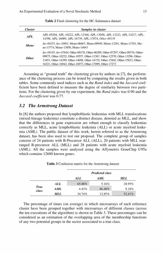
Table 2 Final clustering for the HC-Salamanca dataset
Cluster Samples in cluster
APL APL-05204, APL-10222, APL-12366, APL-13058, APL-13223, APL-14217, APL-14398, APL-16089, APL-16739, APL-17074, Other-00139
Mono Inv-00355, Inv-10891, Mono-06667, Mono-09949, Mono-12361, Mono-13701, Mo-no-13774, Mono-13850, Mono-14043
Other
Inv-00185, Inv-07644, Other-00170, Other-06209, Other-07297, Other-09376, Other-09875, Other-10232, Other-10557, Other-11567, Other-12570, Other-13296, Other-13451, Other-14399, Other-14698, Other-14735, Other-15443, Other-15833, Other-16221, Other-16942, Other-16973, Other-17099, Other-17273
Assuming as “ground truth” the clustering given by authors in [7], the perform-ance of the clustering process can be tested by comparing the results given in both tables. Some commonly used indices such as the Rand index and the Jaccard coef-ficient have been defined to measure the degree of similarity between two parti-tions. For the clustering given by our experiment, the Rand index was 0.90 and the Jaccard coefficient was 0.77.
3.2 The Armstrong Dataset
In [8] the authors proposed that lymphoblastic leukemias with MLL translocations (mixed-lineage leukemia) constitute a distinct disease, denoted as MLL, and show that the differences in gene expression are robust enough to classify leukemias correctly as MLL, acute lymphoblastic leukemia (ALL) or acute myeloid leuke-mia (AML). The public dataset of this work, herein referred to as the Armstrong dataset, has been also used to test our proposal. The complete group of samples consists of 24 patients with B-Precursor ALL (ALL), 20 patients with MLL rear-ranged B-precursor ALL (MLL) and 28 patients with acute myeloid leukemia (AML). All the samples were analyzed using the Affymetrix GeneChip U95a which contains 12600 known genes.
Table 3 Confusion matrix for the Armstrong dataset
Predicted class
ALL AML MLL
ALL 65.88% 5.16% 28.95%
AML 4.42% 86.40% 9.18% True class
MLL 34.74% 12.85% 52.41%
The percentage of times (on average) in which microarrays of each reference cluster have been grouped together with microarrays of different classes (across the ten executions of the algorithm) is shown in Table 3. These percentages can be considered as an estimation of the overlapping area of the membership functions of any two potential groups in the sector associated to a true class.

14 H. Gómez et al.
Table 4 Final clustering for the Armstrong dataset
Cluster Samples in cluster
ALL ALL-01, ALL-02, ALL-04, ALL-05, ALL-06, ALL-07, ALL-08, ALL-09, ALL-10, ALL-11, ALL-12, ALL-13, ALL-14, ALL-15, ALL-16, ALL-17, ALL-18, ALL-19, ALL-20, ALL-58, ALL-59, ALL-60, MLL-25, MLL-32, MLL-34, MLL-62
AML
ALL-03, AML-38, AML-39, AML-40, AML-41, AML-42, AML-43, AML-44, AML-46, AML-47, AML-48, AML-49, AML-50, AML-51, AML-52, AML-53, AML-54, AML-55, AML-56, AML-57, AML-65, AML-66, AML-67, AML-68, AML-69, AML-70, AML-71, AML-72
MLL ALL-61, AML-45, MLL-21, MLL-22, MLL-23, MLL-24, MLL-26, MLL-27, MLL-28, MLL-29, MLL-30, MLL-31, MLL-33, MLL-35, MLL-36, MLL-37, MLL-63, MLL-64
As in the HC-Salamanca dataset, if the highest percentage for each sample determines the cluster of the microarray, the final clustering obtained by our simu-lated annealing-based algorithm is shown in Table 4. As in the previous experi-ment, assuming the clustering given by authors in [8] is the “ground truth”, the Rand index and the Jaccard coefficient for experiments carried out are 0.89 and 0.72, respectively.
4 Discussion
The aim of the experiments reported in the previous section is to test the validity of the proposed clustering method. Dealing with unsupervised classification, it is very difficult to test the ability of a method to perform the clustering since there is no supervision of the process. In this sense, the classification into different groups proposed by the authors in [7, 8] is assumed to be the reference partition of sam-ples in our work. This assumption may be questionable in some cases, since the reference groups are not well established. For example, in the HC-Salamanca dataset the AML with inversion group is established by observation of the karyo-type of cancer cells, but there is no other evidence (biological, genetic) suggesting that this group corresponds to a distinct disease. Even so, the assumption of these prior partitions as reference groups is the only way to evaluate the similarity (or dissimilarity) of the results computed by the proposed method based on existing knowledge. As it turns out, there is no perfect match among the results of our pro-posed method and the reference partitions, but they are compatible with the cur-rent knowledge of each dataset. For example, for the HC-Salamanca dataset the better characterized groups are the APL and Other-AML groups, the worst is the AML with inversion group, and there is some confusion of the monocytic AML with the AML with inversion and Other-AML groups. These results are compati-ble with the state-of-the-art discussed in [7], where the APL group is the better characterized disease (it can be considered as a distinct class), the monocytic AML is a promising disease, the AML with inversion in chromosome 16 is the weaker class, and the Other-AML group acts as the dumping ground for the rest of samples which are not similar enough to the other possible classes. For the
An Experimental Evaluation of a Novel Stochastic Method 15
Armstrong dataset, the AML group is clearly separated from the MLL and ALL groups. It is not surprising since the myeloid leukemia (AML) and lymphoblastic leukaemias (MLL and ALL) represent distinct diseases. Some confusion is present among ALL and MLL groups, but this result is compatible with the assumption (which the authors test in [8]) that the MLL group is a subtype of the ALL disease.
5 Conclusion
The simulated annealing-based algorithm presented in this work is a new algorithm for iterative class discovery that uses fuzzy logic for informative gene selection. An intrinsic advantage of the proposed method is that, assuming the percentage of times in which a given microarray has been grouped with samples of other potential classes, the degree of membership of that microarray to each po-tential group can be deduced. This fact allows a fuzzy clustering of the available microarrays which is more suitable for the current state-of-the-art in gene expres-sion analysis, since it will be very unlikely to state (without uncertainty) that any available microarray only belongs to a unique potential cluster. In this case, the proposed method can help to assess the degree of affinity of each microarray with potential groups and to guide the analyst in the discovery of new diseases.
In addition, the proposed method is also an unsupervised technique for gene se-lection when it is used in conjunction with the concept of discriminant fuzzy pat-tern (DFP) introduced in [9]. Since the selected genes depend on the resulting clustering (they are the genes in the computed DFP obtained from all groups) and the clustering is obtained by maximizing the cost function (which is based on the notion of genetic coherence and assessed by the number of genes in the fuzzy pat-tern of each cluster), then the selected genes jointly depend on all the genes in the microarray, and the proposed method can be also considered a multivariate method for gene selection.
Finally, the proposed technique, in conjunction with our previous developed GENECBR platform [10], represents a more sophisticated tool which integrates three main tasks in expression analysis: clustering, gene selection and classifica-tion. In this context, all the proposed methods are non-parametric (they do not de-pend on assumptions about the underlying distribution of available data), unbiased with regard to the basic computational facility used to construct them (the notion of fuzzy pattern) and with the ability to manage imprecise (and hence, uncertain) information, which is implicit in available datasets in terms of degree of member-ship to linguistic labels (expressions levels, potential categories, etc.).
Acknowledgements
This work is supported in part by the project Development of computational tools for the classification and clustering of gene expression data in order to discover meaningful biological information in cancer diagnosis (ref. VA100A08) from JCyL (Spain).

16 H. Gómez et al.
References
1. Xing, E.P., Karp, R.M.: CLIFF: clustering of high-dimensional microarray data via it-erative feature filtering using normalized cuts. Bioinformatics 17, S306–S315 (2001)
2. Jiang, D., Tang, C., Zhang, A.: Cluster analysis for gene expression data: a survey. IEEE T. Knowl. Data En. 16, 1370–1386 (2004)
3. Ben-Dor, A., Friedman, N., Yakhini, Z.: Class discovery in gene expression data. In: Proceedings of the Fifth Annual International Conference on Computational Biology. ACM, Montreal (2001)
4. von Heydebreck, A., Huber, W., Poustka, A., Vingron, M.: Identifying splits with clear separation: a new class discovery method for gene expression data. Bioinformatics 17, S107–S114 (2001)
5. Tang, C., Zhang, A., Ramanathan, M.: ESPD: a pattern detection model underlying gene expression profiles. Bioinformatics 20, 829–838 (2004)
6. Varma, S., Simon, R.: Iterative class discovery and feature selection using Minimal Spanning Trees. BMC Bioinformatics 5, 126 (2004)
7. Gutiérrez, N.C., López-Pérez, R., Hernández, J.M., Isidro, I., González, B., Delgado, M., Fermiñán, E., García, J.L., Vázquez, L., González, M., San Miguel, J.F.: Gene ex-pression profile reveals deregulation of genes with relevant functions in the different subclasses of acute myeloid leukemia. Leukemia 19, 402–409 (2005)
8. Armstrong, S.A., Staunton, J.E., Silverman, L.B., Pieters, R., den Boer, M.L., Minden, M.D., Sallan, S.E., Lander, E.S., Golub, T.R., Korsmeyer, S.J.: MLL translocations specify a distinct gene expression profile that distinguishes a unique leukemia. Nat. Genet. 30, 41–47 (2002)
9. Díaz, F., Fdez-Riverola, F., Corchado, J.M.: geneCBR: a case-based reasoning tool for cancer diagnosis using microarray data sets. Comput. Intell. 22, 254–268 (2006)
10. Glez-Peña, D., Díaz, F., Hernández, J.M., Corchado, J.M., Fdez-Riverola, F.: ge-neCBR: a translational tool for multiple-microarray analysis and integrative informa-tion retrieval for aiding diagnosis in cancer research. BMC Bioinformatics 10, 187 (2009)

M.P. Rocha et al. (Eds.): IWPACBB 2010, AISC 74, pp. 17–24, 2010. springerlink.com © Springer-Verlag Berlin Heidelberg 2010
Automatic Workflow during the Reuse Phase of a CBP System Applied to Microarray Analysis
Juan F. De Paz, Ana B. Gil, and Emilio Corchado
1
Abstract. The application of information technology in the field of biomedicine has become increasingly important over the last several years. The different possi-bilities for the workflow in the microarray analysis can be huge and it would be very interesting to create an automatic process for establishing the workflows. This paper presents an intelligent dynamic architecture based on intelligent or-ganizations for knowledge data discovery in biomedical databases. The multi-agent architecture incorporates agents that can perform automated planning and find optimal plans. The agents incorporate the CBP-BDI model for developing the automatic planning that makes possible to predict the efficiency of the workflow beforehand These agents propose a new reorganizational agent model in which complex processes are modelled as external services.
Keywords: Multiagent Systems, microarray, Case-based planning.
1 Introduction
The continuous growth of techniques for obtaining cancerous samples, specifically those using microarray technologies, provides a great amount of data. Microarray has become an essential tool in genomic research, making it possible to investigate global genes in all aspects of human disease [4]. Expression arrays [5] contain in-formation about certain genes in a patient’s samples. These data have a high di-mensionality and require new powerful tools.
This paper presents an innovative solution to model reorganization systems in biomedical environments. It is based on a multi-agent architecture that can inte-grate Web services, and incorporates a novel planning mechanism that makes it possible to determine workflows based on existing plans and previous results. The
1 Juan F. De Paz . Ana B. Gil . Emilio Corchado Departamento Informática y Automática Universidad de Salamanca Plaza de la Merced s/n, 37008, Salamanca, Spain e-mail: {fcofds, abg, escorchado}@usal.es

18 J.F. De Paz, A.B. Gil, and E. Corchado
core of the system presented in this paper is a CBP-BDI (Case-based planning) (Belief Desire Intention) agent [3] specifically designed to act as Web services co-ordinator, making it possible to reduce the computational load for the agents in the organization and expedite the classification process. CBP-BDI agents [2] make it possible to formalize systems by using a new planning mechanism that incorpo-rates graph theory as a reasoning engine to generate plans. The system was specifically applied to case studies consisting of the classification of cancers from microarrays. The multi-agent system developed incorporates novel strategies for data analysis and microarray data classification.
The next section describes the expression analysis problem. Section 2 presents a case study consisting of a distributed multi-agent system for cancer detection scenarios. Finally section 3 presents the results and conclusions obtained.
2 Self-Adaptive Multiagent System for Expression Analysis
Nowadays, it is essential to have software solutions that enforce autonomy, ro-bustness, flexibility and adaptability of the system to develop. The dynamic agent organizations that auto-adjust themselves to obtain advantages from their envi-ronment seem to be a technology that is more than suitable for coping with the de-velopment of this type of system. The integration of multi-agent systems with SOA (Service Oriented Architecture) and Web Services approaches has been re-cently explored [7]. Some developments are centered on communication between these models, while others are centered on the integration of distributed services, especially Web Services, into the structure of the agents. [8] Oliva et al. [8] have developed a java-based framework to create SOA and Web Services compliant applications, which are modelled as agents.
The approach presented in this paper is an organizational model for biomedical environments based on a multi-agent dynamic architecture that incorporates agents capable of generating plans for analyzing large amounts of data. The core of the system is a novel mechanism for the implementation of the stages of CBP-BDI mechanisms through Web services that provides a dynamic self-adaptive behaviour to reorganize the environment. The types of agents are distrib-uted in layers within the system according to their functionalities. The agent layers constitute the core and define a virtual organization for massive data analysis:
• Organization: The agents will be responsible for conducting the analysis of information following the CBP-BDI [2] reasoning model. The agents from the organizational layer should be initially configured for the differ-ent types of analysis that will be performed, given that these analyses vary according to the available information and the search results.
• Analysis: The agents in the analysis layer are responsible for selecting the configuration and the flow of services best suited for the problem at hand. They communicate with Web services to generate results. The agents of this layer follow the CBP-BDI [2] reasoning model. The work-flow and configuration of the services to be used is selected with graphs, using information that corresponds to the previously executed plans.

Automatic Workflow during the Reuse Phase of a CBP System 19
• The Controller agent manages the agents available in the different layers of the multiagent system. It allows the registration of agents in the layers, as well as their use in the organization.
• Analysis Services: The analysis services are services used by analysis agents for carrying out different tasks. The analysis services include ser-vices for pre-processing, filtering, clustering and extraction of knowledge.
2.1 Coordinator CBP-BDI Agent
The agents in the analysis layer have the capacity to learn from the analysis car-ried out in previous procedures. They adopt the CBP reasoning model, a speciali-zation of case-based reasoning (CBR) [1]. CBR systems solve new problems by adapting solutions that have been used to solve similar problems in the past, and learning from each new experience. A CBR manages cases (past experiences) to solve new problems. The way cases are managed is known as the CBR cycle, and consists of four sequential phases: retrieve, reuse, revise and retain. CBP is the idea of planning as remembering [2]. In CBP, the solution proposed to solve a given problem is a plan, so this solution is generated by taking into account the plans applied to solve similar problems in the past [6]. The CBP-BDI agents stem from the BDI model [9] and establish a correspondence between the elements from the BDI model and the CBP systems. Fusing the CBP agents together with the BDI model and generating CBP-BDI agents makes it possible to formalize the available information, the definition of the goals and actions that are available for resolving the problem, and the procedure for resolving new problems by adopting the CBP reasoning cycle. Agent plan is the name we give to a sequence of actions that, from a current state e0, defines the path of states through which the agent passes in order to reach the other world state.
))(()()( 0110 eaaeaeep nnnnn ==== − 1aap nn ≡ (1)
Based on this representation, the CBP-BDI coordinator agents combine the initial state of a case, the final state of a case with the goals of the agent, and the inten-tions with the actions that can be carried out in order to create plans that make it possible to reach the final state. The actions that need to be carried out are ser-vices, making a plan an ordered sequence of services. It is necessary to facilitate the inclusion of new services and the discovery of new plans based on existing plans. Services correspond to the actions that can be carried out and that determine the changes in the initial problem data. The plan actions correspond to services and the order in which the actions are applied correspond to the order for execut-ing services. As such, an organizational plan is defined by the services that comprise it and by the order of applying each of those services.
The information corresponding to each plan is represented in bidimensional ar-rays as shown in the chart in figure 1. The chart lists the plans in rows while the colums represent the links between the services that comprise a plan so that Sij
represents the execution of service j occurring after service call i. The second row shows the plan comprised of services a2, a1, with an initial connection S02 that exe-cutes service a2 at the initial stage. The columns for service S2x provide the

20 J.F. De Paz, A.B. Gil, and E. Corchado
connection with the subsequent service, i.e., S21, for which service a1 is executed. Lastly, column S1x executes action S1f.
S01 S02 S21 S23 S2f......S12 S13 S1f...... Si1 Sij Sif......v ......v...... ......
v v ......v...... ......v v......v ...... ......
a1
a2a1
a1a2
Actions/Services
Plan
s v1
v2
v3
Efficiency
Fig. 1 Plans and plan actions carried out through a concatenation of services
Based on the information corresponding to previous experiences (plans already executed) a new plan is generated. To do so, the cases with the greatest and least efficiency with regards to the current problem are retrieved, and the CBP reason-ing cycle is initiated according to the BDI specifications. This way, each plan is represented by the following expression:
{ }))(())(( 0000 eSSeaaaap ikfikf ⋅⋅⋅=⋅⋅⋅= (2)
where e0 represents the initial state that corresponds to the initial value of each probe. As each of the selected services are executed, different states ei, are reached, which contain the new set of probes produced by the application of services.
2.1.1 Retrieve During the retrieval stage, the plans with the greatest and least efficiency are se-lected from among those that have been applied. Microarrays are composed of probes that represent variables that mark the level of significance of specific genes. The retrieval of those cases is performed in one of two ways according to the case study. To retrieve cases, it is important to consider whether there has been a previous analysis of a case study with similar characteristics. If so, the corresponding plans for the same case study are selected.
If there are no plans that correspond to the same case study, or if the number of plans is insufficient, the plans corresponding ot the most similar case study are re-trieved. The selection of the most similar case study is performed according to the cosine distance applied to the following set of variables: Number of probes, Number of cases, Coefficient of the Pearson variation [12] for e0.
The number of efficient and inefficient cases selected is predetermined so that at the end of this stage the following set of elements is obtained:
}},..,{},..,{{ 11in
ii
en
ee ppPppPP ∪= (3)
Pe represents the set of efficient plans and Pi represents the set of inefficient plans. Once the plans have been retrieved, a new efficient plan is generated in the next phase.

Automatic Workflow during the Reuse Phase of a CBP System 21
2.1.2 Reuse This phase takes the plans P obtained in the retrieval phase and generates a new, more efficient plan. The new plan is built according to the efficiency of the actions as estimated by the overall efficiency vi of the plan. Estimating the efficiency of each action is done according to the model defined by the decision trees for select-ing significant nodes [3]. This way, estimating the efficiency of each action is carried out according to the expression (3). This expression is referred to as the winning rate and depends on both node S and the selected attribute B.
∑=
−=t
ii
i SIS
SSIBSG
1
)()(),( (4)
where S represents a node that, in this case, will always be the root node of the
tree, B is the condition for the existing action, iS represents child node i from
node S, iS the number of cases associated with the child node iS . The function
)(SI represents gain and is defined as follows
∑=
⋅−=n
j
Sj
Sj ffSI
1
)log()( (5)
where Sjf represents the frequency relative to class
jC in S , S
SjS
j N
nf = ,
Sjn the
number of elements from class jC in S and SN the total number of elements. In
this case, Cj={efficient, inefficient}. The gain ratio G determines the level of importance for each action by distin-
guishing between an efficient and an inefficient plan. High values for the gain ra-tio indicate that the action should be included in a plan if it involves an action to be carried out in an efficient plan, otherwise it should be eliminated.
A new table listing gain data is formed according to the values of the gain ratio and the efficiency associated with each plan. A new flow of execution for each action is created from the gains table. The gains uses the following formula to establish a value for the significance of each of the actions carried out in each plan:
kijij vSSGkST ⋅= ),('),( (6)
where G´ contains the values of G that are normalized between 0 and 1 with the values being inverted (the maximum value corresponds to 0 and the minimum to 1) and v contains the average value of efficiency for the plans with a connection ij. Each connection ij presents an influence in the final efficiency of the plan that
is represented as ijkt .
Once the graph for the plans has been constructed, the minimal route that goes from the start node to the end node is calculated. In order to calculate the

22 J.F. De Paz, A.B. Gil, and E. Corchado
shortest/longest route, the Dijkstra algorithm is applied since there are implemen-tations for the order n*log n. To apply this algorithm, it is necessary to add to each of the edges the absolute value of the edge with a higher negative absolute value, in order to remove from the graph those edges with negative values.
2.1.3 Revise and Retain The revise phase is carried out automatically according to the final efficiency ob-tained. The different analyses are associated with different measures of efficiency that measure the final quality of the results obtained, making it unnecessary to per-form a manual revision. During the retain phase, the plan is stored in the memory of plans. If a plan with the same flow of execution of services for the same case study already exists, only the information from the plan with the highest quality will be stored. This makes it possible to limit the size of the case memory and select only those plans with certain parameters such as level of significance, correlation coefficient, percentile, etc.
3 Results and Conclusions
This paper has presented a self-adaptive organization based on a multiagent archi-tecture and its application to a real problem. In 2006, there were approximately 64,122 men and women alive in the United States who had a history of cancer of the stomach: 36,725 men and 27,397 women. The age-adjusted incidence rate was 7.9 per 100,000 men and women per year while the fatality rate was 4.0 per 100,000 [11]. The data for gastric cancer were obtained with a HG U133 plus 2.0 chip and corresponded to 234 patients affected by this cancer in 3 different parts of the organism (primary gastric cancer, skin and others) [10]. The data were obtained from a public repository at http://www.ebi.ac.uk.
The experiment consisted of evaluating the services distribution system in the filtering agent for the case study that classified patients affected by different types of cancer. According to the identification of the problem described in table 1, the filtering agent selected the plans with the greatest efficiency, considering the different execution workflows for the services that are in the plans.
The filtering agent in the analysis layer selects the configuration parameters be-tween a specific set of pre-determined values, when it has been told to explore the parameters. Otherwise, for a specific plan, it selects the values that have provided better results based on the measure of the previously established efficiency. The different configurations used are listed in table 1. A depth analysis of these tech-niques can be found in our previous work [10]. The last columns of the table list the final efficiency obtained based a measure and the type of plan (efficient or in-efficient). A value of 1 in the Class column indicates that the plan is efficient while a 0 indicates that the plan is inefficient. The remaining value indicates the order of execution of the services.
Automatic Workflow during the Reuse Phase of a CBP System 23
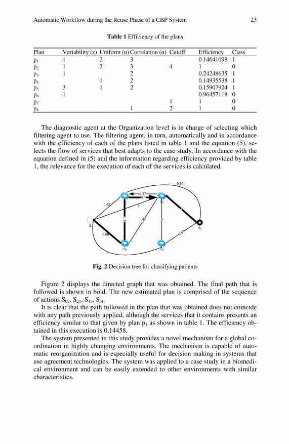
Table 1 Efficiency of the plans
Plan Variability (z) Uniform (α) Correlation (α) Cutoff Efficiency Class p1 1 2 3 0.14641098 1 p2 1 2 3 4 1 0 p3 1 2 0.24248635 1 p4 1 2 0.14935538 1 p5 3 1 2 0.15907924 1 p6 1 0.96457118 0 p7 1 1 0 p8 1 2 1 0
The diagnostic agent at the Organization level is in charge of selecting which
filtering agent to use. The filtering agent, in turn, automatically and in accordance with the efficiency of each of the plans listed in table 1 and the equation (5), se-lects the flow of services that best adapts to the case study. In accordance with the equation defined in (5) and the information regarding efficiency provided by table 1, the relevance for the execution of each of the services is calculated.
S1
S2
S3
S0 Sf
S4
0.14
0.25
0.1
1
0
0.68
0.52
0.37
0.95
1
1
0.06
Fig. 2 Decision tree for classifying patients
Figure 2 displays the directed graph that was obtained. The final path that is followed is shown in bold. The new estimated plan is comprised of the sequence of actions S02, S21, S13, S3f.
It is clear that the path followed in the plan that was obtained does not coincide with any path previously applied, although the services that it contains presents an efficiency similar to that given by plan p1 as shown in table 1. The efficiency ob-tained in this execution is 0.14458.
The system presented in this study provides a novel mechanism for a global co-ordination in highly changing environments. The mechanism is capable of auto-matic reorganization and is especially useful for decision making in systems that use agreement technologies. The system was applied to a case study in a biomedi-cal environment and can be easily extended to other environments with similar characteristics.

24 J.F. De Paz, A.B. Gil, and E. Corchado
Acknowledgments. This development has been partially supported by the projects JCyL SA071A08, of the Junta of Castilla and León (JCyL): [BU006A08], the project of the Span-ish Ministry of Education and Innovation [CIT-020000-2008-2] and [CIT-020000-2009-12], and Grupo Antolin Ingenieria, S.A., within the framework of project MAGNO2008 - 1028.- CENIT also funded by the same Government Ministry.
References
[1] Kolodner, J.: Case-Based Reasoning. Morgan Kaufmann, San Francisco (1993) [2] Glez-Bedia, M., Corchado, J.: A planning strategy based on variational calculus for
deliberative agents. Computing and Information Systems Journal 10(1), 2–14 (2002) [3] Kohavi, R., Ross Quinlan, R.: Decision Tree Discovery Handbook of Data Mining
and Knowledge Discovery, pp. 267–276. Oxford University Press, Oxford (2002) [4] Quackenbush, J.: Computational analysis of microarray data. Nature Review Genet-
ics 2(6), 418–427 (2001) [5] Affymetrix,
http://www.affymetrix.com/support/technical/datasheets/ hgu133arrays_datasheet.pdf
[6] Corchado, J.M., Bajo, J., De Paz, Y., Tapia, D.I.: Intelligent Environment for Moni-toring Alzheimer Patients, Agent Technology for Health Care. Decision Support Sys-tems 44(2), 382–396 (2008)
[7] Ardissono, L., Petrone, G., Segnan, M.: A conversational approach to the interaction with Web Services. Computational Intelligence, vol. 20, pp. 693–709. Blackwell Pub-lishing, Malden (2004)
[8] Oliva, E., Natali, A., Ricci, A., Viroli, M.: An Adaptation Logic Framework for {J}ava-based Component Systems. Journal of Universal Computer Science 14(13), 2158–2181 (2008)
[9] Bratman, M.: Intention, Plans and Practical Reason. Harvard U.P., Cambridge (1987) [10] Corchado, J.M., De Paz, J.F., Rogríguez, S., Bajo, J.: Model of experts for decision
support in the diagnosis of leukemia patients. Artificial Intelligence in Medi-cine 46(3), 179–200 (2009)
[11] Horner, M.J., Ries, L.A.G., Krapcho, M., Neyman, N., Aminou, R., Howlader, N., Altekruse, S.F., Feuer, E.J., Huang, L., Mariotto, A., Miller, B.A., Lewis, D.R., Eis-ner, M.P., Stinchcomb, D.G., Edwards, B.K. (eds.): SEER Cancer Statistics Review, 1975-2006, National Cancer Institute (2009),
http://seer.cancer.gov/csr/1975_2006/ [12] Kuo, C.D., Chen, G.Y., Wang, Y.Y., Hung, M.J., Yang, J.L.: Characterization and
quantification of the return map of RR intervals by Pearson coefficient in patients with acute myocardial infarction. Autonomic Neuroscience 105(2), 145–152 (2003)

M.P. Rocha et al. (Eds.): IWPACBB 2010, AISC 74, pp. 25–32, 2010. springerlink.com © Springer-Verlag Berlin Heidelberg 2010
A Comparative Study of Microarray Data Classification Methods Based on Ensemble Biological Relevant Gene Sets
Miguel Reboiro-Jato, Daniel Glez-Peña, Juan Francisco Gálvez, Rosalía Laza Fidalgo, Fernando Díaz, and Florentino Fdez-Riverola
1
Abstract. In this work we study the utilization of several ensemble alternatives for the task of classifying microarray data by using prior knowledge known to be bio-logically relevant to the target disease. The purpose of the work is to obtain an accurate ensemble classification model able to outperform baseline classifiers by introducing diversity in the form of different gene sets. The proposed model takes advantage of WhichGenes, a powerful gene set building tool that allows the auto-matic extraction of lists of genes from multiple sparse data sources. Preliminary results using different datasets and several gene sets show that the proposal is able to outperform basic classifiers by using existing prior knowledge.
Keywords: microarray data classification, ensemble classifiers, gene sets, prior knowledge.
1 Introduction and Motivation
The advent of microarray technology has become a fundamental tool in genomic research, making it possible to investigate global gene expression in all aspects of human disease. In particular, cancer genetics based on the analysis of cancer geno-types, provides a valuable alternative to cancer diagnosis in both theory and prac-tice [1]. In this context, the automatic classification of cancer patients has been a
1 Miguel Reboiro-Jato . Daniel Glez-Peña . Juan Francisco Gálvez . Rosalía Laza Fidalgo . Florentino Fdez-Riverola ESEI: Escuela Superior de Ingeniería Informática, University of Vigo, Edificio Politécnico, Campus Universitario As Lagoas s/n, 32004, Ourense, Spain e-mail: {mrjato, dgpena, galvez, rlaza, riverola}@uvigo.es
Fernando Díaz EUI: Escuela Universitaria de Informática, University of Valladolid, Plaza Santa Eulalia, 9-11, 40005, Segovia, Spain e-mail: [email protected]
26 M. Reboiro-Jato et al.
promising approach in cancer diagnosis since the early detection and treatment can substantially improve the survival rates. For this task, several computational methods (statistical and machine learning) have been proposed in the literature including linear discriminant analysis (LDA), Naïve-Bayes classifier (NBC), learning vector quantization (LVQ), radial basis function (RBF) networks, deci-sion trees, probabilistic neural networks (PNNs) and support vector machines (SVMs) among others [2]. In the same line, but following the assumption that a classifier ensemble system is more robust than an excellent single classifier [3], some researchers have also successfully applied different classifier ensemble sys-tems to deal with the classification of microarray datasets [4].
In addition to predictive performance, there is also hope that microarray studies uncover molecular disease mechanisms. However, in many cases the molecular signatures discovered by the algorithms are unfocused form a biological point of view [5]. In fact, they often look more like random gene lists than biologically plausible and understandable signatures. Another shortcoming of standard classi-fication algorithms is that they treat gene-expression levels as anonymous attrib-utes. However, a lot is known about the function and the role of many genes in certain biological processes.
Although numerical analysis of microarray data is considerable consolidated, the true integration of numerical analysis and biological knowledge is still a long way off [6]. The inclusion of additional knowledge sources in the classification process can prevent the discovery of the obvious, complement a data-inferred hy-pothesis with references to already proposed relations, help analysis to avoid over-confident predictions and allow us to systematically relate the analysis findings to present knowledge [7]. In this work we would like to incorporate relevant gene sets obtained from WhichGenes [8] in order to make predictions easy to interpret in concert with incorporated knowledge. The study carried out aims to borrow information from existing biological knowledge to improve both predictive accuracy and interpretability of the resulting classifiers.
The rest of the paper is structured as follows: Section 2 presents a brief review about the use of ensemble methods for classifying microarray data. Section 3 de-scribes the selected datasets and base classifiers for the current study, together with the choice of gene sets and the different approaches used for ensemble creation. Finally Section 4 discusses the reported results and concludes the paper.
2 Related Work
Although much research has been performed on applying machine learning tech-niques for microarray data classification during the past years, it has been shown that conventional machine learning techniques have intrinsic drawbacks in achiev-ing accurate and robust classifications. In order to obtain more robust microarray data classification techniques, several authors have investigated the benefits of this approach applied to genomic research.
Díaz-Uriarte and Alvarez de Andrés [9] investigated the use of random forest for multi-class classification of microarray data and proposed a new method of gene selection in classification problems based on random forest. Using simulated

A Comparative Study of Microarray Data Classification Methods 27
and real microarray datasets the authors showed that random forest can obtain comparable performance to other methods, including DLDA, KNN, and SVM.
Peng [10] presented a novel ensemble approach based on seeking an optimal and robust combination of multiple classifiers. The proposed algorithm begins with the generation of a pool of candidate base classifiers based on the gene sub-sampling and then, it performs the selection of a sub-set of appropriate base classi-fiers to construct the classification committee based on classifier clustering. Experimental results demonstrated that the proposed approach outperforms both baseline classifiers and those generated by bagging and boosting.
Liu and Huang [11] applied Rotation Forest to microarray data classification using principal component analysis, non-parametric discriminant analysis and random projections to perform feature transformation in the original rotation forest. In all the experiments, the authors reported that the proposed approach outperformed bagging and boosting alternatives.
More recently, Liu and Xu [12] proposed a genetic programming approach to analyze multiclass microarray datasets where each individual consists of a set of small-scale ensembles containing several trees. In order to guarantee high diver-sity in the individuals a greedy algorithm is applied. Their proposal was tested using five datasets showing that the proposed method effectively implements the feature selection and classification tasks.
As a particular case in the use of ensemble systems, ensemble feature selection represents an efficient method proposed in [13] which can also achieve high clas-sification accuracy by combining base classifiers built with different feature sub-sets. In this context, the works of [14] and [15] study the use of different genetic algorithms alternatives for performing feature selection with the aim of making classifiers of the ensemble disagree on difficult cases. Reported results on both cases showed improvements when compared against other alternatives.
Related with previous work, the aim of this study is to validate the superiority of different classifier ensemble approaches when using prior knowledge in the form of biological relevant gene sets. The objective is to improve the predictive performance of baseline classifiers.
3 Comparative Study
In order to carry out the comparative study, we apply several ensemble alternatives to classify three DNA microarray datasets involving various tumour tissue samples. With the goal of validate the study, we analyze the performance of different base-line classifiers and test our hypothesis using two different sources of information.
3.1 Datasets and Base Classifiers
We carry out the experimentation using three public leukemia datasets taken from the previous studies of Gutiérrez et al [16], Bullinger et al [17] and Valk et al [18]. We have selected samples from each dataset belonging to 4 different groups of acute myeloid leukemias including (i) promyelocytic (APL), (ii) inversion 16, (iii) monocytic and (iv) other AMLs. The distribution of samples is showed in Table 1.

28 M. Reboiro-Jato et al.
Table 1 Distribution of microarray data samples belonging to the public datasets analyzed
APL Inv(16) Monocytic Other Gutiérrez et al 10 4 7 22 Bullinger et al 19 14 64 177 Valk et al 7 10 7 51
In order to compare the performance obtained by the different ensemble ap-proaches, we have selected four well-known classification algorithms: (i) Naïve Bayes (NB) learner is perhaps the most widely used method. Although its inde-pendence assumption is over-simplistic, studies have found NB to be very effec-tive in a wide range of problems; (ii) IB3 represents a variant of the well-known nearest neighbour algorithms implementing a simple version of a lazy learner classifier; (iii) Support Vector Machines (SVMs) constitute a famous family of algorithms used for classification and regression purposes. Their mayor advantage is that their learning capacity does not degrade even if many characteristics exist, being especially applicable to microarray data; (iv) Random Forest (RFs) is a basic ensemble classifier that consists of many decision trees. The method combines bagging idea and random selection of features in order to construct a collection of decision trees with controlled variation.
3.2 Biological Knowledge Gene Sets
For the prior selection of gene sets that represent explicit information available the fol-lowing sources of information have been used: (i) 33 metabolic sub-pathways related to existing cancers in SABiosciences (http://www.sabiosciences.com) previously analyzed in studies by [19] and [20] plus 4 groups extracted from the OMIM (Online Mendelian Inheritance in Man) database (http://www.ncbi.nlm.nih.gov/sites/entrez?db=omim) that correspond to various types of leukemia (myeloid, monocytoid, promyelocytic and general leukemia) and (ii) those pathways from KEGG (Kyoto Encyclopedia of Genes and Genomes) database grouped in both ‘environmental information processing’ and ‘genetic information processing’ categories.
3.3 Ensemble Alternatives
According to Kuncheva [3], several ensembles can be built by introducing varia-tions at four different levels: (i) data level, (ii) feature level, (iii) classifier level and (iv) combination level.
First of all, by using different data subsets at data level or different feature sub-sets at feature level, the space of the problem can be divided into several areas where base classifiers can be trained. This divide-and-conquer strategy can sim-plify the problem, leading to improved performance of the base classifiers. Secondly, at classifier level, different types of classifiers can be used in order to take advantage of the strong points of each classifier type. Although many ensem-ble paradigms employ the same classification model, there is no evidence that one strategy is better than the other [3]. Finally, combination level groups the different ways of combining the classifier decisions.
A Comparative Study of Microarray Data Classification Methods 29 In this study, base classifiers are trained with all the samples in each data set, so
no work is performed at data level. The feature level is carried out by incorporat-ing gene set data to the ensemble models. Each pathway or group of genes is used as a feature selection, so microarray data will be filtered to keep only the expres-sion level of those genes belonging to some group before training base classifiers.
In order to construct the final ensemble, our approach consists on two sequen-tial steps: (i) classifier selection, in which each simple classifier is initially trained with each gene set following a stratified 10-fold cross-validation process for esti-mating its performance and (ii) classifier training, where the selected pairs of simple_classifier/gene_set are trained with the whole data set. All the different strategies proposed in this study for the selection of promising classifiers are based on the value of the kappa statistic obtained for each simple_classifier/gene_set pair in the first step. The proposed heuristics are the following:
• All classifiers [AC]: every simple_classifier/gene_set pair is used for constructing the final ensemble.
• All gene sets [AG]: for each gene set, the simple_classifier/gene_set pair with best kappa value is selected for constructing the final ensemble.
• Best classifiers without type [BCw/oT_%]: a global threshold is calcu-lated as a percentage of the best kappa value obtained by the winner sim-ple_classifier/gene_set pair. Those pairs with a kappa value equal or higher than the computed threshold are selected.
• Best classifier by type [BCbyT_%]: as in the previous heuristic a given threshold is calculated, but in this case there is a threshold for each simple classifier type.
The form in which the final output of the ensemble is calculated is also based on the kappa statistic. The combination approach used on for the proposed ensembles is a weighted majority vote where the weight of each vote is the corresponding classifier’s kappa value.
4 Experimental Results and Discussion
In order to evaluate the heuristics defined in the previous section, a comparative study was carried out using two different sources of information (OMIM and KEGG) in order to classify 392 samples belonging to four classes coming from three real data sets. In addition, the four simple base classifiers used for the ensemble generation (IB3, NBS, RF, SVM) where also tested individually, using as feature selection both those genes included in the OMIM gene sets plus those genes being part of the KEGG gene sets. Classification tests were performed using a stratified 10-fold cross-validation. Tables 2 and 3 summarize the results obtained from the experimentation carried out showing only those classifiers with better performance.
Table 2 presents the accuracy and kappa values achieved by each classifier us-ing KEGG gene sets as prior knowledge. As it can be observed, BCbyT heuristic generally exhibits good performance regardless of the data set. Additionally, BCw/oT heuristic also showed good performance, although in the Gutiérrez data set two single classifiers (IB3 and NBS) performed better than ensembles using this strategy.

30 M. Reboiro-Jato et al.
Table 2 Classification result using KEGG gene sets
Gutiérrez Bullinger Valk Classifier
Accuracy Kappa Accuracy Kappa Accuracy Kappa
AC 76,74% 0,588 76,00% 0,292 76,28% 0,503
AG 79,07% 0,634 76,00% 0,299 75,18% 0,533
BCbyT_90% 81,40% 0,724 82,67% 0,373 77,01% 0,540
BCbyT_95% 83,72% 0,724 82,67% 0,329 78,83% 0,574
BCw/oT_60% 79,07% 0,635 80,00% 0,476 77,37% 0,556
BCw/oT_75% 79,07% 0,635 81,33% 0,367 76,64% 0,555
BCw/oT_85% 76,74% 0,612 80,00% 0,403 75,55% 0,546
IB3 83,72% 0,756 69,33% 0,369 67,52% 0,410
NBS 81,40% 0,679 73,33% 0,269 74,09% 0,530
RF 72,09% 0,533 68,00% 0,123 69,71% 0,337
SVM 51,16% 0,000 68,00% 0,000 64,60% 0,000
Table 3 Classification result using OMIM gene sets
Gutiérrez Bullinger Valk Classifier Accuracy Kappa Accuracy Kappa Accuracy Kappa
AC 76,74% 0,588 76,00% 0,343 74,82% 0,439 AG 76,74% 0,588 76,00% 0,343 76,28% 0,506 BCbyT_90% 81,40% 0,680 82,67% 0,569 75,91% 0,528 BCbyT_95% 86,05% 0,774 82,67% 0,569 75,91% 0,513 BCw/oT_60% 81,40% 0,680 80,00% 0,483 75,91% 0,521 BCw/oT_75% 88,37% 0,809 81,33% 0,526 75,91% 0,530 BCw/oT_85% 79,07% 0,672 80,00% 0,482 76,28% 0,555 IB3 76,74% 0,643 73,33% 0,451 67,52% 0,391 NBS 79,07% 0,634 76,00% 0,370 72,99% 0,510 RF 79,07% 0,658 74,67% 0,372 74,09% 0,420 SVM 51,16% 0,000 68,00% 0,000 77,74% 0,539
Table 3 presents the same experimentation but using the OMIM gene sets. Once again, BCbyT heuristic achieved good performance. Comparing its behav-iour against single classifiers, performance of ensembles is even better than in the previous experimentation (using KEGG gene sets). BCw/oT heuristic also per-forms better with the OMIM gene set, being slightly superior to BCbyT heuristic. Ensembles using this strategy not only performed better than single classifiers, but also achieved the best kappa value in two of the three analyzed data sets.
To sum up, we can conclude that BCbyT heuristic performed as the best base classifier selection strategy, followed closely by BCw/oT heuristic. This fact backs up the following ideas: (i) depending on the data set there is not a single classifier able to achieve good performance in concert with the supplied knowledge and (ii) the presence of each classifier type in the final ensemble may improve the classification performance.
Regardless of the data set both BCw/oT and BCbyT heuristics behave uniformly performing better than single baseline classifiers. This circumstance

A Comparative Study of Microarray Data Classification Methods 31
confirms the fact that ensembles generally perform better than single classifiers, in this case, by taking advantage of using prior structured knowledge.
Acknowledgements. This work is supported in part by the project MEDICAL-BENCH: Platform for the development and integration of knowledge-based data mining techniques and their application to the clinical domain (TIN2009-14057-C03-02) from Ministerio de Ciencia e Innovación (Spain). D. Glez-Peña acknowledges Xunta de Galicia (Spain) for the program Ángeles Álvariño.
References
1. Golub, T.R., Slonim, D.K., Tamayo, P., Huard, C., Gaasenbeek, M., Mesirov, J.P., Coller, H., Loh, M.L., Downing, J.R., Caligiuri, M.A., Bloomfield, C.D., Lander, E.S.: Molecular classification of cancer: class discovery and class prediction by gene ex-pression monitoring. Science 286, 531–537 (1999)
2. Ressom, H.W., Varghese, R.S., Zhang, Z., Xuan, J., Clarke, R.: Classification algo-rithms for phenotype prediction in genomics and proteomics. Frontiers in Biosci-ence 13, 691–708 (2008)
3. Kuncheva, L.I.: Combining Pattern Classifiers: Methods and Algorithms. Wiley Inter-science, Hoboken (2004)
4. Liu, K.H., Li, B., Wu, Q.Q., Zhang, J., Du, J.X., Liu, G.Y.: Microarray data classifica-tion based on ensemble independent component selection. Computers in Biology and Medicine 39(11), 953–960 (2009)
5. Lottaz, C., Spang, R.: Molecular decomposition of complex clinical phenotypes using biologically structured analysis of microarray data. Bioinformatics 21(9), 1971–1978 (2005)
6. Cordero, F., Botta, M., Calogero, R.A.: Microarray data analysis and mining ap-proaches. Briefings in Functional Genomics and Proteomics 6(4), 265–281 (2007)
7. Bellazzi, R., Zupan, B.: Methodological Review: Towards knowledge-based gene ex-pression data mining. Journal of Biomedical Informatics 40(6), 787–802 (2007)
8. Glez-Peña, D., Gómez-López, G., Pisano, D.G., Fdez-Riverola, F.: WhichGenes: a web-based tool for gathering, building, storing and exporting gene sets with applica-tion in gene set enrichment analysis. Nucleic Acids Research 37(Web Server issue), W329–W334 (2009)
9. Díaz-Uriarte, R., Alvarez de Andrés, S.: Gene selection and classification of microar-ray data using random forest. BMC Bioinformatics 7, 3 (2006)
10. Peng, Y.: A novel ensemble machine learning for robust microarray data classification. Computers in Biology and Medicine 36(6), 553–573 (2006)
11. Liu, K.H., Huang, D.S.: Cancer classification using Rotation Forest. Computers in Bi-ology and Medicine 38(5), 601–610 (2008)
12. Liu, K.H., Xu, C.G.: A genetic programming-based approach to the classification of multiclass microarray datasets. Bioinformatics 25(3), 331–337 (2009)
13. Opitz, D.: Feature selection for ensembles. In: Proceedings of 16th National Confer-ence on Artificial Intelligence, Orlando, Florida (1999)
14. Kuncheva, L.I., Jain, L.C.: Designing classifier fusion systems by genetic algorithms. IEEE Transactions on Evolutionary Computation 4(4), 327–336 (2000)

32 M. Reboiro-Jato et al.
15. Oliveira, L.S., Morita, M., Sabourin, R.: Feature selection for ensembles using the multi-objective optimization approach. Studies in Computational Intelligence 16, 49–74 (2006)
16. Gutiérrez, N.C., López-Pérez, R., Hernández, J.M., Isidro, I., González, B., Delgado, M., Fermiñán, E., García, J.L., Vázquez, L., González, M., San Miguel, J.F.: Gene ex-pression profile reveals deregulation of genes with relevant functionsin the different subclasses of acute myeloid leukemia. Leukemia 19(3), 402–409 (2005)
17. Bullinger, L., Döhner, K., Bair, E., Fröhling, S., Schlenk, R.F., Tibshirani, R., Döhner, H., Pollack, J.R.: Use of gene-expression profiling to identify prognostic subclasses in adult acute myeloid leukemia. The New England Journal of Medicine 350(16), 1506–1516 (2004)
18. Valk, P.J., Verhaak, R.G., Beijen, M.A., Erpelinck, C.A., Barjesteh van Waalwijk van Doorn-Khosrovani, S., Boer, J., Beverloo, H., Moorhouse, M., van der Spek, P., Löwenberg, B., Delwel, R.: Prognostically useful gene-expression profiles in Acute Myeloid Leukemia. The New England Journal of Medicine 350(16), 1617–1628 (2004)
19. Tai, F., Pan, W.: Incorporating prior knowledge of predictors into penalized classifiers with multiple penalty terms. Bioinformatics 23(14), 1775–1782 (2007)
20. Wei, Z., Li, H.: Nonparametric pathway-based regression models for analysis of ge-nomic data. Biostatistics 8(2), 265–284 (2007)

Predicting the Start of Proteinα-Helices Using Machine LearningAlgorithms
Rui Camacho, Rita Ferreira, Natacha Rosa, Vania Guimaraes,Nuno A. Fonseca, Vıtor Santos Costa, Miguel de Sousa,and Alexandre Magalhaes
1 Introduction
Proteins are complex structures synthesised by living organisms. They areactually a fundamental type of molecules and can perform a large number offunctions in cell biology. Proteins can assume catalytic roles and accelerate orinhibit chemical reactions in our body. They can assume roles of transporta-tion of smaller molecules, storage, movement, mechanical support, immunityand control of cell growth and differentiation [25]. All of these functions relyon the 3D-structure of the protein. The process of going from a linear se-quence of amino acids, that together compose a protein, to the protein’s 3Dshape is named protein folding. Anfinsen’s work [29] has proven that primarystructure determines the way protein folds. Protein folding is so importantthat whenever it does not occur correctly it may produce diseases such asAlzheimer’s, Bovine Spongiform Encephalopathy (BSE), usually known asmad cows disease, Creutzfeldt-Jakob (CJD) disease, a Amyotrophic LateralSclerosis (ALS), Huntingtons syndrome, Parkinson disease, and other diseasesrelated to cancer.
A major challenge in Molecular Biology is to unveil the process of proteinfolding. Several projects have been set up with that purpose. Although proteinfunction is ultimately determined by their 3D structure there have been identi-fied a set of other intermediate structures that can help in the formation of the
Rui Camacho · Rita Ferreira · Natacha Rosa · Vania GuimaraesLIAAD & Faculdade de Engenharia da Universidade do Porto, Portugal
Nuno A. Fonseca · Vıtor Santos CostaCRACS-INESC Porto LA, Portugal
Vıtor Santos CostaDCC-Faculdade de Ciencias da Universidade do Porto, Portugal
Miguel de Sousa · Alexandre MagalhaesREQUIMTE/Faculdade de Ciencias da Universidade do Porto, Portugal
M.P. Rocha et al. (Eds.): IWPACBB 2010, AISC 74, pp. 33–41, 2010.springerlink.com c© Springer-Verlag Berlin Heidelberg 2010

34 R. Camacho et al.
3D structure. We refer the reader to Section 2 for a more detailed descriptionof protein structure. To understand the high complexity of protein folding itis usual to follow a sequence of steps. One starts by identifying the sequence ofamino acids (or residues) that compose the protein, the so-called primary struc-ture; then we identify the secondary structures made of α-helices and β-sheet;and then we predict the tertiary structure or 3D shape.
In this paper we address the step of predicting α-helices (parts of thesecondary structure) based on the sequence of amino acids that compose aprotein. More specifically, in this study we have built models to predict thestart of α-helices. We have applied Machine Learning to construct such mod-els. We have collected the sequences of 1499 proteins from the PDB and haveassembled data sets that were further used by Machine Learning algorithmsto construct the models. We have applied rule induction algorithms, deci-sion trees, functional trees, Bayesian methods, and ensemble methods. Wehave achieved a 84.4% accuracy and were able to construct some small andintelligible models.
The rest of the paper is organised as follows. Section 2 gives basic defini-tions on proteins required to understand the reported work. Related work isreported in Section 3. Our experiments, together with the results obtained,are presented in Section 4. Conclusions are presented in Section 5.
2 Proteins
Proteins are build up of amino acids, connect by peptide bonds betweenthe carboxyl and amino groups of adjacent amino acid residues as shown inFigure 1b) [24]. All amino acids have common structural characteristics thatinclude an α carbon to which are connected an amino group and a carboxylgroup, an hydrogen and a variable side chain as shown in Figure 1 a). It isthe side chain that determines the identity a specific amino acid. There are20 different amino acids that integrate proteins in cells. Once the amino acidsare connected in the protein chain they are designated as residues.
Fig. 1 a) General Structure of an amino acid; side chain is represented by theletter R. b) A fraction of a proteic chain, showing the peptide bounds
In order to function in an organism a protein has to assume a certain 3Dconformation. To achieve those conformations apart from the peptide bondsthere have to be extra types of weaker bonds between side chains. These extrabonds are responsible for the secondary and tertiary structure of a protein [28].

Predicting the Start of Protein α-Helices 35
Fig. 2 Secondary structure con-formations of a protein: α-helices(left); β-sheet (right)
One can identify four types of struc-tures in a protein. The primary structureof a protein corresponds to the linear se-quence of residues. The secondary struc-ture is composed by subsets of residues ar-ranged as α-helices and β-sheets, as seenin Figure 2. The tertiary structure resultsfor the folding of α-helices or β-sheets.The quaternary structure results from theinteraction of two or more polypeptidechains.
Secondary structures, α-helices and β-sheets, were discovered in 1951 byLinus Carl Pauling. These secondary structures are obtained due to the flexi-bility of the peptide chain that can rotate over three different chemical bonds.Most of the existing proteins have approximately 70% of their structure ashelices that is the most common type of secondary structure.
3 Related Work
Arguably, protein structure prediction is a fundamental problem in Bioin-formatics. Early work by Chou et al. [26], based on single residue statistics,looked for contiguous regions of residues that have an high probability ofbelonging to a secondary structure. The protein samples used was very smallwhich resulted in an overestimation in accuracy of the reported study.
Qian et al [23] used neural networks to predict secondary structures butachieved an accuracy of only 64.3%. They used a window (of size 13) tech-nique where the secondary structure of the central residues was predicted onthe base of its 12 neighbours.
Rost and Sanderwith used the PHD [3] method on the RS126 data set andachieved an accuracy of 73.5%. JPRED [14], exploiting multiple sequence align-ments, got an accuracy of 72.9%. NNSSP [1] is a scored nearest neighbourmethod by considering position of N and C terminal in α-helices and β-strands.Its prediction accuracy for RS126 data set achieved 72.7%. PREDATOR [7]used propensity values for seven secondary structures and local sequence align-ment. The prediction accuracy of this method for RS126 data set achieved70.3%. PSIPRED [8] used a position-specific scoring matrix generated by PSI-BLAST to predict protein secondary structure and achieved 78.3. DSC [18]used amino acid profile, conservation weights, indels, hydrophobicity wereexploited to achieve 71.1% prediction accuracy in the RS126 data set.
Using a Inductive Logic Programming (ILP) another series of studiesimproved the secondary structure prediction score. In 1990 Muggleton etal. [21] used only 16 proteins (in contrast with 1499 used in our study)and the GOLEM [22] ILP system to predict if a given residue in a givenposition belongs or not to an α-helix. They achieved an accuracy of 81%.

36 R. Camacho et al.
Previous results have been reported by [9] using Neural Networks but achiev-ing only 75% accuracy. The propositional learner PROMIS[17, 30] achieved73% accuracy on the GOLEM’s data set.
It has been shown that the helical occurrence of the 20 type of residues ishighly dependent on the location, with a clear distinction between N-terminal,C-terminal and interior positions [16]. The computation of amino acid propen-sities may be a valuable information both for pre-processing the data and forassessing the quality of the constructed models [10]. According to Blader etal. [4] an important influencing factor in the propensity to form α-helicesis the hydrophobicity of the side-chain. Hydrophobic surfaces turn into theinside of the chain giving a strong contribution to the formation of α-helices.It is also known that the protein surrounding environment has influence inthe formation of α-helices. Modelling the influence of the environment inthe formation of α-helices, although important, is very complex from a dataanalysis point of view [19].
4 Experiments
4.1 Experimental Settings
To construct models to predict the start of α-helices we have proceeded asfollows. We first downloaded a list of low homology proteins from the Dunbrakweb site [12]1. The downloaded list contained 1499 low homology proteins. Wethen downloaded the PDBs2 for each of the protein in the list. Each PDBwas then processed in order to extract secondary structure information andthe linear sequence of residues of the protein.
Each example of a data set is a sequence of a fixed number of residues(window) before and after the start or end of a secondary structure. Thewindow size is fixed for each data set and we have produced 4 data sets using4 different window sizes. To obtain the example sequences to use we selectedsequences such that they are:
1. at the start of a α-helix;2. at the end of a α-helix;3. in the interior of a α-helix;4. at the start of a β-strand;5. at the end of a β-strand;6. in the interior of a β-helix.
To do so, we identify the “special” point where the secondary structures startor end, and then add W residues before and after that point. Therefore thesequences are of size 2 ×W + 1, where W ∈ [2, 3, 4, 5]. In the interior of asecondary structure we just pick sequences of 2×W + 1 residues that do notoverlap. With these sequences we envisage to study the start, interior and1 http://dunbrack.fccc.edu/Guoli/PISCES.php2 http://www.rcsb.org/pdb/home/home.do

Predicting the Start of Protein α-Helices 37
end of secondary structures. In this paper, however, we just address the firststep of the study, namely, we focus on the start of α-helices.
The size of the data sets, for the different window sizes, are shown inTable 1.
Table 1 Characterisation of the four data sets according to the window size
Window size 2 3 4 5
Data set size 62053 49243 40529 34337
Number of attributes 253 417 581 745
The attributes used to characterise the examples are of two main types:whole structure attributes; and, window-based attributes. The whole struc-ture attributes include: the size of the structure; the percentage of hydropho-bic residues in the structure; the percentage of polar residues in the structure;the average value of the hydrophobic degree; the average value of the hy-drophilic degree; the average volume of the residues; the average area of theresidues in the structure; the average mass of the residues in the structure;the average isoelectric point of the residues; and, the average topological po-lar surface area. For the window-based attributes we have used a window ofsize W before the “special” point (start or end of either a helix or strand), the“special” point and a window of size W after the “special” point. For each ofthese regions, whenever appropriate, we have computed a set of propertiesbased on the set of individual properties of residues listed in Table 2.
Table 2 List of amino acid properties used in the study
polarity hydrophobicity size isoelectricpt
charge h-bonddonor xlogp3 side chain polarity
acidity rotatable bond count h-bondacceptor side chain charge
For each amino acid of the window and amino acid property we computeother attributes, namely: the value of the property of each residue in thewindow; either if the property “increases” or decreases the value along thewindow; the number of residues in the window with a specified value and;whether a residue at each position of the window belongs to a pre-computedset of values. Altogether there are between 253 (window size of 2) to 745(window size of 5) attributes. We have used boolean values: a sequence in-cludes the start of an helix; the sequence does not contain a start of an helix.All collected sequences where an helix does not start were included in the“nonStartHelix” class. These later sequences include interior of α-helices, endpoints of α-helices, start, interior and end points of beta strands.
The experiments were done in a machine with 2 quad-core Xeon 2.4GHzand 32 GB of RAM, running Ubuntu 8.10. We used machine learning

38 R. Camacho et al.
algorithms from the Weka 3.6.0 toolkit [31]. We used a 10-fold cross valida-tion procedure to estimate the quality of constructed models. We have usedrule induction algorithms (Ridor), decision trees (J48 [27] and ADTree [11]),functional trees (FT [13][20]), instance-based learning (IBk [2]), bayesian al-gorithms (NaiveBayes and BayesNet [15]) and an ensemble method (Random-Forest [5]).
4.2 Experimental Results
The results obtained with the Machine Learning algorithms are resumed inTable 3. Apart from the Bayesian methods, most algorithms achieved an ac-curacy value above the ZeroR predictions. The ZeroR algorithm is used hereas the baseline predictor, it just predicts the majority class. The algorithmthat achieved the best accuracy values was RandomForest, that is an ensem-ble method. Basically RandomForest constructs several CART-like trees [6]and produces its prediction by combining the prediction of the constructedtrees.
For some data mining applications having a very high accuracy is notenough. In some applications it would be very helpful one can extract knowl-edge that helps in the understanding of the underlying phenomena that pro-duced the data. That is very true for most of Biological problems addressedusing data mining techniques. In the problem at hands in this paper wehave algorithms that can produce models that are intelligible to experts. J48and Ridor are examples of such algorithms. Using J48 we mange to producea small size decision tree (shown in Figure 3) that uses very informativeattributes near the root of the tree.
Table 3 Accuracy results (%) of the different algorithms on data sets with windowsof size 2, 3, 4 and 5 residues before and after helix start
Window sizeAlgorithm 2 3 4 5
Ridor 83.4 80.6 76.1 77.3
J48 83.9 81.1 79.4 77.0
RandomForest 84.4 81.6 78.4 77.1
FT 79.9 80.5 80.2 75.5
ADTree 83.4 80.3 75.1 76.1
IBk 81.5 76.1 75.2 70.4
NaiveBayes 71.1 66.1 63.2 62.9
BayesNet 70.3 66.2 64.2 64.0
ZeroR 81.5 76.9 72.4 67.8

Predicting the Start of Protein α-Helices 39
criticalPointSize = tiny| nHydroHydrophilicWb2 ≤ 1| | xlogp3AtPositionA2 ≤ -1.5: noStart (3246.0/816.0)| | xlogp3AtPositionA2 > -1.5: helixStart (51.0/24.0)| nHydroHydrophilicWb2 > 1| | rotatablebondcountAtPositionB1 ≤ 1...| | rotatablebondcountAtPositionB1 > 1...criticalPointSize = small| criticalPtGroup = polarweak| | chargeAtPositionGroupA2 = negativeneutral: helixStart (1778.0/390.0)| | chargeAtPositionGroupA2 = neutralpositive...| criticalPointGroup = nonpolarweak: helixStart (1042.0/35.0)criticalPointSize = large| chargeAtPositionGroupA2 = negativeneutral| | sizeAtPositionGroupB1 = tinysmall...| | sizeAtPositionGroupB1 = smalllarge...
Fig. 3 Attributes tested near the root of a 139 node tree constructed by J48
5 Conclusions and Future Work
In this paper we have addressed a very relevant problem in Molecular Biology,namely that of predicting when, in a sequence of amino acids, an α-helix willstart forming. To study this problem we have collected sequences of aminoacids from proteins described in the PDB. We have defined two class values:a class of sequences were an α-helix starts forming and; all other types ofsequences where an α-helix does not start.
We have applied a set of Machine Learning algorithms and almost all ofthem made predictions above the naive procedure of predicting the majorityclass. We have achieved a maximum score of 84.4% accuracy with an ensemblealgorithm called Random Forest. We have also managed to construct a smalldecision tree that has smaller accuracy than 80%, but that is an intelligiblemodel that can help in unveiling the chemical justification of the formationof α-helices.
Acknowledgements
This work has been partially supported by the project ILP-Web-Service (PTDC-
/EIA/70841/2006), project STAMPA (PTDC/EIA/67738/2006), and by the
Fundacao para a Ciencia e Tecnologia.
References
1. Salamov, A.A., Solovyev, V.V.: Prediction of protein structure by combiningnearest-neighbor algorithms and multiple sequence alignments. J.Mol Biol 247,11–15 (1995)
2. Aha, D., Kibler, D.: Instance-based learning algorithms. Machine Learning 6,37–66 (1991)

40 R. Camacho et al.
3. Rost, B.: Phd: predicting 1d protein structure by profile based neural networks.Meth.in Enzym. 266, 525–539 (1996)
4. Blader, M., Zhang, X., Matthews, B.: Structural basis of aminoacid alpha helixpropensity. Science 11, 1637–1640 (1993),http://www.ncbi.nlm.nih.gov/pubmed/850300
5. Breiman, L.: Random forests. Machine Learning 45(2), 5–32 (2001)6. Breiman, L., Friedman, J.H., Olshen, R.A., Stone, C.J.: Classification and Re-
gression Trees. Wadsworth International Group, Belmont (1984)7. Frishman., D., Argos, P.: Seventy-five percent accuracy in protein secondary
structure prediction. Proteins 27, 329–335 (1997)8. Jones, T.D.: Protein secondary structure prediction based on position-specific
scoring matrices. Journal of Molecular Biology 292, 195–202 (1999)9. Kneller, D., Cohen, F.E., Langridge, R.: Improvements in protein secondary
structure prediction by an enhanced neural network. Journal of Molecular Bi-ology 216, 441–457 (1990)
10. Fonseca, N., Camacho, R., aes, A.M.: A study on amino acid pairing at the n-and c-termini of helical segments in proteins. PROTEINS: Structure, Function,and Bioinformatics 70(1), 188–196 (2008)
11. Freund, Y., Mason, L.: The alternating decision tree learning algorithm. In:Proceeding of the Sixteenth International Conference on Machine Learning,Bled, Slovenia, pp. 124–133 (1999)
12. Wang, G., Dunbrack Jr., R.L.: Pisces: a protein sequence culling server. Bioin-formatics 19, 1589–1591 (2003)
13. Gama, J.: Functional trees. Machine Learning 55(3), 219–250 (2004)14. Cuff, J.A., Clamp, M.E., Siddiqui, A.S., Finlay, M., Barton, J.G., Sternberg,
M.J.E.: Jpred: a consensus secondary structure prediction server. J. Bioinfor-matics 14(10), 892–893 (1998)
15. John, G.H., Langley, P.: Estimating continuous distributions in bayesian clas-sifiers. In: Eleventh Conference on Uncertainty in Artificial Intelligence, pp.338–345. Morgan Kaufmann, San Mateo (1995)
16. Richardson, J., Richardson, D.C.: Amino acid preferences for specific locationsat the ends of α-helices. Science 240, 1648–1652 (1988)
17. King, R., Sternberg, M.: A machine learning approach for the protein secondarystructure. Journal of Molecular Biology 214, 171–182 (1990)
18. King, R., Sternberg, M.: Identification and application of the concepts impor-tant for accurate and reliable protein secondary structure prediction. ProteinSci. 5, 2298–2310 (1996)
19. Krittanai, C., Johnson, W.C.: The relative order of helical propensity of aminoacids changes with solvent environment. Proteins: Structure, Function, andGenetics 39(2), 132–141 (2000)
20. Landwehr, N., Hall, M., Frank, E.: Logistic model trees. Machine Learning 95(1-2), 161–205 (2005)
21. Muggleton, S. (ed.): Inductive Logic Programming. Academic Press, London(1992)
22. Muggleton, S., Feng, C.: Efficient induction of logic programs. In: Proceedingsof the First Conference on Algorithmic Learning Theory, Ohmsha, Tokyo (1990)
23. Qian, N., Sejnowski, T.J.: Predicting the secondary structure of globular pro-teins using neural network models. Journal of Molecular Biology 202, 865–884(1988)

Predicting the Start of Protein α-Helices 41
24. Petsko, G.A., Petsko, G.A.: Protein Stucture and Function (Primers in Biology).New Science Press Ltd. (2007)
25. Pietzsch, J.: The importance of protein folding. Horizon Symposia (2009),http://www.nature.com/horizon/proteinfolding/background/importance.
html
26. Chou, P.Y., Fasman, G.D.: Prediction of secondary structure of proteins fromtheir amino acid sequence. Advances in Enzymology and Related Areas ofMolecular Biology 47, 45–148 (1978)
27. Quinlan, R.: C4.5: Programs for Machine Learning. Morgan Kaufmann Pub-lishers, San Mateo (1993)
28. Saraiva, L., Lopes, L.: Universidade Nova de Lisboa, Instituto de TecnologiaQuımica e Biologica (2007),http://www.cienciaviva.pt/docs/cozinha12.pdf
29. Sela, M., White, F.H., Anfinsen, C.B.: Reductive cleavage of disulfide bridgesin ribonuclease. Science 125, 691–692 (1957)
30. Sternberg, M., Lewis, R., King, R., Muggleton, S.: Modelling the structure andfunction of enzymes by machine learning. Proceedings of the Royal Society ofChemistry: Faraday Discussions 93, 269–280 (1992)
31. Witten, I.H., Frank, E.: Data Mining: Practical machine learning tools andtechniques, 2nd edn. Morgan Kaufmann, San Francisco (2005)

A Data Mining Approach for the Detection ofHigh-Risk Breast Cancer Groups
Orlando Anunciacao, Bruno C. Gomes, Susana Vinga, Jorge Gaspar,Arlindo L. Oliveira, and Jose Rueff
Abstract. It is widely agreed that complex diseases are typically caused by the jointeffects of multiple instead of a single genetic variation. These genetic variationsmay show very little effect individually but strong effect if they occur jointly, a phe-nomenon known as epistasis or multilocus interaction. In this work, we explore theapplicability of decision trees to this problem. A case-control study was performed,composed of 164 controls and 94 cases with 32 SNPs available from the BRCA1,BRCA2 and TP53 genes. There was also information about tobacco and alcoholconsumption. We used a Decision Tree to find a group with high-susceptibility ofsuffering from breast cancer. Our goal was to find one or more leaves with a highpercentage of cases and small percentage of controls. To statistically validate theassociation found, permutation tests were used. We found a high-risk breast cancer
Orlando AnunciacaoIST/INESC-ID, TU Lisbon, Portugale-mail: [email protected]
Bruno C. GomesDG/FCM-UNL, Portugale-mail: [email protected]
Susana VingaINESC-ID/FCM-UNL Lisbon, Portugale-mail: [email protected]
Jorge GasparDG/FCM-UNL, Portugale-mail: [email protected]
Arlindo L. OliveiraIST/INESC-ID, TU Lisbon, Portugale-mail: [email protected]
Jose RueffDG/FCM-UNL, Portugale-mail: [email protected]
M.P. Rocha et al. (Eds.): IWPACBB 2010, AISC 74, pp. 43–51, 2010.springerlink.com c© Springer-Verlag Berlin Heidelberg 2010
44 O. Anunciacao et al.
group composed of 13 cases and only 1 control, with a Fisher Exact Test value of9.7×10−6. After running 10000 permutation tests we obtained a p-value of 0.017.These results show that it is possible to find statistically significant associations withbreast cancer by deriving a decision tree and selecting the best leaf.
1 Introduction
Association studies consist on testing the association between markers (calledsingle-nucleotide polymorphisms - SNPs) that are reasonably polymorphic and aphenotype (for example, a disease). It has been pointed out that there is no singlehaplotype for disease risk and no single protective haplotype but, rather, a collec-tion of haplotypes that confer a graded risk of disease [7]. Probably there is a gradedinfluence of genetic variability in gene expression, whose control depends on manyelements [7].
In an association study it is necessary to consider interactions between geneticvariations. It is widely agreed that diseases such as ashtma, cancer, diabetes, hy-pertension and obesity are typically caused by the joint effects of multiple geneticvariations instead of a single genetic variation [17] [23]. These multiple geneticvariations may show very little effect individually but strong interactions jointly, aphenomenon known as epistasis or multilocus interaction [3] [26].
Methods for the detection of epistatic interactions are very important since ifthe effect of one locus is altered or masked by effects at another locus, power todetect the first locus is likely to be reduced and elucidation of the joint effects atthe two loci will be hindered by their interaction [3]. Recently, an increasing num-ber of reasearchers have reported the presence of epistatic interactions in complexdiseases [5] [26], such as breast cancer [20] and type-2 diabetes [2]. Multifactor-Dimensionality Reduction (MDR) method was used to find a four-locus interactionassociated with breast cancer [20]. MDR was also applied to find a two-locus in-teraction associated with a reduced risk of type-2 diabetes [2]. Exhaustive searchmethods such as MDR work well on small size problem. However, in Genome-Wide Association studies, direct application of these methods is computationallyprohibitive [26].
A number of different methods have been used, including statistical methods(e.g. ATOM [10]), search methods (e.g. BEAM [28]), regression methods (e.g.Lasso Penalized Logistic Regression [24]) and machine learning methods (e.g. [11]or MegaSNPHunter [25]). However, there is a need for new tools to accurately dis-cover the relationship between combinations of SNPs, other genetic variations andenvironmental exposure, with disease susceptibility in the context of Genome-WideAssociation Studies [15]. In this paper, we explore the applicability of decision treelearning to a breast cancer association study.
In this work we are not trying to find a classifier for distinguishing between alltypes of cases and controls. We are focused on finding a classifier that maximizesthe number of cases and minimizes the number of false positives (controls). Wewant a classifier with low probability of producing false positives. Such classifier

A Data Mining Approach for the Detection of High-Risk Breast Cancer Groups 45
will miss many cases (high number of false negatives) but will have high accuracywhen someone is classified as a case (low number of false positives). Decision treeshave the ability to produce such a classifier if we select a leaf with few controlsand many cases. Decision tree inducers select at each step the variable that bestseparates cases from controls, according to a certain splitting criterion (see Section2.2 for more details), and are therefore suitable to find groups with low number offalse positives. On the other hand, decision tree induction is a greedy algorithm andthus can have problems in the detection of multilocus interactions in which eachindividual attribute is not associated with the disease (that is interactions with lowmarginals). However, our results show that, even with this limitation, it is possibleto find a statistically significant association with the disease.
The ultimate goal of association studies is to facilitate a systems-based under-standing of disease, in which we come to understand the full, molecular networkthat is perturbed in disease [7]. The discovery of statistical interaction does notnecessarily imply interaction on the biological or mechanistic level. However, al-lowing for different modes of interaction between potential disease loci can leadto improved power for detection of genetic effects. We may, therefore, succeed inidentifying genetic variants that might otherwise have remained undetected [3].
2 Methods
In this section we present a brief description of the methods that were used anddescribe our experimental procedure.
2.1 Data Description
We used a dataset produced by the Department of Genetics of the Faculty of Med-ical Sciences of Universidade Nova de Lisboa with 164 controls and 94 cases,all of them being portuguese caucasians. Of the 94 cases, 50 of them had its tu-mour detected after menopause in women above 60 years old, while the other44 had its tumour detected before menopause, in women under 50 years old.The tumour type is ductal carcinoma (invasive and in situ). SNPs were selectedwith Minor Allele Frequency above or equal to 5% for european caucasian pop-ulation (HapMap CEU). Tag SNPs were selected with a correlation coefficientr2 = 0.8. A total of 32 SNPs are available, 7 from the BRCA1 gene (rs16942,rs4986850, rs799923, rs3737559, rs8176091, rs8176199 and rs817619), 19 from theBRCA2 gene (rs1801406, rs543304, rs144848, rs28897729, rs28897758, rs15869,rs11571836, rs1799943, rs206118, rs2126042, rs542551, rs206079, rs11571590,rs206119, rs9562605, rs11571686, rs11571789, rs2238163 and rs1012130) and 6from the TP53 gene (rs1042522, rs8064946, rs8079544, rs12602273, rs12951053and rs1625895). SNPs belong to several parts of the gene: regulatory region, codingregion or non-coding region. The genotyping was done with real time PCR (Taqmantechnology). Tobacco and alcohol consumption were also used as attributes for theanalysis.

46 O. Anunciacao et al.
2.2 Decision Trees
Decision Tree Learning is one of the most widely used and practical methods forclassification [14]. In this method, learned trees can be represented as a set of if-thenrules that improve human readability. Decision trees are very simple to understandand interpret by domain experts.
A decision tree consists of nodes that have exactly one incoming edge, except theroot node that has no incoming edges. A node with outgoing edges is an internal (ortest) node, while the other nodes are called leaves (also known as terminal nodes ordecision nodes).
Each internal node splits the instance space into two or more subspaces, accord-ing to a discrete function on the input attributes values. Usually each discrete func-tion is a test that considers a single attribute and its corresponding value. Each leafis associated with one class, representing a value of the target variable given the val-ues of the variables represented by the path from the root node. The classification ofone instance is done by navigating from the root node down to a leaf, according tothe outcome of the tests along the path. For this to be possible, a decision tree mustcover the space of all possible instances. In a decision tree each node is labeled withthe attribute it tests, and its branches are labeled with its corresponding values.
Less complex decision trees increase model interpretability for domain experts.However, the tree complexity has a crucial effect on its accuracy [1]. The tree com-plexity is explicitly controlled by the stopping criteria used and the pruning methodemployed.
To build a decision tree from a given dataset an algorithm called a decision tree in-ducer is used. There are several inducers such as ID3 [18], C4.5 [19] and CART [1].
In general, inducing a minimal decision tree consistent with the training set isNP-Hard [6]. It was also shown that building a minimal binary tree with respectto the expected number of tests required for classifying an unseen instance is NP-complete [8]. Even the problem of finding the minimal equivalent decision tree fora given decision tree is NP-Hard [27].
Since building optimal decision trees is unfeasible in real problems, inductionalgorithms must use heuristics. Most algorithms use recursive top-down approacheswhich partition the training space. These algorithms are greedy since at each stepthe best split is chosen (according to some splitting criterion) [21].
The splitting criterion is the criterion that is used for selecting the best split ateach step of the inducer algorithm. Splitting criteria can be univariate, which meansthat only one attribute is used for partition the space at each step of the algorithm,or multivariate in which multiple attributes are considered at each step. There areseveral multivariate splitting criteria [1] [4] [16]. However, univariate splitting crite-ria are simpler and more popular [21]. There are several univariate splitting criteriasuch as Information Gain, Gain Ratio or Gini Index. In most cases, the choice ofsplitting criteria will not make much difference on the tree performance [21].
Deciding when to stop building a decision tree is not an easy task. Stopping tooearly may result in small and under-fitted decision trees. Stopping too late resultsin overfitted decision trees. The typical way to deal with this problem is to create

A Data Mining Approach for the Detection of High-Risk Breast Cancer Groups 47
an overfitted decision tree and then perform pruning. There are several methods forpruning of decision trees such as Reduced Error Pruning, Minimum-Error Pruningor Minimum Description Length Pruning [13].
2.3 Statistical Validation
In this subsection we present the methods used to statistically validate our results.
2.3.1 Fisher Exact Test
Fisher’s exact test (FET) is a statistical test used to determine if there are nonrandomassociations between two categorical variables [22].
In the case of a 2× 2 matrix, the conditional probability of getting the actualmatrix given the particular row and column sums is given by Equation 1.
Pcutoff =(a + b)!(c + d)!(a + c)!(b +d)!
n!a!b!c!d!(1)
In Equation 1 a, b, c and d are the 4 entries of the 2×2 matrix and n = a+b+c+d.If we want to calculate the p-value of the test, we can do it by computing the sum ofall p-values which are ≤ Pcutoff.
To compute the value of Fisher Exact Test given by Equation 1, we need to de-compose it in order to avoid computing large factorials. An equivalent formulationof Equation 1 is given by:
Pcutoff = es(a+b)+s(c+d)+s(a+c)+s(b+d)−s(n)−s(a)−s(b)−s(c)−s(d) (2)
in which s(m) = ∑mi=1 log i.
This test will be applied to evaluate the quality of leaves in the decision tree asdescribed in Section 3.
2.3.2 Permutation Tests
Permutation tests are non-parametric procedures for determining statistical signif-icance based on rearrangements of the labels of a dataset. It is a robust method,but it can be computationally intensive. A test statistic, which is computed fromthe dataset, is compared with the distribution of permutation values. These permu-tation values are computed similarly to the test statistic, but, under a random rear-rangement of the labels of the dataset [9]. Permutation tests can help to reduce themultiple testing burden [12] and can be used to compare statistical tests [10].
In bioinformatics, permutation tests have become a widely used technique. Thereason for this popularity has to do with its non-parametric nature, since in manybioinformatics applications there is no solid evidence or sufficient data to assumea particular model for the obtained measurements of the biological events underinvestigation [9].
The main disadvantage of permutation testing is that it needs a very large num-ber of permutations when small p-values are to be accurately estimated, which is
48 O. Anunciacao et al.
computationally expensive. To address this problem, the tail of the distribution ofpermutation values can be approximated by a generalized Pareto distribution [9].According to [9] accurate P-value estimates can be obtained with a drastically re-duced number of permutations when compared with the standard empirical way ofcomputing p-values.
3 Experimental Procedure
In order to find a group with high-susceptibility of suffering from breast cancer, westarted by applying decision trees with a 10-fold cross validation strategy. 10-foldcross validation is a strategy that is based on performing 10 iterations. In each of the10 iterations, a different portion of 1/10 of the dataset is used as an independent testset while the remaining 9/10 of the dataset is used for training.
To conduct our experiments, we used Weka J48 Decision Tree which generatesa C4.5 decision tree. Several parameters were tested such as the confidence factorused for pruning, whether to use binary splits or not, whether to prune the tree ornot and the minimum number of instances per leaf. For each different combinationof parameters, we saved the average classification accuracy of the 10 folds. Wethen selected as the best combination of parameters, the combination that had ahigher average classification accuracy on 10-fold cross validation. We used the C4.5decision tree inducer algorithm with the best combination of parameters using theentire dataset for training in order to build our final model.
After our final model is built, we looked into the tree, selected the best leaf L ac-cording to Fisher Exact Test value (lower values of FET mean stronger associations)and saved this value, FET(L).
In order to statistically validate our detected association, we used 10000 permu-tation tests. We state as our null hypothesis H0 that there is no association betweenour variables and the phenotype. If we find a strong association between one or morevariables and the phenotype, then we can reject our null hypothesis. In order to testwhether our null hypothesis can be rejected, for each permutation test we randomlypermute labels (phenotype attribute). We then build a new decision tree with thesame parameters as in our original dataset. We check all leaves from the decisiontree and save the lowest FET value. This means that in each permutation test we savethe FET value of the best leaf. In the end of the execution of the permutation tests,we have 10000 FET values that were generated according to the underlying and un-known distribution of the null hypothesis. We can then check where the FET valueof our leaf L stands on the estimated distribution of our null hypothesis. This waywe can see if FET(L) is extreme enough so that we can reject the null hypothesiswith high statistical confidence, therefore obtaining our adjusted p-value.
4 Results
Figure 1 shows the decision tree learned over the entire dataset using the best pa-rameters found in 10-fold cross validation. We can see that the attribute on the root

A Data Mining Approach for the Detection of High-Risk Breast Cancer Groups 49
Fig. 1 Decision Tree Model learned on our dataset. In the leaves there is information aboutthe controls/cases distribution
of the tree is alcohol. On the questionnaires, people answered if they drink alcoholwith meals (often), socially (occasionally) or if they do not drink alcohol at all (no).There is a very interesting leaf L in this tree: Alcohol=often and rs206118=TT andrs2126042=GG. The group of people that has this combination of factors is com-posed by 13 cases and only 1 control. This gives us a FET(L) = 9.7× 10⁻⁶. Theadjusted p-value obtained with 10000 permutation tests as described in Section 3was 0.017, which means that we can reject our null hypothesis at the 2% level ofconfidence.
5 Conclusions and Future Work
With this methodology, we showed that it is possible to find statistically significantassociations from a breast cancer data set. However, this methodology needs to beevaluated in a larger set of examples in order to find associations with a higherdegree of statistical confidence. Using a larger data set will also enable us to findcorrelations between a bigger set of genes and SNPs. We have to be very carefulwhen trying to extract biological knowledge from the statistical conclusions. In thiswork we found an association from leaf L that involves alcohol consumption andtwo SNPs from BRCA2 gene. To extract biological knowledge from this detectedassociation we have to take into account that SNPs were selected for genotypingusing a tag SNP selection method with a correlation coefficient r2 = 0.8. This meansthat if this detected association has an underlying biological process that supports it,we cannot say which SNPs are involved: if SNPs rs206118 and rs2126042 or otherSNPs that are in linkage disequilibrium with these two. This means that to extractbiological knowledge from a statistically significant association we will need expertknowledge about biological processes related to breast cancer.
We also have to take into account that decision tree learning is a greedy algorithm.It selects at each step the SNP that maximizes the splitting criterion used which has

50 O. Anunciacao et al.
the problem that interactions in which each individual attribute is not associated withthe disease (that is interactions with low marginals) are not detected. The algorithmhas to be modified in order to be able to also detect interactions with low marginals.
Acknowledgements. The authors acknowledge financial support from Fundacao para aCiencia e Tecnologia (SFRH / BD / 41984 / 2007) and project SHIPs: Sat-based HaplotypeInference by Pure Parsimon (FCT Project PTDC/EIA/64164/2006).
References
1. Breiman, L., Friedman, J., Olshen, R., Stone, C.: Classification and regression trees.Wadsworth, Belmont (1984)
2. Cho, Y.M., Ritchie, M.D., Moore, J.H., Park, J.Y., Lee, K.U., Shin, H.D., Lee, H.K., Park,K.S.: Multifactor-dimensionality reduction shows a two-locus interaction associated withType 2 diabetes mellitus. Diabetologia 47(3), 549–554 (2004)
3. Cordell, H.J.: Epistasis: what it means, what it doesn’t mean, and statistical methods todetect it in humans. Human Molecular Genetics 11(20), 2463–2468 (2002)
4. Duda, R., Hart, P.: Pattern Classification and Scene Analysis. Wiley, New York (1973)5. Griffiths, A.J.F., Wessler, S.R., Lewontin, R.C., Gelbart, W.M., Suzuki, D.T., Miller, J.H.:
Introduction to Genetic Analysis. W.H. Freeman and Co Ltd., New York (2008)6. Hancock, T.R., Jiang, T., Li, M., Tromp, J.: Lower bounds on learning decision lists and
trees. Inform. Comput. 126(2), 114–122 (1996)7. Hardy, J., Singleton, A.: Genomewide association studies and human disease. New Eng-
land Journal of Medicine 360(17), 1759–1768 (2009)8. Hyafil, L., Rivest, R.L.: Constructing optimal binary decision trees is np-complete. In-
form. Process. Lett. 5(1), 15–17 (1976)9. Knijnenburg, T.A., Wessels, L.F., Reinders, M.J., Shmulevich, I.: Fewer permutations,
more accurate P-values. In: Bioinformatics, vol. 25(ISMB 2009), pp. i161–i168 (2009)10. Li, M., Wang, K., Grant, S.F.A., Hakonarson, H., Li, C.: ATOM: a powerful gene-based
association test by combining optimally weighted markers. Bioinformatics 25(4), 497(2009)
11. Listgarten, J., Damaraju, S., Poulin, B., Cook, L., Dufour, J., Driga, A., Mackey, J.,Wishart, D., Greiner, R., Zanke, B.: Predictive models for breast cancer susceptibilityfrom multiple single nucleotide polymorphisms. Clinical Cancer Research 10, 2725–2737 (2004)
12. Marchini, J., Donnelly, P., Cardon, L.R.: Genome-wide strategies for detecting multipleloci that influence complex diseases. Nature Genetics 37(4), 413–417 (2005)
13. Mehta, R.L., Rissanen, J., Agrawal, R.: Mdl-based decision tree pruning. In: Proc. 1stInt. Conf. Knowledge Discovery and Data Mining, pp. 216–221 (1995)
14. Mitchell, T.M.: Machine Learning. McGraw-Hill, New York (1997)15. Moore, J.H., Asselbergs, F.W., Williams, S.M.: Bioinformatics Challenges for Genome-
Wide Association Studies. Bioinformatics 26(4), 445–455 (2010)16. Murthy, S.K., Kasif, S., Salzberg, S.: A system for induction of oblique decision trees. J.
Artif. Intell. Res. 2, 1–33 (1994)17. Musani, S.K., Shriner, D., Liu, N., Feng, R., Coffey, C.S., Yi, N., Tiwari, H.K., Alli-
son, D.B.: Detection of gene× gene interactions in genome-wide association studies ofhuman population data. Hum. Hered. 63(2), 67–84 (2007)
18. Quinlan, J.R.: Induction of decision trees. Mach. Learn. 1, 81–106 (1986)

A Data Mining Approach for the Detection of High-Risk Breast Cancer Groups 51
19. Quinlan, J.R.: C4.5: Programs for Machine Learning. Morgan Kaufmann, San Francisco(1993)
20. Ritchie, M.D., Hahn, L.W., Roodi, N., Bailey, L.R., Dupont, W.D., Parl, F.F.,Moore, J.H.: Multifactor-dimensionality reduction reveals high-order interactions amongestrogen-metabolism genes in sporadic breast cancer. The American Journal of HumanGenetics 69(1), 138–147 (2001)
21. Rokach, L., Maimon, O.: Top-down induction of decision trees classifiers - a survey.IEEE Transactions on Systems, Man, and Cybernetics - Part C: Applications and Re-views 35(4), 476–487 (2005)
22. Weisstein, E.W.: Fisher’s exact test. MathWorld – A Wolfram Web Resource.,http://mathworld.wolfram.com/AffineTransformation.html
23. Wongseree, W., Assawamakin, A., Piroonratana, T., Sinsomros, S., Limwongse, C.,Chaiyaratana, N.: Detecting purely epistatic multi-locus interactions by an omnibuspermutation test on ensembles of two-locus analyses. BMC bioinformatics 10(1), 294(2009)
24. Wu, T.T., Chen, Y.F., Hastie, T., Sobel, E., Lange, K.: Genome-wide association analysisby lasso penalized logistic regression. Bioinformatics 25(6), 714–721 (2009)
25. Xiang, W., Can, Y., Qiang, Y., Hong, X., Nelson, T., Weichuan, Y.: MegaSNPHunter: alearning approach to detect disease predisposition SNPs and high level interactions ingenome wide association study. BMC Bioinformatics 10(13) (2009)
26. Yang, C., He, Z., Wan, X., Yang, Q., Xue, H., Yu, W.: SNPHarvester: a filtering-basedapproach for detecting epistatic interactions in genome-wide association studies. Bioin-formatics 25(4), 504 (2009)
27. Zantema, H., Bodlaender, H.L.: Finding small equivalent decision trees is hard. Int. J.Found. Comput. Sci. 11(2), 343–354 (2000)
28. Zhang, Y., Liu, J.S.: Bayesian inference of epistatic interactions in case-control studies.Nature genetics 39(9), 1167–1173 (2007)

M.P. Rocha et al. (Eds.): IWPACBB 2010, AISC 74, pp. 53–60, 2010. springerlink.com © Springer-Verlag Berlin Heidelberg 2010
GRASP for Instance Selection in Medical Data Sets
Alfonso Fernández, Abraham Duarte, Rosa Hernández, and Ángel Sánchez
1
Abstract. Medical data sets consist of a huge amount of data organized in instances, where each one contains several attributes. The quality of the models obtained from a database strongly depends on the information previously stored on it. For this rea-son, these data sets must be preprocessed in order to have fairly information about patients. Data sets are preprocessed reducing the amount of data. For this task, we propose a GRASP algorithm with two different improvement strategies based on Tabu Search and Variable Neighborhood Search. Our procedure is able to widely reduce the original data keeping the most relevant information. Experimental results show how our GRASP is able to outperform the state of the art methods.
1 Introduction
Almost every day, medical staff diagnoses whether a patient has a disease or not in order to apply the pertinent treatment. The diagnosis is based on different ana-lyses/tests performed to the patient and the expertise of the doctors. This process could be eased if medical staff were able to find common patterns with other pa-tients that have suffered the same disease. In this way, if it is compared the medi-cal record of the current patient with other patients previously treated, doctors could infer a diagnosis based of the history. However, it means to deal with mas-sive amounts of information and collections of data. A very active line of research focuses on scaling down data, where the main problem is how to select the rele-vant data. This task is carried out in the data preprocessing phase in a Knowledge Discovery in Databases (KDD) process. The goal of this area consists of withdrawing relevant information from databases using a systematic and detailed analysis of the data [5]. This information is used in Data Mining, DM, to create models useful for science, engineering or economy [8]. As it is reported in the lit-erature, DM models are very dependent on the quality of the stored data. There-fore, the first phase KDD is the preprocessing the original data whose main target is improving the “quality” of data. 1 Alfonso Fernández . Abraham Duarte . Rosa Hernández . Ángel Sánchez Departamento de Ciencias de la Computación, URJC e-mail: [email protected], [email protected], [email protected], [email protected]

54 A. Fernández et al.
In Data Mining there are several preprocessing techniques. Among them, we can highlight Data Reduction, Data Cleaning, Data Integration and Data Trans-formation. The reader is referred to [1] to find detailed descriptions of these strategies. In this work, we focus on Data Reduction (DR). It can be achieved in many ways. Specifically, in the literature we can find DR based on selecting fea-tures, making the feature-values discrete and selecting instances. This paper is de-voted to Instance Selection (IS) as DR mechanism [11]. IS consists of reducing the number of rows in a data set where each row represents an instance. There are several IS strategies. Among them we can highlight sampling, boosting, prototype selection, and active learning. We will study IS from the prototype selection (PS) perspective, called IS-PS.
There are several papers in the literature that have studied this topic. Most of them are based on Evolutionary Strategies. The first relevant paper, presented by Kuncheva [10], is an Evolutionary Algorithm for PS. In [1] is presented PBIL as the first combination of Genetic Algorithm and Competitive Learning designed for searches in binary spaces. Eshelman presented in [3] CHC, considered a reference in the Genetic Algorithm field because it introduces a diversity mechanism to ob-tain a good balance between intensification and diversification in the search proc-ess. Cano et al introduced in [2] a Memetic Algorithm, MA, that solves the scalability problem in prototype selection. Finally, in [6] is presented the most re-cent work in the context of IS-PS. It is an improved MA, called SSMA, which outperforms previous approaches.
In this work, we have designed a procedure based on several metaheuristics, to preprocess medical data sets. The goal of our procedure consists of reducing the set of original data obtaining a subset of data that fairly represents the original set.
2 Preprocessing in KDD
In general, data sets are arranged on a table, OriginalTable, where each row corre-sponds to an Instance and each column to an attribute. Each instance is character-ized by a set of attributes and classified in a determined class (according to the values of their corresponding attributes). IS techniques construct a smaller table, ReducedTable, selecting the smallest set of instances that enable a given algorithm to predict the class of a query instance with the same (or higher) accuracy as the original set. This reduction improves both space and time complexities of subse-quent DM strategies. It is important to remark that removing instances does not necessarily lead to a degradation of the results. This behavior could be explained taking into account that some data with noise or repeated be deleted by removing instances.
The main goal of our proposal consists of constructing the ReducedTable ⊂ OriginalTable with the most representative instances and the larger capacity of classifying new instances. In order to classify an instance in the corresponding class, we will use the Nearest Neighborhood (1-NN strategy) as customary. In or-der to classify a new instance using ReducedTable, we compute the distances from this new instance to the rest of instances in ReducedTable. Finally, the new in-stance is assigned to the same class of the nearest neighbor one. As in previous

GRASP for Instance Selection in Medical Data Sets 55
works, we use the Euclidean distance defined in an n-dimensional space, where n represents the number of attributes [2].
To determine the quality of the IS-PS technique we define a fitness function that combines two values: the classification performance (%Clas) and the percent-age of reduction (%Red). This function is a tradeoff between the ability of Re-ducedTable to classify instances and the reduction in the data performed for IS-PS. In mathematical terms, the fitness function f is:
f = α*(%Clas) + (1-α)*(%Red) (1)
The 1-NN classifier is used for measuring the classification rate, %Clas, and denotes the percentage of correctly classified instances and %Red, is defined as:
%Red = 100* (|OriginalTable| - |ReducedTable|)/|OriginalTable| (2)
where |OriginalTable| is the number of instances in the original table and |ReducedTable| is the number of instances in the reduced table. The objective of the proposed algorithm is to maximize the fitness function. As a consequence, it is maximized the classification rate and minimized the resulting number of in-stances. The value of α ranges from 0 to 1. It measures the emphasis given to pre-cision (percentage of classification) and reduction (percentage of reduction). In this work, we set α to 0.5, balancing precision and reduction.
3 GRASP for IS-PS
The GRASP methodology was developed in the late 1980s, and the acronym was coined by Feo and Resende in 1995[4]. Each iteration consists of constructing a trial solution and then applying an improvement procedure to find a local optimum (i.e., the final solution for that iteration). The construction phase is iterative, ran-domized greedy, and adaptive. In this section we describe our adaptation of the GRASP methodology to IS-PS.
3.1 Constructive Algorithm
The construction phase is greedy, randomized and adaptive. It is greedy because the addition of each element is guided by a greedy function. It is randomized be-cause a random selection takes place and the information provided by the greedy function is used in combination with this random element. Note that the random-ness in GRASP allows multiple iterations obtaining different solutions. Finally, it is adaptive because the element chosen at any iteration in a construction is a function of those previously chosen (updating relevant information from one construction step to the next).
In the context of IS-PS, the constructive algorithm starts by computing the cen-ter of gravity of a class. The center, s_center(X), of a set of elements belonging to class X = {si : i ∈ I} is defined as:

56 A. Fernández et al.
(3)
where I represent the set of different attributes. s_center(X) is “virtual” instance where the value of each attribute is computed as the average of the attributes of every instance that belongs to X. In order to have a “real” instance instead of a “virtual” instance, we select from the original table the nearest instance to each virtual instance. Therefore, if the data set has m classes, we compute m centers of gravity (one for each class), and we initialize ReducedTable with these m real in-stances. One time we have this table; we can compute the fitness as defined above. Obviously, we will have the largest possible percentage of reduction but the per-centage of classification is worst.
To simplify the notation, we call Sel as the set of instances in ReducedTable and Unsel as the set of instances in OriginalTable – ReducedTable. Sel contains the set of selected instances and Unsel contains the set of unselected instances.
The GRASP constructive procedure improves %Class by adding new instances to Sel one at a time. In order to do so, it is computed the fitness f(v), for each in-stance v ∈ Unsel if instance v were included in Sel. Notice that the larger f(v) the better the improvement. This is the greedy part of the algorithm.
All the instances in Unsel with a fitness value strictly positive are candidates to be included in Sel. We call them as Candidate List (CL),
CL = {v ∈ Unsel / f(v) > 0} (4)
We define the Restricted Candidate List (RCL), as the set of elements with larger f(v) values. In mathematical terms:
RCL = {v ∈ CL / f(v) ≥ fth} (5)
where fth is a threshold computed as a percentage β between the maximum, fmax, and minimum, fmin), values of the instances in Unsel:
fth = fmin + β( fmax – fmin) (6)
where fmax = max f(v) fmin = min f(v) with v ∈ CL. If β =1, the algorithm is com-pletely greedy. On the other hand, if β = 0 the algorithm is purely random. To fa-vor the “diversification” of the procedure, an instance is randomly selected at each iteration to be included in Sel. This is the random part of the algorithm. The inclu-sion of the new instance in Sel yields to a modification of the computation of f(v) and then, to a new RCL. This is the adaptive part of the algorithm.
The constructive process is maintained, including instances into Sel, until no further improvement in the fitness is obtained. Then it stops and returns the constructed solution.
3.2 Local Search
The second phase of our solving method is an improvement procedure. Specifi-cally, we propose a local search, LS, based on removing/adding instances. It means that solutions reachable from the incumbent one are those constructed by

GRASP for Instance Selection in Medical Data Sets 57
removing or adding one instance to Sel. Specifically, LS starts by removing in-stances from Sel until no further improvement in the fitness value is obtained. Then, the local search resort to add new instances, selecting in each iteration an instance in Unsel able to improve the current fitness. LS performs insertion movements while the fitness value increases. LS keeps removing/ adding instances until no further improvement is possible.
3.3 Tabu Search
Tabu Search, TS is a metaheuristic that guides a local search procedure to explore the solution space beyond local optimality [7]. One of the main components of TS is its use of adaptive memory, which creates more flexible search behavior.
The structure of a neighborhood in TS goes beyond that used in local search by embracing the types of moves used in constructive and destructive processes (where the foundations for such moves are accordingly called constructive neigh-borhoods and destructive neighborhoods). We can implement memory structures to favor (or avoid) the inclusion of certain elements in the solution previously identified as attractive (or unattractive). Such expanded uses of the neighborhood concept reinforce a fundamental perspective of TS, which is to define neighbor-hoods in dynamic ways that can include serial or simultaneous consideration of multiple types of moves.
We propose a TS strategy based on LS. In destructive neighborhoods, TS se-lects the instance x in Sel with the lowest contribution, f(x), to the fitness function. It means that we would obtain the best possible fitness removing x. On the other hand, in constructive neighborhoods, TS selects the instance y in Unsel which were able to improve upon the fitness value. Every instance involved in a move-ment becomes tabu for Tenure iterations. As it is customary in TS, we permit non-improving moves that deteriorate the objective value. TS stops after MaxIterations without improving the best found solution.
3.4 Variable Neighborhood Search
The Variable Neighborhood Search (VNS), proposed by Hansen and Mladenovíc [9], is a metaheuristic whose basic idea is a systematic change of neighborhood within a local search. Each step in VNS has three major phases: neighbor genera-tion, local search and jump. Unlike to other metaheuristics, VNS allows changes of the neighborhood structure during the search. VNS explores increasingly neighborhoods of the current best found solution. The basic idea is to change the neighborhood structure when the local search is trapped on a local minimum.
Let Nk, k = 1,…, kmax be a set of predefined neighborhood structures and let Nk(x) be the set of solutions in the kth-order neighborhood of a solution x. Specifi-cally the kth-order neighborhood is defined by all solutions that can be derived from the current one by selecting k instances and transferring each instance from Sel to Unsel and vice versa.
Our VNS strategy is based on LS, but it generalizes the constructive/destructive neighborhoods. Specifically, starting from a solution x, VNS select k instances at

58 A. Fernández et al.
random (instead of 1) to be added to/removed from Sel obtaining a solution y. Af-ter that, it applies LS. If the new improved solution has a better fitness than the original one, then k is set to 1 and the search jumps to the new solution. Other-wise, k = k+1 and VNS tries again to add/remove k instances at random. The procedure stops when k reaches a maximum value.
5 Experimental Results
All experiments were conducted on a personal computer with a Pentium IV Core 2 Duo 2.27 GHz with 2 GB RAM. We coded all the procedures in Java and the number of iterations of the GRASP algorithm was set to 20.
In order to evaluate the behavior of the algorithms applied in different size data sets, we have carried out a number of experiments increasing complexity and size of data sets. We have selected seven test sets, which cover a wide size range, as we can see in Table 1. They are available at http://archive.ics.uci.edu/ml/.
Table 1 Medical datasets
Name Instances Attributes Classes
Lymphography 148 18 4
Cleveland 303 14 2
Bupa 345 7 2
Wisconsin 683 9 2
Pima 768 8 2
Splice 6435 36 3
Thyroid 7200 21 3
For example, Cleveland data set contains information about patients with or
without cardiovascular problems. Some of its attributes are the number of ciga-rettes smoked a day, the age of the patient or if an antecessor of the family of the patient suffered from similar problems. In Wisconsin, the data are gathered from the analysis of different samples of lung tissue of patients that could suffer from lung cancer. In this case, the attributes correspond to measurements of cell mor-phology such as area, radius or perimeter. Splice junctions are points on a DNA sequence at which “superfluous” DNA is removed during the process of protein creation in higher organisms. This problem consists of three subtasks: recognizing exon/intron boundaries (referred to as EI sites), recognizing intron/exon bounda-ries (IE sites) or none of them.
Table 2 reports the average results for the test sets introduced in Table 1. All the results were computed using a 10-fold cross validation scheme showing the average values. In the first column, CPU Time, we report the average running time. In the second column, %Class, is represented the average percentage of clas-sification with its corresponding standard deviation. Finally, in the third column, %Red, shows the average percentage of reduction.

GRASP for Instance Selection in Medical Data Sets 59
Table 2 Results for all the medical datasets
Name GRASP_TS GRASP_VNS
CPU Time %Class %Red CPU Time %Class %Red
Lymphography 6.18 91.67 ± 1.19 90.69 ± 1.35 0.89 90.32 ± 1.09 92.19 ± 0.81
Cleveland 30.9 69.18 ± 1.59 90.42 ± 1.27 7.96 65.74 ± 1.45 93.19 ± 0.83
Bupa 37.8 85.76 ± 1.12 91.40 ± 1.20 5.93 79.97 ±1.46 96.01 ± 0.73
Wisconsin 105.5 98.15 ± 0.28 99.38 ± 0.18 4.75 97.82 ± 0.31 99.61 ± 0.08
Pima 172.2 81.48 ± 1.12 97.11 ± 0.68 45.5 80.93 ± 0.70 98.44 ± 0.21
Splice 12384 92.30 ± 0.46 95.53 ± 0.26 3418 91.05 ± 0.46 96.35 ± 0.26
Thyroid 7695 95.11 ± 0.22 99.50 ± 0.10 3067 94.96 ± 0.12 99.64 ± 0.09
Table 2 shows the merit of the proposed procedures. Our GRASP implementa-
tions, GRASP_TS and GRASP_VNS, consistently produce high quality solutions. GRASP_TS marginally improves GRASP_VNS in terms of %Class, while GRASP_VNS improves GRASP_TS in terms of %Red. Summarizing, the behav-ior of both procedures is quite similar. The robustness of the method fact can be observed in the small value of the standard deviation. Regarding the percentage of reduction, as an example, in the test set Wisconsin, the final ReducedTable con-tains only two instances (one for each class) classifying correctly on average 97.65% of the instances. On the other hand, it is important to remark that our ap-proach is able to reduce the set of instances from thousands (i.e Thyroid) to tens (1%), with a CPU time considerably larger.
Having determined the quality of our algorithm, we compare our GRASP algo-rithms with the best method identified in previous studies [6]. We employ in each experiment not only the same test sets but also the conditions and evaluation criteria found in the respective papers. Tables 3 shows the fitness value for both procedures executed over the whole test set.
Table 3 Results for medium medical datasets
Name GRASP_TS GRASP_VNS SSMA
Lymphography 91.18 ± 0.50 91.26 ± 0.41 75.23 ± 1.47
Cleveland 79.80 ± 0.30 79.46 ± 0.45 80.68 ± 0.82
Bupa 88.58 ± 0.38 87.99 ± 0.54 85.78 ± 1.07
Wisconsin 98.76 ± 0.14 98.71 ± 0.15 98.52 ± 0.11
Pima 89.29 ± 0.38 89.68 ± 0.33 89.77 ± 0.48
Splice 93.91 ± 0.14 93.70 ± 0.14 75.23 ± 1.47
Thyroid 97.30 ± 0.09 97.30 ± 0.07 97.08 ± 0.11
Avg. Value 91.26 ± 0.28 91.16 ± 0.29 86.04 ± 0.79
The best values of the fitness are bolded. The results in Tables 3 indicate that
GRASP is capable of finding high quality solutions, defeating to SSMA in 5 (out

60 A. Fernández et al.
of 7) test sets. Regarding the average fitness GRASP compares favorably to SSMA in both improvement methods (TS and VNS).
6 Conclusions
We have described the development and implementation of a GRASP algorithm for IS–PS problem. We propose a new constructive procedure based on the computation of the center of gravity. We have also described a new improvement method based on two different types of movements: exchanges and add/remove instances. Additionally, we have proposed two advanced improvement strategies based on the TS and VNS methodologies. We are able to produce a method that reaches good quality solutions on previously reported problems. Our algorithm is compared to state-of-the-art methods and the outcome of our experiments seems quite conclusive in regard to the merit of the procedure that we propose.
Acknowledgments
This research has been partially supported by the Ministerio de Ciencia e Innov. (Ref. TIN2008-06890-C02-02), and by the Comunidad de Madrid–URJC (Ref. URJC-CM-2008-CET-3731).
References
[1] Baluja, S.: Population-based incremental learning, Carnegie Mellon Univ. Pittsburgh, PA, CMU-CS-94-163 (1994)
[2] Cano, J.R., Herrera, F., Lozano, M.: Using Evolutionary Algorithms as Instance Se-lection for Data Reduction in KDD: An Experimental Study. IEEE Transactions on Evolutionary Computation~7, 561–575 (2003)
[3] Eshelman, L.J.: The adaptive search algorithm: How to have safe search when engag-ing in non-traditional genetic recombination. In: Foundations of Genetic Algorithms-1, pp. 265–283. Morgan-Kauffman, San Francisco (1991)
[4] Feo, T.A., Resende, M.: Greedy adaptive search procedures. Journal of Global Opti-mization~6, 109–133 (1995)
[5] Freitas, A.A.: Data Mining and Knowledge Discovery with Evolutionary Algorithms. Springer, Heidelberg (2002)
[6] Garc\’{\i}a, S., Cano, J.R., Herrera, F.: A memetic algorithm for evolutionary proto-type selection: A scaling up approach. Pattern Recognition~41, 2693–2709 (2008)
[7] Glover, F., Laguna, M.: Tabu Search. Kluwer Academic Publishers, Boston (1997) [8] Han, J., Kamber, M.: Data Mining: Concepts and Techniques. Morgan Kaufmann,
San Francisco (2006) [9] Hansen, P., Mladenov\‘{\i}c, N.: Variable Neightborhood Search. In: Glover, F., Kochen-
berger, G. (eds.) Handbook of Metaheuristics, pp. 145–184. Kluwer, Dordrecht (2003) [10] Kuncheva, L.I.: Editing for the k-nearest neighbors rule by a genetic algorithm. Pat-
tern Recognition Letters~16, 809–814 (1995) [11] Liu, H., Motoda, H.: On issues of instance selection. Data Mining and Knowledge
Discovery~6, 115–130 (2002)

M.P. Rocha et al. (Eds.): IWPACBB 2010, AISC 74, pp. 61–68, 2010. springerlink.com © Springer-Verlag Berlin Heidelberg 2010
Expanding Gene-Based PubMed Queries
Sérgio Matos, Joel P. Arrais, and José Luis Oliveira
1
Abstract. The rapid expansion of the scientific literature is turning the task of find-ing relevant articles into a demanding one for researchers working in the biomedi-cal field. We investigate the use of a query expansion strategy based on a thesaurus built from standard resources such as the Entrez Gene, UniProt and KEGG data-bases. Results obtained on the ad-hoc retrieval task of the TREC 2004 Genomics track show that query expansion improves retrieval performance on gene-centered queries. An overall mean average precision of 0.4504 was obtained, which corresponds to an increase of 96% over the use of PubMed as the retrieval engine.
Keywords: Query Expansion, Information Retrieval, Biomedical Literature.
1 Introduction
The rapid expansion of the scientific literature, especially in the biomedical field, is creating many difficulties for researchers, who need to keep informed about their area of work. In fact, since much more information and publications are produced every day, knowing about the latest developments or finding articles sat-isfying a particular information need is rapidly becoming a demanding task. Struc-tured information, annotated in various biomedical databases, has helped alleviate this problem. However, many relevant research outcomes are still only available in the literature, which remains the major source of information. A significant challenge for researchers is therefore how to identify, within this growing number of publications, the relevant articles for their specific study. This has led to an increasing interest in the application of text mining and information retrieval methods in biomedical literature [1-4].
MEDLINE, the major biomedical literature database, indexes over 17 million citations, which are accessible through the PubMed information retrieval system. PubMed facilitates access to the biomedical literature by combining the Medical
Sérgio Matos . Joel P. Arrais . José Luis Oliveira sd
Universidade de Aveiro, Campus Universitário de Santiago, 3810-193 Aveiro, Portugal e-mail: {aleixomatos,jpa,jlo}@ua.pt

62 S. Matos, J.P. Arrais, and J.L. Oliveira
Subject Headings (MeSH) based indexing from MEDLINE, with Boolean and vector space models for document retrieval, offering a single interface from which these articles can be searched [5]. However, and despite these strong points, there are some limitations in using PubMed or other similar tools. A first limitation comes from the fact that user queries are often not fully specified or clear, which is a main problem in any information retrieval (IR) system [6]. This usually means that users will have to perform various iterations and modifications to their queries in order to satisfy their information need. Another drawback is that PubMed does not sort the retrieved documents in terms of how relevant they are for the user query. Instead, the documents satisfying the query are retrieved and presented in reverse date order. This approach is more suitable to users familiar with a particu-lar field who want to find the most recent publications. However, if this is not the case, the most relevant documents may appear too far down the result list to be easily retrieved by the user.
To address the issues mentioned above, several tools have been developed in the past years that combine information extraction, text mining and natural lan-guage processing techniques to help retrieve relevant articles from the biomedical literature [4, 7]. Despite the availability of such applications, we feel that the de-mand for tools that help finding references relevant for a set of genes is still not fully addressed. This constitutes an important query type, as it is a typical outcome of many experimental techniques. The ability to rapidly identify the literature de-scribing these genes and relations among them may be critical for the success of data analysis. In such cases, the problem of obtaining the documents which are more relevant to the user information need becomes even more critical because of the large number of genes being studied, the high degree of synonymy and multi-plicity of spelling variations, and the ambiguity in gene names.
This article presents evaluation results of a previously proposed method for ex-panding gene-based literature queries [8]. The evaluation was performed on a set of 17 pre-selected gene-centered queries from the ad-hoc retrieval task of the TREC 2004 Genomics track. In order to assess the gain obtained with the proposed method, we compare the retrieval performance against the use of PubMed and against searching a local index of MEDLINE, when no query expansion is used.
2 Query Expansion
The query expansion (QE) strategy presented here follows two different perspec-tives. The first one expands each gene in the query to its known synonyms, in or-der to deal with the different synonyms and spelling variations that can be found in the literature for a given gene [9, 10]. The second perspective includes gene-related terms or concepts in the query, following the ideas of concept-based query expansion [11, 12]. The approach is based on a thesaurus built from standard re-sources such as the Entrez Gene, UniProt and KEGG databases, and from well-established relations between the genes and biological concepts in these resources. This is implemented as a local relational database through which a gene symbol can be expanded to all known synonyms and to the related biomedical entities.

Expanding Gene-Based PubMed Queries 63
Here we present results using gene synonyms, protein names and metabolic path-ways as expansion terms, but the approach is general and can be expanded to include other concepts such as diseases or biological processes.
Query expansion works as follows: for each gene symbol in a gene-based query, the alternative gene symbols, protein names and metabolic pathways are obtained from the database. Then, for each of these terms, we search a local MEDLINE index and retrieve the documents matching that term and the respec-tive search score. All results, composed of a document-score pair, are kept on three different lists, one for each class of search terms: gene, protein, and pathway. Finally, all scores for each retrieved document are accumulated, resulting in a final score for that document. The reason for using separate results lists for each con-cept class is that different weights can be used when accumulating the scores, giving different significance to either class as desired [8]. Fig. 1 illustrates an example of this method.
Fig. 1 Query expansion example. Gene query: ‘CREB1, ATF1, MAPK14’

64 S. Matos, J.P. Arrais, and J.L. Oliveira
3 Results
To evaluate the effectiveness of the proposed method in improving retrieval re-sults for gene-based queries, we tested the performance in terms of the TREC 2004 ad-hoc retrieval task [13]. However, since we follow a gene-centered meth-odology, general queries such as “Gene expression profiles for kidney in mice” or “Cause of scleroderma” had to be excluded. From the 50 available queries, 17 that were found as being more centered in a particular gene (or set of genes) were se-lected. Furthermore, rather than using a more specified query such as the ones used in TREC, these queries had to be pre-processed to select just the gene names. For example, for the queries “Role of TGFB in angiogenesis in skin” and “Role of p63 and p73 in relation to DNA damage”, only the gene name(s) are used for searching (“TGFB” and “p63, p73”, respectively).
As mentioned in the previous section, an important characteristic of the pro-posed strategy is the use of weights for each class of associated concepts used in query expansion. Assigning these weights has a considerable effect in the ordering of retrieved documents and consequently, in retrieval performance. In order to measure this effect, we empirically selected the best weights for maximizing performance. We ran different experiments and compared the results to a baseline obtained by using PubMed as the search engine. In that case, we used the Entrez e-utils [14] to retrieve a maximum of 10000 documents for each query, limited to the dates covered in the TREC 2004 document collection (from 1994 to 2003, in-clusive). The queries used in PubMed were composed of the gene symbols in the TREC queries, joined by a disjunction (‘OR’) in the cases of queries with more than one gene. The results obtained are shown in Fig. 2 and Fig. 3. For the other results shown, we used a local index of the MEDLINE database, created with the Lucene indexing software [15]. We calculated the retrieval performance using the genes in the queries (no expansion), using just the gene synonyms in the expan-sion, using all concepts, and finally, using all concepts and empirically selecting, for each individual query, the weights that maximize the mean average precision (MAP) value.
Using the QE methodology proposed, a mean average precision of 0.4504 can be achieved for these 17 queries, when the best weights, for each concept class, are selected for each query. This compares to a MAP value of 0.2295 when using PubMed (an increase of 96%) and to 0.2920 when the local MEDLINE index is searched without any query expansion (an increase of 54%). Using gene syno-nyms in the query already improved the results to a MAP value of 0.3276, corre-sponding to a 12% increase as compared to no expansion, and 43% as compared to PubMed.
Also shown are other metrics commonly used for assessing retrieval perform-ance: reciprocal rank, which measures the inverse rank of the first relevant article retrieved (average 0.6526 versus 0.1961 in PubMed and 0.7005 for no expansion); precision after ten documents retrieved (0.5118 versus 0.1412 and 0.3882); preci-sion after 100 documents retrieved (0.3412 versus 0.1659 and 0.2365); and recall after 1000 documents (0.6982 versus 0.5521 and 0.4426). The reciprocal rank

Expanding Gene-Based PubMed Queries 65
Fig. 2 Performance results on the TREC 2004 ad-hoc retrieval task: mean average precision (MAP); reciprocal rank; precision after 10 and 100 documents; and recall after 1000 documents
results show that, in average in these 17 queries, only the fifth document in the PubMed results is a relevant document, according to the TREC data. In compari-son, in our results, either the first of second documents retrieved are, in average, relevant. This difference is related to the fact that the results returned by PubMed are not ranked by relevance. Another interesting result is that the reciprocal rank obtained from searching the index with no query expansion, i.e. using just the gene symbol, is slightly higher than when synonyms or associated concepts are added to the query (Fig. 2). This reflects the fact that QE may lead to query drift, which leads to non-relevant documents being added to the results. On the other hand, we can also see from the results that the weighting mechanism allows alleviating this problem and improves the results.
Fig. 3 Performance results on the TREC 2004 ad-hoc retrieval task for each individual query

66 S. Matos, J.P. Arrais, and J.L. Oliveira
As can be seen from the results, although searching the local index using just the gene symbol(s) in the query gives an improvement in all other statistics, as compared to PubMed, the obtained recall is significantly lower. However, when gene synonym expansion was used, the recall achieved the same level as with PubMed (0.5620). The best recall was obtained with the proposed QE method, with an improvement of 26% over the use of PubMed.
4 Discussion
We present the evaluation results of a query expansion method for gene-based lit-erature queries. The proposed approach tries to address many problems related to genomic information retrieval, namely: how to deal with the various names and symbols used for a particular gene [9-10, 16]; how to address the user information need in terms of what are the concepts related to the genes that the user is most in-terested in; and what is the best query expansion strategy for this specific problem, particularly, what are the best terms to use for expanding the query and how should these terms contribute to the expanded query results [16, 17].
The results presented here indicate good overall performance of the proposed method, especially when compared to the use of PubMed. Although PubMed uses query expansion through Automatic Term Mapping (ATM), and includes manu-ally annotated information in the search, through MeSH terms [18], our evaluation results show a 96% increase in mean average precision (0.4504) as compared to PubMed (0.2295). The reduced performance obtained with PubMed in this type of task, and using these performance measures, is related to the lack of any relevance ranking of the resulting documents, leading to relevant documents appearing lower in the returned list. However, since PubMed is still the most popular litera-ture retrieval tool used by biomedical researchers, we feel that using it as a base-line for comparing our results is a valid approach. Also, evaluation metrics such as the mean average precision try to reflect how effectively the retrieval results sat-isfy a particular information need expressed in the query, giving more emphasis to relevant documents that appear higher in the results list. Additionally, our results also show significant improvements in terms of precision and recall.
Although performance measures based on a manually annotated test set give some indication of the method’s retrieval performance, the 2004 TREC genomics evaluation data and methodology may not be entirely suited for testing our method. First of all, it is oriented to a very specific query type as are gene-based queries. Additionally, not all query types in the TREC task could be used. Since this is a gene-centered method, we had to exclude the majority of the queries, end-ing up with 17 which were considered to be more focused on a particular gene (or set of genes). These limitations imply that the results obtained do not allow a completely valid comparison with other systems that use the same evaluation, in-cluding the ones that participated in the TREC task and other more recent ones. Nonetheless, we consider that these results and the analysis presented here show that this method can be used to improve retrieval results for this particular type of queries.

Expanding Gene-Based PubMed Queries 67
A common problem in genomic information retrieval is that of ambiguity, that is, the same symbol identifying different genes and/or proteins. The query expan-sion method discussed here helps addressing this problem through the inclusion of related terms in the query. This is because documents containing more terms asso-ciated to the input genes will have a higher ranking. For example, an abstract con-taining the terms ‘CAT’ and ‘catalase’ will have higher relevance than an abstract containing just the ambiguous term ‘CAT’. We plan to further explore this aspect by introducing reliability (or ambiguity) scores to the terms in our thesaurus.
5 Conclusions
This paper presents an evaluation of a concept-oriented query expansion method-ology for searching the MEDLINE literature database using gene-based queries. The approach allows finding documents containing concepts related to the genes in the user input, such as proteins and pathway names. Results obtained using the TREC 2004 ad-hoc retrieval data show a considerable improvement over the use of PubMed, as measured by the MAP statistic.
Acknowledgments. The research leading to these results has received funding from the European Community's Seventh Framework Programme (FP7/2007-2013) under grant agreement nº 215847 - the EU-ADR project. S. Matos is funded by Fundação para a Ciência e Tecnologia (FCT) under the Ciência2007 programme.
References
1. Altman, R., Bergman, C., Blake, J., Blaschke, C., Cohen, A., Gannon, F., Grivell, L., Hahn, U., Hersh, W., Hirschman, L., et al.: Text mining for biology - the way forward: opinions from leading scientists. Genome Biol. 9(Suppl. 2), S7 (2008)
2. Jensen, L.J., Saric, J., Bork, P.: Literature mining for the biologist: from information retrieval to biological discovery. Nat. Rev. Genet. 7, 119–129 (2006)
3. Rebholz-Schuhmann, D., Kirsch, H., Couto, F.: Facts from text–is text mining ready to deliver? PLoS Biol. 3(2), e65 (2005)
4. Krallinger, M., Valencia, A., Hirschman, L.: Linking genes to literature: text mining, in-formation extraction, and retrieval applications for biology. Genome Biol. 9(Suppl.2), 8 (2008)
5. PubMed, http://www.ncbi.nlm.nih.gov/pubmed 6. Manning, C., Raghavan, P., Schütze, H.: Introduction to Information Retrieval. Cam-
bridge University Press, New York (2008) 7. Weeber, M., Kors, J.A., Mons, B.: Online tools to support literature-based discovery in
the life sciences. Brief Bioinform. 6(3), 277–286 (2005) 8. Arrais, J., Rodrigues, J., Oliveira, J.: Improving Literature Searches in Gene Expres-
sion Studies. In: Proceedings of the 2nd International Workshop on Practical Applica-tions of Computational Biology and Bioinformatics (2009)
9. Chen, L., Liu, H., Friedman, C.: Gene name ambiguity of eukaryotic nomenclatures. Bioinformatics 21, 248–256 (2005)

68 S. Matos, J.P. Arrais, and J.L. Oliveira
10. Koike, A., Takagi, T.: Gene/protein/family name recognition in biomedical literature. In: Proceedings of BioLINK 2004: linking biological literature, ontologies, and data-bases. Association for Computational Linguistics (2004)
11. Lu, Y., Fang, H., Zhai, C.: An empirical study of gene synonym query expansion in biomedical information retrieval. Inf. Retr. 12, 51–68 (2009)
12. Qiu, Y., Frei, H.-P.: Concept based query expansion. In: Proceedings of the 16th an-nual international ACM SIGIR conference on Research and development in informa-tion retrieval. ACM, Pittsburgh (1993)
13. Hersh, W.R., Bhupatiraju, R.T., Ross, L., Roberts, P., Cohen, A.M., Kraemer, D.F.: Enhancing access to the Bibliome: the TREC 2004 Genomics Track. J. Biomed. Dis-cov. Collab. 13, 1–3 (2006)
14. Entrez Programming Utilities, http://eutils.ncbi.nlm.nih.gov/corehtml/query/static/ eutils_help.html
15. Apache Lucene, http://lucene.apache.org/ 16. Lu, Y., Fang, H., Zhai, C.: An empirical study of gene synonym query expansion in
biomedical information retrieval. Inf. Retr. 12(1), 51–68 (2009) 17. Stokes, N., Li, Y., Cavedon, L., Zobel, J.: Exploring criteria for successful query ex-
pansion in the genomic domain. Inf. Retr. 12(1), 17–50 (2009) 18. Lu, Z., Kim, W., Wilbur, W.J.: Evaluation of Query Expansion Using MeSH in Pub-
Med. Inf. Retr. 12(1), 69–80 (2009)

M.P. Rocha et al. (Eds.): IWPACBB 2010, AISC 74, pp. 69–76, 2010. springerlink.com © Springer-Verlag Berlin Heidelberg 2010
Improving Cross Mapping in Biomedical Databases
Joel Arrais, João E. Pereira, Pedro Lopes, Sérgio Matos, and José Luis Oliveira
1
Summary. The complete analysis of many large scale experiments requires the comparison of the produced output with data available in public databases. Because each datapbase uses its own nomenclature to classify entries, this task frequently implies the conversion of identifiers and, due to incomplete mapping between those identifiers, this tasks commonly causes loss of information.
In this paper, we propose a methodology to improve the coverage of the map-ping between database identifiers. As a starting point we use a local warehouse with the default mappings from the most relevant biological databases. Next we apply a methodology to four database identifiers (Ensembl, Entrez Gene, KEGG and UniProt). The results showed an improvement in the coverage of all relation-ships superior to 10% in three and to 7% in five relations.
Keywords: Biomedical databases, identifiers mapping.
1 Introduction
The integration of heterogeneous data sources has been a fundamental problem in database research over the last two decades [1]. The goal is to achieve better methods to combine data residing at different sources, under different schemas and with different formats in order to provide the user with a unified view of the data. Although simple in principle, several constrains turn this into a very chal-lenging task where both the academic and the commercial communities have been working and proposing several solutions that span a wide range of fields.
Life sciences is just one of many fields that take advantage from the advances in data integration methods [2]. This is because the information that describes genes, gene products and the biological processes in which they are involved are dispersed over several databases [3]. In addition, due to the advances in some high throughput techniques, such as microarrays, the experimental results obtained in the laboratory are only valuable after being matched with data stored in public d atabases [4]. 1Joel Arrais . João E. Pereira . Pedro Lopes . Sérgio Matos . José Luis Oliveira University of Aveiro, DETI/IEETA, 3810-193 Aveiro, Portugal e-mail: {jpa, jlo}@ua.pt

70 J. Arrais et al.
One major issue when combining data from different sources consists in estab-lishing a match between the identifiers for the same biological entities. This hap-pens because each database uses its own nomenclature to classify entries, resulting in a multitude of identifiers for the same entity. For instance, the gene BRCA2 has, among others, the following identifiers: hsa:675 for the KEGG [5] database; 675 for the Entrez Gene [6] database; ENSG00000139618 for the Ensembl [7] database; and P51587 for the associated protein in UniProt [8] database.
In spite of the recent notorious effort from major databases to establish associa-tions between their identifiers, the resulting cross-database mapping is still far from perfect due to the low number of matches and included databases. This low or absent coverage creates major obstacles as some biological entities are dis-carded in cross-mappings and, as such, possible meaningful biological results may be overlooked. As a possible example, consider the analysis of the distribution of a set of Ensembl genes to KEGG Pathways. Since such an analysis would require an initial mapping from Ensembl to KEGG identifiers, it is possible to miss some genes and therefore, pathway associations.
In this paper, we propose a simple yet effective methodology to improve the coverage of cross-database mapping. We applied this approach to the identifiers of the four most relevant databases: Ensembl, Entrez Gene, KEGG and UniProt. As a back-end resource we use GeNS (Genomic Name Server) [9] which consists of a extendable platform for the storage of biological identifiers.
2 Related Work
According to the last release of the Nucleic Acids Research Molecular Biology Database Collection there are about 1000 databases in the field of molecular biol-ogy [3]. Each database corresponds to the output of a specific study or community and represents a huge investment whose potential has not been fully explored.
Being able to integrate multiple sources is important because data about one biological entity may be dispersed over several databases. For instance, for a gene, the nucleotide sequence is stored in GenBank , the protein structure on PDB (Pro-tein DataBank), the pathway in KEGG Pathway and the expression data in ArrayExpress. Obtaining a unified view of these data is therefore crucial to understanding the role of the gene.
Much of the work necessary to obtain this “unified view” consists in establish-ing relationships between the identifiers of each database. This identifiers map-ping is already provided by several public databases including KEGG LinkDB and the UniProt ID Mapping, however, they lack global completeness and reliability. One example of such is KEGG and Ensembl that provide gene information and are supposed to cross-reference each other. Other problem consists in the necessity to navigate across several databases to find a relationship between two databases. Those problems are illustrated in Figure 1. For each identifier a graph can be built with the existing relationships in each specific database. For instance, in the data-base Ensembl the gene “keratin associated protein 5-6” with the identifier ENSG00000205864 does not have a direct link to the database KEGG, despite the

Improving Cross Mapping in Biomedical Databases 71
fact that KEGG has a link to Ensembl. The link from Ensembl to KEGG can also be inferred with the intermediate databases HGNC and UniProt.
To address this issue, several efforts to establish unified maps of the various da-tabases have been proposed [10-14] including Onto-Translate [15], IDconverter [16] and MatchMiner [17].
Fig. 1 Example of the lack of completeness in the network of associations between databases
Onto-Translate integrates 17 annotation databases and enables many-to-many conversion between stored identifiers. Given a source identifier and a target identi-fier type, the implemented algorithm obtains a target identifier based on a best match determined via the database trustworthiness. Despite the comprehensive list of included identifiers, it does not include Ensembl, Pubmed and Reactome Pathways identifiers, for example.
IDconverter is another tool that, with a simple query, allows mapping multiple identifiers into multiple outputs. Although the list of connected databases is broad, major limitations are found in the input list because it only accepts gene/protein identifiers. Therefore, if the user has a list of OMIM or pathway identifiers this tool cannot be used. Another limitation is its low number of covered species (Human, Mouse and Rat).
Similarly to IDconverter, the MatchMiner annotation tool is restricted to genes as input identifiers. Moreover, this tool’s output is even more restricted as it does not include relationships to the Gene Ontology, KEGG and PFAM databases, to name just a few. It is also limited to the Human species.
3 Implementation
Based on the previous considerations, we propose a methodology to improve the issue of cross-database mapping. As a starting point, we use the GeNS [9], a local database that contains the most relevant biological resources, including UniProt, Entrez Gene, KEGG, Ensembl and Gene Ontology (Figure 2). By merging these data, we have obtained approximately one thousand species, with over 7 million gene products, 70 million alternative gene/protein identifiers and 70 million asso-ciations to 140 distinct biological entities. For instance, the species Saccharomyces

72 J. Arrais et al.
Cerevisiae has 7421 gene products with 105.000 alternative identifiers and associa-tions with 213.000 biological entities such as pathways, Gene Ontology terms or homologs.
GeNS presents a set of characteristics that turn it a good case study for our goal: firstly, despite being focused on storing biological identifiers, it also contains data commonly stored in warehouses such as BioWarehouse [18]; secondly, it in-tegrates a large number of databases where the lack of full cross-reference is evi-dent, and thirdly, it has a generic database schema that allows effortless addition of new databases and relations (hence, without the need to change the current schema). This generic schema also allows the implementation of a generic inter-face for searching, retrieving and inserting elements, thus enabling easy implementation of recursive algorithms such as the one used in the proposed methodology.
Fig. 2 Biological entities and identifiers stored in GeNS database
Considering each database as a node and each database reference as a connec-tion, we have created, for each entry, a digraph that represents real linkage across databases. To be able to map between the identifier ID1 in database DB1 to ID2 in DB2, one needs to know if there is a direct connection between them. The algorithm acts as follows:
• Firstly, it verifies the existence of a direct connection from (ID1, DB1) to (ID2, DB2). If it exists, the algorithm terminates successfully; if not, it proceeds to the second step;
• Secondly, the algorithm will test the existence of a connection from (ID2, DB2) to (ID1, DB1). If this connection exists, the algorithm will create a reverse connection and terminate successfully; if not, it will proceed to step three;

Improving Cross Mapping in Biomedical Databases 73
• Thirdly, it will repeat the procedure iterating through the nodes directly connected with DB1. When a node that connects to (ID2, DB2) is found, the algorithm adds a new direct connection from (ID1, DB1) to (ID2, DB2) and terminates.
The algorithm’s pseudocode is detailed next – where node is a pair (identifier, da-tabase). It is self-explanatory and its inner functions should implement all the non-described operations.
Function mapping(node1, node2) If node1.hasConnectionTo(node2) Return true If node2.hasConnectionTo(node1) node1.createConnection(node2) Return true
For each node in node1.connectionList If mapping(node, node2) then node1.createConnection(node2) Return true
Return false
4 Analysis of the Coverage Improvements
To analyse the presented methodology we have selected the identifiers from four databases: UniProt Acession, KEGG, Ensembl and Entrez Gene. Altogether, these four databases store links to more than one hundred distinct external databases and, therefore, by improving the coverage between these four identifiers, one is able to extend his search to all the associated ones. We have also restricted this analysis to one organism (Homo sapiens) in order to make this example as simple as possible.
The initial step consisted of measuring the coverage value of each database. By this we mean the percentage of entries in the origin database that have direct cor-respondence in the target database. Table 1 shows the coverage results, for any possible connection, before and after executing the algorithm. Overall, a signifi-cant improvement in the coverage has been obtained in every relationship; Entrez Gene data showed the greater increase essentially due to its low initial coverage: the links from Entrez Gene to UniProt noticed a positive difference of 10,4%, while those to Ensembl increased by 10,2% and to KEGG by 8,0%. Other relevant improvements were registered in the Ensembl to KEGG relationship (38,9%) and in the UniProt to Entrez Gene relationship (7,4%).
We have also compared the results with three tools for database mapping: Onto-Translate, IDConverter and MatchMiner. As input list we used Entrez Gene identifiers annotations for the Affymetrix GeneChip® Human Genome U133 Plus 2.0 Array (19 151 unique identifiers). The graph in Figure 3 shows the coverage of each tool, for each translation. We notice that GeNS obtained an overall high

74 J. Arrais et al.
coverage with a minimum value of 89,9% for the Ensembl identifiers. However, this value is still higher than the one from IDConverter (81,9%), while Onto-Translate and MatchMiner do not allow translating to Ensembl identifers. The major difference found on IDConverter while translating to UniProt (69,7%) is because it only maps to SwissProt. Apart from that, all tools present very high and uniform results.
Table 1 Comparison of the average coverage values with and without the use of the cross-reference algorithm. For each relationship between two databases the coverage values before and after the algorithm are shown
UniProt KEGG Ensembl Entrez Gene
TO
FROM Before
After
Before
After
Before
After
Before
After
UniProt - - 83,8% 83,9% 97,1% 97,4% 85,7% 93,1%
KEGG 76,8% 80,5% - - 77,2% 79,8% 100% 100%
Ensembl 97,7% 97,9% 34,3% 73,2% - - 88,9% 89,2%
Entrez Gene
47% 57,4% 56,3% 64,3% 46,8% 57% - -
�����
�����
�����
���
�����
����
�����
����
�����
� ���
����
�����
�����
���
���
���
���
���
���
���
���
���
�� ��������������
�����������
�� ��������������
���� ��
�� ��������������
������
�� ��������������
�������
��� ���� ! "���"�� ��#��$� �� %"�&'���� Fig. 3 Coverage comparison for the GENS, Onto-Translate, IDConverter and MatchMiner. The input file consists of 19 151 genes (Entrez gene identifiers) obtained from the Affy-metrix GeneChip® Human Genome U133 Plus 2.0 Array. The graph shows the percentage of genes with at least one match for each output format. The empty bars correspond to translations not provided

Improving Cross Mapping in Biomedical Databases 75
5 Usage Example
Taking into consideration the previous mentioned example, a user is trying to de-termine the KEGG identifier for the human protein Keratin-associated protein 5-6 using the Ensembl identifier ENSG00000205864 as a starting point. Before run-ning the algorithm on the database, no direct match could have been established between these two identifiers; nevertheless, we can now obtain matches between Ensembl and KEGG identifiers. This was achieved because, as seen in Figure 1, the HGNC and UniProt accession Q6L8G9 can be used to establish a direct link between the two.
GeNS database provides a set of public web services that allow external appli-cations and users to better exploit its concepts, associations and sources1. One of these methods, ConvertIdentifier, enables real-time identifier conversion and can be used to retrieve identifier associations. As such, the previous example can be replicated through this API using a common web browser. In this case one must run ConvertIdentifier with the parameters (9606, KRTAP5-6, 27, 9), where “9606” refers to the taxonomic identifier of the Homo sapiens species, “27” to an internal data-type identifier that states the source of that input as belonging to Ensembl and “9” to specify the output format of the identifier as a KEGG ID. These IDs can be easily obtained from other web services. Finally, GeNS would then return “hsa:440023” in XML format, thus bridging the gap between these distinct identifiers in the original databases.
6 Conclusion
In this paper, we have presented a methodology to improve the coverage of cross database mapping. Such a methodology is relevant due to the low coverage between certain types of identifiers which, in turn, can result in some biological entities being discarded in cross-mappings, thus possibly ignoring meaningful bio-logical results. This methodology has been implemented over the GeNS database that already stores identifiers for the most relevant biological databases in order to further increase its coverage.
We have shown the gain of the methodology with two distinct analyses. In the first one, we compare the improvement to the coverage with the default links pro-vided by the used databases; we have attained an improvement in all relations be-ing superior to 10% in three and to 7% in five relations. This is relevant because eight of the initial values were already superior to 75%. In the second analysis, we compare the database mapping against three of the most used mapping tools with a gene list from the Affymetrix U133 Plus 2.0 array. In this case we also attained significant improvements, especially when converting to UniProt and Ensembl identifiers.
1 http://bioinformatics.ua.pt/applications/gens/

76 J. Arrais et al.
Acknowledgement
The research leading to these results has received funding from the European Community's Seventh Framework Programme (FP7/2007-2013) under grant agreement nº 200754 - the GEN2PHEN project. S. Matos is funded by Fundação para a Ciência e Tecnologia (FCT) under the Ciência2007 programme.
References
1. Widom, J.: Research problems in data warehousing. In: Proceedings of the fourth in-ternational conference on Information and knowledge management, pp. 25–30. ACM, Baltimore (1995)
2. Goble, C., Stevens, R.: State of the nation in data integration for bioinformatics. J. Biomed. Inform. 41(5), 687–693 (2008)
3. Galperin, M.Y.: The Molecular Biology Database Collection: 2008 update. Nucleic Acids Res. (2007)
4. Al-Shahrour, F., et al.: From genes to functional classes in the study of biological sys-tems. BMC Bioinformatics 8, 114 (2007)
5. Kanehisa, M., et al.: KEGG for linking genomes to life and the environment. Nucleic Acids Res. (2007)
6. Maglott, D., et al.: Entrez Gene: gene-centered information at NCBI. Nucleic Acids Res. 35(Database issue), D26–D31 (2007)
7. Flicek, P., et al.: Ensembl 2008. Nucleic Acids Res. 36(Database issue), 707–714 (2008)
8. Wu, C.H., et al.: The Universal Protein Resource (UniProt): an expanding universe of protein information. Nucleic Acids Res. 34(Database issue), D187–D91 (2006)
9. Arrais, J., et al.: GeNS: a biological data integration platform. In: International Confer-ence on Bioinformatics and Biomedicine, venice, Italy (2009)
10. Diehn, M., et al.: Source: a unified genomic resource of functional annotations, on-tologies, and gene expression data. Nucleic Acids Res. 31(1), 219–223 (2003)
11. Tsai, J., et al.: Resourcerer: a database for annotating and linking microarray resources within and across species. Genome Biol. 2(11) (2001) Software0002
12. Lenhard, B., Wahlestedt, C., Wasserman, W.W.: GeneLynx mouse: integrated portal to the mouse genome. Genome Res. 13(6B), 1501–1504 (2003)
13. Castillo-Davis, C.I., Hartl, D.L.: GeneMerge–post-genomic analysis, data mining, and hypothesis testing. Bioinformatics 19(7), 891–892 (2003)
14. Zhang, J., Carey, V., Gentleman, R.: An extensible application for assembling annota-tion for genomic data. Bioinformatics 19(1), 155–156 (2003)
15. Draghici, S., et al.: Onto-Tools, the toolkit of the modern biologist: Onto-Express, Onto-Compare, Onto-Design and Onto-Translate. Nucleic Acids Res. 31(13), 3775–3781 (2003)
16. Alibes, A., et al.: IDconverter and IDClight: conversion and annotation of gene and protein IDs. BMC Bioinformatics 8, 9 (2007)
17. Bussey, K.J., et al.: MatchMiner: a tool for batch navigation among gene and gene product identifiers. Genome Biol. 4(4), R27 (2003)
18. Lee, T.J., et al.: BioWarehouse: a bioinformatics database warehouse toolkit. BMC Bioinformatics 7, 170 (2006)

An Efficient Multi-class Support VectorMachine Classifier for Protein Fold Recognition
Wiesław Chmielnicki, Katarzyna Stapor, and Irena Roterman-Konieczna
Abstract. Predicting the three-dimensional (3D) structure of a protein is a key prob-lem in molecular biology. It is also interesting issue for statistical methods recogni-tion. In this paper a multi-class Support Vector Machine (SVM) classifier is used ona real world data set. The SVM is a binary classifier and how to effectively extenda binary to the multi-class classifier case is still an on-going research problem. Thenew efficient approach is proposed in this paper. The obtained results are promisingand reveal areas for possible further work.
1 Introduction
Predicting the three-dimensional (3D) structure of a protein is a key problem inmolecular biology. Proteins manifest their function through these structures so it isvery important to know not only sequence of amino acids in a protein molecule, butalso how this sequence is folded.
There are several machine-learning methods to detect the protein folds fromamino acids sequences proposed in literature. Ding and Dubchak [5] experimentswith Support Vector Machine (SVM) and Neural Network (NN). Shen and Chou[17] proposed ensemble model based on nearest neighbour. A modified nearestneighbour algorithm called K-local hyperplane (HKNN) was used by Okun [16].Nanni [15] proposed Ensemble of classifiers: Fishers linear classifier and HKNNclassifier.
Wiesław ChmielnickiFaculty of Physics, Astronomy and Applied Computer Sciencee-mail: [email protected]
Katarzyna StaporSilesian University, Institute of Computer Science
Irena Roterman-KoniecznaJagiellonian University, Faculty of Medicine,Department of Bioinformatics and Telemedicine
M.P. Rocha et al. (Eds.): IWPACBB 2010, AISC 74, pp. 77–84, 2010.springerlink.com c© Springer-Verlag Berlin Heidelberg 2010

78 W. Chmielnicki, K. Stapor, and I. Roterman-Konieczna
This paper focuses on the SVM classifiers. The SVM technique has been usedin different application domains and has outperformed the traditional techniques inerms of generalization capability. However, the SVM is a binary classifier but theprotein fold recognition is a multi-class problem and how to effectively extend abinary to the multi-class classifier case is still an on-going research problem. Thereare many methods proposed to deal with this issue. The most popular is to constructa multi-class classifier by combining binary classifiers.
The number of classes in protein fold problem can be as high as 1000, so someof these strategies might not be applicable according to the number of two-wayclassifiers needed. In this paper the new strategy is presented, which minimizesthe number of two-way classifiers. The results using this method are promisingespecially for the problems with large number of classes.
The rest of this paper is organized as follows: Section 2 introduces the databaseand the feature vectors used is these experiments, Section 3 shortly describes basicsof SVM classifier, Section 4 deals with different ways of solving of multi-classproblem, Section 5 describes the proposed approach to multi-class classifier andSection 6 present experimental results and conclusions.
2 The Database and the Feature Vectors
In experiments described in this paper two data sets derived from SCOP (StructuralClassification of Proteins) database are used. The detailed description of these setscan be found in Ding and Dubchak [5]. The training set consists of 313 proteinsequences and the testing set consists of 385 protein sequences. These data sets in-clude proteins from 27 most populated different classes (protein folds) representingall major structural classes: α , β , α/β and α + β . The training set was based onPDB select sets (Hobohm and Sander [9]) where two proteins have no more than35% of the sequence identity. The testing set was based on PDB-40D set developedby Lo Conte et al. [13] from which representatives of the same 27 largest folds areselected. The proteins that had higher than 35% identity with the proteins of thetraining set are removed from the testing set.
In this paper the feature vectors developed by Ding and Dubchak [5] were used.These feature vectors are based on six parameters: Amino acids composition (C),predicted secondary structure (S), Hydrophobity (H), Normalized van der Waalsvolume (V), Polarity (P) and Polarizability (Z). Each parameter corresponds to 21features except Amino acids composition (C), which corresponds to 20 features.The data sets including these feature vectors are available at http://ranger.uta.edu/˜chqding/protein/. For more concrete details, see Dubchak et al.[6]. In this study the sequence length was added to the Amino acids composition(C) vector and the feature vectors based on these parameters were used in differentcombinations creating vectors from 21D to 126D.

An Efficient Multi-class SVM Classifier for Protein Fold Recognition 79
3 The SVM Classifier
The Support Vector Machine (SVM) is a well known large margin classifier pro-posed by Vapnik [18]. The basic concept behind the SVM classifier is to search anoptimal separating hyperplane, which separates two classes. The perfect separationis not often feasible, so slack variables ξi can be used which measure the degree ofmisclassification. Let us consider a classifier whose decision function is given by:
f (x) = sign(xT w+ b) , (1)
where x denotes a feature vector and w is a weight vector. Then the SVM algorithmminimizes the objective function:
12‖w‖2
2 +Cn
∑i=1
ξi , (2)
subject to: yi(wxi + b)≥ 1− ξi, ξi > 0, i = 1,2, . . . ,n.This problem leads to so called dual optimization problem and finally
(considering non-linear decision hyperplane and using the kernel trick) to:
f (x) = sign( N
∑i=1
αiyiK(xi,x)+ b)
, (3)
where 0 ≤ αi ≤C, i = 1,2, . . . ,N are nonnegative Lagrange multipliers, C is a costparameter, that controls the trade off between allowing training errors and forcingrigid margins, xi are the support vectors and K(xi,x) is the kernel function.
4 A Multi-class SVM
The SVM is a binary classifier, but protein fold recognition is a multi-class prob-lem. Generally, there are two types of approaches to this problem but one of themis considering all classes in one optimization (Lee et al. [12]). In such a case a QP(quadratic problem) with (n−1)k variables, where n is the number of classes, mustbe solved, while using binary SVM there is the QP with k variables. Wang and Shen[20] proposed a L1-norm MSVM (Multi category SVM), which performs classifica-tion and feature selection simultaneously. This algorithm is more effective but stillwhen the number of classes increases this approach can be computationally veryexpensive.
The second approach is to cover one n-class problem into several binary prob-lems. There are many methods proposed in literature, such as one-versus-others,one-versus-one strategies, DAG (Directed Acyclic Graph), ADAG (Adaptive Di-rected Acyclic Graph) methods (Kijsirikul et al. [11]), BDT (Binary DecisionTree) approach (Fei and Liu [7]), DB2 method (Vural and Dy [19]), pairwise cou-pling (Hasti and Tibshirani [8]) or error-correcting output codes (Dietterich andBakiri [4]).

80 W. Chmielnicki, K. Stapor, and I. Roterman-Konieczna
4.1 One-versus-One Method
One of the first and well-known methods is one-versus-one method with max-winvoting strategy. In this method the two-way classifiers are trained between all pos-sible pairs of classes and there are N ∗ (N − 1)/2 of them. All proteins are testedagainst these classifiers and then each classifier votes for a preferred class. Theprotein with maximum number of votes is classified as the correct class.
The number of two-way classifiers in this method is N ∗ (N − 1)/2. In theseexperiments there are 27 classes used, so the number of two-way classifiers is27 ∗ (27− 1)/2 = 351. However, the total number of protein folds is estimated asmany as 1000, so the number of classifiers would be 1000∗(1000−1)/2= 499500.The recognition process using about half a million two-way classifiers would beentirely inefficient.
4.2 Binary Decision Tree Method
This method limits the number of two-way classifiers, so it is more suitable forproblems in which the number of classes is large. The classifiers are arranged in abinary tree structure, each SVM in each node is trained using two sets of classesand in the root node all classes are divided into two sets. The number of classes ineach set is equal (when the total number of classes is even) or almost equal (whenthe total number or classes is odd). Then this procedure is repeated recursively untilall sets contain one class only.
The number of classifiers used in this architecture is N−1, however these N−1classifiers are needed to be trained, but at most �log2N� are required to classify asample. When the 1000 class problem is considered there must be 999 classifierstrained but only 10 are used to classify each sample, compared with the 499500 inone-versus-one method.
The main problem in this method is how to divide classes into subsets and thereare several approaches in literature. For example Madzarov et al. [14] propose akind of similarity measure based on gravity centres of the classes. Jinbai et al. [10]divide randomly the classes, but they used a strategy for error correcting after eachclassification.
A similar strategy was presented by Vural and Dy [19]. This method, called DB2(Divide-by-2), hierarchically divides the data into two subsets until every subsetconsists of one class only. They considered the division step as a clustering problemand proposed three methods of solving it. One method is to use k-means clustering,the second is to use class mean distances from origin and the third is to use balancedsubsets (such subsets that the difference of the samples in each subset is minimum).
5 The Modified Approach to Multi-class Classifier
Let us consider two binary classifiers. For example: one dividing classes into 1,2,4and 3,5,6,7 subsets and second dividing classes into 2,4,5 and 1,3,6,7 subsets.

An Efficient Multi-class SVM Classifier for Protein Fold Recognition 81
It is seen that the intersection of these two classifiers can be used to obtain foursubsets: 2,4 – 3,6,7 – 1 – 5. See fig. 1 (left). This procedure can be recursively usedfor subsets containing more than one class until all classes are recognized. See fig. 1(right). The number of classifiers used in this architecture is N−1 in training stagebut at most �log2N� are required to classify a sample. However some samples areclassified using only two binary classifiers (classes 1 and 5 in our example).
Another approach is to continue the procedure, dividing all classes into two dif-ferent subsets. We assume that both subsets must consist of equal number of classes(or almost equal if the total number of classes is odd). After using two more bi-nary classifiers all classes can be recognized using described intersection scheme.See fig. 2. The number of two-way classifiers used in this strategy is (N + 1) / 2,so it is very useful for applications with a large number of classes. The differencebetween this strategy and recursive strategy is visible when the number of binaryclassifiers to recognize all samples is considered. Using recursive strategy N−1 bi-nary classifiers are needed compared to (N +1)/2 when half-versus-half strategy isused.
Unfortunately the recognition rates obtained using described methods are notsatisfactory. They are even lower than using one-versus-one method. However, theycan be enhanced using different partitions (and corresponding different binary clas-sifiers) with the voting scheme. The multi-class classifier using a set of partitionsvotes for the preferred classes and then the next multi-class classifier using a differ-ent set of partitions is used. Finally the samples with maximum number of votes areassigned to the correct classes.
The results of using this strategy are presented in table 1. There are presentedresults obtained using the classifier with the recursive procedure and the classifierwith half-versus-half strategy. Every classifier was tested without the voting schemeand with the voting scheme using 20, 40 and 60 randomly chosen partitions.
Using different sets of partitions and the voting scheme the recognition rate canbe improved but however at the cost of efficiency. Despite this drawback the pro-posed method allows to control the number of binary classifiers needed to classifythe samples.
Fig. 1 Intersection method using recursive strategy

82 W. Chmielnicki, K. Stapor, and I. Roterman-Konieczna
Fig. 2 Intersection method using recursive strategy
Table 1 Results using proposed method
No voting Voting scheme Voting scheme Voting schemescheme using 20 sets using 40 sets using 60 sets
Recognition rate usingrecursive procedure 48.1% 53.5% 56.1% 57.1%Recognition rate usinghalf-versus-half strategy 50.1% 53.2% 56.4% 57.7%
The well-known LIBSVM library version 2.89 was used in our research (Changand Lin [2]). Although the implementation of this library includes one-versus-onestrategy for the multi category problems only the binary version of the classifier wasused. LIBSVM provides a choice of build-in kernels i.e. Linear, Polynomial. RadialBasis Function (RBF) and Gausian. The RBF kernel:
K(xi,x) =−γ‖x− xi‖2,γ > 0 , (4)
gave the best results in our experiments.The parameters C and γ must be chosen to use the SVM classifier with RBF
kernel. It is not known beforehand which C and γ are the best for one problem. Bothvalues must be experimentally chosen, which was done by using cross-validationprocedure on the training data set. The best recognition ratio was achieved usingparameters values γ = 0.1 and C = 128.
6 Results
In this paper there is a new method presented to deal with the multi-class SVM.The proposed classifier was used to solve a protein fold recognition problem. This

An Efficient Multi-class SVM Classifier for Protein Fold Recognition 83
approach minimizes the number of binary classifiers used, so it is very useful withproblems where the total number of classes is big. The achieved recognition ratiois worse than the result achieved using one-versus-one method but however thereis a strategy proposed to increase recognition efficiency. The best result (57.7%) isachieved using intersection method with half-versus-half strategy and voting schemeusing 60 different subsets.
The accuracy measure used in this paper is the standard Q percentage accuracy(Baldi et al., [1]). Suppose there is N = n1 + n2 + . . . + np test proteins, where ni
is the number of proteins which belongs to the class i. Suppose that ci of proteinsfrom ni are correctly recognised (as belonging to the class i). So the total number ofC = c1 + c2 + . . .+ cp proteins is correctly recognized. Therefore the total accuracyis Q = C/N.
Table 2 Comparison among different methods
Method Recognition ratioSVM [5] 56.0%HKNN [16] 57.4%RS1 HKNN K25 [15] 60.3%MLP [5] 48.8%This paper 48.1% – 57.7%
In this paper there is no strategy proposed to choose a set of partitions of theclasses. The total number of possible partitions is: N!/(N−�N/2�)!�N/2� and notevery partition is good. Some of then are even harmful dividing samples of the sameclass to both subsets. See fig. 2 (class 3). In these experiments the partitions wererandomly chosen, but for example the partitions with the best recognition rate onthe training dataset can be selected.
The results achieved using the proposed strategies are promising. The recogni-tion rates obtained using these algorithms (48,1% - 57,7%) are comparable to thosedescribed in literature (48.8% - 60.3%). The described intersection method providessuperior multi-class classification performance. The results show that this methodoffer comparable recognition rates with improved speed of training and especiallyin the testing phase but however some extra experiments are needed to match up toother methods.
References
1. Baldi, P., Brunak, S., Chauvin, Y., Andersen, C., Nielsen, H.: Assessing the accuracy ofprediction algorithms for classification: an overview. Bioinformatics 16, 412–424 (2000)
2. Chang, C.C., Lin, C.J.: LIBSVM: a library for support vector machines (2001), Softwareavailable at, http://www.csie.ntu.edu.tw/˜cjlin/libsvm

84 W. Chmielnicki, K. Stapor, and I. Roterman-Konieczna
3. Chung, I.F., Huang, C.D., Shen, Y.H., Lin, C.T.: Recognition of structure classificationof protein folding by NN and SVM hierarchical learning architecture. In: Kaynak, O.,Alpaydın, E., Oja, E., Xu, L. (eds.) ICANN 2003 and ICONIP 2003. LNCS, vol. 2714,pp. 1159–1167. Springer, Heidelberg (2003)
4. Dietterich, T.G., Bakiri, G.: Solving multiclass problems via error-correcting outputcodes. Journal of Artificial Intelligence Research 2, 263–286 (1995)
5. Ding, C.H., Dubchak, I.: Multi-class protein fold recognition using support vector ma-chines and neural networks. Bioinformatics 17, 349–358 (2001)
6. Dubchak, I., Muchnik, I., Mayor, C., Dralyuk, I., Kim, S.H.: Recognition of protein foldin the context of the Structural Classification of Proteins (SCOP) classification. Pro-teins 35, 401–407 (1999)
7. Fei, B., Liu, J.: Binary Tree of SVM: A New Fast Multiclass Training and ClassificationAlgorithm. IEEE Transaction on neural networks 17(3) (May 2006)
8. Hastie, T., Tibshirani, R.: Classification by pairwise coupling. Annals of Statistics 26(2),451–471 (1998)
9. Hobohm, U., Sander, C.: Enlarged representative set of Proteins. Protein Sci. 3, 522–524(1994)
10. Jinbai, L., Ben, F., Lihong, X.: Binary tree of Support Vector Machine in multi-classclassification problem 3rd ICECE (2004)
11. Kijsirikul, B., Ussivakul, N.: Multiclass support vector machines using adaptive directedacyclic graph. In: Proceedings of IJCNN, pp. 980–985 (2002)
12. Lee, Y., Lee, C.K.: Classification of Multiple Cancer Types by Multicategory SupportVector Machines Using Gene Expression Data. Bioinformatics 19, 1132–1139 (2003)
13. Lo Conte, L., Ailey, B., Hubbard, T.J.P., Brenner, S.E., Murzin, A.G., Chotchia, C.:SCOP: a structural classification of protein database. Nucleic Acids Res. 28, 257–259(2000)
14. Madzarov, G., Gjorgjevskij, D., Chorbev, I.: A multi-class SVM classifier utilizing deci-sion tree. Informatica 33, 233–241 (2009)
15. Nanni, L.: A novel ensemble of classifiers for protein fold recognition. Neurocomput-ing 69, 2434–2437 (2006)
16. Okun, O.: Protein fold recognition with k-local hyperplane distance nearest neighboralgorithm. In: Proceedings of the Second European Workshop on Data Mining and TextMining in Bioinformatics, Pisa, Italy, pp. 51–57 (September 24, 2004)
17. Shen, H.B., Chou, K.C.: Ensemble classifier for protein fold pattern recognition. Bioin-formatics 22, 1717–1722 (2006)
18. Vapnik, V.: The Nature of Statistical Learning Theory. Springer, New York (1995)19. Vural, V., Dy, J.G.: A hierarchical method for multi-class support vector machines. In:
Proceedings of the twenty-first ICML, Banff, Alberta, Canada, July 04–08, p. 105 (2004)20. Wang, L., Shen, X.: Multi-category support vector machines, feature selection and solu-
tion path. Statistica Sinica 16, 617–633 (2006)
M.P. Rocha et al. (Eds.): IWPACBB 2010, AISC 74, pp. 85–92, 2010. springerlink.com © Springer-Verlag Berlin Heidelberg 2010
Feature Selection Using Multi-Objective Evolutionary Algorithms: Application to Cardiac SPECT Diagnosis
António Gaspar-Cunha
1
Abstract. An optimization methodology based on the use of Multi-Objective Evo-lutionary Algorithms (MOEA) in order to deal with problems of feature selection in data mining was proposed. For that purpose a Support Vector Machines (SVM) classifier was adopted. The aim being to select the best features and optimize the classifier parameters simultaneously while minimizing the number of features necessary and maximize the accuracy of the classifier and/or minimize the errors obtained. The validity of the methodology proposed was tested in a problem of cardiac Single Proton Emission Computed Tomography (SPECT). The results ob-tained allow one to conclude that MOEA is an efficient feature selection approach and the best results were obtained when the accuracy, the errors and the classifiers parameters are optimized simultaneously.
1 Introduction
Feature selection is of crucial importance when dealing with problems with high amount of data. This importance can be due to various reasons: i) the processing of all features available can be computational infeasible; ii) the existence of high number of variables for small number of available data points can invalidate the resolution of the problem; iii) an high number of features can be redundant or ir-relevant for the classification problem under study. Therefore, taking into account the large number of variables usually present, and the frequent correlation between these variables, the existence of a feature selection method able to reduce the number of features considered for analysis is of essential importance [1].
Multi Objective Evolutionary Algorithms (MOEA) is a valid and efficient method to deal with this problem. Recently, some works using this approach have been proposed. A framework for SVM based on multi-objective optimization with the aim of minimizes the risk of the classifier and the model capacity (or accuracy) was proposed by Bi [2]. An identical approach was followed by Igel [3], but now António Gaspar-Cunha IPC/I3N – Institute of Polymers and Composites, University of Minho, Campus de Azurém, Guimarães, Portugal e-mail: [email protected]

86 A. Gaspar-Cunha
the objective concerning the minimization of the risk was replaced by the minimi-zation of the complexity of the model (i.e., the number of features). Oliveira et al. in [4] used an hierarchical MOEA operating at two levels: performing a feature se-lection to generate a set of classifiers (based on artificial neural networks) and se-lecting the best set of classifiers. Hamdani et al. in [5] optimized simultaneously the number of features and the global error obtained by a neural network classifier using the NSGA-II algorithm [6]. Both errors of type I (false positive) and type II (false negative) were taking into account individually through the application of a MOEA by Alfaro-Cid et al. [7]. MOEA were also applied in unsupervised learn-ing. Handl and Knowles studied the problem of feature selection by formulating them as a multi-objective optimization problem [8].
The main ideas of a previous work proposed by the author were take into ac-count [9]. It consisted in using a MOEA to accomplish simultaneously two objec-tives: the minimization of the number of features used and the maximization of the accuracy of the classifier used [9]. This is an important issue since parameter tun-ing is not an easy task [10]. In this work these ideas were extended to deal with the issue of selecting the best accuracy measures [11-13]. Thus, different accuracy measures, such as maximization of the Fmeasure and the minimization of errors (type I and type II) will be tested. Also, an analysis based on ROC curves will be carried out [13]. Simultaneously, the parameters required by the classifier will be optimized. The motivation for doing this work is the development of a methodol-ogy able to deal with bigger problems like gene expression data. However, before applying the methodology to difficult problems the methodology must be tested in small and controllable problems.
This text is organized as follows. The MOEA used will be presented and de-scribed in detail in section 2. In section 3 the classification methods employed and the main accuracy measures employed will be presented and described. The meth-odology proposed will be applied to a case study and the results will be presented and discussed in section 4. Finally, the conclusion will be drawn in section 5.
2 Multi-Objective Evolutionary Algorithms
Due to the complexity in dealing with multiple conflicting objectives problems, MOEAs have been recognized in the last two decades as good methods to explore and find an approximation to the Pareto-optimal front. This is due to the difficulty of traditional exact methods to solve this type of problems and by their capacity to explore and combine various solutions to find the Pareto front in a single run. The Pareto front is constituted by the non-dominated solutions, i.e., the solutions that are not better neither worst than the others. Thus, a MOEA must be able to ac-complish simultaneously two objectives, a homogeneous distribution of the popu-lation along the Pareto frontier in the objective domain and an improvement of the solutions along successive generations [6, 14]. The Reduced Pareto Set Genetic Algorithm with elitism (RPSGAe) is adopted here [14, 15]. This algorithm is based on the use of a clustering technique to reduce the number of solutions on the efficient frontier, which enabled simultaneously the distribution of the solutions along the entire Pareto front and the choice of the best solutions for reproduction.

Feature Selection Using Multi-Objective Evolutionary Algorithms 87
Thus, both the exploration and exploitation of the search space are simultaneously taking into account. Detailed information about this algorithm can be found elsewhere [14, 15].
3 Classification Methods
The methodology proposed here consists in using a MOEA to determine the best compromise between the two and/or the three conflicting objectives. For that pur-pose Support Vector Machines (SVM) will be used to evaluate (or classify) the trial solutions proposed by the MOEA during the successive generations. Support Vector Machines (SVMs) are a set of supervised learning methods based on the use of a kernel, which can be applied to classification and regression. In the SVM a hyper-plane or set of hyper-planes is (are) constructed in a high-dimensional space. In this case, a good separation is achieved by the hyper-plane that has the largest distance to the nearest training data points of any class. Thus, the generali-zation error of the classifier is lower when this margin is larger. SVMs can be seen an extension to nonlinear models of the generalized portrait algorithm developed by Vapnik in [16]. In this work the SVM from LIBSVM was used [17].
The SVM performance depends strongly on the selection of the right kernel, as well the definition of the best kernel parameters [3]. In the present study only the C-SVC method using as kernel the Radial Basis Function (RBF) was tested [17]. Thus, two different SVM parameters are to be selected carefully: the regulariza-tion parameter (C) and the kernel parameter (γ). Another important parameter is the training method. Two different approaches were used for training the SVM, holdout and 10-fold validation. Thus two additional parameters were studied: the Learning Rate (LR) and the Training Fraction (TF). The choice of a performance metric to evaluate the learning methods is nowadays an important issue that must be carefully defined [11-13]. Some recent studies demonstrate that the use of a single measure can introduce an error on the classifier evaluation, since two type of objectives must be accomplished simultaneously, maximization of the classifier accurateness and minimization of the errors obtained [13]. The selection of the best learning algorithm to use and the best performance metric to measure the ef-ficiency of the classifier is nowadays the subject of many studies [11, 13].
The simplest way evaluate a classifier is the use the accuracy given by the ratio between the number instances correctly evaluated and the total number of in-stances, i.e., Accuracy = (TP + TN) /(TP + TN + FP + FN), where, TP are the posi-tives correctly classified, TN are the negatives correctly classified, FP are the positives incorrectly classified and FN are the negative incorrectly classified. It is also important to know the level of the errors accomplished by the classifier. Two different error types can be defined, type I and type II, given respectively by: eI = FP/(FP + TN) and eII = FN/(FN + TP). Another traditional way to evaluate the in-formation is using the sensitivity or recall (R) and the precision (P) of the classi-fier: R = TP/(TP + FN) and P = TP/(TP + FN). Fmeasure, representing the harmonic

88 A. Gaspar-Cunha
mean of R and P, is a global measure often used to evaluate the classifier: Fmeasure = (2.P.R)/(P + R). In order to take into account the problem of simultaneously maximize the classifier accurateness and minimize the errors obtained, ROC curves can be adopted instead [12, 13]. On a ROC graph the False Positive rate (FPrate) is plotted in the X axis and the True Positive rate (TPrate) is plotted on the Y axis. Thus, defining a bi-dimensional Pareto frontier where the aim is to ap-proach the left top corns of this graph [12, 13]. The FPrate is given by the error of type I (eI) and the TPrate is given by the recall (R).
4 Results and Discussion
The MOEA methodology proposed will be used in a diagnostic problem of cardiac Single Proton Emission Computed Tomography (SPECT) images [18]. Each of the patients is classified into two categories: normal and abnormal. The database of 267 SPECT image sets (patients) was processed to extract features that summa-rize the original SPECT images. As a result, 44 continuous feature patterns were created for each patient. The pattern was further processed to obtain 22 binary fea-ture patterns. The aim was finding the minimum number of features while maxi-mizing the accuracy and/or the Fmeasure and minimizing the errors. The database was downloaded from the UCI Machine Learning Repository [19].
Table 1 shows the different experiments tested. Concerning the definition of the decision variables, two possibilities were considered. Initially, a pure feature se-lection problem was analyzed. In this case the parameters of the classifier, such as type of training and learning rate, the SVM parameters (C and γ) and the training fraction of holdout validation, were initially set. In a second approach, these pa-rameters were also included as variables to be optimized. The range of variation allowed for these variables is shown on Table 1. The RPSGAe was applied using the following parameters: 100 generations, crossover rate of 0.8, mutation rate of 0.05, internal and external populations with 100 individuals, limits of the cluster-ing algorithm set at 0.2 and the number of ranks (NRanks) at 30. These values re-sulted from a carefully analysis made previously [14, 15]. Due to the stochastic nature of the initial tentative solutions several runs have to be performed (in the present case 10 runs) for each experiment. Thus, a statistical method based on at-tainment functions was applied to compare the final population for all runs [20, 21]. This method attributes to each objective vector a probability that this point is attaining in one single run [20]. It is not possible to compute the true attainment function, but it can be estimated based upon approximation set samples, i.e., dif-ferent approximations obtained in different runs, which is denoted as Empirical Attainment Function (EAF) [21]. The differences between two algorithms can be visualized by plotting the points in the objective space where the differences be-tween the empirical attainment functions of the two algorithms are significant [22].

Feature Selection Using Multi-Objective Evolutionary Algorithms 89
Table 1 Experiments
Exp. γ C TM LR TF Objectives H01 10 1 K(10) 0.01 * NA + PA H02 10 1 K(10) 0.01 * NA + eI H03 10 1 K(10) 0.01 * NA + eII H04 10 1 K(10) 0.01 * NA + Fm H05 10 1 K(10) 0.01 * NA + eI + Fm H06 [0.01,10] [1,150] K(10) [0.001,0.1] * NA + Fm H07 [0.01,10] [1,150] K(10) [0.001,0.1] * NA + eI + Fm H08 10 1 H 0.01 0.7 NA + Fm H09 [0.01,10] [1,150] H [0.001,0.1] [0.2,0.9] NA + Fm H10 [0.01,10] [1,150] H [0.001,0.1] [0.2,0.9] NA + eI + Fm H11 10 1 K(10) 0.01 * NA + eI + R H12 [0.01,10] [1,150] K(10) [0.001,0.1] * NA + eI + R H13 [0.01,10] [1,150] K(10) [0.001,0.1] * NA + eI + R + Fm
* Not applicable.
Figure 1 shows the initial population and the Pareto front after 100 generations
for the first run of Experiments H01 and H02 (Table 1). Identical results were ob-tained for the remaining runs. As can be observed there is a clear improvement of the solutions proposed during the search process. The algorithm was able to evolve to good values of the Accuracy (graph at the left) using a few features. In fact only six or seven features are needed to reach more than 90% of accuracy. Concerning the experiments were the eI was minimized simultaneously with the number of fea-tures (H02) identical improvements can be noticed. More results can be found at http://www.dep.uminho.pt/agc/agc/Supplementary_Information_Page.html.
The results for the first run of experiment 5 were plotted in Figure 2. In this case a 3-dimensional Pareto front was obtained and some of the points that seem to be dominated in one of the graphs (in each 2D plots) are in reality non-dominated due to the third objective considered in the optimization run. These plots are very similar to those obtained for experiments H01 and H02, but now the solutions resulted from a compromise between the 3 objectives considered simul-taneously. Thus, more features are needed to satisfy simultaneously the maximiza-tion of Fmeasue and the minimization of eI. These plots allow us to observe the shape of the curves and to get some information about the relation between the ob-jectives. This information is important in the sense that will help the decision maker selecting the best solution satisfying their requirements.
The EAFs functions were used to compare experiments H04, H06, H08 and H09 (due to a lack of space these results were presented in the supplementary in-formation page identified above). This analysis allowed concluding that the best performance is obtained with the k-fold validation method when the classifier pa-rameters are optimized simultaneously (experiment H06). Finally, the advantages of using the proposed methodology for dealing with this type of problems, is shown in Figure 3 (Pareto fronts for experiment H13). In this figure is possible to

90 A. Gaspar-Cunha
Generation 100Initial pop.
0
0.2
0.4
0.6
0.8
1A
cc
0
0.2
0.4
0.6
0.8
1
eI
0 4 8 12 16 20
NF
H01 H02
0 4 8 12 16 20
NF
Generation 100Initial pop. Generation 100Initial pop.
0
0.2
0.4
0.6
0.8
1A
cc
0
0.2
0.4
0.6
0.8
1A
cc
0
0.2
0.4
0.6
0.8
1
eI
0
0.2
0.4
0.6
0.8
1
eI
0 4 8 12 16 20
NF
0 4 8 12 16 20
NF
H01 H02
0 4 8 12 16 20
NF
0 4 8 12 16 20
NF
Fig. 1 Pareto fronts after 100 generations for runs H01 and H02 of table 1
0
0.2
0.4
0.6
0.8
1
0 4 8 12 16 20
NF
eI
0
0.2
0.4
0.6
0.8
1
0 4 8 12 16 20
NF
Fm
0
0.2
0.4
0.6
0.8
1
0 4 8 12 16 20
NF
eI
0
0.2
0.4
0.6
0.8
1
0 4 8 12 16 20
NF
eI
0
0.2
0.4
0.6
0.8
1
0 4 8 12 16 20
NF
Fm
0
0.2
0.4
0.6
0.8
1
0 4 8 12 16 20
NF
Fm
Fig. 2 Three-dimensional Pareto fronts after 100 generations for run H05
0
0.2
0.4
0.6
0.8
1
0 4 8 12 16 20
NF
FP
rate
0
0.2
0.4
0.6
0.8
1
0 0.2 0.4 0.6 0.8 1
FPrate
TP
rate
1
2
2
1
33
0
0.2
0.4
0.6
0.8
1
0 4 8 12 16 20
NF
FP
rate
0
0.2
0.4
0.6
0.8
1
0 0.2 0.4 0.6 0.8 1
FPrate
TP
rate
0
0.2
0.4
0.6
0.8
1
0 4 8 12 16 20
NF
FP
rate
0
0.2
0.4
0.6
0.8
1
0 4 8 12 16 20
NF
FP
rate
0
0.2
0.4
0.6
0.8
1
0 0.2 0.4 0.6 0.8 1
FPrate
TP
rate
0
0.2
0.4
0.6
0.8
1
0 0.2 0.4 0.6 0.8 1
FPrate
TP
rate
1
2
2
1
33
Fig. 3 Pareto fronts for experiment H13 (at left is possible to observe the solutions generated in the ROC curve domain)
observe that the algorithm is able to converge to very good solutions since high values for TPrate were obtained simultaneously with low values for FPrate. This in-dicates that the application of a MOEA, where the features to be selected and the parameters of the SVM are optimized simultaneously, is a method with good po-tentialities for solving this type of problems. The solutions identified in this plots

Feature Selection Using Multi-Objective Evolutionary Algorithms 91
are presented in Table 2. These include the decision variables (features selected, and classifier parameters) and the objective values. Identical results were obtained for runs H11 and H12.
Table 2 Best solutions for the first run of experiment H13 and identified in Figure 3
Decision Variables Objectives Sol.
Features selected γ C LR NF FPrate TPrate Fm 1 F3,F4,F11,F13,F14,F16,F18,F22 0.078 0.17 62.7 8 0.013 0.91 0.951
2 F4, F11 0.040 0.43 78.7 2 0.975 1.00 0.886
3 F11, F13 0.043 0.46 81.7 2 0.818 0.97 0.892
5 Conclusions
In this work a MOEA was used for feature selection in data mining problems us-ing a Support Vector Machines classifier. The methodology proposed was able not only to propose solutions with a few number of features necessary but is able also to provide relevant information to the decision maker, such as the best features to be used but, the best parameters of the classifier and the trade-off between the different objectives used. Finally, the approach followed here showed good potentialities in obtaining a good approximation to the ROC curves.
References
1. Guyon, I., Gunn, S., Nikravesh, M., Zadeh, L.: Feature Extraction Foundations and Applications. Springer, Heidelberg (2006)
2. Bi, J.: Multi-Objective Programming in SVMs. In: Proceedings of the Twentieth Inter-national Conference on Machine Learning, ICML-2003, Washington DC (2003)
3. Igel, C.: Multi-Objective Model Selection for Support Vector Machines. In: Coello Coello, C.A., Hernández Aguirre, A., Zitzler, E. (eds.) EMO 2005. LNCS, vol. 3410, pp. 534–546. Springer, Heidelberg (2005)
4. Oliveira, L.S., Morita, M., Sabourin, R.: Feature Selection for Ensembles Using the Multi-Objective Optimization Approach. Studies in Computational Intelligence 16, 49–74 (2006)
5. Hamdani, T.M., Won, J.M., Alimi, A.M., Karray, F.: Multi-objective Feature Selection with NSGA II. In: Beliczynski, B., Dzielinski, A., Iwanowski, M., Ribeiro, B. (eds.) ICANNGA 2007. LNCS, vol. 4431, pp. 240–247. Springer, Heidelberg (2007)
6. Deb, K., Pratap, A., Agarwal, S., Meyarivan, T.: A fast and elitist multi-objective ge-netic algorithm: NSGA-II. IEEE Transaction on Evolutionary Computation 6, 181–197 (2002)
7. Alfaro-Cid, E., Castillo, P.A., Esparcia, A., Sharman, K., Merelo, J.J., Prieto, A., Mora, A.M., Laredo, J.L.: Comparing Multiobjective Evolutionary Ensembles for Minimizing Type I and II Errors for Bankruptcy Prediction. In: Congress on Evolu-tionary Computation - CEC 2008, Washington, USA, pp. 2907–2913 (2008)

92 A. Gaspar-Cunha
8. Handl, J., Knowles, J.: Feature subset selection in unsupervised learning via multiob-jective optimization. International Journal of Computational Intelligence Research 2, 217–238 (2006)
9. Mendes, F., Duarte, J., Vieira, A., Ribeiro, B., Ribeiro, A., Neves, J., Gaspar-Cunha, A.: Feature Selection for Bankruptcy Prediction: A Multi-Objective Optimization Ap-proach. International Journal of Natural Computing Research (2010) (submitted for publication)
10. Kulkarni, A., Jayaraman, V.K., Kulkarni, V.D.: Support vector classification with pa-rameter tuning assisted by agent-based technique. Comp. and Chemical Engineer-ing 28, 311–318 (2004)
11. Caruana, R., Niculescu-Mizil, A.: Data Mining in Metric Space: An Empirical Analy-sis of Supervised Learning Performance Criteria, in Proc. Internat. In: Proc. Internat. Conf. on Knowledge Discovery and Data Mining, Seattle, Washington, pp. 69–78 (2004)
12. Provost, F., Fawcet, T.: Analysis and Verification of Classifier Performance: Classifi-cation under Imprecise Class and Cost Distributions. In: Proc. Internat. Conf. on Knowledge Discovery and Data Mining, KDD 1997, Menlo Park, CA, pp. 43–48 (1997)
13. Fawcet, T.: An introduction to ROC analysis. Pattern Recognition Letters 27, 861–874 (2006)
14. Gaspar-Cunha, A., Covas, J.A.: - RPSGAe - A Multiobjective Genetic Algorithm with Elitism: Application to Polymer Extrusion. In: Jorrand, P., Kelemen, J. (eds.) FAIR 1991. LNCS, vol. 535, pp. 221–249. Springer, Heidelberg (1991)
15. Gaspar-Cunha, A.: Modelling and Optimization of Single Screw Extrusion, Published doctoral dissertation. In: Gaspar-Cunha, A., Köln (eds.) Modelling and Optimization of Single Screw Extrusion: Using Multi-Objective Evolutionary Algorithms. Lambert Academic Publishing, Germany (2000)
16. Cortes, C., Vapnik, V.: Support-Vector Networks. Machine Learning 20, 273–297 (1995)
17. Chang, C.C., Lin, C.J.: LIBSVM a library for support vector machines (Tech. Rep.), Department of Computer Science and Information Engineering, National Taiwan Uni-versity, Taipei, Taiwan (2000)
18. Kurgan, L.A., Cios, K.J., Tadeusiewicz, R., Ogiela, M., Goodenday, L.S.: Knowledge Discovery Approach to Automated Cardiac SPECT Diagnosis. Artificial Intelligence in Medicine 23, 149–169 (2001)
19. Asuncion, A., Newman, D.J.: UCI Machine Learning Repository. University of Cali-fornia, School of Information and Computer Science, Irvine (2007), http://www.ics.uci.edu/~mlearn/MLRepository.html (Accessed 10 February 2010)
20. Fonseca, C., Fleming, P.J.: On the performance assessment and comparison of stochas-tic multiobjective optimizers. In: Ebeling, W., Rechenberg, I., Voigt, H.-M., Schwefel, H.-P. (eds.) PPSN 1996. LNCS, vol. 1141, pp. 584–593. Springer, Heidelberg (1996)
21. Fonseca, V.G., Fonseca, C., Hall, A.: Inferential performance assessment of stochastic optimisers and the attainment function. In: Zitzler, E., Deb, K., Thiele, L., Coello Coello, C.A., Corne, D.W. (eds.) EMO 2001. LNCS, vol. 1993, pp. 213–225. Springer, Heidelberg (2001)
22. López-Ibañez, M., Paquete, L., Stützle, T.: Hybrid population based algorithms for the bi-objective quadratic assignment problem. Journal of Mathematical Modelling and Algorithms 5, 111–137 (2006)

Two Results on Distances for PhylogeneticNetworks
Gabriel Cardona, Merce Llabres, and Francesc Rossello
Abstract. We establish two new results on distances for phylogenetic networks.First, that Nakhleh’s metric for reduced networks [15] is a metric on the class ofsemibinary tree-sibling networks, being thus the only non-trivial metric computablein polynomial-time available so far on this class. And second, that a simple general-ization of the nodal distance from binary phylogenetic trees to binary phylogeneticnetworks has the same separation power as the one given in [8].
1 Introduction
Phylogenetic networks have been studied over the last years as a richer model ofthe evolutionary history of sets of organisms than phylogenetic trees, because theytake into account not only mutation events but also reticulation events, like recom-binations, hybridizations, and lateral gene transfers. Technically, it is accomplishedby modifying the concept of phylogenetic tree in order to allow the existence ofnodes with in-degree greater than one. As a consequence, much progress has beenmade to find practical algorithms for reconstructing a phylogenetic network from aset of sequences or other types of evolutive information. Since different reconstruc-tion methods applied to the same sequences, or a single method applied to differentsequences, may yield different phylogenetic networks for a given set of species,a sound measure to compare phylogenetic networks becomes necessary [13]. Thecomparison of phylogenetic networks is also needed in the assessment of phylo-genetic reconstruction methods [12], and it will be required to perform queries onfuture databases of phylogenetic networks [17].
Several distances for the comparison of phylogenetic networks have been pro-posed so far in the literature, including generalizations to networks of the Robinson-Foulds distance for trees, like the tripartitions distance [13] and the μ-distance [2, 9],
Gabriel Cardona ·Merce Llabres · Francesc RosselloDepartment of Math & Computer Science, University of Balearic Islands, Crta. Valldemossa,km. 7,5, 07122 Palma de Mca, Spaine-mail: {gabriel.cardona,merce.llabres,cesc.rossello}@uib.es
M.P. Rocha et al. (Eds.): IWPACBB 2010, AISC 74, pp. 93–100, 2010.springerlink.com c© Springer-Verlag Berlin Heidelberg 2010

94 G. Cardona, M. Llabres, and F. Rossello
and different types of nodal distances [4, 8]. All polynomial time computable dis-tances for phylogenetic networks introduced up to now do not separate arbitraryphylogenetic networks, that is, zero distance does not imply in general isomorphism.Of course, this is consistent with the equivalence between the isomorphism prob-lems for phylogenetic networks and for graphs, and the general belief that the latterlies in NP−P. Therefore one has to study for which interesting classes of phylo-genetic networks these distances are metrics in the precise mathematical sense ofthe term. The interest of the classes under study may stem from their biologicalsignificance, or from the existence of reconstruction algorithms.
This work contributes to this line of research in two aspects. On the one hand,we prove that a distance introduced recently by Nakhleh [15] separates semibinarytree-sibling phylogenetic networks (roughly speaking, networks where every nodeof in-degree greater than one has in-degree exactly two and at least one sibling ofin-degree 1; see the next section for the exact definition, [2] for a discussion of thebiological meaning of this condition, and [11, 16] for reconstruction algorithms).In this way, this distance turns out to be the only non-trivial metric available so faron this class of networks that is computable in polynomial-time. On the other hand,we propose a simple generalization of the nodal, or path-difference, distance forbinary phylogenetic trees to binary phylogenetic networks that turns out to have thesame separation power, up to the current state of knowledge, as the more involvedgeneralization introduced in [8], but smaller computation time.
2 Preliminaries
Given a set S of labels, a S-DAG is a directed acyclic graph with its leaves bijectivelylabelled by S. In a S-DAG, we shall always identify without any further referenceevery leaf with its label.
Let N = (V,E) be a S-DAG, with V its set of nodes and E its set of edges. A nodeis a leaf if it has out-degree 0 and internal otherwise, a root if it has in-degree 0,of tree type if its in-degree is ≤ 1, and of hybrid type if its in-degree is > 1. N isrooted when it has a single root. A node v is a child of another node u (and henceu is a parent of v) if (u,v) ∈ E . Two nodes with a parent in common are sibling ofeach other. A node v is a descendant of a node u when there exists a path from u tov: we shall also say in this case that u is an ancestor of v. The height h(v) of a nodev is the largest length of a path from v to a leaf.
A phylogenetic network on a set S of taxa is a rooted S-DAG such that no treenode has out-degree 1 and every hybrid node has out-degree 1. A phylogenetic treeis a phylogenetic network without hybrid nodes.
The underlying biological motivation for these definitions is that tree nodesmodel species (either extant, the leaves, or non-extant, the internal tree nodes), whilehybrid nodes model reticulation events. The parents of a hybrid node represent thespecies involved in this event and its single child represents the resulting species(if it is a tree node) or a new reticulation event where this resulting species getsinvolved into without yielding any other descendant (if the child is a hybrid node).

Two Results on Distances for Phylogenetic Networks 95
The tree children of a tree node represent direct descendants through mutation. Theabsence of out-degree 1 tree nodes in phylogenetic network means that every non-extant species has at least two different direct descendants. This is a very commonrestriction in any definition of phylogeny, since species with only one child cannotbe reconstructed from biological data.
Many restrictions have been added to this definition. Let us introduce now someof them. For more information on these restrictions, including their biological ortechnical motivation, see the references accompanying them.
• A phylogenetic network is semibinary if every hybrid node has in-degree 2 [2],and binary if it is semibinary and every internal tree node has out-degree 2.
• A phylogenetic network is tree-child (TC) [9] if every internal node has a childthat is a tree node, and it is tree-sibling (TS) [2, 14] if every hybrid node has asibling that is a tree node.
• A phylogenetic network is a galled tree [10] when no node belongs to two differ-ent reticulation cycles (a reticulation cycle is a pair of paths with the same originand end, and disjoint sets of intermediate nodes). Every galled tree is TC andsemibinary [18].
• A phylogenetic network is time consistent [1] when it admits a time assignment,that is, a mapping τ : V → N such that:
– if (u,v) ∈ E and v is a hybrid node, then τ(u) = τ(v),– if (u,v) ∈ E and v is a tree node, then τ(u) < τ(v).
Time consistent tree-child and tree-sibling phylogenetic networks will be de-noted, for simplicity, TCTC and TSTC, respectively.
• A phylogenetic network is reduced [13] when the only pairs of nodes with thesame sets of descendant leaves consist of a hybrid node and its only child, pro-vided that the latter is of tree type.
3 On Nakhleh’s Distance m
Let us recall the distance m introduced by Nakhleh in [14], in the version describedin [5]. Let N = (V,E) be a phylogenetic network on a set S of taxa. For every nodev ∈V , its nested label λN(v) is defined by recurrence as follows:
• If v is the leaf labelled i, then λN(v) = {i}.• If v is internal and all its children v1, . . . ,vk have been already labelled, then λN(v)
is the multiset {λN(v1), . . . ,λN(vk)} of their labels.
The absence of cycles in N entails that this labelling is well-defined.The nested labels representation of N is the multiset
λ (N) = {λN(v) | v ∈V},
where each nested label appears with multiplicity the number of nodes having it asnested label. Nakhleh’s distance m between a pair of phylogenetic networks N,N′on a same set S of taxa is then

96 G. Cardona, M. Llabres, and F. Rossello
m(N,N′) = |λ (N)�λ (N′)|,
where the symmetric difference and the cardinal refer to multisets.This distance trivially satisfies all axioms of metrics except, at most, the separa-
tion axiom, and thus this is the key property that has to be checked on some classof networks in order to guarantee that m is a metric on it. So far, this distance m isknown to be a metric for reduced networks [15], TC networks [5], and semibinaryTSTC networks [5] (always on any fixed set of labels S). On the other hand, it is nota metric for arbitrary TSTC networks [5]. We add now the following result.
Theorem 1. Nakhleh’s distance m is a metric on the class of all semibinary TSnetworks on any fixed set of labels S.
Proof. Fisrt of all, we prove that two different nodes in a semibinary TS (sbTS, forshort) network have always different nested labels. Indeed, assume that v,w are twonodes in a sbTS network N such that λN(w) = λN(v). Without any loss of generality,we assume that v is a node of smallest height with the same nested label as anothernode. By definition, v cannot be a leaf, because the only node with nested label{i}, with i ∈ S, is the leaf labelled i. Therefore v is internal: let v1, . . . ,vk (k � 1)be its children, so that λN(v) = {λN(v1), . . . ,λN(vk)}. Since λN(w) = λN(v), w hask children, say w1, . . . ,wk, and they are such that λN(vi) = λN(wi) for every i =1, . . . ,k. Then, since v1, . . . ,vk have smaller height than v and by assumption v is anode of smallest height among those nodes with the same nested label as some othernode, we deduce that vi = wi for every i = 1, . . . ,k. Therefore, v1, . . . ,vk are hybrid,and their parents v,w (which are their only parents, by the semibinarity condition)have no more children, which implies that v1, . . . ,vk do not have any tree sibling.This contradicts the TS condition for N.
The non existence of any pair of different nodes with the same nested label in asbTS network N = (V,E) implies that, for every u,v∈V , (u,v)∈E iff λN(v)∈λN(u)(indeed: on the one hand, the very definition of nested label entails that if (u,v)∈ E ,then λN(v)∈ λN(u); and conversely, if λN(v)∈ λN(u), then u has a child v′ such thatλN(v′) = λN(v), and by the injectivity of nested labels, it must happen that v = v′).This clearly implies that a sbTS network can be reconstructed, up to isomorphisms,from its nested labels representation, and hence that non-isomorphic sbTS networksalways have different nested label representations. ��
4 A Simpler Nodal Distance for Binary Networks
For simplicity, assume in this section that S is a finite set of non-negative integers.The path-length LT (i, j) between a pair of leaves i, j ∈ S in a phylogenetic tree Ton S is the length of the unique undirected path connecting them. It is well knownthat the path-lengths vector (LT (i, j))i, j∈S, i< j characterizes up to isomorphism abinary phylogenetic tree, but there exist non-isomorphic non-binary phylogenetictrees with the same path-lengths vectors [7]. This means that any distance for phy-logenetic trees based on the comparison of these vectors will only be a metric forbinary trees.

Two Results on Distances for Phylogenetic Networks 97
In [8] we generalized the notion of path-length between a pair of leaves fromphylogenetic trees to phylogenetic networks, by defining the LCSA-path length be-tween two leaves as the sum of the distances from the leaves to their Least CommonSemistrict Ancestor [3, §IV], a certain uniquely defined common ancestor of themthat plays the role in phylogenetic networks of the least common ancestor in phylo-genetic trees (two leaves in a phylogenetic network need not have a least commonancestor). In this section we use a simpler approach to define a path-length betweena pair of leaves. Actually, the simplest way would be to define the (undirected) path-length between a pair of leaves as the length of a shortest undirected path connect-ing them. But these path-lengths do not characterize a binary phylogenetic network,even in the most restrictive case: time consistent galled trees (see Fig. 1). Therefore,we must take here another approach.
1 2 3 4 1 2 3 4
Fig. 1 Two non-isomorphic binary time consistent galled trees with the same undirectedpath-lengths between pairs of leaves
For every pair of leaves i, j ∈ S of a phylogenetic network N on S, let the TCA-path-length (TCA stands for ‘Through a Common Ancestor’) �N(i, j) between thembe the length of a shortest undirected path consisting of a pair of paths from a com-mon ancestor of i and j to them. Of course, if N is a phylogenetic tree, then theTCA-path-length is equal to the usual path-length.
The TCA-path-lengths vector of N is �(N) = (�N(i, j))i, j∈S, i< j. Since the path-lengths vectors only separate binary phylogenetic trees, it only makes sense to askin which classes of binary phylogenetic networks do the TCA-path-lengths vectorsseparate its members. We have the following result:
Theorem 2. The TCA-path-lengths vectors separate binary TCTC networks, butthey do not separate binary galled trees, TSTC networks, or TC networks.
The counterexamples corresponding to the negative part of this statement can befound in Fig. 2. We now sketch a proof of the positive assertion on binary TCTCnetworks (bTCTC networks, for short), which is based on algebraic induction usingreductions (for a detailed explanation of this technique, see [6, §V]). This proof issimilar to the proof given in [8] of the same property for LCSA-path-length vectors.
To begin with, we introduce a pair of reduction procedures that decrease thenumber of leaves and nodes in a bTCTC network.
(R) Let i, j be two sibling leaves in a bTCTC network N, and let v be their parent.The R(i; j) reduction of N is the bTCTC network NR(i; j) obtained by removingthe leaves i, j from N, together with their incoming arcs, and labelling with jthe node v (which has become a leaf); cf. Fig. 3.

98 G. Cardona, M. Llabres, and F. Rossello
1 2 2 1 1 2 3 4 2 1 4 3
Fig. 2 Left: Two non-isomorphic binary galled trees (and in particular, TC networks) withthe same vectors of TCA-distances. Right: Two non-isomorphic binary TSTC networks withthe same vectors of TCA-distances
(H) Let A be a hybrid node in a bTCTC network N such that its only child is the leafi and its siblings are the leaves j1, j2; let v1 and v2 be, respectively, the parentsof these leaves. The H(i; j1, j2) reduction of N is the bTCTC network NH(i; j1, j2)obtained by removing the nodes i, j1, j2,A, together with their incoming arcs,and labelling the nodes v1 and v2 (which have become leaves) with j1 and j2,respectively; cf. Fig. 3.
v
j i
=⇒ j A
i
v1
j1
v2
j2
=⇒ j1 j2
Fig. 3 Left: The R(i; j) reduction. Right: The H(i; j1, j2) reduction
Let R−1(i; j) and H−1(i; j1, j2) be the inverse expansions of R(i; j) and H(i; j1, j2),respectively. Given a bTCTC network N without any leaf labelled with i:
• The R−1(i; j) expansion can be applied to N if it has a leaf labelled with j, andthen NR−1(i; j) is the bTCTC network obtained by removing this label, adding twotree children to the corresponding node, and labelling them with i and j.
• The H−1(i; j1, j2) expansion can be applied to N if it contains a pair of leaveslabelled with j1 and j2 with the same time value under some time assignment,and then NH−1(i; j1, j2) is the bTCTC network obtained by first removing the la-bels j1 and j2, and then, if we denote by v1 and v2 the resulting nodes, byadding a new (hybrid) node A, three tree leaves labelled with i, j1 and j2, andarcs (v1, j1),(v2, j2),(v1,A),(v2,A),(A, i).
It is straightforward to check that an expansion R−1(i; j) or H−1(i; j1, j2) can alwaysbe applied to the result of an application of the respective R(i; j) or H(i; j1, j2) reduc-tion, and that the application of these expansions preserve isomorphisms. Moreover,arguing as in [8, Prop. 17], we can prove the following result.
Proposition 1. Let N be a bTCTC network with more than one leaf. Then, therealways exist some R or H reduction that can be applied to N.
So, by [6, Lem. 6], and since there is only one bTCTC network with 1 leaf (up torelabelling and isomorphisms), to prove that the TCA-path lengths vectors separate

Two Results on Distances for Phylogenetic Networks 99
bTCTC networks, it is enough to prove that the possibility of applying a reductionto a bTCTC network N can be decided from �(N), and that the TCA-path-lengthsvector of the result of the application of a reduction to a bTCTC network N dependsonly on �(N) and the reduction. These two facts are given by the the followinglemma. Its proof is similar to (and easier than) those of Lemmas 20 and 22 in [8],and we do not include it.
Lemma 1. Let N be a bTCTC network on a set S.
(1) R(i; j) can be applied to N iff �N(i, j) = 2. And if R(i; j) can be applied to N,then
�NR(i; j) ( j,k) = �N( j,k)−1 for every k ∈ S\ {i, j}�NR(i; j) (k, l) = �N(k, l) for every k, l ∈ S\ {i, j}
(2) H(i; j1, j2) can be applied to N iff
• �N(i, j1) = �N(i, j2) = 3,• if �N( j1, j2) = 4, then �N( j1,k) = �N( j2,k) for every k ∈ S\ { j1, j2, i}.And if H(i; j1, j2) can be applied to N, then
�NH(i; j1, j2) ( j1, j2) = �N( j1, j2)−2�NH(i; j1, j2) ( j,k) = �N( j,k)−1 for every k ∈ S\ {i, j1, j2} and j ∈ { j1, j2}�NH(i; j1, j2) (k, l) = �N(k, l) for every k, l ∈ S\ {i, j1, j2}
We define the TCA-nodal distance between a pair of phylogenetic networks N,N′as the Manhattan distance between their TCA-path-lengths vectors:
dTCA(N,N′) = ∑i, j∈S, i< j
|�N(i, j)−dN′(i, j)|.
This distance satisfies trivially all axioms of metrics except, at most, the separationaxiom. Therefore, Thm. 2 implies the following result.
Corollary 1. The TCA-nodal distance is a metric on the class of all bTCTC net-works on a given set S of taxa, but it is not a metric for binary galled trees, TSTCnetworks, or TC networks.
Of course, we could have defined a nodal distance for phylogenetic networks bycomparing their TCA-path lengths vectors using any other metric for real-valuedvectors, for instance the euclidean metric, and the conclusion would be the same.
To frame this corollary, recall that the LCSA-nodal distance defined by comparingthe LCSA-path-lengths vectors using the Manhattan distance satisfies exactly thesame result: it is a metric for bTCTC networks, but not for binary galled trees,TSTC networks, or TC networks [6, 8]. On the other hand, the LCSA-nodal distancebetween a pair of phylogenetic networks with n leaves, m internal nodes and e arcscan be computed in time O(me+n2m) using a simple algorithm (cf. [4]). The naturaladaptation of this algorithm to the computation of the TCA-nodal distance runs intime only O(ne + n2m).

100 G. Cardona, M. Llabres, and F. Rossello
Acknowledgements. This work has been partially supported by the Spanish Governmentand FEDER funds, through project MTM2009-07165 and TIN2008-04487-E/TIN.
References
1. Baroni, M., Semple, C., Steel, M.: Hybrids in real time. Syst. Biol. 55, 46–56 (2006)2. Cardona, G., Llabres, M., Rossello, F., Valiente, G.: A distance metric for a class of
tree-sibling phylogenetic networks. Bioinformatics 24, 1481–1488 (2008)3. Cardona, G., Llabres, M., Rossello, F., Valiente, G.: Metrics for phylogenetic networks
I: Generalizations of the Robinson-Foulds metric. IEEE T. Comput. Biol. 6, 1–16 (2009)4. Cardona, G., Llabres, M., Rossello, F., Valiente, G.: Metrics for phylogenetic networks
II: Nodal and triplets metrics. IEEE T. Comput. Biol. 6, 454–469 (2009)5. Cardona, G., Llabres, M., Rossello, F., Valiente, G.: On Nakhleh’s metric for reduced
phylogenetic networks. IEEE T. Comput. Biol. 6, 629–638 (2009)6. Cardona, G., Llabres, M., Rossello, F., Valiente, G.: Comparison of galled trees. IEEE T.
Comput. Biol. (in press, 2010)7. Cardona, G., Llabres, M., Rossello, F., Valiente, G.: Nodal distances for rooted phyloge-
netic trees. J. Math. Biol. (in press, 2010)8. Cardona, G., Llabres, M., Rossello, F., Valiente, G.: Path lengths in tree-child time con-
sistent hybridization networks. Information Sciences 180, 366–383 (2010)9. Cardona, G., Rossello, F., Valiente, G.: Comparison of tree-child phylogenetic networks.
IEEE T. Comput. Biol. 6, 552–569 (2009)10. Gusfield, D., Eddhu, S., Langley, C.H.: Optimal, efficient reconstruction of phylogenetic
networks with constrained recombination. J. Bioinform. Comput. Biol. 2(1), 173–213(2004)
11. Jin, G., Nakhleh, L., Snir, S., Tuller, T.: Maximum likelihood of phylogenetic networks.Bioinformatics 22(21), 2604–2611 (2006)
12. Moret, B.M.E.: Computational challenges from the tree of life. In: Demetrescu, C.,Sedgewick, R., Tamassia, R. (eds.) Proc. 7th Workshop Algorithm Engineering andExperiments and 2nd Workshop Analytic Algorithmics and Combinatorics, pp. 3–16.SIAM, Philadelphia (2005)
13. Moret, B.M.E., Nakhleh, L., Warnow, T., Linder, C.R., Tholse, A., Padolina, A., Sun, J.,Timme, R.: Phylogenetic networks: Modeling, reconstructibility, and accuracy. IEEE T.Comput. Biol. 1, 13–23 (2004)
14. Nakhleh, L.: Phylogenetic networks. Ph.D. thesis, University of Texas at Austin (2004)15. Nakhleh, L.: A metric on the space of reduced phylogenetic networks. IEEE T. Comput.
Biol. (in press, 2010)16. Nakhleh, L., Warnow, T., Linder, C.R., John, K.S.: Reconstructing reticulate evolution
in species: Theory and practice. J. Comput. Biol. 12(6), 796–811 (2005)17. Page, R.D.M.: Phyloinformatics: Toward a phylogenetic database. In: Wang, J.T.L., Zaki,
M.J., Toivonen, H., Shasha, D. (eds.) Data Mining in Bioinformatics, pp. 219–241.Springer, Heidelberg (2005)
18. Rossello, F., Valiente, G.: All that glisters is not galled. Mathematical Biosciences 221,54–59 (2009)

Cramer Coefficient in Genome Evolution
Vera Afreixo and Adelaide Freitas
Abstract. The knowledge of full genome sequences for a growing number of organ-isms and its accessibility in Web has motivated an increasing development of bothstatistical and bioinformatics tools in Genetics. One of main goals is the identifica-tion of relevant statistical structures in DNA in order to understand the general rulesthat govern gene primary structure organization and its evolution.
In this paper, we analyze the dependence between genetic symbols for the to-tal coding sequences of twelve species. For each specie we define codon bias pro-files calculating the levels of association between codons spaced by d codons andthe levels of association between codons and nucleotides spaced by d nucleotides,d ∈ {0,1,2, . . .}, given by the Cramer coefficient usually applied in contingencytables. Comparisons among the twelve species suggest these profiles can captureessential information about DNA structure in a genomic scale allowing the con-struction of a dendrogram which is, in some aspects, coherent with the biologicallyevolution for these species.
1 Introduction
The DNA coding sequences are composed by sequential non-random associationsof 4 nucleotides (Adenine – A, Cytosine – C, Guanine – G, and Thymine –T ). Thenumber of nucleotides in each coding sequence is multiple of 3 and each triple ofnucleotides in a specific frame define one codon. Each coding sequence is initializedwith the codon AT G and finished with the codon TAA, TAG or T GA (stop codons).
Vera Afreixo · Adelaide FreitasDepartment of Mathematics, University of Aveiro,Campus de Santiago 3810-193 Aveiro, Portugale-mail: [email protected],[email protected]
M.P. Rocha et al. (Eds.): IWPACBB 2010, AISC 74, pp. 101–107, 2010.springerlink.com c© Springer-Verlag Berlin Heidelberg 2010

102 V. Afreixo and A. Freitas
There are 43 = 64 possible codons codifying only 20 proteinic units or amino acidsand 3 stop codons that indicate that the protein in construction is concluded. Thisredundancy has been studied in different manners in order to unveil gene primarystructure features: codon usage, codon pair context, N1 context, codon adaptationindex, among others (see, for example, [2, 3, 4, 5, 8, 10, 11, 12]).
Also distinct statistical methodologies have been applied to test the existenceof bias between genetics symbols. Some of these methodologies are based onstatistic test that compares the observed frequencies with the expected frequenciesunder independence between the variables under study. A ratio called relativeabundance is suggested in [5]. The authors studied the influence of neighbor nu-cleotides surrounding each codon belonging to a pre-defined synonymous group.For codon pair context, in [7, 9] is proposed an analysis of adjusted residuals basedon Pearson’s chi-squared statistic after the construction of the contingency tableobtained by counting all combinations of two consecutive codons from the se-quenced genome. The statistical analysis confirmed the existence of pairs highlybiased. One advantage of this methodology is the existence of complementarytools such as measures of association to quantify the strength of this dependence(bias).
Herein we propose to evaluate the DNA dependence structure through codonbias profiles given by the degrees of association between codons spaced by dcodons and the degrees of association between codons and nucleotides spaced byd nucleotides, d ∈ {0,1,2, . . .}, calculated by the Cramer coefficient usually ap-plied as a measure of association in contingency tables. The application of thismethodology on fully sequenced genomes of 2 Bacteria and 10 Eukaryota pro-vided a tree that describes an expectable phylogenetic evolution of these species.Phylogenetic trees reproduce evolutionary trees that represent the historical rela-tionships between the species. Recent phylogenetic tree algorithms use nucleotidesequences. Typically, these trees are constructed on multiple sequence alignmentsof homologous genes [6], which is a computationally demanding task. Our pro-posal is based on global patterns of the association of codons and codon-nucleotidepairs in the total coding sequences in each specie. Our results on the twelve speciessuggest that an analysis of the Cramer coefficient can shed new light into impor-tant gene primary structure features and provide an algorithm based on associ-ation values between spaced codons that is able to build a kind of phylogenetictrees.
For easy computation we use Anaconda (http://bioinformatics.ua.pt/applications/anaconda) which is a bioinformation system for auto-mated statistical analysis of coding sequences on a genomic scale [9]. In Section2 we descreve the procedures in order to obtain the codon bias profiles in terms ofthe levels of association between genetic symbols. In Section 3 we present the ex-perimental results of our methodology when applied to twelve species, summarizingour conclusions and future research in Section 4.

Cramer Coefficient in Genome Evolution 103
2 Methods
Given a completely sequenced genome, the bioinformatics system Anaconda iden-tifies the start codon and reads the complete gene sequence of an genome fixing acodon (ribosomal P-site) and memorizing its neighbors codons (E-site codon andA-site codon) [9]. The data are then processed into several contingency tables ofvariable pairs: (amino acid, amino acid), (codon, codon), (codon, amino acid), anddepending on the position of a nucleotide in the codon, (codon, first nucleotide),(codon, second nucleotide) and (codon, third nucleotide), considering both 3′ and 5′reading directions by the ribosome, and where the genetic symbols in each pair arespaced by d codons in gene sequences, for any choice of d ∈ {0,1,2, . . .} input byuser [9]. For instance, for the pair (codon, codon) with d = 0 and 3′ direction Ana-conda provides a 61× 64 contingency table of consecutive codon pairs, where the61 rows correspond to the all possible codons in the P-site and the 64 columns to theall codons in the A-site of the ribosome. For the contexts involving one nucleotide,61×4 contingency tables will be obtained.
For testing the independence between the two variables in each table, the Pearsonchi-squared statistic (χ2) is calculated.
One disadvantage to consider χ2 is its dependence on the table dimension and onthe total number of observations. The Cramer coefficient, given by
√χ2/n
min(r−1,c−1),
is a measure of association in r× c contingency tables based on χ2 that is inde-pendent of r, c and the total number of observations (n) allowing then comparisonsbetween different tables [1].
Let CS(d) denote the value of the Cramer coefficient on the contingency tableof the variable pairs (codon, S) spaced by d genomic symbols S in the total cod-ing sequenced genome. In order to explore the codon bias in a genomic scale andbenefit Anaconda outputs, we calculate the levels of the association CS(d) whenS ∈ {codon, nucleotide} and for several values of d.
2.1 DNA Data
For this study we have downloaded the total coding sequences of twelve differ-ent species (Table 1) from the RNA files at the National Center for BiotechnologyInformation ftp site (ftp://ftp.ncbi.nih.gov/genomes/) drawing thecomplete sets of Gnomon ab initio predictions.
2.2 Experimental Procedure
After the acquisition of gene sequences of each specie, we used Anaconda toolsto convert the data into the contingency tables of two variables mentioned above

104 V. Afreixo and A. Freitas
Table 1 List of DNA build references for the twelve species considered in the present study
Species ReferenceHomo sapiens (human) Build 37.1Pan troglodytes (chimpanzee) Build 2.1Rattus norvegicus (brown rat) Build 4.1Ornithorhynchus anatinus (platypus) Build 1.1Gallus gallus (chicken) Build 2.1Apis mellifera (honey bee) Build 4.1Vitis vinifera (grape vine) Build 1.1Arabidopsis thaliana (thale cress) AGI 7.2Saccharomyces cerevisiae str.S228C (budding yeast) SGD 1Schizosaccharomyces pombe (fission yeast) Build 1.1Escherichia coli str.K12 substr.MG1655 (bacterium) NC000913Salmonella typhi (bacterium) NC003198
selecting d ∈ D = {0,1,2,3,4,5}. All tables were obtained excluding the first andthe last codon of each gene and with a gene control available in Anaconda (test threemultiple nucleotide, codon stop, without stop intermediate codon, test start codon,without letters N).
For each specie, we computed CS(d), S ∈ {codon, nucleotide}, and created twovectors (codon bias profiles): one with the levels of the association between codons,[Ccodon(d)]d∈D and another with the levels of the association between codons andnucleotides, [Cnucleotide(d)]d∈D. With these profiles we constructed dendrograms todiscover relationships between the twelve species considered.
3 Results
Since Pearson chi-squared statistic led to the rejection of null hypothesis of in-dependence (p-value< 0.00001) for all contingency tables generated, we investi-gated the levels of associations CS(d), with S ∈ {codon, nucleotide} and d ∈ D. InFigure 1 are illustrated the observed codon bias profiles for each specie.
All the observed levels of association are rather low. In general, the values ofCcodon(d) decrease when the distance d increases observing greater gap from d = 0to d = 1. Nevertheless, as biologically expected [3], the levels of association be-tween contiguous codons are stronger than between codon pairs spaced by k ≥ 1codons. For the values Cnucleotide(d), it seems there are no global regularities. Allspecies except A. mellifera present the highest degree of association between acodon and the first nucleotide of the following one.

Cramer Coefficient in Genome Evolution 105
0 1 2 3 4 50.01
0.015
0.02
0.025
0.03
0.035
0.04
0.045
0.05
0.055
d
Cra
mér
coe
ffici
ent
S.cerevisiaeH.sapiensP.troglodytesS.pombeE.coliS.typhiV.viniferaO.anatinusA.melliferaA.thalianaG.gallusR.norvegicus
0 1 2 3 4 50
0.02
0.04
0.06
0.08
0.1
0.12
0.14
0.16
0.18
d
Cra
mér
coe
ffici
ent
S.cerevisiaeH.sapiensP.troglodytesS.pombeE.coliS.typhiV.viniferaO.anatinusA.melliferaA.thalianaG.gallusR.norvegicus
Fig. 1 Observed values of Ccodon(d) -top- and Cnucleotide(d) -bottom- for the twelve speciesstudied
From Figure 1 the codon bias profiles [CS(d)]d∈D seem to identify each specie,and so may be used as a genomic signature, allowing then the comparison of species.Dendrograms using the set of profiles [Ccodon(d)]d∈D and [Cnucleotide(d)]d∈D of thetwelve species were built with complete linkage clustering and Euclidean distance.The profiles [Ccodon(d)]d∈D allowed to obtain a better dendrogram which can beinterpreted as a kind of phylogenetic tree (see Figure 2). It shows hierarchical clus-ters: bacterias (S. typhi, E. coli), yeasts (S. pombe, S. cerevisiae), plants (A. thaliana,V. vinifera), and animals (H. sapiens, P. troglodytes, R. norvegic, O. anatinus,G. gallus, A mellifera). For animal cluster, we still distinguish a mammaliacluster.

106 V. Afreixo and A. Freitas
0 0.1 0.2 0.3 0.4
E.coli
S.typhi
S.cerevisiae
S.pombe
V.vinifera
A.thaliana
H.sapiens
P.troglodytes
R.norvegicus
O.anatinus
A.mellifera
G.gallus
Fig. 2 Phylogenetic tree for the twelve species studied
4 Conclusions and Future Work
The number of complete sequenced genomes is growing up. However, traditionalsequence alignment algorithms are a computationally demanding task. In our worka new methodology based on Cramer coefficient is proposed. With the associationvalues of limited number of different codon contexts, we construct a short vectorwith dimension 5 (codon bias profile).
The low levels of association in all considered contexts of the studied species sug-gest that the codon bias, when measured in a global manner, represents a small frac-tion of the set of all features that define the rules in the coding sequences. However,these low levels seem to have a biological interpretation and be sufficiently distinctto create a phylogenetic tree. The dendrograms for the considered species are in ac-cordance with the some expected similarities. Some groups can be identified: ani-mals, plants, fungi, bacteria. All these facts suggest that an analysis of the Cramercoefficient can shed new light into aspects of the codon bias and can help to distin-guish species. However, the obtained dendrogram does not separate prokaryotes fromeukaryotes.
As future work, we plan to extend this study with more species and to analyze theinfluence of the dimension of the codon bias profile. Moreover, it is our intention toapply others statistical methodologies to do an automatic taxonomic classificationof species using association profiles of each specie.

Cramer Coefficient in Genome Evolution 107
References
1. Agresti, A.: Categorical Data Analysis. Wiley, Chichester (2002)2. Berg, O.G., Silva, P.J.N.: Codon bias in escherichia coli: The influence of codon context
on mutation and selection. Nucleic Acids Research 25, 1397–1404 (1997)3. Boycheva, S., Chkodrov, G., Ivanov, I.: Codon pairs in genome of Escherichia coli.
Bioinformatics 19, 987–998 (2002)4. Carlini, D.B., Stephan, W.: In vivo introduction of unpreferred synonymous codons into
the drosophila ADH gene results in reduced levels of ADH protein. Genetics 163, 239–243 (2003)
5. Fedorov, A., Saxonov, S., Gilbert, W.: Regularities of context-dependent codon bias ineukaryotic genes. Nucleic Acids Research 30(5), 1192–1197 (2002)
6. Hodge, T., Cope, M.J.T.V.: A myosin family tree. Journal of Cell Science 113, 3353–3354 (2000)
7. Moura, G., Pinheiro, M., Arrais, J., Gomes, A., Carreto, L., Freitas, A., Oliveira, J.,Santos, M.: Large scale comparative codon-pair context analysis unveils general rulesthat fine-tune evolution of mrna primary structure. PLoS ONE 2(9), e847 (2007)
8. Moura, G., Pinheiro, M., Silva, R.M., Miranda, I.M., Afreixo, V.M.A., Dias, G.G., Fre-itas, A., Oliveira, J.L., Santos, M.: Comparative context analysis of codon pairs on anORFeome scale. Genome Biology 28(14), R28(14) (2005)
9. Pinheiro, M., Afreixo, V., Moura, G., Freitas, A., Santos, M.A., Oliveira, J.L.: Statistical,computational and visualization methodologies to unveil gene primary structure features.Methods of Information in Medicine 45, 163–168 (2006)
10. Sivaraman, K., Seshasayee, A., Tarwater, P.M., Cole, A.M.: Codon choice in genes de-pends on flanking sequence informationimplications for theoretical reverse translation.Nucleic Acids Research 36(3), e16 (2008)
11. Wang, F.-P., Li, H.: Codon-pair usage and genome evolution. Gene. 433, 8–15 (2009)12. Wright, F.: The effective number of codons used in a gene. Gene. 87(1), 23–29 (1990)

M.P. Rocha et al. (Eds.): IWPACBB 2010, AISC 74, pp. 109–115, 2010. springerlink.com © Springer-Verlag Berlin Heidelberg 2010
An Application for Studying Tandem Repeats in Orthologous Genes
José Paulo Lousado, José Luis Oliveira, Gabriela Moura, and Manuel A.S. Santos
1
Abstract. Several authors have being suggesting that the occurrence of amino acids repeats in some genes are implied in human diseases. We aim to investigate if these repetitions, which one can observe in humans, also exist in orthologous genes of several organisms, and how they have evolved along time. However, for this kind of study, it is necessary to use different databases and computation methods that are not integrated in any specific tool. In this paper, we present a bioinformatics application, supported by Web Services, that allows to conduct comparative analysis studies for various organisms, along the evolutionary chain.
Keywords: Data integration, Web Services, tandem repeats, codon repetitions.
1 Introduction
The analysis of amino acids sequences of eukaryotic organisms, as well as their evolution over time, has been a highly studied area from the point of view of the evolutionary chain. Several studies [1-4] showed the relationship that exists between some human genes and various illnesses, such as cancer [5], neurodegenerative disorders, and some others [6-7]. Many other studies, which are directed towards the analysis of the human genome, can also be found in the literature. They focus on certain parts of the genomes which have been of the utmost importance for the survival of the human species [8-11]. This refers
1José Paulo Lousado Centro de Estudos em Educação, Tecnologias e Saúde, ESTGL, Instituto Politécnico de Viseu, Campus Politécnico de Viseu, 3504-510 Viseu, Portugal
José Luis Oliveira IEETA, University of Aveiro, Campus Universitário de Santiago, 3810-193 Aveiro, Portugal
Gabriela Moura . Manuel A.S. Santos CESAM, University of Aveiro, Campus Universitário de Santiago, 3810-193 Aveiro, Portugal e-mail: {lousado, jlo}@ua.pt

110 J.P. Lousado et al.
specifically to the repetitions of certain codons and/or amino acids, which have received the deserved attention of biologists and health researchers so as to be able to predict possible diseases and study specific treatments, namely patient oriented medication [12-15].
In [16], Pearson identifies a set of genes with repetitions which are related to various diseases. Knowing the extent to which these repetitions are present in other organisms which are lower in the evolutionary chain is the main question. The answer to this question may have implications at various levels, particularly in terms of prevention and prophylaxis of certain diseases, as well as the potential spread to descendants of genetic diseases, derived from these replicates.
As a follow up to a previously published paper [17], and given the need to expand the work to other human genes, involving other organisms as well, a data integration computer application was developed, with the aim of facilitating the extraction and comparison of human genes which cause diseases with the respective orthologous genes of different organisms so as to analyse the evolution that has occurred from species to species. Thus, this study was conducted so as to determine whether existing repetitions that cause diseases in humans have propagated to less evolved or more evolved organisms, and how that propagation occurred, with random loss or with an increase in the number of repetitions.
The baseline for the study for which the application was developed was the KEGG database [18]. OMIM [19] was also used for search diseases related to gene repetition.
The data in the KEGG [18] database is separated by organisms and it can be accessed remotely. Querying and relating data of orthologous genes with repetitions are extremely time consuming tasks, exacerbate by the fact that there is no integrated tool that specifically performs these comparisons in an automated manner for a large number of organisms. Creating a bioinformatics application to perform these tasks in an autonomous and integrated manner is, therefore, crucial to obtaining timely data and respective results.
Special relevance is given in this article to the ease of obtaining orthologous genes in a more versatile format so that the data may be saved locally in text files for later offline use. The following goal was the automatic analysis of the amino acid repetitions of the various genes involved.
The multi-window functionality introduced in the application is crucial since the user does not lose data from query to query being able to have up to ten completely independent windows of each of the options. Even if windows are closed, they are easily accessible from the drop-down menu.
2 Methods
For this approach we have used web services that are already available in several biological database, such as KEGG. This web-based technology facilitates data gathering, through a real-time programmatic access. A software application can retrieve information on demand, as it is needed, avoiding downloading a bunch of data, typically through file transfer, just to extract a small sample.

An Application for Studying Tandem Repeats in Orthologous Genes 111 In order to carry out this work a standalone application was developed,
following a specific workflow (Fig. 1). It iteratively constructs a relationship between the genes of various organisms using genes that have been previously identified as those which are implicated in diseases, containing codon/amino acid repetitions. Following the work presented by Jones and Pevzner [4], we assume the default value 10 as the minimum representative number of codon and/or amino acid repetitions.
Find Genes relatedwith Human Disease
Apply filter to geneswith repetitions >10
of same codon
Select genes withrepetitions related
with diseases
Select genes withrepetitions not
related with diseases(control group)
Get orthologs fromKEGG database
Compareresults
Get all human genesfrom KEGG
Fig. 1 Data Integration Workflow
The amino acid and codon date are extracted from KEGG reference database. From these files, the application isolates the genes that have replicated codons in sequences, at least with the predefined size threshold.
Once the genes and respective replicated amino acids are identified, a new phase is applied to determine the genes related to diseases. To isolate gene-diseases associations that are caused by tandem repeats, we use OMIM database, since it groups this information in a coherent and effective manner [20].
After that phase, the genes that possess repetitions responsible for diseases are isolated from the remaining genes, which are not directly related to diseases. The purpose of this separation is to create a control group of genes to validate the study. At the end, the results obtained from the test group will be compared with the results from the control group.
From that point, it begins the process of comparing orthologous genes from human to each previously selected organism. A database of human genes and the respective orthologous genes of the various organisms is created.
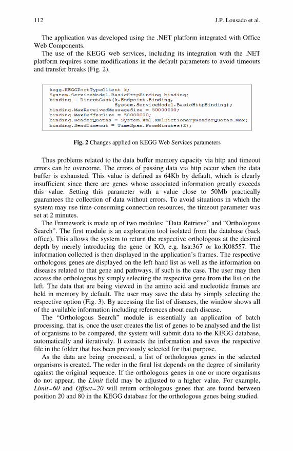
112 J.P. Lousado et al.
The application was developed using the .NET platform integrated with Office Web Components.
The use of the KEGG web services, including its integration with the .NET platform requires some modifications in the default parameters to avoid timeouts and transfer breaks (Fig. 2).
Fig. 2 Changes applied on KEGG Web Services parameters
Thus problems related to the data buffer memory capacity via http and timeout errors can be overcome. The errors of passing data via http occur when the data buffer is exhausted. This value is defined as 64Kb by default, which is clearly insufficient since there are genes whose associated information greatly exceeds this value. Setting this parameter with a value close to 50Mb practically guarantees the collection of data without errors. To avoid situations in which the system may use time-consuming connection resources, the timeout parameter was set at 2 minutes.
The Framework is made up of two modules: “Data Retrieve” and “Orthologous Search”. The first module is an exploration tool isolated from the database (back office). This allows the system to return the respective orthologous at the desired depth by merely introducing the gene or KO, e.g. hsa:367 or ko:K08557. The information collected is then displayed in the application’s frames. The respective orthologous genes are displayed on the left-hand list as well as the information on diseases related to that gene and pathways, if such is the case. The user may then access the orthologous by simply selecting the respective gene from the list on the left. The data that are being viewed in the amino acid and nucleotide frames are held in memory by default. The user may save the data by simply selecting the respective option (Fig. 3). By accessing the list of diseases, the window shows all of the available information including references about each disease.
The “Orthologous Search” module is essentially an application of batch processing, that is, once the user creates the list of genes to be analysed and the list of organisms to be compared, the system will submit data to the KEGG database, automatically and iteratively. It extracts the information and saves the respective file in the folder that has been previously selected for that purpose.
As the data are being processed, a list of orthologous genes in the selected organisms is created. The order in the final list depends on the degree of similarity against the original sequence. If the orthologous genes in one or more organisms do not appear, the Limit field may be adjusted to a higher value. For example, Limit=60 and Offset=20 will return orthologous genes that are found between position 20 and 80 in the KEGG database for the orthologous genes being studied.

An Application for Studying Tandem Repeats in Orthologous Genes 113
Fig. 3 Application Interface With Multiple Windows
The tool also incorporates other functionalities, including the search of repetitions of amino acids with or without the admission of errors by the orthologous of one or more genes placed in the first column. Thus, we can resort to the use of the local files previously saved in Batch Processing, or opt for using a connection to the Web. In this case performance may go down, but on the other hand more up-to-date results may be obtained.
After processing, several spreadsheets are created with the results of the analysis on each of the respective orthologous. These spreadsheets can be processed locally as a single file in XLS format.
3 Discussion
To test the application, we have conducted an analysis in accordance with the previously presented protocol (Figure 1), comparing human genes under the referred conditions with the respective orthologous genes of the organisms presented in Table 1. Obtaining the results was almost immediate for the local source (offline), and it takes only a few seconds, depending on bandwidth, when we use directly the web server as a source of data (online). Integrating scattered data, whether via the Web (several sources), whether by post-processing (offline files), the developed tool becomes a crucial ally for researchers, mainly in situations of massive data extraction.

114 J.P. Lousado et al.
Table 1 Organisms list and genealogic classification
Bos taurus ftp://ftp.genome.jp/pub/kegg/genes/organisms/bta Canis familiaris ftp://ftp.genome.jp/pub/kegg/genes/organisms/cfa Homo sapiens ftp://ftp.genome.jp/pub/kegg/genes/organisms/hsa Mus musculus ftp://ftp.genome.jp/pub/kegg/genes/organisms/mmu
viviparous
Pan troglodytes ftp://ftp.genome.jp/pub/kegg/genes/organisms/ptr marsupial Monodelphis domestica ftp://ftp.genome.jp/pub/kegg/genes/organisms/mdo
mam
mal
s
oviparous Ornithorhynchus anatinus ftp://ftp.genome.jp/pub/kegg/genes/organisms/oaa bird Gallus gallus ftp://ftp.genome.jp/pub/kegg/genes/organisms/gga
verte
brat
e
fish Danio rerio ftp://ftp.genome.jp/pub/kegg/genes/organisms/dre Insect Drosophila melanogaster ftp://ftp.genome.jp/pub/kegg/genes/organisms/dme worm Caenorhabditis elegans ftp://ftp.genome.jp/pub/kegg/genes/organisms/cel plant Arabidopsis thaliana ftp://ftp.genome.jp/pub/kegg/genes/organisms/ath
Aspergillus fumigatus ftp://ftp.genome.jp/pub/kegg/genes/organisms/afm Kluyveromyces lactis ftp://ftp.genome.jp/pub/kegg/genes/organisms/kla Saccharomyces cerevisiae ftp://ftp.genome.jp/pub/kegg/genes/organisms/sce fungus Schizosaccharomyces pombe ftp://ftp.genome.jp/pub/kegg/genes/organisms/spo
protozoan Plasmodium falciparum ftp://ftp.genome.jp/pub/kegg/genes/organisms/pfa Clostridium perfringens ftp://ftp.genome.jp/pub/kegg/genes/organisms/cpe
inve
rtebr
ate
bacteria Mycobacterium tuberculosis ftp://ftp.genome.jp/pub/kegg/genes/organisms/mtu
4 Conclusion
Codon repeats in DNA are contiguous, and some time approximate, copies of a pattern of trinucleotides. These repeats have been associated to specific human diseases, and may play a variety of regulatory and evolutionary roles.
In this paper we presented a computation application that simplifies the study of genes with this type of patterns, along the evolutionary chain. For that the software extracts orthologous genes from public resources and performs a comparative analysis that allows showing how repeats have evolved along the time for the specie other study.
Acknowledgements
J. P. Lousado has funded by the Instituto Politécnico de Viseu under the PROFAD Programme.
References
1. George, R.A., Liu, J.Y., Feng, L.L., Bryson-Richardson, R.J., Fatkin, D., Wouters, M.A.: Analysis of protein sequence and interaction data for candidate disease gene prediction. Nucl. Acids Res. 34, e130 (2006)
2. Sher Ali, S.A., Ehtesham, N.Z., Azfer, M.A., Homkar, U., Rajesh Gopal, S.E.H.: Analysis of the evolutionarily conserved repeat motifs in the genome of the highly endangered central Indian swamp deer Cervus duvauceli branderi. GENE. 223, 361–367 (1998)
3. Fu, Z., Jiang, T.: Clustering of main orthologs for multiple genomes. J. Bioinform. Comput. Biol. 6, 573–584 (2008)

An Application for Studying Tandem Repeats in Orthologous Genes 115
4. Jones, N.C., Pevzner, P.A.: Comparative genomics reveals unusually long motifs in mammalian genomes. Bioinformatics 22, e236–e242 (2006)
5. Lab, P.: Repeat Disease Database (2009), http://www.cepearsonlab.com/rdd.php
6. Brameier, M., Wiuf, C.: Ab initio identification of human microRNAs based on structure motifs. BMC Bioinformatics 8, 478 (2007)
7. Bowen, T.A., Guy, C.A.A., Cardno, A.G.A.B., Vincent, J.B.C., Kennedy, J.L.C., Jones, L.A.A., Gray, M.A., Sanders, R.D.A., McCarthy, G.A., Murphy, K.C.A., Owen, M.J.A.B., O’Donovan, M.C.A.: Repeat sizes at CAG/CTG loci CTG18.1, ERDA1 and TGC13-7a in schizophrenia. Psychiatric Genetics 10, 33–37 (2000)
8. Ferro, P., Catalano, M.G., Dell’Eva, R., Fortunati, N., Pfeffer, U.: The androgen receptor CAG repeat: a modifier of carcinogenesis? Molecular and Cellular Endocrinology 193, 109–120 (2002)
9. Pestova, T.V., Hellen, C.U., Wimmer, E.: A conserved AUG triplet in the 5’ nontranslated region of poliovirus can function as an initiation codon in vitro and in vivo. Virology 204, 729–737 (1994)
10. Freed, K.A., Cooper, D.W., Brennecke, S.P., Moses, E.K.: Detection of CAG repeats in pre-eclampsia/eclampsia using the repeat expansion detection method. Mol. Hum. Reprod. 11, 481–487 (2005)
11. Herishanu, Y.O., Parvari, R., Pollack, Y., Shelef, I., Marom, B., Martino, T., Cannella, M., Squitieri, F.: Huntington disease in subjects from an Israeli Karaite community carrying alleles of intermediate and expanded CAG repeats in the HTT gene: Huntington disease or phenocopy? Journal of the Neurological Sciences 277, 143–146 (2009)
12. Bogaerts, V., Theuns, J., van Broeckhoven, C.: Genetic findings in Parkinson’s disease and translation into treatment: a leading role for mitochondria? Genes. Brain. Behav. 7, 129–151 (2008)
13. Mena, M.A., Rodriguez-Navarro, J.A., Ros, R., de Yebenes, J.G.: On the pathogenesis and neuroprotective treatment of Parkinson disease: what have we learned from the genetic forms of this disease? Curr. Med. Chem. 15, 2305–2320 (2008)
14. Tarini, B.A., Singer, D., Clark, S.J., Davis, M.M.: Parents’ Interest in Predictive Genetic Testing for Their Children When a Disease Has No Treatment. Pediatrics (2009)
15. Hsueh, W.: Genetic discoveries as the basis of personalized therapy: rosiglitazone treatment of Alzheimer’s disease. Pharmacogenomics J. 6, 222–224 (2006)
16. Pearson, C.E., Edumura, N.K., Cleary, J.D.: instability: mechanisms of dynamic mutations. Nat. Rev. Genet. 6, 729–742 (2005)
17. Lousado, J., Oliveira, J., Moura, G., Santos, M.: Analysing the Evolution of Repetitive Strands in Genomes. In: Omatu, S., Rocha, M.P., Bravo, J., Fernández, F., Corchado, E., Bustillo, A., Corchado, J.M. (eds.) IWANN 2009. LNCS, vol. 5518, pp. 1047–1054. Springer, Heidelberg (2009)
18. KEGG: Kyoto Encyclopedia of Genes and Genomes. Kanehisa Laboratories, http://www.kegg.com
19. OMIM, Online Mendelian Inheritance in Man, http://www.ncbi.nlm.nih.gov/omim/
20. Hamosh, A., Scott, A., Amberger, J., Bocchini, C., McKusick, V.: Online Mendelian Inheritance in Man (OMIM), a knowledgebase of human genes and genetic disorders. Nucleic Acids Research 33, D514 (2005)
21. Kanehisa, M., Goto, S., Furumichi, M., Tanabe, M., Hirakawa, M.: KEGG for representation and analysis of molecular networks involving diseases and drugs. Nucl. Acids Res. 38, D355–D360 (2010)

M.P. Rocha et al. (Eds.): IWPACBB 2010, AISC 74, pp. 117–121, 2010. springerlink.com © Springer-Verlag Berlin Heidelberg 2010
Accurate Selection of Models of Protein Evolution
Mateus Patricio, Federico Abascal, Rafael Zardoya, and David Posada
1
Abstract. We carried out computer simulations to assess the accuracy of the pro-gram ProtTest in recovering best-fit empirical models of amino acid replacement. We were able to show that regardless of the selection criteria used, the simulated model or a very close one was identified most of the time. In addition, the esti-mates of the different model parameters were very accurate. Our results suggest that protein model selection works reasonably well.
1 Introduction
The use of different models of nucleotide substitution or amino acid replacement can change the outcome of the phylogenetic analysis [1]. Apart from the different effects on parameter estimation and hypothesis testing, in general, phylogenetic methods may be less accurate –recover more often a wrong tree–, or may be in-consistent –converge to a wrong tree with increased amounts of data– when the assumed model of evolution is wrong. Conveniently, best-fit models of molecular evolution can be selected for the data at hand using sound statistical techniques, like hierarchical likelihood ratio tests, information criteria, Bayesian methods or performance-based approaches [2]. Several of these strategies have been imple-mented in different computer programs like ModelTest [3] and jModelTest [4] for DNA sequences, and ProtTest [5] for proteins. The performance of ModelTest was examined in detail by Posada and Crandall [6], who showed that model selec-tion was very accurate in the case of nucleotides. However, we do not know whether this is the case for protein sequences. In order to answer this question we have used computer simulations to evaluate the ability of ProtTest in recovering the simulated model of amino acid replacement.
1Mateus Patricio . David Posada Departamento de Bioquímica, Genética, e Inmunología, Universidad de Vigo, Vigo, Spain
Federico Abascal . Rafael Zardoya Departamento de Biodiversidad y Biología Evolutiva, Museo Nacional de Ciencias Naturales, Madrid, Spain

118 M. Patricio et al.
2 Materials and Methods
To simulate the protein alignments, we downloaded from http://www.atgc-montpellier.fr/phyml/datasets.php the set of trees that were used to evaluate the performance of the Phyml algorithm [7] for phylogenetic estimation. This set con-tains 5000 simulated non-clock trees comprising 40-taxon each, and includes a va-riety of topologies and tree heights. For each one of these trees, we generated a 40-sequence alignment with 1000 amino acids using Seq-Gen [8], under the JTT [9] matrix of amino acid substitution, with rate variation among sites (number of gamma rate categories = 4; alpha gamma shape = 0.5; proportion of invariable sites = 0.2). This model, whose acronym is JTT+I+G, will be referenced hereafter as the true model. For each alignment, the best-fit model of amino acid replace-ment was selected with ProtTest among 112 candidate models using the uncor-rected and corrected Akaike Information Criterion (AIC and AICc) and the Bayesian Information Criterion (BIC), including model-averaged estimates and parameter importances (see [2]). For the AICc and BIC, sample size was calcu-lated as the number of sites in the alignment. The calculation of the likelihood score and maximum likelihood (ML) tree for each model is very time-consuming, and in order to speed up the whole process all the program executions were carried out using distributed computing techniques. After running ProtTest, we counted the amount of times the generating model was correctly identified and calculated the mean squared error (MSE) of the parameter estimates.
3 Results
ProtTest correctly identified the true model (JTT+I+G; ~90%) or very closely related model (JTT+G; 10%) most of the time (Table 1). In general, the best-fit model was selected with little uncertainty and therefore receiving large weights (Table 2). Table 1 Number of times each model was identified as the best-fit model (percentages in parentheses)
Model JTT+G JTT+I+G JTT+G+F JTT+I
AIC 523
(0.10) 4466 (0.90)
1 (0)
6 (0.001)
AICc 553
(0.11) 4437 (0.90)
6 (0.01)
–
BIC 1034 (0.21)
3956 (0.79)
– 6
(0.001)
Table 2 Average/median model weights for the different models according to the three model selection criteria
Model True Best 2nd Best JTT+G AIC 0.90 0.90 0.31 0.31 AICc 0.89 0.89 0.33 0.33 BIC 0.79 0.79 0.52 0.52

Accurate Selection of Models of Protein Evolution 119
The estimates of the alpha and p-inv parameters were very accurate, regardless of whether they corresponded to the best-fit model, to the true model, or to model-averaged estimates (Fig. 1 and Tables 3 and 4).
Fig. 1 Parameter estimates of the shape of the gamma distribution (alpha) and the propor-tion of invariable sites (p-inv) for the best-fit model, true model and model-averaged esti-mates (the three lines are almost perfectly overlapping) under the AIC framework..Vertical lines correspond to the true simulated values
Table 3 Mean squared error (MSE), mean (Mean) and standard deviation (Sd) of the estimated shape of the gamma distribution (alpha)
MSE Mean Sd Best-fit model 0.016 0.508 0.115 True model 0.013 0.508 0.115 Model-averaged 0.013 0.508 0.115
Table 4 Mean squared error (MSE), mean (Mean) and standard deviation (Sd) for the estimated proportion of invariable sites (p-inv)
MSE Mean Sd Best-fit model 0.004 0.190 0.065 True model 0.004 0.190 0.064 Model-averaged 0.004 0.190 0.064
The importance of the parameters (Fig. 2) shows that the most important parame-ter is the joint contribution made by the proportion of invariable sites plus the shape of the gamma distribution (p-inv + alpha), which is the expected since the true model includes both (JTT+I+G).

120 M. Patricio et al.
Fig. 2 Relative importance of parameters. alpha: Mean = 0.09785 and Sd = 0.20990. p-inv: Mean = 0.00176, and Sd = 0.02630. alpha+p-inv: Mean = 0.90037, Median: 1, Var = 0.04595 and Sd = 0.21436.
4 Discussion
In our simulations ProtTest was able to identify, regardless the selection criteria used, the true generating model (JTT+I+G) or a closely related one (JTT+G) most of the time. Given that the only difference between these two models is that the former assumes a proportion of invariable sites (here p-inv = 0.2), while in the lat-ter this proportion is, by definition, zero, it is not surprising that in some cases JTT+G was preferred over JTT+I+G. The estimation of the different parameters was also very accurate under the thee model selection frameworks explored. Here, the estimates provided by the best-fit and true models or using model averaging, were very similar, which was expected given that the best-fit model usually corre-sponded with the true model and received large weights. Also, the parameter im-portances reflected very well the need for taking into account both a proportion of invariable sites and rate variation among the variable sites, in agreement with the true model.
5 Conclusions
Protein model selection using ProtTest seems to work very well. The AIC and BIC frameworks provides accurate tools for the study of the process of molecular evo-lution at the protein level. Further simulations should explore other generating models and quantify the effect of protein model selection on phylogenetic accuracy.

Accurate Selection of Models of Protein Evolution 121
References
1. Sullivan, J., Joyce, P.: Model selection in phylogenetics. Annual Review of Ecology. Evolution and Systematics 36, 445–466 (2005)
2. Posada, D., Buckley, T.R.: Model selection and model averaging in phylogenetics: ad-vantages of Akaike information criterion and Bayesian approaches over likelihood ratio tests. Syst. Biol. 53(5), 793–808 (2004)
3. Posada, D., Crandall, K.A.: Modeltest: testing the model of DNA substitution. Bioin-formatics 14(9), 817–818 (1998)
4. Posada, D.: jModelTest: phylogenetic model averaging. Mol. Biol. Evol. 25(7), 1253–1256 (2008)
5. Abascal, F., Zardoya, R., Posada, D.: ProtTest: selection of best-fit models of protein evolution. Bioinformatics 21(9), 2104–2105 (2005)
6. Posada, D., Crandall, K.A.: Selecting the best-fit model of nucleotide substitution. Sys-tematic Biology 50, 580–601 (2001)
7. Guindon, S., Gascuel, O.: A simple, fast, and accurate algorithm to estimate large phy-logenies by maximum likelihood. Syst. Biol. 52(5), 696–704 (2003)
8. Rambaut, A., Grassly, N.C.: Seq-Gen: an application for the Monte Carlo simulation of DNA sequence evolution along phylogenetic trees. Comput. Appl. Biosci. 13(3), 235–238 (1997)
9. Jones, D.T., Taylor, W.R., Thornton, J.M.: The rapid generation of mutation data matri-ces from protein sequences. Comput. Appl. Biosci. 8(3), 275–282 (1992)

Scalable Phylogenetics throughInput Preprocessing
Roberto Blanco, Elvira Mayordomo,Esther Montes, Rafael Mayo, and Angelines Alberto
Abstract. Phylogenetic reconstruction is one of the fundamental problems in com-putational biology. The combinatorial explosion of the state space and the com-plexity of mathematical models impose practical limits on workable problem sizes.In this article we explore the scalability of popular algorithms under real datasetsas problem dimensions grow. We furthermore develop an efficient preclassificationand partitioning strategy based on guide trees, which are used to intently define anevolutionary hierarchy of groups of related data, and to determine membership ofindividual data to their corresponding subproblems. Finally, we apply this method toefficiently calculate exhaustive phylogenies of human mitochondrial DNA accord-ing to phylogeographic criteria.
1 Motivation
The organization of living organisms (extant or not) into a “tree of life”, as conceivedby Darwin, is the purpose of the modern discipline of phylogenetics [4]. Continuousadvances in sequencing technologies have supported an exponential growth in pub-licly available biological sequences over the last quarter century. This abundanceoffers extraordinary potential to shed light into the inner workings of evolution.
Phylogenetic techniques infer trees, or generalizations thereof, from multiple se-quence alignments according to a certain optimality criterion. This mathematical
Roberto Blanco · Elvira MayordomoDepartamento de Informatica e Ingenierıa de Sistemas (DIIS)/Instituto de Investigacion enIngenierıa de Aragon (I3A), Universidad de Zaragoza, Marıa de Luna 1,50018 Zaragoza, Spaine-mail: {robertob,elvira}@unizar.es
Angelines Alberto · Rafael Mayo · Esther MontesCentro de Investigaciones Energeticas, Medioambientales y Tecnologicas (CIEMAT),Avenida Complutense 22, 28040 Madrid, Spaine-mail: {angelines.alberto,rafael.mayo,esther.montes}@ciemat.es
M.P. Rocha et al. (Eds.): IWPACBB 2010, AISC 74, pp. 123–130, 2010.springerlink.com c© Springer-Verlag Berlin Heidelberg 2010

124 R. Blanco et al.
scoring scheme acts as a computational surrogate of the true biological objective: torecover the true evolutionary relationships between living organisms, as representedby (usually) aligned, meaningful sequences.
Nevertheless, this is a very challenging problem. Not only are there no efficientmethods to calculate an optimal phylogeny given an alignment and a tree scoringfunction, but the preservation of the optimality of a solution while adding new datato it has been proven to be NP-hard for even the elementary parsimony criterion [3].Therefore, standard practice depends on heuristic methods, which still remain verycostly.
From an information-rich perspective, the main defect of conventional meth-ods is that they are completely blind, whereas it would be desirable to providehints and facts that may constrain and help to simplify problem solution. In thispaper, we resort to evolutionary hypotheses as classifiers and definers of smaller,simpler subproblems, and illustrate the biological and computational benefits ofsuch a methodology.
2 Methods
In this section we introduce the working principles of our technique, providing theexperimental grounds for it as well as its theoretical basis. The illustration of thepractice and benefits of this framework is deferred to the next section.
2.1 Stand-Alone Algorithms
There exist many phylogenetic reconstruction methods, but their principal classifi-cation regards whether they treat statistical quality evaluation as an additional step oras part of the process itself [6]. This assessment is of the utmost importance becauseof the infeasibility of exact algorithms for even small datasets. Both approaches havestrengths and weaknesses, and thus method selection is a very important choice, notleast due to the very poor scaling of most techniques.
To assess the severity of these decisions, we have evaluated the relative perfor-mance and scalability of the main families of methods; our results are summarizedin Fig. 1. Problem dimensions have been chosen to scale up to moderately sized, realdatasets, with which we will deal in Sect. 3. PHYLIP and MrBayes [5, 8] have beenused for traditional and Bayesian methods, respectively, due to their availability andgenerality.
All three traditional methods are seen to follow similar trends, though parsimonyis more abrupt in its progression. Generally speaking, more thorough methods incurin significantly higher costs, quickly becoming impractical. It should be noted thatthese times must be multiplied by the desired number of bootstrap samples for theanalysis, which can nevertheless be executed in parallel.
The raw computational needs of Bayesian methods are more difficult to esti-mate due to their simulational nature, as is their parallelization. Cost ultimately de-pends on both problem dimensions, number of iterations (and its relation to model

Scalable Phylogenetics through Input Preprocessing 125
convergence and stop conditions), and possibly number of processors. For the sakeof measurement we have fixed an appropriate, catch-all number of iterations andassume approximately linear speed-up for the execution setup [1]. Time growth iscomparable, though steeper and orders of magnitude above likelihood search, whichtogether with indivisibility make these methods impracticable for large datasets.
Generally speaking, it can be concluded that, since problem complexity is alwayssuperlinear, partitioning offers very significant improvements and allows agile pro-duction of cleaner results; therefore, it should be exploited whenever possible. Thesegains can be invested in the calculation of a higher degree of statistical support orthe selection of more sophisticated methods and substitution models.
Fig. 1 Performance and scalability of phylogenetic reconstruction methods along bothproblem dimensions: number of sequences s and sequence length l

126 R. Blanco et al.
2.2 The Supertree Approach
Supertree methods have been conceived to combine, and possibly reconcile, a num-ber of input subtrees according to the underlying relations between them that aremanifested through a set of overlapping taxa, which are used to puzzle the treestogether [10]. This approach is advantageous in that it is ideally cost-effective andallows comprehensive studies while preserving known results.
If inputs are reasonably structured and compatible, i.e., there are no unsolvablecontradictions between the inferred sets of clades, it is possible to produce exactsolutions in polynomial time [11]. What we develop here is a further simplificationof the compositional burden based on prior structural knowledge about the data.
Our proposal is an extension of the hierarchical classification problem. If a de-cision tree can be provided that allows simple, recursive categorization of singlesequences and that reflects well-supported phylogenetic knowledge, such a “skele-ton tree” can be employed to obtain groups of related sequences, thus splitting thedata into their corresponding subclades. Each of these can be subsequently com-puted independently and in parallel. In essence, we use supertrees to reduce problemdimensionality through a classic divide and conquer scheme.
Insofar as we know for certain, or are willing to assume as hypotheses, the re-lations between the clades defined by the preprocessing hierarchy, composition ofpartial results into the final tree is limited to substitution of symbolic “clade nodes”by their associated subtrees. The substitution skeleton must, however, accommo-date all clades as leaves of the tree, transferring internal categories down dummyleaf branches if needed. The process is straightforward save for this provision.
3 Case Study: Human Mitochondrial DNA
Mitochondrial DNA (mtDNA) is one of the most important evolutionary markersfor phylogenetics due to its remarkable features: absence of effective recombination,high mutation rate and ease of sequencing, among others. Its prime metabolic rolesalso grant it prominence in the study of rare genetic disease [13].
Consequently, comprehensive research on human mtDNA is of great interest,though the very own wealth of available information deters straightforward, manu-ally supervised trees; we have previously addressed the question in [2] and subse-quent work. At present we can effectively perform periodic updates to the humanmitochondrial phylogeny, though as we endeavor to show there is plenty of roomfor improvement.
3.1 Structural Properties
For the proposed supertree methods to be applicable, firstly a suitable set of classi-fiers needs to be identified. In the case of mtDNA, its matrilineal inheritance alongwith the migrations that scattered the human species around the world gave rise tomitochondrial haplogroups: large population groups related by common descent,

Scalable Phylogenetics through Input Preprocessing 127
Fig. 2 Phylogeographical history of the major human mitochondrial haplogroups, fitted toMITOMAP’s tree skeleton. The star marks the root of the tree. Internal clades that wereexcluded from the hierarchy are greyed out
to which membership can be ascribed simply by checking a handful of definingpolymorphisms.
These groups spread in an arborescent fashion, not unlike a conventional speciestree, as depicted in Fig. 2. The study of human haplogroups is a well-founded areaof ongoing research with diverse applications [12] and a standard cladistic notationestablished in [7]. It is therefore perfectly adequate to our purposes as a recipient ofphylogenetic knowledge.
3.2 Materials and Methods
For the conduction of our experiments we have prepared a curated database of com-pletely sequenced, human mtDNA sequences, partly based on MITOMAP’s queryon GenBank. The aligned sequences (s = 4895, l = 16707) can be assumed to behomogeneous and show no obvious flaws.
Also from the MITOMAP phylogeny [9] we have selected its “Simplified mtDNAlineages” as an adequate guide tree that offers a good level of detail for a first clas-sification. Minor corrections have been made regarding haplogroups B (allowingroom for ambiguity in the definition of its distinctive indel) and I (avoiding a retic-ulation event for which no evidence has been found and promoting it as a directdescendant of N).

128 R. Blanco et al.
Recursive classification has been performed to assign each sequence to its re-lated haplogroup; sequences that fail to match exactly one category have beenexcluded from the analysis (1.7% of the total, a very small fraction given thelow complexity of the skeleton). Haplogroup subtrees have been computed us-ing distance matrices with neighbor joining clustering and bootstrap sampling, andBayesian inference; both under adequate substitution models. Executions have beendistributed across high-performance clusters to exploit the potential parallelism un-veiled by our method.
3.3 Results
As a result of the classification we obtain 28 clade subsets with sizes up to s =583 owing to unequal sequencing of population groups around the globe. Due tothe progression of computation times with s, a handful of prolific groups clearlydominates total execution times. However, the recursive nature of the tree makes itpossible to easily refine copious nodes by simply identifying and adding children
Fig. 3 Human mitochondrial haplogroup supertree. Parent haplogroups have been propa-gated to the top of their subtrees as leaf haplogroups; they are also labels of their associatedclades

Scalable Phylogenetics through Input Preprocessing 129
subtrees as required; this has indeed been the case of Bayesian inference of groupsD, H, M and U, due to technical limitations. In fact, although traditional methodsyield satisfactory throughput, Bayesian inference remains only marginally tractableand on the whole depends on more extensive partitioning.
The improvements derived from preprocessing are very remarkable. As a refer-ence, the cost of computing a single distance matrix for the selected dataset with asuitable, reasonably complex evolutionary model is approximately 105 sec. By con-trast, a single workstation requires the same time to produce reasonably supported(e.g., 100 bootstrap samples per haplogroup) combined phylogenies under the samealgorithm and model, therefore amounting roughly to a 100-fold increase in perfor-mance; additional gains can be achieved by exploiting the larger number of simpler,less costly tasks.
The phylogenies we obtain are qualitatively better than standard, blind resultsin that results are clear, and noise and discordance are confined to individual sub-problems, hence bounding their potential effect and improving overall quality androbustness. One such phylogeny can be seen in Fig. 3.
4 Discussion and Future Work
We have presented an efficient and effective supertree technique that effectivelyperforms a reduction on s, the costliest dimension of the phylogeny reconstructionproblem, through a divide and conquer approach where the penalties of the splitand merge operations are negligible. As a result, computational load is substan-tially lowered, known properties are respected by construction, and the number ofcompletely independent, distributable tasks is increased. These improvements af-ford more detailed treatment of individual problem instances and feasible resolutionof continuously growing inputs.
We also deem it possible to develop reasonably accurate cost prediction, which,despite some measure of input dependence and irregularity, may be of great assis-tance in selecting methods (and models) in accord with available time and resources.Such estimates may also lead to better scheduling and load balancing in distributedenvironments.
It has been stressed that solutions are, as a matter of fact, qualitatively better.Moreover, we would like to know how prior knowledge may affect quantitativescores when pitted against atomic methods, as well as the effect and progressionof individual algorithms and substitution models, and pinpoint the sources of error,including those that might cause incorrect group ascription.
Finally, considering that reliable phylogenetic knowledge is the source of all clas-sification hierarchies, their appraisal merits further attention. The fit of an alignmentand a guide tree, or lack thereof, may evidence a need for (possibly iterative) refine-ment of one or both parts. Likewise, the capacity to generate restricted datasets andtreat them in finer detail could be used to support (sub)haplogroup identificationwhile providing feedback and increasing guide tree resolution.

130 R. Blanco et al.
Acknowledgements. This work was supported in part by the Spanish Ministry of Scienceand Innovation (MICINN) under Action CAC-2007-52 and Project TIN2008-06582-C03-02. Roberto Blanco was supported by Grant AP2008-03447 from the Spanish Ministry ofEducation.
References
1. Altekar, G., Dwarkadas, S., Huelsenbeck, J.P., Ronquist, F.: Parallel Metropolis cou-pled Markov chain Monte Carlo for Bayesian phylogenetic inference. Bioinformatics 20,407–415 (2004)
2. Blanco, R., Mayordomo, E.: ZARAMIT: a system for the evolutionary study of humanmitochondrial DNA. In: Omatu, S., Rocha, M.P., Bravo, J., Fernandez, F., Corchado,E., Bustillo, A., Corchado, J.M. (eds.) IWANN 2009. LNCS, vol. 5518, pp. 1139–1142.Springer, Heidelberg (2009)
3. Bockenhauer, H.J., Hromkovic, J., Kralovic, R., Momkea, T., Rossmanith, P.: Reopti-mization of Steiner trees: changing the terminal set. Theor. Comput. Sci. 410, 3428–3435(2009)
4. Ciccarelli, F.D., Doerks, T., von Mering, C., Creevey, C.J., Snel, B., Bork, P.: Towardautomatic reconstruction of a highly resolved tree of life. Science 311, 1283–1287 (2006)
5. Felsenstein, J.: PHYLIP – Phylogeny Inference Package (version 3.2). Cladistics 5, 164–166 (1989)
6. Holder, M., Lewis, P.O.: Phylogeny estimation: traditional and Bayesian approaches.Nat. Rev. Genet. 4, 275–284 (2003)
7. Richards, M.B., Macaulay, V.A., Bandelt, H.J., Sykes, B.C.: Phylogeography of mito-chondrial DNA in western Europe. Ann. Hum. Genet. 62, 241–260 (1998)
8. Ronquist, F., Huelsenbeck, J.P.: MrBayes 3: Bayesian phylogenetic inference undermixed models. Bioinformatics 19, 1572–1574 (2003)
9. Ruiz-Pesini, E., Lott, M.T., Procaccio, V., Poole, J.C., Brandon, M.C., Mishmar, D.,Yi, C., Kreuziger, J., Baldi, P., Wallace, D.C.: An enhanced MITOMAP with a globalmtDNA mutational phylogeny. Nucleic Acids Res. 35, D823–D828 (2007)
10. Sanderson, M.J., Purvis, A., Henze, C.: Phylogenetic supertrees: assembling the trees oflife. Trends Ecol. Evol. 13, 105–109 (1998)
11. Steel, M., Dress, A.W.M., Bocker, S.: Simple but fundamental limitations on supertreeand consensus tree methods. Syst. Biol. 49, 363–368 (2000)
12. Torroni, A., Achilli, A., Macaulay, V., Richards, M., Bandelt, H.J.: Harvesting the fruitof the human mtDNA tree. Trends Genet. 22, 339–345 (2006)
13. Wallace, D.C.: A mitochondrial paradigm of metabolic and degenerative diseases, aging,and cancer: a dawn for evolutionary medicine. Annu. Rev. Genet. 39, 359–407 (2005)

The Median of the Distance between Two Leavesin a Phylogenetic Tree
Arnau Mir and Francesc Rossello
Abstract. We establish a limit formula for the median of the distance between twoleaves in a fully resolved unrooted phylogenetic tree with n leaves. More precisely,we prove that this median is equal, in the limit, to
√4ln(2)n.
1 Introduction
The definition and study of metrics for the comparison of phylogenetic trees is aclassical problem in phylogenetics [5, Ch. 30], motivated, among other applications,by the need to compare alternative phylogenies for a given set of organisms obtainedfrom different datasets or using different methods. Many metrics for the comparisonof rooted or unrooted phylogenetic trees on the same set of taxa have been proposedso far. Some of the most popular, and oldest, such metrics are based on the com-parison of the vectors of distances between pairs of taxa in the corresponding trees[1, 3, 4, 9, 10, 11]. These metrics aim at the quantification of the rate at which pairsof taxa that are close together in one tree lie at opposite ends in another tree [7]. But,in contrast with other metrics, their statistical properties are mostly unknown.
Steel and Penny [10] computed the mean value of the square of the metric forfully resolved unrooted trees defined through the euclidean distance between theirvectors of distances (they called it the path difference metric). One of the main ingre-dients in their work was the explicit computation of the mean value and the varianceof the distance d between two leaves in a fully resolved unrooted phylogenetic treewith n leaves, obtaining that
μ(d) =22(n−2)
(2(n−2)n−2
) ∼√πn, Var(d) = 4n−6− μ(d)− μ(d)2
Arnau Mir · Francesc RosselloDepartment of Math & Computer Science, University of Balearic Islands, Crta. Valldemossa,km. 7,5, 07122 Palma de Mca, Spaine-mail: {arnau.mir,cesc.rossello}@uib.es
M.P. Rocha et al. (Eds.): IWPACBB 2010, AISC 74, pp. 131–135, 2010.springerlink.com c© Springer-Verlag Berlin Heidelberg 2010

132 A. Mir and F. Rossello
Such values are also of some interest in themselves, because they give figures againstwhich to compare the corresponding values for the distribution of distances betweenleaves in a reconstructed phylogenetic tree, allowing one to assess how “close toaverage” is such a tree. Some specific applications of the probabilistic behaviour ofparameters related to the shape of phylogenetic trees are discussed in [2].
In this work we continue the statistical analysis of this random variable d, bygiving an expression for its median that allows the derivation of a limit formula forit: namely,
median(d)∼√
4n ln2.
The derivation of a limit formula for the median of the aforementioned squared pathdifference metric between fully resolved unrooted phylogenetic trees remains an openproblem. We hope this result will constitute a first step towards its achievement. Weshall report on this application elsewhere.
2 Preliminaries
In this paper, by a phylogenetic tree on a set S we mean a fully resolved (that is, withall its internal nodes of degree 3) unrooted tree with its leaves bijectively labeledin the set S. Although in practice S may be any set of taxa, to fix ideas we shallalways take S = {1, . . . ,n}, with n the number of leaves of the tree, and we shalluse the term phylogenetic tree with n leaves to refer to a phylogenetic tree on thisset. For simplicity, we shall always identify a leaf of a phylogenetic tree with itslabel.
Let Tn be the set of (isomorphism classes of) phylogenetic trees with n leaves.It is well known [5] that |T1| = |T2| = 1 and |Tn| = (2n− 5)!! = (2n− 5)(2n−7) · · ·3 ·1, for every n � 3.
3 Main Result
Let k, l ∈ S = {1, . . . ,n} be any two different labels of trees in Tn. The distancedT (k, l) between the leaves k and l in a phylogenetic tree T ∈Tn is the length of theunique path between them. Let’s consider the random variable
dkl = distance between the labels k and l in one tree in Tn.
The possible values of dkl are 1,2, . . . ,n−1.Our goal is to estimate the value of the median of this variable dkl on Tn when
the tree and the leaves are chosen equiprobably. In this case, dkl = d12, and thus wecan reduce our problem to compute the median of the variable d := d12.
For every i = 1, . . . ,n−1, let ci be the cardinal of {T ∈Tn | dT (1,2)= i}. Arguingas in [10, p. 140], we have the following result.

The Median of the Distance between Two Leaves in a Phylogenetic Tree 133
Lemma 1. cn−1 = (n−2)! and, for every i = 1, . . . ,n−2,
ci = (n−2)!(i−1)(n−1) · · ·(2n− i−4)
(2(n− i−1))!!=
(i−1)(2n− i−4)!(2(n− i−1))!!
.
Lemma 2. For every k=1, . . . ,n−1,1
(2n−5)!!
k
∑i=1
ci=1−2k(n−3)!(−k + 2n−4)!2(2n−5)!(−k + n−2)!
.
Proof. Taking into account that (2 j)!! = 2 j j! and (2 j + 1)!! = (2 j+1)!2 j j!
, for everyj ∈ N, and using Lemma 1, we have:
1(2n−5)!!
k
∑i=1
ci =(n−3)!
4(2n−5)!
k
∑i=2
(i−1)2i(2n− i−4)!(n− i−1)!
=(n−3)!
4(2n−5)!
k−1
∑i=1
i2i+1(2n− i−5)!(n− i−2)!
.
We use now the method in [8, Chap. 5] to compute Sk = ∑k−1i=1
i2i+1(2n−i−5)!(n−i−2)! .
Set ti = i2i+1(2n− i−5)!/(n− i−2)!. Then
ti+1
ti=
2(1 + i)(2 + i−n)i(5 + i−2n)
.
The next step is to find three polynomials a(i),b(i) and c(i) such that
ti+1
ti=
a(i)b(i)· c(i+ 1)
c(i).
We take a(i) = 2(2 + i−n), b(i) = 5 + i−2n and c(i) = i. Next, we have to find apolynomial x(i) such that a(i)x(i+1)−b(i−1)x(i)= c(i). The polynomial x(i) = 1satisfies this equation. Then, by [8, Chap. 5],
Sk =b(k−1)x(k)
c(k)tk + g(n) =
(4 + k−2n)2k+1(2n− k−5)!(n− k−2)!
+ g(n),
where g is a function of n. We find this function from the case k = 2:
4(2n−6)!(n−3)!
= S2 =8(6−2n)(2n−7)!
(n−4)!+ g(n).
From this equality we deduce that g(n) =4(2n−5)!(n−3)!
. We conclude that:
Sk =k−1
∑i=1
i2i+1(2n− i−5)!(n− i−2)!
=(4 + k−2n)2k+1(2n− k−5)!
(n− k−2)!+
4(2n−5)!(n−3)!
.

134 A. Mir and F. Rossello
The formula in the statement follows from this expression.
Theorem 1. Let median(d) be the median of the variable d on Tn. Then,
median(d)√4ln(2)n
= 1 + O(
n−1/2)
.
In particular, limn→∞
median(d)√4ln(2)n
= 1.
Proof. To simplify the notations, we shall denote median(d) by k. By definition,
k = max{
k ∈ N |k
∑i=1
ci � |Tn|2
}= max
{k ∈ N | 2k(n−3)!(−k + 2n−4)!
2(2n−5)!(−k + n−2)!� 1
2
}.
Thus, k is the largest integer value such that
2k(n−3)!(−k+ 2n−4)! � (2n−5)!(−k+ n−2)!.
If we simplify this inequation and take logarithms, this condition becomes
k ln(2) �k+1
∑j=3
ln
(2n− ( j + 2)
n− j
)=
k+1
∑j=3
ln
(2− j+2
n
1− jn
). (1)
Combining the development of the function ln( 2−( j+2)x1− jx ) in x = 0,
ln
(2− ( j + 2)x
1− jx
)= ln(2)+
12( j−2)x +
18( j−2)(3 j + 2)x2 + O
(x3) ,
with equation (1), we obtain:
ln(2) � 12n
k+1
∑j=3
( j−2)+ O
(k3
n2
)=
k(k−1)4n
+ O
(k3
n2
).
So, the first order term of the median k will be the largest integer value that satisfiesk2/4n � ln(2). Therefore, the median will be the closest integer to
√4ln(2)n, from
where the thesis in the statement follows.
4 Conclusions
We have obtained a limit formula for the median of the distance d between twoleaves in a fully resolved unrooted phylogenetic tree with n leaves, namely:
median(d)∼√
4ln(2)n

The Median of the Distance between Two Leaves in a Phylogenetic Tree 135
This value complements the determination of the mean value and the variance of thisdistance carried out by Steel and Penny [10]. Actually, our method allows to findmore terms of the development of the median, with some extra effort. For instance,it can be easily proved that
median(d)∼√
4n ln2+(12− ln2).
The limit formula obtained in this work can be generalized to the p-percentile
xp = max{
k ∈ N | ∑ki=1 ci � |Tn|p
}. Indeed, using our method we obtain that
xp ≈√−4ln(1− p)n.
In the near future we plan to extend this work to arbitrary unrooted phyloge-netic trees, as well as to fully resolved rooted phylogenetic trees (for the mean andvariance figures in the rooted case, see [6]), and to apply this kind of results inthe derivation of a limit formula for the median of the corresponding squared pathdifference metrics.
Acknowledgements. This work has been partially supported by the Spanish Government,through projects MTM2009-07165 and TIN2008-04487-E/TIN.
References
1. Bluis, J., Shin, D.G.: Nodal distance algorithm: Calculating a phylogenetic tree compar-ison metric. In: Proc. 3rd IEEE Symp. BioInformatics and BioEngineering, p. 87 (2003)
2. Chang, H., Fuchs, M.: Limit theorems for patterns in phylogenetic trees. Journal of Math-ematical Biology 60, 481–512 (2010)
3. Farris, J.: A successive approximations approach to character weighting. Syst. Zool. 18,374–385 (1969)
4. Farris, J.: On comparing the shapes of taxonomic trees. Syst. Zool. 22, 50–54 (1973)5. Felsenstein, J.: Inferring Phylogenies. Sinauer Associates Inc., (2004)6. Mir, A., Rossello, F.: The mean value of the squared path-difference distance for rooted
phylogenetic trees. Submitted to J. Math. Biol (2009),http://es.arxiv.org/abs/0906.2470
7. Penny, D., Hendy, M.D.: The use of tree comparison metrics. Syst. Zool. 34(1), 75–82(1985)
8. Petkovsek, M., Wilf, H., Zeilberger, D.: A = B. AK Peters Ltd., Wellesley (1996),http://www.math.upenn.edu/˜wilf/AeqB.html
9. Phipps, J.B.: Dendrogram topology. Syst. Zool. 20, 306–308 (1971)10. Steel, M.A., Penny, D.: Distributions of tree comparison metrics—some new results.
Syst. Biol. 41, 126–141 (1993)11. Williams, W.T., Clifford, H.T.: On the comparison of two classifications of the same set
of elements. Taxon 20(4), 519–522 (1971)

M.P. Rocha et al. (Eds.): IWPACBB 2010, AISC 74, pp. 137–141, 2010. springerlink.com © Springer-Verlag Berlin Heidelberg 2010
In Silico AFLP: An Application to Assess What Is Needed to Resolve a Phylogeny
María Jesús García-Pereira, Armando Caballero, and Humberto Quesada
1
Abstract. We examined the effect of increasing the number of scored AFLP bands to reconstruct an accurate and well-supported AFLP-based phylogeny. In silico AFLP was performed using simulated DNA sequences evolving along a symmetric tree with ancient radiation. The comparison of the true tree to the esti-mated AFLP trees suggests that moderate numbers of AFLP bands are necessary to recover the correct topology with high bootstrap support values (i.e > 70%). However, branch length estimation is rather unreliable and does not improve sub-stantially after a certain number of bands are sampled.
Keywords: AFLP, phylogeny, bootstrap support, simulation, accuracy.
1 Introduction
The amplified fragment length polymorphism (AFLP) technique is becoming ex-tensively used as a source of informative molecular markers for phylogenetic in-ference in many studies of plants, animals, fungi and bacteria [1]. The technique generates highly reproducible fingerprints that are usually recorded as a 1/0 band presence-absence matrix. Phylogenetic relationships are then inferred analyzing the AFLP matrix directly, or converting it into a distance matrix using dissimilar-ity measures.
AFLP markers are appropriate for phylogenetic inference as long as sequence divergence is small, the topology of the underlying evolutionary tree is symmetric, and not very short ancestral branches exist [2]. Recent theoretical studies indicate that a major drawback of this technique is the low information content of AFLP markers. This weakness seems to have a much larger negative impact on tree reli-ability than other commonly invoked limitations of AFLP data sets, such as the occurrence of non homologous bands or the dominant nature of AFLP characters
1María Jesús García-Pereira . Armando Caballero . Humberto Quesada Departamento de Bioquímica, Genética e Inmunología, Facultad de Biología, Universidad de Vigo, 36310 Vigo, Spain e-mail: [email protected]
138 M.J. García-Pereira, A. Caballero, and H. Quesada
[2]. Given that the outcome of any phylogenetic analysis critically depends upon the amount of data available, we focus on determining how many AFLP bands would be needed to resolve a problematic phylogenetic tree. Experimental studies aimed at assessing this question are, however, resource intensive and hampered by the fact that we rarely know the true tree. Here we investigate one potential strat-egy for improving phylogenetic inference. Using in silico AFLP fingerprints, we assess the likelihood that a well supported phylogeny can be resolved using AFLP bands, and how many bands would then be needed.
2 Methods
DNA sequences of 2.8 Mb were generated with the software Seq-Gen [3] using the Jukes and Cantor substitution model. Simulations with Seq-Gen were per-formed along a phylogenetic tree (hereafter referred as the reference tree) contain-ing 16 sequences, with a symmetric topology and a length from the most internal node to the tip of 0.02 substitutions per site. Branch lengths were specified using an ancient radiation model, in which daughter branches were twice as long as the parent branch. This generated a tree with several short internal branches, making it difficult to resolve.
A computer program written in C was used to simulate the cutting of the gener-ated DNA sequences with restriction enzymes EcoRI and MseI, which are the typical enzymes used in AFLP studies. Only fragments sizes between 40 and 440 nucleotides were considered in the subsequent analyses to emulate experimental studies. A combination of selective nucleotides adjacent to the restriction sites was used to simulate the selective amplification of 100 AFLP bands per AFLP profile.
Phylogenies were estimated with PAUP*4 [4] using the minimum evolution method. Estimated AFLP trees were compared with their corresponding reference trees by the program Ktreedist [5]. This program computes a K-score that meas-ures overall differences in the relative branch length and topology of two phyloge-netic trees. Topological differences among reference and estimated trees were assessed using Robinson-Foulds (R-F) [6] distance. High K-scores or R-F dis-tances indicate a poor match between the estimated AFLP-based tree and the ref-erence tree. A total of 50 replicates were run per simulation. An average K-score and R-F distance was computed for each set of replicates.
Branch support was determined running 1000 bootstap replicates per simula-tion. Four different bootstrap consensus trees were estimated with minimum cut-offs of 63%, 86%, 95% and 98% respectively. The average success of resolution [7] was calculated as a weighted average of the four R-F distances resulting from the comparison of the respective consensus trees with the reference tree.
3 Results and Conclusions
All measures of accuracy and support showed a rapid improvement that was subsequently slowed down as an increased number of bands were analyzed

In Silico AFLP: An Application to Assess What Is Needed to Resolve a Phylogeny 139
(Figs. 1-2). This is due to the fact that, as clades are resolved, the total number of newly resolved clades decreases for each further increment in band number. High resolution to recover the correct tree topology (R-F distance) was achieved using a total of about 300 bands (Fig. 1). In contrast, branch length estimation (K-score) was rather unreliable across the entire set of band numbers analyzed and did not improve substantially once the amount of about 500 bands was reached.
Our simulations showed that relatively high bootstrap support values (i.e. ≥ 70%) for most nodes were reached when sampling as few as 500 bands, but that an increase in the number of sampled bands did not necessarily equate to a linear increase in support values (Fig. 2). Bootstrap support values ≥ 98% for all nodes required double number of bands, from 500 to 1000.
0
2
4
6
8
10
12
0 200 400 600 800 1000
K-s
core
R-F
dis
tanc
e
Number of bands
0.000
0.005
0.010
0.015
0.020
0.025
0 200 400 600 800 1000
Number of bands
0
2
4
6
8
10
12
0 200 400 600 800 1000
K-s
core
R-F
dis
tanc
e
Number of bands
0.000
0.005
0.010
0.015
0.020
0.025
0 200 400 600 800 1000
Number of bands
K-s
core
R-F
dis
tanc
e
Number of bands
0.000
0.005
0.010
0.015
0.020
0.025
0 200 400 600 800 1000
Number of bands
Fig. 1 K-scores and R-F distances resulting from the comparison among the true and esti-mated minimum evolution trees based on different numbers of AFLP bands. ∆ K-score and R-F distance for a 1Kb long DNA sequence
R-F
dis
tanc
e
0
3
6
9
12
15
0 200 400 600 800 1000
0
3
6
9
12
15
0 200 400 600 800 10000
3
6
9
12
15
0 200 400 600 800 1000
63% 98% Weighted
Number of bands Number of bands Number of bands
R-F
dis
tanc
e
0
3
6
9
12
15
0 200 400 600 800 1000
0
3
6
9
12
15
0 200 400 600 800 10000
3
6
9
12
15
0 200 400 600 800 1000
63% 98% Weighted
Number of bands Number of bands Number of bands
Fig. 2 Bootstrap support. Topological congruence between the reference and estimated con-sensus trees using different minimum cutoff values and number of sampled AFLP bands
To better visualize the relationship between K-score, R-F distance and tree ac-curacy, we plotted the reference tree and the estimated AFLP-based trees (Fig. 3). External nodes have a higher bootstrap support than deeper nodes, and nodes achieving 90% bootstrap support were more responsive to increasing the number of sampled bands. Our in silico simulations provide new insights into the phy-logenetic utility of AFLPs and suggest that moderate amounts of bands (on the range of 300-600) are necessary to recover most clades with high support values.

140 M.J. García-Pereira, A. Caballero, and H. Quesada
SequenceReference
AFLP AFLP- Bootstrap
Fig. 3 Reference and estimated trees using DNA sequences 1 Kb long (Sequence) and AFLP characters based on 300 bands (AFLP) and 1000 bands after bootstrap re-sampling (AFLP-Bootstrap). Numbers at the nodes indicate the percentage of bootstrap support
Acknowledgments. This work was funded by the Ministerio de Ciencia e Innovación and Fondos Feder (CGL2009-13278-C02).
References
1. Meudt, H.M., Clark, A.C.: Almost forgotten or latest practice? AFLP applications, analyses and advances. Trends Plant. Sci. 12, 106–117 (2007)
2. García-Pereira, M.J., Caballero, A., Quesada, H.: Evaluating the relationship between evolutionary divergence and phylogenetic accuracy in AFLP data sets. Mol. Biol. Evol. (in press, 2010)
3. Rambaut, A., Grassly, N.C.: Seq-Gen: an application for the Monte Carlo simulation of DNA sequence evolution along phylogenetic trees. Comput. Appl. Biosci. 13, 235–238 (1997)
4. Swofford, D.L.: PAUP*: phylogenetic analysis using parsimony (*and other methods), version 4. Sinauer Associates, Sunderland, Massachusetts (1999)

In Silico AFLP: An Application to Assess What Is Needed to Resolve a Phylogeny 141
5. Soria-Carrasco, V., Talavera, G., Igea, J., Castresana, J.: The K tree score: quantifica-tion of differences in the relative branch length and topology of phylogenetic trees. Bio-informatics 23, 2954–2956 (2007)
6. Robinson, D.F., Foulds, L.R.: Comparison of phylogenetic trees. Math. Biosci. 53, 131–147 (1981)
7. Simmons, M.P., Webb, C.T.: Quantification of the success of phylogenetic inference in simulations. Cladistics 22, 249–255 (2006)

M.P. Rocha et al. (Eds.): IWPACBB 2010, AISC 74, pp. 143–150, 2010. springerlink.com © Springer-Verlag Berlin Heidelberg 2010
Employing Compact Intra-genomic Language Models to Predict Genomic Sequences and Characterize Their Entropy
Sérgio Deusdado* and Paulo Carvalho
1
Abstract. Probabilistic models of languages are fundamental to understand and learn the profile of the subjacent code in order to estimate its entropy, enabling the verification and prediction of “natural” emanations of the language. Language models are devoted to capture salient statistical characteristics of the distribution of sequences of words, which transposed to the genomic language, allow model-ing a predictive system of the peculiarities and regularities of genomic code in dif-ferent inter and intra-genomic conditions. In this paper, we propose the application of compact intra-genomic language models to predict the composition of genomic sequences, aiming to achieve valuable resources for data compression and to con-tribute to enlarge the similarity analysis perspectives in genomic sequences. The obtained results encourage further investigation and validate the use of language models in biological sequence analysis.
Keywords: language models, DNA entropy estimation, genomic sequences modeling.
1 Introduction
Language models aim to capture the context of a language based on the study and computation of the probabilities of its patterns [1], developing models to infer the rules behind the successions of its segments, i.e. words, n-grams, sounds, codons, etc. Hidden Markov Models (HMMs) also rely on probabilistic models and are widely used in bioinformatics for gene prediction and profiling of sequences [2]. 1Sérgio Deusdado CIMO - Mountain Research Centre, Polytechnic Institute of Bragança, Portugal e-mail: [email protected]
Paulo Carvalho Department of Informatics, School of Engineering, University of Minho, Braga, Portugal
* Corresponding author.

144 S. Deusdado and P. Carvalho
Entropy measures of DNA sequences estimate their randomness or, inversely, their repeatability [3]. In the field of genomic data compression, fundamentally based on the comprehension of the regularities of genomic language and entropy estimation, language models appear as a promising methodology to characterize the genomic linguistics and to provide predictive models for data compression [4][5] [6], as well as revealing new approaches for sequence similarity analysis [7]. Statistical language models are widely used in speech recognition [8] and have been successfully applied to solve many different information retrieval prob-lems [9]. A good review on statistical language modeling is presented by Rosenfeld in [10].
Currently, the Biological Language Modeling Toolkit is a good example of the in-terest of this field of investigation, developed by the Center for Biological Language Modeling. This toolkit consists on a compilation of various algorithms that have been adapted to biological sequences from language modeling, and specifically it is ori-ented to uncover the "protein sequence language". The toolkit is publicly available at the following URL: http://flan.blm.cs.cmu.edu/12/HomePage.
2 Language Models
Language modeling is the art of determining the probability of a word sequence w1...wn, P(w1...wn) [10]. This probability is typically divided into its component probabilities:
P(w1...wi) = P(w1) × P(w2|w1) × ... × P(wi|w1...wi−1) (1)
= ∏=
n
i 1
P(wi | w 1, w2 , ..., w i-1 )
Since it may be difficult to compute the probability P(wi|w1...wi−1) for large i, it is typically assumed that the probability of a word depends on only the two previous words. Thus, that trigram assumption can be written as:
P(wi|w1...wi−1) ≈ P(wi|wi−2wi−1) (2)
The trigram probabilities can then be estimated from their counts in a training cor-pus. Let C(wi−2wi−1wi) represent the number of occurrences of wi−2wi−1wi in our training corpus, and similarly for C(wi−2wi−1). Then, we can approximate:
P(wi|wi−2wi−1) ≈ C(wi−2wi−1wi) C(wi−2wi−1) (3)
The most obvious extension to trigram models is to move to higher order n-grams, such as four-grams and five-grams. In genomic language modeling is usual to consider codons as words. Codons are three-letter words from the quaternary ge-nomic alphabet {A, C, G, T}, resulting only 64 possible combinations. Thus, genomic language models generally use higher order n-grams to improve their efficiency.
Smoothing techniques are used to avoid zero probability n-grams which may occur from inadequate training data [11]. In fact, rare trigrams should also

Employing Compact Intra-genomic Language Models 145
integrate the predictive model; therefore its probability, even low, must be greater than zero. On the other hand, smoothing affects high probabilities to be adjusted downward. Not only do smoothing methods generally prevent zero probabilities, but they also attempt to improve the accuracy of the model as a whole.
The most commonly used method for measuring language model performance is perplexity. In general, the perplexity of a n-gram language model is equal to the geometric average of the inverse probability of the words measured on test data:
n
n
i ii wwwP∏= −1 11 )...|(
1
(4)
Low perplexity of the model means high fidelity predictions. A language model assigning equal probability to 100 words would have perplexity 100. An alterna-tive, but equivalent measure to perplexity is entropy, which is simply log2 of perplexity.
3 Developed Work
The developed work corresponds to a framework for entropy estimation and anal-ysis of DNA sequences based on cooperative intra-genomic compact language models. These models will obtain a probability distribution of the next symbol at a given position, based on the symbols previously seen. Based on the experiments of Cao et al. [12], we choose to divide our approach into global and local models, combining their contribution to improve the efficiency of the multiparty predictive model. While global models consider the full extension of the analyzed sequences, local models only capture the probabilistic properties of a limited number of bases preceding the base(s) to predict, considering if necessary a variable displacement.
Our aim was to take advantage of the successive probability present mainly in repetitive regions of DNA sequences, as well as in non-repetitive regions where a stochastic model can be efficient too.
We used a backoff n-gram language model [13][14] implemented with arrays of values representing the most probable chain of codons to occur after each one of the 64 possible codons. Our models were not trained based on a corpus because the intention was to apply, subsequently, the resulting framework to an on-line ge-nomic data compression algorithm. In this sense, the resulting compressed file must be self-contained, as the recalculation of probabilities in the decompression process relies only on the data included in the compressed file. Thus, the need for compact models, especially the global model because it is integrated in the com-pressed file. The local models are adaptive and evolve periodically as they receive new input from the history of the sequence already viewed, i.e. the significant por-tion of the sequence preceding the point of prediction. In this way, we produce intra-genomic and very compact models, expecting not to compromise the proc-essing time of the predictive algorithm and, additionally, looking forward to in-clude the essential part of the models in the resulting compressed file to help the initial predictions, when history is not available.

146 S. Deusdado and P. Carvalho Experimental results, using a typical set of DNA sequences (see Table 3)
used in DNA compressors as test corpus, showed that ten-grams/codons corre-sponds to the most appropriated order for global models, considering the tradeoff between model performance and computational cost. For local models, we used order twenty, not codon based but nucleotide based. Each model presents its pre-diction supported by an associated probability, reflecting the model’s confidence. At the end, all local and global models are pooled to elect by a voting system the definitive prediction to be emitted. Independently of the model that produces the prediction, any prediction is just a symbol. Hence, if the prediction is made by a codon-based model only the first nucleotide of the predicted codon is considered.
3.1 Local Models
Local models use single letters (nucleotides) instead of codons and are of order thirty. Being adaptive, they are modified with the latter knowledge obtained from the already predicted - and eventually corrected - sequence. The local models used in our work are based on 1000 nucleotides context, not immediately before the nu-cleotide to predict but forming a window slid back in the sequence. We used two versions based on different displacements, one with 500 bp displacement and the other going backward 3000 bp. We used different types of local models to enlarge the possibilities of our prediction system, trying to take advantage on the best available knowledge, such as being aware of that most repetitions occur hundreds or thousands of bp after its last occurrence. Considering that some DNA regulari-ties occur in the reverse complementary form, the so-called palindromes, we used complimentary local models based on reverse complementary history.
3.2 Global Models
Global models use codons and gather the probabilistic study of ten-grams. A glob-al model based on the reverse complementary sequence was also produced. Global models are meant to be compact, as they will integrate a future compressed file of the DNA sequence. Our global models are based on tables, containing the most probable succession of codons to occur after each one of the 64 possible codons. Without increasing data complexity, it is possible to calculate global models for the three frames of a sequence. In this way, frame 1, 2 and 3 variants were also considered. These models can be consulted also for subsequences of codons, not necessarily initiated at order 0, using a backing off strategy. An example of a global model, upon analysis of the frame 1 of a sequence, is shown in Table 1.
Table 1 Example of a compact global model considering ten-grams
Order Frame 1
0 1 2 3 4 5 6 7 8 9 10
Code Codon Sucession of codons with highest probability
1 AAA 1 4 4 16 63 29 32 1 1 2 34
2 AAC 2 12 12 57 23 44 43 5 4 1 31
… … … … … … … … … … … … …
63 GGT 63 52 2 64 4 11 13 24 6 12 59
64 GGG 64 11 13 24 6 12 59 17 55 32 4

Employing Compact Intra-genomic Language Models 147
3.3 Prediction Process
The test prototype considers six different models, described as follows:
M1 – regular global model; M2 – global model based on the reverse complementary sequence; M3 – regular local model considering 1000 previous symbols context and a re-tro-displacement of 3000 bases; M4 – reverse complementary local model considering 1000 previous symbols context and a retro-displacement of 3000 bases; M5 – regular local model considering 1000 previous symbols context and a re-tro-displacement of 500 bases; M6 – reverse complementary local model considering 1000 previous symbols context and a retro-displacement of 500 bases.
A model emits a prediction based on order n when it contains the knowledge of a probable n-gram equal to the one at the end of the analyzed portion of the se-quence. When there is a conflict between predictions of equal order, global models have priority and their predictions prevail as they derive from the complete se-quence. If a global model produces a prediction of order ≥ 3 then the local models predictions are ignored. Each model votes for its predicted symbol, and in the end a probabilistic distribution emerges from a voting system where global models have more weight on final results than local models. Votes from local models are equal to the order used in the prediction, whereas the global models’ orders used in the predictions are trebled. Table 2 shows an example of the election of a final prediction and its probability distribution based on the following individual pre-dictions cases:
M1 – predicted A with order 5(x3); M2 – predicted C with order 1(x3); M3 – predicted T with order 3; M4 – predicted A with order 1; M5 – predicted C with order 2; M6 – predicted T with order 1;
To prevent zero probability, non-voted symbols receive one vote.
Table 2 Demonstration of the voting system used to achieve the probability distribution
Votes by Model Prediction
M1 M2 M3 M4 M5 M6 Total
Probability distri-bution
A 15 1 16 62%
C 3 2 5 19%
T 3 1 4 15%
G 1 4%

148 S. Deusdado and P. Carvalho
4 Experimental Results
A test prototype was implemented to combine the predictions from the models de-scribed in the previous section in order to assess the predictive capability of our framework. The code was written in C language and compiled using gcc version 3.4.2, configured for maximal code optimization. Tests ran on a system based on Intel Pentium IV – 3,4GHz, 8KB L1 + 512 KB L2 cache, with 1GB RAM-DDR and a 250 GB HD. We tested our prototype on a dataset of DNA sequences typically used in DNA compression studies. The dataset includes 11 sequences: two chloroplast ge-nomes (CHMPXX and CHNTXX); five human genes (HUMDYSTROP, HUMGHCSA, HUMHBB, HUMHDABCD and HUMHPRTB); two mitochondria genomes (MPOMTCG and MTPACG); and genomes of two viruses (HEHCMVCG and VACCG).
Table 3 contains the results obtained, considering the percentage of predictions that matched the corresponding symbol in the original sequence.
Table 3 Experimental results
Sequence Length(bp) % of correct predictions
CHMPXX 121.024 29
CHNTXX 155.844 30
HEHCMVCG 229.354 27
HUMDYSTROP 38.770 26
HUMGHCSA 66.495 37
HUMHBB 73.323 28
HUMHDAB 58.864 29
HUMHPRTB 56.737 28
MPOMTCG 186.608 27
MTPACG 100.314 27
VACCG 191.737 28
Average 116.279 29
Considering the quaternary alphabet and carrying out a random prediction, it
will be expectable, in theory, to obtain 25% of correct predictions, on average. Comparatively, the obtained results exhibit 29% of prediction correctness on aver-age. However, the obtained results are satisfactory considering only intra-genomic study and the reduced size of the used models; moreover the high level of entropy inherent to DNA sequences justifies the quality of the results. HUMGHCSA is the sequence where our predictive model performed better because it is, within the tested set of sequences, the one with lower entropy, i.e. high redundancy, as we may confirm in the literature [4][15].

Employing Compact Intra-genomic Language Models 149
5 Conclusions and Future Work
Experimental results demonstrate a linear correlation facing the entropy of each tested sequenced based on the results of existing DNA data compressors [4][3][12][15]. Sequences with higher levels of entropy are more difficult to mod-el and hence our models get modest results on their analysis. Global models cap-ture the most significant patterns of the sequence and perform generally better. Local models revealed low utility in entropy estimation but they are important to complement predictions. Different sequences may need proper adjustments of the extension and the displacement of the local models to optimize their prediction capability. We believe that it would be useful to determine the profile of the se-quence in advance in order to adaptively adjust the local model’s parameteriza-tion. This will be addressed in future developments.
Our major goal was to test the potential and efficiency of language models as a complementary compression method for biological data compression, for instance, to complement dictionary based techniques. Consequently, our focus was mainly in regions of the sequences where linear patterns are sparse or exist repeatedly but with reduced extension. Additional work is needed to optimize all the models, especially the local ones, but the obtained results encourage further investigation.
References
1. Durbin, R., Eddy, S., Krogh, A., Mitchison, G.: Biological sequence analysis: prob-abilistic models of proteins and nucleic acids. Cambridge University Press, Cambrige (1998)
2. Koski, T.: Hidden Markov Models for Bioinformatics. Kluwer Academic Publishers, Dordrecht (2001)
3. Lanctot, J.K., Li, M., Yang, E.: Estimating DNA sequence entropy. In: SODA 2000: Proceedings of the eleventh annual ACM-SIAM symposium on Discrete algorithms, pp. 409–418. Society for Industrial and Applied Mathematics, San Francisco (2000)
4. Loewenstern, D., Yianilos, P.N.: Significantly Lower Entropy Estimates for Natural DNA Sequences. In: Data Compression Conference (DCC 1997), p. 151 (1997)
5. Osborne, M.: Predicting DNA Sequences using a Backoff Language Model (2000), http://www.cogsci.ed.ac.uk/~osborne/dna-backoff.ps.gz
6. Venugopal, K.R., Srinivasa, K.G., Patnaik, L.M.: Probabilistic Approach for DNA Compression. In: Soft Computing for Data Mining Applications, pp. 279–289. Springer, Heidelberg (2009)
7. Buehler, E.C., Ungar, L.H.: Maximum Entropy Methods for Biological Sequence Modeling. In: Workshop on Data Mining in Bioinformatics (with SIGKDD 2001 Con-ference), San Francisco, CA, USA, pp. 60–64 (2001)
8. Jelinek, F.: Statistical methods for speech recognition. MIT Press, Cambridge (1997) 9. Zhai, C.: Statistical Language Models for Information Retrieval. Synthesis Lectures on
Human Language Technologies 1, 1–141 (2008) 10. Rosenfeld, R.: Two Decades of Statistical Language Modeling: Where Do We Go
from Here? Proceedings of the IEEE 88, 1270–1278 (2000)

150 S. Deusdado and P. Carvalho
11. Chen, S.F., Goodman, J.: An Empirical Study of Smoothing Techniques for Language Modeling. Harvard University (1998)
12. Cao, M.D., Dix, T.I., Allison, L., Mears, C.: A Simple Statistical Algorithm for Bio-logical Sequence Compression. In: 2007 Data Compression Conference (DCC 2007), Snowbird, UT, USA, pp. 43–52 (2007)
13. Katz, S.: Estimation of probabilities from sparse data for the language model compo-nent of a speech recognizer. IEEE Transactions on Acoustics, Speech, and Signal Processing 35, 400–440 (1987)
14. Kneser, R., Ney, H.: Improved backing-off for m-gram language modeling. In: IEEE Int. Conf. Acoustics, Speech and Signal Processing, pp. 181–184. IEEE, Detroit (1995)
15. Korodi, G., Tabus, I.: An efficient normalized maximum likelihood algorithm for DNA sequence compression. ACM Transactions on Information Systems 23, 3–34 (2005)

M.P. Rocha et al. (Eds.): IWPACBB 2010, AISC 74, pp. 151–156, 2010. springerlink.com © Springer-Verlag Berlin Heidelberg 2010
Structure Based Design of Potential Inhibitors of Steroid Sulfatase
Elisangela V. Costa, M. Emília Sousa, J. Rocha, Carlos A. Montanari, and M. Madalena Pinto*
1
Abstract. The enzyme steroid sulfatase (STS) activity is high in breast tumors and elevated levels of STS mRNA expression have been associated with a poor prog-nosis. Potent STS irreversible inhibitors have been developed, paving the way to use this new type of therapy for breast cancer. Synthetic small molecules belonging to a focused library of inhibitors of tumor cell growth already obtained and new molecules planned to be reversible inhibitors of STS were docked into STS using the program AutoDock 4. To guide the docking process of the select ligands through the lattice volume that divides the receptor's area of interest, a full set of grid maps was built using the program AutoGrid. Some of the new designed small molecules showed calculated binding affinity for STS presenting ΔG values in a range of -11.15 to -13.07 kcal.mol-1. The synthesis of the most promising STS inhibitors, based on these results, is in progress.
1 Introduction
The highest frequency of breast cancer is observed in postmenopausal women, as-sociated with high levels of peripherical estrogens produced in situ. The enzyme steroid sulfatase (STS) is responsible for conversion of inactive sulfate-conjugated steroids to active non-conjugated forms (Reed et al. 2005). This phenomenon plays a crucial role in the development of the breast cancer hormone-receptor-positive. 1Elisangela V. Costa . M. Emília Sousa . M. Madalena Pinto Department of Chemistry, Laboratory of Organic and Pharmaceutical Chemistry, Faculty of Pharmacy, University of Porto, Rua Aníbal Cunha, 164, 4050-047 Porto, Portugal e-mail: [email protected]
Elisangela V. Costa . M. Emília Sousa . M. Madalena Pinto CEQUIMED-UP, Center of Medicinal Chemistry – University of Porto, Rua Aníbal Cunha, 164, 4050-047 Porto, Portugal
J. Rocha . Carlos A. Montanari Grupo de Estudos em Química Medicinal de Produtos Naturais – NEQUIMED-PN, Instituto de Química de São Carlos, Universidade de São Paulo, São Carlos, SP, Brasil * Corresponding author.

152 E.V. Costa et al.
STS inhibitors can be classified as reversible and irreversible. Most of the re-versible inhibitors are substrate- or product-based, feature a steroid skeleton, and are generally less potent than the irreversible blockers (Nussbaumer and Billich 2004). Attempts to design nonsteroidal STS inhibitors have revealed the benzo-phenone-4,4′-O,O-bis-sulfamate (BENZOMATE) as a potent STS irreversible in-hibitor (Hejaz et al. 2004). Structure–activity relationship studies showed that the carbonyl group is pivotal for activity and also that the bis-sulfamate moiety is re-sponsible for the irreversible mechanism of action.
Until very recently the field has been dominated by irreversible, arylsulfamate-based inhibitors, although a stable, potent reversible inhibitor should be less prob-lematic for development. The main reason apparently is that the inhibitor design was hampered by the lack of the 3D structure of STS and that the discovery of novel inhibitor types has been limited to high-throughput screening (HTS). None-theless, the structure of STS has already been determined at 2.60 Å resolution by X-ray crystallography (Hernandez-Guzman et al. 2003).
These facts led us to investigate potential STS reversible inhibitors by struc-ture-based design (SBS), with a benzophenone and a xanthone scaffold (Figure 1). The SBS is a molecular docking process that takes small molecule structures from a database of existing compounds (or of compounds that could be synthesized), and docks them into the protein-binding site, which involves the prediction of ligand conformation and orientation (or posing) within the target (Reich et al. 1992).
Fig. 1 Strategy used in this work
In order to proceed with these kinds of studies, the strategy used was the dock-ing of compounds with a benzophenone and a xanthone scaffold provided of a significantly similarity in their structure to BENZOMATE (Figure 1). So, small molecules obtained in our group which have been already described as tumor cell growth inhibitors (Pedro et al. 2002, Sousa et al. 2002, Castanheiro et al. 2007, Sousa et al. 2009), as well as new benzophenone/xanthone derivatives designed to be reversible inhibitors of STS, i.e., without the sulfamate group, were docked into STS. The synthesis of the designed xanthones which showed high affinity for STS was already initiated.

Structure Based Design of Potential Inhibitors of Steroid Sulfatase 153
2 Docking Studies
An automated docking method, AutoDock 4 (Morris et al. 1998, Morris et al. 2009), was used that predicts the bound conformations of flexible ligands to mac-romolecular targets in combination with a new scoring function that estimates the free energy change upon binding. AutoDock 4 program allows fully flexible modeling of specific portions of the protein, in a similar manner as the flexible ligand (Morris et al. 2009) only applied for flexible designed molecules that therefore have potentially a reversible mode of action and not for docking of co-valently-attached complexes, irreversible ones. AutoGrid calculated the non-covalent energy of interaction between the receptor and a probe atom located in the different grid points of a lattice that divides the receptor's area of interest, the active site, in a grid box. The region to be explored was chosen and delimited by a three-dimensional box so that all important residues forming the active site could be taken into consideration during the docking process (red-colored region on Figure 2).
Fig. 2 Grid box
Docking using AutoDock 4 allowed the prediction of the bound conformations of flexible ligands to the macromolecular target. For instance, a xanthone was docked into STS with a good value of ΔG=-12.50 kcal.mol-1 and showed to be well accommodated by a variety of hydrophobic residues such Phe, Val and Leu, which are predominant in STS active site. Moreover, the predicted structure for the ligand-receptor complex suggests two hydrogen bond interactions involving Arg98 and carbonyl group of xanthone scaffold (Figure 3). The cluster analysis shown in Figure 4 of the docked xanthone demonstrates that probably the confor-mation adopted is the one with a value of ΔG = -12.50 kcal.mol-1 (red colored).
The 61 compounds belonging to a focused library of inhibitors of tumor cell growth already obtained were docked into the STS. The respective values of ΔG were determinate in a range of –5.39 to –9.40 kcal.mol-1. Two potent inhibitors against MCF-7 breast adenocarcinoma with the lowest GI50 values of 6.0 and 21.9 µM were associated with favorable ΔG values (-8.58 and -6.40 kcal.mol-1, respec-tively). Some of the new designed xanthones/benzophenones showed high affinity for STS with ΔG values in a range of -11,15 to -13.07 kcal.mol-1. It is possible to observe in Figure 5 the high shape complementarities of two designed molecules

154 E.V. Costa et al.
Fig. 3 Interactions suggested by the predicted structure for the ligand-receptor complex
Fig. 4 Cluster analysis of the docked xanthone
Fig. 5 Superimposition of the best conformations of two molecules docked
with the buried active site of STS. The molecules can adopt conformations that are able to fill the whole cavity and prevent the substrate to access to the catalytic residues.
3 Synthesis
The synthesis of the designed molecules associated to the best results was initiated according to conditions in Figure 6. The coupling reagent, TBTU (O-(benzotriazol-1-yl)-N,N,N’,N’-tetramethyluronium tetrafluoroborate), often used in the peptide synthesis, was applied in the esterification of three carboxylic acids with 3,6-dihydroxyxanthone to afford the corresponding esters (Figure 6A). The introduction of bulky groups was also performed in order to obtain more two de-rivatives (Figure 6B).

Structure Based Design of Potential Inhibitors of Steroid Sulfatase 155
Fig. 6 Ongoing synthesis of new xanthone derivatives potential inhibitors of STS
4 Conclusions and Future Work
Some molecules synthesized in our group already described as tumor cell growth inhibitors were associated to favorable ΔG values. It is expected that those ones might inhibit the tumor cell growth presumably by inhibiting STS. The STS activ-ity of these compounds and the new compounds with favorable ΔG values will be assessed experimentally in the STS assay. We expect that the virtual screening al-lied to the structure-based design provides new STS reversible inhibitors belong-ing to xanthone/benzophenone families.
Acknowledgments
Fundação para a Ciência e a Tecnologia (FCT), Unidade I&D 4040/2007, FEDER, POCI for financial support and for the PhD grant to Elisangela Costa (SFRH/BD/30615/2006).
References
Castanheiro, R., Pinto, M., Silva, A., et al.: Dihydroxyxanthones prenylated derivatives: synthesis, structure elucidation, and growth inhibitory activity on human tumor cell lines with improvement of selectivity for MCF-7. Bioorg. Med. Chem. 15, 6080–6088 (2007)
Hejaz, H., Woo, L., Purohit, A., et al.: Synthesis, in vitro and in vivo activity of benzophe-none-based inhibitors of steroid sulfatase. Bioorg. Med. Chem. 12, 2759–2772 (2004)
Hernandez-G, F., Higashiyama, T., Pangborn, W., et al.: Structure of Human Estrone Sulfa-tase Suggests Functional Roles of Membrane Association. J. Biol. Chem. 278, 22989–22997 (2003)
Morris, G., Goodsell, D., Halliday, R., et al.: Automated Docking Using a Lamarckian Ge-netic Algorithm and an Empirical Binding Free Energy Function. J. Comput. Chem. 19, 1639–1662 (1998)
Morris, G., Huey, R., Lindstrom, W., et al.: AutoDock 4 and AutoDock tools 4: automated docking with selective receptor flexibility. J. Comput. Chem. 00, 1–7 (2009)

156 E.V. Costa et al.
Nussbaumer, P., Billich, A.: Steroid Sulfatase Inhibitors. Med. Res. Rev. 24, 529–576 (2004)
Pedro, M., Cerqueira, F., Sousa, E., et al.: Xanthones as Inhibitors of Growth of Human Cancer Cell Lines and Their Effects on the Proliferation of Human Lymphocytes In Vitro. Bioorg. Med. Chem. 10, 3725–3730 (2002)
Reed, M., Purohit, A., Woo, L., et al.: Steroid sulfatase: molecular biology, regulation, and inhibition. Endocrine Rev. 26, 171–202 (2005)
Reich, S., Fuhry, M., Nguyen, D., et al.: Design and synthesis of novel 6,7-imidazotetrahydroquinoline inhibitors of thymidylate synthase using interactive protein crystal structure analysis. J. Med. Chem. 35, 847–858 (1992)
Sousa, E., Paiva, A., Nazareth, N., et al.: Bromoalkoxyxanthones as promising antitumor agents: Synthesis, crystal structure and effect on human tumor cell lines. Eur. J. Med. Chem. 44, 3830–3835 (2009)
Sousa, E., Silva, A., Pinto, M., et al.: Isomeric Kielcorins and Dihydroxyxanthones: Syn-thesis, Structure Elucidation, and Inhibitory Activities of Growth of Human Cancer Cell Lines and on the Proliferation of Human Lymphocytes In Vitro. Helv. Chim. Acta. 85, 2862–2876 (2002)

M.P. Rocha et al. (Eds.): IWPACBB 2010, AISC 74, pp. 157–164, 2010. springerlink.com © Springer-Verlag Berlin Heidelberg 2010
Agent-Based Model of the Endocrine Pancreas and Interaction with Innate Immune System
Ignacio V. Martínez Espinosa, Enrique J. Gómez Aguilera, María E. Hernando Pérez, Ricardo Villares, and José Mario Mellado García
1
Abstract. In the present work we have developed an agent-based model of the in-teraction between the beta cells of the endocrine pancreas and the macrophages of the innate immune system in a mouse. The aim is to simulate the processes of pro-liferation and apoptosis of the beta cells and the phagocytosis of cell debris by macrophages. We have used data from the literature to make the model architec-ture and to define and set up the input variables. This model obtains good ap-proximations to the real processes modeled and could be used to shed light on some open questions about phagocytosis, wave of apoptosis in the young mice, growing of the beta cell mass and processes that could induce the immune response against beta cells related to type 1 diabetes.
1 Introduction
Diabetes mellitus is a metabolic imbalance characterized by high levels of glucose caused by a deficiency in the secretion or the action of insulin. Type 1 diabetes is the result of the destruction of the cells in the endocrine pancreas that secrete insu-lin (the beta cells) inside Langerhans islets caused by an immune attack (autoim-mune response) against them. The treatment consists of infusion of exogenous
1Ignacio V. Martínez Espinosa . Enrique J. Gómez Aguilera . María E. Hernando Pérez Grupo de Bioingeniería y Telemedicina, Departamento de Tecnología Fotónica, Universidad Politécnica de Madrid, Madrid, España e-mail: {ivme, egomez, elena}@gbt.tfo.upm.es
Ignacio V. Martínez Espinosa . Enrique J. Gómez Aguilera . María E. Hernando Pérez Centro de Investigación Biomédica en Red en Bioingeniería, Biomateriales y Nanomedicina CIBER-BBN, Madrid, España
Ricardo Villares . José Mario Mellado García Departamento de Inmunología y Oncología. Centro Nacional de Biotecnología/CSIC, Madrid, España e-mail: {rvillares, mmellado}@cnb.csic.es

158 I.V.M. Espinosa et al.
insulin in order to control glucose levels depending on food intake [1]. Some efforts nowadays are focusing on creating new therapies to solve the immunologi-cal problem and the present work is an approach on applying computational mod-els to this. A model of a real system can be used to comprehend the entire or part of the processes, to predict actions of the system depending on stimuli and to control those stimuli or inputs knowing the system responses [2]. The in-silico ex-periments would be an example about the feature of prediction. Agent-based mod-els like the one that we propose in this paper are a good approach to cell systems because they are composed of discrete elements with particular actions that inter-act with each other generating a complex behavior [3]. Agent-based models have been used for modeling different problems related to cellular systems and the immune system like the one we propose [4, 5, 6, 7, 8].
The autoimmune response against beta cells needs the loss of control in differ-ent steps. The first step is the activation of the innate immune system by the beta cells [9]. This stimulus can be provoked by the necrotic death of beta cells or the apoptotic death followed by a secondary necrosis [10]. The second step is the an-tigen presentation to T helper lymphocytes (CD4+) so there must be autoreactive lymphocytes to beta cell self-antigens [9]. And the third step consists of a failure of the peripheral tolerance mechanisms mainly due to a lack of regulatory CD4+ lymphocytes action [11]. The present work focuses on the first step, with the proliferation, apoptosis and growing number of the beta cells.
Beta cells in the pancreas carry out proliferation when there’s need to maintain or increase the number of cells and apoptosis when some cells need to be substi-tuted. There’s a process called wave of apoptosis which implies a big loss of beta cells by apoptosis around the time of weaning in mice [12]. This process of beta cell apoptosis has been proposed as the first moment of autoimmune stimulation [12, 13]. A feature detected in innate immune system that is differential in diabetic mice is reduced macrophage phagocytosis rates [13]. There are mathematical ap-proaches to model these first interactions among beta cells and the innate immune system [13]. The present work is a contribution to integrate these characteristics of the beta cells in the pancreas and the first processes of the type 1 diabetes using an agent-based approach with the abstraction of 1 cell – 1 agent.
2 The Model
2.1 Overview
The model simulates a fragment of the pancreas, defined by an initial volume, Vc. This simulated compartment is composed of a number of islets of Langerhans that will be containers of beta cell agents and macrophage agents and manage the in-flux and efflux of agents. Time is represented as discrete entity. The agents will have different states. Beta cell agent can be on 4 different states: resting, prolifer-ating or carrying out the mitosis process, apoptotic and necrotic. The total number of the beta cell agents in each state in the whole model will be denoted as Br, Bp, Ba and Bn respectively. Bt=Br+Bp will represent the total amount of functional beta cells in the compartment. Macrophage agent’s states are 2: resting and activated,

Agent-Based Model of the Endocrine Pancreas and Interaction 159
and the total number of them will be denoted as Mr and Ma. Those numbers of agents will vary during the simulation time and will be taken into account as re-sults of the model. All agents can access population numbers and macrophage agent can set a beta cell agent which is inside the same islet to be eliminated from the simulation, emulating phagocytosis. The simulation time emulates the natural time of the mouse life since birth. All the agents make their actions in each time step and the interval between steps will be denoted as ΔT. Agent actions are decid-ing to proliferate, phagocyte, life time discount, etc and will be explained further. No agent-based modeling platform was used, the model was implemented directly in java and the graphical results displayed using MatLab. Next, we’ll explain the different components of the model and the associated input parameters.
2.2 Compartment and Langerhans Islets
The initial sizes (in cell number) of the Langerhans islets in the compartment will be defined by the Weibull probability distribution that approximates the real size distribution [14]. The density function of this distribution is:
⎥⎥⎦
⎤
⎢⎢⎣
⎡⎟⎟⎠
⎞⎜⎜⎝
⎛−⎟⎟⎠
⎞⎜⎜⎝
⎛=− γγ
ηηηγ ss
sP exp)(1
Where γ is called the shape parameter and η is the scale parameter. The result of the distribution is s, a measurement of islet volume by the beta cell number, n: n=s3. γ doesn’t vary much during time and we take the estimated in [14] as 1.64. η is based on the value for adult mice: 10.15 according to [14]. If the mean islet size is composed of 1800 beta cells in adult and the beta cell number is proportional to body weight after wave of apoptosis [15], the total beta cell loss during this proc-ess is 60% and the ratio of average weight of newborn and adult mice is 1.25g/25g=0.05 [16], we estimate the mean islet size for newborn mice as 0.05·1800/(1-0.60)=225 beta cells. The mean size using the Weibull function is n=η3·Γ(1+3/γ), using n=225 and γ=1.64, the value of η is approximately 5.
We take the volume of a beta cell (Vb) as inverse of beta cell density in an islet, Vb = 1/(4·108 cells/ml) = 2.5·10-9 ml [13]. Initial beta cell density (Di) in the pan-creas is estimated by de 1% of the volume in adults [15]: 0.01·4·108 cells/ml=4·106 cells/ml, taking that the density in newborn is 3.5 times larger than in adults for humans [17] and assuming for mice similar values, the initial density is 3.5·4·106 cells/ml = 14·106 cells/ml of pancreatic volume.
The wave of apoptosis will be defined as a function of time of the proportion of beta-cell dead in each time step. We assume that the 60% of the beta cells die dur-ing the wave with a peak rate of 9% per day around the 15th day of life [12]. We approximate a Gaussian outline for the function of the wave and we have this:
( ) ⎥⎥⎦
⎤
⎢⎢⎣
⎡⎟⎟⎠
⎞⎜⎜⎝
⎛ −−=2
09.0/6.0
15exp
πt
Wp ; ∫=t
pI dtWW0

160 I.V.M. Espinosa et al.
We use average mouse body weight from newborn to adult Mbw [16] (fig. 1.B). The pancreas mass, Pm, has been estimated as 1% of body weight [18].
Number of beta cells to maintain in the compartment (Bman): This is the number that the beta cells agents of the model will need to reach at each time step by un-dergoing cell division. It’s calculated as Bman = Bt0 · (Mbw/Mbw0) · (1 – WI), where Bt0 is the initial number of functional beta cells in the compartment and Mbw0 is the initial average mice body weight (1.25g).
2.3 Beta Cell Agent
The characteristics of the beta cell agent are the life span since it’s created as a re-sult of mitosis until it suffers apoptosis, mitosis duration, proliferation dynamics and duration of apoptotic and necrotic debris.
We estimate for mice in 50 days of mean life span [15] and with an exponential probability distribution. Mitosis duration is about 6 hours [15] and cell cycle time for a beta cell is 14.9 hours [15] so there’s 14.9–6=8.9 hours of refractory time.
Proliferation dynamics is based on the number of Bman to maintain at each time step. All the new beta cells produced will come from the mitosis of the previous [19, 20] and the probability of entering in mitosis of a beta cell is independent of the others in the same or different islets [21]. This dynamics is modeled as a prob-ability of entering in mitosis, pm, in each time step. This probability is separated in two addends: A basal probability that would maintain the beta cell number without gains or losses: pb. And a growing probability, pg, if Bman exceeds Bt. pm = pb + pg, where pb is the result of inverse of life span scaled by ΔT: pb = (1/BL) · ΔT; and pw is calculated by the unitary difference between Bman and Bt scaled by ΔT too: pw = [(Bman – Bt)/ Bt ] · ΔT. There’s a maximum for this probability for limiting the % of beta cells in mitosis. In [22] they kill 75% of the beta cells of a mouse at 5 weeks of age. They calculate de % of beta cells in mitosis in these mice (8.5%) and con-trols (2%). The probability of proliferation is 8.5/2 = 4.25 times bigger. If the rate of beta cell proliferation per day at 5 weeks of age is 5-7% [15] (we take 6%, 6%/2%=3 times bigger than the probability of finding a mitotic cell with the pro-cedures of [22]), then the maximum proliferation rate per day will be 3·8.5% = 25.5% and approximated to 25.5%·ΔT per time step. Finally, duration of apoptotic debris before suffering secondary necrosis is 2 days [10] and duration of necrotic debris is estimated in our model to 10 days.
2.4 Macrophage Agent
Firstly, there’s a macrophage influx rate for reaching the islets. The rate used in [13] is Mi=50000 macrophages/(ml·day) but this rate in our model is underesti-mate if we calculate the influx for each islet applying the islet volume (Vis) as number of beta cells multiplied by Vb. Instead of this we assume a volume wider that double of the islet radius (10 times Vis) and we take absolute macrophage in-flux as 10 · Mi · Vis. We use the estimated mean life span inside the volume (Mv in our case) by [13] as a mean of 10 days with exponential probability distribution.

Agent-Based Model of the Endocrine Pancreas and Interaction 161
The phagocytosis dynamic is modeled as a rate (Pr) of dead beta cells engulfed per unit of time. This rate is not constant because it is know that phagocytosis is enhanced after previous debris intakes [13] so we model this rate as a function of an activation level (Al) and its value will be among a minimum (Pr_min) and a max-imum (Pr_max). Pr = Pr_min + pact · Al, where pact is the parameter that relates linearly Al with Pr. In [23] they find that the maximum Pr is reached after first engulfment. Al increases one unit per engulfed, then pact = Pr_max – Pr_min.
The deactivation rate has an exponential decay of 0.4 per day (Ma = Ma0·e–0.4t)
[23] so we assume a loss of Al with the same exponential decay and we consider activated macrophage when its Al is over e–1 and resting when it is lower. In [23] and [13] they determine a basal phagocytosis rate of 2·10-5 ml/(cell·day) and a maximal phagocytosis rate of 5.10-5 ml/(cell·day) for BALB/c mice (healthy mice) and a basal and maximal phagocytosis rate of 1·10-5 ml/(cell·day) for NOD mice (diabetic). Scaling to 4·108 beta cells/ml [13] we have for a BALB/c macrophage: Pr_min=8000 cells/day, Pr_max=20000 cells/day and pact=12000 cells/(day·Al) and for a NOD macrophage: Pr_min=4000 cells/day, Pr_max=4000 cells/day and pact=0 cells/(day·Al). The density 4·108 cells/ml includes all the beta cells so the macro-phages contact with Pr cells/day and engulf only the apoptotic or necrotic cells, marking them for removing from the islet. Maximum number of engulfed cells is 7 per macrophage and the digestion rate is 25 cells/day [23].
3 Results and Discussion
Apart from the number of agents in different states and Bman, we calculate other rates: percent of beta cells in mitosis (Bmp=100·Bp/Bt), percent of beta cells that proliferates per day (Bpr=100·(Bpn/Bt)·ΔT, where Bpn is the number of new beta cell in mitosis in each time step), number of necrotic cells phagocyted (NBnf), total number of beta cells in the organism (NBt) and beta cell number per body weight (NBm= NBt /Mc). It’s proved that there is no islet neogenesis since early in mouse life [19, 20]. For obtaining NBt, in our model, we assume that there are no new is-lets created after birth, then, the whole amount of islets in the pancreas is propor-tional (K) to the initial volume of the compartment (Vc) and the initial volume of the pancreas (Vp0): K = Vp0/Vc, and the same proportion applies for beta cell num-ber. We assume that the density of the pancreas is nearly the water density (dp=1g/ml), then Vp0=Pm0/dp (Pm0 is the initial pancreatic mass), and finally, the in-itial NBt=K·Bt0. We have run simulations with this model for a life length of 50 days and ΔT=1 hour. Vc=10-4 ml so Bt0=Di·Vc=1400 cells. The results are presented in figure 1. The parameters used for phagocytosis are taken for NOD except in figure 1.E that are taken for NOD and BALB/c.
Bman (fig. 1.A) present a profile with a phase of growth after birth, a plateau around the days of the wave of apoptosis and finally another phase of growing. This profile of Bman is proportional to the profile of NBt (fig. 1.B) and simulates the real growth dynamics of beta cell mass in the real pancreas of mice [24] where we can see the first growth, the plateau between 10 and 20 days of life with even a

162 I.V.M. Espinosa et al.
Fig. 1 Results. A) Bman (green), Bt (blue), Wp·1000/peak (red). B) Mc[grams]·105 (blue), NBt (green). C) NBm. D) Bpr (green), Bmp (blue). E) Mr for NOD (blue), Mr for BALB/c (red), Ma for NOD (green) and Ma for BALB/c (cyan). F) Ba (blue), Bn (green), NBnf (red)
slight decrease, and finally the final growth. This final growth is proportional to body weight in the model and it is the same result who researchers find in muridae after the first month of life [15, 25]. The proliferative dynamics of beta cells fol-lows the conditions of independency [21] and non neogenesis [19, 20] in the mod-el and Bt value follows Bman value (fig. 1.A). The quantification of the rate Bpr in real muridae finds values of 18% at birth, 7% at one month of age and 2-3% dur-ing adulthood [15]. In our model (fig. 1.D) we can see this rate, for the same moments as 22%, 5% and 2-3%, very similar values that reproduce the real prolif-eration dynamics. This decreasing proliferation rate with age is also seen in [12] but with lower values at birth, and if we take into account some result that report percents of beta cells in mitosis using different techniques (BrdU [25] and Ki67 antibody [22] staining protocols) for 1 month of age the results are consistent with the model too. The values of NBm after apoptosis wave are high estimated com-pared with real studies: about 50000 beta cells per gram in the model (fig. 1.C) and around 30000 cells/g in [18, 22], those studies find 0.06-0.07 mg of beta cell mass per gram of body weight and if we assume density of 1g–1ml: 0.07·10-3/Vb is about 30000 cells/g. This difference could come from overestimate Di. The loss of beta cell mass when it’s the onset of type 1 diabetes is 40% for adults and 85% near birth in humans [17]. A minimum threshold of NBm has to exist to maintain the levels of insulin per gram of body weight. Extrapolating these findings to our mouse model, the (100%-40%) of our beta cell mass per gram for adults is about 50000·0.6 = 30000, it would be the NBm threshold for diabetes. At birth, NBm is around 130000 cells/g. To reach the threshold (30000 cells/g), the loss of beta cell mass would need to be of 77%, a value quite similar to the 85% found in [17].

Agent-Based Model of the Endocrine Pancreas and Interaction 163
The macrophage profile found for the different phagocytosis rates for BALB/c and NOD mice shows a high influx for the last one with more number in activated state (fig 1.E), consistent with [13] results and supporting [9] theory about higher and prolonged activation rates of innate immune system that could even lead to a positive feedback of beta cell destruction and immune activation that would lead to type 1 diabetes. The amount of Ba present at early ages is higher than in older mice, another model result (fig. 1.F) consistent with experimentation [15, 25], and a higher NBnf during first weeks, highlighting this period as the more prone to im-mune activation.
4 Conclusions
The model presented achieves the reproduction of beta cell mass increase dynam-ics, proliferation rates, beta cells in mitosis percent and descent of the number of beta cells per body weight. Therefore, this model represents a connection among scientific data in the literature. Hence, it can be considered when it comes to make estimates where variations of parameters represented by inputs in the model could be motif of study or experimentation.
Furthermore, this model obtains different responses of macrophage influx for NOD (diabetic) and BALB/c (healthy) mice depending on phagocytosis rates dur-ing wave of apoptosis. It also finds more contacts with necrotic debris during early life. These results together support the simulation as a predictor of the initials events for the development of autoimmune response of type 1 diabetes and present the agent-based modeling applied to this pathology as a good tool for comprehen-sion and prediction of the processes that lead to its onset.
References
1. Porth, C.M.: Pathophysiology: Concepts of altered health states, 7th edn. Lippincott Williams & Wilkins, USA (2007)
2. Haefner, J.W.: Modeling Biological Systems: Principles and Applications, 2nd edn. Springer, New York (2005)
3. Macal, C.M., North, M.J.: Tutorial on Agent-Based Modeling and Simulation part 2: How to Model with Agents. In: IEEE Proceedings of the 2006 WSC, pp. 73–83 (2006)
4. Duca, K.A., Shapiro, M., Delgado-Eckert, E., et al.: A Virtual Look at Epstein–Barr Virus Infection: Biological Interpretations. PLoS Pathog 3(10), e1388–e1400 (2007)
5. Folcik, V.A., An, G.C., Orosz, C.G.: The Basic Immune Simulator: An agent-based model to study the interactions between innate and adaptive immunity. Theor. Biol. Med. Model 4, 39 (2007)
6. Ballet, P., Tisseau, J., Harrouet, F.: A multiagent system to model an human humoral response. IEEE, Los Alamitos (1977), doi:10.1109/ICSMC.1997.625776
7. Baldazzi, V., Castiglione, F., Bernaschi, M.: An enhanced agent based model of the immune system response. Cell Immunol. 244, 77–79 (2006)
8. Meyer-Hermann, M.E., Maini, P.K., Iber, D.: An analysis of B cell selection mecha-nisms in germinal centers. Math. Med. Biol. 23(3), 255–277 (2006)

164 I.V.M. Espinosa et al.
9. Nerup, J., Mandrup-Poulsen, T., Helqvist, S., et al.: On the pathogenesis of IDDM. Diabetologia 37(Sup.2), S82–S89 (1994)
10. Van Nieuwenhuijze, A.E.M., van Lopik, T., Smeenk, R.J.T., Aarden, L.A.: Time be-tween onset of apoptosis and release of nucleosomes from apoptotic cells: putative im-plications for systemic lupus erythematosus. Ann. Rheum. Dis. 62, 10–14 (2003)
11. Bluestone, J.A., Tang, Q., Sedwick, C.E.: T Regulatory Cells in Autoimmune Diabe-tes: Past Challenges, Future Prospects. J. Clin. Immunol. 28(6), 677–684 (2008)
12. Trudeau, J.D., Dutz, J.P., Arany, E., et al.: Neonatal β-cell Apoptosis: A Trigger for Autoimmune Diabetes? Diabetes 49(1), 1–7 (2000)
13. Marée, A.F.M., Kublik, R., Finegood, D.T., Edelstein-Keshet, L.: Modelling the onset of Type 1 diabetes: can impaired macrophage phagocytosis make the difference be-tween health and disease? Philos. T. R. Soc. A. 364, 1267–1282 (2006)
14. Jo, J., Choi, M.Y., Koh, D.S.: Size Distribution of Mouse Langerhans Islets. Biophyis J. 93, 2655–2666 (2007)
15. Bonner-Weir, S.: β-cell Turnover: Its Assessment and Implications. Diabe-tes 50(Sup.1), 20–24 (2001)
16. The Jackson Laboratory (2001), Mouse Phenome Database, http://www.jax.org/phenome (Accessed 1st February 2010)
17. Klinke, D.J.: Extent of Beta Cell Destruction Is Important but Insufficient to Predict the Onset of Type 1 Diabetes Mellitus. PLoS ONE 3(1), e1374 (2008)
18. Bock, T., Pakkenberg, B., Buschard, K.: Genetic Background Determines the Size and Structure of the Endocrine Pancreas. Diabetes 54(1), 133–137 (2005)
19. Dor, Y., Brown, J., Martínez, O.I., Melton, D.A.: Adult pancreatic β-cells are formed by self-duplication rather than stem-cell differentiation. Nature 429, 41–46 (2004)
20. Meier, J.J., Butler, A.E., Saisho, Y., et al.: β-Cell Replication Is the Primary Mecha-nism Subserving the Postnatal Expansion of β-Cell Mass in Humans. Diabetes 57(6), 1584–1594 (2008)
21. Teta, M., Long, S.Y., Wartschow, L.M., et al.: Very Slow Turnover of β-Cells in Aged Adult Mice. Diabetes 54(9), 2557–2567 (2005)
22. Nir, T., Melton, D.A., Dor, Y.: Recovery from diabetes in mice by βcell regeneration. J. Clin. Invest. 117(9), 2553–2561 (2007)
23. Marée, A.F.M., Komba, M., Dyck, C., et al.: Quantifying macrophage defects in type 1 diabetes. J. Theor. Biol. 233, 533–551 (2005)
24. Scaglia, L., Cahill, C.J., Finegood, D.T., Bonner-Weir, S.: Apoptosis Participates in the Remodeling of the Endocrine Pancreas in the Neonatal Rat. Endocrinology 138(4), 1736–1741 (1997)
25. Montanya, E., Nacher, V., Biarnés, M., Soler, J.: Linear Correlation Between β-Cell Mass and Body Weight Throughout the Lifespan in Lewis Rats. Diabetes 49, 1341–1346 (2000)

State-of-the-Art Genetic Programming forPredicting Human Oral Bioavailability of Drugs
Sara Silva and Leonardo Vanneschi
Abstract. Being able to predict the human oral bioavailability for a potential newdrug is extremely important for the drug discovery process. This problem has beenaddressed by several prediction tools, with Genetic Programming providing some ofthe best results ever achieved. In this paper we use the newest state-of-the-art devel-opments of Genetic Programming, in particular the latest bloat control method, tofind out exactly how much improvement we can achieve on this problem. We showexamples of some actual solutions and discuss their quality from the practitioners’point of view, comparing them with previously published results. We identify someunexpected behaviors and discuss the way for further improving the practical usageof the Genetic Programming approach.
1 Introduction
The success of a drug treatment is strongly related with the ability of a moleculeto reach its target in the patient’s organism without inducing toxic effects. Hu-man oral bioavailability (indicated with %F from now on) is the parameter thatmeasures the percentage of the initial orally submitted drug dose that effectivelyreaches the systemic blood circulation after the passage from the liver. This parame-ter is particularly relevant, because the oral assumption is usually the preferred wayfor supplying drugs to patients and because it is a representative measure of the
Sara SilvaINESC-ID Lisboa, Rua Alves Redol 9, 1000-029 Lisboa, Portugale-mail: [email protected] Center for Informatics and Systems of the University of Coimbra, Portugal
Leonardo VanneschiDepartment of Informatics, Systems and Communication (D.I.S.Co.),University of Milano-Bicocca, Milan, Italye-mail: [email protected] INESC-ID Lisboa, Portugal
M.P. Rocha et al. (Eds.): IWPACBB 2010, AISC 74, pp. 165–173, 2010.springerlink.com c© Springer-Verlag Berlin Heidelberg 2010

166 S. Silva and L. Vanneschi
quantity of active principle that effectively can actuate its therapeutic effect. Beingable to reliably predict the %F value for a potential new drug is outstandingly impor-tant, given that the majority of failures in compounds development from the earlynineties to nowadays are due to a wrong prediction of this pharmacokinetic parame-ter during the drug discovery process [3, 4]. Most pharmacokinetics prediction toolsreported in the literature belong to the category of Quantitative Structure-ActivityRelationship (QSAR) models [11]. The goal of such models is to define a quantita-tive relationship between the structure of a molecule and its biological activity. See[1, 2] for an updated review of these prediction tools.
Genetic Programming (GP) [6] is a computational method aimed at learningcomputer programs that solve specific problems, given their high level specifica-tions. Basically a search process, GP evolves populations of computer programs,using Darwinian evolution and Mendelian genetics as inspiration. It undoubtedlyprovides some of the most powerful and versatile problem solving algorithms de-veloped so far, however its practical usage still poses a few challenges. Because GPuses a variable-length representation for the solutions, the programs are allowed togrow during the evolutionary process, and it usually happens that their size increaseswithout a corresponding improvement of fitness. This is called bloat, a serious prob-lem that can actually stagnate the evolutionary process, besides compromising theunderstandability of the provided solutions. From among the many theories explain-ing the emergence of bloat (reviews in [7, 8]), and the numerous methods attemptingto prevent it (review in [7]), recent theoretical developments led to a new bloat con-trol technique, called Operator Equalisation (OpEq) [9]. Although still recent andrequiring improvements, OpEq has already proven to be more than just a bloat con-trol method. It reveals novel evolutionary dynamics that allow, for the first timeafter more than 15 years of intense bloat research, a successful search without codegrowth.
GP has been used in pharmacokinetics in [5] for classifying molecules in termsof their %F, and also in [2, 1] for quantitatively predicting %F. These studies haveshown that GP is a very promising approach, in most cases able to provide bettersolutions than the other machine learning methods studied. The problem of predict-ing %F has already been addressed by GP with OpEq [10], where the goal was tofind whether the successfulness of OpEq in benchmark problems [9] would holdfor a hard real-life regression problem. In the present paper we are only marginallyinterested in the evolutionary dynamics of the techniques. Instead, we focus our at-tention on the actual solutions that GP can provide to the problem of %F prediction,with and without OpEq. We put ourselves in the role of the practitioners and discussthe achievements from a practical point of view, comparing them with previouslypublished results. We identify some unexpected behaviors and discuss the way forfurther improving the practical usage of GP.
In the next Section we describe the experiments performed in this study. Section 3reports and discusses the results, and Section 4 concludes.

State-of-the-Art GP for Predicting Human Oral Bioavailability of Drugs 167
2 Experiments
We basically replicate the experiments of [10]. The techniques tested were a stan-dard GP implementation (StdGP) and the two different versions of OpEq (DynOpEqand MutOpEq) described in [10]. Being GP a non-deterministic method (meaningthat each GP run may produce a different result), a total of 30 runs were performedwith each technique, to allow for statistic significance. All the runs used popula-tions of 500 individuals allowed to evolve for 100 generations. The function setused to build the candidate solutions only contained the four arithmetic operators+, −, ×, and /. Fitness was calculated as the root mean squared error betweenoutputs and targets, meaning that the lower the fitness, the better the individual.To create new individuals, crossover and mutation were used with probabilities0.9 and 0.1, respectively. Survival from one generation to the other was alwaysguaranteed to the best individual of the population. For the remaining parametersconsult [10].
We have obtained a set of molecular structures and the corresponding %F valuesusing the same data as in [13] and a public database of food and drug Administration(FDA) approved drugs and drug-like compounds [12]. The data has been gathered ina matrix composed by 359 rows and 242 columns. Each row is a vector of moleculardescriptors values identifying a drug; each column represents a molecular descrip-tor, except the last one, that contains the known values of %F1. Training and testsets have been obtained by randomly splitting the dataset: at each GP run, 70% ofthe molecules have been randomly selected with uniform probability and insertedinto the training set, while the remaining 30% form the test set. For more detailsconsult [10].
All the experiments were performed using a modified version of GPLAB2. Sta-tistical significance of the null hypothesis of no difference was determined withpairwise Kruskal-Wallis non-parametric ANOVAs at p = 0.01.
3 Results and Discussion
In the following subsections we use the term training fitness to designate the fitnessmeasured on the training set, and the term test fitness to designate the fitness mea-sured on the test set (by the same individual, unless otherwise indicated). Althoughdebatable from a practitioners’ point of view, we use the term best solution to desig-nate the solution represented by the individual with the best training fitness. We usethe term length of a solution to designate the total number of variables, constantsand operators in the final expression.
1 This dataset, and a lookup table with descriptor acronyms, can be downloaded from,respectively: http://personal.disco.unimib.it/Vanneschi/bioavailability.txthttp://personal.disco.unimib.it/Vanneschi/bioavailability lookup.txt
2 GPLAB – A Genetic Programming Toolbox for MATLAB, freely available at:http://gplab.sourceforge.net

168 S. Silva and L. Vanneschi
Fitness and Length of Solutions. Figure 1 contains two boxplots. The first one (a)refers to the best training fitness achieved on the last generation. The second (b)shows the fitness achieved by the same individual when measured on the test set.All the differences are statistically significant on the training set, where DynOpEqis the technique that reaches better fitness, followed by StdGP, and finally Mu-tOpEq. Remarkably enough, no significant differences are observed on the test set.However, despite all techniques having similar generalization ability, DynOpEq ex-hibits a higher variability of test fitness, with two outliers falling outside the plot (ashinted by the magnitude of the mean value). StdGP and MutOpEq exhibit a moreconstrained behavior, although MutOpEq also has one outlier outside the plot.
Figure 2 contains two plots. The first (a) is an unconventional plot that showsthe evolution of the training fitness of the best individual plotted against its length,median of 30 runs. There is an implicit downwards timeline along the fitness axis.Depending on how fast the fitness improves with the increase of program length, thelines in the plot may point downward (south), or they may point to the right (east).Lines pointing south represent a rapidly improving fitness with little or no codegrowth. Lines pointing east represent a slowly improving fitness with strong codegrowth. Lines pointing southwest (bottom left) represent improvements in fitnessalong with a reduction of program length. We want our lines to point as south (andwest) as possible. As can be seen, both OpEq techniques point down, while StdGPpoints mostly right. At the end of the run there is a significant difference betweenall the techniques, with StdGP producing the longest solutions, and MutOpEq pro-ducing the shortest. From [10] we already knew that the lines referring to averagesolution length behaved like this. Knowing that the best solution length follows thesame trend reveals that OpEq not only allows a better search for shorter solutions,but it actually finds them. The second plot (b) shows the evolution of the best so-lution’s length along the generations, median of 30 runs. Here we can once againobserve the striking difference between StdGP, with its steadily growing solution
StdGP DynOpEq MutOpEq20
22
24
26
28
30
32
34
36
38
40
bes
t tr
ain
ing
fit
nes
s
(a)
StdGP DynOpEq MutOpEq20
40
60
80
100
120
140
160
test
fit
nes
s (o
f b
est
trai
nin
g in
div
idu
al)
(b)
Fig. 1 Boxplots of (a) best training fitnessand (b) test fitness of best training individ-ual. The + represent outliers, and × marksthe mean
0 100 200 30025
30
35
40
45
50(a)
length of best solution
bes
t tr
ain
ing
fit
nes
s
StdGPDynOpEqMutOpEq
0 50 1000
50
100
150
200
250
300(b)
generations
len
gth
of
bes
t so
luti
on
StdGPDynOpEqMutOpEq
Fig. 2 Evolution of (a) training fitness versuslength of best solution and (b) length of bestsolution per generation

State-of-the-Art GP for Predicting Human Oral Bioavailability of Drugs 169
length, and the OpEq techniques with their stabilizing solution length from early inthe run.
Examples of Solutions. So far, the previous results have shown that the solutionsobtained by GP with OpEq are usually shorter than the ones obtained without OpEq.Now we look at some actual solutions obtained during our experiments. Figure 3shows some of the shortest best solutions provided in the last generation, by thethree different techniques. These expressions were chosen for being the shortestafter removing the redundant code and performing a symbolic simplification withMATLAB, and not necessarily the shortest in the raw format returned by GP. Fromamong the 30 runs, we show three solutions (1,2,3) provided by MutOpEq, one (4)by DynOpEq, and also two of the shortest best solutions (5,6) provided by StdGP(and an extra solution provided by DynOpEq, explained later). For each of themwe indicate the technique and run that achieved it, the original length of the rawexpression, and the fitness measured on the training and test datasets.
Comparison with Previous Results. Previous studies on the prediction of %F [1, 2]have compared the results of different machine learning techniques, with and with-out prior feature selection, and concluded that some GP techniques can provide thebest results in terms of the fitness measured in the test set. A direct comparison be-tween these previous results and the present study is not possible, as the experimen-tal setup was not the same, and the results were reported differently. Nevertheless,they are our best term of comparison, so we perform a very light comparison.
The previous studies report the solution that performed better in the test set, fromamong all the individuals ever created with a standard GP technique, to achieve atest fitness of 30.13. The best test fitness achieved by any of the other GP techniquesused in that study was 26.01, using linear scaling and ephemeral random constants[1, 2]. The raw expression of this solution had length 201. We were curious to knowwhether, by looking among the fitness values measured on the test set, we wouldalso find a solution of similar quality. Without doing an exhaustive search, we easilyfound a solution with fitness values of 26.43 and 25.62 on the training and test sets,respectively. Its expression is the last one (7) in Figure 3.
Further Analysis. From the practitioners’ point of view, the last expression of Fig-ure 3 is visually more complex than the other expressions from the OpEq techniques,but its good and similar values of training and test fitness make it very appealing interms of generalization ability. This solution was created by DynOpEq in run 25,and we found it in rank 180 among the 500 individuals of the last generation. Thefirst place in this ranking consisted of a solution with fitness value of 87.62 on thetest set, one of the outliers shown in Figure 1(b). At first, this seemed like a typicalbad case of overfitting, but a closer look revealed an unexpected behavior. At theend of generation 52 the best solution had fitness values of 27.33 and 26.76 in thetraining and test set, respectively. In the next generation the test fitness of the bestindividual had “jumped” to 89.07, and it remained around this value for the rest ofthe run. In the last generation, the individual ranked 180 is just one of the many

170 S. Silva and L. Vanneschi
MutOpEq, run 4, original length 115, training fitness 32.99, test fitness 34.41:
x156 (x30 + x132)x135
+2x182 +3x171 +x18 x64
x156+2x222 +2
x156 x24
x135+3
x30
x18+
x171
x184+
x18 + x100
x92 x186+
x180
x156− x80 +
+2x134 −2x91 +x30 + x132
x24− x171
(x64 +
x180
x171
)x184
−1x73−1x222
−1 − x30 + x132
x184 x228+ x230 (1)
MutOpEq, run 21, original length 75, training fitness 27.96, test fitness 32.93:[
2x2 +x2
x30+ x58 − (x6 − x35)x91 + x231
]x30
−1
(x2 + x231
x200+ x143
)−1
+x30 x45
x149+
x205
x143+
+(
x182 +x116
x131
)x219
−1 − x164 (x160 − x219)
[x200 + x219
−1
(x110 − x2
x30− x58
)−1]−1
(2)
MutOpEq 27, original length 133, training fitness 33.43, test fitness 30.50:
x231 + x227 +x125
x124 x227+ x91 x224 +2
x191
x218+2
x151 x222
x142 x227+3
x201
x91 x170+
x142 x164 x97
x222 x224−5x124 +
x199
x32 x227+
+x164
x227 x199+ x164 x222 x225 − x91 + x5 − x12 − x18 + x191
−1 +2x199−1 +
x106
x97(3)
DynOpEq 14, original length 129, training fitness 27.72, test fitness 35.76:
2x38 −(
8x94 +2x18 +23x28 +x101
x2212 +
x182
x221−2x232 x41 +
x38
x221− x232 − x26
2x94 + x41 +x28
x221
)
(x52 − x189 − x28)−1 +2x26 −3x18 +2x50 + x230 (4)
StdGP, run 8, original length 207, training fitness 27.46, test fitness 30.77:
x17 +
[1+2
x231
x212 x45+(2x4 + x231)
(x9 − x61 − x82
x4
)(x4 + x30)
−1 + x5 x18
(x5
x212+2x17
)−1
x216−1x45
−1 +(x4 + x30)
(x9 − x61 − x82
x238
)−1
+ x212 +x17
x212+10x17 +3x30 +
x5
x212+
x17
x18+
(x17
x18+ x30
)(x9 − x118 − x216
−1)−1+
x17
x4 + x231+
+2x4 + x30
x216+
x4 +4x231 +4x17 +2x37 + x30
x18+2x211 +2
x17
x216+5x4 +2x5 +5x37 +4x231
]x30
−1 − x4 (5)
StdGP, run 12, original length 135, training fitness 28.50, test fitness 30.51:
x45 −[
x3 + x64 − x46 −(
x17
x37 x131− x30 −3x56 + x17
)(x37 −
((x56 − x17)
(x152
x37− x30 − x56 + x17
)−1
− x94 − x231
)
((x131 − x17)x200 − x17)−1−x30 − x76+x56
)−1][(
x17
x30 + x76 − x56− x17
)x37
−1 − x94 − x231
][(x152 − x3)x200 − x17 ]
−1
[x37
x231 − x56 (x64 − x46)x239 − x17− x239 + x121 − x30
]−1
(6)
DynOpEq, run 25, original length 153, training fitness 26.43, test fitness 25.62:(individual ranked 180 in the last generation)[
x37 + x45
(x161 + x89 − x106 (x133 + x231 − x177)
x89 x133
)−1
(x161 + x23)−1 +
(x218 + x89 − x210)x45
x232 (x161 + x23)+
+x231 x210 + x89 − x127x89−1
((x133 + x231 − x177 + x28 +
x89
x42− x3
x29
)x29
−1 + x232 + x45
)−1
−
−x127 −2x85 − x133 − x122]x19−1x28
−1
(x122
x89+ x89 − x210
)−1
+x1
x29+
x3
x231 − x89 − x177+
+x1
[x85 − x29
x85+ x231 − x29 +
x19 x51 (x127 + x231 − x89 −2x177 + x28)x1
x89 (x45 + x127)x29+
x106
x42
]−1
(7)
Fig. 3 Examples of solutions provided by the different GP techniques. Lookuptable with descriptor acronyms available at http://personal.disco.unimib.it/Vanneschi/bioavailability lookup.txt

State-of-the-Art GP for Predicting Human Oral Bioavailability of Drugs 171
remnants of the “pre-jump” phase of the evolution. We soon realized this was notan isolated event, and identified many cases of extreme variability of the test fitnessvalues along the runs. When the 30 runs are regarded in median terms these varia-tions go unnoticed, but this is certainly a subject for future investigation. It may notbe the typical overfitting behavior, and can be caused by possible errors in the data,but the implementation of a method to avoid overfitting, even a simple one like theearly stopping of learning, could prevent good solutions from being lost during theevolution. Overfitting has not yet been intensively studied in GP, but it is anotherproblem that needs to be solved in order to allow its practical and reliable usage.
Feature Selection. Many machine learning techniques rely on prior feature selec-tion to reduce the dimensionality of the search space, but GP is known for perform-ing automatic feature selection during the search. The process that allows this issimple: In this particular problem, GP searches the space of all arithmetic expres-sions of 241 variables. This space contains expressions that use all the variables,and expressions that use a strict subset of them. There is no reason why an expres-sion using less than the 241 variables cannot have better fitness than an expressionusing all the variables. Given that fitness is the only principle that guides the evolu-tionary search, GP may return a lower dimensional expression as the best solutionfound, thus performing automatic feature selection. So, besides seldom returning thesame solution, GP also rarely chooses the same set of features in two different runs,particularly in complex high-dimensional problems like the one we are studying.Promoting the creation of alternative solutions for the same problem has been thesubject of a number of studies, as it potentially enhances creativity and innovation,desirable properties in many application domains [14].
Table 1 lists the features used to construct each of the solutions shown in Figure 3.Not many features appear in more than one solution (indicated in bold). This smallset of example solutions is representative of the entire set of solutions generatedfor this problem. From the 241 features available to predict %F, all the techniquesselect more or less the same number of features, but not the same ones. We could notidentify a core of preferred features, not even a single feature that is always selected
Table 1 Features selected by the solutions of Figure 3. Lookup table with descriptoracronyms available at http://personal.disco.unimib.it/Vanneschi/bioavailability lookup.txt
Solution Features list (in bold, the ones that appear more than once)
(1) xxx18,x24,xxx30,xxx64,x73,x80,xxx91,x92 ,x100,x132,x134,x135,x156,x171,x180,xxx182,x184,x186,xxx222,x228,xxx230
(2) x2,x6,xxx30,x35,xxx45,x58,xxx91,x110,x116,xxx131,x143,x149,x160,xxx164,xxx182,xxx200,x205,x219,xxx231
(3) xxx5,x12,xxx18,x32,xxx91,x97,xxx106,x124,x125,x142,x151,xxx164,x170,x191,x199,x201,xxx218,xxx222,x224,x225,x227,xxx231
(4) xxx18,x26,xxx28,x38,x41,x50,x52,xxx94,x101,xxx182,x189,x221,xxx230,xxx232
(5) x4,xxx5,x9,xxx17,xxx18,xxx30,xxx37,xxx45,x61,x82,x118,x211,x212,x216,xxx231,x238
(6) xxx3,xxx17,xxx30,xxx37,xxx45,x46,x56,xxx64,x76,xxx94,x121,xxx131,x152,xxx200,xxx231,x239
(7) x1,xxx3,x19,x23,xxx28,x29,xxx37,x42,xxx45,x51,x85,x89,xxx106,x122,x127,x133,x161,x177,x210,xxx218,xxx231,xxx232

172 S. Silva and L. Vanneschi
by either of the techniques. There are only two features, x230 and x231 (respectivelyN IoAcAt and N IoBaAt, two descriptors related to ionization in water), that standout for being selected more often than the remaining 239.
4 Conclusions
We have used the newest state-of-the-art developments of GP for predicting thehuman oral bioavailability of medical drugs from a set of molecular descriptors.We have shown that the latest bloat control method allows the production ofmuch shorter solutions, and identified some unexpected behaviors loosely related tooverfitting, whose future resolution will allow a further improvement of results.
Acknowledgements. The authors acknowledge project “EnviGP – Improving Genetic Pro-gramming for the Environment and Other Applications” (PTDC/EIA-CCO/103363/2008)from Fundacao para a Ciencia e a Tecnologia, Portugal.
References
1. Archetti, F., Lanzeni, S., Messina, E., Vanneschi, L.: Genetic programming for humanoral bioavailability of drugs. In: Cattolico, M. (ed.) Proceedings of GECCO-2006, pp.255–262 (2006)
2. Archetti, F., Messina, E., Lanzeni, S., Vanneschi, L.: Genetic programming for computa-tional pharmacokinetics in drug discovery and development. Genetic Programming andEvolvable Machines 8(4), 17–26 (2007)
3. Kennedy, T.: Managing the drug discovery/development interface. Drug Discovery To-day 2, 436–444 (1997)
4. Kola, I., Landis, J.: Can the pharmaceutical industry reduce attrition rates? Nature Re-views Drug Discovery 3, 711–716 (2004)
5. Langdon, W.B., Barrett, S.J.: Genetic Programming in data mining for drug discovery.In: Evolutionary computing in data mining, pp. 211–235 (2004)
6. Poli, R., Langdon, W.B., McPhee, N.F.: A field guide to genetic programming. (Withcontributions by J. R. Koza) (2008), Published via, http://lulu.com and freelyavailable at, http://www.gp-field-guide.org.uk
7. Silva, S.: Controlling bloat: individual and population based approaches in geneticprogramming. PhD thesis, Departamento de Engenharia Informatica, Universidade deCoimbra (2008)
8. Silva, S., Costa, E.: Dynamic limits for bloat control in genetic programming and areview of past and current bloat theories. Genetic Programming and Evolvable Ma-chines 10(2), 141–179 (2009)
9. Silva, S., Dignum, S.: Extending operator equalisation: Fitness based self adaptive lengthdistribution for bloat free GP. In: Vanneschi, L., Gustafson, S., Moraglio, A., De Falco,I., Ebner, M. (eds.) EuroGP 2009. LNCS, vol. 5481, pp. 159–170. Springer, Heidelberg(2009)
10. Silva, S., Vanneschi, L.: Operator Equalisation, Bloat and Overfitting - A Study onHuman Oral Bioavailability Prediction. In: Rothlauf, F., et al. (eds.) Proceedings ofGECCO-2009, pp. 1115–1122. ACM Press, New York (2009)

State-of-the-Art GP for Predicting Human Oral Bioavailability of Drugs 173
11. Van de Waterbeemd, H., Rose, S.: The Practice of Medicinal Chemistry. In: Wermuth,L.G. (ed.), 2nd edn., pp. 1367–1385. Academic Press, London (2003)
12. Wishart, S.D., Knox, C., Guo, A.C., Shrivastava, S., Hassanali, M., Stothard, P., Chang,Z., Woolsey, J.: DrugBank: a comprehensive resource for in silico drug discovery andexploration. Nucleic Acids Research 34 (2006), doi:10.1093/nar/gkj067
13. Yoshida, F., Topliss, J.G.: QSAR model for drug human oral bioavailability. Journal ofMedicinal Chemistry 43, 2575–2585 (2000)
14. Zechman, E.M., Ranjithan, S.R.: Multipopulation Cooperative Coevolutionary Program-ming (MCCP) to Enhance Design Innovation. In: Beyer, H.G., et al. (eds.) Proceedingsof GECCO-2005, pp. 1641–1648. ACM Press, New York (2005)

M.P. Rocha et al. (Eds.): IWPACBB 2010, AISC 74, pp. 175–180, 2010. springerlink.com © Springer-Verlag Berlin Heidelberg 2010
Pharmacophore-Based Screening as a Clue for the Discovery of New P-Glycoprotein Inhibitors
Andreia Palmeira, Freddy Rodrigues, Emília Sousa, Madalena Pinto, M. Helena Vasconcelos, and Miguel X. Fernandes*
1
Abstract. The multidrug resistance (MDR) phenotype exhibited by cancer cells is be-lieved to be hampering successful chemotherapy treatment in cancer patients. A group of ABC drug transporters which particularly include P-glycoprotein (Pgp) con-tribute to this phenotype. Thus, there is a need to anticipate whether drug candidates are possible Pgp substrates or noncompetitive inhibitors. Therefore, a pharmacophore model was created based on known Pgp inhibitors and it was used to screen a data-base of commercial compounds. After the screening, twenty-one candidate compounds were selected and their influence in the intracellular accumulation of Pgp substrate Rhodamine-123 (Rh123) was investigated by flow cytometry. Eleven com-pounds were found to significantly increase the accumulation of Rh123, four were found to decrease and six showed only a slight effect on the accumulation of Rh123. Furthermore, the competitive/non-competitive mechanism for the most promising compounds was determined by a luminescence Pgp’s ATPase assay. Based on the cy-tometry results, a new pharmacophore was created for the Pgp inhibitory activity. The overall results provide important clues on how to proceed towards the discovery of Pgp inhibitors and which type of molecules merit further analysis. 1Andreia Palmeira . Emília Sousa . Madalena Pinto Laboratory of Organic Chemistry, Faculty of Pharmacy, University of Porto, Rua Anibal Cunha 164, 4050-047, Porto
Andreia Palmeira . Emília Sousa . Madalena Pinto Research Center of Medicinal Chemistry (CEQUIMED-UP), University of Porto, Portugal, Rua Anibal Cunha 164, 4050-047, Porto
Andreia Palmeira . M. Helena Vasconcelos Cancer Biology Group, IPATIMUP - Institute of Molecular Pathology and Immunology of the University of Porto, Portugal, Rua Dr. Roberto Frias, s/n, 4200-465 Porto
Freddy Rodrigues . Miguel X. Fernandes Centro de Química da Madeira, Centro de Competência de Ciências Exactas e Engenharias, Universidade da Madeira, Campus da Penteada, 9000-390, Funchal, Portugal e-mail: [email protected]
M. Helena Vasconcelos Laboratory of Microbiology, Faculty of Pharmacy, University of Porto, Portugal, Rua Anibal Cunha 164, 4050-047, Porto * Corresponding author.

176 A. Palmeira et al.
1 Introduction
Resistance to chemotherapy represents a major obstacle in the treatment of cancer. Multidrug resistance (MDR) can be broadly defined as a phenomenon by which tumor cells in vivo and cultured cells in vitro show simultaneous resistance to a variety of structurally and functionally dissimilar cytotoxic and xenobiotic com-pounds (Higgins 2007). P-glycoprotein (Pgp), a 170-KDa plasma membrane pro-tein, represents one of the best characterized barriers to chemotherapeutic treat-ment in cancer. Pgp actively transports to the extracellular space structurally unrelated compounds, conferring the MDR phenotype in cancer. A logical step to reverse MDR phenotype is finding molecules that can directly block the activity of Pgp (Lehne 2000). However, this is a difficult process since the available Pgp structural data has only low-to-medium resolution. Therefore the most suited ap-proach for designing new compounds is ligand-based design (Pajeva et al. 2004).
A direct way to analyse Pgp activity is to determine the mean fluorescence in-tensity of cells jointly exposed to Rhodamine123 (Rh123), a known Pgp substrate, and the potential Pgp inhibitor (Goda et al. 2009). The approach is simple and fast, though indirect. Nonetheless, compounds that enhance the retention of the probe are scored as Pgp ligands, because they interfere with the extrusion of the marker. In order to determine how a ligand interacts with Pgp, the measurement of its ef-fect on the rate of Pgp’s ATP hydrolysis allows to discriminate between noncom-petitive and competitive inhibitors which are themselves substrates for transport (Matsunaga et al. 2006).
Herein, we investigated the effect of twenty-one compounds in the accumula-tion of Rh123 in a leukemia cell line overexpressing Pgp, K562Dox, applying a pharmacophore model. The Pgp’s ATP hydrolysis assay was used to distinguish between noncompetitive and competitive inhibitors (substrates). A 3D-QSAR pharmacophore model was also created according to the results obtained in the Rh123 accumulation assay.
2 Methods
2.1 Pharmacophore Modeling and Virtual Screening of a Database of Compounds
A pharmacophore is the 3D arrangement with the minimal molecular features needed for a compound to show biological activity and is given as a set of dis-tance restraints between features. To create the pharmacophore model we started with 26 Pgp known inhibitors from the flavonoid family. The inhibitors structural data were uploaded in the PharmaGist webserver (Schneidman-Duhovny et al. 2008). After getting the pharmacophore from Pharmagist we used it to screen the database DrugBank (Wishart et al. 2006). To do so, we first edited the database files using small scripts to remove counter-ions, neutralization of partial charges and removal of solvent molecules. Additionally, we converted all structures to 3D using the program Corina (Molecular Networks GmbH, Erlangen, Germany). Af-ter preparing the database we run the program VLifeMDS (VLife Ltd., Pune,

Pharmacophore-Based Screening as a Clue for the Discovery of New Pgp Inhibitors 177
India) to screen virtually the database using the pharmacophore model generated earlier with distance tolerances of 20%. After the screening we discarded the hits with a RMSD, to the pharmacophore model, greater than 0,1Å and also discarded the hits that did not comply with the Lipinski rules (Lipinski 2000).
2.2 Flow Cytometry Using Rhodamine 123
K562 (human chronic myelogenous leukaemia, erythroblastic) and K562Dox (de-rived from K562, overexpesses Pgp) cell lines (Lima et al. 2007) in exponential growth were used in cytometry assays. K562Dox (5 x l06 cells/mL) were incubated for 1 h in the presence of 10 or 20µM of the test compounds, and with 1µM Rh123. K562Dox and K562 alone as well as K562Dox in the presence of Vera-pamil, Mibefradil and Quinidine (10 and 20 µM), known Pgp inhibitors, were used as controls. After the incubation time, cells were washed twice, ressuspended in ice cold PBS and kept at 4ºC in the dark until analysis in the flow cytometer. At least 20 000 cells per sample were counted and analyzed by flow cytometry (Epics XL-MCL, Coulter), and the amount of fluorescence was plotted as a histogram of FL1. Data acquisition was performed using WINMDI (version 2.9) to determine median fluorescence intensity values.
2.3 Determination of ATPase Activity
The ATPase activity of Pgp was determined using the luminescent ATP detection kit (Pgp-Glo Assay Kit, Promega) (Dongping M et al. 2007), using sodium va-nadate (Na3VO4) and Verapamil as controls. Test compounds at 200µM in buffer solution were incubated with 0.5 mg/mL Pgp and 5 mM MgATP at 37°C for 40 min, and the remaining ATP was detected as a luciferase-generated luminescent signal in a luminometer.
2.4 Pharmacophore Hypothesis
A 3D-QSAR pharmacophore model was also created using HypoGen module of Catalyst program (Accelrys v2.1) (Guner et al. 2004) according to the results ob-tained in the accumulation of Rh123 assay for 15 Pgp inhibitors. Conformer gen-eration was carried out with the “Best” algorithm, the feature groups selected were hydrogen bond (Hb)-donor and -acceptor, hydrophobic, positive and negative ion-isable and remaining default parameters. Validation of the pharmacophore, prior to the next cycle of experimental determinations, was performed using an enrich-ment test with 1000 decoy molecules from National Cancer Institute (NCI) with similar characteristics (no. atoms, MW, no. Hb-donnor and Hb-acceptors) and twelve known Pgp inhibitors.
3 Results and Discussion
There were 3 common features present in all 26 inhibitors, 2 aromatic rings and 1 H-bond acceptor and they can be depicted as shown in Figure 1. After the proce-dures described to clean the database, we used 4825 structures from DrugBank

178 A. Palmeira et al.
Fig. 1 Pharmacophore hypothesis used for virtual screening of potential Pgp inhibitors
Fig. 2 Putative pharmacophore for Pgp inhibitors. Green= Hb-acceptor, blue= hydrophobic re-gion; inter-center distances are represented (top). Pharmacophore and Propafenone (botton).
0
1
2
3
4
5
6
7
8
9
1 0
0 5 0 0 1 0 0 0
% d a t a b a s e s c r e e n e d ( n c i )
% li
gan
ds
retr
ieve
d
Fig. 3 Enrichment test for pharmacophore model
which were screened to determine their compliance with the pharmacophore model. The hits retrieved follow a normal distribution with R2 = 0,828 and we found 167 structures that comply with the pharmacophore model with a RMSD of less than 0,1Å. Of these, 20 commercially available molecules were purchased for in vitro testing.
Since K562Dox cell line overexpresses Pgp, differences in the accumulation pattern between the several treatments should be related to modulation of this pump. According to the cytometry assay we found that Verapamil, Quinidine and Mibefradil (known Pgp inhibitors) as well as eleven of the new investigated com-pounds are increasing the intracellular accumulation of Pgp substrate Rh123. Par-ticularly, Propafenone, Azelastine, Amoxapine, and Loxapine showed an effect similar to that elicited by a known Pgp inhibitor, Quinidine. In contrast, Bleb-bistatin, Coelenteramide, Indirubin and Leflunomide showed an effect compatible

Pharmacophore-Based Screening as a Clue for the Discovery of New Pgp Inhibitors 179
with Pgp activation; only a slight effect in the accumulation rate of Rh123 was ob-served for the other selected compounds.
To elucidate which was the mechanism of action of the most promising com-pounds, their effect on the Pgp ATPase activity was investigated. Results showed that Econazole, Amoxapine, Loxapine, Bicalutamide, Zomepirac and Tioconazole are noncompetitive inhibitors of Pgp, blocking the ATPase activity. On the other hand, Propafenone, Hycanthone, Cyclic Pifithryn-α, Diltiazem, Azelastine and Prazosin are like Verapamil, competitive inhibitors of Pgp, stimulating the ATP hydrolysis and being themselves transported by the pump.
Based on the the cytometry assay results, a new refined pharmacophore model was constructed (Figure 2). This pharmacophore included two hydrophobic (HA) regions and two Hb-acceptor (HBA) features which were intercalated with each other. An enrichment test to validate the pharmacophore, prior to validation in the next cycle of screening and experimental determinations, is represented in Figure 3 and shows enrichment rates of 10-fold over random retrieval of com-pounds from a pool of unknown molecules. This new pharmacophore retains fea-tures that explain better the differences between experimental activities. It has one more feature than the initial one (Figure 1) but the similarities are clear. These re-sults will guide the investigation of other molecules, namely new compounds ob-tained by synthesis, in order to validate the pharmacophore, and the accuracy in the prediction of activity.
Acknowledgements
FCT (I&D, nº 226/2003 and I&D, nº 4040/07), FEDER, POCI, for financial support.
References
Dongping, M.: Identify P-glycoprotein Substrates and Inhibitors with the Rapid, HTS Pgp-GloTM Assay System (2007),
http://www.promega.com/pnotes/96/15080_11/15080_11.pdf (Accessed February 12, 2010)
Goda, K., Bacso, Z., et al.: Multidrug resistance through the spectacle of P-glycoprotein. Curr. Cancer Drug Targets 9, 281–297 (2009)
Guner, O., Clement, O., et al.: Pharmacophore modeling and three dimensional database searching for drug design using catalyst: recent advances. Curr. Med. Chem. 11, 2991–3005 (2004)
Higgins, C.F.: Multiple molecular mechanisms for multidrug resistance transporters. Na-ture 446, 749–757 (2007)
Lehne, G.: P-glycoprotein as a drug target in the treatment of multidrug resistant cancer. Curr. Drug Targets 1, 85–99 (2000)
Lima, R.T., Guimarães, J.E., et al.: Overcoming K562Dox resistance to STI571 (Gleevec) by downregulation of P-gp expression using siRNAs. Cancer Ther. 5, 67–76 (2007)
Lipinski, C.A.: Drug-like properties and the causes of poor solubility and poor permeabil-ity. J Pharmacol Toxicol Methods 44, 235–249 (2000)

180 A. Palmeira et al.
Matsunaga, T., Kose, E., et al.: Determination of p-glycoprotein ATPase activity using luciferase. Biol. Pharm. Bull. 29, 560–564 (2006)
Pajeva, I.K., Globisch, C., et al.: Structure-function relationships of multidrug resistance P-glycoprotein. J. Med. Chem. 47, 2523–2533 (2004)
Schneidman-Duhovny, D., Dror, O., et al.: PharmaGist: a webserver for ligand-based pharmacophore detection. Nucleic Acids Res. 228, W223–W228 (2008)
Wishart, D.S., Knox, C., et al.: DrugBank: a comprehensive resource for in silico drug dis-covery and exploration. Nucleic Acids Res. 672, D668–D672 (2006)

e-BiMotif: Combining Sequence Alignment andBiclustering to Unravel Structured Motifs
Joana P. Goncalves and Sara C. Madeira
Abstract. Transcription factors control transcription by binding to specific sites inthe DNA sequences of the target genes, which can be modeled by structured motifs.In this paper, we propose e-BiMotif, a combination of both sequence alignmentand a biclustering approach relying on efficient string matching techniques basedon suffix trees to unravel all approximately conserved blocks (structured motifs)while straightforwardly disregarding non-conserved regions in-between. Since thelength of conserved regions is usually easier to estimate than that of non-conservedregions separating the binding sites, ignoring the width of non-conserved regions isan advantage of the proposed method over other motif finders.
1 Introduction
Transcription factors (TFs) are key elements of regulatory mechanisms binding tospecific sites in the DNA of protein coding genes to enhance or inhibit their tran-scription into mRNA. Binding sites are short stretches with 5 to 25 nucleotides longusually located within non-coding parts of DNA in the so-called promoter regions.Promoter regions can be modeled as structured motifs, that is, sets of conservedsequences, or motifs, separated by non-conserved regions of unspecified length. Itis known that genes regulated by common TFs share identical binding sites. In thiscontext, similar promoter regions can provide important insights into functionallyrelatedness of genes and their corresponding regulatory mechanisms. Identifyingstructured motifs is a challenging problem. On one hand, we do not know whether agiven set of sequences is regulated by the same TFs or not. On the other hand, priorinformation on the composition of the motif is usually unavailable.
Joana P. Goncalves · Sara C. MadeiraKDBIO group, INESC-ID, Lisbon, and Instituto Superior Tecnico,Technical University of Lisbon, Portugale-mail: [email protected],[email protected]
M.P. Rocha et al. (Eds.): IWPACBB 2010, AISC 74, pp. 181–191, 2010.springerlink.com c© Springer-Verlag Berlin Heidelberg 2010

182 J.P. Goncalves and S.C. Madeira
Methods for identifying structured motifs in sequences follow either proba-bilistic or combinatorial approaches. Most probabilistic strategies rely on iterativeExpectation-Maximization (EM) or Gibbs sampling approaches [1, 8], where con-vergence is not guaranteed to lead to a global maximum and noisy data is an issue.
Combinatorial methods typically enumerate all possible motifs and search fortheir occurrences in the sequences using heuristics to reduce the exponential searchspace [2,3,5,6,10]. However, they are not able to discriminate relevant motifs frompotentially numerous random motifs matching the generated models. Furthermore,they require large number of parameters. This is a major limitation when little isknown about the configuration of the motifs and restricts the motifs to be found.
We present e-BiMotif, a method to identify structured motifs, ignoring the widthof non-conserved regions separating the binding sites. This presents an advantageover other motif finders, since the length of conserved regions is usually easier toestimate. Following the approach of Wang et al. [9], e-BiMotif combines sequencealignment, to reveal conserved regions within sequences, with biclustering to furthergroup sequences with similar motif structures.
This paper is outlined as follows. Section 2 describes alternative methods forstructured motif identification. Section 3 presents our approach. Finally, Section 4outlines conclusions and future work.
2 Related Work
SMILE [5] relies on a traversal with backtracking of a generalized suffix tree tospell all occurrences of simple motifs for a structured motif with gaps. The searchfor each motif is guided by a virtual lexicographic trie containing all possible motifsin a range of lengths. Its time complexity is exponential in the number of gaps [2].
Co-Bind [8] models structures of two motifs using Position Weight Matrices(PWMs) and finds PWMs maximizing the joint likelihood of pairwise occurrences.Since a limited number of Gibbs Sampling steps is performed to select motifs, manypatterns are disregarded. Convergence to an optimal PWM is also not guaranteed.
MITRA-dyad [3] reduces the problem of searching for pairs of motifs to the oneof finding a simple motif. It combines SMILE’s tree-like structure and search, andthe Winnower’s graph construction for pruning the search space. MITRA relies on amismatch tree. Although it will typically examine a smaller search space, analyzinga graph per node increases traversal time. RISO [2] is also based on SMILE andintroduces box-links to store the information needed to jump from each motif to an-other and skip the corresponding nodes in the tree. A factor tree is used. Combined,these enhancements produce a significant reduction in both time and space.
ExMotif [10] extracts all frequent occurrences of a structured motif model witha given quorum. Sequences are represented by sorted lists of symbol occurrencepositions. The positional join operation efficiently builds a list of occurrences whenconcatenating two sequences. Occurrences of simple/structured motifs are obtainedby positional joins on the list of symbols/list of occurrences of simple motifs.

e-BiMotif: Combining Sequence Alignment and Biclustering 183
MUSA [6] generates all motif models of a given length. A matrix of co-occurrences is then constructed to depict the ε tolerant score of the most commonconfiguration in the sequences. Biclustering is then applied to group models andidentify structured motifs. Identification of all interesting correlations is not guaran-teed but weak motifs, only revealed by exhaustive enumeration, can be found.
3 Methods
e-BiMotif is based on BlockMSA [9], an algorithm combining global sequencealignment and biclustering to produce local multiple sequence alignment (MSA).Note that, although local MSA and structured motif finding are two differentproblems, both aim at identifying locally conserved regions in sequences.
Given the definitions below, the problem of identifying structured motifstranslates into that of finding optimal ordered sets of non-overlapping blockscomposed of fragments occurring approximately in subsets of sequences. e-BiMotif addresses this problem in two steps: (Step 1) Identify candidate blocks(local conserved regions within subsets of sequences), performed as in [9];(Step 2) Group subsets of sequences exhibiting a similar structure of candidateblocks and report the corresponding structured motifs, using e-BiMotif biclustering.
[Fragment]. For any sequence Sk (with |Sk| symbols), Sk[i.. j] (1≤ i < j≤ |Sk|) is a fragment,i.e., a contiguous subsequence, of sequence Sk starting at position i and ending at position j.
[k-block]. A k-block b = { f1, f2, ..., fk} is an ungapped alignment region conserved in a setof sequences S with k sequences with k equal length fragments, one from each k sequence inS.
[Block similarity score]. Given a k-block b, its similarity score is the sum of scores of allthe
(k2
)pairwise combinations of fragments fi, f j (1 ≤ i < j ≤ k) from b: Scoreblock(b) =
∑1≤i< j≤k Score( fi, f j), where Score( fi, f j) is the score between fi and f j.
[Chain]. A set of k-blocks on a set of k sequences, B = {b1,b2, ...bn}, where each bi (1≤ i≤n) is a k-block, is called a chain if, for all pairwise combinations of blocks, (bi,b j) (1 ≤ i <j ≤ n), bi and b j are non-overlapping blocks.
[Chain similarity score]. The similarity score of a chain of k-blocks, C ={b1,b2, ...,bn}, where each bi (1 ≤ i ≤ n) is a k-block, is defined as the sum ofthe scores of all its k-blocks minus the gap penalties between them: Scorechain(C) =[∑1≤i<n Scoreblock(bi)−Gap(bi,bi+1)
]+Scoreblock(bn)
[Structured motif]. Given a set of chains on a given set of k sequences,Chains = {C1,C2, ...,Cn}, where each Ci (1 ≤ i ≤ n) is a chain, a structured motif isthe chain Ci with the highest score.

184 J.P. Goncalves and S.C. Madeira
3.1 Finding and Reporting Structured Motifs Using e-BiMotif
e-BiMotif differs from BlockMSA [9] in the biclustering step. The differences lie intwo key steps explained in the subsections below: (i) mapping of the candidate blockidentification results to the biclustering formulation and (ii) biclustering method.
BlockMSA defines a binary matrix, where rows and columns represent candidateblocks and sequences, respectively (Fig. 1). Each element is either 1 or 0 dependingon whether the block is in the sequence or not. BiMax [7] is then applied to thematrix. It uses a divide-and-conquer approach to extract biclusters composed of 1snot entirely contained in any other bicluster (inclusion-maximal biclusters).
Fig. 1 shows an example of MSA mapping to biclustering (left), the biclusteringmatrix obtained after applying BiMax (top right), the corresponding mapping frombiclustering results back to MSA adapted from BlockMSA [9] (bottom-right). Notethat in this example, BlockMSA would miss Block3 in bicluster V and sequence S7in bicluster U. The original biclusters V and U could only be eventually recoveredin the block assembly and post-processing step as explained below.
S1
S2
S3
S4
S5
S6
S7
Block1
Block1
Block1
Block1
Block2
Block2
Block2
Block3
Block3
Block3
Block3
Block3
Block5
Block5
Block5
Block5
Block4
Block4
Block4
Block1
S1 S2 S3 S4 S5 S6 S7Block1 1 1 0 1 0 1 1Block2 0 0 1 0 1 0 0Block3 1 1 0 1 1 0 0Block4 0 0 1 0 1 0 1Block5 1 1 0 1 0 1 0
S1
S2
S3
S4
S6
S7
Block1
Block1
Block1
Block1
Block2
Block2
Block3
Block3
Block3
Block3
Block5
Block5
Block5
Block5
Block4
Block4S5
Block2 Block4
S1 S2 S4 S6 S3 S5 S7Block1 1 1 1 1 0 0 1Block3 1 1 1 0 0 1 0Block5 1 1 1 1 0 0 0Block2 0 0 0 0 1 1 0Block4 0 0 0 0 1 1 1
BV
BU
SV SU
Bicluster V
Bicluster U
Fig. 1 Adapted figures from BlockMSA [9]. The original example was changed to present acase where the biclusters are not perfect (only composed of 1s) in order to show the advan-tages of e-BiMotif approach where errors (insertion, deletion, substitution) are considered inthe biclustering method. The changes are highlighted: Block3 was inserted in S5 and deletedfrom S6; Block2 was replaced by Block1 in S7. These resulted in the substitutions 0 ↔ 1highlighted in both matrices
3.1.1 Mapping Candidate Blocks to the Biclustering Formulation
We use the following MSA to biclustering mapping: each sequence is rewritten asthe ordered set of the candidate blocks it contains, disregarding the non-conservedregions in-between. In this case, the alphabet of the new sequences holds theidentifiers of all candidate blocks unraveled in the previous step (see Fig. 2).

e-BiMotif: Combining Sequence Alignment and Biclustering 185
U
V
S1 1 3 5S2 1 3 5S3 2 4S4 1 3 5 S5 2 4S6 1 3 5S7 2 4
M
$5
S1 1 3 5S2 1 3 5S4 1 3 5S6 1 3 5S3 2 4 S5 2 4S7 2 4
U
V
S1 1 3 5S2 1 3 5S3 2 4S4 1 3 5 S5 2 3 4S6 1 5S7 1 4
M
S1 1 3 5S2 1 3 5S4 1 3 5S6 1 5S3 2 4 S5 2 3 4S7 1 4
Fig. 2 Mapping for: the original example in BlockMSA [9] (top), and the adapted example inFig. 1 (bottom). Also presented are the biclusters U and V in the generalized suffix tree usedby e-BiMotif biclustering (details below). Nodes in light and dark grey identify the motifs
The problem of searching for structured motifs then translates into finding se-quences with approximate candidate block structures, that is, identifying e-motifsand its biclusters (see definitions below) in the rewritten sequences. This formula-tion differs from the one in BlockMSA in three major points: (i) the non-conservedregions are disregarded; (ii) the order of blocks now plays an important role; (iii)we introduce an error threshold on the block structure. Essentially, we take advan-tage of block ordering granted by sequence alignment to restrict the problem tothe one of finding contiguous subsequences with a maximum number of errors: e-motifs. Moreover, features (i) and (iii) allow us to eliminate the block assemblyand post-processing step, used by BlockMSA to recover weakly conserved regionsand merge blocks if they are within a relatively short distance. First, the inclusionof errors (i) enables to identify e-motif biclusters containing approximately con-served regions. Second, by disregarding non-conserved regions (iii) we guaranteethat blocks can be included in the same e-motif bicluster regardless of the distancein-between.
[e-motif]. An e-motif is a sequence m of length |m| occurring exactly or within an e-neighborhood in a set of sequences S at potentially different starting positions.
[e-neighborhood]. The e-neighborhood of a sequence Sk of length |Sk|, N(e,Sk), isdefined as the set of sequences S, such that: for each sequence Si (1 ≤ i ≤ |S|) in S,Hamming(Sk,Si) ≤ e, where e is an integer such that e ≥ 0. This means we need at most eoperations (substitution, insertion, deletion) to obtain Si from Sk and vice-versa.

186 J.P. Goncalves and S.C. Madeira
3.1.2 Biclustering Method
e-BiMotif biclustering is based on e-CCC-Biclustering [4]. The major differenceslie in: (i) the use of sequences of variable lengths, opposed to a matrix-like struc-ture; (ii) the elimination of a matrix transformation, which was used to restrict theoccurrences of a model to the same positions in the sequences.
e-BiMotif biclustering identifies and reports all maximal e-motif biclusters in aset of N sequences (see definitions below). In order to be valid, a given e-motifmodel m of length |m| must occur exactly or approximately (any word in its e-neighborhood, N(e,m)) in at least q distinct sequences, where 2≤ q≤N. Formally:given a set of N sequences Si (2 ≤ N) and two integers e ≥ 0 and 2 ≤ q ≤ N,where e is the maximum number of errors allowed per e-motif occurrence and qthe required quorum, e-BiMotif biclustering find all e-motif models m appearingin at least q distinct sequences of Si. Biclusters U and V in the original (top) andadapted (bottom) examples in Fig. 2 are 0-motif biclusters and 1-motif biclusters,respectively.
[e-motif bicluster]. An e-motif bicluster is an e-motif m, a subset of sequences s ={s1,s2, ...,sk} from a set S (|s| ≤ |S|) and a set of initial and final positions p ={(i1, f1),(i2, f2), ...,(ik, fk)}, such that each pair of initial and final positions, (ix, fx) (1 ≤x≤ k), identifies an exact or approximate (in the e-neighborhood) occurrence of e-motif m insequence sx.
[Sequence-maximal e-motif bicluster]. An e-motif bicluster is sequence-maximal if it can-not be added more sequences while maintaining the property referred in the definition of ane-motif.
[Left/Right-maximal e-motif bicluster]. An e-motif bicluster is left/right-maximal if its e-motif cannot be extended by adding a symbol to its beginning/end without losing sequences.
[Maximal e-motif bicluster]. An e-motif bicluster is maximal if it is sequence-left-right-maximal.
e-BiMotif biclustering starts by building a generalized suffix tree T for the set ofsequences Si. After further preprocessing, T is used to spell all valid e-motif mod-els verifying two properties: (i) All prefixes of a valid model are also valid models;(ii) When e = 0, spelling a model leads to one node v in T such that L(v) ≥ q.When e > 0, spelling a model leads to nodes v1, ...,vk in T for which ∑k
j=1 L(v)≥ q.Since occurrences of a valid model are nodes in T , they are called node-occurrences.e-BiMotif identifies valid models by extending them in T and reporting their corre-sponding node-occurrences. Our definition of node-occurrence is an adaptation ofthe one used in e-CCC-Biclustering [4] to allow insertion and deletion errors:
[Node-occurrence]. A node-occurrence of a model m is a triple (v,verr , p), where v is a nodein T , verr is the number of operations needed to transform m into the string-label of v andp ≥ 0 is a position in T such that: (i) If p = 0 we are at node v; (ii) If p > 0 we are inE(v), the edge from f atherv to v, in a point p between two symbols in label(E(v)) such that1≤ p≤ |label(E(v))|.

e-BiMotif: Combining Sequence Alignment and Biclustering 187
e-BiMotif biclustering relies on three Lemmas supporting valid extensions of amodel m to a new model m′ by concatenating model m with a symbol α (α ∈ Σ):
Lemma 1. (v,verr ,0) is a node-occurrence of model m′ = mα , if and only if:(i) (v,verr−1,0) is a node-occurrence of m (Deletion).(ii) ( f atherv,verr,0) is a node-occurrence of m and label(E(v)) = α or ( f atherv,verr,|label(E(v))|−1) is a node-occurrence of m and label(E(v))[|label(E(v))|]) = α (Match).(iii) ( f atherv,verr− 1,0) is a node-occurrence of m and label(E(v)) = β �= α or (v,verr −1, |label(E(v))| − 1) is a node-occurrence of m and label(E(v))[|label(E(v))|]) = β �= α(Substitution).(iv) ( f atherv,verr − 1,0) is a node-occurrence of m and |label(E(v))| = 1 or (v,verr −1, |label(E(v))|−1) is a node-occurrence of m and |label(E(v))|> 1 (Insertion).
Lemma 2. (v,verr ,1) is a node-occurrence of a model m′ = mα , if and only if:(i) (v,verr−1,1) is a node-occurrence of m (Deletion).(ii) ( f atherv,verr,0) is a node-occurrence of m and label(E(v))[1] = α (Match).(iii) ( f atherv,verr−1,0) is a node-occurrence of m and label(E(v))[1] = β �= α (Substitu-tion).(iv) ( f atherv,verr−1,0) is a node-occurrence of m and |label(E(v))|> 1 (Insertion).
Lemma 3. (v,verr , p), where 2 ≤ p < |label(E(v))|, is a node-occurrence of a model m′ =mα , if and only if:(i) (v,verr−1, p) is a node-occurrence of m (Deletion).(ii) (v,verr , p−1) is a node-occurrence of m and label(E(v))[p] = α (Match).(iii) (v,verr−1, p−1) is a node-occurrence of m and label(E(v))[p] = β �= α (Substitution).(iv) (v,verr−1, p−1) is a node-occurrence of m (Insertion).
Algorithm 1. e-BiMotif biclusteringInput : {S1, ...,SN}, T , Σ , e, qs, qm
Output: Maximal e-motif biclusters.modelsOcc←{}1
computeRightMaximalBiclusters(Σ , e, qs, qm, {S1, ...,SN}, modelsOcc)2
deleteNonLeftMaximalBiclusters(modelsOcc)3
if e > 0 then4
deleteRepeatedBiclusters(modelsOcc)5
reportMaximalBiclusters(modelsOcc)6
e-BiMotif biclustering identifies and reports all maximal e-motif biclusterswith at least qs sequences and e-motif length of at least qm in three steps: (i) Com-pute all models corresponding to sequence-right-maximal e-motif biclusters us-ing Proc. computeRightMaximalBiclusters [4] and an adaptation of Proc.spellModels in [4]; (ii) Delete models identifying non left-maximal e-motif bi-clusters (Proc. deleteNonLeftMaximalBiclusters [4]); (iii) Delete mod-els representing same e-motif biclusters (Proc. deleteRepeatedBiclusters[4]). Proc. spellModels traverses the tree to spell valid models and their node-occurrences (see pseudocode below). Proc. extendModelFromNode and Proc.extendModelFromBranch (Appendix A) perform extension of valid models.

188 J.P. Goncalves and S.C. Madeira
Procedure spellModelsInput: Σ , e, qs, qm, modelsOcc, Tright , m, lengthm, Occm, Extm, f atherm,
numberO f SeqOcc f atherm
1 keepModel(qs, qm, modelsOcc, Tright , m, lengthm, Occm, f atherm, numberO f SeqOcc f atherm )if lengthm < maximumModelLength then
2 foreach symbol α in Extm do3 maxSeq ← 04 minSeq ← ∞5 if α is not a string terminator then6 Colorsmα ←{}7 if e > 0 then8 for i from 1 to N do9 Colorsmα [i]← 0
10 Extmα ←{}11 Occmα ←{}12 foreach node-occ (v,verr, p) in Occm do13 removeNodeOccurrence((v,verr, p), Occm)14 if p = 0 then15 extendModelFromNode(Tright , (v,verr, p), α , Occm, Occmα ,
Colorsmα , Extmα , maxSeq, minSeq, 0)16 else17 extendModelFromBranch(Tright , (v,verr, p), α , Occm, Occmα ,
Colorsmα , Extmα , maxSeq, minSeq, 0)18 if modelHasQuorum(maxSeq, minSeq, Colorsmα , qs) then19 spellModels(Σ , e, qs, qm, modelsOcc, Tright , mα , lengthm +1, Occmα ,
Extmα , m, numberO f SeqOccm)
3.2 Complexity Analysis of e-BiMotif
Step 1 (candidate block identification) takes O(N2a2) + O(N f a) time, whereN is the number of sequences, f is the number of seed fragments anda is the average sequence length in an unaligned region [9]. In Step2 (biclustering), Proc. computeRightMaximalBiclusters is O(NLBe),Proc. deleteNonLeft MaximalBiclusters is O(lLBe), and Proc.deleteRepeatedBiclusters and Proc. report MaximalBiclustersare O(NLBe), where L is the sum of the lengths of the sequences, l is the lengthof the longest sequence, B is the size of the alphabet corresponding to the numberof candidate blocks, and e is the maximum number of errors. Thus, Step 2 takesO(NLBe) when N > l and O(lLBe) otherwise.
4 Conclusions and Future Work
We propose e-BiMotif to identify structured motifs in multiple sequences. This bi-clustering approach to motif finding efficiently unravels all approximately conservedblocks while straightforwardly disregarding non-conserved regions in-between.
Currently, e-BiMotif uses a candidate block identification step outlined in [9].However, it remains unclear if global alignment is the best strategy to success-fully identify locally conserved regions. In fact, this is the main motivation for theexistence of local alignment methods. Moreover, the greedy clustering approach

e-BiMotif: Combining Sequence Alignment and Biclustering 189
used for candidate block construction does not lead to an optimal solution. In thiscontext, and since each e-motif actually represents a locally conserved region span-ning a subset of sequences (an e-motif is a candidate block), it would be worth toreplace sequence alignment by an e-BiMotif strategy using the original sequences.
The time complexity of e-BiMotif biclustering is O(NLo) and O(4eNLo) to iden-tify candidate blocks with perfectly and approximately conserved regions, respec-tively, outperforming [9] (N being the number of sequences, Lo the sum of lengths ofthe original sequences and e the number of errors). Moreover, e-BiMotif bicluster-ing guarantees all locally conserved regions are found, while the combined approachof pairwise alignment and greedy clustering does not; there is no restrictions on thewidth of conserved regions, a major advantage when prior knowledge is not avail-able; and the length of each conserved region is maximized, avoiding the generationof an excessive and unnecessary number of overlapping candidate blocks.
BiMax biclustering used in BlockMSA [9] takes O(BNmin(B,N)β ) to identifyperfect biclusters, where B is the number of candidate blocks and β is the number ofbiclusters. e-BiMotif biclustering is O(max{NLrBe, lrLrBe}), where Lr is the totallength of the rewritten sequences and lr the length of the longest rewritten sequence.The biclustering approach in [9] is not able to consider errors or gaps betweenblocks, thus requiring an additional greedy block assembly and post-processing step.
Acknowledgements. This work was partially supported by project ARN,PTDC/EIA/67722/2006, funded by FCT. The work of JPG was supported by FCTgrant SFRH/BD/36586/2007.
References
1. Buhler, J., Tompa, M.: Finding motifs using random projections. Journal of Computa-tional Biology 9(2), 225–242 (2002)
2. Carvalho, A., Freitas, A., Oliveira, A., Sagot, M.F.: An efficient algorithm for the iden-tification of structured motifs in DNA promoter sequences. IEEE/ACM Transactions onComputational Biology and Bioinformatics 3(2), 126–140 (2006)
3. Eskin, E., Pevzner, P.: Finding composite regulatory patterns in DNA sequences. Bioin-formatics 18(Sup. I), S354–S363 (2002)
4. Madeira, S., Oliveira, A.: An efficient biclustering algorithm for finding genes with sim-ilar patterns in time-series expression data. Algorithms in Molecular Biology 4, 8 (2009)
5. Marsan, L., Sagot, M.F.: Extracting structured motifs using a suffix tree - algorithms andapplication to promoter consensus identification. Journal of Computational Biology 7,345–354 (2000)
6. Mendes, N., Casimiro, A., Santos, P., Sa-Correia, I., Oliveira, A., Freitas, A.: MUSA: aparameter free algorithm for the identification of biologically significant motifs. Bioin-formatics 22(24), 2996–3002 (2006)
7. Prelic, A., Bleuler, S., Zimmermann, P., Wille, A., Buhlmann, P., Gruissem, W., Hen-nig, L., Thiele, L., Zitzler, E.: A systematic comparison and evaluation of biclusteringmethods for gene expression data. Bioinformatics 22(9), 1122–1129 (2006)
8. Thakurta, D., Stormo, G.: Identifying target sites for cooperatively binding factors.Bioinformatics 17(7), 608–621 (2001)
9. Wang, S., Gutell, R., Miranker, P.: Biclustering as a method for RNA local multiplesequence alignment. Bioinformatics 23(24), 3289–3296 (2007)
10. Zhang, Y., Zaki, M.: EXMOTIF: efficient structured motif extraction. Algorithms forMolecular Biology 1(21), 126–140 (2006)

190 J.P. Goncalves and S.C. Madeira
A. e-BiMotif: Algorithmic Details
Procedure extendModelFromNodeInput: Tright , (v,verr, p), α , Occm, Occmα , Colorsmα , Extmα , maxSeq, minSeq, level
1 if level = 0 then2 if verr < e then3 extendModel(Tright , α , Occm, Occmα , (v,verr +1, p), Colorsmα , Extmα , maxSeq,
minSeq, level, false)4 if v is an internal node then5 foreach child son of node v do6 if label(E(son))[1] is not a string terminator then7 if |label(E(son))|> 1 then8 pson ← 19 else
10 pson ← 011 tryExtension(Tright , (v,verr, p), son, pson, β , α , Occm, Occmα , Colorsmα , Extmα ,
maxSeq, minSeq, level)
Procedure extendModelFromBranchInput: Tright , (v,verr, p), α , Occm, Occmα , Colorsmα , Extmα , maxSeq, minSeq, level
1 if level = 0 then2 if verr < e then3 extendModel(Tright , α , Occm, Occmα , (v,verr +1, p), Colorsmα , Extmα , maxSeq,
minSeq, level, false)4 if label(E(v))[p+1] is not a string terminator then5 if |label(E(v))|> p then6 pnew = p+17 else8 pnew = 09 tryExtension(Tright , (v,verr, p), son, pson, β , α , Occm, Occmα , Colorsmα , Extmα ,
maxSeq, minSeq, level)
Procedure findMinimumErrorInput: matchError, substitutionError, insertionError, deletionError, β , α
1 minErr ← insertionError2 minErr ← min(minErr,deletionError)3 if β = α then4 minErr ← min(minErr,matchError)5 else6 minErr ← min(minErr,substitutionError)7 return minErr

e-BiMotif: Combining Sequence Alignment and Biclustering 191
Procedure tryExtensionInput: Tright , (v,verr, p), son, pson, β , α , Occm, Occmα , Colorsmα , Extmα , maxSeq, minSeq,
level1 if Occm is not empty then2 (x,xerr, px)← getNextNodeOccurrence(Occm)3 if x = son and px = pson then4 removeNodeOccurrence((x,xerr, px), Occm)5 sonerr ← findMinimumError(verr , verr +1, verr +1, xerr +1, β , α)6 if sonerr ≤ e then7 extendModel(Tright , α , Occm, Occmα , (son,sonerr, pson), Colorsmα , Extmα ,
maxSeq, minSeq, level, true)8 else9 removeChildrenNodeOccs(Occm, son, pson)
10 return11 sonerr ← findMinimumError(verr , verr +1, verr +1, β , α)12 extendModel(Tright , α , Occm, Occmα , (son,sonerr, pson), Colorsmα , Extmα , maxSeq, minSeq,
level, false)
Procedure extendModelInput: Tright , α , Occm, Occmα , Colorsmα , (n,nerr, p), Extmα , maxSeq, minSeq, level
doRecursion1 addNodeOccurrence((n,nerr, p), Colorsmα )2 updateMaxSeqMinSeq(maxSeq, minSeq, n)3 if e > 0 then4 updateColors(Colorsmα , n)5 if nerr = e then6 if p > 0 then7 if label(E(n))[p+1] is not a string terminator then8 addSymbol(label(E(n))[p+1], Extmα )9 if doRecursion = true then
10 extendModelFromBranch(Tright , (n,nerr, p), α , Occm, Occmα , Colorsmα ,Extmα , maxSeq, minSeq, level +1)
11 else12 if n is an internal node then13 foreach child son of node n do14 if label(E(n))[1] is not a string terminator then15 addSymbol(label(E(n))[1], Extmα )16 if doRecursion = true then17 extendModelFromNode(Tright , (n,nerr, p), α , Occm, Occmα , Colorsmα , Extmα ,
maxSeq, minSeq, level +1)18 else19 addAllSymbols(Σ , Extmα )20 if doRecursion = true then21 if p > 0 then22 extendModelFromBranch(Tright , (n,nerr, p), α , Occm, Occmα , Colorsmα ,
Extmα , maxSeq, minSeq, level +1)23 else24 extendModelFromNode(Tright , (n,nerr, p), α , Occm, Occmα , Colorsmα , Extmα ,
maxSeq, minSeq, level +1)

M.P. Rocha et al. (Eds.): IWPACBB 2010, AISC 74, pp. 193–200, 2010. springerlink.com © Springer-Verlag Berlin Heidelberg 2010
Applying a Metabolic Footprinting Approach to Characterize the Impact of the Recombinant Protein Production in Escherichia coli
Sónia Carneiro*, Silas G. Villas-Bôas, Isabel Rocha, and Eugénio C. Ferreira
Abstract. In this study metabolic footprinting was applied to evaluate the metabolic consequences of protein overproduction at slow growth conditions (μ = 0.1 h-1). The extracellular metabolites detected by gas chromatography-mass spectrometry char-acterized the metabolic footprints before and after the induction of the recombinant protein production (i.e. pre- and post-induction phases). Metabolic footprinting en-abled the discrimination between the two growth phases and exposed significant al-terations in the extracellular milieu during the recombinant process.
1 Introduction
Escherichia coli has been exploited for the production of a variety of products, es-pecially recombinant proteins with pharmaceutical applications. Vast efforts have been made to improve the productivity of such bioprocesses, like the optimization of operational conditions, medium composition and the implementation of moni-toring and control strategies [11,12,21]. However, the overproduction of these re-combinant products often causes cellular stress events that result in slow growth and eventually cessation of growth [2,3,8,18]. The rapid exhaustion of essential metabolic precursors and cellular energy due to the expression of recombinant proteins may result in the imbalance of the metabolic load in the host cell, also called metabolic burden [9]. It is believed that the withdrawal of the intermediates that serve as biochemical precursors explains the decreasing tricarboxylic acid (TCA) cycle activity and consequent acetate production that has been reported in many works [1,5-7,10,22,23,25].
In recent years, various high-throughput experimental techniques have been used to understand the physiological behavior of cells during the operation of these bioprocesses and to develop strategies to overcome some of these limita-tions, like the design of improved strains that maximize the yield or productivity *Sónia Carneiro · Isabel Rocha · Eugénio C. Ferreira
IBB - Institute for Biotechnology and Bioengineering, Centre of Biological Engineering, University of Minho, Campus de Gualtar, 4710-057 Braga, Portugal
Silas G. Villas-Bôas School of Biological Sciences, The University of Auckland, 3A Symonds Street, Auckland 1142, New Zealand

194 S. Carneiro et al.
of recombinant proteins [4,14]. Transcriptome and proteome analyses have been widely used to investigate the stress response mechanisms associated with over-production of recombinant proteins in E. coli, but so far metabolomic approaches were scarcely exploited in the characterization of recombinant cultures. Metabolic footprinting, i.e. the analysis of the entire set of metabolites released from cells into the extracellular medium, can be an effective method to characterize the metabolic state of cells at diverse environmental conditions. The secretion of me-tabolites during the production of recombinant proteins may reflect the adjustment of the intracellular metabolism in response to the imposed metabolic demands [13], since the intracellular accumulation of certain metabolites due to metabolic imbalances will most probably result in their excretion. Therefore, metabolic foot-printing can represent an invaluable tool to generate key information that, together with other experimental data, will help in the optimization of recombinant cultures.
In this study, we investigated the usefulness of metabolic footprinting to assess the impact of the induction of recombinant protein production in E. coli cells. To avoid overlapping cellular responses that could be triggered, for example by meta-bolic overflow, cellular growth was maintained at low rates through the control of the glucose feeding profile.
2 Material and Methods
2.1 Growth Conditions
The E. coli strain W3110 (F-, LAM-, IN[rrnD-rrnE]1, rph-1) was transformed with the cloned pTRC-HisA-AcGFP1 plasmid encoding the production of the re-combinant AcGFP1 protein. The gfp gene was amplified from the pAcGFP1 plasmid (from Clontech) that encodes for the green fluorescent protein AcGFP1, a derivative of AcGFP from Aequorea coerulescens.
Cells were first grown in a shake flask pre-culture using minimal medium con-sisting of 5 g·kg-1 of glucose, 6 g·kg-1 of Na2HPO4, 3 g·kg-1 of KH2PO4, 0.5 g·kg-1 of NaCl, 1 g·kg-1 of NH4Cl, 0.015 g·kg-1 of CaCl2, 0.12 g·kg-1 of MgSO4.7H2O, 0.34 g·kg-1 of thiamine, 2 mL·kg-1 of trace-element solution (described elsewhere [16], 2 mL·kg-1 of vitamins solution (described elsewhere [16]), 20 mg·kg-1of L-isoleucine and 100 mg·kg-1 of ampicillin. For fed-batch cultures, cells were there-after transferred to a fermenter with the same minimal medium, except glucose. The feeding medium consisted of 50 g·kg-1 of glucose, 10 g·kg-1 of NH4Cl, 4 g·kg-
1 of MgSO4.7H2O, 20 mg·kg-1of L-isoleucine and 100 mg·kg-1 of ampicillin. Fed-batch fermentation was conducted in a 5L fermenter (Biostat MD) with a
working volume of 2 L at 37ºC, pH 7 and dissolved oxygen (DO) above 30%. The induction of AcGFP1 protein production was performed with 1.5 mM IPTG (iso-propyl β-D-thiogalactoside) when the culture reached an optical density (OD600nm) of 2.3. Fermentation conditions were monitored and controlled via a computer supervisory system. A closed-loop feeding control algorithm was em-ployed to maintain the growth rate (µ) constant in the fed-batch culture [17]. The

Applying a Metabolic Footprinting Approach 195
algorithm is based on a Monod kinetic model using glucose as the only growth-limiting substrate and can be represented by the following equation:
fS
X
R
SY
WXF
.
..μ=
To maintain the specific growth rate (µ) at 0.1h-1, the feeding profile was com-puted based on the growth yield in glucose (YX/S) that was set to 0.35 and the con-centration of glucose in the feed (Sf), kept at 50 g·kg-1. The culture medium weight (WR) was measured online, while the biomass concentration (X) was estimated based on the initial concentration.
2.2 Analytical Methods
Samples were taken from the fermenter approximately every 30 minutes for the determination of OD600nm, AcGFP1 fluorescence, glucose and acetate concentra-tions and the GC-MS analysis of extracellular amino and nonamino organic acids. In order to determine the cell dry weight, 10 mL of broth were centrifuged at 10000 g for 20 min at 4ºC, washed twice with deionized water and dried at 105 °C to constant weight. The production of AcGFP1 was determined by fluorescence measurements at a Jasco FP-6200 spectrofluorometer with excitation and emission wavelengths of 475 and 505 nm, respectively, a bandwidth of 10 nm and a high sensitivity response in 0.1 seconds. His-Tag purification of the AcGFP1 was per-formed with HiTrap columns (GE Healthcare Bio-Sciences AB) and the concen-tration was determined by the Bradford method using BSA as standard. The meta-bolic footprints were analyzed by GC-MS. After the lyophilization of 1 mL of each sample in triplicates, chemical derivatization was performed using the methyl chloroformate (MCF) method described elsewhere [26]. Samples were thereafter analyzed with a GC-MS system – a GC7890 coupled to an MSD5975 - (Agilent Technologies) equipped with a ZB-1701 GC capillary column, 30 m x 250 mm id x 0.15 mm (film thickness) with 5 m guard column (from Phenomenex), at a con-stant flow rate of 1.0 mL/min of helium. Samples (1 µL) were injected onto the column under pulsed splitless mode (1.8 bars until 1 min, 20 mL/min split flow af-ter 1.01 min) and the detector was set with a scan interval of 1.47 seconds and m/z range of 38-650.
2.3 Data Processing and Statistical Analysis
The mass fragmentation spectrum was analyzed with the Automated Mass Spec-tral Deconvolution and Identification System (AMDIS) [24] to identify the me-tabolites matching the analytical chemical standards. The peak intensity values of the identified metabolites in the spectrum were normalized by the peak intensity of the internal standard (D-4-alanine) and the corresponding biomass concentration of the sample. Further data processing and statistical analysis were performed with

196 S. Carneiro et al.
MultiExperiment Viewer (MeV) v4.5 [20]. The normalized peak intensity values were log2 transformed and further computed using K-means clustering (KMC), hi-erarchical clustering (HCL), and principal component analysis (PCA). K-means method was used to group the metabolic profiles into k clusters, while hierarchical clustering distributed samples and metabolites into branched groups represented by a two dimensional tree. Euclidean distance metrics were used in both clustering methods. PCA was further used to visualize whether the samples could be differ-entiated based on their metabolic profiles.
3 Results
In this study the impact of the production of recombinant proteins in the E. coli metabolism was investigated. The resulting growth pattern (Figure 1) shows that the biomass formation was affected by the AcGFP1 production, since before the IPTG-induction the experimental growth rate (0.16 h-1) was higher than the growth rate imposed by the feeding profile. In turn, after IPTG induction the estimated biomass concentration was closer to the experimentally determined, corresponding to a growth rate of approximately 0.09 h-1. This suggests that the biomass yields from glucose (YX/S) in the two growth phases were considerably different. In the first phase (pre-induction) glucose entering the cell was used for growth and maintenance, while in the second phase (post-induction) glucose was also allocated to AcGFP1 formation.
Fig. 1 Growth profile of the recombinant E. coli during the controlled fed-batch fermenta-tion. a) The biomass formation and the AcGFP1 production were monitored in the pre- and post-induction phases. The dashed arrow indicates IPTG addition to the culture and the other arrows point to the samples analyzed in the GC-MS. Samples were identified by the letters A and B, corresponding to the pre- and post induction phases, respectively. b) The feeding profile generated by the model was periodically updated for the estimated biomass concentration

Applying a Metabolic Footprinting Approach 197
Fig. 2 Analysis of the metabolic footprints. a) Hierarchical clustering (HCL) defined clus-ters in the sample and metabolite dimensions. b) Principal component analysis (PCA) grouped samples from the pre-indution phase (group A) isolated from samples taken after IPTG-induction (group B). c) K-Means Clustering (KMC) gives the resulting clusters based on the KMC input parameters (50 interactions upper limit). Metabolite abbreviations: cbm - carbamic acid; 2paac - 2-phenylaminoacetic acid; ocdca – stearic acid; fum – fumaric acid; bnz – benzoic acid; succ – succinic acid; acon-C – cis-aconitic acid; mlt – malonic acid; glu-L – L-glutamic acid; asp-L – L-aspartic acid; 4hbz - hydroxybenzoic acid; itcon – ita-conic acid
Since the experiments were performed at slow growth, no acetate was accumu-lated. However, unexpected metabolites were detected in the extracellular medium during the fed-batch experiment. According to the GC-MS results, important dif-ferences were identified in the metabolic footprints in both growth phases: pre-induction (phase A) and post-induction (phase B).
Results from HCL and PCA analyses (Figure 2a and 2b) show that samples taken during phases A and B presented distinct metabolic footprints. Although HCL shows that samples B5 cluster in a small sub-branch, it is clear that the me-tabolic footprints sampled before IPTG-induction (phase A) are distinct from those sampled after IPTG-induction (phase B). This was also confirmed by the PCA graph that assigned samples into two major groups corresponding to the growth phases. Further examination of the clusters generated by the K-means me-thod (Fig. 2c) reveals that some metabolites presented similar profiles along the fermentation process. For example, cluster 2 was characterized by the extracellular accumulation of cis-aconitic acid (acon-C) and malonic acid (mlt) immediately af-ter the IPTG induction, while metabolites within cluster 1 were secreted approxi-mately two hours later, when the AcGFP1 production was most evident. Carbamic

198 S. Carneiro et al.
acid (cbm), involved in the production of a source of nitrogen for E. coli growth, was the only metabolite that did not cluster with any other metabolite.
4 Discussion and Conclusions
Both PCA and HCL analyses indicate that the recombinant protein production in E. coli has a high impact in the cellular metabolism. Several metabolites were se-creted into the medium after IPTG induction, in particular metabolites that were collected within clusters 1 and 2. For the other metabolites, it is not possible to discern if their profiles were influenced by the production of recombinant protein or by the changing fed-batch conditions (biomass concentration increases during the experiment). However, metabolites collected in clusters 1 and 2 are more like-ly to be modulated by the recombinant process since the accumulation of these metabolites was only observed in phase B.
The accumulation of cis-aconitic acid, that participates in the TCA cycle and two other amino acids, which precursors are TCA intermediates, such as the L-glutamic and L-aspartic acids that are synthesized via the enzymatic conversion of the α-ketoglutaric and oxaloacetic acids, respectively, suggest that this pathway is notably affected by the production of the recombinant protein. As reported [15,19], the metabolic effects imposed by the plasmid maintenance and formation of the recombinant product were found to be associated with the metabolic burden caused by the withdrawal of some metabolic intermediates that serve as biochemi-cal precursors. As a consequence, the activity of many biochemical pathways is affected and it is frequently observed a decrease in the TCA cycle activity and the production of by-products that, at high concentrations, might be toxic to the cells. Therefore, by unbalancing the activity of certain reactions, it is expected that some metabolites are accumulated and subsequently secreted into the extracellular me-dium. This supports the idea that the metabolic adjustments required to compen-sate the additional production of a recombinant product are not as efficient as de-sired from a bioprocess optimization perspective.
Although the metabolic footprint measurements are not entirely informative, since they do not provide a comprehensive analysis of the intracellular metabolic changes, they can be used as variables in a multivariate statistical process control, like dynamic principal component analysis, for the on-line bioprocess monitoring. Ultimately, this information can help to characterize the physiological state and culturing performance during recombinant processes. From an engineering point of view, it is crucial to operate these processes in order to achieve consistent and reproducible qualities by developing modeling strategies using real-time observa-tion of process variables, and furthermore to detect in advance abnormal produc-tion conditions.
Acknowledgments. This work is partly funded by the Portuguese FCT (Fundação para a Ciência e Tecnologia) funded MIT-Portugal Program in Bioengineering (MIT-Pt/BS-BB/0082/2008). The work of Sónia Carneiro is supported by a PhD grant from FCT (ref. SFRH/BD/22863/2005).

Applying a Metabolic Footprinting Approach 199
References
1. Akesson, M., Hagander, P., Axelsson, J.P.: Avoiding acetate accumulation in Es-cherichia coli cultures using feedback control of glucose feeding. Biotechnol. Bio-eng. 73, 223–230 (2001)
2. Bentley, W.E., Mirjalili, N., Andersen, D.C., et al.: Plasmid-encoded protein - the principal factor in the metabolic burden associated with recombinant bacteria. Bio-technol. Bioeng. 35, 668–681 (1990)
3. Bonomo, J., Gill, R.T.: Amino acid content of recombinant proteins influences the metabolic burden response. Biotechnol. Bioeng. 90, 116–126 (2005)
4. Bulter, T., Bernstein, J.R., Liao, J.C.: A perspective of metabolic engineering strate-gies: Moving up the systems hierarchy. Biotechnol. Bioeng. 84, 815–821 (2003)
5. Chou, C.P.: Engineering cell physiology to enhance recombinant protein production in Escherichia coli. Appl. Microbiol. Biotechnol. 76, 521–532 (2007)
6. Dittrich, C.R., Bennett, G.N., San, K.Y.: Characterization of the acetate-producing pathways in Escherichia coli. Biotechnol. Progr. 21, 1062–1067 (2005)
7. Eiteman, M.A., Altman, E.: Overcoming acetate in Escherichia coli recombinant pro-tein fermentations. Trends Biotechnol. 24, 530–536 (2006)
8. Ganusov, V.V., Brilkov, A.V.: Estimating the instability parameters of plasmid-bearing cells. I. Chemostat culture. J Theor. Biol. 219, 193–205 (2002)
9. Glick, B.R.: Metabolic load and heterologous gene-expression. Biotechnol. Adv. 13, 247–261 (1995)
10. Jana, S., Deb, J.K.: Strategies for efficient production of heterologous proteins in Es-cherichia coli. Appl. Microbiol. Biotechnol. 67, 289–298 (2005)
11. Levisauskas, D., Galvanauskas, V., Henrich, S., et al.: Model-based optimization of vi-ral capsid protein production in fed-batch culture of recombinant Escherichia coli. Bioprocess Biosyst. Eng. 25, 255–262 (2003)
12. Mahadevan, R., Doyle, F.J.: On-line optimization of recombinant product in a fed-batch bioreactor. Biotechnol. Progr. 19, 639–646 (2003)
13. Mapelli, V., Olsson, L., Nielsen, J.: Metabolic footprinting in microbiology: methods and applications in functional genomics and biotechnology. Trends Biotechnol. 26, 490–497 (2008)
14. Menzella, H.G., Ceccarelli, E.A., Gramajo, H.C.: Novel Escherichia coli strain allows efficient recombinant protein production using lactose as inducer. Biotechnol. Bio-eng. 82, 809–817 (2003)
15. Ozkan, P., Sariyar, B., Utkur, F.O., et al.: Metabolic flux analysis of recombinant pro-tein overproduction in Escherichia coli. Biochem. Eng. J. 22, 167–195 (2005)
16. Rocha, I., Ferreira, E.C.: On-line simultaneous monitoring of glucose and acetate with FIA during high cell density fermentation of recombinant E. coli. Anal. Chim. Acta. 462, 293–304 (2002)
17. Rocha, I., Veloso, A.C.A., Carneiro, S., et al.: Implementation of a specific rate con-troller in a fed-batch E. coli fermentation. In: Proceedings of the 17th World Congress The International Federation of Automatic Control (2008)
18. Rozkov, A., vignone-Rossa, C.A., Ertl, P.F., et al.: Characterization of the metabolic burden on Escherichia coli DH1 cells imposed by the presence of a plasmid containing a gene therapy sequence. Biotechnol. Bioeng. 88, 909–915 (2004)
19. Saeed, A.I., Sharov, V., White, J., et al.: TM4: a free, open-source system for microar-ray data management and analysis. Biotechniques 34, 374–378 (2003)

200 S. Carneiro et al.
20. Saucedo, V.M., Karim, M.N.: Analysis and comparison of input-output models in a re-combinant fed-batch fermentation. J. Ferment. Bioeng. 83, 70–78 (1997)
21. Shiloach, J., Kaufman, J., Guillard, A.S., et al.: Effect of glucose supply strategy on acetate accumulation, growth, and recombinant protein production by Escherichia coli BL21 ((λDE3) and Escherichia coli JM109. Biotechnol. Bioeng. 49, 421–428 (1996)
22. Shimizu, N., Fukuzono, S., Fujimori, K., et al.: Fed-batch cultures of recombinant Es-cherichia coli with inhibitory substance concentration monitoring. J. Ferment. Tech-nol. 66, 187–191 (1988)
23. Stein, S.E.: An integrated method for spectrum extraction and compound identification from gas chromatography/mass spectrometry data. J. Am. Soc. Mass Spectrom. 10, 770–781 (1999)
24. Suarez, D.C., Kilikian, B.V.: Acetic acid accumulation in aerobic growth of recombi-nant Escherichia coli. Process Biochem. 35, 1051–1055 (2000)
25. Villas-Boas, S.G., Delicado, D.G., Akesson, M., et al.: Simultaneous analysis of amino and nonamino organic acids as methyl chloroformate derivatives using gas chromatog-raphy-mass spectrometry. Anal. Biochem. 322, 134–138 (2003)

Rbbt: A Framework for Fast BioinformaticsDevelopment with Ruby
Miguel Vazquez, Ruben Nogales, Pedro Carmona, Alberto Pascual,and Juan Pavon
Abstract. In a fast evolving field like molecular biology, which produces greatamounts of data at an ever increasing pace, it becomes fundamental the develop-ment of analysis applications that can keep up with that pace. The Rbbt developmentframework intends to support the development of complex functionality with strongdata processing dependencies, as reusable components, and serving them through asimple and consistent API. This way, the framework promotes reuse and accessibil-ity, and complements other solutions like classic APIs and function libraries or webservices. The Rbbt framework currently provides a wide range of functionality fromtext mining to microarray meta-analysis.
1 Background
Molecular biology produces data in many different fields, and in great amounts.There is a great potential for developing new analysis methods and applications byeither merging data from different sources, or by taking advantage of the large scaleof several data repositories. These applications are, however, hindered by the com-plications in developing such systems, as they may require complex data processingpipelines just to set up the application environment. The fact is that many applicationthat implement similar or closely related functionality end up having to roll up theirown processing back-end pipelines, which are often very similar to one another andmay actually account for a great portion of the development time. It would increasethe turnout on these applications if these processing pipelines where implemented
Miguel Vazquez · Juan PavonDep. Ingenierıa del Software e Inteligencia Artificial, Universidad Complutense Madrid
Ruben Nogales · Pedro CarmonaDep. Arquitectura de Computadores y Automatica, Universidad Complutense Madrid
Alberto PascualBiocomputing Unit, National Center for Biotechnology-CSIC
M.P. Rocha et al. (Eds.): IWPACBB 2010, AISC 74, pp. 201–208, 2010.springerlink.com c© Springer-Verlag Berlin Heidelberg 2010

202 M. Vazquez et al.
in a clean and structured way such that they could be shared and reused betweendifferent applications.
In fact, this approach would not only allow for sharing just these pipelines, butwould also allow for more sophisticated functionality to be exported as APIs, thanksto the possibility to easily install and process the supporting data. Things like iden-tifier translation, gene mention recognition and normalization, or annotation enrich-ment analysis are good examples. The problem of providing APIs for these typesof functionality, those that are very data dependant, is partially solved by allowingthe necessary data files to be shipped along with the API. This solution, however,does not apply well when the data is to large, or is not static, either because it mustbe updated periodically, or because it must allow for some type of customization onhow it is produced.
One solution to this problem is to build our own ad-hoc back-end systems, andexport the functionality through the use of web services, such as those following theSOAP and REST communication protocols. This approach has several advantages,in particular, that the complexity of installing and administering the system fallsonly over the system developers and not over the API users. It does, however, haveone important drawback with respect to classic APIs, other than possible reliabilityor latency problems, and that is that open source API can be modified and adapted toparticular needs, while these web services are static, and their behaviour is entirelycontrolled by the developers and maintainers of the application.
The solution proposed in this work, and implemented by the Rbbt framework, isto develop the back-end processes in such a way that they can be shipped with theAPI so that they can install, automatically, the complete execution environment onthe users system. This way, the users will have local access to the functionality whilestill maintaining the possibility of altering the code to fit their needs. Furthermore,by encapsulating all the complexity of the system behind a friendly to use top levelAPI interface, the user can include this functionality, otherwise very complex, easilyinto their own scripts and applications, thus expanding the range of possibilities intheir own analysis workflows.
Another important benefit of this approach is that the users will have direct accessto the data used to provide the functionality, which can, in turn, allow for developingother functionality over this same data. Actually, by having access to the actualprocessing pipelines, these themselves can be adapted to process the data into anyother format that suits better to the needs of the user.
By following a set of design practices, the process of implementing new analysisapplications may leave behind a collection of such high-level functionality that canthen be reused in other applications. In this fashion, the SENT and MARQ appli-cations [10, 11] ended up producing the functionality in Rbbt, which where thenexpanded by including the functionality in Genecodis [6]. These functionality cannow be used to develop new applications very fast, as much of the heavy lifting hasalready been done.

Rbbt: A Framework for Fast Bioinformatics Development with Ruby 203
2 Implementation
Since one of the main objectives was to offer a cohesive top level API that providedaccess to all the functionality, we chose the Ruby language to implement that API.Ruby is a versatile language that can be used for small processing scripts, verymuch like Perl, but can also be used for web development using state-of-the-artframeworks such as the popular Ruby-on-Rails. This way, the usefulness of the APIis maximized, since it can be used over the complete application stack, from smallmaintenance scripts to large web sites.
Ruby can also interface fairly easily with other tools such as the R environment orJava APIs. This allows the Rbbt API to wrap around these tools and offer their ser-vices through the main API, thus helping reduce the complexity of the user code byhiding it behind the API and data processing tools, which can take care of compilingand installing third party software.
Rbbt is designed to serve functionality that otherwise could not be included inclassic API due to their strong data dependence. This means that the API must beable to find this data locally on the system, which in turn, requires a configurationtool that can take care of producing that data and installing it in the appropriate loca-tions. We will refer to such locations as local data stores, and may include anythingfrom data files, to third party software, or sandboxes with training and evaluationdata to train models for machine learning methods. In fact, a few additional bene-fits arise by coupling the API functionality with these data stores, for instance, thepossibility of implementing transparent caching strategies into the API.
The characteristics of data processing pipelines have similarities to compiling asoftware program, where certain files are produced by performing particular actionsover their dependencies. So, for example, to produce a classifier for biomedical arti-cles, one must build the model from the word vectors for positive and negative classarticles, these word vectors are derived in turn from the text of these articles, whichare themselves produced by downloading from PubMed the articles correspondingto the PubMed identifiers that are listed as positive and negative classes. Changingthe way we compute the word vectors, for example, using a different statistic forfeature selection, should only require updating the files downstream. The classicMake tool from UNIX offers a simple and clear way to define these dependenciesand production steps. One drawback of Make is its rigid syntax; for this reason inRbbt we use Rake, a Ruby clone of Make, that implements the same idea, but in100% Ruby code, so that it can directly harness the full potential of the language,including, of course, the Rbbt libraries.
Data files in the local data stores are preferably saved in tab separated format,which is easy to parse, examine and modify using standard text editors. Only whenperformance, or some other factor, becomes an issue a database or a key value storeshould be used. This helps to maintain the interpretability and accessibility of thedata.

204 M. Vazquez et al.
3 Features
The Rbbt package includes a collection of core functionality to help accessing on-line data, and managing the local data stores. These include access to online repos-itories such as PubMed, Entrez, BioMart, The Gene Ontology, etc. Some of theresources accessed through the Rbbt API, such as PubMed articles, or gene recordsfrom Entrez, are cached to increase speed and reduce load on the remote servers.Access to general online resources which are likely to be updated periodically isalso cached, but in a different type of non-persistent cache so that can be purgedeasily when performing system updates.
For managing the data stores, Rbbt includes functionality to work with tab-separated data files. These files often have an identifier in the first column and alist of properties as the successive columns. The Rbbt API includes functions toload this kind of files as a hash of arrays and merge several of such structures bymatching arbitrary columns, which is used for example to build the identifier trans-lation files from data in different sources such as biomart and bach download filesfrom organisms specific databases.
Organism specific information. Rbbt uses a configuration file for each supportedorganism to list all the details for processing the basic information. One of such re-sources, for example, is the identifier file, which lists of the gene identifiers in someparticular format, followed by other equivalent identifiers for that gene in other for-mats. In the case of yeast, for example, the native format is the SGD identifier, andother supported formats include Entrez Gene, Gene Symbol, or several Affymetrixprobe id formats. These identifiers are retrieve from batch download files from or-ganisms specific databases merged with informations gathered from BioMart andEntrez gene. Also, the Rbbt lists Gene Ontology associations for each gene, com-mon synonyms for gene names as can appear on the literature, and PubMed articlesassociated to each gene derived from Entrez GeneRIF or GO association files. Thisfiles are the seed for the rest of Rbbt functionality for that organism, from sim-ple identifier translation to automatic processing of GEO datasets, or models forgene mention and normalization, it all can be processed automatically once thesefiles are in place, which is done by just complete these simple configuration files.Rbbt currently support 8 model organisms: Homo sapiens, Mus musculus, Rattusnorvegicus, Saccharomyces cerevisiae, Schizosaccharomyces pombe, Caenorhabdi-tis elegans, Arabidopsis thaliana, and Candida albicans. Other organisms can beeasily included by just completing the information in their configurations files.
Text mining functionality in Rbbt includes building bag-of-words representa-tions for documents, strategies for feature selection like TF-IDF or Kullback-Leiblerdivergence statistics, document classification, and several strategies for named entityrecognition. In the last category are a general purpose named entity recognition sys-tem using regular expressions, which, coupled with the Polysearch thesaurus can beused to find mentions to diseases, cellular locations, and several other things. Rbbtimplements a special purpose named entity recognition system for genes, which isalso known as gene mention recognition [9], as well as a normalization [5] enginethat can be used to map the mentions into the corresponding genes. Both the gene

Rbbt: A Framework for Fast Bioinformatics Development with Ruby 205
mention recognition and the normalization tasks have specific sandboxes inside thedata stores with training and evaluation data to build and asses the models. Addi-tionally, Rbbt wraps the Abner and Banner software APIs [7, 4] for gene mention,with the same top level interface, so that they can be used interchangeably with itsin-house developed system. Our own gene mention system borrows most of its ideasfrom Abner and Banner; it is based on conditional random fields [3, 8], trained usingCRF++ [2], but has a much simpler and flexible configuration system to define thefeatures.
Microarray Analysis in Rbbt includes automatic processing pipelines that cancompile a database of gene expression patterns from most of the thousands ofdatasets available in GEO [1], as well as other GEO series or any other microarrayrepository with a little configuration. This data consists of gigabytes of expressiondata that can be used in meta analysis applications. It also supports automatic trans-lation of probe ids from different platforms into a organism based common refer-ence format that can be used to perform analysis across experiments using differenttechnologies. The API includes functionality to manage this automatic processingpipelines, an R function library in charge of the actual automatic processing, so thatthe data is easily used from this environment, and a collection of features to performrank based comparison for content based retrieval of similar signatures.
4 Examples of Use
To illustrate the simplicity of using the Rbbt library we will use two example tasks,identifier translation of gene identifiers and gene mention recognition and normal-ization. For more complete examples check the applications sample directory, orthe code for SENT and MARQ, which represent full blown applications using thecomplete Rbbt API.
In order to have access to this functionality the user must only retrieve the rbbtpackage, and run the processing pipelines to set up the necessary data and learningmodels, which is done using the configuration tool packaged in Rbbt.
The first example, in listing 1, is a command-line application that can translategene identifiers for a given organism into Entrez Gene Ids. The input list of geneids, which is provided through standard input one line each, may be specified inany of the supported gene id formats, which, for instance, in the case of H. sapiensincludes more than 34 different formats such as Ensemble Gene Ids, RefSeq, orAffymetrix probes. The whole scripts boils down to loading the translation indexfor the organism and the selected target format (Entrez Gene Id in this case), andthen using that index to resolve all our input ids.
The second example, in listing 2 (only relevant part is shown), is a command-line application that, given an organism, and a query string, performs the query inPubMed and finds mentions to genes in the abstracts of the matching articles. In thiscase the task boils down to loading the gene mention engine (ner), the normaliza-tion engine (norm), performing the query to find the list of articles (pmid), and thengoing through the articles performing the following two steps: use the gene mention

206 M. Vazquez et al.
Listing 1 Translate Identifiers� �
require ’rbbt/sources/organism’require ’rbbt/sources/pubmed’
usage =<<-EOTUsage: #{$0} organism
organism = Sce, Rno, Mmu, etc. See ’rbbt_config organisms’
You will need to have the organism installed. Example:’rbbt_config prepare organism -o Sce’.
This scripts reads the identifiers from STDIN.
Example:cat yeast_identifiers.txt | #{$0} Sce
EOT
organism = ARGV[0]
if organism.nil?puts usageexit
end
index =Organism.id_index(organism, :native => ’Entrez Gene Id’)
STDIN.each_line{|l| puts "#{l.chomp} => #{index[l.chomp]}"}� �
engine to find potential gene mentions in the articles text, which is basically the titleand abstract of the article, and then using the normalization engine to resolve thementions into actual gene identifiers, using the article text to disambiguate betweenties. The gene mention engine has several possible back-ends, Abner, Banner, andour own in-house development RNER, all based on conditional random fields. IfRNER is used, the model for that specific organism must be trained, a process that,while been rather lengthy, is completely automated using the configuration tool,while still having room for customization, and needs only to be performed once. Thenormalization engine needs no training, and also has ample room for configuration.
5 Conclusions
Open source APIs offer an inestimable resource for software developers. How-ever, due to the complexity of bioinformatics analysis, this sharing was unfeasiblefor many functionality due to the strong dependence in elaborate data processingpipelines required to set up the applications environment. The use of web services

Rbbt: A Framework for Fast Bioinformatics Development with Ruby 207
Listing 2 Gene Mention Recognition and Normalization� �
# Load data, this can take a few secondsner = Organism.ner(organism, :rner) # Use RNERnorm = Organism.norm(organism)
# Query PubMed. Take only the last ’max’ articlespmids = PubMed.query(query, max.to_i)
# For each article:PubMed.get_article(pmids).each{|pmid, article|
# 1. Find mentionsmentions = ner.extract(article.text)
# 2. Normalize themcodes = {}mentions.each{|mention|
codes[mention] = norm.resolve(mention, article.text)}
# 3. Print resultsputs pmidputs article.textputs "Mentions: "codes.each{|mention, list|
puts "#{ mention } => #{list.join(", ")}"}puts
}� �
opens the possibility of offering an API over this functionality while hiding thesecomplex processes from the API user. However, web servers may suffer from unre-liability or latency, and have much less room for adapting them to different circum-stances. Rbbt has shown that the approach of constructing the processing pipelinesthemselves so that they can set up the data stores automatically not only allows toprovide these same API locally, but has a number of additional benefits, in partic-ular, more options in terms of modifying and adapting the code, reuse of the datafiles, and reusing the processing pipelines for other tasks.
Rbbt has been successfully used, in whole and in part, in developing several pro-duction ready applications. These applications where developed very fast with alimited development group; Rbbt and agile development practices played a funda-mental role in the their fast turnout.
The source code for the framework, as well as for several applications that use it,can be accessed at http://github.com/mikisvaz.

208 M. Vazquez et al.
Acknowledgments
We acknowledge support from the project Agent-based Modelling and Simulation of ComplexSocial Systems (SiCoSSys), which is financed by Spanish Council for Science and Innovation,with grant TIN2008-06464-C03-01. We also thank the support from the Programa de Creaciny Consolidacin de Grupos de Investigacin UCM-BSCH, GR58/08.
References
1. Barrett, T., Suzek, T.O., Troup, D.B., Wilhite, S.E., Ngau, W.C., Ledoux, P., Rudnev,D., Lash, A.E., Fujibuchi, W., Edgar, R.: NCBI GEO: mining millions of expressionprofiles–database and tools. Nucleic acids research 33(Database Issue), D562 (2005)
2. Kudo, T.: Crf++: Yet another crf toolkit (2005)3. Lafferty, J.D., McCallum, A., Pereira, F.C.N.: Conditional Random Fields: Probabilistic
Models for Segmenting and Labeling Sequence Data. In: Proc. of the Eighteenth Inter-national Conference on Machine Learning table of contents, pp. 282–289 (2001)
4. Leaman, R., Gonzalez, G.: Banner: An executable survey of advances in biomedicalnamed entity recognition. In: Pacific Symposium on Biocomputing, vol. 13, pp. 652–663, Citeseer (2008)
5. Morgan, A., Lu, Z., Wang, X., Cohen, A., Fluck, J., Ruch, P., Divoli, A., Fundel, K., Lea-man, R., Hakenberg, J., et al.: Overview of BioCreative II gene normalization. GenomeBiology 9(Suppl. 2), S3 (2008)
6. Nogales-Cadenas, R., Carmona-Saez, P., Vazquez, M., Vicente, C., Yang, X., Tirado, F.,Carazo, J.M., Pascual-Montano, A.: GeneCodis: interpreting gene lists through enrich-ment analysis and integration of diverse biological information. Nucleic Acids Research(2009)
7. Settles, B.: ABNER: an open source tool for automatically tagging genes, proteins andother entity names in text. Bioinformatics 21(14), 3191 (2005)
8. Settles, B., Collier, N., Ruch, P., Nazarenko, A.: Biomedical Named Entity Recognitionusing Conditional Random Fields and Rich Feature Sets. In: COLING 2004 InternationalJoint workshop on Natural Language Processing in Biomedicine and its Applications(NLPBA/BioNLP) 2004, pp. 107–110 (2004)
9. Smith, L., Tanabe, L., Ando, R., Kuo, C.J., Chung, I.F., Hsu, C.N., Lin, Y.S., Klinger, R.,Friedrich, C., Ganchev, K., et al.: Overview of BioCreative II gene mention recognition.Genome Biology 9(Suppl. 2), S2 (2008)
10. Vazquez, M., Carmona-Saez, P., Nogales-Cadenas, R., Chagoyen, M., Tirado, F.,Carazo, J.M., Pascual-Montano, A.: SENT: semantic features in text. Nucleic Acids Re-search 37(Web Server issue), W153 (2009)
11. Vazquez, M., Nogales-Cadenas, R., Arroyo, J., Botas, P., Garca, R., Carazo, J.M., Tirado,F., Pascual-Montano, A., Carmona-Saez, P.: MARQ: an online tool to mine GEO forexperiments with similar or opposite gene expression signatures (Under submission),http://marq.dacya.ucm.es

M.P. Rocha et al. (Eds.): IWPACBB 2010, AISC 74, pp. 209–215, 2010. springerlink.com © Springer-Verlag Berlin Heidelberg 2010
Analysis of the Effect of Reversibility Constraints on the Predictions of Genome-Scale Metabolic Models
José P. Faria*, Miguel Rocha, Rick L. Stevens, and Christopher S. Henry
Abstract. Reversibility constraints are one aspect of genome-scale metabolic models that has received significant attention recently. This study explores the im-pact of complete removal of reversibility constraints on the gene essentiality and growth phenotype predictions generated using three published genome-scale metabolic models: the iJR904, the iAF1260, and the iBsu1103. In all three models, the accuracy in predicting essential genes declined significantly with the relaxa-tion of reversibility constraints, while the accuracy in predicting nonessential genes increased only for the iJR904 and iAF1260 model. Additionally, the number of inactive reactions in all models declined substantially with the relaxation of the reversibility constraints. This study rapidly reveals the extent to which the reversi-bility constraints included in a metabolic model have been optimized, and it indi-cates those incorrect model predictions that may be repaired and those correct model predictions that may be broken by increasing the number of reversible reac-tions in a model.
1 Introduction
In recent years, Flux Balance Analysis (FBA) and genome-scale metabolic models are increasingly being used as a means of predicting the metabolic capabilities of an organism based on knowledge of the biochemical interactions taking place in the organism’s metabolic pathways. These models are capable of predicting essen-tial genes, growth phenotypes, culture conditions, and metabolic engineering strat-egies [1]. Additionally, the number of models available for analysis is rapidly growing. Currently, models have been published for over 20 microorganisms [2], with new high-throughput reconstruction methods emerging capable of producing thousands of draft models in a single year [3].
*José P. Faria · Miguel Rocha Dep. Informatics/ CCTC, University of Minho, Portugal
José P. Faria · Rick L. Stevens · Christopher S. Henry Computation Institute, The University of Chicago, Chicago, IL, USA
José P. Faria · Rick L. Stevens · Christopher S. Henry Argonne National Laboratory, Argonne, IL, USA

210 J.P. Faria et al.
One aspect of genome-scale metabolic models that has received significant at-tention recently is the reversibility constraints governing the direction(s) of opera-tion for all reactions included in the model. In the first genome-scale metabolic models, these constraints were based largely on data available in biochemical da-tabases and knowledge of pathway directionality in well-known metabolic subsys-tems (e.g. glycolysis) [4, 5]. More recently, methods have emerged for predicting reaction reversibility/directionality based on thermodynamics and simple heuristic rules [6-8]. Finally, methods are available for adjusting reaction reversibil-ity/directionality constraints to fit model predictions to available experimental phenotype data [9, 10]. All of this work demonstrates the impact that small tar-geted changes to model reversibility constraints have on the accuracy of model predictions. Here, we explore the impact of complete removal of reversibility con-straints on the gene essentiality and growth phenotype predictions generated using three published genome-scale metabolic models: the iJR904 [4], the iAF1260 [11], and the iBsu1103 [6]. The iJR904 and iAF1260 are both metabolic models of E. coli K12. The iJR904 model includes 931 reactions encompassing 904 ORFs; the iAF1260 model is a substantial expansion over the iJR904, including 2059 reac-tions and encompassing 1260 ORFs. The iBsu1103 model was created for B. sub-tilis 168 and includes 1437 reactions encompassing 1103 ORFS. The iBsu1103 model was optimized using the GrowMatch [9] method, in contrast to the E. coli models, which were manually optimized. This study is part of a larger study ex-amining the impact of thermodynamic, regulatory, and reversibility constraints on the predictions from multiple genome-scale metabolic models.
2 Methods
2.1 Flux Balance Analysis (FBA)
Flux balance analysis (FBA) is a constraint-based simulation method used to de-fine the limits on the metabolic capabilities of a microorganism [12-14]. In FBA, the interior of the cell is assumed to be in a quasi-steady-state, meaning that the net production/ consumption of each internal metabolite is zero. Based on this as-sumption, linear constraints are established on the flux through each reaction in-volved in the organism metabolism. Reaction fluxes are further constrained based on knowledge of the reversibility and directionality of the metabolic reactions, de-termined from thermodynamics [6-8]. A linear optimization is then performed with these constraints, such that a given metabolic objective function (often cell growth [15]) is maximized subject to the mass balance constraints, the reversibil-ity constraints, and the availability of nutrients in the media. Gene knockouts may also be simulated by blocking all flux through metabolic reactions that are associ-ated with the knocked out genes. Media conditions are set by restricting the com-pounds that can be consumed from the environment by the model reactions.

Analysis of the Effect of Reversibility Constraints 211
2.2 Classification of Reactions Using Flux Variability Analysis
Flux variability analysis (FVA) is an FBA-based method for characterizing the multiple feasible states of genome-scale metabolic models and for classifying the model reactions according to their behavior during simulated growth [16]. The re-action classification is derived from the minimization and maximization of flux through each model reaction while constraining the biomass production in the model to a minimal growth rate. Reactions with a minimum and maximum flux of zero are classified as blocked in the simulated conditions; reactions with a nega-tive maximum flux or positive minimum flux are classified as essential in the si-mulated conditions; and all other reactions are classified as active.
3 Results
3.1 Impact of Reversibility Constrains on Model Accuracy
In order to study the effect of reversibility constraints on the accuracy of genome-scale metabolic model predictions, two genome-scale metabolic models of E. coli K12 (iJR904 [4] and iAF1260 [11]) and one genome-scale metabolic model of B. subtilis 168 (iBsu1103 [6]) were utilized to predict the outcome of gene essential-ity and Biolog growth phenotype experiments. These models were selected for analysis because they represent two of the most-well-studied prokaryotic organ-isms, one gram positive and one gram negative. Also, genome-wide gene essen-tiality and Biolog phenotyping array data are readily available for both of these organisms. Essentiality data is available for E. coli K12 in three distinct media conditions: Luria-Bertani media, glucose minimal media, and glycine minimal media [17, 18]. Essentiality data is also available for B. subtilis 168 in one culture condition: Luria-Bertani media [19].
The metabolic models were utilized to perform gene knockouts in silico, while simulating all culture conditions where experimental data is available. Knockouts were performed while enforcing and relaxing (by making all reactions reversible) the reversibility constraints included in each model. Predictions were then com-pared with experimental data to assess accuracy with and without reversibility constraints (Table 1). In all three models, the accuracy of gene essentiality predic-tions declined significantly with the relaxation of reversibility constraints, while the accuracy in predicting nonessential genes increased only for the iJR904 and iAF1260 models. This relaxation of reversibility constraints consists of making all model reactions reversible.
Biolog phenotyping arrays [20] have also been constructed and utilized to study the ability of E. coli K12 and B. subtilis 168 to metabolize 324 and 242 distinct carbon, nitrogen, phosphate, and sulfate sources respectively. The iJR904, iAF1260, and iBsu1103 models were used to replicate these Biolog growth condi-tions in silico, while enforcing and relaxing the reaction reversibility constraints; all predictions were then compared against the experimental Biolog data (Table 1).

212 J.P. Faria et al.
In these studies, the accuracy of all three models in predicting the metabolized Biolog nutrients improved with the relaxation of reversibility constraints, while accuracy in predicting un-metabolized nutrients declined. However, the improve-ment in the prediction of metabolized nutrients was much more substantial for the iJR904 and iAF1260 models than for the iBsu1103 model.
Table 1 Accuracy of Model Predictions with and without Reversibility Constraints
iJR904* iAF1260* iBsu1103*
Reversibility constraints ON OFF ON OFF ON OFF
Biolog conditions with growth
77/194 (40%)
99/194 (51%)
114/194 (59%)
130/194 (67%)
138/169 (82%)
142/169(84%)
Biolog conditions with no growth
106/130 (82%)
79/130 (61%)
98/130 (75%)
71/130 (55%)
68/73 (93%)
50/73 (68%)
Essential metabolic genes 340/518 (66%)
229/518 (44%)
392/615 (64%)
99/615 (16%)
192/215 (89%)
166/215(77%)
Non-essential metabolic genes
2000/2137 (94%)
2057/2137 (96%)
3053/3165 (95%)
3155/3165 (100%)
873/888 (98%)
873/888(98%)
Overall accuracy 82.1% 80.2% 89.1% 84.2% 94.5% 91.5%
*Gene K.O. simulation results represent the aggregate of 3 media conditions (Luria-Bertani media, glucose minimal media, and glycine minimal media [17, 18]).
3.2 Impact of Reversibility Constraints on Reaction Behavior
Another measure of model quality is the number of inactive reactions in the model. Many reactions are supposed to be inactive during growth on certain con-ditions. For example, reactions involved in glycine metabolism should be inactive during growth on glucose minimal media. However, other reactions are inactive because they either exclusively lead to or are derived from a dead end in the meta-bolic network.
We utilized FVA to identify inactive reactions in the iJR904, iAF1260, and iBsu1103 models during minimal simulated growth in complete media. In com-plete media, any transportable nutrient is allowed to be taken up by the cell, mak-ing it the least restrictive media condition possible. The advantage of performing FVA on complete media is that this enables as many reactions as possible to be active since no uptake pathways are blocked. Thus, reactions identified as inactive in complete media represent those reactions that will never carry flux because they exclusively lead to or are derived from a dead-end metabolite. In some cases, these dead-ends can be eliminated with the relaxation of reversibility constraints. To identify these dead-ends, we repeated the FVA reaction classification to iden-tify reactions that are no longer inactive with reversibility constraints relaxed (Figure 1). In all three models, the number of inactive reactions declined substan-tially with the relaxation of the reversibility constraints.

Analysis of the Effect of Reversibility Constraints 213
162
136
166
122
277
264
672
727
1772
1885
873
907
96
67
121
52
287
266
ON
OFF
ON
OFF
ON
OFFiJR
904
iAF1
260
iBsu
1103
Inactive Reactions Active Reactions Essential Reactions
Fig. 1 Number of inactive, active and essential reactions with reversibility constraints turned “ON” and “OFF”
4 Discussion
The results of our analysis of the effect of reversibility constraints on the accuracy of model predictions demonstrated that complete relaxation of reversibility con-straints always results in a substantial decline in accuracy. However, the results also reveal that many cases where no growth is predicted and growth is observed (false negative predictions) can be corrected with the relaxation of reversibility constraints alone. More rigorous optimization techniques are available [9, 10] for identifying exactly which reactions should be made reversible to correct these predictions; however, this simple study provides a bulk estimate of how effective such efforts will be and it identifies the exact conditions on which such efforts should be applied. This study also reveals the correctly predicted zero-growth conditions that are vulnerable to being broken by the adjustment of reversibility constraints. Both pieces of information can be used to substantially simplify pro-cedures for optimizing reaction reversibility constraints in models to fit experi-mental data.
Another interesting result can be derived from contrasting the effect of the re-versibility constraints on the iJR904 and iAF1260 models versus the iBsu1103 model. While in all three models, the number of false negative predictions de-clined with the relaxation of reversibility constraints, the decline was much more substantial in the E. coli models compared with the iBsu1103 model. Meanwhile, the rise in false positive predictions with the relaxation of reversibility constraints was comparable in all three models. This ratio of errors corrected over errors cre-ated with the relaxation of reversibility constraints can be used as a measure of the extent to which a genome-scale metabolic model has been optimized. Thus, the

214 J.P. Faria et al.
reversibility rules in the iBsu1103 model, which was optimized during reconstruc-tion using the GrowMatch method, show a greater extent of optimality compared with the reversibility rules in the iAF1260 and iJR904 models, which underwent manual optimization only.
Acknowledgements
This work was supported by the U.S. Dept. of Energy under Contract DE- AC02-06CH11357.
References
1. Feist, A.M., Palsson, B.O.: The growing scope of applications of genome-scale meta-bolic reconstructions using Escherichia coli. Nat. Biotechnol. 26(6), 659–667 (2008)
2. Feist, A.M., Herrgard, M.J., Thiele, I., et al.: Reconstruction of Biochemical Networks in Microbial Organisms. Nature Reviews Microbiology 7(2), 129–143 (2009)
3. Henry, C.S., Xia, F., Stevens, R.L.: Application of High-Performance Computing to the Reconstruction, Analysis, and Optimization of Genome-scale Metabolic Models. Journal of Physics: Conference Series 180(012025) (2009)
4. Reed, J.L., Vo, T.D., Schilling, C.H., et al.: An expanded genome-scale model of Es-cherichia coli K-12 (iJR904 GSM/GPR). Genome Biology 4(9), 1–12 (2003)
5. Edwards, J.S., Palsson, B.O.: The Escherichia coli MG1655 in silico metabolic geno-type: its definition, characteristics, and capabilities. Proceedings of the National Acad-emy of Sciences of the United States of America 97(10), 5528–5533 (2000)
6. Henry, C.S., Zinner, J., Cohoon, M., et al.: iBsu1103: a new genome scale metabolic model of B. subtilis based on SEED annotations. Genome Biology 10, R69 (2009)
7. Kummel, A., Panke, S., Heinemann, M.: Systematic assignment of thermodynamic constraints in metabolic network models. BMC Bioinformatics 7, 512 (2006)
8. Henry, C.S., Jankowski, M.D., Broadbelt, L.J., et al.: Genome-scale thermodynamic analysis of Escherichia coli metabolism. Biophysical Journal 90(4), 1453–1461 (2006)
9. Kumar, V.S., Maranas, C.D.: GrowMatch: an automated method for reconciling in silico/in vivo growth predictions. PLoS Comput. Biol. 5(3) (2009) e1000308
10. Kumar, V.S., Dasika, M.S., Maranas, C.D.: Optimization based automated curation of metabolic reconstructions. BMC Bioinformatics 8, 212 (2007)
11. Feist, A.M., Henry, C.S., Reed, J.L., et al.: A genome-scale metabolic reconstruction for Escherichia coli K-12 MG1655 that accounts for 1260 ORFs and thermodynamic information. Mol. Syst. Biol. 3, 121 (2007)
12. Varma, A., Palsson, B.O.: Metabolic capabilities of Escherichia-coli.1. Synthesis of biosynthetic precursors and cofactors. Journal of Theoretical Biology 165(4), 477–502 (1993)
13. Varma, A., Palsson, B.O.: Metabolic capabilities of Escherichia-coli. 2. Optimal-growth patterns. Journal of Theoretical Biology 165(4), 503–522 (1993)
14. Papoutsakis, E.T., Meyer, C.L.: Equations and calculations of product yields and pre-ferred pathways for butanediol and mixed-acid fermentations. Biotechnology and Bio-engineering 27(1), 50–66 (1985)

Analysis of the Effect of Reversibility Constraints 215
15. Edwards, J.S., Ibarra, R.U., Palsson, B.O.: In silico predictions of Escherichia coli metabolic capabilities are consistent with experimental data. Nature Biotechnol-ogy 19(2), 125–130 (2001)
16. Chen, T., Xie, Z.W., Ouyang, Q.: Expanded flux variability analysis on metabolic net-work of Escherichia coli. Chinese Science Bulletin 54(15), 2610–2619 (2009)
17. Joyce, A.R., Reed, J.L., White, A., et al.: Experimental and computational assessment of conditionally essential genes in Escherichia coli. J Bacteriol 188(23), 8259–8271 (2006)
18. Baba, T., Ara, T., Hasegawa, M., et al.: Construction of Escherichia coli K-12 in-frame, single-gene knockout mutants: the Keio collection. Mol. Syst. Biol. 2, 2006 0008 (2006)
19. Kobayashi, K., Ehrlich, S.D., Albertini, A., et al.: Essential Bacillus subtilis genes. Proc. Natl. Acad. Sci. U. S. A 100(8), 4678–4683 (2003)
20. Bochner, B.R.: Global phenotypic characterization of bacteria. Fems Microbiology Reviews 33(1), 191–205 (2009)

Enhancing Elementary Flux Modes AnalysisUsing Filtering Techniques in an IntegratedEnvironment
Paulo Maia, Marcellinus Pont, Jean-François Tomb, Isabel Rocha,and Miguel Rocha
Abstract. Elementary Flux Modes (EFMs) have been claimed as one of the mostpromising approaches for pathway analysis. These are a set of vectors that emergefrom the stoichiometric matrix of a biochemical network through the use of convexanalysis. The computation of all EFMs of a given network is an NP-hard problemand existing algorithms do not scale well. Moreover, the analysis of results is diffi-cult given the thousands or millions of possible modes generated. In this work, wepropose a new plugin, running on top of the OptFlux Metabolic Engineering work-bench, whose aims are to ease the analysis of these results and explore synergiesamong EFM analysis, phenotype simulation and strain optimization.
1 Introduction
Over the last few years, a growing number of genome-scale metabolic models fordifferent organisms have been reconstructed, based on the information contained intheir annotated sequenced genomes, on the application of Bioinformatics tools andon physiological data. Given the major difficulties in obtaining the kinetic param-eters for the whole set of reactions and also in reaching reliable regulatory infor-mation, most methods rely on the analysis of the network stoichiometry, using aconstraint-based approach to reach some conclusions and to achieve the phenotypicsimulation of the system.
Paulo Maia · Isabel RochaDep. Biological Engineering / IBB-CEB, University of Minho, Braga, Portugale-mail: {paulo.maia,irocha}@deb.uminho.pt
Marcellinus Pont · Jean-François TombE.I. DuPont De Nemours & Co., Inc, Dellaware, USAe-mail: {marcellinus.pont,jean-francois.tomb}@usa.dupont.com
Miguel RochaDep. Informatics/ CCTC, University of Minho, Braga, Portugale-mail: [email protected]
M.P. Rocha et al. (Eds.): IWPACBB 2010, AISC 74, pp. 217–224, 2010.springerlink.com c© Springer-Verlag Berlin Heidelberg 2010

218 P. Maia et al.
Metabolic models and stoichiometric network analysis have been successfullyused to address tasks such as assessing the network’s capabilities (e.g. determin-ing maximal product yields), network design (e.g. studying the effects of adding/removing reactions), analysis of functional pathways, analysis of network consis-tency, flexibility or robustness, among others [13]. One of the major applicationfields of stoichiometric network analysis has been Metabolic Engineering (ME), afield that deals with designing organisms with enhanced capabilities regarding theproductivities of desired compounds [12]. Recently, we have developed OptFlux[6], a new computational platform for ME, based on stoichiometric network anal-ysis and constraint-based approaches. The platform implements the major methodsrelated to phenotypical simulation using steady state approaches, such as Flux Bal-ance Analysis (FBA) [3], where a flux distribution that obeys the constraints andmaximizes a pre-defined biomass flux is obtained. Also, the platform provides al-gorithms for strain optimization (e.g. identifying the set of reactions to delete froma model in order to maximize a given objective function).
In contrast to this approach, and though also based on stoichiometric networkanalysis, the field of Pathway Analysis (PA) characterizes the complete space ofadmissible flux distributions. PA allows the analysis of meaningful routes involvedin metabolic networks. In the recent past, two closely related approaches were de-veloped; namely, Elementary Flux Modes (EFMs) [8] and Extreme Pathways (EPs)[7]. Both approaches aim to dissect metabolic networks into basic functional unitsand provide means to understand their behavior.
Given the importance of PA within the stoichiometric analysis framework, thispaper reports on the development of a software tool that addresses the major taskswithin PA. This tool is developed within the OptFlux project as a new plug-in. Themain aims of this work are (i) to enhance the ME capabilities of the OptFlux plat-form using EFM analysis and (ii) to provide a graphical user interface to one of themost effective libraries in the computation of EFMs.
2 Elementary Modes
In this paper, we will use a purely structural analysis of biochemical networks,where the network is represented by: q internal compounds (metabolites), m re-actions and a stoichiometric matrix N with dimensions q×m. The rows of N corre-spond to the compounds, while the columns represent reactions; the elements of thematrix in row i and column j represent the stoichiometric coefficient of compoundi in reaction j. The framework also allows the definition of external metabolites,thought to be sinks or sources, which lie outside the system. Also, reactions are de-fined to be reversible or irreversible. Figure 1 provides a simple example extractedfrom [13] with 6 internal metabolites and 10 reactions; also, this network has 4external metabolites.
In a steady-state situation, the mass-balance in the network can be represented bythe equation:
Nv = 0 (1)

Enhancing EFMA Using Filtering Techniques in an Integrated Environment 219
Fig. 1 The simple network used in this case study. N : q × m is the stoichiomet-ric matrix where each row corresponds to one species and each column to one ofthe reactions. The reversibility information is given by rev = {R2,R8} and irrev ={R1,R3,R4,R5,R6,R7,R9,R10}, where rev is the set of reversible reactions and irrev isthe set of irreversible ones. Also notice that rev∩ irrev = /0
where v is a vector with the fluxes through the set of reactions. Irreversible reactionsare represented by including constraints in the form:
vi ≥ 0 (2)
The set of all flux vectors that obey the constraints imposed by equations 1 and 2represent a convex polyhedral cone or a flux cone in stoichiometric studies.
In this context, Elementary Flux Modes (EFMs) are flux vectors composed of qelements (e1,e2, . . . ,eq), that fulfill the following conditions [8]:
1. Pseudo steady state: Ne = 0, i.e. all EFMs obey equation 1;2. Feasibility: all irreversible reactions proceed in the forward direction, i.e. ei ≥ 0
if reaction i is irreversible (equation 2);3. Non-decomposability: EFMs represent the minimal functional units in the net-
work, therefore no reaction can be deleted from an EFM while maintaing a validflux distribution (that satisfies equations 1 and 2)
This definition imposes the following important properties: (i) there is a unique setof EFMs for a given network; (ii) all feasible steady state flux distributions (thatsatisfy equations 1 and 2) are a nonnegative superposition of the set of EFMs in thenetwork; (iii) when removing a reaction from the network, the set of EFMs for thenew network is equal to the one for the original network but removing all EFMs thatinclude the reaction that was deleted.
Extreme Pathways (EPs) are closely related to EFMs. They are a subset of theEFMs calculated over a reformulated network. Given the similarity of the two con-cepts, EPs will not be further addressed in this paper nor in the current version ofthe plug-in.
EFMs are a very useful tool for the analysis of a metabolic network, since theyprovide the portfolio of all elementary functional units. Thus, EFM analysis can be

220 P. Maia et al.
used, among others, in the following tasks: (i) identify all routes (pathways) thatconvert a substrate into a given product and also identify the ones with maximalyield; (ii) identify the importance of reactions in a given context and the corre-lated reactions; (iii) predict the effect of reaction deletions and viability of resultantmutants.
Since the number of EFMs grows exponentially with the network size, the com-putation of the whole set of EFMs for a metabolic network is a very hard problem.Several algorithms have been proposed to calculate EFMs (or EPs). They are mostlybased on approaches that solve the equivalent problem of extreme ray enumerationfrom computational geometry. The developed algorithms that solve this problem aretypically based on the double description method and can be grouped into two majorapproaches: the canonical basis approach [8] and the nullspace approach [16], whichintroduced simplifications in the algorithm and lead to an improved performance.
To further boost the performance, binary vectors were proposed [1] to store theprocessed reactions in each EFM, reducing memory demands and facilitating setoperations. Also, rank computations were introduced to test elementarity in a di-vide and conquer strategy. Finally, Terzer and Stelling [14] introduced bit patterntrees to index subsets during elementarity testing and also the concept of candidatenarrowing using a recursive enumeration approach.
When discussing software tools for EFM calculation, the METATOOL applica-tion is a reference [15]. METATOOL was developed in MatLab and has been quitepopular since its first version in 1998. It is also included in other more compre-hensive packages such as YANASquare [9] or CellNetAnalyzer [5]. More recently,the EFMTool was developed [14] using the Java language (but including a wrapperallowing it to run over MatLab). This is a library that implements a very efficientalgorithm for EFM enumeration. This most effective approach is currently availablethrough a command line interface. A major objective of our work is to provide agraphical user interface to enable easy access to the EFMTool.
3 Efm4Optflux – An EMA Plugin for the OptFlux Workbench
The need for a rational approach to analyze results generated by the EFM calcula-tion algorithms was the driver behind the creation of a plug-in within the OptFluxME platform. OptFlux is a freely available open-source software. It was developedin a modular fashion to facilitate the addition of new features (plug-in based archi-tecture), it is compatible with the Systems Biology Markup Language (SBML) [2]and the layout information of Cell Designer [4]).
In the current version (2.0), the software accommodates several tools that havebeen developed for the analysis of metabolic models. It incorporates methods forphenotype simulation, such as Flux Balance Analysis, Minimization of MetabolicAdjustment [10] and Regulatory on/off minimization of metabolic flux changes[11], as well as strain optimization algorithms, such as Evolutionary Algorithmsand Simulated Annealing. It also packages a suitable model visualization tool.

Enhancing EFMA Using Filtering Techniques in an Integrated Environment 221
In this work, we present an extension to OptFlux, a plug-in that provides graphi-cal access to the EFMTool calculation and analysis capabilities. The plugin deliversseveral interesting characteristics such as a simple graphical user interface (GUI)and state-of-the-art EFM calculation. It also allows filtering of the results based onan intuitive form, allowing the definition of patterns with presence/absence of ex-ternal metabolites. The organization of the filtered results is done by grouping theEFMs with unique net conversions.
After the calculation of the EFMs, each EFM vector is multiplied by the sub-matrix component of the full stoichiometric matrix containing only the rows relativeto the external metabolites, thus returning the vectors of net conversions. These arescanned and only unique conversions are maintained. All the results are kept in diskin order to ease the memory burden of some EFM computations. The EFMs are keptin one file, the net conversions in another and a lookup table is generated, in a thirdfile, to correlate between them.
Furthermore, for each net conversion, the greatest common divisor is calculatedto improve the reading of the conversion equation. To do so, all the coefficients haveto be integers and therefore the EFM calculation is limited to using big integer arith-metics. In the filtering step, the software filters EFMs based on the presence/absenceof external metabolites in the net conversions. Moreover, it can also order by yield,providing an input and output metabolite is provided for the computation. Whenthe filters have been defined, the software scans the definition files for compatibleconversions and their related EFMs.
The user can browse through the filtered conversions in an intuitive table thatpresents the conversion equation and yields and provides access to the related EFMs.The visualization of these EFMs is presented in a column-wise table, where eachcolumn corresponds to an EFM and each line to a reaction of the model.
Moreover, the user can export the EFM values to CellDesigner, if a valid CellDe-signer SBML file had been previously loaded. The values for each reaction in themode vector are represented by the thickness of the lines in the CellDesigner layout.This thickness varies between a user-defined range and it is relative to the value.
4 Case Study
We present the plugin capabilities, following a simple example from [13]. This net-work is presented in Figure 1. This example is provided in the project homepage(www.optflux.org) as a CellDesigner SBML file.
In order to compute the EFMs for this network, the following steps were required:
1. Load the file Stelling_toy.xml using the New Project Wizard. Select SBML,CellDesigner SBML and default options until the end of the wizard;
2. To execute the EFMs computation, access Plugins → Elementary Modes →Compute Elementary Modes and use all the default options. This computationis instantaneous in any regular PC;

222 P. Maia et al.
3. Clicking the new datatype placed on the clipboard will launch a generic viewer.Press Proceed to filtering and a filtering dialog will appear. In this dialog weselected every filter as Don’t Care and the yield as A_ext→ P_ext.
4. A FilteredEFMResults instance will be placed on the clipboard. Clicking it willlaunch the viewer (Figure 2).
Fig. 2 Screenshot of the Filtered Results Viewer. A total of 5 unique conversions were discov-ered by the algorithm. These are listed together with the conversion equation and respectiveyields. BCY = Biomass/product Coupled Yield; SPY = Substrate to Product Yield; SBY =Substrate to Biomass Yield
The computation resulted in a total of 8 EFMs and 5 unique net conversions. TheEFMs were exported to CellDesigner and the results were compared and validatedwith the ones obtained in [13]. A graphical representation of the layout in CellDe-signer is presented in Figure 3.
5 Conclusion
Despite several incursions regarding the computation of EFMs, no real efforts havebeen made to ease analysis of the results. The proposed plug-in provides a seamlessintegration with the OptFlux ME workbench, thus providing a rational interfaceand smart filters to analyze the large number of EFMs that usually generated insuch analysis approaches. There is, however, still much space for improvement,namely regarding the arithmetics allowed by the platform. The limitation to integers,though consistent with the display mode, is nevertheless, a limitation. Other waysof filtering and sorting the calculated EFMs are also currently under development.
Acknowledgements. The authors wish to thank the financial support of the Portuguese FCTfor the Ph.D grant SFRH/BD/61465/2009 and the company Dupont under the scope of theDupont European University Support Program Award.

Enhancing EFMA Using Filtering Techniques in an Integrated Environment 223
0
1
2
3
4
Fig. 3 Graphical representation of the EMs associated with each unique net conversion.The numbers are the Conversion IDs depicted in Figure 2. The conversions are the follow-ing: 0 :A_ext → P_ext, 1 :A_ext → B_ext, 2 :2A_ext → P_ext + E_ext , 3 :B_ext + A_ext →P_ext +E_ext, 4 :B_ext→ P_ext

224 P. Maia et al.
References
1. Gagneur, J., Klamt, S.: Computation of elementary modes: a unifying framework and thenew binary approach. BMC Bioinformatics 5(175) (2004)
2. Hucka, M., Finney, A., Sauro, H.M., Bolouri, H., Doyle, J.C., Kitano, H., et al.: Thesystems biology markup language (SBML): a medium for representation and exchangeof biochemical network models. Bioinformatics 19(4), 524 (2003)
3. Kauffman, K.J., Prakash, P., Edwards, J.S.: Advances in flux balance analysis. Curr.Opin. Biotechnol. 14, 491–496 (2003)
4. Kitano, H., Funahashi, A., Matsuoka, Y., Oda, K.: Using process diagrams for the graph-ical representation of biological networks. Nature biotechnology 23(8), 961–966 (2005)
5. Klamt, S., Saez-Rodriguez, J., Gilles, E.: Structural and functional analysis of cellularnetworks with cellnetanalyzer. BMC Systems Biology 1(2) (2007)
6. Rocha, I., Maia, P., Evangelista, P., Vilaça, P., Soares, S., Pinto, J.P., Nielsen, J., Patil,K.R., Ferreira, E.C., Rocha, M.: Optflux: an open-source software platform for in silicometabolic engineering. BMC Systems Biology (in Press, 2010)
7. Schilling, C.H., Letscher, D., Palsson, B.Ø.: Theory for the systemic definition ofmetabolic pathways and their use in interpreting metabolic function from a pathway-oriented perspective. Journal of Theoretical Biology 203(3), 229–248 (2000)
8. Schuster, S., Hilgetag, C.: On elementary flux modes in biochemical reaction systems atsteady state. J. Biol. Syst. 2(2), 165–182 (1994)
9. Schwarz, R., Liang, C., Kaleta, C., Kuhnel, M., Hoffmann, E., Kuznetsov, S., Hecker, M.,Griffiths, G., Schuster, S., Dandekar, T.: Integrated network reconstruction, visualizationand analysis using yanasquare. BMC Bioinformatics 8(313) (2007)
10. Segre, D., Vitkup, D., Church, G.M.: Analysis of optimality in natural and perturbedmetabolic networks. Proceedings of the National Academy of Sciences 99(23), 15112(2002)
11. Shlomi, T., Berkman, O., Ruppin, E.: Regulatory on/off minimization of metabolic fluxchanges after genetic perturbations. Proceedings of the National Academy of Sciencesof the United States of America 102(21), 7695 (2005)
12. Stephanopoulos, G., Aristidou, A.A., Nielsen, J.: Metabolic engineering principles andmethodologies. Academic Press, San Diego (1998)
13. Szallasi, Z., Stelling, J., Periwal, V.: System modeling in cell biology: from concepts tonuts and bolts. MIT Press, Cambridge (2006)
14. Terzer, M., Stelling, J.: Large-scale computation of elementary flux modes with bit pat-tern trees. Bioinformatics 24(19), 2229–2235 (2008)
15. von Kamp, A., Schuster, S.: Metatool 5.0: fast and flexible elementary modes analysis.Bioinformatics 22(15), 1930–1931 (2006)
16. Wagner, C.: Nullspace approach to determine the elementary modes of chemical reactionsystems. J. Phys. Chem. B 108, 2425–2431 (2004)

M.P. Rocha et al. (Eds.): IWPACBB 2010, AISC 74, pp. 225–232, 2010. springerlink.com © Springer-Verlag Berlin Heidelberg 2010
Genome Visualization in Space
Leandro S. Marcolino*, Bráulio R.G.M. Couto, and Marcos A. dos Santos
Abstract. Phylogeny is an important field to understand evolution and the organi-zation of life. However, most methods depend highly on manual study and analy-sis, making the construction of phylogeny error prone. Linear Algebra methods are known to be efficient to deal with the semantic relationships between a large number of elements in spaces of high dimensionality. Therefore, they can be use-ful to help the construction of phylogenetic trees. The ability to visualize the rela-tionships between genomes is crucial in this process. In this paper, a linear algebra method, followed by optimization, is used to generate a visualization of a set of complete genomes. Using the proposed method we were able to visualize the rela-tionships of 64 complete mitochondrial genomes, organized as six different groups, and of 31 complete mitochondrial genomes of mammals, organized as nine different groups. The prespecified groups could be seen clustered together in the visualization, and similar species were represented close together. Besides, there seems to be an evolutionary influence in the organization of the graph.
1 Introduction
Phylogeny is a very important field to understand evolution and the organization of life. However, many molecular phylogenies are built using sequences sampled from only a few genes. Besides, most methods depend highly on manual study and analysis, making the construction of phylogeny based on whole genomes difficult and error prone. The problem of analyzing genomes, however, is very similar to information retrieval from a large set of documents. In both problems, it is neces-sary to deal with an enormous amount of information, and to find semantic links between data. Fortunately, there are very good algorithms to deal with information retrieval. Singular value decomposition (SVD), for example, is used with great *Leandro S. Marcolino · Marcos A. dos Santos Departamento de Ciência da Computação, Universidade Federal de Minas Gerais / UFMG Av. Antonio Carlos 6627, Belo Horizonte, Minas Gerais, 31270-010, Brasil e-mail: [email protected], [email protected]
Bráulio R.G.M. Couto Programa de Doutorado em Bioinformática, UFMG and Curso de Ciência da Computação, Centro Universitário de Belo Horizonte / UNIBH Av. Antonio Carlos 6627, Belo Horizonte, Minas Gerais, 31270-010, Brasil e-mail: [email protected]

226 L.S. Marcolino, B.R.G.M. Couto, and M.A. dos Santos
success (Berry et al. 1994). For example, linear algebra methods are used even by Google, enabling a better comprehension of a system as complex as the Internet (Eldén 2006; Stuart et al. 2002) presents a method to build phylogeny trees using SVD to analyze genomes. The method is demonstrated with vertebrate mitochon-drial genomes, and is later used to analyze whole bacterial genomes and whole eukaryotic genomes (Stuart and Berry 2004). Linear algebra methods are also used to study the different genotypes in the human population (Huggins et al. 2007).
Visualization techniques are essential to better analyze complex systems and can be very helpful to categorize species. There are a number of visualization tools to study a single genome (Lewis et al. 2002; Engels et al. 2006; Rutherford et al. 2000; Stothard and Wishart 2005; Gibson and Smith 2003; Ghai et al. 2004). However it is desirable to visualize the relationships between a set of genomes, in order to better comprehend the species. In Xie and Schlick (2000) is presented a visualization technique using SVD to analyze chemical databases. In this paper, we used that technique as a basis to develop a method for using genomes to visu-alize relationships among species in space (2D and 3D). This can facilitate the construction of phylogeny trees, enabling the analyzer to quickly have insights in the similarities between the different species. We are going to show the results of our approach using 832 mitochondrial proteins obtained from 64 whole mitochon-drial genomes of vertebrates.
2 Material and Methods
2.1 Sequence Data
We used the same set of proteins as Stuart et al. (2002), 64 whole mitochondrial genomes from the NCBI genome database, each one with 13 genes, totaling 832 proteins in the data set. The following species were used in this paper: Alliga-tor mississippiensis, Artibeus jamaicensis, Aythya americana, Balaenoptera mus-culus, Balaenoptera physalus, Bos taurus, Canis familiaris, Carassius auratus, Cavia porcellus, Ceratotherium simum, Chelonia mydas, Chrysemys picta, Cico-nia boyciana, Ciconia ciconia, Corvus frugilegus, Crossostoma lacustre, Cypri-nus carpio, Danio rerio, Dasypus novemcinctus, Didelphis virginiana, Dinodon semicarinatus, Equus asinus, Equus caballus, Erinaceus europaeus, Eumeces egregius, Falco peregrinus, Felis catus, Gadus morhua, Gallus gallus, Halichoe-rus grypus, Hippopotamus amphibius, Homo sapiens, Latimeria chalumnae, Loxodonta africana, Macropus robustus, Mus musculus, Mustelus manazo, My-oxus glis, Oncorhynchus mykiss, Ornithorhynchus anatinus, Orycteropus afer, Oryctolagus cuniculus, Ovis aries, Paralichthys olivaceus, Pelomedusa subrufa, Phoca vitulina, Polypterus ornatipinnis, Pongo pygmaeus abelii, Protopterus dol-loi, Raja radiata, Rattus norvegicus, Rhea americana, Rhinoceros unicornis, Salmo salar, Salvelinus alpinus, Salvelinus fontinalis, Scyliorhinus canicula, Smithornis sharpei, Squalus acanthias, Struthio camelus, Sus scrofa, Sciurus vulgaris, Talpa europaea, and Vidua chalybeata.

Genome Visualization in Space 227
2.2 Representation Method
In order to visualize the genomes, we must represent each one as a point in space. The distance between the points should represent the differences in the genomes as a whole. Therefore, we might expect similar species to be close together in space. The genome proteins were represented as vectors of frequencies of groups of amino acids. In this paper, a sliding window of size 3 was used to measure the frequency. To represent the genome we used the vector sum of all its proteins. We are going to evaluate the appropriateness of this representation in the sequence. Therefore, we can obtain a database of genomes, S, as a rectangular matrix, X, where each line corresponds to one of the n genomes:
⎟⎟⎟⎟⎟
⎠
⎞
⎜⎜⎜⎜⎜
⎝
⎛
==
nmnn
m
m
Tn
xxx
xxx
xxx
XXXX …
21
222211
11211
21 ),,(
As can be seen, the representation cannot be visualized in this high-dimensional space. With 20 amino acids, and considering that unknown amino acids are repre-sented as a separated letter of the alphabet, each genome vector has m = 213 = 9, 261 dimensions. Therefore, to generate a suitable visualization, it is necessary to reduce the dimensionality of the space, with the minimum loss of information. When a representation in reduced space, Y, is generated for the database matrix X, we can calculate an error function E as following:
( )∑∑ −=i j
ijijE 2γδ
where δij is the euclidean distance between genome i and j in the original space, represented in the matrix X, and γij is the euclidean distance between genome i and j in the reduced space, represented in the matrix Y . The best representation of S in the reduced space will be the Y with the minimal associated error function. Therefore, we must solve an unconstrained optimization problem. Many methods can be used to solve this problem. In Xie and Schlick (2000), the truncated-newton minimization method is used. In this paper, we used a technique based on the interior-reflective Newton method. Singular value decomposition (SVD) is a popular method to reduce the dimensionality of a space, keeping the fundamental semantic association among the vectors in that space. Therefore, a good initial solution for the optimization problem can be obtained using the singular value de-composition (SVD) of X . The matrix is represented as X = UΣVT , where U = [u1 u2 . . . up], Σ = diag(σ1, σ2, . . . , σp), V = [v1 v2 . . . vp]. An approximation of X in reduced space (Xk) is given by:
.;1
pkvuXp
i
Tiiik ≤=∑
=
σ
In this paper, we generated both two and three dimensional representations. We used a rank 2 approximation of X as the initial solution for the former, and a rank

228 L.S. Marcolino, B.R.G.M. Couto, and M.A. dos Santos
3 approximation as the initial solution for the latter. After the optimization proce-dure, we have the best representation of the genomes to be visualized in a reduced space.
3 Results and Discussion
We used the proposed approach to generate two and three dimensional visualiza-tions of 64 whole mitochondrial genomes with 832 proteins. First, we are going to evaluate if the euclidean distance of genomes using the chosen representation is suitable to evaluate the similarities between them. Couto et al. (2007) showed that the similarity of genome sequences can be measured by the euclidean distance in a reduced dimensional space of tripeptides descriptors. They found a correlation between the euclidean distance and global distance sequence alignment of +0.70. To perform a similar analysis we created 64 supersequences by concatenating the 13 genes from each organism. These supersequences were compared by using global edit distance between each pair of sequences and euclidean distance in the high-dimensional space. As in Couto et al. (2007), the correlation between the edit distance and euclidean distance was +0.70, but this time in a cubic model (P < 0.01; Figure 1). We can see, therefore, that the euclidean distance of genome se-quences using the chosen representation can be used as a measure of similarity.
Fig. 1 Scatter plot of euclidean distance and global edit distance
We classified the species according to the class. Therefore, the following groups were used: Aves, Mammalia, Reptilia, Actinopterygii, Sarcopterygii, Chon-drichtyes. In Figure 2 we can see the 2D and 3D results. As can be observed, the different class had a tendency to form groups in space. In the 2D graph we can see that mammals (mammalia) are in the bottom, birds (aves) are in the upper left, reptiles (reptilia) are generally in the middle left, and fishes (actinopterygii, sarcopterygii, chondirchthyes) are in the upper right. It is notorious how the birds are close together in a single cluster. In the results in 3D the classes are even better

Genome Visualization in Space 229
clustered. This time, reptiles, birds and fishes are in distinctly separated groups. Only the class of the fishes are somewhat mixed.
−140 −120 −100 −80 −60 −40 −20−40
−30
−20
−10
0
10
20
30
40
50
Aves
Mammalia
Reptilia
Actinopterygii
Sarcopterygii
Chondrichthyes
40
60
80
100
120
140 −40
−20
0
20
40−50
0
50
Fig. 2 Visualization of genomes in 2D and in 3D
It is interesting to observe the relationships between the classes, as similar groups tend to be near in space. The position of the class in the graphs seems to be related to the evolutionary scale. Considering the 2D graph as an ellipse, we can see that the reptiles are between the mammals and the fishes. In 3D this can be observed a second time. However, the evolutionary relationship between reptiles and birds is more clear in 3D, as there is no group between them.

230 L.S. Marcolino, B.R.G.M. Couto, and M.A. dos Santos
Both in 2D and in 3D, mammals form a clearly distinct group from all other classes. They occupy a vast area, which might indicate more extensive diversity. We can also note that some mammals form clusters, what might be interesting to analyze. In order to better explore how the mammals are organized we separated this class in nine different groups: (i) Prototheria, corresponding to species in this subclass; (ii) Marsupialia, corresponding to species in this infraclass; (iii) Chirop-tera, corresponding to species in this ordo; (iv) Cetartiodactyla, corresponding to species in this superordo; (v) Carnivora, corresponding to species in this ordo;
−130 −120 −110 −100 −90 −80 −70 −60 −50 −40−40
−35
−30
−25
−20
−15
−10
Prototheria
Marsupialia
Chiroptera
Cetartiodactyla
Carnivora
Perissodactyla
Primates
Rodentia
Placentalia (others)
40
60
80
100
120
140 10
20
30
40−20
0
20
40
Fig. 3 Approximation of the region of the mammals in 2D and in 3D

Genome Visualization in Space 231
(vi) Perissodactyla, corresponding to species in this ordo; (vii) Primates, corre-sponding to individuals in this ordo; (viii) Rodentia, corresponding to indi-viduals in this ordo; (ix) Placentalia, corresponding to all other individuals that are in this infraclass, but were not classified in any other group. In Figure 3 we can see an approximation of the region of the mammals with this new classification. Similar species appeared close together, as was expected. This shows another ad-vantage of the proposed method: as each genome is represented as points in space, we can easily select a region to better explore, zooming in and out in the graph as appropriate for the analysis.
The proposed method, however, allows another way to visualize a selected group of genomes. We can reduce the original set and run the algorithm a second time. Therefore, in order to better visualize the mammals, we executed the algo-rithm with only this class in the database. The result can be seen in Figure 4. It is interesting to note that the 2D graph has a similar elliptic format as in Figure 2. Clusters that were difficult to observe in Figure 3 are very clear in this graph. Similar species are again near to each other, showing visually the proximities of the genomes. In 3D the only group that mixed with the others is the Placentalia, but this was expected, as this group is very general, holding greatly different indi-viduals. All other groups occupy distinct positions in space. We can see, therefore, that the proposed method allows many interesting observations and analysis of a group of genomes. Prespecified groups could be seen as clusters in the resulting graphs and the positions of the species seem to be related to their evolutionary stage. We also showed how approximating a region of the graph or running the al-gorithm a second time with a reduced data set allows a better insight of the rela-tionships among selected groups of genomes. The resulting graphs can be gener-ated both in two and in three dimensions for visualization.
−140 −130 −120 −110 −100 −90 −80 −70 −60 −50−50
−40
−30
−20
−10
0
10
20
30
Prototheria
Marsupialia
Chiroptera
Cetartiodactyla
Carnivora
Perissodactyla
Primates
Rodentia
Placentalia (others)−140
−120
−100
−80
−60
−40 −40
−20
0
20
40−40
−20
0
20
40
Fig. 4 Visualization of a reduced set in 2D and 3D

232 L.S. Marcolino, B.R.G.M. Couto, and M.A. dos Santos
4 Conclusion
In this paper, we used a linear algebra method, followed by optimization, to visualize genomes in two and in three dimensional spaces. A set of complete mitochondrial genomes were used to test the algorithm. Graphs were generated to visualize the complete set and a reduced set of similar species. We noted that the method was able to automatically cluster some of the predefined groups and biologically similar spe-cies were represented as near points in space. We also noted that the position of the genomes in space seems to be related to the evolutionary stage of the species. Our future work is directed towards using this mechanism to visualize a large set of pro-teins. In this way, relationships between them can be easily observed and quickly ex-plored, facilitating new discoveries. It would also be interesting to use this technique to explore a vast number of genomes, and further explore how it can be used to gain insight in evolution and in the phylogenetic relationships between the species.
References
Berry, M.W., Dumais, S.T., O’Brien, G.W.: Using linear algebra for intelligent information retrieval. Technical Report UT-CS-94-270, University of Tennessee, Knoxville, TN, USA (1994)
Couto, B.R.G.M., Ladeira, A.P., Dos Santos, M.A.: Application of latent semantic indexing (LSI) to evaluate the similarity of sets of sequences without multiples alignments char-acter-by-character. Genetics and Molecular Research 6, 983–999 (2007)
Eldén, L.: Numerical linear algebra in data mining. Acta Numerica 15, 327–384 (2006) Engels, R., Yu, T., Burge, C., et al.: Combo: a whole genome comparative browser. Bioin-
formatics 22(14), 1782–1783 (2006) Ghai, R., Hain, T., Chakraborty, T.: Genomeviz: visualizing microbial genomes. BMC Bio-
informatics 5, 198 (2004) Gibson, R., Smith, D.R.: Genome visualization made fast and simple. Bioinformat-
ics 19(11), 1449–1450 (2003) Huggins, P., Pachter, L., Sturmfels, B.: Toward the human genotope. Bulletin of mathe-
matical biology 69(8), 2723–2735 (2007) Lewis, S., Searle, S., Harris, N., et al.: Apollo: a sequence annotation editor. Genome Biol-
ogy (2002), doi:10.1186/gb-2002-3-12-research0082 Rutherford, K., Parkhill, J., Crook, J., et al.: Artemis: sequence visualization and annota-
tion. Bioinformatics 16(10), 944–945 (2000) Stothard, P., Wishart, D.S.: Circular genome visualization and exploration using cgview.
Bioinformatics 21(4), 537–539 (2005) Stuart, G.W., Berry, M.W.: An svd-based comparison of nine whole eukaryotic genomes sup-
ports a coelomate rather than ecdysozoan lineage. BMC Bioinformatics 5, 204 (2004) Stuart, G.W., Moffett, K., Leader, J.J.: A comprehensive vertebrate phylogeny using vector
representations of protein sequences from whole genomes. Molecular Biology and Evo-lution 19(4), 554–562 (2002)
Xie, D., Schlick, T.: Visualization of chemical databases using the singular value decompo-sition and truncated-Newton minimization. In: Floudas, C.A., Pardalos, P.M. (eds.) Op-timization in Computational Chemistry and Molecular Biology: Local and Global Ap-proaches, vol. 40. Kluwer Academic Publishers, Dororecht (2000)

A Hybrid Scheme to Solve the Protein StructurePrediction Problem
Jose C. Calvo, Julio Ortega, and Mancia Anguita
Abstract. This paper proposes an approach to the protein structure prediction (PSP)problem that inserts solutions provided by template-modeling procedures as indi-viduals in the population of a multi-objective evolutionary algorithm. This way, ourprocedure represents a hybrid approach that takes advantage of previous knowledgeabout the known protein structures to improve the effectiveness of an ab initio pro-cedure for the PSP problem. Moreover, the procedure benefits from a parallel anddistributed implementation that allows faster and wider exploration of the confor-mation space. The experimental results obtained from the present implementation ofour procedure show improvements with respect to previously proposed proceduresin the proteins selected as benchmarks from the CASP8 set (up to 28% of RMSDimprovement with respect to TASSER).
1 Introduction
Proteins are chains of amino acids whose sequence determines its 3D structure af-ter a folding process. As the 3D structure of a protein exclusively determines itsfunctionality [1] (transport and transduction of biological signals, the possible en-zymatic activity of some proteins, etc.), there is a high interest in the determinationof the structure of any given proteins. Experimental methods such as X-ray crystal-lography and nuclear magnetic resonance (NMR) allow the determination of the 3Dstructure of a protein although they are complex and expensive. Thus, only about the25% of the known proteins has known structures [2]. The so called, protein struc-ture prediction (PSP) problem is the approach to find the 3D structures of proteinsby using computers.
The procedures for PSP can be classified into two main approaches, templatemodeling and template-free or ab initio procedures [3]. Template-based modeling
J.C. Calvo · J. Ortega ·M. AnguitaDepartment of Computer Architecture and Computer Technology,CITIC-UGR University of Granadae-mail: [email protected], [email protected], [email protected]
M.P. Rocha et al. (Eds.): IWPACBB 2010, AISC 74, pp. 233–240, 2010.springerlink.com c© Springer-Verlag Berlin Heidelberg 2010

234 J.C. Calvo, J. Ortega, and M. Anguita
are based on the experimental conclusion that homologous proteins have similarfolds and functions. This way, once a homology between the query (newly se-quenced) protein and some known protein is determined, it is possible to derivesome knowledge about the structure and function of the query protein. The homol-ogy of two proteins is mainly determined by the similarity of their respective aminoacid sequences. In fact, there is a rule of thumb [4] indicating that two proteinsof about 100 amino acids and 25% of identities in their sequence are related byevolution with a probability of about 50%. Nevertheless, as there are also proteinswith low levels of sequence similarity but similar structure and function, there areapproaches not based on determining an alignment of their amino acids sequencesbut on other techniques such as profile methods, hidden Markov models, sequencesignature libraries, etc.
The ab initio PSP procedures search the protein 3D structure without any knowl-edge of known structures. Thus, it does not require any homology and it can beapplied when an amino acid sequence is not near to any other known one. Never-theless, the high dimensionality of the space of conformations makes difficult for anab initio procedure to find adequate structures for complex proteins, and nowadaysit seems that template-based modeling is the most reliable and accurate approach tothe protein structure prediction problem. Indeed, ab initio procedures frequently usesearching procedures that start from some initial protein conformations that shouldrepresent an efficient sample of the protein 3D structure space to allow the searchprocedure to determine good solutions with high enough probability. Thus, for ex-ample, the Rosetta structure prediction algorithm [5] uses a two-step approach. Inthe first one, the protein is represented by using a low-resolution model based onthe protein-backbone where some selected regions are modified taking into accounta set of fragment libraries. Then, in the second step, the protein is explicitly repre-sented by all its atoms and a specific energy function (the Rosetta energy function)is minimized by an optimization procedure.
In any case, the Protein Structure Prediction (PSP) problem remains unsolveddue to the difficulties in the determination of an accurate energy function thatmakes it possible the identification of the native structure, and the complexity ofthe search process, a consequence of the large dimensionality of the protein con-formation space and the high number of local minima in the energy landscape [6].The different (PSP) procedures proposed up to now usually require many accessesto databases, and a lot of complex processing to determine a plausible protein con-formation. Many alternatives have been considered to deal with the computing re-quirements of PSP. Among these, it is possible to enumerate the use of grid or globalcomputing platforms including public resources [7] and parallel supercomputers [6].In global computing platforms such as Rosetta@Home [8] and Predictor@Home [7](based on BOINC [9]), the computing power is provided by heterogeneous systemof computers interconnected by Internet, with different speeds, architectures, andoperating systems.
In this paper we propose a hybrid template-based and ab initio procedure(Figure 1) that takes advantage of some common techniques in the template-based approaches to drive the search implemented by a multi-objective evolutionary

A Hybrid Scheme to Solve the Protein Structure Prediction Problem 235
algorithm towards the most promising zones of the space. This way, our multi-objective evolutionary algorithm offers the possibility not only to integrate differentstate of the art template-based approaches that provide plausible candidate structures(decoys) but also to take into account the influence of different knowledge-basedpotentials without the need to define a cost function that composes their effects.Moreover, the implicit parallelism shown by evolutionary algorithms can be con-sidered as an interesting characteristic in order to take advantage of present highperformance and heterogeneous computing platforms, as any of the conformationin the initial population can be determined in a different server. Once the initial pop-ulation is built, a parallel platform could efficiently implement the multi-objectiveoptimization procedure, to determine the best conformation.
KnownStructuresDatabases
EDVKAAVAVRGATGLEKKAVESAPKDDAKEKALLKAEAEEG
Homology analysis (TASSER)
Secondary structures
Feasible proteins
Evolutionary Multi-objective Optimization
Sequence
Rotamers
Constraints
Initial Pop
Rotamers analysis
Amino-acids sequence
Fig. 1 A hybrid PSP process joining databases information and ab initio methods
In the paper, Section 2 introduces the knowledge based methods used in this hy-brid scheme. The next section describes the concepts related with multi-objectiveoptimization, and different methods to improve our multi-objective protein struc-ture predictor by reducing the search complexity and the parallel implementationsof the multi-objective approach to PSP problem. Finally, Section 4 provides the ex-perimental results, and Section 5 the conclusions of the paper.
2 Knowledge-Based Methods
In this paper we use torsion angles to represent the conformation of the protein.Three torsion angles are required in the backbone and some additional torsion anglesdepending on the side-chain per each amino acid [1].
Although the PSP problem implies to predict the tertiary structure of a givenprotein from its primary structure, it could be a good idea to use predictions ofthe secondary and super-secondary structures as they give us information about theamino acids involved in one of these structures, determining some constraints inthe torsion angles of each amino acid. In order to get the super-secondary structure

236 J.C. Calvo, J. Ortega, and M. Anguita
given its secondary structure, we have to analyze the conformation of the residues inthe short connecting peptide between two secondary structures. They are classifiedinto five types, namely, a, b, e, l or t [10]. Sun et al. [10] developed a method topredict the eleven most frequently occurring super-secondary structures: H-b-H, H-t-H, H-bb-H, H-ll-E, E-aa-E, H-lbb-H, H-lba-E, E-aal-E, E-aaal-E and H-l-E whereH and E are α helix and β strand, respectively. This way a reduction in the searchspace of the PSP problem is obtained.
Dunbrack et al.[11] give many rotamers libraries that help us to identify con-straints about these torsion angles. These libraries have statistical information aboutside-chain torsion angles given the backbone torsion angles.
To be competitive, present ab initio methods should include strategies to startfrom good enough solutions or solutions that aid in the searching process. For ex-ample, as small proteins can be predicted easier than large ones (the conformationspace grows exponentially with the number of amino acids) many procedures dividethe proteins into a number of fragments that are predicted separately by searchinginto fragment structure libraries. Then, the fragments are assembled through diffe-rent alternatives that are sampled by the searching or optimization procedure.Thehybrid scheme here proposed uses different strategies to determine the initial pop-ulation. The simpler one is to set each variable in the protein conformation to arandom value (using the constraints in the corresponding variable). Other possi-bility is to use a probabilistic method that considers the rotamer libraries [11] toset the variables of each amino acid to their most probable value. Moreover, as itis shown in Fig. 1, it is possible to execute more complex procedures to take intoaccount the known structures. For example, among the best current approaches forPSP are TASSER [12] and ROSETTA [5]. TASSER starts with a template identifi-cation process by iterative threading through the program PROSPECTOR 3, whichis able to identify homologous and analogous templates. Then, the configuration isdivided into continuous aligned fragments with more than five residues, and a MonteCarlo sampling procedure is applied to generate different assemblies of these pro-tein fragments. Finally, the clustering program SPICKER is applied for model selec-tion. ROSETTA also combines small fragments of residues (obtained from knownproteins) by a Monte Carlo strategy. This way, in these procedures some kind oftemplate-modeling is firstly applied before a random exploration of the conforma-tion space spanned by different combining alternatives. The solutions provided bythese procedures could be included in the initial population of an evolutionary opti-mization procedure to help in the search process as those solutions encapsulate theinformation about known structures.
3 The Proposed ab initio Multi-objective Approach
Multi-objective optimization [13] can be defined as the problem of finding a vec-tor (x = [x1,x2, ...,xn]) that satisfies a given restriction set (g(x) ≤ 0,h(x) = 0) andoptimizes the vector of objectives f (x) = { f1(x), f2(x), fm(x)}. The objectives areusually in conflict between themselves, thus, optimizing one of them is carried out

A Hybrid Scheme to Solve the Protein Structure Prediction Problem 237
at the expense of the others. This leads to the need of making a compromise, whichimplies the concept of Pareto optimality. In a multi-objective optimization problem,a decision vector x* is said to be a Pareto optimal solution if there is not any otherfeasible decision vector, x, that improves one objective without worsening at leastone of the other objectives.
In the last few years, some multi-objective approaches to the PSP problem havebeen suggested [1, 14]. For example, as indicated in [14], there are works thatdemonstrate that some evolutionary algorithms improve their effectiveness whenthey are applied to multi-objective algorithms. Indeed, in [1] it is argued that PSPcan be naturally modeled as a multi-objective problem because the protein confor-mations could involve tradeoffs among different objectives as it is experimentallyshown by analyzing the conflict between bonded and non-bonded energies. Morearguments about the usefulness of multi-objective approaches to PSP based on ef-fectiveness and problem simplification can be found in [15, 3].
Although a realistic measure of protein conformation quality should probablyimply considering quantum mechanics principles, it would be too computationallycomplex to become useful. Thus, as it is usual, we have used the AMBER99 energyfunction; in particular, we have used these implemented in the TINKER librarypackage. We propose a cost function with three objectives: the bond energy, thenon-bond Van Der Waals energy and other for the rest of non-bond terms. A noformal proof about conflict between bond and non-bond can be found in [1]. VanDer Waals can hide the other non-bond terms because has higher change range, soit was separated from them. The algorithm also preserves the known structures withanother objective that measures the similarity to the initial proteins.
We have also included two new strategies to improve the performance of an evo-lutionary algorithm solving the PSP problem: (1) Simplified search space: In the firstpart of the EA the search space is a simplification of the real one. This search spaceconsists in only one variable, with only four possible values, per amino acid. Thisway, the EA can take into account the diversity of the search space. After this pe-riod, the search space becomes the real one. (2) Amino acid mutation probability: Anew procedure to manage the mutation probabilities has been included. It takes intoaccount that bond energies are independent of the the location of the correspond-ing amino acid, whereas the non-bonded energies depend on the present shape andstructure as it is shown in Figure 2. Hence, this procedure tries to mutate with moreprobability the amino-acids that make better changes.
As many biological and medical applications, PSP requires intensive computa-tion capabilities on large and usually distributed databases. It needs high perfor-mance computing capabilities, not only to reduce the time required to performa single prediction, but also to get more accurate 3D protein conformations andto increase the size of the considered proteins. In [16] four paradigms of parallelmulti-objective optimization evolutionary algorithms (master-worker, island, diffu-sion and hierarchical) are analyzed with respect to their migration, replacement andniching schemes, and generic parallel formulations for these parallel procedures areprovided. We have implemented several parallel approaches for our multi-objective

238 J.C. Calvo, J. Ortega, and M. Anguita
Fig. 2 Protein evolution: (left) initial protein, (center) changing a torsion angle in a final partand (right) changing a torsion angle in the center of the protein. It could be more interestingto generate big changes than little ones
PSP procedure. They are based on NSGA and PAES as it is described in [17]. Theresults in this paper corresponds to that obtained by our PAES version.
4 Experimental Results
In this section we analyze the results obtained with our parallel multi-objective al-gorithms. To evaluate the accuracy of the protein structures found we consider theRMSD [1] measure that gives the similarity (lower RMSD values are better) be-tween the predicted and known native 3D structures. We also consider GDT-TSmeasure (higher GDT-TS values are better) that compute the percent of residuesthat can fit under distance cutoff 1, 2, 4 and 8 A. We have run our algorithms byusing a benchmark set that includes Free-Modeling proteins in CASP8 of differentsizes and characteristics: T0397, T0416, T0496 and T0513. Initial population useTASSER results from CASP8, to avoid new knowledge in the Data Bases. Table 1compares the results obtained with the TASSER [12] algorithm.
We have executed the algorithm along 250.000 cost function evaluations and wehave selected the solution with better RMSD in the Pareto front. As it is shownin Table 1, the hybrid algorithm provides enough good solutions compared withTASSER in the free modeling proteins, due to its ab initio behaviour when no muchknowledge can be extracted form the sequence.
Table 1 Provided algorithm (Hybrid PAES, HPAES) versus TASSER approach
Protein # amino-acids HPAES RMSD TASSER RMSD HPAES GDT-TS TASSER GDT-TST0397 82 10.981 A 11.239 A 28.35 28.96T0416 52 9.407 A 12.934 A 43.27 41.23T0496 120 11.965 A 11.885 A 23.96 23.96T0513 69 4.292 A 4.297 A 67.03 67.03

A Hybrid Scheme to Solve the Protein Structure Prediction Problem 239
Fig. 3 Comparative with CASP8 algorithms in T0397, T0416, T0496 and T0513 proteinsrespectively. GDT analysis: largest set of CA atoms (percent of the modeled structure) thatcan fit under DISTANCE cutoff: 0.5A, 1.0A,..., 10.0A. Our algorithm is represented by thethicker line. Other three of the best procedures for T0397 have been selected to show theirrelative performance in different proteins
As it is shown in the curves of Figure 3, the relative performance of a givenprocedure can change for different proteins. This way, procedures that outperformours in T0397 are outperformed in other proteins. As it can be seen in the fourproteins considered, the procedure here proposed is among the best procedures.
5 Conclusions
The PSP problem joins biological and computational concepts. It requires accurateand tractable models of the conformations energy and there is still a long way togo to find the procedure that outperforms every other previous approach for all pro-teins. Our contribution in this paper deals with a new procedure for PSP based onhybrid multi-objective optimization that makes it possible to join the knowledgeabout protein structures (for example provided by template-based modeling) and abinitio algorithms. It includes strategies to reduce the search space, some heuristicsto improve the quality of the solutions and an initial phase to get enough good solu-tions based on previous knowledge to initialize the optimization process. Moreover,our parallel implementation of PAES improves the computation efforts by using anadaptive probability of mutation in each amino acid. Particular issues for PSP willbe addressed in future work. For instance, more research is required to benefit fromthe different meta-stable conformations included in the obtained Pareto front [15].

240 J.C. Calvo, J. Ortega, and M. Anguita
Acknowledgements. This paper has been supported by the Spanish Ministerio de Educaciony Ciencia under project TIN2007-60587. The hybrid schema has been developed with thecollaboration of A. Zomaya and J. Taheri (The University of Sydney).
References
1. Cutello, V., Narcisi, G., Nicosia, G.: A multi-objetive evolutionary approach to the pro-tein structure prediction problem. J. R. Soc. Interface 3, 139–151 (2006)
2. Zhang, Y., Skolnick, J.: The protein structure prediction problem could be solved usingthe current pdb library. Proc. Natl. Acad. Sci. USA 102, 1029–1034 (2005)
3. Handl, J., Kell, D., Knowles, J.: Multiobjective optimization in bioinformatics and com-putational biology. IEEE/ACM Transactions on Computational Biology and Bioinfor-matics (TCBB) 4(2), 279–292 (2007)
4. Rychlewski, L., Jaroszewski, L., Li, W., Godzik, A.: Comparison of sequence profiles.strategies for structural predictions using sequence information. Protein Science 9, 232–241 (2000)
5. Rohl, C., Strauss, C., Misura, K., Baker, D.: Protein structure prediction using rosetta.Methods in Enzymology 383, 66–93 (2004)
6. Raman, S., et al.: Advances in rosetta protein structure prediction on massivelly parallelsystems. IBM J. Res. & Dev. 52(1/2) (2008)
7. Taufer, M., An, C., Kerstens, A., Brooks, C.: Predictor@home: A ’protein structure pre-diction supercomputer’ based on global computing. IEEE Transactions on Parallel andDistributed Systems 17(8), 786–796 (2006)
8. Bradley, P., Misura, K., Baker, D.: Toward high-resolution de novo structure predictionfor small proteins. Science 309, 1868–1871 (2005)
9. Anderson, D.: Boinc: A system for public-resource computing and storage. In: Proc.Fifth IEEE/ACM Int’l Workshop Grid Computing (2004)
10. Sun, Z., Jiang, B.: Patterns and conformations of commonly occurring supersecondarystructures (basic motifs) in protein data bank. Journal of Protein Chemistry 15(7) (1996)
11. Dunbrack, R.: Rotamer libraries in the 21st century. Curr. Opin. Struct. Biol. 12, 431–440(2002)
12. Wu, S., Skolnick, J., Zhang, Y.: Ab initio modelling of small proteins by iterative tassersimulations. BMC Biol. 5 (2007)
13. Deb, K., Pratap, A., Agarwal, S., Meyarivan, T.: A fast and elitist multiobjective geneticalgorithm: Nsga-ii. IEEE Trans. on Evol. Comp. 6, 182–197 (2002)
14. Day, R., Zydallis, J., Lamont, G.: Solving the protein structure prediction problemthrough a multiobjective genetic algorithm. Nanotech 2, 32–35 (2002)
15. Tantar, A.-A., Melab, N., Talbi, E.-G., Parent, B., Horvath, D.: A parallel hybrid geneticalgorithm for protein structure prediction on the computational grid. Future GenerationComputer Systems 23, 398–409 (2007)
16. Veldhuizen, D.V., Zidallis, J., Lamont, G.: Considerations in engineering parallel multi-objetive evolutionary algorithms. IEEE Transactions on Evolutionary Computation 7(2)(2003)
17. Calvo, J., Ortega, J., Anguita, M.: Comparison of parallel multi-objective approaches toprotein structure prediction. The Journal of Supercomputing (2009)

Author Index
Abascal, Federico 117Afreixo, Vera 101Aguilera, Enrique J. Gomez 157Alberto, Angelines 123Anguita, Mancia 233Anunciacao, Orlando 43Arrais, Joel 69Arrais, Joel P. 61
Blanco, Roberto 123
Caballero, Armando 137Calvo, Jose C. 233Camacho, Rui 33Cardona, Gabriel 93Carmona, Pedro 201Carneiro, Sonia 193Carvalho, Paulo 143Chmielnicki, Wies�law 77Corchado, Emilio 17Costa, Elisangela V. 151Costa, Vıtor Santos 33Couto, Braulio R.G.M. 225
De Paz, Juan F. 17de Sousa, Miguel 33Deusdado, Sergio 143Dıaz, Fernando 9, 25Duarte, Abraham 53
Espinosa, Ignacio V. Martınez 157
Faria, Jose P. 209Fdez-Riverola, Florentino 9, 25Fernandez, Alfonso 53
Fernandes, Miguel X. 175Ferreira, Eugenio C. 193Ferreira, Rita 33Fidalgo, Rosalıa Laza 25Fonseca, Nuno A. 33Freitas, Adelaide 101
Galvez, Juan Francisco 25Garcıa, Jose Mario Mellado 157Garcıa-Pereira, Marıa Jesus 137Gaspar, Jorge 43Gaspar-Cunha, Antonio 85Gil, Ana B. 17Glez-Pena, Daniel 9, 25Gomes, Bruno C. 43Gomez, Hector 9Goncalves, Joana P. 181Guimaraes, Vania 33
Henry, Christopher S. 209Hernandez, Rosa 53
Kleine, Liliana Lopez 1
Llabres, Merce 93Lopes, Pedro 69Lousado, Jose Paulo 109
Madeira, Sara C. 181Magalhaes, Alexandre 33Maia, Paulo 217Marcolino, Leandro S. 225Matos, Sergio 61, 69Mayo, Rafael 123

242 Author Index
Mayordomo, Elvira 123Mir, Arnau 131Montanari, Carlos A. 151Montes, Esther 123Moura, Gabriela 109
Nogales, Ruben 201
Oliveira, Arlindo L. 43Oliveira, Jose Luis 61, 69, 109Ortega, Julio 233
Palmeira, Andreia 175Pascual, Alberto 201Patricio, Mateus 117Pavon, Juan 201Pavon, Reyes 9Pereira, Joao E. 69Perez, Marıa E. Hernando 157Pinto, M. Madalena 151Pinto, Madalena 175Pont, Marcellinus 217Posada, David 117
Quesada, Humberto 137
Reboiro-Jato, Miguel 9, 25Rocha, Isabel 193, 217Rocha, J. 151
Rocha, Miguel 209Rocha, Miguel 217Rodrigues, Freddy 175Rosa, Natacha 33Rossello, Francesc 93, 131Roterman-Konieczna, Irena 77Rueff, Jose 43Ruiz, Vıctor Andres Vera 1
Sanchez, Angel 53Santos, Manuel A.S. 109Santos, Marcos A. dos 225Silva, Sara 165Sousa, Emılia 175Sousa, M. Emılia 151Stapor, Katarzyna 77Stevens, Rick L. 209
Tomb, Jean-Francois 217
Vanneschi, Leonardo 165Vasconcelos, M. Helena 175Vazquez, Miguel 201Villares, Ricardo 157Villas-Boas, Silas G. 193Vinga, Susana 43
Zardoya, Rafael 117