Rates of Return on Physical and Human Capital inAfrica's Manufacturing Sector

Arne Bigsten , Paul Collier , Stefan Dercon , Marcel Fafchamps ,(1) (2) (3) (4)

Bernard Gauthier , Jan Willem Gunning , Anders Isaksson , Abena(5) (6) (1)

Oduro , Remco Oostendorp , Cathy Pattillo , Mans Soderbom , (7) (6) (8) (1)

Francis Teal , Albert Zeufack(2) (9)

WPS/98-12

May 1998

Centre for the Study of African EconomiesInstitute of Economics and Statistics

University of OxfordSt Cross Building

Manor RoadOxford OX1 3UL

Göteborg University, University of Oxford, University of Oxford and Katholieke Universiteit Leuven,(1) (2) (3)

Stanford University, École des Hautes Études Commerciales, Montréal, Free University, Amsterdam,(4) (5) (6)

University of Ghana, Legon, Research Department, IMF, World Bank. The authors are members of the ISA(7) (8) (9)

(Industrial Surveys in Africa) group which uses multi-country panel datasets to analyse the microeconomics ofindustrial performance in Africa.

JEL Classifications: I21, J31, O55.Key words: investment, human capital, African manufacturing

Correspondence: Dr F J Teal, Centre for the Study of African Economies.E-mail: francis.teal@economics.oxford.ac.uk.

This paper draws on work undertaken as part of the Regional Programme on Enterprise Development (RPED),organised by the World Bank and funded by the Swedish, French, Belgian, UK, Canadian and Dutch governments.Support of the Dutch and UK governments for workshops of the group is gratefully acknowledged. Simon Appletonand Geeta Kingdon have been generous with their time in answering questions. John Knight and Lina Song havebeen very helpful in enabling comparisons to be made between their data from Chinese enterprises and that usedin this paper. The use of the data and the responsibility for the views expressed are those of the authors.

Abstract: In this paper two sets of issues are addressed using panel data from the manufacturing sector of fiveAfrican countries. First, how high are the returns to human relative to physical capital. Second, what is the relativeimportance of technology and endowments of human and physical capital in determining differences in earningsand productivity across the countries. Evidence from earnings functions shows that the private returns to bothexperience and education rise with the level of education. Private returns rise from 3 per cent at the primary level,to 10 per cent at the secondary level and 35 per cent for tertiary. Evidence from the production function gives lowerreturns on education than from the earnings function. Rates of return on physical capital exceed 20 per cent andgreatly exceed the average return on human capital. Data is available on the stocks of human and physical capitalacross the countries. Productivity and earnings differentials are shown to be large between Cameroon and Ghana.These differences are due almost entirely to differences in physical, not human, capital endowments.

1

1. IntroductionIn this paper four policy questions are addressed for five sub-Saharan African countries; theCameroon, Ghana, Kenya, Zambia and Zimbabwe. First, how have real wages changed in theearly 1990s? Second, what are the rates of return on human capital across these countries? Third,how do the rates of return on human and physical capital differ? Fourth, can the differences inlabour productivity in the firms and the earnings of workers, across the five countries, be betterexplained by technology, or by the human capital characteristics of the workers, or by the amountof physical capital per employee in the firm?

Rates of return on human capital in sub-Saharan Africa have been extensively investigated- a recent survey is in Appleton, Hoddinott and Mackinnon (1996). The extension in this paper,to a comparison between the returns on both human and physical capital, is made possible by theuse of data which allows information on worker’s education, and other human capitalcharacteristics, to be combined with firm level information on physical capital and labour inputs.The international comparison is possible as similar data was collected for manufacturingenterprises in five sub-Saharan Africa countries over the same period. The size range of theseenterprises is very large. The smallest in the sample had one employee, the largest over threethousand. The sample allows comparisons to be made across a much wider size range ofenterprises than is possible with some other datasets.

It has been widely argued that human, rather than physical, capital is the major determinantof income differences across countries, Lucas ( 1988, 1990), Romer (1996). Krueger (1968) andFallon and Layard (1975) provide conflicting empirical estimates of the relative importance ofphysical and human capital based on macro data. In this paper a narrower, and microeconomic,focus is taken to that question. It is narrower in that the focus is on the manufacturing sector. Itis well known that in explaining long run income differences across countries changes in sectoralallocation are of major importance. It is microeconomic in that the data is drawn from surveys ofmanufacturing enterprises. While the focus is on micro manufacturing data the question addressedis identical to that posed at the macro level: how can differences in returns to factors acrosscountries be explained?

A much highlighted difference between sub-Saharan Africa and the successful NICs hasbeen the lack of manufacturing exports in the former and their rapid growth in the latter. It hasbeen argued that the underlying cause of the lack of exports of manufacturing from Africaneconomies is that the relative scarcity of skilled labour in Africa ensures that Africa has acomparative advantage in natural resource exports, Wood (1994), Wood and Berge (1997) . Thisargument has recently been extended from a narrow definition of manufactures to one whichincludes the processing of primary products within a definition of manufacturing, Owens andWood (1997). If skilled labour is scarce then an implication would seem to be that the returns toskilled labour in Africa should be relatively high. It is inferences of this form that are the basis forthe view that expanding educational provision is a requirement for a successful programme toaccelerate growth in sub-Saharan African economies.

The view that the return to education in sub-Saharan Africa is high has recently beenchallenged by Bennell (1996). The most recent of the surveys of the evidence by Psacharopoulos(1994) finds that the rate of return on primary education was 24 per cent, for secondary educationit was 18 and for higher education 11 per cent. Bennell argues that “the conventional rate ofreturn on education patterns almost certainly do not prevail in sub-Saharan Africa under currentlabour market conditions.” (p.195) That this objection is possibly correct is suggested by thesurvey of the Mincerian returns to education in sub-Saharan Africa in Appleton, Hoddinott andMackinnon (1996) who show that there is a general pattern by which the returns to education rise

This choice was forced on us as the data for Ghana did not allow us to identify those who started,1

but failed to complete, primary school.

2

with its level. The average returns to education suggested by their survey are substantially belowthose presented in Psacharopoulos (1994). These two sets of arguments present a puzzle. Why,if skilled labour is relatively scarce, is not the return to education high?

This paper investigates the questions posed by two routes. First, by using an earningfunctions on the individual level data and, second, by using a production function incorporatingboth physical and human capital. Section 2 summarises the data on real wages by educationacross the five countries. The returns to education from an earnings function are considered foreach country in section 3 and possible biases in the results discussed. The modelling of bothhuman and physical capital in the production function is taken up in section 4, again for eachcountry. In section 5 the data is pooled across the countries so that the size of underlyingproductivity differentials across the countries can be assessed as can the relationship betweenproductivity and earnings. A final section summarises the argument and provides conclusions.

2. Real wages, Education and Physical CapitalThe data on which the paper draws was collected over three years for a panel of firms within themanufacturing sectors of the Cameroon, Ghana, Kenya, Zambia and Zimbabwe. The sectorswithin the manufacturing sector were chosen so as to be as similar as possible across thecountries. At the same time as the firms were surveyed a parallel interview was carried out for arepresentative sample of the workers in the enterprises. It is therefore possible to match thecharacteristics of workers in the firm with the levels of physical capital, labour inputs and outputof the enterprises in which they work.

Table 1 presents the earnings of all workers across the three waves of the data for the fivecountries. For comparative purposes we provide, at the bottom of the table, the evidence forearnings from a survey of enterprises in China carried out at the same time as the African surveys.Table 1 provides four measures of the earnings of workers in the enterprises. The first twoconvert the domestic currency to US dollars the first using the nominal exchange rate and thesecond using a purchasing power parity (PPP) rate. The third measure is a domestic currencyunits measure of nominal wages. The final measure is a constant price series to see how, whennominal wages are deflated by the domestic consumer price index, real wages are changing indomestic currency terms.

The range of wages across the five countries is high. The PPP monthly wage in Cameroonat US $467 was nearly three times that in Ghana at US $170. Average wages in Kenya andZimbabwe were virtually identical over the period of the survey, while those in Zambia were verysimilar to those in Ghana. The purchasing power parity value of wages in both Zambia and Ghanaare substantially below those in China.

What of changes over time? Real wages in domestic currency stagnated or fell over thesurvey rounds in all the countries except Kenya. In the Cameroon and Zambia these falls appearto have been substantial, of approximately 30 per cent. However, it is necessary to control forpossible changes in the composition of the sample over the survey rounds so we will return to theissue of changes in real wages when an earnings function is presented below.

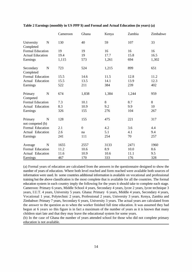
The comparisons presented in Table 1 are extended in Table 2 to see how far the largedifferences remain for workers of a similar educational status. In the comparison the omittedcategory is those who failed to complete primary education. We compare this base category with,1

It will be noted that the value-added per employee figure for Zambia is very low. This is probably2

due to problems in the use of PPP exchange rates to convert the domestic Zambian currency to US dollars.Zambia experienced a period of very high rates of inflation in the early 1990s and it is possible the PPPexchange rate is misleading over the period. The data appendix gives the PPPs used in the calculations.

3

first, primary completed, second, secondary completed and finally, those who completeduniversity. In Table 2 the data is presented for the estimates of the number of years of educationeach of these stages took and the earnings, using PPP exchange rates, for each educationalcategory by country.

There are two ways of measuring years of education from the data. One, termed formalin the table, uses the answers to the questions of level, and form, reached to infer the number ofyears. As forms can be repeated such a procedure provides a minimum estimate of the number ofyears of education. The second way of measuring years of education, termed actual in Table 2,is to assume education began at the age of 6 and then use the information on the year full timeeducation ceased to infer years of education. As many children do not start education at 6 thismethod provides an estimate with opposite errors to the first method. For secondary anduniversity completers the two methods give similar averages. For lower education levels the“actual” figures are in some cases substantially higher than the “formal” figures. The table presentsearnings in US PPP dollars. At the university level there is a very narrow range for three of thecountries, Cameroon, Kenya and Zimbabwe. It will be noted that the relatively high earnings inthe Cameroon are due to much higher wages for secondary completers in that country than forthe others. The low wages in Zambia relative to Ghana are due to the very low wages paid to bothprimary completers and non-completers in that country.

The overall average, for years of education shown in Table 2, is 9.8 and the range acrossthe countries is very small: from 9.5 years in Zimbabwe to 11.6 years in the Cameroon. Ifdifferences in human capital are to explain the differences in wages then this measure must hideeither differences in composition, differences in returns or differences in quality; or somecombination of all three. If earnings for a given skill level differ across the countries thesedifferences will be reflected in differing endowments of capital per worker. The potentialimportance of this factor is brought out in Table 3 which extends Table 2 by showing the physicaland human capital characteristics of the firms.

While the years of education are similar across the countries the proportion of the workforce who had completed secondary education ranged from 16 per cent in Ghana to 40 per centin the Cameroon. Ghana’s workforce is dominated by primary school completers while that ofthe other countries is dominated by secondary school completers. There are also very largedifferences across the countries in the size and capital intensity of the firms. The Zimbabwe samplehas by far the largest firms, an average 300 employees, as compared with only 42 in the Ghanasample. The differences in capital per employee are also large with Ghana, again, far below theother countries. The Ghanaian firms are smaller, have less than a third of the capital per employeeof firms in the other countries, and a less educated work force. The question posed in the2

introduction is how far these differences can explain productivity and earnings differentials. Toanswer that question we must consider how to model these outcomes.

3. Returns to Human Capital from the Earnings FunctionIn Table 4 we present an earnings functions with the human capital variables that we have for allfive countries. Education is measured by the level of formal education completed. Experience ismeasured by age and firm specific learning is measured by the tenure of the worker in their current

The increment in nominal earnings are obtained from the dummy variables as exp(coefficient) -13

as suggested by Halvorsen and Palmquist (1980). These are then deflated by the rise in the price indexgiven at the bottom of Table 4 to obtain the change in real wages.

4

job. These experience variables are modelled with a quadratic term to allow for the expected non-linearities in the effects of experience on earnings. With the exception of the quadratic term ontenure all the variables are highly significant. There are highly significant differences across thecountries. It is possible to use the earning function estimates to assess how real wage havechanged over time, when possible differences in the sample are controlled for, and to estimate thereturns to education. There are numerous reasons, which we consider below, why the estimatesin the earnings functions may be biased.

First we set out the implied changes in real wages across the survey period for each of thecountries. The change vary from a rise of 18 per cent in Kenya to a fall of 40 per cent in theCameroon. This latter figure is higher than that obtained from the raw data and shows the3

importance of controlling for differing characteristics over the course of the surveys. The earningsfunction for the Cameroon implies that in a period when inflation was above 30 per cent perannum, nominal wages fell by about 7 per cent. The second largest fall in real wages was inZambia where large rises in nominal wages were insufficient to compensate for continuing highinflation. In contrast there was a rise of 18 per cent in real wages in Kenya.

The returns to both education and experience can be inferred from Table 4. The age-earning profiles across three of the countries - the Cameroon, Zambia and Zimbabwe - are verysimilar, with Ghana and Kenya being contrasting outliers. Ghana has a particularly steep age-earnings profile while the one in Kenya is much flatter than the average across the countries. Thereturns to education can be calculated in two ways. First it is possible to use the coefficient on thedummy variable for the level of education completed as one measure on the return to education.Such a measure takes no account of the number of years taken to complete the level and, if usedto measure the rate of return, implicitly assumes that the foregone opportunity cost over thoseyears was zero. We present the measure as a maximum number for the rate of return oneducation. A second way of measuring returns is that proposed originally by Mincer (1974). Theassumption which underlies the Mincerian interpretation is that, for each educational level, theforegone opportunity cost is the wage which would have been obtained with the education levelthe one below the one completed. This calculation can be viewed as a minimum for the estimatedrate of return. We continue to abstract from the possibility of bias in the coefficients. In Table 5we present the returns to education implied by both these methods of calculation. The incrementin earnings shown in the Table 5 is, for each educational level, the percentage increase in earningsthat accrues from completing that level of education calculated from the earnings function ofTable 4. The years of education are taken from the formal education figures in Table 2. Rates ofreturn are then simply the increment in earnings divided by the number of years it took to acquirethe increment.

Whichever method is chosen the pattern is the same across all the countries. Private ratesof return to education rise with the level of education. For university completers it is clear thatthe assumption that underlies the maximum calculation is false. However, it is true for allcountries that the returns to university education using the Mincerian assumption are greater thanthe returns to primary education using the maximum assumption, where it is much morereasonable. Have we here the answer to the puzzle we posed in the introduction? Why, if skilledlabour in Africa is scarce, are not the returns to skilled labour high? If by skilled labour is meantsecondary school completion, and beyond, then the return to skilled labour is high.

5

There are several reasons why the returns to education presented in Table 5 may be basedon coefficients that are biased. Bias may arise as we have not allowed for selectivity. Those whowork in the manufacturing sector are highly atypical. Such selectivity bias may not simply meanthat the returns to education are overstated, our sample excludes all those who completededucation and did not get employed in manufacturing, but may bias the estimates so obtained forthose who did get employed. Secondly, such educational measures cannot distinguish betweensignalling and credentionalism as alternatives to the human capital interpretation. Thirdly, it isknown that parental background can play an important role in educational choice. Our sample islimited to those in manufacturing, we have no variables measuring ability or information onparental background. The question we wish to pose is the following: if no controls are includedfor cognitive skills or parental background is there evidence of significant bias up or down in theinterpretation of the crudely measured education variable?

A recent study examining some of these issues for Ghana is Glewwe (1996) who providesevidence that there may be an upward bias. If selectivity is allowed for in the private sectorearnings function for his data then the coefficient on years of schooling becomes insignificant.Glewwe then calculates the rate of return on education based on the measures of cognitive skillsavailable for his data set. He finds a figures of 4 per cent, for an individual aged 25, whichcompares with a rate of return of 7 per cent from the OLS earning function.

Five studies which have information on parental background are, Behrman and Wolfe(1983), Lan and Schoeni (1993), Heckman and Hotz (1986), Krishnan (1996) and Kingdon(1997). The conclusion, which is uniform across the studies, is that the inclusion of parentalbackground reduces the returns to schooling by about 20 per cent. Krishnan (1996) has recentAfrican evidence from Ethiopia and obtains a similar result to earlier studies. Her study shows thatthis effect is due almost entirely to the effects of parental background on access to education.Once the selectivity bias was controlled for the effects from parental background onto returns wassmall. All this evidence suggests that the estimates presented in this paper from the earningsfunction may be upwardly biased. A recent study which uses a panel data set of twins to estimatethe returns to school quality, Behrman, Rosenzweig and Taubman (1996) finds that controllingfor family background does affect the assessment of the returns from school quality but has onlyvery marginal effects on the returns to schooling coefficient. A study which has very detailedinformation on cognitive skills and parental background is that of Knight and Sabot (1990). Theirstudy uses comparative data drawn from workers in the manufacturing sector of Kenya andTanzania. They argue that the returns of education variable is picking up human capital formation.While signalling may play some role, it is not the primary reason years of education determinesearnings.

The conclusion we would draw is that the evidence suggests that the education variablewill overstate the returns to human capital and that the major influence of years of education onearnings is through its effects on cognitive skills and not, as the signalling explanation wouldimply, indirectly through signalling ability. Even if the biases are more significant that theempirical evidence currently suggests, it is not clear that they would explain, or mitigate, the non-linearity in the returns to education.

Education is only one dimension of human capital. Freeman (1986, p.377) notes that“every study also finds that, by itself, years of schooling explains a relatively small part of thevariance of log earnings, say 3-5 percent at most”. It is possible that it is the link betweeneducation and returns to experience and training where substantial increases inearning/productivity might be possible. In the earnings function such returns can be measuredfrom the age variable as a proxy for experience. In the production functions of the next section

6

it will be shown that tenure captures an important aspect of human capital in the productionprocess for some of our countries.

The returns from work experience, in which the age variable in the earnings function isinterpreted as returns to learning, are reported in the bottom part of Table 5. The rate of returnis calculated by asking the average annual increase in earnings for a worker of a given educationallevel over a twenty year period, of which the middle is the average age of workers in thatcategory. The pattern is that which has been observed in other datasets of this form. The returnsto experience rise with educational level. The returns to experience are largest, for both primaryand secondary completers, for Ghana. In all the countries, except Ghana, the weighted averageof the return from experience is lower than that for education, Table 5. In the next section weconsider how these returns compare with those for physical capital from using a productionfunction.

4. Human and Physical Capital in ProductionThe data presented in this paper enables a comparison to be made between the returns fromhuman capital investment with those on physical capital in a production function. It is theexistence of the firm level data that makes such a comparison possible. The discussion is clearestif a simple Cobb-Douglas form of the production function is assumed:[1] Ln Y = $ + $ Ln L + $ Ln K +$ Ln H + controls + uijt 0j 1 ijt 2 ijt 3 ijt ijt

where Y is output, L is labour input, K is physical capital and H is human capital. The subscriptsdenote the i firm, in the j country at time t. The dimensions of human capital that can beth th

measured from the survey are the level of education completed, the number of years of education,experience measured by age and the tenure of workers in the firm.

The variables Y, L and K are measured at the firm level. The human capital variables arebased on the individual data and are averaged across the firm to produce an estimate of the firmlevel composition of these dimensions of human capital. Real wages and the returns to capital aregiven by the marginal productivity relationship so:[2] w = $ Y / L and r = $ Y / Kijt 1 ijt ijt ijt 2 ijt ijt.

P

The returns to human capital in a form commensurate with that for physical capital can beobtained from:[3] r = (dY / Y ) / dH = $ / H .H

ijt ijt ijt ijt 3 ijt

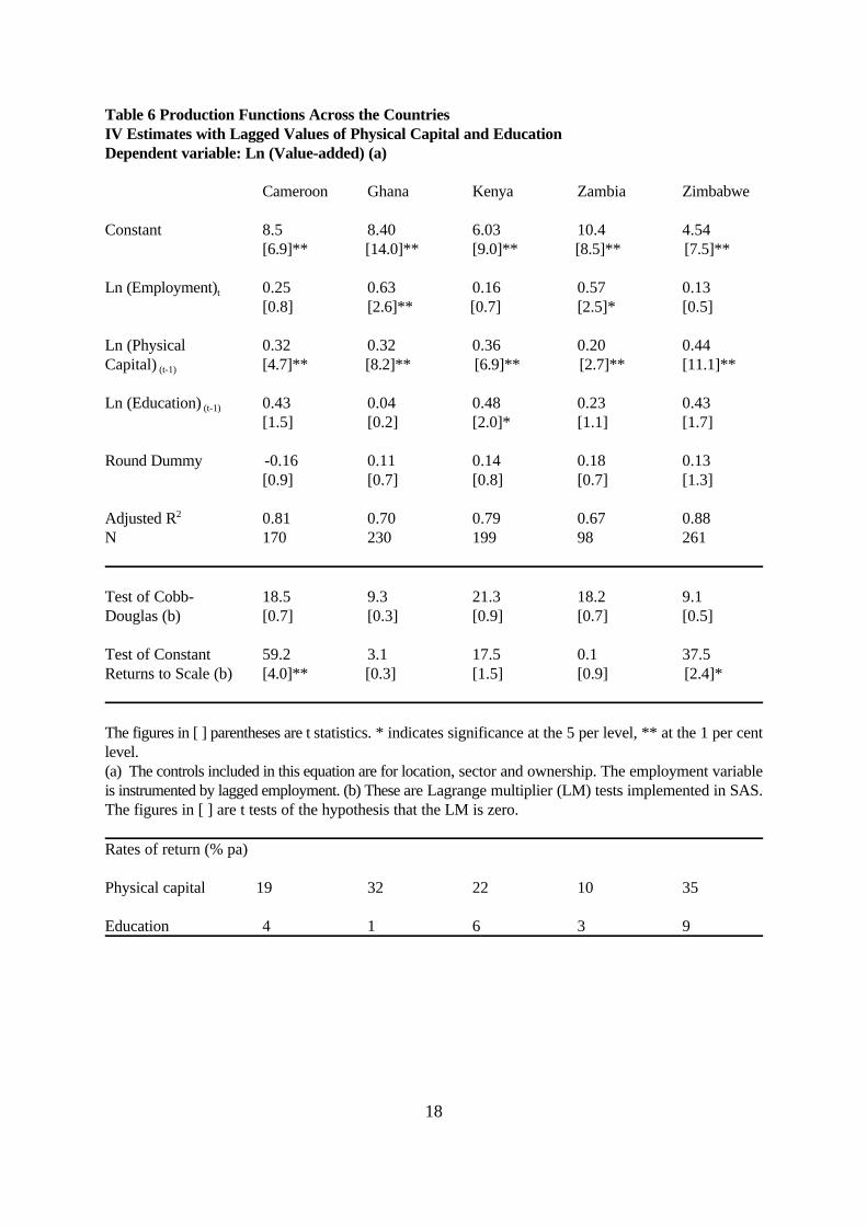
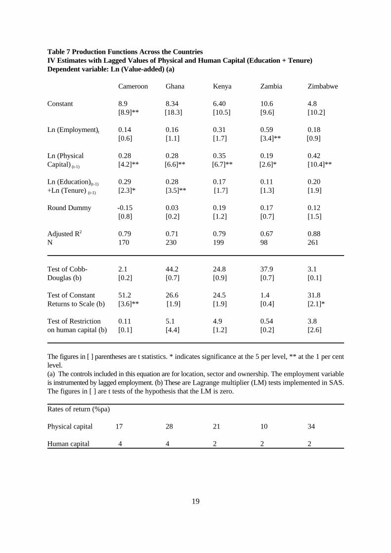
Equation [1] sets out the form of the production function which is estimated for each country andpresented in Tables 6 and 7 which differ by how human capital is measured. In Table 6 theEducation variables used in the regressions in the total years of education in the firms,[4] Education = E x L.In Table 7 human capital is measured by also including total years of tenure ( T x L) in the firmwhere tenure is defined as the length spent in the current job,[5] Human Capital (H) = E x L + T x L.We also experimented with including age as a measure of experience and for no country was thatvariable superior to the measure of human capital in [5] and for some countries it producednegative coefficients on the age variable. We infer that, at the firm level, the average age of theworkforce is an inferior measure of human capital to tenure. In assessing the relative importanceof physical and human capital in the inter-country determinants of earnings and productivity it isnecessary to aggregate equation [1] across countries which gives, assuming constant returns toscale,

7

[6] Ln Y /L = $ + $ Ln K /L $ Ln H / L + controls + ujt jt 0j 2 jt jt + 3 jt jt jt

At the country level the link between earnings an productivity is given by:[7] Ln w = Ln $ + LnY / Ljt 1 jt jt

= Constant +$ Ln K /L $ Ln H /L + controls + u .2 jt jt + 3 jt jt jt

Under the competitive market assumptions differences in labour productivity across countries willbe matched by differences in earnings. At the country level the causality, in fact, runs fromearnings to the capital labour ratio to productivity. Productivity differences will reflect differencesin technology, the country shift parameter in the production function ($ ), and differences in0j

physical and human capital endowments. The micro analogue to the macro questions posed in thepapers by Krueger (1968) and Fallon and Layard (1975) is the respective roles of technology andphysical and human capital endowments across countries in determining differences inproductivity and earnings.

We take up below the comparison of the productivity relationship and earnings functionsacross countries. First we present the estimates for equation [1] in Tables 6 and 7 for each of thecountries. In modelling the production decision of the firm we exploit the panel dimension of thefirm data to make both physical and human capital predetermined variables. Employment in thecurrent period is instrumented by lagged employment. In Table 6 human capital is simply the totalyears of education of workers in the firm. We have used the continuous measure of eduction asthat enables us to set up a translog production function to test the restrictions implied by the useof the Cobb-Douglas form. In both Tables 6 and 7 a test is reported on the move from the generaltranslog to the Cobb-Douglas specification. The restrictions are accepted for all the countries. Atest is also reported for restricting returns to scale to unity and this is rejected at the 1 per centlevel in the Cameroon and Zimbabwe, but accepted in the other countries. In Table 7 a test is alsoreported of restricting the coefficient on the two aspects of human capital, education and tenure,to be the same. This restriction is accepted for all countries. It is clear from a comparison ofTables 6 and 7 that for the Cameroon and Ghana the wider definition of human capital is a moresignificant determinant of output, but for the other countries it makes little difference whichmeasure of human capital is used. At the bottom of the tables we report the implied rates of returnfor physical and human capital for both specifications of the measure of human capital. The rateof return on physical capital is obtained by taking the median value-added to capital ratio givenin Table 3 and multiplying it by the coefficient on the physical capital stock variable in theproduction function. The rate of return on human capital is obtained from using equation [3]above. For all countries, and whichever measure of human capital is used, the returns on physicalcapital massively exceed those on human capital.

A comparison of Tables 5 and 6 shows that, with the exception of Kenya, the returns oneducation as a measure of human capital from the earnings function exceed those from theproduction function. This finding is consistent with the summary presented above that the earningsfunction will, in the form presented in Table 4, overstate the returns on education. The high ratesof return on physical capital are not reflected in high investment by the firms, Bigsten et al (1998).They argue that the implication of the co-existence of high marginal productivities and lowinvestment is that the cost of capital to the firms is high.

5. The Determinants of Productivity and Earnings across CountriesIn Table 8 we pool the earnings functions across the countries using the PPP valuation ofearnings. It is clear from the highly significant, and large, country dummies in these regressionsthat differing human capital characteristics explain only a small part of the earning differentialsacross the countries. Table 8 equation [2] uses firm level controls to see if these explain the

This result for Ghana was first noted by Jones (1994).4

8

country effects. While the inclusion of the controls lowers the returns on education they have noimpact on the country dummies. In Table 9 a calculation is presented as to the implied averagereturn on education across the five countries. The figure is a weighted average across the threecategories of educated labour identified in the earnings function. Without controls the returns toeducation is 9 per cent, with controls it is 7 per cent. We now turn to a comparison between thisresult and that using the production functions.

In Table 10 we pool the production functions across countries using both measures ofhuman capital. For both regressions the hypothesis of common coefficients across the countriesis accepted at the 1 per cent significance level. In comparing the two regressions in Table 10 itis clear that the wider definition of human capital in equation [2] reduces the size of the countrydummies. Cameroon, Kenya and Zimbabwe now pool with Ghana having a technology about 25per cent less efficient than that of the other countries and Zambia a highly significant outlieramong the countries. We report in the table the rates of return on physical and human capitalacross the pooled sample. It will be noted that for both regressions the hypothesis of constantreturns to scale is rejected at the 1 per cent significance level. If this constraint is relaxed thereturns on eduction halve so the imposition of the restraint is acting to increase the returns tohuman capital.

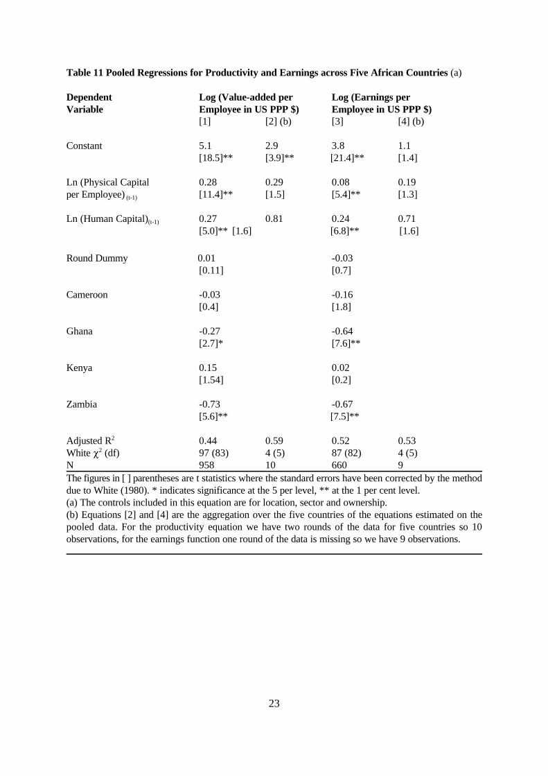
Finally in Table 11 we turn to the determinants of productivity and earnings. In Table 11equation [1] we reproduce the result in Table 10 equation [2] but now presented in terms of theproductivity of labour in the firm. The determinants of productivity can be compared directly withthose of earnings. The terms in human capital are virtually identical between the two equations.4

As noted above, if we move to a country based regression, then the coefficient on the capitallabour ratio in the earnings function should rise in principle to the same value as characterises theproduction function. The level of aggregation leaves very few degrees of freedom but the resultshown in Table 11, equations [3] and [4], is broadly consistent with these expectations with thecoefficient on the log of the capital labour ratio rising from 0.08 to 0.19, close to the value of 0.28from the productivity equation, Table 11 equation [1]. The coefficient on the human capital termfor both the productivity and the earnings equation rises substantially when we aggregate acrosscountries which may capture externalities or may simply reflect the lack of variation of thisvariable across the countries.

We can now ask what are the factors determining differences in productivity and earningsacross the five countries. The factors determining differences in productivity can be directlyinferred from Table 11, equation [1]. With the exception of Zambia, which we have already notedmay reflect problems with the measurement of the PPP exchange rates, differences in technologyplay a small part. There are no significant differences in the underlying production function forthe Cameroon, Kenya and Zimbabwe. The technology in Ghana is 30 per cent less efficient. In thedata from Table 3 the gap in median labour productivity between the Cameroon and Ghana was3.7 times. All but 25 per cent of this difference is explained by differences in physical and humancapital endowments. Again from Table 3 we note that the differences in human capitalendowments are modest, 12 per cent using the definition of human capital which combines bothyears of education and tenure in the firm. In contrast the differential in median physical capitalendowments was 14 times. Using the production function shown in Table 11 such a differentialin physical capital per employee implies a 3.7 differential in labour productivity, exactly as shown

9

in the data. It is clear that virtually all the differences in productivity between the manufacturingsectors in the Cameroon and Ghana are explained by differences in physical capital endowments.

As noted above, under the competitive market assumptions, the differences in labourproductivity should be reflected in differences in earnings. Thus the earnings differential betweenthe Cameroon and Ghana should be 3.7 times. In fact it is less. In Table 1, based on the individualdata, the differential is 2.7 times, while in Table 3, based on the firm level data, it is 2 times. Thereare two possible explanations for the low level of this earning differential between the twocountries. First, it may be due to problems in the use of PPP exchange rates. Using officialexchange rates the earnings differentials across the countries is much larger, 5.4 times. Second,it is possible that earnings do not exactly reflect differences in productivity as the labour marketis not competitive. Whatever the explanation for the failure of earnings to reflect productivitydifferences across the two countries the small difference in human capital, which have beendocumented, imply that such differences cannot play a significant part in explaining differencesin either productivity or earnings.

6. Summary and ConclusionsWe now summarise our answers to the four questions posed at the beginning of this paper. Theanswer to the first is that only in one country, Kenya, did the real wage rise in the early 1990s.Real wages stagnated in Zimbabwe and fell in Zambia, Ghana and the Cameroon. The fall in realwages in the Cameroon was particularly large at 40 per cent. By the end of the survey periodsthree countries, Zimbabwe, Kenya and the Cameroon, had very similar wages in purchasing powerparity terms of about US$ 350 per month. Such wage levels are comparable to those found inChinese rural enterprises. In the case of both Zambia and Ghana wages are substantially lower atabout US$170 per month. The issue that we have addressed is whether, within these averages,the relative wage of skilled workers in Africa is high.

It was to that issue that our second question was addressed: what are the rates of returnon human capital in Africa? The data used in this paper allows a comparison to be made betweenthe answer to that question from earnings functions and from the use of a measure of humancapital in the production function. The rate of return on average for education, across the fivecountries, from the earnings function was 9 per cent. The returns were highly non-linear risingfrom 3 per cent for primary to 14 per cent for secondary completers and 43 per cent for universitycompleters. It has been widely argued that these estimates overstate the return to human capital.Our use of a production function to measure the return supports such arguments; the rate ofreturn on human capital measured by years of education from the production function was 5 percent, again on average across all the five countries. The education variation across firms is toosmall to capture the non-linearity in the returns to education clearly shown by the earningsfunction.

It could be argued that this finding from the earnings function, of a rising return to humancapital with its level, resolves the puzzle, identified in the introduction, as to how an economywith relatively scarce skilled labour has a low return on education. The average return is low.However it is so non-linear that for those with skills from secondary school and beyond thereturns are very high. Insofar as these skills are those used intensively in a successfulmanufacturing sector the relative scarcity of such skills is consistent with the failure of Africa todevelop a successful manufacturing sector.

Out third question concerned the returns on physical capital. Across all the countries thesereturns are far higher than those available from human capital investments measured in theproduction function. Given the very low investment rates in the manufacturing sectors of these

10

countries such high returns must also imply high capital costs facing the firms. This findingsuggests that the failure of Africa to develop a successful manufacturing sector may have itssource, not simply in the market for skills, but also in the costs of capital faced by firms in theAfrican manufacturing sector.

Finally we turn to our fourth question: what is the relative importance of technology andhuman and physical capital in the determination of productivity and earnings differentials acrossthe countries? For three of the countries, the Cameroon, Kenya and Zimbabwe, technology playsno role. The very large productivity differentials which characterise the Cameroon and Ghanaianmanufacturing sectors are due, virtually entirely, to differences in endowments of physical capital,differences in human capital endowment are of negligible importance.

11

ReferencesAppleton, S., Hoddinott, J. and J. Mackinnon (1996) “Education and health in sub-SaharanAfrica, Journal of International Development, Vol. 8, No.3, May-June, pp.307-339.Behrman, J., M.R. Rosenzweig and P. Taubman (1996) “College choice and wages: estimatesusing data on female twins”, Review of Economics and Statistics, Vol. 78, (4), November, pp.672-685.Behrman, J. and B. Wolfe (1983) “The socio-economic impact of schooling in a developingcountry”, Review of Economics and Statistics, 66 (2), 296-303. Bennell, P. (1996) “Rates of return to education: does the conventional pattern prevail in sub-Saharan Africa” World Development, Vol.24, No. 1, pp. 183-199.Bigsten A., P. Collier, S. Dercon, B. Gauthier, J. W. Gunning, A. Isaksson, A.Oduro, R.Oostendorp, C. Pattillo, M. Soderbom, M. Sylvain, F. Teal, A. Zeufack (1998) “Investment inAfrica's Manufacturing Sector: a Four Country Panel Data Analysis “, CSAE, Oxford, mimeo.Fallon, P.R. and Layard, P.R.G. (1975) “Capital-skill complementarity, income distribution andoutput accounting”, Journal of Political Economy, Vol. 83, No.2, 279-296.Freeman, R. (1986) “Demand for Education”, chapter 6 in O. Ashenfelter and R. Layard (eds.)Handbook of Labor Economics, North-Holland, Amsterdam.Glewwe, P. (1996) “The relevance of standard estimates of rates of return to schooling foreducation policy: A critical assessment”, Journal of Development Economics, Vol. 51, pp.267-290.Halvorsen, R. And R. Palmquist (1980) “The interpretation of dummy variables insemilogarithmic equations”, American Economic Review, Vo.70, No.3, 474-475.Heckman, J J and V J Hotz (1986) “An investigation of the labour market earnings of Panamanianmales: evaluating the sources of inequality”, Journal of Human Resources, 21, 507-542.Jones, P. (1994) “Are manufacturing workers really worth their pay?” CSAE Working paper 94-2, Oxford, Oxford university.G. Kingdon (1997) “Does the labour market explain lower female schooling in India”, TheDevelopment Economics Research Programme, Discussion paper No 1, January.Knight, J.B. and R.H. Sabot (1990) Education, Productivity and Inequality: The East AfricanNatural Experiment, Oxford University Press.Knight, J., Song,L. And J. Huaibin (1997) Chinese rural migrants in urban enterprises: threeperspectives, Applied economics Discussion Paper No. 190, January, Institute of Economics andStatistics, University of Oxford.Krishnan, P. (1996) “Family background, education and employment in urban Ethiopia”, OxfordBulletin of Economics and Statistics, 58, 1, pp.167-183.Krueger, A. (1968) “Factor endowments and per capita income differences among countries”,Economic Journal, September 1968, pp.641-659.Lan, D. and R F Schoeni (1993) “Effects of family background on earnings and returns toschooling: evidence from Brazil”, Journal of Political Economy, 101.Lucas, R.E. Jr (1988) “On the mechanics of economic development”, Journal of MonetaryEconomics, Vol. 22, July, pp.3-42.Lucas, R.E. Jr (1990) “Why doesn’t capital flow from rich to poor countries?”, AmericanEconomic Review, Vol. 80, May, pp.92-96.Mincer J. (1974) Schooling, Experience and Earnings, NBER, New York.Owens, T. and A. Wood (1997) “Export Oriented Industrialisation through Primary Processing?”,World Development, 25 (9), September, 1453-1470.

12

Psacharopoulos, G. (1994) “Returns to education: a global update”, World Development, Vol.22,No.9, pp.1325-1343.Romer, D. (1996) Advanced Macroeconomics, McGraw-Hill, New York.White, H. (1980) "A heteroscedasticity-consistent covariance matrix estimator and a direct testfor heteroscedasticity", Econometrica, 48, 817-838.Wood, A. (1994) North-South Trade, Employment and Inequality: Changing fortunes in a skill-driven world, Clarendon Press, Oxford.Wood, A. and K. Berge (1997) “Exporting Manufactures: Human Resources, Natural Resources,and Trade Policy”, Journal of Development Studies, 34 (1), 35-59.

13

Table 1 Monthly Earnings (Earnings includes allowances)

Round 1 Round 2 Round 3 Average

Cameroon N 675 571 409 1,6551993-1995US $ 378 202 239 283US PPP $ 470 535 367 467CFA francs 106,937 111,986 119,407 111,761CFA francs (1990) 110,472 84,852 80,139 91,821

Ghana N 684 743 1,130 2,5571992-1994US$ 64 57 41 52US PPP $ 172 184 160 170Cedis 27,987 37,017 39,415 35,661Cedis (1990) 21,545 22,808 19,445 21,266

Kenya N 1,098 972 1,063 3,1331993-1995(a)US $ 67 75 121 88US PPP $ 312 269 413 333Shillings 3,878 4,222 6,230 4,782Shillings (1990) 1,714 1,446 2,117 1,759

Zambia N 903 864 704 2,4711993-1995(a)US $ 163 128 123 139US PPP $ 194 180 147 176Kwacha 70,886 98,318 102,270 89,419Kwacha (1990) 4,282 3,702 3,024 3,669

Zimbabwe N 1,408 552 na 19601993-1994US$ 145 140 na 143US PPP $ 326 332 328Zimbabwe $ 935 1,143 na 994Zimbabwe $ (1990) 418 418 na 418

N is the number of observations.(a) For both Kenya and Zambia allowances were not collected for the first round of the surveys. The wagefigures have been scaled up by the ratio of wages to allowances for later years to ensure that the data areas comparable as possible across the rounds of the surveys.Average Earnings Chinese Rural Workers (1995)

Yuan per year US$ per month US PPP $ per monthManagerial and technical staff 8,120 81 395Production workers 6,589 66 320Total 6,877 69 334Source: Knight and Song (1997).

14

Table 2 Earnings (monthly in US PPP $) and Formal and Actual Education (in years) (a)

Cameroon Ghana Kenya Zambia Zimbabwe

University N 130 40 59 107 33CompletedFormal Education 19 19 16 16 16Actual Education 19.4 19 17.7 15.8 16.5Earnings 1,115 573 1,261 694 1,302

Secondary N 723 524 1,215 899 651CompletedFormal Education 15.5 14.6 11.5 12.8 11.2Actual Education 15.5 13.5 14.1 13.9 12.3Earnings 522 211 384 239 402

Primary N 674 1,838 1,384 1,244 959CompetedFormal Education 7.3 10.1 8 8.7 8Actual Education 8.3 10.9 9.2 9.9 10Earnings 326 155 276 104 267

Primary N 128 155 475 221 317not competed (b)Formal Education 2.1 0 4.2 3.6 4.4Actual Education 2.6 na 5.1 4.1 9.4Earnings 241 111 254 70 257

Average N 1655 2557 3133 2471 1960Formal Education 11.2 10.6 8.9 10.0 8.6Actual Education 11.6 10.9 10.6 11.1 9.5Earnings 467 170 333 176 328

(a) Formal years of education are calculated from the answers in the questionnaire designed to show thenumber of years of education. Where both level reached and form reached were available both sources ofinformation were used. In some countries additional information is available on vocational and professionaltraining but the above classification is the most complete that is available for all the countries. The formaleducation system in each country imply the following for the years it should take to complete each stage.Cameroon: Primary 6 years, Middle School 4 years, Secondary 4 years, lycee 2 years, lycee technique 3years, I.U.T. 4 years, University 5 years. Ghana: Primary 6 years, Middle 4 years, Secondary 4 years,Vocational 1 year, Polytechnic 2 years, Professional 2 years, University 3 years. Kenya, Zambia andZimbabwe: Primary 7 years, Secondary 6 years, University 3 years. The actual years are calculated fromthe answer to the question as to when the worker finished full time education. It was assumed they hadbegun at 6 years so this figure is in fact a maximum of the number of years as it is known that manychildren start late and that they may leave the educational system for some years.(b) In the case of Ghana the number of years attended school for those who did not complete primaryeducation is not available.

15

Table 3 Firm Size (Number of Employees) , Value-added/Capital, Capital per Employee ( in US PPP$), Value-added per Employee (in US PPP $), Education, Tenure (in years) and Monthly Earnings(in US PPP $) by Country

Cameroon Ghana Kenya Zambia Zimbabwe

N 170 230 199 98 261

Employment Mean 82 42 75 45 300Median 25 17 30 19 110Std 197 77 138 72 534

Value-added/ Mean 1.2 3.8 2.4 2.3 1.7Capital Median 0.6 1.0 0.6 0.5 0.8

Std 2.4 9.2 6.7 5.6 4.8

Capital/ Mean 19,854 5,585 18,593 17,023 21,000Employee Median 8,758 629 7,242 5,426 9,299

Std 26,319 12,565 28,490 29,409 36,695

Value-added/ Mean 14,335 4,868 24,101 4,706 14,373Employee Median 8,214 2,203 7,796 2,465 7,764

Std 19,994 7,171 87,263 6,271 36,185

Education/ Mean 9.7 9.3 7.9 8.6 8.2Employee Median 9.5 9.6 7.9 8.5 8.3(years) Std 2.4 2.2 1.9 1.9 1.3

Tenure/ Mean 5.4 4.2 7.4 5.8 9.2Employee Median 5.0 3.3 7.0 4.9 9.3(years) Std 3.3 3.6 4.2 3.8 4.3

N 136 203 188 89 214

Primary Mean 0.44 0.78 0.43 0.55 0.49Completed Std 0.33 0.26 0.29 0.32 0.26

Secondary Mean 0.39 0.16 0.36 0.31 0.33Completed Std 0.32 0.24 0.28 0.30 0.26

University Mean 0.07 0.01 0.01 0.02 0.01Completed Std 0.13 0.03 0.04 0.07 0.06

N 116 191 182 83 88

Monthly Mean 369 170 389 162 440Earnings Median 284 130 274 117 311

Std 292 127 374 125 410Std is the standard deviation, N is the number of observations

16

Table 4 An Earnings Function Across the Countries: Human Capital Variables Only

Cameroon Ghana Kenya Zambia ZimbabweConstant 7.8 5.1 6.5 7.9 2.6

[23.0]** [27.2]** [36.2]** [37.4]** [11.3]**

Male 0.02 -0.02 0.06 0.008 0.21[0.6] [0.5] [1.9] [0.2] [5.1]**

Age 0.12 0.22 0.05 0.08 0.16[6.3]** [22.4]** [4.8]** [6.0]** [13.0]**

Age -0.001 -0.002 -0.0005 -0.001 -0.0022

[4.5]** [18.5]** [3.5]** [4.6]** [11.6]**

Primary 0.20 0.25 0.17 0.36 0.15Completed [4.1]** [3.9]** [5.6]** [5.6]** [3.6]**

Secondary 0.72 0.57 0.44 1.0 0.77Completed [14.2]** [8.2]** [12.9]** [14.5]** [13.0]**

University 1.57 1.40 1.51 2.13 1.79Completed [22.3]** [12.7]** [13.1]** [20.8]** [10.5]**

Tenure 0.03 0.02 0.003 0.04 0.01[5.2]** [2.5]* [0.6] [5.2]** [2.3]*

Tenure -0.0004 -0.0003 0.0001 -0.001 -0.00012

[1.6] [1.1] [0.9] [3.9]** [0.2]

Wave 2 -0.08 0.28 0.16 0.29 0.20[2.5]* [6.7]** [5.8]** [8.3]** [6.2]**

Wave 3 -0.07 0.35 0.43 0.61[2.1]* [8.5]** [16.1]** [15.7]**

Adjusted R 0.47 0.46 0.22 0.39 0.282

N 1655 2557 3133 2471 1960White P test 93 (53) 209 (54) 136 (53) 124 (53) 145 (44)2

The figures in [ ] parentheses are t statistics using White (1980) corrected standard errors.* indicatessignificance at the 5 per level, ** at the 1 per cent level.Rates of Inflation(% pa) A * indicates that it is the period to which the wave dummy in the regression refers.1992/93 -3.3 24.9* 45.8 189 27.61992/94 30.8 56.0* 88.0 340 56.01993/94 35.1* 24.9 29.0* 52.3* 22.2*1993/95 53.9* 118 30.0* 104* 49.9Change in real wages over survey period

-40 -9 18 -10 0

17

Table 5 Increment in Earnings (%) and Rates of Return (% pa) to Human CapitalCameroon Ghana Kenya Zambia Zimbabwe

Education

Primary CompletersIncrement in Earning 22 28 19 43 16Years 7 10 8 9 8Rate of return 3 3 2 5 2

Secondary CompletersIncrement in Earning 68 38 31 90 86Years 8 3 6 4 3Rate of return 8 15 5 22 27

University CompletersIncrement in Earning 134 129 192 209 177Years 4 4 5 3 5Rate of return 38 29 43 65 37

Weighted Rateof Return 8 5 4 12 12

Age

Primary CompletersAge 0.07 0.24 0.04 0.07 0.12

3.6 [22.5] [3.1] [5.3] [8.3]Age -0.0005 -0.003 -0.0004 -0.0008 -0.0012

[1.9] [18.5] [2.3] [4.3] [7.6]Rate of Return 4 5 1 1 5

Secondary CompletersAge 0.18 0.22 0.04 0.14 0.18

[6.9] [10.7] [2.0] [5.7] [6.1]Age -0.002 -0.002 -0.0001 -0.001 -0.0022

[5.1] [8.1] [0.3] [4.2] [4.1]Rate of Return 4 8 3 7 6

University Completers (a)Age 0.35 0.02 0.45 0.23 0.33

[5.2] [0.2] [3.1] [2.9] [1.98]Age -0.004 0.0 -0.006 -0.003 -0.0042

[4.4] [0.02] [3.1] [2.6] [1.7]Rate of Return 8 na 18 9 8

Weighted Rateof Return 4 6 2 3 5

18

Table 6 Production Functions Across the Countries IV Estimates with Lagged Values of Physical Capital and EducationDependent variable: Ln (Value-added) (a)

Cameroon Ghana Kenya Zambia Zimbabwe

Constant 8.5 8.40 6.03 10.4 4.54[6.9]** [14.0]** [9.0]** [8.5]** [7.5]**

Ln (Employment) 0.25 0.63 0.16 0.57 0.13t

[0.8] [2.6]** [0.7] [2.5]* [0.5]

Ln (Physical 0.32 0.32 0.36 0.20 0.44Capital) [4.7]** [8.2]** [6.9]** [2.7]** [11.1]** (t-1)

Ln (Education) 0.43 0.04 0.48 0.23 0.43 (t-1)

[1.5] [0.2] [2.0]* [1.1] [1.7]

Round Dummy -0.16 0.11 0.14 0.18 0.13[0.9] [0.7] [0.8] [0.7] [1.3]

Adjusted R 0.81 0.70 0.79 0.67 0.882

N 170 230 199 98 261

Test of Cobb- 18.5 9.3 21.3 18.2 9.1Douglas (b) [0.7] [0.3] [0.9] [0.7] [0.5]

Test of Constant 59.2 3.1 17.5 0.1 37.5Returns to Scale (b) [4.0]** [0.3] [1.5] [0.9] [2.4]*

The figures in [ ] parentheses are t statistics. * indicates significance at the 5 per level, ** at the 1 per centlevel.(a) The controls included in this equation are for location, sector and ownership. The employment variableis instrumented by lagged employment. (b) These are Lagrange multiplier (LM) tests implemented in SAS.The figures in [ ] are t tests of the hypothesis that the LM is zero.

Rates of return (% pa)

Physical capital 19 32 22 10 35

Education 4 1 6 3 9

19

Table 7 Production Functions Across the Countries IV Estimates with Lagged Values of Physical and Human Capital (Education + Tenure)Dependent variable: Ln (Value-added) (a)

Cameroon Ghana Kenya Zambia Zimbabwe

Constant 8.9 8.34 6.40 10.6 4.8[8.9]** [18.3] [10.5] [9.6] [10.2]

Ln (Employment) 0.14 0.16 0.31 0.59 0.18t

[0.6] [1.1] [1.7] [3.4]** [0.9]

Ln (Physical 0.28 0.28 0.35 0.19 0.42Capital) [4.2]** [6.6]** [6.7]** [2.6]* [10.4]** (t-1)

Ln (Education) 0.29 0.28 0.17 0.11 0.20(t-1)

+Ln (Tenure) [2.3]* [3.5]** [1.7] [1.3] [1.9](t-1)

Round Dummy -0.15 0.03 0.19 0.17 0.12[0.8] [0.2] [1.2] [0.7] [1.5]

Adjusted R 0.79 0.71 0.79 0.67 0.882

N 170 230 199 98 261

Test of Cobb- 2.1 44.2 24.8 37.9 3.1Douglas (b) [0.2] [0.7] [0.9] [0.7] [0.1]

Test of Constant 51.2 26.6 24.5 1.4 31.8Returns to Scale (b) [3.6]** [1.9] [1.9] [0.4] [2.1]*

Test of Restriction 0.11 5.1 4.9 0.54 3.8on human capital (b) [0.1] [4.4] [1.2] [0.2] [2.6]

The figures in [ ] parentheses are t statistics. * indicates significance at the 5 per level, ** at the 1 per centlevel.(a) The controls included in this equation are for location, sector and ownership. The employment variableis instrumented by lagged employment. (b) These are Lagrange multiplier (LM) tests implemented in SAS.The figures in [ ] are t tests of the hypothesis that the LM is zero.

Rates of return (%pa)

Physical capital 17 28 21 10 34

Human capital 4 4 2 2 2

20

Table 8 Pooled Regressions for Earnings across Five African CountriesDependent Variable Ln (Earnings in US PPP $)

No controls Controls (a)[1] [2]

Constant 1.94 1.66[19.7]** [9.9]**

Primary 0.25 0.17Completed [11.5]** [7.9]**t-1

Secondary 0.69 0.49Completed [29.4]** [20.5]**t-1

University 1.69 1.36Completed [36.9]** [25.2]**t-1

Age 0.14 0.11 t-1

[26.1]** [19.9]**Age -0.002 -0.0012

t-1

[20.5]** [16.1]**

Tenure 0.01 -0.001t-1

[4.2]** [0.1]Tenure 0.0 0.00022

t-1

[0.6] [1.6]

Round 2 -0.02 0.006[1.3] [0.3]

Round 3 -0.01 0.03[0.6] [1.5]

Cameroon 0.23 0.23[9.9]** [9.5]**

Ghana -0.44 -0.45[19.8]** [17.1]**

Kenya 0.10 0.14[5.0]** [6.6]**

Zambia -1.1 -0.91[46.9]** [34.8]**

Adjusted R 0.49 0.522

N 11,776 9,417White test P (df) 510 (98) 872 (292)2

The figures in [ ] parentheses are t statistics where the standard errors have been corrected by the methoddue to White (1980). * indicates significance at the 5 per level, ** at the 1 per cent level.(a) The controls included in this equation are for location, sector and ownership, the capital labour ratioand its square, firm size measured by employment and its square.

21

Table 9 Rates of Return from the Earnings Functions (a)

Proportions Increment in earnings Years of Rates Rates[1] [2] Education of return of returnNo controls Controls no controls controls

Primary 0.58 28 19 9 3 3Completed

Secondary 0.38 55 38 13 14 10Completed

University 0.04 172 139 17 43 35Completed

Weighted average (b) 9 7

(a) The increments in earnings are taken from Table 8. [1] refers to the equation with no controls, [2] tothe equation with controls for location, sector and ownership, the capital labour ratio and its square, firmsize measured by employment and its square.

(b) The weights used are the proportions of each class of completed education across the whole sample.

22

Table 10 Pooled Regressions for Value-added across Five African Countries IV Estimates with Lagged Values of Physical and Human Capital Measures (a)Dependent Variable Ln (Value-added in US PPP $)

[1] [2]Constant 4.8 5.02

[16.9]** [22.3]**

Ln (Employment) 0.25 0.23t

[2.2]* [2.9]**

Ln (Physical 0.33 0.31Capital) [15.6]** [14.1]** (t-1)

Ln (Education) 0.42(t-1)

[3.7]Ln (Education) 0.23(t-1)

+Ln (Tenure) [5.4](t-1)

Round Dummy -0.03 -0.03[0.4] [0.5]

Cameroon -0.29 -0.12[2.6]** [1.1]

Ghana -0.40 -0.22[3.6]** [1.9]*

Kenya 0.08 0.12[0.8] [1.2]

Zambia -1.0 -0.89[7.6]** [7.0]**

Adjusted R 0.83 0.832

N 958 958Test of Pooling 2.18 1.2Coefficients (b) [0.6] [1.5]Test of Constant 119.3 92.6Returns to Scale (b) [4.1]** [3.1]**The figures in [ ] parentheses are t statistics. * indicates significance at the 5 per level, ** at the 1 per centlevel.(a) The controls included in this equation are for location, sector and ownership. The employment variableis instrumented by lagged employment. (b) These are Lagrange multiplier (LM) tests implemented in SAS.The figures in [ ] are t tests of the hypothesis that the LM is zero.

Median Value of Value-added to Capital = 0.7Median Value of Education/Employee = 8.8 yearsMedian Value of Tenure/Employee = 5.6 years

Rates of return (%pa)Physical capital 23 22

Human capital 5 3

23

Table 11 Pooled Regressions for Productivity and Earnings across Five African Countries (a)

Dependent Log (Value-added per Log (Earnings perVariable Employee in US PPP $) Employee in US PPP $)

[1] [2] (b) [3] [4] (b)

Constant 5.1 2.9 3.8 1.1[18.5]** [3.9]** [21.4]** [1.4]

Ln (Physical Capital 0.28 0.29 0.08 0.19per Employee) [11.4]** [1.5] [5.4]** [1.3] (t-1)

Ln (Human Capital) 0.27 0.81 0.24 0.71(t-1)

[5.0]** [1.6] [6.8]** [1.6]

Round Dummy 0.01 -0.03[0.11] [0.7]

Cameroon -0.03 -0.16[0.4] [1.8]

Ghana -0.27 -0.64[2.7]* [7.6]**

Kenya 0.15 0.02[1.54] [0.2]

Zambia -0.73 -0.67[5.6]** [7.5]**

Adjusted R 0.44 0.59 0.52 0.532

White P (df) 97 (83) 4 (5) 87 (82) 4 (5)2

N 958 10 660 9The figures in [ ] parentheses are t statistics where the standard errors have been corrected by the methoddue to White (1980). * indicates significance at the 5 per level, ** at the 1 per cent level.(a) The controls included in this equation are for location, sector and ownership.(b) Equations [2] and [4] are the aggregation over the five countries of the equations estimated on thepooled data. For the productivity equation we have two rounds of the data for five countries so 10observations, for the earnings function one round of the data is missing so we have 9 observations.

24

Data Appendix

In constructing the variables used in the regressions reported in this paper a range of decisions needed tobe taken to construct the data. In this appendix we outline how the variables are constructed.Value-added: The value of sales less material input costs less indirect costs.

Employment: The total number of employees in the firm at the end of the year.

Physical Capital: The replacement value of the capital stock for plant and equipment.

Human Capital: To create measures of human capital stock for firm level data we began with the individuallevel data. From interviews with the employees of the firms we knew the years of education, tenure and ageby occupational classification. The occupational composition of the firm’s workforce was available fromthe firm level data. We combined these two sources of information to create a weighted average of the threehuman capital variables, education, tenure and age where the weights were the proportions of the workforcein each occupation. If there was no worker level information for an occupation that existed for the firm weused the averages for that occupational classification to fill in the missing observations. The human capitalvariable that proved most significant in the production functions over the five countries was an unweightedaverage of years of education and tenure.

Purchasing Power Parity (PPP) Exchange Rates:All the nominal values across countries have been made comparable by the use of PPPs. These wereupdated from the figures given in the PENN world tables. Here we indicate how this was done and give outestimates of the PPPs for each country. The PENN world tables supplies two variables PC and PI whichare the PPPs for consumption and investment expenditures respectively, expressed as a percentage of theofficial exchange rate. These figures end in 1992. We updated both by constructing a real exchange rateseries based on the US export price index and the domestic CPI. We then updated the PPP by the changein the real exchange rate. In the case of Zambia we chose 1990 as the base as the PENN data stops for1991 when radical changes in PI are shown.

1990 1991 1992 1993 1994 1995CameroonPC (%) 87.7 91.6 88.7 80.3 53.9 65.2PI (%) 127.5 139.8 129.2 117.0 78.6 95.0Exchange Rate (CFA Francs/US$) 272.3 282.1 264.7 283.2 555.2 499.2GhanaPC (%) 39.8 40.1 37.0 31.1 25.8 34.1PI (%) 97.0 101.0 90.3 75.8 62.9 83.1Exchange Rate (Cedis/US$) 326.3 367.8 437.1 649.1 956.7 1200.4KenyaPC (%) 30.3 26.7 26.5 21.4 27.9 29.3PI (%) 68.6 61.2 56.2 45.4 59.1 62.1Exchange Rate (Shillings/US$) 22.9 27.5 32.2 58.0 56.1 51.4ZambiaPC (%) 77.5 69.3 81.3 84.2 70.9 83.4PI (%) 73.0 65.3 76.6 79.3 66.8 78.5Exchange Rate (Kwachas/US$) 28.9 61.7 156.3 434.8 769.2 833.3ZimbabwePC (%) 56.1 47.4 44.3 44.4 42.2 46.4PI (%) 69.0 64.1 55.5 55.6 52.9 58.1Exchange Rate (Zimbabwe$/US$) 2.4 3.4 5.1 6.5 8.1 8.7