Rapid estimation of rate constants using on-line SW-NIR and trilinear models

Rapid estimation of rate constants using on-lineSW-NIR and trilinear models

Sabina Bijlsmaa, D.J. Louwerse (Ad)a, Willem Windigb, Age K. Smildea,*

aProcess Analysis and Chemometrics, Department of Chemical Engineering, University of Amsterdam, Nieuwe Achtergracht 166,

NL-1018 WV Amsterdam, NetherlandsbImaging Research and Advanced Development, Eastman Kodak Company, Rochester, NY 14650-2132, USA

Received 28 April 1998; received in revised form 21 July 1998; accepted 30 July 1998

Abstract

In this paper, two algorithms are presented to estimate reaction rate constants from on-line short-wavelength near-infrared

(SW-NIR) measurements. These can be applied in cases where the contribution of the different species in the mixture spectra

is of exponentially decaying character. From a single two-dimensional dataset two two-way datasets are formed by splitting

the original dataset such that there is a constant time lag between the two two-way datasets. Next, a trilinear structure is

formed by stacking these two two-way datasets into a three-way array. In the ®rst algorithm, based on the generalized rank

annihilation method (GRAM), the trilinear structure is decomposed by solving a generalized eigenvalue problem (GEP).

Because GRAM is sensitive to noise it leads to rough estimations of reaction rate constants. The second algorithm (LM±PAR)

is an iterative algorithm, which consists of a combination of the Levenberg±Marquardt algorithm and alternating least squares

steps of the parallel factor analysis (PARAFAC) model using the GRAM results as initial values. Simulations and an

application to a real dataset showed that both algorithms can be applied to estimate reaction rate constants in case of extreme

spectral overlap of different species involved in the reacting system. # 1998 Elsevier Science B.V. All rights reserved.

Keywords: SW-NIR; Trilinear models; Jackknife; GRAM; PARAFAC; Reaction rate constants

1. Introduction

Kinetic approaches have been recognized as very

important in analytical chemistry [1]. For example, in

chemical industry reaction rate constants of a certain

chemical process can be monitored to check if the

process is in or out of control. Therefore, it is impor-

tant that the estimations for the reaction rate constants

are available rapidly in order to control the considered

chemical process.

Short-wavelength near-infrared (SW-NIR) spectro-

scopy can be used to monitor on-line continuous and

batch processes. The use of long pathlengths in SW-

NIR is necessary to compensate for the weak extinc-

tion coef®cients. In addition, long pathlengths ensure

that a spectrum is more representative of the bulk and a

spectrum is not disturbed by absorption of thin layers

on the wall of the cell. A big advantage of the use of

SW-NIR over NIR and IR for example, is the possible

use of ®ber optics, which makes it possible to measure

Analytica Chimica Acta 376 (1998) 339±355

*Corresponding author. Fax: +31-20-5256638; e-mail:

[email protected]

0003-2670/98/$19.00 # 1998 Elsevier Science B.V. All rights reserved.

P I I S 0 0 0 3 - 2 6 7 0 ( 9 8 ) 0 0 5 4 2 - X

on-line while the instrument is located in another safe

place, not close to the process. A very extensive

explanation of (SW)-NIR has been given by Workman

[2].

If spectra have been obtained during a certain time

interval of a process and the kinetic equations are

available, iterative curve resolution methods can be

used to estimate reaction rate constants because these

parameters can be incorporated as `̀ unknowns'' [3].

Sylvestre et al. [4] showed this basic idea of estimating

an unknown parameter, in this case a reaction rate

constant, using recorded spectra from a unimolecular

irreversible reaction for a certain time course and

iterative curve resolution. Mayes et al. [5] determined

the reaction rate constants of the pseudo-®rst-order

two-step epoxidation of 2,5-di-tert-butyl-1,4-benzo-

quinone from SW-NIR spectra of the reacting system

and iterative curve resolution. Tam and Chau [6]

performed a multivariate study of kinetic data for a

two-step consecutive reaction using target factor ana-

lysis. There are also methods to estimate reaction rate

constants which are not based on iterative curve

resolution. GonzaÂlez et al. [7] describe many of these

methods. However, in the mentioned papers, not much

attention is paid to the experimental errors and instru-

mental noise which contribute to the estimate of the

reaction rate constants.

In a previous work [8], a procedure has been

described to estimate reaction rate constants from

on-line SW-NIR measurements in the case of an

extreme spectral overlap using two different iterative

curve resolution algorithms, called the `̀ standard'' and

the `̀ weighted'' algorithm, respectively. Simulations

showed that both algorithms can be applied in case of

an extreme spectral overlap of species involved in the

considered reaction. The procedure was also applied

to the pseudo-®rst-order two-step epoxidation of 2,5-

di-tert-butyl-1,4-benzoquinone. Quality assessment of

the estimated reaction rate constants was performed to

investigate experimental errors and instrumental

noise. The results showed that good estimations are

possible.

In the literature, there are a number of available

algorithms, based on curve resolution, for estimating

unknown parameters from the recorded spectra [8±

12]. However, those algorithms always have an itera-

tive character which is not very attractive to use

because of the time consuming iterations. Moreover,

the speed of iterative algorithms is not known in

advance. The choice of the starting values also plays

a crucial role. For every speci®c case the speed of a

chosen iterative algorithm will be different. Especially

if such algorithms are used to estimate parameters for

example from on-line batch processes in industry,

these have to be fast. A non-iterative algorithm which

has a known speed in advance would be very con-

venient in this case, which need not be very accurate

because a rough estimate of the reaction rate constants

is very often satisfactory. A fast non-iterative algo-

rithm is presented in this paper for the cases where a

fast rough estimate of parameters is desirable. An

improved iterative algorithm is also presented if more

accurate estimates of parameters are wanted.

Recently, Windig and Antalek [13,14] developed a

modi®cation of the generalized rank annihilation

method (GRAM) [15,16] which they have called

the direct exponential curve resolution algorithm

(DECRA). GRAM can be used if two experimental

datasets have a very special relation. Suppose that the

dataset from the ®rst experiment can be expressed as a

product of the concentration matrix and the matrix of

pure spectra, and the datamatrix of the second experi-

ment can be expressed as a product of the concentra-

tion matrix, a diagonal matrix with scaling factors and

the matrix of pure spectra, respectively. Hence, the

matrix of the pure spectra and the concentration matrix

of the two experiments only differ by certain scaling

factors.

If the contribution of the species in the mixture

spectra is of exponentially decaying character, a mod-

i®ed GRAM method separates the two-dimensional

dataset from only one single experiment in two dif-

ferent two-way datasets with a constant time lag. Next,

the two different sets are stacked to construct a tri-

linear structure. Finally, a generalized eigenvalue

problem (GEP) [15] can be solved to decompose

the trilinear structure. In GEP loadings of the second

and third mode are estimated using two samples. From

the decomposition, speci®c parameters can be esti-

mated. Hence, in fact DECRA is the same as GRAM

except that the dataset from one single experiment is

used to build two datasets. Windig and Antalek [14]

used pulsed gradient spin echo nuclear magnetic

resonance (PGSE NMR) data to show the performance

of their described method in practice. In this applica-

tion the decay is a function of the self-diffusion

340 S. Bijlsma et al. / Analytica Chimica Acta 376 (1998) 339±355

coef®cient and PGSE NMR has been used to deter-

mine these coef®cients. Hence, it is also possible to

estimate reaction rate constants using GRAM, because

kinetic equations also have an exponentially decaying

character.

If the noise level of data is low, the described

GRAM procedure will perform very well. If the noise

level is moderate, an iterative algorithm is necessary,

unless a rough estimate of parameters is satisfactory.

The estimations of the parameters from the solution of

a GEP can be used as a very good set of starting values

for the iterative algorithm. A combination of the

Levenberg±Marquardt algorithm and alternating least

squares steps of the PARAFAC [17±19] model using

the GRAM results as initial values can be used as an

iterative method to estimate parameters, as will be

shown in this paper.

In this paper, simulations based on a two-step

consecutive reaction are used to show that both algo-

rithms described can be applied to estimate reaction

rate constants in case of extreme spectral overlap of

different species involved in the reacting system. The

performance of both algorithms is also tested on the

pseudo-®rst-order two-step epoxidation of 2,5-di-tert-

butyl-1,4-benzoquinone [5,8,20]. Quality assessment

of the estimated reaction rate constants is performed

using the jackknife method [21].

2. Theory

2.1. Notation

Boldface capital characters denote matrices, bold-

face lower case characters denote vectors, boldface

underlined capital characters denote a three-way array,

1 denotes a vector with ones and the superscript `̀ T''

denotes a transpose. A(j) is the matrix A after the jth

iteration, ai is the ith column of A and a�j�i is the ith

column of A after the jth iteration. In Appendix A,

there is a convenient summary of the nomenclature of

the most important scalars, vectors and matrices used

in this paper.

2.2. The model

2.2.1. Shifting an exponentially decaying function

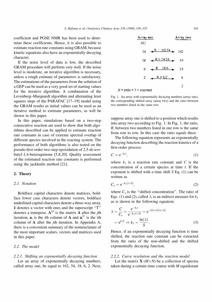
Let an array of exponentially decaying numbers,

called array one, be equal to 162, 54, 18, 6, 2. Next,

suppose array one is shifted to a position which results

into array two according to Fig. 1. In Fig. 1, the ratio,

R, between two numbers listed in one row is the same

from row to row. In this case the ratio equals three.

The following equation represents an exponentially

decaying function describing the reaction kinetics of a

®rst-order process:

C � eÿk1t; (1)

where k1 is a reaction rate constant and C is the

concentration of a certain species at time t. If the

exponent is shifted with a time shift S Eq. (1) can be

written as

Cs � eÿk1�t�S�; (2)

where Cs is the `̀ shifted concentration''. The ratio of

Eqs. (1) and (2), called �, is an indirect measure for k1

as is shown in the following equation:

� � C

Cs

� eÿk1t

eÿk1�t�S� � eÿk1t�k1�t�S�

� ek1S ) k1 � ln��S

: (3)

Hence, if an exponentially decaying function is time

shifted, the reaction rate constant can be extracted

from the ratio of the non-shifted and the shifted

exponentially decaying function.

2.2.2. Curve resolution and the reaction model

Let the matrix X (M�N) be a collection of spectra

taken during a certain time course with M equidistant

Fig. 1. An array with exponentially decaying numbers (array one),

the corresponding shifted array (array two) and the ratio between

two numbers listed in the same row.

S. Bijlsma et al. / Analytica Chimica Acta 376 (1998) 339±355 341

time points at N wavelengths of a reacting system if K

species are involved. In curve resolution the matrix Xcan be expressed as the following equation assuming

the Lambert±Beer law [22]:

X � FDT � E: (4)

The matrices from Eq. (4) have the following prop-

erties:

1. Every row in X denotes a spectrum recorded at a

certain time.

2. F (M�K) is the matrix with concentration profiles.

3. Every column in F denotes the concentration pro-

file of a species in time.

4. D (N�K) is the matrix containing the pure spectra

of the species.

5. Every column in D represents the pure spectrum of

a species.

6. E (M�N) is a matrix of errors (model errors,

experimental errors and instrumental noise).

Suppose that the following ®rst-order consecutive

reaction is considered as the reaction model.

Step 1 : U ! V; with reaction rate constant k1:

Step 2 : V ! W ; with reaction rate constant k2:

Eqs. (5)±(7) are the kinetic rate equations, describing

the concentration pro®les of species U, V and W,

respectively, with initially only U present:

CU;i � CU;0eÿk1ti ; (5)

CV ;i � k1CU;0

�k2 ÿ k1� �eÿk1ti ÿ eÿk2ti�; (6)

CW ;i � CU;0 ÿ CU;i ÿ CV ;i; (7)

where CU,i, CV,i and CW,i are the concentration of

species U, V and W at time ti, respectively; CU,0 is

the initial concentration of species U at time 0.

Eqs. (5)±(7) are the columns of the F matrix. Hence,

every column of F represents a kinetic rate equation.

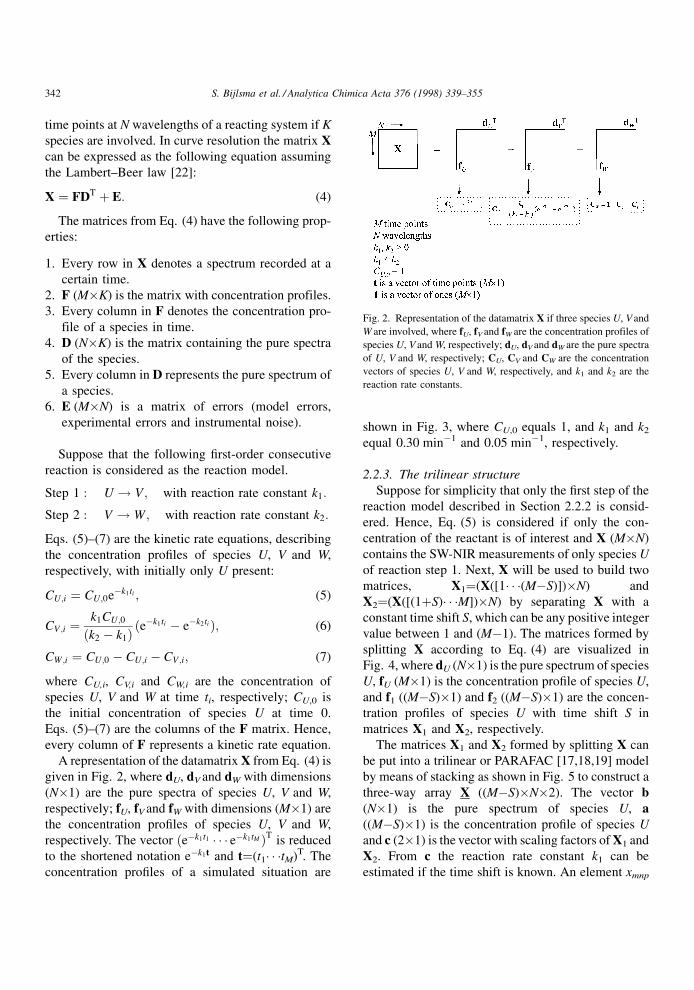
A representation of the datamatrix X from Eq. (4) is

given in Fig. 2, where dU, dV and dW with dimensions

(N�1) are the pure spectra of species U, V and W,

respectively; fU, fV and fW with dimensions (M�1) are

the concentration pro®les of species U, V and W,

respectively. The vector �eÿk1t1 � � � eÿk1tM �T is reduced

to the shortened notation eÿk1t and t�(t1� � �tM)T. The

concentration pro®les of a simulated situation are

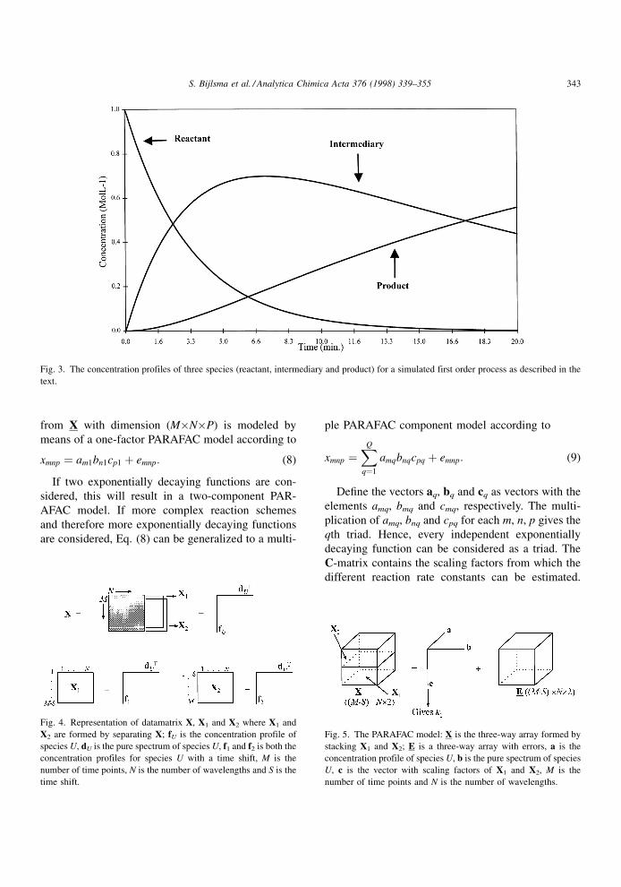
shown in Fig. 3, where CU,0 equals 1, and k1 and k2

equal 0.30 minÿ1 and 0.05 minÿ1, respectively.

2.2.3. The trilinear structure

Suppose for simplicity that only the ®rst step of the

reaction model described in Section 2.2.2 is consid-

ered. Hence, Eq. (5) is considered if only the con-

centration of the reactant is of interest and X (M�N)

contains the SW-NIR measurements of only species U

of reaction step 1. Next, X will be used to build two

matrices, X1�(X([1� � �(MÿS)])�N) and

X2�(X([(1�S)� � �M])�N) by separating X with a

constant time shift S, which can be any positive integer

value between 1 and (Mÿ1). The matrices formed by

splitting X according to Eq. (4) are visualized in

Fig. 4, where dU (N�1) is the pure spectrum of species

U, fU (M�1) is the concentration pro®le of species U,

and f1 ((MÿS)�1) and f2 ((MÿS)�1) are the concen-

tration pro®les of species U with time shift S in

matrices X1 and X2, respectively.

The matrices X1 and X2 formed by splitting X can

be put into a trilinear or PARAFAC [17,18,19] model

by means of stacking as shown in Fig. 5 to construct a

three-way array X ((MÿS)�N�2). The vector b(N�1) is the pure spectrum of species U, a((MÿS)�1) is the concentration pro®le of species U

and c (2�1) is the vector with scaling factors of X1 and

X2. From c the reaction rate constant k1 can be

estimated if the time shift is known. An element xmnp

Fig. 2. Representation of the datamatrix X if three species U, V and

W are involved, where fU, fV and fW are the concentration profiles of

species U, V and W, respectively; dU, dV and dW are the pure spectra

of U, V and W, respectively; CU, CV and CW are the concentration

vectors of species U, V and W, respectively, and k1 and k2 are the

reaction rate constants.


from X with dimension (M�N�P) is modeled by

means of a one-factor PARAFAC model according to

xmnp � am1bn1cp1 � emnp: (8)

If two exponentially decaying functions are con-

sidered, this will result in a two-component PAR-

AFAC model. If more complex reaction schemes

and therefore more exponentially decaying functions

are considered, Eq. (8) can be generalized to a multi-

ple PARAFAC component model according to

xmnp �XQ

q�1

amqbnqcpq � emnp: (9)

De®ne the vectors aq, bq and cq as vectors with the

elements amq, bmq and cmq, respectively. The multi-

plication of amq, bnq and cpq for each m, n, p gives the

qth triad. Hence, every independent exponentially

decaying function can be considered as a triad. The

C-matrix contains the scaling factors from which the

different reaction rate constants can be estimated.

Fig. 3. The concentration profiles of three species (reactant, intermediary and product) for a simulated first order process as described in the

text.

Fig. 4. Representation of datamatrix X, X1 and X2 where X1 and

X2 are formed by separating X; fU is the concentration profile of

species U, dU is the pure spectrum of species U, f1 and f2 is both the

concentration profiles for species U with a time shift, M is the

number of time points, N is the number of wavelengths and S is the

time shift.

Fig. 5. The PARAFAC model: X is the three-way array formed by

stacking X1 and X2; E is a three-way array with errors, a is the

concentration profile of species U, b is the pure spectrum of species

U, c is the vector with scaling factors of X1 and X2, M is the

number of time points and N is the number of wavelengths.


Hence, every combination of exponentially decaying

functions can be modeled, but every combination has

to be written as a sum of separate exponentially

decaying components.

Now, consider the two reactions from the reaction

model described earlier in Section 2 and matrix X(M�N) with SW-NIR measurements of the reacting

system. Suppose CU,0 equals 1. Eqs. (5) and (6) are

already a sum of exponentially decaying functions, but

Eq. (7) is not decaying. Eq. (7) can be written, using

Eqs. (5) and (6), as

CW ;i � 1ÿ eÿk1ti ÿ k�eÿk1ti ÿ eÿk2ti�� e0 ÿ eÿk1ti ÿ keÿk1ti � keÿk2ti ; (10)

where k�k1/(k2ÿk1). Eq. (10) is now a sum of separate

exponentially decaying functions. To make sure that

the term e0 is present in the dataset a column with

constants (M�1), for example (1� � �1)T, has to be

added to the datamatrix X (M�N) to construct an

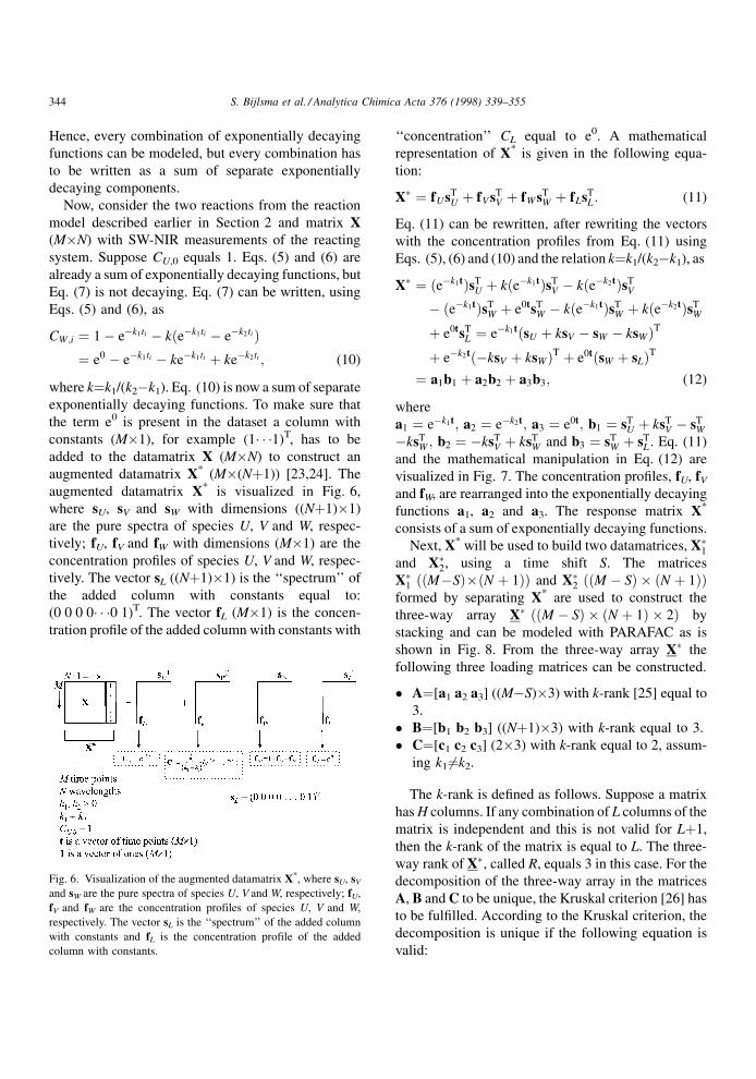
augmented datamatrix X* (M�(N�1)) [23,24]. The

augmented datamatrix X* is visualized in Fig. 6,

where sU, sV and sW with dimensions ((N�1)�1)

are the pure spectra of species U, V and W, respec-

tively; fU, fV and fW with dimensions (M�1) are the

concentration pro®les of species U, V and W, respec-

tively. The vector sL ((N�1)�1) is the `̀ spectrum'' of

the added column with constants equal to:

(0 0 0 0� � �0 1)T. The vector fL (M�1) is the concen-

tration pro®le of the added column with constants with

`̀ concentration'' CL equal to e0. A mathematical

representation of X* is given in the following equa-

tion:

X� � fUsTU � fV sT

V � fWsTW � fLsT

L : (11)

Eq. (11) can be rewritten, after rewriting the vectors

with the concentration pro®les from Eq. (11) using

Eqs. (5), (6) and (10) and the relation k�k1/(k2ÿk1), as

X� � �eÿk1t�sTU � k�eÿk1t�sT

V ÿ k�eÿk2t�sTV

ÿ �eÿk1t�sTW � e0tsT

W ÿ k�eÿk1t�sTW � k�eÿk2t�sT

W

� e0tsTL � eÿk1t�sU � ksV ÿ sW ÿ ksW�T

� eÿk2t�ÿksV � ksW�T � e0t�sW � sL�T� a1b1 � a2b2 � a3b3; (12)

where

a1 � eÿk1t; a2 � eÿk2t; a3 � e0t; b1 � sTU � ksT

V ÿ sTW

ÿksTW ; b2 � ÿksT

V � ksTW and b3 � sT

W � sTL . Eq. (11)

and the mathematical manipulation in Eq. (12) are

visualized in Fig. 7. The concentration pro®les, fU, fV

and fW, are rearranged into the exponentially decaying

functions a1, a2 and a3. The response matrix X*

consists of a sum of exponentially decaying functions.

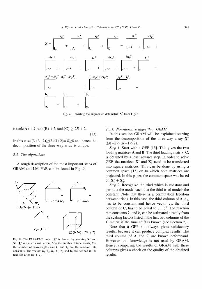
Next, X* will be used to build two datamatrices, X�1and X�2, using a time shift S. The matrices

X�1 ��MÿS��N � 1�� and X�2 ��M ÿ S� � �N � 1��formed by separating X* are used to construct the

three-way array X� ��M ÿ S� � �N � 1� � 2� by

stacking and can be modeled with PARAFAC as is

shown in Fig. 8. From the three-way array X� the

following three loading matrices can be constructed.

� A�[a1 a2 a3] ((MÿS)�3) with k-rank [25] equal to

3.

� B�[b1 b2 b3] ((N�1)�3) with k-rank equal to 3.

� C�[c1 c2 c3] (2�3) with k-rank equal to 2, assum-

ing k1 6�k2.

The k-rank is de®ned as follows. Suppose a matrix

has H columns. If any combination of L columns of the

matrix is independent and this is not valid for L�1,

then the k-rank of the matrix is equal to L. The three-

way rank of X�, called R, equals 3 in this case. For the

decomposition of the three-way array in the matrices

A, B and C to be unique, the Kruskal criterion [26] has

to be ful®lled. According to the Kruskal criterion, the

decomposition is unique if the following equation is

valid:

Fig. 6. Visualization of the augmented datamatrix X*, where sU, sV

and sW are the pure spectra of species U, V and W, respectively; fU,

fV and fW are the concentration profiles of species U, V and W,

respectively. The vector sL is the `̀ spectrum'' of the added column

with constants and fL is the concentration profile of the added

column with constants.


k-rank�A� � k-rank�B� � k-rank�C� � 2R� 2:

(13)

In this case (3�3�2)�(2�3�2))8�8 and hence the

decomposition of the three-way array is unique.

2.3. The algorithms

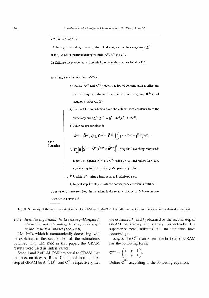
A rough description of the most important steps of

GRAM and LM±PAR can be found in Fig. 9.

2.3.1. Non-iterative algorithm: GRAM

In this section GRAM will be explained starting

from the decomposition of the three-way array X�

((MÿS)�(N�1)�2).

Step 1. Start with a GEP [15]. This gives the two

loading matrices A and B. The third loading matrix, C,

is obtained by a least squares step. In order to solve

GEP, the matrices X�1 and X�2 need to be transferred

into square matrices. This can be done by using a

common space [15] on to which both matrices are

projected. In this paper, the common space was based

on X�1 � X�2.

Step 2. Recognize the triad which is constant and

permute the model such that the third triad models the

constant. Note that there is a permutation freedom

between triads. In this case, the third column of A, a3,

has to be constant and hence vector c3, the third

column of C, has to be equal to (1 1)T. The reaction

rate constants k1 and k2 can be estimated directly from

the scaling factors listed in the ®rst two columns of the

C matrix if the time shift is known (see Section 2).

Note that a GEP not always gives satisfactory

results, because it can produce complex results. The

third column of A and C are known beforehand.

However, this knowledge is not used by GRAM.

Hence, comparing the results of GRAM with these

columns gives a check on the quality of the obtained

results.

Fig. 7. Rewriting the augmented datamatrix X* from Fig. 6.

Fig. 8. The PARAFAC model: X� is formed by stacking X�1 and

X�2; E� is a matrix with errors, M is the number of time points, N is

the number of wavelengths and k1 and k2 are the reaction rate

constants. The vectors a1, a2, a3, b1, b2 and b3 are defined in the

text just after Eq. (12).


2.3.2. Iterative algorithm: the Levenberg±Marquardt

algorithm and alternating least squares steps

of the PARAFAC model (LM±PAR)

LM±PAR, which is monotonically decreasing, will

be explained in this section. For all the estimations

obtained with LM±PAR in this paper, the GRAM

results were used as initial values.

Steps 1 and 2 of LM±PAR are equal to GRAM. Let

the three matrices A, B and C obtained from the ®rst

step of GRAM be A(0), B(0) and C(0), respectively. Let

the estimated k1 and k2 obtained by the second step of

GRAM be start-k1 and start-k2, respectively. The

superscript zero indicates that no iterations have

occurred yet.

Step 3. The C(0) matrix from the ®rst step of GRAM

has the following form:

C�0� � u v 1

x y 1

� �:

De®ne ~C�0�

according to the following equation:

Fig. 9. Summary of the most important steps of GRAM and LM±PAR. The different vectors and matrices are explained in the text.


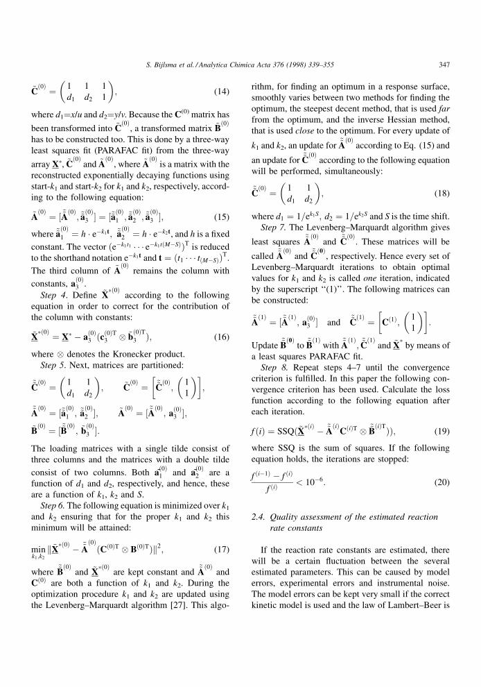
~C�0� � 1 1 1

d1 d2 1

� �; (14)

where d1�x/u and d2�y/v. Because the C(0) matrix has

been transformed into ~C�0�

, a transformed matrix ~B�0�

has to be constructed too. This is done by a three-way

least squares ®t (PARAFAC ®t) from the three-way

array X�, ~C�0�

and ~A�0�

, where ~A�0�

is a matrix with the

reconstructed exponentially decaying functions using

start-k1 and start-k2 for k1 and k2, respectively, accord-

ing to the following equation:

~A�0� � �~~A�0�; ~~a�0�3 � � �~~a

�0�1 ; ~~a

�0�2 ; ~~a

�0�3 �; (15)

where ~~a�0�1 � h � eÿk1t; ~~a

�0�2 � h � eÿk2t, and h is a ®xed

constant. The vector �eÿk1t1 � � � eÿk1t�MÿS��T is reduced

to the shorthand notation eÿk1t and t � �t1 � � � t�MÿS��T.

The third column of ~A�0�

remains the column with

constants, a�0�3 .

Step 4. De®ne ~X��0�

according to the following

equation in order to correct for the contribution of

the column with constants:

~X��0� � X� ÿ a

�0�3 �c�0�T3 ~b

�0�T3 �; (16)

where denotes the Kronecker product.

Step 5. Next, matrices are partitioned:

~~C�0� � 1 1

d1 d2

� �; ~C

�0� � ~~C�0�;

1

1

� �� ;

~~A�0� � �~~a�0�1 ; ~~a

�0�2 �; ~A

�0� � �~~A�0�; a�0�3 �;

~B�0� � �~~B�0�; ~b

�0�3 �:

The loading matrices with a single tilde consist of

three columns and the matrices with a double tilde

consist of two columns. Both a~~�0�1 and a~~

�0�2 are a

function of d1 and d2, respectively, and hence, these

are a function of k1, k2 and S.

Step 6. The following equation is minimized over k1

and k2 ensuring that for the proper k1 and k2 this

minimum will be attained:

mink1;k2

k~X��0� ÿ ~~A

�0��C�0�T B�0�T�k2; (17)

where ~~B�0�

and ~X��0�

are kept constant and ~~A�0�

and

C�0� are both a function of k1 and k2. During the

optimization procedure k1 and k2 are updated using

the Levenberg±Marquardt algorithm [27]. This algo-

rithm, for ®nding an optimum in a response surface,

smoothly varies between two methods for ®nding the

optimum, the steepest decent method, that is used far

from the optimum, and the inverse Hessian method,

that is used close to the optimum. For every update of

k1 and k2, an update for ~~A�0�

according to Eq. (15) and

an update for ~~C�0�

according to the following equation

will be performed, simultaneously:

~~C�0� � 1 1

d1 d2

� �; (18)

where d1 � 1=ek1S; d2 � 1=ek2S and S is the time shift.

Step 7. The Levenberg±Marquardt algorithm gives

least squares ~~A�0�

and ~~C�0�

. These matrices will be

called ~~A�0�

and ~~C�0�

, respectively. Hence every set of

Levenberg±Marquardt iterations to obtain optimal

values for k1 and k2 is called one iteration, indicated

by the superscript `̀ (1)''. The following matrices can

be constructed:

~~A�1� � �~~A�1�; a

�0�3 � and ~~C

�1� � C�1�; 1

1

� �� :

Update ~~B�0�

to ~~B�1�

with ~~A�1�; ~~C�1�

and ~X�

by means of

a least squares PARAFAC ®t.

Step 8. Repeat steps 4±7 until the convergence

criterion is ful®lled. In this paper the following con-

vergence criterion has been used. Calculate the loss

function according to the following equation after

each iteration.

f �i� � SSQ�~X��i� ÿ ~~A�i�

C�i�T ~~B�i�T��; (19)

where SSQ is the sum of squares. If the following

equation holds, the iterations are stopped:

f �iÿ1� ÿ f �i�

f �i�< 10ÿ6: (20)

2.4. Quality assessment of the estimated reaction

rate constants

If the reaction rate constants are estimated, there

will be a certain ¯uctuation between the several

estimated parameters. This can be caused by model

errors, experimental errors and instrumental noise.

The model errors can be kept very small if the correct

kinetic model is used and the law of Lambert±Beer is


valid. Experimental errors are always present and are

caused by concentration errors and errors due to the

start of the reaction, for example. Instrumental noise is

also always present and is caused by variations of the

instrument. If reaction rate constants are estimated for

several repeated individual batch processes and the

individual standard deviation is estimated, this repre-

sents the upper error limit. Note that this is the worst

case, because both experimental errors and instru-

mental noise are involved.

A lower error limit caused by mainly instrumental

noise is estimated using the jackknife method. The

theory of the jackknife method is very well explained

in the book by Shao and Tu [21]. Consider the mean

batch run obtained from averaging all the repeated

individual batch process runs. Hence, experimental

errors and also instrumental noise are averaged. In

the jackknife procedure a ®xed number of spectra

from the three-way array ~X�

based on the mean batch

run are left out several times according to a ®xed

interval, and hence the three-way array ~X�

is reduced.

Finally, for the mean batch process a set of estima-

tions for the reaction rate constants are obtained.

The individual standard deviation of these estimations

represents the lower error limit, because mainly in-

strumental noise is involved. The jackknife procedure

is visualized in Fig. 10, where a two-way representa-

tion of the three-way array by means of unfolding ~X�

is given to illustrate the jackknife procedure much

easier.

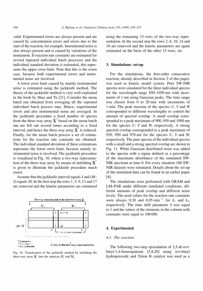
Assume that the jackknife interval equals 4 and (M±

S) equals 20. In the ®rst step the rows 1, 5, 9, 13 and 17

are removed and the kinetic parameters are estimated

using the remaining 15 rows of the two-way repre-

sentation. In the second step the rows 2, 6, 10, 14 and

18 are removed and the kinetic parameters are again

estimated on the basis of the other 15 rows, etc.

3. Simulations: set-up

For the simulations, the ®rst-order consecutive

reaction, already described in Section 2 of this paper,

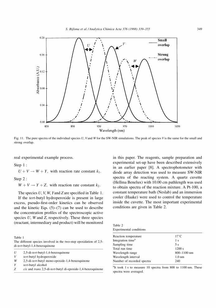
was used as kinetic model system. Pure SW-NIR

spectra were simulated for the three individual species

for the wavelength range 850±1050 nm with incre-

ments of 1 nm using Gaussian peaks. The time range

was chosen from 0 to 20 min with increments of

1 min. The peak maxima of the species U, V and W

corresponded to different wavelengths to control the

amount of spectral overlap. A small overlap corre-

sponded to a peak maximum of 900, 950 and 1000 nm

for the species U, V and W, respectively. A strong

spectral overlap corresponded to a peak maximum of

930, 950 and 970 nm for the species U, V and W,

respectively. The pure spectra of the individual species

with a small and a strong spectral overlap are shown in

Fig. 11. White Gaussian distributed noise was added

to the spectra with a sigma de®ned as a percentage

of the maximum absorbance of the simulated SW-

NIR spectrum at time 0. For every situation 100 SW-

NIR datasets were simulated. Details about the set-up

of the simulated data can be found in an earlier paper

[8].

The simulations were performed with GRAM and

LM±PAR under different simulated conditions: dif-

ferent amounts of peak overlap and different noise

levels. The used values for the reaction rate constants

were always 0.30 and 0.05 minÿ1 for k1 and k2,

respectively. The time shift parameter S was equal

to 1 and the values of the elements in the column with

constants were equal to 100 000.

4. Experimental

4.1. The reaction

The following two-step epoxidation of 2,5-di-tert-

butyl-1,4-benzoquinone [5,8,20] using tert-butyl

hydroperoxide and Triton B catalyst was used as aFig. 10. Visualization of the jackknife method by unfolding the

three-way array X� into the matrices X�1 and X�2.


real experimental example process.

Step 1 :

U � V ! W � Y; with reaction rate constant k1:

Step 2 :

W � V ! Y � Z; with reaction rate constant k2:

The species U, V, W, Yand Z are speci®ed in Table 1.

If the tert-butyl hydroperoxide is present in large

excess, pseudo-®rst-order kinetics can be observed

and the kinetic Eqs. (5)±(7) can be used to describe

the concentration pro®les of the spectroscopic active

species U, W and Z, respectively. These three species

(reactant, intermediary and product) will be monitored

in this paper. The reagents, sample preparation and

experimental set-up have been described extensively

in an earlier paper [8]. A spectrophotometer with

diode array detection was used to measure SW-NIR

spectra of the reacting system. A quartz cuvette

(Hellma Benelux) with 10.00 cm pathlength was used

to obtain spectra of the reaction mixture. A Pt-100, a

constant temperature bath (Neslab) and an immersion

cooler (Haake) were used to control the temperature

inside the cuvette. The most important experimental

conditions are given in Table 2.

Fig. 11. The pure spectra of the individual species U, V and W for the SW-NIR simulations. The peak of species V is the same for the small and

strong overlap.

Table 1

The different species involved in the two-step epoxidation of 2,5-

di-tert-butyl-1,4-benzoquinone

U 2,5-di-tert-butyl-1,4-benzoquinone

V tert-butyl hydroperoxide

W 2,5-di-tert-butyl mono-epoxide-1,4-benzoquinone

Y tert-butyl alcohol

Z cis and trans 2,5-di-tert-butyl di-epoxide-1,4-benzoquinone

Table 2

Experimental conditions

Reaction temperature 178CIntegration timea 1 s

Sampling time 5 s

Total run time 1200 s

Wavelength range 800±1100 nm

Wavelength interval 1.0 nm

Number of recorded spectra 240

aIt took 1 s to measure 10 spectra from 800 to 1100 nm. These

spectra were averaged.


4.2. Data processing

The data processing procedure is described in an

earlier paper [8]. Here a short summary of the most

important aspects is given. The spectra of one indi-

vidual batch process run are shown in a previous paper

[8]. The ®rst few spectra do not match with the other

spectra, because these spectra are the ®rst just after

addition of the catalyst and it takes some time to mix

very well. The reproducibility of each recorded spec-

trum was calculated in order to decide which spectra

had to be deleted and which spectrum had to be used as

blank in order to estimate second derivative difference

spectra. Based on this criterion, the fourth spectrum

was used as blank. A Savitzky±Golay ®lter [28] of 15

data points was used to estimate the second derivative

spectra in order to remove baseline effects and drift.

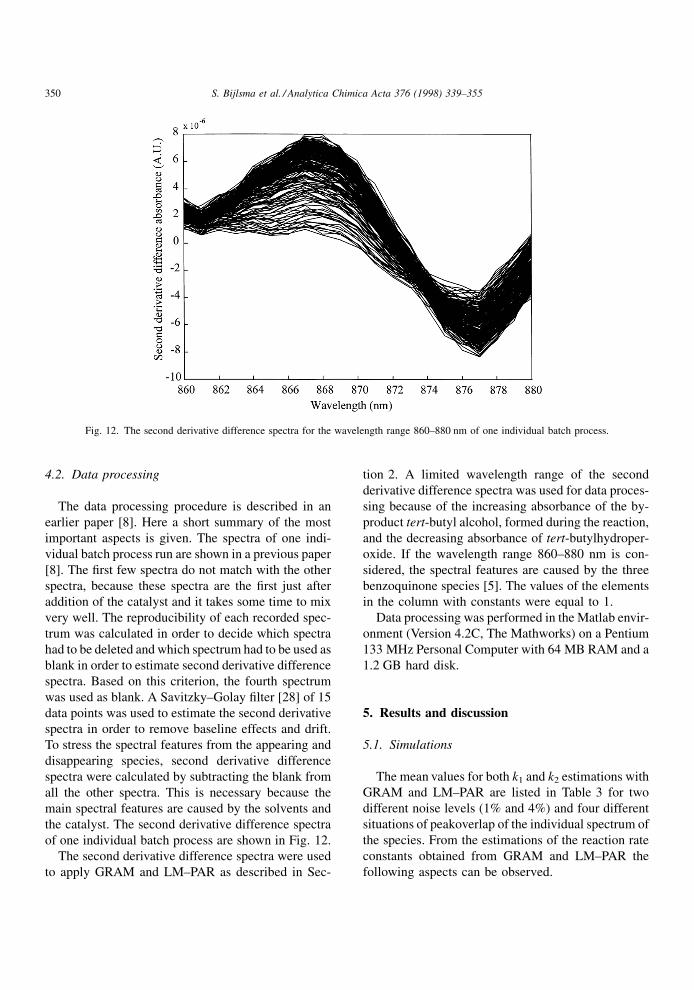
To stress the spectral features from the appearing and

disappearing species, second derivative difference

spectra were calculated by subtracting the blank from

all the other spectra. This is necessary because the

main spectral features are caused by the solvents and

the catalyst. The second derivative difference spectra

of one individual batch process are shown in Fig. 12.

The second derivative difference spectra were used

to apply GRAM and LM±PAR as described in Sec-

tion 2. A limited wavelength range of the second

derivative difference spectra was used for data proces-

sing because of the increasing absorbance of the by-

product tert-butyl alcohol, formed during the reaction,

and the decreasing absorbance of tert-butylhydroper-

oxide. If the wavelength range 860±880 nm is con-

sidered, the spectral features are caused by the three

benzoquinone species [5]. The values of the elements

in the column with constants were equal to 1.

Data processing was performed in the Matlab envir-

onment (Version 4.2C, The Mathworks) on a Pentium

133 MHz Personal Computer with 64 MB RAM and a

1.2 GB hard disk.

5. Results and discussion

5.1. Simulations

The mean values for both k1 and k2 estimations with

GRAM and LM±PAR are listed in Table 3 for two

different noise levels (1% and 4%) and four different

situations of peakoverlap of the individual spectrum of

the species. From the estimations of the reaction rate

constants obtained from GRAM and LM±PAR the

following aspects can be observed.

Fig. 12. The second derivative difference spectra for the wavelength range 860±880 nm of one individual batch process.


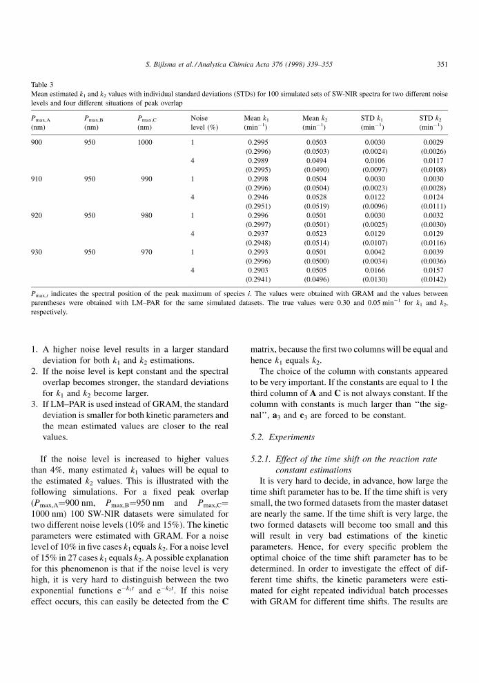
1. A higher noise level results in a larger standard

deviation for both k1 and k2 estimations.

2. If the noise level is kept constant and the spectral

overlap becomes stronger, the standard deviations

for k1 and k2 become larger.

3. If LM±PAR is used instead of GRAM, the standard

deviation is smaller for both kinetic parameters and

the mean estimated values are closer to the real

values.

If the noise level is increased to higher values

than 4%, many estimated k1 values will be equal to

the estimated k2 values. This is illustrated with the

following simulations. For a ®xed peak overlap

(Pmax,A�900 nm, Pmax,B�950 nm and Pmax,C�1000 nm) 100 SW-NIR datasets were simulated for

two different noise levels (10% and 15%). The kinetic

parameters were estimated with GRAM. For a noise

level of 10% in ®ve cases k1 equals k2. For a noise level

of 15% in 27 cases k1 equals k2. A possible explanation

for this phenomenon is that if the noise level is very

high, it is very hard to distinguish between the two

exponential functions eÿk1t and eÿk2t. If this noise

effect occurs, this can easily be detected from the C

matrix, because the ®rst two columns will be equal and

hence k1 equals k2.

The choice of the column with constants appeared

to be very important. If the constants are equal to 1 the

third column of A and C is not always constant. If the

column with constants is much larger than `̀ the sig-

nal'', a3 and c3 are forced to be constant.

5.2. Experiments

5.2.1. Effect of the time shift on the reaction rate

constant estimations

It is very hard to decide, in advance, how large the

time shift parameter has to be. If the time shift is very

small, the two formed datasets from the master dataset

are nearly the same. If the time shift is very large, the

two formed datasets will become too small and this

will result in very bad estimations of the kinetic

parameters. Hence, for every speci®c problem the

optimal choice of the time shift parameter has to be

determined. In order to investigate the effect of dif-

ferent time shifts, the kinetic parameters were esti-

mated for eight repeated individual batch processes

with GRAM for different time shifts. The results are

Table 3

Mean estimated k1 and k2 values with individual standard deviations (STDs) for 100 simulated sets of SW-NIR spectra for two different noise

levels and four different situations of peak overlap

Pmax,A

(nm)

Pmax,B

(nm)

Pmax,C

(nm)

Noise

level (%)

Mean k1

(minÿ1)

Mean k2

(minÿ1)

STD k1

(minÿ1)

STD k2

(minÿ1)

900 950 1000 1 0.2995 0.0503 0.0030 0.0029

(0.2996) (0.0503) (0.0024) (0.0026)

4 0.2989 0.0494 0.0106 0.0117

(0.2995) (0.0490) (0.0097) (0.0108)

910 950 990 1 0.2998 0.0504 0.0030 0.0030

(0.2996) (0.0504) (0.0023) (0.0028)

4 0.2946 0.0528 0.0122 0.0124

(0.2951) (0.0519) (0.0096) (0.0111)

920 950 980 1 0.2996 0.0501 0.0030 0.0032

(0.2997) (0.0501) (0.0025) (0.0030)

4 0.2937 0.0523 0.0129 0.0129

(0.2948) (0.0514) (0.0107) (0.0116)

930 950 970 1 0.2993 0.0501 0.0042 0.0039

(0.2996) (0.0500) (0.0034) (0.0036)

4 0.2903 0.0505 0.0166 0.0157

(0.2941) (0.0496) (0.0130) (0.0142)

Pmax,i indicates the spectral position of the peak maximum of species i. The values were obtained with GRAM and the values between

parentheses were obtained with LM±PAR for the same simulated datasets. The true values were 0.30 and 0.05 minÿ1 for k1 and k2,

respectively.


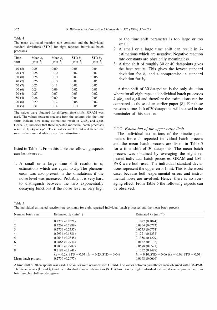
listed in Table 4. From this table the following aspects

can be observed.

1. A small or a large time shift results in k1

estimations which are equal to k2. The phenom-

enon was also present in the simulations if the

noise level was increased. Probably, it is very hard

to distinguish between the two exponentially

decaying functions if the noise level is very high

or the time shift parameter is too large or too

small.

2. A small or a large time shift can result in k2

estimations which are negative. Negative reaction

rate constants are physically meaningless.

3. A time shift of roughly 30 or 40 datapoints gives

the best results. This gives the lowest standard

deviation for k1 and a compromise in standard

deviation for k2.

A time shift of 30 datapoints is the only situation

where for all eight repeated individual batch processes

k1 6�k2 and k2>0 and therefore the estimations can be

compared to those of an earlier paper [8]. For these

reasons a time shift of 30 datapoints will be used in the

remainder of this section.

5.2.2. Estimation of the upper error limit

The individual estimations of the kinetic para-

meters for each repeated individual batch process

and the mean batch process are listed in Table 5

for a time shift of 30 datapoints. The mean batch

process was obtained by averaging the eight re-

peated individual batch processes. GRAM and LM±

PAR were both used. The individual standard devia-

tions represent the upper error limit. This is the worst

case, because both experimental errors and instru-

mental noise are involved. Hence, there is no aver-

aging effect. From Table 5 the following aspects can

be observed.

Table 4

The mean estimated reaction rate constants and the individual

standard deviations (STDs) for eight repeated individual batch

processes

Time

shift

Mean k1

(minÿ1)

Mean k2

(minÿ1)

STD k1

(minÿ1)

STD k2

(minÿ1)

10 (5) 0.25 0.09 0.05 0.04

20 (7) 0.28 0.10 0.02 0.07

30 (8) 0.28 0.10 0.03 0.06

40 (7) 0.26 0.10 0.02 0.05

50 (7) 0.25 0.11 0.02 0.05

60 (6) 0.24 0.09 0.02 0.03

70 (4) 0.27 0.07 0.03 0.02

80 (4) 0.26 0.09 0.04 0.05

90 (6) 0.29 0.12 0.08 0.02

100 (5) 0.31 0.14 0.10 0.05

The values were obtained for different time shifts. GRAM was

used. The values between brackets from the column with the time

shifts indicate how many estimations result in k16�k2 and k2>0.

Hence, (5) indicates that three repeated individual batch processes

result in k1�k2 or k2<0. These values are left out and hence the

mean values are calculated over five estimations.

Table 5

The individual estimated reaction rate constants for eight repeated individual batch processes and the mean batch process

Number batch run Estimated k1 (minÿ1) Estimated k2 (minÿ1)

1 0.2779 (0.2521) 0.1097 (0.1044)

2 0.3268 (0.2899) 0.0804 (0.0773)

3 0.2756 (0.2757) 0.0775 (0.0774)

4 0.2934 (0.1881) 0.1721 (0.1232)

5 0.2643 (0.2345) 0.1358 (0.1229)

6 0.2865 (0.2734) 0.0132 (0.0132)

7 0.2818 (0.2787) 0.0578 (0.0571)

8 0.2197 (0.1841) 0.1752 (0.1489)�k1 � 0:28; STD � 0:03 ��k1 � 0:25; STD � 0:04� �k2 � 0:10; STD � 0:06 ��k2 � 0:09;STD � 0:04�

Mean batch process 0.2756 (0.2677) 0.0668 (0.0666)

A time shift of 30 datapoints was used. The values were obtained with GRAM. The values between parentheses were obtained with LM±PAR.

The mean values (�k1 and �k2) and the individual standard deviations (STDs) based on the eight individual estimated kinetic parameters from

batch number 1±8 are also given.


1. If the individual standard deviations are consid-

ered, the standard deviation is smaller for k2 if

LM±PAR is used instead of GRAM.

2. The spread of the k2 estimations is larger than the

spread of the k1 estimations because k1 is more

dominant than k2. A large spread in general is

caused by the high noise level of the experimental

data.

3. GRAM estimates nearly always higher values for

the kinetic parameters than LM±PAR.

There appeared to be a big difference in speed

between GRAM and LM±PAR. In this case GRAM

only took a few seconds whereas LM±PAR took a few

hours.

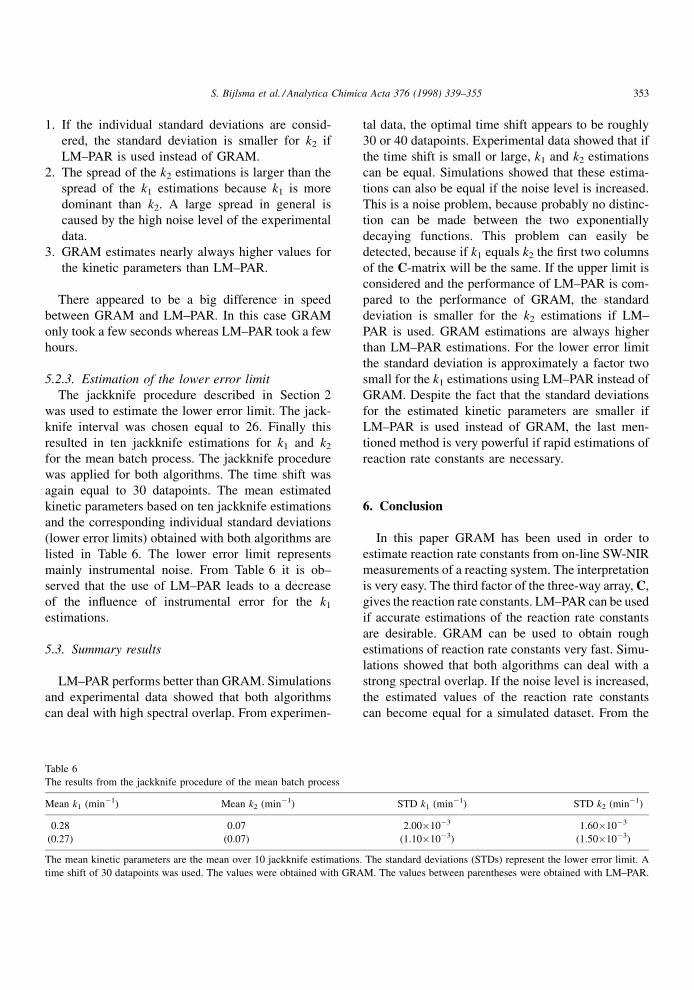
5.2.3. Estimation of the lower error limit

The jackknife procedure described in Section 2

was used to estimate the lower error limit. The jack-

knife interval was chosen equal to 26. Finally this

resulted in ten jackknife estimations for k1 and k2

for the mean batch process. The jackknife procedure

was applied for both algorithms. The time shift was

again equal to 30 datapoints. The mean estimated

kinetic parameters based on ten jackknife estimations

and the corresponding individual standard deviations

(lower error limits) obtained with both algorithms are

listed in Table 6. The lower error limit represents

mainly instrumental noise. From Table 6 it is ob±

served that the use of LM±PAR leads to a decrease

of the in¯uence of instrumental error for the k1

estimations.

5.3. Summary results

LM±PAR performs better than GRAM. Simulations

and experimental data showed that both algorithms

can deal with high spectral overlap. From experimen-

tal data, the optimal time shift appears to be roughly

30 or 40 datapoints. Experimental data showed that if

the time shift is small or large, k1 and k2 estimations

can be equal. Simulations showed that these estima-

tions can also be equal if the noise level is increased.

This is a noise problem, because probably no distinc-

tion can be made between the two exponentially

decaying functions. This problem can easily be

detected, because if k1 equals k2 the ®rst two columns

of the C-matrix will be the same. If the upper limit is

considered and the performance of LM±PAR is com-

pared to the performance of GRAM, the standard

deviation is smaller for the k2 estimations if LM±

PAR is used. GRAM estimations are always higher

than LM±PAR estimations. For the lower error limit

the standard deviation is approximately a factor two

small for the k1 estimations using LM±PAR instead of

GRAM. Despite the fact that the standard deviations

for the estimated kinetic parameters are smaller if

LM±PAR is used instead of GRAM, the last men-

tioned method is very powerful if rapid estimations of

reaction rate constants are necessary.

6. Conclusion

In this paper GRAM has been used in order to

estimate reaction rate constants from on-line SW-NIR

measurements of a reacting system. The interpretation

is very easy. The third factor of the three-way array, C,

gives the reaction rate constants. LM±PAR can be used

if accurate estimations of the reaction rate constants

are desirable. GRAM can be used to obtain rough

estimations of reaction rate constants very fast. Simu-

lations showed that both algorithms can deal with a

strong spectral overlap. If the noise level is increased,

the estimated values of the reaction rate constants

can become equal for a simulated dataset. From the

Table 6

The results from the jackknife procedure of the mean batch process

Mean k1 (minÿ1) Mean k2 (minÿ1) STD k1 (minÿ1) STD k2 (minÿ1)

0.28 0.07 2.00�10ÿ3 1.60�10ÿ3

(0.27) (0.07) (1.10�10ÿ3) (1.50�10ÿ3)

The mean kinetic parameters are the mean over 10 jackknife estimations. The standard deviations (STDs) represent the lower error limit. A

time shift of 30 datapoints was used. The values were obtained with GRAM. The values between parentheses were obtained with LM±PAR.


simulations it can be concluded that LM±PAR always

leads to more precise estimations for the reaction rate

constants compared to GRAM.

The two-step epoxidation of 2,5-di-tert-butyl-1,4-

benzoquinone showed a small difference between

GRAM and LM±PAR, but LM±PAR always leads

to more precise estimations for the reaction rate con-

stants compared to GRAM. The optimal time shift

appeared to be roughly 30 or 40 datapoints in this case.

If the time shift parameter is too large or too small, the

estimations of the reaction rate constants can become

equal. Probably, it is very hard to distinguish between

exponentially decaying functions for these choices of

the time shift parameter. Upper and lower error limits

were also estimated for quality assessment.

GRAM is a very powerful method for estimating

reaction rate constants very fast. The speed of the

algorithm is known in advance, because it is non-

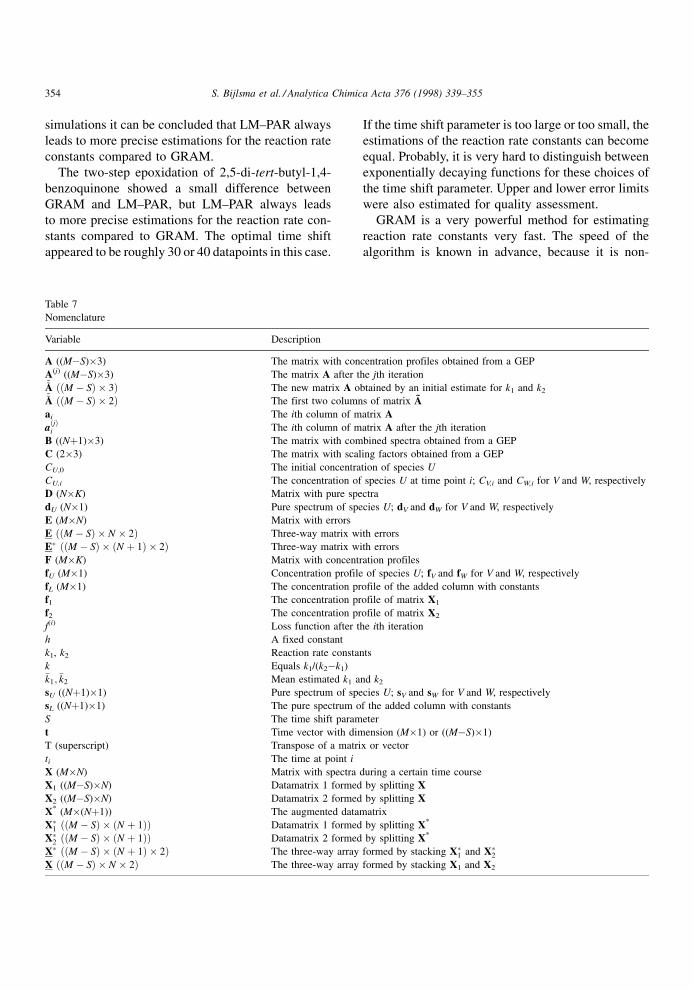
Table 7

Nomenclature

Variable Description

A ((MÿS)�3) The matrix with concentration profiles obtained from a GEP

A(j) ((MÿS)�3) The matrix A after the jth iteration~~A ��M ÿ S� � 3� The new matrix A obtained by an initial estimate for k1 and k2~~A ��M ÿ S� � 2� The first two columns of matrix AÄ

ai The ith column of matrix A

a�j�i The ith column of matrix A after the jth iteration

B ((N�1)�3) The matrix with combined spectra obtained from a GEP

C (2�3) The matrix with scaling factors obtained from a GEP

CU,0 The initial concentration of species U

CU,i The concentration of species U at time point i; CV,i and CW,i for V and W, respectively

D (N�K) Matrix with pure spectra

dU (N�1) Pure spectrum of species U; dV and dW for V and W, respectively

E (M�N) Matrix with errors

E ��M ÿ S� � N � 2� Three-way matrix with errors

E� ��M ÿ S� � �N � 1� � 2� Three-way matrix with errors

F (M�K) Matrix with concentration profiles

fU (M�1) Concentration profile of species U; fV and fW for V and W, respectively

fL (M�1) The concentration profile of the added column with constants

f1 The concentration profile of matrix X1

f2 The concentration profile of matrix X2

f(i) Loss function after the ith iteration

h A fixed constant

k1, k2 Reaction rate constants

k Equals k1/(k2ÿk1)�k1;�k2 Mean estimated k1 and k2

sU ((N�1)�1) Pure spectrum of species U; sV and sW for V and W, respectively

sL ((N�1)�1) The pure spectrum of the added column with constants

S The time shift parameter

t Time vector with dimension (M�1) or ((MÿS)�1)

T (superscript) Transpose of a matrix or vector

ti The time at point i

X (M�N) Matrix with spectra during a certain time course

X1 ((MÿS)�N) Datamatrix 1 formed by splitting X

X2 ((MÿS)�N) Datamatrix 2 formed by splitting X

X* (M�(N�1)) The augmented datamatrix

X�1 ��M ÿ S� � �N � 1�� Datamatrix 1 formed by splitting X*

X�2 ��M ÿ S� � �N � 1�� Datamatrix 2 formed by splitting X*

X� ��M ÿ S� � �N � 1� � 2� The three-way array formed by stacking X�1 and X�2X ��M ÿ S� � N � 2� The three-way array formed by stacking X1 and X2


iterative. GRAM can be used if a rough estimation of

the kinetic parameters is desirable, for instance if

(batch) processes are to be monitored. LM±PAR is

in this case not very convenient to use because of the

time consuming iterations. In the case of LM±PAR the

speed of the algorithm is not known in advance. If the

batch time is elapsed, LM±PAR can be used to esti-

mate accurately kinetic parameters. Since many mea-

surements are based on exponentially decaying

functions, GRAM and LM±PAR can have many appli-

cations.

Acknowledgements

The authors wish to thank the people from the

mechanical workshop and the glass-works for con-

struction of the cell-holder and the cooling units of the

cuvette, respectively.

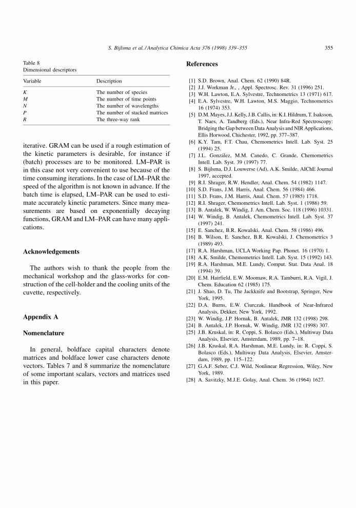
Appendix A

Nomenclature

In general, boldface capital characters denote

matrices and boldface lower case characters denote

vectors. Tables 7 and 8 summarize the nomenclature

of some important scalars, vectors and matrices used

in this paper.

References

[1] S.D. Brown, Anal. Chem. 62 (1990) 84R.

[2] J.J. Workman Jr., , Appl. Spectrosc. Rev. 31 (1996) 251.

[3] W.H. Lawton, E.A. Sylvestre, Technometrics 13 (1971) 617.

[4] E.A. Sylvestre, W.H. Lawton, M.S. Maggio, Technometrics

16 (1974) 353.

[5] D.M. Mayes, J.J. Kelly, J.B. Callis, in: K.I. Hildrum, T. Isaksson,

T. Naes, A. Tandberg (Eds.), Near Infra-Red Spectroscopy:

Bridging the Gap between Data Analysis and NIR Applications,

Ellis Horwood, Chichester, 1992, pp. 377±387.

[6] K.Y. Tam, F.T. Chau, Chemometrics Intell. Lab. Syst. 25

(1994) 25.

[7] J.L. GonzaÂlez, M.M. Canedo, C. Grande, Chemometrics

Intell. Lab. Syst. 39 (1997) 77.

[8] S. Bijlsma, D.J. Louwerse (Ad), A.K. Smilde, AIChE Journal

1997, accepted.

[9] R.I. Shrager, R.W. Hendler, Anal. Chem. 54 (1982) 1147.

[10] S.D. Frans, J.M. Harris, Anal. Chem. 56 (1984) 466.

[11] S.D. Frans, J.M. Harris, Anal. Chem. 57 (1985) 1718.

[12] R.I. Shrager, Chemometrics Intell. Lab. Syst. 1 (1986) 59.

[13] B. Antalek, W. Windig, J. Am. Chem. Soc. 118 (1996) 10331.

[14] W. Windig, B. Antalek, Chemometrics Intell. Lab. Syst. 37

(1997) 241.

[15] E. Sanchez, B.R. Kowalski, Anal. Chem. 58 (1986) 496.

[16] B. Wilson, E. Sanchez, B.R. Kowalski, J. Chemometrics 3

(1989) 493.

[17] R.A. Harshman, UCLA Working Pap. Phonet. 16 (1970) 1.

[18] A.K. Smilde, Chemometrics Intell. Lab. Syst. 15 (1992) 143.

[19] R.A. Harshman, M.E. Lundy, Comput. Stat. Data Anal. 18

(1994) 39.

[20] E.M. Hairfield, E.W. Moomaw, R.A. Tamburri, R.A. Vigil, J.

Chem. Education 62 (1985) 175.

[21] J. Shao, D. Tu, The Jackknife and Bootstrap, Springer, New

York, 1995.

[22] D.A. Burns, E.W. Ciurczak, Handbook of Near-Infrared

Analysis, Dekker, New York, 1992.

[23] W. Windig, J.P. Hornak, B. Antalek, JMR 132 (1998) 298.

[24] B. Antalek, J.P. Hornak, W. Windig, JMR 132 (1998) 307.

[25] J.B. Kruskal, in: R. Coppi, S. Bolasco (Eds.), Multiway Data

Analysis, Elsevier, Amsterdam, 1989, pp. 7±18.

[26] J.B. Kruskal, R.A. Harshman, M.E. Lundy, in: R. Coppi, S.

Bolasco (Eds.), Multiway Data Analysis, Elsevier, Amster-

dam, 1989, pp. 115±122.

[27] G.A.F. Seber, C.J. Wild, Nonlinear Regression, Wiley, New

York, 1989.

[28] A. Savitzky, M.J.E. Golay, Anal. Chem. 36 (1964) 1627.

Table 8

Dimensional descriptors

Variable Description

K The number of species

M The number of time points

N The number of wavelengths

P The number of stacked matrices

R The three-way rank


Rapid estimation of rate constants using on-line SW-NIR and trilinear models

Documents

Transcript of Rapid estimation of rate constants using on-line SW-NIR and trilinear models