Multi-dimensional Rankings, Program Termination,and Complexity Bounds of Flowchart Programs

Christophe Alias1, Alain Darte1, Paul Feautrier1, and Laure Gonnord2

1 Compsys team, LIP, Lyon, FranceUMR 5668 CNRS—ENS Lyon—UCB Lyon—Inria

Firstname.Lastname@ens-lyon.fr2 LIFL - UMR CNRS/USTL 8022, INRIA Lille - Nord Europe

40 avenue Halley, 59650 Villeneuve d’Ascq, FranceLaure.Gonnord@lifl.fr

Abstract. Proving the termination of a flowchart program can be done by ex-hibiting a ranking function, i.e., a function from the program states to a well-founded set, which strictly decreases at each program step. A standard method toautomatically generate such a function is to compute invariants for each programpoint and to search for a ranking in a restricted class of functions that can be han-dled with linear programming techniques. Previous algorithms based on affinerankings either are applicable only to simple loops (i.e., single-node flowcharts)and rely on enumeration, or are not complete in the sense that they are not guaran-teed to find a ranking in the class of functions they consider, if one exists. Our firstcontribution is to propose an efficient algorithm to compute ranking functions: Itcan handle flowcharts of arbitrary structure, the class of candidate rankings itexplores is larger, and our method, although greedy, is provably complete. Oursecond contribution is to show how to use the ranking functions we generate toget upper bounds for the computational complexity (number of transitions) of thesource program. This estimate is a polynomial, which means that we can handleprograms with more than linear complexity. We applied the method on a collec-tion of test cases from the literature. We also show the links and differences withprevious techniques based on the insertion of counters.

1 Introduction and motivation

The problem of proving program correctness has been with us since the early days ofComputer Science. In a seminal paper [20], R. W. Floyd proposed what has become oneof the standard approaches: affix assertions to each program point and prove that theyare consequences of the assertions of its predecessors in the program control graph. Theassertions at the entry point of the program are its preconditions, the assertions at loopentry points are invariants, while the assertions at its exit point must entail correctness,according to some set of requirements. Constructing the required set of assertions is atedious and error-prone task. The automatic construction of invariants has been provedto be intractable in the general case [6]. However, partial or conservative solutions canbe obtained by abstract interpretation methods [14].

At the same time, it was soon realized that this method proves only partial correct-ness, i.e., that the program gives the correct result if and when it terminates. To prove

termination, one needs a variant or ranking function (a W-function in Floyd’s terminol-ogy), i.e., a function from the states of the program to some well-founded set, whichstrictly decreases at each program step. Of course, designing an algorithm for build-ing ranking functions in all cases is not possible since it would give a solution to theundecidable halting problem. However, this does not preclude the existence of partialsolutions, which, e.g., handle only programs (or approximated models) of a restrictedshape, or look for rankings in a restricted class of functions. Our first contribution isto generalize previous work for generating ranking functions. We design an algorithmwith the following features:

– It can handle flowcharts of arbitrary structure.– The class of rankings we consider is much larger: in the global ranking function we

generate, each program point can have its own multi-dimensional affine expression.– Our algorithm is based on a greedy mechanism. Nevertheless, our technique is

provably complete, even for our larger class of ranking functions.There are many variations on the above theme. For instance, as in [27], one may selecta set of cutpoints, with the property that their removal makes the flowchart acyclic. Itis then enough to exhibit a function, non increasing everywhere, that decreases and iswell-founded at each cutpoint. One may even proceed each flowchart cycle at a time.

Our second contribution is to show that the global ranking functions we generate canbe used to give upper bounds on the worst-case computational complexity (WCCC) ofthe program execution, i.e., the number of transitions that can be made in an executiontrace. Obviously, if a program does not terminate, its WCCC is infinite. If the programterminates and a one-dimensional ranking function exists, its value at program start isan upper bound on the number of steps before termination since it decreases at leastby one at each program step. The situation is more complicated in the case of multi-dimensional ranking functions but we show how the WCCC can be computed thanksto counting techniques in polyhedra. Furthermore, our ranking algorithm has an addi-tional important feature: It generates a multi-dimensional affine ranking function whosedimension is minimal. This is important to get an accurate upper bound on the WCCCof the flowchart program. To the best of our knowledge, our technique is the first onethat uses ranking functions to compute upper bounds on the number of iterations ofarbitrary loops (a particular case of the WCCC).

The rest of the paper is organized as follows. Section 2 gives some basic notationsand concepts: the program abstraction we use (integer interpreted automata) and theclass of ranking functions we consider. Section 3 presents our method for construct-ing multi-dimensional affine ranking functions and states its completeness. Section 4explains how we infer the computational complexity of the source program. Section 5reports on our implementation through a collection of benchmarks from the literature.Section 6 describes other approaches to the termination problem and WCCC evaluation.We then conclude pointing to some unsolved problems and outlining future work.

2 Notations and Definitions

We write matrices with capital letters (as A) and column vectors in boldface (as x).If x has dimension d, its components are denoted x[i], with 0 ≤ i < d. Thus, its i-thcomponent is x[i − 1]. Sets are represented with calligraphic letters such asW, K , etc.

2.1 Integer Interpreted Automata

In the tradition of most previous work on program termination and static analysis, wefirst transform the program to be analyzed into an abstraction: the associated integerinterpreted automaton. This is similar to the flowcharts used a long time ago to expressprograms (see, e.g., Manna’s book [27]) until the advent of structured programming. Infact, when one looks at real-life programs, many deviations from the strict structuredmodel can occur, including premature loop termination, exceptions, and even the occa-sional goto. Reasoning with flowcharts abstracts the details of the syntax and semanticsof the source language, which can be dealt with by an appropriate preprocessor.

In our work, a program is represented by an affine (integer) interpreted automaton(K , n, kinit,T ) defined by:

– a finite set K of control points;– n integer variables represented by a vector x of size n;– an initial control point kinit ∈ K ;– a finite set T of 4-tuples (k, g, a, k′), called transitions, where k ∈ K (resp. k′ ∈ K)

is the source (resp. target) control point, g : Zn 7→ B = {true, false}, the guard, is alogical formula expressed with affine inequalities Gx + g ≥ 0, and a : Zn 7→ Zn, theaction, assigns, to each variable valuation x, a vector x ′ of size n, expressed by anaffine expression x ′ = Ax + a. Here, G and A are matrices, g and a are vectors.

To represent non-determinism or to approximate non-affine or non-analyzable assign-ments in the program, we may have to assign the value “?”, representing an arbitraryinteger, to a variable, but we will not elaborate on this point. This is equivalent to dealwith affine relations between x and x ′ instead of functions, see [1] for details.

Semantics The set of states is K × Zn. A trace from (k0, x0) to (k, x) is a sequence(k0, x0), (k1, x1), . . . , (kp, xp) such that kp = k, xp = x and for each i, 0 ≤ i < p, thereexists in T a transition (ki, gi, ai, ki+1) such that gi(xi) = true and xi+1 = ai(xi). Givenan initial valuation v, a state (k, x) is reachable from v iff (if and only if) there is a tracefrom (kinit, v) to (k, x). A state (k, x) is reachable if there exists v ∈ Zn such that (k, x) isreachable from v. The set of reachable states is denoted by R.

Invariants The guard g in a transition t = (k, g, a, k′) gives a necessary condition onvariables x to traverse the transition t and to apply its corresponding action a. To getthe exact valuations x of variables for which the action a can be performed, one wouldneed to take into account the initial valuations and the successive conditions that led tothe control point k. We denote by Rk the set of possible valuations x of variables whenthe control is in k:

Rk = {x ∈ Zn | (k, x) ∈ R}.

Then, there exists a trace containing the transition (k, g, a, k′) iff x ∈ Rk and g(x) is true.Note that Rk does not depend on any initial valuation. More precisely, it is the union,for all initial valuations v, of the set of vectors x such that (k, x) is reachable from v.

In practice, it is difficult to determine the setRk exactly but it is possible to give over-approximations, thanks to the notion of invariants. An invariant on a control point k is aformula φk(x) that is true for all reachable states (k, x). It is affine if it is the conjunctionof a finite number of affine conditions on program variables. The set Rk is then over-approximated by the integer points within a polyhedron Pk. To compute invariants, we

rely on standard abstract interpretation techniques, widely studied since the seminalpaper [14]. These sets Pk represent all the information on the values of variables thatcan be deduced from the program by state-of-the-art analysis techniques. Unlike [8, 24]where the construction of invariants is coupled with the termination proof or evalua-tion of iteration bounds, the invariants Pk are pre-computed and are the inputs of thetechniques developed in the next sections.

2.2 Termination and Ranking Functions

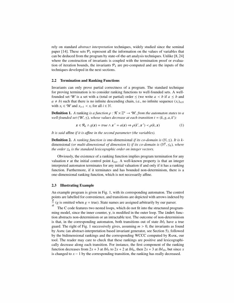
Invariants can only prove partial correctness of a program. The standard techniquefor proving termination is to consider ranking functions to well-founded sets. A well-founded set W is a set with a (total or partial) order � (we write a ≺ b if a � b anda , b) such that there is no infinite descending chain, i.e., no infinite sequence (xi)i∈N

with xi ∈ W and xi+1 ≺ xi for all i ∈ N.

Definition 1. A ranking is a function ρ : K × Zn →W, from the automaton states to awell-founded set (W,�), whose values decrease at each transition t = (k, g, a, k′):

x ∈ Rk ∧ g(x) = true ∧ x ′ = a(x)⇒ ρ(k′, x ′) ≺ ρ(k, x) (1)

It is said affine if it is affine in the second parameter (the variables).

Definition 2. A ranking function is one-dimensional if its co-domain is (N,≤). It is k-dimensional (or multi-dimensional of dimension k) if its co-domain is (Nk,�k), wherethe order �k is the standard lexicographic order on integer vectors.

Obviously, the existence of a ranking function implies program termination for anyvaluation v at the initial control point kinit. A well-known property is that an integerinterpreted automaton terminates for any initial valuation if and only if it has a rankingfunction. Furthermore, if it terminates and has bounded non-determinism, there is aone-dimensional ranking function, which is not necessarily affine.

2.3 Illustrating Example

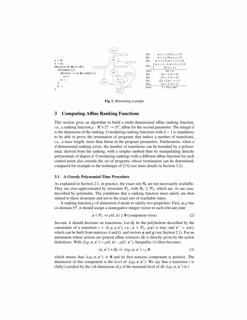
An example program is given in Fig. 1, with its corresponding automaton. The controlpoints are labelled for convenience, and transitions are depicted with arrows indexed byga

(g is omitted when g = true). State names are assigned arbitrarily by our parser.The C code features two nested loops, which do not fit into the structured program-

ming model, since the inner counter, y, is modified in the outer loop. The indet func-tion abstracts non-determinism or an intractable test. The outcome of non-determinismis that, in the corresponding automaton, both transitions out of state lbl5 have a trueguard. The right of Fig. 1 successively gives, assuming m > 0, the invariants as foundby A (an abstract-interpretation based invariant generator, see Section 5), followedby the bidimensional rankings and the corresponding WCCC computed by R, ourtool. The reader may care to check that these rankings are positive and lexicographi-cally decrease along each transition. For instance, the first component of the rankingfunction decreases from 2x + 3 at lbl5 to 2x + 2 at lbl6, then 2x + 3 at lbl10, but since xis changed to x − 1 by the corresponding transition, the ranking has really decreased.

y = 0;x = m;while(x>=0 && y>=0){if(indet()){while(y <= m && indet())y++;

x--;}y--;

}

start

lbl4

lbl5

stop lbl6

lbl10

x := m; y := 0

0 6 x ∧ 0 6 yx < 0 ∨ y < 0

true

true

y 6 m

y := y + 1

x := x − 1

y := y − 1

lbl4 m ≥ x > 0,m ≥ y > 0lbl5 m ≥ x ≥ 0,m ≥ y ≥ 0lbl6 m ≥ x ≥ 0,m + 1 ≥ y ≥ 0

lbl10

{m ≥ x ≥ −1,m + 1 ≥ y ≥ 0

2m ≥ x + ystart 2m + 4lbl4 (2x + 3, 3y + 3)lbl5 (2x + 3, 3y + 2)lbl6 (2x + 2,m − y + 1)lbl10 (2x + 3, 3y + 1) 5 + 7m + 4m2

Fig. 1. Illustrating example

3 Computing Affine Ranking Functions

This section gives an algorithm to build a multi-dimensional affine ranking function,i.e., a ranking function ρ : K ×Zn → Nd, affine for the second parameter. The integer dis the dimension of the ranking. Considering ranking functions with d > 1 is mandatoryto be able to prove the termination of programs that induce a number of transitions,i.e., a trace length, more than linear in the program parameters. Furthermore, when ad-dimensional ranking exists, the number of transitions can be bounded by a polyno-mial, derived from the ranking, with a simpler method than by manipulating directlypolynomials of degree d. Considering rankings with a different affine function for eachcontrol point also extends the set of programs whose termination can be determined,compared for example to the technique of [13] (see more details in Section 3.2).

3.1 A Greedy Polynomial-Time Procedure

As explained in Section 2.1, in practice, the exact sets Rk are not necessarily available.They are over-approximated by invariants Pk, with Rk ⊆ Pk, which are, in our case,described by polyhedra. The conditions that a ranking function must satisfy are thenrelated to these invariants and not to the exact sets of reachable states.

A ranking function ρ of dimension d needs to satisfy two properties. First, as ρ hasco-domain Nd, it should assign a nonnegative integer vector to each relevant state:

x ∈ Pk ⇒ ρ(k, x) ≥ 0 (component-wise) (2)

Second, it should decrease on transitions. Let Qt be the polyhedron described by theconstraints of a transition t = (k, g, a, k′), i.e., x ∈ Pk, g(x) is true, and x ′ = a(x),which can be built from matrices A and G, and vectors a and g (see Section 2.1). For anautomaton whose actions are general affine relations, Qt is directly given by the actiondefinitions. With ∆t(ρ, x, x ′) = ρ(k, x) − ρ(k′, x ′), Inequality (1) then becomes:

(x, x ′) ∈ Qt ⇒ ∆t(ρ, x, x ′) �d 0 (3)

which means that ∆t(ρ, x, x ′) , 0 and its first nonzero component is positive. Thedimension of this component is the level of ∆t(ρ, x, x ′). We say that a transition t is(fully) satisfied by the i-th dimension of ρ if the maximal level of all ∆t(ρ, x, x ′) is i.

To build a ranking ρ, the difficulty is to decide, for each transition t and for eachpair (x, x ′) ∈ Qt, at which dimension its first nonzero component occurs, and at whichdimension the transition is satisfied. A potentially exponential search, as in [8], shouldbe avoided. To address this issue, our algorithm uses the same greedy mechanism asin [25, 19, 13]. We build the different dimensions of the ranking ρ, one after the other,from the first one to the last one. For a dimension σ of ρ and a transition t not yetsatisfied by one of the previous dimensions, we consider the constraint:

(x, x ′) ∈ Qt ⇒ ∆t(σ, x, x ′) ≥ εt with 0 ≤ εt ≤ 1. (4)

and we select a ranking such that as many transitions as possible have εt = 1, i.e.,are now satisfied. Surprisingly, despite this greedy approach, our technique is provablycomplete (see Theorem 1), which means that if a multi-dimensional affine ranking ex-ists, our algorithm finds one. Our algorithm can then be summarized as follows:

1: i = 0; T = T ; . Initialize T to the set of all transitions2: while T is not empty do3: Find a 1D affine function σ and values εt such that all inequalities (2) and (4) are satisfied

and as many εt as possible are equal to 1; . This means maximizing∑

t∈T εt

4: Let ρi = σ ; i = i + 1; . σ defines the i-th dimension of ρ5: If no transition t with εt = 1, return false . No multi-dimensional affine ranking.6: Remove from T all transitions t such that εt = 1; . The transitions have level i7: end while;8: d = i; return true; . There is a d-dimensional ranking

For Line 3, any solution σ leading to εt > 0 can be multiplied by a suitable positiveconstant to get a solution with εt = 1. Thus, for any solution maximizing

∑t∈T εt, a

transition t has either εt = 0 or εt = 1. At each iteration of the while loop, σ is used as anew dimension of the ranking ρ (Line 4). By construction, ρ is strictly decreasing at thislevel for all transitions t with εt = 1. No need to consider them any longer, which meansthat they are removed for subsequent dimensions (Line 6). If no transition is removed,no ranking function is derived and the automaton may not terminate.

To find a suitable function σ at Line 3, we use linear programming. The set ofinequalities that we need to solve are Inequalities (2) (with σ instead of ρ) and (4). Thestandard method (used in [19, 28, 8]) is to rely on the affine form of Farkas lemma [30]:

Lemma 1 (Farkas lemma, affine form). An affine form φ : Rn → R with φ(x) =

c.x + c0 is nonnegative everywhere in a non-empty polyhedron {x | Ax + a ≥ 0} iff:

∃λ ∈ (R+)n, λ0 ∈ R+ such that φ(x) ≡ λ.(Ax + a) + λ0

The notation ≡ is a formal equality, which means that x can be eliminated and coeffi-cients identified. In other words:

∃λ ∈ (R+)n, λ0 ∈ R+ such that c = λ.A and c0 = λ.a + λ0

We can now apply the affine form of Farkas lemma to Inequalities (2) (with σ insteadof ρ) and (4). With Pk = {x | Pk x + pk ≥ 0}, we transform Inequality (2) into:

∃λk ∈ (R+)n, λ0k ∈ R

+ such that σ(k, x) ≡ λk.(Pk x + pk) + λ0k (5)

Similarly, with Qt = {y = (x, x ′) | Qt y + qt ≥ 0}, we transform Inequality (4) into:

∃µt ∈ (R+)n, µ0t ∈ R

+ s.t. ∆t(σ, x, x ′) − 1 ≡ µt.(Qt y + qt) + µ0t (6)

A substitution of (5) in (6) and an identification on each dimension of y leads to a setof linear inequalities. Considering all inequalities obtained for all transitions t ∈ T andmaximizing

∑t∈T εt (Line 3 of the algorithm) leads to the desired function σ.

Note: As we use linear programming, but not integer linear programming, we mayend up with a function σ with rational components. However, we can always multiplyit by a suitable integer to get a ranking function with integer values.

Example of Section 2.3 (Cont’d) Write σk(x, y) = ak x + bky + ck the first dimensionof the ranking. Consider any transition, e.g., lbl4 → lbl5. The non-increasing constraintgives (a4 − a5)x + (b4 − b5)y + c4 − c5 ≥ 0. Letting x = 0 and y = m, and noticing that mcan be arbitrarily large, gives b4 ≥ b5. The same technique applied to all transitions ofa cycle shows that all bk (same for all ak) of a strongly connected component are equal:let b this value. For the self-loop on lbl6, σ6(x, y) ≥ σ6(x, y+1) implies b ≤ 0. The cyclelbl4 → lbl5 → lbl10 → lbl4 implies σ4(x, y) ≥ σ4(x, y−1), thus b ≥ 0. Hence, these twocycles cannot be satisfied at the first level. However, the two transitions lbl5 → lbl6 andlbl6 → lbl10 can be satisfied, disconnecting these two cycles and allowing them to besatisfied separately at the 2nd level. In this presentation, we have deliberately simplifiedthe problem by ignoring the positivity constraints and using qualitative reasoning foranalyzing the descent constraints. In our tool, linear programming replaces intuition.

3.2 Completeness

Since non-terminating programs exist, there is no hope of proving that a ranking func-tion always exists. Moreover, there are terminating affine interpreted automata with nomulti-dimensional affine ranking. Thus, all we can prove is that, if a multi-dimensionalaffine ranking exists, our algorithm finds one, i.e., it is complete for the class of multi-dimensional affine rankings. Also, as the sets Rk are over-approximated by the invari-ants Pk, completeness has to be understood with respect to these invariants, whichmeans that if the algorithm fails when an affine ranking exists, it is because invariantsare not accurate enough. In this section, we just sketch the completeness proof. Theproof itself, quite long and technical, can be found in the long version of this paper [2].

Theorem 1. If an affine interpreted automaton, with associated invariants, has a multi-dimensional affine ranking function, then the algorithm of Section 3.1 finds one. More-over, the dimension of the generated ranking is minimal.

There can be several reasons why a greedy algorithm could be incomplete. First,we could make a bad choice when selecting the transitions that are satisfied at a givendimension. However, there is no decision to make: if two transitions can be satisfied,one by a function σ1, the other by a function σ2, both can be simultaneously satisfied bythe function σ1 + σ2. Second, enforcing that each transition is satisfied at the smallestpossible dimension could also be a bad decision. Third, keeping all pairs (x, x ′) inInequality (4) until the transition is fully satisfied, even those for which the ranking is

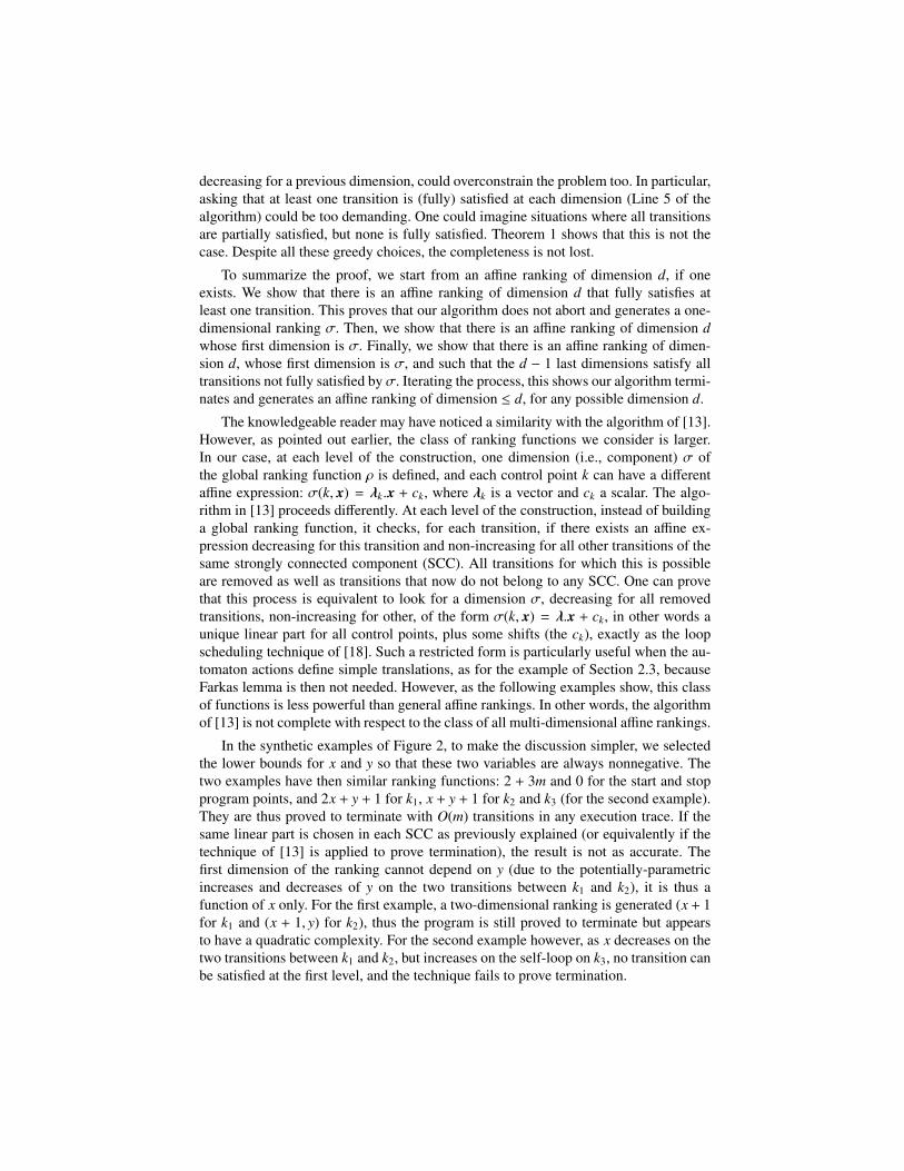
decreasing for a previous dimension, could overconstrain the problem too. In particular,asking that at least one transition is (fully) satisfied at each dimension (Line 5 of thealgorithm) could be too demanding. One could imagine situations where all transitionsare partially satisfied, but none is fully satisfied. Theorem 1 shows that this is not thecase. Despite all these greedy choices, the completeness is not lost.

To summarize the proof, we start from an affine ranking of dimension d, if oneexists. We show that there is an affine ranking of dimension d that fully satisfies atleast one transition. This proves that our algorithm does not abort and generates a one-dimensional ranking σ. Then, we show that there is an affine ranking of dimension dwhose first dimension is σ. Finally, we show that there is an affine ranking of dimen-sion d, whose first dimension is σ, and such that the d − 1 last dimensions satisfy alltransitions not fully satisfied by σ. Iterating the process, this shows our algorithm termi-nates and generates an affine ranking of dimension ≤ d, for any possible dimension d.

The knowledgeable reader may have noticed a similarity with the algorithm of [13].However, as pointed out earlier, the class of ranking functions we consider is larger.In our case, at each level of the construction, one dimension (i.e., component) σ ofthe global ranking function ρ is defined, and each control point k can have a differentaffine expression: σ(k, x) = λk.x + ck, where λk is a vector and ck a scalar. The algo-rithm in [13] proceeds differently. At each level of the construction, instead of buildinga global ranking function, it checks, for each transition, if there exists an affine ex-pression decreasing for this transition and non-increasing for all other transitions of thesame strongly connected component (SCC). All transitions for which this is possibleare removed as well as transitions that now do not belong to any SCC. One can provethat this process is equivalent to look for a dimension σ, decreasing for all removedtransitions, non-increasing for other, of the form σ(k, x) = λ.x + ck, in other words aunique linear part for all control points, plus some shifts (the ck), exactly as the loopscheduling technique of [18]. Such a restricted form is particularly useful when the au-tomaton actions define simple translations, as for the example of Section 2.3, becauseFarkas lemma is then not needed. However, as the following examples show, this classof functions is less powerful than general affine rankings. In other words, the algorithmof [13] is not complete with respect to the class of all multi-dimensional affine rankings.

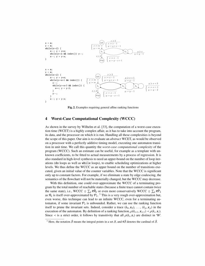
In the synthetic examples of Figure 2, to make the discussion simpler, we selectedthe lower bounds for x and y so that these two variables are always nonnegative. Thetwo examples have then similar ranking functions: 2 + 3m and 0 for the start and stopprogram points, and 2x + y + 1 for k1, x + y + 1 for k2 and k3 (for the second example).They are thus proved to terminate with O(m) transitions in any execution trace. If thesame linear part is chosen in each SCC as previously explained (or equivalently if thetechnique of [13] is applied to prove termination), the result is not as accurate. Thefirst dimension of the ranking cannot depend on y (due to the potentially-parametricincreases and decreases of y on the two transitions between k1 and k2), it is thus afunction of x only. For the first example, a two-dimensional ranking is generated (x + 1for k1 and (x + 1, y) for k2), thus the program is still proved to terminate but appearsto have a quadratic complexity. For the second example however, as x decreases on thetwo transitions between k1 and k2, but increases on the self-loop on k3, no transition canbe satisfied at the first level, and the technique fails to prove termination.

x = m;y = m;while(x>=2) {

x--; y = y+x;while(y>=x && indet()) y--;x--; y = y-x;

}

k1

init{

x := m

y := m

stop

x < 2

k2

{

x := x − 1

y := y + x − 1

x > 2

y := y − 1

y > x

{

x := x − 1

y := y − x + 1

x = m;y = m;while(x>=2) {

x--; y = y+x;while(y>=x+1 && indet()) {y--;while(y>=x+3 && indet()) {x++; y = y-2;

}y--;

}x--; y = y-x;

}

k1

init{

x := m

y := m

stop

x < 2

k2

{

x := x − 1

y := y + x − 1

x > 2

{

x := x − 1

y := y − x + 1

k3

y := y − 1

y := y − 1

y > x + 1

{

x := x + 1

y := y − 2

y > x + 3

Fig. 2. Examples requiring general affine ranking functions

4 Worst-Case Computational Complexity (WCCC)

As shown in the survey by Wilhelm et al. [33], the computation of a worst-case execu-tion time (WCET) is a highly complex affair, as it has to take into account the program,its data, and the processor on which it is run. Handling all these complexities is beyondthe scope of this paper. Our aim is to evaluate an abstract WCET, as would be observedon a processor with a perfectly additive timing model, executing one automaton transi-tion in unit time. We call this quantity the worst-case computational complexity of theprogram (WCCC). Such an estimate can be useful, for example as a template with un-known coefficients, to be fitted to actual measurements by a process of regression. It isalso standard in high-level synthesis to need an upper-bound on the number of loop iter-ations (do loops as well as while loops), to enable scheduling optimizations at higherlevels. We thus define the WCCC as an upper bound on the number of transitions exe-cuted, given an initial value of the counter variables. Note that the WCCC is significantonly up to constant factors. For example, if we eliminate a state by edge coalescing, thesemantics of the flowchart will not be materially changed, but the WCCC may decrease.

With this definition, one could over-approximate the WCCC of a terminating pro-gram by the total number of reachable states (because a finite trace cannot contain twicethe same state), i.e., WCCC ≤

∑k #Rk or even more conservatively WCCC ≤

∑k #Pk

as Rk is itself over-approximated by Pk. 3 This is a very rough over-approximation but,even worse, this technique can lead to an infinite WCCC, even for a terminating au-tomaton, if some invariant Pk is unbounded. Rather, we can use the ranking functionitself to prune the invariant sets. Indeed, consider a trace (k0, x0), . . . , (kp, xp) in theexecution of the automaton. By definition of a ranking function, ρ(ki+1, xi+1) ≺ ρ(ki, xi).Since ≺ is a strict order, it follows by transitivity that all ρ(ki, xi) are distinct in W.

3 Here, the notation S means the integral points in a set S, and #S denotes the cardinal of S.

Hence, the length of the trace is bounded by the cardinal of the co-domain of ρ:

WCCC ≤ #⋃

k

ρ(k, Pk) ≤∑

k

#ρ(k, Pk) (7)

The first inequality is more accurate but harder to compute as it involves a union of sets.So far, in our implementation, we use the second less accurate inequality.

Let us see how we can compute #ρ(k, Pk) for a given control point k. To makenotations simpler, we drop the index k: we let ρ(k, x) = ρ(x) = Rx + r and P = Pk.To compute #ρ(P), we can ignore the constant vector r. The number of different valuesin ρ(P) is then the number of points in the image of a Z-polyhedron (intersection ofan integral lattice, here Zn, and a polyhedron, here P) by an affine function. If R isinjective, it is of course equal to the number of integral points in the invariant itself.Otherwise, there are three issues: the fact that several points can have the same image(thus the kernel of the mapping must be identified), the fact that some regular holescan arise (sub-lattice of Zn) in the image of the polyhedron, and the fact that someirregular holes can appear on its boundaries. Such problems have been widely studiedin the literature using various techniques related to Ehrhart polynomials [11, 31]. So far,we implemented a simpler over-approximation method, which normalizes R in such away that ρ(P) no longer contains regular holes. This way, a standard computation ofintegral points can be applied. This normalization is done thanks to the Smith normal

form. We compute R = US V , where U and V are unimodular, S =

[D 00 0

], and D is

a diagonal positive matrix of rank d (the rank of R). We compute V the polyhedronobtained by projecting the polyhedron VP = {V x | x ∈ P} on its d first coordinates.#V is actually a slight over-approximation of #ρ(P). Indeed, two vectors x and y in Phave the same image by ρ if and only if V x and V y have the same d first components.The over-approximation comes from the fact that, in very specific cases, not all integralvectors in V are obtained by projection of an integral vector in VP. The number ofintegral vectors inV is then computed using Ehrhart polynomials.

It is important to minimize the rank of D because the WCCC will tend to be smallerif the dimension ofV is smaller. This is why it is important to generate rankings of mini-mal dimension as our algorithm does (Theorem 1). However, adding linearly-dependentcomponents to the ranking will simply add null rows at the bottom of the matrix S . Fromthis follows that the WCCC will at most be O(Mn), if M is an upper bound for all vari-ables, since it is impossible to build more than n linear forms on n variables. This boundcannot be improved, since with n variables, one can write a system of n perfectly nestedloops, which achieves the required complexity.

The factors affecting the precision of the WCCC, beside the union computation,are the presence of non affine guards and of non affine domains. For example, the loopfor(j=1; j<m; j=2*j) has invariant 2 ≤ j < m (in the loop) and ranking j, whichgives a WCCC of m instead of the correct value log2 m. Such a WCCC cannot be ob-tained by an affine technique, which grossly over-estimates the domain of j by a poly-hedron. Another problem is that the invariant at a loop entry is often a coarse polyhedralapproximation of a union of more accurate invariants on each path in the loop. Imposingthe non-negative constraint (2) for such a control point is not necessary. It is enough toimpose it for one control point per circuit of the automaton where invariants are more

accurate. Note also that, if one wants to count the number of loop traversals and notthe number of transitions, it is not necessary to extend the sum in (7) to all nodes. Forinstance, if we include only one well-chosen state per loop, we will get a bound on thetotal number of loop traversals in an execution of the program.

Example of Section 2.3 (Cont’d) Inequality (7) gives the upper bound:

WCCC ≤ #ρ(Pstart) + #ρ(Plbl4 ) + #ρ(Plbl5 ) + #ρ(Plbl6 ) + #ρ(Plbl10 ) + #ρ(Pstop)

Let us detail the computation of #ρ(Plbl4 ). ρ(Plbl4 , x, y,m) =

[2 0 00 3 0

]( x y m )T +

[33

]Here, the mapping is bijective, so it should be sufficient to count the integral points in

Plbl4 . But let us do the computation:[

2 0 00 3 0

]= U×D×V =

[2 13 1

]×

[1 0 00 6 0

]×

−2 3 01 −1 00 0 1

.Projecting VPlbl4 along its first two dimensions amounts to consider the linear system:{p1 = −2x+3y, p2 = x−y, 0 < x ≤ m, 0 < y ≤ m} and to eliminate every variable exceptp1, p2 and m (the parameter). This gives the polyhedron V defined by the constraints{1 ≤ p1 + 2p2 ≤ m, 1 ≤ p1 + 3p2 ≤ m}, whose number of points is an upper boundfor #ρ(Plbl4 ). The cardinal of V is computed thanks to Ehrhart polynomials [10] (seeSection 5). The result is, in general, a collection of polynomial formulas guarded byaffine constraints on the parameters. Here, we get: #ρ(Plbl4 ) ≤ #V = m2 as expected.Applying the same process on the other control points, we finally obtain:

WCCC ≤ 1 + (m2) + (1 + 2m + m2) + (2 + 3m + m2) + (2m + m2) + 1 = 5 + 7m + 4m2.

5 Implementation and Experimental Results

We have built a tool suite that converts a C program into an integer interpreted automa-ton, constructs its invariants, tests its termination and, if successful, computes an upperbound for its worst-case computational complexity WCCC.

The first tool, 2, turns a C program into an integer interpreted automaton, doingthe relevant approximations when the program cannot be exactly translated. Our guide-lines have been to consider only assignments to integer variables, and to give a variablean undefined value unless it is expressed as an affine form of integer variables. This toolalso implements dead code elimination, useless variables elimination, and, as an option,the selection of cutpoints and the elimination of other control points. Note that it maybe possible to extract flowcharts from binaries or assembly code, thus greatly extendingthe scope of the method.

The second tool, A ([21], http://laure.gonnord.org/aspic/), a public-domain implementation of abstract acceleration [14], computes the invariants for everycontrol point of the obtained integer interpreted automaton. Compared to the standardwidening approach, this method computes a more precise reachability set for “acceler-able” loops, which locally avoids the use of widening and globally increases precision.

The third tool, R, implements the method described in this paper. Starting fromthe integer interpreted automaton and the invariants given by A, R tries to prove

the termination of the program by computing (multidimensional affine) ranking func-tions. In case of success, R computes the worst-case computational complexity ofthe program. Also, in case of failure, R tries to exhibit a counterexample that causesnon-termination. The linear programs involved in the termination part are solved thanksto the PIP tool (Parametric Integer Programming). The WCCC part requires countingthe number of points into a Z-polyhedron. This is done thanks to the Ehrhart polynomialpart of the Polylib library (http://icps.u-strasbg.fr/polylib). The final resultis a set of Ehrhart polynomials, guarded by affine predicates on program parameters.

A table of experimental results can be found on the webpage http://www.ens-lyon.fr/LIP/COMPSYS/Tools/Ranking/. Exemples were collected from the extent lit-terature, and notably from http://www.eecs.qmul.ac.uk/~aziem/esop.html. Inall test cases we were able to prove termination, even for nondeterministic examples.Nested loops are correctly handled, and we find multi-dimensional rankings for them.Although WCCCs are returned by R as piecewise functions depending on the initialvalues of the variables, we only provide the most general term of these expressions.

We were also able to prove the termination of some classical sortings algorithms.The rankings for these codes may seem of the wrong dimensions, but the additionaldimensions have constant values and the orders of magnitude of the WCCC are still asexpected, e.g., O(N2) for bubblesort. For heapsort, our algorithm finds an O(N2)WCCC instead of the correct O(N log2 N), see Section 4 for an explanation.

Our tools are completely autonomous within the stated limitations on input pro-grams. The precision of the results is strongly dependent on the quality of the invariantsand of the affine approximation of some (non affine) affectations in the C programs.This is not a surprise as stated by Theorem 1: the quality of our technique is to beunderstood with respect to the quality of invariants that are provided.

6 Related Work

Our work establishes connections with at least three different techniques. Firstly, itbrings to the field of program termination, techniques primarily designed for schedulingand optimizing loops, in the context of automatic parallelization [17]. The fundamen-tal difference is that, for program termination, each problem dimension corresponds toan integer variable while, for automatic parallelization, it corresponds to a predefinedloop counter. In this sense, it has also some similarities with the seminal work of Karp,Miller, and Winograd on systems of uniform recurrence equations [25]. Our algorithmto generate ranking functions is inspired by the algorithm of Feautrier [19] and its com-pleteness [32] for scheduling affine loops. Counting techniques using Ehrhart polyno-mials are also standard for optimizing loops [11].

Second, it extends the ranking techniques previously proposed to prove the termi-nation of programs. Using ranking functions to prove correctness was first proposed in[20]. Early approaches were semi-automatic: one had to guess ranking functions, andthen prove their correctness using some form of Hoare logic. Attempts to automate thisprocess started, first with one-dimensional linear rankings such as in [12, 28], then withmulti-dimensional rankings such as in [13, 8], and propositions to build some formsof polynomial rankings followed [7, 15]. Unlike ours, the techniques of Podelski andRybalchenko [28] and of Bradley, Manna, and Sipma [8] are designed for “single-path

linear loops”, i.e., programs abstracted by an automaton with a single node. [28] formu-lates the constraints to get a one-dimensional ranking if it exists using Farkas lemma,while [8] gives a complete method to derive, for a single node, a multi-dimensionalranking. It also tries to compute the invariants and the ranking functions simultaneously.Unlike these two methods, the technique of Colón and Sipma [13] can handle flowchartprograms of arbitrary structure. As explained in Section 3.2, the space of rankings itcan generate corresponds to affine rankings where all control points within the stronglyconnected component being considered have the same linear part. It is not complete forthe class of general multi-dimensional affine ranking functions, as the examples of Sec-tion 3.2 demonstrate. Finally, none of these techniques has been designed or extendedto compute upper bounds on the WCCC, i.e., the maximal length of an execution trace.

To summarize, we extend previous work on affine ranking functions in several di-rections. First, unlike [28, 8], we are not limited to one loop, i.e., our automaton canhave an arbitrary number of vertices (as in reference [13]). As shown by the example ofSection 2.3, this is mandatory to analyze complex loops, either nested loops, or multi-path simple loops that have been transformed into an automaton with several verticesby path-sensitive analysis. Second, to decide for which dimension of the ranking func-tion a transition decreases (it must be non-increasing in the previous dimensions), thealgorithm has_llrf in [8, Figure 2] is a potentially-exponential recursive exploration.Since the algorithm is also potentially exhaustive, there is no need to prove complete-ness. In contrast, as our algorithm is greedy, a completeness proof is needed, which isalso an order of magnitude more general since we deal with the much larger space of allmulti-dimensional affine ranking functions, not just one single lexicographic function.Third, unlike previous papers, we are able to prove that we get the smallest numberof dimensions for each ranking function. In [7], the authors do notice that they mayhave as many dimensions as the number of transitions. As explained in Section 4, thisdimension reduction is important for the computation of the WCCC.

In a different context, a large body of research followed the introduction of the sizechange termination (SCT) principle in [26]. The difference in the two approaches arefirst in semantics: the automaton represents a call graph instead of a control graph, andthe variables may be summary information about data structures, like the length of a listor the size of a tree. More importantly, the relations between input and output variablesof a transition are restricted to one of the two forms x′ < y and x′ ≤ y. Attempts torelax this restriction can be found in [3–5]. Once a set of size change relations has beenfound, termination follows if one can combine them in such a way that one variableat least is guaranteed to decrease. Such a combination can be interpreted as a rankingfunction, albeit of a shape fairly different from ours.

Another trend of research has been started in [29] and pursued in [9]. Here, one usesseveral (local) ranking relations, all of them well founded, the intuition being that eachrelation proves termination of a part of the program. A consistency condition is neces-sary: the transitive closure of the transition relation of the program must be included inthe union of all local ranking relations. The problem is how to find the local rankings,and how to prove the consistency condition. It may be that we can help at least for thefirst problem: apply our algorithm to cleverly chosen subsets of the automaton states,as for example strongly connected components or loops.

The third and last connection with previous work is related to the WCCC compu-tation. The method of Gulwani et al. [24, 23] for proving termination and boundingthe complexity consists in creating counters – new variables which are incrementedwhen traversing some transitions – and asking an invariant generator for bounds onthe counter values. An elaborate system is proposed for selecting the transitions to becounted, which necessitates repeated calls to the invariant generator. Our method is re-lated to this work in the following way. After a first round of computation of rankingfunctions, let us create a new counter which is reset to zero at the beginning of the pro-gram and incremented at each transition satisfied by the first dimension of our ranking(transitions t for which the variable εt of Section 3.1 is equal to 1). By construction, ateach control point, the sum of the counter value and the affine expression given by theranking is non-increasing, which provides an affine bound for this counter. We can con-tinue in this way as the construction of ranking functions progresses and transitions areremoved, making sure that new counters are reset to zero at the entry to each programfragment (i.e., on incoming transitions that were previously satisfied). If and when alledges are satisfied, we have found a system of counters which meets the constraintsof Gulwani et al. Hence, our approach can be seen as a replacement for the counterplacement algorithm of [24]. Both techniques rely on abstract interpretation to buildinitial invariants. Our technique is then guaranteed to find an adequate placement ofcounters if one exists, given these initial invariants, while the approach of Gulwani etal. is dependent on the unavoidable approximations made in abstract interpretation tobuild new invariants including the counters. However, which method is best from thepoint of view of practical complexity is difficult to ascertain, since we avoid calling theinvariant generator many times, but at the price of having to solve much larger linearprogramming problems. However, we point out that, in [24], counters are placed onlyon particular transitions selected a priori, typically the back edges of the control-flowgraph. But, in the example of Section 2.3, both back edges (the self-loop on lbl6 and thetransition from lbl10 to lbl4) are traversed a quadratic number of times, so there is notransition to place a linearly-bounded counter and the algorithm of [24] would fail. Asour ranking function shows, the “outer” counter should be placed either on the transitionfrom lbl5 to lbl6 or on the transition from lbl6 to lbl10. Or the graph must be transformedas proposed in [23], but with a risk of complexity increase. We believe that our workbridges the gap between techniques based on the placement of counters and the use ofabstract interpretation to bound them, and techniques based on global ranking functionsto derive complexity bounds.

7 Conclusion

7.1 Contributions

The first main contribution of this paper is the design of an algorithm for the construc-tion of multi-dimensional affine ranking functions, which, in contrast to the combinato-rial algorithm of [7], is greedy but nevertheless complete (with respect to the invariantsfound and the class of ranking functions considered) and optimal in the dimension ofthe ranking function. The algorithm makes no assumption on the shape of the source

program, and can handle, with proper preprocessing (i.e., after the program is approx-imated to fit into the affine interpreted automaton model), multiple loops of arbitrarynesting patterns, premature termination and gotos, nondeterministic choices and val-ues, exceptions, and affine guards of arbitrary structure. We also point out that, in caseof failure, our algorithm may exhibit a certificate of non termination in the form of anexecution trace which may not terminate. The computation of the worst-case computa-tional complexity (WCCC) is delegated to a very comprehensive stand-alone algorithm.This means that no arbitrary restrictions about the shape of loops and tests are neces-sary. We can directly rely on existing methods and tools for counting integer pointswithin Z-polyhedra and images of Z-polyhedra by affine functions.

More generally, our work establishes a strong link with computation models, theo-retical results, and tools developed by the automatic parallelization and high-performancecomputing community, and which seem to be not so used (or partly re-discovered) inthe context of program termination. We believe that this connection can lead to furtherfruitful advances in the solution of problems faced by both communities.

7.2 Future Work

There is nevertheless room for many improvements. The preprocessor we use for con-verting a program into an interpreted automaton is somewhat brute force: any constructthat is not affine in integer variables is replaced by the bottom value, which is absorbing(⊥ ⊕ x = ⊥ for most operators), and which prints as true in a guard and as a questionmark in an action. This can be improved by noticing that some operations, like moduloand integer division, can be linearized by the introduction of fresh variables, or that abottom value may be constrained: for instance, a square is always non-negative. Also,variables with a finite domain, like Booleans and enums, can be used to refine the states.This may result in a large increase in the size of the automaton but has the direct benefitof extending the class of ranking functions considered, as these do not need to be affineanymore for such “unrolled” variables. Making sure that domains of integer variablesare “fat” (to use the terminology of [16]) increases the chance that an affine rankingexists and improves the quality of the WCCC produced.

There is always room for improving an invariant constructor like A. One mayfor instance improve the acceleration algorithms and loops treatment, or use additionalabstract interpretation frameworks, like the congruences and lattices of [22]. It may alsobe interesting to construct the invariants on demand, both to improve the accuracy andto reduce the overhead of the method.

Last but not least, the power of the ranking algorithm can be increased in manyways. For instance, imposing that ranking functions are nonnegative everywhere (seeInequality (2)) is too strong a constraint. It is enough to impose it at a set of cut points.If the automaton graph becomes acyclic when these cut points are removed, then ter-mination is still guaranteed, notwithstanding the relaxed nonnegativity constraint. In away, eliminating all states but cutpoints before computing a ranking (by path compres-sion) is equivalent to relaxing the positivity constraint, but it is obtained at the cost of apotential increase in the number of transitions: if the eliminated state has n ingoing andm outgoing transitions, its elimination will generate n × m transitions. We still need toexplore this trade-off and analyze its consequences on the WCCC computations.

Research on the SCT paradigm has shown that ranking functions of a more complexshape, like piecewise affine functions, are necessary in some cases. In our framework,this means splitting the invariant of some state(s) by an affine constraint. How to choosethe states to split and the splitting predicate is left for future research.

A point we have not investigated is the termination of distributed programs. Ouralgorithm fails when termination depends on a fairness hypothesis.

References

1. Alias, C., Darte, A., Feautrier, P., Gonnord, L.: Bounding the computational complexity offlowchart programs with multi-dimensional rankings. Research Report 7235, INRIA (March2010)

2. Alias, C., Darte, A., Feautrier, P., Gonnord, L., Quinson, C.: Program termination and worst-time complexity with multi-dimensional affine ranking functions. Research Report 7037,INRIA (November 2009)

3. Anderson, H., Khoo, S.C.: Affine-based size-change termination. In: Ohori, A. (ed.) 1stAsian Symposium on Programming Languages and Systems (APLAS’03). Lecture Notesin Computer Science, vol. 2895, pp. 122–140. Springer Verlag, Beijing (2003)

4. Ben-Amram, A.M.: Size-change termination with difference constraints. ACM Transactionson Programming Languages and Systems (TOPLAS) 30(3), 1–31 (2008)

5. Ben-Amram, A.M.: Size change termination, monotonicity constraints, and ranking func-tions. In: Bouajjani, A., Maler, O. (eds.) 21st International Conference on Computer AidedVerification (CAV). LNCS, vol. 5643, pp. 109–123. Springer (2009)

6. Blass, A., Gurevich, Y.: Inadequacy of computable loop invariants. ACM Transactions onComputational Logic (TOCL) 2(1), 1–11 (2001)

7. Bradley, A.A., Manna, Z., Sipma, H.B.: The polyranking principle. In: 32nd InternationalColloquium on Automata, Languages and Programming (ICALP). Lecture Notes in Com-puter Science, vol. 3580, pp. 1349–1361. Springer Verlag (Jul 2005)

8. Bradley, A.R., Manna, Z., Sipma, H.B.: Linear ranking with reachability. In: Etessami, K.,Rajamani, S.K. (eds.) 17th International Conference on Computer Aided Verification (CAV).Lecture Notes in Computer Science, vol. 3576, pp. 491–504. Springer Verlag (Jul 2005)

9. Chawdhary, A., Cook, B., Gulwani, S., Sagiv, M., Yang, H.: Ranking abstractions. In: 17thEuropean Symposium on Programming (ESOP’08). Lecture Notes in Computer Science,vol. 4960, pp. 81–92. Springer Verlag, Budapest (Apr 2008)

10. Clauss, P.: Counting solutions to linear and nonlinear constraints through Ehrhart polynomi-als: Applications to analyze and transform scientific programs. In: International Conferenceon Supercomputing (ICS’96). pp. 278–285. ACM (1996)

11. Clauss, P.: Handling memory cache policy with integer points counting. In: Parallel Process-ing, 3rd International Euro-Par Conference. Lecture Notes in Computer Science, vol. 1300,pp. 285–293. Springer Verlag, Passau (Aug 1997)

12. Colón, M., Sipma, H.: Synthesis of linear ranking functions. In: 7th International Conferenceon Tools and Algorithms for the Construction and Analysis of Systems (TACAS’01). LectureNotes in Computer Science, vol. 2031, pp. 67–81. Springer Verlag (2001)

13. Colón, M.A., Sipma, H.B.: Practical methods for proving program termination. In: 14th In-ternational Conference on Computer Aided Verification (CAV). Lecture Notes in ComputerScience, vol. 2404, pp. 442–454. Springer Verlag (Jan 2002)

14. Cousot, P., Halbwachs, N.: Automatic discovery of linear restraints among variables of aprogram. In: 5th ACM Symposium on Principles of Programming Languages (POPL’78).pp. 84–96. Tucson (Jan 1978)

15. Cousot, P.: Proving program invariance and termination by parametric abstraction, La-grangian relaxation, and semidefinite programming. In: 6th International Conference onVerification, Model Checking and Abstract Interpretation (VMCAI’05). Lecture Notes inComputer Science, vol. 3385, pp. 1–24. Springer Verlag, Paris (Jan 2005)

16. Darte, A., Khachiyan, L., Robert, Y.: Linear scheduling is nearly optimal. Parallel ProcessingLetters 1(2), 73–81 (1991)

17. Darte, A., Robert, Y., Vivien, F.: Scheduling and Automatic Parallelization. Birkhauser(2000), iSBN 0-8176-4149-1

18. Darte, A., Vivien, F.: Optimal fine and medium grain parallelism detection in polyhedralreduced dependence graphs. International Journal of Parallel Programming 25(6), 447–496(Dec 1997)

19. Feautrier, P.: Some efficient solutions to the affine scheduling problem, part II, multi-dimensional time. International Journal of Parallel Programming 21(6), 389–420 (Dec 1992)

20. Floyd, R.W.: Assigning meaning to programs. In: Schwartz, J.T. (ed.) Symposium on Ap-plied Mathematics. vol. 19, pp. 19–32. A.M.S. (1967)

21. Gonnord, L., Halbwachs, N.: Combining widening and acceleration in linear relation analy-sis. In: 13th International Static Analysis Symposium (SAS’06). Lecture Notes in ComputerScience, vol. 4134, pp. 144–160. Springer Verlag, Seoul (Aug 2006)

22. Granger, P.: Static analysis of linear congruence equalities among variables of a program.In: International Joint Conference on Theory and Practice of Software Development (TAP-SOFT’91). Lecture Notes in Computer Science, vol. 493, pp. 169–192. Springer Verlag,Brighton (1991)

23. Gulwani, S., Jain, S., Koskinen, E.: Control-flow refinement and progress invariants forbound analysis. In: ACM SIGPLAN Conference on Programming Language Design andImplementation (PLDI’09). pp. 375–385. ACM, Dublin (2009)

24. Gulwani, S., Mehra, K.K., Chilimbi, T.: SPEED: Precise and efficient static estimation ofprogram computational complexity. In: 36th ACM Symposium on Principles of Program-ming Languages (POPL’09). pp. 127–139. Savannah (Jan 2009)

25. Karp, R.M., Miller, R.E., Winograd, S.: The organization of computations for uniform recur-rence equations. Journal of the ACM 14(3), 563–590 (Jul 1967)

26. Lee, C.S., Jones, N.D., Ben-Amram, A.M.: The size-change principle for program termina-tion. ACM SIGPLAN Notices 36(3), 81–92 (2001)

27. Manna, Z.: Mathematical Theory of Computing. MacGraw-Hill (1974)28. Podelski, A., Rybalchenko, A.: A complete method for the synthesis of linear ranking func-

tions. In: Steffen, B., Levi, G. (eds.) Verification, Model Checking, and Abstract Interpre-tation (VMCAI’03). Lecture Notes in Computer Science, vol. 2937, pp. 239–251. SpringerVerlag (2004)

29. Podelski, A., Rybalchenko, A.: Transition invariants. In: Ganzinger, H. (ed.) IEEE Sympo-sium on Logic in Computer Science (LICS’04). pp. 32–41. IEEE Computer Society (Jul2004)

30. Schrijver, A.: Theory of linear and integer programming. Wiley, NewYork (1986)31. Verdoolaege, S., Seghir, R., Beyls, K., Loechner, V., Bruynooghe, M.: Counting integer

points in parametric polytopes using Barvinok’s rational functions. Algorithmica 48(1), 37–66 (2007)

32. Vivien, F.: On the optimality of Feautrier’s scheduling algorithm. Concurrency and Compu-tation: Practice and Experience 15(11-12), 1047–1068 (Sep 2003), euro-Par’02 special issue

33. Wilhelm, R., Engblom, J., Ermedahl, A., Holsti, N., Thesing, S., Whalley, D., Bernat, G.,Ferdinand, C., Heckmann, R., Mueller, F., Puaut, I., Puschner, P., Staschulat, J., Stenström,P.: The determination of worst-case execution times—overview of the methods and surveyof tools. ACM Transactions on Embedded Computing Systems (TECS) 7(3), 1–53 (2008)